Journal of Asian Earth Sciences 40 (2011) 1250–1256

Contents lists available at ScienceDirect

Journal of Asian Earth Sciences

journal homepage: www.elsevier .com/locate / jseaes

Normalizing XRF-scanner data: A cautionary note on the interpretationof high-resolution records from organic-rich lakes

L. Löwemark a,*, H.-F. Chen b, T.-N. Yang c, M. Kylander a, E.-F. Yu d, Y.-W. Hsu d, T.-Q. Lee c, S.-R. Song e,S. Jarvis f

a Department of Geological Sciences, Stockholm University, 10691 Stockholm, Swedenb Institute of Applied Geosciences, National Taiwan Ocean University, Keelung 20224, Taiwanc Institute of Earth Sciences, Academia Sinica, Taipei 11529, Taiwand Department of Earth Sciences, National Taiwan Normal University, Taiwane Institute of Geosciences, National Taiwan University, Taipei 10617, Taiwanf National Oceanography Centre, Southampton, United Kingdom

a r t i c l e i n f o

Article history:Available online 16 June 2010

Keywords:XRF-scanningNormalizationLake sediment

1367-9120/$ - see front matter � 2010 Elsevier Ltd. Adoi:10.1016/j.jseaes.2010.06.002

* Corresponding author. Tel.: +46 8 164749.E-mail address: loewemark@gmail.com (L. Löwem

a b s t r a c t

X-ray fluorescence (XRF) scanning of unlithified, untreated sediment cores is becoming an increasinglycommon method used to obtain paleoproxy data from lake records. XRF-scanning is fast and delivershigh-resolution records of relative variations in the elemental composition of the sediment. However,lake sediments display extreme variations in their organic matter content, which can vary from just afew percent to well over 50%. As XRF scanners are largely insensitive to organic material in the sediment,increasing levels of organic material effectively dilute those components that can be measured, such asthe lithogenic material (the closed-sum effect). Consequently, in sediments with large variations inorganic material, the measured variations in an element will to a large extent mirror the changes inorganic material. It is therefore necessary to normalize the elements in the lithogenic component ofthe sediment against a conservative element to allow changes in the input of the elements to beaddressed. In this study we show that Al, which is the lightest element that can be measured usingthe Itrax XRF-scanner, can be used to effectively normalize the elements of the lithogenic fraction ofthe sediment against variations in organic content. We also show that care must be taken when choosingresolution and exposure time to ensure optimal output from the measurements.

� 2010 Elsevier Ltd. All rights reserved.

1. Introduction

The recognition that the anthropogenic emission of CO2 is likelyto cause a significant warming of the global climate (IPCC, 2007)has fueled an intense search for records of past climate variabilityto constrain model simulations of how the climate reacts tochanges in different forcings. A relatively new technique that isgaining importance is the micro X-ray fluorescence (XRF) scanningof sedimentary records (Rothwell and Rack, 2006). This techniqueprovides high-resolution relative variations of most elements andhas been applied to sediments from a large range of settings, bothlacustrine and marine sediments spanning from subtropical (Diek-mann et al., 2008; Haug et al., 2003; Yancheva et al., 2007) to Arctic(Löwemark et al., 2008) environments.

XRF-core scanning is a fast, non-destructive technique thatdelivers information about elemental variations directly from un-

ll rights reserved.

ark).

treated sediment at sub-millimeter resolution (e.g., Croudaceet al., 2006; Haschke, 2006; Richter et al., 2006; Sakamoto et al.,2006). Depending on the X-ray tube used, elements from Al to Ucan be detected with detection limits in the ppm range for manyelements. The elemental variations in the sediment contain cluesabout environmental shifts and climatic changes as well as of pos-sible anthropogenic influence on the sedimentary system.

The usefulness of the XRF-scanning technique is, however, lim-ited by a few factors. The most obvious is that elemental variationsare measured as counts rather than concentrations, and that cali-bration to actual concentrations requires quantitative analysis ofthe bulk sediment chemistry. Other sedimentary factors influenc-ing XRF measurements are water content, surface roughness, andgrain size variations (Böning et al., 2007; Tjallingii et al., 2007;Weltje and Tjallingii, 2008). Furthermore, the aging of the X-raytube also influences the counts measured, making it difficult tocompare different sections of the same core unless they were mea-sured with the same X-ray tube relatively closely in time. Theselimitations are of technical nature and can be easily overcome bya stringent sampling and measurement protocol.

L. Löwemark et al. / Journal of Asian Earth Sciences 40 (2011) 1250–1256 1251

An additional problem, related to the composition of the mea-sured sediment, has the potential to cause much more severe mis-interpretations. As the X-ray fluorescence signal emitted from thesample surface is a function of the composition of the sediment,large variations in light elements, outside the measuring range ofthe XRF-detector such as carbon, oxygen, and nitrogen, can causea dilution effect resulting in lower counts for heavier elements.In other words, an increase in the organic matter content will re-sult in a decrease in the absolute counts detected for all measuredelements, and vice versa, the well-known closed-sum effect (Cal-vert, 1983; Rollinson, 1993). Conventional XRF is often performedafter loss on ignition, therefore already only reflecting the litho-genic component of the sediment. As the strength of the XRF-scan-ning method lies in the relative variations in the elements(Croudace et al., 2006), it becomes important to normalize themeasured counts in order to obtain an environmentally relevantsignal. Otherwise, all interpretations run the risk of becoming amirror of organic matter (or carbonate) variations.

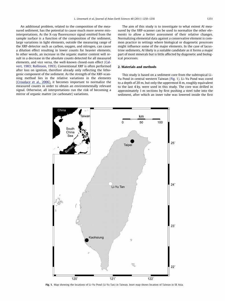
Fig. 1. Map showing the locations of Li–Yu Pond (Li-Yu Tan) i

The aim of this study is to investigate to what extent Al mea-sured by the XRF-scanner can be used to normalize the other ele-ments to allow a better assessment of their relative changes.Normalizing elemental data against a conservative element is com-mon practice in settings where biological or diagenetic processesmight influence some of the major elements. In the case of lacus-trine sediments, Al likely is a suitable candidate as it forms a majorpart of most minerals but is little affected by diagenetic and biolog-ical processes.

2. Materials and methods

This study is based on a sediment core from the subtropical Li–Yu Pond in central western Taiwan (Fig. 1). Li–Yu Pond was coredto a depth of 20 m, but only the uppermost 8 m, roughly equivalentto the last 4 ky, were used in this study. The core was drilled inapproximately 1 m sections by first pushing a steel tube into thesediment, after which an inner tube was lowered inside the first

n Taiwan. Inset map shows location of Taiwan in SE Asia.

Table 1Radiocarbon ages used for age control of the uppermost 8 m of the Li–Yu Pond record (Hsu, 2007).

Depth (cm) Sample ID/lab code Material 14C age (BP) Age range (Cal. y BP) Cal. age error (Cal. y BP)

47 R28804-1/NZA 21661 Plant fragment 117 ± 30 8–278 143 ± 135132 R28804-2/NZA 21662 Plant fragment 1297 ± 35 1170–1290 1230 ± 60210 R28804-3/NZA 21663 Plant fragment 1423 ± 30 1284–1360 1322 ± 38290 R28804-4/NZA 21664 Plant fragment 1629 ± 35 1415–1607 1511 ± 96414 R28804-5/NZA 21665 Plant fragment 1713 ± 30 1535–1705 1620 ± 85638 R28804-6/NZA 21666 Plant fragment 2511 ± 30 2468–2740 2604 ± 136656.5 R28804-7/NZA 21667 Plant fragment 2523 ± 30 2482–2744 2613 ± 131

1252 L. Löwemark et al. / Journal of Asian Earth Sciences 40 (2011) 1250–1256

to collect the sediment. This process was then repeated until thebasement in the basin was reached. The XRF-scans were performedon U-channels originally subsampled at Academia Sinica for min-eral–magnetic studies. The U-channels were transported to Stock-holm University and scanned on the Itrax XRF-core scanner at theDepartment of Geological Sciences and Geochemistry. For detailson the Itrax XRF-scanner please refer to Croudace et al. (2006).The core was measured with 2 mm resolution and an exposuretime of 8 s with the Mo-tube, and with a resolution of 5 mm and30 s exposure time with the Cr-tube. The energy spectrum emittedby the Cr-tube primarily excites electrons in lighter elements, mak-ing it more suitable for measurements of elements lighter than Cr,while the energy spectrum emitted by the Mo-tube primarily ex-cites electrons in the shells of heavier elements, making it less suit-able for measurements of elements lighter than K, but suitable formeasurement on heavier elements. Here we present Fe and Ti-data, two elements often used in paleoenvironmental studies, to-gether with Al-data, which is used to normalize the Fe and Ti mea-surements to allow an assessment of relative variations in thelithological component of the sediment. For the calculation of ele-ment/Al-ratios the Li–Yu Pond data were resampled with 5 mmresolution. The calculated ratios then were plotted both raw andsmoothed with a 5-point moving average. Analyses of TOC andTN of organic-containing samples followed standard procedures(Chen et al., 2009; Ku et al., 2005). In brief, an aliquot of decalcifiedsample was wrapped in a tin capsule and then combusted using aThermoQuest EA1110 elemental analyzer at the Department ofGeosciences, National Taiwan University (NTU) to measure theTOC and TN contents, and thus the atom/atom TOC/TN ratio. Theprecision of measurement was 0.2 wt.% and 0.3 wt.% for TOC andTN, respectively. TOC of the core was measured every 20 cm forthe whole core with additional analyses (�45 data in total) wher-ever significant changes in layers and many biogeochemical prop-erties were observed. These additional analyses were done toincrease resolution, and then to better understand changes in bio-geochemical properties of the core. Age control on the upper 8 mfrom Li–Yu Pond was obtained from seven radiocarbon dates mea-sured at the Rafter Radiocarbon Laboratory, Institute of Geologicaland Nuclear Sciences, New Zealand (Hsu, 2007) (Table 1).

3. Results

The uppermost 8 m of Li–Yu Pond consist of an alternating se-quence of greenish, grayish, brownish layers of mud with interca-lated siltier or sandier layers (Hsu, 2007). TOC values showrelatively little variability in the lower 6 m with values typicallybetween 1% and 4%, while the uppermost 2 m display rapid swingsfrom below 1% to well above 10% (Fig. 2). Aluminium was mea-sured with both the Cr- and the Mo-tube. As anticipated, the Mo-data show considerably lower counts and a much lower signal-to-noise ratio than the Cr-data (Fig. 2). This is only partly due tothe shorter exposure time used with the Mo-tube, as mentionedpreviously; the emitted energy spectrum from the Cr-tube is bettersuited to excite electrons in lighter elements compared to the Mo-

tube. Nevertheless, the general trend is in good agreement with thedata obtained from the Cr-tube. Aluminium-values in the lowerpart of the core are relatively stable, but with a few rapid shifts.In contrast, the upper part shows a number of rapid oscillationsthat roughly mirror variations in TOC; peaks in TOC correspondto minima in Al.

Titanium, also determined with both X-ray tubes, shows a sim-ilar pattern as Al. In the lower part of the core the Ti-levels arerather stable, while they are considerably more variable in theupper part. As with Al, dips in Ti tend to correspond to maximain TOC (Fig. 2). However, in comparison to Al, there are only smalldifferences in the shape of the profiles obtained from the two X-raytubes, although the actual number of counts differ by more thanone order of magnitude. The Fe record shows a somewhat similar,although spikier, pattern to Ti having a correlation coefficient of0.45 (both elements obtained with the Mo-tube). Lows in Fe gener-ally tend to occur in intervals with high TOC. When Ti and Fe arenormalized against Al, the Ti/Al and the Fe/Al curves still show astrong resemblance to each other (r = 0.95), but a slightly new pat-tern appears. The lower part is still fairly stable with minor varia-tions, but in the upper part, the element-to-Al ratios display adistinctly different pattern from the elemental counts. In particu-lar, several intervals characterized by increased Ti and Fe levels,display low element-to-Al ratios, and vice versa. It is especiallyinteresting to notice that the upper intervals characterized by highTOC levels (over 10%) and low element counts show increased ele-ment-to-Al ratios. This suggests a change in the composition of thelithogenic component. The calculated element-to-Al ratios displaya number of extreme peaks caused by very low, or zero, Al counts.In the plots this problem is in part overcome by the removal of ex-treme outliers and by presenting a 5-point running average.

4. Discussion

The most striking feature of the XRF records is probably thehigh-frequency variability (Fig. 2). In part this is noise, but it also re-flects the way that the XRF-scanner measurements are performed.The obtained XRF-scanner measurements reflect the compositionof a thin (sub-mm) layer on top of the sediment surface and cantherefore display considerable high-amplitude variability causedby variations in the sediment composition over small distances.These small scale variations tend to become averaged out by con-ventional measurements which represent an average of the bulkcomposition over a cm or more. It is therefore not surprising thatXRF-scanner data display considerably more high-frequency,high-amplitude variability than conventional measurements. Thedata quality is also affected by cracks or gaps in the sample surface.These can be caused by the coring or sampling process, or due todesiccation of the sediment during storage or measurement. Whilegaps are fairly easy to detect as indicated by sharp drops in all ele-ments over the interval, cracks tend to result in extreme spikes fol-lowed by dips. Gaps and cracks can usually be easily identified inthe line scan photograph and X-ray radiographs produced duringscanning (Fig. 3). Surface roughness and variations in water content

Fig. 2. Total organic carbon and XRF-counts measured in the Li–Yu Tan. Al measured with the Cr-tube (black) shows considerably higher counts and less variability comparedto the data obtained with the Mo-tube (gray). The Ti-records measured with Cr (black) and Mo-tubes (gray) display similar record although with different absolute counts.When normalized against Al, the variations in Ti and Fe display a similar pattern (gray lines are raw data, black line show 5-point moving average with outliers removed fromthe data set). Gray bars indicate the position of major cracks and gaps in the sedimentary record.

L. Löwemark et al. / Journal of Asian Earth Sciences 40 (2011) 1250–1256 1253

(Tjallingii et al., 2007) also influence the data quality to some de-gree, but these factors are much more difficult to identify comparedto gaps and cracks.

Titanium and Fe values display a number of sharp peaks anddips concomitant with similar features in the Al-record, whichtherefore are attributable to gaps and cracks in the sediment. Thisis confirmed by the inspection of instrument parameters such asthe mean standard error (MSE, an expression of the fit betweentheoretical to measured XRF spectra) and total counts per secondand from studies of X-ray radiographs of the sediment (Fig. 3).When ignoring the artifacts caused by cracks in the sediment,the elemental records still indicate a number of abrupt changesin the depositional system. In a similar setting in southeastern Chi-na, the Huguang Maar, variations in the Ti content in the sedimentwere interpreted as variations in aeolian dust controlled by varia-tions in the strength of the East Asian winter monsoon (Yanchevaet al., 2007). It is tempting to interpret the observed variations inelements in a similar manner, directly reflecting a climatic signal.However, although these changes certainly do reflect changes inthe depositional system, the environmental interpretation is com-plicated by two important factors, the matrix effect and the dilu-tion effect.

In the ideal case, the counts measured should be directly pro-portional to the concentration of the element in the sediment. Inreality, however, the signal depends on the presence and concen-trations of other elements that might attenuate or enhance theXRF-signal (Beckhoff et al., 2006). For example, X-ray fluorescencefrom atoms deeper in the sample must first pass through the uppersediment layers on their way to the detector. During this transfer

through the sediment parts of the fluorescence might get absorbedby overlying atoms. However, the fluorescence from one elementmight become enhanced because its atoms interact with and areexcited by fluorescent photons from a second element. This resultsin a corresponding decrease in detected fluorescence of the secondelement as a portion of its fluorescent photons are attenuated bythe first element and fail to reach the detector. The secondary fluo-rescence therefore enhances the counts of certain elements whiledecreasing the counts of others (Berth, 1969). This matrix effectcan be corrected for if the approximate concentrations of the dif-ferent elements in the sample are known. In the case of unlithifiedsediment cores where both water content and organic carbon con-tent vary it is usually not in practice possible to correct for the ma-trix effect.

The matrix effect is somewhat related to the dilution effectbeing caused by variations in biogenic material. An increase in or-ganic material, consisting primarily of C, H, N, will inevitably leadto a decrease in the concentration of all other elements, andaccordingly, to a decrease in the measured counts of these otherindividual elements (closed-sum effect). Consequently, an ob-served increase or decrease in an element does not by necessitymean that there has been an increase or decrease in the flux of thatelement, rather this may have been caused by a change in thedeposition rate of the diluting agent, which in lakes usually is or-ganic matter. In the marine realm, this effect is well-known andhandled through flux calculations, comparison with a standard,or normalization against a conservative element (Brumsack,2006). Normalization to Al allows the relative variations in the lith-ogenic component of the sediment to be addressed. This informa-

Fig. 3. Detail of Section 4 in Li–Yu Pond from measurement with the Mo-tube. X-ray radiograph showing variations in sediment density and two cracks (light bands). Totalcounts (1000 counts s�1), mean square error between measured data and fit (MSE), Ti- and Fe-counts all display distinct dips in relation to the cracks. The Al-data here wasmeasured with the Mo-tube and contain too much noise to allow a comparison with the X-ray radiograph.

1254 L. Löwemark et al. / Journal of Asian Earth Sciences 40 (2011) 1250–1256

tion can be used to separate the aeolian, terrestrial, and biogenicinput into the system.

To illustrate the effect of dilution by TOC on the measuredintensity of an element in the lithogenic component, a typicalexample is calculated. The TOC content of subtropical lake sedi-ment typically varies between a few percent to over 50% (Maxwell,2001; Selvaraj et al., 2007). However, as organic matter also con-sists of a large portion of other light elements such as H, O, N,and S, the organic component of the sediment can be considerablyhigher than indicated by TOC alone. The carbon component of theorganic matter increases with the maturity of the organic matter,but in unlithified sediment, the percentage of C in organic matteroften is lower than 50% (Cambardella et al., 2000; Tyson, 1995).As a result, sediment with a TOC content around 25% (organ-ic = 50%) might only contain 50% lithogenic material. Assumingfor simplicity’s sake, that the organic matter in the lake sedimentconsists to 50% of carbon, and to 50% of H, N, O, and S, then the lith-ogenic component would make up about 100% � (2 � TOC). Conse-quently, if the TOC level rises from for example 1% to 25%, theelements in the lithogenic component would decrease by about50%. This effect of dilution by organic material is well know (theclosed-sum effect) (Calvert, 1983; Rollinson, 1993), but there isno straight forward method to deal with it since XRF-scannersdeliver counts rather than concentrations. In marine settings, thesedimentary composition is often compared to the average compo-sition of a typical sediment, such as black shales (cf. Tribovillardet al., 2006). In more variable settings, as in lakes for instance, itis often more useful to look at the relative variations of the differ-ent elements compared to a major, conservative element. Prefera-bly, the element should not itself be a proxy nor affected by

biological or redox processes. Elements such as Fe or Mn areunsuitable because of their redox sensitive nature while elementslike Ca or Si are strongly affected by biological processes. Othermajor elements such as Na, K, Sr, or Mg are easily dissolved andweathered, also making them unsuitable for normalization. Tita-nium is an important component in many minerals, is abundant,and biologically not very active. However, Ti is enriched in heavyminerals and in aeolian dust and is therefore used as a proxy forhigh-current regimes (Schnetger et al., 2000) or enhanced windactivity (Wehausen and Brumsack, 1999; Yancheva et al., 2007).Furthermore, Ti content is also highly influenced by the composi-tion of the original protolith (Rundnick and Fountain, 1995; Rund-nick and Gao, 2003). The most suitable element therefore is likelyAl. It is abundant, little active biologically, and is not particularlyaffected by redox variations (Brumsack, 2006). As Al is a majorstructural component in the sand, silt and clay that enters thebasin, a normalization of the other elements against Al allows usto see how the proportion of the individual elements in the litho-genic part of the sediment have changed relative to each other overtime.

After normalization, the pattern displayed by Ti/Al and Fe/Aldiffer markedly from the Ti- and Fe-records in the studied core.It now becomes apparent that the three intervals characterizedby enhanced TOC levels, 480–440 cm, 170–120 cm, and 80–50 cm, are also distinguished by strong increases in Ti- and Fe-to-Al ratios. It is tempting to interpret these concomitant changesin TOC levels and in element-to-Al ratios as a climatic signal likelycaused by a change in weathering conditions. That the enhancedTi/Al levels should be caused by an increase in aeolian dust inputseems unlikely. Although element-to-Al ratios are high in TOC-rich

L. Löwemark et al. / Journal of Asian Earth Sciences 40 (2011) 1250–1256 1255

intervals, the absolute counts in Ti and Fe actually decrease, indi-cating a drop in the input of these elements. Weathering is primar-ily influenced by precipitation and temperature, and the rate ofweathering for various minerals is generally the reverse of Bowen’sreaction series, meaning that minerals rich in quartz and Al remainin the soil while more easily dissolved elements would be weath-ered from the soil and transported to the depositional basin (Brady,1990; Fang et al., 2003; Selly, 1994). Consequently, the simulta-neous increase of TOC and Ti- and Fe-to-Al ratios observed in Li–Yu Pond could be interpreted to be the result of periods of in-creased precipitation leading to increased chemical weathering inthe catchment, enhanced flushing of soil organic matter into thelake, and possibly also to higher lake levels causing dysoxic condi-tions on the lake floor enhancing preservation of organic material(cf. Yancheva et al., 2007). However, increased TOC could also bedue to peat formation during lake level low-stands, a thoroughpaleoenvironmental interpretation of the Li–Yu Pond record is be-yond the scope of this study.

From the above discussion it should be clear that elementalvariations obtained by XRF-scanning, although a very powerfultool, cannot be taken at face value, at least not in settings thatshow large variations in the non-lithogenic component of the sed-iment. Aluminium-normalization as outlined above is a powerfulway to standardize the obtained XRF-scanner data to make com-parisons between different intervals and sites possible. However,Al-normalization of XRF-scanner data is also marked by a numberof limitations. The most severe being the poor detection of Al.While data obtained using the Cr-tube give reasonable Al-data,the detection of heavier elements is not optimal, thus requiring asecond run with the Mo-tube for each core and a switch of tubes.This procedure effectively doubles the machine time, increasesthe risk of the sediment drying out, and introduces an alignmenterror as it is often difficult to align two datasets with mm-preci-sion. Aluminium-measurements also require considerably longerexposure times than are necessary for most other elements, furtherincreasing time consumption during measurement. Perhaps mostimportantly, however, is the fact that the detection limit for Almay not be reached in organic-rich intervals, thus making normal-ization in the intervals where normalization is the most neededdifficult. Other solutions to the normalization problem would in-clude using other elements, but it is difficult to identify an elementthat is both abundant and conservative enough, or to normalizeagainst the organic matter, carbonate fraction or total lithogenicfraction (Sanei et al., 2001). The latter three would however requirequantitative, destructive measurements on the samples, thusdeparting from the basic concept of fast non-destructive XRF mea-surements. Another potential avenue to address the normalizationproblem has recently been indicated by Guyard et al. (2006). Theyshowed that the ratio between the incoherent and coherent scat-tering (indirect measures of the number of light and heavier ele-ments, respectively) was closely correlated to the TOC content.The usefulness of this method will need to be tested on a largerange of materials before it can be applied routinely to standardizeXRF-scanner data.

5. Conclusions

From the study of TOC and XRF-scanner elemental data fromsubtropical lake sediments from central Taiwan several conclu-sions regarding the interpretation of XRF-scanner data can bedrawn.

s The number of counts measured for the individual elements isstrongly influenced by variations in the organic component ofthe sediment. Therefore the measured signal needs to be nor-

malized or standardized against a standard or a conservativeelement.

s The most suitable element to be used for normalization will inmost settings be Al since it is abundant, among the last to beaffected by weathering, and is also little affected by biologicaland redox processes.

s However, Al-measurements are hampered by the poor detec-tion limits for Al, requiring the sediments to be measured withdifferent X-ray tubes to obtain the full spectrum of elements,and the use of long exposure times to ensure reliable Al-data.

We therefore strongly recommend that a normalization or stan-dardization of XRF-scanner data is performed before any paleoen-vironmental interpretation is attempted. This is particularlyimportant in settings where large fluctuations in the organic frac-tion of the sediment can be anticipated.

Acknowledgments

This study was supported by the National Science Council of theROC under Grant NSC NSC 97-2116-M-019-004 to CHF. YEFacknowledges grants from NSC, Academia Sinica, and from Na-tional Taiwan Normal University. LL and YTN also acknowledgesfinancial support from Swedish Research Council. Nathalie Ljung-gren is thanked for assistance with the Itrax measurements. AndersRindby is thanked for help with the discussion on XRF-scannermethodology. We gratefully acknowledge the constructive reviewsby Nicolaj K. Larsen and one anonymous reviewer who helped im-prove this study.

References

Beckhoff, B., Kanngieber, B., Langhoff, N., Wedell, R., Wolff, H., 2006. Handbook ofPractical X-Ray Fluorescence Analysis. Springer, Heidelberg. 843 pp.

Berth, E.P., 1969. Principles and Practice of X-Ray Spectrometric Analysis. PlenumPress, New York.

Böning, P., Bard, E., Rose, J., 2007. Toward direct, micron-scale XRF elemental mapsand quantitative profiles of wet marine sediments. Geochemistry, Geophysics,Geosystems 8, Q05004. doi:10.1029/2006GC001480.

Brady, N.C., 1990. The Nature and Properties of Soil. Macmillan, New York. 621 pp.Brumsack, H.-J., 2006. The trace metal content of recent organic carbon-rich

sediments: implications for Cretaceous black shale formation. Palaeogeography,Palaeoclimatology, Palaeoecology 232 (2–4), 344–361.

Calvert, S.E., 1983. Geochemistry of Pleistocene sapropels and associated sedimentsfrom the eastern Mediterranean. Oceanologica Acta 6, 255–267.

Cambardella, C.A., Gajda, A.M., Doran, J.W., Wienhold, B.J., Kettler, T.A., 2000.Estimation of particulate and total organic mater by weight loss-on-ignition. In:Lal, R., Kimble, J.M., Follett, R.F., Stewart, B.A. (Eds.), Assessment Methods forSoil Carbon. Advances in Soil Science. Lewis Publishers, pp. 349–359.

Chen, S.-H., Wu, J.-T., Yang, T.-N., Chuang, P.-P., Huang, S.-Y., Wang, Y.-S., 2009. LateHolocene paleoenvironmental changes in subtropical Taiwan inferred frompollen and diatoms in lake sediments. Journal of Paleolimnology 41 (2), 315–327.

Croudace, I.W., Rindby, A., Rothwell, R.G., 2006. ITRAX: description and evaluationof a new multi-function X-ray core scanner. In: Rothwell, R.G. (Ed.), NewTechniques in Sediment Core Analysis. Geological Society of London, London,pp. 51–63.

Diekmann, B., Hofmann, J., Henrich, R., Fütterer, D.K., Röhl, U., Wei, K.Y., 2008.Detrital sediment supply in the southern Okinawa Trough and its relation tosea-level and Kuroshio dynamics during the late Quaternary. Marine Geology255, 83–95.

Fang, J.N., Lo, H.J., Song, S.R., Chung, S.H., Chen, Y.L., Lin, I.C., Yu, B.S., Chen, H.F., Li,L.J., Liu, C.M., 2003. Hydrothermal alteration of andesite in acid solutions:experimental study in 0.05 M H2SO4 solution at 110 �C. Journal of the ChineseChemical Society 50 (2), 239–244.

Guyard, H., Chapron, E., St-Onge, G., Anselmetti, F.S., Arnaud, F., Magand, O., Francus,P., Mélières, M.-A., 2006. High-altitude varve records of abrupt environmentalchanges and mining activity over the last 4000 years in the Western French Alps(Lake Bramant, Grandes Rousses Massif). Quaternary Science Reviews 26, 2644–2660.

Haschke, M., 2006. The Eagle III BKA system, a novel sediment core X-rayfluorescence analyser with very high spatial resolution. In: Rothwell, R.G.(Ed.), New Techniques in Sediment Core Analysis. Geological Society of London,London, pp. 31–37.

Haug, G.H., Günther, D., Peterson, L.C., Sigman, D.M., Hughen, K.A., Aeschlimann, B.,2003. Climate and the collapse of Maya civilization. Science 299, 1731–1735.

1256 L. Löwemark et al. / Journal of Asian Earth Sciences 40 (2011) 1250–1256

Hsu, Y.-W., 2007. Late Holocene paleoclimate change at Central Taiwan:Biogeochemical proxy analysis of lacustrine sediments from Li-Yu Pond, Puli.Master Thesis. National Taiwan Normal University. 111 pp (in Chinese).

IPCC, 2007. Climate Change 2007. Synthesis Report.Ku, H.-W., Chen, Y.-G., Liu, T.-K., 2005. Environmental change in the southwestern

coastal plain of Taiwan since late Pleistocene: using multiple proxies ofsedimentary organic matter. Terrestrial Atmospheric Oceanic Sciences 16,1079–1096.

Löwemark, L., Jakobsson, M., Mörth, M., Backman, J., 2008. Arctic Ocean Mn contentsand sediment color cycles. Polar Research 27, 105–113.

Maxwell, A.L., 2001. Holocene monsoon changes inferred from lake sediment pollenand carbonate records, Northeastern Cambodia. Quaternary Research 56, 390–400.

Richter, T.O., van der Gaast, S., Koster, B., Vaars, A., Gieles, R., de Stigter, H.C., deHaas, H., van Weering, T.C.E., 2006. The Avaatech XRF core scanner: technicaldescription and applications to NE Atlantic sediments. In: Rothwell, R.G. (Ed.),New Techniques in Sediment Core Analysis. Geological Society of London,London, pp. 39–50.

Rollinson, H.R., 1993. Using Geochemical Data: Evaluation, Presentation,Interpretation. Pearson Education, Upper Saddle River, New Jersey.

Rothwell, R.G., Rack, F.R., 2006. New techniques in sediment core analysis: anintroduction. In: Rothwell, R.G. (Ed.), New Techniques in Sediment CoreAnalysis. Geological Society of London, London, pp. 1–29.

Rundnick, R.L., Fountain, D.M., 1995. Nature and composition of the continentalcrust: a lower crustal perspective. Reviews of Geophysics 33 (3), 267–309.

Rundnick, R.L., Gao, S., 2003. Composition of the continental crust. In: Rundnick, R.L.(Ed.), Treatise on geochemistry. Elsevier, pp. 1–64.

Sakamoto, T., Kuroki, K., Sugawara, T., Aoike, Kan., Iijima, K., Sugisaki, S., 2006. Non-destructive X-ray fluorescence (XRF) core-imaging scanner, TATSCAN-F2.Scientific Drilling 2, 37–39.

Sanei, H., Goodarzi, F., Flier-Keller, E.V.D., 2001. Historical variation of elementswith respect to different geochemical fractions in recent sediments fromPigeon Lake, Alberta, Canada. Journal of Environmental Monitoring 3, 27–36.

Schnetger, B., Brumsack, H.J., Schale, H., Hinrichs, J., Dittert, L., 2000. Geochemicalcharacteristics of deep-sea sediments from the Arabian Sea: a high-resolutionstudy. Deep Sea Research Part II 47, 2735–2768.

Selly, R.C., 1994. Applied Sedimentology. Academic Press, London. 446 pp.Selvaraj, K., Chen, C.T.A., Lou, J.-Y., 2007. Holocene East Asian monsoon variability:

Links to solar and tropical Pacific forcing. Geophysics Research Letters 34,L01703. doi:10.1029/2006GL028155.

Tjallingii, R., Röhl, U., Kölling, M., Bickert, T., 2007. Influence of the water contenton X-ray fluorescence corescanning measurements in soft marine sedi-ments. Geochemistry, Geophysics, Geosystems 8 (2), Q02004. doi:10.1029/2006GC001393.

Tribovillard, N., Algeo, T.J., Lyons, T., Riboulleau, A., 2006. Trace metals aspaleoredox and paleoproductivity proxies: an update. Chemical Geology 232(1–2), 12–32.

Tyson, R.V., 1995. Sedimentary Organic Matter. Chapman and Hall, London. 615 pp.Wehausen, R., Brumsack, H.J., 1999. Cyclic variations in the chemical composition of

eastern Mediterranean Pliocene sediments: a key for understanding sapropelformation. Marine Geology 153 (1–4), 161–176.

Weltje, G.J., Tjallingii, R., 2008. Calibration of XRF core scanners for quantitativegeochemical logging of sediment cores: theory and application. Earth PlanetScience Letters 274 (3–4), 423–438.

Yancheva, G., Nowaczyk, N.R., Mingram, J., Dulski, P., Schettler, G., Negendank,J.F.W., Liu, J., Sigman, D.M., Peterson, L.C., Haug, G.H., 2007. Influence of theintertropical convergence zone on the East Asian monsoon. Nature 445 (7123),74–77.