THESIS

Submitted to obtain the doctor degree (PhD)

presented by

Tamara Fernández Arévalo

Under the supervision of

Eduardo José Ayesa Iturrate and

Paloma Grau Gumbau Donostia-San Sebastián, November 2016

NEW HEAT TRANSFER AND OPERATING COST MODELS FOR THE PLANT-WIDE SIMULATIONS OF FULL-SCALE WWTPS

UNIVERSITY OF NAVARRA

TECHNOLOGICAL CAMPUS, TECNUN

DONOSTIA - SAN SEBASTIÁN

NEW HEAT TRANSFER AND OPERATING COST

MODELS FOR THE PLANT-WIDE SIMULATIONS OF FULL-SCALE WWTPS

THESIS SUBMITTED to obtain the doctor degree (PhD)

presented by

TAMARA FERNÁNDEZ ARÉVALO

under the supervision of

Eduardo José Ayesa Iturrate and Paloma Grau Gumbau

Donostia – San Sebastián, November 2016

A mi familia

v

A ACKNOWLEDGEMENTS

“Si se siente gratitud y no se la expresa es como envolver un regalo y no darlo”

William Arthur Ward

Al acercarse al final de una etapa conviene reflexionar y recordar a toda esa gente que ha participado en ella, ya que sin su colaboración, cariño y apoyo esto no hubiera sido posible. Para finalizar esta larga etapa llamada tesis, no me queda más que agradeceros a todos vosotros el que hayáis contribuido con vuestro pequeño granito de arena. Han sido todos esos granitos de arena los que han hecho posible esta tesis.

En primer lugar me gustaría agradecer a mi director de tesis Eduardo Ayesa la confianza depositada en mí. Por todas las horas que pacientemente ha dedicado a la perfección de los artículos que a día de hoy son capítulos de esta tesis, por haber creído en mí y en mis posibilidades, por su optimismo y por su cercanía. Gracias por haberme ayudado a crecer como investigadora y también como persona. A mi codirectora de tesis Paloma Grau por el apoyo prestado tanto en los buenos como en los malos momentos. Gracias por preocuparte e intentar ayudar con todos los medios que tenías, ¡te lo agradezco de corazón!

Al centro tecnológico Ceit-IK4 y a la Universidad de Navarra por la formación proporcionada en los últimos años y por haberme dado la oportunidad de llevar a cabo esta tesis.

Agradecer también a la administración central por el proyecto Consolider en el que se enmarca esta tesis. Gracias al proyecto Novedar se ha formado una gran familia de la que me siento orgullosa y feliz de ser miembro. Los seminarios, reuniones y cursos en los que he podido participar con vosotros me han aportado mucho profesional y personalmente. Gracias a Sergi, Maria, Jose, Manel, Leticia, Nuria, Theo, Ignasi, Quim, Raúl, etc., y en general a todos por vuestro apoyo y cercanía.

vi Acknowledgements

Después de 3 largos años por fin hemos terminado el famoso paper de las configuraciones. Gracias a Sebastià Puig, Manel Poch, Miquel Rigola, Fernando Fdez.-Polanco, Sara I. Pérez-Elvira y Juan M. Garrido por vuestra colaboración y apoyo.

Quisiera agradecer también al Consorcio de Aguas Bilbao-Bizkaia (CABB), a la Empresa Municipal de Aguas y Alcantarillado de Palma de Mallorca (EMAYA), a Calvià 2000, a Utedeza, a Veolia Water Iberica y a la Mancomunidad de la Comarca de Pamplona por la confianza depositada en Ceit-IK4 y Conaqua para la realización de estudios por simulación.

Esta tesis no hubiera sido posible sin la ayuda del informático jefe del departamento. A día de hoy los modelos no hubieran funcionado así de bien sin tu mano. Haces el trabajo sucio, que pocas veces se valora, pero que sepas que gran parte de esta tesis te pertenece. No tengo palabras para agradecerte todo lo que me has ayudado en estos años. Has hecho de psicólogo en mis momentos de bloqueo, me has escuchado cuando lo he necesitado, has programado mis invenciones y siempre has estado dispuesto a ayudar. Seguro que por algún lado queda algún apanito sin borrar… Tú me has enseñado a programar, a que la solución de cualquier problema pasa por reiniciar el ordenador, a buscar la solución de todo en google, a cuidar de mis plantas y a que una no se puede quejar si no ha hecho trescientas copias de seguridad (como mínimo). Pero todavía no entiendo porque un informático no tiene ni idea de electricidad ni de ofimática. ¡Mil gracias Alain!

A vosotras dos, ¡sentí un gran vacío cuando os fuiste del departamento! El departamento ha perdido a dos grandes personas. Maider, siempre has estado ahí para aconsejarme y ayudarme a tomar las mejores decisiones. ¡Mil gracias por escucharme y aconsejarme! Hemos pasado grandes momentos trabajando juntas pero sobre todo fuera del trabajo: partidos de Champions en los que nos perdíamos el himno, grandes celebraciones de Donosti, pequeñas vueltecitas… Sabes que me tienes aquí siempre que necesites. Ahora tendremos que cambiar las pequeñas vueltecitas por los paseítos con Lucas. Carmen, nos vemos poco pero cuando nos vemos es como si no hubiera pasado el tiempo. Gracias por enseñarme a relativizar, por ser tan atenta y estar siempre pendiente. ¡Siempre dando pero nunca pidiendo nada a cambio! Espero que sigamos haciendo esos pintxo-pote de los viernes por mucho tiempo y esas charlas hasta el amanecer arreglando el mundo. Gracias a las dos por todo el apoyo que me habéis dado en estos años y que me seguís dando aunque no estéis en el

Acknowledgements vii

departamento, por estar siempre que os he necesitado, pero sobre todo por ser grandes amigas.

A mis compañeros de despacho, primero Mikel y Myriam, y ahora Jon y Leyre. Gracias a todos por haberme dado tan buenos momentos. Qué hubiera sido del despacho sin Mikel hablando del Athletic o yo picándolo... pobre Myriam, lo que tuvo que aguantar… Mikel tranquilo que aunque te hayas ido no me libro del Athletic. Gracias a los dos por los buenos momentos que pasamos dentro y fuera del despacho, siempre estuvisteis dispuestos a ayudar y siempre me demostrasteis vuestro cariño y amistad. ¡Muchas Gracias! Myriam, eskerrik asko laguntzeko prest egon zinelako. Zuri esker ikasi nuen biokimika ta analitiken inguruan! Orain dantza surfagatik aldatu dezun arren, ea noiz botatzen degun aspaldiko dantza saio haietako bat! Jon, ezin aukerau despatxokide hobiagua! Momentu on edo ez oso onetan hor eon zealako, nei entzun ta animuak ematen. Eskerrik asko goizero irribar batekin hartzeagatik, zure positibotasunagatik eta zure gertukotasunagatik! Despatxua ez zan berdina izango mundua konpontzeko gure txarla luze hoiek gabe. Karamelito bat nahi? Leyre, eskerrik asko nerekin hain ona ta detailezalia izateagatik. Denbora gutxi pasa deu despatxuan baina nahikua izan da zure bihotz ona ikusteko. Mila esker zure post-it, istorio ta detaile txikiekin eguna alaitzeagatik! Nahi dezuneako Zumaiamin nao! Zorte on tesiyakin ta iten dezun guztiarekin! Meresi dezu ta! Ez zait ahazten poteotxo bat pendiente dakaula hirurok tesiya ospatzeko!

Izaro, modeluekin borrokan urtiak pasa ta gero, azkenian bukatu deu biyok. Luzia izan badare oroitzapen polittak gordeko diteu pasatako etapa hontaz. Eskerrik asko urte hauetan emandako laguntzagatik. Beñat, apoyo haundiya izan zea tesiko azken une hauetan. Mila esker zure eguneroko animuengatik, zure gertukotasunagatik eta beti entzuteko prest egoteagatik. Zure akatsik hauendiyena Athletikekua izatia da baina ze ingo diou… Mertzi bihotzez! Yaiza, has traído la alegría y la vitalidad a la unidad. ¡Gracias por transmitirme esa energía!

Lerro hauen bitartez, eskerrak eman nahiko nizkioke baita Mikel Maizari. Conaquako bidea hasi genuenean sostengu garrantzitsu bat izan zinen. Hasieratik sinetsi zenuen nigan eta aurrera jarraitzeko indarra eta konfidantza eman zenizkidan. Honengatik eta nigatik egin dezun guztiarengatik, mila esker Mikel!

Gracias a Enrique Aymerich, Luis Sancho y Luis Larrea por tener siempre la puerta de vuestro despacho abierta, por vuestra disponibilidad y por el cariño que me habéis mostrado siempre. Cuando he necesitado consultaros alguna cuestión de proceso os

viii Acknowledgements

habéis mostrado siempre dispuestos a ayudarme y me habéis recibido con una amplia sonrisa, ¡Eskerrik asko por todo! Gracias también al resto de investigadores y compañeros del antiguo departamento de Ingeniería Ambiental: a Bixen del Barrio, Jaime Gonzales, Ion Irizar, Jaime Luis García de las Heras, Antonio Salterain, Sergio Beltrán y Susana Rodriguez.

Muchas gracias también a todos los que habéis pasado por el departamento y con los que he compartido grandes momentos. A Naiara, Elena Gonzalez, Patri, Ane Orbegozo, Ane Arregi, Igotz, Ander, Oier, Mikel Aguirre, Carlos, Nagore, Agirtze, Claudia, Jesus, Isabel, Ángel, Juan, Remy, Patxi… y a todos aquellos con los que he tenido el placer de coincidir en el departamento. Eskerrik asko danei eman dizkidazuen uneengatik!

Nork esango luke Inasmeten orain dela 9 urte sartu ginenean, horrelako harremana egingo genuela. Eskerrik asko Mery, Unzu, Olax, Marta, Esti, Nagore, Alba, Txemita, Jonzu ta Ekaini urteak pasata ere hor egoteagatik.

Nerekin dantzan ibiltzen zareten guztioi (Neo-klasiko taldia, Alima dantza eta Astindu dantza elkarteari). Eskerrik asko deskonektatzen laguntzeagatik, beti agertu didazuen maitasunagatik eta une ahaztezinak eskeintzeagatik! Zuekin dantza egitea plazer bat da! Mertzi!

Nola ez eskertu unibertzitatean ezagutu baina orain lagun zaretenoi. Bost urte pasa genituen Leioan, baina mila abentura eta oroitzapen pilatu ditugu ordundik. Argi geratu zitzigun behintzat matlaben 2+2=1.328 zela eta laborategia oso urrun zegoela! Eskerrik asko bihotzez Joseba, Campos, Madari, Jasone eta Goñiri urte guzti hauetan nire alboan egoteagatik! Badakizue Zumaian bigarren etxia dakazuela nahi dezuenerako! ¡A ver cuando organizamos la próxima salida acuática-primaveral o la otoño-cultural que ya estamos tardando!

Eskerrik asko baita, nola ez, nere kuadriyakoei: Arri, Nayi, Tuko, Mir, Zori, Aitor, Eli, Cris, Jon Mikel eta Sandrari. Zuek izan zeate tesi hau gehien sufritu dezuenak. Badakit zuetako askok ez dezuela ulertzen zertan pasatzen nuen hainbeste denbora… ba liburu hontan! Baina lasai, bukatu detela! Oin ospatzea besteik ez zaigu falta! Mila esker etapa hontan ta txikitatik nere aldamenian egoteagatik. Milaka momentu, afari, bueltita, kafe ta barre bizi izan diteu batea (Mirren kangrejua ta sirenita, Elin aktuaziyuak…). Espero det askoz ere gehiago biltzea, beraz, noiz hasiko gea ospatzen nere tesiyataz librau zeatela? Eskerrik asko “divinities” eman dizkidazuen

Acknowledgements ix

animoengatik eta baita deskonektatzen laguntzeagatik. Mertzi girls! Bereziki mila esker Arriri! Momentu on, erdipurdi eta txar danetan hor eon zealako nerekin. Mertzi, beti euki dituzun hitz onengatik eta eman dizkidazun gomendioengatik. Eskerrik asko bihotzez!

Y cómo no, a mi familia. No tengo palabras para agradeceros todo lo que siempre me habéis dado incondicionalmente. Gracias por apoyarme en todas las decisiones que he tomado a lo largo de mi vida, por la confianza que habéis depositado en mí para todo lo que me he propuesto, y sobre todo por el cariño que me habéis ofrecido siempre. Gracias por sentiros siempre orgullosos de mí. Yo también me siento orgullosa de teneros. Y en especial a ti papa. No has podido estar en el final de esta etapa de mi vida, pero sé que donde estés estarás orgulloso de mí. Me enseñaste a pelear para conseguir todo lo que me proponía igual que hiciste tú hasta el último momento, y ya está, terminé la tesis también. ¡Os quiero!

Eskerrik asko bihotz-bihotzez

Tamara

xi

A ABSTRACT

The main objective of this thesis has been to develop and validate a systematic and rigorous procedure for constructing mathematical models describing both heat transfers and operating costs in Wastewater Treatment Plants (WWTPs).

In order to achieve this objective, the thesis presents a new modelling methodology for calculating the heat variations produced by biochemical, chemical and physico-chemical transformations in any unit. The methodology is based on the estimation of the heat of reaction of each phase (liquid, solid or gaseous) by the enthalpies of formation of model components, applying the Hess's law. The detailed characterisation of the components that provides the Plant-Wide Modelling (PWM) methodology, enables the estimation of the enthalpy of formation for each model component and makes possible a systematic and dynamic calculation of the heat released or absorbed by each transformation, guaranteeing heat energy continuity in parallel with the mass continuity at any point in the plant.

This methodology has been incorporated into a complete and generic heat transfer model for predicting the temperature of any phase present in the unit-processes.

Regarding the operating cost models, the thesis presents an extensive library of actuator models based on engineering equations. The engineering expressions adapted depend closely on the operational variables of the process (solids concentration, flowrates, enthalpy changes of reaction, etc.), allowing a more detailed and realistic estimate.

The heat transfer and operating costs models developed in this thesis, along with the physico-chemical model developed by Lizarralde et al. (2015), have been used to update the Ceit-IK4 PWM methodology to a new version of the methodology called Extended Plant-Wide Modelling (E-PWM).

xii Abstract

The modelling methodology developed for calculating heat variations caused by transformations has been validated with experimental and theoretical data obtained in literature. After validation, a verification of the predictive capacity of the heat transfer model was carried out by simulating the behaviour of an Autothermal Thermophilic Aerobic Digester (ATAD). In order to test the usefulness and applicability of the overall heat transfer model, two case studies have been carried out. In the first study, the same ATAD reactor was simulated, and in the second case study a global reference plant (BSM2) was used.

In order to show the potential of the library, three evolutionary WWTPs were compared from a techno-economic standpoint. The selected configurations were (1) a conventional WWTP based on a modified version of the Benchmark Simulation Model No. 2, (2) an upgraded or retrofitted WWTP, and (3) a new Wastewater Resource Recovery Facility (WRRF) concept denominated as C/N/P decoupling WWTP.

Subsequently, the thesis presents three case studies conducted in full-scale wastewater treatment plant in order to show the usefulness of adapted and flexible model libraries for optimising real full-scale WWTPs, as is the case of the PWM library.

The thesis concludes with a chapter devoted to the most significant conclusions, the bibliography, and a set of appendixes with additional information, such as the detailed description of the models and the characterisation of the components.

xiii

R RESUMEN

El principal objetivo de esta tesis ha sido el de desarrollar y validar un procedimiento riguroso y sistemático para construir modelos matemáticos que describan las transferencias de calor y los costes operacionales en estaciones depuradoras de aguas residuales (EDARs).

Con el fin de lograr este objetivo, la tesis presenta una nueva metodología de modelado para el cálculo de las variaciones de calor producidas por las reacciones bioquímicas, químicas y físico-químicas en cualquier unidad. La metodología se basa en la estimación del calor de reacción de cada fase (líquida, sólida o gaseosa) mediante las entalpias de formación de los componentes del modelo y aplicando la Ley de Hess. La detallada caracterización de los componentes que ofrece la metodología Plant-Wide Modelling (PWM), permite la estimación de las entalpías de formación de cada componente del modelo, y hace posible un cálculo sistemático y dinámico del calor liberado o absorbido por cada transformación, garantizando en todo momento la continuidad de energía calorífica en paralelo con la continuidad de masa en cualquier punto de la planta.

Esta metodología ha sido incorporada a un completo y genérico modelo de transferencias de calor para la predicción de la temperatura de cualquier fase (líquida, sólida o gaseosa) presente en las unidades de proceso.

En lo que respecta a los modelos de costes de operación, la tesis presenta una amplia librería de modelos de actuadores basados en ecuaciones ingenieriles. La utilización de expresiones ingenieriles ha permitido tener una estimación más detallada y realista de los costes operacionales, por el hecho de estar éstos asociados a variables operacionales de proceso (caudales, entalpías de reacción, concentración de sólidos, etc.).

xiv Resumen

Los modelos de transferencias de calor y los modelos de costes operacionales desarrollados en esta tesis, junto con el modelo físico-químico desarrollado por Lizarralde et al., (2015) han servido para actualizar la metodología Ceit-IK4 PWM, a una nueva versión de la metodología denominada Extended Plant-Wide Modelling (E-PWM).

La metodología de modelado desarrollada para el cálculo de las variaciones de calor producidas por las transformaciones ha sido validada mediante una comparación con datos experimentales y teóricos bibliográficos. Mientras que la verificación de la capacidad predictiva del modelo de transferencias de calor se ha llevado a cabo mediante la simulación del comportamiento dinámico de un digestor aerobio termófilo auto-sostenido (ATAD). Para testear la utilidad y aplicabilidad del modelo térmico global, se han realizado dos estudios por simulación, uno de ellos en el mismo reactor ATAD y otro en una planta global de referencia (BSM2).

Con el objetivo de mostrar el potencial de la librería, se han comparado tres plantas evolutivas desde un punto de vista técnico-económico. Las configuraciones seleccionados han sido: (1) una EDAR convencional basada en una versión modificada del modelo de simulación de referencia No. 2 (BSM2), (2) una versión mejorada o reequipada de la EDAR convencional, y (3) un nuevo concepto de planta denominado EDAR con desacople de C/N/P.

Posteriormente, la tesis presenta tres casos de estudio realizados en plantas de tratamiento de aguas residuales a escala real con el objetivo de mostrar la utilidad de las librerías de modelos adaptadas y flexibles frente a optimizaciones de plantas a gran escala, como es el caso de la librería de modelos PWM.

La exposición finaliza con un capítulo dedicado a las conclusiones más significativas, la bibliografía utilizada y una serie de anexos que proporcionan información adicional a la incluida en la memoria, como por ejemplo la descripción detallada de los modelos y la caracterización de los componentes del modelo.

xv

L LABURPENA

Tesi honen helburu nagusia, modelo matematikoak eraikitzeko beharrezkoa den prozedura zorrotz eta sistematikoa garatu ata balioztatzea izan da, hondakin uren araztegia (HUA) osatzen duten prozesu ororen bero transferentzia eta eragiketa-kostuak deskribatu ahal izateko.

Helburu hau erdiesteko asmoz, tesiak modelaketa metodologia berri bat aurkezten du, unitateetan eman daitezkeen erreakzio biokimiko, kimiko eta fisiko-kimikoek sor ditzaketen bero aldaketak zenbatezteko. Metodologia, fase (likido, gas nahiz solido) bakoitzeko erreakzio-beroen zenbatezpenean oinarritzen da, formazio entalpiak erabiliz eta Hess-en legea aplikatuz. Plant-Wide Modelling (PWM) metodologiak eskaintzen duen osagaien karakterizazio xehatuak, osagai bakoitzaren formazio entalpiaren zenbatespena ahalbidetzen du, baita erreakzio-beroaren kalkulu sistemiko eta dinamikoa ere, uneoro planta osoan zehar energia termikoaren ata masikoaren jarraitasuna bermatuz.

Metodologia hau, bero transferentzia modelo orokor batetara gehitu da prozesuko unitateetan aurki daitezkeen faseen temperaturak iragartzeko asmoz.

Eragiketa-kostu modeloei dagokienez, tesiak ingeniaritzan erabiltzen diren adierazpenetan oinarritutako eragingailuen bilduma zabala aurkezten du. Adierazpen hauen erabilerak, eragiketa-kostuen zenbatezpen zehatz eta errealista ahalbidetzen du, hauek prozesuko aldagaiekin (emari, erreakzio entalpia, solidoen kontzentrazio, etab.) duten lotura estuari esker.

Tesi honetan garatutako bero transferentzia eta kostu modeluek, eta Lizarralde eta kol-ek (2015) aurkeztutako modelu fisiko-kimikoak, Ceit-IK4 PWM metodologia eguneratzen lagundu dute, Extended Plant-Wide Modelling (E-PWM) metodología izenekora.

xvi Laburpena

Erreakzio-beroaren zenbatezpenerako garatutako modelaketa metodologia, datu teoriko eta experimentalekin balioztatu da. Bero transferentzia modeloaren iragartze ahalmena berriz, digestio aerobio termofilo eta autoiraunkor (DATA) baten portaeraren simulazio bitartez egiaztatu da. Modelo termiko orokorraren baliagarritasuna eta aplikagarritasuna frogatzeko, simulazio bidezko bi azterketa-kasu burutu dira, lehenengoan DATA erreaktorea simulatuz eta bigarrengoan erreferentzizko planta global bat erabiliz (BSM2).

Modelo bildumaren ahalmena erakusteko asmoz, hiru HUA ebolutibo alderatu dira ikuspuntu tekniko-ekonomiko batetatik. Aukeratutako konfigurazioak ondorengoak dira: (1) Ohiko hondakin uren araztegi bat erreferentzizko bigarren simulazio modelo (BSM2) eraldatuan oinarritua, (2) Ohiko HUAren bertsio hobetu eta berhornitua, eta (3) arazketa kontzeptu berri batean oinarritutako konfigurazio bat, C/N/P banandua duen arategia izenekoa.

Ondoren, hiru HUA errealetan burututako azterketa-kasuak aurkezten dira modelo bilduma egokitu eta malguen baliagarritasuna erakusteko, hau da, PWM modelo bildumaren baliagarritasuna.

Bukatzeko, tesiaren ondorio nagusiak biltzen dituen atala, erabilitako erreferentzi bibliografiko zehatzen zerrenda eta tesian aurkeztutako informazioa osatzen duten zenbait eranskin gehitu dira.

xvii

T TABLE OF CONTENTS

ACKNOWLEDGEMENTS ................................................................................... V ABSTRACT ...........................................................................................................XI RESUMEN ......................................................................................................... XIII LABURPENA ...................................................................................................... XV TABLE OF CONTENTS ................................................................................. XVII LIST OF FIGURES ........................................................................................ XXIII LIST OF TABLES .......................................................................................... XXIX NOTATION AND ABBREVIATIONS ...................................................... XXXIII INTRODUCTION ................................................................................................... 1

1.1 Problem identification .......................................................................... 1 1.2 Objective of the thesis .......................................................................... 3 1.3 Contents of the thesis ........................................................................... 4

NEW SYSTEMATIC METHODOLOGY FOR INCORPORATING DYNAMIC HEAT TRANSFER MODELLING IN MULTI-PHASE REACTORS ............................................................................................................. 7

2.1 Abstract ................................................................................................ 7 2.2 Introduction .......................................................................................... 8 2.3 Methodology for predicting the transformation heats ........................ 12

2.3.1. Description of the methodology......................................................... 12 2.3.2. Methods for the estimation of the enthalpies of formation ................ 13 2.3.3. Implementation of the transformations enthalpy estimation

methodology into the matrix notation ................................................ 19 2.4 Generic mass and heat transfer model for multi-phase reactors ........ 21

2.4.1. Description of the generic multi-phase mass balance ........................ 22 2.4.2. Description of the generic multi-phase heat transfer model .............. 29

2.5 Summary ............................................................................................ 38 DEFINITION OF COST MODELS .................................................................... 41

xviii Table of contents

3.1 Abstract .............................................................................................. 41 3.2 Introduction ........................................................................................ 42 3.3 Actuator models ................................................................................. 44

3.3.1. Stirrer engine cost models .................................................................. 44 3.3.2. Hydraulic pump models ..................................................................... 46 3.3.3. Blower and compressor models ......................................................... 46 3.3.4. Turbine model .................................................................................... 47

3.4 Support models .................................................................................. 48 3.4.1. Water/Air distribution model ............................................................. 49 3.4.2. Electricity/cost conversion model ...................................................... 50

3.5 Specific energy and Cost models ....................................................... 50 3.5.1. Specific energy ratios ......................................................................... 50 3.5.2. Dosage cost models ........................................................................... 51

3.6 Unit-process models composed of actuators ...................................... 52 3.6.1. Cogeneration unit models .................................................................. 53 3.6.2. Incineration unit model ...................................................................... 55

3.7 Summary ............................................................................................ 59 PWM LIBRARY: IMPLEMENTATION OF THE DYNAMIC HEAT TRANSFER MODELLING AND COST MODELS INTO THE LIBRARY.. 61

4.1 Abstract .............................................................................................. 62 4.2 Introduction ........................................................................................ 62 4.3 Fundamentals of the Extended Plant-Wide Modelling methodology 64 4.4 Description of the Plant-Wide Modelling library .............................. 65

4.4.1. Category selection.............................................................................. 66 4.4.2. Unit-process models selection ........................................................... 67 4.4.3. Actuator, specific energy ratios and dosage cost models selection.... 69

4.5 Summary ............................................................................................ 69 MODEL-BASED EXPLORATION OF HEAT TRANSFERS AND ENTHALPY CHANGES OF REACTION ......................................................... 71

5.1 Abstract .............................................................................................. 71 5.2 Validation of the methodology for estimating transformation heats.. 72 5.3 Verification of the heat transport model: ATAD Case Study ............ 82

5.3.1. Description of the auto-thermal thermophilic aerobic digestion (ATAD) reactor used for model verification ..................................... 83

5.3.2. Construction of the model in the simulation platform ....................... 85

Table of contents xix

5.3.3. Biological and heat model parameters estimation ............................. 89 5.3.4. Dynamic simulation of the operation of the ATAD........................... 91 5.3.5. Model-based exploration of the effect of air flow in an ATAD digester

........................................................................................................... 93 5.3.6. Model-based exploration of influent characterisation in an ATAD

reactor ................................................................................................ 94 5.4 Analysis of the dynamic heat exchanges in the BSM2 layout ........... 96

5.4.1. Description of the BSM2 layout ........................................................ 96 5.4.2. Construction of the model in the simulation platform ....................... 97 5.4.3. Energetic analysis of the activated sludge process ............................ 99 5.4.4. Analysis of transformations heat exchanges generated in an anaerobic

digester ............................................................................................. 101 5.5 Conclusions ...................................................................................... 103

QUANTITATIVE ASSESSMENT OF ENERGY AND RESOURCE RECOVERY IN EVOLUTIONARY WWTPS BASED ON PLANT-WIDE SIMULATIONS .................................................................................................. 105

6.1 Abstract ............................................................................................ 105 6.2 Introduction ...................................................................................... 106 6.3 Description of the scenarios ............................................................. 108

6.3.1. Plant layouts definition .................................................................... 108 6.3.2. Plant-Wide Model construction ....................................................... 112

6.4 Simulation analysis: Energy and nutrient management exploration 113 6.4.1. General considerations about COD and nutrients energy use and

recovery options in WWT processes ............................................... 114 6.4.2. Analysis of the energy use of a conventional wastewater treatment plant

......................................................................................................... 115 6.4.3. Comparative analysis of COD and nutrient (N/P) flux distributions in a

conventional, upgraded and C/N/P decoupling WWTP .................. 118 6.4.4. Analysis of the costs distributions in a conventional, upgraded and

C/N/P decoupling WWTP for different influent COD/N/P ratios ... 125 6.5 Discussion and Conclusions ............................................................ 130

DIAGNOSIS AND OPTIMISATION OF WWTPS USING THE PWM LIBRARY: FULL-SCALE EXPERIENCES .................................................... 133

7.1 Abstract ............................................................................................ 134 7.2 Introduction ...................................................................................... 134

xx Table of contents

7.3 La Cartuja WWTP (Zaragoza) ......................................................... 135 7.3.1. Description of La Cartuja WWTP ................................................... 136 7.3.2. Construction of the model in the simulation platform ..................... 138 7.3.3. Calibration of the biological model and aeration system parameters

......................................................................................................... 146 7.3.4. Simulation-based study for assessing the aeration system of La Cartuja

WWTP ............................................................................................. 147 7.4 Galindo-Bilbao WWTP ................................................................... 149

7.4.1. Description of Galindo-Bilbao WWTP............................................ 149 7.4.2. Construction of the model in the simulation platform ..................... 150 7.4.3. Calibration of the biological and cost models’ parameters .............. 155 7.4.4. Comprehensive energy and operating cost analysis of Galindo-Bilbao

WWTP ............................................................................................. 159 7.4.5. Model-Based exploration of different alternatives to manage the COD

......................................................................................................... 161 7.5 Palma 1 and Palma 2 WWTPs ......................................................... 162

7.5.1. Description of Palma 1 and Palma 2 WWTPs ................................. 163 7.5.2. Objective of the study ...................................................................... 166 7.5.3. Construction of the model in the simulation platform ..................... 166 7.5.4. Economic analysis of P removal/recovery alternatives ................... 170

7.6 Conclusions ...................................................................................... 173 CONCLUSIONS AND FUTURE RESEARCH LINES................................... 175

8.1 Conclusions ...................................................................................... 175 8.2 Future research lines ........................................................................ 179

REFERENCES .................................................................................................... 181 DESCRIPTION OF PWM LIBRARY’S CATEGORIES ............................... 205

A.1. Scope of the PWM Categories ......................................................... 205 A.2. Specifications for state-variables to ensure mass and charge continuity

in the model ..................................................................................... 207 A.2.1. Software implementation approach ................................................. 208 A.3. Component vector ............................................................................ 211 A.4. Transformation list: Stoichiometry and kinetics .............................. 214 A.4.1. Intracellular aerobic COD biodegradation ....................................... 216 A.4.2. Intracellular aerobic total and partial nitrification ........................... 218 A.4.3. Intracellular aerobic phosphorus removal ........................................ 219

Table of contents xxi

A.4.4. Intracellular anoxic COD biodegradation ........................................ 221 A.4.5. Intracellular anoxic Anammox bacteria activity .............................. 223 A.4.6. Intracellular anoxic phosphorus removal ......................................... 224 A.4.7. Intracellular anaerobic Acidogenesis ............................................... 225 A.4.8. Intracellular anaerobic Acetogenesis ............................................... 226 A.4.9. Intracellular anaerobic Methanogenesis........................................... 228 A.4.10. Extracellular enzymatic composite disintegration ........................... 229 A.4.11. Extracellular enzymatic biomass disintegration............................... 230 A.4.12. Extracellular biomass thermal disintegration ................................... 230 A.4.13. Extracellular XI and XP thermal disintegration ................................ 231 A.4.14. Extracellular enzymatic hydrolysis .................................................. 232 A.4.15. Biomass decay ................................................................................. 234 A.4.16. Lysis of products stored in XPAO ...................................................... 239 A.4.17. Acid-Base equilibria ........................................................................ 241 A.4.18. CxHyOzNaPb combustion .................................................................. 243 A.4.19. Liquid-Gas transfers ........................................................................ 243 A.4.20. Liquid-Solid transfers ...................................................................... 245 A.5. Stoichiometric and kinetic parameters ............................................. 247

HEAT TRANSFER AND COST MODEL PARAMETERS DESCRIPTION ............................................................................................................................... 263

B.1. Advective heat flux parameters ....................................................... 263 B.2. Conduction heat flux parameters ..................................................... 265 B.3. Convection heat flux parameters ..................................................... 266 B.4. Shortwave (solar) and longwave (atmospheric) radiation heat fluxes

parameters ........................................................................................ 267 B.5. kLa estimation parameters ............................................................... 268 B.6. Cost models parameters ................................................................... 269

INFLUENT CHARACTERISATION ............................................................... 273 C.1. Characterisation of the component vector based on ASM1 model .. 274 C.2. Characterisation of the component vector based on analytical measures

......................................................................................................... 278 PUBLICATIONS GENERATED ...................................................................... 283

International Journals......................................................................................... 283 Book Chapters ................................................................................................... 284 International Conference Proceedings ............................................................... 285

xxii Table of contents

National Conference Proceedings ...................................................................... 286

xxiii

L LIST OF FIGURES

Figure 2.1 Rupture of peptide bonds ....................................................................... 15 Figure 2.2 Schematic representation of the XP and biomass interrelation with the components XLI, XCH and XPR ................................................................................. 19 Figure 2.3 Schematic representation of the matrix restructuration.......................... 23 Figure 2.4 Schematic representation of the mass balance in an O-CSTR. .............. 25 Figure 2.5 Schematic representation of the mass balance in a C-CSTR. ................ 26 Figure 2.6 Schematic representation of the mass balance in an O-CSTR with two gaseous phase (left) and one gaseous phases (right). Note: Only the transformation between phases in one direction has been considered in the figure. ....................... 27 Figure 2.7 Schematic representation of the heat balance in an O-CSTR (enthalpy changes of reaction have not been plotted). ............................................................ 32 Figure 2.8 Schematic representation of the heat balance in a C-CSTR (enthalpy changes of reaction have not been plotted). ............................................................ 32 Figure 3.1 Distribution of energy usage in a typical wastewater treatment plant employing the activated sludge process (EPRI, 1994) ............................................ 43 Figure 3.2 Distribution of operating costs (Molinos, 2009) .................................... 43 Figure 3.3 T-S diagrams for water: left) one step reversible (1→3) and irreversible (1→3’) expansion; and right) two step reversible (1→2 and 2→3) and irreversible (1→2’ and 2’→3’) expansions ................................................................................ 48 Figure 3.4 Schematic representation of the mass and energy balances of a cogeneration plant with micro-turbine connected to generator ............................... 54 Figure 3.5 Schematic representation of the mass and energy balances of a cogeneration plant with combustion engine ............................................................ 54 Figure 3.6 Schematic representation of the mass balances of an incineration unit . 57 Figure 3.7 Schematic representation of the energy balances of an incineration unit ................................................................................................................................. 57

xxiv List of figures

Figure 4.1 Interest in activated sludge modelling by number of publications from Web of Science between 1985 and 2015 (adapted from Gujer 2006 and Rieger et al., 2010) ................................................................................................................. 62 Figure 4.2 Schematic representation of the Plant-Wide Modelling Library ............ 66 Table 5.1 Enthalpy change of reactions of the biochemical transformations .......... 72 Table 5.2 Enthalpy change of reactions of acid-base equilibria (HA → H+ + A-) .. 75 Table 5.3 Enthalpy change of reactions of liquid-gas transfers............................... 75 Table 5.4 Heat of combustion or energy content of the components ...................... 76 Table 5.5 Enthalpy change of reactions of liquid-solid transfers ............................ 78 Table 5.6 Comparison of transformation heat estimated in modelling with experimental theoretical literature data ................................................................... 80 Table 5.7 Specific heat yields (or energy content) estimated for the different substrates used in the model .................................................................................... 82 Table 5.8 Operating conditions of the ATAD reactor (Source: Gómez, 2007). ...... 84 Table 5.9 Influent characterization in the model components ................................. 85 Table 5.10 Elemental mass fractions of the heterogeneous components ................ 86 Table 5.11 Stoichiometric parameters of XC1 and XC2 disintegration ..................... 86 Table 5.12 Stoichiometric matrix of the thermal solubilisation process (ETST) .... 88 Table 5.13 Stoichiometric and biochemical kinetic parameters .............................. 89 Table 5.14 Stoichiometric and biochemical kinetic parameters .............................. 90 Table 5.15 Characterization of the influent for the model based exploration ......... 95 Table 5.16 Elemental mass fractions of the heterogeneous components ................ 97 Table 5.17 Stoichiometric parameters of XC2 disintegration ................................... 97 Figure 6.1 Conventional wastewater treatment plant (based on BSM2 layout) .... 109 Figure 6.2 Upgraded wastewater treatment plant .................................................. 110 Figure 6.3 New WRRF concept: C/N/P decoupling WWTP. ............................... 111 Figure 6.4 Simulation of the wastewater mass and energy content distribution throughout the conventional WWTP. .................................................................... 117 Figure 6.5 Simulation of the total COD and (biodegradable COD) flux distributions throughout: (a) a conventional WWTP, (b) an upgraded WWTP, and (c) a C/N/P decoupling WWTP ................................................................................................ 120 Figure 6.6 Simulation of the TN and (NHX-N) flux distributions throughout: (a) a conventional WWTP, (b) an upgraded WWTP, and (c) a C/N/P decoupling WWTP ............................................................................................................................... 121

List of figures xxv

Figure 6.7 Simulation of the TP and ortho-P flux distributions throughout: (a) a conventional WWTP, (b) an upgraded WWTP, and (c) a C/N/P decoupling WWTP ............................................................................................................................... 122 Figure 6.8 Operating cost analysis in a conventional, upgraded and C/N/P decoupled WWTP for different COD/TN ratios: Cost distribution in columns and net operating costs represented by the blue dots (€/d). ............................................................... 127 Figure 6.9 (a) Aeration Power, and (b) dosage costs in a conventional, upgraded and C/N/P decoupled WWTP for different COD/TN ratios ........................................ 128 Figure 6.10 (a) Electricity production, and (b) plant self-sufficiency in a conventional, upgraded and C/N/P decoupled WWTP for different COD/TN ratios ............................................................................................................................... 129 Figure 7.1 Panoramic view of La Cartuja WWTP (Source: Google maps) .......... 136 Figure 7.2 left) Image of Polcon Helixor type coarse bubble aerators, right) Image of fine bubble diffusers.......................................................................................... 137 Figure 7.3 left) Configuration with aerated reactors using thick bubble diffusers, right) Phoredox configuration with fine bubble diffusers. .................................... 137 Figure 7.4 a) Fraction of the influent soluble and colloidal COD distribution into model components, b) Fraction of the influent particulate COD distribution into model components................................................................................................. 139 Figure 7.5 La Cartuja WWTP layout built on the WEST simulation platform ..... 140 Figure 7.6 Upgraded La Cartuja WWTP layout built on the WEST simulation platform ................................................................................................................. 141 Figure 7.7 Schematic representation of the mass balance in the activated sludge reactors. ................................................................................................................. 141 Figure 7.8 Schematic representation of the aeration model. ................................. 142 Figure 7.9 Schematic representation of the line and node network identified in the air distribution system of La Cartuja WWTP. ............................................................ 144 Figure 7.10 Analysis of the air flow (m s-1) that passes thought one of the air control valve: a) coarse bubble diffusers, b) fine bubble diffusers .................................... 144 Figure 7.11 (a) Summary of terms used for the description of processes and sub-systems that compose the overall aeration system; (b) schematic representation of the line and node network identified in the air distribution system; (c) analysis of the air flow (m/s) that passes through one of the air control valve (L201) for different blower pressures and valve opening degrees; (d) Cartuja WWTP layout; (e) valve opening degree distribution over a year of operation, with new diffusers. ......................... 145

xxvi List of figures

Figure 7.12 Simulation and experimental results of the air flow in line 1. ........... 146 Figure 7.13 Simulation and experimental results of the total aeration power. ...... 146 Figure 7.14 Simulation of the valves’ opening degree predicted by the model for the first reactor. ........................................................................................................... 147 Figure 7.15 Simulation and experimental results of the total aeration power. ...... 147 Figure 7.16 Comparison of the electric power consumed by the blowers for the coarse and fine bubble diffusers ....................................................................................... 148 Figure 7.17 Panoramic view of Galindo WWTP (Source: Google maps) ............ 149 Figure 7.18 Schematic representation of the water line of Galindo WWTP ......... 150 Figure 7.19 Galindo WWTP layout built on the WEST simulation platform ....... 153 Figure 7.20 Scheme of the Rankine cycle for the water/steam circuit of the Galindo WWTP incinerator ................................................................................................ 155 Figure 7.21 Comparison of experimental data and simulation results of the effluent NH4-N and NOx-N concentrations. ....................................................................... 156 Figure 7.22 Comparison of experimental data and simulation results of the effluent TCOD concentration. ............................................................................................ 156 Figure 7.23 Relation between the aspired mass air flow and the SOTE ............... 157 Figure 7.24 Comparison of the aeration power experimental data and simulation results. ................................................................................................................... 157 Figure 7.25 Comparison of experimental data and simulation results for the ash flow produced in the incineration process. .................................................................... 159 Figure 7.26 Electricity production in the turbines of the incineration process. ..... 159 Figure 7.27 Cost distribution over a year of operation. ......................................... 160 Figure 7.28 Global operating cost analysis (€ d-1) for different primary clarifiers TSS removal efficiencies and MLSS concentrations, left) in winter, and right) in summer. ............................................................................................................................... 162 Figure 7.29 Panoramic view of Palma 2 WWTP (Source: Google maps) ............ 163 Figure 7.30 Panoramic view of Palma 1 WWTP (Source: Google maps) ............ 164 Figure 7.31 Schematic representation of the water line of Palma 1 WWTP. ........ 164 Figure 7.32 Schematic representation of Palma 1 and Palma 2 WWTPs. ............. 165 Figure 7.19 Palma 1 and Palma 2 WWTPs layout built on the WEST simulation platform ................................................................................................................. 169 Figure 7.34 Total P balance in Palma 1 WWTP.................................................... 171 Figure 7.35 PO4-P balance in Palma 1 WWTP ..................................................... 172

List of figures xxvii

Figure A.1 Transformation List (C: blue; N: grey; 2N: purple; Pchem: yellow; P: green; Pprec: orange; and AnD: pink) .............................................................. 215

xxviii List of figures

xxix

L LIST OF TABLES

Table 2.1 Liquid phase enthalpies of formation ...................................................... 16 Table 2.2 Gas phase formation enthalpies ............................................................... 18 Table 2.3 Solid phase formation enthalpies ............................................................ 18 Table 3.1 Typical energy consumptions of various treatment processes on wastewater treatment. ................................................................................................................. 51 Table 3.2 Definition of the streams present in an incineration unit......................... 56 Table 5.1 Enthalpy change of reactions of the biochemical transformations .......... 72 Table 5.2 Enthalpy change of reactions of acid-base equilibria (HA → H+ + A-) .. 75 Table 5.3 Enthalpy change of reactions of liquid-gas transfers............................... 75 Table 5.4 Heat of combustion or energy content of the components ...................... 76 Table 5.5 Enthalpy change of reactions of liquid-solid transfers ............................ 78 Table 5.6 Comparison of transformation heat estimated in modelling with experimental theoretical literature data ................................................................... 80 Table 5.7 Specific heat yields (or energy content) estimated for the different substrates used in the model .................................................................................... 82 Table 5.8 Operating conditions of the ATAD reactor (Source: Gómez, 2007). ...... 84 Table 5.9 Influent characterization in the model components ................................. 85 Table 5.10 Elemental mass fractions of the heterogeneous components ................ 86 Table 5.11 Stoichiometric parameters of XC1 and XC2 disintegration ..................... 86 Table 5.12 Stoichiometric matrix of the thermal solubilisation process (ETST) .... 88 Table 5.13 Stoichiometric and biochemical kinetic parameters .............................. 89 Table 5.14 Stoichiometric and biochemical kinetic parameters .............................. 90 Table 5.15 Characterization of the influent for the model based exploration ......... 95 Table 5.16 Elemental mass fractions of the heterogeneous components ................ 97 Table 5.17 Stoichiometric parameters of XC2 disintegration ................................... 97

xxx List of tables

Table 6.1 Specific heat yields (or energy content) estimated with the PWM methodology .......................................................................................................... 115 Table 6.2 C/N ratios considered for the influent characterization ......................... 125 Table 7.1 Average influent characteristics of La Cartuja WWTP ......................... 138 Table 7.2 Ratios of average influent characteristics of La Cartuja WWTP .......... 139 Table 7.3 Elemental mass fractions of the heterogeneous components ................ 140 Table 7.4 Stoichiometric parameters of XC2 disintegration ................................... 140 Table 7.5 Average influent characteristics of Galindo WWTP ............................. 151 Table 7.6 Elemental mass fractions of the heterogeneous components ................ 152 Table 7.7 Stoichiometric parameters of XC2 disintegration ................................... 152 Table 7.8 Water characteristics considered in the water/steam circuit. ................. 154 Table 7.9 Characteristics of the biological reactors. ............................................. 156 Table 7.9 Incinerator model parameters. ............................................................... 158 Table 7.11 Average influent characteristics of Palma 1 & Palma 2 WWTP ......... 167 Table 7.12 Elemental mass fractions of the heterogeneous components .............. 168 Table 7.13 Stoichiometric parameters of XC2 disintegration ................................. 168 Table 7.14 Elemental mass fractions of the heterogeneous components .............. 172 Table A.1 Specifications for the implementation of the state variables in the software. ............................................................................................................................... 210 Table A.2 Liquid phase components ..................................................................... 211 Table A.3 Gas phase components ......................................................................... 213 Table A.4 Solid phase components ....................................................................... 213 Table A.5 Stoichiometric parameters .................................................................... 247 Table A.6 Biochemical kinetic parameters ........................................................... 249 Table A.7 Chemical kinetic parameters ................................................................ 260 Table A.8 Liquid-Gas transfer kinetic parameters ................................................ 260 Table A.9 Liquid-Solid transfer kinetic parameters .............................................. 261 Table B.1 Isobaric heat capacity, reference temperature and reference enthalpy of ideal gases and liquid components (Source: Perry & Green, 1999 and NIST) ..... 264 Table B.2 Parameters to estimate the ktherm/L of solid materials [W m-2 ºC-1] ...... 265 Table B.3 Parameters to estimate the ktherm of components at 298.15 K [W m-1 ºC-1] ............................................................................................................................... 265 Table B.4 Parameters to estimate the convection heat flux ................................... 267 Table B.5 Parameters to estimate the convection heat flux ................................... 268 Table B.6 Parameters to estimate the kLa with one gaseous phase ....................... 268

List of tables xxxi

Table B.7 Parameters to describe the agitation engine .......................................... 269 Table B.8 Parameters to describe the pumps ......................................................... 269 Table B.9 Parameters to describe the blowers ....................................................... 270 Table B.10 Parameters to describe the turbines .................................................... 270 Table B.11 Parameters to describe the BSM2 layout water distribution system (Source: Gernaey et al., 2006)............................................................................... 270 Table B.12 Parameters to describe the electricity/cost conversion model (EUROSTAT 2016) .............................................................................................. 271 Table B.13 Parameters to describe the dosage cost models .................................. 271 Table C.1 ASM1 components definition ............................................................... 274 Table C.2 Liquid phase PWM components characterisation................................. 275 Table C.3 Liquid phase PWM components characterisation................................. 278

xxxiii

N NOTATION AND ABBREVIATIONS

Abbreviations A/O Phoredox process AC Air Condenser AS Activated Sludge ATAD Autothermal Thermophilic Aerobic Digestion BOD5 Five-day Biological Oxygen Demand BSM2 Benchmark Simulation Model No 2 CxHyOzNaPb Standard expression for organic components C Carbon C-CSTR Closed-Completely Stirred Tank Reactor Ca Calcium CABB Bilbao Bizkaia water authority CE Combustion engine CC Combustion chamber CC_Combust Combustion kinetic CComp Combustion component CEPT Chemically Enhanced Primary Treatment CH4 Methane CHP Combined Heat and Power system Cl Chlorine COD Chemical Oxygen Demand COP Ratio of heating provided to work required D Degassing Tank DAF Dissolved Air Flotation DN Denitrification-Nitrification configuration

xxxiv Notation and Abbreviations

DNDN Denitrification-Nitrification-Denitrification-Nitrification configuration

DRDN Denitrification-Regeneration-Denitrification-Nitrification configuration

DSS Decision Support System E-PWM Extended Plant-Wide Modelling EBPR Enhanced Biological Phosphorus Removal EL Element (C, H, O, N, P, etc.) EMAYA Municipal Water and Sewerage Company of Palma de

Mallorca Fe Iron Fe2(SO4)3 Ferric sulphate FeCl3 Ferric chloride FB Fluidised Bed GC Gas compressor H Hydrogen HE Heat exchanger HHV Higher heating value HN High total Nitrogen concentration HRT Hydraulic Retention Time K Potassium LCA Life Cycle Analysis LCFA Long Chain Fatty Acid LEM Low energy mainline LN Low total Nitrogen concentration Mg Magnesium MgNH4PO4·6H2O Struvite MLSS Mixed liquor suspended solids MN Medium total Nitrogen concentration MWW Municipal Wastewater N Nitrogen NAP Number of adjacent phases NBiom Number of biomasses NCC Number of combustion components NC Number of components in the i phase

Notation and Abbreviations xxxv

NE Number of elements NHX-N Ammonium NO2-N Nitrites NO3-N Nitrates NT Number of transformations in the i phase ortho-P Orthophosphates O Oxygen O-CSTR Open-Completely Stirred Tank Reactor OLR Organic Loading Rate OM Organic Matter removal configuration OTE Oxygen Transfer Efficiency polyP Polyphosphates P Phosphorus P1, P2 First and second Pump PAO Phosphorus accumulating organisms PC-PWM Physico-Chemical Plant-Wide Modelling PCOD Particulate Chemical Oxygen Demand PE Population Equivalent PHA Polyhydroxyalkanoate PRR Partition-Release-Recover PWM Plant-Wide Modelling RDN Regeneration-Denitrification-Nitrification configuration SAA Amino Acids SFA Long chain fatty acid SHAC Acetic acid SHBU Butyric acid SHPRO Propionic acid SHVA Valeric acid SI Soluble Inerts SP Lysis soluble Products SSU Monosaccharides SCOD Soluble Chemical Oxygen Demand SOTR Standard Oxygen Transfer Rate SRT Solids Retention Time SS Suspended Solids

xxxvi Notation and Abbreviations

T Turbine TCOD Total Chemical Oxygen Demand TH Thermal Hydrolysis TKN Total Kjeldahl Nitrogen TN Total Nitrogen TP Total Phosphorus TS Total Solids TSS Total Suspended Solids UPM Unit-Process Model UWW Urban Wastewater VFA Volatile fatty acids VS Volatile Solids VSS Volatile Suspended Solids WRRF Wastewater Resource Recovery Facilities WW Wastewater WWT Wastewater Treatment WWTP Wastewater Treatment Plant XAA Amino acid degrader bacteria XAC Acetate degrader bacteria XAN Anammox bacteria XAOB Nitrosomona bacteria XC1 Composites XC2 Decay complex XC4 Valerate/butyrate degrader bacteria XCH Carbohydrates XCH4,NG Fraction of CH4 in the natural gas XFA LCFA degrader bacteria XH Heterotrophic bacteria XH2 Hydrogen degrader bacteria XI Particulate Inert components XII Inorganic Inert matter XLI Lipids XN Autotrophic bacteria XNOB Nitrobacter bacteria XP Lysis particulate product

Notation and Abbreviations xxxvii

XPAO Phosphorus accumulating bacteria XPR Proteins XPRO Propionate degrader bacteria XSU Sugar degrader bacteria

English letters A,B,C,D,E Specific isobaric heat capacity constants ai interfacial surface area to rector volume ratio [m2 m-3] Acontact Contact area [m2] Ai Contact area between aqueous and i phase [m2] cs Up-flow velocity [m d-1] C*

Oxygen saturation concentration [gO2 m-3] Cp Specific isobaric heat capacity [kJ gE-1 K-1] (Cp(T)comp)i Specific isobaric heat capacity of i phase components at T

temperature [kJ gE-1 K-1] Cphs Forced convection heat flux constant Costactuator Cost of the energy consumed/produced by the actuator [€

d-1] Costchem Chemical agent specific cost [€ kg-1] Costdosage Chemical agent dosage cost [€ d-1] db Bubble diameter [m] dp Solid particles average diameter [m] DL,comp Diffusivity of the component [m2 d-1] Dpipe Pipe diameter [m] Dstir Impeller diameter [m] E Stoichiometric coefficient [g g-1] E Stoichiometric coefficient matrix [gE gE-1] Ei,j i phase stoichiometric matrix for the transformations

between i and j phases [gE gE-1] Ek Kinetic energy [kJ d-1] Ep Potential energy [kJ d-1] ET Total energy [kJ] ETS Stoichiometric matrix for the thermal solubilisation

transformations [gE gE-1] EXCair Excess air factor

xxxviii Notation and Abbreviations

fCH,XC1 Fraction of carbohydrate production from composites fCH,XC2 Fraction of carbohydrate production from decay complexes fLI,XC1 Fraction of lipids production from composites fLI,XC2 Fraction of lipids production from decay complexes fmoody Friction factor fPR,XC1 Fraction of proteins production from composites fPR,XC2 Fraction of proteins production from decay complexes fSI,XC1 Fraction of soluble inerts production from composites fSP,XC2 Fraction of lysis soluble products from decay complexes fXS Non-colloidal fraction of the slowly biodegradable matter FkLa Diffusers fouling factor Foversize Safety factor Fr Froude number g Gravitational acceleration [m s-2] G Average velocity gradient [s-1] Gr Grashof number h Specific enthalpy [kJ g-1] (hcomp)i,ref Specific reference enthalpy of i phase components [kJ g-1] hphs Convection heat transfer coefficient [kJ m-2 K-1] H Enthalpy [kJ d-1] H1, H2, etc. First, second, etc. streams enthalpies of the incineration unit

water circuit [kJ d-1] Hg,exh Exhaust gases output enthalpies [kJ d-1] Hg,"unit",out Output enthalpies of the analysed “unit” (C, CC, CE, T, etc.)

[kJ d-1] Hi,in i phase Input enthalpy [kJ d-1] Hi,in i phase Input enthalpies [kJ d-1] Hi,in1, Hi,in2, etc. First, second, etc. i phase input enthalpies [kJ d-1] Hi,j Advective heat fluxes due to transformations [kJ d-1] Hi,out i phase output enthalpy [kJ d-1] Hi,out i phase output enthalpies [kJ d-1] Hi,under i phase concentrated output enthalpies [kJ d-1] HT,i i phase total enthalpy [kJ] HL Distribution system heat losses [m] HLf Distribution system friction heat losses [m]

Notation and Abbreviations xxxix

HLl Distribution system minor heat losses [m] HLs Distribution system static heat losses [m] icomp j

Conversion factor vector that relates the elemental mass of each element and the stoichiometric unit of the j phase components [gelement gE-1]

kLa Mass transfer rate coefficient [d-1] kLaO2 Oxygen mass transfer rate coefficient [d-1] kL/Gi Mass transfer rate coefficient vector of the i phase

components [m d-1] kCEPT CEPT process constant [gchem m-3] kpoly,sludge Poly-electrolyte dosage to TSS concentration ratio [gpoly

kgTSS-1]

ksolrd Direct measurement of the total energy incident to the surface [kJ d-1 m-2]

ktherm Thermal conductivity of the material [W m-1 K-1] ktherm,comp Thermal conductivity of the component [W m-1 K-1] L Length of the plate in the flow direction [m] Lpipe Pipe equivalent length [m] m1, m2, etc. First, second, etc. mass flux streams of the incineration unit

water circuit [gE d-1] mg,exh Exhaust gases mass flux vector [gE d-1] mi,in i phase inlet mass flux [gE d-1] mi,in i phase inlet mass flux vector [gE d-1] mi,in1, mi,in2, etc. First, second, etc. i phase inlet mass flux vector [gE d-1] mi,j Mass flux transport between i and j phases [gE d-1] mi,out i phase outlet mass flux [gE d-1] mi,out i phase outlet mass flux vector [gE d-1] mi,under i phase concentrated output mass flux vector (concentrated

sludge, ashes, etc.) [gE d-1] (min)X prod. Vector with the particulate products of the thermal

solubilisation process (XC1, XC2, XPR, XCH and XLI) [gE d-1] mphs Re number exponent constant M Mass [gE] M Mass vector [gE] M Mass flux vector [gE d-1]

xl Notation and Abbreviations

Mi Mass vector for the components present in the i phase [gE] MGi i gaseous component mass [gE] MPi i precipitate component mass [gE] MSi i soluble component mass [gE] MU Monetary unit [€ kJ-1] MW Molecular weight [g mol-1] MW Molecular weight vector [g mol-1] MXi i particulate component mass [gE] nCEPT kCEPT exponent constant nphs Pr number exponent constant Njs Impeller rotational speed for off-bottom suspension of

solids particles [Hz, rps] Np Impeller power number Nu Nusselt number P Pressure [kPa] Pg,in Input absolute pressure [bar] Pg,out Output absolute pressure [bar] Pgoff Off-gas phase pressure or atmospheric pressure in open

reactors [bar] Pr Prandtl number Qi,in i phase inflow [m3 d-1] Q Net heat exchanger over the control volume [kJ d-1] QAct Heat flux transmitted by the actuators [kJ d-1] Qatmrd Long-wave (atmospheric) radiation flux [kJ d-1] Qatmrd,c,i Long-wave (atmospheric) radiation flux to i phase when the

fluid is covered by a solid [kJ d-1] Qatmrd,o,i Long-wave (atmospheric) radiation flux to i phase when the

fluid is in contact with the atmosphere [kJ d-1] Q"i"c,out Convection heat transfer flux to “i” phase [kJ d-1] Q"i"c,c,out Convection heat transfer flux to “i” phase when the fluid is

covered by a solid [kJ d-1] Q"i"c,"unit",out Convection heat transfer flux to “i” phase when the fluid is

covered by a solid and this transfer is performed in the unit C, CC, CE, T, etc. [kJ d-1]

Qm Mechanical heat transfer [kJ d-1]

Notation and Abbreviations xli

Qphs,i,j Conduction heat transfer flux [kJ d-1] Qsolrd Short-wave (solar) radiation flux [kJ d-1] Qsolrd,c,i Short-wave (solar) radiation flux to i phase when the fluid

is covered by a solid [kJ d-1] Qsolrd,o,i Short-wave (solar) radiation flux to i phase when the fluid

is in contact with the atmosphere [kJ d-1] R Gas constant [J K-1 mol-1] Re Reynold number S Impeller/Tank geometry factor SOTE Standard oxygen transfer efficiency of the diffusers t Time [d] Tatm Atmospheric temperature [K] (Tcomp)i,ref Temperature corresponding to the reference enthalpy of the

i phase components [K] Ti,in i phase input temperature [K] Ti i phase temperature [K] Ti,out i phase output temperature [K] u Internal energy [kJ g-1] uw Fluid velocity [m s-1] Vi i phase volume [m3] W Power [kJ d-1] Wact Power supplied by the actuators [kJ d-1] Wblow Gaseous components compression power [W] WCHP Electric power produced in CHP unit [W] Wpump Pumping power [W] Wstir Stirrer engine electrical consumption [W] Wturbine Turbine energy production [W] Xcomp,j Mass fraction of the j phase components [gEcomp gEphase

-1] XTSS Weigh percentage of solids in suspension

Greek symbols kLa Process water to clean water mass transfer ratio rad Solar absorptivity phs Volume expansion coefficient [K-1] rad Atmospheric radiation factor

xlii Notation and Abbreviations

g,comp Heat capacity ratio of gaseous phase components Characteristic length of the geometry [m] hf Specific enthalpy of formation [kJ gE-1] hr Specific enthalpy of reaction [kJ gE-1] Hr Net enthalpy of reaction [kJ d-1] T Temperature difference [K] i i phase emissivity i i phase dynamic viscosity [kg m-1 s-1] ((T)comp)j Dynamic viscosity of the j phase components for the T

temperature [g m-1 s-1] act Actuator efficiency blow Blower efficiency CEPT Real CEPT efficiency max Maximum CEPT efficiency min Minimum CEPT efficiency pump Pump efficiency stir Stirrer engine efficiency turb Turbine efficiency TSS Primary clarifier TSS removal efficiency kLa Correction factor of transfer rate due to temperature i,j Stoichiometric coefficient for the j component in the i

transformation [gE gEreference component-1]

Kinetic rate [gEcompound removed d-1] ρ Kinetic rate vector [gEcompound removed d-1] ρi,j Kinetic rate for the transformations between i and j phases

[gEcompound removed d-1] rad Reflectivity Stefan-Boltzmann’s constant [W m-2 K-4] rad Solar transmissivity Specific volume [m3 g-1] comp Kinematic viscosity of the components [m2 s-1] j Kinematic viscosity of the fluid in the j phase [m2 s-1] i i phase density [kg m-3]

Notation and Abbreviations xliii

Superscripts * Absolute temperature [ºC] º Standard state values (25 ºC)

Subscripts comp Component in the analysed phase g Gaseous phase g1 1st gaseous phase or off-gas phase for closed reactors and

atmosphere for open reactors g2 2nd gaseous phase or hold-up phase ghu hold-up phase goff off-gas phase i Analysed phase in Input j Adjacent phase k No. of transformations in the water phase m No. of state variables in the off-gas phase n No. of state variables in the water phase o No. of state variables in the solid phase out Output prod Products pump Output by pumping react Reactants s Solid phase w Aqueous phase z No. of state variables in the gas hold-up phase

1

1

INTRODUCTION

1.1 PROBLEM IDENTIFICATION Recent concerns about climate change or sustainability have led to an increasing awareness of the importance of energy minimisation, resource recovery, and environmental impact assessment. This awareness has generated a changing paradigm in the water sector. Wastewater traditionally considered as a pollution problem and an energy- and chemical-intensive activity, is starting to be thought of as a continuous and sustainable source of chemical energy and resources (Frijns et al., 2013). As a result, wastewater treatment plants (WWTPs) are now considered to be Wastewater Resource Recovery Facilities (WRRF) from which valuable products like chemicals, nutrients, bioenergy and bio-products can be obtained (Keller, 2008, Guest et al., 2009).

To make this change possible, the water sector is developing new and innovative treatment technologies, such as energy-efficient nutrient removal or recovery technologies, phototropic bacteria, high rate algae systems, sludge pre-treatment processes and systems for the production of microbial polymers. This awareness, in conjunction with the increase in energy prices and the changes in regulation, community and national standards, has led many WWTPs have to be updated, retrofitted and redesigned.

The most immediate step to transform the WWTPs in WRRFs is the updating or retrofitting of existing plants by incorporating these innovative technologies. By

2 Introduction

contrast, the most extreme option is the complete plants redesign, changing the traditional treatment scheme. However, prior to exploring any full-scale implementation, a preliminary assessment is recommended in order to analyse the economic feasibility of the proposed changes as well as the effect of incorporating technologies or processes in the whole plant.

In this context, model-based explorations are a very useful tool quickly assessing WWTP upgrades, retrofits or redesigns. In the last decades, dynamic mathematical modelling has been a useful tool for the design, operation, diagnosis and optimisation of WWTPs. Some of the first work in this field was gathered in the Activated Sludge Model No. 1 (ASM1) (Henze et al., 1987) that, in addition to describe organic matter and nitrogen removal in an activated sludge system, entailed a standardisation in biological processes description, water characterisation and computational code development. To date, the framework developed by this work, together with subsequent further development of the ASM models (Henze et al., 2000), Anaerobic Digestion Model (ADM1) (Batstone et al., 2002) or biofilm models (Wanner et al., 2006) has formed the basis for wastewater modelling practice.

Mathematical modelling has been evolving to keep up the new innovations in technology and processes. For example, models have been developed for, among many things, describing chemical and physico-chemical phenomena (Batstone et al., 2012; Flores-Alsina et al., 2015; Kazadi Mbamba et al., 2015a,b; Lizarralde et al., 2015), for estimating operational costs (Simba, 1999; Copp 2002; Rieger et al, 2006; Descoins et al., 2012; Fernández-Arévalo et al., 2015; Aymerich et al., 2015), for describing the heat transfer in unit-processes (Gillot & Vanrolleghem 2003; Makinia et al., 2005; Gómez et al., 2007; de Gracia et al., 2009; Fernández-Arévalo et al., 2014; Corbalá-Robles et al., 2016), and for predicting the production of greenhouse gases emissions (Ni et al., 2011, 2013, 2014; Guo et al., 2012, 2014; Mampaey et al., 2013; Snip et al., 2014).

Due to the complexity of the new configurations and processes where there are recirculations and interrelations among the units, it is necessary to consider a plant-wide perspective in order to establish an optimum solution for the design or operation of the entire plant (Jeppsson et al., 2007; Grau et al., 2007; Nopens et al., 2009). In addressing this need, different models or methodologies have also been developed in order to describe the whole plant, considering both, the water line and the sludge line

Objective of the thesis 3

(Ekama et al., 2006; Grau et al., 2007; Jeppsson et al., 2007; Barat et al., 2013; Ikumi et al., 2014, 2015; Flores-Alsina et al., 2015).

Despite the progress, each model has its components, its structure and its scope. Thus, the bottleneck appears when all or many of these models are to be used together. Knowledge and tools are published, but a phase of standardisation is necessary for a global models compatibility.

In the thesis of Grau (2007), a modelling methodology called Plant Wide Modelling (PWM) methodology was developed. The objective of this methodology was to allow the systematic and rigorous construction of integrated plant wide models for describing the dynamic behaviour of the water and sludge lines in an integrated manner. The development and evolution of this methodology continued with the thesis presented by Lizarralde (2016), in which a methodology to describe the chemical and physico-chemical transformations (Physico-Chemical Plant-Wide Modelling, PC-PWM) was incorporated.

The main purpose of this thesis has been the upgrading of this methodology for incorporating heat transfer and operating cost models, all of them developed under common and compatible modelling guidelines. In this manner, a new tool for the description and the joint analysis of the needs and concerns identified in real plants by plant operators and by the water sector authorities in general is provided.

The main objectives of this thesis are detailed below.

1.2 OBJECTIVE OF THE THESIS The main objective of this thesis has been the development of new mathematical models, for describing (1) heat transfers in any unit-process, and (2) the most significant operating costs in WWTPs. These new models have been constructed according to the Ceit-IK4 PWM methodology and, therefore, it makes possible the direct connection between unit-process and the systematic and straightforward construction and simulation of plant-wide models.

In order to achieve these main objectives, the following partial objectives arise:

Development of the necessary models for the description of these heat transfers and operating costs. This sub-objective was achieved by:

4 Introduction

- The development of a new modelling methodology for the dynamic calculation of the enthalpy change of reaction in all unit-processes involved in the wastewater treatment. This methodology was introduced in a general heat transfer model developed in this thesis for describing the heat transfers in any unit-process models.

- The definition of a comprehensive set of operating cost models in wastewater treatment plants.

- The definition of a complete and structured model library to bring together in a structured way all models needed for describing conventional and advanced wastewater treatment plants.

Validation and verification of the models developed in the thesis.

- Validation of the methodology proposed for calculating dynamically the enthalpy change of reactions.

- Verification of the predictive capacity of the heat transfer model using real experimental data of an Autothermal Thermophilic Aerobic Digestion (ATAD).

- Model-based assessment of the influence of sludge composition and air flowrate in the thermal behaviour of an ATAD and evaluation of the dynamic heat exchanges in a conventional WWTP.

Demonstration of the potential of the PWM library,

- For assessing the energy and resource recovery in conventional and evolutionary wastewater treatment plants.

- For diagnosing and optimising the operation of real full-scale WWTPs and for evaluating and prioritising improvements.

1.3 CONTENTS OF THE THESIS The contents of the present Thesis are distributed into eight chapters, as detailed below:

Chapter 1 (Introduction) introduces the context or background for which this Thesis has been carried out. Subsequently, the general objectives of the Thesis are presented. And finally, the structure of the Thesis is summarised.

Contents of the thesis 5

Chapter 2 (New systematic methodology for incorporating dynamic heat transfer modelling in multi-phase reactors) describes the new modelling methodology proposed for the dynamic calculation of the enthalpy change of reaction in all unit involved in the wastewater treatment by estimating the heat transferred from each reaction and applying the Hess’s law. In addition to the methodology, a general heat transfer model has been proposed using this methodology and considering the effects of biochemical, chemical and physico-chemical transformations, conduction and convection heat transfer fluxes, heat energy fluxes transmitted by the actuators and short-wave (solar) and long-wave (atmospheric) radiation fluxes.

Chapter 3 (Definition of cost models) offers a comprehensive model library of operating costs models for the correct prediction of the expenses in a wastewater treatment plant.

Chapter 4 (PWM library: Implementation of the dynamic heat transfer modelling and cost models into the library) presents the basis of the Plant-Wide Modelling Library developed in this Thesis. Thanks to the incorporation of the models developed in previous works (de Gracia et al., 2006; Grau et al., 2007; de Gracia et al., 2009; Lizarralde et al., 2015), the library consists of a set of biochemical, chemical and physico-chemical transformation models, conventional and advance unit-process models defined by mass and heat balances, and cost models, all under the E-PWM methodology. The main contribution of this Thesis has been the reorganisation of the models and the incorporation of heat transfer and cost models.

The main purpose of Chapter 5 (Model-bases exploration of heat transfers and enthalpy changes of reaction) is the validation of the methodology for calculating the enthalpy change of reaction presented and the verification of the heat transfer model proposed in Chapter 2. To do this, the enthalpy changes of reaction estimated with the model were validated with experimental and theoretical data obtained in literature. In a second step, the verification of the predictive capacity of the heat transfer model was carried out. Based on the works of Gómez et al. (2007) and de Gracia et al. (2009) the verification consisted of simulating the behaviour of an Autothermal Thermophilic Aerobic Digestion (ATAD). Finally, a model-based analysis was performed in the same ATAD reactor, and in the

6 Introduction

widely known Benchmark Simulation Model No 2 (BSM2; Jeppsson et al., 2007).

The main objective of Chapter 6 (Quantitative assessment of energy and resource recovery in evolutionary wastewater treatment plants based on Plant-Wide simulations) is the comparison of different plant configurations using the Plant-Wide Modelling library. In order to demonstrate the potential of the library and the need to run simulation analyses, this Chapter carries out a comparative analysis of evolutionary WWTP, from a techno-economic point of view. The selected layouts were (1) a conventional WWTP based on a modified version of the Benchmark Simulation Model No. 2, (2) an upgraded or retrofitted WWTP, and (3) a new WRRF concept denominated as C/N/P decoupling WWTP.

The main aim of Chapter 7 (Diagnosis and optimisation of WWTPs using the PWM library: Full-scale experiences) is to present, by three real WWTP studies, the usefulness of adapted and flexible modelling libraries. With this purpose, the Chapter analyse in detail the aeration system of La Cartuja WWTP, performs a comprehensive cost analysis in Galindo WWTP, and carries out an economic study to analyse the different ways to manage the phosphorus in Palma 1 WWTP.

Finally, Chapter 8 (Conclusions and future research lines) summarises the main conclusions of the Thesis and proposes further research lines.

The Appendix includes:

Appendix A: Description of PWM library’s categories

Appendix B: Heat transfer and cost model parameters description

Appendix C: Influent characterisation

Appendix D: Publications generated

7

2

NEW SYSTEMATIC METHODOLOGY FOR

INCORPORATING DYNAMIC HEAT TRANSFER MODELLING

IN MULTI-PHASE REACTORS

A summary of this Chapter has been published in:

Fernández-Arévalo T., Lizarralde I., Grau P., Ayesa E., 2014. New systematic methodology for incorporating dynamic heat transfer modelling in multi-phase biochemical reactors. Water Research, 60, 141-155.

2.1 ABSTRACT This Chapter proposes a new modelling methodology for calculating the enthalpy change of reaction of all units involved in the wastewater treatment. The methodology is based on the estimation of the heat transferred from each reaction by applying the Hess’s law. In addition to the methodology, a general heat transfer model has been proposed using this methodology and considering the effects of biochemical, chemical and physico-chemical transformations, conduction and

8 New systematic methodology for incorporating dynamic heat transfer modelling

convection heat transfer fluxes, heat energy fluxes transmitted by the actuators and short-wave (solar) and long-wave (atmospheric) radiation fluxes.

2.2 INTRODUCTION The medium temperature prediction and the correct estimation of thermal energy transfers play a key role in the context of wastewater treatment plants upgrading and optimisation. With respect to individual processes, temperature dynamics affect microbial activity as well as physicochemical properties, such as dissolved oxygen saturation concentration, diffusivity, viscosity, density and the settling velocity (Sedory and Stenstrom 1995). An increased temperature of a few degrees might stimulate the metabolic activity of the bacteria, while a substantial reduction of several degrees would result in reduced process stability, albeit temporarily, and a possible shift in the population of the reactor (Gallert and Winter, 2005). This is due to the fact that each bacteria population has an optimum temperature range for their activity. In the case of conventional mesophilic bacteria, the optimal temperature range is between 26 ºC and 35 ºC, whereas the nitrifying bacteria have a tighter range that goes from 29 ºC to 33 ºC (Cruikshank et al., 2007). This disparity in the optimal ranges of bacterial growth can be used in same processes, in ammonia oxidation processes for example, to uncouple reaction rates and to out-compete certain bacteria (Vázquez-Padín et al., 2009).

The causes of these temperature variations are often due to a combination of different factors. The most representative are conduction/convection phenomena, short-wave and long-wave radiations, the heat transmitted by the actuators and, to a greater or lesser degree, the heat produced or consumed by biochemical, chemical or physico-chemical transformations. The influence of each term in the system is varied and depends largely on the analysed process and climate of the place.

In the activated sludge units, a typical diurnal temperature difference between water inlet and outlet fluxes only varies between 0.5 and 1 degree (Makinia et al, 2005). However, in some parts of the world, treatment systems are subjected to significant winter cooling and summer heating. In some nontemperate zones for instance, the atmospheric diurnal air temperature variation can be considerable, ranging from 2 degrees during the early morning to over 25 degrees during mid-afternoon (Paul, 2013), affecting considerably to the water temperature. In membrane bioreactors, the temperature rise in the tank may be quite significant comparing with the activated

Introduction 9

sludge reactors because of the higher biological heat production. These reactors have a higher biomass concentration and bacterial activity, which implies a higher biological heat production due to the exothermicity of the oxidation, nitrification and denitrification reactions (Sethi et al., 2011).

In sludge line processes, the effect of temperature has greater importance and practically all units work above atmospheric temperature. The anaerobic digestion for example, is often an endothermic process which operates around 35 or 55 degrees, thus requiring a heat supply to maintain the digester temperature and support the microbial activity (Inoije et al., 1996), and in the Autothermal Thermophilic Aerobic Digestion (ATAD) the organic matter is oxidised under aerobic conditions with a concomitant biological heat release that is able to maintain thermophilic temperatures.

Despite the clear knowledge that exists to date on the phenomena involved in the transfer of heat, the exact influence of temperature is difficult to determine because of its interaction with mass transfer, chemical equilibrium and growth rate (Van Hulle et al., 2010). It is for this reason that the joint modelling of biological transformations and accurate heat transfer models are becoming increasingly practical and necessary, not only to predict the temperature of the system, but also to identify the diverse heat flows, to analyse the contribution of these flows in the heat transfers, to relate the thermal variations with the chemical, biochemical and physico-chemical transformations and, ultimately, to understand the process better. An accurate temperature model allows determining a precise microbial activity, which is extremely important aspect in the analysis of new operational strategies as well as new configurations. In a global context, the recovery and reuse of thermal energy contributes to the overall optimisation of wastewater treatment plants. Nowadays, thermal processes are increasingly being incorporated into treatment plants (Daigger, 2011), making temperature prediction models essential for a proper use and recovery of the heat.

Nonetheless, most of the existing mathematical models of activated sludge units and anaerobic digestion models focus mainly on microbiology and often assume constant temperature (Makinia et al., 2005). Even so, there are several works in literature which have included the temperature prediction in the general model and in which have been demonstrated the need of the heat balance.

10 New systematic methodology for incorporating dynamic heat transfer modelling

The earliest temperature model included only an empirical relationship to estimate the evaporation rate in aerated lagoons (Eckenfelder, 1966). Later Ford et al. (1972) developed an empirical method based on iteration approach for estimating temperature variations in activated sludge units through the heat losses from the aeration spray. Novotny and Krenkel (1973) proposed a similar approach including four energy terms in the balance: shortwave solar radiation, longwave atmospheric radiation, surface evaporation and convection. Argaman and Adams (1977) extended the steady state model to include the terms for heat gained from mechanical energy input, biological reactions and heat conduction through the basin walls. Talati and Stenstrom (1990) and Brown and Enzminger (1991) simplified the model to reduce the information needed and improved the previous models accuracy including new functions for the aeration-systems heat-exchange terms. Sedony and Stenstrom (1995), Bround and Scherfig (1994) and Scherfig et al. (1996) modified the steady state model for dynamic simulation incorporating changes in wastewater temperature and weather conditions. Gillot and Vanrolleghem (2003) compared the Talati and Stenstrom model to a simplified model (Van der Graaf, 1976) to predict the equilibrium temperature in aerated tanks and showed that for this specific case (temperature prediction of an industrial aerated lagoon) the prediction was suitable.

La Cour Jansen et al. (1992) developed a steady state model based on a simplified energy model but including a significant modification in the biological reaction term based on Gibb´s free energy. The previous models only take into account the organic removal, and this approach also considered nitrification and denitrification effects. Makinia et al. (2005), based on Cour Jansen et al. biological reaction term approach, developed a comprehensive dynamic temperature model to analyse both conventional activated sludge systems and biological nutrient removal systems.

In 2009, Lippi et al. developed a new steady state model improving the Sedony and Stenstrom (1995) model, including the biological reaction term of la Cour Jansen et al. (1992) and two new expressions for surface convection and evaporation heat exchange. And finally, Corbala-Robles et al. (2016) extended the model to consider the foam formation on basin surfaces.

In the field of municipal sludge digestion, particularly in the case of Autothermal Thermophilic Aerobic Digestion, Vismara (1985) developed a steady state model defining the energy balance by 3 terms: liquid phase evaporation, conduction through the reactor walls and biological reactions. Later, Messenger et al. (1992, 1993)

Introduction 11

developed a very detailed energy balance by including the biological generation of heat associated with the consumption of oxygen, the heat gained from mechanical energy input and the heat addition or loss caused by phase changes. Lapara et al. (1999) based on Talati and Stenstrom (1990) and Messenger et al. (1992, 1993) works, present a modified solution to predict autothermal reactor temperature as a function of sludge age, ambient temperature, oxygen transfer efficiency (OTE) and chemical oxygen demand (COD) removal. Finally, Gómez et al. (2007) and de Gracia et al. (2009) adapted previous models for dynamic simulation incorporating two phases in the analysis, the aqueous medium and the gaseous medium.

All these publications propose a detailed and accurate heat transfer model for a precise prediction of the temperature. However, most of them are very specific for the system under study and with a limited capacity for being expanded or adapted to include additional transformations in water or gas phases. Moreover, the description of heat generated or consumed in biochemical transformations are normally only based on COD removal. Therefore, a rigorous and systematic methodology for constructing more detailed and flexible heat transfer models in unit-processes is demanded.

Observing the low-detail used in the definition of reaction heats, the first sub-objective of this thesis has been the development of a systematic, generic and rigorous methodology for the dynamic prediction of the heat produced and consumed in all transformations of any biological reactor. The second sub-objective has been the development of a generic heat transfer model for multi-phase reactors based on the automatic calculation of the enthalpy change of reaction associated with all transformations of the system.

To allow the modeller to construct mathematical models as complex as required in a systematic and modular manner, the models have been adapted to the PWM modelling methodology.

With the incorporation of the heat transfer model described in this Chapter, the cost models described in Chapter 3 and the physico-chemical model (PC-PWM) described in Lizarralde et al. (2015), a new version of this PWM methodology called Extended Plant-Wide Modelling (E-PWM) methodology has been developed.

12 New systematic methodology for incorporating dynamic heat transfer modelling

2.3 METHODOLOGY FOR PREDICTING THE TRANSFORMATION HEATS

The change in the term to refer to Wastewater Treatment Plants, now Water Resource Recovery Facilities, has also allowed an update on the perception that the water sector had on water treatments. The reactions or transformations that occur in a WWTP are common reactions, although many of them are carried out in the presence of bacteria. That is why, the basic thermodynamic concepts can also be applied to a wastewater treatment plants, as today these are applied to any other chemical industry.

In this section, the enthalpy change of reaction of each transformation present in the water treatment is calculated based on basic thermodynamic concepts and not on empirical estimates.

2.3.1. Description of the methodology

The specific enthalpy change of reaction (Δhºr in kJ gstoich.unit-1 or kJ gE-1) due to

biochemical, physico-chemical or chemical transformations can be defined as the difference between the enthalpy of formation (Δhºf) of the products and the enthalpy of formation of the reactants, applying Hess’s law.

2.1

where E [g g-1] is the stoichiometric coefficient of the products and reactants and the superscript º is used to indicate the standard state values (25 ºC).

As previously mentioned, the PWM methodology is based on the components characterisation in their elemental mass and charge density. This quality is essential to avoid redundancies in component definition and to guarantee elemental mass and charge continuity throughout the whole plant. This detailed components characterisation is also the one that enables the estimation of formation enthalpies for each model component and makes possible a systematic calculation of the heat released or absorbed by each transformation, guaranteeing heat energy continuity at any point in the plant.

Considering absolute units, the net enthalpy change of reaction (ΔHºr in kJ d-1) can be estimated by multiplying the specific enthalpy of formation of each component by its corresponding E and kinetics ( in gE compound removed d-1).

∆h°r= Eprod ∆h°f (prod) – Ereact ∆h°f (react)

Methodology for predicting the transformation heats 13

2.2

2.3.2. Methods for the estimation of the enthalpies of formation

In literature there are studies that have estimated experimentally the energy content of the organic matter in different streams by combusting a sample in an oxygen bomb calorimeter, i.e., the energy of reaction. For example, Rodriguez-Añón et al. (1998) measure the energy content of municipal solid waste, Núñez-Regueira et al. (2001a, b) the energy in a forest waste biomass, Zanoni & Mueller (1982) and Vesilind & Ramsey (1996) the energy in a wastewater treatment plant sludge and Shizas & Bagley (2004) the energy of raw municipal wastewaters.

However, the key to this approach is the use of the energies of formation of each component individually, and then combine all Δhºf to calculate the enthalpy change of reaction of the mixture. It can be said that this is the most difficult point of this methodology. Even so, there are numerous methods and approaches for its estimation, as can be seen below:

2.3.2.1. Literature reviews

Most of the enthalpies of formation of inorganic compounds, gaseous components and some typical organic compounds can be found in chemical handbooks (Perry & Green, 1999; Brown et al., 1993; Chang, 1999) and in specialised databases (National Institute of Standards and Technology, NIST).

2.3.2.2. Indirectly calculated by enthalpies of reaction

To estimate the enthalpy of formation of some compounds, the biomass for example, the "reverse calculation" can been used. This method is based on the estimation of the enthalpy of formation from the enthalpy of reaction using Hess's law. The enthalpy of a reaction is equal to the sum of the enthalpy of formation of all products minus the sum of the enthalpy of formation of all reactants. In literature there are many works to estimate the combustion enthalpy of products, mainly for compound mixtures or for untypical compounds. Thus, the equation 2.3 shows the combustion expression for any organic component (CxHyOzNaPb).

CxHyOzNaPb+ x+5b4

+y4

–z2

O2→xCO2+bH3PO4+a2

N2+y–3b

2H2O 2.3

∆H°r= Eprod ρprod ∆h°f (prod) – ν react ρreact ∆h°f (react)

14 New systematic methodology for incorporating dynamic heat transfer modelling

Using tabulated values for the enthalpy of formation of the products, the Δhºf [kJ g-1] of the component CxHyOzNaPb is as follows:

2.4

where MW is the molecular weight of the component [g mol-1].

In the case of bacteria, the most complete work belongs to Prochazka, Payne and Mayberry (1973) in which the combustion of 182 samples from 15 species of bacteria is analysed, obtaining a combustion enthalpy of 22.6 kJ g-1 cell weight on an ash free basic (range 21.3 to 23.8 kJ g-1 cell).

2.3.2.3. Molecular Group Contribution Approach

The main aim of the Group Contribution (GC) methods is to correlate structural molecular properties with mathematical functions to estimate and predict thermodynamic and other properties by means of statistical methods. In literature, there are many methods to estimate de standard enthalpy of formation at 298 K (Benson et al., 1965; Joback et al., 1987; Constantinou and Gani, 1994; Marrero and Gani, 2001; Hukkerikar et al., 2013). For this thesis, the Marrero-Gain’s GC-model has been used with the new structural parameters proposed by Hukkerikar et al. (2013). Compared with other methods, the method of Hukkerikar provides greater accuracy and a lower estimation error. The predictions are based exclusively on the molecular structure of the compounds, also allowing the distinction between isomers.

This method, like those mentioned above, is used to estimate the formation enthalpy of the gaseous phase components. To extend the possibility to the aqueous phase components, as is the case of this thesis, it is also necessary the estimation of the vaporisation enthalpy of each components using the same method.

2.3.2.4. Strengths of Bonds

The last method used in this thesis is based on the estimation of the enthalpy of reaction calculated from the strength of bonds. Due to the principle of conservation of energy, the reaction energy released or absorbed in the reaction must come from the difference in bond energies of the products and the reactants (Nelson et al., 2005).

∆hºf,CxHyOzNaPb=x∆hºf,CO2+b∆hºf,H3PO4+ y-3b

2 ∆hºf,H2O– ∆hºrMWCxHyOzNaPb

MWCxHyOzNaPb

Methodology for predicting the transformation heats 15

2.5

This method requires knowledge of the molecular structure of the component to be analysed, since it is necessary to know broken and created bonds. In Figure 2.1 the breaking of a peptide bond is shown to form two amino acids from a protein. By using this method the enthalpy of reaction has been estimated at 22 kJ mol-1, and applying the inverse calculation method the enthalpy of formation of proteins in 284.10 kJ mol-1.

Figure 2.1 Rupture of peptide bonds

All of these approaches or methods have been used to calculate the Δhºf mentioned in this thesis, but these can be suitable for any other compound estimation, if the molecular structure is known. In this respect, the detailed characterisation of the components, that provides the E-PWM methodology, which can distinguish between monomers and VFAs for soluble substrate and carbohydrates, proteins and lipids for particulates, allows this detailed estimation.

Table 2.1, Table 2.2 and Table 2.3 summarize the enthalpies of formation assigned to each component.

There are components such as XC1, XP, SP, XI and SI that are closely related to the influent characterisation. XI and SI components practically do not react in any WWT process and remain unaltered in the system, so the correct characterisation of these components is not critical in the heat balance. By contrast, in severe thermal processes such as supercritical oxidation or incineration, the characterisation of these components and the estimation of enthalpies of formation is essential. The heat released in the combustion or oxidation depends on the enthalpy of formation of the components, and these enthalpies are in turn estimated from elemental characterisation of components.

∆h°r= Ereact. ∆h°fbonds broken/created in react – Eprod. ∆h°fbonds broken/created in prod

16 New systematic methodology for incorporating dynamic heat transfer modelling

Table 2.1 Liquid phase enthalpies of formation

Name Formula Description Δhf º (kJ mol-1)

Δhf º (kJ gE-1)

Ref

SH2O H2O Water steam -285.84 -15.88 kJ gH2O-1 [1]

SO2 O2 Dissolved Oxygen 0.00 0.00 kJ gO2-1 [1]

SH+ H+ Protons 0.00 0.00 kJ gH-1 [2]

SOH- OH- Hydroxide ions -230.00 -230.00 kJ gH-1 [2]

SH2PO4- (H2PO4)- Dihydroxy phosphate -1302.48 -42.01 kJ gP-1 [3]

SHPO4= (HPO4)= Hydroxy phosphate -1298.70 -41.89 kJ gP-1 [3]

SPO4-3 (PO4)-3 Phosphate -1277.40 -42.07 kJ gP-1 [4]

SNH4+ (NH4)+ Ammonium -132.50 -9.46 kJ gN-1 [2]

SNH3 NH3 Ammonia -80.29 -5.73 kJ gN-1 [2]

SCO2 CO2 Dis. Carbon dioxide -412.90 -34.41 kJ gC-1 [3]

SHCO3- (HCO3)- Bicarbonate -691.10 -57.59 kJ gC-1 [3]

SCO3= (CO3)= Carbonate ion -677.10 -56.43 kJ gC-1 [5]

SCa+2 Ca+2 Calcium ion -542.80 -13.57 kJ gCOD-1 [4]

SMg+2 Mg+2 Magnesium ion -466.90 -19.21 kJ gCOD-1 [4]

SK+ K+ Potassium ion -252.40 -6.47 kJ gCOD-1 [4]

SSU C6H12O6 Monosaccharides -1268.20 -6.61 kJ gCOD-1 [6]

SAA C4H6.101.2N Amino acids -306.10 -2.29 kJ gCOD-1 [7]

SFA C16O2H32 Long chain fatty acid -848.40 -1.15 kJ gCOD-1 [8]

SHVA C5H10O2 Valeric acid -558.90 -2.69 kJ gCOD-1 [9]

SVA- C5H9O2- Valerate -501.07 -2.41 kJ gCOD

-1 [10] SHBU C4H8O2 Butyric acid -533.92 -3.34 kJ gCOD

-1 [8] SBU- C4H7O2

- Butyrate -519.20 -3.25 kJ gCOD-1 [11

] SHPRO C3H6O2 Propionic acid -510.80 -4.56 kJ gCOD-1 [8]

SPRO- C3H5O2- Propionate -507.79 -4.53 kJ gCOD

-1 [11] SHAC C2H4O2 Acetic acid -483.52 -7.56 kJ gCOD

-1 [12] SAC- C2H3O2

- Acetate -482.09 -7.53 kJ gCOD-1 [11

] SH2 H2 Hydrogen 0.00 0.00 kJ gCOD-1 [1]

SCH4 CH4 Dis. Methane -82.97 -1.30 kJ gCOD-1 [7]

SN2 N2 Dis. Nitrogen 0.00 0.00 kJ gN-1 [1]

SNO2- NO2- Nitrites -104.60 -7.47 kJ gN

-1 [5] SHNO2 HNO2 Nitrous acid -116.00 -8.29 kJ gN

-1 [13] SNO3- (NO3)- Nitrates -206.57 -14.76 kJ gN

-1 [3] SI C7H9.1O2.65NP0.0

Soluble Inerts -495.00 -1.34 kJ gCOD

-1 [*] SP C7H9.1O2.65NP0.0

Lysis sol. Product -495.00 -1.34 kJ gCOD

-1 [*] SFe+3 Fe+3 Iron (III) ion -48.50 -0.87 kJ gCOD

-1 [4]

Methodology for predicting the transformation heats 17

Table 2.1 Liquid phase formation enthalpies (Continued)

Name Formula Description Δhf º (kJ mol-1)

Δhf º (kJ gE-1)

Ref.

SCl- Cl- Chloride ion -167.20 -4.72 kJ gCOD-1 [4]

XC1 C13.7H24O3.8N0.5P0.03

Composites -555.90 -1.94 kJ gCOD-1 [*]

XC2 C5H6.9O2NP0.1 Decay complex -414.02 -2.54 kJ gCOD-1 [14]

XCH C6H9.95O5P0.05 Carbohydrates -979.00 -5.06 kJ gCOD-1 [2]

XPR (C4H6.1O1.2N)x Proteins -284.10 -2.13 kJ gCOD-1 [15]

XLI C51H97.9O6P0.1 Lipids -2474.17

-1.06 kJ gCOD-1 [16]

XH C5H6.9O2NP0.1 Heterotrophic bac. -414.02 -2.54 kJ gCOD-1 [14]

XN C5H6.9O2NP0.1 Autotropic bac. -414.02 -2.54 kJ gCOD-1 [14]

XAOB C5H6.9O2NP0.1 Nitrosomona bac. -414.02 -2.54 kJ gCOD-1 [14]

XNOB C5H6.9O2NP0.1 Nitrobacter bac. -414.02 -2.54 kJ gCOD-1 [14]

XPAO C5H6.9O2NP0.1 Phosphorus accumulating bac. -414.02 -2.54 kJ gCOD

-1 [14]

XPHA C4H6O2 Organic storage products of PAO -270.20 -1.88 kJ gCOD

-1 [10]

XSU C5H6.9O2NP0.1 Sugar degrader bac. -414.02 -2.54 kJ gCOD-1 [14]

XAA C5H6.9O2NP0.1 Amino-acid degrader bac. -414.02 -2.54 kJ gCOD

-1 [14]

XFA C5H6.9O2NP0.1 LCFA degrader bac. -414.02 -2.54 kJ gCOD-1 [14]

XC4 C5H6.9O2NP0.1 Val/but degrader bac. -414.02 -2.54 kJ gCOD-1 [14]

XPRO C5H6.9O2NP0.1 Propionate degrader bac. -414.02 -2.54 kJ gCOD

-1 [14]

XAC C5H6.9O2NP0.1 Acetate degrader bac. -414.02 -2.54 kJ gCOD-1 [14]

XH2 C5H6.9O2NP0.1 Hydrogen degrader bac. -414.02 -2.54 kJ gCOD

-1 [14]

XAN C5H6.9O2NP0.1 Anammox bac. -414.02 -2.54 kJ gCOD-1 [14]

XI C7H9.1O2.65NP0.05 Particulate inert -718.41 -3.11 kJ gCOD-1 [*]

XP C7H9.1O2.65NP0.05 Lysis particulate product -718.41 -3.11 kJ gCOD

-1 [*]

XII X Inorganic inert - - - XPP K0.33Mg0.33PO3 Polyphosphate -

1223.48 -39.467 kJ gP

-1 [17] [1] Perry & Green, 1999; [2] Brown et al., 1993; [3] Chang et al., 1999; [4]

Wagman et al., 1982; [5] Masterton et al., 2003; [6] Reger et al., 2010; [7] NIST; [8] Lebedeva, 1964; [9] Adriaanse et al., 1965; [10] Hukkerikar et al., 2013; [11]

Everett et al., 1939; [12] Steele et al., 1997; [13] Guillaumont et al., 2003; [14] Prochazka et al., 1973; [15] Nelson et al., 2005; [16] Freedman et al., 1989; [17]

La Iglesia, 2009; [*] Need estimation (depend on influent characterisation).

18 New systematic methodology for incorporating dynamic heat transfer modelling

Table 2.2 Gas phase formation enthalpies

Name Formula Description Δhf ºg (kJ mol-1)

Δhf ºg (kJ gE-1)

Ref.

GCO2 CO2 Carbon dioxide -393.51 -32.79 kJ gC-1 [1]

GH2 H2 Hydrogen 0.00 0.00 kJ gCOD-1 [1]

GCH4 CH4 Methane -74.80 -1.17 kJ gCOD-1 [1]

GNH3 NH3 Ammonia -45.90 -3.28 kJ gN-1 [1]

GN2 N2 Nitrogen 0.00 0.00 kJ gN-1 [1]

GO2 O2 Oxygen 0.00 0.00 kJ gO2-1 [1]

GH2O H2O Water steam -241.81 -13.43 kJ gH2O-1 [1]

[1] Perry & Green, 1999

Table 2.3 Solid phase formation enthalpies

Name Formula Description Δhf ºs (kJ mol-1)

Δhf ºs (kJ gSS-1)

Ref.

PCaCO3 CaCO3 Calcite -1206.90 -12.07 [1] PMgCO3 MgCO3 Magnesite -1095.80 -13.00 [1] PACP Ca3(PO4)2 Amorphous

calcium phosphate

-4120.80 -13.29 [2]

PSTRU MgNH4PO4·6H2O Struvite -3681.90 -15.01 [2] PKSTRU MgKPO4·3H2O K-struvite - - [*] PNEW MgHPO4·3H2O Newberyite - - [*] PFeCl3 FeCl3 Ferric Chloride -396.02 -2.44 [3] PFePO4 FePO4 Ferric

Phosphate -1247.70 -8.27 [4]

PFe(OH)3 Fe(OH)3 Ferric Hydroxide

-823.00 -7.70 [5] [1] Masterton et al., 2003; [2] Dean, 1979; [3] Lavut et al., 1984; [4] Stumm et al.,

1995; [5] Wagman et al., 1982; [*] Unknown values.

The characterisation of XP and SP is performed under two assumptions:

(1) XP consists of non-biodegradable lipids, carbohydrates and proteins (linear combination of XLI, XCH and XPR), so its enthalpy of formation will be estimated from these proportions (Figure 2.2).

(2) The formation of XP in the XC2 disintegration process and in its own disintegration in thermal processes will not release heat.

Methodology for predicting the transformation heats 19

Finally, the characterisation of the component XC1, composed of primary and/or secondary sludge, follows the two assumptions made for the compound XP, in this case ensuring an adiabatic XC1 disintegration.

Figure 2.2 Schematic representation of the XP and biomass interrelation with the components XLI, XCH and XPR

2.3.3. Implementation of the transformations enthalpy estimation methodology into the matrix notation

With the publication of ASM1 model (Henze et al., 1987) began the standardisation of WWT mathematical models. The ASM1 model was presented in a matrix format (also known as Peterson matrix or Gujer matrix; Petersen, 1965), grouping in this matrix E, the stoichiometric coefficients and in ρ vector the kinetics to calculated the state vector .This representation helped to present the model in a condensed form, facilitating its understanding.

Using this philosophy, this thesis proposes the dynamic calculation of the net energy of reaction using a matrix notation. The development of the methodology followed is described below.

The stoichiometric matrix is defined as:

2.6 E=

⎝

⎜⎜⎛

ν11 ν21 … νj1 … νn1ν12 ν22 … νj2 … νn2 ⋮ ⋮ ⋮ ⋮ ν1i ν2i … νji … νni ⋮ ⋮ ⋮ ⋮ ν1k ν2k … νjk … νnk ⎠

⎟⎟⎞

20 New systematic methodology for incorporating dynamic heat transfer modelling

where j,i is the stoichiometric coefficient for the j component in the i transformation [gE gEreference component

-1], n is the number of state variables in the aqueous phase, and k is the number of transformations in the aqueous phase.

The kinetic vector () is defined as:

2.7

So, the mass balance can be described as:

2.8

or,

2.9

Therefore, the net enthalpy change of reaction (∆H°r) can be expressed as a function of the well-known Gujer transformation matrix (equation 2.9; Henze et al, 2000) and the enthalpy of formation vector (Δhf°).

2.10

In this way the multiplication of the stoichiometry matrix and the kinetic vector by the enthalpy of formation vector results in the net enthalpy change of reaction (∆H°r):

ρ =

⎝

⎜⎜⎛

ρ1ρ2⋮ρi⋮

ρk⎠

⎟⎟⎞

M =

⎝

⎜⎜⎛

ν11 ν12 … ν1i … ν1kν21 ν22 … ν2i … ν2k ⋮ ⋮ ⋮ ⋮ νj1 νj2 … νji … νjk ⋮ ⋮ ⋮ ⋮ νn1 νn2 … νni … νnk ⎠

⎟⎟⎞

⎝

⎜⎜⎛

ρ1ρ2⋮ρi⋮

ρk⎠

⎟⎟⎞

M = ET ρ

Δhf° =

⎝

⎜⎜⎛

Δhf,1Δhf,2

⋮Δhf,j

⋮Δhf,n⎠

⎟⎟⎞

Generic mass and heat transfer model for multi-phase reactors 21

2.11

or,

2.12

The stoichiometry provides the calculation of relative quantities between reactants and products as well as its sign. The multiplication of this matrix with the kinetic vector supplies the mass of each component that makes up the system (products positive sign and reactants negative sign). Enthalpy is a state function, it only depends on the initial and final conditions, so the multiplication of the mass vector with the enthalpy of formation vector will provide the reaction enthalpy of the mixture as a whole.

This close relationship maintaining mass and heat balances makes it a systematic methodology that can be easily integrated into the numerical solution of any existing mathematical model. The only requisite is the definition of the enthalpies of formation of the compounds present in these transformations.

2.4 GENERIC MASS AND HEAT TRANSFER MODEL FOR MULTI-PHASE REACTORS

The increasing awareness of resource and energy recovery has led to the development of new technologies, in which the main character is not just the liquid phase. Taking into account these new technologies or also the traditional processes and the new goals to be reached in WWTPs, more than one phase (liquid, gaseous and solid) can be considered.

This new conception directly affects the heat balance. For a correct description of the thermal flows and therefore the temperature of media it is essential the definition and study of all phases present in the system independently. The thermodynamic properties of each phase are different (density, specific heat, conductivity, emissivity, etc.), which entails a heat transfer with greater or lesser intensity between the phases.

∆H°r= Δhf,1 Δhf,2 … Δhf,j … Δhf,n ·

⎝

⎜⎜⎛

ν11 ν12 … ν1i … ν1kν21 ν22 … ν2i … ν2k ⋮ ⋮ ⋮ ⋮ νj1 νj2 … νji … νjk ⋮ ⋮ ⋮ ⋮ νn1 νn2 … νni … νnk ⎠

⎟⎟⎞

⎝

⎜⎜⎛

ρ1ρ2⋮ρi⋮

ρk⎠

⎟⎟⎞

∆H°r = Δhf°T ET ρ

22 New systematic methodology for incorporating dynamic heat transfer modelling

In this section, a generic description of the mass and energy balances for any multi-phase reactor are presented.

2.4.1. Description of the generic multi-phase mass balance

With the purpose to develop flexible and easily understood models, the E-PWM methodology proposes a general procedure for multi-phase model construction, selecting the phases present in the system and afterwards including all interrelations among them.

The first step of the procedure consists on the selection of the type of phases (gas, liquid, solid) and number of phases (1 liquid + 1 gas phase, 1 liquid + 2 gas phases, 1 liquid + 1 gas phase + 1 solid phase, 1 liquid + 2 gas phases + 1 solid phase, etc.) required to describe the unit-processes under study.

Usually, although there may be exceptions, unit-processes present in a WWTP are composed of a maximum of 4 phases:

(1) An aqueous phase.

(2) A solid phase representing the precipitates formed during the process.

(3) A first gas phase which describe the gaseous phase in contact with the free surface of the mixed liquor (an off-gas phase for closed units and the atmosphere for open reactors).

(4) A second gas phase or a gas holp-up phase symbolising the gas phase or bubbles contained in the liquid phase.

The E-PWM methodology proposes that each phase is an independent system with its corresponding mass vector (M).

The second step consists on the definition of transformations inside phases and mass transfers among the different phases (the definition of transfers between different phases are available in Lizarralde et al., 2015).

To compartmentalize the model and facilitate its understanding, each phase will have an independent stoichiometric matrix ( , ) and kinetic vector ( , ) to define the transformations that take place in the phase. Therefore, the aqueous phase will contain all the biochemical and chemical reactions and the first gas phase the combustion reactions (reactions in solid and gas holp-up phases are not expected).

Generic mass and heat transfer model for multi-phase reactors 23

Following the methodology, each group of interactions between phases will have its own stoichiometric matrix ( , ) and kinetic vector ( , ) to describe evaporation/condensation, stripping/absorption, precipitation/dissolution or deposition/sublimation reactions.

With respect to the notation, E sub-matrixes and ρ sub-vectors include two subscripts to specify the involved phases in the transformations: “w” for the aqueous phase, “g1” for the off-gas phase or the atmosphere, “g2” for the gas hold-up phase and “s” for the solid phase. Subscripts whose two letters are different mean an interaction between two different phases, whereas subscripts whose two letters are the same refer to transformations that take place in a sole phase. Moreover, given a certain Ei,j sub-matrix, the first letter i represents the phase in which the stoichiometry is defined and the second one represents the phase with which it interacts. For example, Ew,g1 and Eg1,w represent in both cases the interaction between the water phase and the first gaseous phase, but Ew,g1 represents the stoichiometry of these transformations in the water phase and Eg1,w represents the stoichiometry in the first gas phase.

These phase differentiation involves the restructuring of traditional modelling approach. Thus, the model will be constructed using as many matrices as phases with reactions and interactions between phases. This modular construction can be visualised by means of the generic example depicted in Figure 2.3.

Figure 2.3 Schematic representation of the matrix restructuration

MW (NCwx1)

w,w Ew,w (NTw x NCw)

Mg (NCgx1)

g,g Eg,g (NTg x NCg)

Ew,g (NTwg x NCw)

w,g =

g,

w

Ms (NCsx1)

Es,w (NTws x NCs)Ew,s (NTws x NCw)

w,s =

s,w

g,s =

s,g

Eg,s (NTgs x NCg)

Eg,w (NTwg x NCg)

Es,g (NTgs x NCs)

... ... ...

Transformations in the aqueous phase

Transformations in the gas phase

Liquid-Gas / Gas-Liquid transfers Evaporation / Condensation & Stripping / Absorption

Liquid-Solid / Solid-Liquid transfers: Precipitation / Dissolution

Gas-Solid / Solid-Gas transfers: Deposition / Sublimation

AQUEOUS GASEOUS SOLID

24 New systematic methodology for incorporating dynamic heat transfer modelling

where NC is the number of components in the “i” phase and NT is the number of transformations in the “i” phase.

Finally, the third step consists on the definition of the mass balances of each phase, considering each phase as a completely stirred reactor. The mass balance shall be composed of transport phenomena (advective mass fluxes for each component, mi in gEcomp d-1) and reactions. The definition of the set of matrices allows a systematic mass balance description based on the structure shown in equation 2.13.

d Mdt

i

= Ei,iT

ρi,i + Ei,jT

ρi,j

No. adj. phase

j=1

+ mi,inin

– mi,outout

2.13

i = 1, 2 … No. of phases (analysed phases)

j = 1, 2… No. of adj. phase (number of adjacent phases or NAP)

As a result, the mass balance in each phase will be constructed as follows: the matrix with the transformations that take place in the phase (Ei,i·ρi,i), plus the matrix with the transformations between different phases (Ei,j ρi,j), plus the mass inputs and outputs of the system (advective fluxes).

According to the structure of the equation 2.13, mass balances for the 4 phases mentioned are described below (the mass balance of the first gas phase in open systems is not necessary, since it corresponds to atmosphere balance):

Aqueous phase mass balance:

2.14

Off-gas phase mass balance:

2.15

Gas hold-up phase mass balance:

2.16

Solid phase mass balance:

2.17

d Mw

dt=Ew,w

T ρw,w+Ew,g1T ρw,g1+Ew,g2

T ρw,g2+Ew,sT ρw,s+ mw,in − mw,out

d Mg1

dt=Eg1,g1

T ρg1,g1 +Eg1,wT ρg1,w + mg2,g1 − mg,out

d Mg2

dt=Eg2,w

T ρg2,w + mg,in − mg2,g1

d Ms

dt=Es,w

T ρs,w − ms,out

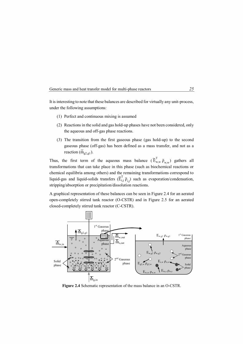
Generic mass and heat transfer model for multi-phase reactors 25

It is interesting to note that these balances are described for virtually any unit-process, under the following assumptions:

(1) Perfect and continuous mixing is assumed

(2) Reactions in the solid and gas hold-up phases have not been considered, only the aqueous and off-gas phase reactions.

(3) The transition from the first gaseous phase (gas hold-up) to the second gaseous phase (off-gas) has been defined as a mass transfer, and not as a reaction (mg2,g1).

Thus, the first term of the aqueous mass balance ( Ew,wT

ρw,w) gathers all transformations that can take place in this phase (such as biochemical reactions or chemical equilibria among others) and the remaining transformations correspond to liquid-gas and liquid-solids transfers (Ei,j

T ρi,j) such as evaporation/condensation,

stripping/absorption or precipitation/dissolution reactions.

A graphical representation of these balances can be seen in Figure 2.4 for an aerated open-completely stirred tank reactor (O-CSTR) and in Figure 2.5 for an aerated closed-completely stirred tank reactor (C-CSTR).

Figure 2.4 Schematic representation of the mass balance in an O-CSTR.

mw,in

mw,outAqueous

phase

1st Gaseous phase

2nd Gaseous phase

mg2,g1

mg,in

Solid phase

ms,outAqueous

phase

1st Gaseous phase

2nd Gaseous phase

Ew,g2 ρw,g2

Eg2,w ρg2,w

Ew,g1 ρw,g1

Ew,w ρw,w

Solid phase

Es,w ρs,w

Ew,s ρw,s

26 New systematic methodology for incorporating dynamic heat transfer modelling

Figure 2.5 Schematic representation of the mass balance in a C-CSTR.

This way of distinguishing the different phases and applying mass balances in each one, enables the modeller to construct systematically mathematical models as complex as required, considering different aqueous, gaseous or solid phases in a single unit-process. For example, in the case of layered models for settlers or biofilm systems in which biological reactions need to be included, each layer is considered to be an aqueous phase and mass transfers among them due to diffusion, convection or gravity effects are described by means of a stoichiometric matrix and kinetic vector.

The above is the usual and generalised form of models proposed. However, simplification can be made. The most remarkable is the gas transfer definition. In this transfer, it is possible to define the aeration of biological reactors or the introduction of a gaseous phase into the system with two gas phases (as previously described) or with a single gas phase (see Figure 2.6). The first option (2 gas phases) considers that the atmosphere and bubbles contained in the liquid have a different composition and temperature, and the second option considers similar features.

When the composition of the bubbles introduced/produced in the system (2nd gaseous phase) is very different from the off-gas phase (atmosphere for an open reactor, 1st gaseous phase) or when the importance of considering two different gas phases for the correct prediction of aquatic chemistry is critical, it is necessary to differentiate between two gas phases in the model (gas hold-up and off-gas phases, Figure 2.6 left). This would be the case where pure gases are introduced into the system, such

mw,in

mw,out

mg,out

Aqueous phase

1st Gaseous phase

2nd Gaseous phase

mg2,g1

mg,in

Solid phase

ms,out Aqueous phase

1st Gaseous phase

2nd Gaseous phase

Ew,g2 ρw,g2

Eg2,w ρg2,w

Eg1,w ρg1,w

Ew,g1 ρw,g1

Ew,w ρw,w

Solid phase

Es,w ρs,w

Ew,s ρw,s

Generic mass and heat transfer model for multi-phase reactors 27

as pure oxygen, when the reactors submergence is high or for systems with significant pH variations, in which this variation modifies or inhibits the system.

Figure 2.6 Schematic representation of the mass balance in an O-CSTR with two

gaseous phase (left) and one gaseous phases (right). Note: Only the transformation between phases in one direction has been considered in the figure.

In this case, the transfer between gas hold-up to off-gas phase is estimated by a transport term (mghu,off), and not by physico-chemical reactions as mentioned in the assumptions of the general model. Although mghu,off represents a system output, the gas outlet has a delay that will be equivalent to the path that the bubbles have to cover from the tank bottom to the surface. In this manner, this transport is a function of the up-flow velocity of bubbles and submergence, as these are the variables that establish the contact time; and the volume of the bubbles that depends on gas hold-up components mass and the pressure at a height half of the tank.

2.18

where, cs is the up-flow velocity [m d-1], Tghu and mghu represent the temperature [K] and the mass of the components present in the gas hold-up phase [gEcomp], respectively, R is the gas constant [J K-1 mol-1] and Pgoff is the atmospheric pressure [bar].

As shown in Figure 2.6, all transfers are defined as the multiplication of the kinetic vector and stoichiometry matrix. The difference between the two models (one gas phase and two gas phase models) is therefore the way in which these kinetic are

Vw

Vgoff

mw,in

mw,out

mg,out

mg,in

mw,pump

Vghu

Aqueous phase

1st Gaseous phase

2nd Gaseous phase

Vwmw,in

mw,out

mg,outmg,in

mw,pump

Aqueous phase

1st Gaseous phase

Vgoff

mghu,off

Eghu,w ρghu,wEw,goff ρw,goff Egoff,w ρgoff,w

mghu,off =cs

Submergence mghu

28 New systematic methodology for incorporating dynamic heat transfer modelling

assessed, more specifically, the manner in which the mass transfer coefficient (kLa) is estimated. In the two-phase model, the kLa is calculated as the multiplication of the kL/G parameter [m s-1] and the interfacial surface area to reactor volume ratio (a [m2 m-3]), as can be seen in equation 2.19 for gas hold-up and water transfer and in equation 2.20 for off-gas water transfer:

kLaghu = kL/Gghu

Aghu

Vw=kL/Gghu

6 mghu R Tghu

Vw db MW Pgoff + 12 Submergence

10.33

2.19

kLagoff = kL/Ggoff

Agoff

Vw 2.20

where, db is the bubble diameter [m] assuming spherical bubbles and Aghu and Agoff are the contact areas of gas hold-up and water and off-gas and water [m2], respectively (more information of this model in Lizarralde et al., 2015).

For cases in which a more simplified model wants to be used (one gaseous phase, Figure 2.6 right), it is possible to directly use an adaptation of the ASCE procedure (ASCE, 1984; 1991; 1997) to estimate the oxygen transfer coefficient (kLaO2) as a function of air flow and the system characteristics. In this case, it is necessary to know in greater detail the system characteristics, especially it is important to have the standard oxygen transfer efficiency (SOTE) of the diffusers used. The model describes a non-linear relationship between kLa and airflow or oxygen mass flow according to equation 2.21:

2.21

where, kLa is the ratio of process water to clean water mass transfer coefficient, FkLa is the diffusor fouling factor,Ti is the water phase temperature [K], kLa is the correction factor of transfer rate due to temperature and C*

is the oxygen saturation concentration [gO2 m-3]. The kLa coefficient for the other components of the gas phase can be estimated by relating the diffusivities (DL,comp).

kLa comp= kLa O2 DL,comp

DL,O2 2.22

kLa O2= αkLa FkLa θkLaTi-293

SOTE293 mg,in GO2

Vi C∞*

Generic mass and heat transfer model for multi-phase reactors 29

2.4.2. Description of the generic multi-phase heat transfer model

The completely mixing assumption commonly used in wastewater treatment plant process modelling permits thermal uniformity in the reactor, avoiding temperature gradients, and allowing the use of one-dimensional models. The heat transfer model proposed to describe multi-phase reactors is based on the first law of thermodynamics or on the declaration of the conservation of energy principle (equation 2.23) for control volumes.

2.23

where ET is the total energy [kJ], u is the internal energy [kJ g-1], P is the pressure [kPa], is the specific volume [m3 g-1], Ek is the kinetic energy [kJ d-1], Ep is the potential energy [kJ d-1], W is the power [kJ d-1], and Q is net heat exchange over a control volume [kJ d-1].

Considering negligible changes in kinetic and potential energies, a null accumulation of these terms and an absence of power, the heat transfer model proposed can be expressed as an enthalpy balance.

2.24

As for the mass balances, each phase (i) will have its enthalpy balance for the estimation of the total enthalpy of each of them (HT,i in kJ) and consequently the temperature (Ti in K).

The net heat exchange over the control volume can be expressed as a sum of several components contributing to the overall heat balance. These components are the heat transfers due to biochemical, chemical or physico-chemical transformations (Hr), conduction (Qphs,i,j in kJ d-1) and convection heat transfer fluxes (Q”i”c,out in kJ d-1), heat energy fluxes transmitted by the actuators (QAct for general use or Qm,in for mechanical heat transfers in kJ d-1) and short-wave (solar) and long-wave (atmospheric) radiation fluxes (Qsolrd and Qatmrd, respectively in kJ d-1). Considering the conduction/convection phenomena, heat fluxes transmitted by the actuators and radiation fluxes as advective heat fluxes, the overall heat balance has a similar structure to the mass balance, also considering transport phenomena and the effect of the transformations (equation 2.25).

dET

dt= min u + P υ + Ek + Ep in

– mout u + P υ + Ek + Ep out+ Q – W

d (h m)dt

= dHdt

= min hin– mout hout + Q = Hin – Hout + Q

30 New systematic methodology for incorporating dynamic heat transfer modelling

dHT

dt i =ΔHr + Hi

in

+ Hiout

+ Qphs,i,j + Qic,out + QAct +

Qsolrd + Qatmrd 2.25

Applying the methodology developed in this thesis to calculate the enthalpy of reaction (equations 2.9 and 2.12) and the multi-phase concept (equation 2.13), the heat transfer expression (equation 2.25) could be generalised to the equation 2.26.

dHT

dt i = – Δhf,i

TEi,i

T ρi,i – Δhf,i

TEi,j

T ρi,j +

NAP

j=1

Δhf,jT

Ej,iT

ρj,i + Hi,i

NC

comp=1

NAP

j=1

+ Hi,in

NC

comp=1

+ Hi,out+NC

comp=1

Qphs,i,j + Qic,out + QAct + Qsolrd + Qatmrd

2.26

Analysing the terms related to the transformations, the first term of the generic heat balance Δhf,i

TEi,i

T ρi,i refers to the heat associated to the transformations that

take place in the analysed phase, namely, biochemical and chemical reactions heat in the liquid enthalpy balance and combustion heat in the off-gas phase enthalpy balance.

The second term Δhf,iT

Ei,jT

ρi,j provides the stoichiometric enthalpies of formation of the components present in the interactions between the “i” phase and the “j” phase, but the term includes only the enthalpies of the analysed phase (“i” phase). And the third term Δhf,j

TEj,i

T ρj,i supplies the stoichiometric enthalpies

of formation of the components present in the interactions between the “i” phase and the “j” phase, but in this case, the term will only include the enthalpies of the adjacent phase ("j"). Applying the first law of thermodynamics, the sum of both terms (second and third terms of the generic heat balance) refers to the heat transferred due to the evaporation/condensation, stripping/absorption, precipitation/dissolution or deposition/sublimation reactions.

In such a transfer, besides heat production or consumption, an enthalpy associated to the matter is transferred between the phases (fourth term), producing an increase in the net heat of the target phase, though not of the specific heat of the components (Hi,i).

Generic mass and heat transfer model for multi-phase reactors 31

Based on mass balances (equations 2.14-2.17) and the assumptions made for these balances, the generic heat transfer balances corresponding to each phase are the following:

Aqueous phase mass balance:

dHT

dt w = – Δhf,w

TEw,w

T ρw,w –

Δhf,wT

Ew,g1T

ρw,g1 + Δhf,g1T

Eg1,wT

ρg1,w –

Δhf,wT

Ew,g2T

ρw,g2 + Δhf,g2T

Eg2,wT

ρg2,w –

Δhf,wT

Ew,sT

ρw,s + Δhf,sT

Es,wT

ρs,w +

Hw,g1

n

comp=1

+ Hw,g2

n

comp=1

+ Hw,s

n

comp=1

+ Hw,in – Hw,out –

Qphs,w,g1 –Qphs,w,g2 +Qm,in + Qwc,out + Qatmrd,c,w + Qsolrd,c,w– Qatmrd,o,w + Qsolrd,o,w

2.27

Gas hold-up phase mass balance:

dHT

dt g2 = Hg,in

z

i=1

+ Hg2,w

z

i=1

+ Hg2,g1

z

i=1

+Qphs,w,g2 2.28

Off-gas phase mass balance:

dHT

dt g1 = – Δhf,g1

TEg1,g1

T ρg1,g1 +

Hg1,w

m

i=1

+ Hg1,g2

m

i=1

– Hg,out

m

i=1

+Qphs,w,g1+

Qgc,c,out – Qatmrd,c,g1+ Qsolrd,c,g1

2.29

Solid phase mass balance:

dHT

dt s = Hs,w

o

i=1

– Hs,out

o

i=1

+ Qsc,out 2.30

where n, m, z and o are the number of state variables of the water, off-gas, gas hold-up and solid phases, respectively, Qsolrd,c,i and Qatmrd,c,i are solar and atmospheric radiation fluxes for fluids covered by solid materials and Qsolrd,o,i and Qatmrd,o,i are solar and atmospheric radiation fluxes for fluids in contact with the atmosphere. The

32 New systematic methodology for incorporating dynamic heat transfer modelling

positive terms represent heat gains or an increase in temperature and the negative terms represent heat losses or a decrease in temperature.

A graphical representation of these balances can be seen in Figure 2.8 for a C-CSTR and in Figure 2.8 for a C-CSTR.

Figure 2.7 Schematic representation of the heat balance in an O-CSTR (enthalpy changes of reaction have not been plotted).

Figure 2.8 Schematic representation of the heat balance in a C-CSTR (enthalpy changes of reaction have not been plotted).

After explaining the terms related to the enthalpy change of reaction, the approaches to modelling the individual contributions of each term are discussed below.

Hw,in Hw,outAqueous

phase

2nd Gaseous phase

Hg,in

Qwc,outQphs,w,g2Qsolrd,c,w

Qatmrd,c,wSolid phase

Hs,out

Qsc,out

Qm,in

Qphs,w,g1

1st Gaseous phase

Qsolrd,o,w

Qatmrd,o,w

Hw,in Hw,out

Hg,out

Aqueous phase

1st Gaseous phase

2nd Gaseous phase

Hg,in

Qgc,c,out

Qwc,out

Qm,inQphs,w,g1

Qphs,w,g2

Qsolrd,c,g1

Qsolrd,c,w

Qatmrd,c,w

Qatmrd,c,g1

Solid phase

Hs,out

Qsc,out

Hg2,g1

Hg2,w

Hw,g2

Hg1,g2

Hw,g1

Hg1,wAqueous

phase

1st Gaseous phase

2nd Gaseous phase

Solid phase

Hs,w

Hw,s

Hg2,w

Hw,g2

Hg1,g2

Hw,g1

Hg1,wAqueous

phase

1st Gaseous phase

2nd Gaseous phase

Solid phase

Hs,w

Hw,s

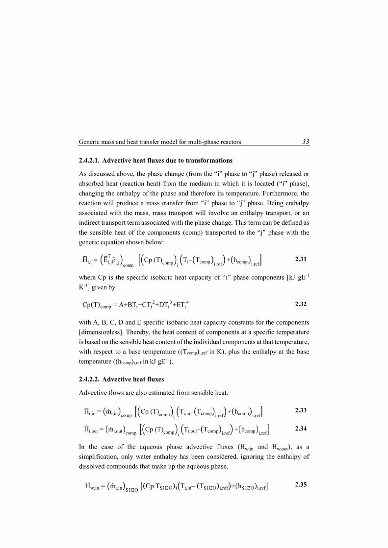
Generic mass and heat transfer model for multi-phase reactors 33

2.4.2.1. Advective heat fluxes due to transformations

As discussed above, the phase change (from the “i” phase to “j” phase) released or absorbed heat (reaction heat) from the medium in which it is located (“i” phase), changing the enthalpy of the phase and therefore its temperature. Furthermore, the reaction will produce a mass transfer from “i” phase to “j” phase. Being enthalpy associated with the mass, mass transport will involve an enthalpy transport, or an indirect transport term associated with the phase change. This term can be defined as the sensible heat of the components (comp) transported to the “j” phase with the generic equation shown below:

Hi,j = Ei,jT

ρi,j comp Cp (T)comp i

Ti– Tcomp i,ref+ hcomp i,ref

2.31

where Cp is the specific isobaric heat capacity of “i” phase components [kJ gE-1 K-1] given by

Cp(T)comp = A+BTi+CTi2+DTi

3+ETi4 2.32

with A, B, C, D and E specific isobaric heat capacity constants for the components [dimensionless]. Thereby, the heat content of components at a specific temperature is based on the sensible heat content of the individual components at that temperature, with respect to a base temperature ((Tcomp)i,ref in K), plus the enthalpy at the base temperature ((hcomp)i,ref in kJ gE-1).

2.4.2.2. Advective heat fluxes

Advective flows are also estimated from sensible heat.

2.33

2.34

In the case of the aqueous phase advective fluxes (Hw,in and Hw,out), as a simplification, only water enthalpy has been considered, ignoring the enthalpy of dissolved compounds that make up the aqueous phase.

2.35

Hi,in = mi,in comp Cp (T)comp i

Ti,in– Tcomp i,ref+ hcomp i,ref

Hi,out = mi,out comp Cp (T)comp iTi,out– Tcomp i,ref

+ hcomp i,ref

Hw,in = mi,in SH2O (Cp TSH2O)i Ti,in– (TSH2O)i,ref +(hSH2O)i,ref

34 New systematic methodology for incorporating dynamic heat transfer modelling

2.36

2.4.2.3. Conduction heat fluxes

The conduction is the heat transfer from the more energetic phase to the adjacent less energetic phase. Due to the low thermal conductivity of liquids (between 0.2 and 8 W m-1 K-1; Ҫengel, 1997) and gases (0.03-0.3 W m-1 K-1; Ҫengel, 1997), only heat transfer by conduction of solid phases has been considered. Analysing the heat balances, there are three possibilities: the enthalpy lost/gained through wall and pipes by conduction in the aqueous (Qwc,out) and off-gas (Qgc,out) phases and the heat transfer between the liquid and the solid phase (Qsc,out). The expression to estimate the heat conduction is known as Fourier’s law.

Qic,c,out = – ktherm

LAcontact ∆T 2.37

where ktherm is the thermal conductivity of the material which is a measure of the ability of the material to conduct heat [W m-1 K-1], T is the temperature difference across the layer [K], L is the thickness of the material used in the transfer [m] and Acontact is the contact area [m2].

If the analysed phase is in contact with more than one different solid surfaces, as many terms of thermal conductivity as solid surfaces will be raised.

2.4.2.4. Convection heat fluxes

Convection is classified as natural or forced convection, depending on how the fluid motion is initiated. In forced convection the fluid is forced to move over a surface by external means and it is strong function of velocity. In contrast, in the natural convection the fluid motion is much lower (typically under 1 m s-1) and normally the motion occurs by natural means such as buoyancy.

In this thesis the fluid velocity (uw in m s-1) has been used to classify heat transfers by forced or natural convection. Velocities greater than or equal to 1 m s-1 will be considered forced convection (convection between the liquid phase and the first gas phase for almost all open unit-processes) and less than 1 m s-1 natural convection (convection between the liquid phase and the first gas phase for all closed reactors and convection between the liquid phase and the gas hold-up phase of any reactor).

Hw,out = mi,out SH2O (Cp TSH2O)i Ti,out– (TSH2O)i,ref +(hSH2O)i,ref

Generic mass and heat transfer model for multi-phase reactors 35

For all these options, the rate of convection heat transfer is proportional to the temperature difference, and it is expressed by Newton’s law of cooling as

Qphs,i,j = hphs Acontact ∆T 2.38

where hphs is the convection heat transfer coefficient [kJ m2 K-1].

Forced Convection heat fluxes (open unit-processes with fluid velocities above 1 m s-1)

The hphs is closely related to the dimensionless Nusselt number (Nu). In forced convection, Nu can be estimated from the dimensionless Reynold (Re) and Prandtl (Pr) numbers as

Nu = hphs Lktherm

= Cphs Remphs Prnphs 2.39

where Cphs, mphs and nphs are constants, ktherm is the thermal conductivity of the fluid [W m-1 K-1] and L is the length of the plate in the flow direction [m]. The Reynolds number relates the inertial forces to viscous forces in the fluid from the following expression:

Re = uw δ

υj 2.40

where is the characteristic length of the geometry [m] and j is the kinematic viscosity of the fluid in the “j” phase [m2 s-1] given by

υj = η(T)comp j

Tj R

105 Pj MWcomp Xcomp,j icomp j

NE

EL=1

m

comp=1

2.41

with Xcomp,j the mass fraction of the “j” phase components [gEi gEphase-1], comp

the dynamic viscosity [g m-1 s-1] in function of the phase temperature [Tj in K], R the gas constant [J K-1 mol-1], Pj the pressure of the gaseous phase [bar], NE the number of elements and icomp j the conversion factor vector that relates the elemental mass of each element (EL) and the stoichiometric unit of the components of the “j” phase [gelement gE-1].

36 New systematic methodology for incorporating dynamic heat transfer modelling

The dimensionless Prandtl number is defined as the ratio of momentum diffusivity to thermal diffusivity in form of

Pr = η(T)comp j

Cp(T)comp j

ktherm,comp Xcomp icomp j

NE

EL=1

m

comp=1

2.42

Depending on whether the flow is laminar (Pr 0.6) or a combination of laminar and turbulent flows (0.6 Pr 60 and 5·105 Re 107), the equation 2.39 will take the following values:

Nu = 0.664 Re0.5 Pr1 3⁄ (Pr ≥0.6) 2.43

Nu = 0.037 Re0.8-871 Pr1 3⁄ (0.6 ≤ Pr ≤ 60) & 5·105 ≤ Re ≤ 107 2.44

Natural Convection heat fluxes (closed reactors or open unit-processes with fluid velocities under 1 m s-1)

In natural convection, the hphs depends on the dimensionless Grashof (Gr) and Prandtl numbers. The structure is very similar to that defined for forced convection.

Nu = hphs δktherm

= Cphs (Gr Pr)nphs 2.45

In this case, Grashof number presents the ratio of the buoyancy force to the viscous force. That is,

Gr = g βphs Tw-Tj δ3

υcomp2 Xcomp icomp j

NE

EL=1

m

comp=1

2.46

where g is the gravitational acceleration [m s-2] and phs is coefficient of volume expansion [K-1].

For the case of natural convection also there are different approaches of equation 2.39. For horizontal plates, the expressions are the following:

Nu = 0.54 (Gr Pr)0.25 104 ≤ (Gr Pr) ≤ 107 2.47

Generic mass and heat transfer model for multi-phase reactors 37

Nu = 0.15 (Gr Pr)1 3⁄ 107 ≤ (Gr Pr) ≤ 1011 2.48

2.4.2.5. Shortwave solar radiation heat fluxes

The net energy input from the sun to the unit-process is a function of the time of the year, latitude and meteorological conditions or cloud cover (Makinia, 2010). The estimate of this energy can be done in two ways: using data directly from meteorological stations or using empirical equations for its estimation (Argaman and Adams, 1977; Talati and Stenstrom, 1990; La Cour Jansen et al., 1992; Sedory and Stenstrom, 1995; Scherfig et al., 1996; Allen et al., 1998).

Most solids materials, such as metals, wood, bricks or rocks are opaque to the thermal radiation. In these opaque materials, the radiation is considered to be a surface phenomenon. The radiation incident on these bodies is only absorbed into a few microns to within the solid, without penetrating to the flux contained in the units (null transmissivity). This is the reason that, radiation heat transfers to liquid or gaseous fluids covered by solid materials can be considered zero. Despite this, radiation fluxes have been included in the energy balances, as there are materials that allow transmissivity, although these are not typical materials in WWTs (glass, certain plastic materials and some minerals).

In this thesis, the expression for estimating the solar radiation transmitted to the system (Qsolrd) is based on direct measurements of the total energy incident to the surface (ksolrd in kJ d-1 m-2) provided by meteorological stations, corrected with the solar transmissivity of the fluids (rad) for phases in contact with the atmosphere (2.49) and corrected with the solar absorptivity (rad) and transmissivity for fluids covered by solid materials (or the reflectivity, rad = 1 - rad - rad; equation 2.50).

Qsolrd,c,i = τrad ksolrd Acontact 2.49

Qsolrd,o,i = (αrad+ τrad) ksolrd Acontact 2.50

2.4.2.6. Longwave atmospheric radiation heat fluxes

The atmospheric radiation is the longwave radiation energy emitted or reflected by the constituents of the atmosphere. The estimation of atmospheric radiation is based

38 New systematic methodology for incorporating dynamic heat transfer modelling

on the Stefan-Boltzmann’s fourth power radiation law as the difference between the absorbed and emitted radiation from the following expressions:

Qatmrd,c,i = σ Acontact εi · Ti* 4

–(τrad)βrad Tatm* 4

2.51

Qatmrd,o,i = σ Acontact εi · Ti* 4

– 1-ρrad βair Tatm* 4

2.52

where is the Stefan-Boltzmann’s constant [5.67·10-8 W m-2 K-4], is the emissivity of the analysed phase, Tatm is the atmospheric temperature [K], rad is the atmospheric radiation factor which is a function of the cloud and vapour pressure (Raphael, 1962) and the superscripts * indicate absolute temperature [ºC].

2.4.2.7. Heat energy fluxes transmitted by the actuators

Finally, the actuators do not have a 100 % efficiency (act). When these actuators are immersed in a phase, the energy not used in its action (1-act) is released as heat to the phase, increasing the temperature of the medium by the following expression:

QAct = WAct 1-ηAct 2.53

where Wact is the power supplied by the actuators [kJ d-1].

2.5 SUMMARY In view of the importance of correct heat transfer estimations in the context of wastewater treatment plants upgrading and optimisation, this Chapter provides a systematic methodology for estimating enthalpy changes of reaction, from the enthalpies of formation of each component. The methodology allows the overall estimate of the enthalpy change of reaction whatever the transformations that take place in the system. For any new reaction that wants to be introduce in the model, if the components are defined, the reaction enthalpy of this transformation will be estimated automatically without the need to look for it in literature.

One of the most important aspects that has enabled the systematisation of the methodology has been the detailed characterisation of the components that provides the E-PWM methodology, a key factor in a correct prediction.

Summary 39

The second step of this Chapter has been the development of generic mass and heat transfer models for multi-phase reactors using this automatic methodology for estimating the enthalpy change of reaction.

With the purpose to develop flexible and easily understood models, this thesis proposed the restructuring of traditional modelling approach by a phase differentiation. Each phase will be an independent system with its corresponding mass vector, stoichiometric matrix and kinetic vector. This way of distinguishing the different phases and applying mass and heat balances in each one will allow the modeller to construct systematically mathematical models as complex as required, considering different aqueous, gaseous or solid phases in a single unit-process. In this manner, thanks to the compartmentalisation, the heat produced in each phase will be estimated independently, allowing the quantification of heat transfers between different phases mechanically.

It is worth mentioning that the methodology described in this Chapter has allowed the updating of the PWM methodology. Thereby, with the incorporation of the heat transfer model described in this Chapter, the cost models described in Chapter 3 and the physico-chemical model (PC-PWM) described in Lizarralde et al. (2015), a new version of this PWM methodology called Extended Plant-Wide Modelling (E-PWM) methodology has been developed.

40 New systematic methodology for incorporating dynamic heat transfer modelling

41

3

DEFINITION OF COST MODELS

A summary of this Chapter has been published in:

Fernández-Arévalo, T., Lizarralde, I., Pérez-Elvira, S.I., Garrido, J.M., Puig, S., Poch, M., Grau, P., Ayesa, E., 2015. Conceptual design and comparative assessment of WWTP layouts based on plant-wide model simulations. Oral presentation at the 9th IWA Symposium on System Analysis and Integrated Assessment (Watermatex15). Gold Coast, Australia, 11-14 June.

Fernández-Arévalo, T., Grau, P., Jeppsson, U., Mauricio-Iglesias, M., Vrecko, D., Flores-Alsina, X., Ayesa, E., 2017. Model-based comparative assessment of innovative processes. In Lema, J.M., Suarez-Martinez, S. (Eds.), Innovative wastewater treatment & resource recovery technologies. Impacts on energy, economy and environment, IWA Publishing. ISBN13: 9781780407869

3.1 ABSTRACT This Chapter offers a comprehensive library of operating costs models for the correct prediction of the expenses in a wastewater treatment plant. As will be detailed

42 Definition of cost models

throughout the Chapter, the models are adaptations of engineering expressions, rewritten to achieve a compatibly with the PWM methodology.

3.2 INTRODUCTION The increase in energy prices (according to EUROSTAT 2016, 0.0756 € kWh-1 in 2005, 0.1039 € kWh-1 in 2010 and 0.1207 € kWh-1 in 2015 on average in the EU-28) has led to a growing interest in WWTs optimisation. The aims of plants optimisations, which until recently focused mainly on ensuring effluent quality, have been extended to a broader frame that includes the optimal use of resources and energy.

The treatment of wastewater is an energy-intensive activity. The power required for the treatment of urban wastewater in Spain is approximately 300 MW, equivalent to an average of 5.6 W PE-1 or a consumption of 50 kWh PEyear

-1. In other words, the purification of the 3,000 hm3 year-1 of municipal wastewater generated on average in Spain represents 1 % of national energy consumption (AEDyR, 2010). A survey of the US Protection Agency indicates that an estimated 3 % of USA energy consumption is used for drinking water and wastewater services and 1 % and 3 % in Sweden and in the UK, respectively, while in Israel it is around 10 % (Olsson, 2013).

For conventional WWTPs energy consumption distribution, the aeration system is the process that consumes more energy, reaching values of up to 50 %, followed by pumping, flotation and sludge treatments (WEF 2009). A distribution of energy usage in a typical wastewater treatment plant employing the activated sludge process can be seen in Figure 3.1. Framing the energy consumed in a global balance, electricity consumption can entail the 19 % of the overall costs (Figure 3.2). The amount of energy required for the general plant or for these individual processes is highly variable depending on the influent characteristics, effluent quality, the size of the plant and the technologies used for the treatment.

Under this energy framework, it seems clear the need to study how this energy is produced in the different elements or actuators involved in the plant to try to identify potential areas for improvement and optimisation.

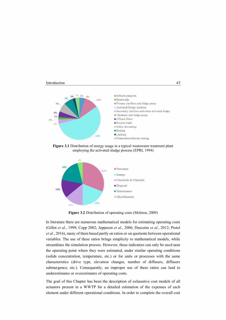
Introduction 43

Figure 3.1 Distribution of energy usage in a typical wastewater treatment plant

employing the activated sludge process (EPRI, 1994)

Figure 3.2 Distribution of operating costs (Molinos, 2009)

In literature there are numerous mathematical models for estimating operating costs (Gillot et al., 1999; Copp 2002; Jeppsson et al., 2006; Descoins et al., 2012; Pretel et al., 2016), many of them based partly on ratios or on quotients between operational variables. The use of these ratios brings simplicity to mathematical models, while streamlines the simulation process. However, these indicators can only be used near the operating point where they were estimated, under similar operating conditions (solids concentration, temperature, etc.) or for units or processes with the same characteristics (drive type, elevation changes, number of diffusers, diffusers submergence, etc.). Consequently, an improper use of these ratios can lead to underestimates or overestimates of operating costs.

The goal of this Chapter has been the description of exhaustive cost models of all actuators present in a WWTP for a detailed estimation of the expenses of each element under different operational conditions. In order to complete the overall cost

44 Definition of cost models

balance in a plant, different specific costs have been proposed in order to relate the operating costs of a unit-process with the flow or the fluid characteristics.

3.3 ACTUATOR MODELS To avoid potential issues and to create flexible and useful models, all actuator models presented in this Chapter have been developed by engineering expressions, instead of directly using experimental ratios or cost curves. The engineering expressions used depend closely on the operational variables of the process (flowrates, enthalpy changes of reaction, solids concentration, etc.), allowing a more realistic and dynamic estimate.

3.3.1. Stirrer engine cost models

Depending on the purpose of mixing in the model (mixing of one substance completely with another, flocculation of wastewater particles, continuous mixing of liquid suspensions or heat transfer), the mathematical models used to estimate the agitation costs have been classified as models based on the maintenance of particles in suspension or models based on the average velocity gradient.

3.3.1.1. Stirrers used for maintaining solids in suspension

The anoxic and anaerobic reactors should be stirred to avoid settling and to keep solids in suspension. In these cases, submersible mechanical agitators are widely used in WWT processes to maintain this suspension conditions. The required energy depends largely on reactor volume and geometry, agitator type, suspended particles diameter and density of the medium. Even so, in the estimation of this stirring energy, the specific power (W m-3) has been used extensively in literature, only considering the reactor volume as operating variable and omitting key factors such as the mixed liquor suspended solids (MLSS) concentration.

Given the large variability found in literature, with variations between 3 and 14 W m-3 (US EPA, 1979; Zakkour et al., 2001; Tchobanoglous et al., 2003; Zaher et al., 2009), and based on the works of Olsson (2011) and Thöle (2008), which discussed the possibility to use specific powers of 2-3 W m-3 without comprising the agitation, this thesis proposes a theoretical expression for estimating the energy needed to keep particles in suspension.

Actuator models 45

Thus, equation 3.1 is based on the estimation of the minimum energy to just suspend the particles (Zaher et al., 2009), multiplied by a safety factor (Foversize).

Wstir= NPφS Njs

3 Dstir5

ηstirFoversize 3.1

where NP is the power number of the impeller, Dstir is the impeller diameter [m], i is the density of the “i” phase [kg m-3], stir and Wstir are the efficiency and the electrical consumption [W] of the stirrer engine, respectively, and Njs is the impeller rotational speed for off-bottom suspension of solids particles [Hz, rps] given by the equation proposed by Zwietering (1958).

Njs= Sg φs-φw

φw

0.45XTSS

0.13dp0.2υw

0.1

Dstir0.85 3.2

with S the impeller/tank geometry factor, XTSS the weight percentage of solids in the suspension and dp the average diameter of the solid particles [m].

A stirring speed of less than Njs will conduct a solids deposition on the tank floor. In turn, to ensure that all this solids are distributed throughout the whole depth, the modified Froude number (Fr) must be greater than 20 (Tatterson, 1994). If the value is smaller, the value of Njs should be recalculated to ensure the solids distribution.

Fr = φW Njs

2 Dstir2

g φS-φW dp

dp

Dstir

0.45

> 20 3.3

3.3.1.2. Stirrers used for rapid mixing or flocculation

Continuous rapid stirring is used to bind chemicals with wastewater or to add chemicals to sludge and biosolids to improve their dewatering characteristics (Tchobanoglous et al., 2014). For these types of mixing the equation proposed by Camp and Stein (1943) is widely applied in engineering, which relates the power required for mixing with the average velocity gradient, G [s-1].

Wstir= G2 ηw Vw 3.4

where Vw and w are the volume [m3] and the dynamic viscosity [kg m-1 s-1] of the liquid phase. Typical values of G can be found in literature, being a dependent parameter of the analysed case and operational conditions. Analysing the equation

46 Definition of cost models

3.4, it can be seen that the aim of the G parameter is similar to the specific power ratio (W m-3), with the difference that this expression also considers the properties of the medium (w).

3.3.2. Hydraulic pump models

Centrifugal pumps for lifting water and sludge and positive displacement pumps for pumping high concentrated liquids (primary, thickened or digested sludge) are the most used pumps (WEF, 2009).

In this thesis, pumps have been designed as units without volume or point models where the mass is not accumulated so no reactions occur.

3.5

The pumping energy consumption is closely related to the head loss (HL in m) of the distribution system. Thereby, the pumping power (Wpump in W) can be estimated by the following expression:

Wpump = φw g Qw,in HL ηpump 3.6

where Qw is the propelled flow [m3 s-1] and pump is the efficiency of the pump. No bomb has a 100 % efficiency. Therefore these hydraulic and friction losses will be transformed into heat and transmitted to the fluid. The temperature variation is usually minimal, but it is possible to estimate the enthalpy change using the following expression:

Hw,out = Hw,in+Wpump 1-ηpump 3.7

3.3.3. Blower and compressor models

There are four types of blowers commonly used in WWT processes: single-stage centrifugal, multi-stage centrifugal, high speed turbo and positive displacement blowers (Tchobanoglous et al., 2014). However, centrifugal blowers are the most used.

As with the pumps or like the rest of actuators, the blowers have been designed as units without volume, according to the mass balance of the equation 3.5. The goal of

mw,in = mw,out

Actuator models 47

this model is the estimate of the energy absorbed in the compression of any gaseous phase to overcome all the head losses of the system (the head losses inside the pipe network, submergence of the aeration system and aeration elements). Thus, this power depends on the compressor outlet pressure and the gas flow that wishes to supply to the tank.

The blower model selected to estimate the energy required in the gaseous components compression (Wblow in W) is based on the supposition of an adiabatic irreversible compression as shown in equation 3.8.

3.8

where g,comp is the heat capacity ratio of the gaseous phase components, blow is the efficiency of the blower and Pg,in and Pg,out are the absolute gas pressures at the blower/compressor inlet and outlet, respectively [bar].

For the adiabatic irreversible pressure variation of any ideal gas, the temperature variation is defined as

3.9

Even so, usually the compressors are provided with a cooling jacket for circulating water or other coolant maintaining the temperature of the gas phase (Tg,out = Tg,in).

3.3.4. Turbine model

Gas and steam turbines generate power by expanding hot combustion gases or steam. In wastewater treatment processes, the turbines are mainly used in systems for the production of energy, such as incineration processes and cogeneration units, transforming the energy content of the components into electrical energy.

The turbine model selected to estimate the energy production (Wturbine) is based on the supposition of an adiabatic irreversible expansion. This expansion can be conducted in one step or two steps, depending on the needs of the system (Figure

Wblow=

⎣⎢⎢⎢⎡ mg,in comp

R Tg,in

(MW)comp γg,comp–1

γg,comp ηblow⎦

⎥⎥⎥⎤m

comp=1

Pg,out

Pg,in

γg,comp-1γg,comp

–1

Tg,out = Tg,in

ηblow

⎝

⎜⎛ mg,in comp

∑ mg,in compmcomp=1

Pg,out

Pg,in

γg,comp-1γg,comp

– 1–ηblow

⎠

⎟⎞

m

comp=1

48 Definition of cost models

3.3). When expansion is carried out in two steps, the intermediate pressure/temperature has to be defined.

Figure 3.3 T-S diagrams for water: left) one step reversible (1→3) and irreversible (1→3’) expansion; and right) two step reversible (1→2 and 2→3) and irreversible

(1→2’ and 2’→3’) expansions

The expression for calculating the power of expansion of each step is shown in equation 3.10.

3.10

And the output temperature of an ideal gas is defined as

3.11

where turb is the efficiency of the turbine.

3.4 SUPPORT MODELS For the definition of operating costs, it is necessary to define additional models that act as support for actuator models. These elements provide the input for actuator models (water/air distribution models) and transform the estimated power in monetary unit (electricity/cost conversion model).

Wturbine=

⎣⎢⎢⎢⎡ mg,in comp

R Tg,in

(MW)comp γg,comp-1γg,comp ⎦

⎥⎥⎥⎤m

comp=1

ηturb −Pg,in

Pg,out

1−γg,compγg,comp

Tg,out = Tg,in

⎝

⎜⎛ mg,in comp

∑ mg,in compmcomp=1

Pg,out

Pg,in

γg,comp-1γg,comp

+ 1–ηturb

⎠

⎟⎞

m

comp=1

Support models 49

3.4.1. Water/Air distribution model

The aim of pumps or blowers is to drive a fluid between two points (1→2). The pressure transmitted by actuators to fluid must be enough to overcome the heat losses (HL) of the intermediate elements and reach point 2. The goal of this model is to estimate these losses and provide the minimum output pressure for blower models or the global HL for pumps.

Pi,out = Pi,out+ HL φi g · 10-5 3.12

These losses depend closely on the water or gas distribution system of the plant under study, and it is difficult to make a generalisation that satisfies all processes. In this frame, the distribution system model is the only model of this thesis that cannot be standardised and therefore needs a detailed plant layout in which the pipe lengths and diameters, the height variations and material specifications are defined.

The head losses are caused mainly by the difference in levels (or static head, HLs), by the friction of the fluid particles among themselves and against the walls of the pipe that contains (friction head loss, HLf) and by singularities at specific points such as elbows, inlet and outlet structures, branches and pipe fittings among others (minor losses, HLl).

HL = HLs + HLl + HLf 3.13

Static losses are calculated directly with the elevation difference between the two points. The friction head loss in a pipe, can be estimated using the Darcy-Weisbach expression (Weisbach, 1845):

HLf = fmoodyLpipe

Dpipe

uw

2 g 3.14

where fmoody is the friction factor obtained from Moody diagram and Dpipe and Lpipe are the pipe diameter and equivalent length [m], respectively.

Finally, the minor losses can be defined as equivalent pipe lengths (L/D), allowing the application of the equation 3.14 (For more information on the values consult Albright, 2009).

50 Definition of cost models

The information needed to estimate these head losses, is not always available, or a high degree of detail is not always required in the study. For these cases, it is possible to apply the expression of equation 3.15, widely used in design (CEDEX, 2004):

Pg,out=φW g (Submergence [m] +1) 10 3.15

3.4.2. Electricity/cost conversion model

The main operating costs in WWT processes are electricity power and raw material costs. In order to analyse all of them together, it is required to transform the power of actuators (Wactuator kJ d-1) to a monetary unit (MU, € kJ-1).

Costactuator=Wact MU 3.16

3.5 SPECIFIC ENERGY AND COST MODELS Some operational costs cannot be defined with actuator models described or is difficult to obtain the information for its estimate. In other cases, simple model want to be used even knowing that it is possible to make a miscalculation (overestimating or underestimating). For all these cases, there are functions or ratios to calculate these costs or these energy consumptions which are considered specific, i.e., energy and costs that depend on the influent fluid flow (kWh m-3), unit solids mass flux (kWh tDS-1) or the price of the raw material (€ d-1).

3.5.1. Specific energy ratios

A list of the most used specific energy ratios can be seen in Table 3.1. As shown in the table, most ratios depends on influent water flow and a few of them on the solids concentration fed to the unit. If both possibilities are tabulated, the second option is the most accurate, as it considers operating variables.

Specific energy and Cost models 51

Table 3.1 Typical energy consumptions of various treatment processes on wastewater treatment.

Treatment Energy Consumption Ref.

Wastewater influent pumping 0.032-0.045 kWh m-3 [1] Screens 0.0003-0.0005 kWh m-3 [2] Aerated grit removal 0.003-0.013 kWh m-3 [1] Primary settling 0.010 kWh m-3 [1] Tricking filters 0.061-0.093 kWh m-3 [1] Activated Sludge for COD removal 0.14 kWh m-3 [1] Activated Sludge with nitrification/denitrification

0.23 kWh m-3 [1] Membrane bioreactor 0.5-1.0 kWh m-3 [3] Return sludge pumping 0.008-0.013 kWh m-3 [1] Secondary settling 0.003-0.004 kWh m-3 [2] Dissolved air flotation 0.03-0.053 kWh m-3 [1] Sludge pumping 0.0008 kWh m-3 or

0.05 kWh m-3 (*) [1] [4]

Sludge thickening (gravity belt) 0.0003-0.0016 kWh m-3 or 30 kWh TDS-1

[2] [5]

Sludge thickening (centrifuge) 300 kWh TDS-1 [5] Aerobic Digestion 0.13-0.32 kWh m-3 [2] Mesophilic anaerobic digestion 0.093-0.16 kWh m-3 [2] Mesophilic anaerobic digestion 0.093-0.16 kWh m-3 [2] Anaerobic Membrane Bioreactor 250 kWh TDS-1 (**) [6] Sludge dewatering (centrifuge) 0.005-0.013 kWh m-3 [2] Sludge dewatering (belt filter press) 0.0005-0.00013 kWh

m-3 or 50 kWh TDS-1 [2] [7]

[1] Burton, 1996; [2] Tchobanoglous et al., 2014; [3] Krzeminski et al., 2012; [4] Foley et al., 2010; [5] Albertson et al., 1987; [6] Judd, 2011; [7] Mills et al., 2014.

(*) function of pumped flow (**) function of treated flow

3.5.2. Dosage cost models

In cases in which the chemical agent reacts with the ions of the medium, it is possible to estimate the cost of the chemical agent dosage directly (Costdosage in € d-1), as the chemical agent is a component of the model (e.g. chemical phosphorus removal with FeCl3). For these cases, the only data required is the specific cost of the chemical agent (CostChem in € kg-1). In contrast, in cases where the chemical agent improves a

52 Definition of cost models

transformation of a physical property of the system (e.g. the addition of FeCl3 to improve the sedimentation process or the addition of polyelectrolyte to improve the dewaterability) it is necessary to use experimental relations for its estimation. In literature, it is possible to find information that relates the dosage of chemical with process variables. This is the case of using the ratio kpoly,sludge [gpoly kgTSS

-1] to estimate the poly-electrolyte dosage costs to improve the dewaterability,

Costdosage=CostChem· TSSsludge Qw kPoly,sludge

Nº of kinds of sludge

sludge=1

3.17

or the ratio kCEPT [gchem m-3] to estimate the addition of chemical in the Chemically Enhanced Primary Treatment (CEPT, an adaptation of the expression of Tik et al., 2013):

Costdosage=CostChem Qw,in

kCEPTnCEPT 1-

ηmax-ηCEPTηmax-ηmin

ηmax-ηCEPTηmax-ηmin

1 nCEPT

3.18

where the subscript sludge is the kind of sludge analysed, i.e., primary sludge, secondary sludge, digested sludge, etc., nCEPT is the CEPT constant and max, min and CEPT are the maximum, minimum and real CETP efficiencies, respectively.

3.6 UNIT-PROCESS MODELS COMPOSED OF ACTUATORS

The four actuators described (pump, blower, mixer and turbine) can be used and combined in numerous processes. This section briefly describes the unit processes defined from these models, i.e., more complex unit-processes composed of sub-unit-process and sub-actuator models, such as the incineration plant and the different cogeneration processes. The main characteristic of these unit-processes is that all models are composed of algebraic equations or point models, so all reactions and transformations will be considered instantaneous.

Unit-process models composed of actuators 53

3.6.1. Cogeneration unit models

In the cogeneration unit (or combined heat and power system, CHP), the biogas generated in the anaerobic digester is converted into thermal energy (cooling water, Hw,out; and heating gas, Hg,out) and electricity (WCHP). The most common facilities at WWTPs are combustion engines (available for an operating range less than 5 MW, US EPA, 2008) and micro-turbines (available in the range of 30 kW-250 kW, US EPA, 2008) connected to generators (Tchobanoglous et al., 2014).

A micro-turbine is a compact system that combines a gas turbine (T), a gas compressor (GC), a combustion chamber (CC) and a heat exchanger (HE). In micro-turbine cogeneration plant models, the air (mg,in2) in excess (Excair) is compressed isentropically before being supplied to the combustion chamber along with the biogas (mg,in1). The hot exhaust gases produced in the combustion chamber (up to 950 ºC to avoid turbine damages, US EPA, 2008) are expanded to an approximate temperature of 550 °C generating electricity (15-30 % depending on the exhaust gases temperature before and after expansion, fuel composition and compression and expansion efficiencies). Finally, the exhaust gases are cooled to a temperature close to 120 °C (US EPA, 2008), using the heat exchanged (45-50 % of the combustion energy) to produce steam or hot gases.

The combustion engine model instead consists of a combustion engine (CE) and two heat exchangers. In combustion engine cogeneration plant models, biogas is oxidised in the combustion engine releasing heat and producing electricity in the engine itself. The first heat recovery stage is carried out by cooling the engine by means of engine jacket water and auxiliary oil cooling loops, in which 20 % (ADBA, 2013) of the energy is recovered as hot process water ( 90 ºC). The exhaust gases leave the engine at a temperature of about 550 °C (Jacobs et al., 2009), transforming the rest of the energy into electrical power (approximately 37-42 %). Finally, as in the gas turbine cogeneration plant, the exhaust gases are cooled to a temperature close to 150 °C (CH2M HILL, 2007) to produce steam or hot gases (35-43 % of the produced energy).

The models proposed for both processes are similar, differing mainly at the point where the electrical energy is produced (turbine or combustion engine). The fuel oxidation is considered an instantaneous reaction of complete combustion, so the waste can be considered zero (mw,under=0). A schematic representation of the mass and energy balances is presented in Figure 3.4 and Figure 3.5.

54 Definition of cost models

Figure 3.4 Schematic representation of the mass and energy balances of a cogeneration

plant with micro-turbine connected to generator

Figure 3.5 Schematic representation of the mass and energy balances of a cogeneration plant with combustion engine

Enthalpies at each point of the system can be calculated using equation 2.35 and equation 2.33 which describe the sensible heat of liquid and gas phases respectively, the changes of temperature due to the compression and expansion of gases using equation 3.9 and equation 3.11 and the power required for compression and the power released in the expansion by the equations 3.8 and 3.10 respectively. The remaining balances are presented below.

Mass balances of both models:

3.19

CC

HE

~

mg,exh

mw,under mg,exh

T

mg,in1

mg,in2

mg,in3mg,out

GC

CC

HE

~

Hg,CC,out

Hw,under Hg,exh

T

Hg,in1

Hg,in2

Hg,in3Hg,out

Hg,T,out

GC

Qgc,c,CC,out

WCHP

mg,exh

Qgc,c,HE,out

Hg,C,out

CE

HE

mg,exh

mw,under mg,exh

mg,in1

mg,in2

mg,in3mg,out

CE

HE

Hg,CE,out

Hw,under Hg,exh

Hg,in1

Hg,in2

Hg,in3Hg,out

Qgc,c,CE,out

Hw,in Hw,out

~ ~

WCHP

mw,in mw,out

Qgc,c,HE,out

mg,exh Comp=mg,in1+ mg,in2+

Eg1,g1 CH4_Combust Comp

Eg1,g1 CH4_Combust GCH4

mg,in1 GCH4

Unit-process models composed of actuators 55

3.20

3.21

3.22

Energy balances of micro-turbine cogeneration plant model:

3.23

3.24

Energy balance of combustion engine cogeneration plant model:

3.25

3.6.2. Incineration unit model

Incineration is an advanced thermal oxidation of sludge and biosolids used for the conversion of organic matter into oxidised end products. The incineration unit model consists of a fluidised bed (FB), a steam turbine (T), three heat exchange units (HE1, HE2 and HE3), an air condenser (AC), two pumps (P1 and P2) and a degassing tank (D). In the FB, the soluble and particulate COD present in the sludge is oxidised with preheated air (following equation 2.3) to produce exhaust gases and ashes. Oxidation produces heat which is released into the unit. If the COD present in the sludge does not produce enough heat to get the combustion temperature (due to the high amount of non-biodegradable material or low sludge dryness), natural gas will be introduced in the chamber. The heat accumulated in the exhaust gases is then transferred to a water circuit in order to produce electricity.

In the proposed incineration model, 3 assumptions have been made:

mg,in2 Comp= mg,in1 GCH4

Eg1,g1 CH4_Combust GO2

Eg1,g1 CH4_Combust GCH4

XComp

XGO2Excair

mw,in = mw,out

mg,in3 = mg,out

Hg,CC,out= – mg1,in GCH4 Eg1,g1 Δhf,g1 CH4_Combust

–

mg,exh – mg,in1+ mg,in2 GH2O Ew,g1 Δhf,w – Eg1,w

Δhf,g1 H2O_Evaporation+ Hg,in1

m

i=1

+ Hg,GC,out

m

i=1

– Qgc,c,CC,out

WCHP= Wturbine − Wblow

WCHP= Hg,in1

m

i=1

+ Hg,in2

m

i=1

– mg1,in GCH4Eg1,g1 Δhf,g1 CH4_Combust

–

56 Definition of cost models

(1) The COD oxidation is considered an instantaneous reaction of complete combustion.

(2) Ashes consist of phosphates and inorganic inert matter (XII).

(3) The ash flow produced is minimal compared to the feed stream (mw,under≪ mw,in).

A description of all the streams can be seen in Table 3.2 and a schematic representations of mass and energy balances of the incineration unit model in Figure 3.6 and Figure 3.7, respectively.

Table 3.2 Definition of the streams present in an incineration unit

Subscript Flux description Subscript Flux description w,in Dewatered sludge 4 Low pressure steam g,in1 Air for combustion and

fluidisation 5 Steam resulting from the

first extraction of the T g,HE2,out Preheated air for

combustion and fluidisation

6 Steam extracted from the T

g,in2 Natural gas 7 Saturated liquid at the AC outlet

w,under Ashes 8 Compressed liquid at the inlet of the D

g,FB,out Hot exhaust gases 9 Saturated liquid g,out Exhaust gases 10 Saturated liquid at the

outlet of the D 1 Steam 11 Compressed liquid 2 Steam for air heating 12 Compressed liquid at the

inlet of the first HE 3 Steam fed to the T

As in the previous case, enthalpies at each point can be estimated using equation 2.35 and equation 2.33 which describe the sensible heat of liquid and gas phases respectively, the changes of temperature due to the expansion of gases using equation 3.11 and the power released in the expansion by the equations 3.10. As shown in Figure 3.6, the expansion in the turbine is performed in two stages to produce high pressure and low pressure steam, so the thermodynamic definition of the first extraction is required (temperature and pressure).

Unit-process models composed of actuators 57

Figure 3.6 Schematic representation of the mass balances of an incineration unit

Figure 3.7 Schematic representation of the energy balances of an incineration unit

FB HE1

HE3

~

D

HE2

AC P1

P2

mw,in· ·mg,out

·mw,under

·mg,out

m1·

m2· m3

·

m4·

m5· m6

·m7·

m10·

m9·

m8·

m11·m12

·

T

·mg,in1

·mg,in2

HE3

~

D

AC P1

P2

Hg,in1

Hg,out

H1

H2 H3H4

H5 H6

H7

H10

H9

H8H11H12

Hg,HE2,out

T

Hg,in2

Hw,in

Qgc,c,AC,out

Qgc,c,D,out

HE2 Qgc,c,HE2,out

Qgc,c,FB,out Qgc,c,HE3,out

FB HE1

Qgc,c,HE1,out

Hg,FB,out

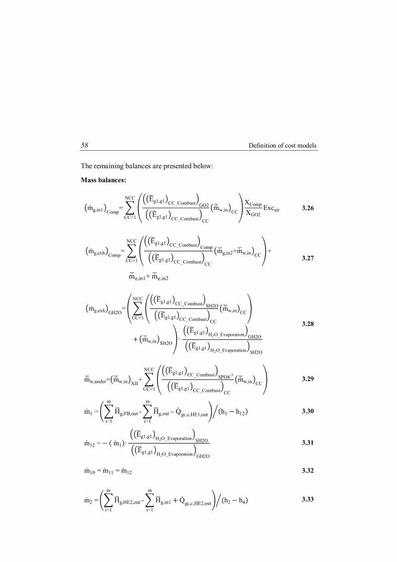
58 Definition of cost models

The remaining balances are presented below:

Mass balances:

3.26

3.27

3.28

3.29

3.30

3.31

3.32

3.33

mg,in1 Comp=

Eg1,g1 CC_Combust GO2

Eg1,g1 CC_Combust CC

mw,in CC

XComp

XGO2

NCC

CC=1

Excair

mg,exh Comp=

Eg1,g1 CC_Combust Comp

Eg1,g1 CC_Combust CC

mg,in2+mw,in CC+

NCC

CC=1

mg,in1+ mg,in2

mg,exh GH2O=

Eg1,g1 CC_Combust SH2O

Eg1,g1 CC_Combust CC

mw,in CC

NCC

CC=1

+ mw,in SH2O·

Eg1,g1 H2O_Evaporation GH2O

Eg1,g1 H2O_Evaporation SH2O

mw,under= mw,in XII+

Eg1,g1 CC_Combust SPO4-3

Eg1,g1 CC_Combust CC

mw,in CC

NCC

CC=1

m1 = Hg,FB,out

m

i=1

- Hg,out

m

i=1

– Qgc,c,HE1,out (h1 − h12)

m12 = − ( m1)·Eg1,g1 H2O_Evaporation SH2O

Eg1,g1 H2O_Evaporation GH2O

m10 = m11 = m12

m2 = Hg,HE2,out

m

i=1

- Hg,in1

m

i=1

+ Qgc,c,HE2,out (h2 − h4)

Summary 59

3.34

3.35

3.36

3.37

3.38

3.39

3.40

Energy balances:

3.41

where CComp is the combustion component, NCC is the number of combustion components in the analysed phase and CC_Combust is the combustion kinetic of the CC.

3.7 SUMMARY The correct estimation and prediction of operating costs is essential for the optimisation and re-design of treatment plants. Even being in a period of paradigm shift, the key factor for decision-making remains operational cost of the plant. In this framework numerous studies of cost analysis and plant layout comparisons have been carried out, many of them based partly on ratios or on quotients between operational

m3 = m1 − m2

m4 = m2

m5 = H12 − H11 + Qgc,c,HE3,out (h5 − h9)

m6 = m3 − m5

m7 = − ( m6)·Eg1,g1 H2O_Evaporation SH2O

Eg1,g1 H2O_Evaporation GH2O

m8 = m7

m9 = − ( m5)·Eg1,g1 H2O_Evaporation SH2O

Eg1,g1 H2O_Evaporation GH2O

60 Definition of cost models

variables. Although the use of these indicators brings simplicity to the cost evaluation, these ratios have been estimated from experimental measurements, which require a knowledge of their estimation and utilisation ranges before being used. To avoid underestimates or overestimates of operating costs produced by the use of these measures, this thesis proposes exhaustive cost models based on engineering expressions.

These Chapter divides operational costs in two main areas: electricity costs associated with actuators (stirrer engines, hydraulic pumps, blower or compressor and turbines) or complex units composed of actuators (incineration and cogeneration units models); and specific or raw material costs. The detailed description of the models allows estimating costs under all operating conditions, providing flexibility to the model.

As the heat transfer model described in Chapter 2, cost models have been developed under the guidelines of the Extended Plant-Wide Modelling methodology. The compatibility of all the models described in this thesis, along with the methodologies developed in the thesis of Grau (2007) and Lizarralde (2015) for defining biological, chemical and physico-chemical reactions, has allowed the development of a library of compatible models will be described in Chapter 4.

61

4

PWM LIBRARY: IMPLEMENTATION OF THE DYNAMIC HEAT TRANSFER

MODELLING AND COST MODELS INTO THE LIBRARY

The content of this Chapter has been published in:

Fernández-Arévalo, T., Lizarralde, I., Maiza, M., Beltrán, S., Grau, P., Ayesa, E., 2016. Diagnosis and optimization of WWTPs using the PWM library: Full-scale experiences. Water Science and Technology DOI: 10.2166/wst.2016.482 (in press).

Fernández-Arévalo, T., Grau, P., Jeppsson, U., Mauricio-Iglesias, M., Vrecko, D., Flores-Alsina, X., Ayesa, E., 2017. Model-based comparative assessment of innovative processes. In Lema, J.M., Suarez-Martinez, S. (Eds.), Innovative wastewater treatment & resource recovery technologies. Impacts on energy, economy and environment, IWA Publishing.

62 PWM Library

4.1 ABSTRACT This Chapter presents the basis of the Plant-Wide Modelling Library developed in this thesis. Thanks to the incorporation of the models developed in previous works (de Gracia et al., 2006; Grau et al., 2007; de Gracia et al., 2009; Lizarralde et al., 2015), the library consists of a set of biochemical, chemical and physico-chemical transformation models, conventional and advance unit-process models defined by mass and heat balances, and cost models, all under the E-PWM methodology. The main contribution of this thesis has been the reorganisation of the models and the incorporation of heat transfer and cost models.

4.2 INTRODUCTION Wastewater treatment modelling originated in the field of academia, developed mainly by academics interested in research. At the end of the last century, it became established as a tool for research. Proof of this is the linear rise in the last 25 years of publications related to activated sludge modelling (adapted from Gujer, 2006 and Rieger et al., 2010), which has become a suitable tool for the optimisation of WWT processes, the design of new wastewater treatment plants (WWTP) and the upgrading of existing ones.

Figure 4.1 Interest in activated sludge modelling by number of publications from Web of Science between 1985 and 2015 (adapted from Gujer 2006 and Rieger et al., 2010)

Depending on these application areas (academia, research or consultancy), the perception of the usefulness of a model may differ. For the fields of applied research and consulting, which are the areas where plant optimisations and diagnostics are framed, a model has to be an abstract representation of the real system to support

Web of Science keywords: Activated AND sludge AND model

Introduction 63

decision-making. Thus, the value of a model should depend on its usefulness in supporting decision-making (Daigger, 2011).

While a few years ago this decision-making was focused solely on ensuring effluent quality and minimising energy consumption, the scarcity of natural resources and concern about climate change have led to an increasing awareness of the importance of resource recovery, energy minimisation and environmental impact assessment. In order to address this change, the water sector is developing new and innovative treatment technologies, such as resource recovery systems, partial nitritation/Anammox technologies for nitrogen (N) treatment and sludge pre-treatment processes, among others. Combining these innovative processes with traditional technologies has led to new plant configurations that are based on offering sustainable solutions for obtaining effluent quality while at the same time optimising the recovery of valuable by-products and energy. This awareness, in conjunction with the changes in regulation, community and national standards, has led many WWTPs have to be updated and retrofitted.

Mathematical modelling has been evolving to keep up the new innovations in technology. For example, models have been developed for, among many things, describing chemical and physico-chemical phenomena (Batstone et al., 2012; Flores-Alsina et al., 2015; Kazadi Mbamba et al., 2015a,b; Lizarralde et al., 2015), for estimating operational costs (Simba, 1999; Copp 2002; Rieger et al, 2006; Descoins et al., 2012; Fernández-Arévalo et al., 2015; Aymerich et al., 2015), for describing the heat transfer in unit-processes (Gillot & Vanrolleghem 2003; Makinia et al., 2005; Gómez et al., 2007; de Gracia et al., 2009; Fernández-Arévalo et al., 2014; Corbalá-Robles et al., 2016) and for predicting the production of greenhouse gases emissions (Ni et al., 2011, 2013, 2014; Guo et al., 2012, 2014; Mampaey et al., 2013; Snip et al., 2014). Due to the complexity of the new configurations and processes where there are recirculations and interrelations among the units, it is necessary to consider a plant-wide perspective in order to establish an optimum solution for the design or operation of the entire plant (Jeppsson et al., 2007; Grau et al., 2007; Nopens et al., 2009). In addressing this need, different models or methodologies have also been developed in order to describe the whole plant, considering both, the water line and the sludge line (Ekama et al., 2006; Grau et al., 2007; Jeppsson et al., 2007; Barat et al., 2013; Ikumi et al., 2014, 2015; Flores-Alsina et al., 2015).

64 PWM Library

The knowledge gained about process modelling is extensive. Proof of this is the number of works mentioned. However, the bottleneck appears when all or many of these models are to be used together; that is, when knowledge has to be integrated in a compatible way. Each model has its components and its structure, and the combination of these is not always easy and immediate. The tool proposal in this thesis is the Extended Plant-Wide Modelling methodology (E-PWM). This methodology was first proposed in 2006, and since then it has undergone continual improvement, adding features to keep it up to date (de Gracia et al., 2006; Grau et al., 2007; de Gracia et al., 2009; Fernández-Arévalo et al., 2014; Lizarralde et al., 2015; Fernández-Arévalo et al., 2015). The methodology allows to adapt existing models, ensuring the continuity of mass and energy in each transformation in order to obtain compatible models and transformations. The methodology’s bases have made it possible to develop and standardize a flexible and expandable model repository or model library that can be adapted to any plant configuration and any set of current or future process transformations. This model library should include models that are complex enough to describe biological and abiotic phenomena in as detailed a manner as required, but there also need to have elements that translate this complexity into variables that can be used and understood by engineers and plant operators.

The aim of this Chapter is to detail the basis of this new modelling methodology as well as the description of the model library developed from this methodology.

4.3 FUNDAMENTALS OF THE EXTENDED PLANT-WIDE MODELLING METHODOLOGY

The Extended Plant-Wide Modelling (E-PWM) methodology (Grau et al., 2007; Fernández-Arévalo et al., 2014; Lizarralde et al., 2015) allows the rigorous and systematic construction of compatible unit-process models (UPM) for describing the dynamic behaviour of the water and sludge lines in an integrated manner. In contrast with modelling methodologies that use interfaces, the E-PWM methodology is based on selecting the set of process transformations required to model all unit-processes incorporated into each specific WWTP. In this manner, with a unique standard model it is possible to simulate the plant that is needed in each case. The unification of these set of transformations permits the definition of a unique component vector to be defined for the whole plant, without the need to develop specific transformers for

Description of the Plant-Wide Modelling library 65

interfacing unit-process models. The use of a common list allows a more realistic component characterisation, with constant elemental mass fractions and constant stoichiometric values throughout the plant, thus avoiding some of the uncertainty caused by the interfaces (Grau et al., 2009). Accurately defining the stoichiometry ensures the elemental mass (in terms of C, N, O, H, P or other elements) and charge continuity in all these transformations (Grau et al., 2007), while defining the enthalpies of formation of each component allows the reaction heat of each transformation to be estimated (Chapter 2 or Fernández-Arévalo et al., 2014). Thus, this methodology allows the straightforward construction of compatible mathematical models, being especially suitable for the comparative assessment of any combination of existing or under development technologies and configurations.

4.4 DESCRIPTION OF THE PLANT-WIDE MODELLING LIBRARY

Based on this E-PWM methodology, a new model library has been developed to bring together all the models in a structured manner. The library compiles information arranged by the various aspect that need to be considered in the construction of the model, such that the modeller can select the ones that are of interest to the case under study, following these three steps:

i. Selection of the category. The library contains different categories that compile the model required for the representation of biochemical, chemical and physic-chemical reactions.

ii. Selection of the Unit Process models, wherein the mass and heat transports are defined depending on the phases considered in the unit processes under study (e.g. for CSTR reactors, primary or secondary settlers, solid separation systems, etc.).

iii. Selection of the actuator, specific energy ratios and dosage cost models which are required in the costs estimation.

Once the categories, the unit-processes, and cost models have been selected, the global model is constituted and ready for use. A schematic description of the Plant-Wide Modelling library with the presented models can be seen in Figure 4.2.

66 PWM Library

4.4.1. Category selection

The selection of the category must ensure the correct description of the biochemical, chemical, and physico-chemical transformations that may take place throughout the plant. In the first step, the modeller must select the biochemical and physico-chemical transformations it deems necessary to describe the plant, considering the aim of and accuracy required in the study. For instance, the modeller must decide, among other aspects, whether the model needs to describe the nitrogen removal process in one-step or two-steps, incorporate chemical or biological phosphorus (P) removal transformations, or analyse the recovery of compounds. In the second step, the modeller is able to select those chemical components, species, and transformations (acid-base and ion paring equilibrium reactions) that are relevant for the definition of the plant, depending on the biochemical and physico-chemical transformations selected in the previous step (Grau et al., 2007; Lizarralde et al., 2015).

Figure 4.2 Schematic representation of the Plant-Wide Modelling Library

Description of the Plant-Wide Modelling library 67

On order to facilitate the work, the library contains different categories or model packages that include all the transformations present in characteristic plants. Thus, the modeller can select one category or another depending on the requirements and goals of the study (the definition of each category can be found in Appendix A). The encoding used for the definition of the categories is as follows: “C”, “N” and “P” for describing biological organic matter and N biodegradation and biological and chemical P removal, respectively, all of them in aerobic and anoxic conditions at low and high temperatures (thermal hydrolysis or TH reactions); “2N” for detailing two step N removal and Anammox reactions; “Pchem” for considering chemical P removal, but not biological P removal; “Pprec” for including precipitation reactions; and finally, “AnD” for describing anaerobic conditions at low and high temperatures (fermentation and digestion).

One of the features of the library is that it is composed of existing models, all of which have been adapted or re-written for compatibility. On this basis, transformations describing biological processes in all categories are based on the ASM1/2d models (Henze et al., 2000) for COD, N and P removal, the ADM1 model (Batstone et al., 2002) for the anaerobic COD biodegradation and in the works of Hellinga et al (1999) and Hao et al., (2002 a, b) for the Anammox and two step N removal. The chemical and physico-chemical transformations were selected based on the work by Ikumi et al. (2014) and then incorporated according to the methodology and kinetic expressions presented in Lizarralde et al., (2015).

The organised structure that the methodology presents enables a straightforward development of categories, allowing the library to be continuous updating.

4.4.2. Unit-process models selection

The library contains a comprehensive set of unit-process models, as can be shown in Figure 4.2. At this stage, all unit-process models needed to complete the plant under study must be selected.

The first step consists in deciding on the number of phases that each UPM contains. In some of them such a decision is not necessary since the processes are defined for a given number of phases (for e.g. separation processes, incineration units, cogeneration units, etc.). In the case of completely stirred open tank reactors (O-CSTR) and completely stirred closed tank reactors (C-CSTR), one must decide between one or two gaseous phases to describe the liquid-gas transfer, and if the

68 PWM Library

process needs the definition of a solid phase due to a controlled or uncontrolled precipitation of solids (for e.g. struvite precipitation in anaerobic digesters).

The second step consists on the definition of the mass balances of each phase. Each UPM incorporates the mathematical description of the mass transport for each phase (liquid, gaseous, solid) and the transformations designated in the category by following the matrix structure shown in Equation 4.1 (Chapter 2 or Fernández-Arévalo et al., 2014).

4.1

In the third step, the modeller decides whether it is necessary to ensure the overall heat balance of the plant or the balance of some units in particular. Thus, each UPM incorporates the mathematical description of the heat balance for each phase (liquid, gaseous, solid), in addition to the transport model and transformations designated in the category. Based on the energy conservation principle, the general one-dimensional dynamic heat transfer model can be shown in equation 4.2.

dHT

dt i =ΔHr + Hi

in

+ Hiout

+ Qphs,i,j + Qic,out + QAct +

Qsolrd + Qatmrd 4.2

A detailed characterisation of the components (elemental mass characterisation) enables an estimation of the enthalpy of formation (Δhºf) for each model component and makes possible a systematic calculation of the heat released or absorbed by each transformation, guaranteeing heat energy continuity at any point in the plant. Thus, the specific enthalpy change of reaction (Δhºr in kJ gstoich.unit

-1) due to biochemical, physico-chemical, or chemical transformations can be defined as the difference between the enthalpy of formation of the products and the enthalpy of formation of the reactants, applying Hess’s law. Additional information on the heat balance with an exhaustive definition of each term can be found in Chapter 2.

The main feature of these models is that they are compatible and standard. The models are defined and developed in such a way that they can be used for any existing or future category, and they are defined based on the phases contained (number and type), and system inputs and outputs. In this manner, it is possible to use the same model to describe thermal hydrolysis or aerobic digestion processes.

d Mdt

i= Ei,i

T ρi,i + Ei,jT ρi,j

No. adj. phase

j=1

+ miin

– miout

Summary 69

4.4.3. Actuator, specific energy ratios and dosage cost models selection

Finally, the library includes a set of actuator, specific energy ratios and dosage cost models for a detailed estimation of the costs of each element (see Chapter 3). All actuator models are developed based on engineering expressions instead of directly using cost curves or fixed values. This creates a connection between all elements of the library, since the actuator expressions depend on operational variables (flowrates, enthalpy changes of reaction, solids concentration, etc.) that are estimated in the UPM and the UPMs depends on categories. The goal is to have more accurate models in which the oversimplifications and low degree of standardisation of some expressions are avoided. The models are standardised, so they can be used interchangeably in any category. The standardisation of the models has been pursued to keep future model adaptations from being needed when new components are incorporated, and to keep in line with the standardisation philosophy of the Plant-Wide Modelling methodology.

4.5 SUMMARY Recent works in the mathematical modelling of WWTPs show the need to update conventional models in order to facilitate the straightforward incorporation of new processes, technologies and plant configurations from the perspective of resource recovery (energy and nutrients). For this purpose, this thesis proposes a change from the traditional procedure for WWTP model building (based on the combination of unit-process models) to a more flexible and expandable methodology based on the combination of the compatible and mass-balanced transformations required in each case study.

In order to demonstrate the usefulness and the applicability of this library, Chapter 6 presents a comparative analysis of evolutionary WWTP and Chapter 7 the diagnosis and optimisation of three full-scale WWTPs.

71

5

MODEL-BASED EXPLORATION OF HEAT TRANSFERS AND

ENTHALPY CHANGES OF REACTION

The content of this Chapter has been published in:

Fernández-Arévalo T., Lizarralde I., Grau P., Ayesa E., 2014. New systematic methodology for incorporating dynamic heat transfer modelling in multi-phase biochemical reactors. Water Research, 60, 141-155.

5.1 ABSTRACT The main purpose of this Chapter is the validation of the methodology proposed in this Thesis for model-based calculation of the enthalpy change of reactions and the heat transfer. To do this, the enthalpy changes of reaction estimated with the proposed model-based methodology were compared with experimental and theoretical data obtained in literature. In a second step, the verification of the predictive capacity of the heat transfer model was carried out. Based on the works of Gómez et al. (2007)

72 Model-based exploration of heat transfers and enthalpy changes of reaction

and de Gracia et al. (2009) the predictive capacity of the proposed heat model has been verified using the Autothermal Thermophilic Aerobic Digestion (ATAD) as an illustrative case-study. Finally, a dynamic and detailed model-based analysis of the heat generation and transfer was performed in the same ATAD reactor, and in the widely known Benchmark Simulation Model No 2 (BSM2; Jeppsson et al., 2007).

5.2 VALIDATION OF THE METHODOLOGY FOR ESTIMATING TRANSFORMATION HEATS

The methodology proposed in Chapter 2.3 for the model-based calculation of enthalpy change of reactions have been applied to the long list of biochemical transformations, the acid-base equilibria, the liquid-gas transfers, the liquid-solid transfer and the combustion of the model components included in the Ceit-IK4 PWM library. The results obtained are presented in Table 5.1, Table 5.2, Table 5.3, Table 5.4 and Table 5.5.

A first analysis of the numerical values of the enthalpy change of reactions show that, the reactions associated with the nitrogen removal are the ones that release more heat to the medium, that is, the nitrification reactions in one or two steps and the anaerobic ammonium oxidation (or Anammox) reaction. In the COD removal transformations (Table 5.1), part of the COD is used for biomass growth (0.67 gbiomass gsubstrate

-1 for aerobic and one step anoxic biodegradation and 0.53 gbiomass gsubstrate

-1 for two step anoxic biodegradation; Henze et al., 2000), limiting the potential use of this COD as a heat source. Even so, the high COD concentrations in the biological processes make these reactions fundamental in estimating the heat of reaction.

Table 5.1 Enthalpy change of reactions of the biochemical transformations

Reaction hrº (kJ gEmain comp.-1) hrº (kJ mol-1)

SSU aer. consumption -5.27 -1010.90 SAA aer. consumption -4.41 -589.69 SFA aer. consumption -4.07 -2996.99 SHVA aer. consumption -4.14 -862.02 SHBU aer. consumption -4.17 -666.59 SHPRO aer. consumption -4.19 -469.31 SHAC aer. consumption -4.32 -276.18 XN growth -21.61 -302.52 XAOB growth -16.04 -221.58

Validation of the methodology for estimating transformation heats 73

Table 5.1 Enthalpy change of reactions of the biochemical transformations (Continued)

Reaction hrº (kJ gEmain comp.-1) hrº (kJ mol-1)

XNOB growth -6.09 -85.31 XPHA storage on SHVA 1.11 231.30 XPHA storage on SHBU 1.09 174.42 XPHA storage on SHPRO 1.07 119.40 XPHA storage on SHAC 0.94 60.23 XPP aer. storage -2.29 -71.10 XPAO aer. growth -6.25 -1020.34 SSU anox. Consumption on NOX -4.74 -910.08 SAA anox. consumption on NOX -3.89 -519.53 SFA anox. consumption on NOX -3.55 -2610.50 SHVA anox. consumption on NOX -3.62 -752.80 SHBU anox. consumption on NOX -3.64 -582.58 SHPRO anox. consumption on NOX -3.67 -410.49 SHAC anox. consumption on NOX -3.79 -242.57 SSU anox. Consumption on NO3 -4.35 -835.59 SAA anox. consumption on NO3 -3.50 -467.70 SFA anox. consumption on NO3 -3.16 -2324.97 SHVA anox. consumption on NO3 -3.23 -672.10 SHBU anox. consumption on NO3 -3.25 -520.50 SHPRO anox. consumption on NO3 -3.28 -367.04 SHAC anox. consumption on NO3 -3.40 -217.74 SSU anox. Consumption on NO2 -8.10 -1554.79 SAA anox. consumption on NO2 -7.25 -968.14 SFA anox. consumption on NO2 -6.90 -5081.88 SHVA anox. consumption on NO2 -6.98 -1451.23 SHBU anox. consumption on NO2 -7.00 -1119.83 SHPRO anox. consumption on NO2 -7.02 -786.57 SHAC anox. consumption on NO2 -7.15

-457.48

XPP anox. storage -1.98 -61.24 XPAO anox. growth -5.66 -922.95 XAN growth -23.32 -326.49 SSU acidogenesis -0.33 -62.48 SAA acidogenesis 0.07 9.24 SFA acetogenesis 1.29 949.23 SHVA acetogenesis 0.65 134.89 SHBU acetogenesis 0.86 137.37

74 Model-based exploration of heat transfers and enthalpy changes of reaction

Table 5.1 Enthalpy change of reactions of the biochemical transformations (Continued)

Reaction hrº (kJ gEmain comp.-1) hrº (kJ mol-1)

SHPRO acetogenesis 1.63 182.38 Acetoclastic methanogenesis -0.15 -9.84 Hydrogenotrophic methanogenesis -3.73 -59.68 XC1 disintegration (aer., anox., anaer.,) -0.10 -23.68 XC2 disintegration (aer., anox., anaer.,) -0.24 -39.66 XC2 thermal disintegration -0.24 -39.66 XI disintegration -0.49 -113.57 XP disintegration -0.06 -12.68 XCH hydrolysis (aer., anox., anaer.,) -0.08 -15.34 XPR hydrolysis (aer., anox., anaer.,) -0.16 -22.00 XLI hydrolysis (aer., anox., anaer.,) 0.04 87.42 XH decay (aer., anox., anaer.,) 0.00 0.00 XN decay (aer., anox., anaer.,) 0.00 0.00 XAOB decay (aer., anox., anaer.,) 0.00 0.00 XNOB decay (aer., anox., anaer.,) 0.00 0.00 XSU decay (aer., anox., anaer.,) 0.00 0.00 XAA decay (aer., anox., anaer.,) 0.00 0.00 XFA decay (aer., anox., anaer.,) 0.00 0.00 XC4 decay (aer., anox., anaer.,) 0.00 0.00 XPRO decay (aer., anox., anaer.,) 0.00 0.00 XAC decay (aer., anox., anaer.,) 0.00 0.00 XH2 decay (aer., anox., anaer.,) 0.00 0.00 XPAO decay (aer., anox., anaer.,) 0.00 0.00 XPHA decay (aer., anox., anaer.,) -1.35 -3.78 XPP decay (aer., anox., anaer.,) -0.82 -0.08 XAN decay (aer., anox., anaer.,) 0.00 0.00

Transfers between phases and chemical equilibria are not usually considered in the estimation of the heat of reaction, except for the heat lost in the evaporation. Table 5.2 and Table 5.3 show the heats of reaction of chemical equilibria and liquid-gas transfers, respectively, in which values similar to those obtained in the COD removal processes are observed for some reactions (SNO and SNH equilibria, NH3 dissolution, etc.). As is known, the concentrations of these transformations reactants are low, so the net heat released by these transformations will be low, but in no case insignificant. Especially, these reactions may have their importance in processes with low stability

Validation of the methodology for estimating transformation heats 75

or intermittent stability (considerable variations in pH and/or temperature). In these cases, the need for the incorporation of these reactions becomes clear.

Table 5.2 Enthalpy change of reactions of acid-base equilibria (HA → H+ + A-)

Reaction hrº (kJ gEmain comp.-1) hrº (kJ mol-1)

H2O equilibrium 3.10 55.84 CIN equilibrium 0.64 7.64 CIN2 equilibrium 1.16 13.96 SNH equilibrium 3.73 52.21 SNO equilibrium 6.13 85.80 PIN equilibrium 0.12 3.78 PIN2 equilibrium 0.70 21.70 SHVA equilibrium 0.41 85.00 SHBU equilibrium 0.09 14.72 SHPRO equilibrium 0.03 3.01 SHAC equilibrium 0.02 1.43

Table 5.3 Enthalpy change of reactions of liquid-gas transfers

Reaction hrº (kJ gEmain comp.-1) hrº (kJ mol-1)

CO2 dissolution -1.62 -19.39 O2 dissolution 0.00 0.00 H2O evaporation 2.45 44.03 NH3 dissolution -2.46 -34.39 CH4 dissolution -0.13 -8.17 N2 dissolution 0.00 0.00 H2 dissolution 0.00 0.00

Table 5.4 shows the heat of combustion obtained in the incineration and cogeneration processes. The heat of combustion for compounds containing N, Cl, and P, may be unreliable due to the uncertainty in the specific compounds formed. In order to estimate the heat of combustion of all model components, the following assumptions have been made (adapted from Niessen, 2002):

Elemental or organic carbon + O2 → gaseous CO2: Assumption of complete combustion, although in a real systems, a fraction of the carbon is incompletely oxidised. It appears as unburned solid matter, as hydrocarbons, and as CO in the effluent gases.

Elemental or organic hydrogen + O2 → H2O (aq.).

76 Model-based exploration of heat transfers and enthalpy changes of reaction

Nitrogen leaves as NO2 gas (33.2 kJ mol-1; Masterton et al., 2003).

Organic phosphorus precipitates as P2O5 (-360.0 kJ mol-1; Perry et al., 1999) and inorganic phosphorus precipitates as H3PO4 (-1266.92 kJ mol-1; Dean, 1979).

Oxygen associated with non-metallic elements (K+, Ca+2, or Mg+2) precipitate as organic compounds (K2O: -284.5 kJ mol-1; Dean, 1979; CaO: -635.1 kJ mol-1; Masterton et al., 2003; and MgO: -601.7 kJ mol-1; Masterton et al., 2003) and oxygen associated with metals (Fe+3) in oxides (Fe2O3: -824.2 kJ mol-1; Masterton et al., 2003).

Organic chlorine is usually preferred oxidising agent for hydrogen (gaseous HCl: -92.30 kJ mol-1; Dean, 1979).

Struvite combustion produces Mg2P2O7 (-2419.76 kJ mol-1; La Iglesia, 2009).

As can be seen in Table 5.4, some reactions have a positive sign even though they have been raised as reactions within the combustion. This happens mainly with inorganic components, since these components react under synthesis or equilibrium transformations.

Table 5.4 Heat of combustion or energy content of the components

Reaction hrº (kJ gEmain comp.-1) hrº (kJ mol-1)

SH2O 0.00 0.00 SO2 0.00 0.00 SH+ 0.00 0.00 SOH- 0.00 0.00 SH2PO4- 4.24 131.38 SHPO4= 2.56 79.32 SPO4-3 5.34 165.52 SNH4+ -18.79 -263.06 SNH3 -22.52 -315.27 SCO2 1.62 19.39 SHCO3- 5.63 67.59 SCO3= 9.12 109.47 SCa+2 -2.31 -92.3 SMg+2 -5.55 -134.85 SK+ -0.82 -32.12

Validation of the methodology for estimating transformation heats 77

Table 5.4 Heat of combustion or energy content of the components (Continued)

Reaction hrº (kJ gEmain comp.-1) hrº (kJ mol-1)

SSU -14.62 -2807.90 SAA -15.77 -2106.55 SFA -13.62 -10021.20 SHVA -13.64 -2837.85 SVA- -13.78 -2867.01 SHBU -13.65 -2183.48 SBU- -13.39 -2142.36 SHPRO -13.64 -1527.25 SPRO- -13.16 -1474.42 SHAC -13.67 -875.18 SAC- -12.82 -820.77 SH2 -17.86 -285.84 SCH4 -13.78 -882.22 SN2 0.00 0.00 SNO2- 3.62 50.72 SHNO2 0.68 9.48 SNO3- 10.91 152.69 SI -15.21 -3535.94 SP -12.84 -3557.62 SFe+3 1.17 -65.16 SCl- 3.68 130.70 XC1 -15.52 -3607.28 XC2 -15.47 -2524.48 XCH -14.53 -2813.11 XPR -15.93 -2128.55 XLI -13.60 -31604.71 XH -15.47 -2524.48 XN -15.47 -2524.48 XAOB -15.47 -2524.48 XNOB -15.47 -2524.48 XPAO -15.47 -2524.48 XPHA -15.30 -2203.59 XSU -15.47 -2524.48 XAA -15.47 -2524.48 XFA -15.47 -2524.48 XC4 -15.47 -2524.48

78 Model-based exploration of heat transfers and enthalpy changes of reaction

Table 5.4 Heat of combustion or energy content of the components (Continued)

Reaction hrº (kJ gEmain comp.-1) hrº (kJ mol-1)

XPRO -15.47 -2524.48 XAC -15.47 -2524.48 XH2 -15.47 -2524.48 XAN -15.47 -2524.48 XI -14.04 -3263.13 XP -14.98 -2960.11 XII 0.00 0.00 XPP 2.61 80.79 GCO2 0.00 0.00 GN2 2.37 66.4 GO2 0.00 0.00 GH2 -17.87 -285.84 GCH4 -13.91 -890.39 GNH3 -24.97 -349.66 GH2O -2.45 -44.03 PCaCO3 2.38 238.29 PMgCO3 1.66 515.02 PACP 1.66 515.02 PSTRU 0.89 218.50 PKSTRU - - PNEW - - PFeCl3 0.84 135.78 PFePO4 4.35 655.60 PFe(OH)3 -0.17 -17.86

Finally, the liquid-solid transfers (Table 5.5) do not release/absorb excessive heat, but these heat transfers can be automatically estimated by the methodology for calculating the heats of reaction.

Table 5.5 Enthalpy change of reactions of liquid-solid transfers

Reaction hrº (kJ gEmain comp.-1) hrº (kJ mol-1)

FeCl3 dissolution -0.95 -154.08 FePO4 dissolution -0.52 -78.2 Fe(OH)3 dissolution 0.79 84.5 Calcite precipitation 0.13 13 Magnesite precipitation 0.57 48.2

Validation of the methodology for estimating transformation heats 79

Table 5.5 Enthalpy change of reactions of liquid-solid transfers (Continued)

Reaction hrº (kJ gEmain comp.-1) hrº (kJ mol-1)

ACP precipitation 0.20 62.4 Struvite precipitation -0.37 -90.06 K-Struvite precipitation - - Newberyite precipitation - -

First validation of the proposed methodology has been focused on comparing the theoretical model-based heat values obtained with the E-PWM methodology with other studies. Table 5.6 shows a comparison between the transformation heat values calculated with the proposed methodology and a set of values presented in bibliography, previously estimated both experimentally (E) or theoretically (T). In order to validate the methodology as rigorously as possible, some model reactions had to be modified (for example, some bibliographic reactions don’t consider the biomass growth) to make more validation cases available.

It is interesting to note that the deviations with almost all reactions have been as low as 5 %, with the exception of the enthalpy change of reaction estimated theoretically for the conversion of acetic acid to methane (reaction 7), where the discrepancies may be due to differences in the enthalpies of formation used for the products and/or reactants. Therefore, these comparative results confirm that the enthalpy change of reaction estimated by the Extended Plant-Wide modelling methodology is in accordance with the values traditionally estimated both theoretically and experimentally.

Despite numerous experimental studies published, there is no consensus on the determination of the specific heat yields (Reaction 1, Table 5.6), although it has been estimated an approximate range of 12–18 kJ gCOD-1

removed. These discrepancies can be attributed to the heterogeneity in the samples’ composition due to the diversity in the organic components present (Cooney et al., 1968). It is also important to note that, although the enthalpy change of reaction values proposed in literature are attributed to the oxidation of organic materials, these experimental estimations implicitly include other smaller transformation heats like, for example, those associated with hydrolysis or CO2 stripping.

80 Model-based exploration of heat transfers and enthalpy changes of reaction

Table 5.6 Comparison of transformation heat estimated in modelling with experimental theoretical literature data

Ref

eren

ce

Coo

ney

et a

l., 1

968

And

rew

s and

K

ambh

u, 1

969

McC

arty

, 197

2

Zano

ni a

nd

Mue

ller,

1982

Je

wel

l, 19

82

Hei

nritz

et a

l., 1

990

Mes

seng

er e

t al.,

19

92

Pitt

et a

l., 1

995

Rile

y an

d Fo

rste

r, 20

02

Shiz

as a

nd B

agle

y,

2004

G

ómez

et a

l., 2

007

Hei

dric

h et

al.,

20

11

hº

r

Lite

ratu

re

12.2

8 –

16.4

6 kJ

gC

OD

-1 re

m(E

)

13.3

2 –

15.1

2 kJ

gC

OD

-1 re

m(E

)

14.3

0 kJ

gC

OD

-1 re

m(E

)

13.5

kJ g

CO

D-1

rem

(E)

12.5

0 –

16.6

6 kJ

gC

OD

-1 re

m(E

)

13.6

kJ g

CO

D-1

rem

(E)

12.1

– 1

3.7

kJ g

CO

D-1

rem

(E)

12.8

kJ g

CO

D-1

rem

(E)

15.6

8 kJ

gC

OD

-1 re

m(E

)

12.4

kJ g

CO

D-1

rem

(E)

13.9

kJ g

CO

D-1

rem

(E)

17.8

kJ g

CO

D-1

rem

(E)

Mod

el

13.6

2 –

14.6

2 kJ

gC

OD

-1re

m

Rea

ctio

n

Subs

trate

(aq.

) + x

O2(

g) →

y

H2O

(l) +

zC

O2(

g) +

Bio

mas

s

1

Validation of the methodology for estimating transformation heats 81

Table 5.6 Comparison of transformation heat estimated in modelling with experimental theoretical literature data (Continued)

Ref

eren

ce

Gal

lert

et a

l., 2

005

Dav

erio

et a

l., 2

003a

Dav

erio

et a

l., 2

003a

But

tiglie

ri et

al.,

201

0

Gal

lert

et a

l., 2

005

Oh

et a

l., 2

007

Oh

et a

l., 2

007

Oh

et a

l., 2

007

Oh

et a

l., 2

010

Oh

et a

l., 2

010

Oh

et a

l., 2

010

Oh

et a

l., 2

010

hº

r

Lite

ratu

re

-890

.0 k

J mol

SSU

rem

(T)

-259

.0 k

J mol

N re

m(T

)

-99.

4 kJ

mol

N re

m(T

)

-333

.0 k

J mol

N re

m(T

)

-131

.0 k

J mol

SSU

rem

(T)

-15.

3 kJ

mol

SHA

C re

m(T

)

Δhºr

< 0

(T)

Δhº r

< 0

(T)

Δhº r

< 0

(T)

Δhºr

>0

Δhºr,

11 >

Δhºr,

10 (T

)

Δhºr

> 0

Δh

ºr,12

>Δh

ºr,11

(T)

Δhºr

>0 (T

) Δh

ºr,13

>Δh

ºr,12

(T)

Mod

el

-893

.1 k

J mol

SSU

rem

-258

.0 k

J mol

N re

m

-102

.0 k

J mol

N re

m

-334

.6 k

J mol

N re

m

-132

.8 k

J mol

SSU

rem

-12.

4 kJ

mol

SHA

C re

m

-4.8

kJ m

olSH

AC

rem

15.2

kJ m

olSH

AC

rem

-9.8

kJ m

olSH

AC

rem

0.6

kJ m

olSH

PRO

rem

6.8

kJ m

olSH

BU

rem

16.9

kJ m

olSH

VA

rem

Rea

ctio

n

C6H

12O

6(aq

.)+3O

2(g)

→3H

2O(l)

+

3CO

2(g)

+Bio

mas

s

NH

4+ (aq.

)+1.

5 O

2 (g)

→ 2

H+ (a

q.) +

N

O2- (a

q.)+

H2O

(l)

NO 2- (a

q.)+

0.5

O2 (

g) →

NO

3- (aq.

)

NH

4+ (aq.

)+N

O2- (a

q.)→

N2 (

g)+

2H2O

(l)

C6H

12O

6(aq

.)→2.

85CH

4(g)

+2.8

5CO

2(g)

CH

3CO

OH

(aq.

)→ C

H4(

aq.)

+ C

O2(

aq.)

CH

3CO

OH

(aq.

)→ C

H4(

g) +

CO

2(aq

.)

CH

3CO

OH

(aq.

)→ C

H4(

g) +

CO

2(g)

HA

C d

iges

tion

(aq.

) (m

etha

noge

nesi

s)

HPR

O d

iges

tion

(aq.

) (ac

etog

enes

is &

m

etha

noge

nesi

s)

HB

U d

iges

tion

(aq.

) (ac

etog

enes

is &

m

etha

noge

nesi

s)

HV

A d

iges

tion

(aq.

) (ac

etog

enes

is &

m

etha

noge

nesi

s)

2 3 4 5 6 7 8 9 10

11

12

13

82 Model-based exploration of heat transfers and enthalpy changes of reaction

In order to show the additional information offered by the proposed methodology, Table 5.7 second column presents the theoretical specific heat yields for the seven carbonaceous substrates included in the model, showing the small differences associated with substrate composition, but within the range proposed in literature. Additionally, the third column illustrates the expected changes in the theoretical heats when substrate oxidation and CO2 stripping transformations are both considered in the calculations, demonstrating the relevance of taking into account all the simultaneous transformations. This fact can explain some of the discrepancies found in the experimental results presented in the literature.

Table 5.7 Specific heat yields (or energy content) estimated for the different substrates used in the model

Name Oxidation heats (kJ gCODrem

-1) Oxidation + CO2 stripping heats

(kJ gCODrem-1)

SSU -15.23 -14.62 SAA -14.38 -13.80 SFA -14.64 -13.62 SHVA -14.11 -13.64 SHBU -14.13 -13.65 SHPRO -14.16 -13.64 SHAC -14.28 -13.67

Once the appropriate calculation of the specific heat yields has been validated, the verification of the general heat transfer model has been carried out.

5.3 VERIFICATION OF THE HEAT TRANSPORT MODEL: ATAD CASE STUDY

In order to analyse the predictive capacity of the heat transfer model and the methodology for calculating the enthalpy change of reaction, the simulation of the behaviour of an Autothermal Thermophilic Aerobic Digestion (ATAD) has been carried out. The verification has consisted in the comparison of simulation results and the experimental data obtained in the full scale ATAD at the Tudela (Navarra, Spain) WWTP (Gómez et al., 2007; de Garcia et al., 2009).

The ATAD digesters exhibit a high organic matter oxidation, being able to maintain thermophilic conditions without the external addition of heat (except

Verification of the heat transport model: ATAD Case Study 83

recirculations/mixing energy). This quality make the ATAD reactor an ideal framework for heat transfer model verification.

5.3.1. Description of the auto-thermal thermophilic aerobic digestion (ATAD) reactor used for model verification

The ATAD digester of Tudela WWTP is an aerated completely stirred tank reactor with a maximum effective volume of 350 m3. The geometry of the reactor is cylindrical with an inner height of 6.5 m and an inner diameter of 9.25 m. The digester was designed to withstand the high temperatures produced in the process (75 °C). To obtain this insulation, the entire digester (base, cover and sides) was covered with a layer of insulation material, a layer of concrete and an inner plastic waterproofing. In addition, the sides were coated with stainless steel sheets to protect the reactor from inclement weather. Figure 5.1 (left) shows the outer appearance of the reactor. The aeration and mixing of the system is carried out by means of two venturi type ejectors submerged inside the reactor, as can be seen in Figure 5.1 (right). With this arrangement, the heat dissipated by the engines is used to heat the sludge. One of these pumps is connected to an external blower to introduce the atmospheric air into the digester, while the second pump entrained off gas from digester dome together with the foam produced during biological transformations.

Figure 5.1 Full-scale ATAD reactor of the Tudela WWTP: left) exterior view; right)

schematic representation (Source: Gómez, 2007).

5.3.1.1. Experimental situation

In the 23-day period used for model verification (Gómez, 2007), the ATAD reactor was operated as a single treatment of the sludge line, at high values of hydraulic

Foam sensor

Blower

84 Model-based exploration of heat transfers and enthalpy changes of reaction

retention time (HRT), and with a low organic loading rate. The digester operated about 10 days HRT with discontinuous charges and discharges of the reactor every 24 h (30 min for the discharge phase, 30 min for the feeding phase and 23 h for the operation step). A period with abrupt changes in the organic loading rate (OLR) was selected for the verification of the thermal model under both oxygen limiting and substrate limiting conditions. To achieve these two conditions, the aeration flow rate of 9,200 Nm3 d-1 remained constant, gradually increasing the OLR (see Table 5.8).

Table 5.8 Operating conditions of the ATAD reactor (Source: Gómez, 2007).

Ope

ratio

n C

ycle

(h)

19.5

23.5

23.5

23

23

20

23

22

21

45 23

22.5

23

23

21

24

22

23

22.5

23.5

16.5

- TS

in a

nd V

S in:

Influ

ent T

otal

and

Vol

atile

Sol

ids;

TC

OD

and

SC

OD

: Inf

luen

t Tot

al a

nd S

olub

le C

hem

ical

Oxy

gen

Dem

and;

O

LR in

VS

and

OLR

in C

OD

: org

anic

load

ing

rate

in kg

VS m

dige

ster

-3 d

-1 a

nd in

kgC

OD m

dige

ster

-3 d

-1

Qg,

in

(Nm

3 h-1

) 40

3.6

403.

6

403.

6

403.

6

403.

6

403.

6

403.

6

403.

6

403.

6

403.

6

403.

6

225.

0

225.

0

225.

0

403.

6

403.

6

403.

6

403.

6

403.

6

403.

6

270.

0

403.

6

403.

6

T w,o

ut

(ºC)

60.2

5

61.0

4

62.1

2

62.2

7

61.2

2

60.1

0

60.9

5

60.9

7

59.0

4

58.2

7

57.9

4

57.2

5

59.9

6

62.2

8

64.5

7

65.8

7

66.5

8

67.1

6

66.6

7

66.9

4

64.2

5

61.9

9

T ini

tial

(ºC)

55.0

3

56.5

7

56.5

7

57.5

1

57.3

9

57.4

2

55.9

6

57.2

5

56.6

3

55.1

2

54.4

9

53.4

5

53.3

9

56.1

0

57.9

5

60.0

3

61.2

2

62.2

0

63.6

9

62.5

5

60.8

3

60.0

5

OLR

(in

CO

D)

2.87

3.14

3.80

3.50

3.52

4.89

5.54

5.23

5.55

4.40

4.10

3.29

3.01

OLR

(in

VS)

1.

85

2.39

1.83

1.57

2.31

2.09

2.44

3.08

3.44

3.17

3.54

2.65

2.33

1.89

2.27

2.21

2.12

SCO

D

(kg

m-3

) 2.

39

2.29

2.66

2.44

2.43

4.05

4.06

4.00

3.98

3.03

4.99

3.81

4.28

TCO

D

(kg

m-3

) 33

.00

34.9

6

38.6

6

35.6

3

35.8

1

48.8

9

55.4

2

53.2

0

56.4

8

44.8

0

41.7

6

43.9

9

40.2

2

VS i

n (k

g m

-3)

21.3

3

27.4

7

21.0

5

18.1

0

23.5

1

21.3

0

24.8

2

30.8

5

34.3

6

32.2

7

36.0

4

27.0

5

23.7

7

25.3

5

30.3

5

16.6

6

15.9

8

TSin

(k

g m

-3)

28.4

0

38.9

4

29.1

7

24.9

7

34.1

7

31.4

0

37.4

3

45.9

7

61.1

3

50.8

0

62.0

7

41.9

1

34.4

6

34.6

9

43.6

8

23.9

1

22.8

3

HR

T (d

) 11

.5

11.5

11.5

11.5

11.5

11.5

10.2

10.2

10.2

20.0

-

10.0

10.0

10.2

10.2

10.2

10.2

10.2

10.2

13.4

13.4

7.5

7.5

Qw

,in

(m3 d

-1)

26.9

26.9

26.9

26.9

26.9

26.9

30.9

30.9

30.9

30.9

0 30.9

30.9

30.9

30.9

30.9

30.9

30.9

30.9

23.5

23.5

41.7

41.7

Vol

ume

Dig

. (m

3 )

309

309

309

309

309

309

314.

5

314.

5

314.

5

309

309

309

309

314.

5

314.

5

314.

5

314.

5

314.

5

314.

5

314.

5

314.

5

314.

5

314.

5

Dat

a

09/0

3/06

10/0

3/06

11/0

3/06

12/0

3/06

13/0

3/06

14/0

3/06

15/0

3/06

16/0

3/06

17/0

3/06

18/0

3/06

19/0

3/06

20/0

3/06

21/0

3/06

22/0

3/06

23/0

3/06

24/0

3/06

25/0

3/06

26/0

3/06

27/0

3/06

28/0

3/06

29/0

3/06

30/0

3/06

31/0

3/06

Verification of the heat transport model: ATAD Case Study 85

5.3.2. Construction of the model in the simulation platform

The ATAD reactor was simulated using the WEST simulation platform (www.mikebydhi.com) and the Ceit PWM library described in Chapter 4, following these steps describe below.

5.3.2.1. Category selection and influent characterisation

Given the characteristics of the reactor and the process, the CN_AnD category was selected from the Ceit PWM library to reproduce the behaviour of the digester. The biochemical reactions considered in the model were the ones that are necessary to describe biological organic matter and one-step nitrogen removal under different environmental conditions (aerobic, anoxic and anaerobic). The chemical transformations considered in the model were the weak acid-base and complex ion-pairing equilibrium reactions between volatile fatty acids (VFAs), inorganic carbon, nitrogen and phosphorus. Finally, liquid-gas transfer reactions were considered, regulated by gaseous partial pressure according to Henry’s law of dissolution.

One of the key points to conduct a correct simulation analysis is to achieve a good characterisation of the influent water or sludge to be treated. The influent characterisation consists in transforming information given by experimental measurements of contaminants (Table 5.8) into model components (Appendix A, Table A.2 and Table A.3). For this case study, the characterisations carried out by de Gracia (2007) and Gómez (2007) were taken as a basis. This characterisation adapted to the components of the CN_AnD category is summarised in Table 5.9.

Table 5.9 Influent characterisation in the model components

Name Values (gE m-3) Name Values (gE m-3) Name Values (gE m-3) SH2O Table 5.8 SCO3= 0.00 SAC- 0.004 · SCOD SO2 0.0 SSU 0.30 · SCOD SH2 0.0 SH+ 6.15 E-05 SAA 0.00 · SCOD SCH4 0.0 SOH- 1.05 E-04 SFA 0.29 · SCOD SN2 0.0 SH2PO4- 786.20 SHVA 0.00 · SCOD SNO3- 0.0 SHPO4= 762.60 SVA- 0.00 · SCOD SI 0.0 SPO4-3 0.00 SHBU 0.42 % SBU- SP 0.0 SNH4+ 735.42 SBU- 0.04 · SCOD XC1 15459.03† SNH3 4.59 SHPRO 0.48 % SPRO- XC2 8043.29† SCO2 10.42 SPRO- 0.365 · SCOD XCH 931.48† SHCO3- 69.98 SHAC 0.36 % SAC- XPR 931.48†

86 Model-based exploration of heat transfers and enthalpy changes of reaction

Table 5.9 Influent characterisation in the model components (Continued)

Name Values (gE m-3) Name Values (gE m-3) Name Values (gE m-3) XLI 752.67† XFA 0.0 XI 15549.52† XH 0.0 XC4 0.0 XP 0.0 XN 0.0 XPRO 0.0 XII TS – VS XSU 0.0 XAC 0.0 XAA 0.0 XH2 0.0

† Average values: The values corresponding to each day have been estimated with the characterisation tool developed by de Gracia et al., 2011

In order to complete the characterisation, elemental mass fractions of certain heterogeneous components and its associated enthalpies of formation must be characterised. These are usually particulate and soluble inert components (XI and SI), particulate and soluble lysis products (XP and SP) and composites (XC1). In the case of the disintegrable matter (XC1 and XC2), it is also necessary to estimate the stoichiometric parameters of the disintegration reaction. Table 5.10 and Table 5.11 show the values used for the simulation (adapted from Gracia, 2007).

Table 5.10 Elemental mass fractions of the heterogeneous components

Name C H O N P Ch hf º (kJ gE-1) SI 0.610 0.070 0.280 0.030 0.010 0.000 -1.33 SP 0.557 0.060 0.280 0.093 0.010 0.000 -0.83 XC1 0.552 0.098 0.294 0.045 0.011 0.000 -1.98 XI 0.446 0.101 0.371 0.067 0.015 0.000 -3.09 XP 0.554 0.028 0.318 0.090 0.010 0.000 -3.11

Table 5.11 Stoichiometric parameters of XC1 and XC2 disintegration

fSI,XC1 fCH,XC1 fPR,XC1 fLI,XC1 fXI,XC1 XC1 0.068 0.190 0.253 0.189 0.318 fSP,XC2 fCH,XC2 fPR,XC2 fLI,XC2 fXP,XC2 XC2 0.015 0.103 0.413 0.285 0.184

5.3.2.2. Unit-process and cost models selection

The plant layout (Figure 5.2) is made up of a single completely stirred closed tank reactor which represents the ATAD reactor, a thermal solubilisation unit to describe the initial thermal shock produced in the reactor, previously characterised dynamic

Verification of the heat transport model: ATAD Case Study 87

sludge influent, a dynamic gas input to introduce the air to the system, and finally mass and temperature converter units and control inputs (atmospheric temperature, charge/discharge cycles, etc.).

Figure 5.2 Configuration of the ATAD system built on the WEST simulation platform.

The digester consists of a liquid phase and a single gas phase C-CSTR unit. The use of two gaseous phases was not necessary as the difference in concentration and temperature of the off-gas and gas hold-up phases was not significant enough. Mass and heat transfer balances of both phases (liquid and off-gas) were described in the reactor, following the schematic balance presented in Figure 5.3.

Figure 5.3 Schematic representation of the mass and heat balance in the ATAD unit.

mw,in

mw,out

mg,out

Aqueous phase

1st Gaseous phase

mg,in

Ew,w ρw,w

Hw,in Hw,out

Hg,out

Aqueous phase

1st Gaseous phase

Hg,in

Qgc,c,out

Qwc,out

Qm,inQphs,w,g1

Eg1,w ρg1,w

Ew,g1 ρw,g1

Thermal solubilisation

Atmospheric temperature

Temperature / Enthalpy converser

TS

Volume / Mass converser

Air

88 Model-based exploration of heat transfers and enthalpy changes of reaction

When the raw sludge enters the digester its temperature suddenly rises due to the contact with the remaining sludge. This thermal shock is a phenomenon that occurs in the initial 15 minutes producing the solubilisation of a certain fraction of the particulate organic matter. Being an instantaneous transformation, the thermal solubilisation reaction has been extracted from the C-CSTR model and a new point unit has been developed to describe this phenomenon (a thermal solubilisation unit).

In this unit, the concentration of biomasses, XC1, XC2, XPR, XCH and XLI, is turned into soluble matter with a yield of fTS. The value of this fraction was assumed as a 10 % of the total biodegradable organic matter, based on the results from Csikor et al. (2002) and Gómez (2007). The concentration of this new fraction of soluble organic matter is added to the soluble components SSU, SAA, SFA, SI and SP according to the following stoichiometry.

Table 5.12 Stoichiometric matrix of the thermal solubilisation process (ETST )

MSSU MSAA MSFA MSI MSP MXCH MXPR MXLI MXBiom MXC1 MXC2 XBiom thermal solub. fCH,XC2 fPR,XC2 fLI,XC2 fSP,XC2 -1 XC1 thermal solub. fCH,XC1 fPR,XC1 fLI,XC1 fSI,XC1 -1 XC2 thermal solub. fCH,XC2 fPR,XC2 fLI,XC2 fSP,XC2 -1 XCH thermal solub. 1 -1 XPR thermal solub. 1 -1 XLI thermal solub. 1 -1

where XBiom represents all biomasses of the model (XH, XN, XAOB, XNOB, XPAO, XSU, XAA, XFA, XC4, XPRO, XAC, XH2 and XAN), and fCH,XC2, fPR,XC2, fLI,XC2, fSP,XC2, fCH,XC1, fPR,XC1, fLI,XC1, and fSI,XC1 are the carbohydrates, proteins, lipids and lysis soluble products or soluble inerts production from decay complexes and composites, respectively. The values of these stoichiometric parameters can be found in Table 5.11.

Although not shown in the stoichiometric matrix, the sink source components have been estimated for each reaction in order to guarantee the mass continuity of the system. The overall mass balance for each component would be as follows:

5.1

where (min)X prod is a vector with the particulate products mass flows of the thermal solubilisation process (XC1, XC2, XPR, XCH and XLI).

mi,out = mi,in +fTS · ETST · mi,in X prod.

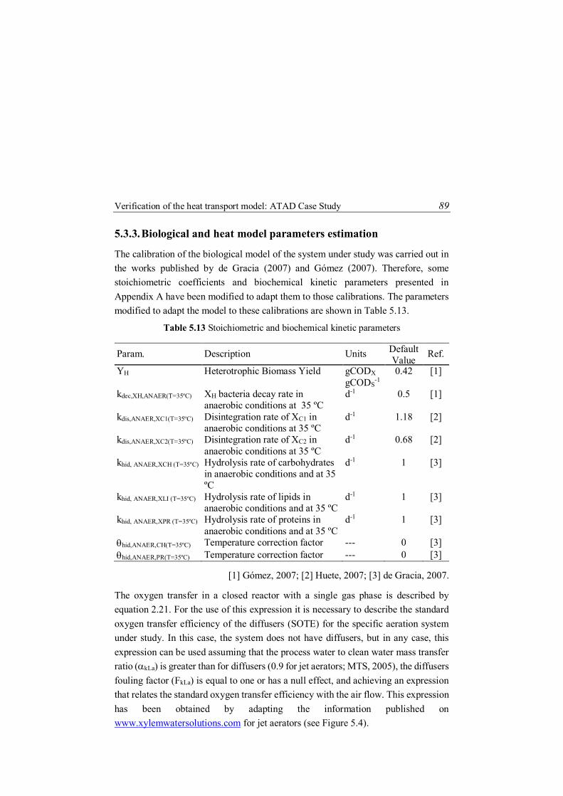
Verification of the heat transport model: ATAD Case Study 89

5.3.3. Biological and heat model parameters estimation

The calibration of the biological model of the system under study was carried out in the works published by de Gracia (2007) and Gómez (2007). Therefore, some stoichiometric coefficients and biochemical kinetic parameters presented in Appendix A have been modified to adapt them to those calibrations. The parameters modified to adapt the model to these calibrations are shown in Table 5.13.

Table 5.13 Stoichiometric and biochemical kinetic parameters

Param. Description Units Default Value

Ref.

YH Heterotrophic Biomass Yield gCODX gCODS

-1 0.42 [1]

kdec,XH,ANAER(T=35ºC) XH bacteria decay rate in anaerobic conditions at 35 ºC

d-1 0.5 [1]

kdis,ANAER,XC1(T=35ºC) Disintegration rate of XC1 in anaerobic conditions at 35 ºC

d-1 1.18 [2]

kdis,ANAER,XC2(T=35ºC) Disintegration rate of XC2 in anaerobic conditions at 35 ºC

d-1 0.68 [2]

khid, ANAER,XCH (T=35ºC) Hydrolysis rate of carbohydrates in anaerobic conditions and at 35 ºC

d-1 1 [3]

khid, ANAER,XLI (T=35ºC) Hydrolysis rate of lipids in anaerobic conditions and at 35 ºC

d-1 1 [3]

khid, ANAER,XPR (T=35ºC) Hydrolysis rate of proteins in anaerobic conditions and at 35 ºC

d-1 1 [3]

hid,ANAER,CH(T=35ºC) Temperature correction factor --- 0 [3] hid,ANAER,PR(T=35ºC) Temperature correction factor --- 0 [3]

[1] Gómez, 2007; [2] Huete, 2007; [3] de Gracia, 2007.

The oxygen transfer in a closed reactor with a single gas phase is described by equation 2.21. For the use of this expression it is necessary to describe the standard oxygen transfer efficiency of the diffusers (SOTE) for the specific aeration system under study. In this case, the system does not have diffusers, but in any case, this expression can be used assuming that the process water to clean water mass transfer ratio (kLa) is greater than for diffusers (0.9 for jet aerators; MTS, 2005), the diffusers fouling factor (FkLa) is equal to one or has a null effect, and achieving an expression that relates the standard oxygen transfer efficiency with the air flow. This expression has been obtained by adapting the information published on www.xylemwatersolutions.com for jet aerators (see Figure 5.4).

90 Model-based exploration of heat transfers and enthalpy changes of reaction

Figure 5.4 Relation between the aspired mass air flow, the standard oxygen transfer rate and the standard oxygen transfer efficiency (Source: adapted from

http://www.xylemwatersolutions.com)

Parametrising the information, the following expression is obtained which can be used directly in equation 2.21.

5.2

With regard to the terms associated with heat transfer, table 2 shows the parameters estimated experimentally by Gómez (2007) and adapted to the model proposed in this thesis.

Table 5.14 Stoichiometric and biochemical kinetic parameters

Param. Description Units Default Value Ref.

Atank Contact area m2 67.2 + 26.7 · Tw(K)

Estimated for 9200 Nm3 d-1

kgas Gas extraction constant - 200000 Estimated ktherm/L Thermal conductivity of

the material kJ K-1 m-2 d-1

25 Gómez, 2007

WAct Actuator power kW 30 Gómez, 2007 Act Actuator efficiency - 0 Gómez, 2007 kLa Temperature correction

factor - 1.02 Estimated

The contact area between the liquid and gas phases has been estimated on the basis of equations 2.13, 2.14 and 5.2, for a bubble diameter of 6 mm (Issa, 2013), an up-flow velocity of 0.24 m s-1 (Pradhan, 2012) and for an air flow of 9200 m3 d-1.

SOTE = 0.2233·mGO2,in + 20561.0

Verification of the heat transport model: ATAD Case Study 91

5.3.4. Dynamic simulation of the operation of the ATAD

The dynamic results obtained in the simulation are shown in Figure 5.5, where the experimental and simulated aqueous phase temperatures obtained in the selected period are compared, obtaining a proper fit both in terms of substrate limiting conditions (days 0 to 11 and 19 to 23) and oxygen limiting conditions (days 11 to 19). The evolution of temperature in oxygen limiting conditions makes possible the calibration of the oxygen transfer coefficient (kLa), whereas temperature data under substrate limiting conditions supplies the information required for calibrating the heat flux associated with aeration.

Figure 5.5 Experimental and simulation results comparison of the aqueous phase

temperature profile in the full scale ATAD

In turn, Figure 5.6 shows the ability of the model to predict total COD concentration variations inside the digester. As can be observed in Figure 5.6, the obtained adjustment is satisfactory since it correctly predicts the total COD variation trends. The advantage of the proposed thermal model is the possibility of estimating the heat of reaction or the specific heat yield at each moment (Figure 5.7), instead of using a fixed value (13.93 kJ gCODrem

-1 in Gomez, 2007). This fact has allowed a more accurate prediction of the temperature of the aqueous and gaseous phases, successfully reproducing the curvatures produced by a lack or by an excess of substrate.

As discussed in the previous section, the consideration of all transformations is essential for a correct estimation of the heat of reaction. In Figure 5.7, the difference between considering only the oxidation transformations or total transformations can

92 Model-based exploration of heat transfers and enthalpy changes of reaction

be observed. When the system operates under oxygen limiting conditions the difference between considering only oxidation reactions or all reactions is a constant gap (days 11 to 19). By contrast, under substrate limiting conditions (days 0 to 11 and 19 to 23), when the substrate is depleted, the other transformations take on more prominence (such as CO2 stripping) and the heat of reaction decreases slightly increasing the gap at the end of the cycle.

Figure 5.6 Experimental and simulation results comparison of total COD concentration

variations inside the digester

Figure 5.7 Specific heat yields evolution in the full scale ATAD

By analysing the thermal fluxes of the system (Figure 5.8), it can be seen that biological processes (ΔHr water) are the most important heat flux contributors, representing 60-70 % of the heat in the process. The contour of this flux area shows the evolution of organic matter oxidation, clearly differentiating substrate limiting and oxygen limiting areas. The heat dissipated due to the liquid and gas phase transformations (ΔHr water-gas) is the second most important heat flux, representing

Verification of the heat transport model: ATAD Case Study 93

15-30 % of the heat in the process. Of this percentage, 10 % corresponds to CO2 stripping, and the remaining 90 % to the heat lost by evaporation. In this example, atmospheric and solar radiation have not been graphed since they were negligible compared to other terms. On day 10, the reactor is not charged producing a considerable drop in the overall net heat value. The negative values obtained represent satisfactorily the temperature drop of the system in the middle of cycle (Figure 5.5) and the consequent curvature in the evolution of the temperature.

Figure 5.8 Total enthalpy produced and consumed in the system with the contribution

of each thermal flux

The proposed E-PWM methodology also makes possible a detailed dynamic analysis of the different terms in heat generation and transport as a function of the influent load or operational strategies. Next examples briefly show the effect of ventilation and the substrate fed in the ATAD temperature.

5.3.5. Model-based exploration of the effect of air flow in an ATAD digester

Aeration is a key factor in aerobic digestion from the point of view of biological reaction and heat balance. If the process is working with oxygen concentrations under the stoichiometric value (oxygen limiting conditions), the oxygen transfer will mark the substrate consumption rate of the system and therefore the sludge heating (Messenger et al., 1990). Thus, the digester temperature can be controlled with the air flow, until the substrate is exhausted or the stoichiometric oxygen value is reached. Conversely, if the system is working with oxygen concentrations over the stoichiometric (substrate limiting conditions), the heating degree will depend on the

94 Model-based exploration of heat transfers and enthalpy changes of reaction

amount of substrate fed. In contrast to oxygen limiting conditions, an excess of aeration can cause digester cooling due to the temperature gradient of the bubbles and the liquid phase.

The model's ability to identify these ventilation effects is essential for an appropriate selection of the operational conditions. Still, it is important to mention that for a correct prediction of the heat of reaction, it is necessary to estimate experimentally the respiration quotient, especially important when the system is working under substrate limiting conditions. Figure 5.9 shows an exploration of the expected reactor temperature of the Tudela ATAD for the same OLR of 4.0 KgCOD m-3 d-1 under different aeration flows.

Figure 5.9 Behaviour of the temperature in a full scale ATAD for constant OLR and

variable aeration flows

It can be clearly observed how excess air can cause a cooling of the aqueous phase, decreasing the temperature to values obtained with oxygen limiting conditions, with the disadvantage of having higher costs. Model-based exploration can facilitate the selection of the most appropriate aeration flow. The proposed E-PWM methodology is already prepared for dealing with different gas phases, making possible the simulation of pure oxygen supply.

5.3.6. Model-based exploration of influent characterisation in an ATAD reactor

Different studies (Heijnen, 1999; Heidrich et al., 2011; Hill et al., 2012) have shown that oxidation heat is closely related to the composition of the feed. In this section, the effect of a change in the composition of the sludge fed in the liquid phase has

Verification of the heat transport model: ATAD Case Study 95

been explored by simulation, using the E-PWM methodology. Table 5.15 shows the three influent characterisations used for the model-based exploration.

Table 5.15 Characterisation of the influent for the model based exploration

Fraction of lipids

Fraction of proteins

Fraction of carbohydrates

Fraction of Inert

Baseline characterisation 19 % 25 % 19 % 37 % Characterisation 1 15 % 20 % 28 % 37 % Characterisation 2 22 % 31 % 10 % 37 %

Figure 5.10a shows the predicted evolution of process temperature for the three load characterisations. The rise in the concentration of carbohydrates has led to an increase in liquid temperature of 0.4 °C for this specific OLR (a decrease of 0.4 °C for Characterisation 2). This temperature variation would have been greater using a higher OLR or energy crops such as maize grains, artichoke or wheat, among others. The enthalpy change of reaction of each characterisation is plotted in Figure 5.10b showing the capacity of E-PWM methodology for exploring the effect of influent characterisation in temperature.

Figure 5.10 (a) Temperature evolution for different influent characterisations, (b) Aqueous transformations heats (specific heat yield) for different influent

characterisations

96 Model-based exploration of heat transfers and enthalpy changes of reaction

As expected the greatest heat are obtained for the influent rich in carbohydrates. It is interesting to note that the global transformations heat and, consequently the specific heat yield, is varying in time, depending on the evolution of substrate fractioning within the reactor.

5.4 ANALYSIS OF THE DYNAMIC HEAT EXCHANGES IN THE BSM2 LAYOUT

As a final example of the possibilities offered by the heat transfer model, this last case study shows the usefulness of the E-PWM methodology for a detailed prediction of the dynamic evolution of the heat exchanges generated in a WWTP. The simulation example corresponds to the water line and to the anaerobic digester of the Benchmark Simulation Model No. 2 layout (BSM2; Jeppsson et al., 2007), maintaining its physical attributes and using the 365-day dynamic influent data file.

5.4.1. Description of the BSM2 layout

The BSM2 platform is a general simulation protocol for benchmarking of operational and control strategies at WWTPs. The plant layout (Figure 5.11) is constituted by a primary clarifier for the pre-treatment step, an activated sludge process for C and N removal based on a Modified Ludzack-Ettinger configuration (2 anoxic and 3 aerobic tanks and a secondary clarifier), a dissolved air flotation (DAF) unit, an anaerobic digestion process and a dewatering step.

Figure 5.11 Schematic representation of the Benchmark Simulation Model No. 2 layout

Primary Clarifier Anox. 1 Anox. 2 Aero. 1 Aero. 2 Aero. 3 Secondary Settler

Air Flotation Unit

Anaerobic digesterCHP

Dewatering

Sludge Disposal

Influent

Blow. 1 Blow. 2 Blow. 3

Electricity

Boiler Heat

Electricity

Effluent

Analysis of the dynamic heat exchanges in the BSM2 layout 97

5.4.2. Construction of the model in the simulation platform

As in the previous case, the layout was simulated using the WEST simulation platform and the Ceit PWM library, following these steps describe below.

5.4.2.1. Category selection and influent characterisation

Given the characteristics of the plant, the CN_AnD category was selected from the Ceit PWM library (the description of this category can be found in section 5.3.2.1).

Influent wastewater was simulated using the one year dynamic influent defined for the BSM2 (Gernaey et al., 2014), following the characterisation guidelines given in Appendix C.1. In order to complete the characterisation, elemental mass fractions of certain heterogeneous components and its associated enthalpies of formation were characterised (Table 5.16 and Table 5.17).When global plants are simulated, it is not necessary to analyse the XC1 component since it is used to characterize sludges.

Table 5.16 Elemental mass fractions of the heterogeneous components

Name C H O N P Ch hf º (kJ gE-1) SI 0.557 0.060 0.280 0.093 0.010 0.000 -2.704 SP 0.500 0.010 0.178 0.083 0.229 0.000 -0.835 XI 0.557 0.060 0.280 0.093 0.010 0.000 -2.692 XP 0.503 0.057 0.311 0.084 0.045 0.000 -2.605

Table 5.17 Stoichiometric parameters of XC2 disintegration

fSP,XC2 fCH,XC2 fPR,XC2 fLI,XC2 fXP,XC2 XC2 water line 0.000 0.083 0.722 0.115 0.080 XC2 sludge line 0.008 0.003 0.532 0.165 0.292

5.4.2.2. Unit-process and cost models selection

The plant layout (Figure 5.12) is made up of a five completely stirred open tank reactor for simulating the activated sludge process, a completely stirred closed tank reactor for reproducing the anaerobic digestion process, a primary clarifier, a secondary clarifier, a thickening unit for representing the DAF unit, a dewatering unit, a CHP unit and a heat exchanger unit for closing the energy balance of the digester, previously characterised dynamic water influent, a dynamic water temperature and atmospheric information (temperature, pressure and humidity) inputs, a set of units to reproduce the aeration of biological reactors (controllers, gas

98 Model-based exploration of heat transfers and enthalpy changes of reaction

generators, mass converters and blowers), and finally mass and temperature converter units, combiners and splitters, and controllers (biological TSS concentration, anaerobic digestion temperature and aeration controllers).

Figure 5.12 BSM2 layout built on the WEST simulation platform

The activated sludge units consist of a liquid phase and an atmospheric phase and the digester consists of a liquid phase and a gas phase. Mass and heat transfer balances of both phases (liquid and off-gas) were raised in all the biological reactors, following the schematic balances presented in Figure 5.13 and Figure 5.14.

Figure 5.13 Schematic representation of the mass and heat balance in the activated

sludge reactors.

mw,in

mw,outAqueous

phase

1st Gaseous phase

mg,in

Hw,in Hw,outAqueous

phase

Hg,in

Qwc,out

Qm,in

Qphs,w,g1

1st Gaseous phase

Qsolrd,o,w

Qatmrd,o,w

Analysis of the dynamic heat exchanges in the BSM2 layout 99

Figure 5.14 Schematic representation of the mass and heat balance in the anaerobic digestion unit.

The data of atmospheric temperature, solar radiation and wind velocity have been extracted from the Spanish National Meteorological Agency (http://www.aemet.es) corresponding to measurements made in northern Spain in 2012. Regarding the influent water temperature, the profile has been estimated from atmospheric data and previous year’s tendencies in that area (every day of the year, the input water temperature is higher than the temperature of the atmosphere).

Figure 5.15 Water and atmospheric temperatures used for the simulation

5.4.3. Energetic analysis of the activated sludge process

Figure 5.16a shows the predicted contribution of the most significant heat fluxes in the overall balance. The mild temperatures and abundant rainfall that characterised the oceanic climate means that the solar radiation flux (ΔH radiation) and the

mw,in

mw,out

mg,out

Aqueous phase

1st Gaseous phase

Ew,w ρw,w

Hw,in Hw,out

Hg,out

Aqueous phase

1st Gaseous phase

Qgc,c,out

Qwc,out

Qm,inQphs,w,g1

Eg1,w ρg1,w

Ew,g1 ρw,g1

100 Model-based exploration of heat transfers and enthalpy changes of reaction

conduction and convection fluxes (ΔH cond/conv) do not have the significance that can be expected in other areas. Although surprised that the term of heat transfer due to aeration hasn’t appeared in the Figure 5.16a, this term in the ΔH cond/conv term has been included along with the transfer between the atmosphere and the water phase. The aeration provide heat to the system but this heat is offset by losses due to contact between the atmosphere and the water.

Figure 5.16b shows a detailed description of the main heat fluxes within the reactors, differentiating between the heat supplied by the biological transformations and the heat consumed by evaporation and stripping. Simulations results clearly show how the most significant heat fluxes are due to COD removal (denitrification in anoxic reactors and heterotrophic growth in aerobic reactors) and nitrification reactions. To a lesser extent, but also relevant is the stripping of CO2 and evaporation.

Figure 5.16 (a) Total enthalpy produced and consumed in the system with the

contribution of each thermal flux, (b) Transformation heat fluxes

Simulation results have shown that the expected overall increase in the water temperature from influent to effluent ranges between 0.8 and 1.5 degrees depending

Analysis of the dynamic heat exchanges in the BSM2 layout 101

on the radiation term (Figure 5.17), coinciding with the ranges previously published by la Cour Jansen et al. (1992) and Makinia et al (2005).

Figure 5.17 Water influent and effluent temperatures

The proposed E-PWM methodology facilitates a detailed description of the contribution of different transformations in the heat flows and temperature variations. For example, at this particular case-study, simulation results show that the nitrification and heterotrophic growth reactions increase the tank temperature 0.6-0.8 degrees while denitrification only by 0.23 degrees. Evaporation and stripping reactions are widely influenced by atmospheric temperature, and decrease the temperature by 0.05-0.2 degrees. As expected, the effect of transformation heats in process temperature is not very relevant in conventional activated sludge reactors. However, it can be very significant in other processes that exhibit higher biological activity and lower heat transport with the environment like, for example, the Autothermal Thermophilic Aerobic Digesters previously analysed.

5.4.4. Analysis of transformations heat exchanges generated in an anaerobic digester

The heat associated to sludge anaerobic digestion transformations is minimal, and it is for this reason that the calorific studies published around this process tends to be scarce. Besides scarcity, in these studies a wide range of views about digestion exothermicity or endothermicity has been published, without reaching a consensus. Within this frame, in this final analysis, transformations heat exchanges generated in an anaerobic digester has been analysed for different influents, comparing the

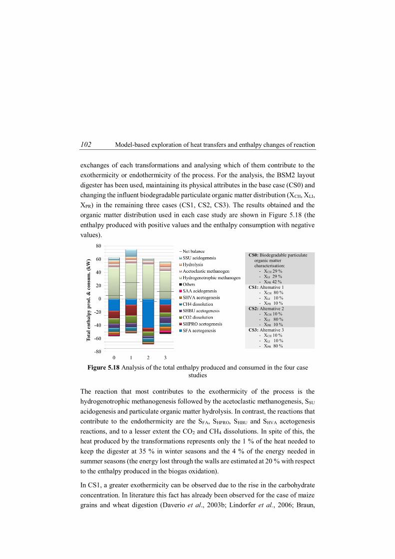
102 Model-based exploration of heat transfers and enthalpy changes of reaction

exchanges of each transformations and analysing which of them contribute to the exothermicity or endothermicity of the process. For the analysis, the BSM2 layout digester has been used, maintaining its physical attributes in the base case (CS0) and changing the influent biodegradable particulate organic matter distribution (XCH, XLI, XPR) in the remaining three cases (CS1, CS2, CS3). The results obtained and the organic matter distribution used in each case study are shown in Figure 5.18 (the enthalpy produced with positive values and the enthalpy consumption with negative values).

CS0: Biodegradable particulate organic matter characterisation:

- XCH 29 % - XLI 29 % - XPR 42 %

CS1: Alternative 1 - XCH 80 % - XLI 10 % - XPR 10 %

CS2: Alternative 2 - XCH 10 % - XLI 80 % - XPR 10 %

CS3: Alternative 3 - XCH 10 % - XLI 10 % - XPR 80 %

Figure 5.18 Analysis of the total enthalpy produced and consumed in the four case studies

The reaction that most contributes to the exothermicity of the process is the hydrogenotrophic methanogenesis followed by the acetoclastic methanogenesis, SSU acidogenesis and particulate organic matter hydrolysis. In contrast, the reactions that contribute to the endothermicity are the SFA, SHPRO, SHBU and SHVA acetogenesis reactions, and to a lesser extent the CO2 and CH4 dissolutions. In spite of this, the heat produced by the transformations represents only the 1 % of the heat needed to keep the digester at 35 % in winter seasons and the 4 % of the energy needed in summer seasons (the energy lost through the walls are estimated at 20 % with respect to the enthalpy produced in the biogas oxidation).

In CS1, a greater exothermicity can be observed due to the rise in the carbohydrate concentration. In literature this fact has already been observed for the case of maize grains and wheat digestion (Daverio et al., 2003b; Lindorfer et al., 2006; Braun,

Conclusions 103

2007). This exothermicity is mainly the result of the hydrogenotrophic methanogenesis increased. When predominant components are lipids (CS2), SFA acetogenesis reaction (highly endothermic) influences the process, providing a global endothermicity. In this case, the reaction would become endothermic, requiring a supply of heat for the bacteria maintenance. Finally, case CS3, where mainly proteins are oxidised, is in an intermediate position, producing a slight heat release.

All these hypotheses can provide answers to the scientific community uncertainty around digestion heat or even can help to understand the process better. It has been seen that due to the numerous reactions involved in the anaerobic digestion, the estimation of a specific reaction heat is not possible, since the heat transferred depends on factors such as the influent composition.

5.5 CONCLUSIONS In view of the importance of a correct temperature estimation, this Chapter contains the validation of the methodology for calculating the enthalpy change of reaction and the verification of the heat transfer model proposed in Chapter 2.

By comparing the transformation heat values calculated with the methodology and the values obtained in bibliography, the ability of the methodology for predicting the enthalpy change of reaction of any transformation has been demonstrated, only knowing the enthalpy of formation of the products and the reagents. This makes it a useful tool for automatically estimating the heat of reaction without the need to look for it in literature.

At the same time, the detailed characterisation of the components that provides the Plant-Wide Modelling methodology has helped explain the discrepancies found in literature about the enthalpy change of reaction of the COD oxidation reactions (hºr, methodology = 13.62-14.62 kJ gCOD-1

removed). Although it has been seen that the main reactions that bring heat to the system are this oxidation reactions, all other reactions are necessary since they can change the obtained result by up to 10 %. Above all, it is important to consider the nitrogen removal transformations and the CO2 stripping and H2O evaporation reactions.

With the autothermal thermophilic aerobic digestion reactor behaviour analysis, the predictive capability of the model to successfully reproduce liquid and gas temperature variations in periods with abrupt OLR changes has been verified. The

104 Model-based exploration of heat transfers and enthalpy changes of reaction

model effectively reproduced the mass/energy nexus, maintaining the same stoichiometric and kinetic parameters for all simulated scenarios. In view of the results obtained, it can be affirmed that the predictive capacity of the model developed during this thesis is validated. Within this framework, the characteristics of the heat transfer model allow to:

Predict the temperature of each phase (liquid, gaseous and solid phases)

Identify the heat flows presents in the system.

Analyse the contribution of these flows in the heat transfers.

Relate the thermal variations with the chemical, biochemical and physico-chemical transformations.

Analysing the results obtained in the model-based explorations, it has been seen that in aerated reactors (active sludge and aerobic digestion reactors), the heat released in the transformations represents 60-70 % of the process heat, confirming the need for an adequate estimation of the heat of reaction. Under anaerobic conditions, in turn, a great utility of the model has been seen for detecting the autothermicity of the process and for estimating the additional heat needs by the system to maintain the operating temperature.

Finally, the model-based explorations has shown the capacity of the methodology and the general heat transfer model for exploring the effect of ventilation and the effect of influent characterisation in temperature.

105

6 QUANTITATIVE ASSESSMENT OF ENERGY AND RESOURCE

RECOVERY IN EVOLUTIONARY WWTPS BASED ON PLANT-WIDE

SIMULATIONS

The contents of this Chapter have been included in the next publication:

Fernández-Arévalo, T., Lizarralde, I., Pérez-Elvira, S.I., Garrido, J.M., Puig, S., Poch, M., Grau, P., Ayesa, E., 2016. Quantitative assessment of energy and resource recovery in evolutionary wastewater treatment plants based on Plant-Wide simulations. Submitted to the journal Water Research.

6.1 ABSTRACT The main objective of this Chapter is the comparison of different plant configurations using the Plant-Wide Modelling library. In order to demonstrate the potential of the library and the need to run simulation analyses, this Chapter carries out a comparative analysis of evolutionary WWTP, from a techno-economic point of view. The selected layouts were (1) a conventional WWTP based on a modified version of the

106 Quantitative assessment of energy and resource recovery in evolutionary WWTP

Benchmark Simulation Model No. 2, (2) an upgraded or retrofitted WWTP, and (3) a new WRRF concept denominated as C/N/P decoupling WWTP. The study was based on a preliminary analysis of the organic matter and nutrient energy use and recovery options, a comprehensive mass and energy flux distribution analysis in each configuration in order to compare and identify areas for improvement, and a cost analysis of these plants for different influent COD/TN/TP ratios. The plant layouts proposed in this Chapter are just a sample of the possibilities offered by current technologies. Even so, the library presented in Chapter 4 is generic and can be used to construct any other plant layout, provided that a model is available.

6.2 INTRODUCTION The purpose of the design and upgrade of conventional waste(water) treatment plants has traditionally been to remove the residual organic compounds and nutrients contained in the water to fulfil the quality standards set by the regulations established for the treated area. Resource or energy recovery was focused exclusively on obtaining energy from the biogas produced in anaerobic sludge digestion. This biogas production can supply from a quarter to half of the energy requirements for a WWTP with activated sludge (AS) process (Crawford et al., 2010; McCarty et al., 2011; Puchongkawarin et al., 2015), which needs between 0.3 and 0.6 kWh m-3 treated water (Foley et al., 2010) to fulfil the energetic needs of the plant. Nevertheless, this value is only one tenth of that associated to the heat of combustion of organic compounds contained in the wastewater (McCarty et al., 2011; Shoener et al., 2014; Kokabian et al., 2015). Hence, if a greater proportion of this energy were recovered, treatment plants could become self-sufficient and producers of energy (Logan, 2004; Guest et al., 2009).

Recent concerns about climate change or sustainability have led to an increasing awareness of the importance of resource recovery, energy minimisation and environmental impact assessment, which in turn has resulted in tightening effluent standards. Under this changing context, a new paradigm has emerged in which municipal wastewater (MWW), traditionally considered to be a pollution problem and an energy- and chemical-intensive activity with excess sludge disposal issues (Gude, 2015), is starting to be thought of as a continuous and sustainable source of chemical energy and resources (Frijns et al., 2013). As a result, WWTPs are now considered to be Wastewater Resource Recovery Facilities (WRRF), from which

Introduction 107

valuable products such as chemicals, nutrients (mainly phosphorus, P), bioenergy (methane from anaerobic digestion), and bio-products can be obtained (Keller, 2008, Guest et al., 2009). To make this change possible, the water sector is developing new and innovative treatment technologies, such as energy-efficient nutrient removal or recovery technologies with Anammox, struvite crystallisers, phototropic bacteria, high rate algae systems, sludge pre-treatment processes, or systems for the production of microbial polymers.

Immersed in a process of change, WWTPs need a change in philosophy: from waste to resource. The most immediate step is the updating of existing plants by incorporating these innovative technologies in order to reduce overall operating costs and recover resources. Thanks to the incorporation of these improvements, energy self-sufficient WWTPs is a feasible goal (Jeppsson et al., 2007). Proof of this comes from the Strass and Wolfgangsee-Ischl WWTPs in Vienna (Wett et al., 2007; Nowak et al., 2011). This self-sufficiency is subject to the influent itself (influent load, C/N/P ratio and temperature), effluent discharge limits, plant design or layout, unit-process efficiencies, operating factors and environmental conditions. Therefore, in any analysis or comparison, these data should be specified. The second and final step would be to design new plant layouts from the perspective of reuse and recovery, incorporating the most suitable and novel processes. As stated in the work of Batstone et al. (2015), currently there are two extended philosophies to address the transition from WWTPs to WRRF’s. One is the low energy mainline (LEM) configuration, which focuses on using low strength anaerobic digestion processes for treating raw domestic sewage, followed by nutrient removal processes (McCarty et al., 2011). The other is the Partition-Release-Recover (PRR) configuration, which focuses on a first stage of COD and nutrient accumulation in the solids, a second stage of release through the digestion process, and a final stage of digestate treatment (Verstraete et al., 2009).

In the literature there are numerous studies comparing different plant layouts and analysing the energy consumption of conventional WWTPs (Nowak, 2003; Gude, 2015, Tchobanoglous et al., 2014, Mininni et al., 2015), and fewer studies analysing advanced WWTPs (Garrido et al., 2013; Batstone et al., 2015; Khiewwijit et al., 2015), many of which use life cycle analysis (LCA) methods and decision support system (DSS) tools (Foley et al., 2010; Garrido-Baserba et al., 2014; Bisinella de Faria, et al., 2015; Castillo et al., 2016). Even so, virtually all these studies are based on operating cost analysis and/or are largely dependent on the quality of the data used

108 Quantitative assessment of energy and resource recovery in evolutionary WWTP

and their specifications. One of the main problems encountered in these energy assessments is the limited information available to reproduce disturbances or unusual situations (Jenkins et al., 2014). It is for this reason that the best tool for overcoming all these obstacles is to conduct mass balances for COD, N and P for the whole plant (Spindler & Vanrolleghem, 2012; Jenkins et al., 2014). The detailed analysis of each stream allows a better understanding of the process, identifying areas for improvement and opportunity for resource and energy recovery. Among the existing approaches in the literature, the Plant-Wide Modelling (PWM) methodology proposed by in this thesis constitutes a very suitable tool for rigorously and globally assessing the incorporation of new leading-edge technologies in conventional plant layouts (Fernández-Arévalo et al., 2015, Fernández-Arévalo et al., 2017) or selecting the most appropriate operating strategies at existing full-scale facilities (Fernández-Arévalo et al., 2016; Chapter 7).

The main challenge of this Chapter is to conduct a comparative analysis of evolutionary WWTPs, from a techno-economic point of view, analysing in turn organic matter and nutrient energy use and recovery options. To do this, an upgraded plant and a newly designed plant have been analysed and compared against a conventional plant (based on the BSM2 configuration; Jeppsson et al., 2007). In the upgraded or retrofitted WWTP, thermal hydrolysis (TH) technology and a nitritation/Anammox process have been incorporated into the reference plant, and the new plant is a C/N/P decoupling WWTP, which is based on the PRR configuration proposed by Batstone et al., (2015).

6.3 DESCRIPTION OF THE SCENARIOS The comparative analysis of the three configurations selected (conventional WWTP, upgraded WWTP and C/N/P decoupling WWTP) has been based on PWM simulations. This section details the description of these plant layouts and the steps followed to build the model.

6.3.1. Plant layouts definition

6.3.1.1. Conventional WWTP

The reference WWTP considered in the study is a biological nutrient removal plant based on the Benchmark Simulation Model No. 2 (BSM2; Jeppsson et al., 2007). As

Description of the scenarios 109

discussed in Chapter 5, the plant consists of a primary clarifier, 2 anoxic and 3 aerobic tanks, a secondary clarifier, a dissolved air flotation unit, an anaerobic digestion and a dewatering step. A ferric chloride dosage is delivered to the output from the third aerobic tank for chemical P removal. Besides adding the chemical agents for P removal, ferric chloride can also be added to enhance the settling characteristics of the primary sludge for cases in which the production of primary sludge needs to be maximised. Finally, two other chemical additions are required in flotation and dewatering processes.

Figure 6.1 Conventional wastewater treatment plant (based on BSM2 layout)

In order to measure the full potential of the plant configuration, an overall heat and cost balance of the plant was carried out. This heat balance mainly made it possible to estimate the heat required to maintain the anaerobic digester at 35 ºC. The heat produced in cogeneration or combined heat and power (CHP) unit could not be always enough to supply the heat requirements of the digester. In those cases, it was necessary to divert a portion of the biogas produced in the anaerobic digestion to a boiler to cause combustion without producing electricity. Regarding the cost balance, the most representative power consumption/production and chemical agent costs were estimated. These were elements such as the power consumption in the aeration, pumping, flotation, mixing and dewatering processes, the energy produced in the CHP unit, and the chemical agent costs.

Primary Clarifier Anox. 1 Anox. 2 Aer. 1 Aer. 2 Aer. 3 Secondary Settler

Air Flotation Unit

Anaerobic DigesterCHP

Dewatering

Sludge Disposal

Influent

Blow. 1 Blow. 2 Blow. 3

Electricity

BoilerHeat

Electricity

Effluent

110 Quantitative assessment of energy and resource recovery in evolutionary WWTP

6.3.1.2. Upgraded WWTP

This second layout is based on the reference case (conventional WWTP), but with two advanced technologies being incorporated in the sludge line: a TH reactor and a nitritation/Anammox process for treating the rejected supernatants (Figure 6.2).

Figure 6.2 Upgraded wastewater treatment plant

The aim of the TH process is to maximise biogas production by increasing the biodegradability of the sludge. For this, pressurised steam must be fed to the reactor to maintain the chamber at 170 ºC (Fernández-Polanco et al., 2008). In this scenario, part of the biogas produced in the anaerobic digestion was diverted to a boiler to cause combustion and produce the required steam. The amount of biogas required for the TH and consequently, the benefits in electricity generation will depend on the incoming sludge temperature and concentration that will be crucial for the profitability of the process. The increase in sludge biodegradability also involves an extra release of ammonium (NHX-N), which must be treated in situ. To remove this surplus of N and the NHX-N released in anaerobic digestion, a nitritation/Anammox process is an interesting approach. In the Anammox process, ammonium is oxidised with the nitrites formed in the previous nitritation process, without oxygen and COD consumption, raising the stoichiometric aeration cost savings up to 63 % (Volcke et al., 2006).

Primary Clarifier Anox. 1 Anox. 2 Aer. 1 Aer. 2 Aer. 3 Secondary Settler

Anaerobic Digester

CHP

Dewatering

Sludge Disposal

Influent

Blow. 1 Blow. 2 Blow. 3

Electricity

Chemicals

Heat

Electricity

Effluent

Exhaust gas boiler

Thermal Hydrolysis

PartialNitritation

Blow. 4Anammox

Air Flotation Unit

Description of the scenarios 111

6.3.1.3. New WRRF concept: C/N/P decoupling WWTP

The partition-release-recover (PRR) concept proposed by Batstone et al., (2015) was used as an example of new WRRF concept. This configuration completely decouples COD and nutrient treatments in order to seek greater process performance. In the work of Gao et al. (2014), the decoupling of COD and N removal was already mentioned as a promising strategy for minimising energy requirements. The configuration (Figure 6.3) consists of a Phoredox (A/O) process for the biological P accumulation, a thermal hydrolysis technology to increase the biodegradability and dewaterability of sludge, an anaerobic sludge digestion process for the COD removal and P and N release, a crystalliser for P precipitation as struvite, and a partial nitritation/Anammox process in the mainstream and side stream to treat the N.

Figure 6.3 New WRRF concept: C/N/P decoupling WWTP.

In the Phoredox process, soluble COD and orthophosphates (ortho-P) are accumulated in the solids (heterotrophic organisms, polyphosphate (polyP) accumulating organisms (PAO), polyhydroxyalkanoates (PHA) and polyP) thanks to the combination of anaerobic and aerobic conditions. If these reactors are operated at very short sludge retention time or SRT (2-4 days, depending on the temperature), only the strictly necessary N for the growth of the microorganisms will be consumed. The secondary sludge produced is sent to the TH process to transform part of the non-biodegradable material in biodegradable. The primary sludge and the pre-treated

Primary Clarifier Anaer. 1 Aer. 1 Aer. 2 Secondary Settler

Anaerobic Digester CHP

DewateringSludge Disposal

Influent

Blow. 1 Blow. 2

Electricity

Chemicals

Heat

Electricity

Effluent

Exhaust gas boiler

Thermal Hydrolysis

Blow. 3

PartialNitritation

Anammox

Struvite

Secondary Settler

Crystalliser

Air Flotation Unit

112 Quantitative assessment of energy and resource recovery in evolutionary WWTP

secondary sludge are sent to the anaerobic digester, where the biodegradation of the organic matter occurs. The carbonaceous matter is released as biogas (gas phase) and at the same time the N and P become soluble matter in the form of NHX-N and ortho-P (liquid phase). After dehydrating the digested sludge, the resulting rejected supernatant flow has a high content in nutrients. This side stream is suitable for recovering nutrients such as struvite (MgNH4PO4·6H2O). Finally, after the struvite precipitation, the remaining N joins the mainstream and both are treated with a partial nitritation/Anammox process.

6.3.2. Plant-Wide Model construction

Thanks to the availability of a complete and compatible model library, it is easy to combine the units and actuators that are necessary to describe the case study in a simple and tailored way. Thus, the three scenarios were simulated using the WEST simulation platform (www.mikebydhi.com) and the Ceit PWM library following these steps describe below.

6.3.2.1. Category selection and influent characterisation

Given the characteristics of the three plant layouts, the C2NPprec_AnD category from the Ceit PWM library was selected to reproduce the behaviour of all plants. The biochemical reactions considered in the model were the ones that are necessary to describe biological organic matter, P and two-step N removal under different environmental conditions (aerobic, anoxic and anaerobic). The chemical transformations considered in the model were the weak acid-base and complex ion-pairing equilibrium reactions between volatile fatty acids (VFAs), inorganic carbon, N, P, calcium, magnesium and potassium. Finally, two types of physico-chemical transformations were considered: (1) liquid-gas transfer, regulated by gaseous partial pressure according to Henry’s law of dissolution, and (2) the precipitation-redissolution equilibrium.

Influent wastewater was simulated using the average flow-weighted influent concentrations calculated for one year of influent defined in BSM2 (Gernaey et al., 2014), with some minor modifications and additions. The influent proposed in BSM2 has a very low SCOD/TCOD ratio (0.14 gSCOD/gTCOD) and does not provide information about the proportion of VFA, colloidal matter and P. This low concentration of soluble matter can limit the denitrification and fermentation

Simulation analysis: Energy and nutrient management exploration 113

processes, which makes it possible to distort the conclusions drawn. To avoid any issues, the same influent COD concentration was maintained. However, a ratio of 0.44 gSCOD/gTCOD was established, being the VFA concentration a 15 % of the soluble and colloidal COD (Henze et al., 2008). The colloidal fraction of the slowly biodegradable matter remained at 25 %, the TKN/TP ratio stayed at 5 and the VSS/TSS at 0.76.

6.3.2.2. Unit-process and cost models selection

In each configuration, the units were selected to describe the detailed layouts in the previous section (Completely stirred open and closed tank reactors, primary and secondary clarifiers, thickener and dewatering units, biofilm reactors, CHP units, boilers, heat exchangers and precipitation units), and in all models the mass and heat balances were used to analyse in detail the mass and heat flows in the plant. To describe the major costs of the system the following models were selected: blowers, pumps, stirrer engines, gas and water distribution systems, specific energy ratios, dosage costs and electricity/cost conversion models. To describe the costs of certain units, such as the costs of flotation and dewatering, it is necessary to combine more than one cost model. The dehydration process is described from specific energy ratios and dosage costs, and in the case of flotation the process is described by specific energy ratios and pumping, aeration and dosage costs. All these cost models were calibrated from standard engineering values.

6.4 SIMULATION ANALYSIS: ENERGY AND NUTRIENT MANAGEMENT EXPLORATION

Based on the detailed configurations, (steady state) simulations were carried out to analyse the organic matter and nutrient energy use and recovery options in: (1) a conventional WWTP, (2) an upgraded WWTP, and (3) a New WRRF. Finally, a cost analysis of these plants for different influent C/N/P ratios was considered. To avoid possible interference from other factors that affect operation (plant oversising, unit-process efficiencies, environmental factors, etc.), reactor volumes and recycle flows have been optimised for each plant layout and for each influent in order to fulfil a fixed effluent quality of 10 gN m-3, 1 gP m-3, 125 gCOD m-3 and 35 gSS m-3, accordingly to the European Directive 91/271/EEC.

114 Quantitative assessment of energy and resource recovery in evolutionary WWTP

6.4.1. General considerations about COD and nutrients energy use and recovery options in WWT processes

In analysing the different conventional options of getting energy from COD removal, the most effective and typical way was to transform the organic matter into CH4 (the hrºCH4 is 13.91 kJ gCOD-1 or 890 kJ mol-1) and use its combustion to produce thermal and electric energy. Considering that the anaerobic COD conversion efficiency into CH4 was 0.84-0.95 % (considering a reasonable range of variation for urban wastewater composition) and that the reactions can be exothermic or endothermic (Table 6.1), the overall reaction heat of the CH4 formed in the anaerobic digester per unit of COD feed was 11.86-13.37 kJ gCODrem

-1. For aerobic or anoxic oxidations in AS processes, in turn, the heat released was much lower. In these processes a large proportion of the COD is used for biomass growth. The heat of reaction of COD in aerobic reactions is between 4.07 kJ gCODrem

-1 and 5.27 kJ gCODrem

-1, and for anoxic reactions is between 3.52 kJ gCODrem-1 and 4.74 kJ

gCODrem-1 (Table 6.1). In addition to providing almost twice as much energy per

gram of COD removal in anaerobic conditions, the oxidation of the COD in the aqueous phase was not as effective as biogas combustion in gaseous phase. The proportion of organic matter in a secondary treatment was minimal (0.2-0.4 %), and all the released heat was used to warm the medium, in this case the water. This makes the energy recovery or reuse unaffordable. Therefore, the option to remove the COD under anaerobic conditions (anaerobic digestion) has three advantages: (1) the heat of reaction is higher, (2) the energy recovery from biogas combustion is more effective, and (3) aeration costs are reduced. Thus, the clearest alternative to maximise the recovery or reuse of the COD energy potential is to minimise the COD oxidation in AS processes. This can be obtained by producing more primary sludge and working at lower SRT in the secondary biological treatment.

Although, as it has been abovementioned, the energy recover from compounds is more efficient when they are in a gaseous phase. In the case of the ammonia, its solubility in water is very high, necessitating stripping methods for transferring from water into gas phase. This, added to the fact that ammonia requires a catalyst for its oxidation in gas phase (Jones et al., 1999), makes this process economically unfeasible. Moreover, the nitrogen recovery techniques (ion exchange methods or stripping processes) consume more energy than removal processes, with the exception of struvite recovery technologies. Consequently, from an economic perspective, the destruction of nitrogen compounds appears the most logical route

Simulation analysis: Energy and nutrient management exploration 115

(Matassa et al., 2016) and low-energy alternatives can be proposed, such as the use of Anammox bacteria, anaerobic phototropic bacteria or high-rate algae (Batstone and Virdis, 2014).

Table 6.1 Specific heat yields (or energy content) estimated with the PWM methodology

Transformations † SSU SAA SFA SHVA SHBU SHPRO SHAC

COD rem. heat (kJ gCOD rem.-1) Aerobic -5.27 -4.41 -4.07 -4.14 -4.17 -4.19 -4.32 Anoxic -4.74 -3.89 -3.55 -3.52 -3.64 -3.67 -3.79 Anaerobic‡ -1.01 -0.17 0.14 0.08 0.04 0.00 -0.15 COD rem. heat (kJ molCOD rem.-1) Aerobic -1011 -2997 -2997 -862 -667 -469 -276 Anoxic -910 -520 -2610 -753 -583 -410 -243 Anaerobic‡ -195 -22 101 17 9 1 -25

† CO2 stripping is not included in the specific heat yield estimations, but the COD used for biomass growth is included.

‡ The estimation of the reaction heat includes the acidogenesis, acetogenesis and methanogenesis reactions.

Comparing the N oxidation reactions in the aqueous phase, the Anammox reaction is the one that release more energy to the medium (23.32 kJ gNrem

-1), followed by nitritation (15.46 kJ gNrem

-1) and nitratation (6.09 kJ gNrem-1) reactions. Thus,

Nitritation/Anammox reactions maximise the energy utilisation of the N and minimise oxygen consumption in the process that leads to a reduction in the aeration costs.

Finally, the scarcity of natural phosphorus resources converts the recovery of P into the first alternative for use. Currently, P recovery methods from MWW include the agricultural use of sludge, production of struvite, particularly in enhanced biological P removal (EBPR) plants, and the recovery of P from ash (Wilfert et al., 2015). On the other hand, phosphorus removal itself, using biological or chemical processes does not exert any effect on energy balances.

6.4.2. Analysis of the energy use of a conventional wastewater treatment plant

To analyse the degree of utilisation of thermal energy content (energy associated with the fluid temperature) and mass energy content (energy associated with the

116 Quantitative assessment of energy and resource recovery in evolutionary WWTP

composition of water), a global plant-wide simulation of a conventional plant was carried out under stationary conditions for a critical temperature of 13 °C.

Based on the mass and energy fluxes proposed by Pagilla et al. (2004), Figure 6.4 shows the maximum energy potential of the wastewater in each point of the plant. The top of the figure shows the total thermal energy or enthalpy (not exergy) associated with temperature, while the bottom part reflects the maximum energy potential of the constituents in the water, or the energy released upon oxidation of all water components to CO2 (g), H2O (aq.), NO2, H3PO4, P2O5, Fe2O3, and Mg2P2O7 (see Chapter 5).

In a conventional plant, a considerable fraction of the mass energy content escaped as biological heat (35-40 %) due to the transformations that occurred in the system. Among these transformations, nitrification reactions brought more specific energy to the system (21.61 kJ gNrem

-1), followed by the COD oxidation reactions (Table 6.1). Around 30 % of the mass energy content is converted into biogas and goes to the CHP unit. Depending on the COD flow fed to digestion and depending on water temperature, part of this biogas may have to be carried to a boiler to produce the thermal energy needed to maintain the digestion temperature. For a mass flow of 7.7 tCOD d-1 (42.6 kgCOD m-3) and a temperature of 13 °C, for example, it is not possible to maintain the mesophilic temperature, and 3-5 % of COD is destined to the boiler, reducing the electrical energy production. Only 10 % of the mass energy content in MWW is converted into electricity, losing the remaining energy for heat dissipation (4 %), through the effluent (8 % mass content and 37 % thermal content), through the sludge (26 %), and through the use of this energy in the system itself to heat the digester (15 %).

Simulation analysis: Energy and nutrient management exploration 117

Figure 6.4 Simulation of the wastewater mass and energy content distribution

throughout the conventional WWTP.

118 Quantitative assessment of energy and resource recovery in evolutionary WWTP

The biological heat and the solar and atmospheric radiations increased the liquid temperature by 0.5-2 degrees (1.5 °C for this case study) and the thermal energy output of the plant by 10 % (energy loss through the effluent). Heat recovery technologies (Wanner et al., 2005; Corbala-Robles et al., 2016) could be an appropriate solution for taking advantage of this thermal energy. However, the obtained heat (55-75 ºC, Alekseiko et al., 2014) is a very low exergy stream and its application is limited to use in the plant itself or in WWTPs located near a residential area or near hot water demanding areas (IWA Resource Recovery Cluster, 2015). In spite of this, its high coefficient of performance (COP or the ratio of heating provided to work required), which is between 1.77 and 10.63, makes it a promising technology (Hepbasli et al., 2014).

In sum, it can be said that much of the influent energy potential is lost as heat (digester heating and oxidation reactions). Solutions should aim at strategies for the appropriate use of organic matter and nutrients. To do this, an analysis of the use of these compounds throughout the plant could be a good starting point.

6.4.3. Comparative analysis of COD and nutrient (N/P) flux distributions in a conventional, upgraded and C/N/P decoupling WWTP

In order to analyse the potential of the wastewater mass energy content in a context of efficient management, a set of PWM simulations has been carried out. To that end, the distribution of COD, N and P flows throughout the plants was assessed in a traditional, upgraded and C/N/P decoupling plant under stationary conditions for a temperature of 18 °C. At 13 °C (previous simulations), a fraction of the biogas produced was sent to a boiler to maintain digestion temperature. To avoid distortion in these results and to enable a pure comparison, this study and the following have been carried out at a temperature at which all the biogas is conducted to CHP. Thus, this analysis has made it possible to compare plant layouts from a standpoint of consumption and use of nutrients.

Conventional WWTP

As discussed in the previous section, the way to harness the maximum energy content of COD is to convert this organic matter into CH4. In the conventional plant analysis (Figure 6.5, Figure 6.6 and Figure 6.7), 29 % of the influent COD is transformed into biogas, which represents a low utilisation of the COD energy content. However,

Simulation analysis: Energy and nutrient management exploration 119

considering that the influent non-biodegradable organic matter represents 20 % of the COD (SI, XI) and after estimating that the non-biodegradable fraction produced in the plant stands at about 12 % (SP, XP), the use of biodegradable COD (68 %) is not so slight and it is located at 43 %. Thus, most of the remainder of the biodegradable organic matter is lost by oxidation (33 % of total COD and 49 % of the biodegradable COD), and the effluent and sludge flux only have the 6 % of biodegradable matter. Given this situation, the clearest alternatives to maximising the biogas production are producing more primary and secondary sludge (which is aligned with the conclusion drawn in the analysis of energy content) and transforming this non-biodegradable organic matter into biodegradable matter, for example, by using mechanical (ultrasound treatments, high-pressure homogenisation), thermal (thermal hydrolysis), chemical (ozonation, Alkali treatments) or biological alternatives (Pérez-Elvira et al., 2006).

Regarding the total N (TN) balance, 58 % of the N is denitrified, 17 % and 25 % are extracted from the effluent and dewatered sludge, respectively, and 25 % of the N is recirculated back to the water line as NHX-N. The N percentage extracted by this dewatered sludge is not a fixed value, and it is closely related to the anaerobic digestion process. Depending on the degree of volatile solids (VS) removed in the digestion process, the released NHX-N will vary, and with this variation the N flux of the reject water also vary. The volatile solids removal efficiency is approximately proportional to the degree of NHX-N released. In this case, for a VS removal of 51 %, a formation of 51 % NHX-N with respect to the TN feed to the digester has been observed. Thus, in processes without anaerobic digestion, N flows change radically, and the extracted sludge can lead to N fluxes of up to 50 %.

Finally, as previously mentioned, P is a component that is extracted from the plant only within the effluent and sludge. Thus, the flow of total P (TP) in the dewatered sludge (80 %) depends on the P concentration in the influent and in the effluent quality to be obtained. For a high P load influent (25 gP m-3, Henze et al, 2008) the percentage of TP extracted as solids can be 92-96 %, while for a low P load influent (6 gP m-3, Henze et al, 2008) it can be about 60-80 % in accordance with our calculations (Figure 6.7).

120 Quantitative assessment of energy and resource recovery in evolutionary WWTP

Figure 6.5 Simulation of the total COD and (biodegradable COD) flux distributions

throughout: (a) a conventional WWTP, (b) an upgraded WWTP, and (c) a C/N/P decoupling WWTP

a)

b)

c)

Simulation analysis: Energy and nutrient management exploration 121

Figure 6.6 Simulation of the TN and (NHX-N) flux distributions throughout: (a) a

conventional WWTP, (b) an upgraded WWTP, and (c) a C/N/P decoupling WWTP

a)

b)

c)

122 Quantitative assessment of energy and resource recovery in evolutionary WWTP

Figure 6.7 Simulation of the TP and ortho-P flux distributions throughout: (a) a conventional WWTP, (b) an upgraded WWTP, and (c) a C/N/P decoupling WWTP

a)

b)

c)

Simulation analysis: Energy and nutrient management exploration 123

Upgraded WWTP

Incorporating a technology for the thermal pre-treatment of sludge, such as the thermal hydrolysis technology, allows the secondary sludge biodegradability to be increased (by 40 % in this particular study), thus converting the non-biodegradable matter, XP, into biodegradable matter (XCH, XPR, XLI) and consequently increasing biogas production by 27 % (when compared to the conventional plant; it increases by 40 % when only secondary sludge is digested). This production depends mainly on the proportions of primary and secondary sludge fed to the digester. The extra amount of COD transformed into methane is approximately the same as the amount by which COD decreased in the dewatered sludge, in this way the extracted COD was reduced by 19 % and the sludge produced by 12 % (as a function of the VSS/TSS ratio). The degradation of this new fraction of biodegradable organic matter (part of XP) will release 25 % more NHX-N and 23 % more ortho-P in the digested sludge, thereby decreasing the content of TN and TP in dewatered sludge and increasing the content of NHX-N and ortho-P slightly (by 25 % and 23 %, respectively). The resulting reject water will dissolve the N and P released in the digestion, contributing to an increase in the N load to be treated in the AS process by up to 30 %. This can be a problem if the biological plant does not have sufficient capacity to treat this additional nitrogen load. Thus, before incorporating any technology, it is useful to analyse its repercussions and viability in the plant as a whole.

In this upgraded plant, a nitritation/Anammox process was incorporated to remove the extra NHX-N produced in the TH process and the NHX-N released in anaerobic digestion. This technology reduced the total N flux in the reject water stream by 70 % and the NHX-N flux by 92 %, decreasing in turn the NHX-N to be treated in the AS process by 28 %. By using either energy-efficient technologies (nitritation/Anammox) or conventional N removal technologies (denitrification-nitrification processes), the N gas released to the atmosphere is similar in both cases (58 %). In this plant layout, due to the pre-treatment incorporated (TH), the plant has to treat more NHX-N or more biodegradable nitrogen. This results in increased amounts of nitrogen lost by stripping (64 %).

The release of these extra nutrients can increase the probability of uncontrolled precipitation of salts (struvite, calcium ortho-P, etc.), if the concentration of ions (Mg++, Ca++, etc.) is considerable and if the process conditions favour them. Thus,

124 Quantitative assessment of energy and resource recovery in evolutionary WWTP

although the plant does not have biological P removal, the P released in the digestion can be enough to generate uncontrolled precipitation problems.

New WRRF concept: C/N/P decoupling WWTP

This new treatment concept consists of treating each element (organic matter, N and P) in the most efficient way possible, promoting recovery and maximising energy use: organic matter is valorised as biogas, the P is recovered as struvite and the N is treated with energy-efficient technologies.

By working at low solids retention time of 3 days (to avoid nitrification and an excessive accumulation of inerts), the production of non-biodegradable organic matter, due to decay processes, is lower (12 % lower than in a conventional configuration), but the same amount of CO2 is produced due to acidogenesis, PAO bacteria growth and polyP storage reactions. Therefore, this plant layout will not be used with the goal of increasing biogas production. Once again, to increase the biodegradability of the sludge, a thermal hydrolysis unit was introduced to the global plant configuration, obtaining in this case a 21 % increase in biogas production. If the objective had been to only maximise the production of biogas, without paying attention to the removal and recovery of P, the configuration could have been modified to a high load fully aerated configuration (without anaerobic reactors to accumulate the P), and in that case, biogas production would have increased up to 40 % (about 20 % - 25 % due to the thermal hydrolysis and another 15 % - 20 % due to the high-rate process).

In the anaerobic digestion process the ortho-P accumulated in PAO bacteria is released, along with the ortho-P previously released into the TH process. Unlike a configuration without biological P removal, in which the percentage of ortho-P at the outlet of digestion is 9-11 % of the TP influent, in a configuration with P accumulation this percentage can increase up to 54 %. Thus, the dewatered sludge will contain 72 % less P, but a greater amount of ortho-P. The recovery of this ortho-P can be accomplished by recovery in crystallisation units. The percentage of P recovered depend on factors such as the influent P and ions (uncontrolled precipitation problems) composition, the required effluent quality, the P accumulation efficiency of AS processes, the need for chemical agents in the water line (FeCl3) and the efficiency of VS removal in digestion, among other things, making it possible to recover 43 % of P as struvite.

Simulation analysis: Energy and nutrient management exploration 125

Finally, a large proportion of the influent N (79 %) will be treated with efficient technologies, since N fluxes recovered as struvite and released by stripping into the AS process were minimal (4 % and 6 %, respectively).

6.4.4. Analysis of the costs distributions in a conventional, upgraded and C/N/P decoupling WWTP for different influent COD/N/P ratios

The most influential factors on WWTP operating costs are the plant layout and the composition of the MWW influent. In order to analyse the effect of these factors, a global economic analysis of each plant layout was carried out for different influent COD/TN ratios (Table 6.2), under stationary conditions and for a temperature of 18 °C. The ratio TN/TP has been maintained constant. Reactor volumes and operational set-points have been optimised for each particular plant layout and for each influent composition.

Table 6.2 C/N ratios considered for the influent characterisation

Low C Medium C High C 444 gCOD m-3 592 gCOD m-3 740 gCOD m-3 Low TN (LN) 43 gN m-3 COD/TN = 10.3 COD/TN = 13.8 COD/TN = 17.2 Medium TN (MN) 57 gN m-3 COD/TN = 7.8 COD/TN = 10.4 COD/TN = 13.0 High TN (HN) 71 gN m-3 COD/TN = 6.3 COD/TN = 8.3 COD/TN = 10.4

Figure 6.8 summarizes the results obtained in all these optimisations. The operating cost distributions of each plant and for each influent are represented by the bars, the CHP electric energy recovery has been included as a negative cost, while the net cost is represented by blue dots. A first analysis of the cost distribution shows that positive operating costs are very similar for the conventional and upgraded WWTP, while the C/N/P decoupling WWTP reduces the expenses significantly. For all configurations, these operating costs are mainly associated with influent N concentration and show a low dependence to the variations of influent C load. In the upgraded and C/N/P decoupling plants, negative operational costs (energy recovery) are increased, due to a more efficient use of the influent COD. Contrarily to the positive costs, energy recovery is mainly associated with C load and exhibits a very low dependence with the N concentration in the influent (except for the critical case of very low C/N ratio in the conventional plant). Finally, total costs are clearly positive in a conventional plant, while the upgraded configurations could theoretically get a neutral cost balance

126 Quantitative assessment of energy and resource recovery in evolutionary WWTP

only for high C/N load ratios. However, the C/N/P decoupling plant has a real potential for obtaining a negative cost balance for a broad range of influent characteristics.

In Figure 6.9 and Figure 6.10 show the effect of influent concentrations on the most representative costs (aeration and dosage costs and electricity production) and on the plant self-sufficiency (%) for the three plant-layouts under study.

The aeration costs exhibits a logical growing trend in the three configurations for increasing N and COD loads (Figure 6.9a). It is also remarkable the very limited influence of N load to the aeration power in the C/N/P Decoupling WWTP, reflecting the high efficiency of this advanced configuration for the removal of N. The Upgraded plant has incorporated a Nitritation/Anammox process to treat rejected supernatants, reducing overall aeration costs around 6-15 % without sludge pre-treatment processes, and somewhat lower, at around 3-11 %, when a thermal hydrolysis is incorporated. For the C/N/P Decoupling plant layout, aeration savings of 16-29 % are achieved for low-medium COD loads and savings of 4-8 % for higher concentrations.

In dosage costs (Figure 6.9b), a similar trend has been also found in the three configurations. Ferric chloride dosage depends directly on the influent P content, but indirectly on the C/N ratio. In the first two configurations dosage costs are similar, since in both configurations ferric chloride is used to remove all the phosphorus. The third configuration in turn provides savings in chemical reagents, 78-80 % for high C/N ratios and savings of 42-61 % for low ratios. Phosphorus removal is performed through biological reactions, and chemical agents are only used to adjust the water line effluent and the rejected water (after recovering 85 % of ortho-P as struvite) to effluent quality standards. In addition to the significant reduction in operating costs this configuration provides a value-added product such as the struvite. The analysis didn’t consider the costs of production of struvite, but neither the profit after its sale. It was considered a neutral balance. Still, using the Sankey diagrams such as those used in the previous section (Figure 6.7c), a struvite maximum production of 3.7 kgstruvite kgPinf

-1 for virtually all influents was estimated. Thus, the third plant minimises operating costs by promoting the recovery of biological products and maximising the use of energy.

Simulation analysis: Energy and nutrient management exploration 127

Figure 6.8 Operating cost analysis in a conventional, upgraded and C/N/P decoupled WWTP for different COD/TN ratios: Cost distribution in columns and net operating

costs represented by the blue dots (€/d).

128 Quantitative assessment of energy and resource recovery in evolutionary WWTP

Figure 6.9 (a) Aeration Power, and (b) dosage costs in a conventional, upgraded and

C/N/P decoupled WWTP for different COD/TN ratios

Con

vent

iona

l WW

TP

Upg

rade

d W

WTP

C

/N/P

Dec

oupl

ing

WW

TP

a)

b)

Simulation analysis: Energy and nutrient management exploration 129

Figure 6.10 (a) Electricity production, and (b) plant self-sufficiency in a conventional,

upgraded and C/N/P decoupled WWTP for different COD/TN ratios

Con

vent

iona

l WW

TP

Upg

rade

d W

WTP

C

/N/P

Dec

oupl

ing

WW

TP

a) b)

130 Quantitative assessment of energy and resource recovery in evolutionary WWTP

Analysing Figure 6.10a, it can be seen, as expected, that the biogas production depends exclusively on the influent COD concentration. The incorporation of the TH process has led to increased biogas production by increasing the biodegradability of the sludge. For both configurations the increased production is close to 20 %. Being clear the COD dependence, it is possible to set a ratio to estimate the electrical energy generated in CHP per unit of COD fed to the plant: 0.46 kWh kgCODinf

-1 for the conventional plant, 0.55 kWh kgCODinf

-1 for the upgraded plant and 0.52 kWh kgCODinf

-1 for the C/N/P decoupling WWTP.

Finally, the Figure 6.10b shows a comparative picture of the self-sufficiency for the three plants. Conventional WWTPs were designed based on traditional biological treatments under a “removal philosophy”, being difficult to achieve the total energy self-sufficiency. As shown in Figure 6.10b, the total self-sufficiency degree is closely linked to the C/N influent ratio, and this can vary in the conventional plant from 12 % for very low COD/TN ratios, up to 85 % for very high ratios. Consequently, the treatment plant layouts comparison with different influent ratios would not be entirely correct, nor ensuring that a configuration is always self-sufficient without mentioning the influent ratio of the analysed plant (Jenkins et al., 2014). The philosophy of the second configuration is based primarily on increasing energy production in order to achieve a net overall balance closer to self-sufficiency, in this case between 33 % and 103 %. In this second configuration it is possible to achieve the self-sufficiency but only with high COD/TN ratios (Figure 6.10b). Finally, the main objective of the third configuration (C/N/P decoupling WWTP) is the operational costs minimisation, by promoting the recovery of bio-products and maximising the use of energy. With this configuration it is possible to achieve the plant self-sufficiency for almost all COD/TN influent ratios (58 % for low COD/N ratios and up to 130 % for high ratios).

6.5 DISCUSSION AND CONCLUSIONS Plant-Wide simulations allows a thorough, comprehensive and accurate analysis of different plant configurations from an energy and resource recovery perspective. To demonstrate the potential of the tool and the need for simulation analysis, this paper compared three different plants: (1) a conventional WWTP, (2) an upgraded or retrofitted WWTP, and (3) a new WRRF concept known as a C/N/P decoupling WWTP.

Discussion and Conclusions 131

Analysing the layouts from a standpoint of resources and energy utilisation, a low utilisation of the energy content of the components could be observed in all configurations. The only resource that can be recovered efficiently as energy is the organic matter transmitted to the gas phase. The oxidation of the components in the aqueous medium (AS process and nitritation/Anammox technology) releases a large amount of energy as heat that is transmitted to the atmosphere or extracted by the effluent (in these simulations about 37 %). This energy is difficult to recover or the recovered energy has a low exergy. Therefore, oxidations in the aqueous medium should be minimised and instead oxidations should be promoted in the gaseous phase. Another key to maximising the COD energy use is to incorporate technologies that increase sludge biodegradability (XP→ XCH, XPR, XLI), such as the TH process incorporated in the second and third layouts. In the conventional plant, the COD used to produce biogas was around 29 %. The TH technology increased this to 36 % in the upgraded plant and 34 % in the C/N/P decoupling WWTP. In turn, the process reduced sludge production by 12 % and by 22 %, respectively, in these two plants.

Regarding resource recovery methods, N recovery techniques are really expensive (ion exchange methods or stripping processes), or as in the case of the technique that could compete with the removal processes, struvite precipitation, the N recovered is minimal (4 % estimated by the C/N/P decoupling WWTP simulation, Figure 6.6). In the case of P, the scarcity of natural P resources converts the recovery of P in the first alternative. The conventional and the upgraded plants removed P by FeCl3 precipitation and only the third configuration attempted to recover the P. The maximum estimated struvite recovery was 43 % (Figure 6.7) and the estimated maximum struvite production was 3.7 kgstruvite kgPinf

-1 for virtually all influents.

Analysing the costs obtained in the study, it can be seen that WWTP self-sufficiency is closely linked to the influent COD/TN/TP ratio. In all plants the trend was similar, the highest degree of self-sufficiency was obtained for the higher ratio values. Achieving self-sufficiency was not possible in conventional plant, in the upgraded plant it depended on the influent ratio, and in the C/N/P decoupling WWTP layout self-sufficiency was feasible for almost all influents (58 % for low COD/TN ratios and up to 130 % for high ratios). Simulations for different influents showed that, as expected, operating costs increased with the influent load. Assessing costs in detail, aeration was the most significant cost in all configurations (36-48 % in the conventional and upgraded plants and 41-65 % in the C/N/P decoupling WWTP) followed by the chemical dosage, especially in the first and second configurations

132 Quantitative assessment of energy and resource recovery in evolutionary WWTP

(20-48 % in the conventional and upgraded plants and 5-28 % in the C/N/P decoupling WWTP). Regarding plant qualities, the differentiating factor of the upgraded WWTP layout was the increased biogas production. The thermal hydrolysis process increased the biodegradability of the secondary sludge by 40 % and electricity production by 19-21 % for medium/high COD concentrations and by 43-162 % for low COD concentrations. The decrease in aeration costs was not significant in this second configuration (3-11 %) due to the NHX-N release in the TH process (25 % more NHX-N), although efficient nitritation/Anammox technologies had been used to treat rejected water. The fundamental feature of the C/N/P decoupling WWTP was the increase in electricity production (savings of 10-20 % for high COD/TN ratios and 39-198 % for low ratios) and the decrease in FeCl3 requirements (78-80 % for high COD/TN ratios and 42-61 % for low ratios) and aeration costs (16-29 % for high COD/TN ratios and 4-8 % for low ratios), three qualities that enable the plant self-sufficiency.

Through simulation it has been found that each resource has its optimal way of being treated, and thus the key to maximising the recovery of resources and energy is the independent treatment of nutrients and COD, valorising the organic matter, and recovering or treating the nutrients.

The plant layouts proposed in this thesis are just a sample of the possibilities for upgrading or designing innovative plants, but they have enabled an analysis of the current needs and challenges that need to be addressed. Even so, the methodology presented here is generic and can be used for any other plant. The use of plant-wide models is, in this context, very useful to ensuring that complex plants featuring different technologies can be analysed reliably and that the model faithfully reproduces the plant behaviour, also in terms of energy and chemical consumption.

133

7

DIAGNOSIS AND OPTIMISATION OF WWTPS USING THE PWM LIBRARY:

FULL-SCALE EXPERIENCES

The content of this Chapter has been published in:

Fernández-Arévalo, T., Lizarralde, I., Maiza, M., Beltrán, S., Grau, P., Ayesa, E., 2016. Diagnosis and optimization of WWTPs using the PWM library: Full-scale experiences. Water Science and Technology. DOI: 10.2166/wst.2016.482 (in press)

The content of this Chapter has been presented in:

Ayesa, E., Fernández-Arévalo, T., Lizarralde, I., Grau, P., 2016. Utilidad real de los simuladores dinámicos para optimizar la explotación de las EDAR urbanas. In: Proceedings of the Seminar “Tecnologías Innovadoras para el tratamiento de Aguas Residuales, Lodos de Depuradora y Residuos”. Madrid, Spain, November 3.

Fernández-Arévalo, T., Lizarralde, I., Grau, P., Ayesa, E., 2016. Modelización de los flujos de masa y energía en las EDAR. In: Proceed. of “Procesos Avanzados para Tratamiento y Postratamiento de Aguas Residuales”. Santander, Spain, Oct. 20-21.

134 Diagnosis and optimisation of WWTPs using the PWM library

7.1 ABSTRACT The main purpose of this Chapter is to show, by three real WWTP studies, the usefulness of adapted and flexible modelling libraries. With this aim, this Chapter describes the studies carried out in La Cartuja (Zaragoza), Galindo-Bilbao, and Palma WWTPs by using the PWM library described in Chapter 4. The objectives of these three case studies have been varied in order to show the potential of the library: a detailed aeration system assessment, a global energy analysis, and an economic analysis of P removal/recovery alternatives.

7.2 INTRODUCTION In applied research simulation studies in particular, the response time must be short. Immediate answers are expected, with proven models. For these types of studies, the key to running a correct simulation study is to follow simulation guidelines that are based on high methodological rigor and appropriate modelling tools. With regard to modelling tools, the complexity of the models used and their degree of detail has always been a topic of discussion. But experience has shown that the solution is not to use complex models in all cases in order to obtain accurate results, nor is it to shorten the time and effort that go into calibration and simulation. Instead, the solution is to use the particular model that is adapted to the needs of the case study.

In WWTP diagnosis and optimisation assessments contracted by companies or water authorities, the aim of the study is not always specific. In many cases the purpose of the study is to optimise the plant operation and evaluate improvements proposing prioritisations. These two objectives are very broad. In a plant optimisation analysis could arise many questions or issues, e.g. “Is the WWTP optimised?”, “Can costs be reduced?”, “How can costs be reduced?”, “Can a biological treatment line be stopped in summer?”, “Could the plant configuration be changed?”, “Is it possible to reduce the mixed liquor suspended solids (MLSS) concentration in the biological reactors?”, “Can operating criteria adapted to the plant be constructed?”, etc. The same issue arises when investments want to be prioritised. In this case the questions can be: “Is it worth replacing the diffusers?”, “How much can it save us?”, “Could the plant biologically remove phosphorus?”, “How much?”, “Is it possible to recover struvite?”, “What is the time necessary to amortize the aeration or dosage controllers?”, “Which is the effect in the plant operation when new advanced technologies are introduced in the plant layout?” etc.

La Cartuja WWTP (Zaragoza) 135

Answering these questions requires varied and compatible model libraries to minimise working time. This is exactly one of the advantages offered by the PWM library: the compatibility, the flexibility, the expandability and the modularity.

This Chapter shows by three real WWTP studies the usefulness of adapted and flexible modelling libraries, as is the case of the PWM library. Although during the thesis numerous full-scale WWTP studies have been performed using the PWM library, for this thesis, the three case studies detailed below have been selected. The evaluations cover some of the most significant utilities of the library and kept in line with the models developed in this thesis.

1. La Cartuja WWTP (Zaragoza): Detailed aeration system assessment to analyse the problem from a biological point of view and also from an engineering perspective.

2. Galindo-Bilbao WWTP: Global energy analysis of the plant to assist in decision-making.

3. Palma 1 and Palma 2 WWTPs (Palma de Mallorca): Economic analysis of P removal/recovery alternatives for helping companies to prioritize investments.

The three full-scale plants selected to illustrate examples of model-based diagnosis and optimisation are located in Spain. All these plant layouts have been constructed and implemented in the WEST simulation platform (www.mikebydhi.com), using models of the PWM library.

7.3 LA CARTUJA WWTP (ZARAGOZA) The study presented in this section is framed in the project entitled “Simulation-based study for optimising the aeration system of La Cartuja WWTP” and has been promoted by Veolia Water System Iberica Company. The main goal of the model-based diagnosis for La Cartuja WWTP was to carry out a comprehensive analysis of the aeration system. More specifically, to assess replacing coarse bubble diffusers with fine bubble diffusers and the effect on the air control valves degree of opening and the discharge pressure requirements.

136 Diagnosis and optimisation of WWTPs using the PWM library

7.3.1. Description of La Cartuja WWTP

La Cartuja WWTP treats 92 % of Zaragoza’s (Spain) urban wastewater (UWW) and the stormwater. The plant was designed to treat 260000 m3 d-1 and has a design capacity of 1.2 million population equivalent (PE), although the flow-rate it receives nowadays is 40 % lower than its maximum capacity.

The WWTP consists of a wastewater treatment process, a system for treating the sludge produced in the plant and a deodorisation treatment. As it can be seen in the panoramic view of the WWTP (Figure 7.1), both primary and secondary treatments are inside of a building, thus a complete deodorisation system is required. The water line consists of rough pre-treatments, sand and grease removal systems, a mechanical pre-treatment with twelve primary lamellar clarifiers, and a biological part with three activated sludge lines to remove the organic matter. The plant has no nitrogen restrictions, but have to fulfil the phosphorous regulation. To do this, the phosphorus removal is carried out chemically by adding ferric chloride (FeCl3) in the end zone of the biological process. The sludge treatment line includes different sludge thickening systems, a dewatering process and ends with an incineration step in fluidised bed furnaces. Finally, for deodorisation of the environment are available chemical washing towers.

Figure 7.1 Panoramic view of La Cartuja WWTP (Source: Google maps)

La Cartuja WWTP (Zaragoza) 137

7.3.1.1. Update of La Cartuja WWTP

The plant has three biological treatment lines, each of them divided into four aerated channels. The oversised nature of the plant allows regular operation with two lines, and for this reason the plant’s simulation was carried out in two lines. In replacing the diffusers (Figure 7.2), the first channel of each line was converted to an anaerobic zone followed by a facultative zone (with diffusers), transforming the plant into a Phoredox (A/O) configuration (Figure 7.3). The differences in the pipe network of each line that makes up the aeration system, makes it necessary to simulate both treatment lines.

Figure 7.2 left) Image of Polcon Helixor type coarse bubble aerators, right) Image of fine bubble diffusers.

Figure 7.3 left) Configuration with aerated reactors using thick bubble diffusers, right)

Phoredox configuration with fine bubble diffusers.

mixers

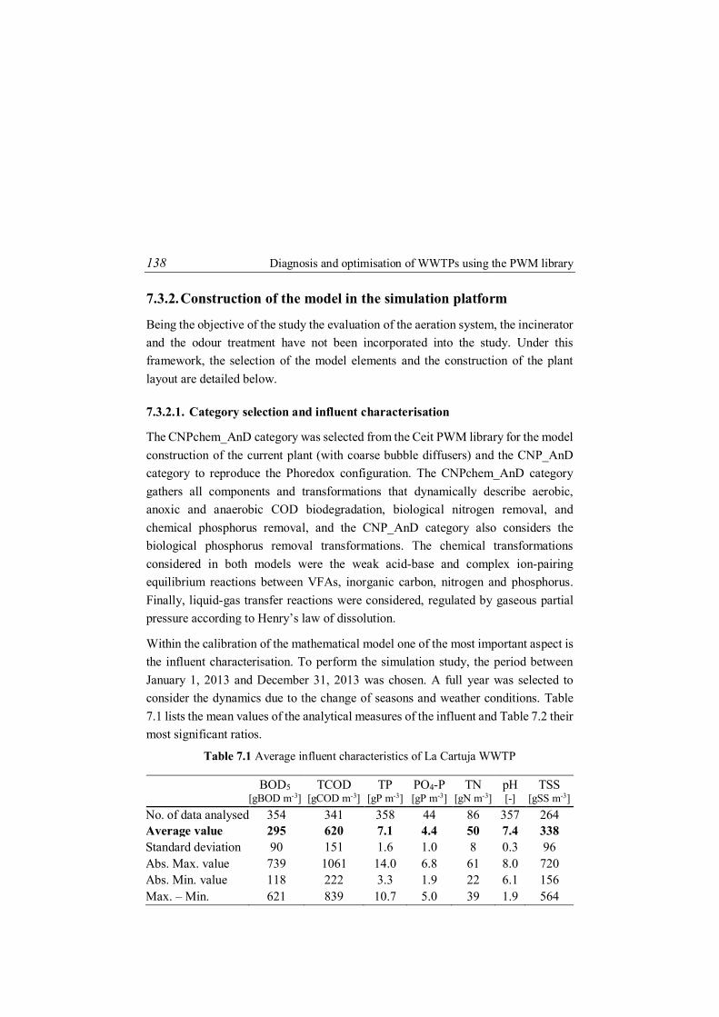
138 Diagnosis and optimisation of WWTPs using the PWM library

7.3.2. Construction of the model in the simulation platform

Being the objective of the study the evaluation of the aeration system, the incinerator and the odour treatment have not been incorporated into the study. Under this framework, the selection of the model elements and the construction of the plant layout are detailed below.

7.3.2.1. Category selection and influent characterisation

The CNPchem_AnD category was selected from the Ceit PWM library for the model construction of the current plant (with coarse bubble diffusers) and the CNP_AnD category to reproduce the Phoredox configuration. The CNPchem_AnD category gathers all components and transformations that dynamically describe aerobic, anoxic and anaerobic COD biodegradation, biological nitrogen removal, and chemical phosphorus removal, and the CNP_AnD category also considers the biological phosphorus removal transformations. The chemical transformations considered in both models were the weak acid-base and complex ion-pairing equilibrium reactions between VFAs, inorganic carbon, nitrogen and phosphorus. Finally, liquid-gas transfer reactions were considered, regulated by gaseous partial pressure according to Henry’s law of dissolution.

Within the calibration of the mathematical model one of the most important aspect is the influent characterisation. To perform the simulation study, the period between January 1, 2013 and December 31, 2013 was chosen. A full year was selected to consider the dynamics due to the change of seasons and weather conditions. Table 7.1 lists the mean values of the analytical measures of the influent and Table 7.2 their most significant ratios.

Table 7.1 Average influent characteristics of La Cartuja WWTP

BOD5 [gBOD m-3]

TCOD [gCOD m-3]

TP [gP m-3]

PO4-P [gP m-3]

TN [gN m-3]

pH [-]

TSS [gSS m-3]

No. of data analysed 354 341 358 44 86 357 264 Average value 295 620 7.1 4.4 50 7.4 338 Standard deviation 90 151 1.6 1.0 8 0.3 96 Abs. Max. value 739 1061 14.0 6.8 61 8.0 720 Abs. Min. value 118 222 3.3 1.9 22 6.1 156 Max. – Min. 621 839 10.7 5.0 39 1.9 564

La Cartuja WWTP (Zaragoza) 139

Table 7.2 Ratios of average influent characteristics of La Cartuja WWTP

TCODBOD5

TCOD

TN

TCODTP

PO4-P

TP

TCODTSS

No. of data analysed 341 81 341 44 256 Average value 2.2 13.8 89.9 0.6 1.8 Standard deviation 0.3 1.9 13.7 0.1 0.2 Abs. Max. value 3.8 18.6 154.6 0.8 2.2 Abs. Min. value 1.4 9.0 34.6 0.5 1.3 Max. – Min. 2.4 9.6 120.0 0.3 0.9

Analysing water characteristics, the influent has a medium load (620 gCOD m-3) according to the average values published in literature (Henze et al., 2008; Tchobanoglous et al., 2003) and a very high TCOD/TP ratio (90 gCOD gP-1) implying a more favourable biological phosphorus removal.

In order to complete the characterisation, additional analytical measurements were performed: the total COD to particulate COD ratio was set at 0.63 and the non-colloidal fraction of the slowly biodegradable matter (fXS) in 0.52.

Using the values of Table 7.1, the estimated ratios for the additional measures, and the assumptions made in Appendix C.1 (only for cases where information was not available), the characterisation based on the guidelines of Appendix C.2 has provided the following distribution of COD components.

Soluble and Colloidal COD

Particulate COD

Figure 7.4 a) Fraction of the influent soluble and colloidal COD distribution into model components, b) Fraction of the influent particulate COD distribution into model

components

a) b)

140 Diagnosis and optimisation of WWTPs using the PWM library

In order to complete the characterisation, elemental mass fractions of certain heterogeneous components were characterised.

Table 7.3 Elemental mass fractions of the heterogeneous components

Name C H O N P Ch SI 0.606 0.061 0.283 0.050 0.000 0.000 SP 0.649 0.013 0.230 0.108 0.000 0.000 XI 0.618 0.067 0.310 0.005 0.000 0.000 XP 0.460 0.050 0.442 0.031 0.017 0.000

Table 7.4 Stoichiometric parameters of XC2 disintegration

fSP,XC2 fCH,XC2 fPR,XC2 fLI,XC2 fXP,XC2 XC2 water line 0.015 0.103 0.413 0.285 0.184

7.3.2.2. Unit-process and cost models selection

From the unit-process model library, one primary and two secondary clarifiers (one for each line), eight completely stirred open tank reactors (four aerated reactors in each line) for the current plant and ten completely stirred open tank reactors (one anaerobic reactor, one facultative reactor and three aerated reactors in each line) for the Phoredox configuration, two thickening units, a dewatering unit, a dynamic influent and a FeCl3 dosage for the current configuration were selected to construct the layout. A graphical representation of both configurations can be seen in Figure 7.5 and Figure 7.6.

Figure 7.5 La Cartuja WWTP layout built on the WEST simulation platform

La Cartuja WWTP (Zaragoza) 141

Figure 7.6 Upgraded La Cartuja WWTP layout built on the WEST simulation platform

The activated sludge units consist of a liquid phase, an atmospheric phase and a gas hold-up phase. In this study, the mass flow of the system was only analysed, following the schematic balances presented in Figure 7.7.

Figure 7.7 Schematic representation of the mass balance in the activated sludge reactors.

7.3.2.3. Detailed description of the aeration system

The aeration system can be described in detail by combining the five sub-models shown in Figure 7.8, which are based on the work of Beltrán et al. (2013). All these models are detailed in Chapter 4 (Definition of cost models) and Chapter 5 (PWM library).

mw,in

mw,outAqueous

phase

1st Gaseous phase

2nd Gaseous phase

mg2,g1

mg,in

Aqueous phase

1st Gaseous phase

2nd Gaseous phase

Ew,g2 ρw,g2

Eg2,w ρg2,w

Ew,g1 ρw,g1

Ew,w ρw,w

142 Diagnosis and optimisation of WWTPs using the PWM library

Figure 7.8 Schematic representation of the aeration model.

The first sub-model (biochemical process model) is constituted by the selected PWM category. The objective of this sub-model is to estimate the oxygen requirements of the system or the kLa needed. The second sub-model (transfer system model) is described by the O-CSTR unit-process with one or two gaseous phases (supplied air and open atmosphere). This sub-model describes mass transfers between supplied air and aqueous phases, and therefore it relates the oxygen requirements estimated in sub-model 1 with the gas flow provided by sub-model 3. The third sub-model is the air distribution system model. The goal of this model is to estimate the pressure loss in the distribution system depending on the gas flow that circulates through the system (estimated in the sub-model 2). This model is the only model in the library that cannot be standardised. The head losses depend closely on the gas distribution system elements of the plant under study, and it is difficult to make a generalisation that satisfies all processes. Therefore, the model needs a detailed plant layout in

PWM category

kL = f(Ti, kLa)a = f(Qg, dB, FkLa)

Qg = f(Pg,out, f, valve opening

degree)

W = f(blow, Pg,out, Qg)

Biochemical process

O2 Transfer system

Air distribution system (1)

Blower system

kLaSOTEcw

(Manufacturer)

QgKla, FkLa

(Calibration)

Wblow

blow

(Calibration)

Environmental conditionskLa = f(SOTEcw, Qg, kLa, FkLa)

Transfer system

Environmental conditions

dB (Manufacturer)

kla, Fkla (Calibration)

kL (Literature)

Pg,out = f(submergence)

Pg,out

Pg,out

Air distribution system (2)

Cost = f(Wactuator, MU)

Electricity/Cost conversion model

CostelecMonetary unit (MU, € kJ-1)

La Cartuja WWTP (Zaragoza) 143

which the pipe lengths and diameters, the height variations, and the material specifications are defined. Finally, the fourth sub-model (blower) estimates the electric power supplied by the blower, which depends on the estimated air flow and pressure, and the last sub-model (electricity/cost conversion model) transforms this energy into electricity cost.

As mentioned, the air distribution system is the only model of the library that cannot be standardised. For this reason, the first step in analysing the distribution system (sub-model 3) in detail is to identify all nodes or elements/accessories that compose the aeration system. The schematic representation of the line and node network identified in the air distribution system of La Cartuja WWTP can be seen in Figure 7.9.

Thereafter, an energy continuity balance between each node is proposed to determine the heat losses between each element/accessory. As a result, the model provides the air flow exiting the diffuser (m s-1), for a blower output pressure and valve opening degree: pressure losses in the air line due to friction caused by piping are described by the Darcy-Weisbach equation (equation 3.14), while in the case of control valves and aeration diffusers the pressure loss is obtained for each operating point based on the data provided in the manufacturer data-sheets.

By repeating the resolution for different pressures and opening degrees, a matrix is obtained. In Figure 7.10, one of the matrices obtained for the current coarse bubble diffusers and another for the new fine bubble diffusers can be seen. The head loss provided by the Polcon type diffusers is practically nil. In contrast, fine bubble diffusers can have a pressure drop of 100-600 meters of air column depending on the air flow circulating through the diffuser (Standard 9" Disc - AF270, SSI). This head loss is reflected in Figure 7.10. The system will not be able to continue operating at pressures below 0.9 bar (relative pressure), and the operation with the new diffusers will have to be slightly higher. In contrast, the oxygen transfer efficiency of these fine bubble diffusers is greater, so the airflow required by the system will be lower.

After the matrix is parameterised, it can be introduced as input in the standard air distribution system model, and the simulation can be performed in order to obtain information about the valve opening degree. A graphic description of the procedure can be seen in Figure 7.11.

144 Diagnosis and optimisation of WWTPs using the PWM library

Figure 7.9 Schematic representation of the line and node network identified in the air distribution system of La Cartuja WWTP.

Figure 7.10 Analysis of the air flow (m s-1) that passes thought one of the air control valve: a) coarse bubble diffusers, b) fine bubble diffusers

1 2 3 4 5 6 7 8

9 10 11 12 13 14 15 16

17 18 19 20 21 22 23 24

25 26 27 28 29 30 31 32

PipeDN 800 / 4m Heat E xchanger Pipe

DN 800 / 1mPipe

DN 800 / 0.5m Check valve ValveT001

PipeDN 800 / 3m

PipeDN 800 / 4m Hea t Exchanger

PipeDN 800 / 1m

PipeDN 800 / 0.5m Check va lve

Va lveT002

PipeDN 800 / 3m

PipeDN 800 / 4m Hea t Exchanger

PipeDN 800 / 1m

PipeDN 800 / 0.5m Check va lve

Va lveT003

PipeDN 800 / 3m

PipeDN 800 / 4m Hea t Exchanger Pipe

DN 800 / 1mPipe

DN 800 / 0.5m Check va lve Va lveT004

PipeDN 800 / 3m

PipeDN 1400 / 7.5m

PipeDN 1400 / 7.5m

PipeDN 1400 / 7.5m

PipeDN 1400 / 5.5m

3334

35

37

38

39

40

41

42 43

44

47

48

49

50

51

60

61

54

55

59

46

52

53

56

57

58

73

75

76

80

62

63

64

68

65

66

67

69

70

71

72

74

77

78

79

81

82

83

84

85

36

45

86

87

88

89

93

90

91

92

94

9798

99

100

104

101

105

102

103

106

107

PipeDN 1400 / 17m

PipeDN 800 / 15m

PipeDN 600 / 2m

ValveL101

PipeDN 800 / 4m

ValveL102

PipeDN 800 / 0.5m

ValveL103

PipeDN 800 / 1m

PipeDN 600 / 8m

PipeDN 400 / 59m

PipeDN 400 / 47m

Diffusers144 ud.

Diffusers144 ud.

Va lveL104

PipeDN 600 / 0.5m

PipeDN 350 / 1m

ValveL105

PipeDN 350 / 51m

Diffusers88 ud.

PipeDN 600 / 6.5m

PipeDN 350 / 10.5m

ValveL106

PipeDN 350 / 50m

Diffusers88 ud.

PipeDN 1200 / 28.5m

PipeDN 800 / 16.5m

PipeDN 600 / 2m

Va lveL201

PipeDN 600 / 1m

PipeDN 400 / 1m

ValveL202

PipeDN 400 / 50.5m

Diffusers144 ud.

PipeDN 600 / 7.5m

PipeDN 400 / 8.5m

ValveL203

PipeDN 400 / 50m

Diffusers144 ud.

PipeDN 600 / 22m

ValveL204

PipeDN 600 / 5.5m

PipeDN 350 / 1.5m

ValveL205

PipeDN 350 / 55.5m

Diffusers88 ud.

PipeDN 600 / 8m

PipeDN 350 / 6.5m

Va lveL206

PipeDN 350 / 50.5m

Diffusers88 ud.

PipeDN 800 / 64m

95

96

PipeDN 600 / 30.5m

PipeDN 600 / 2.5m

PipeDN 600 / 1m

PipeDN 400 / 1m

ValveL302

PipeDN 400 / 50m

Diffusers144 ud.

PipeDN 600 / 6.5m

Va lveL301

ValveL304

PipeDN 350 / 1.5m

ValveL305

PipeDN 350 / 50m

Diffusers88 ud.

PipeDN 400 / 14.5m

ValveL303

PipeDN 400 / 50m

Diffusers144 ud.

PipeDN 350 / 12m

ValveL306

PipeDN 350 / 53m

Diffusers88 ud.

b) a)

La Cartuja WWTP (Zaragoza) 145

Figure 7.11 (a) Summary of terms used for the description of processes and sub-systems that compose the overall aeration system; (b) schematic representation of the line and node network identified in the air distribution system; (c) analysis of the air

flow (m/s) that passes through one of the air control valve (L201) for different blower pressures and valve opening degrees; (d) Cartuja WWTP layout; (e) valve opening

degree distribution over a year of operation, with new diffusers.

146 Diagnosis and optimisation of WWTPs using the PWM library

7.3.3. Calibration of the biological model and aeration system parameters

The first step of the study was the calibration of the model for the old aeration system. This simulation allowed to determine the efficiency of blowers (Blow = 70%) and the parameters of the gas transfer model (kLa = 1.03 and kLa·FkLa = 0.49, although for the new system the kLa·FkLa factor will be different). The parameters of the biological model were maintained with the reference values set out in Appendix A.5. The comparison of the experimental data and simulation results for the aeration flow rate of the first biological reactor and the total power supplied by the blowers can be seen in Figure 7.12 and Figure 7.13.

Figure 7.12 Simulation and experimental results of the air flow in line 1.

Figure 7.13 Simulation and experimental results of the total aeration power.

The plant did not store the information regarding the valves’ opening degree, but a follow-up of one week was done with the aim of calibrating the system's heat losses. For a blower output pressure of 0.906 bar (relative pressure used in the coarse bubble aerator system), the values of the valves’ opening degree predicted by the model for the first reactor are shown in Figure 7.14.

La Cartuja WWTP (Zaragoza) 147

Figure 7.14 Simulation of the valves’ opening degree predicted by the model for the first reactor.

7.3.4. Simulation-based study for assessing the aeration system of La Cartuja WWTP

The main goal of the model-based diagnosis for La Cartuja WWTP was to assess replacing coarse bubble diffusers with fine bubble diffusers and the effect on the air control valves degree of opening and the discharge pressure requirements.

Based on the calibrated plant, new air flow matrices (Figure 7.10) and fine bubble diffusers specifications (bubble diameter of 2 mm according to US EPA, 1989; up-flow velocity of 0.16 m s-1 according to Pradhan, 2012; and an kLa·FkLa design parameter of 0.5 according to EnviroSim, 2004) were incorporated into the model.

In analysing the results, Figure 7.15 shows the opening degree of the four control valves over one year of operation with fine bubble diffusers (each line has two control valves, as can be seen in Figure 7.6).

Figure 7.15 Simulation and experimental results of the total aeration power.

The plant has a control loop to manipulate the valves’ opening degree according to the oxygen needs and a manual control for the blowers’ output pressure. In the

148 Diagnosis and optimisation of WWTPs using the PWM library

absence of an automatic pressure control, the plant requires supervision of the valves’ opening degree in order to study whether it is necessary to increase or decrease the pressure. When the opening degree is close to zero, the pressure may be reduced and when the valves are fully open, the process will require increased pressure to achieve the objectives of dissolved oxygen. The results show an excessive strangling of valves. After the diffusers were replaced, the air requirement dropped considerably (the new diffusers have a higher transfer efficiency), but the blower output pressure rose slightly from 0.906 bar to 0.924 bar (relative pressures). As shown in Figure 7.10, at low pressures, the variation of the air flow is lower. In this case, in the face of an unexpected need for oxygen, the process could lead to a valve opening of 100 % and to an inability to supply the needed oxygen, revealing a slower process of manoeuvrability. This is a clear sign of air distribution system oversising.

With respect to the electric power consumed by the blowers, a considerable decrease has been observed in the simulation (Figure 7.16). The expected savings with the incorporation of the fine bubble diffusers has been 50 %, while the reduction of the air flow to be supplied has been estimated at 52 %.

Figure 7.16 Comparison of the electric power consumed by the blowers for the coarse and fine bubble diffusers

The conclusion reached after the study was that the air distribution system was oversised for new diffusers and that the substitution of certain pipes that made up the aeration system was necessary. Although this study was done over an existing air distribution system, the model could have been used to design the system, avoiding future design pitfalls such as oversising blower pressure, an excessive number of diffusers or wrong pipe diameters. Thus, the model can be used not only to detect design errors or operating problems regarding the aeration system, but to also design new air distribution systems, together with their optimal control.

Galindo-Bilbao WWTP 149

7.4 GALINDO-BILBAO WWTP The study presented in this section is framed in the project entitled “Comprehensive energy and operating cost analysis of Galindo-Bilbao WWTP” and has been promoted by the Bilbao Bizkaia Water Authorities (CABB). As the title mentions, the main aim of this model-based study was to carry out a comprehensive energy and operating cost analysis of Galindo-Bilbao WWTP.

7.4.1. Description of Galindo-Bilbao WWTP

Galindo WWTP located in Sestao (Bizkaia, Spain) treats the urban wastewater and the stormwater of 20 municipalities in the metropolitan area of Bilbao (Figure 7.17). The plant was designed to treat 346000 m3 d-1 and has a design capacity of 1.5 million population equivalent (PE).

Figure 7.17 Panoramic view of Galindo WWTP (Source: Google maps)

The WWTP consists of a wastewater treatment process and a system for treating the sludge produced in the plant. The water line consists of rough pre-treatments, sand and grease removal systems, a mechanical pre-treatment with thirteen primary clarifiers (four of them operated as storm tanks), and a biological part with sex activated sludge lines to remove the organic matter and nitrogen. Each of them is designed so that it can operate in four different configurations: Organic Matter removal (OM), Denitrification-Nitrification (DN), Regeneration-Denitrification-

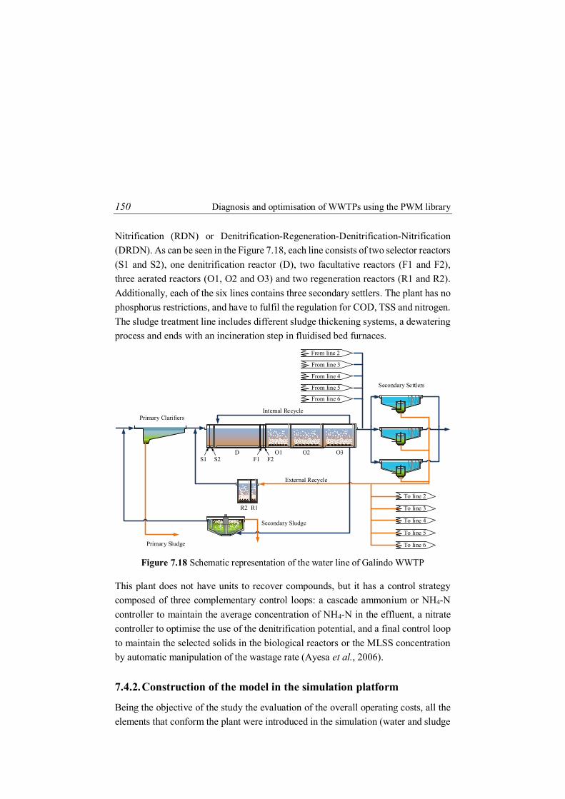
150 Diagnosis and optimisation of WWTPs using the PWM library

Nitrification (RDN) or Denitrification-Regeneration-Denitrification-Nitrification (DRDN). As can be seen in the Figure 7.18, each line consists of two selector reactors (S1 and S2), one denitrification reactor (D), two facultative reactors (F1 and F2), three aerated reactors (O1, O2 and O3) and two regeneration reactors (R1 and R2). Additionally, each of the six lines contains three secondary settlers. The plant has no phosphorus restrictions, and have to fulfil the regulation for COD, TSS and nitrogen. The sludge treatment line includes different sludge thickening systems, a dewatering process and ends with an incineration step in fluidised bed furnaces.

Figure 7.18 Schematic representation of the water line of Galindo WWTP

This plant does not have units to recover compounds, but it has a control strategy composed of three complementary control loops: a cascade ammonium or NH4-N controller to maintain the average concentration of NH4-N in the effluent, a nitrate controller to optimise the use of the denitrification potential, and a final control loop to maintain the selected solids in the biological reactors or the MLSS concentration by automatic manipulation of the wastage rate (Ayesa et al., 2006).

7.4.2. Construction of the model in the simulation platform

Being the objective of the study the evaluation of the overall operating costs, all the elements that conform the plant were introduced in the simulation (water and sludge

Secondary Settlers

Internal Recycle

O3

R2 R1

O1 O2F1 F2

DS1 S2

External Recycle

To line 2

To line 3

To line 4

To line 5

To line 6

From line 3

From line 4

From line 5

From line 6

From line 2

Primary Clarifiers

Primary Sludge

Secondary Sludge

Galindo-Bilbao WWTP 151

line processes, detailed aeration and incineration models and operating costs models). Under this framework, the selection of the model elements and the construction of the plant layout are detailed below.

7.4.2.1. Category selection and influent characterisation

Given the Galindo WWTP’s characteristics, the CN category was selected in order to reproduce the behaviour of the plant. This category gathers all components and transformations that describe dynamic aerobic and anoxic COD biodegradation and N removal. The chemical transformations considered in the model were the weak acid-base and complex ion-pairing equilibrium reactions between VFAs, inorganic carbon, nitrogen and phosphorus. Finally, liquid-gas transfer reactions were considered, regulated by gaseous partial pressure according to Henry’s law of dissolution.

As in the case of La Cartuja WWTP, a full year of operation was selected for the study, and the period between January 1, 2012 and December 31, 2012 was chosen. Table 7.5 lists the mean values of the analytical measures of the influent.

Table 7.5 Average influent characteristics of Galindo WWTP

TCOD [gCOD m-3]

NHX-N [gN m-3]

NO3-N [gN m-3]

NO2-N [gN m-3]

TSS [gSS m-3]

VSS [gSS m-3]

No. of data analysed 182 188 188 188 157 157 Average value 634 29.1 <1 0.22 338 279 Standard deviation 214 7.1 0.22 0.13 113 113 Abs. Max. value 1878 39.1 2.26 0.67 846 639 Abs. Min. value 172 6.2 <1 0.05 63 45 Max. – Min. 1706 32.9 - 0.62 783 594

In order to perform the characterisation, the following assumptions were made: the particulate COD to VSS ratio was set at 1.72, and the alkalinity at 10 mol m-3. From the design data of the Galindo WWTP, an ammonium to total nitrogen ratio of 0.63 was estimated. Taking this information as a base, the characterisation was carried out following the guidelines of appendix C.2.

It can be said that the influent has a medium load (634 gCOD m-3) according to the average values published in literature (Henze et al., 2008; Tchobanoglous et al., 2003) and a high TCOD/TN ratio (13.7 gCOD gN-1) implying a more favourable biological nitrogen removal.

152 Diagnosis and optimisation of WWTPs using the PWM library

To conclude the characterisation, elemental mass fractions and stoichiometric parameters of certain heterogeneous components were characterised.

Table 7.6 Elemental mass fractions of the heterogeneous components

Name C H O N P Ch SI 0.577 0.096 0.308 0.020 0.000 0.000 SP 0.649 0.013 0.230 0.108 0.000 0.000 XI 0.551 0.033 0.375 0.027 0.014 0.000 XP 0.460 0.050 0.442 0.031 0.017 0.000

Table 7.7 Stoichiometric parameters of XC2 disintegration

fSP,XC2 fCH,XC2 fPR,XC2 fLI,XC2 fXP,XC2 XC2 water line 0.015 0.103 0.413 0.285 0.184

7.4.2.2. Unit-process and cost models selection

From the unit-process model library, a primary and secondary clarifier, ten completely stirred open tank reactors, one buffer tank, two thickening units, a dewatering unit and two incineration units were selected. Finally, blower, pump, agitation engine, dosage costs and electricity conversion models were selected from the cost model list. Specifically, in this study, the elemental mass characterisation of model components and the consideration of heat balances in certain units was fundamental for the study. This had an important effect on the incineration process, as will be seen in the discussion about the results. A graphical representation of the configuration can be seen in Figure 7.19.

The activated sludge units consist of a liquid phase and an atmospheric phase. In this study, the mass flow of the system was only analysed, following the schematic balances presented in Figure 5.13.

7.4.2.3. Detailed incineration model

As discussed in the Chapter 3, the incineration unit model consists of a fluidised bed (FB), a steam turbine (T), three heat exchange units (HE1, HE2 and HE3), an air condenser (AC), two pumps (P1 and P2) and a degassing tank (D). In the two furnaces, the combustion is carried out producing exhaust gases and ashes. The soluble and particulate COD present in the sludge is oxidised with preheated air, but also the remaining sludge components.

Galindo-Bilbao WWTP 153

Figure 7.19 Galindo WWTP layout built on the WEST simulation platform

154 Diagnosis and optimisation of WWTPs using the PWM library

The combustion of each element is carried out under the guidelines formulated in section 5.2, obtaining the heats of combustion of Table 5.4. The estimated heat of combustion is described as the higher heating value (HHV), so the heat of vaporisation of the water vapour must be subtracted from the value obtained. The oxidation of the components produces heat which is released into the unit. If the COD present in the sludge does not produce enough heat to get the combustion temperature (900 ºC), natural gas is introduced in the chamber. The heat accumulated in the exhaust gases is then transferred to the closed water/steam circuit in order to produce electricity in the two step steam turbine. The characteristics of the water at each point in the closed water/steam circuit are shown in Table 2.

Table 7.8 Water characteristics considered in the water/steam circuit.

Stream Temperature [ºC]

Pressure [bar]

hi (*) [kJ g-1]

Vapour quality

Saturation pressure [bar]

1 400 40.0 3.21 - - 2 400 40.0 3.21 - - 3 400 40.0 3.21 - - 4 105 1.20 0.44 - 1.20 5 147.5 4.16 2.74 - 4.45 6 50 0.12 2.33 0.89 0.12 7 50 0.12 0.21 - 0.12 8 50 1.20 0.21 - 0.12 9 145 4.16 0.61 - 0.12 10 105 1.20 0.44 - 1.20 11 105 42.11 0.44 - 1.20 12 140 40.00 0.59 - 3.62

(*) Values estimated with the model

The thermodynamic cycle that follows the water/steam streams can be described by the Rankine cycle. The temperature vs. specific entropy diagram of the Galindo WWTP incinerator water/steam circuit can be seen in Figure 7.20.

Galindo-Bilbao WWTP 155

Figure 7.20 Scheme of the Rankine cycle for the water/steam circuit of the Galindo WWTP incinerator

7.4.3. Calibration of the biological and cost models’ parameters

The parameters of the biological model were maintained with the reference values set out in Appendix A.5. Through the studies, it has been seen that a correct calibration can be carried out by maintaining the values of the stoichiometry and kinetic parameters accepted by the scientific community (included in Appendix A.5) and performing a proper influent characterisation.

Under this premise, the comparison of the experimental data and simulation results for effluent NH4-N, NOx-N and TCOD concentrations can be seen in Figure 7.21 and Figure 7.22.

The first step in the estimation of operating costs consisted in the calibration of the aeration system model. The detailed aeration model was also used for this study (Figure 7.8).

156 Diagnosis and optimisation of WWTPs using the PWM library

Figure 7.21 Comparison of experimental data and simulation results of the effluent NH4-N and NOx-N concentrations.

Figure 7.22 Comparison of experimental data and simulation results of the effluent TCOD concentration.

Table 7.9 shows the characteristics of each reactor (the arrangement of the reactors is shown in Figure 7.18) and the kLa·FkLa factor obtained in the calibration of the aeration system.

Table 7.9 Characteristics of the biological reactors.

R1 R2 S1 S2 D F1 F2 N1 N2 N3 Volume [m3] 1250 2500 482 482 10000 665 665 5330 6660 6660 No diffusers 388 833 - - - 261 261 1574 1725 748 Type diffuser (*) MD MD MD MD CD CD CD kLa · FkLa (**)

0.45 0.45 0.6 0.6 0.65 0.65 0.65

(*) MD: Membrane diffuser, and CD: Ceramic diffuser; (**) Calibration

Galindo-Bilbao WWTP 157

The submersion of all reactors was 8.65 m and the expressions that relate the air flow and the standard oxygen transfer efficiency (SOTE) are presented in Figure 7.23. By means of the calibration it was determined that blower’s efficiency was 76% (n the range of the usual efficiency of the blowers).

Figure 7.23 Relation between the aspired mass air flow and the SOTE

The satisfactory predictive capacity of the model can be seen in Figure 7.24, which shows the comparison of experimental and simulated aeration power.

Figure 7.24 Comparison of the aeration power experimental data and simulation results.

As far as the calibration of the incinerator is concerned, the assumptions formulated in Chapter 3 were performed. These were as follows:

(1) Oxidation reactions are considered instantaneous reactions of complete combustion, following the guidelines of Chapter 5.

(2) Ashes consist of phosphates and inorganic inert matter (XII).

158 Diagnosis and optimisation of WWTPs using the PWM library

(3) The ash flow produced is minimal compared to the feed stream (mw,under≪ mw,in).

The average exhaust gas temperature at each point in the system was known (see Table 7.10). From this information and knowing the average values of steam production, electric energy production, air flow fed to the system and annual natural gas consumption, units’ heat dissipations were fixed and the heat balance of the system was closed. Table 7.10 shows the values of the model parameters estimated for this specific case study.

Table 7.10 Incinerator model parameters.

Param. Description Units Default Value

Qgc,c,HE1,out HE1 unit convection heat % 0.025 Qgc,c,HE2,out HE2 unit convection heat % 0.025 Qgc,c,HE3,out HE3 unit convection heat % 0.025 Qgc,c,FB,out First FB unit convection heat % 0.92 Qgc,c,FB,out Second FB unit convection heat % 0.04 Qgc,c,AC,out AC unit convection heat % 0.025 Qgc,c,D,out D unit convection heat % 0.025

pump Pumps efficiency (P1 and P2) - 0.7 Excair Excess air - 1.4 XCH4,NG Fraction of CH4 in the natural gas flow % 97

Tg,out Temperature of the exhaust gases at the exit of the plant

ºC 200

Tg,FB,out Temperature of the exhaust gases at the exit of the furnace

ºC 900

Tg,HE2,out Temperature of the preheated air (1st furnace) ºC 150 Tg,HE2,out Temperature of the preheated air (2nd furnace) ºC 220

To demonstrate the predictive capacity of the model, Figure 7.25 shows the dynamic ash production in the incinerator. As can be seen, the model perfectly follows the trend. On the one hand, this supports the assumptions made and on the other hand demonstrates the overall predictive ability of the model to simulate the whole plant.

The incineration process is located at the end of a series of processes (as a result of the water and sludge line), so the predictive potential of the model at this point in the plant demonstrates the validity of the previous models.

Galindo-Bilbao WWTP 159

Figure 7.25 Comparison of experimental data and simulation results for the ash flow

produced in the incineration process.

In order to show the potential of the tool, Figure 7.26 shows the prediction of the electric energy production of the incineration units, results that are among the expected values (845 kW the FB1 and 1800 kW the FB2).

Figure 7.26 Electricity production in the turbines of the incineration process.

The remaining operational costs were not calibrated since the measurements or reference values were not available, but the design data were used for their estimation (design data available in the internal project report, 410138/R01).

7.4.4. Comprehensive energy and operating cost analysis of Galindo-Bilbao WWTP

The study was divided into two parts. The first analysis consisted of an assessment of current operation, paying attention to the distribution of operational costs over one

160 Diagnosis and optimisation of WWTPs using the PWM library

year of operation in order to identify the most significant operating expenses and the variability of each. Once identified the most significant operating costs, the second part of the study consisted of an analysis of different operational strategies for expenses minimisation.

As an example that illustrates of the potential of PWM simulations, Figure 7.27 shows the distribution of the most significant operational costs over a year of operation: aeration, pumping and dewatering electricity costs and polyelectrolyte and natural gas (NG) dosage costs.

Figure 7.27 Cost distribution over a year of operation.

In this first analysis, fixed costs or costs which cannot be manipulated (main pumping, pre-treatment, scrapers, odour treatment, flotation, mixing and auxiliary services) have not been considered. Taking average values, the plant’s operating costs were divided as follows: 22 % aeration, 7.5 % pumping, 7 % dewatering, 7.5 % polyelectrolyte dosage, 6 % NG fed into incineration and 50 % other costs (fixed costs or costs which cannot be handled). As can be seen, aeration costs represent a small part of the overall costs. In the Galindo WWTP, this is a consequence of both the high treatment capacity of the plant which allows the use of more powerful and efficient blowers, and the use of advanced ammonium and nitrate controllers. In assessing the dynamic operating costs (Figure 7.27), it can be seen that periods with higher operating costs correspond with considerable use of NG in incineration. The incineration process needs to maintain the combustion temperature ( 900 ºC) in order to properly remove the matter. In cases in which the dewatered sludge does not generate enough energy to achieve this temperature, NG is fed into it, which significantly increases overall operating costs. After a thorough analysis of the data,

Galindo-Bilbao WWTP 161

it was found that these variations correspond to periods of high rainfall. These weather conditions diluted the concentrations of COD, NH4-N and volatile suspended solids (VSS) and increased inert inorganic solids concentrations. Since the degree of dryness of dewatered sludge was kept constant throughout the year, a sludge with a lower VSS/TSS (volatile and total suspended solids) ratio was obtained in times of high rainfall. This situation produces a sludge with less biodegradable material and needs more NG in order to be incinerate. To reduce this NG consumption, the dehydration criterion had to be changed from constant dryness to a constant VSS concentration.

7.4.5. Model-Based exploration of different alternatives to manage the COD

The main objective of this study was to propose operational improvements. As the plant did not wish to make physical or equipment improvements, one of the clearest alternatives for minimising operating costs was to explore via simulation the different alternatives for COD management throughout the entire plant, an analysis that is tackled in the second part of the study. The overall study helped with the operational decision-making, not only from the standpoint of ensuring the quality of the effluent, but also from a perspective of energy minimisation.

With this plant, a scenario analysis was carried out by assessing the operating cost for different primary clarifier TSS removal efficiencies (TSS) and MLSS concentrations, that is, different options for managing the COD in the plant in winter and summer. To simulate the TSS increase, a dosage of ferric chloride (FeCl3) was added to the primary clarifier. The amount of added concentration was estimated based on the expression proposed by Tik et al. (2013) and the cost function is presented in Chapter 3. The MLSS concentration, in turn, was modified by the automatic manipulation of the wastage rate (solids retention time or SRT variation). To interpret the results, regimen maps were used (Figure 7.28), and in all cases the effluent quality requirements were guaranteed thanks to the control loops. Analysing the results shows that in both scenarios (winter or Figure 7.28 left and summer or Figure 7.28 right) operating costs are lower when the solids removal efficiency of the primary settling is increased, despite having to add FeCl3. This occurs as a result of the sum of several factors: air requirements are lower, the secondary sludge pumping has higher operational costs, the needs for polyelectrolyte is lower for primary sludge than for secondary sludge, and the energy generated in the incineration process is

162 Diagnosis and optimisation of WWTPs using the PWM library

greater, and thus a lower NG dosage is required. Regarding the effect of solids concentration in biological reactors, the smaller the SRT, the greater the operating costs. In this case, it can be explained as follows: the higher the solids concentration in the biological reactor, the higher the costs of aeration, but the lower the dosage (polyelectrolyte and NG) and pumping costs.

Figure 7.28 Global operating cost analysis (€ d-1) for different primary clarifiers TSS removal efficiencies and MLSS concentrations, left) in winter, and right) in summer.

In the operation of a real plant it is difficult to control the TSS, as it is dependent on the influent and rejected water composition, load and flow, in addition to weather conditions. All this makes it difficult to achieve the efficiencies established in the study. Still, it provides an overview of the effect of variations in COD and the possible behaviour of the plant. Thus, these diagrams can assist plant operators in selecting the most appropriate operational strategy.

7.5 PALMA 1 AND PALMA 2 WWTPS The last study presented in this section is framed in the project entitled “Technical support for the diagnosis and operational optimisation of Palma 1 and Palma 2 WWTPs” and has been promoted by the Municipal Water and Sewerage Company of Palma de Mallorca (EMAYA). The objective of the original study was to propose operation improvements of both plants and investments proposals. In this thesis, a small part of this study is presented, that consisted in comparing and proposing alternatives to remove/recover phosphorus.

Palma 1 and Palma 2 WWTPs 163

7.5.1. Description of Palma 1 and Palma 2 WWTPs

Palma de Mallorca’s wastewater is treated in two WWTPs, each of which receives a similar flow-rate. Palma 2 WWTP (Palma de Mallorca, Spain) treats part of the urban wastewater coming from the city of Palma de Mallorca (Figure 7.29). The plant treats 50000-60000 m3 d-1 and has a design capacity of 350,000 population equivalent (PE).

Figure 7.29 Panoramic view of Palma 2 WWTP (Source: Google maps)

The WWTP consists solely of a wastewater treatment process. The sludge generated in this plant is sent to Palma 2 WWTP for its treatment. The water line consists of rough pre-treatments, sand and grease removal systems, a mechanical pre-treatment with four primary clarifiers, and a biological part. The biological treatment of this plant divides the biological process into two phases, decoupling the organic matter removal and the nitrogen oxidation or nitrification. COD removal and N oxidation is carried out in two channels. The COD removal channel contains three superficial turbines for the aeration and the N oxidation channel has six superficial turbines (simulated in 3 + 2 aerated zones).

Palma 1 WWTP (Palma de Mallorca, Spain) treats the urban wastewater coming from the beach of Palma, Sant Jordi, S'Aranjassa, Es Pillarí, the airport of Son Sant Joan and part of the waters generated in the city of Palma de Mallorca (Figure 7.30). The plant treats 45000-50000 m3 d-1 (25000-30000 m3 comes from the Palma 2 WWTP) and has a design capacity of 460000 population equivalent (PE).

164 Diagnosis and optimisation of WWTPs using the PWM library

Figure 7.30 Panoramic view of Palma 1 WWTP (Source: Google maps)

The WWTP consists of a wastewater treatment process and a system for treating the sludge produced in this plant and in Palma 2 WWTP. The water line consists of rough pre-treatments, sand and grease removal systems, a mechanical pre-treatment with three primary clarifiers, and a biological part with three activated sludge lines to remove biologically the organic matter and the nitrogen and chemically the phosphorus. Due to the excessive capacity of the biological treatment, the plant operates only with 2 treatment lines.

COD and N removal and chemical P precipitation with FeCl3 or Fe2(SO4)3 is carried out in a Denitrification/Nitrification or DNDN configuration (double Denitrification/ Nitrification configuration). The process consists of an anoxic zone composed of three separate reactors, a first facultative zone, an aerobic zone composed of three reactors, a second facultative zone, and a reaeration zone (Figure 7.31).

Figure 7.31 Schematic representation of the water line of Palma 1 WWTP.

Primary ClarifiersSecondary ClarifiersInfluent

Fe2(SO4)3

Biological treatment

O3O1 O2F1 F2A1 A2 A3 O4

Pre-treatment

To tertiary treatment

Secondary SludgePrimary Sludge

Palma 1 and Palma 2 WWTPs 165

The sludge treatment line includes different sludge thickening systems, four anaerobic digesters, and ends with a dewatering process.

As mentioned, both plants are connected. The sludge generated in Palma 2 is treated in Palma 1, creating a large amount of sludge to be treated in one plant. Furthermore, in the digestion process a large amount of VSS is biodegraded, resulting in rejected water with high N and P concentration. Figure 7.32 shows schematically the interrelations between the Palma 1 and 2 WWTPs.

Figure 7.32 Schematic representation of Palma 1 and Palma 2 WWTPs.

Primary Clarifiers Zone 2 Zone 3Secondary ClarifiersInfluent Emissary

Blow. 5-8 Blow. 9-12 Qr

Fe2(SO4)3

Zone 1Pre-treatment

Sands

Blow. 1-4

Conventional biological treatment

Lagune

Reactor 2

Blow. 14

Reactor 1

Blow. 13

Secondary Clarifiers

To tertiary treatment

TAS

Reactor 4

Blow. 16

Reactor 3

Blow. 15

Reactor 6

Blow. 18

Reactor 5

Blow. 17

Primary ClarifiersSecondary ClarifiersInfluent

Fe2(SO4)3

Sands

Biological treatment

O3O1 O2F1 F2A1 A2 A3 O4

Anaerobic digestion

CHP

Sludge

Sieve 1 Thickener 1

Sieve 2 Thickener 2

Mixed sludge tank Mixing chamber

Centrifuges Thickener 3

Pre-treatment

To tertiary treatment

166 Diagnosis and optimisation of WWTPs using the PWM library

7.5.2. Objective of the study

Taking into account the high sludge load treated in Palma 1 (coming from Palma 1 and 2), one of the goals of the simulation study was to assess different design and operational scenarios for optimum N and P management in this WWTP, while trying to reduce chemical dosages. To that end, sex different alternatives were considered (in all of them the configurations of Palma 2 WWTP has been mandated with the current configuration):

(1) A carbon and nitrogen removal plant without chemical phosphorus removal.

(2) A carbon and nitrogen removal plant with chemical phosphorus removal and the current Fe2(SO4)3 dosage (current plant).

(3) A plant re-design for biological P removal since the plant is oversised for the current load based on the A2O configuration (Anaerobic/Anoxic/Aerobic reactors).

(4) The plant re-design in alternative (3) with simultaneous P precipitation (chemical and biological), dosing the current Fe2(SO4)3 dosage.

(5) The plant re-design in alternative (3) with simultaneous P precipitation (chemical and biological), but dosing the Fe2(SO4)3 strictly necessary.

(6) The inclusion of a technology for struvite recovery in the sludge line in alternative (3).

Some of these simulations required a modification in the plant layout to move from a biological COD and N removal process to a biological COD, N and P removal configuration. For that, the A2O (Anaerobic/Anoxic/Aerobic reactors) configuration was chosen. Although the A2O configuration is not the most appropriate process for this plant, it is the configuration that requires the fewest modifications. The operating conditions were also modified slightly in line with typical design parameters used in the A2O process (Tchobanoglous et al, 2014).

7.5.3. Construction of the model in the simulation platform

Although in this study only a comparative analysis of the alternatives to remove/ recover phosphorus is presented, as discussed previously, in the original study operating improvements of both plants were also analysed. This was the reason for the requirement to analyse and simulate both plants as a whole. Under this

Palma 1 and Palma 2 WWTPs 167

framework, the selection of the model elements and the construction of the plant layout are detailed below.

7.5.3.1. Category selection and influent characterisation

For alternative (1), the model was constructed by selecting the CN_AnD category from the Ceit PWM library. The biochemical reactions considered in the model were the ones that are necessary to describe biological organic matter and one-step nitrogen removal under different environmental conditions (aerobic, anoxic and anaerobic). For alternative (2), the CNPchem_AnD category was selected from the Ceit PWM library. The CNPchem_AnD category gathers all components and transformations that dynamically describe aerobic, anoxic and anaerobic COD biodegradation, biological nitrogen removal, and chemical phosphorus removal. For alternatives (3), (4) and (5) the CNP_AnD category was selected, that also considers the biological phosphorus removal transformations. And finally, to reproduce alternative (6) the CNPprec_AnD category was selected, that also considers the precipitation reactions. The chemical transformations considered in the model for all configurations were the weak acid-base and complex ion-pairing equilibrium reactions between VFAs, inorganic carbon, nitrogen and phosphorus. Finally, two types of physico-chemical transformations were considered: (1) liquid-gas transfer, regulated by gaseous partial pressure according to Henry’s law of dissolution, and (2) the precipitation-redissolution equilibrium for the case of CNPprec_AnD category.

As in the previous cases, a full year of operation was selected for the study. The chosen period was from January 1, 2013 to December 31, 2013. In both cases the characteristics of the influent water were similar. Table 7.11 lists the mean values of the analytical measures of the influent.

Table 7.11 Average influent characteristics of Palma 1 & Palma 2 WWTP

BOD5 [gBOD m-3]

TCOD [gCOD m-3]

TP [gP m-3]

NH4-N [gN m-3]

TN [gN m-3]

pH [-]

TSS [gSS m-3]

No. of data analysed 242 244 155 244 150 240 245 Average value 412 864 8.9 41 65 8 408 Standard deviation 143 211 3.1 9 13 0 171 Abs. Max. value 960 2108 30.0 103 147 9 1788 Abs. Min. value 60 371 0.8 44 36 7 62 Max. – Min. 900 1737 29.2 4 111 2 1726

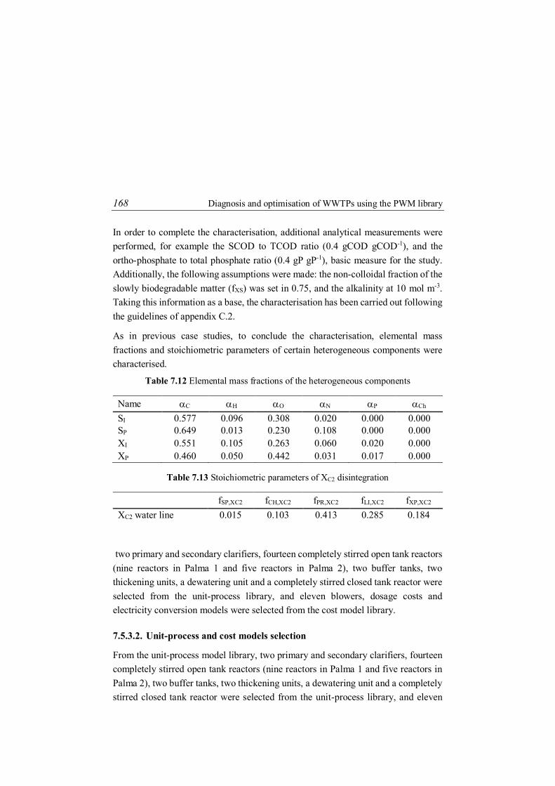
168 Diagnosis and optimisation of WWTPs using the PWM library

In order to complete the characterisation, additional analytical measurements were performed, for example the SCOD to TCOD ratio (0.4 gCOD gCOD-1), and the ortho-phosphate to total phosphate ratio (0.4 gP gP-1), basic measure for the study. Additionally, the following assumptions were made: the non-colloidal fraction of the slowly biodegradable matter (fXS) was set in 0.75, and the alkalinity at 10 mol m-3. Taking this information as a base, the characterisation has been carried out following the guidelines of appendix C.2.

As in previous case studies, to conclude the characterisation, elemental mass fractions and stoichiometric parameters of certain heterogeneous components were characterised.

Table 7.12 Elemental mass fractions of the heterogeneous components

Name C H O N P Ch SI 0.577 0.096 0.308 0.020 0.000 0.000 SP 0.649 0.013 0.230 0.108 0.000 0.000 XI 0.551 0.105 0.263 0.060 0.020 0.000 XP 0.460 0.050 0.442 0.031 0.017 0.000

Table 7.13 Stoichiometric parameters of XC2 disintegration

fSP,XC2 fCH,XC2 fPR,XC2 fLI,XC2 fXP,XC2 XC2 water line 0.015 0.103 0.413 0.285 0.184

two primary and secondary clarifiers, fourteen completely stirred open tank reactors (nine reactors in Palma 1 and five reactors in Palma 2), two buffer tanks, two thickening units, a dewatering unit and a completely stirred closed tank reactor were selected from the unit-process library, and eleven blowers, dosage costs and electricity conversion models were selected from the cost model library.

7.5.3.2. Unit-process and cost models selection

From the unit-process model library, two primary and secondary clarifiers, fourteen completely stirred open tank reactors (nine reactors in Palma 1 and five reactors in Palma 2), two buffer tanks, two thickening units, a dewatering unit and a completely stirred closed tank reactor were selected from the unit-process library, and eleven

Palma 1 and Palma 2 WWTPs 169

blowers, dosage costs and electricity conversion models were selected from the cost model library.

Figure 7.33 Palma 1 and Palma 2 WWTPs layout built on the WEST simulation

platform

170 Diagnosis and optimisation of WWTPs using the PWM library

7.5.4. Economic analysis of P removal/recovery alternatives

In the calibration step, the parameters of the biological model were maintained with the reference values set out in Appendix A.5, obtaining a satisfactory calibration results.

As previously mentioned, the study consisted in the analysis of the alternatives to remove/recover phosphorus with the 6 configurations mentioned in section 7.5.2.

(1) DN configuration.

(2) DN configuration + Fe2(SO4)3 dosage (current plant).

(3) A2O configuration.

(4) A2O configuration with simultaneous P precipitation.

(5) A2O configuration with simultaneous P precipitation (70% of the current dose).

(6) A2O configuration + struvite recovery.

The results obtained in these simulations can be seen in summaries in Figure 7.34 and Figure 7.35, where the total phosphorus and PO4-P flows are shown throughout the plant.

The results show that in a configuration in which the phosphorus is not treated (alternative (1)), the total phosphorus concentration at the exit of the plant would be 11.4 gP m-3. Alternative (2) shows the current configuration. In the analysed period the TP restrictions of 2 gP m-3 were not fulfilled, but this result was taken as base for the comparison of the other configurations. The results obtained by simulating alternative (3) showed that the biological P removal without chemical dosage (for P removal) in Palma 1 is not possible if the water quality requirements in the effluent are to be fulfilled. The P stored in the phosphorus-accumulating bacteria (XPAO) is released in the digester, coupled with a high organic matter load in the sludge line (from Palma 1 & 2) and a high degree of VSS removal in the digestion process, makes the phosphorus concentration in rejected water too high (low COD/TP ratio) for Palma 1’s biological process capacity. Therefore, a minimum dosage of Fe2(SO4)3 or FeCl3 is required to fulfil the effluent requirements, which is the layout proposed in alternative (4) and (5).

Palma 1 and Palma 2 WWTPs 171

Figure 7.34 Total P balance in Palma 1 WWTP

With the same amount of Fe2(SO4)3 as in the base configuration (alternative (4)), the quality improved more than needed. Simulating alternative (5) obtained the same effluent quality requirements with a dosage that was 30 % less. Simulating alternative (5) obtained the same effluent quality requirements with a dosage that was 30 % less. Finally, alternative (6) allowed the removal of all Fe2(SO4)3 dosing by adding a crystallizer unit for struvite precipitation and obtaining the same effluent quality.

Finally, Table 7.14 shows the most representative operating costs of the plant that are the aeration and iron dosage costs.

172 Diagnosis and optimisation of WWTPs using the PWM library

Figure 7.35 PO4-P balance in Palma 1 WWTP

Table 7.14 Elemental mass fractions of the heterogeneous components

Alt (1) Alt (2) Alt (3) Alt (4) Alt (5) Alt (6) TP effluent (gP m-3) 11.4 2.9 8.5 1.3 2.9 3.0 Fe2(SO4)3 cost savings compared to Alt (2) 100% - 100% 0% 30% 100%

Fe2(SO4)3 costs (€ year-1) 0 326300 0 326300 228400 0

As seen in Table 7.14, it seems clear that alternative (6) could lead to an optimum solution: P and N would be removed from the Palma 1 WWTP while obtaining simultaneously struvite (a valuable product). The balance would provide a cost

Conclusions 173

reduction of 326 M€. It is worth noting that in the study, only dosing costs have been analysed, which is why, in general terms or in percentages, the savings would be much smaller.

7.6 CONCLUSIONS This chapter shows through 3 full-scale simulation studies the appropriateness of this proposed Extended Plant-Wide Modelling (E-PWM) methodology for the rigorous and straightforward construction of complex plant models. Through the case of the Galindo WWTP, the usefulness of plant-wide models in decision-making was illustrated, not only from the standpoint of ensuring effluent quality, but also from the perspective of energy minimisation. In the case of the Cartuja WWTP, detailed aeration models were needed in order to analyse the problem from a biological point of view and also from an engineering perspective. Finally, the case of the Palma 1 and 2 WWTPs showed the usefulness of the advanced model libraries in helping companies to prioritize investments. In short, these three simulation studies have demonstrated the usefulness of a compatible and complete model library for analysing and diagnosing the concerns and interests of water authorities and plant operators and to let them know the most appropriate operation criteria and prioritising investments.

Experience gained from these three and other simulation studies carried out in recent years confirms the suitability of the model library approach for facing current engineering and plant operator demands in WWTPs. Moreover, the use of a standard library would greatly facilitate the development of new complementary tools that are also very important in practice, like influent characterisation tools, data reconciliation tools, etc.

175

8 CONCLUSIONS AND FUTURE

RESEARCH LINES

8.1 CONCLUSIONS This thesis proposes mathematical models for describing both heat transfers in any unit-process of a Wastewater Treatment Plant (WWTP) and the most representative operating costs.

Given the oversimplifications observed in literature for describing the heat produced/consumed in a system, in this thesis a new systematic modelling methodology has been developed for the dynamic calculation of the enthalpy change of reaction of any multi-phase reactor involved in the wastewater treatment.

One of the most important aspects that has enabled the systematisation of the methodology has been the detailed characterisation of the components that provides the Plant-Wide Modelling (PWM) methodology. Thus, under the guidelines of the PWM methodology, the most significant characteristics or advantages of this new methodology are listed below.

The methodology allows estimating the enthalpy change of reaction of any transformation, knowing only the enthalpies of formation of the components. Thus, for any new reaction the enthalpy change of reaction of this

176 Conclusions and future research lines

transformation is estimated automatically without the need to look for it in literature.

The matrix notation used allows a systematic estimate of the global heat produced/consumed by all transformations presents in a reactor.

The methodology allows the individual estimation of the enthalpy change of reaction of each phase and of each transfer between phases.

The methodology has helped explain the discrepancies found in literature about the enthalpy change of reaction of the COD oxidation reactions (hºr, methodology = 13.62-14.62 kJ gCOD-1

removed).

The transformation heats or the specific heat yields estimated with the proposed methodology have been successfully contrasted with other experimental and theoretical studies previously presented in the literature. By this comparison, the predictive capability of the methodology has been validated, obtaining deviations below 5 %.

The second contribution of the thesis has been the development of generic mass and heat transfer models for multi-phase reactors using the automatic and dynamic methodology for estimating the enthalpy change of reaction. The model characteristics have allowed to:

Predict the temperature of each phase (liquid, gaseous and solid phases)

Identify the heat flows presents in the system.

Analyse the contribution of these flows in the heat transfers.

Relate the thermal variations with the chemical, biochemical and physico-chemical transformations.

The predictive capacity of this model has been verified simulating the behaviour of an Autothermal Thermophilic Aerobic Digester (ATAD). The model has allowed the detailed dynamic analysis of the different terms in the heat generation and transport as a function of the influent load and the operational strategies.

The model has successfully reproduced the heat transfers between phases thanks to the multiphase model and the correct prediction of the temperature of each phase, and the model has also shown its ability for exploring the effect of influent characterisation in temperature.

Conclusions 177

It is interesting to remark that the proposed heat transfer modelling methodology can be easily incorporated to the existing WWTPs simulators that are based on a detailed description of model components and transformations like, for example, those based on the PWM methodology.

The third contribution of the thesis has been the adaptation or the rewriting of actuator engineering expressions to avoid underestimates or overestimates of operating costs. In the studies conducted in real plants, a need for a correct estimate of these costs has been observed, as these have a direct influence on the optimisation and viability of plants.

Finally, the last contribution of this thesis has been the demonstration of the potential and the usefulness of the PWM library, both in a theoretical analysis of advanced WWTPs and in full-scale WWTP case-studies.

The techno-economic comparative analysis of evolutionary WWTP layouts (a conventional WWTP, an upgraded or retrofitted WWTP, and a new WRRF concept denominated as C/N/P decoupling WWTP) has demonstrated the potential of the library to analyse advanced WWTPs considering effluent quality and at the same time optimising the recovery of valuable by-products and energy.

The plant layouts proposed in this thesis have been just a sample of the possibilities for upgrading or designing innovative plants, but they have enabled an analysis of the current needs and challenges. The most significant conclusions drawn from this study are as follows:

It has been seen that the self-sufficiency of WWTPs is closely linked to the influent COD/TN/TP ratio, being in all plants the trend similar. The highest degree of self-sufficiency was obtained for the higher ratio values. Achieving self-sufficiency was not possible in conventional plant, in the upgraded plant it depended on the influent ratio, and in the C/N/P decoupling WWTP layout self-sufficiency was feasible for almost all influents.

Aeration was the most significant cost in all configurations followed by the chemical dosage, especially in the configurations without biological phosphorus removal processes.

A low utilisation of the energy content of the components was observed in all analysed configurations. The only resource that can be recovered efficiently as

178 Conclusions and future research lines

energy was the organic matter transmitted to the gas phase. Therefore, a new plant layout re-design is necessary.

One of the keys to maximising the COD energy use was to incorporate technologies that increase sludge biodegradability, such as the thermal hydrolysis (TH) processes. These technologies increased biogas production by 18-25 %.

The decrease in aeration costs was not significant in configurations with TH technologies and nitritation/Anammox processes for treating the rejected supernatants (3-11 %) due to the ammonium release in the TH process (25 % more ammonium).

Finally, with the studies conducted in La Cartuja (Zaragoza), Galindo-Bilbao and Palma WWTPs, the usefulness of adapted and flexible model libraries has been demonstrated. The main conclusions drawn from these full-scale studies are as follows:

The library has shown its capability to reproduce the behaviour of real WWTPs.

The global energy analysis carried out at Galindo WWTP has assisted in the decision-making from a broader point of view that includes the optimal use of the energy at all times ensuring the quality of the effluent. Thanks to the cost models introduced in this thesis, particularly the incineration model, the model has been able to estimate the energy production/consumption in the plant, considering influent load fluctuations and providing a more realistic analysis. The global model, in turn, has allowed the analysis of the optimal management of the COD throughout the plant, thanks to the compatibility of the entire library.

The library has offered the possibility of carrying out an economic analysis of phosphorus removal/recovery alternatives at Palma WWTPs for helping the company to prioritize investments.

The detailed air distribution system model built for La Cartuja WWTP has been able to detect errors in the design and problems in the operation of the aeration system. Thus, the model has shown its qualities to be used as a tool for designing new aeration systems or for proposing improvements to an already designed system.

Future research lines 179

The methodology presented here is generic and can be used for any other plant. The use of plant-wide models is, in this context, very useful to ensuring that complex plants featuring different technologies can be analysed reliably and that the model faithfully reproduces the plant behaviour.

Experience gained from the real WWTPs studies confirms the suitability of the model library approach for facing current engineering and plant operator demands in WWTPs.

8.2 FUTURE RESEARCH LINES The organised structure that the methodology presents enables a straightforward development of models, allowing the library to be continuous updating. In this frame, the following future research lines are proposed:

Incorporation of additional biochemical, chemical and physico-chemical transformations into the general list (reactions to predict the sulphur removal, nitrite depended anaerobic methane oxidation (N-DAMO) microorganism growth, etc.).

Development of advanced characterisation and data processing tools to facilitate and reduce studies execution time.

180 Conclusions and future research lines

181

9

REFERENCES

ADBA (Anaerobic digestion & Biogas Association), 2013. The practical guide to AD. Chapter 5. Produce and using biogas. http://adbioresources.org/library/purchase-the-practical-guide-to-ad/

Adriaanse, N., Dekker, H., Coops, J., 1965. Heats of combustion of normal saturated fatty acids and their methyl esters, Rec. Trav. Chim. Pays/Bas, 84, 393-407.

AEDyR (Asociación Española de Desalación y Reutilización), 2010. www.aedyr.es

Al-Shemmeri, T., 2012. Engineering Fluid Mechanics. Al-Shemmeri & Ventus Publishing ApS. pp. 17–18.

Albertson, O.E., Burris, B.E., Reed, S.C., Semon, J.A., Smith, J.E., Wallace, A.T., 1987. Design manual: dewatering municipal wastewater sludges. US EPA, Cincinnati, Ohio.

Albright, F., 2009. Albright’s Chemical Engineering Handbook. CRC Press, Taylor & Francis Group. New York.

Alekseikoa, L.N., Slesarenkob, V.V., Yudakovc, A.A., 2014. Combination of wastewater treatment plants and heat pumps. Pacific Science Review, 16(1), 36–39.

Allen, R.G., Pereira, L.S., Raes, D., Smith, M., 1998. Crop Evapotranspiration-Guidelines for Computing Crop Water Requirements. FAO Irrigation and Drainage Paper 56. Food and Agriculture Organization of the United Nations: Rome.

182 References

Andreoli, C.V., von Sperling, M., Fernandes, F., 2007. Sludge treatment and disposal, Biological Wastewater treatment series. Vol. 6, IWA Publishing.

Andrews J.F., Kambhu K., 1969. Aerobic thermophilic process for the biological treatment of wastes – simulation studies. J Water Pollut. Control Fed. 41. 127-141.

Argaman, Y., Adams, C.E. Jr., 1977. Comprehensive temperature model for aerated biological systems. Prog. Water Technol. 9(2), 397–409.

Arogo, J., Zhang, R.H., Riskowski, G.L., Christianson, L.L., Day, D.L., 1999. Mass transfer coefficient of ammonia in liquid swine Manure and aqueous solutions. J. Agric Eng. Res. 73, 77-86.

ASCE (American Society of Civil Engineers), 2007. Measurement of oxygen transfer in clean water. Standards ASCE/EWRI 2-06, American Society of Civil Engineers, USA.

ASCE (American Society of Civil Engineers), 1997. Standard Guidelines for In-Process Oxygen Transfer Testing, ASCE 18-96, New York, USA.

ASCE (American Society of Civil Engineers), 1984, 1991. Measurement of Oxygen Transfer in Clean Water. ASCE 2-91, American Society of Civil Engineers, New York.

Astals, S., Esteban-Gutiérrez, M., Fernández-Arévalo, T., Aymerich, E., García de las Heras, J.L., Mata-Álvarez, J., 2013. Anaerobic digestion of seven different sewage sludges: a biodegradability and modelling study. Water Research, 47(16), 6033-6043.

Ayesa, E., De la Sota, A., Grau, P., Sagarna, J. M., Salterain, A., Suescun, J., 2006. Supervisory control strategies for the new WWTP of Galindo-Bilbao: the long run from the conceptual design to the full-scale experimental validation. Water Sci. Technol. 53(4–5), 193–201.

Aymerich I., Rieger L., Sobhani R., Rosso D., Corominas L., 2015. The difference between energy consumption and energy cost: Modelling energy tariff structures for water resource recovery facilities. Water Research, 81, 113-123.

Ayranci, I., Kresta, M., 2011. Design rules for suspending concentrated mixtures of solids in stirred tanks. Chemical engineering research and design, 89, 1961-1971.

References 183

Barat R., Serralta J., Ruano, M.V., Jimenez, E., Ribes, J., Seco, A., Ferrer, J., 2013. Biological nutrient removal Model No2 (BNRM2): a general model for wastewater treatment plants. Water Sci. Technol. 67(7), 1481 e1489.

Barat, R., 2004. Estudio de la precipitación de fósforo inducida biológicamente en el tratamiento de las aguas residuales. PhD Thesis, Polytechnic University of Valencia, Spain.

Batstone, D.J., Hülsen, T., Mehta, C.M., Keller, J., 2015. Platforms for energy and nutrient recovery from domestic wastewater: A review. Chemosphere, 140, 2-11.

Batstone, D.J., Virdis, B., 2014. The role of anaerobic digestion in the emerging energy economy. Current opinion in Biotechnology, 27, 142-149.

Batstone, D.J., Amerlinck Y., Ekama G., Goel R., Grau P., Johnson B., Kaya I., Steyer J.P., Tait S., Takacs I., Vanrolleghem P.A., Brouckaert C.J., Volcke E. 2012. Towards a generalized physicochemical framework. Water Sci. Technol. 66(6), 1147-1161.

Batstone, D.J., Keller, J., Angelidaki, I., Kalyuzhnyi, S.V., Pavlostathis, S.G., Rozzi, A., Sanders, W.T.M., Siegrist, H., Vavilin, V.A., 2002. Anaerobic Digestion Model No. 1. Scientific and Technical Report No. 13. IWA Publishing, London.

Belessiotis, V., Kalogirou, S., Delyannis, E., 2016. Thermal solar desalination: Methods and systems. Elsevier, London.

Beltrán, S., Irizar, I., de la Sota, A., Villanueva, J.M., Ayesa, E., 2013. Model-based optimization of aeration systems in WWTPs. 11th IWA conference on instrumentation control and automation (ICA2013), 18-20 September, Narbonne, France.

Benson, S.W., 1965. Journal of Chemical Education, 42, 502-518.

Bisinella de Faria, A.B., Spérandio, M., Ahmadi, A., Tiruta-Barna, L., 2015. Evaluation of new alternatives in wastewater treatment plants based on dynamic modelling and life cycle assessment (DM-LCA). Water Research, 84, 99-111.

Bourke, M.R., Harleman, D., Li, H., Murcott, S., Narasimhan, G., Yu, I., 2002. Innovative Wastewater Treatment in the Developing World. Civil Engineering Practice, 17(1), 25-34.

184 References

Braun, R., 2007. Anaerobic digestion: a multi-facetted process for energy, environmental management and rural development. Improvement of Crop Plants for Industrial End Uses, Springer, Dordrecht (NL), pp. 335–416.

Brown, T.L., LeMay, H.E. Jr, Bursten, B.E., 1993. Química. La ciencia central. McGraw-Hill, Ed.5, USA.

Briggs, T.A., 1996. Dynamic Modelling of Chemical Phosphorus Removal in the Activated Sludge Process. M. Eng. Thesis, School of Graduate Studies, McMaster Univ., Hamilton, Ontario, Canada.

Burton, F.L., 1996. Water and Wastewater industries: Characteristics and energy management opportunities. CEC Report 106941, Electric Power Research Institute, St Louis, MO.

Buttiglieri, G., Bouju, H., Malpei, F., Ficara, E., Canziani, R., 2010. Microcalorimetry: A tool to investigate aerobic, anoxic and anaerobic autotrophic and heterotrophic biodegradation. Biochemical Engineering Journal, 52(1), 25-32.

Camp, T.R., Stein, P.C., 1943. Velocity gradients and internal work in fluid motion. J. Boston Soc. Of Civil Eng., 30(4), 2119-237.

Castillo, A., Cheali, P., Gómez, V., Comas, J., Poch, M., Sin, G., 2016. An integrated knowledge-based and optimization tool for the sustainable selection of wastewater treatment process concepts. Environmental Modelling & Software, 84, 177–192.

CEDEX, 2004. Curso sobre tratamiento de aguas residuales y explotación de estaciones depuradoras. Madrid. Vol. I.

CH2M HILL, 2006. City of Brockville Water Pollution Control Centre Cogeneration Feasibility Assessment. Final report. CH2M HILL Canada Limited.

Chang R., 1999. Química, Ed 6, McGraw-Hill, México.

Csikor, Z, Miháltz, P, Hanifa, A., Kovácks, R., Dahab, M.F., 2002. Identification of factors contributing to degradation in autothermal thermophilic sludge digestion. Water Science and Technology 46(10), 131-138.

Constantinou, L., Gani, R., 1994. New Group Contribution Method for Estimating Properties of Pure Compounds, AIChE J., 40(10), 1697-1710.

References 185

Cooney, C.L., Wang, D.I.C., Mateles, R.I., 1968. Measurement of Heat Evolution and Correlation with Oxygen Consumption during Microbial Growth. Biotech. & Bioengineering, XI, 269-281.

Copp J.B. editor. 2002. The COST Simulation Benchmark: Description and Simulator Manual, Office for Official Publications of the European Communities, Luxembourg (144 pages).

Corbala-Robles, L., Volcke, E.I.P., Samijn, A., Ronsse, F., Pieters, J.G., 2016. Effect of foam on temperature prediction and heat recovery potential from biological wastewater treatment. Water Research, 95, 340-347.

Crawford, G., Sandino, J., 2010. Energy efficiency in wastewater treatment in North America: a compendium of best practices and case studies of novel approaches. Report #OWSO4R07e, Water Environmental Research Foundation and IWA Publishing.

Cruikshank, C.L., Gilles, D., 2007. Temperature modelling and control for biological wastewater treatment design. Proceedings of the Water Environment Federation, Industrial Water Quality. 120-132(13).

de Gracia, M., Huete, E., Beltrán, S., Grau, P., Ayesa, E., 2011. Automatic characterisation of primary, secondary and mixed sludge inflow in terms of the mathematical generalised sludge digester model. Water Science and Technology, 43(18), 557-567.

de Gracia, M., Grau, P., Huete, E., Gómez, J., García-Heras, J.L., Ayesa, E., 2009. New generic mathematical model for WWTP sludge digesters operating under aerobic and anaerobic conditions: Model building and experimental verification. Water Research, 64(3), 4626-4642.

de Gracias, M., 2007. Modelado matemático de los reactores de digestión de lodos de E.D.A.R. PhD Thesis, University of Navarra, Spain.

de Gracia M., Sancho L., García-Heras J.L., Vanrolleghem P.A., Ayesa E., 2006. Mass and Charge Conservation Check in Dynamic Models: Application to the New ADM1 Model. Water Science & Technology, 53(1), 225-240.

Daigger, G.T., 2011. A practitioner’s perspective on the uses and future development for wastewater treatment modelling. Wat. Sci. Tech., 63(3), 516-526.

186 References

Daverio, E., Aulenta, F., Ligthart, J., Bassani, C., Rozzi, A., 2003a. Application of calorimetric measurements for biokinetic characterisation of nitrifying population in activated sludge. Water Research, 37(11), 2723-2731.

Daverio, E., Spanjers, H., Bassani, C., Ligthart, J., Nieman, H., 2003b. Calorimetric investigation of anaerobic digestion. Biotechnology and Bioengineering, 82, 499–505.

Dean, J.A., 1979. Lange's Handbook of Chemistry, 12th ed.; McGraw-Hill Book Company: New York.

Demars, B.O.L., Manson, J.R., 2013. Temperature dependence of stream aeration coefficients and the effect of water turbulence: a critical review. Water Research 47(1), 1-15.

Descoins, N., Deleris, S., Lestienne, R., Trouvé, E., Maréchal, F., 2012. Energy efficiency in waste water treatments plants: Optimization of activated sludge process coupled with anaerobic digestion. Energy, 41(1), 153-164.

Ekama, G.A., Sotemann, S.W., Wentzel, M.C., 2006. Mass balance-based plant-wide wastewater treatment plant models. Part 3: biodegradability of activated sludge organics under anaerobic conditions. Water SA, 32(3), 287-296.

EnviroSim, 2004. Releases notes for BioWin 2.1. EnviroSim Associates Ltd., Canada.

Electric Power Research Institute (EPRI), 1994. Energy audit manual for wastewater facilities, Electric Power Research Institute, St. Louis, MO.

EUROSTAT, 2016. http://ec.europa.eu/eurostat/web/main/home

Everett, D.H., Wynne-Jones, F.K., 1939. The thermodynamics of acid-base equilibria. Transaction of the Faraday Society. 35, 1380-1401.

Ferguson, J.F., McCarty, P., 1971. Effects of carbonate and magnesium on calcium phosphate precipitation. Environmental Science and Technology, 5(6), 534-540.

Fernández-Arévalo, T., Grau, P., Jeppsson, U., Mauricio-Iglesias, M., Vrecko, D., Flores-Alsina, X., Ayesa, E., 2017. Model-based comparative assessment of innovative processes. In Lema, J.M., Suarez-Martinez, S. (Eds.), Innovative wastewater treatment & resource recovery technologies. Impacts on energy, economy and environment, IWA Publishing.

References 187

Fernández-Arévalo, T., Lizarralde, I., Pérez-Elvira, S.I., Garrido, J.M., Puig, S., Poch, M., Grau, P., Ayesa, E., 2016. Quantitative assessment of energy and resource recovery in evolutionary wastewater treatment plants based on Plant-Wide simulations. Submitted to the journal Water Research.

Fernández-Arévalo T., Lizarralde I., Pérez-Elvira S.I., Garrido J.M., Puig S., Poch M., Grau P., Ayesa E. 2015. Conceptual design and comparative assessment of WWTP layouts based on plant-wide model simulations. In: Proceedings of the 9th IWA Symposium on System Analysis and Integrated Assessment (Watermatex15). Gold Coast, Australia, 11-14 June.

Fernández-Arévalo T., Lizarralde I., Grau P., Ayesa E. 2014. New systematic methodology for incorporating dynamic heat transfer modelling in multi-phase biochemical reactors. Water Research, 60, 141-155.

Fernández-Polanco, F., Velázques, R., Pérez-Elvira, S.I., Casas, C., Del Barrio, D., Cantero, F.J., Fernández-Polanco, M., Rodríguez, P., Panizo, L., Serrat, J., Rouge, P., 2008. Continuous thermal hydrolysis and energy integration in sludge anaerobic digestion plants. Water Sci. Technol. 57(8), 1221-1226.

Flores-Alsina, X., Solon, K., Kazadi Mbamba, C., Tait, S., Gernaey, K.V., Jeppsson, U., Batstone, D.J., 2016. Modelling phosphorus (P), sulfur (S) and iron (Fe) interactions for dynamic simulations of anaerobic digestion processes. Water Research, 95, 370-382.

Flores-Alsina, X., Kazadi Mbamba, C., Solon, K., Vrecko, D., Tait, S., Batstone, D.J., Jeppsson, U., Gernaey, K.V., 2015. A plant-wide aqueous phase chemistry module describing pH variations and ion speciation/pairing in wastewater treatment process models. Water Research 85, 255-265.

Foley, J., de Haas, D., Hartley, K., Lant, P., 2010. Comprehensive life cycle inventories of alternative wastewater treatment systems. Water Res. 44, 1654–1666.

Freedman, B., Bagby, M.O., Khoury, H., 1989. Correlation of heats of combustion with empirical formulas for fatty alcohols, J. Am. Oil Chem. Soc., 66, 595-596.

Frijns, J., Hofman, J., Nederlof, M., 2013. The potential of (waste)water as energy carrier. Energy conversion and management, 65, 357-363.

188 References

Gallert, C., Winter, J., 2005. Bacterial Metabolism in Wastewater Treatment Systems. In: Jördening, H.J., Winter, J. (Eds.), Environmental Biotechnology – Concepts and Applications. Wiley-VCH, Weinheim. 1-48.

Ganigue, R., Volcke, E.I.P., Puig, S., Balaguer, M.D., Colprim, J., Sin, G., 2010. Systematic model development for partial nitrification of landfill leachate in a SBR. Water Sci. Technol. 61(9), 2199–2210.

Gao, H., Scherson, Y.D., Wells, G.F., 2014. Towards energy neutral wastewater treatment: methodology and state of the art. Environmental Science: Processes & Impact, 16(6):1223-46.

Garrido, J.M., Fdz-Polanco, M., Fdz-Polanco, F., 2014. Working with energy and mass balances: a conceptual framework to understand the limits of municipal wastewater treatment. Water Science & Tecnology, 67(10), 2294-2301.

Garrido-Baserba, M., Hospido, A., Reif, R., Molinos-Senante, M., Comas, J., Poch, M., 2014. Including the environmental criteria when selecting a wastewater treatment plant. Environmental Modelling & Software, 56, 74-82.

Gernaey, K.V., Jeppsson, U., Vanrolleghem, P.A., Copp, J. (IWA Task Group on Benchmarking of Control Strategies for Wastewater Treatment Plants), 2014. Benchmarking of Control Strategies for Wastewater Treatment Plants. Scientific and technical report No. 23. IWA publishing, London.

Gernaey, K.V., Nopens, I., Vrecko, D., Alex, J., Dudley, J., 2006. An updated proposal for including further detail in the BSM2 PE calculation. IWA BSM TG Technical Report, 13 pages.

Gillot, S., Héduit, A., 2008. Prediction of alpha factor values for fine pore aeration systems. Water Science & Technology 57(8), 1265-1269.

Gillot, S., Vanrolleghem, P.A., 2003. Equilibrium temperature in aerated basins-comparison of two prediction models. Water Research 37, 3742-3748.

Gillot, S., Vermeire, P., Jacquet, P., Grootaerd, H., Derycke, D., Simoens, F., Vanrolleghem, P.A., 1999. Integration of wastewater treatment plants investment and operating costs for scenario analysis using simulation. 13th Forum applied biotechnology. Med. Fac. Landbouww. Univ. Gent, Belgium, 13-20.

References 189

Gómez, J., de Gracia, M., Ayesa, E., de las Heras, J.L., 2007. Mathematical modelling of autothermal thermophilic aerobic digesters. Water Research, 41, 959-968.

Gómez, J., 2007. Digestión aerobia termófila autosostenida (ATAD) de fangos. Estudio experimental a escala real y modelización matemática del reactor. PhD Thesis, University of Navarra, Spain.

Grau, P. Copp J., Vanrolleghem P.A., Takács I., Ayesa E., 2009. A comparative analysis of different approaches for integrated WWTP modelling. Water Science and Technology, 59(1), 141–147.

Grau, P., 2007. Nueva metodología de modelado matemático integral de las EDAR. PhD Thesis, University of Navarra, Spain.

Grau, P., de Gracia, M., Vanrolleghem, P., Ayesa, E., 2007. A new Plant-Wide modelling methodology for WWTPs. Water Research, 41(19), 4357-4372.

Gude, V.G., 2015. Energy and autarky of wastewater treatment and power generation systems. Renewable and sutainable energy reviews, 45, 52-68.

Guest, J.S., Skerlos, S.J., Barnard, J.L., Beck, M.B., Daigger, G.T., Hilger, H., Jackson, S.J., Karvazy, K., Kelly, L., MacPherson, L., Mihelcic, J.R., Pramanik, A., Raskin, L., van Loosdrecht, M.C., Yeh, D., Love, N.G., 2009. A new planning and design paradigm to achieve sustainable resource recovery from wastewater. Environ. Sci. Technol. 43, 6126–6130.

Guillaumont, R., Fanghänel, T., Fuger, J., Grenthe, I., Neck, V., Palmer, D.A., Rand, M.H., 2003. Update on the Chemical Thermodynamics of Uranium, Neptunium, Plutonium, Americium and Technetium. Elsevier Science, Amsterdam.

Guisasola, A., Jubany, I., Baeza, J.A., Carrera, J., Lafuente, J., 2005. Respirometric estimation of the oxygen affinity constants for biological ammonium and nitrite oxidation, J. Chem. Technol. Biotechnol. 80, 388–396.

Gujer, W., 2006. Activated sludge modelling: past, present and future. Wat. Sci. Tech., 53(3), 111-119.

Guo L., Vanrolleghem, P.A., 2014. Calibration and validation of an activated sludge model for greenhouse gases no. 1 (ASMG1): prediction of temperature dependent N2O emission dynamics. Bioprocess Biosyst. Eng. 37, 151–163.

190 References

Guo, L., Porro, J., Sharma, K.R., Amerlinck, Y., Benedetti, L., Nopens, I., Shaw, A., Van Hulle, S.W.H., Yuan, Z., Vanrolleghem, P.A., 2012. Towards a benchmarking tool for minimizing wastewater utility greenhouse gas footprints. Water Sci. Technol. 66(11), 2483–2495.

Hao, X., Heijnen J.J., van Loosdrecht, M.C.M., 2002a. Model-based evaluation of temperature and inflow variations on a partial nitrification-ANAMMOX biofilm process. Water Research, 36, 4839-4849.

Hao, X., Heijnen, J.J., van Loosdrecht, M.C.M., 2002b. Sensitivity analysis of a biofilm model describing a one-stage completely autotrophic nitrogen removal (CANON) process. Biotechnology & Bioengineering, 77, 266-277.

Hauduc, H., Takács, I., Smith, S., Szabo, A., Murthy, S., Daigger, G.T., Spérandio, M., 2015. A dynamic physicochemical model for chemical phosphorus removal. Water Research, 73, 157-170.

Heidrich, E.S., Curtis, T.P., Dolfing, J., 2011. Determination of the internal chemical Energy of wastewater. Environ. Sci. Technol., 45, 827-832.

Heijnen, J.J., 1999. Bioenergetics of Microbial Growth. In: Flickinger, M.C., Drew, S.W. (Eds.), Encyclopedia of Bioprocess Technology: Fermentation, Biocatalysis, and Bioseparation. Wiley-Interscience, New York, pp. 267-291.

Heidrich, E.S., Curtis, T.P., Dolfing, J., 2011. Determination of the Internal Chemical Energy of Wastewater. Environ. Sci. Technology. 45, 827-832.

Heinritz B., Gehrhardt M., Baumann F., Rogge G., Hedlich R., Ringpfeil M., 1990. Biomass production by thermophilic microorganisms simultaneously using reaction heat. J. Chem. Tech. Biotechnol. 49, 285-295.

Hellinga, C., van Loosdrecht, M.C.M., Heijnen, J. J., 1999. Model based design of a novel process for nitrogen removal from concentrated flow. Math. Comput. Model. Dyn. Syst. 5, 351–371.

Henze, M., Comeau, Y., 2008. Wastewater Characterization. Biological Wastewater treatment: Principles, Modelling and Design. Edited by Henze, M., van Loosdrecht, M.C.M., Ekama, G.A., Brdjanovic, D. IWA publishing, London, UK.

References 191

Henze, M., Gujer, W., Mino, T., Van Loosdrecht, M.C.M., 2000. Activated Sludge Models ASM1, ASM2, ASM2d and ASM3. Scientific and Technical Report Nº9, IWA Publishing, London.

Henze, M., Grady, C.P.L., Gujer, W., Marais, G.v.R., Matsuo, T., 1987. Activated sludge model No. 1. IAWPRC Scientific and Technical Reports No. 1. IWA Publications, London.

Hepbasli, A., Biyik, E., Ekren, O., Gunerhan, H., Araz, M., 2014. A key review of wastewater source heat pump (WWSHP) systems. Energy conservation and management, 88, 700-722.

Hill, R.W., Wyse, G.A., Anderson, M., 2012. Animal Physiology, third ed. Sinauer Associates Inc., Sunderland, MA.

Horai, K., Simmons, G., 1969. Thermal conductivity of rock-forming minerals. Earth and Planet. Sci. Lett., 6, 359-368.

Huete, E., 2007. Estudio comparativo de la digestión anaerobia mesófila y termófila de fangos urbanos. Estado del arte, parámetros de operación y modelado matemático del sistema. PhD Thesis, University of Navarra, Spain.

Hukkerikar, A.S., Meier, R., Sin, Gürkan, Gani, R., 2013. A method to estimate the enthalpy of formation of organic compounds with chemical accuracy. Fluid Phase Equilibria Volume 348(25), 23-32.

Iacopozzi, I., Innocenti, V., Marsili-Libelli, S., Giusti, E., 2007. A modified Activated Sludge Model No. 3 (ASM3) with two-step nitrification-denitrification. Environmental Modelling & Software 22, 847-861.

Ikumi, D.S., Harding, T.H., Brouckaert, C.J., Ekama, G.A., 2014. Plant Wide Integrated Biological, Chemical and Physical Processes Modelling of Wastewater Treatment Plants in Three Phases (Aqueous eGas eSolid). Research Report W138. Dep. of Civil Engineering, University of Cape Town, South Africa.

Inoije, S., Sawayama, S., Ogi, T., Yokoyama, S.Y., 1996. Organic Composition of Liquidized Sewage Sludge. Biomass and Bioenergy. 10, 37–40.

Issa, H.M., 2013. Characterization and improvement of surface aerator for water treatment. PhD Thesis, University of Toulouse, France.

192 References

IWA Resource Recovery Cluster, 2015. State of the art compendium report on resource recovery from water. IWA publishing, London.

Jacobs III, J.A., Schneider, M., 2009. Cogeneration application considerations. GE Energy.

Jenkins, D., Wanner, J., 2014. Activated sludge – 100 years and counting. IWA publishing, London.

Jeppsson, U., Pons, M.N., Nopens, I., Alex, J., Copp, J.B., Gerneay, K.V., Rosen, C., Steyer, J.P., Vanrolleghem, P.A., 2007. Benchmark simulation model No 2 – general protocol and exploratory case studies. Wat. Sci. Tech., 53(8), 67-78.

Jeppsson, U., Rosen, C., Alex, J., Copp, J., Gernaey, K.V., Pons, M.-N., Vanrolleghem, P.A., 2006. Towards a benchmark simulation model for plant-wide control strategy performance evaluation of WWTPs, Wat. Sci. Tech., 53(1), 287-295.

Jewell W.J., 1982. Autoheated Aerobic Thermophilic Digestion with Air Aeration. EPA project No. R 804636, MERL Report, NTIS PB-82-196908.

Joback, K.G., Reid, R.C., 1987. Estimation of Pure-Component Properties from Group-Contributions, Chem. Eng. Commun., 57, 233-243.

Joint Task Force of Water Environmental Federation and American Society of Civil Engineers, 1992. Design of municipal wastewater treatment plants. Vol. 1, WEF MOP 8, Water Environmental Federation, Alexandria, VA.

Jones, A.V., Clemmet, M., Higton, A., Golding, E., 1999. Access to chemistry. Royal Society of Chemistry. p. 250. ISBN 0-85404-564-3.

Jubany, I., Carrera, J., Lafuente, J., Baeza, J.A., 2008. Start-up of a nitrification system with automatic control to treat highly concentrated ammonium wastewater. Experimental results and modelling, Chem. Eng. J. 144, 407–419.

Kaelin, D., Manser, R., Rieger, L., Eugster, J., Rottermann, K., Siegrist, H., 2009. Extension of ASM3 for two-step nitrification and denitrification and its calibration and validation with batch tests and pilot scale data. Water Research, 43, 1680-1692.

Judd, S., 2011. The MBR Book: Principles and applications of membrane bioreactors for waste and wastewater treatment. Butterworth-Heinemann, Burlington.

References 193

Kazadi Mbamba, C., Batstone, D.J., Flores-Alsina, X., Tait, S., 2015a. A generalised chemical precipitation modelling approach in wastewater treatment applied to calcite. Water Research 68, 342-353.

Kazadi Mbamba, C., Batstone, D.J., Flores-Alsina, X., Tait, S. 2015b. A systematic study of multiple minerals precipitation modelling in wastewater treatment. Water Research 85, 359-370.

Keller, J., 2008. Paradigm shift from wastewater treatment to resource recovery system. Australian-German workshop on sustainable urban water management, Melbourne, Australia.

Khiewwijit, R., Temmink, H., Rijnaarts, H., Keesman, K.J., 2015. Energy and nutrient recovery for municipal wastewater treatment: How to design a feasible plant layout? Environmental Modelling & Software, 68, 156-165.

Kokabian, B., Gude, V.G., 2015. Role of membranes in bioelectrochemical systems. Membr. Water Treat. 6(1), 53-75.

Krzeminski, P., van der Graaf, J.H.J.M., van Lier, J.B., 2012. Specific energy consumption of membrane bioreactor (MBR) for sewage treatment. Water science and technology, 65(2), 380-392.

la Cour Jansen, J., Kristensen, G.H., Laursen, K.D., 1992. Activated sludge nitrification in temperature climate. Water Sci. Technol. 25(4–5), 177–184.

La Iglesia, 2009. Estimating the thermodynamic properties of phosphateminerals at high and low temperature from the sumof constituent units. Estudios Geológicos, 65(2), 109-119.

Lapara, T.M., Alleman, J.E., 1999. Thermophilic aerobic biological wastewater treatment. Water Research, 33(4), 895-908.

Larrea, L., Irizar, I., Hidalgo, M.E., 2002. Improving the predictions of ASM2d through modelling in practice. Water science and technology, 45(6), 199-208.

Latimer, R.J., Paul, P.A., Rohrbacher, J., Bilyk, K., 2007. BNR/ENR calibration experience indicates deviations in key modeling parameters and lessons learned. In proceedings of the WEF/IWA Nutrient removal conference, Baltimore, 4-6 March, 1215-1223.

194 References

Lavut, E.G., Timofeyev, B.I., Yuldasheva. V.M., 1984. Enthalpy of formation of iron(III) chloride. The Journal of Chemical Thermodynamics, 16(2), 101-104.

Lebedeva, N.D., 1964. Heats of combustion of monocarboxylic acids, Russ. J. Phys. Chem. (Engl. Transl.), 38, 1435-1437.

Lindorfer, H., Braun, R., Kirchmayr, R., 2006. Self-heating of anaerobic digesters using energy crops. Water Science and Technology 53(8), 159-166.

Lippi, S., Rosso, D., Lubello, C., Canziani, R., Strenstrom, M., 2009. Temperature modelling and prediction for activated sludge systems. Water Science and Technology 59, 125-131.

Lizarralde, I., 2015. A new systematic methodology for incorporating chemical and physico-chemical transformations into multi-phase wastewater treatment process models. PhD Thesis, University of Navarra, Spain.

Lizarralde, I., Fernández-Arévalo, T., Brouckaert, C.J., Vanrolleghem, P.A., Ikumi, D.S., Ekama, G.A., Ayesa, E., Grau, P., 2015. A new general methodology for incorporating physico-chemical transformations into multi-phase wastewater treatment process models. Water Research, 74, 239-256.

Logan, B.E., 2004. Extracting hydrogen and electricity from renewable resources. Environ. Sci, Technol. 38(9), 160-167.

McCarty, P.L., Bae, J., Kim, J., 2011. Domestic wastewater treatment as a net energy producer-can this be achieved? Environ Sci Technol, 45, 7100-7106.

McCarty P.L., 1972. Energetics of organic matter degradation. Water Pollution Microbiology, R. Mitchell Ed., Wiley-Interscience, NY.

Makinia, J., 2010. Mathematical Modelling and Computer Simulation of Activated Sludge Systems. IWA Publishing, London.

Makinia, J., Scott, A., Zima, P., 2005. Temperature modeling in activated sludge systems - A case study. Water Environ. Res. 77, 525–532.

Mampaey, K.E., Beuckels, B., Kampschreur, M.J., Kleerebezem, R., van Loosdrecht, M.C.M., Volcke, E.I.P., 2013. Modelling nitrous and nitric oxide emissions by autotrophic ammonia-oxidizing bacteria. Environ. Technol. 34(12), 1555–1566.

Marrero, J., Gani, R., 2001. Group-contribution based estimation of pure component properties. Fluid Phase Equilibria, Vol 183–184, 183–208.

References 195

Masterton, W.L., Hurley, C.N., 2003. Química. Principios y Reacciones. Ediciones Paraninfo, Ed 4. Madrid.

Matassa, S., Batstone, D.J., Hülsen, T., Schnoor, J., Verstraete, W., 2015. Can Direct Conversion of Used Nitrogen to New Feed and Protein Help Feed the World? Environmental Science & Technology, 49, 5247-5254.

Messenger, J.R., Ekama, G.A., 1993. Evaluation of the dual digestion system: Part 4 - Simulation of the temperature profile in the batch fed aerobic reactor. Water SA, 19(3) 209-215.

Messenger J.R., Ekama G.A., de Villiers H.A., Kenmuir K. and Laubscher S.A., 1992. Evaluation and optimisation of dual digestion of sewage sludge – Part 2: Aerobic reactor performance. Final report WRC 189/3/92, Water Research Commission, PO Box 824, Pretoria, 0001.

Messenger, J.R., de Villiers, H.A., Ekama, G.A., 1990. Oxygen utilization rate as a control parameter for the aerobic stage in dual digestion. Water Science and Technology, 22(12), 217-227.

Mills, N., Pearce, P., Farrow, F., Thorpe, R.B., Kirkby, N.F., 2014. Environmental & economic life cycle assessment of current & future sewage sludge to energy technologies. Waste Management, 34(1), 185-195.

Mininni, G., Laera, G., Bertanza, G., Canato, M., Sbrilli, A., 2015. Mass and energy balances of sludge processing in reference and upgraded wastewater treatment plants. Environ Sci. Pollut Res, 22, 7203-7215.

Molinos, M., 2009. Análisis Coste Beneficio del tratamiento de aguas residuales con valoración de externalidades ambientales. Master Thesis. University of Valencia.

MTS (Mass transfer systems), 2005. MTS jet aeration systems. MTS, Massachusetts, USA.

Muller, A., Wentzel, M.C., Loewenthal, R.E., Ekama, G.A., 2003 Heterotroph anoxic yield in anoxic aerobic activated sludge systems treating municipal wastewater. Water Res. 37, 2435–2441.

Murray, K., May, P.M., 1996. Joint Expert Speciation System (JESS). An international computer system for determining chemical speciation in aqueous and non aqueous

196 References

environments. Supplied by Murdoch University, Murdoch 6150, Western Australia and the Division of Water Technology, CSIR, PO Box 395, Pretoria, South Africa.

National Institute of Standards and Technology. http://www.nist.gov

Nelson, L.D., Cox, M,M., 2005. Lehninger, Principles of biochemistry. N. H. Freeman, Ed. 4, New York.

National Electrical Manufacturers Association (NEMA). http://www.nema.org

Ni, B.J., Ruscalleda, M., Pellicer-Nàcher, C., Smets, B.F., 2011. Modeling nitrous oxide production during biological nitrogen removal via nitrification and denitrification: extensions to the General ASM Models. Environ. Sci. Technol. 45, 7768–7776.

Ni, B.J., Ye, L., Law, Y., Byers, C., Yuan, Z., 2013. Mathematical modeling of nitrous oxide (N2O) emissions from full-scale wastewater treatment plants. Environ. Sci. Technol. 47(14), 7795–7803.

Ni, B.J., Peng, L., Law, Y., Guo, J., Yuan, Z., 2014. Modeling of nitrous oxide production by autotrophic ammonia- oxidizing bacteria with multiple production pathways. Environ. Sci. Technol. 48, 3916–3924.

Niessen, W.R., 2002. Combustion and incineration processes. Marcel Dekker, Inc. 3rd ed. Revised and expanded. New York.

Nopens, I., Batstone, D., Copp, J.B., Jeppsson, U., Volcke, E., Alex, J., Vanrolleghem, P.A., 2009. An ASM/ADM model interface for dynamic plant-wide simulation. Water Sci. Technol. 43(7), 1913-1923.

Novotny, V., Krenkel, P., 1973. Evaporation and heat balance in aerated basins. AIChE Symp. Series, Water 70(136), 150–159.

Nowak, O., Keil, S., Fimml., C., 2011. Water Science & Technology, 64(1), 1-6.

Nowak, O., 2003. Benchmarking for the energy demand of nutrient removal plants. Water science and technology, 47(12), 125-132.

Núñez-Regueira, L., Rodríguez Añón, J., Proupín-Castiñeiras, J., Vilanova-Diz, A., Montero-Santoveña, N., 2001a. Determination of calorific values of forest waste biomass by static bomb calorimetry. Thermochimica Acta, 371(1-2), 23-31.

References 197

Núñez-Regueira, L., Rodríguez-Añón, J., Proupín-Castiñeiras, J., Romero-García, A., 2001b. Energetic Evaluation of Biomass Originating from Forest Waste by Bomb Calorimetry. Journal of Thermal Analysis and Calorimetry 66(1), 281–292.

Oh, S.T., Martin, A.D., 2010. Long chain fatty acids degradation in anaerobic digester: Thermodynamic equilibrium consideration. Process Biochemistry. 45(3): 335-345.

Oh, S.T., Martin, A.D., 2007. Thermodynamic Equilibrium Model in anaerobic digestion process. Biochemical Engineering Journal. 34(3): 256-266.

Olsson, G., 2011. Water and Energy Nexus. In Encyclopedia of Sustainability Science and Technology, Springer.

Olsson, G., 2013. Water and Energy. Threats and Opportunities. IWA Publishing, London, UK.

Pagilla, K.R., Nouri, J., 2004. Energy Management in Wastewater Treatment Plants: Optimization of Energy Production, Res. J. Chem. Environ., 8(2), 26-33.

Pambrun V., Paul E., Sperandio M., 2006. Modeling the Partial Nitrification in Sequencing Batch Reactor for Biomass Adapted to High Ammonia Concentrations. Biotechnology and Bioengineering, 95(1), 120-131.

Paul, P., 2013. Assessing the influence of pronounced diurnal temperature variations in nontemperate zones on the denitrification/nitrification rate using the COST Benchmark activated sludge model no. 1 simulation. Water and Environmental Journal. Print ISSN 1747-6585.

Pérez-Elvira, S.I., Nieto-Diez, P., Fdz-Polanco, F., 2006. Sludge minimization technologies. Rev. Environ. Sci. Bio Technol., 5, 375-398.

Perry R.H., Green, D.W., 1999. Perry´s “Chemical Engineer´s Handbook”, McGraw-Hill, USA.

Perry R.H., Chilton, C.H., 1973. Chemical Engineer´s Handbook, 5th ed., McGraw-Hill, New York.

Petersen, E.E., 1965. Chemical Reaction Analysis. Prentice-Hall, Englewood Cliffs, NJ.

Pitt, A.J., Ekama, G.A., 1996. Dual digestion of sewage sludge with air and pure oxygen. Procs 69th Water Environment Federation Annual conference and exhibition, Dallas TX, 2, 69-82.

198 References

Pitt, A.J., Ekama, G.A., 1995. The dual digestion of sewage sludge using air and pure oxygen. UCT Report No 87/1995, Dept. of Eng., Univ. of Cape Town, Rondebosch, Cape, RSA.

Poon, C.S., Chu, C.W., 1999. The use of ferric chloride and anionic polymer in the chemically assisted primary sedimentation process. Chemosphere, 39(10), 1573-1582.

Pradhan, M., 2012. Hydrodynamic Study on Fouling Control in Submerged Membrane Microfiltration. PhD Thesis, University of Technology, Sidney, Australia.

Pretel, R., Robles, A., Ruano, M.V., Seco, A., Ferrer, J., 2016. A plant-wide energy model for wastewater treatment plants: application to anaerobic membrane bioreactor technology. Environ Technol., 37(18), 2298-2315.

Prochazka, G.J., Payne, W.J., Mayberry, W.R., 1973. Calorific Contents of Microorganisms. Biotechnology and Bioengineering, 15, 1007-1010.

Puchongkawarin, C., Gomez-Mont, C., Stuckey, D.C., Chachuat, B., 2015. Optimization-based methodology for the development of wastewater facilities for energy and nutrient recovery. Chemosphere, 140, 150-158.

Raphael, J.M., 1962. Prediction of temperatures in river and reservoirs. J. Power, 88, 157-181.

Reichert, P., Bordchardt, D., Henze, M., Rauch, W., Shanahan, P., Somlyódy, L., Vanrolleghem, P.A., 2001. River Water Quality Model No. 1. IWA PUblishing, 1st ed., London, UK.

Reger, D.L., Goode, S.L., Ball, D.W., 2010. Chemistry: Principles and Practice. Ed. 3. Chemistry Department Books. Bedford. CA.

Rieger, L., Alex, L., Gujer, W., Siegrist, H., 2006. Modelling of aeration systems at wastewater treatment plants. Water Science & Technology, 53(4-5), 439–447.

Rieger, L., Takacs, I., Shaw, A., Winkler, S., Ohtsuki, T., Langergraber, G., Gillot, S., 2010. Editorial: Status and future of wastewater treatment modelling. Water Science & Technology, 61(4), 821–823.

Riley, D.W., and Forster, C.F., 2002. An evaluation of an autothermal aerobic digestion system. Transactions of the Institution of Chemical Engineers, Part B - Process Safety and Env. Protection, 80B. pp. 100-104.Sethi, G., Kumar, D., Sarna, J.,

References 199

Maurya, L., Ram, R.B., 2011. Future of water treatment: Membrane bioreactor technology. IPPTA J. 4, 145-149.

Rodríguez-Añón, J., Proupín, J., González-Añón, M., Núñez-Regueira, L., 1998. Energy Recovery from Municipal Solid Waste in Small Communities. Journal of thermal analysis, 52, 1005-1012.

Rosso, D., Stenstrom, M.K., 2006. Economic implications of fine-pore diffuser-aging. Water Environment Research 78(8), 810-815.

Scherfig J. Schleisner L., Brond S., Klide N., 1996. Dynamic temperature changes in wastewater treatment plants. Water Environment Research, 68, 143-151.

Sedory, P.E., Stenstrom, M.K., 1995. Dynamic prediction of wastewater aeration basin temperature. Journal of Environmental Engineering. 121, 609-618.

Sethi, G., Kumar, D., Sarna, J., Maurya, L., Ram, R.B., 2011. Future of water treatment: Membrane bioreactor technology. IPPTA J. 4, 145-149.

Shizas, I,, Bagley, D.M., 2004. Experimental Determination of Energy Content of Unknown Organics in Municipal wastewater Streams. Journal of Energy Engineering. 130(2), 45-53.

Shoener, B.D., Bradley, I.M., Cusick, R.D., Guest, J.S., 2014. Energy positive domestic wastewater treatment: the roles of anaerobic and phototropic technologies. Environ. Sci. Process Impacts, 16, 1204-1222.

Sin, G., Niville, K., Bachis, G., Jiang, T., Nopens, I., Van Hulle, S., Vanrolleghem, P.A., 2008. Nitrite effect on the phosphorus uptake activity of phosphate accumulating organisms (PAOs) in pilot-scale SBR and MBR reactors. Water SA 34, 249–260.

SIMBA, 1999. Simulation of Biological Wastewater Treatment. User’s Manual SIMBA 3.4+, ifak Magdeburg, Germany.

Snip, L.J.P., Boiocchi, R., Flores-Alsina, X., Jeppsson, U., Gernaey, K.V., 2014. Challenges encountered when expanding activated sludge models: a case study based on N2O production. Water Sci. Technol. 70(7), 1251–1260.

Söhnel, O., Novotny, P., 1985. Densities of Aqueous Solutions of Inorganic Substances, Elsevier, Amsterdam.

200 References

Spindler, A., Vanrolleghem, P.A., 2012. Dynamic mass balancing for wastewater treatment data quality control using CUSUM charts. Water Science & Technology, 65(12), 2148-2153.

SSI. Technical data sheet: Fine bubble diffusers. http://www.ssiaeration.com/

Steele, W.V., Chirico, R.D., Cowell, A.B., Knipmeyer, S.E., Nguyen, A., 1997. Thermodynamic properties and ideal-gas enthalpies of formation for 2-aminoisobutyric acid (2-methylalanine), acetic acid, (4-methyl-3-penten-2-one), 4-methylpent-1-ene, 2,2'-bis(phenylthio)propane, and glycidyl phenyl ether (1,2-epoxy-3-phenoxypropane). J. Chem. Eng. Data, 42, 1052-1066.

Strous, M., Heijnen, J.J., Kunen, J.G., Jetten, M.S.M., 1998. The sequencing batch reactor as a powerful tool for the study of slowly growing anaerobic ammonium-oxidising micro-organisms. Appl Microbiol Biotechnol 50:589-596.

Stumm, W., Morgan, J.J., 1995. Aquatic chemistry: an introduction emphasizing chemical equilibria in natural waters. 3rd ed., John Wiley & Sons, New York.

Stumm, W., Morgan, J.J., 1995. Aquatic chemistry: Chemical equilibria and rates in natural waters. 3 ed., John Wiley & sons, New York.

Talati, S.N., Stenstrom, M.K., 1990. Aeration basin heat loss. J. Environ. Eng. ASCE 116, 70–86.

Tatterson, G.B., 1994. Scaleup and Design of Industrial Mixing Processes. McGraw-Hill, Inc., New York.

Tchobanoglous G., Stensel H.D., Tsuchihashi R., Burton F., 2014. Wastewater Engineering: Treatment and resource recovery, 5th Ed., McGraw-Hill, New York.

Tchobanoglous, G., Burton, F.L., Stensel, H.D., 2003. Metcalf and Eddy, Wastewater Engineering: Treatment and Reuse. McGraw-Hill, Boston.

Tik, S., Vanrolleghem, P.A., 2013. Establishment of control strategies for chemically enhanced primary treatment based on online turbidity data. 11th IWA Conference on Instrumentation, Control and Automation (ICA2013). Narbonne, France, September 18-20, 2013.

Thöle, D., 2008. Ways to identify possibilities of energy saving at wastewater treatment plants. Water and energy workshop, IWA World Water Congress, Vienna, Austria.

References 201

US EPA (US Environmental Protection Agency), 2008. Catalog of CHP technologies. https://www.epa.gov/sites/production/files/2015-07/documents/catalog_of_chp_technologies.pdf

US EPA, 1989. Process Design Manual. Fine pore aeration system, EPA 625/1-89-023, US Environmental Protection Agency, Washington, DC.

US EPA, 1979. Process Design Manual for Sludge Treatment and Disposal, EPA 625/1-79-001, US Environmental Protection Agency, Washington, DC.

US EPA, 1975. Process Design Manual for Suspended Solids Removal, EPA 625/1-75-003a, US Environmental Protection Agency, Washington, DC.

van Hulle, S.W.H., Vandeweyer, H.J.P., Meesschaert, B.D., Vanrolleghem, P.A., Dejans, P., Dumoulin, A., 2010. Engineering aspects and practical application of autotrophic nitrogen removal from nitrogen rich streams, Chem. Eng. J., 162, 1–20.

van Hulle, S.W.H., 2005. Modelling, simulation and optimization of autotrophic nitrogen removal processes PhD Thesis. Faculty of bioengineering sciences. Ghent University. pp. 228.

Vázquez-Padín, J.R., Fernández, I., Figueroa, M., Mosquera-Corral, A., Campos, J.L., Méndez, R., 2009. Applications of Anammox based processes to treat anaerobic digester supernatant at room temperature. Bioresource Technology, 100, 2988–2994.

Verstraete, W., Van de Caveye, P., Diamantis, V., 2009. Maximum use of resources present in domestic “used water”. Bioresour. Technol. 100(23), 5537-5545.

Vesilind, P.A., Ramsey, T.B., 1996. Effect of drying temperature on the fuel value of wastewater sludge. Waste Manage. Res. 14(2), 189-196.

Veys, P., Vandeweyer, H., Audenaert, W., Monballiu, A., Dejans, P., Jooken, E., Dumoulin, A., Meesschaert, B.D., Van Hulle, S.W.H., 2010. Performance analysis and optimization of autotrophic nitrogen removal in different reactor configurations: a modelling study. Environmental Technology, 31(12), 1311-1324.

Vismara, R., 1985. A model for autothermic aerobic digestion. Wat. Res. 19, 441-447.

Vogelaar J.C.T., Klapwijk B., van Lier J.B., Rulkens W.H., 2000. Temperature effects on the oxygen transfer rate between 20 and 55 ºC. Water Research. 34(3), 435-442.

202 References

Volcke, E.I.P., Gernaey, K.V., Vrecko, D., Jeppsson, U., van Loosdrecht, M.C.M., Vanrolleghem, P.A., 2006. Plant-wide (BSM2) evaluation of reject water treatment with SHARON-Anammox process. Water Sci. Technol. 54(8), 93-100.

Wagman, D.D., Evans, W.H., Parker, V.B., Schumm, R.H., Halow, I., Baley, S.M., Churney, K.L. Nuttall, R.L., 1982. The NBS Tables of Chemical Thermodynamic Properties, J. Phys. Chem. Ref. Data. Vol. 11, Suppl. 2.

Wanner, O., Eberl, H., Morgenroth, E., Noguera, D., Picioreanu, C., Rittmann, B.E., van Loosdrecht, M.C.M., 2006. Mathematical Modeling of Biofilms. Report of the IWA Biofilm Modeling Task Group, Scientific and Technical Report No. 18, IWA Publishing, London.

Wanner, O., Panagiotidis, V., Clavadetscher, P., Siegrist, H., 2005. Effect of heat recovery from raw wastewater on nitrification and nitrogen removal in activated sludge plants. Water Research, 39, 4725-4734.

WEF (Water Environment Federation), 2009. Design of Municipal Wastewater Treatment Plants, Manual of Practice No. 8, ASCE Manual and Report on Engineering Practice No. 76. WEF Press, USA.

Weisbach, J., 1845. Lehrbuch der Ingenieur- und Maschinen-Mechanik, Vol. 1. Theoretische Mechanik, Vieweg und Sohn, Braunschweig. 535 pages (in German).

WERF (Water Environmental Research Foundation), 2003. Methods for wastewater characterization in activated sludge modeling. Water Environmental Research Foundation report 99 – WMF-3, WERF and IWA publishing.

Wett, B., Buchauer, K., Fimml, C., 2007. Energy self-sufficiency as a feasible concept for wastewater treatment system. In: IWA Leading Edge Technology Conference. Asian Water, Singapore, pp. 21-24.

Wett, B., Rauch, W., 2003. The role of inorganic carbon limitation in biological nitrogen removal of extremely ammonia concentrated wastewater. Water Research. 37, 1100–1110.

Wiechers, H.N.S., Loewenthal, R.E., Marais, Gv. R., 1980. Lime treatment of wastewater: Development and application of a simple graphical technique for precipiting the chemical composition of lime-treated secondary effluent. Prog. Water Technol., 12, 347-358.

References 203

Wiesmann, U., 1994. Biological nitrogen removal from wastewater, in Advances in biochemical engineering/biotechnology, A. Fiechter, ed., vol. 51, Springer Verlag, Berlin, pp. 113-154.

Wilfert, P., Kumar, P.S., Korving, L., Witkamp, G.J., van Loosdrecht, M.C.M., 2015. The relevance of phosphorus and iron chemistry to the recovery of phosphorus from wastewater: A review. Environmental science and technology, 46(16), 9400-9414.

Zaher, U., Chen, S., Chenlin, L., Yu, L., Ewing, T., 2009. Producing Energy and Fertilizer from Organic Municipal Solid Waste: Enhancing Hydrolysis and Bacterial Populations and Mixing and Thermodynamic Modeling of New Solid Waste Treatment Technology. Ecology Publication Number 09-07-064.

Zakkour, P.D., Gaterell, M.R., Griffin, P., Gochin, R.J., Lester, J.N., 2001. Anaerobic treatment of domestic wastewater in temperate climates: treatment plant modelling with economic considerations. Water Res. 35, 4137–4149.

Zanoni, A.E., Mueller, D.L., 1982. Calorific value of wastewater plant sludge. J. Environ. Eng. Div. (Am. Soc. Civ. Eng.). 108(1), 187-195.

Zwietering, Th.N., 1985. Suspending of solid particles in liquid by agitators. Chemical engineering science, 8, 244-253.

205

A

DESCRIPTION OF PWM LIBRARY’S CATEGORIES

This appendix describes the categories of the PWM library. First, the scope of the different categories are presented, also showing the main characteristics of the PWM methodology. Second, the specifications for state-variables to ensure mass and charge continuity have been detailed, with a small section dedicated to software implementation. Third, the state-variable vector or the component vector is presented. And finally, the stoichiometric matrix and the kinetic vector of each category are described.

A.1. SCOPE OF THE PWM CATEGORIES As was discussed in Chapter 5, the library contains different categories or model packages that include all the transformations present in characteristic plants in order to facilitate the work. The contents of each category is as follows:

CN: This category gathers all components and transformations able to describe dynamically aerobic and anoxic COD biodegradation and N removal.

206 Description of PWM library’s Categories

CN_AnD: This category gathers all components and transformations able to describe dynamically aerobic, anoxic and anaerobic COD biodegradation, and N removal at low and high temperatures (thermal hydrolysis reactions).

C2N_AnD: This category gathers all components and transformations able to describe dynamically aerobic, anoxic and anaerobic COD biodegradation, and two step N removal at low and high temperatures (thermal hydrolysis reactions).

CNPchem_AnD: This category gathers all components and transformations able to describe dynamically aerobic, anoxic and anaerobic COD biodegradation, biological N removal, and chemical P removal at low and high temperatures (thermal hydrolysis reactions).

CNP_AnD: This category gathers all components and transformations able to describe dynamically aerobic, anoxic and anaerobic COD biodegradation, biological N removal, and chemical and biological P removal at low and high temperatures (thermal hydrolysis reactions).

CNPprec_AnD: This category gathers all components and transformations able to describe dynamically aerobic, anoxic and anaerobic COD biodegradation, biological N removal, chemical and biological P removal at low and high temperatures (thermal hydrolysis reactions), and precipitation reactions.

C2NPchem_AnD: This category gathers all components and transformations able to describe dynamically aerobic, anoxic and anaerobic COD biodegradation, biological two steps N removal, and chemical P removal at low and high temperatures (thermal hydrolysis reactions).

C2NP_AnD: This category gathers all components and transformations able to describe dynamically aerobic, anoxic and anaerobic COD biodegradation, biological two step N removal, and chemical and biological P removal at low and high temperatures (thermal hydrolysis reactions).

C2NPprec_AnD: This category gathers all components and transformations able to describe dynamically aerobic, anoxic and anaerobic COD biodegradation, biological two step N removal, chemical and biological P removal at low and high temperatures (thermal hydrolysis reactions), and precipitation reactions.

Specifications for state-variables to ensure mass and charge continuity in the model 207

The definition of the components and transformations included in these categories have been mainly based on ASM1/2d models (Henze et al., 2000), the ADM1 model (Batstone et al., 2002), and in the works of Hellinga et al (1999) and Hao et al., (2002 a,b). However, some of them have been rewritten and others have been added according to the main PWM characteristics:

(1) PWM categories consider different phases (liquid, gaseous and solids) and the interactions among them. Therefore, some compounds (CO2, H2O, NH3, N2, CH4, O2 and H2) will be splitted into two state-variables to express its mass as dissolved in the liquid phase, and its mass in the gaseous phase.

(2) For clearness in model definition and calculations in each phase, components, stoichiometries and kinetic equations must be defined in terms of mass or mass rates and not in terms of concentrations.

(3) Model transformations must include the required activation/inhibition terms in order to describe properly the biochemical activity under different environmental conditions (electrons acceptor, pH, temperature, etc.).

(4) Total elemental mass continuity must be guaranteed in each transformation of the model and, according to this, components must be characterised by their elemental mass composition.

According to the latest characteristic, the next section details some specifications related to components (state-variables) and transformations that must be fulfilled to guarantee the mass and charge continuity in the model.

A.2. SPECIFICATIONS FOR STATE-VARIABLES TO ENSURE MASS AND CHARGE CONTINUITY IN THE MODEL

In order to ensure mass and charge continuity in all transformations, the state-variables have to rely on three main pillars.

Firstly, the molecular composition of every state-variable must be expressed in terms of a set of pre-defined elements. The categories defined to date consider an element list (EL) with a maximum of twelve elements depending on the category: EL = {C, N, P, H, O, Ca, Fe, Cl, Mg, K, X, charge}. X refers to all those elements different than C, H, O, N, P, Ca, Fe, Cl, Mg and K. This element will only be used for inorganic

208 Description of PWM library’s Categories

components (XII). According to this hypothesis, each state-variable is defined in terms of their elemental fraction (α = [αC, αN, αP, αH, αO, αCa, αFe, αCl, αMg, αK, αX, αCh]). Those unitary factors depend on both the molecular composition of the state-variable and the atomic weights of each element. Obviously, the following expression ∑αEL = 1 must be satisfied for all state-variables.

Secondly, all state-variables are expressed in different mass units (mass of C, mass of N, mass of COD, mass of component, etc.). The following list of units is considered for state-variables: (1) gC; (2) gN; (3) gP; (4) gH; (5) gO; (6) gCa; (7) gFe; (8) gCl; (9) gMg; (10) gK; (11) gCOD; and (12) g of state-variable or gSS.

Every transformation must be balanced in terms of both total mass and charge. The continuity equation must be fulfilled for every transformation for EL = {C, N, P, H, O, Ca, Fe, Cl, Mg, K, charge}. X mass continuity in transformations does not need to be fulfilled in transformations. Its value only represents the mass composition of those elements whose mass continuity is not relevant in the category.

Given the heterogeneity of state units, the inclusion of conversion factors is needed to convert units of state-variables to units of elements. In this manner, each state-variable has its corresponding i-vector. The conversion is straightforward in the case of state-variables whose units are gC, gN, gP, gH, gO, gCa, gFe, gCl, gMg, gK or g of state-variable; it results respectively in 1/αC, 1/αN, 1/αP, 1/αH, 1/αO, 1/αCa, 1/αFe, 1/αCl, 1/αMg, 1/αK and 1. However, state-variables expressed in gCOD units require a new term, the Theoretical Oxygen Demand (ThOD), to be introduced. ThOD represents the mass of oxygen needed to oxidise 1 g of state-variable (i.e., gCOD g of state-variable-1). This parameter is calculated for every state-variable as the product of both its α-vector and the ThODEL of its elements.

A.2.1. Software implementation approach A software implementation approach for instancing PWM state-variables is proposed in this section. Since the basis for the definition of state-variables is to specify their molecular composition, first of all, a constant element list (EL) with all those elements considered in each category must be defined (see Table A.1).

The size of EL, determines the size of the Molecular Composition (MC) vector. The MC vector specifies the molecular structure of each state-variable. Obviously, item positions in MC and EL refer to the same element. As an example, the MC

Specifications for state-variables to ensure mass and charge continuity in the model 209

vector for the SHPO4= state-variable in the CN_AnD category (molecular structure HPO4

=) would be MCHPO4= = [0, 0, 1, 1, 4, 0, -2].

The definition of EL brings about another constant list ZW with the atomic weights of the mass elements listed in EL (see Table A.1). The last term of each ZW vector does not represent mass, but mole of unitary charge (dimensionless).

Finally, a constant ThODEL list for each element considered in each category must be defined (see Table A.1).

Table A.1 enumerates constant vectors associated to state-variables that should be considered in the software implementation.

The following expressions summarize how to calculate some attributes for the state-variables:

Molecular weight:

ELjwhere)ZWMC(MWelements.No

1jjj

Mass fraction of each ELj in the component:

ELj MW

ZWMC jjj

Theoretical oxygen demand per unit of component mass:

ELj ThODThODelements.No

1jjEL j

Conversion factor of EL in the component:

Components with gk units (k = C, N, P, H, O, Fe, Cl, Mg, K, Ca)

ELj ik

jj

210 Description of PWM library’s Categories

Components with gCOD units

ELj ThOD

i jj

Components with g state-variable units

ELj i jj

Table A.1 Specifications for the implementation of the state variables in the software.

CN, CN_AnD and C2N_AnD categories EL = {C, N, P, H, O, X, charge} ZW = {12, 14, 31, 1, 16, 1, 1} ThODEL = {32/12, -24/14, 40/31, 8, -16/16, 0, -8} CNPchem_AnD and C2NPchem_AnD categories EL = {C, N, P, H, O, Fe, Cl, X, charge} ZW = {12, 14, 31, 1, 16, 55.8, 35.5, 1, 1} ThODEL = {32/12, -24/14, 40/31, 8, -16/16, 24/55.8, -8/35.5, 0, -8} CNP_AnD and C2NP_AnD categories EL = {C, N, P, H, O, Fe, Cl, Mg, K, X, charge} ZW = {12, 14, 31, 1, 16, 55.8, 35.5, 24.3, 39, 1, 1}

ThODEL = {32/12, -24/14, 40/31, 8, -16/16, 24/55.8, -8/35.5, 16/24.3, 8/39, 0, -8}

CNPprec_AnD and C2NPprec_AnD categories EL = {C, N, P, H, O, Fe, Cl, Mg, K, Ca, X, charge} ZW = {12, 14, 31, 1, 16, 55.8, 35.5, 24.3, 39, 40, 1, 1}

ThODEL = {32/12, -24/14, 40/31, 8, -16/16, 24/55.8, -8/35.5, 16/24.3, 8/39, 16/40, 0, -8}

To complete the implementation, the source/sink components must be defined. A source/sink component is required for each element in the stoichiometric matrix. In all categories, the source/sink components that guarantee the mass balance for C, H, O, N, P, Fe, Cl, Mg, K, Ca and Charge are respectively CO2, H2O, O2, NH4

+, PO4-3,

Fe+3, Cl-, Mg+2, K+1, Ca+2, and H+. Since H and O are present in several source/sink compounds the order applied to close the mass balance in transformations is important. First, the balance for C, N, P, Fe, Cl, Mg, K, and Ca must be solved (in any order); then, the balance for Charge, H and O in this order is solved.

Component vector 211

A.3. COMPONENT VECTOR Table A.2, Table A.3 and Table A.4 compiles and describe aqueous, gaseous and solid phase components included in all categories. The second column of each table shows the category of each component (the notation used in the table is explained in Chapter 4).

Table A.2 Liquid phase components

No. Category Name Formula Description Unit

1 C SH2O H2O Water steam gH2O 2 C SO2 O2 Dissolved Oxygen gO2 3 C SH+ H+ Protons gH 4 C SOH- OH- Hydroxide ions gH 5 C SH2PO4- (H2PO4)- Dihydroxy phosphate gP 6 C SHPO4= (HPO4)= Hydroxy phosphate gP 7 C SPO4-3 (PO4)-3 Phosphate gP 8 C SNH4+ (NH4)+ Ammonium gN 9 C SNH3 NH3 Ammonia gN 10 C SCO2 CO2 Dis. Carbon dioxide gC 11 C SHCO3- (HCO3)- Bicarbonate gC 12 C SCO3= (CO3)= Carbonate ion gC 13 Pprec SCa+2 Ca+2 Calcium ion gCa 14 P SMg+2 Mg+2 Magnesium ion gMg 15 P SK+ K+ Potassium ion gK 16 C SSU C6H12O6 Monosaccharides gCOD 17 C SAA C4H6.101.2N Amino acids gCOD 18 C SFA C16O2H32 Long chain fatty acid gCOD 19 C SHVA C5H10O2 Valeric acid gCOD 20 C SVA- C5H9O2

- Valerate gCOD 21 C SHBU C4H8O2 Butyric acid gCOD 22 C SBU- C4H7O2

- Butyrate gCOD 23 C SHPRO C3H6O2 Propionic acid gCOD 24 C SPRO- C3H5O2

- Propionate gCOD 25 C SHAC C2H4O2 Acetic acid gCOD 26 C SAC- C2H3O2- Acetate gCOD 27 AnD SH2 H2 Hydrogen gCOD 28 AnD SCH4 CH4 Dis. Methane gCOD 29 C SN2 N2 Dis. Nitrogen gN

212 Description of PWM library’s Categories

Table A.2 Liquid phase components (Continued)

No. Category Name Formula Description Unit

30 2N SNO2- NO2

- Nitrites gN 31 2N SHNO2 HNO2 Nitrous acid gN 32 C SNO3

- (NO3)- Nitrates gN 33 C SI C7H9.1O2.65NP0.05 Soluble Inerts gCOD 34 C SP C7H9.1O2.65NP0.05 Lysis sol. Product gCOD 35 Pchem SFe+3 Fe+3 Iron (III) ion gFe 36 Pchem SCl- Cl-1 Chloride ion gCl 37 C XC1 C13.7H24O3.8N0.5P0.035 Composites gCOD 38 C XC2 C5H6.9O2NP0.1 Decay complex gCOD 39 C XCH C6H9.95O5P0.05 Carbohydrates gCOD 40 C XPR (C4H6.1O1.2N)x Proteins gCOD 41 C XLI C51H97.9O6P0.1 Lipids gCOD 42 C XH C5H6.9O2NP0.1 Heterotrophic bac. gCOD 43 N XN C5H6.9O2NP0.1 Autotropic bac. gCOD 44 2N XAOB C5H6.9O2NP0.1 Nitrosomona bac. gCOD 45 2N XNOB C5H6.9O2NP0.1 Nitrobacter bac. gCOD 46 P XPAO C5H6.9O2NP0.1 Phosphorus-accumulating

bac. gCOD

47 P XPHA C4H6O2 Organic storage products of PAO

gCOD 48 AnD XSU C5H6.9O2NP0.1 Sugar degrader bac. gCOD 49 AnD XAA C5H6.9O2NP0.1 Amino-acid degrader bac. gCOD 50 AnD XFA C5H6.9O2NP0.1 LCFA degrader bac. gCOD 51 AnD XC4 C5H6.9O2NP0.1 Val/but degrader bac. gCOD 52 AnD XPRO C5H6.9O2NP0.1 Propionate degrader bac. gCOD 53 AnD XAC C5H6.9O2NP0.1 Acetate degrader bac. gCOD 54 AnD XH2 C5H6.9O2NP0.1 Hydrogen degrader bac. gCOD 55 2N XAN C5H6.9O2NP0.1 Anammox bac. gCOD 56 C XI C7H9.1O2.65NP0.05 Particulate inert gCOD 57 C XP C7H9.1O2.65NP0.05 Lysis particulate product gCOD 58 C XII X Inorganic inert gSS 59 P XPP K0.33Mg0.33PO3 Polyphosphate gP

Component vector 213

Table A.3 Gas phase components

No. Category Name Formula Description Unit

1 C GCO2 CO2 Carbon dioxide gC 2 AnD GH2 H2 Hydrogen gCOD 3 AnD GCH4 CH4 Methane gCOD 4 C GNH3 NH3 Ammonia gN 5 C GN2 N2 Nitrogen gN 6 C GO2 O2 Oxygen gO2 7 C GH2O H2O Water steam gH2O

Table A.4 Solid phase components

No. Category Name Formula Description Unit

1 Pprec PCaCO3 CaCO3 Calcite gSS 2 Pprec PMgCO3 MgCO3 Magnesite gSS 3

Pprec PACP Ca3(PO4)2 Amorphous calcium

phosphate gSS

4 Pprec PSTRU MgNH4PO4·6H2O Struvite gSS 5 Pprec PKSTRU MgKPO4·3H2O K-struvite gSS 6 Pprec PNEW MgHPO4·3H2O Newberyite gSS 7 Pchem PFeCl3 FeCl3 Ferric Chloride gSS 8 Pchem PFePO4 FePO4 Ferric Phosphate gSS 9 Pchem PFe(OH)3 Fe(OH)3 Ferric Hydroxide gSS

Note: P category includes the components of Pchem category and Pprec category includes the components of P category

Stoichiometric formula for SI, SP, XC1, XI and XP can vary depending on the case study. The formulas presented in the tables for all these components have been calculated from the default contents of N and P given in ASM2 (Henze et al., 2000) and the elemental mass fractions proposed in the River Water Quality Model no. 1 (RWQM1; Reichert et al., 2000).

In the model, the XC2 component is considered to be composed mainly of biomass. Thus the stoichiometric formula has been assumed to be equal to the proposed stoichiometric formula of biomass. And the stoichiometric formula of XC1 has been calculated from the fraction of soluble and particulate inerts, carbohydrates, lipids and proteins, in which XC1 is decomposed during the disintegration step. Using the

214 Description of PWM library’s Categories

composition and stoichiometric formula of these compounds the elemental mass fractions in XC1 has been calculated and therefore it’s stoichiometric formula.

A.4. TRANSFORMATION LIST: STOICHIOMETRY AND KINETICS

A comprehensive description of the stoichiometry and kinetics of all transformations considered in the PWM categories are presented in this section. As mentioned in previous sections, some requirements are needed in the transformations definition according to PWM specifications:

Stoichiometry must be defined in such a way that C, N, P, H, O, Ca, Fe, Cl, Mg, K mass and charge continuity is well guaranteed.

Kinetic equations must include the required activation/inhibition terms in order to describe the biological activity under different environment conditions.

Since PWM models are aimed at allowing the formulation of liquid, gaseous and solid phases (with different volumes) and the interactions among them, it has been decided for consistency to adopt mass rate units (g d-1) as the standard unit for ρ equations (henceforth, named ρ* to distinguish from the original ρ), instead of the units proposed by ASMs models (g mw

-3 d-1).

Figure A.1 shows a diagram with the transformations compiled in the global transformation list. As has been made for the components, the global list of transformations is encoded by colours, using different colours for each set of transformations (C, N, 2N, Pchem, P, Pprec and AnD). The combination of these groups will lead to the categories of the library (CN, CN_AnD, C2N_AnD, etc.).

As discussed throughout the thesis, this list can be expanded with additional transformations thanks to the flexibility offered by the methodology.

All transformations that form the library are presented below.

Note: The temperature (Tw) of all kinetics is expressed in ºC.

Transformation list: Stoichiometry and kinetics 215

Figure A.1 Transformation List (C: blue; N: grey; 2N: purple; Pchem: yellow;

P: green; Pprec: orange; and AnD: pink)

216 Description of PWM library’s Categories

A.4.1. Intracellular aerobic COD biodegradation Stoichiometry: MSSU MSAA MSFA MSHVA MSHBU MSHPRO MSHAC MXH 1 SSU aerobic consumption -1 YH

2 SAA aerobic consumption -1 YH 3 SFA aerobic consumption -1 YH 4 SHVA aerobic consumption -1 YH 5 SHBU aerobic consumption -1 YH 6 SHPRO aerobic consumption -1 YH 7 SHAC aerobic consumption -1 YH

Notice that in the above table, blank cells mean zero values; missing state-variables are also zero except the source/sink state-variables which must close the mass and charge balance in every transformation.

Common factors:

- Maximum growth rate depending on temperature:

2

w

2w

w

55T01.0)Cº55T(XH,m)Cº55T(

35T01.0)Cº35T(XH,m)Cº35T(

)20T(XH,m)Cº20T(XH,m)Cº20T(XH,m

ekA

ekA

kAk

- Sum of the free forms of dissolved states in chemical equilibria:

ACHACPROHPRO

BUHBUVAHVAFAAASUS

CSCSCSCSCSCSCSCSCSCSCSCS

- Sums of the free forms of inorganic C, N and P in chemical equilibria:

2CO3HCO3COIC CSCSCSCS 3NH4NHIN CSCSCS 4PO2H4HPO34POIP CSCSCSCS

- Sums of the free forms of organic VFAs in chemical equilibria:

VAHVATVA CSCSCS BUHBUTBU CSCSCS PROHPROTPRO CSCSCS ACHACTAC CSCSCS

Transformation list: Stoichiometry and kinetics 217

- Activation terms:

2O2O,A

2O2O CSK

CSA

Activation due to oxygen

ICIC,A

ICIC CSK

CSA

Activation due to carbon

ININ,A

ININ CSK

CSA

Activation due to nitrogen

IPIP,A

IPIP CSK

CSA

Activation due to phosphorous

Kinetic Vectors:

HICIPIN2OSS

SUXH,m

* MXAAAACSK

CSk1

HICIPIN2OSS

AAXH,m

* MXAAAACSK

CSk2

HICIPIN2OSS

FAXH,m

* MXAAAACSK

CSk3

HICIPIN2OSS

TVAXH,m

* MXAAAACSK

CSk4

HICIPIN2OSS

TBUXH,m

* MXAAAACSK

CSk5

HICIPIN2OSS

TPROXH,m

* MXAAAACSK

CSk6

HICIPIN2OSS

TACXH,m

* MXAAAACSK

CSk7

218 Description of PWM library’s Categories

A.4.2. Intracellular aerobic total and partial nitrification Stoichiometry: MSNO2- MSNO3- MSNH4+ MXN MXAOB MXNOB 8 XN growth 1 -1-iN,XN·YN YN

9 XAOB growth 1 -1-iN,XAOB·YAOB YAOB 10 XNOB growth -1 1 -iN,XNOB·YNOB YNOB

Common factors:

- Maximum growth rate depending on temperature:

)20T(XN,m)Cº20T(XN,m)Cº20T(XN,mwkAk

15.29315.273TR20T

68000

)Cº20T(XAOB,mXAOB,mw

w

ekk

15.29315.273TR20T

44000

)Cº20T(XNOB,mXNOB,mw

w

ekk

- Inhibition terms:

2H

2N,H,A

2H

2H

2N,H,I

2N,H,I

N,pH CSKCS

CSK

KI

Inhibition of bacteria due to pH

3NHXAOB,3NH,I

XAOB,3NH,IXAOB,3NH CSK

KI

Inhibition due to ammonia

3NHXNOB,3NH,I

XNOB,3NH,IXNOB,3NH CSK

KI

Inhibition due to ammonia

2HNOXAOB,2HNO,I

XAOB,2HNO,IXAOB,2HNO CSK

KI Inhibition due to nitrous acid

2HNOXNOB,2HNO,I

XNOB,2HNO,IXNOB,2HNO CSK

KI Inhibition due to nitrous acid

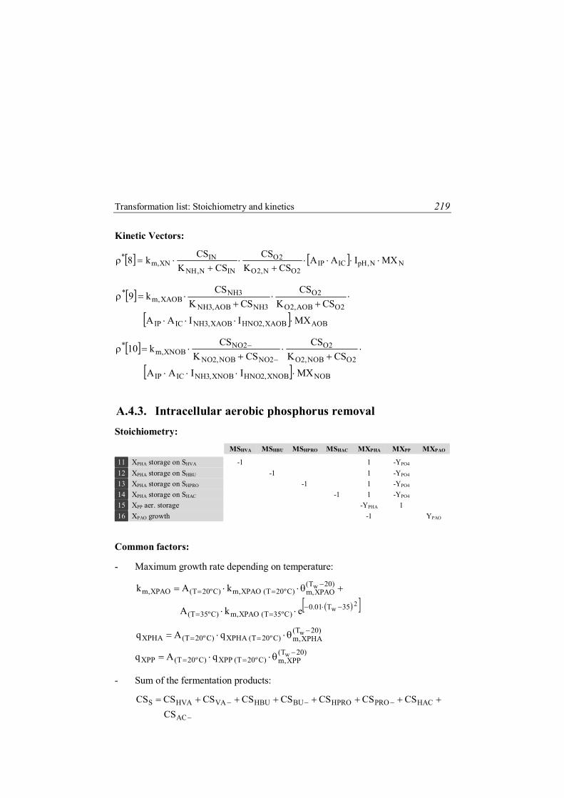
Transformation list: Stoichiometry and kinetics 219

Kinetic Vectors:

NN,pHICIP2ON,2O

2O

INN,NH

INXN,m

* MXIAACSK

CSCSK

CSk8

AOBXAOB,2HNOXAOB,3NHICIP

2OAOB,2O

2O

3NHAOB,3NH

3NHXAOB,m

*

MXIIAA

CSKCS

CSKCS

k9

NOBXNOB,2HNOXNOB,3NHICIP

2ONOB,2O

2O

2NONOB,2NO

2NOXNOB,m

*

MXIIAA

CSKCS

CSKCS

k10

A.4.3. Intracellular aerobic phosphorus removal Stoichiometry: MSHVA MSHBU MSHPRO MSHAC MXPHA MXPP MXPAO 11 XPHA storage on SHVA -1 1 -YPO4 12 XPHA storage on SHBU -1 1 -YPO4 13 XPHA storage on SHPRO -1 1 -YPO4 14 XPHA storage on SHAC -1 1 -YPO4 15 XPP aer. storage -YPHA 1 16 XPAO growth -1 YPAO

Common factors:

- Maximum growth rate depending on temperature:

2

w

w

35T01.0)Cº35T(XPAO,m)Cº35T(

)20T(XPAO,m)Cº20T(XPAO,m)Cº20T(XPAO,m

ekA

kAk

)20T(XPHA,m)Cº20T(XPHA)Cº20T(XPHA

wqAq

)20T(XPP,m)Cº20T(XPP)Cº20T(XPP

wqAq

- Sum of the fermentation products:

AC

HACPROHPROBUHBUVAHVAS

CSCSCSCSCSCSCSCSCS

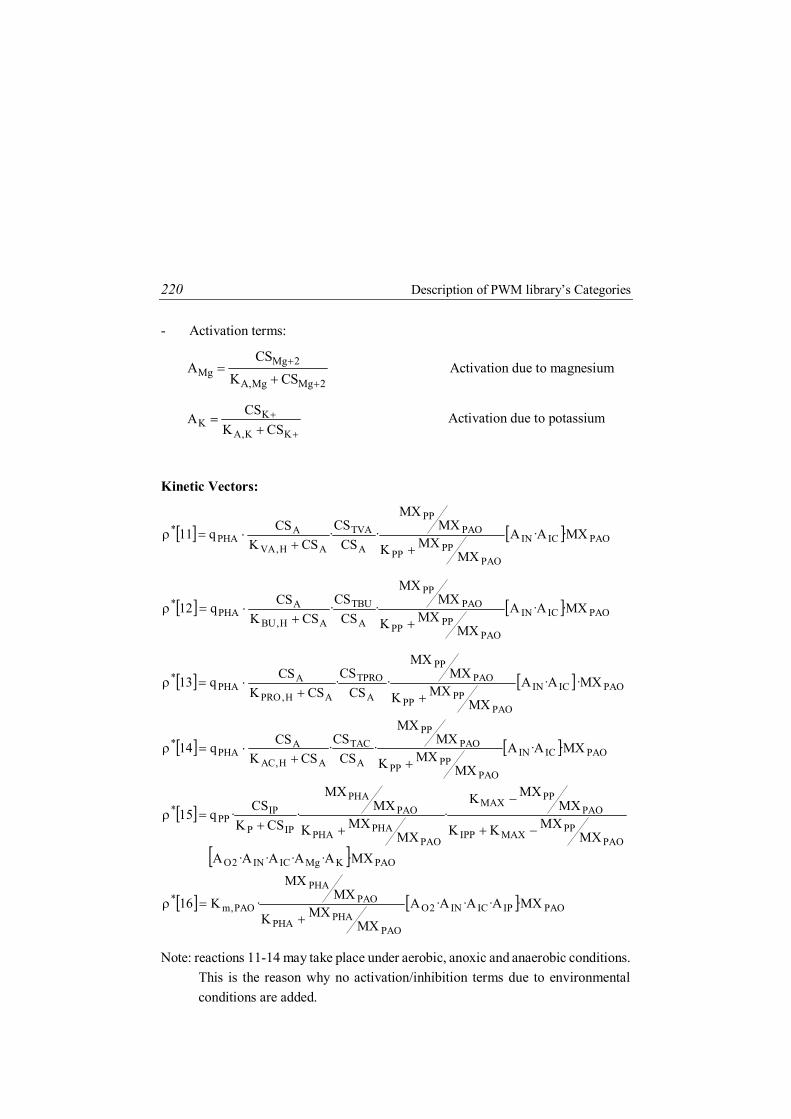
220 Description of PWM library’s Categories

- Activation terms:

2MgMg,A

2MgMg CSK

CSA

Activation due to magnesium

KK,A

KK CSK

CSA Activation due to potassium

Kinetic Vectors:

PAOICIN

PAOPPPP

PAOPP

A

TVA

AH,VA

APHA

* MX·A·A

MXMXK

MXMX

·CS

CS·

CSKCSq11

PAOICIN

PAOPPPP

PAOPP

A

TBU

AH,BU

APHA

* MX·A·A

MXMXK

MXMX

·CS

CS·

CSKCSq12

PAOICIN

PAOPPPP

PAOPP

A

TPRO

AH,PRO

APHA

* MX·A·A

MXMXK

MXMX

·CS

CS·

CSKCSq13

PAOICIN

PAOPPPP

PAOPP

A

TAC

AH,AC

APHA

* MX·A·A

MXMXK

MXMX

·CS

CS·

CSKCSq14

PAOKMgICIN2O

PAOPPMAXIPP

PAOPPMAX

PAOPHAPHA

PAOPHA

IPP

IPPP

*

MX·A·A·A·A·AMX

MXKK

MXMXK

·

MXMXK

MXMX

·CSK

CS·q15

PAOIPICIN2O

PAOPHAPHA

PAOPHA

PAO,m* MX·A·A·A·A

MXMXK

MXMX

·K16

Note: reactions 11-14 may take place under aerobic, anoxic and anaerobic conditions. This is the reason why no activation/inhibition terms due to environmental conditions are added.

Transformation list: Stoichiometry and kinetics 221

A.4.4. Intracellular anoxic COD biodegradation Stoichiometry:

MX

H

YH

,NO

3

YH

,NO

3

YH

,NO

3

YH

,NO

3

YH

,NO

3

YH

,NO

3

YH

,NO

3

YH

,NO

3

YH

,NO

3

YH

,NO

3

YH

,NO

3

YH

,NO

3

YH

,NO

3

YH

,NO

3

YH

,NO

2

YH

,NO

2

YH

,NO

2

YH

,NO

2

YH

,NO

2

YH

,NO

2

YH

,NO

2

MX

NO

3

(YH

,NO

3 - 1

) ·

ZW

N /

[T

hOD

(SN

2) ·

ZW

N -

Th

OD

(SN

O3- )

· M

WSN

O3- ]

(YH

,NO

3,2N

- 1)

·

ZWN /

[ThO

D(S

NO

2- ) ·

MW

SNO

2- - Th

OD

(SN

O3- )

· M

WSN

O3- ]

MS N

O2

(1 -

YH

,NO

3,2N

) ·

ZW

N /

[ThO

D(S

NO

2- ) ·

MW

SNO

2- - Th

OD

(SN

O3- )

· M

WSN

O3- ]

(YH

,NO

2 - 1

) ·

ZW

N /

[T

hOD

(SN

2) ·

ZW

N -

Th

OD

(SN

O2- )

· M

WSN

O2- ]

MS N

2

(1 -

YH

,NO

3)·Z

WN /

[ThO

D(S

N2)

·

ZWN -

Th

OD

(SN

O3- )

· M

WSN

O3- ]

(1 -

YH

,NO

2-) ·

ZWN /

[T

hOD

(SN

2) ·

ZW

N -

Th

OD

(SN

O2- )

· M

WSN

O2- ]

MS H

AC

-1 -1 -1

MS H

PRO

-1 -1 -1

MS H

BU

-1 -1 -1

MS H

VA

-1 -1 -1

MS F

A

-1 -1 -1

MS A

A

-1 -1 -1

MS S

U

-1 -1 -1

S S

U c

onsu

m. w

ith N

OX

S AA c

onsu

m. w

ith N

OX

S FA

cons

um. w

ith N

OX

S HV

A co

nsum

. with

NO

X

S HB

U co

nsum

. with

NO

X

S HPR

O co

nsum

. with

NO

X

S HA

C co

nsum

. with

NO

X

S SU c

onsu

m. w

ith N

O2

S AA c

onsu

m. w

ith N

O2

S FA

cons

um. w

ith N

O2

S HV

A co

nsum

. with

NO

2

S HB

U co

nsum

. with

NO

2

S HPR

O co

nsum

. with

NO

2

S HA

C co

nsum

. with

NO

2

S SU c

onsu

m. w

ith N

O3

S AA c

onsu

m. w

ith N

O3

S FA

cons

um. w

ith N

O3

S HV

A co

nsum

. with

NO

3

S HB

U co

nsum

. with

NO

3

S HPR

O co

nsum

. with

NO

3

S HA

C co

nsum

. with

NO

3

17

18

19

20

21

22

23

24

25

26

27

28

29

30

31

32

33

34

35

36

37

222 Description of PWM library’s Categories

Common factors:

- Inhibition/Activation terms:

2O2O,A

2O,A2O CSK

KI

Inhibition due to oxygen

3NO3NO,A

3NO3NO CSK

CSA Activation due to nitrates

2NO2NO,A

2NO2NO CSK

CSA Activation due to nitrites

Kinetic Vectors:

HICIPIN3NO2OSS

SU3NOXH,m

* MXAAAAICSK

CSk17

HICIPIN3NO2OSS

AA3NOXH,m

* MXAAAAICSK

CSk18

HICIPIN3NO2OSS

FA3NOXH,m

* MXAAAAICSK

CSk19

HICIPIN3NO2OSS

TVA3NOXH,m

* MXAAAAICSK

CSk20

HICIPIN3NO2OSS

TBU3NOXH,m

* MXAAAAICSK

CSk21

HICIPIN3NO2OSS

TPRO3NOXH,m

* MXAAAAICSK

CSk22

HICIPIN3NO2OSS

TAC3NOXH,m

* MXAAAAICSK

CSk23

HICIPIN3NO2OSS

SUN2,3NOXH,m

* MXAAAAICSK

CSk24

HICIPIN3NO2OSS

AAN2,3NOXH,m

* MXAAAAICSK

CSk25

HICIPIN3NO2OSS

FAN2,3NOXH,m

* MXAAAAICSK

CSk26

HICIPIN3NO2OSS

TVAN2,3NOXH,m

* MXAAAAICSK

CSk27

Transformation list: Stoichiometry and kinetics 223

HICIPIN3NO2OSS

TBUN2,3NOXH,m

* MXAAAAICSK

CSk28

HICIPIN3NO2OSS

TPRON2,3NOXH,m

* MXAAAAICSK

CSk29

HICIPIN3NO2OSS

TACN2,3NOXH,m

* MXAAAAICSK

CSk30

HICIPIN2NO2OSS

SU2NOXH,m

* MXAAAAICSK

CSk31

HICIPIN2NO2OSS

AA2NOXH,m

* MXAAAAICSK

CSk32

HICIPIN2NO2OSS

FA2NOXH,m

* MXAAAAICSK

CSk33

HICIPIN2NO2OSS

TVA2NOXH,m

* MXAAAAICSK

CSk34

HICIPIN2NO2OSS

TBU2NOXH,m

* MXAAAAICSK

CSk35

HICIPIN2NO2OSS

TPRO2NOXH,m

* MXAAAAICSK

CSk36

HICIPIN2NO2OSS

TAC2NOXH,m

* MXAAAAICSK

CSk37

A.4.5. Intracellular anoxic Anammox bacteria activity Stoichiometry: MSNO2- MSNO3- MSNH4+ MSN2 MXAN 38 XAN growth -1.3 0.239 -1 2.056 YAN

Common factors:

- Maximum growth rate depending on temperature:

15.29315.273TR20T70000

)Cº20T(XAN,mXAN,mw

w

ekk

224 Description of PWM library’s Categories

Kinetic Vectors:

ANICIP

2OAN,2O

AN,2O

INAN,NH

IN

2NOAN,2NO

2NOXAN,m

*

MXAA

CSKK

CSKCS

CSKCS

k38

A.4.6. Intracellular anoxic phosphorus removal Stoichiometry: MSN2 MSNO3- MXPHA MXPP MXPAO

39 XPP anox. storage - YPHA ·ZWN / [ThOD(SN2) ·

ZWN - ThOD(SNO3-) ·

MWSNO3-]

YPHA ·ZWN / [ThOD(SN2) · ZWN - ThOD(SNO3

-) · MWSNO3

-] -YPHA 1

40 XPAO anox. growth (1 - YH,NO3)·ZWN /

[ThOD(SN2) · ZWN - ThOD(SNO3

-) · MWSNO3-]

(YH,NO3 - 1) ·ZWN / [ThOD(SN2) · ZWN -

ThOD(SNO3-) · MWSNO3

-] -1 YPAO

Common factors:

- Activation terms:

3NO2NONOX,A

3NO2NONOX CSCSK

CSCSA Activation due to NOX

Kinetic Vectors:

PAOKMgIPICINNOX2OPAO,3NO

PAOPP

MAXIPP

PAOPP

MAX

PAOPHA

PHA

PAOPHA

IPP

IPPP

*

MX·A·A·A·A·A·A·IMX

MXKK

MXMXK

·

MXMXK

MXMX

·CSK

CS·q39

PAO

IPICINNOX2O

PAOPHAPHA

PAOPHA

PAO,3NOPAO,m*

MX

·A·A·A·A·I

MXMXK

MXMX

·K40

Transformation list: Stoichiometry and kinetics 225

A.4.7. Intracellular anaerobic Acidogenesis Stoichiometry: MSSU MSAA MSHVA MSHBU MSHPRO MSHAC MSH2 MXSU MXAA 41 SSU acidogenesis

-1 (1-YSU) ·

fBU,SU (1-YSU) ·

fPRO,SU (1-YSU) ·

fAC,SU (1-YSU) ·

fH2,SU YSU

42 SAA acidogenesis

-1 (1-YAA) · fVA,AA

(1-YAA) · fBU,AA

(1-YAA) · fPRO,AA

(1-YAA) · fAC,AA

(1-YAA) · fH2,AA YAA

Common factors:

- Maximum growth rate depending on temperature:

2w

2w

w

55T01.0)Cº55T(XSU,m)Cº55T(

35T01.0

)Cº35T(XSU,m)Cº35T()20T(

XSU,m)Cº20T(XSU,m)Cº20T(XSU,m

ekAe

kAkAk

2w

2w

w

55T01.0)Cº55T(XAA,m)Cº55T(

35T01.0

)Cº35T(XAA,m)Cº35T()20T(

XAA,m)Cº20T(XAA,m)Cº20T(XAA,m

ekAe

kAkAk

- Saturation constants depending on temperature: 35T

)Cº35T(XSU,SUXSU,SUwXSU,SUeKK

35T

)Cº35T(XAA,AAXAA,AAwXAA,AAeKK

- Inhibition/Activation terms:

3NO2NONOX,I

NOX,INOX CSCSK

KI Inhibition due to nitrates and nitrites

H22

XAA,H,I

2XAA,H,I

AA,pH CSK

KI Inhibition due to pH of acidogenesis

and acetogenesis transformations

Kinetic Vectors:

SUAA,pHICIPINNOX2OSUXSU,SU

SUXSU,m

* MXIAAAIICSK

CSk41

AAAA,pHICIPINNOX2OAAXAA,AA

AAXAA,m

* MXIAAAIICSK

CSk42

226 Description of PWM library’s Categories

A.4.8. Intracellular anaerobic Acetogenesis Stoichiometry: MSFA MSHVA MSHBU MSHPRO MSHAC MSH2 MXFA MXC4 MXPRO 43 SFA acetogenesis

-1 (1-YFA) ·

fAC,FA (1-YFA) ·

fH2,FA YFA

44 SHVA acetogenesis

-1 (1-YC4) · fPRO,VA

(1-YC4) · fAC,C4

(1-YC4) · fH2,C4

YC4

45 SHBU acetogenesis

-1 (1-YC4) · fAC,C4

(1-YC4) · fH2,C4

YC4

46 SHPRO acetogenesis

-1 (1-YPRO) · fAC,PRO

(1-YPRO) · fH2,PRO YPRO

Common factors:

- Maximum growth rate depending on temperature:

2w

2w

w

55T01.0)Cº55T(XFA,m)Cº55T(

35T01.0

)Cº35T(XFA,m)Cº35T()20T(

XFA,m)Cº20T(XFA,m)Cº20T(XFA,m

ekAe

kAkAk

2w

2w

w

55T01.0)Cº55T(4XC,m)Cº55T(

35T01.0

)Cº35T(4XC,m)Cº35T()20T(

4XC,m)Cº20T(4XC,m)Cº20T(4XC,m

ekAe

kAkAk

2

w

2w

w

55T01.0

)Cº55T(XPRO,m)Cº55T(35T01.0

)Cº35T(XPRO,m

)Cº35T()20T(

XPRO,m)Cº20T(XPRO,m)Cº20T(XPRO,m

e

kAek

AkAk

- Saturation constants depending on temperature:

35T)Cº35T(XFA,FAXFA,FA

wXFA,FAeKK

35T)Cº35T(4XC,4C4XC,4C

w4XC,4CeKK

35T)Cº35T(XPRO,PROXPRO,PRO

wXPRO,PROeKK

- Inhibition constants depending on temperature:

35T)Cº35T(FA,2H,IFA,2H,I

wFA,2H,IeKK

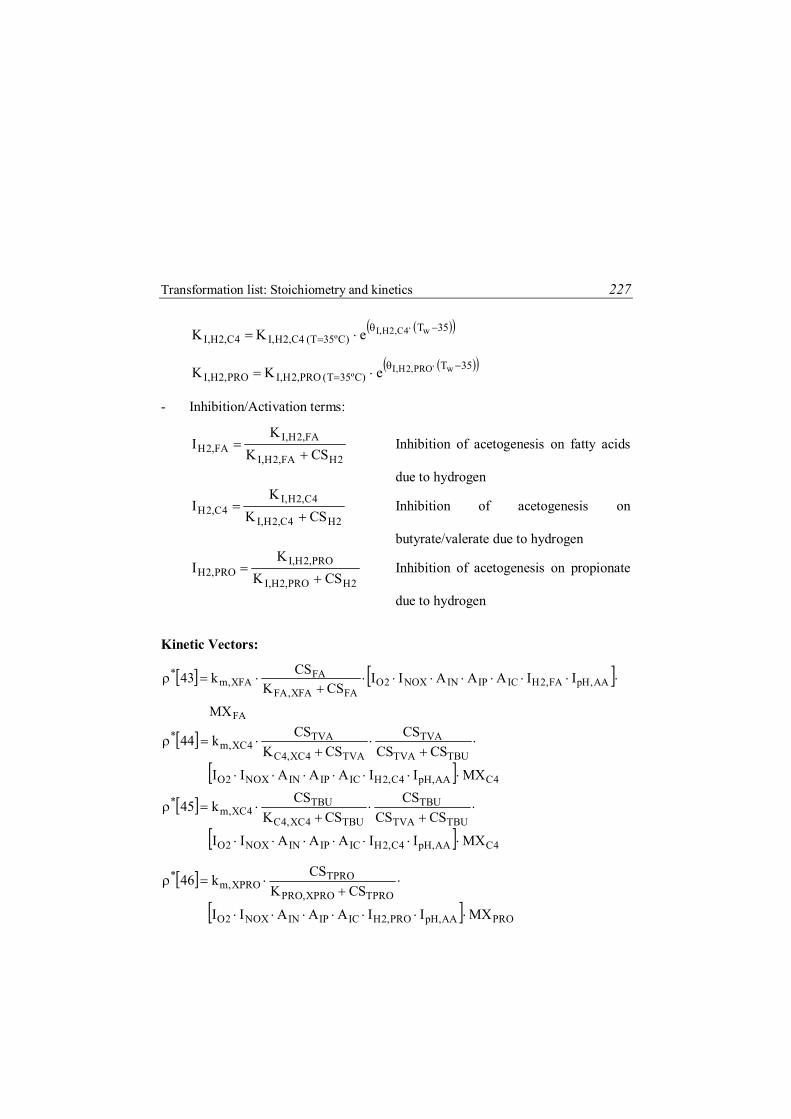
Transformation list: Stoichiometry and kinetics 227

35T)Cº35T(4C,2H,I4C,2H,I

w4C,2H,IeKK

35T)Cº35T(PRO,2H,IPRO,2H,I

wPRO,2H,IeKK

- Inhibition/Activation terms:

2HFA,2H,I

FA,2H,IFA,2H CSK

KI

Inhibition of acetogenesis on fatty acids

due to hydrogen

2H4C,2H,I

4C,2H,I4C,2H CSK

KI

Inhibition of acetogenesis on

butyrate/valerate due to hydrogen

2HPRO,2H,I

PRO,2H,IPRO,2H CSK

KI

Inhibition of acetogenesis on propionate

due to hydrogen

Kinetic Vectors:

FA

AA,pHFA,2HICIPINNOX2OFAXFA,FA

FAXFA,m

*

MX

IIAAAIICSK

CSk43

4CAA,pH4C,2HICIPINNOX2O

TBUTVA

TVA

TVA4XC,4C

TVA4XC,m

*

MXIIAAAII

CSCSCS

CSKCSk44

4CAA,pH4C,2HICIPINNOX2O

TBUTVA

TBU

TBU4XC,4C

TBU4XC,m

*

MXIIAAAII

CSCSCS

CSKCSk45

PROAA,pHPRO,2HICIPINNOX2O

TPROXPRO,PRO

TPROXPRO,m

*

MXIIAAAII

CSKCSk46

228 Description of PWM library’s Categories

A.4.9. Intracellular anaerobic Methanogenesis Stoichiometry: MSHAC MSH2 MSCH4 MXAC MXH2 47 Acetoclastic Methanogenesis -1 1-YAC 1-YAC 48 Hydrogenotrophic Methanogenesis -1 1- YH2 YH2

Common factors:

- Maximum growth rate depending on temperature:

2w

2w

w

55T01.0)Cº55T(XAC,m)Cº55T(

35T01.0

)Cº35T(XAC,m)Cº35T()20T(

XAC,m)Cº20T(XAC,m)Cº20T(XAC,m

ekAe

kAkAk

2w

2w

w

55T01.0)Cº55T(2XH,m)Cº55T(

35T01.0

)Cº35T(2XH,m)Cº35T()20T(

2XH,m)Cº20T(2XH,m)Cº20T(2XH,m

ekAe

kAkAk

- Saturation constants depending on temperature:

35T)Cº35T(XAC,ACXAC,AC

wXAC,ACeKK

35T)Cº35T(2XH,2H2XH,2H

w2XH,2HeKK

- Inhibition constants depending on temperature:

35T)Cº35T(3NH,I3NH,I

w3NH,IeKK

- Inhibition/Activation terms:

3NH3NH,I

3NH,I3NH CSK

KI

Inhibition due to NH3

3H

3

3

AC,pH CSK

KI

XAC,H,I

XAC,H,I

Inhibition of acetoclastic methanogenesis

due to pH

3H

3

3

2H,pH CSK

KI

2XH,H,I

2XH,H,I

Inhibition of hydrogenotrophic

methanogenesis due to pH

Transformation list: Stoichiometry and kinetics 229

Kinetic Vectors:

AC

AC,pH3NHICIPINNOX2OTACXAC,AC

TACXAC,m

*

MX

IIAAAIICSK

CSk47

2H2H,pHICIPINNOX2O2H2XH,2H

2H2XH,m

* MXIAAAIICSK

CSk48

A.4.10. Extracellular enzymatic composite disintegration Stoichiometry: MSI MXC1 MXCH MXPR MXLI MXI 49 XC1 aerobic disintegration fSI,XC1 -1 fCH,XC1 fPR,XC1 fLI,XC1 fXI,XC1 50 XC1 anoxic disintegration fSI,XC1 -1 fCH,XC1 fPR,XC1 fLI,XC1 fXI,XC1 51 XC1 anaerobic disintegration fSI,XC1 -1 fCH,XC1 fPR,XC1 fLI,XC1 fXI,XC1

Common factors:

- Maximum growth rate depending on temperature:

35T)Cº35T(1XC,AER,dis)Cº35T(

)20T()Cº20T(1XC,AER,dis))Cº20T(1XC,AER,dis)Cº20T(1XC,AER,dis

w)Cº35T(1XC,AER,dis

w

ekA

kAk

35T)Cº35T(1XC,ANOX,dis)Cº35T(

)20T()Cº20T(1XC,ANOX,dis))Cº20T(1XC,ANOX,dis)Cº20T(1XC,ANOX,dis

w)Cº35T(1XC,ANOX,dis

w

ekA

kAk

35T)Cº35T(1XC,ANAER,dis)Cº35T(1XC,ANAER,dis

w)Cº35T(1XC,ANAER,dise

kAk

Kinetic Vectors:

1CICIPIN2O1XC,AER,dis* MXAAAAk49

1CICIPINNOX2O1XC,ANOX,dis* MXAAAAIk50

1CICIPINNOX2O1XC,ANAER,dis* MXAAAIIk51

230 Description of PWM library’s Categories

A.4.11. Extracellular enzymatic biomass disintegration Stoichiometry: MSP MXC1 MXCH MXPR MXLI MXP 52 XC2 aerobic disintegration fSP,XC2 -1 fCH,XC2 fPR,XC2 fLI,XC2 fXP,XC2 53 XC2 anoxic disintegration fSP,XC2 -1 fCH,XC2 fPR,XC2 fLI,XC2 fXP,XC2 54 XC2 anaerobic disintegration fSP,XC2 -1 fCH,XC2 fPR,XC2 fLI,XC2 fXP,XC2

Common factors:

- Maximum growth rate depending on temperature:

35T)Cº35T(2XC,AER,dis)Cº35T(

)20T()Cº20T(2XC,AER,dis))Cº20T(2XC,AER,dis)Cº20T(2XC,AER,dis

w)Cº35T(2XC,AER,dis

w

ekA

kAk

35T)Cº35T(2XC,ANOX,dis)Cº35T(

)20T()Cº20T(2XC,ANOX,dis))Cº20T(2XC,ANOX,dis)Cº20T(2XC,ANOX,dis

w)Cº35T(2XC,ANOX,dis

w

ekA

kAk

35T)Cº35T(2XC,ANAER,dis)Cº35T(

)20T()Cº20T(2XC,ANAER,dis))Cº20T(2XC,ANAER,dis)Cº20T(2XC,ANAER,dis

w)Cº35T(2XC,ANAER,dis

w

ekA

kAk

Kinetic Vectors:

2CICIPIN2O2XC,AER,dis* MXAAAAk52

2CICIPINNOX2O2XC,ANOX,dis* MXAAAAIk53

2CICIPINNOX2O2XC,ANAER,dis* MXAAAIIk54

A.4.12. Extracellular biomass thermal disintegration Stoichiometry: MSP MXC1 MXCH MXPR MXLI MXP 55 XC2 thermal disintegration fSP,XC2,TH -1 fCH,XC2,TH fPR,XC2,TH fLI,XC2,TH fXP,XC2,TH

Transformation list: Stoichiometry and kinetics 231

Common factors:

- Maximum growth rate depending on temperature: 25T

))Cº25T(2XC,S)TH(2XC,Sw)Cº25T(2XC,THekAk

- Input components concentration correction considering the water variations in the unit (*c):

O2SHstepprevious,O2SHg,wT

g,win,w

comp,in,wc*comp,in,w

E~Q

mC

Kinetic Vectors:

conv,2XCc*

2XC,in,wNBiom

1biomassbiomass,in,wdec2XC,w

w2XC,S*

f1CCfC

Vk55

where NBiom is the number of biomasses in the category selected.

A.4.13. Extracellular XI and XP thermal disintegration Stoichiometry: MSI MSP MXCH MXPR MXLI MXI MXP 56 XI thermal disintegration fSI,XI,TH fCH,XI,TH fPR,XI,TH fLI,XI,TH -1 57 XP thermal disintegration fSP,XP,TH fCH,XP,TH fPR,XP,TH fLI,XP,TH -1

Common factors:

- Maximum growth rate depending on temperature: 25T

))Cº25T(XI,S)TH(XI,Sw)Cº25T(XI,THekAk

25T))Cº25T(XP,S)TH(XP,S

w)Cº25T(XP,THekAk

Kinetic Vectors:

232 Description of PWM library’s Categories

conv,XIc*

XI,in,wXI,wwXI,S* f1CCVk55

conv,XPdisc*

2XC,in,wNBiom

1biomassbiomass,in,wdec2XC,w

wXP,S*

f1fCCfC

Vk57

A.4.14. Extracellular enzymatic hydrolysis Stoichiometry: MSSU MSAA MSFA MXCH MXPR MXLI 58 XCH hydrolysis 1 -1 59 XPR hydrolysis 1 -1 60 XLI hydrolysis 1-fFA,LI fFA,LI -1 61 XCH hydrolysis 1 -1 62 XPR hydrolysis 1 -1 63 XLI hydrolysis 1-fFA,LI fFA,LI -1 64 XCH hydrolysis 1 -1 65 XPR hydrolysis 1 -1 66 XLI hydrolysis 1-fFA,LI fFA,LI -1

Common factors:

- Maximum growth rate depending on temperature:

35T)Cº35T(AER,hid

)Cº35T()20T(

)Cº20T(AER,hid)Cº20T(AER,hid)Cº20T(AER,hid

w)Cº35T(AER,hid

w

ek

AkAk

35T)Cº35T(ANOX,hid

)Cº35T()20T(

)Cº20T(ANOX,hid)Cº20T(ANOX,hid)Cº20T(ANOX,hid

w)Cº35T(ANOX,hid

w

ek

AkAk

Transformation list: Stoichiometry and kinetics 233

35T)Cº35T(XCH,ANAER,hid)Cº35T(

)20T()Cº20T(XCH,ANAER,hid)Cº20T(XCH,ANAER,hid)Cº20T(XCH,ANAER,hid

w)Cº35T(XCH,ANAER,hid

w

ekA

kAk

35T)Cº35T(XPR,ANAER,hid)Cº35T(

)20T()Cº20T(XPR,ANAER,hid)Cº20T(XPR,ANAER,hid)Cº20T(XPR,ANAER,hid

w)Cº35T(XPR,ANAER,hid

w

ekA

kAk

35T)Cº35T(XLI,ANAER,hid)Cº35T(

)20T()Cº20T(XLI,ANAER,hid)Cº20T(XLI,ANAER,hid)Cº20T(XLI,ANAER,hid

w)Cº35T(XLI,ANAER,hid

w

ekA

kAk

)20T(x,hid)Cº20T(xx

wKK

Kinetic Vectors:

H

HLIPRCH

x

H

LI

PR

CH

ICIPIN2OAER,hid*

*

*

MX

CX)CXCXCX(K

CX1

CXCXCX

AAAAk605958

H

HLIPRCH

x

H

LI

PR

CH

ICIPINNOX2OANOX,hid*

*

*

MX

CX)CXCXCX(K

CX1

CXCXCX

AAAAIk636261

CHICIPINNOX2OXCH,ANAER,hid* MXAAAIIk64

PRICIPINNOX2OXPR,ANAER,hid* MXAAAIIk65

LIICIPINNOX2OXLI,ANAER,hid* MXAAAIIk66

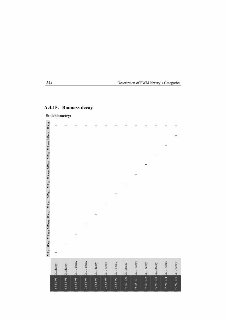
234 Description of PWM library’s Categories

A.4.15. Biomass decay Stoichiometry:

MX

C2

1 1 1 1 1 1 1 1 1 1 1 1 1

MX

AN

-1

MX

PAO

-1

MX

H2

-1

MX

AC

-1

MX

PRO

-1

MX

C4

-1

MX

FA

-1

MX

AA

-1

MX

SU

-1

MX

NO

B

-1

MX

AO

B

-1

MX

N

-1

MX

H

-1

X

H d

ecay

XN d

ecay

XA

OB d

ecay

XN

OB d

ecay

XSU

dec

ay

XA

A d

ecay

XFA

dec

ay

XC

4 dec

ay

XPR

O d

ecay

XA

C d

ecay

XH

2 dec

ay

XPA

O d

ecay

XA

N d

ecay

67

-80-

93

68-8

1-94

68-8

2-95

70-8

3-96

71-8

4-97

72-8

5-98

73-8

6-99

74-8

7-10

0

75-8

8-10

1

76-8

9-10

2

77-9

0-10

3

78-9

1-10

4

79-9

2-10

5

Transformation list: Stoichiometry and kinetics 235

Common factors:

- Maximum growth rate depending on temperature:

35T)Cº35T(AER,XH,dec

)Cº35T()20T(

)Cº20T(AER,XH,dec)Cº20T(AER,XH,dec)Cº20T(AER,XH,dec

w)Cº35T(AER,XH,dec

w

ek

AkAk

35T)Cº35T(AER,XN,dec

)Cº35T()20T(

)Cº20T(AER,XN,dec)Cº20T(AER,XN,dec)Cº20T(AER,XN,dec

w)Cº35T(AER,XN,dec

w

ek

AkAk

)20T()Cº20T(AER,XAOB,dec)Cº20T(AER,XAOB,decAER,XAOB,dec

wkk

)20T()Cº20T(AER,XNOB,dec)Cº20T(AER,XNOB,decAER,XNOB,dec

wkk

35T)Cº35T(AER,XSU,dec)Cº35T(

)20T()Cº20T(AER,XSU,dec)Cº20T(AER,XSU,dec)Cº20T(AER,XSU,dec

w)Cº35T(AER,XSU,dec

w

ekA

kAk

35T)Cº35T(AER,XAA,dec)Cº35T(

)20T()Cº20T(AER,XAA,dec)Cº20T(AER,XAA,dec)Cº20T(AER,XAA,dec

w)Cº35T(AER,XAA,dec

w

ekA

kAk

35T)Cº35T(AER,XFA,dec)Cº35T(

)20T()Cº20T(AER,XFA,dec)Cº20T(AER,XFA,dec)Cº20T(AER,XFA,dec

w)Cº35T(AER,XFA,dec

w

ekA

kAk

35T)Cº35T(AER,4XC,dec)Cº35T(

)20T()Cº20T(AER,4XC,dec)Cº20T(AER,4XC,dec)Cº20T(AER,4XC,dec

w)Cº35T(AER,4XC,dec

w

ekA

kAk

35T)Cº35T(AER,XPRO,dec)Cº35T(

)20T()Cº20T(AER,XPRO,dec)Cº20T(AER,XPRO,dec)Cº20T(AER,XPRO,dec

w)Cº35T(AER,XPRO,dec

w

ekA

kAk

35T)Cº35T(AER,XAC,dec)Cº35T(

)20T()Cº20T(AER,XAC,dec)Cº20T(AER,XAC,dec)Cº20T(AER,XAC,dec

w)Cº35T(AER,XAC,dec

w

ekA

kAk

35T)Cº35T(AER,2XH,dec)Cº35T(

)20T()Cº20T(AER,2XH,dec)Cº20T(AER,2XH,dec)Cº20T(AER,2XH,dec

w)Cº35T(AER,2XH,dec

w

ekA

kAk

35T)Cº35T(AER,XPAO,dec)Cº35T(

)20T()Cº20T(AER,XPAO,dec)Cº20T(AER,XPAO,dec)Cº20T(AER,XPAO,dec

w)Cº35T(AER,XPAO,dec

w

ekA

kAk

236 Description of PWM library’s Categories

)20T()Cº20T(AER,XAN,dec)Cº20T(AER,XAN,decAER,XAN,dec

wkk

35T)Cº35T(ANOX,XH,dec)Cº35T(

)20T()Cº20T(ANOX,XH,dec)Cº20T(ANOX,XH,dec)Cº20T(ANOX,XH,dec

w)Cº35T(ANOX,XH,dec

w

ekA

kAk

35T)Cº35T(ANOX,XN,dec)Cº35T(

)20T()Cº20T(ANOX,XN,dec)Cº20T(ANOX,XN,dec)Cº20T(ANOX,XN,dec

w)Cº35T(ANOX,XN,dec

w

ekA

kAk

)20T()Cº20T(ANOX,XAOB,dec)Cº20T(ANOX,XAOB,decANOX,XAOB,dec

wkk

)20T()Cº20T(ANOX,XNOB,dec)Cº20T(ANOX,XNOB,decANOX,XNOB,dec

wkk

35T)Cº35T(ANOX,XSU,dec)Cº35T(

)20T()Cº20T(ANOX,XSU,dec)Cº20T(ANOX,XSU,dec)Cº20T(ANOX,XSU,dec

w)Cº35T(ANOX,XSU,dec

w

ekA

kAk

35T)Cº35T(ANOX,XAA,dec)Cº35T(

)20T()Cº20T(ANOX,XAA,dec)Cº20T(ANOX,XAA,dec)Cº20T(ANOX,XAA,dec

w)Cº35T(ANOX,XAA,dec

w

ekA

kAk

35T)Cº35T(ANOX,XFA,dec)Cº35T(

)20T()Cº20T(ANOX,XFA,dec)Cº20T(ANOX,XFA,dec)Cº20T(ANOX,XFA,dec

w)Cº35T(ANOX,XFA,dec

w

ekA

kAk

35T)Cº35T(ANOX,4XC,dec)Cº35T(

)20T()Cº20T(ANOX,4XC,dec)Cº20T(ANOX,4XC,dec)Cº20T(ANOX,4XC,dec

w)Cº35T(ANOX,4XC,dec

w

ekA

kAk

35T)Cº35T(ANOX,XPRO,dec)Cº35T(

)20T()Cº20T(ANOX,XPRO,dec)Cº20T(ANOX,XPRO,dec)Cº20T(ANOX,XPRO,dec

w)Cº35T(ANOX,XPRO,dec

w

ekA

kAk

35T)Cº35T(ANOX,XAC,dec)Cº35T(

)20T()Cº20T(ANOX,XAC,dec)Cº20T(ANOX,XAC,dec)Cº20T(ANOX,XAC,dec

w)Cº35T(ANOX,XAC,dec

w

ekA

kAk

35T)Cº35T(ANOX,2XH,dec)Cº35T(

)20T()Cº20T(ANOX,2XH,dec)Cº20T(ANOX,2XH,dec)Cº20T(ANOX,2XH,dec

w)Cº35T(ANOX,2XH,dec

w

ekA

kAk

35T)Cº35T(ANOX,XPAO,dec)Cº35T(

)20T()Cº20T(ANOX,XPAO,dec)Cº20T(ANOX,XPAO,dec)Cº20T(ANOX,XPAO,dec

w)Cº35T(ANOX,XPAO,dec

w

ekA

kAk

)20T()Cº20T(ANOX,XAN,dec)Cº20T(ANOX,XAN,decANOX,XAN,dec

wkk

Transformation list: Stoichiometry and kinetics 237

35T)Cº35T(ANAER,XH,dec)Cº35T(

)20T()Cº20T(ANAER,XH,dec)Cº20T(ANAER,XH,dec)Cº20T(ANAER,XH,dec

w)Cº35T(ANAER,XH,dec

w

ekA

kAk

35T)Cº35T(ANAER,XN,dec)Cº35T(

)20T()Cº20T(ANAER,XN,dec)Cº20T(ANAER,XN,dec)Cº20T(ANAER,XN,dec

w)Cº35T(ANAER,XN,dec

w

ekA

kAk

)20T()Cº20T(ANAER,XAOB,dec)Cº20T(ANAER,XAOB,decANAER,XAOB,dec

wkk

)20T()Cº20T(ANAER,XNOB,dec)Cº20T(ANAER,XNOB,decANAER,XNOB,dec

wkk

35T)Cº35T(ANAER,XSU,dec)Cº35T(

)20T()Cº20T(ANAER,XSU,dec)Cº20T(ANAER,XSU,dec)Cº20T(ANAER,XSU,dec

w)Cº35T(ANAER,XSU,dec

w

ekA

kAk

35T)Cº35T(ANAER,XAA,dec)Cº35T(

)20T()Cº20T(ANAER,XAA,dec)Cº20T(ANAER,XAA,dec)Cº20T(ANAER,XAA,dec

w)Cº35T(ANAER,XAA,dec

w

ekA

kAk

35T)Cº35T(ANAER,XFA,dec)Cº35T(

)20T()Cº20T(ANAER,XFA,dec)Cº20T(ANAER,XFA,dec)Cº20T(ANAER,XFA,dec

w)Cº35T(ANAER,XFA,dec

w

ekA

kAk

35T)Cº35T(ANAER,4XC,dec)Cº35T(

)20T()Cº20T(ANAER,4XC,dec)Cº20T(ANAER,4XC,dec)Cº20T(ANAER,4XC,dec

w)Cº35T(ANAER,4XC,dec

w

ekA

kAk

35T)Cº35T(ANAER,XPRO,dec)Cº35T(

)20T()Cº20T(ANAER,XPRO,dec)Cº20T(ANAER,XPRO,dec)Cº20T(ANAER,XPRO,dec

w)Cº35T(ANAER,XPRO,dec

w

ekA

kAk

35T)Cº35T(ANAER,XAC,dec)Cº35T(

)20T()Cº20T(ANAER,XAC,dec)Cº20T(ANAER,XAC,dec)Cº20T(ANAER,XAC,dec

w)Cº35T(ANAER,XAC,dec

w

ekA

kAk

35T)Cº35T(ANAER,2XH,dec)Cº35T(

)20T()Cº20T(ANAER,2XH,dec)Cº20T(ANAER,2XH,dec)Cº20T(ANAER,2XH,dec

w)Cº35T(ANAER,2XH,dec

w

ekA

kAk

35T)Cº35T(ANAER,XPAO,dec)Cº35T(

)20T()Cº20T(ANAER,XPAO,dec)Cº20T(ANAER,XPAO,dec)Cº20T(ANAER,XPAO,dec

w)Cº35T(ANAER,XPAO,dec

w

ekA

kAk

)20T()Cº20T(ANAER,XAN,dec)Cº20T(ANAER,XAN,decANAER,XAN,dec

wkk

238 Description of PWM library’s Categories

Kinetic Vectors:

H2OAER,XH,dec* MXAk67

N2OAER,XN,dec* MXAk68

AOB2OAER,XAOB,dec* MXAk69

NOB2OAER,XNOB,dec* MXAk70

SU2OAER,XSU,dec* MXAk71

AA2OAER,XAA,dec* MXAk72

FA2OAER,XFA,dec* MXAk73

4C2OAER,4XC,dec* MXAk74

PRO2OAER,XPRO,dec* MXAk75

AC2OAER,XAC,dec* MXAk76

2H2OAER,2XH,dec* MXAk77

PAO2OAER,XPAO,dec* MXAk78

AN2OAER,XAN,dec* MXAk79

HNOX2OANOX,XH,dec* MXAIk80

NNOX2OANOX,XN,dec* MXAIk81

AOBNOX2OANOX,XAOB,dec* MXAIk82

NOBNOX2OANOX,XNOB,dec* MXAIk83

SUNOX2OANOX,XSU,dec* MXAIk84

AANOX2OANOX,XAA,dec* MXAIk85

FANOX2OANOX,XFA,dec* MXAIk86

4CNOX2OANOX,4XC,dec* MXAIk87

PRONOX2OANOX,XPRO,dec* MXAIk88

ACNOX2OANOX,XAC,dec* MXAIk89

2HNOX2OANOX,2XH,dec* MXAIk90

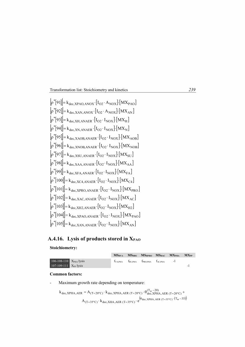
Transformation list: Stoichiometry and kinetics 239

PAONOX2OANOX,XPAO,dec* MXAIk91

ANNOX2OANOX,XAN,dec* MXAIk92

HNOX2OANAER,XH,dec* MXIIk93

NNOX2OANAER,XN,dec* MXIIk94

AOBNOX2OANAER,XAOB,dec* MXIIk95

NOBNOX2OANAER,XNOB,dec* MXIIk96

SUNOX2OANAER,XSU,dec* MXIIk97

AANOX2OANAER,XAA,dec* MXIIk98

FANOX2OANAER,XFA,dec* MXIIk99

4CNOX2OANAER,4XC,dec* MXIIk100

PRONOX2OANAER,XPRO,dec* MXIIk101

ACNOX2OANAER,XAC,dec* MXIIk102

2HNOX2OANAER,2XH,dec* MXIIk103

PAONOX2OANAER,XPAO,dec* MXIIk104

ANNOX2OANAER,XAN,dec* MXIIk105

A.4.16. Lysis of products stored in XPAO Stoichiometry: MSHVA MSHBU MSHPRO MSHAC MXPHA MXPP 106-108-110 XPHA lysis fVA,PHA fBU,PHA fPRO,PHA fAC,PHA -1 107-109-111 XPP lysis -1

Common factors:

- Maximum growth rate depending on temperature:

35T)Cº35T(AER,XHA,dec)Cº35T(

)20T()Cº20T(AER,XPHA,dec)Cº20T(AER,XPHA,dec)Cº20T(AER,XPHA,dec

w)Cº35T(AER,XPHA,dec

w

ekA

kAk

240 Description of PWM library’s Categories

35T)Cº35T(AER,XPP,dec)Cº35T(

)20T()Cº20T(AER,XPP,dec)Cº20T(AER,XPP,dec)Cº20T(AER,XPP,dec

w)Cº35T(AER,XPP,dec

w

ekA

kAk

35T)Cº35T(ANOX,XHA,dec)Cº35T(

)20T()Cº20T(ANOX,XPHA,dec)Cº20T(ANOX,XPHA,dec)Cº20T(ANOX,XPHA,dec

w)Cº35T(ANOX,XPHA,dec

w

ekA

kAk

35T)Cº35T(ANOX,XPP,dec)Cº35T(

)20T()Cº20T(ANOX,XPP,dec)Cº20T(ANOX,XPP,dec)Cº20T(ANOX,XPP,dec

w)Cº35T(ANOX,XPP,dec

w

ekA

kAk

35T)Cº35T(ANAER,XHA,dec)Cº35T(

)20T()Cº20T(ANAER,XPHA,dec)Cº20T(ANAER,XPHA,dec)Cº20T(ANAER,XPHA,dec

w)Cº35T(ANAER,XPHA,dec

w

ekA

kAk

35T)Cº35T(ANAER,XPP,dec)Cº35T(

)20T()Cº20T(ANAER,XPP,dec)Cº20T(ANAER,XPP,dec)Cº20T(ANAER,XPP,dec

w)Cº35T(ANAER,XPP,dec

w

ekA

kAk

Kinetic Vectors:

PHA2OAER,XPHA,dec* MXAk106

PP2OAER,XPP,dec* MXAk107

PHANOX2OANOX,XPHA,dec* MXAIk108

PPNOX2OANOX,XPP,dec* MXAIk109

PHANOX2OANAER,XPHA,dec* MXIIk110

PPNOX2OANAER,XPP,dec* MXIIk111

Transformation list: Stoichiometry and kinetics 241

A.4.17. Acid-Base equilibria Stoichiometry:

MS A

C-

1

MS H

AC

-1

MS P

RO

-

1

MS H

PRO

-1

MS B

U-

1

MS H

BU

-1

MS A

C

1

MS H

AC

-1

MS C

O3=

1

MS H

CO

3-

1 -1

MS N

O2-

1

MS H

NO

2

-1

MS N

H3

1

MS P

O4-3

1

MS H

PO4=

1 -1

MS O

H-

1

H

2O

equi

libriu

m

PIN

eq

uilib

rium

PIN

2 eq

uilib

rium

SNH

eq

uilib

rium

SNO

eq

uilib

rium

CIN

eq

uilib

rium

CIN

2 eq

uilib

rium

SHV

A

equi

libriu

m

SHB

U

equi

libriu

m

SHPR

O

equi

libriu

m

SHA

C

equi

libriu

m

11

2

113

114

115

116

117

118

119

120

121

122

242 Description of PWM library’s Categories

Common factors:

- Acid-base equilibrium constants:

15.273T

115.298

1314.8

55900

)Cº25T(O2H,aO2H,aweKK H+-OH- equilibrium

15.273T

115,298

1314.8

4200

)Cº25T(IP,aIP,aweKK H2PO4

--HPO4= equilibrium

15.273T

115,298

1314.8

16743

)Cº25T(IP,2aIP,2aweKK HPO4

=-PO4-3 equilibrium

15.273T

115.298

1314.8

51965

)Cº25T(IN,aIN,aweKK NH4

+-NH3 equilibrium

15.273T

115.298

1314.8

12800

)Cº25T(2NO,a2NO,aweKK HNO2-NO2

- equilibri.

15.273T

115.298

1314.8

7646

)Cº25T(IC,aIC,aweKK CO2

--HCO3- equilibrium

15.273T

115.298

1314.8

14869

)Cº25T(IC,2aIC,2aweKK HCO3

--CO3= equilibrium

Kinetic Vectors:

wHOH6

O2H,aO2H,ab* VCSCS10Kk112

wH4HPO4PO2HIP,aIP,ab* VCSCSCS1000Kk113

wH34PO4HPOIP,2aIP,2ab* VCSCSCS1000Kk114

wH3NH4NHIN,aIN,ab* VCSCSCS1000Kk115

wH2NO2HNO2NO,a2NO,ab* VCSCSCS1000Kk116

wH3HCO2COIC,aIC,ab* VCSCSCS1000Kk117

wH3CO3HCOIC,2aIC,2ab* VCSCSCS1000Kk118

Transformation list: Stoichiometry and kinetics 243

wHVAHVAHVA,aHVA,ab* VCSCSCS1000Kk119

wHBUHBUHBU,aHBU,ab* VCSCSCS1000Kk120

wHPROHPROHPRO,aHPRO,ab* VCSCSCS1000Kk121

wHACHACHAC,aHAC,ab* VCSCSCS1000Kk122

A.4.18. CxHyOzNaPb combustion Stoichiometry: MSO2 MSCO2 MSPO4-3 MSN2 MSH2O MCxHyOzNaPb

CxHyOzNaPb combustion

- x+5b4

+y4

–z2

x b a2

y–3b

2 -1

Note: Instantaneous reaction (without kinetic) to describe the combustion of any component of the model.

A.4.19. Liquid-Gas transfers Stoichiometry: MSH2O MSO2 MSNH3 MSCO2 MSCH4 MSH2 MSN2 MGH2OMGO2 MGNH3 MGCO2 MGCH4 MGH2 MGN2 123 CO2 diss. 1 -1 124 O2 diss. 1 -1 125 H2O eva. -1 1 126 NH3 diss. 1 -1 127 CH4 diss. 1 -1 128 H2 diss. 1 -1 129 N2 diss. 1 -1

Common factors:

- Henry’s constants:

15.273T

115.298

1314.8

19410

)Cº25T(2CO,H2CO,HweKK for CO2

15.273T

115.298

1314.8

12741

)Cº25T(2O,H2O,HweKK for O2

244 Description of PWM library’s Categories

15.273T

115.298

1314,8

34100

)Cº25T(3NH,H3NH,Hwe.KK for NH3

15.273T

115.298

1314.8

14240

)Cº25T(4CH,H4CH,HweKK for CH4

15.273T

115.298

1314.8

10808

)Cº25T(2N,H2N,HweKK for N2

15.273T

115.298

1314.8

4180

)Cº25T(2H,H2H,HweKK for H2

Kinetic Vectors:

2CO2CO,g2CO,HW2CO,a_L* CSp12000KVk1

2O2O,g2O,HW2O,a_L* CSp32000KVk2

O2H,gSAT

O2H,gg

WO2H,a_M* pP

)T15.273(082.018000Vk3

3NH3NH,g3NH,HW3NH,a_L* CSp14000KVk4

4CH4CH,g4CH,HW4CH,a_L* CSp64000KVk5

2N2N,g2N,HW2N,a_L* CSp28000KVk6

2H2H,g2H,HW2H,a_L* CSp16000KVk7

where pg,comp is the partial pressure of the corresponding component in the gas phase.

Transformation list: Stoichiometry and kinetics 245

A.4.20. Liquid-Solid transfers Stoichiometry: MSOH MPCaCO3 MPMgCO3 MPACP MPSTRU MPKSTRU MPNEW MPFeCl3 MPFePO4 MPFe(OH)3 1 FeCl3 dissol. -162.15 2 FePO4 dissol. -150.8 3 Fe(OH)3 dissol. 3 -106.85 4 Calcite precip/red. 100 5 Magnesite p/r. 84.3 6 ACP precip/red. 246 7 Struvite prec./red. 245 8 K-Struvite p/r. 153.3 9 Newberyite p/r. 120

Common factors:

- Solubility products depending on temperature:

31SCl3SFe

15.273T1

15.2981

314.8154080

)Cº25T(3FeCl,sp3FeCl,sp MW·MW·eKK w

34SPO3SFe15.273T

115.298

1314.8

78900

)Cº25T(4FePO,sp4FePO,sp MW·MW·eKK w

3SOH3SFe

15.273T1

15.2981

314.884500

)Cº25T(3)OH(Fe,sp3)OH(Fe,sp MW·MW·eKK w

3SCO2SCa15.273T

115.298

1314.8

12348

)Cº25T(3CaCO,sp3CaCO,sp MW·MW·eKK w

3SCO2SMg15.273T

115.298

1314.8

48200

)Cº25T(3MgCO,sp3MgCO,sp MW·MW·eKK w

234SPO

32SCa

15.273T1

15.2981

314.862400

)Cº25T(ACP,spACP,sp

MW

·MW·eKK w

34SPO4SNH

2SMg15.273T

115.298

1314.8

90060

)Cº25T(STRU,spSTRU,sp

MWMW

·MW·eKK w

246 Description of PWM library’s Categories

34SPOSK

2SMg15.273T

115.298

1314.8H

)Cº25T(KSTRU,spKSTRU,sp

MWMW

·MW·eKK wr

4SHPO2SMg15.273T

115.298

1314.8H

)Cº25T(NEW,spNEW,sp MW·MW·eKK wr

Note: The enthalpy change of reaction (Hr) of PKSTRU and PNEW is unknown.

Kinetic Vectors:

w

23FeCl

3FeCl3FeCl

13Cl3Fe

3Cl3Fe

24/13FeCl,sp

4/33Cl

4/13Fe3FeCl,r

*

VkMP

MPkMS·MS

MS·MS

KMS·MSk1

w

24FePO

4FePO4FePO

134PO3Fe

34PO3Fe

22/14FePO,sp

2/134PO

2/13Fe4FePO,r

*

VkMP

MPkMS·MS

MS·MS

KMS·MSk2

w23)OH(Fe

3)OH(Fe3)OH(Fe

1OH3Fe

OH3Fe

22/13)OH(Fe,sp

4/3OH

4/13Fe3)OH(Fe,r

*

VkMP

MPkMS·MS

MS·MS

KMS·MSk3

w

23CaCO

3CaCO3CaCO

13CO2Ca

3CO2Ca

22/13CaCO,sp

2/13CO

2/12Ca3CaCO,r

*

VkMP

MPkMS·MS

MS·MS

KMS·MSk4

w23MgCO

3MgCO3MgCO

13CO2Mg

3CO2Mg

22/13MgCO,sp

2/13CO

2/12Mg3MgCO,r

*

VkMP

MPkMS·MS

MS·MS

KMS·MSk5

Stoichiometric and kinetic parameters 247

w

2ACP

ACPACP

134PO2Ca

34PO2Ca

25/1ACP,sp

5/234PO

5/32CaACP,r

*

VkMP

MPkMS·MS

MS·MS

KMS·MSk6

w2STRU

STRUSTRU

134PO4NH2Mg

34PO4NH2Mg

23/1STRU,sp

3/134PO

3/14NH

3/12MgSTRU,r

*

VkMP

MPkMS·MS·MS

MS·MS·MS

KMS·MS·MSk7

w2KSTRU

KSTRUKSTRU

134POK2Mg

34POK2Mg

23/1KSTRU,sp

3/134PO

3/1K

3/12MgKSTRU,r

*

VkMP

MPkMS·MS·MS

MS·MS·MS

KMS·MS·MSk8

w2NEW

NEWNEW

14HPO2Mg

4HPO2Mg

22/14MgHPO,sp

2/14HPO

2/12MgNEW,r

*

VkMP

MPkMS·MS

MS·MS

KMS·MSk9

A.5. STOICHIOMETRIC AND KINETIC PARAMETERS A description of the stoichiometry and kinetic parameters of all transformations considered in the PWM categories are presented in this section. These parameters are those used in the thesis.

Table A.5 Stoichiometric parameters

Param. Description Units Default Value Ref.

fAC,AA Acetate from amino acids --- 0.4 [1] fAC,BU Acetate from Butyrate --- 0.8 [1] fAC,FA Acetate from fatty acids --- 0.7 [1] fAC,PHA Acetate from PHA --- 0.4 [2] fAC,PRO Acetate from propionate --- 0.57 [1] fAC,SU Acetate from sugars --- 0.41 [1] fAC,VA Acetate from valerate --- 0.31 [1] fBU,AA Butyrate from amino acids --- 0.26 [1] fBU,PHA Butyrate from PHA --- 0.1 [2] fBU,SU Butyrate from sugars --- 0.13 [1] fCH,XC1 Carbohydrates from composite --- † [*] fCH,XC2 Carbohydrates from decay complex --- † [*]

248 Description of PWM library’s Categories

Table A.5 Stoichiometric parameters (Continued)

Param. Description Units Default Value Ref.

fCH,XC2,TH Carbohydrates from decay complex in TH process --- † [*] fCH,XI,TH Carbohydrates from XI in TH process --- † [*] fCH,XP,TH Carbohydrates from XP in TH process --- † [*] fFA,LI Fatty acids from lipids --- 0.95 [1] fH2,AA Hydrogen from amino acids --- 0.06 [1] fH2,BU Hydrogen from butyrate --- 0.2 [1] fH2,FA Hydrogen from fatty acids --- 0.3 [1] fH2,PRO Hydrogen from propionate --- 0.43 [1] fH2,SU Hydrogen from sugars --- 0.19 [1] fH2,VA Hydrogen from valerate --- 0.15 [1] fLI,XC1 Lipids from composite --- † [*] fLI,XC2 Lipids from decay complex --- † [*] fLI,XC2,TH Lipids from decay complex in TH process --- † [*] fLI,XI,TH Lipids from XI in TH process --- † [*] fLI,XP,TH Lipids from XP in TH process --- † [*] fPR,XC1 Proteins from composite --- † [*] fPR,XC2 Proteins from decay complex --- † [*] fPR,XC2,TH Proteins from decay complex in TH process --- † [*] fPR,XI,TH Proteins from XI in TH process --- † [*] fPR,XP,TH Proteins from XP in TH process --- † [*] fPRO,AA Propionate from amino acids --- 0.05 [1] fPRO,PHA Propionate from PHA --- 0.4 [2] fPRO,SU Propionate from sugars --- 0.27 [1] fPRO,VA Propionate from valerate --- 0.54 [1] fSI,XC1 Lysis sol. Product from composite --- † [*] fSI,XI,TH Lysis sol. Product from XI in TH process --- † [*] fSP,XC2 Lysis sol. Product from decay complex --- † [*] fSP,XC2,TH Lysis sol. Product from decay complex in TH

process --- † [*]

fSP,XP,TH Lysis sol. Product from XP in TH process --- † [*] fXI,XC1 Lysis particulate product from composite --- † [*] fXP,XC2 Lysis particulate product from decay complex --- † [*] fXP,XC2,TH Lysis particulate product from decay complex in TH

process --- † [*]

fVA,AA Valerate from amino acids --- 0.23 [1] fVA,PHA Valerate from PHA --- 0.1 [2] YAA XAA biomass Yield gCODX gCODS

-1 0.08 [1] YAC XAC biomass Yield gCODX gCODS

-1 0.05 [1] YAN Anammox Biomass Yield gCODX gN-1 0.159 [3] YAOB Ammonia Oxidising Biomass Yield gCODX gN-1 0.16 [4] YC4 XC4 Biomass Yield gCODX gCODS

-1 0.06 [1] YFA XFA Biomass Yield gCODX gCODS

-1 0.07 [1] YH Heterotrophic Biomass Yield gCODX gCODS

-1 0.67 [5] YH,NO2 Heterotrophic Biomass Yield gCODX gCODS

-1 0.53 [6]

Stoichiometric and kinetic parameters 249

Table A.5 Stoichiometric parameters (Continued)

Param. Description Units Default Value Ref.

YH,NO3 Heterotrophic Biomass Yield gCODX gCODS-1 0.67 [5]

YH,NO3,2N Heterotrophic Biomass Yield gCODX gCODS-1 0.53 [7]

YH2 XH2 biomass Yield gCODX gCODS-1 0.06 [1]

YN Ammonia Oxidising Biomass Yield gCODX gN-1 0.24 [8] YNOB Nitrite Oxidising Biomass Yield gCODX gN-1 0.08 [4] YPAO Phosphorus accumulating organisms Yield gCODX gCOD-1 0.625 [5] YPHA PHA requirement for PP storage gCODX gP-1 0.2 [5] YPO4 PP requirement (PO4 release) per PHA storage gP gCOD-1 0.4 [5] YPRO XPRO Biomass Yield gCODX gCODS

-1 0.04 [1] YSU XSU biomass Yield gCODX gCODS

-1 0.1 [1]

[1] Batstone et al., 2002; [2] Flores-Alsina et al., 2016; [3] Strous, et al., 1998; [4] Jubany et al., 2008; [5]

Henze et al., 2000; [6] Ganigue et al., 2010; [7] Muller et al., 2003; [8] Pambrun et al., 2006; [*] Estimated

values.

† Dependent on the case study

Table A.6 Biochemical kinetic parameters

Param. Description Units Default Value Ref.

A(T=20ºC) Activation/deactivation term at 20 ºC (1 or 0) --- 1 - A(T=35ºC) Activation/deactivation term at 35 ºC (1 or 0) --- 0 - A(T=55ºC) Activation/deactivation term at 55 ºC (1 or 0) --- 0 - A(TH) Activation/ inhibition term for TH reactions --- 0 - fdec Biomass decay fraction in TH process --- † [*] fdis XC2 disintegration fraction in TH process --- † [*] fXC2,conv XC2 conversion fraction in TH process --- † [*] fXI,conv XI conversion fraction in TH process --- † [*] fXP,conv XP conversion fraction in TH process --- † [*] kdec,XAA,AER(T=20ºC) XAA bacteria decay rate in aerobic conditions at

20 ºC d-1 0.2 [*]

kdec,XAA,AER(T=35ºC) XAA bacteria decay rate in anaerobic conditions at 35 ºC

d-1 0.02 [*]

kdec,XAA,ANAER(T=20ºC) XAA bacteria decay rate in anaerobic conditions at 20 ºC

d-1 0.2 [*]

kdec,XAA,ANAER(T=35ºC) XAA bacteria decay rate in aerobic conditions at 35 ºC

d-1 0.02 [1]

kdec,XAA,ANOX(T=20ºC) XAA bacteria decay rate in aerobic conditions at 20 ºC

d-1 0.2 [*]

kdec,XAA,ANOX(T=35ºC) XAA bacteria decay rate in aerobic conditions at 35 ºC

d-1 0.02 [*]

kdec,XAC,AER(T=20ºC) XAC bacteria decay rate in aerobic conditions at 20 ºC

d-1 0.2 [*]

250 Description of PWM library’s Categories

Table A.6 Biochemical kinetic parameters (Continued)

Param. Description Units Default Value Ref.

kdec,XAC,AER(T=35ºC) XAC bacteria decay rate in anaerobic conditions at 35 ºC

d-1 0.02 [*]

kdec,XAC,ANAER(T=20ºC) XAC bacteria decay rate in anaerobic conditions at 20 ºC

d-1 0.2 [*]

kdec,XAC,ANAER(T=35ºC) XAC bacteria decay rate in aerobic conditions at 35 ºC

d-1 0.02 [1]

kdec,XAC,ANOX(T=20ºC) XAC bacteria decay rate in aerobic conditions at 20 ºC

d-1 0.2 [*]

kdec,XAC,ANOX(T=35ºC) XAC bacteria decay rate in aerobic conditions at 35 ºC

d-1 0.02 [*]

kdec,XAOB,AER(T=20ºC) XAOB bacteria decay rate in aerobic conditions at 20 ºC

d-1 0.05 [2]

kdec,XAOB,ANAER(T=20ºC) XAOB bacteria decay rate in anaerobic conditions at 20 ºC

d-1 0.05 [2]

kdec,XAOB,ANOX(T=20ºC) XAOB bacteria decay rate in anoxic conditions at 20 ºC

d-1 0.05 [2]

kdec,XAN,AER(T=20ºC) XAN bacteria decay rate in aerobic conditions at 20 ºC

d-1 0.05 [2]

kdec,XAN,ANAER(T=20ºC) XAN bacteria decay rate in anaerobic conditions at 20 ºC

d-1 0.05 [2]

kdec,XAN,ANOX(T=20ºC) XAN bacteria decay rate in anoxic conditions at 20 ºC

d-1 0.05 [2]

kdec,XC4,AER(T=20ºC) XC4 bacteria decay rate in aerobic conditions at 20 ºC

d-1 0.2 [*]

kdec,XC4,AER(T=35ºC) XC4 bacteria decay rate in anaerobic conditions at 35 ºC

d-1 0.02 [*]

kdec,XC4,ANAER(T=20ºC) XC4 bacteria decay rate in anaerobic conditions at 20 ºC

d-1 0.2 [*]

kdec,XC4,ANAER(T=35ºC) XC4 bacteria decay rate in aerobic conditions at 35 ºC

d-1 0.02 [1]

kdec,XC4,ANOX(T=20ºC) XC4 bacteria decay rate in aerobic conditions at 20 ºC

d-1 0.2 [*]

kdec,XC4,ANOX(T=35ºC) XC4 bacteria decay rate in aerobic conditions at 35 ºC

d-1 0.02 [*]

kdec,XFA,AER(T=20ºC) XFA bacteria decay rate in aerobic conditions at 20 ºC

d-1 0.2 [*]

kdec,XFA,AER(T=35ºC) XFA bacteria decay rate in anaerobic conditions at 35 ºC

d-1 0.02 [*]

kdec,XFA,ANAER(T=20ºC) XFA bacteria decay rate in anaerobic conditions at 20 ºC

d-1 0.2 [*]

kdec,XFA,ANAER(T=35ºC) XFA bacteria decay rate in aerobic conditions at 35 ºC

d-1 0.02 [1]

kdec,XFA,ANOX(T=20ºC) XFA bacteria decay rate in aerobic conditions at 20 ºC

d-1 0.2 [*]

kdec,XFA,ANOX(T=35ºC) XFA bacteria decay rate in aerobic conditions at 35 ºC

d-1 0.02 [*]

kdec,XH,AER(T=20ºC) XH bacteria decay rate in aerobic conditions at 20 ºC

d-1 0.62 [3]

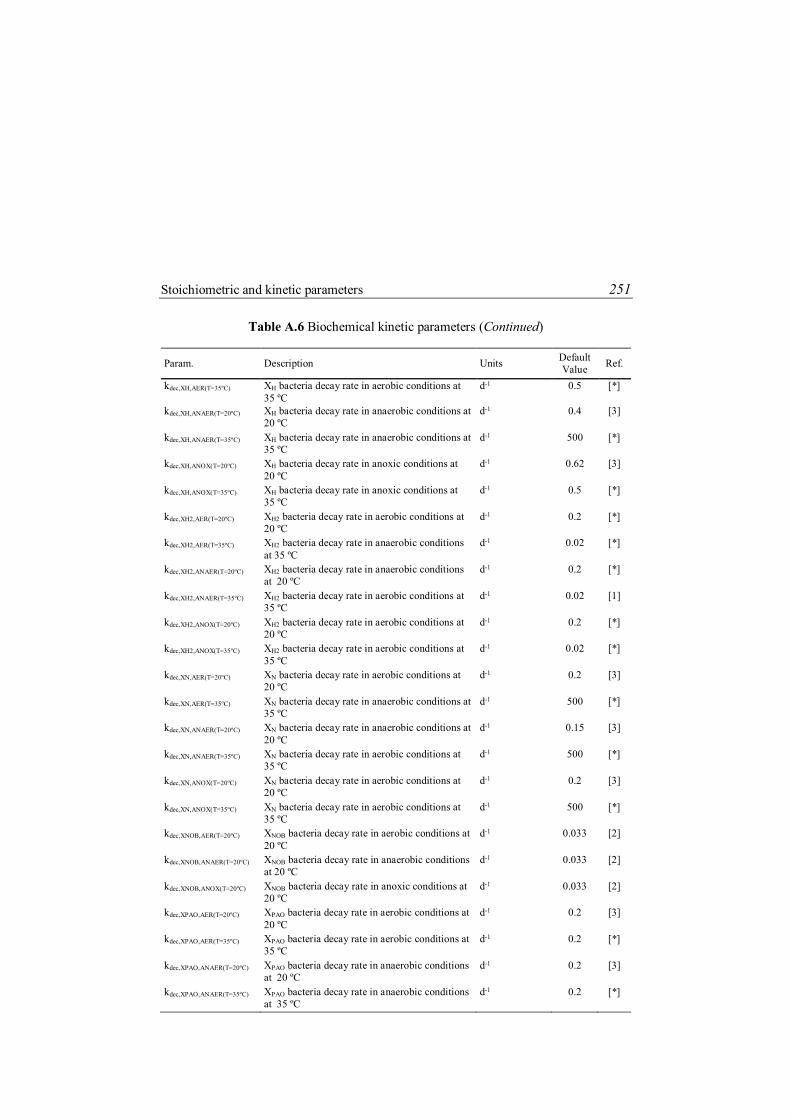
Stoichiometric and kinetic parameters 251

Table A.6 Biochemical kinetic parameters (Continued)

Param. Description Units Default Value Ref.

kdec,XH,AER(T=35ºC) XH bacteria decay rate in aerobic conditions at 35 ºC

d-1 0.5 [*]

kdec,XH,ANAER(T=20ºC) XH bacteria decay rate in anaerobic conditions at 20 ºC

d-1 0.4 [3]

kdec,XH,ANAER(T=35ºC) XH bacteria decay rate in anaerobic conditions at 35 ºC

d-1 500 [*]

kdec,XH,ANOX(T=20ºC) XH bacteria decay rate in anoxic conditions at 20 ºC

d-1 0.62 [3]

kdec,XH,ANOX(T=35ºC) XH bacteria decay rate in anoxic conditions at 35 ºC

d-1 0.5 [*]

kdec,XH2,AER(T=20ºC) XH2 bacteria decay rate in aerobic conditions at 20 ºC

d-1 0.2 [*]

kdec,XH2,AER(T=35ºC) XH2 bacteria decay rate in anaerobic conditions at 35 ºC

d-1 0.02 [*]

kdec,XH2,ANAER(T=20ºC) XH2 bacteria decay rate in anaerobic conditions at 20 ºC

d-1 0.2 [*]

kdec,XH2,ANAER(T=35ºC) XH2 bacteria decay rate in aerobic conditions at 35 ºC

d-1 0.02 [1]

kdec,XH2,ANOX(T=20ºC) XH2 bacteria decay rate in aerobic conditions at 20 ºC

d-1 0.2 [*]

kdec,XH2,ANOX(T=35ºC) XH2 bacteria decay rate in aerobic conditions at 35 ºC

d-1 0.02 [*]

kdec,XN,AER(T=20ºC) XN bacteria decay rate in aerobic conditions at 20 ºC

d-1 0.2 [3]

kdec,XN,AER(T=35ºC) XN bacteria decay rate in anaerobic conditions at 35 ºC

d-1 500 [*]

kdec,XN,ANAER(T=20ºC) XN bacteria decay rate in anaerobic conditions at 20 ºC

d-1 0.15 [3]

kdec,XN,ANAER(T=35ºC) XN bacteria decay rate in aerobic conditions at 35 ºC

d-1 500 [*]

kdec,XN,ANOX(T=20ºC) XN bacteria decay rate in aerobic conditions at 20 ºC

d-1 0.2 [3]

kdec,XN,ANOX(T=35ºC) XN bacteria decay rate in aerobic conditions at 35 ºC

d-1 500 [*]

kdec,XNOB,AER(T=20ºC) XNOB bacteria decay rate in aerobic conditions at 20 ºC

d-1 0.033 [2]

kdec,XNOB,ANAER(T=20ºC) XNOB bacteria decay rate in anaerobic conditions at 20 ºC

d-1 0.033 [2]

kdec,XNOB,ANOX(T=20ºC) XNOB bacteria decay rate in anoxic conditions at 20 ºC

d-1 0.033 [2]

kdec,XPAO,AER(T=20ºC) XPAO bacteria decay rate in aerobic conditions at 20 ºC

d-1 0.2 [3]

kdec,XPAO,AER(T=35ºC) XPAO bacteria decay rate in aerobic conditions at 35 ºC

d-1 0.2 [*]

kdec,XPAO,ANAER(T=20ºC) XPAO bacteria decay rate in anaerobic conditions at 20 ºC

d-1 0.2 [3]

kdec,XPAO,ANAER(T=35ºC) XPAO bacteria decay rate in anaerobic conditions at 35 ºC

d-1 0.2 [*]

252 Description of PWM library’s Categories

Table A.6 Biochemical kinetic parameters (Continued)

Param. Description Units Default Value Ref.

kdec,XPAO,ANOX(T=20ºC) XPAO bacteria decay rate in anoxic conditions at 20 ºC

d-1 0.2 [3]

kdec,XPAO,ANOX(T=35ºC) XPAO bacteria decay rate in anoxic conditions at 35 ºC

d-1 0.2 [*]

kdec,XPHA,AER(T=20ºC) XPHA bacteria decay rate in aerobic conditions at 20 ºC

d-1 0.2 [3]

kdec,XPHA,AER(T=35ºC) XPHA bacteria decay rate in anaerobic conditions at 35 ºC

d-1 0.02 [*]

kdec,XPHA,ANAER(T=20ºC) XPHA bacteria decay rate in anaerobic conditions at 20 ºC

d-1 0.2 [3]

kdec,XPHA,ANAER(T=35ºC) XPHA bacteria decay rate in aerobic conditions at 35 ºC

d-1 0.02 [*]

kdec,XPHA,ANOX(T=20ºC) XPHA bacteria decay rate in aerobic conditions at 20 ºC

d-1 0.2 [3]

kdec,XPHA,ANOX(T=35ºC) XPHA bacteria decay rate in aerobic conditions at 35 ºC

d-1 0.02 [*]

kdec,XPP,AER(T=20ºC) XPHA bacteria decay rate in aerobic conditions at 20 ºC

d-1 0.2 [3]

kdec,XPP,AER(T=35ºC) XPHA bacteria decay rate in anaerobic conditions at 35 ºC

d-1 0.02 [*]

kdec,XPP,ANAER(T=20ºC) XPHA bacteria decay rate in anaerobic conditions at 20 ºC

d-1 0.2 [3]

kdec,XPP,ANAER(T=35ºC) XPHA bacteria decay rate in aerobic conditions at 35 ºC

d-1 0.02 [*]

kdec,XPP,ANOX(T=20ºC) XPHA bacteria decay rate in aerobic conditions at 20 ºC

d-1 0.2 [3]

kdec,XPP,ANOX(T=35ºC) XPHA bacteria decay rate in aerobic conditions at 35 ºC

d-1 0.02 [*]

kdec,XPRO,AER(T=20ºC) XPRO bacteria decay rate in aerobic conditions at 20 ºC

d-1 0.2 [*]

kdec,XPRO,AER(T=35ºC) XPRO bacteria decay rate in anaerobic conditions at 35 ºC

d-1 0.02 [*]

kdec,XPRO,ANAER(T=20ºC) XPRO bacteria decay rate in anaerobic conditions at 20 ºC

d-1 0.2 [*]

kdec,XPRO,ANAER(T=35ºC) XPRO bacteria decay rate in aerobic conditions at 35 ºC

d-1 0.02 [1]

kdec,XPRO,ANOX(T=20ºC) XPRO bacteria decay rate in aerobic conditions at 20 ºC

d-1 0.2 [*]

kdec,XPRO,ANOX(T=35ºC) XPRO bacteria decay rate in aerobic conditions at 35 ºC

d-1 0.02 [*]

kdec,XSU,AER(T=20ºC) XSU bacteria decay rate in aerobic conditions at 20 ºC

d-1 0.2 [*]

kdec,XSU,AER(T=35ºC) XSU bacteria decay rate in anaerobic conditions at 35 ºC

d-1 0.02 [*]

kdec,XSU,ANAER(T=20ºC) XSU bacteria decay rate in anaerobic conditions at 20 ºC

d-1 0.2 [*]

kdec,XSU,ANAER(T=35ºC) XSU bacteria decay rate in aerobic conditions at 35 ºC

d-1 0.02 [1]

Stoichiometric and kinetic parameters 253

Table A.6 Biochemical kinetic parameters (Continued)

Param. Description Units Default Value Ref.

kdec,XSU,ANOX(T=20ºC) XSU bacteria decay rate in aerobic conditions at 20 ºC

d-1 0.2 [*]

kdec,XSU,ANOX(T=35ºC) XSU bacteria decay rate in aerobic conditions at 35 ºC

d-1 0.02 [*]

kdis,AER,XC1(T=20ºC) Disintegration rate of XC1 in aerobic conditions at 20 ºC

d-1 500 [*]

kdis,AER,XC1(T=35ºC) Disintegration rate of XC1 in aerobic conditions at 35 ºC

d-1 1.18 [*]

kdis,AER,XC2(T=20ºC) Disintegration rate of XC2 in aerobic conditions at 20 ºC

d-1 500 [*]

kdis,AER,XC2(T=35ºC) Disintegration rate of XC2 in aerobic conditions at 35 ºC

d-1 0.68 [*]

kdis,ANAER,XC1(T=35ºC) Disintegration rate of XC1 in anaerobic conditions at 35 ºC

d-1 0.5 [1]

kdis,ANAER,XC2(T=35ºC) Disintegration rate of XC2 in anaerobic conditions at 35 ºC

d-1 0.5 [1]

kdis,ANOX,XC1(T=20ºC) Disintegration rate of XC1 in anoxic conditions at 20 ºC

d-1 500 [*]

kdis,ANOX,XC1(T=35ºC) Disintegration rate of XC1 in anoxic conditions at 35 ºC

d-1 1.18 [*]

kdis,ANOX,XC2(T=20ºC) Disintegration rate of XC2 in anoxic conditions at 20 ºC

d-1 500 [*]

kdis,ANOX,XC2(T=35ºC) Disintegration rate of XC2 in anoxic conditions at 35 ºC

d-1 0.68 [*]

khid,AER(T=20ºC) Hydrolysis rate of carbohydrates, proteins and lipids in aerobic conditions and at 20 ºC

d-1 3 [3]

khid,AER(T=35ºC) Hydrolysis rate of carbohydrates, proteins and lipids in aerobic conditions and at 35 ºC

d-1 1.5 [*]

khid,ANAER,XCH(T=20ºC) Hydrolysis rate of carbohydrates in anaerobic conditions and at 20 ºC

d-1 1 [*]

khid, ANAER,XCH (T=35ºC) Hydrolysis rate of carbohydrates in anaerobic conditions and at 35 ºC

d-1 10 [1]

khid,ANAER,XLI(T=20ºC) Hydrolysis rate of lipids in anaerobic conditions and at 20 ºC

d-1 1 [*]

khid, ANAER,XLI (T=35ºC) Hydrolysis rate of lipids in anaerobic conditions and at 35 ºC

d-1 10 [1]

khid,ANAER,XPR(T=20ºC) Hydrolysis rate of proteins in anaerobic conditions and at 20 ºC

d-1 1 [*]

khid, ANAER,XPR (T=35ºC) Hydrolysis rate of proteins in anaerobic conditions and at 35 ºC

d-1 10 [1]

khid,ANOX(T=20ºC) Hydrolysis rate of carbohydrates, proteins and lipids in anoxic conditions and at 20 ºC

d-1 1.2 [3]

khid,ANOX(T=35ºC) Hydrolysis rate of carbohydrates, proteins and lipids in anoxic conditions and at 35 ºC

d-1 1.5 [*]

km,XAA(T=20ºC) Substrate consumption rate by XAA bacteria at 20 ºC

gCODS gCODX

-1 d-1 5.5 [*]

km,XAA(T=35ºC) Substrate consumption rate by XAA bacteria at 35 ºC

gCODS gCODX

-1 d-1 50 [1]

254 Description of PWM library’s Categories

Table A.6 Biochemical kinetic parameters (Continued)

Param. Description Units Default Value Ref.

km,XAA(T=55ºC) Substrate consumption rate XAA bacteria at 55 ºC gCODS gCODX

-1 d-1 70 [1]

km,XAC(T=20ºC) Substrate consumption rate by XAC bacteria at 20 ºC gCODS gCODX

-1 d-1 5.5 [*]

km,XAC(T=35ºC) Substrate consumption rate by XAC bacteria at 35 ºC gCODS gCODX

-1 d-1 8 [1]

km,XAC(T=55ºC) Substrate consumption rate XAC bacteria at 55 ºC gCODS gCODX

-1 d-1 16 [1]

km,XAN (T=20ºC) Substrate consumption rate by aerobic/ anoxic Anammox bacteria

gCODS gCODX

-1 d-1 0.028 / YAN [4]

km,XAOB,max Maximum NH4+ consumption rate by Nitrosomonas

bacteria gN gCODX

-1 d-1 0.8 / YAOB [4]

km,XC4(T=20ºC) Substrate consumption rate by XC4 bacteria at 20 ºC gCODS gCODX

-1 d-1 5.5 [*]

km,XC4(T=35ºC) Substrate consumption rate by XC4 bacteria at 35 ºC gCODS gCODX

-1 d-1 20 [1]

km,XC4(T=55ºC) Substrate consumption rate XC4 bacteria at 55 ºC gCODS gCODX

-1 d-1 30 [1]

km,XFA(T=20ºC) Substrate consumption rate by XFA bacteria at 20 ºC gCODS gCODX

-1 d-1 5.5 [*]

km,XFA(T=35ºC) Substrate consumption rate by X-FA bacteria at 35 ºC

gCODS gCODX

-1 d-1 6 [1]

km,XFA(T=55ºC) Substrate consumption rate XFA bacteria at 55 ºC gCODS gCODX

-1 d-1 10 [1]

km,XH (T=20ºC) Substrate consumption rate by aerobic/ anoxic heterotrophic bacteria

gCODS gCODX

-1 d-1 6 / YH [3]

km,XH(T=35ºC) Substrate consumption rate by aerobic/ anoxic heterotrophic bacteria at 35 ºC

gCODS gCODX

-1 d-1 17 [*]

km,XH(T=55ºC) Substrate consumption rate by aerobic/ anoxic heterotrophic bacteria at 55 ºC

gCODS gCODX

-1 d-1 28 [*]

km,XH2(T=20ºC) Substrate consumption rate by XFA bacteria at 20 ºC gCODS gCODX

-1 d-1 5.5 [*]

km,XH2(T=35ºC) Substrate consumption rate by XH2 bacteria at 35 ºC gCODS gCODX

-1 d-1 35 [1]

km,XH2(T=55ºC) Substrate consumption rate XH2 bacteria at 55 ºC gCODS gCODX

-1 d-1 35 [1]

km,XN (T=20ºC) N-NHX consumption rate gN gCODX-1 d-1 0.8 / YN [3]

km,XNOB,max Maximum NO2 consumption rate by Nitrobacter bacteria

gN gCODX-1 d-1 0.79 / YNOB [4]

km,XPAO (T=20ºC) Substrate consumption rate by aerobic/ anoxic PAO bacteria at 20 ºC

gCODS gCODX

-1 d-1 1 / YPAO [3]

km,XPAO (T=35ºC) Substrate consumption rate by aerobic/ anoxic PAO bacteria at 35 ºC

gCODS gCODX

-1 d-1 1 / YPAO [3]

km,XPRO(T=20ºC) Substrate consumption rate by XPRO bacteria at 20 ºC gCODS gCODX

-1 d-1 5.5 [*]

km,XPRO(T=35ºC) Substrate consumption rate by X-PRO bacteria at 35 ºC gCODS gCODX

-1 d-1 13 [1]

km,XPRO(T=55ºC) Substrate consumption rate XPRO bacteria at 55 ºC gCODS gCODX

-1 d-1 20 [1]

Stoichiometric and kinetic parameters 255

Table A.6 Biochemical kinetic parameters (Continued)

Param. Description Units Default Value Ref.

km,XSU(T=20ºC) Substrate consumption rate by XSU bacteria at 20 ºC

gCODS gCODX

-1 d-1 5.5 [*]

km,XSU(T=35ºC) Substrate consumption rate by XSU bacteria at 35 ºC gCODS gCODX

-1 d-1 30 [1]

km,XSU(T=55ºC) Substrate consumption rate XSU bacteria at 55 ºC gCODS gCODX

-1 d-1 70 [1]

KA,H,N Activation in the bacteria growth due to high pH gH m-3 10-7 [*] KA,IC Activation/ inhibition constant for inorganic carbon gC m-3 0.001 [*] KA,IN Activation/ inhibition constant for inorganic nitrogen gN m-3 0.001 [*] KA,IP Activation/ inhibition constant for inorganic

phosphorous gP m-3 0.001 [*]

KA,K Activation/ inhibition constant for inorganic potassium

gK m-3 0.001 [*]

KA,Mg Activation/ inhibition constant for inorganic magnesium

gMg m-3 0.001 [*]

KA,NO2 Activation/inhibition constant for nitrites gN m-3 0.5 [5] KA,NO3 Activation/inhibition constant for nitrates gN m-3 0.5 [3] KA,NOX Activation constant for NOX gN m-3 0.5 [3] KA,O2 Activation/ inhibition constant for oxygen gO2 m-3 0.2 [*] KAA,XAA(T=35ºC) Amino acids saturation constant gCOD m-3 300 [1] KAC,H Saturation growth rate of heterotrophic biomass over

Acetic acid gCOD m-3 4 [3]

KAC,XAC(T=35ºC) Acetate saturation constant for methanogenic biomass

gCOD m-3 150 [1]

KBU,H Saturation growth rate of heterotrophic biomass over Butyric acid

gCOD m-3 4 [3]

KC4,XC4(T=35ºC) Butyrate/Valerate saturation constant gCOD m-3 200 [1] KFA,XFA(T=35ºC) Fatty acids saturation constant gCOD m-3 400 [1] KH2,XH2(T=35ºC) Hydrogen saturation constant for methanogenic

biomass gCOD m-3 0.007 [1]

KI,H,N Inhibition in the bacteria growth due to low pH gH m-3 0.00085 [*] KI,H,XAA Inhibition constant for pH in the acidogenesis and

acetogenesis gH m-3 0.0155 [1]

KI,H,XAC Inhibition constant for pH in the acetoclastic methanogenesis

gH m-3 0.000316 [1]

KI,H,XH2 Inhibition constant for pH in the hydrogenotrophic methanogenesis

gH m-3 0.00316 [1]

KI,H2,C4(T=35ºC) Inhibition of acidogenesis on butyrate/ valerate due to hydrogen

gCOD m-3 0.01 [1]

KI,H2,FA(T=35ºC) Inhibition of acidogenesis on fatty acids due to hydrogen

gCOD m-3 0.005 [1]

KI,H2,PRO(T=35ºC) Inhibition of acidogenesis on propionic acid due to hydrogen

gCOD m-3 0.0035 [1]

KI,HNO2,XAOB Nitrosomonas growth inhibition constant due to ammonia

gN m-3 0.49 [6]

KI,HNO2,XNOB Nitrobacter growth inhibition constant due to nitrous acid

gN m-3 0.26 [6]

256 Description of PWM library’s Categories

Table A.6 Biochemical kinetic parameters (Continued)

Param. Description Units Default Value Ref.

KI,NH3(T=35ºC) Inhibition coefficient due to NH3 gN m-3 25.2 [1]

KI,NH3,XAOB Nitrosomonas growth inhibition constant due to ammonia

gN m-3 3000 [7]

KI,NH3,XNOB Nitrobacter growth inhibition constant due to ammonia

gN m-3 14.8 [6]

KI,NOX Inhibition constant for NOX gN m-3 0.1 [1] KIPP Inhibition coefficient for PP storage gXPP gXPAO

-1 0.02 [3]

KMAX Maximum ratio of XPP/XPAO gXPP gXPAO-1 0.02 [3]

KNH,AN Inhibition coefficient ammonium/ammonia gN m-3 0.07 [8] KNH,N Nitrifiers bacteria growth saturation constant gN m-3 1 [3] KNH3,AOB Nitrosomonas bacteria growth saturation constant gN m-3 1 [3] KNO2,AN Anammox growth saturation constant from NO2

- gN m-3 0.05 [2] KNO2,NOB Nitrobacter growth saturation constant from NO2

- gN m-3 0.28 [9] KO2,AN Oxygen inhibition coefficient gO2 m-3 0.01 [8] KO2,N Substrate degradation saturation constant gO2 m-3 0.4 [3] KO2,AOB Substrate degradation saturation constant gO2 m-3 0.3 [10] KO2,NOB Nitrobacter growth saturation constant from O2 gO2 m-3 1.75 [11] KP Saturation coefficient for phosphate (nutrient) gP m-3 0.01 [3] KPHA Saturation coefficient for PHA gXPHA gXPAO

-1 0.01 [3] KPP Saturation coefficient for polyphosphate gXPP gXPAO

-1 0.01 [3] KPRO,H Saturation growth rate of heterotrophic biomass over

Propionic acid gCOD m-3 4 [3]

KPRO,XPRO(T=35ºC) Propionate saturation constant gCOD m-3 100 [1] KS Half saturation coefficient for heterotrophic biomass gCOD m-3 20 [3]

KS,XC2(T=25ºC) Disintegration rate of XC2 at high temperature d-1 5000 [*] KS,XI(T=25ºC) Disintegration rate of XI at high temperature d-1 5000 [*] KS,XP(T=25ºC) Disintegration rate of XP at high temperature d-1 5000 [*] KSU,XSU(T=35ºC) Sugar saturation constant gCOD m-3 500 [1] Kx(T=20ºC) Half saturation coefficient for hydrolysis of slowly

biodegradable substrate gCOD gCOD -1 0.1 [1]

KVA,H Saturation growth rate of heterotrophic biomass over Valeric acid

gCOD m-3 4 [3]

qXPHA Rate constant for storage of XPHA (base XPP) gXPHA gXPAO-1

d-1 6 [12]

qXPP Rate constant for storage of XPP gXPHA gXPAO-1

d-1 1.5 [3]

NO2 Anoxic growth correction constant --- 0.6 [6] NO3 Anoxic growth correction constant --- 0.8 [3] NO3,2N Anoxic growth correction constant --- 0.6 [6] NO3,PAO Anoxic growth correction constant --- 0.6 [3] AA,XAA Temperature correction factor --- 0 [1] AC,XAC Temperature correction factor --- 0.035 [1]

Stoichiometric and kinetic parameters 257

Table A.6 Biochemical kinetic parameters (Continued)

Param. Description Units Default Value Ref.

C4,XC4 Temperature correction factor --- 0.035 [1] dec,XAA,AER(T=20ºC) Temperature correction factor --- 1.07 [*] dec,XAA,AER(T=35ºC) Temperature correction factor --- 0.035 [*] dec,XAA,ANAER(T=20ºC) Temperature correction factor --- 1.07 [*] dec,XAA,ANAER(T=35ºC) Temperature correction factor --- 0.035 [1] dec,XAA,ANOX(T=20ºC) Temperature correction factor --- 1.07 [*] dec,XAA,ANOX(T=35ºC) Temperature correction factor --- 0.035 [*] dec,XAC,AER(T=20ºC) Temperature correction factor --- 1.07 [*] dec,XAC,AER(T=35ºC) Temperature correction factor --- 0.035 [*] dec,XAC,ANAER(T=20ºC) Temperature correction factor --- 1.07 [*] dec,XAC,ANAER(T=35ºC) Temperature correction factor --- 0.035 [1] dec,XAC,ANOX(T=20ºC) Temperature correction factor --- 1.07 [*] dec,XAC,ANOX(T=35ºC) Temperature correction factor --- 0.035 [*] dec,XAOB,AER(T=20ºC) Temperature correction factor --- 1.144 [13] dec,XAOB,ANOX(T=20ºC) Temperature correction factor --- 1.144 [13] dec,XAOB,ANAER(T=20ºC) Temperature correction factor --- 1.144 [13] dec,XAN,AER(T=20ºC) Temperature correction factor --- 1.11 [14] dec,XAN,ANOX(T=20ºC) Temperature correction factor --- 1.11 [14] dec,XAN,ANAER(T=20ºC) Temperature correction factor --- 1.11 [14] dec,XC4,AER(T=20ºC) Temperature correction factor --- 1.07 [*] dec,XC4,AER(T=35ºC) Temperature correction factor --- 0.035 [*] dec,XC4,ANAER(T=20ºC) Temperature correction factor --- 1.07 [*] dec,XC4,ANAER(T=35ºC) Temperature correction factor --- 0.035 [1] dec,XC4,ANOX(T=20ºC) Temperature correction factor --- 1.07 [*] dec,XC4,ANOX(T=35ºC) Temperature correction factor --- 0.035 [*] dec,XFA,AER(T=20ºC) Temperature correction factor --- 1.07 [*] dec,XFA,AER(T=35ºC) Temperature correction factor --- 0.035 [*] dec,XFA,ANAER(T=20ºC) Temperature correction factor --- 1.07 [*] dec,XFA,ANAER(T=35ºC) Temperature correction factor --- 0.035 [1] dec,XFA,ANOX(T=20ºC) Temperature correction factor --- 1.07 [*] dec,XFA,ANOX(T=35ºC) Temperature correction factor --- 0.035 [*] dec,XH,AER(T=20ºC) Temperature correction factor --- 1.12 [3] dec,XH,AER(T=35ºC) Temperature correction factor --- 0.055 [*] dec,XH,ANAER(T=20ºC) Temperature correction factor --- 1.07 [3] dec,XH,ANAER(T=35ºC) Temperature correction factor --- 0.055 [*] dec,XH,ANOX(T=20ºC) Temperature correction factor --- 1.12 [3] dec,XH,ANOX(T=35ºC) Temperature correction factor --- 0.055 [*] dec,XH2,AER(T=20ºC) Temperature correction factor --- 1.07 [*] dec,XH2,AER(T=35ºC) Temperature correction factor --- 0.035 [*] dec,XH2,ANAER(T=20ºC) Temperature correction factor --- 1.07 [*] dec,XH2,ANAER(T=35ºC) Temperature correction factor --- 0.035 [1] dec,XH2,ANOX(T=20ºC) Temperature correction factor --- 1.07 [*] dec,XH2,ANOX(T=35ºC) Temperature correction factor --- 0.035 [*]

258 Description of PWM library’s Categories

Table A.6 Biochemical kinetic parameters (Continued)

Param. Description Units Default Value Ref.

dec,XN,AER(T=20ºC) Temperature correction factor --- 1.103 [3] dec,XN,AER(T=35ºC) Temperature correction factor --- 0.055 [*] dec,XN,ANAER(T=20ºC) Temperature correction factor --- 1.103 [3] dec,XN,ANAER(T=35ºC) Temperature correction factor --- 0.055 [*] dec,XN,ANOX(T=20ºC) Temperature correction factor --- 1.116 [3] dec,XN,ANOX(T=35ºC) Temperature correction factor --- 0.055 [*] dec,XNOB,AER(T=20ºC) Temperature correction factor --- 1.14 [15] dec,XNOB,ANOX(T=20ºC) Temperature correction factor --- 1.14 [15] dec,XNOB,ANAER(T=20ºC) Temperature correction factor --- 1.14 [15] dec,XPAO,AER(T=20ºC) Temperature correction factor --- 1.07 [*] dec,XPAO,AER(T=35ºC) Temperature correction factor --- 0.035 [*] dec,XPAO,ANAER(T=20ºC) Temperature correction factor --- 1.07 [*] dec,XPAO,ANAER(T=35ºC Temperature correction factor --- 0.035 [1] dec,XPAO,ANOX(T=20ºC) Temperature correction factor --- 1.07 [*] dec,XPAO,ANOX(T=35ºC) Temperature correction factor --- 0.035 [*] dec,XPHA,AER(T=20ºC) Temperature correction factor --- 1.07 [*] dec,XPHA,AER(T=35ºC) Temperature correction factor --- 0.035 [*] dec,XPHA,ANAER(T=20ºC) Temperature correction factor --- 1.07 [*] dec,XPHA,ANAER(T=35ºC) Temperature correction factor --- 0.035 [1] dec,XPHA,ANOX(T=20ºC) Temperature correction factor --- 1.07 [*] dec,XPHA,ANOX(T=35ºC) Temperature correction factor --- 0.035 [*] dec,XPRO,AER(T=20ºC) Temperature correction factor --- 1.07 [*] dec,XPRO,AER(T=35ºC) Temperature correction factor --- 0.035 [*] dec,XPRO,ANAER(T=20ºC) Temperature correction factor --- 1.07 [*] dec,XPRO,ANAER(T=35ºC) Temperature correction factor --- 0.035 [1] dec,XPRO,ANOX(T=20ºC) Temperature correction factor --- 1.07 [*] dec,XPRO,ANOX(T=35ºC) Temperature correction factor --- 0.035 [*] dec,XSU,AER(T=20ºC) Temperature correction factor --- 1.07 [*] dec,XSU,AER(T=35ºC) Temperature correction factor --- 0.035 [*] dec,XSU,ANAER(T=20ºC) Temperature correction factor --- 1.07 [*] dec,XSU,ANAER(T=35ºC) Temperature correction factor --- 0.035 [1] dec,XSU,ANOX(T=20ºC) Temperature correction factor --- 1.07 [*] dec,XSU,ANOX(T=35ºC) Temperature correction factor --- 0.035 [*] dis,AER,XC1(T=20ºC) Temperature correction factor --- 1 [*] dis,AER,XC1(T=35ºC) Temperature correction factor --- 0.035 [*] dis,AER,XC2(T=20ºC) Temperature correction factor --- 1 [*] dis,AER,XC2(T=35ºC) Temperature correction factor --- 0.035 [*] dis,ANAER,XC1(T=35ºC) Temperature correction factor --- 0.035 [1] dis,ANAER,XC2(T=35ºC) Temperature correction factor --- 0.035 [1] dis,ANOX,XC1(T=20ºC) Temperature correction factor --- 1 [*] dis,ANOX,XC1(T=35ºC) Temperature correction factor --- 0.035 [*] dis,ANOX,XC2(T=20ºC) Temperature correction factor --- 1 [*] dis,ANOX,XC2(T=35ºC) Temperature correction factor --- 0.035 [*]

Stoichiometric and kinetic parameters 259

Table A.6 Biochemical kinetic parameters (Continued)

Param. Description Units Default Value Ref.

hid,AER(T=20ºC) Temperature correction factor --- 1.116 [3] hid,AER(T=35ºC) Temperature correction factor --- 0.08 [*] hid,ANAER,CH(T=20ºC) Temperature correction factor --- 1.116 [3] hid,ANAER,CH(T=35ºC) Temperature correction factor --- 0.024 [1] hid,ANAER,LI(T=20ºC) Temperature correction factor --- 1.116 [3] hid,ANAER,LI(T=35ºC) Temperature correction factor --- 0 [1] hid,ANAER,PR(T=20ºC) Temperature correction factor --- 1.116 [3] hid,ANAER,PR(T=35ºC) Temperature correction factor --- 0.024 [1] hid,ANOX(T=20ºC) Temperature correction factor --- 1.116 [3] hid,ANOX(T=35ºC) Temperature correction factor --- 0.05 [*] hid,x(T=20ºC) Temperature correction factor --- 1.116 [3] FA,XFA Temperature correction factor --- 0 [1] H2,XH2 Temperature correction factor --- 0.018 [1] I,H2,C4 Temperature correction factor --- 0.01 [1] I,H2,FA Temperature correction factor --- 0 [1] I,H2,PRO Temperature correction factor --- 0.055 [1] I,NH3 Temperature correction factor --- 0.091 [1] TH,XC2(T=25ºC) Temperature correction factor --- 0 [*] TH,XI(T=25ºC) Temperature correction factor --- 0 [*] TH,XP(T=25ºC) Temperature correction factor --- 0 [*] m,XAA Temperature correction factor --- 1.07 [*] m,XAC Temperature correction factor --- 1.07 [*] m,XC4 Temperature correction factor --- 1.07 [*] m,XFA Temperature correction factor --- 1.07 [*] m,XH Temperature correction factor --- 1.072 [*] m,XH2 Temperature correction factor --- 1.07 [*] m,XN Temperature correction factor --- 1.103 [3] m,XPAO Temperature correction factor --- 1.104 [3] m,XPHA Temperature correction factor --- 1.104 [3] m,XPP Temperature correction factor --- 1.104 [3] m,XPRO Temperature correction factor --- 1.07 [*] m,XSU Temperature correction factor --- 1.07 [*] PRO,XPRO Temperature correction factor --- 0.055 [1] SU,XSU Temperature correction factor --- 0.035 [*]

[1] Batstone et al., 2002; [2] Veys et al., 2010; [3] Henze et al., 2000; [4] Hao et al., 2002a; [5] Iacopozzi et

al., 2007; [6] Ganigue et al., 2010; [7] Wett et al., 2003; [8] Hao et al., 2002b; [9] Kaelin et al., 2009; [10]

Wiesmann, 1994; [11] Guisasola et al., 2005; [12] Larrea et al., 2002; [13] Adapted from Sin et al., 2008;

Jubany et al., 2008 and Veys et al., 2010; [14] Adapted from van Hulle, 2005; [15] Adapted from Jubany et

al., 2008 and Veys et al., 2010; [*] Estimated values; † Dependent on the case study

260 Description of PWM library’s Categories

Table A.7 Chemical kinetic parameters

Param. Description Units Default Value Ref.

Ka,H2O(T=25ºC) Equilibrium constant of H+-OH- molH l-1 10-14 [1] Ka,HAC(T=25ºC) Equilibrium constant of HAC-AC- molH l-1 10-4.76 [1] Ka,HBU(T=25ºC) Equilibrium constant of HBU-BU- molH l-1 10-4.82 [1] Ka,HPRO(T=25ºC) Equilibrium constant of HPRO-PRO- molH l-1 10-4.88 [1] Ka,HVA(T=25ºC) Equilibrium constant of HVA-VA- molH l-1 10-4.86 [1] Ka,IC(T=25ºC) Equilibrium constant of CO2-HCO3

- molH l-1 10-6.35 [1] Ka,IN(T=25ºC) Equilibrium constant of NH4

+-NH3 molH l-1 10-9.25 [1] Ka,IP(T=25ºC) Equilibrium constant of H2PO4

--HPO4= molH l-1 10-7.21 [1]

Ka2,IC(T=25ºC) Equilibrium constant of HCO3--CO3

= molH l-1 10-10.3 [1] Ka2,IP(T=25ºC) Equilibrium constant of HPO4

=-PO4-3 molH l-1 10-12.37 [1] Ka,NO2(T=25ºC) Equilibrium constant of HNO2-NO2

- molH l-1 10-3.29 [1] Kab,H2O Equilibrium rate of H+-OH- m3 gH-1 d-1 10-8.0 [*] Kab,HAC Equilibrium rate of HAC-AC- m3 gH-1 d-1 10-8.0 [*] Kab,HBU Equilibrium rate of HBU-BU- m3 gH-1 d-1 10-8.0 [*] Kab,HPRO Equilibrium rate of HPRO-PRO- m3 gH-1 d-1 10-8.0 [*] Kab,HVA Equilibrium rate of HVA-VA- m3 gH-1 d-1 10-8.0 [*] Kab,ÎC Equilibrium rate of CO2-HCO3

- m3 gH-1 d-1 10-8.0 [*] Kab,IN Equilibrium rate of NH4

+-NH3 m3 gH-1 d-1 10-8.0 [*] Kab,IP Equilibrium rate of H2PO4

--HPO4= m3 gH-1 d-1 10-8.0 [*]

Kab,NO2 Equilibrium rate of HNO2-NO2- m3 gH-1 d-1 10-8.0 [*]

Kab2,IC Equilibrium rate of HCO3--CO3

= m3 gH-1 d-1 10-8.0 [*] Kab2,IP Equilibrium rate of HPO4

=-PO4-3 m3 gH-1 d-1 10-8.0 [*]

[1] Perry and Chilton, 1973; [*] Estimated values.

Table A.8 Liquid-Gas transfer kinetic parameters

Param. Description Units Default Value Ref.

DL,CH4 Ammonium transfer rate at 20 ºC m2 d-1 0.000192 [1] DL,CO2 Ammonium transfer rate at 20 ºC m2 d-1 0.000169 [1] DL,H2 Ammonium transfer rate at 20 ºC m2 d-1 0.000505 [1] DL,N2 Ammonium transfer rate at 20 ºC m2 d-1 0.000164 [1] DL,NH3 Ammonium transfer rate at 20 ºC m2 d-1 0.000119 [1] DL,O2 Ammonium transfer rate at 20 ºC m2 d-1 0.000216 [1] kL/G,NH3(T=20ºC) Ammonium transfer rate at 20 ºC m d-1 0.074 [1] kL/G,O2(T=20ºC) Oxygen transfer rate at 20 ºC m d-1 0.18 [2] KH,CH4(T=25ºC) Henry’s constant for CH4 mol l-1 bar-1 0.0014 [3] KH,CO2(T=25ºC) Henry’s constant for CO2 mol l-1 bar-1 0.035 [3] KH,H2(T=25ºC) Henry’s constant for H2 mol l-1 bar-1 0.00078 [3] KH,N2(T=25ºC) Henry’s constant for N2 mol l-1 bar-1 0.00065 [3] KH,NH3(T=25ºC) Henry’s constant for NH3 mol l-1 bar-1 59 [3] KH,O2(T=25ºC) Henry’s constant for O2 mol l-1 bar-1 0.0013 [3]

Stoichiometric and kinetic parameters 261

Table A.8 Liquid-Gas transfer kinetic parameters (Continued)

Param. Description Units Default Value Ref.

KM,H2O Evaporation constant d-1 10000000 [*]

[1] Vogelaar et al., 2000; [2] Arogo et al., 1999; [3] Perry and Chilton, 1973; [*] Estimated values; †

Dependent on the case study

Table A.9 Liquid-Solid transfer kinetic parameters

Param. Description Units Default Value Ref.

k1 Precipitation constant --- 0.001 [*] k2 Precipitation constant --- 0.001 [*] kr,FeCl3 Kinetic rate constant d-1 † [*] kr,FePO4 Kinetic rate constant d-1 100000 [1] kr,Fe(OH)3 Kinetic rate constant d-1 † [*] kr,ACP Kinetic rate constant d-1 350 [2] kr,CaCO3 Kinetic rate constant d-1 1477 [2] kr,MgCO3 Kinetic rate constant d-1 50 [2] kr,STRU Kinetic rate constant d-1 3000 [2] kr,KSTRU Kinetic rate constant d-1 1 [*] kr,NEW Kinetic rate constant d-1 0.05 [2] Ksp,FeCl3(T=25ºC) Solubility product constant for PACP --- 10-47.7 [3] Ksp,FePO4(T=25ºC) Solubility product constant for PACP --- 10-28.75 [4] Ksp,Fe(OH)3(T=25ºC) Solubility product constant for PACP --- 10-38.2 [4] Ksp,ACP(T=25ºC) Solubility product constant for PACP --- 10-25.46 [5] Ksp,CaCO3(T=25ºC) Solubility product constant for PCACO3 --- 10-6.7 [6] Ksp,MgCO3(T=25ºC) Solubility product constant for PMgCO3 --- 10-7.46 [7] Ksp,STRU(T=25ºC) Solubility product constant for PSTRU --- 10-13.16 [8] Ksp,KSTRU(T=25ºC) Solubility product constant for PKSTRU --- 10-11.55 [9] Ksp,NEWT=25ºC) Solubility product constant for PNEW --- 10-5.8 [8] FeCl3 Growth of interfacial area concentration --- 0.5 [*] FePO4 Growth of interfacial area concentration --- 0.5 [*] Fe(OH)3 Growth of interfacial area concentration --- 0.5 [*] ACP Growth of interfacial area concentration --- 0.5 [*] CaCO3 Growth of interfacial area concentration --- 0.5 [*] MgCO3 Growth of interfacial area concentration --- 0.5 [*] STRU Growth of interfacial area concentration --- 0.5 [*] KSTRU Growth of interfacial area concentration --- 0.5 [*] NEW Growth of interfacial area concentration --- 0.5 [*]

[1] Hauduc et al., 2015; [2] Barat, 2004; [3] Söhnel et al., 1985; [4] Briggs, 1996; [5] Ferguson et al., 1971;

[6] Wiechers et al., 1980; [7] Stumm and Morgan, 1996; [8] Murray et al., 1996; [9] Flores-Alsina et al.,

2016; [*] Estimated values; † Dependent on the case study

263

B

HEAT TRANSFER AND COST MODEL PARAMETERS

DESCRIPTION

The following section shows the values assigned to the parameters of heat transfer and cost models described in this thesis and used in the simulations.

B.1. ADVECTIVE HEAT FLUX PARAMETERS In order to describe the advective heat fluxes, the properties of the components that undergo this advection must be defined. As discussed in Chapter 2, in the aqueous phase advective fluxes only water enthalpy has been considered, ignoring the enthalpy of dissolved compounds that make up the aqueous phase. In the case of transfers between phases by contrast, all the elements that form the advective flow are considered, since their proportions are not insignificant as in the case of the aqueous medium. It is for this reason that the components necessary to describe the advection are the SH2O, SCO2, SH2, SCH4, SNH3, SN2, SO2, GCO2, GH2, GCH4, GNH3, GN2, GO2 and GH2O.

For the estimation of isobaric heat capacity (Cp in kJ mol-1 K-1) as a function of i phase temperature (Ti in K) there are three types of expressions that are shown below:

264 Heat transfer and cost model parameters description

Cp(T)comp = A + B Ti + C Ti2 + D Ti

3 + E Ti4 B.1

Cp(T)comp =A2

1- TiTc

+ B-2 A C 1-Ti

Tc-A D 1-

Ti

Tc

2

-C2 1- Ti

Tc

3

3-

C2D 1- Ti

Tc

4

2-D2 1- Ti

Tc

5

5

B.2

Cp(T)comp = A + B C Ti⁄

sinh(C Ti⁄ )

2

+ D E Ti⁄

cosh(E Ti⁄ )

2

B.3

where A, B, C, D and E are specific isobaric heat capacity constants for the components [dimensionless] and Tc the critical temperature [K]. The values for each component and the equation to be used are shown in Table B.1. This table also collects the reference enthalpies and the reference temperatures to estimate the advective flow.

Table B.1 Isobaric heat capacity, reference temperature and reference enthalpy of ideal gases and liquid components (Source: Perry & Green, 1999 and NIST)

Name Cp(T) (Tcomp)i,ref

[K] (hcomp)i,ref [kJ mol-1] A B C D E Tc [K] Ec.

SCO2 -8304300 104370 -433.33 0.60052 304.21 B.1 216.59 0.000 SH2 66.653 6765.9 -123.63 478.27 33.19 B.2 20.37 0.000 SCH4 65.708 38883 -257.95 614.07 190.564 B.2 110.69 -0.054 SNH3 61.289 80925 799.4 -2651 405.65 B.2 205.50 0.722 SN2 281970 -12281 248 -2.2182 0.0074802 126.2 B.1 77.36 -3.418 SO2 175430 -6152.3 113.92 -0.92382 0.0027963 154.58 B.1 74.36 -5.121 SH2O 276.370 -2090.1 8.125 -0.014116 9.3701E-06 647.096 B.1 273.15 1.074 GCO2 29370 34540 1428 26400 588 304.21 B.3 216.59 19.344 GH2 27617 9560 2466 3760 567.6 33.19 B.3 20.37 0.905 GCH4 33298 79933 2086.9 41602 991.96 190.564 B.3 111.67 8.195 GNH3 33427 48980 2036 22560 882 405.65 B.3 239.56 26.591 GN2 29105 8614.9 1701.6 103.47 909.79 126.2 B.3 77.35 2.162 GO2 29103 10040 2526.5 9356 1143.8 154.58 B.3 90.19 2.550 GH2O 33363 26790 2610.5 8896 1169 647.096 B.3 373.15 48.16

Conduction heat flux parameters 265

B.2. CONDUCTION HEAT FLUX PARAMETERS The Table B.2 and Table B.3 show the values of the thermal conductivity of different materials and components.

Table B.2 Parameters to estimate the ktherm/L of solid materials [W m-2 ºC-1]

Description Values Ref.

Fixed steel cover (6 mm plate) 5.186 (*) 4.0-5.4

[1] [2]

Fixed concrete cover (230 mm thick) 3.305 [1] Fixed concrete cover (225 mm thick), not insulated 3.0-3.6 [2] Fixed concrete cover 100 mm thick and covered with built-up roofing, and not insulated 4.0-5.0 [2] Fixed concrete cover 100 mm thick and covered, but insulated with 25 mm thick insulating board

1.2-1.6 [2]

Floating cover (Downes-type with wood composition roof) 1.881 [1] Floating cover with 35 mm wood deck, build-up roofing, and no insulation 1.8-2.0 [2] Floating cover with 25 mm insulating board installed under the roofing 0.9-1.0 [2] Concrete wall (300 mm thick) exposed to air 4.901 (*) [1] Concrete wall (300 mm thick), 25 mm air space and 100 mm brick 1.539 [1] Plain concrete walls (above ground) 300 mm thick wall with air space plus facing 1.8-2.4 [2] Plain concrete walls (above ground) 300 mm thick wall with insulation 0.6-0.8 [2] Plain concrete walls (above ground) 300 mm thick, not insulated 4.7-5.1 [2] Plain concrete walls (below ground) surrounding by dry earth 0.57-0.68 [2] Plain concrete walls (below ground) surrounding by moist earth 1.1-1.4 [2] Concrete wall or floor (300 mm thick) exposed to wet earth (3 m thick) 0.627 (*) [1] Plain concrete floor (300 mm thick) in contract with moist earth 2.85 [2] Concrete wall or floor (300 mm thick) exposed to dry earth (3 m thick) 0.342 [1] Plain concrete floor (300 mm thick) in contract with dry earth 1.7 [2]

[1] US EPA, 1979; [2] Tchobanoglous et al., 2014. (*) Values used in case studies Table B.3 Parameters to estimate the ktherm of components at 298.15 K [W m-1 ºC-1]

Component Values Ref.

Liquids 0.2-8 [1] Water (aq.) 0.613 [1] Gases 0.03-0.3 [1] Air (g) 0.026 [1] CO2 (g) 0.01-0.2 [1] H2 (g) 0.1-0.2 [1] Non-metallic precipitated oxides 0.2-50 [1] CaCO3 3.590 [2] Al(OH)3 2.598 [2] FeS2 19.200 [2] MgCO3 5.832 [2]

[1] Ҫengel, 1997; [2] Horai et al., 1969.

266 Heat transfer and cost model parameters description

B.3. CONVECTION HEAT FLUX PARAMETERS In order to estimate the convective flux as a function of i phase temperature (Ti in K), the thermal conductivity (ktherm,comp in W m-1 ºC-1) and the dynamic viscosity (comp in g m-1 s-1) of the gaseous phase components must be fixed.

ktherm,GNH3 = 0.0000096608 · Ti1.3799 B.4

ktherm,GH2 = 0.002653 ·Ti

0.7452

1+ 12.0Ti

B.5

ktherm,GCH4 = 0.0000083983 ·Ti

1.4268

1- 49.654Ti

B.6

ktherm,GN2 = 0.00033143 ·Ti

0.7722

1+ 16.323Ti

+ 373.72Ti

2

B.7

ktherm,GO2 = 0.00044994 ·Ti

0.7456

1+ 56.669Ti

B.8

ktherm,GH2O = 0.0000062041 · Ti1.3973 B.9

ktherm,GCO2 = 3.69 ·Ti

-0.3838

1+ 964.0Ti

+ 1860000Ti

2

B.10

GNH3 = 0.000000041855 · Ti

0.9806

1+ 30.8Ti

B.11

GH2 = 0.0000001797 ·Ti

0.685

1- 0.59Ti

+ 140Ti

2

B.12

GCH4 = 0.00000052546 ·Ti

0.59006

1+ 105.67Ti

B.13

Shortwave (solar) and longwave (atmospheric) radiation heat fluxes parameters 267

GN2 = 0.00000065592 ·Ti

0.6081

1+ 54.714Ti

B.14

GO2 = 0.000001101 ·Ti

0.5634

1+ 96.3Ti

B.15

GH2O = 0.000000017096 · Ti1.1146 B.16

GCO2 = 0.000002148 ·Ti

0.46

1+ 290.0Ti

B.17

To complete the estimation of the convective flow, Table B.4 shows the values of the remaining parameters.

Table B.4 Parameters to estimate the convection heat flux

Param. Description Units Values Ref.

g Gravitational acceleration m s-1 9.81 [1] R Ideal gas constant kJ mol-1 K-1 0.008314 [1] XTSS Weight percentage of solids in the suspension % Variable Simulation phs Volume expansion coefficient (contact between

w and j phases) K-1 2

Tw+ Tj [1]

Characteristic length of the geometry (vertical plate or vertical cylinder)

m Length [1]

Characteristic length of the geometry (horizontal plate)

m Area/perimeter [1]

[1] Ҫengel, 1997.

B.4. SHORTWAVE (SOLAR) AND LONGWAVE (ATMOSPHERIC) RADIATION HEAT FLUXES PARAMETERS

The Table B.5 shows the values needed for estimating the shortwave and longwave radiation fluxes. The total energy incident to the surface (ksolrd in kJ d-1 m-2), in turn, can be provided by meteorological stations.

268 Heat transfer and cost model parameters description

Table B.5 Parameters to estimate the convection heat flux

Param. Description Units Values Ref.

rad Solar absorptivity (Concrete) - 0.60 [1] rad Solar absorptivity (Stainless steel, polished) - 0.37 [1] rad Solar absorptivity (Water) - 0.30 [2] air Atmospheric radiation factor - 0.95 [1] i i phase emissivity (Concrete) - 0.88 [1] i i phase emissivity (Stainless steel, polished) - 0.60 [1] rad Solar reflectivity (Water) - 0.02 [2] Stefan-Boltzmann’s constant W m-2 K-4 5.67·10-8 [1] rad Solar transmissivity (Concrete) - 0 [1] rad Solar transmissivity (Stainless steel, polished) - 0 [1] rad Solar transmissivity (Water) - 0.64-0.68 [2]

[1] Ҫengel, 1997; [2] Belessiotis, et al., 2016.

B.5. KLA ESTIMATION PARAMETERS For cases in which a more simplified model wants to be used to estimate the aeration, it is possible to directly use an adaptation of the ASCE procedure (ASCE, 1984; 1991; 1997). This methodology estimates the oxygen transfer coefficient (kLaO2) as a function of air flow and the system characteristics. Table B.6 shows the values necessary for their estimation.

Table B.6 Parameters to estimate the kLa with one gaseous phase

Param. Description Units Values used in the thesis Ref.

FkLa Fouling factor - 0.85 (0.65-0.9)

[1] [1]

SOTE Oxygen transfer rate at 293 K - Estimated (*) [2] kLa Alpha factor, ratio of process water to clean water

mass transfer coefficient - 0.72

(0.44-0.98) [3] [4]

kLa Constant for temperature effect on kLa - 1.024 (1.005-1.042)

[5] [6]

[1] Tchobanoglous et al., 2003; [2] SSI; [3] Rosso & Stenstrom, 2006; [4] Gillot & Héduit, 2008; [5] ASCE, 2007; [6] Demars et al., 2013.

(*) SOTE= 10-12 mg,in GO2

2-7·10-7 mg,in GO2

+ 0.3357 (Valid for porous membrane disks at an immersion of 4 m)

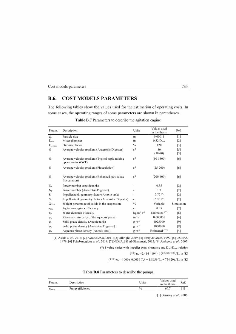
Cost models parameters 269

B.6. COST MODELS PARAMETERS The following tables show the values used for the estimation of operating costs. In some cases, the operating ranges of some parameters are shown in parentheses.

Table B.7 Parameters to describe the agitation engine

Param. Description Units Values used in the thesis Ref.

dp Particle size m 0.00011 [1] Dstir Mixer diameter m 0.52 Dtank [2] Foversize Oversize factor % 120 [3] G Average velocity gradient (Anaerobic Digester) s-1 80

(50-80) [5] [5]

G Average velocity gradient (Typical rapid mixing operation in WWT)

s-1 (50-1500) [6]

G Average velocity gradient (Flocculation) s-1 (25-200) [6]

G Average velocity gradient (Enhanced particulate flocculation)

s-1 (200-400) [6]

NP Power number (anoxic tank) - 0.35 [2] NP Power number (Anaerobic Digester) - 1.7 [2] S Impeller/tank geometry factor (Anoxic tank) - 7.72 (*) [2] S Impeller/tank geometry factor (Anaerobic Digester) - 5.30 (*) [2] XTSS Weight percentage of solids in the suspension % Variable Simulation ηstir Agitation engines efficiency - 0.85 [7] ηw Water dynamic viscosity kg m-1 s-1 Estimated (**) [8] w Kinematic viscosity of the aqueous phase m2 s-1 0.000001 [4] φs Solid phase density (Anoxic tank) g m-3 1025000 [9] φs Solid phase density (Anaerobic Digester) g m-3 1030000 [9] φw Aqueous phase density (Anoxic tank) g m-3 Estimated (***) [4]

[1] Astals et al., 2013; [2] Ayranci et al., 2011; [3] Albright, 2009; [4] Perry & Green, 1999; [5] US EPA, 1979; [6] Tchobanoglous et al., 2014; [7] NEMA; [8] Al-Shemmeri, 2012; [9] Andreolo et al., 2007.

(*) S value varies with impeller type, clearance and Dstir/Dtank relation

(**) ηw =2.414 · 10-5 · 10247.8/(Tw-140), Tw in [K]

(***) φw =1000 (-0.0036 Tw2 + 1.8959 Tw + 754.29), Tw in [K]

Table B.8 Parameters to describe the pumps

Param. Description Units Values used in the thesis Ref.

ηpump Pump efficiency % 66.7 [1]

[1] Gernaey et al., 2006.

270 Heat transfer and cost model parameters description

Table B.9 Parameters to describe the blowers

Param. Description Units Values used in the thesis Ref.

Pg,in Absolute gas pressure at the blower/compressor inlet bar 1.01325 [1] Submergence Submergence m 4(**) [4] ηblow Blowers/compressors efficiency % 70 [2] g,GCO2 Heat capacity ratio of GCO2 - 1.300 [1] g,GCO2 Heat capacity ratio of GCO2 - 1.300 [1] g,GH2 Heat capacity ratio of GH2 - 1.410 [1] g,GCH4 Heat capacity ratio of GCH4 - 1.320 [1] g,GNH3 Heat capacity ratio of GNH3 - 1.310 [1] g,GN2 Heat capacity ratio of GN2 - 1.404 [1] g,GO2 Heat capacity ratio of GO2 - 1.400 [1] g,GH2O Heat capacity ratio of GH2O - 1.330 [1]

[1] Perry & Green, 1999; [2] Tchobanoglous et al., 2003. (*) Submergence used in the BSM2 layout

Table B.10 Parameters to describe the turbines

Param. Description Units Values used in the thesis Ref.

ηturb Gas turbines (simple cycle) efficiency % 25-40 [1] ηturb Gas turbines (combined cycle) efficiency % 40-60 [1] ηturb Micro-turbines efficiency % 25-35 [1]

[1] Tchobanoglous et al., 2014.

Table B.11 Parameters to describe the BSM2 layout water distribution system (Source:

Gernaey et al., 2006)

Pumped from: AS R5 Underflow SC Underflow SC Underflow PC Underflow DAF Dewatering To: Inlet AS R1 Inlet AS R1 Inlet DAF Inlet digester Inlet digester Inlet PC

HLs [m] 0.25 1 1 4 17 13 fmoody [m] 0.03 0.03 0.03 0.06 0.80 0.03 Lpipe [m] 56 95 95 85 25 68 Dpipe [m] 0.84 0.42 0.13 0.10 0.10 0.10 90º elbows (*) 3 2 3 2 2 1 45º elbows (*) 0 3 3 3 0 0 No. of pipe junctions (**) 0 0 1 1 0 0

No. of outflow structures (**) 1 1 1 1 1 1

AS: Activated sludge; DAF: Dissolved air flotation; PC: Primary Clarifier; R1: First AS reactor; R5: Fifth AS reactor; SC: Secondary clarifier.

(*) The equivalent pipe length for a 90 degree elbow (Lpipe/Dpipe) is assumed to be “30 · Dpipe”, and for 45 degree elbow a value of “20 · Dpipe” is applied (www.aquatext.com/tables/frict-wat.htm).

Cost models parameters 271

(**) It has been assumed that pipe junctions and outflow structures corresponds to minor losses equivalent to a static head of 0.5 m.

Table B.12 Parameters to describe the electricity/cost conversion model (EUROSTAT 2016)

Param. Description Units Values used in the thesis

MU Monetary unit (or price of the electricity) € kWh-1 0.1207

Table B.13 Parameters to describe the dosage cost models

Param. Description Units Values used in the thesis Ref.

CostChem FeCl3 cost € kg-1 0.11-0.12 [*] kCEPT CEPT process constant gchem m-3 58 [**] Kpoly,sludge Poly-electrolyte dosage to TSS concentration ratio

(primary sludge) gpoly kgTSS

-1 3.5 (2-8)

[1] [1]

Kpoly,sludge Poly-electrolyte dosage to TSS concentration ratio (secondary sludge)

gpoly kgTSS-1 8

(6-20) [1] [1]

Kpoly,sludge Poly-electrolyte dosage to TSS concentration ratio (50 % primary sludge and 50 % secondary sludge)

gpoly kgTSS-1 (4-16) [1]

[1]

Kpoly,sludge Poly-electrolyte dosage to TSS concentration ratio (60 % primary sludge and 40 % secondary sludge)

gpoly kgTSS-1 (4-20) [1]

[1]

nCEPT kCEPT exponent constant - 7 [**] CEPT CEPT process constant - 0.60† [**] max Maximum CEPT efficiency - 0.88 [**] min Minimum CEPT efficiency - 0.60 [**]

[1] Joint Task Force, 1992;

[*] Internal information;

[**] Model calibration for a mixture of FeCl3 and polymer from the information published by poon et al., 1999; US EPA, 1975; Bourke et al., 2000.

273

C

INFLUENT CHARACTERISATION

The influent characterisation is the process to establish a series of relationships between analytical measurement and concentrations of the model components. The problem of characterisation is to determine, from a series of analytical measurements, the most appropriate values of the concentrations of the model components and the mass fractions of all those that do not have a fixed stoichiometric formula. Analytical measurements are usually not enough to fully characterize the wastewater input, so experimental data is supplemented with additional information about the characteristics and expected relationships in an urban wastewater taken from literature.

This appendix explains the procedure used to characterize the different influents used throughout the thesis. Depending on the starting data, the characterisation can be of two types:

Adaptation of the information to the components of the selected category: when the starting point is an influent characterised for another model.

Establishment of a series of relationships between analytical measurement and concentrations of the model components: when the starting point are analytical measures.

274 Influent Characterisation

C.1. CHARACTERISATION OF THE COMPONENT VECTOR BASED ON ASM1 MODEL

When the characterisation starts from a characterisation made for another model it is necessary to adapt that information to the model being used. In this case, this section presents the characterisation made for any category of the library from the ASM1 model. Table C.1 presents the components of this ASM1 model, which is one of the most used models in the mathematical modelling of residual waters.

Table C.1 ASM1 components definition

No. Name ASM1 Unit Description

1 SI gCOD m-3 Soluble inert organic matter 2 SS gCOD m-3 Readily biodegradable substrate 3 XI gCOD m-3 Particulate inert organic matter 4 XS gCOD m-3 Slowly biodegradable substrate 5 XBH gCOD m-3 Active heterotrophic biomass 6 XBA gCOD m-3 Active autotrophic biomass 7 XP gCOD m-3 Particulate products arising from biomass decay 8 SO gCOD m-3 Oxygen 9 SNO gN m-3 Nitrate and nitrite nitrogen 10 SNH gN m-3 NH4

+ + NH3 11 SND gN m-3 Soluble biodegradable organic nitrogen 12 XND gN m-3 Particulate biodegradable organic nitrogen 13 SALK mol m-3 Alkalinity

The ASM1 model is characterised by its simplicity. It is for this reason that certain assumptions must be made for the characterisation of the PWM components.

The ASM1 model does not provide information about VFA, phosphorus, total nitrogen and colloidal matter. If the information is unknown the following ratios can be used:

o The colloidal fraction of the slowly biodegradable matter (1 - fXS) may represent 25 % of the total XS concentration (WERF, 2003; Latimer et al., 2007).

o In a typical characterisation of raw municipal wastewaters with minor contributions of industrial waters the TKN/TP ratio remains

Characterisation of the component vector based on ASM1 model 275

at 4 for medium-high load wastewaters and in 5 for low load wastewater (Henze et al., 2008).

o The VFA concentration may represent 15 % of the soluble and colloidal COD (Henze et al., 2008): VFA/SCOD = 0.15.

o In a typical characterisation of raw municipal wastewater the NH4-N/TN ratio remains at 0.75 (Henze et al., 2008).

It is necessary to set information such as temperature, pH, TSS, and water flow.

Finally, certain global variables must be calculated.

TNN4NH

STN NH

TPTKN

TNTP

PBABHIISS XXXXSXSTCOD

IS SSSCOD

Table C.2 presents the expressions used for the characterisation of the components ensuring the mass, charge and total solids continuity throughout the characterisation.

Table C.2 Liquid phase PWM components characterisation

No. Name E-PWM Unit Description

1 SH2O m3 d-1 Qw,in 2 SO2 gO2 m-3 SO 3 SH+ gH m-3 1000·10 pH 4 SOH- gH m-3

H

O2H,a

S1000000·K

5 SH2PO4- gP m-3 1000000·K·K

S·S

IP,2aIP,a

43PO2

H

6 SHPO4= gP m-3

1000·K

S·S

IP,2a

43POH

276 Influent Characterisation

Table C.2 Liquid phase PWM components characterisation (Continued)

No. Name E-PWM Unit Description

7 SPO4-3 gP m-3

1000000·K·K

S

1000·K

S1

i·CTP

IP,2aIP,a

2H

IP,2a

H

59

1ii,Pi

8 SNH4+ gN m-3 3NHNH SS 9 SNH3 gN m-3

1000·K

S1

S

IN,a

H

NH

10 SCO2 gC m-3

1000·K

S·S

IC,a

3HCOH

11 SHCO3- gC m-3 12·SSS OHHALK

12 SCO3= gC m-3

H

3HCOIC,2aS

S·1000·K

13 SCa+2 gCa m-3 0.00 14 SMg+2 gMg m-3 Minimum concentration to ensure the formation of

XPP 15 SK+ gK m-3 Minimum concentration to ensure the formation of

XPP 16 SSU gCOD m-3

21XX PRS

17 SAA gCOD m-3

SSAAN,NDS

SSAAN,NDSAAN,ND

Si/S ifS

Si/S ifi/S

18 SFA gCOD m-3 21XX PRS

19 SHVA gCOD m-3

1000·K

S·S

HVA,a

VAH

20 SVA- gCOD m-3 1000·KS

1000·K41

SCODVFASCOD

HVA,aH

HVA,a

21 SHBU gCOD m-3

1000·K

S·S

HBU,a

BUH

Characterisation of the component vector based on ASM1 model 277

Table C.2 Liquid phase PWM components characterisation (Continued)

No. Name E-PWM Unit Description

22 SBU- gCOD m-3 1000·KS

1000·K41

SCODVFASCOD

HBU,aH

HBU,a

23 SHPRO gCOD m-3

1000·K

S·S

HPRO,a

PROH

24 SPRO- gCOD m-3 1000·KS

1000·K41

SCODVFASCOD

HPRO,aH

HPRO,a

25 SHAC gCOD m-3

1000·K

S·S

HAC,a

ACH

26 SAC- gCOD m-3 1000·KS

1000·K41

SCODVFASCOD

HAC,aH

HAC,a

27 SH2 gCOD m-3 0.00 28 SCH4 gCOD m-3 0.00 29 SN2 gN m-3 0.00 30 SNO2

- gN m-3 0.00 31 SHNO2 gN m-3 0.00 32 SNO3

- gN m-3 SNO 33 SI gCOD m-3 SI 34 SP gCOD m-3 0.00 35 SFe+3 gFe m-3 0.00 36 SCl- gCl m-3 0.00 37 XC1 gCOD m-3 0.00 38 XC2 gCOD m-3 0.00 39 XCH gCOD m-3

54XX PRS

40 XPR gCOD m-3

SXPRN,NDS

SXPRN,NDXPRN,ND

Xi/X ifX

Xi/X ifi/X

41 XLI gCOD m-3 XS – XPR – XCH 42 XH gCOD m-3 XBH 43 XN gCOD m-3 0.00 44 XAOB gCOD m-3 XBA 46 XPAO gCOD m-3 0.00 47 XPHA gCOD m-3 0.00 48 XSU gCOD m-3 0.00

278 Influent Characterisation

Table C.2 Liquid phase PWM components characterisation (Continued)

No. Name E-PWM Unit Description

49 XAA gCOD m-3 0.00 50 XFA gCOD m-3 0.00 51 XC4 gCOD m-3 0.00 52 XPRO gCOD m-3 0.00 53 XAC gCOD m-3 0.00 54 XH2 gCOD m-3 0.00 55 XAN gCOD m-3 0.00 56 XI gCOD m-3 XI 57 XP gCOD m-3 XP 58 XII gSS m-3 TSS 59 XPP gP m-3 0.00

C.2. CHARACTERISATION OF THE COMPONENT VECTOR BASED ON ANALYTICAL MEASURES

When the characterisation starts from an analytical measures, a series of relationships between analytical measurement and concentrations of the model components need to be established. Table C.3 presents the expressions used for the characterisation of the components ensuring the mass, charge and total solids continuity throughout the characterisation.

Table C.3 Liquid phase PWM components characterisation

No. Name E-PWM Unit Description

1 SH2O m3 d-1 Qw,in 2 SO2 gO2 m-3 0.00 3 SH+ gH m-3 1000·10 pH 4 SOH- gH m-3

H

O2H,a

S1000000·K

5 SH2PO4- gP m-3 1000000·K·K

S·S

IP,2aIP,a

43PO2

H

6 SHPO4= gP m-3

1000·K

S·S

IP,2a

43POH

Characterisation of the component vector based on analytical measures 279

Table C.3 Liquid phase PWM components characterisation (Continued)

No. Name E-PWM Unit Description

7 SPO4-3 gP m-3

1000000·K·K

S

1000·K

S1

i·CTP

IP,2aIP,a

2H

IP,2a

H

59

1ii,Pi

8 SNH4+ gN m-3 When the ammonium concentration is known: 3NH4 SNNH

When the ammonium concentration is unknown:

3NH59

1ii,Ni2HNO2NO3NO Si·CSSSTN

9 SNH3 gN m-3 When the ammonium concentration is known:

1000·K

S1

NNH

IN,a

H

4

When the ammonium concentration is unknown:

1000·K

S1

i·CSSSTN

IN,a

H

59

1ii,Ni2HNO2NO3NO

10 SCO2 gC m-3

1000·K

S·S

IC,a

3HCOH

11 SHCO3- gC m-3 12·SSS OHHALK

12 SCO3= gC m-3

H

3HCOIC,2aS

S·1000·K

13 SCa+2 gCa m-3 0.00 14 SMg+2 gMg m-3 Minimum concentration to ensure the formation of

XPP 15 SK+ gK m-3 Minimum concentration to ensure the formation of

XPP 16 SSU gCOD m-3

f

SUDQO

STCODSCODTCOD

17 SAA gCOD m-3

f

SAADQOS

TCODSCODTCOD

280 Influent Characterisation

Table C.2 Liquid phase PWM components characterisation (Continued)

No. Name E-PWM Unit Description

18 SFA gCOD m-3 SCOD

STCODSCODTCOD FA

19 SHVA gCOD m-3

1000·K

S·S

HVA,a

VAH

20 SVA- gCOD m-3 1000·KS

1000·KSCODS

TCODSCODTCOD

HVA,aH

HVA,aTVA

21 SHBU gCOD m-3

1000·K

S·S

HBU,a

BUH

22 SBU- gCOD m-3 1000·KS

1000·KSCODS

TCODSCODTCOD

HBU,aH

HBU,aTBU

23 SHPRO gCOD m-3

1000·K

S·S

HPRO,a

PROH

24 SPRO- gCOD m-3 1000·KS

1000·KSCODS

TCODSCODTCOD

HPRO,aH

HPRO,aTPRO

25 SHAC gCOD m-3

1000·K

S·S

HAC,a

ACH

26 SAC- gCOD m-3 1000·KS

1000·KSCODS

TCODSCODTCOD

HAC,aH

HAC,aTAC

27 SH2 gCOD m-3 0.00 28 SCH4 gCOD m-3 0.00 29 SN2 gN m-3 0.00 30 SNO2

- gN m-3 0.00 31 SHNO2 gN m-3 0.00 32 SNO3

- gN m-3 NO3-N or 0.00 33 SI gCOD m-3

SCODS

TCODSCODTCOD I

34 SP gCOD m-3 0.00 35 SFe+3 gFe m-3 0.00 36 SCl- gCl m-3 0.00 37 XC1 gCOD m-3 0.00 38 XC2 gCOD m-3 0.00 39 XCH gCOD m-3

PCODX

TCODPCODTCOD

SCODX

TCODSCODTCOD CHCH

Characterisation of the component vector based on analytical measures 281

Table C.2 Liquid phase PWM components characterisation (Continued)

No. Name E-PWM Unit Description

40 XPR gCOD m-3 PCODX

TCODPCODTCOD

SCODX

TCODSCODTCOD CPRPR

41 XLI gCOD m-3 PCOD

XTCODPCODTCOD

SCODX

TCODSCODTCOD LILI

42 XH gCOD m-3 PCOD

XTCODPCODTCOD H

43 XN gCOD m-3 0.00 44 XAOB gCOD m-3 0.00 46 XPAO gCOD m-3 0.00 47 XPHA gCOD m-3 0.00 48 XSU gCOD m-3 0.00 49 XAA gCOD m-3 0.00 50 XFA gCOD m-3 0.00 51 XC4 gCOD m-3 0.00 52 XPRO gCOD m-3 0.00 53 XAC gCOD m-3 0.00 54 XH2 gCOD m-3 0.00 55 XAN gCOD m-3 0.00 56 XI gCOD m-3

PCODX

TCODPCODTCOD i

57 XP gCOD m-3 0.00 58 XII gSS m-3

59

37ii

iT ThOD

PCODX

TCODPCODTCODSS

59 XPP gP m-3 0.00

The characterisation based on analytical measures also needs the formulation of some assumptions, since it is not always possible to make measurements for the characterisation of all components.

282 Influent Characterisation

283

DB

PUBLICATIONS GENERATED

The scientific publications derived from the present thesis are listed below:

INTERNATIONAL JOURNALS Published papers

1. Fernández-Arévalo, T., Lizarralde, I., Maiza, M., Beltrán, S., Grau, P., Ayesa, E., 2016. Diagnosis and optimization of WWTPs using the PWM library: Full-scale experiences. Accepted in Water Science and Technology.

2. Lizarralde, I., Fernández-Arévalo, T., Brouckaert, C.J., Vanrolleghem, P.A., Ikumi, D.S., Ekama, G.A., Ayesa, E., Grau, P., 2015. A new general methodology for incorporating physico-chemical transformations into multi-phase wastewater treatment process models. Water Research, 74, 239-256.

3. Fernández-Arévalo T., Lizarralde I., Grau P., Ayesa E. 2014. New systematic methodology for incorporating dynamic heat transfer modelling in multi-phase biochemical reactors. Water Research, 60, 141-155.

4. Astals, S., Esteban-Gutiérrez, M., Fernández-Arévalo, T., Aymerich, E., García de las Heras, J.L., Mata-Álvarez, J., 2013. Anaerobic digestion of seven different

284 Publications generated

sewage sludges: a biodegradability and modelling study. Water Research, 47(16), 6033-6043.

Submitted papers

1. Fernández-Arévalo, T., Lizarralde, I., Pérez-Elvira, S.I., Garrido, J.M., Puig, S., Poch, M., Grau, P., Ayesa, E., 2016. Quantitative assessment of energy and resource recovery in evolutionary wastewater treatment plants based on Plant-Wide simulations. Submitted to the journal Water Research.

Papers in preparation

1. Lizarralde, I., Fernández-Arévalo, T., Beltrán, S., Ayesa, E. and Grau, P. Validation of a multi-phase plant-wide model for the description of the aeration process in a WWTP.

BOOK CHAPTERS 1. Fernández-Arévalo, T., Grau, P., Jeppsson, U., Mauricio-Iglesias, M., Vrecko,

D., Flores-Alsina, X., Ayesa, E., 2017. Model-based comparative assessment of innovative processes. In Lema, J.M., Suarez-Martinez, S. (Eds.), Innovative wastewater treatment & resource recovery technologies. Impacts on energy, economy and environment, IWA Publishing. ISBN13: 9781780407869.

2. Beltran, B., Fernández-Arévalo, T., Odriozola, J.V., Sainz, M., Ayesa, E., 2012. Mathematical modelling and automatic control of WWTPs. In Garrido-Baserba, M., Poch, M. (Eds.), Environmental Decision Support Systems (EDSSs). A tool for wastewater management in the XXI Century. Universitat de Girona. ISBN: 978-84-8458-360-8.

3. Beltran, S., Fernández-Arévalo, T., Barrena, I., Grau, P., Ayesa, E., 2010. Modelado matemático y control del consumo energético en las EDAR. In Mata-Álvarez, J., Fdez.-Polanco, F. (Eds.), Eco-eficiencia en la EDAR del siglo XXI. Aspectos ambientales y energéticos. Editorial Lápices 4, Santiago de Compostela. ISBN: 978-84-693-7960-8.

International Conference Proceedings 285

INTERNATIONAL CONFERENCE PROCEEDINGS 1. Fernández-Arévalo, T., Grau, P., Jeppsson, U., Mauricio-Iglesias, M., Vrecko,

D., Flores-Alsina, X., Ayesa, E., 2016. Model-based comparative assessment of innovative processes. In: Proceedings of the State of the art. Innovative Wastewater Treatment and Resource Recovery Technologies. Barcelona, Spain, November 18.

2. Fernández-Arévalo, T., Lizarralde, I., Maiza, M., Grau, P., Ayesa, E., 2016. Global optimization and resource recovery analysis in WWTPs using PWM simulations: Full-scale experiences. In: Proceedings of the 3rd Eco-technologies for Wastewater Treatment: Technical, Environmental & Economic Challenges. EcoSTP2016. Cambridge, England, June 27-30.

3. Lizarralde, I., Fernández-Arévalo, T., Ayesa, E., Grau, P., 2016. New advanced model-based tool for the integrated assessment of nutrient treatment solutions in WRRF. In: Proceeding of the 13th IWA Leading Edge Conference on Water and Wastewater Technologies. Evaluating Impacts of Innovation (LET2016). Jerez de la Frontera, Spain, June 13-16.

4. Fernández-Arévalo, T., Lizarralde, I., Maiza, M., Grau, P., Ayesa, E., 2016. Diagnosis and optimization of WWTPs using the PWM library: Full-scale experiences. In: Proceedings of the 5th IWA/WEF Wastewater Treatment Modelling Seminar (WWTmod2016). Annecy, France, April 2-6.

5. Lizarralde, I., Fernández-Arévalo, T., Monge, S., Manas, A., Maiza, M., Ayesa, E., Grau, P., Suescun, J., 2016. Model based assessment of the optimum phosphorus management strategies in a full-scale WWTP. In: Proceedings of the 5th IWA/WEF Wastewater Treatment Modelling Seminar (WWTmod2016). Annecy, France, April 2-6.

6. Fernández-Arévalo, T., Grau, P., Jeppsson, U., Mauricio-Iglesias, M., Ayesa, E., 2015. Model-based comparative assessment of innovative processes. Oral communication in: COST Action no. ES1202. Conceiving Wastewater Treatment in 2020 - Energetic, environmental and economic challenges (Water_2020). Catania, Italy, October 19-20.

7. Fernández-Arévalo T., Lizarralde I., Pérez-Elvira S.I., Garrido J.M., Puig S., Poch M., Grau P., Ayesa E. 2015. Conceptual design and comparative assessment of WWTP layouts based on plant-wide model simulations. In:

286 Publications generated

Proceedings of the 9th IWA Symposium on System Analysis and Integrated Assessment (Watermatex15). Gold Coast, Australia, June 11-14.

8. Lizarralde, I., Fernández-Arévalo, T., Beltrán, S., Ayesa, E., Grau, P., 2015. Validation of a multi-phase Plant-Wide Model for the description of the aerations system in a WWTP. In: Proceedings of the 9th IWA Symposium on System Analysis and Integrated Assessment (Watermatex15). Gold Coast, Australia, June 11-14.

9. Sainz, M., Fernández-Arévalo, T., Odriozola, J., Ayesa, E., 2015. A robust calibration methodology of wastewater treatment models based on Markov Chain Monte Carlo (MCMC) algorithms. In: Proceedings of the 9th IWA Symposium on System Analysis and Integrated Assessment (Watermatex15). Gold Coast, Australia, June 11-14.

10. Lizarralde, I., Fernández-Arévalo, T., Maiza, M., Grau, P., Ayesa, E., 2014. Plant-Wide Model simulations for studying phosphorous recovery and energy costs in WWTPs. In: Proceedings of the 2nd Ecotechnologies for Wastewater Treatment: Technical, Environmental & Economic Challenges. EcoSTP2014. Verona, Italy, June 23-25.

11. Fernandez, T., Grau, P., Abelleira, J., Donoso-Bravo, A., Pérez-Elvira, S., Lema, J.M., Campos, J.L., Suárez, S., Mosquera-Corral, A., Ayesa, E., 2012. Simulation based analysis of new layouts for eco-efficient sewage treatment plants. In: Proceedings of the Ecotechnologies for Wastewater Treatment: Technical, Environmental & Economic Challenges. EcoSTP. Santiago de Compostela, Spain, June 25-27.

12. Fernandez, T., Grau, P., Bengoechea, A., Beltran, S., Ayesa, E., 2011. Integrated simulation of mass and energy for optimising operational strategies in WWTPs. In: Proceedings of the 8th IWA Symposium on Systems Analysis and Integrated Assessment, Watermatex 2011, San Sebastian, Spain, June 20-22.

NATIONAL CONFERENCE PROCEEDINGS 1. Ayesa, E., Fernández-Arévalo, T., Lizarralde, I., Grau, P., 2016. Utilidad real de

los simuladores dinámicos para optimizar la explotación de las EDAR urbanas. In: Proceedings of the Technical Seminar “Tecnologías Innovadoras para el

National Conference Proceedings 287

tratamiento de Aguas Residuales, Lodos de Depuradora y Residuos”. Madrid, Spain, November 3.

2. Fernández-Arévalo, T., Lizarralde, I., Grau, P., Ayesa, E., 2016. Modelización de los flujos de masa y energía en las EDAR. In: Proceedings of the Technical Seminar “Procesos Avanzados para Tratamiento y Postratamiento de Aguas Residuales”. Santander, Spain, October 20-21.

3. Fernández-Arévalo, T., Lizarralde, I., Grau, P., Ayesa, E., 2013. Extended Plant-Wide Modelling: New methodology for analysing innovative plant layouts. In: Proceedings of the Novedar young water researchers workshop. Innovative technologies for the XXI century Wastewater treatment plant and future perspectives. Santander, Spain, May 9-10.

4. Lizarralde, I., Fernández-Arévalo, T., Ayesa, E., Grau, P., 2013. Incorporating water chemistry into the Extended Plant Wide Model (E-PWM). In: Proceedings of the Novedar young water researchers workshop. Innovative technologies for the XXI century Wastewater treatment plant and future perspectives. Santander, Spain, May 9-10.

5. Astals, S., Esteban-Gutiérrez, M., Fernández-Arévalo, T., Aymerich, E., García de las Heras, J.L., Mata-Álvarez, J., 2013. Anaerobic digestion of sewage sludge: a biodegradability and modelling study. In: Proceedings of the Novedar young water researchers workshop. Innovative technologies for the XXI century Wastewater treatment plant and future perspectives. Santander, Spain, May 9-10.

6. Abelleira, J.M., Sánchez-Oneto, J., Portela, J.R., Pérez-Elvira, S.I., Muñoz, R., Lebrero, R., Fernández-Arévalo, T., Esteban-Gutiérrez, M., Garrido-Baserba, M., Lotti, T., Martínez de la Ossa, E.J., Nebot, E., 2013. High pressure processes integration for the treatment of sewage sludge. In: Proceedings of the Novedar young water researchers workshop. Innovative technologies for the XXI century Wastewater treatment plant and future perspectives. Santander, Spain, May 9-10.

7. Fernández-Arévalo, T., Ayesa, E., 2011. Modelling and Control. Oral communication in: Novedar_Consolider meeting. Santiago de Compostela, Spain. November 7-8.

288 Publications generated

8. Beltran, S., Fernández-Arévalo, T., Barrena, I., Grau, P., Ayesa, E., 2010. Modelado matemático y control del consumo energético en las EDAR. Oral communication in: Eco-eficiencia en la EDAR del siglo XXI. Aspectos ambientales y energéticos, Barcelona, Spain, November 15.