
OPERATING SYSTEMS - electrobian
191
OPERATING SYSTEMS 10EC65 Dept of ECE, SJBIT OPERATING SYSTEMS Subject Code: 10EC65 IA Marks: 25 No. of Lecture Hrs/Week: 04 Exam Hours: 03 Total no. of Lecture Hrs: 52 Exam Marks : 100 PART – A UNIT - 1 INTRODUCTION AND OVERVIEW OF OPERATING SYSTEMS: Operating system, Goals of an O.S, Operation of an O.S, Resource allocation and related functions, User interface related functions, Classes of operating systems, O.S and the computer system, Batch processing system, Multi programming systems, Time sharing systems, Real time operating systems, distributed operating systems. 6 Hours UNIT - 2 STRUCTURE OF THE OPERATING SYSTEMS: Operation of an O.S, Structure of the supervisor, Configuring and installing of the supervisor, Operating system with monolithic structure, layered design, Virtual machine operating systems, Kernel based operating systems, and Microkernel based operating systems. 7 Hours UNIT - 3 PROCESS MANAGEMENT: Process concept, Programmer view of processes, OS view of processes, Interacting processes, Threads, Processes in UNIX, Threads in Solaris. 6 Hours UNIT - 4 MEMORY MANAGEMENT: Memory allocation to programs, Memory allocation preliminaries, Contiguous and noncontiguous allocation to programs, Memory allocation for program controlled data, kernel memory allocation. 7 Hours PART – B UNIT - 5 VIRTUAL MEMORY: Virtual memory basics, Virtual memory using paging, Demand paging, Page replacement, Page replacement policies, Memory allocation to programs, Page sharing, UNIX virtual memory. 6 Hours
-
Upload
khangminh22 -
Category
Documents
-
view
0 -
download
0
Transcript of OPERATING SYSTEMS - electrobian
OPERATING SYSTEMS 10EC65
Dept of ECE, SJBIT
OPERATING SYSTEMS
Subject Code: 10EC65 IA Marks: 25
No. of Lecture Hrs/Week: 04 Exam Hours: 03
Total no. of Lecture Hrs: 52 Exam Marks : 100
PART – A
UNIT - 1
INTRODUCTION AND OVERVIEW OF OPERATING SYSTEMS: Operating system,
Goals of an O.S, Operation of an O.S, Resource allocation and related functions, User
interface related functions, Classes of operating systems, O.S and the computer system,
Batch processing system, Multi programming systems, Time sharing systems, Real time
operating systems, distributed operating systems. 6 Hours
UNIT - 2
STRUCTURE OF THE OPERATING SYSTEMS: Operation of an O.S, Structure of the
supervisor, Configuring and installing of the supervisor, Operating system with monolithic
structure, layered design, Virtual machine operating systems, Kernel based operating
systems, and Microkernel based operating systems. 7 Hours
UNIT - 3
PROCESS MANAGEMENT: Process concept, Programmer view of processes, OS view of
processes, Interacting processes, Threads, Processes in UNIX, Threads in Solaris. 6 Hours
UNIT - 4
MEMORY MANAGEMENT: Memory allocation to programs, Memory allocation
preliminaries, Contiguous and noncontiguous allocation to programs, Memory allocation for
program controlled data, kernel memory allocation. 7 Hours
PART – B
UNIT - 5
VIRTUAL MEMORY: Virtual memory basics, Virtual memory using paging, Demand
paging, Page replacement, Page replacement policies, Memory allocation to programs, Page
sharing, UNIX virtual memory. 6 Hours
OPERATING SYSTEMS 10EC65
Dept of ECE, SJBIT
UNIT - 6
FILE SYSTEMS: File system and IOCS, Files and directories, Overview of I/O
organization, Fundamental file organizations, Interface between file system and IOCS,
Allocation of disk space, Implementing file access, UNIX file system. 7 Hours
UNIT - 7
SCHEDULING: Fundamentals of scheduling, Long-term scheduling, Medium and short
term scheduling, Real time scheduling, Process scheduling in UNIX. 6 Hours
UNIT - 8
MESSAGE PASSING: Implementing message passing, Mailboxes, Interprocess
communication in UNIX. 7 Hours
TEXT BOOK:
1. ―Operating Systems - A Concept based Approach‖, D. M. Dhamdhare, TMH, 3rd Ed,
2010.
REFERENCE BOOK:
1. Operating Systems Concepts, Silberschatz and Galvin, John Wiley India Pvt. Ltd, 5th
Edition, 2001.
2. Operating System – Internals and Design Systems, Willaim Stalling, Pearson Education,
4th Ed, 2006.
3. Design of Operating Systems, Tennambhaum, TMH, 2001.

OPERATING SYSTEMS 10EC65
Dept of ECE, SJBIT
INDEX SHEET
UNIT TOPIC PAGE NO
UNIT-1: INTRODUCTION AND OVERVIEW OF OPERATING SYSTEMS 01
1.1 Efficient use 01
1.2 User convenience
02
1.3 Non-interference
02
1.4 Operation of an os
03
1.5 Classes of operating systems
06
1.6 Batch processing systems
08
1.7 Time-sharing systems
13
1.8 Real-time operating systems
16
1.9 Distributed operating systems
18
UNIT-2: STRUCTURE OF THE OPERATING SYSTEMS 21
2.1 Operation of an os
21
2.2 Structure of an operating system
22
2.3 Operating systems with monolithic structure 24
2.4 Layered design of operating systems
25
2.5 Virtual machine operating systems
26
2.6 Kernel-based operating systems
28
2.7 Microkernel-based operating systems
31
2.8 Case studies
32
UNIT – 3: PROCESS MANAGEMENT 37
3.1 Processes and programs
37
3.2 Implementing processes
42
3.3 Threads
56
3.4 Case studies of processes and threads
66
UNIT - 4 : MEMORY MANAGEMENT 71
4.1 Managing the memory hierarchy 71
4.2 Static and dynamic memory allocation
72
4.3 Execution of programs
73
4.4 Memory allocation to a process
78
4.5 Heap management
81
4.6 Contiguous memory allocation
89
4.7 Noncontiguous memory allocation
90
4.8 Paging
93
4.9 Segmentation
94
4.10 Segmentation with paging
95
4.11 Kernel memory allocation 96

OPERATING SYSTEMS 10EC65
Dept of ECE, SJBIT
UNIT – 5: VIRTUAL MEMORY
100
5.1 Virtual memory basics
100
5.2 Demand paging
102
5.3 The virtual memory manager
112
5.4 Page replacement policies 115
5.5 Controlling memory allocation to a process 120
5.6 Shared pages
121
5.7 Case studies of virtual memory using paging
123
UNIT – 6: FILE SYSTEMS 126
6.1 Overview of file processing
126
6.2 Files and file operations
128
6.3 Fundamental file organizations and access methods
130
6.4 Directories
133
6.5 File protection
137
6.6 Allocation of disk space
138
6.7 Performance issues
142
6.8 Interface between file system and iocs
142
6.9 Unix file system
145
UNIT – 7: SCHEDULING 150
7.1 Scheduling Terminology and Concepts
150
7.2 Nonpreemptive scheduling policies
153
7.3 Preemptive scheduling policies
156
7.4 Scheduling in practice
160
7.5 Real-time scheduling
166
7.6 Case studies
170
UNIT – 8: MESSAGE PASSING
8.1 Overview of message passing
174
8.2 Implementing message passing
178
8.3 Mailboxes
180
8.4 Higher-level protocols using message passing 182
8.5 Case studies in message passing
184

OPERATING SYSTEMS 10EC65
Dept of ECE, SJBIT Page 1
UNIT-1
INTRODUCTION AND OVERVIEW OF OPERATING
SYSTEMS
An operating system (OS) is different things to different users. Each user's view is
called an abstract view because it emphasizes features that are important from the viewer‘s
perspective, ignoring all other features. An operating system implements an abstract view by
acting as an intermediary between the user and the computer system. This arrangement not
only permits an operating system to provide several functionalities at the same time, but also
to change and evolve with time.
An operating system has two goals—efficient use of a computer system and user
convenience. Unfortunately, user convenience often conflicts with efficient use of a computer
system- Consequently; an operating system cannot provide both. It typically strikes a balance
between the two that is most effective in the environment in which a computer system is
used—efficient use is important when a computer system is shared by several users while
user convenience is important in personal computers.
The fundamental goals of an operating system are:
• Efficient use: Ensure efficient use of a computer‘s resources.
• User convenience: Provide convenient methods of using a computer system.
• Non-interference: Prevent interference in the activities of its users.
The goals of efficient use and user convenience sometimes conflict. For example, emphasis
on quick service could mean that resources like memory have to remain allocated to a
program even when the program is not in execution; however, it would lead to inefficient use
of resources. When such conflicts arise, the designer has to make a trade-off to obtain the
combination of efficient use and user convenience that best suits the environment. This is the
notion of effective utilization of the computer system. We find a large number of operating
systems in use because each one of them provides a different flavour of effective utilization.
At one extreme we have OSs that provide fast service required by command and control
applications, at the other extreme we have OSs that make efficient use of computer resources
to provide low-cost computing, while in the middle we have OSs that provide different
combinations of the two. Interference with a user‘s activities may take the form of illegal use
or modification of a user‘s programs or data, or denial of resources and services to a user.
Such interference could be caused by both users and nonusers, and every OS must
incorporate measures to prevent it. In the following, we discuss important aspects of these
fundamental goals.
1.1 Efficient Use
An operating system must ensure efficient use of the fundamental computer system resources
of memory, CPU, and I/O devices such as disks and printers. Poor efficiency can result if a
program does not use a resource allocated to it, e.g., if memory or I/O devices allocated to a

OPERATING SYSTEMS 10EC65
Dept of ECE, SJBIT Page 2
program remain idle. Such a situation may have a snowballing effect: Since the resource is
allocated to a program, it is denied to other programs that need it. These programs cannot
execute, hence resources allocated to them also remain idle. In addition, the OS itself
consumes some CPU and memory resources during its own operation, and this consumption
of resources constitutes an overhead that also reduces the resources available to user
programs. To achieve good efficiency, the OS must minimize the waste of resources by
programs and also minimize its own overhead. Efficient use of resources can be obtained by
monitoring use of resources and performing corrective actions when necessary. However,
monitoring use of resources increases the overhead, which lowers efficiency of use. In
practice, operating systems that emphasize efficient use limit their overhead by either
restricting their focus to efficiency of a few important resources, like the CPU and the
memory, or by not monitoring the use of resources at all, and instead handling user programs
and resources in a manner that guarantees high efficiency.
1.2 User Convenience
User convenience has many facets, as Table 1.1 indicates. In the early days of computing,
user convenience was synonymous with bare necessity—the mere ability to execute a
program written in a higher level language was considered adequate. Experience with early
operating systems led to demands for better service, which in those days meant only fast
response to a user request. Other facets of user convenience evolved with the use of
computers in new fields. Early operating systems had command-line interfaces, which
required a user to type in a command and specify values of its parameters. Users needed
substantial training to learn use of the commands, which was acceptable because most users
were scientists or computer professionals. However, simpler interfaces were needed to
facilitate use of computers by new classes of users. Hence graphical user interfaces (GUIs)
were evolved. These interfaces used icons on a screen to represent programs and files and
interpreted mouse clicks on the icons and associated menus as commands concerning them.
Table 1.1 Facets of User Convenience
Facet Examples
Fulfillment of necessity Ability to execute programs, use the file system
Good Service Speedy response to computational requests
User friendly interfaces Easy-to-use commands, graphical user interface
(GUI)
New programming model Concurrent programming
Web-oriented features Means to set up Web-enabled servers
Evolution Add new features, use new computer
technologies
1.3 Non-interference
A computer user can face different kinds of interference in his computational activities.
Execution of his program can be disrupted by actions of other persons, or the OS services
which he wishes to use can be disrupted in a similar manner.

OPERATING SYSTEMS 10EC65
Dept of ECE, SJBIT Page 3
The OS prevents such interference by allocating resources for exclusive use of programs and
OS services, and preventing illegal accesses to resources. Another form of interference
concerns programs and data stored in user files. A computer user may collaborate with some
other users in the development or use of a computer application, so he may wish to share
some of his files with them. Attempts by any other person to access his files are illegal and
constitute interference. To prevent this form of interference, an OS has to know which files of
a user can be accessed by which persons. It is achieved through the act of authorization,
whereby a user specifies which collaborators can access what files. The OS uses this
information to prevent illegal accesses to files.
1.4 OPERATION OF AN OS
The primary concerns of an OS during its operation are execution of programs, use of
resources, and prevention of interference with programs and resources. Accordingly, its three
principal functions are:
• Program management: The OS initiates programs, arranges their execution on the CPU,
and terminates them when they complete their execution. Since many programs exist in the
system at any time, the OS performs a function called scheduling to select a program for
execution.
• Resource management: The OS allocates resources like memory and I/O devices when a
program needs them. When the program terminates, it deallocates these resources and
allocates them to other programs that need them.
• Security and protection: The OS implements non-interference in users‘ activities through
joint actions of the security and protection functions. As an example, consider how the OS
prevents illegal accesses to a file. The security function prevents nonusers from utilizing the
services and resources in the computer system, hence none of them can access the file. The
protection function prevents users other than the file owner or users authorized by him, from
accessing the file.
Table 1.2 describes the tasks commonly performed by an operating system. When a computer
system is switched on, it automatically loads a program stored on a reserved part of an I/O
device, typically a disk, and starts executing the program. This program follows a software
technique known as bootstrapping to load the software called the boot procedure in
memory—the program initially loaded in memory loads some other programs in memory,
which load other programs, and so on until the complete boot procedure is loaded. The boot
procedure makes a list of all hardware resources in the system, and hands over control of the
computer system to the OS.

OPERATING SYSTEMS 10EC65
Dept of ECE, SJBIT Page 4
Table 1.2 Common Tasks Performed by Operating Systems
Task When performed
Construct a list of resources during booting
Maintain information for security while registering new users
Verify identity of a user at login time
Initiate execution of programs at user commands
Maintain authorization information when a user specifies which
Collaborators can access what programs
or data.
Perform resource allocation when requested by users or programs
Maintain current status of resources during resource allocation/deallocation
Maintain current status of programs continually during OS operation
and perform scheduling
The following sections are a brief overview of OS responsibilities in managing programs and
resources and in implementing security and protection.
1.4.1 Program Management
Modern CPUs have the capability to execute program instructions at a very high rate, so it is
possible for an OS to interleave execution of several programs on a CPU and yet provide
good user service. The key function in achieving interleaved execution of programs is
scheduling, which decides which program should be given the CPU at any time. Figure 1.3
shows an abstract view of scheduling. The scheduler, which is an OS routine that performs
scheduling, maintains a list of programs waiting to execute on the CPU, and selects one
program for execution.
In operating systems that provide fair service to all programs, the scheduler also specifies
how long the program can be allowed to use the CPU. The OS takes away the CPU from a
program after it has executed for the specified period of time, and gives it to another program.
This action is called preemption. A program that loses the CPU because of preemption is put
back into the list of programs waiting to execute on the CPU. The scheduling policy
employed by an OS can influence both efficient use of the CPU and user service. If a
program is preempted after it has executed for only a short period of time, the overhead of
scheduling actions would be high because of frequent preemption. However, each program
would suffer only a short delay before it gets an opportunity to use the CPU, which would
result in good user service. If preemption is performed after a program has executed for a
longer period of time, scheduling overhead would be lesser but programs would suffer
longer delays, so user service would be poorer.
1.4.2 Resource Management
Resource allocations and deallocations can be performed by using a resource table. Each
entry in the table contains the name and address of a resource unit and its present status,
indicating whether it is free or allocated to some program. Table 1.3 is such a table for
management of I/O devices. It is constructed by the boot procedure by sensing the presence

OPERATING SYSTEMS 10EC65
Dept of ECE, SJBIT Page 5
of I/O devices in the system, and updated by the operating system to reflect the allocations
and deallocations made by it. Since any part of a disk can be accessed directly, it is possible
to treat different parts
Figure 1.1 A schematic of scheduling.
Table 1.3 Resource Table for I/O Devices
Resource name Class Address Allocation status
printer1 Printer 101 Allocated to P1
printer2 Printer 102 Free
printer3 Printer 103 Free
disk1 Disk 201 Allocated to P1
disk2 Disk 202 Allocated to P2
cdw1 CD writer 301 Free
Virtual Resources A virtual resource is a fictitious resource—it is an illusion supported by
an OS through use of a real resource. An OS may use the same real resource to support
several virtual resources. This way, it can give the impression of having a larger number of
resources than it actually does. Each use of a virtual resource results in the use of an
appropriate real resource. In that sense, a virtual resource is an abstract view of a resource
taken by a program.
Use of virtual resources started with the use of virtual devices. To prevent mutual
interference between programs, it was a good idea to allocate a device exclusively for use by
one program. However, a computer system did not possess many real devices, so virtual
devices were used. An OS would create a virtual device when a user needed an I/O device;
e.g., the disks called disk1 and disk2 in Table 1.3 could be two virtual disks based on the real
disk, which are allocated to programs P1 and P2, respectively. Virtual devices are used in
contemporary operating systems as well. A print server is a common example of a virtual
device.
When a program wishes to print a file, the print server simply copies the file into the print
queue. The program requesting the print goes on with its operation as if the printing had been
performed. The print server continuously examines the print queue and prints the files it finds
in the queue. Most operating systems provide a virtual resource called virtual memory, which
is an illusion of a memory that is larger in size than the real memory of a computer. Its use
enables a programmer to execute a program whose size may exceed the size of real memory.

OPERATING SYSTEMS 10EC65
Dept of ECE, SJBIT Page 6
1.5 Classes of Operating Systems
Classes of operating systems have evolved over time as computer systems and users‘
expectations of them have developed; i.e., as computing environments have evolved. As we
study some of the earlier classes of operating systems, we need to understand that each was
designed to work with computer systems of its own historical period; thus we will have to
look at architectural features representative of computer systems of the period. Table 1.4 lists
five fundamental classes of operating systems that are named according to their defining
features. The table shows when operating systems of each class first came into widespread
use; what fundamental effectiveness criterion, or prime concern, motivated its development;
and what key concepts were developed to address that prime concern.
Computing hardware was expensive in the early days of computing, so the batch processing
and multiprogramming operating systems focused on efficient use of the CPU and other
resources in the computer system. Computing environments were noninteractive in this era.
In the 1970s, computer hardware became cheaper, so efficient use of a computer was no
longer the prime concern and the focus shifted to productivity of computer users. Interactive
computing environments were developed and time-sharing operating systems facilitated
Table 1.4 Key Features of Classes of Operating Systems
better productivity by providing quick response to subrequests made to processes. The 1980s
saw emergence of real-time applications for controlling or tracking of real-world activities, so
operating systems had to focus on meeting the time constraints of such applications. In the
1990s, further declines in hardware costs led to development of distributed systems, in which
several computer systems, with varying sophistication of resources, facilitated sharing of
resources across their boundaries through networking.
The following paragraphs elaborate on key concepts of the five classes of operating systems
mentioned in Table 1.4.

OPERATING SYSTEMS 10EC65
Dept of ECE, SJBIT Page 7
Batch Processing Systems
In a batch processing operating system, the prime concern is CPU efficiency. The batch
processing system operates in a strict one job- at-a-time manner; within a job, it executes the
programs one after another.
Thus only one program is under execution at any time. The opportunity to enhance CPU
efficiency is limited to efficiently initiating the next program when one program ends, and the
next job when one job ends, so that the CPU does not remain idle.
Multiprogramming Systems
A multiprogramming operating system focuses on efficient use of both the CPU and I/O
devices. The system has several programs in a state of partial completion at any time. The OS
uses program priorities and gives the CPU to the highest-priority program that needs it. It
switches the CPU to a low-priority program when a high-priority program starts an I/O
operation, and switches it back to the high-priority program at the end of the I/O operation.
These actions achieve simultaneous use of I/O devices and the CPU.
Time-Sharing Systems
A time-sharing operating system focuses on facilitating quick response to subrequests made
by all processes, which provides a tangible benefit to users. It is achieved by giving a fair
execution opportunity to each process through two means: The OS services all processes by
turn, which is called round-robin scheduling. It also prevents a process from using too much
CPU time when scheduled to execute, which is called time-slicing. The combination of these
two techniques ensures that no process has to wait long for CPU attention.
Real-Time Systems
A real-time operating system is used to implement a computer application for controlling or
tracking of real-world activities. The application needs to complete its computational tasks in
a timely manner to keep abreast of external events in the activity that it controls. To facilitate
this, the OS permits a user to create several processes within an application program, and
uses real-time scheduling to interleave the execution of processes such that the application
can complete its execution within its time constraint.
Distributed Systems A distributed operating system permits a user to access resources
located in other computer systems conveniently and reliably. To enhance convenience, it does
not expect a user to know the location of resources in the system,which is called
transparency. To enhance efficiency, it may execute parts of a computation in different
computer systems at the same time. It uses distributed control; i.e., it spreads its decision-
making actions across different computers in the system so that failures of individual
computers or the network does not cripple its operation.

OPERATING SYSTEMS 10EC65
Dept of ECE, SJBIT Page 8
1.6 BATCH PROCESSING SYSTEMS
Computer systems of the 1960s were non interactive. Punched cards were the primary input
medium, so a job and its data consisted of a deck of cards. A computer operator would load
the cards into the card reader to set up the execution of a job. This action wasted precious
CPU time; batch processing was introduced to prevent this wastage.
A batch is a sequence of user jobs formed for processing by the operating system. A
computer operator formed a batch by arranging a few user jobs in a sequence and inserting
special marker cards to indicate the start and end of the batch. When the operator gave a
command to initiate processing of a batch, the batching kernel set up the processing of the
first job of the batch. At the end of the job, it initiated execution of the next job, and so on,
until the end of the batch. Thus the operator had to intervene only at the start and end of a
batch. Card readers and printers were a performance bottleneck in the 1960s, so batch
processing systems employed the notion of virtual card readers and printers (described in
Section 1.3.2) through magnetic tapes, to improve the system‘s throughput. A batch of jobs
was first recorded on a magnetic tape, using a less powerful and cheap computer. The batch
processing system processed these jobs from the tape, which was faster than processing them
from cards, and wrote their results on another magnetic tape. These were later printed and
released to users. Figure 1.2 shows the factors that make up the turnaround time of a job.
User jobs could not interfere with each other‘s execution directly because they did not coexist
in a computer‘s memory. However, since the card reader was the only input device available
to users, commands, user programs, and data were all derived from the card reader, so if a
program in a job tried to read more data than provided in the job, it would read a few cards of
the following job! To protect against such interference between jobs, a batch processing
system required
Figure 1.2 Turnaround time in a batch processing system.

OPERATING SYSTEMS 10EC65
Dept of ECE, SJBIT Page 9
// JOB ―Start of job‖ statement
// EXEC FORTRAN Execute the Fortran compiler
Fortran
program
// EXEC Execute just compiled program
Data for
Fortran
program
/* ―End of data‖ statement
/& ―End of job‖ statement
Figure 1.3 Control statements in IBM 360/370 systems.
a user to insert a set of control statements in the deck of cards constituting a job. The
command interpreter, which was a component of the batching kernel, read a card when the
currently executing program in the job wanted the next card. If the card contained a control
statement, it analyzed the control statement and performed appropriate actions; otherwise, it
passed the card to the currently executing program. Figure 3.2 shows a simplified set of
control statements used to compile and execute a Fortran program. If a program tried to read
more data than provided, the command interpreter would read the /*, /& and // JOB cards. On
seeing one of these cards, it would realize that the program was trying to read more cards
than provided, so it would abort the job. A modern OS would not be designed for batch
processing, but the technique is still useful in financial and scientific computation where the
same kind of processing or analysis is to be performed on several sets of data. Use of batch
processing in such environments would eliminate time-consuming initialization of the
financial or scientific analysis separately for each set of data.
1.6 MULTIPROGRAMMING SYSTEMS
Multiprogramming operating systems were developed to provide efficient resource utilization
in a noninteractive environment.
Figure 1.4 Operation of a multiprogramming system: (a) program2 is in execution while
program1 is performing an I/O operation; (b) program2 initiates an I/O operation, program3
is scheduled; (c) program1‘s I/O operation completes and it is scheduled.

OPERATING SYSTEMS 10EC65
Dept of ECE, SJBIT Page 10
A multiprogramming OS has many user programs in the memory of the computer at any
time, hence the name multiprogramming. Figure 1.4 illustrates operation of a
multiprogramming OS. The memory contains three programs. An I/O operation is in progress
for program1, while the CPU is executing program2. The CPU is switched to program3
when program2 initiates an I/O operation, and it is switched to program1 when program1‘s
I/O operation completes. The multiprogramming kernel performs scheduling, memory
management and I/O management.
A computer must possess the features summarized in Table 1.5 to support multiprogramming.
The DMA makes multiprogramming feasible by permitting concurrent operation of the CPU
and I/O devices. Memory protection prevents a program from accessing memory locations
that lie outside the range of addresses defined by contents of the base register and size
register of the CPU. The kernel and user modes of the CPU provide an effective method of
preventing interference between programs.
Table 1.5 Architectural Support for Multiprogramming
The CPU initiates an I/O operation when an I/O instruction is executed. The DMA
implements the data transfer involved in the I/O operation without involving the CPU and
raises an I/O interrupt when the data transfer completes. Memory protection a program can
access only the part of memory defined by contents of the base register and size register.
Kernel and user modes of CPU Certain instructions, called privileged instructions, can be
performed only when the CPU is in the kernel mode. A program interrupt is raised if a
program tries to execute a privileged instruction when the CPU is in the user mode. The CPU
is in the user mode; the kernel would abort the program while servicing this interrupt.
The turnaround time of a program is the appropriate measure of user service in a
multiprogramming system. It depends on the total number of programs in the system, the
manner in which the kernel shares the CPU between programs, and the program‘s own
execution requirements.

OPERATING SYSTEMS 10EC65
Dept of ECE, SJBIT Page 11
1.6.1 Priority of Programs
An appropriate measure of performance of a multiprogramming OS is throughput, which is
the ratio of the number of programs processed and the total time taken to process them.
Throughput of a multiprogramming OS that processes n programs in the interval between
times t0 and tf is n/(tf − t0). It may be larger than the throughput of a batch processing system
because activities in several programs may take place simultaneously—one program may
execute instructions on the CPU, while some other programs perform I/O operations.
However, actual throughput depends on the nature of programs being processed, i.e., how
much computation and how much I/O they perform, and how well the kernel can overlap
their activities in time.
The OS keeps a sufficient number of programs in memory at all times, so that the CPU and
I/O devices will have sufficient work to perform. This number is called the degree of
multiprogramming. However, merely a high degree of multiprogramming cannot guarantee
good utilization of both the CPU and I/O devices, because the CPU would be idle if each of
the programs performed I/O operations most of the time, or the I/O devices would be idle if
each of the programs performed computations most of the time. So the multiprogramming OS
employs the two techniques described in Table 1.6 to ensure an overlap of CPU and I/O
activities in programs: It uses an appropriate program mix, which ensures that some of the
programs in memory are CPU-bound programs, which are programs that
Table 1.6 Techniques of Multiprogramming
involve a lot of computation but few I/O operations, and others are I/O-bound programs,
which contain very little computation but perform more I/O operations. This way, the
programs being serviced have the potential to keep the CPU and I/O devices busy
simultaneously. The OS uses the notion of priority-based preemptive scheduling to share the
CPU among programs in a manner that would ensure good overlap of their CPU and I/O
activities. We explain this technique in the following.

OPERATING SYSTEMS 10EC65
Dept of ECE, SJBIT Page 12
The kernel assigns numeric priorities to programs. We assume that priorities are positive
integers and a large value implies a high priority. When many programs need the CPU at the
same time, the kernel gives the CPU to the program with the highest priority. It uses priority
in a preemptive manner; i.e., it pre-empts a low-priority program executing on the CPU if a
high-priority program needs the CPU. This way, the CPU is always executing the highest-
priority program that needs it. To understand implications of priority-based preemptive
scheduling, consider what would happen if a high-priority program is performing an I/O
operation, a low-priority program is executing on the CPU, and the I/O operation of the high-
priority program completes—the kernel would immediately switch the CPU to the high-
priority program. Assignment of priorities to programs is a crucial decision that can influence
system throughput. Multiprogramming systems use the following priority assignment rule:
An I/O-bound program should have a higher priority than a CPU-bound program.
Figure 1.5 Timing chart when I/O-bound program has higher priority.
Table 1.7 Effect of Increasing the Degree of Multiprogramming
Table 1.7 describes how addition of a CPU-bound program can reduce CPU idling without
affecting execution of other programs, while addition of an I/O-bound program can improve

OPERATING SYSTEMS 10EC65
Dept of ECE, SJBIT Page 13
I/O utilization while marginally affecting execution of CPU-bound programs. The kernel can
judiciously add CPU-bound or I/O-bound programs to ensure efficient use of resources.
When an appropriate program mix is maintained, we can expect that an increase in the degree
of multiprogramming would result in an increase in throughput. Figure 1.6 shows how the
throughput of a system actually varies with the degree of multiprogramming. When the
degree of multiprogramming is 1, the throughput is dictated by the elapsed time of the lone
program in the system. When more programs exist in the system, lower-priority programs
also contribute to throughput. However, their contribution is limited by their opportunity to
use the CPU. Throughput stagnates with increasing values of the degree of
multiprogramming if low-priority programs do not get any opportunity to execute.
Figure 1.6 Variation of throughput with degree of multiprogramming.
Figure 1.7 A schematic of round-robin scheduling with time-slicing.
1.7 TIME-SHARING SYSTEMS
In an interactive computing environment, a user submits a computational requirement—a
subrequest—to a process and examines its response on the monitor screen. A time-sharing
operating system is designed to provide a quick response to subrequests made by users. It
achieves this goal by sharing the CPU time among processes in such a way that each process
to which a subrequest has been made would get a turn on the CPU without much delay.

OPERATING SYSTEMS 10EC65
Dept of ECE, SJBIT Page 14
The scheduling technique used by a time-sharing kernel is called round-robin scheduling with
time-slicing. It works as follows (see Figure 1.7): The kernel maintains a scheduling queue of
processes that wish to use the CPU; it always schedules the process at the head of the queue.
When a scheduled process completes servicing of a subrequest, or starts an I/O operation, the
kernel removes it from the queue and schedules another process. Such a process would be
added at the end of the queue when it receives a new subrequest, or when its I/O operation
completes. This arrangement ensures that all processes would suffer comparable delays
before getting to use the CPU. However, response times of processes would degrade if a
process consumes too much CPU time in servicing its subrequest. The kernel uses the notion
of a time slice to avoid this situation. We use the notation δ for the time slice.
Time Slice The largest amount of CPU time any time-shared process can consume when
scheduled to execute on the CPU. If the time slice elapses before the process completes
servicing of a subrequest, the kernel preempts the process, moves it to the end of the
scheduling queue, and schedules another process. The preempted process would be
rescheduled when it reaches the head of the queue once again.
The appropriate measure of user service in a time-sharing system is the time taken to service
a subrequest, i.e., the response time (rt). It can be estimated in the following manner: Let the
number of users using the system at any time be n. Let the complete servicing of each user
subrequest require exactly δ CPU seconds, and let σ be the scheduling overhead; i.e., the
CPU time consumed by the kernel to perform scheduling. If we assume that an I/O operation
completes instantaneously and a user submits the next subrequest immediately after receiving
a response to the previous subrequest, the response time (rt) and the CPU efficiency (η) are
given by
rt = n × (δ + σ) (1.1)
η = δ
δ + σ (1.2)
The actual response time may be different from the value of rt predicted by Eq. (1.1), for two
reasons. First, all users may not have made subrequests to their processes. Hence rt would not
be influenced by n, the total number of users in the system; it would be actually influenced by
the number of active users. Second, user subrequests do not require exactly δ CPU seconds to
produce a response. Hence the relationship of rt and η with δ is more complex than shown in
Eqs (1.1) and (1.2).
1.7.1 Swapping of Programs
Throughput of subrequests is the appropriate measure of performance of a timesharing
operating system. The time-sharing OS of Example 3.2 completes two subrequests in 125 ms,
hence its throughput is 8 subrequests per second over the period 0 to 125 ms. However, the
throughput would drop after 125 ms if users do not make the next subrequests to these
processes immediately.

OPERATING SYSTEMS 10EC65
Dept of ECE, SJBIT Page 15
Figure 1.8 Operation of processes P1 and P2 in a time-sharing system.
Figure 1.8 Swapping: (a) processes in memory between 0 and 105 ms; (b) P2 is replaced by
P3 at 105 ms; (c) P1 is replaced by P4 at 125 ms; (d) P1 is swapped in to service the next
subrequest made to it.
The CPU is idle after 45 ms because it has no work to perform. It could have serviced a few
more subrequests, had more processes been present in the system. But what if only two
processes could fit in the computer‘s memory? The system throughput would be low and
response times of processes other than P1 and P2 would suffer. The technique of swapping is
employed to service a larger number of processes than can fit into the computer‘s memory. It
has the potential to improve both system performance and response times of processes.
The kernel performs a swap-out operation on a process that is not likely to get scheduled in
the near future by copying its instructions and data onto a disk. This operation frees the area
of memory that was allocated to the process. The kernel now loads another process in this
area of memory through a swap-in operation.
The kernel would overlap the swap-out and swap-in operations with servicing of other
processes on the CPU, and a swapped-in process would itself get scheduled in due course of
OPERATING SYSTEMS 10EC65
Dept of ECE, SJBIT Page 16
time. This way, the kernel can service more processes than can fit into the computer‘s
memory. Figure 1.9 illustrates how the kernel employs swapping. Initially, processes P1 and
P2 exist in memory. These processes are swapped out when they complete handling of the
subrequests made to them, and they are replaced by processes P3 and P4, respectively. The
processes could also have been swapped out when they were preempted. A swapped-out
process is swapped back into memory before it is due to be scheduled again, i.e., when it
nears the head of the scheduling queue in Figure 1.7.
1.8 REAL-TIME OPERATING SYSTEMS
In a class of applications called real-time applications, users need the computer to perform
some actions in a timely manner to control the activities in an external system, or to
participate in them. The timeliness of actions is determined by the time constraints of the
external system. Accordingly, we define a real-time application as follows:
If the application takes too long to respond to an activity, a failure can occur in the external
system. We use the term response requirement of a system to indicate the largest value of
response time for which the system can function perfectly; a timely response is one whose
response time is not larger than the response requirement of the system.
Consider a system that logs data received from a satellite remote sensor. The satellite sends
digitized samples to the earth station at the rate of 500 samples per second. The application
process is required to simply store these samples in a file. Since a new sample arrives every
two thousandth of a second, i.e., every 2 ms, the computer must respond to every ―store the
sample‖ request in less than 2 ms, or the arrival of a new sample would wipe out the previous
sample in the computer‘s memory. This system is a real-time application because a sample
must be stored in less than 2 ms to prevent a failure. Its response requirement is 1.99 ms. The
deadline of an action in a real-time application is the time by which the action should be
performed. In the current example, if a new sample is received from the satellite at time t, the
deadline for storing it on disk is t + 1.99 ms. Examples of real-time applications can be found
in missile guidance, command and control applications like process control and air traffic
control, data sampling and data acquisition systems like display systems in automobiles,
multimedia systems, and applications like reservation and banking systems that employ large
databases. The response requirements of these systems vary from a few
microseconds or milliseconds for guidance and control systems to a few seconds for
reservation and banking systems.
1.8.1 Hard and Soft Real-Time Systems
To take advantage of the features of real-time systems while achieving maximum cost
effectiveness, two kinds of real-time systems have evolved. A hard real-time system is
typically dedicated to processing real-time applications, and provably meets the response
requirement of an application under all conditions. A soft real-time system makes the best
effort to meet the response requirement of a real-time application but cannot guarantee that it
will be able to meet it under all conditions. Typically, it meets the response requirements in

OPERATING SYSTEMS 10EC65
Dept of ECE, SJBIT Page 17
some probabilistic manner, say, 98 percent of the time. Guidance and control applications fail
if they cannot meet the response requirement; hence they are serviced by hard real-time
systems. Applications that aim at providing good quality of service, e.g., multimedia
applications and applications like reservation and banking, do not have a notion of failure, so
they may be serviced by soft real-time systems—the picture quality provided by a video-on-
demand system may deteriorate occasionally, but one can still watch the video!
1.8.2 Features of a Real-Time Operating System
A real-time OS provides the features summarized in Table 3.7. The first three features help
an application in meeting the response requirement of a system as follows: A real-time
application can be coded such that the OS can execute its parts concurrently, i.e., as separate
processes. When these parts are assigned priorities and priority-based scheduling is used, we
have a situation analogous to multiprogramming within the application—if one part of the
application initiates an I/O operation, the OS would schedule another part of the application.
Thus, CPU and I/O activities of the application can be overlapped with one another, which
helps in reducing the duration of an application, i.e., its running time. Deadline-aware
scheduling is a technique used in the kernel that schedules processes in such a manner that
they may meet their deadlines.
Ability to specify domain-specific events and event handling actions enables a real-time
application to respond to special conditions in the external system promptly. Predictability of
policies and overhead of the OS enables an application developer to calculate the worst-case
running time of the application and decide whether the response requirement of the external
system can be met.
A real-time OS employs two techniques to ensure continuity of operation when faults
occur—fault tolerance and graceful degradation. A fault-tolerant computer system uses
redundancy of resources to ensure that the system will keep functioning even if a fault
occurs; e.g., it may have two disks even though the application actually needs only one disk.
Graceful degradation is the ability of a system to fall back to a reduced level of service when
a fault occurs and to revert to normal operations when the fault is rectified.
Table 1.8 Essential Features of a Real-Time Operating System

OPERATING SYSTEMS 10EC65
Dept of ECE, SJBIT Page 18
The programmer can assign high priorities to crucial functions so that they would be
performed in a timely manner even when the system operates in a degraded mode.
1.9 DISTRIBUTED OPERATING SYSTEMS
A distributed computer system consists of several individual computer systems
connected through a network. Each computer system could be a PC, a multiprocessor system
or a cluster, which is itself a group of computers that work together in an integrated manner
.Thus, many resources of a kind, e.g., many memories, CPUs and I/O devices, exist in the
distributed system. A distributed operating system exploits the multiplicity of resources and
the presence of a network to provide the benefits summarized in Table 1.9. However, the
possibility of network faults or faults in individual computer systems complicates functioning
of the operating system and necessitates use of special techniques in its design. Users also
need to use special techniques to access resources over the network. Resource sharing has
been the traditional motivation for distributed operating systems. A user of a PC or
workstation can use resources such as printers over a local area network (LAN), and access
specialized hardware or software resources of a geographically distant computer system over
a wide area network (WAN).
A distributed operating system provides reliability through redundancy of computer systems,
resources, and communication paths—if a computer system or a resource used in an
application fails, the OS can switch the application to another computer system or resource,
and if a path to a resource fails, it can utilize another path to the resource. Reliability can be
used to offer high availability of resources and services, which is defined as the fraction of
time a resource or service is operable. High availability of a data resource, e.g., a file, can be
provided by keeping copies of the file in various parts of the system. Computation speedup
implies a reduction in the duration of an application, i.e., in its running time.
Table 1.9 Benefits of Distributed Operating Systems
It is achieved by dispersing processes of an application to different computers in the
distributed system, so that they can execute at the same time and finish earlier than if they
were to be executed in a conventional OS. Users of a distributed operating system have user
ids and passwords that are valid throughout the system. This feature greatly facilitates
communication between users in two ways. First, communication through user ids
automatically invokes the security mechanisms of the OS and thus ensures authenticity of

OPERATING SYSTEMS 10EC65
Dept of ECE, SJBIT Page 19
communication. Second, users can be mobile within the distributed system and still be able to
communicate with other users through the system.
1.9.1 Special Techniques of Distributed Operating Systems
A distributed system is more than a mere collection of computers connected to a network
functioning of individual computers must be integrated to achieve the benefits summarized in
Table 1.8. It is achieved through participation of all computers in the control functions of the
operating system. Accordingly, we define a distributed system as follows:
Table 1.10 summarizes three key concepts and techniques used in a distributed OS.
Distributed control is the opposite of centralized control—it implies that the control functions
of the distributed system are performed by several computers in the system instead of being
performed by a single computer. Distributed control is essential for ensuring that failure of a
single computer, or a group of computers, does not halt operation of the entire system.
Transparency of a resource or service implies that a user should be able to access it without
having to know which node in the distributed system contains it. This feature enables the OS
to change the position of a software resource or service to optimize its use by applications.
Table 1.10 Key Concepts and Techniques Used in a Distributed OS
For example, in a system providing transparency, a distributed file system could move a file
to the node that contains a computation using the file, so that the delays involved in accessing
the file over the network would be eliminated. The remote procedure call (RPC) invokes a
procedure that executes in another computer in the distributed system. An application may
employ the RPC feature to either performa part of its computation in another computer,
which would contribute to computation speedup, or to access a resource located in that
computer.

OPERATING SYSTEMS 10EC65
Dept of ECE, SJBIT Page 20
Recommended Questions
1. Explain the goals of an operating system, its operations and resource allocation of OS.
2. List the common tasks performed by an OS. Explain briefly.
3. Explain the features and special techniques of distributed OS.
4. Discuss the spooling technique with a block representation.
5. Explain briefly the key features of different classes of OS.
6. Explain the concepts of memory compaction and virtual memory with respect to
memory management.
7. Define an OS. What are the different facets of user convenience?
8. Explain partition and pool based resource allocation strategies.
9. Explain time sharing OS with respect to i) scheduling and ii) memory management.
10. Describe the batch processing system and functions of scheduling and memory
management for the same.

OPERATING SYSTEMS 10EC65
Dept of ECE, SJBIT Page 21
UNIT-2
STRUCTURE OF THE OPERATING SYSTEMS
During the lifetime of an operating system, we can expect several changes to take place in
computer systems and computing environments. To adapt an operating system to these
changes, it should be easy to implement the OS on a new computer system, and to add new
functionalities to it. These requirements are called portability and extensibility of an operating
system, respectively.
Early operating systems were tightly integrated with the architecture of a specific computer
system. This feature affected their portability. Modern operating systems implement the core
of an operating system in the form of a kernel or a microkernel, and build the rest of the
operating system by using the services offered by the core. This structure restricts
architecture dependencies to the core of the operating system, hence portability of an
operating system is determined by the properties of its kernel or microkernel. Extensibility of
an OS is determined by the nature of services offered by the core.
2.1 OPERATION OF AN OS
When a computer is switched on, the boot procedure analyzes its configuration, CPU type,
memory size, I/O devices, and details of other hardware connected to the computer. It then
loads a part of the OS in memory, initializes its data structures with this information, and
hands over control of the computer system to it.
Figure 2.1 is a schematic diagram of OS operation. An event like I/O completion or
end of a time slice causes an interrupt. When a process makes a system call, e.g., to request
resources or start an I/O operation, it too leads to an interrupt called a software interrupt.
Figure 2.1 Overview of OS operation.

OPERATING SYSTEMS 10EC65
Dept of ECE, SJBIT Page 22
Table 2.1 Functions of an OS
The interrupt action switches the CPU to an interrupt servicing routine. The interrupt
servicing routine performs a context save action to save information about the interrupted
program and activates an event handler, which takes appropriate actions to handle the event.
The scheduler then selects a process and switches the CPU to it. CPU switching occurs twice
during the processing of an event—first to the kernel to perform event handling and then to
the process selected by the scheduler.
2.2 STRUCTURE OF AN OPERATING SYSTEM
2.2.1 Policies and Mechanisms
In determining how an operating system is to perform one of its functions, the OS designer
needs to think at two distinct levels:
• Policy: A policy is the guiding principle under which the operating system will perform the
function.
• Mechanism: A mechanism is a specific action needed to implement a policy.
A policy decides what should be done, while a mechanism determines how something should
be done and actually does it. A policy is implemented as a decision-making module that
decides which mechanism modules to call under what conditions. A mechanism is
implemented as a module that performs a specific action. The following example identifies
policies and mechanisms in round-robin scheduling.
Example 2.1 Policies and Mechanisms in Round-Robin Scheduling
In scheduling, we would consider the round-robin technique to be a policy. The following
mechanisms would be needed to implement the round-robin scheduling policy:
Maintain a queue of ready processes
Switch the CPU to execution of the selected process (this action is called dispatching).

OPERATING SYSTEMS 10EC65
Dept of ECE, SJBIT Page 23
The priority-based scheduling policy, which is used in multiprogramming systems (see
Section 3.5.1),would also require a mechanism for maintaining information about ready
processes; however, it would be different from the mechanism used in round-robin
scheduling because it would organize information according to process priority. The
dispatching mechanism, however, would be common to all scheduling policies.
Apart from mechanisms for implementing specific process or resource management policies,
the OS also has mechanisms for performing housekeeping actions. The context save action
mentioned in Section 4.1 is implemented as a mechanism.
2.2.2 Portability and Extensibility of Operating Systems
The design and implementation of operating systems involves huge financial investments. To
protect these investments, an operating system design should have a lifetime of more than a
decade. Since several changes will take place in computer architecture, I/O device
technology, and application environments during this time, it should be possible to adapt an
OS to these changes. Two features are important in this context—portability and
extensibility.
Porting is the act of adapting software for use in a new computer system.
Portability refers to the ease with which a software program can be ported—it is inversely
proportional to the porting effort. Extensibility refers to the ease with which new
functionalities can be added to a software system.
Porting of an OS implies changing parts of its code that are architecture dependent so that the
OS can work with new hardware. Some examples of architecture-dependent data and
instructions in an OS are:
• An interrupt vector contains information that should be loaded in various fields of the PSW
to switch the CPU to an interrupt servicing routine. This information is architecture-specific.
• Information concerning memory protection and information to be provided to the memory
management unit (MMU) is architecture-specific.
• I/O instructions used to perform an I/O operation are architecture-specific.
The architecture-dependent part of an operating system‘s code is typically associated with
mechanisms rather than with policies. An OS would have high portability if its architecture-
dependent code is small in size, and its complete code is structured such that the porting
effort is determined by the size of the architecture dependent code, rather than by the size of
its complete code. Hence the issue of OS portability is addressed by separating the
architecture-dependent and architecture-independent parts of an OS and providing well-
defined interfaces between the two parts.
Extensibility of an OS is needed for two purposes: for incorporating new

OPERATING SYSTEMS 10EC65
Dept of ECE, SJBIT Page 24
hardware in a computer system—typically newI/O devices or network adapters— and for
providing new functionalities in response to new user expectations. Early operating systems
did not provide either kind of extensibility. Hence even addition of a newI/O device required
modifications to theOS. Later operating systems solved this problem by adding a
functionality to the boot procedure. It would check for hardware that was not present when
the OS was last booted, and either prompt the user to select appropriate software to handle
the new hardware, typically a set of routines called a device driver that handled the new
device, or itself select such software. The new software was then loaded and integrated with
the kernel so that it would be invoked and used appropriately.
2.3 OPERATING SYSTEMS WITH MONOLITHIC STRUCTURE
An OS is a complex software that has a large number of functionalities and may contain
millions of instructions. It is designed to consist of a set of software modules, where each
module has a well-defined interface that must be used to access any of its functions or data.
Such a design has the property that a module cannot ―see‖ inner details of functioning of
other modules. This property simplifies design, coding and testing of an OS.
Early operating systems had a monolithic structure, whereby the OS formed a single software
layer between the user and the bare machine, i.e., the computer system‘s hardware (see
Figure 2.2). The user interface was provided by a command interpreter. The command
interpreter organized creation of user processes. Both the command interpreter and user
processes invoked OS functionalities and services through system calls.
Two kinds of problems with the monolithic structure were realized over a period of time. The
sole OS layer had an interface with the bare machine. Hence architecture-dependent code was
spread throughout the OS, and so there was poor portability. It also made testing and
debugging difficult, leading to high costs of maintenance and enhancement. These problems
led to the search for alternative ways to structure an OS.
• Layered structure: The layered structure attacks the complexity and cost of developing and
maintaining an OS by structuring it into a number of layers.
The multiprogramming system of the 1960s is a well known example of a layered OS.
• Kernel-based structure: The kernel-based structure confines architecture dependence to a
small section of the OS code that constitutes the kernel, so that portability is increased. The
Unix OS has a kernel-based structure.
Figure 2.2 Monolithic OS.

OPERATING SYSTEMS 10EC65
Dept of ECE, SJBIT Page 25
• Microkernel-based OS structure: The microkernel provides a minimal set of facilities and
services for implementing an OS. Its use provides portability. It also provides extensibility
because changes can be made to the OS without requiring changes in the microkernel.
2.4 LAYERED DESIGN OF OPERATING SYSTEMS
The monolithic OS structure suffered from the problem that all OS components had to be
able to work with the bare machine. This feature increased the cost and effort in developing
an OS because of the large semantic gap between theoperating system and the bare machine.
The semantic gap can be illustrated as follows: A machine instruction implements a machine-
level primitive operation like arithmetic or logical manipulation of operands. An OS module
may contain an algorithm, say, that uses OS-level primitive operations like saving the context
of a process and initiating an I/O operation. These operations are more complex than the
machine-level primitive operations. This difference leads to a large semantic gap, which has
to be bridged through programming. Each operation desired by the OS now becomes a
sequence of instructions, possibly a routine (see Figure 2.3). It leads to high programming
costs.
The semantic gap between an OS and the machine on which it operates can be reduced by
either using a more capable machine—a machine that provides instructions to perform some
(or all) operations that operating systems have to perform—or by simulating a more capable
machine in the software. The former approach is expensive.
Figure 2.3 Semantic gap.
In the latter approach, however, the simulator, which is a program, executes on the bare
machine and mimics a more powerful machine that has many features desired by the OS.
This new ―machine‖ is called an extended machine, and its simulator is called the extended
machine software.
Figure 2.4 illustrates a two-layered OS. The extended machine provides operations like
context save, dispatching, swapping, and I/O initiation. The operating system layer is located
on top of the extended machine layer. This arrangement considerably simplifies the coding
and testing of OS modules by separating the algorithm of a function from the implementation
of its primitive operations. It is now easier to test, debug, and modify an OS module than in a

OPERATING SYSTEMS 10EC65
Dept of ECE, SJBIT Page 26
monolithic OS. We say that the lower layer provides an abstraction that is the extended
machine. We call the operating system layer the top layer of the OS.
The layered structures of operating systems have been evolved in various ways—using
different abstractions and a different number of layers.
Figure 2.4 Layered OS design.
The layered approach to OS design suffers from three problems. The operation of a system
may be slowed down by the layered structure. Each layer can interact only with adjoining
layers. It implies that a request for OS service made by a user process must move down from
the highest numbered layer to the lowest numbered layer before the required action is
performed by the bare machine. This feature leads to high overhead.
The second problem concerns difficulties in developing a layered design. Since a layer can
access only the immediately lower layer, all features and facilities needed by it must be
available in lower layers. This requirement poses a problem in the ordering of layers that
require each other‘s services. This problem is often solved by splitting a layer into two and
putting other layers between the two halves.
2.5 VIRTUAL MACHINE OPERATING SYSTEMS
Different classes of users need different kinds of user service. Hence running a single OS on
a computer system can disappoint many users. Operating the computer under different OSs
during different periods is not a satisfactory solution because it would make accessible
services offered under only one of the operating systems at any time. This problem is solved
by using a virtual machine operating system.
(VM OS) to control the computer system. The VM OS creates several virtual machines. Each
virtual machine is allocated to one user, who can use any OS of his own choice on the virtual
machine and run his programs under this OS. This way user of the computer system can use
different operating systems at the same time.
OPERATING SYSTEMS 10EC65
Dept of ECE, SJBIT Page 27
Each of these operating systems a guest OS and call the virtual machine OS the host OS. The
computer used by the VM OS is called the host machine. A virtual machine is a virtual
resource. Let us consider a virtual machine that has the same architecture as the host
machine; i.e., it has a virtual CPU capable of executing the same instructions, and similar
memory and I/O devices. It may, however, differ from the host machine in terms of some
elements of its configuration like memory size and I/O devices. Because of the identical
architectures of the virtual and host machines, no semantic gap exists between them, so
operation of a virtual machine does not introduce any performance, software intervention is
also not needed to run a guest OS on a virtual machine.
The VM OS achieves concurrent operation of guest operating systems through an action that
resembles process scheduling—it selects a virtual machine and arranges to let the guest OS
running on it execute its instructions on the CPU. The guest OS in operation enjoys complete
control over the host machine‘s environment, including interrupt servicing. The absence of a
software layer between the host machine and guest OS ensures efficient use of the host
machine.
A guest OS remains in control of the host machine until the VM OS decides to switch to
another virtual machine, which typically happens in response to an interrupt. The VM OS can
employ the timer to implement time-slicing and round-robin scheduling of guest OSs.
A somewhat complex arrangement is needed to handle interrupts that arise when a guest OS
is in operation. Some of the interrupts would arise in its own domain, e.g., an I/O interrupt
from a device included in its own virtual machine, while others would arise in the domains of
other guest OSs. The VM OS can arrange to get control when an interrupt occurs, find the
guest OS whose domain the interrupt belongs to, and ―schedule‖ that guest OS to handle it.
However, this arrangement incurs high overhead because of two context switch operations—
the first context switch passes control to the VM OS, and the second passes control to the
correct guest OS. Hence the VM OS may use an arrangement in which the guest OS in
operation would be invoked directly by interrupts arising in its own domain. It is
implemented as follows: While passing control to a guest operating system, the VMOS
replaces its own interrupt vectors by those defined in the guest OS. This action ensures that
an interrupt would switch the CPU to an interrupt servicing routine of the guest OS. If the
guest OS finds that the interrupt did not occur in its own domain, it passes control to the VM
OS by making a special system call ―invoke VM OS.‖ The VM OS now arranges to pass the
interrupt to the appropriate guest OS. When a large number of virtual machines exists,
interrupt processing can cause excessive shuffling between virtual machines, hence the
VMOS may not immediately activate the guest OS in whose domain an interrupt occurred—
it may simply note occurrence of interrupts that occurred in the domain of a guest OS and
provide this information to the guest OS the next time it is ―scheduled.‖
OPERATING SYSTEMS 10EC65
Dept of ECE, SJBIT Page 28
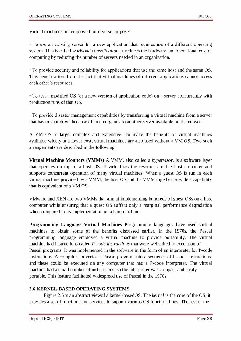
Virtual machines are employed for diverse purposes:
• To use an existing server for a new application that requires use of a different operating
system. This is called workload consolidation; it reduces the hardware and operational cost of
computing by reducing the number of servers needed in an organization.
• To provide security and reliability for applications that use the same host and the same OS.
This benefit arises from the fact that virtual machines of different applications cannot access
each other‘s resources.
• To test a modified OS (or a new version of application code) on a server concurrently with
production runs of that OS.
• To provide disaster management capabilities by transferring a virtual machine from a server
that has to shut down because of an emergency to another server available on the network.
A VM OS is large, complex and expensive. To make the benefits of virtual machines
available widely at a lower cost, virtual machines are also used without a VM OS. Two such
arrangements are described in the following.
Virtual Machine Monitors (VMMs) A VMM, also called a hypervisor, is a software layer
that operates on top of a host OS. It virtualizes the resources of the host computer and
supports concurrent operation of many virtual machines. When a guest OS is run in each
virtual machine provided by a VMM, the host OS and the VMM together provide a capability
that is equivalent of a VM OS.
VMware and XEN are two VMMs that aim at implementing hundreds of guest OSs on a host
computer while ensuring that a guest OS suffers only a marginal performance degradation
when compared to its implementation on a bare machine.
Programming Language Virtual Machines Programming languages have used virtual
machines to obtain some of the benefits discussed earlier. In the 1970s, the Pascal
programming language employed a virtual machine to provide portability. The virtual
machine had instructions called P-code instructions that were wellsuited to execution of
Pascal programs. It was implemented in the software in the form of an interpreter for P-code
instructions. A compiler converted a Pascal program into a sequence of P-code instructions,
and these could be executed on any computer that had a P-code interpreter. The virtual
machine had a small number of instructions, so the interpreter was compact and easily
portable. This feature facilitated widespread use of Pascal in the 1970s.
2.6 KERNEL-BASED OPERATING SYSTEMS
Figure 2.6 is an abstract viewof a kernel-basedOS. The kernel is the core of the OS; it
provides a set of functions and services to support various OS functionalities. The rest of the

OPERATING SYSTEMS 10EC65
Dept of ECE, SJBIT Page 29
OS is organized as a set of nonkernel routines, which implement operations on processes and
resources that are of interest to users, and a user interface.
Figure 2.6 Structure of a kernel-based OS.
A system call may be made by the user interface to implement a user command, by a process
to invoke a service in the kernel, or by a nonkernel routine to invoke a function of the kernel.
For example, when a user issues a command to execute the program stored in some file, say
file alpha, the user interface makes a system call, and the interrupt servicing routine invokes a
nonkernel routine to set up execution of the program. The nonkernel routine would make
system calls to allocate memory for the program‘s execution, open file alpha, and load its
contents into the allocated memory area, followed by another system call to initiate operation
of the process that represents execution of the program. If a process wishes to create a child
process to execute the program in file alpha, it, too, would make a system call and identical
actions would follow.
The historical motivations for the kernel-based OS structure were portability of the OS and
convenience in the design and coding of nonkernel routines.
Portability of the OS is achieved by putting architecture-dependent parts of OS code—which
typically consist of mechanisms—in the kernel and keeping architecture-independent parts of
code outside it, so that the porting effort is limited only to porting of the kernel. The kernel is
typically monolithic to ensure efficiency; the nonkernel part of an OS may be monolithic, or
it may be further structured into layers.
Table 2.3 contains a sample list of functions and services offered by the kernel to support
various OS functionalities. These functions and services provide a set of abstractions to the
nonkernel routines; their use simplifies design and coding of nonkernel routines by reducing
the semantic gap faced by them.
For example, the I/O functions of Table 4.3 collectively implement the abstraction of virtual
devices. A process is another abstraction provided by the kernel.
Akernel-based design may suffer from stratification analogous to the layered
OS design because the code to implement an OS command may contain an architecture-
dependent part, which is typically a mechanism that would be included in the kernel, and an

OPERATING SYSTEMS 10EC65
Dept of ECE, SJBIT Page 30
architecture-independent part, which is typically the implementation of a policy that would be
kept outside the kernel.
These parts would have to communicate with one another through system calls, which would
add to OS overhead because of interrupt servicing actions. Consider the command to initiate
execution of the program in a file named alpha. As discussed earlier, the nonkernel routine
that implements the command would make four system calls to allocate memory, open file
alpha, load the program contained in it into memory, and initiate its execution, which would
incur considerable overhead. Some operating system designs reduce OS overhead by
including the architecture-independent part of a function‘s code also in the kernel.
Table 2.3 Typical Functions and Services Offered by the Kernel
Thus, the nonkernel routine that initiated execution of a program would become a part of the
kernel. Other such examples are process scheduling policies, I/O scheduling policies of
device drivers, and memory management policies. These inclusions reduce OS overhead;
however, they also reduce portability of the OS.
Kernel-based operating systems have poor extensibility because addition of a new
functionality to the OS may require changes in the functions and services offered by the
kernel.
2.6.1 Evolution of Kernel-Based Structure of Operating Systems
The structure of kernel-based operating systems evolved to offset some of its drawbacks.
Two steps in this evolution were dynamically loadable kernel modules and user-level device
drivers.
To provide dynamically loadable kernel modules, the kernel is designed as a set of modules
that interact among themselves through well-specified interfaces.

OPERATING SYSTEMS 10EC65
Dept of ECE, SJBIT Page 31
A base kernel consisting of a core set of modules is loaded when the system is booted. Other
modules, which conform to interfaces of the base kernel, are loaded when their functionalities
are needed, and are removed from memory when they are no longer needed. Use of loadable
modules conserves memory during OS operation because only required modules of the kernel
are in memory at any time. It also provides extensibility, as kernel modules can be modified
separately and new modules can be added to the kernel easily. Use of loadable kernel
modules has a few drawbacks too. Loading and removal of modules fragments memory,
so the kernel has to perform memory management actions to reduce its memory
requirement.
2.7 MICROKERNEL-BASED OPERATING SYSTEMS
Putting all architecture-dependent code of the OS into the kernel provides good portability.
However, in practice, kernels also include some architecture independent code. This feature
leads to several problems. It leads to a large kernel size, which detracts from the goal of
portability. It may also necessitate kernel modification to incorporate new features, which
causes low extensibility.
A large kernel supports a large number of system calls. Some of these calls may be used
rarely, and so their implementations across different versions of the kernel may not be tested
thoroughly. This compromises reliability of the OS.
The microkernel was developed in the early 1990s to overcome the problems concerning
portability, extensibility, and reliability of kernels. A microkernel is an essential core of OS
code, thus it contains only a subset of the mechanisms typically included in a kernel and
supports only a small number of system calls, which are heavily tested and used.
Figure 2.7 Structure of microkernel-based operating systems.
This feature enhances portability and reliability of the microkernel. Less essential parts of OS
code are outside the microkernel and use its services, hence these parts could be modified
without affecting the kernel; in principle, these modifications could be made without having
to reboot the OS! The services provided in a microkernel are not biased toward any specific
features or policies in an OS, so new functionalities and features could be added to the OS to
suit specific operating environments.

OPERATING SYSTEMS 10EC65
Dept of ECE, SJBIT Page 32
Figure 2.7 illustrates the structure of a microkernel-based OS. The microkernel includes
mechanisms for process scheduling and memory management, etc., but does not include a
scheduler or memory handler. These functions are implemented as servers, which are simply
processes that never terminate. The servers and user processes operate on top of the
microkernel, which merely performs interrupt handling and provides communication between
the servers and user processes.
The small size and extensibility of microkernels are valuable properties for the embedded
systems environment, because operating systems need to be both small and fine-tuned to the
requirements of an embedded application. Extensibility of microkernels also conjures the
vision of using the same microkernel for a wide spectrum of computer systems, from palm-
held systems to large parallel and distributed systems. This vision has been realized to some
extent.
2.8 CASE STUDIES
2.8.1 Architecture of Unix
Unix is a kernel-based operating system. Figure 4.8 is a schematic diagram of the
Unix kernel. It consists of two main components—process management and file
management. The process management component consists of a module for interprocess
communication, which implements communication and synchronization between processes,
and the memory management and scheduling modules. The file management component
performs I/O through device drivers. Each device driver handles a specific class of I/O
devices and uses techniques like disk scheduling to ensure good throughput of an I/O device.
The buffer cache is used to reduce both the time required to implement a data transfer
between a process and an I/O device, and the number of I/O operations performed on devices
like disks
.
The process management and file management components of the kernel are activated
through interrupts raised in the hardware and system calls made by processes and nonkernel
routines of the OS. The user interface of the OS is a command interpreter, called a shell, that
runs as a user process. The Unix kernel cannot be interrupted at any arbitrary moment of
time; it can be interrupted only when a process executing kernel code exits, or when its
execution reaches a point at which it can be safely interrupted. This feature ensures that the
kernel data structures are not in an inconsistent state when an interrupt occurs and another
process starts executing the kernel code, which considerably simplifies coding of the kernel.
The Unix kernel has a long history of over four decades. The original kernel was small and
simple. It provided a small set of abstractions, simple but powerful features like the pipe
mechanism, which enabled users to execute several programs concurrently, and a small file
system that supported only one file organization called the byte stream organization. All
devices were represented as files, which unified the management of I/O devices and files.

OPERATING SYSTEMS 10EC65
Dept of ECE, SJBIT Page 33
Figure 2.8 Kernel of the Unix operating system.
The kernel was written in the C language and had a size of less than 100 KB. Hence it was
easily portable.
However, the Unix kernel was monolithic and not very extensible. So it had to be modified as
new computing environments, like the client–server environment, evolved. Interprocess
communication and threads were added to support client–server computing. Networking
support similarly required kernel modification.
2.8.2 The Kernel of Linux
The Linux operating system provides the functionalities of Unix System V and Unix
BSD; it is also compliant with the POSIX standard. It was initially implemented on the Intel
80386 and has since been implemented on later Intel processors and several other
architectures.
Linux has a monolithic kernel. The kernel is designed to consist of a set of individually
loadable modules. Each module has a well-specified interface that indicates how its
functionalities can be invoked and its data can be accessed by other modules. Conversely, the
interface also indicates the functions and data of other modules that are used by this module.
Each module can be individually loaded into memory, or removed from it, depending on
whether it is likely to be used in near future. In principle, any component of the kernel can be
structured as a loadable module, but typically device drivers become separate modules.
A few kernel modules are loaded when the system is booted. A new kernel module is loaded
dynamically when needed; however, it has to be integrated with the kernel modules that
already existed in memory so that the modules can collectively function as a monolithic
kernel. This integration is performed as follows: The kernel maintains a table in which it
records the addresses of functions and data that are defined in the modules existing in
memory. While loading a new module, the kernel analyzes its interface and finds which

OPERATING SYSTEMS 10EC65
Dept of ECE, SJBIT Page 34
functions and data of other modules it uses, obtains their addresses from the table, and inserts
them in appropriate instructions of the new module. At the end of this step, the kernel updates
its table by adding the addresses of functions and data defined in the new module.
Use of kernel modules with well-specified interfaces provides several advantages. Existence
of the module interface simplifies testing and maintenance of the kernel. An individual
module can be modified to provide new functionalities or enhance existing ones. This feature
overcomes the poor extensibility typically associated with monolithic kernels. Use of
loadable modules also limits the memory requirement of the kernel, because some modules
may not be loaded during an operation of the system. To enhance this advantage, the kernel
has a feature to automatically remove unwanted modules from memory—it produces an
interrupt periodically and checks which of its modules in memory have not been used since
the last such interrupt. These modules are delinked from the kernel and removed from
memory. Alternatively, modules can be individually loaded and removed from memory
through system calls.
The Linux 2.6 kernel, which was released in 2003, removed many of the limitations of the
Linux 2.5 kernel and also enhanced its capabilities in several ways. Two of the most
prominent improvements were in making the system more responsive and capable of
supporting embedded systems.Kernels up to Linux 2.5 were non-preemptible, so if the kernel
was engaged in performing a low-priority task, higher-priority tasks of the kernel were
delayed. The Linux 2.6 kernel is preemptible, which makes it more responsive to users and
application programs.
2.8.3 The Kernel of Solaris
Early operating systems for Sun computer systems were based on BSD Unix;
however, later development was based on Unix SVR4. The pre-SVR4 versions of the OS are
called SunOS, while the SVR4-based and later versions are called Solaris. Since the 1980s,
Sun has focused on networking and distributed computing; several networking and
distributed computing features of its operating systems have become industry standards, e.g.,
remote procedure calls (RPC), and a file system for distributed environments (NFS). Later,
Sun also focused on multiprocessor systems, which resulted in an emphasis on multithreading
the kernel, making it preemptible, and employing fast synchronization techniques in the
kernel.
The Solaris kernel has an abstract machine layer that supports a wide range of processor
architectures of the SPARC and Intel 80x86 family, including multiprocessor architectures.
The kernel is fully preemptible and provides real-time capabilities. Solaris 7 employs the
kernel-design methodology of dynamically loadable kernel modules. The kernel has a core
module that is always loaded; it contains interrupt servicing routines, system calls, process
and memory management, and a virtual file system framework that can support different file
systems concurrently. Other kernel modules are loaded and unloaded dynamically. Each

OPERATING SYSTEMS 10EC65
Dept of ECE, SJBIT Page 35
module contains information about other modules on which it depends and about other
modules that depend on it. The kernel maintains a symbol table containing information about
symbols defined in currently loaded kernel modules. This information is used while loading
and linking a new module. New information is added to the symbol table after a module is
loaded and some information is deleted after a module is deleted.
The Solaris kernel supports seven types of loadable modules:
• Scheduler classes
• File systems
• Loadable system calls
• Loaders for different formats of executable files
• Streams modules
• Bus controllers and device drivers
• Miscellaneous modules
Use of loadable kernel modules provides easy extensibility. Thus, new file systems, new
formats of executable files, new system calls, and new kinds of buses and devices can be
added easily. An interesting feature in the kernel is that when a new module is to be loaded,
the kernel creates a new thread for loading, linking, and initializing working of the new
module. This arrangement permits module loading to be performed concurrently with normal
operation of the kernel. It also permits loading of several modules to be performed
concurrently.
2.8.4 Architecture of Windows
Figure 2.9 shows architecture of the Windows OS. The hardware abstraction layer
(HAL) interfaces with the bare machine and provides abstractions of the I/O interfaces,
interrupt controllers, and interprocessor communication mechanisms in a multiprocessor
system. The kernel uses the abstractions provided by the HAL to provide basic services such
as interrupt processing and multiprocessor synchronization. This way, the kernel is shielded
from peculiarities of a specific architecture, which enhances its portability. The HAL and the
kernel are together equivalent to a conventional kernel. A device driver also uses the
abstractions provided by theHALto manage I/O operations on a class of devices.
The kernel performs the process synchronization and scheduling functions. The executive
comprises nonkernel routines of the OS; its code uses facilities in the kernel to provide
services such as process creation and termination, virtual memory management, an
interprocess message passing facility for client–server communication called the local
procedure call (LPC), I/O management and a file cache to provide efficient file I/O, and a
security reference monitor that performs file access validation. The I/O manager uses device
drivers, which are loaded dynamically when needed.
Many functions of the executive operate in the kernel mode, thus avoiding frequent context
switches when the executive interacts with the kernel; it has obvious performance benefits.

OPERATING SYSTEMS 10EC65
Dept of ECE, SJBIT Page 36
Figure 2.9 Architecture of Windows.
The environment subsystems provide support for execution of programs developed for other
operating systems like MS-DOS, Win32, and OS/2. Effectively, an environment subsystem is
analogous to a guest operating system within a virtual machine OS. It operates as a process
that keeps track of the state of user applications that use its services. To implement the
interface of a guest OS, each environment subsystem provides a dynamic link library (DLL)
and expects a user application to invoke the DLL when it needs a specific system service.
The DLL either implements the required service itself, passes the request for service to the
executive, or sends a message to the environment subsystem process to provide the service.
Recommended Questions
1. What are the problems associated with monolithic structure OS?
2. Explain i) layered structure of OS and ii) kernel based OS.
3. Describe the functions of an OS.
4. Discuss OS with monolithic structure and multi-programming system.
5. Explain with block diagram the structures of micro kernel based, time sharing and real
time OS classes.
6. Define process, process states and state transitions.
7. Explain VMOS. What are the advantages of virtual machines?
8. Explain system generation operations.
9. Compare kernel based and micro kernel based OS functions.
10. How is layered OS structure superior to monolithic structure?
11. In a batch processing system, the results of 1000 students are to be printed. Reading a
card or printing a result takes 100 ms whereas read/write operation in a disk needs
only 20 ms. Processing a record needs only 10 ms of CPU time. Compute the program
elapsed time and CPU idle time with and without spooling.

OPERATING SYSTEMS 10EC65
Dept of ECE, SJBIT Page 37
UNIT-3
PROCESS MANAGEMENT
The process concept helps to explain, understand and organize execution of programs in an
OS. A process is an execution of a program. The emphasis on 'an' implies that several
processes may represent executions of the same program. This situation arises when several
executions of a program are initiated, each with its own data, and when a program that is
coded using concurrent programming techniques is in execution.
A programmer uses processes to achieve execution of programs in a sequential or concurrent
manner as desired. An OS uses processes to organize execution of programs. Use of the
process concept enables an OS to execute both sequential and concurrent programs equally
easily.
A thread is an execution of a program that uses the environment of a process, that is. its code,
data and resources. If many threads use the environment of the same process, they share its
code, data and resources. An OS uses this fact to reduce its overhead while switching
between such threads.
3.1 PROCESSES AND PROGRAMS
A program is a passive entity that does not perform any actions by itself; it has to be executed
if the actions it calls for are to take place. A process is an execution of a program. It actually
performs the actions specified in a program. An operating system shares the CPU among
processes. This is how it gets user programs to execute.
3.1.1 What Is a Process?
To understand what a process is, let us discuss how the OS executes a program. Program P
shown in Figure 5.1(a) contains declarations of file info and a variable item, and statements
that read values from info, use them to perform some calculations, and print a result before
coming to a halt.
Figure 3.1 A program and an abstract view of its execution.

OPERATING SYSTEMS 10EC65
Dept of ECE, SJBIT Page 38
During execution, instructions of this program use values in its data area and the stack to
perform the intended calculations. Figure 3.1(b) shows an abstract view of its execution.
The instructions, data, and stack of program P constitute its address space. To realize
execution of P, the OS allocates memory to accommodate P‘s address space, allocates a
printer to print its results, sets up an arrangement through which P can access file info, and
schedules P for execution. The CPU is shown as a lightly shaded box because it is not always
executing instructions of P—the OS shares the CPU between execution of P and executions
of other programs.
3.1.2 Relationships between Processes and Programs
A program consists of a set of functions and procedures. During its execution, control flows
between the functions and procedures according to the logic of the program. Is an execution
of a function or procedure a process? This doubt leads to the obvious question: what is the
relationship between processes and programs?
The OS does not know anything about the nature of a program, including functions and
procedures in its code. It knows only what it is told through system calls. The rest is under
control of the program. Thus functions of a program may be separate processes, or they may
constitute the code part of a single process.
Table 3.1 shows two kinds of relationships that can exist between processes and programs. A
one-to-one relationship exists when a single execution of a sequential program is in progress,
for example, execution of program P in Figure 3.1. A many-to-one relationship exists
between many processes and a program in two cases: Many executions of a program may be
in progress at the same time; processes representing these executions have a many-to-one
relationship with the program. During execution, a program may make a system call to
request that a specific part of its code should be executed concurrently, i.e., as a separate
activity occurring at the same time. The kernel sets up execution of the specified part of the
code and treats it as a separate process. The new process and the process representing
execution of the program have a many-to-one relationship with the program. We call such a
program a concurrent program.
Processes that coexist in the system at some time are called concurrent processes.
Table 3.1 Relationships between Processes and Programs
Relationship Examples

OPERATING SYSTEMS 10EC65
Dept of ECE, SJBIT Page 39
Concurrent processes may share their code, data and resources with other processes; they
have opportunities to interact with one another during their execution.
3.1.3 Child Processes
The kernel initiates an execution of a program by creating a process for it. For lack of a
technical term for this process, we will call it the primary process for the program execution.
The primary process may make system calls as described in the previous section to create
other processes—these processes become its child processes, and the primary process
becomes their parent.
A child process may itself create other processes, and so on. The parent–child relationships
between these processes can be represented in the form of a process tree, which has the
primary process as its root. A child process may inherit some of the resources of its parent; it
could obtain additional resources during its operation through system calls.
Typically, a process creates one or more child processes and delegates some of its work to
each of them. It is called multitasking within an application. It has the three benefits
summarized in Table 3.2. Creation of child processes has the same benefits as the use of
multiprogramming in an OS—the kernel may be able to interleave operation of I/O-bound
and CPU-bound processes in the application, which may lead to a reduction in the duration,
i.e., running time, of an application. It is called computation speedup. Most operating systems
permit a parent process to assign priorities to child processes. A real-time application can
assign a high priority to a child process that performs a critical function to ensure that its
response requirement is met.
The third benefit, namely, guarding a parent process against errors in a child process, arises
as follows: Consider a process that has to invoke an untrusted code.
Table 3.2 Benefits of Child Processes

OPERATING SYSTEMS 10EC65
Dept of ECE, SJBIT Page 40
If the untrusted code were to be included in the code of the process, an error in the untrusted
code would compel the kernel to abort the process; however, if the process were to create a
child process to execute the untrusted code, the same error would lead to the abort of the
child process, so the parent process would not come to any harm. The OS command
interpreter uses this feature to advantage. The command interpreter itself runs as a process,
and creates a child process whenever it has to execute a user program. This way, its own
operation is not harmed by malfunctions in the user program.
Programmer view of processes
Child Processes in a Real-Time Application
Example 3.1
The real-time data logging application of Section 3.7 receives data samples from a satellite at
the rate of 500 samples per second and stores them in a file. We assume that each sample
arriving from the satellite is put into a special register of the computer. The primary process
of the application, which we will call the data_logger process, has to perform the following
three functions:
1. Copy the sample from the special register into memory.
2. Copy the sample from memory into a file.
3. Perform some analysis of a sample and record its results into another file used for future
processing.
It creates three child processes named copy_sample, record_sample, and housekeeping,
leading to the process tree shown in Figure 3.2(a). Note that a process is depicted by a circle
and a parent–child relationship is depicted by an arrow. As shown in Figure 3.2(b),
copy_sample copies the sample from the register into a memory area named buffer_area that
can hold, say, 50 samples. record_sample writes a sample from buffer_area into a file.
housekeeping analyzes a sample from buffer_area and records its results in another file.
Arrival of a new sample causes an interrupt, and a programmer-defined interrupt servicing
routine is associated with this interrupt. The kernel executes this routine whenever a new
sample arrives. It activates copy_sample.
Operation of the three processes can overlap as follows: copy_sample can copy a sample into
buffer_area, record_sample can write a previous sample to the file, while housekeeping can
analyze it and write its results into the other file. This arrangement provides a smaller worst-
case response time of the application than if these functions were to be executed sequentially.
So long as buffer_area has some free space, only copy_sample has to complete before the
next sample arrives. The other processes can be executed later. This possibility is exploited
by assigning the highest priority to copy_sample.
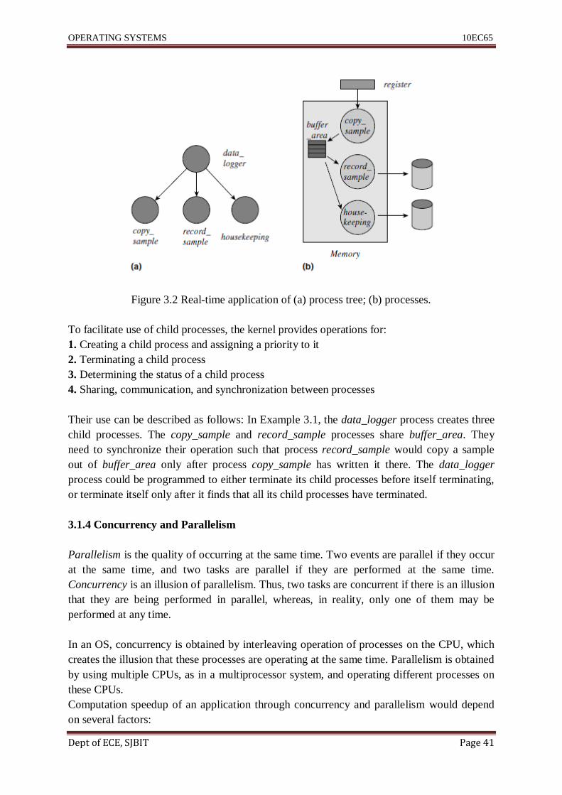
OPERATING SYSTEMS 10EC65
Dept of ECE, SJBIT Page 41
Figure 3.2 Real-time application of (a) process tree; (b) processes.
To facilitate use of child processes, the kernel provides operations for:
1. Creating a child process and assigning a priority to it
2. Terminating a child process
3. Determining the status of a child process
4. Sharing, communication, and synchronization between processes
Their use can be described as follows: In Example 3.1, the data_logger process creates three
child processes. The copy_sample and record_sample processes share buffer_area. They
need to synchronize their operation such that process record_sample would copy a sample
out of buffer_area only after process copy_sample has written it there. The data_logger
process could be programmed to either terminate its child processes before itself terminating,
or terminate itself only after it finds that all its child processes have terminated.
3.1.4 Concurrency and Parallelism
Parallelism is the quality of occurring at the same time. Two events are parallel if they occur
at the same time, and two tasks are parallel if they are performed at the same time.
Concurrency is an illusion of parallelism. Thus, two tasks are concurrent if there is an illusion
that they are being performed in parallel, whereas, in reality, only one of them may be
performed at any time.
In an OS, concurrency is obtained by interleaving operation of processes on the CPU, which
creates the illusion that these processes are operating at the same time. Parallelism is obtained
by using multiple CPUs, as in a multiprocessor system, and operating different processes on
these CPUs.
Computation speedup of an application through concurrency and parallelism would depend
on several factors:

OPERATING SYSTEMS 10EC65
Dept of ECE, SJBIT Page 42
• Inherent parallelism within the application: Does the application have activities that can
progress independently of one another.
• Overhead of concurrency and parallelism: The overhead of setting up and managing
concurrency should not predominate over the benefits of performing activities concurrently,
e.g., if the chunks of work sought to be performed concurrently are too small, the overhead of
concurrency may swamp its contributions to computation speedup.
• Model of concurrency and parallelism supported by the OS: How much overhead does the
model incur, and how much of the inherent parallelism within an application can be exploited
through it.
3.2 IMPLEMENTING PROCESSES
In the operating system‘s view, a process is a unit of computational work. Hence the kernel‘s
primary task is to control operation of processes to provide effective utilization of the
computer system. Accordingly, the kernel allocates resources to a process, protects the
process and its resources from interference by other processes, and ensures that the process
gets to use the CPU until it completes its operation.
Figure 3.3 Fundamental functions of the kernel for controlling processes.
The kernel is activated when an event, which is a situation that requires the kernel‘s attention,
leads to either a hardware interrupt or a system call. The kernel now performs four
fundamental functions to control operation of processes (see Figure 5.3):
1. Context save: Saving CPU state and information concerning resources of the process
whose operation is interrupted.

OPERATING SYSTEMS 10EC65
Dept of ECE, SJBIT Page 43
2. Event handling: Analyzing the condition that led to an interrupt, or the request by a process
that led to a system call, and taking appropriate actions.
3. Scheduling: Selecting the process to be executed next on the CPU.
4. Dispatching: Setting up access to resources of the scheduled process and loading its saved
CPU state in the CPU to begin or resume its operation.
The kernel performs the context save function to save information concerning the interrupted
process. It is followed by execution of an appropriate event handling routine, which may
inhibit further operation of the interrupted process,
e.g., if this process has made a system call to start an I/O operation, or may enable operation
of some other process, e.g., if the interrupt was caused by completion of its I/O operation.
The kernel now performs the scheduling function to select a process and the dispatching
function to begin or resume its operation.
3.2.1 Process States and State Transitions
An operating system uses the notion of a process state to keep track of what a process is
doing at any moment.
The kernel uses process states to simplify its own functioning, so the number of process states
and their names may vary across OSs. However, most OSs use the four fundamental states
described in Table 3.3. The kernel considers a process to be in the blocked state if it has made
a resource request and the request is yet to be granted, or if it is waiting for some event to
occur. A CPU should not be allocated to such a process until its wait is complete. The kernel
would change the state of the process to ready when the request is granted or the event for
which it is waiting occurs. Such a process can be considered for scheduling. The kernel
would change the state of the process to running when it is dispatched. The state would be
changed to terminated when execution of the process completes or when it is aborted by the
kernel for some reason.
A conventional computer system contains only one CPU, and so at most one process can be
in the running state. There can be any number of processes in the blocked, ready, and
terminated states. An OS may define more process states to simplify its own functioning or to
support additional functionalities like swapping.

OPERATING SYSTEMS 10EC65
Dept of ECE, SJBIT Page 44
Table 3.3 Fundamental Process States
Process State Transitions A state transition for a process Pi is a change in its state. A state
transition is caused by the occurrence of some event such as the start or end of an I/O
operation. When the event occurs, the kernel determines its influence on activities in
processes, and accordingly changes the state of an affected process.
When a process Pi in the running state makes an I/O request, its state has to be changed to
blocked until its I/O operation completes. At the end of the I/O operation, Pi ‘s state is
changed from blocked to ready because it now wishes to use the CPU. Similar state changes
are made when a process makes some request that cannot immediately be satisfied by the OS.
The process state is changed to blocked when the request is made, i.e., when the request event
occurs, and it is changed to ready when the request is satisfied. The state of a ready process is
changed to running when it is dispatched, and the state of a running process is changed to
ready when it is preempted either because a higher-priority process became ready or because
its time slice elapsed. Table 3.4 summarizes causes of state transitions.
Figure 3.4 diagrams the fundamental state transitions for a process. A new process is put in
the ready state after resources required by it have been allocated. It may enter the running,
blocked, and ready states a number of times as a result of events described in Table 3.4.
Eventually it enters the terminated state.

OPERATING SYSTEMS 10EC65
Dept of ECE, SJBIT Page 45
Table 3.4 Causes of Fundamental State Transitions for a Process

OPERATING SYSTEMS 10EC65
Dept of ECE, SJBIT Page 46
3.2.1.1 Suspended Processes
A kernel needs additional states to describe the nature of the activity of a process that is not in
one of the four fundamental states described earlier.
Figure 3.4 Fundamental state transitions for a process.
Table 3.5 Process State Transitions in a Time-Sharing System
Consider a process that was in the ready or the blocked state when it got swapped out of
memory. The process needs to be swapped back into memory before it can resume its
activity. Hence it is no longer in the ready or blocked state; the kernel must define a new state
for it. We call such a process a suspended process. If a user indicates that his process should
not be considered for scheduling for a specific period of time, it, too, would become a
suspended process. When a suspended process is to resume its old activity, it should go back
to the state it was in when it was suspended. To facilitate this state transition, the kernel may
define many suspend states and put a suspended process into the appropriate suspend state.
We restrict the discussion of suspended processes to swapped processes and use two suspend
states called ready swapped and blocked swapped. Accordingly, Figure 3.5 shows process

OPERATING SYSTEMS 10EC65
Dept of ECE, SJBIT Page 47
states and state transitions. The transition ready → ready swapped or blocked → blocked
swapped is caused by a swap-out action.
The reverse state transition takes place when the process is swapped back into memory. The
blocked swapped → ready swapped transition takes place if the request for which the process
was waiting is granted even while the process is in a suspended state, for example, if a
resource for which it was blocked is granted to it. However, the process continues to be
swapped out.
Figure 3.5 Process states and state transitions using two swapped states.
When it is swapped back into memory, its state changes to ready and it competes with other
ready processes for the CPU. A new process is put either in the ready state or in the ready
swapped state depending on availability of memory.
3.2.2 Process Context and the Process Control Block
The kernel allocates resources to a process and schedules it for use of the CPU. Accordingly,
the kernel‘s view of a process consists of two parts:
• Code, data, and stack of the process, and information concerning memory and other
resources, such as files, allocated to it.

OPERATING SYSTEMS 10EC65
Dept of ECE, SJBIT Page 48
• Information concerning execution of a program, such as the process state, the CPU state
including the stack pointer, and some other items of information described later in this
section.
These two parts of the kernel‘s view are contained in the process context and the process
control block (PCB), respectively (see Figure 3.6). This arrangement enables different OS
modules to access relevant process-related information conveniently and efficiently.
Process Context The process context consists of the following:
1. Address space of the process: The code, data, and stack components of the Process.
2. Memory allocation information: Information concerning memory areas allocated to a
process. This information is used by the memory management unit (MMU) during operation
of the process.
3. Status of file processing activities: Information about files being used, such as current
positions in the files.
Figure 5.6 Kernel‘s view of a process.
4. Process interaction information: Information necessary to control interaction of the
process with other processes, e.g., ids of parent and child processes, and interprocess
messages sent to it that have not yet been delivered to it.
5. Resource information: Information concerning resources allocated to the process.
6. Miscellaneous information: Miscellaneous information needed for operation of a process.
The OS creates a process context by allocating memory to the process, loading the process
code in the allocated memory and setting up its data space. Information concerning resources
allocated to the process and its interaction with other processes is maintained in the process
context throughout the life of the process.

OPERATING SYSTEMS 10EC65
Dept of ECE, SJBIT Page 49
This information changes as a result of actions like file open and close and creation and
destruction of data by the process during its operation.
Process Control Block (PCB) The process control block (PCB) of a process contains three
kinds of information concerning the process—identification information such as the process
id, id of its parent process, and id of the user who created it; process state information such as
its state, and the contents of the PSW and the general-purpose registers (GPRs); and
information that is useful in controlling its operation, such as its priority, and its interaction
with other processes. It also contains a pointer field that is used by the kernel to form PCB
lists for scheduling, e.g., a list of ready processes. Table 5.6 describes the fields of the PCB
data structure.
The priority and state information is used by the scheduler. It passes the id of the selected
process to the dispatcher. For a process that is not in the running state, the PSW and GPRs
fields together contain the CPU state of the process when it last got blocked or was pre-
empted. Operation of the process can be resumed by simply loading this information from its
PCB into the CPU. This action would be performed when this process is to be dispatched.
When a process becomes blocked, it is important to remember the reason. It is done by noting
the cause of blocking, such as a resource request or an
Table 5.6 Fields of the Process Control Block (PCB)

OPERATING SYSTEMS 10EC65
Dept of ECE, SJBIT Page 50
I/O operation, in the event information field of the PCB. Consider a process Pi that is blocked
on an I/O operation on device d. The event information field in Pi ‘s PCB indicates that it
awaits end of an I/O operation on device d. When the I/O operation on device d completes,
the kernel uses this information to make the transition blocked→ready for process Pi .
3.2.3 Context Save, Scheduling, and Dispatching
The context save function performs housekeeping whenever an event occurs. It saves the
CPU state of the interrupted process in its PCB, and saves information concerning its context.
The interrupted process would have been in the running state before the event occurred. The
context save function changes its state to ready. The event handler may later change the
interrupted process‘s state to blocked, e.g., if the current event was a request for I/O initiation
by the interrupted processes itself.
The scheduling function uses the process state information from PCBs to select a ready
process for execution and passes its id to the dispatching function.
The dispatching function sets up the context of the selected process, changes its state to
running, and loads the saved CPU state from its PCB into the CPU.
To prevent loss of protection, it flushes the address translation buffers used by the memory
management unit (MMU). Example 5.3 illustrates the context save, scheduling, and
dispatching functions in an OS using priority-based scheduling.
Process Switching
Switching between processes also occurs when a running process becomes blocked as a result
of a request or gets pre-empted at the end of a time slice. An event does not lead to switching
between processes if occurrence of the event either (1) causes a state transition only in a
process whose priority is lower than that of the process whose operation is interrupted by the
event or (2) does not cause any state transition, e.g., if the event is caused by a request that is
immediately satisfied. In the former case, the scheduling function selects the interrupted
process itself for dispatching. In the latter case, scheduling need not be performed at all; the
dispatching function could simply change the state of the interrupted process back to running
and dispatch it.
Switching between processes involves more than saving the CPU state of one process and
loading the CPU state of another process. The process context needs to be switched as well.
We use the term state information of a process to refer to all the information that needs to be
saved and restored during process switching. Process switching overhead depends on the size
of the state information of a process. Some computer systems provide special instructions to
reduce the process switching overhead, e.g., instructions that save or load the PSW and all
general-purpose registers, or flush the address translation buffers used by the memory
management unit (MMU).

OPERATING SYSTEMS 10EC65
Dept of ECE, SJBIT Page 51
Process switching has some indirect overhead as well. The newly scheduled process may not
have any part of its address space in the cache, and so it may perform poorly until it builds
sufficient information in the cache. Virtual memory operation is also poorer initially because
address translation buffers in the MMU do not contain any information relevant to the newly
scheduled process.
3.2.4 Event Handling
The following events occur during the operation of an OS:
1. Process creation event: A new process is created.
2. Process termination event: A process completes its operation.
3. Timer event: The timer interrupt occurs.
4. Resource request event: Process makes a resource request.
5. Resource release event: A process releases a resource.
6. I/O initiation request event: Process wishes to initiate an I/O operation.
7. I/O completion event: An I/O operation completes.
8. Message send event: A message is sent by one process to another.
9. Message receive event: A message is received by a process.
10. Signal send event: A signal is sent by one process to another.
11. Signal receive event: A signal is received by a process.
12. A program interrupt: The current instruction in the running process malfunctions.
13. A hardware malfunction event: A unit in the computer‘s hardware malfunctions.
The timer, I/O completion, and hardware malfunction events are caused by situations that are
external to the running process. All other events are caused by actions in the running process.
The kernel performs a standard action like aborting the running process when
events 12 or 13 occur.
Events Pertaining to Process Creation, Termination, and Preemption
When a user issues a command to execute a program, the command interpreter of the user
interface makes a create_ process system call with the name of the program as a
parameter.When a process wishes to create a child process to execute a program, it itself
makes a create_ process system call with the name of the program as a parameter.
The event handling routine for the create_ process system call creates a PCB for the new
process, assigns a unique process id and a priority to it, and puts this information and id of the
parent process into relevant fields of the PCB. It now determines the amount of memory
required to accommodate the address space of the process, i.e., the code and data of the
program to be executed and its stack, and arranges to allocate this much memory to the
process (memory allocation techniques are discussed later in Chapters 11 and 12). In most
operating systems, some standard resources are associated with each process, e.g., a
keyboard, and standard input and output files; the kernel allocates these standard resources to
the process at this time. It now enters information about allocated memory and resources into
the context of the new process. After completing these chores, it sets the state of the process
to ready in its PCB and enters this process in an appropriate PCB list.

OPERATING SYSTEMS 10EC65
Dept of ECE, SJBIT Page 52
When a process makes a system call to terminate itself or terminate a child process, the
kernel delays termination until the I/O operations that were initiated by the process are
completed. It now releases the memory and resources allocated to it. This function is
performed by using the information in appropriate fields of the process context. The kernel
now changes the state of the process to terminated.
The parent of the process may wish to check its status sometime in future, so the PCB of the
terminated process is not destroyed now; it will be done sometime after the parent process
has checked its status or has itself terminated. If the parent of the process is already waiting
for its termination, the kernel must activate the parent process. To perform this action, the
kernel takes the id of the parent process from the PCB of the terminated process, and checks
the event information field of the parent process‘s PCB to find whether the parent process is
waiting for termination of the child process.
The process in the running state should be preempted if its time slice elapses. The context
save function would have already changed the state of the running process to ready before
invoking the event handler for timer interrupts, so the event handler simply moves the PCB of
the process to an appropriate scheduling list. Preemption should also occur when a higher-
priority process becomes ready, but that is realized implicitly when the higher-priority
process is scheduled so an event handler need not perform any explicit action for it.
Events Pertaining to Resource Utilization When a process requests a resource through a
system call, the kernel may be able to allocate the resource immediately, in which case event
handling does not cause any process state transitions, so the kernel can skip scheduling and
directly invoke the dispatching function to resume operation of the interrupted process. If the
resource cannot be allocated, the event handler changes the state of the interrupted process to
blocked and notes the id of the required resource in the event information field of the
PCB.When a process releases a resource through a system call, the event handler need not
change the state of the process that made the system call. However, it should check whether
any other processes were blocked because they needed the resource, and, if so, it should
allocate the resource to one of the blocked processes and change its state to ready. This action
requires a special arrangement that we will discuss shortly.
A system call to request initiation of an I/O operation and an interrupt signaling end of the
I/O operation lead to analogous event handling actions.
The state of the process is changed to blocked when the I/O operation is initiated and the
cause of blocking is noted in the event information field of its PCB; its state is changed back
to ready when the I/O operation completes. A request to receive a message from another
process and a request to send a message to another process also lead to analogous actions.
Event Control Block (ECB) When an event occurs, the kernel must find the process whose
state is affected by it. For example, when an I/O completion interrupt occurs, the kernel must
identify the process awaiting its completion.

OPERATING SYSTEMS 10EC65
Dept of ECE, SJBIT Page 53
It can achieve this by searching the event information field of the PCBs of all processes.
Figure 3.7 Event control block (ECB).
This search is expensive, so operating systems use various schemes to speed it up. We
discuss a scheme that uses event control blocks (ECBs). As shown in Figure 3.7, an ECB
contains three fields. The event description field describes an event, and the process id field
contains the id of the process awaiting the event. When a process Pi gets blocked for
occurrence of an event ei , the kernel forms an ECB and puts relevant information concerning
ei and Pi into it. The kernel can maintain a separate ECB list for each class of events like
interprocess messages or I/O operations, so the ECB pointer field is used to enter the newly
created ECB into an appropriate list of ECBs.
Summary of Event Handling Figure 3.9 illustrates event handling actions of the kernel
described earlier. The block action always changes the state of the process that made a system
call from ready to blocked. The unblock action finds a process whose request can be fulfilled
now and changes its state from blocked to ready. A system call for requesting a resource
leads to a block action if the resource cannot be allocated to the requesting process. This
action is followed by scheduling and dispatching because another process has to be selected
for use of the CPU. The block action is not performed if the resource can be allocated
straightaway. In this case, the interrupted process is simply dispatched again.
Figure 3.8 PCB-ECB interrelationship.

OPERATING SYSTEMS 10EC65
Dept of ECE, SJBIT Page 54
Figure 3.9 Event handling actions of the kernel.
When a process releases a resource, an unblock action is performed if some other process is
waiting for the released resource, followed by scheduling and dispatching because the
unblocked process may have a higher priority than the process that released the resource.
Again, scheduling is skipped if no process is unblocked because of the event.
3.2.5 Sharing, Communication, and Synchronization between Processes
Processes of an application need to interact with one another because they work toward a
common goal. Table 3.7 describes four kinds of process interaction. We summarize their
important features in the following.
Data Sharing A shared variable may get inconsistent values if many processes update it
concurrently. For example, if two processes concurrently execute the statement a:= a+1,
where a is a shared variable, the result may depend on the way the kernel interleaves their
execution—the value of a may be incremented by only 1. To avoid this problem, only one
process should access shared data at any time, so a data access in one process may have to be
delayed if another process is accessing the data. This is called mutual exclusion. Thus, data
sharing by concurrent processes incurs the overhead of mutual exclusion.

OPERATING SYSTEMS 10EC65
Dept of ECE, SJBIT Page 55
Message Passing A process may send some information to another process in the form of a
message. The other process can copy the information into its own data structures and use it.
Both the sender and the receiver process must anticipate the information exchange, i.e., a
process must know when it is expected to send or receive a message, so the information
exchange becomes a part of the convention or protocol between processes.
Synchronization The logic of a program may require that an action ai should be performed
only after some action aj has been performed. Synchronization between processes is required
if these actions are performed in different processes—the process that wishes to perform
action ai is made to wait until another process performs action aj .
Signals A signal is used to convey an exceptional situation to a process so that it may
handlethe situation through appropriate actions. The code that a process wishes to execute on
receiving a signal is called a signal handler. The signal mechanism is modeled along the lines
of interrupts. Thus, when a signal is sent to a process, the kernel interrupts operation of the
process and executes a signal handler, if one has been specified by the process; otherwise, it
may perform a default action. Operating systems differ in the way they resume a process after
executing a signal handler.
Table 3.7 Four Kinds of Process Interaction
3.2.6 Signals
A signal is used to notify an exceptional situation to a process and enable it to attend to it
immediately. A list of exceptional situations and associated signal names or signal numbers
are defined in an OS, e.g., CPU conditions like overflows, and conditions related to child
processes, resource utilization, or emergency communications from a user to a process. The
kernel sends a signal to a process when the corresponding exceptional situation occurs. Some
kinds of signals may also be sent by processes. A signal sent to a process because of a
condition in its own activity, such as an overflow condition in the CPU, is said to be a
synchronous signal, whereas that sent because of some other condition is said to be an
asynchronous signal.

OPERATING SYSTEMS 10EC65
Dept of ECE, SJBIT Page 56
To utilize signals, a process makes a register_handler system call specifying a routine that
should be executed when a specific signal is sent to it; this routine is called a signal handler.
If a process does not specify a signal handler for a signal, the kernel executes a default
handler that performs some standard actions like dumping the address space of the process
and aborting it.
Figure 3.10 Signal handling by process Pi : (a) registering a signal handler; (b) invoking a
signal handler.
Let process Pi get preempted when it was about to execute the instruction with address b1. A
little later, some process Pj makes the system call signal (Pi , sig1). The kernel locates the
PCB of Pi , obtains the address of its signal vectors area and locates the signal vector for sig1.
It nowarranges for process Pi to execute the signal handler starting at addresssh1before
resuming normal execution as follows: It obtains the address contained in the program
counter (PC) field of the saved state of Pi ,which is the address b1 because Pi was about
to execute the instruction with this address. It pushes this address on Pi ‘s stack, and puts the
address sh1 in the program counter field of the saved state of Pi .
This way, when process Pi is scheduled, it would execute the signal handler function with the
start address sh1. The last instruction of sh1 would pop the address b1 off the stack and pass
control to the instruction with address b1, which would resume normal operation of process
Pi. In effect, as shown by the broken arrows in Figure 3.10(b), Pi ‘s execution would be
diverted to the signal handler starting at address sh1, and it would be resumed after the signal
handler is executed.
3.3 THREADS
Applications use concurrent processes to speed up their operation. However,
switching between processes within an application incurs high process switching overhead
because the size of the process state information is large, so operating system designers
developed an alternative model of execution of a program, called a thread, that could provide

OPERATING SYSTEMS 10EC65
Dept of ECE, SJBIT Page 57
concurrency within an application with less overhead.
To understand the notion of threads, let us analyze process switching overhead and see where
a saving can be made. Process switching overhead has two components:
• Execution related overhead: The CPU state of the running process has to be saved and the
CPU state of the new process has to be loaded in the CPU. This overhead is unavoidable.
• Resource-use related overhead: The process context also has to be switched. It involves
switching of the information about resources allocated to the process, such as memory and
files, and interaction of the process with other processes. The large size of this information
adds to the process switching overhead.
Consider child processes Pi and Pj of the primary process of an application. These processes
inherit the context of their parent process. If none of these processes have allocated any
resources of their own, their context is identical; their state information differs only in their
CPU states and contents of their stacks. Consequently, while switching between Pi and Pj
,much of the saving and loading of process state information is redundant. Threads exploit
this feature to reduce the switching overhead.
A process creates a thread through a system call. The thread does not have resources of its
own, so it does not have a context; it operates by using the context of the process, and
accesses the resources of the process through it. We use the phrases ―thread(s) of a process‖
and ―parent process of a thread‖ to describe the relationship between a thread and the process
whose context it uses.
Figure 3.11 illustrates the relationship between threads and processes. In the abstract view of
Figure 3.11(a), processPi has three threads,which are represented by wavy lines inside the
circle representing process Pi . Figure 3.11(b) shows an implementation arrangement. Process
Pi has a context and a PCB. Each thread of Pi is an execution of a program, so it has its own
stack and a thread control block (TCB),which is analogous to the PCB and stores the
following information:
1. Thread scheduling information—thread id, priority and state.
2. CPU state, i.e., contents of the PSW and GPRs.
3. Pointer to PCB of parent process.
4. TCB pointer, which is used to make lists of TCBs for scheduling.
Use of threads effectively splits the process state into two parts—the resource state remains
with the process while an execution state, which is the CPU state, is associated with a thread.
The cost of concurrency within the context of a process is now merely replication of the
execution state for each thread. The execution states need to be switched during switching
between threads.
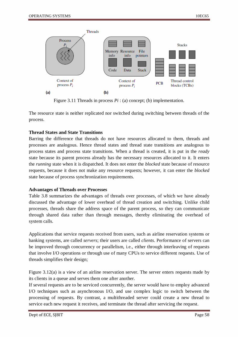
OPERATING SYSTEMS 10EC65
Dept of ECE, SJBIT Page 58
Figure 3.11 Threads in process Pi : (a) concept; (b) implementation.
The resource state is neither replicated nor switched during switching between threads of the
process.
Thread States and State Transitions
Barring the difference that threads do not have resources allocated to them, threads and
processes are analogous. Hence thread states and thread state transitions are analogous to
process states and process state transitions. When a thread is created, it is put in the ready
state because its parent process already has the necessary resources allocated to it. It enters
the running state when it is dispatched. It does not enter the blocked state because of resource
requests, because it does not make any resource requests; however, it can enter the blocked
state because of process synchronization requirements.
Advantages of Threads over Processes
Table 3.8 summarizes the advantages of threads over processes, of which we have already
discussed the advantage of lower overhead of thread creation and switching. Unlike child
processes, threads share the address space of the parent process, so they can communicate
through shared data rather than through messages, thereby eliminating the overhead of
system calls.
Applications that service requests received from users, such as airline reservation systems or
banking systems, are called servers; their users are called clients. Performance of servers can
be improved through concurrency or parallelism, i.e., either through interleaving of requests
that involve I/O operations or through use of many CPUs to service different requests. Use of
threads simplifies their design;
Figure 3.12(a) is a view of an airline reservation server. The server enters requests made by
its clients in a queue and serves them one after another.
If several requests are to be serviced concurrently, the server would have to employ advanced
I/O techniques such as asynchronous I/O, and use complex logic to switch between the
processing of requests. By contrast, a multithreaded server could create a new thread to
service each new request it receives, and terminate the thread after servicing the request.

OPERATING SYSTEMS 10EC65
Dept of ECE, SJBIT Page 59
Table 3.8 Advantages of Threads over Processes
Figure 3.12 Use of threads in structuring a server: (a) server using sequential code; (b)
multithreaded server; (c) server using a thread pool.
Coding for Use of Threads
Threads should ensure correctness of data sharing and synchronization. Action 5.3.1
describes features in the POSIX threads standard that can be used for this purpose.
Correctness of data sharing also has another facet. Functions or subroutines that use static or
global data to carry values across their successive activations may produce incorrect results
when invoked concurrently, because the invocations effectively share the global or static data
concurrently without mutual exclusion. Such routines are said to be thread unsafe. An
application that uses threads must be coded in a thread safe manner and must invoke routines
only from a thread safe library.
Signal handling requires special attention in a multithreaded application. When several
threads are created in a process, which thread should handle a signal? There are several
possibilities. The kernel may select one of the threads for signal handling. This choice can be
made either statically, e.g., either the first or the last thread created in the process, or
dynamically, e.g., the highest priority thread. Alternatively, the kernel may permit an
application to specify which thread should handle signals at any time.

OPERATING SYSTEMS 10EC65
Dept of ECE, SJBIT Page 60
A synchronous signal arises as a result of the activity of a thread, so it is best that the thread
itself handles it. Ideally, each thread should be able to specify which synchronous signals it is
interested in handling.
3.3.1 POSIX Threads
The ANSI/IEEE Portable Operating System Interface (POSIX) standard defines the
pthreads application program interface for use by C language programs. Popularly called
POSIX threads, this interface provides 60 routines that perform the following tasks:
• Thread management: Threads are managed through calls on thread library routines for
creation of threads, querying status of threads, normal or abnormal termination of threads,
waiting for termination of a thread, setting of scheduling attributes, and specifying thread
stack size.
• Assistance for data sharing: Data shared by threads may attain incorrect values if two or
more threads update it concurrently. A feature called mutex is provided to ensure mutual
exclusion between threads while accessing shared data, i.e., to ensure that only one thread is
accessing shared data at any time. Routines are provided to begin use of shared data in a
thread and indicate end of use of shared data. If threads are used in Example 5.5, threads
copy_sample and record_sample would use a mutex to ensure that they do not access and
update no_of_samples_in_buffer concurrently.
• Assistance for synchronization: Condition variables are provided to facilitate coordination
between threads so that they perform their actions in the desired order. If threads are used in
Figure 3.13 illustrates use of pthreads in the real-time data logging application. A pthread is
created through the call
pthread_create(< data structure >,< attributes >,
< start routine >,< arguments >)
where the thread data structure becomes the de facto thread id, and attributes indicate
scheduling priority and synchronization options. A thread terminates through a pthread_exit
call which takes a thread status as a parameter. Synchronization between the parent thread
and a child thread is performed through the pthread_join call, which takes a thread id and
some attributes as parameters. On issuing this call, the parent thread is blocked until the
thread indicated in the call has terminated; an error is raised if the termination status of the
thread does not match the attributes indicated in the pthread_join call. Some thread
implementations require a thread to be created with the attribute ―joinable‖ to qualify for such
synchronization. The code in Figure 3.13 creates three threads to perform the functions
performed by processes in Example 3.1. As mentioned above, and indicated through
comments in Figure 3.13, the threads would use the mutex buf_mutex to ensuremutually
exclusive access to the buffer and use condition variables buf_full and buf_empty to ensure
that they deposit samples into the buffer and take them out of the buffer in the correct order.
We do not show details of mutexes and condition variables here; they are discussed later in

OPERATING SYSTEMS 10EC65
Dept of ECE, SJBIT Page 61
3.3.2 Kernel-Level, User-Level, and Hybrid Threads
These three models of threads differ in the role of the process and the kernel in the creation
and management of threads. This difference has a significant impact on the overhead of
thread switching and the concurrency and parallelism within a process.
3.3.2.1 Kernel-Level Threads
A kernel-level thread is implemented by the kernel. Hence creation and termination of kernel-
level threads, and checking of their status, is performed through system calls. Figure 3.14
shows a schematic of how the kernel handles kernel-level threads. When a process makes a
create_thread system call, the kernel creates a thread, assigns an id to it, and allocates a
thread control block (TCB). The TCB contains a pointer to the PCB of the parent process of
the thread.
#include <pthread.h>
#include <stdio.h>
int size, buffer[100], no_of_samples_in_buffer;
int main()
{
pthread_t id1, id2, id3;
pthread_mutex_t buf_mutex, condition_mutex;
pthread_cond_t buf_full, buf_empty;
pthread_create(&id1, NULL, move_to_buffer, NULL);
pthread_create(&id2, NULL, write_into_file, NULL);
pthread_create(&id3, NULL, analysis, NULL);
pthread_join(id1, NULL);
pthread_join(id2, NULL);
pthread_join(id3, NULL);
pthread_exit(0);
}
void *move_to_buffer()
{
/* Repeat until all samples are received */
/* If no space in buffer, wait on buf_full */
/* Use buf_mutex to access the buffer, increment no. of samples */
/* Signal buf_empty */
pthread_exit(0);
}
void *write_into_file()
{
/* Repeat until all samples are written into the file */
/* If no data in buffer, wait on buf_empty */
/* Use buf_mutex to access the buffer, decrement no. of samples */
/* Signal buf_full */
pthread_exit(0);

OPERATING SYSTEMS 10EC65
Dept of ECE, SJBIT Page 62
}
void *analysis()
{
/* Repeat until all samples are analyzed */
/* Read a sample from the buffer and analyze it */
pthread_exit(0);
}
Figure 3.13 Outline of the data logging application using POSIX threads.
Figure 3.14 Scheduling of kernel-level threads.
TCB to check whether the selected thread belongs to a different process than the interrupted
thread. If so, it saves the context of the process to which the interrupted thread belongs, and
loads the context of the process to which the selected thread belongs. It then dispatches the
selected thread. However, actions to save and load the process context are skipped if both
threads belong to the same process. This feature reduces the switching overhead, hence
switching between kernel-level threads of a process could be as much as an order of
magnitude faster, i.e., 10 times faster, than switching between processes.
Advantages and Disadvantages of Kernel-Level Threads
A kernel-level thread is like a process except that it has a smaller amount of state
information. This similarity is convenient for programmers—programming for threads is no
different from programming for processes. In a multiprocessor system, kernel-level threads
provide parallelism, as many threads belonging to a process can be scheduled simultaneously,
which is not possible with the user-level threads described in the next section, so it provides
better computation speedup than user-level threads.
However, handling threads like processes has its disadvantages too. Switching between
threads is performed by the kernel as a result of event handling. Hence it incurs the overhead
of event handling even if the interrupted thread and the selected thread belong to the same
process. This feature limits the savings in the thread switching overhead.
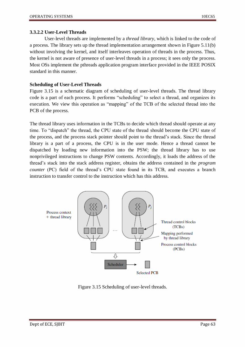
OPERATING SYSTEMS 10EC65
Dept of ECE, SJBIT Page 63
3.3.2.2 User-Level Threads
User-level threads are implemented by a thread library, which is linked to the code of
a process. The library sets up the thread implementation arrangement shown in Figure 5.11(b)
without involving the kernel, and itself interleaves operation of threads in the process. Thus,
the kernel is not aware of presence of user-level threads in a process; it sees only the process.
Most OSs implement the pthreads application program interface provided in the IEEE POSIX
standard in this manner.
Scheduling of User-Level Threads
Figure 3.15 is a schematic diagram of scheduling of user-level threads. The thread library
code is a part of each process. It performs ―scheduling‖ to select a thread, and organizes its
execution. We view this operation as ―mapping‖ of the TCB of the selected thread into the
PCB of the process.
The thread library uses information in the TCBs to decide which thread should operate at any
time. To ―dispatch‖ the thread, the CPU state of the thread should become the CPU state of
the process, and the process stack pointer should point to the thread‘s stack. Since the thread
library is a part of a process, the CPU is in the user mode. Hence a thread cannot be
dispatched by loading new information into the PSW; the thread library has to use
nonprivileged instructions to change PSW contents. Accordingly, it loads the address of the
thread‘s stack into the stack address register, obtains the address contained in the program
counter (PC) field of the thread‘s CPU state found in its TCB, and executes a branch
instruction to transfer control to the instruction which has this address.
Figure 3.15 Scheduling of user-level threads.

OPERATING SYSTEMS 10EC65
Dept of ECE, SJBIT Page 64
Advantages and Disadvantages of User-Level Threads
Thread synchronization and scheduling is implemented by the thread library. This
arrangement avoids the overhead of a system call for synchronization between threads, so the
thread switching overhead could be as much as an order of magnitude smaller than in
kernel-level threads.
Figure 3.16 Actions of the thread library (N,R,B indicate running, ready, and blocked).
This arrangement also enables each process to use a scheduling policy that best suits its
nature. A process implementing a real-time application may use priority-based scheduling of
its threads to meet its response requirements, whereas a process implementing a
multithreaded server may perform round-robin scheduling of its threads. However,
performance of an application would depend on whether scheduling of user-level threads
performed by the thread library is compatible with scheduling of processes performed by the
kernel.
For example, round-robin scheduling in the thread library would be compatible with either
round-robin scheduling or priority-based scheduling in the kernel, whereas priority-based
scheduling would be compatible only with priority-based scheduling in the kernel.
3.3.2.3 Hybrid Thread Models
A hybrid thread model has both user-level threads and kernel-level threads and a
method of associating user-level threads with kernel-level threads. Different methods of
associating user- and kernel-level threads provide different combinations of the low
switching overhead of user-level threads and the high concurrency and parallelism of kernel-
level threads.
Figure 3.17 illustrates three methods of associating user-level threads with kernel-level
threads. The thread library creates user-level threads in a process and associates a thread
control block (TCB) with each user-level thread. The kernel creates kernel-level threads in a
process and associates a kernel thread control block (KTCB) with each kernel-level thread. In

OPERATING SYSTEMS 10EC65
Dept of ECE, SJBIT Page 65
the many-to-one association method, a single kernel-level thread is created in a process by
the kernel and all userlevel threads created in a process by the thread library are associated
with this kernel-level thread. This method of association provides an effect similar to mere
user-level threads: User-level threads can be concurrent without being parallel, thread
switching incurs low overhead, and blocking of a user-level thread leads to blocking of all
threads in the process.
In the one-to-one method of association, each user-level thread is permanently mapped into a
kernel-level thread. This association provides an effect similar to mere kernel-level threads:
Threads can operate in parallel on different CPUs of a multiprocessor system; however,
switching between threads is performed at the kernel level and incurs high overhead.
Blocking of a user-level thread does not block other user-level threads of the process because
they are mapped into different kernel-level threads.
The many-to-many association method permits a user-level thread to be mapped into
different kernel-level threads at different times.
It provides parallelism between user-level threads that are mapped into different kernel-level
threads at the same time, and provides low overhead of switching between user-level threads
that are scheduled on the same kernel-level thread by the thread library. However, the many-
to-many association method requires a complex implementation.
Figure 3.17 (a) Many-to-one; (b) one-to-one; (c) many-to-many associations in hybrid
threads.

OPERATING SYSTEMS 10EC65
Dept of ECE, SJBIT Page 66
3.4 CASE STUDIES OF PROCESSES AND THREADS
3.4.1 Processes in Unix
Data Structures Unix uses two data structures to hold control data about processes:
• proc structure: Contains process id, process state, priority, information about relationships
with other processes, a descriptor of the event for which a blocked process is waiting, signal
handling mask, and memory management information.
• uarea (stands for ―user area‖): Contains a process control block, which stores the CPU state
for a blocked process; pointer to proc structure, user and group ids, and information
concerning the following: signal handlers, open files and the current directory, terminal
attached to the process, and CPU usage by the process.
These data structures together hold information analogous to the PCB data structure. The
proc structure mainly holds scheduling related data while the u area contains data related to
resource allocation and signal handling. The proc structure of a process is always held in
memory. The u area needs to be in memory only when the process is in operation.
Types of Processes Two types of processes exist in Unix—user processes and kernel
processes. A user process executes a user computation. It is associated with the user‘s
terminal. When a user initiates a program, the kernel creates the primary process for it, which
can create child processes. A daemon process is one that is detached from the user‘s terminal.
It runs in the background and typically performs functions on a system wide basis, e.g., print
spooling and network management. Once created, daemon processes can exist throughout the
lifetime of the OS. Kernel processes execute code of the kernel.
They are concerned with background activities of the kernel like swapping. They are created
automatically when the system is booted and they can invoke kernel functionalities or refer to
kernel data structures without having to perform a system call.
Process Creation and Termination The system call fork creates a child process and sets up
its context (called the user-level context in Unix literature). It allocates a proc structure for
the newly created process and marks its state as ready, and also allocates a u area for the
process. The kernel keeps track of the parent–child relationships using the proc structure. fork
returns the id of the child process.
The user-level context of the child process is a copy of the parent‘s user level context. Hence
the child executes the same code as the parent. At creation, the program counter of the child
process is set to contain the address of the instruction at which the fork call returns. The fork
call returns a 0 in the child process, which is the only difference between parent and child
processes. A child process can execute the same program as its parent, or it can use a system
call from the exec family of system calls to load some other program for execution. Although
this arrangement is cumbersome, it gives the child process an option of executing the parent‘s
code in the parent‘s context or choosing its own program for execution. The former

OPERATING SYSTEMS 10EC65
Dept of ECE, SJBIT Page 67
alternative was used in older Unix systems to set up servers that could service many user
requests concurrently.
The complete view of process creation and termination in Unix is as follows: After booting,
the system creates a process init. This process creates a child process for every terminal
connected to the system. After a sequence of exec calls, each child process starts running the
login shell. When a programmer indicates the name of a file from the command line, the shell
creates a new process that executes an exec call for the named file, in effect becoming the
primary process of the program. Thus the primary process is a child of the shell process. The
shell process now executes the wait system call described later in this section to wait for end
of the primary process of the program. Thus it becomes blocked until the program completes,
and becomes active again to accept the next user command. If a shell process performs an
exit call to terminate itself, init creates a new process for the terminal to run the login shell.
A process Pi can terminate itself through the exit system call exit (status_ code), where
status_code is a code indicating the termination status of the process. On receiving the exit
call the kernel saves the status code in the proc structure of Pi , closes all open files, releases
the memory allocated to the process, and destroys its u area. However, the proc structure is
retained until the parent of Pi destroys it. This way the parent of Pi can query its termination
status any time it wishes. In essence, the terminated process is dead but it exists, hence it is
called a zombie process. The exit call also sends a signal to the parent of Pi. The child
processes of Pi are made children of the kernel process init. This way init receives a signal
when a child of Pi, say Pc, terminates so that it can release Pc‘s proc structure.
Waiting for Process Termination A process Pi can wait for the termination of a child
process through the system call wait (addr(. . .)), where addr(. . .) is the address of a variable,
say variable xyz, within the address space of Pi . If process Pi has child processes and at least
one of them has already terminated, the wait call stores the termination status of a terminated
child process in xyz and immediately returns with the id of the terminated child process. If
more terminated child processes exist, their termination status will be made available to Pi
only when it repeats the wait call. The state of process Pi is changed to blocked if it has
children but none of them has terminated. It will be unblocked when one of the child
processes terminates. The wait call returns with a ―−1‖ if Pi has no children.
Waiting for Occurrence of Events A process that is blocked on an event is said to sleep on
it; e.g., a process that initiates an I/O operation would sleep on its completion event. Unix
uses an interesting arrangement to activate processes sleeping on an event. It does not use
event control blocks (ECBs); instead it uses event addresses. A set of addresses is reserved in
the kernel, and every event is mapped into one of these addresses. When a process wishes to
sleep on an event, the address of the event is computed, the state of the process is changed to
blocked, and the address of the event is put in its process structure. This address serves as the
description of the event awaited by the process. When the event occurs, the kernel computes
its event address and activates all processes sleeping on it.

OPERATING SYSTEMS 10EC65
Dept of ECE, SJBIT Page 68
main()
{
int saved_status;
for (i=0; i<3; i++)
{
if (fork()==0)
{ /* code for child processes */
...
exit();
}
}
while (wait(&saved_status) !=-1);
/* loop till all child processes terminate */
}
Figure 3.18 Process creation and termination in Unix.
Interrupt Servicing Unix avoids interrupts during sensitive kernel-level actions by assigning
each interrupt an interrupt priority level (ipl). Depending on the program being executed by
the CPU, an interrupt priority level is also associated with the CPU.When an interrupt at a
priority level l arises, it is handled only if l is larger than the interrupt priority level of the
CPU; otherwise, it is kept pending until the CPU‘s interrupt priority level becomes < l. The
kernel uses this feature to prevent inconsistency of the kernel data structures by raising the ipl
of the CPU to a high value before starting to update its data structures and lowering it after
the update is completed.
System Calls When a system call is made, the system call handler uses the system call
number to determine which system functionality is being invoked. From its internal tables it
knows the address of the handler for this functionality. It also knows the number of
parameters this call is supposed to take. However, these parameters exist on the user stack,
which is a part of the process context of the process making the call. So these parameters are
copied from the process stack into some standard place in the u area of the process before
control is passed to the handler for the specific call. This action simplifies operation of
individual event handlers.

OPERATING SYSTEMS 10EC65
Dept of ECE, SJBIT Page 69
Table 3.9 Interesting Signals in Unix
Process States and State Transitions
A process in the running state is put in the ready state the moment its execution is
interrupted. A system process then handles the event that caused the interrupt. If the running
process had itself caused a software interrupt by executing an <SI_instrn>, its state may
further change to blocked if its request cannot be granted immediately. In this model a user
process executes only user code; it does not need any special privileges. A system process
may have to use privileged instructions like I/O initiation and setting of memory protection
information, so the system process executes with the CPU in the kernel mode. Processes
behave differently in the Unix model. When a process makes a system call, the process itself
proceeds to execute the kernel code meant to handle the system call. To ensure that it has the
necessary privileges, it needs to execute with the CPU in the kernel mode. A mode change is
thus necessary every time a system call is made. The opposite mode change is necessary after
processing a system call. Similar mode changes are needed when a process starts executing
the interrupt servicing code in the kernel because of an interrupt, and when it returns
after servicing an interrupt.
The Unix kernel code is made reentrant so that many processes can execute it concurrently.
This feature takes care of the situation where a process gets blocked while executing kernel
code, e.g., when it makes a system call to initiate an I/O operation, or makes a request that
cannot be granted immediately. To ensure reentrancy of code, every process executing the
kernel code must use its own kernel stack. This stack contains the history of function
invocations since the time the process entered the kernel code. If another process also enters
the kernel code, the history of its function invocations will be maintained on its own kernel
stack. Thus, their operation would not interfere. In principle, the kernel stack of a process
need not be distinct from its user stack; however, distinct stacks are used in practice because
most computer architectures use different stacks when the CPU is in the kernel and user
modes.
Unix uses two distinct running states. These states are called user running and kernel running
states. A user process executes user code while in the user running state, and kernel
codewhile in the kernel running state. Itmakes the transition from user running to kernel

OPERATING SYSTEMS 10EC65
Dept of ECE, SJBIT Page 70
running when it makes a system call, or when an interrupt occurs. It may get blocked while in
the kernel running state because of an I/O operation or nonavailability of a resource.
Figure 3.19 Process state transitions in Unix.
Recommended Questions
1. List the different types of process interaction and explain them in brief.
2. What is a process? Describe the components of the process environment.
3. List the events that occur during the operation of an OS.
4. Explain in detail the programmer view of processes.
5. What is a process state? Explain the various states of a process giving state transition
diagram.
6. Explain event handling pertaining to a process.
7. Explain arrangement and working of threads in SOLARIS with a neat block diagram.
8. Explain with neat diagram i) user threads ii) kernel level threads.
9. With a neat diagram explain different states of a process and state transitions in the
UNIX OS.
10. Mention the three kinds of entities used for concurrency within a process in threads in
SOLARIS along with a diagram.
11. With a state transition diagram and PCB structure, explain the function of the states,
state transitions and functions of a schedule.
12. Explain the race condition in airline reservation system with an algorithm.

OPERATING SYSTEMS 10EC65
Dept of ECE, SJBIT Page 71
UNIT-4
Memory Management
The memory hierarchy comprises the cache, the memory management unit (MMU), random
access memory (RAM), which is simply called memory in this chapter, and a disk. We
discuss management of memory by the OS in two parts—this chapter discusses techniques
for efficient use of memory, whereas the next chapter discusses management of virtual
memory, which is part of the memory hierarchy consisting of the memory and the disk.
Memory binding is the association of memory addresses with instructions and data of a
program. To provide convenience and flexibility, memory binding is performed several times
to a program—the compiler and linker perform it statically, i.e., before program execution
begins, whereas the OS performs it dynamically, i.e., during execution of the program. The
kernel uses a model of memory allocation to a process that provides for both static and
dynamic memory binding.
The speed of memory allocation and efficient use of memory are the two fundamental
concerns in the design of a memory allocator. To ensure efficient use, the kernel recycles the
memory released by a process to other processes that need it. Memory fragmentation is a
problem that arises in memory reuse, leading to inefficient use of memory.
4.1 MANAGING THE MEMORY HIERARCHY A memory hierarchy comprises cache memories like the L1 and L3 caches, the
memory management unit (MMU), memory, and a disk. Its purpose is to create an illusion of
a fast and large memory at a low cost. The upper half of Figure 4.1 illustrates the memory
hierarchy.

OPERATING SYSTEMS 10EC65
Dept of ECE, SJBIT Page 72
Levels How managed Performance issues
Caches Allocation and use is managed Ensuring high hit ratios
by hardware
Memory Allocation is managed by the (1)Accommodating more process
kernel and use of allocated in memory,(2) Ensuring high hit
memory is managed by run-time ratios
libraries
Disk Allocation and use is managed Quick loading and storing of
by the kernel parts of process address spaces
Figure 4.1 Managing the memory hierarchy. CPU refers to the fastest memory, the cache,
when it needs to access an instruction or data. If the required instruction or data is not
available in the cache, it is fetched from the next lower level in the memory hierarchy, which
could be a slower cache or the random access memory (RAM), simply called memory in this
book. If the required instruction or data is also not available in the next lower level memory,
it is fetched there from a still lower level, and so on. Performance of a process depends on the
hit ratios in various levels of the memory hierarchy, where the hit ratio in a level indicates
what fraction of instructions or data bytes that were looked for in that level were actually
present in it.
The caches are managed entirely in the hardware. The kernel employs special techniques to
provide high cache hit ratios for a process. For example, the kernel switches between threads
of the same process whenever possible to benefit from presence of parts of the process
address space in the cache, and it employs affinity scheduling in a multiprocessor system (see
Section 10.5), to schedule a process on the same CPU every time to achieve high cache hit
ratios. Memory is managed jointly by the kernel and the run-time library of the programming
language in which the code of the process is written. The kernel allocates memory to user
processes. The primary performance concern in this function is accommodating more user
processes in memory, so that both system performance and user service would improve. The
kernel meets this concern through efficient reuse of memory when a process completes.
During operation, a process creates data structures within the memory already allocated to it
by the kernel. This function is actually performed by the run-time library. It employs
techniques that efficiently reuse memory when a process creates and destroys data structures
during its operation. Thus some of the concerns and techniques employed by the kernel and
the run-time libraries are similar. As a sequel to the kernel‘s focus on accommodating a large
number of processes in memory, the kernel may decide on keeping only a part of each
process‘s address space in memory. It is achieved by using the part of the memory hierarchy
called virtual memory that consists of memory and a disk (see the dashed box in Figure 4.1).
4.2 STATIC AND DYNAMIC MEMORY ALLOCATION
Memory allocation is an aspect of a more general action in software operation known as
binding. Two other actions related to a program—its linking and loading—are also aspects of
binding. Any entity in a program, e.g., a function or a variable, has a set of attributes, and
each attribute has a value. Binding is the act of specifying the value of an attribute. For
example, a variable in a program has attributes such as name, type, dimensionality, scope,
and memory address. A name binding specifies the variable‘s name and a type binding

OPERATING SYSTEMS 10EC65
Dept of ECE, SJBIT Page 73
specifies its type. Memory binding is the act of specifying the variable‘s memory address; it
constitutes memory allocation for the variable. Memory allocation to a process is the act of
specifying memory addresses of its instructions and data. A binding for an attribute of an
entity such as a function or a variable can be performed any time before the attribute is used.
Different binding methods perform the binding at different times. The exact time at which
binding is performed may determine the efficiency and flexibility with which the entity can
be used. Broadly speaking, we can differentiate between early binding and late binding. Late
binding is useful in cases where the OS or run-time library may have more information about
an entity at a later time, using which it may be able to perform a better quality binding. For
example, it may be able to achieve more efficient use of resources such as memory. Early and
late binding are represented by the two fundamental binding methods of static and dynamic
binding, respectively.
Static Binding A binding performed before the execution of a program (or operation of a
software system) is set in motion.
Dynamic Binding A binding performed during the execution of a program (or operation of a
software system).
Static memory allocation can be performed by a compiler, linker, or loader while a program
is being readied for execution. Dynamic memory allocation is performed in a ―lazy‖ manner
during the execution of a program; memory is allocated to a function or a variable just before
it is used for the first time. Static memory allocation to a process is possible only if sizes of
its data structures are known before its execution begins. If sizes are not known, they have to
be guessed; wrong estimates can lead to wastage of memory and lack of flexibility. For
example, consider an array whose size is not known during compilation. Memory is wasted if
we overestimate the array‘s size, whereas the process may not be able to operate correctly if
we underestimate its size. Dynamic memory allocation can avoid both these problems by
allocating a memory area whose size matches the actual size of the array, which would be
known by the time the allocation is performed. It can even permit the array size to vary
during operation of the process. However, dynamic memory allocation incurs the overhead of
memory allocation actions performed during operation of a process. Operating systems
choose static and dynamic memory allocation under different circumstances to obtain the best
combination of execution efficiency and memory efficiency. When sufficient information
about memory requirements is available a priori, the kernel or the run-time library makes
memory allocation decisions statically, which provides execution efficiency. When little
information is available a priori, the memory allocation decisions are made dynamically,
which incurs higher overhead but ensures efficient use of memory. In other situations, the
available information is used to make some decisions concerning memory allocation
statically, so that the overhead of dynamic memory allocation can be reduced.
4.3 EXECUTION OF PROGRAMS A program P written in a language L has to be transformed before it can be executed. Several
of these transformations perform memory binding—each one binds the instructions and data
of the program to a new set of addresses. Figure 4.2 is a schematic diagram of three
transformations performed on program P before it can be loaded in memory for execution.
• Compilation or assembly: A compiler or an assembler is generically called a translator. It
translates program P into an equivalent program in the object module form. This program
contains instructions in the machine language of the computer. While invoking the translator,

OPERATING SYSTEMS 10EC65
Dept of ECE, SJBIT Page 74
the user specifies the origin of the program, which is the address of its first instruction or
byte; otherwise, the translator assumes a default address, typically 0. The translator
accordingly assigns addresses to other instructions and data in the program and uses these
addresses as operand addresses in its instructions. The execution start address or simply the
start address of a program is the address of the instruction with which its execution is to
begin. It can be the same as the origin of the program, or it can be different. The addresses
assigned by the translator are called translated addresses. Thus, the translator binds
instructions and data in program P to translated addresses. An object module indicates the
translated origin of the program, its translated start address, and size.
• Linking: Program P may call other programs during its execution, e.g., functions from
mathematical libraries. These functions should be included in the program, and their start
addresses should be used in the function call instructions in P. This procedure is called
linking. It is achieved by selecting object modules for the called functions from one or more
libraries and merging them with program P.
Figure 4.2 Schematic diagram of transformation and execution of a program.
• Relocation: Some object module(s) merged with program P may have conflicting translated
time addresses. This conflict is resolved by changing the memory binding of the object
module(s); this action is called relocation of object modules. It involves changing addresses
of operands used in their instructions.
The relocation and linking functions are performed by a program called a linker. The
addresses assigned by it are called linked addresses. The user may specify the linked origin
for the program; otherwise, the linker assumes the linked origin to be the same as the
translated origin. In accordance with the linked origin and the relocation necessary to avoid
address conflicts, the linker binds instructions and data of the program to a set of linked
addresses. The resulting program, which is in a ready-to-execute program form called a
binary program, is stored in a library. The directory of the library stores its name, linked
origin, size, and the linked start address. A binary program has to be loaded in memory for
execution. This function is performed by the loader. If the start address of the memory area
where a program is to be loaded, which is called its load origin, differs from the linked origin
of program, the loader has to change its memory binding yet again. A loader possessing this
capability is called a relocating loader, whereas a loader without this capability is called an
absolute loader.
A Simple Assembly Language An assembly language statement has the following format:
[Label] <Opcode> <operand spec>,<operand spec>

OPERATING SYSTEMS 10EC65
Dept of ECE, SJBIT Page 75
The first operand is always a general-purpose-register (GPR)—AREG, BREG, CREG or
DREG. The second operand is either a GPR or a symbolic name that corresponds to a
memory byte. Self-explanatory opcodes like ADD and MULT are used to designate
arithmetic operations. The MOVER instruction moves a value from its memory operand to its
register operand, whereas the MOVEM instruction does the opposite. All arithmetic is
performed in a register and sets a condition code. The condition code can be tested by a
branch-on-condition (BC) instruction. The assembly statement corresponding to it has the
format BC <condition code spec>, <instruction address> where <condition code spec> is a
self-explanatory character string describing a condition, e.g., GT for > and EQ for =. The BC
instruction transfers control to the instruction with the address <instruction address> if the
current value of condition code matches<condition code spec>. For simplicity, we assume
that all addresses and constants are in decimal, and all instructions occupy 4 bytes. The sign
is not a part of an instruction.
Static and Dynamic Relocation of Programs
When a program is to be executed, the kernel allocates it a memory area that is large enough
to accommodate it, and invokes the loader with the name of the program and the load origin
as parameters. The loader loads the program in the memory allocated to it, relocates it using
the scheme illustrated in Example 4.1 if the linked origin is different from the load origin, and
passes it control for execution. This relocation is static relocation as it is performed before
execution of the program begins. Sometime after the program‘s execution has begun, the
kernel may wish to change the memory area allocated to it so that other programs can be
accommodated in memory. This time, the relocation has to be performed during execution of
the program, hence it constitutes dynamic relocation. Dynamic relocation can be performed
by suspending a program‘s execution, carrying out the relocation procedure described earlier,
and then resuming its execution. However, it would require information concerning the
translated origin and address-sensitive instructions to be available during the program‘s
execution. It would also incur the memory and processing costs described earlier. Some
computer architectures provide a relocation register to simplify dynamic relocation. The
relocation register is a special register in the CPU whose contents are added to every memory
address used during execution of a program. The result is another memory address, which is
actually used to make a memory reference. Thus,
Effective memory address = memory address used in the current
instruction + contents of relocation register
The following example illustrates how dynamic relocation of a program is achieved by using
the relocation register.
Example 4.2 Dynamic Relocation through Relocation Register A program has the linked origin of 50000, and it has also been loaded in the memory area
that has the start address of 50000. During its execution, it is to be shifted to the memory area
having the start address of 70000, so it has to be relocated to execute in this memory area.
This relocation is achieved simply by loading an appropriate value in the relocation register,
which is computed as follows:
Value to be loaded in relocation register
= start address of allocated memory area − linked origin of program
= 70000 − 50000 = 20000

OPERATING SYSTEMS 10EC65
Dept of ECE, SJBIT Page 76
Figure 4.4 Program relocation using a relocation register: (a) program; (b) its execution.
Consider execution of the Add instruction in the program shown in Figure 4.4(a). This
instruction has the linked address 55000 in the program and uses an operand whose linked
address is 65784. As a result of relocation, the program exists in the memory area starting
with the address 70000. Figure 11.4(b) shows the load addresses of its instructions and data;
the corresponding linked addresses are shownin parenthesis for easy reference. TheAdd
instruction exists in the location with address 75000. The address of its operand is 65784 and
the relocation register contains 20000, so during execution of the instruction, the effective
address of its operand is 65784 + 20000 = 85784. Hence the actual memory access is
performed at the address 85784.
4.3.2 Linking
An ENTRY statement in an assembly program indicates symbols that are defined in the
assembly program and may be referenced in some other assembly programs. Such symbols
are called entry points. An EXTRN statement in an assembly program indicates symbols that
are used in the assembly program but are defined in some other assembly program. These
symbols are called external symbols and uses of these symbols in the assembly program are
called external references. The assembler puts information about the ENTRY and EXTRN
statements in an object module for use by the linker.
Linking is the process of binding an external reference to the correct linked address. The
linker first scans all object modules being linked together to collect the names of all entry
points and their linked addresses. It stores this information in a table for its own use. It then
considers each external reference, obtains the linked address of the external symbol being
referenced from its table, and puts this address in the instruction containing the external
reference. This action is called resolution of an external reference. The next example
illustrates the steps in linking.
Static and Dynamic Linking/Loading The distinction between the terms linking and
loading has become blurred in modern operating systems. However, we use the terms as
follows: A linker links modules together to form an executable program. A loader loads a
program or a part of a program in memory for execution. In static linking, the linker links all
modules of a program before its execution begins; it produces a binary program that does not
contain any unresolved external references. If several programs use the same module from a
library, each program will get a private copy of the module; several copies of the module
might be present in memory at the same time if programs using the module are executed
simultaneously.

OPERATING SYSTEMS 10EC65
Dept of ECE, SJBIT Page 77
Dynamic linking is performed during execution of a binary program. The linker is invoked
when an unresolved external reference is encountered during its execution. The linker
resolves the external reference and resumes execution of the program. This arrangement has
several benefits concerning use, sharing, and updating of library modules. Modules that are
not invoked during execution of a program need not be linked to it at all. If the module
referenced by a program has already been linked to another program that is in execution, the
same copy of the module could be linked to this program as well, thus saving memory.
Dynamic linking also provides an interesting benefit when a library of modules is updated—a
program that invokes a module of the library automatically starts using the new version of the
module! Dynamically linked libraries (DLLs) use some of these features to advantage. To
facilitate dynamic linking, each program is first processed by the static linker. The static
linker links each external reference in the program to a dummy module whose sole function
is to call the dynamic linker and pass the name of the external symbol to it. This way, the
dynamic linker is activated when such an external reference is encountered during execution
of the program. It maintains a table of entry points and their load addresses. If the external
symbol is present in the table, it uses the load address of the symbol to resolve the external
reference. Otherwise, it searches the library of object modules to locate a module that
contains the required symbol as an entry point. This object module is linked to the binary
program through the scheme illustrated in Example 4.3 and information about its entry points
is added to the linker‘s table.
4.3.3 Program Forms Employed in Operating Systems
Two features of a program influence its servicing by an OS:
• Can the program execute in any area of memory, or does it have to be executed in a specific
memory area?
• Can the code of the program be shared by several users concurrently?
If the load origin of the program does not coincide with the start address of the memory area,
the program has to be relocated before it can execute. This is expensive. A program that can
execute in any area of memory is at an advantage in this context. Shareability of a program is
important if the program may have to be used by several users at the same time. If a program
is not shareable, each user has to have a copy of the program, and so several copies of the
program will have to reside in memory at the same time. Table 4.1 summarizes important
programs employed in operating systems. An object module is a program form that can be
relocated by a linker, whereas a binary program cannot be relocated by a linker. The
dynamically linked program form conserves memory by linking only those object modules
that are referenced during its execution.
Table 4.1 Program Forms Employed in Operating Systems

OPERATING SYSTEMS 10EC65
Dept of ECE, SJBIT Page 78
4.3.3.1 Self-Relocating Programs
Recall from Section 11.3.1 that relocation of a program involves modification of its address-
sensitive instructions so that the program can execute correctly from a desired area of
memory. Relocation of a program by a linker requires its object module form to be available;
it also incurs considerable overhead. The self relocating program form was developed to
eliminate these drawbacks; it performs its own relocation to suit the area of memory allocated
to it. A self-relocating program knows its own translated origin and translated addresses of its
address-sensitive instructions. It also contains a relocating logic, i.e., code that performs its
own relocation. The start address of the relocating logic is specified as the execution start
address of the program, so the relocating logic gains control when the program is loaded for
execution. It starts off by calling a dummy function. The return address formed by this
function call is the address of its next instruction. Using this address, it obtains address of the
memory area where it is loaded for execution, i.e., its load origin.
4.4 MEMORY ALLOCATION TO A PROCESS 4.4.1 Stacks and Heaps The compiler of a programming language generates code for a program and allocates its static
data. It creates an object module for the program. The linker links the program with library
functions and the run-time support of the programming language, prepares a ready-to-execute
form of the program, and stores it in a file. The program size information is recorded in the
directory entry of the file. The run-time support allocates two kinds of data during execution
of the program. The first kind of data includes variables whose scope is associated with
functions, procedures, or blocks, in a program and parameters of function or procedure calls.
This data is allocated when a function, procedure or block is entered and is deallocated when
it is exited. Because of the last-in, first-out nature of the allocation/deallocation, the data is
allocated on the stack. The second kind of data is dynamically created by a program through
language features like the new statement of Pascal, C++, or Java, or the malloc, calloc
statements of C. We refer to such data as program-controlled dynamic data (PCD data). The
PCD data is allocated by using a data structure called a heap.
Stack In a stack, allocations and deallocations are performed in a last-in, firstout (LIFO)
manner in response to push and pop operations, respectively. We assume each entry in the
stack to be of some standard size, say, l bytes. Only the last entry of the stack is accessible at
any time. A contiguous area of memory is reserved for the stack.Apointer called the stack
base (SB) points to the first entry of the stack, while a pointer called the top of stack (TOS)
points to the last entry allocated in the stack. We will use the convention that a stack grows
toward the lower end of memory; we depict it as upward growth in the figures. During
execution of a program, a stack is used to support function calls. The group of stack entries
that pertain to one function call is called a stack frame; it is also called an activation record in
compiler terminology. A stack frame is pushed on the stack when a function is called. To
start with, the stack frame contains either addresses or values of the function‘s parameters,
and the return address, i.e., the address of the instruction to which control should be returned
after completing the function‘s execution. During execution of the function, the run-time
support of the programming language in which the program is coded creates local data of the
function within the stack frame. At the end of the function‘s execution, the entire stack frame
is popped off the stack and the return address contained in it is used to pass control back to
the calling program. Two provisions are made to facilitate use of stack frames: The first entry
in a stack frame is a pointer to the previous stack frame on the stack. This entry facilitates
popping off of a stack frame. A pointer called the frame base (FB) is used to point to the start

OPERATING SYSTEMS 10EC65
Dept of ECE, SJBIT Page 79
of the topmost stack frame in the stack. It helps in accessing various stack entries in the stack
frame. Example 11.4 illustrates how the stack is used to implement function calls.
Figure 4.7 Stack after (a) main calls sample; (b) sample calls calc.
Heap A heap permits allocation and deallocation of memory in a random order. An
allocation request by a process returns with a pointer to the allocated memory area in the
heap, and the process accesses the allocated memory area through this pointer. A deallocation
request must present a pointer to the memory area to be deallocated. The next example
illustrates use of a heap to manage the PCD data of a process. As illustrated there, ―holes‖
develop in the memory allocation as data structures are created and freed. The heap allocator
has to reuse such free memory areas while meeting future demands for memory.
4.4.2 The Memory Allocation Model
The kernel creates a new process when a user issues a command to execute a program. At this
time, it has to decide how much memory it should allocate to the following components:
• Code and static data of the program
• Stack
• Program-controlled dynamic data (PCD data)
Figure 4.8 (a) A heap; (b) A ―hole‖ in the allocation when memory is deallocated.

OPERATING SYSTEMS 10EC65
Dept of ECE, SJBIT Page 80
Figure 4.9 Memory allocation model for a process.
The size of the program can be obtained from its directory entry. Sizes of the stack and the
PCD data vary during execution of a program, so the kernel does not know how much
memory to allocate to these components. It can guess the maximum sizes the stack and the
heap would grow to, and allocate them accordingly. However, this amounts to static
allocation, which lacks flexibility. The allocated memory may be wasted or a process may
run out of memory during its operation. To avoid facing these problems individually for these
two components, operating systems use the memory allocation model shown in Figure 4.9.
The code and static data components in the program are allocated memory areas that exactly
match their sizes. The PCD data and the stack share a single large area of memory but grow
in opposite directions when memory is allocated to new data. The PCD data is allocated by
starting at the low end of this area while the stack is allocated by starting at the high end of
the area. The memory between these two components is free. It can be used to create new
data in either component. In this model the stack and PCD data components do not have
individual size restrictions. A program creates or destroys PCD data by calling appropriate
routines of the run-time library of the programming language in which it is coded. The library
routines perform allocations/deallocations in the PCD data area allocated to the process.
Thus, the kernel is not involved in this kind of memory management. In fact it is oblivious to
it.
4.4.3 Memory Protection
Memory protection is implemented through two control registers in the CPU called the base
register and the size register. These registers contain the start address of the memory area
allocated to a process and its size, respectively. The memory protection hardware raises a
memory protection violation interrupt if a memory address used in the current instruction of
the process lies outside the range of addresses defined by contents of the base and size
registers (see Figure 2.5). On processing this interrupt, the kernel aborts the erring process.
The base and size registers constitute the memory protection
information (MPI) field of the program status word (PSW). The kernel loads appropriate
values into these registers while scheduling a process for execution. A user process, which is
executed with the CPU in the user mode, cannot tamper with contents of these registers
because instructions for loading and saving these registers are privileged instructions. When a
relocation register is used, memory protection checks become simpler if every program has
the linked origin of 0.

OPERATING SYSTEMS 10EC65
Dept of ECE, SJBIT Page 81
4.5 HEAP MANAGEMENT 4.5.1 Reuse of Memory
The speed of memory allocation and efficient use of memory are the two fundamental
concerns in the design of a memory allocator. Stack-based allocation addresses both these
concerns effectively since memory allocation and deallocation is very fast—the allocator
modifies only the SB, FB, and TOS pointers to manage the free and allocated memory and
released memory is reused automatically when fresh allocations are made. However, stack
based allocation cannot be used for data that are allocated and released in an unordered
manner. Hence heap allocators are used by run-time support of programming languages to
manage PCD data, and by the kernel to manage its own memory requirements. In a heap,
reuse of memory is not automatic; the heap allocator must try to reuse a free memory area
while making fresh allocations. However, the size of a memory request rarely matches the
size of a previously used memory area, so some memory area is left over when a fresh
allocation is made. This memory area will be wasted if it is too small to satisfy a memory
request, so the allocator must carefully select the memory area that is to be allocated to the
request. This requirement slows down the allocator. Because of the combined effect of
unusably small memory areas and memory used by the allocator for its own data structures, a
heap allocator may not be able to ensure a high efficiency of memory utilization.
The kernel uses the three functions described in Table 4.2 to ensure efficient reuse of
memory. The kernel maintains a free list to keep information about free memory areas in the
system.
Table 4.2 Kernel Functions for Reuse of Memory
Figure 4.10 Free area management: (a) singly linked free list; (b) doubly linked free list.

OPERATING SYSTEMS 10EC65
Dept of ECE, SJBIT Page 82
A memory request is satisfied by using the free memory area that is considered most suitable
for the request, and the memory left over from this memory area is entered in the free list.
The allocation policy prevents free memory areas from becoming unusably small. The kernel
tries to merge free areas of memory into larger free areas so that larger memory requests can
be granted.
4.5.1.1 Maintaining a Free List
The kernel needs to maintain two items of control information for each memory area in the
free list: the size of the memory area and pointers used for forming the list. To avoid
incurring a memory overhead for this control information, the kernel stores it in the first few
bytes of a free memory area itself. Figure 4.10(a) shows a singly linked free list in a heap that
contains five areas marked a–e in active use and three free areas x–z. Each memory area in
the free list contains its size and a pointer to the next memory area in the list. This
organization is simple; however, it requires a lot of work when a memory area is to be
inserted into the list or deleted from it. For example, deletion of a memory area from the list
requires a change in the pointer stored in the previous memory area in the list. Insertion of a
memory area at a specific place in the list also involves a similar
operation.
4.5.1.2 Performing Fresh Allocations by Using a Free List
Three techniques can be used to perform memory allocation by using a free list:
• First-fit technique
• Best-fit technique
• Next-fit technique
To service a request for n bytes of memory, the first-fit technique uses the first free memory
area it can find whose size is ≥ n bytes. It splits this memory area in two parts. n bytes are
allocated to the request, and the remaining part of the memory area, if any, is put back into
the free list. This technique may split memory areas at the start of the free list repeatedly, so
free memory areas become smaller with time. Consequently, the allocator may not have any
large free memory areas left to satisfy large memory requests. Also, several free memory
areas may become unusably small. The best-fit technique uses the smallest free memory area
with size≥ n. Thus, it avoids needless splitting of large memory areas; however it tends to
generate a small free memory area at every split. Hence in the long run it, too, may suffer
from the problem of numerous small free memory areas. The best-fit technique also incurs
higher allocation overhead because it either has to process the entire free list at every
allocation or maintain the free list in ascending order by size of free memory areas. The next-
fit technique remembers which entry in the free list was used to make the last allocation. To
make a new allocation, it searches the free list starting from the next entry and performs
allocation using the first free memory area of size≥ n bytes that it can find. This way, it
avoids splitting the same free area repeatedly as in the first-fit technique and also avoids the
allocation overhead of the best-fit technique.

OPERATING SYSTEMS 10EC65
Dept of ECE, SJBIT Page 83
Figure 4.11 (a) Free list; (b)–(d) allocation using first-fit, best-fit and next-fit.
First, Best, and Next-Fit Allocation
Example 4.6
The free list in Figure 4.11(a) contains three free memory areas of size 200, 170, and 500
bytes, respectively. Processes make allocation requests for 100, 50, and 400 bytes. The first-
fit technique will allocate 100 and 50 bytes from the first free memory area, thus leaving a
free memory area of 50 bytes, and allocates 400 bytes from the third free memory area. The
best-fit technique will allocate 100 and 50 bytes from the second free memory area, leaving a
free memory area of 20 bytes. The next-fit technique allocates 100, 50, and 400 bytes from
the three free memory areas.
• Knuth (1973) presents experimental data on memory reuse and concludes that both first-fit
and next-fit perform better than best-fit. However, next-fit tends to split all free areas if the
system has been in operation long enough, whereas first-fit may not split the last few free
areas. This property of first-fit facilitates allocation of large memory areas.
4.5.1.3 Memory Fragmentation
Memory Fragmentation: The existence of unusable areas in the memory of a computer
system.
Table 4.3 describes two forms of memory fragmentation. External fragmentation occurs
when a memory area remains unused because it is too small to be allocated. Internal
fragmentation occurs when some of the memory allocated to a process remains unused,
which happens if a process is allocated more memory than it needs. In Figure 4.11(c), best-fit
allocation creates a free memory area of 20 bytes, which is too small to be allocated. It is an
example of external fragmentation. We would have internal fragmentation if an allocator
were to allocate, say, 100 bytes of memory when a process requests 50 bytes; this would
happen if an allocator dealt exclusively with memory blocks of a few standard sizes to limit
its overhead. Memory fragmentation results in poor utilization of memory. In this section,
and in the remainder of this chapter, we discuss several techniques to avoid or minimize
memory fragmentation.

OPERATING SYSTEMS 10EC65
Dept of ECE, SJBIT Page 84
Table 4.3 Forms of Memory Fragmentation
4.5.1.4 Merging of Free Memory Areas
External fragmentation can be countered by merging free areas of memory to form larger free
memory areas. Merging can be attempted every time a new memory area is added to the free
list. A simple method would be to search the free list to check whether any adjoining area is
already in the free list. If so, it can be removed from the free list and merged with the new
area to form a larger free memory area. This action can be repeated until no more merging is
possible, and the free memory area at hand can be added to the free list. However, this
method is expensive because it involves searching of the free list every time a new memory
area is freed.
Boundary Tags A tag is a status descriptor for a memory area. It consists of an ordered pair
giving allocation status of the area; whether it is free or allocated, represented by F or A,
respectively; and its size. Boundary tags are identical tags stored at the start and end of a
memory area, i.e., in the first and last few bytes of the area. If a memory area is free, the free
list pointer can be put following the tag at its starting boundary. Figure 4.12 shows this
arrangement. When an area of memory becomes free, the kernel checks the boundary tags of
its neighbouring areas. These tags are easy to find because they immediately precede and
follow boundaries of the newly freed area. If any of the neighbours are free, it is merged with
the newly freed area. Figure 4.13 shows actions to be performed when memory areas X, Y,
and Z are freed while a system using boundary tags is in the situation depicted in Figure
4.13(a). In Figure 4.13(b), memory area X is freed. Only its left neighbour is free, and so X is
merged with it. Boundary tags are now set for the merged area. The left neighbour already
existed in the free list, so it is enough to simply change its size field. Only the right neighbour
of Y is free. Hence when Y is freed, it is merged with its right neighbour and boundary tags
are set for the merged area. Now the free list has to be modified to remove the entry for the
right neighbour and add an entry for the merged area.
Figure 4.12 Boundary tags and the free list pointer.

OPERATING SYSTEMS 10EC65
Dept of ECE, SJBIT Page 85
Figure 4.13 Merging using boundary tags: (a) free list; (b)–(d) freeing of areas X, Y, and Z,
respectively.
A relation called the 50-percent rule holds when we use this method of merging. When an
area of memory is freed, the total number of free areas in the system increases by 1, decreases
by 1 or remains the same depending on whether the area being freed has zero, two, or one
free areas as neighbours. These areas of memory are shown as areas of type C, A, and B,
respectively, in the following:
When an allocation is made, the number of free areas of memory reduces by 1 if the
requested size matches the size of some free area; otherwise, it remains unchanged since the
remaining free area would be returned to the free list. Free list header
Figure 4.14 Memory compaction.
Assuming a large memory so that the situation at both ends of memory can be ignored, and
assuming that each area of memory is equally likely to be released,
we have
where #A is the number of free areas of type A etc. In the steady state #A = #C. Hence m =
n/2, that is, the number of free areas is half the number of allocated areas. This relation is
called the 50-percent rule. The 50-percent rule helps in estimating the size of the free list and,
hence, the effort involved in an allocation method like the best-fit method that requires the
entire free list to be analyzed. It also gives us a method of estimating the free area in memory
at any time. If sf is the average size of free areas of memory, the total free memory is sf × n/2.

OPERATING SYSTEMS 10EC65
Dept of ECE, SJBIT Page 86
Memory Compaction In this approach memory bindings are changed in such a manner that
all free memory areas can be merged to form a single free memory area. As the name
suggests, it is achieved by ―packing‖ all allocated areas toward one end of the memory.
Figure 4.14 illustrates compaction to merge free areas. Compaction is not as simple as
suggested by this discussion because it involves movement of code and data in memory. If
area b in Figure 4.14 contains a process, it needs to be relocated to execute correctly from the
new memory area allocated to it. Relocation involves modification of all addresses used by a
process, including addresses of heap-allocated data and addresses contained in general
purpose registers. It is feasible only if the computer system provides a relocation register;
relocation can be achieved by simply changing the address in the relocation register.
4.5.2 Buddy System and Power-of-2 Allocators
The buddy system and power-of-2 allocators perform allocation of memory in blocks of a
few standard sizes. This feature leads to internal fragmentation because some memory in each
allocated memory block may be wasted. However, it enables the allocator to maintain
separate free lists for blocks of different sizes. This arrangement avoids expensive searches in
a free list and leads to fast allocation and deallocation.
Buddy System Allocator A buddy system splits and recombines memory blocks in a
predetermined manner during allocation and deallocation. Blocks created by splitting a block
are called buddy blocks. Free buddy blocks are merged to form the block that was split to
create them. This operation is called coalescing. Under this system, adjoining free blocks that
are not buddies are not coalesced. The binary buddy system, which we describe here, splits a
block into two equal-size buddies. Thus each block b has a single buddy block that either
precedes b in memory or follows b in memory.
Memory block sizes are 2n for different values of n ≥ t, where t is some threshold value. This
restriction ensures that memory blocks are not meaninglessly small in size. The buddy system
allocator associates a 1-bit tag with each block to indicate whether the block is allocated or
free. The tag of a block may be located in the block itself, or it may be stored separately. The
allocator maintains many lists of free blocks; each free list is maintained as a doubly linked
list and consists of free blocks of identical size, i.e., blocks of size 2k for some k ≥ t.
Operation of the allocator starts with a single free memory block of size 2z, for some z > t. It
is entered in the free list for blocks of size 2z. The following actions are performed when a
process requests a memory block of size m. The system finds the smallest power of 2 that is ≥
m. Let this be 2i . If the list of blocks with size 2i is not empty, it allocates the first block
from the list to the process and changes the tag of the block from free to allocated. If the list
is empty, it checks the list for blocks of size 2i+1. It takes one block off this list, and splits it
into two halves of size 2i . These blocks become buddies. It puts one of these blocks into the
free list for blocks of size 2i and uses the other block to satisfy the request. If a block of size
2i+1 is not available, it looks into the list for blocks of size 2i+2, splits one of them to obtain
blocks of size 2i+1, splits one of these blocks further to obtain blocks of size 2i , and
allocates one of them, and so on. Thus, many splits may have to be performed before a
request can be satisfied. When a process frees a memory block of size 2i , the buddy system
changes the tag of the block to free and checks the tag of its buddy block to see whether the
buddy block is also free. If so, it merges these two blocks into a single block of size 2i+1. It
now repeats the coalescing check transitively; i.e., it checks whether the buddy of this new
block of size 2i+1 is free, and so on. It enters a block in a free list only when it finds that its
buddy block is not free.

OPERATING SYSTEMS 10EC65
Dept of ECE, SJBIT Page 87
Operation of a Buddy System
Example 4.7
Figure 4.15 illustrates operation of a binary buddy system. Parts (a) and (b) of the figure
show the status of the system before and after the block marked with the symbol is released
by a process. In each part we show two views of the system. The upper half shows the free
lists while the lower half shows the layout of memory and the buddy blocks. For ease of
reference, corresponding blocks in the two halves carry identical numbers. The block being
released has a size of 16 bytes. Its buddy is the free block numbered 1 in Figure 4.15(a), and
so the buddy system allocator merges these two blocks to form a new block of 32 bytes. The
buddy of this new block is block 2, which is also free. So block 2 is removed from the free
list of 32-byte blocks and merged with the new block to form a free block of size 64 bytes.
This free block is numbered 4 in Figure 4.15(b). It is now entered in the appropriate free list.
Figure 11.15 Buddy system operation when a block is released.
The check for a buddy‘s tag can be performed efficiently because block sizes are powers of 2.
Let the block being freed have a size of 16 bytes. Since 16 is 24, its address is of the form . . .
y0000, where four 0s follow y, and y is 0 or 1. Its buddy block has the address . . . z0000
where z = 1 − y. This address can be obtained simply by performing an exclusive or operation
with a number . . . 10000, i.e., with 24. For example, if the address of a block is 101010000,
its buddy‘s address is 101000000. In general, address of the buddy of a block of size 2n bytes
can be found by performing exclusive or with 2n. This advantage is applicable even if the
tags are stored separately in a bitmap.
Power-of-2 Allocator As in the binary buddy system, the sizes of memory blocks are powers
of 2, and separate free lists are maintained for blocks of different sizes. Similarity with the
buddy system ends here, however. Each block contains a header element that contains the
address of the free list to which it should be added when it becomes free. When a request is
made for m bytes, the allocator first checks the free list containing blocks whose size is 2i for

OPERATING SYSTEMS 10EC65
Dept of ECE, SJBIT Page 88
the smallest value of i such that 2i ≥ m. If this free list is empty, it checks the list containing
blocks that are the next higher power of 2 in size, and so on. An entire block is allocated to a
request, i.e., no splitting of blocks takes place. Also, no effort is made to coalesce adjoining
blocks to form larger blocks; when released, a block is simply returned to its free list. System
operation starts by forming blocks of desired size and entering them into the appropriate free
lists. New blocks can be created dynamically either when the allocator runs out of blocks of a
given size, or when a request cannot be fulfilled.
4.5.3 Comparing Memory Allocators
Memory allocators can be compared on the basis of speed of allocation and efficient use of
memory. The buddy and power-of-2 allocators are faster than the first-fit, best-fit, and next-
fit allocators because they avoid searches in free lists. The power-of-2 allocator is faster than
the buddy allocator because it does not need to perform splitting and merging. To compare
memory usage efficiency in different memory allocators, we define a memory utilization
factor as follows:
where memory in use is the amount of memory being used by requesting processes, and total
memory committed includes memory allocated to processes, free memory existing with the
memory allocator, and memory occupied by the allocator‘s own data structures. Memory in
use may be smaller than memory allocated to processes because of internal fragmentation and
smaller than total memory committed because of external fragmentation. The largest value of
the memory utilization factor represents the best-case performance of an allocator and the
smallest value at which the allocator fails to grant a memory request represents its worst-case
performance.
4.5.4 Heap Management in Windows
The Windows operating system uses a heap management approach that aims at providing low
allocation overhead and low fragmentation. By default, it uses a free list and a best-fit policy
of allocation. However, this arrangement is not adequate for two kinds of situations: If a
process makes heavy use of the heap, it might repeatedly allocate and free memory areas of a
few specific sizes, so the overhead incurred by the best-fit policy and the merging of free
areas is unnecessary. In a multiprocessor environment, the free list may become a
performance bottleneck. So in such situations Windows uses an arrangement called the low-
fragmentation heap (LFH).
The low-fragmentation heap maintains many free lists, each containing memory areas of a
specific size. The sizes of memory areas are multiples of 8 bytes up to 256 bytes, multiples of
16 bytes up to 512 bytes, multiples of 32 bytes up to 1 KB, where 1 KB = 1024 bytes, etc., up
to and including multiples of 1 KB up to 16 KB. When a process requests a memory area that
is less than 16 KB in size, a memory area is taken off an appropriate free list and allocated.
Neither splitting nor merging is performed for such memory areas. This arrangement is
analogous to that used in the power-of-2 allocator, though the blocks are not powers of two,
so it inherits its advantages and disadvantages—memory allocation is fast but internal
fragmentation exists in an allocated area. For satisfying memory requests exceeding 16 KB in
size, the heap manager maintains a single free list and allocates a memory area whose size
exactly matches the request. If the heap manager cannot find an appropriately sized memory
area in a free list for a request <16 KB, it passes the request to the core heap manager. It also
keeps statistics of the requests and the way they were satisfied, e.g., the rate at which memory

OPERATING SYSTEMS 10EC65
Dept of ECE, SJBIT Page 89
areas of a specific size were requested and a count of the number of times it could not find
memory areas of a specific size, and uses it to fine-tune its own performance by creating free
memory areas of appropriate sizes ahead of the actual requests for them.
4.6 CONTIGUOUS MEMORY ALLOCATION Contiguous memory allocation is the classical memory allocation model inwhich each
process is allocated a single contiguous area in memory. Thus the kernel allocates a large
enough memory area to accommodate the code, data, stack, and PCD data of a process as
shown in Figure 11.9. Contiguous memory allocation faces the problem of memory
fragmentation. In this section we focus on techniques to address this problem.
Handling Memory Fragmentation
Internal fragmentation has no cure in contiguous memory allocation because the kernel has
no means of estimating the memory requirement of a process accurately. The techniques of
memory compaction and reuse of memory discussed earlier in Section 11.5 can be applied to
overcome the problem of external fragmentation. Example 11.8 illustrates use of memory
compaction.
Figure 4.16 Memory compaction.
Contiguous Memory Allocation
Example 4.8
Processes A, B, C, and D are in memory in Figure 11.16(a). Two free areas of memory exist
after B terminates; however, neither of them is large enough to accommodate another process
[see Figure 11.16(b)]. The kernel performs compaction to create a single free memory area
and initiates process E in this area [see Figure 11.16(c)]. It involves moving processes C and
D in memory during their execution.
Memory compaction involves dynamic relocation, which is not feasible without a relocation
register. In computers not having a relocation register, the kernel must resort to reuse of free
memory areas. However, this approach incurs delays in initiation of processes when large
free memory areas do not exist, e.g., initiation of process E would be delayed in Example 4.8
even though the total free memory in the system exceeds the size of E.
Swapping The kernel swaps out a process that is not in the running state by writing out its code and data
space to a swapping area on the disk. The swapped out process is brought back into memory
before it is due for another burst of CPU time. A basic issue in swapping is whether a
swapped-in process should be loaded back into the same memory area that it occupied before
it was swapped out. If so, it‘s swapping in depends on swapping out of some other process
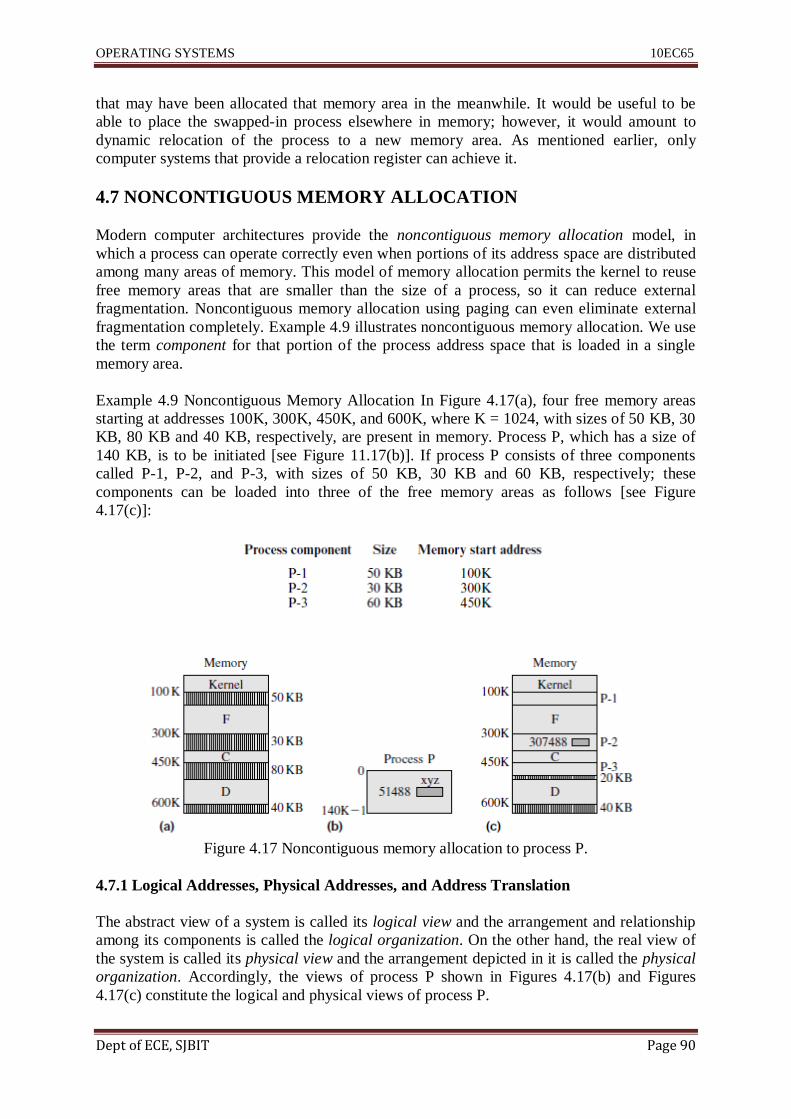
OPERATING SYSTEMS 10EC65
Dept of ECE, SJBIT Page 90
that may have been allocated that memory area in the meanwhile. It would be useful to be
able to place the swapped-in process elsewhere in memory; however, it would amount to
dynamic relocation of the process to a new memory area. As mentioned earlier, only
computer systems that provide a relocation register can achieve it.
4.7 NONCONTIGUOUS MEMORY ALLOCATION
Modern computer architectures provide the noncontiguous memory allocation model, in
which a process can operate correctly even when portions of its address space are distributed
among many areas of memory. This model of memory allocation permits the kernel to reuse
free memory areas that are smaller than the size of a process, so it can reduce external
fragmentation. Noncontiguous memory allocation using paging can even eliminate external
fragmentation completely. Example 4.9 illustrates noncontiguous memory allocation. We use
the term component for that portion of the process address space that is loaded in a single
memory area.
Example 4.9 Noncontiguous Memory Allocation In Figure 4.17(a), four free memory areas
starting at addresses 100K, 300K, 450K, and 600K, where K = 1024, with sizes of 50 KB, 30
KB, 80 KB and 40 KB, respectively, are present in memory. Process P, which has a size of
140 KB, is to be initiated [see Figure 11.17(b)]. If process P consists of three components
called P-1, P-2, and P-3, with sizes of 50 KB, 30 KB and 60 KB, respectively; these
components can be loaded into three of the free memory areas as follows [see Figure
4.17(c)]:
Figure 4.17 Noncontiguous memory allocation to process P.
4.7.1 Logical Addresses, Physical Addresses, and Address Translation
The abstract view of a system is called its logical view and the arrangement and relationship
among its components is called the logical organization. On the other hand, the real view of
the system is called its physical view and the arrangement depicted in it is called the physical
organization. Accordingly, the views of process P shown in Figures 4.17(b) and Figures
4.17(c) constitute the logical and physical views of process P.

OPERATING SYSTEMS 10EC65
Dept of ECE, SJBIT Page 91
A logical address is the address of an instruction or data byte as used in a process; it may be
obtained using index, base, or segment registers. The logical addresses in a process constitute
the logical address space of the process. A physical address is the address in memory where
an instruction or data byte exists. The set of physical addresses in the system constitutes the
physical address space of the system.
The schematic diagram of Figure 4.18 shows how the CPU obtains the physical address that
corresponds to a logical address. The kernel stores information about the memory areas
allocated to process P in a table and makes it available to the memory management unit
(MMU).
Figure 4.18 A schematic of address translation in noncontiguous memory allocation.
4.7.2 Approaches to Noncontiguous Memory Allocation
There are two fundamental approaches to implementing noncontiguous memory allocation:
• Paging
• Segmentation
In paging, each process consists of fixed-size components called pages. The size of a page is
defined by the hardware of a computer, and demarcation of pages is implicit in it. The
memory can accommodate an integral number of pages. It is partitioned into memory areas
that have the same size as a page, and each of these memory areas is considered separately
for allocation to a page. This way, any free memory area is exactly the same size as a page, so
external fragmentation does not arise in the system. Internal fragmentation can arise because

OPERATING SYSTEMS 10EC65
Dept of ECE, SJBIT Page 92
the last page of a process is allocated a page-size memory area even if it is smaller than a
page in size. In segmentation, a programmer identifies components called segments in a
process. A segment is a logical entity in a program, e.g., a set of functions, data structures, or
objects. Segmentation facilitates sharing of code, data, and program modules between
processes. However, segments have different sizes, so the kernel has to use memory reuse
techniques such as first-fit or best-fit allocation. Consequently, external fragmentation can
arise. A hybrid approach called segmentation with paging combines the features of both
segmentation and paging. It facilitates sharing of code, data, and program modules between
processes without incurring external fragmentation; however, internal fragmentation occurs
as in paging.
Table 4.4 Comparison of Contiguous and Noncontiguous
Table 4.4 summarizes the advantages of noncontiguous memory allocation over contiguous
memory allocation. Swapping is more effective in non-contiguous memory allocation
because address translation enables the kernel to load components of a swapped-in process in
any parts of memory.
4.7.3 Memory Protection
Each memory area allocated to a program has to be protected against interference from other
programs. The MMU implements this function through a bounds check. While performing
address translation for a logical address (compi , bytei ), theMMUchecks whether compi
actually exists in the program and whether bytei exists in compi . A protection violation
interrupt is raised if either of these checks fails. The bounds check can be simplified in
paging—it is not necessary to check whether bytei exists in compi because, as we shall see in
the next section, a logical address does not have enough bits in it to specify a value of bytei
that exceeds the page size.

OPERATING SYSTEMS 10EC65
Dept of ECE, SJBIT Page 93
4.8 PAGING
In the logical view, the address space of a process consists of a linear arrangement of pages.
Each page has s bytes in it, where s is a power of 2. The value of s is specified in the
architecture of the computer system. Processes use numeric logical addresses. The MMU
decomposes a logical address into the pair (pi , bi ), where pi is the page number and bi is the
byte number within page pi . Pages in a program and bytes in a page are numbered from 0;
so, in a logical address (pi, bi), pi ≥ 0 and 0 ≤ bi < s. In the physical view, pages of a process
exist in nonadjacent areas of memory.
Consider two processes P and R in a system using a page size of 1 KB. The bytes in a page
are numbered from 0 to 1023. Process P has the start address 0 and a size of 5500 bytes.
Hence it has 6 pages numbered from 0 to 5. The last page contains only 380 bytes. If a data
item sample had the address 5248, which is 5 × 1024 + 128, the MMU would view its
address as the pair (5, 128). Process R has a size of 2500 bytes. Hence it has 3 pages,
numbered from 0 to 2. Figure 11.19 shows the logical view of processes P and R. The
hardware partitions memory into areas called page frames; page frames in memory are
numbered from 0. Each page frame is the same size as a page. At any moment, some page
frames are allocated to pages of processes, while others are free. The kernel maintains a list
called the free frames list to note the frame numbers of free page frames. While loading a
process for execution, the kernel consults the free frames list and allocates a free page frame
to each page of the process. To facilitate address translation, the kernel constructs a page
table (PT) for each process. The page table has an entry for each page of the process, which
indicates the page frame allocated to the page. While performing address translation for a
logical address (pi , bi), the MMU uses the page number pi to index the page table of the
process, obtains the frame number of the page frame allocated to pi , and computes the
effective memory address according to Eq above.
Figure 4.20 shows the physical view of execution of processes P and R. Each page frame is 1
KB in size. The computer has a memory of 10 KB, so page frames are numbered from 0 to 9.
Six page frames are occupied by process P, and three page frames are occupied by process R.
The pages contained in the page frames are shown as P-0, . . . , P-5 and R-0, . . . , R-2. Page
frame 4 is free. Hence the free frames list contains only one entry. The page table of P
indicates the page frame allocated to each page of P. As mentioned earlier, the variable
sample process P has the logical address (5, 128).
Figure 4.19 Logical view of processes in paging.

OPERATING SYSTEMS 10EC65
Dept of ECE, SJBIT Page 94
Figure 4.20 Physical organization in paging.
When process P uses this logical address during its execution, it will be translated into the
effective memory address by using Eq. as follows:
Effective memory address of (5, 128)
= start address of page frame #8 + 128
=8 × 1024 + 128
=8320
We use the following notation to describe how address translation is actually performed:
s Size of a page
ll Length of a logical address (i.e., number of bits in it)
lp Length of a physical address
nb Number of bits used to represent the byte number in a logical address
np Number of bits used to represent the page number in a logical address
nf Number of bits used to represent the frame number in a physical address
The size of a page, s, is a power of 2. nb is chosen such that s = 2nb . Hence the least
significant nb bits in a logical address give us bi , the byte number within a page. The
remaining bits in a logical address form pi , the page number.
Example 4.11 Address Translation in Paging A hypothetical computer uses 32-bit logical addresses and a page size of 4KB. 12 bits are
adequate to address the bytes in a page. Thus, the higher order 20 bits in a logical address
represent pi and the 12 lower order bits represent bi . For a memory size of 256 MB, lp = 28.
Thus, the higher-order 16 bits in a physical address represent qi . If page 130 exists in page
frame 48, pi = 130, and qi = 48. If bi = 600, the logical and physical addresses look as
follows: Logical address
During address translation, the MMU obtains pi and bi merely by grouping the bits of the
logical address as shown above. The 130th entry of the page table is now accessed to obtain
qi , which is 48. This number is concatenated with bi to form the physical address.
4.9 SEGMENTATION A segment is a logical entity in a program, e.g., a function, a data structure, or an object.
Hence it is meaningful to manage it as a unit—load it into memory for execution or share it

OPERATING SYSTEMS 10EC65
Dept of ECE, SJBIT Page 95
with other programs. In the logical view, a process consists of a collection of segments. In the
physical view, segments of a process exist in nonadjacent areas of memory. A process Q
consists of five logical entities with the symbolic names main, database, search, update, and
stack.While coding the program, the programmer declares these five as segments in Q. This
information is used by the compiler or assembler to generate logical addresseswhile
translating the program. Each logical address used in Q has the form (si , bi ) where si and bi
are the ids of a segment and a byte within a segment. For example, the instruction
corresponding to a statement call get_sample, where get_sample is a procedure in segment
update, may use the operand address (update, get_sample). Alternatively, it may use a
numeric representation in which si and bi are the segment number and byte number within a
segment, respectively
Figure 4.21 A process Q in segmentation.
4.10 SEGMENTATION WITH PAGING
In this approach, each segment in a program is paged separately. Accordingly, an integral
number of pages is allocated to each segment. This approach simplifies memory allocation
and speeds it up, and also avoids external fragmentation. A page table is constructed for each
segment, and the address of the page table is kept in the segment‘s entry in the segment table.
Address translation for a logical address (si , bi) is now done in two stages. In the first stage,
the entry of si is located in the segment table, and the address of its page table is obtained.
The byte number bi is now split into a pair (psi , bpi), where psi is the page number in
segment si , and bpi is the byte number in page pi . The effective address calculation is now
completed as in paging, i.e., the frame number of psi is obtained and bpi is concatenated with
it to obtain the effective address.
Figure 4.22 A process Q in segmentation with paging.
Figure 4.22 shows processQof Figure 4.21 in a system using segmentation with paging. Each
segment is paged independently, so internal fragmentation exists in the last page of each

OPERATING SYSTEMS 10EC65
Dept of ECE, SJBIT Page 96
segment. Each segment table entry now contains the address of the page table of the segment.
The size field in a segment‘s entry is used to facilitate a bound check for memory protection.
4.11 KERNEL MEMORY ALLOCATION
The kernel creates and destroys data structures at a high rate during its operation. These are
mostly control blocks that control the allocation and use of resources in the system. Some
familiar control blocks are the process control block (PCB) created for every process and the
event control block (ECB) created whenever the occurrence of an event is anticipated.
The I/O control block (IOCB) created for an I/O operation and the file control block (FCB)
created for every open file.) The sizes of control blocks are known in the design stage of an
OS. This prior knowledge helps make kernel memory allocation simple and efficient—
memory that is released when one control block is destroyed can be reused when a similar
control block is created. To realize this benefit, a separate free list can be maintained for each
type of control block. Kernels of modern operating systems use noncontiguous memory
allocation with paging to satisfy their own memory requirements, and make special efforts to
use each page effectively. Three of the leading memory allocators are:
• McKusick–Karels allocator
• Lazy buddy allocator
• Slab allocator
McKusick--Karels Allocator:
This is a modified power-of-2 allocator; it is used in Unix 4.4 BSD. The allocator has an
integral number of pages at its disposal at any time, and asks the paging system for more
pages when it runs out of memory to allocate. The basic operating principle of the allocator is
to divide each page into blocks of equal size and record two items of information—the block
size, and a free list pointer—under the logical address of the page. This way, the address of
the page in which a block is located will be sufficient for finding the size of the block and the
free list to which the block should be added when it is freed. Hence,
it is not necessary to have a header containing this information in each allocated block as in a
conventional power-of-2 allocator. With the elimination of the header element, the entire
memory in a block can be used for the intended purpose.
Consequently, the McKusick–Karels allocator is superior to the power-of-2 allocator when a
memory request is for an area whose size is an exact power of 2. A block of identical size can
be allocated to satisfy the request, whereas the conventional power-of-2 allocator would have
allocated a block whose size is the next higher power of 2. The allocator seeks a free page
among those in its possession when it does not find a block of the size it is looking for. It then
divides this page into blocks of the desired size. It allocates one of these blocks to satisfy the
current request, and enters the remaining blocks in the appropriate free list. If no free page is
held by the allocator, it asks the paging system for a new page to be allocated to it. To ensure
that it does not consume a larger number of pages than necessary, the allocator marks any
page in its possession as free when all blocks in it become free. However, it lacks a feature to
return free pages to the paging system. Thus, the total number of pages allocated to the
allocator at any given moment is the largest number of pages it has held at any time. This
burden may reduce the memory utilization factor.

OPERATING SYSTEMS 10EC65
Dept of ECE, SJBIT Page 97
Lazy Buddy Allocator: The buddy system in its basic form may perform one or more splits
at every allocation and one or more coalescing actions at every release. Some of these actions
are wasteful because a coalesced block may need to be split again later. The basic design
principle of the lazy buddy allocator is to delay coalescing actions if a data structure requiring
the same amount of memory as a released block is likely to be created. Under the correct set
of conditions, this principle avoids the overhead of both coalescing and splitting. The lazy
buddy allocator used in Unix 5.4 works as follows: Blocks with the same size are considered
to constitute a class of blocks. Coalescing decisions for a class are made on the basis of the
rates at which data structures of the class are created and destroyed. Accordingly, the
allocator characterizes the behaviour of the OS with respect to a class of blocks into three
states called lazy, reclaiming, and accelerated. For simplicity we refer to these as states of a
class of blocks. In the lazy state, allocations and releases of blocks of a class occur at
matching rates. Consequently, there is a steady and potentially wasteful cycle of splitting and
coalescing. As a remedy, excessive coalescing and splitting can both be avoided by delaying
coalescing. In the reclaiming state, releases occur at a faster rate than allocations so it is a
good idea to coalesce at every release. In the accelerated state, releases occur much faster
than allocations, and so it is desirable to coalesce at an even faster rate; the allocator should
attempt to coalesce a block being released, and, additionally, it should also try to coalesce
some other blocks that were released but not coalesced in the past. The lazy buddy allocator
maintains the free list as a doubly linked list. This way both the start and end of the list can be
accessed equally easily. A bit map is maintained to indicate the allocation status of blocks. In
the lazy state, a block being released is simply added to the head of the free list. No effort is
made to coalesce it with its buddy. It is also not marked free in the bit map. This way the
block will not be coalesced even if its buddy is released in future. Such a block is said to be
locally free. Being at the head of the list, this block will be allocated before any other block in
the list. Its allocation is efficient and fast because the bit map does not need to be updated—it
still says that the block is allocated. In the reclaiming and accelerated states a block is both
added to the free list and marked free in the bit map. Such a block is said to be globally free.
Globally free blocks are added to the end of the free list. In the reclaiming state the allocator
tries to coalesce a new globally free block transitively with its buddy. Eventually a block is
added to some free list—either to a free list to which the block being released would have
belonged, or to a free list containing larger-size blocks. Note that the block being added to a
free list could be a locally free block or a globally free block according to the state of that
class of blocks. In the accelerated state the allocator tries to coalesce the block being released,
just as in the reclaiming state, and additionally tries to coalesce one other locally free block—
the block found at the start of the free list—with its buddy. The state of a class of blocks is
characterized as follows: Let A, L, and G be the number of allocated, locally free, and
globally free blocks of a class, respectively. The total number of blocks of a class is given by
N = A + L + G. A parameter called slack is computed as follows:
slack = N − 2 × L – G
A class is said to be in the lazy, reclaiming, or accelerated state if the value of slack is ≥ 2, 1,
or 0, respectively. (The allocator ensures that slack is never < 0.)
The coalescing overhead is different in these three states. There is no overhead in the lazy
state. Hence release and allocation of blocks is fast. In the reclaiming state the overhead
would be comparable with that in the buddy system, whereas in the accelerated state the
overhead would be heavier than in the buddy system. It has been shown that the average
delays with the lazy buddy allocator are 10 to 32 percent lower than average delays in the

OPERATING SYSTEMS 10EC65
Dept of ECE, SJBIT Page 98
case of a buddy allocator. The implementation of the lazy buddy allocator in Unix 5.4 uses
two kinds of blocks. Small blocks vary in size between 8 and 256 bytes. Large blocks vary in
size between 512 and 16 KB. The allocator obtains memory from the paging system in 4 KB
areas. In each area, it creates a pool of blocks and a bit map to keep track of the allocation
status of the blocks. When all blocks in the pool are free, it returns the area to the paging
system. This action overcomes the problem of nonreturnable blocks seen in the McKusick–
Karels allocator.
Slab Allocator:
The slab allocator was first used in the Solaris 2.4 operating system; it has been used in Linux
since version 2.2. A slab consists of many slots, where each slot can hold an active object that
is a kernel data structure, or it may be empty. The allocator obtains standard-size memory
areas from the paging system and organizes a slab in each memory area. It obtains an
additional memory area from the paging system and constructs a slab in it when it runs out of
memory to allocate, and it returns a memory area to the paging system when all slots in its
slab are unused. All kernel objects of the same class form a pool. For small objects, a pool
consists of many slabs and each slab contains many slots.
The slabs of a pool are entered in a doubly linked list to facilitate addition and deletion of
slabs. A slab may be full, partially empty, or empty, depending on the number of active
objects existing in it. To facilitate searches for an empty slab, the doubly linked list
containing the slabs of a pool is sorted according to the slab‘s status—all full slabs are at the
start of the list, partially empty slabs are in the middle, and empty slabs are at the end of the
list. Each slab contains a free list from which free slots can be allocated. Each pool contains a
pointer to the first slab that contains a free slot. This arrangement makes allocation very
efficient.
Figure 4.23 shows the format of a slab. When the allocator obtains a memory area from the
paging system, it formats the memory area into a slab by creating an integral number of slots,
a free list containing all slots, and a descriptor field at the end of the slab that contains both
the count of active objects in it and the free list header. Each slot in the slab is then
initialized; this action involves initializing the various fields in it with object-specific
information like fixed strings of constant values.When allocated, the slot can be used as an
object straightaway.
Figure 4.23 Format of a slab.
At deallocation time, the object is brought back to its allocation time status, and the slot is
added to the free list. Since some fields of the objects never change, or change in such a
manner that their values at deallocation time are the same as their values at allocation time,
this approach eliminates the repetitive overhead of object initialization suffered in most other
allocators. However, use of initialized objects has some implications for the memory
utilization factor. If a free slot were simply free memory, a part of this memory itself could be
used as the free list pointer; but a slot is an initialized object, and so the pointer field must be
located outside the object‘s area even when the slot is free.

OPERATING SYSTEMS 10EC65
Dept of ECE, SJBIT Page 99
Recommended Questions
1. Describe the features of static and dynamic memory allocation. What are the four
program components for which memory is to be allocated?
2. Compare contiguous and non-contiguous memory allocation. Enumerate the practical
issues associated with them.
3. Explain the slab allocator of solaris 2.4 system.
4. With a neat diagram mention the components of a memory allocation to a program
during its execution. Also describe the memory allocation preliminaries.
5. Explain the working of a buddy system allocator for program controlled data. How
does it differ from process-of-two allocator?
6. What is memory fragmentation? Discuss the method of memory compaction and
reuse of memory concepts to overcome the problem of memory fragmentation. Give
examples.
7. Explain the techniques used to perform memory allocation using a free list.
8. Explain internal and external fragmentation with examples.
9. Describe i) best fit technique for free space allocation ii) variable partitioned
allocation with their merits and demerits.

OPERATING SYSTEMS 10EC65
Dept of ECE, SJBIT Page 100
UNIT-5
Virtual Memory
Virtual memory is a part of the memory hierarchy that consists of memory and a disk. In
accordance with the principle of memory hierarchies only some portions of the address space
of a process—that is, of its code and data—exist in memory at any time; other portions of its
address space reside on disk and are loaded into memory when needed during operation of
the process. The kernel employs virtual memory to reduce the memory commitment to a
process so that it can service a large number of processes concurrently, and to handle
processes whose address space is larger than the size of memory.
Virtual memory is implemented through the noncontiguous memory allocation model and
comprises both hardware components and a software component called a virtual memory
manager. The hardware components speed up address translation and help the virtual
memory manager perform its tasks more effectively. The virtual memory manager decides
which portions of a process address space should be in memory at any time.
5.1 VIRTUAL MEMORY BASICS
Users always want more from a computer system—more resources and more services. The
need for more resources is satisfied either by obtaining more efficient use of existing
resources, or by creating an illusion that more resources exist in the system. A virtual
memory is what its name indicates—it is an illusion of a memory that is larger than the real
memory, i.e., RAM, of the computer system.
As we pointed out in Section 1.1, this illusion is a part of a user‘s abstract view of memory. A
user or his application program sees only the virtual memory. The kernel implements the
illusion through a combination of hardware and software means. We refer to real memory
simply as memory.We refer to the software component of virtual memory as a virtual
memory manager.
The illusion of memory larger than the system‘s memory crops up any time a process whose
size exceeds the size of memory is initiated. The process is able to operate because it is kept
in its entirety on a disk and only its required portions are loaded in memory at any time. The
basis of virtual memory is the non-contiguous memory allocation model. The address space
of each process is assumed to consist of portions called components. The portions can be
loaded into nonadjacent areas of memory. The address of each operand or instruction in the
code of a process is a logical address of the form (compi , bytei ).
The memory management unit (MMU) translates it into the address in memory where the
operand or instruction actually resides.
Figure 5.1 shows a schematic diagram of a virtual memory. The logical address space of the
process shown consists of five components. Three of these components are presently in
memory. Information about the memory areas where these components exist is maintained in
a data structure of the virtual memory manager. This information is used by the MMU during
address translation. When an instruction in the process refers to a data item or instruction that
is not in memory, the component containing it is loaded from the disk. Occasionally, the

OPERATING SYSTEMS 10EC65
Dept of ECE, SJBIT Page 101
virtual memory manager removes some components from memory to make room for other
components.
Figure 5.1 Overview of virtual memory.
Virtual Memory A memory hierarchy, consisting of a computer system‘s memory and a
disk, that enables a process to operate with only some portions of its address space in
memory.
Demand Loading of Process Components The virtual memory manager loads only one
component of a process address space in memory to begin with—the component that contains
the start address of the process, that is, address of the instruction with which its execution
begins. It loads other components of the process only when they are needed. This technique is
called demand loading. To keep the memory commitment to a process low, the virtual
memory manager removes components of the process from memory from time to time. These
components would be loaded back in memory when needed again.
Performance of a process in virtual memory depends on the rate at which its components
have to be loaded into memory. The virtual memory manager exploits the law of locality of
reference to achieve a low rate of loading of process components. We discuss this law in
Table 5.1 Comparison of Paging and Segmentation

OPERATING SYSTEMS 10EC65
Dept of ECE, SJBIT Page 102
Paging and Segmentation The two approaches to implementation of virtual memory differ
in the manner in which the boundaries and sizes of address space components are determined.
Table 5.1 compares the two approaches. In paging, each component of an address space is
called a page. All pages have identical size, which is a power of two. Page size is defined by
the computer hardware and demarcation of pages in the address space of a process is
performed implicitly by it. In segmentation, each component of an address space is called a
segment. A programmer declares some significant logical entities (e.g., data structures or
objects) in a process as segments. Thus identification of components is performed by the
programmer, and segments can have different sizes. This fundamental difference leads to
different implications for efficient use of memory and for sharing of programs or data. Some
systems use a hybrid segmentation-with-paging approach to obtain advantages of both
the approaches.
5.2 DEMAND PAGING
A process is considered to consist of pages, numbered from 0 onward. Each page is of size s
bytes, where s is a power of 2. The memory of the computer system is considered to consist
of page frames, where a page frame is a memory area that has the same size as a page. Page
frames are numbered from 0 to #frames−1 where #frames is the number of page frames of
memory. Accordingly, the physical address space consists of addresses from 0 to #frames × s
− 1. At any moment, a page frame may be free, or it may contain a page of some process.
Each logical address used in a process is considered to be a pair (pi , bi), where pi is a page
number and bi is the byte number in pi, 0 ≤ bi < s.
The effective memory address of a logical address (pi , bi ) is computed as follows:
Effective memory address of logical address (pi , bi)
= start address of the page frame containing page pi + bi (5.1)
The size of a page is a power of 2, and so calculation of the effective address is performed
through bit concatenation, which is much faster than addition.
Figure 5.2 is a schematic diagram of a virtual memory using paging in which page size is
assumed to be 1KB, where 1KB = 1024 bytes. Three processes P1, P2 and P3, have some of
their pages in memory. The memory contains 8 page frames numbered from 0 to 7. Memory
allocation information for a process is stored in a page table. Each entry in the page table
contains memory allocation information for one page of a process. It contains the page frame
number where a page resides. Process P2 has its pages 1 and 2 in memory. They occupy page
frames 5 and 7 respectively. Process P1 has its pages 0 and 2 in page frames 4 and 1, while
process P3 has its pages 1, 3 and 4 in page frames 0, 2 and 3, respectively. The free frames
list contains a list of free page frames. Currently only page frame 6 is free.

OPERATING SYSTEMS 10EC65
Dept of ECE, SJBIT Page 103
Figure 5.2 Address translation in virtual memory using paging.
Process P2 is currently executing the instruction ‗Add ·· 2528‘, so the MMU uses P2‘s page
table for address translation. TheMMUviews the operand address 2528 as the pair (2, 480)
because 2528=2×1024+480. It now accesses the entry for page 2 in P2‘s page table. This
entry contains frame number 7, so the MMU forms the effective address 7×1024+480
according to Eq. (5.1), and uses it to make a memory access. In effect, byte 480 in page frame
7 is accessed.
5.2.1 Demand Paging Preliminaries
If an instruction of P2 in Figure 5.2 refers to a byte in page 3, the virtual memory manager
will load page 3 in memory and put its frame number in entry 3 of P2‘s page table. These
actions constitute demand loading of pages, or simply demand paging.
To implement demand paging, a copy of the entire logical address space of a process is
maintained on a disk. The disk area used to store this copy is called the swap space of a
process. While initiating a process, the virtual memory manager allocates the swap space for
the process and copies its code and data into the swap space. During operation of the process,
the virtual memory manager is alerted when the process wishes to use some data item or
instruction that is located in a page that is not present in memory. It now loads the page from
the swap space into memory. This operation is called a page-in operation. When the virtual
memory manager decides to remove a page from memory, the page is copied back into the
swap space of the process to which it belongs if the page was modified since the last time it
was loaded in memory. This operation is called a page-out operation.
This way the swap space of a process contains an up-to-date copy of every page of the
process that is not present in memory. A page replacement operation is one that loads a page
into a page frame that previously contained another page.
It may involve a page-out operation if the previous page was modified while it occupied the
page frame, and involves a page-in operation to load the new page.

OPERATING SYSTEMS 10EC65
Dept of ECE, SJBIT Page 104
Page Table The page table for a process facilitates implementation of address translation,
demand loading, and page replacement operations. Figure 5.3 shows the format of a page
table entry. The valid bit field contains a Boolean value to indicate whether the page exists in
memory. We use the convention that 1 indicates ―resident in memory‖ and 0 indicates ―not
resident in memory.‖ The page frame# field, which was described earlier, facilitates address
translation. The misc info field is divided into four subfields. Information in the prot info field
is used for protecting contents of the page against interference. It indicates whether the
process can read or write data in the page or execute instructions in it. ref info contains
information concerning references made to the page while it is in memory.
The modified bit indicates whether the page has been modified, i.e., whether it is dirty. It is
used to decide whether a page-out operation is needed while replacing the page. The other
info field contains information such as the address of the disk block in the swap space where
a copy of the page is maintained.
Page Faults and Demand Loading of Pages
Table 5.2 summarizes steps in address translation by the MMU. While performing address
translation for a logical address (pi , bi), theMMUchecks the valid bit of the page table entry
of pi
Figure 5.3 Fields in a page table entry.

OPERATING SYSTEMS 10EC65
Dept of ECE, SJBIT Page 105
Table 5.2 Steps in Address Translation by the MMU
Figure 5.4 Demand loading of a page.
. If the bit indicates that pi is not present in memory, the MMU raises an interrupt called a
missing page interrupt or a page fault, which is a program interrupt (see Section 2.2.5). The
interrupt servicing routine for program interrupts finds that the interrupt was caused by a page
fault, so it invokes the virtual memory manager with the page number that caused the page
fault, i.e., pi , as a parameter. The virtual memory manager now loads page pi in memory and
updates its page table entry. Thus, the MMU and the virtual memory manager interact to
decide when a page of a process should be loaded in memory.
Figure 5.4 is an overview of the virtual memory manager‘s actions in demand loading of a
page. The broken arrows indicate actions of the MMU, whereas firm arrows indicate accesses
to the data structures, memory, and the disk by the virtual memory manager when a page
fault occurs. The numbers in circles indicate the steps in address translation, raising, and
handling of the page fault—

OPERATING SYSTEMS 10EC65
Dept of ECE, SJBIT Page 106
Steps 1–3 were described earlier in Table 12.2. Process P2 of Figure 5.2 is in operation.
While translating the logical address (3, 682), the MMU raises a page fault because the valid
bit of page 3‘s entry is 0.
Page-in, Page-out, and Page Replacement Operations
Figure 5.4 showed how a page-in operation is performed for a required page when a page
fault occurs in a process and a free page frame is available in memory. If no page frame is
free, the virtual memory manager performs a page replacement operation to replace one of
the pages existing in memory with the page whose reference caused the page fault. It is
performed as follows: The virtual memory manager uses a page replacement algorithm to
select one of the pages currently in memory for replacement, accesses the page table entry of
the selected page to mark it as ―not present‖ in memory, and initiates a page-out operation for
it if the modified bit of its page table entry indicates that it is a dirty page.
In the next step, the virtual memory manager initiates a page-in operation to load the required
page into the page frame that was occupied by the selected page. After the page-in operation
completes, it updates the page table entry of the page to record the frame number of the page
frame, marks the page as ―present,‖ and makes provision to resume operation of the process.
The process now reexecutes its current instruction. This time, the address translation for the
logical address in the current instruction completes without a page fault. The page-in and
page-out operations required to implement demand paging constitute page I/O; we use the
termpage traffic to describe movement of pages in and out of memory. Note that page I/O is
distinct from I/O operations performed by processes,whichwe will call programI/O. The state
of a process that encounters a page fault is changed to blocked until the required page is
loaded in memory, and so its performance suffers because of a page fault. The kernel can
switch theCPU to another process to safeguard system performance.
Effective Memory Access Time The effective memory access time for a process in demand
paging is the average memory access time experienced by the process.
It depends on two factors: time consumed by the MMU in performing address translation,
and the average time consumed by the virtual memory manager in handling a page fault. We
use the following notation to compute the effective memory access time:
pr1 probability that a page exists in memory
tmem memory access time
tpfh time overhead of page fault handling
pr1 is called the memory hit ratio. tpfh is a few orders of magnitude larger than tmem
because it involves disk I/O—one disk I/O operation is required if only a page-in operation is
sufficient, and two disk I/O operations are required if a page replacement is necessary.
A process‘s page table exists in memory when the process is in operation. Hence, accessing
an operand with the logical address (pi , bi ) consumes two memory cycles if page pi exists in
memory—one to access the page table entry of pi for address translation, and the other to
access the operand in memory using the effective memory address of (pi , bi ). If the page is
not present in memory, a page fault is raised after referencing the page table entry of pi , i.e.,
after one memory cycle.

OPERATING SYSTEMS 10EC65
Dept of ECE, SJBIT Page 107
Accordingly, the effective memory access time is as follows:
Effective memory access time = pr1 × 2 × tmem + (1 − pr1) × (tmem + tpfh + 2 × tmem)
(5.2)
The effective memory access time can be improved by reducing the number
of page faults.
5.2.1.1 Page Replacement
Page replacement becomes necessary when a page fault occurs and there are no free page
frames in memory. However, another page fault would arise if the replaced page is referenced
again. Hence it is important to replace a page that is not likely to be referenced in the
immediate future. But how does the virtual memory manager know which page is not likely
to be referenced in the immediate future?
The empirical law of locality of reference states that logical addresses used by a process in
any short interval of time during its operation tend to be bunched together in certain portions
of its logical address space. Processes exhibit this behaviour for two reasons. Execution of
instructions in a process is mostly sequential in nature, because only 10–20 percent of
instructions executed by a process are branch instructions. Processes also tend to perform
similar operations on several elements of nonscalar data such as arrays. Due to the combined
effect of these two reasons, instruction and data references made by a process tend to be in
close proximity to previous instruction and data references made by it.
We define the current locality of a process as the set of pages referenced in its previous few
instructions. Thus, the law of locality indicates that the logical address used in an instruction
is likely to refer to a page that is in the current locality of the process.
The virtual memory manager can exploit the law of locality to achieve an analogous effect—
fewer page faults would arise if it ensures that pages that are in the current locality of a
process are present in memory.
Note that locality of reference does not imply an absence of page faults. Let the proximity
region of a logical address ai contain all logical addresses that are in close proximity to ai .
Page faults can occur for two reasons: First, the proximity region of a logical address may not
fit into a page; in this case, the next address may lie in an adjoining page that is not included
in the current locality of the process. Second, an instruction or data referenced by a process
may not be in the proximity of previous references. We call this situation a shift in locality of
a process. It typically occurs when a process makes a transition from one action in its logic to
another. The next example illustrates the locality of a process.
The law of locality helps to decide which page should be replaced when a page fault occurs.
Let us assume that the number of page frames allocated to a process Pi is a constant. Hence
whenever a page fault occurs during operation of Pi , one of Pi ‘s own pages existing in
memory must be replaced. Let t1 and t2 be the periods of time for which pages p1 and p2
have not been referenced during the operation of Pi . Let t1 > t2, implying that some byte of
page p2 has been referenced or executed (as an instruction) more recently than any byte of
page p1.

OPERATING SYSTEMS 10EC65
Dept of ECE, SJBIT Page 108
Hence page p2 is more likely to be a part of the current locality of the process than page p1;
that is, a byte of page p2 is more likely to be referenced or executed than a byte of page p1.
We use this argument to choose page p1 for replacement when a page fault occurs. If many
pages of Pi exist in memory, we can rank them according to the times of their last references
and replace the page that has been least recently referenced. This page replacement policy is
called LRU page replacement.
Figure 5.5 Proximity regions of previous references and current locality of a process.
5.2.1.2 Memory Allocation to a Process
Figure 5.6 shows how the page fault rate of a process should vary with the amount of
memory allocated to it. The page fault rate is large when a small amount of memory is
allocated to the process; however, it drops when more memory is allocated to the process.
This page fault characteristic of a process is desired because it enables the virtual memory
manager to take corrective action when it finds that a process has a high page fault rate—it
can bring about a reduction in the page fault rate by increasing the memory allocated to the
process.
As we shall discuss in Section 5.4, the LRU page replacement policy possesses a page fault
characteristic that is similar to the curve of Figure 12.6 because it replaces a page that is less
likely to be in the current locality of the process than other pages of the process that are in
memory.
How much memory should the virtual memory manager allocate to a process? Two opposite
factors influence this decision. From Figure 5.6, we see that an overcommitment of memory
to a process implies a low page fault rate for the process; hence it ensures good process
performance. However, a smaller number of processes would fit in memory, which could
cause CPU idling and poor system performance. An undercommitment of memory to a
process causes a high page fault rate, which would lead to poor performance of the process.
The desirable operating zone marked in Figure 5.6 avoids the regions of overcommitment and
under commitment of memory.

OPERATING SYSTEMS 10EC65
Dept of ECE, SJBIT Page 109
The main problem in deciding how much memory to allocate to a process is that the page
fault characteristic, i.e., the slope of the curve and the page fault rate in Figure 5.6, varies
among processes. Even for the same process, the page fault characteristic may be different
when it operates with different data.
Figure 5.6 Desirable variation of page fault rate with memory allocation.
If all processes in the system operate in the region of high page fault rates, the CPU would be
engaged in performing page traffic and process switching most of the time. CPU efficiency
would be low and system performance, measured either in terms of average response time or
throughput, would be poor. This situation is called thrashing.
Thrashing A condition in which high page traffic and low CPU efficiency coincide. Note
that low CPU efficiency can occur because of other causes as well, e.g., if too few processes
exist in memory or all processes in memory perform I/O operations frequently. The thrashing
situation is different in that all processes make poor progress because of high page fault rates.
From Figure 5.6, we can infer that the cause of thrashing is an under commitment of memory
to each process. The cure is to increase the memory allocation for each process. This may
have to be achieved by removing some processes from memory—that is, by reducing the
degree of multiprogramming.
A process may individually experience a high page fault rate without the system thrashing.
The same analysis now applies to the process—it must suffer from an undercommitment of
memory, so the cure is to increase the amount of memory allocated to it.
5.2.1.3 Optimal Page Size
The size of a page is defined by computer hardware. It determines the number of bits required
to represent the byte number in a page. Page size also determines
1. Memory wastage due to internal fragmentation
2. Size of the page table for a process
3. Page fault rates when a fixed amount of memory is allocated to a process

OPERATING SYSTEMS 10EC65
Dept of ECE, SJBIT Page 110
Consider a process Pi of size z bytes. A page size of s bytes implies that the process has n
pages, where n = _z/s_ is the value of z/s rounded upward. Average internal fragmentation is
s/2 bytes because the last page would be half empty on the average. The number of entries in
the page table is n. Thus internal fragmentation varies directly with the page size, while page
table size varies inversely with it.
5.2.2 Address Translation and Page Fault Generation
The MMU follows the steps of Table 5.2 to perform address translation. For a logical address
(pi , bi ), it accesses the page table entry of pi by using pi ×lPT_entry as an offset into the
page table, where lPT_entry is the length of a page table entry.
lPT_entry is typically a power of 2, so pi ×lPT_entry can be computed efficiently by shifting
the value of pi by a few bits.
Address Translation Buffers A reference to the page table during address translation
consumes one memory cycle because the page table is stored in memory. The translation
look-aside buffer (TLB) is a small and fast associative memory that is used to eliminate the
reference to the page table, thus speeding up address translation. The TLB contains entries of
the form (page #, page frame #, protection info) for a few recently accessed pages of a
program that are in memory. During address translation of a logical address (pi , bi ), the TLB
hardware searches for an entry of page pi . If an entry is found, the page frame # from the
entry is used to complete address translation for the logical address (pi , bi ). Figure 5.8
illustrates operation of the TLB. The arrows marked 2_ and 3_ indicate TLB lookup. The
TLB contains entries for pages 1 and 2 of process P2. If pi is either 1 or 2, the TLB lookup
scores a hit, so the MMU takes the page frame number from the TLB and completes address
translation. A TLB miss occurs if pi is some other page, hence theMMUaccesses the page
table and completes the address translation if page pi is present in memory; otherwise, it
generates a page fault, which activates the virtual memory manager to load pi in memory.
Figure 5.8 Address translation using the translation look-aside buffer and the page table.

OPERATING SYSTEMS 10EC65
Dept of ECE, SJBIT Page 111
Figure 5.9 Summary of address translation of (pi , bi ) (note: PT = page table).
Figure 5.9 summarizes the MMU and software actions in address translation and page fault
handling for a logical address (pi , bi ). MMU actions concerning use of the TLB and the
page table are as described earlier. The virtual memory manager is activated by a page fault.
If an empty page frame is not available to load page pi , it initiates a page-out operation for
some page pj to free the page frame, say page frame fj , occupied by it. pj ‘s page table entry
is updated to indicate that it is no longer present in memory. If pj has an entry in the TLB, the
virtual memory manager erases it by executing an ―erase TLB entry‖ instruction. This action
is essential for preventing incorrect address translation at pj ‘s next reference. A page-in
operation is now performed to load pi in page frame fj , and pi ‘s page table entry is updated
when the page-in operation is completed. Execution of the instruction that caused the page
fault is repeated when the process is scheduled again. This time pi does not have an entry in
the TLB but it exists in memory, and so the MMU uses information in the page table to
complete the address translation. An entry for pi has to be made in the TLB at this time.
We use the following notation to compute the effective memory access time when a TLB is
used:
pr1 probability that a page exists in memory
pr2 probability that a page entry exists in TLB
tmem memory access time
tTLB access time of TLB
tpfh time overhead of page fault handling
pr1 is the memory hit ratio and tmem is a few orders of magnitude smaller than tpfh.
Typically tTLB is at least an order of magnitude smaller than tmem. pr2 is called the TLB hit
ratio.
When the TLB is not used, the effective memory access time is as given by Eq. (5.2). The
page table is accessed only if the page being referenced does not have an entry in the TLB.
Accordingly, a page reference consumes (tTLB +tmem) time if the page has an entry in the
TLB, and (tTLB + 2 × tmem) time if it does not have a TLB entry but exists in memory. The
probability of the latter situation is (pr1− pr2). When the TLB is used, pr2 is the probability

OPERATING SYSTEMS 10EC65
Dept of ECE, SJBIT Page 112
that an entry for the required page exists in the TLB. The probability that a page table
reference is both necessary and sufficient for address translation is (pr1− pr2). The time
consumed by each such reference is (tTLB + 2 × tmem) since an unsuccessful TLB search
would precede the page table lookup. The probability of a page fault is (1−pr1).
It occurs after the TLB and the page table have been looked up, and it requires (tpfh + tTLB
+ 2 × tmem) time if we assume that the TLB entry is made for the page while the effective
memory address is being calculated. Hence the effective memory access time is
Effective memory access time = pr2 × (tTLB + tmem) + (pr1 − pr2) × (tTLB + 2 × tmem)
+ (1 − pr1) × (tTLB + tmem + tpfh + tTLB + 2 × tmem)
(5.3)
To provide efficient memory access during operation of the kernel, most
computers provide wired TLB entries for kernel pages. These entries are never
touched by replacement algorithms.
5.3 THE VIRTUAL MEMORY MANAGER
The virtual memory manager uses two data structures—the page table, whose entry format is
shown in Figure 5.3, and the free frames list. The ref info and modified fields in a page table
entry are typically set by the paging hardware. All other fields are set by the virtual memory
manager itself. Table 5.4 summarizes the functions of the virtual memory manager.
Management of the Logical Address Space of a Process The virtual memory manager
manages the logical address space of a process through the following subfunctions:
1. Organize a copy of the instructions and data of the process in its swap space.
2. Maintain the page table.
3. Perform page-in and page-out operations.
4. Perform process initiation.
A copy of the entire logical address space of a process is maintained in the swap space of the
process. When a reference to a page leads to a page fault, the page is loaded from the swap
space by using a page-in operation. When a dirty page is to be removed from memory, a
page-out operation is performed to copy it from memory into a disk block in the swap space.
Thus the copy of a page in the swap space is current if that page is not in memory, or it is in
memory but it has not been modified since it was last loaded.
For other pages the copy in the swap space is stale (i.e., outdated), whereas that in memory is
current.

OPERATING SYSTEMS 10EC65
Dept of ECE, SJBIT Page 113
Table 5.4 Functions of the Virtual Memory Manager
Management of Memory The free frames list is maintained at all times. A page frame is
taken off the free list to load a new page, and a frame is added to it when a page-out operation
is performed. All page frames allocated to a process are added to the free list when the
process terminates.
Protection During process creation, the virtual memory manager constructs its page table
and puts information concerning the start address of the page table and its size in the PCB of
the process. The virtual memory manager records access privileges of the process for a page
in the prot info field of its page table entry.
During dispatching of the process, the kernel loads the page-table start address of the process
and its page-table size into registers of the MMU. During translation of a logical address (pi ,
bi), the MMU ensures that the entry of page pi exists in the page table and contains
appropriate access privileges in the prot info field.
Collection of Information for Page Replacement The ref info field of the page table entry
of a page indicates when the page was last referenced, and the modified field indicates
whether it has been modified since it was last loaded in memory.
Page reference information is useful only so long as a page remains in memory; it is
reinitialized the next time a page-in operation is performed for the page. Most computers
provide a single bit in the ref info field to collect page reference information. This
information is not adequate to select the best candidate for page replacement. Hence the
virtual memory manager may periodically reset the bit used to store this information.

OPERATING SYSTEMS 10EC65
Dept of ECE, SJBIT Page 114
Example: Page Replacement
The memory of a computer consists of eight page frames. A process P1 consists of five pages
numbered 0 to 4. Only pages 1, 2, and 3 are in memory at the moment; they occupy page
frames 2, 7, and 4, respectively. Remaining page frames have been allocated to other
processes and no free page frames are left in the system.
Figure 5.13 Data structures of the virtual memory manager: (a) before and (b) after a page
replacement.
Figure 4.13(a) illustrates the situation in the system at time instant t+11, i.e., a little after t11.
Only the page table of P1 is shown in the figure since process P1 has been scheduled.
Contents of the ref info and modified fields are shown in the misc info field. Pages 1, 2, and 3
were last referenced at time instants t4, t11, and t9, respectively. Page 1 was modified
sometime after it was last loaded. Hence the misc info field of its page table entry contains the
information t4,m.
At time instant t12, process P1 gives rise to a page fault for page 4. Since all page frames in
memory are occupied, the virtual memory manager decides to replace page 1 of the process.
The mark m in the misc info field of page 1‘s page table entry indicates that it was modified
since it was last loaded, so a page-out\ operation is necessary. The page frame # field of the
page table entry of page 1 indicates that the page exists in page frame 2. The virtual memory
manager performs a page-out operation to write the contents of page frame 2 into the swap
area reserved for page 1 of P1, and modifies the valid bit in the page table entry of page 1 to
indicate that it is not present in memory. A page-in operation is now initiated for page 4 of
P1. At the end of the operation, the page table entry of page 4 is modified to indicate that it
exists in memory in page frame 2.
Execution of P1 is resumed. It now makes a reference to page 4, and so the page reference
information of page 4 indicates that it was last referenced at t12. Figure 5.13(b) indicates the
page table of P1 at time instant t+12.
5.3.1 Overview of Operation of the Virtual Memory Manager
The virtual memory manager makes two important decisions during its
operation:

OPERATING SYSTEMS 10EC65
Dept of ECE, SJBIT Page 115
• When a page fault occurs during operation of some process proci , it decides
which page should be replaced.
• Periodically it decides howmuch memory, i.e., howmany page frames, should
be allocated to each process.
Figure 5.14 Modules of the virtual memory manager.
5.4 PAGE REPLACEMENT POLICIES
A page replacement policy should replace a page that is not likely to be referenced in the
immediate future. We evaluate the following three page replacement policies to see how well
they fulfill this requirement.
• Optimal page replacement policy
• First-in, first-out (FIFO) page replacement policy
• Least recently used (LRU) page replacement policy
For the analysis of these page replacement policies, we rely on the concept of page reference
strings. A page reference string of a process is a trace of the pages accessed by the process
during its operation. It can be constructed by monitoring the operation of a process, and
forming a sequence of page numbers that appear in logical addresses generated by it. The
page reference string of a process depends on the data input to it, so use of different data
would lead to a different page reference string for a process.
For convenience we associate a reference time string t1, t2, t3, . . . with each page reference
string. This way, the kth page reference in a page reference string is assumed to have
occurred at time instant tk. (In effect, we assume a logical clock that runs only when a
process is in the running state and gets advanced only when the process refers to a logical
address.) Example 5.5 illustrates the page reference string and the associated reference time
string for a process.
Page Reference String Example 5.5
A computer supports instructions that are 4 bytes in length, and uses a page size of 1KB. It
executes the following nonsense program in which the symbols A and B are in pages 2 and 5,
respectively:

OPERATING SYSTEMS 10EC65
Dept of ECE, SJBIT Page 116
START 2040
READ B
LOOP MOVER AREG, A
SUB AREG, B
BC LT, LOOP
...
STOP
A DS 2500
B DS 1
END
The page reference string and the reference time string for the process are as
follows:
Page reference string 1, 5, 1, 2, 2, 5, 2, 1, . . .
Reference time string t1, t2, t3, t4, t5, t6, t7, t8, . . .
The logical address of the first instruction is 2040, and so it lies in page 1. The first page
reference in the string is therefore 1. It occurs at time instant t1. B, the operand of the
instruction is situated in page 5, and so the second page reference in the string is 5, at time t2.
The next instruction is located in page 1 and refers to A, which is located in page 2, and thus
the next two page references are to pages 1 and 2. The next two instructions are located in
page 2, and the instruction with the label LOOP is located in page 1. Therefore, if the value
of B input to the READ statement is greater than the value of A, the next four page references
would be to pages 2, 5, 2 and 1, respectively; otherwise, the next four page references would
be to pages 2, 5, 2 and 2, respectively.
Optimal Page Replacement Optimal page replacement means making page replacement
decisions in such a manner that the total number of page faults during operation of a process
is the minimum possible; i.e., no other sequence of page replacement decisions can lead to a
smaller number of page faults. To achieve optimal page replacement, at each page fault, the
page replacement policy would have to consider all alternative page replacement decisions,
analyze their implications for future page faults, and select the best alternative. Of course,
such a policy is infeasible in reality: the virtual memory manager does not have knowledge of
the future behaviour of a process. As an analytical tool, however, this policy provides a useful
comparison in hindsight for the performance of other page replacement policies.
Although optimal page replacement might seem to require excessive analysis, Belady (1966)
showed that it is equivalent to the following simple rule: At a page fault, replace the page
whose next reference is farthest in the page reference string.
FIFO Page Replacement At every page fault, the FIFO page replacement policy replaces the
page that was loaded into memory earlier than any other page of the process. To facilitate
FIFO page replacement, the virtual memory manager records the time of loading of a page in
the ref info field of its page table entry.
When a page fault occurs, this information is used to determine pearliest, the page that was
loaded earlier than any other page of the process. This is the page that will be replaced with
the page whose reference led to the page fault.

OPERATING SYSTEMS 10EC65
Dept of ECE, SJBIT Page 117
LRU Page Replacement The LRU policy uses the law of locality of reference as the basis
for its replacement decisions. Its operation can be described as follows: At every page fault
the least recently used (LRU) page is replaced by the required page. The page table entry of a
page records the time when the page was last referenced. This information is initialized when
a page is loaded, and it is updated every time the page is referenced. When a page fault
occurs, this information is used to locate the page pLRU whose last reference is earlier than
that of every other page. This page is replaced with the page whose reference led to the page
fault.
Analysis of Page Replacement Policies Example 5.6 illustrates operation of
the optimal, FIFO, and LRU page replacement policies.
Example 5.6 Operation of Page Replacement Policies
A page reference string and the reference time string for a process P are as follows:
Page reference string 0, 1, 0, 2, 0, 1, 2, . . . (5.4)
Reference time string t1, t2, t3, t4, t5, t6, t7, . . . (5.5)
Figure 5.15 illustrates operation of the optimal, FIFO and LRU page replacement policies for
this page reference string with alloc = 2. For convenience, we show only two fields of the
page table, valid bit and ref info. In the interval t0 to t3 (inclusive), only two distinct pages
are referenced: pages 0 and 1. They can both be accommodated in memory at the same time
because alloc = 2. t4 is the first time instant when a page fault leads to page replacement.
Figure 5.15 Comparison of page replacement policies with alloc = 2.

OPERATING SYSTEMS 10EC65
Dept of ECE, SJBIT Page 118
The left column shows the results for optimal page replacement. Page reference information
is not shown in the page table since information concerning past references is not needed for
optimal page replacement. When the page fault occurs at time instant t4, page 1 is replaced
because its next reference is farther in the page reference string than that of page 0. At time t6
page 1 replaces page 0 because page 0‘s next reference is farther than that of page 2.
The middle column of Figure 5.15 shows the results for the FIFO replacement policy. When
the page fault occurs at time t4, the ref info field shows that page 0 was loaded earlier than
page 1, and so page 0 is replaced by page 2.
The last column of Figure 5.15 shows the results for the LRU replacement policy. The ref
info field of the page table indicates when a page was last referenced. At time t4, page 1 is
replaced by page 2 because the last reference of page 1 is earlier than the last reference of
page 0.
The total number of page faults occurring under the optimal, FIFO, and LRU policies are 4,
6, and 5, respectively. By definition, no other policy has fewer page faults than the optimal
page replacement policy.
Problems in FIFO Page Replacement
Example 5.7
Consider the following page reference and reference time strings for a process:
Page reference string 5, 4, 3, 2, 1, 4, 3, 5, 4, 3, 2, 1, 5, . . . (5.6)
Reference time string t1, t2, t3, t4, t5, t6, t7, t8, t9, t10, t11, t12, t13, . . . (5.7)
Figure 5.17 shows operation of the FIFO and LRU page replacement policies for this page
reference string. Page references that cause page faults and result in page replacement are
marked with a ∗ mark. A column of boxes is associated with each time instant. Each box is a
page frame; the number contained in it indicates which page occupies it after execution of the
memory reference marked under the column.
•
Figure 5.18 illustrates the page fault characteristic of FIFO and LRU page replacement for
page reference string (12.6). For simplicity, the vertical axis shows the total number of page
faults rather than the page fault frequency.
Figure 5.18(a) illustrates an anomaly in behavior of FIFO page replacement— the number of
page faults increases when memory allocation for the process is increased. This anomalous
behavior was first reported by Belady and is therefore known as Belady‘s anomaly.

OPERATING SYSTEMS 10EC65
Dept of ECE, SJBIT Page 119
Figure 5.18 (a) Belady‘s anomaly in FIFO page replacement; (b) page fault characteristic for
LRU page replacement.
The virtual memory manager cannot use FIFO page replacement because increasing the
allocation to a process may increase the page fault frequency of the process. This feature
would make it difficult to combat thrashing in the system.
However, when LRU page replacement is used, the number of page faults is a nonincreasing
function of alloc. Hence it is possible to combat thrashing by increasing the value of alloc for
each process.

OPERATING SYSTEMS 10EC65
Dept of ECE, SJBIT Page 120
5.5 CONTROLLING MEMORY ALLOCATION TO A PROCESS
Section 12.2 described how an overcommitment of memory to processes affects system
performance because of a low degree of multiprogramming, whereas an under commitment
of memory to processes leads to thrashing, which is characterized by high page I/O, low CPU
efficiency, and poor performance of processes and the system. Keeping the memory
allocation for a process within the desirable operating zone shown in Figure 5.6 avoids both
overcommitment and undercommitment of memory to a process. However, it is not clear how
the virtual memory manager should decide the correct number of page frames to be allocated
to each process, that is, the correct value of alloc for each process.
Two approaches have been used to control the memory allocation for a process:
• Fixed memory allocation: The memory allocation for a process is fixed. Hence performance
of a process is independent of other processes in the system. When a page fault occurs in a
process, one of its own pages is replaced. This approach is called local page replacement.
• Variable memory allocation: The memory allocation for a process may be varied in two
ways: When a page fault occurs, all pages of all processes that are present in memory may be
considered for replacement. This is called global page replacement. Alternatively, the virtual
memory manager may revise the memory allocation for a process periodically on the basis of
its locality and page fault behaviour, but perform local page replacement when a page fault
occurs.
In fixed memory allocation, memory allocation decisions are performed statically. The
memory to be allocated to a process is determined according to some criterion when the
process is initiated. To name a simple example, the memory allocated to a process could be a
fixed fraction of its size. Page replacement is always performed locally. The approach is
simple to implement, and the overhead of page replacement is moderate, as only pages of the
executing process are considered in a page replacement decision. However, the approach
suffers from all problems connected with a static decision. An undercommitment or
overcommitment of memory to a process would affect the process‘s own performance and
performance of the system. Also, the system can encounter thrashing.
In variable memory allocation using global page replacement, the allocation for the currently
operating process may grow too large. For example, if an LRU or NRU page replacement
policy is used, the virtual memory manager will be replacing pages of other processes most of
the time because their last references will precede references to pages of the currently
operating process. Memory allocation to a blocked process would shrink, and so the process
would face high page fault rates when it is scheduled again.
In variable memory allocation using local page replacement, the virtual memory manager
determines the correct value of alloc for a process from time to time.
Working Set Model The concept of a working set provides a basis for deciding how many
and which pages of a process should be in memory to obtain good performance of the
process. A virtual memory manager following the working set model is said to be using a
working set memory allocator.

OPERATING SYSTEMS 10EC65
Dept of ECE, SJBIT Page 121
Working Set The set of pages of a process that have been referenced in the
previous_instructions of the process,where_is a parameter of the system.
The previous _ instructions are said to constitute the working set window.
We introduce the following notation for our discussion:
5.6 SHARED PAGES
Static sharing results from static binding performed by a linker or loader before execution of
a program begins. Figure 5.22(a) shows the logical address space of program C. The Add
(4,12) instruction in page 1 has its operand in page 4.With static binding, if two processes A
and B statically share program C, then C is included in the code of both A and B. Let the 0th
page of C become page i of process A [see Figure 5.22(a)]. The instruction Add (4,12) in
page 1 of program would be relocated to use the address (i+4,12). If the 0th page of C
becomes page j in process B, the Add instruction would be relocated to become Add (j +4,
12) Thus, each page of program C has two copies in the address spaces of A and B. These
copies may exist in memory at the same time if processes A and B are in operation
simultaneously.
Dynamic binding can be used to conserve memory by binding the same copy of a program or
data to several processes. In this case, the program or data to be shared would retain its
identity [see Figure 5.22(c)]. It is achieved as follows: The virtual memory manager
maintains a shared pages table to hold information about shared pages in memory. Process A
makes a system call to bind program C as a shared program starting at a specific page, say,
page i, in its logical address space. The kernel invokes the virtual memory manager, which
creates entries in the page table of A for pages of program C, and sets an s flag in each of
these entries to indicate that it pertains to a shared page. It now checks whether the pages of
program C have entries in the shared pages table. If not, it makes such entries now, sets up
the swap space for program C, and invokes the dynamic linker, which dynamically binds
program C to the code of process A. During this binding, it relocates the address-sensitive
instructions of C. Thus, the Add instruction in page 1 of program C is modified to read Add (i
+ 4, 12) [see Figure 5.22(c)]. When a reference to an address in program C page faults, the
virtual memory manager finds that it is a shared page, so it checks the shared pages table to
check whether the required page is already in memory, which would happen if another
process had used it recently. If so, it copies the page frame number of the page from the
shared pages table into the entry of that page in A‘s page table; otherwise, it loads the page in
memory and updates its entry in A‘s page table and in the shared pages table.
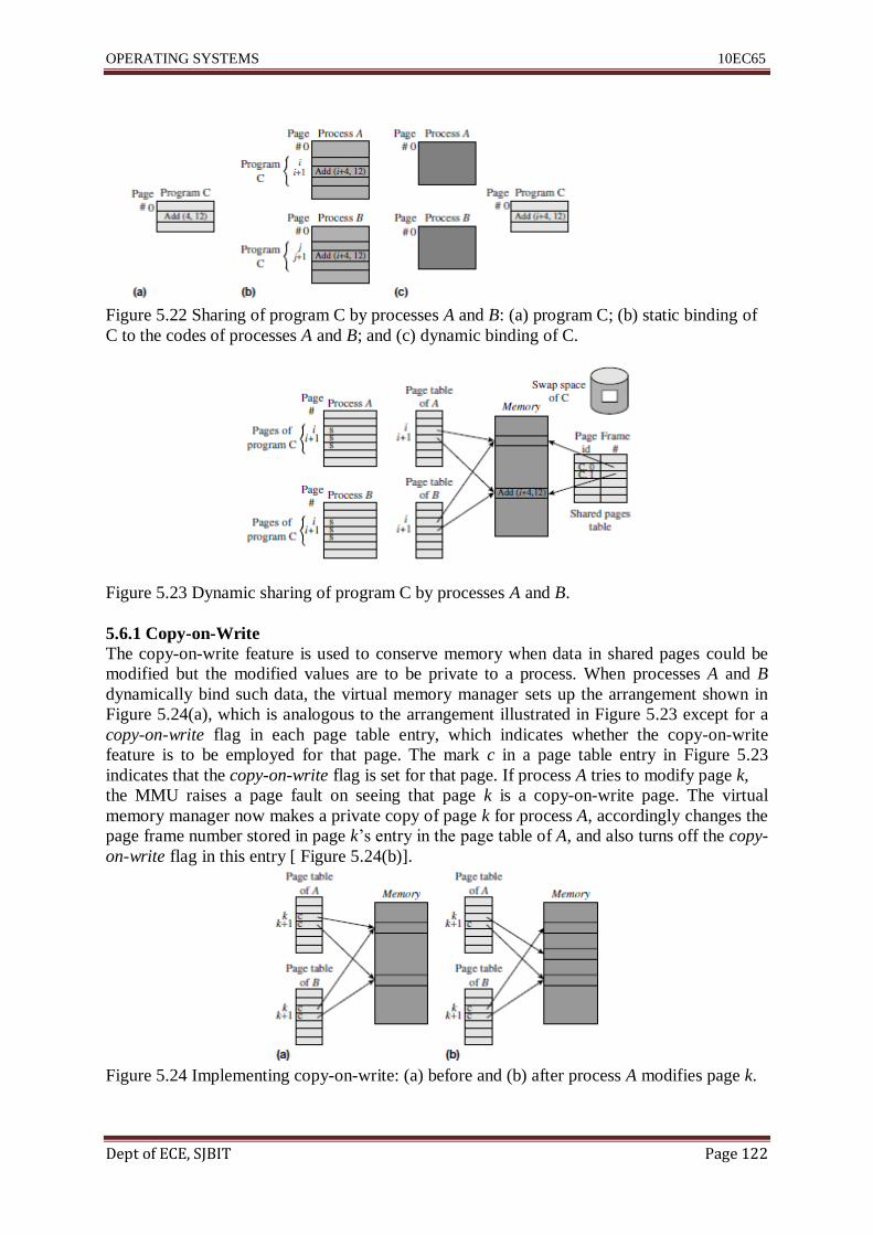
OPERATING SYSTEMS 10EC65
Dept of ECE, SJBIT Page 122
Figure 5.22 Sharing of program C by processes A and B: (a) program C; (b) static binding of
C to the codes of processes A and B; and (c) dynamic binding of C.
Figure 5.23 Dynamic sharing of program C by processes A and B.
5.6.1 Copy-on-Write
The copy-on-write feature is used to conserve memory when data in shared pages could be
modified but the modified values are to be private to a process. When processes A and B
dynamically bind such data, the virtual memory manager sets up the arrangement shown in
Figure 5.24(a), which is analogous to the arrangement illustrated in Figure 5.23 except for a
copy-on-write flag in each page table entry, which indicates whether the copy-on-write
feature is to be employed for that page. The mark c in a page table entry in Figure 5.23
indicates that the copy-on-write flag is set for that page. If process A tries to modify page k,
the MMU raises a page fault on seeing that page k is a copy-on-write page. The virtual
memory manager now makes a private copy of page k for process A, accordingly changes the
page frame number stored in page k‘s entry in the page table of A, and also turns off the copy-
on-write flag in this entry [ Figure 5.24(b)].
Figure 5.24 Implementing copy-on-write: (a) before and (b) after process A modifies page k.

OPERATING SYSTEMS 10EC65
Dept of ECE, SJBIT Page 123
Other processes sharing page k would continue to use the original copy of page k in memory;
each of them would get a private copy of the page if they modified it. In Unix systems, a
child process starts off with the code and data of the parent process; however, it can modify
the data and the modified values are private to it. The copy-on-write feature is used for the
entire address spaces of the parent and child processes. It speeds up process creation. It also
avoids copying of code pages because they are never modified; only data pages would be
copied if they are modified.
5.7 CASE STUDIES OF VIRTUAL MEMORY USING PAGING
5.7.1 Unix Virtual Memory
Unix has been ported on computer systems with diverse hardware designs. A variety of
ingenuous schemes have been devised to exploit features of the paging hardware of different
host machines. This section describes some features common to all Unix virtual memory
implementations and some interesting techniques used in different versions of Unix. Its
purpose is to provide a view of the practical issues in virtual memory implementations rather
than to study the virtual memory manager of any specific Unix version in detail.
Logical Address Space and Swap Space The page table of a process differentiates among
three kinds of pages—resident, unaccessed, and swapped-out pages. A resident page is
currently in memory. An unaccessed page is one that has not been accessed even once during
operation of the process and therefore has never been loaded in memory. It will be loaded
when a reference to it causes a page fault.
An unaccessed page may be a text page or a data page. A text page is loaded from an
executable file existing in the file system. Locating such a page in the file system may require
reading of several disk blocks in the inode and the file allocation table. To avoid this
overhead, the virtual memory manager maintains information about text pages in a separate
table and refers to it when a page needs to be loaded. As described later, the 4.3BSD virtual
memory manager maintains this information in the page table entry itself. This information
gets overwritten by the page frame number when the page is loaded in memory, and so it is
not available if the page gets removed from memory and has to be reloaded. To overcome
this difficulty, the virtual memory manager writes out a text page into the swap space when it
is removed from memory for the first time, and thereafter loads it from the swap space on
demand. A data page is called a zero-fill page; it is filled with zeroes when its first use leads
to a page fault. Thereafter, it is either a resident page or a swapped-out page.
A text page may remain in memory even if it is marked nonresident in its page table entry.
This situation arises if some other process is using the page (or has used it in the past).When
a page fault occurs for a text page, the virtual memory manager first checks whether the page
already exists in memory. If so, it simply puts the page frame information in its page table
entry and marks it as resident.
This action avoids a page-in operation and also conserves memory. To conserve disk space,
an effort is made to allocate as little swap space as possible. To start with, sufficient swap
space is allocated to accommodate the user stack and the data area. Thereafter swap space is
allocated in large chunks whenever needed. This approach suffers from the problem that
swap space in the system may become exhausted when the data area of a process grows; the
process then has to be suspended or aborted.
OPERATING SYSTEMS 10EC65
Dept of ECE, SJBIT Page 124
Copy-on-Write The semantics of fork require that the child process should obtain a copy of
the parent‘s address space. These semantics can be implemented by allocating distinct
memory areas and a swap space for the child process. However, child processes frequently
discard the copy of their parent‘s address space by loading some other program for execution
through the exec call. In any case, a child process may not wish to modify much of the
parent‘s data. Hence memory and swap space can be optimized through the copy-on-write
feature.
Copy-on-write is implemented as follows: When a process is forked, the reference count of
all data pages in the parent‘s address space is incremented by 1 and all data pages are made
read-only by manipulating bits in the access privileges field of their page table entries. Any
attempt at modifying a data page raises a protection fault. The virtual memory manager finds
that the reference count of the page is > 1, so it realizes that this is not a protection fault but a
reference to a copy-on-write page. It now reduces the count, makes a copy of the page for the
child process and assigns the read and write privileges to this copy by setting appropriate bits
in its page table entry. If the new reference count is = 1, it also enables the read and write
privileges in the page table entry that had led to the page fault because the entry no longer
pertains to a shared page.
Efficient Use of Page Table and Paging Hardware If a page is not present in memory, the
valid bit of its page table entry is ―off.‖ Under these circumstances, bits in other fields of this
entry, like the ref info field or the page frame # field, do not contain any useful information.
Hence these bits can be used for some other purposes. Unix 4.3BSD uses these bits to store
the address of a disk block in the file system that contains a text page.
The VAX 11 architecture does not provide a reference bit to collect page reference
information. Its absence is compensated by using the valid bit in a novel manner.
Periodically, the valid bit of a page is turned off even if the page is in memory. The next
reference to the page causes a page fault. However, the virtual memory manager knows that
this is not a genuine page fault, and so it sets the valid bit and resumes the process. In effect,
the valid bit is used as the reference bit.
Page Replacement The system permits a process to fix a certain fraction of its pages in
memory to reduce its own page fault rate and improve its own performance. These pages
cannot be removed from memory until they are unfixed by the process. Interestingly, there is
no I/O fixing of pages in Unix since I/O operations take place between a disk block and a
block in the buffer cache rather than between a disk block and the address space of a process.
Unix page replacement is analogous to the schematic of Figure 5.19, including the use of a
clock algorithm. To facilitate fast page-in operations, Unix virtual memory manager maintain
a list of free page frames and try to keep at least 5 percent of total page frames on this list at
all times. A daemon called the pageout daemon (which is labeled process 2 in the system) is
created for this purpose. It is activated any time the total number of free page frames falls
below 5 percent. It tries to add pages to the free list and puts itself to sleep when the free list
contains more than 5 percent free page frames. Some versions of Unix use two thresholds—a
high threshold and a low threshold—instead of a single threshold at 5 percent. The daemon
goes to sleep when it finds that the number of pages in the free list exceeds the high
threshold. It is activated when this number falls below the low threshold. This arrangement
avoids frequent activation and deactivation of the daemon.

OPERATING SYSTEMS 10EC65
Dept of ECE, SJBIT Page 125
The virtual memory manager divides pages that are not fixed in memory into active pages,
i.e., pages that are actively in use by a process, and inactive pages, i.e., pages that have not
been referenced in the recent past. The virtual memory manager maintains two lists, the
active list and the inactive list. Both lists are treated as queues. A page is added to the active
list when it becomes active, and to the inactive list when it is deemed to have become
inactive. Thus the least recently activated page is at the head of the active list and the oldest
inactive page is at the head of the inactive list. A page is moved from the inactive list to the
active list when it is referenced. The pageout daemon tries to maintain a certain number of
pages, computed as a fraction of total resident pages, in the inactive list. If it reaches the end
of the inactive list while adding page frames to the free list, it checks whether the total
number of pages in the inactive list is smaller than the expected number. If so, it transfers a
sufficient number of pages from the active list to the inactive list.
Swapping The Unix virtual memory manager does not use a working set memory allocator
because of the high overhead of such an allocator. Instead it focuses on maintaining needed
pages in memory. A process is swapped out if all its required pages cannot be maintained in
memory and conditions resembling thrashing exist in the system. An inactive process, i.e., a
process that is blocked for a long time, may also be swapped out in order to maintain a
sufficient number of free page frames. When this situation arises and a swap-out becomes
necessary, the pageout daemon activates the swapper, which is always process 0 in the
system.
The swapper finds and swaps out inactive processes. If that does not free sufficient memory,
it is activated again by the pageout daemon. This time it swaps out the process that has been
resident the longest amount of time. When swapped out processes exist in the system, the
swapper periodically checks whether sufficient free memory exists to swap some of them
back in. A swap-in priority—which is a function of when the process was swapped out, when
it was last active, its size and its nice value—is used for this purpose (see Section 7.6.1 for
details of the nice value). This function ensures that no process remains swapped out
indefinitely.
In Unix 4.3BSD, a process was swapped-in only if it could be allocated as much memory as
it held when it was swapped out. In Unix 4.4BSD this requirement was relaxed; a process is
brought in if enough memory to accommodate its user structure and kernel stack can be
allocated to it.
Recommended Questions
1. Explain the important concepts in the operation of demand paging.
2. Write a note on page replacement policies and page sharing.
3. How can virtual memory be implemented?
4. Explain FIFO and LRU page replacement policy.
5. What are the functions performed by a virtual memory manager? Explain.
6. Explain ―page-out daemon‖ for handling virtual memory in UNIX OS.
7. Describe the address translation using TU and TLB in demand paged allocation with a
block diagram.
8. For the following page reference string, calculate the number of page faults with FIFO
and LRU page replacement policies when i) number of page frames=3 ii) number of
page frames=4.
Page reference string: 5 4 3 2 1 4 3 5 4 3 2 1 5. Reference time string: t1,t2,……,t13

OPERATING SYSTEMS 10EC65
Dept of ECE, SJBIT Page 126
UNIT-6
FILE SYSTEMS
This chapter deals with the design of the file system. After discussing the basics of file
organizations, directory structures and disk space management, we describe the file sharing
semantics that govern concurrent sharing of files and file system reliability.
Computer users store programs and data in files so that they can be used conveniently and
preserved across computing sessions. A user has many expectations when working with files,
namely
• Convenient and fast access to files
• Reliable storage of files
• Sharing of files with collaborators
The resources used for storing and accessing files are I/O devices. As it must, the OS ensures
both efficient performance of file processing activities in processes and efficient use of I/O
devices.
Operating systems organize file management into two components called the file system and
the input-output control system (IOCS) to separate the file-level concerns from concerns
related to efficient storage and access of data. Accordingly, a file system provides facilities
for creating and manipulating files, for ensuring reliability of files when faults such as power
outages or I/O device mal functions occur, and for specifying how files are to be shared
among users. The IOCS provides access to data stored on I/O devices and good performance
of I/O devices.
6.1 OVERVIEW OF FILE PROCESSING
We use the term file processing to describe the general sequence of operations of opening a
file, reading data from the file or writing data into it, and closing the file. Figure 6.1 shows
the arrangement through which an OS implements file processing activities of processes.
Each directory contains entries describing some files. The directory entry of a file indicates
the name of its owner, its location on a disk, the way its data is organized, and which users
may access it in what manner.
The code of a process Pi is shown in the left part of Figure 6.1. When it opens a file for
processing, the file system locates the file through the directory

OPERATING SYSTEMS 10EC65
Dept of ECE, SJBIT Page 127
Figure 6.1 File system and the IOCS.
structure, which is an arrangement of many directories. In Figure 6.1, there are two files
named beta located in different directories. When process Pi opens beta, the manner in which
it names beta, the directory structure, and identities of the user who initiated process Pi will
together determine which of the two files will be accessed.
A file system provides several file types. Each file type provides its own abstract view of
data in a file— it is logical view of data. Figure 6.1 shows that file beta opened by process Pi
has a record-oriented logical view, while file phi has a byte stream–oriented logical view in
which distinct records do not exist.
The IOCS organizes a file‘s data on an I/O device in accordance with its file type. It is the
physical view of the file‘s data. The mapping between the logical view of the file‘s data and
its physical view is performed by the IOCS. The IOCS also provides an arrangement that
speeds up a file processing activity—it holds some data from a file in memory areas
organized as buffers, a file cache, or a disk cache. When a process performs a read operation
to get some data from a file, the IOCS takes the data from a buffer or a cache if it is present
there. This way, the process does not have to wait until the data is read off the I/O device that
holds the file. Analogously, when a process performs a write operation on a file, the IOCS
copies the data to be written in a buffer or in a cache. The actual I/O operations to read data
from an I/O device into a buffer or a cache, or to write it from there onto an I/O device, are
performed by the IOCS in the background.

OPERATING SYSTEMS 10EC65
Dept of ECE, SJBIT Page 128
6.1.1 File System and the IOCS
A file system views a file as a collection of data that is owned by a user, can be shared by a
set of authorized users, and has to be reliably stored over an extended period of time. A file
system gives users freedom in naming their files, as an aspect of ownership, so that a user can
give a desired name to a file without worrying whether it conflicts with names of other users‘
files; and it provides privacy by protecting against interference by other users. The IOCS, on
the other hand, views a file as a repository of data that need to be accessed speedily and are
stored on an I/O device that needs to be used efficiently.
Table 6.1 summarizes the facilities provided by the file system and the IOCS. The file system
provides directory structures that enable users to organize their data into logical groups of
files, e.g., one group of files for each professional activity. The file system provides
protection against illegal file accesses and ensures correct operation when processes access
and update a file concurrently. It also ensures that data is reliably stored, i.e., data is not lost
when system crashes occur. Facilities of the IOCS are as described earlier.
The file system and the IOCS form a hierarchy. Each of them has policies and provides
mechanisms to implement the policies.
Table 6.1 Facilities Provided by the File System and the Input-Output Control System
File System
• Directory structures for convenient grouping of files
• Protection of files against illegal accesses
• File sharing semantics for concurrent accesses to a file
• Reliable storage of files
Input-Output Control System (IOCS)
• Efficient operation of I/O devices
• Efficient access to data in a file
Data and Metadata A file system houses two kinds of data—data contained within files, and
data used to access files. We call the data within files file data, or simply data. The data used
to access files is called control data, or metadata. In the logical view shown in Figure 6.1,
data contained in the directory structure is metadata.
6.2 FILES AND FILE OPERATIONS
File Types A file system houses and organizes different types of files, e.g., data files,
executable programs, object modules, textual information, documents, spreadsheets, photos,
and video clips. Each of these file types has its own format for recording the data. These file
types can be grouped into two classes:
• Structured files
• Byte stream files
A structured file is a collection of records, where a record is a meaningful unit for processing

OPERATING SYSTEMS 10EC65
Dept of ECE, SJBIT Page 129
of data.Arecord is a collection of fields, and a field contains a single data item. Each record in
a file is assumed to contain a key field. The value in the key field of a record is unique in a
file; i.e., no two records contain an identical key.
Many file types mentioned earlier are structured files. File types used by standard system
software like compilers and linkers have a structure determined by the OS designer, while file
types of user files depend on the applications or programs that create them.
A byte stream file is ―flat.‖ There are no records and fields in it; it is looked upon as a
sequence of bytes by the processes that use it. The next example illustrates structured and
byte stream files.
Structured and Byte Stream Files Example 6.1
Figure 6.2(a) shows a structured file named employee_info. Each record in the file contains
information about one employee. A record contains four fields: employee id, name,
designation, and age. The field containing the employee id is the key field. Figure 6.3(b)
shows a byte stream file report.
Figure 6.2 Logical views of (a) a structured file employee_info; (b) a byte stream file report.
File Attributes A file attribute is a characteristic of a file that is important either to its users
or to the file system, or both. Commonly used attributes of a file are: type, organization, size,
location on disk, access control information, which indicates the manner in which different
users can access the file; owner name, time of creation, and time of last use. The file system
stores the attributes of a file in its directory entry. During a file processing activity, the file
system uses the attributes of a file to locate it, and to ensure that each operation being
performed on it is consistent with its attributes. At the end of the file processing activity, the
file system stores changed values of the file‘s attributes, if any, in the file‘s directory entry.

OPERATING SYSTEMS 10EC65
Dept of ECE, SJBIT Page 130
Table 6.2 Operations on Files
6.3 FUNDAMENTAL FILE ORGANIZATIONS AND ACCESS METHODS
The term ―record access pattern‖ to describe the order in which records in a file are accessed
by a process. The two fundamental record access patterns are sequential access, in which
records are accessed in the order in which they fall in a file (or in the reverse of that order),
and random access, in which records may be accessed in any order. The file processing
actions of a process will execute efficiently only if the process‘s record access pattern can be
implemented efficiently in the file system. The characteristics of an I/O device make it
suitable for a specific record access pattern. For example, a tape drive can access only the
record that is placed immediately before or after the current position of its read/write head.
Hence it is suitable for sequential access to records. A disk drive can directly access any
record given its address. Hence it can efficiently implement both the sequential and random
record access patterns.
A file organization is a combination of two features—a method of arranging records in a file
and a procedure for accessing them. A file organization is designed to exploit the
characteristics of an I/O device for providing efficient record access for a specific record
access pattern. A file system supports several file organizations so that a process can employ
the one that best suits its file processing requirements and the I/O device in use. This section
describes three fundamental file organizations—sequential file organization, direct file
organization and index sequential file organization. Other file organizations used in practice
are either variants of these fundamental ones or are special-purpose organizations that exploit
less commonly used I/O devices. Accesses to files governed by a specific file organization
are implemented by an IOCS module called an access method. An access method is a policy
module of the IOCS. While compiling a program, the compiler infers the file organization
governing a file from the file‘s declaration statement (or from the rules for default, if the

OPERATING SYSTEMS 10EC65
Dept of ECE, SJBIT Page 131
program does not contain a file declaration statement), and identifies the correct access
method to invoke for operations on the file.
6.3.1 Sequential File Organization
In sequential file organization, records are stored in an ascending or descending sequence
according to the key field; the record access pattern of an application is expected to follow
suit. Hence sequential file organization supports two kinds of operations: read the next (or
previous) record, and skip the next (or previous) record. A sequential-access file is used in an
application if its data can be conveniently presorted into an ascending or descending order.
The sequential file organization is also used for byte stream files.
6.3.2 Direct File Organization
The direct file organization provides convenience and efficiency of file processing when
records are accessed in a random order. To access a record, a read/write command needs to
mention the value in its key field. We refer to such files as direct-access files. A direct-access
file is implemented as follows: When a process provides the key value of a record to be
accessed, the access method module for the direct file organization applies a transformation
to the key value that generates the address of the record in the storage medium. If the file is
organized on a disk, the transformation generates a (track_no, record_no) address. The disk
heads are now positioned on the track track_no before a read or write command is issued
on the record record_no.
Consider a file of employee information organized as a direct-access file. Let p records be
written on one track of the disk. Assuming the employee numbers and the track and record
numbers of the file to start from 1, the address of the record for employee number n is (track
number (tn), record number (rn)) where
and [. . .] indicates a rounded-up integer value.
Direct file organization provides access efficiency when records are processed randomly.
However, it has three drawbacks compared to sequential file organization:
• Record address calculation consumes CPU time.
• Disks can store much more data along the outermost track than along the innermost
track.However, the direct file organization stores an equal amount of data along each track.
Hence some recording capacity is wasted.
• The address calculation formulas work correctly only if a record exists for every possible
value of the key, so dummy records have to exist for keys that are not in use. This
requirement leads to poor utilization of the I/O medium. Hence sequential processing of
records in a direct-access file is less efficient than processing of records in a sequential-access
file.
Example 6.2 Sequential and Direct-Access Files
Figure 6.3 shows the arrangement of employee records in sequential and direct file
organizations. Employees with the employee numbers 3, 5–9 and 11 have left the

OPERATING SYSTEMS 10EC65
Dept of ECE, SJBIT Page 132
organization. However, the direct-access file needs to contain a record for each of these
employees to satisfy the address calculation formulas. This fact leads to the need for dummy
records in the direct access file.
Figure 6.3 Records in (a) sequential file; (b) direct-access file.
6.3.3 Index Sequential File Organization
An index helps to determine the location of a record from its key value. In a pure indexed file
organization, the index of a file contains an index entry with the format (key value, disk
address) for each key value existing in the file. To access a record with key k, the index entry
containing k is found by searching the index, and the disk address mentioned in the entry is
used to access the record. If an index is smaller than a file, this arrangement provides high
access efficiency because a search in the index is more efficient than a search in the file.
The index sequential file organization is a hybrid organization that combines elements of the
indexed and the sequential file organizations. To locate a desired record, the access method
module for this organization searches an index to identify a section of the disk that may
contain the record, and searches the records in this section of the disk sequentially to find the
record. The search succeeds if the record is present in the file; otherwise, it results in a
failure. This arrangement requires a much smaller index than does a pure indexed file
because the index contains entries for only some of the key values. It also provides better
access efficiency than the sequential file organization while ensuring comparably efficient
use of I/O media.
Index Sequential File Organization
Example 6.3
Figure 6.5 illustrates a file of employee information organized as an index sequential file.
Records are stored in ascending order by the key field. Two indexes are built to facilitate
speedy search. The track index indicates the smallest and largest key value located on each
track (see the fields named low and high in Figure 6.5). The higher-level index contains
entries for groups of tracks containing 3 tracks each. To locate the record with a key k, first
the higher-level index is searched to locate the group of tracks that may contain The desired
record. The track index for the tracks of the group is now searched to locate the track that
may contain the desired record, and the selected track is searched sequentially for the record
with key k. The search ends unsuccessfully if it fails to find the record on the track.
Figure 6.5 Track index and higher-level index in an index sequential file.

OPERATING SYSTEMS 10EC65
Dept of ECE, SJBIT Page 133
6.3.4 Access Methods An access method is a module of the IOCS that implements accesses to a class of files using a
specific file organization. The procedure to be used for accessing records in a file, whether by
a sequential search or by address calculation, is determined by the file organization. The
access method module uses this procedure to access records. It may also use some advanced
techniques in I/O programming to make file processing more efficient. Two such techniques
are buffering and blocking of records.
Buffering of Records The access method reads records of an input file ahead of the time
when they are needed by a process and holds them temporarily in memory areas called
buffers until they are actually used by the process. The purpose of buffering is to reduce or
eliminate the wait for an I/O operation to complete; the process faces a wait only when the
required record does not already exist in a buffer. The converse actions are performed for an
output file. When the process performs a write operation, the data to be written into the file is
copied into a buffer and the process is allowed to continue its operation. The data is written
on the I/O device sometime later and the buffer is released for reuse. The process faces a wait
only if a buffer is not available when it performs a write operation.
Blocking of Records The access method always reads or writes a large block of data, which
contains several file records, from or to the I/O medium. This feature reduces the total
number of I/O operations required for processing a file, thereby improving the file processing
efficiency of a process. Blocking also improves utilization of an I/O medium and throughput
of a device.
6.4 DIRECTORIES
A directory contains information about a group of files. Each entry in a directory contains the
attributes of one file, such as its type, organization, size, location, and the manner inwhich it
may be accessed by various users in the system. Figure 6.6 shows the fields of a typical
directory entry. The open count and lock fields are used when several processes open a file
concurrently. The open count indicates the number of such processes. As long as this count is
nonzero, the file system keeps some of the metadata concerning the file in memory to speed
up accesses to the data in the file. The lock field is used when a process desires exclusive
access to a file. The flags field is used to differentiate between different kinds of directory
entries. We put the value ―D‖ in this field to indicate that a file is a directory, ―L‖ to indicate
that it is a link, and ―M‖ to indicate that it is a mounted file system. Later sections in this
chapter will describe these uses. The misc info field contains information such as the file‘s
owner, its time of creation, and last modification.
A file system houses files owned by several users. Therefore it needs to grant users two
important prerogatives:
• File naming freedom: A user‘s ability to give any desired name to a file, without being
constrained by file names chosen by other users.
• File sharing: A user‘s ability to access files created by other users, and ability to permit
other users to access his files.

OPERATING SYSTEMS 10EC65
Dept of ECE, SJBIT Page 134
Figure 6.5 Fields in a typical directory entry.
Figure 6.6 A directory structure composed of master and user directories.
The file system creates several directories and uses a directory structure to organize them for
providing file naming freedom and file sharing.
Figure 6.7 shows a simple directory structure containing two kinds of directories. A user
directory (UD) contains entries describing the files owned by one user. The master directory
contains information about the UDs of all registered users of the system; each entry in the
master directory is an ordered pair consisting of a user id and a pointer to a UD. In the file
system shown, users A and B have each created their own file named beta. These files have
entries in the users‘ respective UDs.
The directory structure shown in Figure 6.7 as a two-level directory structure.

OPERATING SYSTEMS 10EC65
Dept of ECE, SJBIT Page 135
Use of separate UDs is what provides naming freedom. When a process created by user A
executes the statement open (beta, ...), the file system searches the master directory to locate
A‘s UD, and searches for beta in it. If the call open(beta, ...) had instead been executed by
some process created by B, the file system would have searched B‘s UD for beta. This
arrangement ensures that the correct file is accessed even if many files with identical names
exist in the system.
Use of UDs has one drawback, however. It inhibits users from sharing their files with other
users. A special syntax may have to be provided to enable a user to refer to another user‘s
file. For example, a process created by user C may execute the statement open (A→beta, ...)
to open A‘s file beta. The file system can implement this simply by using A‘s UD, rather than
C‘s UD, to search and locate file beta. To implement file protection, the file system must
determine whether user C is permitted to open A‘s file beta. It checks the protection info field
of beta‘s directory entry for this purpose.
6.4.1 Directory Trees
The MULTICS file system of the 1960s contained features that allowed the user to create a
new directory, give it a name of his choice, and create files and other directories in it up to
any desired level. The resulting directory structure is a tree, it is called the directory tree.
After MULTICS, most file systems have provided directory trees.
Figure 6.7 Directory trees of the file system and of user A.
A user can create a file to hold data or to act as a directory. When a distinction between the
two is important, we will call these files respectively data files and directory files, or simply
directories. The file system provides a directory called root that contains the home directory
for each user, which is a directory file that typically has the same name as the user‘s name. A
user structures his information by creating directory files and data files in his home directory,
creating files and other directories in a directory file, and so on. We will assume that the file
system puts a ―D‖ in the flags field of a file‘s entry if the file is a directory file. Figure 13.8
shows the directory tree of the file system. The root of this tree is the directory root, which
contains a home directory for each user that bears the user‘s name. User A has created a file
called alpha and directories called admin and projects. The projects directory contains a
directory real_time, which contains a file main_pgm. Thus user A has a directory tree of his
own; its root is his home directory.

OPERATING SYSTEMS 10EC65
Dept of ECE, SJBIT Page 136
At any time, a user is said to be ―in‖ some specific directory,which is called his current
directory.When the user wishes to open a file, the file name is searched for in this
directory.Whenever the user logs in, the OS puts him in his home directory; the home
directory is then the user‘s current directory. A user can change his current directory at any
time through a ―change directory‖ command.
A file‘s name may not be unique in the file system, so a user or a process uses a path name to
identify it in an unambiguous manner. A path name is a sequence of one or more path
components separated by a slash (/), where each path component is a reference through a
directory and the last path component is the name of the file. Path names for locating a file
from the current directory are called relative path names. Relative path names are often short
and convenient to use; however, they can be confusing because a file may have different
relative path names when accessed from different current directories. For example, in Figure
6.7, the file alpha has the simple relative path name alpha when accessed from current
directory A, whereas it has relative path names of the form ../alpha and ../../alphawhen
accessed fromthe directories projects and real_time, respectively. To facilitate use of relative
path names, each directory stores information about its own parent directory in the directory
structure.
6.4.2 Directory Graphs
In a directory tree, each file except therootdirectory has exactly one parent directory. This
directory structure provides total separation of different users‘ files and complete file naming
freedom. However, it makes file sharing rather cumbersome.
A user wishing to access another user‘s files has to use a path name that involves two or more
directories. For example, in Figure 6.8, user B can access file beta using the path name
../A/projects/beta or ˜A/projects/beta.
Use of the tree structure leads to a fundamental asymmetry in the way different users can
access a shared file. The file will be located in some directory belonging to one of the users,
who can access it with a shorter path name than can other users. This problem can be solved
by organizing the directories in an acyclic graph structure. In this structure, a file can have
many parent directories, and so a shared file can be pointed to by directories of all users who
have access to it. Acyclic graph structures are implemented through links.
Links A link is a directed connection between two existing files in the directory structure. It
can be written as a triple (<from_ file_name>, <to_ file_name>,
<link_name>),where<from_ file_name>is a directory and<to_ file_name>can be a directory
or a file. Once a link is established,<to_ file_name>can be accessed as if it were a file named
<link_name> in the directory <from_ file_name>. The fact that <link_name> is a link in the
directory <from_ file_name> is indicated by putting the value ―L‖ in its flags field. Example
6.4 illustrates how a link is set up.
Example 6.4 Link in a Directory Structure
Figure 6.8 shows the directory structure after user C creates a link using the command (˜C,
˜C/software/web_server, quest). The name of the link is quest. The link is made in the
directory ˜C and it points to the file ˜C/software/web_server. This link permits
˜C/software/web_server to be accessed by the name ˜C/quest.

OPERATING SYSTEMS 10EC65
Dept of ECE, SJBIT Page 137
Figure 6.8 A link in the directory structure.
An unlink command nullifies a link. Implementation of the link and unlink commands
involves manipulation of directories that contain the files <from_ file_name> and <to_
file_name>. Deadlocks may arise while link and unlink commands are implemented if
several processes issue these commands simultaneously.
6.5 FILE PROTECTION
A user would like to share a file with collaborators, but not with others. We call this
requirement controlled sharing of files. To implement it, the owner of a file specifies which
users can access the file in what manner. The file system stores this information in the
protection info field of the file‘s directory entry, and uses it to control access to the file.
Different methods of structuring the protection information of files. In this section,we assume
that a file‘s protection information is stored in the form of an access control list. Each
element of the access control list is an access control pair of the
form(<user_name>,<list_of_access_privileges>). When a process executed by some user X
tries to perform an operation <opn> on file alpha, the file system searches for the pair with
<user_name>= X, in the access control list of alpha and checks whether <opn> is consistent
with the <list_of_access_privileges>. If it is not, the attempt to access alpha fails. For
example, a write attempt by X will fail if the entry for user X in the access control list is (X,
read), or if the list does not contain an entry for X.
The size of a file‘s access control list depends on the number of users and the number of
access privileges defined in the system. To reduce the size of protection information, users
can be classified in some convenient manner and an access control pair can be specified for
each user class rather than for each individual user. Now an access control list has only as
many pairs as the number of user classes. For example, Unix specifies access privileges for
three classes of users— the file owner, users in the same group as the owner, and all other
users of the system.
In most file systems, access privileges are of three kinds—read, write, and execute. A write
privilege permits existing data in the file to be modified and also permits new data to be
added: One can further differentiate between these two privileges by defining a new access
privilege called append; however, it would increase the size of the protection information.
The execute privilege permits a user to execute the program contained in a file. Access
privileges have different meanings for directory files. The read privilege for a directory file
implies that one can obtain a listing of the directory, while the write privilege for a directory
implies that one can create new files in the directory. The execute privilege for a directory
permits an access to be made through it—that is, it permits a file existing in the directory to

OPERATING SYSTEMS 10EC65
Dept of ECE, SJBIT Page 138
be accessed. A user can use the execute privilege of directories to make a part of his directory
structure visible to other users.
6.6 ALLOCATION OF DISK SPACE
A disk may contain many file systems, each in its own partition of the disk. The file system
knows which partition a file belongs to, but the IOCS does not. Hence disk space allocation is
performed by the file system.
Early file systems adapted the contiguous memory allocation model by allocating a single
contiguous disk area to a file when it was created. This model was simple to implement. It
also provided data access efficiency by reducing disk head movement during sequential
access to data in a file. However, contiguous allocation of disk space led to external
fragmentation. Interestingly, it also suffered from internal fragmentation because the file
system found it prudent to allocate some extra disk space to allow for expansion of a file.
Contiguity of disk space also necessitated complicated arrangements to avoid use of bad disk
blocks: The file system identified bad disk blocks while formatting the disk and noted their
addresses. It then allocated substitute disk blocks for the bad ones and built a table showing
addresses of bad blocks and their substitutes. During a read/write operation, the IOCS
checked whether the disk block to be accessed was a bad block. If it was, it obtained the
address of the substitute disk block and accessed it. Modern file systems adapt the
noncontiguous memory allocation model to disk space allocation. In this approach, a chunk
of disk space is allocated on demand, i.e., when the file is created or when its size grows
because of an update operation. The file system has to address three issues for implementing
this approach:
• Managing free disk space: Keep track of free disk space and allocate from it when a file
requires a new disk block.
• Avoiding excessive disk head movement: Ensure that data in a file is not dispersed to
different parts of a disk, as it would cause excessive movement of the disk heads during file
processing.
• Accessing file data: Maintain information about the disk space allocated to a file and use it
to find the disk block that contains required data.
The file system can maintain a free list of disk space and allocate from it when a file requires
a new disk block. Alternatively, it can use a table called the disk status map (DSM) to
indicate the status of disk blocks. The DSM has one entry for each disk block, which
indicates whether the disk block is free or has been allocated to a file. This information can
be maintained in a single bit, and so a DSM is also called a bit map. Figure 13.12 illustrates a
DSM. A 1 in an entry indicates that the corresponding disk block is allocated. The DSM is
consulted every time a new disk block has to be allocated to a file. To avoid dispersing file
data to different parts of a disk, file systems confine the disk space allocation for a file either
to consecutive disk blocks, which form an extent, also called a cluster, or consecutive
cylinders in a disk, which form cylinder groups .

OPERATING SYSTEMS 10EC65
Dept of ECE, SJBIT Page 139
Figure 6.9 Disk status map (DSM).
Use of a disk status map, rather than a free list, has the advantage that it allows the file
system to readily pick disk blocks from an extent or cylinder group.
The two fundamental approaches to noncontiguous disk space allocation. They differ in the
manner they maintain information about disk space allocated to a file.
6.6.1 Linked Allocation
A file is represented by a linked list of disk blocks. Each disk block has two fields in it—data
and metadata. The data field contains the data written into the file, while the metadata field
is the link field, which contains the address of the next disk block allocated to the file. Figure
6.10 illustrates linked allocation. The location info field of the directory entry of file alpha
points to the first disk block of the file. Other blocks are accessed by following the pointers in
the list of disk blocks. The last disk block contains null information in its metadata field.
Thus, file alpha consists of disk blocks 3 and 2, while file beta consists of blocks 4, 5,
and 7. Free space on the disk is represented by a free list in which each free disk block
contains a pointer to the next free disk block.When a disk block is needed to store new data
added to a file, a disk block is taken off the free list and added to the file‘s list of disk blocks.
To delete a file, the file‘s list of disk blocks is simply added to the free list.
Figure 6.10 Linked allocation of disk space.
Linked allocation is simple to implement, and incurs a low allocation/ deallocation overhead.
It also supports sequential files quite efficiently. However, files with nonsequential
organization cannot be accessed efficiently. Reliability is also poor since corruption of the
metadata field in a disk block may lead to loss of data in the entire file. Similarly, operation
of the file system may be disrupted if a pointer in the free list is corrupted.
6.6.2 File Allocation Table (FAT) MS-DOS uses a variant of linked allocation that stores
the metadata separately from the file data. A file allocation table (FAT) of a disk is an array
that has one element corresponding to every disk block in the disk. For a disk block that is
allocated to a file, the corresponding FAT element contains the address of the next disk

OPERATING SYSTEMS 10EC65
Dept of ECE, SJBIT Page 140
block. Thus the disk block and its FAT element together form a pair that contains the same
information as the disk block in a classical linked allocation scheme.
Figure 6.11 File Allocation Table (FAT).
The directory entry of a file contains the address of its first disk block. The FAT element
corresponding to this disk block contains the address of the second disk block, and so on. The
FAT element corresponding to the last disk block contains a special code to indicate that the
file ends on that disk block. Figure 6.11 illustrates the FAT for the disk of Figure 6.10. The
file alpha consists of disk blocks 3 and 2. Hence the directory entry of alpha contains 3. The
FAT entry for disk block 3 contains 2, and the FAT entry for disk block 2 indicates that the
file ends on that disk block. The file beta consists of blocks 4, 5, and 7. The FAT can also be
used to store free space information. The list of free disk blocks can be stored as if it were a
file, and the address of the first free disk block can be held in a free list pointer. Alternatively,
some special code can be stored in the FAT element corresponding to a free disk block, e.g.
the code ―free‖ in Figure 6.11. Use of the FAT rather than the classical linked allocation
involves a performance penalty, since the FAT has to be accessed to obtain the address of the
next disk block. To overcome this problem, the FAT is held in memory during file
processing. Use of the FAT provides higher reliability than classical linked allocation
because corruption of a disk block containing file data leads to limited damage. However,
corruption of a disk block used to store the FAT is disastrous.
6.6.3 Indexed Allocation
In indexed allocation, an index called the file map table (FMT) is maintained to note the
addresses of disk blocks allocated to a file. In its simplest form, an FMT can be an array
containing disk block addresses. Each disk block contains a single field—the data field. The
location info field of a file‘s directory entry points to the FMT for the file.
Figure 6.12 Indexed allocation of disk space.
In the following discussion we use the notation fmtalpha for the FMT of the file alpha. If the
size of the file alpha grows, the DSM is searched to locate a free block, and the address of the
block is added to fmtalpha. Deallocation is performed when alpha is deleted. All disk blocks

OPERATING SYSTEMS 10EC65
Dept of ECE, SJBIT Page 141
pointed to by fmtalpha are marked free before fmtalpha and the directory entry of alpha are
erased.
The reliability problem is less severe in indexed allocation than in linked allocation because
corruption of an entry in an FMT leads to only limited damage.
Compared with linked allocation, access to sequential-access files is less efficient because the
FMT of a file has to be accessed to obtain the address of the next disk block. However, access
to records in a direct-access file is more efficient since the address of the disk block that
contains a specific record can be obtained directly from the FMT. For example, if address
calculation anal shows that a required record exists in the ith disk block of a file, its address
can be obtained from the ith entry of the FMT. For a small file, the FMT can be stored in the
directory entry of the file; it is both convenient and efficient. For a medium or large file, the
FMT will not fit into the directory entry. A two-level indexed allocation depicted in Figure
6.13 may be used for such FMTs. In this organization, each entry of the FMT contains the
address of an index block.Anindex block does not contain data; it contains entries that contain
addresses of data blocks. To access the data block, we first access an entry of the FMT and
obtain the address of an index block.
Figure 6.13 A two-level FMT organization.
Figure 6.14 A hybrid organization of FMT.
data blocks as in the conventional indexed allocation. Other entries point to index blocks. The
advantage of this arrangement is that small files containing n or fewer data blocks continue to
be accessible efficiently, as their FMT does not use index blocks. Medium and large files
suffer a marginal degradation of their access performance because of multiple levels of
indirection. The Unix file system uses a variation of the hybrid FMT organization.

OPERATING SYSTEMS 10EC65
Dept of ECE, SJBIT Page 142
6.7 Performance Issues
Two performance issues are associated with the use of a disk block as the unit of disk space
allocation—size of the metadata, i.e., the control data of the file system; and efficiency of
accessing file data. Both issues can be addressed by using a larger unit of allocation of disk
space. Hence modern file systems tend to use an extent, also called a cluster, as a unit of disk
space allocation. An extent is a set of consecutive disk blocks. Use of large extents provides
better access efficiency. However, it causes more internal fragmentation. To get the best of
both worlds, file systems prefer to use variable extent sizes. Their metadata contains the size
of an extent along with its address.
6.8 INTERFACE BETWEEN FILE SYSTEM AND IOCS
The file system uses the IOCS to perform I/O operations and the IOCS implements them
through kernel calls. The interface between the file system and the IOCS consists of three
data structures—the file map table (FMT), the file control block (FCB), and the open files
table (OFT)—and functions that perform I/O operations. Use of these data structures avoids
repeated processing of file attributes by the file system, and provides a convenient method of
tracking the status of ongoing file processing activities.
The file system allocates disk space to a file and stores information about the allocated disk
space in the file map table (FMT). The FMT is typically held in memory during the
processing of a file.
A file control block (FCB) contains all information concerning an ongoing file processing
activity. This information can be classified into the three categories shown in Table 6.3.
Information in the file organization category is either simply extracted from the file
declaration statement in an application program, or inferred from it by the compiler, e.g.,
information such as the size of a record and number of buffers is extracted from a file
declaration, while the name of the access method is inferred from the type and organization
of a file. The compiler puts this information as parameters in the open call. When the call is
made during execution of the program, the file system puts this information in the FCB.
Directory information is copied into the FCB through joint actions of the file system and the
IOCS when a new file is created. Information concerning the current state of processing is
written into the FCB by the IOCS. This information is continually updated during the
processing of a file. The open files table (OFT) holds the FCBs of all open files. The OFT
resides in the kernel address space so that user processes cannot tamper with it. When a file is
opened, the file system stores its FCB in a new entry of the OFT. The offset of this entry in
the OFT is called the internal id of the file. The internal id is passed back to the process,
which uses it as a parameter in all future file system calls.
Figure 6.15 shows the arrangement set up when a file alpha is opened. The file system copies
fmtalpha in memory; creates fcbalpha, which is an FCB for alpha, in the OFT; initializes its
fields appropriately; and passes back its offset in OFT, which in this case is 6, to the process
as internal_idalpha.

OPERATING SYSTEMS 10EC65
Dept of ECE, SJBIT Page 143
Table 6.3 Fields in the File Control Block (FCB)
Figure 6.15 Interface between file system and IOCS—OFT, FCB and FMT.
The file system supports the following operations:
• open (<file_name>, <processing_mode>, <file_attributes>)
• close (<internal_id_of_file>)
• read/write (<internal_id_of_file>, <record_info>, <I/O_area_addr>) <file_name> is an
absolute or relative path name of the file to be opened. <processing_mode> indicates what
kind of operations will be performed on the file—the values ―input,‖ ―create,‖ and ―append‖
of it have obvious meanings, while ―update‖ indicates that the process intends to update
existing data in place.
<file_attributes> is a list of file attributes, such as the file‘s organization, record size, and
protection information. It is relevant only when a new file is being created—attributes from
the list are copied into the directory entry of the file at this time. <record_info> indicates the
identity of the record to be read or written if the file is being processed in a nonsequential
mode. <I/O_area addr> indicates the address of the memory area where data from the record
should be read, or the memory area that contains the data to be written into the record.
The IOCS interface supports the following operations:
• iocs-open (<internal_id_of_file>, <directory_entry_address>)

OPERATING SYSTEMS 10EC65
Dept of ECE, SJBIT Page 144
• iocs-close (<internal_id_of_file>, <directory_entry_address>)
• iocs-read/write (<internal_id_of_file>, <record_info>, <I/O_area_addr>)
Figure 6.16 Overview of file processing.
Each of these operations is a generic operation for the various file organizations supported by
the file system. It works in two parts: It performs some actions that are common to all file
organizations, and invokes a module of the access method mentioned in the FCB of the file
for performing special actions required for specific file organizations.
The iocs-open and iocs-close operations are specialized read and write operations that copy
information into the FCB from the directory entry or from the FCB into the directory entry.
The iocs-read/write operations access the FCB to obtain information concerning the current
state of the file processing activity, such as the address of the next record to be processed.
When a write operation requires more disk space, iocs-write invokes a function of
the file system to perform disk space allocation.
Figure 6.16 is a schematic diagramof the processing of an existing filealpha in a process
executed by some user U. The compiler replaces the statements open, read, and close in the
source program with calls on the file system operations open, read, and close, respectively.
The following are the significant steps in file processing involving the file system and the
IOCS, shown by numbered arrows in Figure 6.16:
1. The process executes the call open (alpha, ‗read,‘ <file_attributes>). The call returns with
internal_idalpha if the processing mode ―read‖ is consistent with protection information of
the file. The process saves internal_idalpha for use while performing operations on file alpha.
2. The file system creates a new FCB in the open files table. It resolves the path name alpha,
locates the directory entry of alpha, and stores the information about it in the new FCB for
use while closing the file. Thus, the new FCB becomes fcbalpha. The file system now makes
a call iocs-open with internal_idalpha and the address of the directory entry of alpha as
parameters.
3. The IOCS accesses the directory entry of alpha, and copies the file size and address of the
FMT, or the FMT itself, from the directory entry into fcbalpha.
OPERATING SYSTEMS 10EC65
Dept of ECE, SJBIT Page 145
4. When the process wishes to read a record of alpha into area xyz, it invokes the read
operation of the file system with internal_idalpha, <record_info>, and Ad(xyz) as
parameters.
5. Information about the location of alpha is now available in fcbalpha. Hence the read/write
operations merely invoke iocs-read/write operations.
6. The process invokes the close operation with internal_idalpha as a parameter.
7. The file system makes a call iocs-close with internal_idalpha.
8. The IOCS obtains information about the directory entry of alpha from fcbalpha and copies
the file size and FMT address, or the FMT itself, from fcbalpha into the directory entry of
alpha.
Case Studies
6.9 Unix File System
The design of the Unix file system is greatly influenced by the MULTICS file system. In this
section we describe important features common to most versions of Unix, in the context of
the generic description of file processing.
Inodes, File Descriptors, and File Structures The information that constituted the directory
entry of a file in Figure 6.6 is split in Unix between the directory entry and the inode of the
file. The directory entry contains only the file name and the inode number; the bulk of the
information concerning a file is contained in its inode. Files are considered to be streams of
characters and are accessed sequentially. The system administrator can specify a disk quota
for each user. It prevents a user from occupying too much disk space. The inode data
structure is maintained on disk. Some of its fields contain the following information:
• File type, e.g., whether directory, link, or special file
• Number of links to the file
• File size
• Id of the device on which the file is stored
• Inode serial number
• User and group ids of the owner
• Access permissions
• Allocation information
The splitting of the conventional directory entry into the directory entry and the inode
facilitates creation and deletion of links. A file can be deleted when its number of links drops
to zero. Note the similarity between fields of the inode and those of the FCB (see Table 6.3).
Figure 6.17 illustrates the arrangement in memory during the processing of a file. It consists
of inodes, file structures, and file descriptors. A file structure contains two fields—the current
position in an open file, which is in the form of an offset from the start of the file; and a
pointer to the inode for the file. Thus an inode and a file structure together contain all the
information necessary to access the file. A file descriptor points to a file structure. File
descriptors are stored in a per-process table. This table resembles the open files table (OFT).
When a process opens a file alpha, the directory entry for alpha is located. A directory lookup
cache is employed to speed up this operation. Once the entry of alpha is located, its inode is
copied into memory, unless memory already contains such a copy. The arrangement shown in
Figure 6.17 is now set up and the index of the file descriptor in the file descriptors table,
which is an integer, is passed back to the process that opened the file.

OPERATING SYSTEMS 10EC65
Dept of ECE, SJBIT Page 146
Figure 6.17 Unix file system data structures.
The process can use it in a manner that resembles use of the internal id of a file in the generic
arrangement. When a process creates a child process, a table of descriptors is created for the
child process, and the file descriptors of the parent process are copied into it. Thus more than
one file descriptor may point to the same file structure. Processes owning these file
descriptors share the offset into the file. A read or write by one process will modify the offset
for the other processes as well.
File Sharing Semantics Several processes may independently open the same file. In that
case, the arrangement of Figure 6.17 is set up for each process. Thus, two or more file
structures may point to the same inode. Processes using these file structures have their own
offsets into the file, so a read or write by one process does not modify the offset used by other
processes.
Unix provides single-imagemutable file semantics for concurrent file sharing. As shown in
Figure 6.17, every process that opens a file points to the copy of its inode through the file
descriptor and file structure. Thus, all processes sharing a file use the same copy of the file;
changes made by one process are immediately visible to other processes sharing the file.
Implementation of these semantics is aided by the fact that Unix uses a disk cache called
buffer cache rather than buffers for individual file processing activities.
To avoid race conditions while the inode of a shared file is accessed, a lock field is provided
in the memory copy of an inode. A process trying to access an inode must sleep if the lock is
set by some other process. Processes concurrently using a filemust make their own
arrangements to avoid race conditions on data contained in the file.
Disk Space Allocation Unix uses indexed disk space allocation, with a disk block size of 4
KB. Each file has a file allocation table analogous to an FMT, which is maintained in its
inode. The allocation table contains 15 entries.
Twelve of these entries directly point to data blocks of the file. The next entry in the
allocation table points to an indirect block, i.e., a block that itself contains pointers to data
blocks. The next two entries point to double and triple indirect blocks, respectively. In this
manner, the total file size can be as large as 242 bytes.

OPERATING SYSTEMS 10EC65
Dept of ECE, SJBIT Page 147
Figure 6.18 Unix file allocation table.
However, the file size information is stored in a 32-bit word of the inode. Hence file size is
limited to 232−1 bytes, for which the direct, single, and double indirect blocks of the
allocation table are adequate.
For file sizes smaller than 48 KB, this arrangement is as efficient as the flat FMT
arrangement discussed in Section 13.7. Such files also have a small allocation table that can
fit into the inode itself. The indirect blocks permit files to grow to large sizes, although their
access involves traversing the indirection in the file allocation table. A survey of Unix file
sizes conducted in 1996 reported that the average file size in Unix was 22 KB, and over 93
percent of files had sizes smaller than 32 KB. Thus the Unix file allocation table is as
efficient as the flat FMT for most files.
Unix maintains a free list of disk blocks. Each entry in the list is similar to an indirect block
in an FMT—it contains addresses of free disk blocks, and the id of the next disk block in the
free list. This arrangement minimizes the overhead of adding disk blocks to the free list when
a file is deleted; only marginal processing is required for files that contain only direct and
single indirect blocks. A lock field is associated with the free list to avoid race conditions
when disk blocks are added and deleted from it. A file system program named mkfs is used to
form the free list when a new file system is created. mkfs lists the free blocks in ascending
order by block number while forming the free list. However, this ordering is lost as disk
blocks are added to and deleted from the free list during file system operation.
The file system makes no effort to restore this order. Thus blocks allocated to a file may be
dispersed throughout a disk, which reduces the access efficiency of a file. BSD Unix uses
cylinder groups to address this issue.
Multiple File Systems The root of a file system is called the superblock. It contains the size
of the file system, the free list, and the size of the inode list. In the interest of efficiency, Unix
maintains the superblock in memory but copies it onto the disk periodically. This
arrangement implies that some part of file system state is lost in the event of a system crash.
The file system can reconstruct some of this information, e.g., the free list, by analyzing the
disk status. This is done as a part of the system booting procedure.

OPERATING SYSTEMS 10EC65
Dept of ECE, SJBIT Page 148
There can be many file systems in a Unix system. Each file system has to be kept on a single
logical disk device; hence files cannot span different logical disks. A physical disk can be
partitioned into many logical disks and a file system can be constructed on each of them.
Such partitioning provides some protection across file systems, and also prevents a file
system from occupying too much disk space. A file system has to be mounted before being
accessed. Only a user with the root password, typically a system administrator, can mount a
file system.
Mounting and unmounting of file systems works as follows: A logical disk containing a file
system is given a device special file name. This name is indicated as FS_name in a mount
command. When a file system is mounted, the superblock of the mounted file system is
loaded in memory. Disk block allocation for a file in the mounted file system is performed
within the logical disk device of the mounted file system. Files in a mounted file system are
Accessed.
A file open call in Unix specifies three parameters—path name, flags, and mode. Flags
indicate what kind of operations will be performed on the file— whether read, write, or
read/write.
6.9.1 Berkeley Fast File System
The Berkeley fast file system (FFS) for Unix was developed to address the limitations of the
file system s5fs. It supports a symbolic link, which is merely a file that contains a reference to
another file. If the symbolic link is encountered during path name resolution, the path name
resolution is simply continued at the referenced file. It also includes several innovations
concerning disk block allocation and disk access, which we describe in the following.
FFS permits use of large disk blocks—blocks can be as large as 8 KB.
Different file systems can use different block sizes; however, block size cannot vary within
one file system. A large block size makes larger files accessible through the direct blocks in
the file allocation table. A large block size also makes I/O operations more efficient and
makes efficient use of the disk. However, a large block size leads to large internal
fragmentation in the last disk block of a file. FFS counters this effect by allocating a part of a
disk block to the last portion of a file. This way, a disk block may be shared by many files.
To facilitate such allocation, a disk block is divided into equal-size parts called fragments.
The number of fragments in a disk block is a parameter of a file system, and is either 1, 2, 4,
or 8. FFS uses a bit map to keep track of free fragments of a block. File growth requires
special attention in this scheme, because a file may need more fragments, which might not be
available in the same disk block. In such cases, all its fragments are moved to another disk
block and the previously allocated fragments are freed.
FFS uses the notion of cylinder groups to reduce the movement of disk heads To reduce disk
head movement further, it puts all inodes of a file system in the same cylinder group and tries
to put the inode of a file and the file itself in the same cylinder group. It also prevents a file
from filling up a cylinder group. If a file grows to a size that would violate this constraint, it
relocates the entire file into a larger cylinder group. This technique increases the possibility
that concurrently accessed files will be found within the same cylinder group, which would
reduce disk head movement. FFS tries to minimize rotational latency while reading a
sequential file.

OPERATING SYSTEMS 10EC65
Dept of ECE, SJBIT Page 149
Recommended Questions
1. Describe the different operations performed on files.
2. Explain the UNIX file system.
3. Explain the file system and IOCS in detail.
4. Discuss the methods of allocation of disk space with block representation.
5. Explain briefly the file control block.
6. Explain the index sequential file organization with an example.
7. What is a link? With an example, illustrate the use of a link in an acyclic graph
structure directory.
8. Compare sequential and direct file organization.
9. Describe the interface between file system and IOCS.
10. Explain the file system actions when a file is opened and a file is closed.

OPERATING SYSTEMS 10EC65
Dept of ECE, SJBIT Page 150
UNIT-7
SCHEDULING
A scheduling policy decides which process should be given the CPU at the present moment.
This decision influences both system performance and user service. The scheduling policy in
a modern operating system must provide the best combination of user service and system
performance to suit its computing environment.
A scheduling policy employs three fundamental techniques to achieve the desired
combination of user service and system performance.
Assignment of priorities to processes can provide good system performance, as in a
multiprogramming system; or provide favoured treatment to important functions, as in a real-
time system.
Variation of time slice permits the scheduler to adapt the time slice to the nature of a process
so that it can provide an appropriate response time to the process, and also control its own
overhead.
Reordering of processes can improve both system performance, measured as throughput, and
user service, measured as turnaround times or response times of processes. We discuss the
use of these techniques and a set of scheduling heuristics in modern operating systems.
7.1 Scheduling Terminology and Concepts
Scheduling, very generally, is the activity of selecting the next request to be serviced by a
server. Figure 7.1 is a schematic diagram of scheduling. The scheduler actively considers a
list of pending requests for servicing and selects one of them. The server services the request
selected by the scheduler. This request leaves the server either when it completes or when the
scheduler preempts it and puts it back into the list of pending requests. In either situation, the
scheduler selects the request that should be serviced next. From time to time, the scheduler
admits one of the arrived requests for active consideration and enters it into the list of
pending requests. Actions of the scheduler are shown by the dashed arrows in Figure 7.
Figure 7.1 A schematic of scheduling.
Events related to a request are its arrival, admission, scheduling, preemption, and completion.

OPERATING SYSTEMS 10EC65
Dept of ECE, SJBIT Page 151
Table 7.1 Scheduling Terms and Concepts

OPERATING SYSTEMS 10EC65
Dept of ECE, SJBIT Page 152
Turnaround time differs from the service time of a job or process because it also includes the
time when the job or process is neither executing on the CPU nor performing I/O operations.
7.1.1 Fundamental Techniques of Scheduling
Schedulers use three fundamental techniques in their design to provide good user service or
high performance of the system:
• Priority-based scheduling: The process in operation should be the highest priority process
requiring use of the CPU. It is ensured by scheduling the highest-priority ready process at any
time and preempting it when a process with a higher priority becomes ready.
multiprogramming OS assigns a high priority to I/O-bound processes; this assignment of
priorities provides high throughput of the system.
• Reordering of requests: Reordering implies servicing of requests in some order other than
their arrival order. Reordering may be used by itself to improve user service, e.g., servicing
short requests before long ones reduces the average turnaround time of requests. Reordering
of requests is implicit in preemption, which may be used to enhance user service, as in a
time-sharing system, or to enhance the system throughput, as in a multiprogramming
system.
• Variation of time slice: When time-slicing is used, η = δ/(δ + σ) where η is the CPU
efficiency, δ is the time slice and σ is the OS overhead per scheduling decision. Better
response times are obtained when smaller values of the time slice are used; however, it
lowers the CPU efficiency because considerable process switching overhead is incurred. To
balance CPU efficiency and response times, an OS could use different values of δ for
different requests—a small value for I/O-bound requests and a large value for CPU-bound
requests—or it could vary the value of δ for a process when its behavior changes from CPU-
bound to I/O-bound, or from I/O bound to CPU-bound.
7.1.2 The Role of Priority
Priority is a tie-breaking rule that is employed by a scheduler when many requests await
attention of the server. The priority of a request can be a function of several parameters, each
parameter reflecting either an inherent attribute of the request, or an aspect concerning its
service. It is called a dynamic priority if some of its parameters change during the operation
of the request; otherwise, it called a static priority.
Some process reordering could be obtained through priorities as well. For example, short
processes would be serviced before long processes if priority is inversely proportional to the
service time of a process, and processes that have received less CPU time would be processed
first if priority is inversely proportional to the CPU time consumed by a process. However,
complex priority functions may be needed to obtain some kinds of process reordering such as
those obtained through time-slicing; their use would increase the overhead of scheduling. In
such situations, schedulers employ algorithms that determine the order in which requests
should be serviced. If two or more requests have the same priority, which of them should be
scheduled first? A popular scheme is to use round-robin scheduling among such requests.
This way, processes with the same priority share the CPU among themselves when none of
the higher-priority processes is ready, which provides better user service than if one of the
requests is favoured over other requests with the same priority.

OPERATING SYSTEMS 10EC65
Dept of ECE, SJBIT Page 153
Priority-based scheduling has the drawback that a low-priority request may never be serviced
if high-priority requests keep arriving. This situation is called starvation. It could be avoided
by increasing the priority of a request that does not get scheduled for a certain period to time.
This way, the priority of a low-priority request would keep increasing as it waits to get
scheduled until its priority exceeds the priority of all other pending requests. At this time, it
would get scheduled. This technique is called aging of requests.
7.2 Nonpreemptive Scheduling Policies
In nonpreemptive scheduling, a server always services a scheduled request to completion.
Thus, scheduling is performed only when servicing of a previously scheduled request is
completed and so preemption of a request as shown in Figure 7.1 never occurs.
Nonpreemptive scheduling is attractive because of its simplicity—the scheduler does not
have to distinguish between an unserviced request and a partially serviced one. Since a
request is never preempted, the scheduler‘s only function in improving user service or system
performance is reordering of requests. The three nonpreemptive scheduling policies are:
• First-come, first-served (FCFS) scheduling
• Shortest request next (SRN) scheduling
• Highest response ratio next (HRN) scheduling
For simplicity we assume that these processes do not perform I/O operations.
7.2.1 FCFS Scheduling
Requests are scheduled in the order in which they arrive in the system. The list of pending
requests is organized as a queue. The scheduler always schedules the first request in the list.
An example of FCFS scheduling is a batch processing system in which jobs are ordered
according to their arrival times (or arbitrarily, if they arrive at exactly the same time) and
results of a job are released to the user immediately on completion of the job. The following
example illustrates operation of an FCFS scheduler.
Table 7.2 Processes for Scheduling
Example 7.1 FCFS Scheduling
Figure 7.2 illustrates the scheduling decisions made by the FCFS scheduling policy for the
processes of Table 7.2. Process P1 is scheduled at time 0. The pending list contains P2 and
P3 when P1 completes at 3 seconds, so P2 is scheduled. The Completed column shows the id
of the completed process and its turnaround time (ta) and weighted turnaround (w). The mean
values of ta and w (i.e., ta and w) are shown below the table. The timing chart of Figure 7.2
shows how the processes operated.

OPERATING SYSTEMS 10EC65
Dept of ECE, SJBIT Page 154
Figure 7.2 Scheduling using the FCFS policy.
7.2.2 Shortest Request Next (SRN) Scheduling
The SRN scheduler always schedules the request with the smallest service time. Thus, a
request remains pending until all shorter requests have been serviced.
Example 7.2 Shortest Request Next (SRN) Scheduling
Figure 7.3 illustrates the scheduling decisions made by the SRN scheduling policy for the
processes of Table 7.2, and the operation of the processes. At time 0, P1 is the only process in
the system, so it is scheduled. It completes at time 3 seconds. At this time, processes P2 and
P3 exist in the system, and P2 is shorter than P3. So P2 is scheduled, and so on. The mean
turnaround time and the mean weighted turnaround are better than in FCFS scheduling
because short requests tend to receive smaller turnaround times and weighted turnarounds
than in FCFS scheduling. This feature degrades the service that long requests receive;
however, their weighted turnarounds do not increase much because their service times are
large. The throughput is higher than in FCFS scheduling in the first 10 seconds of the
schedule because short processes are being serviced; however, it is identical at the end of the
schedule because the same processes have been serviced.

OPERATING SYSTEMS 10EC65
Dept of ECE, SJBIT Page 155
Figure 7.3 Scheduling using the shortest request next (SRN) policy.
Use of the SRN policy faces several difficulties in practice. Service times of processes are not
known to the operating system a priori, hence the OS may expect users to provide estimates
of service times of processes. However, scheduling performance would be erratic if users do
not possess sufficient experience in estimating service times, or they manipulate the system to
obtain better service by giving low service time estimates for their processes. The SRN policy
offers poor service to long processes, because a steady stream of short processes arriving in
the system can starve a long process.
7.2.3 Highest Response Ratio Next (HRN) Scheduling
The HRN policy computes the response ratios of all processes in the system according to Eq.
(7.1) and selects the process with the highest response ratio.
The response ratio of a newly arrived process is 1. It keeps increasing at the rate (1/service
time) as it waits to be serviced. The response ratio of a short process increases more rapidly
than that of a long process, so shorter processes are favored for scheduling. However, the
response ratio of a long process eventually becomes large enough for the process to get
scheduled. This feature provides an effect similar to the technique of aging, so long processes
do not starve. The next example illustrates this property.
Example 7.3 Highest Response Ratio Next (HRN) Scheduling
Operation of the HRN scheduling policy for the five processes shown in Table 7.2 is
summarized in Figure 7.4. By the time process P1 completes, processes P2 and P3 have

OPERATING SYSTEMS 10EC65
Dept of ECE, SJBIT Page 156
arrived. P2 has a higher response ratio than P3, so it is scheduled next. When it completes,
P3 has a higher response ratio than before; however, P4, which arrived after P3, has an even
higher response ratio because it is a shorter process, so P4 is scheduled. When P4 completes,
P3 has a higher response ratio than the shorter process P5 because it has spent a lot of time
waiting, whereas P5 has just arrived. Hence P3 is scheduled now. This action results in a
smaller weighted turnaround for P3 than in SRN scheduling (see Figure 7.3). Thus, after a
long wait, a long process gets scheduled ahead of a shorter one.
Figure 7.4 Operation of highest response ratio (HRN) policy.
7.3 Preemptive Scheduling Policies
In preemptive scheduling, the server can be switched to the processing of a newrequest before
completing the current request. The preempted request is put back into the list of pending
requests (see Figure 7.1). Its servicing is resumed when it is scheduled again. Thus, a request
might have to be scheduled many times before it completed. This feature causes a larger
scheduling overhead than when nonpreemptive scheduling is used.
The three preemptive scheduling policies are:
• Round-robin scheduling with time-slicing (RR)
• Least completed next (LCN) scheduling
• Shortest time to go (STG) scheduling
The RR scheduling policy shares the CPU among admitted requests by servicing them in
turn. The other two policies take into account the CPU time required by a request or the CPU

OPERATING SYSTEMS 10EC65
Dept of ECE, SJBIT Page 157
time consumed by it while making their scheduling decisions.
7.3.1 Round-Robin Scheduling with Time-Slicing (RR)
The RR policy aims at providing good response times to all requests. The time slice, which is
designated as δ, is the largest amount of CPU time a request may use when scheduled. A
request is preempted at the end of a time slice. To facilitate this, the kernel arranges to raise a
timer interrupt when the time slice elapses.
TheRRpolicy provides comparable service to all CPU-bound processes. This feature is
reflected in approximately equal values of their weighted turnarounds. The actual value of the
weighted turnaround of a process depends on the number of processes in the
system.Weighted turnarounds provided to processes that perform I/O operations would
depend on the durations of their I/O operations. The RR policy does not fare well on
measures of system performance like throughput because it does not give a favored treatment
to short processes. The following example illustrates the performance of RR scheduling.
Example 7.4 Round-Robin (RR) Scheduling
Around-robin scheduler maintains a queue of processes in the ready state and simply selects
the first process in the queue. The running process is pre-empted when the time slice elapses
and it is put at the end of the queue. It is assumed that a new process that was admitted into
the system at the same instant a process was preempted will be entered into the queue before
the pre-empted process.
Figure 7.5 summarizes operation of the RR scheduler with δ = 1 second for the five processes
shown in Table 7.2. The scheduler makes scheduling decisions every second. The time when
a decision is made is shown in the first row of the table in the top half of Figure 7.5. The next
five rows show positions of the five processes in the ready queue. A blank entry indicates that
the process is not in the system at the designated time. The last row shows the process
selected by the scheduler; it is the process occupying the first position in the ready queue.
Consider the situation at 2 seconds. The scheduling queue contains P2 followed by P1. Hence
P2 is scheduled. Process P3 arrives at 3 seconds, and is entered in the queue. P2 is also
preempted at 3 seconds and it is entered in the queue. Hence the queue has process P1
followed by P3 and P2, so P1 is scheduled.
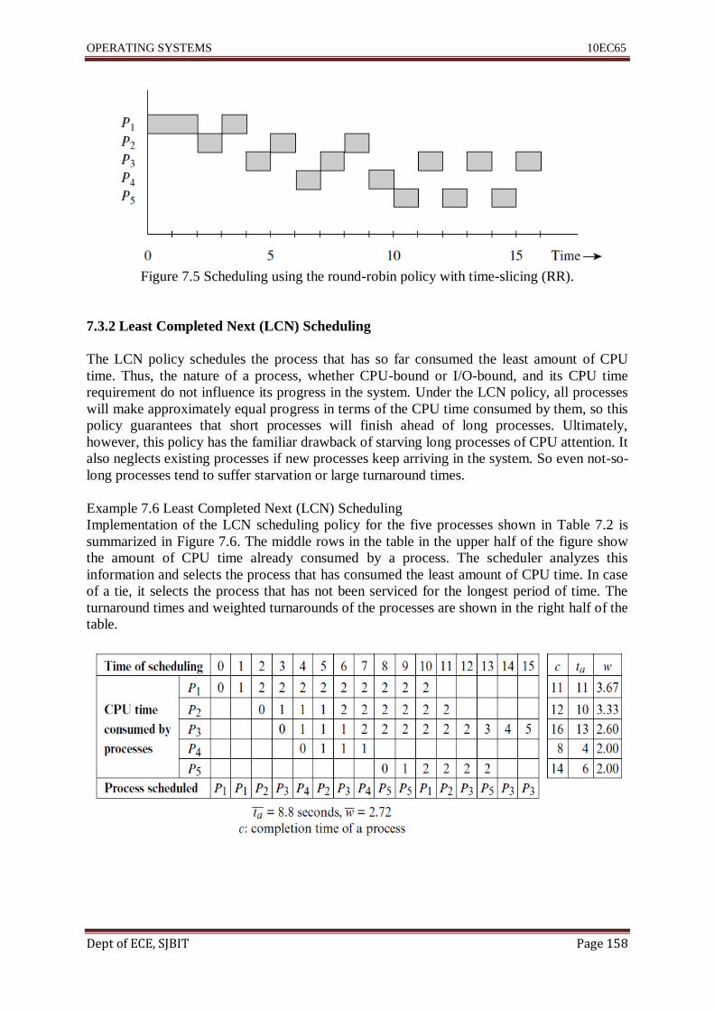
OPERATING SYSTEMS 10EC65
Dept of ECE, SJBIT Page 158
Figure 7.5 Scheduling using the round-robin policy with time-slicing (RR).
7.3.2 Least Completed Next (LCN) Scheduling
The LCN policy schedules the process that has so far consumed the least amount of CPU
time. Thus, the nature of a process, whether CPU-bound or I/O-bound, and its CPU time
requirement do not influence its progress in the system. Under the LCN policy, all processes
will make approximately equal progress in terms of the CPU time consumed by them, so this
policy guarantees that short processes will finish ahead of long processes. Ultimately,
however, this policy has the familiar drawback of starving long processes of CPU attention. It
also neglects existing processes if new processes keep arriving in the system. So even not-so-
long processes tend to suffer starvation or large turnaround times.
Example 7.6 Least Completed Next (LCN) Scheduling
Implementation of the LCN scheduling policy for the five processes shown in Table 7.2 is
summarized in Figure 7.6. The middle rows in the table in the upper half of the figure show
the amount of CPU time already consumed by a process. The scheduler analyzes this
information and selects the process that has consumed the least amount of CPU time. In case
of a tie, it selects the process that has not been serviced for the longest period of time. The
turnaround times and weighted turnarounds of the processes are shown in the right half of the
table.

OPERATING SYSTEMS 10EC65
Dept of ECE, SJBIT Page 159
Figure 7.6 Scheduling using the least completed next (LCN) policy.
It can be seen that servicing of P1, P2, and P3 is delayed because new processes arrive and
obtain CPU service before these processes can make further progress. The LCN policy
provides poorer turnaround times and weighted turnarounds than those provided by the RR
policy (See Example 7.4) and the STG policy (to be discussed next) because it favours newly
arriving processes over existing processes in the system until the new processes catch up in
terms of CPU utilization; e.g., it favours P5 over P1, P2, and P3.
7.3.3 Shortest Time to Go (STG) Scheduling
The shortest time to go policy schedules a process whose remaining CPU time requirements
are the smallest in the system. It is a preemptive version of the shortest request next (SRN)
policy. So it favours short processes over long ones and provides good throughput.
Additionally, the STG policy also favours a process that is nearing completion over short
processes entering the system. This feature helps to improve the turnaround times and
weighted turnarounds of processes. Since it is analogous to the SRN policy, long processes
might face starvation.
Figure 7.7 Scheduling using the shortest time to go (STG) policy.

OPERATING SYSTEMS 10EC65
Dept of ECE, SJBIT Page 160
Example 7.7 Shortest Time to Go (STG) Scheduling
Figure 7.7 summarizes performance of the STG scheduling policy for the five processes
shown in Table 7.2. The scheduling information used by the policy is the CPU time needed
by each process for completion. In case of a tie, the scheduler selects whatever process has
not been serviced for the longest period of time. Execution of P3 is delayed because P2, P4,
and P5 require lesser CPU time than it.
7.4 Scheduling In Practice
To provide a suitable combination of system performance and user service, an operating
system has to adapt its operation to the nature and number of user requests and availability of
resources. A single scheduler using a classical scheduling policy cannot address all these
issues effectively. Hence, a modern OS employs several schedulers—up to three schedulers,
and some of the schedulers may use a combination of different scheduling policies.
7.4.1 Long-, Medium-, and Short-Term Schedulers
These schedulers perform the following functions:
• Long-term scheduler: Decides when to admit an arrived process for scheduling, depending
on its nature (whether CPU-bound or I/O-bound) and on availability of resources like kernel
data structures and disk space for swapping.
• Medium-term scheduler: Decides when to swap-out a process from memory and when to
load it back, so that a sufficient number of ready processes would exist in memory.
• Short-term scheduler: Decides which ready process to service next on the CPU and for how
long. Thus, the short-term scheduler is the one that actually selects a process for operation.
Hence it is also called the process scheduler, or simply the scheduler.
Figure 7.8 shows an overview of scheduling and related actions. The operation of the kernel
is interrupt-driven. Every event that requires the kernel‘s attention causes an interrupt.

OPERATING SYSTEMS 10EC65
Dept of ECE, SJBIT Page 161
Figure 7.9 Event handling and scheduling.
Long-Term Scheduling The long-term scheduler may defer admission of a request for two
reasons: it may not be able to allocate sufficient resources like kernel data structures or I/O
devices to a request when it arrives, or it may find that admission of a request would affect
system performance in some way; e.g., if the system currently contained a large number of
CPU-bound requests, the scheduler might defer admission of a new CPU-bound request, but
it might admit a new I/O-bound request right away.
Long-term scheduling was used in the 1960s and 1970s for job scheduling because computer
systems had limited resources, so a long-term scheduler was required to decide whether a
process could be initiated at the present time. It continues to be important in operating
systems where resources are limited. It is also used in systems where requests have deadlines,
or a set of requests are repeated with a known periodicity, to decide when a process should be
initiated to meet response requirements of applications. Long-term scheduling is not relevant
in other operating systems.

OPERATING SYSTEMS 10EC65
Dept of ECE, SJBIT Page 162
Medium-Term Scheduling Medium-term scheduling maps the large number of requests that
have been admitted to the system into the smaller number of requests that can fit into the
memory of the system at any time. Thus its focus is on making a sufficient number of ready
processes available to the short-term scheduler by suspending or reactivating processes. The
medium term scheduler decides when to swap out a process from memory and when to swap
it back into memory, changes the state of the process appropriately, and enters its process
control block (PCB) in the appropriate list of PCBs. The actual swapping-in and swapping-
out operations are performed by the memory manager.
The kernel can suspend a process when a user requests suspension, when the kernel runs out
of free memory, or when it finds that the CPU is not likely to be allocated to the process in
the near future. In time-sharing systems, processes in blocked or ready states are candidates
for suspension.
Short-Term Scheduling Short-term scheduling is concerned with effective use of the CPU.
It selects one process from a list of ready processes and hands it to the dispatching
mechanism. It may also decide how long the process should be allowed to use the CPU and
instruct the kernel to produce a timer interrupt accordingly.
7.4.2 Scheduling Data Structures and Mechanisms
Figure 7.10 A schematic of the process scheduler.
Figure 7.10 is a schematic diagram of the process scheduler. It uses several lists of PCBs
whose organization and use depends on the scheduling policy. The process scheduler selects
one process and passes its id to the process dispatching mechanism. The process dispatching
mechanism loads contents of two PCB fields—the program status word (PSW) and general-
purpose registers (GPRs) fields—into the CPU to resume operation of the selected process.
Thus, the dispatching mechanism interfaces with the scheduler on one side and the hardware
on the other side. The context save mechanism is a part of the interrupt processing routine.
When an interrupt occurs, it is invoked to save the PSW and GPRs of the interrupted process.
The priority computation and reordering mechanism recomputes the priority of requests and
reorders the PCB lists to reflect the new priorities.

OPERATING SYSTEMS 10EC65
Dept of ECE, SJBIT Page 163
This mechanism is either invoked explicitly by the scheduler when appropriate or invoked
periodically. Its exact actions depend on the scheduling policy in use.
7.4.3 Priority-Based Scheduling
Figure 7.12 shows an efficient arrangement of scheduling data for priority-based scheduling.
A separate list of ready processes is maintained for each priority value; this list is organized
as a queue of PCBs, in which a PCB points to the PCB of the next process in the queue. The
header of a queue contains two pointers.
Figure 7.11 Ready queues in priority-based scheduling.
One points to the PCB of the first process in the queue, and the other points to the header of
the queue for the next lower priority. The scheduler scans the headers in the order of
decreasing priority and selects the first process in the first nonempty queue it can find. This
way, the scheduling overhead depends on the number of distinct priorities, rather than on the
number of ready processes.
Priority-based scheduling can lead to starvation of low-priority processes. The technique of
aging of processes, which increases the priority of a ready process if it does not get scheduled
within a certain period of time, can be used to overcome starvation. In this scheme, process
priorities would be dynamic, so the PCB of a process would be moved between the different
ready queues shown in Figure 7.11.
Starvation in priority-based scheduling can also lead to an undesirable situation called
priority inversion. Consider a high-priority process that needs a resource that is currently
allocated to a low-priority process. If the low-priority process faces starvation, it cannot use
and release the resource. Consequently, the high-priority process remains blocked
indefinitely. This situation is addressed through the priority inheritance protocol, which
temporarily raises the priority of the low-priority process holding the resource to the priority
value of the high priority process that needs the resource. The process holding the resource
can now obtain the CPU, use the resource, and release it. The kernel changes its priority back
to the earlier value when it releases the resource.
7.4.4 Round-Robin Scheduling with Time-Slicing
Round-robin scheduling can be implemented through a single list of PCBs of ready
processes. This list is organized as a queue. The scheduler always removes the first PCB from
the queue and schedules the process described by it. If the time slice elapses, the PCB of the
process is put at the end of the queue. If a process starts an I/O operation, its PCB is added at
the end of the queue when its I/O operation completes. Thus the PCB of a ready process

OPERATING SYSTEMS 10EC65
Dept of ECE, SJBIT Page 164
moves toward the head of the queue until the process is scheduled.
7.4.5 Multilevel Scheduling
The multilevel scheduling policy combines priority-based scheduling and roundrobin
scheduling to provide a good combination of system performance and response times. A
multilevel scheduler maintains a number of ready queues. A priority and a time slice are
associated with each ready queue, and round-robin scheduling with time-slicing is performed
within it. The queue at a high priority level has a small time slice associated with it, which
ensures good response times for processes in this queue, while the queue at a low priority
level has a large time slice, which ensures low process switching overhead. A process at the
head of a queue is scheduled only if the queues for all higher priority levels are empty.
Scheduling is preemptive, so a process is pre-empted when a new process is added to a queue
at a higher priority level. As in round-robin scheduling with time-slicing, when a process
makes an I/O request, or is swapped out, its PCB is removed from the ready queue. When the
I/O operation completes, or the process is swapped in, its PCB is added at the end of that
ready queue where it existed earlier.
7.4.6 Fair Share Scheduling
A common criticism of all scheduling policies discussed so far is that they try to provide
equitable service to processes, rather than to users or their applications. If applications create
different numbers of processes, an application employing more processes is likely to receive
more CPU attention than an application employing fewer processes.
The notion of a fair share addresses this issue. A fair share is the fraction of CPU time that
should be devoted to a group of processes that belong to the same user or the same
application; it ensures an equitable use of the CPU by users or applications. The actual share
of CPU time received by a group of processes may differ from the fair share of the group if
all processes in some of the groups are inactive. For example, consider five groups of
processes, G1–G5, each having a 20 percent share of CPU time. If all processes in G1 are
blocked, processes of each of the other groups should be given 25 percent of the available
CPU time so that CPU time is not wasted. What should the scheduler do when processes of
G1 become active after some time? Should it give them only 20 percent of CPU time after
they wake up, because that is their fair share of CPU time, or should it give them all the
available CPU time until their actual CPU consumption since inception becomes 20 percent?
Lottery scheduling, which we describe in the following, and the scheduling policies used in
the Unix and Solaris operating systems.
Lottery scheduling is a novel technique proposed for sharing a resource in a probabilistically
fair manner. Lottery ―tickets‖ are distributed to all processes sharing a resource in such a
manner that a process gets as many tickets as its fair share of the resource. For example, a
process would be given five tickets out of a total of 100 tickets if its fair share of the resource
is 5 percent. When the resource is to be allocated, a lottery is conducted among the tickets
held by processes that actively seek the resource. The process holding the winning ticket is
then allocated the resource. The actual share of the resources allocated to the process depends
on contention for the resource. Lottery scheduling can be used for fair share CPU scheduling
as follows: Tickets can be issued to applications (or users) on the basis of their fair share of
CPU time. An application can share its tickets among its processes in any manner it desires.

OPERATING SYSTEMS 10EC65
Dept of ECE, SJBIT Page 165
To allocate a CPU time slice, the scheduler holds a lottery in which only tickets of ready
processes participate. When the time slice is a few milliseconds, this scheduling method
provides fairness even over fractions of a second if all groups of processes are active.
7.4.7 Scheduling Heuristics
Schedulers in modern operating systems use many heuristics to reduce their overhead, and to
provide good user service. These heuristics employ two main techniques:
• Use of a time quantum
• Variation of process priority
A time quantum is the limit on CPU time that a process may be allowed to consume over a
time interval. It is employed as follows: Each process is assigned a priority and a time
quantum. A process is scheduled according to its priority, provided it has not exhausted its
time quantum. As it operates, the amount of CPU time used by it is deducted from its time
quantum. After a process has exhausted its time quantum, it would not be considered for
scheduling unless the kernel grants it another time quantum, which would happen only when
all active processes have exhausted their quanta. This way, the time quantum of a process
would control the share of CPU time used by it, so it can be employed to implement fair
share scheduling.
Process priority could be varied to achieve various goals. The priority of a process could be
boosted while it is executing a system call, so that it would quickly complete execution of the
call, release any kernel resources allocated to it, and exit the kernel. This technique would
improve response to other processes that are waiting for the kernel resources held by the
process executing the system call.
Priority inheritance could be implemented by boosting the priority of a process holding a
resource to that of the highest-priority process waiting for the resource. Process priority may
also be varied to more accurately characterize the nature of a process. When the kernel
initiates a new process, it has no means of knowing whether the process is I/O-bound or
CPU-bound, so it assigns a default priority to the process. As the process operates, the kernel
adjusts its priority in accordance with its behaviour using a heuristic of the following kind:
When the process is activated after some period of blocking, its priority may be boosted in
accordance with the cause of blocking. For example, if it was blocked because of an I/O
operation, its priority would be boosted to provide it a better response time. If it was blocked
for a keyboard input, it would have waited for a long time for the user to respond, so its
priority may be given a further boost. If a process used up its time slice completely, its
priority may be reduced because it is more CPU-bound than was previously assumed.
7.4.8 Power Management
When no ready processes exist, the kernel puts the CPU into an idle loop. This solution
wastes power in executing useless instructions. In power-starved systems such as embedded
and mobile systems, it is essential to prevent this wastage of power.
To address this requirement, computers provide special modes in the CPU. When put in one
of these modes, the CPU does not execute instructions, which conserves power; however, it
can accept interrupts, which enables it to resume normal operation when desired. We will use
the term sleep mode of the CPU generically for such modes. Some computers provide several
sleep modes. In the ―light‖ sleep mode, the CPU simply stops executing instructions. In a

OPERATING SYSTEMS 10EC65
Dept of ECE, SJBIT Page 166
―heavy‖ sleep mode, the CPU not only stops executing instructions, but also takes other steps
that reduce its power consumption, e.g., slowing the clock and disconnecting the CPU from
the system bus. Ideally, the kernel should put the CPU into the deepest sleep mode possible
when the system does not have processes in the ready state. However, a CPU takes a longer
time to ―wake up‖ from a heavy sleep mode than it would from a light sleep mode, so the
kernel has to make a trade-off here.
It starts by putting the CPU in the light sleep mode. If no processes become ready for some
more time, it puts the CPU into a heavier sleep mode, and so on. This way, it provides a
trade-off between the need for power saving and responsiveness of the system.
Operating systems like Unix and Windows have generalized power management to include
all devices. Typically, a device is put into a lower power consuming state if it has been
dormant at its present power consuming state for some time. Users are also provided with
utilities through which they can configure the power management scheme used by the OS.
7.5 Real-Time Scheduling
Real-time scheduling must handle two special scheduling constraints while trying to meet the
deadlines of applications. First, the processes within a real-time application are interacting
processes, so the deadline of an application should be translated into appropriate deadlines for
the processes. Second, processes may be periodic, so different instances of a process may
arrive at fixed intervals and all of them have to meet their deadlines. Example 7.10 illustrates
these constraints; in this section, we discuss techniques used to handle them.
Example 7.10 Dependences and Periods in a Real-Time Application
Consider a restricted form of the real-time data logging application of Example 5.1, in which
the buffer_area can accommodate a single data sample. Since samples arrive at the rate of
500 samples per second, the response requirement of the application is 1.99 ms. Hence,
processes copy_sample and record_sample must operate one after another and complete their
operation within 1.99 ms. If process record_sample requires 1.5 ms for its operation, process
copy_sample has a deadline of 0.49 ms after arrival of a message. Since a new sample arrives
every 2 ms, each of the processes has a period of 2 ms.
7.5.1 Process Precedences and Feasible Schedules
Processes of a real-time application interact among themselves to ensure that they perform
their actions in a desired order (see Section 6.1).We make the simplifying assumption that
such interaction takes place only at the start or end of a process. It causes dependences
between processes, whichmust be taken into account while determining deadlines and while
scheduling. We use a process precedence graph (PPG) to depict such dependences between
processes.
Process Pi is said to precede process Pj if execution of Pi must be completed beforePj can
begin its execution. The notationPi → Pj shall indicate that process Pi directly precedes
process Pj . The precedence relation is transitive; i.e., Pi → Pj andPj → Pk implies thatPi
precedesPk. The notationPi→* Pk is used to indicate that process Pi directly or indirectly
precedes Pk. A process precedence graph is a directed graph G ≡ (N, E) such that Pi ∈ N
represents a process, and an edge (Pi , Pj ) ∈ E implies Pi → Pj . Thus, a path Pi , . . . , Pk in
PPG implies Pi→* Pk. A process Pk is a descendant of Pi if Pi→* Pk.
A hard real-time system as one that meets the response requirement of a real-time application

OPERATING SYSTEMS 10EC65
Dept of ECE, SJBIT Page 167
in a guaranteed manner, even when fault tolerance actions are required. This condition
implies that the time required by the OS to complete operation of all processes in the
application does not exceed the response requirement of the application. On the other hand, a
soft real-time system meets the response requirement of an application only in a probabilistic
manner, and not necessarily at all times. The notion of a feasible schedule helps to
differentiate between these situations.
Feasible Schedule A sequence of scheduling decisions that enables the processes of an
application to operate in accordance with their precedences and meet the response
requirement of the application.
Table 7.3 Approaches to Real-Time Scheduling
7.5.2 Deadline Scheduling
Two kinds of deadlines can be specified for a process: a starting deadline, i.e., the latest
instant of time by which operation of the process must begin, and a completion deadline, i.e.,
the time by which operation of the process must complete.
Deadline Estimation A system analyst performs an in-depth analysis of a realtime
application and its response requirements. Deadlines for individual processes are determined
by considering process precedences and working backward from the response requirement of
the application. Accordingly, Di , the completion deadline of a process Pi, is
Where Dapplication is the deadline of the application, xk is the service time of process Pk, and
descendant(i) is the set of descendants of Pi in the PPG, i.e., the set of all processes that lie
on some path between Pi and the exit node of the PPG. Thus, the deadline for a process Pi is
such that if it is met, all processes that directly or indirectly depend on Pi can also finish by
the overall deadline of the application. This method is illustrated in Example 7.11.

OPERATING SYSTEMS 10EC65
Dept of ECE, SJBIT Page 168
Determining Process Deadlines Example 7.11
Each circle is a node of the graph and represents a process. The number in a circle indicates
the service time of a process. An edge in the PPG shows a precedence constraint. Thus,
process P2 can be initiated only after process P1 completes, process P4 can be initiated only
after processes P2 and P3 complete, etc. We assume that processes do not perform I/O
operations and are serviced in a nonpreemptive manner. The total of the service times of the
processes is 25 seconds. If the application has to produce a response in 25 seconds, the
deadlines of the processes would be as follows:
Figure 7.12 shows the PPG of a real-time application containing 6 processes.
Process P1 P2 P3 P4 P5 P6
Deadline 8 16 16 20 20 25
A practical method of estimating deadlines will have to incorporate several other constraints
as well. For example, processes may perform I/O. If an I/O operation of one process can be
overlapped with execution of some independent process, the deadline of its predecessors (and
ancestors) in the PPG can be relaxed by the amount of I/O overlap. For example, processes
P2 and P3 in Figure 7.13 are independent of one another. If the service time of P2 includes 1
second of I/O time, the deadline of P1 can be made 9 seconds instead of 8 seconds if the I/O
operation of P2 can overlap with P3‘s processing. However, overlapped execution of
processes must consider resource availability as well. Hence determination of deadlines is far
more complex than described here.
Earliest Deadline First (EDF) Scheduling As its name suggests, this policy always selects
the process with the earliest deadline. Consider a set of real-time processes that do not
perform I/O operations. If seq is the sequence in which processes are serviced by a deadline
scheduling policy and pos(Pi ) is the position of process Pi in seq, a deadline overrun does
not occur for process Pi only if the sum of its own service time and service times of all
processes that precede it in seq does not exceed its own deadline, i.e.,
where xk is the service time of process Pk, and Di is the deadline of process Pi. If this
condition is not satisfied, a deadline overrun will occur for process Pi. When a feasible
schedule exists, it can be shown that Condition 7.3 holds for all processes; i.e., a deadline
overrun will not occur for any process. Table 7.4 illustrates operation of the EDF policy for

OPERATING SYSTEMS 10EC65
Dept of ECE, SJBIT Page 169
the deadlines of Example 7.11. The notation P4: 20 in the column processes in system
indicates that process P4 has the deadline 20. Processes P2, P3 and P5, P6 have identical
deadlines, so three schedules other than the one shown in Table 7.4 are possible with EDF
scheduling. None of them would incur deadline overruns.
The primary advantages of EDF scheduling are its simplicity and nonpreemptive nature,
which reduces the scheduling overhead. EDF scheduling is a good policy for static
scheduling because existence of a feasible schedule, which can be checked a priori, ensures
that deadline overruns do not occur. It is also a good dynamic scheduling policy for use in
soft real-time system; however, the number of processes that miss their deadlines is
unpredictable. The next example illustrates this aspect of EDF scheduling.
Table 7.4 Operation of Earliest Deadline First (EDF) Scheduling
7.5.3 Rate Monotonic Scheduling
When processes in an application are periodic, the existence of a feasible schedule can be
determined in an interesting way. Consider three independent processes that do not perform
I/O operations:
Process P1 repeats every 10 ms and needs 3 ms of CPU time. So the fraction of the CPU‘s
time that it uses is 3/10, i.e., 0.30. The fractions of CPU time used by P2 and P3 are
analogously 5/15 and 9/30, i.e., 0.33 and 0.30. They add up to 0.93, so if the CPU overhead
of OS operation is negligible, it is feasible to service these three processes. In general, a set of
periodic processes P1, . . . , Pn that do not perform I/O operations can be serviced by a hard
real-time system that has a negligible overhead if
where Ti is the period of Pi and xi is its service time.
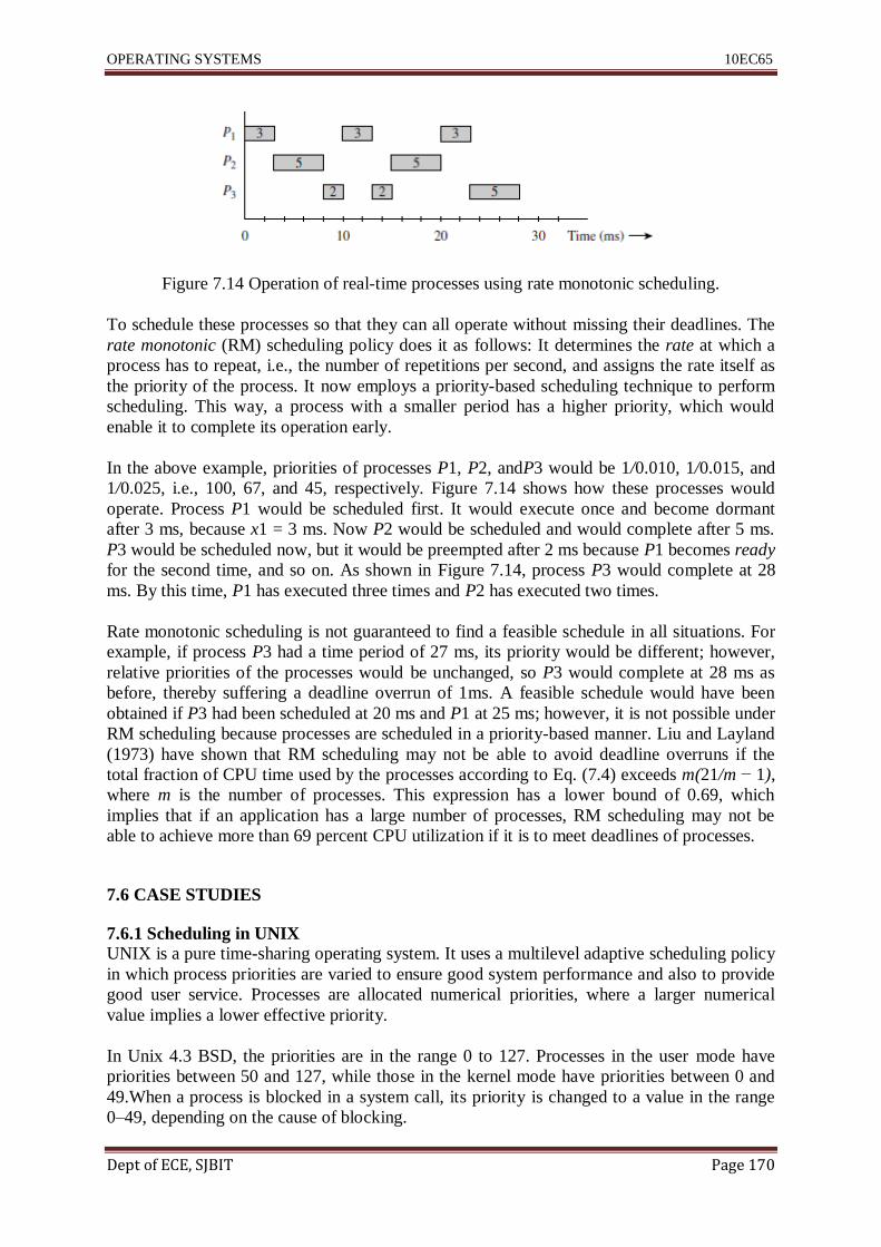
OPERATING SYSTEMS 10EC65
Dept of ECE, SJBIT Page 170
Figure 7.14 Operation of real-time processes using rate monotonic scheduling.
To schedule these processes so that they can all operate without missing their deadlines. The
rate monotonic (RM) scheduling policy does it as follows: It determines the rate at which a
process has to repeat, i.e., the number of repetitions per second, and assigns the rate itself as
the priority of the process. It now employs a priority-based scheduling technique to perform
scheduling. This way, a process with a smaller period has a higher priority, which would
enable it to complete its operation early.
In the above example, priorities of processes P1, P2, andP3 would be 1/0.010, 1/0.015, and
1/0.025, i.e., 100, 67, and 45, respectively. Figure 7.14 shows how these processes would
operate. Process P1 would be scheduled first. It would execute once and become dormant
after 3 ms, because x1 = 3 ms. Now P2 would be scheduled and would complete after 5 ms.
P3 would be scheduled now, but it would be preempted after 2 ms because P1 becomes ready
for the second time, and so on. As shown in Figure 7.14, process P3 would complete at 28
ms. By this time, P1 has executed three times and P2 has executed two times.
Rate monotonic scheduling is not guaranteed to find a feasible schedule in all situations. For
example, if process P3 had a time period of 27 ms, its priority would be different; however,
relative priorities of the processes would be unchanged, so P3 would complete at 28 ms as
before, thereby suffering a deadline overrun of 1ms. A feasible schedule would have been
obtained if P3 had been scheduled at 20 ms and P1 at 25 ms; however, it is not possible under
RM scheduling because processes are scheduled in a priority-based manner. Liu and Layland
(1973) have shown that RM scheduling may not be able to avoid deadline overruns if the
total fraction of CPU time used by the processes according to Eq. (7.4) exceeds m(21/m − 1),
where m is the number of processes. This expression has a lower bound of 0.69, which
implies that if an application has a large number of processes, RM scheduling may not be
able to achieve more than 69 percent CPU utilization if it is to meet deadlines of processes.
7.6 CASE STUDIES
7.6.1 Scheduling in UNIX
UNIX is a pure time-sharing operating system. It uses a multilevel adaptive scheduling policy
in which process priorities are varied to ensure good system performance and also to provide
good user service. Processes are allocated numerical priorities, where a larger numerical
value implies a lower effective priority.
In Unix 4.3 BSD, the priorities are in the range 0 to 127. Processes in the user mode have
priorities between 50 and 127, while those in the kernel mode have priorities between 0 and
49.When a process is blocked in a system call, its priority is changed to a value in the range
0–49, depending on the cause of blocking.

OPERATING SYSTEMS 10EC65
Dept of ECE, SJBIT Page 171
When it becomes active again, it executes the remainder of the system call with this priority.
This arrangement ensures that the process would be scheduled as soon as possible, complete
the task it was performing in the kernel mode and release kernel resources. When it exits the
kernel mode, its priority reverts to its previous value, which was in the range 50–127.
Unix uses the following formula to vary the priority of a process:
It is implemented as follows: The scheduler maintains the CPU time used by a process in its
process table entry. This field is initialized to 0. The real-time clock raises an interrupt 60
times a second, and the clock handler increments the count in the CPU usage field of the
running process. The scheduler recomputes process priorities every second in a loop. For
each process, it divides the value in the CPU usage field by 2, stores it back, and also uses it
as the value of f. Recall that a large numerical value implies a lower effective priority, so the
second factor in Eq. (7.5) lowers the priority of a process. The division by 2 ensures that the
effect of CPU time used by a process decays; i.e., it wears off over a period of time, to avoid
the problem of starvation faced in the least completed next (LCN) policy.
A process can vary its own priority through the last factor in Eq. (7.5). The system call
―nice(<priority value>);‖ sets the nice value of a user process. It takes a zero or positive
value as its argument. Thus, a process can only decrease its effective priority to be nice to
other processes. It would typically do this when it enters a CPU-bound phase.
Table 7.5 Operation of a Unix-like Scheduling Policy When Processes Perform I/O

OPERATING SYSTEMS 10EC65
Dept of ECE, SJBIT Page 172
Example 7.13 Process Scheduling in Unix
Table 7.5 summarizes operation of the Unix scheduling policy for the processes in Table 7.2.
It is assumed that process P3 is an I/O bound process that initiates an I/O operation lasting
0.5 seconds after using the CPU for 0.1 seconds, and none of the other processes perform I/O.
The T field indicates the CPU time consumed by a process and the P field contains its
priority. The scheduler updates the T field of a process 60 times a second and recomputes
process priorities once every second. The time slice is 1 second, and the base priority of user
processes is 60. The first line of Table 7.5 shows that at 0 second, only P1 is present in the
system. Its T field contains 0, hence its priority is 60. Two lines are shown for the time 1
second. The first line shows the T fields of processes at 1 second, while the second line shows
the P and T fields after the priority computation actions at 1 second. At the end of the time
slice, the contents of the T field of P1 are 60. The decaying action of dividing the CPU time
by 2 reduces it to 30, and so the priority ofP1 becomes 90. At 2 seconds, the effective priority
of P1 is smaller than that of P2 because their T fields contain 45 and 0, respectively, and so
P2 is scheduled. Similarly P3 is scheduled at 2 seconds.
SinceP3 uses the CPU for only 0.1 second before starting an I/O operation, it has a higher
priority than P2 when scheduling is performed at 4 seconds; hence it is scheduled ahead of
process P2. It is again scheduled at 6 seconds. This feature corrects the bias against I/O-
bound processes exhibited by pure round-robin scheduling.
Table 7.6 Operation of Fair Share Scheduling in Unix
Fair Share Scheduling To ensure a fair share of CPU time to groups of processes, Unix schedulers add the term f
(CPU time used by processes in the group) to Eq. (7.5). Thus, priorities of all processes in a
group reduce when any of them consumes CPU time. This feature ensures that processes of a
group would receive favored treatment if none of them has consumed much CPU time
recently. The effect of the new factor also decays over time.

OPERATING SYSTEMS 10EC65
Dept of ECE, SJBIT Page 173
Fair Share Scheduling in Unix
Example 7.14
Table 7.6 depicts fair share scheduling of the processes of Table 7.2. Fields P, T, and G
contain process priority, CPU time consumed by a process, and CPU time consumed by a
group of processes, respectively. Two process groups exist.
The first group contains processes P1, P2, P4, and P5, while the second group contains
process P3 all by itself. At 2 seconds, process P2 has just arrived. Its effective priority is low
because process P1, which is in the same group, has executed for 2 seconds. However, P3
does not have a low priority when it arrives because the CPU time already consumed by its
group is 0. As expected, process P3 receives a favored treatment compared to other
processes. In fact, it receives every alternate time slice. Processes P2, P4, and P5 suffer
because they belong to the same process group. These facts are reflected in the turnaround
times and weighted turnarounds of the processes, which are as follows:
Mean turnaround time (ta) = 9.2 seconds
Mean weighted turnaround ( 𝑊 ) = 3.15
Recommended Questions
1. With a neat block diagram, explain event handling and scheduling.
2. Explain scheduling in UNIX.
3. Summarize the main approaches to real time scheduling.
4. What is scheduling? What are the events related to scheduling?
5. Explain briefly the mechanism and policy modules of short term process scheduler
with a neat block diagram.
6. Briefly explain the features of time sharing system. Also explain process state
transitions in time sharing system.
7. Compare i) pre-emptive and non-preemptive scheduling
ii) long term and short term schedulers
8. Describe SRN and HRN scheduling policies and determine the average turn around
time and weighted turn-around time for the following set of processes-
Processes P1 P2 P3 P4 P5
Arrival time 0 2 3 4 8
Service time 3 3 5 2 3
9. What are the functions of medium and short term schedulers?

OPERATING SYSTEMS 10EC65
Dept of ECE, SJBIT Page 174
UNIT-8
Message Passing
Message passing suits diverse situations where exchange of information between processes
plays a key role. One of its prominent uses is in the client–server paradigm, wherein a server
process offers a service, and other processes, called its clients, send messages to it to use its
service. This paradigm is used widely—a microkernel- based OS structures functionalities
such as scheduling in the form of servers, a conventional OS offer services such as printing
through servers, and, on the Internet, a variety of services are offered by Web servers.
Another prominent use of message passing is in higher-level protocols for exchange of
electronic mails and communication between tasks in parallel or distributed programs. Here,
message passing is used to exchange information, while other parts of the protocol are
employed to ensure reliability.
The key issues in message passing are how the processes that send and receive messages
identify each other, and how the kernel performs various actions related to delivery of
messages—how it stores and delivers messages and whether it blocks a process that sends a
message until its message is delivered. These features are operating system–specific. We
describe different message passing arrangements employed in operating systems and discuss
their significance for user processes and for the kernel. We also describe message passing in
UNIX and in Windows operating systems.
8.1 OVERVIEW OF MESSAGE PASSING
The four ways in which processes interact with one another—data sharing, message passing,
synchronization, and signals. Data sharing provides means to access values of shared data in
a mutually exclusive manner. Process synchronization is performed by blocking a process
until other processes have performed certain specific actions. Capabilities of message passing
overlap those of data sharing and synchronization; however, each form of process interaction
has its own niche application area.
.Figure 8.1 shows an example of message passing. Process Pi sends a message to process Pj
by executing the statement send (Pj ,<message>). The compiled code of the send statement
invokes the library module send. send makes a system call send, with Pj and the message as
parameters. Execution of the statement receive (Pi, msg_area), where msg_area is an area in
Pj ‘s address space, results in a system call receive.
Figure 8.1 Message passing.
The semantics of message passing are as follows: At a send call by Pi , the kernel checks
whether process Pj is blocked on a receive call for receiving a message from process Pi . If
so, it copies the message into msg_area and activates Pj. If process Pj has not already made a
receive call, the kernel arranges to deliver the message to it when Pj eventually makes a
receive call. When process Pj receives the message, it interprets the message and takes an

OPERATING SYSTEMS 10EC65
Dept of ECE, SJBIT Page 175
appropriate action. Messages may be passed between processes that exist in the same
computer or in different computers connected to a network. Also, the processes participating
in message passing may decide on what a specific message means and what actions the
receiver process should perform on receiving it. Because of this flexibility, message passing
is used in the following applications:
• Message passing is employed in the client–server paradigm, which is used to communicate
between components of a microkernel-based operating system and user processes, to provide
services such as the print service to processes within an OS, or to provideWeb-based services
to client processes located in other computers.
• Message passing is used as the backbone of higher-level protocols employed for
communicating between computers or for providing the electronic mail facility.
• Message passing is used to implement communication between tasks in a parallel or
distributed program.
In principle, message passing can be performed by using shared variables. For example,
msg_area in Figure 8.1 could be a shared variable. Pi could deposit a value or a message in it
and Pj could collect it from there. However, this approach is cumbersome because the
processes would have to create a shared variable with the correct size and share its name.
They would also have to use synchronization analogous to the producers–consumers problem
to ensure that a receiver process accessed a message in a shared variable only after a sender
process had deposited it there. Message passing is far simpler in this situation. It is also more
general, because it can be used in a distributed system environment, where the shared
variable approach is not feasible.
The producers–consumers problem with a single buffer, a single producer process, and a
single consumer process can be implemented by message passing as shown in Figure 8.2. The
solution does not use any shared variables. Instead, process Pi, which is the producer process,
has a variable called buffer and process Pj , which is the consumer process, has a variable
called message_area. The producer process produces in buffer and sends the contents of
buffer in a message to the consumer.
begin
Parbegin
var buffer : . . . ; var message_area : . . . ;
repeat repeat
{ Produce in buffer } receive (Pi , message_area);
send (Pj , buffer); { Consume from message_area }
{ Remainder of the cycle } { Remainder of the cycle }
forever; forever;
Parend;
end.
Process Pi Process Pj
Figure 8.2 Producers–consumers solution using message passing.

OPERATING SYSTEMS 10EC65
Dept of ECE, SJBIT Page 176
The consumer receives the message in message_area and consumes it from there. The send
system call blocks the producer process until the message is delivered to the consumer, and
the receive system call blocks the consumer until a message is sent to it.
Issues in Message Passing
Two important issues in message passing are:
• Naming of processes: Whether names of sender and receiver processes are explicitly
indicated in send and receive statements, or whether their identities are deduced by the kernel
in some other manner.
• Delivery of messages: Whether a sender process is blocked until the message sent by it is
delivered, what the order is in which messages are delivered to the receiver process, and how
exceptional conditions are handled.
These issues dictate implementation arrangements and also influence the generality of
message passing. For example, if a sender process is required to know the identity of a
receiver process, the scope of message passing would be limited to processes in the same
application. Relaxing this requirement would extend message passing to processes in
different applications and processes operating in different computer systems. Similarly,
providing FCFS message delivery may be rather restrictive; processes may wish to receive
messages in some other order.
8.1.1 Direct and Indirect Naming In direct naming, sender and receiver processes mention each other‘s name. For example, the
send and receive statements might have the following syntax:
send (<destination_ process>,<message_length>,<message_address>);
receive (<source_ process>,<message_area>);
where <destination_ process> and <source_ process> are process names (typically, they are
process ids assigned by the kernel), <message_address> is the address of the memory area in
the sender process‘s address space that contains the textual formof the message to be sent,
and<message_area>is a memory area in the receiver‘s address space where the message is to
be delivered. The processes of Figure 8.2 used direct naming.
Direct naming can be used in two ways: In symmetric naming, both sender and receiver
processes specify each other‘s name. Thus, a process can decide which process to receive a
message from. However, it has to know the name of every process that wishes to send it a
message, which is difficult when processes of different applications wish to communicate, or
when a server wishes to receive a request from any one of a set of clients. In asymmetric
naming, the receiver does not name the process from which it wishes to receive a message;
the kernel gives it a message sent to it by some process.
In indirect naming, processes do not mention each other‘s name in send and receive
statements.
8.1.2 Blocking and Nonblocking Sends
A blocking send blocks a sender process until the message to be sent is delivered to the
destination process. This method of message passing is called synchronous message passing.

OPERATING SYSTEMS 10EC65
Dept of ECE, SJBIT Page 177
A nonblocking send call permits a sender to continue its operation after making a send call,
irrespective of whether the message is delivered immediately; such message passing is called
asynchronous message passing. In both cases, the receive primitive is typically blocking.
Synchronous message passing provides some nice properties for user processes and
simplifies actions of the kernel. A sender process has a guarantee that the message sent by it
is delivered before it continues its operation. This feature simplifies the design of concurrent
processes. The kernel delivers the message immediately if the destination process has already
made a receive call for receiving a message; otherwise, it blocks the sender process until the
destination process makes a receive call. The kernel can simply let the message remain in the
sender‘s memory area until it is delivered. However, use of blocking sends has one
drawback—it may unnecessarily delay a sender process in some situations, for example,
while communicating with a heavily loaded print server.
Asynchronous message passing enhances concurrency between the sender and receiver
processes by letting the sender process continue its operation. However, it also causes a
synchronization problem because the sender should not alter contents of the memory area
which contains text of the message until the message is delivered. To overcome this problem,
the kernel performs message buffering—when a process makes a send call, the kernel
allocates a buffer in the system area and copies the message into the buffer. This way, the
sender process is free to access the memory area that contained text of the message.
8.1.3 Exceptional Conditions in Message Passing
To facilitate handling of exceptional conditions, the send and receive calls take two additional
parameters. The first parameter is a set of flags indicating how the process wants exceptional
conditions to be handled; we will call this parameter flags. The second parameter is the
address of a memory area in which the kernel provides a condition code describing the
outcome of the send or receive call; we will call this area status_area.
When a process makes a send or receive call, the kernel deposits a condition code in
status_area. It then checks flags to decide whether it should handle any exceptional
conditions and performs the necessary actions. It then returns control to the process. The
process checks the condition code provided by the kernel and handles any exceptional
conditions it wished to handle itself.
Some exceptional conditions and their handling actions are as follows:
1. The destination process mentioned in a send call does not exist.
2. In symmetric naming, the source process mentioned in a receive call does not exist.
3. A send call cannot be processed because the kernel has run out of buffer memory.
4. No message exists for a process when it makes a receive call.
5. Aset of processes becomes deadlocked when a process is blocked on a receive call.
In cases 1 and 2, the kernelmay abort the process that made the send or receive call and set its
termination code to describe the exceptional condition. In case 3, the sender process may be
blocked until some buffer space becomes available. Case 4 is really not an exception if
receives are blocking (they generally are!), but it may be treated as an exception so that the
receiving process has an opportunity to handle the condition if it so desires. A process may
prefer the standard action, which is that the kernel should block the process until a message
arrives for it, or it may prefer an action of its own choice, like waiting for a specified amount
of time before giving up.

OPERATING SYSTEMS 10EC65
Dept of ECE, SJBIT Page 178
More severe exceptions belong to the realm of OS policies. The deadlock situation of case 5
is an example. Most operating systems do not handle this particular exception because it
incurs the overhead of deadlock detection. Difficult-to handle situations, such as a process
waiting a long time on a receive call, also belong to the realm of OS policies.
8.2 IMPLEMENTING MESSAGE PASSING
8.2.1 Buffering of Interprocess Messages
When a process Pi sends a message to some process Pj by using a nonblocking send, the
kernel builds an interprocess message control block (IMCB) to store all information needed
to deliver the message (see Figure 8.3). The control block contains names of the sender and
destination processes, the length of the message, and the text of the message. The control
block is allocated a buffer in the kernel area. When process Pj makes a receive call, the
kernel copies the message from the appropriate IMCB into the message area provided by Pj .
The pointer fields of IMCBs are used to form IMCB lists to simplify message delivery.
Figure 9.4 shows the organization of IMCB lists when blocking sends and FCFS message
delivery are used. In symmetric naming, a separate list is used for every pair of
communicating processes. When a process Pi performs a receive call to receive a message
from process Pj , the IMCB list for the pair Pi–Pj is used to deliver the message. In
asymmetric naming, a single IMCB list can be maintained per recipient process. When a
process performs a receive, the first IMCB in its list is processed to deliver a message.
If blocking sends are used, at most one message sent by a process can be undelivered at any
point in time. The process is blocked until the message is delivered. Hence it is not necessary
to copy the message into an IMCB.
Figure 8.3 Interprocess message control block (IMCB).
Figure 8.4 Lists of IMCBs for blocking sends in (a) symmetric naming; (b) asymmetric
naming.

OPERATING SYSTEMS 10EC65
Dept of ECE, SJBIT Page 179
The kernel can simply note the address of the message text in the sender‘s memory area, and
use this information while delivering the message. This arrangement saves one copy
operation on the message.
8.2.2 Delivery of Interprocess Messages
When a process Pi sends a message to process Pj , the kernel delivers the message to Pj
immediately if Pj is currently blocked on a receive call for a message from Pi , or from any
process. After delivering the message, the kernel must also change the state of Pj to ready. If
process Pj has not already performed a receive call, the kernel must arrange to deliver the
message when Pj performs a receive call later.
Thus, message delivery actions occur at both send and receive calls.
The kernel uses an event control block (ECB) to note actions that should be performed when
an anticipated event occurs. The ECB contains three fields:
• Description of the anticipated event
• Id of the process that awaits the event
• An ECB pointer for forming ECB lists
Figure 8.5 shows use of ECBs to implement message passing with symmetric naming and
blocking sends.When Pi makes a send call, the kernel checks whether an ECB exists for the
send call by Pi , i.e., whether Pj had made a receive call and was waiting for Pi to send a
message. If it is not the case, the kernel knows that the receive call would occur sometime in
future, so it creates an ECB for the event ―receive from Pi by Pj‖ and specifies Pi as the
process that will be affected by the event. Process Pi is put into the blocked state and the
address of the ECB is put in the event info field of its PCB [see Figure 8.5(a)].
Figure 8.5 ECBs to implement symmetric naming and blocking sends (a) at send; (b) at
receive.
Figure 8.5(b) illustrates the case when process Pj makes a receive call before Pi makes a send
call. An ECB for a ―send to Pj by Pi‖ event is now created. The id of Pj is put in the ECB to
indicate that the state of Pj will be affected when the send event occurs.
Figure 8.6 shows complete details of the kernel actions for implementing message passing by
using symmetric naming and blocking sends. For reasons mentioned earlier, the kernel
creates an IMCB even though a sender process is blocked until message delivery. When
process Pi sends a message to process Pj , the kernel first checks whether the send was
anticipated, i.e., whether an ECB was created for the send event. It will have happened if
process Pj has already made a receive call for a message fromPi . If this is the case, action S3
immediately delivers the message to Pj and changes its state from blocked to ready. The ECB
and the IMCB are now destroyed. If an ECB for send does not exist, step S4 creates an ECB
for a receive call by process Pj , which is now anticipated, blocks the sender process, and
enters the IMCB in the IMCB list of process Pj . Converse actions are performed at a receive
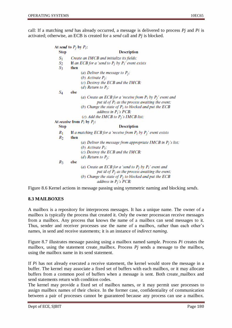
OPERATING SYSTEMS 10EC65
Dept of ECE, SJBIT Page 180
call: If a matching send has already occurred, a message is delivered to process Pj and Pi is
activated; otherwise, an ECB is created for a send call and Pj is blocked.
Figure 8.6 Kernel actions in message passing using symmetric naming and blocking sends.
8.3 MAILBOXES
A mailbox is a repository for interprocess messages. It has a unique name. The owner of a
mailbox is typically the process that created it. Only the owner processcan receive messages
from a mailbox. Any process that knows the name of a mailbox can send messages to it.
Thus, sender and receiver processes use the name of a mailbox, rather than each other‘s
names, in send and receive statements; it is an instance of indirect naming.
Figure 8.7 illustrates message passing using a mailbox named sample. Process Pi creates the
mailbox, using the statement create_mailbox. Process Pj sends a message to the mailbox,
using the mailbox name in its send statement.
If Pi has not already executed a receive statement, the kernel would store the message in a
buffer. The kernel may associate a fixed set of buffers with each mailbox, or it may allocate
buffers from a common pool of buffers when a message is sent. Both create_mailbox and
send statements return with condition codes.
The kernel may provide a fixed set of mailbox names, or it may permit user processes to
assign mailbox names of their choice. In the former case, confidentiality of communication
between a pair of processes cannot be guaranteed because any process can use a mailbox.

OPERATING SYSTEMS 10EC65
Dept of ECE, SJBIT Page 181
Confidentiality greatly improves when processes can assign mailbox names of their own
choice.
To exercise control over creation and destruction of mailboxes, the kernel may require a
process to explicitly ―connect‖ to a mailbox before starting to use it, and to ―disconnect‖
when it finishes using it.
Figure 9.7 Creation and use of mailbox sample.
This way it can destroy a mailbox if no process is connected to it. Alternatively, itmay
permit the owner of a mailbox to destroy it. In that case, it has the responsibility of informing
all processes that have ―connected‖ to the mailbox. The kernel may permit the owner of a
mailbox to transfer the ownership to another process.
Use of a mailbox has following advantages:
• Anonymity of receiver: A process sending a message to request a service may have no
interest in the identity of the receiver process, as long as the receiver process can perform the
needed function. A mailbox relieves the sender process of the need to know the identity of
the receiver. Additionally, if the OS permits the ownership of a mailbox to be changed
dynamically, one process can readily take over the service of another.
• Classification of messages: A process may create several mailboxes, and use each mailbox
to receive messages of a specific kind. This arrangement permits easy classification of
messages (see Example 8.1, below).
Example 8.1 Use of Mailboxes
An airline reservation system consists of a centralized data base and a set of booking
processes; each process represents one booking agent. Figure 8.8 shows a pseudocode for the
reservation server. It uses three mailboxes named enquire, book, and cancel, and expects a
booking process to send enquiry, booking, and cancellation messages to these mailboxes,
respectively. Values of flags in the receive calls are chosen such that a receive call returns
with an error code if no message exists. For improved effectiveness, the server processes all
pending cancellation messages before processing a booking request or an enquiry, and
performs bookings before enquiries.
repeat

OPERATING SYSTEMS 10EC65
Dept of ECE, SJBIT Page 182
while receive (book, flags1, msg_area1) returns a message
while receive (cancel, flags2, msg_area2) returns a message
process the cancellation;
process the booking;
if receive (enquire, flags3, msg_area3) returns a message then
while receive (cancel, flags2, msg_area2) returns a message
process the cancellation;
process the enquiry;
forever
Figure 8.8 Airline reservation server using three mailboxes: enquire, book, and cancel.
8.4 HIGHER-LEVEL PROTOCOLS USING MESSAGE PASSING
In this section, we discuss three protocols that use the message passing paradigm to provide
diverse services. The simple mail transfer protocol (SMTP) delivers electronic mail. The
remote procedure call (RPC) is a programming language facility for distributed computing; it
is used to invoke a part of a program that is located in a different computer. Parallel virtual
machine (PVM) and message passing interface (MPI) are message passing standards for
parallel programming.
8.4.1 The Simple Mail Transfer Protocol (SMTP)
SMTP is used to deliver electronic mail to one or more users reliably and efficiently.
It uses asymmetric naming. A mail would be delivered to a user‘s terminal if the user is
currently active; otherwise, it would be deposited in the user‘s mailbox. The SMTP protocol
can deliver mail across a number of interprocess communication environments (IPCEs),
where an IPCE may cover a part of a network, a complete network, or several networks.
SMTP is an applications layer protocol. It uses the TCP as a transport protocol and IP as a
routing protocol.
SMTP consists of several simple commands. The relevant ones for our purposes are as
follows: The MAIL command indicates who is sending a mail.
It contains a reverse path in the network, which is an optional list of hosts and the name of the
sender mailbox. The RCPT command indicates who is to receive the mail. It contains a
forward path that is an optional list of hosts and a destination mailbox. One or more RCPT
commands can follow a MAIL command.
The DATA command contains the actual data to be sent to its destinations. After processing
the DATA command, the sender host starts processing of the MAIL command to send the
data to the destination(s). When a host accepts the data for relaying or for delivery to the
destination mailbox, the protocol generates a timestamp that indicates when the data was
delivered to the host and inserts it at the start of the data. When the data reaches the host
containing the destination mailbox, a line containing the reverse path mentioned in the MAIL
command is inserted at the start of the data. The protocol provides other commands to deliver
a mail to the user‘s terminal, to both the user‘s terminal and the user‘s mailbox, and either to
the user‘s terminal or the user‘s mailbox. SMTP does not provide a mailbox facility in the
receiver, hence it is typically used with either the Internet Message Access Protocol (IMAP)
or the Post Office Protocol (POP); these protocols allow users to save messages in mailboxes.

OPERATING SYSTEMS 10EC65
Dept of ECE, SJBIT Page 183
8.4.2 Remote Procedure Calls
Parts of a distributed program are executed in different computers. The remote procedure
call (RPC) is a programming language feature that is used to invoke such parts. Its semantics
resemble those of a conventional procedure call. It‘s typical syntax is
call <proc_id> (<message>);
where<proc_id>is the id of a remote procedure and<message>is a list of parameters.
The call results in sending<message>to remote procedure<proc_id>. The result of the call is
modeled as the reply returned by procedure <proc_id>. RPC is implemented by using a
blocking protocol. We can view the caller–callee relationship as a client–server relationship.
Thus, the remote procedure is the server and a process calling it is a client. We will call the
computers where the client and the server processes operate as the client node and server
node, respectively.
Parameters may be passed by value or by reference. If the architecture of the server node is
different from that of the client node, the RPC mechanism performs appropriate conversion
of value parameters. For reference parameters, the caller must construct system wide
capabilities for the parameters. These capabilities would be transmitted to the remote
procedure in the message. Type checks on parameters can be performed at compilation time
if the caller and the callee are integrated during compilation; otherwise, type checks have to
be performed dynamically when a remote procedure call is made.
The schematic diagram of Figure 8.9 depicts the arrangement used to implement a remote
procedure call. The server procedure is the remote procedure that is to be invoked. The client
process calls the client stub procedure, which exists in the same node. The client stub
marshals the parameters—collects the parameters, converts them into a machine-independent
format, and prepares a message containing this representation of parameters. It now calls the
server stub, which exists in the node that contains the remote procedure. The server stub
converts the parameters into a machine-specific form and invokes the remote procedure.
Results of the procedure call are passed back to the client process through the server stub and
the client stub.
Figure 8.9 Overview of a remote procedure call (RPC).
Two standards for remote procedure calls—Sun RPC and OSF/DCE—have emerged and are
in use widely. Their use simplifies making of RPCs, and makes programs using RPCs
portable across computers and their operating systems.
These standards specify an external representation of data for passing parameters and results
between the client and the server, and an interface compiler that handles the drudgery of
marshaling of parameters.

OPERATING SYSTEMS 10EC65
Dept of ECE, SJBIT Page 184
8.4.3 Message Passing Standards for Parallel Programming
A parallel program consists of a set of tasks that can be performed in parallel. Such programs
can be executed on a heterogeneous collection of computers or on a massively parallel
processor (MPP). Parallel programs use message passing libraries that enable parallel
activities to communicate through messages.
Parallel virtual machine (PVM) and message passing interface (MPI) are the two standards
that are used in coding message passing libraries. Both standards provide the following
facilities:
• Point-to-point communication between two processes, using both symmetric and
asymmetric naming, and collective communication among processes, which includes an
ability to broadcast a message to a collection of processes.
• Barrier synchronization between a collection of processes wherein a process invoking the
barrier synchronization function is blocked until all processes in that collection of processes
have invoked the barrier synchronization function.
• Global operations for scattering disjoint portions of data in a message to different processes,
gathering data from different processes, and performing global reduction operations on the
received data.
In the PVM standard, a collection of heterogeneous networked computers operates as a
parallel virtual machine, which is a single large parallel computer. The individual systems
can be workstations, multiprocessors, or vector supercomputers.
Hence message passing faces the issue of heterogeneous representation of data in different
computers forming the parallel virtual machine. After a message is received, a sequence of
calls can be made to library routines that unpack and convert the data to a suitable form for
consumption by the receiving process.
PVM also provides signals that can be used to notify tasks of specific events. MPI is a
standard for a massively parallel processor. It provides a nonblocking send, which is
implemented as follows: The message to be sent, which is some data, is copied into a buffer,
and the process issuing the send is permitted to continue its operation. However, the process
must not reuse the buffer before the previous send on the buffer has been completed. To
facilitate it, a request handle is associated with every nonblocking send, and library calls are
provided for checking the completion of a send operation by testing its request handle and for
blocking until a specific send operation, or one of many send operations, is completed.
8.5 CASE STUDIES IN MESSAGE PASSING
8.5.1 Message Passing in Unix
Unix supports three interprocess communication facilities called pipes, message queues, and
sockets. A pipe is a data transfer facility, while message queues and sockets are used for
message passing. These facilities have one common feature— processes can communicate
without knowing each other‘s identities. The three facilities are different in scope. Unnamed
pipes can be used only by processes that belong to the same process tree, while named pipes
can be used by other processes as well. Message queues can be used only by processes
existing within the ―Unix system domain,‖ which is the domain of Unix operating on one
computer system.

OPERATING SYSTEMS 10EC65
Dept of ECE, SJBIT Page 185
Sockets can be used by processes within the Unix system domain and within certain Internet
domains. Figure 8.10 illustrates the concepts of pipes, message queues, and sockets.
Pipes A pipe is a first-in, first-out (FIFO) mechanism for data transfer between processes
called reader processes and writer processes. A pipe is implemented in the file system in
many versions of Unix; however, it differs from a file in one important respect—the data put
into a pipe can be read only once. It is removed from the pipe when it is read by a process.
Unix provides two kinds of pipes, called named and unnamed pipes. Both kinds of pipes are
created through the system call pipe. Their semantics are identical except for the following
differences:
A named pipe has an entry in a directory and can thus be used by any process, subject to file
permissions, through the system call open. It is retained in the system until it is removed by
an unlink system call.
Figure 9.10 Interprocess communication in Unix: (a) pipe; (b) message queue; (c) socket.
An unnamed pipe does not have an entry in a directory; it can be used only by its creator and
its descendants in the process tree. The kernel deletes an unnamed pipe when readers or
writers no longer exist for it.
A pipe is implemented like a file, except for two differences. The size of a pipe is limited so
that data in a pipe is located in the direct blocks of the inode. The kernel treats a pipe as a
queue by maintaining two offsets—one offset is used for writing data into the pipe and the
other for reading data from the pipe [see Figure 8.10(a)]. The read and write offsets are
maintained in the inode instead of in the file structure. This arrangement forbids a process
from changing the offset of a pipe through any means other than reading or writing of data.
When data is written, it is entered into the pipe by using the write offset, and the write offset
is incremented by the number of bytes written. Data written by multiple writers gets mixed up
if their writes are interleaved. If a pipe is full, a process wishing to write data into it would be
put to sleep. A read operation is performed by using the read offset, and the read offset is
incremented by the number of bytes read. A process reading data from a pipe would be put to
sleep if the pipe is empty.
Message Queues A message queue in Unix is analogous to a mailbox. It is created and
owned by one process. Other processes can send or receive messages to or from a queue in
accordance with access permissions specified by the creator of the message queue [see Figure
8.10(b)]. These permissions are specified by using the same conventions as file permissions

OPERATING SYSTEMS 10EC65
Dept of ECE, SJBIT Page 186
in Unix (see Section 15.6.3). The size of a message queue, in terms of the number of bytes
that it can buffer, is specified at the time of its creation.
A message queue is created by a system call msgget (key, flag) where key specifies the name
of the message queue and flag indicates some options. The kernel maintains an array of
message queues and their keys. The position of a message queue in this array is used as the
message queue id; it is returned by the msgget call, and the process issuing the call uses it for
sending or receiving messages. The naming issue is tackled as follows: If a process makes a
msgget call with a key that matches the name of an existing message queue, the kernel simply
returns its message queue id. This way, a message queue can be used by any process in the
system. If the key in a msgget call does not match the name of an existing message queue, the
kernel creates a new message queue, sets the key as its name, and returns its message queue
id. The process making the call becomes the owner of the message queue.
Each message consists of a message type, in the form of an integer, and a message text. The
kernel copies each message into a buffer and builds a message header for it indicating the size
of the message, its type, and a pointer to the memory area where the message text is stored. It
also maintains a list of message headers for each message queue to represent messages that
were sent to the message queue but have not yet been received.
Messages are sent and received by using following system calls: msgsnd (msgqid,
msg_struct_ ptr, count, flag) msgrcv (msgqid, msg_struct_ ptr, maxcount, type, flag)
The count and flag parameters of a msgsnd call specify the number of bytes in a message and
the actions to be taken if sufficient space is not available in the message queue, e.g., whether
to block the sender, or return with an error code. msg_struct_ ptr is the address of a structure
that contains the type of a message, which is an integer, and the text of the message;
maxcount is the maximum length of the message; and type indicates the type of the message
to be received.
When a process makes a msgrcv call, the type parameter, which is an integer, indicates the
type of message it wishes to receive.When the type parameter has a positive value, the call
returns the first message in the queue with a matching type. If the type value is negative, it
returns the lowest numbered message whose type is smaller than the absolute value of the
type. If the type value is zero, it returns with the first message in the message queue,
irrespective of its type. The process becomes blocked if the message queue does not contain
any message that can be delivered to it.
When a process makes a msgsnd call, it becomes blocked if the message queue does not
contain sufficient free space to accommodate the message. The kernel activates it when some
process receives a message from the message queue, and the process repeats the check to find
whether its message can be accommodated in the message queue. If the check fails, the
process becomes blocked once again. When it eventually inserts its message into the message
queue, the kernel activates all processes blocked on a receive on the message queue. When
scheduled, each of these processes checks whether a message of the type desired by it is
available in the message queue. If the check fails, it becomes blocked once again.
Sockets A socket is simply one end of a communication path. Sockets can be used for
interprocess communication within the Unix system domain and in the Internet domain; we
limit this discussion to the Unix system domain. A communication path between a client and
the server is set up as follows: The client and server processes create a socket each. These

OPERATING SYSTEMS 10EC65
Dept of ECE, SJBIT Page 187
two sockets are then connected together to set up a communication path for sending and
receiving messages [see Figure 8.10(c)]. The server can set up communication paths with
many clients simultaneously.
The naming issue is tackled as follows: The server binds its socket to an address that is valid
in the domain in which the socket will be used. The address is now widely advertised in the
domain. A client process uses the address to perform a connect between its socket and that of
the server. This method avoids the use of process ids in communication; it is an instance of
indirect naming (see Section 8.1.1).
A server creates a socket s using the system call s = socket (domain, type, protocol) where
type and protocol are irrelevant in the Unix system domain. The socket call returns a socket
identifier to the process. The server process now makes a call bind (s, addr, . . . ), where s is
the socket identifier returned by the socket call and addr is the address for the socket. This
call binds the socket to the address addr; addr now becomes the ‗name‘ of the socket, which
is widely advertised in the domain for use by clients. The server performs the system call
listen (s, . . . ) to indicate that it is interested in considering some connect calls to its socket s.
A client creates a socket by means of a socket call, e.g., cs = socket (. . .), and attempts to
connect it to a server‘s socket using the system call connect (cs, server_socket_addr,
server_socket_addrlen)
The server is activated when a client tries to connect to its socket. It now makes the call
new_soc = accept (s, client_addr, client_addrlen). The kernel creates a new socket, connects
it to the socket mentioned in a client‘s connect call, and returns the id of this new socket. The
server uses this socket to implement the client–server communication. The socket mentioned
by the server in its listen call is used merely to set up connections. Typically, after the
connect call the server forks a new process to handle the new connection. This method leaves
the original socket created by the server process free to accept more connections through
listen and connect calls. Communication between a client and a server is implemented
through read and write or send and receive calls. A send call has the format count = send (s,
message, message_length, flags) It returns the count of bytes actually sent. A socket
connection is closed by using the call close (s) or shutdown (s, mode).
Recommended Questions
1. Write short notes on i) Buffering of interprocess messages
ii) Processes and threads
iii) Process control block
2. Explain interprocess communication in UNIX in detail.
3. What is a mailbox? With an example, explain its features and advantages.
4. Explain implementation of message passing in detail.
5. Explain i) direct and indirect naming ii) blocking and non-blocking sends.
6. Explain the primitives used for the transmission and reception of messages in an OS.
7. Describe message delivery protocols and the exceptional conditions during message
delivery with an example.