New equations for binary gas transport in porous media,Part 1: equation development

Andrew S. Altevogt a,*, Dennis E. Rolston b, Stephen Whitaker c

a Department of Civil and Environmental Engineering, Princeton University, Princeton, NJ 08544, USAb Department of Land Air and Water Resources, University of California, Davis One Shields Avenue, Davis, CA 95616, USA

c Department of Chemical Engineering, University of California, Davis One Shields Avenue, Davis, CA 95616, USA

Received 1 April 2002; received in revised form 11 April 2003; accepted 11 April 2003

Abstract

A rigorous understanding of the mass and momentum conservation equations for gas transport in porous media is vital for many

environmental and industrial applications. We utilize the method of volume averaging to derive Darcy-scale, closure-level coupled

equations for mass and momentum conservation. The up-scaled expressions for both the gas-phase advective velocity and the mass

transport contain novel terms which may be significant under flow regimes of environmental significance. New terms in the velocity

expression arise from the inclusion of a slip boundary condition and closure-level coupling to the mass transport equation. A new

term in the mass conservation equation, due to the closure-level coupling, may significantly affect advective transport. Order of

magnitude estimates based on the closure equations indicate that one or more of these new terms will be significant in many cases of

gas flow in porous media.

� 2003 Elsevier Science Ltd. All rights reserved.

Keywords: Advection; Diffusion; Slip flow; Volume averaging; Micro-scale coupling

1. Introduction

Knowledge of the underlying physics governing gas-phase transport in porous media is of considerable in-

terest for many applications ranging from contaminant

transport in soils to diffusion in porous catalysts. Recent

laboratory studies [1] including those presented in Part 2

[2] have demonstrated that the traditional forms of the

gas-phase, mass and momentum transport equations for

porous media may not accurately describe the underlying

physical phenomena. The flow scenarios examined inthese studies were analogous to those expected in situa-

tions of environmental concern with all chemical and

physical parameters measured independently. Numerical

models based on traditional representations of the trans-

port equations accurately matched the experimental data

only for purely diffusive flow regimes (i.e. mass fractions

less than 1 · 10�4 and no external driving forces). Outside

of this flow regime model output did not match the data.

In Part 1 of this work we utilize the method of volume

averaging to derive macro-scale gas transport equationsthat are coupled at the closure level. In Part 2 we examine

these newly derived equations through the use of labo-

ratory experiments and numerical modeling.

The method of volume averaging provides a powerful

tool with which to derive up-scaled conservation equa-

tions. This technique has been utilized in the derivation

of Darcy�s Law [3,4], multi-phase advection–dispersionequations [5–7] and heat transfer equations [8]. One ofthe principal advantages of using the method of volume

averaging is that it provides a mathematical framework

with which to directly derive volume averaged (porous

media) conservation equations from well known and

well understood point equations and boundary condi-

tions. The development of closure problems which relate

micro-scale and macro-scale parameters allows exact

mathematical representations of up-scaled transportparameters. A full introduction to the method of volume

averaging is provided by Whitaker [9].

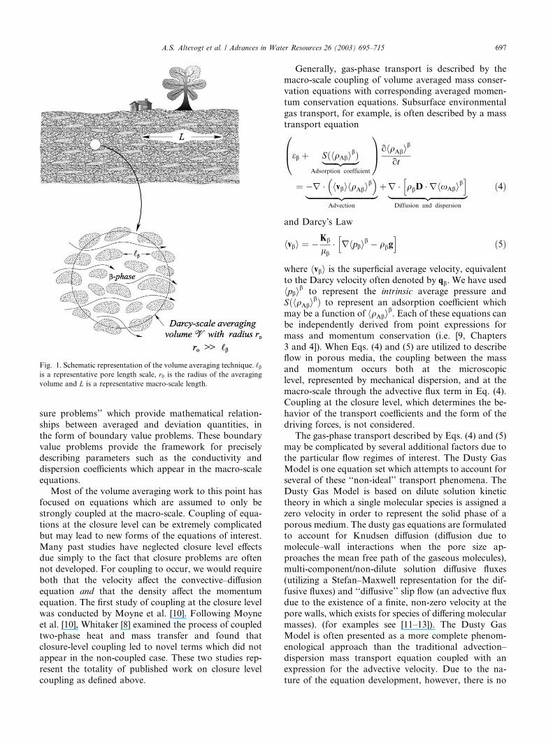
The method of volume averaging can be repre-

sented schematically as in Fig. 1. Equations governing

transport and transformation at the pore scale, such as

*Corresponding author. Tel.: +1-609-258-4599; fax: +1-609-258-

1270.

E-mail addresses: andrewa@princeton.edu, andrewa@alum.mit.edu

(A.S. Altevogt), derolston@ucdavis.edu (D.E. Rolston), swhitaker@

ucdavis.edu (S. Whitaker).

0309-1708/03/$ - see front matter � 2003 Elsevier Science Ltd. All rights reserved.

doi:10.1016/S0309-1708(03)00050-2

Advances in Water Resources 26 (2003) 695–715

www.elsevier.com/locate/advwatres

Eqs. (6) and (7), are mathematically averaged, and

macro-scale equations applicable at laboratory or field

scales are obtained.

Two integral expressions are utilized to express av-

eraged quantities,

Superficial average: hFbi ¼1

V

ZVbðtÞ

Fb dV ð1aÞ

Intrinsic average: hFbib ¼ 1

VbðtÞ

ZVbðtÞ

Fb dV ð1bÞ

where ‘‘Fb’’ is an arbitrary b-phase scalar or tensor vari-able. The superficial and intrinsic averages are related by

hFbi ¼ ebhFbib ð2Þwhere eb is the b-phase volume fraction, or porosity.It is often convenient to represent point, or pore scale

parameters as the sum of the intrinsic average and the

deviation from the average:

Fb ¼ hFbib þ eFFb ð3ÞAs one proceeds through the averaging process, ex-

pressions will often appear containing averaged and

deviation quantities. The overall goal of the volume

averaging process is to derive equations which contain

only averaged quantities. This requires setting up ‘‘clo-

Nomenclature

av interfacial area per unit volume, m�1

Abr area of the b–r interface contained within theaveraging volume, m2

Aeb area occupied by the b-phase at the outersurface of the averaging volume, m2

DAB binary molecular diffusion coefficient for

species A and B, m2/s

Deff effective diffusion coefficient in porous media

tensor, m2/s

g gravitational acceleration vector, m/s2

I unit tensor

k ¼ kk�1

sorption/desorption rate constant in Lang-

muir type sorption relation, m

k1 adsorption rate constant, m/s

k�1 desorption rate constant, s�1

ksorb;b sorptive ‘‘conductivity’’ vector in intrinsic

velocity expression, m4/kg

K� adsorption rate constant, m3/kg sK sorption/desorption rate constant in Lang-

muir type sorption relation, m3/kg

Kb permeability tensor, m2

Kslip;b slip conductivity tensor, m2/s

‘b characteristic b-phase micro-length scale, mL characteristic macro-length scale, m

MA molecular weight of species A, g/mol

nbr ¼ �nrb unit normal vector directed from the b-phase to the r-phase

pb total b-phase pressure, Pahpbib intrinsic average pressure in the b-phase, Pa~ppb ¼ pb � hpbib local spatial deviation pressure, Par position vector, m

Rb slip coupling tensor

R estimate of the magnitude of Rb

SðhqAbibÞ sorption coefficient, function of hqAbi

b

t time, s

t� characteristic process time, s

tbr unit tangent vector between the b-phase andthe r-phase

uA species A diffusive velocity vector, m/s

vAb ¼ uAb þ vb species A total velocity vector, m/s

vb mass average velocity vector in the b-phase,m/s

hvbib intrinsic average velocity vector in the b-phase, m/s

hvbi superficial average velocity vector in the b-phase, m/s

~vvb ¼ vb � hvbib local spatial deviation velocity vector,

m/s

V local averaging volume, m3

zbr ¼ DABtbr

hqAbib

hqbib

� �þa

slip coefficient utilized in the closure

problem, m2/s

Greek symbols

a ¼ffiffiffiffiffiMA

pffiffiffiffiffiMB

p�ffiffiffiffiffiMA

p factor in the slip velocity expression

eb volume fraction of the b-phaseqAb species A mass density in the b-phase, kg/m3

hqAbibintrinsic average species A mass density,

kg/m3

~qqAb ¼ qAb � hqAbiblocal spatial deviation species A

density, kg/m3

qAS total b-phase density, kg/m2

qb total b-phase density, kg/m3

hqbib

intrinsic average total density, kg/m3

~qqb ¼ qb � hqbiblocal spatial deviation total density,

kg/m3

lb b-phase viscosity, Pa sxAb species A mass fraction

hxAbib intrinsic average species A mass fraction~xxAb ¼ xAb � hxAbib local spatial deviation species A

mass fraction

Sub/superscripts

s solid surface

b gas phase

r solid phase

696 A.S. Altevogt et al. / Advances in Water Resources 26 (2003) 695–715

sure problems’’ which provide mathematical relation-

ships between averaged and deviation quantities, in

the form of boundary value problems. These boundary

value problems provide the framework for precisely

describing parameters such as the conductivity anddispersion coefficients which appear in the macro-scale

equations.

Most of the volume averaging work to this point has

focused on equations which are assumed to only be

strongly coupled at the macro-scale. Coupling of equa-

tions at the closure level can be extremely complicated

but may lead to new forms of the equations of interest.

Many past studies have neglected closure level effectsdue simply to the fact that closure problems are often

not developed. For coupling to occur, we would require

both that the velocity affect the convective–diffusion

equation and that the density affect the momentum

equation. The first study of coupling at the closure level

was conducted by Moyne et al. [10]. Following Moyne

et al. [10], Whitaker [8] examined the process of coupled

two-phase heat and mass transfer and found thatclosure-level coupling led to novel terms which did not

appear in the non-coupled case. These two studies rep-

resent the totality of published work on closure level

coupling as defined above.

Generally, gas-phase transport is described by the

macro-scale coupling of volume averaged mass conser-

vation equations with corresponding averaged momen-

tum conservation equations. Subsurface environmental

gas transport, for example, is often described by a masstransport equation

eb

0B@ þ SðhqAbibÞ|fflfflfflfflfflffl{zfflfflfflfflfflffl}Adsorption coefficient

1CA ohqAbib

ot

¼ �r � hvbihqAbib

� �|fflfflfflfflfflfflfflfflfflfflfflfflfflfflffl{zfflfflfflfflfflfflfflfflfflfflfflfflfflfflffl}

Advection

þr � qbD � rhxAbibh i

|fflfflfflfflfflfflfflfflfflfflfflfflfflfflfflfflffl{zfflfflfflfflfflfflfflfflfflfflfflfflfflfflfflfflffl}Diffusion and dispersion

ð4Þ

and Darcy�s Law

hvbi ¼ �Kb

lb

� rhpbibh

� qbgi

ð5Þ

where hvbi is the superficial average velocity, equivalentto the Darcy velocity often denoted by qb. We have used

hpbib to represent the intrinsic average pressure andSðhqAbi

bÞ to represent an adsorption coefficient whichmay be a function of hqAbi

b. Each of these equations can

be independently derived from point expressions for

mass and momentum conservation (i.e. [9, Chapters

3 and 4]). When Eqs. (4) and (5) are utilized to describeflow in porous media, the coupling between the mass

and momentum occurs both at the microscopic

level, represented by mechanical dispersion, and at the

macro-scale through the advective flux term in Eq. (4).

Coupling at the closure level, which determines the be-

havior of the transport coefficients and the form of the

driving forces, is not considered.

The gas-phase transport described by Eqs. (4) and (5)may be complicated by several additional factors due to

the particular flow regimes of interest. The Dusty Gas

Model is one equation set which attempts to account for

several of these ‘‘non-ideal’’ transport phenomena. The

Dusty Gas Model is based on dilute solution kinetic

theory in which a single molecular species is assigned a

zero velocity in order to represent the solid phase of a

porous medium. The dusty gas equations are formulatedto account for Knudsen diffusion (diffusion due to

molecule–wall interactions when the pore size ap-

proaches the mean free path of the gaseous molecules),

multi-component/non-dilute solution diffusive fluxes

(utilizing a Stefan–Maxwell representation for the dif-

fusive fluxes) and ‘‘diffusive’’ slip flow (an advective flux

due to the existence of a finite, non-zero velocity at the

pore walls, which exists for species of differing molecularmasses). (for examples see [11–13]). The Dusty Gas

Model is often presented as a more complete phenom-

enological approach than the traditional advection–

dispersion mass transport equation coupled with an

expression for the advective velocity. Due to the na-

ture of the equation development, however, there is no

Fig. 1. Schematic representation of the volume averaging technique. ‘b

is a representative pore length scale, r0 is the radius of the averagingvolume and L is a representative macro-scale length.

A.S. Altevogt et al. / Advances in Water Resources 26 (2003) 695–715 697

theoretical means of determining the effective transport

coefficients that appear in the model. The transport

coefficients in the Dusty Gas Model must always be

determined experimentally.

Other attempts at equation derivation include ther-modynamic up-scaling work of the type popularized by

Hassanizadeh and co-workers [14–17]. This approach

entails up-scaling thermodynamic relationships, gener-

ally from the micro-scale to the macro-scale. In several

papers [15,17], the authors examined the up-scaling of

mass and momentum conservation expressions to arrive

at equations analogous to Eqs. (4) and (5). The resultant

macro-scale mass and momentum expressions containnovel terms which do not arise in the traditional devel-

opment. As with the Dusty Gas Model, no closure

problems are developed and values of the transport

coefficients can only be obtained experimentally.

Up to this point, there has been no closure level,

coupled up-scaling of the gas-phase mass and momen-

tum equations. Although derivations of averaged mass

and momentum equations are fairly common in theliterature there are none which have attempted to couple

the conservation equations at the closure level. As stated

above, this type of coupling requires that the velocity

affect the mass conservation equation and the species

density affect the momentum equation at the closure

level. The nature of the coupling can be seen by exam-

ination of the point equations represented as

Mass:

Species:oqAb

otþr � ðqAbvAbÞ ¼ 0 ð6aÞ

B:C:1 nbr � ðqAbvAbÞ ¼oqASot

at Abr ð6bÞ

B:C:2 qAb ¼ f ðr; tÞ at Abe ð6cÞ

I:C: qAb ¼ gðrÞ at t ¼ 0 ð6dÞ

Total: r � vb ¼ 0 in the b-phase ð6eÞ

Total momentum:

0 ¼ �rpb þ qbgþ lbr2vb in the b-phase ð7aÞ

B:C:1 vb � tbr ¼ mslip ¼DABtbr � rxAb

xAb þ aat Abr ð7bÞ

B:C:2 vb � nbr ¼ 0 at Abr ð7cÞ

B:C:3 vb ¼ fðr; tÞ at Abe ð7dÞ

Coupling between mass and momentum transport oc-

curs through Eq. (6a) and in the boundary conditions

given by Eq. (6b) and (7b). The assumptions that lead

to Eqs. (6e) and (7a)–(7d) are discussed in Appendix

A. Here we have presented the species and total

mass conservation equations and the total momen-

tum equation. The species momentum conservation

will be expressed by utilizing Fick�s Law, as discussedbelow.

The first boundary condition (Eq. (7b)) in the mo-mentum equation represents the tangential slip bound-

ary condition at the pore walls. This condition states

that the gas velocity will be finite and non-zero, tan-

gential to the interface between the gas and solid phases.

This phenomena was first noted experimentally by

Graham [18] and provides the advective velocity neces-

sitated by Graham�s Law. The theory for binary flowin a capillary tube was first explored by Kramers andKistemaker [19]. This theory (for a binary system)

can be derived directly from kinetic theory, as demon-

strated on a molar basis by Jackson [11]. It is easy to

show that this condition will be important in flow re-

gimes where neither diffusion nor advection is dominant.

These are the types of flows that can be expected in

many situations of environmental concern. In the case

of advection dominated transport, this slip velocitytangential to the solid surface will become negligible

relative to the mean velocity. It should be noted that this

phenomenon is different than Knudsen slip mentioned

above.

The purpose of this work is to utilize the method of

volume averaging to simultaneously up-scale the point

mass and momentum conservation equations repre-

sented by Eqs. (6) and (7), allowing for coupling at theclosure level. In doing so, we hope to account for all

important transport processes at the Darcy scale which

arise due to coupling between the equations. We will

consider the case of two species gas-phase flow in a dry

porous medium. Mathematical constraints on the aver-

aging procedure are developed and presented through-

out the work. By utilizing derived closure expressions,

we will obtain estimates for new macro-scale par-ameters.

2. Volume averaging

2.1. Mass conservation equations

The first step in the averaging process will be to ex-

amine the first boundary condition in the mass conser-

vation problem. We will employ Fick�s law, representedas uAbqAb ¼ �qDABrxAb as our species momentum

equation. This form of the equation can be derived di-

rectly from the Stefan–Maxwell equations and will onlyhold for binary or dilute solution systems. Utilizing the

Langmuir–Hinshelwood formulation for sorptive inter-

actions at the gas solid interface, and following the ar-

guments presented in Appendix A.3, the first boundary

condition in the mass conservation statement can be

represented as

698 A.S. Altevogt et al. / Advances in Water Resources 26 (2003) 695–715

B:C:1 � nbr � qbDABrxAb

¼ ð1� xAbÞkð1þ KqAbÞ

2

oqAb

otat Abr ð8Þ

The form of this equation arises from the assumptions

that have been made about the sorptive interactions at

the b–r interface. It is important to note that we havenot assumed that nbr � vb will be equal to zero in themass conservation equations. As demonstrated in Ap-

pendix A, we may neglect terms containing nbr � vb in themomentum equations, but in order to neglect this term

in the mass conservation boundary condition, the fairly

stringent ‘‘dilute solution’’ criteria of OðxAbÞ � 1 must

be met. In order to preserve the generality of this work

we will not invoke the dilute solution restriction.The mass fraction term in Eq. (8) can be expanded as

ð1� xAbÞ ¼ 1�

� hxAbib � ~xxAb

�ð9Þ

For traditional heat and mass transfer processes [5,9,20],

the spatial deviation is related to the average by

~xxAb ¼ O hxAbib‘b

L

� �ð10Þ

This indicates that we may estimate the order of mag-

nitude of the deviation species density as the intrinsic

average species density multiplied by the ratio of themicro- to macro-length scales. We can neglect the de-

viation mass fraction on the right-hand side of Eq. (9)

with respect to average mass fraction subject to

Constraint: ‘b � L ð11Þ

The boundary condition given by Eq. (8) will thus take

the form

B:C:1 � nbr � qbDABrxAb

¼k 1� hxAbib� �ð1þ KqAbÞ

2

oqAb

otat Abr ð12Þ

The sorptive term, k=ð1þ KqAbÞ2, can be expanded by

utilizing the decomposition qAb ¼ hqAbib þ ~qqAb followed

by a Taylor series expansion around ~qqAb ¼ 0. Subject toplausible constraints, we will arrive at the relationship

(for details see Appendix B.1.1)

k

ð1þ KqAbÞ2¼ k

1þ KhqAbib

� �2 ð13Þ

Utilizing Eq. (13) in Eq. (12) yields

B:C:1 � nbr � qbDABrxAb

¼k 1� hxAbib� �1þ KhqAbi

b� �2 oqAb

otat Abr ð14Þ

We will now turn our attention to developing the

volume averaged form of the transport equation (Eq.

(6a)). Employing a Fick�s Law representation for binarydiffusive flux allows us to express Eq. (6a) as

oqAb

otþr � ðqAbvbÞ ¼ r � ðqbDABrxAbÞ ð15Þ

Following the arguments presented in Whitaker [9,

Chapter 3] we can form the superficial average of Eq.

(15), where we have employed the relationship repre-

sented by Eq. (2), and arrive at

eb

ohqAbib

otþr � ðebhqAbi

bhvbibÞ þ r � h~qqAb~vvbi

þ 1

V

ZAbr

nbr � qAbvb dA ¼ hr � ðqbDABrxAbÞi ð16Þ

The area integral term arises from the fact that the

component of the advective velocity normal to the b–rinterface cannot be neglected in the mass conservation

problem as stated above. The term on the right-hand

side of Eq. (16) can be expanded by utilizing the spatialaveraging theorem [9, Section 1.2.1] to yield

eb

ohqAbib

otþr � ebhqAbi

bhvbib� �

þr � h~qqAb~vvbi

þ 1

V

ZAbr

nbr � qAbvb�

� qbDABrxAb

�dA

¼ r � hqbDABrxAbi ð17Þ

Utilizing B.C.1 as represented by Eq. (A.28) and the

relationship given by Eq. (13) this becomes

eb

ohqAbib

otþr � ebhqAbi

bhvbib� �

þr � h~qqAb~vvbi

þ k

1þ KhqAbib

� �2 1VZAbr

oqAb

otdA

¼ r � hqbDABrxAbi ð18Þ

We will now proceed with further simplifications to

the area integral term in Eq. (18). Following the example

presented by Ochoa-Tapia et al. [21] we can exchange

differentiation and integration. The area averaged spe-

cies density can be further simplified as indicated in

Whitaker [9, Section 1.3.3]. This simplification entails

expressing the area averaged species density in terms ofthe volume averaged species density by means of a

Taylor series expansion around the centroid of the av-

eraging volume. Higher order terms are eliminated and

we arrive at the estimate that the area averaged species

density can be approximated by the volume averaged

species density. We will be able to express Eq. (18) as

A.S. Altevogt et al. / Advances in Water Resources 26 (2003) 695–715 699

eb

ohqAbib

otþr � ðebhqAbi

bhvbibÞ þ r � h~qqAb~vvbi

þ avk

ð1þ KhqAbibÞ2

ohqAbib

ot

¼ r � hqbDABrxAbi ð19Þ

subject to the constraint that the radius of the averaging

volume is significantly less than a representative mac-

roscopic length scale.

We now focus our attention on the term on the righthand side of Eq. (19). We assume that variations of both

DAB and qb can be neglected within the averaging vol-

ume. This allows us to simplify the diffusive term ac-

cording to

hqbDABrxAbi ¼ qbDABhrxAbi ð20Þ

This simplification for the total density, qb, is based on

Eqs. (9)–(11) as they apply to hqbiband ~qqb. At this point,

we make use of the spatial averaging theorem a second

time and follow the development given by Whitaker [9,

Section 1.3] in order to expand the diffusive term and

express Eq. (19) in the form

eb

ohqAbib

ot¼ �r � ebhqAbi

bhvbib� �

�r � h~qqAb~vvbi

þ r � DABqbebrhxAbib� �

þr � DABqb

1

V

ZAbr

nbr ~xxAb dA

!

� avk

1þ KhqAbib

� �2 ohqAbib

otð21Þ

If we assume reb ¼ 0 and divide Eq. (21) by eb, we ar-

rive at the unclosed form of the averaged species con-

tinuity equation

ohqAbib

ot¼ �r � hvbibhqAbi

b� �

� e�1b r � h~qqAb~vvbi

þ e�1b r � DABqbebrhxAbib� �

þ e�1b r � DABqb

1

V

ZAbr

nbr ~xxAb dA

!

� ave�1b

k

1þ KhqAbib

� �2 ohqAbib

otð22aÞ

along with the boundary conditions given by

B:C:1 � nbrr � qbDABrxAb

¼k 1� hxAbib� �1þ KhqAbi

b� �2 oqAb

otat Abr ð22bÞ

B:C:2 ~qqAb ¼ f ðr; tÞ at Abe ð22cÞ

I:C: ~qqAb ¼ gðrÞ; t ¼ 0 ð22dÞ

In order to develop a closed form of Eq. (22a), we willneed to develop a closure problem from which we can

derive expressions for the deviation quantities which

appear in Eq. (22a). In brief, a complete statement of the

closure equations requires the development of boundary

value problems for each of the deviation quantities of

interest. The process begins by subtracting the unclosed

averaged equation (Eq. (22a)) from the point equation

(Eq. (15)), utilizing the representation for point quanti-ties given by Eq. (7) yielding a partial differential

equation for the deviation of the species density. This

equation can then be simplified by employing reasonable

constraints. Following the detailed derivation given in

Appendix B.1.2, we will arrive at a boundary value

problem for the species density deviation (referred to as

a closure problem) which can be expressed as

r � ð~vvbhqAbibÞ|fflfflfflfflfflfflfflfflfflffl{zfflfflfflfflfflfflfflfflfflffl}

Coupling and source

þr � ðvb~qqAbÞ

¼ r � DABr~qqAb

þ ave�1b

k

1þ KhqAbib

� �2 ohqAbib

ot|fflfflfflfflfflfflfflfflfflfflfflfflfflfflfflfflfflfflfflfflffl{zfflfflfflfflfflfflfflfflfflfflfflfflfflfflfflfflfflfflfflfflffl}Source

ð23aÞ

B:C:1 � nbrDAB � r~qqAb

¼ nbr �DABhqbibr

hqAbib

hqbib

!|fflfflfflfflfflfflfflfflfflfflfflfflfflfflfflfflfflfflfflfflfflfflffl{zfflfflfflfflfflfflfflfflfflfflfflfflfflfflfflfflfflfflfflfflfflfflffl}

Source

þk 1� hqAbib

hqbib

� �� �ð1þKhqAbi

bÞ2ohqAbi

b

ot|fflfflfflfflfflfflfflfflfflfflfflfflfflfflfflfflfflfflfflffl{zfflfflfflfflfflfflfflfflfflfflfflfflfflfflfflfflfflfflfflffl}Source

at Abr ð23bÞ

Periodicity: ~qqAbðrþ ‘iÞ ¼ ~qqAbðrÞ; i ¼ 1; 2; 3 ð23cÞ

where all terms containing averaged species densities areidentified as sources for the deviation species density.

2.2. Momentum conservation equations

The boundary value problem for momentum con-

servation is presented by Eqs. (7). It is important to note

that, based on the arguments presented in Appendix A,

boundary condition represented by Eq. (7c) will be valid

for the point momentum conservation equations al-

though it will not be valid for the point mass conservation

equations (see Eqs. (A.29)–(A.33)).

700 A.S. Altevogt et al. / Advances in Water Resources 26 (2003) 695–715

Following the methods of Whitaker [9, Chapter 4] we

may form the volume average of Eq. (7a) and obtain

0 ¼ �ebrhpbib �1

V

ZAbr

nbr~ppb dAþ ebqbg

þ lb r � hrvbi"

þ 1

V

ZAbr

nbr � rvb dA#

ð24Þ

It must be noted that several constraints underlie Eq.

(24). We have assumed that variations in the viscosity

and total density can be neglected within the averagingvolume. Restrictions have been invoked to constrain

variations in the porosity. The representative micro-

scale is constrained to be significantly smaller than the

radius of the averaging volume, and the radius of the

averaging volume must be significantly smaller than a

representative macro-scale.

The bracketed term in Eq. (24) can be further ex-

panded by applying the spatial averaging theorem. Re-membering that at the b–r interface vb ¼ tbrmslip, andfollowing Whitaker [9, Section 4.1.2], the bracketed term

can be expanded as

r � hrvbi þ1

V

ZAbr

nbr � rvb dA

¼ r2 ebhvbib� �

þr � 1

V

ZAbr

nbrtbrmslip dA

" #

�reb � rhvbib þ1

V

ZAbr

nbr � r~vvb dA ð25Þ

Order of magnitude estimates of the two integral terms

on the right-hand side of Eq. (25) can be expressed as

r � 1

V

ZAbr

nbrtbrmslip dA

" #¼ O avhvbib

L

!ð26aÞ

and

1

V

ZAbr

nbr � r~vvb dA ¼ O avhvbib

‘b

!ð26bÞ

The appropriate length scale in Eq. (26a) is the macro-

scale because it is associated with the divergence of anarea averaged slip velocity, while in Eq. (26b) we utilize

the micro-length scale because we have the divergence of

a deviation velocity. In Eq. (26a) we have assumed that

the slip velocity will be the same order of magnitude as

hvbib. On the basis of these estimates we may neglect thefirst integral term on the left-hand side with respect to

the second term constrained by ‘b � L. Eq. (24) canthus be expressed as

0 ¼ �ebrhpbib þ ebqbgþ lbr2 ebhvbib� �

� lbreb � rhvbib þ1

V

ZAbr

nbr � ½�I~ppb þ lbr~vvb�dA

ð27Þ

If we neglect all terms containing reb and divide by eb

we will obtain the unclosed form of the volume averaged

momentum equation containing both average and de-

viation quantities

0 ¼ �rhpbib þ qbgþ lbr2hvbib

þ e�1b

1

V

ZAbr

nbr � ½�I~ppb þ lbr~vvb�dA ð28Þ

As in the mass averaging process, we subtract this vol-

ume averaged equation from the point equation (Eq.

(7a)). The spatial deviation momentum equation can be

expressed as

0 ¼ �r~ppb þ lbr2~vvb � e�1b

1

V

ZAbr

nbr � ½�I~ppb þ lbr~vvb�dA

ð29Þ

Examining the first boundary condition (Eq. (7b)),

we expand vb and xAb into their average and deviation.

We then utilize Eqs. (10) and (11) in order to obtain the

relationship hxAbib � ~xxAb, allowing us to express the

boundary condition as

B:C:1 ~vvb � tbr ¼ DABtbr � rhxAbib

hxAbib þ aþ DABtbr � r ~xxAb

hxAbib þ a

� hvbib � tbr at Abr ð30Þ

where it should be noted that we cannot a priori elimi-

nate r ~xxAb with respect rhxAbib because of the differ-ence in length scales associated with hxAbib and ~xxAb. As

in the mass closure problem (Eqs. (23), governing the

deviation species density), we would like to express the

average and deviation of the mass fraction in terms ofthe averaged total density and the average and deviation

of the species densities, respectively (see Eqs. (B.32)–

(B.34))). Based on these representations we can state the

full simplified momentum closure problem (governing

the deviation velocity and pressure) as

0 ¼ �r~ppb þ lbr2~vvb

� e�1b1

V

ZAbr

nbr � ½�I~ppb þ lbr~vvb�dA ð31aÞ

r � ~vvb ¼ 0 ð31bÞ

B:C:1 ~vvb � tbr ¼DABtbr � r hqAbi

b=hqbi

b� �

hqAbib=hqbi

b� �

þ a|fflfflfflfflfflfflfflfflfflfflfflfflfflfflfflfflfflfflfflfflfflffl{zfflfflfflfflfflfflfflfflfflfflfflfflfflfflfflfflfflfflfflfflfflffl}Source

þDABtbr � r ~qqAb=hqbi

b� �

hqAbib=hqbi

b� �

þ a|fflfflfflfflfflfflfflfflfflfflfflfflfflfflfflfflfflfflffl{zfflfflfflfflfflfflfflfflfflfflfflfflfflfflfflfflfflfflffl}Coupling

�hvbib � tbr|fflfflfflfflfflffl{zfflfflfflfflfflffl}Source

at Abr ð31cÞ

A.S. Altevogt et al. / Advances in Water Resources 26 (2003) 695–715 701

B:C:2 ~vvb � nbr ¼ �hvbib � nbr|fflfflfflfflfflfflfflffl{zfflfflfflfflfflfflfflffl}Source

at Abr ð31dÞ

Periodicity: ~ppbðrþ ‘iÞ ¼ ~ppbðrÞ;~vvbðrþ ‘iÞ ¼ ~vvbðrÞ; i ¼ 1; 2; 3

ð31eÞ

Average: h~vvbib ¼ 0 ð31fÞ

The expression for the deviation continuity equation

(Eq. (31b)) is obtained directly from arguments pre-sented in Whitaker [9, Section 4.2.2] which demonstrate

that the source which appears in this continuity equa-

tion will be negligible compared to the source in Eq.

(31d). The arguments in favor of replacing the third

boundary condition with the periodicity condition rep-

resented by Eq. (31e) are explained in Whitaker [9,

Section 4.2.5].

3. Coupled closure

3.1. Closure variables and boundary value problems

In order to complete the closure process and solve for~qqAb, ~mmb, and ~ppb, we will need to define closure variables

which will account for the coupling between the aver-

aged mass and momentum transport equations. The

closure variables relate the sources identified in Eqs. (23)and (31) to ~qqAb, ~mmb, and ~ppb. By doing so we can obtain an

understanding of how averaged parameters relate to and

control the behavior of the deviation variables. The

deviation velocity, pressure and species density can be

represented by closure variables and volume averaged

quantities in the following manner:

~vvb ¼ Bb � hvbib þ Cb � rhqAbi

b

hqbib

!

þ hbk

ð1þ KhqAbibÞ2

ohqAbib

otð32Þ

~ppb ¼ lbbb � hvib þ lbcb � rhqAbi

b

hqbib

!

þ lbjbk

ð1þ KhqAbibÞ2

ohqAbib

otð33Þ

~qqAb ¼ db � hvbib þ eb � rhqAbi

b

hqbib

!

þ fbk

ð1þ KhqAbibÞ2

ohqAbib

otð34Þ

Governing equations for the closure variables (Bb, Cb,

hb, bb, cb, jb, db, eb, fb) can be obtained by utilizing the

method of superposition, following the techniques uti-

lized in other volume averaging studies [3,5,6,9]. It must

be noted that there is no proof of superposition when

local thermal equilibrium is not valid. On the other

hand, the comparison between theory and experiment[22, p. 441 and 446] suggests that superposition is an

acceptable approximation for the very severe cases that

were examined therein. Expressions for the closure

variables are determined by the boundary value prob-

lems presented in Appendix C.

3.2. Closed momentum equation and simplifications

In order to fully close the volume averaged momen-

tum equation, the expressions given by Eqs. (32)–(34)

must be substituted into the unclosed averaged equation

(Eq. (28)) yielding

0 ¼ �rhpbib þ qbgþ lbr2hvbib

þ e�1b

1

V

ZAbr

nbr � ½"

� lbIbb þ lbrBb�dA#� hvbib

þ e�1b

1

V

ZAbr

nbr � ½"

� lbIcb þ lbrCb�dA#� rhxAbib

þ e�1b

1

V

ZAbr

nbr � ½

264 � lbIjb þ lbrhb�

� k

1þ KhqAbib

� �2 dA375 ohqAbi

b

otð35Þ

Utilizing the definitions

e�1b

1

V

ZAbr

nbr � ½"

� Ibb þrBb�dA#¼ �ebK

�1b ð36Þ

e�1b

1

V

ZAbr

nbr � ½"

� Icb þrCb�dA#¼ Lb ð37Þ

k

1þ KhqAbib

� �2 e�1b

1

V

ZAbr

nbr � ½"

� Ijb þrhb�dA#¼ mb

ð38Þ

and the relationship ebhvbib ¼ hvbi we will arrive at

hvbi ¼ �Kb

lb

� ½rhqbib � qbg� þ Kslip;b � rhxAbib

þ Kb � r2hvbib þ ksorb;bohqAbi

b

otð39Þ

702 A.S. Altevogt et al. / Advances in Water Resources 26 (2003) 695–715

where Kslip;b ¼ Lb � Kb is a macroscopic slip ‘‘con-

ductivity’’ and ksorb;b ¼ mb � Kb is a sorptive ‘‘conduc-

tivity’’. The third term on the right-hand side is known

as the Brinkman correction and will generally be neg-

ligible on the basis of the length scale constraints im-posed in the derivation of Eq. (39) (see [9, Section

4.2.6]).

In order to be able to more readily utilize the fully

closed momentum equation represented by Eq. (39) we

need to obtain expressions for the two ‘‘conductivity’’

tensors Kb, Kslip;b and the sorptive ‘‘conductivity’’ vector

ksorb;b. The traditional permeability term has been ex-

plored elsewhere [9] and we will retain the form pre-sented therein. Exact solutions for the other two

‘‘conductivity’’ terms could be obtained by solving the

closure variable equations (Eqs. (C.3)–(C.8)). Due to the

difficulty in obtaining solutions to these equations, we

will focus on obtaining estimates for these two new

terms in the velocity equation. Following the presenta-

tion contained in Appendix C and neglecting the

Brinkman correction, we arrive at the form of the cou-pled momentum equation for gas flow in porous media

based on order of magnitude estimates of the derived

conductivity terms

hvbi ¼ �Kb

lb

� rhpbibh

� qbgiþ Kslip;b � rhxAbib

þ ksorb;bohqAbi

b

otð40Þ

where our order of magnitude estimates indicate that

ksorb;b ¼ O k

1þ KhqAbib

� �0@ 1A hxAbib � 1

hqAbib þ hqbi

ba

!24 35ð41Þ

and

Kslip;b ¼ O DAb

hxAbib þ a

!ð42Þ

3.3. Closed mass conservation equation and simplifica-

tions

The closed form of the volume averaged mass con-servation equation is obtained by first utilizing the

relationship ~xx ¼ ~qqAb=hqbiband the approximation

qb ¼ hqbibin the final term of Eq. (22a). We then sub-

stitute our expressions for the deviation density and

velocity equations (32) and (34) into Eq. (22a) and

arrive at

1

þ ave�1b

k

ð1þ KhqAbibÞ2

!ohqAbi

b

ot

¼ �e�1b r � ~vvb db � hvbib *

þ eb � rhxAbib

þ fbk

ð1þ KhqAbibÞ2

ohqAbib

ot

!+

þ e�1b r � DAB1

V

ZAbr

nbr db � hvbib0B@

264 þ eb � rhxAbib

þ fbk

1þ KhqAbib

� �2 ohqAbib

ot

1CAdA375

�r � hvbibhqAbib

� �þ e�1b r � ðDABqbebrhxAbibÞ

ð43Þ

Grouping the closure terms containing similar volumeaveraged variables allows us to express Eq. (43) as

1

0B@ þave�1b

k

1þKhqAbib

� �21CAohqAbi

b

ot

¼�r� ðhvbibhqAbibÞþ e�1b r� ðDABqbebrhxAbibÞ

þ e�1b r� k

1þKhqAbib

� �2 DAB1

V

ZAbr

nbrfbdA

!(264

�h~vvbfbi)ohqAbi

b

ot

375þ e�1b r� DAB

1

V

ZAbr

nbrdbdA

!("�h~vvbdbi

)� hvbib

#

þ e�1b r� DABqbeb q�1b

1

V

ZAbr

nbrebdA

!("

�h~vvbebi)�rhxAbib

#ð44Þ

As with the momentum equation, we would like to ob-

tain estimates of the closure variable terms in Eq. (44).

On the basis of arguments presented in Appendix C, we

will be able to neglect the time derivative term on the

right-hand side relative to the left-hand side. The aver-

aged mass continuity equation will thus become

A.S. Altevogt et al. / Advances in Water Resources 26 (2003) 695–715 703

1þ ave�1b

k

1þKhqAbib

� �20B@

1CA|fflfflfflfflfflfflfflfflfflfflfflfflfflfflfflfflfflfflfflfflfflfflfflfflfflffl{zfflfflfflfflfflfflfflfflfflfflfflfflfflfflfflfflfflfflfflfflfflfflfflfflfflffl}

Retardation

ohqAbib

ot

¼�r � ðhvbibhqAbibÞ|fflfflfflfflfflfflfflfflfflfflfflfflfflffl{zfflfflfflfflfflfflfflfflfflfflfflfflfflffl}

Advection

þ e�1b r� Db �rhxAbibh i

|fflfflfflfflfflfflfflfflfflfflfflfflfflfflfflfflfflffl{zfflfflfflfflfflfflfflfflfflfflfflfflfflfflfflfflfflffl}Mechanical dispersion

þr � Deffqb �rhxAbibh i

|fflfflfflfflfflfflfflfflfflfflfflfflfflfflfflfflfflffl{zfflfflfflfflfflfflfflfflfflfflfflfflfflfflfflfflfflffl}Diffusion

þ e�1b r� DAB1

V

ZAbr

nbrdbdA

!�h~vvbdbi

( )� hvbib

" #|fflfflfflfflfflfflfflfflfflfflfflfflfflfflfflfflfflfflfflfflfflfflfflfflfflfflfflfflfflfflfflfflfflfflfflfflfflfflfflfflfflfflfflfflfflfflffl{zfflfflfflfflfflfflfflfflfflfflfflfflfflfflfflfflfflfflfflfflfflfflfflfflfflfflfflfflfflfflfflfflfflfflfflfflfflfflfflfflfflfflfflfflfflfflffl}

Slip coupling effect

ð45Þ

where

Deff ¼ DABeb I

þ q�1

b

1

V

ZAbr

nbreb dA

!is the binary effective diffusivity and Db ¼ �h~vvbebi is themechanical dispersion coefficient in the porous media of

interest. The diffusion and dispersion terms are kept

separate in Eq. (45) in order to explore an important

caveat on the use of mechanical dispersion. We canutilize the estimate represented by Eq. (C.16) in order to

obtain

Db ¼ �h~vvbebi ¼ Oðhvbib‘bhqbibÞ ð46Þ

The mechanical dispersive term will be negligible com-pared with diffusive flux in many cases of gas flow in

porous media based on

Constraint:hvbib‘b

DAB� 1 ð47Þ

This constraint is entirely consistent with dispersion

criteria which have been well known, although often

ignored, for many years [9,23–25]. Simply put, this

constraint indicates that mechanical dispersion in ahomogeneous porous medium will be negligible when

the micro-scale Peclet number is less than one. We will

retain mechanical dispersion in our formulation in order

to preserve generality, with the understanding that in

many situations of environmental concern it will be

negligible.

The ‘‘slip coupling’’ term in Eq. (45) is the last re-

maining new term in the mass conservation equation.Again, we will explore its behavior through the use of

order of magnitude estimates, the details of which are

presented in Appendix C. We will utilize the estimate

represented by Eq. (C.30b) (recognizing that at Peclet

numbers significantly greatly than 1, the term repre-

sented by Eq. (C.30a) may be more dominant) in order

to express the mass conservation equation for gas flow

in porous media as

1þ ave�1b

k

1þ KhqAbib

� �20B@

1CA|fflfflfflfflfflfflfflfflfflfflfflfflfflfflfflfflfflfflfflfflfflfflfflfflfflffl{zfflfflfflfflfflfflfflfflfflfflfflfflfflfflfflfflfflfflfflfflfflfflfflfflfflffl}

Retardation

ohqAbib

ot

¼ �r � ðhvbibhqAbibÞ|fflfflfflfflfflfflfflfflfflfflfflfflfflfflffl{zfflfflfflfflfflfflfflfflfflfflfflfflfflfflffl}

Advection

þ e�1b r � Db � rhxAbibh i

|fflfflfflfflfflfflfflfflfflfflfflfflfflfflfflfflfflffl{zfflfflfflfflfflfflfflfflfflfflfflfflfflfflfflfflfflffl}Mechanical dispersion

þ e�1b r � Deffqb � rhxAbibh i

|fflfflfflfflfflfflfflfflfflfflfflfflfflfflfflfflfflfflfflfflfflffl{zfflfflfflfflfflfflfflfflfflfflfflfflfflfflfflfflfflfflfflfflfflffl}Diffusion

þ e�1b r � Rb � hvbibh i

|fflfflfflfflfflfflfflfflfflfflfflfflfflffl{zfflfflfflfflfflfflfflfflfflfflfflfflfflffl}Slip coupling effect

ð48Þ

Rb ¼ OðhqAbibÞ is a term arising from the closure level

coupling between mass and momentum which augmentsthe traditional advective term. Expanding the intrinsic

average velocity by utilizing Eq. (2) and assuming

reb ¼ 0 leads to the final form of the volume averaged

mass conservation equation

eb þ avk

1þ KhqAbib

� �20B@

1CA|fflfflfflfflfflfflfflfflfflfflfflfflfflfflfflfflfflfflfflfflfflfflfflffl{zfflfflfflfflfflfflfflfflfflfflfflfflfflfflfflfflfflfflfflfflfflfflfflffl}

Retardation

ohqAbib

ot

¼ �r ��hvbi � IhqAbi

b � Rb

� ��|fflfflfflfflfflfflfflfflfflfflfflfflfflfflfflfflfflfflfflfflfflfflfflfflfflffl{zfflfflfflfflfflfflfflfflfflfflfflfflfflfflfflfflfflfflfflfflfflfflfflfflfflffl}

Advection and slip coupling

þ r � Deffqb � rhxAbibh i

|fflfflfflfflfflfflfflfflfflfflfflfflfflfflfflfflfflfflffl{zfflfflfflfflfflfflfflfflfflfflfflfflfflfflfflfflfflfflffl}Diffusion

þ r � Db � rhxAbibh i

|fflfflfflfflfflfflfflfflfflfflfflfflfflfflffl{zfflfflfflfflfflfflfflfflfflfflfflfflfflfflffl}Mechanical dispersion

ð49Þ

4. Conclusions

Accounting for coupling between the gas-phase mass

and momentum conservation equations at the closure

level leads to non-traditional terms in the Darcy scaletransport equations. The momentum equation for gas

flow in porous media gains two new terms; the first due

to the existence of a finite non-zero velocity at the gas–

solid interface, the second due to the contribution of

adsorption/desorption at the interface. The first of these

conditions arises from inclusion of the slip velocity

boundary condition at the micro-scale, the second stems

from the closure level coupling with the mass equation.The mass transport equation contains a new term which

arises due to coupling with the momentum equation.

Estimates of this new term indicate that it may be quite

significant relative to the traditional advective flux term.

Order of magnitude estimates indicate that it may be

significant in many gas flow regimes with significant

704 A.S. Altevogt et al. / Advances in Water Resources 26 (2003) 695–715

advective fluxes. This new ‘‘slip coupling’’ flux term has

a different functional form than the traditional me-

chanical dispersion term and it will be important in

situations where mechanical dispersion is negligible

(Peclet numbers less than one). In Part 2 we employlaboratory experiments and numerical models in order

to explore the validity of these equations.

Acknowledgements

This publication was made possible by grant number

5 P42 ES04699-16 from the National Institute of Envi-ronmental Health Sciences, NIH with funding provided

by EPA and the USEPA Center of Ecological Health

Research (R819658, R825433) at UC Davis. Its contents

are solely the responsibility of the authors and do not

necessarily represent the official views of the NIEHS,

NIH or EPA.

Appendix A. Exploration of the point conservation equa-

tions

A.1. Point total momentum equations––simplification of

the Navier–Stokes equation

The point momentum conservation equations can be

restated as

0 ¼ �rpb þ qbgþ lbr2vb in the b-phase ðA:1aÞ

B:C:1 vb � tbr ¼ mslip ¼DABtbr � rxA

xA þ aat Abr ðA:1bÞ

B:C:2 vb � nbr ¼ 0 at Abr ðA:1cÞ

B:C:3 vb ¼ fðr; tÞ at Abe ðA:1dÞ

The boundary condition represented by Eq. (A.1c) can

be extracted from the following arguments. The Navier–

Stokes equation (not restricted by the traditional in-

compressible fluid assumption) expressed as:

o

otqbvb þr � ðqbvbvbÞ ¼ �rpb þ qbgþ lbr2vb ðA:2Þ

Taking the volume average of Eq. (A.2) and utilizing the

spatial averaging theorem yields

r � hqbvbvbi þ1

V

ZAbr

nbr � ðqbvbvbÞdA

¼ 1

V

ZVb

lbr2vb dV þ � � � ðA:3Þ

The term inside the area integral can be represented as

nbr � ðqbvbvbÞ ¼ nbr � ðqAbvbvbÞ þ nbr � ðqBbvbvbÞ ðA:4Þ

The second term on the right-hand side will be equal to

zero if species ‘‘B’’ does not partition from the b-phaseto the r-phase. Thus, the area integral in Eq. (A.3) canbe represented as

1

V

ZAbr

nbr � ðqbvbvbÞdA ¼ 1

V

ZAbr

nbr � ðqAbvbvbÞdA

ðA:5ÞThe two integral terms in Eq. (A.3) thus be can be

represented by the following estimates:

1

V

ZAbr

nbr � ðqAbvbvbÞdA ¼ O 1

‘bqbðv�bÞ

2

� �ðA:6Þ

1

V

ZVb

lbr2vb dV ¼ O eblb

vb

‘2b

!ðA:7Þ

The expression 1V

RAbrnbr dA is represented as av which

can be estimated as ‘�1b [9]. The characteristic velocity at

the pore wall, v�b, can be represented by the following

estimate:

v�b ¼ ODAB

hxAbib

L

� �1� hxAbib

;DAB

hxAbib

L

� �hxAbib þ a

0@ 1A ðA:8Þ

The first term arises from the expression for the normal

component developed in the mass averaging procedure

(Eq. (A.33)). The second term follows from the tan-

gential or slip velocity represented by Eq. (A.1b). Wehave estimated that changes in the mass fraction at the

b–r interface will be on the order of the average massfraction and will occur over the large length scale L.We can invoke the restriction

1

V

ZAbr

nbr � ðqbvbvbÞdA � 1

V

ZVb

lbr2vb dV ðA:9aÞ

subject to

Constraint: hqbib

DABhxAbib

L

� �1� hxAbib

;DAB

hxAbib

L

� �hxAbib þ a

0@ 1A2

� eblb

hvbib

‘bðA:9bÞ

With the idea that small causes give rise to small effects,

the restriction represented by (A.9a) leads to the

boundary condition

B:C:2 vb � nbr ¼ 0 at Abr ðA:10Þ

In other words, Eq. (A.10) is the non-trivial conse-quence of the restriction given by Eq. (A.9a). If the

constraint represented by Eq. (A.9b) holds, vb � nbr will

have to become small at the b–r interface in order forthe left-hand side of Eq. (A.9a) to be small compared to

the right-hand side. It is important to note that the

contribution of the normal component of the advective

A.S. Altevogt et al. / Advances in Water Resources 26 (2003) 695–715 705

velocity at the b–r interface is negligible in the mo-

mentum conservation equation, but it may not be neg-

ligible in the mass conservation problem.

We would like to explore several of the assumptions

which underlie the point momentum expressions, asrepresented by Eqs. (A.1). Eq. (A.2) can be simplified to

r � ðqbvbvbÞ ¼ �rpb þ qbgþ lbr2vb ðA:11Þ

based on the constraint lbt�=qb‘

2b � 1 [3]. This con-

straint is consistent with the restriction qov=ot � lr2v

which indicates that the flow is quasi-steady. Eq. (A.11)

can be at further simplified based on the restriction

r � ðqbvbvbÞ � lbr2vb. Where we have utilized the esti-

mates

r � ðqbvbvbÞ ¼ O hqbib ðhvbibÞ2

‘b

!ðA:12Þ

lbr2vb ¼ O lb

hvbib

‘2b

!ðA:13Þ

Constraint:hqbi

bhvbib‘b

lb

� 1 ðA:14Þ

Yielding

0 ¼ �rpb þ qbgþ lbr2vb ðA:15Þ

The estimates indicated by Eqs. (A.12) and (A.13) are

based on the idea that the changes in the point velocity

will be on the order of the average and that they willoccur over the small length-scale ‘b.

A.2. Point total mass equation––condition of incompress-

ibility

r � vb ¼ 0 in the b-phase ðA:16Þ

The condition of incompressibility represent by Eq.

(A.16) can be obtained by starting with the total mass

conservation equation

oqb

otþr � ðvbqbÞ ¼ 0 ðA:17Þ

This can be rearranged to yield

r � vb ¼ �q�1b

oqb

ot� q�1

b vb � rqb ðA:18Þ

The following order of magnitude estimates can be

made for each of the terms in Eq. (A.18):

r � vb ¼ O hvbib

‘b

!ðA:19aÞ

q�1b

oqb

ot¼ O

Dqb

qbt�

� �ðA:19bÞ

q�1b vb � rqb ¼ O

Dqb

qbLhvbib

� �ðA:19cÞ

The estimates employed in Eqs. (A.19) are based on

arguments presented above. The gradient of the velocity

on the left hand side of Eq. (A.18) will be the dominant

with respect to each of the individual terms on the right-

hand side subject to

Constraint: hvbib �Dqb

qb

‘b

t�ðA:20Þ

Constraint:Dqb

qb

‘b

L� 1 ðA:21Þ

Eq. (A.17) thus becomes

r � vb ¼ 0 ðA:20Þ

A.3. Point mass equations––sorptive boundary condition

Focusing on the first boundary condition in the point

mass conservation equations (Eq. (6b)), we may utilizeFick�s Law in order to obtain

B:C:1 nbr � ðqAbvb � qbDABrxAbÞ ¼oqASot

at Abr

ðA:22ÞWe would like to be able to express this boundary

condition in terms of qAb. If the surface sorption de-

pends on the number of vacant sites and the number

of vacant sites can be expressed as linear function of

the surface density (the conditions for the Langmuir–Hinshelwood formulation) we can express the net rate of

adsorption (in the absence of surface reaction and

transport) as [9]

oqASot

¼ ðk1 � K�qASÞqAb � k�1qAS ðA:23Þ

where qAS is the density of species A at the adsorbing

surface (for addition details see [26]). If we assume local

sorptive equilibrium, Eq. (A.23) becomes

0 ¼ ðk1 � K�qASÞqeqAb � k�1qAS ðA:24Þ

where qeqAb is the equilibrium species A density in the

b-phase. Eq. (A.24) is equivalent to

ðk�1 þ K�qeqAbÞqAS ¼ k1qeqAb ðA:25Þ

Defining the constants k ¼ k1=k�1, and K ¼ K�=k�1, thesurface density may be expressed as

qAS ¼kqeqAb

1þ KqeqAb

ðA:26Þ

706 A.S. Altevogt et al. / Advances in Water Resources 26 (2003) 695–715

This is equivalent to a Langmuir sorption isotherm.

Taking the derivative with respect to time and using the

local equilibrium assumption, qeqAb ¼ qAb, yields

oqASot

¼ k

ð1þ KqAbÞ2

oqAb

otat Abr ðA:27Þ

Substituting this expression into B.C.1 gives

B:C:1 nbr � ðqAbvb � qbDABrxAbÞ

¼ k

ð1þ KqAbÞ2

oqAb

otat Abr ðA:28Þ

In the traditional derivation of the volume averaged

mass conservation equation, the assumption nbr � vb ¼ 0is utilized in order to simplify the form of this boundarycondition. We would like to examine this assumption

and determine its range of validity. The advective term

in Eq. (A.28) can be represented (for a binary system) as

nbr � qAbvb ¼ qAbðxAbvAb þ xBbvBbÞ � nbr ðA:29Þ

where vAb and vBb are the species velocities of the com-ponents of the system. For the case where component B

does not partition from the b-phase to the r-phase (as isoften assumed for air, for example)

vBb � nbr ¼ 0 at Abr ðA:30Þ

Eq. (A.29) can thus be expressed as

nbr � qAbvb ¼ qAb xAbvb

�þ

qAbuAb

qb

�� nbr ðA:31Þ

where uAb is the diffusive velocity of species A. The

diffusive flux of species A, qAbuAb, can be expressed

equivalently, using Fick�s Law, to yield

nbr � qAbvb ¼ qAb xAbvb

��

qbDAbrxAb

qb

�� nbr ðA:32Þ

Eq. (A.32) is equivalent to

nbr � qAbvb ¼ �nbr � xAb

1� xAb

� �qbDABrxAb

& 'ðA:33Þ

This expression clearly demonstrates that the assump-

tion nbr � vb ¼ 0 will only be valid at the b–r interfacewhen the constraint ðxAb=1� xAbÞ � 1 is met. In order

preserve the generality of our equations, we will not

restrict our analysis to this case. Substituting Eq. (A.33)

into Eq. (A.28) gives

nbr �&� xAb

1� xAb

� �qbDABrxAb � qbDABrxAb

'¼ k

ð1þ KqAbÞ2

oqAb

otat Abr ðA:34Þ

After algebraic manipulation of the left-hand side, this

yields the boundary condition

B:C:1 � nbr �qbDABrxAb

1� xAb

� �¼ k

ð1þ KqAbÞ2

oqAb

otat Abr ðA:35aÞ

or equivalently

B:C:1 � nbr � qbDABrxAb ¼ð1�xAbÞkð1þ KqAbÞ

2

oqAb

otat Abr

ðA:35bÞ

Appendix B. Volume averaging

B.1. Mass conservation equations

B.1.1. Sorptive terms

We can utilize the decomposition qAb ¼ hqAbib þ ~qqAb

to expand the sorption isotherm term in Eq. (13) as

k

ð1þKqAbÞ2¼ k 1&

þ2KðhqAbib þ ~qqAbÞ

þK2 ~qq2Ab

�þ2hqAbi

b~qqAb þ hqAbib

� �2�'�1ðB:1Þ

Combining the deviation terms yields

k

ð1þ KqAbÞ2¼ k 1h

þ 2KhqAbib þ K2ðhqAbi

bÞ2

þ ~qqAb 2K�

þ 2K2hqAbib�þ K2~qq2Ab

i�1ðB:2Þ

We would like to simplify this expression as much as

possible in order to more easily utilize it in our averaged

equation. If we define function HðhqAbib; ~qqAbÞ as the

right-hand side of Eq. (B.2) we can express it as a Taylorseries expanded around ~qqAb ¼ 0

HðhqAbib; ~qqAbÞ ¼ HðhqAbi

b; 0Þ þ ~qqAb

oHðhqAbib; 0Þ

o~qqAb

þ~qq2Ab

2

o2HðhqAbib; 0Þ

o~qq2Ab

þ � � � ðB:3Þ

We can express HðhqAbib; 0Þ and its derivatives as

HðhqAbib; 0Þ ¼ k 1

hþ 2KhqAbi

b þ K2ðhqAbibÞ2i�1

ðB:4aÞ

oHðhqAbib; 0Þ

o~qqAb

¼ �k 1h

þ 2KhqAbib þ K2ðhqAbi

bÞ2i�2

� ð2K þ 2K2hqAbibÞ ðB:4bÞ

o2H hqAbib; 0

� �o~qq2Ab

¼ 6kK2 1h

þ 2KhqAbib þ K2ðhqAbi

bÞ2i�2

ðB:4cÞ

A.S. Altevogt et al. / Advances in Water Resources 26 (2003) 695–715 707

Defining C ¼ 1þ 2KhqAbib þ K2ðhqAbi

bÞ2h i�1

we can

express Eq. (B.3) as

HðhqAbib; ~qqAbÞ ¼ kC � ~qqAbð2K þ 2K2hqAbi

bÞkC2

þ 3~qq2AbK2KC2 þ � � � ðB:5Þ

We can now proceed with simplifications to this ex-

pression. The third term on the right-hand side can be

eliminated by employing the estimate and constraint

represented by Eqs. (10) and (11). The third term on the

right-hand side of Eq. (B.5) will be negligible compared

to the first term on the right-hand side if the following

holds:

Constraint:3 hqAbi

b� �2

ð‘b=LÞ2K2

1þ 2KhqAbib þ ðhqAbi

bÞ2h i� 1 ðB:6Þ

In order to demonstrate the utility of the constraint

represented by Eq. (B.6), we can examine simplifications

of the constraint for specific values of hqAbiband K. For

hqAbib � 1 kg/m3 and K ¼ Oð1Þ m3/kg the constraint

represented by Eq. (B.6) will reduce to 3ðhqAbibÞ2�

ð‘b=LÞ2 � 1. For hqAbib ¼ O(1) kg/m3 and K ¼ Oð1Þ

m3/kg the constraint will become ‘b � ð2=ffiffiffi3

pÞL.

Similarly, the second term on the right-hand side ofEq. (B.5) can be discarded with respect to the first term

on the right-hand side if the following holds:

Constraint:hqAbi

bð‘b=LÞð2K þ 2K2hqAbibÞ

1þ 2KhqAbib þ K2ðhqAbi

bÞ2� 1

ðB:7Þ

As with the previous constraint we can utilize particular

values of hqAbiband K in order to examine the validity

of Eq. (B.7). For hqAbib � 1 kg/m3 and K ¼ Oð1Þ m3/kg

the constraint represented by Eq. (B.7) will reduce to

hqAbib‘b=Ln1. For hqAbi

b ¼ Oð1Þ kg/m3 L and K ¼Oð1Þ m3/kg the constraint will become ‘b � L. On thebasis of these simplifications we can express Eq. (B.1) as

k

ð1þ KqAbÞ2¼ k 1&

þ 2KhqAbib þ K2 hqAbi

b� �2'�1

or, equivalently

k

ð1þ KqAbÞ2¼ k

1þ KhqAbib

� �2 ðB:8Þ

B.1.2. Development of the mass conservation closure

problem

The closure problem will be set up by first subtracting

the unclosed averaged mass conservation equation

ohqAbib

ot¼ �r � hvbibhqAbi

b� �

� e�1b r � h~qqAb~vvbi

þ e�1b r � DABqbebrhxAbib� �

þ e�1b r � DABqb

1

V

ZAbr

nbr ~xxAb dA

!

� ave�1b

k

1þ KhqAbib

� �2 ohqAbib

otðB:9Þ

from the point equation

oqAb

ot¼ �r � ðvbqAbÞ þ r � ðqbDABrxAbÞ ðB:10Þ

in order to obtain

o~qqAb

ot¼ �r � ðvbqAbÞ þ r � hvbibhqAbi

b� �

þ e�1b r � h~vvb~qqAbi þ r � qbDABrhxAbib� �

þr � ðqbDABr ~xxAbÞ � e�1b r � DABqbebrhxAbib� �

� e�1b r � DABqb

1

V

ZAbr

nbr ~xxAb dA

!

þ ave�1b

k

1þ KhqAbib

� �2 ohqAbib

otðB:11aÞ

B:C:1 � nbr � ðqbDABr ~xxAbÞ

¼ nbr � qbDABrhxAbib� �

þk 1� hxAbib� �1þ KhqAbi

b� �2 o~qqAb

ot

þk 1� hxAbib� �1þ KhqAbi

b� �2 ohqAbi

b

otat Abr

ðB:11bÞ

B:C:2 ~qqAb ¼ f ðr; tÞ at Abe ðB:11cÞ

I:C: ~qqAb ¼ gðrÞ; t ¼ 0 ðB:11dÞ

where we have decomposed the boundary condition

given by Eq. (22b).

We can now proceed with simplifications to Eqs.

(B.11a) and (B.11b). As in the derivation of the volumeaveraged equations, we will develop estimates of various

terms in the equations of interest and eliminate those

terms which can be neglected on the basis of reasonable

constraints on the system. First we will focus on the

‘‘local diffusion’’ term in Eq. (B.11a) and make the es-

timates

708 A.S. Altevogt et al. / Advances in Water Resources 26 (2003) 695–715

e�1b r � DABqb

1

V

ZAbr

nbr ~xxAb dA

!

¼ ODqb ~xxAbDABe�1b

L‘b

!ðB:12Þ

r � ðqbDABr ~xxAbÞ ¼ OqbDAB ~xxAb

‘2b

!ðB:13Þ

The gradient of the area integral will be associated with

a macro-length-scale, L. As described in Appendix A,the area integral term will be estimated by ‘�1b . Em-

ploying these estimates we can neglect the local ‘‘diffu-sion’’ term relative to r � ðqbDABr ~xxAbÞ, subject to

Constraint:Dqb

qb

‘b

L� eb ðB:14Þ

The volume diffusive source e�1b r � ðDABqbebrhxAbibÞcan be neglected relative to the surface diffusive source

nbr � ðqbDABrhxAbibÞ following Whitaker [9, Section

1.4.2] subject to:

Constraint:volume source # 1

surface source¼ O ‘b

LDeb

� �� 1

ðB:15Þ

Employing the estimates

1

V

ZAbr

nbr � qbDABrhxAbib� �

dA

¼ O avqbDABrhxAbib� �

ðB:16Þ

1

V

ZVb

r � qbDABrhxAbib� �h i

dV

¼ OebqbDABrhxAbib

L

!ðB:17Þ

and invoking similar arguments we will caneliminate 1

V

RVb½r � ðqbDABrhxAbibÞ�dV relative to

1V

RAbrnbr � ðqbDABrhxAbibÞdA, subject to

Constraint:volume source # 2

surface source¼ O eb‘b

L

� �� 1

ðB:18Þ

where we have assumed that av ¼ Oð‘�1b Þ (see [9,

Chapter 1]). The above simplifications allow us to ex-

press the closure Eq. (B.11a) as

o~qqAb

ot¼ �r � ðvbqAbÞ þ r � hvbibhqAbi

b� �

þ e�1b r � h~vvb~qqAbi þ r � ðqbDABr ~xxAbÞ

þ ave�1b

k

1þ KhqAbib

� �2 ohqAbib

otðB:19Þ

The first two terms on the right-hand side of Eq. (B.19)

can be expanded as

�r � ðvbqAbÞ þ r � hvbibhqAbib

� �¼ �hvbib � rhqAbi

b � hqAbibr � hvbib

�r � ~vvbhqAbib

� �� vb � r~qqAb � ~qqAbr � vb

þ hvbib � rhqAbib þ hqAbi

br � hvbib ðB:20aÞ

or equivalently

�r � ðvbqAbÞ þ r � hvbibhqAbib

� �¼ �r � ~vvbhqAbi

b� �

�r � ðvb~qqAbÞ ðB:20bÞ

The closure equation thus becomes

o~qqAb

ot¼ �r � ~vvbhqAbi

b� �

�r � ðvb~qqAbÞ

þ e�1b r � h~vvb~qqAbi þ r � ðqbDABr ~xxAbÞ

þ ave�1b

k

1þ KhqAbib

� �2 ohqAbib

otðB:21Þ

The estimates

e�1b r � h~vvb~qqAbi ¼ O hvbib~qqAb

L

!ðB:22Þ

r � ðvb~qqAbÞ ¼ O hvbib~qqAb

‘b

!ðB:23Þ

have disparate length-scales due to the fact that the term

in Eq. (B.22) contains the divergence of an macro-scale

quantity, while in Eq. (B.23) we are taking the diver-

gence of micro-scale quantities. We will neglecte�1b r � h~vvb~qqAbi relative to r � hvb~qqAbi based on

Constraint: ‘b � L ðB:24Þ

The closure equation is thus simplified to

o~qqAb

ot¼ �r � ~vvbhqAbi

b� �

�r � ð~vvb~qqAbÞ

þ r � ðqbDABr ~xxAbÞ þ ave�1b

k

1þ KhqAbib

� �2 ohqAbib

ot

ðB:25Þ

A.S. Altevogt et al. / Advances in Water Resources 26 (2003) 695–715 709

We will now examine the constraints associated with

assuming that the closure problem is quasi-steady. The

first step is to employ the estimates

o~qqAb

ot¼ O

~qqAb

t�

!ðB:26Þ

r � ðqbDABr ~xxAbÞ ¼ ODAB~qqAb

‘2b

!ðB:27Þ

The closure equation will be quasi-steady if

r � ðqbDABr ~xxAbÞ � o~qqAb=ot, which implies

Constraint:DABt�

‘2b� 1 ðB:28Þ

The simplified closure equation can be expressed as

r � ~vvbhqAbib

� �þr � ðvb~qqAbÞ

¼ r � ðqbDABr ~xxAbÞ þ ave�1b

k

1þ KhqAbib

� �2 ohqAbib

ot

ðB:29aÞ

B:C:1 � nbr � ðqbDABr ~xxAbÞ

¼ nbr � qbDABrhxAbib� �

þk 1� hxAbib� �1þ KhqAbi

b� �2 o~qqAb

ot

þk 1� hxAbib� �1þ KhqAbi

b� �2 ohqAbi

b

otat Abr

ðB:29bÞ

Similarly, the boundary condition will be quasi-steady if

the second term on the right-hand side of Eq. (B.29b)

can be neglected relative to the term on the left-hand

side, subject to

Constraint:DABt� 1þ KhqAbi

b� �2

‘bk 1� hxAbib� � � 1 ðB:30Þ

The quasi-steady boundary condition is thus

B:C:1 � nbr � ðqbDABr ~xxAbÞ

¼ nbr � qbDABrhxAbib� �

þk 1� hxAbib� �1þKhqAbi

b� �2 ohqAbi

b

otat Abr ðB:31Þ

In order to simplify the solution of the closure

problem all terms containing hxAbib and ~xxAb in the

governing equation and the boundary condition need to

be expressed in terms of hqAbib, ~qqAb, and hqbi

b. The first

step is to express the mass fraction in the following

manner:

xAb ¼qAb

qb

¼hqAbi

b þ ~qqAb

hqbib þ ~qqb

ðB:32Þ

and then define

hxAbib ¼hqAbi

b

hqbib þ ~qqb

and ~xxAb ¼~qqAb

hqbib þ ~qqb

ðB:33Þ

If we assume that hqbib � ~qqb, then we can express the

average and deviation of the mass fraction as

hxAbib ¼hqAbi

b

hqbib and ~xxAb ¼

~qqAb

hqbib ðB:34Þ

Employing the expansion qb ¼ hqbib þ ~qqb, and assuming

qb � ~qqb, yields the estimate qb ¼ hqbiband expanding

the mass fraction terms in (B.29a) and (B.31)

r � ~vvbhqAbib

� �þr � ðvb~qqAbÞ

¼ r � DAB r~qqAb

�

~qqAb

hqbib rhqbi

b

!

þ ave�1b

k

1þ KhqAbib

� �2 ohqAbib

otðB:35aÞ

B:C:1 � nbrDAB � r~qqAb

�

~qqAb

hqbib rhqbi

b

!

¼ nbr � DAB rhqAbib

�hqAbi

b

hqbib rhqbi

b

!

þk 1� hqAbib

hqbib

� �� �1þ KhqAbi

b� �2 ohqAbi

b

otat Abr

ðB:35bÞ

The terms containing ð~qqAb=hqbibÞrhqbi

b�1can be elim-

inated based on estimates

r~qqAb ¼ O~qqAb

‘b

!ðB:36Þ

ð~qqAb=hqbibÞrhqbi

b�1 ¼ Ohqbi

b~qqAb

LDqb

!ðB:37Þ

and subject to

Constraint:‘b

L

Dhqbib

hqbib � 1 ðB:38Þ

For a spatially periodic porous media (see [9, Section

3.3.1]) the full simplified closure problem is

710 A.S. Altevogt et al. / Advances in Water Resources 26 (2003) 695–715

r � ~vvbhqAbib

� �þr � ðvb~qqAbÞ

¼ r � DABr~qqAb þ ave�1b

k

1þ KhqAbib

� �2 ohqAbib

ot

ðB:39aÞ

B:C:1 � nbrDAB � r~qqAb

¼ nbr � DABhqbibr

hqAbib

hqbib

!

þk 1� hqAbib

hqbib

� �� �1þ KhqAbi

b� �2 ohqAbi

b

otat Abr

ðB:39bÞ

Periodicity: ~qqAbðrþ ‘iÞ ¼ ~qqAbðrÞ; i ¼ 1; 2; 3ðB:39cÞ

Appendix C. Closure equations and estimates for closure

variables

C.1. Development of coupled boundary value problems

The closure equations for mass and momentum can

be restated as

Mass:

r � hqAbib~vvb

� �|fflfflfflfflfflfflfflfflfflfflffl{zfflfflfflfflfflfflfflfflfflfflffl}Coupling and source

þr � ðvb~qqAbÞ

¼ r � DABr~qqAb þ ave�1b

k

1þ KhqAbib

� �2 ohqAbib

ot|fflfflfflfflfflfflfflfflfflfflfflfflfflfflfflfflfflfflfflfflffl{zfflfflfflfflfflfflfflfflfflfflfflfflfflfflfflfflfflfflfflfflffl}Source

ðC:1aÞ

B:C:1 � nbr � DABr~qqAb

¼ nbr � DABhqbibr

hqAbib

hqbib

!|fflfflfflfflfflfflfflfflfflfflfflfflfflfflfflfflfflfflfflfflfflfflffl{zfflfflfflfflfflfflfflfflfflfflfflfflfflfflfflfflfflfflfflfflfflfflffl}

Source

þk 1� hqAbib

hqbib

� �1þ KhqAbi

b� �2 ohqAbi

b

ot|fflfflfflfflfflfflfflfflfflfflfflfflfflfflfflfflfflfflfflfflffl{zfflfflfflfflfflfflfflfflfflfflfflfflfflfflfflfflfflfflfflfflffl}Source

at Abr

ðC:1bÞ

Periodicity: ~qqAbðrþ ‘iÞ ¼ ~qqAbðrÞ; i ¼ 1; 2; 3 ðC:1cÞ

Momentum:

0 ¼ �r~ppb þ lbr2~vvb

� e�1b

1

V

ZAbr

nbr � ½�I~ppb þ lbr~vvb�dA ðC:2aÞ

r � ~vvb ¼ 0 ðC:2bÞ

B:C:1 ~vvb � tbr ¼ zbr � rhqAbi

b

hqbib

!|fflfflfflfflfflfflfflfflfflfflfflfflfflffl{zfflfflfflfflfflfflfflfflfflfflfflfflfflffl}

Source

þ zbr � r~qqAb

hqbib

!|fflfflfflfflfflfflfflfflfflfflfflfflffl{zfflfflfflfflfflfflfflfflfflfflfflfflffl}

Coupling

� hvbib � tbr|fflfflfflfflfflffl{zfflfflfflfflfflffl}Source

at Abr ðC:2cÞ

B:C:2 ~vvb � nbr ¼ �hvbib � nbr|fflfflfflfflfflffl{zfflfflfflfflfflffl}Source

at Abr ðC:2dÞ

Periodicity: ~ppbðrþ ‘iÞ ¼ ~ppbðrÞ; ~vvbðrþ ‘iÞ ¼ ~vvbðrÞ;

i ¼ 1; 2; 3 ðC:2eÞ

Average: h~vvbib ¼ 0 ðC:2fÞ

where we have utilized the definition

zbr ¼ DABtbr

hqAbib

hqbib

!þ a

Employing the method of superposition, we can de-

velop boundary value problems for our closure variables

(Eqs. (32)–(34)) based on Eqs. (C.1) and (C.2).

Velocity and pressure closure:

Problem I

0 ¼ �rbb þr2Bb � e�1b

1

V

ZAbr

nbr � ½�Ibb þrBb�dA

ðC:3aÞ

r � Bb ¼ 0 ðC:3bÞ

B:C: Bb � tbr ¼ zbr � r db

hqbib

!� I � tbr at Abr

ðC:3cÞ

B:C: Bb � nbr ¼ �I � nbr at Abr ðC:3dÞ

Periodicity: bbðrþ ‘iÞ ¼ bbðrÞ; Bbðrþ ‘iÞ ¼ BbðrÞ;

i ¼ 1; 2; 3 ðC:3eÞ

Average: hBbib ¼ 0 ðC:3fÞ

A.S. Altevogt et al. / Advances in Water Resources 26 (2003) 695–715 711

Problem II

0 ¼ �rcb þr2Cb

� e�1b

1

V

ZAbr

nbr � ½�Icb þrCb�dA ðC:4aÞ

r � Cb ¼ 0 ðC:4bÞ

B:C: Cb � tbr ¼ zbr � I

þr eb

hqbib

!!at Abr

ðC:4cÞ

B:C: Cb � nbr ¼ 0 at Abr ðC:4dÞ

Periodicity: cbðrþ ‘iÞ ¼ cbðrÞ; Cbðrþ ‘iÞ ¼ CbðrÞ;i ¼ 1; 2; 3 ðC:4eÞ

Average: hCbib ¼ 0 ðC:4fÞ

Problem III

0 ¼ �rjb þr2hb � e�1b

1

V

ZAbr

nbr � ½�‘jb þrhb�dA

ðC:5aÞ

r � hb ¼ 0 ðC:5bÞ

B:C: hb � tbr ¼ zbr � r fb

hqbib

!at Abr ðC:5cÞ

B:C: hb � nbr ¼ 0 at Abr ðC:5dÞ

Periodicity: jbðrþ ‘iÞ ¼ jbðrÞ; hbðrþ ‘iÞ ¼ hbðrÞ;i ¼ 1; 2; 3 ðC:5eÞ

Average: hhbib ¼ 0 ðC:5fÞ

Species density closure:

Problem I

hvbib � r � ðvbdbÞ þ r � Bb � hvbibhqAbib

� �¼ r � DABhvbib � rdb

� �ðC:6aÞ

B:C: nbr � rdb ¼ 0 at Abr ðC:6bÞ

Periodicity: dbðrþ ‘iÞ ¼ dbðrÞ; i ¼ 1; 2; 3 ðC:6cÞ

We have neglected variations of the volume averagevelocity in the first term on the left-hand side and the

term on the right-hand side in Eq. (C.6a). These varia-

tions cannot be neglected in the second term on the left-

hand side because of the presence of the volume average

species density within the gradient along with Eq. (C.3b)

which states r � Bb ¼ 0. In other words, the divergenceof the average velocity would not be a dominant term in

the first term on the left-hand side and the term on the

right-hand side of Eq. (C.6a) but it may be in the second

term on the left-hand side.

Problem II

r � ðvbebÞ þ r � ðCbÞhqAbib

h i¼ r � ðDABrebÞ ðC:7aÞ

B:C: � nbr � reb ¼ nbr � Ihqbibat Abr ðC:7bÞ

Periodicity: ebðrþ ‘iÞ ¼ ebðrÞ; i ¼ 1; 2; 3 ðC:7cÞWe have ignored variations in the gradient of the species

mass fraction in all terms in Eq. (C.7a).

Problem III

r � ðvbfbÞ þk

1þ KhqAbib

� �2 ohqAbib

ot

0B@1CA

�1

r � hbk

1þ KhqAbib

� �2 ohqAbib

ot

0B@1CAhqAbi

b

264375

¼ r � ðDABrfbÞ þ ave�1b ðC:8aÞ

B:C: � nbr � rfb ¼1� hqAbib

hqbib

� �DAB

at Abr ðC:8bÞ

Periodicity: fbðrþ ‘iÞ ¼ fbðrÞ; i ¼ 1; 2; 3 ðC:8cÞ

C.2. Estimates of the conductivity terms in the closed

momentum equation

The sorptive ‘‘conductivity’’ term in Eq. (40) can be

expanded as

ksorb;b

¼Kb �k

1þKhqAbib

� �2 e�1b

1

V

ZAbr

nbr � ½�Ijb þrhb�dA" #

|fflfflfflfflfflfflfflfflfflfflfflfflfflfflfflfflfflfflfflfflfflfflfflfflfflfflfflfflfflfflfflfflfflfflfflfflfflfflfflfflfflfflfflfflffl{zfflfflfflfflfflfflfflfflfflfflfflfflfflfflfflfflfflfflfflfflfflfflfflfflfflfflfflfflfflfflfflfflfflfflfflfflfflfflfflfflfflfflfflfflffl}mb

ðC:9Þ

From the closure equation (C.5a), the term in brackets

can be expressed as

e�1b

1

V

ZAbr

nbr � ½�Ijb þrhb�dA ¼ �rjb þr2hb ðC:10Þ

We estimate fb from Eq. (C.8b) as

fb ¼ OhqAbib

hqbib� 1

� �‘b

DAB

0B@1CA ðC:11Þ

712 A.S. Altevogt et al. / Advances in Water Resources 26 (2003) 695–715

where the divergence of fb has been estimated as the

magnitude of fb divided by the micro-length-scale. An

expression for hb can be obtained from Eq. (C.5c). We

can estimate hb utilizing Eq. (C.11) and the definition of

zbr

hb ¼ OhqAbib

hqbib� 1

hqAbib þ hqbi

ba

0B@1CA ðC:12Þ

Utilizing this estimate in Eq. (C.10) we will arrive at

e�1b

1

V

ZAbr

nbr � ½�Ijb þrhb�dA

¼ O 1

‘2b

hqAbib

hqbib� 1

hqAbib þ hqbi

ba

0B@1CA

0B@1CA ðC:13Þ

where we should note that Eq. (C.13) relies on the as-

sumption that jb 6OðrhbÞ. If the estimate representedby Eq. (C.13) is employed in Eq. (C.9) along with the

idea that Kb ¼ Oð‘2bÞ, we obtain the final estimate

ksorb;b ¼ O k

1þ KhqAbib

� �20B@

1CA hxAbib � 1hqAbi

b þ hqbiba

!264375

ðC:14ÞTurning our attention to the slip velocity term the slip

‘‘conductivity’’ can be expanded as

Kslip;b ¼ Kb e�1b

1

V

ZAbr

nbr � ½"

� Icb þrCb�dA#

ðC:15Þ

From Eq. (C.7b), we obtain the estimate

eb ¼ O ‘bhqbib

� �ðC:16Þ

Utilizing this estimate in Eq. (C.4c) yields

Cb ¼ O DABhxAbib þ a

!ðC:17Þ

when combined with the closure Eq. (C.4a), we obtain

e�1b

1

V

ZAbr

nbr � ½�Icb þrCb�dA

¼ O 1

‘2b

DABhxAbib þ a

!ðC:18Þ

where Eq. (C.18) assumes cb 6OðrCbÞ. If the estimaterepresented by Eq. (C.18) is employed in Eq. (C.23)

along with the idea that Kb ¼ Oð‘2bÞ we obtain the finalestimate

Kslip;b ¼ O DABhxAbib þ a

!ðC:19Þ

which provides a macroscopic slip velocity with the

same form as the micro-scale representation presented in

Eq. (7c).

C.3. Estimates of the closure terms in the closed mass

equation

First we will examine the time derivative term on the

right-hand side. From Eq. (C.8b) we can obtain the es-timate (as in Eq. (C.11))

fb ¼ O‘b hxAbib � 1� �

DAB

0@ 1A ðC:20Þ

Estimates of the two components of the time derivative

term in Eq. (44) can be made as follows:

e�1b r � k

1þKhqAbib

� �2DAB 1

V

ZAbr

nbrfbdA

!ohqAbi

b

ot

264375

¼O k

1þKhqAbib

� �2 hxAbib � 1� �

Le�1b

ohqAbib

ot

0B@1CAðC:21aÞ

e�1b r� k

1þKhqAbib

� �2 h~vvbfbiohqAbi

b

ot

264375

¼O k

1þKhqAbib

� �2 hvbib‘b hxAbib �1� �DABL

e�1b

ohqAbib

ot

0B@1CA

ðC:21bÞ

In both case divergences are taken of averaged and

macro-scale terms so the length scale L is utilized. Theadsorption term on the left-hand side can be expressed

as

ave�1b

k

1þ KhqAbib

� �20B@

1CA ohqAbib

ot

¼ Oe�1b

‘b

k

1þ KhqAbib

� �20B@

1CA ohqAbib

ot

0B@1CA ðC:22Þ

On the basis of these estimates, we can eliminate the

time derivative variable on the right-hand side of

Eq. (44) relative to the left-hand side subject to

A.S. Altevogt et al. / Advances in Water Resources 26 (2003) 695–715 713

Constraint:‘b

LhxAbib�(

� 1�;

‘b

LhxAbib�"

� 1�

� hvbib‘b

DAB

!#)� 1 ðC:23Þ

The last term in Eq. (45) can be estimated based on

the following arguments. First, expanding the sourceterm in (C.6a) and utilizing Eq. (C.3b) yields

r � Bb � hvbibhqAbib

� �¼ BbhqAbi

b : rhvbib þ Bb � hvbib � rhqAbib ðC:24Þ

Employing the idea that in the closure equations the

volume averaged velocity changes over the small length

scale, ‘b while the averaged species density changes over

the large length scale L the following estimates can beobtained:

BbhqAbib : rhvbib ¼ O

BbhqAbibhvbib

‘b

!ðC:25aÞ

Bb � hvbib � rhqAbib ¼ O

BbhqAbibhvbib

L

!ðC:25bÞ

In the closure problem variation of the average velocitywill correlate with the micro-length-scale (i.e., for a

problem posed at the pore scale the velocity will vary

significantly over the diameter of the pore) while varia-

tions in the average species density will occur only

over the macro-scale. Eq. (C.3d) gives us the further

estimate

Bb ¼ Oð1Þ ðC:26Þ

Along with Eqs. (C.25a) and (C.25b) this allows us to

estimate the terms in Eq. (C.6a) as

Ohvbib� �2

db

‘b

0B@1CAþO

hvbibhqAbib

‘b

!

¼ O DABhvbibdb

‘2b

!ðC:27Þ

Thus, db can be expressed as

db ¼ OhqAbi

b

DAB=‘b � hvbib

!ðC:28Þ

For many cases of environmental significance in the gas-

phase, DAB=‘b � hvbib leading to

db ¼ OhqAbi

b‘b

DAB

!ðC:29Þ

This allows us to obtain the estimates

h~vvbdbi ¼ Ohvbib‘b

DAB

!hqAbi

b

" #ðC:30aÞ

DAB1

V

ZAbr

nbrdb dA

!¼ O hqAbi

b� �

ðC:30bÞ

For many cases of gas flow in porous media the estimate

represented by Eq. (C.30b) will dominate over that in

Eq. (C.30a) subject to the constraint (presented in Eq.

(47))

hvbib‘b

DAB� 1

References

[1] Altevogt AS, Rolston DE, Venterea RT. Density and pressure

effects on the transport of gas-phase chemicals in unsaturated

porous media. Water Resour Res 2003;39(3). Available from: doi:

10.1029/2002WR001338.

[2] Altevogt AS, Rolston DE, Whitaker S. Newly derived equations

for binary gas transport in porous media, Part 2: experimental

validation. Adv Water Res, this issue.

[3] Quintard M, Whitaker S. Transport in chemically and mechan-

ically heterogeneous porous media. 1: theoretical development of

region-averaged equations for slightly compressible single-phase

flow. Adv Water Res 1996;19(1):29–47.

[4] Whitaker S. Mass transport and reaction in catalyst pellets.

Transp Porous Media 1987;2:269–99.

[5] Wood BD, Whitaker S. Diffusion and reaction in biofilms. Chem

Eng Sci 1998;53(3):397–425.

[6] Quintard M, Whitaker S. Dissolution of an immobile phase

during flow in porous media. Ind Eng Chem 1999;38(3):833–44.

[7] Moyne C. Two-equation model for a diffusive process in porous

media using the volume averaging method with an unsteady-state

closure. Adv Water Res 1997;20(2–3):63–76.

[8] Whitaker S. Coupled transport in multiphase systems: a theory of

drying. Adv Heat Transfer 1998;31:1–104.

[9] Whitaker S. The method of volume averaging. In: Bear J, editor.

Theory and applications of transport in porous media. Boston:

Kluwer Academic Publishers; 1999.

[10] Moyne C, Batsale J-C, Degiovanni A. Approche experimentale

et theorique de la conductivite thermique des milieux poreux

himides II: Theorie. Int J Heat Mass Transfer 1988;31:2319–30.

[11] Jackson R. Transport in porous catalysts. In: Churchill SW,

editor. Chemical engineering monographs, vol. 4. Amsterdam:

Elsevier; 1977. p. 197.

[12] Thorstenson DC, Pollock DW. Gas transport in unsaturated

zones: multicomponent systems and the adequacy of Fick�s law.Water Resour Res 1989;25(3):477–507.

[13] Mason EA, Malinauskas AP. Gas transport in porous media: the

dusty gas model. New York: Elsevier; 1983.

[14] Hassanizadeh M, Gray WG. General conservation equations for

multi-phase systems. 2: mass momenta, energy, and entropy

equations. Adv Water Res 1979;2:191–203.

[15] Hassanizadeh SM. Derivation of basic equations of mass trans-

port in porous media. Part 2: macroscopic balance laws. Adv

Water Res 1986;9(4):207–22.

[16] Hassanizadeh SM. Derivation of basic equations of mass trans-

port in porous media. Part 1: macroscopic balance laws. Adv

Water Res 1986;9(4):196–206.

714 A.S. Altevogt et al. / Advances in Water Resources 26 (2003) 695–715

[17] Hassanizadeh SM, Leijnse T. On the modeling of brine transport

in porous media. Water Resour Res 1988;24(3):321–30.

[18] Graham T. On the law of the diffusion of gases. Philos Mag

1833;2:175–90, 269–76, 351–58.

[19] Kramers HA, Kistemaker J. On the slip of a diffusing gas mixture

along a wall. Physica 1943;X(8):699–713.

[20] Quintard M, Whitaker S. Transport in ordered and disordered

porous media: volume-averaged equations, closure problems, and

comparison with experiment. Chem Eng Sci 1993;48(14):2537–64.

[21] Ochoa-Tapia JA, DelRio JAP, Whitaker S. Bulk and surface

diffusion in porous media: an application of the surface-averaging

theorem. Chem Eng Sci 1993;48(11):2061–82.

[22] Quintard M, Whitaker S. One- and two-equation models for

transient diffusion processes in two-phase systems. Adv Heat

Transfer 1993;23:369–465.

[23] Bear J. Dynamics of fluids in porous media. New York: Dover

Publications; 1988. p. 764.

[24] Aris R. On the dispersion of a solute in a fluid flowing through a

tube. Proc Royal Soc London Ser A: Math Phys Sci 1956;235:67–

77.

[25] Perkins TK, Johnston OC. A review of diffusion and dispersion in

porous media. Soc Pet Eng J 1963;3(1):70–84.

[26] Whitaker S. The species mass jump condition at a singular

surface. Chem Eng Sci 1992;47(7):1677–85.

A.S. Altevogt et al. / Advances in Water Resources 26 (2003) 695–715 715