Southern Methodist University Southern Methodist University

SMU Scholar SMU Scholar

Operations Research and Engineering Management Theses and Dissertations

Operations Research and Engineering Management

Fall 2018

Network Design for In-motion Wireless Charging of Electric Network Design for In-motion Wireless Charging of Electric

Vehicles: Models and Algorithms Vehicles: Models and Algorithms

Mamdouh Mubarak Southern Methodist University, mmubarak@smu.edu

Follow this and additional works at: https://scholar.smu.edu/engineering_managment_etds

Part of the Operational Research Commons

Recommended Citation Recommended Citation Mubarak, Mamdouh, "Network Design for In-motion Wireless Charging of Electric Vehicles: Models and Algorithms" (2018). Operations Research and Engineering Management Theses and Dissertations. 3. https://scholar.smu.edu/engineering_managment_etds/3

This Dissertation is brought to you for free and open access by the Operations Research and Engineering Management at SMU Scholar. It has been accepted for inclusion in Operations Research and Engineering Management Theses and Dissertations by an authorized administrator of SMU Scholar. For more information, please visit http://digitalrepository.smu.edu.

NETWORK DESIGN FOR

IN-MOTION WIRELESS CHARGING OF ELECTRIC VEHICLES:

MODELS AND ALGORITHMS

Approved by:

Dr. Halit UsterProfessor of EMIS

Dr. Sila CetinkayaDepartment Chair and Professor of EMIS

Dr. Eli OlinickAssociate Professor of EMIS

Dr. Khaled AbdelghanyAssociate Professor of CEE

Dr. Mohammad KhodayarAssistant Professor of EE

NETWORK DESIGN FOR

IN-MOTION WIRELESS CHARGING OF ELECTRIC VEHICLES:

MODELS AND ALGORITHMS

A Dissertation Presented to the Graduate Faculty of the

Bobby B. Lyle School of Engineering

Southern Methodist University

in

Partial Fulfillment of the Requirements

for the degree of

Doctor of Philosophy

with a

Major in Operations Research

by

Mamdouh Mubarak

B.Sc., Mechanical Engineering, Damascus University, SyriaM.Sc., Engineering Management, Southern Methodist University

December 15, 2018

Copyright (2018)

Mamdouh Mubarak

All Rights Reserved

iii

ACKNOWLEDGMENTS

I first would like to express my sincere gratitude to my advisor, Dr. Halit Uster for

his continuous support and guidance. I am beyond grateful for having the opportunity to

work under his supervision and could not have asked for a better mentor. He taught me the

fundamentals of conducting scientific research and continually challenged me to perform to

the best of my abilities.

I am extremely thankful to Dr. Khaled Abdelghany and Dr. Mohammad Khodayar for

their invaluable contribution to my dissertation work and their continuous support.

I also would like to thank Dr. Sila Cetinkaya and Dr. Eli Olinick for serving on my

supervisory committee and for their insightful comments and suggestions.

My sincere thanks to Ala Alnawaiseh and Hossein Hashemi for their kind help during

the initial stage of my project.

My thanks also to my graduate student colleagues: Nadereh Mansouri, Farnaz Nour-

bakhsh, Amin Ziaeifar, Nahal Sakhavand, Angelika Leskovskaya, Zahra Gharibi, Pete Furseth,

and Siavash Tabrizian, whom I had the pleasure of working, studying, and spending time

with during my Ph.D. journey.

I am genuinely grateful to my wonderful friends that I was lucky to share my journey

in Dallas with. My deepest appreciation goes to Obada Alhaj, Adel Ben Othman, Edoardo

Rubino, Jumana Alhaj Abed, Ricardo Araujo, Andres Ruzo, Faris Tamimi, Mahdi Hei-

darizad, Sameen Wajid, Juman Haddad, Rafal Czajkowski, Essa Haddad, Lama Muwanas,

Mo Sharafeddine, Fahed Alhaj, Mahmoud Badi, Areej Bashir, Paula Walvoord, Shahzoda-

hon Hatamova, Marıa Elena Villamil, Leo Pei Yu, Elise Sherron, Olga Boudali, Suzzane

Horani, Rawan Shishakly, Rouba Shishakly, and Nora Abdullah for the countless wonderful

memories we have together and for making my journey in Dallas truly remarkable.

Last but not least, I would like to thank my parents, my grandparents, my sister, and

iii

my extended family, for their constant love and support throughout my time at SMU and

life in general. Without them, this achievement would never have been possible.

There are so many wonderful people, that I could not mention here, that supported me

throughout this journey. I am indebted for every one of them.

iv

NOMENCLATURE

B&C Branch and Cut

BD Benders Decomposition

BRP Bureau of Public Roads

CV Conventional Vehicle

DRPS Dual of Relaxed Subproblem

DSP Dual of Subproblem

EV Electric Vehicle

EVPR Electric Vehicle Penetration Rate

IPT Inductive Power Transfer

MIP Mixed Integer Program

MP Master Problem

SO System Optimal

SOC State Of Charge

SP Subproblem

UBH Upper Bound Heuristic

UE User Equilibrium

V2I Vehicle to Infrastructure

WCS Wireless Charging Station

v

Mubarak, Mamdouh B.Sc., Mechanical Engineering, Damascus University, SyriaM.Sc., Engineering Management, Southern Methodist University

Network Design forIn-motion Wireless Charging of Electric Vehicles:Models and Algorithms

Advisor: Dr. Halit UsterDoctor of Philosophy degree conferred December 15, 2018Dissertation completed August, 27, 2018

The aim of this research is to study the optimal deployment of wireless charging stations

(WCS) in urban transportation networks. It is widely acknowledged that the relatively short

driving range of EV and the long battery charging times collectively lead to a phenomenon

known as “range anxiety” of EV drivers. This phenomenon remains to be the major factor

that hampers EV adoption. Thus, in this dissertation, we study a cost-effective deployment

plan of WCSs that facilitates EV adoption by alleviating the two major causes of the “range

anxiety” phenomenon.

In the first part of this dissertation, we propose a deployment plan that, for societal

benefits, satisfies the charging demands of all EVs in the traffic network at the minimum

investment cost. For this purpose, we formulate a new mathematical model to strategically

deploy WCSs in the traffic network in such a way that EVs can reach their destination without

running out of energy. To solve the proposed model, we devise a combined combinatorial-

classical Benders Decomposition approach and enhance its efficiency further via employing

surrogate constraints and an upper bound heuristic. The model and algorithm are tested on a

real network with data from Chicago, IL for a sensitivity analysis and a deeper understanding

of different design components of the wireless charging system.

In the second part, we illustrate that the WCS deployment plan can be greatly influenced

by the frequently-changing traffic pattern in the road network under study. We demonstrate

how a WCS network design, that is obtained based on input data of a single traffic period,

iv

might not be able to satisfy the charging demands during other traffic periods. We further

show that even a WCS network design that is based on the peak traffic period might fail

to satisfy the demands during less congested periods. That is, the peak traffic period is not

the sole determinant of the optimal design. To that end, we study a robust deployment plan

that is feasible and cost-effective across different realizations of traffic data. We build on

the first part of this dissertation to propose a robust model where we consider the dynamic

nature of the daily traffic patterns when we optimize the network design of the wireless

charging infrastructure. We devise a customized Benders Decomposition approach to solve

the proposed robust model, and we test the model and the algorithm on a real network data

from Dallas, TX.

Finally, in the third part, we propose a new framework to plan the deployment of WCSs

with the objective of influencing the routing behavior of EV drivers in an effort to improve

the traffic assignment in the road network and alleviate congestion. For this purpose, we

propose a new optimization model and test the applicability of the suggested approach on the

famous Braess network and on Nguyen-Dupuis network. We illustrate, via the two examples,

how an optimal WCS deployment can reform the traffic assignment and shift it from the

(selfish-optimal) user equilibrium (UE) to the system (socially) optimal (SO) assignment.

We further conduct sensitivity analyses to form a deeper understanding of the effectiveness

of the suggested approach. The sensitivity analyses provide insights into the dependency of

the traffic assignment on the EV population in the network, and on the attractiveness of the

deployed WCSs for EVs

v

TABLE OF CONTENTS

NOMENCLATURE . . . . . . . . . . . . . . . . . . . . . . . . . . . . . . . . . . . . . . . . . . . . . . . . . . . . . . . . . . . . . . . . . v

LIST OF FIGURES . . . . . . . . . . . . . . . . . . . . . . . . . . . . . . . . . . . . . . . . . . . . . . . . . . . . . . . . . . . . . . . . . ix

LIST OF TABLES . . . . . . . . . . . . . . . . . . . . . . . . . . . . . . . . . . . . . . . . . . . . . . . . . . . . . . . . . . . . . . . . . . xi

CHAPTER

1. INTRODUCTION . . . . . . . . . . . . . . . . . . . . . . . . . . . . . . . . . . . . . . . . . . . . . . . . . . . . . . . . . . . . 1

1.1. Background . . . . . . . . . . . . . . . . . . . . . . . . . . . . . . . . . . . . . . . . . . . . . . . . . . . . . . . . . . . . . . 1

1.2. Motivation . . . . . . . . . . . . . . . . . . . . . . . . . . . . . . . . . . . . . . . . . . . . . . . . . . . . . . . . . . . . . . . 3

1.3. Brief System Description . . . . . . . . . . . . . . . . . . . . . . . . . . . . . . . . . . . . . . . . . . . . . . . . . 6

1.4. Summary of Contributions . . . . . . . . . . . . . . . . . . . . . . . . . . . . . . . . . . . . . . . . . . . . . . . 8

1.5. Dissertation Organization . . . . . . . . . . . . . . . . . . . . . . . . . . . . . . . . . . . . . . . . . . . . . . . . 10

2. RELATED LITERATURE . . . . . . . . . . . . . . . . . . . . . . . . . . . . . . . . . . . . . . . . . . . . . . . . . . . . 11

3. NETWORK DESIGN FOR IN-MOTION WIRELESS CHARGING OF ELEC-TRIC VEHICLES . . . . . . . . . . . . . . . . . . . . . . . . . . . . . . . . . . . . . . . . . . . . . . . . . . . . . . . . . . . . . 16

3.1. Introduction . . . . . . . . . . . . . . . . . . . . . . . . . . . . . . . . . . . . . . . . . . . . . . . . . . . . . . . . . . . . . 16

3.2. Problem Definition and Formulation . . . . . . . . . . . . . . . . . . . . . . . . . . . . . . . . . . . . . . 19

3.2.1. Problem Setting and Definitions . . . . . . . . . . . . . . . . . . . . . . . . . . . . . . . . . . . 21

3.2.2. Model Formulation . . . . . . . . . . . . . . . . . . . . . . . . . . . . . . . . . . . . . . . . . . . . . . . . 23

3.3. Solution Methodology . . . . . . . . . . . . . . . . . . . . . . . . . . . . . . . . . . . . . . . . . . . . . . . . . . . . 27

3.3.1. Combinatorial Benders Decomposition . . . . . . . . . . . . . . . . . . . . . . . . . . . . . 29

3.3.2. Benders Cuts based on Relaxed SP . . . . . . . . . . . . . . . . . . . . . . . . . . . . . . . . 31

3.3.3. Problem-Specific Surrogate Constraints for MP . . . . . . . . . . . . . . . . . . . 33

3.3.4. Upper Bound Heuristic . . . . . . . . . . . . . . . . . . . . . . . . . . . . . . . . . . . . . . . . . . . . 34

3.3.5. BD Implementation . . . . . . . . . . . . . . . . . . . . . . . . . . . . . . . . . . . . . . . . . . . . . . . 37

vi

3.4. Computational Study on Algorithmic Performance . . . . . . . . . . . . . . . . . . . . . . . . 39

3.4.1. Data Generation . . . . . . . . . . . . . . . . . . . . . . . . . . . . . . . . . . . . . . . . . . . . . . . . . . 39

3.4.2. Numerical Results . . . . . . . . . . . . . . . . . . . . . . . . . . . . . . . . . . . . . . . . . . . . . . . . . 41

3.5. A Case Study: Chicago Sketch Network. . . . . . . . . . . . . . . . . . . . . . . . . . . . . . . . . . . 43

3.5.1. Vehicle Charging Power (%) vs. Total Cost . . . . . . . . . . . . . . . . . . . . . . . . . 43

3.5.2. System Efficiency (η) vs. Total Cost . . . . . . . . . . . . . . . . . . . . . . . . . . . . . . . 45

3.5.3. Battery Capacity vs. Total Cost . . . . . . . . . . . . . . . . . . . . . . . . . . . . . . . . . . . 46

3.6. Concluding Remarks . . . . . . . . . . . . . . . . . . . . . . . . . . . . . . . . . . . . . . . . . . . . . . . . . . . . . 47

4. ROBUST NETWORK DESIGN FOR IN-MOTION WIRELESS CHARG-ING OF ELECTRIC VEHICLES . . . . . . . . . . . . . . . . . . . . . . . . . . . . . . . . . . . . . . . . . . . . . . 50

4.1. Introduction . . . . . . . . . . . . . . . . . . . . . . . . . . . . . . . . . . . . . . . . . . . . . . . . . . . . . . . . . . . . . 50

4.2. Robust Optimization . . . . . . . . . . . . . . . . . . . . . . . . . . . . . . . . . . . . . . . . . . . . . . . . . . . . . 53

4.3. Problem Definition . . . . . . . . . . . . . . . . . . . . . . . . . . . . . . . . . . . . . . . . . . . . . . . . . . . . . . . 55

4.3.1. Model Formulation . . . . . . . . . . . . . . . . . . . . . . . . . . . . . . . . . . . . . . . . . . . . . . . . 56

4.4. Illustrating the Need for a Robust Solution . . . . . . . . . . . . . . . . . . . . . . . . . . . . . . . 60

4.4.1. Single-OD Network Example . . . . . . . . . . . . . . . . . . . . . . . . . . . . . . . . . . . . . . 60

4.4.2. Nguyen-Dupuis Network . . . . . . . . . . . . . . . . . . . . . . . . . . . . . . . . . . . . . . . . . . 62

4.5. Solution Methodology . . . . . . . . . . . . . . . . . . . . . . . . . . . . . . . . . . . . . . . . . . . . . . . . . . . . 72

4.5.1. Benders Subproblem and Dual Subproblem . . . . . . . . . . . . . . . . . . . . . . . . 73

4.5.2. Benders Master Problem . . . . . . . . . . . . . . . . . . . . . . . . . . . . . . . . . . . . . . . . . . 75

4.5.3. Surrogate Constraints for MP . . . . . . . . . . . . . . . . . . . . . . . . . . . . . . . . . . . . . 76

4.5.3.1. Constraint on Exposure Time over Route . . . . . . . . . . . . . . . . . 76

4.5.3.2. Constraint on Charging Availability over the Initial Partof the Trip . . . . . . . . . . . . . . . . . . . . . . . . . . . . . . . . . . . . . . . . . . . . . . . 77

4.5.3.3. Constraint on Charging Availability over the Last Partof the Trip . . . . . . . . . . . . . . . . . . . . . . . . . . . . . . . . . . . . . . . . . . . . . . . 78

4.5.3.4. Constraint on Maximum Power Capacity . . . . . . . . . . . . . . . . . 78

vii

4.5.3.5. Lower Bound on the Auxiliary Variable . . . . . . . . . . . . . . . . . . . 81

4.5.4. Benders Cut Strengthening . . . . . . . . . . . . . . . . . . . . . . . . . . . . . . . . . . . . . . . . 82

4.5.5. Upper Bound Heuristic (UBH) . . . . . . . . . . . . . . . . . . . . . . . . . . . . . . . . . . . . 83

4.5.6. BD Implementation . . . . . . . . . . . . . . . . . . . . . . . . . . . . . . . . . . . . . . . . . . . . . . . 84

4.6. Computational Study on Algorithmic Performance . . . . . . . . . . . . . . . . . . . . . . . . 86

4.6.1. Data Generation . . . . . . . . . . . . . . . . . . . . . . . . . . . . . . . . . . . . . . . . . . . . . . . . . . 86

4.6.2. Numerical Results . . . . . . . . . . . . . . . . . . . . . . . . . . . . . . . . . . . . . . . . . . . . . . . . . 87

4.7. A Case Study: U.S. 75 Corridor Network . . . . . . . . . . . . . . . . . . . . . . . . . . . . . . . . . 89

4.8. Concluding Remarks . . . . . . . . . . . . . . . . . . . . . . . . . . . . . . . . . . . . . . . . . . . . . . . . . . . . . 92

5. UTILIZING WIRELESS CHARGING OF ELECTRIC VEHICLES TO IM-PROVE TRAFFIC ASSIGNMENTS IN CONGESTED NETWORKS . . . . . . . . . . 99

5.1. Introduction . . . . . . . . . . . . . . . . . . . . . . . . . . . . . . . . . . . . . . . . . . . . . . . . . . . . . . . . . . . . . 99

5.2. Definitions and Background . . . . . . . . . . . . . . . . . . . . . . . . . . . . . . . . . . . . . . . . . . . . . . 100

5.2.1. User Equilibrium (UE) . . . . . . . . . . . . . . . . . . . . . . . . . . . . . . . . . . . . . . . . . . . . 101

5.2.2. System Optimal (SO) . . . . . . . . . . . . . . . . . . . . . . . . . . . . . . . . . . . . . . . . . . . . . 103

5.3. Problem Definition and Formulation . . . . . . . . . . . . . . . . . . . . . . . . . . . . . . . . . . . . . . 103

5.4. Illustrating Example - Single OD Network . . . . . . . . . . . . . . . . . . . . . . . . . . . . . . . . 106

5.4.1. Evaluating the Potential Impact of Optimal WCS Deploymenton Traffic Assignment . . . . . . . . . . . . . . . . . . . . . . . . . . . . . . . . . . . . . . . . . . . . . 109

5.5. Illustrating Example - Multi-OD Network . . . . . . . . . . . . . . . . . . . . . . . . . . . . . . . . . 111

5.6. Concluding Remarks . . . . . . . . . . . . . . . . . . . . . . . . . . . . . . . . . . . . . . . . . . . . . . . . . . . . . 120

6. CONCLUSIONS AND FUTURE DIRECTIONS . . . . . . . . . . . . . . . . . . . . . . . . . . . . . . . 121

APPENDIX

A. The Method of Successive Averages (MSA) . . . . . . . . . . . . . . . . . . . . . . . . . . . . . . . . . . . . . 124

viii

LIST OF FIGURES

Figure Page

1.1 Qualcomm and Renault testing dynamic wireless charging in France. Adoptedfrom [28, 50] . . . . . . . . . . . . . . . . . . . . . . . . . . . . . . . . . . . . . . . . . . . . . . . . . . . . . . . . . . . . . . 2

1.2 An illustration of the dynamic charging mechanism . . . . . . . . . . . . . . . . . . . . . . . . . . . 6

3.1 A small two-paths network example with OD pairs A-D and E-F . . . . . . . . . . . . . . 19

3.2 Vehicle charging power vs. total cost . . . . . . . . . . . . . . . . . . . . . . . . . . . . . . . . . . . . . . . . . 45

3.3 Chicago sketch network . . . . . . . . . . . . . . . . . . . . . . . . . . . . . . . . . . . . . . . . . . . . . . . . . . . . . . 46

3.4 Charging efficiency vs. total cost . . . . . . . . . . . . . . . . . . . . . . . . . . . . . . . . . . . . . . . . . . . . . 47

3.5 Battery capacity vs. total cost . . . . . . . . . . . . . . . . . . . . . . . . . . . . . . . . . . . . . . . . . . . . . . . 48

4.1 An example of typical variation of traffic density throughout the day. Source:Federal Highway Administration [18] . . . . . . . . . . . . . . . . . . . . . . . . . . . . . . . . . . . . . . 51

4.2 Nguyen-Dupuis network . . . . . . . . . . . . . . . . . . . . . . . . . . . . . . . . . . . . . . . . . . . . . . . . . . . . . . 62

4.3 Single-period optimal WCS network design for traffic period s1 . . . . . . . . . . . . . . . . 66

4.4 Single-period optimal solution for traffic period s2 . . . . . . . . . . . . . . . . . . . . . . . . . . . . . 67

4.5 Single-period optimal solution for traffic period s3 . . . . . . . . . . . . . . . . . . . . . . . . . . . . . 71

4.6 U.S. 75 corridor daily traffic pattern . . . . . . . . . . . . . . . . . . . . . . . . . . . . . . . . . . . . . . . . . . 90

4.7 U.S. 75 corridor network . . . . . . . . . . . . . . . . . . . . . . . . . . . . . . . . . . . . . . . . . . . . . . . . . . . . . 94

4.8 Cost comparison between the robust solution and the individual solutionsunder each traffic period . . . . . . . . . . . . . . . . . . . . . . . . . . . . . . . . . . . . . . . . . . . . . . . . . . 95

4.9 Number of deployed WCSs and deployed charging units in the robust solu-tion vs. the individual solutions under each traffic period . . . . . . . . . . . . . . . . . . 96

4.10 Cost comparison between the robust solution and the individual solutionsunder each traffic period . . . . . . . . . . . . . . . . . . . . . . . . . . . . . . . . . . . . . . . . . . . . . . . . . . 97

4.11 Number of deployed WCSs and deployed charging units in the robust solu-tion vs. the individual solutions under each traffic period . . . . . . . . . . . . . . . . . . 98

ix

5.1 Braess network . . . . . . . . . . . . . . . . . . . . . . . . . . . . . . . . . . . . . . . . . . . . . . . . . . . . . . . . . . . . . . . 107

5.2 WCS deployment plan - Braess network . . . . . . . . . . . . . . . . . . . . . . . . . . . . . . . . . . . . . . 108

5.3 Experiment results - Braess network . . . . . . . . . . . . . . . . . . . . . . . . . . . . . . . . . . . . . . . . . . 110

5.4 Nguyen-Dupuis network . . . . . . . . . . . . . . . . . . . . . . . . . . . . . . . . . . . . . . . . . . . . . . . . . . . . . . 111

5.5 Experiment results - Nguyen-Dupuis network . . . . . . . . . . . . . . . . . . . . . . . . . . . . . . . . . 115

5.6 Optimal WCS deployment plan - Nguyen-Dupuis network . . . . . . . . . . . . . . . . . . . . . 116

x

LIST OF TABLES

Table Page

3.1 Data classes and their sizes . . . . . . . . . . . . . . . . . . . . . . . . . . . . . . . . . . . . . . . . . . . . . . . . . . . 40

3.2 Parameter of EV classes . . . . . . . . . . . . . . . . . . . . . . . . . . . . . . . . . . . . . . . . . . . . . . . . . . . . . . 40

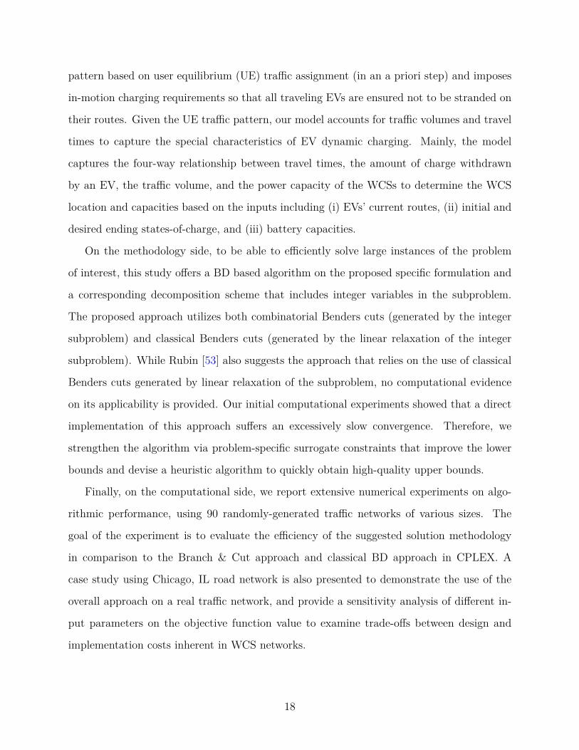
3.3 Numerical results (N.B. : no bound obtained) . . . . . . . . . . . . . . . . . . . . . . . . . . . . . . . . . 42

3.4 Numerical results (N.B. : no bound obtained) . . . . . . . . . . . . . . . . . . . . . . . . . . . . . . . . . 42

3.5 EV classes parameters . . . . . . . . . . . . . . . . . . . . . . . . . . . . . . . . . . . . . . . . . . . . . . . . . . . . . . . . 43

4.1 Routes data . . . . . . . . . . . . . . . . . . . . . . . . . . . . . . . . . . . . . . . . . . . . . . . . . . . . . . . . . . . . . . . . . . 60

4.2 UE data of peak period s1 . . . . . . . . . . . . . . . . . . . . . . . . . . . . . . . . . . . . . . . . . . . . . . . . . . . . 61

4.3 Wireless charging system parameters . . . . . . . . . . . . . . . . . . . . . . . . . . . . . . . . . . . . . . . . . 63

4.4 Demand matrices . . . . . . . . . . . . . . . . . . . . . . . . . . . . . . . . . . . . . . . . . . . . . . . . . . . . . . . . . . . . 63

4.5 Routes parameters associated with the UE of traffic period s1 . . . . . . . . . . . . . . . . . 64

4.6 Arcs parameters associated with the UE of traffic period s1 . . . . . . . . . . . . . . . . . . . 65

4.7 Routes parameters associated with the UE of traffic period s2 . . . . . . . . . . . . . . . . . 67

4.8 Arcs parameters associated with the UE of traffic period s2 . . . . . . . . . . . . . . . . . . . 68

4.9 Routes parameters associated with the UE of traffic period s3 . . . . . . . . . . . . . . . . . 69

4.10 Arcs parameters associated with the UE of traffic period s3 . . . . . . . . . . . . . . . . . . . 70

4.11 Optimal solutions under different scenarios . . . . . . . . . . . . . . . . . . . . . . . . . . . . . . . . . . . 72

4.12 Data classes and the associated sizes . . . . . . . . . . . . . . . . . . . . . . . . . . . . . . . . . . . . . . . . . . 87

4.13 Wireless charging system parameters . . . . . . . . . . . . . . . . . . . . . . . . . . . . . . . . . . . . . . . . . 87

4.14 EV classes data . . . . . . . . . . . . . . . . . . . . . . . . . . . . . . . . . . . . . . . . . . . . . . . . . . . . . . . . . . . . . . 87

4.15 Numerical results . . . . . . . . . . . . . . . . . . . . . . . . . . . . . . . . . . . . . . . . . . . . . . . . . . . . . . . . . . . . 89

4.16 EV classes data . . . . . . . . . . . . . . . . . . . . . . . . . . . . . . . . . . . . . . . . . . . . . . . . . . . . . . . . . . . . . . 91

xi

4.17 Costs comparison . . . . . . . . . . . . . . . . . . . . . . . . . . . . . . . . . . . . . . . . . . . . . . . . . . . . . . . . . . . 92

4.18 Costs comparison . . . . . . . . . . . . . . . . . . . . . . . . . . . . . . . . . . . . . . . . . . . . . . . . . . . . . . . . . . . 93

5.1 Routes flows and travel times under UE and SO - Braess network . . . . . . . . . . . . . 107

5.2 Arcs flows and travel times under UE and SO - Braess network . . . . . . . . . . . . . . . 107

5.3 Routes flows, travel times, and disutilities under the WCS deployment plan . . . . 108

5.4 Arcs flows, travel times, and disutilities under the WCS deployment plan . . . . . . 108

5.5 Arcs and their associated parameters - Nguyen-Dupuis network . . . . . . . . . . . . . . . 112

5.6 Travel demands - Nguyen-Dupuis network . . . . . . . . . . . . . . . . . . . . . . . . . . . . . . . . . . . . 112

5.7 Arcs flows and travel times under UE and SO - Nguyen-Dupuis network . . . . . . . 113

5.8 Routes flows and travel times under UE and SO - Nguyen-Dupuis network . . . . 114

5.9 Routes flows, travel times, and disutilities under the new UE which emergesas a response to the optimal WCS deployment under EVPR = 100%and αEV = −1 . . . . . . . . . . . . . . . . . . . . . . . . . . . . . . . . . . . . . . . . . . . . . . . . . . . . . . . . . . . . 116

5.10 Arcs flows, travel times, and disutilities under the new UE which emergesas a response to the optimal WCS deployment under EVPR = 100%and αEV = −1 . . . . . . . . . . . . . . . . . . . . . . . . . . . . . . . . . . . . . . . . . . . . . . . . . . . . . . . . . . . . 117

5.11 Arcs flows, travel times, and disutilities under the new UE which emergesas a response to the optimal WCS deployment under EVPR = 100%and αEV = −1.25 . . . . . . . . . . . . . . . . . . . . . . . . . . . . . . . . . . . . . . . . . . . . . . . . . . . . . . . . . 118

5.12 Routes flows, travel times, and disutilities under the new UE which emergesas a response to the optimal WCS deployment under EVPR = 100%and αEV = −1.25 . . . . . . . . . . . . . . . . . . . . . . . . . . . . . . . . . . . . . . . . . . . . . . . . . . . . . . . . . 119

A.1 BRP function parameters. Source: Horowitz [26] . . . . . . . . . . . . . . . . . . . . . . . . . . . . . . 126

xii

I dedicate this work to my family.

Chapter 1

INTRODUCTION

1.1. Background

Extraordinary investments poured from both public and private sector into the electric

vehicle (EV) industry to achieve the ambitious goal of putting one million electric vehicles

on the road by the end of 2015 [59]. However, EV adoption has been dramatically lagging

behind anticipation; it was not until 2018 that the U.S. fleet of EVs reached 800,000 [2].

The relatively short driving range of EVs, mainly due to low energy-density of the batter-

ies, and the long battery charging times remain to be the major factors that are keeping

many consumers away from buying into the EV technology, despite the availability of EV

conventional charging facilities.

To overcome these drawbacks, dynamic charging (also referred to as in-motion charging

or on-line charging) was proposed, and successfully demonstrated in Onar et al. [49] and

Jang et al. [30], as a promising convenient and safe solution. This innovative technology

enables EVs to draw power wirelessly from roadbed transmitters while the vehicle is moving.

This technology helps to reduce the range anxiety of EV owners, paving the way for an

extensive market penetration for EV. Further, it allows automakers to produce EVs with

smaller batteries which are highly desirable to facilitate market adoption by reducing the

cost of the vehicle [39]. Another key advantage of dynamic wireless charging is that it paves

the way for the realization of full autonomy of EV; eliminating the need for charging stops

allows for an almost indefinite movement of autonomous EVs.

Enabling dynamic charging requires EVs with wireless charging abilities and roads with

inductive power capabilities. The wireless charging technology has already been tested on

numerous EV platforms, including Tesla, Renault, Nissan, BMW and Honda [23]. Other

1

automakers such as Mercedes-Benz and General Motors have declared their plans to intro-

duce EVs with wireless charging capabilities to the market [23, 65]. On the other hand,

experiments on roads with inductive power capabilities are being conducted in England and

France to support the growth of the technology [13, 28]. Figure 1.1 features photos of test-

ing Qualcomm dynamic wireless charging system on an EV by Renault in France. These

attempts indicate that the future of dynamic charging looks very encouraging. We envision

that with the advancement of driverless vehicles the interest and need for wireless in-motion

charging will only increase at a higher rate. The technology pioneers such as Qualcomm

and Momentum Dynamics has already announced their visions for “limitless EV range” and

high-power charging infrastructure [12, 23].

Figure 1.1: Qualcomm and Renault testing dynamic wireless charging in France. Adoptedfrom [28, 50]

.

2

1.2. Motivation

Despite the technological advancements in electric vehicles charging mechanisms, the

shortage of EV charging facilities remains to be the “fundamental challenge” facing the

growth of EV markets [24]. While many potential consumers are shying away from switching

to EVs because of this particular limitation, both public and private sectors seem reluctant

when it comes to investing in charging infrastructure. The reason behind this hesitation is

the insufficient number of EVs on the road. The solution to this (chicken-and-egg) dilemma

depends profoundly on a strategic deployment of charging stations that optimizes both lo-

cations and scales of these stations in urban areas [56].

This problem is addressed in the first study of this dissertation via an analytical

approach in which the deployment of the new wireless charging technology is optimized to

minimize the investment cost while capturing the existing traffic pattern on the road network

represented by the user equilibrium (UE) traffic assignment [63]. In doing so, our approach

encourages EV adoption by alleviating the two major anti-adoption factors, namely the long

charging times and short ranges, without disturbing the existing traffic pattern.

More specifically, we examine the infrastructure deployment in a way that puts no ex-

tra burden on EV drivers to identify new routes for themselves and change their travel

behaviors.

We approach the problem from the perspective of a city as the decision maker whose

aim, for societal benefits, is to satisfy the charging demands of all EVs in its urban network

at the minimum investment cost which, for our purposes, include both the installation cost

(paid by tax-payers) and the travelers’ usage costs. For this purpose, we suggest a new

mathematical model to strategically deploy wireless charging stations (WCS) in the network

in such a way that no EV runs out of energy before reaching its destination. We envision

that, ultimately, the optimal locations of the WCSs at their corresponding capacities are

constructed and operated by private entities as contractors.

3

To solve the proposed model, we develop a Benders Decomposition (BD) based algorithm

as a solution methodology. In particular, we devise a combined combinatorial-classical BD

approach and enhance its efficiency further for the specific problem at hand via devising

surrogate constraints and an upper bound heuristic. We illustrate the applicability of our

model and the solution algorithm via a case study with urban network data from Chicago,

IL.

Another motivation for this research is to investigate the effect of varying wireless charging

parameters and product design characteristics on the network design and the implementation

cost of the infrastructure. This investigation is crucial at this early stage of the technology

maturity to support the product design and offer insights, for the technology developers, on

the effect of technical parameters on the system implementation cost. To that end, we con-

duct a sensitivity analysis on key system parameters to examine trade-offs between design

and implementation costs inherent in WCS networks.

We observe that the network design of the wireless charging infrastructure is heavily

dependent on the frequently-changing traffic condition in the road network. That is, an

optimal WCS network design proposed to serve charging demands at a certain traffic pe-

riod is not necessarily optimal (or feasible) during a different traffic period. Driven by this

observation, in the second study of the dissertation, we investigate the dependency

of the optimal WCS network design on the dynamic traffic patten. Specifically, we use the

widely referenced Nguyen-Dupuis network, as an example, to show that a WCS network

design, that is obtained based on input data of a single traffic period, might not be able to

satisfy the charging demands during other traffic periods. We further illustrate that even

the peak-period WCS network design might fail to satisfy the charging demands during less

congested traffic periods. Therefore, we conclude that the peak traffic period cannot be con-

sidered as worst-case scenario when optimizing the WCS network design. We then, building

on the first study, approach the network design problem at hand while considering multiple

traffic periods, rather than a single traffic period. Our goal is to generate a robust optimal

4

solution that is feasible, and cost-effective, across all realizations of traffic conditions. For

this purpose, we build on the model proposed in the first study to formulate a new robust

network design model for the deployment of WCSs in urban traffic networks. We further

devise a BD based solution algorithms tailored to solve the proposed model. The algorithm

is strengthened via multiple sets of problem-specific surrogate constraints and a new upper

bound heuristic for improved efficiency. The robust model and the proposed algorithm are

tested on real network data from Dallas, TX.

Finally, the third study in this dissertation is motivated by a long-sought goal in

the field of transportation: alleviating congestion in urban traffic networks by improving the

efficiency of the network utilization. We recognize that unless the WCS network is designed

to serve and maintain the existing traffic assignment in the road network, as in the approach

of the first two studies, it can potentially disturb and change the traffic assignment. The

reason is that as a response to the network design, EV drivers will have to change their

route selection strategy to account for the availability of WCSs on their routes. Therefore,

motivated by the potential impact of WCS network design on the traffic assignment, we

introduce the idea of employing WCS network as a traffic management tool to influence the

traffic assignment in a way that minimizes congestion in the road network. Specifically, we

propose a new mathematical model with the objective of generating WCS network designs

that can shift the traffic assignment from the selfish-optimal UE toward the system (socially)

optimal (SO) traffic assignment, which corresponds to the optimal utilization of the road

network. We further examine the validity of this concept by illustrating the proposed model

on the well known Braess network and on the Nguyen-Dupuis network, and we conduct

sensitivity analyses to measure the potential impact of the proposed approach on alleviating

congestion.

5

1.3. Brief System Description

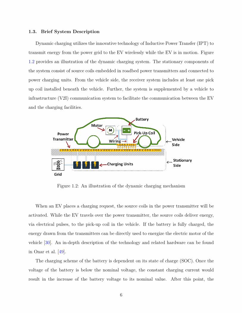
Dynamic charging utilizes the innovative technology of Inductive Power Transfer (IPT) to

transmit energy from the power grid to the EV wirelessly while the EV is in motion. Figure

1.2 provides an illustration of the dynamic charging system. The stationary components of

the system consist of source coils embedded in roadbed power transmitters and connected to

power charging units. From the vehicle side, the receiver system includes at least one pick

up coil installed beneath the vehicle. Further, the system is supplemented by a vehicle to

infrastructure (V2I) communication system to facilitate the communication between the EV

and the charging facilities.

Figure 1.2: An illustration of the dynamic charging mechanism

When an EV places a charging request, the source coils in the power transmitter will be

activated. While the EV travels over the power transmitter, the source coils deliver energy,

via electrical pulses, to the pick-up coil in the vehicle. If the battery is fully charged, the

energy drawn from the transmitters can be directly used to energize the electric motor of the

vehicle [30]. An in-depth description of the technology and related hardware can be found

in Onar et al. [49].

The charging scheme of the battery is dependent on its state of charge (SOC). Once the

voltage of the battery is below the nominal voltage, the constant charging current would

result in the increase of the battery voltage to its nominal value. After this point, the

6

battery will be charged using a constant voltage scheme and the current is regulated. In

both charging schemes, the injected power can be regulated by controlling the voltage or

the current. As the state of charge increases beyond 90%, the charging power decreases

slightly; however, the charging power remains constant once the SOC of the battery is below

90% [60]. In this context, it is unlikely that an EV will wirelessly recharge above 90%.

Therefore, considering fixed charging power for the battery is a valid assumption. In fact,

technically the charging power can be regulated by changing the injected current and voltage

as stated before. Several studies address similar concept including Khodayar et al. [33]. Fixed

charging power for EV battery is considered in other related studies such as Chen et al. [9].

Specifically, consideration (IV) in page 346 which reads: “the amount of electricity charged

is equal to a constant charging rate multiplying the charging time.”

In this dissertation, we use the term Wireless Charging Station (WCS) to refer to the

stationary side of the dynamic charging system installed on a segment of the road, i.e., the

WCS consists of a number of charging units and roadbed power transmitters installed. The

station’s power capacity refers to the total power capacity of all charging units in a WCS.

In our modeling approach, we consider long loop configuration for a WCS where the

power transmitter is installed along a whole road segment. Thus, an EV is assumed to be

exposed to the power transmitter as long as it is traveling on the road segment with a WCS.

Nevertheless, our models can be generalized to other design configurations such as sectional

wired loop and spaced loop (see Yilmaz et al. [66] for various configurations) by adjusting

the effective charging time in the models.

Finally, it’s worth mentioning that the dynamic charging system has low efficiency com-

pared to conventional static charging. Thus, the dynamic charging system, at least at this

stage of its technical development, is meant to only increase the EV driving range but not

to replace the need for conventional stationary charging. The latter has been accounted for

in our modeling approach by considering initial state-of-charge for EVs.

7

1.4. Summary of Contributions

The contributions of this dissertation can be summarized as follows. The first study of

this dissertation tackles the WCS network design problem with the goal of optimizing the

deployment of the wireless charging infrastructure in traffic networks in an effort to support

EV adoption. The study is motivated by the notion that, given the high cost associated

with the cutting-edge wireless charging technology, delivering the substantial benefits of this

technology can only be achieved via an optimized deployment of the infrastructure. The

problem is approached via an analytical scheme and molded as a mixed integer program.

The model decides on the WCS locations and the corresponding power capacity allocations.

The goal is to minimize the infrastructure deployment cost from a system perspective, and

the usage cost for the users. The model is structured to generate WCS network designs that

can serve the EV charging demands in the traffic network without disturbing the existing

traffic condition represented by the UE traffic assignment. From an algorithmic perspec-

tive, the first study offers a BD framework to solve the proposed optimization model. The

proposed framework adopts features from classical BD and combinatorial BD. This solution

framework has the potential to be generalized for other network design applications. The

solution framework is strengthened via an upper bound heuristic and surrogate constraints

for improved convergence. The model and the solution methodology are put to work on a

case study using real network with data from Chicago, IL. In an effort to support the prod-

uct design of the maturing wireless charging technology, the case study includes a sensitivity

analysis that captures the interaction between key technical parameters of the wireless charg-

ing system and the infrastructure deployment cost. The study also paves the way for similar

investigations of the interactions between product design and technology implementation

cost.

The second study of this dissertation offers a robust framework to tackle the WCS

network design problem. Specifically, the second study considers the interactions between

the WCS network design and the dynamic traffic condition in the road networks. We provide

examples to illustrate that, due to the strong dependency between the WCS network design

8

and the traffic conditions, WCS networks should be designed while considering the variability

of the daily traffic pattern. That is, multiple traffic periods should be considered when

planning the deployment of the wireless charging infrastructure. Our findings indicate that

when it comes to WCS network design, even the peak traffic period cannot be singled out

as a worst-case scenario, although it does correspond to the highest demands. We provide

a detailed explanation of this phenomenon. To that end, the second study introduces an

absolute robust WCS network design model. The model captures the interaction between

WCS network design and the frequently-changing traffic pattern by considering multiple

traffic periods rather than a single period. The model generates WCS network designs that

are robust against the changes in the traffic conditions. From the methodological side, the

study provides a BD solution algorithm tailored to solve the robust model. The algorithm is

strengthened via several techniques including problem-specific surrogate constraints, a new

upper bound heuristic, and cut strengthening. The robust model and the solution algorithm

are then tested via a case study with real data from Dallas, TX. The results of the case study

confirm the necessity of a robust solution to the problem at hand. We further provide a

detailed cost breakdown analysis to investigate how different cost components differ between

the robust solution and the individual single period solutions.

Finlay, the third study of this dissertation contributes to the field of traffic man-

agement with the new concept of employing the WCSs in the road network as a traffic

management tool. Particularly, we propose the idea of taking advantage of the attractive-

ness of the deployed WCSs for EV drivers to influence their travel behaviors in an effort

to improve the traffic assignment in the network. This study is motivated by the notion

that the UE traffic assignment, which offers a realistic representation of traffic flows in a

steady-state, does not correspond to the optimal utilization for the traffic system. To that

end, we propose a mathematical model to locate WCSs in the network so that as a response

to the WCS deployment, the traffic will re-regulate itself in a new equilibrium state which is

closer to SO than the original UE. The validity of the proposed idea is tested on two widely

referenced networks in the field of transportation including Braess network and Nguyen-

9

Dupuis network. Our findings confirm the validity of the proposed concept. Specifically, we

conclude that the optimal WCS deployment plan, generated by our model, is able to improve

the road network utilization by shifting the traffic assignment from original UE toward SO,

which corresponds to the optimal utilization of the road network. We also find the shift from

UE toward SO, as resulted by the WCS deployment, is dependent on the EV population in

the network under study, and on the attractiveness of WCS as viewed by EV drivers. To

that end, we conduct sensitivity analyses to investigate these dependencies. We conclude

that shifting the traffic assignment from UE completely toward SO is only possible if the

EV population in the network and the attractiveness of WCS for EV drivers, each crosses a

certain threshold.

1.5. Dissertation Organization

The rest of this dissertation is organized as follows: A review of the related literature is

provided in Chapter 2. The network design for in-motion wireless charging of electric vehicles

is studied in Chapter 3. In Chapter 4 we introduce the robust version of the network design

problem at hand. In Chapter 5 we provide a study on the concept of utilizing wireless

charging of EVs to improve traffic assignments in congested traffic networks. Finally, we

highlight the results and findings of this dissertation and discuss potential future research

directions in Chapter 6.

10

Chapter 2

RELATED LITERATURE

Problems dealing with the optimal location of refueling/plug-in-recharging facilities has

been well covered in the literature. Hodgson [25] developed a flow capturing location model

(FCLM) with the goal of maximizing the covered demands between the network’s origins and

destinations by locating a fixed number of refueling facilities in the network. Kuby and Lim

[36] proposed flow refueling location model (FRLM) to determine the locations of refueling

stations for alternative fuel vehicles with limited driving range. Kuby and Lim [37] then

enhanced the model with three methods to add candidate sites on arcs. Upchurch et al. [58]

proposed a capacitated FRLM which forces a limit on the number of vehicles that can be

charged at a certain facility. Wang and Lin [61] utilized a set covering approach to optimize

the location of vehicle refueling stations. Later, MirHassani and Ebrazi [45] proposed a

flexible reformulation of Wang and Lin [61] model. Wang and Lin [62] also developed a

mixed integer programming model to locate multiple-types of recharging stations for EVs,

and showed that an optimal deployment in planning areas can be achieved through the

employment of multiple types of charging stations. More recently, Zheng et al. [67] studied

the EV user equilibrium traffic assignment and the optimal locations of conventional charging

facilities, subject to the range limitation.

In terms of dynamic wireless charging, most of the existing literature targets the technical

side of the maturing technology. Yilmaz et al. [66] discuss the general design requirements

of the dynamic wireless charging system. Their study includes an evaluation of the effect

of different configurations of the roadbed power transmitter on the overall system efficiency.

Covic and Boys [17] describe the different components of the wireless charging system in

technical details. Onar et al. [49] demonstrate the concept of EV dynamic wireless charging

on a laboratory prototype. They further investigate the effect of different road surfacing

11

materials, that cover the wireless power transmitter, on the transparency of the wireless

power transfer magnetic field exposure. Lukic and Pantic [41] present a review of the basics

of the state of the art IPT technology as used in dynamic wireless charging. Miller et al. [44]

present an analysis for the power flow in wireless power transfer systems. Their analysis is

based on experimental data from Oak Ridge National Laboratory.

When it comes to the operation and system studies of dynamic wireless charging, a re-

cent survey paper by Jang [29] provides a thorough review of the literature in this area. The

author reviews the related studies according to their focus area from five different perspec-

tives including: charging infrastructure allocation; driving range extension; cost and benefit

analyses; supporting systems; and miscellaneous perspectives. The study also discusses the

recent developments and commercialization activities in the field.

Studies on driving range extension investigates the possible extension of the EV range

using dynamic wireless charging. Examples of these studies are Chopra and Bauer [11] and

Garcıa-Vazquez et al. [22]. Studies providing cost benefits analyses can be found in Ko and

Jang [34], Jang et al. [31], and Fuller [21].

Studies that are most related to the research in this dissertation are the ones focusing on

charging infrastructure allocation.

Ko and Jang [34] present a mathematical formulation to optimize the design of the

dynamic-charging-based mass transportation system On-Line Electric Vehicle (OLEV) de-

veloped by Korea Advanced Institute of Science and Technology (KAIST). Their formulation

considers the route of the bus as a continuous spatial decision space to determine the the

starting and end points of each wireless charging lane. Their model also addresses the trade-

off between the number of deployed power transmitters and the size of the batteries on

buses.

Jang et al. [31] adopts the same setting of Ko and Jang [34] (i.e., OLEV transportation

system). However, in this study, the authors consider a discretized decision space as they

divide the route of the bus into multiple segments. Therefore, the continuous problem

introduced in Ko and Jang [34] is turned into a discrete optimization problem in Jang et al.

12

[31].

Hwang et al. [27] also build on the same setting of Ko and Jang [34]. Specifically, the

anthers generalize the single-route problem in Ko and Jang [34] to cinder multiple routes in

the mass transportation system.

Liu and Song [40] also consider a multiple-route transportation system setting in an

optimization problem with the goal of optimizing the locations of wireless charging facilities

and the battery size of the electric buses. This is done while addressing the uncertainty of

energy consumption and travel time in a robust optimization approach.

Riemann et al. [52] propose a flow-capturing location model with stochastic user equi-

librium under a fixed number of wireless charging facilities. The authors consider the maxi-

mization of captured EV flow by locating a fixed number of WCSs without cost and capacity

considerations. They also assume that an EV’s battery is charged fully when an EV travels

on a road segment with a WCS regardless of the travel time, i.e, WCSs are assumed to have

infinite power capacities and charging rates. The use of the model was demonstrated on a

network with 13 nodes and 19 arcs using data in [48].

Chen et al. [9] study the optimal deployment of charging lanes under a limited budget

and a fixed charging power of the charging lanes. Their model minimizes the total travel

time in the network while selecting arcs as charging lanes. They also illustrate their model

on the same small network used in [52].

In another related study on dynamic charging implementation, Fuller [21] considers in-

vestment cost minimization for a WCS infrastructure that allows EV travel between 39 key

origin-destination pairs in California. Specifically, the study utilizes the set covering model

developed by Wang and Lin [61] (which was proposed with the goal of locating station-

ary refueling facilities) to locate fixed capacity recharging stations on the shortest paths of

origin-destination pairs of interest. The model is solved using Branch and Bound technique

as implemented by CPLEX.

More recently, Chen et al. [10] study the competitiveness of dynamic charging against

stationary charging. Their study includes a deployment model for both charging lanes rep-

13

resenting dynamic chargers and stationary charging stations. The authors state that their

model adopts a “highly simplified” setting where one traffic corridor is considered. That is,

the authors consider a single road segment rather than a general network, and all EVs take

identical trips from the beginning of the corridor to the end of it. The deployment model

decides on the length and charging power of charging lanes, however, as a “macroscopic

model,” it does not optimize the locations of these charging lanes. The authors also assume

that all EVs have identical batteries and start there trips with a full charge. The model

further assumes a constant speed across the traffic corridor. They conclude that the use of

charging lanes is preferable over the stationary charging stations for improved efficiency in

transportation operations.

The above mentioned charging infrastructure allocation studies are the closest to our first

study in this dissertation. However, our approach to the problem is significantly different.

To start with, rather than considering a mass transportation system operating in a closed

environment (as in Ko and Jang [34], Jang et al. [31], Hwang et al. [27], and Liu and

Song [40]), or one traffic corridor with identical trips (as in Chen et al. [10]), we consider

a complete traffic network with EVs taking different trips, originating from, and ending at

different locations.

To promote EV adoption without causing disturbance to the traffic pattern, we locate

facilities and further determine their associated power capacities by exploiting the economies-

of- scale to serve EV charging demands on all used routes, at the minimum cost. By serving

demands on all used routes in current UE, EV drivers will have no incentive to change their

original routes. Consequently, the UE traffic assignment will remain undisturbed. In this

context, the number of installed wireless charging stations is decided by our cost minimization

model to capture all the EV traffic flow (as apposed to assuming a fixed number of stations

as in Riemann et al. [52], or a fixed budget as in Chen et al. [9]).

Furthermore, considering a realistic implementation, we take into account charging rates

and levels on road segments with WCSs in a way that is explicitly determined by the travel

time and charging power installed on the road segments (as opposed to assuming full battery

14

charge once an EV travels on any WCS as in Riemann et al. [52]). This will be further

discussed in Chapter 3.

The novelty of our second study in this dissertation lies in that, to our best knowledge, it

is the first to consider the variability in the traffic pattern while optimizing the deployment

of the wireless charging infrastructure.

Finally, our third study is novel in that it integrates the charging infrastructure allocation

problem with the system optimal traffic assignment problem.

15

Chapter 3

NETWORK DESIGN FOR IN-MOTION WIRELESS CHARGING OF ELECTRIC

VEHICLES

3.1. Introduction

Mass adoption of electric vehicles (EV) leads economies away from the dependency on

fossil fuels, and promises an extensive reduction in pollution levels. This, motivated govern-

ments around the world to invest billions of dollars and to introduce a lot of policies and

programs in effort to promote EV adoption. However, potential EV consumers continue to

be concerned about the range anxiety; a phenomenon caused by the two major drawbacks

of EVs, namely, the short driving range and the long charging time.

To alleviate range anxiety, dynamic (in-motion) wireless charging was proposed as a

promising solution that would allow EVs to recharge while traveling in the road network.

The ability to charge while in-motion also allows for a significant reduction in the size of

the EV battery which, in turn, significantly reduces the cost and weight of EVs [32]. Jeong

et al. [32] also found that dynamic wireless charging is beneficial to the extension of the

battery life. Another key advantage of dynamic wireless charging is that it paves the way

for the realization of full autonomy of EV; eliminating the need for charging stops allows for

an almost indefinite movement of autonomous EVs. However, due to high costs associated

with the deployment of this new technology, delivering the benefits of wireless charging can

only be achieved via a strategic optimized deployment of the wireless charging facilities.

In this study, we propose a mathematical approach to address the problem of optimizing

the deployment of wireless charging stations (WCS) in urban traffic networks. The proposed

approach aims to generate WCS deployment plans to serve the charging demands of EVs in

traffic networks, in effort to encourage EV adoption, while minimizing the investment costs.

16

We intend to design the wireless charging infrastructure network in a way that serves EV

drivers without putting an extra burden on them to change routes. To this end, we first

identify the usual UE travel pattern of the travelers (i.e., the routes that they currently

choose before the deployment of the wireless charging infrastructure) and seek to identify

best wireless charging network design to serve this pattern. Therefore, travelers do not need

to change their routes to seek wireless charging; traffic assignments are not affected. That is,

we are solving our problem to capture all flow for a well-defined long-term representation of

the traffic pattern without impacting it. Our approach ensures that we provide the charging

capacity along the different routes in such a way that the EV drivers do not need to change

their routes in order to recharge on their daily routes.

Our contributions in this study can be summarized under three headings as follows.

On the modeling side, our study contributes to the recent, and rather limited, literature

in network planning for EV dynamic charging with a new mathematical formulation for

strategic deployment of WCSs in urban networks. Unlike the previous models, the aim of our

model is to optimally decide both location and power capacity of WSCs in a transportation

network, while minimizing the total investment and charging related costs on the user.

Instead of considering one traffic corridor with identical trips (as in Chen et al. [10]), we

consider the whole traffic network with EVs taking different trips, originating from, and

ending at different locations. Further, instead of assuming a fixed charging power (as in

Chen et al. [9], Fuller [21]) or infinite capacity (as in Riemann et al. [52]), our model allows

for incremental expansion of the power capacity on arcs independently. This feature of the

model, while useful in bringing the model closer to reality, makes our cost function more

complex; specifically, instead of assuming a fixed number of WCSs (as in Riemann et al. [52]),

or a fixed budget and a fixed installation cost for WCSs (as in Chen et al. [9]), we employ a

cost function that includes three types of costs: a fixed and a variable cost associated with

the installation of WCSs (including base capacity and expansion costs of both inverters and

the charging pads) in addition to a charging cost. Further, to promote EV adoption without

causing disturbance to the traffic pattern, our approach first determines the existing traffic

17

pattern based on user equilibrium (UE) traffic assignment (in an a priori step) and imposes

in-motion charging requirements so that all traveling EVs are ensured not to be stranded on

their routes. Given the UE traffic pattern, our model accounts for traffic volumes and travel

times to capture the special characteristics of EV dynamic charging. Mainly, the model

captures the four-way relationship between travel times, the amount of charge withdrawn

by an EV, the traffic volume, and the power capacity of the WCSs to determine the WCS

location and capacities based on the inputs including (i) EVs’ current routes, (ii) initial and

desired ending states-of-charge, and (iii) battery capacities.

On the methodology side, to be able to efficiently solve large instances of the problem

of interest, this study offers a BD based algorithm on the proposed specific formulation and

a corresponding decomposition scheme that includes integer variables in the subproblem.

The proposed approach utilizes both combinatorial Benders cuts (generated by the integer

subproblem) and classical Benders cuts (generated by the linear relaxation of the integer

subproblem). While Rubin [53] also suggests the approach that relies on the use of classical

Benders cuts generated by linear relaxation of the subproblem, no computational evidence

on its applicability is provided. Our initial computational experiments showed that a direct

implementation of this approach suffers an excessively slow convergence. Therefore, we

strengthen the algorithm via problem-specific surrogate constraints that improve the lower

bounds and devise a heuristic algorithm to quickly obtain high-quality upper bounds.

Finally, on the computational side, we report extensive numerical experiments on algo-

rithmic performance, using 90 randomly-generated traffic networks of various sizes. The

goal of the experiment is to evaluate the efficiency of the suggested solution methodology

in comparison to the Branch & Cut approach and classical BD approach in CPLEX. A

case study using Chicago, IL road network is also presented to demonstrate the use of the

overall approach on a real traffic network, and provide a sensitivity analysis of different in-

put parameters on the objective function value to examine trade-offs between design and

implementation costs inherent in WCS networks.

18

The rest of the chapter is organized as follows: The problem is described and formulated

in Section 3.2. In Section 3.3, we describe the solution algorithm proposed to solve the

problem. And in Section 3.4, we present the computational experiment and numerical results

of testing the efficiency of the proposed algorithm. A case study is presented in Section 3.5.

3.2. Problem Definition and Formulation

We consider two costs associated with installing a WCS: the first one is the fixed cost

that represents initial set up cost with a base power capacity; and the second one is the

variable cost associated with unit power capacity expansion over the base capacity. These

costs mainly capture the capital cost of the inverter as well as the installation cost associated

with it. Furthermore, the cost of the charging pad proportionally increases with the capacity

of the installed inverter. Therefore, the fixed and variable installation costs assumed in this

study can also include the cost associated with the charging pads.

To set the stage for our formulation, we start by explaining the electric vehicle dynamic

recharging logic which also provides insights into the interactions between network design

and operations. In designing the network for EV wireless charging, two interdependent

decisions include the locations of WCSs and their power capacities.

The interaction between these two decisions can be illustrated on a small network depicted

in Figure 3.1. In this example, we consider 6 nodes and 5 arcs where on each arc (length in

miles, travel time in minutes) data is provided.

A

B C

E D

F

(40, 70)

D

F

CBA

E

Figure 3.1: A small two-paths network example with OD pairs A-D and E-F

19

Assume that an EV1 with γ1 kWh battery capacity, and a driving range of R1 is traveling

between OD-pair A-D on path A-B-C-D of length lAD. We assume that EV1 starts the trip

at node A with a pA% state-of-charge and the driver wants to reach node D with at least pD%

state-of-charge (pD < pA). Let ξAD denote the energy consumed by the EV when traveling

between OD-pair A-D. Due to energy conservation, the amount of charge that EV1 should

receive on its path is c1 = ξAD + pD% γ1 − pA% γ1. To receive the required c1 kWh, at

least one WCS is needed on the path between A and D. The location of the WCS should

be selected in a way that EV1 does not run out of energy at any point of the path. In this

example, we assume that all three arcs AB, BC, and CD are feasible candidates to install

WCS on the path between A and D.

Note that electrical power P (kW) for a WCS is equal to c/(η t) where C (kWh) is the

energy that the WCS can deliver in one hour, η is the IPT system efficiency, and t is the

effective charging hours (i.e., arc travel time). For example, if arc AB is selected to host the

WCS, the installed capacity must be at least PAB = c1/(η tAB) kW to deliver the required

energy c1 to EV1. Observing that tAB < tBC < tCD as given is Figure 3.1, we must have

PAB > PBC > PCD.

We consider a WCS installation cost (inverters and charging pads) function of the form

fc+ vc Y where fc is the fixed cost of base power capacity installation, vc is the cost of unit

capacity increment, and Y is the number of capacity units installed. Since there is a positive

correlation between the cost and the capacity of a WCS (as implied by the term vc Y ), we

find that arc CD is the best (least costly) option to host the WCS on EV1’s path.

Now consider another electric vehicle EV2 traveling between OD-pair E-F on path E-B-

C-F. Under the same assumptions applied to EV1 above, we conclude that arc CF is the

best candidate to host a WCS on the path E-B-C-F for EV2.

However, when examining the network as a whole, and by taking into account the

economies-of-scale as implied by the fixed cost term fc, it can be argued that serving both

EVs through one WCS (on arc BC) with a higher power level PBC = [(c1 + c2)/(η tBC)] kW

capacity, instead of two separate WCSs on CD and CF, might be economically preferable.

20

This example provides an insight on favorable WCS locations and capacity levels in the

case that the objective is to capture the current UE traffic pattern so as to promote EV

adoption. In particular, it illustrates that it is preferable to choose WCS locations on the

arcs with longer travel times (to reduce variable costs due to lower capacity installations)

and/or on the arcs that are shared by multiple paths (to take advantage of economies-of-

scale). Nonetheless, it is usually the case in traffic networks that the shared arcs are the most

congested ones, and thus have longer travel times. This implies that more congested arcs are

better candidates to host WCS(s), not only to take advantage of the economies-of-scale, but

also because high travel volume on the arc increases the travel time, and therefore, decreases

the required capacity (because the EV can charge for a longer duration) and associated cost

of the installed WCS. We later use this insight in devising an upper bound heuristic employed

to increase the efficiency of our solution algorithm.

3.2.1. Problem Setting and Definitions

We consider a directed graph G(N ,A) representing the traffic network where N is the

set of nodes and A is the set of directed arcs. Each node represents an origin and/or a

destination, as well as an intersection. Each arc represents a road segment and a candidate

site for a WCS. Let Q be the set of all OD-pairs in the network, and Rq be the set of all

routes between a certain OD-pair q ∈ Q.

For operational purposes, electric vehicles traveling in the system can be divided into

different classes based on (i) the initial state of charge of the EV, (ii) the desired ending

state of charge1, and (iii) the battery capacity. Let K be the set of all EV classes in the

network. Note that related studies assumed that all EVs in the network start their trips

fully charged and share the same battery size. We believe that our suggested classification

of EVs, performed by the planning entity, brings the problem closer to reality. We define a

cluster as a group of EVs of class k ∈ K traveling between a certain OD-pair q ∈ Q using a

1The dynamic charging system is meant to only increase the EV driving range, not to replace theconventional charging stations. Therefore, the ending state of charge of the EV battery (SOC) is typicallyexpected to be less than the initial SOC for all practical purposes.

21

certain route r ∈ Rq.

The traffic pattern in the network is assumed to follow a UE traffic assignment which

offers a suitable system representation for long term planning purposes [43]. Specifically, the

UE traffic assignment represents the steady-state of the traffic condition in traffic networks.

Under this assignment, the traffic flows on each OD-pair follows Wardrop’s first principle

which reads:

The journey times on all routes actually used are equal, and less than those which

would be experienced by a single vehicle on any unused route [63].

Therefore, under UE, no driver can improve her travel time by switching route. It is im-

portant to note that this principle assumes that all travelers in the network have complete

awareness of the current traffic condition.

We consider the UE of a peak traffic period as it corresponds to the highest traffic volume

and therefore, the highest charging demands. The UE algorithm is executed prior to our

network design optimization to generate part of the input to our model. Specifically, the

algorithm’s output includes the traffic flows on routes which, in turn, dictates the traffic

volume and associated traffic density on each arc of the network, i.e., the parameters vij

(vehicles/hour) and κij (vehicles/mile) on each arc (i, j) ∈ A of the network under study.

Using this data as well as the arc proportion2 and the EV penetration rate for class k,

denoted by EVPRk, we calculate the average number of EVs of class k that are occupying

arc (i, j) while traveling between OD-pair q along route r as

ρqrkij = κij lij

δqrij fqr∑

s∈Q

∑t∈Rq

(δstij f st)

EVPRk (3.1)

where

lij is the length of arc (i, j)

2For an arc (i, j) on a route r, arc proportion is the proportion of the flow on (i, j) that belongs to router to the total flow on (i, j). It is expressed as the fraction on the right-hand side of (3.1).

22

δqrij is an indicator with value of 1 if arc (i, j) is part of route r, 0 otherwise

f qr is the traffic volume on route r measured in vehicles/hour, obtained from UE.

The travel times on arcs are also determined by the UE algorithm using the Bureau of Public

Roads (BRP) arc performance function [55] given as

tij = tminij

(1 + α( vij

tcij)β)

(3.2)

where

tminij is the free-flow travel time on arc (i, j)

tcij is the traffic capacity of arc (i, j) measured in vehicles/hour

α and β are deterministic permeates associated with the type of the road.

Next, we provide our model formulation to determine the optimal locations of WCSs,

their capacity levels, and assignments of EV clusters to WCSs for recharging on their routes

dictated by UE solution. We assume a planning horizon of a number of years during which

the expected demand for wireless EV charging is steady, for example a desired target value,

therefore, we assume that all costs are adjusted to reflect annual values.

3.2.2. Model Formulation

We first introduce the following notation used in our formulation.

Sets:

N set of nodes, i, j ∈ N

O set of origins, o ∈ O ⊂ N

D set of destinations, d ∈ D ⊂ N

A set of arcs, (i, j) ∈ A

23

Q set of all OD-pairs within the network, q ∈ Q

Rq set of all used routes between a certain OD-pair q, r ∈ Rq where

or and dr are the origin node and destination node of route r, respectively.

Nr set of nodes on a route r ∈ Rq, Nr ⊂ N

Ar set of arcs on a route r ∈ Rq, Ar ⊂ A

K set of EV classes, k ∈ K

Parameters:

fc ij fixed cost ($) associated with installing a WCS with basic capacity on arc (i, j)

vc variable cost ($) associated with adding one expansion charging unit to a WCS

cc charging cost ($/kWh)

tr average number of trips taken by an EV during one year period

bcap basic power capacity (kW) of a WCS

ecap power capacity (kW) associated with adding one expansion charging unit to a WCS

mcap maximum power capacity (kW) that can be installed on one mile of a one-lane road

segment

η efficiency coefficient of the wireless power transfer system

ξij energy consumption (kWh) on arc (i, j)

ξr energy consumption (kWh) on route r

% vehicle charging power (kW)

γk battery capacity (kWh) of an EV of class k

24

ρqrkij the average number of EVs of class k, that are occupying arc (i, j) while traveling

between OD-pair q along route r, q ∈ Q, r ∈ Rq, k ∈ K, (i, j) ∈ Ar

lij length of arc (i, j) (mile)

nij number of lanes on arc (i, j)

tij travel time on arc (i, j) (hour)

δqrij an indicator with value of one if arc (i, j) is part of route r, 0 otherwise

iek initial energy level of an EV of class k ∈ K

eek ending energy level of an EV of class k ∈ K

Decision Variables:

xij 1 if a WCS is installed on candidate arc (i, j), 0 otherwise

yij number of power expansion charging units installed on arc (i, j)

eqrki energy level at node i of an EV of class k, traveling between OD-pair q on route r,

q ∈ Q, r ∈ Rq, k ∈ K, i ∈ Nr

cqrkij amount of charge an EV of class k, traveling between OD-pair q on route r, receives

from WCS on arc (i, j), q ∈ Q, r ∈ Rq, k ∈ K, (i, j) ∈ Ar

The wireless charging stations network design problem (P) can then be formulated as:

Minimize∑

(i,j)∈A(fc ij xij + vc yij) +

∑q∈Q

∑r∈Rq

∑k∈K

∑(i,j)∈r

(cc tr cqrkij ) (3.3)

subject to

eqrkor+

∑(i,j)∈r

cqrkij − eqrkdr

= ξr ∀ q ∈ Q, r ∈ Rq, k ∈ K (3.4)

25

eqrki + cqrkij − eqrkj = ξij ∀ q ∈ Q, r ∈ Rq, k ∈ K, i, j,∈ Nr, (i,j) ∈ Ar (3.5)

eqrki − ξij (1− xij) ≥ 0 ∀ q ∈ Q, r ∈ Rq, k ∈ K, i ∈ Nr, (i,j) ∈ Ar (3.6)

cqrkij ≤ % tij xij ∀ q ∈ Q, r ∈ Rq, k ∈ K, (i,j) ∈ Ar (3.7)∑q∈Q

∑r∈Rq

∑k∈K

(δqrij ρqrkij cqrkij )

≤ η (bcap xij + ecap yij) tij ∀ (i, j) ∈ A (3.8)

bcap xij + ecap yij ≤ mcap nij lij ∀ (i, j) ∈ A (3.9)

eqrki + cqrkij ≤ γk + ξij ∀ q ∈ Q, r ∈ Rq, k ∈ K, i ∈ Nr, (i,j) ∈ Ar (3.10)

eqrkor= iek ∀ q ∈ Q, r ∈ Rq, k ∈ K (3.11)

eqrkdr≥ eek ∀ q ∈ Q, r ∈ Rq, k ∈ K (3.12)

eqrki , cqrkij ≥ 0, xij ∈ 0, 1, yij ∈ Z+ ∀ q ∈ Q, r ∈ Rq, k ∈ K, i ∈ N , (i, j) ∈ A (3.13)

The first term in the objective function (3.3) represents the total cost of deploying all

WCSs in the network. This includes the fixed installment cost of both inverters and charging

pads to support a base power capacity as well as their variable costs associated with capacity

expansions. As a part of the overall cost, the second term sums the charging cost (electricity

cost) that an EV of cluster qrk consumes during one year period. A further motivation for

this term is to reduce the number of possible optimal solutions by minimizing the amount

of charge that each EV draws from the network. Specifically, for a traveler, there may

be alternative locations to charge on the given route without violating remaining energy

requirements, thus, this term on charging costs helps to differentiate between them and

provides methodological benefit in solving the model.

Constraints (3.4) and (3.5) are the energy conservation constraints over paths and over

arcs, respectively. Note that constraint (3.4) is redundant once constraint (3.5) is satisfied.

However, our initial computational experiments showed that constraint (3.4) is helpful when

solving the MIP. Constraints (3.6) ensure that at each node, each EV has enough energy

to go to the next node on its route, if there is no WCS installed before the next node is

26

reached. Constraints (3.7) are linking constraints that serve two purposes. Each of these

constraints ensures that a WCS is installed on arc (i, j) when EVs of a certain cluster is to

recharge on the arc (as assigned by the model). A constraint of this type also enforces the

maximum amount of energy that an EV can intake on a certain arc as an upper bound on

the continuous variables cqrkij . Constraints (3.8) ensure that a WCS installed on an arc has

enough power capacity to satisfy all the charging demands on that arc. Constraints (3.9)

bound the installed power capacity of WCSs. Constraints (3.10) bound the energy level of

each EV by its battery capacity. Constraints (3.11) and (3.12) assign the values of initial

and desired ending energy level for each cluster in the system to the corresponding variables.

Finally, constraints (3.13) provides the structural requirements of the model.

Note that although the UE problem is solved on the overall underlying network (N ,A)

the network can be reduced in the above optimization problem by setting N and A to

N = ⋃q∈Q, r∈Rq

Nr and A = ⋃q∈Q, r∈Rq

Ar, respectively.

3.3. Solution Methodology

Based on our initial computational experiments on solving the smallest of our test in-

stances (10 by 10 grid network), we observed that the Branch&Cut algorithm as implemented

in CPLEX was not efficient especially due to excessive run times to generate good bounds.

Therefore, in this section we devise an exact solution algorithm based on a framework that

combines combinatorial BD with classical BD.

Classical BD [6] involves splitting a mixed integer program (MIP) into two problems: (i)

Master Problem (MP) which includes all the integer variables from the original program, and

(ii) Subproblem (SP) which includes only the continuous variables. In addition to the integer

variables, MP includes a continuous auxiliary variable that facilitates the communication

between the two problems. In general, the overall approach involves solving MP, which

is a relaxation of the original problem and thus it provides a lower bound on the original

MIP (in case of a minimization problem). The solution generated by MP is then used by

fixing the values of the integer variables and utilizing them as inputs to solve the Dual

27

Subproblem (DSP) as a pure linear program. If DSP is feasible and bounded, its optimal

objective function value and the integer part of MP’s objective provide an upper bound on

the original MIP. If a stopping criterion (solution quality or time) is not met the solution

of DSP is used to generate a Benders optimality cut which is added to MP in the next

iteration. On the other hand, if DSP is unbounded, we use its extreme rays to generate a

Benders feasibility cut and add it to MP. This iterative process is continued until at least

one stopping criterion is met.

More recently, combinatorial BD which employs Benders combinatorial cuts was sug-

gested as an alternative to classical BD [14]. Similar to classical BD, the integer solution of

the master problem is passed, iteratively, to the linear subproblem. Nonetheless, combinato-

rial BD deviates from classical BD by the types of cuts utilized and the process of reaching

optimality. Specifically, in combinatorial BD, if MP’s solution makes the subproblem in-

feasible, then a combinatorial Benders cut is appended to MP to force at least one of its

binary variables to change its value from the previous iteration. Consequently, the new MP

solution will generate a new SP. In case the objective function of the original problem does

not contain any terms with continuous variables (that can serve to form the objective of SP),

the iterative approach (and therefore generating combinatorial cuts) continues until reaching

a feasible subproblem. This indicates that the most recent MP solution is also optimal for

the original problem. On the other hand, if the objective function of the original problem

contains only terms with continuous variables that also forms the SP objective function, a

feasible MP solution is first obtained. If this solution produces a feasible SP, the incumbent

solution is updated and the combinatorial cuts are added to MP to find a better feasible

integer solution. This process is continued until MP is infeasible.

In this study, we combine features from classical and combinatorial BD after moving a

set of integer variables from MP to SP to reduce the size (and consequently the difficulty) of

MP at the cost of having to deal with a more complex integer SP. Only a handful of applica-

tions employed BD with integer subproblem. For example, in a study concerning integrated

aircraft routing and crew scheduling problem [16], the decomposed model contained a binary

28

MP and a binary SP. The model is solved using a three-phase algorithm. The first phase

includes a relaxation of all integrality constraints, and BD is used together with column

generation to solve the LP relaxation of the integer model. The integrality constraints on

MP are enforced in phase two and the integer MP is solved at each iteration of the BD

algorithm. In the third phase, the integrality constraints on SP are re-enforced and SP is

solved once for a fixed MP solution. In another study, Naoum-Sawaya and Elhedhli [47]

devised a nested Benders approach with an integer SP to solve a telecommunication network

planning problem. The authors used combinatorial BD to decompose the MIP model into

a binary MP and an integer SP. In the solution approach, Benders combinatorial cuts are

added to the binary MP after each iteration, while the integer SP is solved using classical

BD. Our proposed BD approach works in a different fashion; a Benders combinatorial cut

is generated whenever the integer SP is infeasible. On the other hand, if the integer SP is

feasible, we generate a classical Benders optimality cut based on the solution of the linear

relaxation of the integer SP. In what follows, we first present the components of the overall

BD approach including combinatorial and classical Benders cuts, surrogate constraints, and

an upper bound heuristic. Later, in Section 3.3.5 we present the overall BD algorithm for

our problem.

3.3.1. Combinatorial Benders Decomposition

Our model can be expressed as a two-stage decision model. The first stage is to decide

the locations of the WCSs in the network. The second-stage decision deals with the power

capacities of the stations and the amount of electrical charge that each EV cluster should

receive at each station. Accordingly, Benders subproblem can be obtained for a fixed set of

locations of WCSs in the network, i.e., for given values of binary variables xij, obtained from

MP, SP(eqrki , cqrkij , yij | xij) can be formulated as follows:

29

Minimize ζ =∑

(i,j)∈A(vc yij) +

∑q∈Q

∑r∈Rq

∑k∈K

∑(i,j)∈r

(cc tr cqrkij ) (3.14)

subject to

(3.4), (3.5), (3.10), (3.11), (3.12),

eqrki − ξij (1− xij) ≥ 0 ∀ q ∈ Q, r ∈ Rq, k ∈ K, i ∈ Nr, (i,j) ∈ Ar (3.15)

cqrkij ≤ % tij xij ∀ q ∈ Q, r ∈ Rq, k ∈ K, (i,j) ∈ Ar (3.16)∑q∈Q

∑r∈Rq

∑k∈K

(δqrij ρqrkij cqrkij )

≤ η (bcap xij + ecap yij) tij ∀ (i, j) ∈ A (3.17)

bcap xij + ecap yij ≤ mcap nij lij ∀ (i, j) ∈ A (3.18)

eqrki , cqrkij ,≥ 0, yij ∈ Z+ ∀ q ∈ Q, r ∈ Rq, k ∈ K, i ∈ N , (i, j) ∈ A (3.19)

and, thus, the master problem MP is given as

Minimize∑

(i,j)∈A(fc ij xij) + ζ

subject to xij ∈ 0, 1

For given values of X, if SP is infeasible, then at least one of the xij variables in MP should

be forced to change its value. Thus, a Benders combinatorial cut (i.e., no-good cut in [14])

of the form

∑(i,j):xij=0

xij +∑

(i,j):xij=1(1− xij) ≥ 1 (3.20)

30

is added to the master problem. Let Vu denote the sets of all combinatorial cuts associated

with infeasible subproblems in the first u iterations. Then, MP in iteration u + 1 can be

stated as

Minimize∑

(i,j)∈A(fc ij xij) + ζ (3.21)

subject to∑(i,j):xv

ij=0xij +

∑(i,j):xv

ij=1(1− xij) ≥ 1 ∀ v ∈ Vu (3.22)

xij ∈ 0, 1 ∀ (i, j) ∈ A. (3.23)

Clearly, the MP formulation above is a relaxation of our original problem P, and thus,

provides a lower bound when the subproblems are infeasible. Observe that the optimum

value of ζ will always be zero in the solution. To avoid this situation and to improve the

value of the lower bound provided by MP, we strengthen the MP formulation by utilizing

classical Benders cuts as described next.

3.3.2. Benders Cuts based on Relaxed SP

To strengthen the lower bound provided by MP, in addition to combinatorial Benders

cut, we consider adding classical Benders cuts obtained via a linear relaxation of SP, denoted

by RSP. For this purpose, we relax the integrality requirements on the yij variables. First,

ensuring that for a given MP solution X, SP is feasible, we use the dual of RSP to generate a

classical Benders cut. Let ψijqrk, σijqrk, θqrk, τqrk, υ

ijqrk, ν

ijqrk, ωij, and $ij be the dual variables as-

sociated with (3.5), (3.10), (3.11), (3.12), (3.15), (3.16), (3.17), and (3.18), respectively3. Fur-

ther, define binary parameters λiqr and εiqr as one if i ∈ O and i ∈ D, respectively, zero other-

wise. Then, the dual of the RSP, denoted as DRSP(ψijqrk, σijqrk, θqrk, τqrk, υ

ijqrk, ν

ijqrk, ωij, $ij|xij)

3Constraint (3.4), while helpful in solving integer SP, is redundant and, thus, omitted in constructingthe dual of RSP.

31

is obtained as

Maximize ζR =∑q∈Q

∑r∈Rq

∑k∈K

∑(i,j)∈r

(ξij ψ

ijqrk + ξij (1− xij) υijqrk

+ % tij xij νijqrk + (γk + ξij)σijqrk

)+

∑(i,j)∈A

(η bcap xij tij ωij + (mcap nij lij − bcap X)$ij

)

+∑q∈Q

∑r∈Rq

∑k∈K

(iek θqrk + eek τqrk) (3.24)

subject to

λiqr (θqrk + ψijqrk + υijqrk + σijqrk)+

εiqr (τqrk − ψijqrk) + (1− λiqr − εiqr)×

(ψijqrk − ψk i−1 j−1qr + υijqrk + σijqrk) ≤ 0 ∀ q ∈ Q, r ∈ Rq, k ∈ K, i ∈ Nr (3.25)

ψijqrk + νijqrk + ρqrkij ωij + σijqrk ≤ cc tr ∀ q ∈ Q, r ∈ Rq, k ∈ K, (i,j) ∈ Ar (3.26)

− η ecap tij ω + ecap$ ≤ vc ∀ (i, j) ∈ A (3.27)

ψijqrk, θqrk URS; (3.28)

υijqrk, τqrk ≥ 0, νijqrk, ωij, $ij, σijqrk ≤ 0 ∀ q ∈ Q, r ∈ Rq, k ∈ K, (i, j) ∈ A (3.29)

Let P denote the set of all extreme points of DRSP polyhedron given by (3.25) - (3.29), and

let ψijpqrk, σijpqrk, θ

pqrk, τ

pqrk, υ

ijpqrk, ν

ijPqrk , ω

pij, $

pij, and ζpR denote the associated dual variables and

the value of the objective function respectively. Further, let ζ∗ denote the optimal value of

DRSP. Since ζpR ≤ ζ∗, ∀p ∈ P , DRSP can be restated as minζ≥0ζ : ζp ≤ ζ, ∀p ∈ P, where

32

ζpR =∑q∈Q

∑r∈Rq

∑k∈K

∑(i,j)∈r

(ξij ψ

ijpqrk + ξij (1− xij) υijpqrk

+ % tij xij νijpqrk + (γk + ξij σ

ijpqrk

)+

∑ij∈A

(η bcap xij tij ωij + (mcap nij lij − bcap X)$ij

)

+∑q∈Q

∑r∈Rq

∑k∈K

(iek θpqrk + eek τpqrk)

The above representation of DRSP gives:

ζ ≥ ζpR ∀ p ∈ P (3.30)

which represents a classical Benders optimality cut that can be generated for each feasible SP

and then added to MP. Further, if SP and its linear relaxation are both infeasible problems,

then a classical Benders feasibility cut may be generated based on the extreme rays of the

unbounded DRSP polyhedron. In the course of the iterative procedure, classical Benders

cuts are added to MP whenever the integer SP is feasible in an iteration.

3.3.3. Problem-Specific Surrogate Constraints for MP

To further improve the solution quality of MP, we propose three sets of surrogate con-

straints that are valid while redundant for the original problem P. We also define new aux-

iliary non-negative variables c′qrkij , and new auxiliary parameters cqrk. As a duplicate of

variable cqrkij in the original MIP, the auxiliary variable c′qrkij refers to the amount of charge

an EV of a cluster qrk (i.e., an EV of class k traveling on route r between the OD pair q)

will receive when charging at a WCS located on arc (i, j). Parameter cqrk is calculated as

the required amount of charge of an EV of a cluster qrk based on the given values of the

initial and ending SOC levels. The first surrogate constraint is obtained from (3.4), and it

ensures that each EV of a certain cluster will receive enough charge to finish its trip with

33

the required ending SOC:

∑(i,j)∈Ar

c′qrkij ≥ cqrk ∀ q ∈ Q, r ∈ Rq, k ∈ K. (3.31)

The second surrogate constraint is given as

c′qrkij ≤ % tij xij ∀ q ∈ Q, r ∈ Rq, k ∈ K, (i,j) ∈ Ar, (3.32)

which is a copy of constraint (3.7) in the original problem. Finally, the third surrogate

constraint is derived from (3.8) and (3.9) and is given as follows:

∑q∈Q

∑r∈Rq

∑k∈K

(δqrij ρqrkij c′qrkij ) ≤ η (mcap nij lij) tij ∀ (i, j) ∈ A. (3.33)

3.3.4. Upper Bound Heuristic

In our preliminary computational experiment, MP always produced solutions that led to

infeasible subproblems and, consequently, the generation of too many combinatorial cuts.

A feasible subproblem (and therefore an upper bound solution) was never attainable in an

acceptable amount of time. Therefore, to guarantee feasibility in SP, and thus, to generate

good upper bounds and Benders optimality cuts, we devise a heuristic approach.

The idea of this approach is to determine WCSs locations and their capacities by consid-

ering subsets of OD pairs and sequentially solving smaller problems until all OD pairs are

handled. Observe that, since the routes are known for OD pairs, a given subset of OD pairs

in a step s of the process, Qs, dictates a subnetwork (N s, As) of the traffic network at hand.

Therefore, our approach essentially relies on splitting the traffic network into several smaller

subnetworks sequentially and solving a modified version (Ps) of the original MIP P for each

such subnetwork. In doing so, while solving for a subnetwork, we assume the existence of

a set S which represents the arcs with installed WCS with known capacities up until that

point.

34

The new mixed integer program (Ps), where the superscript s refers to a subnetwork, has

the same objective function and constraints as P, but it is solved for only a subnetwork defined

by Qs ⊂ Q, N s ⊂ N , and As ⊂ A, and it has the following two additional constraints:

xij = 1 ∀ (i, j) ∈ S ∩ As (3.34)∑q∈Q

∑r∈Rq

∑k∈K

(δqrij ρqrkij cqrkij ) ≤ η (ecap yij) tij ∀ (i, j) ∈ S ∩ As. (3.35)

Constraint (3.34) ensures that all WCSs resulted by solving for previous subnetworks do

exist (are installed) when solving for the next subnetwork. Constraint (3.35) is derived from

constraint (3.8) in the original problem P and it ensures that, for WCSs that have been

already installed (when solving for previous subnetworks), the added power capacity (the

right hand side of 3.35) corresponds only to the expansion needed at that step. Further, to

avoid arcs over-capacitating (in terms of electric power) that might result from the integral-

ity constraints on variables yij, in problem Ps, we relax these constraints, i.e., yij ∈ IR+.

Moreover, constraint (3.9) is adjusted to account for the capacities that have already been

installed when solving previous subproblems:

bcap xij + ecap yij ≤ mcap nij lij − ecap yij ∀ (i, j) ∈ As (3.36)

where yij is a parameter representing the existing power capacities installed on arc (i, j) for

which the already installed base capacity is accounted for by constraints (3.34). Because

of the relaxation of the integrality constraint on variable yij, constraint (3.36) needs to be

reformulated in order to avoid solutions of Ps that might make P infeasible. Thus, we rewrite

constraint (3.36) as follows

yij ≤⌊mcap nij lij − ecap yij − bcap

ecap

⌋xij ∀ (i, j) ∈ As (3.37)

For example, with values of bcap and ecap equal to 30 and 15 respectively, for an arc with a

total capacity (mcap nij lij) of 100, yij can be at most four.

35

To decide on how to best construct the smaller subnetworks with each containing n OD

pairs in sequence, we build on the insight provided in Section 3.2 which implies that the

more congested arcs are better candidates to host WCSs. Therefore, at each step of our

heuristic, we construct a subnetwork out of the n ODs with the highest traffic volume. The

proposed upper bound heuristic (UBH) is displayed in Algorithm 1.

The inputs to UBH include a set of arcs S, with existing WCSs as potential candidates

for capacity expansion along with there existing capacity levels (given by yij values), and

the parameter n to limit the size of subset Qs, where s represents the step number in the

sequential algorithm.

We initiate the sequential algorithm (line 2) with a set T that initially contains all OD

pairs in the network, and set Qs as an empty set.

Algorithm 1 Upper Bound Heuristic (UBH)1: inputs S = (i, j) | xij = 1, yij ∀(i, j) ∈ A, and n

2: initialize Qs = ∅, T = Q, s = 0

3: while T 6= ∅ do

4: set Qs = ∅

5: choose min(|T |, n) OD pairs with the highest traffic volume from T

6: move them from T to Qs, and also from set As

7: solve Ps to obtain xij , yij,

8: for each (i, j) ∈ As do

9: if xij = 1 then

10: S = (i, j) ∪ S

11: yij = yij + yij

12: end if

13: end for

14: end while

15: solve P with constraint xij = 0, ∀ (i, j) ∈ A \ S, to obtain the objective value ZP

16: return ZP

36

At the beginning of each step we choose the n OD pairs with the highest traffic volume

(demand) from set T and we move them to set Qs (line 5 and 6). We solve Ps and we add

the resulting WCSs to set S and update the potential capacities of these WCSs (lines 7 -

13). When the sequential procedure is over, as the last step, we solve a modified version

of the original problem P, denoted by P which considers only the locations contained in set

S as candidates for WCS locations (line 15). This helps in obtaining a further improved

upper bound in a short runtime because the number of potential locations, and therefore the

number of binary variables in the problem P is reduced to |S|, rather than |A|.

3.3.5. BD Implementation

We provide our overall Benders approach that combines all the ingredients described

above in Algorithm 2 in which the best upper and lower bounds are represented by UB and

LB, respectively. Parameter ε represents the allowed optimality gap and parameter optgap

denotes the optimality gap with the best current bounds (calculated as (UB − LB)/UB).

We start the iterations (itr = 1) by obtaining an initial solution, with ZUBH and xij, via

our upper bound heuristic (UBH) (lines 2 - 4). The xij values obtained are passed to Benders

(integer) subproblem SP which is guaranteed to provide a feasible solution with an objective

value ZSP (line 7). Then, a new upper bound is calculated as ∑(i,j)(fcij xij) + ZSP and the

best UB is updated if necessary (lines 8 - 9). We next proceed to solve the dual problem of the

LP relaxation of the integer subproblem DRSP(ψijqrk, υijqrk, ν

ijqrk, ωij, $ij, σ

ijqrk, θqrk, τqrk | xij).

Using the dual variables obtained, we generate a Benders classical optimality cut (3.30) and

add it to MP (lines 12 - 13). Next, MP is solved to obtain a lower bound on the original

problem P (lines 14 - 16). At this point, we check the stopping criteria, which include

the runtime and optimality gap calculated based on the current best bounds values, and

terminate the algorithm if at least one criterion is met (line 17). Otherwise, we continue by

solving a new SP with the most recent xij values generated by MP (line 20). Note that the

locations xij generated by MP are not guaranteed to render a feasible SP. Therefore, if SP is

feasible, we update the upper bound (line 22), and we check the stopping criteria (line 24).

37

Algorithm 2 BD Implementation1: initialize itr = 1, S = ∅, UB = ∞, LB = 0, ε = 0.02, runtime=0, stoptime=7200 seconds,

and n

2: solve UBH(eqrki , cqrkij , yij , xij | S, n) for ZUBH = ZP and xij3: if ZUBH < UB then UB = ZUBH4: end if5: if optgap < ε or runtime ≥ stoptime then break (return best UB solution)6: else7: solve SP(eqrki , cqrkij , yij | xij) for ZSP8: if

∑(i,j)(fcij xij) + ZSP < UB then UB = ∑

(i,j)(fcij xij) + ZSP9: end if

10: if optgap < ε or runtime ≥ stoptime then break (return best UB solution)11: else12: solve DRSP(ψijqrk, υ

ijqrk, ν

ijqrk, ωij , $ij , σ

ijqrk, θqrk, τqrk | xij)

13: generate classical Benders optimality cut (3.30) and add it to MP14: solve MP for ZMP and xij15: if ZMP > LB then LB = ZMP16: end if17: if optgap < ε or runtime ≥ stoptime then break (return best UB solution)18: else19: itr + +20: solve SP(eqrki , cqrkij , yij | xij)21: if SP is feasible then22: if ZSP + ZMP − ζ < UB then UB = ZSP + ZMP − ζ23: end if24: if optgap < ε or runtime ≥ stoptime then break (return best UB solution)25: else26: go to step 1227: end if28: else29: for each (i, j) ∈ A do30: if xij = 1 then S = (i, j) ∪ S31: end if32: end for33: generate combinatorial Benders cut (3.22) and add it to MP34: n = n itr

35: end if36: end if37: end if38: end if39: go to step 2

38

If the corresponding objective value (new UB) still does not produce an acceptable opti-

mality gap, we proceed with solving the dual of the LP relaxation of SP (line 26). On the

other hand, if SP is not feasible, we update the set of candidate locations S based on the

current MP solution (line 30), and we generate a combinatorial Benders cut to be added to

MP (3.22). We also update the value of parameter n (line 34) before we invoke a new UBH

(39) with input including the updated set S and parameter n. As described in Algorithm 1,

parameter n refers to the size of the OD subsets in each step and varying its value in suc-

cessive UBH runs helps to improve the solution quality. The iterative procedure continues

in this fashion until a stopping criterion is met in line 17 or 24.

3.4. Computational Study on Algorithmic Performance

The effectiveness of the proposed solution methodology is assessed based on comparisons

to (i) Branch & Cut (B&C) approach implemented by CPLEX, and (ii) standard Benders

Decomposition implemented by CPLEX. Random data sets are generated to represent dif-

ferent transportation networks in the state of traffic UE. Experiments are conducted using

Java environment with CPLEX and Concert Technology (IBM, Inc.) on a machine with

Intel Core i7 3.60 GHz processor and 32.0 GB RAM running 64-bit OS.

3.4.1. Data Generation

To test the performance of the proposed algorithm, we employ 3 data sets, each with

three different data classes. Test classes are obtained by considering three different sizes of

grid networks including 10 × 10, 20 × 20, and 30 × 30 grids and each data class consist of

10 randomly generated network instances. The input network data is summarized in Table

3.1 where, for a network class, |N |, |A|, and |Q| represent the number of nodes, the average

number of arcs over the 10 instances, and the number of OD pairs, respectively.

Each grid network (test instance) is constructed on a square geographical area of size 40

units. Links are randomly generated in a way that ensures a connected graph and a density

in the range 58%-62%. After selecting a |Q| number of OD pairs randomly in each data set,

39

Table 3.1: Data classes and their sizes

Data set S1 S2 S3

Data class C1 C2 C3 C4 C5 C6 C7 C8 C9

|N | 100 400 900 100 400 900 100 400 900

|A| 349 1462 3332 349 1462 3332 349 1462 3332

|Q| 5000 5000 5000 6536 6536 6536 8000 8000 8000

their traffic demands are generated in a way that the average speed in the networks under UE

is in the range of 22 to 25 miles/hour. This has been achieved through some experimentation

in the initial stage of the computational study. Specifically, on each generated test instance,

the UE traffic assignment is first performed using the Method of Successive Averages4; and

then, traffic volume and density values are calculated accordingly for each arc to be used as

input to our model from the UE results obtained.

We consider 3 classes of EVs (|K| = 3), where the parameters associated with each class

are given in Table 3.2. We assume that the classes A, B, and C constitute 35%, 35%, and

30% of the EVs in the network, respectively. The values of the rest of the model parameters,

and the test instances can be found online at http://lyle.smu.edu/INETS/TestInstances/

EV-wireless-charging-network-data1.htm.

Table 3.2: Parameter of EV classes

γ ie ee

EV class A 30 U[15,20] (medium SOC) U[0,5] (low SOC)EV class B 30 U[25,30] (high SOC) U[10,15] (medium SOC)EV class C 40 U[27,40] (high SOC) U[0,13] (low SOC)

4The Method of Successive Averages is presented in Appendix A

40

3.4.2. Numerical Results

The results on runtimes and optimality gaps obtained by the B&C and our customized

BD approaches are presented in Table 3.3. Similarly, the results on runtimes and optimality

gaps obtained by the standard BD as implemented by CPLEX compared to our customized

BD approach are presented in Table 3.4. Our initial approach to evaluate the effectiveness

of our customized BD algorithm was to solve the test instances using B&C, and using BD,

to the same optimality gap and compare the runtimes of the two methods. However, the

initial runs using B&C as implemented by CPLEX indicated that for most of the instances,

the solver could not obtain acceptable gaps even when left running for long times. For many

instances, CPLEX could not reach acceptable gaps even after 48 hours of runtime. Therefore,

and due to the excessive solution times with the B&C method, for a fair comparison, we

solve each instance first by using the proposed BD approach with an optimality gap of 2.0%

and record the runtime. The BD runtime is employed as a stopping criterion when solving

the same instance using the B&C approach and the optimality gap upon termination is

recorded.

The results show superior performance for the proposed methodology in comparison to

the B&C approach. For all tested data classes, under the same runtimes, our suggested BD

approach was able to solve the model to optimality gaps significantly less than 2%. On the

other hand, B&C produced low-quality solutions, specifically with poor upper bound values

and, most of the time, without lower bounds which are the cases noted as N.B. in Table 3.3.

Comparing our customized BD algorithm to the standard BD as implemented by CPLEX

12.8 provides further evidence in favor of the quality of our algorithm (Table 3.4). Under

the same runtimes, our customized BD was able to solve all test instances to optimality

gaps significantly less than 2%, while the standard BD implementation provided low-quality

solutions with very high gaps. These results prove our finding in 3.3.4 that a direct imple-

mentation of BD algorithm was found unsatisfactory to solve the problem at hand. The

results confirm the essentiality of the roles played by the upper bound heuristic as well as

the surrogate constraints in the algorithmic performance of the customized BD.

41

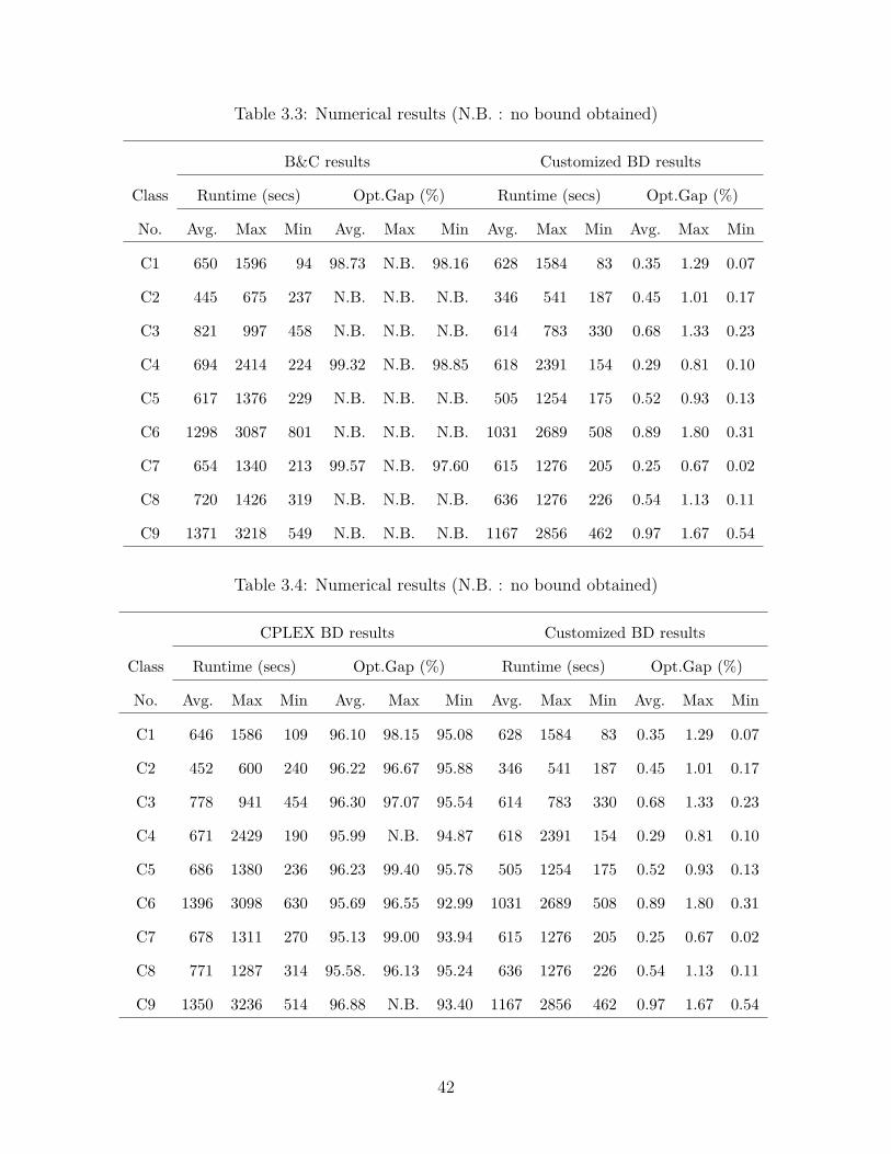
Table 3.3: Numerical results (N.B. : no bound obtained)

B&C results Customized BD results

Class Runtime (secs) Opt.Gap (%) Runtime (secs) Opt.Gap (%)

No. Avg. Max Min Avg. Max Min Avg. Max Min Avg. Max Min

C1 650 1596 94 98.73 N.B. 98.16 628 1584 83 0.35 1.29 0.07

C2 445 675 237 N.B. N.B. N.B. 346 541 187 0.45 1.01 0.17

C3 821 997 458 N.B. N.B. N.B. 614 783 330 0.68 1.33 0.23

C4 694 2414 224 99.32 N.B. 98.85 618 2391 154 0.29 0.81 0.10

C5 617 1376 229 N.B. N.B. N.B. 505 1254 175 0.52 0.93 0.13

C6 1298 3087 801 N.B. N.B. N.B. 1031 2689 508 0.89 1.80 0.31

C7 654 1340 213 99.57 N.B. 97.60 615 1276 205 0.25 0.67 0.02

C8 720 1426 319 N.B. N.B. N.B. 636 1276 226 0.54 1.13 0.11

C9 1371 3218 549 N.B. N.B. N.B. 1167 2856 462 0.97 1.67 0.54

Table 3.4: Numerical results (N.B. : no bound obtained)

CPLEX BD results Customized BD results

Class Runtime (secs) Opt.Gap (%) Runtime (secs) Opt.Gap (%)

No. Avg. Max Min Avg. Max Min Avg. Max Min Avg. Max Min

C1 646 1586 109 96.10 98.15 95.08 628 1584 83 0.35 1.29 0.07

C2 452 600 240 96.22 96.67 95.88 346 541 187 0.45 1.01 0.17

C3 778 941 454 96.30 97.07 95.54 614 783 330 0.68 1.33 0.23

C4 671 2429 190 95.99 N.B. 94.87 618 2391 154 0.29 0.81 0.10

C5 686 1380 236 96.23 99.40 95.78 505 1254 175 0.52 0.93 0.13

C6 1396 3098 630 95.69 96.55 92.99 1031 2689 508 0.89 1.80 0.31

C7 678 1311 270 95.13 99.00 93.94 615 1276 205 0.25 0.67 0.02

C8 771 1287 314 95.58. 96.13 95.24 636 1276 226 0.54 1.13 0.11

C9 1350 3236 514 96.88 N.B. 93.40 1167 2856 462 0.97 1.67 0.54

42

3.5. A Case Study: Chicago Sketch Network

Chicago sketch network is an aggregated traffic network that provides a reasonably real-

istic representation of Chicago area for which the data is available online [4]. The network

consists of 933 nodes, 2,950 arcs, and 378 zones. Our goal in this case study is to demon-

strate the applicability of our model and the proposed algorithm on real traffic network

and provide a sensitivity analyses on some of the system parameters that affect the sys-

tem cost. We assume that all of the 1,260,907 vehicles traveling in the network are EVs

with wireless charging capabilities. We also assume that these EVs are classified as follows:

35% of the EVs are of class D, 35% are of class E, and 30% are of class F. The parame-

ters associated with each EV class are provided in Table 3.5. For the model parameters,

we use the nominal values provided online at http://lyle.smu.edu/INETS/TestInstances/

EV-wireless-charging-network-data1.htm. However, to be able to observe changes in system

cost values more thoroughly, for parameters %, mcap, and η, we assume the nominal values

of 100, 1000, and 70%, respectively.

Table 3.5: EV classes parameters

γ ie ee

EV class D 30 (medium SOC) (low SOC)EV class E 30 (high SOC) (medium SOC)EV class F 30 (high SOC) (low SOC)

Next, we present an analysis on the effects of varying values of system and product

design characteristics – including vehicle charging power (%), system efficiency (η), and the

battery capacity (γ) – on the total system implementation cost.

3.5.1. Vehicle Charging Power (%) vs. Total Cost

Vehicle charging power (i.e., car charger) is the maximum charging power of the EV. The

value of this parameter ranges from 1 to 200 kW [19]. To evaluate the effect of this parameter

on the total system cost, we solve our optimization model for charging power values of 20

43

kW up to 200 kW. Moreover, to detect any interactions between vehicle charging power (%)

and system efficiency (η), we run the model for each value of parameter % while considering

three different values for η, including 0.5, 0.7, and 0.9. Likewise, to detect any interactions

between % and battery capacity (γ) we run the model for each value of % with γ values of

20, 30, and 40 kWh.

The results of this experiment are summarized in Figures 3.2a and 3.2b. The blue curve

in each figure represents the behavior of the cost function under the nominal values for η

(=0.7) and γ (=30). The curve indicates that an increase in the vehicle charging power from

20 kW to 60 kW results in 14% decrease in the total annual system cost ($31.6 million to $

27.3 million). It also shows that a further increase of the vehicle charging power will have

a lesser impact on the total cost. The cost function almost flattens as the vehicle charging

power exceeds 140 kW. The figures also show large shifts in the cost curve under different

values of system efficiency and battery capacity (Note that when parameters γ and % are

both equal to 20 (red curve), the charging demands could not be met, i.e., the problem is

infeasible).

We observe that our model captures the interaction between the parameters systems

efficiency, charging power, and battery capacity as they relate to the total system cost.

Specifically, trade-offs in our case study can be summarized as follows. A reduction in the

system efficiency by 0.2 increased the total cost by 32% on average, while increasing it by 0.2

decreased the total cost by 18%. Similarly, decreasing battery capacity by 10 units increases

the system cost by 61% on average, while increasing it by 10 units decreases the cost by 42%

on average.

Figure 3.3 shows two different network designs for Chicago region based on two different

values of vehicle charging power. The total annual costs of the designs with % = 200 kW

and % = 20 kW are $26.8 million (with 121 WCSs) and $ 31.6 million (with 312 WCSs),

respectively. Increasing the vehicle charging power means that more energy can be passed

from a WCS to an EV. Therefore, design with % = 200 kW employs a smaller number of

WCSs but with larger power capacity per WCS to satisfy the recharging demands. On the

44

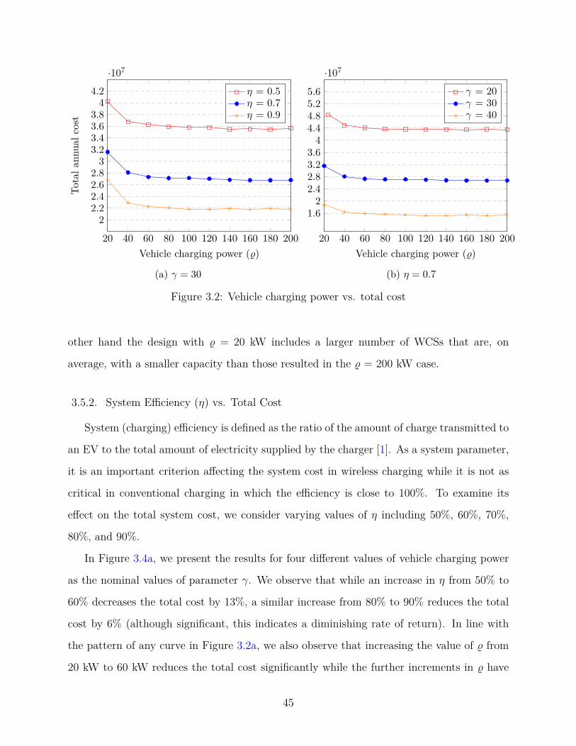
20 40 60 80 100 120 140 160 180 200

22.22.42.62.8

33.23.43.63.8

44.2·107

Vehicle charging power (%)

Tota

lann

ualc

ost

η = 0.5η = 0.7η = 0.9

(a) γ = 30

20 40 60 80 100 120 140 160 180 200

1.62

2.42.83.23.6

44.44.85.25.6

·107

Vehicle charging power (%)

γ = 20γ = 30γ = 40

(b) η = 0.7

Figure 3.2: Vehicle charging power vs. total cost

other hand the design with % = 20 kW includes a larger number of WCSs that are, on

average, with a smaller capacity than those resulted in the % = 200 kW case.

3.5.2. System Efficiency (η) vs. Total Cost

System (charging) efficiency is defined as the ratio of the amount of charge transmitted to

an EV to the total amount of electricity supplied by the charger [1]. As a system parameter,

it is an important criterion affecting the system cost in wireless charging while it is not as

critical in conventional charging in which the efficiency is close to 100%. To examine its

effect on the total system cost, we consider varying values of η including 50%, 60%, 70%,

80%, and 90%.

In Figure 3.4a, we present the results for four different values of vehicle charging power

as the nominal values of parameter γ. We observe that while an increase in η from 50% to

60% decreases the total cost by 13%, a similar increase from 80% to 90% reduces the total

cost by 6% (although significant, this indicates a diminishing rate of return). In line with

the pattern of any curve in Figure 3.2a, we also observe that increasing the value of % from

20 kW to 60 kW reduces the total cost significantly while the further increments in % have

45

(a) % = 200 kW (b) % = 20 kW

HighwayRoadWCS

Figure 3.3: Chicago sketch network

little impact on the total cost.

Further, Figure 3.4b presents the results for the nominal values of parameter % and three

different values of parameter γ including 20, 30, and 40 kWh. The three curves in Figure

3.4b show that the system cost decreases with increased battery capacity shifts. It is also

important to observe that the rate of change in cost decrease with increasing efficiency is

more significant if the battery capacity is low. It gradually becomes less significant with

increasing battery capacity. In a way, efficiency and battery capacity act as surrogates to

each other.

3.5.3. Battery Capacity vs. Total Cost

Battery capacity determines the EV range which has always been considered the bot-

tleneck in EV design. As we mentioned in Chapter 1, one of the benefits of implementing

dynamic charging technology is to allow EV manufacturers to design EVs with smaller bat-

46

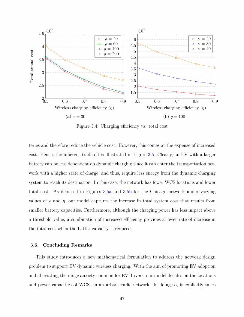
0.5 0.6 0.7 0.8 0.92

2.5

3

3.5

4

4.5 ·107

Wireless charging efficiency (η)

Tota

lann

ualc

ost

% = 20% = 60% = 100% = 200

(a) γ = 30

0.5 0.6 0.7 0.8 0.9

1.52

2.53

3.54

4.55

5.56

·107

Wireless charging efficiency (η)

γ = 20γ = 30γ = 40

(b) % = 100

Figure 3.4: Charging efficiency vs. total cost

teries and therefore reduce the vehicle cost. However, this comes at the expense of increased

cost. Hence, the inherent trade-off is illustrated in Figure 3.5. Clearly, an EV with a larger

battery can be less dependent on dynamic charging since it can enter the transportation net-

work with a higher state of charge, and thus, require less energy from the dynamic charging

system to reach its destination. In this case, the network has fewer WCS locations and lower

total cost. As depicted in Figures 3.5a and 3.5b for the Chicago network under varying

values of % and η, our model captures the increase in total system cost that results from

smaller battery capacities. Furthermore, although the charging power has less impact above

a threshold value, a combination of increased efficiency provides a lower rate of increase in

the total cost when the batter capacity is reduced.

3.6. Concluding Remarks

This study introduces a new mathematical formulation to address the network design

problem to support EV dynamic wireless charging. With the aim of promoting EV adoption

and alleviating the range anxiety common for EV drivers, our model decides on the locations

and power capacities of WCSs in an urban traffic network. In doing so, it explicitly takes

47

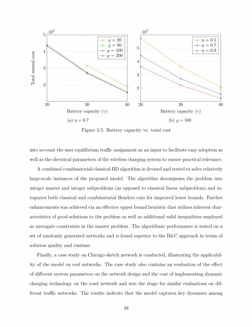
20 30 40

2

3

4

5 ·107

Battery capacity (γ)

Tota

lann

ualc

ost

% = 20% = 60% = 100% = 200

(a) η = 0.7

20 30 40

2

3

4

5

·107

Battery capacity (γ)

η = 0.5η = 0.7η = 0.9

(b) % = 100

Figure 3.5: Battery capacity vs. total cost

into account the user equilibrium traffic assignment as an input to facilitate easy adoption as

well as the electrical parameters of the wireless charging system to ensure practical relevance.

A combined combinatorial-classical BD algorithm is devised and tested to solve relatively

large-scale instances of the proposed model. The algorithm decomposes the problem into

integer master and integer subproblems (as opposed to classical linear subproblem) and in-

tegrates both classical and combinatorial Benders cuts for improved lower bounds. Further

enhancements was achieved via an effective upper bound heuristic that utilizes inherent char-

acteristics of good solutions to the problem as well as additional valid inequalities employed

as surrogate constraints in the master problem. The algorithmic performance is tested on a

set of randomly generated networks and is found superior to the B&C approach in terms of

solution quality and runtime.

Finally, a case study on Chicago sketch network is conducted, illustrating the applicabil-

ity of the model on real networks. The case study also contains an evaluation of the effect

of different system parameters on the network design and the cost of implementing dynamic

charging technology on the road network and sets the stage for similar evaluations on dif-

ferent traffic networks. The results indicate that the model captures key dynamics among

48

input parameters including battery capacity, charging power, and system efficiency and thus

provide the means of analyzing trade-offs involved in different real networks.

49

Chapter 4

ROBUST NETWORK DESIGN FOR IN-MOTION WIRELESS CHARGING OF

ELECTRIC VEHICLES

4.1. Introduction

Wireless charging of electric vehicles (EV) has made strides in the past few years within

the domain of automotive research and has recently made multiple appearances at several

prestigious motor shows around the globe [64] [20] [57]. This cutting-edge technology has

been under development as an EV power management solution to overcome the range anxiety

of EV drivers, and therefore accelerate EV adoption. The concept lies on transmitting energy

wirelessly from a roadbed inductive power line via electromagnetic pulses, to a power receiver

embedded in the EV. In the case of in-motion wireless charging, the power transmission can

take place dynamically as EVs travel on the electrified road segments.

Deploying in-motion wireless charging technology in the road network has many poten-

tial benefits including alleviating the range anxiety and reducing the battery size and the

cost of EVs. It is also a step forward toward the realization of EV full automation. But

this deployment also comes with the challenge of finding the most economic wireless charg-

ing infrastructure network design to serve the charging demands for EVs, at the minimum

investment cost, while causing no disturbance to the traffic on the road network.

The network design of the wireless charging infrastructure is associated with two main

decisions including (i) the multiple locations of wireless charging stations(WCS), and (ii) the

power capacities associated with each station. These two decisions are heavily dependent

on the traffic parameters of the road network including speeds, travel times, and EV flows

on each road segment. In turn, these traffic parameters are dictated by the user equilibrium

(UE) traffic assignment, which provides an adequate description of the traffic condition for

50

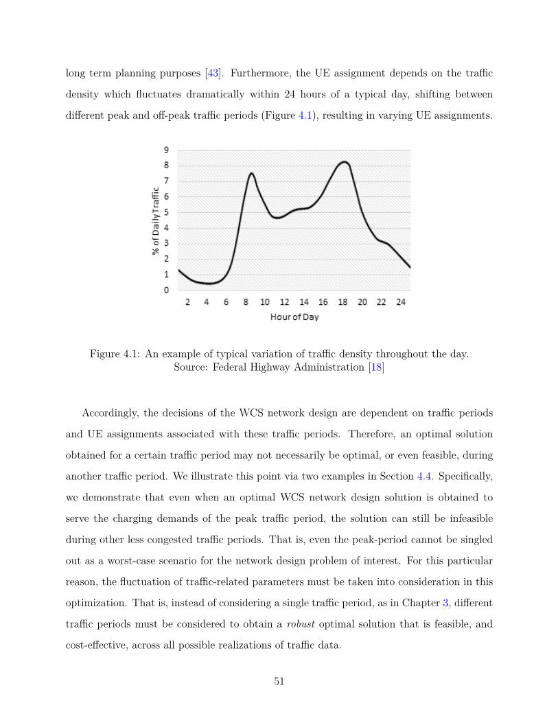
long term planning purposes [43]. Furthermore, the UE assignment depends on the traffic

density which fluctuates dramatically within 24 hours of a typical day, shifting between

different peak and off-peak traffic periods (Figure 4.1), resulting in varying UE assignments.

Figure 4.1: An example of typical variation of traffic density throughout the day.Source: Federal Highway Administration [18]

Accordingly, the decisions of the WCS network design are dependent on traffic periods

and UE assignments associated with these traffic periods. Therefore, an optimal solution

obtained for a certain traffic period may not necessarily be optimal, or even feasible, during

another traffic period. We illustrate this point via two examples in Section 4.4. Specifically,

we demonstrate that even when an optimal WCS network design solution is obtained to

serve the charging demands of the peak traffic period, the solution can still be infeasible

during other less congested traffic periods. That is, even the peak-period cannot be singled

out as a worst-case scenario for the network design problem of interest. For this particular

reason, the fluctuation of traffic-related parameters must be taken into consideration in this

optimization. That is, instead of considering a single traffic period, as in Chapter 3, different

traffic periods must be considered to obtain a robust optimal solution that is feasible, and

cost-effective, across all possible realizations of traffic data.

51

Driven by this motivation, we propose a robust optimization model to plan the deploy-

ment of WCSs in urban traffic networks. Through this model, we consider the dynamic

nature of daily traffic patterns as we optimize the WCS network design including the loca-

tions and power capacities of WCSs. We build on the study in Chapter 3 as we adopt a

perspective of a city, as a planning entity, in an effort to minimize the deployment cost of

the wireless charging infrastructure and the charging cost for users. Furthermore, in order

not to overburden EV drivers with any changes in route selection or driving behavior, we

intend to generate optimal designs that maintain the UE traffic assignment in each traffic

period. This is achieved by capturing the entire flow of the EV fleet on each used route of

the network.

Considering multiple traffic periods, instead of a single-period, increases the complexity

of the WCS network design problem. Specifically, the number of continuous variables and the

number of constraints are multiplied by the number of considered traffic periods. Therefore,

to solve the robust model, we devise a customized Benders Decomposition based algorithm.

The algorithm builds on the solution framework presented in Chapter 3. However, to deal

with the increase in the problem complexity, we apply a slight tweak to the formulation

for algorithmic purposes. We then devise multiple new sets of problem-specific surrogate

constraints as well as a new upper bound heuristic for improved efficiency. In addition, we

employ a cut strengthening technique for faster convergence. We provide computational

evidence to demonstrate the effectiveness of the proposed algorithm. We lastly apply the

proposed approach in a case study and we compare the robust optimal solution to different

individual single-period solutions obtained under different traffic periods.

The rest of this chapter is organized as follows: In Section 4.2 we explain the robust

optimization approach selected to tackle the problem at hand. In section 4.3 we provide

the definition and the formulation for the problem at hand. In Section 4.4 we illustrate

the need for a robust solution via two examples representing two different traffic networks.

The proposed BD solution algorithm is parented in Section 4.5. An extensive computational

experiment on the performance of the proposed algorithm is presented in Section 4.6. Finally,

52

a case study is presented in Section 4.7.

4.2. Robust Optimization

Robust Optimization (RO) is a decision making tool that deals with decision making

under uncertainty. Instead of optimizing a certain problem based on a specific data scenario,

RO offers decision makers the opportunity to obtain a Robust Decision, that is feasible and

performs well across all scenarios of input data.

While we are not dealing with uncertainty in this study, a robust optimization approach

can be useful to tackle the problem of interest. Specifically, by viewing each traffic period as

an input data “scenario”, a robust optimization model can generate a WCS network design

that is feasible, and cost-effective, across all daily traffic periods.

Kouvelis and Yu [35] lists three different robustness criteria including Absolute Robust-

ness, Robust Deviation, and Relative Robustness.

The Absolute Robustness criterion is the most conservative robustness criterion. The

approach minimizes the maximum cost taken across all possible scenarios.

The Robust Deviation criterion minimizes the maximum regret across all scenarios. Here,

regret is defined, for each scenario, as the difference between the cost of the robust solution,

and the cost of the optimal solution under the input data for that scenario. That is, ro-

bust deviation corresponds to the best worst-case deviation from optimality under all input

scenarios.

Finally, the Relative Robustness criterion also minimizes the maximum regret across all

scenarios. However, regret here is defined as the ratio of regret, as defined in the Robust

Deviation case, to the cost of the optimal solution of each scenario. That is, this criterion

corresponds to the worst-best-case percentage deviation from optimality under all input

scenarios.

Both robust deviation and relative robustness criteria are less conservative than the

absolute robustness criterion since they both account for the “missed opportunity” of a

robust decision by comparing it to the optimal decisions under the different scenarios.

53

We now present the mathematical formulation associated with each of the three robust-

ness criteria.

Given an LP defined for a specific input data scenario s as

zs = min csx

subject to

Asx = bs

x ≥= 0,

let S be the set of all possible scenarios. Then the absolute robust linear programming

problem is given as

zA = min [ maxs∈S

csx ]

subject to

Asx = bs ∀ s ∈ S

x ≥= 0.

Further, the robust deviation linear programming problem is given as

zD = min [ maxs∈S

csx− zs ]

subject to

Asx = bs ∀ s ∈ S

x ≥= 0.

Finally, the relative robust linear programming problem is given as

zR = min[

maxs∈S

csx− zs

zs

]subject to

54

Asx = bs ∀ s ∈ S

x ≥= 0.

In this study, we adopt an absolute robustness approach in an effort to generate network

designs that are feasible and cost-effective across all scenarios (traffic periods). Another

key advantage of the absolute robustness approach is that it is computationally easier when

compared to the other two criteria. This is because, unlike the other two criteria, the

absolute robustness does not require computing the optimal solutions for each input scenario

individually.

Next, building on the definition of the absolute robustness, we define and formulate the

robust WCS network design problem.

4.3. Problem Definition

We define the problem on a traffic network represented by a directed graph G(N ,A)

where N represents a set of nodes and A represents a set of arcs. We consider a set of

traffic periods S. Each traffic period s ∈ S is associated with a traffic pattern defined by

a state of user equilibrium UEs which provides a proper characterization of a traffic system

for long term planning purposes [43] . Each traffic period is also associated with a set of

origin-destination (OD) pairs Qs, and each OD pair q ∈ Qs is connected with a set of routes

Rq containing at least one route r ∈ Rq. The used routes at each traffic period s are defined

by the associated UE traffic pattern UEs.

We further consider a set K representing different classes of EVs, where each class k ∈ K

is characterized by the initial and desired ending states of charge as well as the capacity of

the battery. Based on the above-mentioned definitions, we define a commodity (sqrk) as a

fleet of EVs belonging to a class k ∈ K traveling in the network during traffic period s ∈ S

between an OD-pair q ∈ Qs using route r.

Finally, we assume that installing a WCS on a road segment is associated with two costs;

the first is a per-mile construction cost associated with building one mile of WCS. The second

55

cost is a power installation cost associated with installing one charging unit at a WCS. While

we considered, in Chapter 3, a “base power capacity” associated with installing a WCS, here,

we relax this assumption for algorithmic purposes. This “tweak” allows us to devise the new

surrogate constraint 4.49.

We next present the model formulation of the robust network design for in-motion wireless

charging of electric vehicles.

4.3.1. Model Formulation

We first introduce an expanded notation used in our robust formulation.

Sets:

N set of nodes, i, j ∈ N

O set of origins, o ∈ O ⊂ N

D set of destinations, d ∈ D ⊂ N

A set of arcs, (i, j) ∈ A

S set of traffic periods, s ∈ S

Qs set of all OD-pairs within the network during traffic period s, q ∈ Qs

Rq set of all used routes between a certain OD-pair q, r ∈ Rq where

or and dr are the origin node and destination node of route r, respectively.

Nr set of nodes on a route r ∈ Rq, Nr ⊂ N

Ar set of arcs on a route r ∈ Rq, Ar ⊂ A

K set of EV classes, k ∈ K

56

Parameters:

fc construction cost ($) associated with constructing one mile of a WCS

vc power installation cost ($) associated with installing one charging unit at a WCS

cc charging cost ($/kWh)

tr average number of trips taken by an EV during project lifetime

pcap power capacity (kW) associated with installing one charging unit at a WCS

mcap maximum power capacity (kW) that can be installed on one mile of a one-lane road

segment

η efficiency coefficient of the wireless power transfer system

ξij energy consumption (kWh) on arc (i, j)

ξr energy consumption (kWh) on route r

% vehicle charging power (kW)

γk battery capacity (kWh) of an EV of class k

vsqrk traffic volume of EV fleet of class k on route r that are traveling between OD-pair

q during traffic period s

ρsqrkij the expected number of EVs of class k, that are occupying arc (i, j) under traffic

pattern of period s while traveling between OD-pair q along route r, s ∈ S, q ∈

Qs, r ∈ Rq, k ∈ K, (i, j) ∈ Ar

lij length of arc (i, j) (mile)

nij number of lanes on arc (i, j)

tsij travel time (hour) on arc (i, j) during traffic period s

δsqrij an indicator with value of one if arc (i, j) is part of route r, 0 otherwise, s ∈ S, q ∈

Qs, r ∈ Rq, k ∈ K, (i, j) ∈ Ar

57

iek initial energy level of an EV of class k ∈ K

eek ending energy level of an EV of class k ∈ K

Decision Variables:

xij 1 if a WCS is installed on candidate arc (i, j), 0 otherwise

yij number of power charging units installed on arc (i, j)

esqrki energy level at node i of an EV of class k, traveling between OD-pair q on route r

under traffic pattern of period s ∈ S, q ∈ Qs, r ∈ Rq, k ∈ K, i ∈ Nr

csqrkij amount of charge an EV of class k, traveling between OD-pair q on route r under

traffic pattern of period s, receives from charging station at arc (i, j), s ∈ S, q ∈

Qs, r ∈ Rq, k ∈ K, (i, j) ∈ Ar

The wireless charging stations robust network design problem (R) can then be formulated

as follows:

min[ ∑

(i,j)∈A(fc lij nij xij + vc yij) + max

s∈S

∑q∈Qs

∑r∈Rq

∑k∈K

∑(i,j)∈Ar

(cc tr vsqrkcsqrkij )]

(4.1)

subject to

esqrkor+

∑(i,j)∈Ar

csqrkij − esqrkdr= ξr ∀ s ∈ S, q ∈ Qs, r ∈ Rq, k ∈ K (4.2)

esqrki + csqrkij − esqrkj = ξij ∀ s ∈ S, q ∈ Qs, r ∈ Rq, k ∈ K, (i,j) ∈ Ar (4.3)

esqrki − ξij (1− xij) ≥ 0 ∀ s ∈ S, q ∈ Qs, r ∈ Rq, k ∈ K, i ∈ Nr, (i,j) ∈ Ar (4.4)

csqrkij ≤ % tsij xij ∀ s ∈ S, q ∈ Qs, r ∈ Rq, k ∈ K, (i,j) ∈ Ar (4.5)∑q∈Qs

∑r∈Rq

∑k∈K

(δsqrij ρsqrkij csqrkij )

≤ η (pcap yij) tsij ∀ s ∈ S, (i, j) ∈ A (4.6)

58

pcap yij ≤ mcap nij lij ∀ (i, j) ∈ A (4.7)

esqrki + csqrkij ≤ γk + ξij ∀ s ∈ S, q ∈ Qs, r ∈ Rq, k ∈ K, i ∈ Nr, (i,j) ∈ Ar (4.8)

esqrkor= iek ∀ s ∈ S, q ∈ Qs, r ∈ Rq, k ∈ K (4.9)

esqrkdr≥ eek ∀ s ∈ S, q ∈ Qs, r ∈ Rq, k ∈ K (4.10)

esqrki , csqrkij ≥ 0,

xij ∈ 0, 1, yij ∈ Z+ ∀ s ∈ S, q ∈ Qs, r ∈ Rq, k ∈ K, i ∈ N , (i, j) ∈ A (4.11)

The objective function (4.1) minimizes the infrastructure deployment cost and the maxi-

mum charging cost across all considered traffic periods. The infrastructure deployment cost

incorporates two types of costs. The first is the construction cost of WCS. The second is

a variable cost, representing the cost of the power capacity units installed on WCS. Con-

straints (4.2) and (4.3) represent the energy conservation constraints over paths and over

arcs, respectively. Constraints (4.4) ensure that the energy level at each node is sufficient to

energize the EV until reaching the next WCS. Constraint (4.5) is a dual-purpose constraint.

It ensures that charging on an arc is only possible if the arc is electrified (has a WCS on it).

It also links the amount of charge that an EV can receive on a certain arc to the exposure

time between the EV and the WCS.

Constraints (4.6) ensure that the power installation on each WCS is sufficient to serve the

charging demands on the WCS. Note that in the single-period model presented in Chapter

3, the power installation constraint includes a base power installation in the right hand side

on the constraint. For algorithmic purposes, we are not considering a base power installation

in this formulation. Still, any deployed WCS will contain at least one charging unit. This is

because the binary variable xij, in constraint (4.5), and the integer variable yij, in constraint

(4.6), are both triggered by the continuous variable csqrkij . That is, when csqrkij is positive, it

triggers both xij and yij. Therefore, we will not run into a situation where the model deploys

a WCS on a certain arc (i.e., xij = 1), with no power installation on the arc (i.e., yij = 0).

59

Constraints (4.7) enforce a limit on the power installation on each WCS. Constraints (4.8)

limit the amount of charge of an EV by the capacity of its battery (EV range). Constraints

(4.9) and (4.10) bound the initial and ending energy levels of EVs. Lastly, constraints (4.11)

define nonnegativity and integrality requirements of the decision variables.

4.4. Illustrating the Need for a Robust Solution

Unlike many other strategic infrastructure planning problems, designing the network of

WCS when considering only the peak traffic period (as a bottleneck associated with the

highest traffic demands) might lead to solutions that are infeasible for other off-peak traffic

periods. That is, an optimal solution for the problem that is obtained for a single traffic

period is not necessarily feasible for another traffic period with less traffic demands. We

illustrate this point in what follows through a single-OD network example first, and then on

a multi-OD network.

4.4.1. Single-OD Network Example

Consider three different routes (r1, r2, r3) connecting an OD pair. For the sake of

simplicity and without loss of generality, assume that each route is represented by one arc

only. The lengths, speed limits, free-flow travel times, and the traffic capacities of the three

routes (arcs) are given in Table 4.1.

Table 4.1: Routes data

r1 r2 r3

Length 40 40 40Speed limit 60 75 50Free-flow travel time ftr (min) 40 32 48Traffic capacity 2,000 2,000 2,000

60

Assume that during the peak traffic period s1, the traffic demands between the OD pair

is 4000. We use the Method of Successive Averages1 to obtain the UE assignment which

is described by the volumes and travel times given in Table 4.2, where vr and tr represent

traffic volume and travel time (minutes), respectively.

Table 4.2: UE data of peak period s1

r1 r2 r3

vr (vehicle/hr) 1,365 1,795 840tr (min) 52 52 52

Now consider solving a single period WCS network design problem considering these

three routes and the peak traffic period s1. Assume that each EV needs to be recharged

with 8 kWh to complete its trip along each route. Using an EV charging power of % = 10

kW and the travel times associated with s1 (provided in Table 4.2), we find that electrifying

the three routes can provide each EV with c = % ∗ tr = 10 ∗ 5260 = 8.67 kWh of energy along

each route.

Finally, consider an off-peak traffic period s2 where only r2 is being used (as it is the

fastest path between the OD pair) and the traffic is moving with the free flow speed of 75

mile/hr. Accordingly, electrifying this route can provide, during traffic period s2, each EV

with c = % ∗ ftr2 = 10 ∗ 3260 = 5.33 kWh of energy. Therefore, the charging demands of 8

kWh per EV cannot be met during s2.

This example illustrates that given two traffic periods s1 and s2, if the traffic demands

during s1 are higher than those during s2, a solution for the WCS network design problem

obtained only considering the traffic pattern of s1 is not necessarily feasible for s2.

1The Method of Successive Averages is presented in Appendix A

61

4.4.2. Nguyen-Dupuis Network

Consider the Nguyen-Dupuis network, presented in Figure 4.2, with a set of four OD

pairs: Q = (1− 2), (1− 3), (4− 2), (4− 3).

1 12

654

9 10

7 8

11 2

13 3

2

1

3

4

5

6

7

8

9

10

14 15

11

18

13

12

19

15

16

17

Figure 4.2: Nguyen-Dupuis network

We assume that the travel times on links are dictated by Bureau of Public Roads (BRP)

arc performance function [55] given as

tij = tminij

(1 + α( vij

tcij)β)

(4.12)

where

tminij is the free-flow travel time on arc (i, j)

vij is the traffic volume on arc (i, j)

tcij is the traffic capacity of arc (i, j) measured in vehicles/hour

α and β are deterministic permeates associated with the type of the road.

62

We consider the values of 0.88 and 9.8 for α and β, respectively [26]. We further assume

a link capacity of 300 vehicle/hr, and a free flow speed of 65 mile/hr on each link. Further,

consider an EV wireless charging system with the parameters given in Table 4.3.

Table 4.3: Wireless charging system parameters

Parameter fc vc cc tr pcap % mcap ξ η γk

Value $800,000 $11,000 $0.15 7,200 20 20 1,000 0.33 80% 20

Now consider three different traffic periods s1, s2, and s3 with the demand matrices

provided in Table 4.4.

Table 4.4: Demand matrices

s1 s2 s3

2 3 2 3 2 3

1 300 600 200 400 133 2674 450 150 300 100 200 67

As shown in Table 4.4, the number of travelers between each OD pair decreases by a

rate of 13 between traffic period s1 and traffic period s2. Similarly, the number of travelers

between each OD pair decreases by the same rate going from traffic period s2 into traffic

period s3. Assume that the initial state of charge (SOC) for all EVs is 20 kWh, and the

required ending SOC at the destinations is at least 10 kWh.

The UE solution associated with the first (peak) traffic period s1, obtained using the

Method of Successive Averages, contains 17 routes connecting the two origins with the two

destinations. The average arcs speed, as resulted by solving the UE, is 27 mile/hr. The UE

parameters associated with the routes and with the arcs are given in Tables 4.5 and 4.6,

respectively.

63

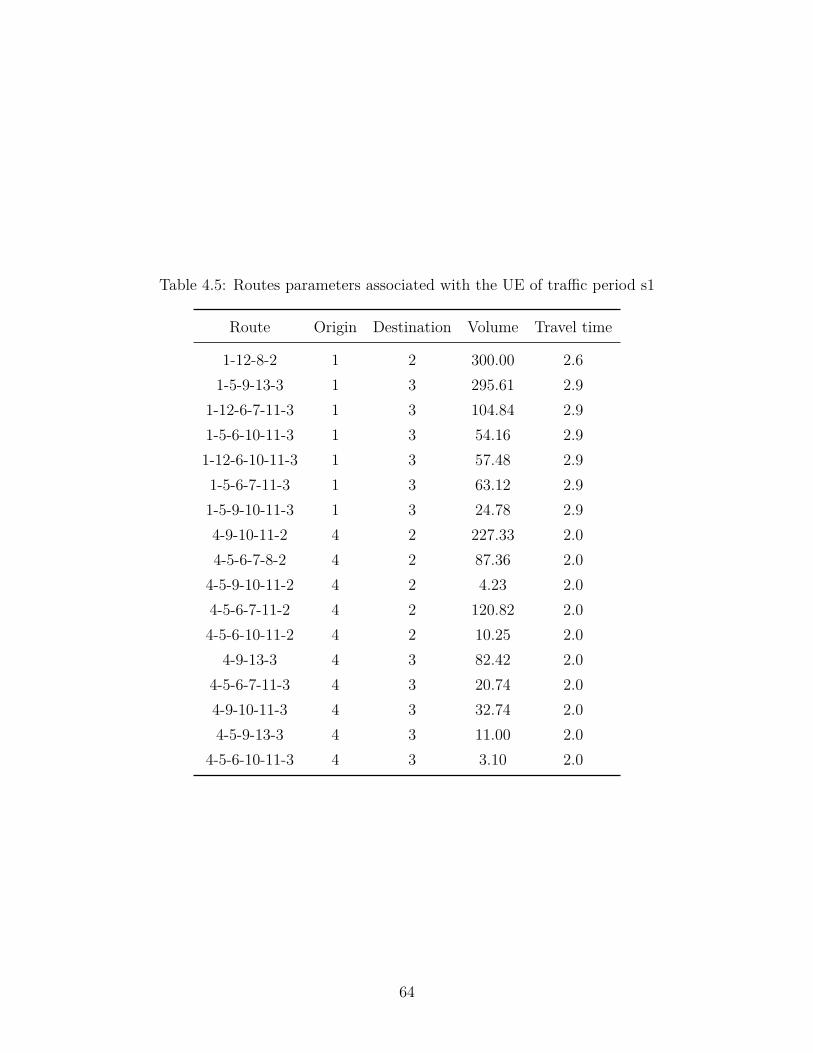
Table 4.5: Routes parameters associated with the UE of traffic period s1

Route Origin Destination Volume Travel time

1-12-8-2 1 2 300.00 2.61-5-9-13-3 1 3 295.61 2.9

1-12-6-7-11-3 1 3 104.84 2.91-5-6-10-11-3 1 3 54.16 2.91-12-6-10-11-3 1 3 57.48 2.91-5-6-7-11-3 1 3 63.12 2.91-5-9-10-11-3 1 3 24.78 2.94-9-10-11-2 4 2 227.33 2.04-5-6-7-8-2 4 2 87.36 2.0

4-5-9-10-11-2 4 2 4.23 2.04-5-6-7-11-2 4 2 120.82 2.04-5-6-10-11-2 4 2 10.25 2.0

4-9-13-3 4 3 82.42 2.04-5-6-7-11-3 4 3 20.74 2.04-9-10-11-3 4 3 32.74 2.04-5-9-13-3 4 3 11.00 2.0

4-5-6-10-11-3 4 3 3.10 2.0

64

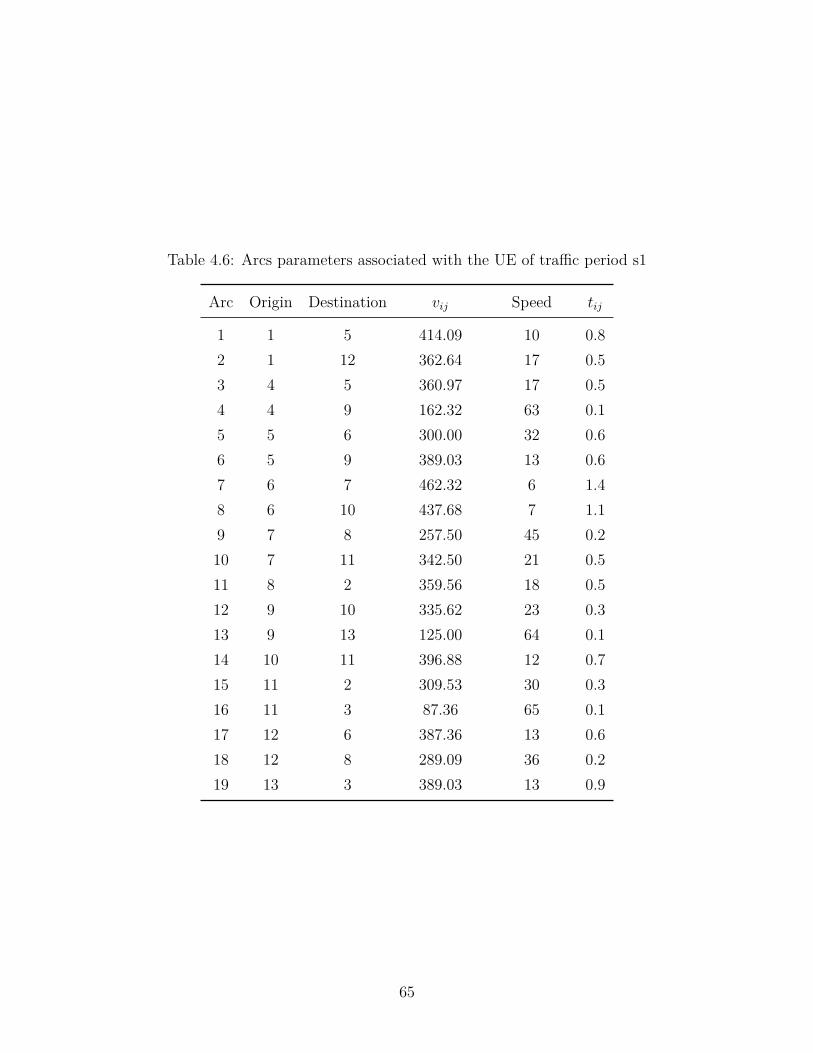
Table 4.6: Arcs parameters associated with the UE of traffic period s1

Arc Origin Destination vij Speed tij

1 1 5 414.09 10 0.82 1 12 362.64 17 0.53 4 5 360.97 17 0.54 4 9 162.32 63 0.15 5 6 300.00 32 0.66 5 9 389.03 13 0.67 6 7 462.32 6 1.48 6 10 437.68 7 1.19 7 8 257.50 45 0.210 7 11 342.50 21 0.511 8 2 359.56 18 0.512 9 10 335.62 23 0.313 9 13 125.00 64 0.114 10 11 396.88 12 0.715 11 2 309.53 30 0.316 11 3 87.36 65 0.117 12 6 387.36 13 0.618 12 8 289.09 36 0.219 13 3 389.03 13 0.9

65

Given the UE solution for s1 and the parameters in Table 4.3, the optimal solution for the

single-period network design problem at hand features four WCSs with 63 charging units as

depicted in Figure 4.3. The associated construction and power installation cost is $26.29M.

1 12

654

9 10

7 8

11 2

13 3iWCS j

iRoad j

y = 15

y = 21

y = 16

y = 11

Figure 4.3: Single-period optimal WCS network design for traffic period s1

Now consider traffic period s2 were the travel demands decrease by a rate of 13 . The UE

solution associated with this period contains 14 routes connecting the two origins with the

two destinations. Moreover, as a result of the decrease in the traffic volume, the average arc

speed, as resulted by UE solution, goes up to 51 mile/hr. Tables 4.7 and 4.8 provide the

new UE parameters associated with the routes and with the arcs, respectively.

Given the new UE and the system parameters in Table 4.3, the optimal solution for

the single-period network design problem is illustrated in Figure 4.4. The solution also

features four WCSs, but with only 41 charging units. The associated construction and

power installation cost is $26.05M - only slightly lower than the cost associated with s1.

66

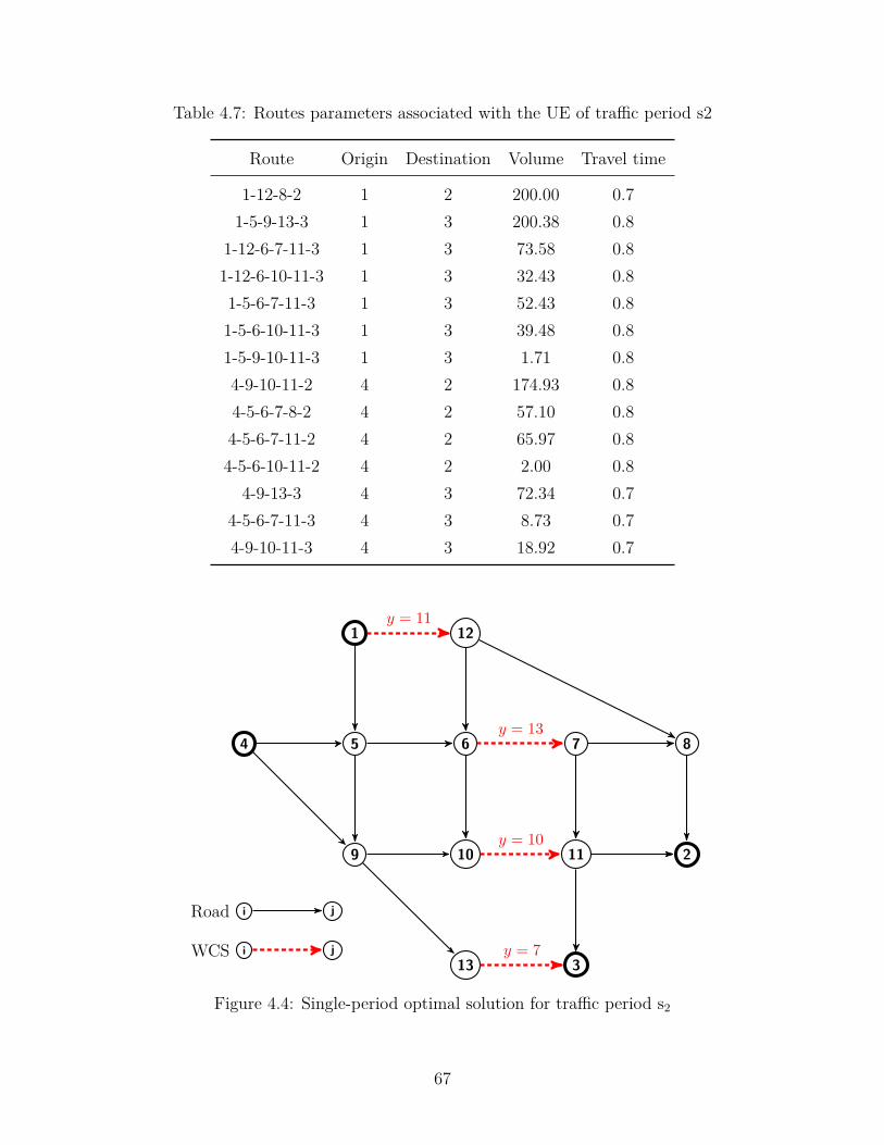
Table 4.7: Routes parameters associated with the UE of traffic period s2

Route Origin Destination Volume Travel time

1-12-8-2 1 2 200.00 0.71-5-9-13-3 1 3 200.38 0.8

1-12-6-7-11-3 1 3 73.58 0.81-12-6-10-11-3 1 3 32.43 0.81-5-6-7-11-3 1 3 52.43 0.81-5-6-10-11-3 1 3 39.48 0.81-5-9-10-11-3 1 3 1.71 0.84-9-10-11-2 4 2 174.93 0.84-5-6-7-8-2 4 2 57.10 0.84-5-6-7-11-2 4 2 65.97 0.84-5-6-10-11-2 4 2 2.00 0.8

4-9-13-3 4 3 72.34 0.74-5-6-7-11-3 4 3 8.73 0.74-9-10-11-3 4 3 18.92 0.7

1 12

654

9 10

7 8

11 2

13 3iWCS j

iRoad j

y = 11

y = 13

y = 10

y = 7

Figure 4.4: Single-period optimal solution for traffic period s2

67

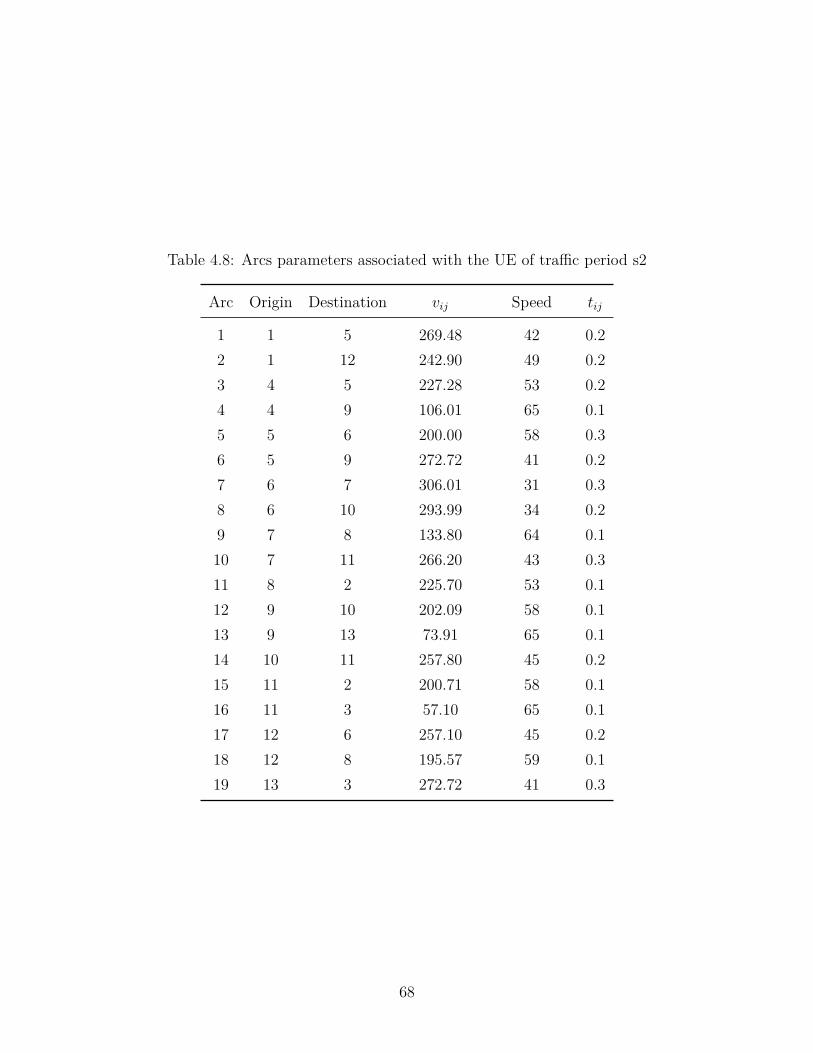
Table 4.8: Arcs parameters associated with the UE of traffic period s2

Arc Origin Destination vij Speed tij

1 1 5 269.48 42 0.22 1 12 242.90 49 0.23 4 5 227.28 53 0.24 4 9 106.01 65 0.15 5 6 200.00 58 0.36 5 9 272.72 41 0.27 6 7 306.01 31 0.38 6 10 293.99 34 0.29 7 8 133.80 64 0.110 7 11 266.20 43 0.311 8 2 225.70 53 0.112 9 10 202.09 58 0.113 9 13 73.91 65 0.114 10 11 257.80 45 0.215 11 2 200.71 58 0.116 11 3 57.10 65 0.117 12 6 257.10 45 0.218 12 8 195.57 59 0.119 13 3 272.72 41 0.3

68

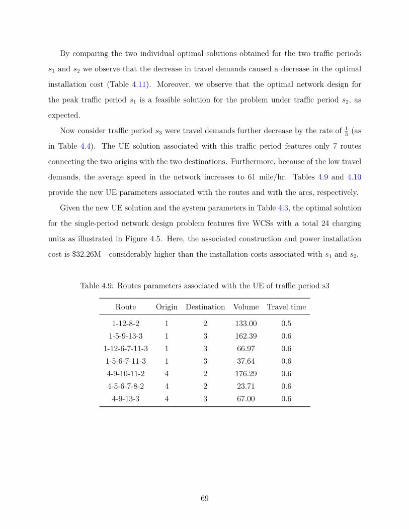
By comparing the two individual optimal solutions obtained for the two traffic periods

s1 and s2 we observe that the decrease in travel demands caused a decrease in the optimal

installation cost (Table 4.11). Moreover, we observe that the optimal network design for

the peak traffic period s1 is a feasible solution for the problem under traffic period s2, as

expected.

Now consider traffic period s3 were travel demands further decrease by the rate of 13 (as

in Table 4.4). The UE solution associated with this traffic period features only 7 routes

connecting the two origins with the two destinations. Furthermore, because of the low travel

demands, the average speed in the network increases to 61 mile/hr. Tables 4.9 and 4.10

provide the new UE parameters associated with the routes and with the arcs, respectively.

Given the new UE solution and the system parameters in Table 4.3, the optimal solution

for the single-period network design problem features five WCSs with a total 24 charging

units as illustrated in Figure 4.5. Here, the associated construction and power installation

cost is $32.26M - considerably higher than the installation costs associated with s1 and s2.

Table 4.9: Routes parameters associated with the UE of traffic period s3

Route Origin Destination Volume Travel time

1-12-8-2 1 2 133.00 0.51-5-9-13-3 1 3 162.39 0.6

1-12-6-7-11-3 1 3 66.97 0.61-5-6-7-11-3 1 3 37.64 0.64-9-10-11-2 4 2 176.29 0.64-5-6-7-8-2 4 2 23.71 0.6

4-9-13-3 4 3 67.00 0.6

69

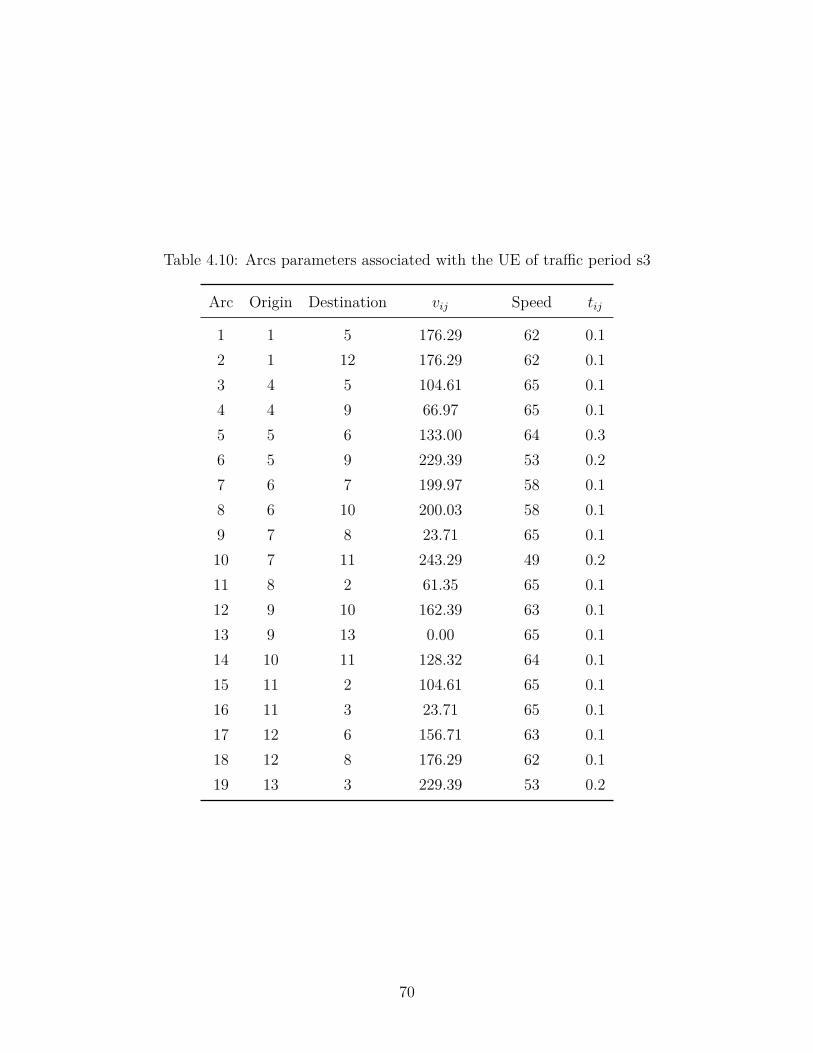
Table 4.10: Arcs parameters associated with the UE of traffic period s3

Arc Origin Destination vij Speed tij

1 1 5 176.29 62 0.12 1 12 176.29 62 0.13 4 5 104.61 65 0.14 4 9 66.97 65 0.15 5 6 133.00 64 0.36 5 9 229.39 53 0.27 6 7 199.97 58 0.18 6 10 200.03 58 0.19 7 8 23.71 65 0.110 7 11 243.29 49 0.211 8 2 61.35 65 0.112 9 10 162.39 63 0.113 9 13 0.00 65 0.114 10 11 128.32 64 0.115 11 2 104.61 65 0.116 11 3 23.71 65 0.117 12 6 156.71 63 0.118 12 8 176.29 62 0.119 13 3 229.39 53 0.2

70

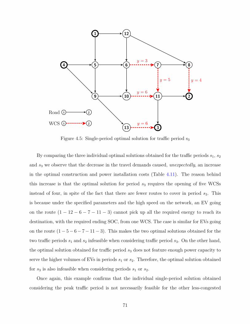
1 12

654

9 10

7 8

11 2

13 3iWCS j

iRoad j

y = 3

y = 5

y = 6

y = 4

y = 6

Figure 4.5: Single-period optimal solution for traffic period s3

By comparing the three individual optimal solutions obtained for the traffic periods s1, s2

and s3 we observe that the decrease in the travel demands caused, unexpectedly, an increase

in the optimal construction and power installation costs (Table 4.11). The reason behind

this increase is that the optimal solution for period s3 requires the opening of five WCSs

instead of four, in spite of the fact that there are fewer routes to cover in period s3. This

is because under the specified parameters and the high speed on the network, an EV going

on the route (1 − 12 − 6 − 7 − 11 − 3) cannot pick up all the required energy to reach its

destination, with the required ending SOC, from one WCS. The case is similar for EVs going

on the route (1− 5− 6− 7− 11− 3). This makes the two optimal solutions obtained for the

two traffic periods s1 and s2 infeasible when considering traffic period s3. On the other hand,

the optimal solution obtained for traffic period s3 does not feature enough power capacity to

serve the higher volumes of EVs in periods s1 or s2. Therefore, the optimal solution obtained

for s3 is also infeasible when considering periods s1 or s2.

Once again, this example confirms that the individual single-period solution obtained

considering the peak traffic period is not necessarily feasible for the other less-congested

71

Table 4.11: Optimal solutions under different scenarios

Traffic Traffic Number Avg. Number Construction & Powerperiod volume of routes speed of WCSs installation cost ($M)

s1 1500 17 27 4 26.29s2 1000 14 51 4 26.05s3 667 7 61 5 32.26

traffic periods. Therefore a robust solution is needed to guarantee that all charging demands

are met during all traffic periods.

4.5. Solution Methodology

To solve the large instances of the problem at hand, we devise a customized Benders

decomposition (BD) framework and employ problem-specific surrogate constraints for im-

proved efficiency. In the classic BD framework, large-scaled MIPs are decomposed into a

master problem (MP) and a subproblem (SP). MP includes the integer variables from the

original MIP, while SP includes the continuous ones. The algorithm iterates between the two

problems, passing forward integer solutions of MP to SP and passing back Benders cuts from

SP to MP. The algorithm terminates once the gap between the upper bound (determined

after solving SP) and the lower bound (given by MP) is less than a preferred threshold.[6].

Our decomposition scheme in this study is different than the classical BD. Specifically,

we build on the solution framework devised in Chapter 3 as we decompose the problem in a

way where both MP and SP are integer programs. This decomposition scheme dramatically

reduces the complexity of MP as one set of integer variables is moved from MP to SP.

Furthermore, the binary structure of MP allows the generation of combinatorial Benders cuts

whenever an MP solution leads to an infeasible SP. To tackle the increase in the problem

size and complexity associated with considering multiple traffic periods rather than a single

period, we introduce five new sets of surrogate constraints to be added to MP. We further

strengthen the proposed algorithm with a new upper bound heuristic, and we employ a cut

72

strengthening technique for improved efficiency. In what follows, we present the details of

our BD framework.

4.5.1. Benders Subproblem and Dual Subproblem

For a fixed binary vector X representing the set of opened locations of WCSs, we obtain

subproblem SP(esqrki , csqrkij , yij | X) as:

min[ ∑

(i,j)∈A(vc yij) + max

s∈S

∑q∈Qs

∑r∈Rq

∑k∈K

∑(i,j)∈Ar

(cc tr vsqrkcsqrkij )]

(4.13)

subject to

(4.2), (4.3), (4.6), (4.7), (4.8), (4.9), (4.10), and

esqrki − ξij (1− xij) ≥ 0 ∀ s ∈ S, q ∈ Qs, r ∈ Rq, k ∈ K, i ∈ Nr, (i,j) ∈ Ar (4.14)

csqrkij ≤ % tsij xij ∀ s ∈ S, q ∈ Qs, r ∈ Rq, k ∈ K, (i,j) ∈ Ar (4.15)

esqrki , csqrkij ≥ 0, yij ∈ Z+ ∀ s ∈ S, q ∈ Qs, r ∈ Rq, k ∈ K, i ∈ N , (i, j) ∈ A (4.16)

By introducing the non-negative auxiliary variable u, SP can be rewritten as:

min u (4.17)

subject to

(4.2), (4.3), (4.6), (4.7), (4.8), (4.9), (4.10), (4.14), (4.15), (4.16),∑q∈Qs

∑r∈Rq

∑k∈K

∑(i,j)∈Ar

(cc tr vsqrkcsqrkij ) +∑

(i,j)∈A(vc yij) ≤ u ∀ s ∈ S (4.18)

u ≥ 0 (4.19)

Let ψijsqrk, υijsqrk, ν

ijqrk, ω

sij, ϕij, σ

ijsqrk, θsqrk, τsqrk, and $s be the dual variables associated with

the linear relaxation of constraints (4.3), (4.14), (4.15), (4.6), (4.7), (4.8), (4.9), (4.10), and

73

(4.18) respectively. Moreover, define binary parameters λisqr and εisqr as one if i ∈ O and

i ∈ D, respectively, zero otherwise. Then, the dual of the linear relaxation of SP, denoted as

DRSP(ψijsqrk, υijsqrk, ν

ijsqrk, ω

sij, ϕij, σ

ijsqrk, θsqrk, τsqrk, $s | X) is obtained as

Maximize ζR =∑s∈S

∑q∈Qs

∑r∈Rq

∑k∈K

∑(i,j)∈Ar

(ξij ψ

ijsqrk + ξij (1− xij) υijsqrk +

% tsij xij νijsqrk + (γk + ξij)σijsqrk

)+

∑(i,j)∈Ar

(mcap nij lij)ϕij +

∑s∈S

∑q∈Qs

∑r∈Rq

∑k∈K

(iek θsqrk + eek τsqrk) (4.20)

subject to

λisqr (θsqrk + ψijsqrk + υijsqrk + σijsqrk)+

εisqr (τsqrk − ψijsqrk)(1− λisqr − εisqr) × +

(ψijsqrk − ψi−1 j−1sqrk + υijsqrk + σijsqrk) ≤ 0 ∀ s ∈ S, q ∈ Qs, r ∈ Rq,

k ∈ K, i ∈ Nr (4.21)

ψijsqrk + νijsqrk + ρsqrkij ωsij + σijsqrk + cc tr vsqrk ≤ 0 ∀ s ∈ S, q ∈ Qs, r ∈ Rq,

k ∈ K, (i,j) ∈ Ar (4.22)

−$s ≤ 1 ∀ s ∈ S (4.23)

ψijsqrk, θsqrk URS;

υijsqrk, τsqrk ≥ 0, νijsqrk, ωij, $ij, σijsqrk ≤ 0 ∀ s ∈ S, q ∈ Qs, r ∈ Rq,

k ∈ K, (i, j) ∈ A (4.24)

Let P denote the set of all extreme points of DRSP polyhedron given by (4.21) -

(4.24), and let ψijpsqrk, υijpsqrk, ν

ijpqrk, ω

sijp, ϕijp, σ

ijpsqrk, θ

psqrk, τ

psqrk, $

ps and ζpR denote the associated

dual variables and the value of the objective function respectively. Further, let ζ∗ de-

74

note the optimal value of DRSP. Since ζpR ≤ ζ∗, ∀p ∈ P , DRSP can be restated as

minζ≥0ζ : ζp ≤ ζ, ∀p ∈ P, where

ζpR =∑s∈S

∑q∈Q

∑r∈Rq

∑k∈K

∑(i,j)∈Ar

(ξij ψ

ijpsqrk + ξij (1− xij) υijpsqrk +

% tsij xij νijpsqrk + (γk + ξij)σijpsqrk

)+

∑(i,j)∈r

(mcap nij lij)ϕijp +

∑s∈S

∑q∈Q

∑r∈Rq

∑k∈K

(iek θpsqrk + eek τpsqrk) (4.25)

The above representation of DRSP gives:

ζ ≥ ζpR ∀ p ∈ P (4.26)

which represents a classical Benders optimality cut that can be generated for each feasible

SP and then added to MP.

4.5.2. Benders Master Problem

Given the above representation of DRSP, a lower bound on the overall problem can be

obtained as:

min∑

(i,j)∈A(fc lij nij xij) + ζ (4.27)

subject to (4.26)

But due to the large number of constraints (4.26), and because not all of them will

be binding at optimality, in the BD framework, we solve a relaxed version of the above

program where Benders cuts (4.26) are added in a delayed fashion, one at each iteration.

Therefore, the relaxed version of the lower bound problem, called Benders master prob-

lem (MP), contains only a subset of constraints (4.26) and its optimal solution provides

75

a valid lower bound on the overall problem. To generate Benders cuts, at each iteration,

DRSP(ψijsqrk, υijsqrk, ν

ijsqrk, ω

sij, ϕij, σ

ijsqrk, θsqrk, τsqrk, $s | X) is solved and the optimal values of

the dual variables are used to construct a Benders cut (4.26).

In the case where MP solution (represented by the binary locations vector X) causes

DRSP to be unbounded (SP is infeasible), the binary structure of MP allows the generation

of Benders combinatorial cut of the form:

∑(i,j):xij=0

xij +∑

(i,j):xij=1(1− xij) ≥ 1 (4.28)

where xij ∈ X. This cut forces MP to exclude the combination of binary variables that led

to the unboundedness of DRSP. [14]

4.5.3. Surrogate Constraints for MP

To improve the quality of MP solution and to reduce the possibility of generating MP so-

lutions that will lead to the infeasibility of SP, we introduce five sets of surrogate constraints.

While these constraints are valid, they are also redundant in the original formulation.

4.5.3.1. Constraint on Exposure Time over Route

Let csqrk denote the minimum amount of charge required by an EV of commodity (sqrk),

i.e.,

∑(i,j)∈Ar

csqrkij ≥ csqrk ∀ s ∈ S, q ∈ Qs, r ∈ Rq, k ∈ K

Using the bounds on the initial and ending levels of energy for each commodity (iek and eek,

respectively), csqrk can be pre-calculated as:

csqrk = ξr + eek − iek ∀ s ∈ S, q ∈ Qs, r ∈ Rq, k ∈ K

76

Then, an aggregated version of the dual-purpose constraint (4.5) can be given as:

∑(i,j)∈Ar

% tsij xij ≥ csqrk ∀ s ∈ S, q ∈ Qs, r ∈ Rq, k ∈ K (4.29)

A constraint of this type ensures that enough number of WCSs are selected by MP to provide

enough exposure time for EVs to receive the minimum amount of charge required on their

routes.

4.5.3.2. Constraint on Charging Availability over the Initial Part of the Trip

Let esqrkor= iek be the energy of EVs of commodity (sqrk) at the origin of route r (node or).

Further, let Ar ⊂ Ar be the subset of connected arcs of route r that EVs of this commodity

can travel starting from or until running out of charge (including the arc at which the EVs

will run out of charge). That is, Ar represents the initial part of the commodity’s trip. Then,

to ensure that EVs will not run out of charge on the initial part of the trip, the following

constraint can be added to MP:

∑(i,j)∈Ar

xij ≥ 1 ∀ s ∈ S, q ∈ Qs, r ∈ Rq, k ∈ K (4.30)

This constraint ensures that, for each commodity, at least one WCS is installed on the

commodity’s route between the commodity’s origin and the point where EVs will run out of

charge.

By taking into consideration the exposure time between WCSs and EVs, a tighter version

of constraint (4.30) can be given as:

∑(i,j)∈Ar

% tsij xij ≥ ξr − iek ∀ s ∈ S, q ∈ Qs, r ∈ Rq, k ∈ K (4.31)

where ξr is the energy consumption over Ar. Not only this form of the constraint ensures

the opening of at least one WCS on the initial part of the route before EVs runs out of

energy, but it also guarantees that the opened station(s) can provide enough exposure times

77

for the EVs to receive enough charge to travel the initial part of the trip.

4.5.3.3. Constraint on Charging Availability over the Last Part of the Trip

Let esqrkdr= eek be the minimum required energy of EVs of commodity (sqrk) at the

destination of route r (node dr). Further, let Ar ⊂ Ar be the largest subset of connected

arcs at the end of route r such that if an EV of type k enters the first arc of Ar with a

full range, then it can reach the end of route r with a level of energy esqrkdr≥ eek. Let

Ar = Ar ∪ (a) where (a) is the arc of Ar that directly precede Ar. Accordingly, if none of

the arcs of Ar has a WCS, EVs cannot reach the destination with the required amount of

energy. Therefore, we can construct the following constraint for each commodity:

∑(i,j)∈Ar

xij ≥ 1 ∀ s ∈ S, q ∈ Qs, r ∈ Rq, k ∈ K (4.32)

These constraints ensure that, for each commodity, at least one WCS is installed on the last

part of the commodity’s route to serve the charging demands at that part of the route.

By taking into consideration the exposure time between WCSs and EVs, a tighter version

of this constraint can be given as:

∑(i,j)∈Ar

% tsij xij ≥ ξAr+ γk − eek ∀ s ∈ S, q ∈ Qs, r ∈ Rq, k ∈ K (4.33)

where ξArrepresents the energy consumption on Ar. Similar to constraint (4.31), this form

of this surrogate constraint ensures that the selected WCS at the last part of the route can

provide enough exposure time to satisfy the charging demands on that part of the route.

4.5.3.4. Constraint on Maximum Power Capacity

While the first three surrogate constraints (4.29), (4.31), and (4.33) deal with the exposure

time between the EVs and the selected WCSs, the fourth constraint deals with the length

of these stations. Specifically, to assist getting a feasible SP, the WCSs featured in the MP

78

solution should provide enough millage to host the power capacity required to serve the

minimum charging demands. That is, MP solution should provide enough electrified millage

in order for constant (4.7) in SP to hold. By substituting constraint (4.7) from the original

problem in (4.6) we obtain

∑q∈Qs

∑r∈Rq

∑k∈K

(δsqrij ρsqrkij csqrkij ) ≤ η (mcap nij lij) tsij ∀ s ∈ S, (i, j) ∈ A. (4.34)

If no WCS is installed on arc (i, j), i.e., xij = 0, then the left hand side of (4.34) must be

equal to zero. Therefore, it is valid to write

∑q∈Qs

∑r∈Rq

∑k∈K

(δsqrij ρsqrkij csqrkij ) ≤ η (mcap nij lij) tsij xij ∀ s ∈ S, (i, j) ∈ A. (4.35)

Let Gsij be defined as the set of all routes that pass through arc (i, j) during traffic period

s. For each route g ∈ Gsij let qg denote the OD pair of route g. Accordingly, equation (4.35)

can be rewritten as

∑g∈Gs

ij

∑k∈K

(ρsqggkij c

sqggkij ) ≤ η (mcap nij lij) tsij xij ∀ s ∈ S, (i, j) ∈ A. (4.36)

Now let AGsij

be the set of arcs that form all routes in set Gsij. Then, an aggregation of

equation (4.36) over set AGsij

can be written as

∑a∈AGs

ij

∑g∈Gs

a

∑k∈K

(ρsqggka csqggk

a ) ≤∑

a∈AGsij

η (mcap na la) tsa xa ∀ s ∈ S, (i, j) ∈ A. (4.37)

Since Gsij ⊆⋃a∈AGs

ij

Gsa for all (i, j) ∈ A, it is valid to write

∑a∈AGs

ij

∑g∈Gs

ij

∑k∈K

(ρsqggka csqggk

a ) ≤∑

a∈AGsij

∑g∈Gs

a

∑k∈K

(ρsqggka csqggk

a ) ∀ s ∈ S, (i, j) ∈ A (4.38)

79

therefore, by combining (4.37) and (4.38) we obtain

∑a∈AGs

ij

∑g∈Gs

ij

∑k∈K

(ρsqggka csqggk

a ) ≤∑

a∈AGsij

η (mcap na la) tsa xa ∀ s ∈ S, (i, j) ∈ A. (4.39)

Now let csqggk denote the minimum amount of charge required by an EV of commodity

(sqggk), i.e.,

∑a∈Ag

csqggka ≥ csqggk ∀ s ∈ S, g ∈ Gsij, (i, j) ∈ A, k ∈ K (4.40)

where Ag is the set of arcs that form route g ∈ Gsij. Also, by letting ρsqggk(min) = min

a∈Ag

ρsqggka :

∀ s ∈ S, g ∈ Gsij, (i, j) ∈ A, k ∈ K, we obtain

∑a∈Ag

ρsqggka csqggk

a ≥ ρsqggk(min) c

sqggk ∀ s ∈ S, g ∈ Gsij, (i, j) ∈ A, k ∈ K. (4.41)

By aggregating (4.41) over sets (Gsij) and (K) we obtain

∑a∈Ag

∑g∈Gs

ij

∑k∈K

ρsqggka csqggk

a ≥∑g∈Gs

ij

∑k∈K

ρsqggk(min) c

sqggk ∀ s ∈ S, (i, j) ∈ A. (4.42)

And since Ag ⊆ AGsij

for all g ∈ Gsij, then

∑a∈AGs

ij

∑g∈Gs

ij

∑k∈K

ρsqggka csqggk

a ≥∑a∈Ag

∑g∈Gs

ij

∑k∈K

ρsqggka csqggk

a ∀ s ∈ S, (i, j) ∈ A. (4.43)

Therefore, in view of equations (4.39), (4.42), and (4.43) we may write

∑g∈Gs

ij

∑k∈K

ρsqggk(min) c

sqggk ≤ η mcap

∑a∈Ag

(na la tsa xa) ∀ s ∈ S, (i, j) ∈ A (4.44)

which is a valid inequality that could be added to MP as a fourth set of surrogate constraints.

80

4.5.3.5. Lower Bound on the Auxiliary Variable

The fifth surrogate constraint to be added to MP provides a lower bound on the auxiliary

variable ζ. This MP variable represents the value of SP objective. Therefore, by letting α

denote a lower bound on any feasible SP, it is valid to write

ζ ≥ α (4.45)

We obtain α as follows. The objective (4.17) of SP is given as

min[ ∑

(i,j)∈A(vc yij) + max

s∈S

∑q∈Qs

∑r∈Rq

∑k∈K

∑(i,j)∈Ar

(cc tr vsqrkcsqrkij )].

Let ymin be the minimum amount of total power capacity installation required to satisfy

the charging demands on the whole network, i.e., for any feasible solution of the original

problem, we must have the following constraint to hold:

vc ymin ≤∑

(i,j)∈A(vc yij). (4.46)

Therefore, the term (vc ymin) provides a lower bound on the first part of the SP objective

function (4.17). We calculate ymin by solving a version of SP where all arcs are WCSs, i.e.,

SP(esqrki , csqrkij , yij | xij = 1).

Further, let csqrk be the minimum amount of charge required by commodity (sqrk) as

defined in 4.5.3.1. Accordingly, any feasible solution of the problem needs to satisfy the

following equation:

∑q∈Qs

∑r∈Rq

∑k∈K

(cc tr vsqrkcsqrk) ≤∑q∈Qs

∑r∈Rq

∑k∈K

∑(i,j)∈r

(cc tr vsqrkcsqrkij ) ∀s ∈ S.

81

Therefore, we have

maxs∈S

∑q∈Qs

∑r∈Rq

∑k∈K

(cc tr vsqrkcsqrk) ≤ maxs∈S

∑q∈Qs

∑r∈Rq

∑k∈K

∑(i,j)∈Ar

(cc tr vsqrkcsqrkij ). (4.47)

That is, the left hand side of (4.47) is a lower bound on the second part of SP objective

(4.17). Thus, since the left hand side of (4.46), and the left hand side of (4.47) provide lower

bounds on the first part and the second part of SP objective, respectively, it is valid to write

α = vc ymin + maxs∈S

∑q∈Qs

∑r∈Rq

∑k∈K

(cc tr vsqrkcsqrk) (4.48)

where α is a lower bound on SP objective function, by definition. By substituting (4.48) in

(4.45) we obtain

ζ ≥ vc ymin + maxs∈S

∑q∈Qs

∑r∈Rq

∑k∈K

(cc tr vsqrkcsqrk) (4.49)

which is the fifth surrogate constraint to be added to MP.

4.5.4. Benders Cut Strengthening

For a fixed binary vector X representing MP solution, subproblem SP(esqrki , csqrkij , yij | X)

may possess degeneracy. Therefore, the associated DRSP may have multiple optimal solu-

tions, and a different Benders cut can be generated based on each solution. Thus, we

seek to generate the strongest cut possible at each iteration. For an optimization prob-

lem miny∈Y,z∈Rz : z ≥ f(w) + yg(w), ∀w ∈ W, a cut z ≥ f(v) + yg(v) is stronger

than another cut z ≥ f(w) + yg(w) if f(v) + yg(v) ≥ f(w) + yg(w),∀y ∈ Y and if

f(v)+yg(v) > f(w)+yg(w) for at least one y ∈ Y [42]. To obtain a stronger cut at a certain

iteration (n), we start by solving DRSP(ψijsqrk, υijsqrk, ν

ijsqrk, ω

sij, ϕij, σ

ijsqrk, θsqrk, τsqrk, $s | X) for

the associated dual vector (ψn, υn, νn, ωn, ϕn, σn, θn, τn, $n). Then, we fix the dual variables

that are associated with the nonzero coefficients in (4.20), and consider the remaining dual

variables as decision variables as we solve a second problem:

82

DRSP2(ψijsqrk, υijsqrk, ν

ijsqrk, ω

sij, ϕij, σ

ijsqrk, θsqrk, τsqrk, $s | ψn, υn, νn, ωn, ϕn, σn, θn, τn, $n, X)

which is given as:

Maximize∑s∈S

∑q∈Qs

∑r∈Rq

∑k∈K

∑(i,j)∈Ar

(ξij (1− xij) υijsqrk + % tsij xij ν

ijsqrk

)(4.50)

subject to (4.21) to (4.24)

The idea here is to maximize the values of the dual variables that are associated with

zero coefficients in the objective function of DRSP since these variables can hold any value

without affecting the optimal value of the objective function. We use the new values of the

dual variables obtained by solving DRSP2 to generate a stronger Benders cut.

4.5.5. Upper Bound Heuristic (UBH)

While the surrogate constraints help improving the quality of MP solution, the addition of

these constraints does not guarantee that the binary vector representing the MP solution will

lead to a feasible SP. This might delay obtaining a feasible solution to the overall problem.

Therefore, to guarantee obtaining a feasible solution to the problem at an early stage of the

solution procedure, we devise an optimization-based greedy heuristic that is solved at the

very beginning of the procedure.

The heuristic first reduces the size of the problem by selecting (in a greedy fashion) only

a subset of arcs as candidates for WCSs. The candidates are selected based on their travel

time. Specifically, the algorithm selects, on each route, a subset of arcs with the longest

travel time to provide maximum exposure time between the EVs and WCSs while keeping

the number of WCSs at minimum. After the subset of candidates is formed, it is passed

to a modified version of the original problem which is solved only considering a subset of

candidates, providing an upper bound on the original problem. The heuristic procedure is

presented in Algorithm 3.

83

Algorithm 3 UBH1: initialize set of candidate arcs C = ∅

2: for each commodity (sqrk) do

3: calculate the minimum amount of charge required by commodity, csqrk

4: initialize set of candidate arcs to serve commodity (sqrk), Lsqrk = ∅

5: let Ar be the set of links on route (r), sorted (in a non-increasing order) based on travel

time

6: for link (i, j) ∈ Ar do

7: Lsqrk = (i, j) ∪ Lsqrk

8: if commodity can be served by Lsqrk then

9: C = Lsqrk ∪ C

10: break

11: end if

12: end for

13: end for

14: solve problem P(esqrki , csqrkij , yij , xij | xij = 0, ∀ (i, j) ∈ A \ C) for an upper bound

4.5.6. BD Implementation

The overall implementation of our customized BD solution methodology is displayed in

Algorithm 4. We denote the best upper bound, the best lower bound, and the optimality gap

by UB, LB, and ε, respectively. After initializing the algorithmic parameters (line 1), The

algorithm starts by solving problem SP(esqrki , csqrkij , yij | xij = 1) in order to calculate the

minimum required power capacity as ymin = ∑(i,j)∈A

yij to use it in the surrogate constraint

(4.49). We then solve the upper bound heuristic (UBH) for an upper bound solution (lines 3

- 5). Then, we use the locations vector X as resulted by solving UBH to generate an initial

Benders cut (lines 6 - 7). After obtaining an upper bound and an initial Benders cut we

start the iterative procedure (line 8).

84

Algorithm 4 BD Implementation1: initialize C = ∅, UB =∞, LB = 0, ε = 0.02, runtime=0, and stoptime=1800 seconds

2: solve SP(esqrki , csqrkij , yij | xij = 1) to obtain ymin = ∑(i,j)∈A

yij

3: solve UBH(esqrki , csqrkij , yij , xij | C) for ZUBH and X

4: if ZUBH < UB then UB = ZUBH

5: end if

6: solve DRSP(ψijsqrk, υijsqrk, ν

ijsqrk, ω

sij , ϕij , σ

ijsqrk, θsqrk, τsqrk, $s | X)

7: generate initial Benders optimality cut (4.26) and add it to MP

8: while (runtime ≤ stoptime and optgap > ε) do

9: solve MP for ZMP and X

10: if ZMP > LB then LB = ZMP

11: end if

12: if optgap < ε or runtime ≥ stoptime then break (return best UB solution)

13: end if

14: solve DRSP(ψijsqrk, υijsqrk, ν

ijsqrk, ω

sij , ϕij , σ

ijsqrk, θsqrk, τsqrk, $s | X)

15: if DRSP is bounded then

16: solve SP(esqrki , csqrkij , yij | X)

17: if ZSP + ZMP − ζ < UB then UB = ZSP + ZMP − ζ

18: if optgap < ε or runtime ≥ stoptime then break (return best UB solution)

19: end if

20: generate initial Benders optimality cut (4.26) and add it to MP

21: end if

22: else

23: generate combinatorial Benders cut (4.28) and add it to MP

24: end if

25: end while

85

The iterative procedure then starts by solving MP for a lower bound and a locations

vector X (line 9). If none of the stopping criteria are met, we proceed by solving DRSP

(line 14). If DRSP is found to be bounded, we proceed by solving SP for a new upper bound

(lines 16 - 18), and use the solution of DRSP to generate a Benders cut (line 20). In the

case where DRSP is unbounded, we generate a combinatorial Benders cut and add it to MP

(line 23). The iterative procedure continues until at least one stopping creation is met.

4.6. Computational Study on Algorithmic Performance

To assess the efficiency of the proposed solution algorithm, we conduct a computational

experiment to compare the performance of the proposed algorithm to the Branch and Cut

method (B&C) as implemented by CPLEX. For this purpose, we randomly generate 6 data

sets, each consisting of 10 different networks. Furthermore, to evaluate the effectiveness of

the cut strengthening technique and the proposed upper bound heuristic, we solve each test

instance using four different algorithmic settings. At first, we use BD as described above but

with the exclusion of the upper bound heuristic and the cut strengthening. We denote this

setting by BD I. For the second setting (BD II), we add cut strengthening as described in 4.5.4

to BD I. The third setting BD III consists of BD I and the upper bound heuristic. Finally, the

fourth setting (BD IV) combines BD I with cut strengthening and the upper bound heuristic.

Experiments are conducted using Java environment with CPLEX and Concert Technology

(IBM, Inc.) on a machine with Intel Core i7 3.60 GHz processor and 32.0 GB RAM running

64-bit OS.

4.6.1. Data Generation

For the computational experiments, we generate 6 data sets, each consisting of 10 different

randomly generated instances representing different traffic networks. To generate the test

instances, we consider 3 sizes of grids including 10 × 10, 15 × 15, and 20 × 20. For each

network, we consider 12 different traffic periods, representing peak and off-peak periods.

For each traffic period, we consider a set of origin/destination nodes and we generate traffic

86

demands accordingly. We obtain the UE assignment for each traffic period using the Method

of Successive Averages (presented in Appendix A). We summarize the input data in Table

4.12. We denote the number of nodes, the average number of arcs over the 10 instances

of a data set, and the number of OD pairs by |N |, |A|, and |Q|, respectively. The test

instances full data including networks topology and traffic assignments can be found online

at http://lyle.smu.edu/INETS/TestInstances/EV-wireless-charging-network-data2.htm.

The wireless charging system associated parameters are provided in Table 4.13. We

further consider 3 different classes of EVs and we provide the associated data in Table 4.14.

We assume that all vehicles in the networks are EVs with wireless charging capabilities and

that each EV class represents one-third of the vehicles in each network.

Table 4.12: Data classes and the associated sizes

Data set c1 c2 c3 c4 c5 c6

|N | 100 225 400 100 225 400

|A| 325 732 1315 325 732 1315

|Q| 500 500 500 750 750 750

Table 4.13: Wireless charging system parameters

Parameter fc vc cc tr pcap % mcap ξ η

Value $800,000 $11,000 $0.15 7,200 20 200 5,000 0.33 80%

Table 4.14: EV classes data

γ ie ee

EV class A 40 U[30,35] U[5,10]EV class B 40 U[35,40] U[15,20]EV class C 40 U[20,25] U[0,5]

87

4.6.2. Numerical Results

Table 4.15 provides the numerical results of the computational experiments described

above. For each data set, we provide the runtimes and optimality gaps obtained using B&C

and using each algorithmic setting of our proposed BD algorithm. The results indicate that

all four settings of the proposed BD outperform B&C since the latter could not provide

bounds for any of the test instances before reaching the stopping time limit.

The results also show that for the data sets containing the smallest test instances (i.e.,

data sets c1 and c2), the algorithmic setting BD I is found to be the preferred setting as it

outperforms the rest of the settings in terms of algorithmic convergence. That is, performing

cut strengthening and adding the UBH did not help the convergence when applied to the

test instances in data sets c1 and c2.

In the case of data set c3, the algorithmic setting BD I provided the fastest average

runtime, while the setting BD II provided a slightly longer average runtime but, on average,

slightly better optimality gaps.

The results of data set c4 is similar to the results obtained for data sets c1 and c2. That

is, for these 10 X 10 test instances, BD I outperformed the other settings in convergence.

The case is different when considering the two data sets c5 and c6 that contain the

largest test instances. Specifically, the results show that the algorithmic settings BD III and

BD IV dramatically outperformed the other two settings. That is, implementing the UBH is

very essential for the effectiveness of the algorithm to solve the large test instances in these

data sets. This is because BD I and BD II could not always generate feasible solutions to the

problems before reaching the stopping time limit. On the other hand, the UBH implemented

in BD III and BD IV guarantees obtaining a feasible solution at an early stage of the algorithm.

Finally, we observe that combining UBH and cut strengthening, while not helpful in the case

of data set c5, was useful in obtaining better bounds at shorter runtimes when applied to

data set c6 corresponding to the largest test instances.

88

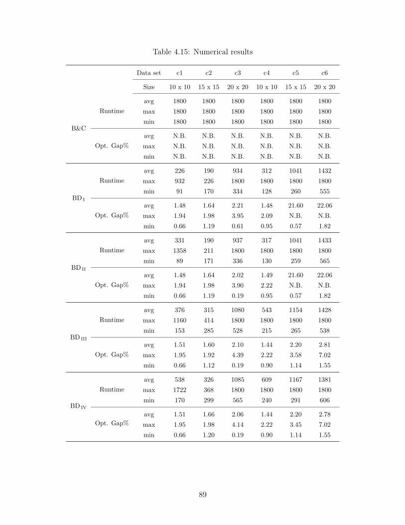
Table 4.15: Numerical results

Data set c1 c2 c3 c4 c5 c6

Size 10 x 10 15 x 15 20 x 20 10 x 10 15 x 15 20 x 20

B&C

Runtimeavg 1800 1800 1800 1800 1800 1800max 1800 1800 1800 1800 1800 1800min 1800 1800 1800 1800 1800 1800

Opt. Gap%avg N.B. N.B. N.B. N.B. N.B. N.B.max N.B. N.B. N.B. N.B. N.B. N.B.min N.B. N.B. N.B. N.B. N.B. N.B.

BD I

Runtimeavg 226 190 934 312 1041 1432max 932 226 1800 1800 1800 1800min 91 170 334 128 260 555

Opt. Gap%avg 1.48 1.64 2.21 1.48 21.60 22.06max 1.94 1.98 3.95 2.09 N.B. N.B.min 0.66 1.19 0.61 0.95 0.57 1.82

BD II

Runtimeavg 331 190 937 317 1041 1433max 1358 211 1800 1800 1800 1800min 89 171 336 130 259 565

Opt. Gap%avg 1.48 1.64 2.02 1.49 21.60 22.06max 1.94 1.98 3.90 2.22 N.B. N.B.min 0.66 1.19 0.19 0.95 0.57 1.82

BD III

Runtimeavg 376 315 1080 543 1154 1428max 1160 414 1800 1800 1800 1800min 153 285 528 215 265 538

Opt. Gap%avg 1.51 1.60 2.10 1.44 2.20 2.81max 1.95 1.92 4.39 2.22 3.58 7.02min 0.66 1.12 0.19 0.90 1.14 1.55

BD IV

Runtimeavg 538 326 1085 609 1167 1381max 1722 368 1800 1800 1800 1800min 170 299 565 240 291 606

Opt. Gap%avg 1.51 1.66 2.06 1.44 2.20 2.78max 1.95 1.98 4.14 2.22 3.45 7.02min 0.66 1.20 0.19 0.90 1.14 1.55

89

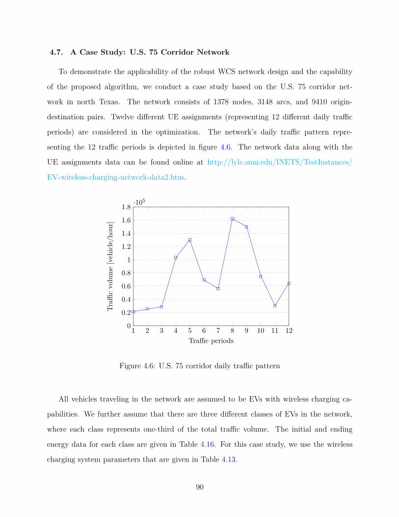
4.7. A Case Study: U.S. 75 Corridor Network

To demonstrate the applicability of the robust WCS network design and the capability

of the proposed algorithm, we conduct a case study based on the U.S. 75 corridor net-

work in north Texas. The network consists of 1378 nodes, 3148 arcs, and 9410 origin-

destination pairs. Twelve different UE assignments (representing 12 different daily traffic

periods) are considered in the optimization. The network’s daily traffic pattern repre-

senting the 12 traffic periods is depicted in figure 4.6. The network data along with the

UE assignments data can be found online at http://lyle.smu.edu/INETS/TestInstances/

EV-wireless-charging-network-data2.htm.

1 2 3 4 5 6 7 8 9 10 11 120

0.2

0.4

0.6

0.8

1

1.2

1.4

1.6

1.8 ·105

Traffic periods

Traffi

cvo

lum

e[v

ehic

le/h

our]

Figure 4.6: U.S. 75 corridor daily traffic pattern

All vehicles traveling in the network are assumed to be EVs with wireless charging ca-

pabilities. We further assume that there are three different classes of EVs in the network,

where each class represents one-third of the total traffic volume. The initial and ending

energy data for each class are given in Table 4.16. For this case study, we use the wireless

charging system parameters that are given in Table 4.13.

90

Table 4.16: EV classes data

γ ie ee

EV class D 40 40 35EV class E 40 30 25EV class F 40 25 15

To observe the differences between the robust solution and the single-period solutions

obtained when considering each traffic period individually, we first solve a single period

problem for each traffic period (s1 to s12) individually. Then we solve the robust model

considering all 12 traffic periods together. The optimization results are provided in Table

4.17 and depicted in Figures 4.7, 4.8 and 4.9. Specifically, Table 4.17 and the two figures

4.8 and 4.9 show, for each component of the total cost, a comparison between the robust

solution and the individual single-period solutions. The results show that the cost of the

robust solution is $M43.21 (%38.32) higher than the optimal cost under the morning peak

period (s5). As illustrated in Figure 4.8, the biggest portion of this difference ($M34.61)

is associated with the charging cost, while the construction cost and the power installation

cost account for $M2.98 and $M5.62 of the difference, respectively.

Comparing the robust solution to the solution of the evening peak period (s8) tells a

different story. The difference here is only $M3.61 (%3.2). Figure 4.8 shows that this

difference is mainly due to the construction cost and the power installations cost.

To better recognize the differences between the robust solution and the individual single-

period solutions, we repeat the optimization while considering a new value for parameter %.

Specifically, we consider % = 50. The new results are provided in Table 4.18 and depicted

in Figure 4.10 and Figure 4.11. The results show that under the new value of parameter

%, the relative differences between the cost of the robust solution and the costs of the two

peak periods solutions are significantly higher than the first case. Specifically, the total

cost of the robust solution is %40.51 and %11.67 higher than the costs associated with

the individual single-period solutions under the morning peak period and the evening peak

91

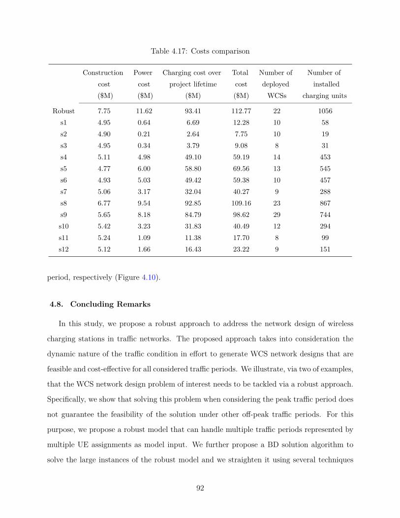
Table 4.17: Costs comparison

Construction Power Charging cost over Total Number of Number ofcost cost project lifetime cost deployed installed($M) ($M) ($M) ($M) WCSs charging units

Robust 7.75 11.62 93.41 112.77 22 1056s1 4.95 0.64 6.69 12.28 10 58s2 4.90 0.21 2.64 7.75 10 19s3 4.95 0.34 3.79 9.08 8 31s4 5.11 4.98 49.10 59.19 14 453s5 4.77 6.00 58.80 69.56 13 545s6 4.93 5.03 49.42 59.38 10 457s7 5.06 3.17 32.04 40.27 9 288s8 6.77 9.54 92.85 109.16 23 867s9 5.65 8.18 84.79 98.62 29 744s10 5.42 3.23 31.83 40.49 12 294s11 5.24 1.09 11.38 17.70 8 99s12 5.12 1.66 16.43 23.22 9 151

period, respectively (Figure 4.10).

4.8. Concluding Remarks

In this study, we propose a robust approach to address the network design of wireless

charging stations in traffic networks. The proposed approach takes into consideration the

dynamic nature of the traffic condition in effort to generate WCS network designs that are

feasible and cost-effective for all considered traffic periods. We illustrate, via two of examples,

that the WCS network design problem of interest needs to be tackled via a robust approach.

Specifically, we show that solving this problem when considering the peak traffic period does

not guarantee the feasibility of the solution under other off-peak traffic periods. For this

purpose, we propose a robust model that can handle multiple traffic periods represented by

multiple UE assignments as model input. We further propose a BD solution algorithm to

solve the large instances of the robust model and we straighten it using several techniques

92

Table 4.18: Costs comparison

Construction Power Charging cost over Total Number of Number ofcost cost project lifetime cost deployed installed($M) ($M) ($M) ($M) WCSs charging units

Robust 29.42 11.65 93.42 134.48 49 1059s1 18.51 0.67 6.70 25.89 22 61s2 18.54 0.29 2.59 21.42 24 26s3 18.50 0.39 3.78 22.67 24 35s4 17.90 5.16 49.14 72.21 27 469s5 15.85 6.27 58.81 80.93 27 570s6 18.02 5.14 49.47 72.63 24 467s7 19.74 3.31 32.09 55.15 26 301s8 15.67 9.91 93.21 118.79 30 901s9 16.18 8.80 84.94 109.92 49 800s10 20.03 3.34 31.80 55.17 26 304s11 20.05 1.14 11.38 32.58 27 104s12 19.79 1.68 16.40 37.87 27 153

including surrogate constraints, cut strengthening, and an upper bound heuristic. We provide

an extensive computational experiment illustrating the effectiveness of each strengthening

technique individually. Finally, we illustrate the applicability of the robust approach by

conducting a case study on real traffic network from Dallas, TX where we compare the

robust optimal solution to the single-period optimal solutions obtained individually for each

traffic period. We further analyze the difference in the total system implementation cost

between the robust optimal solution and the single-period optimal solutions, and we explain

how the different components of the total cost differ between the two cases.

93

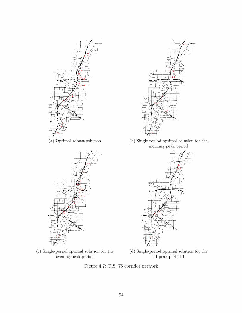
(a) Optimal robust solution (b) Single-period optimal solution for themorning peak period

(c) Single-period optimal solution for theevening peak period

(d) Single-period optimal solution for theoff-peak period 1

Figure 4.7: U.S. 75 corridor network

94

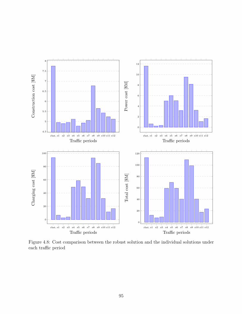
rbst. s1 s2 s3 s4 s5 s6 s7 s8 s9 s10 s11 s124.5

5

5.5

6

6.5

7

7.5

8

Traffic periods

Con

stru

ctio

nco

st[$

M]

rbst. s1 s2 s3 s4 s5 s6 s7 s8 s9 s10 s11 s12

0

2

4

6

8

10

12

Traffic periods

Powe

rco

st[$

M]

rbst. s1 s2 s3 s4 s5 s6 s7 s8 s9 s10 s11 s12

0

20

40

60

80

100

Traffic periods

Cha

rgin

gco

st[$

M]

rbst. s1 s2 s3 s4 s5 s6 s7 s8 s9 s10 s11 s12

0

20

40

60

80

100

120

Traffic periods

Tota

lcos

t[$

M]

Figure 4.8: Cost comparison between the robust solution and the individual solutions undereach traffic period

95

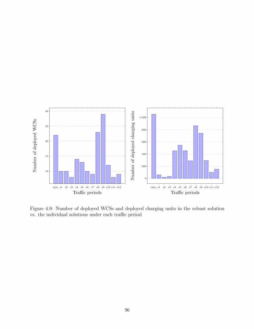
rbst. s1 s2 s3 s4 s5 s6 s7 s8 s9 s10 s11 s12

10

15

20

25

30

Traffic periods

Num

ber

ofde

ploy

edW

CSs

rbst. s1 s2 s3 s4 s5 s6 s7 s8 s9 s10 s11 s12

0

200

400

600

800

1,000

Traffic periods

Num

ber

ofde

ploy

edch

argi

ngun

its

Figure 4.9: Number of deployed WCSs and deployed charging units in the robust solutionvs. the individual solutions under each traffic period

96

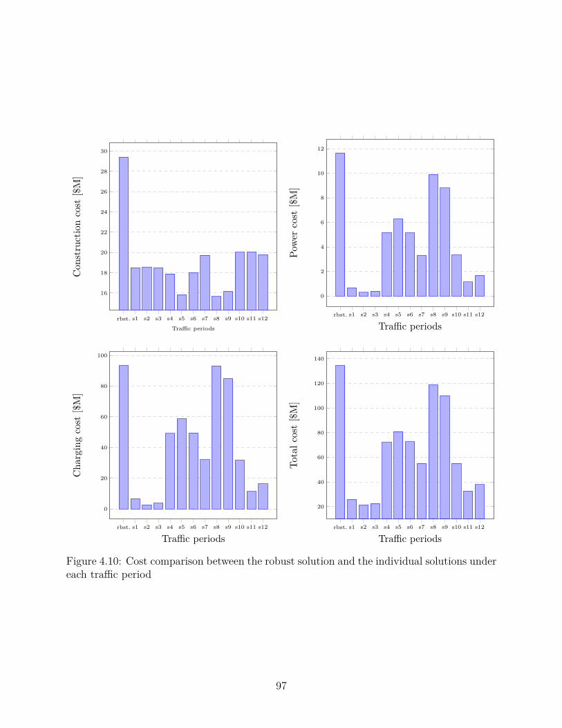
rbst. s1 s2 s3 s4 s5 s6 s7 s8 s9 s10 s11 s12

16

18

20

22

24

26

28

30

Traffic periods

Con

stru

ctio

nco

st[$

M]

rbst. s1 s2 s3 s4 s5 s6 s7 s8 s9 s10 s11 s12

0

2

4

6

8

10

12

Traffic periods

Powe

rco

st[$

M]

rbst. s1 s2 s3 s4 s5 s6 s7 s8 s9 s10 s11 s12

0

20

40

60

80

100

Traffic periods

Cha

rgin

gco

st[$

M]

rbst. s1 s2 s3 s4 s5 s6 s7 s8 s9 s10 s11 s12

20

40

60

80

100

120

140

Traffic periods

Tota

lcos

t[$

M]

Figure 4.10: Cost comparison between the robust solution and the individual solutions undereach traffic period

97

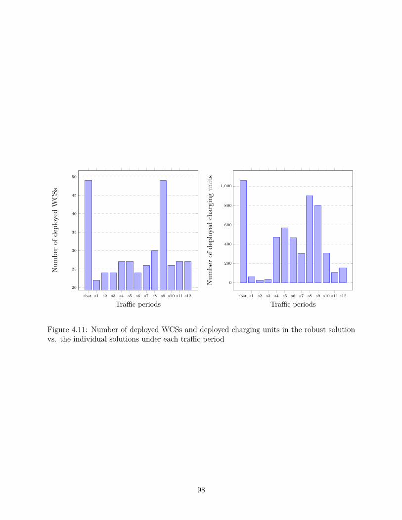
rbst. s1 s2 s3 s4 s5 s6 s7 s8 s9 s10 s11 s12

20

25

30

35

40

45

50

Traffic periods

Num

ber

ofde

ploy

edW

CSs

rbst. s1 s2 s3 s4 s5 s6 s7 s8 s9 s10 s11 s12

0

200

400

600

800

1,000

Traffic periods

Num

ber

ofde

ploy

edch

argi

ngun

its

Figure 4.11: Number of deployed WCSs and deployed charging units in the robust solutionvs. the individual solutions under each traffic period

98

Chapter 5

UTILIZING WIRELESS CHARGING OF ELECTRIC VEHICLES TO IMPROVE

TRAFFIC ASSIGNMENTS IN CONGESTED NETWORKS

5.1. Introduction

Traffic congestion remains to be a serious threat to economic prosperity and quality of

life in urban areas. A recent study estimated the cost of congestion across 25 major cities in

the U.S. to reach $480 billion over the next decade [51]. Lost time and wasted fuel are major

components of this cost. From a transportation planning point of view, congestion can be

reduced via an efficient utilization of the road network which can only be achieved if travelers

cooperate with one another. However, acting on self-interests, travelers select their routes in

a way that minimizes their individual travel times under the traffic condition. According to

Wardrop’s first principle, this behavior leads the road network into a state of user equilibrium

(UE) where travel times on all used routes between a certain origin-destination pair are equal

[63]. Nevertheless, from a system perspective, UE does not necessarily represent the most

efficient utilization of the road network. That is, the traffic assignment that minimizes the

total travel time in the system usually differs from UE, and is referred to as the system

optimal (SO) traffic assignment. In that sense, UE is considered to be a “selfish” optimal

assignment, while SO is the socially optimal one. The difference between the two traffic

assignments (UE and SO) is best illustrated in the well known Braess Paradox [7] [8].

To shift traffic flows from UE toward SO, traffic planners may encourage traffic redistri-

bution by imposing tolls on certain road segments. The imposed tolls disturb the existing

UE assignment as they motivate a portion of users to change their routes. The principle of

toll pricing dictates that an optimal tolling policy is designed such that the tolled UE traffic

assignment is an un-tolled system optimal [3]. Alternatively, traffic planners can encourage a

99

portion of travelers to change their routing behavior by offering incentives as “negative tolls.”

These incentives can include cash, store credit, or HOV (high-occupancy vehicle) passes [38].

For EV drivers, an opportunity to recharge while traveling could be viewed as a great

incentive as it helps them reduce their range anxiety. Therefore, a route that offers wireless

charging might seem more attractive than another route with a similar (or even shorter)

travel time but does not offer the same service. This “attractiveness” of electrified road

segments could be viewed as a negative toll and can be utilized to influence the traffic flows

in congested networks. Motivated by this idea, we propose the concept of utilizing wireless

charging stations (WCS) as a traffic redistribution tool to influence the travel behavior of EV

drivers in an effort to achieve system optimality. Specifically, in contrast to our approach

in the previous chapters, which maintains the UE traffic assignment, in this chapter, we

study a deployment plan of WCSs that does disturb UE and induce the traffic flows to shift

toward SO. To that end, in what follows we propose a mathematical model to optimize the

deployment plan of WCSs with the objective of minimizing the total travel time in the traffic

network.

The rest of this chapter is organized as follows: In Section 5.2, we present the formulations

of the traffic assignment models including the multiclass UE and SO. In Section 5.3, we

provide the definition and formulation of the problem of interest. In Section 5.4 we illustrate

the applicability of the proposed approach on the famous Braess Network. In Section 5.5

we provide another example to illustrate our approach by testing the proposed model on

Nguyen-Dupuis network.

5.2. Definitions and Background

To set the stage for our problem definition, we start by presenting the formulations of

two traffic assignment models including UE and SO. We consider a directed graph G(N ,A)

representing a traffic network with N representing the set of nodes and A representing the

set of arcs. For a better representation of the real life application, we consider two classes

of vehicles traveling in a traffic network: conventional vehicles (CVs), and electric vehicles

100

(EVs). We now introduce the following notations.

Sets:

A set of arcs, a ∈ A

Q set of all OD-pairs within the network, q ∈ Q

Rq set of routes connecting a certain OD-pair q, r ∈ Rq

K set of vehicle classes, k ∈ K

Parameters:

dkq travel demands of class k ∈ K between OD pair q ∈ Q

δra an indicator with value of one if arc a is part of route r, 0 otherwise, a ∈ A, r ∈

Rq, q ∈ Q

Decision Variables:

vka traffic flow of class k ∈ K on arc a ∈ A

va traffic flow on arc a ∈ A

ta travel time on arc a ∈ A

uka disutility of on arc a for a vehicle of class k, a ∈ A, k ∈ K

fkr traffic flow of class k ∈ K on route r ∈ Rq, q ∈ Q

ukr disutility of route r for a vehicle of class k, r ∈ Rq, q ∈ Q, k ∈ K

5.2.1. User Equilibrium (UE)

According to Wardrop [63], if drivers are completely aware of the current traffic condition,

they will act on their self interest and select a route that will minimize their individual travel

disutility. Such behavior leads the traffic network into a steady-state of UE where no driver

101

can improve her travel disutility by changing her route. Wardrop [63] describes this steady-

state, between each OD-pair in the network, in his first principle which reads:

The journey times on all routes actually used are equal, and less than those which

would be experienced by a single vehicle on any unused route.

Let travel times define travel disutilities on arcs. To handle the two classes of vehicles

(CVs and EVs), we consider a multiclass UE formulation as introduced by [46]. Given the

above notations, the time-dependent multiclass user equilibrium formulation is given as

∑r∈Rq

fkr = dkq ∀ q ∈ Q, k ∈ K (5.1)

vka =∑q∈Q

∑r∈Rq

δra fkr ∀ a ∈ A, k ∈ K (5.2)

va =∑k∈K

vka ∀ a ∈ A (5.3)

ta = f(va) ∀ a ∈ A (5.4)

ukr =∑a∈A

δra ta ∀ r ∈ Rq, q ∈ Q, k ∈ K (5.5)

ukr

= λkr if fkr > 0

≤ λkr if fkr = 0∀ r ∈ Rq, q ∈ Q, k ∈ K (5.6)

vka , va, fkr , ta, u

kr ≥ 0 ∀ a ∈ A, r ∈ Rq, q ∈ Q, k ∈ K (5.7)

The first three sets of constraints are flow conservation constraints. Constraints (5.1) indicate

that the traffic demands of each class of vehicles between each OD pair is equal to the sum

of the flows of that class on all the routes connecting the OD pair. Constraints (5.2) dictate

that the traffic flow of each class of vehicles on each arc is equal to the sum of the flows

of that class on each route that contains that arc. Constraints (5.3) indicate that the total

traffic flow on each arc is equal to the sum of the flows of all classes of vehicles on that arc.

Constraints (5.4) represent the travel time function associated with each arc. Constraints

(5.5) state that the travel disutility of each route is equal to the summation of the travel

102

times of all the arcs that form the route. Constraints (5.6) are the multiclass equilibrium

constraint following Wardrop’s first principle, stating that all used routes between an OD

pair have equal and minimal travel disutility. Finally, constraints (5.7) are the non-negativity

constraints.

5.2.2. System Optimal (SO)

SO traffic assignment aims to minimize congestion in the traffic network. Therefore, in

contrast to UE, SO assignment minimizes the travel time for the whole system rather than

the individual travel times for drivers. This traffic assignment is based on Wardrop’s second

principle which describes SO as the traffic assignment where

The average journey time is a minimum [63].

Reaching the state of SO can be achieved if drivers cooperate with one another. The math-

ematical formulation for SO is given as

Minimize∑a∈A

va ta (5.8)

subject to (5.1) - (5.5), and (5.7)

Note that (5.6) is not a part of the SO formulation since SO is not associated with

equilibrium condition.

SO is not behaviorally realistic. However, understanding SO helps traffic planning entities

to design the appropriate traffic management tools and regulations that could potentially

shift the traffic flows from UE toward SO, and therefore minimize congestion.

5.3. Problem Definition and Formulation

We consider a traffic network, as defined above, with conventional vehicles and electric

vehicles, i.e., K = CV,EV . For simplicity and without loss of generality, all EVs in the

network are assumed to be capable of wireless charging. For CVs, we let travel times define

103

travel disutilities of arcs. By contrast, for EVs, the availability of a WCS on a certain arc

lessens the arc’s disutility. Therefore, we define a non-positive parameter αEV to represent

the attractiveness of a WCS for EVs, measured in time value (TV). Accordingly, we define

travel disutility for EVs, on electrified arcs, by the summation of travel time and parameter

αEV . Since αEV is non-positive by definition, locating a WCS on a given arc can only decrease

the arc’s disutility for EVs. On the other hand, travel disutilities of un-electrified arcs are

considered to be equal to the travel times of these arcs. Clearly, for CVs, the attractiveness

of a WCS, αCV , is equal to zero.

Based on the above definition of travel disutility, the deployment of WCSs in the network

will adjust travel disutilities of arcs for EVs. Therefore, motivated by the attractiveness of

the deployed infrastructure, EV drivers will select new routes to minimize their adjusted

individual travel disutilities. That is, the infrastructure deployment plan could potentially

disturb the existing UE and lead to a new UE based on the new disutilities vector1. Our

objective is to determine the WCSs deployment plan that disturbs the existing UE in such

a way that new UE assignment is shifted toward SO. Specifically, we optimize the number

and the locations of WCSs in the network in such a way that minimizes the total travel time

(system time) associated with the new UE which results as a response to the deployment of

the WCSs.

In contrast to the toll pricing problem where the flows vector is fixed (set equal to SO

flows vector) and the tolls are optimized to achieve the fixed flows, in this framework we

optimize the flow and the locations of WCSs based on presumed values of the attractiveness

of WCS (negative toll). To that end, we introduce a binary variable xa equal to one if a

WCS is installed on arc a, zero otherwise. Accordingly, our problem can be formulated as

follows:

1unless all used routes in the network are served as discussed in the previous two chapters.

104

Minimize∑a∈A

va ta (5.9)

subject to∑r∈Rq

fkr = dkq ∀ q ∈ Q, k ∈ K (5.10)

vka =∑q∈Q

∑r∈Rq

δra fkr ∀ a ∈ A, k ∈ K (5.11)

va =∑k∈K

vka ∀ a ∈ A (5.12)

ta = f(va) ∀ a ∈ A (5.13)

uka = ta + αk xa ∀ a ∈ A k ∈ K (5.14)

ukr =∑a∈A

δra uka ∀ r ∈ Rq, q ∈ Q, k ∈ K (5.15)

ukr

= λkr if fkr > 0

≤ λkr if fkr = 0∀ r ∈ Rq, q ∈ Q, k ∈ K (5.16)

vka , va, fkr , ta, u

ka u

kr ≥ 0, xa ∈ 0, 1 ∀ a ∈ A, r ∈ Rq, q ∈ Q, k ∈ K (5.17)

The objective function (5.9) minimizes the total travel time in the system. Constraints

(5.10), (5.11), and (5.12) are the flow conservation constraints as defined in 5.2.1. Constraints

(5.13) are the travel time function constraints. Constraints (5.14) are the arc disutility

constraints for each class of vehicles. Since αEV is non-positive by definition, triggering the

binary variable xa (installing a WCS on arc a) reduces the disutility of the arc for EVs by

αEV units of time. Constraints (5.15) are the route disutility constraint for each class of

vehicles. Constraints (5.16) are the multiclass UE condition as defined in 5.2.1. Finally,

Constraints (5.17) provide the structural requirements of the model.

The logic of our formulation can be described as follows. The objective of the model is

105

to regulate the traffic in the network in a way that shifts the traffic assignment form UE

toward SO. Because our goal is to get as close as possible to SO, we adopt the objective

function associated with SO, i.e., minimizing the total travel time in the system. The flows

conservation constraints are required to obtain feasible assignments. The UE constraint is

adopted because the traffic will regulate itself, after the WCS deployment, to reach a new

UE. The key in our model, is constraint (5.14). Specifically, the model will trigger variables

xa to reduce the disutilities of some arcs for EVs. As a response to the reduction in traffic

disutility for EVs, a new UE must emerge in order for the UE constraint (5.16) to hold.

And since the disutilities ua, the volumes va, and the travel times ta are interconnected via

constraints (5.13) and (5.14), triggering variables xij leads to adjustments in variables va and

variables ta. Thus, the model uses variables xij as regulates to adjust the values of variables

va and variables ta in order to minimize the value of the objective function.

Note that the model formulation is nonlinear due to the nonlinear objective (5.9), and

the UE constraint (5.16). Furthermore, depending on the netowrk under study, the travel

time function (5.13) could also be nonlinear as we assume in a later example.

In what follows, we put the model to work and illustrate its applicability vie two examples.

5.4. Illustrating Example - Single OD Network

To illustrate the proposed approach, we apply our model on the well known Braess

network (Figure 5.1). The network contains four nodes and five arcs. A hundred travelers

are assumed to be traveling from node A to node D. The labels on the arcs represent the

assumed travel time functions adopted from [15]. The optimal flows and travel times

associated with both UE and SO are presented in Tables 5.1 and 5.2. As shown in the

Tables, UE assigns 25 vehicles to route ABD, 50 vehicles to route ABCD, and 25 vehicles

to route ACD. As a result of this assignment, the travel time on each route is equal to 3.75

time units. The total travel time in the system is equal to (75 × 1.75) + (25 × 2) + (50 ×

0.25) + (25× 2) + (75× 1.75) = 375 time units. By contrast, SO assigns 50 vehicles to route

ABD and 50 vehicles to route ACD. No vehicle is assigned to route ABCD. As a result, the

106

B

A

C

D

2va

100 + 1

0.25

2 va100 + 1

Figure 5.1: Braess network

travel times on the used routes drop to 3.5 time units, and the total travel time in the system

drops to (50× 1.5) + (50× 2) + (0× 0.25) + (50× 2) + (50× 1.5) = 350 time units.

Table 5.1: Routes flows and travel times under UE and SO - Braess network

User Equilibrium System Optimal

fr tr fr tr

ABD 25 3.75 50 3.5ABCD 50 3.75 0 3.25ACD 25 3.75 50 3.5

Table 5.2: Arcs flows and travel times under UE and SO - Braess network

User Equilibrium System Optimal

va ta va ta

AB 75 1.75 50 1.5AC 25 2 50 2BC 50 0.25 0 0.25BD 25 2 50 2CD 75 1.75 50 1.5

In this example, we assume an electric vehicle penetration rate (EVPR) of 50%, i.e.,

dEVAD = dCVAD = 50. We further assume that αEV = −0.25. We use COUENNE (which is a

107

solver designed to solve MINLPs with nonlinear objective function) to solve our proposed

model considering the network at hand [5]. The solution is depicted in Figure 5.2 where the

dashed red arc represents a WCS. The flows, travel times, and disutilities associated with

the solution are presented in Tables 5.3 and 5.4.

B

A

C

D

jiRoad iWCS j

Figure 5.2: WCS deployment plan - Braess network

Table 5.3: Routes flows, travel times, and disutilities under the WCS deployment plan

fEVr fCVr fr tr uEVr uCVr

ABD 50 0 50 3.75 3.5 3.75ABCD 0 25 25 3.5 3.5 3.5ACD 0 25 25 3.5 3.5 3.5

Table 5.4: Arcs flows, travel times, and disutilities under the WCS deployment plan

vEVa vCVa va ta uEVa uCVa

AB 50 25 75 1.75 1.75 1.75AC 0 25 25 2 2 2BC 0 25 25 0.25 0.25 0.25BD 50 0 50 2 1.75 2CD 0 50 50 1.5 1.5 1.5

108

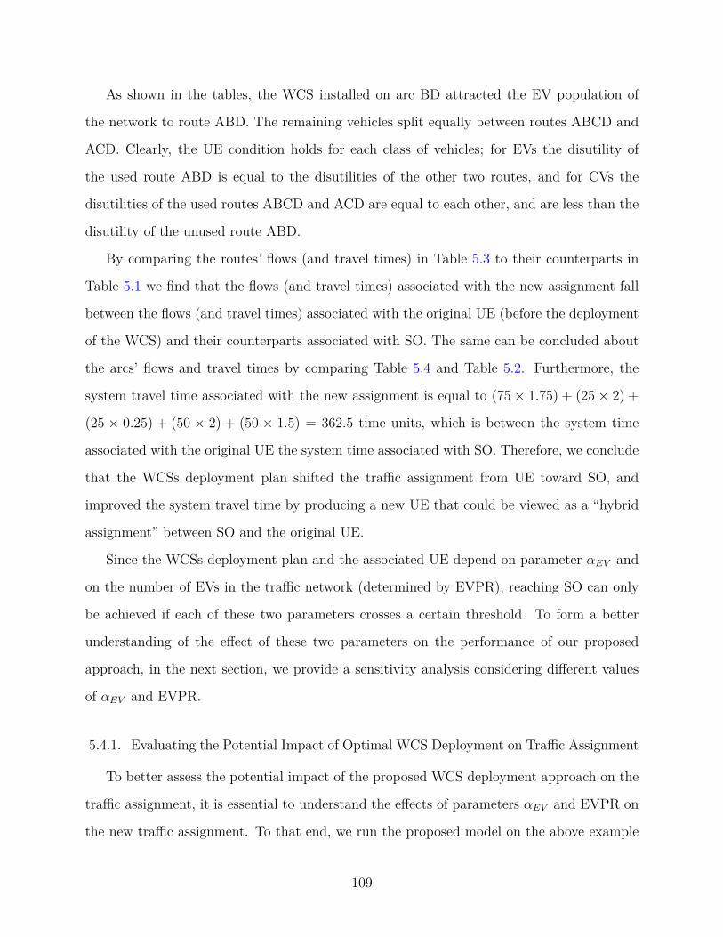
As shown in the tables, the WCS installed on arc BD attracted the EV population of

the network to route ABD. The remaining vehicles split equally between routes ABCD and

ACD. Clearly, the UE condition holds for each class of vehicles; for EVs the disutility of

the used route ABD is equal to the disutilities of the other two routes, and for CVs the

disutilities of the used routes ABCD and ACD are equal to each other, and are less than the

disutility of the unused route ABD.

By comparing the routes’ flows (and travel times) in Table 5.3 to their counterparts in

Table 5.1 we find that the flows (and travel times) associated with the new assignment fall

between the flows (and travel times) associated with the original UE (before the deployment

of the WCS) and their counterparts associated with SO. The same can be concluded about

the arcs’ flows and travel times by comparing Table 5.4 and Table 5.2. Furthermore, the

system travel time associated with the new assignment is equal to (75× 1.75) + (25× 2) +

(25 × 0.25) + (50 × 2) + (50 × 1.5) = 362.5 time units, which is between the system time

associated with the original UE the system time associated with SO. Therefore, we conclude

that the WCSs deployment plan shifted the traffic assignment from UE toward SO, and

improved the system travel time by producing a new UE that could be viewed as a “hybrid

assignment” between SO and the original UE.

Since the WCSs deployment plan and the associated UE depend on parameter αEV and

on the number of EVs in the traffic network (determined by EVPR), reaching SO can only

be achieved if each of these two parameters crosses a certain threshold. To form a better

understanding of the effect of these two parameters on the performance of our proposed

approach, in the next section, we provide a sensitivity analysis considering different values

of αEV and EVPR.

5.4.1. Evaluating the Potential Impact of Optimal WCS Deployment on Traffic Assignment

To better assess the potential impact of the proposed WCS deployment approach on the

traffic assignment, it is essential to understand the effects of parameters αEV and EVPR on

the new traffic assignment. To that end, we run the proposed model on the above example

109

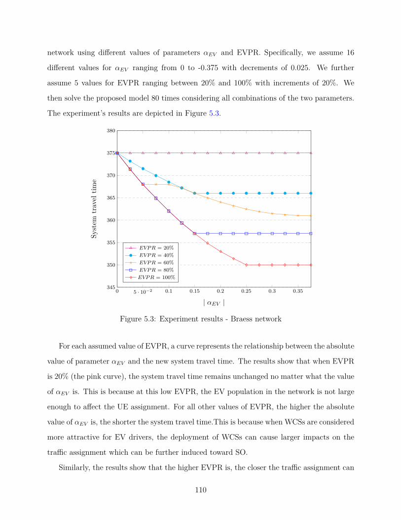
network using different values of parameters αEV and EVPR. Specifically, we assume 16

different values for αEV ranging from 0 to -0.375 with decrements of 0.025. We further

assume 5 values for EVPR ranging between 20% and 100% with increments of 20%. We

then solve the proposed model 80 times considering all combinations of the two parameters.

The experiment’s results are depicted in Figure 5.3.

0 5 · 10−2 0.1 0.15 0.2 0.25 0.3 0.35345

350

355

360

365

370

375

380

| αEV |

Syst

emtr

avel

time

EVPR = 20%EVPR = 40%EVPR = 60%EVPR = 80%EVPR = 100%

Figure 5.3: Experiment results - Braess network

For each assumed value of EVPR, a curve represents the relationship between the absolute

value of parameter αEV and the new system travel time. The results show that when EVPR

is 20% (the pink curve), the system travel time remains unchanged no matter what the value

of αEV is. This is because at this low EVPR, the EV population in the network is not large

enough to affect the UE assignment. For all other values of EVPR, the higher the absolute

value of αEV is, the shorter the system travel time.This is because when WCSs are considered

more attractive for EV drivers, the deployment of WCSs can cause larger impacts on the

traffic assignment which can be further induced toward SO.

Similarly, the results show that the higher EVPR is, the closer the traffic assignment can

110

get to SO; in this example, when EVPR is 100%, the traffic assignment can be completely

shifted to SO and the system travel times can drop to 350.

To summarize, the results show a dependency between the potential impact of WCS

deployment on traffic assignment and the two parameters αEV and EVPR; in this example,

the more attractive WCSs are considered by EV drivers, and the larger the population of EVs

in the network is, the higher the potential impact of WCS deployment on traffic assignment.

5.5. Illustrating Example - Multi-OD Network

To form a deeper understanding of the effect of both αEV and EVPR on the system

travel time, we further test our model on the Nguyen-Dupuis network - an extensively used

network in the transportation literature (Figure 5.4).

1 12

654

9 10

7 8

11 2

13 3

2

1

3

4

5

6

7

8

9

10

14 15

11

18

13

12

19

15

16

17

Figure 5.4: Nguyen-Dupuis network

We consider two OD pairs including (1-3) and (4-2). We further consider an asymmetric

affine travel time function, adopted from Nguyen and Dupuis [48], of the form: ta = ca va+ba,

where ca and ba are both input parameters. The values of parameters ca and ba are provided

in Table 5.5. The travel demands are given in Table 5.6. The optimal flows and travel times

111

associated with UE and SO are given in Tables 5.7 and 5.8.

Table 5.5: Arcs and their associated parameters - Nguyen-Dupuis network

arc origin destination ca ba

1 1 5 0.0125 72 1 12 0.01 93 4 5 0.01 94 4 9 0.005 125 5 6 0.0075 36 5 9 0.0075 97 6 7 0.0125 58 6 10 0.005 139 7 8 0.0125 510 7 11 0.0125 911 8 2 0.0125 912 9 10 0.005 1013 9 13 0.005 914 10 11 0.0025 615 11 2 0.005 916 11 3 0.01 817 12 6 0.0025 718 12 8 0.01 1419 13 3 0.01 11

Table 5.6: Travel demands - Nguyen-Dupuis network

OD travel demands

(1-3) 80(4-2) 60

We assume 7 different values for parameter αEV ranging from 0 to -1.5 with decrements of

0.25. We further consider 5 values for EVPR ranging between 20% and 100% with increments

112

Table 5.7: Arcs flows and travel times under UE and SO - Nguyen-Dupuis network

User Equilibrium System Optimal

arc va ta va ta

1 80.00 8.00 80.00 8.002 0.00 9.00 0.00 9.003 60.00 9.60 43.42 9.434 0.00 12.00 16.58 12.085 130.77 3.98 88.52 3.666 9.23 9.07 34.90 9.267 130.77 6.63 88.52 6.118 0.00 13.00 0.00 13.009 60.00 5.75 43.42 5.5410 70.77 9.88 45.10 9.5611 60.00 9.75 43.42 9.5412 0.00 10.00 16.58 10.0813 9.23 9.05 34.90 9.1714 0.00 6.00 16.58 6.0415 0.00 9.00 16.58 9.0816 70.77 8.71 45.10 8.4517 0.00 7.00 0.00 7.0018 0.00 14.00 0.00 14.0019 9.23 11.09 34.90 11.35

113

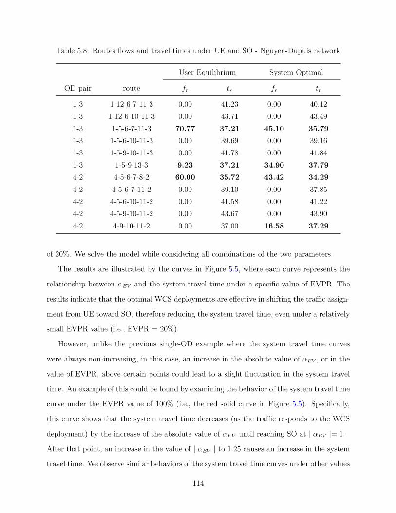
Table 5.8: Routes flows and travel times under UE and SO - Nguyen-Dupuis network

User Equilibrium System Optimal

OD pair route fr tr fr tr

1-3 1-12-6-7-11-3 0.00 41.23 0.00 40.121-3 1-12-6-10-11-3 0.00 43.71 0.00 43.491-3 1-5-6-7-11-3 70.77 37.21 45.10 35.791-3 1-5-6-10-11-3 0.00 39.69 0.00 39.161-3 1-5-9-10-11-3 0.00 41.78 0.00 41.841-3 1-5-9-13-3 9.23 37.21 34.90 37.794-2 4-5-6-7-8-2 60.00 35.72 43.42 34.294-2 4-5-6-7-11-2 0.00 39.10 0.00 37.854-2 4-5-6-10-11-2 0.00 41.58 0.00 41.224-2 4-5-9-10-11-2 0.00 43.67 0.00 43.904-2 4-9-10-11-2 0.00 37.00 16.58 37.29

of 20%. We solve the model while considering all combinations of the two parameters.

The results are illustrated by the curves in Figure 5.5, where each curve represents the

relationship between αEV and the system travel time under a specific value of EVPR. The

results indicate that the optimal WCS deployments are effective in shifting the traffic assign-

ment from UE toward SO, therefore reducing the system travel time, even under a relatively

small EVPR value (i.e., EVPR = 20%).

However, unlike the previous single-OD example where the system travel time curves

were always non-increasing, in this case, an increase in the absolute value of αEV , or in the

value of EVPR, above certain points could lead to a slight fluctuation in the system travel

time. An example of this could be found by examining the behavior of the system travel time

curve under the EVPR value of 100% (i.e., the red solid curve in Figure 5.5). Specifically,

this curve shows that the system travel time decreases (as the traffic responds to the WCS

deployment) by the increase of the absolute value of αEV until reaching SO at | αEV |= 1.

After that point, an increase in the value of | αEV | to 1.25 causes an increase in the system

travel time. We observe similar behaviors of the system travel time curves under other values

114

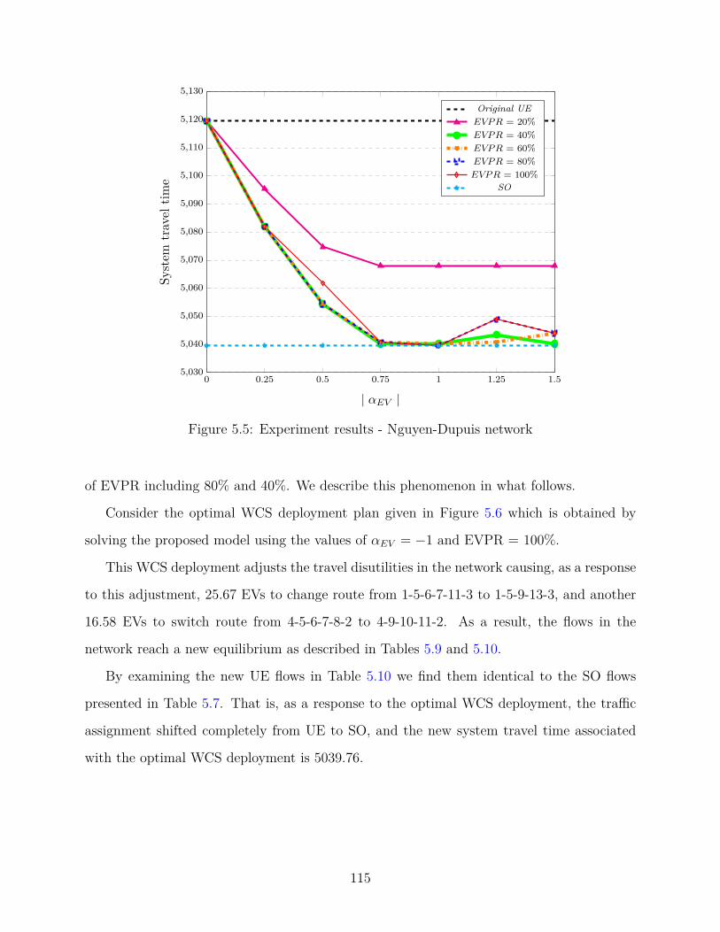
0 0.25 0.5 0.75 1 1.25 1.55,030

5,040

5,050

5,060

5,070

5,080

5,090

5,100

5,110

5,120

5,130

| αEV |

Syst

emtr

avel

time

Original UEEVPR = 20%EVPR = 40%EVPR = 60%EVPR = 80%EVPR = 100%

SO

Figure 5.5: Experiment results - Nguyen-Dupuis network

of EVPR including 80% and 40%. We describe this phenomenon in what follows.

Consider the optimal WCS deployment plan given in Figure 5.6 which is obtained by

solving the proposed model using the values of αEV = −1 and EVPR = 100%.

This WCS deployment adjusts the travel disutilities in the network causing, as a response

to this adjustment, 25.67 EVs to change route from 1-5-6-7-11-3 to 1-5-9-13-3, and another

16.58 EVs to switch route from 4-5-6-7-8-2 to 4-9-10-11-2. As a result, the flows in the

network reach a new equilibrium as described in Tables 5.9 and 5.10.

By examining the new UE flows in Table 5.10 we find them identical to the SO flows

presented in Table 5.7. That is, as a response to the optimal WCS deployment, the traffic

assignment shifted completely from UE to SO, and the new system travel time associated

with the optimal WCS deployment is 5039.76.

115

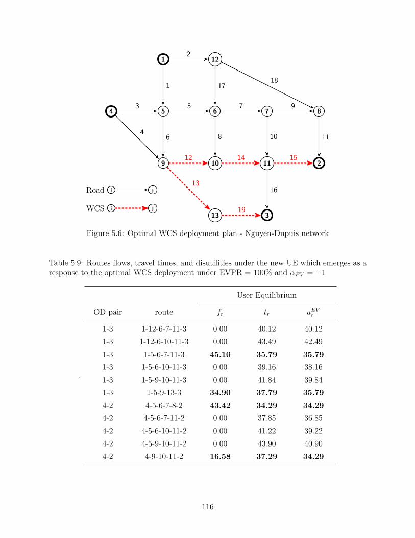
1 12

654

9 10

7 8

11 2

13 3iWCS j

iRoad j

2

1

3

4

5

6

7

8

9

10

14

11

18

13

12

19

15

16

17

Figure 5.6: Optimal WCS deployment plan - Nguyen-Dupuis network

Table 5.9: Routes flows, travel times, and disutilities under the new UE which emerges as aresponse to the optimal WCS deployment under EVPR = 100% and αEV = −1

.

User Equilibrium

OD pair route fr tr uEVr

1-3 1-12-6-7-11-3 0.00 40.12 40.121-3 1-12-6-10-11-3 0.00 43.49 42.491-3 1-5-6-7-11-3 45.10 35.79 35.791-3 1-5-6-10-11-3 0.00 39.16 38.161-3 1-5-9-10-11-3 0.00 41.84 39.841-3 1-5-9-13-3 34.90 37.79 35.794-2 4-5-6-7-8-2 43.42 34.29 34.294-2 4-5-6-7-11-2 0.00 37.85 36.854-2 4-5-6-10-11-2 0.00 41.22 39.224-2 4-5-9-10-11-2 0.00 43.90 40.904-2 4-9-10-11-2 16.58 37.29 34.29

116

Table 5.10: Arcs flows, travel times, and disutilities under the new UE which emerges as aresponse to the optimal WCS deployment under EVPR = 100% and αEV = −1

.

User Equilibrium

arc va ta ua

1 80.00 8.00 8.002 0.00 9.00 9.003 43.42 9.43 9.434 16.58 12.08 12.085 88.52 3.66 3.666 34.90 9.26 9.267 88.52 6.11 6.118 0.00 13.00 13.009 43.42 5.54 5.5410 45.10 9.56 9.5611 43.42 9.54 9.5412 16.58 10.08 9.0813 34.90 9.17 8.1714 16.58 6.04 5.0415 16.58 9.08 8.0816 45.10 8.45 8.4517 0.00 7.00 7.0018 0.00 14.00 14.0019 34.90 11.35 10.35

Now consider solving the model again under αEV = −1.25. In this case, the optimal

deployment plan is found to be identical to the one obtained under αEV = −1 (i.e., the

deployment plan depicted in Figure 5.6). Tables 5.11 and 5.12 provide the flows, travel

times, and disutilities associated with the new UE which emerges as a response to the

optimal deployment plan under αEV = −1.25.

Since | αEV | is higher in this case (i.e., WCS is more attractive for EVs), each WCS

attracts more EVs than the case where αEV = −1. Specifically, 4.93 additional EVs change

117

route from 1-5-6-7-11-3 to 1-5-9-13-3, and another 8.99 EVs switch route from 4-5-6-7-8-2 to

4-9-10-11-2. This behavior creates congestion on the WCS hosting arcs, and therefore, drives

the traffic assignment away from SO which is reached under αEV = −1. In this case, the new

system travel time associated with the optimal WCS deployment is 5048.97 - slightly higher

than the system travel time associated with SO (5039.76), but still, considerably lower then

the system travel time associated with the original UE (5119.54).

Table 5.11: Arcs flows, travel times, and disutilities under the new UE which emerges as aresponse to the optimal WCS deployment under EVPR = 100% and αEV = −1.25

.

User Equilibrium

arc va ta ua

1 80.00 8.00 8.002 0.00 9.00 9.003 34.43 9.34 9.344 25.57 12.13 12.135 74.61 3.56 3.566 39.83 9.30 9.307 74.61 5.93 5.938 0.00 13.00 13.009 34.43 5.43 5.4310 40.17 9.50 9.5011 34.43 9.43 9.4312 25.57 10.13 8.8813 39.83 9.20 7.9514 25.57 6.06 4.8115 25.57 9.13 7.8816 40.17 8.40 8.4017 0.00 7.00 7.0018 0.00 14.00 14.0019 39.83 11.40 10.15

118

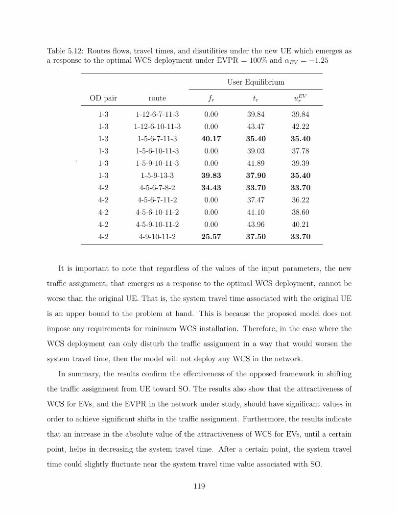
Table 5.12: Routes flows, travel times, and disutilities under the new UE which emerges asa response to the optimal WCS deployment under EVPR = 100% and αEV = −1.25

.

User Equilibrium

OD pair route fr tr uEVr

1-3 1-12-6-7-11-3 0.00 39.84 39.841-3 1-12-6-10-11-3 0.00 43.47 42.221-3 1-5-6-7-11-3 40.17 35.40 35.401-3 1-5-6-10-11-3 0.00 39.03 37.781-3 1-5-9-10-11-3 0.00 41.89 39.391-3 1-5-9-13-3 39.83 37.90 35.404-2 4-5-6-7-8-2 34.43 33.70 33.704-2 4-5-6-7-11-2 0.00 37.47 36.224-2 4-5-6-10-11-2 0.00 41.10 38.604-2 4-5-9-10-11-2 0.00 43.96 40.214-2 4-9-10-11-2 25.57 37.50 33.70

It is important to note that regardless of the values of the input parameters, the new

traffic assignment, that emerges as a response to the optimal WCS deployment, cannot be

worse than the original UE. That is, the system travel time associated with the original UE

is an upper bound to the problem at hand. This is because the proposed model does not

impose any requirements for minimum WCS installation. Therefore, in the case where the

WCS deployment can only disturb the traffic assignment in a way that would worsen the

system travel time, then the model will not deploy any WCS in the network.

In summary, the results confirm the effectiveness of the opposed framework in shifting

the traffic assignment from UE toward SO. The results also show that the attractiveness of

WCS for EVs, and the EVPR in the network under study, should have significant values in

order to achieve significant shifts in the traffic assignment. Furthermore, the results indicate

that an increase in the absolute value of the attractiveness of WCS for EVs, until a certain

point, helps in decreasing the system travel time. After a certain point, the system travel

time could slightly fluctuate near the system travel time value associated with SO.

119

5.6. Concluding Remarks

This chapter introduces a new approach to plan the deployment of WCSs in traffic net-

works. The goal of this approach is to take advantage of the attractiveness of WCSs for

EV drivers to influence their routing choices in an effort to reach system optimal traffic

assignment.

For this purpose, a new mathematical model is proposed. The model locates WCSs in

the network with the objective of minimizing the system time associated with the UE traffic

assignment which emerges as a response to the WCSs deployment.

The applicability of the proposed model is first illustrated on the well known Braess

network, and a sensitivity analysis is conducted. The results show that the optimal deploy-

ment plan produced by the model can potentially shift the traffic assignment in the network

from UE toward SO. As a response to the optimal deployment plan, the traffic redistributes,

causing a new UE to emerge. The new UE can be viewed as a “hybrid assignment” between

the original UE and SO.

The results also show that the emerged hybrid assignment gets closer to SO when the

EV population in the network is high and when WCSs are considered more attractive by EV

drivers. We further found that reaching SO can only be achieved when the EV population in

the network and the attractiveness of WCSs for EV drivers, each crosses a certain threshold.

The model is then tested on the multi-ODs Nguyen-Dupuis network, and a new sensitivity

analysis is conducted. The results confirm the effectiveness of the proposed approach in

shifting the traffic assignment from UE toward SO.

The results also provide a deeper understanding of the relationship between the attrac-

tiveness of WCS for EVs and the system travel time. Specifically, we find that an increase

in the absolute value of the attractiveness of WCS for EVs is helpful, in improving the sys-

tem travel time, until a certain point after which the system travel time begins to slightly

fluctuate.

120

Chapter 6

CONCLUSIONS AND FUTURE DIRECTIONS

In this dissertation, we present three studies, each proposing a different framework to

address the deployment of wireless charging stations in urban traffic networks.

In Chapter 3, we propose a single-period network design model to optimize the locations

and power capacities of the wireless charging stations in effort to promote EV adoption. The

objective of the proposed model is to minimize the deployment cost of the infrastructure and

the usage cost for EV drivers while producing a network design that does not disturb the

current traffic condition in the read network. To solve the large scale instances of this prob-

lem, we propose a Benders decomposition framework where we employ a combination of

classical Benders cuts and combinatorial Benders cuts for improved algorithmic effective-

ness. We further strengthen the proposed solution algorithm via utilizing different sets of

surrogate constraints and an upper bound heuristic. The efficiency of the proposed algorithm

is tested via an extensive computational experiment. We further conduct a case study using

read network data from Chicago, IL, and we perform a sensitivity analysis to investigate

the relationships between key technical parameters of the wireless charging system and the

implementation cost of the wireless charging infrastructure.

In Chapter 4, we build on the study presented in Chapter 3 to propose a robust framework

for the network design of wireless charging stations. The robust approach considers the

variability of the traffic condition and aims to produce network designs that are feasible and

cost-effective across the traffic conditions of all possible traffic periods. We provide examples

illustrating the need for a robust solution and we show that the peak traffic periods can

not be considered as bottlenecks when solving the problem of interest. We present a new

robust formulation that handles multiple traffic periods, and we propose a straightened BD

algorithm to solve the proposed model. We further propose four different algorithmic settings

121

for the proposed solution algorithm and we provide an extensive computational experiment

to evaluate the effectiveness of each strengthening technique individually. We conduct a

case study on real network data from Dallas, TX, illustrating the applicability of the robust

approach in solving the problem of interest.

Finally, in Chapter 5 we present a new framework for the deployment of wireless charging

stations with the aim of improving the traffic conditions in congested networks by taking

advantage of the attractiveness of wireless charging for EV drivers. In effort to shift the

traffic assignment from the selfish-optimal UE to the socially-optimal SO, we propose a new

mathematical formulation that deploys wireless charging stations in a way that influences

the routing choices of EV drivers in effort to improve the traffic condition. We illustrate

the applicability of the proposed model on the well-known Braess network and we conduct a

sensitivity analysis to determine the conditions that would shift the traffic completely from

UE to SO.

The first two studies in this dissertation can be extended to incorporate static charging

facilities along with the in-motion wireless charging stations. The formulations can also be

extended to account for uncertainty in initial and ending states-of-charge at different origins

and destinations of the network.

Moreover, these studies set the stage for further studies on the integration of the opera-

tional aspects in design, the interaction between pricing and routing decisions in the network

design, and integration of design decisions regarding the cost-effective expansion of electrical

networks to support EV charging.

Extending the third study can be done by providing a quantifying method to measure the

attractiveness of wireless charging for EV drivers. Specifically, while we assumed constant

values for this parameter, it is essential to determine the different factors that contribute

to the value of this parameter on different road segments. Another possible extension is to

consider the uncertainty in the attractiveness of wireless charging stations for EV drivers as

well as the uncertainty in the EVPR and the effect of these uncertainties on the infrastructure

deployment plan and the associated traffic assignment. Furthermore, a the third study can

122

be tackled with a robust approach (similar to our approach in the second study) to account

for the variability in the traffic pattern.

123

Appendix A

The Method of Successive Averages (MSA)

In this appendix, we present the Method of Successive Averages (MSA), which is used

to solve the UE traffic assignment problem [54]. We employ this method to obtain the UE

traffic assignments for our test instances, examples, and case studies presented in Chapter 3

and Chapter 4. The algorithm is widely used to solve the UE problem whose mathematical

formulation is provided in 5.2.1. In what follows we present the procedure of the Method of

Successive Averages. We first introduce the following notations.

Notations:

A set of arcs, a ∈ A

Q set of OD-pairs in the network, q ∈ Q

R set of all used routes in the network, R

i iteration number

tia travel time of arc a ∈ A at iteration i.

fq traffic flow between OD pair q ∈ Q.

f iqr traffic assignment between OD pair q ∈ Q on route r ∈ R at iteration i.

yiqr auxiliary traffic assignment between OD pair q ∈ Q on route r ∈ R.

xa traffic flow on arc a ∈ A

ε marginal contribution of successive iterations

Ω convergence tolerance

124

The Method of Successive Averages:

1. Set i = 0 and determine an initial set of feasible routes R. For this purpose find the

shortest path between each origin-destination pair q ∈ Q based on the arcs free-flow

travel times t0a.

2. For each OD pair q ∈ Q, assign all the OD demands fq to the shortest path r ∈ R.

This gives the route assignments f iqr for each OD pair q ∈ Q and route r ∈ R.

3. Calculate the traffic flows on arcs based on fqr as follows:

xa =∑q

∑r

fqr

4. Update the travel times on arcs using the calculated arcs flows.

5. Update the set of feasible routes by finding the new shortest path between each OD

pair q ∈ Q based on the updated travel times.

6. For each OD pair q ∈ Q, assign all the OD demands fq to the shortest path r ∈ R.

This generates new route assignments yiqr for each OD pair q ∈ Q and route r ∈ R.

7. Determine the routes assignments of the next iteration f i+1qr as follows:

f i+1qr = 1

i+ 1 yiqr + (1− 1

i+ 1)f iqr

8. Compare the routes assignments of the next iteration f i+1qr with the current routes

assignments f iqr. Record the number of cases N where the absolute difference is greater

than ε, i.e.,

| f i+1qr − f iqr |≤ ε

9. If N ≥ Ω, the convergence criterion is not met. Thus, update i = i+ 1 and go to step

2 with the current routes assignments f i+1qr .

125

To update the travel times on arcs (step 4 of the MSA procedure) we use the Bureau of

Public Roads (BRP) arc performance function [55] given as

tij = tminij

(1 + α( vij

tcij)β)

(A.1)

where

tij is the travel time on arc (i, j)

tminij is the free-flow travel time on arc (i, j)

vij is the traffic volume on arc (i, j)

tcij is the traffic capacity of arc (i, j) measured in vehicles/hour

α and β are deterministic permeates associated with the type of the road.

We adopt the following values for α and β:

Table A.1: BRP function parameters. Source: Horowitz [26]

Freeways Multilane

Speed (mph) 70 60 50 70 60 50

α 0.88 0.83 0.56 1 0.83 0.71β 9.8 5.5 3.6 5.4 2.7 2.1

126

Bibliography

[1] Y. Arai and S. Satake. Method and unit for computing charging efficiency and charged

electrical quantity of battery, February 24 2004. US Patent 6,696,818.

[2] Argonne National Labs. Light duty electric drive vehicles monthly

sales updates, 2018. URL http://www.anl.gov/energy-systems/project/

light-duty-electric-drive-vehicles-monthly-sales-updates.

[3] R. Arnott and K. Small. The economics of traffic congestion. American scientist, 82

(5):446–455, 1994.

[4] H. Bar-Gera. Transportation test problems, 2016. URL https://github.com/bstabler/

TransportationNetworks.

[5] P. Belotti. Couenne: a user’s manual. Technical report, Technical report, Lehigh

University, 2009.

[6] J. F. Benders. Partitioning procedures for solving mixed-variables programming prob-

lems. Numerische Mathematik, 4:238–252, 1962.

[7] D. Braess. Uber ein paradoxon aus der verkehrsplanung. Unternehmensforschung, 12

(1):258–268, 1968.

[8] D. Braess, A. Nagurney, and T. Wakolbinger. On a paradox of traffic planning. Trans-

portation science, 39(4):446–450, 2005.

[9] Z. Chen, F. He, and Y. Yin. Optimal deployment of charging lanes for electric vehicles in

transportation networks. Transportation Research Part B: Methodological, 91:344–365,

2016.

[10] Z. Chen, W. Liu, and Y. Yin. Deployment of stationary and dynamic charging infras-

tructure for electric vehicles along traffic corridors. Transportation Research Part C:

Emerging Technologies, 77:185–206, 2017.

127

[11] Swagat Chopra and Pavol Bauer. Driving range extension of ev with on-road contactless

power transfer-a case study. IEEE transactions on industrial electronics, 60(1):329–338,

2013.

[12] Cleantechnica.com. 200 kW Wireless EV Charging? Momentum Dy-

namics Says So, 2016. URL https://cleantechnica.com/2016/04/20/

200-kw-wireless-ev-charging-momentum-dynamics-says/.

[13] CNN. These roads will charge cars as they drive, 2015. URL http://www.money.cnn.

com/2015/08/18/technology/uk-electric-cars-roads.

[14] G. Codato and M. Fischetti. Combinatorial benders’ cuts for mixed-integer linear pro-

gramming. Operations Research, 54(4):756–766, 2006.

[15] S. Colak, A. Lima, and Ma. C. Gonzalez. Understanding congested travel in urban

areas. Nature communications, 7:10793, 2016.

[16] J. F. Cordeau, G. Stojkovic, F. Soumis, and J. Desrosiers. Benders decomposition

for simultaneous aircraft routing and crew scheduling. Transportation Science, 35(4):

375–388, 2001.

[17] Grant Anthony Covic and John Talbot Boys. Modern trends in inductive power transfer

for transportation applications. IEEE Journal of Emerging and Selected topics in power

electronics, 1(1):28–41, 2013.

[18] Federal Highway Administration. Traffic analysis toolbox volume xiv: Guidebook on

the utilization of dynamic traffic assignment in modeling, 2017. URL https://ops.fhwa.

dot.gov/publications/fhwahop13015/sec6.htm.

[19] T. M. Fisher, K. B. Farley, Y. Gao, H. Bai, Z. Tse, and H. Tsz. Electric vehicle wireless

charging technology: a state-of-the-art review of magnetic coupling systems. Wireless

Power Transfer, 1(02):87–96, 2014.

[20] fleetcarma.com. How soon is wireless electric vehicle charging coming?, 2018. URL

https://www.fleetcarma.com/soon-wireless-electric-vehicle-charging-coming/.

128

[21] M. Fuller. Wireless charging in california: Range, recharge, and vehicle electrification.

Transportation Research Part C: Emerging Technologies, 67:343–356, 2016.

[22] Carlos A Garcıa-Vazquez, Francisco Llorens-Iborra, Luis M Fernandez-Ramırez, Higinio

Sanchez-Sainz, and Francisco Jurado. Comparative study of dynamic wireless charging

of electric vehicles in motorway, highway and urban stretches. Energy, 137:42–57, 2017.

[23] greentechmedia.com. Wireless charging: Coming soon to an electric ve-

hicle near you, 2016. URL https://www.greentechmedia.com/articles/read/

wireless-charging-coming-to-an-electric-vehicle-near-you.

[24] G. Haddadian, M. Khodayar, and M. Shahidehpour. Accelerating the global adoption

of electric vehicles: Barriers and drivers. The Electricity Journal, 28(10):53–68, 2015.

[25] M. J. Hodgson. A flow-capturing location-allocation model. Geographical Analysis, 22

(3):270–279, 1990.

[26] A. J. Horowitz. Delay-volume relations for travel forecasting: based on the 1985 Highway

Capacity Manual. US Department of Transportation, Federal Highway Administration,

1991.

[27] Illhoe Hwang, Young Jae Jang, Young Dae Ko, and Min Seok Lee. System optimization

for dynamic wireless charging electric vehicles operating in a multiple-route environ-

ment. IEEE Transactions on Intelligent Transportation Systems, 2017.

[28] insideevs.com. Dynamic ev charging at up to 60 mph, 2017. URL https://insideevs.

com/dynamic-ev-charging/.

[29] Y. J. Jang. Survey of the operation and system study on wireless charging electric

vehicle systems. Transportation Research Part C: Emerging Technologies, 2018.

[30] Y. J. Jang, Y. D. Ko, and S. Jeong. Optimal design of the wireless charging electric

vehicle. In Electric Vehicle Conference (IEVC), pages 1–5. IEEE, 2012.

129

[31] Young Jae Jang, Seungmin Jeong, and Young Dae Ko. System optimization of the

on-line electric vehicle operating in a closed environment. Computers & Industrial

Engineering, 80:222–235, 2015.

[32] Seungmin Jeong, Young Jae Jang, and Dongsuk Kum. Economic analysis of the dynamic

charging electric vehicle. IEEE Transactions on Power Electronics, 30(11):6368–6377,

2015.

[33] M. E. Khodayar, L. Wu, and M. Shahidehpour. Hourly coordination of electric vehicle

operation and volatile wind power generation in scuc. IEEE Transactions on Smart

Grid, 3(3):1271–1279, 2012.

[34] Y. D. Ko and Y. J. Jang. The optimal system design of the online electric vehicle

utilizing wireless power transmission technology. Intelligent Transportation Systems,

IEEE Transactions on, 14(3):1255–1265, 2013.

[35] P. Kouvelis and G. Yu. Approaches for handling uncertainty in decision making. In

Robust Discrete Optimization and Its Applications, pages 1–25. Springer, 1997.

[36] M. Kuby and S. Lim. The flow-refueling location problem for alternative-fuel vehicles.

Socio-Economic Planning Sciences, 39(2):125–145, 2005.

[37] M. Kuby and S. Lim. Location of alternative-fuel stations using the flow-refueling loca-

tion model and dispersion of candidate sites on arcs. Networks and Spatial Economics,

7(2):129–152, 2007.

[38] R. Leblanc and J. L. Walker. Which is the biggest carrot? comparing nontraditional

incentives for demand management. In Proceedings of the Transportation Research

Board 92nd Annual Meeting, number 13-5039, 2013.

[39] S. Li and C. C. Mi. Wireless power transfer for electric vehicle applications. IEEE

Journal of Emerging and Selected Topics in Power Electronics, 3(1):4–17, 2015.

[40] Zhaocai Liu and Ziqi Song. Robust planning of dynamic wireless charging infrastructure

for battery electric buses. Transportation Research Part C: Emerging Technologies, 83:

77–103, 2017.

130

[41] S. Lukic and Z. Pantic. Cutting the cord: Static and dynamic inductive wireless charging

of electric vehicles. IEEE Electrification Magazine, 1(1):57–64, 2013.

[42] T. L. Magnanti and R. T. Wong. Accelerating benders decomposition: Algorithmic

enhancement and model selection criteria. Operations research, 29(3):464–484, 1981.

[43] H. S. Mahmassani. Development and testing of dynamic traffic assignment and sim-

ulation procedures for ATIS / ATMS applications. Technical Report DTFH6 1-90-

R-00074-FG, Center for Transportation Research, The University of Texas at Austin,

1994.

[44] J. M. Miller, O. C. Onar, and M. Chinthavali. Primary-side power flow control of

wireless power transfer for electric vehicle charging. IEEE Journal of Emerging and

Selected Topics in Power Electronics, 3(1):147–162, 2015.

[45] S. MirHassani and R. Ebrazi. A flexible reformulation of the refueling station location

problem. Transportation Science, 47(4):617–628, 2012.

[46] A. Nagurney. A multiclass, multicriteria traffic network equilibrium model. Mathemat-

ical and Computer Modelling: An International Journal, 32(3-4):393–411, 2000.

[47] J. Naoum-Sawaya and S. Elhedhli. A nested benders decomposition approach for

telecommunication network planning. Naval Research Logistics (NRL), 57(6):519–539,

2010.

[48] S. Nguyen and C. Dupuis. An efficient method for computing traffic equilibria in net-

works with asymmetric transportation costs. Transportation Science, 18(2):185–202,

1984.

[49] O. C. Onar, J. M. Miller, S. L. Campbell, C. Coomer, C. White, L. E. Seiber, et al.

A novel wireless power transfer for in-motion EV/PHEV charging. In Applied Power

Electronics Conference and Exposition (APEC), Twenty-Eighth Annual IEEE, pages

3073–3080, 2013.

[50] Courtney P. Goodbye range anxiety, 2017. URL https://rac.com.au/car-motoring/info/

future charging-roads.

131

[51] B. Pishue. Us traffic hot spots: Measuring the impact of congestion in the united states.

2017.

[52] R. Riemann, D. Z. Wang, and F. Busch. Optimal location of wireless charging facilities

for electric vehicles: flow-capturing location model with stochastic user equilibrium.

Transportation Research Part C: Emerging Technologies, 58:1–12, 2015.

[53] P. Rubin. Benders decomposition with integer subproblems, 2013. URL http://

orinanobworld.blogspot.com/2013/07/benders-decomposition-with-integer.html.

[54] Y. Sheffi. Urban transportation networks, volume 6. Prentice-Hall, Englewood Cliffs,

NJ, 1985.

[55] P. A. Steenbrink. Optimization of transport networks. John Wiley & Sons, 1974.

[56] T. Trigg, P. Telleen, et al. Global EV outlook: Understanding the electric vehicle

landscape to 2020. Int. Energy Agency, pages 1–40, 2013.

[57] trustedreviews.com. Smart roads could charge your electric car as

you drive by 2030, 2017. URL http://www.trustedreviews.com/news/

smart-roads-could-charge-your-electric-car-as-you-drive-by-2030-3287692.

[58] C. Upchurch, M. Kuby, and S. Lim. A model for location of capacitated alternative-fuel

stations. Geographical Analysis, 41(1):85–106, 2009.

[59] U.S. Department of Energy. One million electric vehicles by 2015, 2011. URL https:

//www.eere.energy.gov/vehiclesandfuels/pdfs/1 million electric vehicles rpt.pdf.

[60] H. Wang, S. Dusmez, and A. Khaligh. Design and analysis of a full-bridge llc-based

pev charger optimized for wide battery voltage range. IEEE Transactions on Vehicular

technology, 63(4):1603–1613, 2014.

[61] Y. W. Wang and C. C. Lin. Locating road-vehicle refueling stations. Transportation

Research Part E: Logistics and Transportation Review, 45(5):821–829, 2009.

132

[62] Y. W. Wang and C. C. Lin. Locating multiple types of recharging stations for battery-

powered electric vehicle transport. Transportation Research Part E: Logistics and Trans-

portation Review, 58:76–87, 2013.

[63] J. G. Wardrop. Some theoretical aspects of road traffic research. Proceedings of the

Institution of Civil Engineers, 1(3):325–362, 1952.

[64] witricity.com. Hyundai demonstrates wireless charging at 2018 geneva auto show, 2018.

URL http://witricity.com/hyundai-demonstrates-wireless-charging-geneva-auto-show.

[65] Yahoo News. GM to test wireless electric car charging, 2016. URL http://sports.yahoo.

com/news/gm-test-wireless-electric-car-charging-095554691.html.

[66] M. Yilmaz, V. T. Buyukdegirmenci, and P. T. Krein. General design requirements

and analysis of roadbed inductive power transfer system for dynamic electric vehicle

charging. In Transportation Electrification Conference and Expo (ITEC), IEEE, pages

1–6, 2012.

[67] H. Zheng, X. He, Y. Li, and S. Peeta. Traffic equilibrium and charging facility locations

for electric vehicles. In Transportation Research Board 95th Annual Meeting, number

16-0715, pages 1–23, 2016.

133