CUSC - SECTION 14 CHARGING METHODOLOGIES ...

CUSC v1.33

of 140 V1.33 – 17 January 2022

CUSC - SECTION 14

CHARGING METHODOLOGIES

CONTENTS

14.1 Introduction

Part I -The Statement of the Connection Charging Methodology 14.2 Principles 14.3 The Calculation of the Basic Annual Connection Charge for an Asset 14.4 Other Charges 14.5 Connection Agreements 14.6 Termination Charges 14.7 Contestability 14.8 Asset Replacement 14.9 Data Requirements 14.10 Applications 14.11 Illustrative Connection Charges 14.12 Examples of Connection Charge Calculations 14.13 Nominally Over Equipped Connection Sites Part 2 -The Statement of the Use of System Charging Methodology

Section 1 – The Statement of the Transmission Use of System Charging Methodology;

14.14 Principles

14.15 Derivation of Transmission Network Use of System Tariff

14.16 Derivation of the Transmission Network Use of System Energy Consumption Tariff and Short Term Capacity Tariffs

14.17 Demand Charges

CUSC v1.33

of 140 V1.33 – 17 January 2022

14.18 Generation Charges

14.19 Data Requirements

14.20 Applications

14.21 Transport Model Example

14.22 Illustrative Calculation of Boundary Sharing Factors (BSFs) and Shared / Not-Shared incremental km

14.23 Example: Calculation of Zonal Generation Tariffs and Charges

14.24 Example: Calculation of Zonal Demand Tariff

14.25 Reconciliation of Demand Related Transmission Network Use of System Charges

14.26 Classification of parties for charging purposes

14.27 Transmission Network Use of System Charging Flowcharts

14.28 Example: Determination of The Company’s Forecast for Demand Charge Purposes

14.29 Stability & Predictability of TNUoS tariffs

Section 2 – The Statement of the Balancing Services Use of System Charging Methodology

14.30 Principles

14.31 Calculation of the Daily Balancing Services Use of System charge

14.32 Settlement of BSUoS

14.33 Examples of Balancing Services Use of System (BSUoS) Daily Charge Calculations

CUSC v1.33

of 140 V1.33 – 17 January 2022

CUSC - SECTION 1

CHARGING METHODOLOGIES

14.1 Introduction

14.1.1 This section of the CUSC sets out the statement of the Connection Charging Methodology and the Statement of the Use of System Methodology

CUSC v1.33

of 140 V1.33 – 17 January 2022

Part 1 - The Statement of the Connection Charging Methodology

14.2 Principles Costs and their Allocation

14.2.1 Connection charges enable The Company to recover, with a reasonable rate of return,

the costs involved in providing the assets that afford connection to the National Electricity Transmission System.

14.2.2 Connection charges relate to the costs of assets installed solely for and only capable

of use by an individual User. These costs may include civil costs, engineering costs, and land clearance and preparation costs associated with the connection assets, but for the avoidance of doubt no land purchase costs will be included..

14.2.3 Connection charges are designed not to discriminate between Users or classes of User.

The methodology is applied to both connections that were in existence at Vesting (30 March 1990) and those that have been provided since.

Connection/Use of System Boundary

14.2.4 The first step in setting charges is to define the boundary between connection assets

and transmission system infrastructure assets. 14.2.5 In general, connection assets are defined as those assets solely required to connect

an individual User to the National Electricity Transmission System, which are not and would not normally be used by any other connected party (i.e. “single user assets”). For the purposes of this Statement, all connection assets at a given location shall together form a connection site.

14.2.6 Connection assets are defined as all those single user assets which:

a) for Double Busbar type connections, are those single user assets connecting the User’s assets and the first transmission licensee owned substation, up to and including the Double Busbar Bay;

b) for teed or mesh connections, are those single user assets from the User’s assets up

to, but not including, the HV disconnector or the equivalent point of isolation;

c) for cable and overhead lines at a transmission voltage, are those single user connection circuits connected at a transmission voltage equal to or less than 2km in length that are not potentially shareable.

14.2.7 Shared assets at a banked connection arrangement will not normally be classed as

connection assets except where both legs of the banking are single user assets under the same Bilateral Connection Agreement.

14.2.8 Where customer choice influences the application of standard rules to the connection

boundary, affected assets will be classed as connection assets. For example, in England & Wales NGET does not normally own busbars below 275kV, where The Company and the customer agree that NGET will own the busbars at a low voltage substation, the assets at that substation will be classed as connection assets and will not automatically be transferred into infrastructure.

CUSC v1.33

of 140 V1.33 – 17 January 2022

14.2.9 The design of some connection sites may not be compatible with the basic boundary

definitions in 14.2.6 above. In these instances, a connection boundary consistent with the principles described above will be applied.

CUSC v1.33

of 140 V1.33 – 17 January 2022

14.3 The Calculation of the Basic Annual Connection Charge for an Asset Pre and Post Vesting Connections 14.3.1 Post Vesting connection assets are those connection assets that have been

commissioned since 30 March 1990. Pre Vesting connection assets are those that were commissioned on or before the 30 March 1990.

14.3.2 The basic connection charge has two components. A non-capital component, for

which both pre and post vesting assets are treated in the same way and a capital component for which there are slightly different options available for pre and post vesting assets. These are detailed below.

Calculation of the Gross Asset Value (GAV)

14.3.3 The GAV represents the initial total cost of an asset to the transmission licensee. For

a new asset it will be the costs incurred by the transmission licensee in the provision of that asset. Typically, the GAV is made up of the following components:

Construction Costs - Costs of bought in services Engineering - Allocated equipment and direct engineering cost Interest During Construction – Financing cost Liquidated Damages Premiums - Premium required to cover Liquidated Damages if applicable.

Some of these elements may be optional at the User’s request and are a matter of discussion and agreement at the time the connection agreement is entered into.

14.3.4 The GAV of an asset is re-valued each year normally using one of two methods. For

ease of calculation, April is used as the base month.

• In the Modern Equivalent Asset (MEA) revaluation method, the GAV is indexed each year with reference to the prevailing price level for an asset that performs the same function as the original asset;

• In the Transmission Owner Price Index (TOPI) revaluation method, the original cost of an asset is indexed each year by the TOPI formula set out in paragraph 14.3.6. For Pre Vesting connection assets commissioned on or before 30 March 1990, the original cost is the 1996/97 charging GAV (MEA re-valued from vesting). The original costs of Post Vesting assets are calculated based on historical cost information provided by the transmission licensee’s.

14.3.5 In the MEA revaluation method, the MEA value is based on a typical asset. An MEA

ratio is calculated to account for specific site conditions, as follows:

• The outturn GAV (as calculated in paragraph 14.3.4 above) is re-indexed by TOPI to the April of the Financial Year the Charging Date falls within;

• This April figure is compared with the MEA value of the asset in the Financial Year the Charging Date falls within and a ratio calculated;

• If the asset was commissioned at a Connection Site where, due to specific conditions, the asset cost more than the standard MEA value, the ratio would be greater than 1. For example, if an asset cost 10% more to construct and commission than the typical

CUSC v1.33

of 140 V1.33 – 17 January 2022

asset the MEA ratio would be 1.1. If, however, the asset was found only to cost 90% of the typical MEA value the ratio would be 0.9;

• The MEA ratio is then used in all future revaluations of the asset. The April GAV of the asset in any year is thus the current MEA value of the asset multiplied by the ratio calculated for the Financial Year the Charging Date falls within.

14.3.6 The TOPI revaluation method is as follows:

• The outturn GAV (as calculated in paragraph 14.3.4 above) is re-indexed by TOPI to the April of the Financial Year the Charging Date falls within. This April GAV is thus known as the Base Amount;

• The Base Amount GAV is then indexed to the following April by using the TOPI formula used in the Transmission Owner’s Price Control. April GAVs for subsequent charging years are found using the same process of indexing by TOPI.

i.e. GAVn = GAVn-1 * TOPIn

• The TOPI calculation for year n is as follows:

Calculation of Net Asset Value

14.3.7 The Net Asset Value (NAV) of each asset for year n, used for charge calculation, is the

average (mid year) depreciated GAV of the asset. The following formula calculates the NAV of an asset, where An is the age of the asset (number of completed charging years old) in year n:

14.3.8 In constant price terms an asset with an initial GAV of £1m and a depreciation period

of 40 years will normally have a NAV in the year of its commissioning of £0.9875m (i.e. a reduction of 1.25%) and in its second year of £0.9625m (i.e. a further reduction of 2.5% or one fortieth of the initial GAV). This process will continue with an annual reduction of 2.5% for each year of the asset's life.

Capital Components of the Connection charge for Post Vesting Connection Assets

14.3.9 The standard terms for a connection offer will be:

• 40 year life (with straight line depreciation);

• TOPI indexation 14.3.10 In addition a number of options exist:

• a capital contribution based on the allocated GAV at the time of commissioning will reduce capital. Typically a capital contribution made in advance of or at the time of

Periodon Depreciati

0.5)A(Periodon Depreciati *GAVNAV

nnn

+−=

CUSC v1.33

of 140 V1.33 – 17 January 2022

commissioning will include costs to cover the elements outlined below and charges are calculated as set out in the equations below;

− Construction costs

− Engineering costs (Engineering Charge x job hours)

− Interest During Construction (IDC)

− Return element (6%)

− Liquidated Damages Premium (LD) (if applicable) General Formula:

Capital Contribution Charge = (Construction Costs + Engineering Charges) x (1+Return %) + IDC + LD Premium

• The MEA and TOPI revaluation methods are described further in 14.3.21. As an example, we will assume MEA revaluation is a 7.5% rate of return, and 6% on the TOPI revaluation basis;

• annual charges based on depreciation periods other than 40 years;

• annuity based charging;

• indexation of GAVs based on principles other than MEA revaluation and TOPI indexation. No alternative forms of indexation have been employed to date.

14.3.11 For new connection assets, should a User wish to agree to one or more of the options

detailed above, instead of the standard connection terms, the return elements charged by the transmission licensee may also vary to reflect the re-balancing of risk between the transmission licensee and the User. For example, if Users choose a different indexation method, an appropriate rate of return for such indexation method will be derived.

14.3.12 A User can choose to make a capital contribution based on the allocated and depreciated NAV of a commissioned asset. For a capital contribution to take account at the start of charging year n, the User may, at most once per year, make a full or partial capital contribution of at least 10% of the NAV prevailing as of 31st March in year n-1. The User shall notify the Company of the capital contribution amount no later than 1st September in year n-1, and pay the capital contribution 45 days prior to the start of charging year n which will be applied to the NAV prevailing at the start of year n. As the capital component of the connection charge for year n will reduce as a result of the capital contribution, a reduced rate of return element will be payable and a lower security requirement will be required in charging year n and subsequent years.

Capital Components of the Connection charge for Pre Vesting Connection Assets

14.3.13 The basis of connection charges for GB assets commissioned on or before 30 March

1990 is broadly the same as the standard terms for connections made since 30 March 1990. Specifically charges for pre vesting connection assets are based on the following principles:

• The GAV is the 1996/97 charging GAV (MEA re-valued from vesting) subsequently indexed by the same measure of TOPI as used in the Transmission Owner’s Price Control;

• 40 year life (with straight line depreciation);

CUSC v1.33

of 140 V1.33 – 17 January 2022

• 6% rate of return 14.3.14 Pre-vesting 1996 MEA GAVs for Users’ connection sites are available from The

Company on request from the Charging Team. Non-Capital Components - Charging for Maintenance and Transmission Running Costs 14.3.15 The non-capital component of the connection charge is divided into two parts, as set out

below. Both of these non-capital elements will normally be identified in the charging appendices of relevant Bilateral Agreements.

Part A: Site Specific Maintenance Charges 14.3.16 This is a maintenance only component that recovers a proportion of the costs and

overheads associated with the maintenance activities conducted on a site-specific basis for connection assets of the transmission licensees.

14.3.17 Site-specific maintenance charges will be calculated each year based on the forecast

total site specific maintenance for NETS divided by the total GAV of the transmission licensees NETS connection assets, to arrive at a percentage of total GAV. For 2010/11 this will be 0.52%. For the avoidance of doubt, there will be no reconciliation of the site-specific maintenance charge.

Part B: Transmission Running Costs

14.3.18 The Transmission Running Cost (TRC) factor is calculated at the beginning of each price

control to reflect the appropriate amount of other Transmission Running Costs (rates, operation, indirect overheads) incurred by the transmission licensees that should be attributed to connection assets.

14.3.19 The TRC factor is calculated by taking a proportion of the forecast Transmission

Running Costs for the transmission licensees (based on operational expenditure figures from the latest price control) that corresponds with the proportion of the transmission licensees’ total connection assets as a function of their total business GAV. This cost factor is therefore expressed as a percentage of an asset's GAV and will be fixed for the entirety of the price control period. The currently applicable TRC factor, calculated as above, is detailed in The Company's Statement of Use of System Charges which is

available from the Charging website3. 14.3.20 To illustrate the calculation, the following example uses the average operating

expenditure from the published price control and the connection assets of each transmission licensee expressed as a percentage of their total system GAV to arrive at the 2010/11 GB TRC value of 1.45%:

Example:

Connection assets as a percentage of total system GAV for each TO:

Scottish Power Transmission Ltd 15.1%

Scottish Hydro Transmission Ltd 8.6%

NGET 12.5%

3 https://www.nationalgrideso.com/industry-information/charging

CUSC v1.33

of 140 V1.33 – 17 January 2022

Published current price control average annual operating expenditure (£m):

Scottish Power Transmission Ltd 29.1

Scottish Hydro Transmission Ltd 11.3

NGET 295.2

Total GB Connection GAV = £2.12bn GB TRC Factor = (15.1% x £29.1m + 8.6% x £11.3m + 12.5% x £295.2m) / £2.12bn GB TRC Factor = 1.99% Net GB TRC Factor = Gross GB TRC Factor – Site Specific Maintenance Factor* Net GB TRC Factor = 1.99% - 0.54% = 1.45% * Note – the Site Specific Maintenance Factor used to calculate the TRC Factor is that which applies for the first year of the price control period or in this example, is the 2007/8 Site Specific Maintenance Factor of 0.54%.

The Basic Annual Connection Charge Formula 14.3.21 The charge for each connection asset in charging year n can be derived from the general

formula below. This is illustrated more fully by the examples in Appendix 2: Examples of Connection Charge Calculations.

Annual Connection Chargen = Dn (GAVn) + Rn (NAVn) + SSFn (TOPIGAVn) + TCn

(GAVn)

Where: For n = year to which charge relates within the Depreciation Period n = year to which charge relates GAVn = GAV for year n re-valued by relevant indexation method TOPIGAVn = GAV for year n re-valued by TOPI indexation NAVn = NAV for year n based on re-valued GAVn Dn = Depreciation rate as percentage (equal to 1/Depreciation Period)

(typically 1/40 = 2.5% of GAV) Rn = For assets subject to TOPI indexation, the real pre-tax Weighted Average Cost of Capital for the Relevant Transmission Licensee for year n (WACCn). For asset subject to MEA indexation, the real pre-tax Weighted Average Cost of Capital for the Relevant Transmission Licensee for year n (WACCn0 plus 1.5 percentage points. Where for the year n:

𝑊𝐴𝐶𝐶𝑛 = ((𝑟𝑒𝑎𝑙 𝑝𝑜𝑠𝑡 𝑡𝑎𝑥 𝑐𝑜𝑠𝑡 𝑜𝑓 𝑒𝑞𝑢𝑖𝑡𝑦

1 − 𝑐𝑜𝑟𝑝𝑜𝑟𝑎𝑡𝑖𝑜𝑛 𝑡𝑎𝑥 𝑟𝑎𝑡𝑒) × (1 − 𝑛𝑜𝑡𝑖𝑜𝑛𝑎𝑙 𝑔𝑒𝑎𝑟𝑖𝑛𝑔 %))

+ (𝑟𝑒𝑎𝑙 𝑐𝑜𝑠𝑡 𝑜𝑓 𝑑𝑒𝑏𝑡 × 𝑛𝑜𝑡𝑖𝑜𝑛𝑎𝑙 𝑔𝑒𝑎𝑟𝑖𝑛𝑔 %)

CUSC v1.33

of 140 V1.33 – 17 January 2022

And where for the calculation of WACCn: The real post-tax cost of equity, notional gearing %, real cost of debt and the corporation tax rate, are as specified in the latest published Ofgem Price Control Financial Model (PCFM) relating to year n, or should Ofgem fail to publish or cease to publish a PCFM, those specified in the latest public regulatory determination(s) or decision(s) should be used.

SSFn = Site Specific Factor for year n as a % (equal to the Site Specific

Cost/Total Site GAV) TCn = Transmission Running Cost component for year n (other Transmission

Owner Activity costs). For n = year to which charge relates beyond the Depreciation Period n = year to which charge relates GAVn = GAV for year n re-valued by relevant indexation method TOPIGAVn = GAV for year n re-valued by TOPI indexation NAVn = 0 Dn = 0 Rn = 0 SSFn = Site Specific Factor for year n as a % (equal to the Site Specific

Cost/Total Site GAV) TCn = Transmission Running cost component for year n (other Transmission

Owner Activity costs). 14.3.22 Note that, for the purposes of deriving asset specific charges for site-specific

maintenance, the TOPI re-valued GAV is used. This is to ensure that the exact site charges are recovered from the assets at the site. The site costs are apportioned to the assets on the basis of the ratio of the asset GAV to total Site GAV.

Adjustment for Capital Contributions 14.3.23 If a User chooses to make a 100% capital contribution (either pre-commissioning or

post-commissioning) to The Company towards their allocation of a connection asset then no capital charges will be payable and hence the connection charges for that asset would be calculated as follows:

Annual Connection Chargen = SSFn (TOPIGAVn) + TCn (GAVn)

14.3.24 If a User chooses to make a partial capital contribution(s) (either pre-commissioning or

post-commissioning) to The Company towards their allocation of a connection asset, for example PCCF = 50%, then the connection charges for that asset would be calculated as follows:

Annual Connection Chargen = Dn (GAVn*PCCF) + Rn (NAVn*PCCF) + SSFn (TOPIGAVn) + TCn (GAVn)

PCCF = Partial Capital Contribution Factor taking into account a capital contribution made pre-commissioning compared to the GAV (as outlined in 14.3.10), and any capital contributions made post-commissioning compared to the appropriate NAV (as outlined in 14.3.12) as appropriate.

CUSC v1.33

of 140 V1.33 – 17 January 2022

Modification of Connection Assets 14.3.25 Where a modification to an existing connection occurs at the User’s request or due to

developments to the transmission system, their annual connection charges will reflect any additional connection assets that are necessary to meet the User's requirements. Charges will continue to be levied for existing assets that remain in service. Termination charges as described in Chapter 5 below will be charged for any existing connection assets made redundant as a result of the modification.

CUSC v1.33

of 140 V1.33 – 17 January 2022

14.4 Other Charges 14.4.1 In addition to the basic annual connection charges set out above, the User may pay

The Company for certain other costs related to their connection. These will be set out in the Bilateral and Construction Agreements where appropriate and are described below.

One-off Works

14.4.2 To provide or modify a connection, the transmission licensee may be required to carry

out works on the transmission system that, although directly attributable to the connection, may not give rise to additional connection assets. These works are defined as “one-offs”. Liability for one-off charges is established with reference to the principles laid out below:

• Where a cost cannot be capitalised into either a connection or infrastructure asset, typically a revenue cost

• Where a non-standard incremental cost is incurred as a result of a User's request, irrespective of whether the cost can be capitalised

• Termination Charges associated with the write-off of connection assets at the connection site.

Consistent with these principles and in accordance with Connection Charging Methodology modification GB ECM-01, which was implemented on 1 December 2005, a one-off charge will be levied for a Category 1 Intertripping Scheme or a Category 3 Intertripping Scheme. A one-off charge will not be levied for a Category 2 Intertripping Scheme or a Category 4 Intertripping Scheme.

14.4.3 The one-off charge is a charge equal to the cost of the works involved, together with a

reasonable return, as shown in 14.4.4 below. 14.4.4 For information, the general formula for the calculation of the one-off charge for works

is outlined below.

One-off Charge = (Construction Costs + Engineering Charges) x (1 + Return %) + IDC + LD Premium

Where: Engineering Charges = “Engineering Charge” x job hours

Return % = 6% IDC = Interest During Construction LD Premium = The Company Liquidated Damages Premium (if applicable)

14.4.5 The calculation of the one-off charge for write-off of assets is outlined below: Write-off Charge = 100% of remaining NAV of redundant assets 14.4.6 One-offs are normally paid on an agreed date, which is usually upon completion of the

works. However, arrangements may be agreed between the transmission licensee and the User to pay the charge over a longer period. If a one-off is paid over a longer period it is termed a Transmission Charge. It is usually a depreciating finance charge or annuity based charge with a rate of return element and may include agreement on a schedule of termination payments if the agreement is terminated before the end of the annuity

CUSC v1.33

of 140 V1.33 – 17 January 2022

period. The charge is usually inflated annually by the same TOPI figure that is used to inflate GAVs, though Users can request alternative indexation methods.

14.4.7 Where an infrastructure asset has been subject to One-off Works, and a User has

paid a relating charge calculated in accordance with paragraph 14.4.4, The Company may adjust the treatment of the assets within the TNUoS transport model as set out in paragraphs 14.15.15 to 14.15.22.

Miscellaneous Charges

14.4.8 Other contract specific charges may be payable by the User, these will be set out in

the Bilateral and Construction Agreements where appropriate.

Rental sites

14.4.9 Where The Company owns a site that is embedded within a distribution network, the

connection charge to the User is based on the capital costs and overheads but does not include maintenance charges.

Final Metering Scheme (FMS)/Energy Metering Systems

14.4.10 Charges for FMS metering are paid by the registrant of the FMS metering at the

connection site. It is charged on a similar basis as other Connection Assets. The electronic components of the FMS metering have a replacement and depreciation period in line with those advised by the transmission licensees, whilst the non-electronic components normally retain a 40 year replacement and depreciation period (or a User specified depreciation period as appropriate).

CUSC v1.33

of 140 V1.33 – 17 January 2022

14.5 Connection Agreements Indicative Agreement

14.5.1 The standard connection agreement offered by The Company is an indicative price

agreement. From the Charging Date as set out in the User's Bilateral Connection Agreement, the User's initial connection charge is based on a fair and reasonable estimate of the expected costs of the connection.

Outturning the Indicative Agreement 14.5.2 Once the works required to provide a new or modified connection are completed and

the costs finalised, the connection scheme is "outturned". The Company reconciles the monies paid by the User on the indicative charge basis against the charges that would have been payable based on the actual costs incurred in delivering the project together with any relevant interest. This process involves agreeing a new charging GAV (The Base Amount) with the User in line with the elements stated in paragraph 14.3.3 and then calculating connection charges with this GAV.

14.5.3 In addition, for Users that have chosen MEA revaluation their MEA ratios are agreed

at outturn and this ratio is used for MEA revaluation in subsequent years. 14.5.4 In the case of connection asset replacement where there is no initiating User, the

outturn is agreed with the User at the site. Firm Price Agreement

14.5.5 In addition to the options stated in paragraph 14.3.10 above, firm price agreements

are also available. Typically with this option the charges to be incurred, and any indexation, are agreed between The Company and the User and connection charges are not recalculated once outturn costs are known. A typical example of a firm price agreement is:

− Capital Contribution

− Firm Price GAV

− Running Costs (based on a firm price GAV)

− Fixed Schedule of Termination Amounts 14.5.6 When a User selects a firm price agreement some or all of the above elements can be

made firm. Any elements of the agreement that have not been made firm will be charged on an indicative basis in accordance with this statement.

14.5.7 Final Sums and Consents costs are never made firm in a Firm Price Agreement.

Details of both are set out in the Construction Agreement.

CUSC v1.33

of 140 V1.33 – 17 January 2022

Monthly Connection Charges

14.5.8 The connection charge is an annual charge payable monthly.

14.5.9 If the initial Charging Date does not fall within the current Financial Year being charged

for and there are no revisions to charges during the year, the monthly connection charge will equal the annual connection charge divided by twelve.

14.5.10 For the Financial Year in which the Charging Date occurs (as set out in the User's

Bilateral Agreement) or for any Financial Year in which a revision to charges has occurred during the Financial Year, for each complete calendar month from the Charging Date (or effective date of any charge revision) to the end of the Financial Year in which the Charging Date (or charge revision) occurs, the monthly connection charge shall be equal to the annual connection charge divided by twelve.

14.5.11 For each part of a calendar month, the charge will be calculated as one twelfth of the

annual connection charge prorated by the ratio of the number of days from and including the Charging Date to the end of the month that the Charging Date falls in and the number of days in that month.

14.5.12 For example, say the annual connection charge for Financial Year 2010/11 is £1.2m and

the Charging Date falls on the 15th November 2010, the monthly charges for the Financial Year 2010/11 would be as follows:

• November = £1,200,000/12 * (16/30) = £53,333.33

• Dec 10, Jan 11, Feb 11, Mar 11 = £1,200,000/12 = £100,000.00

14.5.13 The above treatment does not apply to elements such as Miscellaneous Charges (as

defined in 14.4.8) and Transmission Charges (annuitised one-offs, as defined in 14.4.6). If the Charging Date falls within a Financial Year, then the full annual charge will remain payable and will be spread evenly over the remaining months. This is because these payments are an annuitisation of charges that would normally be paid up-front as one-off payments.

CUSC v1.33

of 140 V1.33 – 17 January 2022

14.6 Termination Charges Charges Liable

14.6.1 Where a User wholly or partially disconnects from the transmission system they will

pay a termination charge. The termination charge will be calculated as follows:

• Where the connection assets are made redundant as a result of the termination or modification of a Bilateral Connection Agreement, the User will be liable to pay an amount equal to the NAV of such assets as at the end of the financial year in which termination or modification occurs, plus:

• The reasonable costs of removing such assets. These costs being inclusive of the costs of making good the condition of the connection site

• If a connection asset is terminated before the end of a Financial Year, the connection charge for the full year remains payable. Any remaining Use of System Charges (TNUoS and BSUoS) also remain payable

• For assets where it has been determined to replace upon the expiry of the relevant Replacement Period in accordance with the provisions set out in the CUSC and in respect of which a notice to Disconnect or terminate has been served in respect of the Connection Site at which the assets were located; and due to the timing of the replacement of such assets, no Connection Charges will have become payable in respect of such assets by the User by the date of termination; the termination charges will include the reasonable costs incurred by the transmission licensee in connection with the installation of such assets

• Previous capital contributions paid to The Company will be taken into account

14.6.2 The Calculation of Termination amounts for financial year n is as follows: Termination Chargen = UoSn + Cn + NAVan + R - CC

Where: UoSn = Outstanding Use of System Charge for year (TNUoS and BSUoS) Cn = Outstanding Connection Charge for year NAVan = NAV of Type A assets as at 31 March of financial year n R = Reasonable costs of removal of redundant assets and making good CC = An allowance for previously paid capital contributions

14.6.3 Examples of reasonable costs of removal for terminated assets and making good the

condition of the site include the following:

• If a circuit breaker is terminated as a result of a User leaving a site, this may require modifications to the protection systems.

• If an asset were terminated and its associated civils had been removed to 1m below ground then the levels would have to be made up. This is a common condition of planning consent.

CUSC v1.33

of 140 V1.33 – 17 January 2022

Repayment on Re-Use of Assets 14.6.4 If any assets in respect of which a termination charge was made to The Company are

re-used at the same site or elsewhere on the system, including use as infrastructure assets, The Company will make a payment to the original terminating User to reflect the fact that the assets are being re-used.

14.6.5 The arrangements for such repayments for re-use of Assets are that The Company will

pay the User a sum equal to the lower of:

i.) the Termination Amount paid in respect of such Assets; or ii.) the NAV attributed to such Assets for charging purposes upon their re-use

less any reasonable costs incurred in respect of the storage of those assets.

14.6.6 The definition of re-use is set out in the CUSC. Where The Company decides to

dispose of a terminated asset where it is capable of re-use, The Company shall pay the User an appropriate proportion of the sale proceeds received.

Valuation of Assets that are re-used as connection assets or existing infrastructure assets re-allocated to connection

14.6.7 If an asset is reused following termination or allocated to connection when it has

previously been allocated to TNUoS, a value needs to be determined for the purposes of connection charges. In both instances the connection charge will be based on the standard formula set out in paragraph 14.3.20. The Gross Asset Value will be based on the original construction costs and indexed by TOPI. Where original costs are not known a reasonable value will be agreed between The Company and the User based on similar types of asset in use. The Net Asset Value will be calculated as if the asset had been in continuous service as a connection asset from its original commissioning date taking into account the depreciation period.

14.6.8 Where an asset has been refurbished or updated to bring it back into service a

new value and an appropriate replacement period will be agreed between The Company and the User. This will be based on the value of similar types of asset in service and the costs of the refurbishment.

CUSC v1.33

of 140 V1.33 – 17 January 2022

14.7 Contestability

14.7.1 Some connection activities may be undertaken by the User. The activities are the

provision, or construction, of connection assets, the financing of connection assets and the ongoing maintenance of those assets. While some Users have been keen to see contestability wherever possible, contestability should not prejudice system integrity, security and safety. These concerns have shaped the terms that are offered for contestability in construction and maintenance.

Contestability in Construction

14.7.2 Users have the option to provide (construct) connection assets if they wish. Formal

arrangements for Users exercising this choice are available and further information on User choice in construction can be obtained from The Company.

CUSC v1.33

of 140 V1.33 – 17 January 2022

14.8 Asset Replacement 14.8.1 Appendix A of a User's Bilateral Connection Agreement specifies the age (number of

complete charging years old), for charging purposes, of each of the NETS connection assets at the Connection Site for the corresponding Financial Year. Connection charges are calculated on the assumption that the assets will not need to be replaced until the charging age has reached the duration of the asset’s Replacement Period.

If a connection asset is to be replaced, The Company will enter into an agreement for the replacement with the User. Where replacement occurs before the original asset’s charging age has reached the duration of its Replacement Period, The Company will continue to charge for the original asset and make no charge to the existing User for the new asset until the original asset’s charging age has reached the duration of its Replacement Period. Where the replacement occurs after the original asset’s charging age has reached the duration of its Replacement Period, The Company will charge on the basis of the original asset until replaced and on the basis of the new asset on completion of the works.

14.8.2 When the original asset’s charging age has reached the duration of its Replacement

Period the User’s charge will be calculated on the then Net Asset Value of the new asset. The new asset begins depreciating for charging purposes upon completion of the asset replacement.

The Basic Annual Connection Charge Formulae are set out in Chapter 2: The Basic Annual Connection Charge Formula.

Asset Replacement that includes a change of Voltage 14.8.3 There are a number of situations where an asset replacement scheme may involve a

change in the voltage level of a User's connection assets. These replacement schemes can take place over a number of years and may involve a long transitory period in which connection assets are operational at both voltage levels.

14.8.4 These situations are inevitably different from case to case and hence further charging

principles will need to be developed over time as more experience is gained. Set out below, are some generic principles. This methodology will be updated as experience develops.

14.8.5 The general principles used to date are to ensure that, in the transitory period of an asset

replacement scheme, the User does not pay for two full transmission voltage substations and that the charges levied reflect the Replacement Period of the original connection assets. In addition, in line with paragraph 14.8.1 above, charges will only be levied for the new assets once the original assets would have required replacement.

14.8.6 For example, a transmission licensee in investing to meet a future Security Standard need

on the main transmission system, may require the asset replacement of an existing 275kV substation with a 400kV substation prior to the expiry of the original assets’ Replacement Period. In this case, The Company will seek to recover the connection asset component via connection charges when the assets replaced were due for asset replacement. Prior to this, the User should not see an increase in charges and therefore the investment costs would be recovered through TNUoS charges.

In addition, if in the interim stage the User has, say, one transformer connected to the

275kV substation and one transformer connected to the 400kV substation, the charge will comprise an appropriate proportion of the HV assets at each site and not the full costs of

CUSC v1.33

of 140 V1.33 – 17 January 2022

the two substations. Note that the treatment described above is only made for transitory asset replacement and not enduring configurations where a User has connection assets connected to two different voltage substations.

CUSC v1.33

of 140 V1.33 – 17 January 2022

14.9 Data Requirements

14.9.1 Under the connection charging methodology no data is required from Users in order to calculate the connection charges payable by the User.

CUSC v1.33

of 140 V1.33 – 17 January 2022

14.10 Applications 14.10.1 Application fees are payable in respect of applications for new connection agreements

and modifications to existing agreements based on the reasonable costs transmission licensees incur in processing these applications. Users can opt to pay a fixed price application fee in respect of their application or pay the actual costs incurred. The fixed price fees for applications are detailed in the Statement of Use of System Charges.

14.10.2 If a User chooses not to pay the fixed fee, the application fee will be based on an

advance of transmission licensees’ Engineering and out-of pocket expenses and will vary according to the size of the scheme and the amount of work involved. Once the associated offer has been signed or lapses, a reconciliation will be undertaken. Where actual expenses exceed the advance, The Company will issue an invoice for the excess. Conversely, where The Company does not use the whole of the advance, the balance will be refunded.

14.10.3 The Company will refund the first application fee paid (the fixed fee or the amount post-

reconciliation) made under the Construction Agreement for new or modified existing agreements. The refund shall be made either on commissioning or against the charges payable in the first three years of the new or modified agreement. The refund will be net of external costs.

14.10.4 The Company will not refund application fees for applications to modify a new

agreement or modified existing agreement at the User’s request before any charges become payable. For example, The Company will not refund an application fee to delay the provision of a new connection if this is made prior to charges becoming payable.

CUSC v1.33

of 140 V1.33 – 17 January 2022

14.11 Illustrative Connection Charges From 2021/22 First Year Connection Charges based on the TOPI Method (6% rate of return used as an example)

14.11.1 The following table provides an indication of typical charges for new connection assets.

Before using the table, it is important to read through the notes below as they explain the assumptions used in calculating the figures.

Calculation of Gross Asset Value (GAV) 14.11.2 The GAV figures in the following table were calculated using the following assumptions:

• Each asset is new

• The GAV includes estimated costs of construction, engineering, Interest During Construction and Liquidated Damages premiums

For details of the Calculation of the Gross Asset Value, see Chapter 2 of this Statement. Calculation of first year connection charge 14.11.3 The first year connection charges in the following table were calculated using the

following assumptions:

• The assets are new

• The assets are depreciated over 40 years

• The rate of return is assumed to be 6% for TOPI indexation

• The connection charges include maintenance costs at a rate of 0.52% of the GAV

• The connection charges include Transmission Running Costs at a rate of 1.45% of the GAV For details of the Basic Annual Connection Charge Formula, see Chapter 2 of this Statement. Please note that the actual charges will depend on the specific assets at a site. Agreement specific NAVs and GAVs for each User will be made available on request. Notes on Assets The charges for Double and Single Busbar Bays include electrical and civil costs. Transformer cable ratings are based on winter soil conditions. In this example, transformer charges include civil costs of plinth and noise enclosure and estimated transport costs, but not costs of oil dump tank and fire trap moat. Transport costs do not include hiring heavy load sea transportation or roll-on roll-off ships.

CUSC v1.33

of 140 V1.33 – 17 January 2022

£000’s

400kV 275kV 132kV

GAV Charge GAV Charge GAV Charge

Double Busbar Bay 2300 239 1890 197 630 65 Single Busbar Bay 1830 190 460 50

Transformer Cables 100m (incl. Cable sealing ends)

120MVA 970 100 310 30 180MVA 1480 150 970 101 320 30 240MVA 1520 158 980 102 355 37 750MVA 1540 160 1135 118

Transformers 45MVA 132/66kV 1060 110 90MVA 132/33kV 102 0 106 120MVA 275/33kV 2110 219 180MVA 275/66kV 2560 266 180MVA 275/132kV 2180 227 240MVA 275/132kV 2630 273 240MVA 400/132kV 3180 340

CUSC v1.33

of 140 V1.33 – 17 January 2022

Connection Examples

Example 1

NEW SUPERGRID CONNECTION

SINGLE SWITCH MESH TYPE

A

B

C

A

B

C

Lower

Voltage

Transmission

Voltage

SCHEDULE FOR NEW CONNECTION

Ref

A

B

C

2 x 90MVA Transformers

2 x 100m 90MVA Cables

2 x Double Busbar

Transformer Bays

Description

212

20

20

252Total

KEY:

Existing Transmission Assets (infrastructure)

New connection assets wholly charged to

customer

Customer Assets

New Transmission Assets (infrastructure)

132/33kV 400/132kV

Description

First Year

Charges

(£000s)

First Year

Charges

(£000s)



2 x Double Busbar

Transformer Bays

680

72

130

882Total

CUSC v1.33

of 140 V1.33 – 17 January 2022

Example 2

NEW SUPERGRID CONNECTION

DOUBLE BUSBAR TYPE

A

B

C

A

B

C

DD

Transmission

Voltage

Lower

Voltage

KEY:

Customer Assets


Ref

A

B

C

D

2 x Double Busbar

Transformer Bays



2 x Double Busbar

Transformer Bays

Description

382Total

132/33kV 400/132kV

Description

First Year

Charges

(£000s)

1362Total




customer

130

212

20

20

2 x Double Busbar

Transformer Bays



2 x Double Busbar

Transformer Bays

478

680

74

130

First Year

Charges

(£000s)

CUSC v1.33

of 140 V1.33 – 17 January 2022

Example 3

EXTENSION OF SINGLE SWITCH MESH

TO FOUR SWITCH MESH

(extension to single user site)

A A

Transmission

Voltage

BB

C C

D D

Lower

Voltage

KEY:


customer

Customer Assets

Existing connection assets wholly charged to

another user




Ref

A

B

C

D




2 x Double Busbar

Transformer Bays

Description

326Total

132/33kV 400/132kV

Description

First Year

Charges

(£000s)

1200Total

74

212

20

20




2 x Double Busbar

Transformer Bays

316

680

74

130

First Year

Charges

(£000s)

Other Users Assets

CUSC v1.33

of 140 V1.33 – 17 January 2022

14.12 Examples of Connection Charge Calculations The following examples of connection charge calculations are intended as general illustrations. Example 1 14.12.1 This example illustrates the method of calculating the first year connection charge for a

given asset value. This method of calculation is applicable to indicative price agreements for new connections, utilising the TOPI method of charging, and assuming:

i) the asset is commissioned on 1 April 2010 ii) there is no inflation from year to year i.e. GAV remains constant iii) the site specific maintenance charge component remains constant throughout the 40

years at 0.52% of GAV iv) the Transmission Running Cost component remains constant throughout the 40 years at

1.45% of GAV v) the asset is depreciated over 40 years vi) the rate of return charge remains constant at 6% for the 40 year life of the asset vii) the asset is terminated at the end of its 40 year life For the purpose of this example, the asset on which charges are based has a Gross Asset Value of £3,000,000 on 1 April 2010.

Charge Calculation

Site Specific Maintenance Charge (0.52% of GAV)

3,000,000 x 0.52% £15,600

Transmission Running Cost (1.45% of GAV)

3,000,000 x 1.45% £43,500

Capital charge (40 year depreciation 2.5% of GAV)

3,000,000 x 2.5% £75,000

Return on mid-year NAV (6%)

2,962,500 x 6% £177,750

TOTAL £311,850

The first year charge of £311,850 would reduce in subsequent years as the NAV of the asset is reduced on a straight-line basis.

This gives the following annual charges over time (assuming no inflation):

Year Charge

1 £311,850 2 £307,350 10 £271,350 40 £136,350

Based on this example, charges of this form would be payable until 31 March 2050. Example 2

CUSC v1.33

of 140 V1.33 – 17 January 2022

14.12.2 The previous example assumes that the asset is commissioned on 1 April 2010. If it is assumed that the asset is commissioned on 1 July 2010, the first year charge would equal 9/12th of the first year annual connection charge i.e. £233,887.50

This gives the following annual charges over time:

Year Charge

1 £233,887.50 (connection charge for period July to March) 2 £307,350 10 £271,350 40 £136,350

Example 3

14.12.3 In the case of a firm price agreement, there will be two elements in the connection charge,

a finance component and a running cost component. These encompass the four elements set out in the examples above. Using exactly the same assumptions as those in example 1 above, the total annual connection charges will be the same as those presented. These charges will not change as a result of the adoption of a different charging methodology by The Company, providing that the connection boundary does not change.

Example 4

14.12.4 If a User has chosen a 20-year depreciation period for their Post Vesting

connection assets and subsequently remains connected at the site beyond the twentieth year their charges are calculated as follows.

For years 21-40 they will pay a connection charge based on the following formula: Annual Connection Chargen = SSFn (TOPIGAVn)+ TCn (GAVn) The NAV will be zero and the asset will be fully depreciated so there will be no rate of return or depreciation element to the charge.

CUSC v1.33

of 140 V1.33 – 17 January 2022

14.13 Nominally Over Equipped Connection Sites 14.13.1 This chapter outlines examples of ways in which a connection site can be considered

as having connection assets that exceed the strict, theoretical needs of the individual Users at the connection site. These can be described as:

Historical

14.13.2 This is where the connection assets at the connection site were installed to meet a

requirement of the Users for connection capacity that no longer exists. An example would be where a User, at one time, had a requirement for, say, 270 MW. This would allocate three 240 MVA 400/132kV transformers to the User. Due to reconfiguration of that User’s network only 200 MW is now required from the connection site. The lower requirement would only allocate two transformers, but all the transformers are kept in service. The connection assets will continue to be assigned to the User’s connection, and charged for as connection, until the User makes a Modification Application to reduce the historical requirement. In some cases the Modified requirement will mean that Termination Payments will have to be made on some connection assets.

Early Construction

14.13.3 If a User has a multi-phase project, it may be necessary to install connection assets for

the latter phases at the time of the first phase. These connection assets could be charged from the first phase charging date.

Connection site Specific Technical or Economic Conditions

14.13.4 In circumstances where the transmission licensee has identified a wider requirement for

development of the transmission system, it may elect to install connection assets of greater size and capacity than the practicable minimum scheme required for a particular connection. In these circumstances, however, connection charges for the party seeking connection will normally be based on the level of connection assets consistent with the practicable minimum scheme needed to meet the applicant's requirements.

14.13.5 There may be cases where there are specific conditions such that the practicable

minimum scheme at a site has to be greater than the strict, theoretical interpretation of the standards. In these cases all assets will still be assigned to connection and connection charges levied.

14.13.6 A practicable minimum scheme is considered in terms of the system as a whole and

may include a change in voltage level.

CUSC v1.33

of 140 V1.33 – 17 January 2022

Part 2 - The Statement of the Use of System Charging Methodology

Section 1 – The Statement of the Transmission Use of System

Charging Methodology

14.14 Principles

14.14.1 Transmission Network Use of System charges reflect the cost of installing, operating and maintaining the transmission system for the Transmission Owner (TO) Activity function of the Transmission Businesses of each Relevant Transmission Licensee. These activities are undertaken to the standards prescribed by the Transmission Licences, to provide the capability to allow the flow of bulk transfers of power between connection sites and to provide transmission system security.

14.14.2 A Maximum Allowed Revenue (MAR) defined for these activities and those

associated with pre-vesting connections is set by the Authority at the time of the Transmission Owners’ price control review for the succeeding price control period. Transmission Network Use of System Charges are set to recover the Maximum Allowed Revenue as set by the Price Control (where necessary, allowing for any Kt adjustment for under or over recovery in a previous year net of the income recovered through pre-vesting connection charges).

14.14.3 The basis of charging to recover the allowed revenue is the Investment Cost

Related Pricing (ICRP) methodology, which was initially introduced by The Company in 1993/94 for England and Wales. The principles and methods underlying the ICRP methodology were set out in the The Company document "Transmission Use of System Charges Review: Proposed Investment Cost Related Pricing for Use of System (30 June 1992)".

14.14.4 In December 2003, The Company published the Initial Thoughts consultation

for a GB methodology using the England and Wales methodology as the basis for consultation. The Initial Methodologies consultation published by The Company in May 2004 proposed two options for a GB charging methodology with a Final Methodologies consultation published in August 2004 detailing The Company’s response to the Industry with a recommendation for the GB charging methodology. In December 2004, The Company published a Revised Proposals consultation in response to the Authority’s invitation for further review on certain areas in The Company’s recommended GB charging methodology.

14.14.5 In April 2004 The Company introduced a DC Loadflow (DCLF) ICRP based

transport model for the England and Wales charging methodology. The DCLF model has been extended to incorporate Scottish network data with existing England and Wales network data to form the GB network in the model. In April 2005, the GB charging methodology implemented the following proposals:

i.) The application of multi-voltage circuit expansion factors with a forward-

looking Expansion Constant that does not include substation costs in its derivation.

ii.) The application of locational security costs, by applying a multiplier to the

Expansion Constant reflecting the difference in cost incurred on a secure network as opposed to an unsecured network.

CUSC v1.33

of 140 V1.33 – 17 January 2022

iii.) The application of a de-minimus level demand charge of £0/kW for Half

Hourly and £0/kWh for Non Half Hourly metered demand to avoid the introduction of negative demand tariffs.

iv.) The application of 132kV expansion factor on a Transmission Owner basis

reflecting the regional variations in network upgrade plans.

v.) The Company will set tariffs in a manner so that the locational varying

element, as established by the DCLF ICRP model and, where appropriate, local substation and local circuit charges, are levied on all Generator and Demand Users. Any remaining Transmission Owner revenues will be recovered from demand only in a non-locational manner through a residual charge.

vi.) For the purpose of compliance with the Limiting Regulation in the context

of setting limits on the annual charges paid by generation The Company will exclude Charges for Physical Assets Required for Connection when calculating the total amount to be recovered from Generators (GCharge (Forecast)).

vii.) If having applied the exclusion of Charges for Physical Assets Required for

Connection The Company identifies that an adjustment to TNUoS Charges is required to remain compliant with the Limiting Regulation then an Adjustment Tariff will be applied to all Generators in the following circumstances.

i.) The Adjustment Tariff will be applied if The Company identifies that either:

a. Annual average TNUoS charges payable by Generator Users will fall below €0/MWh

OR b. Annual average TNUoS charges payable by Generator Users will exceed €2.50/MWh adjusted by a risk margin to allow for error in tariff setting.

ii.) Where annual average TNUoS charges to Generators are positive under the GCharge (Forecast) the Adjustment Tariff will be applied if the Adjustment Revenue is less than £0. The Adjustment Revenue is expressed as:

𝐴𝑑𝑗𝑅𝑒𝑣𝑒𝑛𝑢𝑒 = (𝐺𝑂 ∗ ((𝐶𝑎𝑝𝐸𝐶 ∗ (1 − 𝑦)) ∗ 𝐸𝑅)) –

𝐺𝐶ℎ𝑎𝑟𝑔𝑒(𝐹𝑜𝑟𝑒𝑐𝑎𝑠𝑡)

iii.) Where annual average TNUoS charges to Generators are negative under the GCharge (Forecast) the Adjustment Revenue will be the difference between £0 and the total recovered from Generators. The Adjustment Revenue will be expressed as: 𝐴𝑑𝑗𝑅𝑒𝑣𝑒𝑛𝑢𝑒 = 0 − 𝐺𝐶ℎ𝑎𝑟𝑔𝑒(𝐹𝑜𝑟𝑒𝑐𝑎𝑠𝑡)

iv.) The total adjusted revenue expected to be recovered from Generators (AdjGenRev) through TNUoS tariffs can therefore be expressed as: 𝐴𝑑𝑗𝐺𝑒𝑛𝑅𝑒𝑣 = 𝐺𝐶ℎ𝑎𝑟𝑔𝑒(𝐹𝑜𝑟𝑒𝑐𝑎𝑠𝑡) + 𝐴𝑑𝑗𝑅𝑒𝑣𝑒𝑛𝑢𝑒

CUSC v1.33

of 140 V1.33 – 17 January 2022

v.) The error margin used in calculating TNUoS tariffs for the charging year is expressed as: y = (1+ ErrorGenRev) / (1 - ErrorGO) -1

vi.) Where:

y = error margin expressed in %.

ErrorGenRev = the highest absolute percentage error in generation revenue collection, adjusted by systemic error, from the past 5 full years (year t-6 to t-2 inclusive). Systemic error is the average of %error in generation revenue collection for the past 5 full years. Systemic error can be positive or negative.

ErrorGO = the highest absolute percentage error in generation TWh outputs, from the past 5 full years (year t-6 to t-2 inclusive).

vii.) The Company will use the latest OBR Forecast of £/€ exchange rate

published prior to the 31st October in the year preceding the relevant charging year to convert average annual TNUoS charges payable by Generators in the GCharge (Forecast) to a comparable value for the purposes of assessing compliance with the Limiting Regulation.

viii.) The Adjustment Tariff used in the calculation will be either:

1. a negative £/kW tariff that reduces annual average TNUoS charges to Generators to below the risk adjusted upper limit of the Limiting Regulation in accordance with 14.14.5 (vi).

OR

2. a positive £/kW tariff that increases annual average TNUoS charges to

Generators to above the lower limit of the Limiting Regulation in accordance with 14.14.5 (vi).

Expressed in either case as:

𝐴𝑑𝑗𝑇𝑎𝑟𝑖𝑓𝑓 = 𝐴𝑑𝑗𝑅𝑒𝑣𝑒𝑛𝑢𝑒 𝐶ℎ𝑎𝑟𝑔𝑒𝑎𝑏𝑙𝑒𝐶𝑎𝑝𝑎𝑐𝑖𝑡y

Where;

CapEC = Upper limit of the range specified in the Limiting Regulation y = Error margin built in to adjust CapEC GO = Forecast GB Generation Output for generation liable for Transmission

charges (i.e. energy injected into the transmission network in MWh) for the charging year

ER = The latest OBR Forecast €/£ Exchange Rate published prior to the 31st October in the year preceding the relevant charging year

GCharge (Forecast) =The total forecast TNUoS revenue to be recovered from Generators in the charging year minus Charges for Physical Assets Required for Connection.

AdjRevenue = Adjustment Revenue Chargeable Capacity = as per paragraph 14.18.6 AdjTariff = Any Adjustment Tariff required to remain compliant with the Limiting

Regulation.

CUSC v1.33

of 140 V1.33 – 17 January 2022

viii.) The currently applicable number of generation zones, determined in

accordance with 14.15.37 and using the criteria outlined in paragraph 14.15.42, is detailed in The Company’s Statement of Use of System Charges which is available from the Charging website and has been determined as 27.

ix.) The number of demand zones has been determined as 14, corresponding

to the 14 GSP groups.

14.14.6 The underlying rationale behind Transmission Network Use of System charges is that efficient economic signals are provided to Users when services are priced to reflect the incremental costs of supplying them. Therefore, charges should reflect the impact that Users of the transmission system at different locations would have on the Transmission Owner's costs, if they were to increase or decrease their use of the respective systems. These costs are primarily defined as the investment costs in the transmission system, maintenance of the transmission system and maintaining a system capable of providing a secure bulk supply of energy.

The Transmission Licence requires The Company to operate the National Electricity Transmission System to specified standards. In addition The Company with other transmission licensees are required to plan and develop the National Electricity Transmission System to meet these standards. These requirements mean that the system must conform to a particular Security Standard and capital investment requirements are largely driven by the need to conform to both the deterministic and supporting cost benefit analysis aspects of this standard. It is this obligation, which provides the underlying rationale for the ICRP approach, i.e. for any changes in generation and demand on the system, The Company must ensure that it satisfies the requirements of the Security Standard.

14.14.7 The Security Standard identifies requirements on the capacity of component

sections of the system given the expected generation and demand at each node, such that demand can be met and generators’ output over the course of a year (capped at their Transmission Entry Capacity, TEC) can be accommodated in the most economic and efficient manner. The derivation of the incremental investment costs at different points on the system is therefore determined against the requirements of the system both at the time of peak demand and across the remainder of the year. The Security Standard uses a Demand Security Criterion and an Economy Criterion to assess capacity requirements. The charging methodology therefore recognises both these elements in its rationale.

14.14.8 The Demand Security Criterion requires sufficient transmission system capacity

such that peak demand can be met through generation sources as defined in the Security Standard, whilst the Economy Criterion requires sufficient transmission system capacity to accommodate all types of generation in order to meet varying levels of demand efficiently. The latter is achieved through a set of deterministic parameters that have been derived from a generic Cost Benefit Analysis (CBA) seeking to identify an appropriate balance between constraint costs and the costs of transmission reinforcements.

14.14.9 The TNUoS charging methodology seeks to reflect these arrangements through

the use of dual backgrounds in the Transport Model, namely a Peak Security background representative of the Demand Security Criterion and a Year Round background representative of the Economy Criterion.

CUSC v1.33

of 140 V1.33 – 17 January 2022

14.14.10 To recognise that various types of generation will have a different impact on incremental investment costs the charging methodology uses a generator’s TEC, Peak Security flag, and Annual Load Factor (ALF) when determining Transmission Network Use of System charges relating to the Peak Security and Year Round backgrounds respectively. For the Year Round background the diversity of the plant mix (i.e the proportion of low carbon and carbon generation) in each charging zone is also taken into account.

14.14.11 In setting and reviewing these charges The Company has a number of further

objectives. These are to:

• offer clarity of principles and transparency of the methodology;

• inform existing Users and potential new entrants with accurate and stable cost messages;

• charge on the basis of services provided and on the basis of incremental rather than average costs, and so promote the optimal use of and investment in the transmission system; and

• be implementable within practical cost parameters and time-scales.

14.14.12 Condition C13 of the Transmission Licence governs the adjustment to Use of System charges for small generators. Under the condition, The Company is required to reduce TNUoS charges paid by eligible small generators by a designated sum, which will be determined by the Authority. The licence condition describes an adjustment to generator charges for eligible plant, and a consequential change to demand charges to recover any shortfall in revenue. The mechanism for recovery will ensure revenue neutrality over the lifetime of its operation although it does allow for effective under or over recovery within any year. For the avoidance of doubt, Condition C13 does not form part of the Use of System Charging Methodology.

14.14.13 The Company will typically calculate TNUoS tariffs annually, publishing final tariffs

in respect of a Financial Year by the end of the preceding January. However The Company may update the tariffs part way through a Financial Year.

CUSC v1.33

of 140 V1.33 – 17 January 2022

14.15 Derivation of the Transmission Network Use of System Tariff

14.15.1 The Transmission Network Use of System (TNUoS) Tariff comprises two separate elements. Firstly, a locationally varying element derived from the DCLF ICRP transport model to reflect the costs of capital investment in, and the maintenance and operation of, a transmission system to provide bulk transport of power to and from different locations. Secondly, a non-locationally varying element related to the provision of residual revenue recovery from demand only. The combination of both these elements forms the TNUoS tariff.

14.15.2 For generation TNUoS tariffs the locational element itself is comprised of five

separate components. Three wider components –

o Wider Peak Security Component o Wider Year Round Not-shared component o Wider Year Round component These components reflect the costs of the wider network under the different generation backgrounds set out in the Demand Security Criterion (for Peak Security component) and Economy Criterion (for both Year Round components) of the Security Standard. The two Year Round components reflect the unshared and shared costs of the wider network based on the diversity of generation plant types. Two local components – o Local substation, and o Local circuit

These components reflect the costs of the local network.

Accordingly, the wider tariff represents the combined effect of the three wider locational tariff components and the local tariff represents the combination of the two local locational tariff components. Finally, an Adjustment Tariff component may also be charged to Generators as per paragraph 14.14.5.

14.15.3 The process for calculating the TNUoS tariff is described below.

The Transport Model

Model Inputs

14.15.4 The DCLF ICRP transport model calculates the marginal costs of investment in

the transmission system which would be required as a consequence of an increase in demand or generation at each connection point or node on the transmission system, based on a study of peak demand conditions using both Peak Security and Year Round generation backgrounds on the transmission system. One measure of the investment costs is in terms of MWkm. This is the concept that ICRP uses to calculate marginal costs of investment. Hence, marginal costs are estimated initially in terms of increases or decreases in units of kilometres (km) of the transmission system for a 1 MW injection to the system.

CUSC v1.33

of 140 V1.33 – 17 January 2022

14.15.5 The transport model requires a set of inputs representative of the Demand

Security and Economy Criterion set out in the Security Standards. These conditions on the transmission system are represented in the Peak Security and Year Round background respectively as follows:

• Nodal generation information per node (TEC, plant type and SQSS scaling factors)

• Nodal net demand information

• Transmission circuits between these nodes

• The associated lengths of these routes, the proportion of which is overhead line or cable and the respective voltage level

• The cost ratio of each of 132kV overhead line, 132kV underground cable, 275kV overhead line, 275kV underground cable and 400kV underground cable to 400kV overhead line to give circuit expansion factors

• The cost ratio of each separate sub-sea AC circuit and HVDC circuit to 400kV overhead line to give circuit expansion factors

• 132kV overhead circuit capacity and single/double route construction information is used in the calculation of a generator’s local charge.

• Offshore transmission cost and circuit/substation data

14.15.6 For a given charging year "t", the nodal generation TEC figure and generation plant types at each node will be based on the Applicable Value for year "t" in the NETS Seven Year Statement in year "t-1" plus updates to the October of year "t-1". The contracted TECs and generation plant types in the NETS Seven Year Statement include all plant belonging to generators who have a Bilateral Agreement with the TOs. For example, for 2010/11 charges, the nodal generation data is based on the forecast for 2010/11 in the 2009 NETS Seven Year Statement plus any data included in the quarterly updates in October 2009.

14.15.7 Scaling factors for different generation plant types are applied on their aggregated capacity for both Peak Security and Year Round backgrounds. The scaling is either Fixed or Variable (depending on the total demand level) in line with the factors used in the Security Standard, for example as shown in the table below.

Generation Plant Type

Peak Security Background

Year Round Background

Intermittent Fixed (0%) Fixed (70%)

Nuclear & CCS Variable Fixed (85%)

Interconnectors Fixed (0%) Fixed (100%)

Hydro Variable Variable

Pumped Storage Variable Fixed (50%)

Peaking Variable Fixed (0%)

Other (Conventional) Variable Variable

These scaling factors and generation plant types are set out in the Security Standard. These may be reviewed from time to time. The latest version will be used in the calculation of TNUoS tariffs and is published in the Statement of Use of System Charges

14.15.8 The Company will categorise plant based on the categorisations described in the

Security Standard. Peaking plant will include oil and OCGT technologies and Other (Conv.) represents all remaining conventional plant not explicitly stated elsewhere in the table In the event that a power station is made up of more than one technology type, the type of the higher Transmission Entry Capacity (TEC) would apply.

CUSC v1.33

of 140 V1.33 – 17 January 2022

14.15.9 Nodal net demand data for the transport model will be based upon the GSP net

demand that Users have forecast to occur at the time of National Grid Peak Average Cold Spell (ACS) Demand for year "t" in the April Seven Year Statement for year "t-1" plus updates to the October of year "t-1".

14.15.10 Subject to paragraphs 14.15.15 to 14.15.22, Transmission circuits for charging

year "t" will be defined as those with existing wayleaves for the year "t" with the associated lengths based on the circuit lengths indicated for year "t" in the April NETS Seven Year Statement for year "t-1" plus updates to October of year "t-1". If certain circuit information is not explicitly contained in the NETS Seven Year Statement, The Company will use the best information available.

14.15.11 The circuit lengths included in the transport model are solely those, which relate

to assets defined as 'Use of System' assets.

14.15.12 For HVDC circuits, the impedance will be calculated to provide flows based on a

ratio of the capacity provided by the HVDC link relative to the capacities on all major transmission system boundaries that it parallels.

14.15.13 The transport model employs the use of circuit expansion factors to reflect the

difference in cost between (i) AC Circuits and HVDC circuits, (ii) underground and sub-sea circuits, (iii) cabled circuits and overhead line circuits, (iv) 132kV and 275kV circuits, (v) 275kV circuits and 400kV circuits, and (vi) uses 400kV overhead line (i.e. the 400kV overhead line expansion factor is 1). As the transport model expresses cost as marginal km (irrespective of cables or overhead lines), some account needs to be made of the fact that investment in these other types of circuit (specifically HVDC and sub-sea cables of various voltages, 400kV underground cable, 275kV overhead line, 275kV underground cable, 132kV overhead line and 132kV underground cable) is more expensive than for 400kV overhead line. This is done by effectively 'expanding' these more expensive circuits by the relevant circuit expansion factor, thereby producing a larger marginal kilometre to reflect the additional cost of investing in these circuits compared to 400kV overhead line. When calculating the local circuit tariff for a generator, alternative 132kV and offshore expansion factors to those used in the remainder of the tariff calculation are applied to the generator’s local circuits.

14.15.14 The circuit expansion factors for HVDC circuits and AC subsea cables are

determined on a case by case basis using the costs which are specific to individual projects containing HVDC or AC subsea circuits.

Adjustments to Model Inputs associated with One-off Works 14.15.15 Where, following the implementation of CUSC Modification CMP203, a User has

paid a One-Off Charge that related to One-off Works carried out on an onshore circuit, and such One-off Works would affect the value of a TNUoS tariff paid by the User, the transport model inputs associated with the onshore circuit shall be adjusted by The Company to reflect the asset value that would have been modelled if the works had been undertaken on the basis of the original asset design rather than the One-off Works.

14.15.16 Subject to paragraphs 14.15.17 to 14.15.19, where, prior to the implementation

of CUSC Modification CMP203, a User has paid a One-Off Charge (or has paid a charge to the relevant TO prior to 1st April 2005 on the same principles as a One-Off Charge) that related to works equivalent to those described under

CUSC v1.33

of 140 V1.33 – 17 January 2022

paragraph 14.15.15, an adjustment equivalent to that under paragraph 14.15.15 shall be made to the transport model inputs as follows.

14.15.17 Such adjustment shall be made following a User’s request, which must be

received by The Company no later than the second occurrence of 31st December following the implementation of CUSC Modification CMP203.

14.15.18 The Company shall only make an adjustment to the transport model inputs,

under paragraph 14.15.16 where the charge was paid to the relevant TO prior to 1st April 2005 where evidence has been provided by the User that satisfies The Company that works equivalent to those under paragraph 14.15.15 were funded by the User.

14.15.19 Where a User has sufficient reason to believe that adjustments under paragraph

14.15.18 should be made in relation to specific assets that affect a TNUoS tariff that applies to one of its sites and outlines its reasoning to The Company, The Company shall (upon the User’s request and subject to the User’s payment of reasonable costs incurred by The Company in doing so) use its reasonable endeavours to assist the User in obtaining any evidence The Company or a TO may have to support its position.

14.15.20 Where a request is made under paragraph 14.15.16 on or prior to 31st December

in a charging year, and The Company is satisfied based on the accompanying evidence provided to The Company under paragraph 14.15.17 that it is a valid request, the transport model inputs shall be adjusted accordingly and taken into account in the calculation of TNUoS tariffs effective from the year commencing on the 1st April following this and otherwise from the next subsequent 1st April.

14.15.21 The following table provides examples of works for which adjustments to

transport model inputs would typically apply:

Ref Description of works Adjustments

1 Undergrounding - A User requests to underground an overhead line at a greater cost.

As the cable cost will be more expensive than the overhead line (OHL) equivalent, the circuit will be modelled as an OHL.

2 Substation Siting Decision - A User requests to move the existing or a planned substation location to a place that means that the works cannot be justified as economic by the TO.

As the revised substation location may result in circuits being extended. If this is the case, the originally designed circuit lengths (as per the originally designed substation location) would be used in the transport model.

3 Circuit Routing Decision - A User asks to move an existing or a planned circuit route in a way in which the works cannot be justified as economic by the TO.

As any circuit route changes that extend circuits are likely to result in a greater TNUoS tariff, the originally designed circuit lengths would be used in the transport model.

CUSC v1.33

of 140 V1.33 – 17 January 2022

Ref Description of works Adjustments

4 Building circuits at lower voltages - A User requests lower tower height and therefore a different voltage.

As lower voltage circuits result in a higher expansion factor being used, the circuits would be modelled at the originally designed higher voltage.

14.15.22 The following table provides examples of works for which adjustments to

transport model typically would not apply:

Ref Description of works Reasoning

1 Undergrounding - A User chooses to have a cable installed via a tunnel rather than buried.

Cable expansion factors are applied in the transport model regardless of whether a cable is tunnelled and buried, so there is no increased TNUoS cost.

2 Additional circuit route works - A User asks for screening to be provided around a new or existing circuit route.

Circuit expansion factors are applied in the transport model irrespective of these works, so there is no increased TNUoS cost.

3 Additional circuit route works - A User requests that a planned overhead line route is built using alternative transmission tower designs.

Circuit expansion factors are applied in the transport model irrespective of these works, so there is no increased TNUoS cost.

4 Additional substation works - A User asks for screening to be provided around a new or existing substation.

The additional substation works will not affect the User’s TNUoS charge as there is no effect on power flows or circuit costs within the transport model.

5 Additional substation works - Changes to connection assets (e.g. HV-LV transformers and associated switchgear), metering, additional LV supplies, additional protection equipment, additional building works, etc.

The additional substation works will not affect the User’s TNUoS charge as there is no effect on power flows or circuit costs within the transport model.

6 Diversion - A User asks to temporarily move an existing or a planned circuit route in a way in which the works cannot be justified as economic by the TO.

The temporary circuit changes will not be incorporated into the transport model.

CUSC v1.33

of 140 V1.33 – 17 January 2022

14.15.23 The Company shall publish any adjusted transport model inputs that it intends

to use in the calculation of TNUoS tariffs effective from the year commencing on the following 1st April in the NETS Seven Year Statement October Update. Any further adjustments that The Company makes shall be published by The Company upon the publication of the final TNUoS tariffs for the year concerned.

Model Outputs

14.15.24 The transport model takes the inputs described above and carries out the

following steps individually for Peak Security and Year Round backgrounds.

14.15.25 Depending on the background, the TEC of the relevant generation plant types are scaled by a percentage as described in 14.15.7, above. The TEC of the remaining generation plant types in each background are uniformly scaled such that total national generation (scaled sum of contracted TECs) equals total national ACS Demand.

14.15.26 For each background, the model then uses a DCLF ICRP transport algorithm to derive the resultant pattern of flows based on the network impedance required to meet the nodal net demand using the scaled nodal generation, assuming every circuit has infinite capacity. Flows on individual transmission circuits are compared for both backgrounds and the background giving rise to the highest flow is considered as the triggering criterion for future investment of that circuit

7 Connection Entry Capacity (CEC) before Transmission Entry Capacity (TEC). A User asks for a connection in a year prior to the relating TEC; i.e. physical connection without capacity.

No additional works are being undertaken, works are simply being completed well in advance of the generator commissioning. The One-Off Charge reflects the depreciated value of the assets prior to commissioning (and any TNUoS being charged).

8 Early asset replacement - An asset is replaced prior to the end of its expected life.

As the asset is simply replaced, no data in the transport model is expected to change.

9 Additional Engineering/ Mobilisation costs - A User requests changes to the planned works, that results in additional operational costs.

The data in the transport model is unaffected.

10 Offshore (Generator Build) - Any of the works described above or under paragraph 14.15.18.

The value of the works will not form part of the asset transfer value therefore will not be used as part of the offshore tariff calculation.

11 Offshore (Offshore Transmission Owner (OFTO) Build) - Any of the works described above or under paragraph 14.15.18.

As part of determining the TNUoS revenue associated with each asset, the value of the One-Off Works would be excluded when pro-rating the OFTO’s allowed revenue against assets by asset value.

CUSC v1.33

of 140 V1.33 – 17 January 2022

for the purposes of the charging methodology. Therefore all circuits will be tagged as Peak Security or Year Round depending upon the background resulting in the highest flow. In the event that both backgrounds result in the same flow, the circuit will be tagged as Peak Security. Then it calculates the resultant total network Peak Security MWkm and Year Round MWkm, using the relevant circuit expansion factors as appropriate.

14.15.27 Using these baseline networks for Peak Security and Year Round backgrounds,

the model then calculates for a given injection of 1MW of generation at each node, with a corresponding 1MW offtake (net demand) distributed across all demand nodes in the network, the increase or decrease in total MWkm of the whole Peak Security and Year Round networks. The proportion of the 1MW offtake allocated to any given demand node will be based on total background nodal net demand in the model. For example, with a total net GB demand of 60GW in the model, a node with a net demand of 600MW would contain 1% of the offtake i.e. 0.01MW.

14.15.28 Given the assumption of a 1MW injection, for simplicity the marginal costs are

expressed solely in km. This gives a Peak Security marginal km cost and a Year Round marginal km cost for generation at each node (although not that used to calculate generation tariffs which considers local and wider cost components). The Peak Security and Year Round marginal km costs for demand at each node are equal and opposite to the Peak Security and Year Round nodal marginal km respectively for generation and this is used to calculate demand tariffs. Note the marginal km costs can be positive or negative depending on the impact the injection of 1MW of generation has on the total circuit km.

14.15.29 Using a similar methodology as described above in 14.15.27, the local and wider

marginal km costs used to determine generation TNUoS tariffs are calculated by injecting 1MW of generation against the node(s) the generator is modelled at and increasing by 1MW the offtake across the distributed reference node. It should be noted that although the wider marginal km costs are calculated for both Peak Security and Year Round backgrounds, the local marginal km costs are calculated on the Year Round background.

14.15.30 In addition, any circuits in the model, identified as local assets to a node will have

the local circuit expansion factors which are applied in calculating that particular node’s marginal km. Any remaining circuits will have the TO specific wider circuit expansion factors applied.

14.15.31 An example is contained in 14.21 Transport Model Example.

Calculation of local nodal marginal km

14.15.32 In order to ensure assets local to generation are charged in a cost reflective

manner, a generation local circuit tariff is calculated. The nodal specific charge provides a financial signal reflecting the security and construction of the infrastructure circuits that connect the node to the transmission system.

14.15.33 Main Interconnected Transmission System (MITS) nodes are defined as:

• Grid Supply Point connections with 2 or more transmission circuits connecting at the site; or

• connections with more than 4 transmission circuits connecting at the site.

14.15.34 Where a Grid Supply Point is defined as a point of supply from the National Electricity Transmission System to network operators or non-embedded

CUSC v1.33

of 140 V1.33 – 17 January 2022

customers excluding generator or interconnector load alone. For the avoidance of doubt, generator or interconnector load would be subject to the circuit component of its Local Charge. A transmission circuit is part of the National Electricity Transmission System between two or more circuit-breakers which includes transformers, cables and overhead lines but excludes busbars and generation circuits.

14.15.35 Generators directly connected to a MITS node will have a zero local circuit tariff.

14.15.36 Generators not connected to a MITS node will have a local circuit tariff derived

from the local nodal marginal km for the generation node i.e. the increase or decrease in marginal km along the transmission circuits connecting it to all adjacent MITS nodes (local assets).

Calculation of zonal marginal km

14.15.37 Given the requirement for relatively stable cost messages through the ICRP methodology and administrative simplicity, nodes are assigned to zones. The currently applicable number of generation zones is detailed in The Company's Statement of Use of System Charges which is available from the Charging website.

14.15.38 Demand zone boundaries have been fixed and relate to the GSP Groups used

for energy market settlement purposes.

14.15.39 The nodal marginal km are amalgamated into zones by weighting them by their relevant generation or demand capacity.

14.15.40 Generators will have zonal tariffs derived from both, the wider Peak Security

nodal marginal km; and the wider Year Round nodal marginal km for the generation node calculated as the increase or decrease in marginal km along all transmission circuits except those classified as local assets.

The zonal Peak Security marginal km for generation is calculated as:

Where

Gi = Generation zone j = Node

NMkmPS = Peak Security Wider nodal marginal km from transport model WNMkmPS = Peak Security Weighted nodal marginal km ZMkmPS = Peak Security Zonal Marginal km Gen = Nodal Generation (scaled by the appropriate Peak Security Scaling

factor) from the transport model Similarly, the zonal Year Round marginal km for generation is calculated as

=

Gij

j

jPSj

PSjGen

GenNMkmWNMkm

=Gij

PSjPSGi WNMkmZMkm

CUSC v1.33

of 140 V1.33 – 17 January 2022

Where NMkmYR = Year Round Wider nodal marginal km from transport model WNMkmYR = Year Round Weighted nodal marginal km ZMkmYR = Year Round Zonal Marginal km Gen = Nodal Generation (scaled by the appropriate Year Round Scaling

factor) from the transport model 14.15.41 The zonal Peak Security marginal km for demand zones are calculated as

follows. If Nodal Demand from a node is less than 0 (Exporting) the nodal demand will be set to zero and therefore not contribute to the Zonal marginal km

Where: Di = Demand zone Dem = Positive Nodal Net Demand from transport model

Similarly, the zonal Year Round marginal km for demand zones are calculated as follows:

14.15.42 The number of generation zones will be fixed to 27 zones and the assignment of existing relevant nodes to these 27 generation zones will be fixed to those that are effective as of 31st March 2021 based on methodology in effect during the 2020/21. Relevant nodes are considered to be those with generation connected to them. charging year. Any newly created relevant nodes will be assigned to one of the 27 generation zones.

14.15.43 Not Used

14.15.44 Not Used

=

Gij

j

jYRj

YRjGen

GenNMkmWNMkm

=Gij

jYRGiYR WNMkmZMkm

−=

Dij

j

jPSj

PSjDem

DemNMkmWNMkm

1

=Dij

PSjPSDi WNMkmZMkm

−=

Dij

j

jjYR

jYRDem

DemNMkmWNMkm

1

=Dij

jYRDiYR WNMkmZMkm

CUSC v1.33

of 140 V1.33 – 17 January 2022

14.15.45 Not Used

Accounting for Sharing of Transmission by Generators 14.15.46 A proportion of the marginal km costs for generation are shared incremental km

reflecting the ability of differing generation technologies to share transmission investment. This is reflected in charges through the splitting of Year Round marginal km costs for generation into Year Round Shared marginal km costs and Year Round Not-Shared marginal km which are then used in the calculation of the wider £/kW generation tariff.

14.15.47 The sharing between different generation types is accounted for by (a) using

transmission network boundaries between generation zones set by connectivity between generation charging zones, and (b) the proportion of Low Carbon and Carbon generation behind these boundaries.

14.15.48 The zonal incremental km for each generation charging zone is split into each

boundary component by considering the difference between it and the neighbouring generation charging zone using the formula below;

Where; BIkmab = boundary incremental km between generation charging zone A and generation charging zone B ZIkm = generation charging zone incremental km.

14.15.49 The table below shows the categorisation of Low Carbon and Carbon generation. This table will be updated by The Company in the Statement of Use of System Charges as new generation technologies are developed.

Carbon Low Carbon

Coal Wind

Gas Hydro (excl. Pumped Storage)

Biomass Nuclear

Oil Marine

Pumped Storage Tidal

Interconnectors

Determination of Connectivity

14.15.50 Connectivity is based on the existence of electrical circuits between TNUoS generation charging zones that are represented in the Transport model. Where such paths exist, generation charging zones will be effectively linked via an incremental km transmission boundary length. These paths will be simplified through in the case of;

• Parallel paths – the longest path will be taken. An illustrative example is shown below with x, y and z representing the incremental km between zones.

abab ZIkmZIkmBIkm −=

CUSC v1.33

of 140 V1.33 – 17 January 2022

• Parallel zones – parallel zones will be amalgamated with the incremental km immediately beyond the amalgamated zones being the greater of those existing prior to the amalgamation. An illustrative example is shown below with a, b, c, and d representing the initial incremental km between zones, and x and y representing the final incremental km following zonal amalgamation.

14.15.51 An illustrative Connectivity diagram is shown below:

CUSC v1.33

of 140 V1.33 – 17 January 2022

The arrows connecting generation charging zones and amalgamated generation charging zones represent the incremental km transmission boundary lengths towards the notional centre of the system. Generation located in charging zones behind arrows is considered to share based on the ratio of Low Carbon to Carbon cumulative generation TEC within those zones.

14.15.52 The Company will review Connectivity at the beginning of a new price control period, and under exceptional circumstances such as major system reconfigurations. If any such reassessment is required, it will be undertaken against a background of minimal change to existing Connectivity and in line with the notification process set out in the Transmission Licence and the CUSC.

Calculation of Boundary Sharing Factors

14.15.53 Boundary sharing factors (BSFs) are derived from the comparison of the

cumulative proportion of Low Carbon and Carbon generation TEC behind each of the incremental MWkm boundary lengths using the following formulae –

If , then all Year round marginal km costs are shared i.e. the

BSF is 100%. Where: LC = Cumulative Low Carbon generation TEC behind the relevant transmission boundary C = Cumulative Carbon generation TEC behind the relevant transmission boundary

If then the BSF is calculated using the following formula: -

5.0+ CLC

LC

5.0+ CLC

LC

CUSC v1.33

of 140 V1.33 – 17 January 2022

Where: BSF = boundary sharing factor.

14.15.54 The shared incremental km for each boundary are derived from the multiplication

of the boundary sharing factor by the incremental km for that boundary;

Where; SBIkmab = shared boundary incremental km between generation charging zone A and generation charging zone B BSFab = generation charging zone boundary sharing factor.

14.15.55 The shared incremental km is discounted from the incremental km for that

boundary to establish the not-shared boundary incremental km. The not-shared boundary incremental km reflects the cost of transmission investment on that boundary accounting for the sharing of power stations behind that boundary.

Where; NSBIkmab = not shared boundary incremental km between generation charging zone A and generation charging zone B.

14.15.56 The shared incremental km for a generation charging zone is the sum of the

appropriate shared boundary incremental km for that generation charging zone as derived from the connectivity diagram.

Where; ZMkmnYRS = Year Round Shared Zonal Marginal km for

generation charging zone n.

14.15.57 The not-shared incremental km for a generation charging zone is the sum of the

appropriate not-shared boundary incremental km for that generation charging zone as derived from the connectivity diagram.

Where;

ZMkmnYRNS = Year Round Not-Shared Zonal Marginal km for generation zone n. Deriving the Final Local £/kW Tariff and the Wider £/kW Tariff

14.15.58 The zonal marginal km (ZMkmGi) are converted into costs and hence a tariff by

multiplying by the Expansion Constant and the Locational Security Factor (see below). The nodal local marginal km (NLMkmL) are converted into costs and hence a tariff by multiplying by the Expansion Constant and a Local Security Factor.

22 +

+−=

CLC

LCBSF

ababab BSFxBIIkmSBIkm =

ababab SBIkmBIkmNSBIkm −=

nYRS

n

a ab ZMkmNSBIkm =

nYRNS

n

a ab ZMkmNSBIkm =

CUSC v1.33

of 140 V1.33 – 17 January 2022

The Expansion Constant

14.15.59 The expansion constant, expressed in £/MWkm, represents the annuitised value of the transmission infrastructure capital investment required to transport 1 MW over 1 km. Its magnitude is derived from the projected cost of 400kV overhead line, including an estimate of the cost of capital, to provide for future system expansion.

14.15.60 In the methodology, the expansion constant is used to convert the marginal km

figure derived from the transport model into a £/MW signal. The tariff model performs this calculation, in accordance with 14.15.95 – 14.15.117, and also then calculates the residual element of the overall tariff (to ensure correct revenue recovery in accordance with the price control), in accordance with 14.15.133.

14.15.61 The transmission infrastructure capital costs used in the calculation of the

expansion constant are provided via an externally audited process. They also include information provided from all onshore Transmission Owners (TOs). They are based on historic costs and tender valuations adjusted by a number of indices (e.g. global price of steel, labour, inflation, etc.). The objective of these adjustments is to make the costs reflect current prices, making the tariffs as forward looking as possible. This cost data represents The Company’s best view; however it is considered as commercially sensitive and is therefore treated as confidential. The calculation of the expansion constant also relies on a significant amount of transmission asset information, much of which is provided in the Seven Year Statement.

14.15.62 For each circuit type and voltage used onshore, an individual calculation is

carried out to establish a £/MWkm figure, normalised against the 400KV overhead line (OHL) figure, these provide the basis of the onshore circuit expansion factors discussed in 14.15.70 – 14.15.77. In order to simplify the calculation a unity power factor is assumed, converting £/MVAkm to £/MWkm. This reflects that the fact tariffs and charges are based on real power.

14.15.63 The table below shows the first stage in calculating the onshore expansion

constant. A range of overhead line types is used and the types are weighted by recent usage on the transmission system. This is a simplified calculation for 400kV OHL using example data:

400kV OHL expansion constant calculation

MW Type £(000)/km

Circuit km* £/MWkm Weight

A B C D E = C/A F=E*D

6500 La 700 500 107.69 53846

6500 Lb 780 0 120.00 0

3500 La/b 600 200 171.43 34286

3600 Lc 400 300 111.11 33333

4000 Lc/a 450 1100 112.50 123750

5000 Ld 500 300 100.00 30000

5400 Ld/a 550 100 101.85 10185

Sum 2500 (G) 285400 (H)

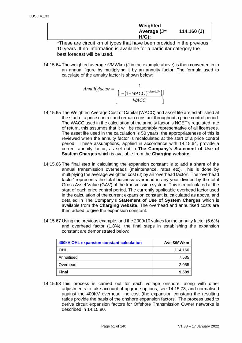
CUSC v1.33

of 140 V1.33 – 17 January 2022

Weighted Average (J= H/G):

114.160 (J)

*These are circuit km of types that have been provided in the previous 10 years. If no information is available for a particular category the best forecast will be used.

14.15.64 The weighted average £/MWkm (J in the example above) is then converted in to

an annual figure by multiplying it by an annuity factor. The formula used to calculate of the annuity factor is shown below:

14.15.65 The Weighted Average Cost of Capital (WACC) and asset life are established at

the start of a price control and remain constant throughout a price control period. The WACC used in the calculation of the annuity factor is NGET’s regulated rate of return, this assumes that it will be reasonably representative of all licensees. The asset life used in the calculation is 50 years; the appropriateness of this is reviewed when the annuity factor is recalculated at the start of a price control period. These assumptions, applied in accordance with 14.15.64, provide a current annuity factor, as set out in The Company's Statement of Use of System Charges which is available from the Charging website.

14.15.66 The final step in calculating the expansion constant is to add a share of the

annual transmission overheads (maintenance, rates etc). This is done by multiplying the average weighted cost (J) by an ‘overhead factor’. The ‘overhead factor’ represents the total business overhead in any year divided by the total Gross Asset Value (GAV) of the transmission system. This is recalculated at the start of each price control period. The currently applicable overhead factor used in the calculation of the current expansion constant is, calculated as above, and detailed in The Company's Statement of Use of System Charges which is available from the Charging website. The overhead and annuitised costs are then added to give the expansion constant.

14.15.67 Using the previous example, and the 2009/10 values for the annuity factor (6.6%)

and overhead factor (1.8%), the final steps in establishing the expansion constant are demonstrated below:

400kV OHL expansion constant calculation Ave £/MWkm

OHL 114.160

Annuitised 7.535

Overhead 2.055

Final 9.589

14.15.68 This process is carried out for each voltage onshore, along with other

adjustments to take account of upgrade options, see 14.15.73, and normalised against the 400KV overhead line cost (the expansion constant) the resulting ratios provide the basis of the onshore expansion factors. The process used to derive circuit expansion factors for Offshore Transmission Owner networks is described in 14.15.80.

( )( )

+−=

−

WACC

WACCtorAnnuityfac

AssetLife11

1

CUSC v1.33

of 140 V1.33 – 17 January 2022

14.15.69 This process of calculating the incremental cost of capacity for a 400kV OHL, along with calculating the onshore expansion factors is carried out for the first year of the price control and is increased by inflation, TOPI, (May–October average increase, as defined in the Transmission Licence) each subsequent year of the price control period. The current applicable expansion constant is detailed in The Company's Statement of Use of System Charges which is available from the Charging website.

14.15.69A Notwithstanding Paragraph 14.15.69 from the first year of (and during) the T2

price control (which starts on 1st April 2021), until a further change is made, the Expansion Constant will be that used in the 2020/21 charging year inflated in accordance with TOPI as per paragraph 14.15.69; and plus inflation as defined in the Transmission Licence for each subsequent year of the T2 price control.

Onshore Wider Circuit Expansion Factors 14.15.70 Base onshore expansion factors are calculated by deriving individual expansion

constants for the various types of circuit, following the same principles used to calculate the 400kV overhead line expansion constant. The factors are then derived by dividing the calculated expansion constant by the 400kV overhead line expansion constant. The factors will be fixed for each respective price control period.

14.15.71 In calculating the onshore underground cable factors, the forecast costs are

weighted equally between urban and rural installation, and direct burial has been assumed. The operating costs for cable are aligned with those for overhead line. An allowance for overhead costs has also been included in the calculations.

14.15.72 The 132kV onshore circuit expansion factor is applied on a TO basis. This is to

reflect the regional variation of plans to rebuild circuits at a lower voltage capacity to 400kV. The 132kV cable and line factor is calculated on the proportion of 132kV circuits likely to be uprated to 400kV. The 132kV expansion factor is then calculated by weighting the 132kV cable and overhead line costs with the relevant 400kV expansion factor, based on the proportion of 132kV circuitry to be uprated to 400kV. For example, in the TO areas of NGET and Scottish Power where there are no plans to uprate any 132kV circuits, the full cable and overhead line costs of 132kV circuit are reflected in the 132kV expansion factor calculation.

14.15.73 The 275kV onshore circuit expansion factor is applied on a GB basis and

includes a weighting of 83% of the relevant 400kV cable and overhead line factor. This is to reflect the averaged proportion of circuits across all three Onshore Transmission Licensees which are likely to be uprated from 275kV to 400kV across GB within a price control period.

14.15.74 The 400kV onshore circuit expansion factor is applied on a GB basis and reflects

the full costs for 400kV cable and overhead lines.

14.15.75 AC sub-sea cable and HVDC circuit expansion factors are calculated on a case

by case basis using actual project costs (Specific Circuit Expansion Factors). 14.15.76 Calculation of HVDC circuit expansion factors, and AC sub-sea circuit expansion

factors, shall include only: the cost of the converters (where applicable); and the cost of the cable; and a percentage of the total overhead project costs, defined as the combined costs of the cables and converters (as relevant) divided by the total capital cost of the project

CUSC v1.33

of 140 V1.33 – 17 January 2022

14.15.77 The TO specific onshore circuit expansion factors which are currently applicable, are detailed in The Company's Statement of Use of System Charges which is available from the Charging website.

Onshore Local Circuit Expansion Factors 14.15.78 The local onshore circuit tariff is calculated using local onshore circuit expansion

factors. These expansion factors are calculated using the same methodology as the onshore wider expansion factor but without taking into account the proportion of circuit kms that are planned to be uprated.

14.15.79 In addition, the 132kV onshore overhead line circuit expansion factor is sub

divided into four more specific expansion factors. This is based upon maximum (winter) circuit continuous rating (MVA) and route construction whether double or single circuit. The 132kV onshore overhead line circuit expansion factors which are currently applicable, are detailed in The Company's Statement of Use of System Charges which is available from the Charging website.

Onshore Expansion Factors in RIIO-T2

14.15.79A Notwithstanding Paragraph 14.15.69, the previous paragraphs and following the same intent as adopted at Paragraph 14.15.69A, from the first year of (and during) the T2 price control (which starts on 1st April 2021), until a further change is made, the Onshore expansion factors (being the Onshore local circuit factors and the Onshore wider circuit expansion factors, except those used for HVDC circuits and sub-sea AC cable) will be the value used in the 2020/21 charging year. For clarity HVDC circuits and sub-sea AC cable will continue to be calculated in accordance with 14.15.75.

Offshore Circuit Expansion Factors

14.15.80 Offshore expansion factors (£/MWkm) are derived from information provided by Offshore Transmission Owners for each offshore circuit. Offshore expansion factors are Offshore Transmission Owner and circuit specific. Each Offshore Transmission Owner will periodically provide, via the STC, information to derive an annual circuit revenue requirement. The offshore circuit revenue shall include revenues associated with the Offshore Transmission Owner’s reactive compensation equipment, harmonic filtering equipment, asset spares and HVDC converter stations.

14.15.81 In the year that the offshore transmission assets are transferred to the Offshore

Transmission Owner , the offshore circuit expansion factor would be calculated as follows:

Where: CRevOFTO1 = The offshore circuit revenue in £ for Year 1 L = The total circuit length in km of the offshore circuit CircRat = The continuous rating of the offshore circuit

ConstantExpansionOHL400kVOnshoreCircRatL

CRevOFTO1

CUSC v1.33

of 140 V1.33 – 17 January 2022

14.15.82 In all subsequent years, the offshore circuit expansion factor would be calculated as follows:

Where: AvCRevOFTO = The annual offshore circuit revenue averaged over the

remaining years of the onshore National Electricity Transmission System Operator (NETSO) price control

L = The total circuit length in km of the offshore circuit CircRat = The continuous rating of the offshore circuit 14.15.83 For the avoidance of doubt, the offshore circuit revenue values, CRevOFTO1 and

AvCRevOFTO shall be determined using asset values after the removal of any One-Off Charges.

14.15.84 Prevailing OFFSHORE TRANSMISSION OWNER specific expansion factors

will be published in The Company's Statement of Use of System Charges which is available from the Charging website. These shall be recalculated for the start of each price control period using the formula in paragraph 14.15.82. For each subsequent year within the price control period, these expansion factors will be adjusted by the annual Offshore Transmission Owner specific indexation factor, OFTOInd, calculated as follows;

where: OFTOIndt,f = the indexation factor for Offshore Transmission Owner f in respect of charging year t; OFTORevIndt,f = the indexation rate applied to the revenue of

Offshore Transmission Owner f under the terms of its transmission licence in respect of charging year t; and

TOPIt = the indexation rate applied to the expansion constant in respect of charging year t.

Offshore Interlinks 14.15.85 The revenue associated with an Offshore Interlink shall be divided entirely

between those generators benefiting from the installation of that Offshore Interlink. Each of these Users will be responsible for their charge from their charging date, meaning that a proportion of the Offshore Interlink revenue may be socialised prior to all relevant Users being chargeable. The proportion associated with each User will be based on the Measure of Capacity to the MITS using the Offshore Interlink(s) in the event of a single circuit fault on the User’s circuit from their offshore substation towards the shore, compared to the Measure of Capacity of the other Users.

ConstantExpansionOHL400kVOnshoreCircRatL

AvCRevOFTO

CUSC v1.33

of 140 V1.33 – 17 January 2022

Where: An Offshore Interlink is a circuit which connects two offshore substations that are connected to a Single Common Substation. It is held in open standby until there is a transmission fault that limits the User’s ability to export power to the Single Common Substation. In the Transport Model, they are to be modelled in open standby. A Single Common Substation is a substation where: i. each substation that is connected by an Offshore Interlink is connected

via at least one circuit without passing through another substation; and ii. all routes connecting each substation that is connected by an Offshore

Interlink to the MITS pass through. The Measure of Capacity to the MITS for each Offshore substation is the result of the following formula or zero whichever is larger. For the situation with only one interlink, all terms relating to C should be set to zero: For Substation A: min { CapIAB, ILFA × TECA - RCapA, CapB - ILFB × TECB + min (CapIBC, CapC - ILFC × TECC

) } For Substation B: min { ILFB × TECB - RCapB, min (CapIAB, CapA - ILFA × TECA ) + min ( CapIBC, CapC - ILFC × TECC) } For Substation C: min { CapIBC, ILFC × TECC - - RCapC, CapB - ILFB × TECB + min (CapIAB, CapA – ILFA × TECA

) } and CapIAB = total capacity of the Offshore Interlink between substations A and B CapIBC = total capacity of the Offshore Interlink between substations B and C CapX = total capacity of the circuit between offshore substation X and the

Single Common Substation, where X is A, B or C. RCapX = remaining capacity of the circuit between offshore substation X

and the Single Common Substation in the event of a single cable fault, where X is A, B or C.

TECX = the sum of the TEC for the Users connected, or contracted to connect, to offshore substation X, where X is A, B or C, where the value of TEC will be the maximum TEC that each User has held since the initial charging date, or is contracted to hold if prior to the initial charging date.

ILFX = Offshore Interlink Load Factor, where X is A, B or C. The Offshore Interlink Load Factor (ILF) is based on the Annual Load Factor (ALF). Until all the Users connected to a Single Common Substation have a station specific Annual Load Factor based on five years of data, the generic ALF for the fuel type will be used as the ILF for all stations. When all Users have a station specific ALF, the value of the ALF in the first such year will be used as the ILF in the calculation for all subsequent charging years.

CUSC v1.33

of 140 V1.33 – 17 January 2022

14.15.86 The apportionment of revenue associated with Offshore Interlink(s) in 14.15.85 applies in situations where the Offshore Interlink was included in the design phase, or if one or more User(s) has already financially committed or been commissioned then only where that User(s) agrees to the Offshore Interlink.

14.15.87 Alternatively to the formula specified in 14.15.85 the proportion of the

OFTO revenue associated with the Offshore Interlink allocated to each generator benefiting from the installation of an Offshore Interlink may be agreed between these Users. In this event:

a. All relevant Users shall notify The Company of its respective proportions three months prior the OTSDUW asset transfer in the case of a generator build, or the charging date of the first generator, in the case of an OFTO build.

b. All relevant Users may agree to vary the proportions notified under (a) by each writing to The Company three months prior to the charges being set for a given charging year.

c. Once a set of proportions of the OFTO revenue associated with the Offshore Interlink has been provided to The Company, these will apply for the next and future charging years unless and until The Company is informed otherwise in accordance with (b) by all of the relevant Users.

d. If all relevant Users are unable to reach agreement on the proportioning of the OFTO revenue associated with the Offshore Interlink they can raise a dispute. Any dispute between two or more Users as to the proportioning of such revenue shall be managed in accordance with CUSC Section 7 Paragraph 7.4.1 but the reference to the ‘Electricity Arbitration Association’ shall instead be to the ‘Authority’ and the Authority’s determination of such dispute shall, without prejudice to apply for judicial review of any determination, be final and binding on the Users.

The Locational Onshore Security Factor

14.15.88 The locational onshore security factor for everything other than Identified Onshore Circuits is derived by running a secure DCLF ICRP transport study of the network excluding local circuits and Identified Onshore Circuits based on the same market background as used for Zoning in the DCLF ICRP transport model. This calculates the nodal marginal costs where peak net demand can be met despite the Security and Quality of Supply Standard contingencies (simulating single and double circuit faults) on the network. Essentially the calculation of secured nodal marginal costs is identical to the process outlined above except that the secure DCLF study additionally calculates a nodal marginal cost taking into account the requirement to be secure against a set of worse case contingencies in terms of maximum flow for each circuit.

14.15.89 For the purposes of 14.15.88 the secured nodal cost differential is compared to

that produced by the DCLF ICRP transport model and the resultant ratio of the two determines the locational security factor using the Least Squares Fit method. Further information may be obtained from the charging website4.

14.15.90 For the purposes of 14.15.88 the locational onshore security factor, derived in

accordance with paragraphs 14.15.88 and 14.15.89 and expressed to two decimal places, is based on an average from a number of studies conducted by The Company to account for future network developments. This security factor

4 https://www.nationalgrideso.com/industry-information/charging

CUSC v1.33

of 140 V1.33 – 17 January 2022

is reviewed for each price control period and fixed for the duration. The locational onshore security factor which is currently applicable, is detailed in The Company's Statement of Use of System Charges, which is available from the Charging website.

14.15.90A An Identified Onshore Circuit shall be defined as a single transmission HVDC

subsea circuit or a single transmission AC subsea circuit between two MITS Nodes where there is only one route for the power to flow between the two MITS Nodes. The expansion factors for Identified Onshore Circuits are adjusted by dividing the applicable expansion factor for the Identified Onshore Circuits, calculated as per Sections 14.15.70 to 14.15.77, by the locational onshore security factor calculated in 14.15.90. When the locational onshore security factor is applied as per Section 14.15.96 and 14.15.97, this would result in an effective locational onshore security factor for Identified Onshore Circuits of 1.0.

Local Security Factors

14.15.91 Local onshore security factors are generator specific and are applied to a generator’s local onshore circuits. If the loss of any one of the local circuits prevents the export of power from the generator to the MITS then a local security factor of 1.0 is applied. For generation with circuit redundancy, a local security factor is applied that is equal to the locational security factor, derived in accordance with paragraphs 14.15.88 and 14.15.90.

14.15.92 Where a Transmission Owner has designed a local onshore circuit (or otherwise

that circuit once built) to a capacity lower than the aggregated TEC of the generation using that circuit, then the local security factor of 1.0 will be multiplied by a Counter Correlation Factor (CCF) as described in the formula below;

Where; Dmin = minimum annual net demand (MW) supplied via that circuit in the absence of that generation using the circuit

Tcap = transmission capacity built (MVA)

Gcap = aggregated TEC of generation using that circuit

CCF cannot be greater than 1.0.

14.15.93 A specific offshore local security factor (LocalSF) will be calculated for each

offshore connection using the following methodology:

Where: NetworkExportCapacity = the total export capacity of the network disregarding any

Offshore Interlinks k = the generation connected to the offshore network

cap

cap

G

TDCCF

+=

min

=

k

kGen

yortCapacitNetworkExpLocalSF

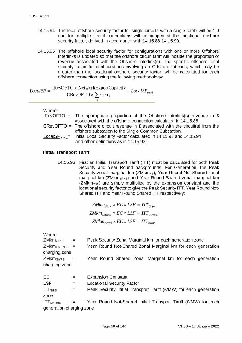
CUSC v1.33

of 140 V1.33 – 17 January 2022

14.15.94 The local offshore security factor for single circuits with a single cable will be 1.0

and for multiple circuit connections will be capped at the locational onshore security factor, derived in accordance with 14.15.88-14.15.90.

14.15.95 The offshore local security factor for configurations with one or more Offshore

Interlinks is updated so that the offshore circuit tariff will include the proportion of revenue associated with the Offshore Interlink(s). The specific offshore local security factor for configurations involving an Offshore Interlink, which may be greater than the locational onshore security factor, will be calculated for each offshore connection using the following methodology:

Where: IRevOFTO = The appropriate proportion of the Offshore Interlink(s) revenue in £

associated with the offshore connection calculated in 14.15.85 CRevOFTO = The offshore circuit revenue in £ associated with the circuit(s) from the

offshore substation to the Single Common Substation. LocalSFinitial = Initial Local Security Factor calculated in 14.15.93 and 14.15.94

And other definitions as in 14.15.93.

Initial Transport Tariff

14.15.96 First an Initial Transport Tariff (ITT) must be calculated for both Peak Security and Year Round backgrounds. For Generation, the Peak Security zonal marginal km (ZMkmPS), Year Round Not-Shared zonal marginal km (ZMkmYRNS) and Year Round Shared zonal marginal km (ZMkmYRS) are simply multiplied by the expansion constant and the locational security factor to give the Peak Security ITT, Year Round Not-Shared ITT and Year Round Shared ITT respectively:

Where ZMkmGiPS = Peak Security Zonal Marginal km for each generation zone

ZMkmGiYRNS = Year Round Not-Shared Zonal Marginal km for each generation

charging zone

ZMkmGiYRS = Year Round Shared Zonal Marginal km for each generation

charging zone

EC = Expansion Constant

LSF = Locational Security Factor

ITTGiPS = Peak Security Initial Transport Tariff (£/MW) for each generation

zone

ITTGiYRNS = Year Round Not-Shared Initial Transport Tariff (£/MW) for each

generation charging zone

initial

k

kGenCRevOFTO

yortCapacitNetworkExpIRevOFTOLocalSFLocalSF +

=

PSGiPSGi ITTLSFECZMkm =

GiYRNSGiYRNS ITTLSFECZMkm =

GiYRSGiYRS ITTLSFECZMkm =

CUSC v1.33

of 140 V1.33 – 17 January 2022

ITTGiYRS = Year Round Shared Initial Transport Tariff (£/MW) for each

generation charging zone.

14.15.97 Similarly, for demand the Peak Security zonal marginal km ( ZMkmPS) and Year Round zonal marginal km (ZMkmYR) are simply multiplied by the expansion constant and the locational security factor to give the Peak Security ITT and Year Round ITT respectively:

Where ZMkmDiPS = Peak Security Zonal Marginal km for each demand zone

ZMkmDiYR = Year Round Zonal Marginal km for each demand zone

ITTDiPS = Peak Security Initial Transport Tariff (£/MW) for each demand one

ITTDiYR = Year Round Initial Transport Tariff (£/MW) for each demand zone

14.15.98 The next step is to multiply these ITTs by the expected metered triad gross GSP group demand and generation capacity to gain an estimate of the initial revenue recovery for both Peak Security and Year Round backgrounds. The metered triad gross GSP group demand and generation capacity are based on analysis of forecasts provided by Users and are confidential.

Metered triad gross GSP group demand is net demand for all GSP groups less embedded exports for all GSP groups.

a.

Where ITRRG = Initial Transport Revenue Recovery for generation GGi = Total forecast Generation for each generation zone (based

on analysis of confidential User forecasts) ITRRD = Initial Transport Revenue Recovery for gross GSP group

demand DDi = Total forecast Metered Triad gross GSP group Demand for

each demand zone (based on analysis of confidential User forecasts)

In addition, the initial tariffs for generation are also multiplied by the Peak Security flag when calculating the initial revenue recovery component for the Peak Security background. When calculating the initial revenue recovery for the Shared component of the Year Round background, the initial tariffs are multiplied by the Annual Load Factor (see below). When calculating the initial revenue recovery for the Not Shared component of the Year Round background, the initial tariffs are multiplied by the Year Round Not Shared Flag.

Peak Security (PS) Flag

PSDiPSDi ITTLSFECZMkm =

YRDiYRDi ITTLSFECZMkm =

CUSC v1.33

of 140 V1.33 – 17 January 2022

14.15.99 The revenue from a specific generator due to the Peak Security locational tariff needs to be multiplied by the appropriate Peak Security (PS) flag. The PS flags indicate the extent to which a generation plant type contributes to the need for transmission network investment at peak demand conditions. The PS flag is derived from the contribution of differing generation sources to the demand security criterion as described in the Security Standard. In the event of a significant change to the demand security assumptions in the Security Standard, National Grid will review the use of the PS flag.

Generation Plant Type PS flag

Intermittent 0

Other 1

Year Round Not Shared (YRNS) Flag

14.15.100 The revenue from a specific generator due to the Year Round Not Shared locational tariff needs to be multiplied by the appropriate Year Round Not Shared (YRNS) flag. The YRNS flag indicates the extent to which a generation plant type contributes to the need for transmission network investment at year round demand conditions in areas of the System where the proportion of Low Carbon generation exceeds Carbon generation as defined in 14.15.49.

Generation Plant Type YRNS flag

Non Conventional Carbon 1

Conventional Carbon ALF

Annual Load Factor (ALF)

14.15.101 The ALF for each individual Power Station is calculated using the relevant TEC (MW) and corresponding output data. Where output data is not available for a Power Station, including for new Power Stations and emerging Power Station technologies, generic data for the appropriate generation plant type will be used.

14.15.102 For a given charging year “t” the Power Station ALF will be based on

information from the previous five charging years, calculated for each charging year as set out below.

Where: GMWhp is the maximum of FPN or actual metered output in a Settlement Period related to the power station TEC (MW); and TECp is the TEC (MW) applicable to that Power Station for that Settlement Period including any STTEC and LDTEC, accounting for any trading of TEC.

=

=

=17520

1

17520

1

5.0p

p

p

TECp

GMWh

ALF

CUSC v1.33

of 140 V1.33 – 17 January 2022

14.15.103 The appropriate output (FPN or actual metered) figure is derived from BM Unit data available to The Company and relates to the total TEC of the Power Station.

14.15.104 Once all five charging year ALFs have been calculated for the individual

Power Station they are compared, and the highest and lowest figures are discarded. The final ALF, to be used for transmission charging purposes, is calculated as the average of the remaining three ALFs.

14.15.105 In the event that only four charging years of complete output (FPN or

actual metered) data are available for an individual Power Station then the higher three charging years ALF would be used in the calculation of the final ALF. In the event that only three charging years of complete output (FPN or actual metered) data are available then these three charging years would be used.

14.15.106 Due to the aggregation of output (FPN or actual metered) data for

dispersed generation (e.g. cascade hydro schemes), where a single generator BMU consists of geographically separated power stations, the ALF would be calculated based on the total output of the BMU and the overall TEC of those Power Stations.

14.15.107 In the event that there are not three full charging years of an individual

power station’s output available, missing output (FPN or actual metered) data would be replaced by generic data for that generation plant type to ensure three charging years of information are available for the Power Station. The derivation of the generic data is described in paragraphs 14.15.111-14.15.114.

14.15.108 Users will receive draft ALFs before 25th December of the charging year

(t-1) for the charging year (t) and will have a period of 15 working days from date of publishing to notify the Company of any errors. Failure to agree changes relating to errors will be treated as a charging dispute under the CUSC.

14.15.109 The ALFs used in the setting of final tariffs will be published in the

annual Statement of Use of System Charges. Changes to ALFs after this publication will not result in changes to published tariffs (e.g. following dispute resolution).

Derivation of Generic ALFs

14.15.110 The generic ALF is derived from the average annual output of the ten

most recently commissioned GB generation of a particular generation plant type that have at least five charging years’ data, using an identical methodology to that used for the Power Station specific calculation described above. Where less than ten GB generators of a particular generation plant type exist, then data from all existing generators of that particular generation plant type will be used. Example generation plant type categories are listed below;

Fuel Type

Biomass

Coal

Gas

Hydro

CUSC v1.33

of 140 V1.33 – 17 January 2022

Nuclear (by reactor type)

Oil & OCGTs

Pumped Storage

Onshore Wind

Offshore Wind

CHP

14.15.111 The Company will keep these categories under review and update as necessary. Where within a category there is a significant locational difference consideration will be given to zonal generic factors. The factors used will be published in the Statement of Use of System Charges and will be reviewed annually.

14.15.112 If a User can demonstrate that the generation plant type of a Power

Station has changed, consideration will be given to the use of relevant generic ALF information in the calculation of their charges until sufficient specific data is available.

14.15.113 For new and emerging generation plant types, where insufficient data

is available to allow a generic ALF to be developed, The Company will use the best information available e.g. from manufactuers and data from use of similar technologies outside GB. The factor will be agreed with the relevant Generator. In the event of a disagreement the standard provisions for dispute in the CUSC will apply.

TNUoS Embedded Export Tariff

14.15.114 Embedded exports are exports measured on a half-hourly basis by

Metering Systems, in accordance with the BSC, that are not subject to generation TNUoS.

14.15.115 The embedded export tariff will be applied to the metered Triad volumes

of Embedded Exports for each demand zone as follows:

𝐸𝐸𝑇𝐷𝑖 = 𝐼𝑇𝑇𝐷𝑖𝑃𝑆 + 𝐼𝑇𝑇𝐷𝑖𝑌𝑅 + 𝐸𝑋

Where

ITTDiPS = Peak Security Initial Transport Tariff for the demand zone; ITTDiYR = Year Round Initial Transport Tariff for the demand zone, and EX: First Charging year following the implementation date of CMP 264/265:

=2

3(𝑋𝑃 − 𝐴𝐺𝐼𝐶) + 𝐴𝐺𝐼𝐶

Second charging year following the implementation date of CMP 264/265:

=1

3(𝑋𝑃 − 𝐴𝐺𝐼𝐶) + 𝐴𝐺𝐼𝐶

Third charging year following the implementation date of CMP 264/265 and every subsequent charging year:

= AGIC

CUSC v1.33

of 140 V1.33 – 17 January 2022

Where XP = Value of demand residual in charging year prior to implementation AGIC = The Avoided GSP Infrastructure Credit (AGIC) which represents the unit cost of infrastructure reinforcement at GSPs which is avoided as a consequence of embedded generation connected to the distribution networks served by those GSPs. It is calculated from the average annuitised cost of that infrastructure reinforcement divided by the average capacity delivered by a supergrid transformer. The Avoided GSP Infrastructure Credit is calculated at the beginning of each price control period and in the first applicable charging year following the implementation date of CMP264/265 using data submitted by onshore TSOs as part of the price control process. The data used is from the most recent [20] schemes submitted under the price control process and indexed each year by the TOPI formula set out in 14.3.6 until the end of the price control. For the avoidance of doubt, this approach does not include the cost of the supergrid transformers or any other connection assets as they are paid for by the relevant DNOs thorough their connection charges. The Value of EETDi will be floored at zero, so that EETDi is always zero or positive.

Initial Revenue Recovery

14.15.116 For the Peak Security background the initial tariff for generation is multiplied by the total forecast generation capacity and the PS flag to give the initial revenue recovery:

Where

ITRRGPS = Peak Security Initial Transport Revenue Recovery for

generation

GGi = Total forecast Generation for each generation zone (based on

analysis of confidential User forecasts)

FPS = Peak Security flag appropriate to that generator type

n = Number of generation zones

The initial revenue recovery for gross GSP group demand for the Peak Security background is calculated by multiplying the initial tariff by the total forecast metered triad gross GSP group demand:

Where:

ITRRDPS = Peak Security Initial Transport Revenue Recovery for gross GSP

group demand

DDi = Total forecast Metered Triad gross GSP group Demand for each

demand zone (based on analysis of confidential User forecasts)

14.15.117 For the Year Round background, the initial tariff for generation is multiplied by the total forecast generation capacity whilst calculating Initial Recovery for the Not-Shared component from Non Conventional Carbon. For Conventional Carbon the initial tariff for the Not Shared component is multiplied by both, the total forecast generation capacity and the ALF to give the initial revenue recovery. The initial tariff for the

( )=

=n

Gi

GPSPSGiPSGi ITRRFGITT1

( )=

=14

1Di

DPSDiDiPS ITRRDITT

CUSC v1.33

of 140 V1.33 – 17 January 2022

Shared component is multiplied by both, the total forecast generation capacity and the ALF to give the initial revenue recovery:

∑ (𝐼𝑇𝑇𝐺𝑖𝑌𝑅𝑁𝑆𝑁𝐶𝐶 × 𝐺𝐺𝑖)

𝑛

𝐺𝑖=1

= 𝐼𝑇𝑅𝑅𝐺𝑌𝑅𝑁𝑆𝑁𝐶𝐶

∑ (𝐼𝑇𝑇𝐺𝑖𝑌𝑅𝑁𝑆𝐶𝐶 × 𝐺𝐺𝑖 × 𝐴𝐿𝐹)

𝑛

𝐺𝑖=1

= 𝐼𝑇𝑅𝑅𝐺𝑌𝑅𝑁𝑆𝐶𝐶

𝐼𝑇𝑅𝑅𝐺𝑌𝑅𝑁𝑆 = 𝐼𝑇𝑅𝑅𝐺𝑌𝑅𝑁𝑆𝑁𝐶𝐶 + 𝐼𝑇𝑅𝑅𝐺𝑌𝑅𝑁𝑆𝐶𝐶

Where:

ITRRGYRNSNCC = Year Round Not-Shared Initial Transport Revenue Recovery for Non Conventional Carbon generation ITRRGYRNSCC = Year Round Not-Shared Initial Transport Revenue Recovery for Conventional Carbon generation ITRRGYRNS = Year Round Not-Shared Initial Transport Revenue Recovery for generation ITRRGYRS = Year Round Shared Initial Transport Revenue Recovery for generation

ALF = Annual Load Factor appropriate to that generator.

14.15.118 Similar to the Peak Security background, the initial revenue recovery for

gross GSP group demand for the Year Round background is calculated by multiplying the initial tariff by the total forecast metered triad gross GSP group demand:

Where:

ITRRDYR = Year Round Initial Transport Revenue Recovery for gross GSP

group demand

14.15.119 The initial revenue recovery for Embedded Exports is the Embedded

Export Tariff multiplied by the total forecast volume of Embedded Export at triad:

𝐼𝑇𝑅𝑅𝐸𝐸 = ∑ (𝐸𝐸𝑇𝐷𝑖 × 𝐸𝐸𝑉𝐷𝑖)

14

𝐷𝑖=1

( )=

=n

GiYRSGGiYRSGi ITRRALFGITT

1

( )=

=14

1Di

DYRDiDiYR ITRRDITT

CUSC v1.33

of 140 V1.33 – 17 January 2022

Where

ITRREE = Initial Revenue impact for Embedded Exports

EEVDi = Forecast Embedded Export metered volume at Triad (MW)

For the avoidance of doubt, the initial revenue recovery for embedded exports

can be positive or negative.

Deriving the Final Local Tariff (£/kW)

Local Circuit Tariff

14.15.120 Generation with a local circuit tariff is calculated by multiplying the Year

Round nodal marginal km along the local circuit by the expansion constant and the relevant local security factor (whether onshore or offshore) and summing across local circuits to give the local circuit tariff:

Where

k = Local circuit k for generator

NLMkmGjL = Year Round Nodal marginal km along local circuit k using local

circuit expansion factor.

EC = Expansion Constant

LocalSFk = Local Security Factor for circuit k

CLTGi = Circuit Local Tariff (£/kW)

Onshore Local Substation Tariff

14.15.121 All chargeable generation is subject to the local substation tariff component which is determined by assessing the generation substation type which is the substation at the connection charging boundary, against three cost determining factors:

(a) HV connection voltage – the voltage at the boundary between the User’s

connection assets and the transmission system; (b) Sum of TEC at the generation substation – the combined TEC of all generation at

the connecting substation; and (c) The level of redundancy at the generation substation – single busbar / single switch

mesh connections are examples of no redundancy connections, whereas examples of connections with redundancy include double busbar and mesh sub station designs.

14.15.122 Using the above factors, the corresponding £/kW tariffs that are

currently applicable, are detailed in The Company's Statement of Use of System Charges which is available from the Charging website.

Gi

k

k

L

GjCLT

LocalSFECNLMkm=

1000

CUSC v1.33

of 140 V1.33 – 17 January 2022

14.15.123 The process for calculating Local Substation Tariffs will be carried out for the first year of the price control and will subsequently be indexed by TOPI for each subsequent year of the price control period.

14.15.124 The effective Local Tariff (£/kW) is calculated as the sum of the circuit

and substation onshore and/or offshore components:

Where ELTGi = Effective Local Tariff (£/kW) SLTGi = Substation Local Tariff (£/kW)

14.15.125 Where tariffs do not change mid way through a charging year, final local tariffs will be the same as the effective tariffs:

ELTGi = LTGi

Where LTGi = Final Local Tariff (£/kW)

14.15.126 Where tariffs are changed part way through the year, the final tariffs will be calculated by scaling the effective tariffs to reflect that the tariffs are only applicable for part of the year and parties may have already incurred TNUoS liability.

and

Where: b = number of months the revised tariff is applicable for FLL = Forecast local liability incurred over the period that the original tariff is applicable for

14.15.127 For the purposes of charge setting, the total local charge revenue is calculated by:

Where LCRRG = Local Charge Revenue Recovery Gj = Forecast chargeable Generation or Transmission Entry Capacity in

kW (as applicable) for each generator (based on analysis of

confidential information received from Users)

Offshore substation local tariff

14.15.128 All offshore chargeable generation is subject to an offshore substation tariff. The offshore substation tariff shall be the sum of transformer, switchgear and platform components.

14.15.129 Each tariff component, expressed in £/kW, shall be the ratio of the

Offshore Transmission Owner revenue (£) and rating associated with the transformers, switchgear or platform (kW) at each offshore

GiGiGi SLTCLTELT +=

=

=

−

=21

1

21

1

12

Gi

Gi

Gi

Gi

GiGi

Gi

Gb

FLLGELT

LT

=

=

−

=14

1

14

1

12

Di

Di

Di

Di

DiDi

Di

Db

FLDET

FT

j

Gij

G*LT LCRR GiG =

=

CUSC v1.33

of 140 V1.33 – 17 January 2022

substation. The Offshore Transmission Owner revenue of each tariff component shall include that associated with asset spares. In the case of the platform component, the relevant rating shall be the lower of the transformer or switchgear ratings. As with the offshore circuit expansion factors, the Offshore Transmission Owner revenue associated with each tariff component shall be averaged over the remaining years of the NETSO price control.

14.15.130 Offshore Transmission Owner revenue associated with interest during

construction and project development overheads will be attributed to the relevant asset category with which it is associated. If these or any other costs included in the Offshore Transmission Owner revenue are not readily attributable to a given asset category, they will be pro-rated across the various asset categories based on their relative cost.

14.15.131 A discount shall be provided to the offshore substation tariff to reflect

the average cost of civil engineering for onshore substations. The currently applicable discount is detailed in The Company's Statement of Use of System Charges which is available from the Charging website. This will be inflated by TOPI each year and reviewed every price control period.

14.15.132 Offshore substation tariffs shall be reviewed at the start of every

onshore price control period. For each subsequent year within the price control period, these shall be inflated in the same manner as the associated Offshore Transmission Owner Revenue.

14.15.133 The revenue from the offshore substation local tariff is calculated by:

Where: SLTk = the offshore substation tariff for substation k Genk = the generation connected to offshore substation k The Residual Tariff

14.15.134 The total revenue to be recovered through TNUoS charges is determined each year with reference to the Transmission Licensees’ Price Control formulas less the costs expected to be recovered through Pre-Vesting connection charges. Hence in any given year t, a target revenue figure for TNUoS charges (TRRt) is set after adjusting for any under or over recovery for and including, the small generators discount is as follows:

Where TRRt = TNUoS Revenue Recovery target for year t Rt = Forecast Revenue allowed under The Company’s Price Control for year t

(this term includes a number of adjustments, including for over/under recovery from the previous year). For further information, refer to Special Condition D2 of The Company’s Transmission Licence.

PVCt = Forecast Revenue from Pre-Vesting connection charges for year t SGt-1 = The proportion of the under/over recovery included within Rt which relates

to the operation of statement C13 of the The Company Transmission

=

ssubstationoffshoreAll k

kk GenSLTSLTR

1−−−= tttt SGPVCRTRR

CUSC v1.33

of 140 V1.33 – 17 January 2022

Licence. Should the operation of statement C13 result in an under recovery in year t – 1, the SG figure will be positive and vice versa for an over recovery.

14.15.135 In normal circumstances, the revenue forecast to be recovered from the initial transport tariffs will not equate to the total revenue target. This is due to a number of factors. For example, the transport model assumes, for simplicity, smooth incremental transmission investments can be made. In reality, transmission investment can only be made in discrete 'lumps'. The transmission system has been planned and developed over a long period of time. Forecasts and assessments used for planning purposes will not have been borne out precisely by events and therefore some distinction between an optimal system for one year and the actual system can be expected.

14.15.136 As a result of the factors above, in order to ensure adequate recovery of total Transmission Owner revenue, a constant non-locational Residual Tariff for demand is calculated, which includes infrastructure substation asset costs. This tariff is added to the initial transport tariffs for demand only so that the total revenue recovery is achieved.

𝑇𝑅𝑅 − 𝐼𝑇𝑅𝑅𝐷𝑃𝑆 − 𝐼𝑇𝑅𝑅𝐷𝑌𝑅 − 𝐼𝑇𝑅𝑅𝐸𝐸 − 𝐼𝑇𝑅𝑅𝐺𝑃𝑆 − 𝐼𝑇𝑅𝑅𝐺𝑌𝑅𝑁𝑆 − 𝐼𝑇𝑅𝑅𝐺𝑌𝑅𝑆 − 𝐿𝐶𝑅𝑅𝐺𝐺 − 𝐴𝑑𝑗𝑅𝑒𝑣𝑒𝑛𝑢𝑒

∑ 𝐷𝐷𝑖14𝐷𝑖=1

Where

RT = Residual Tariff (£/MW)

p = Proportion of revenue to be recovered from demand

AdjRevenue = Adjustment Revenue as per paragraph 14.14.5

Final £/kW Tariff

14.15.137 The effective Transmission Network Use of System tariff (TNUoS) for

generation and gross demand can now be calculated as the sum of the initial transport wider tariffs for Peak Security and Year Round backgrounds and the non-locational residual tariff (for demand) or Adjustment Tariff and local tariff (for generation):

𝐸𝑇𝐺𝑖 = 𝐼𝑇𝑇𝐺𝑖𝑃𝑆 + 𝐼𝑇𝑇𝐺𝑖𝑌𝑅𝑁𝑆 + 𝐼𝐹𝐹𝐺𝑖𝑌𝑅𝑆 + 𝐴𝑑𝑗𝑇𝑎𝑟𝑖𝑓𝑓𝑖

1000+ 𝐿𝑇𝐺𝑖

and

𝐸𝑇𝐷𝑖 = 𝐼𝑇𝑇𝐷𝑖𝑃𝑆 + 𝐼𝑇𝑇𝐷𝑖𝑌𝑅 + 𝑅𝑇

1000

Where

ETGi= Effective Generation TNUoS Tariff expressed in £/kW (ETGi would only be

applicable to a Power Station with a PS flag of 1 and ALF of 1; in all other

circumstances ITTGiPS, ITTGiYRNS and ITTGiYRS will be applied using Power Station

specific data)

CUSC v1.33

of 140 V1.33 – 17 January 2022

AdjTariffi = AdjTariff (from 14.14.5) applicable in time period ‘i’.

ETDi= Effective Gross Demand TNUoS Tariff expressed in £/kW

The effective Transmission Network Use of System tariff (TNUoS) for embedded

exports can now be calculated by expressing the embedded export tariff in £/kW

values:

𝐸𝑇𝐸𝐸𝑖 =𝐸𝐸𝑇𝐷𝑖

1000

Where ETEEi= Effective Embedded Export TNUoS Tariff expressed in £/kW

For the purposes of the annual Statement of Use of System Charges ETGi will be published

as ITTGiPS; ITTGiYRNS, ITTGiYRS, RTG and LTGi and AdjTariffi (if required)

14.15.138 Where tariffs do not change mid way through a charging year, final demand and generation tariffs will be the same as the effective tariffs.

𝐹𝑇𝐸𝐸𝐴𝑖 = 𝐸𝑇𝐸𝐸𝑖

14.15.139 Where tariffs are changed part way through the year, the final tariffs will be calculated by scaling the effective tariffs to reflect that the tariffs are only applicable for part of the year and parties may have already incurred TNUoS liability.

and 𝐹𝑇𝐸𝐸𝑖 =12×(𝐸𝑇𝐸𝐸𝑖×∑ 𝐸𝐸𝑇𝐷𝑖−𝐹𝐿𝐷𝑖)14

𝐷𝑖=1

𝑏×∑ 𝐸𝐸𝑇𝐷𝑖14𝐷𝑖=1

Where: b = number of months the revised tariff is applicable for FL = Forecast liability incurred over the period that the original tariff is applicable for

Note: The ETGi element used in the formula above will be based on an individual Power Stations PS flag and ALF for Power Station GGi, aggregated to ensure overall correct revenue recovery.

14.15.140 If the final gross demand TNUoS Tariff results in a negative number then this is collared to £0/kW with the resultant non-recovered revenue smeared over the remaining demand zones:

If , then i = 1 to z

GiGi ETFT =

DiDi ETFT =

=

=

−

=27

1

20

1

12

Gi

Gi

Gi

GiGiGi

Gi

Gb

FLGET

FT

=

=

−

=14

1

14

1

12

Di

Di

Di

Di

DiDi

Di

Db

FLDET

FT

0DiFT

CUSC v1.33

of 140 V1.33 – 17 January 2022

Therefore,

Therefore the revised Final Tariff for the gross demand zones with positive Final tariffs is

given by:

For i= 1 to z:

For i=z+1 to 14:

Where

NRRTD = Non Recovered Revenue Tariff (£/kW)

RFTDi = Revised Final Tariff (£/kW)

14.15.141 The tariffs applicable for any particular year are detailed in The

Company's Statement of Use of System Charges, which is available from the Charging website. Archived tariff information may also be obtained from the Charging website.

14.15.142 The zonal maps referenced in The Company's Statement of Use of

System Charges and available on the Charging website contain detailed information for the charging year in question of which Grid Supply Points fall into which TNUoS zones.

14.15.143 New Grid Supply Points will be classified into zones on the following

basis:

• For demand zones, according to the GSP Group to which the Grid Supply Point is allocated for energy market settlement purposes.

• For generation zones, with reference to the geographic proximity to existing zones and, where close to a boundary between existing zones, with reference to the marginal costs arising from transport model studies. The GSP will then be allocated to the zone, which contains the most similar marginal costs.

14.15.144 The Company has available, upon request, the DCLF ICRP transport

model, tariff model template and data necessary to run the model, consisting of nodal values of generation and demand connection points to the NETS. The model and data will enable the basic nodal charges to be determined and will also allow sensitivity analysis concerning alternative developments of generation and demand to be undertaken. The model is available from the Charging Team and whilst it is free of charge, it is provided under licence to restrict its distribution and commercial use.

14.15.145 The Company will be pleased to run specific sensitivity studies for Users

under a separate study contract in line with the fees set out in the Statement of Use of System Charges. Please contact the Charging Team.

( )

+=

=

=14

1

1

zi

Di

z

i

DiDi

D

D

DFT

NRRT

0=DiRFT

DDiDi NRRTFTRFT +=

CUSC v1.33

of 140 V1.33 – 17 January 2022

14.15.146 The factors which will affect the level of TNUoS charges from year to year include-;

• the forecast level of peak demand on the system

• the Price Control formula (including the effect of any under/over recovery from the previous year),

• the expansion constant,

• the locational security factor,

• the PS flag

• the Year Round Not Shared (YRNS) Flag

• the ALF of a generator

• changes in the transmission network

• HVDC circuit impedance calculation

• changes in the pattern of generation capacity and demand.

• changes in the pattern of embedded exports

• the £/€ exchange rate and expected Generator Output

14.15.147 In accordance with Standard Licence Condition C13, generation directly connected to the NETS 132kV transmission network which would normally be subject to generation TNUoS charges but would not, on the basis of generating capacity, be liable for charges if it were connected to a licensed distribution network qualifies for a reduction in transmission charges by a designated sum, determined by the Authority. Any shortfall in recovery will result in a unit amount increase in gross demand charges to compensate for the deficit. Further information is provided in the Statement of the Use of System Charges.

Stability & Predictability of TNUoS tariffs

14.15.148 A number of provisions are included within the methodology to promote the stability and predictability of TNUoS tariffs. These are described in 14.29.

CUSC v1.33

of 140 V1.33 – 17 January 2022

14.16 Derivation of the Transmission Network Use of System Energy Consumption Tariff and Short Term Capacity Tariffs

14.16.1 For the purposes of this section, Lead Parties of Balancing Mechanism (BM) Units that are liable for Transmission Network Use of System Demand Charges are termed Suppliers.

14.16.2 Following calculation of the Transmission Network Use of System £/kW Gross

Demand Tariff (as outlined in Chapter 2: Derivation of the TNUoS Tariff) for each GSP Group is calculated as follows:

p/kWh Tariff = (NHHDF * £/kW Tariff - FLG) *100

NHHCG

Where: £/kW Tariff = The £/kW Effective Gross Demand Tariff (£/kW), as calculated

previously, for the GSP Group concerned.

NHHDF = The Company’s forecast of Suppliers’ non-half-hourly metered Triad Demand (kW) for the GSP Group concerned. The forecast is based on historical data. FLG = Forecast Liability incurred for the GSP Group concerned. NHHCG = The Company’s forecast of GSP Group non-half-hourly metered total energy consumption (kWh) for the period 16:00 hrs to 19:00hrs inclusive (i.e. settlement periods 33 to 38) inclusive over the period the tariff is applicable for the GSP Group concerned.

Short Term Transmission Entry Capacity (STTEC) Tariff

14.16.3 The Short Term Transmission Entry Capacity (STTEC) tariff for positive zones is derived from the Effective Tariff (ETGi) annual TNUoS £/kW tariffs (14.15.112). If multiple set of tariffs are applicable within a single charging year, the Final Tariff used in the STTEC calculation will be prorated in an identical manner to that used when calculating a generators annual liability. The periods over which the tariff would be prorated would be identical to the periods used when calculating the wider tariff (i.e. over the whole financial year, not just the period that the STTEC is applicable for). STTECs will not be reconciled following a mid year charge change. The premium associated with the flexible product is associated with the analysis that 90% of the annual charge is linked to the system peak. The system peak is likely to occur in the period of November to February inclusive (120 days, irrespective of leap years). The calculation for positive generation zones is as follows:

STTEC tariff (£/kW/period)

Where:

FT = Final annual TNUoS Tariff expressed in £/kW Gi = Generation zone STTEC Period = A period applied for in days as defined in the CUSC

=

120

9.0 PeriodSTTECFTGi

CUSC v1.33

of 140 V1.33 – 17 January 2022

14.16.4 For the avoidance of doubt, the charge calculated under 14.16.3 above will represent each single period application for STTEC. Requests for multiple /STTEC periods will result in each STTEC period being calculated and invoiced separately.

14.16.5 The STTEC tariff for generators with negative final tariffs is set to zero to prevent

Users receiving greater than 100% of the annual TNUoS payment that would have been received for that capacity under a firm TEC.

Limited Duration Transmission Entry Capacity (LDTEC) Tariffs

14.16.6 The Limited Duration Transmission Entry Capacity (LDTEC) tariff for positive zones is derived from the equivalent zonal STTEC tariff for up to the initial 17 weeks of LDTEC in a given charging year (whether consecutive or not). For the remaining weeks of the year, the LDTEC tariff is set to collect the balance of the annual TNUoS liability over the maximum duration of LDTEC that can be granted in a single application. If multiple set of tariffs are applicable within a single charging year, the Final Tariff used in the LDTEC calculation will be prorated in an identical manner to that used when calculating a generators annual liability. The periods over which the tariff would be prorated would be identical to the periods used when calculating the wider tariff (ie over the whole financial year, not just the period that the STTEC is applicable for). LDTECs will not be reconciled following a mid year charge change:

Initial 17 weeks (high rate):

Remaining weeks (low rate):

where FT is the final annual TNUoS tariff expressed in £/kW; Gi is the generation TNUoS zone; and P is the premium in % above the annual equivalent TNUoS charge as determined by The Company, which shall have the value 0.

14.16.7 The LDTEC tariff for generators with negative final tariffs is set to zero to prevent

Users receiving greater than 100% of the annual TNUoS payment that would have been received for that capacity under a firm TEC.

14.16.8 The tariffs applicable for any particular year are detailed in The Company's

Statement of Use of System Charges which is available from the Charging website. Historical tariffs are also available on the Charging website.

120

79.0 )(£/kW/week tariff LDTEC

=

GiFT

( )PFTGi

+−

= 1

120316

71075.0 )(£/kW/week tariff LDTEC

CUSC v1.33

of 140 V1.33 – 17 January 2022

14.17 Demand Charges Parties Liable for Demand Charges

14.17.1 Demand charges are subdivided into charges for gross demand, energy and

embedded export. The following parties shall be liable for some or all of the categories of demand charges:

• The Lead Party of a Supplier BM Unit;

• Power Stations with a Bilateral Connection Agreement;

• Parties with a Bilateral Embedded Generation Agreement

14.17.2 Classification of parties for charging purposes, section 14.26, provides an

illustration of how a party is classified in the context of Use of System charging and refers to the paragraphs most pertinent to each party.

Basis of Gross Demand Charges

14.17.3 Gross Demand charges are based on a de minimis £0/kW charge for Half Hourly and £0/kWh for Non Half Hourly metered demand.

14.17.4 Chargeable Gross Demand Capacity is the value of Triad gross demand (kW).

Chargeable Energy Capacity is the energy consumption (kWh). The definition of both these terms is set out below.

14.17.5 If there is a single set of gross demand tariffs within a charging year, the

Chargeable Gross Demand Capacity is multiplied by the relevant gross demand tariff, for the calculation of gross demand charges.

14.17.6 If there is a single set of energy tariffs within a charging year, the Chargeable

Energy Capacity is multiplied by the relevant energy consumption tariff for the calculation of energy charges.

14.17.7 If multiple sets of gross demand tariffs are applicable within a single charging

year, gross demand charges will be calculated by multiplying the Chargeable Gross Demand Capacity by the relevant tariffs pro rated across the months that they are applicable for, as below,

𝐴𝑛𝑛𝑢𝑎𝑙 𝐿𝑖𝑎𝑏𝑖𝑙𝑖𝑡𝑦𝐷𝑒𝑚𝑎𝑛𝑑 = × ((𝑎×𝑇𝑎𝑟𝑖𝑓𝑓 1)+(𝑏×𝑇𝑎𝑟𝑖𝑓𝑓 2)

12)

where:

Tariff 1 = Original tariff,

Tariff 2 = Revised tariff,

a = Number of months over which the original tariff is applicable,

b = Number of months over which the revised tariff is applicable.

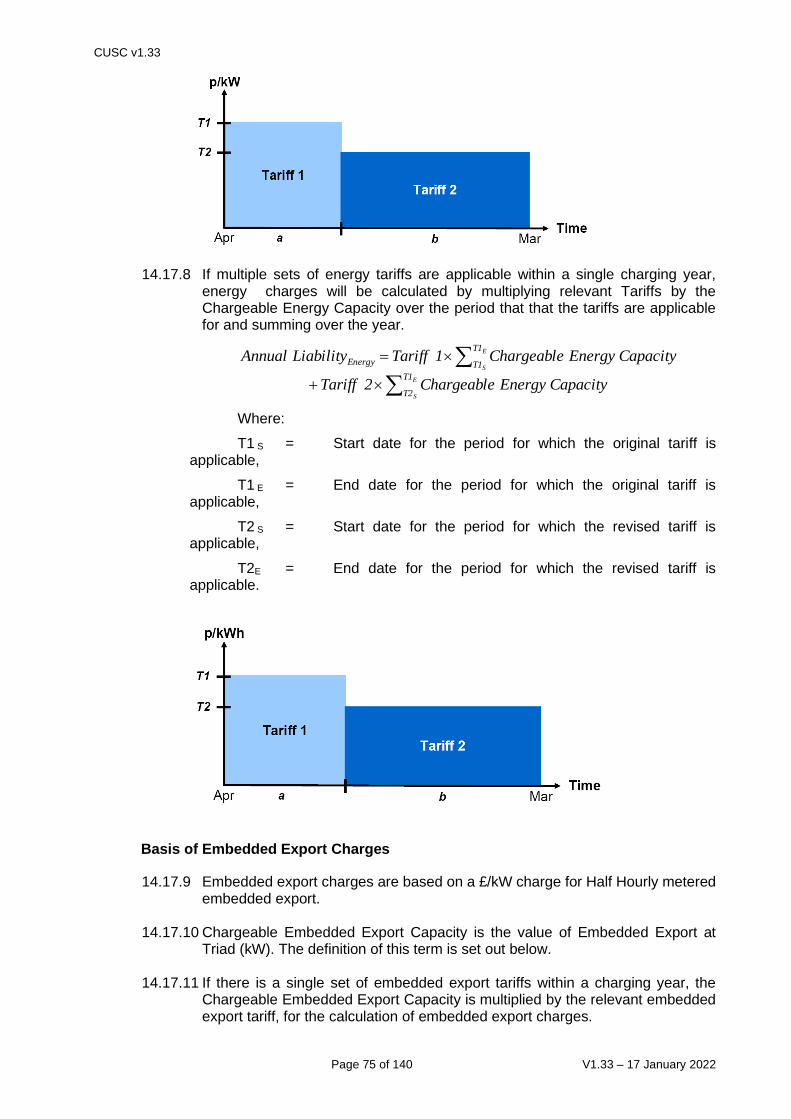
CUSC v1.33

of 140 V1.33 – 17 January 2022

14.17.8 If multiple sets of energy tariffs are applicable within a single charging year, energy charges will be calculated by multiplying relevant Tariffs by the Chargeable Energy Capacity over the period that that the tariffs are applicable for and summing over the year.

Where:

T1 S = Start date for the period for which the original tariff is applicable,

T1 E = End date for the period for which the original tariff is applicable,

T2 S = Start date for the period for which the revised tariff is applicable,

T2E = End date for the period for which the revised tariff is applicable.

Basis of Embedded Export Charges

14.17.9 Embedded export charges are based on a £/kW charge for Half Hourly metered embedded export.

14.17.10 Chargeable Embedded Export Capacity is the value of Embedded Export at Triad (kW). The definition of this term is set out below.

14.17.11 If there is a single set of embedded export tariffs within a charging year, the Chargeable Embedded Export Capacity is multiplied by the relevant embedded export tariff, for the calculation of embedded export charges.

+

=

E

S

E

S

T1

T2

T1

T1Energy

CapacityEnergyChargeable2Tariff

CapacityEnergyChargeable1TariffLiabilityAnnual

CUSC v1.33

of 140 V1.33 – 17 January 2022

14.17.12 If multiple sets of embedded export tariffs are applicable within a single charging year, embedded export charges will be calculated by multiplying the Chargeable Embedded Export Capacity by the relevant tariffs pro rated across the months that they are applicable for, as below,

𝐴𝑛𝑛𝑢𝑎𝑙 𝐿𝑖𝑎𝑏𝑖𝑙𝑖𝑡𝑦𝐷𝑒𝑚𝑎𝑛𝑑 = × ((𝑎×𝑇𝑎𝑟𝑖𝑓𝑓 1)+(𝑏×𝑇𝑎𝑟𝑖𝑓𝑓 2)

12)

where:

Tariff 1 = Original tariff,

Tariff 2 = Revised tariff,

a = Number of months over which the original tariff is applicable,

b = Number of months over which the revised tariff is applicable.

Supplier BM Unit

14.17.13 A Supplier BM Unit charges will be the sum of its energy, gross demand and embedded export liabilities where:

• The Chargeable Gross Demand Capacity will be the average of the Supplier BM Unit's half-hourly metered gross demand during the Triad (and the £/kW tariff), and

• The Chargeable Embedded Export Capacity will be the average of the Supplier BM Unit's half-hourly metered embedded export during the Triad (and the £/kW tariff), and

• The Chargeable Energy Capacity will be the Supplier BM Unit's non half-hourly metered energy consumption over the period 16:00 hrs to 19:00 hrs inclusive every day over the Financial Year (and the p/kWh tariff).

Power Stations with a Bilateral Connection Agreement and Licensable Generation with a Bilateral Embedded Generation Agreement

14.17.14 The Chargeable Demand Capacity for a Power Station with a Bilateral Connection Agreement or Licensable Generation with a Bilateral Embedded Generation Agreement will be based on the average of the net import over each Triad leg of the BM Units associated with the Power Station (in Appendix C of its Bilateral Connection Agreement or Bilateral Embedded Generation Agreement, including metered additional load) during the Triad.

Exemptible Generation and Derogated Distribution Interconnectors with a Bilateral Embedded Generation Agreement

14.17.15 The demand charges for Exemptible Generation and Derogated Distribution Interconnector with a Bilateral Embedded Generation Agreement will be the sum of its gross demand and embedded export liabilities where:

• The Chargeable Gross Demand Capacity for Exemptible Generation and Derogated Distribution Interconnectors with a Bilateral Embedded Generation Agreement will be based on the average of the metered gross demand of each BM Unit specified in Appendix C of the Bilateral Embedded Generation Agreement during the Triad.

• The Chargeable Embedded Export Capacity for Exemptible Generation and Derogated Distribution Interconnectors with a Bilateral Embedded Generation Agreement will be based on the average of the metered embedded export of each BM Unit specified in Appendix C of the Bilateral Embedded Generation Agreement during the Triad.

CUSC v1.33

of 140 V1.33 – 17 January 2022

Small Generators Tariffs

14.17.16 In accordance with Standard Licence Condition C13, any under recovery from

the MAR arising from the small generators discount will result in a unit amount of increase to all GB gross demand tariffs.

The Triad

14.17.17 The Triad is used as a short hand way to describe the three settlement periods of highest transmission system demand within a Financial Year, namely the half hour settlement period of system peak net demand and the two half hour settlement periods of next highest net demand, which are separated from the system peak net demand and from each other by at least 10 Clear Days, between November and February of the Financial Year inclusive. Exports on directly connected Interconnectors and Interconnectors capable of exporting more than 100MW to the Total System shall be excluded when determining the system peak netdemand. An illustration is shown below.

Half-hourly metered demand charges

14.17.18 For Supplier BMUs and BM Units associated with Exemptible Generation and

Derogated Distribution Interconnectors with a Bilateral Embedded Generation Agreement, if the average half-hourly metered gross demand volume over the Triad results in an import, the Chargeable Gross Demand Capacity will be positive resulting in the BMU being charged. If the average half-hourly metered embedded export volume over the Triad results in an export, the Chargeable Embedded Export Capacity will be negative resulting in the BMU being paid the relevant tariff; where the tariff is positive. For the avoidance of doubt, parties with Bilateral Embedded Generation Agreements that are liable for Generation charges will not be eligible for payment of the embedded export tariff.

Monthly Charges

1999/2000 Triad Season - Peak System Demands

0

10

20

30

40

50

60

Date

Pea

k S

yste

m D

eman

d (

GW

)

1 Nov 99 29 Feb 00

20/12/9920/01/0008/12/99

CUSC v1.33

of 140 V1.33 – 17 January 2022

14.17.19 Throughout the year Users will submit a Demand Forecast. A Demand Forecast will include:

• half-hourly metered gross demand to be supplied during the Triad for each BM Unit

• half-hourly metered embedded export to be exported during the Triad for each BM Unit

• non-half hourly metered energy to be supplied over the period 16:00 hrs to 19:00 hrs inclusive every day over the Financial Year for each BM Unit

14.17.20 Throughout the year Users’ monthly demand charges will be based on their

Demand Forecast of:

• half-hourly metered gross demand to be supplied during the Triad for each BM Unit, multiplied by the relevant zonal £/kW tariff; and

• half-hourly metered embedded export to be supplied during the Triad for each BM Unit, multiplied by the relevant zonal £/kW tariff; and

• non-half hourly metered energy to be supplied over the period 16:00 hrs to 19:00 hrs inclusive every day over the Financial Year for each BM Unit, multiplied by the relevant zonal p/kWh tariff

Users’ annual TNUoS demand charges are based on these forecasts and are split evenly over the 12 months of the year. Users have the opportunity to vary their demand forecasts on a quarterly basis over the course of the year, with the demand forecast requested in February relating to the next Financial Year. Users will be notified of the timescales and process for each of the quarterly updates. The Company will revise the monthly Transmission Network Use of System demand charges by calculating the annual charge based on the new forecast, subtracting the amount paid to date, and splitting the remainder evenly over the remaining months. For the avoidance of doubt, only positive demand forecasts (i.e. representing a net import from the system) will be used in the calculation of charges. Demand forecasts for a User will be considered positive where:

• The sum of the gross demand forecast and embedded export forecast is positive; and

• The non-half hourly metered energy forecast is positive.

14.17.21 Users should submit reasonable demand forecasts of gross demand, embedded export and energy in accordance with the CUSC. The Company shall use the following methodology to derive a forecast to be used in determining whether a User's forecast is reasonable, in accordance with the CUSC, and this will be used as a replacement forecast if the User's total forecast is deemed unreasonable. The Company will, at all times, use the latest available Settlement data.

For existing Users: i) The User’s Triad gross demand and embedded export for the preceding

Financial Year will be used where User settlement data is available and where The Company calculates its forecast before the Financial Year. Otherwise, the User's average weekday settlement period 35 half-hourly

CUSC v1.33

of 140 V1.33 – 17 January 2022

metered (HH) gross demand and embedded export in the Financial Year to date is compared to the equivalent average gross demand and embedded export for the corresponding days in the preceding year. The percentage difference is then applied to the User's HH gross demand and embedded export at Triad in the preceding Financial Year to derive a forecast of the User's HH gross demand and embedded export at Triad for this Financial Year.

ii) The User's non half-hourly metered (NHH) energy consumption over the

period 16:00 hrs to 19:00 hrs every day in the Financial Year to date is compared to the equivalent energy consumption over the corresponding days in the preceding year. The percentage difference is then applied to the User's total NHH energy consumption in the preceding Financial Year to derive a forecast of the User's NHH energy consumption for this Financial Year.

For new Users who have completed a Use of System Supply Confirmation Notice in the current Financial Year: iii) The User's average weekday settlement period 35 half-hourly metered

(HH) gross demand and embedded export over the last complete month for which The Company has settlement data is calculated. Total system average HH gross demand and embedded export for weekday settlement period 35 for the corresponding month in the previous year is compared to total system HH gross demand and embedded export at Triad in that year and a percentage difference is calculated. This percentage is then applied to the User's average HH gross demand and embedded export for weekday settlement period 35 over the last month to derive a forecast of the User's HH gross demand and embedded export at Triad for this Financial Year.

iv) The User's non half-hourly metered (NHH) energy consumption over the

period 16:00 hrs to 19:00 hrs every day over the last complete month for which The Company has settlement data is noted. Total system NHH energy consumption over the corresponding month in the previous year is compared to total system NHH energy consumption over the remaining months of that Financial Year and a percentage difference is calculated. This percentage is then applied to the User's NHH energy consumption over the month described above, and all NHH energy consumption in previous months is added, in order to derive a forecast of the User's NHH metered energy consumption for this Financial Year.

14.17.22 14.28 Determination of The Company’s Forecast for Demand Charge Purposes

illustrates how the demand forecast will be calculated by The Company. Reconciliation of Demand Charges and TNUoS Charges in the event of exceeding the limits to Generator charges in the Limiting Regulation

14.17.23 The reconciliation process is set out in the CUSC. The demand reconciliation process compares the monthly charges paid by Users against actual outturn charges. Due to the Settlements process, reconciliation of demand charges is carried out in two stages; initial reconciliation and final reconciliation.

14.17.24 In the event of annual average transmission charges incurred by Generator Users in the charging year not being in compliance with the upper or lower limits in the Limiting Regulation an Ex-Post Reconciliation adjustment will be applied to Generator and Demand Users to bring charges back into compliance.

CUSC v1.33

of 140 V1.33 – 17 January 2022

Initial Reconciliation of demand charges

14.17.25 The initial reconciliation process compares Users' demand forecasts and corresponding monthly charges paid over the year against actual outturn data (using latest Settlement data available at the time) and corresponding charges. Initial reconciliation is carried out in two parts; Initial Reconciliation Part 1 deals with the reconciliation of half-hourly metered demand charges and Initial Reconciliation Part 2 deals with the reconciliation of non-half-hourly metered demand charges.

Initial Reconciliation Part 1– Half-hourly metered demand

14.17.26 The Company will identify the periods forming the Triad once it has received Central Volume Allocation data from the Settlement Administration Agent for all days up to and including the last day of February. Once The Company has notified Users of the periods forming the Triad they will not be changed even if disputes are subsequently resolved which would change the periods forming the Triad.

14.17.27 Initial outturn charges for half-hourly metered gross demand will be determined

using the latest available data of actual average Triad gross demand (kW) multiplied by the zonal gross demand tariff(s) (£/kW) applicable to the months concerned for each zone for that Financial Year. These actual values are then reconciled against the monthly charges paid in respect of half-hourly gross demand.

14.17.28 Initial outturn charges for half-hourly metered embedded export will be

determined using the latest available data of actual average Triad embedded export (kW) multiplied by the zonal embedded export tariff(s) (£/kW) applicable to the months concerned for each zone for that Financial Year. These actual values are then reconciled against the monthly charges paid in respect of half-hourly embedded exports.

Initial Reconciliation Part 2 – Non-half-hourly metered demand

14.17.29 Actual payments for non-half-hourly metered demand will be determined using the latest available actual energy consumption data (kWh) for the period 16:00 hrs to 19:00 hrs inclusive (i.e. settlement periods 33 to 38) over the year multiplied by the energy consumption tariff(s) (p/kWh) applicable to the months concerned for each zone. These actual values are then reconciled against the monthly charges paid in respect of non-half-hourly energy consumption.

Final Reconciliation of demand charges

14.17.30 The final reconciliation process compares Users' charges (as calculated during the initial reconciliation process using the latest available data) against final outturn demand charges (based on final settlement data of half-hourly gross demand, embedded exports and non-half-hourly energy consumption).

14.17.31 Final actual charges will be determined using the final demand reconciliation

data taken from the Final Reconciliation Settlement Run or the Final Reconciliation Volume Allocation Run.

Reconciliation of manifest errors

CUSC v1.33

of 140 V1.33 – 17 January 2022

14.17.32 In the event that a manifest error, or multiple errors in the calculation of TNUoS tariffs results in a material discrepancy in aUsers TNUoS tariff, the reconciliation process for all Users qualifying under Section 14.17.34 33 will be in accordance with Sections 14.17.254 to 14.17.3130. The reconciliation process shall be carried out using recalculated TNUoS tariffs. Where such reconciliation is not practicable, a post-year reconciliation will be undertaken in the form of a one-off payment.

14.17.33 A manifest error shall be defined as any of the following:

a) an error in the transfer of relevant data between the Transmission

Licensees or Distribution Network Operators; b) an error in the population of the Transport Model with relevant data; c) an error in the function of the Transport Model; or d) an error in the inputs or function of the Tariff Model.

14.17.34 A manifest error shall be considered material in the event that such an error or,

the net effect of multiple errors, has an impact of the lesser of either:

a) an error in a User’s TNUoS tariff of at least +/-£0.50/kW; or b) an error in a User’s TNUoS tariff which results in an error in the annual

TNUoS charge of a User in excess of +/-£250,000.

14.17.35 A manifest error shall only be reconciled if it has been identified within the charging year for which the error has an effect. Errors identified outside of this period will not be eligible for reconciliation retrospectively.

Ex-post Reconciliation of Generator and Demand Charges in the event of exceeding the limits to Generator charges in the Limiting Regulation 14.17.36 The Company shall, following the completion of each charging year, produce a

statement setting out the annual average transmission charges paid in aggregate by Generators in €/MWh as per paragraph 14.14.5.

14.17.37 In the event that the annual average transmission charges attributable to Generators exceeds the upper limit established in the Limiting Regulation then an Ex-post Reconciliation will be calculated for Generator and Demand Users as per the below and will be invoiced at the time of generation reconciliation and initial demand reconciliation.

i) The Ex-post Reconciliation amount for Demand Users will be calculated as:

Dadj = GCharge (Actual)-( 𝐺𝑂𝐴 ∗ (𝐶𝑎𝑝𝐸𝐶 ∗ 𝐸𝑅𝐴))

Where:

Dadj = Revenue to be recovered from Demand GOA = Actual generator output in the previous charging year CapEC = The upper limit of the Limiting Regulation

𝐸𝑅𝐴 = Actual exchange rate in the previous charging year

GCharge (Actual) = Actual charges to Generators in the previous charging year

ii) The rate applied to HH gross Demand, in order to adjust for any TNUoS recovery from generation outside of the range of the Limiting Regulation

𝐷𝑅𝑎𝑑𝑗 = (Dadj

𝐺𝑇𝐷)

CUSC v1.33

of 140 V1.33 – 17 January 2022

Where DRadj = Rate applied to AHHD in £/kW GTD = Total actual system metered Gross Triad Demand (kW)

iii) The rate applied to NHH energy consumption, in order to adjust for compliance with the Limiting Regulation in the charging year is calculated by:

𝐸𝑅𝑎𝑑𝑗 = (𝐷𝑎𝑑𝑗−(𝐴𝐻𝐻𝐷 × 𝐷𝑅𝑎𝑑𝑗)

𝐴𝑁𝐻𝐻𝐶) x 100

Where AHHD = The actual gross half-hourly metered Triad Demand (kW) for half-hourly demand ERadj = Rate applied to energy consumption for the demand recovery in p/kWh ANHHC = Total actual annual non-half-hourly metered energy consumption (kWh) for the period 16:00 hrs to 19:00 hrs inclusive (i.e. settlement periods 33 to 38) for each day of the preceding charging year,

iv) The Ex-Post Reconciliation amount for Generator Users will be calculated as:

Gadj = 𝐷𝑎𝑑𝑗 ∗ −1

Where:

Dadj = Revenue to be recovered from Demand Users Gadj = Revenue to be paid to Generator Users

v) The rate applied to Generator Chargeable Capacity in the preceding charging

year, in order to adjust for any recovery of TNUoS from generation outside of the range of the Limiting Regulation, is:

GRadj = 𝐺𝑎𝑑𝑗

𝐶ℎ𝑎𝑟𝑔𝑒𝑎𝑏𝑙𝑒𝐶𝑎𝑝𝑎𝑐𝑖𝑡𝑦

Where: GRadj = Adjustment rate to be applied to Generators Chargeable Capacity = As per paragraph 14.18.6 14.17.38 In the event that the annual average transmission charges attributable to Generators is below the lower limit established in the Limiting Regulation then an Ex-post Reconciliation will be calculated for Generator and Demand Users as per the below and will be invoiced at the time of generation reconciliation and initial demand reconciliation. i) Ex-post reconciliation for Demand Users:

Dadj = GCharge (Actual)-0

Where:

Dadj = Revenue to be credited to Demand GCharge (Actual) = Actual charges to Generators in the previous charging year

CUSC v1.33

of 140 V1.33 – 17 January 2022

ii) The rate applied to HH gross Demand, in order to adjust for any recovery of TNUoS from generation outside of the range of the Limiting Regulation

𝐷𝑅𝑎𝑑𝑗 = (𝐷𝑎𝑑𝑗

𝐺𝑇𝐷)

Where DRadj = Rate applied to AHHD in £/kW GTD = Total actual system metered gross triad demand (kW)

iii) The rate applied to NHH energy consumption, in order to adjust for compliance with the Limiting Regulation in the charging year is calculated by:

𝐸𝑅𝑎𝑑𝑗 = (𝐷𝑎𝑑𝑗 −(𝐴𝐻𝐻𝐷 × 𝐷𝑅𝑎𝑑𝑗)

𝐴𝑁𝐻𝐻𝐶) x 100

Where AHHD = The actual gross half-hourly metered Triad Demand (kW) for half-hourly demand ERadj = Rate applied to energy consumption for the demand recovery in p/kWh ANHHC = Total actual annual non-half-hourly metered energy consumption (kWh) for the period 16:00 hrs to 19:00 hrs inclusive (i.e. settlement periods 33 to 38) for each day of the preceding charging year

Ex-post reconciliation for Generator Users:

The recovery from Generator Users will be

Gadj = 𝐷𝑎𝑑𝑗 ∗ −1

Where:

Dadj = Revenue to be dispersed to Demand Gadj = Revenue to be recovered from Generator Users

iv) The rate applied to Generator Chargeable Capacity in the preceding charging year, in order to adjust for any recovery of TNUoS from generation outside of the range of the Limiting Regulation, is:

GRadj = 𝐺𝑎𝑑𝑗

𝐶ℎ𝑎𝑟𝑔𝑒𝑎𝑏𝑙𝑒𝐶𝑎𝑝𝑎𝑐𝑖𝑡𝑦

Where: GRadj = Adjustment rate to be applied to Generators Chargeable Capacity = As per paragraph 14.18.6

Implementation of P272

CUSC v1.33

of 140 V1.33 – 17 January 2022

14.17.35.1 BSC modification P272 requires Suppliers to move Profile Classes 5-8 to

Measurement Class E - G (i.e. moving from NHH to HH settlement) by April 2016. The majority of these meters are expected to transfer during the preceding Charging Years up until the implementation date of P272 and some meters will have been transferred before the start of 1ST April 2015. A change from NHH to HH within a Charging Year would normally result in Suppliers being liable for TNUoS for part of the year as NHH and also being subject to HH charging. This section describes how the Company will treat this situation in the transition to P272 implementation for the purposes of TNUoS charging; and the forecasts that Suppliers should provide to the Company.

14.17.35.2 Notwithstanding 14.17.13, for each Charging Year which begins after 31 March 2015 and prior to implementation of BSC Modification P272, all demand associated with meters that are in NHH Profile Classes 5 to 8 at the start of that charging year as well as all meters in Measurement Classes E G will be treated as Chargeable Energy Capacity (NHH) for the purposes of TNUoS charging for the full Charging Year unless 14.17.35.3 applies

14.17.35.3 The Company will calculate the Chargeable Energy Capacity associated

with meters that have transferred to HH settlement but are still treated as NHH for the purposes of TNUoS charging from Settlement data provided directly from Elexon i.e. Suppliers need not Supply any additional information if they accept this default position

14.17.35.4 The forecasts that Suppliers submit to the Company under CUSC 3.10,

3.11 and 3.12 for the purpose of TNUoS monthly billing referred to in 14.17.20 and 14.17.21 for both Chargeable Demand Capacity and Chargeable Energy Capacity should reflect this position i.e. volumes associated those Metering Systems that have transferred from a Profile Class to a Measurement Class in the BSC (NHH to HH settlement) but are to be treated as NHH for the purposes of TNUoS charging should be included in the forecast of Chargeable Energy Capacity and not Chargeable Demand Capacity, unless 14.17.35.3 applies.

14.17.35.5 Where a Supplier wishes for Metering Systems that have transferred from

Profile Class to Measurement Class in the BSC (NHH to HH settlement) prior to 1st April 2015, to be treated as Chargeable Demand Capacity (HH/ Measurement Class settled) it must inform the Company prior to October 2015. The Company will treat these as Chargeable Demand Capacity (HH / Measurement Class settled) for the purposes of calculating the actual annual liability for the Charging Years up until implementation of P272. For these cases only, the Supplier should notify the Company of the Meter Point Administration Number(s) (MPAN). For these notified meters the Supplier shall provide the Company with verified metered demand data for the hours between 4pm and 7pm of each day of each Charging Year up to implementation of P272 and for each Triad half hour as notified by the Company prior to May of the following Charging Year up until two years after the implementation of P272 to allow reconciliation (e.g. May 2017 and May 2018 for the Charging Year 2016/17). Where the Supplier fails to provide the data or the data is incomplete for a Charging Year TNUoS charges for that MPAN will be reconciled as part of the Supplier’s NHH BMU (Chargeable Energy Capacity). Where a Supplier opts, if eligible, for TNUoS liability to be calculated on Chargeable Demand Capacity it shall submit the forecasts referred to in 14.17.35.5 taking account of this.

14.17.35.6 The Company will maintain a list of all MPANs that Suppliers have elected to be treated as HH. This list will be updated monthly and will be provided to registered Suppliers upon request.

CUSC v1.33

of 140 V1.33 – 17 January 2022

HH Elective Metering from 1st April 2017. The following section describes how meters migrating to, or already within, Measurement Classes E,F and G will be charged in terms of TNUoS after 31st March 2017.

14.17.29.8 A change from NHH to HH within a Charging Year would normally result in

Suppliers being liable for TNUoS for part of the year as NHH and also being subject to HH charging. This section describes how the Company will treat this situation for Non-Half Hourly (NHH) meters migrating to Measurement Classes E, F & G for the charging year which begins after 31 March 2017.

14.17.29.9 Notwithstanding 14.17.9, for each Charging Year which begins after 31 March 2017 demand associated with Measurement Classes F and G will be treated as Chargeable Energy Capacity (NHH) for the purposes of TNUoS charging for the full Charging Year up until the Charging Year which begins after 31st March 2023. Demand associated with Measurement Class E will continue to be treated as Chargeable Demand Capacity (HH).

14.17.29.10 The Company will calculate the Chargeable Energy Capacity associated

with meters that have transferred to HH settlement but are still treated as NHH for the purposes of TNUoS charging from Settlement data provided directly from ELEXON i.e. Suppliers need not Supply any additional information.

14.17.29.11 The forecasts that Suppliers submit to the Company under CUSC 3.10,

3.11 and 3.12 for the purpose of TNUoS monthly billing referred to in 14.17.16 and 14.17.17 for both Chargeable Demand Capacity and Chargeable Energy Capacity should reflect the basis on which demand will be charged for TNUoS i.e. volumes associated with those Metering Systems that have transferred to Measurement Class F & G in the BSC (NHH to HH settlement) but are to be treated as NHH for the purposes of TNUoS charging should be included in the forecast of Chargeable Energy Capacity and not Chargeable Demand Capacity.

Further Information

14.17.38 14.25 Reconciliation of Demand Related Transmission Network Use of System

Charges of this statement illustrates how the monthly charges are reconciled against the actual values for gross demand, embedded consumption and consumption for half-hourly gross demand, embedded export and non-half-hourly metered demand respectively.

14.17.39 The Statement of Use of System Charges contains the £/kW zonal gross

demand tariffs, the £/kW zonal embedded export tariffs, and the p/kWh energy consumption tariffs for the current Financial Year.

14.17.40 Transmission Network Use of System Charging Flowcharts of this statement

contains flowcharts demonstrating the calculation of these charges for those parties liable.

CUSC v1.33

of 140 V1.33 – 17 January 2022

14.18 Generation charges Parties Liable for Generation Charges

14.18.1 The following CUSC parties shall be liable for generation charges:

i) Parties of Generators that have a Bilateral Connection Agreement with The Company.

ii) Parties of Licensable Generation that have a Bilateral Embedded

Generation Agreement with The Company.

14.18.2 14.26 Classification of parties for charging purposes provides an illustration of

how a party is classified in the context of Use of System charging and refers to the relevant paragraphs most pertinent to each party.

Structure of Generation Charges

14.18.3 Generation Tariffs are comprised of Wider and Local Tariffs. The Wider Tariff is

comprised of (i) a Peak Security element, (ii) a Year Round Not-Shared element, (iii) Year Round Shared element and (iv) and, (iv) the Adjustment tariff (if required). The Peak Security element of the Wider Tariff is not applicable for intermittent generators as the PS flag is set to zero. The Year Round Not Shared element is multiplied by the YRNS Flag, which for Non-Conventional Carbon Generators results in no change to the tariff, whereas for Conventional Carbon generators the tariff is reduced by ALF

14.18.4 The Local Tariff contains a substation element and may also contain a circuit element. Specifically, all transmission connected generation will be liable to pay a local substation charge, with some of these also being liable to pay a local circuit charge. For the avoidance of doubt, embedded generation has a zero local tariff.

14.18.5 The intention of the charging rules is to charge the same physical entity only

once.

14.18.6 The basis of the generation charge for Power Stations is the Chargeable Capacity and the short-term chargeable capacity (as defined below for positive and negative charging zones).

14.18.7 If there is a single set of Wider and Local generation tariffs within a charging

year, the Chargeable Capacity is multiplied by the relevant generation tariff to calculate the annual liability of a generator.

The Wider Tariff is broken down into components as described in 14.18.3. The breakdown of the Wider Charge for Conventional and Intermittent Power Stations are given below: Conventional Low Carbon-

𝑊𝑖𝑑𝑒𝑟 𝐴𝑛𝑛𝑢𝑎𝑙 𝐿𝑖𝑎𝑏𝑖𝑙𝑖𝑡𝑦= 𝐶ℎ𝑎𝑟𝑔𝑒𝑎𝑏𝑙𝑒 𝐶𝑎𝑝𝑐𝑖𝑡𝑦 × (𝑃𝑆 𝑇𝑎𝑟𝑖𝑓𝑓 + 𝑌𝑅𝑁𝑆 𝑇𝑎𝑟𝑖𝑓𝑓)+ (𝑌𝑅𝑆 𝑇𝑎𝑟𝑖𝑓𝑓 × 𝐴𝐿𝐹) + 𝐴𝑑𝑗𝑇𝑎𝑟𝑖𝑓𝑓

Conventional Carbon

TariffLocalCapacityeableChLiabilityAnnualLocal = arg

CUSC v1.33

of 140 V1.33 – 17 January 2022

𝑊𝑖𝑑𝑒𝑟 𝐴𝑛𝑛𝑢𝑎𝑙 𝐿𝑖𝑎𝑏𝑖𝑖𝑡𝑦

= 𝐶ℎ𝑎𝑟𝑔𝑒𝑎𝑏𝑙𝑒 𝐶𝑎𝑝𝑎𝑐𝑖𝑡𝑦 × (𝑃𝑆 𝑇𝑎𝑟𝑖𝑓𝑓 + (𝑌𝑅𝑁𝑆 𝑇𝑎𝑟𝑖𝑓𝑓 × 𝐴𝐿𝐹)+ (𝑌𝑅𝑆 𝑇𝑎𝑟𝑖𝑓𝑓 × 𝐴𝐿𝐹) + 𝐴𝑑𝑗𝑇𝑎𝑟𝑖𝑓𝑓)

Intermittent -

𝑊𝑖𝑑𝑒𝑟 𝐴𝑛𝑛𝑢𝑎𝑙 𝐿𝑖𝑎𝑏𝑖𝑖𝑡𝑦= 𝐶ℎ𝑎𝑟𝑔𝑒𝑎𝑏𝑙𝑒 𝐶𝑎𝑝𝑎𝑐𝑖𝑡𝑦 × (𝑌𝑅𝑁𝑆 𝑇𝑎𝑟𝑖𝑓𝑓+ (𝑌𝑅𝑆 𝑇𝑎𝑟𝑖𝑓𝑓 × 𝐴𝐿𝐹) + 𝐴𝑑𝑗𝑇𝑎𝑟𝑖𝑓𝑓)

Where: PS Tariff = Wider Peak Security Tariff YRNS Tariff = Wider Year Round Not-Shared Tariff YRS Tariff = Wider Year Round Shared Tariff Adj Tariff = Adjustment Tariff

14.18.8 If multiple sets of Wider and Local generation tariffs are applicable within a single charging year, the Chargeable Capacity is multiplied by the relevant tariffs pro rated over the entire charging year, across the months that they are applicable for.

where:

Liability 1 = Original annual liability,

Liability 2 = Revised annual liability,

a = Number of months over which the original liability is applicable,

b = Number of months over which the revised liability is applicable.

14.18.9 For the avoidance of doubt if there are multiple sets of Wider and Local

generation tariffs applicable within a single charging year and a tariff changes from being positive to negative or vice versa, the Chargeable Capacity for the entire charging year will be determined based on the net position of the pro rated tariffs for each affected generator.

Basis of Wider Generation Charges

Generation with positive wider tariffs

+=

12

2Tariffb1TariffaCapacityChargeableLiabilityAnnual

CUSC v1.33

of 140 V1.33 – 17 January 2022

14.18.10 The Chargeable Capacity for Power Stations with positive wider generation tariffs is the highest Transmission Entry Capacity (TEC) applicable to that Power Station for that Financial Year. A Power Station should not exceed its TEC as to do so would be in breach of the CUSC, except where it is entitled to do so under the specific circumstances laid out in the CUSC (e.g. where a User has been granted Short Term Transmission Entry Capacity, STTEC). For the avoidance of doubt, TNUoS Charges will be determined on the TEC held by a User as specified within a relevant bilateral agreement regardless of whether or not it enters into a temporary TEC Exchange (as defined in the CUSC).

14.18.11 The short-term chargeable capacity for Power Stations situated with positive

generation tariffs is any approved STTEC or LDTEC applicable to that Power Station during a valid STTEC Period or LDTEC Period, as appropriate.

14.18.12 For Power Stations, the short term chargeable capacity for LDTEC with positive

generation tariffs referred to in Paragraph 14.18.11will be the capacity purchased either on a profiled firm5 or indicative6 basis and shall be assessed according to the capacity purchased on a weekly basis. The short-term chargeable capacity for LDTEC in any week may comprise of a number of increments, which shall be determined by considering LDTEC purchased previously in the Financial Year (whether or not in the same LDTEC Period). For example, if in a given week the LDTEC is 200MW but in a previous week the LDTEC had been 150MW, the short-term chargeable capacity in the latter week would comprise of two increments: one of 150MW and a second of 50MW. Further examples are provided in 14.16.6.

Generation with negative wider tariffs

14.18.13 The Chargeable Capacity for Power Stations with negative wider generation tariffs is the average of the capped metered volumes during the three settlement periods described in 14.18.14 below, for the Power Station (i.e. the sum of the metered volume of each BM Unit associated with Power Station in Appendix C of its Bilateral Agreement). A Power Station should not exceed its TEC as to do so would be in breach of the CUSC, except where it is entitled to do so under the specific circumstances laid out in the CUSC (e.g. where a User has been granted Short Term Transmission Entry Capacity). If TEC is exceeded, the metered volumes would each be capped by the TEC for the Power Station applicable for that Financial Year. For the avoidance of doubt, TNUoS Charges will be determined on the TEC held by a User as specified within a relevant bilateral agreement regardless of whether or not it enters into a temporary TEC Exchange (as defined in the CUSC).

14.18.14 The three settlement periods are those of the highest metered volumes for the

Power Station and the two half hour settlement periods of the next highest metered volumes which are separated from the highest metered volumes and each other by at least 10 Clear Days, between November and February of the relevant Financial Year inclusive. These settlement periods do not have to coincide with the Triad.

Example

5 where an LDTEC Block Offer has been accepted (Profiled Block LDTEC) and a firm profile of capacity has been

purchased.

6 where an LDTEC Indicative Block Offer has been accepted (Indicative Profiled Block LDTEC) and a right to future additional capacity up to a requested level has been purchased, the availability of which will be notified on a weekly basis in accordance with the CUSC.

CUSC v1.33

of 140 V1.33 – 17 January 2022

If the highest TEC for a Power Station were 250MW and the highest metered volumes and resulting capped metered volumes were as follows:

Date 19/11/08 13/12/08 06/02/09

Highest Metered Volume in month (MW)

245.5 250.3 251.4

Capped Metered Volume (MW)

245.5 250.0 250.0

Then, the chargeable Capacity for the Power Station would be:

= 248.5 MW

Note that in the example above, the Generator has exceeded its TEC on 13

December 2007 and 6 February 2008 and would therefore be in breach of the CUSC unless the generator had an approved STTEC or LDTEC value. (The STTEC and LDTEC charge for negative zones is currently set at zero).

14.18.15 The short-term chargeable capacity for Power Stations with negative generation

tariffs is any approved STTEC or LDTEC applicable to that Power Station during a valid STTEC Period or LDTEC Period, as applicable.

14.18.16 For Power Stations with negative generation tariffs, the short-term chargeable

capacity for LDTEC referred to in Paragraph 14.18.15 will be the capacity purchased either on a profiled firm or indicative basis and shall be assessed according to the capacity purchased on a weekly basis. The short-term chargeable capacity for LDTEC in any week may comprise of a number of increments, which shall be determined by considering LDTEC purchased previously in the Financial Year (whether or not in the same LDTEC Period). For example, if in a given week the LDTEC is 200MW but in a previous week the LDTEC had been 150MW, the short-term chargeable capacity in the latter week would comprise of two increments: one of 150MW and a second at 50MW.

14.18.17 As noted above, a negative LDTEC tariff in negative generation charging zones

is set to zero. Accordingly no payments will be made for use of LDTEC (in any of its forms) in these zones.

Basis of Local Generation Charges

14.18.18 The Chargeable Capacity for Power Stations will be the same as that used for wider generation charges, except that each component of the local tariff shall be considered separately as to whether it is a positive or negative tariff component. This means that where a local circuit tariff is negative, the final charging liability for this element will be based on actual metered output as described in Paragraph 14.18.12.

Small Generators Charges

14.18.19 Eligible small generators’ tariffs are subject to a discount of a designated sum defined by Licence Condition C13 as 25% of the combined residual charge for generation and demand. The calculation for small generators charges is not part of the methodology however, for information the designated sum is included in The Statement of Use of System Charges.

++

3

250250245.5

CUSC v1.33

of 140 V1.33 – 17 January 2022

Monthly Charges

14.18.20 Initial Transmission Network Use of System Generation Charges for each Financial Year will be based on the Power Station Transmission Entry Capacity (TEC) for each User as set out in their Bilateral Agreement. The charge is calculated as above. This annual TNUoS generation charge is split evenly over the months remaining in the year. For positive final generation tariffs, if TEC increases during the charging year, the party will be liable for the additional charge incurred for the full year, which will be recovered uniformly across the remaining chargeable months in the relevant charging year (subject to Paragraph 14.18.21 below). An increase in monthly charges reflecting an increase in TEC during the charging year will result in interest being charged on the differential sum of the increased and previous TEC charge. The months liable for interest will be those preceding the TEC increase from April in year t. For negative final generation tariff, any increase in TEC during the year will lead to a recalculation of the monthly charges for the remaining chargeable months of the relevant charging year. However, as TEC decreases do not become effective until the start of the financial year following approval, no recalculation is necessary in these cases. As a result, if TEC increases, monthly payments to the generator will increase accordingly.

14.18.21 The provisions described above for increases in TEC during the charging year

shall not apply where the LDTEC (in any of its forms) has been approved for use before the TEC is available, which will typically mean the LDTEC has been approved after the TEC increase has been approved. In such instances, the party shall commence payments for TEC during the LDTEC Period for LDTEC purchased up to the future level of TEC and LDTEC Charges will only apply to LDTEC that is incremental to the TEC increase. For the avoidance of doubt, where TEC has been approved after LDTEC in a given year, these provisions shall not apply and the LDTEC shall be considered additional to the TEC and charged accordingly.

Ad hoc Charges

14.18.22 For each STTEC period successfully applied for, a charge will be calculated by

multiplying the STTEC by the tariff calculated in accordance with Paragraph 14.16.3. The Company will invoice Users for the STTEC charge once the application for STTEC is approved.

14.18.23 For Power Stations utilising LDTEC (in any of its forms) the LDTEC Charge for

each LDTEC Period is the sum of the charging liabilities associated with each incremental level of short term chargeable capacity provided by LDTEC within the LDTEC Period (assessed on a weekly basis). The charging liability for a given incremental level of short term chargeable capacity is the sum of:

i) the product of the higher tariff rate (calculated in accordance with Paragraph

14.16.6) and capacity purchased at this increment for the first 17 weeks in a Financial Year (whether consecutive or not); and

ii) the product of the lower tariff rate (calculated in accordance with Paragraph 14.16.6) and capacity purchased at this increment in any additional weeks within the same Financial Year (whether consecutive or not).

14.18.24 For each LDTEC Period successfully applied for, the LDTEC Charge will be split evenly over the relevant LDTEC Period and charged on a monthly basis. LDTEC charges will apply to both LDTEC (in any of its forms) and Temporary Received

CUSC v1.33

of 140 V1.33 – 17 January 2022

TEC held by a User. For the avoidance of doubt, the charging methodology will not differentiate between access rights provided to a generator by LDTEC or through Temporary Received TEC obtained through a Temporary TEC Exchange (as defined in the CUSC).

Example

The diagrams below show two cases where LDTEC has been purchased: in Case A, two LDTEC Periods have been purchased; and in Case B one LDTEC Period has been purchased. The total capacity purchased in both cases is the same. The top diagrams illustrate the capacity purchased, while lower diagrams illustrate the incremental levels of short term chargeable capacities of LDTEC and the tariff rate that would apply to that capacity.

In both cases, the total amount charged for the LDTEC would be the same:

❑ Capacity charges at the higher tariff rate:

• 17 weeks at the 100MW increment

• 12 weeks at the 30MW increment

❑ Capacity charges at the lower tariff rate:

• 19 weeks at the 100MW increment ❑

Embedded Transmission Use of System Charges “ETUoS”

14.18.25 The ETUoS charges are a component of Use of System charges levied on offshore generators whose offshore transmission connection is embedded in an onshore distribution network. The charge relates to the provision and use of the onshore distribution network.

14.18.26 The main purpose of ETUoS charges is to pass through the charges that are

levied by the DNO on the NETSO to the offshore generator(s). This charge, known as the ETUoSDNO charge, reflects the charges levied by the DNO for the costs of any works on and use of the DNO network in accordance with the DNO’s charging statements and will include, but is not limited to, upfront charges and capital contributions in respect of any works as well as the ongoing and annual Use of System charges for generation connected to the distribution network.

14.18.27 In the case of some relevant transitional offshore generation projects, ETUoS

will also be used to pass through historic DNO capital contributions forming part

MW12 weeks

High

Tariff

19 weeks

Low

Tariff

MW

100MW

36 weeks

24 weeks

12 weeks

LDTEC

17 weeks

High

Tariff 100MW

LDTEC 2

LDTEC 1

MW

Low

Tariff

12 weeks

Low

7

High

Tariff30MW

17 weeks

High

Tariff

MW

100MW

24 weeks 12 weeks

LDTEC 1 LDTEC 2

130MW

100MW

Case A Case B

MW12 weeks

High

Tariff

19 weeks

Low

Tariff

MW

100MW

36 weeks

24 weeks

12 weeks

LDTEC

17 weeks

High

Tariff 100MW

LDTEC 2

LDTEC 1

MWMW

Low

Tariff

12 weeks

Low

Tariff

12 weeks

Low

7

High

Tariff

High

Tariff30MW30MW

17 weeks

High

Tariff

MW

100MW

24 weeks 12 weeks

LDTEC 1 LDTEC 2

130MW

MW

100MW

24 weeks 12 weeks

LDTEC 1 LDTEC 2

130MW

100MW100MW

Case A Case B

CUSC v1.33

of 140 V1.33 – 17 January 2022

of the Offshore Transmission Owner tender revenue stream, this is known as the ETUoSOFTO tariff.

i) The ETUoSOFTO tariff shall be the ratio of the Offshore Transmission

Owner revenue (£) associated with DNO capital contributions and the Transmission Entry Capacity (TEC) of the generation connected to the offshore substation.

ii) In the year of asset transfer to the OFTO, the ETUoSOFTO tariff would be calculated as follows:

𝐷𝑁𝑅𝑒𝑣𝑂𝐹𝑇𝑂1

𝑇𝐸𝐶

Where: 𝐷𝑁𝑅𝑒𝑣𝑂𝐹𝑇𝑂1 =The offshore revenue associated to DN capital contributions, in £, for Year 1

𝑇𝐸𝐶 = the Transmission Entry Capacity of the generation connected to the offshore substation

iii) In all subsequent years, the ETUoSOFTO tariff would be calculated as follows:

𝐴𝑣𝐷𝑁𝑅𝑒𝑣𝑂𝐹𝑇𝑂

𝑇𝐸𝐶

Where: 𝐴𝑣𝐷𝑁𝑅𝑒𝑣𝑂𝐹𝑇𝑂 = The annual offshore revenue associated to

DN capital contributions averaged over the remaining years of the National Electricity Transmission System Operator (NETSO) price control, in £

𝑇𝐸𝐶 = the Transmission Entry Capacity of the generation connected to the offshore substation

iv) ETUoSOFTO tariffs shall be reviewed at the start of every onshore price

control period. For each subsequent year within the price control period, these shall be inflated in the same manner as the associated Offshore Transmission Owner Revenue.

14.18.28 The specific nature of the ETUoSDNO charge and the payment profile for these will depend upon the charging arrangements of the relevant DNO and reference should be made to the relevant DNO’s charging statement. In terms of applicable transitional offshore generation projects the ETUoSOFTO payment profile will be consistent with the recovery of the Offshore Transmission Owner revenue stream, and paragraph 14.18.27.

14.18.29 Where a DNO’s charge relates to more than one offshore generator, the related

ETUoSDNO charge will represent a straight pass through of the distribution charge specific to each relevant offshore generator. Where specific information is not available, charges will be pro-rated based on the TEC of the relevant offshore generators connected to that offshore network.

14.18.30 Invoices for ETUoSDNO charges shall be levied by The Company on the offshore

generator as soon as reasonably practicable after invoices have been received by The Company for payment such that The Company can meet its payment

CUSC v1.33

of 140 V1.33 – 17 January 2022

obligations to the DNO. The initial payments and payment dates will be outlined in a User’s Construction Agreement and/or Bilateral Agreement.

14.18.31 As the ETUoSDNO charges reflect the DNO charges to The Company, such

charges will be subject to variation when varied by the DNO. Where the User disputes regarding the ETUoSDNO charge please note that this will result in a dispute between The Company and DNO under the DCUSA.

Reconciliation of Generation Charges

14.18.32 The reconciliation process is set out in the CUSC and in line with the principles set out above.

14.18.33 In the event of a manifest error in the calculation of TNUoS charges which results

in a material discrepancy in a User’s TNUoS charge as defined in Sections 14.17.33 to 14.17.35, the generation charges of Users qualifying under Section 14.17.3417.34 will be reconciled in line with 14.18.20 and 14.18.25 using the recalculated tariffs.

Further Information

14.18.34 The Statement of Use of System Charges contains the £/kW generation zonal tariffs for the current Financial Year.

CUSC v1.33

of 140 V1.33 – 17 January 2022

14.19 Data Requirements Data Required for Charge Setting

14.19.1 Users who are Generators or Interconnector Asset Owners provide to The

Company a forecast for the following Financial Year of the highest Transmission Entry Capacity (TEC) applicable to each Power Station or Interconnector for that Financial Year. For Financial Year 2008/9 Scottish Generators or Interconnector Asset Owners provide to The Company a forecast of the equivalent highest ‘export’ capacity figure. This data is required by The Company as the basis for setting TNUoS tariffs. The Company may request these forecasts in the November prior to the Financial Year to which they relate, in accordance with the CUSC. Additionally users who are Generators provide to The Company details of their generation plant type.

14.19.2 Users who are owners or operators of a User System (e.g. Distribution

companies) provide a forecast for the following Financial Year of the Natural Demand attributable to each Grid Supply Point equal to the forecasts of Natural Demand under both Annual Average Cold Spell (ACS) Conditions and a forecast of the average metered Demand attributable to such Grid Supply Point for the National Grid Triad. This data is published in table 2.4 of the Seven Year Statement and is compiled from week 24 data submitted in accordance with the Grid Code.

14.19.3 For the following Financial Year, The Company shall use these forecasts as the

basis of Transmission Network Use of System charges for such Financial Year. A description of how this data is incorporated is included in 14.15 Derivation of the Transmission Network Use of System Tariff.

14.19.4 If no data is received from the User, then The Company will use the best

information available for the purposes of calculation of the TNUoS tariffs. This will normally be the forecasts provided for the previous Financial Year.

Data Required for Calculating Users’ Charges

14.19.5 In order for The Company to calculate Users' TNUoS charges, Users who are Suppliers shall provide to The Company forecasts of half-hourly and non-half-hourly demand in accordance with paragraph 14.17.14 and 14.17.15 and in accordance with the CUSC.

CUSC v1.33

of 140 V1.33 – 17 January 2022

14.20 Applications

14.20.1 Application fees are payable in respect of applications for new Use of System

agreements; modifications to existing agreements; and applications for short-term access products or services. These are based on the reasonable costs that transmission licensees incur in processing these applications.

Applications for short-term access

14.20.2 Application fees for short-term access products or services are fixed and detailed in the Statement of Use of System Charges. These are non-refundable except for the following limited instances:

• Where a User (or Users) withdraw their application in accordance with any interactivity provisions that may be contained within the CUSC; or

• Where the application fee covers ongoing assessment work that is contingent on the acceptance of the offer.

14.20.3 In either case, the refunded amount will be proportional to the remaining

assessment time available.

14.20.4 To ensure that application fees for short-term access are cost reflective, fees may be comprised of a number of components. For instance, the LDTEC Request Fee is comprised of a number of components and the total fee payable is the sum of those components that apply to the type(s) of LDTEC Offer(s) requested. For example:

• The LDTEC Request Fee for an LDTEC Block Offer is the basic request fee.

• The LDTEC Request Fee for an LDTEC Indicative Block Offer is the sum of the basic request fee and the additional rolling assessment fee.

• The LDTEC Request Fee payable for a combined LDTEC Block Offer and LDTEC Indicative Block Offer is the sum of the basic request fee, the additional rolling assessment fee, and the additional combined application fee.

Applications for new or modified existing Use of System Agreements

14.20.5 Users can opt to pay a fixed price application fee in respect of their application

or pay the actual costs incurred. The fixed price fees for applications are detailed in the Statement of Use of System Charges.

14.20.6 If a User chooses not to pay the fixed fee, the application fee will be based on

an advance of transmission licensees’ Engineering and out-of pocket expenses and will vary according to the size of the scheme and the amount of work involved. Once the associated offer has been signed or lapsed, a reconciliation will be undertaken. Where actual expenses exceed the advance, The Company will issue an invoice for the excess. Conversely, where The Company does not use the whole of the advance, the balance will be returned to the User.

14.20.7 The Company will refund the first application fee paid (the fixed fee or the amount

post-reconciliation) and consent payments made under the Construction Agreement for new or modified existing agreements. The refund shall be made

CUSC v1.33

of 140 V1.33 – 17 January 2022

either on commissioning or against the charges payable in the first three years of the new or modified agreement. The refund will be net of external costs.

14.20.8 The Company will not refund application fees for applications to modify a new

agreement or modified existing agreement at the User’s request before any charges become payable. For example, The Company will not refund an application fee to delay the provision of a new connection if this is made prior to charges becoming payable.

CUSC v1.33

of 140 V1.33 – 17 January 2022

14.21 Transport Model Example For the purposes of the DCLF Transport algorithm, it has been assumed that the value of circuit impedance is equal to the value of circuit reactance. Consider the following 3-node network, where generation at node A is intermittent and generation at node B is conventional:

Denotes cable

For both Peak Security and Year Round generation backgrounds, the nodal generation is scaled according to the relevant Scaling Factors as set out in the Security Standard, such that total system generation equals total system demand.

Peak Security background:

A fixed scaling factor of 0% is applied to intermittent generation at node A and a variable scaling factor is applied to the conventional generation at node B so that the total generation is equal to the total demand.

Node A Generation =

0 * 643MW = 0MW

Node B Generation = 1150/

1500 * 1500MW = 1150MW

This gives the following balanced system , where the actual generation after the application of scaling factors is shown:

Node

A

Node

B

Node

C

3km 275kV OHL

6km 400kV OHL

2km 400kV cable

10km 400kV OHL

Gen = 650MW

Dem = 100MW

Gen = 845MW

Dem = 50MW

Gen = 0MW

Dem = 1000MW

Total Gen = 1495MW

Total Dem = 1150MW

Gen Scaling Factor =

0.7692308

Impedance = 2X

Impedance = X

Impedance = X

CUSC v1.33

of 140 V1.33 – 17 January 2022

Assuming Node A is the reference node†,, each 400kV circuit has impedance X, the 275kV circuit has impedance 2X, the 400kV cable circuit expansion factor is 10 and the 275kV overhead line circuit expansion factor is 2, the DCLF transport algorithm calculates the base case power flows for Peak Security background as follows:

Node B exports, whilst Nodes A and C import. Hence the DCLF algorithm derives flows to deliver export power from Node B to meet import needs at Nodes A and C. Step 1: Net export from Node B to Node A is 100MW; both routes BA and BC-CA have impedance

2X; hence 50MW would flow down both routes.

Step 2: Net export from Node B to Node C is 1000MW; route BC has impedance X and route BA-AC has impedance 3X; hence 750MW would flow down BC and 250MW along BA-AC

† For simplicity, fixed reference node has been used instead of a distributed reference node.

Node

A

Node

B

Node

C

3km 275kV OHL

6km 400kV OHL

2km 400kV cable

10km 400kV OHL

Gen = 500MW

Dem = 100MW

Gen = 650MW

Dem = 50MW

Gen = 0MW

Dem = 1000MW

Total Scaled Gen =

1150MW

Total Dem = 1150MW

Impedance = X

Impedance =2X

Impedance = X

Node

A

Node

B

Node

C

3km 275kV OHL

6km 400kV OHL

2km 400kV cable

10km 400kV OHL

Gen = 500MW

Dem = 100MW

Gen = 650MW

Dem = 50MW

Gen = 0MW

Dem = 1000MW

Total Scaled Gen =

1150MW

Total Dem = 1150MW

Impedance = X

Impedance =2X

Impedance = X

CUSC v1.33

of 140 V1.33 – 17 January 2022

Step 3: Using super-position to add the flows derived in Steps 1 and 2 derives the following; Flow AC = -50MW + 250MW = 200MW Flow AB = -50MW – 250MW = -300MW Flow BC = 50MW + 750MW = 800MW Year Round background:

A fixed scaling factor of 70% is applied to intermittent generation at node A and a variable scaling factor is applied to the conventional generation at node B so that the total generation is equal to the total demand.

Node A Generation = 70% * 643MW = 450MW

Node B Generation = (1150-450)/1500 * 1500MW = 700MW

This gives the following balanced system, where the actual generation after the application of scaling factors is shown:

Assuming the same circuit impedances and expansion factors as used above in the Peak Security background, the DCLF transport algorithm calculates the base case power flows for Year Round background as follows:

Node

A

Node

B

Node

C

3km 275kV OHL

6km 400kV OHL

2km 400kV cable

10km 400kV OHL

Gen = 450MW

Dem = 100MW

Gen = 700MW

Dem = 50MW

Gen = 0MW

Dem = 1000MW

Total Scaled Gen = 1150MW

Total Dem = 1150MW

Impedance = 2X

Impedance = X

Impedance = X

CUSC v1.33

of 140 V1.33 – 17 January 2022

Nodes A and B export, whilst Node C imports. Hence the DCLF algorithm derives flows to deliver export power from Nodes A and B to meet import needs at Node C. Step 1: Net export from Node A is 350MW; route AC has impedance X and route AB-BC has

impedance 3X; hence 262.5MW would flow down AC and 87.5MW along AB-BC Step 2: Net export from Node B is 650MW; route BC has impedance X and route BA-AC has

impedance 3X; hence 487.5MW would flow down BC and 162.5MW along BA-AC Step 3: Using super-position to add the flows derived in Steps 1 and 2 derives the following; Flow AC = 262.5MW + 162.5MW = 425MW Flow AB = 87.5MW – 162.5MW = -75MW Flow BC = 87.5MW + 487.5MW = 575MW

Then, based on the background giving rise to highest flow, each circuit is tagged as either Peak Security or Year Round.

Node

A

Node

B

Node

C

3 x 2 = 6km & Imp =2X

6 + (2 x 10) = 26km & Imp =X10km &

Imp =X

Gen = 450MW

Dem = 100MW

Gen = 700MW

Dem = 50MW

Gen = 0MW

Dem = 1000MW

power flows from node B to node C

inversely proportional to the sum of

impedances for BC and BAC. Same

principle is true for node A. Super-

position of these derives final net

circuit flows for AB, AC & BC

75MW

425MW 575MW

CUSC v1.33

of 140 V1.33 – 17 January 2022

Therefore, circuits AB and BC are tagged as Peak Security and AC is tagged as Year Round.

Total Peak Security cost = (300 X 6) + (800 X 26) = 22,600MWkm (base case) Total Year Round cost = 425 X 10 = 4,250 MWkm (base case) We then ‘inject’ 1MW of generation at each node with a corresponding 1MW offtake (demand) at the reference node and recalculate the total Peak Security MWkm cost and Year Round MWkm cost (noting that each circuit is only in one background). The difference from the base case for Peak Security and Year Round costs is the marginal km or shadow cost for Peak Security and Year Round networks respectively. The size and direction of the incremental MW is shown below along with the resultant when superimposed on the relevant base case flow (i.e. higher of the Peak Security and Year Round) depicted in brackets:.

Node

A

Node

B

Node

C

300MW

575MW

800MW200MW

Gen = 643MW

Dem = 100MW

Gen = 1500MW

Dem = 50MW

Gen = 0MW

Dem = 1000MW

75MW

425MW

CUSC v1.33

of 140 V1.33 – 17 January 2022

To calculate relevant Peak Security and Year Round the marginal km for node C: Total Peak Security Cost = (300.25 x 6) + (799.75 x 26) =22,595 Total Year Round Cost = 424.25 X 10 = 4,242.5 MWkm Marginal Peak Security cost = Incremental total Peak Security cost – Base case total Peak Security cost = 22595 – 22600 = -5MWkm Marginal Year Round cost = Incremental total Year Round cost – Base case total Year Round cost = 4242.5 – 4250 = -7.5MWkm Thus the overall cost has reduced by .5 for Peak Security (i.e. the marginal km = 5) and by 7.5 for Year Round (i.e the Year Round marginal km = -7.5)

CUSC v1.33

of 140 V1.33 – 17 January 2022

14.22 Illustrative Calculation of Boundary Sharing Factors (BSFs) and Shared / Not-Shared incremental km

The following illustrative example shows how the boundary sharing factors and shared / not-shared incremental km are calculated for the transmission system described in the table below.

Generation Charging Zone

A B C D

Zonal MWkm 450 350 150 100

The digram below shows the expanded connectivity of this transmission system.

up

The above figure illustrates how the Year Round marginal km are split into Shared and Not-Shared.

CUSC v1.33

of 140 V1.33 – 17 January 2022

(a) For Boundary AB (where 50MW of the generation is Low Carbon (LC) and 0MW of the generation is Carbon (C) and Year Round boundary marginal km = 100km) -

which is greater than 0.5, therefore the following formula will be

used to calculate the Boundary Sharing Factor (BSF) –

Year Round Shared marginal km = 0.0 * 100km = 0 km Year Round Not-Shared marginal km = (100 – 0)km = 100 km (b) For Boundary BC (where 130MW of generation is Low Carbon (LC) and 50MW of generation is Carbon (C) and Year Round boundary marginal km = 200km) –

which is greater than 0.5, therefore the following

formula will be used to the BSF –

Year Round Shared marginal km = 0.556 * 200km = 111 km Year Round Not-Shared marginal km = (200 – 111)km = 89 km (c) For Boundary CD (where 250MW of generation is Low Carbon (LC) and 170MW of generation is Carbon (C) and Year Round boundary marginal km = 50km) –

which is greater than 0.5, therefore the

following formula will be used to calculate the BSF –

Year Round Shared marginal km = 0.81 * 50km = 40.5 km Year Round Not-Shared marginal km = (50 – 40.5)km = 9.5 km (d) For Doundary D-rest of system (where 330MW of generation is Low Carbon (LC) and 330MW of generation is Carbon (C) and Year Round boundary marginal km = 100km) –

therefore it is at the threshold at

which maximum sharing occurs between LC and C generation. Therefore 100% of the Year Round zonal marginal km will be shared. (i.e. BSF=1.0); Year Round Shared marginal km = 1.0 * 100 = 100 km Year Round Not-Shared marginal km = (100 – 100)km = 0 km The shared zonal marginal km for each generation charging zone will be the sum of the relevant shared boundary marginal km as shown in the table below (assuming the node below D is the

( )1

050

50=

+=

+ CLC

LC

( )%002050

50222 =+

+−=+

+−=

CLC

LCBSF

( )( )

( ) ( )722.0

5008050

8050=

+++

+=

+ CLC

LC

( )%6.55556.0250130

130222 =+

+−=+

+−=

CLC

LCBSF

( )( )

( )595.0

)120500(1208050

1208050=

+++++

++=

+ CLC

LC

%)81(810.02170250

250222 =+

+−=+

+−=

CLC

LCBSF

( )( )

( ) ( )5.0

160120500801208050

801208050=

+++++++

+++=

+ CLC

LC

CUSC v1.33

of 140 V1.33 – 17 January 2022

centre of the system i.e. zonal MWkm of 0). These not-shared zonal incremental km are then use to calculate wider £/kW generation tariffs.

Boundary/Zone A B C D A-B 0 B-C 111 111 C-D 40.5 40.5 40.5 D-rest of system 100 100 100 100 Shared Zonal MWkm

251.5 251.5 140.5 100

Total Zonal MWkm 450 350 150 100 The not-shared zonal marginal km for each generation charging zone will be the sum of the relevant not-shared boundary marginal km as shown in the table below (assuming the node below D is the centre of the system i.e. zonal MWkm of 0). These not-shared zonal incremental km are then use to calculate wider £/kW generation tariffs.

Boundary/Zone A B C D A-B 100 B-C 89 89 C-D 9.5 9.5 9.5 D-rest of system 0 0 0 0 Not-Shared Zonal MWkm

198.5 98.5 9.5 0

Total Zonal MWkm 450 350 150 100

CUSC v1.33

of 140 V1.33 – 17 January 2022

14.23 Example: Calculation of Zonal Generation Tariff Wider Let us consider all nodes in a generation zone in this example. The table below shows a sample output of the transport model comprising the node, the Peak Security wider nodal marginal km and Year Round wider nodal marginal km (observed on non-local assets) of an injection at the node with a consequent withdrawal across distributed reference node, the generation sited at the node, scaled to ensure total national generation equals total national demand, for both Peak Security and Year Round generation backgrounds..

Gen Zone

Node Wider Nodal Marginal km

(Peak Security)

Scaled Generation

(Peak Security)

Wider Nodal Marginal km

(Year Round)

Scaled Generation

(Year Round) 4 ABNE10 5.73 0.00 459.90 0.00 4 CLAY1S 239.67 0.00 306.47 0.00 4 CLUN1S 46.41 22.90 502.16 18.76 4 COUA10 45.39 0.00 423.30 0.00 4 DYCE1Q 162.70 0.00 357.81 0.00 4 ERRO10 46.82 56.13 534.03 45.99 4 FIDD1B 91.88 0.00 220.59 0.00 4 FINL1Q 79.69 12.35 495.63 10.12 4 GRIF1S 33.31 0.00 521.16 71.40 4 KIIN10 79.69 0.00 495.63 0.00 4 LOCH10 79.69 35.18 495.63 28.82 4 MILC10 117.69 0.00 328.86 0.00 4 PERS20 266.00 0.00 384.05 0.00 4 TUMB1Q 46.82 0.00 536.27 0.00

Totals 126.56 175.09 In order to calculate the generation tariff we would carry out the following steps. (i) calculate the generation weighted wider nodal shadow costs. For this example zone this would be as follows:

CUSC v1.33

of 140 V1.33 – 17 January 2022

Gen Zone

Node


(Peak Security)

Scaled Generation

(Peak Security) (MW)

Gen Weighted Wider Nodal Marginal km

(Peak Security)


(Year Round)

Scaled Generation

(Year Round) (MW)

Gen Weighted Wider Nodal Marginal km

(Year Round)

4 CLUN1S 46.41 22.90 8.39 502.16 18.76 53.80 4 ERRO10 46.82 56.13 20.76 534.03 45.99 140.27 4 FINL1Q 79.69 12.35 7.77 495.63 10.12 28.65 4 GRIF1S N/A N/A N/A 521.16 71.40 212.52 4 LOCH10 79.69 35.18 22.15 495.63 28.82 81.58 Totals 126.56 175.09

(ii) sum the generation weighted wider nodal shadow costs to give Peak Security and Year

Round zonal figures For this example zone this would be:

.Peak Security: (8.39 + 20.76+7.77+22.15) km = 59.07km

Year Round: (53.80 + 140.27 + 28.65 + 212.52 + 81.58) = 516.82 km (iii) In this example we have assumed that accounting for sharing in the Year Round

background gives:

Year Round Shared marginal km = 344.56km Year Round Not-Shared marginal km = 172.26km

)

(iv) calculate the initial Peak Security wider transport tariff, Year Round Shared wider transport tariff and Year Round Not-Shared wider transport tariff by multiplying the figure in (iii) above by the expansion constant (& dividing by 1000 to put into units of £/kW).

For zone 4 and assuming an expansion constant of £10.07/MWkm and a locational security factor of 1.8: (a) Initial Peak Security wider tariff - 59.07 km * £10.07/MWkm * 1.8 = £1.071/kW

1000 b) Initial Year Round Shared wider tariff -

344.56 km * £10.07/MWkm * 1.8 = £6.245/kW

1000

CUSC v1.33

of 140 V1.33 – 17 January 2022

c) Initial Year Round Not-Shared wider tariff -

172.26 km * £10.07/MWkm * 1.8 = £1.309/kW

1000

Local

(v) If we assume (for the sake of this example) that the generator connecting at CLUN1S is

a thermal plant with a Peak Security flag of 1 and an Annual Load Factor (ALF) of 60%, which connects via 10km of 132kV 100MVA rated single circuit overhead line from the nearest MITS node, with no redundancy, the substation is rated at less than 1320MW, and there is no other generation or demand connecting to this circuit, then:

a) referencing the table in paragraph 14.15.118, the local substation tariff will be

£0.133/kW; and b) running the transport model with a local circuit expansion factor of 10.0 applied to the

10km of overhead line connecting CLUN1S to the nearest MITS node and the wider circuit expansion factors applied to all other circuits, gives a local nodal maginal cost of 100MWkm. This is the additional MWkm costs associated with the node’s local assets. Applying the expansion constant of £10.07/MWkm and local security factor of 1.0 and dividing by 1000 gives a local circuit tariff of £1.007/kW.

Adjustment Tariff

We now need to calculate the Adjustment Tariff. This is calculated by taking the Adjustment Revenue and dividing this by the Chargable Generation Capacity (as per 14.14.5(ii) and 14.14.5(iii)) to create a £/kW figure vi)

Assuming annual average transmission charges paid by Generators is due to fall below €0, The Company will add Adjustment Revenue to ensure that compliance with the Limiting Regulation is maintained – in this example let us assume it is £260m and the GB-wide generation Chargable Capacity is 60GW (60,000,000kW). This would mean the non-locational Adjustment Tariff would be calculated as;

𝐴𝑑𝑗𝑢𝑠𝑡𝑚𝑒𝑛𝑡 𝑇𝑎𝑟𝑖𝑓𝑓 (𝐴𝑑𝑗𝑇𝑎𝑟𝑖𝑓𝑓) = 𝐴𝑑𝑗𝑢𝑠𝑡𝑚𝑒𝑛𝑡 𝑅𝑒𝑣𝑒𝑛𝑢𝑒

𝐶ℎ𝑎𝑟𝑔𝑎𝑏𝑙𝑒 𝐶𝑎𝑝𝑎𝑐𝑖𝑡𝑦

𝐴𝑑𝑗𝑢𝑠𝑡𝑚𝑒𝑛𝑡 𝑇𝑎𝑟𝑖𝑓𝑓 (𝐴𝑑𝑗𝑇𝑎𝑟𝑖𝑓𝑓) = £260𝑚

60,000,000𝑘𝑊

𝐴𝑑𝑗𝑢𝑠𝑡𝑚𝑒𝑛𝑡 𝑇𝑎𝑟𝑖𝑓𝑓 (𝐴𝑑𝑗𝑇𝑎𝑟𝑖𝑓𝑓) = £4.33/𝑘𝑊

(vi) Therefore the charges for thermal plant with a TEC of 100MW and an ALF of 60%, connecting at CLUN1S is: = Wider Peak Security Tariff * PS Flag * TEC = 1.071 * 1 * 100,000

= Wider Year Round Shared Tariff * ALF * TEC = 6.245 * 0.6 * 100,000

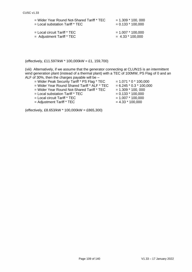
CUSC v1.33

of 140 V1.33 – 17 January 2022

= Wider Year Round Not-Shared Tariff * TEC = 1.309 * 100, 000 = Local substation Tariff * TEC = 0.133 * 100,000 = Local circuit Tariff * TEC = 1.007 * 100,000 = Adjustment Tariff * TEC = 4.33 * 100,000

(effectively, £11.597/kW * 100,000kW = £1, 159,700) (viii) Alternatively, if we assume that the generator connecting at CLUN1S is an intermittent wind generation plant (instead of a thermal plant) with a TEC of 100MW, PS Flag of 0 and an ALF of 30%, then the charges payable will be –

= Wider Peak Security Tariff * PS Flag * TEC = 1.071 * 0 * 100,000 = Wider Year Round Shared Tariff * ALF * TEC = 6.245 * 0.3 * 100,000 = Wider Year Round Not-Shared Tariff * TEC = 1.309 * 100, 000 = Local substation Tariff * TEC = 0.133 * 100,000 = Local circuit Tariff * TEC = 1.007 * 100,000

= Adjustment Tariff * TEC = 4.33 * 100,000 (effectively, £8.653/kW * 100,000kW = £865,300)

CUSC v1.33

of 140 V1.33 – 17 January 2022

14.24 Example: Calculation of Zonal Gross Demand Tariff Let us consider all nodes in the same demand zone in this example The table below shows an example output of the transport model comprising the node, the Peak Security and Year Round nodal marginal km of an injection at the node with a consequent withdrawal at the distributed reference node, the generation sited at the node, scaled to ensure total national generation = total national net demand and the net demand sited at the node. Where the Demand (MW) is negative this indicates that the Demand node is Exporting rather than importing.

Demand Zone

Node

Peak Security

Nodal Marginal

km

Year Round Nodal

Marginal km

Demand (MW)

1 A 110 80 100

1 B 140 90 100

1 C 120 80 0

1 D 100 100 -50

1 E 100 70 50

Totals 200

Demand Zone

Node Peak Security

Nodal Marginal km

Year Round Nodal Marginal

km

Net Demand

(MW) 14 ABHA4A -77.25 -230.25 127 14 ABHA4B -77.27 -230.12 127 14 ALVE4A -82.28 -197.18 100 14 ALVE4B -82.28 -197.15 100 14 AXMI40_SWEB -125.58 -176.19 97 14 BRWA2A -46.55 -182.68 96 14 BRWA2B -46.55 -181.12 96 14 EXET40 -87.69 -164.42 340 14 HINP20 -46.55 -147.14 0 14 HINP40 -46.55 -147.14 0 14 INDQ40 -102.02 -262.50 444 14 IROA20_SWEB -109.05 -141.92 462 14 LAND40 -62.54 -246.16 262 14 MELK40_SWEB 18.67 -140.75 83 14 SEAB40 65.33 -140.97 304 14 TAUN4A -66.65 -149.11 55 14 TAUN4B -66.66 -149.11 55 Totals 2748

CUSC v1.33

of 140 V1.33 – 17 January 2022

In order to calculate the gross demand tariff we would carry out the following steps:

(i) Change Negative Demand values to 0 (zero) , which in this example is Node D

Demand Zone

Node Peak Security

Nodal Marginal km

Year Round Nodal

Marginal km

Demand (MW)

1 A 110 80 100

1 B 140 90 100

1 C 120 80 0

1 D 100 100 0

1 E 100 70 50

Totals 250

(ii) calculate the demand weighted nodal shadow costs

For this example zone this would be as follows:

Demand Zone

Node

Peak Security

Nodal Marginal

km

Year Round Nodal

Marginal km

Demand (MW)

Peak Security Demand

Weighted Nodal

Marginal km

Year Round

Demand Weighted

Nodal Marginal

km

1 A 110 80 100 44 32

1 B 140 90 100 56 36

1 C 120 80 0 0 0

1 D 100 100 0 0 0

1 E 100 70 50 20 14

Totals 250 120 82

CUSC v1.33

of 140 V1.33 – 17 January 2022

(iii) sum the Peak Security and Year Round demand weighted nodal shadow costs to give

zonal figures. For this example zone this is shown in the above table and is 120km for Peak Security background and 82km for Year Round background.

(iv) calculate the transport (locational) tariffs by multiplying the figures in (ii) above by -1. This changes the original Nodal Marginal Km for injecting (Generation) into Nodal Marginal Km for withdrawing (Demand). Then multiply by the expansion constant, the locational security factor and then divide by 1000 to put into units of £/kW: For this example zone, assuming an expansion constant of £10.07/MWkm and a locational security factor of 1.80: a) Peak Security tariff – - (120km * £10.07/MWkm * 1.8) = -£2.47/kW

1000

b) Year Round tariff - - (82* £10.07/MWkm * 1.8) = -£1.49/kW

1000 The Locational signal for Demand within this zone is negative for both Peak and Year Round, which indicates withdrawing at this part of the network, reduces total system flows.

(v) We now need to calculate the residual tariff. This is calculated by taking the total revenue

to be recovered from demand less the revenue which would be recovered through the demand transport tariffs and revenue recovery through embedded export tariffs, divided by total expected gross GSP group demand.

Assuming the total revenue to be recovered from gross GSP group demand = £779m. Assuming the total recovery from gross GSP group demand transport tariffs is £140m, total recovery from embedded export tariffs is -£10m and total forecast chargeable gross GSP group demand capacity is 50000MW, the demand residual tariff would be as follows:

£779𝑚−£140𝑚−−£10𝑚

50,000𝑀𝑊= £12.98/𝑘𝑊

(vi) to get to the final tariff, we simply add on the demand residual tariff calculated in (v) to the

zonal transport tariffs calculated in (iii(a)) and (iii(b))

For zone 1: -£2.47/kW + -£1.49/kW + £12.98/kW = £9.32/kW

To summarise, in order to calculate the gross demand tariffs, we evaluate a net demand weighted zonal marginal km cost multiply by the expansion constant and locational security factor then we add a constant (termed the residual cost) to give the overall tariff.

(vii) The final demand tariff is subject to further adjustment to allow for the minimum £0/kW

gross demand charge. The application of a discount for small generators pursuant to Licence Condition C13 will also affect the final gross demand tariff.

CUSC v1.33

of 140 V1.33 – 17 January 2022

14.25 Reconciliation of Gross Demand Related Transmission Network Use of System Charges This appendix illustrates the methodology used by The Company in the reconciliation of Transmission Network Use of System charges for gross demand. The example highlights the different stages of the calculations from the monthly invoiced amounts, right through to Final Reconciliation.

Monthly Charges

Suppliers provide half-hourly (HH) gross demand and embedded export forecasts and non-half-hourly (NHH) demand forecasts by BM Unit every quarter. An example of such forecasts and the corresponding monthly invoiced amounts, based on tariffs of £10.00/kW for gross demand, £5.00/kW for embedded export and 1.20p/kWh for energy consumption, is as follows:

Forecast HH

Triad Gross Demand

HHDF (kW)

HH Gross Demand Monthly Invoiced

Amount (£)

Forecast HH

Triad Embedded

Export HHEEF (kW)

HH Embedded Generation

Monthly Invoiced

Amount (£)

Forecast NHH

Energy Consumpti

on NHHCF(kW

h)

NHH Monthly Invoiced

Amount (£)

Net Monthly Invoiced

Amount (£)

Apr 12,000 10,000 -600 (250) 15,000,000 15,000 24,750 May 12,000 10,000 -600 (250) 15,000,000 15,000 24,750 Jun 12,000 10,000 -600 (250) 15,000,000 15,000 24,750 Jul 12,000 10,000 -600 (250) 18,000,000 19,000 28,750 Aug 12,000 10,000 -600 (250) 18,000,000 19,000 28,750 Sep 12,000 10,000 -600 (250) 18,000,000 19,000 28,750 Oct 12,000 10,000 -600 (250) 18,000,000 19,000 28,750 Nov 12,000 10,000 -600 (250) 18,000,000 19,000 28,750 Dec 12,000 10,000 -600 (250) 18,000,000 19,000 28,750 Jan 7,200 (6,000) -600 (250) 18,000,000 19,000 12,750

CUSC v1.33

of 140 V1.33 – 17 January 2022

Feb 7,200 (6,000) -600 (250) 18,000,000 19,000 12,750 Mar 7,200 (6,000) -600 (250) 18,000,000 19,000 12,750

Total 72,000 (3,000) 216,000 297,000

As shown, for the first nine months the Supplier provided a 12,000kW HH triad gross demand forecast, and hence paid HH gross demand monthly charges of £10,000 ((12,000kW x £10.00/kW)/12) for that BM Unit. In January the Supplier provided a revised forecast of 7,200kW, implying a forecast annual charge reduced to £72,000 (7,200kW x £10.00/kW). The Supplier had already paid £90,000, so the excess of £18,000 was credited back to the supplier in three £6,000 instalments over the last three months of the year.

The Supplier provided an embedded export triad forecast of -600kW and hence was paid an embedded export credit of £250 ((600kW x £5.00/kW)/12) for that BM Unit (For the avoidance of doubt, if the embedded export tariff is negative this will result in a debit).

The Supplier also initially provided a 15,000,000kWh NHH energy consumption forecast, and hence paid NHH monthly charges of £15,000 ((15,000,000kWh x 1.2p/kWh)/12) for that BM Unit. In July the Supplier provided a revised forecast of 18,000,000kWh, implying a forecast annual charge increased to £216,000 (18,000,000kWh x 1.2p/kWh). The Supplier had already paid £45,000, so the remaining £171,000 was split into payments of £19,000 for the last nine months of the year.

The right hand column shows the net monthly charges for the BM Unit.

Initial Reconciliation (Part 1a)

The Supplier’s outturn HH triad gross demand, based on initial settlement data (and therefore subject to change in subsequent settlement runs), was 9,000kW. The HH triad gross demand reconciliation charge is therefore calculated as follows:

HHD Reconciliation Charge = (HHDA - HHDF) x £/kW Tariff

= (9,000kW - 7,200kW) x £10.00/kW

= 1,800kW x £10.00/kW

= £18,000

To calculate monthly interest charges, the outturn HHD charge is split equally over the 12-month period. The monthly reconciliation amount is the monthly outturn HHD charge less the HH gross demand monthly invoiced amount. Interest payments are calculated based on these monthly reconciliation amounts using Barclays Base Rate.

Initial Reconciliation (Part 1b) The Supplier’s outturn HH triad embedded export, based on initial settlement data (and therefore subject to change in subsequent settlement runs), was 700kW. The HH triad embedded export reconciliation charge is therefore calculated as follows:

HHEE Reconciliation Charge = (HHEEA – HHEEF) x £/kW Tariff

CUSC v1.33

of 140 V1.33 – 17 January 2022

= (-500kW - -600kW) x £5.00/kW

= 100kW x £5.00/kW

= £500

To calculate monthly interest charges, the outturn HHEE charge is split equally over the 12-month period. The monthly reconciliation amount is the monthly outturn HHEE charge less the HH embedded generation monthly invoiced amount. Interest payments are calculated based on these monthly reconciliation amounts using Barclays Base Rate.

Initial Reconciliation (Part 2)

The Supplier's outturn NHH energy consumption, based on initial settlement data, was 17,000,000kWh. The NHH energy consumption reconciliation charge is therefore calculated as follows:

NHHC Reconciliation Charge = (NHHCA - NHHCF) x p/kWh Tariff

100

= (17,000,000kWh - 18,000,000kWh) x 1.20p/kWh

100

= -1,000,000kWh x 1.20p/kWh 100

worked example 4.xls - Initial!J104 = -£12,000 The monthly reconciliation amount is equal to the outturn energy consumption charge for that month less the NHH monthly invoiced amount. Interest payments are calculated based on the monthly reconciliation amounts using Barclays Base Rate.

The net initial TNUoS demand reconciliation charge is therefore £6,500 (£18,000 = £500 - £12,000). Final Reconciliation

Finally, let us now suppose that after all final Settlement data has been received (up to 14 months after the relevant dates), the outturn HH triad gross demand, HH triad embedded export and NHH energy consumption values were 9,500kW, -550kW and 16,500,000kWh, respectively.

Final HH Gross Demand = (9,500kW - 9,000kW) x £10.00/kW

Reconciliation Charge = £5,000

Final HH Embedded Export = (-550kW - -500kW) x £5.00/kW

file:///C:/Users/urmi.mistry/AppData/Local/Microsoft/Windows/AppData/Local/Microsoft/Windows/Temporary%20Internet%20Files/AppData/Roaming/AppData/Local/Microsoft/Windows/Temporary%20Internet%20Files/AppData/Local/Microsoft/Windows/Temporary%20Internet%20Files/Content.Outlook/AppData/Local/Microsoft/Windows/Temporary%20Internet%20Files/Content.Outlook/AppData/Local/Microsoft/Windows/Temporary%20Internet%20Files/Content.Outlook/AppData/Local/Microsoft/Windows/Temporary%20Internet%20Files/Content.Outlook/AppData/Local/Microsoft/Windows/Temporary%20Internet%20Files/AppData/Local/Microsoft/Windows/Temporary%20Internet%20Files/Content.Outlook/AppData/Local/Microsoft/Windows/Temporary%20Internet%20Files/Content.Outlook/AppData/Local/Microsoft/Windows/Temporary%20Internet%20Files/Content.Outlook/AppData/Local/Microsoft/Windows/Temporary%20Internet%20Files/Content.Outlook/AppData/Local/Microsoft/Windows/Temporary%20Internet%20Files/Content.Outlook/AppData/Local/Microsoft/Documents%20and%20Settings/bali.virk/Local%20Settings/bali.virk/Local%20Settings/Temporary%20Internet%20Files/Local%20Settings/Temporary%20Internet%20Files/OLK6E8/worked%20example%204.xls#Initial!J104

CUSC v1.33

of 140 V1.33 – 17 January 2022

Reconciliation Charge = -£250 Final NHH Reconciliation Charge = (16,700,000kWh – 17,000,000kWh) x 1.20p/kWh

100

= -£3,600

Consequently, the net final TNUoS demand reconciliation charge will be £1, 150 (£5,000 + -£250 + -£3,600).. Interest payments are calculated based on the monthly reconciliation amounts using Barclays Base Rate. Outturn data for BM Units with a net export over the Triad will be received at this stage and final reconciliation will be carried out, as required. Interest will be calculated as described above.

Terminology:

HHDA = The Supplier's outturn half-hourly metered Triad Gross Demand (kW) for the demand zone concerned.

HHDF = The Supplier's forecast half-hourly metered Triad Gross Demand (kW) for the demand zone concerned. HHEEA = The Supplier's outturn half-hourly metered Triad Embedded Export (kW) for the demand zone concerned.

HHEEF = The Supplier's forecast half-hourly metered Triad Embedded Export (kW) for the demand zone concerned.

NHHCA = The Supplier's outturn non-half-hourly metered daily Energy Consumption (kWh) for the period 16:00 hrs to 19:00 hrs inclusive (i.e. settlement periods 33 to 38) from April 1st to March 31st, for the demand zone concerned. NHHCF = The Supplier's forecast non-half-hourly metered daily Energy Consumption (kWh) for the period 16:00 hrs to 19:00 hrs inclusive (i.e. settlement periods 33 to 38) from April 1st to March 31st, for the demand zone concerned.

£/kW Tariff = The £/kW Gross Demand or Embedded Export Tariff as shown in Schedule 1 of The Statement of Use of System Charges for the demand zone concerned.

p/kWh Tariff = The Energy Consumption Tariff shown in Schedule 1 of The Statement of Use of System Charges for the demand zone concerned.

CUSC v1.33

of 140 V1.33 – 17 January 2022

14.26 Classification of parties for charging purposes In the event of any conflict between this Appendix and the main text within this Statement, the main text within the Statement shall take precendence. In the following diagrams, the parties liable for Transmission Network Use of System charges are outlined in red.

SUPPLIER

Demand Charges

See 14.17.13 and 14.17.18.

Generation Charges

None.

POWER STATION WITH A BILATERAL CONNECTION AGREEMENT

Demand Charges

See 14.17.18.

Generation Charges

See 14.18.1 i) and 14.18.3 to 14.18.9 and 14.18.18.

For generators in positive zones, see 14.18.10 to 14.18.12.

For generators in negative zones, see 14.18.13 to 14.18.17.

Gen Unit

BMU1 Gen Unit

BMUn Station

Load BMU

Bilateral Connection Agreement Appendix C

Additional Load BMU

Supplier

BMU1 Supplier

BMUn

Supplier Use of System Agreement

CUSC v1.33

of 140 V1.33 – 17 January 2022

PARTY WITH A BILATERAL EMBEDDED GENERATION AGREEMENT

Demand Charges

See 14.17.14, 14.17.15 and 14.17.18.

Generation Charges

See 14.18.1 ii).

For generators in positive zones, see 14.18.3 to 14.18.12 and 14.18.18.

For generators in negative zones, see 14.18.3 to 14.18.9 and 14.18.13 to 14.18.18.

Gen Unit

BMU1 Gen Unit

BMUn Station

Load BMU

Bilateral Embedded Generation Agreement Appendix C

Additional Load BMU

CUSC v1.33

of 140 V1.33 – 17 January 2022

14.27 Transmission Network Use of System Charging Flowcharts The following flowcharts illustrate the parties liable for Demand and Generation TNUoS charges and the calculation of those charges. In the event of any conflict between this Appendix and the main text within this Statement, the main text within the Statement shall take precedence. Demand Charges

NB. If the average HH metered volume of

the Exempt Export BMU over the Triad

results in an import, the BMU will pay the

amount of the average import x relevant

£/kW tariff

If the average HH metered volume of the

Exempt Export BMU over the Triad

results in an export, the BMU will be paid

the amount of the average export x

relevant £/kW tariff

BMU = BM Unit DDI = Derogated Distribution Interconnector

HH = half hourly NHH = Non-half hourly

Demand Charging

Start

Average of each

BMU's HH metered

volume during the

Triad (x £/kW tariff)

Select

appropriate

party

Average net metered

import of Power Station

(including metered

additional load) during the


Power Stations with a

Bilateral Connection

Agreement or Licensable

Generation with a Bilateral

Embedded Generation

Agreement

Lead Party of

Supplier BMU

Exemptable Generation

and DDI with a Bilateral

Embedded Generation

Agreement

Average metered

volume of Exempt

Export BMU during the


Each BMU's NHH metered

energy consumption during

16.00-19.00 inclusive every

day over the Financial Year

(x p/kWh tariff)

AND

CUSC v1.33

of 140 V1.33 – 17 January 2022

Generation Charges

CUSC v1.33

of 140 V1.33 – 17 January 2022

14.28 Example: Determination of The Company’s Forecast for Demand Charge Purposes The Company will use the latest available settlement data for calculation of HH demand and NHH energy consumption forecasts for the Financial Year. The Financial Year runs from 1st April to 31st March inclusive and for the purpose of these examples the year April 2005 to March 2006 is used. Where the preceding year’s settlement data is not available at the time that The Company needs to calculate its forecast, The Company will use settlement data from the corresponding period in Financial Year minus two unless indicated otherwise. All values used with the examples are purely for illustrative purposes only. i) Half-Hourly (HH) Metered Demand Forecast – Existing User At the time of calculation of a HH demand forecast before the relevant Financial Year (approximately 10th March), The Company will be aware at a system level which dates will be used for the determination of Triad. However, The Company may not have settlement data at a User level if the Triad dates were to span a period that includes the latter half of February. When undertaking forecasting before the relevant Financial Year, The Company will use the User’s Triad demand for the previous year for its forecast providing it holds User settlement data for this period, thus: F = T where: F = Forecast of User’s HH demand at Triad for the Financial Year T = User’s HH gross demand and embedded export at Triad in Financial Year minus one Where The Company determines its forecast within a Financial Year: F = T * D/P where: F = Forecast of User’s HH demand at Triad for the Financial Year T = User’s HH gross demand and embedded export at Triad in the preceding Financial Year D = User’s average half hourly metered gross demand and embedded export in settlement

period 35 in the Financial Year to date P = User’s average half hourly metered gross demand and embedded export in settlement

period 35 for the period corresponding to D in the preceding Financial Year Where The Company determines its forecast before the relevant Financial Year and User settlement data for the Triad period is not available, The Company shall apply the formula immediately above (within year forecast) but substitute the following definitions for the values T, D, and P: T = User’s HH gross demand and embedded export at Triad in the Financial Year minus two

CUSC v1.33

of 140 V1.33 – 17 January 2022

D = User’s average half hourly metered gross demand and embedded export in settlement

period 35 in the Financial Year minus one, to date P = User’s average half hourly metered gross demand and embedded export in settlement

period 35 for the period corresponding to D in the Financial Year minus two Example (where User settlement data is not yet available for the Triad period): The Company calculates a HH demand forecast on the above methodology at 10th March 2005 for the period 1st April 2005 to 31st March 2006. Gross demand: F = 10,000 * 13,200 / 12,000 F = 11,000 kW where: T = 10,000 kW (period November 2003 to February 2004) D = 13,200 kW (period 1st April 2004 to 15th February 2005#) P = 12,000 kW (period 1st April 2003 to 15th February 2004) # Latest date for which settlement data is available. Embedded export: F = -280 * -300 / -350 F = -240 kW where: T = -280 kW (period November 2003 to February 2004) D = -300 kW (period 1st April 2004 to 15th February 2005#) P = -350 kW (period 1st April 2003 to 15th February 2004) # Latest date for which settlement data is available. ii) Non Half-Hourly (NHH) Metered Energy Consumption Forecast – Existing User F = E * D/P where: F = Forecast of User’s NHH metered energy consumption for the Financial Year E = User’s summed NHH energy consumption over the hours 16:00 to 19:00 for each day in

the preceding Financial Year

CUSC v1.33

of 140 V1.33 – 17 January 2022

D = User’s summed NHH energy consumption for the hours 16:00 to 19:00 for each day for the Financial Year to date

P = User’s summed NHH energy consumption for the hours 16:00 to 19:00 for each day for

the period corresponding to D in the preceding Financial Year Example: The Company calculates a NHH energy consumption forecast on the above methodology at 10th June 2005 for the period 1st April 2005 to 31st March 2006. F = 50,000,000 * 4,400,000 / 4,000,000 F = 55,000,000 kWh where: E = 50,000,000 kWh (period 1st April 2004 to 31st March 2005) D = 4,400,000 kWh (period 1st April 2005 to 15th May 2005#) P = 4,000,000 kWh (period 1st April 2004 to 15th May 2004) # Latest date for which settlement data is available Where forecasting before the relevant Financial Year concerned, The Company would in the above example use values for E and P from Financial Year 2003/04 and D from Financial Year 2004/05. iii) Half-Hourly (HH) Metered Demand Forecast – New User F = M * T/W where: F = Forecast of User’s HH metered gross demand and embedded export at Triad for the Financial Year M = User’s HH average weekday period 35 demand for the last complete month for which

settlement data is available T = Total system HH gross demand and embedded export at Triad in the preceding Financial Year W = Total system HH average weekday settlement period 35 metered demand for the

corresponding period to M for the preceding year Example: The Company calculates a HH demand forecast on the above methodology at 10th September 2005 for a new User registered from 10th June 2005 for the period 10th June 2004 to 31st March 2006. Gross demand: F = 1,000 * 17,000,000 / 18,888,888

CUSC v1.33

of 140 V1.33 – 17 January 2022

F = 900 kW where: M = 1,000 kW (period 1st July 2005 to 31st July 2005) T = 17,000,000 kW (period November 2004 to February 2005) W = 18,888,888 kW (period 1st July 2004 to 31st July 2004) Embedded export: F = -150 * -7,200,000 /- 6,000,000 F = -180 kW where: M = -150 kW (period 1st July 2005 to 31st July 2005) T = -7,200,000 kW (period November 2004 to February 2005) W = -6,000,000 kW (period 1st July 2004 to 31st July 2004) iv) Non Half Hourly (NHH) Metered Energy Consumption Forecast – New User F = J + (M * R/W)

CUSC v1.33

of 140 V1.33 – 17 January 2022

where: F = Forecast of User’s NHH metered energy consumption for the Financial Year J = Residual part month summed NHH metered energy consumption for the hours 16:00 to

19:00 for each day where new User registration takes place other than on the first of a month

M = User’s summed NHH metered energy consumption for the hours 16:00 to 19:00 for each

day for the last complete month for which settlement data is available R = Total system summed NHH metered energy consumption for the hours 16:00 to 19:00 for

each day for the period from the start of that defined under M but for the preceding year and until the end of that preceding Financial Year

W = Total system summed NHH metered energy consumption for the hours 16:00 to 19:00 for

each day for the period identified in M but for the preceding Financial Year Example: The Company calculates a NHH energy consumption forecast on the above methodology at 10th September 2005 for a new User registered from 10th June 2005 for the period 10th June 2005 to 31st March 2006. F = 500 + (1,000 * 20,000,000,000 / 2,000,000,000) F = 10,500 kWh where: J = 500 kWh (period 10th June 2005 to 30th June 2005) M = 1,000 kWh (period 1st July 2005 to 31st July 2005) R = 20,000,000,000 kWh (period 1st July 2004 to 31st March 2005) W = 2,000,000,000 kWh (period 1st July 2004 to 31st July 2004)

CUSC v1.33

of 140 V1.33 – 17 January 2022

14.29 Stability & Predictability of TNUoS tariffs Stability of tariffs The Transmission Network Use of System Charging Methodology has a number of elements to enhance the stability of the tariffs, which is an important aspect of facilitating competition in the generation and supply of electricity. This appendix seeks to highlight those elements. Each node of the transmission network is assigned to a zone, these zones are themselves fixed. The result of this is to dampen fluctuations that would otherwise be observed at a given node caused by changes in generation, demand, and network parameters. The criteria used to establish generation zones are part of the methodology and are described in Paragraph 14.15.42. In addition to fixing zones, other key parameters within the methodology are also fixed for the duration of the price control period or annual changes restricted in some way. Specifically:

• the expansion constant, which reflects the annuitised value of capital investment required to transport 1MW over 1km by a 400kV over-head line, changes annually according to TOPI. The other elements used to derive the expansion constant are only reviewed at the beginning of a price control period to ensure that it remains cost-reflective. This review will consider those components outlined in Paragraph 14.15.59 to Paragraph 14.15.69.

• the expansion factors, which are set on the same basis of the expansion constant and used to reflect the relative investment costs in each TO region of circuits at different transmission voltages and types, are fixed for the duration price control. These factors are reviewed at the beginning of a price control period and will take account of the same factors considered in the review of the expansion constant.

• the locational security factor, which reflects the transmission security provided under the NETS Security and Quality of Supply Standard, is fixed for the duration of the price control period and reviewed at the beginning of a price control period.

Predictability of tariffs The Company revises TNUoS tariffs each year to ensure that these remain cost-reflective and take into account changes to allowable income under the price control and TOPI. There are a number of provisions within the Transmission Licence and the CUSC designed to promote the predictability of annually varying charges. Specifically, The Company is required to give the Authority 150 days notice of its intention to change use of system charges together with a reasonable assessment of the proposals on those charges; and to give Users 2 months written notice of any revised charges. The Company typically provides an additional months notice of revised charges through the publication of “indicative” tariffs. Shorter notice periods are permitted by the framework but only following consent from the Authority. These features require formal proposals to change the Transmission Use of System Charging Methodology to be initiated in October to provide sufficient time for a formal consultation and the Authority’s veto period before charges are indicated to Users. More fundamentally, The Company also provides Users with the tool used by The Company to calculate tariffs. This allows Users to make their own predictions on how future changes in the generation and supply sectors will influence tariffs. Along with the price control information, the data from the Seven Year Statement, and Users own prediction of market activity, Users are able to make a reasonable estimate of future tariffs and perform sensitivity analysis.

CUSC v1.33

of 140 V1.33 – 17 January 2022

To supplement this, The Company also prepares an annual information paper that provides an indication of the future path of the locational element of tariffs over the next five years.7 This analysis is based on data included within the Seven Year Statement. This report typically includes:

• an explanation of the events that have caused tariffs to change;

• sensitivity analysis to indicate how generation and demand tariffs would change as a result of changes in generation and demand at certain points on the network that are not included within the SYS;

• an assessment of the compliance with the zoning criteria throughout the five year period to indicate how generation zones might need to change in the future, with a view to minimising such changes and giving as much notice of the need, or potential need, to change generation zones; and

• a complete dataset for the DCLF Transport Model developed for each future year, to allow Users to undertake their own sensitivity analysis for specific scenarios that they may wish to model.

The first year of tariffs forecasted in the annual information paper are updated twice throughout the proceeding financial year as the various Transport and Tariff model inputs are received or amended. These updates are in addition to the Authority 150 days notice and publication of “indicative” tariffs. The parameters used in the calculation of generation cap (in paragraph 14.15.5 v.)) will be published along with the forecast and confirmed values in the Tariff Information Paper which is produced in compliance with Condition 5 (of the NGC’s proposed GB electricity transmission use of system charging methodology - the Authority’s decisions document March 2005 80/5). In addition, The Company will, when revising generation charging zones prior to a new price control period, undertake a zoning consultation that uses data from the latest information paper. The purpose of this consultation will be to ensure tariff zones are robust to contracted changes in generation and supply, which could be expected to reduce the need for re-zoning exercises within a price control period.

7 http://www.nationalgrid.com/uk/Electricity/Charges/gbchargingapprovalconditions/5/

CUSC v1.33

of 140 V1.33 – 17 January 2022

Section 2 – The Statement of the Balancing Services Use of System Charging Methodology

14.29 Principles

14.29.1 The Transmission Licence allows The Company to derive revenue in respect of the Balancing Services Activity through the Balancing Services Use of System (BSUoS) charges. This statement explains the methodology used in order to calculate the BSUoS charges.

14.29.2 The Balancing Services Activity is defined in the Transmission Licence as the

activity undertaken by The Company as part of the Transmission Business including the operation of the transmission system and the procuring and using of Balancing Services for the purpose of balancing the transmission system.

14.29.3 The Company keeps the electricity system in balance (energy balancing) and

maintains the quality and security of supply (system balancing). The Company is incentivised on the procurement and utilisation of services to maintain the energy and system balance and other costs associated with operating the system. Users pay for the cost of these services and any incentivised payment/receipts through the BSUoS charge.

14.29.4 All CUSC Parties acting as Generators and Suppliers (for the avoidance of doubt

excluding all BMUs and Trading Units associated with either Interconnectors or Virtual Lead Parties) are liable for Balancing Services Use of System charges based on their energy taken from or supplied to the National Grid system in each half-hour Settlement Period.

14.29.5 BSUoS charges comprise the following costs:

(i) The Total Costs of the Balancing Mechanism (ii) Total Balancing Services Contract costs (iii) Payments/Receipts from The Company’s incentive schemes (iv) Internal costs of operating the System (v) Costs associated with contracting for and developing Balancing

Services (vi) Adjustments (vii) Costs invoiced to The Company associated with Manifest Errors and

Special Provisions. (viii) BETTA implementation costs (ix) Financing and administrative costs, as agreed by The Authority,

associated with the management of the Covid Support Scheme in 14.30.12 and Exceptional Costs Support Scheme in 14.30.21.

CUSC v1.33

of 140 V1.33 – 17 January 2022

14.30 Calculation of the Daily Balancing Services Use of System charge

Calculation of the Daily Balancing Services Use of System charge

14.30.1 The BSUoS charge payable by customer c, on Settlement Day d, will be

calculated in accordance with the following formula:

Where: i - refers to the individual BM Unit j - refers to an individual Settlement Period

- refers to the sum over all BM units ‘i’, for which

customer ‘c’ is the Lead Party summed over all Settlement Periods ‘j’ on a Settlement Day ‘d’

14.30.2 The BSUoS tariff for each settlement period is calculated by the following

formula:

Where: BSUoSTOT

j - refers to the total BSUoS Charge that needs to be recovered for

Settlement Period j TQM j – refers to the total Transmission Connected Site BM Unit Metered Volume for Settlement Period j SGQM j – refers to the Gross Demand BM Unit Volume for Settlement Period j

14.30.3 A Supplier BM Unit’s and Exempt Export BM Unit’s charge is calculated by the

following formula:

14.30.4 All other BSUoS liable customers with a Bilateral Agreement with The Company will have their charge calculated by the following formula:

or CUSC party associated with the BMUnits (listed in Appendix C of the BEGA) who is exempt from also being a BSC Party

ijci djcd TOTBSUoSBSUoSTOT =

ci dj

CUSC v1.33

of 140 V1.33 – 17 January 2022

Interconnector BM Units

14.30.5 BM Unit and Trading Units associated with Interconnectors, including those

associated with the Interconnector Error Administrator, are not liable for BSUoS charges. BM Units, including Secondary BM Units, which are associated with Virtual Lead Parties are not liable for BSUoS charges.

Storage Facilities

14.30.6 The BM Units associated with CVA Storage Facilities will not be charged BSUoS against imported volumes where the imports of that BM Unit are solely for the purposes of operating that CVA Storage Facility.

14.30.7 Where the BM Unit is a Supplier BM Unit and one or more SVA Storage Facilities are registered to that Supplier BM Unit, the Supplier shall be liable for BSUoS in accordance with 14.30.3, excluding any imports to such SVA Storage Facilities where those imports are solely for the purposes of operating that Storage Facility.

14.30.8 In all cases, where a facility ceases to be a CVA Storage Facility, the exemption

in para 14.30.6 shall no longer apply. The User, shall inform The Company as soon as is reasonably practicable and in any event no more than 5 Working Days from the date on which the facility ceased to be a CVA Storage Facility.

Total BSUoS Charge (Internal + External) for each Settlement Period (BSUoSTOTjd)

14.30.9 The Total BSUoS charges for each Settlement Period (BSUoSTOTjd) for a particular day are calculated by summing the external BSUoS charge (BSUoSEXTjd) and internal BSUoS charge (BSUoSINTjd) for each Settlement Period.

External BSUoS Charge for each Settlement Period (BSUoSEXTjd)

14.30.10 The External BSUoS Charges for each Settlement Period (BSUoSEXTjd) are calculated by taking each Settlement Period System Operator BM Cash Flow (CSOBMj) and Balancing Service Variable Contract Cost (BSCCVj) and allocating the daily elements on a MWh basis across each Settlement Period in a day.

jdjdjd BSUoSINTBSUoSEXTBSUoSTOT +=

CUSC v1.33

of 140 V1.33 – 17 January 2022

Internal BSUoS Charge for each Settlement Period (BSUoSINTjd)

14.30.11 The Internal BSUoS Charges (BSUoSINTjd) for each Settlement Period j for a particular day are calculated by taking the incentivised and non-incentivised SO Internal Costs (as determined in line with Transmission Licence Special Condition 4.1) for each Settlement Day allocated on a MWh basis across each Settlement Period in a day.

Inclusion of Profiling Factors

14.30.12 Profiling factors have been included to give an effective mechanism for

calculating a representative level of the incentive payments to/from The Company according to the time of year. All PFTk are assumed to be one for the duration of the current external incentive scheme

Covid-19 specific changes

14.30.13 As a result of the Coronavirus-19 (Covid-19) pandemic, The Company will make specific and time-limited changes to the BSUoS methodology in this Section 2 to support those Users identified in 14.29.4. This will consist of deferring the BSUoS costs associated with Covid-19 (“Covid Costs”) from the calculation in 14.30.9 to a later date as described in 14.30.14 and 14.30.15 (the “Covid Support Scheme”).

14.30.14 Covid Costs shall be calculated as;

If BSUoSTOTj <= COVIDCAPTOTj, then BSUoSCOVIDj = £0 Or BSUoSTOTj > COVIDCAPTOTj, then BSUoSCOVIDj = BSUoSTOTj - COVIDCAPTOTj Where; From 25th June 2020 until the Business Day after the Authority’s decision on CMP350, COVIDCAPTOTj is calculated as;

£15/𝑀𝑊ℎ ∗ {|∑ (𝑄𝑀𝐵𝑆𝑈𝑜𝑆𝑖𝑗 ∗ 𝑇𝐿𝑀𝑖𝑗)+

| + |∑ (𝑄𝑀𝐵𝑆𝑈𝑜𝑆𝑖𝑗 ∗ 𝑇𝐿𝑀𝑖𝑗)−

|}

+

+

++++−++

+=

dj ijij

ijdijd

ddddddd

jdjdjd

SGQMTQM

SGQMTQM

DBSUoSCCOVILOCTRUSOTOCBSCOMTotAdjBSCCA

BSCCVCSOBMBSUoSEXT

)(

/)(*

)(

++

+=

dj ijijijdijd

ddjd

SGQMTQMSGQMTQM

SOLARADJRBSUoSINT

)(/)(*

)(

CUSC v1.33

of 140 V1.33 – 17 January 2022

And From the first Settlement Period of the Business Day after the Authority’s decision on CMP350 to the Covid Support Scheme End Date, COVIDCAPTOTj is calculated as;

£10/𝑀𝑊ℎ ∗ {|∑(𝑄𝑀𝐵𝑆𝑈𝑜𝑆𝑖𝑗 ∗ 𝑇𝐿𝑀𝑖𝑗)

+

| + |∑(𝑄𝑀𝐵𝑆𝑈𝑜𝑆𝑖𝑗 ∗ 𝑇𝐿𝑀𝑖𝑗)

−

|}

14.30.15 Between 2 working days from The Authority’s decision on CMP345 and the Covid Support Scheme End Date, the formula in 14.30.9 shall be updated so that Covid Costs (BSUoSCOVIDjd) for Settlement Period j in Settlement Day d are removed as follows;

BSUoSTOTjd = BSUoSEXTjd + BSUoSINTjd - BSUoSCOVIDjd

The Covid Support Scheme End Date shall be the earlier of: 1. The 25th October 2020, or, 2. The day as advised by The Company as described in 14.30.18

14.30.16 During the Financial Year 2021/22, the formula in 14.30.9 shall be updated so

that Covid Costs (BSUoSCOVIDjd) for Settlement Period j in Settlement Day d are added as follows; BSUoSTOTjd = BSUoSEXTjd + BSUoSINTjd + BSUoSCOVIDjd

Where BSUoSCOVIDjd, is the cumulative total Covid Cost of the Covid Support Scheme (including any administrative or financing cost borne by The Company, as agreed by The Authority) recovered equally from each Settlement Period in the Financial Year.

Outside of the date ranges listed in 14.30.15, and 14.30.16 the formula in 14.30.9 shall be unchanged and in effect.

14.30.17 The Company shall provide weekly updates to notify industry of the total Covid Costs removed under paragraphs 14.30.14 and 14.30.15. When BSUoSCOVIDjd

reaches a value of £60m, The Company shall revise the frequency of these updates to each Business Day from the next Business Day after BSUoSCOVIDjd reaches a value of £60m.

14.30.18 When The Company, exercising its reasonable judgement, has reason to believe that the cumulative total for BSUoSCOVIDjd since 25th June 2020 could exceed £100m (excluding of VAT), The Company shall notify Users of when the Covid Support Scheme will end. The Company shall give no less than 2 Business Days notice of the Covid Support Scheme ending. Such notice shall be accompanied by an opinion which states that it is the reasonable judgement of The Company that if the Covid Support Scheme continued beyond the notified end date then the cumulative total for BSUoSCOVIDjd from 25th June 2020 would exceed £100m.

2020/21 Under Recovered Costs

CUSC v1.33

of 140 V1.33 – 17 January 2022

14.30.19 Given the circumstances giving rise to the £33,163,790.21 under recovery of

external BSUoS costs during financial year 2020/21 (the “2020/21 Under Recovered Costs”, which sum is separate and in addition to the COVID Costs) The Company will make specific and time-limited changes to the BSUoS methodology. This consists of deferring the recovery of the 2020/21 Under Recovered Costs from recovery through the Final Reconciliation Settlement Run (RF) for financial year 2020/21 for Settlement Days 30th September 2020 to 9th March 2021 to a later date as described in 14.30.20

14.30.20 The formula in 14.30.10 shall be updated between 1st October 2021 and 31st

March 2022 so that the 2020/21 Under Recovered Costs (BSUoSUR20d) for Settlement Day d are added as follows;

𝐵𝑆𝑈𝑜𝑆𝐸𝑋𝑇𝑗𝑑 = 𝐶𝑆𝑂𝐵𝑀𝑗𝑑 + 𝐵𝑆𝐶𝐶𝑉𝑗𝑑

+ [ (𝐵𝑆𝐶𝐶𝐴𝑑 + 𝑇𝑜𝑡𝐴𝑑𝑗𝑑 − 𝑂𝑀𝑑 + 𝐵𝑆𝐶𝑑 + 𝑆𝑂𝑇𝑂𝐶𝑑 + 𝐿𝑂𝐶𝑇𝑅𝑈𝑑

+ 𝐵𝑆𝑈𝑜𝑆𝐶𝐶𝑂𝑉𝐼𝐷𝑑 + 𝐵𝑆𝑈𝑜𝑆𝑈𝑅20𝑑) ∗ (𝑇𝑄𝑀𝑖𝑗𝑑

+ 𝑆𝐺𝑄𝑀𝑖𝑗𝑑)/ ∑ (𝑇𝑄𝑀𝑖𝑗 + 𝑆𝐺𝑄𝑀𝑖𝑗)]𝑗∈𝑑

Outside of the date range listed in 14.30.20 the formula in 14.30.10 shall be unchanged by 14.30.20.

Temporary BSUoS Cost Deferral

14.30.21 As a result of the exceptional market conditions, The Company will make

specific and time-limited changes to the BSUoS methodology in this Section 2 to support those Users identified in 14.29.4. This will consist of deferring the BSUoS costs associated with the exceptional market conditions (“Exceptional Costs”) above a defined £/MWh value from the calculation in 14.30.9 to a later date as described in 14.30.22 and 14.30.23 (the “Exceptional Costs Support Scheme”).

14.30.22 Exceptional Costs for Settlement Period j (BSUoSEXCj) shall be calculated as;

If BSUoSTOTj <= EXCCAPTOTj, then BSUoSEXCj = £0 Or BSUoSTOTj > EXCCAPTOTj, then BSUoSEXCj = BSUoSTOTj - EXCCAPTOTj Where EXCCAPTOTj is calculated as follows;

£20/𝑀𝑊ℎ ∗ (∑ 𝑆𝐺𝑄𝑀𝑗 + ∑ 𝑇𝑄𝑀𝑗)

14.30.23 From the first Settlement Period on the implementation date specified in the

Authority’s decision on CMP381 until the Exceptional Costs Support Scheme End Date, the formula in 14.30.9 and 14.30.16 shall be updated so that Exceptional Costs (BSUoSEXCjd) for Settlement Period j in Settlement Day d are removed as follows; BSUoSTOTjd = BSUoSEXTjd + BSUoSINTjd + BSUoSCOVIDjd - BSUoSEXCjd

CUSC v1.33

of 140 V1.33 – 17 January 2022

The Exceptional Costs Support Scheme End Date shall be the earlier of: 1. The end of the last Settlement Period (23:30 – 00:00) of 31st March

2022, or, 2. The Settlement Period as advised by The Company in accordance

with 14.30.26

14.30.24 During the Financial Year 2022/23, the formula in 14.30.10 shall be updated so that Exceptional Costs (BSUoSEXCd) in Settlement Day d are added as follows;

𝐵𝑆𝑈𝑜𝑆𝐸𝑋𝑇𝑗𝑑 = 𝐶𝑆𝑂𝐵𝑀𝑗𝑑 + 𝐵𝑆𝐶𝐶𝑉𝑗𝑑

+ [ (𝐵𝑆𝐶𝐶𝐴𝑑 + 𝑇𝑜𝑡𝐴𝑑𝑗𝑑 − 𝑂𝑀𝑑 + 𝐵𝑆𝐶𝑑 + 𝑆𝑂𝑇𝑂𝐶𝑑 + 𝐿𝑂𝐶𝑇𝑅𝑈𝑑

+ 𝐵𝑆𝑈𝑜𝑆𝐸𝑋𝐶𝑑) ∗ (𝑇𝑄𝑀𝑖𝑗𝑑

+ 𝑆𝐺𝑄𝑀𝑖𝑗𝑑)/ ∑ (𝑇𝑄𝑀𝑖𝑗 + 𝑆𝐺𝑄𝑀𝑖𝑗)]𝑗∈𝑑

Where BSUoSEXCd, is the cumulative total deferred value of the Exceptional Costs Support Scheme, including any administrative or financing cost borne by The Company, as agreed by the Authority.

14.30.25 The Company shall provide weekly updates to notify industry of the total

Exceptional Costs removed under paragraphs 14.30.22 and 14.30.23. When BSUoSEXCd reaches a value of £120m, The Company shall revise the frequency of these updates to each Business Day from the next Business Day.

14.30.26 The £20/MWh cap (as introduced in paragraph 14.30.22) will not be applied in the first and subsequent Settlement Periods where the £200m limit would have otherwise been breached. Once the Initial Settlement Run confirming this has been completed, The Company will notify Users to confirm that the Exceptional Costs Support Scheme has ended, providing the precise Settlement Day, Settlement Period and value of BSUoSEXCd.

14.31 Settlement of BSUoS Settlement and Reconciliation of BSUoS charges

14.31.1 There are two stages of the reconciliation of BSUoS charges described below:

• Initial Settlement (SF)

• Final Reconciliation (RF)

Initial Settlement of BSUoS

14.31.2 The Company will calculate initial settlement (SF) BSUoS charges in accordance

with the methodology set out in section 14.30 above, using the latest available data, including data from the Initial Settlement Run and the Initial Volume Allocation Run.

Reconciliation of BSUoS Charges

14.31.3 Final Reconciliation will result in the calculation of a reconciled charge for each settlement day in the scheme year. The Company will calculate Final

CUSC v1.33

of 140 V1.33 – 17 January 2022

Reconciliation (RF) BSUoS charges (with the inclusion of interest as defined in the CUSC) in accordance with the methodology set out in section 14.30 above, using the latest available data, including data from the Final Reconciliation Settlement Run and the Final Reconciliation Volume Allocation Run.

Unavailability of Data

14.31.4 If any of the elements required to calculate the BSUoS charges in respect of any Settlement Day have not been notified to The Company in time for it to do the calculations then The Company will use data for the corresponding Settlement Day in the previous week. If no such values for the previous week are available to The Company then The Company will substitute such variables as it shall, at its reasonable discretion, think fit and calculate Balancing Services Use of System charges on the basis of these values. When the actual data becomes available a reconciliation run will be undertaken.

Disputes

14.31.5 If The Company or any customer identifies any error which would affect the total

Balancing Services Use of System charge on a Settlement Day then The Company will recalculate the charges following resolution of the error. Revised invoices and/or credit notes will be issued for the change in charges, plus interest as set out in the CUSC. The charge recalculation and issuing of revised invoices and/or credit notes will not take place for any day where the total change in the Balancing Services charge is less than £2000.

CUSC v1.33

of 140 V1.33 – 17 January 2022

Relationship between the Statement of the Use of System Charging Methodology and the Transmission Licence

14.31.6 BSUoS charges are made on a daily basis and as such of this Statement sets

out the details of the calculation of such charges on a daily basis. Customers may, when verifying charges for Balancing Services Use of System refer to the Transmission Licence which sets out the maximum allowed revenue that The Company may recover in respect of the Balancing Services Activity.

14.31.7 The Company has, where possible and appropriate, attempted to ensure that

acronyms allocated to variables within the Balancing Services charging software, and associated reporting, match with the acronyms given to those variables used within this statement.

CUSC v1.33

of 140 V1.33 – 17 January 2022

14.31.8 Balancing Services Use of System Acronym Definitions

For the avoidance of doubt “as defined in the BSC” relates to the Balancing and Settlement Code as published from time to time.

1 Current electricity transmission network price control starting 2021 (RIIO-T2) licence drafting being updated

EXPRESSION ACRONYM Unit Definition

Daily Adjusted Revenue

ADJRd £

Means adjusted revenue published by the Authority pursuant to Special Condition 5.2 (Annual Iteration Process for the ESO Price Control Financial Model) prior to the end of Regulatory Year t; as calculated for Settlement Day, d,

BETTA Preparation Costs

BI £ As defined in the Transmission Licence

Balancing Mechanism Unit

BM Unit or BMU

As defined in the BSC

Black Start Costs BSC £ As defined in the Transmission Licence1

Balancing service contract costs – non-Settlement Period specific

BSCCAd £

Non Settlement Period specific Balancing Contract Costs for settlement day d less any costs incurred within these values relating to Supplementary Balancing Reserve and Demand Side Balancing Reserve

Balancing Service Contract Cost

BSCCj £

Balancing Service Contract Cost from purchasing Ancillary services applicable to a Settlement Period j less any costs incurred within these values relating to Supplementary Balancing Reserve and Demand Side Balancing Reserve

Balancing service contract costs – Settlement Period specific

BSCCVjd £ Settlement Period j specific Balancing Contract Costs for settlement day d

Cost of the Covid Support Scheme incurred in 2020/21

BSUoSCOVIDd £ As defined in the Transmission Licence calculated for Settlement Day, d

External Balancing Services Use of System charge

BSUoSEXTjd £ External System Operator (SO) Balancing Services Use of System charge applicable to Settlement Period j for settlement day d

Internal Balancing Services Use of System charge

BSUoSINTjd £ Internal System Operator (SO) Balancing Services Use of System charge applicable to Settlement Period j for settlement day d

Balancing Services Use of System tariff

BSUoStariffj £/MWh

Tariff for the Balancing Services Use of System charge applicable to Settlement Period j

Total Balancing Services Use of System charge

BSUoSTOTcd £ The sum determined for each customer, c, in accordance with this Statement and payable by that customer in respect of

CUSC v1.33

of 140 V1.33 – 17 January 2022

each Settlement Day d, in accordance with the terms of the Supplemental Agreement

Total Balancing Services Use of System charge

BSUoSTOTj £ Total Balancing Services Use of System Charge applicable for Settlement Period j

BSUoS 2020/21 Under Recovered Costs

BSUoSUR20d £

The External System Operator (SO) Balancing Services Use of System charges in the sum of £33,163,790.21 due in financial year 2020 / 2021 divided equally over the settlement days between 1st October 2021 to 31st March 2022 inclusive. This is separate, and in addition to, the Covid Support Scheme.

System Operator BM Cash Flow

CSOBMj £

As defined in the Balancing and Settlement Code in force immediately prior to 1 April 2001 less any costs incurred within these values relating to Supplementary Balancing Reserve and Demand Side Balancing Reserve

Daily balancing services adjustment

TotAdjd £

Is the contribution on Settlement Day, d, to the value of TotAdjt where TotAdjt is determined pursuant to part B of Special Condition 4.2 of the Transmission Licence

Forecast incentivised Balancing Cost

FBCd £ Forecast incentivised Balancing Cost for duration of the Incentive Scheme as at settlement day d

Allowed Income Adjustment relating to the SO-TO Code

IAT £ As defined in the Transmission Licence

Legacy adjustment with respect to actual and assumed RPI values

LOCTRUd £ As defined in the Transmission Licence, calculated for Settlement Day,d.

Cost associated with the Provision of Balancing Services to others

OMd £

Is the contribution on Settlement Day, d, to the value of OMt where OMt is determined pursuant to part C of special Condition 4.2 of the Transmission Licence

Outage change allowance amount

ON £ As defined in the Transmission Licence

BM Unit Metered Volume

QMij MWh As defined in the BSC

Gross Demand BM Unit Volume

SGQM MWh

The Import data as at the Transmission System Boundary by Settlement Period for Supplier BM Units and Exempt Export BM Units, minus imports for registered SVA storage facilities where those imports are solely for the purposes of operating that Storage Facility, multiplied by the applicable TLM

SO-TO funding allowance

SOTOC £

As defined in the Transmission Licence means the SO-TO cost allowance term, calculated in accordance with Special Condition 4.4 (SO-TO Mechanism)

CUSC v1.33

of 140 V1.33 – 17 January 2022

Supplier BM Unit As defined in the BSC

System Operator Legacy Adjustments

SOLARd £ As defined in the Transmission Licence calculated for Settlement Day, d

Trading Unit Delivery Mode Multiplier

Trading Units as defined in the Balancing and Settlement Code can be either in ‘delivering’ or ‘offtaking’ mode. If the Trading Unit Delivery Mode of a Trading Unit is ‘Delivering’ the Trading Unit Delivery Mode Multiplier is +1 for all BM Units within that Trading Unit. If the Trading Unit Delivery Mode of a Trading Unit is ‘offtaking’ the Trading Unit Delivery Mode Multiplier is -1 for all BM Units within that Trading Unit.

Transmission Loss Multiplier

TLMij As defined in the BSC

Transmission Connected Site BM Unit Metered Volume

TQM MWh

The BM Unit Metered Volume for BSUoS liable Users with a Bilateral Agreement with The Company, excluding Exempt Export BM Units, minus imports to registered CVA storage facilities where those imports are solely for the purposes of operating that Storage Facility, which is multiplied by the TLM and Trading Unit Delivery Mode Multiplier

Transmission System Boundary

As defined in the Balancing and Settlement Code

Total System Energy Imbalance Volume

TQEIj MWh As defined in the Balancing and Settlement Code in force immediately prior to 1 April 2001

Final Reconciliation Settlement Run


Final Reconciliation Volume Allocation Run


Initial Settlement Run As defined in the BSC

Initial Volume Allocation Run


Lead Party As defined in the BSC

CUSC v1.33

of 140 V1.33 – 17 January 2022

CUSC - SECTION 14 CHARGING METHODOLOGIES ...

Documents

Transcript of CUSC - SECTION 14 CHARGING METHODOLOGIES ...