
nespoli.pdf - TDX (Tesis Doctorals en Xarxa)
270
DEPARTAMENT D’ASTRONOMIA MULTIWAVELENGTH STUDY OF ACCRETION-POWERED PULSARS. ELISA NESPOLI UNIVERSITAT DE VALÈNCIA Servei de Publicacions 2010
-
Upload
khangminh22 -
Category
Documents
-
view
3 -
download
0
Transcript of nespoli.pdf - TDX (Tesis Doctorals en Xarxa)
DEPARTAMENT D’ASTRONOMIA MULTIWAVELENGTH STUDY OF ACCRETION-POWERED PULSARS. ELISA NESPOLI
UNIVERSITAT DE VALÈNCIA Servei de Publicacions
2010
Aquesta Tesi Doctoral va ser presentada a València el dia 18 de juny de 2010 davant un tribunal format per:
- Dr. Josep Maria Paredes Roy - Dr. Pere Blay Serrano - Dr. Jorge Casares Velázquez - Dr. José Miguel Torrejón Vázquez - Dra. Silvia Martínez Núñez
Va ser dirigida per: Dr. Juan Fabregat Llueca Dr. Pablo Reig Torres ©Copyright: Servei de Publicacions Elisa Nespoli
Dipòsit legal: V-2053-2011 I.S.B.N.: 978-84-370-7913-4
Edita: Universitat de València Servei de Publicacions C/ Arts Gràfiques, 13 baix 46010 València Spain
Telèfon:(0034)963864115

ii

!
!!!!!
!
!
!
Dr. Juan Fabregat Llueca,
Profesor titular del Departamento de Astronomía y Astrofísica de la Universidad de Valencia,
CERTIFICA
Que la presente memoria, “Multiwavelength study of accretion-powered pulsars”, ha sido realizada bajo su dirección por Elisa Nespoli, y que constituye su tesis doctoral para optar al grado de Doctor en Física.
Y para que quede constancia y tenga los efectos oportunos, firmo el presente documento en Paterna, a 13 de Abril de 2010.
Firmado: Juan Fabregat Llueca
! !

iv

!
!!!
!
!
!
Dr. Pablo Reig Torres,
Investigador del Foundation for Research & Technology – HELLAS (FORTH), Grecia
CERTIFICA
Que la presente memoria, “Multiwavelength study of accretion-powered pulsars”, ha sido realizada bajo su dirección por Elisa Nespoli, y que constituye su tesis doctoral para optar al grado de Doctor en Física.
Y para que quede constancia y tenga los efectos oportunos, firmo el presente documento en Paterna, a 13 de Abril de 2010.
Firmado: Pablo Reig Torres
! !

vi

ai miei genitori
vii

viii

Contents
1 Introduction: X-Ray Binaries 1
1.1 Scientific context . . . . . . . . . . . . . . . . . . . . . . . . . . . . 11.2 A brief historical review . . . . . . . . . . . . . . . . . . . . . . . . 41.3 The primary star: a compact object . . . . . . . . . . . . . . . . . 61.4 The secondary star: a massive OB star . . . . . . . . . . . . . . . . 9
1.4.1 Stellar winds . . . . . . . . . . . . . . . . . . . . . . . . . . 101.4.2 The Be-phenomenon . . . . . . . . . . . . . . . . . . . . . . 11
1.5 High-mass X-ray binaries: observational properties . . . . . . . . . 121.5.1 X-ray observations . . . . . . . . . . . . . . . . . . . . . . . 131.5.2 IR observations . . . . . . . . . . . . . . . . . . . . . . . . . 17
I IR photometry and spectroscopy 19
2 Search for IR counterparts to obscured HMXBs 21
2.1 Scientific objective . . . . . . . . . . . . . . . . . . . . . . . . . . . 212.2 A new photometric technique . . . . . . . . . . . . . . . . . . . . . 222.3 Observations . . . . . . . . . . . . . . . . . . . . . . . . . . . . . . 242.4 Data reduction . . . . . . . . . . . . . . . . . . . . . . . . . . . . . 28
2.4.1 Inter-quadrant row cross-talk . . . . . . . . . . . . . . . . . 282.4.2 Sky subtraction . . . . . . . . . . . . . . . . . . . . . . . . . 292.4.3 Flat fields . . . . . . . . . . . . . . . . . . . . . . . . . . . . 292.4.4 Image alignment and combination . . . . . . . . . . . . . . 302.4.5 PSF-fitting photometry . . . . . . . . . . . . . . . . . . . . 302.4.6 Photometric calibration and aperture correction . . . . . . 34
2.5 Results . . . . . . . . . . . . . . . . . . . . . . . . . . . . . . . . . . 362.6 First tests . . . . . . . . . . . . . . . . . . . . . . . . . . . . . . . . 49
3 NIR spectral analysis and classification of HMXBs identified by INTE-GRAL 53
3.1 Scientific objective . . . . . . . . . . . . . . . . . . . . . . . . . . . 533.2 Observations . . . . . . . . . . . . . . . . . . . . . . . . . . . . . . 543.3 Data reduction . . . . . . . . . . . . . . . . . . . . . . . . . . . . . 55
ix

CONTENTS
3.3.1 Inter-quadrant row cross-talk . . . . . . . . . . . . . . . . . 563.3.2 Sky subtraction . . . . . . . . . . . . . . . . . . . . . . . . . 583.3.3 Flat fields . . . . . . . . . . . . . . . . . . . . . . . . . . . . 593.3.4 Extraction of the one dimensional spectra . . . . . . . . . . 593.3.5 Wavelength calibration . . . . . . . . . . . . . . . . . . . . . 603.3.6 Telluric absorption correction . . . . . . . . . . . . . . . . . 63
3.4 Results . . . . . . . . . . . . . . . . . . . . . . . . . . . . . . . . . . 673.4.1 Spectral analysis and classification . . . . . . . . . . . . . . 683.4.2 Reference spectra of Be stars . . . . . . . . . . . . . . . . . 773.4.3 Reddening and distance estimation . . . . . . . . . . . . . . 79
3.5 Discussion . . . . . . . . . . . . . . . . . . . . . . . . . . . . . . . . 803.6 Conclusions . . . . . . . . . . . . . . . . . . . . . . . . . . . . . . . 83
4 K-band spectroscopy of two INTEGRAL sources reveals two new SyXBs 87
4.1 Symbiotic X-ray binaries . . . . . . . . . . . . . . . . . . . . . . . . 874.2 IGR J16358-4726 and IGR J16393-4643 . . . . . . . . . . . . . . . 884.3 Observations and data reduction . . . . . . . . . . . . . . . . . . . 904.4 Results . . . . . . . . . . . . . . . . . . . . . . . . . . . . . . . . . . 91
4.4.1 Spectral classification . . . . . . . . . . . . . . . . . . . . . 914.4.2 SED fitting . . . . . . . . . . . . . . . . . . . . . . . . . . . 95
4.5 Discussion . . . . . . . . . . . . . . . . . . . . . . . . . . . . . . . . 984.6 Conclusions . . . . . . . . . . . . . . . . . . . . . . . . . . . . . . . 104
5 Conclusions and future projects 105
5.1 Main results . . . . . . . . . . . . . . . . . . . . . . . . . . . . . . . 1055.2 Future work . . . . . . . . . . . . . . . . . . . . . . . . . . . . . . . 106
II X-ray analysis 107
6 X-ray analysis techniques 109
6.1 Spectral analysis . . . . . . . . . . . . . . . . . . . . . . . . . . . . 1106.1.1 Multy-band photometry . . . . . . . . . . . . . . . . . . . . 1106.1.2 Spectral fitting . . . . . . . . . . . . . . . . . . . . . . . . . 110
6.2 Timing analysis . . . . . . . . . . . . . . . . . . . . . . . . . . . . . 1116.3 This work . . . . . . . . . . . . . . . . . . . . . . . . . . . . . . . . 1126.4 Spectral states . . . . . . . . . . . . . . . . . . . . . . . . . . . . . 113
6.4.1 Neutron star LMXBs states . . . . . . . . . . . . . . . . . . 1136.4.2 Black-holes states . . . . . . . . . . . . . . . . . . . . . . . 116
x

CONTENTS
7 X-ray spectral and timing analysis of Be/XRBs during giant outbursts121
7.1 Scientific objective . . . . . . . . . . . . . . . . . . . . . . . . . . . 1217.2 The sources . . . . . . . . . . . . . . . . . . . . . . . . . . . . . . . 122
7.2.1 KS 1947+300 . . . . . . . . . . . . . . . . . . . . . . . . . . 1237.2.2 EXO 2030+375 . . . . . . . . . . . . . . . . . . . . . . . . . 1247.2.3 4U 0115+63 . . . . . . . . . . . . . . . . . . . . . . . . . . . 1247.2.4 V 0332+53 . . . . . . . . . . . . . . . . . . . . . . . . . . . 125
7.3 The instrument . . . . . . . . . . . . . . . . . . . . . . . . . . . . . 1267.4 Observations, data reduction and analysis . . . . . . . . . . . . . . 128
7.4.1 Spectral analysis . . . . . . . . . . . . . . . . . . . . . . . . 1297.4.2 Timing analysis . . . . . . . . . . . . . . . . . . . . . . . . . 132
7.5 Results . . . . . . . . . . . . . . . . . . . . . . . . . . . . . . . . . . 1337.5.1 KS 1947+300 . . . . . . . . . . . . . . . . . . . . . . . . . . 1337.5.2 EXO 2030+375 . . . . . . . . . . . . . . . . . . . . . . . . . 1437.5.3 4U 0115+63 . . . . . . . . . . . . . . . . . . . . . . . . . . . 1537.5.4 V 0332+53 . . . . . . . . . . . . . . . . . . . . . . . . . . . 164
7.6 Discussion . . . . . . . . . . . . . . . . . . . . . . . . . . . . . . . . 1787.6.1 Source states in HMXBs . . . . . . . . . . . . . . . . . . . . 1787.6.2 Physical interpretation . . . . . . . . . . . . . . . . . . . . . 1887.6.3 Two classes of Be/XRBs? . . . . . . . . . . . . . . . . . . . 195
8 Conclusions and future projects 197
8.1 Main results . . . . . . . . . . . . . . . . . . . . . . . . . . . . . . . 1978.2 Future work . . . . . . . . . . . . . . . . . . . . . . . . . . . . . . . 198
A X-ray energy and power spectral fits 199
B Resumen del trabajo de tesis 223
B.1 Binarias de rayos X . . . . . . . . . . . . . . . . . . . . . . . . . . . 223B.1.1 Objetos compactos . . . . . . . . . . . . . . . . . . . . . . . 224B.1.2 Estrellas OB masivas . . . . . . . . . . . . . . . . . . . . . . 224B.1.3 Binarias de rayos X de alta masa . . . . . . . . . . . . . . . 225
B.2 Busqueda de contrapartidas infrarrojas de HMXBs oscurecidas . . 226B.2.1 Justificacion cientifıca . . . . . . . . . . . . . . . . . . . . . 226B.2.2 Observaciones y analisis de datos . . . . . . . . . . . . . . . 226B.2.3 Resultados . . . . . . . . . . . . . . . . . . . . . . . . . . . 228
B.3 Analisis y clasificacion espectral NIR de HMXBs identificadas porINTEGRAL . . . . . . . . . . . . . . . . . . . . . . . . . . . . . . . 228B.3.1 Objetivo cientıfico . . . . . . . . . . . . . . . . . . . . . . . 228B.3.2 Observaciones y analisis de datos . . . . . . . . . . . . . . . 229B.3.3 Resultados . . . . . . . . . . . . . . . . . . . . . . . . . . . 230
B.4 Espectroscopıa en la banda K revela dos nuevas SyXBs . . . . . . 231B.4.1 Binarias simbioticas de rayos X . . . . . . . . . . . . . . . . 231
xi
CONTENTS
B.4.2 IGR J16358–4726 y IGR J16393–4643, . . . . . . . . . . . . 232B.4.3 Observaciones, analisis y resultados . . . . . . . . . . . . . . 232B.4.4 Conclusiones . . . . . . . . . . . . . . . . . . . . . . . . . . 233
B.5 Analisis espectral/temporal de BeXRBs durante outbursts gigantes 234B.5.1 Tecnicas de analisis de datos X . . . . . . . . . . . . . . . . 234B.5.2 Este trabajo . . . . . . . . . . . . . . . . . . . . . . . . . . . 235B.5.3 Estados espectrales . . . . . . . . . . . . . . . . . . . . . . . 236B.5.4 Las fuentes analizadas . . . . . . . . . . . . . . . . . . . . . 237B.5.5 Observaciones, reduccion de datos y analisis . . . . . . . . . 238B.5.6 Resultados . . . . . . . . . . . . . . . . . . . . . . . . . . . 239
Acknowledgments 245
Bibliography 247
xii
Felix qui potuit rerum cognoscere
causam
Virgilio 1Introduction: X-Ray Binaries
1.1 Scientific context
X-ray binaries are among the brightest extra-solar objects in the sky and arecharacterized by dramatic variability in brightness on timescales ranging frommilliseconds to months and years. Their main source of power is the gravita-tional energy released by matter accreted from a companion star and falling ontoa neutron star (NS) or a black hole (BH) in a close binary system. X-ray binariestherefore serve as rich sources of information about compact stellar objects, and,once understood, could be used as unique natural laboratories for the propertiesof matter under extreme conditions. In recent years, the launching of a numberof X-ray observatories has marked the beginning of a new era in X-ray astronomy.These include BeppoSAX, RXTE, Chandra X-ray observatory, XMM-Newton andINTEGRAL. These facilities provided unprecedented sensitivity, all-sky coverageand timing resolution, and led to a range of new discoveries related to X-raybinaries, such as millisecond-oscillations, superbursts, quiescent luminosity mea-surements in transients, and the discovery of new classes of sources as well.
We are now aware that in our galaxy there are more than 200 bright X-raysources with fluxes well above 10−10 erg cm−2 s−1 in the energy range 1–10 keV(above the Earth’s atmosphere) (see Liu et al. 2006, 2007, for recent catalogues).The distribution of these sources shows a clear concentration towards the Galactic
1

1.1. Scientific context
center and also towards the Galactic plane, indicating that the majority belongindeed to our galaxy. Furthermore, several dozen strong sources are found inGalactic globular clusters and in the Magellanic Clouds.
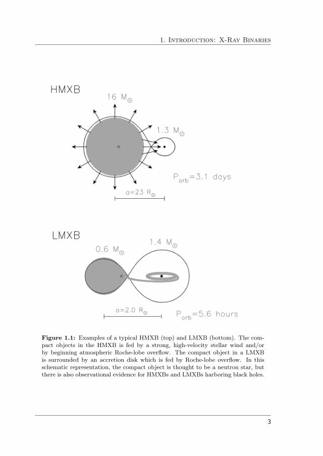
In the 40 years since the first X-ray binary was optically identified (ScoX-1),the basic division of X-ray binaries into the high-mass (HMXBs) and low-mass(LMXBs) systems has become firmly established. The nomenclature refers to thenature of the mass donor, with HMXBs normally taken to be ≥ 10 M⊙, andLMXBs ≤ 1 M⊙. However, the last decade has seen the identification and mea-surement of a significant number of X-ray binaries whose masses are intermediatebetween these limits. Nevertheless, the nature of the mass-transfer process (stel-lar wind dominated in HMXBs, Roche lobe overflow in LMXBs), together withdifferences in the accreting compact stars (i.e. strongly magnetic NS in HMXBsversus weakly magnetic NS in LMXBs), produces quite different properties in thetwo groups (see Fig. 1.1 and Table 1.1).
Table 1.1: The two main classes of Galactic X-ray sources
HMXB LMXB
X-ray spectra: kT ≥ 15 keV (hard) kT ≤ 10 keV (soft)Type of time variability: regular X-ray pulsations only a very few pulsars
no X-ray bursts often X-ray burstsAccretion process: wind (or incipient RLO) Roche-lobe overflowTimescale of accretion: 105 yr 107 − 109 yrAccreting compact star: high �B-field NS (or BH) low �B-field NS (or BH)Spatial distribution: Galactic Plane Galactic center and
spread around the planeStellar population: young, age < 107 yr old, age > 109 yrCompanion stars: luminous, Lopt/LX > 1 faint, Lopt/LX � 0.1
early-type O(B)-stars late-type G-M stars> 10M⊙ (Pop. I) ≤ 1M⊙ (Pop. I and II)
2
1. Introduction: X-Ray Binaries
Figure 1.1: Examples of a typical HMXB (top) and LMXB (bottom). The com-pact objects in the HMXB is fed by a strong, high-velocity stellar wind and/orby beginning atmospheric Roche-lobe overflow. The compact object in a LMXBis surrounded by an accretion disk which is fed by Roche-lobe overflow. In thisschematic representation, the compact object is thought to be a neutron star, butthere is also observational evidence for HMXBs and LMXBs harboring black holes.
3

1.2. A brief historical review
1.2 A brief historical review
The X-ray fluxes measured for these systems correspond to typical source lumi-nosities of 1034 – 1038 erg s−1(which is more than 25 000 times the total energyoutput of our Sun). Table 1.2 lists the rates of accretion (M = dm/dt) requiredto generate a typical X-ray luminosity of 1037 erg s−1. Also listed is the amountof gravitational potential energy released per unit mass (∆U/m = GM/R) byaccretion onto a 1 M⊙ stellar (compact) object, as well as the column densitytowards the stellar surface (or Schwarzschild radius) in the case of spherical ac-cretion, σ = LX4π
�R/(GM)3. The table shows that only for accreting neutron
stars and black holes is the column density low enough to allow X-rays to escape,as X-rays are stopped at column densities larger than a few g cm−2 (see, for in-stance, Frank et al. 2002). Hence, the brightest Galactic X-ray sources cannot beaccreting white dwarfs.
Table 1.2: Energetics of accretion
Stellar object Radius ∆U/mc2 ∆U/m dm/dt
a Columndensitya
1M⊙ (km) (erg/g) (M⊙/yr) (g/cm2)
Sun 7× 10⁵ 2× 10⁻⁶ 2× 10¹⁵ 1× 10⁻⁴ 140
White dwarf 6000 2× 10⁻⁴ 1× 10¹⁷ 1× 10⁻⁶ 16
Neutron star 10 0.15 1× 10²⁰ 1× 10⁻⁹ 0.5
Black hole 3 0.1 ∼ 0.4 4× 10²⁰ 4× 10⁻¹⁰ 0.3a
required to power Lx = 1037 erg/s
The recognition that neutron stars and black holes can exist in close binarysystems came at first as a surprise. It was known that the initially more massivestar should evolve first and explode in a supernova (SN). However, as a simpleconsequence of the virial theorem, the orbit of the post-SN system should bedisrupted if more than half of the total mass of the binary is suddenly ejected.For X-ray binaries like Cen X-3 it was soon realized (van den Heuvel & Heise1972) that the survival of the system was due to the effects of large-scale mass
4

1. Introduction: X-Ray Binaries
transfer that must have occurred prior to the SN.
The formation of LMXBs (Mdonor ≤ 1.5M⊙) with observed orbital periodsmostly between 11 min and 12 hr, as well as the discovery of the double neutronstar system PSR 1913+16 with an orbital period of 7.75 hr, was an even harderproblem to solve since the progenitor star of the neutron star must have had aradius much larger than the current separation. It was clear that such systemsmust have lost a large amount of orbital angular momentum. The first modelsto include large loss of angular momentum were made by van den Heuvel &de Loore (1973) for the later evolution of HMXBs, showing that in this way veryclose systems like Cyg X-3 can be formed; on the other hand, Sutantyo (1975)proposed the same mechanism for the origin of LMXBs.
Furthermore, the important concept of a “common envelope” (CE) evolutionwas introduced by Paczynski (1976) and Ostriker et al. (1976). In this scenario aneutron star is captured by the expansion of a giant companion star and is forcedto move through the giant’s envelope. The resulting frictional drag will cause itsorbit to shrink rapidly while, at the same time, ejecting the envelope before thenaked core of the giant star explodes to form another neutron star.
It was suggested by Smarr & Blandford (1976) that it is an old “spun-up”neutron star what is observed as a radio pulsar in PSR 1913+16. The magneticfield of this pulsar is relatively weak (∼ 1010 Gauss, some two orders of magnitudelower than the average pulsar magnetic field) and its spin period is very short(59 ms). Hence, this pulsar is most likely spun-up (or “recycled”) in an X-raybinary where mass and angular momentum from an accretion disk is fed to theneutron star. The other neutron star in the system was then produced by thesecond supernova explosion and must be a young, strong �B-field neutron star(it is not observable, either because it has already rapidly spun-down, due todipole radiation; or because the Earth is not hit by the pulsar beam; or becauseof centrifugal inhibition, if the drag exerted by the rotating magnetosphere onthe accreting matter gives rise to a centrifugal force that is locally stronger thangravity).
The idea of recycling pulsars was given a boost by the discovery of the firstmillisecond radio pulsar (Backer et al. 1982). As a result of the long accretionphase in LMXBs, millisecond pulsars are believed to be formed in such systems
5

1.3. The primary star: a compact object
(Alpar et al. 1982; Radhakrishnan & Srinivasan 1982). This model was beautifullyconfirmed by the discovery of the first millisecond X-ray pulsar in the LMXB SAX1808.4-3658 (Wijnands & van der Klis 1998).
Finally, another ingredient which has important consequences for close binaryevolution is the event of a “kick” imparted to newborn neutron stars as a resultof an asymmetric SN and/or the sudden loss of matter ejected in a symmetricSN explosion (the so-called Blaauw kick). There is now ample evidence for theoccurrence of such kicks inferred from the space velocities of pulsars and fromdynamical effects on surviving binaries.
This work will concentrate on results from HMXBs observations: in the nexttwo sections an overview of the two single components of these systems is pre-sented, compact objects, including white dwarfs for completeness, in Sect. 1.3,and hot OB stars in Sect. 1.4. In Sect. 1.5 their observational properties will beexplored.
1.3 The primary star: a compact object
The gravitational collapse of normal matter produces the most exotic objects inthe Universe – neutron stars and black holes. Proving that these objects exist inNature occupied theoretical and observational astrophysicists for much of the 20thcentury. As the endpoint states of stellar evolution, they form today fundamentalconstituents of galaxies. As a class of astronomical objects, compact objectsinclude white dwarfs, neutron stars and black holes. For a complete and recentreview of compact objects, see, for example, Camenzind (2007).
A study of compact objects begins when normal stellar evolution ends. Theseobjects differ from normal stars in at least three aspects:
- They are not burning nuclear fuel, and they cannot support themselvesagainst gravitational collapse by means of thermal pressure. Instead whitedwarfs are supported by the pressure of the degenerate electrons, and neu-tron stars are largely supported by the pressure of the degenerate neutronsand quarks. Only black holes represent completely collapsed stars, assem-bled by mere self-graviting forces.
6
1. Introduction: X-Ray Binaries
- The second characteristic property of compact stars is their compact size.They are much smaller than normal star, thus have much stronger surfacegravitational fields.
- Often compact objects carry strong magnetic fields.
White dwarfs
White dwarfs are stars of about one solar mass with a characteristic radius of5000 km, corresponding to a mean density of 106 g cm−3. They are no longerburning nuclear fuel but are steadily cooling away their internal heat since intheir interior gravitation forces are balanced by electron degeneracy pressure. In1926, only three white dwarfs were firmly detected. In that year, Dirac formu-lated the Fermi-Dirac statistics, which was used by Fowler in the same year toexplain the puzzling nature of white dwarf stars. He identified the pressure hold-ing up the stars from gravitational collapse with the electron degeneracy pressure.
Actual models of white dwarfs, taking into account the special relativisticeffects in the degenerate electron equation of state, were constructed by Chan-drasekhar (1931). He made the fundamental discovery of a maximum mass, theChandrasekhar limit, of (about) 1.4 M⊙, above which a white dwarf would un-dergo gravitational collapse.
Many nearby young white dwarf have been discovered as sources of soft X-rays;recently, soft X-ray and extreme ultraviolet observations have become a powerfultool in the study of the composition and structure of the thin atmosphere of thesestars. As shown before, white dwarfs do not take part in the formation of X-raybinaries (see Table 1.2).
Neutron stars
Neutron stars are about 20 km in diameter and have a mass of about 1.4 times thatof our Sun. Because of its small size and high density, a neutron star possessesa very strong surface gravitational field. Neutron stars are one of the possibleend states for a massive star (M > 6–8 M⊙). After these stars have finishedburning their nuclear fuel, they undergo a supernova explosion. This explosion
7
1.3. The primary star: a compact object
blow off the outer layers of a star in a supernova remnant. The central region ofthe star collapses under gravity so much that protons and electrons combine toform neutrons.
Massive stars at the end of their lives are believed to consist of a white dwarf-like iron core of mass (1.2 - 1.4) M⊙, having low entropy, and surrounded by layersof less processed material from nuclear shell burning. The effective Chandrasekharmass is dictated by the lepton number YL believed to be around 0.41 - 0.43. Asmass is added to the core by shell Si-burning, the core becomes unstable andcollapses.
During the collapse, the lepton content decreases due to net electron captureon nuclei and free protons. When the core density approaches 1012 g cm−3, theneutrinos can no longer escape from the core on the dynamical time-scale. Afterneutrinos become trapped, the lepton number is frozen at a value of about 0.38-0.40, and the entropy also remains fixed. The core continues to collapse at abounce density of a few times nuclear density. This bounce results in a shockwhich is largely dissipated by the energy required to dissociate massive nuclei inthe still infalling matter of the original iron core. The larger lepton number YL ofthe core, the larger its mass and the smaller this shell. The final lepton number isthen controlled by weak interactions, and is strongly dependent upon the numberof protons, xp. So the properties of nuclear matter determine largely the outcomeof the collapse, in particular the resulting mass of the newly formed neutron star.Many questions are still open in this field.
Black holes
Einstein’s general theory of relativity predicts the existence of black holes as as-trophysical objects so dense that even light cannot escape from them. Whereasthe solutions for rotating neutron stars can only be discussed within the frame-work of a numerical approach, black holes represent pure gravitational fields witha globally vanishing energy-momentum tensor, T
αβ = 0. Phenomenologically, thefirst type of black holes have measured masses ranging between 3–30 M⊙ and arebelieved to form during supernova explosions. On the other hand, galaxy-massblack holes are found in nearby galaxies and active galactic nuclei. These arethought to have the mass of about a few million to 10 billion solar masses. The
8

1. Introduction: X-Ray Binaries
masses of these supermassive black holes have been recently measured using var-ious kinematic methods. X-ray observations of iron lines in the accretion disksmay actually be showing the effects of such massive black holes as a well. Addi-tionally, there is some evidence for intermediate-mass black holes, with masses ofa few hundred to a few thousand M⊙. These objects may be responsible for theemission of radiation with LX ≈ 1039−41 erg/s observed in nearby galaxies, theso called ultraluminous X-ray sources.
Candidates for stellar-mass black holes were identified mainly by their strongX-ray radiation and the presence of accretion disks of the right size and speed,without the irregular flare-ups that are expected from disks around other compactobjects. And about 20 of them have been confirmed through dynamical studies.
1.4 The secondary star: a massive OB star
Massive early-type stars are the typical counterparts to HMXBs. Isolated OBstars, because of their fast and peculiar evolution, are very interesting laboratoriesto test theories of stellar and circumstellar structure and evolution.
While in the main sequence, they are perfect probes of the composition of theirsurroundings as they are very little evolved and their envelopes present the samecomposition as the local interstellar matter from which they formed. Because ofthis reason, they are often used as metallicity indicators. They also trace star-forming regions because do not grow old.
Many hot, luminous, OB-type stars, and their accompanying mass outflows,are highly structured and variable on a range of spatial and temporal scales. Theirstudy allows to improve our knowledge on the underlying physical processes forsuch activity – magnetic fields, pulsation, rotation, radiative instabilities, binarity– with focus on implications for the structure and evolution of the central star,as well as any associated circumstellar envelope, disk, and mass outflow.
In particular, two extreme phenomena play a crucial role in the case of OBstars in HMXBs, since they are related to the mechanism that drives the accretionflow on to the compact object: stellar winds and the Be phenomenon.
9

1.4. The secondary star: a massive OB star
1.4.1 Stellar winds
All hot stars are known to lose matter in the form of a stellar wind driven byradiation. Stellar winds are able to modify the ionizing radiation of hot stars dra-matically and become directly observable in both spectral energy distributionsand spectral lines as soon as the stars are above certain luminosity thresholds.The streaming matter from stellar winds contributes to the enrichment of theinterstellar medium; in the case of binary systems, it can be partially accreted orproduce shocks of colliding winds, resulting in X-ray emission in both cases. Nev-ertheless, due to their soft emission (E � 2 keV), these systems are not regardedas X-ray binaries.
Radiation-driven winds work on the principle that momentum contained in thestellar radiation field is transferred to gas particles in the wind via the scatteringof photons. The main point is that momentum is a vector quantity and that thephotons before scattering are all moving in one direction, i.e. away from the star,while they move in a random direction after the scattering. The result is that theassociated radiative force is directed away from the star. The scattering processtakes place via spectral lines of the gas particles in the outer atmosphere. Lucy& Solomon (1970) were among the first to realize that the scattering of photonsover a few strong resonance lines would result in a strong enough force to drivea wind. An essential ingredient is that the wind in its way out reaches velocitieswhich are about a 100 times larger than the typical thermal width of the spectrallines, so that due to the doppler shift of the lines many more photons can be“tapped” compared to the static case.
Winds of hot stars are characterized by two global parameters, the terminalvelocity v∞ and the rate of mass loss M . The velocity v∞ reached at very largedistance from the star, where the radiative acceleration approaches zero becauseof the geometrical dilution of the photospheric radiation field, corresponds to themaximum velocity of the stellar wind. If we assume that winds are stationaryand spherically symmetric, then the equation of continuity yields at any radialcoordinate R in the wind
M = 4πρ(R)V (R). (1.1)
10
1. Introduction: X-Ray Binaries
V (R) and ρ(R) are the velocity field and density distribution, respectively, andcan be regarded as local stellar wind parameters. A determination of globalparameters from the observed spectra is only possible with realistic assumptionsabout the stratification of the local parameters. Global parameters, in fact, are notdirect observables, but their determination relies on stellar atmospheres models.For a review of physical and observational properties of winds from hot stars, seeKaper (1998) and Kudritzki & Puls (2000).
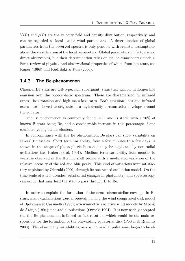
1.4.2 The Be-phenomenon
Classical Be stars are OB-type, non supergiant, stars that exhibit hydrogen lineemission over the photospheric spectrum. These are characterized by infraredexcess, fast rotation and high mass-loss rates. Both emission lines and infraredexcess are believed to originate in a high density circumstellar envelope aroundthe equator.
The Be phenomenon is commonly found in O and B stars, with a 20% ofknown B stars being Be, and a considerable increase in this percentage if oneconsiders young stellar clusters.
In concomitance with the Be phenomenon, Be stars can show variability onseveral timescales. Short term variability, from a few minutes to a few days, isshown in the shape of photospheric lines and may be explained by non-radialoscillations (see Hubert et al. 1997). Medium term variability, from months toyears, is observed in the Hα line shell profile with a modulated variation of therelative intensity of the red and blue peaks. This kind of variations were satisfac-tory explained by Okazaki (2000) through its one-armed oscillation model. On thetime scale of a few decades, substantial changes in photometry and spectroscopycan occur that may lead the star to pass through B to Be.
In order to explain the formation of the dense circumstellar envelope in Bestars, many explanations were proposed, namely the wind compressed disk modelof Bjorkman & Cassinelli (1993); axi-symmetric radiative wind models by Stee &de Araujo (1994); non-radial pulsations (Owocki 1994). It is now widely acceptedthe the Be phenomenon is linked to fast rotation, which would be the main re-sponsible for the formation of the outwarding equatorial disk (Porter & Rivinius2003). Therefore many instabilities, as e.g. non-radial pulsations, begin to be ef-
11
1.5. High-mass X-ray binaries: observational properties
fective for orbital ejection. Very interestingly, recent interferometric observationsbrought strong support to the idea that these stars are very fast rotators, showingfor the first time the oblateness of a Be star, Archenar, (Domiciano de Souza et al.2003), which suggests that the star is indeed rotating near the critical limit. Fora recent study on how the surface velocity varies during the Main Sequence andthe possible origin on Be stars, see Ekstrom et al. (2008).
1.5 High-mass X-ray binaries: observational proper-
ties
There are two main sub-groups of HMXBs, the supergiant counterparts (normallyof luminosity class I or II), and the Be/X-ray (or BeX) binary systems (normallyluminosity class III to V). Recently, a new class has been added by Negueruelaet al. (2006), the Supergiant Fast X-ray transients (SFXTs), with peculiar X-rayproperties. All sub-groups involve OB type stars and are commonly found in thegalactic plane and the Magellanic Clouds, among their OB-type progenitor stars.They mainly differ in accretion modes with the supergiant systems accreting froma radially outflowing stellar wind, and the BeX binaries accreting directly fromthe circumstellar disc (possibly with some limited Roche lobe overflow on rareoccasions). As a result the supergiants are persistent sources of X-rays (with theexception of the SFXTs, see below), while the BeX systems are very variable (oftenunobservable for months to years) and occasionally much brighter, characterizingthemselves as transient systems.
In the present work, both X-ray and IR data were employed. While thenature of the compact object and its properties are largely determined from X-raystudies, longer-wavelength observations allow detailed studies of the properties ofthe mass donor. This is most straightforward for the intrinsically luminous early-type companions of HMXBs, which provides the potential for a full solution of thebinary parameters for those systems containing X-ray pulsars. In the frameworkof HMXB evolution, it allows a comparison of the derived masses with thoseobtained for neutron stars in the much older binary radio pulsar systems. Inthe following sections, the main observational properties of HMXBs, as exhibitedfrom X-ray and IR data, will be explored.
12

1. Introduction: X-Ray Binaries
1.5.1 X-ray observations
Supergiant-XRBs
SGXBs are systems composed of an accreting compact object and a massive su-pergiant early-type star (OB). The X-ray emission is powered by accretion ofmaterial originating from the donor star through strong stellar wind or occasion-ally by Roche-lobe overflow. Up to recently SGXBs were believed to be very rareobjects due to the evolutionary timescales involved; supergiant stars have a veryshort lifetime. This idea was supported by the fact that only a dozen of SGXBshave been discovered in almost 40 years of X-ray astronomy and it was largelybelieved that the dozen of known objects represented a substantial fraction of allSGXBs in our Galaxy. The INTEGRAL satellite is changing this classical pictureon SGXBs. Since its launch in 2002, INTEGRAL in just a few years doubled thepopulation of SGXBs. The majority of them are persistent X-ray sources whichescaped previous detection because of their very strong absorbed nature, beingthe NH typically greater than 1023 cm−2 (Walter et al. 2006; Nespoli et al. 2008b).
As the compact object always orbits within the stellar wind, these systems arepersistent X-ray emitting objects and show high variations on short time scales.They have Porb ≤ 10 days and e ≤ 0.1. According to their X-ray luminosity, theyare divided into high-luminosity sources and low-luminosity sources.
The high-luminosity sources (1037–1038 erg s−1), and “standard” systems suchas Cen X-3 and SMC X-1, are characterized by the occurrence of regular X-rayeclipses and double-wave ellipsoidal light variations produced by tidally deformed(“pear-shaped”) giant or sub-giant companion stars with masses > 10M⊙. How-ever, the optical luminosities (Lopt > 105
L⊙) and spectral types of the companionsindicate original zero-age main-sequence (ZAMS) masses ≥ 20M⊙, correspondingto O-type progenitors. The companions have radii 10 – 30 R⊙ and (almost) filltheir critical Roche-lobes. The mass transfer process takes place in the form ofRoche lobe overflow. Among the standard HMXBs, there are at least three sys-tems that are thought to harbor black holes: Cyg X-1, LMC X-1 and LMC X-3.
The low-luminosity SGXBs (∼ 1036 erg s−1) show erratic flaring activity, withlarge luminosity changes on a timescale of tens of minutes. The X-ray luminosity
13

1.5. High-mass X-ray binaries: observational properties
is consistent with the accretion process being driven by material captured fromthe stellar wind of the optical companion. Vela X-1 is an example of this kind ofsystems. For this class of HMXBs, the X-ray characteristics tend to be not verydramatic. Because of the predominantly circular orbits and the quite steady windoutflow, the X-ray emission tends to be a regular low-level effect, if considered onmedium time scales.
Supergiant Fast X-ray transients
This new class of HMXBs, introduced by Negueruela et al. (2006), is character-ized by the occurrence of X-ray outbursts of a very different nature from thoseseen in other X-ray binaries. These outbursts are very short (lasting from ∼3 to∼8 hours) and display very sharp rises, reaching the peak of the flare in ≤1 h.The decay is generally characterized by a complex structure, with two or threefurther flares. The physical reason for fast outbursts is still unknown, althoughtheoretical speculations have been made which would connect them to some formof discrete mass ejection from the supergiant donor (Golenetskii et al. 2003) or towind clumping (in’t Zand 2005; Walter & Zurita Heras 2007). Numerical simula-tions (Runacres & Owocki 2005) predict low density contrasts in the wind up to∼10R�, when they become of the order of 10−18 – 10−13 g cm−3.
Classical SGXBs are characterized by small orbital radii, with Rorb = (1.5 –2.5) R�. Within the frame of wind clumping, the main difference between SFXTsand classical SGXBs could thus be their orbital radius. At very low orbital radius(< 1.5R�) tidal accretion would take place through an accretion disk and thesystem would evolve to a common envelope stage. At low orbital radius (∼2R�),the wind would be perturbed in any case and efficient wind accretion will leadto persistent X-ray emission. At larger orbital radius (∼10R�) and if the windis clumpy, the SFXT behavior is expected (see also Negueruela 2009; Blay et al.2008).
Some of the known SFXTs are associated with O-type supergiants. Thoughno pulsations have been detected, they display spectra typical of accreting neu-tron stars. The other known sources are X-ray pulsars and are associated withluminous early B-type stars. This class differ from classical wind-fed SGXBs,
14
1. Introduction: X-Ray Binaries
whose X-ray luminosity is variable but always detectable around LX ∼ 1036 ergs−1. Quiescent fluxes of SFXTs have been near the sensitivity limit of focusingobservatories, with values or upper limits in the range of ∼ 1032 to 1033 erg s−1.It is important to point out that without the identification of the optical/infraredcounterpart with an OB supergiant, little can be said about the belonging of anobject to the class of the SFXTs. In fact, the only X-ray behavior is not enoughto unambiguously characterize the X-ray emitter, since short X-ray outbursts aretypical of an extensive range of classes, including for instance flare stars, RS CVnbinaries, or LMXBs showing superbursts.
Since the SFXTs are difficult to detect and their number is growing fast andsteadily since the launch of INTEGRAL, they could actually represent a majorclass of X-ray binaries.
Be/XRBs
Another group of HMXBs consists of the moderately wide, eccentric binaries withPorb � 20 − 100 days and e � 0.3 − 0.5. The orbital separation is too large toallow Roche-lobe overflow. They are in general transient systems. A new (sub-)group, proposed by Reig & Roche (1999), is constituted by persistent systemswith Porb � 30 − 250 days and small eccentricities e < 0.2. Together thesetwo groups form a separate sub-class of HMXBs: the Be-star X-ray binaries (seeFigure 1.2), first recognized as a class by Maraschi et al. (1976). In the Be/X-raybinaries the companions are rapidly rotating OB-emission stars situated on, orclose to, the main-sequence (luminosity class III-V).
The BeX binary systems represent until now the largest sub-class of HMXBs.Of the currently proposed HMXB pulsars, 57% are identified as BeX type. TheBe-stars are deep inside their Roche-lobes, as is indicated by their generally longorbital periods and by the absence of X-ray eclipses and of ellipsoidal light varia-tions. The X-ray emission from Be/XRBs tends to be extremely variable, rangingfrom complete absence to giant transient outbursts lasting weeks to months. Dur-ing such an outburst episode one often observes orbital modulation of the X-rayemission, due to the motion of the neutron star in an eccentric orbit, see Figure1.2.
The recurrent X-ray outbursts have been explained by Okazaki & Negueruela
15

1.5. High-mass X-ray binaries: observational properties
Figure 1.2: Schematic model of a Be-star X-ray binary system. The neutronstar moves in an eccentric orbit around the Be-star which is not filling its Roche-lobe. However, near the periastron passage the neutron star accretes circumstellarmatter, ejected from the rotating Be-star, resulting in an X-ray burst lasting severaldays.
(2001) in terms of the decretion disc model. The circumstellar discs of the pri-maries are truncated because of the tidal and resonant effect of the neutron star.The geometry of the systems and the value of viscosity determine the presence orabsence of Type I X-ray outbursts. The interaction of a strongly disturbed discwith the neutron star originates Type II X-ray and optical outbursts.
Be/XRBs show hard X-ray spectra (1-20 keV) which, in combination with theregular X-ray pulsations, indicate that the compact object must be a stronglymagnetized neutron star. Pulse periods range from a few seconds to ∼ 103 sec-onds. During X-ray outbursts, spin-up phenomena have been observed in severalsystems (A 0535+26, 4U 0118-61). This is consistent with the formation of anaccretion disc. During quiescence, a spin-down phase is expected, as the rota-tional period is largely greater at the beginning of an X-ray outburst than thatmeasured at the end of the previous one.
16

1. Introduction: X-Ray Binaries
Schematically, X-ray behavioral features of Be/XRB systems include:
• short (a few days) outbursts (LX ∼ 1036 − 1037 erg s−1) occurring in seriesseparated by the orbital period (Type I), generally (but not always) closeto the time of periastron passage of the neutron star;
• giant (or Type II) outbursts (LX ≥ 1037 erg s−1), which do not correlateclearly with orbital parameters and last several weeks.
• shifting outburst phases due to the rotation of density structures in thecircumstellar disc (Wilson et al. 2002).
1.5.2 IR observations
Optical/IR observations reveal that many of the counterparts to HMXBs exhibitmass outflow to the extent of creating a circumstellar disc or spherical envelopeof material around the mass donor. Free-free and bound-free IR emission fromthis disc show themselves as a significant excess over the normal stellar spectrumat all wavelengths greater than the V band. This IR signature, often quantifiedas a J-K color excess, is important for the following reasons:
• in order to detect sources which are obscured due to high interstellar ex-tinction;
• in confirming the identity of a Be star in the absence of optical spectralinformation;
• in providing an estimate of the size of the circumstellar disc (this is oftendirectly related to the magnitude of the X-ray emission);
One system that has been the subject of extensive IR observations over theyears is X-Per. Detailed study by Telting et al. (1998) found that the density ofthe disc varies along with the brightness of X-Per, and that in optical high statesthe disc is among the densest of all Be stars, with ρ0 = (1.5±0.3)×10−10 g cm−3.The disc density at the photosphere varies by a factor of at least 20 from opticalhigh to low states.
17

1.5. High-mass X-ray binaries: observational properties
With the recent advent of IR spectroscopy on large telescopes, the possibilitiesof obtaining spectra despite high levels of extinction have become a reality. Thisis a very powerful tool not only for exploring previously inaccessible objects – ithas in fact allowed the first detailed investigations of X-ray binaries in the innerparts of the Galactic Plane and the Galactic Center – but also directly collectinginformation on the circumstellar environment. The project to which this workbelongs, takes its place within this scenario of research. A good example of thestrength of this tool may be seen in Clark et al. (1999b): we report in Fig. 1.3their IR spectra of 5 HMXBs.
Figure 1.3: K band spectra of BeX binaries (Clark et al, 1999). The positions ofprominent H, He and metallic transitions are marked.
Just as the optical spectrum is dominated by Balmer emission, we see the sameeffect from the Brackett series emission in the IR. In addition, emission lines fromHe and metallic transitions are also detected.
18

Part I
IR photometry and
spectroscopy
19

20

We are all in the gutter, but some
of us are looking at the stars.
Oscar Wilde 2Search for IR counterparts to obscured
HMXBs
2.1 Scientific objective
Up to now, the INTEGRAL survey of the Galactic Plane and central regions hasrevealed the existence of more than 200 sources (Bird et al. 2007; Bodaghee et al.2007) in the energy range 20–100 keV, with a position accuracy of 2�−3�, depend-ing on count rate, position in the FOV and exposure. A large fraction of the newlydiscovered sources are found to be heavily obscured, displaying much larger col-umn densities (NH � 1023 cm−2) than would be expected along the line of sight(see Kuulkers 2005). These sources were missed by previous high-energy missions,whose onboard instruments were sensitive to a softer energy range. Moreover, op-tical counterparts to these obscured sources are poorly observable due to the highinterstellar extinction, with AV in excess of up to ∼ 20 mag.
It is remarkable that the vast majority of HMXBs in the Norma and Scutumregions, whose optical/IR counterparts have been identified, are SGXBs. Con-versely, no one Be/XRB has been found yet. This is in strong contrast with therest of the Galactic Plane, where BeXRBs outnumber SGXBs by a factor of threeto five. We propose that this anomaly is due to an observational effect, becauseof the transient nature of BeXRBs which precludes follow-up surveys in the X-ray
21

2.2. A new photometric technique
band.
In this chapter we present the photometric technique we developed in order toidentify IR counterparts to obscured HMXBs in the Scutum and Norma galacticarms, looking for Be/XRBs. This technique was tested with known Be/XRBs,providing successful results. Eventually, we applied it to ten newly discoveredINTEGRAL sources, selecting possible Be counterparts.
2.2 A new photometric technique
We selected suitable candidates by means of a photometric search for emission-linestars in the error boxes of the X-γ ray sources detected by the ISGRI instrumenton board INTEGRAL.
Be stars are characterized by strong emission features, being He I 20 581 Aand Brγ 21 670 A the most remarkable ones in the K band. This is clearly shownin Fig. 2.1, which report SOFI Ks spectra of four known classical Be stars andone supergiant B star with emission lines (first spectrum from the top). Datawere collected during our spectroscopy observing campaign (see Chapter 3).
20500 21000 21500 22000 22500
Wavelength (Angstrom)
0.5
1
1.5
2
2.5
Norm
aliz
ed s
pec
trum
+ o
ffse
t
BD-13 5550 - B1 Ibe
HD 28497 - B2 V:ne
HD 30076 - B2 Ve
HD 131168 - B3 Ve
HD 156468 - B1 Ve
HeI HeI Br!
Figure 2.1: Ks-band spectra of classical Be-stars (first four spectra from thebottom) and one supergiant B star with emission lines (first spectrum from thetop). The positions of identified spectral features are marked by solid lines.
22
2. Search for IR counterparts to obscured HMXBs
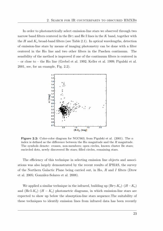
In order to photometrically select emission-line stars we observed through twonarrow band filters centered in the Brγ and He I lines in the K band, together withthe H and Ks broad-band filters (see Table 2.1). In optical wavelengths, detectionof emission-line stars by means of imaging photometry can be done with a filtercentered in the Hα line and two other filters in the Paschen continuum. Thesensibility of the method is improved if one of the continuum filters is centered in– or close to – the Hα line (Grebel et al. 1992; Keller et al. 1999; Pigulski et al.2001, see, for an example, Fig. 2.2).
Figure 2.2: Color-color diagram for NGC663, from Pigulski et al. (2001). The αindex is defined as the difference between the Hα magnitude and the R magnitude.The symbols denote: crosses, non-members; open circles, known cluster Be stars;encircled dots, newly discovered Be stars; filled circles, remaining stars.
The efficiency of this technique in selecting emission line objects and associ-ations was also largely demonstrated by the recent results of IPHAS, the surveyof the Northern Galactic Plane being carried out, in Hα, R and I filters (Drewet al. 2005; Gonzalez-Solares et al. 2008).
We applied a similar technique in the infrared, building up (Brγ-Ks)–(H−Ks)and (He I-Ks)–(H −Ks) photometric diagrams, in which emission-line stars areexpected to show up below the absorption-line stars sequence.The suitability ofthese techniques to identify emission lines from infrared data has been recently
23

2.3. Observations
demonstrated by Groh et al. (2006), who detected additional Wolf-Rayet stars inthe starburst cluster Westerlund I (see Fig 2.3).
Figure 2.3: Line-continuum versus continuum diagram for the narrow-band filtersused by Groh at al. (2007). Upper panel: filter centered at He II 1.0124 µm. Lowerpanel: filter centered at He I 1.0830 µm. New candidate WRs are identified byletters.
We applied the technique to field stars, and with this objective, for the firsttime. The most critical factors are, in our case, the large error circle of IBISdetection and the crowdedness of the Galactic Plane.
The described strategy would represent a very strong tool to detect counter-parts to Be/XRBs, which constitute ∼ 80% of all HMXBs. In the case of SGXBs,which are persistent X-ray emitters, dedicated observations with X-ray observa-tories with high spatial resolution, like XMM or Chandra, can produce very smallerror circles and facilitate the detection of the counterpart.
2.3 Observations
Data were obtained during one observing run in 2008, at the European SouthernObservatory (ESO), in Chile. The employed instrument was SOFI (Moorwoodet al. 1998c), on the 3.5m New Technology Telescope (NTT) at La Silla. TheSOFI camera has a largest field of view of 4.92 arcmin, a pixel scale of 0.288arcsec/pixel and covers the 0.9-2.5 micron wavelength range.
24

2. Search for IR counterparts to obscured HMXBs
The optical layout is shown in Fig. 2.4.
Figure 2.4: Optical layout of SOFI.
The filters employed in this work, together with their central wavelengths andwidths at half maximum, are listed in Table 2.1
Table 2.1: The broad band and narrow band Sofi filters employed in this work.
Filter Central wavelength Width Peak transmissionname (µm) (µm) (%)
H 1.653 0.297 83Ks 2.162 0.275 88NB HeI 2.059 0.028 81NB Brγ 2.167 0.028 71
Transmission curves for each filter, together with the atmospheric transmis-sion, are shown in Fig. 2.5. The K short or Ks filter is different from both thestandard K filter and the K
� filter defined by Wainscoat & Cowie (1992). The
25

2.3. Observations
long wavelength edge of the Ks filter is similar to that of the K� filter, but the
short wavelength edge is similar to that of the K filter. Thus, the Ks filter avoidsboth the atmospheric absorption feature at 1.9 µm and radiation from the ther-
Figure 2.5: SOFI filters. The solid (red) lines indicate the currently availablebroad-band J , Js, H and Ks filters. The short-dashed (magenta) lines are theavailable narrow-band filters. The long-dashed (red) lines show the soon to becommissioned Js filter (top panel) and the typical broad K filter (Persson et al.1998, AJ, 116, 2475; see their Table 10). The dotted (blue) line is the atmospherictransmission model for Mauna Kea, for airmass = 1 and water vapor column of1mm (Lord, S.D. 1992, NASA Technical Memor. 103957; courtesy of Gemini Ob-servatory).
26
2. Search for IR counterparts to obscured HMXBs
mal background beyond 2.3 µm. The difference between Ks and K is given byK −Ks = −0.005 (J −K).
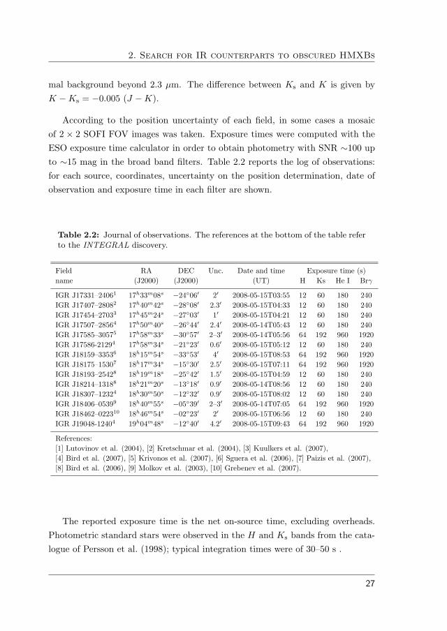
According to the position uncertainty of each field, in some cases a mosaicof 2 × 2 SOFI FOV images was taken. Exposure times were computed with theESO exposure time calculator in order to obtain photometry with SNR ∼100 upto ∼15 mag in the broad band filters. Table 2.2 reports the log of observations:for each source, coordinates, uncertainty on the position determination, date ofobservation and exposure time in each filter are shown.
Table 2.2: Journal of observations. The references at the bottom of the table referto the INTEGRAL discovery.
Field RA DEC Unc. Date and time Exposure time (s)name (J2000) (J2000) (UT) H Ks He I Brγ
IGR J17331–24061 17h33m08s −24◦06� 2� 2008-05-15T03:55 12 60 180 240IGR J17407–28082 17h40m42s −28◦08� 2.3� 2008-05-15T04:33 12 60 180 240IGR J17454–27033 17h45m24s −27◦03� 1� 2008-05-15T04:21 12 60 180 240IGR J17507–28564 17h50m40s −26◦44� 2.4� 2008-05-14T05:43 12 60 180 240IGR J17585–30575 17h58m33s −30◦57� 2–3� 2008-05-14T05:56 64 192 960 1920IGR J17586-21294 17h58m34s −21◦23� 0.6� 2008-05-15T05:12 12 60 180 240IGR J18159–33536 18h15m54s −33◦53� 4� 2008-05-15T08:53 64 192 960 1920IGR J18175–15307 18h17m34s −15◦30� 2.5� 2008-05-15T07:11 64 192 960 1920IGR J18193–25428 18h19m18s −25◦42� 1.5� 2008-05-15T04:59 12 60 180 240IGR J18214–13188 18h21m20s −13◦18� 0.9� 2008-05-14T08:56 12 60 180 240IGR J18307–12324 18h30m50s −12◦32� 0.9� 2008-05-15T08:02 12 60 180 240IGR J18406–05399 18h40m55s −05◦39� 2–3� 2008-05-14T07:05 64 192 960 1920IGR J18462–022310 18h46m54s −02◦23� 2� 2008-05-15T06:56 12 60 180 240IGR J19048-12404 19h04m48s −12◦40� 4.2� 2008-05-15T09:43 64 192 960 1920
References:[1] Lutovinov et al. (2004), [2] Kretschmar et al. (2004), [3] Kuulkers et al. (2007),[4] Bird et al. (2007), [5] Krivonos et al. (2007), [6] Sguera et al. (2006), [7] Paizis et al. (2007),[8] Bird et al. (2006), [9] Molkov et al. (2003), [10] Grebenev et al. (2007).
The reported exposure time is the net on-source time, excluding overheads.Photometric standard stars were observed in the H and Ks bands from the cata-logue of Persson et al. (1998); typical integration times were of 30–50 s .
27
2.4. Data reduction
2.4 Data reduction
Data reduction was performed using the IRAF package. Pre-reduction requiredthe following procedures:
1. correcting for inter-quadrant row cross talk
2. combining dithered frames to create a sky image and subtracting it to eachimage
3. performing flat field correction
4. aligning and combining the reduced images
Finally, on the reduced, co-alligned images, point-spread function (PSF) fit-ting photometry was performed. Through the final steps of aperture correctionand photometric calibration, the obtained magnitudes were transformed to thestandard system.
2.4.1 Inter-quadrant row cross-talk
The inter-quadrant row cross-talk is a feature affecting high SNR images takenwith SOFI. It is apparent when part of the array is exposed to bright illuminationand faint objects have to be detected on the same rows which are exposed to thebright illumination. A bright source imaged on the array produces “ghosts” thataffects all the lines where the source is and all the corresponding lines in the otherhalf of the detector.
The effect is a peculiarity of the instrument array and, though it is not com-pletely understood, it is well described and can be easily corrected. The intensityof the ghost is in fact 1.4× 10⁻⁵ times the integrated flux of the line. In order toremove it, we used an IRAF script, available from the instrument web-pages fordownloading. This is an efficient and simple algorithm which removes the effectof row cross-talk without any degradation of image quality. The principles for theconstruction of the algorithm employed are illustrated below.
28
2. Search for IR counterparts to obscured HMXBs
Model for row cross-talk
The row cross-talk is uniform within one row and does not depend on columnindex j. Let Ii,j be the intensity of the pixel at row i and column j. Due to rowcross-talk the observed intensity is modified as follows
I�i,j
= Ii,j + Ci + Ci±512. (2.1)
The row cross-talk consists of two terms, namely the intraquadrant row cross-talk Ci and the interquadrant row cross-talk Ci±512. The plus sign applies forindices i ≤ 512, the minus sign for 512 < i ≤ 1024. Both cross-talk terms dependlinearly on the integrated intensity of row number i and row number i± 512:
Ci = α1024�
k=1
Ii,k. (2.2)
The intensity Ii,j can be derived from the observed intensity I�i,j
by subtractingthe row cross-talk as follows
Ii,j = I�i,j− Ci − Ci±512. (2.3)
2.4.2 Sky subtraction
This is a critical operation, especially if dealing with very crowded images, likeours. For each field and filter, we took 3–6 images at different location. Themore dithered frames we had, the better the results. The images were scaledto a common median, which to first approximation is the sky image. This wasimproved after some tests, by a 3σ rejection. The sky image was scaled to havethe same median as the image from which it would be subtracted, and then thesubtraction was carried out. This method reduces the negative traces of stellarimages on the sky-subtracted data.
2.4.3 Flat fields
At the telescope, images of the dome flat field screen with the dome lamp on andoff were taken. The simplest way of creating flat fields is to subtract the averageof the lamp-off images to the average of the lamp-on ones. However, in this case
29
2.4. Data reduction
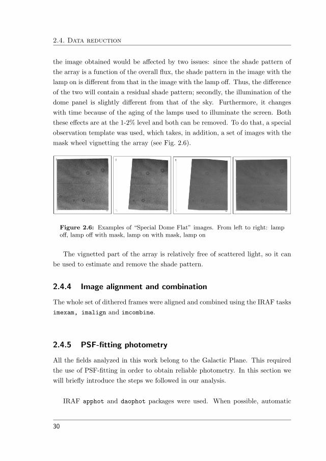
the image obtained would be affected by two issues: since the shade pattern ofthe array is a function of the overall flux, the shade pattern in the image with thelamp on is different from that in the image with the lamp off. Thus, the differenceof the two will contain a residual shade pattern; secondly, the illumination of thedome panel is slightly different from that of the sky. Furthermore, it changeswith time because of the aging of the lamps used to illuminate the screen. Boththese effects are at the 1-2% level and both can be removed. To do that, a specialobservation template was used, which takes, in addition, a set of images with themask wheel vignetting the array (see Fig. 2.6).
Figure 2.6: Examples of “Special Dome Flat” images. From left to right: lampoff, lamp off with mask, lamp on with mask, lamp on
The vignetted part of the array is relatively free of scattered light, so it canbe used to estimate and remove the shade pattern.
2.4.4 Image alignment and combination
The whole set of dithered frames were aligned and combined using the IRAF tasksimexam, imalign and imcombine.
2.4.5 PSF-fitting photometry
All the fields analyzed in this work belong to the Galactic Plane. This requiredthe use of PSF-fitting in order to obtain reliable photometry. In this section wewill briefly introduce the steps we followed in our analysis.
IRAF apphot and daophot packages were used. When possible, automatic
30

2. Search for IR counterparts to obscured HMXBs
procedures were developed. However, some operations required the visual inspec-tion of each image, mainly to determine the typical parameters like FWHMs,standard deviation of the background, minimum and maximum good data value.Together with the characteristics of the detector (read-out noise, gain), these val-ues were used as input for daofind in order to produce a list of coordinates foreach object identified. The four images, one for each filter, were aligned and onlyobjects for one of them (the Ks image, usually the best quality one) were detected.The same list of coordinates was then used as input for phot, once for each image.This allowed to obtain aperture photometry for the same objects in all the filters.
Candidate PSF stars were selected from the photometry catalogue producedby phot in an automatic way, using pstselect. A second run of pstselect
on the candidate stars, in interactive mode, allowed a convenient selection of thebrightest, least crowded stars. In some cases, due to the crowdedness of the fields,no more than three PSF stars could be found.
In order to construct the optimum PSF, an iterative procedure was developed.As a first step, the PSF model was computed using only an analytic function, cho-sen among various profiles as the one producing the smallest standard deviationfor the model fit. The PSF model was constant over the image. The size of thePSF radius was then decreased in order to exclude possible contributions fromobjects different than the PSF stars. The PSF stars and their neighbors werefitted using nstar. Then the fitted PSF star neighbors were subtracted from theimage with substar. An improved PSF was then built, increasing the PSF radiusback to the original value (11 pixels were used), from the image with the neighborssubtracted. In this step, the analytic function and one look-up table containingthe deviations of the true PSF from the analytic model PSF were used. Again,the PSF star and their neighbors were fitted and subtracted from the image. Theresult was inspected, and if good, we proceed by lowering again the PSF radius,building the final PSF profile on the image subtracted by the PSF neighbors. Fi-nally, PSF-fitting was performed simultaneously on all the stars of the field, withallstar.
An example of the PSF profile for the IGR J18159–3353 field, through the
31
2.4. Data reduction
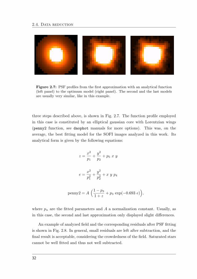
Figure 2.7: PSF profiles from the first approximation with an analytical function(left panel) to the optimum model (right panel). The second and the last modelsare usually very similar, like in this example.
three steps described above, is shown in Fig. 2.7. The function profile employedin this case is constituted by an elliptical gaussian core with Lorentzian wings(penny2 function, see daophot manuals for more options). This was, on theaverage, the best fitting model for the SOFI images analyzed in this work. Itsanalytical form is given by the following equations:
z =x
2
p1+
y2
p2+ p5 x y
e =x
2
p21
+y2
p22
+ x y p4
penny2 = A
�1− p3
1 + z+ p3 exp(−0.693 e)
�,
where pn are the fitted parameters and A a normalization constant. Usually, asin this case, the second and last approximation only displayed slight differences.
An example of analyzed field and the corresponding residuals after PSF fittingis shown in Fig. 2.8. In general, small residuals are left after subtraction, and thefinal result is acceptable, considering the crowdedness of the field. Saturated starscannot be well fitted and thus not well subtracted.
32

2. Search for IR counterparts to obscured HMXBs
Figure 2.8: Example of PSF fitting for one of the fields studied in this work.Above, the pre-reduced image in the Ks filter. Below, residuals after PSF fittingand subtraction. The image refers to IGR J18159–3353 (one of the 2 × 2 mosaicframes).
33

2.4. Data reduction
2.4.6 Photometric calibration and aperture correction
The aperture correction was estimated as the difference between aperture pho-tometry and the retrieved PSF photometry. For each field, this difference wascomputed on the brightest and well isolated stars (typically the PSF stars). Ac-cording to the field, the difference varied between 0–0.1 mag both in Ks and in H.When necessary, PSF photometry was then corrected according to the obtainedvalues.
Photometric calibrations were carried out in a two-step way. Firstly, for eachnight, filter and standard star, we obtained the Bouguer’s law plotting the in-strumental magnitudes vs. the corresponding value of airmass. Linear fit wasperformed in order to obtain a value for the extinction coefficients in Ks and inH. The highest accuracy was obtained for data from May 14, so that we em-ployed the instrumental system defined by that night to calculate the extinctioncoefficients for both nights. The retrieved coefficients, kH and kKs, are shown inTable 2.3.
Table 2.3: Retrieved extinction coefficients for the two observing nights.
May 13 May 14
kH 0.050± 0.002 0.062± 0.008kKs 0.061± 0.002 0.051± 0.004
The second step consisted in solving the standard transformation equations,using the instrumental magnitudes corrected for the extinction. All the 2-nightdata for each filter were used together this time, providing excellent results.
The resulting transformation equations are the following:
Ks(std) −Ks(ins) = 0.0024 (H −Ks)std + 18.86
(H −Ks)std = 1.02 (H −Ks)ins + 0.59
34

2. Search for IR counterparts to obscured HMXBs
Results for the linear fit solving the transformation equations are shown inFig. 2.9.
Figure 2.9: Linear fit solving the standard transformation equations. Error barsare within the marks.
The reduced chi square for the two linear fits is 3×10⁻⁴ for the first equationand 6×10⁻⁵ for the second one. The obtained accuracy of the transformationis 0.007 mag in Ks and 0.008 mag in H. These are calculated as the standarddeviations of the residuals mean values. This contribution, quadratically summed
35

2.5. Results
to the instrumental error of the PSF photometry, constitutes the final error onthe calibrated photometry
2.5 Results
Candidate counterparts were selected from both color-color diagrams, (Brγ−Ks)–(H−Ks) and (He I−Ks)–(H−Ks). Brγ is the most prominent feature in Be starsin the K band, while He I 20 580 A is found in early type Be stars, up to B2.5(see, for instance Clark & Steele 2000). Since it was demonstrated that Be/XRBshave early counterparts, with spectral type up to B3 (Negueruela 1998), in ourselection we considered both criteria as equivalent.
We select as candidates the objects that are below the sequence defined by thefield stars in both photometric diagrams. This selection can be done statistically.To do so, the locus of the sequence is represented by a function obtained by a loworder polynomial fit to all points in the photometric plane. The stars outside thesequence are selected by a n-sigma clipping criterion. The star selected in thisway are removed from the whole sample, and the locus of the sequence is recalcu-lated. This procedure is repeated until convergence (i.e. until no star is rejectedby the n-sigma clipping criterion). All stars rejected in the above procedure donot belong to the stellar sequence of the photometric plane. Those of them whichare placed below the sequence are candidate emission-line stars.
On the other hand, Be stars present moderate emission line strengths, whencompared to other groups like YSO, CV, PN, and others. Therefore, stars belowthe photometric sequence with an important separation are not likely to be Bestars. These classes of stars can be also selected by their distance to the sequencein terms of sigma. In conclusion, Be star candidates are objects below the se-quence locus, with separations between n-sigma and m-sigma.
The critical point is to select the right values of n and m for the sigma clip-ping. This should be done from the knowledge of the situation in the photometricdiagrams of the different classes of emission-line objects. In our case, as we areproposing the use of photometric diagrams which have not been used before for
36

2. Search for IR counterparts to obscured HMXBs
the selection of emission-line stars, we have no previous knowledge of the typicalloci of the different stars. The arbitrary selection of values for n and m wouldlack of statistical and physical sense.
For this reason, we have choosen to select the Be star candidates just fromvisual inspection of the diagrams, by using the two following criteria:
- The points are below the photometric sequence, and clearly detached from it.
- The distance to the mean sequence is lower that 0.3 mag to avoid the verystrong emitters which are unlikely to be Be stars.
Obviously, this selection criterion has some amount of subjectivity. But weare just trying to explore a new technique without any previous development.Once we can probe our technique is efficient to detect emission-line stars andstudy where these stars are placed in the photometric diagrams, we will easilyimplement statistic selection criteria as explained above.
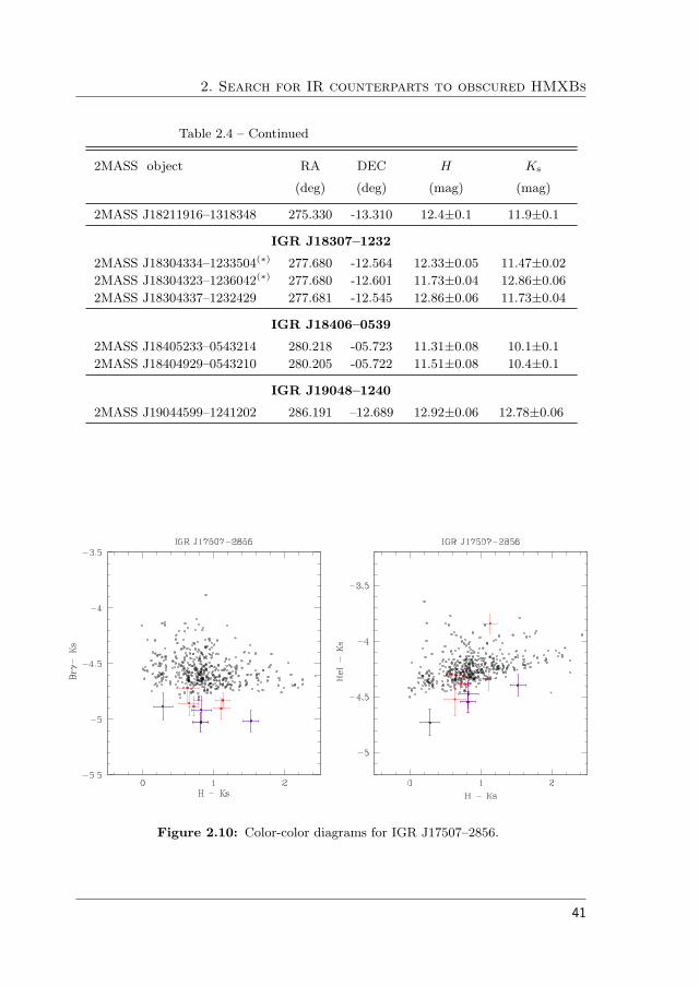
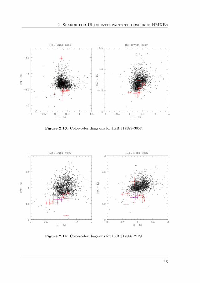
We report in Table 2.4 the selected candidate counterparts for each field. Theobtained color-color diagrams for each field are shown in Figs. 2.10–2.22. Can-didate counterparts retrieved from any color-color diagram are marked in bothdiagrams with red points; the strongest candidates, i.e. those emerging from bothdiagrams, are shown with blue points. For the selected candidates, error bars aredisplayed. We obtained emission-line candidates from all the field analyzed inthis work, except for IGR J17331–2406. The corresponding color-color diagramsare reported for the sake of completeness in Fig. 2.23.
The selected candidate counterparts will be observed in July 2010 during aspectroscopy campaign already awarded by ESO. Data will be analyzed and clas-sified in the same manner as presented in the next chapter. This will constitutethe final validation of the technique illustrated here.
For IGR J175866–2129, 2MASS J17583455-2123215 was recently proposed ascounterpart by Tomsick et al. (2009), based on CHANDRA localization. Nooptical/IR spectra of this object are available. Since the X-ray spectrum of the
37
2.5. Results
system is hard, they suggest it is a HMXB. The suggested counterpart is notamong our candidates.
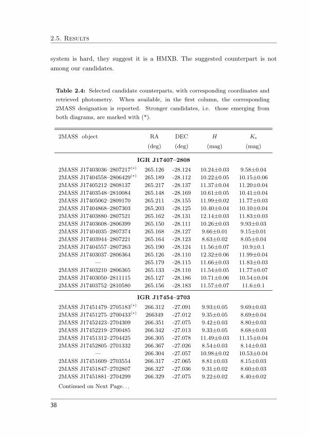
Table 2.4: Selected candidate counterparts, with corresponding coordinates and
retrieved photometry. When available, in the first column, the corresponding
2MASS designation is reported. Stronger candidates, i.e. those emerging from
both diagrams, are marked with (*).
2MASS object RA DEC H Ks
(deg) (deg) (mag) (mag)
IGR J17407–2808
2MASS J17403036–2807217(∗) 265.126 -28.124 10.24±0.03 9.58±0.04
2MASS J17404558–2806429(∗) 265.189 -28.112 10.22±0.05 10.15±0.06
2MASS J17405212–2808137 265.217 -28.137 11.37±0.04 11.20±0.04
2MASS J17403548–2810084 265.148 -28.169 10.61±0.05 10.41±0.04
2MASS J17405062–2809170 265.211 -28.155 11.99±0.02 11.77±0.03
2MASS J17404868–2807303 265.203 -28.125 10.40±0.04 10.10±0.04
2MASS J17403880–2807521 265.162 -28.131 12.14±0.03 11.83±0.03
2MASS J17403608–2806399 265.150 -28.111 10.26±0.03 9.93±0.03
2MASS J17404035–2807374 265.168 -28.127 9.66±0.01 9.15±0.01
2MASS J17403944–2807221 265.164 -28.123 8.63±0.02 8.05±0.04
2MASS J17404557–2807263 265.190 -28.124 11.56±0.07 10.9±0.1
2MASS J17403037–2806364 265.126 -28.110 12.32±0.06 11.99±0.04
— 265.179 -28.115 11.66±0.03 11.83±0.03
2MASS J17403210–2806365 265.133 -28.110 11.54±0.05 11.77±0.07
2MASS J17403050–2811115 265.127 -28.186 10.71±0.06 10.54±0.04
2MASS J17403752–2810580 265.156 -28.183 11.57±0.07 11.6±0.1
IGR J17454–2703
2MASS J17451479–2705183(∗) 266.312 -27.091 9.93±0.05 9.69±0.03
2MASS J17451275–2700433(∗) 266349 -27.012 9.35±0.05 8.69±0.04
2MASS J17452423–2704309 266.351 -27.075 9.42±0.03 8.80±0.03
2MASS J17452219–2700485 266.342 -27.013 9.33±0.05 8.68±0.03
2MASS J17451312–2704425 266.305 -27.078 11.49±0.03 11.15±0.04
2MASS J17452805–2701332 266.367 -27.026 8.54±0.03 8.14±0.03
— 266.304 -27.057 10.98±0.02 10.53±0.04
2MASS J17451609–2703554 266.317 -27.065 8.81±0.03 8.15±0.03
2MASS J17451847–2702807 266.327 -27.036 9.31±0.02 8.60±0.03
2MASS J17451881–2704299 266.329 -27.075 9.22±0.02 8.40±0.02
Continued on Next Page. . .
38

2. Search for IR counterparts to obscured HMXBs
Table 2.4 – Continued
2MASS object RA DEC H Ks
(deg) (deg) (mag) (mag)
2MASS J17453482–2701416 266.395 -27.028 11.82±0.06 11.43±0.05
2MASS J17452723–2705224 266.363 -27.089 10.82±0.02 10.59±0.03
2MASS J17452398–2700538 266.350 -27.015 12.47±0.05 12.15±0.04
2MASS J17452128–2704125 266.339 -27.070 12.18±0.05 11.77±0.06
2MASS J17453298–2701550 266.387 -27.032 12.36±0.04 12.16±0.04
2MASS J17451826–2705155 266.326 -27.088 11.52±0.02 11.44±0.04
2MASS J17453460–2701261 266.394 -27.023 12.40±0.07 12.13±0.08
2MASS J17451714–2704331 266.321 -27.076 10.24±0.02 9.98±0.03
2MASS J17451348–2703568 266.306 -27.066 11.10±0.02 10.98±0.02
2MASS J17452856–2701171 266.397 -27.021 10.02±0.04 9.86±0.03
IGR J17507–2856
2MASS J17503177–2857557(∗) 267.633 -28.965 13.07± 0.07 12.34±0.06
2MASS J17505339–2856338(∗) 267.723 -28.943 12.36±0.09 12.17±0.09
2MASS J17503610–2858431(∗) 267.650 -28.979 9.76±0.07 8.33±0.07
2MASS J17504298–2858139 267.683 -28.971 10.59±0.05 9.86±0.03
2MASS J17504462–2858074 267.691 -28.97 12.33±0.06 11.70±0.04
2MASS J17503197–2858364 267.633 -28.977 12.02 ±0.09 11.01±0.07
2MASS J17504193–2855251 267.729 -28.983 10.55±0.09 9.99±0.06
2MASS J17505268–2859009 267.719 -28.983 12.36±0.10 12.17±0.10
IGR J17585–3057
2MASS J17584038–3058446 269.668 -30.979 12.3±0.1 11.85±0.04
2MASS J17583570–3058214 269.649 -30.973 11.75±0.05 11.22±0.05
2MASS J17584243–3105527 269.677 -31.098 12.6±0.1 12.26±0.05
— 269.677 -31.011 12.40±0.07 11.94±0.05
2MASS J17584299–3059450 269.679 -30.996 12.10±0.07 11.58±0.04
2MASSJ17583584–3059084 269.649 -30.986 12.45±0.08 12.11±0.06
2MASS J17580987–3059295 269.541 -30.991 9.93±0.05 9.67±0.05
2MASS J17581935–3100102 269.581 -31.003 11.66±0.04 11.8±0.02
2MASS J17581805–3059260 269.575 -30.990 12.41±0.07 12.09±0.03
2MASS J17581721–3057460 269.572 -30.963 11.06±0.04 11.09±0.05
2MASS J17580982–3101485 269.540 -31.030 9.68±0.07 9.53±0.05
IGR J17586–2129
2MASS J17583417–2128409(∗) 269.642 -21478 10.23±0.06 9.22±0.04
2MASS J17585005–2123516(∗) 269.708 -21.398 12.42±0.09 11.55±0.08
2MASS J17583428–2124204 269.643 -21.406 11.3±0.1 10.60±0.09
Continued on Next Page. . .
39

2.5. Results
Table 2.4 – Continued
2MASS object RA DEC H Ks
(deg) (deg) (mag) (mag)
2MASS J17583402–2121472 269.642 -21.363 12.61±0.06 11.94±0.03
2MASS J17583400–2124046 269.642 -21.401 11.56±0.03 11.04±0.03
2MASS J17585226–2124452 269.718 -21.412 12.12±0.05 11.05±0.03
— 269.712 -21.372 13.05±0.04 11.82±0.04
— 269.712 -21.405 12.96±0.05 11.76±0.03
2MASS J17581598–2125052 269.566 -21.418 11.25±0.15 10.03±0.04
2MASS J17582842–2124127 269.618 -21.403 8.81±0.03 9.71±0.04
IGR J18159–3353
2MASS J18155120–3359003 273.963 -33.983 11.20±0.08 10.55±0.08
2MASS J18155364–3358596 273.957 -33.986 11.06±0.05 10.48±0.05
2MASS J18161193–3400384 274.050 -34.011 10.95±0.06 10.19±0.07
IGR J18175–1530
2MASS J18171361–1537072(∗) 274.307 -15.619 9.39±0.08 8.52±0.05
2MASS J18171363–1536307(∗) 274.307 -15.608 11.18±0.07 9.97±0.04
2MASS J18173021–1536034(∗) 274.376 -15.601 12.27±0.05 11.04±0.05
2MASS J18173011–1538088(∗) 274.375 -15.636 12.38±0.04 11.62±0.04
2MASS J18171668–1531004 274.319 -15.517 12.74±0.09 11.95±0.04
2MASS J18171361–1532057 274.307 -15.535 12.2±0.1 11.58±0.03
2MASS J18171421–1533556 274.309 -15.565 11.97±0.07 10.43±0.07
2MASS J18171382–1534432 274.308 -15.579 12.04±0.09 11.07±0.05
— 274.307 -15.525 12.82±0.09 11.96±0.03
— 274.307 -15.587 12.54±0.07 11.81±0.06
2MASS J18171417–1534552 274.309 -15.582 12.62±0.08 11.26±0.07
2MASS J18173028–1535409 274.377 -15.595 11.40±0.06 10.28±0.04
2MASS J18171364–1535344 274.307 -15.593 11.52±0.05 10.65±0.04
IGR J18193–2542
2MASS J18192899–2544090 274.871 -25.736 12.45±0.05 12.29±0.04
2MASS J18190771–2544469 274.782 -25.747 12.44±0.08 12.12±0.04
IGR J18214–1318
— 275.330 -13.310 12.90±0.08 12.37±0.08
2MASS J18213778–1315082 275.407 -13.252 12.6±0.1 11.9±0.1
2MASS J18212903–1315070 275.371 -13.252 10.12±0.04 10.75±0.05
2MASS J18213468–1315587 275.395 -13.266 12.37±0.08 11.8±0.1
2MASS J18213438–1317445 275.393 -13.296 12.3±0.1 11.5±0.1
Continued on Next Page. . .
40
2. Search for IR counterparts to obscured HMXBs
Table 2.4 – Continued
2MASS object RA DEC H Ks
(deg) (deg) (mag) (mag)
2MASS J18211916–1318348 275.330 -13.310 12.4±0.1 11.9±0.1
IGR J18307–1232
2MASS J18304334–1233504(∗) 277.680 -12.564 12.33±0.05 11.47±0.02
2MASS J18304323–1236042(∗) 277.680 -12.601 11.73±0.04 12.86±0.06
2MASS J18304337–1232429 277.681 -12.545 12.86±0.06 11.73±0.04
IGR J18406–0539
2MASS J18405233–0543214 280.218 -05.723 11.31±0.08 10.1±0.1
2MASS J18404929–0543210 280.205 -05.722 11.51±0.08 10.4±0.1
IGR J19048–1240
2MASS J19044599–1241202 286.191 –12.689 12.92±0.06 12.78±0.06
Figure 2.10: Color-color diagrams for IGR J17507–2856.
41

2.5. Results
Figure 2.11: Color-color diagrams for IGR J17407–2808.
Figure 2.12: Color-color diagrams for IGR J17454–2703.
42
2. Search for IR counterparts to obscured HMXBs
Figure 2.13: Color-color diagrams for IGR J17585–3057.
Figure 2.14: Color-color diagrams for IGR J17586–2129.
43

2.5. Results
Figure 2.15: Color-color diagrams for IGR J18159–3353.
Figure 2.16: Color-color diagrams for IGR J18175–1530.
44

2. Search for IR counterparts to obscured HMXBs
Figure 2.17: Color-color diagrams for IGR J18193–2542.
Figure 2.18: Color-color diagrams for IGR J18214–1318.
45

2.5. Results
Figure 2.19: Color-color diagrams for IGR J18307–1232.
Figure 2.20: Color-color diagrams for IGR J18406–0539.
46

2. Search for IR counterparts to obscured HMXBs
Figure 2.21: Color-color diagrams for IGR J18462–0223.
Figure 2.22: Color-color diagrams for IGR J19048–1240.
47
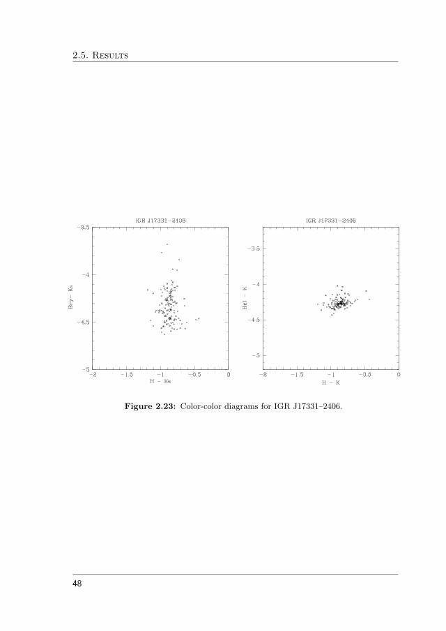
2.5. Results
Figure 2.23: Color-color diagrams for IGR J17331–2406.
48
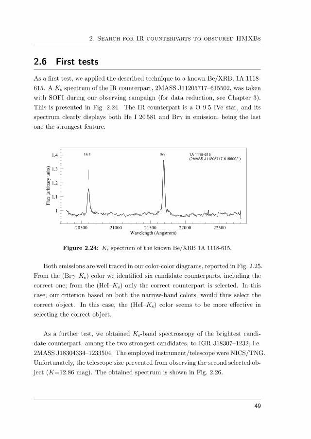
2. Search for IR counterparts to obscured HMXBs
2.6 First tests
As a first test, we applied the described technique to a known Be/XRB, 1A 1118-615. A Ks spectrum of the IR counterpart, 2MASS J11205717–615502, was takenwith SOFI during our observing campaign (for data reduction, see Chapter 3).This is presented in Fig. 2.24. The IR counterpart is a O 9.5 IVe star, and itsspectrum clearly displays both He I 20 581 and Brγ in emission, being the lastone the strongest feature.
20500 21000 21500 22000 22500Wavelength (Angstrom)
1
1.1
1.2
1.3
1.4
Flu
x (
arbit
rary
unit
s)
Br! 1A 1118-615(2MASS J11205717-6155002 )
He I
Figure 2.24: Ks spectrum of the known Be/XRB 1A 1118-615.
Both emissions are well traced in our color-color diagrams, reported in Fig. 2.25.From the (Brγ–Ks) color we identified six candidate counterparts, including thecorrect one; from the (HeI–Ks) only the correct counterpart is selected. In thiscase, our criterion based on both the narrow-band colors, would thus select thecorrect object. In this case, the (HeI–Ks) color seems to be more effective inselecting the correct object.
As a further test, we obtained Ks-band spectroscopy of the brightest candi-date counterpart, among the two strongest candidates, to IGR J18307–1232, i.e.2MASS J18304334–1233504. The employed instrument/telescope were NICS/TNG.Unfortunately, the telescope size prevented from observing the second selected ob-ject (K=12.86 mag). The obtained spectrum is shown in Fig. 2.26.
49

2.6. First tests
Figure 2.25: Color-color diagrams for the known Be/XRB 1A 1118-615.
20500 21000 21500 22000 22500Wavelength (Angstrom)
0
0.5
1
1.5
2
2.5
3
Flu
x (
arbit
rary
unit
s)
2MASS J18304334-1233504He I
Figure 2.26: Ks spectrum of one candidate counterpart to IGR J18307–1232.
This displays He I 20 581 A in quite strong emission, as expected from ourcolor-color diagram. Instead, no Brγ emission is detected. No other spectralfeature is recognizable. In fact, the retrieved spectrum does not present Brγ ei-ther in emission or in absorption: while the emission feature is a characteristicphenomenon of Be stars, in most stars this line is present in absorption. Theselected candidate thus stands out in the (Brγ-Ks) – (H − Ks) color-color di-agram just because it does not have Brγ in absorption, as most field stars do.
50

2. Search for IR counterparts to obscured HMXBs
Since He I emission is a typical feature of early-type companions in HMXBs, andBrγ emission, although typical, is not always present in this kind of objects, (see,for instance, Clark & Steele 2000), NICS data give support to this candidate assuitable counterpart, i.e. validate our detection technique.
However, a different candidate counterpart to this INTEGRAL source wasrecently proposed by Butler et al. (2009). The object, with I = 16 mag, is notpresent in the 2MASS catalogue due to its faintness, and for the same reason wasnot included in our photometry. Its optical spectrum is typical of either CVs orLMXBs, so that the possibility for the system to be a Be/XRB is consistentlyruled out. These findings, although indicating a different star as the counterpartto IGR J18307–1232, do not weaken the general validation of our technique fromNICS data.
51

2.6. First tests
52

And over all the sky — the sky!
far, far out of reach, studded,
breaking out, the eternal stars.
Walt Whitman 3NIR spectral analysis and classification of
HMXBs identified by INTEGRAL
3.1 Scientific objective
As we already discussed in the previous chapter, many of the new galactic X-raysources discovered by INTEGRAL are found to be heavily obscured. Counter-parts to these objects are hard to observe in the optical band due to the highinterstellar extinction, with AV in excess of up to ∼ 20 mag.
In this context, the recent availability of infrared spectroscopy has emerged asa strong tool to characterize these systems and, together with high-energy data,reveal the HMXB sub-class they belong to. This results in the identification of themass transfer process of the system, with information about the intrinsic physicsof the X-ray binary. The need for low energy data is particularly urgent in thecase of SFXTs, which show X-ray properties common to other objects (such asRS CVs binaries and Low Mass X-ray binaries) and thus crucially require thespectral classification of their counterpart in order to be properly discerned.
In this chapter we present spectral analysis and classification of seven HMXBsdiscovered (or re-discovered) by INTEGRAL. The selected IGR sources are thefollowing: IGR J16207–5129, IGR J16465–4507, IGR J16479–4514, IGR J16493–
53
3.2. Observations
4348, AX J1841.0–0536 and IGR J19140+0951. We also included the well knownsystem 4U 1907+09 since the spectral classification of its counterpart has been amatter of debate in the past, and no infrared spectra have been published up tonow. The first four sources are located in the direction of the Norma-arm tangentregion, the next one in the Scutum-arm tangent region and the last two in theSagittarius arm tangent. Moreover, 5 reference spectra of isolated Be stars weretaken during poor weather conditions. These would allow us, by comparison, tobetter classify the spectra if one of our candidates was a Be star. Eventually,none of them turned out to be a Be star, nevertheless we will report them forcompleteness in Sect. 3.4.2
In the next two sections we describe the observations and data reduction; inSection 3.4 we report the obtained spectra, analyze their features and propose aclassification; we calculate the interstellar hydrogen column density and estimatethe distance to each source; in section 3.5 we discuss our results, before concluding.
3.2 Observations
We selected proposed counterparts, choosing sources observed by the X-ray mis-sions XMM, Chandra and Swift, which produce a very small error circle andfacilitate the detection of the counterpart.
Data were obtained during several observing runs at the European SouthernObservatory (ESO), in Chile. The employed instruments were, in visiting mode,SOFI (Moorwood et al. 1998c), on the 3.5m New Technology Telescope (NTT)at La Silla, in July 2006 and May 2005; and, in service mode, ISAAC (Moorwoodet al. 1998a) on the 8.2m UT1 in Paranal, in April 2007.
Since all the spectra analyzed in this chapter except one were obtained withSOFI, only this instrument will be described here. For an overview on ISAAC, seeChapter 4. The SOFI spectrograph has a largest field of view of 4.92 arcmin, andit covers the 0.9-2.5 micron wavelength range with spectral resolution from 600to 2200. There are three grisms available with SOFI: two low resolution grismsand a medium resolution grism. Of the two low resolution grisms, one covers
54
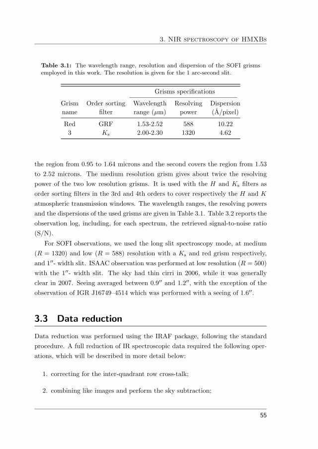
3. NIR spectroscopy of HMXBs
Table 3.1: The wavelength range, resolution and dispersion of the SOFI grismsemployed in this work. The resolution is given for the 1 arc-second slit.
Grisms specifications
Grism Order sorting Wavelength Resolving Dispersionname filter range (µm) power (A/pixel)
Red GRF 1.53-2.52 588 10.223 Ks 2.00-2.30 1320 4.62
the region from 0.95 to 1.64 microns and the second covers the region from 1.53to 2.52 microns. The medium resolution grism gives about twice the resolvingpower of the two low resolution grisms. It is used with the H and Ks filters asorder sorting filters in the 3rd and 4th orders to cover respectively the H and K
atmospheric transmission windows. The wavelength ranges, the resolving powersand the dispersions of the used grisms are given in Table 3.1. Table 3.2 reports theobservation log, including, for each spectrum, the retrieved signal-to-noise ratio(S/N).
For SOFI observations, we used the long slit spectroscopy mode, at medium(R = 1320) and low (R = 588) resolution with a Ks and red grism respectively,and 1��- width slit. ISAAC observation was performed at low resolution (R = 500)with the 1��- width slit. The sky had thin cirri in 2006, while it was generallyclear in 2007. Seeing averaged between 0.9�� and 1.2��, with the exception of theobservation of IGR J16749–4514 which was performed with a seeing of 1.6��.
3.3 Data reduction
Data reduction was performed using the IRAF package, following the standardprocedure. A full reduction of IR spectroscopic data required the following oper-ations, which will be described in more detail below:
1. correcting for the inter-quadrant row cross-talk;
2. combining like images and perform the sky subtraction;
55

3.3. Data reduction
3. creating a flat field and perform flat field correction;
4. extracting the spectra;
5. applying wavelength calibration;
6. applying terrestial atmospheric (telluric) correction.
3.3.1 Inter-quadrant row cross-talk
This feature affects both imaging and spectroscopy performed with SOFI andISAAC. Unlike the imaging, when users can rotate the instrument to avoid it,the spectra are always aligned along the array columns, so a ghost of the upperhalf of the spectrum always appears in the lower one, and vice versa. In our case,since we are mainly looking for emission lines, the effect is particularly danger-ous because ghosts of emission lines are emission line like and can be confusing.For instance, one has to account for this effect when faint lines have to be de-tected between bright OH lines, or when the continuum-to-line ratio is of interest.
Figs. 3.1 and 3.2 from Finger & Nicolini (1998) show the shading effect witha long slit oriented parallel to the rows of the detector. The slitwidth is in thiscase 2 arcseconds on the sky. The image shows the spectrum of ambient back-ground radiation observed with the narrow-band CO filter and the red grism ofSOFI. The dispersion of the grism is 10.22 A/pixel. The peak flux in the centerof the slit image is 1374 e−/sec/pixel. The calculated photon flux for the giveninstrument setup is 1846 photons/sec/pixel. The rows in quadrants III and IVnear row 798, which have increased intensity but do not receive any photons, areread out at the same time as the rows close to row 286, which are illuminated bythe slit. The intensity of row 798 is 1.5% of the intensity of row 286.The result of the correction algorithm (2.3) is demonstrated in Fig. 3.3 by com-parison of the raw Ks-band spectrum with the modified Ks-band spectrum: onecan clearly see that the row cross-talk can be well removed.
56
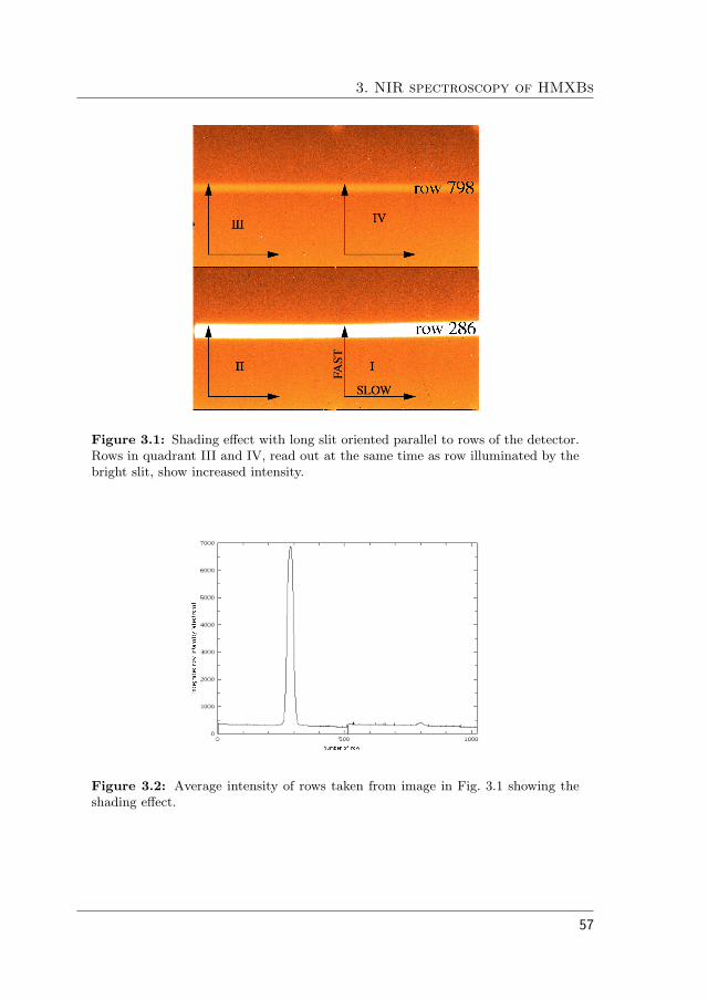
3. NIR spectroscopy of HMXBs
Figure 3.1: Shading effect with long slit oriented parallel to rows of the detector.Rows in quadrant III and IV, read out at the same time as row illuminated by thebright slit, show increased intensity.
Figure 3.2: Average intensity of rows taken from image in Fig. 3.1 showing theshading effect.
57

3.3. Data reduction
Figure 3.3: Comparison between a raw Ks-band spectrum (on the left) and theKs-band spectrum (on the right) modified by the correction algorithm using equa-tion (2.3).
3.3.2 Sky subtraction
Below about 2.3µm most the sky emission arises from molecules (primarily OHand O2) excited by solar radiation during the day. These emission lines typicallyfar exceed the counts in the target star, so they must be removed before the two-dimensional spectrum is summed along the cross-dispersed direction to obtainthe one-dimensional spectrum. The strength of the sky emission is a function ofairmass and atmospheric conditions, and significant variations occur over time-scales of approximately tens of minutes in clear weather.
We attained the best results by subtracting one slit position from anotherunique slit position, the preceding one or the following one during the execution(task imarith of IRAF). Obviously, one chooses to subtract the image with thetarget in a different position along the slit with respect to the image that onewants to correct. The advantage of this technique is that it takes into account skyvariation on time-scale a few DIT1 times, so that we could achieve a good qualitysubtraction even in case of thin cirrus and very low target signal, i.e. when thesky is variable and dominant on the object. In Fig. 3.4 one can appreciate the
1In the context of the ESO detectors control system, the DIT, or Detector Integration Time,
is defined as the amount of time during which the signal is integrated onto the detector diodes.
For SOFI, under the worst transparency conditions, we chose typical values of 30-35 s, while
under the best conditions we chose ∼ 60s DITs. For ISAAC, the DIT was 60s.
58

3. NIR spectroscopy of HMXBs
Figure 3.4: A single frame before (left panel) and after (right panel) sky subtrac-tion. The “negative” spectra appearing in the final image are a secondary result ofthe subtraction, which doesn’t affect data analysis.
effect of sky subtraction on a single frame of data.
3.3.3 Flat fields
A dome flat-field was create by obtaining, both at medium and low resolution, aset of alternated images of an illuminated/unilluminated panel inside the dome.The average of the unilluminated set of images was subtracted from the aver-age of the illuminated ones (tasks imcombine and imarith of IRAF). The two-dimensional dome flat was then normalized to unit taking care of the large-scalevariations, using the task response with a spline3 function of high order (45) tobest follow the pixel variations; finally, the sky-subtracted, two-dimensional datawere divided by the normalized dome flat field to remove pixel-to-pixel sensitivityvariations in the array.
3.3.4 Extraction of the one dimensional spectra
The two-dimensional spectra were in this phase integrated along the cross-disperseddirection and displayed as counts versus pixel position along the dispersed direc-tion. In the package apextract, we used the task apsum interactively in order tocarefully inspect each image and identify the correct aperture.
The task apsum calls several other tasks (apdefault, aptrace, apfind andapedit). The steps that mark this phase are: selecting the object window bydefining the aperture size one wants to use in the extraction of the spectrum;
59

3.3. Data reduction
Figure 3.5: The different phases in the extraction of a one-dimensional spectrum,as performed using the task apsum. From top left: definition of the aperture size;definition of the background window; tracing the spectrum; the final extraction ofthe one-dimensional spectrum displayed as counts versus pixel position.
selecting the background window and fitting it; tracing the spectrum, i.e. fittingthe center of the star profile along the image; extracting the one dimensionalspectrum. This stages are graphically shown in Fig. 3.5.
Since the regions of the sky we observed, belonging to the Galactic Plane,are very crowded, in a few cases there was no chance of excluding other – evenbrighter – objects from the field of view. That resulted in the presence of morethan one two-dimensional spectrum in the frames, but this inconvenience couldbe easily overcome in the extraction phase.
3.3.5 Wavelength calibration
After extracting the one-dimensional spectrum for the arcs – both at medium andlow resolution – one is able to perform the wavelength calibration, which consists
60

3. NIR spectroscopy of HMXBs
of three steps. The first one was done interactively with the task identify whichallows to get from an arc a dispersion solution (wavelength versus pixel), using thecalibration arc spectra with identified lines reported in instrument manuals. Thecalibration arc spectra are shown in Figs. 3.6 and 3.7 for SOFI, and in Fig. 3.8for ISAAC.
0
Figure 3.6: A Xenon and Neon arc spectrum taken with SOFI medium resolutiongrism at the Ks atmospheric window. The main lines are marked.
With identify, features in the input images are identified interactively andassigned user coordinates. A “coordinate function” mapping pixel coordinates touser coordinates may be determined from the identified features. We used a cubicfit to calibrate the dispersion both for the medium resolution and the red grism.The dispersion solution is the output from the task and it is stored in a text file.
The next step consists in assigning arc references to scientific objects; thisstep was performed with the task refspectra which writes this assignment inthe header of the objects under the keywords REFSPEC1 and REFSPEC2. Thethird step consists in linearizing the x-axis of the extracted spectra with the task
61

3.3. Data reduction
Figure 3.7: A Xenon arc spectrum taken with SOFI low resolution red grism.The main lines are marked.
dispcor using the reference found in the header and the corresponding solutionfrom the database. The output of the task is a wavelength calibrated image, withx-scale in Angstrom.
After wavelength calibrating, and before performing the removal of telluricfeatures, we graphically removed spurious features such as bad pixels or cosmicrays (task splot), we added up all the one-dimensional spectra for each observa-tion (task sarith), cut the resulting spectrum in order to keep only the regionwhere the transmission function of the Ks filter is nearly constant (task scopy),and finally we normalized the obtained spectrum (task continuum) by dividing itby a fitted polynomial continuum.
62

3. NIR spectroscopy of HMXBs
Figure 3.8: A Xenon/Argon arc spectrum taken with ISAAC low resolution grism.The main lines are marked.
3.3.6 Telluric absorption correction
The near-infrared spectrum of the atmosphere from 1 to 5 µm is dominated bytelluric water and CO2 absorption, between which the major observing windowsin the wavelength region are defined. Broad molecular absorption bands of CO2
are resolved at moderate spectral resolution into individual pressure-broadenedrotovibrational transitions. These transitions vary in both time and observed ele-vation, making their removal problematic in ground-based spectroscopic studies.There is a tremendous impetus from astronomers to obtain highly accurate spec-tral profiles for lines existing in the near-infrared. For hot stars like the ones wewere interested into, an important line for spectral classification – but also forthe modeling of extended atmospheres and stellar winds – is the HeI transitionat 2.058 µm (Clark & Steele 2000): this line is located near the short-wavelengthedge of the Ks-band window, where CO2 absorption bands dominate the spec-trum. The challenge for observational astronomers is to obtain observations of
63

3.3. Data reduction
the 2.058 µm line profile with a high enough signal-to-noise ratio to be suitablefor detailed modeling despite considerable telluric contamination.
In order to correct for telluric absorption, it is necessary to divide the objectspectrum by the spectrum of what one can call a telluric standard. We adoptedthe procedure outlined by Hanson et al. (1996). At the telescope, we observed anA0-A3 III-V star immediately before or after each target and a G2-3 V star onceper hour in order to obtain very small differences in airmass (differences between0.01 and 0.04 airmasses were generally accomplished). The only non-telluric fea-ture in the A star spectra is Brγ. A simple interpolation over this feature is notappropriate however, as there is also a telluric feature at this wavelength thatwould lead to spurious emission features contaminating the strength and profileof the Brγ emission lines we expected from the targets. Instead we used the Gstar observations divided by the solar spectrum to calculate the telluric featuresin the region of Brγ (between 21590 A and 21739 A).
In order to do that, we employed a high resolution (R = 40 000) K-bandspectrum of the sun2. We degraded it to the resolution of SOFI/ISAAC spectrausing the task gauss which performs a convolution with an elliptical – circular,in our case – Gaussian function; we also applied to the solar spectrum the samedispersion solution than SOFI/ISAAC data (task dispcor). In order to ensurethat the A star, G star and solar spectra were all properly aligned in wavelengthspace, when necessary, appropriate offsets were applied. The ratio between theG star and the solar spectrum in the Brγ region was patched into the A starspectrum (tasks scopy and scombine), obtaining a specific telluric spectrum foreach target. Fig. 3.9 shows an example of a telluric spectrum and the A and Gstar spectrum from which it was derived.
After constructing the specific telluric spectrum for each target, we appliedthe removal of telluric features by dividing the targets by the shifted and scaledtelluric spectra.
In the case of low-resolution observations, the H-band spectra were correctedfor telluric features by ratioing observed G type standards with the solar spec-
2NSO/Kitt Peak FTS data, that were produced by NSF/NOAO.
64

3. NIR spectroscopy of HMXBs
2.04 2.06 2.08 2.1 2.12 2.14 2.16 2.18 2.2 2.22 2.24
0.2
0.4
0.6
0.8
1
1.2
Wavelength (µm)
No
rmal
ized
co
un
tsTelluric spectrum
A star sepctrum (HIP 21837)
G star spectrum (HIP 21488)
Figure 3.9: Construction of telluric spectrum from A and G star spectra. Theregion marked by dashed lines indicates where the ratio between the G star andsolar spectrum was patched into the A star spectrum. The spectra have beennormalized to 1 and displayed with an offset for clarity.
trum to remove features within their photosphere, and then ratioing the objectspectrum with the modified standard spectrum.
The correction was done interactively with the task telluric, which is char-acterized by the parameters of the shift and the scale. The shifting takes intoaccount possible small misalignments or errors in the dispersion zeropoints, whilethe intensity scaling allows for differences in the airmass and variations in theabundance of the telluric species. The intensity scale used Beer’s law which is theapproximation that the change in absorption with abundance is an exponentialrelation. The task determines the best values of the shift and scale parametersby cross-correlating the calibration and scientific spectra to find the parametersvalues that minimize the RMS of the output corrected spectrum, which is calcu-lated as follows. Let J
�(xi) be the calibration spectrum at a set of pixel xi. Aninterpolation function is fit to this spectrum to give J
�(x). The shifted and scaled
65
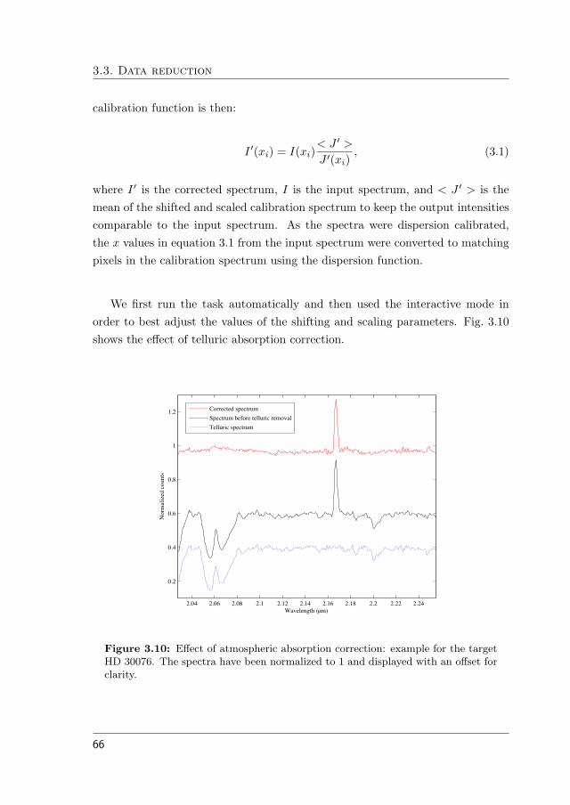
3.3. Data reduction
calibration function is then:
I�(xi) = I(xi)
< J�>
J �(xi), (3.1)
where I� is the corrected spectrum, I is the input spectrum, and < J
�> is the
mean of the shifted and scaled calibration spectrum to keep the output intensitiescomparable to the input spectrum. As the spectra were dispersion calibrated,the x values in equation 3.1 from the input spectrum were converted to matchingpixels in the calibration spectrum using the dispersion function.
We first run the task automatically and then used the interactive mode inorder to best adjust the values of the shifting and scaling parameters. Fig. 3.10shows the effect of telluric absorption correction.
2.04 2.06 2.08 2.1 2.12 2.14 2.16 2.18 2.2 2.22 2.24
0.2
0.4
0.6
0.8
1
1.2
Wavelength (µm)
No
rmal
ized
co
un
ts
Corrected spectrum
Spectrum before telluric removal
Telluric spectrum
Figure 3.10: Effect of atmospheric absorption correction: example for the targetHD 30076. The spectra have been normalized to 1 and displayed with an offset forclarity.
66

3. NIR spectroscopy of HMXBs
3.4 Results
In this section we present the results of spectral classification and analysis foreach target. The field of NIR spectral classification is still very young and thelevel of required S/N and resolution to perform a quantitative profile analysis arevery high (R ∼ 12 000 and S/N � 250), especially for young massive stars, asshown by Hanson et al. (2005b). The difficulty of the analysis depends on thefew lines available and the relatively large uncertainty in their strength, due totheir intrinsic weakness; moreover, some significant spectral regions, specificallythrough the 20 580 He I and the Brγ features, pose systematic complicationsbecause of the strong telluric absorption.
Under this premise, our analysis will be qualitative, based on the comparisonwith available NIR spectral atlases (Hanson et al. 1996, 2005a). According toour estimation, this approach implies that the resulting spectral classificationis provided with an uncertainty of no more than one luminosity subclass. Thespectral type is precise up to one subtype.
Some of the identified features exhibit a 10-20 A displacement with respect tothe nominal values, consistent with the instrumental resolution. Greater displace-ments, up to a maximum of 29 A, are found corresponding to lines characterizedby a complex profile, such as Brγ, or placed in a region of strong telluric absorp-tion, such as both H i 20 581 A and Brγ.
In the next sub-section we will classify the spectra, showing the features wewere able to identify, with the corresponding equivalent width. Although it waspointed out (Hanson et al. 1996) that equivalent widths may show variationsbetween stars, we report them for completeness. The values we calculated areaffected by an average 15% error. For each object, a figure displays the spectrumwe obtained, together with some comparative spectra from the atlas of Hansonet al. (1996) in a separate box. At the end of this chapter, Table 3.3 summarizesthe line identifications for all the observed targets.
67
3.4. Results
3.4.1 Spectral analysis and classification
IGR J16207–5129
The source was discovered by IBIS/ISGRI in the first Galactic Plane Surveyperformed by INTEGRAL (Bird et al. 2004), which measured a flux of 3.8 ±0.3 mCrab in the 20–40 keV range. Instead, only the upper limit of < 4 mCrabwas obtained in the 40–100 keV band. Subsequent Chandra observations allowedthe identification of the optical/infrared counterpart. This was associated withUSNO-B1.0 0384-0560857 = 2MASS J16204627-5130060 by Tomsick et al. (2006).The power-law spectral fit provided NH = 3.7+1.4
−1.2× 1022 cm−2 and photon indexequal to 0.5+0.6
−0.5, indicating an intrinsically hard source. The lower limit to thestellar temperature was estimated to > 18 000 K, revealing the presence of a veryhot, massive star. From the fit of optical/IR spectral energy distributions, thedistance was estimated to be between 3-10 kpc (3-9 kpc in the case of a supergiantclassification). Subsequent optical spectroscopy from Masetti et al. (2006a) refinedthe distance estimate to 4.6 kpc. Negueruela & Schurch (2007), from opticalobservations, constrained the spectral type to earlier than B1.
Fig. 3.11 shows the Ks spectrum we obtained, with identified spectral featuresmarked. The spectrum shows no metal lines (no N iii or C iv), strong He i 20 581A emission, He i absorption at 21 126 A and moderately strong Brγ absorption.The atomic transitions observed are the typical of OB star spectra. The He i
20 581 A line is a prominent feature in supergiant stars, so that it is considered animportant tracer of stars with extended atmospheres. It becomes weak or evendisappears in main sequence stars and it is observed in emission in B type su-pergiants, whereas it is in absorption in O type supergiants (Hanson et al. 1996).The He i 21 126 A line is present in late O – early B spectra.
For what was outlined above, and by visually comparing the relative strengthsof the identified lines with those of Hanson et al. (1996, 2005a), we estimate thespectral type of the IGR J16207–5129 counterpart to be B1 Ia. This allows us toclassify the system as a SGXRB, as also inferred by Negueruela & Schurch (2007).
68

3. NIR spectroscopy of HMXBs
Figure 3.11: Ks spectrum for 2MASS 16204627–5130060, the infrared counterpartof IGR J16207-5129. The positions of identified spectral features are marked bysolid lines.
IGR J16465-4507
The source was discovered by INTEGRAL during its only observed X-ray flare on2004 September 6th-7th (Lutovinov et al. 2004). Using data of XMM/Newton,Lutovinov et al. (2005) found pulsations with period Ps = 228 s in the X-ray fluxand high photoabsorption, with NH ∼ 7 × 1023 cm−2. The single star falling inthe XMM/Newton error circle was identified by Zurita & Walter (2004) as thecounterpart to the X-ray source, and associated with 2MASS J16463526-4507045.
From an optical spectrum, Negueruela et al. (2006) classified the source as aB1 Ib supergiant, subsequently refining their classification to B0.5 Ib (Negueruelaet al. 2007). They also estimated the distance of the source to 8 kpc.
Our IR data suggest a different spectral classification. Fig. 3.12 shows the Ks
spectrum we obtained, with identified spectral features marked.
The spectrum shows He i 20 581 A in quite strong absorption; a feature at20 730 A is possibly identifiable with a faint blend of the C iv transitions at 20 690,20 780 and 20 830 A, which appear in the atlas from Hanson et al. (1996) onlyin the very high S/N spectra. We observe He i 21 126 and Brγ, both in strong
69

3.4. Results
Figure 3.12: Ks spectrum for 2MASS J16463526-4507045, the infrared counter-part of IGR J16465-4507. The positions of identified spectral features are markedby solid lines.
absorption.We agree with Negueruela et al. (2007) in the classification of the counterpart
as an early supergiant. However, we suggest that the observed features point toan earlier type than B1: in fact, the He i 20 581 A line is seen in emission in B1supergiants, while it is in absorption in late-O supergiant. Visually comparing therelative strengths of the outlined features with those from the atlases of Hansonet al. (1996, 2005a), we refine the spectral classification of the source to O9.5Ia. We thus confirm the supergiant nature of the companion, which, togetherwith the X-ray behavior of the system, classifies it as an SFXT, as proposed byNegueruela et al. (2006).
IGR J16479–4514
The source was discovered by INTEGRAL (Molkov et al. 2003) during an out-burst. The X-ray spectrum is fitted with a power law with a high-energy cut-off,with spectral index Γ = 1.4, and the column density is NH = 12 × 1022 cm−2
(Lutovinov et al. 2005).IGR J16479–4514 showed short outbursts with very fast rises, observed in 2003
70
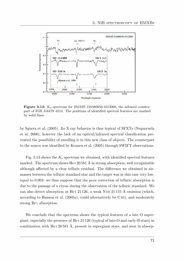
3. NIR spectroscopy of HMXBs
Figure 3.13: Ks spectrum for 2MASS J16480656-4512068, the infrared counter-part of IGR J16479–4514. The positions of identified spectral features are markedby solid lines.
by Sguera et al. (2005). Its X-ray behavior is thus typical of SFXTs (Negueruelaet al. 2006), however the lack of an optical/infrared spectral classification pre-vented the possibility of enrolling it in this new class of objects. The counterpartto the source was identified by Kennea et al. (2005) through SWIFT observations.
Fig. 3.13 shows the Ks spectrum we obtained, with identified spectral featuresmarked. The spectrum shows He i 20 581 A in strong absorption, well recognizablealthough affected by a clear telluric residual. The difference we obtained in air-masses between the telluric standard star and the target was in this case very low,equal to 0.004: we thus suppose that the poor correction of telluric absorption isdue to the passage of a cirrus during the observation of the telluric standard. Wecan also detect absorption at He i 21 126, a weak N iii 21 155 A emission (which,according to Hanson et al. (2005a), could alternatively be C iii), and moderatelystrong Brγ absorption.
We conclude that the spectrum shows the typical features of a late O super-giant, especially the presence of He i 21 126 (typical of late-O and early-B stars) incombination with He i 20 581 A, present in supergiant stars, and seen in absorp-
71

3.4. Results
tion in late-O supergiants. Through the visual comparison with the atlases fromHanson et al. (1996, 2005a), we estimate the spectral type to be O9.5 Iab. Thisresult, together with those from X-ray data, allows us to affirm that the objectbelongs to the new class of SFXTs.
IGR J16493–4348
This INTEGRAL source was discovered by Grebenev et al. (2005). RXTE obser-vations by Markwardt et al. (2005) found that the mean spectrum is consistentwith a heavily absorbed power law with NH ∼ 1023 cm−2 and a photon indexof 1.4. The retrieved flux was 1.0 × 10⁻¹¹ erg cm−2 s−1 in the 2–10, 10–20and 20–40 keV energy bands. Chandra imaging of the field of IGR J16493–4348was performed for 4.1 ks by Kuiper et al. (2005). They detected a single pointsource within the 2� error circle of the INTEGRAL source at R.A. =16h49m26.92s,Dec =−43◦49�8.96��, with a 0.6�� error in each coordinate. No spectrum could beextracted from these data and Kuiper et al. (2005) noted that previous measure-ments of IGR J16493–4348 by RXTE may be contaminated by another X-raysource, 1RXS J164913.6–435527, located ∼ 6.7� away. From INTEGRAL data,Hill et al. (2008) discarded the previously proposed association with the free radiopulsar PSR J1649–4349; the best fit of the X-ray spectrum was obtained with anabsorbed cut-off power-law with NH = 5.4× 10²² and Γ = 0.6.
The infrared counterpart to the source was proposed by Kuiper et al. (2005),who reported a single 2MASS source, 2MASS J16492695–4349090, compatiblewith both the Chandra and Swift/XRT positions. Kuiper et al. (2005) observedthe source in the Ks band and found a magnitude of 12, consistent with the2MASS magnitude. No optical/IR spectrum of the counterpart are available, andthe nature of the source, although with position and X-ray behavior pointing toa HMXB system, is not proved.
Fig. 3.14 shows the Ks spectrum we obtained, with identified spectral featuresmarked. The spectrum shows He I 20 581 A in strong emission, He I 21 126 A inabsorption and Brγ 21 661 A in relatively strong absorption. We possibly identifyalso a N III/C III line in very faint emission. The atomic transitions detected arethe typical ones of OB stars spectra. In particular, He I 20 581 A is a prominent
72
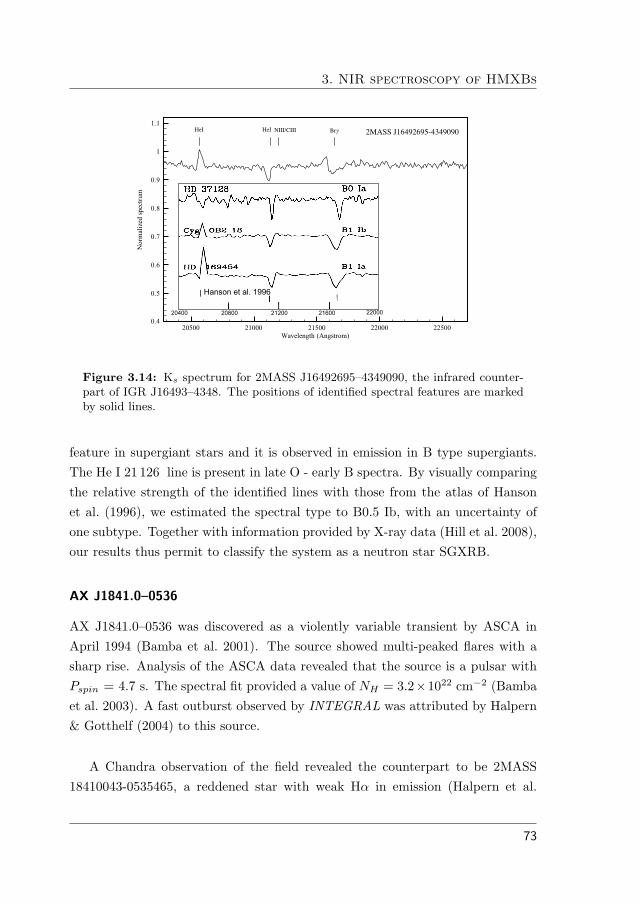
3. NIR spectroscopy of HMXBs
!"#"" !$""" !$#"" !!""" !!#""
%&'()(*+,-./0*+1,2345
"67
"6#
"68
"69
"6:
"6;
$
$6$
<324&)=>(?.1@(A,2B4
!"#$$%&'()*!(*+,)-)*.*./01 /01 211134111 56!
20400
Hanson et al. 1996
20800 21200 21600 22000
Figure 3.14: Ks spectrum for 2MASS J16492695–4349090, the infrared counter-part of IGR J16493–4348. The positions of identified spectral features are markedby solid lines.
feature in supergiant stars and it is observed in emission in B type supergiants.The He I 21 126 line is present in late O - early B spectra. By visually comparingthe relative strength of the identified lines with those from the atlas of Hansonet al. (1996), we estimated the spectral type to B0.5 Ib, with an uncertainty ofone subtype. Together with information provided by X-ray data (Hill et al. 2008),our results thus permit to classify the system as a neutron star SGXRB.
AX J1841.0–0536
AX J1841.0–0536 was discovered as a violently variable transient by ASCA inApril 1994 (Bamba et al. 2001). The source showed multi-peaked flares with asharp rise. Analysis of the ASCA data revealed that the source is a pulsar withPspin = 4.7 s. The spectral fit provided a value of NH = 3.2×1022 cm−2 (Bambaet al. 2003). A fast outburst observed by INTEGRAL was attributed by Halpern& Gotthelf (2004) to this source.
A Chandra observation of the field revealed the counterpart to be 2MASS18410043-0535465, a reddened star with weak Hα in emission (Halpern et al.
73

3.4. Results
2004), suggesting it was a Be star. Negueruela et al. (2006), from optical spec-troscopy, proposed the star is instead a luminous B0-1 type, although with someuncertainty, classifying the system as an SFXT.
Fig. 3.15 shows the Ks spectrum we obtained, with identified spectral featuresmarked.
Figure 3.15: Ks spectrum for 2MASS 18410043-0535465, the infrared counterpartof AX J1841.0-0536. The positions of identified spectral features are marked bysolid lines.
The spectrum shows He i 20 581 A emission, accompanied by a spurious fea-ture, possibly due to poor telluric component removal; we observe absorption atHe i 21 126, a weak N iii (C iii) 21 155 A emission; moreover, there is moderatelystrong Brγ absorption. The side features of the Brγ absorption profile are prob-ably due to poor telluric correction, but they do not prevent us from measuringthe equivalent width.
The observed transitions are typical of an early supergiant, and by comparisonwith the atlases from Hanson et al. (1996, 2005a), we can conclude that the staris of B1 Ib type. Together with X-ray properties, this NIR spectral classificationallows us to confirm the nature of the system as an SFXT.
74

3. NIR spectroscopy of HMXBs
4U 1907+09
The wind-accreting system 4U 1907+09 (Giacconi et al. 1971) is a known HMXBconsisting of a neutron star in an eccentric (e = 0.28) 8.3753 day orbit around itscompanion, which has been optically identified as a highly reddened star (Schwartzet al. 1980). The spectral classification of the counterpart to 4U 1907+09 has beenmatter of debate. The presence of X-ray flaring seen twice per neutron star orbit(Marshall & Ricketts 1980) had led some authors (e.g. Makishima et al. 1984;Cook & Page 1987; Iye 1986) to the hypothesis of a Be star companion. However,this classification would require a distance of <1.5 kpc, which is in contradictionwith the significant interstellar extinction measured in optical observations byvan Kerkwijk et al. (1989), who also classified the counterpart as a B supergiant.Using interstellar atomic lines of Na I and K I, Cox et al. (2005) set a lower limitof 5 kpc for the distance and proposed that the stellar companion is instead aO8-O9 Ia supergiant with an effective temperature of 30 500 K, a radius of 26 R⊙,a luminosity of 5× 10⁵ L⊙, and a mass loss rate of 7× 10⁻⁶ M⊙ yr−1.
Figure 3.16: Ks spectrum for 2MASS J19093804+0949473, the infrared counter-part of 4U 1907+09. The positions of identified spectral features are marked bysolid lines.
Similarly to other accreting neutron stars, the X-ray continuum of 4U 1907+09
75

3.4. Results
can be described by a power-law spectrum with an exponential turnover at 13 keV.The spectrum is modified by strong photoelectric absorption with a column den-sity NH = 1.5− 5.7× 1022 cm−2 (e.g. Cook & Page 1987).
We show for the first time an infrared spectrum of the source, which permitsus to confirm the spectral classification as estimated from optical data. Fig. 3.16presents the Ks spectrum we obtained, with identified spectral features marked.The spectrum shows He i absorption both at 20 580 A and at 21 126 A, a weak NIII (or C III) emission line at 21 155 A and strong Brγ absorption (EW < 4 A), thetypical features of an early supergiant. The presence of He i 20 580 in absorptionstrongly constrains the spectral type to a late O star. By visual comparison withthe atlases from Hanson et al. (1996, 2005a), especially from the relative ratiobetween the He i and Brγ features, we conclude that the star is an O9.5 Iab. Wethus confirm and refine the previous spectral classification.
IGR J19140+0951
The INTEGRAL discovery of this source was reported by Hannikainen et al.(2003). Observations with the Rossi X-Ray Timing Explorer (RXTE) revealeda rather hard spectrum, fitted with a power law of photon index 1.6 and anabsorption column density of NH = 6× 1022 cm−2 (Swank & Markwardt 2003).Timing analysis of the RXTE All-Sky Monitor (ASM) data showed an X-rayperiod of 13.55 days (Corbet et al. 2004).
Hannikainen et al. (2004) presented high energy spectral analysis of the periodof the discovery, concluding that the source manifests two distinct spectral behav-iors, the first showing a thermal component in the soft X-ray and hard X-ray tail,the second being harder and possibly originating from thermal Comptonization.This second, low-luminosity, behavior was confirmed to be the preferred state ofthe source (Rodriguez et al. 2005).
The optical/infrared counterpart to IGR J19140+0951 was identified by in’tZand et al. (2006), from Chandra accurate position determination, as the heavilyreddened 2MASS 19140422+0952577.
Fig. 3.17 shows the Ks spectrum we obtained, with identified spectral features
76
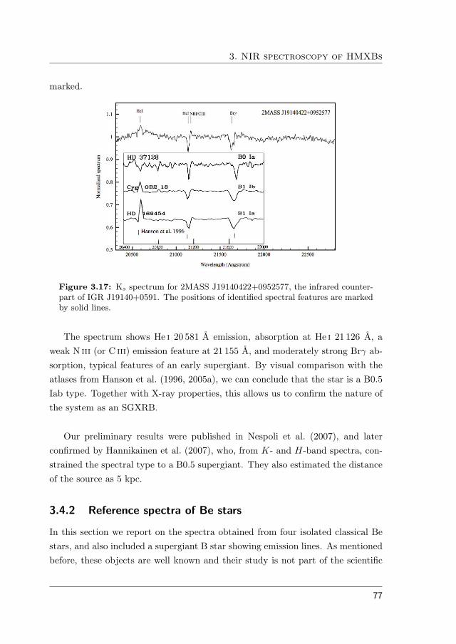
3. NIR spectroscopy of HMXBs
marked.
Figure 3.17: Ks spectrum for 2MASS J19140422+0952577, the infrared counter-part of IGR J19140+0591. The positions of identified spectral features are markedby solid lines.
The spectrum shows He i 20 581 A emission, absorption at He i 21 126 A, aweak N iii (or C iii) emission feature at 21 155 A, and moderately strong Brγ ab-sorption, typical features of an early supergiant. By visual comparison with theatlases from Hanson et al. (1996, 2005a), we can conclude that the star is a B0.5Iab type. Together with X-ray properties, this allows us to confirm the nature ofthe system as an SGXRB.
Our preliminary results were published in Nespoli et al. (2007), and laterconfirmed by Hannikainen et al. (2007), who, from K- and H-band spectra, con-strained the spectral type to a B0.5 supergiant. They also estimated the distanceof the source as 5 kpc.
3.4.2 Reference spectra of Be stars
In this section we report on the spectra obtained from four isolated classical Bestars, and also included a supergiant B star showing emission lines. As mentionedbefore, these objects are well known and their study is not part of the scientific
77

3.4. Results
objective of this project. They are almost all very bright objects, and data weretaken in bad transparency conditions, in order to have reference spectra for theclassification of the proposed IR counterparts to HMXBs in case a Be star wasfound. Fig. 3.18 illustrates the spectra and marks the identified spectral features.
20500 21000 21500 22000 22500
Wavelength (Angstrom)
0.5
1
1.5
2
2.5
No
rmal
ized
sp
ectr
um
+ o
ffse
t
BD-13 5550 - B1 Ibe
HD 28497 - B2 V:ne
HD 30076 - B2 Ve
HD 131168 - B3 Ve
HD 156468 - B1 Ve
HeI HeI Br!
Figure 3.18: Ks-band spectrum for four classical Be-stars (first four spectra fromthe bottom) and one supergiant B star showing emission lines (first spectrum fromthe top). The positions of identified spectral features are marked by solid lines.
We will now analyze the variation of the observed features on the basis of bothtemperature and luminosity.
The spectra show hydrogen and helium lines, typical features of OB types.The 21 660 Brγ line is in emission in the earliest both supergiant and Be stars(first 4 spectra from the top in Fig. 3.18).
For Be stars, the known general trend of stronger Brγ emission at earlierspectral types was explained with simulations of the infrared spectrum of ψ Per(Marlborough et al. 1997). It was shown that the strenght of Brγ is very sensitive
78

3. NIR spectroscopy of HMXBs
to both changes in disc temperature and density (and the radial gradients of theseparameters). For the near infrared hydrogen lines, a decrease in disc temperaturein general leads to a decrease in the line emission. Firstly, the source function ofthe line, taken to be the Planck function, decreases with temperature. Also, thetemperature dependent factors in the disc opacity term (Equation (5) in Marl-borough et al. 1997) cause the opacity to increase with decreasing temperaturefor the majority of the disc. Therefore both effects combine to reduce the lineemission from the disc as the temperature decreases. Since the disc temperatureis likely to be a function of stellar temperature, a reduction in line emission fromearly to late stars is expected.
In HD 131168 we observe instead Brγ in absorption: the object could havebeen misclassified and correspond to a B star, or alternatively, since the Be phe-nomenon is known to be variable it may simply mean that this object have un-dergone a phase change from emission to non-emission.
The He I triplet at 21 126 A is seen in the late-O and early-B stars. Theindividual features in this triplet are not detectable at our resolution, and the lineis apreciable just in the only early B supergiant (BD 135550). The main He Isinglet line at 20 581 A, which is a strong transition, is very weak or absent in themain-sequence (dwarf and giant) stars, while it becomes prominent in emissionor both in emission and in absorption in the supergiant stars and thus is animportant tracer of stars with extended atmospheres. The line is also known tovary with respect to the spectral type, being confined to stars earlier than B2.5.In fact the two requirements for this line to be produced in emission are a largeionizing flux and a dense circumstellar environment, characteristic of the earliesttypes.
3.4.3 Reddening and distance estimation
From the identified spectral types, we obtained the intrinsic colors (J −K)0 fromWegner (1994); we then calculated, from 2MASS photometry, the instrumentalcolors (J −K)2MASS , properly transformed through the formula from Carpenter
79
3.5. Discussion
(2001) 3 to the Bessell & Brett (1988) homogenized photometric system in orderto estimate the infrared color excess E(J − K). Assuming the mean extinctionlaw (RV = 3.1), from AV /E(J −K) = 5.82± 0.10 (Rieke & Lebofsky 1985), weobtained the total measured visual extinction AV and the corresponding hydrogencolumn density value from NH/AV = 1.79±0.03×10²¹ atoms cm−2 mag (Predehl& Schmitt 1995). We were thus able to compare the retrieved interstellar value ofNH with the one provided by X-ray data. In our calculation, we estimated errorsthrough error propagation. Errors in the final values of NH are mainly due toerrors in the infrared colors and the transformation between the two photometricsystems.
We also estimated the distance of the seven sources, applying the relationMK = K + 5 − 5 log d − AK . For each source, MV was obtained from ourproposed spectral type (Wegner 2006), the intrinsic color index (K − V )0 fromWegner (1994) was used in order to calculate MK , and the 2MASS K magnitudewas employed. We derived AK from the relation Aλ/E(J −K) = 2.4(λ)−1.75, forλ = 2.2 µm (Draine 1989).
The results of our calculations are given in Table 3.4, together with somecrucial quantities used in the calculations or displayed for comparison.
The distance estimation is mainly affected by the uncertainty in the value ofthe absolute magnitude MV , which is due to two contributions, the errors givenin the tabulated values of MV and the uncertainty in the spectral classification,from which the absolute magnitude is determined. The largest role is played bythe errors in the mean tabulated values themselves (see Wegner 2006 for moredetails). The retrieved values for d must thus be assumed with prudence.
3.5 Discussion
Using near-infrared spectroscopy of seven high-energy sources, IGR J16207–5129,IGR J16465–4507, IGR J16479–4514, IGR J16493–348, AX J1841.0–0536, 4U1907+097 and IGR J19140+0951, we classified their counterparts through com-parison with published atlases. We found that all the observed systems have a
3In its updated version at http://www.astro.caltech.edu/∼jmc/2mass/v3/transformations/
80

3. NIR spectroscopy of HMXBs
supergiant companion. Our results, combined with information from X-ray data,allow for the first time to firmly include one source, IGR J16479–4514, in thenewly discovered class of the SFXTs. Moreover, we can confirm with infrareddata the identification of IGR J16465–4507 and AX J1841.0–0536 as SFXTs, asrecently proposed by Negueruela et al. (2007) from optical spectra.
From our spectral classification, we estimated the distance of the seven sources.The retrieved values are consistent with the location of the sources in the Norma(IGR J16207–5129, IGR J16465–4507, IGR J16479–4514, IGR J16493–4348), Scu-tum (AX J1841.0–0536) and Sagittarius arm (4U 1907+097 and IGR J19140+0951)regions respectively. This determination, although affected by some uncertainty,can be considered an a posteriori confirmation of the proposed spectral classifi-cation.
This work allowed us to calculate the extinction from IR data for the sevensystems. Recently, it has been pointed out (see Kuulkers 2005; Chaty 2007) thatINTEGRAL is revealing two new classes of supergiant HMXBs, the highly ob-scured HMXBs and the SFXTs. The first ones are characterized by strong intrin-sic absorption, the second by strong and short X-ray outbursts. High, variable,hydrogen column densities have in some cases been measured for SFXTs (e.g.IGR J11215–5952: Smith et al. 2006a; IGR J17391–3021: Smith et al. 2006b),suggesting a possible intrinsic absorption for this class as well, and marking apotential overlap between the two new classes. The origin and position (aroundthe compact object only, or enveloping the entire system) of the absorbing ma-terial are still a matter of debate, and only multiwavelength studies are able toaddress the problem, distinguishing between the absorption in X-ray and in theIR/optical bands. We calculated the effective interstellar extinction AV and con-verted it into hydrogen column density NH . Our results can be compared withthe values obtained from X-ray data. If the two retrieved values are compatiblewithin the corresponding errors, we face two possible scenarios: either the sourceof absorption is just the interstellar medium or there is a contribution from anextensive envelope around the whole binary system, if the extinction shows anexcess of some orders of magnitude with respect to the estimated IS value. Con-versely, if the reddening (measured from the IR colors) is low for the measured
81
3.5. Discussion
NH from X-rays, this reveals the presence of an additional source of extinction,which only affects the compact object in which the X-ray emission originates, andthat can be regarded as the presence of absorbing material around it.
In our case, the comparison reveals that for four systems, IGR J16465–4507,IGR J16479–4514, AX J1841.0–0536 and IGR J19140+0951, the extinction mea-sured at high energy shows an excess of one or two orders of magnitude withrespect to that obtained from IR data, probing that the material absorbing theX-rays is concentrated around the neutron star. Our result is consistent with thedetection of the Fe fluorescence line at 6.4 KeV in the X-ray spectra of all the foursources (Walter et al. 2006; Bamba et al. 2001; Rodriguez et al. 2005), which isconsidered a signature of a dense spherical envelope around the compact object.
Usually, the so called highly absorbed IGR sources are identified from theirmeasured NH being � 1023 cm−2, i.e. one to two orders of magnitude higher thanthe assumed Galactic value of ∼ 1022 cm−2 (Kuulkers 2005). The comparison ofX-ray data, which are sensitive to the absorption from the environment of thecompact object, with infrared data, which are in general only absorbed by theinterstellar medium, can be a strong and alternative criterion to recognize thisclass of highly absorbed sources. In particular, all the three identified SFXTsshow strong intrinsic absorption from circumstellar material, reported as well forother members of this new class (e.g. Negueruela et al. 2006; Pellizza et al. 2006),and so emerging as a common feature of the group. This scenario is relevant todiscussions about the physical mechanism, still unknown, which powers the fastoutbursts that these sources undergo. Together with their X-ray fast transientnature, the high intrinsic absorption can be regarded as one of the reasons whythis class has remained undiscovered until only recently.
A more complete, multiwavelength investigation is necessary to reveal thenature of these systems, especially if it is able to find and physically describecorrelations between their X-ray behavior and IR properties. In the case of SFXTsthis is possibly the only way to explore the physical mechanism driving the fastoutbursts.
82
3. NIR spectroscopy of HMXBs
3.6 Conclusions
From near-infrared spectroscopy of the seven high-energy sources, we have foundthat:
- the proposed optical counterparts were confirmed and the spectral classifi-cation of the sources provided; all the sources were classified as HMXBs;
- one source, IGR J16479–4514, was added to the SFXTs and the confirmationof IGR J16465–4507 and AX J1841.0–0536 as members of the class wasproven with infrared data;
- the comparison between NH obtained from X-ray data and interstellar ex-tinction from our data showed for four systems (IGR J16465–4507, IGRJ16479–4514, AX J1841.0–0536 and IGR J19140+0951) the presence of anabsorbing envelope, strictly confined around the compact object;
- all the three identified SFXTs are intrinsically absorbed, suggesting thatthis might be a characteristic of the class;
- the distance estimation, compatible with the location of the sources in therespective galactic arms, is a possible confirmation of the spectral classifi-cation provided here.
Results from this study were partly published in Nespoli et al. (2008b).
83
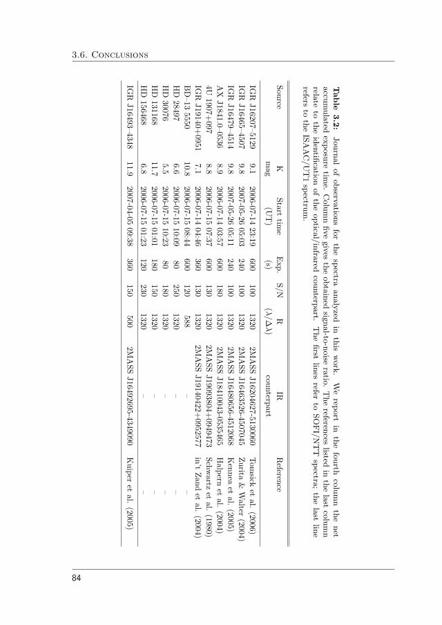
3.6. Conclusions
Table
3.2
:Jou
rnal
ofob
servations
forth
esp
ectraan
alyzed
inth
isw
ork.
We
report
inth
efou
rthcolu
mn
the
net
accum
ulated
exposu
retim
e.C
olum
nfive
givesth
eob
tained
signal-to-n
oiseratio.
The
references
listedin
the
lastcolu
mn
relateto
the
iden
tification
ofth
eop
tical/infrared
counterp
art.T
he
first
lines
referto
SO
FI/N
TT
spectra;
the
lastlin
erefers
toth
eIS
AA
C/U
T1
spectru
m.
SourceK
Starttim
eE
xp.S/N
RIR
Reference
mag
(UT
)(s)
(λ/∆
λ)counterpart
IGR
J16207–51299.1
2006-07-1423:19
600100
13202M
ASS
J16204627-5130060Tom
sicket
al.(2006)
IGR
J16465–45079.8
2007-05-2605:03
240100
13202M
ASS
J16463526-4507045Zurita
&W
alter(2004)
IGR
J16479–45149.8
2007-05-2605:11
240100
13202M
ASS
J16480656-4512068K
enneaet
al.(2005)
AX
J1841.0–05368.9
2006-07-1403:57
600180
13202M
ASS
J18410043-0535465H
alpernet
al.(2004)
4U1907+
0978.8
2006-07-1507:37
600130
13202M
ASS
J19093804+0949473
Schwartz
etal.
(1980)IG
RJ19140+
09517.1
2006-07-1404:46
360130
13202M
ASS
J19140422+0952577
in’tZand
etal.
(2004)B
D–13
555010.8
2006-07-1508:44
600120
588–
–H
D28497
6.62006-07-15
10:0980
2501320
––
HD
300765.5
2006-07-1510:23
80180
1320–
–H
D131168
11.72006-07-15
01:01180
1501320
––
HD
1564686.8
2006-07-1501:23
120230
1320–
–
IGR
J16493–434811.9
2007-04-0509:38
360150
5002M
ASS
J16492695-4349090K
uiperet
al.(2005)
84
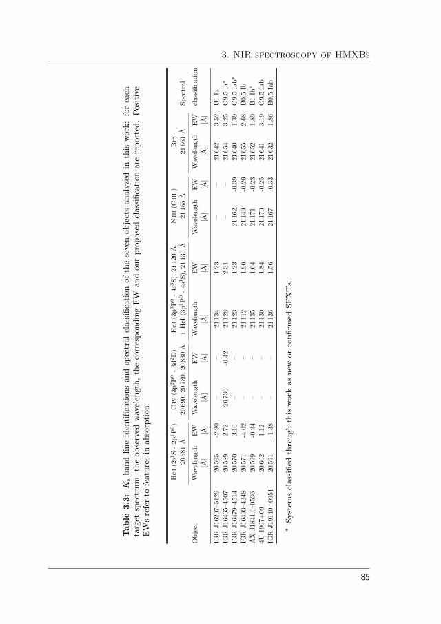
3. NIR spectroscopy of HMXBs
Table
3.3
:K
s-b
and
line
iden
tifica
tion
san
dsp
ectr
alcl
assi
fica
tion
ofth
ese
ven
obje
cts
anal
yze
din
this
wor
k:
for
each
targ
etsp
ectr
um
,th
eob
serv
edw
avel
engt
h,
the
corr
espon
din
gE
Wan
dou
rpro
pos
edcl
assi
fica
tion
are
repor
ted.
Pos
itiv
eE
Ws
refe
rto
feat
ure
sin
abso
rption
.
Hei
(2s1
S-
2p1P
0)
Civ
(3p2
P0
-3d
2D
)H
ei(3
p3P
0-
4s3S)
,21
120
AN
iii(C
iii)
Brγ
2058
1A
2069
0,20
780,
2083
0A
+H
eI(3
p1P
0-
4s1S)
,21
130
A21
155
A21
661
ASp
ectr
al
Obj
ect
Wav
elen
gth
EW
Wav
elen
gth
EW
Wav
elen
gth
EW
Wav
elen
gth
EW
Wav
elen
gth
EW
clas
sific
atio
n[A
][A
][A
][A
][A
][A
][A
][A
][A
][A
]
IGR
J162
07–5
129
2059
5-2
.90
––
2113
41.
23–
–21
642
3.52
B1
IaIG
RJ1
6465
–450
720
589
2.72
2073
0-0
.42
2112
82.
31–
–21
654
3.25
O9.
5Ia∗
IGR
J164
79–4
514
2057
03.
10–
–21
123
1.23
2116
2-0
.39
2164
01.
39O
9.5
Iab∗
IGR
J164
93–4
348
2057
1-4
.02
––
2111
21.
9021
149
-0.2
021
655
2.68
B0.
5Ib
AX
J184
1.0–
0536
2059
9-0
.94
––
2113
51.
6421
171
-0.2
321
652
1.89
B1
Ib∗
4U19
07+
0920
602
1.12
––
2113
01.
8421
170
-0.2
521
641
3.19
O9.
5Ia
bIG
RJ1
9140
+09
5120
591
-1.3
8–
–21
136
1.56
2116
7-0
.33
2163
21.
86B
0.5
Iab
∗Syst
ems
clas
sified
thro
ugh
this
wor
kas
new
orco
nfirm
edSFX
Ts.
85

3.6. Conclusions
Table
3.4
:Sum
mary
ofth
esp
ectralan
alysis
and
extin
ctioncalcu
lations
forth
eseven
objects
studied
inth
isw
ork.
For
eachob
servedsou
rcein
the
first
colum
n,th
eob
tained
spectral
classification
,in
trinsic
infrared
colors,2M
ASS
photom
etry,calcu
latedin
fraredex
cess,hydrogen
colum
nden
sityob
tained
fromX
-raypublish
edm
easurem
ents,
effective
interstellar
colum
nden
sityob
tained
fromou
rw
orkan
ddistan
ceestim
ationare
reported
.See
text
forcorresp
ondin
greferen
ces.
SourceSpectraltype
(J−
K)0
(J−
K)2M
AS
SE
(J−
K)
NH
fromX
-raydata
InterstellarN
HD
istance[m
ag][m
ag][m
ag][10
22
cm−
2][10
22
cm−
2][kpc]
IGR
J16207–5129B
1Ia
-0.121.31
1.433.7
+1.4
−1.2
1.53
±1.02
6.1(-3
.5,+
8.9
)
IGR
J16465–4507O
9.5Ia
-0.150.69
0.8472±
60.87
±0.56
9.5(-5
.7,+
14.1
)
IGR
J16479–4514O
9.5Iab
-0.143.19
3.3312±
43.47
±2.16
2.8(-1
.7,+
4.9
)
IGR
J16493–4348B
0.5Ib
-0.122.66
2.815.4
2.92
±1.96
15.3(-9
.0,+
11.0
)
AX
J1841.0–0536B
1Ib
-0.130.80
0.933.2
0.97
±0.64
3.2(-1
.5,+
2.0
)
4U1907+
097O
9.5Iab
-0.141.22
1.361.7
–5.7
1.42
±0.90
3.0(-1
.9,+
5.1
)
IGR
J19140+0951
B0.5
Iab-0.12
1.501.62
∼6
a1.68
±1.5
1.1(-0
.8,+
2.3
)
aA
maxim
umvalue
of10.1±
0.2×
1022
cm−
2w
asreported
byR
odriguezet
al.2005.
86
There’s real poetry in the real
world. Science is the poetry of
reality.
Richard Dawkins 4K-band spectroscopy of two INTEGRAL
sources reveals two new SyXBs
4.1 Symbiotic X-ray binaries
Low-mass X-ray Binaries (LMXBs) are interacting systems constituted by an ac-creting compact object and a low-mass (typically ≤ 1 M⊙) main-sequence orslightly evolved late-type star. Recently, a new sub-class of LMXBs is emerg-ing, in which the secondary is an M-type giant. This rare class of systems wasnamed Symbiotic X-ray Binaries (SyXBs) after Masetti et al. (2006b) by analogywith symbiotic binaries, in which a white dwarf accretes matter from an M giantcompanion, either from the wind of the M star or via Roche-lobe overflow. Atpresent, only six X-ray sources are known to belong to this subclass: GX 1+4(Davidsen et al. 1977; Chakrabarty & Roche 1997), 4U 1700+24 (Garcıa et al.1983; Masetti et al. 2002), 4U 1954+319 (Masetti et al. 2006b; Mattana et al.2006), Scutum X-1 (Kaplan et al. 2007), IGR J16194-2810 (Masetti et al. 2007)and 1RXS J180431.1-273932 (Nucita et al. 2007). See Masetti et al. (2007), Ta-ble 3, for a summary of the main properties of the first 5 SyXBs; see Nucita et al.(2007) for the last discovered one.
The increasing number of systems with an evolved giant donor makes this sub-class an emerging evolutionary channel of X-ray Binaries. Moreover, they have
87
4.2. IGR J16358-4726 and IGR J16393-4643
been proposed as the probable progenitors of most wide-orbit LMXBs (Chakrabarty& Roche 1997).
4.2 IGR J16358-4726 and IGR J16393-4643
During our campaign of spectroscopic observations of IR counterparts to HMXBs(see Chapter 3), we took data of IGR J16358-4726 and IGR J16393-4643, twosupposed HMXBs.
IGR J16358-4726 was discovered by Revnivtsev et al. (2003), then serendipi-tously observed by Chandra that located the source at RA = 16h35m53.8s, DEC= -47◦25�41.1��, with an accuracy of 0.6�� (Kouveliotou et al. 2003). This allowedthem to suggest an infrared counterpart, 2MASS J16355369-4725398. Subsequentastrometry performed by Chaty et al. (2008), although stating that the 2MASSobject is 1.2�� from the Chandra detection, resulted in substantiating it as theactual counterpart, mainly because of its brightness (J = 15.41 mag, H = 13.44mag, K = 12.59 mag).
The X-ray source was identified as a transient, and its spectrum fitted with apower law with spectral index Γ ∼ 0.5, hydrogen column density NH ∼ 3.3×10²³
cm−2 and a FeKα fluorescence line at 6.4 keV (Patel et al. 2007). Periodic varia-tions of 5880 ± 50 s were found by Patel et al. (2004), then confirmed by severalauthors (Lutovinov et al. 2005; Mereghetti et al. 2006). From accurate spectraland timing analysis of multi-satellite data, Patel et al. (2007) argued the neutronstar nature of the source, estimating the magnetic field between 1013 and 1015
G if the retrieved spin up was due to disk accretion, and thus proposed that theobject might be a magnetar. The source is thought to be located in the NormaGalactic arm, at a distance of 5–6 kpc or 12–13 kpc, depending on which crossingof the arm with the line of sight is chosen (Lutovinov et al. 2005). From NIRspectroscopy, Chaty et al. (2008) suggested that the system is a HMXB, showingthat the counterpart might be a sgB[e] star since the detection of H Brackettseries, He I and He II absorption lines and the presence of a forbidden [FeII] lineat 2.22 µm. This result was then corroborated by Rahoui et al. (2008) throughSED fitting.
88

4. Two new SyXBs
IGR J16393-4643 was first discovered by the ASCA satellite (Sugizaki et al.2001) and listed as AX J16390.4-4642. It was later detected by INTEGRALduring the first Galactic Plane Scan (Malizia et al. 2004).
Subsequent observations with XMM-Newton/EPIC derived an improved posi-tion (RA = 16h39m05.4s, DEC = −46◦42�12��) that allowed Bodaghee et al. (2006)to identify 2MASS J16390535-4642137 as the most probable counterpart to thesource. The X-ray spectrum was fitted with a highly absorbed (NH = 2.5× 10²³
cm−2) power law (Γ = 0.8± 0.2); together with the discovery of a pulse period of912.0 ± 0.1 s, this led to conclude that the source is an X-ray pulsar (Bodagheeet al. 2006). Thompson et al. (2006, hereafter T06) used RXTE data to carry outpulse timing analysis in order to determine the orbital parameters of the system.They obtained three mathematical solutions, among which the most plausible oneindicated, with an orbital period of 3.7 days and a mass function of 6.5 ±1 M⊙,that the system would be a HMXB. The other two solutions foresaw the followingparameters: an orbital period of 50.2 days together with a mass function of 0.092M⊙ and an orbital period of 8.1 days with a mass function of 221 M⊙; both ofthem were rejected by the authors because they are statistically and physicallyweaker. Chaty et al. (2008) obtained accurate astrometry and photometry of thefield of IGR J16393-4643, finding three more candidate counterparts, althoughtheir lower NIR brightness seemed to favor the 2MASS object. They also per-formed SED fitting of optical to MIR observation, inferring a BIV-V spectral typefor the companion.
In this chapter we present K-band spectroscopy of the proposed counterpartsto the two X-ray systems. In the case of IGR J16393-4643, ours is the first avail-able IR spectrum; in the case of IGR J16358-4726, ours is the first IR spectrumbeyond 2.3 µm, covering a range that is crucial, as our analysis will show, for thespectral classification of the star. We will show the need for a new classificationof the counterparts, which implies a new classification of the systems as SyXBs,if the proposed counterparts are the actual ones.
89

4.3. Observations and data reduction
4.3 Observations and data reduction
The two proposed counterparts to the X-ray sources were observed in service modeon 2007 April 5 with the ISAAC spectrograph (Moorwood et al. 1998b) on UT1at ESO/Paranal observatory. The optical layout of ISAAC is shown in Fig. 4.1.At the top and bottom are two cameras which are optimized for the 1–2.5 µmand 2–5 µm ranges and used to either re-image the telescope focal plane or theintermediate spectrum produced by the grating spectrometer. Data were taken inthe Short Wavelength - Low Resolution mode, with a pixel scale of 0.147��/pixeland a resolution of 500.
Figure 4.1: ISAAC optical layout.
The sky was clear during the observations, the seeing was ≤ 1.4�� and the
90
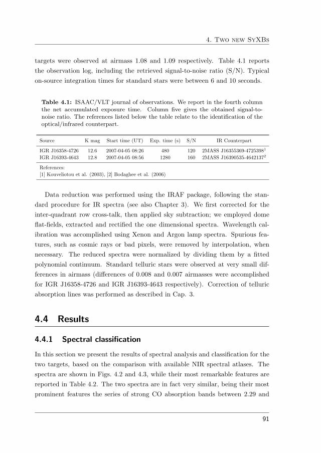
4. Two new SyXBs
targets were observed at airmass 1.08 and 1.09 respectively. Table 4.1 reportsthe observation log, including the retrieved signal-to-noise ratio (S/N). Typicalon-source integration times for standard stars were between 6 and 10 seconds.
Table 4.1: ISAAC/VLT journal of observations. We report in the fourth columnthe net accumulated exposure time. Column five gives the obtained signal-to-noise ratio. The references listed below the table relate to the identification of theoptical/infrared counterpart.
Source K mag Start time (UT) Exp. time (s) S/N IR Counterpart
IGR J16358-4726 12.6 2007-04-05 08:26 480 120 2MASS J16355369-47253981
IGR J16393-4643 12.8 2007-04-05 08:56 1280 160 2MASS J16390535-46421372
References:[1] Kouveliotou et al. (2003), [2] Bodaghee et al. (2006)
Data reduction was performed using the IRAF package, following the stan-dard procedure for IR spectra (see also Chapter 3). We first corrected for theinter-quadrant row cross-talk, then applied sky subtraction; we employed domeflat-fields, extracted and rectified the one dimensional spectra. Wavelength cal-ibration was accomplished using Xenon and Argon lamp spectra. Spurious fea-tures, such as cosmic rays or bad pixels, were removed by interpolation, whennecessary. The reduced spectra were normalized by dividing them by a fittedpolynomial continuum. Standard telluric stars were observed at very small dif-ferences in airmass (differences of 0.008 and 0.007 airmasses were accomplishedfor IGR J16358-4726 and IGR J16393-4643 respectively). Correction of telluricabsorption lines was performed as described in Cap. 3.
4.4 Results
4.4.1 Spectral classification
In this section we present the results of spectral analysis and classification for thetwo targets, based on the comparison with available NIR spectral atlases. Thespectra are shown in Figs. 4.2 and 4.3, while their most remarkable features arereported in Table 4.2. The two spectra are in fact very similar, being their mostprominent features the series of strong CO absorption bands between 2.29 and
91

4.4. Results
2.40 µm, which are characteristic of late-type stars.
!"### !!### !$### !%###
&'()*)+,-./01+,2-3456
#78
#79
#7:
#7;
"
"7"
<*=>/0'3?@-3'3A/=+@-26
!"#$
%&#$
%&#$ '"#$
()#$
*+',
*-',
$./#0*1-23456+17+(899#0*1-22-1:456+2-:3;
<&#$#=
>?!
()#$
Figure 4.2: K-band spectrum of 2MASS J16355369-4725398, the infrared counter-part to IGR J16358-4726. The positions of identified spectral features are markedby solid lines.
!"### !!### !$### !%###
&'()*)+,-./01+,2-3456
#78
#79
#7:
#7;
"
"7"
<*=>/0'3?@-3'3A/=+@-26
!"#$
%&#$
%&#$ '"#$
()#$
*+',
*-',
./)
$01#2*3-4-5636-7+(899#2*3-4:;-;5636+*-<=
()#$ 8>#$
Figure 4.3: K-band spectrum of 2MASS J16390535-4642137, the infrared counter-part to IGR J16393-4643. The positions of identified spectral features are markedby solid lines.
Several metallic lines are clearly recognizable as well, although at our reso-lution they are generally blended. Although weaker than the CO bands, theyappear significative within the retrieved errors. We also tentatively propose the
92
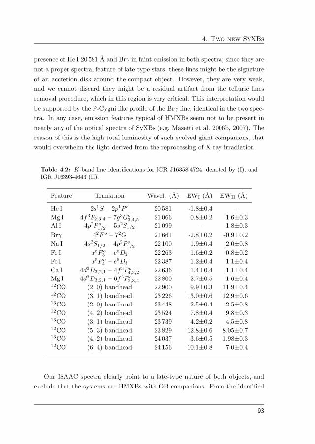
4. Two new SyXBs
presence of He I 20 581 A and Brγ in faint emission in both spectra; since they arenot a proper spectral feature of late-type stars, these lines might be the signatureof an accretion disk around the compact object. However, they are very weak,and we cannot discard they might be a residual artifact from the telluric linesremoval procedure, which in this region is very critical. This interpretation wouldbe supported by the P-Cygni like profile of the Brγ line, identical in the two spec-tra. In any case, emission features typical of HMXBs seem not to be present innearly any of the optical spectra of SyXBs (e.g. Masetti et al. 2006b, 2007). Thereason of this is the high total luminosity of such evolved giant companions, thatwould overwhelm the light derived from the reprocessing of X-ray irradiation.
Table 4.2: K-band line identifications for IGR J16358-4724, denoted by (I), andIGR J16393-4643 (II).
Feature Transition Wavel. (A) EWI (A) EWII (A)
He I 2s1S – 2p
1P
o 20 581 -1.8±0.4 –Mg I 4f
3F2,3,4 – 7g
3G
o
3,4,5 21 066 0.8±0.2 1.6±0.3Al I 4p
2P
o
1/2 – 5s2S1/2 21 099 – 1.8±0.3
Brγ 42F
o – 72G 21 661 -2.8±0.2 -0.9±0.2
Na I 4s2S1/2 – 4p
2P
o
1/2 22 100 1.9±0.4 2.0±0.8Fe I x
5F
o
3 – e5D2 22 263 1.6±0.2 0.8±0.2
Fe I x5F
o
4 – e5D3 22 387 1.2±0.4 1.1±0.4
Ca I 4d3D3,2,1 – 4f
3F
o
4,3,2 22 636 1.4±0.4 1.1±0.4Mg I 4d
3D3,2,1 – 6f
3F
o
2,3,4 22 800 2.7±0.5 1.6±0.412CO (2, 0) bandhead 22 900 9.9±0.3 11.9±0.412CO (3, 1) bandhead 23 226 13.0±0.6 12.9±0.613CO (2, 0) bandhead 23 448 2.5±0.4 2.5±0.812CO (4, 2) bandhead 23 524 7.8±0.4 9.8±0.313CO (3, 1) bandhead 23 739 4.2±0.2 4.5±0.812CO (5, 3) bandhead 23 829 12.8±0.6 8.05±0.713CO (4, 2) bandhead 24 037 3.6±0.5 1.98±0.312CO (6, 4) bandhead 24 156 10.1±0.8 7.0±0.4
Our ISAAC spectra clearly point to a late-type nature of both objects, andexclude that the systems are HMXBs with OB companions. From the identified
93
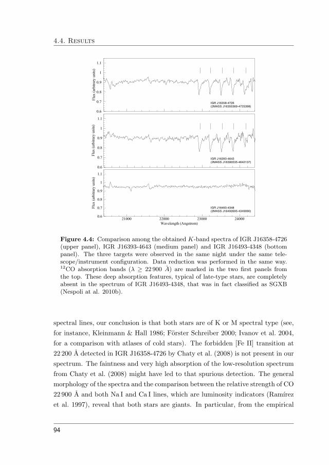
4.4. Results
!"#
!"$
!"%
!"&
'
'"'
()*+,-./012/./3,*41256
!"#$%&'()*+,-.'/.0122$%&'())('3+,-.)(3*4
!"#
!"$
!"%
!"&
'
'"'
()*+,-./012/./3,*41256
!"#$%&'(3(+,',(/.0122$%&'(35)()+,',.&(-4
7'!!! 77!!! 78!!! 79!!!
:.;<)<4=2>,-?4=52/@A6
!"#
!"$
!"%
!"&
'
'"'
()*+,-./012/./3,*41256
!"#$%&',3(+,(,*/.0122$%&',3.'3)+,(,35354
Figure 4.4: Comparison among the obtained K-band spectra of IGR J16358-4726(upper panel), IGR J16393-4643 (medium panel) and IGR J16493-4348 (bottompanel). The three targets were observed in the same night under the same tele-scope/instrument configuration. Data reduction was performed in the same way.12CO absorption bands (λ ≥ 22 900 A) are marked in the two first panels fromthe top. These deep absorption features, typical of late-type stars, are completelyabsent in the spectrum of IGR J16493-4348, that was in fact classified as SGXB(Nespoli at al. 2010b).
spectral lines, our conclusion is that both stars are of K or M spectral type (see,for instance, Kleinmann & Hall 1986; Forster Schreiber 2000; Ivanov et al. 2004,for a comparison with atlases of cold stars). The forbidden [Fe II] transition at22 200 A detected in IGR J16358-4726 by Chaty et al. (2008) is not present in ourspectrum. The faintness and very high absorption of the low-resolution spectrumfrom Chaty et al. (2008) might have led to that spurious detection. The generalmorphology of the spectra and the comparison between the relative strength of CO22 900 A and both Na I and Ca I lines, which are luminosity indicators (Ramırezet al. 1997), reveal that both stars are giants. In particular, from the empirical
94
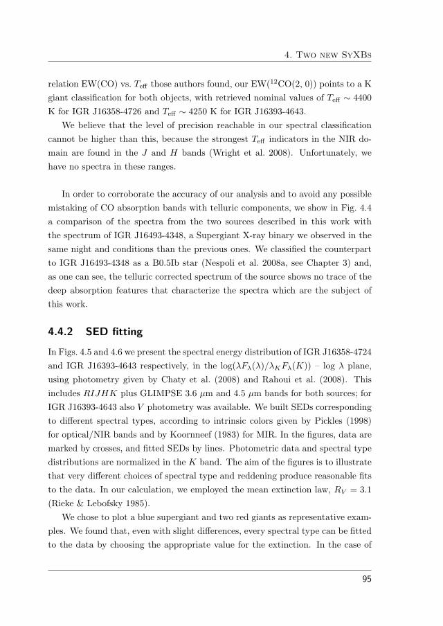
4. Two new SyXBs
relation EW(CO) vs. Teff those authors found, our EW(12CO(2, 0)) points to a Kgiant classification for both objects, with retrieved nominal values of Teff ∼ 4400K for IGR J16358-4726 and Teff ∼ 4250 K for IGR J16393-4643.
We believe that the level of precision reachable in our spectral classificationcannot be higher than this, because the strongest Teff indicators in the NIR do-main are found in the J and H bands (Wright et al. 2008). Unfortunately, wehave no spectra in these ranges.
In order to corroborate the accuracy of our analysis and to avoid any possiblemistaking of CO absorption bands with telluric components, we show in Fig. 4.4a comparison of the spectra from the two sources described in this work withthe spectrum of IGR J16493-4348, a Supergiant X-ray binary we observed in thesame night and conditions than the previous ones. We classified the counterpartto IGR J16493-4348 as a B0.5Ib star (Nespoli et al. 2008a, see Chapter 3) and,as one can see, the telluric corrected spectrum of the source shows no trace of thedeep absorption features that characterize the spectra which are the subject ofthis work.
4.4.2 SED fitting
In Figs. 4.5 and 4.6 we present the spectral energy distribution of IGR J16358-4724and IGR J16393-4643 respectively, in the log(λFλ(λ)/λKFλ(K)) – log λ plane,using photometry given by Chaty et al. (2008) and Rahoui et al. (2008). Thisincludes RIJHK plus GLIMPSE 3.6 µm and 4.5 µm bands for both sources; forIGR J16393-4643 also V photometry was available. We built SEDs correspondingto different spectral types, according to intrinsic colors given by Pickles (1998)for optical/NIR bands and by Koornneef (1983) for MIR. In the figures, data aremarked by crosses, and fitted SEDs by lines. Photometric data and spectral typedistributions are normalized in the K band. The aim of the figures is to illustratethat very different choices of spectral type and reddening produce reasonable fitsto the data. In our calculation, we employed the mean extinction law, RV = 3.1(Rieke & Lebofsky 1985).
We chose to plot a blue supergiant and two red giants as representative exam-ples. We found that, even with slight differences, every spectral type can be fittedto the data by choosing the appropriate value for the extinction. In the case of
95
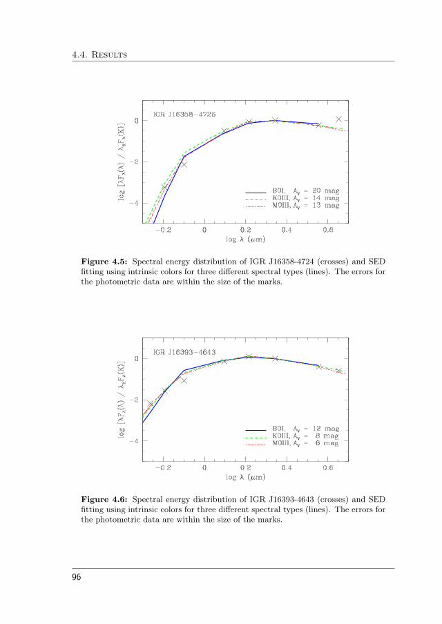
4.4. Results
Figure 4.5: Spectral energy distribution of IGR J16358-4724 (crosses) and SEDfitting using intrinsic colors for three different spectral types (lines). The errors forthe photometric data are within the size of the marks.
Figure 4.6: Spectral energy distribution of IGR J16393-4643 (crosses) and SEDfitting using intrinsic colors for three different spectral types (lines). The errors forthe photometric data are within the size of the marks.
96

4. Two new SyXBs
IGR J16358-4726, we obtained best fits choosing AV = 20 mag for a B0I type,AV = 14 mag for a K0III type and AV = 13 mag for a M0III type. Analogousresults were obtained for IGR J16393-4643, with AV = 12 for a B0I, AV = 8 fora K0III and AV = 6 for a M0III.
The reason why very different spectral types are able to reasonably fit the datamust be found in the degeneracy between the direction of the reddening vectorand the effective temperature variation in the spectral range we employed, whichmakes almost every spectral type possible if the opportune extinction value ischosen. Consequently, the results provided by SED fitting do not allow the im-provement of the spectral classification. They provide a valuable tool, however,to calculate the interstellar extinction for any assumed spectral type.
In the case of IGR J16393-4643, the low values retrieved for the extinction arein contrast with the high hydrogen column density measured in the X-ray range,namely NH = 2.5× 1023 cm−2. This could be an indication that the star is notthe actual counterpart to the system; another explanation could be the presenceof an additional source of extinction intrinsic to the system, which only affectsthe compact object where the X-ray emission originates. Huge absorption, withNH ∼ 1023 cm−2, has been observed in other SyXBs, (see, for instance, Mattanaet al. 2006).
For the aforementioned spectral types and corresponding extinction value, wecalculated the distance from the relation MK = K + 5 − 5 log d − AK . In eachcase, absolute magnitudes and intrinsic color indexes were obtained from Pickles(1998). The estimated distance values were, for IGR J16358-4726: 36.6 kpc (ifB0I), 1.4 kpc (if K0III) and 20.1 kpc (if M0III); for IGR J16393-4643: 24.1 kpc(if B0I), 1.0 kpc (if K0III), 13.9 kpc (if M0III). For both sources, a type B0Icounterpart would thus result in an unrealistically large value of the distance; thesame occurs, for IGR J16358-4726 only, in the case of a M0III companion.
The remaining estimates are compatible with both the classical (four arms,Vallee 2008) and the recently proposed (two main arms, Churchwell et al. 2009)spiral structure models of our Galaxy. A K0I companion would locate both sourcesin the Sagittarius/Carina inner arm according with the classical model, or the
97

4.5. Discussion
Sagittarius minor arm, according to the recently proposed one. Finally, a M0IIIcompanion for IGR J16393-4643 would imply that the source is placed in thetangential region of the Norma arm with both models.
The error estimation on the distance is mainly affected by the error on themean absolute magnitude assigned to the spectral type, which can be very large,and can reach more than 50% when propagated to the distance calculation. More-over, since the retrieved extinction value for each type would also apply to a widerange of subtypes, the consequent distance value range would largely extend. Re-trieved distance estimates are thus to be taken with prudence.
4.5 Discussion
From the spectral classification of the proposed counterparts as cold giants orsupergiants and from the X-ray features of the systems illustrated in Sect. 4.2, wepropose that both of them belong to the class of SyXBs, in which the companionto the neutron star is an evolved late-type star. In the discussion that follows weuse the terms giant and supergiant in its physical sense, i.e., related to the mass,internal structure and evolutionary status of the star and not to the luminosityclass. As discussed above, a precise determination of the spectral type and lumi-nosity class is difficult from our K-band spectra.
A red giant is the late evolutionary stage of either a low mass star (0.8 to2.3 M⊙) or an intermediate-mass star (2.3 to 10 M⊙). The red giant phaseincludes the shell hydrogen-burning phase (first giant branch), the core helium-burning phase (horizontal branch or “red clump” for low-mass stars, “blue loop”for intermediate-mass stars), and the shell helium-burning phase (asymptotic gi-ant branch). See, for instance, Iben (1974) and Iben & Renzini (1983). Redsupergiants are short-lived stages in the late evolution of moderately massivestars (10 to 25 M⊙, e.g. Massey et al. 2009; Figer et al. 2006)
In the case of IGR J16358-4724, we classified the proposed counterpart as aK-M giant/supergiant. The evidence that the system houses a neutron star is
98

4. Two new SyXBs
strongly supported by the detection of X-ray pulsations (Patel et al. 2004) to-gether with the description of the X-ray energy spectrum by an absorbed powerlaw model plus a high energy cut-off and an Fe line (Patel et al. 2007), whichare typical features of neutron stars in galactic X-ray binaries. The designationof 2MASS J16355369-4725398 as counterpart was as well doubly validated in theliterature (see Kouveliotou et al. 2003; Chaty et al. 2008). Previous NIR spec-troscopy from Chaty et al. (2008) led to a proposal of classification as sgB[e],but, as the authors warned, their NIR spectrum was very faint and extremelyabsorbed. Moreover, ending at 2.3 µm, it missed the last and most significantportion of the K band, where the presence of CO bands clearly reveals the K-Mspectral type of the star. We propose that these factors could lead to a misclas-sification of the system.
In the case of IGR J16393-4643, our spectrum reveals a K-M giant/supergiantas well. The presence of a pulsar in the binary system is validated both by thespectral shape of the X-ray emission (Bodaghee et al. 2006) and by the finding ofpulsations (T06). The optical counterpart we considered is, because of its magni-tude, the most probable one among the four objects falling in the error circle ofthe X-ray detection.
According to T06, IGR J16393-4643 has an orbital period of 3.7 days and amass function of 6.5 M⊙ (orbital solution 1 in T06). It seems unlikely that anintermediate-mass red giant can fit in such a narrow orbit. To check this, we willuse the physical parameters of a 7 M⊙ star along its evolutionary track given bySchaller et al. (1992).
The size of the Roche lobe of a star in a binary system is usually characterizedby the Roche lobe radius RL, defined as the radius of a sphere which has thesame volume as the Roche lobe. To calculate the Roche lobe radius, we used theEggleton (1983) approximation:
RL
a=
0.49 q2/3
0.6 q2/3 + ln (1 + q1/3), (4.1)
where a is the semimajor axis and q is the mass ratio of the binary components
99
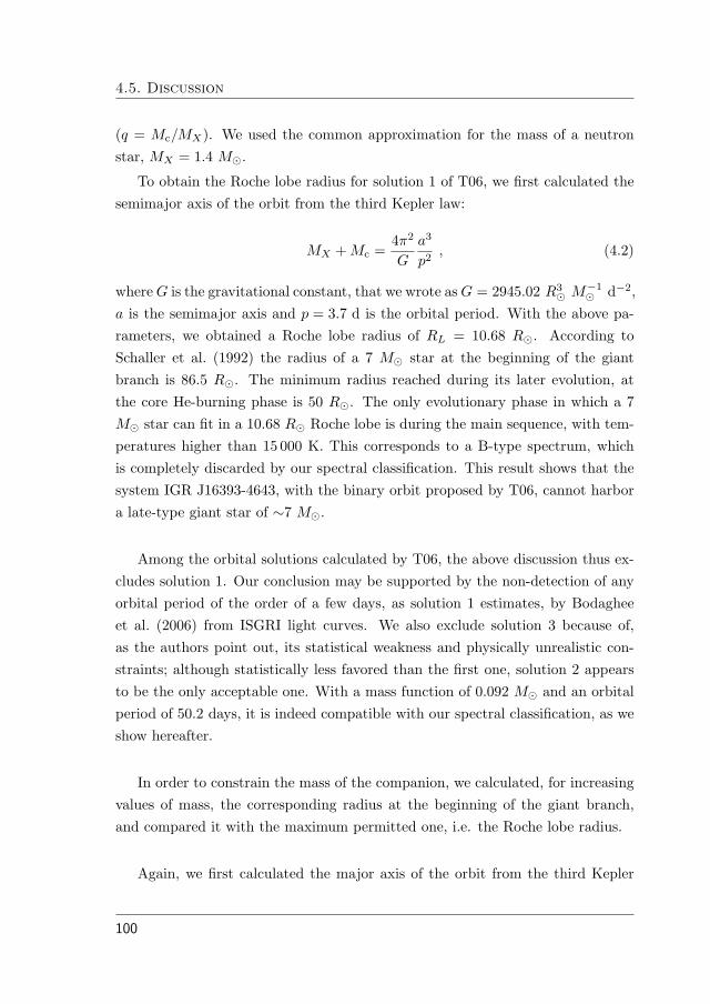
4.5. Discussion
(q = Mc/MX). We used the common approximation for the mass of a neutronstar, MX = 1.4 M⊙.
To obtain the Roche lobe radius for solution 1 of T06, we first calculated thesemimajor axis of the orbit from the third Kepler law:
MX + Mc =4π2
G
a3
p2, (4.2)
where G is the gravitational constant, that we wrote as G = 2945.02 R3⊙ M
−1⊙ d−2,
a is the semimajor axis and p = 3.7 d is the orbital period. With the above pa-rameters, we obtained a Roche lobe radius of RL = 10.68 R⊙. According toSchaller et al. (1992) the radius of a 7 M⊙ star at the beginning of the giantbranch is 86.5 R⊙. The minimum radius reached during its later evolution, atthe core He-burning phase is 50 R⊙. The only evolutionary phase in which a 7M⊙ star can fit in a 10.68 R⊙ Roche lobe is during the main sequence, with tem-peratures higher than 15 000 K. This corresponds to a B-type spectrum, whichis completely discarded by our spectral classification. This result shows that thesystem IGR J16393-4643, with the binary orbit proposed by T06, cannot harbora late-type giant star of ∼7 M⊙.
Among the orbital solutions calculated by T06, the above discussion thus ex-cludes solution 1. Our conclusion may be supported by the non-detection of anyorbital period of the order of a few days, as solution 1 estimates, by Bodagheeet al. (2006) from ISGRI light curves. We also exclude solution 3 because of,as the authors point out, its statistical weakness and physically unrealistic con-straints; although statistically less favored than the first one, solution 2 appearsto be the only acceptable one. With a mass function of 0.092 M⊙ and an orbitalperiod of 50.2 days, it is indeed compatible with our spectral classification, as weshow hereafter.
In order to constrain the mass of the companion, we calculated, for increasingvalues of mass, the corresponding radius at the beginning of the giant branch,and compared it with the maximum permitted one, i.e. the Roche lobe radius.
Again, we first calculated the major axis of the orbit from the third Kepler
100

4. Two new SyXBs
Table 4.3: Results from the analysis of the orbital parameters of IGR J16393-4643for different values of mass of the companion star Mc. Tabulated values for Teff
and L are taken from Schaller et al. 1992, for a star at the beginning of the giantbranch. For each case, the last column shows the corresponding spectral type. Upto Mc = 5 M⊙, a red giant is able to fit in the orbit foreseen by solution 2 of T06.Results for Mc = 5M⊙ are shown for completeness.
Mc a RL log Teff log(L/L⊙) Rc i Sp. t.(M⊙) (R⊙) (R⊙) (R⊙) (◦)
1 76.5 26.8 3.72 0.33 1.75 54.0 G5 III2 85.9 35.2 3.71 1.23 5.19 30.7 G5 III3 93.6 41.7 3.70 1.95 12.46 23.8 G8 III4 100.3 47.3 3.68 2.46 24.35 20.3 K0 III5 106.1 52.1 3.67 2.85 40.93 18.1 K1 III
7 116.2 60.5 3.64 3.39 86.5 15.4 K3 III
law (4.2), using p = 50.2 d from solution 2 as the orbital period. Taking thecommon approximation MX = 1.4 M⊙, we solved equation 4.2 with respect toa for different values of Mc, and employed the retrieved value in equation 4.1to obtain the corresponding Roche lobe radius. We then considered a red giantat the beginning of the giant branch, took tabulated values of Teff and L fromSchaller et al. (1992), and solved the black-body equation, L = 4πR
2σT4eff , to
obtain the stellar radius. For each value of mass, starting with Mc = 1 M⊙, wecompared the retrieved radius with the Roche lobe radius of the system. Resultsfrom this analysis are reported in Table 4.3, where we also show, for each case,the corresponding spectral type, obtained from temperature and luminosity, andthe inclination i of the system as calculated from the mass function of solution 2.
We stress that the parameters Rc and i in Table 4.3 correspond to the begin-ning of the first giant branch ascent. In consequence, they only represent a lowerlimit to the radius and upper limit to the inclination angle for stars of the givenmass.
Up to Mc = 5 M⊙, a red giant is able to fit in the orbit foreseen by solution
101

4.5. Discussion
2 of T06, while for higher values the stellar radius would exceed the Roche loberadius of the system. We thus set an upper limit of 5 M⊙ to the mass of thecompanion star. This mass limit excludes the possibility that the companion isa supergiant since the lower limit for the mass of a red supergiant is 10 M⊙ asdiscussed above.
Figure 4.7: Possible counterparts to IGR J16393-4643 within the error circleof XMM /Newton. SOFI/NTT K-band image from Chaty et al. (2008). Thecounterpart we adopted in this work is number 1.
An alternative explanation is that 2MASS J16390535-4642137 is not the actualoptical/infrared counterpart to IGR J16393-4643. A spectroscopic study of theother three stars (see Fig. 4.7, from Chaty et al. 2008) found in the error box ofthe X-ray source is needed in order to confirm or exclude this case. If one of thosetargets were an OB supergiant, this would then support the classification of thesystem as a HMXB, and would make the orbital solution 1 from T06 acceptable.
For the sake of comparison, we collect in Table 4.4 the main properties of thetwo systems studied, thus extending Table 3 by Masetti et al. (2007).
The mass accretion rate was calculated from the X-ray luminosity, as
M =LXR
GM, (4.3)
102
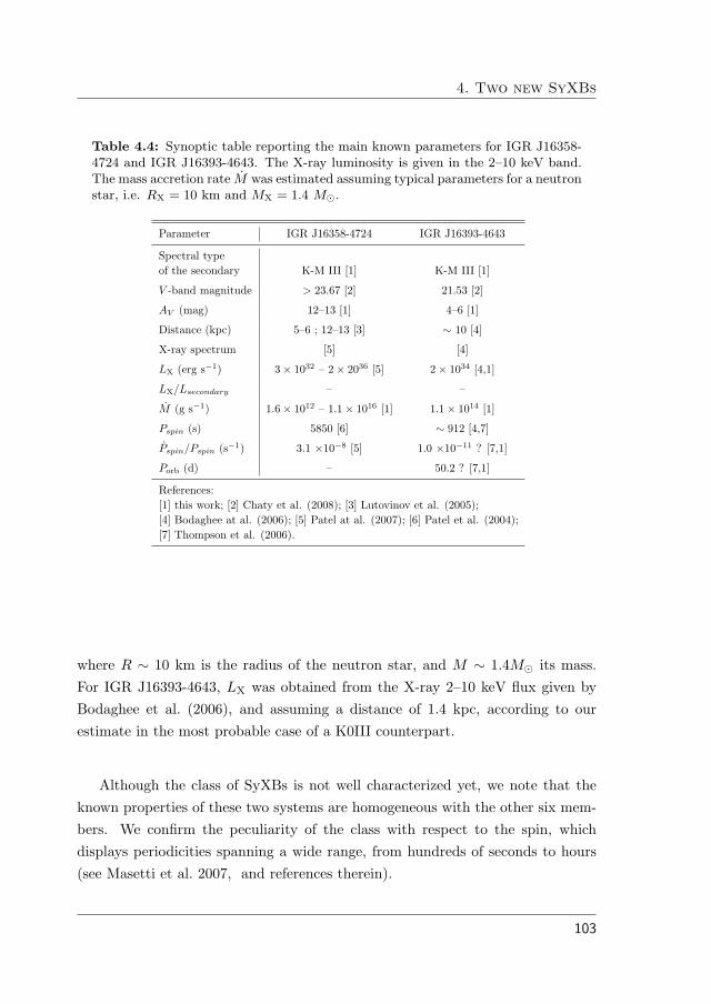
4. Two new SyXBs
Table 4.4: Synoptic table reporting the main known parameters for IGR J16358-4724 and IGR J16393-4643. The X-ray luminosity is given in the 2–10 keV band.The mass accretion rate M was estimated assuming typical parameters for a neutronstar, i.e. RX = 10 km and MX = 1.4 M⊙.
Parameter IGR J16358-4724 IGR J16393-4643
Spectral typeof the secondary K-M III [1] K-M III [1]
V -band magnitude > 23.67 [2] 21.53 [2]
AV (mag) 12–13 [1] 4–6 [1]
Distance (kpc) 5–6 ; 12–13 [3] ∼ 10 [4]
X-ray spectrum [5] [4]
LX (erg s−1) 3× 1032 – 2× 2036 [5] 2× 1034 [4,1]
LX/Lsecondary – –
M (g s−1) 1.6× 10¹² – 1.1× 10¹⁶ [1] 1.1× 10¹⁴ [1]
Pspin (s) 5850 [6] ∼ 912 [4,7]
Pspin/Pspin (s−1) 3.1 ×10⁻⁸ [5] 1.0 ×10⁻¹¹ ? [7,1]
Porb (d) – 50.2 ? [7,1]
References:[1] this work; [2] Chaty et al. (2008); [3] Lutovinov et al. (2005);[4] Bodaghee at al. (2006); [5] Patel at al. (2007); [6] Patel et al. (2004);[7] Thompson et al. (2006).
where R ∼ 10 km is the radius of the neutron star, and M ∼ 1.4M⊙ its mass.For IGR J16393-4643, LX was obtained from the X-ray 2–10 keV flux given byBodaghee et al. (2006), and assuming a distance of 1.4 kpc, according to ourestimate in the most probable case of a K0III counterpart.
Although the class of SyXBs is not well characterized yet, we note that theknown properties of these two systems are homogeneous with the other six mem-bers. We confirm the peculiarity of the class with respect to the spin, whichdisplays periodicities spanning a wide range, from hundreds of seconds to hours(see Masetti et al. 2007, and references therein).
103
4.6. Conclusions
4.6 Conclusions
We used infrared medium-resolution spectroscopy to classify the proposed coun-terparts to IGR J16358-4724 and IGR J16393-4643. The results we obtained forIGR J16393-4643 are valid if the candidate counterpart is confirmed by excludingas possible companion one of the other three sources found in the error circle ofthe XMM-Newton position. Future spectroscopic studies of these faint sourceswill be able to confirm without any doubt the classification of the system. Bythis work, we have found that:
- both objects show the typical features of cold giant or supergiant stars. Ourclassification constrains the spectral type to K-M.
- previous classification of the systems as HMXBs is dismissed.
- spectral classifications of the counterparts as late type giant stars, togetherwith X-ray behavior characteristic of neutron stars known from previousworks, allowed us to include both systems in SyXB class, increasing thenumber of this recently discovered group from six to eight members.
- among the orbital solutions for IGR J16393-4643 proposed by Thompsonet al. (2006) from pulse timing analysis, only one, with a mass function of0.092 M⊙ and orbital period of 50.2 days, is compatible with our spectralclassification.
- an upper limit to the mass of the companion star in IGR J16393-4643 wasset to 5 M⊙.
We emphasized the failure of SED fitting techniques alone with the aim ofspectral classification in the K-band, due to the degeneracy between the directionof the reddening vector and the effective temperature variation. Moreover, ourdata clearly stress the importance to obtain K-band spectroscopy beyond 2.3 µm,where CO absorption features are located. With spectra limited before this range,which can be featureless in particular at low resolution and S/N, classification canbe misleading.
104
5Conclusions and future projects
5.1 Main results
- We elaborated a photometric technique in the IR in order to select Becounterparts to obscured X-ray sources discovered by INTEGRAL.
- For each field, a number of 1–3 strong candidate counterparts, i.e. objectsselected from both (Brγ-Ks) – (H−Ks) and (He I-Ks) – (H−Ks) color-colordiagrams, were found.
- First tests validated the proposed technique.
- From IR spectroscopy of seven proposed counterparts to high-energy sources– IGR J16207–5129, IGR J16465–4507, IGR J16479–4514, IGR J16493–4348, AX J1841.0–0536 and IGR J19140+0951 and 4U 1907+09 –, we clas-sified all of them as HMXBs,by identifying three of them as SFXTs and fourof them SGXBs.
- We found that all the three SFXTs are intrinsically absorbed, suggestingthat this might be a characteristic of the entire class.
- For the seven objects analyzed, we estimated the distance to values com-patible with the location of the sources in the respective galactic arms.
- From K-band spectroscopy of two INTEGRAL objects, IGR J16358–4724and IGR J16393–4643, we proposed to classify both of them as two new
105

5.2. Future work
SyXBs, dismissing previous classification as HMXBs.
- We compared the previously proposed orbital solutions for IGR J16393–4643 with our findings and concluded that only one of them is compatiblewith our classification.
- We set an upper limit of 5 M⊙ to the mass of the companion star to IGRJ16393–4643.
5.2 Future work
As a future project, we plan to observe the photometrically selected emission-lineobjects with intermediate resolution spectroscopy in the K band. Observing timefor these objects has already been awarded by ESO for 2010. This will be theimmediate exploitation of the technique developed with this work and will provideits final validation.
The characterization of the systems with identified counterparts will makeuse of both infrared and high-energy observations. This project will signicantlycontribute to map the distribution of HMXRBs in the inner parts of our galaxy,and to trace the star formation regions at opposite sides of the Milky Way.
106

Part II
X-ray analysis
107

108

Science is a way of trying not to
fool yourself. The first principle
is that you must not fool yourself,
and you are the easiest person to
fool.
Richard Feynman 6X-ray analysis techniques
In the last quarter of a century, thanks to the large amount of new informationavailable from X-ray observatories, a unified characterization of the spectral evo-lution of LMXBs, both containing a neutron star and a black hole, was madepossible (Homan & Belloni 2005; Dunn et al. 2010; Belloni 2010). In this chapterwe describe the main tools employed in the X-ray analysis of LMXBs and blackhole binaries, since most of previous work was performed for these systems. Inthe next chapter the same techniques will be applied to study HMXBs.
Two different techniques of analysis are mainly in use to characterize theobserved X-ray emission from X-ray binaries, namely broad-band spectral andtiming analysis. They both approach source emission changes appearing on sec-onds to minutes time scales. Average energy spectra over a few days are also usedsometimes.
Variations in broad-band (∆E/E > 0.1, usually continuum-dominated) X-ray spectral shape are diagnosed by two complementary methods: multi-bandphotometry and spectral fitting, while temporal variability of the X-ray emissionis assessed typically by flux time-series through the methods of Fourier powerspectral analysis. All the three procedures were employed in this work, so wedescribe them in this section, before entering the specifics of our analysis in thefollowing sections.
109

6.1. Spectral analysis
6.1 Spectral analysis
6.1.1 Multy-band photometry
In analogy with optical photometry, one can quantify broad-band X-ray spectralshape by defining X-ray colors. An X-ray color, also named “hardness”, is theratio between the photon counts in two broad bands. Since the ∼ 2–30 keV X-ray continuum spectra of virtually all HMXBs can be characterized by a powerlaw (i.e. a straight line in log-log plots), a color thus corresponds to a roughmeasure of spectral slope. The low-energy region of the spectrum is called the“soft” part, while the high-energy region is called the “hard” part. A color-colordiagram (CD) is the plot of one color vs. another calculated in a different energyband. The higher energy range color, corresponding to harder X-ray emission, iscalled hard color, while the lower energy range is the soft color. There is not inthe literature a unique definition for the energy bands to choose, which can varyaccording to the category of the studied source (if black hole or neutron star),the author, and the sensitivity of the detector employed, although their meaningis uniquely identified. A hardness-intensity diagram (HID) is instead the plot ofa color vs. the count-rate in some broad spectral range. These kind of diagramsare model-independent and reflect the intrinsic properties of the system. In thestudy of LMXBs, they have become an essential tool of analysis by introducingthe notion of spectral states. A state is defined by the sudden appearance of aspectral or timing component associated with a particular and well-recognizableposition in the CD/HID (see Sect. 6.4). The curve length along a traced one-dimensional track on the CD/HID is conventionally indicated with the symbol S,Sz and Sa for Z and atoll sources, respectively. Examples of CDs/HID for neutronstars are provided in Fig. 6.1
6.1.2 Spectral fitting
X-ray spectral variations can be described in a more detailed way in terms ofa combination of one or more physically motivated mathematical functions, ormodels, fitted to the observed spectra. The analysis of the behavior of modelparameters while the source emission evolves along the CD/HID describing apattern, together with the identification of parameters correlations, is a strong
110

6. X-ray analysis techniques
Figure 6.1: Typical spectral branches for neutron stars LMXBs from RXTE data.(a) CD of the atoll source 4U 1608-52, (b) CD of the GX atoll source GX 9+1, and(c) HID of the Z source GX 340+1. Diagrams from van Straaten et al. (2003), vander Klis (2006), Jonker et al. (2000) respectively.
tool to characterize the source states and to individuate state transitions (seeSect. 6.4).
Both methods have in fact limitations, in the first case due to unavoidable detec-tor dependence, in the second case because of the presence of many parametersand because the correct models are in fact not known and in many cases thedata can be satisfactorily described by different models. Thus experience andcombinations of both methods are absolutely necessary.
6.2 Timing analysis
Observations of X-ray binaries show considerable variability on a wide range oftime scales in all wavelengths and down to less than a millisecond in X-rays. Themain tool used for studying the timing properties of an X-ray source is the Fourierpower spectrum, or a Power Spectral Density (PSD), of the count-rate time series,in which data are transformed from the time to the frequency domain. This tech-nique is particularly needed when the counting noise dominates the time seriesand it is only possible to study the averaged properties of the timing phenom-ena. A number of variability components, or power-spectral components, togethermake up the power spectrum. An aperiodic component by definition covers sev-
111
6.3. This work
eral frequency resolution elements. Broad features are called noise and narrowfeatures are called quasi-periodic oscillations (QPOs). With the aim of providinga unified description of the aperiodic variability, timing components are usuallyfitted with Lorentzian functions (Li). For an extensive overview of how Fouriertechniques are used in X-ray variability studies, we refer to van der Klis (1989).
As can be seen in Figs. 6.3 and 6.4, the power spectrum consists of a superpo-sition of different components. Unfortunately, there is no physical model able todescribe all these components consistently, as the real processes behind the X-rayvariability are still poorly understood.
6.3 This work
While there have been numerous studies on the application of CD/HID and spec-tral analysis techniques to LMXBs, very little work of this kind has been done onhigh-mass X-ray binaries. Belloni & Hasinger (1990) performed an aperiodic vari-ability study on a sample of 14 X-ray binaries, among which 12 were HMXBs: tenof them were SGXRBs; the only BeXRBs were EXO 2030+375 and V 0332+53.Data from EXO 2030+375 only covered a part of the decay of the 1985 outburst;data from V 0332+53 did not correspond to a major outburst. After the discov-ery of aperiodic variability in V 0332+53 (Stella et al. 1985), timing analysis onaccreting pulsars have concentrated on the detection of QPOs (see, for instance,Angelini et al. 1989; Jernigan et al. 2000; Qu et al. 2005). The only study ofaperiodic variability on Be/XRBs was recently accomplished by Reig (2008), whocharacterized the spectral/timing behavior of four systems through CD/HID andtiming from RXTE data, constructing time-averaged energy and PSD.
This work is intended to provide for the first time a systematic study of fourBe/XRBs during giant outburst, using the three techniques introduced before,namely CD/HID, spectral fitting and timing, simultaneously, and using the re-trieved results and correlations to try to define and characterize spectral statesfor this class of systems.
We have used the same data set as Reig (2008). However, while Reig (2008)
112

6. X-ray analysis techniques
divided the outburst into several (between 7–9) intervals and extracted averagedpower spectra for each interval, in this work we obtained energy spectra and PSDfor each RXTE observation interval. In Reig (2008) each observation interval hada duration of a few days to weeks. In this work, each observation interval is afew thousand seconds long. This order of magnitude increase in time resolutionallows us to:
1. Track much faster changes, likely to be associated with accretion;
2. Search for correlations between the spectral and timing parameters.
6.4 Spectral states
Although this work is addressed to the investigation and characterization of pos-sible spectral states in HMXBs, for the sake of comparison we give in this sectionan overview of the present definitions of states for LMXBs, both those containingneutron stars and black holes.
6.4.1 Neutron star LMXBs states
Hasinger & van der Klis (1989) classified the neutron star LMXBs based on thecorrelated variations of X-ray spectral and rapid aperiodic variability properties.They distinguished two sub-classes, the Z sources and the atoll sources, whosenames were inspired by the shapes of the tracks that they trace out in an X-rayCD on time scales of hours to days. The Z sources are the brightest of these twoclasses and are believed to accrete at near-Eddington luminosities (0.5 LEdd – 1.0LEdd; van der Klis 2006), while the atoll sources cover a much wider range inluminosities. Generally, the atoll sources tend to have harder spectra and to showlarger amplitude variability.
It has been observed that in these sources X-ray luminosity LX tends to cor-relate with state only within a source, not across sources, while X-ray spectralshape, i.e. the position of the source in the CD/HID, correlates with timing char-acteristics much better than LX (see, for instance, van der Klis 2000). For each
113

6.4. Spectral states
type of source, several spectral/timing states are identified, which are thoughtto arise from qualitatively different inner flow configurations (e.g. differences inmass accretion rate M , presence or absence of a corona, structure of accretiondisk, jets). Nevertheless, at the time of writing, differences between Z and atollsources still need an explanation, as well as those among states of each class.
Z sources
They are characterized by three-branched tracks in their CDs (see Fig. 6.1, panelc, and Fig. 6.2 as examples) and HIDs, which in some cases resemble the character“Z” (Cyg-like sources). In other cases they have a more “ν”-like shape (Sco-likesources), but are referred to as Z tracks nevertheless. From top to bottom, thethree branches of the Z track are described as the horizontal branch (HB), normalbranch (NB; “normal” because it was supposed that this state was more commonthan the HB state), and flaring branch (FB; named “flaring” after the flaringshown by Sco X-1 when moving up this branch).
Despite the various differences existing among the Z sources, it has often beenassumed that in all of them the mass accretion rate increases monotonically fromthe HB, via the NB, to the FB. If this is the correct interpretation, it would implythat X-ray luminosity does not track M .
Motion along the branches of the Z usually takes place on timescales of hours todays. On longer timescales it has been observed that the entire Z track changes itslocation in the CD and HID, or even changes its morphology (“secular motion”),as is best observed in Cyg X-2 (Kuulkers et al. 1996; Wijnands et al. 1997).
The power spectra of the Z sources show several types of QPOs and noisecomponents (see fig. 6.2; for reviews, see van der Klis 2006). Their presence andproperties are strongly correlated with the position of the source along the Z track(Hasinger & van der Klis 1989). Three types of low-frequency (<100 Hz) QPOsare seen in the Z sources: the horizontal branch (HBOs), normal branch (NBOs),and flaring branch oscillations (FBOs). Their names derive from the branches onwhich they were originally found. The HBO is found on the HB and NB with afrequency (15–60 Hz) that gradually increases along the HB toward the NB. TheNBO and FBO are most likely part of one single phenomenon. They are foundon the NB and FB (near the NB/ FB vertex) but not on the HB. On the NB theQPO has a frequency of ∼ 5–7 Hz, which (only in the Sco-like sources) rapidly
114

6. X-ray analysis techniques
Figure 6.2: Left: Example of CD for a typical Z source (Sco-type) with Sz pa-rameterization shown. Right: For nine different Sz selections, representative power-spectra for the same Z source, with power-spectral components marked. Adaptedfrom Homan et al. 2002.
increases to ∼20 Hz when the source moves across the NB/FB vertex (Priedhorskyet al. 1986; Dieters & van der Klis 2000; Casella et al. 2006). Twin kHz QPOshave been found in all Z sources. They are often observed simultaneously, with afrequency difference of ∼300 Hz, and have frequencies between 215 and 1130 Hz,which increase from the HB to the NB (in Sco X-1 also onto the FB; van der Kliset al. 1996).
Two types of noise are seen in the Z sources. These are the very low frequencynoise (VLFN) and the low-frequency noise (LFN). The VLFN, which is found atfrequencies below 1 Hz, is generally described by a power law and is found on all
115
6.4. Spectral states
branches, whereas the LFN, which is a peaked or flat-topped noise component(with cutoff frequencies of 2–10 Hz), is only observed on the HB and NB.
Atoll sources
At high X-ray luminosity, atoll sources follow a well defined curved banana branchin the CD/HID (see Fig. 6.1, panel a), along which sources move back and forthwith no hysteresis on time scales of hours to a day, showing sometimes secularmotion than does not affect the variability. The banana branch is further sub-divided into the upper banana (UB), dominated by the VLFN, the lower banana(LB), dominated by 10-Hz band-limited noise components (BLN), and the lowerleft banana (LLB), where twin kHz QPOs are observed. At the lower luminosityand generally corresponding to harder emission, the source trace the so-calledisland state (IS), whose power spectra are characterized by broad features anda dominant BLN component which becomes stronger and lower in characteristicfrequency as the flux decreases and the spectrum gets harder above 6 keV. Thehardest, lowest luminosity state is the extreme island state (EIS), characterizedby strong, low-frequency flat-topped noise. The topology of this state has been amatter of some debate as similarities between this branch and the Z-source HBwere claimed by a number of authors (Gierlinski & Done 2002; Muno et al. 2002);nevertheless, studies by Barret & Olive (2002); van Straaten et al. (2003); Reiget al. (2004) later pointed out that differences in the luminosity associated withthe spectral transitions, in spectral shape and mainly in timing features testify adifferent nature of the two classes.
In Fig. 6.3, a schematic CD/HID and representative power spectra for theEIS, IS, LLB, LB and the UB states are shown.
6.4.2 Black-holes states
The X-ray spectral properties of black holes LMXBs can be classified into twomain components, a hard and a soft one. When a hard, non-thermal, power-lawcomponent with photon index in the range 1.5–2 dominates the energy spectrum,the source is in its Low/hard State (LS); when a soft, thermal, black-body likecomponent with temperature kT � 1 keV dominates, then the source is in itsHigh/soft State (HS). In between the low and the high states, the intermediate
116

6. X-ray analysis techniques
Figure 6.3: Left: Schematic HID and CD for a typical atoll source. The solid lineshows the track the source follows during the outburst. Note that some sourcesshow transitions among all states, while others are only observed in some of them.Right: Representative power-spectra for atoll sources states, with power-spectralcomponents marked. Adapted from Klein-Wolt & van der Klis 2007.
117
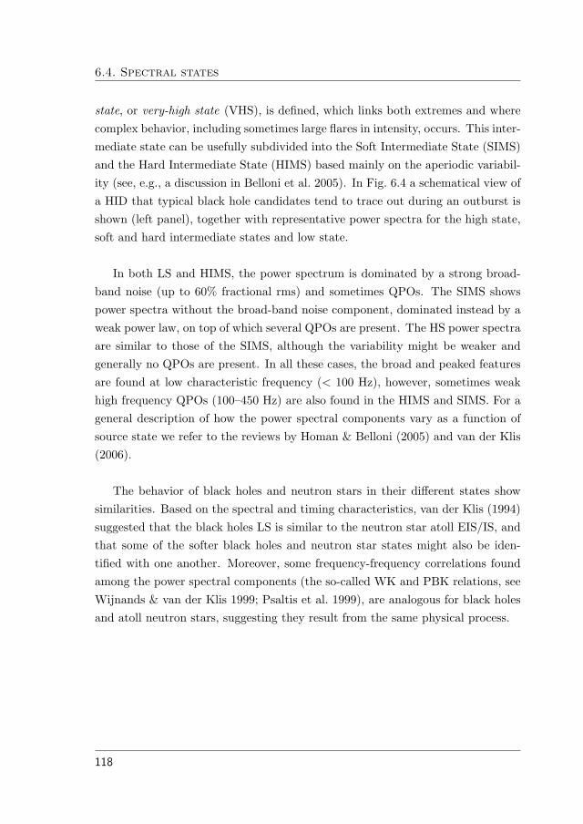
6.4. Spectral states
state, or very-high state (VHS), is defined, which links both extremes and wherecomplex behavior, including sometimes large flares in intensity, occurs. This inter-mediate state can be usefully subdivided into the Soft Intermediate State (SIMS)and the Hard Intermediate State (HIMS) based mainly on the aperiodic variabil-ity (see, e.g., a discussion in Belloni et al. 2005). In Fig. 6.4 a schematical view ofa HID that typical black hole candidates tend to trace out during an outburst isshown (left panel), together with representative power spectra for the high state,soft and hard intermediate states and low state.
In both LS and HIMS, the power spectrum is dominated by a strong broad-band noise (up to 60% fractional rms) and sometimes QPOs. The SIMS showspower spectra without the broad-band noise component, dominated instead by aweak power law, on top of which several QPOs are present. The HS power spectraare similar to those of the SIMS, although the variability might be weaker andgenerally no QPOs are present. In all these cases, the broad and peaked featuresare found at low characteristic frequency (< 100 Hz), however, sometimes weakhigh frequency QPOs (100–450 Hz) are also found in the HIMS and SIMS. For ageneral description of how the power spectral components vary as a function ofsource state we refer to the reviews by Homan & Belloni (2005) and van der Klis(2006).
The behavior of black holes and neutron stars in their different states showsimilarities. Based on the spectral and timing characteristics, van der Klis (1994)suggested that the black holes LS is similar to the neutron star atoll EIS/IS, andthat some of the softer black holes and neutron star states might also be iden-tified with one another. Moreover, some frequency-frequency correlations foundamong the power spectral components (the so-called WK and PBK relations, seeWijnands & van der Klis 1999; Psaltis et al. 1999), are analogous for black holesand atoll neutron stars, suggesting they result from the same physical process.
118

6. X-ray analysis techniques
Figure 6.4: Left: Schematic HID for a typical black hole source outburst. Thesolid line shows the track the source follows during the outburst. Right: Represen-tative power-spectra for black hole states, with power-spectral components marked.Adapted from Klein-Wolt & van der Klis 2007.
119

6.4. Spectral states
120

Puedo escribir los versos mas
tristes esta noche; escribir, por
ejemplo: “La noche esta estrellada,
y tiritan, azules, los astros, a lo
lejos”
Pablo Neruda 7X-ray spectral and timing analysis of
Be/XRBs during giant outbursts
7.1 Scientific objective
With the work presented in this chapter we investigated the spectral and timingvariability of four accreting X-ray pulsars with Be-type companions during majoroutbursts. By major outbursts we mean type II outbursts in which the X-rayluminosity reaches Eddington values, similarly to X-ray outbursts from transientLMXBs and black-hole binaries. Based on the spectral and timing properties, onthe position of the sources in the color-color diagram along the outburst, and thecorrelations between all these features, we aim to define and characterize possible“source states” as in Low Mass X-ray Binaries (LMXBs) and Black Holes.
The systems analyzed in our work, Be/XRBs, display two kind of variabilityin X-ray intensity, being one of them strictly periodic and the other one aperiodic.The X-ray periods range from a fraction of a second to several months, and canbe separated into coherent modulation due to the rotation of the neutron star(spin or pulse period) and modulation due to the orbital motion on the neutronstar around the Be star companion.
As the neutron star rotates, the polar hotspots, i.e. the regions where gasaccreted from the stellar companion is channeled by the neutron star’s magnetic
121
7.2. The sources
field, move in and out of view if the magnetic axis is tilted with respect to thespin axis. This results in X-ray pulsations. The pulse periods lie in the range10−1 − 103 s.
The orbit of the neutron star around the Be star and the transfer of massfrom the massive companion together with the strong gravitational potential ofthe compact object originate high-energy radiation which in many cases is modu-lated. In fact, in some cases the only estimate of the orbital period of the systemcomes from the periodic modulation of the X-ray emission (e.g type I outbursts),which covers the range of 10− 102 days. The X-ray periodic variability is not thesubject of this work.
Instead, we focused on rapid aperiodic variability, as this is one of the phe-nomena that are firmly grounded in the unique physics of the process of accretiononto a compact object. During the accretion, large amounts of gravitational en-ergy (∼ 1038 erg s−1, or 105 L⊙) are released in a small volume (� 104 km3),which leads to high temperatures (T ∼ 107 K) and results in the emission of high-energy photons. The accreting matter moves through the small emitting volumeunder influence of a large gravitational force which produces strong accelerations.The resulting high velocity (∼ 0.1c) lead to short characteristic time scale (thedynamical time scale, τ =
�r3/GM is about 0.1 ms). Therefore, one may expect
to observe rapidly variable X-rays in these systems.As the X-ray spectrum and the rapid X-ray variability arise through processes
in the same physical region, their properties may be expected to be coupled. Themonitoring and analysis of these properties in X-ray pulsars are the subject ofthis chapter.
7.2 The sources
During type II outbursts, Be/XRBs display 2–3 orders of magnitude variations inX-ray intensity. It is believed that a temporary accretion disk is formed aroundthe neutron star during these major outbursts (although no Roche lobe overflowoccurs): these two features (transient nature and accretion disc) appear as apossible analogy domain with LMXBs, for which a well established description interms of source states has been provided.
122

7. X-ray spectral and timing analysis of Be/XRBs
7.2.1 KS 1947+300
The Be/X-ray binary KS 1947+300 was first detected in the X-ray band on June8, 1989 by the TTM coded mask X-ray spectrograph on the Kvant module of theMir space station (Borozdin et al. 1990) with a peak flux of 70 mCrab. About35 days later the flux was at the limit of sensitivity of the instrument with a 3σ
upper limit of 10 mCrab. X-ray pulsations with a pulse period of 18.7 s werefound in the X-ray flux of GRO J1948+32 in April 1994 by the all-sky monitorBATSE aboard CGRO (Chakrabarty et al. 1995). The source reached a peakpulse flux of 50 mCrab in the energy range 20–75 keV. About 25 days later theflux decayed below the detection threshold of BATSE. Due to the very large errorbox of GRO J1948+32, no connection with this source and KS 1947+300 wasrealized at first. The source remained in quiescence until the beginning of 2001(Galloway et al. 2004). In this occasion the source reached a maximum flux of 120mCrab, the largest in its history. This outburst is the subject of the present work.
Prior to this major outburst, weak emission (∼ 20 mCrab) and X-ray pulsa-tions (18.7579±0.0005 s) from KS 1947+300 had been detected in November 2000(Levine & Corbet 2000; Swank & Morgan 2000). The coincidence in the value ofthe pulse period and the location of KS 1947+300 inside the GRO J1948+32 errorbox suggested that the two sources were in fact the same object. Pulse timinganalysis allowed to solve for the orbital parameters, resulting in orbital periodPorb = 40.415 ±0.010 d, eccentricity e = 0.033± 0.013 and projected semi-majoraxis aX sin i = 137± 3 lt-s (Galloway et al. 2004). A broad-band spectral studyof KS 1947+300 using BeppoSAX observations (Naik et al. 2006) showed thatthe energy spectrum in the 0.1–100 keV energy band has three components: aComptonized component, a ∼0.6 keV blackbody component, and a narrow, weakiron emission line at 6.7 keV with a low column density of material in the line ofsight.
The optical counterpart to KS 1947+300 was correctly identified soon afterthe Kvant detection (Goranskii et al. 1991; Grankin et al. 1991), but its iden-tification as a Be/X-ray binary was suggested later by Negueruela et al. (2003).KS 1947+300 is associated with a moderately reddened V=14.2 B0Ve star located
123

7.2. The sources
at ∼10 kpc.
7.2.2 EXO 2030+375
EXO 2030+375 is a 42s transient accreting X-ray pulsar discovered with EXOSATduring a giant outburst in 1985 (Parmar et al. 1989). Extensively observed sinceits detection in the X/γ-ray band, this system is the prototype for X-ray variabilityin Be/XRBs. A normal outburst has been detected for nearly every periastronpassage since 1991 (Wilson et al. 2002, 2005). For these normal outbursts, theintensity and the global spin-up rate appeared to be tied to the K-band intensityof the Be star. In June 2006 EXO 2030+375 underwent its first giant outburstsince its discovery (Corbet & Levine 2006; Krimm et al. 2006; McCollough et al.2006). In this work we analyze data from this latest event.
In this system, the pulsar (Pspin = 41.7 s) orbits a B0 Ve star (Motch & Janot-Pacheco 1987; Reig & Coe 1998) in a moderately eccentric (e = 0.4) orbit every46 days (Wilson et al. 2005). The system is located at about 7.1 kpc (Wilsonet al. 2002). Like other HMXBs, the continuum spectral shape in the range 1–30keV can be modeled with a power law with an exponential cutoff (Reynolds et al.1993). The inclusion of a blackbody component has been reported to give goodfits at very high (LX ∼ 1038 erg s−1) luminosity (Sun et al. 1994) and relativelylow (LX ∼ 1036 erg s−1) luminosity (Reig & Coe 1999). A cyclotron resonantscattering feature (CRSF) at ∼ 11 keV was identified by Wilson et al. (2008)during the brightest phase of the 2006 outburst.
7.2.3 4U 0115+63
This source is one of the most active and extensively studied Be/X-ray transientsas it was one of the first to be discovered. It was detected by the UHURU observa-tory (Giacconi et al. 1972). Rappaport et al. (1978) determined the binary mainparameters based on the known pulsation period of ∼3.6 s (Cominsky et al. 1978):orbital period of 24.3 days, orbital eccentricity e = 0.34, and projected semimajoraxis aX sin i ∼ 140 light seconds. During RXTE’s lifetime, three major outburstshave been detected, in 1999, 2000 and 2004. Here we analyse observations fromthe 2004 event. The optical counterpart to the X-ray source is the star V635 Cas(Hutchings & Crampton 1981). Optical observations performed by Negueruela &
124

7. X-ray spectral and timing analysis of Be/XRBs
Okazaki (2001) allowed its spectral classification to B0.2Ve, and distance estima-tion to 7–8 kpc.
The X-ray spectrum shows up to five CRSFs, with the fundamental at ∼12keV (Wheaton et al. 1979), and four harmonics, making this pulsar the neutronstar with the highest number of cyclotron lines (Heindl et al. 2004). During the1999 and 2004 outbursts, mHz QPOs were detected (Heindl et al. 1999; Coburnet al. 2004).
7.2.4 V 0332+53
The transient X-ray pulsar V0332+53 was discovered by the Vela 5B observatoryin 1973 (Terrell & Priedhorsky 1984) during an outburst when its intensity reached∼ 1.4 Crab in the 3–12 keV energy band. The outburst lasted about three monthsbefore the source became undetectable again.
Through observations of three small outbursts in 1983–1984, the pulsars andorbital parameters were determined with the EXOSAT observatory: the pulse pe-riod was determined to be 4.4 s, the orbital period 34.25 days, eccentricity 0.31,and the projected semimajor axis aXsini ∼ 48 lt-s (Stella et al. 1985). Later,when the source was observed by the Ginga observatory, a cyclotron resonanceat Ec = 28.5 ± 0.5 keV was detected in its spectrum. This energy correspondsto a magnetic field on the neutron star surface of ∼3 ×10¹² G (Makishima et al.1990). Later Mihara et al. (1998) reported measurements of two different valuesof the resonance energy for different levels of the source intensity. During thesubsequent major outburst in 2004–2005, two harmonics were observed as well(Coburn et al. 2005). Data from this latest outburst are analyzed in this work.
The optical counterpart to the system, BQ Cam, was classified as O8-9Ve byNegueruela et al. (1999), who also estimated the distance to ∼ 7 kpc.
We provide in Table 7.1 the duration and peak intensity of each individualoutburst studied in this work, together with some basic information about thesystems.
125

7.3. The instrument
Table 7.1: Relevant optical/X-ray information on the systems and on the out-bursts analyzed in this work.
Source Spectral Pspin Porb Distance Outburst LX,peakname type (s) (d)
e(kpc) duration (d) 3–30 kev (erg s−1)
KS 1947+300 B0V 18.7 40.4 0.03 10.0 165 7.1×1037
EXO 2030+375 B0.5III-V 41.8 46.0 0.41 7.1 155 1.5×1038
4U 0115+63 B0.2V 3.6 24.3 0.34 8.1 55 1.4×1038
V 0332+53 O8-9V 4.4 34.2 0.30 7.0 105 3.4×1038
7.3 The instrument
We employed archive data by the Proportional Counter Array (PCA) onboardthe Rossi X-ray Timing Explorer (RXTE, Bradt et al. 1993). The satellite waslaunched on December 30, 1995 and at the time of writing it is still operating.It orbits at 580 km around Earth, with an inclination of 22◦, completing a circlearound our planet every 100 minutes. Its primary objective is the study of phe-nomena associated to galactic stellar systems containing compact objects, bothfrom the timing and the broad band spectral point of view. This is accomplishedwith three instruments: the All-Sky Monitor (ASM), the PCA, and the HighEnergy Timing Experiment (HEXTE). Fig. 7.1 shows a schematic view of thesatellite and its instruments.
The objective of the ASM is the continuous sky monitoring in order to revealtransient sources. It is composed by three screening shadow cameras operating inthe 1.3–12 keV band, that rotate by 6◦ every 90s, thus covering the 80% of the skyin 90 minutes. The high pointing velocity allows RXTE to observe X-ray sourceswith very low dead-times. The PCA is the main instrument onboard RXTE. It is apointed instrument, co-aligned with the HEXTE and having the same collimatedfield of view of ∼ 1◦. It consists of five Proportional Counter Units (PCUs) witha total collecting area of ∼ 6250 cm2, operates in the 2–60 keV range and hasa nominal energy resolution of 18% at 6 keV. The HEXTE is constituted by 2clusters of 4 NaI/CsI scintillation counters, with a total collecting area of 2× 800cm2, sensitive in the 15–250 keV band with a nominal energy resolution of 15% at60 keV. Both instruments have a maximum time resolution of ∼ 1µs. Thanks to
126

7. X-ray spectral and timing analysis of Be/XRBs
Figure 7.1: Diagram of the RXTE spacecraft, with instruments labeled
this very high temporal resolution, a very accurate analysis of aperiodic variationsin X-ray sources became possible. With the exception of regions near the centerof the Galaxy, the source density on the sky is low enough to provide sufficientpositional resolution and avoid source confusion.
Multiple combinations of modes and configurations for PCA data are possible,nevertheless there are only two basic formats for science data: science array andscience event. The science array format is used for data binned at regular intervalsby the spacecraft electronics. An example is the Standard 2 configuration, whichcontains 129–channel spectra accumulated every 16 seconds. Given its high spec-tral resolution, this configuration was employed in this work for spectral analysis.The science event format is used for unbinned data, i.e. for individual events. Anexample is the Good Xenon configuration which contains time-stamped eventswith 256-channel resolution, PCU ID and anode ID. This kind of mode, with thehighest temporal resolution, was employed for timing analysis.
127

7.4. Observations, data reduction and analysis
7.4 Observations, data reduction and analysis
Table 7.2: Journal of RXTE observations.
Source N. of observations Proposal ID MJD range On-source time (ks)
KS 1947+300 33 50425 51874.1502–51968.5641 81.953 60402 51970.2075–52878.0486 50.1
EXO 2030+375 84 91089 53914.8867–53998.6609 83.548 92067 53999.5903–54046.9378 56.6
4U 0115+63 19 90089 53254.0689–53280.6947 58.810 90014 53282.5716–53297.5954 37.6
V 0332+53 28 90089 53340.2869–53365.9140 82.27 90427 53367.2273–53376.6352 13.138 90014 53378.4241–53430.5380 79.2
The data analyzed in this work correspond to epochs in which the sourceswent through a type II outburst. Table 7.2 gives the observations log.
The PCA is the most appropriate instrument onboard RXTE to perform thetype of analysis that we wish to carry out. It provides time resolution down to1 µs and has a large collecting area. In addition, it is sensitive to X-rays below∼ 30 keV where most of the analysis in LMXBs and BHs, with which our studyintends to compare, has been done.
Due to the aging of the detectors, each PCU provides at present a differentperformance. Only data from PCU2, the most convenient unit since its good op-erational status and its constant enabling, were employed for color and spectralanalysis. All the PCU that were on were used for timing.
Due to the low-Earth orbit, observations consist of a number of contiguousdata intervals (typically 1h long) interspersed with observational gaps producedby Earth occultations of the target and passages through the South AtlanticAnomaly, where the high flux of energetic particles make the instruments unus-able. We will refer to each of these intervals as “pointings”.
128

7. X-ray spectral and timing analysis of Be/XRBs
7.4.1 Spectral analysis
Using Heasarc FTOOLS version 6.6.3, a spectrum was produced for each observa-tion, after filtering out unsuitable data according to the recommended criteria1.For extracting spectra, Standard 2 mode data were used, which have a time res-olution of 16s and cover the 2–60 keV range with 129 channels. All spectra werebackground-subtracted and, when necessary, dead-time corrected. By dead timewe mean any process by which the detection of an event subsequently changesthe sensitivity of the detectors. For each observation, the spectrum was fittedin the 3–50 keV range, using XSPEC version 12.4 (Arnaud 1996). This energyrange, extending to high energies, is accessible thanks to the high luminosity ofthe systems studied, showing high S/N in the DB (> 90% of the observations).For the sake of completeness we have also obtained spectra in the same range forthe HB, although the S/N is considerably lower above 30 keV. Nevertheless, thebest-fit values of the spectral parameters are not affected by whether we use 3–30keV or 3–50 keV. In Fig. 7.2 we show a plot of an unsubtracted source (blackpoints) and background (red points) together: it corresponds to the faintest ofthe four systems, KS 1947+300, at LX ∼ 40% of the peak luminosity. Althoughthe contribution of the background strongly increases above 25 keV, the unsub-tracted spectrum still lies on top of it.
During the fitting, a systematic error of 0.6% was added to the spectra, whichis a common practice. The lack of adequate theoretical continuum models foraccreting neutron stars imposes the use of empirical models to describe the ob-servations. In order to consistently compare fitting results from the four sources,we tried to employ the same (or very similar, if leading to better fit) spectralcomponents. We used a model composed by a combination of photoelectric ab-sorption (PHABS in XSPEC), a power law with high-energy exponential cutoff(CUTOFFPL or POWERLAW × HIGHECUT, according to the case) and a gaus-sian line profile (GAUSS) at ∼ 6.5 keV to account for Fe Kα fluorescence. Threesources, EXO 2030+375, 4U 0115+63 and V 0332+53, are known to be character-ized by cyclotron absorption, which we accounted for with the dedicated GABS or
1Among which, elevation from the Earth greater than 10◦ and pointing offset lower than
0.02◦; see PCA digest at http://heasarc.gsfc.nasa.gov/docs/xte/pca news.html or, e.g., van
Straaten et al. (2003)
129

7.4. Observations, data reduction and analysis
!"# $"
!!"
%&'()*+,-./0&1%23/3
! /4-5
!
6%-'78/94-5:
Figure 7.2: Plot of an unsubtracted source, KS 1947+300 (black points), togetherwith the corresponding background (red points). In the range we considered, 3–50keV, the source spectrum always lies on top of the background.
CYCLABS XSPEC components, both gaussian optical depth profiles. In general,the value of the hydrogen column density NH cannot be well constrained by thePCA, whose energy threshold for the fit is 3 keV. When known from previousworks with higher sensitive instruments below 3 keV, it was fixed to the knownvalue. Fixing the absorption makes the fitting procedure more stable, mainlyduring error calculation.
In Fig. 7.3 we give an example of unfolded spectrum, for the observation90014-02-01-01 of 4U 0115+63. The retrieved reduced chi-square for this fit wasχ2
red = 1.06.
Integrated fluxes were calculated through XSPEC in the 3–30 keV using thebest-fit model.
130

7. X-ray spectral and timing analysis of Be/XRBs
!"# $"
!"!%
"&"!
'()*)+,-./
!$-,!!-012
!!
3+1456-70128
9""!:!"$!"!!"!
Figure 7.3: Example of the unfolded spectrum of 4U 0115+63, described by amodel constituted by photoelectric absorption, power law with high-energy cutoff(dotted line), gaussian line (dashed line) and cyclotron absorption. In this kind ofrepresentation, only the additive components are shown. Data points are markedby black crosses, the resulting fitting model is marked by a red line.
CD and HID were directly obtained from count rate in the following energybands:
- soft color (SC): 7–10 keV / 4–7 keV
- hard color (HC): 15–30 keV / 10–15 keV
Standard 2 mode data were used to obtain the lightcurves from which the colorsare calculated. The average value of count rate for each observation was employedin order to have colors with the same sampling than the energy spectra (one pointper observation).
131
7.4. Observations, data reduction and analysis
7.4.2 Timing analysis
Power spectral density (PSD) was computed using mainly Good Xenon or Eventmode data. According to archive availability, in some cases also Binned and SingleBit mode were used.
We first extracted, for each observation, a light curve in the energy range 2–20keV (channels 0–49) with a time resolution of 2−8 s. The light curve was thendivided into 256-s segments and a Fast Fourier Transform was computed for eachsegment. The final PSD was computed as the average of all the power spectraobtained for each segment. The final power spectra were logarithmically rebinnedin frequency and corrected for dead time effects according to the prescriptiongiven in Nowak et al. (1999).
Power spectra were normalized such that the integral over the PSD is equal tothe squared fractional rms amplitude, according to the so-called rms-normalization(Belloni & Hasinger 1990; Miyamoto et al. 1991).
In order to have a unified phenomenological description of the timing featureswithin a source and among the four different sources, we fitted noise and QPOswith a function consisting of one or multiple Lorentzians, each denoted as Li,where i determines the type of component. The characteristic frequency νmax ofLi is denoted νi. This is the frequency where the component contributes most ofits variance per logarithmic frequency interval and is defined (Belloni et al. 2002)as
νmax =�
ν20 + (FWHM/2)2 = ν0
�1 + 1/4Q2 , (7.1)
where ν0 is the centroid frequency and FWHM the full width at half maximumof the Lorentzian component. Note that νmax �= ν0. The broader the noisecomponent, the larger the difference between νmax and ν0.
The quality factor Q is defined as Q = ν0/FWHM , and is used as a measureof the coherence of the variability feature.
Our choice of this over other models (such as a combination of power law andGaussian functions) was motivated by the fact that the multi-Lorentzian modelgives the possibility to identify and follow the characteristics of power spectralcomponents as they evolve in time and as a function of spectral state using onlyone type of function (i.e., a Lorentzian function). This also allowed us to compare
132

7. X-ray spectral and timing analysis of Be/XRBs
the characteristics of different components. The peaks derived from the neutronstars pulsations were fitted to Lorentzian functions with frequency fixed at theexpected value according to the spin period and width equal to 0.001 Hz (approx-imately, the inverse of the timing resolution of the PSD). The results from theuse of Lorentzians are best visualized using the ν×Pν representation, where eachpower is multiplied by the corresponding frequency. In this representation, themaximum power is attained at ν = νmax.
We show an example of fitted PSD in the ν × Pν representation in Fig. 7.4.The spectrum is from observation 90089-01-04-02 of 4U 0115+63; each fittingcomponent is represented by a colored line, while the whole resulting fit is shownas black solid line. The retrieved reduced chi-square for the fit was χ2
red = 1.2.
7.5 Results
Here we present, for each system, the results of our analysis. For representativeenergy spectra and PSD, see the next section, where a comprehensive discussionis given.
7.5.1 KS 1947+300
The total duration of the outburst was ∼ 165 days. The peak X-ray luminosity,found at MJD = 51950, is LX = 7.1 × 1037 erg s−1, assuming a distance of 10kpc.
Spectral analysis
In Fig. 7.5 we show the behavior of the 3–30 keV flux during the outburst. Wenote that the outburst is well sampled, from its very beginning until its finaldecay. It is asymmetrical, characterized by a steeper rise and a slower decay. Ittook ∼70 days to rise from quiescence to maximun flux and about 120 days toreturn to quiescence.
In Fig. 7.6 we display the corresponding HIDs and colors trends. While Fig. 7.5was obtained after the spectral fitting, which is a necessary step in order tocalculate the flux from the source, Fig. 7.6 was directly retrieved from count rate.
133
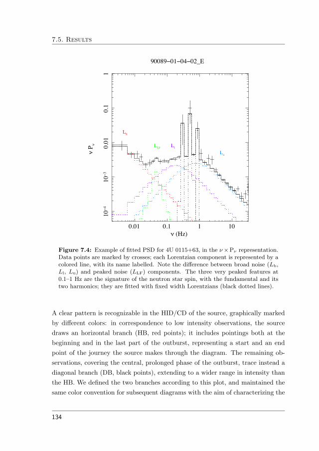
7.5. Results
!"!# !"# # #!
#!!$
#!!%
!"!#
!"#
#
!&'
!
!&()*+
,!!-,!!#!!$!!./0
12
113
14
15
Figure 7.4: Example of fitted PSD for 4U 0115+63, in the ν×Pν representation.Data points are marked by crosses; each Lorentzian component is represented by acolored line, with its name labelled. Note the difference between broad noise (Lb,Ll, Lu) and peaked noise (LLF) components. The three very peaked features at0.1–1 Hz are the signature of the neutron star spin, with the fundamental and itstwo harmonics; they are fitted with fixed width Lorentzians (black dotted lines).
A clear pattern is recognizable in the HID/CD of the source, graphically markedby different colors: in correspondence to low intensity observations, the sourcedraws an horizontal branch (HB, red points); it includes pointings both at thebeginning and in the last part of the outburst, representing a start and an endpoint of the journey the source makes through the diagram. The remaining ob-servations, covering the central, prolonged phase of the outburst, trace instead adiagonal branch (DB, black points), extending to a wider range in intensity thanthe HB. We defined the two branches according to this plot, and maintained thesame color convention for subsequent diagrams with the aim of characterizing the
134
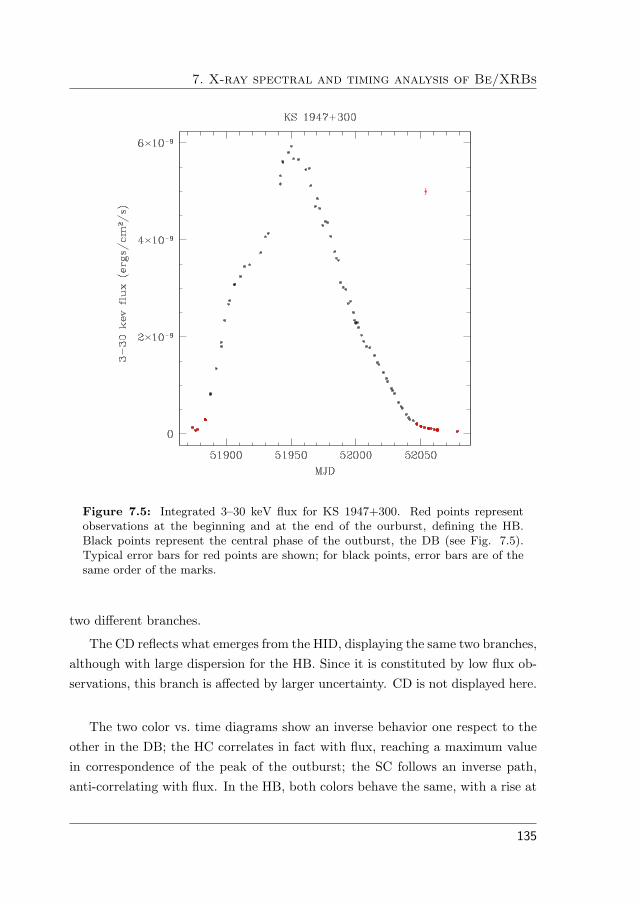
7. X-ray spectral and timing analysis of Be/XRBs
Figure 7.5: Integrated 3–30 keV flux for KS 1947+300. Red points representobservations at the beginning and at the end of the ourburst, defining the HB.Black points represent the central phase of the outburst, the DB (see Fig. 7.5).Typical error bars for red points are shown; for black points, error bars are of thesame order of the marks.
two different branches.
The CD reflects what emerges from the HID, displaying the same two branches,although with large dispersion for the HB. Since it is constituted by low flux ob-servations, this branch is affected by larger uncertainty. CD is not displayed here.
The two color vs. time diagrams show an inverse behavior one respect to theother in the DB; the HC correlates in fact with flux, reaching a maximum valuein correspondence of the peak of the outburst; the SC follows an inverse path,anti-correlating with flux. In the HB, both colors behave the same, with a rise at
135

7.5. Results
Figure 7.6: HIDs and colors behavior during KS 1947+300 outburst. Typicalerror bars are shown.
the beginning of the outburst, and a decay at the end.
Energy spectra were fitted by a model constituted by photoelectric absorption,a power law with high-energy cutoff and an iron fluorescence line. The photoab-sorption was fixed at 4.5×10⁻²¹ cm−2 according to what Naik et al. (2006) foundfrom BeppoSAX data. Leaving this parameter free did not result in consistent
136

7. X-ray spectral and timing analysis of Be/XRBs
fitted values along the outburst, so that we preferred to constrain it to the Bep-poSAX value.
In Fig. 7.7 we display the behavior of the spectral parameters of the powerlaw component, i.e. the spectral index Γ and the cutoff energy.
Figure 7.7: High-energy cutoff power law behavior during KS 1947+300 outburst.
Their trend with time (left side) and flux (right side) is shown. The spectral
137

7.5. Results
index clearly correlates with flux in the DB, while anti-correlates with it in theHB. A similar trend is sketched by the cutoff energy. We show in Fig. 7.8 a ten-tative correlation between the two power law parameters.
Figure 7.8: Relation between the spectral index and the cutoff energy.
In Fig. 7.9 the behavior of the Fe line with time and flux is presented. Thiscomponent is needed to obtain best fit for all observations, except for the verylast ones of the decay phase (until MJD = 52050). For the line energy, althoughshowing a larger range of variability along the HB than in the DB, no clear trendduring the outburst can be identified. The line width (σ) was almost constantduring the outburst, and was eventually fixed at 0.5 keV in all the fits. Thenormalization is correlated with flux. The EW of the line is anti-correlated withflux at low luminosity, up to LX = 3.4 × 1037 ergs cm−1 (or flux = 2×10⁹ ergscm−2 s−1), when it reaches an almost constant value of about 0.05 keV. This isdue to an almost 1:1 relation between the normalization of the component andthe total flux at high luminosity.
138

7. X-ray spectral and timing analysis of Be/XRBs
Figure 7.9: Fe fluorescence line during KS 1947+300 outburst.
139
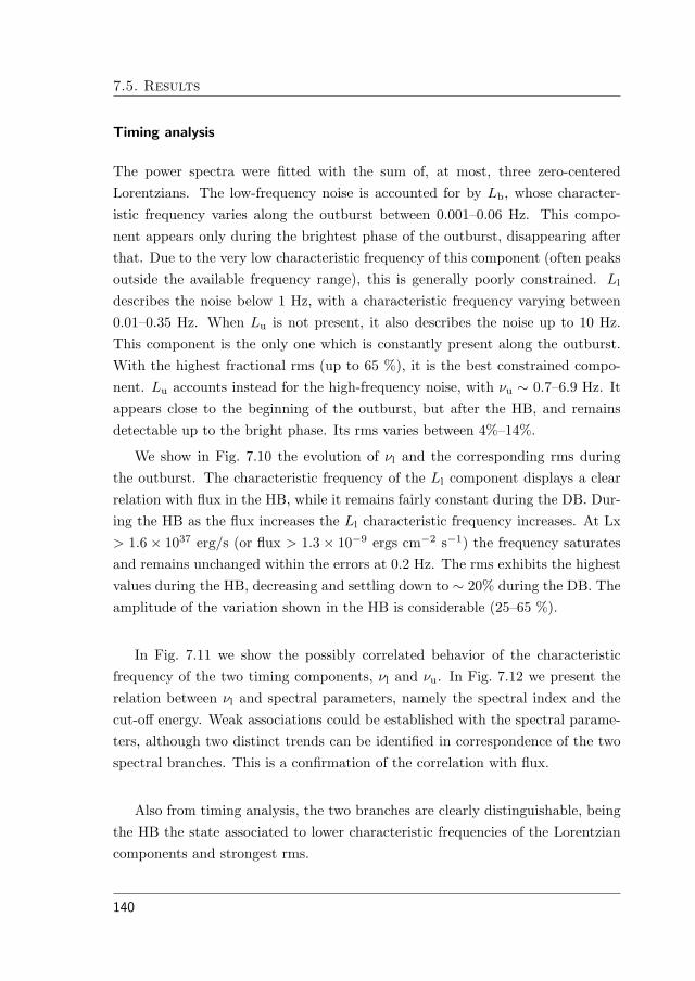
7.5. Results
Timing analysis
The power spectra were fitted with the sum of, at most, three zero-centeredLorentzians. The low-frequency noise is accounted for by Lb, whose character-istic frequency varies along the outburst between 0.001–0.06 Hz. This compo-nent appears only during the brightest phase of the outburst, disappearing afterthat. Due to the very low characteristic frequency of this component (often peaksoutside the available frequency range), this is generally poorly constrained. Ll
describes the noise below 1 Hz, with a characteristic frequency varying between0.01–0.35 Hz. When Lu is not present, it also describes the noise up to 10 Hz.This component is the only one which is constantly present along the outburst.With the highest fractional rms (up to 65 %), it is the best constrained compo-nent. Lu accounts instead for the high-frequency noise, with νu ∼ 0.7–6.9 Hz. Itappears close to the beginning of the outburst, but after the HB, and remainsdetectable up to the bright phase. Its rms varies between 4%–14%.
We show in Fig. 7.10 the evolution of νl and the corresponding rms duringthe outburst. The characteristic frequency of the Ll component displays a clearrelation with flux in the HB, while it remains fairly constant during the DB. Dur-ing the HB as the flux increases the Ll characteristic frequency increases. At Lx> 1.6 × 1037 erg/s (or flux > 1.3 × 10⁻⁹ ergs cm−2 s−1) the frequency saturatesand remains unchanged within the errors at 0.2 Hz. The rms exhibits the highestvalues during the HB, decreasing and settling down to ∼ 20% during the DB. Theamplitude of the variation shown in the HB is considerable (25–65 %).
In Fig. 7.11 we show the possibly correlated behavior of the characteristicfrequency of the two timing components, νl and νu. In Fig. 7.12 we present therelation between νl and spectral parameters, namely the spectral index and thecut-off energy. Weak associations could be established with the spectral parame-ters, although two distinct trends can be identified in correspondence of the twospectral branches. This is a confirmation of the correlation with flux.
Also from timing analysis, the two branches are clearly distinguishable, beingthe HB the state associated to lower characteristic frequencies of the Lorentziancomponents and strongest rms.
140
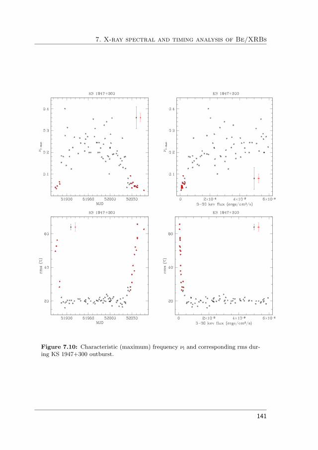
7. X-ray spectral and timing analysis of Be/XRBs
Figure 7.10: Characteristic (maximum) frequency νl and corresponding rms dur-ing KS 1947+300 outburst.
141

7.5. Results
Figure 7.11: Relation between νl and νu.
Figure 7.12: Relation between νl and spectral parameters.
142

7. X-ray spectral and timing analysis of Be/XRBs
7.5.2 EXO 2030+375
The total duration of the outburst was ∼ 155 days, the peak intensity was a factorof 4 larger than KS 1947+300. A peak X-ray luminosity of LX = 1.5 × 1038 ergs−1 is obtained at MJD = 53965, assuming a distance of 7.1 kpc. Spectral analysisof RXTE data from the 2004 outburst of EXO 2030+375 was also performed byWilson et al. (2008): in this work, we extend their study to a low luminosityrange.
Spectral analysis
This source is known to be characterized by a weak cyclotron resonance scatteringfeature at ∼10 keV (Wilson & Finger 2006; Klochkov et al. 2007). In our spectraits presence was consistently found only in correspondence to the brightest, centralpart of the outburst, while including it in spectra of observation taken at MJD> 53 993 did not result in a better fit. No harmonics were found. To account forthis feature, we employed the GABS component in XSPEC, a gaussian absorptionline described by the following profile:
I(E) = exp(−(τ/
√2π σ) exp(−0.5((E − Ec)/σ)2)) ,
where Ec is the line energy in keV, σ is the line width in keV, and τ is the opticaldepth at the line center.
In Fig. 7.13 we show the trend followed by the 3–30 keV flux during the out-burst. In this case the outburst is not as well sampled as for KS 1947+300, missingthe very first phase of its rising phase. This is reflected in the HIDs (Fig. 7.14),where the HB, clearly recognizable in this source as well, is made up only byobservations covering the last part of the outburst. In Fig. 7.14 we also presentthe behavior of the two colors along the outburst.
A trend very similar to that of KS 1947+300 is shown: two branches are rec-ognizable in the CD as well, although with larger dispersion than in the HID; theHC correlates with flux, displaying a peak in correspondence with the peak of theoutburst, while an opposite behavior characterizes the SC. This is true for theDB, while in the HB the two colors seem both to decrease with time (and thus
143
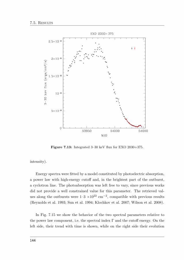
7.5. Results
Figure 7.13: Integrated 3–30 keV flux for EXO 2030+375.
intensity).
Energy spectra were fitted by a model constituted by photoelectric absorption,a power law with high-energy cutoff and, in the brightest part of the outburst,a cyclotron line. The photoabsorption was left free to vary, since previous worksdid not provide a well constrained value for this parameter. The retrieved val-ues along the outbursts were 1–3 ×1022 cm−2, compatible with previous results(Reynolds et al. 1993; Sun et al. 1994; Klochkov et al. 2007; Wilson et al. 2008).
In Fig. 7.15 we show the behavior of the two spectral parameters relative tothe power law component, i.e. the spectral index Γ and the cutoff energy. On theleft side, their trend with time is shown, while on the right side their evolution
144

7. X-ray spectral and timing analysis of Be/XRBs
Figure 7.14: HIDs and colors behavior during EXO 2030+375 outburst.
145

7.5. Results
with flux is presented. Again, strong similarities with KS 1947+300 can be estab-lished, as the spectral index correlates with flux in the DB, while anti-correlateswith it in the HB. An analogous trend is sketched by the cutoff energy, pointing toa physical consistence of this phenological model, since the same physical processmust be involved in order to produce both features.
Figure 7.15: High-energy cutoff power law behavior during EXO 2030+375 out-burst.
146

7. X-ray spectral and timing analysis of Be/XRBs
Figure 7.16: Relation between the spectral index and the cutoff energy.
We clarify this in Fig. 7.16, where a clear correlation can be seen during allthe outburst, although different slopes mark the two branches.
In Fig. 7.17 the behavior of the Fe line energy with respect to time and flux isshown. The width of the component was fixed at 0.5 keV. No clear trend duringthe outburst can be identified in this case for the line energy and EW and thelarge dispersion shown in the HB may be due to the lower statistics of low fluxobservations. The component is very faint during the HB, so that also its centralenergy was fixed at 6.4 keV, while the normalization was left free to vary. Thecorresponding pointings are only shown in the plots of the normalization. Thestrength of this component is strongly correlated with flux. The equivalent widthweakly correlates with flux.
The CRSF was found not to vary during the outburst, within the errors.Fitting its three parameters with a constant, gave the following results:
147

7.5. Results
Figure 7.17: Fluerescence Fe line during EXO 2030+375 outburst.
148
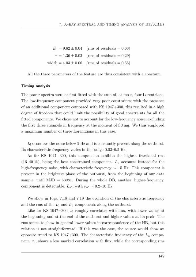
7. X-ray spectral and timing analysis of Be/XRBs
Ec = 9.62± 0.04 (rms of residuals = 0.63)
τ = 1.36± 0.03 (rms of residuals = 0.29)
width = 4.03± 0.06 (rms of residuals = 0.55)
All the three parameters of the feature are thus consistent with a constant.
Timing analysis
The power spectra were at first fitted with the sum of, at most, four Lorentzians.The low-frequency component provided very poor constraints; with the presenceof an additional component compared with KS 1947+300, this resulted in a highdegree of freedom that could limit the possibility of good constraints for all thefitted components. We chose not to account for the low-frequency noise, excludingthe first three channels in frequency at the moment of fitting. We thus employeda maximum number of three Lorentzians in this case.
Ll describes the noise below 5 Hz and is constantly present along the outburst.Its characteristic frequency varies in the range 0.02–0.5 Hz.
As for KS 1947+300, this components exhibits the highest fractional rms(16–40 %), being the best constrained component. Lu accounts instead for thehigh-frequency noise, with characteristic frequency ∼1–5 Hz. This component ispresent in the brightest phase of the outburst, from the beginning of our datasample, until MJD = 53981. During the whole DB, another, higher-frequency,component is detectable, Lu� , with νu� ∼ 0.2–10 Hz.
We show in Figs. 7.18 and 7.19 the evolution of the characteristic frequencyand the rms of the Ll and Lu components along the outburst.
Like for KS 1947+300, νl roughly correlates with flux, with lower values atthe beginning and at the end of the outburst and higher values at its peak. Therms seems to show in general lower values in correspondence of the HB, but thisrelation is not straightforward. If this was the case, the source would show anopposite trend to KS 1947+300. The characteristic frequency of the Lu compo-nent, νu, shows a less marked correlation with flux, while the corresponding rms
149
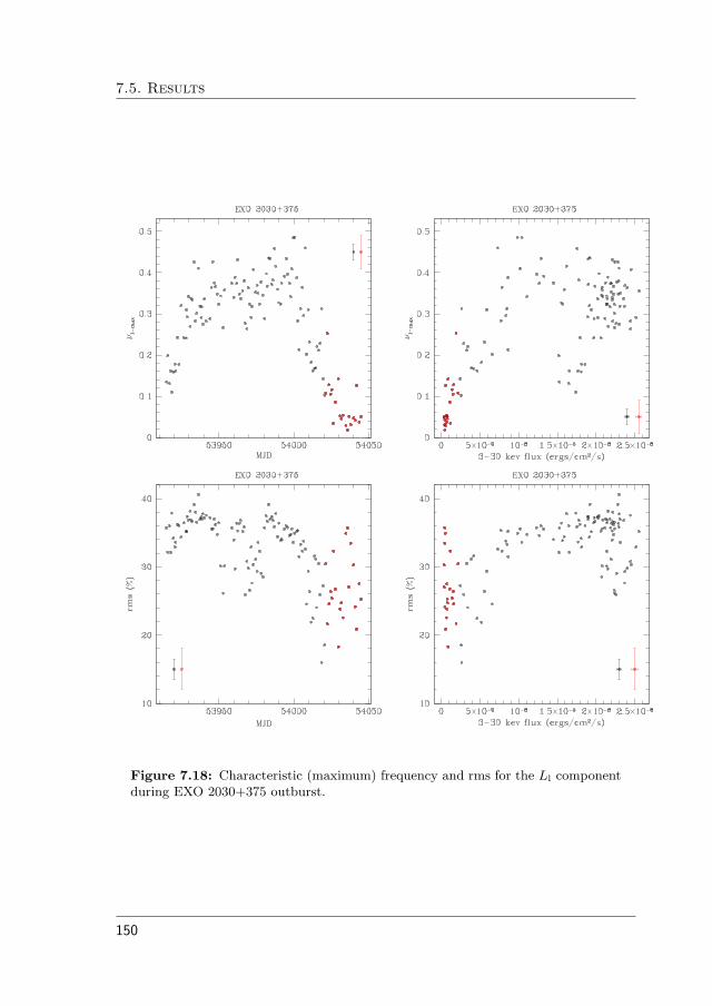
7.5. Results
Figure 7.18: Characteristic (maximum) frequency and rms for the Ll componentduring EXO 2030+375 outburst.
150
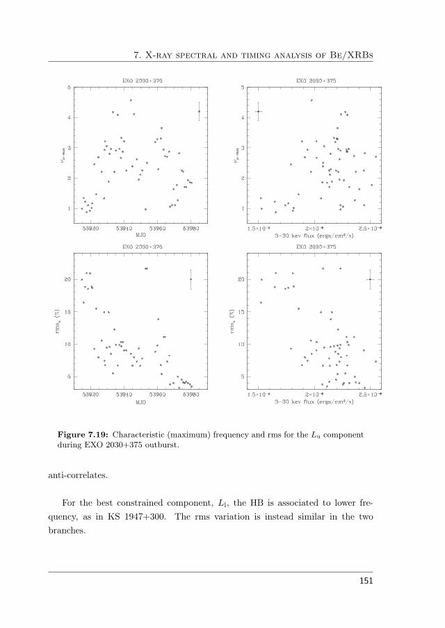
7. X-ray spectral and timing analysis of Be/XRBs
Figure 7.19: Characteristic (maximum) frequency and rms for the Lu componentduring EXO 2030+375 outburst.
anti-correlates.
For the best constrained component, Ll, the HB is associated to lower fre-quency, as in KS 1947+300. The rms variation is instead similar in the twobranches.
151

7.5. Results
Figure 7.20: Characteristic (maximum) frequency νl vs. spectral parameters dur-ing EXO 2030+375 outburst.
Figure 7.21: Correlation between the characteristic frequencies of the three timingcomponents.
152

7. X-ray spectral and timing analysis of Be/XRBs
In Fig. 7.20 the relation between the characteristic frequency νl and the spec-tral parameters (spectral index, cutoff) is shown. No clear correlations can beestablished in this case.
In Fig. 7.21 we show correlations between the characteristic frequencies of thethree timing components, νl, νu and νu� .
7.5.3 4U 0115+63
The total duration of the outburst was ∼55 days, the shortest among the sourcesanalyzed in this work. The rise covered by RXTE data was shorter than thedecay (∼6 days vs. ∼35 days). The brightest phase of the outburst displays adouble-peak profile and lasted for ∼9 days. The maximum X-ray luminosity wasreached at MJD ∼ 53262 and amounted to 1.4× 1038 erg s−1.
Spectral analysis
The retrieved 3–30 keV flux is shown in Fig. 7.22.The energy spectrum is known to be complicated by a fundamental and up
to four harmonics CRSFs. In the energy range considered in this work, namely3–30 keV, not only the fundamental at 11 keV but also the first harmonic of thecyclotron line distort the spectral continuum. We obtained the best fit by usingin this case the CYCLABS component in XSPEC (Mihara et al. 1990), describedby the following profile:
I(E) =�− τf
(σfE/Ec)2
(E − Ec)2 + σ2f
+ τ2h(σ2hE/2Ec)2
(E − 2Ec)2 + σ22h
�,
where τf is the optical depth of the fundamental; Ec is the cyclotron energy inkeV; σf is the width of the fundamental in keV; τ2h is the optical depth of thefirst harmonic; σ2h is the width of the first harmonic. This component, analogousin profile to the GABS component, simultaneously accounts for the fundamentaland its first harmonic. The central energy of the first harmonic is not a free pa-rameter, being fixed, in this model, to the double of the fundamental.
153

7.5. Results
Figure 7.22: Integrated 3–30 keV flux for 4U 0115+63.
In Fig. 7.23 we show the HID, CD and colors trends during the outburst. TheSC and HC follow a trend similar to that of KS 1947+300 and EXO 2030+375:in the DB, the HC correlates with flux and the SC anti-correlates with it; in theHB both colors anti-correlate with flux. For this source as well, we identified twospectral branches in the HID/CD. Moreover, we found that the system exhibitshysteresis both in the HID and in the CD. It means that points corresponding toobservations of the rising phase of the outburst (black points) are shifted in colorcompared with those of the decay phase (green points), despite that the flux issimilar. For similar values of flux, during the decay the emission is softer thanduring the rise. This effect was also present in EXO 2030+375, although not assignificant as for this source.
154

7. X-ray spectral and timing analysis of Be/XRBs
Figure 7.23: HID, CD and colors behavior during 4U 0115+63 outburst. Greenpoints correspond to the decay phase, before the HB. Black error bars apply toboth black and green points.
155

7.5. Results
Figure 7.24: High-energy cutoff power law behavior during 4U 0115+63 outburst.
Energy spectra were fitted by a model constituted by photoelectric absorption,a power law with high-energy cutoff and a cyclotron absorption feature with twoharmonics. The photoabsorption was left free to vary along the outburst, with aretrieved value of 0.9–1.5 ×1022 cm−2, consistent with recent results by Ferrignoet al. (2009). It was eventually fixed at 0.9 ×1022 cm−2 for all the observations.
In Fig. 7.24 we show the behavior of the two spectral parameters of the power
156

7. X-ray spectral and timing analysis of Be/XRBs
law component, i.e. the spectral index Γ and the cutoff energy. On the left side,their trend with time is shown, while on the right side their evolution with fluxis reported. Again, for the spectral index we found correlation with flux in theDB and anti-correlation in the HB, like in the previously analyzed systems. Thecutoff anti-correlates with flux in both states. We illustrate the relation betweenthe two parameters in Fig. 7.25.
Figure 7.25: Relation between the spectral index and the cutoff energy.
In Fig. 7.26 the behavior of the Fe line with time (left panel) and flux (rightpanel) is displayed. During the fit, the width of the line was fixed at 0.5 keV.The normalization of the component correlates with flux. With an average valueof 0.1±0.05, the equivalent width of the line is constant along the outburst.
We show in Fig. 7.27 the trend followed by the parameters characterizingthe cyclotron feature (first harmonic). The fundamental energy varies along theoutburst mainly between 10.5 and 17.5 keV, confirming results by Tsygankovet al. (2007). Its average optical depth varies between 0.2–0.5, while the linewidth varies between 2–11 keV. In 4U 0115+63 the CRSF firmly marks the twosource states. In the DB, the central energy varies by ∼10% and it shows the
157

7.5. Results
Figure 7.26: Fe fluorescence line during 4U 0115+63 outburst.
158

7. X-ray spectral and timing analysis of Be/XRBs
Figure 7.27: Cyclotron line parameters during 4U 0115+63 outburst.
159

7.5. Results
lower values; in the HB, it varies with time by 17%, from lower to higher values.In the HB the highest values are retrieved. Anti-correlation with flux is shownin the HB, while no change is observed in the DB. The optical depth also showsthe largest variation during the HB; it correlates with flux during the HB andanti-correlates during the DB. The same behavior is followed by the line width.A first harmonic is needed in order to obtain acceptable fits.
Timing analysis
The power spectra were fitted with the sum of, at most, four Lorentzians. Thelow-frequency noise is accounted for by Lb, whose fitted characteristic frequencyis always < 0.02 Hz. This component is present along the whole outburst, withthe exception of the first two observations (corresponding to a X-ray luminosityof 7–9 × 1037 erg s−1), where its inclusion did not lead to a better fit. Like forthe other sources, due to the very low characteristic frequency of this component,this is generally poorly constrained. Ll describes the noise below 1 Hz and, likein the other systems, is constantly present along the outburst. Its characteristicfrequency displays a variation between 0.1–1.2 Hz. Lu accounts for the high-frequency noise, with νu ∼ 0.7–2.1 Hz. It appears very close to the beginning ofthe outburst (MJD = 53267.2 ) and remains detectable only in the few observa-tions of the very bright phase (MJD = 53278.6), in correspondence of the DB.
In addition to the aforementioned broad noise components, a peaked noisecomponent is also present, LLF. We will refer to this as a QPO, although the Qvalue is not always larger than 2. In fact, at the very beginning of the outburst,this is a zero-centered broad component (Q = 0), which evolves into a QPO afterthe first 4 observations (MJD = 53262.1). Its characteristic frequency varies be-tween 0.03–0.16 Hz. We found evidence for this component in the entire DB andin only two observations of the HB.
We show in Fig. 7.28 the evolution of νl and the corresponding rms duringthe outburst. The characteristic frequency of the Ll component displays a ratherclear correlation with flux, with lower values at the end of the outburst and highervalues at its peak; the rms varies between 10%–31%, showing the strongest vari-ability in the HB. While it is constant on average in the DB, it exhibits a pro-
160

7. X-ray spectral and timing analysis of Be/XRBs
Figure 7.28: Characteristic (maximum) frequency and rms for the Ll componentduring 4U 0115+63 outburst.
nounced anti-correlation with flux during the HB: the strongest power for thiscomponent is given at the very end of the outburst, like for KS 1947+300. Forboth parameters we found evidence of two distinct trends during the two branches.
In Fig. 7.29 we show the evolution of νLF and the corresponding rms. No cleartrend can be invoked in this case.
161
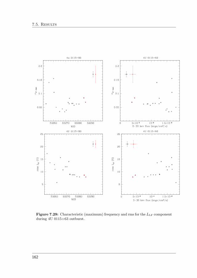
7.5. Results
Figure 7.29: Characteristic (maximum) frequency and rms for the LLF componentduring 4U 0115+63 outburst.
162

7. X-ray spectral and timing analysis of Be/XRBs
In Fig. 7.30 we show the relation between spectral and timing fit parameters.No correlations are found. Also, in this case no marked distinction emerges be-tween the DB and the HB, with the exception of the plot of νl vs. the centralenergy of the cyclotron absorption line: here the two branches are distinguishable,with low values of νl associated to large values of the cyclotron energy and viceversa.
Figure 7.30: Timing vs. spectral fit parameters during 4U 0115+63 outburst.
163
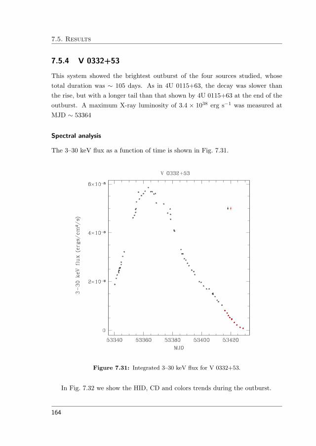
7.5. Results
7.5.4 V 0332+53
This system showed the brightest outburst of the four sources studied, whosetotal duration was ∼ 105 days. As in 4U 0115+63, the decay was slower thanthe rise, but with a longer tail than that shown by 4U 0115+63 at the end of theoutburst. A maximum X-ray luminosity of 3.4 × 1038 erg s−1 was measured atMJD ∼ 53364
Spectral analysis
The 3–30 keV flux as a function of time is shown in Fig. 7.31.
Figure 7.31: Integrated 3–30 keV flux for V 0332+53.
In Fig. 7.32 we show the HID, CD and colors trends during the outburst.
164

7. X-ray spectral and timing analysis of Be/XRBs
Figure 7.32: HID, CD and colors behavior during V 0332+53 outburst. Greenpoints correspond to the decay phase, before the HB. Black error bars apply toboth black and green data points.
165
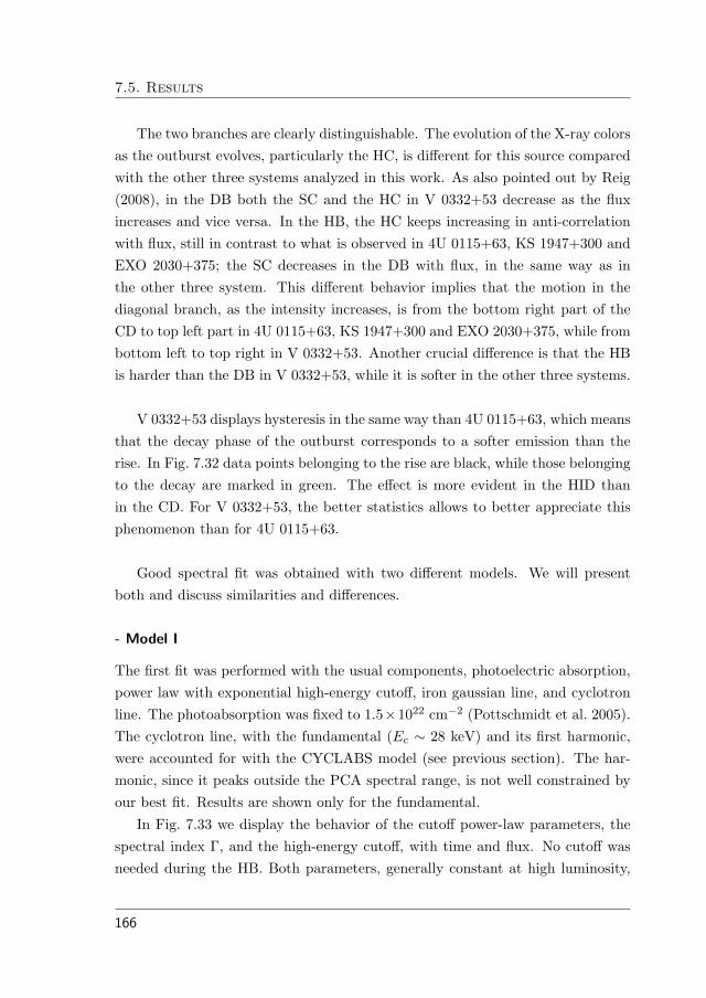
7.5. Results
The two branches are clearly distinguishable. The evolution of the X-ray colorsas the outburst evolves, particularly the HC, is different for this source comparedwith the other three systems analyzed in this work. As also pointed out by Reig(2008), in the DB both the SC and the HC in V 0332+53 decrease as the fluxincreases and vice versa. In the HB, the HC keeps increasing in anti-correlationwith flux, still in contrast to what is observed in 4U 0115+63, KS 1947+300 andEXO 2030+375; the SC decreases in the DB with flux, in the same way as inthe other three system. This different behavior implies that the motion in thediagonal branch, as the intensity increases, is from the bottom right part of theCD to top left part in 4U 0115+63, KS 1947+300 and EXO 2030+375, while frombottom left to top right in V 0332+53. Another crucial difference is that the HBis harder than the DB in V 0332+53, while it is softer in the other three systems.
V 0332+53 displays hysteresis in the same way than 4U 0115+63, which meansthat the decay phase of the outburst corresponds to a softer emission than therise. In Fig. 7.32 data points belonging to the rise are black, while those belongingto the decay are marked in green. The effect is more evident in the HID thanin the CD. For V 0332+53, the better statistics allows to better appreciate thisphenomenon than for 4U 0115+63.
Good spectral fit was obtained with two different models. We will presentboth and discuss similarities and differences.
- Model I
The first fit was performed with the usual components, photoelectric absorption,power law with exponential high-energy cutoff, iron gaussian line, and cyclotronline. The photoabsorption was fixed to 1.5×1022 cm−2 (Pottschmidt et al. 2005).The cyclotron line, with the fundamental (Ec ∼ 28 keV) and its first harmonic,were accounted for with the CYCLABS model (see previous section). The har-monic, since it peaks outside the PCA spectral range, is not well constrained byour best fit. Results are shown only for the fundamental.
In Fig. 7.33 we display the behavior of the cutoff power-law parameters, thespectral index Γ, and the high-energy cutoff, with time and flux. No cutoff wasneeded during the HB. Both parameters, generally constant at high luminosity,
166
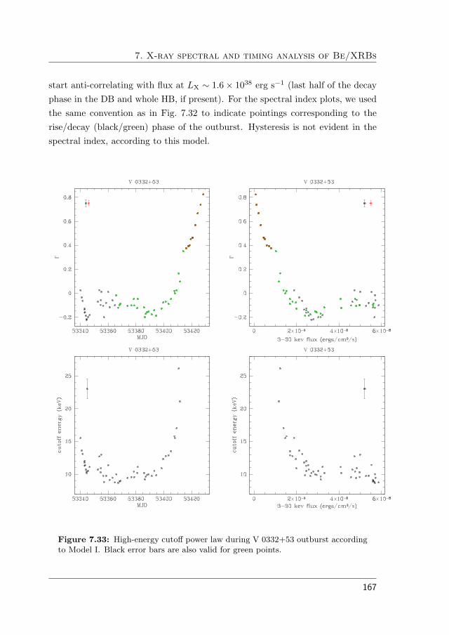
7. X-ray spectral and timing analysis of Be/XRBs
start anti-correlating with flux at LX ∼ 1.6× 1038 erg s−1 (last half of the decayphase in the DB and whole HB, if present). For the spectral index plots, we usedthe same convention as in Fig. 7.32 to indicate pointings corresponding to therise/decay (black/green) phase of the outburst. Hysteresis is not evident in thespectral index, according to this model.
Figure 7.33: High-energy cutoff power law during V 0332+53 outburst accordingto Model I. Black error bars are also valid for green points.
167

7.5. Results
We illustrate the relation between the two parameters in Fig. 7.34.
Figure 7.34: Relation between the spectral index and the cutoff energy (ModelI).
In Fig. 7.35 the behavior of the Fe line with time (left panel) and flux (rightpanel) is presented. Also for this system, the line width was fixed at 0.5 keV.The line energy shows very little variation during the outburst, with an averagevalue of ∼ 6.5 keV. In the HB, this feature is very weak and its energy was fixedat 6.4 keV in the last observations. The corresponding pointings are not shownin the plot of the line energy. Like in the other systems studied in this work, thenormalization correlates with flux. Since the relation is almost 1:1, the EW isgenerally constant.
We show in Fig. 7.36 the trend followed by the parameters characterizing thecyclotron feature (first harmonic). The fundamental energy varies along the out-burst between 23 and 28 keV, confirming results by Tsygankov et al. (2009). Itsoptical depth varies between 1.4 and 3, while the width varies between 3.5–9.3keV. The central energy shows a strong anti-correlation with flux, as also pointedout by Tsygankov et al. (2009). This behavior is common to the two branches.
168
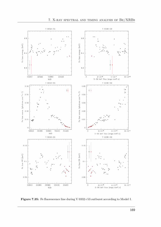
7. X-ray spectral and timing analysis of Be/XRBs
Figure 7.35: Fe fluorescence line during V 0332+53 outburst according to Model I.
169

7.5. Results
Figure 7.36: Cyclotron line parameters during V 0332+53 outburst according toModel I.
170

7. X-ray spectral and timing analysis of Be/XRBs
The optical depth and the line width correlate with flux in the HB and anti-correlate with it in the DB, similarly to what we observed for 4U 0115+63.
- Model II
As a test, a good fit was also obtained without exponential cutoff. The remainingcomponents were the same as Model I. Again, the photoabsorption was fixed to1.5 × 1022 cm−2. The cyclotron line (fundamental and first harmonic) was ac-counted for with the CYCLABS model. Also in this case, results are shown onlyfor the fundamental. The spectral range we employed in this case was limitedbetween 3–30 keV, in order to use best signal-to-noise data.
In Fig. 7.37 we display the behavior of the spectral index Γ, with time andflux. With this model, the trend of the spectral index is clearly different in the twobranches. It anti-correlates with flux in the HB and correlates with it in the DB,displaying a behavior common to all the systems analyzed in this work. Hysteresisis evident, using this model, in the spectral index trend, which is generally softerduring the decay of the outburst, in accordance with the HID (see Fig.7.32).
Figure 7.37: Spectral index behavior during V 0332+53 outburst according toModel II. Black error bars are also valid for green points.
171

7.5. Results
Figure 7.38: Cyclotron line parameters during V 0332+53 outburst according toModel II..
172

7. X-ray spectral and timing analysis of Be/XRBs
The main difference in comparison with Model I is found with respect to thecentral energy of the CRSF. This is displayed in Fig. 7.38, together with the otherparameters of the feature.
The fundamental energy varies along the outburst between 23.5 and 30.5 keV.The optical depth varies between 1 and 4, while the width varies between 3–16keV. All the three parameters reach slightly higher values than with Model I. Asa general trend, in the DB the central energy shows a strong anti-correlation withflux, like with Model I. The final phase of the DB marks a change in this trend,as this starts displaying a correlation with flux as the emission gets fainter; thesame effect is also displayed by the optical depth. In the DB, τ does not showany specific behavior, while in the HB it correlates with flux. The line width onaverage correlates with flux along the whole outburst.
The two main spectral features, the power law and the cyclotron line, bothfollow different trends with the two models. With Model I, the range of vari-ation of the spectral index is higher, and also covers negative values. At lowluminosities, with both models Γ anti-correlates with flux, but with a substantialdifference: with Model II the HB marks the turning point, while with Model Ithe anti-correlation starts in the middle of the decay phase of the DB. Moreover,no hysteresis is found with Model I, while general softer spectral indexes are re-trieved for the decay than for the rise of the outburst with Model II. This is indeedexpected from the HID.
However, the most remarkable divergence between the two models is repre-sented by the cyclotron feature. With Model I, the central energy of the lineshows a variation of 19% in the DB and is roughly constant in the HB. In thiscase, during the whole outburst the central energy anti-correlates with flux. Ac-cording to Model II, the line energy varies instead in anti-correlation with fluxat high luminosity, and in correlation at low luminosity. This could be explainedif the accretion took place within two different regimes (super-Eddington andsub-Eddington limits, see also Staubert et al. 2007, and Sect. 7.6.2). Althoughnot well constrained due to its central energy, which peaks at ∼ 50 keV, a firstharmonic is needed to obtain good fits.
173

7.5. Results
Timing analysis
The power spectra were fitted with the sum of up to four Lorentzians. The low-frequency noise is accounted for by Lb, whose fitted characteristic frequency isalways < 0.02 Hz. This component is present along the whole outburst, with theexception of the first ∼10 day observations of the decay phase (53374.0 < MJD< 53385.8). Like for the other sources, due to the very low characteristic fre-quency of this component, this is generally poorly constrained. Ll describes thenoise below 1 Hz and is constantly present along the outburst. Its characteristicfrequency varies between 0.09–1.94 Hz.
In addition to the broad noise components, two peaked noise components arealso present, LLF and Ls. As for 4U 0115+63, we will refer to these as QPOs,although the Q value is not always larger than 2. LLF, with a characteristic fre-quency variable between 0.01–0.09 Hz, is observable along the whole outburst. Ls
has a characteristic frequency coinciding with the frequency of the fundamentalpeak (0.23 Hz) of the pulse period and remains roughly constant throughout theoutburst. It is not present during the HB and in the last 5 observations of theDB. In contrast with 4U 0115+63, when present, both components are peakedsince the beginning until the end of the outburst, not constituting the evolution-ary stage from a broad component.
We show in Fig. 7.39 the evolution of νl and the corresponding rms duringthe outburst. Like for 4U 0115+63, the characteristic frequency of the Ll com-ponent correlates with flux, with lower values at the beginning and at the endof the outburst and higher values at its peak; the rms, instead, during the DBanti-correlates with flux: the strongest power for this component is given at theend of the DB, then it starts decreasing. For both parameters we found evidenceof two distinct trends during the two branches. The characteristic frequency νl
is almost constant in the HB and shows the lower values; the corresponding rmsshows the higher values in the HB, when it starts decreasing, in correlation withflux.
In Fig. 7.40, the evolution of νLF and the corresponding rms during the out-burst is presented.
174

7. X-ray spectral and timing analysis of Be/XRBs
Figure 7.39: Characteristic (maximum) frequency and rms for the Ll componentduring V 0332+53 outburst.
175
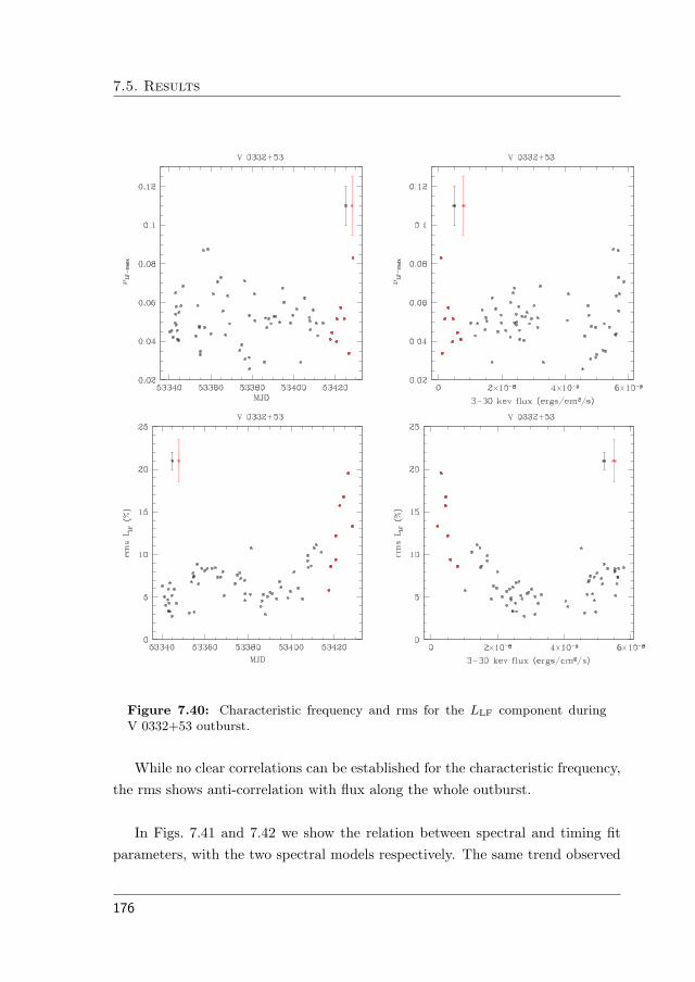
7.5. Results
Figure 7.40: Characteristic frequency and rms for the LLF component duringV 0332+53 outburst.
While no clear correlations can be established for the characteristic frequency,the rms shows anti-correlation with flux along the whole outburst.
In Figs. 7.41 and 7.42 we show the relation between spectral and timing fitparameters, with the two spectral models respectively. The same trend observed
176

7. X-ray spectral and timing analysis of Be/XRBs
Figure 7.41: Timing vs. spectral fit parameters during V 0332+53 outburst usingspectral Model I.
Figure 7.42: The same as Fig. 7.41, with spectral Model II.
for νl vs. the cyclotron line energy in 4U 0115+63 is displayed here in all the threecases (νl vs. Γ, the cyclotron energy, τ). To lower values of the spectral parametercorrespond a high range of retrieved νl and vice versa.
177

7.6. Discussion
7.6 Discussion
7.6.1 Source states in HMXBs
In the previous section several common behaviors among the four systems aroseand two distinct source states became evident. Here we try to describe moresystematically what emerges from our work by comparing the results from thefour systems. Our final goal is to provide a characterization of source states inHMXBs, from color, spectral and timing point of view.
Color features
In all the four systems studied in this work, two distinct branches or spectral statescan be distinguished in the HID/CD. We shall refer to them as the diagonalbranch (DB) and horizontal branch (HB) according to the shape they trace inthe HID/CD. The diagonal branch corresponds to high-intensity flux and thehorizontal branch to low-intensity flux. The DB is where the sources spend most ofthe time during the outbursts (70%-80% of the total duration). Typical timescalesare months in the DB and weeks in the HB.
From our data set, the horizontal branch contains points both from the verybeginning and from the end of the outburst only for KS 1947+300, while for theother three systems, since the PCA monitoring began when the outbursts werealready in progress, only observations from the end of the outbursts are included.From KS 1947+300 data, it is reasonable to assume that the general propertyof the HB is to describe low-flux observations, regardless of whether they belongto the beginning or the end of the outburst, marking the HB the start and theend point of the source in its journey through the CD/HID while the outburstproceeds.
The transition between states takes place at LX ∼10% of the peak value inKS 1947+300, EXO 2030+375 and V 0332+53. For 4U 0115+63, this change isobserved at a higher ratio, LX = 25% of the peak value.
The two branches are recognizable in both CD and HID, as often is observedfor LMXBs states, although the HID gives a clearer pattern than the CD forKS 1947+300 and EXO 2030+375. These two systems have, on average, a softer
178

7. X-ray spectral and timing analysis of Be/XRBs
spectrum in the HB than 4U 0115+63 and V 0332+53. This translates into largeruncertainties in the X-ray colors (especially the hard color) for KS 1947+300 andEXO 2030+375 in the HB. However, when the hard color is replaced by intensity,in the HID, the HB is well depicted in all the four systems.
The soft color shows the same pattern in all the four systems, anti-correlatingwith flux during the DB and correlating in the HB. The hard color distinguishesV 0332+53 from the other three sources. In fact, while we observe a generalcorrelation between the hard color and flux in KS 1947+300, EXO 2030+375 and4U 0115+63, the trend sketched by V 0332+53 is of anti-correlation, with thehard color decreasing in the first part of the outburst until the outburst peak,and subsequently increasing until the end. As pointed out in Sect. 7.5.4, thisimplies that the motion in the diagonal branch, as the intensity increases, is fromthe bottom right part of the CD to top left part in 4U 0115+63, KS 1947+300and EXO 2030+375, while from bottom left to top right in V 0332+53. Anothercrucial difference is that the HB is harder than the DB in V 0332+53, while itis softer in 4U 0115+63, KS 1947+300 and EXO 2030+375. In this sense, in thelast three systems, the horizontal branch represents a low-soft branch (in termsof hard color), a state that is not seen in LMXBs or in black-hole binaries, wherelow-intensity states correspond to hard spectra.
4U 0115+63 and V 0332+53 display hysteresis both in the HID and in the CD(see Figs. 7.23 and 7.32). This means that points corresponding to observationsof the rising phase of the outburst are shifted in color in comparison with those ofthe decay phase, despite that the flux is similar. For similar values of flux, duringthe decay the emission is softer than during the rise.
Spectral features
Also, according to the spectral parameters retrieved from best fits, the two branchesare always distinguishable. We present in Table 7.3 the range of variability of thespectral parameters and of the X-ray luminosity in the two branches. See Ap-pendix A for the full retrieved set of spectral fit parameters.
For each system, in Figs. 7.43, 7.44, 7.45 and 7.46 typical energy spectra cor-
179

7.6. Discussion
Table 7.3: Average main spectral parameters and LX during the outburst forthe four systems analyzed in this work. For each source, we defined a lower andand upper DB (l. DB and u. DB respectively, in the table) according to luminosityranges indicated in the last line. For V 0332+53, only the “standard” fit withModel I is shown. The retrieved χ2
red was between 0.6–1.9.
Parameter Branch KS 1947+300 EXO 2030+375 4U 0115+63 V 0332+53 (I)
Γ u. DB 1.0±0.1 1.18±0.08 0.37±0.03 -0.10±0.06l. DB 0.5±0.2 0.85±0.11 0.24±0.06 -0.07±0.13HB 0.6±0.2 1.15±0.12 0.52±0.15 0.53±0.16
Cutoff u. DB 23.4±5.4 18.9±1.6 8.5±0.2 14.5±3.5energy (keV) l. DB 12.4±2.6 13.5±1.7 8.7±0.2 9.7±8.7
HB 11.3±2.3 14.6±2.3 9.3±0.5 –
Cyclotron line u. DB – 9.60±0.04 11.0±0.2(∗) 24.9±1.0(∗)energy (keV) l. DB – – 10.7±0.1 27.0±0.4(∗)
HB – – 16.0±0.9 28±0.2(∗)
τ u. DB – 1.36±0.03 0.32±0.05 1.8±0.2l. DB – – 0.40±0.05 2.1±0.2HB – – 0.4±0.1 2.6±0.1
Cyclotron line u. DB – 4.03±0.06 4.0±0.9 7.8±0.5width (keV) l. DB – – 5.2±2.5 7.3±0.5
HB – – 6.2±2.2 6.4±1.8
LX u. DB 2.7–7.1 8.0–15.4 11.5–13.7 16.9–33.9(1037 erg s−1) l. DB 0.3–2.8 1.5–7.8 5.7–10.0 6.4–16.4
HB 0.1–0.3 0.2–1.3 0.7–3.5 0.4–4.7
(∗) Besides the fundamental, in these systems also the first harmonic is needed in orderto fit the energy spectra
responding to different X-ray luminosity are shown2. The additive model compo-nents are shown (power law and iron fluorescence line) with dashed lines, whilethe resulting model is marked by a solid line. Below each panel, the correspondingresiduals after fitting are displayed.
2The complete set of fitted energy spectra and PSD is available at the following URL:
http://www.uv.es/∼nese/spectra.pdf
180
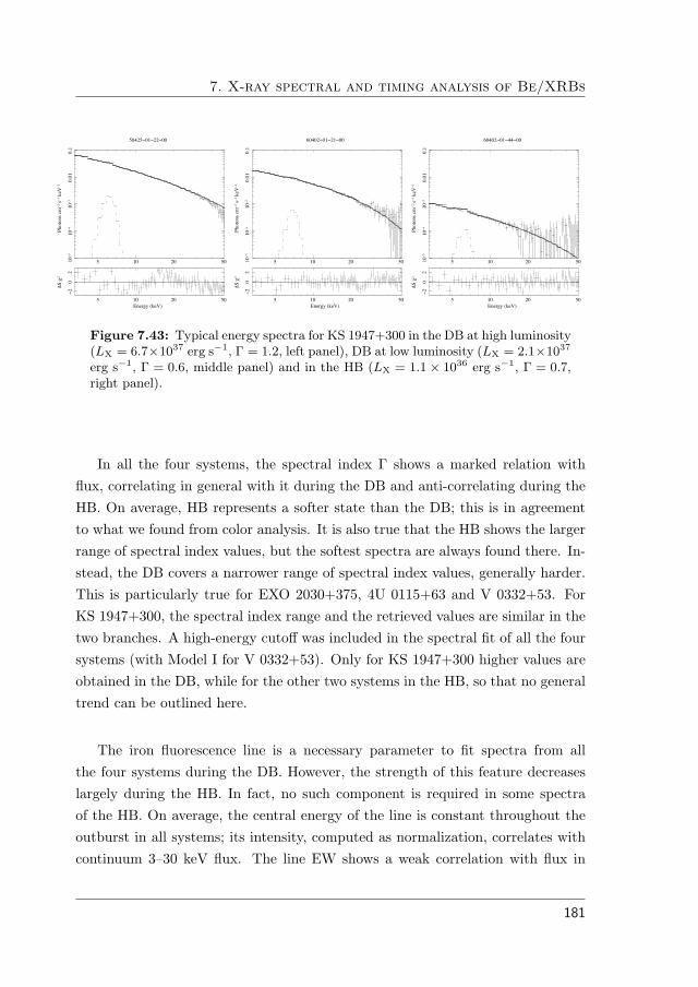
7. X-ray spectral and timing analysis of Be/XRBs
!"# $" #"!"#
!"%
!"&
"'"!
"'!
()*+*,-./0
$ .-! .123
!
#"%$# "! $$ ""
!"# $" #"!"#
!"%
!"&
"'"!
"'!
()*+*,-./0
$ .-! .123
!
4"%"$ "! $! ""
!"# $" #"!"#
!"%
!"&
"'"!
"'!
()*+*,-./0
$ .-! .123
!
4"%"$ "! %% ""
!"# $" #"
$"
$
%&$
'()*+,&-.)/0!"# $" #"
$"
$
%&$
'()*+,&-.)/0!"# $" #"
$"
$
%&$
'()*+,&-.)/0
Figure 7.43: Typical energy spectra for KS 1947+300 in the DB at high luminosity(LX = 6.7×1037 erg s−1, Γ = 1.2, left panel), DB at low luminosity (LX = 2.1×1037
erg s−1, Γ = 0.6, middle panel) and in the HB (LX = 1.1 × 1036 erg s−1, Γ = 0.7,right panel).
In all the four systems, the spectral index Γ shows a marked relation withflux, correlating in general with it during the DB and anti-correlating during theHB. On average, HB represents a softer state than the DB; this is in agreementto what we found from color analysis. It is also true that the HB shows the largerrange of spectral index values, but the softest spectra are always found there. In-stead, the DB covers a narrower range of spectral index values, generally harder.This is particularly true for EXO 2030+375, 4U 0115+63 and V 0332+53. ForKS 1947+300, the spectral index range and the retrieved values are similar in thetwo branches. A high-energy cutoff was included in the spectral fit of all the foursystems (with Model I for V 0332+53). Only for KS 1947+300 higher values areobtained in the DB, while for the other two systems in the HB, so that no generaltrend can be outlined here.
The iron fluorescence line is a necessary parameter to fit spectra from allthe four systems during the DB. However, the strength of this feature decreaseslargely during the HB. In fact, no such component is required in some spectraof the HB. On average, the central energy of the line is constant throughout theoutburst in all systems; its intensity, computed as normalization, correlates withcontinuum 3–30 keV flux. The line EW shows a weak correlation with flux in
181
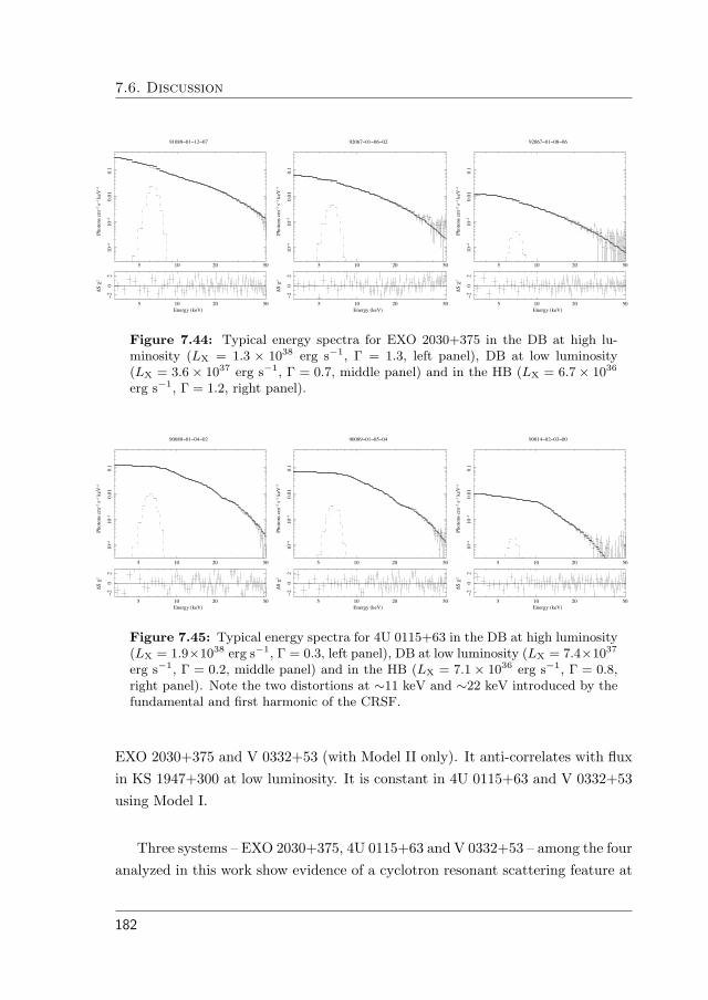
7.6. Discussion
!"# $" #"
!"%
!"&
"'"!
"'!
()*+*,-./0
$ .-! .123
!
4!"54 "! !$ "6
!"# $" #"
!"%
!"&
"'"!
"'!
()*+*,-./0
$ .-! .123
!
4$"56 "! "5 "$
!"# $" #"
!"%
!"&
"'"!
"'!
()*+*,-./0
$ .-! .123
!
4$"56 "! "7 "5
!"# $" #"
$"
$
%&$
'()*+,&-.)/0!"# $" #"
$"
$
%&$
'()*+,&-.)/0!"# $" #"
$"
$
%&$
'()*+,&-.)/0
Figure 7.44: Typical energy spectra for EXO 2030+375 in the DB at high lu-minosity (LX = 1.3 × 1038 erg s−1, Γ = 1.3, left panel), DB at low luminosity(LX = 3.6× 1037 erg s−1, Γ = 0.7, middle panel) and in the HB (LX = 6.7× 1036
erg s−1, Γ = 1.2, right panel).
!"# $" #"
!"%
!"&
"'"!
"'!
()*+*,-./0
$ .-! .123
!
4""54 "! "% "$
!"# $" #"
!"%
!"&
"'"!
"'!
()*+*,-./0
$ .-! .123
!
4""54 "! "# "%
!"# $" #"
!"%
!"&
"'"!
"'!
()*+*,-./0
$ .-! .123
!
4""!% "$ "& ""
!"# $" #"
$"
$
%&$
'()*+,&-.)/0!"# $" #"
$"
$
%&$
'()*+,&-.)/0!"# $" #"
$"
$
%&$
'()*+,&-.)/0
Figure 7.45: Typical energy spectra for 4U 0115+63 in the DB at high luminosity(LX = 1.9×1038 erg s−1, Γ = 0.3, left panel), DB at low luminosity (LX = 7.4×1037
erg s−1, Γ = 0.2, middle panel) and in the HB (LX = 7.1 × 1036 erg s−1, Γ = 0.8,right panel). Note the two distortions at ∼11 keV and ∼22 keV introduced by thefundamental and first harmonic of the CRSF.
EXO 2030+375 and V 0332+53 (with Model II only). It anti-correlates with fluxin KS 1947+300 at low luminosity. It is constant in 4U 0115+63 and V 0332+53using Model I.
Three systems – EXO 2030+375, 4U 0115+63 and V 0332+53 – among the fouranalyzed in this work show evidence of a cyclotron resonant scattering feature at
182

7. X-ray spectral and timing analysis of Be/XRBs
!"# $"
!"%
!"&
"'"!
"'!
!
()*+*,-./0
$ .-! .123
!
4"%$5 "! "! "!
!"# $"
!"%
!"&
"'"!
"'!
!
()*+*,-./0
$ .-! .123
!
4""!% "! "& "!
!"# $"
!"%
!"&
"'"!
"'!
!
()*+*,-./0
$ .-! .123
!
4""!% "! "5 ""
!"# $"
$"
$
%&$
'()*+,&-.)/0!"# $"
$"
$
%&$
'()*+,&-.)/0!"# $"
$"
$
%&$
'()*+,&-.)/0
Figure 7.46: Typical energy spectra for V 0332+53 in the DB at high luminosity(LX = 3.3×1038 erg s−1, Γ = 0.4, left panel), DB at low luminosity (LX = 1.4×1038
erg s−1, Γ = 0.3, middle panel) and in the HB (LX = 7.1 × 1036 erg s−1, Γ = 0.7,right panel).
∼10 keV, ∼11 keV and ∼30 keV respectively. However, EXO 2030+375 spectraneed this feature only in the bright phase of the outburst; for this source, thecentral energy of the line shows no large variability, less than 10% in the majorpart of the observations. A fit to a constant gives a rms of residuals of 0.63 for thecentral energy, 0.29 for the optical depth and 0.55 for the line width, i.e. consistentwith no change for all the three parameters of the component. No harmonic isrequired for this system. In 4U 0115+63 and V 0332+53 the central energy of theline is higher in the HB than in the DB, which means that it is anti-correlated withflux, with higher values observed at lower flux. On average, the same behavioris shown by the optical depth. Both systems need, besides the fundamental, thefirst harmonic in order to obtain a good fit.
Timing features
After fitting the peaks of the pulse components with fixed Lorentzians for eachsource, the power-spectra of Be/X-ray binaries are characterized by band-limitednoise (BLN). All the spectra analyzed in this work were conveniently fitted withthe sum of a small number of Lorentzians. Ignoring the peaks of the pulse com-ponents, for each system, 2–4 Lorentzian profiles are needed to obtain acceptablefits. Considering all the systems, we identified six different types of noise compo-nents, four of which are band-limited (Lb, Ll, Lu, Lu�) and two are QPOs (LLF
183
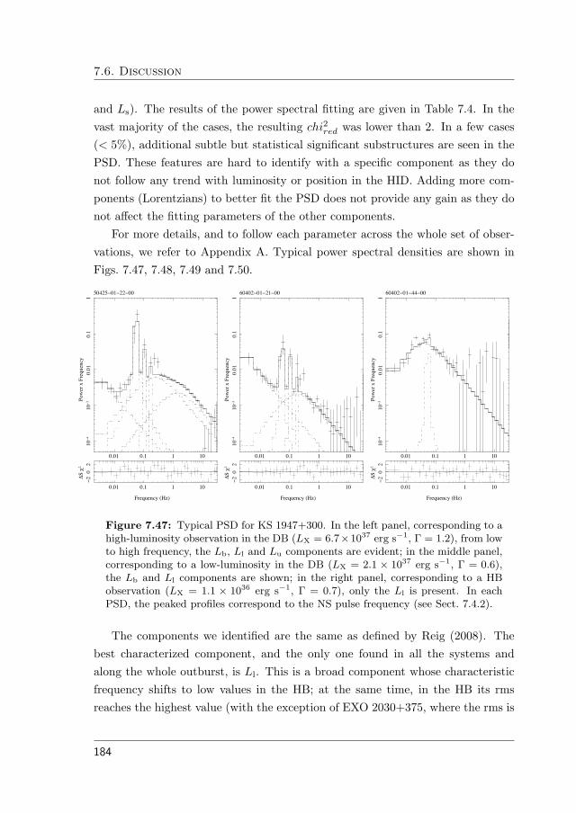
7.6. Discussion
and Ls). The results of the power spectral fitting are given in Table 7.4. In thevast majority of the cases, the resulting chi
2red
was lower than 2. In a few cases(< 5%), additional subtle but statistical significant substructures are seen in thePSD. These features are hard to identify with a specific component as they donot follow any trend with luminosity or position in the HID. Adding more com-ponents (Lorentzians) to better fit the PSD does not provide any gain as they donot affect the fitting parameters of the other components.
For more details, and to follow each parameter across the whole set of obser-vations, we refer to Appendix A. Typical power spectral densities are shown inFigs. 7.47, 7.48, 7.49 and 7.50.
!"!# !"# # #!
#!$
#!%
!"!#
!"#
#&'()*+,+-*)./)012
3!$43 !# 44 !!
!"!# !"# # #!
#!$
#!%
!"!#
!"#
#&'()*+,+-*)./)012
3!$!4 !# 4# !!
!"!# !"# # #!
#!$
#!%
!"!#
!"#
#&'()*+,+-*)./)012
3!$!4 !# $$ !!
!"!# !"# # #!
$!$
%&$
'()*+),-.&/012
!"!# !"# # #!
$!$
%&$
'()*+),-.&/012
!"!# !"# # #!
$!$
%&$
'()*+),-.&/012
Figure 7.47: Typical PSD for KS 1947+300. In the left panel, corresponding to ahigh-luminosity observation in the DB (LX = 6.7×1037 erg s−1, Γ = 1.2), from lowto high frequency, the Lb, Ll and Lu components are evident; in the middle panel,corresponding to a low-luminosity in the DB (LX = 2.1 × 1037 erg s−1, Γ = 0.6),the Lb and Ll components are shown; in the right panel, corresponding to a HBobservation (LX = 1.1 × 1036 erg s−1, Γ = 0.7), only the Ll is present. In eachPSD, the peaked profiles correspond to the NS pulse frequency (see Sect. 7.4.2).
The components we identified are the same as defined by Reig (2008). Thebest characterized component, and the only one found in all the systems andalong the whole outburst, is Ll. This is a broad component whose characteristicfrequency shifts to low values in the HB; at the same time, in the HB its rmsreaches the highest value (with the exception of EXO 2030+375, where the rms is
184

7. X-ray spectral and timing analysis of Be/XRBs
Table 7.4: Range of variability of the timing features during the outburst forthe four systems analyzed in this work. For each spectral branch and for eachcomponent, the corresponding characteristic frequency and rms are shown.
Feature Branch KS 1947+300 EXO 2030+375 4U 0115+63 V 0332+53
Lb ν (Hz) u. DB < 0.01 – < 0.01 < 0.02l. DB < 0.01 – < 0.01 < 0.01HB – – < 0.01 < 0.03
rms (%) u. DB 14±5 – 25±21 55±101l. DB 19±12 – 21±19 78±117HB – – 41±40 56±49
Ll ν (Hz) u. DB 0.23±0.05 0.32±0.08 0.8±0.2 0.93±0.54l. DB 0.18±0.08 0.30±0.06 0.6±0.2 0.35±0.10HB 0.05±0.01 0.08±0.06 0.21±0.05 0.13±0.02
rms (%) u. DB 20±1 35±3 15±3 10±3l. DB 22±9 30±6 13.6±1.7 15±3HB 44±13 27±5 26±4 25±7
Lu ν (Hz) u.DB 1.6±0.6 2.3±0.9 1.0±0.3 –l. DB – – 1.8±0.3 –HB – – – –
rms (%) u. DB 11±2 10±5 10.7±1.6 –l. DB – – 6.1±1.6 –HB – – – –
Lu� ν (Hz) u. DB – 4.9±1.6 – –l. DB – 2.6±1.3 – –HB – – – –
rms (%) u. DB – 7±3 – –l. DB – 13±5 – –HB – – – –
LLF ν (Hz) u. DB – – 0.07±0.04 0.05±0.02l. DB – – 0.07±0.02 0.051±0.008HB – – 0.08±0.01 0.05±0.01
rms (%) u. DB – – 12±3 6±2l. DB – – 10±3 6±2HB – – 8.2±0.5 12±4
Ls ν (Hz) u. DB – – – 0.25±0.01l. DB – – – 0.23±0.02HB – – – –
rms (%) u. DB – – – 6.4±1.4l. DB – – – 6±3HB – – – –
LX u. DB 2.7–7.1 8.0–15.4 11.5–13.7 16.9–33.9(1037 erg s−1) l. DB 0.3–2.8 1.5–7.8 5.7–10.0 6.4–16.4
HB 0.1–0.3 0.2–1.3 0.7–3.5 0.4–4.7
185
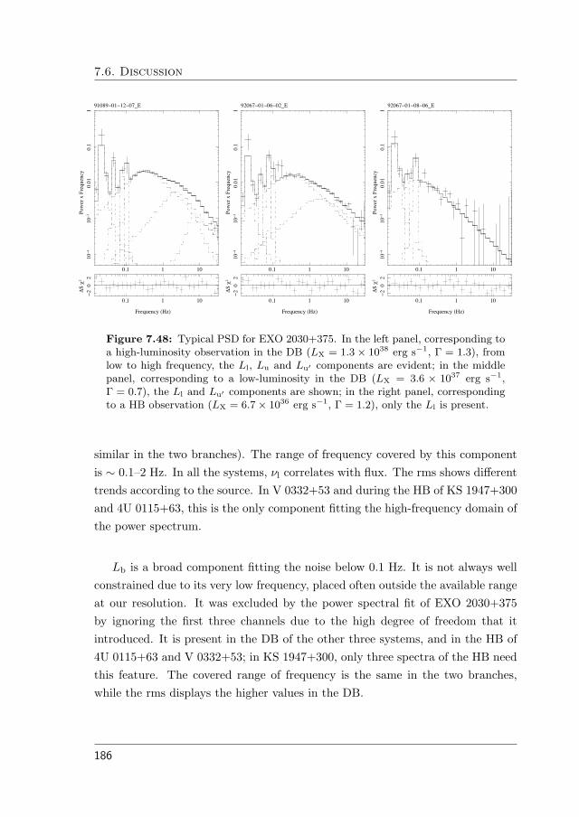
7.6. Discussion
!"# # #!
#!$
#!%
!"!#
!"#
#&'()*+,+-*)./)012
3#!43 !# #5 !678
!"# # #!
#!$
#!%
!"!#
!"#
#&'()*+,+-*)./)012
34!56 !# !5 !478
!"# # #!
#!$
#!%
!"!#
!"#
#&'()*+,+-*)./)012
34!56 !# !7 !589
!"# # #!
$!$
%&$
'()*+),-.&/012
!"# # #!
$!$
%&$
'()*+),-.&/012
!"# # #!
$!$
%&$
'()*+),-.&/012
Figure 7.48: Typical PSD for EXO 2030+375. In the left panel, corresponding toa high-luminosity observation in the DB (LX = 1.3× 1038 erg s−1, Γ = 1.3), fromlow to high frequency, the Ll, Lu and Lu� components are evident; in the middlepanel, corresponding to a low-luminosity in the DB (LX = 3.6 × 1037 erg s−1,Γ = 0.7), the Ll and Lu� components are shown; in the right panel, correspondingto a HB observation (LX = 6.7× 1036 erg s−1, Γ = 1.2), only the Ll is present.
similar in the two branches). The range of frequency covered by this componentis ∼ 0.1–2 Hz. In all the systems, νl correlates with flux. The rms shows differenttrends according to the source. In V 0332+53 and during the HB of KS 1947+300and 4U 0115+63, this is the only component fitting the high-frequency domain ofthe power spectrum.
Lb is a broad component fitting the noise below 0.1 Hz. It is not always wellconstrained due to its very low frequency, placed often outside the available rangeat our resolution. It was excluded by the power spectral fit of EXO 2030+375by ignoring the first three channels due to the high degree of freedom that itintroduced. It is present in the DB of the other three systems, and in the HB of4U 0115+63 and V 0332+53; in KS 1947+300, only three spectra of the HB needthis feature. The covered range of frequency is the same in the two branches,while the rms displays the higher values in the DB.
186

7. X-ray spectral and timing analysis of Be/XRBs
!"!# !"# # #!
#!$
#!%
!"!#
!"#
#&'()*+,+-*)./)012
3!!43 !# !$ !5
!"!# !"# # #!
#!$
#!%
!"!#
!"#
#&'()*+,+-*)./)012
3!!43 !# !5 !$
!"!# !"# # #!
#!$
#!%
!"!#
!"#
#&'()*+,+-*)./)012
3!!#$ !4 !% !!
!"!# !"# # #!
$!$
%&$
'()*+),-.&/012
!"!# !"# # #!
$!$
%&$
'()*+),-.&/012
!"!# !"# # #!
$!$
%&$
'()*+),-.&/012
Figure 7.49: Typical PSD for 4U 0115+63. In the left (DB, LX = 1.9× 1038 ergs−1, Γ = 0.3), and in the middle panel (DB, LX = 7.4×1037 erg s−1, Γ = 0.2) fromlow to high frequency, the Lb, LLF, Ll and Lu components are evident; in the rightpanel, corresponding to a HB observation (LX = 7.1× 1036 erg s−1, Γ = 0.8), onlythe Lb and Ll are present.
Lu describes the high-frequency noise, covering a broad range of frequency,above 1–5 Hz. It is associated to high-luminosity observations, since it is onlyfound in the DB. Its presence is consistently needed for three of the four systems,KS 1947+300, EXO 2030+375 and 4U 0115+63. In EXO 2030+375, its charac-teristic frequency shows a weak correlation with flux, while the corresponding rmsanti-correlates with it.
In the power spectra of EXO 2030+375 another high-frequency componentwas identified, Lu� , whose characteristic frequency varies between 0.2–10.2 Hz.Like Lu, it is only found the DB. Its characteristic frequency weakly correlateswith flux.
Two narrow components, which we will refer to as QPOs, are found in thefaster pulsars, 4U 0115+63 and V 0332+53. LLF, with a characteristic frequencybetween 0.02–0.15 Hz, is common among the two sources. In V 0332+53, whoseobservations provide a better statistics, the rms clearly anti-correlates with flux.
187

7.6. Discussion
!"!# !"# # #!
#!$
#!%
!"!#
!"#
#&'()*+,+-*)./)012
3!$45 !# !# !#678
!"!# !"# # #!
#!$
#!%
!"!#
!"#
#&'()*+,+-*)./)012
3!!#$ !# !% !#45
!"!# !"# # #!
#!$
#!%
!"!#
!"#
#&'()*+,+-*)./)012
3!!#$ !# !4 !!56
!"!# !"# # #!
$!$
%&$
'()*+),-.&/012
!"!# !"# # #!
$!$
%&$
'()*+),-.&/012
!"!# !"# # #!
$!$
%&$
'()*+),-.&/012
Figure 7.50: Typical PSD for V 0332+53. In the left (DB, LX = 3.3 × 1038 ergs−1, Γ = 0.4), and in the middle panel (DB, LX = 1.4×1038 erg s−1, Γ = 0.3) fromlow to high frequency, the Lb, LLF, Ls and Ll components are evident; in the rightpanel, corresponding to a HB observation (LX = 7.1 × 1036 erg s−1, Γ = 0.7), theLb, LLF and Ll are present.
Ls is only found in V 0332+53; its characteristic frequency range, between 0.2–0.3 Hz, roughly corresponds to the frequency of the fundamental pulse peak (0.23Hz). This component is only present in the DB.
7.6.2 Physical interpretation
With this work we identified two source states during Be/XRB giant outbursts.According to spectral analysis, the power law is a component always presentduring the outbursts of the four systems, as typically shown in X-ray pulsar spec-tra. In the physical scenario adopted for these accreting systems (see Davidson& Ostriker 1973; Becker & Wolff 2007), this feature is a signature of the bulkComptonization process occurring in the accretion column. Within this picture,for strong magnetic fields (B ∼ 1011−12 G) of the compact object, the plasma isthreaded at several hundreds NS radii and then channelled along the magneticfield lines onto the magnetic poles, forming one or two accretion columns. Thesystem is powered by the conversion of gravitational potential energy into kinetic
188

7. X-ray spectral and timing analysis of Be/XRBs
energy, which is eventually emitted in the form of X-rays as the plasma decel-erates, possibly through a radiative shock, and settles onto the stellar surface.Most of the photons are produced in a dense “thermal mound” at the base of thecolumn, just above the stellar surface. These relatively low-energy photons areupscattered in the shock and eventually diffuse through the walls of the column,carrying away the kinetic energy of the gas. This Fermi mechanism characteristi-cally produces a power-law continuum at high energies.
The inclusion of an exponential high-energy cutoff is a necessary step in bothstates for all the four systems analyzed here. This is usually interpreted as a traceof thermal Comptonization. A good fit was also obtained for V 0332+53 with-out this feature: this may be explained in connection with the cyclotron centralenergy of this system, which covers the characteristic values of the cutoff energy.As shown by Makishima et al. (1990), the CRSF may be, in fact, responsible forthe formation of the cutoff.
A Fe fluorescence line is present in the DB of all the sources, while it is notnecessary in half of the EXO 2030+375 HB. The Kα iron line from X-ray pulsaris ascribed to emission from less ionized iron in relatively cool matter. Iron inthe circumstellar matter absorbs X-rays from the central source and produces thefluorescence line. This feature is not well constrained by RXTE data because ofthe poor spectral resolution at low energy. We found a well marked correlationof its intensity with flux, in all systems/states. As the 3–30 keV flux increases,so does the line intensity. A fit to a straight line gives a slope of ∼1. As a result,the EW remains fairly constant.
A unique spectral characteristic of many HMXBs is the presence of CRSFs,which provide a tool for direct measurement of the magnetic-field strengths of ac-creting pulsars. The fundamental line appears at Ecyc = 11.6 B12×(1+z)−1 keV,where B12 is the magnetic field strength in units of 1012 G and z is the gravita-tional redshift in the line-forming region (Wasserman & Shapiro 1983). We foundevidence from CRSFs in the three higher-luminosity systems, EXO 2030+375,4U 0115+63 and V 0332+53, confirming previous works. This feature is presentin both states of 4U 0115+63 and V 0332+53, while it is not found in the HB
189

7.6. Discussion
of EXO 2030+375. According to our results, its presence seems to be associ-ated to high luminosity systems. Also, while the X-ray spectra of 4U 0115+63and V 0332+53 require the inclusion of the first harmonic of the cyclotron line,no such component is detected in EXO 2030+375. It is known since GINGAobservations of 4U 0115+63 (Mihara et al. 1998) that the energies of cyclotronabsorption features vary with X-ray luminosity. Such variations are interpreted interms of the height of the line-forming region above the neutron star surface. Bothpositive and negative correlation between the cyclotron line energy and X-ray lu-minosity were observed in X-ray pulsars (see, for instance, Mihara et al. 1998;Tsygankov et al. 2006; Staubert et al. 2007), with a prevalent anti-correlation inhigh-luminosity pulsars and correlation in low-luminosity ones. This can beenexplained, according to Staubert et al. (2007), by considering if the accretionregime takes place in the super-Eddington or sub-Eddington limit. In this view,in the radiation-dominated super-Eddington regime, the height of the accretioncolumn increases with luminosity (Burnard et al. 1991). Since the magnetic fieldvalue decreases with the height above the NS surface, this explains the observedanti-correlation between the CRSF energy in spectra of bright X-ray pulsars withluminosity. In the sub-Eddington accretion regime, Staubert et al. (2007) sug-gested that the fractional change in cyclotron line energy is directly proportionalto the fractional change in luminosity.
For V 0332+53, we obtained two different trends of the CRSFs depending onthe spectral model employed. The inclusion of a high-energy exponential cutoffled to results similar to Tsygankov et al. (2009), with a correlated behavior of thecentral energy of the cyclotron line with flux during the whole outburst. In theabsence of a cutoff, things change and we observe correlation of Ec with flux atlow luminosity (HB) and anti-correlation at high luminosity (DB). In this case,the CRSF displays within the same system both prevalent behaviors seen in X-raypulsars, correlation and anti-correlation, according to the luminosity regime (sub-Eddington or super-Eddington) in which accretion takes place. Here we derive thecritical luminosity which sets the sub-/super-Eddington accretion for V 0332+53and compare it to our retrieved values.
The critical luminosity is given by the local Eddington luminosity LE (Nelson
190

7. X-ray spectral and timing analysis of Be/XRBs
et al. 1993)
LE =2πGMcmp
σT
�σT
σm
�θ2c � 1036erg/s
�σT
σm
��θc
0.1
�2
, (7.2)
where M is the mass of the neutron star, σm is the photon-electron scatteringcross-section in the magnetic field, σT is the Thomson cross-section, and θc is thehalf-opening angle of the polar cap magnetic field lines. We note that this limitcannot be judged by the observed luminosity alone: decisive is the local accre-tion rate which depends on the accretion area and the photon-electron scatteringcross-section, which in turn depends on the strength and structure of the magneticfield. For photon energies below the cyclotron line (∼30 keV) as the one expectedfrom the polar caps (∼0.5–2 keV) , i.e. E � Ec, σT/σm ∼ (E/Ec)−2 (Harding& Lai 2006). Thus, at low energies, σm/σT � 1 and for θc < 0.1, the criticalluminosity is LE � 5 × 1037 erg s−1, consistent with the turning point betweenthe DB and the HB in V 0332+53. Therefore, within the aforementioned limit,we can confidently affirm that in the case of V 0332+53 accretion takes place atsub-Eddington luminosity regime in the HB and at super-Eddington luminosityregime in the DB, which explains the twofold behavior seen in the CRSFs withModel II.
The evident contrast between findings with the two models are still an openmatter of debate and will be investigated in a further study.
The X-ray colors give an immediate picture of the state evolution and alloweasy comparison among the four sources. In fact, the two branches are definedfrom HID/CD, although good correspondences with spectral/timing parametersare found. It is remarkable that the SC evolves exactly in the same manner inall the systems analyzed in this work. This finds correspondence in the spectralindex trend, which is the same for all the systems. In the SC vs. time diagram,the sources move smoothly along the sketched pattern in both states, but a dis-continuity shows up at the moment of the transition between them (see Fig.7.51for a summary). Unlike the turning point during the DB, in correspondence withthe outburst peak, this second discontinuity is not associated to any change inthe source flux. In fact, the SC, which anti-correlates with flux in all the DB,
191

7.6. Discussion
Figure 7.51: Soft color vs. time, for the four systems analyzed in this work. Theturning point that marks the transition between the two states is shown with agreen circle.
suddenly starts to correlate with it. This turning point in the SC defines the HB.One could fairly ask the reason why this turning point occurs, making the sourcessofter as the X-ray luminosity decreases. We try to provide a phenomenologicalexplanation to this.
The decrease of the SC during the HB, indicates that the spectrum becomessofter as the source progresses in this state. In other words, extra emission atlow energies is produced. We assume that during the DB the X-ray emissioncomes from the standing shock above the NS surface in the accretion column,as a results of Comptonization of low-energy photons coming from the thermal
192
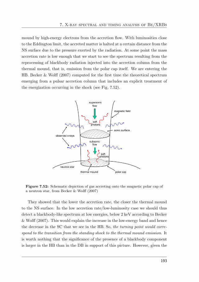
7. X-ray spectral and timing analysis of Be/XRBs
mound by high-energy electrons from the accretion flow. With luminosities closeto the Eddington limit, the accreted matter is halted at a certain distance from theNS surface due to the pressure exerted by the radiation. At some point the massaccretion rate is low enough that we start to see the spectrum resulting from thereprocessing of blackbody radiation injected into the accretion column from thethermal mound, that is, emission from the polar cap itself. We are entering theHB. Becker & Wolff (2007) computed for the first time the theoretical spectrumemerging from a pulsar accretion column that includes an explicit treatment ofthe energization occurring in the shock (see Fig. 7.52).
Figure 7.52: Schematic depiction of gas accreting onto the magnetic polar cap ofa neutron star, from Becker & Wolff (2007)
They showed that the lower the accretion rate, the closer the thermal moundto the NS surface. In the low accretion rate/low-luminosity case we should thusdetect a blackbody-like spectrum at low energies, below 2 keV according to Becker& Wolff (2007). This would explain the increase in the low-energy band and hencethe decrease in the SC that we see in the HB. So, the turning point would corre-spond to the transition from the standing shock to the thermal mound emission. Itis worth nothing that the significance of the presence of a blackbody componentis larger in the HB than in the DB in support of this picture. However, given the
193
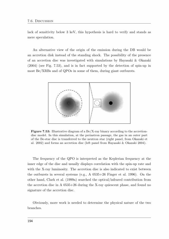
7.6. Discussion
lack of sensitivity below 3 keV, this hypothesis is hard to verify and stands asmere speculation.
An alternative view of the origin of the emission during the DB would bean accretion disk instead of the standing shock. The possibility of the presenceof an accretion disc was investigated with simulations by Hayasaki & Okazaki(2004) (see Fig. 7.53), and is in fact supported by the detection of spin-up inmost Be/XRBs and of QPOs in some of them, during giant outbursts.
Figure 7.53: Illustrative diagram of a Be/X-ray binary according to the accretion-disc model. In this simulation, at the periastron passage, the gas in an outer partof the Be-star disc is transferred to the neutron star (right panel, from Okazaki etal. 2002) and forms an accretion disc (left panel from Hayasaki & Okazaki 2004).
The frequency of the QPO is interpreted as the Keplerian frequency at theinner edge of the disc and usually displays correlation with the spin-up rate andwith the X-ray luminosity. The accretion disc is also indicated to exist betweenthe outbursts in several systems (e.g., A 0535+26 Finger et al. 1996). On theother hand, Clark et al. (1999a) searched the optical/infrared contribution fromthe accretion disc in A 0535+26 during the X-ray quiescent phase, and found nosignature of the accretion disc.
Obviously, more work is needed to determine the physical nature of the twobranches.
194
7. X-ray spectral and timing analysis of Be/XRBs
7.6.3 Two classes of Be/XRBs?
Following the LMXBs classification, which subdivides neutron star systems intoatoll and Z sources, it is interesting to attempt to identify subgroups of Be/XRBs,according to similarities and differences found with this study.
A two-branch pattern is traced in the CD/HID of all the four systems duringgiant outbursts, making it the best characterized, common feature of the wholeclass. As in low-mass systems, the sources do not jump through the diagram,but move smoothly along it, following the pattern. The HB corresponds to alow-intensity state and displays on average the higher fractional rms, similar tothe island state in atolls and horizontal branch in Z sources. This represents thestart and the end states of the source through the outburst. In the high-intensityDB the noise components display higher characteristic frequencies and lower rmsthan in the HB. The power law component of spectral fits shows a marked relationwith flux, correlating in general with it during the DB and anti-correlating duringthe HB.
Differences among systems easily distinguishes two subgroups, with the slowerpulsars, KS 1947+300 and EXO 2030+375, on one side, and the faster ones,4U 0115+63 and V 0332+53, on the other. The first group is characterized bysofter spectra in the HB compared with the other systems. This results in a clearerpattern in the CD of 4U 0115+63 and V 0332+53, in the same way as for atollsources compared with Z sources. Hysteresis is not observed in the slower pulsars,while it is evident in V 0332+53 and, although with less intensity, 4U 0115+63.sCRSFs are crucial in the spectral shape of V 0332+53 and 4U 0115+63, wherealso a harmonic is observed in the energy range analyzed in this work. They areinstead absent or very weak in the first group.
According to timing features, a strong difference among the two groups isthe presence of QPOs in the faster pulsars. No narrow components are foundin KS 1947+300 and EXO 2030+375, where a combination of only three broadnoise Lorentzians are needed to fit PSD during the whole outburst. Instead, in4U 0115+63 and V 0332+53, two more, peaked noise components are required,
195

7.6. Discussion
that we referred to as QPOs since they represent a substantial concentration ofpower in a limited frequency range, although their Q values are not always lowerthan 2. In particular, LLF, with a characteristic frequency of 0.02–0.15 Hz, iscommon among the two systems. The other peaked component, Ls, associatedwith the peaks of the periodic modulations, is only found in V 0332+53.
According to what we found, no evident correlations between spectral andtiming parameters are present in Be/XRBs. This is an important difference com-pared to what is known on low-mass systems (see, for instance Kaaret et al.1998; Bradshaw et al. 2007). The physical explanation of correlations observed inLMXBs is not clear, although some scenarios have been proposed. In general, themechanism responsible for those correlations involves the presence of an accretiondisk (Kaaret et al. 1998), which is considered responsible for the appearance ofQPOs, and could also produce a blackbody flux. The blackbody spectral com-ponent would thus be related with the QPO frequency. The power law spectralcomponent could instead arise from a corona. The flux of photons from the diskblackbody emission would cool the corona via Compton scattering, thus leadingto a power-law spectrum that steepens as the blackbody flux increases. Both phe-nomena – correlation between QPO frequency and blackbody flux and betweenthe photon index and the blackbody flux – are actually observed in LMXBs. Thelack of this kind of relation in Be/XRBs is thus possibly related to the lack ofan accretion disk. This is a merely speculative explanation, and only furtherinvestigation on both LMXBs and HMXBs outbursts will be able to solve thequestion.
196

Le vent se leve!. . . Il faut tenter de
vivre!
Paul Valery 8Conclusions and future projects
8.1 Main results
- We have performed for the first time a systematic X-ray color, spectraland timing analysis on four Be/XRBs – KS 1947+300, EXO 2030+375, 4U0115+63 and V 0332+53 – during giant outbursts.
- Two distinct spectral states emerged in the CD/HID of all the four sys-tems, with specific spectral and timing features depending on the state.We dubbed them the horizontal branch, at low intensity, and the diagonalbranch, at high intensity.
- We phenomenologically explained the transition between the two states,which is characterized by an extra emission at low energies, as due to thetransition from the standing shock to the thermal mound emission.
- From marked differences in color, spectral and timing properties, we identi-fied two subgroups in Be/XRBs, the fast pulsars on one side, and the slowones on the other.
- The lack of correlations between spectral and timing parameters, differentlyfrom what is observed in low-mass systems, is possibly due to the lack of anaccretion disk.
197
8.2. Future work
8.2 Future work
Our plans for the future foresee to extend the characterization of X-ray pulsarspectral states, including both more systems and more data from new X-ray emis-sion. Results from this work are in fact limited by poor statistics, since the num-ber of sources is not large enough to draw definite conclusions on the underlyingphysical parameters that may explain the differences between the two subgroups.The main difficulty is found in the transient nature of their X-ray emission andunpredictability of the type II outbursts.
In this context, we also mean to explore the properties of QPOs during giantoutbursts. Several models have been proposed to explain the QPO generationmechanism in accretion-powered X-ray pulsars, among which the Keplerian fre-quency model and the beat-frequency model, but up to now there is no one uniqueparadigm able to describe the QPO frequencies observed. This research will con-stitute a firm starting point for the development of physical models for the giantoutbursts of X-ray pulsars.
198

AX-ray energy and power spectral fits
In this appendix, for each system, a table shows the spectral and timing param-eters obtained from our best fits. For the spectral components, the width of theiron gaussian line was always fixed at 0.5 keV, and its value is not shown in thetables. Also, since the first harmonics of 4U 0115+63 and V 0332+53 CRSF arepoorly constrained, they are not included in the results shown.
For the power spectral components, the frequency shown is the characteristic(or maximum) frequency of the Lorentzian.
199

Table
A.1
:Spec
tral
para
met
ers
obta
ined
for
the
KS
1947+
300
outb
urs
t.W
hen
erro
rsare
not
dis
-
pla
yed
,th
eco
rres
pondin
gpara
met
erw
as
fixed
toth
ebes
t-fit
valu
eduring
erro
rca
lcula
tion.
The
NH
was
fixed
at
4.3×
1021
cm−
2(N
aik
etal.
2006).
The
last
colu
mn
show
sth
ere
trie
ved
reduce
dχ
2.
Bes
t
fits
wer
eobta
ined
with
73–74
DO
F.
LX
Fe
line
Pow
erla
wχ2 re
dO
bs.
IDM
JD
×1037
Enorm
.Γ
Cuto
ffen
.norm
.
(erg
s−1)
(keV
)(p
h.
cm−
2s−
1)
(keV
)
50425-0
1-0
5-0
051874.1
50.1
66.1
7+
0.3
2−
0.3
20.0
002+
0.0
001
−0
.0001
0.6
4+
0.1
5−
0.1
512.5
+3
.6−
2.4
0.0
039+
0.0
006
−0
.0006
0.8
50425-0
1-0
6-0
051876.4
10.0
96.0
4+
0.3
4−
0.3
40.0
002+
0.0
001
−0
.0001
0.7
0+
0.2
2−
0.2
411.3
+5
.2−
3.0
0.0
031+
0.0
007
−0
.0006
0.5
50425-0
1-0
7-0
051878.2
70.1
26.3
9+
0.2
7−
0.2
60.0
002+
0.0
001
−0
.0001
0.7
5+
0.1
8−
0.1
913.3
+5
.5−
3.3
0.0
037+
0.0
007
−0
.0006
0.6
50425-0
1-0
8-0
151883.8
30.3
56.4
5+
0.3
0−
0.3
10.0
004+
0.0
002
−0
.0001
0.2
9+
0.1
5−
0.1
69.3
+1
.9−
1.4
0.0
055+
0.0
009
−0
.0008
0.6
50425-0
1-0
8-0
051883.8
90.3
56.4
5+
0.2
3−
0.2
30.0
005+
0.0
001
−0
.0001
0.3
5+
0.1
3−
0.1
39.9
+1
.7−
1.3
0.0
059+
0.0
008
−0
.0007
0.7
50425-0
1-0
9-0
051888.0
10.9
96.2
8+
0.1
8−
0.1
90.0
008+
0.0
002
−0
.0002
0.1
8+
0.0
5−
0.0
58.8
+0
.5−
0.4
0.0
130+
0.0
008
−0
.0007
0.7
50425-0
1-0
9-0
151888.0
70.9
76.2
3+
0.1
5−
0.1
50.0
009+
0.0
002
−0
.0002
0.1
7+
0.0
5−
0.0
58.6
+0
.4−
0.4
0.0
128+
0.0
007
−0
.0007
0.5
50425-0
1-1
0-0
051892.2
21.6
06.4
6+
0.1
6−
0.1
60.0
009+
0.0
002
−0
.0002
0.3
0+
0.0
3−
0.0
39.3
+0
.3−
0.3
0.0
259+
0.0
009
−0
.0009
1.6
50425-0
1-1
1-0
051896.2
02.2
66.6
0+
0.2
0−
0.2
00.0
008+
0.0
002
−0
.0002
0.5
6+
0.0
3−
0.0
312.1
+0
.5−
0.4
0.0
496+
0.0
016
−0
.0016
1.3
50425-0
1-1
1-0
151896.5
22.1
56.3
7+
0.2
2−
0.2
20.0
012+
0.0
003
−0
.0003
0.6
2+
0.0
5−
0.0
513.4
+0
.9−
0.8
0.0
496+
0.0
028
−0
.0027
0.8
50425-0
1-1
2-0
051898.9
82.7
96.4
8+
0.1
8−
0.1
80.0
012+
0.0
002
−0
.0002
0.7
7+
0.0
2−
0.0
216.7
+0
.6−
0.6
0.0
754+
0.0
021
−0
.0021
0.6
50425-0
1-1
3-0
051901.9
13.1
96.6
0+
0.3
1−
0.3
00.0
012+
0.0
004
−0
.0004
0.7
8+
0.0
4−
0.0
416.6
+1
.2−
1.1
0.0
887+
0.0
044
−0
.0042
0.7
50425-0
1-1
3-0
151902.8
93.2
86.4
2+
0.2
0−
0.2
00.0
013+
0.0
004
−0
.0004
0.8
8+
0.0
3−
0.0
319.7
+1
.2−
1.1
0.1
010+
0.0
038
−0
.0037
0.8
50425-0
1-1
4-0
051906.1
33.6
86.4
7+
0.2
3−
0.2
30.0
010+
0.0
003
−0
.0003
0.8
5+
0.0
2−
0.0
218.8
+0
.9−
0.8
0.1
110+
0.0
034
−0
.0033
1.1
50425-0
1-1
4-0
151906.7
23.6
76.3
1+
0.4
5−
6.3
10.0
007+
0.0
005
−0
.0005
0.8
6+
0.0
3−
0.0
419.2
+1
.4−
1.2
0.1
120+
0.0
049
−0
.0048
0.6
50425-0
1-1
5-0
051910.9
03.8
76.4
5+
0.1
7−
0.1
60.0
013+
0.0
003
−0
.0003
0.8
7+
0.0
2−
0.0
219.5
+0
.8−
0.7
0.1
180+
0.0
032
−0
.0032
1.0
50425-0
1-1
6-0
051914.1
84.1
26.3
6+
0.1
8−
0.1
80.0
012+
0.0
003
−0
.0003
0.8
9+
0.0
2−
0.0
220.1
+0
.7−
0.7
0.1
300+
0.0
032
−0
.0031
1.0
50425-0
1-1
7-0
051918.1
64.1
56.5
4+
0.3
9−
0.3
70.0
009+
0.0
004
−0
.0005
0.9
2+
0.0
3−
0.0
320.6
+1
.3−
1.1
0.1
380+
0.0
050
−0
.0049
0.8
50425-0
1-1
8-0
051926.6
94.4
56.3
2+
0.2
4−
0.2
40.0
013+
0.0
005
−0
.0005
0.9
4+
0.0
3−
0.0
320.9
+1
.2−
1.1
0.1
520+
0.0
052
−0
.0051
0.8
50425-0
1-1
9-0
051930.2
84.8
46.2
4+
0.1
8−
0.1
80.0
016+
0.0
005
−0
.0005
1.0
0+
0.0
2−
0.0
223.9
+1
.2−
1.1
0.1
760+
0.0
051
−0
.0049
0.9
50425-0
1-2
0-0
051932.3
34.9
36.2
7+
0.2
2−
0.2
20.0
016+
0.0
005
−0
.0005
0.9
8+
0.0
2−
0.0
222.5
+1
.1−
1.0
0.1
770+
0.0
051
−0
.0050
1.0
50425-0
1-2
1-0
151941.6
86.1
46.1
5+
0.1
8−
0.1
80.0
024+
0.0
006
−0
.0006
1.1
1+
0.0
2−
0.0
228.3
+1
.6−
1.5
0.2
700+
0.0
075
−0
.0074
1.4
50425-0
1-2
1-0
051941.7
56.3
46.1
3+
0.1
9−
0.1
90.0
022+
0.0
006
−0
.0006
1.1
3+
0.0
2−
0.0
229.3
+1
.5−
1.4
0.2
890+
0.0
073
−0
.0072
1.6
50425-0
1-2
2-0
051943.7
46.7
06.1
2+
0.1
6−
6.1
20.0
026+
0.0
006
−0
.0006
1.1
6+
0.0
2−
0.0
231.4
+1
.7−
1.6
0.3
170+
0.0
080
−0
.0078
1.9
50425-0
1-2
3-0
151943.8
06.6
76.1
3+
0.1
7−
0.1
60.0
024+
0.0
006
−0
.0006
1.1
7+
0.0
2−
0.0
232.9
+1
.7−
1.6
0.3
170+
0.0
075
−0
.0074
1.5
50425-0
1-2
3-0
051948.1
26.9
26.2
3+
0.1
7−
0.1
70.0
022+
0.0
005
−0
.0005
1.1
8+
0.0
1−
0.0
133.2
+1
.3−
1.2
0.3
330+
0.0
066
−0
.0065
1.9
50425-0
1-1
7-0
151950.1
87.0
86.2
5+
0.2
0−
0.2
10.0
022+
0.0
006
−0
.0006
1.1
9+
0.0
2−
0.0
233.7
+1
.8−
1.7
0.3
480+
0.0
083
−0
.0082
1.5
50425-0
1-2
4-0
051952.0
36.7
66.2
2+
0.1
5−
0.1
50.0
026+
0.0
006
−0
.0006
1.1
8+
0.0
2−
0.0
233.0
+1
.7−
1.5
0.3
250+
0.0
075
−0
.0074
1.4
Conti
nued
on
Nex
tPage.
..
200

A. X-ray energy and power spectral fitsTable
A.1
–C
onti
nued
LX
Fe
line
Pow
erla
wχ2 re
dO
bs.
IDM
JD
×1037
Enorm
.Γ
Cuto
ffen
.norm
.
(erg
s−1)
(keV
)(p
h.
cm−
2s−
1)
(keV
)
50425-0
1-2
5-0
051955.6
36.7
56.3
0+
0.2
4−
0.2
50.0
020+
0.0
006
−0
.0006
1.1
3+
0.0
2−
0.0
228.9
+1
.6−
1.4
0.3
060+
0.0
081
−0
.0079
1.1
50425-0
1-2
6-0
051961.5
36.4
96.2
6+
0.1
8−
0.1
80.0
022+
0.0
006
−0
.0006
1.1
4+
0.0
2−
0.0
229.4
+1
.5−
1.3
0.3
040+
0.0
074
−0
.0072
1.6
50425-0
1-2
7-0
051963.9
76.5
36.1
2+
0.2
4−
0.2
40.0
021+
0.0
008
−0
.0007
1.1
4+
0.0
2−
0.0
229.2
+2
.1−
1.8
0.3
040+
0.0
098
−0
.0096
1.5
50425-0
1-2
9-0
051968.5
65.5
96.3
7+
0.2
2−
0.2
20.0
016+
0.0
005
−0
.0005
1.0
7+
0.0
2−
0.0
227.3
+1
.5−
1.4
0.2
290+
0.0
064
−0
.0062
1.0
60402-0
1-0
1-0
051970.2
15.7
86.3
5+
0.2
4−
0.2
40.0
016+
0.0
006
−0
.0006
1.0
8+
0.0
2−
0.0
226.7
+1
.6−
1.5
0.2
430+
0.0
073
−0
.0071
0.7
60402-0
1-0
2-0
051972.1
95.5
56.2
1+
0.2
5−
0.2
50.0
020+
0.0
007
−0
.0007
1.1
0+
0.0
3−
0.0
327.9
+2
.2−
1.9
0.2
410+
0.0
087
−0
.0085
1.0
60402-0
1-0
3-0
051974.5
85.1
36.2
5+
0.2
0−
0.2
10.0
018+
0.0
005
−0
.0005
1.0
3+
0.0
2−
0.0
224.5
+1
.4−
1.2
0.2
010+
0.0
060
−0
.0059
0.8
60402-0
1-0
4-0
051976.2
45.2
36.1
6+
0.2
7−
0.2
70.0
012+
0.0
005
−0
.0005
1.0
0+
0.0
2−
0.0
223.0
+1
.1−
1.0
0.1
980+
0.0
057
−0
.0055
1.0
60402-0
1-0
5-0
051978.2
35.2
06.3
1+
0.2
5−
0.2
50.0
010+
0.0
005
−0
.0005
1.0
2+
0.0
2−
0.0
223.5
+1
.3−
1.2
0.2
050+
0.0
060
−0
.0057
1.3
60402-0
1-0
6-0
051980.7
44.8
66.2
4+
0.2
5−
0.2
00.0
013+
0.0
004
−0
.0005
0.9
6+
0.0
2−
0.0
221.8
+0
.9−
0.9
0.1
710+
0.0
045
−0
.0044
1.1
60402-0
1-0
7-0
051983.8
64.4
86.3
4+
0.2
1−
0.2
20.0
015+
0.0
005
−0
.0005
0.9
4+
0.0
3−
0.0
321.3
+1
.2−
1.1
0.1
510+
0.0
051
−0
.0050
0.9
60402-0
1-0
8-0
051984.8
64.3
26.2
8+
0.2
7−
0.2
70.0
013+
0.0
004
−0
.0004
0.9
1+
0.0
2−
0.0
220.6
+1
.0−
0.9
0.1
400+
0.0
042
−0
.0041
0.9
60402-0
1-0
9-0
051986.5
84.2
76.5
2+
0.2
6−
0.2
60.0
011+
0.0
004
−0
.0004
0.9
0+
0.0
3−
0.0
320.8
+1
.2−
1.1
0.1
340+
0.0
045
−0
.0043
0.8
60402-0
1-1
0-0
051988.2
73.7
36.4
7+
0.4
4−
0.4
40.0
011+
0.0
006
−0
.0007
0.8
8+
0.0
5−
0.0
519.4
+2
.0−
1.7
0.1
170+
0.0
069
−0
.0066
0.6
60402-0
1-1
1-0
051990.1
23.6
06.3
7+
0.4
2−
0.4
20.0
005+
0.0
005
−0
.0005
0.8
0+
0.0
4−
0.0
417.2
+1
.2−
1.0
0.1
010+
0.0
023
−0
.0045
0.7
60402-0
1-1
2-0
051992.1
73.5
66.4
8+
0.4
8−
0.4
80.0
006+
0.0
007
−0
.0006
0.8
6+
0.0
6−
0.0
619.1
+2
.4−
2.0
0.1
070+
0.0
077
−0
.0075
0.6
60402-0
1-1
3-0
051994.2
33.2
26.5
2+
0.4
3−
0.5
40.0
002+
0.0
006
−0
.0003
0.8
1+
0.0
5−
0.0
517.2
+1
.6−
1.3
0.0
927+
0.0
058
−0
.0052
0.8
60402-0
1-1
4-0
051996.0
83.2
76.5
8+
0.4
2−
0.4
20.0
008+
0.0
004
−0
.0004
0.8
2+
0.0
4−
0.0
417.7
+1
.2−
1.1
0.0
956+
0.0
041
−0
.0040
1.2
60402-0
1-1
5-0
051998.1
42.9
96.4
6+
0.4
6−
0.4
60.0
008+
0.0
006
−0
.0005
0.8
0+
0.0
5−
0.0
516.6
+1
.7−
1.4
0.0
861+
0.0
056
−0
.0053
0.7
60402-0
1-1
5-0
151999.0
62.8
06.4
9+
0.5
0−
0.5
00.0
006+
0.0
005
−0
.0002
0.7
6+
0.0
5−
0.0
516.4
+1
.5−
1.3
0.0
746+
0.0
041
−0
.0044
0.8
60402-0
1-1
6-0
151999.9
82.7
26.4
4+
0.3
1−
0.3
20.0
009+
0.0
003
−0
.0004
0.7
6+
0.0
4−
0.0
416.4
+1
.1−
1.0
0.0
714+
0.0
033
−0
.0032
0.9
60402-0
1-1
6-0
052000.0
62.7
36.3
7+
0.3
1−
0.3
00.0
012+
0.0
005
−0
.0005
0.7
1+
0.0
5−
0.0
515.1
+1
.4−
1.2
0.0
684+
0.0
045
−0
.0042
1.0
60402-0
1-1
6-0
252001.0
52.7
46.5
8+
0.3
4−
0.3
40.0
010+
0.0
005
−0
.0004
0.7
0+
0.0
5−
0.0
515.7
+1
.3−
1.1
0.0
659+
0.0
038
−0
.0037
0.7
60402-0
1-1
7-0
052002.0
42.6
26.3
6+
0.3
7−
0.3
50.0
008+
0.0
005
−0
.0005
0.7
7+
0.0
5−
0.0
517.1
+1
.7−
1.4
0.0
687+
0.0
047
−0
.0044
0.9
60402-0
1-1
8-0
052004.3
82.4
36.2
1+
0.2
3−
0.2
30.0
005+
0.0
005
−0
.0002
0.7
3+
0.0
6−
0.0
316.1
+1
.6−
1.4
0.0
617+
0.0
023
−0
.0040
0.6
60402-0
1-1
9-0
052006.0
92.2
86.5
1+
0.2
7−
0.2
80.0
010+
0.0
004
−0
.0003
0.6
8+
0.0
5−
0.0
514.8
+1
.2−
1.0
0.0
543+
0.0
031
−0
.0030
1.0
60402-0
1-2
0-0
052008.2
12.1
46.4
0+
0.1
9−
0.1
90.0
012+
0.0
003
−0
.0003
0.6
8+
0.0
4−
0.0
415.0
+1
.1−
1.0
0.0
502+
0.0
027
−0
.0026
0.9
60402-0
1-2
1-0
052010.8
02.1
26.9
3+
0.9
3−
0.5
20.0
008+
0.0
004
−0
.0005
0.6
7+
0.0
7−
0.0
714.3
+1
.7−
1.4
0.0
509+
0.0
042
−0
.0040
0.5
60402-0
1-2
2-0
052014.3
91.9
36.4
3+
0.2
9−
0.2
80.0
009+
0.0
003
−0
.0003
0.5
9+
0.0
5−
0.0
512.9
+0
.9−
0.8
0.0
429+
0.0
024
−0
.0023
0.7
60402-0
1-2
3-0
052016.3
71.7
66.6
7+
0.2
4−
0.2
30.0
010+
0.0
003
−0
.0003
0.5
9+
0.0
5−
0.0
513.3
+1
.0−
0.9
0.0
378+
0.0
022
−0
.0021
0.7
60402-0
1-2
4-0
052017.6
31.7
26.4
4+
0.2
5−
0.2
40.0
008+
0.0
003
−0
.0003
0.6
5+
0.0
5−
0.0
514.4
+1
.2−
1.0
0.0
392+
0.0
023
−0
.0022
1.2
60402-0
1-2
5-0
052021.0
61.5
16.4
3+
0.3
9−
0.3
50.0
009+
0.0
003
−0
.0004
0.5
0+
0.0
8−
0.0
811.7
+1
.3−
1.1
0.0
295+
0.0
027
−0
.0013
0.7
Conti
nued
on
Nex
tPage.
..
201

Table
A.1
–C
onti
nued
LX
Fe
line
Pow
erla
wχ2 re
dO
bs.
IDM
JD
×1037
Enorm
.Γ
Cuto
ffen
.norm
.
(erg
s−1)
(keV
)(p
h.
cm−
2s−
1)
(keV
)
60402-0
1-2
6-0
052023.5
91.3
66.8
5+
0.2
6−
0.2
60.0
011+
0.0
003
−0
.0004
0.6
5+
0.0
9−
0.0
915.7
+2
.8−
2.1
0.0
288+
0.0
031
−0
.0029
0.8
60402-0
1-2
7-0
052024.3
21.3
06.5
3+
0.2
7−
0.2
80.0
010+
0.0
003
−0
.0003
0.4
9+
0.0
7−
0.0
711.8
+1
.2−
1.0
0.0
248+
0.0
021
−0
.0020
0.8
60402-0
1-2
8-0
052027.3
51.1
26.3
1+
0.3
1−
0.3
10.0
007+
0.0
002
−0
.0002
0.4
1+
0.0
7−
0.0
711.1
+1
.0−
0.9
0.0
189+
0.0
015
−0
.0015
0.9
60402-0
1-2
9-0
052028.2
31.0
76.3
6+
0.2
0−
0.2
00.0
009+
0.0
002
−0
.0002
0.4
8+
0.0
6−
0.0
611.9
+1
.0−
0.9
0.0
197+
0.0
015
−0
.0014
0.6
60402-0
1-3
0-0
052029.8
31.0
06.4
9+
0.3
1−
0.3
20.0
005+
0.0
003
−0
.0002
0.4
0+
0.0
8−
0.0
810.3
+1
.1−
0.9
0.0
178+
0.0
017
−0
.0016
0.7
60402-0
1-3
1-0
052032.9
30.7
86.3
7+
0.1
8−
0.1
80.0
008+
0.0
002
−0
.0001
0.4
1+
0.0
7−
0.0
711.1
+1
.0−
0.9
0.0
129+
0.0
011
−0
.0010
1.3
60402-0
1-3
2-0
052034.9
20.6
76.2
8+
0.3
2−
0.3
20.0
005+
0.0
002
−0
.0002
0.5
1+
0.0
8−
0.0
812.3
+1
.5−
1.3
0.0
127+
0.0
012
−0
.0011
0.6
60402-0
1-3
3-0
052035.7
20.6
36.3
6+
0.4
0−
0.4
00.0
004+
0.0
002
−0
.0002
0.4
1+
0.1
0−
0.0
911.1
+1
.6−
1.3
0.0
107+
0.0
013
−0
.0012
0.7
60402-0
1-3
4-0
052038.7
00.4
86.4
8+
0.3
0−
0.3
00.0
004+
0.0
002
−0
.0002
0.4
1+
0.1
3−
0.1
311.2
+2
.2−
1.6
0.0
080+
0.0
012
−0
.0011
0.7
60402-0
1-3
5-0
052040.6
90.4
06.6
5+
0.5
0−
0.5
00.0
003+
0.0
002
−0
.0001
0.2
7+
0.1
5−
0.1
69.4
+1
.9−
1.4
0.0
058+
0.0
010
−0
.0009
0.7
60402-0
1-3
6-0
052041.5
50.3
66.3
4+
0.2
7−
0.2
70.0
004+
0.0
002
−0
.0002
0.3
5+
0.1
6−
0.1
710.0
+2
.4−
1.7
0.0
060+
0.0
012
−0
.0010
0.5
60402-0
1-3
7-0
052044.0
80.3
26.2
1+
0.3
4−
0.3
40.0
005+
0.0
002
−0
.0002
0.1
1+
0.2
2−
0.2
48.1
+2
.2−
1.5
0.0
040+
0.0
011
−0
.0009
0.6
60402-0
1-3
8-0
152046.9
90.2
66.4
0+
0.4
6−
0.4
60.0
004+
0.0
002
−0
.0002
0.6
9+
0.3
0−
0.3
114.1
+14
.4−
5.2
0.0
065+
0.0
025
−0
.0019
0.5
60402-0
1-3
8-0
052047.0
60.2
46.0
3+
0.3
5−
0.1
60.0
008+
0.0
004
−0
.0003
0.3
4+
0.4
9−
0.5
29.8
+12
.2−
3.7
0.0
038+
0.0
028
−0
.0016
0.5
60402-0
1-3
9-0
052050.1
10.1
96.0
2+
0.3
1−
0.3
10.0
000+
0.0
003
−0
.0000
0.2
5+
0.5
1−
0.5
17.4
+6
.5−
2.3
0.0
040+
0.0
022
−0
.0016
0.5
60402-0
1-3
9-0
152050.1
80.1
86.3
0+
0.5
2−
0.5
20.0
006+
0.0
004
−0
.0004
0.4
0+
1.0
3−
0.3
810.2
+5
.2−
5.8
0.0
034+
0.0
050
−0
.0018
0.6
60402-0
1-4
0-0
052052.9
50.1
66.3
2+
0.3
4−
6.3
20.0
004+
0.0
002
−0
.0002
0.7
8+
0.4
2−
0.3
913.9
+32
.8−
5.9
0.0
051+
0.0
028
−0
.0017
0.7
60402-0
1-4
1-0
052055.8
20.1
46.9
9+
0.6
2−
0.6
20.0
003+
0.0
002
−0
.0002
0.7
9+
0.1
7−
0.1
613.0
+32
.8−
5.9
0.0
048+
0.0
014
−0
.0014
0.6
60402-0
1-4
1-0
152056.2
10.1
46.3
2+
0.6
0−
0.6
00.0
001+
0.0
002
−0
.0001
0.6
0+
0.9
6−
0.6
610.3
+38
.8−
5.1
0.0
040+
0.0
035
−0
.0019
0.6
60402-0
1-4
2-0
052057.8
70.1
36.3
2+
0.7
0−
0.7
00.0
001+
0.0
001
−0
.0001
0.7
0+
0.4
0−
0.5
611.6
+16
.4−
5.3
0.0
040+
0.0
019
−0
.0017
0.5
60402-0
1-4
3-0
052060.3
10.1
16.0
4+
0.9
5−
0.9
50.0
001+
0.0
001
−0
.0001
0.6
0+
0.3
6−
0.3
79.9
+7
.5−
3.2
0.0
032+
0.0
015
−0
.0010
0.5
60402-0
1-4
4-0
152062.8
20.1
06.6
5+
0.6
5−
0.6
50.0
001+
0.0
001
−0
.0001
0.6
9+
0.3
9−
0.5
812.0
+15
.5−
5.4
0.0
029+
0.0
014
−0
.0013
0.6
60402-0
1-4
4-0
252062.8
90.0
96.0
0+
0.5
0−
0.5
00.0
001+
0.0
001
−0
.0001
0.2
4+
0.3
8−
0.4
26.9
+3
.5−
1.9
0.0
019+
0.0
009
−0
.0007
0.4
60402-0
1-4
5-0
052078.0
50.0
66.3
0+
0.3
5−
0.3
00.0
002+
0.0
001
−0
.0001
0.9
4+
0.3
4−
0.3
814.9
+25
.8−
6.4
0.0
027+
0.0
012
−0
.0009
0.5
202

A. X-ray energy and power spectral fitsTable
A.2
:T
he
sam
eas
Table
A.1
,fo
rEX
O2030+
375.
Bes
tfits
wer
eobta
ined
with
47–72
DO
F.
LX
NH
Cyclo
tron
line
Fe
line
Pow
er
law
χ2 r
Obs.
IDM
JD
×1037
Eσ
τE
norm
.Γ
cuto
ffnorm
.
(erg
/s)
cm−
2(k
eV)
(keV
)(k
eV)
(ph./
cm2/s)
(keV
)
91089-0
1-0
7-0
053914.8
99.2
11.4
98.6
+1
.4−
4.3
4.5
+6
.4−
1.4
1.1
8+
7.4
5−
0.6
86.4
4+
0.1
1−
0.1
00.0
159+
0.0
060
−0
.0031
1.0
8+
0.3
0−
0.0
917.4
+3
.2−
1.1
1.1
3+
0.6
8−
0.2
11.0
91089-0
1-0
7-0
153915.8
39.1
71.0
19.4
+0
.9−
3.2
3.9
+1
.9−
1.0
0.9
4+
2.3
6−
0.4
56.4
3+
0.1
0−
0.1
00.0
167+
0.0
041
−0
.0030
1.0
4+
0.1
7−
0.0
717.4
+1
.8−
1.0
0.9
8+
0.5
0−
0.1
40.8
91089-0
1-0
8-0
053916.8
19.9
31.5
28.4
+1
.4−
7.1
4.4
+3
.1−
1.2
1.3
1+
8.8
6−
0.7
46.4
9+
0.1
0−
0.1
00.0
187+
0.0
058
−0
.0034
1.1
2+
0.3
3−
0.0
917.8
+3
.5−
1.2
1.2
7+
1.2
7−
0.2
50.7
91089-0
1-0
8-0
153917.7
69.9
90.8
49.6
+0
.6−
1.2
3.7
+1
.5−
0.8
1.0
0+
0.8
1−
0.3
36.4
0+
0.0
9−
0.0
90.0
178+
0.0
029
−0
.0026
1.0
5+
0.0
8−
0.0
516.8
+0
.8−
0.6
1.0
9+
0.2
5−
0.1
20.8
91089-0
1-0
8-0
253918.5
010.4
91.2
69.1
+1
.0−
2.8
4.5
+2
.6−
1.4
1.4
8+
3.7
3−
0.7
56.4
0+
0.1
0−
0.1
00.0
196+
0.0
054
−0
.0035
1.0
8+
0.1
9−
0.0
817.0
+1
.7−
1.0
1.2
7+
0.6
0−
0.2
20.8
91089-0
1-0
8-0
353919.6
110.9
01.5
49.1
+0
.8−
1.6
4.4
+1
.3−
0.8
1.7
1+
1.5
2−
0.6
16.4
8+
0.0
9−
0.0
80.0
208+
0.0
038
−0
.0031
1.1
2+
0.1
2−
0.0
717.3
+1
.2−
0.8
1.4
3+
0.4
9−
0.2
20.9
91089-0
1-0
8-0
653920.7
110.9
51.0
99.6
+0
.5−
1.0
3.7
+1
.0−
0.7
1.1
8+
0.7
4−
0.3
56.4
3+
0.0
9−
0.0
80.0
200+
0.0
032
−0
.0028
1.0
9+
0.0
8−
0.0
517.2
+0
.8−
0.6
1.3
2+
0.2
8−
0.1
50.8
91089-0
1-0
8-0
453921.0
710.6
71.0
39.4
+0
.6−
1.6
3.4
+1
.3−
0.7
0.9
3+
1.1
8−
0.3
56.3
4+
0.0
9−
0.0
90.0
214+
0.0
043
−0
.0035
1.1
0+
0.1
2−
0.0
617.7
+1
.4−
1.0
1.2
6+
0.4
3−
0.1
60.7
91089-0
1-0
8-0
553922.2
810.8
01.3
79.2
+0
.8−
1.6
4.2
+1
.4−
0.8
1.4
7+
1.4
0−
0.5
26.4
5+
0.0
9−
0.0
90.0
201+
0.0
037
−0
.0030
1.1
1+
0.1
1−
0.0
717.5
+1
.2−
0.8
1.3
7+
0.4
4−
0.2
00.9
91089-0
1-0
9-0
053923.3
311.2
11.5
38.6
+1
.0−
2.8
4.7
+1
.7−
1.0
1.8
5+
3.0
7−
0.8
06.4
8+
0.0
8−
0.0
80.0
226+
0.0
052
−0
.0035
1.1
7+
0.1
7−
0.0
818.3
+1
.8−
1.0
1.6
0+
1.2
5−
0.2
91.2
91089-0
1-0
9-0
153924.7
011.5
51.1
79.8
+0
.5−
0.8
3.5
+1
.0−
0.7
1.1
2+
0.6
6−
0.3
26.4
2+
0.0
9−
0.0
90.0
213+
0.0
036
−0
.0033
1.1
3+
0.0
7−
0.0
517.9
+1
.0−
0.9
1.4
8+
0.2
9−
0.1
60.9
91089-0
1-0
9-0
353926.6
311.8
81.2
59.3
+0
.6−
1.1
4.1
+0
.9−
0.6
1.6
2+
1.0
3−
0.4
86.4
1+
0.0
8−
0.0
80.0
245+
0.0
038
−0
.0033
1.1
3+
0.0
9−
0.0
617.3
+0
.9−
0.7
1.5
8+
0.4
0−
0.2
10.9
91089-0
1-0
9-0
453928.1
812.4
31.3
89.4
+0
.7−
1.4
4.3
+1
.5−
1.0
1.8
6+
1.5
9−
0.6
76.4
3+
0.0
9−
0.0
90.0
249+
0.0
049
−0
.0041
1.1
6+
0.1
1−
0.0
717.8
+1
.3−
1.0
1.7
8+
0.6
0−
0.2
80.9
91089-0
1-0
9-0
553928.6
411.4
01.0
29.5
+0
.5−
1.0
3.5
+1
.1−
0.7
1.2
4+
0.9
3−
0.4
06.4
3+
0.0
8−
0.0
80.0
242+
0.0
043
−0
.0037
1.1
1+
0.0
9−
0.0
617.4
+1
.1−
0.9
1.4
4+
0.3
8−
0.1
80.9
91089-0
1-0
9-0
653929.6
112.5
91.1
59.9
+0
.4−
0.8
3.9
+0
.7−
0.5
1.4
6+
0.7
9−
0.4
06.4
3+
0.0
9−
0.0
90.0
243+
0.0
039
−0
.0035
1.1
4+
0.0
7−
0.0
518.0
+0
.9−
0.8
1.6
7+
0.3
3−
0.1
90.8
91089-0
1-1
0-0
053930.7
913.0
11.2
19.6
+0
.5−
1.0
3.9
+0
.9−
0.6
1.3
8+
0.9
3−
0.4
26.4
1+
0.0
8−
0.0
80.0
257+
0.0
040
−0
.0036
1.1
7+
0.0
8−
0.0
519.0
+1
.0−
0.8
1.8
0+
0.4
2−
0.2
20.9
91089-0
1-1
0-0
153931.3
912.9
41.2
59.8
+0
.4−
0.7
3.3
+0
.6−
0.5
1.0
3+
0.4
7−
0.2
56.4
7+
0.0
8−
0.0
80.0
240+
0.0
036
−0
.0034
1.1
8+
0.0
6−
0.0
519.5
+0
.9−
0.8
1.7
5+
0.2
8−
0.1
70.8
91089-0
1-1
0-0
253932.2
413.3
51.3
19.7
+0
.5−
0.7
3.9
+0
.9−
0.6
1.6
4+
0.7
2−
0.4
16.4
5+
0.0
8−
0.0
80.0
274+
0.0
041
−0
.0038
1.1
6+
0.0
7−
0.0
518.4
+1
.0−
0.8
1.8
6+
0.3
6−
0.2
20.9
91089-0
1-1
0-0
353933.3
613.7
51.3
79.7
+0
.5−
0.8
4.0
+0
.9−
0.6
1.7
1+
0.8
7−
0.4
66.4
4+
0.0
8−
0.0
80.0
287+
0.0
044
−0
.0039
1.1
9+
0.0
8−
0.0
618.8
+1
.0−
0.8
2.0
3+
0.4
3−
0.2
50.7
91089-0
1-1
0-0
453934.2
613.3
61.3
59.8
+0
.4−
0.7
3.6
+0
.8−
0.5
1.4
1+
0.6
3−
0.3
56.4
6+
0.0
8−
0.0
80.0
266+
0.0
041
−0
.0037
1.1
9+
0.0
7−
0.0
519.1
+1
.0−
0.8
1.9
2+
0.3
5−
0.2
10.8
91089-0
1-1
0-0
553935.1
813.4
81.4
19.8
+0
.4−
0.7
3.6
+0
.7−
0.5
1.5
1+
0.7
3−
0.3
86.4
7+
0.0
9−
0.0
90.0
262+
0.0
045
−0
.0040
1.1
9+
0.0
7−
0.0
519.1
+1
.1−
1.0
1.9
4+
0.3
9−
0.2
30.7
91089-0
1-1
0-0
653936.3
013.8
51.5
39.7
+0
.5−
0.8
4.0
+0
.7−
0.5
1.7
1+
0.8
7−
0.4
56.4
5+
0.0
8−
0.0
80.0
296+
0.0
046
−0
.0040
1.2
4+
0.0
8−
0.0
619.9
+1
.1−
0.9
2.1
9+
0.4
8−
0.2
70.9
91089-0
1-1
1-0
053937.3
513.9
21.4
99.6
+0
.4−
0.7
3.9
+0
.7−
0.5
1.6
6+
0.7
6−
0.4
16.4
6+
0.0
8−
0.0
80.0
286+
0.0
043
−0
.0038
1.2
3+
0.0
7−
0.0
519.9
+1
.1−
0.9
2.1
6+
0.4
4−
0.2
60.9
91089-0
1-1
1-0
153938.1
712.1
90.8
69.5
+0
.9−
3.2
4.5
+3
.1−
1.4
2.9
9+
7.2
1−
1.4
66.4
0+
0.1
5−
0.1
40.0
310+
0.0
172
−0
.0086
1.0
5+
0.3
0−
0.1
514.9
+2
.6−
2.0
1.6
2+
1.7
9−
0.4
30.7
91089-0
1-1
1-0
253938.4
313.1
21.6
29.2
+0
.7−
0.7
4.2
+1
.1−
0.6
2.0
4+
2.5
8−
0.7
86.4
4+
0.0
9−
0.0
80.0
296+
0.0
076
−0
.0049
1.2
2+
0.1
6−
0.0
818.8
+1
.6−
1.1
2.0
9+
0.8
6−
0.3
80.9
91089-0
1-1
1-0
353939.2
513.8
51.2
29.8
+0
.4−
0.7
3.5
+0
.8−
0.6
1.3
0+
0.6
1−
0.3
46.4
6+
0.0
9−
0.0
90.0
261+
0.0
043
−0
.0039
1.2
0+
0.0
7−
0.0
519.4
+1
.0−
0.9
1.9
8+
0.3
6−
0.2
11.0
91089-0
1-1
1-0
453940.1
312.1
80.4
110.0
+0
.5−
1.2
3.7
+1
.3−
0.8
1.6
9+
1.6
8−
0.6
46.4
4+
0.1
3−
0.1
30.0
250+
0.0
071
−0
.0056
1.0
8+
0.1
3−
0.0
717.4
+2
.0−
1.7
1.4
1+
0.5
5−
0.2
01.0
91089-0
1-1
1-0
553941.4
414.7
31.5
99.1
+0
.8−
2.4
4.4
+1
.0−
0.6
2.0
6+
3.2
5−
0.8
46.4
5+
0.0
9−
0.0
80.0
326+
0.0
094
−0
.0054
1.3
0+
0.1
9−
0.0
821.2
+2
.5−
1.4
2.6
5+
1.2
3−
0.5
00.9
91089-0
1-1
1-0
653942.2
614.2
91.3
69.6
+0
.5−
0.8
4.0
+1
.0−
0.7
1.7
1+
0.8
9−
0.4
66.4
3+
0.0
8−
0.0
80.0
309+
0.0
048
−0
.0042
1.2
4+
0.0
8−
0.0
619.6
+1
.2−
1.0
2.2
8+
0.5
1−
0.2
91.0
91089-0
1-1
2-0
053944.0
511.9
11.0
39.5
+0
.8−
6.0
3.4
+2
.7−
0.8
1.0
3+
9.0
4−
0.5
56.4
0+
0.1
1−
0.1
10.0
312+
0.0
221
−0
.0069
1.2
6+
0.3
9−
0.1
022.8
+6
.6−
2.7
1.7
6+
2.9
3−
0.3
20.7
91089-0
1-1
2-0
153944.9
712.5
31.7
69.7
+0
.5−
1.1
4.3
+1
.0−
0.6
2.8
1+
2.1
4−
0.9
36.3
6+
0.1
0−
0.1
00.0
325+
0.0
083
−0
.0062
1.2
2+
0.1
3−
0.0
919.0
+2
.1−
1.7
2.0
9+
0.9
1−
0.4
01.1
Conti
nued
on
Nex
tPage.
..
203
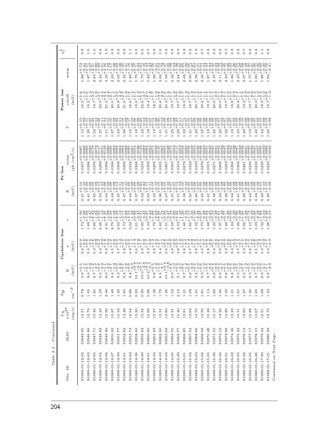
Table
A.2
–C
onti
nued
LX
NH
Cyclo
tron
line
Fe
line
Pow
er
law
χ2 r
Obs.
IDM
JD
×1037
Eσ
τE
norm
.Γ
cuto
ffnorm
.
(erg
/s)
cm−
2(k
eV)
(keV
)(k
eV)
(ph./
cm2/s)
(keV
)
91089-0
1-1
2-0
253945.9
513.5
10.7
89.9
+0
.5−
1.1
3.6
+0
.9−
0.6
1.7
3+
1.5
6−
0.6
06.4
1+
0.1
0−
0.1
00.0
357+
0.0
087
−0
.0066
1.1
3+
0.1
3−
0.0
916.5
+1
.8−
1.5
1.8
8+
0.7
2−
0.3
10.8
91089-0
1-1
2-0
353946.8
612.7
91.0
59.6
+0
.5−
0.9
3.5
+0
.8−
0.5
1.4
9+
1.0
9−
0.4
76.4
1+
0.0
9−
0.0
90.0
286+
0.0
060
−0
.0050
1.2
0+
0.1
1−
0.0
719.2
+1
.6−
1.3
1.8
7+
0.5
7−
0.2
71.0
91089-0
1-1
2-0
553947.7
113.4
21.8
58.7
+1
.2−
3.7
5.3
+1
.6−
0.8
3.8
0+
8.3
2−
1.8
56.4
5+
0.0
9−
0.0
90.0
376+
0.0
179
−0
.0079
1.3
2+
0.2
9−
0.1
219.7
+3
.2−
1.9
2.8
4+
2.3
1−
0.8
01.0
91089-0
1-1
2-0
453948.8
213.4
31.5
99.5
+0
.8−
2.9
4.4
+2
.3−
0.9
2.4
6+
5.5
3−
1.1
36.5
0+
0.1
3−
0.1
30.0
289+
0.0
117
−0
.0071
1.2
7+
0.2
6−
0.1
122.0
+3
.7−
2.5
2.2
4+
1.8
9−
0.5
10.8
91089-0
1-1
2-0
653949.8
012.9
02.4
68.0
+1
.1−
3.7
5.3
+1
.8−
0.9
4.3
1+
8.2
5−
1.9
96.5
4+
0.0
8−
0.0
80.0
396+
0.0
128
−0
.0080
1.4
1+
0.3
4−
0.1
521.3
+4
.4−
2.2
3.3
5+
2.4
6−
1.0
91.0
91089-0
1-1
2-0
753950.9
212.8
71.4
99.4
+0
.7−
1.4
4.5
+1
.0−
0.6
2.7
9+
2.5
9−
1.0
26.4
4+
0.0
8−
0.0
80.0
384+
0.0
095
−0
.0063
1.2
7+
0.1
5−
0.0
920.0
+2
.1−
1.7
2.2
9+
1.1
7−
0.4
60.9
91089-0
1-1
3-0
053951.7
713.1
81.4
69.3
+0
.9−
2.8
4.7
+2
.9−
1.2
2.6
3+
4.3
8−
1.1
36.4
5+
0.1
2−
0.1
10.0
306+
0.0
068
−0
.0064
1.2
3+
0.2
2−
0.1
120.8
+3
.9−
2.2
2.0
5+
1.6
9−
0.4
60.8
91089-0
1-1
3-0
153952.8
213.4
81.8
59.4
+0
.7−
1.6
3.8
+1
.0−
0.6
1.7
3+
2.1
1−
0.6
66.4
7+
0.1
0−
0.1
00.0
302+
0.0
084
−0
.0060
1.3
0+
0.1
6−
0.0
921.6
+2
.7−
1.9
2.3
5+
1.2
5−
0.4
10.9
91089-0
1-1
3-0
253953.7
312.5
40.8
89.4
+0
.9−
2.0
4.9
+2
.0−
1.1
3.0
2+
3.5
3−
1.2
26.4
4+
0.0
9−
0.0
90.0
332+
0.0
095
−0
.0061
1.1
5+
0.1
7−
0.1
016.9
+1
.8−
1.5
1.8
9+
1.1
6−
0.4
01.1
91089-0
1-1
4-0
653958.6
013.2
00.9
310.1
+0
.4−
0.7
3.6
+1
.4−
0.9
1.6
1+
0.8
8−
0.4
76.3
7+
0.0
9−
0.0
90.0
306+
0.0
054
−0
.0048
1.1
6+
0.0
8−
0.0
619.0
+1
.5−
1.3
1.7
5+
0.3
7−
0.2
20.9
91089-0
1-1
4-0
053959.8
213.3
20.9
010.0
+0
.7−
2.8
2.9
+1
.7−
0.8
0.9
9+
3.2
1−
0.4
76.4
2+
0.2
3−
6.4
20.0
233+
0.0
122
−0
.0089
1.2
2+
0.2
5−
0.1
222.6
+5
.3−
3.7
1.7
9+
1.6
4−
0.3
50.6
91089-0
1-1
4-0
153960.6
012.9
60.9
610.2
+0
.4−
0.7
3.3
+1
.7−
0.8
1.3
4+
0.9
7−
0.4
46.4
3+
0.1
1−
0.1
10.0
300+
0.0
064
−0
.0055
1.1
9+
0.0
9−
0.0
719.4
+2
.0−
1.8
1.8
2+
0.4
3−
0.2
30.7
91089-0
1-1
4-0
253961.9
313.2
71.3
89.8
+0
.5−
1.2
3.8
+1
.3−
0.5
1.7
6+
1.6
6−
0.6
36.4
2+
0.1
0−
0.1
00.0
295+
0.0
073
−0
.0056
1.1
9+
0.1
2−
0.0
818.5
+1
.7−
1.4
1.9
6+
0.7
6−
0.3
10.9
91089-0
1-1
4-0
353962.5
013.3
11.7
98.5
+1
.3−
3.7
5.4
+2
.7−
1.1
3.4
2+
8.9
6−
1.7
56.3
6+
0.1
0−
0.0
90.0
335+
0.0
135
−0
.0067
1.3
1+
0.3
0−
0.1
220.8
+3
.8−
2.0
2.6
2+
1.5
3−
0.7
21.0
91089-0
1-1
4-0
453963.6
813.8
01.2
610.1
+0
.4−
0.8
3.6
+0
.8−
0.5
1.5
1+
0.9
9−
0.4
76.4
7+
0.1
0−
0.1
00.0
267+
0.0
055
−0
.0048
1.2
1+
0.0
8−
0.0
620.2
+1
.6−
1.4
1.9
9+
0.4
7−
0.2
50.8
91089-0
1-1
4-0
553964.5
514.2
11.5
49.0
+0
.8−
1.0
4.8
+0
.9−
0.6
2.5
8+
2.3
4−
0.9
06.4
1+
0.0
7−
0.0
70.0
367+
0.0
072
−0
.0052
1.2
5+
0.1
4−
0.0
819.7
+1
.7−
1.2
2.4
2+
1.0
8−
0.4
40.9
91089-0
1-1
5-0
053965.7
715.4
02.1
59.1
+0
.9−
2.7
4.6
+2
.3−
1.0
2.5
3+
4.2
2−
1.1
66.5
1+
0.1
2−
0.1
20.0
313+
0.0
111
−0
.0073
1.2
9+
0.2
3−
0.1
119.7
+3
.0−
1.9
2.9
4+
1.9
8−
0.6
70.9
91089-0
1-1
5-0
153966.8
513.8
11.2
19.7
+0
.6−
1.2
3.8
+1
.0−
0.7
1.4
6+
1.2
6−
0.5
06.3
8+
0.1
0−
0.1
00.0
276+
0.0
059
−0
.0050
1.2
2+
0.1
1−
0.0
719.9
+1
.7−
1.4
2.0
8+
0.6
5−
0.3
00.9
91089-0
1-1
5-0
253967.5
413.6
21.0
89.8
+0
.5−
0.9
3.7
+1
.4−
0.8
1.6
0+
1.1
3−
0.5
06.4
0+
0.0
9−
0.0
90.0
322+
0.0
058
−0
.0049
1.2
1+
0.1
0−
0.0
719.7
+1
.6−
1.3
2.0
0+
0.5
6−
0.2
70.6
91089-0
1-1
5-0
353968.6
614.7
51.4
19.4
+0
.5−
1.0
3.8
+1
.2−
0.7
1.5
2+
1.0
0−
0.4
56.4
0+
0.0
8−
0.0
70.0
333+
0.0
053
−0
.0046
1.2
6+
0.0
9−
0.0
620.7
+1
.4−
1.0
2.3
6+
0.6
3−
0.3
11.0
91089-0
1-1
5-0
453969.5
814.5
01.8
19.3
+0
.6−
1.0
4.0
+1
.0−
0.7
1.7
3+
0.9
7−
0.4
96.4
5+
0.0
9−
0.0
90.0
270+
0.0
048
−0
.0043
1.2
7+
0.0
9−
0.0
620.4
+1
.4−
1.1
2.4
6+
0.6
4−
0.3
40.7
91089-0
1-1
5-0
553970.4
813.4
81.1
39.7
+0
.5−
0.8
3.8
+0
.8−
0.6
1.6
8+
0.8
4−
0.4
56.4
1+
0.0
8−
0.0
80.0
315+
0.0
051
−0
.0045
1.1
8+
0.0
8−
0.0
619.5
+1
.4−
1.2
1.8
7+
0.4
3−
0.2
40.8
91089-0
1-1
5-0
653971.5
515.1
71.6
69.8
+0
.4−
0.6
3.4
+0
.7−
0.5
1.2
0+
0.5
2−
0.2
96.4
8+
0.0
9−
0.0
90.0
271+
0.0
045
−0
.0041
1.2
5+
0.0
6−
0.0
520.9
+1
.1−
0.9
2.3
7+
0.4
0−
0.2
40.9
91089-0
1-1
6-0
053972.1
914.2
61.4
09.8
+0
.4−
0.7
3.6
+0
.6−
0.5
1.3
7+
0.6
1−
0.3
36.4
4+
0.0
9−
0.0
90.0
266+
0.0
043
−0
.0039
1.2
2+
0.0
7−
0.0
520.0
+1
.1−
0.9
2.1
1+
0.3
9−
0.2
30.9
91089-0
1-1
6-0
153972.9
814.8
01.4
39.8
+0
.5−
0.8
3.9
+0
.9−
0.6
1.4
6+
0.7
7−
0.4
06.3
8+
0.0
9−
0.0
90.0
283+
0.0
047
−0
.0042
1.2
2+
0.0
7−
0.0
519.7
+1
.1−
1.0
2.2
3+
0.4
5−
0.2
60.7
91089-0
1-1
6-0
253974.4
813.2
31.2
19.8
+0
.4−
0.6
3.4
+0
.6−
0.5
1.2
4+
0.5
6−
0.3
06.4
4+
0.0
8−
0.0
80.0
260+
0.0
042
−0
.0038
1.1
8+
0.0
7−
0.0
518.8
+1
.0−
0.9
1.8
6+
0.3
3−
0.2
00.9
91089-0
1-1
6-0
353975.4
214.3
11.6
19.5
+0
.5−
1.0
3.7
+1
.2−
0.7
1.2
8+
0.8
6−
0.3
96.4
1+
0.0
9−
0.0
90.0
268+
0.0
047
−0
.0043
1.2
4+
0.0
9−
0.0
620.4
+1
.4−
1.1
2.2
3+
0.5
5−
0.2
80.8
91089-0
1-1
6-0
453976.1
213.9
51.2
79.5
+0
.7−
1.3
4.3
+1
.5−
0.9
1.6
6+
1.3
0−
0.5
66.3
8+
0.0
9−
0.0
80.0
281+
0.0
048
−0
.0041
1.2
0+
0.1
0−
0.0
619.3
+1
.2−
0.9
2.0
7+
0.5
8−
0.2
80.7
91089-0
1-1
6-0
553977.1
712.8
81.3
09.5
+0
.5−
1.0
3.6
+1
.0−
0.6
1.1
3+
0.7
4−
0.3
36.4
4+
0.0
9−
0.0
90.0
236+
0.0
040
−0
.0036
1.1
9+
0.0
8−
0.0
519.7
+1
.2−
0.9
1.7
7+
0.4
0−
0.2
10.9
91089-0
1-1
6-0
653978.1
513.6
71.2
59.7
+0
.5−
0.9
3.5
+0
.8−
0.5
1.0
3+
0.6
0−
0.2
96.4
4+
0.0
9−
0.0
90.0
239+
0.0
041
−0
.0037
1.2
0+
0.0
7−
0.0
520.0
+1
.2−
1.0
1.9
0+
0.3
6−
0.2
00.8
91089-0
1-1
7-0
053979.3
412.5
11.6
88.9
+0
.9−
2.1
4.0
+1
.3−
0.9
1.3
2+
1.8
4−
0.5
46.4
9+
0.1
0−
0.1
00.0
220+
0.0
050
−0
.0039
1.2
2+
0.1
5−
0.0
819.9
+2
.2−
1.2
1.8
8+
0.6
8−
0.3
01.1
91089-0
1-1
7-0
153980.3
912.7
51.4
38.8
+1
.1−
2.6
4.0
+1
.7−
0.9
1.2
8+
2.2
8−
0.5
56.4
6+
0.1
0−
0.0
90.0
225+
0.0
066
−0
.0042
1.2
0+
0.1
9−
0.0
819.7
+2
.6−
1.2
1.8
4+
0.7
6−
0.3
10.9
Conti
nued
on
Nex
tPage.
..
204
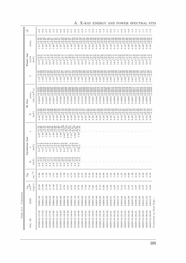
A. X-ray energy and power spectral fitsTable
A.2
–C
onti
nued
LX
NH
Cyclo
tron
line
Fe
line
Pow
er
law
χ2 r
Obs.
IDM
JD
×1037
Eσ
τE
norm
.Γ
cuto
ffnorm
.
(erg
/s)
cm−
2(k
eV)
(keV
)(k
eV)
(ph./
cm2/s)
(keV
)
91089-0
1-1
7-0
253981.3
612.2
90.8
89.8
+0
.4−
0.8
3.4
+0
.7−
0.5
0.9
7+
0.5
3−
0.2
66.4
0+
0.0
9−
0.0
90.0
218+
0.0
035
−0
.0032
1.1
2+
0.0
6−
0.0
517.9
+0
.8−
0.7
1.5
1+
0.2
6−
0.1
50.9
91089-0
1-1
7-0
353982.1
411.9
81.4
88.5
+1
.0−
4.8
4.3
+1
.2−
0.7
1.5
3+
5.9
5−
0.7
36.4
4+
0.0
9−
0.0
80.0
231+
0.0
063
−0
.0039
1.2
2+
0.2
8−
0.0
819.6
+3
.5−
1.1
1.8
3+
0.7
6−
0.3
40.8
91089-0
1-1
7-0
453983.2
011.5
81.1
99.2
+0
.8−
2.1
3.7
+1
.4−
0.8
1.0
3+
1.5
7−
0.4
26.4
5+
0.1
0−
0.1
00.0
197+
0.0
044
−0
.0036
1.1
4+
0.1
4−
0.0
718.1
+1
.1−
1.0
1.4
8+
0.4
7−
0.2
10.7
91089-0
1-1
7-0
553984.2
411.4
71.6
38.4
+1
.0−
3.5
4.0
+1
.1−
0.7
1.2
7+
3.3
4−
0.5
76.4
4+
0.0
9−
0.0
80.0
221+
0.0
063
−0
.0037
1.2
2+
0.2
5−
0.0
919.7
+3
.7−
1.2
1.7
2+
1.3
9−
0.3
10.9
91089-0
1-1
7-0
653985.2
211.4
61.6
18.4
+1
.1−
3.0
4.3
+1
.4−
0.8
1.5
6+
2.9
9−
0.6
86.4
4+
0.0
9−
0.0
80.0
217+
0.0
039
−0
.0036
1.1
7+
0.2
1−
0.0
918.2
+2
.5−
1.0
1.6
6+
0.9
1−
0.3
11.0
91089-0
1-1
8-0
153986.0
710.7
30.8
69.0
+0
.8−
2.2
3.7
+1
.3−
0.7
0.9
5+
1.5
6−
0.4
06.3
8+
0.0
9−
0.0
90.0
202+
0.0
042
−0
.0033
1.0
9+
0.1
4−
0.0
717.3
+1
.0−
0.9
1.2
5+
0.4
0−
0.1
70.8
91089-0
1-1
8-0
053986.9
910.5
71.0
49.0
+0
.9−
2.8
3.8
+1
.7−
0.9
1.0
0+
1.9
7−
0.4
56.4
3+
0.1
0−
0.1
00.0
186+
0.0
045
−0
.0035
1.0
9+
0.1
7−
0.0
817.2
+1
.9−
1.1
1.2
7+
0.5
1−
0.1
90.8
91089-0
1-1
8-0
253988.0
09.7
61.7
85.6
+9
.7−
5.6
6.4
+8
.2−
3.9
2.6
9+
12
.08
−2
.54
6.4
6+
0.1
8−
0.1
60.0
169+
0.0
076
−0
.0088
1.2
4+
0.5
1−
0.2
118.8
+7
.7−
3.1
1.6
7+
0.6
3−
0.6
50.9
91089-0
1-1
8-0
353989.1
69.5
71.5
16.0
+2
.2−
6.8
5.5
+2
.81
.42.6
0+
11
.47
−1
.89
6.4
0+
0.1
0−
0.0
90.0
196+
0.0
067
−0
.0044
1.2
0+
0.3
6−
0.1
917.7
+5
.1−
2.0
1.5
5+
0.7
9−
0.5
50.9
91089-0
1-1
8-0
453990.0
39.3
70.7
54.8
+5
.3−
4.8
8.7
+7
.9−
4.6
7.2
7+
15
.01
−6
.51
6.3
8+
0.1
6−
0.1
50.0
218+
0.0
209
−0
.0080
1.0
9+
0.3
1−
0.2
414.4
+4
.2−
2.7
1.4
9+
1.3
1−
0.6
40.7
91089-0
1-1
8-0
553991.1
29.4
50.9
78.4
+1
.4−
8.0
3.9
+2
.1−
0.8
0.8
2+
11
.69
−0
.52
6.3
9+
0.1
0−
0.1
00.0
168+
0.0
084
−0
.0034
1.0
5+
0.4
3−
0.0
916.7
+5
.1−
1.0
1.0
4+
0.4
2−
0.1
90.8
91089-0
1-1
8-0
653991.7
98.7
50.9
28.4
+1
.4−
8.4
3.3
+1
.10
.60.4
9+
9.7
6−
0.3
06.4
5+
0.1
0−
0.1
00.0
143+
0.0
067
−0
.0031
1.0
2+
0.4
4−
0.0
816.6
+4
.9−
1.0
0.8
9+
0.4
4−
0.1
40.9
91089-0
1-1
9-0
053993.6
97.9
90.5
7–
––
6.2
7+
0.1
4−
6.2
70.0
110+
0.0
023
−0
.0023
1.0
0+
0.0
5−
0.0
516.6
+1
.0−
0.9
0.7
4+
0.0
7−
0.0
70.9
91089-0
1-1
9-0
153995.0
17.7
80.2
2–
––
6.3
5+
0.1
1−
0.1
10.0
128+
0.0
022
−0
.0023
0.9
5+
0.0
6−
0.0
415.6
+1
.0−
0.6
0.6
7+
0.0
7−
0.0
41.1
91089-0
1-1
9-0
253995.7
97.4
40.4
5–
––
6.3
6+
0.0
8−
0.0
70.0
130+
0.0
016
−0
.0016
0.9
6+
0.0
4−
0.0
416.1
+0
.7−
0.6
0.6
4+
0.0
5−
0.0
41.3
91089-0
1-1
9-0
353997.0
47.6
50.0
4–
––
6.2
5+
0.1
0−
6.2
50.0
161+
0.0
021
−0
.0027
0.9
0+
0.0
7−
0.0
215.4
+1
.1−
0.5
0.5
8+
0.0
8−
0.0
20.8
91089-0
1-1
9-0
453997.8
26.7
00.4
8–
––
6.3
8+
0.1
1−
0.1
00.0
109+
0.0
019
−0
.0019
0.9
0+
0.0
6−
0.0
615.0
+0
.9−
0.8
0.5
4+
0.0
6−
0.0
51.1
91089-0
1-1
9-0
553998.6
66.1
50.4
0–
––
6.3
4+
0.0
9−
0.0
90.0
102+
0.0
015
−0
.0015
0.8
9+
0.0
5−
0.0
514.7
+0
.7−
0.6
0.4
9+
0.0
4−
0.0
40.8
92067-0
1-0
4-1
053999.5
96.2
80.8
8–
––
6.3
4+
0.1
0−
0.1
00.0
097+
0.0
016
−0
.0016
0.9
2+
0.0
5−
0.0
515.1
+0
.8−
0.7
0.5
3+
0.0
5−
0.0
51.3
92067-0
1-0
5-0
054000.6
25.9
40.6
9–
––
6.2
9+
0.1
2−
6.2
90.0
099+
0.0
020
−0
.0020
0.8
8+
0.0
7−
0.0
314.2
+0
.9−
0.8
0.4
7+
0.0
6−
0.0
50.7
92067-0
1-0
5-0
154002.0
15.2
21.2
4–
––
6.3
6+
0.1
3−
0.1
20.0
075+
0.0
015
−0
.0015
0.8
8+
0.0
6−
0.0
614.2
+0
.8−
0.7
0.4
2+
0.0
4−
0.0
40.6
92067-0
1-0
5-0
254002.7
24.6
51.3
0–
––
6.5
1+
0.2
0−
0.1
80.0
064+
0.0
018
−0
.0018
0.9
1+
0.0
9−
0.0
914.2
+1
.3−
1.2
0.4
1+
0.0
6−
0.0
61.0
92067-0
1-0
5-0
354003.5
75.2
11.3
6–
––
6.4
1+
0.1
8−
0.1
70.0
065+
0.0
018
−0
.0018
0.8
9+
0.0
7−
0.0
714.3
+1
.1−
0.9
0.4
3+
0.0
6−
0.0
51.1
92067-0
1-0
5-0
454004.4
45.1
31.2
7–
––
6.3
2+
0.1
2−
0.1
10.0
082+
0.0
016
−0
.0016
0.8
5+
0.0
6−
0.0
613.7
+0
.8−
0.8
0.4
1+
0.0
5−
0.0
40.8
92067-0
1-0
5-0
554005.6
74.7
31.8
2–
––
6.5
8+
0.2
5−
0.2
10.0
059+
0.0
018
−0
.0018
0.9
2+
0.0
9−
0.0
914.3
+1
.3−
1.2
0.4
3+
0.0
7−
0.0
60.9
92067-0
1-0
5-0
654006.5
85.0
50.8
8–
––
6.3
6+
0.1
3−
0.1
20.0
090+
0.0
018
−0
.0018
0.8
4+
0.0
7−
0.0
813.9
+1
.0−
0.9
0.3
8+
0.0
5−
0.0
50.8
92067-0
1-0
6-0
054007.5
64.4
11.4
8–
––
6.4
0+
0.2
1−
0.1
90.0
057+
0.0
017
−0
.0017
0.8
4+
0.0
8−
0.0
913.4
+1
.1−
1.0
0.3
5+
0.0
5−
0.0
51.0
92067-0
1-0
6-0
154008.4
33.9
72.3
2–
––
6.5
4+
0.1
5−
0.1
40.0
052+
0.0
011
−0
.0011
0.9
1+
0.0
6−
0.0
614.3
+0
.9−
0.8
0.3
5+
0.0
4−
0.0
31.4
92067-0
1-0
6-0
254009.5
93.5
61.3
4–
––
6.3
8+
0.2
0−
0.1
80.0
056+
0.0
017
−0
.0016
0.7
6+
0.1
0−
0.1
112.3
+1
.2−
1.1
0.2
5+
0.0
5−
0.0
41.1
92067-0
1-0
6-0
354010.3
73.3
72.3
2–
––
6.5
7+
0.1
5−
0.1
40.0
048+
0.0
010
−0
.0010
0.8
7+
0.0
6−
0.0
713.3
+0
.8−
0.8
0.2
9+
0.0
3−
0.0
31.1
92067-0
1-0
6-0
454011.5
53.1
51.9
2–
––
6.3
4+
0.1
7−
6.3
40.0
055+
0.0
015
−0
.0015
0.8
1+
0.1
0−
0.1
012.6
+1
.3−
1.1
0.2
4+
0.0
5−
0.0
41.0
92067-0
1-0
6-0
554012.7
32.8
03.1
8–
––
6.4
9+
0.1
5−
0.1
30.0
044+
0.0
009
−0
.0009
0.9
1+
0.0
7−
0.0
713.5
+1
.0−
0.9
0.2
6+
0.0
3−
0.0
31.0
Conti
nued
on
Nex
tPage.
..
205

Table
A.2
–C
onti
nued
LX
NH
Cyclo
tron
line
Fe
line
Pow
er
law
χ2 r
Obs.
IDM
JD
×1037
Eσ
τE
norm
.Γ
cuto
ffnorm
.
(erg
/s)
cm−
2(k
eV)
(keV
)(k
eV)
(ph./
cm2/s)
(keV
)
92067-0
1-0
6-0
654013.7
12.5
43.1
2–
––
6.5
9+
0.2
0−
0.1
70.0
032+
0.0
009
−0
.0008
0.9
3+
0.0
7−
0.0
813.5
+1
.1−
0.9
0.2
5+
0.0
3−
0.0
31.0
92067-0
1-0
7-0
054014.6
32.3
62.5
3–
––
6.2
0+
0.5
6−
6.2
00.0
030+
0.0
023
−0
.0025
0.8
3+
0.2
2−
0.2
112.4
+3
.0−
2.0
0.2
0+
0.0
9−
0.0
60.7
92067-0
1-0
7-0
154015.4
42.0
73.1
5–
––
6.4
5+
0.1
5−
0.1
40.0
038+
0.0
008
−0
.0008
0.9
0+
0.0
9−
0.0
913.2
+1
.2−
1.0
0.2
0+
0.0
3−
0.0
30.8
92067-0
1-0
7-0
254016.5
92.0
01.6
9–
––
6.2
6+
0.5
6−
6.2
60.0
030+
0.0
020
−0
.0020
0.7
3+
0.2
2−
0.2
311.3
+2
.6−
1.8
0.1
4+
0.0
6−
0.0
50.6
92067-0
1-0
7-0
354017.4
71.7
73.1
8–
––
6.4
9+
0.3
0−
0.2
40.0
022+
0.0
008
−0
.0007
0.8
8+
0.1
0−
0.1
012.8
+1
.3−
1.1
0.1
7+
0.0
3−
0.0
30.9
92067-0
1-0
7-0
454018.4
91.6
12.2
8–
––
6.4
00.0
028+
0.0
013
−0
.0007
0.6
7+
0.1
9−
0.1
910.2
+1
.8−
1.4
0.1
1+
0.0
4−
0.0
31.1
92067-0
1-0
7-0
554019.4
31.5
03.0
3–
––
6.4
00.0
020+
0.0
007
−0
.0007
0.9
1+
0.1
0−
0.1
012.3
+1
.3−
1.1
0.1
6+
0.0
3−
0.0
21.2
92067-0
1-0
7-0
654020.5
21.5
60.7
0–
––
6.4
00.0
021+
0.0
018
−0
.0021
0.4
2+
0.3
0−
0.1
88.2
+2
.1−
1.3
0.0
8+
0.0
5−
0.0
20.8
92067-0
1-0
8-0
054021.3
11.3
23.1
4–
––
6.4
00.0
017+
0.0
006
−0
.0006
1.0
4+
0.1
1−
0.1
114.8
+2
.1−
1.7
0.1
6+
0.0
3−
0.0
31.6
92067-0
1-0
8-0
154022.3
11.1
73.1
1–
––
6.4
00.0
014+
0.0
006
−0
.0006
0.9
9+
0.1
1−
0.1
213.6
+1
.9−
1.5
0.1
4+
0.0
3−
0.0
21.4
92067-0
1-0
8-0
254023.4
60.9
92.2
4–
––
6.4
00.0
005+
0.0
011
−0
.0005
0.6
6+
0.2
8−
0.2
99.7
+2
.8−
1.8
0.0
7+
0.0
4−
0.0
31.0
92067-0
1-0
8-0
354024.5
80.9
43.0
6–
––
6.4
00.0
012+
0.0
005
−0
.0005
1.0
4+
0.1
2−
0.1
214.9
+2
.5−
1.9
0.1
1+
0.0
2−
0.0
21.0
92067-0
1-0
8-0
454025.3
90.8
73.1
8–
––
6.4
00.0
014+
0.0
005
−0
.0005
1.1
8+
0.1
3−
0.1
317.9
+4
.0−
2.8
0.1
3+
0.0
3−
0.0
21.0
92067-0
1-0
8-0
554026.4
20.7
43.2
6–
––
6.4
00.0
012+
0.0
004
−0
.0005
1.1
4+
0.1
4−
0.1
416.4
+3
.7−
2.6
0.1
0+
0.0
3−
0.0
21.1
92067-0
1-0
8-0
654027.6
50.6
72.4
8–
––
6.4
00.0
007+
0.0
004
−0
.0005
1.2
7+
0.1
5−
0.1
618.7
+5
.6−
3.6
0.1
2+
0.0
3−
0.0
30.8
92067-0
1-0
9-0
054028.7
70.5
82.7
6–
––
6.4
00.0
008+
0.0
004
−0
.0004
1.1
8+
0.1
5−
0.1
516.6
+4
.2−
2.8
0.0
9+
0.0
2−
0.0
20.9
92067-0
1-0
9-0
154029.6
80.5
52.8
2–
––
6.4
00.0
010+
0.0
004
−0
.0004
0.9
5+
0.1
9−
0.1
912.2
+3
.0−
2.0
0.0
6+
0.0
2−
0.0
20.9
92067-0
1-0
9-0
354031.7
80.4
82.5
0–
––
6.4
00.0
006+
0.0
004
−0
.0004
1.1
7+
0.1
8−
0.1
815.2
+4
.6−
2.9
0.0
8+
0.0
2−
0.0
20.6
92067-0
1-0
9-0
554033.5
00.3
92.5
2–
––
6.4
00.0
006+
0.0
004
−0
.0004
1.0
1+
0.2
2−
0.2
212.3
+3
.7−
2.4
0.0
5+
0.0
2−
0.0
10.6
92067-0
1-0
9-0
654034.7
90.3
32.2
0–
––
6.4
00.0
007+
0.0
005
−0
.0004
1.1
9+
0.2
4−
0.2
514.9
+6
.8−
3.6
0.0
6+
0.0
3−
0.0
20.8
92067-0
1-1
0-0
054035.7
70.3
02.4
4–
––
6.4
00.0
007+
0.0
004
−0
.0004
1.0
8+
0.2
8−
0.3
012.5
+5
.8−
3.2
0.0
4+
0.0
2−
0.0
20.9
92067-0
1-1
0-0
154036.7
90.2
42.7
0–
––
6.4
00.0
003+
0.0
004
−0
.0003
1.1
6+
0.4
4−
0.4
610.9
+8
.4−
3.5
0.0
5+
0.0
5−
0.0
30.5
92067-0
1-1
0-0
254037.8
70.2
92.8
3–
––
6.4
00.0
004+
0.0
003
−0
.0003
1.4
5+
0.2
6−
0.2
719.6
+15
.7−
6.3
0.0
8+
0.0
4−
0.0
20.8
92067-0
1-1
0-0
354038.8
20.2
52.8
7–
––
6.4
00.0
003+
0.0
005
−0
.0003
1.3
5+
0.4
1−
0.4
115.0
+19
.3−
5.5
0.0
6+
0.0
6−
0.0
30.6
92067-0
1-1
0-0
454039.8
70.2
42.1
4–
––
6.4
00.0
003+
0.0
005
−0
.0003
1.2
6+
0.5
4−
0.5
914.7
+37
.3−
6.7
0.0
5+
0.0
6−
0.0
30.6
92067-0
1-1
0-0
554040.8
80.3
02.2
3–
––
6.4
00.0
004+
0.0
003
−0
.0004
1.1
4+
0.2
7−
0.2
513.3
+5
.9−
3.1
0.0
5+
0.0
2−
0.0
20.5
92067-0
1-1
0-0
654041.9
00.3
62.8
1–
––
6.4
00.0
006+
0.0
007
−0
.0006
1.2
2+
0.4
3−
0.4
414.2
+16
.2−
5.1
0.0
7+
0.0
6−
0.0
30.9
92067-0
1-1
1-0
054042.4
20.4
42.8
5–
––
6.4
00.0
009+
0.0
004
−0
.0004
1.1
4+
0.2
1−
0.2
114.2
+4
.8−
2.9
0.0
7+
0.0
3−
0.0
20.9
92067-0
1-1
1-0
154043.7
20.4
43.0
5–
––
6.4
00.0
010+
0.0
005
−0
.0005
1.0
8+
0.2
8−
0.2
813.5
+6
.3−
3.4
0.0
6+
0.0
3−
0.0
20.9
92067-0
1-1
1-0
254044.9
80.4
93.2
1–
––
6.4
00.0
011+
0.0
004
−0
.0004
1.0
9+
0.1
8−
0.1
813.6
+3
.5−
2.4
0.0
7+
0.0
2−
0.0
20.9
92067-0
1-1
1-0
354045.8
20.4
73.5
6–
––
6.4
00.0
009+
0.0
007
−0
.0007
1.1
5+
0.3
5−
0.3
416.1
+13
.5−
5.1
0.0
7+
0.0
5−
0.0
30.7
206
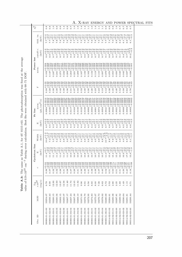
A. X-ray energy and power spectral fitsTable
A.3
:T
he
sam
eas
Table
A.1
,fo
r4U
0115+
63.
The
photo
abso
rption
was
fixed
at
the
aver
age
valu
eof0.9×
1022
cm−
2during
erro
rca
lcula
tion.
Bes
tfits
wer
eobta
ined
with
68–71
DO
F.
LX
Cyclo
tron
line
Fe
line
Pow
er
law
χ2 r
Obs.
IDM
JD
×1037
τE
Wid
thE
norm
.Γ
norm
.cu
toff
e.fo
ld.
en.
(erg
/s)
(keV
)(k
eV)
(keV
)(p
h./
cm2/s)
(keV
)(k
eV)
90089-0
1-0
1-0
053254.0
76.7
80.3
6+
0.0
4−
0.0
311.4
+0
.7−
0.2
10.6
+1
.0−
1.5
6.5
+0
.2−
0.2
0.0
064+
0.0
014
−0
.0013
0.2
4+
0.0
3−
0.0
30.1
02+
0.0
04
−0
.004
9.0
+0
.2−
0.2
7.7
+0
.4−
0.3
0.8
90089-0
1-0
2-0
053256.4
38.9
90.3
7+
0.0
2−
0.0
211.4
+0
.2−
0.2
7.3
+0
.4−
0.4
6.5
+0
.1−
0.1
0.0
100+
0.0
016
−0
.0016
0.2
8+
0.0
2−
0.0
20.1
47+
0.0
05
−0
.004
8.9
+0
.1−
0.1
7.7
+0
.1−
0.1
0.8
90089-0
1-0
3-0
153260.1
512.6
60.3
2+
0.0
2−
0.0
211.1
+0
.2−
0.2
5.5
+0
.3−
0.2
6.3
+0
.1−
0.1
0.0
166+
0.0
021
−0
.0023
0.3
8+
0.0
2−
0.0
20.2
47+
0.0
01
−0
.001
8.7
+0
.2−
0.2
7.8
+0
.1−
0.1
1.0
90089-0
1-0
3-0
353260.5
612.6
90.3
2+
0.0
2−
0.0
211.2
+0
.1−
0.1
5.2
+0
.2−
0.2
6.4
+0
.1−
0.1
0.0
161+
0.0
022
−0
.0024
0.3
8+
0.0
2−
0.0
20.2
41+
0.0
08
−0
.008
8.7
+0
.2−
0.2
7.8
+0
.1−
0.1
0.9
90089-0
1-0
3-0
053262.1
513.6
70.2
8+
0.0
4−
0.0
411.0
+0
.2−
0.1
4.4
+0
.3−
0.2
6.3
+0
.1−
6.3
0.0
183+
0.0
026
−0
.0029
0.4
2+
0.0
3−
0.0
30.2
75+
0.0
11
−0
.011
8.7
+0
.2−
0.3
7.6
+0
.2−
0.2
0.9
90089-0
1-0
4-0
653265.0
712.5
80.3
1+
0.0
3−
0.0
311.0
+0
.1−
0.1
3.8
+0
.2−
0.1
6.3
+0
.1−
6.3
0.0
164+
0.0
024
−0
.0027
0.3
8+
0.0
2−
0.0
30.2
42+
0.0
09
−0
.009
8.5
+0
.2−
0.2
7.6
+0
.1−
0.1
1.4
90089-0
1-0
4-0
153267.1
711.4
90.2
8+
0.0
4−
0.0
411.0
+0
.2−
0.2
3.0
+0
.3−
0.4
6.3
+0
.1−
6.3
0.0
143+
0.0
034
−0
.0038
0.3
6+
0.0
4−
0.0
40.2
09+
0.0
13
−0
.013
8.2
+0
.3−
0.3
7.6
+0
.3−
0.2
0.9
90089-0
1-0
4-0
453267.2
411.7
30.3
7+
0.1
3−
0.0
610.6
+0
.2−
0.3
3.5
+0
.3−
0.3
6.3
+0
.3−
6.3
0.0
117+
0.0
041
−0
.0044
0.3
1+
0.0
5−
0.0
80.2
03+
0.0
16
−0
.021
8.4
+0
.6−
0.4
7.2
+0
.3−
0.4
0.7
90089-0
1-0
4-0
553267.3
012.0
50.2
9+
0.0
4−
0.0
310.9
+0
.1−
0.1
3.2
+0
.2−
0.3
6.2
+0
.1−
6.2
0.0
163+
0.0
032
−0
.0033
0.3
7+
0.0
3−
0.0
30.2
21+
0.0
12
−0
.010
8.2
+0
.3−
0.2
7.7
+0
.2−
0.2
1.0
90089-0
1-0
4-0
253269.1
011.9
20.3
1+
0.0
3−
0.0
210.9
+0
.1−
0.1
3.3
+0
.1−
0.1
6.2
+0
.1−
6.2
0.0
133+
0.0
024
−0
.0029
0.3
4+
0.0
2−
0.0
30.2
09+
0.0
08
−0
.009
8.3
+0
.2−
0.2
7.7
+0
.1−
0.1
1.9
90089-0
1-0
4-0
353271.9
59.9
60.3
6+
0.0
4−
0.0
310.7
+0
.1−
0.1
3.4
+0
.1−
0.1
6.4
+0
.1−
0.1
0.0
123+
0.0
018
−0
.0019
0.3
2+
0.0
2−
0.0
30.1
67+
0.0
06
−0
.006
8.7
+0
.2−
0.2
7.5
+0
.1−
0.1
1.4
90089-0
1-0
5-0
053272.7
99.5
50.3
6+
0.0
3−
0.0
310.8
+0
.1−
0.1
3.6
+0
.1−
0.1
6.4
+0
.1−
0.1
0.0
109+
0.0
017
−0
.0018
0.3
0+
0.0
2−
0.0
20.1
56+
0.0
06
−0
.006
8.6
+0
.2−
0.2
7.5
+0
.1−
0.1
1.4
90089-0
1-0
5-0
553272.9
59.5
60.4
1+
0.0
4−
0.0
410.7
+0
.1−
0.1
3.6
+0
.1−
0.1
6.5
+0
.1−
0.2
0.0
092+
0.0
022
−0
.0021
0.3
0+
0.0
8−
0.0
50.1
62+
0.0
35
−0
.016
8.8
+0
.2−
0.2
7.4
+0
.2−
0.2
1.1
90089-0
1-0
5-0
153274.8
38.6
00.3
8+
0.0
3−
0.0
310.7
+0
.1−
0.1
4.2
+0
.1−
0.1
6.4
+0
.1−
0.1
0.0
092+
0.0
017
−0
.0017
0.2
6+
0.0
2−
0.0
20.1
34+
0.0
05
−0
.005
8.5
+0
.2−
0.2
7.6
+0
.1−
0.1
1.0
90089-0
1-0
5-0
253275.6
78.0
00.3
9+
0.0
3−
0.0
310.7
+0
.1−
0.1
4.5
+0
.2−
0.1
6.5
+0
.1−
0.1
0.0
081+
0.0
015
−0
.0015
0.2
3+
0.0
2−
0.0
20.1
19+
0.0
04
−0
.004
8.7
+0
.2−
0.2
7.6
+0
.1−
0.1
1.4
90089-0
1-0
5-0
353276.7
37.3
80.3
7+
0.0
3−
0.0
310.6
+0
.1−
0.1
4.9
+0
.2−
0.2
6.5
+0
.1−
0.1
0.0
074+
0.0
015
−0
.0015
0.2
3+
0.0
2−
0.0
20.1
10+
0.0
04
−0
.004
8.6
+0
.2−
0.2
7.5
+0
.1−
0.1
1.1
90089-0
1-0
5-0
453278.6
26.6
20.4
0+
0.0
2−
0.0
210.7
+0
.1−
0.1
6.8
+0
.5−
0.4
6.6
+0
.2−
0.2
0.0
054+
0.0
014
−0
.0014
0.1
9+
0.0
2−
0.0
20.0
97+
0.0
04
−0
.003
8.7
+0
.2−
0.2
7.4
+0
.1−
0.1
1.1
90089-0
1-0
6-0
053280.6
95.7
20.5
2+
0.0
3−
0.0
311.0
+0
.2−
0.2
10.7
+0
.8−
0.8
6.7
+0
.2−
0.2
0.0
041+
0.0
012
−0
.0012
0.1
2+
0.0
2−
0.0
20.0
79+
0.0
03
−0
.003
9.1
+0
.1−
0.1
7.7
+0
.3−
0.3
0.9
90014-0
2-0
1-0
253284.6
13.5
20.5
1+
0.0
8−
0.0
815.4
+0
.5−
0.7
8.8
+1
.4−
1.3
6.8
+0
.2−
0.2
0.0
035+
0.0
009
−0
.0009
0.3
8+
0.0
4−
0.0
40.0
70+
0.0
03
−0
.004
8.8
+0
.2−
0.2
7.4
+0
.5−
0.4
0.9
90014-0
2-0
1-0
153285.9
82.8
60.5
0+
0.1
7−
0.1
715.4
+0
.8−
0.8
7.8
+2
.1−
2.5
6.7
+0
.2−
0.2
0.0
024+
0.0
011
−0
.0012
0.3
5+
0.0
7−
0.0
80.0
55+
0.0
05
−0
.006
8.7
+0
.2−
0.2
7.0
+0
.9−
0.7
0.8
90014-0
2-0
2-0
053287.8
12.3
50.5
1+
0.1
1−
0.1
115.2
+0
.7−
0.8
8.3
+1
.7−
1.7
6.8
+0
.2−
0.2
0.0
021+
0.0
006
−0
.0006
0.4
0+
0.0
4−
0.0
60.0
50+
0.0
03
−0
.003
9.1
+0
.2−
0.2
6.9
+0
.6−
0.5
1.0
90014-0
2-0
2-0
153289.5
21.8
90.3
1+
0.1
9−
0.0
916.0
+0
.4−
0.4
4.9
+3
.3−
1.9
6.7
+0
.3−
0.3
0.0
015+
0.0
005
−0
.0005
0.5
2+
0.0
3−
0.0
60.0
49+
0.0
02
−0
.004
9.1
+0
.2−
0.1
6.2
+0
.8−
0.4
0.7
90014-0
2-0
2-0
253290.6
41.4
90.3
0+
0.1
8−
0.0
916.9
+0
.4−
0.5
4.0
+3
.2−
1.7
6.5
+0
.4−
0.4
0.0
009+
0.0
004
−0
.0004
0.5
8+
0.0
3−
0.0
50.0
43+
0.0
02
−0
.003
9.4
+0
.2−
0.1
6.1
+0
.7−
0.4
0.7
90014-0
2-0
2-0
353291.8
11.1
50.4
0+
0.2
5−
0.2
117.5
+0
.8−
0.9
6.5
+3
.9−
3.3
6.6
+0
.5−
0.5
0.0
002+
0.0
004
−0
.0002
0.6
4+
0.0
4−
0.0
70.0
37+
0.0
02
−0
.003
9.7
+0
.2−
0.2
6.6
+1
.1−
0.8
0.8
90014-0
2-0
3-0
053293.4
40.7
10.1
6+
0.1
1−
0.0
815.9
+0
.8−
1.0
3.1
+2
.7−
1.7
6.6
+0
.5−
0.5
0.0
002+
0.0
002
−0
.0002
0.7
6+
0.0
2−
0.0
30.0
28+
0.0
01
−0
.001
10.2
+0
.2−
0.2
6.1
+0
.5−
0.3
0.7
207
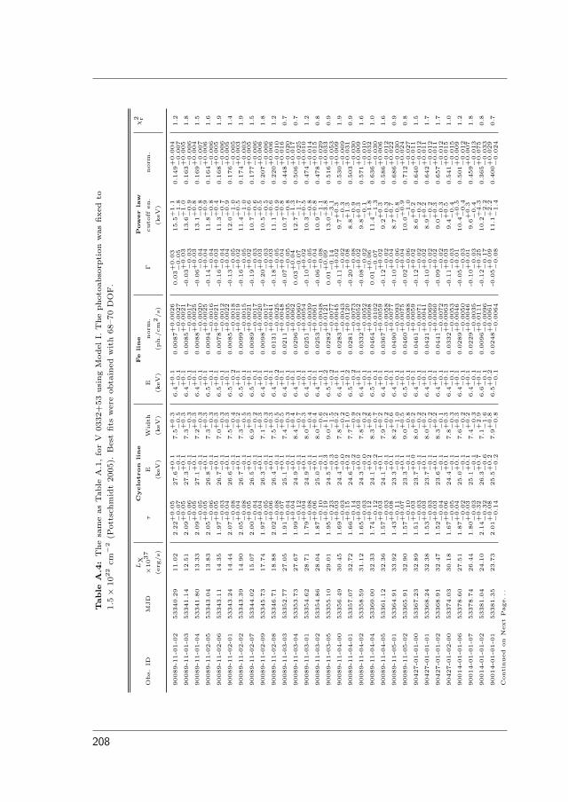
Table
A.4
:T
he
sam
eas
Table
A.1
,fo
rV
0332+
53
usi
ng
Model
I.T
he
photo
abso
rption
was
fixed
to
1.5×
1022
cm−
2(P
ott
schm
idt
2005).
Bes
tfits
wer
eobta
ined
with
68–70
DO
F.
LX
Cyclo
tron
line
Fe
line
Pow
er
law
χ2 r
Obs.
IDM
JD
×1037
τE
Wid
thE
norm
.Γ
cuto
ffen
.norm
.
(erg
/s)
(keV
)(k
eV)
(keV
)(p
h./
cm2/s)
(keV
)
90089-1
1-0
1-0
253340.2
911.0
22.2
2+
0.0
5−
0.0
727.6
+0
.1−
0.1
7.5
+0
.3−
0.5
6.4
+0
.1−
0.1
0.0
087+
0.0
026
−0
.0027
0.0
3+
0.0
3−
0.0
515.5
+1
.1−
1.8
0.1
49+
0.0
04
−0
.007
1.2
90089-1
1-0
1-0
353341.1
412.5
12.0
9+
0.0
5−
0.0
627.3
+0
.1−
0.1
7.3
+0
.3−
0.3
6.4
+0
.1−
0.1
0.0
085+
0.0
021
−0
.0017
-0.0
3+
0.0
3−
0.0
313.6
+1
.0−
0.9
0.1
63+
0.0
05
−0
.006
1.8
90089-1
1-0
1-0
453341.8
013.3
32.0
9+
0.0
5−
0.0
527.1
+0
.1−
0.1
7.2
+0
.3−
0.3
6.4
+0
.1−
0.1
0.0
088+
0.0
025
−0
.0020
-0.0
6+
0.0
3−
0.0
413.1
+0
.8−
0.8
0.1
69+
0.0
04
−0
.007
1.5
90089-1
1-0
2-0
553343.0
413.8
32.0
5+
0.0
5−
0.0
626.8
+0
.1−
0.1
7.3
+0
.3−
0.3
6.5
+0
.1−
0.1
0.0
094+
0.0
025
−0
.0016
-0.1
4+
0.0
4−
0.0
411.8
+0
.9−
0.8
0.1
64+
0.0
06
−0
.006
1.6
90089-1
1-0
2-0
653343.1
114.3
51.9
7+
0.0
5−
0.0
326.7
+0
.1−
0.1
7.0
+0
.3−
0.3
6.5
+0
.1−
0.1
0.0
078+
0.0
021
−0
.0012
-0.1
6+
0.0
3−
0.0
411.3
+0
.4−
0.7
0.1
68+
0.0
05
−0
.006
1.9
90089-1
1-0
2-0
153343.2
414.4
42.0
7+
0.0
4−
0.0
826.6
+0
.1−
0.1
7.5
+0
.3−
0.4
6.5
+0
.1−
0.2
0.0
085+
0.0
022
−0
.0018
-0.1
3+
0.0
4−
0.0
512.0
+0
.9−
1.0
0.1
76+
0.0
05
−0
.005
1.4
90089-1
1-0
2-0
253343.3
914.9
02.0
5+
0.0
4−
0.0
826.7
+0
.1−
0.1
7.3
+0
.2−
0.5
6.5
+0
.1−
0.1
0.0
099+
0.0
019
−0
.0015
-0.1
6+
0.0
2−
0.0
511.4
+0
.5−
1.0
0.1
74+
0.0
03
−0
.003
1.9
90089-1
1-0
2-0
753344.0
215.0
72.0
0+
0.0
5−
0.0
426.5
+0
.1−
0.1
6.9
+0
.3−
0.2
6.5
+0
.1−
0.1
0.0
089+
0.0
021
−0
.0017
-0.1
9+
0.0
2−
0.0
310.7
+0
.6−
0.6
0.1
77+
0.0
05
−0
.006
1.5
90089-1
1-0
2-0
953345.7
317.7
41.9
7+
0.0
4−
0.0
526.3
+0
.1−
0.1
7.1
+0
.3−
0.3
6.4
+0
.1−
0.1
0.0
098+
0.0
020
−0
.0017
-0.2
0+
0.0
3−
0.0
310.5
+0
.5−
0.5
0.2
07+
0.0
06
−0
.006
1.8
90089-1
1-0
2-0
853346.7
118.8
82.0
2+
0.0
6−
0.0
826.4
+0
.1−
0.1
7.5
+0
.3−
0.5
6.4
+0
.1−
0.2
0.0
131+
0.0
041
−0
.0025
-0.1
8+
0.0
3−
0.0
511.1
+0
.6−
0.9
0.2
20+
0.0
06
−0
.010
1.2
90089-1
1-0
3-0
353352.7
727.0
51.9
1+
0.0
7−
0.0
425.1
+0
.1−
0.1
7.4
+0
.5−
0.3
6.4
+0
.1−
0.1
0.0
211+
0.0
048
−0
.0035
-0.0
7+
0.0
4−
0.0
510.7
+0
.8−
0.8
0.4
48+
0.0
16
−0
.020
0.7
90089-1
1-0
3-0
453353.7
327.6
71.9
9+
0.0
4−
0.1
224.9
+0
.1−
0.1
8.4
+0
.4−
0.7
6.4
+0
.1−
0.1
0.0
296+
0.0
062
−0
.0060
0.0
3+
0.0
4−
0.0
712.7
+1
.3−
1.7
0.5
06+
0.0
17
−0
.025
0.7
90089-1
1-0
3-0
153354.6
228.7
11.7
9+
0.0
4−
0.0
824.9
+0
.1−
0.1
8.0
+0
.3−
0.4
6.4
+0
.1−
0.1
0.0
251+
0.0
054
−0
.0039
-0.1
0+
0.0
2−
0.0
510.3
+0
.5−
0.8
0.4
74+
0.0
10
−0
.014
1.2
90089-1
1-0
3-0
253354.8
628.0
41.8
7+
0.0
6−
0.1
025.0
+0
.1−
0.1
8.0
+0
.4−
0.6
6.4
+0
.1−
0.1
0.0
253+
0.0
061
−0
.0048
-0.0
6+
0.0
4−
0.0
810.9
+0
.8−
1.1
0.4
78+
0.0
15
−0
.029
0.8
90089-1
1-0
3-0
553355.1
029.0
11.9
5+
0.1
9−
0.2
324.5
+0
.3−
0.3
9.0
+1
.2−
1.5
6.5
+0
.2−
0.2
0.0
282+
0.0
121
−0
.0077
0.0
1+
0.0
9−
0.1
413.0
+3
.8−
3.1
0.5
16+
0.0
33
−0
.053
0.9
90089-1
1-0
4-0
053356.4
930.4
51.6
9+
0.0
3−
0.0
324.4
+0
.0−
0.0
7.8
+0
.2−
0.2
6.4
+0
.1−
0.1
0.0
283+
0.0
045
−0
.0043
-0.1
1+
0.0
2−
0.0
29.7
+0
.3−
0.3
0.5
30+
0.0
09
−0
.009
1.9
90089-1
1-0
4-0
153357.0
732.7
21.6
6+
0.1
5−
0.1
424.6
+0
.2−
0.2
7.7
+1
.0−
0.9
6.5
+0
.2−
0.2
0.0
281+
0.0
120
−0
.0073
-0.2
0+
0.0
8−
0.0
88.8
+1
.3−
0.9
0.5
03+
0.0
31
−0
.030
0.9
90089-1
1-0
4-0
253358.5
931.1
21.6
5+
0.0
3−
0.0
324.3
+0
.0−
0.0
7.8
+0
.2−
0.2
6.4
+0
.1−
0.1
0.0
332+
0.0
052
−0
.0052
-0.0
8+
0.0
2−
0.0
29.8
+0
.3−
0.1
0.5
71+
0.0
09
−0
.010
1.6
90089-1
1-0
4-0
453360.0
032.3
31.7
4+
0.1
2−
0.1
224.1
+0
.2−
0.2
8.3
+0
.8−
0.7
6.5
+0
.1−
0.1
0.0
464+
0.0
098
−0
.0102
0.0
1+
0.0
6−
0.0
711.4
+1
.8−
1.3
0.6
36+
0.0
32
−0
.030
1.0
90089-1
1-0
4-0
553361.1
232.3
61.5
7+
0.0
3−
0.0
324.1
+0
.1−
0.1
7.9
+0
.2−
0.2
6.4
+0
.1−
0.1
0.0
367+
0.0
059
−0
.0058
-0.1
2+
0.0
2−
0.0
29.2
+0
.3−
0.3
0.5
86+
0.0
06
−0
.012
1.6
90089-1
1-0
5-0
153364.9
133.9
21.4
3+
0.0
8−
0.1
123.3
+0
.1−
0.1
8.2
+0
.6−
1.0
6.4
+0
.1−
0.1
0.0
490+
0.0
077
−0
.0093
-0.1
0+
0.0
4−
0.0
68.7
+0
.7−
0.8
0.6
86+
0.0
22
−0
.030
0.9
90089-1
1-0
5-0
253365.9
132.9
01.5
7+
0.0
7−
0.1
023.3
+0
.1−
0.1
9.0
+0
.5−
0.8
6.5
+0
.1−
0.1
0.0
460+
0.0
075
−0
.0088
-0.0
2+
0.0
4−
0.0
610.0
+0
.9−
1.0
0.7
12+
0.0
24
−0
.027
0.8
90427-0
1-0
1-0
053367.2
332.8
91.5
1+
0.0
3−
0.0
323.7
+0
.0−
0.1
8.0
+0
.2−
0.2
6.4
+0
.1−
0.1
0.0
461+
0.0
059
−0
.0071
-0.1
2+
0.0
2−
0.0
28.6
+0
.2−
0.2
0.6
40+
0.0
11
−0
.012
1.5
90427-0
1-0
1-0
153368.2
432.3
81.5
3+
0.0
3−
0.0
323.7
+0
.1−
0.1
8.0
+0
.2−
0.2
6.4
+0
.1−
0.1
0.0
421+
0.0
041
−0
.0069
-0.1
0+
0.0
2−
0.0
28.9
+0
.2−
0.2
0.6
42+
0.0
11
−0
.012
1.7
90427-0
1-0
1-0
253368.9
132.4
71.5
2+
0.0
3−
0.0
423.6
+0
.1−
0.1
8.3
+0
.2−
0.1
6.4
+0
.1−
0.1
0.0
441+
0.0
060
−0
.0072
-0.0
9+
0.0
2−
0.0
29.0
+0
.3−
0.3
0.6
57+
0.0
11
−0
.012
1.7
90427-0
1-0
2-0
053374.0
330.1
81.6
7+
0.0
6−
0.0
524.4
+0
.1−
0.1
7.8
+0
.3−
0.3
6.4
+0
.1−
0.1
0.0
332+
0.0
063
−0
.0053
-0.1
1+
0.0
3−
0.0
39.4
+0
.5−
0.4
0.5
41+
0.0
15
−0
.015
1.0
90014-0
1-0
1-0
653378.6
027.5
11.8
7+
0.0
4−
0.0
225.0
+0
.1−
0.1
7.6
+0
.3−
0.2
6.4
+0
.1−
0.1
0.0
289+
0.0
046
−0
.0050
-0.0
5+
0.0
1−
0.0
310.4
+0
.5−
0.4
0.5
01+
0.0
09
−0
.012
1.2
90014-0
1-0
1-0
753378.7
426.4
41.8
0+
0.0
3−
0.0
325.1
+0
.1−
0.1
7.4
+0
.2−
0.3
6.4
+0
.1−
0.1
0.0
229+
0.0
046
−0
.0035
-0.1
0+
0.0
1−
0.0
39.6
+0
.3−
0.4
0.4
59+
0.0
07
−0
.013
1.8
90014-0
1-0
1-0
253381.0
424.1
02.1
4+
0.3
2−
0.3
226.3
+0
.7−
0.6
7.1
+2
.9−
1.6
6.6
+0
.1−
0.1
0.0
096+
0.0
111
−0
.0096
-0.1
2+
0.2
5−
0.1
710.2
+4
.3−
2.2
0.3
65+
0.0
75
−0
.033
0.8
90014-0
1-0
1-0
153381.3
523.7
32.0
1+
0.0
8−
0.1
425.5
+0
.2−
0.2
7.9
+0
.8−
0.8
6.5
+0
.2−
0.1
0.0
248+
0.0
061
−0
.0064
-0.0
5+
0.0
9−
0.0
811.1
+2
.2−
1.4
0.4
00+
0.0
29
−0
.024
0.7
Conti
nued
on
Nex
tPage.
..
208

A. X-ray energy and power spectral fitsTable
A.4
–C
onti
nued
LX
Cyclo
tron
line
Fe
line
Pow
er
law
χ2 r
Obs.
IDM
JD
×1037
τE
Wid
thE
norm
.Γ
cuto
ffen
.norm
.
(erg
/s)
(keV
)(k
eV)
(keV
)(p
h./
cm2/s)
(keV
)
90014-0
1-0
2-0
353385.8
719.3
91.9
8+
0.0
6−
0.1
126.1
+0
.1−
0.1
7.7
+0
.3−
0.6
6.4
+0
.1−
0.1
0.0
147+
0.0
033
−0
.0025
-0.1
2+
0.0
3−
0.0
710.2
+0
.5−
1.0
0.2
93+
0.0
09
−0
.017
1.2
90014-0
1-0
2-1
053387.1
218.3
31.9
2+
0.0
5−
0.0
526.2
+0
.1−
0.1
7.2
+0
.3−
0.3
6.4
+0
.1−
0.1
0.0
141+
0.0
024
−0
.0020
-0.1
7+
0.0
3−
0.0
49.6
+0
.4−
0.5
0.2
58+
0.0
07
−0
.008
1.4
90014-0
1-0
2-1
553389.0
816.8
81.9
5+
0.0
5−
0.0
626.4
+0
.1−
0.1
7.4
+0
.2−
0.2
6.5
+0
.1−
0.1
0.0
151+
0.0
029
−0
.0026
-0.1
5+
0.0
3−
0.0
410.0
+0
.6−
0.5
0.2
35+
0.0
07
−0
.008
1.8
90014-0
1-0
3-0
153393.2
114.4
41.9
5+
0.0
4−
0.0
526.6
+0
.1−
0.1
7.2
+0
.2−
0.3
6.5
+0
.1−
0.1
0.0
147+
0.0
023
−0
.0028
-0.1
4+
0.0
3−
0.0
410.5
+0
.3−
0.7
0.1
92+
0.0
04
−0
.009
1.8
90014-0
1-0
3-0
253394.5
914.1
01.9
5+
0.0
5−
0.0
526.7
+0
.1−
0.1
7.0
+0
.3−
0.3
6.4
+0
.1−
0.1
0.0
122+
0.0
022
−0
.0022
-0.1
9+
0.0
3−
0.0
49.8
+0
.4−
0.5
0.1
81+
0.0
05
−0
.006
1.9
90014-0
1-0
4-0
053398.4
611.6
92.0
3+
0.0
5−
0.0
626.9
+0
.1−
0.1
6.5
+0
.2−
0.3
6.5
+0
.1−
0.1
0.0
125+
0.0
014
−0
.0021
-0.1
3+
0.0
3−
0.0
410.9
+0
.6−
0.6
0.1
51+
0.0
04
−0
.006
1.7
90014-0
1-0
4-0
153399.6
011.5
62.0
7+
0.0
7−
0.0
926.9
+0
.2−
0.2
7.2
+0
.4−
0.6
6.5
+0
.1−
0.1
0.0
114+
0.0
023
−0
.0024
-0.0
8+
0.0
4−
0.0
712.3
+1
.1−
1.4
0.1
51+
0.0
06
−0
.008
1.2
90014-0
1-0
4-0
253401.3
710.6
32.0
6+
0.0
8−
0.0
726.9
+0
.2−
0.1
7.3
+0
.4−
0.4
6.6
+0
.1−
0.1
0.0
119+
0.0
025
−0
.0026
-0.0
7+
0.0
5−
0.0
612.8
+1
.0−
1.3
0.1
37+
0.0
05
−0
.004
1.5
90014-0
1-0
4-0
353403.3
49.9
42.0
7+
0.0
7−
0.0
827.0
+0
.2−
0.2
7.0
+0
.4−
0.4
6.6
+0
.1−
0.1
0.0
097+
0.0
023
−0
.0026
-0.0
9+
0.0
5−
0.0
712.9
+1
.0−
1.4
0.1
20+
0.0
04
−0
.007
1.2
90014-0
1-0
5-0
053405.2
49.9
42.1
6+
0.0
8−
0.0
927.1
+0
.2−
0.2
7.0
+0
.4−
0.5
6.6
+0
.1−
0.1
0.0
099+
0.0
021
−0
.0023
-0.0
5+
0.0
4−
0.0
713.5
+1
.2−
1.7
0.1
27+
0.0
05
−0
.007
0.9
90014-0
1-0
5-0
453407.7
68.9
22.2
5+
0.0
7−
0.0
927.2
+0
.2−
0.2
7.4
+0
.4−
0.4
6.5
+0
.1−
0.1
0.0
091+
0.0
022
−0
.0018
0.0
2+
0.0
4−
0.0
615.8
+1
.7−
1.9
0.1
20+
0.0
05
−0
.005
1.2
90014-0
1-0
5-0
553407.9
68.6
32.2
6+
0.0
7−
0.0
627.4
+0
.1−
0.1
7.5
+0
.3−
0.4
6.5
+0
.1−
0.1
0.0
064+
0.0
015
−0
.0010
-0.0
0+
0.0
5−
0.0
415.5
+1
.0−
1.4
0.1
11+
0.0
04
−0
.003
1.4
90014-0
1-0
5-0
353410.7
57.2
02.4
3+
0.2
4−
0.2
027.5
+0
.5−
0.4
7.8
+1
.3−
1.0
6.6
+0
.3−
0.3
0.0
061+
0.0
050
−0
.0029
0.1
7+
0.1
7−
0.1
126.1
+1
.3−
8.3
0.1
04+
0.0
15
−0
.009
1.0
90014-0
1-0
5-0
653411.6
26.8
62.4
7+
0.1
2−
0.1
427.7
+0
.3−
0.2
7.4
+0
.4−
0.6
6.3
+0
.1−
0.3
0.0
036+
0.0
013
−0
.0007
0.1
0+
0.0
5−
0.0
621.1
+4
.6−
3.7
0.0
92+
0.0
04
−0
.005
0.9
90014-0
1-0
6-0
053414.0
45.9
92.8
8+
0.1
1−
0.0
927.8
+0
.3−
0.2
9.4
+0
.4−
0.3
6.6
+0
.1−
0.2
0.0
047+
0.0
010
−0
.0009
0.3
5+
0.0
1−
0.0
1–
0.0
90+
0.0
02
−0
.002
1.2
90014-0
1-0
6-0
153416.0
74.6
62.8
6+
0.1
0−
0.1
127.8
+0
.2−
0.2
8.3
+0
.3−
0.3
6.4
+0
.2−
0.1
0.0
032+
0.0
006
−0
.0006
0.3
7+
0.0
1−
0.0
1–
0.0
73+
0.0
02
−0
.001
1.3
90014-0
1-0
6-0
253417.5
84.0
82.8
2+
0.0
1−
0.0
128.1
+0
.3−
0.2
8.4
+0
.3−
0.3
6.5
+0
.4−
0.2
0.0
026+
0.0
002
−0
.0002
0.3
9+−
0.0
1−
0.0
1–
0.0
65+
0.0
01
−0
.001
1.1
90014-0
1-0
6-0
353418.4
73.4
22.6
3+
0.1
2−
0.1
227.8
+0
.3−
0.3
7.9
+0
.3−
0.4
6.4
0.0
018+
0.0
005
−0
.0006
0.4
0+
0.0
1−
0.0
1–
0.0
55+
0.0
01
−0
.001
1.1
90014-0
1-0
7-0
153419.4
12.9
62.6
6+
0.1
7−
0.1
627.9
+0
.3−
0.3
7.0
+0
.4−
0.4
6.4
0.0
018+
0.0
005
−0
.0006
0.4
5+
0.0
1−
0.0
1–
0.0
53+
0.0
01
−0
.002
1.1
90014-0
1-0
7-0
253420.6
42.5
72.6
4+
0.1
1−
0.1
128.4
+0
.2−
0.3
7.6
+0
.4−
0.5
6.2
+0
.4−
0.2
0.0
011+
0.0
002
−0
.0002
0.4
6+
0.0
1−
0.0
1–
0.0
47+
0.0
01
−0
.001
1.9
90014-0
1-0
7-0
353420.7
12.6
32.5
6+
0.1
4−
0.1
427.8
+0
.3−
0.3
6.9
+0
.3−
0.4
6.4
0.0
016+
0.0
005
−0
.0005
0.4
6+
0.0
1−
0.0
1–
0.0
47+
0.0
01
−0
.001
1.3
90014-0
1-0
7-0
453422.6
11.8
02.6
2+
0.0
1−
0.1
028.1
+0
.4−
0.2
5.6
+0
.3−
0.4
6.2
+0
.4−
0.2
0.0
011+
0.0
002
−0
.0002
0.5
7+
0.0
1−
0.0
1–
0.0
41+
0.0
01
−0
.001
1.6
90014-0
1-0
8-0
053426.4
70.6
92.4
0+
0.8
1−
0.4
527.8
+0
.7−
0.7
4.1
+0
.5−
0.7
6.4
0.0
004+
0.0
002
−0
.0002
0.7
4+
0.0
2−
0.0
2–
0.0
23+
0.0
00
−0
.001
1.2
90014-0
1-0
8-0
153428.5
00.4
52.6
0+
0.0
1−
0.0
128.0
+0
.4−
0.5
3.4
+0
.5−
0.6
6.4
0.0
003+
0.0
002
−0
.0002
0.8
2+
0.0
1−
0.0
1–
0.0
10+
0.0
01
−0
.001
1.0
209
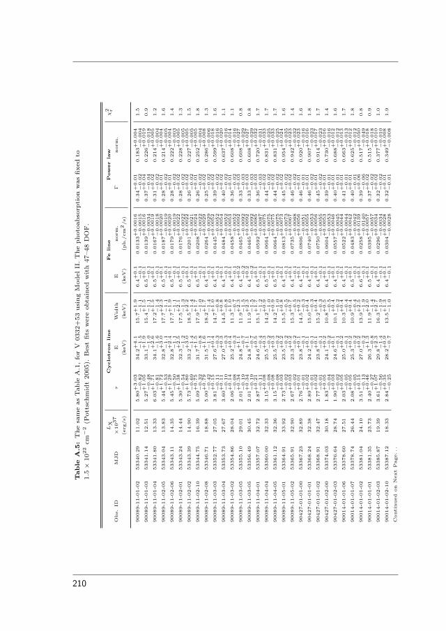
Table
A.5
:T
he
sam
eas
Table
A.1
,fo
rV
0332+
53
usi
ng
Model
II.T
he
photo
abso
rption
was
fixed
to
1.5×
1022
cm−
2(P
ott
schm
idt
2005).
Bes
tfits
wer
eobta
ined
with
47–48
DO
F.
LX
Cyclo
tron
line
Fe
line
Pow
er
law
χ2 r
Obs.
IDM
JD
×1037
τE
Wid
thE
norm
.Γ
norm
.
(erg
/s)
(keV
)(k
eV)
(keV
)(p
h./
cm2/s)
90089-1
1-0
1-0
253340.2
911.0
25.8
0+
3.0
3−
0.8
234.2
+4
.1−
1.5
15.7
+1
.9−
1.1
6.4
+0
.1−
0.1
0.0
133+
0.0
016
−0
.0015
0.3
4+
0.0
1−
0.0
20.1
83+
0.0
04
−0
.004
1.5
90089-1
1-0
1-0
353341.1
412.5
15.2
7+
1.0
5−
0.4
833.1
+1
.9−
1.0
15.4
+1
.5−
1.1
6.5
+0
.1−
0.1
0.0
139+
0.0
016
−0
.0034
0.3
7+
0.0
4−
0.0
40.2
26+
0.0
19
−0
.018
0.9
90089-1
1-0
1-0
453341.8
013.3
36.0
3+
1.7
1−
0.8
134.1
+2
.6−
1.6
17.2
+1
.5−
1.4
6.5
+0
.1−
0.1
0.0
167+
0.0
019
−0
.0018
0.3
1+
0.0
2−
0.0
20.2
14+
0.0
05
−0
.004
1.2
90089-1
1-0
2-0
553343.0
413.8
35.4
4+
1.7
2−
0.5
332.8
+3
.0−
1.1
17.7
+2
.3−
1.1
6.5
+0
.1−
0.1
0.0
187+
0.0
020
−0
.0019
0.2
8+
0.0
1−
0.0
20.2
14+
0.0
04
−0
.005
1.6
90089-1
1-0
2-0
653343.1
114.3
55.4
5+
1.2
9−
0.5
032.8
+2
.4−
1.1
17.7
+1
.9−
1.1
6.5
+0
.1−
0.1
0.0
179+
0.0
020
−0
.0019
0.2
8+
0.0
1−
0.0
20.2
22+
0.0
04
−0
.003
1.4
90089-1
1-0
2-0
153343.2
414.4
45.3
0+
1.3
8−
0.5
432.3
+2
.5−
1.2
17.5
+2
.1−
1.3
6.5
+0
.1−
0.1
0.0
176+
0.0
022
−0
.0022
0.2
8+
0.0
2−
0.0
20.2
28+
0.0
05
−0
.005
1.3
90089-1
1-0
2-0
253343.3
914.9
05.7
3+
1.8
0−
0.6
933.2
+3
.0−
1.4
18.5
+2
.2−
1.4
6.5
+0
.1−
0.1
0.0
201+
0.0
022
−0
.0021
0.2
6+
0.0
2−
0.0
20.2
27+
0.0
05
−0
.005
1.5
90089-1
1-0
2-1
053344.7
516.3
95.0
9+
0.7
5−
0.3
231.7
+1
.5−
0.8
17.9
+1
.7−
1.0
6.5
+0
.1−
0.1
0.0
208+
0.0
024
−0
.0022
0.2
6+
0.0
1−
0.0
20.2
52+
0.0
05
−0
.004
1.8
90089-1
1-0
2-0
853346.7
118.8
85.0
0+
0.7
9−
0.4
231.5
+1
.6−
1.1
18.2
+1
.7−
1.4
6.4
+0
.1−
0.1
0.0
264+
0.0
029
−0
.0029
0.2
5+
0.0
2−
0.0
20.2
86+
0.0
08
−0
.006
1.3
90089-1
1-0
3-0
353352.7
727.0
53.8
1+
0.1
5−
0.1
127.6
+0
.4−
0.3
14.7
+1
.0−
0.8
6.4
+0
.1−
0.1
0.0
445+
0.0
052
−0
.0052
0.3
9+
0.0
2−
0.0
20.5
99+
0.0
18
−0
.016
1.6
90089-1
1-0
3-0
453353.7
327.6
73.6
0+
0.1
1−
0.1
027.0
+0
.3−
0.3
14.5
+0
.8−
0.8
6.4
+0
.1−
0.1
0.0
484+
0.0
054
−0
.0052
0.4
0+
0.0
2−
0.0
20.6
37+
0.0
20
−0
.016
1.1
90089-1
1-0
3-0
253354.8
628.0
42.0
6+
0.1
4−
0.0
825.2
+0
.4−
0.3
11.3
+1
.0−
0.7
6.4
+0
.1−
0.1
0.0
458+
0.0
053
−0
.0052
0.3
6+
0.0
1−
0.0
20.6
08+
0.0
14
−0
.016
1.1
90089-1
1-0
3-0
553355.1
029.0
12.0
1+
0.3
4−
0.1
924.8
+1
.1−
0.7
11.9
+2
.3−
1.5
6.4
+0
.2−
0.2
0.0
465+
0.0
092
−0
.0092
0.3
3+
0.0
3−
0.0
30.6
08+
0.0
27
−0
.029
0.8
90089-1
1-0
3-0
553356.4
930.4
52.0
1+
0.3
4−
0.1
924.8
+1
.1−
0.7
11.9
+2
.3−
1.5
6.4
+0
.2−
0.2
0.0
465+
0.0
092
−0
.0092
0.3
3+
0.0
3−
0.0
30.6
08+
0.0
27
−0
.029
0.8
90089-1
1-0
4-0
153357.0
732.7
22.8
7+
0.2
1−
0.1
124.6
+0
.5−
0.4
15.1
+1
.7−
1.2
6.5
+0
.1−
0.1
0.0
592+
0.0
085
−0
.0087
0.3
6+
0.0
3−
0.0
30.7
20+
0.0
32
−0
.031
1.7
90089-1
1-0
4-0
453360.0
032.3
33.1
5+
0.0
8−
0.0
825.5
+0
.3−
0.2
14.2
+0
.9−
1.0
6.5
+0
.1−
0.1
0.0
664+
0.0
075
−0
.0075
0.4
4+
0.0
2−
0.0
20.8
31+
0.0
33
−0
.025
1.7
90089-1
1-0
4-0
553361.1
232.3
63.1
5+
0.0
8−
0.0
825.5
+0
.3−
0.2
14.2
+0
.9−
1.0
6.5
+0
.1−
0.1
0.0
664+
0.0
075
−0
.0075
0.4
4+
0.0
2−
0.0
20.8
31+
0.0
33
−0
.025
1.7
90089-1
1-0
5-0
153364.9
133.9
22.7
3+
0.0
3−
0.0
223.5
+0
.2−
0.2
15.5
+0
.8−
0.5
6.4
+0
.1−
0.1
0.0
813+
0.0
073
−0
.0073
0.4
5+
0.0
2−
0.0
20.9
54+
0.0
24
−0
.035
1.6
90089-1
1-0
5-0
253365.9
132.9
02.6
7+
0.0
3−
0.0
223.3
+0
.2−
0.2
15.3
+0
.7−
0.5
6.4
+0
.1−
0.1
0.0
735+
0.0
067
−0
.0068
0.4
6+
0.0
2−
0.0
20.9
42+
0.0
23
−0
.032
1.4
90427-0
1-0
1-0
053367.2
332.8
92.7
6+
0.0
1−
0.0
123.8
+0
.1−
0.1
14.5
+0
.2−
0.3
6.4
+0
.1−
0.1
0.0
806+
0.0
056
−0
.0051
0.4
6+
0.0
1−
0.0
10.9
20+
0.0
23
−0
.016
1.6
90427-0
1-0
1-0
153368.2
432.3
82.8
9+
0.0
2−
0.0
124.2
+0
.1−
0.1
15.0
+0
.4−
0.3
6.4
+0
.1−
0.1
0.0
740+
0.0
055
−0
.0053
0.4
6+
0.0
1−
0.0
20.9
07+
0.0
16
−0
.023
1.8
90427-0
1-0
1-0
253368.9
132.4
72.7
7+
0.0
2−
0.0
123.8
+0
.1−
0.1
15.2
+0
.4−
0.3
6.4
+0
.1−
0.1
0.0
750+
0.0
056
−0
.0055
0.4
5+
0.0
1−
0.0
20.9
14+
0.0
17
−0
.023
1.7
90427-0
1-0
2-0
053374.0
330.1
81.8
3+
0.0
5−
0.0
424.1
+0
.2−
0.2
10.8
+0
.5−
0.5
6.4
+0
.1−
0.1
0.0
604+
0.0
053
−0
.0053
0.3
9+
0.0
1−
0.0
10.7
30+
0.0
16
−0
.016
1.4
90427-0
1-0
2-0
353376.6
428.7
41.9
0+
0.0
3−
0.0
224.6
+0
.1−
0.1
10.1
+0
.4−
0.2
6.4
+0
.1−
0.1
0.0
557+
0.0
046
−0
.0045
0.4
0+
0.0
1−
0.0
10.6
88+
0.0
12
−0
.012
1.6
90014-0
1-0
1-0
653378.6
027.5
12.0
3+
0.0
5−
0.0
525.0
+0
.2−
0.1
10.3
+0
.4−
0.4
6.4
+0
.1−
0.1
0.0
522+
0.0
044
−0
.0044
0.4
1+
0.0
1−
0.0
10.6
63+
0.0
13
−0
.013
1.7
90014-0
1-0
1-0
753378.7
426.4
42.0
8+
0.0
5−
0.0
525.3
+0
.2−
0.2
10.9
+0
.4−
0.4
6.5
+0
.1−
0.1
0.0
483+
0.0
042
−0
.0042
0.4
0+
0.0
1−
0.0
10.6
25+
0.0
12
−0
.012
1.8
90014-0
1-0
1-0
253381.0
424.1
03.5
1+
0.1
5−
0.1
327.0
+0
.2−
0.2
13.9
+2
.5−
1.9
6.6
+0
.1−
0.1
0.0
258+
0.0
139
−0
.0140
0.3
9+
0.0
6−
0.0
60.5
17+
0.0
50
−0
.049
0.8
90014-0
1-0
1-0
153381.3
523.7
32.4
0+
0.4
6−
0.2
726.3
+1
.3−
0.8
11.9
+2
.0−
1.4
6.5
+0
.1−
0.1
0.0
395+
0.0
057
−0
.0057
0.3
7+
0.0
2−
0.0
20.5
15+
0.0
18
−0
.018
0.9
90014-0
1-0
2-0
353385.8
719.3
93.6
1+
1.0
7−
0.5
629.8
+2
.3−
1.4
16.3
+2
.7−
1.9
6.4
+0
.1−
0.1
0.0
296+
0.0
034
−0
.0034
0.3
2+
0.0
2−
0.0
20.3
77+
0.0
10
−0
.010
1.0
90014-0
1-0
2-1
053387.1
218.3
32.8
4+
0.3
5−
0.2
528.2
+0
.9−
0.7
13.5
+1
.3−
1.0
6.4
+0
.1−
0.1
0.0
304+
0.0
028
−0
.0028
0.3
2+
0.0
1−
0.0
10.3
49+
0.0
08
−0
.008
1.9
Conti
nued
on
Nex
tPage.
..
210
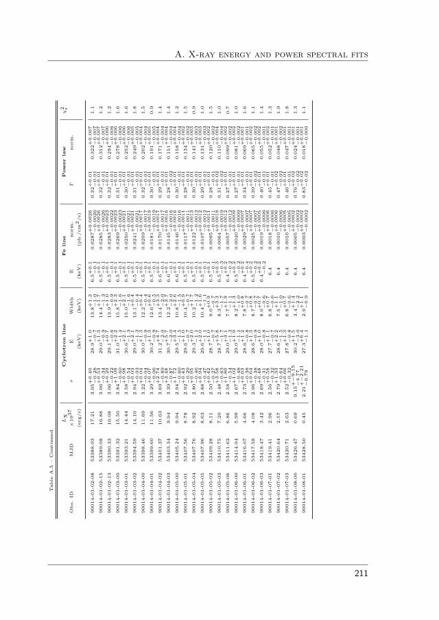
A. X-ray energy and power spectral fitsTable
A.5
–C
onti
nued
LX
Cyclo
tron
line
Fe
line
Pow
er
law
χ2 r
Obs.
IDM
JD
×1037
τE
Wid
thE
norm
.Γ
norm
.
(erg
/s)
(keV
)(k
eV)
(keV
)(p
h./
cm2/s)
90014-0
1-0
2-0
853388.0
317.2
13.0
5+
0.4
0−
0.2
828.9
+1
.0−
0.7
13.8
+1
.3−
1.0
6.5
+0
.1−
0.1
0.0
287+
0.0
026
−0
.0026
0.3
2+
0.0
1−
0.0
10.3
22+
0.0
07
−0
.007
1.1
90014-0
1-0
2-1
553389.0
816.8
83.0
6+
0.5
3−
0.3
429.0
+1
.3−
0.9
14.4
+1
.7−
1.3
6.5
+0
.1−
0.1
0.0
285+
0.0
026
−0
.0026
0.3
2+
0.0
1−
0.0
10.3
12+
0.0
07
−0
.007
1.2
90014-0
1-0
2-1
353390.3
316.0
83.0
6+
0.2
9−
0.2
229.1
+0
.7−
0.6
13.9
+1
.0−
0.9
6.5
+0
.1−
0.1
0.0
283+
0.0
023
−0
.0022
0.3
2+
0.0
1−
0.0
10.2
94+
0.0
06
−0
.006
1.2
90014-0
1-0
3-0
053391.3
215.5
03.8
4+
1.0
9−
0.6
031.0
+2
.2−
1.4
15.8
+2
.3−
1.6
6.5
+0
.1−
0.1
0.0
269+
0.0
023
−0
.0023
0.3
1+
0.0
1−
0.0
10.2
78+
0.0
06
−0
.006
1.6
90014-0
1-0
3-0
153393.2
114.4
43.5
8+
0.9
8−
0.5
430.6
+2
.1−
1.3
15.0
+2
.1−
1.6
6.5
+0
.1−
0.1
0.0
250+
0.0
021
−0
.0021
0.3
0+
0.0
1−
0.0
10.2
52+
0.0
06
−0
.006
1.6
90014-0
1-0
3-0
253394.5
914.1
02.9
4+
0.0
3−
0.0
329.0
+2
.1−
1.3
13.1
+0
.4−
0.4
6.5
+0
.1−
0.1
0.0
241+
0.0
021
−0
.0021
0.3
1+
0.0
1−
0.0
10.2
49+
0.0
05
−0
.005
1.8
90014-0
1-0
4-0
053398.4
611.6
93.2
2+
0.0
4−
0.0
430.0
+1
.3−
0.9
12.2
+0
.4−
0.4
6.5
+0
.1−
0.1
0.0
209+
0.0
017
−0
.0017
0.3
2+
0.0
1−
0.0
10.2
02+
0.0
04
−0
.004
1.5
90014-0
1-0
4-0
153399.6
011.5
63.2
9+
0.0
7−
0.0
630.2
+1
.3−
0.9
12.6
+0
.6−
0.5
6.5
+0
.1−
0.1
0.0
181+
0.0
019
−0
.0019
0.3
0+
0.0
1−
0.0
10.1
91+
0.0
05
−0
.005
0.9
90014-0
1-0
4-0
253401.3
710.6
33.6
9+
2.7
4−
0.8
931.2
+4
.7−
2.0
13.4
+3
.3−
2.0
6.6
+0
.1−
0.1
0.0
170+
0.0
017
−0
.0017
0.2
9+
0.0
1−
0.0
10.1
71+
0.0
04
−0
.004
1.4
90014-0
1-0
4-0
353403.3
49.9
43.3
9+
3.4
8−
0.8
730.7
+5
.7−
2.0
12.2
+3
.7−
2.0
6.6
+0
.1−
0.1
0.0
145+
0.0
016
−0
.0016
0.2
8+
0.0
1−
0.0
20.1
51+
0.0
04
−0
.004
1.4
90014-0
1-0
5-0
053405.2
49.9
42.9
4+
1.7
2−
0.6
029.5
+3
.4−
1.5
10.8
+2
.6−
1.5
6.6
+0
.1−
0.1
0.0
146+
0.0
016
−0
.0016
0.3
0+
0.0
1−
0.0
10.1
58+
0.0
04
−0
.004
1.2
90014-0
1-0
5-0
153407.5
68.7
82.9
2+
0.4
3−
0.2
929.6
+1
.0−
0.7
10.4
+0
.9−
0.7
6.5
+0
.1−
0.1
0.0
117+
0.0
011
−0
.0011
0.2
8+
0.0
1−
0.0
10.1
34+
0.0
02
−0
.002
1.5
90014-0
1-0
5-0
453407.7
68.9
22.8
0+
0.9
5−
0.4
629.3
+2
.0−
1.1
10.2
+1
.7−
1.2
6.5
+0
.1−
0.1
0.0
122+
0.0
013
−0
.0013
0.3
0+
0.0
1−
0.0
10.1
41+
0.0
03
−0
.003
0.9
90014-0
1-0
5-0
553407.9
68.6
32.8
8+
0.9
4−
0.4
729.6
+2
.0−
1.1
10.4
+1
.6−
1.1
6.5
+0
.1−
0.1
0.0
107+
0.0
012
−0
.0012
0.2
9+
0.0
1−
0.0
10.1
31+
0.0
03
−0
.003
1.0
90014-0
1-0
5-0
253409.2
88.1
12.5
0+
0.4
2−
0.2
728.7
+1
.0−
0.7
9.0
+0
.9−
0.7
6.5
+0
.1−
0.1
0.0
095+
0.0
011
−0
.0011
0.2
8+
0.0
1−
0.0
10.1
20+
0.0
02
−0
.002
1.5
90014-0
1-0
5-0
353410.7
57.2
02.4
8+
3.5
8−
0.6
328.7
+5
.8−
1.7
8.3
+3
.3−
1.7
6.5
+0
.3−
0.3
0.0
064+
0.0
019
−0
.0019
0.3
1+
0.0
2−
0.0
20.1
10+
0.0
04
−0
.004
1.0
90014-0
1-0
5-0
653411.6
26.8
62.5
8+
1.8
0−
0.5
429.0
+3
.1−
1.3
7.7
+1
.9−
1.1
6.4
+0
.2−
0.2
0.0
057+
0.0
012
−0
.0012
0.2
7+
0.0
1−
0.0
10.0
99+
0.0
02
−0
.002
0.7
90014-0
1-0
6-0
053414.0
45.9
92.6
7+
1.0
2−
0.4
829.0
+1
.9−
1.1
8.2
+1
.3−
1.0
6.5
+0
.2−
0.2
0.0
040+
0.0
009
−0
.0009
0.2
7+
0.0
1−
0.0
10.0
81+
0.0
02
−0
.002
1.0
90014-0
1-0
6-0
153416.0
74.6
62.7
3+
0.6
3−
0.3
828.6
+1
.2−
0.8
7.8
+0
.8−
0.7
6.4
+0
.2−
0.4
0.0
029+
0.0
007
−0
.0007
0.3
4+
0.0
1−
0.0
10.0
69+
0.0
01
−0
.001
1.6
90014-0
1-0
6-0
253417.5
84.0
82.9
6+
0.6
4−
0.3
828.6
+1
.3−
0.9
8.7
+0
.8−
0.7
6.5
+0
.2−
0.2
0.0
025+
0.0
007
−0
.0007
0.3
9+
0.0
1−
0.0
20.0
65+
0.0
02
−0
.002
1.1
90014-0
1-0
6-0
353418.4
73.4
22.6
9+
0.4
8−
0.3
128.0
+1
.0−
0.8
8.0
+0
.7−
0.6
6.4
+0
.2−
0.2
0.0
019+
0.0
005
−0
.0006
0.4
0+
0.0
1−
0.0
10.0
55+
0.0
02
−0
.001
1.4
90014-0
1-0
7-0
153419.4
12.9
62.5
6+
0.5
8−
0.3
227.7
+1
.1−
0.7
6.8
+0
.7−
0.6
6.4
0.0
018+
0.0
006
−0
.0006
0.4
5+
0.0
1−
0.0
10.0
52+
0.0
02
−0
.001
1.3
90014-0
1-0
7-0
253420.6
42.5
72.7
9+
1.3
3−
0.6
428.6
+2
.2−
1.5
7.5
+1
.1−
1.0
6.4
0.0
010+
0.0
006
−0
.0006
0.4
7+
0.0
2−
0.0
20.0
48+
0.0
01
−0
.002
1.9
90014-0
1-0
7-0
353420.7
12.6
32.5
2+
0.6
6−
0.3
227.8
+1
.3−
0.8
6.8
+0
.7−
0.6
6.4
0.0
016+
0.0
005
−0
.0005
0.4
6+
0.0
1−
0.0
10.0
47+
0.0
01
−0
.001
1.8
90014-0
1-0
8-0
053426.4
70.6
99.1
5+−
9.1
5−
4.7
730.2
+1
.5−
3.0
3.4
+1
.4−
2.2
6.4
0.0
005+
0.0
002
−0
.0002
0.7
6+
0.0
2−
0.0
20.0
24+
0.0
01
−0
.001
1.3
90014-0
1-0
8-0
153428.5
00.4
52.2
1+−
2.2
1−
0.7
927.3
+6
.4−
1.1
2.9
+1
.1−
0.9
6.4
0.0
003+
0.0
002
−0
.0002
0.8
3+
0.0
2−
0.0
20.0
18+
0.0
01
−0
.000
1.1
211

Table
A.6
:Pow
ersp
ectr
alfit
para
met
ers
obta
ined
for
the
KS
1947+
300
outb
urs
t.
Obs.
IDM
JD
LX
Lb
Ll
Lu
χ2 r
(1037
erg
s−1)
νb
(Hz)
rms
(%)
νl
(Hz)
rms
(%)
νu
(Hz)
rms
(%)
50425-0
1-0
5-0
051874.1
50.1
6–
–0.0
4+
0.0
1−
0.0
149.6
+2
.5−
2.4
––
1.6
50425-0
1-0
6-0
051876.4
10.0
9–
–0.0
3+
0.0
1−
0.0
052.7
+2
.5−
2.3
––
2.2
50425-0
1-0
7-0
051878.2
70.1
2–
–0.0
4+
0.0
1−
0.0
156.2
+2
.4−
2.2
––
2.2
50425-0
1-0
8-0
151883.8
30.3
5–
–0.0
7+
0.0
2−
0.0
228.3
+2
.5−
2.6
––
0.7
50425-0
1-0
8-0
051883.8
90.3
5–
–0.0
5+
0.0
1−
0.0
131.6
+1
.9−
2.0
––
1.5
50425-0
1-0
9-0
051888.0
10.9
9–
–0.1
8+
0.0
6−
0.0
319.0
+2
.0−
2.2
––
1.2
50425-0
1-0
9-0
151888.0
70.9
7–
–0.1
5+
0.0
4−
0.0
222.1
+1
.7−
2.4
––
1.2
50425-0
1-1
0-0
051892.2
21.6
0–
–0.1
8+
0.0
4−
0.0
319.5
+1
.6−
1.7
––
1.3
50425-0
1-1
1-0
051896.2
02.2
6–
–0.4
0+
0.0
7−
0.1
016.1
+2
.0−
1.4
––
1.0
50425-0
1-1
1-0
151896.5
22.1
5–
–0.2
8+
0.1
3−
0.0
719.0
+3
.1−
3.4
––
1.0
50425-0
1-1
2-0
051898.9
82.7
9–
–0.1
4+
0.0
1−
0.0
019.5
+2
.4−
1.7
0.7
+0
.5−
0.2
13.0
+1
.6−
3.2
1.3
50425-0
1-1
3-0
051901.9
13.2
8–
–0.3
1+
0.0
4−
0.0
320.5
+0
.7−
0.7
––
1.9
50425-0
1-1
4-0
051906.1
33.6
8–
–0.2
1+
0.0
7−
0.0
818.7
+1
.9−
1.6
1.1
+0
.7−
0.4
10.0
+2
.7−
2.5
1.3
50425-0
1-1
4-0
151906.7
23.6
7–
–0.1
8+
0.0
2−
0.0
220.5
+1
.2−
1.1
2.3
+1
.2−
0.7
9.5
+1
.2−
1.3
1.5
50425-0
1-1
5-0
051910.9
03.8
7–
–0.1
2+
0.0
2−
0.0
120.5
+1
.1−
1.3
1.0
+0
.2−
0.1
11.8
+1
.2−
1.4
1.5
50425-0
1-1
6-0
051914.1
84.1
2–
–0.2
2+
0.1
0−
0.0
318.7
+1
.3−
1.9
1.1
+0
.5−
0.2
10.5
+1
.8−
2.1
1.8
50425-0
1-1
7-0
051918.1
64.1
5–
–0.2
7+
0.1
1−
0.0
420.0
+1
.5−
3.5
2.9
+2
.8−
1.5
7.7
+2
.2−
0.8
0.9
50425-0
1-1
8-0
051926.6
94.4
5–
–0.1
9+
0.0
6−
0.0
321.2
+1
.5−
1.9
1.6
+0
.8−
0.4
9.5
+1
.6−
1.5
1.7
50425-0
1-1
9-0
051930.2
84.8
4–
–0.2
7+
0.0
3−
0.0
621.2
+1
.5−
1.4
2.5
+2
.4−
1.0
7.7
+3
.1−
1.6
0.8
50425-0
1-2
0-0
051932.3
34.9
3–
–0.2
4+
0.0
4−
0.0
520.2
+1
.4−
0.9
2.1
+0
.4−
0.3
10.0
+0
.6−
0.8
2.4
50425-0
1-2
1-0
151941.6
86.1
4–
–0.2
4+
0.0
6−
0.0
320.0
+1
.3−
1.3
1.2
+0
.1−
0.1
12.6
+0
.6−
2.5
1.7
50425-0
1-2
1-0
051941.7
56.3
4–
–0.2
1+
0.0
7−
0.0
320.0
+2
.1−
1.9
1.3
+0
.3−
0.2
12.2
+1
.8−
1.6
1.9
50425-0
1-2
2-0
051943.7
46.7
0–
–0.2
6+
0.0
3−
0.0
519.5
+1
.4−
0.8
1.4
+0
.2−
0.2
11.8
+1
.1−
1.6
1.6
50425-0
1-2
3-0
151943.8
06.6
7–
–0.2
8+
0.0
7−
0.0
420.7
+1
.6−
1.3
1.7
+0
.5−
0.5
10.0
+2
.5−
1.4
1.5
50425-0
1-2
3-0
051948.1
26.9
2–
–0.2
7+
0.0
4−
0.0
618.4
+1
.3−
0.7
1.4
+0
.2−
0.1
13.0
+1
.3−
0.9
1.5
50425-0
1-1
7-0
151950.1
87.0
8–
–0.2
3+
0.0
5−
0.0
421.9
+1
.3−
1.5
1.9
+0
.4−
0.4
10.9
+1
.4−
1.1
1.3
50425-0
1-2
4-0
051952.0
36.7
6–
–0.2
0+
0.0
4−
0.0
621.4
+2
.1−
2.1
1.4
+0
.4−
0.3
13.0
+2
.6−
1.6
1.9
50425-0
1-2
5-0
051955.6
36.7
5–
–0.2
0+
0.0
8−
0.1
420.0
+3
.4−
1.7
1.3
+0
.5−
0.2
13.8
+4
.6−
2.1
0.9
50425-0
1-2
6-0
051961.5
36.4
9–
–0.3
5+
0.2
4−
0.1
519.0
+2
.2−
4.0
1.4
+1
.1−
0.5
10.5
+4
.1−
4.0
1.7
50425-0
1-2
7-0
051963.9
76.5
3–
–0.2
7+
0.0
8−
0.0
719.5
+1
.9−
2.2
1.4
+0
.6−
0.4
12.2
+2
.4−
2.3
0.9
50425-0
1-2
8-0
051965.3
76.1
0–
–0.3
1+
0.1
4−
0.0
818.4
+1
.7−
2.2
1.5
+0
.6−
0.4
10.9
+2
.8−
2.0
1.6
50425-0
1-2
9-0
051968.5
65.5
9–
–0.2
4+
0.0
4−
0.0
720.5
+1
.6−
1.2
1.4
+0
.3−
0.4
10.5
+2
.9−
2.1
1.4
Conti
nued
on
Nex
tPage.
..
212

A. X-ray energy and power spectral fitsTable
A.6
–C
onti
nued
Obs.
IDM
JD
LX
Lb
Ll
Lu
χ2 r
(1037
erg
s−1)
νb
(Hz)
rms
(%)
νl
(Hz)
rms
(%)
νu
(Hz)
rms
(%)
60402-0
1-0
1-0
051970.2
15.7
8–
–0.2
4+
0.0
4−
0.0
920.2
+2
.0−
2.8
1.2
+0
.5−
0.4
11.4
+4
.6−
2.2
1.2
60402-0
1-0
2-0
051972.1
95.5
5–
–0.2
0+
0.0
6−
0.0
320.0
+1
.6−
2.6
1.1
+0
.2−
0.1
12.6
+1
.3−
1.5
1.2
60402-0
1-0
3-0
051974.5
85.1
3–
–0.2
4+
0.0
6−
0.0
521.0
+1
.5−
1.8
1.5
+0
.4−
0.4
10.5
+2
.4−
1.8
1.1
60402-0
1-0
4-0
051976.2
45.2
3–
–0.2
0+
0.0
7−
0.0
522.1
+1
.8−
1.5
1.5
+1
.0−
0.6
10.0
+3
.6−
1.8
1.1
60402-0
1-0
5-0
051978.2
35.2
0–
–0.2
2+
0.0
5−
0.0
520.2
+1
.5−
1.5
1.5
+0
.3−
0.3
10.9
+1
.5−
1.4
1.6
60402-0
1-0
6-0
051980.7
44.8
6–
–0.1
8+
0.0
6−
0.0
420.5
+1
.6−
1.6
1.3
+0
.2−
0.3
11.8
+1
.6−
1.5
1.8
60402-0
1-0
7-0
051983.8
64.4
8–
–0.1
7+
0.0
4−
0.0
219.0
+1
.7−
1.7
1.1
+0
.4−
0.2
12.6
+2
.3−
2.1
1.8
60402-0
1-0
8-0
051984.8
64.3
2–
–0.2
4+
0.0
8−
0.0
621.4
+1
.5−
1.2
1.9
+3
.4−
1.0
8.4
+2
.0−
1.8
1.6
60402-0
1-0
9-0
051986.5
84.2
70.0
032+
0.0
040
−0
.0022
15.2
+5
.6−
3.1
0.3
3+
0.0
6−
0.0
420.2
+1
.1−
1.1
2.6
+1
.3−
0.8
8.4
+1
.4−
1.3
2.8
60402-0
1-1
0-0
051988.2
73.7
30.0
006+
0.0
048
−0
.0006
28.4
+5
.6−
11
.70.2
6+
0.0
3−
0.0
422.1
+1
.6−
1.2
––
0.9
60402-0
1-1
1-0
051990.1
23.6
00.0
114+
0.0
210
−0
.0114
12.3
+2
.6−
2.3
0.1
6+
0.1
6−
0.1
120.0
+3
.6−
6.5
0.8
+1
.4−
0.7
11.5
+8
.2−
4.3
0.8
60402-0
1-1
2-0
051992.1
73.5
60.0
339+
0.0
297
−0
.0198
14.1
+5
.0−
3.6
0.2
9+
0.1
1−
0.1
018.4
+3
.0−
2.2
––
1.7
60402-0
1-1
3-0
051994.2
33.2
20.0
054+
0.0
051
−0
.0021
14.2
+2
.7−
2.1
0.1
8+
0.0
6−
0.0
322.0
+1
.4−
2.9
––
1.7
60402-0
1-1
4-0
051996.0
83.2
70.0
015+
0.0
041
−0
.0015
17.8
+16
.9−
5.8
0.2
7+
0.0
3−
0.0
421.3
+1
.1−
10
.7–
–1.4
60402-0
1-1
5-0
051998.1
42.9
90.0
009+
0.0
213
−0
.0008
8.9
+1785
.2−
3.3
0.1
0+
0.0
8−
0.0
419.8
+3
.1−
1.6
0.9
+0
.4−
0.3
14.1
+0
.9−
1.3
1.8
60402-0
1-1
5-0
151999.0
62.8
00.0
092+
0.0
149
−0
.0065
9.7
+1
.6−
1.9
0.1
7+
0.0
6−
0.0
322.0
+1
.8−
1.9
––
0.8
60402-0
1-1
6-0
151999.9
82.7
20.0
070+
0.0
037
−0
.0043
15.8
+4
.3−
1.9
0.2
2+
0.0
5−
0.0
819.9
+2
.2−
1.4
2.9
+3
.1−
1.6
7.7
+8
.1−
1.8
1.4
60402-0
1-1
6-0
052000.0
62.7
30.0
134+
0.0
271
−0
.0134
9.1
+4
.6−
1.4
0.2
2+
0.0
7−
0.2
219.9
+1
.2−
10
.01.8
+1
.8−
1.8
5.0
+48
.1−
2.5
1.4
60402-0
1-1
6-0
252001.0
52.7
40.0
007+
0.0
034
−0
.0007
26.8
+4
.6−
2.3
0.2
8+
0.0
8−
0.0
321.3
+1
.0−
1.4
––
2.4
60402-0
1-1
7-0
052002.0
42.6
20.0
037+
0.0
024
−0
.0017
11.9
+2
.3−
1.8
0.2
4+
0.0
8−
0.0
520.4
+1
.8−
2.0
––
1.9
60402-0
1-1
8-0
052004.3
82.4
30.0
207+
0.0
120
−0
.0065
37.2
+4
.4−
5.3
0.3
6+
0.1
9−
0.1
517.1
+4
.4−
2.3
––
1.1
60402-0
1-1
9-0
052006.0
92.2
80.0
010+
0.0
039
−0
.0010
15.8
+8
.6−
5.0
0.1
9+
0.0
3−
0.0
321.6
+1
.2−
1.2
––
1.2
60402-0
1-2
0-0
052008.2
12.1
40.0
001+
0.0
018
−0
.0001
59.9
+285
.7−
19
.00.1
9+
0.0
3−
0.0
222.5
+1
.1−
0.8
––
1.3
60402-0
1-2
2-0
052014.3
91.9
30.0
065+
0.0
063
−0
.0036
12.0
+2
.1−
2.2
0.1
9+
0.0
4−
0.0
419.2
+1
.6−
1.2
––
2.2
60402-0
1-2
3-0
052016.3
71.7
60.0
024+
0.0
033
−0
.0023
14.0
+25
.9−
3.5
0.2
1+
0.0
6−
0.0
420.3
+1
.6−
1.7
––
1.1
60402-0
1-2
4-0
052017.6
31.7
20.0
253+
0.0
420
−0
.0184
12.5
+2
.1−
1.9
0.1
9+
0.1
7−
0.0
620.5
+3
.5−
5.7
––
0.7
60402-0
1-2
5-0
052021.0
61.5
10.0
012+
0.0
150
−0
.0146
16.6
+1
.6−
1.5
0.1
4+
0.0
3−
0.0
221.3
+1
.3−
1.8
––
1.0
60402-0
1-2
6-0
052023.5
91.3
60.0
026+
0.0
140
−0
.0019
9.0
+43
.2−
2.7
0.1
4+
0.0
3−
0.0
421.3
+1
.5−
1.7
––
1.1
60402-0
1-2
7-0
052024.3
21.3
00.0
001+
0.3
672
−0
.0001
22.5
+149
.8−
11
.20.1
7+
0.0
5−
0.0
318.8
+1
.5−
1.8
––
1.2
60402-0
1-2
9-0
052028.2
31.0
70.0
371+
0.0
175
−0
.0130
14.9
+1
.4−
2.8
0.2
7+
0.1
6−
0.0
916.5
+3
.3−
2.9
––
1.0
60402-0
1-3
0-0
052029.8
31.0
00.0
029+
0.0
096
−0
.0012
10.9
+5
.8−
2.6
0.1
3+
0.0
3−
0.0
221.8
+1
.2−
2.0
––
1.1
60402-0
1-3
1-0
052032.9
30.7
80.0
109+
0.0
073
−0
.0047
13.8
+1
.5−
1.6
0.1
8+
0.1
6−
0.0
519.6
+2
.5−
3.0
––
1.0
60402-0
1-3
2-0
052034.9
20.6
70.0
179+
0.0
217
−0
.0102
11.9
+1
.9−
2.0
0.1
8+
0.1
2−
0.0
619.4
+3
.1−
3.5
––
0.9
Conti
nued
on
Nex
tPage.
..
213

Table
A.6
–C
onti
nued
Obs.
IDM
JD
LX
Lb
Ll
Lu
χ2 r
(1037
erg
s−1)
νb
(Hz)
rms
(%)
νl
(Hz)
rms
(%)
νu
(Hz)
rms
(%)
60402-0
1-3
3-0
052035.7
20.6
30.0
104+
0.0
124
−0
.0066
11.1
+2
.3−
2.5
0.1
2+
0.0
6−
0.0
618.7
+2
.7−
3.4
––
1.9
60402-0
1-3
4-0
052038.7
00.4
80.0
008+
1.4
742
−0
.0007
16.2
+13
.4−
4.0
0.0
4+
0.7
5−
0.0
423.3
+2
.6−
11
.3–
–1.7
60402-0
1-3
5-0
052040.6
90.4
00.0
589+
0.0
589
−0
.0589
27.7
+3
.0−
13
.80.1
4+
0.2
9−
0.2
967.4
+51
.0−
3.8
––
1.2
60402-0
1-3
6-0
052041.5
50.3
6–
–0.0
8+
0.0
2−
0.0
226.3
+2
.7−
2.9
––
1.9
60402-0
1-3
7-0
052044.0
80.3
2–
–0.0
5+
0.0
2−
0.0
225.8
+3
.1−
2.9
––
1.6
60402-0
1-3
8-0
152046.9
90.2
6–
–0.0
6+
0.0
2−
0.0
228.4
+3
.0−
3.1
––
1.4
60402-0
1-3
8-0
052047.0
60.2
4–
–0.0
9+
0.0
3−
0.0
326.5
+3
.3−
3.4
––
1.0
60402-0
1-3
9-0
052050.1
10.1
9–
–0.0
4+
0.0
1−
0.0
131.1
+3
.1−
2.8
––
2.0
60402-0
1-3
9-0
152050.1
80.1
8–
–0.0
6+
0.0
1−
0.0
135.9
+3
.2−
3.1
––
4.5
60402-0
1-4
0-0
052052.9
50.1
6–
–0.0
6+
0.0
1−
0.0
141.1
+3
.5−
3.9
––
1.8
60402-0
1-4
1-0
052055.8
20.1
4–
–0.0
4+
0.0
1−
0.0
138.0
+3
.9−
3.8
––
2.2
60402-0
1-4
1-0
152056.2
10.1
4–
–0.0
5+
0.0
1−
0.0
147.7
+2
.9−
3.8
––
1.5
60402-0
1-4
2-0
052057.8
70.1
3–
–0.0
4+
0.0
1−
0.0
152.1
+3
.9−
4.1
––
1.6
60402-0
1-4
3-0
052060.3
10.1
1–
–0.0
4+
0.0
1−
0.0
150.2
+3
.6−
3.5
––
2.1
60402-0
1-4
4-0
052062.6
80.1
1–
–0.0
4+
0.0
1−
0.0
157.8
+3
.0−
2.9
––
1.3
60402-0
1-4
4-0
152062.8
20.1
0–
–0.0
4+
0.0
1−
0.0
157.2
+5
.0−
4.8
––
1.9
60402-0
1-4
4-0
252062.8
90.0
9–
–0.0
5+
0.0
1−
0.0
165.7
+3
.9−
4.0
––
1.9
60402-0
1-4
5-0
052078.0
50.0
6–
–0.0
3+
0.0
1−
0.0
162.7
+4
.6−
4.8
––
1.7
214

A. X-ray energy and power spectral fitsTable
A.7
:Pow
ersp
ectr
alfit
para
met
ers
obta
ined
for
the
EX
O2030+
375
outb
urs
t.
Obs.
IDM
JD
LX
Ll
Lu
Lu�
χ2 r
(1037
erg
s−1)
νl
(Hz)
rms
(%)
νu
(Hz)
rms
(%)
νu�
(Hz)
rms
(%)
91089-0
1-0
7-0
053914.8
99.2
10.1
35+
0.0
35
−0
.026
36±
20.9
9+
0.1
7−
0.1
419.9
+2
.4−
2.1
––
1.8
91089-0
1-0
7-0
153915.8
39.1
70.1
98+
0.0
53
−0
.041
32±
21.3
4+
0.3
8−
0.2
816.4
+3
.0−
2.4
––
1.3
91089-0
1-0
8-0
053916.8
19.9
30.1
30+
0.0
52
−0
.031
36±
31.2
3+
0.2
8−
0.2
218.8
+2
.4−
2.1
––
1.9
91089-0
1-0
8-0
153917.7
69.9
90.1
61+
0.0
38
−0
.029
32±
20.8
7+
0.1
4−
0.1
121.0
+2
.3−
2.3
––
1.3
91089-0
1-0
8-0
253918.5
010.4
90.1
10+
0.0
26
−0
.021
38±
31.1
0+
0.2
4−
0.1
918.5
+2
.4−
2.0
––
1.5
91089-0
1-0
8-0
353919.6
110.9
00.1
60+
0.0
41
−0
.033
34±
20.9
3+
0.1
7−
0.1
320.9
+2
.8−
2.5
––
1.8
91089-0
1-0
8-0
653920.7
110.9
50.1
78+
0.0
56
−0
.039
33±
21.0
1+
0.2
6−
0.1
618.9
+2
.8−
2.9
––
2.2
91089-0
1-0
8-0
453921.0
710.6
70.1
60+
0.0
31
−0
.028
34±
21.1
6+
0.3
3−
0.2
518.7
+3
.2−
2.4
––
2.2
91089-0
1-0
8-0
553922.2
810.8
00.2
42+
0.0
34
−0
.026
36±
12.4
5+
0.4
3−
0.3
89.3
+2
.1−
1.5
––
1.9
91089-0
1-0
9-0
053923.3
311.2
10.1
76+
0.0
36
−0
.026
36±
21.4
6+
0.2
3−
0.1
615.5
+2
.2−
2.4
––
1.3
91089-0
1-0
9-0
153924.7
011.5
50.3
20+
0.0
36
−0
.043
34±
12.6
8+
0.3
0−
0.5
58.0
+2
.4−
1.0
––
2.1
91089-0
1-0
9-0
353926.6
311.8
80.2
41+
0.0
22
−0
.026
36±
12.2
1+
0.2
3−
0.3
210.6
+2
.4−
1.1
––
1.7
91089-0
1-0
9-0
453928.1
812.4
30.2
41+
0.0
72
−0
.046
35+
3−
41.3
3+
1.5
6−
0.4
214.9
+5
.4−
6.2
––
1.7
91089-0
1-0
9-0
753928.3
211.6
90.3
09+
0.0
43
−0
.040
35±
12.9
3+
0.6
2−
0.9
27.5
+3
.4−
1.5
––
1.3
91089-0
1-0
9-0
553928.6
411.4
00.2
92+
0.0
32
−0
.034
37±
13.2
1+
0.5
1−
0.9
56.7
+3
.0−
1.1
––
1.8
91089-0
1-0
9-0
653929.6
112.5
90.3
41+
0.0
37
−0
.045
37±
13.0
5+
0.3
8−
0.5
59.5
+2
.7−
1.2
––
1.6
91089-0
1-1
0-0
053930.7
913.0
10.2
69+
0.0
40
−0
.037
38+
1−
21.8
8+
0.3
2−
0.2
914.9
+3
.6−
2.4
––
1.4
91089-0
1-1
0-0
153931.3
912.9
40.3
38+
0.0
50
−0
.064
37±
12.8
0+
0.5
6−
0.7
49.6
+5
.8−
1.9
––
3.0
91089-0
1-1
0-0
253932.2
413.3
50.3
34+
0.0
39
−0
.046
37±
12.9
7+
0.6
6−
0.7
98.5
+5
.3−
1.7
––
1.9
91089-0
1-1
0-0
353933.3
613.7
50.4
25+
0.0
35
−0
.032
39±
14.1
8+
0.5
9−
0.7
75.5
+1
.5−
1.0
––
2.3
91089-0
1-1
0-0
453934.2
613.3
60.2
82+
0.0
33
−0
.034
38±
12.2
0+
0.3
2−
0.3
612.3
+3
.3−
1.8
––
1.6
91089-0
1-1
0-0
553935.1
813.4
80.3
01+
0.0
31
−0
.033
37±
12.9
1+
0.5
4−
0.5
89.9
+3
.0−
1.6
––
1.4
91089-0
1-1
0-0
653936.3
013.8
50.4
11+
0.0
30
−0
.032
41±
14.0
8+
0.4
7−
0.7
36.7
+1
.7−
0.9
––
2.1
91089-0
1-1
1-0
053937.3
513.9
20.3
18+
0.0
31
−0
.032
37±
12.9
7+
0.4
0−
0.4
89.9
+2
.3−
1.2
––
1.5
91089-0
1-1
1-0
153938.1
712.1
90.2
91+
0.0
43
−0
.046
37+
1−
22.6
8+
0.5
1−
0.5
610.3
+3
.6−
1.7
––
1.5
91089-0
1-1
1-0
253938.4
313.1
20.3
17+
0.0
46
−0
.046
37±
13.3
3+
0.7
0−
0.8
69.7
+4
.3−
1.8
––
1.6
91089-0
1-1
1-0
353939.2
513.8
50.2
74+
0.0
37
−0
.033
38±
12.8
7+
0.3
6−
0.3
910.3
+1
.7−
1.2
––
1.9
91089-0
1-1
1-0
453940.1
312.1
80.3
35+
0.0
32
−0
.032
37±
13.2
2+
0.3
6−
0.4
19.0
+1
.5−
1.0
––
1.9
91089-0
1-1
1-0
553941.4
414.7
30.2
82+
0.0
36
−0
.031
38±
15.8
4+
0.8
6−
1.5
05.1
+3
.6−
1.4
2.2
5+
0.4
4−
0.6
79.0
+2
.6−
3.0
1.5
91089-0
1-1
2-0
053944.0
511.9
10.2
88+
0.0
38
−0
.035
37±
14.5
8+
1.2
9−
1.0
38.5
+2
.8−
2.7
––
1.4
91089-0
1-1
2-0
153944.9
712.5
30.3
64+
0.0
32
−0
.034
36±
12.4
0+
0.4
6−
0.5
76.8
+3
.0−
1.7
5.8
3+
0.5
2−
0.5
76.8±
1.0
2.2
91089-0
1-1
2-0
253945.9
513.5
10.4
26+
0.0
38
−0
.034
36±
14.1
2+
2.0
2−
0.7
28.0
+4
.0−
0.1
––
1.7
Conti
nued
on
Nex
tPage.
..
215

Table
A.7
–C
onti
nued
Obs.
IDM
JD
LX
Ll
Lu
Lu�
χ2 r
(1037
erg
s−1)
νl
(Hz)
rms
(%)
νu
(Hz)
rms
(%)
νu�
(Hz)
rms
(%)
91089-0
1-1
2-0
353946.8
612.7
90.3
75+
0.0
34
−0
.019
37±
10.0
1+
0.0
1−
0.0
17.6
+2
.0−
0.1
3.7
5+
0.3
4−
0.3
28.6
+0
.4−
0.3
1.0
91089-0
1-1
2-0
553947.7
113.4
20.3
66+
0.0
40
−0
.038
36±
12.6
3+
0.7
3−
1.2
07.3
+4
.8−
2.1
––
2.2
91089-0
1-1
2-0
453948.8
213.4
30.3
48+
0.0
39
−0
.024
35±
11.9
5+
0.4
5−
0.3
59.3
+2
.7−
1.5
––
3.2
91089-0
1-1
2-0
653949.8
012.9
00.3
23+
0.0
33
−0
.038
36±
12.1
1+
0.5
6−
0.7
96.6
+8
.7−
2.7
4.5
2+
1.6
2−
0.8
77.8
+2
.5−
3.4
1.0
91089-0
1-1
2-0
753950.9
212.8
70.3
43+
0.0
29
−0
.023
30±
12.2
6+
0.1
1−
0.1
07.8
+2
.5−
3.4
7.0
2+
0.5
4−
0.6
13.7
+0
.4−
0.3
2.0
91089-0
1-1
3-0
153952.8
213.4
80.2
7+
0.0
8−
0.0
826.1
+8
.1−
5.9
0.9
7+
0.3
6−
0.4
022±
64.0
6+
0.7
9−
1.0
17.0
+4
.5−
1.8
2.4
91089-0
1-1
3-0
253953.7
312.5
40.3
57+
0.0
30
−0
.026
30±
12.5
0+
0.1
5−
0.1
721.6
+6
.0−
6.3
7.9
4+
0.7
3−
0.7
92.8
+0
.3−
0.3
1.7
91089-0
1-1
4-0
653958.6
013.2
00.3
74+
0.0
48
−0
.041
36±
13.1
9+
0.5
5−
0.5
58.9
+1
.3−
1.5
––
1.1
91089-0
1-1
4-0
053959.8
213.3
20.3
40+
0.0
51
−0
.044
34±
13.2
9+
0.8
8−
0.5
99.8
+1
.9−
2.5
––
1.3
91089-0
1-1
4-0
153960.6
012.9
60.3
89+
0.0
57
−0
.072
30±
52.2
9+
0.4
8−
0.3
313.8
+3
.8−
3.4
––
1.8
91089-0
1-1
4-0
253961.9
313.2
70.3
73+
0.0
44
−0
.044
36±
13.3
1+
0.5
6−
0.7
66.7
+2
.2−
1.7
7.7
0+
1.3
9−
1.8
13.2
+2
.2−
1.0
1.2
91089-0
1-1
4-0
353962.5
013.3
10.4
31+
0.0
34
−0
.035
35±
13.6
5+
0.4
2−
0.4
75.4
+2
.9−
1.5
7.0
5+
1.1
0−
1.2
13.7
+1
.5−
1.5
1.1
91089-0
1-1
4-0
453963.6
813.8
00.3
48+
0.0
38
−0
.038
36±
12.9
3+
0.3
1−
1.6
011.1
+1
.7−
0.8
––
0.9
91089-0
1-1
4-0
553964.5
514.2
10.3
36+
0.0
43
−0
.043
37±
12.7
3+
0.5
7−
0.6
911.1
+2
.7−
2.1
––
1.1
91089-0
1-1
5-0
053965.7
715.4
00.3
55+
0.0
41
−0
.039
35±
12.7
0+
0.5
2−
0.6
57.3
+3
.1−
2.0
6.2
0+
0.9
7−
1.0
44.8
+1
.7−
1.4
1.0
91089-0
1-1
5-0
153966.8
513.8
10.3
79+
0.0
49
−0
.047
36±
12.8
8+
0.6
1−
0.7
78.2
+3
.3−
2.1
7.6
6+
1.0
3−
1.5
13.8
+1
.8−
1.2
1.8
91089-0
1-1
5-0
253967.5
413.6
20.2
76+
0.0
36
−0
.022
26±
11.0
6+
0.0
9−
0.1
03.8
+1
.8−
1.2
3.4
5+
0.4
1−
0.3
013.3
+1
.1−
1.4
1.5
91089-0
1-1
5-0
353968.6
614.7
50.2
63+
0.0
27
−0
.030
31±
11.1
1+
0.0
9−
0.0
82.0
+1
.8−
1.2
4.0
0+
0.3
2−
0.2
710.5
+1
.3−
0.5
0.9
91089-0
1-1
5-0
453969.5
814.5
00.3
62+
0.0
33
−0
.030
30±
11.6
4+
0.1
5−
0.4
24.0
+1
.8−
1.2
5.0
8+
0.4
5−
0.6
16.5
+2
.3−
0.3
2.1
91089-0
1-1
5-0
553970.4
813.4
80.3
23+
0.0
23
−0
.036
27±
11.1
1+
0.1
2−
0.1
32.0
+1
.8−
1.2
3.5
5+
0.2
5−
0.2
211.8
+0
.4−
0.4
0.8
91089-0
1-1
5-0
653971.5
515.1
70.2
91+
0.0
26
−0
.025
33±
11.7
8+
0.1
8−
0.3
01.0
+1
.8−
1.2
4.8
8+
0.4
6−
0.5
86.2
+1
.8−
0.9
1.8
91089-0
1-1
6-0
053972.1
914.2
60.3
18+
0.0
35
−0
.042
28±
11.2
7+
0.1
0−
0.0
85.0
+1
.8−
1.2
4.3
4+
0.2
5−
0.2
09.1
+0
.2−
0.5
1.5
91089-0
1-1
6-0
153972.9
814.8
00.4
08+
0.0
28
−0
.038
30±
12.8
2+
0.1
6−
0.1
73.3
+1
.8−
1.2
8.0
4+
0.3
9−
0.2
22.0
+0
.4−
0.4
1.2
91089-0
1-1
6-0
253974.4
813.2
30.3
52+
0.0
25
−0
.026
31+
2−
12.2
5+
0.3
0−
0.1
94.5
+1
.8−
1.2
6.1
0+
1.3
2−
1.3
94.4
+1
.5−
1.3
2.1
91089-0
1-1
6-0
353975.4
214.3
10.3
69+
0.0
35
−0
.036
29±
12.2
2+
0.2
0−
0.4
14.1
+1
.8−
1.2
6.1
3+
0.5
5−
0.6
14.4
+0
.4−
0.5
1.6
91089-0
1-1
6-0
453976.1
213.9
50.3
50+
0.0
28
−0
.038
34+
3−
11.7
1+
0.5
1−
0.4
64.0
+1
.8−
1.2
5.8
0+
1.1
6−
1.4
45.5
+1
.2−
1.5
1.0
91089-0
1-1
6-0
553977.1
712.8
80.3
24+
0.0
42
−0
.024
32±
11.7
1+
0.1
7−
0.3
34.2
+1
.8−
1.2
4.7
5+
0.3
5−
0.6
06.7
+2
.2−
0.3
1.7
91089-0
1-1
6-0
653978.1
513.6
70.3
77+
0.0
36
−0
.048
29±
11.9
3+
0.1
6−
0.2
84.0
+1
.8−
1.2
5.8
5+
0.6
7−
0.6
75.3
+1
.7−
0.4
1.9
91089-0
1-1
7-0
053979.3
412.5
10.3
45+
0.0
36
−0
.049
29±
11.8
5+
0.1
5−
0.1
83.8
+1
.8−
1.2
5.6
1+
0.4
9−
0.9
06.1
+1
.7−
1.0
1.4
91089-0
1-1
7-0
153980.3
912.7
50.2
89+
0.0
38
−0
.028
36±
11.8
5+
0.3
8−
0.4
13.5
+1
.8−
1.2
5.5
3+
1.1
3−
1.6
64.5
+3
.1−
1.5
1.4
91089-0
1-1
7-0
253981.3
612.2
90.3
97+
0.0
36
−0
.034
37±
1–
–3.4
9+
0.5
0−
0.5
38.6
+1
.7−
1.2
0.9
91089-0
1-1
7-0
353982.1
411.9
80.3
67+
0.0
37
−0
.036
37±
1–
–3.6
3+
0.6
4−
0.6
78.3
+2
.0−
1.3
1.1
91089-0
1-1
7-0
453983.2
011.5
80.4
35+
0.0
40
−0
.037
39±
1–
–5.2
9+
0.9
1−
1.3
05.0
+1
.8−
1.0
1.7
Conti
nued
on
Nex
tPage.
..
216

A. X-ray energy and power spectral fitsTable
A.7
–C
onti
nued
Obs.
IDM
JD
LX
Ll
Lu
Lu�
χ2 r
(1037
erg
s−1)
νl
(Hz)
rms
(%)
νu
(Hz)
rms
(%)
νu�
(Hz)
rms
(%)
91089-0
1-1
7-0
553984.2
411.4
70.4
33+
0.0
39
−0
.038
37±
1–
–4.3
0+
1.0
3−
1.0
96.9
+2
.4−
1.4
1.7
91089-0
1-1
7-0
653985.2
211.4
60.3
71+
0.0
29
−0
.028
37±
1–
–3.3
6+
0.3
9−
0.4
19.2
+1
.4−
1.0
2.1
91089-0
1-1
8-0
153986.0
710.7
30.3
82+
0.0
35
−0
.034
37±
1–
–3.9
5+
0.7
1−
0.7
39.5
+2
.2−
1.4
1.4
91089-0
1-1
8-0
053986.9
910.5
70.4
59+
0.0
55
−0
.051
36±
1–
–3.7
6+
0.6
3−
0.7
86.2
+2
.0−
1.3
1.6
91089-0
1-1
8-0
253988.0
09.7
60.4
16+
0.0
60
−0
.064
38±
1–
–3.5
4+
0.9
6−
1.1
47.9
+4
.6−
2.0
1.2
91089-0
1-1
8-0
353989.1
69.5
70.3
59+
0.0
57
−0
.053
34±
1–
–3.2
6+
0.7
6−
0.7
210.4
+3
.7−
2.1
1.2
91089-0
1-1
8-0
453990.0
39.3
70.3
27+
0.0
51
−0
.048
36±
1–
–2.9
0+
0.6
7−
0.6
410.3
+3
.6−
2.0
1.2
91089-0
1-1
8-0
553991.1
29.4
50.3
24+
0.0
78
−0
.078
34±
2–
–2.1
2+
0.5
4−
0.6
114.7
+7
.9−
3.3
1.3
91089-0
1-1
8-0
653991.7
98.7
50.3
74+
0.0
64
−0
.062
34+
1−
2–
–2.3
0+
0.5
8−
0.6
112.5
+6
.0−
2.9
1.4
91089-0
1-1
9-0
053993.6
97.9
90.3
91+
0.0
48
−0
.044
36±
1–
–3.6
0+
0.7
9−
1.0
27.1
+2
.5−
1.5
1.8
91089-0
1-1
9-0
153995.0
17.7
80.4
34+
0.0
44
−0
.044
36±
1–
–4.6
7+
1.5
4−
1.7
76.2
+4
.1−
1.5
1.1
91089-0
1-1
9-0
253995.7
97.4
40.3
96+
0.0
42
−0
.041
36±
1–
–3.8
0+
0.8
0−
0.9
37.9
+2
.6−
1.4
2.1
91089-0
1-1
9-0
353997.0
47.6
50.3
74+
0.0
53
−0
.054
35±
1–
–3.4
5+
1.0
5−
1.2
18.6
+6
.8−
2.0
1.4
91089-0
1-1
9-0
453997.8
26.7
00.3
42+
0.0
52
−0
.051
35±
1–
–3.0
4+
0.6
6−
0.6
09.8
+3
.0−
1.8
1.3
91089-0
1-1
9-0
553998.6
66.1
50.4
09+
0.0
45
−0
.046
36±
1–
–4.3
8+
1.1
3−
1.8
46.5
+3
.7−
1.3
1.8
92067-0
1-0
4-1
053999.5
96.2
80.4
84+
0.0
58
−0
.055
34±
1–
–4.1
2+
0.7
4−
0.9
35.3
+2
.0−
1.2
1.4
92067-0
1-0
5-0
054000.6
25.9
40.4
86+
0.0
63
−0
.071
35+
1−
2–
–4.9
8+
2.7
7−
2.6
46.2
+8
.3−
2.0
1.8
92067-0
1-0
5-0
154002.0
15.2
20.3
88+
0.0
48
−0
.052
35±
1–
–4.2
2+
1.6
0−
1.1
97.7
+4
.5−
1.9
1.0
92067-0
1-0
5-0
254002.7
24.6
50.2
83+
0.0
77
−0
.077
35±
2–
–2.4
3+
1.8
1−
1.0
413.2
+4
.8−
4.6
1.1
92067-0
1-0
5-0
354003.5
75.2
10.2
13+
0.0
76
−0
.050
32+
3−
4–
–1.2
3+
0.4
9−
0.3
219.1
+5
.1−
4.9
0.9
92067-0
1-0
5-0
454004.4
45.1
30.3
12+
0.0
73
−0
.070
33±
2–
–3.0
3+
0.9
1−
0.8
910.6
+7
.2−
2.3
1.8
92067-0
1-0
5-0
554005.6
74.7
30.3
64+
0.0
86
−0
.077
32±
2–
–2.3
5+
0.6
5−
0.7
110.4
+6
.1−
2.6
1.3
92067-0
1-0
5-0
654006.5
85.0
50.2
95+
0.0
71
−0
.059
34+
2−
3–
–1.7
8+
0.9
4−
0.6
713.8
+4
.8−
4.5
1.4
92067-0
1-0
6-0
054007.5
64.4
10.4
59+
0.0
76
−0
.081
33±
1–
–4.0
8+
1.2
0−
1.7
87.0
+5
.1−
1.8
1.2
92067-0
1-0
6-0
154008.4
33.9
70.2
02+
0.1
61
−0
.130
25+
9−
7–
–1.0
2+
0.4
4−
0.3
422.2
+8
.9−
5.9
0.9
92067-0
1-0
6-0
254009.5
93.5
60.3
10+
0.0
83
−0
.087
29+
3−
6–
–1.8
4+
0.8
5−
0.6
414.8
+6
.2−
3.2
1.4
92067-0
1-0
6-0
354010.3
73.3
70.2
31+
0.0
71
−0
.064
26+
5−
4–
–1.5
9+
0.5
1−
0.3
419.3
+3
.1−
3.1
1.6
92067-0
1-0
6-0
454011.5
53.1
50.1
82+
0.0
65
−0
.052
22+
4−
3–
–0.9
9+
0.3
7−
0.2
223.4
+3
.0−
3.8
1.0
92067-0
1-0
6-0
554012.7
32.8
00.1
62+
0.0
97
−0
.087
22+
8−
4–
–0.9
9+
0.9
3−
0.2
422.8
+2
.7−
6.1
1.2
92067-0
1-0
6-0
654013.7
12.5
40.1
67+
0.0
42
−0
.031
32±
4–
–2.4
2+
0.8
5−
0.6
015.2
+2
.1−
1.8
2.5
92067-0
1-0
7-0
054014.6
32.3
60.1
68+
0.2
26
−0
.114
31+
3−
11
––
1.3
3+
4.6
2−
1.0
016.0
+8
.2−
5.9
1.4
92067-0
1-0
7-0
154015.4
42.0
70.2
20+
0.0
66
−0
.068
24+
6−
4–
–1.8
4+
1.7
1−
0.6
913.2
+3
.5−
3.0
1.6
92067-0
1-0
7-0
254016.5
92.0
00.2
11+
0.0
60
−0
.048
30+
3−
4–
–4.0
1+
4.2
1−
2.5
17.8
+3
.0−
1.5
1.1
Conti
nued
on
Nex
tPage.
..
217
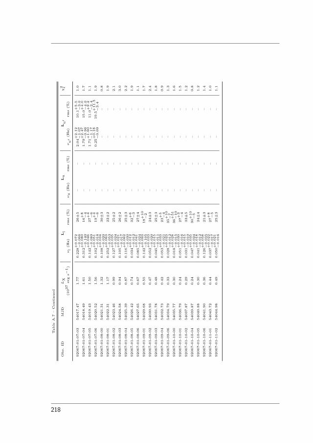
Table
A.7
–C
onti
nued
Obs.
IDM
JD
LX
Ll
Lu
Lu�
χ2 r
(1037
erg
s−1)
νl
(Hz)
rms
(%)
νu
(Hz)
rms
(%)
νu�
(Hz)
rms
(%)
92067-0
1-0
7-0
354017.4
71.7
70.2
28+
0.0
72
−0
.066
26±
5–
–2.0
4+
2.1
2−
1.0
710.1
+5
.5−
3.0
1.0
92067-0
1-0
7-0
454018.4
91.6
10.3
12+
0.0
80
−0
.140
16+
8−
4–
–1.7
9+
2.4
7−
0.9
615.0
+4
.0−
4.0
1.7
92067-0
1-0
7-0
554019.4
31.5
00.1
42+
0.0
46
−0
.089
27+
4−
6–
–1.7
1+
1.6
0−
1.1
711.0
+9
.2−
2.4
1.1
92067-0
1-0
7-0
654020.5
21.5
60.1
02+
0.0
51
−0
.018
19+
4−
6–
–0.2
5+
0.1
8−
0.0
919.5
+11
.5−
3.4
1.9
92067-0
1-0
8-0
054021.3
11.3
20.1
08+
0.0
34
−0
.020
30±
3–
––
–0.8
92067-0
1-0
8-0
154022.3
11.1
70.2
52+
0.0
63
−0
.053
22±
2–
––
–1.9
92067-0
1-0
8-0
254023.4
60.9
90.1
27+
0.0
35
−0
.024
25±
2–
––
–2.1
92067-0
1-0
8-0
354024.5
80.9
40.1
05+
0.0
21
−0
.017
26±
2–
––
–3.0
92067-0
1-0
8-0
454025.3
90.8
70.1
16+
0.0
62
−0
.030
25±
3–
––
–2.2
92067-0
1-0
8-0
554026.4
20.7
40.0
34+
0.0
12
−0
.012
32+
6−
3–
––
–1.9
92067-0
1-0
8-0
654027.6
50.6
70.0
85+
0.0
41
−0
.024
27±
4–
––
–1.1
92067-0
1-0
9-0
154029.6
80.5
50.1
42+
0.0
93
−0
.105
18+
10
−2
––
––
1.7
92067-0
1-0
9-0
254030.9
30.4
70.0
52+
0.0
33
−0
.020
24±
3–
––
–2.4
92067-0
1-0
9-0
354031.7
80.4
80.0
45+
0.0
15
−0
.011
25±
3–
––
–1.8
92067-0
1-0
9-0
454032.7
30.4
20.0
53+
0.0
33
−0
.021
23+
5−
4–
––
–0.9
92067-0
1-0
9-0
654034.7
90.3
30.0
28+
0.0
23
−0
.012
35+
10
−7
––
––
1.3
92067-0
1-1
0-0
054035.7
70.3
00.0
18+
0.0
28
−0
.015
36+
51
−10
––
––
1.6
92067-0
1-1
0-0
154036.7
90.2
40.0
51+
0.0
30
−0
.016
27+
3−
4–
––
–1.5
92067-0
1-1
0-0
254037.8
70.2
90.0
31+
0.0
15
−0
.010
33±
5–
––
–1.2
92067-0
1-1
0-0
454039.8
70.2
40.0
47+
0.0
35
−0
.024
30+
10
−5
––
––
0.8
92067-0
1-1
0-0
554040.8
80.3
00.0
41+
0.0
18
−0
.012
24±
4–
––
–1.2
92067-0
1-1
0-0
654041.9
00.3
60.1
26+
0.0
58
−0
.035
21±
3–
––
–1.4
92067-0
1-1
1-0
154043.7
20.4
40.0
37+
0.0
22
−0
.017
27+
8−
5–
––
–1.0
92067-0
1-1
1-0
254044.9
80.4
90.0
50+
0.0
21
−0
.016
25±
3–
––
–1.1
218

A. X-ray energy and power spectral fitsTable
A.8
:Pow
ersp
ectr
alfit
para
met
ers
obta
ined
for
the
4U
0115+
63
outb
urs
t.
Obs.
IDM
JD
LX
Lb
LLF
Ll
Lu
χ2 r
(1037
erg
s−1)
νb
(Hz)
rms
(%)
νLF
(Hz)
rms
(%)
νl
(Hz)
rms
(%)
νu
(Hz)
rms
(%)
90089-0
1-0
1-0
053254.0
76.7
80.0
07+
0.0
00
−0
.000
6.9
+3
.4−
3.5
0.0
68+
0.0
20
−0
.027
15.7
+1
.8−
4.4
0.9
6+
0.2
3−
0.2
511.6
+4
.3−
1.7
––
1.0
90089-0
1-0
2-0
053256.4
38.9
90.0
05+
0.0
12
−0
.002
27.6
+5
.0−
5.0
0.1
23+
0.0
59
−0
.065
14.2
+2
.1−
3.1
1.0
6+
0.3
0−
0.2
110.7
+1
.5−
2.2
––
0.8
90089-0
1-0
3-0
153260.1
512.6
60.0
03+
0.0
02
−0
.001
27.7
+6
.7−
6.4
0.1
55+
0.0
32
−0
.042
12.8
+1
.2−
0.7
1.1
2+
0.4
0−
0.2
410.1
+2
.9−
2.1
––
1.3
90089-0
1-0
3-0
353260.5
612.6
90.0
01+
0.0
02
−0
.001
64.0
+20
.2−
24
.00.1
04+
0.0
34
−0
.028
10.9
+0
.9−
0.6
0.7
3+
0.1
7−
0.1
114.0
+1
.4−
1.5
––
1.6
90089-0
1-0
3-0
053262.1
513.6
70.0
01+
0.0
02
−0
.001
122.7
+30
.8−
49
.70.0
50+
0.0
11
−0
.007
5.7
+0
.7−
0.9
1.2
1+
0.0
9−
0.0
822.6
+0
.7−
0.7
––
1.7
90089-0
1-0
4-0
653265.0
712.5
80.0
02+
0.0
01
−0
.001
121.8
+88
.1−
57
.60.0
35+
0.0
07
−0
.006
15.6
+0
.9−
0.8
0.6
2+
0.0
4−
0.0
514.9
+0
.6−
0.7
––
1.2
90089-0
1-0
4-0
153267.1
711.4
90.0
13+
0.0
36
−0
.006
5.1
+1
.1−
1.2
0.0
45+
0.0
50
−0
.012
10.8
+0
.9−
1.1
0.5
7+
0.0
6−
0.0
416.7
+0
.7−
0.6
––
1.3
90089-0
1-0
4-0
253269.1
011.9
20.0
02+
0.0
01
−0
.000
21.1
+5
.3−
1.5
0.0
34+
0.0
06
−0
.004
12.0
+0
.5−
0.4
0.5
5+
0.1
5−
0.0
316.0
+0
.6−
1.1
0.8
+0
.1−
0.1
12.6
+0
.7−
2.0
1.2
90089-0
1-0
4-0
053270.3
911.2
50.0
02+
0.0
00
−0
.001
18.4
+2
.2−
1.8
0.0
40+
0.0
08
−0
.011
12.0
+1
.2−
0.3
0.6
0+
0.0
2−
0.1
115.0
+0
.5−
2.3
1.1
+0
.1−
0.5
10.0
+5
.3−
0.3
1.4
90089-0
1-0
4-0
353271.9
59.9
60.0
02+
0.0
00
−0
.001
12.9
+3
.0−
1.0
0.0
68+
0.0
12
−0
.011
14.0
+0
.6−
0.7
0.6
9+
0.1
3−
0.0
814.0
+5
.6−
2.1
1.3
+0
.4−
0.4
9.6
+1
.8−
2.2
1.6
90089-0
1-0
5-0
053272.7
99.5
50.0
03+
0.0
03
−0
.003
14.2
+6
.3−
2.7
0.0
63+
0.0
07
−0
.009
9.0
+1
.2−
0.8
0.5
2+
0.1
3−
0.1
715.6
+1
.1−
1.3
2.1
+1
.0−
1.2
4.2
+7
.1−
1.8
1.0
90089-0
1-0
5-0
553272.9
59.5
60.0
08+
0.0
05
−0
.004
9.5
+1
.1−
1.6
0.0
83+
0.0
60
−0
.011
8.9
+0
.7−
0.6
0.5
2+
0.0
7−
0.2
514.6
+0
.8−
0.8
2.1
+0
.4−
0.5
4.8
+4
.6−
0.8
2.0
90089-0
1-0
5-0
153274.8
38.6
00.0
03+
0.0
01
−0
.001
13.8
+1
.5−
2.9
0.0
65+
0.0
07
−0
.008
8.7
+0
.5−
0.5
0.3
6+
0.0
6−
0.0
512.1
+0
.7−
0.7
1.5
+0
.2−
0.2
7.7
+0
.7−
0.7
1.6
90089-0
1-0
5-0
253275.6
78.0
00.0
02+
0.0
01
−0
.000
15.2
+1
.6−
3.0
0.0
64+
0.0
07
−0
.005
8.8
+0
.5−
0.5
0.3
6+
0.0
4−
0.0
413.8
+0
.9−
0.8
1.3
+0
.2−
0.2
8.3
+1
.0−
0.7
1.0
90089-0
1-0
5-0
353276.7
37.3
80.0
02+
0.0
04
−0
.002
15.6
+45
.6−
3.8
0.0
57+
0.0
08
−0
.006
8.7
+0
.7−
1.2
0.3
5+
0.2
6−
0.0
514.6
+1
.2−
1.0
1.6
+1
.2−
1.1
6.8
+0
.8−
2.7
1.7
90089-0
1-0
5-0
453278.6
26.6
20.0
03+
0.0
03
−0
.002
16.9
+13
.2−
3.6
0.0
62+
0.0
07
−0
.007
8.0
+0
.6−
0.7
0.4
0+
0.1
1−
0.0
714.7
+0
.8−
0.9
2.0
+0
.6−
0.6
5.3
+1
.7−
1.5
1.7
90089-0
1-0
6-0
053280.6
95.7
20.0
01+
0.0
02
−0
.001
70.9
+17
.1−
13
.10.0
62+
0.0
11
−0
.009
8.0
+1
.0−
1.1
0.5
6+
0.0
8−
0.0
515.0
+0
.6−
0.8
––
1.4
90014-0
2-0
1-0
253284.6
13.5
2-0
.001+
0.0
02
−0
.001
55.0
+6
.8−
8.1
0.0
84+
0.0
07
−0
.010
8.6
+2
.2−
1.9
0.3
1+
0.0
8−
0.0
619.4
+1
.9−
1.8
––
1.3
90014-0
2-0
1-0
153285.9
82.8
60.0
01+
0.0
02
−0
.001
52.5
+11
.0−
10
.50.0
69+
0.0
21
−0
.066
7.9
+1
.0−
1.1
0.2
9+
0.0
3−
0.0
320.9
+0
.9−
0.8
––
1.3
90014-0
2-0
2-0
053287.8
12.3
50.0
06+
0.0
06
−0
.004
10.2
+2
.4−
2.2
––
0.1
7+
0.0
2−
0.0
125.0
+0
.8−
0.9
––
1.2
90014-0
2-0
2-0
153289.5
21.8
90.0
25+
0.0
21
−0
.012
14.9
+1
.6−
2.6
––
0.1
9+
0.0
4−
0.0
323.4
+1
.8−
2.5
––
1.3
90014-0
2-0
2-0
253290.6
41.4
90.0
09+
0.0
23
−0
.009
8.8
+2
.1−
3.1
––
0.1
5+
0.0
2−
0.0
130.3
+1
.2−
1.1
––
1.1
90014-0
2-0
2-0
353291.8
11.1
50.0
10+
0.0
03
−0
.002
20.3
+2
.0−
1.8
––
0.2
1+
0.0
2−
0.0
226.1
+0
.9−
0.9
––
1.5
90014-0
2-0
3-0
053293.4
40.7
10.0
12+
0.0
03
−0
.003
30.8
+2
.4−
2.5
––
0.2
0+
0.0
2−
0.0
129.3
+1
.2−
1.2
––
1.0
90014-0
2-0
3-0
153295.6
80.3
20.0
07+
0.0
01
−0
.002
36.0
+2
.8−
3.0
––
0.1
8+
0.0
1−
0.0
131.0
+1
.4−
0.9
––
1.3
90014-0
2-0
3-0
253297.6
00.1
60.0
01+
0.0
01
−0
.001
139.3
+69
.9−
44
.2–
–0.2
0+
0.0
2−
0.0
229.3
+1
.5−
2.1
––
1.7
219
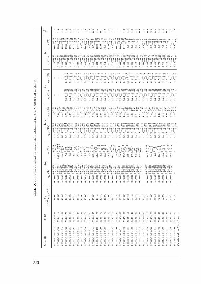
Table
A.9
:Pow
ersp
ectr
alfit
para
met
ers
obta
ined
for
the
V0332+
53
outb
urs
t.
Obs.
IDM
JD
LX
Lb
LLF
Ls
Ll
χ2 r
(1037
erg
s−1)
νb
(Hz)
rms
(%)
νLF
(Hz)
rms
(%)
νs
(Hz)
rms
(%)
νl
(Hz)
rms
(%)
90089-1
1-0
1-0
253340.2
911.0
00.0
001+
0.0
006
−0
.0001
70.0
+29
.3−
34
.90.0
45+
0.0
08
−0
.005
6.3
+0
.5−
0.6
––
0.2
6+
0.0
1−
0.0
116.4
+0
.3−
0.3
1.4
90089-1
1-0
1-0
353341.1
412.5
00.0
001+
0.0
001
−0
.0001
295.2
+113
.4−
108
.20.0
46+
0.0
06
−0
.005
5.0
+0
.5−
0.5
––
0.2
6+
0.0
1−
0.0
115.8
+0
.2−
0.2
1.5
90089-1
1-0
1-0
453341.8
013.3
00.0
003+
0.0
021
−0
.0003
12.9
+6
.6−
5.5
0.0
42+
0.0
40
−0
.020
4.0
+2
.1−
1.0
––
0.2
5+
0.0
1−
0.0
115.0
+0
.5−
0.3
1.0
90089-1
1-0
2-0
053342.7
914.1
00.0
032+
0.0
010
−0
.0009
7.2
+1
.2−
0.9
0.0
50+
0.0
04
−0
.005
4.7
+0
.7−
0.3
0.2
2+
0.0
1−
0.0
15.0
+0
.8−
0.3
0.3
8+
0.0
1−
0.0
212.0
+0
.1−
0.3
1.5
90089-1
1-0
2-0
553343.0
413.8
00.0
018+
0.0
158
−0
.0011
8.6
+3
.8−
2.2
0.0
65+
0.0
46
−0
.016
5.9
+6
.0−
0.8
0.2
3+
0.0
2−
0.0
26.0
+1
.1−
0.6
0.4
8+
0.0
5−
0.0
710.5
+1
.3−
1.3
1.4
90089-1
1-0
2-0
653343.1
114.4
00.0
002+
0.0
078
−0
.0001
18.7
+10
.5−
7.6
0.0
54+
0.0
10
−0
.019
3.4
+0
.5−
0.7
0.2
1+
0.0
2−
0.0
33.1
+1
.0−
0.5
0.3
1+
0.0
6−
0.0
613.3
+0
.2−
0.2
1.3
90089-1
1-0
2-0
153343.2
414.4
00.0
004+
0.0
002
−0
.0003
16.9
+5
.2−
7.4
0.0
49+
0.0
04
−0
.005
3.3
+0
.4−
0.5
0.2
1+
0.0
3−
0.0
34.3
+1
.0−
0.9
0.2
9+
0.0
4−
0.0
113.7
+0
.4−
0.3
1.4
90089-1
1-0
2-0
253343.3
914.9
00.0
033+
0.0
022
−0
.0016
6.5
+1
.9−
1.3
0.0
58+
0.0
07
−0
.006
4.3
+0
.5−
0.7
0.2
2+
0.0
2−
0.0
17.4
+0
.8−
1.1
0.5
9+
0.1
3−
0.0
79.6
+1
.2−
0.3
1.4
90089-1
1-0
2-0
353343.7
615.0
00.0
014+
0.0
005
−0
.0005
9.7
+4
.0−
1.9
0.0
46+
0.0
05
−0
.005
6.6
+0
.4−
0.2
0.2
2+
0.0
2−
0.0
15.7
+0
.3−
0.3
0.4
3+
0.0
2−
0.0
210.9
+0
.1−
0.3
1.8
90089-1
1-0
2-0
753344.0
215.1
00.0
036+
0.0
014
−0
.0011
7.7
+1
.9−
1.2
0.0
41+
0.0
03
−0
.002
3.3
+0
.3−
0.5
0.2
2+
0.0
2−
0.0
17.5
+0
.4−
0.5
0.5
7+
0.0
6−
0.0
49.6
+0
.3−
0.5
1.6
90089-1
1-0
2-0
453344.5
515.8
00.0
001+
0.0
001
−0
.0001
519.2
+0
.00
.00.0
41+
0.0
04
−0
.006
5.2
+0
.4−
0.3
0.2
4+
0.0
4−
0.0
27.3
+0
.5−
0.7
0.4
8+
0.0
4−
0.0
49.7
+0
.3−
0.6
0.9
90089-1
1-0
2-1
053344.7
516.4
00.0
001+
0.0
004
−0
.0001
53.8
+8
.1−
18
.30.0
55+
0.0
08
−0
.021
2.8
+0
.4−
0.4
0.2
8+
0.0
3−
0.0
21.5
+0
.9−
0.5
0.3
2+
0.0
1−
0.0
213.0
+0
.2−
0.2
1.5
90089-1
1-0
2-0
953345.7
317.7
00.0
001+
0.0
006
−0
.0001
53.1
+14
.3−
26
.30.0
58+
0.0
21
−0
.013
5.9
+1
.6−
0.6
0.2
8+
0.1
1−
0.0
41.9
+2
.7−
0.6
0.3
4+
0.0
5−
0.0
511.9
+0
.6−
1.6
0.6
90089-1
1-0
2-0
853346.7
118.9
00.0
001+
0.0
006
−0
.0001
41.5
+18
.4−
33
.70.0
68+
0.0
70
−0
.042
4.3
+3
.0−
0.9
0.2
6+
0.0
9−
0.0
75.4
+5
.8−
2.0
0.5
2+
0.4
9−
0.1
99.8
+3
.1−
4.6
1.0
90089-1
1-0
3-0
353352.7
727.0
00.0
021+
0.0
051
−0
.0016
3.5
+3
.0−
1.3
0.0
43+
0.0
41
−0
.010
3.2
+0
.3−
0.5
0.2
4+
0.0
1−
0.0
16.8
+0
.7−
2.1
0.5
1+
0.0
4−
0.0
311.9
+0
.7−
0.7
1.3
90089-1
1-0
3-0
453353.7
327.7
00.0
001+
0.0
001
−0
.0001
60.0
+15
.0−
26
.00.0
58+
0.0
15
−0
.013
6.8
+0
.4−
0.4
0.2
4+
0.0
1−
0.0
15.0
+0
.4−
0.5
0.7
2+
0.2
4−
0.0
49.5
+0
.3−
1.2
1.2
90089-1
1-0
3-0
053354.5
129.2
00.0
001+
0.0
001
−0
.0001
15.3
+6
.6−
7.3
0.0
47+
0.0
07
−0
.008
7.8
+0
.4−
0.5
0.2
3+
0.0
1−
0.0
16.2
+1
.4−
1.2
0.7
1+
0.1
2−
0.0
910.1
+0
.9−
1.0
1.1
90089-1
1-0
3-0
153354.6
228.7
00.0
001+
0.0
001
−0
.0001
23.4
+5
.4−
5.0
0.0
48+
0.0
10
−0
.007
7.3
+0
.4−
0.4
0.2
3+
0.0
1−
0.0
16.0
+0
.6−
1.4
0.6
9+
0.1
0−
0.0
710.8
+0
.6−
1.0
1.1
90089-1
1-0
3-0
253354.8
628.0
00.0
001+
0.0
001
−0
.0001
20.3
+10
.3−
7.6
0.0
33+
0.0
15
−0
.011
7.4
+0
.5−
0.8
0.2
3+
0.0
1−
0.0
15.8
+1
.5−
1.4
0.6
4+
0.1
3−
0.0
811.1
+0
.9−
1.3
1.2
90089-1
1-0
3-0
553355.1
029.0
00.0
001+
0.0
001
−0
.0001
505.1
+0
.00
.00.0
35+
0.0
03
−0
.005
3.3
+0
.3−
0.5
0.3
0+
0.1
5−
0.0
210.5
+0
.5−
0.4
1.2
0+
0.1
2−
0.1
16.6
+1
.6−
0.2
1.9
90089-1
1-0
4-0
053356.4
930.4
00.0
001+
0.0
001
−0
.0001
27.5
+0
.00
.00.0
87+
0.0
51
−0
.037
8.8
+2
.2−
1.1
0.2
5+
0.0
8−
0.0
65.1
+6
.8−
1.5
0.8
6+
0.1
4−
0.1
29.9
+1
.2−
2.0
1.0
90089-1
1-0
4-0
153357.0
732.7
00.0
001+
0.0
001
−0
.0001
94.9
+0
.00
.00.0
47+
0.0
36
−0
.025
6.5
+1
.6−
1.0
0.2
3+
0.0
3−
0.0
36.2
+1
.7−
1.1
1.1
3+
0.2
1−
0.1
19.1
+2
.0−
1.3
1.6
90089-1
1-0
4-0
253358.5
931.1
00.0
001+
0.0
001
−0
.0001
94.9
+0
.00
.00.0
88+
0.0
28
−0
.030
8.4
+0
.9−
1.2
0.2
4+
0.0
2−
0.0
16.1
+1
.4−
1.2
1.0
9+
0.1
7−
0.1
99.6
+1
.8−
1.1
0.9
90089-1
1-0
4-0
453360.0
032.3
0–
–0.0
44+
0.0
11
−0
.009
8.1
+0
.6−
0.7
0.2
6+
0.0
4−
0.0
25.1
+1
.4−
1.9
0.9
3+
0.2
0−
0.1
99.8
+2
.2−
1.3
1.5
90089-1
1-0
4-0
553361.1
232.4
00.0
001+
0.0
067
−0
.0061
32.7
+14
.0−
15
.70.0
65+
0.0
23
−0
.021
8.3
+0
.9−
1.1
0.2
7+
0.0
4−
0.0
26.8
+2
.1−
1.0
1.8
4+
0.1
9−
0.2
17.3
+0
.9−
0.6
0.9
90089-1
1-0
5-0
053363.2
333.0
00.0
001+
0.0
056
−0
.0041
24.4
+4
.7−
4.9
0.0
71+
0.0
22
−0
.018
8.4
+0
.7−
0.8
0.2
5+
0.0
2−
0.0
16.3
+1
.2−
0.8
1.9
4+
0.1
6−
0.1
66.5
+0
.5−
0.4
2.0
90089-1
1-0
5-0
153364.9
133.9
00.0
039+
0.0
050
−0
.0039
4.1
+1
.7−
1.0
0.0
73+
0.0
24
−0
.008
8.4
+0
.4−
0.4
0.2
7+
0.0
2−
0.0
16.5
+1
.1−
0.9
1.8
5+
0.1
5−
0.1
06.5
+0
.3−
0.3
2.2
90089-1
1-0
5-0
253365.9
132.9
00.0
001+
0.0
050
−0
.0009
35.6
+7
.1−
8.2
0.0
56+
0.0
17
−0
.017
7.3
+0
.7−
0.9
0.2
5+
0.0
2−
0.0
26.7
+1
.3−
0.6
1.7
9+
0.1
8−
0.2
36.6
+0
.7−
0.4
1.4
90427-0
1-0
1-0
053367.2
332.9
00.0
001+
0.0
050
−0
.0029
51.2
+12
.3−
11
.80.0
43+
0.0
05
−0
.009
7.4
+0
.4−
0.4
0.2
5+
0.1
7−
0.0
17.0
+0
.3−
0.3
1.6
0+
0.1
2−
0.0
97.3
+0
.2−
0.5
1.4
90427-0
1-0
1-0
153368.2
432.4
00.0
001+
0.0
050
−0
.0031
57.3
+13
.1−
14
.20.0
64+
0.0
45
−0
.026
8.0
+1
.6−
1.4
0.2
7+
0.0
6−
0.0
47.4
+3
.2−
1.8
1.8
8+
0.1
9−
0.2
26.4
+0
.6−
0.9
0.6
90427-0
1-0
1-0
253368.9
132.5
00.0
001+
0.0
050
−0
.0037
44.1
+15
.1−
16
.20.0
49+
0.0
44
−0
.025
5.2
+1
.5−
1.3
0.2
7+
0.0
6−
0.0
38.4
+2
.5−
1.4
1.7
1+
0.2
3−
0.2
77.0
+1
.2−
1.0
1.8
90427-0
1-0
2-0
053374.0
330.2
0–
–0.0
35+
0.0
16
−0
.021
6.5
+1
.3−
1.2
0.2
7+
0.1
4−
0.0
97.5
+4
.0−
2.6
1.4
3+
0.7
5−
0.4
06.8
+1
.7−
2.4
1.0
Conti
nued
on
Nex
tPage.
..
220
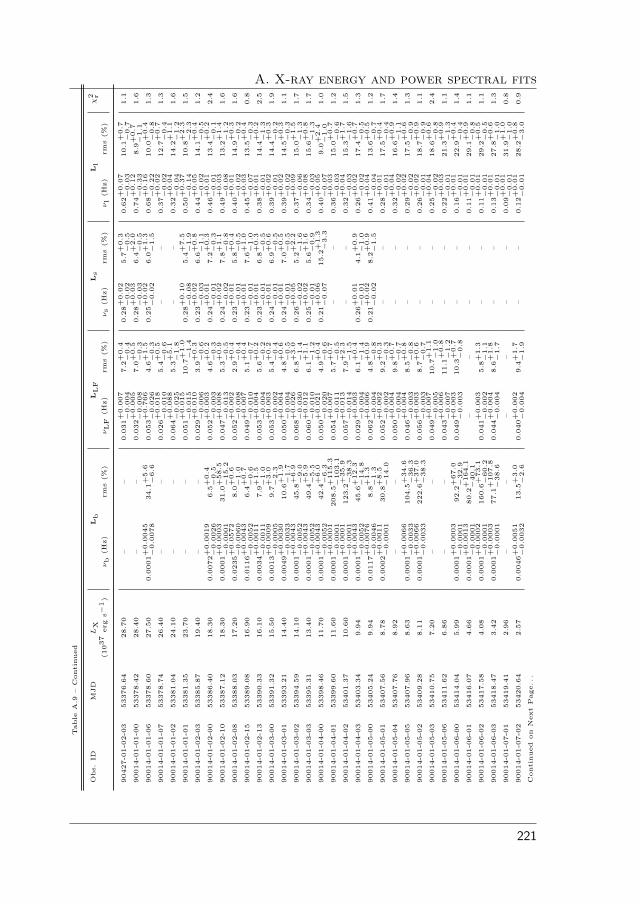
A. X-ray energy and power spectral fitsTable
A.9
–C
onti
nued
Obs.
IDM
JD
LX
Lb
LLF
Ls
Ll
χ2 r
(1037
erg
s−1)
νb
(Hz)
rms
(%)
νLF
(Hz)
rms
(%)
νs
(Hz)
rms
(%)
νl
(Hz)
rms
(%)
90427-0
1-0
2-0
353376.6
428.7
0–
–0.0
31+
0.0
07
−0
.004
7.2
+0
.4−
0.4
0.2
8+
0.0
2−
0.0
25.7
+0
.3−
0.5
0.6
2+
0.0
7−
0.0
310.1
+0
.7−
0.7
1.1
90014-0
1-0
1-0
053378.4
228.4
0–
–0.0
32+
0.0
05
−0
.008
7.0
+0
.5−
0.3
0.2
8+
0.0
3−
0.0
36.4
+2
.0−
0.5
0.7
4+
0.1
2−
0.3
38.9
+0
.7−
1.1
1.6
90014-0
1-0
1-0
653378.6
027.5
00.0
001+
0.0
045
−0
.0078
34.1
+5
.6−
6.6
0.0
53+
0.7
66
−0
.026
4.6
+1
.5−
0.3
0.2
5+
0.0
2−
0.0
26.0
+1
.3−
1.5
0.6
8+
0.1
6−
0.2
210.0
+0
.4−
0.8
1.3
90014-0
1-0
1-0
753378.7
426.4
0–
–0.0
26+
0.0
18
−0
.010
5.4
+0
.5−
0.6
––
0.3
7+
0.0
2−
0.0
212.7
+0
.7−
0.4
1.3
90014-0
1-0
1-0
253381.0
424.1
0–
–0.0
64+
0.0
88
−0
.025
5.3
+5
.1−
1.8
––
0.3
2+
0.0
4−
0.0
414.2
+1
.1−
1.2
1.6
90014-0
1-0
1-0
153381.3
523.7
0–
–0.0
51+
0.0
15
−0
.015
10.7
+1
.0−
1.4
0.2
8+
0.1
0−
0.0
85.4
+7
.5−
1.9
0.5
0+
0.3
7−
0.1
410.8
+2
.3−
2.3
1.5
90014-0
1-0
2-0
353385.8
719.4
0–
–0.0
29+
0.0
10
−0
.006
3.9
+0
.3−
0.6
0.2
3+
0.0
2−
0.0
36.6
+0
.8−
1.1
0.4
4+
0.0
5−
0.0
214.1
+0
.4−
0.5
1.2
90014-0
1-0
2-0
053386.4
018.3
00.0
072+
0.0
019
−0
.0026
6.5
+0
.4−
0.5
0.0
52+
0.0
03
−0
.003
4.6
+0
.2−
0.3
0.2
4+
0.0
1−
0.0
17.2
+0
.3−
0.3
0.4
6+
0.0
1−
0.0
113.4
+0
.2−
0.1
2.4
90014-0
1-0
2-1
053387.1
218.3
00.0
001+
0.0
003
−0
.0001
31.0
+58
.5−
15
.20.0
47+
0.0
08
−0
.013
5.3
+0
.9−
0.5
0.2
4+
0.0
2−
0.0
27.8
+1
.1−
0.8
0.4
9+
0.0
3−
0.0
813.2
+1
.4−
1.2
1.6
90014-0
1-0
2-0
853388.0
317.2
00.0
235+
0.0
572
−0
.0060
8.0
+0
.6−
1.0
0.0
52+
0.0
02
−0
.008
2.9
+0
.4−
0.4
0.2
3+
0.0
1−
0.0
15.8
+0
.4−
0.5
0.4
0+
0.0
1−
0.0
214.9
+0
.3−
0.2
1.6
90014-0
1-0
2-1
553389.0
816.9
00.0
116+
0.0
043
−0
.0052
6.4
+0
.7−
0.6
0.0
49+
0.0
07
−0
.010
5.1
+0
.4−
0.7
0.2
3+
0.0
1−
0.0
17.6
+1
.0−
1.0
0.4
5+
0.0
3−
0.0
713.5
+0
.4−
0.3
0.8
90014-0
1-0
2-1
353390.3
316.1
00.0
034+
0.0
011
−0
.0011
7.9
+1
.5−
1.0
0.0
53+
0.0
04
−0
.004
5.6
+0
.2−
0.2
0.2
3+
0.0
1−
0.0
16.8
+0
.3−
0.5
0.3
8+
0.0
1−
0.0
114.4
+0
.2−
1.3
2.5
90014-0
1-0
3-0
053391.3
215.5
00.0
013+
0.0
009
−0
.0005
9.7
+3
.0−
2.3
0.0
53+
0.0
03
−0
.002
5.4
+0
.2−
0.4
0.2
4+
0.0
1−
0.0
16.9
+0
.6−
0.5
0.3
9+
0.0
2−
0.0
114.4
+0
.3−
0.2
1.9
90014-0
1-0
3-0
153393.2
114.4
00.0
049+
0.0
030
−0
.0033
10.6
+1
.9−
1.7
0.0
50+
0.0
04
−0
.004
4.8
+0
.6−
0.5
0.2
4+
0.0
1−
0.0
17.0
+0
.5−
0.5
0.3
9+
0.0
2−
0.0
214.5
+0
.3−
0.3
1.1
90014-0
1-0
3-0
253394.5
914.1
00.0
001+
0.0
043
−0
.0052
45.8
+6
.9−
9.0
0.0
68+
0.0
26
−0
.030
6.8
+3
.0−
1.4
0.2
6+
0.0
5−
0.0
25.2
+2
.2−
1.6
0.3
7+
0.0
9−
0.0
615.0
+1
.5−
1.3
1.7
90014-0
1-0
3-0
353395.3
113.4
00.0
001+
0.0
043
−0
.0052
49.4
+5
.9−
5.5
0.0
60+
0.0
12
−0
.010
6.1
+1
.1−
1.2
0.2
5+
0.0
2−
0.0
15.6
+1
.6−
0.9
0.3
4+
0.0
8−
0.0
315.6
+0
.8−
1.3
1.7
90014-0
1-0
4-0
053398.4
611.7
00.0
001+
0.0
043
−0
.0052
42.4
+6
.0−
6.3
0.0
50+
0.0
21
−0
.020
4.9
+0
.4−
0.6
0.2
1+
0.0
6−
0.0
715.2
+1
.3−
3.3
0.4
0+
0.0
5−
0.0
79.0
+2
.4−
1.0
1.0
90014-0
1-0
4-0
153399.6
011.6
00.0
001+
0.0
001
−0
.0001
208.5
+115
.3−
103
.10.0
54+
0.0
07
−0
.011
5.7
+0
.7−
0.5
––
0.3
6+
0.0
3−
0.0
315.0
+0
.7−
0.6
1.2
90014-0
1-0
4-0
253401.3
710.6
00.0
001+
0.0
001
−0
.0001
123.2
+35
.9−
38
.30.0
57+
0.0
13
−0
.014
7.9
+2
.3−
1.5
––
0.3
2+
0.0
4−
0.0
315.3
+1
.7−
1.6
1.5
90014-0
1-0
4-0
353403.3
49.9
40.0
001+
0.0
043
−0
.0052
45.6
+12
.3−
14
.80.0
29+
0.0
03
−0
.004
6.1
+0
.4−
1.4
0.2
6+
0.0
1−
0.0
14.1
+0
.9−
1.0
0.2
6+
0.0
2−
0.0
217.4
+0
.7−
0.5
1.3
90014-0
1-0
5-0
053405.2
49.9
40.0
117+
0.0
076
−0
.0046
8.8
+1
.3−
1.3
0.0
62+
0.0
06
−0
.004
4.8
+0
.9−
0.8
0.2
1+
0.0
2−
0.0
28.2
+0
.9−
1.5
0.4
1+
0.0
4−
0.0
413.6
+0
.5−
0.7
1.2
90014-0
1-0
5-0
153407.5
68.7
80.0
002+
0.0
011
−0
.0001
30.8
+8
.5−
14
.00.0
52+
0.0
02
−0
.002
9.2
+0
.3−
0.3
––
0.2
8+
0.0
1−
0.0
117.5
+0
.4−
0.4
1.7
90014-0
1-0
5-0
453407.7
68.9
2–
–0.0
50+
0.0
04
−0
.004
9.8
+0
.7−
0.7
––
0.3
2+
0.0
4−
0.0
216.6
+0
.9−
1.1
1.4
90014-0
1-0
5-0
553407.9
68.6
30.0
001+
0.0
066
−0
.0033
104.5
+34
.6−
36
.30.0
46+
0.0
04
−0
.003
8.5
+0
.8−
0.8
––
0.2
9+
0.0
2−
0.0
217.5
+0
.6−
0.9
1.3
90014-0
1-0
5-0
253409.2
88.1
10.0
001+
0.0
066
−0
.0033
222.6
+37
.0−
38
.30.0
56+
0.0
03
−0
.003
8.7
+0
.6−
0.7
––
0.2
6+
0.0
2−
0.0
118.7
+0
.9−
0.9
1.1
90014-0
1-0
5-0
353410.7
57.2
0–
–0.0
49+
0.0
07
−0
.005
10.7
+1
.1−
1.0
––
0.2
5+
0.0
4−
0.0
218.6
+0
.6−
0.8
2.4
90014-0
1-0
5-0
653411.6
26.8
6–
–0.0
43+
0.0
06
−0
.007
11.1
+0
.8−
1.2
––
0.2
2+
0.0
3−
0.0
121.3
+0
.9−
1.3
1.1
90014-0
1-0
6-0
053414.0
45.9
90.0
001+
0.0
003
−0
.0001
92.2
+67
.0−
32
.90.0
49+
0.0
03
−0
.003
10.3
+0
.7−
0.8
––
0.1
6+
0.0
1−
0.0
122.9
+0
.4−
0.4
1.4
90014-0
1-0
6-0
153416.0
74.6
60.0
001+
0.0
013
−0
.0001
80.2
+164
.1−
40
.1–
––
–0.1
1+
0.0
1−
0.0
129.1
+0
.9−
0.8
1.1
90014-0
1-0
6-0
253417.5
84.0
80.0
001+
0.0
002
−0
.0001
160.6
+73
.1−
60
.20.0
41+
0.0
03
−0
.002
5.8
+1
.3−
1.1
––
0.1
1+
0.0
1−
0.0
129.2
+0
.5−
0.5
1.1
90014-0
1-0
6-0
353418.4
73.4
20.0
001+
0.0
003
−0
.0001
77.1
+107
.8−
38
.60.0
44+
0.0
04
−0
.004
8.6
+1
.8−
1.7
––
0.1
3+
0.0
1−
0.0
127.8
+0
.6−
1.0
1.3
90014-0
1-0
7-0
153419.4
12.9
6–
––
––
–0.0
9+
0.0
1−
0.0
131.9
+1
.0−
1.0
0.8
90014-0
1-0
7-0
253420.6
42.5
70.0
046+
0.0
051
−0
.0032
13.5
+3
.0−
2.6
0.0
40+
0.0
02
−0
.004
9.4
+1
.7−
1.9
––
0.1
2+
0.0
1−
0.0
128.2
+0
.8−
3.0
0.9
Conti
nued
on
Nex
tPage.
..
221
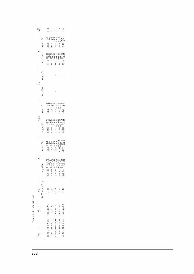
Table
A.9
–C
onti
nued
Obs.
IDM
JD
LX
Lb
LLF
Ls
Ll
χ2 r
(1037
erg
s−1)
νb
(Hz)
rms
(%)
νLF
(Hz)
rms
(%)
νs
(Hz)
rms
(%)
νl
(Hz)
rms
(%)
90014-0
1-0
7-0
353420.7
12.6
30.0
082+
0.0
079
−0
.0037
11.8
+2
.4−
1.9
0.0
52+
0.0
74
−0
.011
12.2
+1
.2−
1.4
––
0.1
3+
0.0
1−
0.0
126.9
+1
.0−
5.8
1.4
90014-0
1-0
7-0
453422.6
11.8
00.0
070+
0.0
041
−0
.0028
15.7
+2
.9−
1.9
0.0
57+
0.0
20
−0
.017
15.7
+1
.1−
2.0
––
0.1
3+
0.0
1−
0.0
125.1
+1
.6−
3.6
1.8
90014-0
1-0
7-0
053424.3
71.1
70.0
118+
0.0
488
−0
.0050
18.8
+2
.3−
2.1
0.0
52+
0.0
21
−0
.003
16.8
+1
.7−
1.6
––
0.1
5+
0.0
1−
0.0
122.6
+2
.4−
2.2
2.0
90014-0
1-0
8-0
053426.4
70.6
90.0
002+
0.0
063
−0
.0002
47.0
+58
.3−
20
.70.0
34+
0.0
07
−0
.007
19.5
+2
.1−
1.9
––
0.1
3+
0.0
1−
0.0
124.2
+1
.9−
1.3
1.1
90014-0
1-0
8-0
153428.5
00.4
50.0
001+
0.0
065
−0
.0073
83.7
+25
.8−
23
.50.0
83+
0.0
15
−0
.035
13.3
+1
.9−
3.9
––
0.1
6+
0.0
2−
0.0
57.2
+7
.7−
2.7
1.8
222
BResumen del trabajo de tesis
B.1 Binarias de rayos X
Las binarias de rayos X se encuentran entre los mas brillantes objetos extra-solaresdel cielo y estan caracterizadas por intensa variabilidad en escalas temporales demilisegundos hasta meses y anos. Su principal fuente de energıa es de tipo grav-itacional, la cual se libera como consecuencia de un proceso de acrecimiento demateria procedente de la estrella masiva sobre la superficie de la estrella de neu-trones. Estos sistemas representan, por tanto, laboratorios unicos para el estudiode las propiedades de la materia bajo condiciones extremas.
Gracias a los observatorios en banda X, lanzados en anos recientes, sabemosque en nuestra galaxia hay mas de 200 fuentes X brillantes, con flujo > 10−10 ergcm−2 s−1. Estas fuentes se distribuyen por el Centro Galactico y por el PlanoGalactico.
Mas del 90% de fuentes X galacticas son binarias de rayos X. Tradicionalmente,estos sistemas se dividen en dos subgrupos, las binarias de rayos X de alta masa(HMXBs) y las binarias de rayos X de baja masa (LMXBs). Este trabajo secentra en el estudio del primer subgupo. En las siguientes secciones se dara unadescripcıon de las dos componentes de estos sistemas, es decir objetos compactos,incluyendo a las enanas blancas por completitud, y estrellas OB calientes.
223

B.1. Binarias de rayos X
B.1.1 Objetos compactos
El colapso gravitacional produce los objetos mas exoticos del Universo: agujerosnegros y estrellas de neutrones. Este tipo de estrellas representan el estado finalde la evolucion estelar y conforman hoy en dıa los constituyentes fundamentalesde las galaxias.
Las enanas blancas son estrellas de aproximadamente una masa solar y unradio caracterıstico de 5 000 km, con una densidad media de 106 g cm−3. Sonobjetos en estado de enfriamiento estacionario, ya que en su interior las fuerzasgravitacionales estan equilibradas por la presion de degeneracion de los electrones.Las enanas blancas no participan en la formacion de binarias de rayos X.
Las estrellas de neutrones poseen un diametro de aproximadamente 20 km ytienen un masa de 1.4 M⊙. Debido a su pequeno tamano y alta densidad, unaestrella de neutrones presenta un campo gravitacional superficial muy intenso.Estos objetos representan la evolucion final de estrellas masivas, con M >6–8M⊙. Despues de explotar como supernova, el nucleo de la estrella colapsa bajo sugravedad a tal punto que protones y electrones se combinan para formar neutrones.
La existencia de agujeros negros esta predicha por la teorıa de la relatividadgeneral de Einstein. Hay agujeros negros de tipo estelar, que se supone se formana partir de una explosion de supernova, y otros supermasivos, encontrados engalaxias y nucleos galacticos activos.
B.1.2 Estrellas OB masivas
Estrellas masivas de tipo espectral temprano son las tıpicas contrapartidas enHMXBs. Existen dos formas de transferencia de materia desde la companeramasiva a la estrella compacta en las HMXBs: viento estelar y disco circunestelar(originario del llamado “fenomeno Be”).
Todas las estrellas calientes presentan un viento radiativo intenso. La materiadel viento estelar contribuye a enriquecer el medio interestelar y, en caso de sis-temas binarios, puede participar en el proceso de acrecimiento o producir shocksde vientos en colision, generando en ambos casos emision X.
Las estrellas Be clasicas son estrellas de tipo OB, no supergigantes, que presen-tan o han presentado emision en las lıneas del hidrogeno. Estan caracterizadas por
224

B. Resumen del trabajo de tesis
exceso infrarrojo, rotacion rapida y alta tasa de perdida de materia. Las lıneasde emision y el exceso infrarrojo se originan en un disco circunestelar. Variashipotesis han sido formuladas para explicar la formacion del disco circunestelar,aunque en todas ellas la rapida rotacion de la estrella B juega un papel destacado.
B.1.3 Binarias de rayos X de alta masa
Las HMXBs se dividen en dos clases: aquellas que contienen a una estrella su-pergigante (SGXBs) y aquellas que contienen a una estrella Be (Be/XRBs). Losdos grupos tienen contrapartida de tipo OB y se encuentran en el Plano Galacticoy en las Nubes de Magallanes.
En las SGXBs el proceso de acrecimiento tiene lugar en forma de viento estelaru, ocasionalmente, rebosamiento del lobulo de Roche. Son sistemas persistentesen la banda X y muestran fuertes variaciones en escalas temporales breves. Suluminosidad X varıa entre 1036 − 1038 erg s−1, segun la forma de acrecimiento.
Las Be/XRBs son sistemas excentricos, en general transitorios. Representanla mayorıa de HMXBs. La emision X es muy variable, desde total ausencia hastaoutbursts gigantes de duracion de semanas y meses. Los outbursts estan clasi-ficados en dos tipos, siendo unos breves y recurrentes, separados por el periodoorbital (Tipo I, con LX ∼ 1036−1037 erg s−1) y otros ocasionales, y muy intensos(Tipo II, LX ≥ 1037 erg s−1.)
Recientemente, gracias a observaciones de INTEGRAL, otra subclase ha sidodefinida, los SFXTs, caracterizados por la ocurrencia de outbursts de rayos Xmuy cortos e intensos. La razon fısica para estos outbursts es todavıa desconocida,aunque especulaciones teoricas los conectarıan a alguna forma de eyeccion discretade masa desde la supergigante, o a variabilidad del viento. Este grupo se considerauna subclase de SGXBs debido a que su contrapartida es una supergigante, aunqueestos sistemas son de tipo transitorio.
225

B.2. Busqueda de contrapartidas infrarrojas de HMXBs oscurecidas
B.2 Busqueda de contrapartidas infrarrojas de HMXBs
oscurecidas
B.2.1 Justificacion cientifıca
En los ultimos siete anos la mision INTEGRAL de la Agencia Espacial Europeaha revelado la presencia de una importante poblacion de HMXBs en los brazosgalacticos de Scutum y Norma, regiones ambas ricas en nubes moleculares densas.La gran profundidad optica de estas nubes produce una importante extincion enla banda optica, ultravioleta y de rayos X, que constituyen las ventanas obser-vacionales clasicas en las que la gran mayorıa de HMXBs han sido descubiertasy sus contrapartidas identificadas. Las unicas ventanas practicables para buscarbinarias de rayos X en las regiones mas internas de las nubes moleculares masivasson el infrarrojo y los rayos gamma, donde la fotoabsorcion es significativamentemas baja.
En efecto, la mayorıa de las nuevas HMXBs descubiertas por INTEGRALestan fuertemente absorbidas, con fotoabsorcion de NH ∼ 1023 cm−2 o mayor,virtualmente inobservables a energıas inferiores a los 4 keV. Eso explica comono fueron detectadas por las misiones de rayos X anteriores a INTEGRAL. Lascontrapartidas opticas de estas fuentes son difıcilmente observables a causa dela elevada extincion interestelar, con AV superior a 20 mag. Debido a esto, lacontrapartida de la gran mayorıa de estas fuentes todavıa no se ha encontrado.La identificacion de contrapartidas opticas/IR es un paso necesario para realizarun estudio detallado de estos sistemas. Con datos limitados al rango de las altasenergıas, la comprension de su compleja estructura y dinamica no puede ser com-pleta.
B.2.2 Observaciones y analisis de datos
En este contexto, hemos desarrollado una tecnica fotometrica apta para selec-cionar estrellas con lıneas de emision en el cırculo de error de las fuentes X detec-tadas por INTEGRAL, las cuales serıan las naturales candidatas a contrapartidas
226
B. Resumen del trabajo de tesis
en sistemas Be/XRBs. Las caracteristicas mas notables de las estrellas Be en elinfrarrojo son las lıneas de emision de hidrogeno y helio I. Nuestra tecnica prevela construccion de diagramas color-color utilizando dos filtros de banda ancha, H
y Ks, y dos de banda estrecha, Brγ y He I. En diagramas del tipo (Brγ - Ks)–(H- Ks) y (He I - Ks)–(H-Ks), estrellas con emision deberıan destacarse debajo dela secuencia de estrellas con lıneas de absorcion. Esta tecnica fue aplicada en elIR a estrellas de campo por primera vez en este trabajo.
Las observaciones fueron tomadas en el observatorio de ESO, en Chile, du-rante dos noches en modo visita. El instrumento empleado fue SOFI, en el NewTechnology Telescope, en La Silla. Los datos fueron reducidos segun el procesoestandar, con rutinas de IRAF. Primero se corrigio el interquadrant-raw crosstalk, una caracterıstica que afecta a los detectores IR; las imagenes se combina-ron obteniendo la mediana para crear una imagen de cielo, que se sustrajo decada una; se corrigio de flat-field; se alinearon y combinaron las imagenes reduci-das para obtener la imagen final.
El paso mas crıtico de la reduccion fue obtener fotometrıa PSF, para lo cual sedesarrollo una rutina iterativa. En el primer paso, el modelo de PSF se computoutilizando solo una funcion analıtica, eligiendo entre varios perfiles el que pro-ducıa la menor desviacion estandar en el ajuste. El radio de la PSF se disminuyopara excluir posibles contribuciones desde objetos diferentes de las estrellas elegi-das para determinar la PSF. El perfil de la estrellas de PSF y sus vecinos fueronajustados y los vecinos restados de la imagen. Desde la imagen con los vecinosrestados se construyo un modelo mejorado de PSF, aumentando de nuevo el radiode ajuste en su valor original (se utilizaron 11 pixeles). En este paso se empleo,junto con la funcion analıtica, una tabla con las desviaciones de los perfiles realesde luminosidad desde el modelo. Se ajustaron y restaron de nuevo las estrellas dePSF y sus vecinos y, si el resultado era satisfactorio, se siguio bajando el radiode PSF y obteniendo el perfil final de PSF. Al final, se aplico el ajuste de PSFsimultaneamente a todas las estrellas del campo.
La correccion de apertura fue estimada como diferencia entre la fotometrıade apertura y la fotometrıa PSF obtenida. La calibracion fue realizada en dos
227

B.3. Analisis y clasificacion espectral NIR de HMXBs identificadaspor INTEGRAL
pasos, determinando los coeficientes de extincion a traves de la recta de Bouguer,y luego resolviendo las ecuaciones de trasformacion estandar.
B.2.3 Resultados
La tecnica fue aplicada a 14 campos de fuentes descubiertas por INTEGRAL. Paratodos los campos menos uno hemos podido seleccionar candidatos a contrapartida.Entre ellos, consideramos como candidatos mas probables los que destacan enambos diagramas color-color.
Para testar nuestra tecnica fotometrica, la aplicamos a una Be/XRB cono-cida, 1A1118–615. Tomamos un espectro Ks de su contrapartida, que claramentemuestra He I y Brγ en emision. Tomamos tambien imagenes en los cuatro fil-tros, H, Ks, Brγ y He I; obtuvimos fotometrıa PSF y los diagramas color-color.El resultado de la prueba fue que la contrapartida de este sistema fue correcta-mente identificada en ambos diagramas. Esta prueba es una primera validacionde nuestro trabajo.
Ademas, tomamos espectroscopıa Ks con el instrumento NICS del TelescopioNazionale Galileo del candidato a contrapartida mas brillante de IGR J18307–1322, 2MASS J18304334–1233504. La unica caracterıstica detectada es He Ien emision. En nuestros diagramas, el objeto deberıa tambien mostrar Brγ enemision. Como la mayorıa de las estrellas de campo muestra Brγ en absorcion,mientras el espectro obtenido no muestra Brγ ni en absorcion ni en emision, estojustifica que sea seleccionado en el diagrama (Brγ-Ks)–(H-Ks). Nuestros datosentonces apuntan a este objeto como posible contrapartida de IGR J18307–1322,ya que varias Be/XRBs, aun teniendo He I en emision, no presentan la lınea Brγ.
B.3 Analisis y clasificacion espectral NIR de HMXBs
identificadas por INTEGRAL
B.3.1 Objetivo cientıfico
Como se ha mencionado en la seccion anterior, muchas de las nuevas fuentes derayos X descubiertas por INTEGRAL presentan un elevado nivel de absorcion.
228

B. Resumen del trabajo de tesis
Las recientes tecnicas de espectroscopıa infrarroja emergen entonces como her-ramientas utiles para caracterizar estos sistemas y, junto con datos de alta en-ergıa, revelar la clase a la que pertenecen. En particular, en el caso de los SFXTs,los datos de baja energıa son de importancia crucial para su clasificacion, ya quesus propiedades en la banda X son comunes a otros objetos (binarias RS CVn yLMXBs).
B.3.2 Observaciones y analisis de datos
Observaciones de contrapartidas propuestas para fuentes descubiertas por IN-TEGRAL fueron tomadas a lo largo de varios turnos, en 2006, 2007 y 2008 enlos observatorios de ESO, en La Silla y Paranal, en Chile. Se utilizo, en modovisita, el instrumento SOFI en el NTT, y, en modo servicio, ISAAC en el VLT.Segun el instrumento, las observaciones se hicieron en media o baja resolucionrespectivamente. Para el analisis y clasificacion se utilizo la banda Ks. Lasfuentes observadas fueron IGR J16207–5129, IGR J16465–4507, IGR J16479–4514, IGR J16493–4348, AX J1841.0–0536 and IGR J19140+0951. Tambien seincluyo 4U 1907+09 porque su clasificacion ha sido un tema muy discutido en elpasado, y todavıa no existen espectros IR de esta fuente.
Los datos fueron reducidos segun el procesado estandar, con rutinas de IRAF.Primero se corrigio por el inter-quadrant row cross-talk, que afecta a los espectrostanto como a las imagenes de detectores IR; se combinaron las imagenes paraobtener una imagen de cielo, que se resto; se corrigio por flat-field; se extrajeronlos espectros monodimensionales de manera interactiva; se calibraron en longitudde onda utilizando espectros de lamparas; se corrigio la absorcion telurica. Elultimo paso es el mas crıtico en la reduccion de espectros IR. En la region infrar-roja, entre 1 y 5 µm, el espectro de la atmosfera esta dominado por transicionesde agua telurica y CO2. Estas lıneas varıan rapidamente con el tiempo y la ele-vacion. En particular para estrellas calientes, una lınea muy importante para laclasificacion es la de He I en 2.058 µm, la cual se encuentra en un rango espectraldonde bandas de absorcion de CO2 dominan el espectro. Para nuestro objetivo,esto vuelve de crucial importancia la correcta sustraccion de las bandas teluricas.
La tecnica que se utilizo fue observar, para cada espectro cientıfico, espectros
229

B.3. Analisis y clasificacion espectral NIR de HMXBs identificadaspor INTEGRAL
de una estrella de tipo A0-A3 III-V y de una de tipo G2-3 V. Para obtenerdiferencias pequenas en masa de aire, la primera se observaba inmediatamenteantes o despues del objeto cientıfico, mientras que la segunda en un intervalo deuna hora. Las estrellas de tipo A poseen como caracteristica propia solo unalınea de Brγ en absorcion, pudiendose considerar el rango restante de la bandaKs un puro espectro telurico. En la region de Brγ, utilizamos el espectro de laestrella G dividido por el espectro solar; insertamos la relacion obtenida en elespectro de la estrella A, obteniendo un espectro final telurico. Esto se repitiopara cada objeto cientıfico, obteniendo un espectro telurico para cada uno. Lacorreccion se hizo de manera interactiva, dividiendo el espectro cientıfico por elcorrespondiente espectro telurico, despues de aplicar un factor de correccion deescala y desplazamiento para corregir diferencias en masa de aire y alineado.
B.3.3 Resultados
Los espectros se analizaron y clasificaron en comparacion con atlas IR. Las lıneasespectrales detectadas en los espectros fueron, en general, He I 20 581 A, He I21 120 A, N III 21 155 A y Brγ 21 661 A. Todas las fuentes fueron clasificadascomo HMXBs. Los resultados obtenidos son los siguientes:
IGR J16207–5129: la contrapartida fue clasificada B1 Ia; el sistema es en-tonces una SGXB;
IGR J16465–4507: la contrapartida fue clasificada O9.5 Ia; junto con infor-macion de datos X, nuestro analisis confirmio la inclusion del sistema en laclase de SFXTs, ya propuesta a partir de espectros opticos;
IGR J16479–4514: la contrapartida fue clasificada O9.5 Iab, y el sistema comoSFXT;
IGR J16493–4348: la contrapartida fue clasificada B0.5 Ib, y el sistema comoSGXB;
AX J1841.0–0536: la contrapartida fue clasificada B1 Ib; junto con informa-cion de datos X, nuestro analisis confirmio la inclusion del sistema en laclase de SFXTs, ya propuesta desde espectros opticos;
230
B. Resumen del trabajo de tesis
IGR J19140+0951: la contrapartida fue clasificada O8.5 Iab, y el sistemacomo SGXB;
4U 1907+09: la contrapartida fue clasificada O8.5 Iab, y se confirmio el sistemacomo SGXB.
Para cada fuente se estimo el reddening y la distancia, y se comparo la ex-tincion interestelar obtenida con el valor de NH conocido a partir de los datos X.En particular, para cuatro objetos – IGR J16465–4507, IGR J16479–4514, AXJ1841.0–0536 y IGR J19140+0951 – la extincion obtenida con nuestros datos IRresulto una o dos magnitudes inferior a la derivada con los datos X. Esto significaque la fuente de absorcion en la banda X se encuentra concentrada alrededor dela estrella de neutrones. Esto es consistente con la observacion de la lınea defluorescencia del hierro en 6.4 keV en los espectros X de las cuatro fuentes, ya queesta se considera una traza de la capa esferica de material alrededor del objetocompacto. Los sistemas que fueron clasificados como SFXTs presentan un elevadonivel de absorcion intrınseco, sugeriendo que esta podrıa ser una propiedad de laclase.
Nuestros resultados sobre la estimacion de la distancia, aunque afectados porincertidumbres importantes, son compatibles con los brazos galacticos de Norma,Scutum o Sagitario, segun la fuente.
Parte de estos resultados se publicaron en Nespoli et al. (2008b).
B.4 Espectroscopıa en la banda K revela dos nuevas
SyXBs
B.4.1 Binarias simbioticas de rayos X
Las binarias simbioticas de rayos X (SyXBs) son una subclase, recientementeintroducida, de LMXBs, caracterizada por la presencia de una contrapartida detipo gigante tardıo. Se trata de una clase rara, llamada ası por analogıa con lasbinarias simbioticas, sistemas constituidos por una enana blanca y una gigante
231

B.4. Espectroscopıa en la banda K revela dos nuevas SyXBs
de tipo M. Hasta ahora, solo seis sistemas conocidos pertenecen a este grupo, locual vuelve su estudio de gran interes.
B.4.2 IGR J16358–4726 y IGR J16393–4643,
Durante la campana de epectroscopıa IR de contrapartidas de HMXBs, se tomarondatos de IGR J16358–4726 y IGR J16393–4643, dos fuentes descubiertas por IN-TEGRAL, supuestas HMXBs.
En el caso de la primera fuente, IGR J16358–4726, trabajos con datos Xrevelaron la presencia de una estrella de neutrones. A partir de espectroscopıaNIR, Chaty et al. (2008) sugirieron que la contrapartida es una sgB[e], y el sistemaentonces una HMXBs, perteneciente a una clase peculiar de SGXBs.
Respecto a IGR J16393–4643, la fuente de rayos X fue identificada como unpulsar; el estudio de los parametros orbitales del sistema, a partir del analisis tem-poral de las pulsaciones, produjo cuatro soluciones matematicas, entre las cualesThomson et al. (2006) propusieron como mas probable la que propone un periodoorbital de 3.7 dıas y una funcion de masa de 6.5±1 M⊙. Esto corresponderıa a unaHMXB. Ademas de la contrapartida inicialmente propuesta, fotometrıa recientede Chaty et al. (2008) descubrio tres candidatos mas, que se descartaron por sumagnitud debil. Resultados de ajuste de SED, utlizando observaciones desde elrango optico hasta el MIR, sugirieron un tipo espectral BIV-V.
B.4.3 Observaciones, analisis y resultados
Las contrapartidas propuestas fueron observadas en 2007 con el espectrografoISAAC, en el telescopio UT1, en Paranal (ESO). Los datos fueron tomados en bajaresolucion. La reduccion se hizo con IRAF, utilizando los metodos estandares. Lacorreccion de absorcion telurica se hizo de la misma forma que se describio en laseccion precedente.
El analisis y la clasificacion espectral utilizaron los atlas NIR disponibles. Losdos espectros que presentamos son, para IGR J16358–4726, el primer espectro in-frarrojo, y, para IGR J16393–4643, el primero que incluye el rango mas alla de 2.3µm. Los espectros de las dos fuentes son muy parecidos, siendo su caracterısticamas evidente las intensas bandas de CO en absorcion entre 2.29 y 2.40 µm, tıpicas
232

B. Resumen del trabajo de tesis
de estrellas tardıas. Se pueden reconocer tambien varias lıneas metalicas, aunqueen general no se puedan resolver.
Detectamos tambien He I 20 281 A y Brγ en debil emision en ambos espec-tros: como estas no son caracterısticas propias de estrellas de tipo tardıo, podrıanser la traza de un disco de acrecimiento alrededor de un objeto compacto. Sinembargo, dada su debilidad, esta es solo una hipotesis y de hecho podrıan serincluso el residuo de la correccion telurica, que en esas regiones es muy crıtica.En cualquier caso, las lıneas de emision tıpicas de las binarias de rayos X pare-cen no estar presentes en los espectros opticos de las otras SyXBs conocidas. Larazon se deberıa a la elevada luminosidad total de las companeras gigantes, quedeslumbrarıa la emision derivada del reprocesado de la radiacion X.
Nuestros espectros K claramente indican que ambos objetos son de tipo tardıo,y excluyen que los sistemas sean HMXBs con companeras de tipo OB. La mor-fologıa general de los espectros y la comparacion entre las intensidades relativasde CO 22 900 A y de las lıneas de Na I y Ca I, que son indicadores de luminosidad,revelan que ambas estrellas son gigantes o supergigantes.
Lamentablemente, un ajuste de SED no pudo mejorar la clasificacion espectraldebido a la degeneracion entre la direccion del vector de reddening y la variacionde la temperatura efectiva en el rango espectral empleado.
B.4.4 Conclusiones
Nuestra clasificacion espectral apunta a gigantes o supergigantes tardıas. Juntocon las caracterısticas conocidas a partir de estudios en la banda X, nos permiteproponer que ambos sistemas pertenecen a la clase de SyXBs.
En el caso de IGR J16393–4643, la solucion orbital propuesta como mas prob-able por Thompson et al. (2006), no resulta compatible con nuestra clasificacionespectral. Entre las otras soluciones matematicas, excluyendo la solucion 3 por sudebilidad estadıstica, solo la solucion 2 es aceptable. Esta consiste en una funcionde masa de 0.092 M⊙ y un periodo orbital de 50.2 dıas. Derivamos un lımite ala masa de una gigante roja que quepa en la orbita prevista por la solucion 2,obteniendo un valor de 7 M⊙.
233
B.5. Analisis espectral/temporal de BeXRBs durante outburstsgigantes
Los resultados obtenidos para IGR J16393–4643 son validos siempre que lacontrapartida sea confirmada, excluyendo como possibles companeras los otrosobjetos que se encuentran en el cırculo de error de XMM/Newton.
B.5 Analisis espectral/temporal de BeXRBs durante
outbursts gigantes
Con este trabajo investigamos la variabilidad espectral y temporal de cuatropulsares de rayos X con companera Be durante outbursts de tipo gigante. Poroutbursts gigantes nos referimos a outbursts de tipo II, donde la luminosidad enla banda X llega al lımite de Eddington. Nuestro objetivo es definir y caracterizarposibles estados espectrales, tal y como se ha hecho para las LMXBs y agujerosnegros. Para ello haremos uso de las propiedades espectrales y temporales, laposicion de las fuentes en el diagrama color-color a lo largo del outburst y de lascorrelaciones de esas propiedades entre ellas.
B.5.1 Tecnicas de analisis de datos X
Fotometrıa en multibanda
En analogıa con la fotometrıa optica, en la banda X es posible caracterizar laforma espectral definiendo colores X. El color se define como el cociente entreel numero de cuentas (fotones) en dos bandas de energıa. Tambien se le sueledenominar razon de “dureza” (harness ratio). Dado que el continuo X entre 2–30keV de virtualmente todas las HMXBs puede ser representado por una ley depotencia, es decir, una lınea recta en los diagramas log-log, un color correspondea una medida aproximada de la pendiente espectral. Un diagrama color-colores el grafico de un color en funcion de otro, calculado en una banda de energıadiferente. El color en el rango de energıa mas alto, se le denomina color “duro”,mientras que el de rango de energıa mas bajo se le denomina color “blando”. Undiagrama intensidad-color es el grafico de un color en funcion de la intensidad enun determinado rango espectral.
Estos tipos de diagramas son independientes del modelo de ajuste espectralempleado y reflejan las propiedades intrınsecas de los sistemas. En el estudio de las
234

B. Resumen del trabajo de tesis
LMXBs se han convertido en una herramienta esencial de analisis introduciendoel concepto de estados espectrales. Un estado se define a partir de la aparicion deuna componente espectral o temporal asociada con una posicion bien reconocibleen el CD/HID.
Ajuste espectral
Las variaciones espectrales se pueden describir de una manera mas detallada enterminos de una combinacion de una o mas funciones matematicas motivadasfısicamente, o modelos, ajustados a los espectros observados. El analisis del com-portamiento de los parametros del modelo mientras la fuente evoluciona en elCD/HID, junto con la identificacion de correlaciones entre parametros, es unaherramienta muy util para caracterizar los estados del sistema y estudiar las tran-siciones entre dichos estados.
Analisis temporal
Las observaciones de las binarias de rayos X muestran una gran variabilidad enun amplio rango de escalas temporales en todas las longitudes de onda y hasta elmilisegundo en la banda X. La herramienta principal utilizada para estudiar laspropiedades temporales de una fuente X es el espectro de potencia de Fourier, oPower Spectral Density (PSD), de las series temporales de la intensidad de la ra-diacion X, o curvas de luz. Esta tecnica es particularmente importante cuando elruido domina sobre la senal y solo es posible estudiar las propiedades promediadasde los fenomenos temporales. Al igual que en los espectros en energıa, los espec-tros de potencia son modelizados mediante el ajuste de funciones matematicaso componentes del espectro de potencia. Desgraciadamente no existe un mod-elo fısico capaz de describir las componentes temporales de forma consistente,dado que los procesos que determinan la variabilidad en banda X son todavıa dedifıcil interpretacion. Las componentes anchas se denominan ruido y las estrechasoscilaciones casi-periodicas (QPOs).
B.5.2 Este trabajo
Mientras existen numerosos estudios sobre la aplicacion de CD/HID y tecnicasde analisis espectral a binarias de rayos X de baja masa, muy poco trabajo de
235

B.5. Analisis espectral/temporal de BeXRBs durante outburstsgigantes
este tipo se ha hecho sobre binarias de rayos X de alta masa. El objetivo de estetrabajo es realizar por primera vez un estudio sistematico de cuatro Be/XRBsdurante outbursts gigantes, utilizando las tres tecnicas introducidas antes, si-multaneamente, y empleando los resultados y las correlaciones obtenidos paraintentar definir y caracterizar estados espectrales para esta clase de sistemas.
B.5.3 Estados espectrales
En esta seccion presentamos las actuales definiciones de estados en LMXBs, seaque contengan estrellas de neutrones, sea agujeros negros.
Estados en LMXBs con estrellas de neutrones
Segun la forma de los trazados que dibujan en el CD/HID, con escalas temporalesde horas hasta dıas, se distinguen dos subclases, las fuentes Z y las fuentes atoll.Las fuentes Z son la subclase mas brillante, caracterizada por una trazado de tresramas in los CDs/HIDs, que en algunos casos parece una “Z”, en otros una “ν”.Las tres ramas se denominan “horizontal branch” (HB), “normal branch” (NB) y“flaring branch” (FB). Los espectros de potencia de las fuentes Z muestran variostipos de QPOs ası como de componentes de ruido. Su presencia y propiedadesestan fuertemente correlacionadas con la posicion de la fuente a lo largo del trazadode Z.
Las fuentes atoll cubren un rango mucho mas amplio de luminosidades y suelentener un espectro mas duro y variabilidad de mayor amplitud. En alta luminosi-dad, siguen en el CD/HID un trazado denominado “banana branch”, que esta asu vez subdividido en “upper banana”, “lower banana”, dominados por compo-nentes de ruido, y “lower left banana”, donde se observan QPOs gemelas en elrango de los kHz. En baja luminosidad, la emision X es, en general, mas dura yla fuente se encuentra en el “island state” (IS). El estado correspondiente al nivelmas bajo de luminosidad se le denomina “extreme island state” (EIS).
Estados en agujeros negros
Los espectros X de agujeros negros en LMXBs en el rango 3-30 keV se pueden rep-resentar utilizando dos componentes principales, una ley de potencias, que ajusta
236
B. Resumen del trabajo de tesis
el espectro a altas energıas (> 10 keV) y la ley de Planck que representa la inten-sidad de la radiacion emitida por un cuerpo negro, la cual cuando esta presentaajusta el espectro a bajas energıas. Cuando una ley de potencias, de naturalezano termica, con ındice espectral en el rango 1.5–2 domina el espectro, la fuente seencuentra en el “low/hard state” (LS); cuando una componente blanda, termica,de cuerpo negro con temperatura kT � 1 keV domina, la fuente se encuentra enel “high/soft state” (HS). Entre ellos, se define el “intermediate state”, que a suvez se subdivide en “soft intermediate state” (SIMS) y “hard intermediate state”(HIMS). Durante el LS y el HIMS, el espectro de potencias esta dominado porintensas componentes de ruido y a veces QPOs. El SIMS muestra espectros depotencias dominados por una debil ley de potencias y varias QPOs. Durante elHS los espectros de potencias son parecidos a los del SIMS, pero con variabilidadmenos intensa y ausencia en general de QPOs.
En general, a partir de caracterısticas espectrales y temporales, el LS enagujeros negros se parece a EIS/IS de sistemas atoll con estrellas de neutrones.Ademas, algunas correlaciones entre frecuencias encontradas en las componentestemporales son similares para agujeros negros y estrellas de neutrones de tipoatoll, sugiriendo que resultan del el mismo proceso fısico.
B.5.4 Las fuentes analizadas
Los sistemas estudiados en este trabajo son las siguientes Be/XRBs:
- KS 1947+300: el sistema muestra pulsaciones X con periodo de 18.7 s.y su periodo orbital es de 40.4 dıas. El espectro de energıa entre 0.1–100 keVfue ajustado a partir de datos de BeppoSAX utilizando tres componentes: unacomponente de comptonizacion, una componente de cuerpo negro en ∼0.6 keVy una debil lınea de emision de hierro en 6.7 keV, con una debil absorcion. Lacontrapartida fue identificada como una estrella enrojecida de tipo B0Ve, situadaa una distancia de ∼10 kpc.
- EXO 2030+375: desde su descubrimiento en 1985, el sistema mostro suprimer outburst gigante en junio de 2006. En este trabajo analizamos datos deese evento. El sistema, situado a una distancia de 7.1 kpc, esta constituido por
237

B.5. Analisis espectral/temporal de BeXRBs durante outburstsgigantes
un pulsar de Pspin = 41.7 s y una estrella de tipo B0Ve. El continuo del espectroX puede ser ajustado con una ley de potencias con cutoff exponencial, y eventual-mente una componente de cuerpo negro, en fases de muy alta o baja luminosidad.Una lınea de ciclotron (CRSF) fue detectada en 11 keV durante el pico mas bril-lante del outburst de 2006.
- 4U 0115+63 Este sistema muy activo y estudiado presenta pulsaciones deperiodo ∼3.6 s. Desde el lanzamiento de RXTE, se ha observado tres outburstsgigantes, en 1999, 2000 y 2004 respectivamente. En este trabajo analizamos datosdel evento de 2004. La contrapartida es una estrella de tipo B0.2 Ve, y su dis-tancia se estima en 7–8 kpc. El espectro X del sistema muestra hasta cinco CRSFs.
- V 0332+53 La fuente fue descubierta en 1984. Su periodo de spin es de 4.4s. y su periodo orbital de 34.25 dıas. La contrapartida optica, BQ Cam, es de tipoO8-9 Ve, situada a una distancia de ∼7 kpc. Una CRSF con pico fundamental ydos harmonicos fue detectada en el espectro X de la fuente durante el outburstgigante de 2004–2005, el mismo analizado en este trabajo.
B.5.5 Observaciones, reduccion de datos y analisis
Los datos analizados en este trabajo provienen del satelite RXTE. Se utilizo elinstrumento PCA, con dos configuraciones diferentes de datos: para el analisisespectral, se emplearon datos de un solo detector, el PCU2, de tipo “Standard 2”,es decir con alta resolucion espectral (129 canales y resolucion temporal de 16 s);para el analisis temporal, se emplearon datos de todos los detectores, en generalde tipo “Good Xenon”, con 256 canales.
Analisis espectral
Para cada observacion, se obtuvo un espectro utilizando el paquete FTOOLS deHeasarc, version 6.6.3. Los espectros fueron corregidos de la intensidad del fondo ydel tiempo muerto del detector. Cada espectro fue ajustado en el rango 3–50 keV,con XSPEC, version 12.4, incluyendo un error sistematico de 0.6%. En general, elmodelo empleado esta constituido por absorcion fotoelectrica, una ley de poten-
238
B. Resumen del trabajo de tesis
cias con cutoff exponencial en alta energıa y un perfil gaussiano en ∼6.5 keV quecorresponde a una lınea de emision del hierro. Ademas, para tres fuentes, EXO2030+375, 4U 0115+63 y V 0332+53, se incluyo una lınea de ciclotron con perfilgaussiano. En particular, para V 0332+53, se obtuvieron dos ajustes buenos condos modelos diferentes, incluyendo en uno el cutoff y excluyendolo en el otro. Losresultados obtenidos, con similitudes y diferencias, seran comentado en la seccionsiguiente.
Los diagramas CD/HID se obtuvieron directamente desde la intensidad de laradiacion X, a partir de curvas de luz.
Analisis temporal
Se extrajeron espectros de potencias de cada observacion, a partir de una curva deluz en el rango 2–20 keV, con una resolucion final de 256 s. Los ajustes emplearonperfiles lorentzianos sea en el caso de QPOs, sea para componentes de ruido. Estonos permitio identificar y estudiar las caracterısticas de las componentes tempo-rales utilizando un solo tipo de funcion, y comparar las diferentes componentesentre ellas y entre los diferentes sistemas. Los picos de pulsaciones se ajustaroncon Lorentzianas de frecuencia fijada en el valor esperado y anchura fijada a 0.001Hz.
B.5.6 Resultados
Colores
En los cuatro sistemas estudiados, se pueden distinguir dos ramas diferentes, oestados espectrales, en el HID/CD. Segun la forma que estas dibujan en los dia-gramas, las nombramos rama horizontal (HB) y rama diagonal (DB). La primera,breve, corresponde a bajo flujo, la segunda, mas larga, a alto flujo. La transicionde uno a otro estado ocurre en LX ∼10% del valor del pico para KS 1947+300,EXO 2030+375 y V 0332+53, mientras para 4U 0115+63 ese cambio se observaen LX = 25% del valor del pico.
El color blando muestra el mismo comportamiento en todos los cuatro sis-temas, en anti-correlacion con el flujo durante la DB y en correlacion durantela HB. El color duro en general correlaciona con el flujo, con la excepcion de V
239

B.5. Analisis espectral/temporal de BeXRBs durante outburstsgigantes
0332+53. Otra importante diferencia es que la HB es mas dura que la DB enV 0332+53, mientras que es mas blanda en las demas fuentes. En este sentido,para KS 1947+300, EXO 2030+375 y 4U 0115+63, la HB representa una ramade tipo “low-soft” (bajo flujo y emision blanda), un estado que no se observa enlas LMXBs o en agujeros negros.
4U 0115+63 y V 0332+53 muestran histeresis en sus CD/HID. Esto significaque observaciones de la fase de subida del outburst estan desplazadas respecto alas de flujo parecido en la fase de bajada. Durante la bajada la emision es masblanda.
Los dos estados estan definidos a partir del cambio de tendencia del SC. Sudisminucion en la HB indica que el espectro se vuelve mas blando mientras lafuente progresa en este estado. Es decir, se produce emision adicional en bajaenergıa. Suponemos que durante la DB la emision X provenga desde el “standingshock” arriba de la superficie de la estrella de neutrones en la columna de acrec-imiento, como resultado de Comptonizacion de fotones de baja energıa desde elcasquete polar por parte de electrones de alta energıa desde el flujo de acrecion.Con luminosidades cerca del lımite de Eddington, la materia acrecida es paradaa una cierta distancia desde la superficie de la estrella de neutrones debido a lapresion de radiacion. En algun momento la tasa de acrecimiento de masa es losuficientemente baja como para que empecemos a ver el espectro resultante delreprocesado de la radiacion de cuerpo negro inyectada en la columna de acrec-imiento desde el casquete polar. En ese momento estamos entrando en la HB. Elpunto de inversion corresponderıa entonces a la transicion desde la emision del“standing shock” a la del casquete polar.
Caracterısticas espectrales
Las dos ramas se pueden distinguir tambien desde el punto de vista espectral.En todos los sistemas el ındice espectral muestra una fuerte relacion con el flujo,correlacionando en general con el durante la DB y anti-correlacionando durante laHB, en acuerdo con lo que ensena el analisis de los colores. El cutoff exponencialno muestra ninguna tendencia comun en los sistemas analizados en este trabajo.
La lınea del hierro es una componente necesaria para ajustar los espectros detodas las cuatro fuentes durante la DB. Su intensidad disminuye mucho durante
240

B. Resumen del trabajo de tesis
la HB, y en varios espectros de ese estado no es necesario incluirla. En general,su energıa central es constante a lo largo del outburst en todos los sistemas; suintensidad correlaciona con el flujo calculado entre 3–30 keV.
Tres sistemas – EXO 2030+375, 4U 0115+63 y V 0332+53 – entre los cuatroanalizados en este trabajo muestran evidencia de una lınea de ciclotron. Sin em-bargo, los espectros de EXO 2030+375 solo la requieren en la fase mas brillantedel outburst y sus parametros caracterısticos no varıan dentro de los errores a lolargo del outburst. En 4U 0115+63 y V 0332+53, la energıa central de la lınea esmayor en la HB que en la DB, en anti-correlacion con el flujo total. En prome-dio la profundidad optica muestra un comportamiento parecido. Ambos sistemasrequieren, ademas del pico fundamental, tambien el primer armonico. Para V0332+53 se obtuvieron buenos ajustes empleando dos modelos diferentes, es decirincluyendo en el primero un cutoff, y excluyendolo en el segundo. Con el primermodelo, la energıa de la lınea de ciclotron correlaciona con el flujo total durantetodo el outburst; con el segundo modelo, su comportamiento es muy diferente, decorrelacion en baja luminosidad (HB) y de anti-correlacion en alta luminosidad(DB). Lo que se observa con el segundo modelo se puede explicar si suponemosque el acrecimiento tiene lugar en regimen de luminosidad sub-Eddington en laHB y super-Eddington en la DB. Calculamos la luminosidad crıtica que define elumbral entre los dos regımenes, obteniendo valores comparables con el punto deinversion entre DB y HB (LE ∼ 5×1037 erg s−1) en el lımite de baja energıa de losfotones producidos y valores del semi-angulo de las lıneas del campo magneticoen los polos θc < 0.1.
Sin embargo las diferencias entre los resultados del primer modelo y el segundoson todavıa materia de debate y seran investigadas en un estudio futuro.
Caracterısticas temporales
Despues de ajustar los picos de las componentes de pulsaciones, los espectrosde potencia de las Be/XRBs son caracterizados por ruido limitado (BLN). To-dos los espectros analizados en este trabajo se ajustaron con la suma de 2–4Lorentzianas. Considerando todos los sistemas, identificamos seis tipos diferentesde componentes temporales, de las cuales, cuatro son de ruido limitado (Lb, Ll,Lu, Lu� , con frecuencia caracterıstica creciente) y dos son QPOs (LLF y Ls).
241

B.5. Analisis espectral/temporal de BeXRBs durante outburstsgigantes
La componente mejor caracterizada es Ll, que cubre un rango de frecuenciasentre 0.1–2 Hz. En todos los sistemas su frecuencia maxima, νl correlaciona conel flujo, mientras que su intensidad muestra tendencias diferentes segun la fuente.
Las dos componentes estrechas solo se observan en 4U 0115+63 y V 0332+53.LLF, con frecuencia caracterıstica entre 0.02–0.15 Hz, es comun entre los dossistemas, mientras que Ls solo se observa en V 0332+53 en la DB: su frecuen-cia caracterıstica varıa entre 0.2–0.3 Hz, que corresponde aproximadamente a lafrecuencia del pico fundamental de las pulsaciones.
¿Dos clases de Be/XRBs?
Como las LMXBs estan divididas en fuentes “atoll” y fuentes Z, es interesanteintentar definir subgrupos en las Be/XRBs.
Un patron de dos ramas es trazado en el CD/HID de los cuatro sistemas du-rante outbursts gigantes, siendo este el rasgo comun mejor caracterizado. Comoen los sistemas de baja masa, las fuentes no saltan por el diagrama, sino se muevende manera continua y progresiva en el, siguiendo el patron. La HB corresponde aun estado de baja intensidad y muestra en promedio la rms fraccional mas alta,ası como el “island state” en los atolls y la rama horizontal en las fuentes Z. LaHB representa el estadio inicial y final de la fuente en el outburst. En la DB,correspondiente a alta intensidad, las componentes de ruido muestran frecuenciascaracterısticas mas altas y rms mas bajas que en la HB. La ley de potencia en losajustes espectrales muestra una firme relacion con el flujo, correlacionando con elen la DB y anti-correlacionando en la HB.
Las diferencias entre los sistemas identifican claramente dos subgrupos, conlos pulsares mas lentos, KS 1947+300 y EXO 2030+375, por un lado, y los masrapidos, 4U 0115+63 y V 0332+53, por el otro. El primer grupo se caracteriza porespectros mas blandos en la HB respecto a los otros sistemas. Se observa histeresissolo en los pulsares rapidos. Las CRSFs, muy evidentes en los espectros de 4U0115+63 y V 0332+53, no se observan o son muy debiles en los otros sistemas.
Desde el punto de vista del analisis temporal, la principal diferencia entre losdos grupos es la presencia de QPOs, que son tıpicas en los PSD de los pulsaresrapidos, mientras que no se observan en los otros sistemas.
242

B. Resumen del trabajo de tesis
Ninguna evidente correlacion se encontro entre los parametros espectrales ytemporales de las Be/XRBs. Esto representa una diferencia importante respectoa los sistemas de baja masa. Para las LMXBs la razon de tales correlacioneses todavıa desconocida, pero una posible explicacion encuentra su origen en lapresencia de un disco de acrecimiento. La falta de correlaciones en Be/XRBsse podrıa entonces deber a la falta de un disco de acrecimiento en esta clase desistemas. Esta descripcion es puramente especulativa, y solo ulterior investigacionde outbursts de ambas clases, LMXBs y HMXBs, podra resolver la cuestion.
243

B.5. Analisis espectral/temporal de BeXRBs durante outburstsgigantes
244

E quindi uscimmo a riveder le
stelle.
Dante Alighieri
Acknowledgments
Quiero agradecer a mis dos directores de tesis, Juan y Pablo, porque este trabajoes el resultado de un esfuerzo conjunto por parte de los tres. Gracias por vuestroapoyo, paciencia (o incluso impaciencia, cuando hacıa falta), y sobre todo por sersiempre guıas, y conducirme hacia los resultados de forma excelente y rigurosa.Gracias tambien a Ronald, cuya colaboracion fue desde el principio preciosa paraacercarme al entonces desconocido mundo de la espectroscopıa infrarroja. E, sulversante scientifico, un grazie enorme a Tomaso, che per primo desto il mio in-teresse nei confronti delle Binarie X, ben otto anni or sono, e che con grandeottimismo mi ha sempre appoggiato e confortato, da lontano, in questi anni.
Un agradecimiento especial va a Alberto y Amelia, porque sin vuestra ayudatodo esto nunca hubiera podido siquiera empezar. Gracias por el apoyo del princi-pio, por el soporte practico con el papeleo para la matrıcula (y las becas), cuandola burocracia espanola todavıa era todo un mundo incomprensible (bueno, estopoco ha cambiado desde entonces), por los emails/llamadas/fax (¿y que mas?)a todo el mundo, para que se aceptara la documentacion italiana, por acogernosincluso por un tiempo en vuestra casa :), por . . . de verdad, mil gracias por todolo que habeis hecho por Mauro y por mı, desde mucho antes de que llegaramosaquı.
En estos anos tuve la suerte de trabajar en un entorno absolutamente positivocomo el del OAUV. Gracias a todos los que habeis compartido este tiempo con-migo, por hacer que la atmosfera del dıa a dıa fuese la mas relajada y amistosaque un estudiante puede esperar haciendo su tesis. Y gracias a Feli, por hacerque la burocracia no hundiese a mi tesis (y a mı con ella).
245

Acknowledgments
El nivel cientıfico de mi tesis se ha beneficiado ciertamente de las sugerenciasy correcciones de los tres evaluadores, Pere Blay, Jorge Casares, Jose Miguel Tor-rejon, con quienes hubo un muy interesante intercambio de ideas. Mil gracias porvuestra paciencia y detenimiento en la lectura de este largo trabajo.
Voglio ringraziare la mia famiglia, mia madre, mio padre e mio fratello, peril sostegno che non avete mai smesso di darmi, per l’appoggio incondizionato allemie scelte, anche quelle rischiose, o che implicavano un oceano di troppo tra me evoi, per l’incoraggiamento costante nei momenti difficili (e ne avro ancora bisogno,ma gia lo sapete . . . ).
Ma, soprattutto, un grazie tutto speciale a Mauro, dolce compagno, guidaintelligente da cui ho tratto tante idee e soluzioni, costante punto fermo di questianni della mia vita. Questa tesi e un’avventura comune, ha comportato sceltecomuni, rinunce e speranze comuni. Grazie per l’incrollabile fiducia in me, peril sostegno di ogni giorno, per il tuo smisurato affetto e per la tenerezza, che midanno la gioia di alzarmi ogni mattina.
246
Bibliography
Alpar, M. A., Cheng, A. F., Ruderman, M. A., & Shaham, J. 1982, Nat, 300, 728
Angelini, L., Stella, L., & Parmar, A. N. 1989, ApJ, 346, 906
Arnaud, K. A. 1996, in Astronomical Society of the Pacific Conference Series, Vol. 101,Astronomical Data Analysis Software and Systems V, ed. G. H. Jacoby & J. Barnes,17–+
Backer, D. C., Kulkarni, S. R., Heiles, C., Davis, M. M., & Goss, W. M. 1982, Nat, 300,615
Bamba, A., Ueno, M., Koyama, K., & Yamauchi, S. 2003, ApJ, 589, 253
Bamba, A., Yokogawa, J., Ueno, M., Koyama, K., & Yamauchi, S. 2001, PASJ, 53, 1179
Barret, D. & Olive, J.-F. 2002, ApJ, 576, 391
Becker, P. A. & Wolff, M. T. 2007, ApJ, 654, 435
Belloni, T. & Hasinger, G. 1990, A&A, 230, 103
Belloni, T., Homan, J., Casella, P., et al. 2005, A&A, 440, 207
Belloni, T., Psaltis, D., & van der Klis, M. 2002, ApJ, 572, 392
Belloni, T. M. 2010, in Lecture Notes in Physics, Berlin Springer Verlag, Vol. 794,Lecture Notes in Physics, Berlin Springer Verlag, ed. T. Belloni, 53–+
Bessell, M. S. & Brett, J. M. 1988, PASP, 100, 1134
Bird, A. J., Barlow, E. J., Bassani, L., et al. 2004, ApJL, 607, L33
Bird, A. J., Malizia, A., Bazzano, A., et al. 2007, ApJS, 170, 175
Bjorkman, J. E. & Cassinelli, J. P. 1993, ApJ, 409, 429
Blay, P., Martınez-Nunez, S., Negueruela, I., et al. 2008, A&A, 489, 669
Bodaghee, A., Courvoisier, T. J.-L., Rodriguez, J., et al. 2007, A&A, 467, 585
Bodaghee, A., Walter, R., Zurita Heras, J. A., et al. 2006, A&A, 447, 1027
Borozdin, K., Gilfanov, M., Sunyaev, R., et al. 1990, Soviet Astronomy Letters, 16, 345
247
Bibliography
Bradshaw, C. F., Titarchuk, L., & Kuznetsov, S. 2007, ApJ, 663, 1225
Bradt, H. V., Rothschild, R. E., & Swank, J. H. 1993, A&AS, 97, 355
Burnard, D. J., Arons, J., & Klein, R. I. 1991, ApJ, 367, 575
Butler, S. C., Tomsick, J. A., Chaty, S., et al. 2009, ApJ, 698, 502
Camenzind, M. 2007, Compact objects in astrophysics : white dwarfs, neutron stars,and black holes (Compact objects in astrophysics : white dwarfs, neutron stars andblack holes, Astronomy and astrophysics library. Edited by M. Camenzind. ISBN9783540257707 Berlin: Springer-Verlag, 2007)
Carpenter, J. M. 2001, AJ, 121, 2851
Casella, P., Belloni, T., & Stella, L. 2006, A&A, 446, 579
Chakrabarty, D., Koh, T., Bildsten, L., et al. 1995, ApJ, 446, 826
Chakrabarty, D. & Roche, P. 1997, ApJ, 489, 254
Chandrasekhar, S. 1931, ApJ, 74, 81
Chaty, S. 2007, ArXiv e-prints, 710
Chaty, S., Rahoui, F., Foellmi, C., et al. 2008, A&A, 484, 783
Churchwell, E., Babler, B. L., Meade, M. R., et al. 2009, PASP, 121, 213
Clark, J. S., Lyuty, V. M., Zaitseva, G. V., et al. 1999a, MNRAS, 302, 167
Clark, J. S. & Steele, I. A. 2000, A&AS, 141, 65
Clark, J. S., Steele, I. A., Fender, R. P., & Coe, M. J. 1999b, A&A, 348, 888
Coburn, W., Kalemci, E., Kretschmar, P., et al. 2004, The Astronomer’s Telegram, 337,1
Coburn, W., Kretschmar, P., Kreykenbohm, I., et al. 2005, The Astronomer’s Telegram,381, 1
Cominsky, L., Clark, G. W., Li, F., Mayer, W., & Rappaport, S. 1978, Nat, 273, 367
Cook, M. C. & Page, C. G. 1987, MNRAS, 225, 381
Corbet, R. H. D., Hannikainen, D. C., & Remillard, R. 2004, The Astronomer’s Tele-gram, 269, 1
Corbet, R. H. D. & Levine, A. M. 2006, The Astronomer’s Telegram, 843, 1
Cox, N. L. J., Kaper, L., & Mokiem, M. R. 2005, A&A, 436, 661
Davidsen, A., Malina, R., & Bowyer, S. 1977, ApJ, 211, 866
248
Bibliography
Davidson, K. & Ostriker, J. P. 1973, ApJ, 179, 585
Dieters, S. W. & van der Klis, M. 2000, MNRAS, 311, 201
Domiciano de Souza, A., Kervella, P., Jankov, S., et al. 2003, A&A, 407, L47
Draine, B. T. 1989, in ESA Special Publication, Vol. 290, Infrared Spectroscopy inAstronomy, ed. E. Bohm-Vitense, 93–+
Drew, J. E., Greimel, R., Irwin, M. J., et al. 2005, MNRAS, 362, 753
Dunn, R. J. H., Fender, R. P., Kording, E. G., Belloni, T., & Cabanac, C. 2010, MNRAS,403, 61
Eggleton, P. P. 1983, ApJ, 268, 368
Ekstrom, S., Meynet, G., Maeder, A., & Barblan, F. 2008, A&A, 478, 467
Ferrigno, C., Becker, P. A., Segreto, A., Mineo, T., & Santangelo, A. 2009, A&A, 498,825
Figer, D. F., MacKenty, J. W., Robberto, M., et al. 2006, ApJ, 643, 1166
Finger, G. & Nicolini, G. 1998, Interquadrant raw crosstalk (European Southern Obser-vatory)
Finger, M. H., Wilson, R. B., & Harmon, B. A. 1996, ApJ, 459, 288
Forster Schreiber, N. M. 2000, AJ, 120, 2089
Frank, J., King, A., & Raine, D. J. 2002, Accretion Power in Astrophysics: ThirdEdition, ed. Frank, J., King, A., & Raine, D. J.
Galloway, D. K., Morgan, E. H., & Levine, A. M. 2004, ApJ, 613, 1164
Garcıa, M., Baliunas, S. L., Elvis, M., et al. 1983, ApJ, 267, 291
Giacconi, R., Kellogg, E., Gorenstein, P., Gursky, H., & Tananbaum, H. 1971, ApJL,165, L27+
Giacconi, R., Murray, S., Gursky, H., et al. 1972, ApJ, 178, 281
Gierlinski, M. & Done, C. 2002, MNRAS, 331, L47
Golenetskii, S., Aptekar, R., Frederiks, D., et al. 2003, ApJ, 596, 1113
Gonzalez-Solares, E. A., Walton, N. A., Greimel, R., et al. 2008, MNRAS, 388, 89
Goranskii, V. P., Esipov, V. F., Lyutyi, V. M., & Shugarov, S. Y. 1991, Soviet AstronomyLetters, 17, 399
Grankin, K. N., Shevchenko, V. S., & Yakubov, S. D. 1991, Soviet Astronomy Letters,17, 415
249

Bibliography
Grebel, E. K., Richtler, T., & de Boer, K. S. 1992, A&A, 254, L5+
Grebenev, S. A., Bird, A. J., Molkov, S. V., et al. 2005, The Astronomer’s Telegram,457, 1
Groh, J. H., Damineli, A., Teodoro, M., & Barbosa, C. L. 2006, A&A, 457, 591
Halpern, J. P. & Gotthelf, E. V. 2004, The Astronomer’s Telegram, 341, 1
Halpern, J. P., Gotthelf, E. V., Helfand, D. J., Gezari, S., & Wegner, G. A. 2004, TheAstronomer’s Telegram, 289, 1
Hannikainen, D. C., Rawlings, M. G., Muhli, P., et al. 2007, ArXiv e-prints, 706
Hannikainen, D. C., Rodriguez, J., Cabanac, C., et al. 2004, A&A, 423, L17
Hannikainen, D. C., Rodriguez, J., & Pottschmidt, K. 2003, IAUC, 8088, 4
Hanson, M. M., Conti, P. S., & Rieke, M. J. 1996, ApJS, 107, 281
Hanson, M. M., Kudritzki, R.-P., Kenworthy, M. A., Puls, J., & Tokunaga, A. T. 2005a,ApJS, 161, 154
Hanson, M. M., Puls, J., & Repolust, T. 2005b, in IAU Symposium, Vol. 227, MassiveStar Birth: A Crossroads of Astrophysics, ed. R. Cesaroni, M. Felli, E. Churchwell,& M. Walmsley, 376–382
Harding, A. K. & Lai, D. 2006, Reports on Progress in Physics, 69, 2631
Hasinger, G. & van der Klis, M. 1989, A&A, 225, 79
Hayasaki, K. & Okazaki, A. T. 2004, MNRAS, 350, 971
Heindl, W. A., Coburn, W., Gruber, D. E., et al. 1999, ApJL, 521, L49
Heindl, W. A., Rothschild, R. E., Coburn, W., et al. 2004, in American Institute ofPhysics Conference Series, Vol. 714, X-ray Timing 2003: Rossi and Beyond, ed.P. Kaaret, F. K. Lamb, & J. H. Swank, 323–330
Hill, A. B., Dean, A. J., Landi, R., et al. 2008, MNRAS, 385, 423
Homan, J. & Belloni, T. 2005, APSS, 300, 107
Hubert, A. M., Floquet, M., Hao, J. X., et al. 1997, A&A, 324, 929
Hutchings, J. B. & Crampton, D. 1981, ApJ, 247, 222
Iben, Jr., I. 1974, ARA&A, 12, 215
Iben, Jr., I. & Renzini, A. 1983, ARA&A, 21, 271
in’t Zand, J. J. M. 2005, A&A, 441, L1
250

Bibliography
in’t Zand, J. J. M., Jonker, P. G., Nelemans, G., Steeghs, D., & O’Brien, K. 2006, A&A,448, 1101
Ivanov, V. D., Rieke, M. J., Engelbracht, C. W., et al. 2004, ApJS, 151, 387
Iye, M. 1986, PASJ, 38, 463
Jernigan, J. G., Klein, R. I., & Arons, J. 2000, ApJ, 530, 875
Kaaret, P., Yu, W., Ford, E. C., & Zhang, S. N. 1998, ApJL, 497, L93+
Kaper, L. 1998, in ESA Special Publication, Vol. 413, Ultraviolet Astrophysics Beyondthe IUE Final Archive, ed. W. Wamsteker, R. Gonzalez Riestra, & B. Harris, 149–+
Kaplan, D. L., Levine, A. M., Chakrabarty, D., et al. 2007, ApJ, 661, 437
Keller, S. C., Wood, P. R., & Bessell, M. S. 1999, A&AS, 134, 489
Kennea, J. A., Pagani, C., Markwardt, C., et al. 2005, The Astronomer’s Telegram, 599,1
Kleinmann, S. G. & Hall, D. N. B. 1986, ApJS, 62, 501
Klochkov, D., Horns, D., Santangelo, A., et al. 2007, A&A, 464, L45
Koornneef, J. 1983, A&A, 128, 84
Kouveliotou, C., Patel, S., Tennant, A., et al. 2003, IAUC, 8109, 2
Krimm, H., Barthelmy, S., Gehrels, N., et al. 2006, The Astronomer’s Telegram, 861, 1
Kudritzki, R.-P. & Puls, J. 2000, ARA&A, 38, 613
Kuiper, L., Jonker, P., Hermsen, W., & O’Brien, K. 2005, The Astronomer’s Telegram,654, 1
Kuulkers, E. 2005, in American Institute of Physics Conference Series, Vol. 797, Inter-acting Binaries: Accretion, Evolution, and Outcomes, ed. L. Burderi, L. A. Antonelli,F. D’Antona, T. di Salvo, G. L. Israel, L. Piersanti, A. Tornambe, & O. Straniero,402–409
Kuulkers, E., van der Klis, M., & Vaughan, B. A. 1996, A&A, 311, 197
Levine, A. & Corbet, R. 2000, IAUC, 7523, 2
Liu, Q. Z., van Paradijs, J., & van den Heuvel, E. P. J. 2006, A&A, 455, 1165
Liu, Q. Z., van Paradijs, J., & van den Heuvel, E. P. J. 2007, A&A, 469, 807
Lucy, L. B. & Solomon, P. M. 1970, ApJ, 159, 879
Lutovinov, A., Revnivtsev, M., Gilfanov, M., et al. 2005, A&A, 444, 821
251

Bibliography
Lutovinov, A., Rodrigues, J., Budtz-Jorgensen, C., Grebenev, S., & Winkler, C. 2004,The Astronomer’s Telegram, 329, 1
Makishima, K., Kawai, N., Koyama, K., et al. 1984, PASJ, 36, 679
Makishima, K., Mihara, T., Ishida, M., et al. 1990, ApJL, 365, L59
Malizia, A., Bassani, L., di Cocco, G., et al. 2004, The Astronomer’s Telegram, 227, 1
Maraschi, L., Treves, A., & van den Heuvel, E. P. J. 1976, Nat, 259, 292
Markwardt, C. B., Swank, J. H., & Smith, E. 2005, The Astronomer’s Telegram, 465, 1
Marlborough, J. M., Zijlstra, J.-W., & Waters, L. B. F. M. 1997, A&A, 321, 867
Marshall, N. & Ricketts, M. J. 1980, MNRAS, 193, 7P
Masetti, N., Dal Fiume, D., Cusumano, G., et al. 2002, A&A, 382, 104
Masetti, N., Landi, R., Pretorius, M. L., et al. 2007, A&A, 470, 331
Masetti, N., Morelli, L., Palazzi, E., et al. 2006a, A&A, 459, 21
Masetti, N., Orlandini, M., Palazzi, E., Amati, L., & Frontera, F. 2006b, A&A, 453, 295
Massey, P., Silva, D. R., Levesque, E. M., et al. 2009, ApJ, 703, 420
Mattana, F., Gotz, D., Falanga, M., et al. 2006, A&A, 460, L1
McCollough, M. L., Turler, M., Willis, D., & Shaw, S. E. 2006, The Astronomer’sTelegram, 868, 1
Mereghetti, S., Esposito, P., Tiengo, A., et al. 2006, ApJ, 653, 1423
Mihara, T., Makishima, K., & Nagase, F. 1998, Advances in Space Research, 22, 987
Mihara, T., Makishima, K., Ohashi, T., Sakao, T., & Tashiro, M. 1990, Nat, 346, 250
Miyamoto, S., Kimura, K., Kitamoto, S., Dotani, T., & Ebisawa, K. 1991, ApJ, 383,784
Molkov, S., Mowlavi, N., Goldwurm, A., et al. 2003, The Astronomer’s Telegram, 176,1
Moorwood, A., Cuby, J.-G., Biereichel, P., et al. 1998a, The Messenger, 94, 7
Moorwood, A., Cuby, J.-G., Biereichel, P., et al. 1998b, The Messenger, 94, 7
Moorwood, A., Cuby, J.-G., & Lidman, C. 1998c, The Messenger, 91, 9
Motch, C. & Janot-Pacheco, E. 1987, A&A, 182, L55
Muno, M. P., Remillard, R. A., & Chakrabarty, D. 2002, ApJL, 568, L35
252

Bibliography
Naik, S., Callanan, P. J., Paul, B., & Dotani, T. 2006, ApJ, 647, 1293
Negueruela, I. 1998, A&A, 338, 505
Negueruela, I. 2009, ArXiv e-prints
Negueruela, I., Israel, G. L., Marco, A., Norton, A. J., & Speziali, R. 2003, A&A, 397,739
Negueruela, I. & Okazaki, A. T. 2001, A&A, 369, 108
Negueruela, I., Roche, P., Fabregat, J., & Coe, M. J. 1999, MNRAS, 307, 695
Negueruela, I. & Schurch, M. P. E. 2007, A&A, 461, 631
Negueruela, I., Smith, D. M., Reig, P., Chaty, S., & Torrejon, J. M. 2006, in ESA SpecialPublication, ed. A. Wilson, Vol. 604, 165–170
Negueruela, I., Smith, D. M., Torrejon, J. M., & Reig, P. 2007, ArXiv e-prints, 704
Nelson, R. W., Salpeter, E. E., & Wasserman, I. 1993, ApJ, 418, 874
Nespoli, E., Fabregat, J., & Mennickent, R. 2007, The Astronomer’s Telegram, 983, 1
Nespoli, E., Fabregat, J., & Mennickent, R. E. 2008a, The Astronomer’s Telegram, 1396,1
Nespoli, E., Fabregat, J., & Mennickent, R. E. 2008b, A&A, 486, 911
Nowak, M. A., Vaughan, B. A., Wilms, J., Dove, J. B., & Begelman, M. C. 1999, ApJ,510, 874
Nucita, A. A., Carpano, S., & Guainazzi, M. 2007, A&A, 474, L1
Okazaki, A. T. 2000, in Astronomical Society of the Pacific Conference Series, Vol. 214,IAU Colloq. 175: The Be Phenomenon in Early-Type Stars, ed. M. A. Smith, H. F.Henrichs, & J. Fabregat, 409–+
Okazaki, A. T. & Negueruela, I. 2001, A&A, 377, 161
Ostriker, J. P., Weaver, R., Yahil, A., & McCray, R. 1976, ApJL, 208, L61
Owocki, S. P. 1994, in IAU Symposium, Vol. 162, Pulsation; Rotation; and Mass Lossin Early-Type Stars, ed. L. A. Balona, H. F. Henrichs, & J. M. Le Contel, 475–+
Paczynski, B. 1976, in IAU Symposium, Vol. 73, Structure and Evolution of Close BinarySystems, ed. P. Eggleton, S. Mitton, & J. Whelan, 75–+
Parmar, A. N., White, N. E., Stella, L., Izzo, C., & Ferri, P. 1989, ApJ, 338, 359
Patel, S. K., Kouveliotou, C., Tennant, A., et al. 2004, ApJL, 602, L45
Patel, S. K., Zurita, J., Del Santo, M., et al. 2007, ApJ, 657, 994
253

Bibliography
Pellizza, L. J., Chaty, S., & Negueruela, I. 2006, A&A, 455, 653
Persson, S. E., Murphy, D. C., Krzeminski, W., Roth, M., & Rieke, M. J. 1998, AJ, 116,2475
Pickles, A. J. 1998, PASP, 110, 863
Pigulski, A., Kopacki, G., & Ko�laczkowski, Z. 2001, A&A, 376, 144
Porter, J. M. & Rivinius, T. 2003, PASP, 115, 1153
Pottschmidt, K., Kreykenbohm, I., Wilms, J., et al. 2005, ApJL, 634, L97
Predehl, P. & Schmitt, J. H. M. M. 1995, A&A, 293, 889
Priedhorsky, W., Hasinger, G., Lewin, W. H. G., et al. 1986, ApJL, 306, L91
Psaltis, D., Belloni, T., & van der Klis, M. 1999, ApJ, 520, 262
Qu, J. L., Zhang, S., Song, L. M., & Falanga, M. 2005, ApJL, 629, L33
Radhakrishnan, V. & Srinivasan, G. 1982, Current Science, 51, 1096
Rahoui, F., Chaty, S., Lagage, P.-O., & Pantin, E. 2008, A&A, 484, 801
Ramırez, S. V., Depoy, D. L., Frogel, J. A., Sellgren, K., & Blum, R. D. 1997, AJ, 113,1411
Rappaport, S., Clark, G. W., Cominsky, L., Li, F., & Joss, P. C. 1978, ApJL, 224, L1
Reig, P. 2008, A&A, 489, 725
Reig, P. & Coe, M. J. 1998, MNRAS, 294, 118
Reig, P. & Coe, M. J. 1999, MNRAS, 302, 700
Reig, P. & Roche, P. 1999, MNRAS, 306, 100
Reig, P., van Straaten, S., & van der Klis, M. 2004, ApJ, 602, 918
Revnivtsev, M. G., Sazonov, S. Y., Gilfanov, M. R., & Sunyaev, R. A. 2003, AstronomyLetters, 29, 587
Reynolds, A. P., Parmar, A. N., & White, N. E. 1993, ApJ, 414, 302
Rieke, G. H. & Lebofsky, M. J. 1985, ApJ, 288, 618
Rodriguez, J., Cabanac, C., Hannikainen, D. C., et al. 2005, A&A, 432, 235
Runacres, M. C. & Owocki, S. P. 2005, A&A, 429, 323
Schaller, G., Schaerer, D., Meynet, G., & Maeder, A. 1992, A&AS, 96, 269
254

Bibliography
Schwartz, D. A., Griffiths, R. E., Bowyer, S., Thorstensen, J. R., & Charles, P. A. 1980,AJ, 85, 549
Sguera, V., Barlow, E. J., Bird, A. J., et al. 2005, A&A, 444, 221
Smarr, L. L. & Blandford, R. 1976, ApJ, 207, 574
Smith, D. M., Bezayiff, N., & Negueruela, I. 2006a, The Astronomer’s Telegram, 766, 1
Smith, D. M., Heindl, W. A., Markwardt, C. B., et al. 2006b, ApJ, 638, 974
Staubert, R., Shakura, N. I., Postnov, K., et al. 2007, A&A, 465, L25
Stee, P. & de Araujo, F. X. 1994, A&A, 292, 221
Stella, L., White, N. E., Davelaar, J., et al. 1985, ApJL, 288, L45
Sugizaki, M., Mitsuda, K., Kaneda, H., et al. 2001, ApJS, 134, 77
Sun, X.-J., Li, T.-P., Wu, M., & Cheng, L.-X. 1994, A&A, 289, 127
Sutantyo, W. 1975, A&A, 41, 47
Swank, J. & Morgan, E. 2000, IAUC, 7531, 4
Swank, J. H. & Markwardt, C. B. 2003, The Astronomer’s Telegram, 128, 1
Telting, J. H., Waters, L. B. F. M., Roche, P., et al. 1998, MNRAS, 296, 785
Terrell, J. & Priedhorsky, W. C. 1984, ApJL, 285, L15
Thompson, T. W. J., Tomsick, J. A., Rothschild, R. E., in’t Zand, J. J. M., & Walter,R. 2006, ApJ, 649, 373
Tomsick, J. A., Chaty, S., Rodriguez, J., et al. 2006, ApJ, 647, 1309
Tomsick, J. A., Chaty, S., Rodriguez, J., Walter, R., & Kaaret, P. 2009, ApJ, 701, 811
Tsygankov, S., Lutovinov, A., & Serber, A. 2009, ArXiv e-prints
Tsygankov, S. S., Lutovinov, A. A., Churazov, E. M., & Sunyaev, R. A. 2006, MNRAS,371, 19
Tsygankov, S. S., Lutovinov, A. A., Churazov, E. M., & Sunyaev, R. A. 2007, AstronomyLetters, 33, 368
Vallee, J. P. 2008, AJ, 135, 1301
van den Heuvel, E. P. J. & de Loore, C. 1973, A&A, 25, 387
van den Heuvel, E. P. J. & Heise, J. 1972, Nat, 239, 67
van der Klis, M. 1989, in Timing Neutron Stars, ed. H. Ogelman & E. P. J. van denHeuvel, 27–+
255
Bibliography
van der Klis, M. 1994, A&A, 283, 469
van der Klis, M. 2000, ARA&A, 38, 717
van der Klis, M. 2006, in Compact stellar X-ray sources, ed. M. van der Klis & W. H. G.Lewin (Cambridge University Press)
van der Klis, M., Swank, J. H., Zhang, W., et al. 1996, ApJL, 469, L1+
van Kerkwijk, M. H., van Oijen, J. G. J., & van den Heuvel, E. P. J. 1989, A&A, 209,173
van Straaten, S., van der Klis, M., & Mendez, M. 2003, ApJ, 596, 1155
Wainscoat, R. J. & Cowie, L. L. 1992, AJ, 103, 332
Walter, R. & Zurita Heras, J. 2007, A&A, 476, 335
Walter, R., Zurita Heras, J., Bassani, L., et al. 2006, A&A, 453, 133
Wasserman, I. & Shapiro, S. L. 1983, ApJ, 265, 1036
Wegner, W. 1994, MNRAS, 270, 229
Wegner, W. 2006, MNRAS, 371, 185
Wheaton, W. A., Doty, J. P., Primini, F. A., et al. 1979, Nat, 282, 240
Wijnands, R. & van der Klis, M. 1998, Nat, 394, 344
Wijnands, R. & van der Klis, M. 1999, ApJ, 514, 939
Wijnands, R. A. D., van der Klis, M., Kuulkers, E., Asai, K., & Hasinger, G. 1997,A&A, 323, 399
Wilson, C. A., Fabregat, J., & Coburn, W. 2005, ApJL, 620, L99
Wilson, C. A. & Finger, M. H. 2006, The Astronomer’s Telegram, 877, 1
Wilson, C. A., Finger, M. H., & Camero-Arranz, A. 2008, ApJ, 678, 1263
Wilson, C. A., Finger, M. H., Coe, M. J., Laycock, S., & Fabregat, J. 2002, ApJ, 570,287
Wright, N. J., Greimel, R., Barlow, M. J., et al. 2008, MNRAS, 390, 929
Zurita, J. & Walter, R. 2004, The Astronomer’s Telegram, 336, 1
256