Não linearidades, mudanças de regime e assimetrias na taxa de inflação brasileira: análise a...

APPLYING SETAR MODEL TO DETECT SOME NONLINEARITIES,

CHANGE OF REGIME AND ASYMMETRIES IN THE BRAZILIAN

INFLATION RATE, 1944-2009

André M. Marques1

RESUMO: O objetivo principal deste estudo é investigar assimetrias e não linearidades na inflação

brasileira, descrevendo-a como um processo auto-regressivo sujeito a mudanças de regime. A

metodologia empregada baseia-se na aplicação de testes para três tipos de não linearidade. A seguir,

foi estimado um modelo SETAR com dois regimes, capaz de captar o comportamento não linear e

assimétrico de um processo auto-regressivo. Todos os testes indicaram a não linearidade da inflação

brasileira. Os resultados das estimações sugerem que há pelo menos dois regimes distintos para a

inflação brasileira com diferentes processos geradores. O regime de baixa inflação é o menos volátil

e o mais persistente. A despeito dos períodos de alta inflação, conclui-se que o regime de baixa

inflação com baixa volatilidade é uma característica quase permanente da economia brasileira.

Palavras-chave: Inflação; SETAR; economia brasileira.

ABSTRACT: We consider a threshold time series model in order to take into account some

nonlinearities, asymmetries and change of regime in the Brazilian inflation rate for a long time span.

By following Keenan (1985), Tsay (1986) and Cryer and Chan (2008), we test Brazilian dataset for

several types of nonlinearities applying Lagrange multiplier type tests. Then, we apply the more

recent methodology of Self-Exciting Threshold Autoregressive (SETAR) model to point out some

threshold to which a signal of turning point could be given in the states of the inflationary process.

All the tests suggest the Brazilian inflation rate is highly nonlinear and cannot be modeled as if it

were a linear and time reversible process. The results support the hypothesis that there are two

distinct regimes with different generating processes and different volatilities and persistence. A

lower inflation rate regime is more persistent with lower volatility.

Key words: Inflation; Threshold model; Brazilian economy.

1. Introduction

The major concerns of a policymaker in a decentralized economy may be growth,

distribution, development, stable prices, and so on. Yet, in an instable economy with high inflation

rate these possible objectives could hardly be met. So, it appears to be an important target of a

policymaker the occurrence of a regime of stable prices with low volatility in the economy: may be

a condition to other objectives of policy.

In the Brazilian economy, since the elaboration and implementation of Real Plan in 1994, the

low inflation rate predominates in the domestic ambient. In spite of this, there is a wide view that

Brazilian economy was an instable economy for a long time span. In a long run perspective, since

the initial period of industrialization, high inflation rate appears, at first sight, to predominate. This

seems to be a commonsense in the literature.

1 Professor of Economics, Universidade Federal do Rio Grande do Norte, Brazil. Mail address:

[email protected]

Artigo aceito para apresentação no III Encontro da Associação Keynesiana Brasileira De 11 a 13 de agosto de 2010

mailto:[email protected]

2

However, there are few authors who investigate the elements of the truth of this proposition.

It is true that several authors have studied the behavior of Brazilian inflation rate for different

periods of the history. However, the analysis carried out until now does not present an explicit test

that take into account possible nonlinearities and change of regime that the Brazilian economy has

passed in the long time span, since 1944, when the official monthly index prices turns to be

available and the country has experimented the initial phase of its industrialization process.

Also, in a theoretical point of view2, there is little doubt about the elements of inertial nature

of Brazilian inflation in that period3. Several studies performed using the price indexes of Brazilian

economy do not rejected that hypothesis, especially Figueiredo and Marques (2009), Reisen et. al.

(2003), Cati et. al. (1999), Câmpelo and Cribari-Neto (2003), Cribari-Neto and Cassiano (2005), and

Maia and Cribari-Neto (2006). Laurini and Vieira (2005), emphasize that inflation rate in the period

after Real Plan contains some elements of heteroskedasticity, especially in times of crises.

It is important to point out that the results presented by Laurini and Vieira (2005) and

Figueiredo and Marques (2009), heavily suggest that Brazilin inflation rate is generated by a

nonlinear process, so would be required an adequate model to take into account these characteristics

of the series. Until now, however, there wasn‟t a study that performed specific tests for nonlinearity

in the Brazilian inflation rate yet. The authors listed above only assume this feature in some of your

models and estimations. Before we examine in detail this series we checked some characteristics

that can indicate nonlinear need of modeling such as asymmetries in the distribution of the data.

The relation between nonlinear behavior and economic theory is logical and historically

linked and can be easily illustrated by the fact that in nonlinear models (as the SETAR model) it can

contain and describe endogenous dynamics, which means to say that even in the absence of shocks

over macroeconomic variables, these series will fluctuate endogenously. This is in sharp contrast

with linear time series, for which the fluctuations are caused entirely by the exogenous shocks, in

general with some assumed statistical properties ( t ).

The immediate implication for economic policy of these observations is but clear. Since the

fluctuations in the output and/or inflation are endogenous, follow that an active Keynesian policy of

aggregate demand, for example, will be a logical necessity to attain and maintain full employment of

labor. This is in sharp contrast with new classical economics, which assumes that the

macroeconomy is asymptotically stable so long as there are, no exogenous shocks. If some

macroeconomic variables had a nonlinear dynamics there are good reasons to assume that the

economic system is inherently unstable. So, a visible hand will be required to stabilize it. In a related

study, Liu et. al. (1992: S38) conclude: “Any economy is in theory essentially nonlinear in nature

with complex interactions among many variables of economic significance”.

Two main classes of nonlinear models had been extensively applied in this field. Markov-

Switching models popularized by Hamilton (1989), had been extensively used in business cycle

analysis in order to describe economic fluctuations. Franses and Djik (2003), offer a study in depth

of this approach. In this first class of models one assumes that the regime or state of the world

cannot actually be observed but is determined by an underlying unobservable stochastic process.

2 The major theoretical works about inertial inflation are Lopes and Williamson (1980), Modiano (1983; 1985), Lopes

(1985) and Resende (1985a, b). 3 The success of Real Plan can be interpreted as evidence which corroborates that hypothesis since its elaboration;

implementation and results were attained by that theoretical perspective. See Bacha (1997) for a detailed analysis of this

point.


3

The second class of nonlinear models (SETAR and STAR models), in contrast, assumes that the

regimes or states of the world can be determined (characterized) by an observable variable. This

perspective will be followed in this paper4.

The Self-Exciting Threshold Autoregressive model (SETAR) introduced by Tong and Lim

(1980), Tong (1983; 1990), pertains to this last class of models. Cryer and Chan (2008: Chap. 15),

have studied the main case of this model and Franses and Dijk (2003: Chap. 3), offer a detailed

study of nonlinear approach to economic time series including SETAR and STAR (Smooth

Transition Autoregressive) models.

Several studies had been performed using SETAR and STAR models in recent times. Potter

(1995), estimates a nonlinear SETAR model to US GNP and presents evidence of asymmetric

effects of shocks over the business cycle. According to the author, the nonlinear model suggests that

the post-1945 US economy is significantly more stable than the pre-1945 US economy. The same

model was applied by Proietti (1998), also by Tiao and Tsay (1994), to model quarterly US GNP.

León-Ledesma (2006), estimates a SETAR model to analyze US, Germany and UK GNP.

Having these studies as basis and those related with Brazilian inflation rate listed above, the

main task of this paper, by following Keenan (1985), Tsay (1986) and Cryer and Chan (2008), is to

test Brazilian dataset for several types of nonlinearities applying Lagrange multiplier type tests.

Then, we apply the more recent methodology of Self-Exciting Threshold Autoregressive (SETAR)

model to point out some threshold to which a signal of turning point could be given in the states of

the inflationary process. We consider a threshold time series model in order to take into account

some nonlinearity, asymmetries and change of regime in the Brazilian inflation rate for a long time

span with different heteroskedasticity in each one.

All the tests performed in the paper do suggest the Brazilian inflation rate is highly nonlinear

and cannot be modeled as if it were a linear and time reversible process. The results support the

hypothesis that there are two distinct regimes with different generating processes and different

volatilities and persistence. A lower inflation rate regime is more persistent with lower volatility.

The organization of the paper is as follow. After the Introduction, in the second section is

presented the methodology of some Lagrange Multiplier type tests for nonlinearity. The third

section presents the SETAR model. The next section presents some results, evaluation, and

discussions. Finally, in the end section some final comments are made.

2. Testing for nonlinearities in the Brazilian inflation rate

Some of the main properties of a nonlinear time series are the asymmetries of realizations,

presence of different regimes (or different generating process to the series) and some

heteroskedasticity in the data appearing generally in clusters. Asymmetries amount that the series is

somewhat cyclical, generally with asymmetrical cycles where the series tend to drop rather sharply

but rise relatively slowly. This feature seems present in the Brazilian inflation rate (see Figure 1

below).

The presence of this feature means that the probabilistic structure of the process will be

different if we reverse direction of time. This is called time irreversibility. Also, the

heteroskedasticity in the data seems to appear at different periods of time, in clusters, reflecting

4 It appears that this would be a preferable alternative in line with the Cambridge School in which the observable and

persistent factors should be predominant in economic analysis. See Eatwell and Milgate (1984).


4

different volatilities of the time span. These characteristics have been studied in depth by the authors

Cryer and Chan (2008, Chap. 15) and Franses and van Dijk (2003).

By observing some general descriptive measures of the series can help to take some general

view of its distribution. The Table 1 below show some descriptive statistics of the Brazilian inflation

rate from February 1944 to November 2009. To express Brazilian inflation rate, like Figueiredo and

Marques (2009), and Reisen et. al. (2003), we use monthly IGP-DI5 that is a syntax of another

indices. This is a generalized measure of inflationary process of the Brazilian economy.

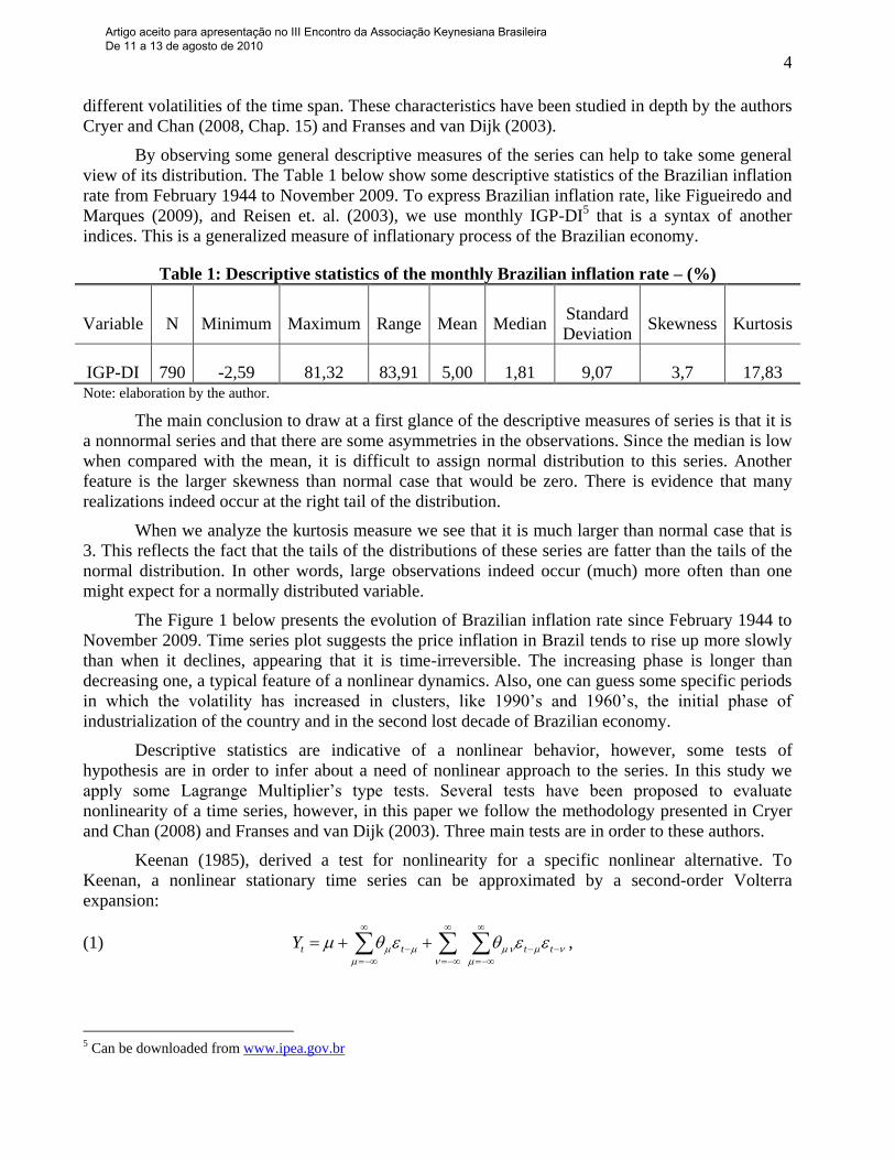
Table 1: Descriptive statistics of the monthly Brazilian inflation rate – (%)

Variable N Minimum Maximum Range Mean Median Standard

Deviation Skewness Kurtosis

IGP-DI 790 -2,59 81,32 83,91 5,00 1,81 9,07 3,7 17,83 Note: elaboration by the author.

The main conclusion to draw at a first glance of the descriptive measures of series is that it is

a nonnormal series and that there are some asymmetries in the observations. Since the median is low

when compared with the mean, it is difficult to assign normal distribution to this series. Another

feature is the larger skewness than normal case that would be zero. There is evidence that many

realizations indeed occur at the right tail of the distribution.

When we analyze the kurtosis measure we see that it is much larger than normal case that is

3. This reflects the fact that the tails of the distributions of these series are fatter than the tails of the

normal distribution. In other words, large observations indeed occur (much) more often than one

might expect for a normally distributed variable.

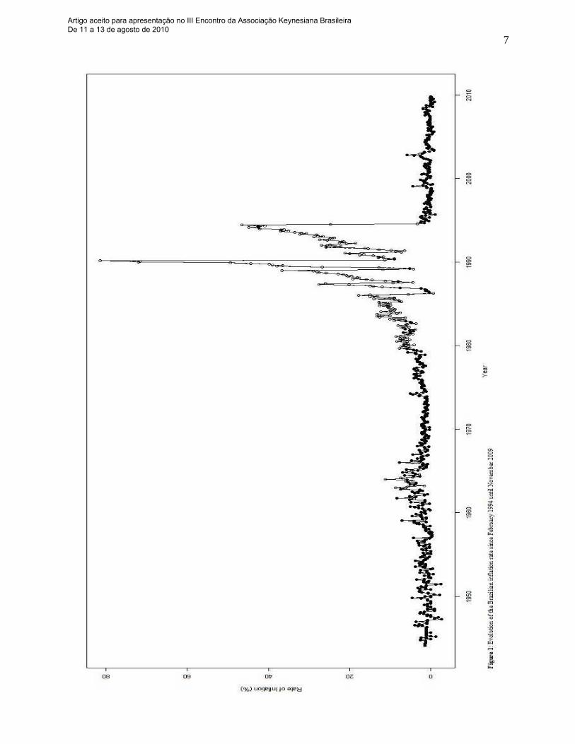
The Figure 1 below presents the evolution of Brazilian inflation rate since February 1944 to

November 2009. Time series plot suggests the price inflation in Brazil tends to rise up more slowly

than when it declines, appearing that it is time-irreversible. The increasing phase is longer than

decreasing one, a typical feature of a nonlinear dynamics. Also, one can guess some specific periods

in which the volatility has increased in clusters, like 1990‟s and 1960‟s, the initial phase of

industrialization of the country and in the second lost decade of Brazilian economy.

Descriptive statistics are indicative of a nonlinear behavior, however, some tests of

hypothesis are in order to infer about a need of nonlinear approach to the series. In this study we

apply some Lagrange Multiplier‟s type tests. Several tests have been proposed to evaluate

nonlinearity of a time series, however, in this paper we follow the methodology presented in Cryer

and Chan (2008) and Franses and van Dijk (2003). Three main tests are in order to these authors.

Keenan (1985), derived a test for nonlinearity for a specific nonlinear alternative. To

Keenan, a nonlinear stationary time series can be approximated by a second-order Volterra

expansion:

(1)

ttttY ,

5 Can be downloaded from www.ipea.gov.br


http://www.ipea.gov.br/

5

where },{ tt is i.i.d. with zero-mean random variables. The process }{ tY will be linear if

the double sum of the right-hand side of (1) does not exist. Keenan‟s test statistic is denoted by F̂ .

Under the null of linearity, the test statistic F̂ is approximately distributed as an F-distribution with

degrees of freedom 1 and 22 mn . Cryer and Chan (2008: 390-1) show that Keenan‟s test is

equivalent to testing if 0 in the multiple regression model:

(2) ttmtmtt YYYY

2

110ˆ...

However, Tsay (1986), extended Keenan‟s test to more general nonlinear alternatives and he shows

that is equivalent to considering the next quadratic regression model:

(3)

tmtmmmtmtmmmtmm

mttmttt

mttmttt

mtmtt

YYYY

YYYYY

YYYYY

YYY

2

,1,1

2

1,1

2,2323,2

2

22,2

1,1212,1

2

11,1

110

...

......

...

...

and to test whether or not all the 2/)1( mm coefficients ji, are zero. Again, this can be made by

the same F-test that all ji, ‟s are zero. To specify the m value, in practice, the AIC information

criteria is used. Another tests can be applied to search for nonlinearities in the times series, like BDS

test based in concepts from chaos theory (see Liu et. al. (1992)).

While Tsay‟s and Keenan‟s tests can detect some quadratics nonlinearities, with them it is

not possible to detect specific threshold nonlinearity as the alternative. Chan (1990), developed a

test for nonlinearity with this specific alternative (See also Cryer and Chan (2008)). These authors

carried the likelihood ratio test for threshold nonlinearity, with the null hypothesis being a normal

AR (p) process and the alternative hypothesis being a stationary SETAR model of order p with

normally distributed errors. The general model of the alternative hypothesis can be written as:

(4) tdtptpt

ptptt

erYIYY

YYY

)(}...{

...

,211,20,2

,111,10,1

where the )(I is an indicator variable that equals 1 if only if the expression enclosed is true and

zero otherwise. The test is performed with fixed p and d (an integer time delay) and it can be shown

to be equivalent to:

(5)

)(ˆ

)(ˆlog)(

1

2

0

2

H

HpnTn

where n-p is the (effective) sample size, )(ˆ0

2 H is the maximum likelihood estimator of the noise

variance from the linear AR (p) fit and )(ˆ1

2 H from the SETAR fit with the threshold searched

over some finite interval. The likelihood ratio test (5) does not have a standard distribution. Chan

(1991), derived an approximation method for computing the p-values of the test highly precise. The

test depends upon on the interval over which the threshold parameter is searched. As well as Cryer

and Chan (2008), we adopt 10th and 90th percentiles of sample to do this.

The results of these three tests are presented below. In general it can be inferred that

Brazilian inflation rate does not have the properties of a linear time series and one linear AR (p)

model would not be adequate to model, describe and forecast it.


6

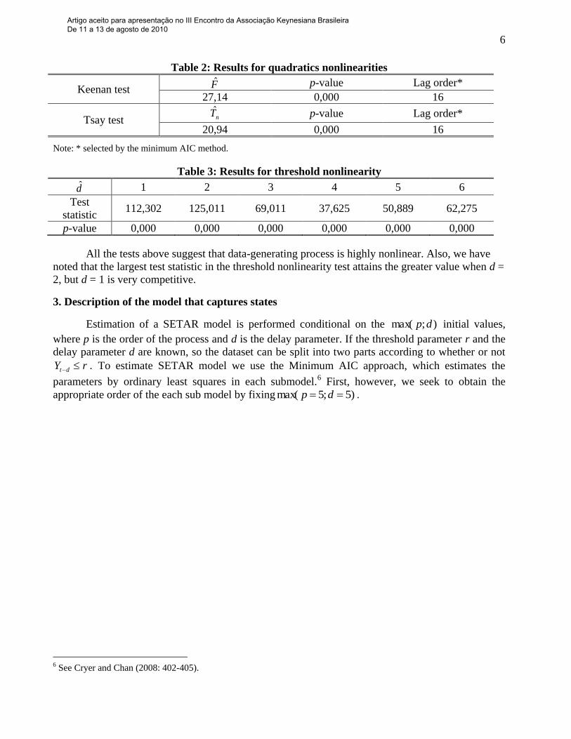
Table 2: Results for quadratics nonlinearities

Keenan test F̂ p-value Lag order*

27,14 0,000 16

Tsay test nT̂ p-value Lag order*

20,94 0,000 16

Note: * selected by the minimum AIC method.

Table 3: Results for threshold nonlinearity

d̂ 1 2 3 4 5 6

Test

statistic 112,302 125,011 69,011 37,625 50,889 62,275

p-value 0,000 0,000 0,000 0,000 0,000 0,000

All the tests above suggest that data-generating process is highly nonlinear. Also, we have

noted that the largest test statistic in the threshold nonlinearity test attains the greater value when d =

2, but d = 1 is very competitive.

3. Description of the model that captures states

Estimation of a SETAR model is performed conditional on the );max( dp initial values,

where p is the order of the process and d is the delay parameter. If the threshold parameter r and the

delay parameter d are known, so the dataset can be split into two parts according to whether or not

rY dt . To estimate SETAR model we use the Minimum AIC approach, which estimates the

parameters by ordinary least squares in each submodel.6 First, however, we seek to obtain the

appropriate order of the each sub model by fixing )5;5max( dp .

6 See Cryer and Chan (2008: 402-405).


7


8

For sake of simplicity we describe the model that can capture only two regimes. Yet, the

general case of m regimes can be easily generalized. For this point, the reader can consult Cryer and

Chan (2008: Chap. 15) and Franses and van Dijk (2003: Chap. 3). The stationary process ( tY ) will

follow a two-regime Self-Exciting Threshold Autoregressive process, denoted by ),,2( 21 ppSETAR

with delay d if it attends the equation:

(6)

rYifeYY

rYifeYYY

dttptpt

dttptpt

t

2,211,20,2

1,111,10,1

22

11

...

...

where r is the threshold, 0d is the parameter delay, te a standard white noise process. The )(I is

the indicator variable such that 1)( rYI dt if rY dt and zero otherwise. For a given threshold r

and the position of the random variable dtY with respect to this threshold r, the process ( tY ) follows

here a particular AR (p) submodel.

The autoregressive orders 1p and 2p need not to be identical, and the time delay d may be

larger than maximum autoregressive orders. Also, and importantly, the standard variance errors 1

and 2 need not to be identical for the two regimes, so the SETAR model can account for some

conditional heteroscedasticity in the data. This is a very important property of the model, since the

conditional heteroskedasticity of Brazilian inflation rate is well documented in the literature.

In particular, by the MAIC method, the best order is selected traditionally and each sub

model on each regime is estimated by ordinary least squares using dataset of falling in each regime.

Also, the less biased estimator of the noise variance can be estimated in within-regime residual sum

of squared errors normalized by the effective sample size. Then the unbiased noise variance 2~i of

the ith

regime can be obtained by the formula:

(7) 1

ˆ~ 22

ii

iii

pn

n ,

where ip is the autoregressive order of the ith

fitted submodel.

4. Empirical results and discussion

By applying the MAIC method, fixing )5;5max( dp and searching for the threshold

roughly between 10th

percentile and 90th

percentile we have the following results. The objective was

to test some different orders to SETAR model and different parameters delay.

Table 4: Nominal AIC of the SETAR models fitted to the Brazilian inflation rate for 51 d

d̂ AIC r̂ 1p̂ 2p̂

1 3126 5,14 3 4

2 3195 4,21 3 4

3 3223 4,21 3 4

4 3203 4,21 3 4

5 3178 6,52 3 4 Note: calculations by the author.

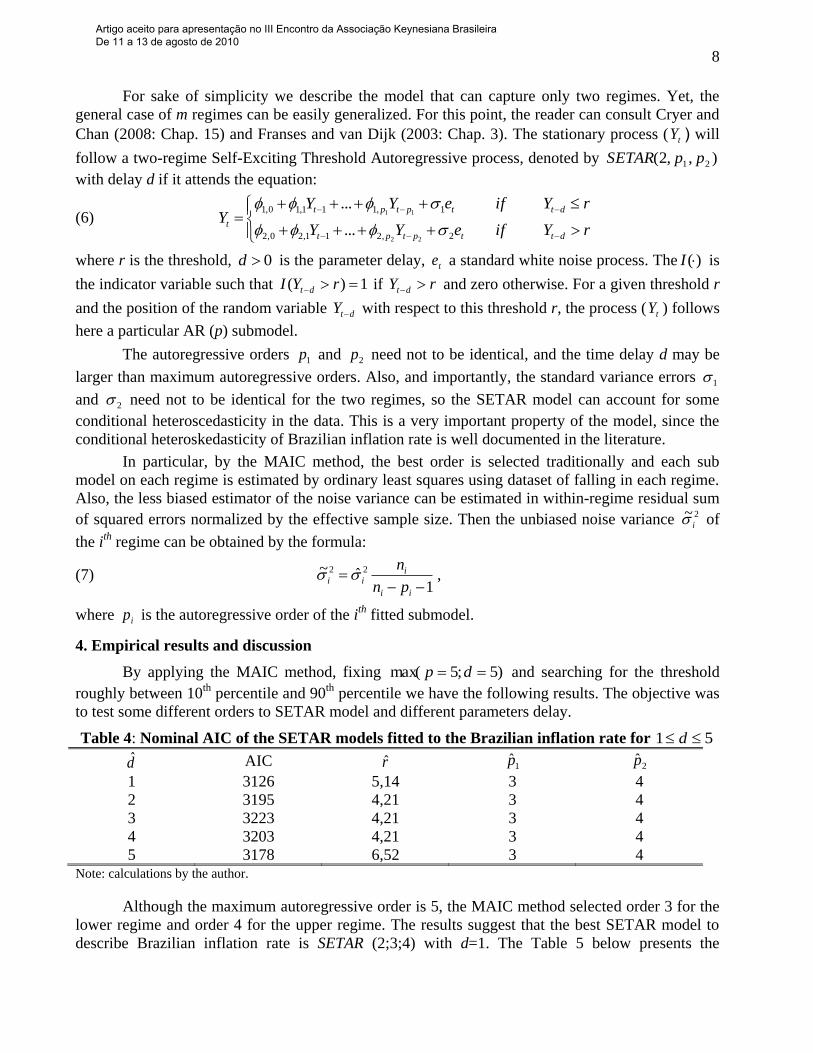
Although the maximum autoregressive order is 5, the MAIC method selected order 3 for the

lower regime and order 4 for the upper regime. The results suggest that the best SETAR model to

describe Brazilian inflation rate is SETAR (2;3;4) with d=1. The Table 5 below presents the


9

parameters estimates of that model and diagnostics of residuals by the Box-Pierce test for null

hypothesis of autocorrelation of lag )( .

Table 5: Fitted SETAR (2;3;4) model for the Brazilian inflation rate: 1944:01-2009:11

Estimate Std. Error t-statistic p-value

d̂ 1

r̂ 5,14

Lower Regime )603( 1 n

0,1̂ 0,382 0,073 5,258 0,000***

1,1̂ 0,733 0,044 16,701 0,000***

2,1̂ 0,022 0,044 0,497 0,619

3,1̂ 0,051 0,022 2,253 0,025**

2

1~ 1,334

Upper Regime )183( 2 n

0,2̂ 1,571 0,856 1,836 0,068*

1,2̂ 0,960 0,078 12,356 0,000***

2,2̂ -0,010 0,106 -0,091 0,927

3,2̂ -0,244 0,111 -2,1963 0,029**

4,2̂ 0,177 0,080 2,222 0,027**

2

2~ 46,860

BP(3) 0,911

BP(6) 0,933

BP(12) 0,249

MAIC 3128

Note: (*), (**), (***) denote 10%, 5% and 1% of significance, respectively. BP )( denotes the lags of Box-Pierce test

for autocorrelations of residuals and their p-values of fitted model.

In general, for each regime, the t-statistics and corresponding p-values reported in Table 5

above are similar. Notice that coefficients of lag two in both regimes are not significant statistically.

This can indicate that the model could be reduced to a lower order in each regime but this procedure

will not be pursued here. The conditional heteroskedasticity in the upper regime is several times

greater than low inflation regime. Another interesting result is that empirical unconditional

probabilities of being in each regime are 0,76331 and 0,23162 which can indicate that

lower inflation regime can with occur at much more higher probability than upper regime.7

The estimated threshold is 5,14 at 76,7th

percentile of the dataset. One way to explore these

results is to split and show the two regime of inflation at a graphical level. Indeed, it is done by

plotting separate observations to entire sample in Figure 1 on page 7 above. In that Figure, we can

7 n

n i i , where n is total sample size and in is the effective sample size falling in that regime.


10

identify data falling in the lower regime, that is, those lag 1 values are less or equal than 5,14 are

pictured as solid circles. In contrast, those observations that falling in the upper regime are displayed

as open circles which values exceed threshold parameter.

There is some pattern in that series. In general, estimated lower regime corresponds to the

increasing phase of inflationary process and vice-versa. Especially in the 1990‟s decade, it is clear

that lower regime inflation persists in the increasing phase and higher regime persists on the peak

and thought decreasing phase of process, but there are asymmetric evolution in the series, since

increasing phase are slower then decreasing phase. This is the time irreversible phenomenon. The

split observations in two different regimes in the Figure 1 can show this pattern.

The estimated model can capture the successive acceleration of inflation rate and their plans

of stabilization during that long time, since 1960‟s decade. In the 1980‟s decade, after some

conservative effort to stabilize price inflation in the initial phase of period with recession and

unemployment, some plans based on inertial inflation hypothesis were implemented, like Plano

Cruzado in 1986. Thereafter, there were successive attempts to hit price inflation indexation in

Brazilian economy. However, after some unsuccessful plans based on direct control on prices and

wages, the Real Plan in 1994, which was a great and complex Monetary Reform introduced in

stages to remove indexation, did the job without recession and unemployment and as well as without

the approval of International Monetary Fund, whose staff members do not understudy the theoretical

premises of that plan8.

Another interesting feature of this model is the possibility of capture the asymmetric

movement of the series without treat the governmental intervention as if was an aberrant or

exogenous event. The linear approach to time series in general treat aberrant observations as if

outliers. It is not the case in the nonlinear approach (See Franses and Dijk (2003) for a detailed

discussion).

This was the interpretation of Cati et. al. (1999), in the context of a unit root test by treating

Brazilian inflation rate as if was a linear time series. The evidence presented here suggests that

interpretation is difficult to maintain, because beyond the governmental intervention the nonlinear

process can have an endogenous dynamics. This also may have been the case of Germany

hyperinflation at the early 19209.

Beyond the residuals test, the fitted model can be evaluated analytically or by simulation.

Some authors have implemented several methods. If the lag of model is one it is possible to make

this analytically, but it is not the case here. For models of order higher than one, it can be quite

difficult to establish the existence of equilibria, attractors and/or limit cycles analytically. One way

to proceed is to follow Franses and Dijk (2003), and make a deterministic simulation by the skeleton

of the model, by dropping the noise term. However, the option adopted here was to make a

stochastic simulation, following Cryer and Chan (2008), since the number of observations and their

behavior can be easily plotted in a graphical form.

8 Since its origin, the inertialists do have make two alternative proposals to hit price inflation. First, could be a policy

direct control of prices and wages, by freezing some key prices of the economy. The alternative was to make a complex

Monetary Reform simulating a hyperinflation process in stages. Both proposals were implemented but the last one (Real

Plan) has made the process to complex to economists that do not know Brazilian economy. See Bacha (1997) about this

point. 9 See Lopes (1985).


11

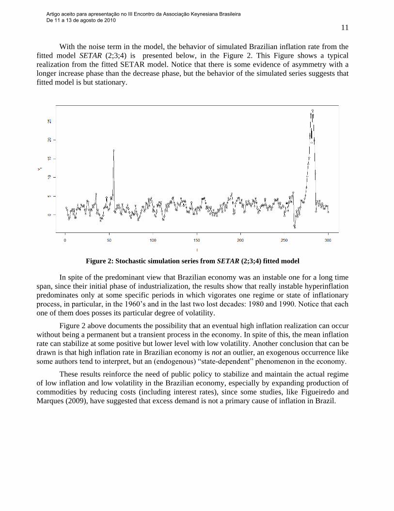
With the noise term in the model, the behavior of simulated Brazilian inflation rate from the

fitted model SETAR (2;3;4) is presented below, in the Figure 2. This Figure shows a typical

realization from the fitted SETAR model. Notice that there is some evidence of asymmetry with a

longer increase phase than the decrease phase, but the behavior of the simulated series suggests that

fitted model is but stationary.

Figure 2: Stochastic simulation series from SETAR (2;3;4) fitted model

In spite of the predominant view that Brazilian economy was an instable one for a long time

span, since their initial phase of industrialization, the results show that really instable hyperinflation

predominates only at some specific periods in which vigorates one regime or state of inflationary

process, in particular, in the 1960‟s and in the last two lost decades: 1980 and 1990. Notice that each

one of them does posses its particular degree of volatility.

Figure 2 above documents the possibility that an eventual high inflation realization can occur

without being a permanent but a transient process in the economy. In spite of this, the mean inflation

rate can stabilize at some positive but lower level with low volatility. Another conclusion that can be

drawn is that high inflation rate in Brazilian economy is not an outlier, an exogenous occurrence like

some authors tend to interpret, but an (endogenous) “state-dependent” phenomenon in the economy.

These results reinforce the need of public policy to stabilize and maintain the actual regime

of low inflation and low volatility in the Brazilian economy, especially by expanding production of

commodities by reducing costs (including interest rates), since some studies, like Figueiredo and

Marques (2009), have suggested that excess demand is not a primary cause of inflation in Brazil.


12

5. Conclusions

The main task of this paper was to detect some nonlinearities and asymmetric behavior of the

Brazilian inflation rate by applying Lagrange type tests for nonlinearity. Doing this, then we split the

inflationary process in the two state-dependent regimes: lower inflation and volatility and, in

contrast, high inflation and higher volatility. The analysis carried out shows that SETAR model can

reasonably describe long run behavior of Brazilian inflation rate. The stochastic simulation suggests

that model is stationary as well.

Two distinct regimes were detected by the estimation of a SETAR model. The lower regime

is characterized by a lower inflation rate with substantially lower volatility and higher unconditional

probability of occurrence. Another feature of this regime is the lower degree of indexation of the

economy, since the constant and the autoregressive parameters are low when compared with that

upper regime. In contrast, upper regime of inflationary process has a higher rate of inflation with

inertial component being substantially higher, expressed by the higher intercept and other

autoregressive parameters of that regime. Also, we can conclude that this last regime has lower

unconditional probability of occurrence.

Since the persistence of lower regime is but greater, the low inflation regime can actually

occur for a long time span. However, as the series does have nonlinear dynamics, to control

inflationary process in the Brazilian economy there is an explicit needed of governmental policy to

maintain this state of affairs. Otherwise, the inflationary process can assume a “self-dynamic” and

so change of regime to a higher inflation process endogenously. There is an inherent instability in

the Brazilian economy that needs to be controlled by the visible hand of the State in that period.

Because the autoregressive components in the lower regime are almost all significant it will

be a good strategy of the government hit some indexed prices that still remain in the Brazilian

economy, reducing the inertial component or, in other words, the degree of indexation. This can be a

better strategy of policy than create a climate of recession and unemployment of labor by a credit

restriction. One lesson is but clear: the stability of prices in the Brazilian economy is to far from

being automatic.

Bibliography

ASIMAKOPULOS, A. (1995) Keynes´s General Theory and Accumulation. Cambridge: Cambridge

University Press.

BACHA, E. L. (1997) “O Plano Real: uma avaliação”, In: MERCADANTE, A. (Org.) O Brasil pós-

Real: a política econômica em debate, Campinas: Unicamp-IE, p. 11-69.

BOLLERSLEV, T. (1986). “Generalized autoregressive conditional heteroskedasticity”, Journal of

Econometrics, 31(3): 307-327

CAMPÊLO, A. K.; CRIBARI-NETO, F. (2003) “Inflation inertia and „inliers‟: the case of Brazil”,

Revista Brasileira de Economia, 57(4): 713-719.

CATI, R. C.; GARCIA, M. G. P.; PERRON, P. (1999) “Unit roots in the presence of abrupt

governmental interventions with an application to Brazilian data”, Journal of Applied

Econometrics, 14: 27-56.

CHAN, K. S. (1990) “Testing for threshold autoregression”, The Annals of Statistics, 18(4): 1886-

1894.


13

CHAN, K. S. (1991) “Percentage points of likelihood ratio tests for threshold autoregression”,

Journal of Royal Statistical Society, Series B, 53(3): 691-696.

CRIBARI-NETO, F.; CASSIANO, K. (2005). “Uma análise da dinâmica inflacionária brasileira”,

Revista Brasileira de Economia, 59(4): 535-566.

CRYER, J. D.; CHAN, K. S. (2008) Time Series Analysis. New York: Springer.

EATWELL, J.; MILGATE, M. (1984) (eds.) Keynes’s economics and the theory of value and

distribution. London: Duckworth.

FIGUEIREDO, E. A.; MARQUES, A. M. (2009) “Inflação inercial como um processo de longa

memória: análise a partir de um modelo arfima-figarch”, Estudos Econômicos, 39(2): 437-458.

FRANSES, P. H.; van DIJK, D. (2003) Nonlinear Time Series Models in Empirical Finance.

Cambridge: Cambridge University Press.

HAMILTON, J. (1989) “A New Approach to the Economic Analysis of Nonstationary Time Series

and Business Cycle”, Econometrica, 57(2): 357-384.

KALDOR, N. (1982) The Scourge of Monetarism. London: Oxford University Press.

KEENAN, D. (1985) “A Tukey nonlinear type test for time series nonlinearities”, Biometrika, 72:

39-44.

KEYNES, J. M. (1936) The General Theory of Employment, Interest and Money. London:

Macmillan.

LAURINI, M.; VIEIRA, H. (2005) “A dynamic econometric model for inflationary inertia in

Brazil”, IBMEC, forthcoming.

LE BOURVA, J. (1992) “Money creation and credit multipliers”, Review of Political Economy,

4(4): 447-466.

LÉON-LEDESMA, M. A. (2006). “Cycles, aggregate demand, and growth”, In: ARESTIS, P.;

McCOMBIE, J.; VICKERMAN, R. (eds). Growth and Economic Development. Cheltenham,

UK: Edward Elgar Publishing, pp. 82-95.

LIU, T.; GRANGER, C. W. J.; HELLER, W. P. (1992) “Using the correlation exponent to decide

whether an economic series is chaotic”, Journal of Applied Econometrics, 7 (Supplement): S25-

S39.

LOPES, F. L.; WILLIAMSON, J. (1980) “A teoria da indexação consistente”, Estudos Econômicos,

10(3): 61-99.

LOPES, F. L. (1985) “Inflação inercial, hiperinflação e desinflação: notas e conjecturas”, Revista de

Economia Política, 5(2): 135-151.

MAIA, A. L. S.; CRIBARI-NETO, F. (2006) “Dinâmica inflacionária brasileira: resultados de auto-

regressão quantílica”. Revista Brasileira de Economia, 60(2): 153-165.

MODIANO, E. (1983) “A dinâmica de salários e preços na economia brasileira: 1966-1981”,

Pesquisa e Planejamento Econômico, 13(1): 39-68.

MODIANO, E. (1985) “Salários, preços e câmbio: os multiplicadores dos choques numa economia

indexada”, Pesquisa e Planejamento Econômico, 15(1): 1-32.

POTTER, S. M. (1995). “A nonlinear approach to US GNP”, Journal of Applied Econometrics,

10(2): 109-125.

PROIETTI, T. (1998) “Characterizing Asymmetries in Business Cycles Using Smooth-Transition

Structural Time Series Models”, Studies in Nonlinear Dynamics and Econometrics, 3: 141-156.


14

REISEN, V. A.; CRIBARI-NETO, F.; JENSEN, M. J. (2003) “Long memory inflationary dynamics:

the case of Brazil”, Studies in Nonlinear Dynamics & Econometrics, 7(3): 1-16.

RESENDE, A. L. (1985a) “A moeda indexada: nem mágica nem panacéia”, Revista de Economia

Política, 5(2): 124-129.

RESENDE, A. L. (1985b) “A moeda indexada: uma proposta para eliminar a inflação inercial”,

Revista de Economia Política, 5(2): 130-134.

SHONE, R. (1997) Economic Dynamics: Phase diagrams and their economic application.

Cambridge: Cambridge University Press.

SIMONSEN, M. H. (1985) “A inflação brasileira: lições e perspectivas”. Revista de Economia

Política, 5(4): 15-30.

TEJADA, C. A. O.; PORTUGAL, M. S. (2001). “Credibilidade e inércia inflacionária no Brasil:

1986-1998”, Estudos Econômicos, 31(3):459-494.

THE R DEVELOPMENT CORE TEAM (2008). R: A language and environment for statistical

computing. R Foundation for Statistical Computing, Vienna, Austria. <http://www.r-

project.org>.

TIAO, G. C.; TSAY, R. S. (1994) “Some Advances in Non-Linear and Adaptive Modeling in Time

Series”, Journal of Forecasting, 13: 109-131.

TONG, H.; LIM, K. S. (1980) “Threshold autoregression, limit cycles and cyclical data (with

discussion)”, Journal of the Royal Statistical Society B, 42: 245-292.

TONG, H. (1983) Threshold Models In Non-linear Time Series Analysis, New York: Springer, pp.

101-141.

TONG, H. (1990) Non-linear Time Series, Oxford: Clarendon Press.

TONG, H. (2007) “Birth of threshold time series model”, Statistica Sinica, 17: 8-14.

TSAY, R. S. (1986) “Nonlinearity tests for time series”, Biometrika, 73: 461-466.

TSAY, R. S. (1991) “Detecting and modeling nonlinearity in univariate time series analysis”,

Statistica Sinica, 1: 431-451.


Não linearidades, mudanças de regime e assimetrias na taxa de inflação brasileira: análise a...

Documents

Transcript of Não linearidades, mudanças de regime e assimetrias na taxa de inflação brasileira: análise a...