NaNoC - CORDIS

Contract no. 248972FP7 STREP Project

NaNoCNanoscale Silicon-Aware Network-on-Chip Design Platform

D2.3: Report on Service Differentiation Techniquewith Packet Formats to Support Quality of Service

Due Date of Deliverable 31st December, 2012

Completion Date of Deliverable 31st December, 2012

Start Date of Project 1st January, 2010 - Duration 36 Months

Lead partner for Deliverable Lantiq Deutschland GmbH (Lorenzo Di Gregorio)Approval Status Approved by all partners on February 13, 2013

Revision: v1.0

Project co-funded by the European Commission within the 7th Framework Programme (2007-2013)Dissemination Level

PU Public ØPP Restricted to other programme participants (including Commission Services)RE Restricted to a group specified by the consortium (including Commission Services)CO Confidential, only for members of the consortium (including Commission Services)

PUBLIC

Contents

1 Introduction 11.1 Motivation for a lightweight approach . . . . . . . . . . . . . . . . . . . . . . . . . . . . . . . . 1

1.1.1 Microarchitectual level . . . . . . . . . . . . . . . . . . . . . . . . . . . . . . . . . . . . . 11.1.2 Application-level . . . . . . . . . . . . . . . . . . . . . . . . . . . . . . . . . . . . . . . . . 21.1.3 Experimental Results . . . . . . . . . . . . . . . . . . . . . . . . . . . . . . . . . . . . . . 3

1.2 Related work . . . . . . . . . . . . . . . . . . . . . . . . . . . . . . . . . . . . . . . . . . . . . . . . 3

2 Reservation Frameworks 52.1 Reservations on individual nodes . . . . . . . . . . . . . . . . . . . . . . . . . . . . . . . . . . . 52.2 The NoC as a resource . . . . . . . . . . . . . . . . . . . . . . . . . . . . . . . . . . . . . . . . . . 5

2.2.1 Service Curves . . . . . . . . . . . . . . . . . . . . . . . . . . . . . . . . . . . . . . . . . . 62.2.2 Traffic Envelope . . . . . . . . . . . . . . . . . . . . . . . . . . . . . . . . . . . . . . . . . 7

3 Serving Traffic 83.1 Traffic Models . . . . . . . . . . . . . . . . . . . . . . . . . . . . . . . . . . . . . . . . . . . . . . . 8

3.1.1 Simple traffic models . . . . . . . . . . . . . . . . . . . . . . . . . . . . . . . . . . . . . . 83.1.2 Complex traffic models . . . . . . . . . . . . . . . . . . . . . . . . . . . . . . . . . . . . . 10

3.2 Service models . . . . . . . . . . . . . . . . . . . . . . . . . . . . . . . . . . . . . . . . . . . . . . . 123.2.1 Serving simple traffic . . . . . . . . . . . . . . . . . . . . . . . . . . . . . . . . . . . . . . 123.2.2 Serving complex traffic . . . . . . . . . . . . . . . . . . . . . . . . . . . . . . . . . . . . . 13

4 Advances on QoS bounds 154.1 Remaining Utilization . . . . . . . . . . . . . . . . . . . . . . . . . . . . . . . . . . . . . . . . . . 154.2 Bounded Periods . . . . . . . . . . . . . . . . . . . . . . . . . . . . . . . . . . . . . . . . . . . . . . 184.3 Network Latency . . . . . . . . . . . . . . . . . . . . . . . . . . . . . . . . . . . . . . . . . . . . . 204.4 The Nested QoS problem . . . . . . . . . . . . . . . . . . . . . . . . . . . . . . . . . . . . . . . . 214.5 Calculation of Deadline Curves . . . . . . . . . . . . . . . . . . . . . . . . . . . . . . . . . . . . . 23

5 Classes of Service 285.1 Periodic / sporadic . . . . . . . . . . . . . . . . . . . . . . . . . . . . . . . . . . . . . . . . . . . . 28

5.1.1 Indirection of priorities . . . . . . . . . . . . . . . . . . . . . . . . . . . . . . . . . . . . . 285.1.2 Route discovery . . . . . . . . . . . . . . . . . . . . . . . . . . . . . . . . . . . . . . . . . . 28

5.2 Latency-Rate . . . . . . . . . . . . . . . . . . . . . . . . . . . . . . . . . . . . . . . . . . . . . . . . 29

6 Experimental Results 306.1 Models for networks-on-chip . . . . . . . . . . . . . . . . . . . . . . . . . . . . . . . . . . . . . . 30

6.1.1 Note on topologies for NoC . . . . . . . . . . . . . . . . . . . . . . . . . . . . . . . . . . 32

NaNoC Deliverable-2.3-v2.0

PUBLIC

6.1.2 Head-of-Line-Blocking Prevention . . . . . . . . . . . . . . . . . . . . . . . . . . . . . . 326.2 Simulation platform . . . . . . . . . . . . . . . . . . . . . . . . . . . . . . . . . . . . . . . . . . . 32

6.2.1 Processor-based System . . . . . . . . . . . . . . . . . . . . . . . . . . . . . . . . . . . . . 346.2.2 Software Application . . . . . . . . . . . . . . . . . . . . . . . . . . . . . . . . . . . . . . 35

6.3 Results at NoC-level . . . . . . . . . . . . . . . . . . . . . . . . . . . . . . . . . . . . . . . . . . . 356.4 Results at application-level . . . . . . . . . . . . . . . . . . . . . . . . . . . . . . . . . . . . . . . 38

6.4.1 Syntetic results . . . . . . . . . . . . . . . . . . . . . . . . . . . . . . . . . . . . . . . . . . 386.4.2 Real-world results . . . . . . . . . . . . . . . . . . . . . . . . . . . . . . . . . . . . . . . . 42


PUBLIC

List of Figures

1.1 Illustration of the “nested QoS” problem: the QoS provided by the NoC to the processoraffects the QoS provided by the processor to the line interface. . . . . . . . . . . . . . . . . . 3

2.1 Relation of the task models to the traffic models . . . . . . . . . . . . . . . . . . . . . . . . . . 62.2 On the left a service curve and on the right a workload realization with the same service

curve in evidence. . . . . . . . . . . . . . . . . . . . . . . . . . . . . . . . . . . . . . . . . . . . . . 62.3 Periodic model which envelopes a traffic trace. . . . . . . . . . . . . . . . . . . . . . . . . . . . 7

3.1 Relation between data rate, latency and backlog . . . . . . . . . . . . . . . . . . . . . . . . . . 93.2 Relation of the service curve to a traffic realization . . . . . . . . . . . . . . . . . . . . . . . . 113.3 Relation of the SCED deadlines to the actual traffic . . . . . . . . . . . . . . . . . . . . . . . . 113.4 Deadlines for a server with fix latency and constant rate. . . . . . . . . . . . . . . . . . . . . . 123.5 Route A-B-C-D interferes with route E-F-G. . . . . . . . . . . . . . . . . . . . . . . . . . . . . . 123.6 Service curves for a high and low priority transfer. . . . . . . . . . . . . . . . . . . . . . . . . . 14

4.1 Graphical interpretation of the remaining utilization. . . . . . . . . . . . . . . . . . . . . . . . 174.2 Higher utilization achieved by shorter periods. . . . . . . . . . . . . . . . . . . . . . . . . . . . 184.3 Calculation of utilization achieved by a bound on period. . . . . . . . . . . . . . . . . . . . . 194.4 Implementation of (4.6) in Octave . . . . . . . . . . . . . . . . . . . . . . . . . . . . . . . . . . . 204.5 Utilization under rate monotonic with release times. . . . . . . . . . . . . . . . . . . . . . . . 204.6 Top: a service curve σ(t) is obtained from C(t) by (4.9). Bottom: the preemption γ

modifies the service curve from σ(t) to σγ(t). . . . . . . . . . . . . . . . . . . . . . . . . . . . 224.7 Tolerable capacity delay: assuming a flow can start only at time s, the variable capacity

Ci(·) can be delayed at time t by an amount q − t without violating the minimal servicecurve σi(·). . . . . . . . . . . . . . . . . . . . . . . . . . . . . . . . . . . . . . . . . . . . . . . . . . 24

4.8 Tolerable delay during scheduling: the tolerable delay ζi(t) is reduced after the variablecapacity Ci(·) has been scheduled by δi(·). . . . . . . . . . . . . . . . . . . . . . . . . . . . . . 26

4.9 Feasible Region for deadlines: the upper bound of the gray area is the pseudo-inverse ofthe “as-late-as-possible” deadline curve. . . . . . . . . . . . . . . . . . . . . . . . . . . . . . . . 26

6.1 Components of the simulation infrastructure . . . . . . . . . . . . . . . . . . . . . . . . . . . . 306.2 Block diagram of a SystemC model of a NoC node . . . . . . . . . . . . . . . . . . . . . . . . . 316.3 One full mash configuration used for experiments. . . . . . . . . . . . . . . . . . . . . . . . . . 316.4 Dynamic assignment of virtual channels to prioritized traffic . . . . . . . . . . . . . . . . . . 326.5 Block diagram of a generic multiprocessor system-on-chip. . . . . . . . . . . . . . . . . . . . 336.6 Top level specification of the simulation environment, blocks in gray are available from

third parties. . . . . . . . . . . . . . . . . . . . . . . . . . . . . . . . . . . . . . . . . . . . . . . . . 34


PUBLIC

6.7 Case study for hyperbolic bound on node reservations. . . . . . . . . . . . . . . . . . . . . . . 366.8 Low utilization for figure 6.7: slack available. . . . . . . . . . . . . . . . . . . . . . . . . . . . . 366.9 Critical utilization for figure 6.7: within deadlines. . . . . . . . . . . . . . . . . . . . . . . . . 376.10 Overload condition for figure 6.7: deadlines missed. . . . . . . . . . . . . . . . . . . . . . . . 376.11 Case study for utilization bound on network latency. . . . . . . . . . . . . . . . . . . . . . . . 386.12 Low utilization for figure 6.11: interference with slack. . . . . . . . . . . . . . . . . . . . . . . 396.13 Critical utilization for figure 6.11: interference at critical point. . . . . . . . . . . . . . . . . 396.14 Overload condition for figure 6.11: interference under overload. . . . . . . . . . . . . . . . . 406.15 Random delay distributions with same average . . . . . . . . . . . . . . . . . . . . . . . . . . . 406.16 Service curves obtained for random delay distributions with same average . . . . . . . . . . 416.17 Detail of the service curves shown in figure 6.16 . . . . . . . . . . . . . . . . . . . . . . . . . . 416.18 Data transport to be achieved under increased latency guarantee in the NoC: the goal is

to be compliant with the worst case . . . . . . . . . . . . . . . . . . . . . . . . . . . . . . . . . . 426.19 Performance of a processor core under increasing latency guarantee on NoC traffic . . . . 436.20 Service provided by the processor to the software application under increaded latency

guarantee in the NoC . . . . . . . . . . . . . . . . . . . . . . . . . . . . . . . . . . . . . . . . . . . 436.21 Service provided by the application to the packet stream under increased latency guarantee

in the NoC . . . . . . . . . . . . . . . . . . . . . . . . . . . . . . . . . . . . . . . . . . . . . . . . . 446.22 Tolerable slack profile obtained on the processor’s capacity toward the worst case service

to be provided to the packet stream . . . . . . . . . . . . . . . . . . . . . . . . . . . . . . . . . . 44


PUBLIC

1. Introduction

In this document we report on investigation and implemention activities within the NaNoC project re-garding the definition and experimentation of novel techniques for supporting quality-of-service (QoS)withingeneric networks-on-chip (NoCs) from the microarchitecture level up to the application level.

As explained in the subsequent section 1.1, our goal has been to identify and develop lightweighttechniques for providing QoS guarantees at microarchitectural level, because single NoC transactionstake place at a very small time scale and do not impact directly application-level QoS. Instead, QoS atapplication-level is guaranteed by software applications whose performance is in turn affected at themicroarchitectural level by overall NoC transport characteristics. Because these characteristics are onlyindirectly and loosely related to the hardware structures on chip, we are not willing to spend significantsilicon and workload on QoS and an outcome of this work is that this cost is also not necessary to obtainvery good QoS guarantees, because they can be achieved already by defining static routes, computingschedulability conditions and performance bounds already at design time rather than at execution time.

The novel problem setting of QoS over NoC has driven us to obtain significant theoretical advancesin two areas which have been rather dry for almost a decade:

• utilization-based scheduling

• service curve scheduling

In order to validate and evaluate these advances, we have developed simulation infrastructures basedon SystemC:

• NoC models employing the SystemQ library [17]

• MPSoC (multiprocessor systems-on-chip) models employing the Open Virtual Platform of Imperaswith SystemC wrappers

1.1 Motivation for a lightweight approach

In this section we state the need we see in QoS over NoC at both microarchitectural and application-level.We argue that the purpose of QoS at microarchitectural level is chiefly to ease the design process, whereasguarantees obtained at the application level demand a different solution based on holistic techniques.

1.1.1 Microarchitectual level

From a practical and systemic point of view, the extent to which QoS is a necessity within a NoC isquestionable: in real-time applications at a macroscopic level, data transactions over a NoC are hardlyperceived and their lack of determinism is usually only a small component of the overall variability in thesystem. Existing real-time operating systems are able to achieve sub-millisecond accuracy without anyspecial hardware support.

NaNoC Deliverable-2.3-v2.0 Page 1 of 46

PUBLIC

Nevertheless, hardware must be designed for absolute worst cases and QoS in NoCs significantlyimpacts on design in several microarchitectural aspects of multiprocessor systems-on-chip (MPSoC): frombuffer sizing to composition of hardware and software modules, reliable timing characteristics are knownto be largely beneficial to the overall design process. For example, due to long worst case response times,costly measures are required to prevent devices’ starvation or race conditions: with QoS and deterministicresponse times in place, this prevention can be achieved by scheduling rather than, for example, bybloating hardware buffers of every individual module to ensure that enough data is available under worstcase circumstances. Furthermore, QoS enables the allocation of cycle budgets for multiple componentssharing common resources over the network: this budgeting avoids the typical simulate-and-tweak loop,offering a widely acknowledged benefit in any platform-based design process.

For all these reasons, we have sought an approach which does enable QoS in NoCs, although withlittle or possibly no hardware impact. Although we have tried to cover all directions, we have focused ontechniques in which the nodes are not burdened by additional dedicated features: static routes, which canbe set and canceled according to usual connection protocols, are provisioned with QoS by non-exclusivebandwidth reservation managed in software. Consequently, we have focused on techniques by which thesoftware overhead for defining many routes through a NoC remains low, in fact we do not see a need tosqueeze out the last bit of performance on QoS routes and expect that at the least some best-effort trafficwill be transported under all practical circumstances.

1.1.2 Application-level

We know from experience in soft real-time scheduling that remarkable improvements of the processor’sutilization can be achieved allowing small overload phases, which show no practical impact on the appli-cation’s quality. This happens because the models employed by the theory must make largely conservativeassumptions and absolute worst cases are anyway extremely unlikely to be hit in practice.

While the timing of individual transactions over a NoC does not practically affect application levelguarantees, the plurality of transactions taking place in a NoC does affect the performance of the softwarewhich provides application level guarantees. A QoS guarantee provided to an application by a processorconsists of sustainability for workload characteristics seen at the application’s programming interfaces.A QoS guarantee provided to a processor by a NoC consists of sustainability for traffic characteristics seenat the processor’s interfaces like latency, data rate, burst size etc. The application-level characteristicsin a network device are conceptually pretty much the same latency, data rate, burst size etc, seen at themicroarchitectural level, just on another order of magnitude.

Since service to an application by a processor depends largely, although not only, on the service to thatthe processor by a NoC, we could term the problem setting as “nested QoS” problem: how does the QoSguarantee to an application change, if the QoS to the underlaying processor changes?

In section 4.4 we give a precise formulation of this nested QoS problem, which is illustrated by figure1.1. In order to master such complex of problems it is most useful to gain confidence with the concept ofservice curve, which is presented in textbooks like [8]. We can say in informal wording that service curveis the worst case service seen by a serviced item, such as a data packet, arriving at any random time at aserver, such as a processor.

One important feature of the concept behind service curves is that it is holistic: it does not require adecomposition of the system under analysis and can hence be employed for complex systems. The servicecurve can be devised from design parameters or actually measured from workload realizations. In thelatter case it models only corner cases which are actually hit during the system’s evolution and it might


PUBLIC

processor memoryNoC

transport logic

line interface

NoC latency-rateprocessor’s capacity

system’s service

Figure 1.1: Illustration of the “nested QoS” problem: the QoS provided by the NoC to the processoraffects the QoS provided by the processor to the line interface.

turn out in unlikely situations to be over-pessimistic: in such cases the analysis must be done for multipleservice curves, since a single one cannot represent the characteristics of interest. In principle it is alsopossible and actually straightforward to disregard corner cases which are extremely unlikely, though thisis seldom a practice because one must discover that such cases are unlikely to take place and this requiresretaining statistical information about the whole evolution of the system.

A solution for the nested QoS problem, is reported in section 4.5 and the presentation relies heavilyon network calculus formalisms. The proposed solution performs the conversion of the service curvepresented by a processor to an application into a service curve presented by the NoC to the processor.

Once the service curves demanded on the interfaces of a processor have been determined accordingto the algorithm presented in section 4.5, the required latencies and throughputs can be obtained fromthe NoC employing the techniques we have devised at microarchitectural level for defining static routesunder QoS provisioning.

1.1.3 Experimental Results

Section 6.2 describes in practical details the simulation infrastructure and application scenarios requiredto carry out this work.

1.2 Related work

The groundwork for supporting QoS by reserving bandwidth in the nodes of a NoC consists of the twoclassical schemes for resource reservation: rate monotonic and earliest deadline first scheduling (for ex-ample see [15] for an overview).

Qian et al. have employed network calculus concatenations in [11] to calculate the service curvesfor a priority scheduler and a weighted round-robin scheduled and concluded that weighted round-robin


PUBLIC

schedulers are more flexible than priority schedulers because of the difficulties involved in obtainingguarantees on delays employing priorities. Quite surprisingly, though, the authors appear to have missedthe whole literature about periodic scheduling.

In contrast, Shi and Burns presented in [16] a framework based on to predict the latency of trafficflows under periodic scheduling, regarding the NoC nodes as resources which can be reserved in a pre-emptive manner through a monotonic priority assignment of concurring transactions. They develop amethod for analyzing the interference jitters within a NoC, i.e. the deviations in the release times of flitsindirectly caused by higher priority traffic flows. An obstacle to the practical application of their work,though, is that they employ the classical latency formula by Audsley in [2], which is computationallyquite demanding (pseudo-polynomial complexity) for being employed within a traffic management soft-ware for a NoC. One can conjecture that a redesign of the algorithm proposed by Bini e Buttazzo in [5]would reduce this complexity.

We address both the priority scheduling area, employing the hyperbolic bound presented by Bini etal. in [4], and the network calculus area, pointing out that the service-curve earliest deadline (SCED)algorithm by Sariowan et al. in [14] can be employed to derive further policies. A work in this contextwhich is losely related to ours is the one initiated by Thiele in [18], where the capacity curve has beenintroduced and the calculation of the service curve obtained from a variable capacity has been presentedalong with other results. Our work can be viewed as a conceptual inversion, in which we devise how fara capacity curve can be distorted in order to remain compliant to a given service curve.


PUBLIC

2. Reservation Frameworks

In the reservation frameworks we have investigated, a NoC node is regarded as a resource to be reservedand for which multiple data transactions are competing. Every transaction consists of a set of datatransfers to be transported and a set of deadlines, each associated to a transfer, to be met. The goal ofthe schedule is to ensure, whenever possible, that all transactions meet their deadlines while the data isbeing transported over the NoC node.

2.1 Reservations on individual nodes

Two major models are available for resource reservation among concurring transactions:

• task model: in this model a node can be either busy on a transfer or not. Meeting a deadline meansthat a total amount of busy time must be served to a transaction before the deadline expires.

• flow model: in this model, a cumulative function represents how much data has been transfered.The cumulative function must lay above a boundary which represents the deadlines.

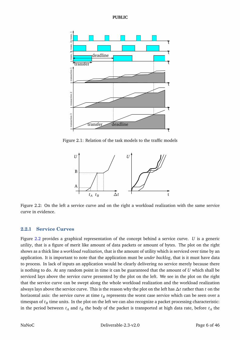
These models are different and equivalent interpretations of the transactions which take place in aNoC: the task model focuses on busy time of the node while the flow model focuses on the amount ofdata transported by the node. Two graphical representations of these models, showing their equivalence,are provided in figure 2.1 for three transactions which transport periodic data transfers. The upper threediagrams represent these transactions according to a task model while the lower three diagrams repre-sent the same transactions according to a flow model. These data transfers can be sporadic: a commonmisconception about the scheduling of periodic tasks is that the tasks must actually show periodicity overthe whole time axis, indeed the theory behind the task model is devised for scheduling tasks which maycreated and terminate at any time, as long as they show periodicity during their life time.

The task model can be employed for simple traffic models, introduced in section 3.1.1, while the flowmodel is employed for more complex traffic models introduced in section 3.1.2.

2.2 The NoC as a resource

Having implemented reservations on individual nodes, we can regard a route as a virtual path with giventransport characteristics. These characteristics can become, in general, rather complex and difficult toanalyze at larget time scales than the one of single transactions.

In order to solve these problems, we have elaborated an holistic solution based on network calculusand in particular on the concept of the service curve, which opens the possibility to effectively use furtherreadily available results from the existing literature like the SCED scheduling [13] discipline.

In the following two sections we provide a background on the concepts of service curve and trafficenvelope: these are fundamental tools for the analysis of complex systems, because complex servicecurves are hardly manageable and they must be approximated by simpler service curves.


PUBLIC

tran

s.1

tran

s.2

tran

s.3

tran

sact

ion

1tr

ansa

ctio

n2

tran

sact

ion

3

deadline

transfer t

t

t

t

t

t

deadlinetransfer

Figure 2.1: Relation of the task models to the traffic models

∆t

U U

t

A

B

tA tB

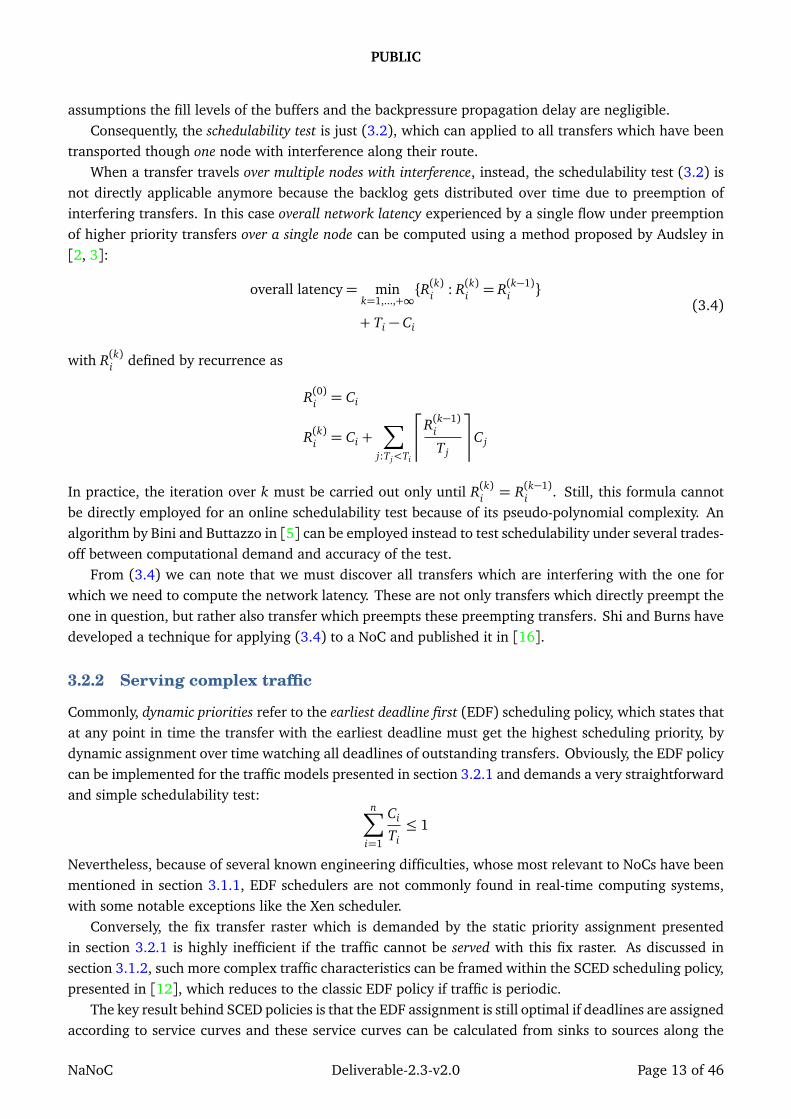
Figure 2.2: On the left a service curve and on the right a workload realization with the same servicecurve in evidence.

2.2.1 Service Curves

Figure 2.2 provides a graphical representation of the concept behind a service curve. U is a genericutility, that is a figure of merit like amount of data packets or amount of bytes. The plot on the rightshows as a thick line a workload realization, that is the amount of utility which is serviced over time by anapplication. It is important to note that the application must be under backlog, that is it must have datato process. In lack of inputs an application would be clearly delivering no service merely because thereis nothing to do. At any random point in time it can be guaranteed that the amount of U which shall beserviced lays above the service curve presented by the plot on the left. We see in the plot on the rightthat the service curve can be swept along the whole workload realization and the workload realizationalways lays above the service curve. This is the reason why the plot on the left has∆t rather than t on thehorizontal axis: the service curve at time tB represents the worst case service which can be seen over atimespan of tB time units. In the plot on the left we can also recognize a packet processing characteristic:in the period between tA and tB the body of the packet is transported at high data rate, before tA the


PUBLIC

traffic

periodic model

time

bits

t

Figure 2.3: Periodic model which envelopes a traffic trace.

header is processed at a lower data rate, because the software must carry out more operations per byte,and after tB the packet has been transported and there is a small inter-packet gap, likely to be caused byframing.

2.2.2 Traffic Envelope

In this section we explain in simple terms what is a traffic envelope.A traffic model is a defined function which represents a traffic level over time. For example we can

term a periodic model with period T and burst C the function:

f (x) =

∫ x

0

S(kT − C , kT )dx

where S(a, b) is C between a and b and 0 elsewhere.The traffic obtained from such a periodic model is presented in figure 2.3. This model is an envelope

for a traffic trace, i.e. a realization of traffic over time, if it lays always above the trace regardless of thepoint at which the trace is observed.

In figure 2.3 the worst case traffic begins at time point t: this traffic is represented at time point 0 bythe dotted line. The periodic model represented in figure 2.3 is the lowest model which lays above thedotted line.

The dotted line is called in network calculus the arrival curve of the traffic and it represents at ageneric time t the maximum increment presented by the traffic between two generic time points q andq+ t.


PUBLIC

3. Serving Traffic

For implementing QoS, incoming traffic must be served by NoC nodes. In the context of this document,classes of service presented in chapter 5 represent a classification of traffic within the NoC according tocharacteristics which are suitable for enforcing QoS. For determining which characteristics are relevant,in this chapter we study traffic models in section 3.1 and technique to serve traffic under these models insection 3.2. In order to increase the efficiency in QoS over NoCs, we propose in chapter 4 some advanceson utilization bounds presented in section 3.2.1.

3.1 Traffic Models

Traffic models can be regarded as processes whose realizations are subject to given traffic characteristics.In sections 3.1.1 and 3.1.2 we present models for which schedulability analysis has been successfullyemployed and are hence supported by QoS techniques.

3.1.1 Simple traffic models

Rate-monotonic scheduling is the most common technique for resource reservation. It is commonlyapplied to a set of software tasks, but it can be equally applied to a set of transactions if the busy time of atask represents the busy time of a data transfer, as shown in section 2. With the terminology introduced tothis purpose within this document, rate-monotonic scheduling consists of associating to each transactiona priority which is inversely proportional to the period of the deadlines. In their seminal work in [10],Liu and Leyland demonstrated that if the highest priority is always scheduled first and all transactions arepreempt-able, all deadlines are met as long as the n data rates Ui,∀i ∈ 1, . . . , n of all ongoing transactionssatisfy:

n∑

i=1

Ui ≤ n(np

2− 1) (3.1)

where:

Ui.= Ci/Ti is the definition of data rate.

Ci busy time for one periodic transfer within the transaction i.

Ti period of the deadline within the transaction i.

n number of simultaneous transactions.

The inequality (3.1) states a simple condition under which it is ensured that a set of transactionsbearing periodic transfers whose sole data rate is known, is guaranteed specific bandwidth and latency.

This condition is sufficient but not necessary, and it is not tight in the sense that there exist setsU1, . . . , Un which violate (3.1) although there exist no combination of C1, . . . , Cn and T1, . . . , Tn whichcannot meet all deadlines under rate-monotonic scheduling.


PUBLIC

tran

s.3

tran

sact

ion

3

deadline

transfer t

t

t

average data ratetransfer rate

latency

backlog

Figure 3.1: Relation between data rate, latency and backlog in a guaranteed traffic flow, derived fromthe real-time scheduling model of periodic tasks.

Bini et al. have identified in [4] the tightest sufficient condition based on sole data rates Ui, which is:

n∏

i=1

(Ui + 1)≤ 2 (3.2)

This condition is still sufficient and not necessary, but it can be proved that this is the tightest conditionif only data rates Ui are known, because for every set U1, . . . , Un which violates (3.2) there is at the leastone combination of C1, . . . , Cn and T1, . . . , Tn which cannot meet all deadlines under rate-monotonicscheduling.

Condition (3.2) imposes an upper limit to the utilization U.=∏n

i=1(Ui + 1) of a NoC node underperiodic guaranteed traffic if only data rates are known.

The periodic or sporadic traffic flows, sustainable through bound (3.2), must bear sufficient backlogat the beginning of the period: to make this point clear consider that if all flows would start transportingtheir backlog just in time to comply with their deadline, without leaving any slack, it would not bepossible to meet all deadlines if any two intervals between start and deadline would overlap. Figure 3.1provides a graphical representation of the relations among the traffic characteristics of one individualflow, in particular:

flow latency= deadline

�

1−average data rate

transfer rate

�

(3.3)

because it is clear from figure 3.1 that

average data rate=backlog

deadline

transfer rate=backlog

deadline− latency

In symbols, the flow latency expressed by (3.3) is merely Ti − Ci and it states the necessity of havingthe backlog ready at the beginning of the period in order to schedule it under the test of (3.2), in fact thelatency Ti − Ci is exactly the one we have declared by setting the deadline Ti on the flow.

Transporting data over one node delays it because of other interfering transfers, i.e. transfers whichbear a higher priority and increase the latency of the current transfer by preempting it. Consequently,the backlog after transversing the first node is not ready anymore at the beginning of the period and thepreemption time due to higher priority transfers must be accounted in the schedulability condition. Thedelay to which a transfer is subject due to preemptions, is called network latency, not to be confused withthe flow latency expressed by (3.3).


PUBLIC

One straightforward approach to account network latency consists of enlarging Ci to cover the pre-emption time, but this grossly reduces the achievable real utilization of the node, i.e. its the busy time,because it disregards the fact that during the preemption time of one backlog the node could actuallytransport data of another backlog.

In order to increase the utilization of the NoC nodes under further types of guaranteed traffic, furtherinsight into the traffic characteristics of the transactions must be won. A first step can be carried out byknowing the deadlines Ti of the transactions and the elapsed fraction of busy time Ci per transaction.With this data, the earliest deadline first (EDF) scheduling, consisting of scheduling always the transactionwhose earliest deadline is next, can achieve up to 100% utilization of NoC nodes under guaranteed traffic.While EDF scheduling appears attractive of a single node, it comes on system level at the price of havingto sort out at any generic time all transactions in order to find out which one bears the next earliestdeadline on a node along the route through interfering transaction. This is clearly not feasible.

A feasible solution consists in applying a technique known as deadline monotonic scheduling, proposedby Audsley in [2], and consisting of assigning the higher priorities to transfers which get closer to theirdeadlines. In this solution, the network latency can be simply subtracted from the deadline to produce anew deadline on which the deadline monotonic scheme can be applied. Yet, before a route can be defineda schedulability test must be carried out to determine whether the QoS in presence of network latencycan be met and this test is more demanding than the ones based on utilization, which we have seen sofar. A test developed by Bini and Buttazzo in [5] offers a parametrized trade-off between tightness andcomplexity, hence it can be employed according to the demands of its users.

While EDF scheduling might definitely be an overkill for simple traffic models, traffic characteristicscan definitely be too complex to be efficiently embedded in periodic sequences of data transfers at fixrates. If traffic significantly differs from the periodic model into which it has to be embedded, fittingit into a periodic model would lead to gross loss of utilization. In such cases, loading the node with ahigher utilization might justify more costly solutions and requires exploiting further traffic characteristicsfor which classic EDF scheduling does not apply. Service curve scheduling techniques, introduced in thesection 3.1.2, provide solutions to schedule more complex traffic.

3.1.2 Complex traffic models

The traffic characteristics which can be sustained by heterogeneous components can be rather complex:for example it is common to accept a maximum burst size and a lower data rate, which needs to be pausedby short recovery times, sometimes known in packet-based networks as “inter-frame gap”.

Such components can be characterized by service curves, introduced by Cruz in [6, 7]: figure 3.2provides a graphical representation of a service curve along with the traffic which has generated it. Theservice curve at time t represents the minimal amount of traffic that a component can serve within a timewindow of size t if backlog is available. The “translated service curve” in figure 3.2 demonstrates that ifthe origin of the service curve is translated to any generic point of a traffic realization, the service curvealways constitutes a lower bound of the traffic. Obviously, the service curve must be the highest of alllower bounds in order to be a tight bound on the traffic.

An application of service curves in resource reservation for QoS is featured by the SCED algorithm,proposed in [12]. Behind the formalism employed in [12], the generic SCED algorithm consists of assign-ing deadlines to data packets outgoing from one node according to the service curves to be guaranteedto every traffic flow: if packets under such deadlines are scheduled by an EDF policy and the scheduleis feasible (i.e. no overloading situation takes place), then the EDF policy guarantees to every flow its


PUBLIC

traffic

service curve

translated service curve

t

serv

ice

Figure 3.2: Relation of the service curve to a traffic realization

time

data

SCED deadlines

Traffic

Service curves

Figure 3.3: Relation of the SCED deadlines to the actual traffic

assigned service curve even if traffic is random. A representation of a traffic flow with the associatedservice curve and deadlines is presented in figure 3.3: the SCED deadlines are constructed sweeping theservice curve along the traffic flow and obtaining the infimum1 of all swept curves.

An implementation of the generic SCED algorithm is not feasible, because it requires iterations overa long record of past traffic and future deadlines: one should constantly calculate the infimum betweenthe service curve applied to the current traffic and the already calculated future deadlines. In order toavoid this computational effort, the work in [12] proposes a class of simple service curves for which thiscomputation reduces to few simple operations.

This class consists of curves shown in figure 3.4, which present a latency and a constant service rate:In this case, the deadlines are a straightforward function of the accumulated traffic, with a reset as

soon as the deadlines fall at the value of the latency. Figure 3.4 shows this computation in a graphicalway: one can ideally picture to attach the service curve to the traffic as it had been done in figure 3.3 andas soon as one translated service curve falls below the currently effective one, it dominates it completelyand becomes the new effective service curve.

1For practical purposes it is obvious that the infimum, also known as greatest lower bound, always corresponds to the mini-mum, but in network calculus theory it is common to refer to the infimum in order to keep results valid for fluid traffic models.


PUBLIC

t

data

Figure 3.4: Deadlines for a server with fix latency and constant rate.

A

CB D

E

F

G

Figure 3.5: Route A-B-C-D interferes with route E-F-G.

3.2 Service models

Service models can be regarded as time partitioning rules for access to a NoC node or a communicationsink. Simple traffic models are served by techniques mentioned in section 3.2.1. Some advances onthese techniques have been reported in chapter 4. Section 3.2.2 reports management techniques formore complex traffic, discussed in section 3.1.2.

3.2.1 Serving simple traffic

In this section we employ the bound (3.2) for sustaining traffic guarantees for simple periodic trafficmodels to which we assign static priorities. Although the same reasoning applies also to the bound (3.1),we do not employ this bound because it is looser and merely bears the advantage of a slightly lowercomputational effort, which is not significant in our context. In chapter 4 we will present some noveltighter bounds.

For serving simple traffic, every traffic flow (Ci, Ti) must be transported over a static route throughthe NoC, ensuring that the utilization of every node is sufficient for sustaining required throughputs andachieving achieving given latencies.

Figure 3.5 presents a route across multiple nodes: the route E-F-G interferes with all nodes on theroute A-B-C-D, because they all stop transporting data due to backpressure from the single link sustainingtrunks C and F, if the transfer E-G has higher priority.

Although this is an idealization, because nodes have some buffer and backpressure has a propaga-tion delay, schedulability analysis assumes worst case phase shifts and stationary behavior: under these


PUBLIC

assumptions the fill levels of the buffers and the backpressure propagation delay are negligible.Consequently, the schedulability test is just (3.2), which can applied to all transfers which have been

transported though one node with interference along their route.When a transfer travels over multiple nodes with interference, instead, the schedulability test (3.2) is

not directly applicable anymore because the backlog gets distributed over time due to preemption ofinterfering transfers. In this case overall network latency experienced by a single flow under preemptionof higher priority transfers over a single node can be computed using a method proposed by Audsley in[2, 3]:

overall latency= mink=1,...,+∞

{R(k)i : R(k)i = R(k−1)i }

+ Ti − Ci

(3.4)

with R(k)i defined by recurrence as

R(0)i = Ci

R(k)i = Ci +∑

j:T j<Ti

&

R(k−1)i

T j

'

C j

In practice, the iteration over k must be carried out only until R(k)i = R(k−1)i . Still, this formula cannot

be directly employed for an online schedulability test because of its pseudo-polynomial complexity. Analgorithm by Bini and Buttazzo in [5] can be employed instead to test schedulability under several trades-off between computational demand and accuracy of the test.

From (3.4) we can note that we must discover all transfers which are interfering with the one forwhich we need to compute the network latency. These are not only transfers which directly preempt theone in question, but rather also transfer which preempts these preempting transfers. Shi and Burns havedeveloped a technique for applying (3.4) to a NoC and published it in [16].

3.2.2 Serving complex traffic

Commonly, dynamic priorities refer to the earliest deadline first (EDF) scheduling policy, which states thatat any point in time the transfer with the earliest deadline must get the highest scheduling priority, bydynamic assignment over time watching all deadlines of outstanding transfers. Obviously, the EDF policycan be implemented for the traffic models presented in section 3.2.1 and demands a very straightforwardand simple schedulability test:

n∑

i=1

Ci

Ti≤ 1

Nevertheless, because of several known engineering difficulties, whose most relevant to NoCs have beenmentioned in section 3.1.1, EDF schedulers are not commonly found in real-time computing systems,with some notable exceptions like the Xen scheduler.

Conversely, the fix transfer raster which is demanded by the static priority assignment presentedin section 3.2.1 is highly inefficient if the traffic cannot be served with this fix raster. As discussed insection 3.1.2, such more complex traffic characteristics can be framed within the SCED scheduling policy,presented in [12], which reduces to the classic EDF policy if traffic is periodic.

The key result behind SCED policies is that the EDF assignment is still optimal if deadlines are assignedaccording to service curves and these service curves can be calculated from sinks to sources along the


PUBLIC

high priority

low priority

Figure 3.6: Service curves for a high and low priority transfer.

routes in a NoC. In general, these service curves need only to be convex, but the SCED policy can only beenforced at acceptable costs if the service curves consist of latency-rate characteristics, as shown in figure3.4.

Figure 3.6 presents a graphical example of this calculation based on a concatenation theorem reportedin [9]. In practice, the service curves are calculated along paths from sources to sinks, adding latenciesand taking the lower slopes. When transfers are transported over common links, either one transfer isprioritized, as in the example in figure 3.6 or both are interleaved in some round-robin fashion. Theincreased latency must be accounted according to the chosen arbitration scheme: in the example shownin figure 3.6, the high priority transfer retains its latency while the low priority transfer must account forthe preemption time due to the high priority transfer.

Once the service curves are calculated, SCED deadlines can be assigned on every node and EDFscheduling on every node ensures locally that these deadlines are not violated. The QoS experienced atthe sink is clearly looser than the one imposed at the source: in order to meet given constraints, though,the computation of the service curves can also be carried out also backward, from sinks to sources. Inthis case the traffic is schedulable if the QoS demanded at the sinks is loose enough to accommodaterates and latencies met along the path and present feasible service curves at the sources.


PUBLIC

4. Advances on QoS bounds

In this chapter we report some advances we developed on utilization-based scheduling, which is partic-ularly attractive if the data rates are known but the burst characteristics of the traffic are not entirelyknown, and service curve scheduling, which is attractive to hierarchically propagate the effect of trafficcharacteristics of the NoC to the system by modeling the slowdown caused on the software. In section4.1 a new theorem on utilitation-based scheduling will be introduced and we will show a graphical in-terpretation of the results which leads to two further theorems in sections 4.2 and 4.3. In section 4.5 atheory is given leading to an algorithm which determines a bound on the service provided by a NoC inorder to let the software being executed be compliant with service constraints imposed at system level.

4.1 Remaining Utilization

In this section we introduce a theorem for calculating the utilization of the nodes in a NoC under periodictraffic models presented in section 3.1.1. We provide for this theorem an algebraic proof which demon-strates that its main formula (4.1) is equivalent to the hyperbolic bound (3.2) presented in [4]. Moreinterestingly, we provide a graphical interpretation of this result from which tighter bounds are derivedin sections 4.2 and 4.3: these results are no contradiction of the proof in [4] that the hyperbolic bound(4.1) is the tightest bound on utilization, because they employ the backlog Ck and period Tk individuallyand not just Uk

.= Ck/Tk.

To begin with, we state the following theorem.

Theorem 1 (remaining utilization). If a node under a utilization Ui−1 becomes subject to a periodic trafficwith backlog Ci and period Ti, its utilization becomes:

Ui =TiUi−1 − Ci

Ti + Ci(4.1)

In order to prove this theorem, we employ just the hyperbolic bound (3.2) and show that formula(4.1 can be obtained by algebraic manipulation.

Proof. By employing the hyperbolic bound (3.2) for a set of transfers (C1, T1), . . . , (Cn, Tn), we can findout what is the remaining utilization Un as:

n∏

i=1

�

Ci

Ti+ 1

�

(Un + 1) = 2

from which one can rather simply obtain:

Un =2∏n

i=1 Ti −∏n

i=1(Ci + Ti)∏n

i=1(Ci + Ti)(4.2)


PUBLIC

Now we must express the product∏n

i=1(Ci + Ti) in an explicit form. By executing the first iterationsof the product:

n∏

i=1

(Ci + Ti) = C1

n∏

i=2

(Ci + Ti) + T1

n∏

i=2

(Ci + Ti)

= C1C2

n∏

i=3

(Ci + Ti) + C1T2

n∏

i=3

(Ci + Ti) + T1C2

n∏

i=3

(Ci + Ti) + T1T2

n∏

i=3

(Ci + Ti)

it can be seen that the product consists of a sum of all possible product sequences M1 · · ·Mn with Mi ∈{Ci, Ti}.

The product∏n

i=1(Ci + Ti) can be expressed in the following form:

n∏

i=1

(Ci + Ti) = Cn

n−1∏

i=1

(Ci + Ti)+

TnCn−1

n−2∏

i=1

(Ci + Ti)+

TnTn−1Cn−2

n−3∏

i=1

(Ci + Ti)+

...

Tn · · · T4C3

2∏

i=1

(Ci + Ti)+

Tn · · · T4T3C2(C1 + T1)+

Tn · · · T4T3T2C1+

Tn · · · T4T3T2T1

(4.3)

Observing that the last addend of (4.3) is∏n

i=1 Ti, (4.3) can be substituted in (4.2), obtaining:

Un = −Cn∏n−1

i=1 (Ci + Ti)∏n

i=1(Ci + Ti)+

−TnCn−1

∏n−2i=1 (Ci + Ti)

∏ni=1(Ci + Ti)

+

−TnTn−1Cn−2

∏n−3i=1 (Ci + Ti)

∏ni=1(Ci + Ti)

+

...

−Tn · · · T4C3

∏2i=1(Ci + Ti)

∏ni=1(Ci + Ti)

+

−Tn · · · T4T3C2(C1 + T1)

∏ni=1(Ci + Ti)

+

−Tn · · · T4T3T2C1∏n

i=1(Ci + Ti)+

+Tn · · · T4T3T2T1∏n

i=1(Ci + Ti)


PUBLIC

Ui−1

Ui

Ti

Ci

Ti + CiTi+Ci

2

backlog

time

TiUi−1

Ti Ui−1−Ci

2

Figure 4.1: Graphical interpretation of the remaining utilization.

and simplifying the ratios we obtain:

Un = −Cn

Cn + Tn+

−TnCn−1

∏ni=n−1(Ci + Ti)

+

−TnTn−1Cn−2

∏ni=n−2(Ci + Ti)

+

...

−Tn · · · T4C3

∏ni=3(Ci + Ti)

+

−Tn · · · T4T3C2∏n

i=2(Ci + Ti)+

+Tn · · · T4T3T2∏n

i=2(Ci + Ti)

T1 − C1

C1 + T1

These terms can be reorganized as:

Un =Tn

Cn + Tn

Tn−1

Cn−1 + Tn−1· · ·

T2

C2 + T2

T1 − C1

C1 + T1

−Tn

Cn + Tn

Tn−1

Cn−1 + Tn−1· · ·

T3

C3 + T3

C2

C2 + T2...

−Tn

Cn + Tn

Tn−1

Cn−1 + Tn−1

Cn−2

Cn−2 + Tn−2

−Tn

Cn + Tn

Cn−1

Cn−1 + Tn−1

−Cn

Cn + Tn

from which the recursive structure of (4.1) can be recognized assuming that the node is initially empty,hence U0 = 1.

A graphical interpretation of formula (4.1) is presented in figure 4.1: a backlog Ci must be deployedwithin a period Ti on a node under utilization Ui−1. The utilization Ui−1 guarantees that a total backlog of


PUBLIC

Ui

backlog

time

Ui

Figure 4.2: Higher utilization achieved by shorter periods.

TiUi−1 can be transported, hence a total backlog of TiUi−1−Ci remains available for transport by a furthertransaction and a total time of Ti − Ci remains available for transporting it. The remaining transactionsmust be periodic, transport the whole backlog TiUi−1 − Ci, and the worst utilization is achieved if thewhole remaining backlog is transported as shown in the figure, because it achieves the maximum distancefrom the utilization Ui: every shorter period would increase the utilization. The period for this transactionis exactly Ti+Ci

2and the backlog is Ti Ui−1−Ci

2, the utilization Ui is defined as the fraction of backlog by

utilization and corresponds to formula (4.1).

4.2 Bounded Periods

The graphical interpretation of figure 4.1 has shown that the utilization employed for the hyperbolicbound (3.2) involves no assumption on the individual backlog and period of the transfers. The utiliza-tion Ui can only be achieved if the period is Ti+Ci

2and the corresponding backlog is Ti Ui−1−Ci

2and gets

transported at the beginning of the two periods: shorter periods would be able to transport the samebacklog in more periods, achieving a higher utilization. This is demonstrated by figure 4.2, which dis-plays a utilization Ui > Ui for transporting the same total backlog.

This reasoning can be applied to increase the available utilization if we know that the set of subsequenttransfer, from i + 1 onward, will have an overall period bounded by a known upper limit Ti+1. This isthe case if merely one subsequent transfer is scheduled or if subsequent transfers i + 1, i + 2, . . . areharmonic: for example, if Ti+1 = 4 and Ti+2 = 2, they are harmonic because it holds with Ti+1 ≥ Ti+2

that Ti+1/Ti+2 ∈ N, then Ti+1 = 4. This is also the case if the subsequent transfers i + 1, i + 2, . . . arenot harmonic but they bear relatively small periods with respect to the current transfer i: for example, ifTi = 10, Ti+1 = 3 and Ti+2 = 2, then Ti+1 = 6 is considerably lower than Ti.

Figure 4.1 has shown that the remaining utilization is the worst case one reached by a periodictransfer which transports the backlog TiUi−1−Ci within the time Ti. The problem in this case consists ofdetermining the Ci+1 which transports the same backlog if the period Ti+1 is bounded by the upper limitTi+1.

This problem is solved by the following theorem.

Theorem 2 (tighter utilization). If a node under a utilization Ui−1 becomes subject to a periodic traffic withbacklog Ci and period Ti, and the schedule of further transfers bears a period equal to or lower than Ti+1,


PUBLIC

backlog

time

Ui+1

Ti+1 2Ti+1 4Ti+1

TiUi−1 − Ci

Ti

Ci+1

j

Ti

Ti+1

k

Ti+1

Figure 4.3: Calculation of utilization achieved by a bound on period.

its utilization becomes:

Ui =Ci+1

Ti+1(4.4)

where

Ci+1 =TiUi−1 − Cij

Ti

Ti+1

k

+ 1if Ci+1 ≤ Ti −

�

Ti

Ti+1

�

Ti+1 (4.5)

Ci+1 =TiUi−1 − Ci − Ti +

j

Ti

Ti+1

k

Ti+1j

Ti

Ti+1

k if Ci+1 ≥ Ti −�

Ti

Ti+1

�

Ti+1 (4.6)

Proof. Inspecting figure 4.3, it can be noted that the backlog transported within Ti depends on whetherthe last transfer Ci can complete within Ti or not. If it can be complete within Ti, then the transportedbacklog is merely Ci+1 for the number of periods which fit into Ti, hence:

Ci+1

�

Ti

Ti+1

�

if it cannot be completed within Ti, the part of backlog which can be transported within the last period is

Ti −�

Ti

Ti+1

�

Ti+1

These formulae can be organized into the following equation which states that the transfer with periodTi+1 must be able to transport the whole remaining backlog TiUi−1 − Ci:

TiUi−1 − Ci = Ci+1

�

Ti

Ti+1

�

+min

�

Ci+1, Ti −�

Ti

Ti+1

�

Ti+1

�

from this formula Ci+1 can be determined according to (4.5) and (4.6).

As shown in figure 4.4, one can simply try the computation of Ci+1 according to the more likelybetween (4.5) and (4.6) and verify if the condition on Ci+1 is met. If it is not met, then it must be met inthe other case if the i-th transfer (Ci, Ti) is schedulable.

A careful reader might observe that for Ti+1→ 0 the utilization Ui →Ti Ui−1−Ci

Ti(hint:

j

Ti

Ti+1

k

+1≈ Ti

Ti+1

when Ti+1→ 0).


PUBLIC

1 function [Ui] = utilization_bp(Ci ,Ti,Uim ,Tbip)

2

3 Cbip=(Ti*Uim -Ci)/( floor(Ti/Tbip )+1);

4

5 if Cbip >= Ti-floor(Ti/Tbip)*Tbip

6 Cbip=(Ti*Uim -Ci-Ti+floor(Ti/Tbip)*Tbip)/floor(Ti/Tbip);

7 end

8

9 Ui=Cbip/Tbip;

Figure 4.4: Implementation of (4.6) in Octave: Ci is Ci, Ti is Ti, Uim is Ui−1, Tbip is Ti+1, Cbip is Ci+1

and Ui is Ui.

Ui−1

Ui

Ti

Ci Ti+Ci+Ri

2

backlog

time

TiUi−1

min(Ti Ui−1−Ci ,Ti−Ci−Ri)2

Ri + Ci

Ri

Figure 4.5: Utilization under rate monotonic with release times.

4.3 Network Latency

In a NoC, after a transfer has been subject to interference, the backlog has accumulated a network latencyas high as the preemption time due to higher priority transfers. As mentioned in section 3.1.1, if thebacklog to be transfered within a period is not available at the beginning of the period, the schedulabilitytests do not guarantee the deadlines anymore.

In this section we employ our graphical interpretation of the schedulability tests to give tighter boundson schedulability of transfers subject to propagation delay. As Shi and Burns noted in [16], this problemis in general NP-hard.

While there are several techniques to deal with schedulability under release times, it is attractiveto retain the simplicity of the rate monotonic scheduling. A straightforward way to do so consists ofreplacing the transfer length Ci with the sum Ri+Ci, hence considering the network latency a part of thetransfer.

Figure 4.5 shows an improvement over this basic method: the red curve indicates a transfer of backlogCi subject to network latency Ri. Taking the same approach employed in section 4.1, we allocate Ci idletime between Ri and Ti in the worst case condition, considering that if Ci +Ri gets too close to Ti, theremight be no time to transfer TiUi−1 − Ci backlog and only Ti − Ci − Ri can be transported. The reasonbehind this observation is that it might be entirely possible to construct models with one instant in whicha node remains idle for the whole time up to Ri and then must transport Ci plus the backlog resultingfrom the utilization Ui. These considerations can be casted as the following theorem.

Theorem 3 (utilization under release times). If a node under a utilization Ui−1 becomes subject to a periodic


PUBLIC

traffic with backlog Ci, period Ti and latency Ri, its utilization becomes:

Ui =min(TiUi − Ci, Ti − Ci − Ri)

Ti + Ci + Ri(4.7)

Although this result is an improvement over the basic method, it is clear that the bound is still ratherlose and especially if Ri grows high, the scheduling can become rather inefficient. For example note thatif Ci + Ri = Ti, the remaining utilization drops to zero, so this single transfer can occupy an entire noderegardless of the size of Ci.

The reason for this inefficiency is the fact that the utilization parameter does not contain enoughinformation: in the case Ci + Ri = Ti this is evident because when the transfer i starts at time Ri itmay not be preempted anymore and any utilization greater than zero would allow another transfer withshorter period to preempt it.

Audsley has proposed in [2] a different policy called deadline monotonic scheduling. In this approachthe priorities are not assigned according to the periods of the transfers, but instead they are assignedaccording to the slack available before each deadline. The network latency in this case can be simplyconsidered a part of the size (Ci → Ci + Ri) and results in a tighter deadline, which in turn results in ahigher priority.

The network latency affecting a flow can be calculated according to [16, eq. (15)], which is a latencyanalysis equation to be solved iteratively. An important property is that if a node is executing a deadlinemonotonic policy, the utilization-based tests can still be applied: in fact it can be proved that if a set oftransfers is schedulable, the deadline monotonic policy implements a feasible schedule.

We can improve theorem 3 for the deadline monotonic case observing that the problem discussedfor the case Ri + Ci = Ti does not exist under the deadline monotonic policy because the zero slackcorresponds to the top priority. Consequently the minimum operator can be removed, leading to thefollowing theorem.

Theorem 4 (utilization under release times in deadline monotonic scheduling). If a node under a utiliza-tion Ui−1 and a deadline monotonic policy becomes subject to a periodic traffic with backlog Ci, period Ti

and latency Ri, its utilization becomes:

Ui =TiUi − Ci

Ti + Ci + Ri(4.8)

A better test, with the property of being scalable in workload versus accuracy, has been developed byBini and Buttazzo in [5] but it could not be directly employed to our problems and a redesign to applyits concepts to our context has not been carried out because of a prospective little potential for practicalimprovements.

4.4 The Nested QoS problem

Rather than carrying out a static timing analysis of the worst-case execution times (WCET analysis), theframework of network calculus extracts performance characteristics from a statistically representativepopulation of workload realizations (soft real-time) or from an analytical model of the workload (hardreal-time). In network calculus, a service curve provides a guaranteed lowest bound on the amount ofevents which can be processed over time by the workload. This is a deterministic bound and, if the


PUBLIC

Figure 4.6: Top: a service curve σ(t) is obtained from C(t) by (4.9). Bottom: the preemption γmodifiesthe service curve from σ(t) to σγ(t).

worst-case is present among the realizations, it corresponds to the outcome of a WCET analysis. Inpractice the service curve presents often a more realistic and usually less pessimistic bound than theone derived by a WCET analysis, because it is extremely unlikely that any reasonable single realizationcan stimulate all longest code paths. Furthermore, WCET analysis can hardly account for variabilityeffects such as the ones described in [1], which are more correctly represented in a proper population ofworkload realizations from which the service curve gets computed.

The lowest service curve which a software application must guarantee is a system demand and canbe considered as given: we term it the “target” service curve. Conversely, it can be useful to compute theservice curve presented by a software application with the purpose of testing whether the target curvelays below the offered one and hence it is satisfied.

For simplification we consider one single software thread in charge of executing an application, al-though our results can be easily extended to a whole system if the time scale being regarded is largeenough. This thread may be preempted by stalling on NoC accesses only as long as the service curve re-sulting from the preempted realization of the thread remains above the target one. In order to highlightthat our results are holistic and can be employed for any software which can be regarded as sequentialat a time scale high enough, rather than referring to a thread we refer to a virtual processor.

An example showing the effect of preemption on a service curve is presented in figure 4.6. C(t) isthe capacity of a software to provide a service over time: we will show later how it can be extracted fromseveral workload realizations. σ(t) is the service curve obtained from C(t) according to [18] as

σ(∆) =mint≥0{C(∆+ t)− C(t)} (4.9)

and it lays above σ(t), which is the target service curve. The effect of thread preemption on C(t) isrepresented by C[γ(t)], from which the service curveσγ(t) is obtained asσγ(∆) =mint≥0{C[γ(∆+ t)]−C[γ(t)]} according to (4.9). σγ(t) lays just above σ(t) and shows that γ(t) is one limit of the preemption


PUBLIC

which C(t) can tolerate if a minimal service σ(t) has to be guaranteed. In order to determine a validthread schedule, we must determine for every thread a γ(t) such that C[γ(t)] delivers σγ(t)≥ σ(t).

Since we could find no solution for this problem in the existing literature, we have developed a novelalgorithm for determining an upper bound on every feasible γ(t) and hence providing necessary andsufficient conditions for the delay which may be introduced into the thread without violating the targetcurve. These upper bounds are called deadline curves δi(t) and their calculation can be carried outthrough algorithm 1 presented in section 4.5.

4.5 Calculation of Deadline Curves

Because the terminology in [8] has become quite widespread, we borrow and slightly reformulate ithere to adapt it to our case. In agreement with [18] we mean by “traffic flow” a flow of demand forcomputation and by the related “backlog” the amount of demand can be placed before results are neededto generate further demand: this quantity models the latency tolerance capability of a processor, e.g. dueto outstanding load mechanisms, as well as the latency tolerance capability of an application due to non-blocking accesses to components connected to a NoC.

Definition 1 (arrival curve). Say αi(·) the arrival curve associated to the i-th virtual processor, such that:

αi(t) = supRi(·)

sups{Ri(t + s)− Ri(s)}

according to [18, Prop. 2], where Ri(·) varies over the family of input flows.

This means that αi(·) is the arrival curve for the worst-case input flow.

Definition 2 (variable capacity). Say Ci(·) the variable capacity associated to the trace of the i-th virtualprocessor, such that C(t) is maximum guaranteed service provided by the i-th virtual processor up to t timeafter it starts.

Definition 3 (service curve). Say σi(·) the service curve associated to the i-th virtual processor, such that:

σi(t).= sup

s{Ci(t + s)− Ci(s)}

according to [18, Prop. 3].

Let the maximal virtual delay to which the i-th traffic flow is subject be Di and let the maximal backlogsize reserved to the said traffic flow be Mi: this bounds the service presented to the i-th traffic flow by aminimal service curve:

Lemma 1 (minimal service). Given a maximal virtual delay Di and a maximal backlog Mi associated tothe i-th traffic flow, the minimal service curve σi(t) that the i-th thread may present to the flow is

σi(t).= sup

t≥0(αi(t − Di),αi(t)−Mi, 0)

Proof. this is a straightforward consequence of [8, Th. 1.4.1] and [8, Th. 1.4.2]

A deadline curve δi(·) is a generalization of the usual concept of deadline. We define it as follows:


PUBLIC

timeqi(t,s)capacityts Ci(·)i(·)Figure 4.7: Tolerable capacity delay: assuming a flow can start only at time s, the variable capacity Ci(·)can be delayed at time t by an amount q− t without violating the minimal service curve σi(·).

Definition 4 (deadline curve). The deadline curve δi(·) represents the amount of time δi(t) which has tobe spent in the i-th virtual processor trace before time t, for avoiding service violations of the lower boundσi(t).

Obviously δi(t) is a positive wide-sense increasing function and, since in a scalar architecture no morethan one instruction per unit time can be executed, it must hold that:

0≤∂∑

i δi(t)∂ t

≤ 1 (4.10)

Based on this definition, the capacity of the i-th virtual processor, once it has been scheduled, isCi[δi(·)]. Now conditions must be determined on δi(·), such that the service curve of the scheduled i-thvirtual processor is above the the minimal service curve: σi(t)≥ σi(t),∀t. To this purpose the tolerablecapacity delay is defined as follows:

Definition 5 (tolerable delay). Given a variable capacity curve Ci(·) and a minimal service curve σi(·), letζi(t, s) be the tolerable capacity delay at time t for a service begun at time s:

ζi(t, s).= inf

q≥s{q : Ci(t) = σi(q− s) + Ci(s)}

−sup t{ t : Ci( t) = Ci(t)}}

Referring to the figure 4.7, a flow starting at time s must obtain at time q at least a service σi(q −s) + Ci(s). Ci(·) reaches this level at t and may not increase it until a time t, motivating the definition.In order to effectively compute the values, it is useful to introduce the pseudo-inverse [8, Def. 3.1.7].

Definition 6 (pseudo-inverse).

f U(x).= sup

t{t : f (t)≤ x} upper pseudo-inverse

f L(x).= inf

t{t : f (t)≥ x} lower pseudo-inverse

Once σLi (·) and CU

i (·) have been computed, the tolerable capacity delay can be obtained as follows.


PUBLIC

Lemma 2 (tolerable delay). The tolerable delay ζi(t, s) of a variable capacity Ci(·) serving within a servicebound σi(·) a flow started at time s is:

ζi(t, s) = σLi [Ci(t)− Ci(s)] + s− CU

i (t)

Proof. per definition of ζi(t, s), Ci(t) = σi(q−s)+Ci(s). This leads to q = σLi (Ci(t)−Ci(s))+s, where the

lower pseudo-inverse is required by the inf in the definition of ζi(t, s). The proof is concluded observingthat ζi(t, s) = q− t and t = CU

i (t)

For each instant t, there is a minimal tolerable capacity delay ζi(t) which can be achieved for flowsstarting at a unique instant time s(t):

Definition 7 (minimal tolerable delay). Given a tolerable delay ζi(t, s), the minimal tolerable delay in tis:

ζi(t).= inf

s{ζi(t, s)}

and this is achieved for a single bounding instant s(t) such that:

s(t).= inf

s{s : ζi(t, s)≥ ζi(t)}

We just write s(t) rather than si(t) because we always refer to the same trace i. This capacity delaybound can be employed to bound the deadline curve:

Theorem 5 (deadline bound). A virtual processor i, sustaining its arrival curve αi(·), services its flow witha maximal Di virtual delay and a maximal Mi backlog if its deadline curve is such that:

δUi (t)−δ

Li [s(t)]≤ ζi(t) + t − s(t)

Proof. the condition on δi(·) which makes σi(t)≥ σi(t), with σi(t) being the arrival curve of the sched-uled capacity Ci[δi(·)], is:

infs{Ci[δi(t + s)]− Ci[δi(s)]} ≥ σi(t)

this condition is equivalent to:

Ci[δi(t)]− Ci[δi(s)]≥ σi(t − s),∀s

Referring to figure 4.8, this condition is verified if the delay introduced between t and s(t) by schedul-ing Ci(t) is less than ζi(t), because s(t) is the earliest point at which the tolerable delay reaches itsminimum and ∂ δi(t)/∂ t ≤ 1, i.e. the scheduling cannot increase the tolerable delay.

Say u the “delayed” s(t), i.e. u= infu{u : Ci[s(t)] = Ci[δi(u)]}, and q the “delayed” t, i.e. q = infq{q :Ci(t) = Ci[δi(q)]}. The scheduling does not violate the minimal tolerable delay if:

ζi(t)≥ (q− u)− [t − s(t)]

the proof is concluded observing that s(t) = δi(u) and t = δi(q), hence u= δLi [s(t)] and q = δU

i (t)


PUBLIC

timeqcapacity ts(t) Ci(·) iCi[ (·)]i(t) Remainingtolerable delayuFigure 4.8: Tolerable delay during scheduling: the tolerable delay ζi(t) is reduced after the variablecapacity Ci(·) has been scheduled by δi(·).

Figure 4.9: Feasible Region for deadlines: the upper bound of the gray area is the pseudo-inverse of the“as-late-as-possible” deadline curve.


PUBLIC

This theorem shows that for every instant t, there is a limit to the delay that the deadline curve mayintroduce during the last t− s(t) execution time. If this limit is not exceeded, the service provided by thescheduled thread’s capacity satisfies the requirements.

We can employ this observation for defining a feasible region in which the deadline curve must lay.

Algorithm 1 (Feasibility Region). Say

sn(t).= s(· · · s︸︷︷︸

n times

(t) · · · ),Φs,h,e(t).=

¨

h+ t − s,∀t ∈ [s, e]0 otherwise

and build the sequenceδL

i (t, t).= Φs( t),ζi( t), t(t)· · ·

δLi (t, sn(t1))

.= Φsn+1( t),ζi(sn( t)),sn( t)(t)+δL

i [t, sn−1( t)]

then takeδL

i (t) = inft{ lim

n→∞δL

i [t, sn( t)]}

Referring to figure 4.9, it is easy to see that limn→∞δLi (t, sn(t1)) converges to the dashed line from

below. For a different time instant t2, the continuous line in figure 4.9 is generated. Repeating thisprocess for a sufficiently large number of instants and taking the infimum of all the generated lines, anupper bound to δL

i (t) can be determined and this directly corresponds by pseudo-inversion to a lowerbound to δi(t).


PUBLIC

5. Classes of Service

Based on the traffic and service models studied in sections 3.1 and 3.2, we can identify two main classesof service which can be offered for QoS over NoC: the periodic / sporadic classes presented in section 5.1and the latency-rate classes presented in section 5.2. In these sections we describe the information whichhas to be included in the packet formats for supporting these classes.

5.1 Periodic / sporadic

While scheduling transactions has been traditionally linked to a priority field, we have seen that forperiodic models the knowledge of the backlog per period Ci and the duration of the period Ti allow thecomputation of tighter bounds on real-time traffic. This information can be employed by the softwarefor schedulability testing and for assigning a priority to a transaction and does not need to be includedin an header flit: for canonical NoC models which feature virtual channels for wormhole routing and ascheme for prevention of head-of-line-blocking like the one presented later in figure 6.4, the priority fieldis everything we need in the header.

5.1.1 Indirection of priorities

The priority field must be large enough to accommodate a priority for every possible parallel transferpresent in the NoC. The software must hash the values 1/Ti,∀i to an ordered set of priorities such thatTi > T j → priority(Ti) <→ priority(T j). If the width of this field is limited, this hashing is impossible toachieve in the general case, hence the priority assignment must always be carried out exploiting specificknowledge of the traffic. One possibility to provide a general scheme is to add one level of indirectionto the values, hence rather than the priorities themselves the header flit includes merely an index toa table of priorities and the software has the possibility of dynamically updating this table. For doingthat, though, it must address all nodes containing a replica of this table and update it, consequently aprotocol must be supported to make all transactions update the tables along their static routes. This canbe implemented as additional set of parameters on the same model employed for programming tables todefine static routes.

5.1.2 Route discovery

In some implementations the addressing scheme of the nodes might enable some route discovery tech-niques: every node can address a multicast set of nodes, so that from source to destination a directedmulti-level network is available in which header flits must select one static route, if available, or causebackpressure. This scheme is more demanding on the nodes but eases the traffic management in soft-ware. The computation of the remaining utilization, shown throughout chapter 4, can be employed fordiscovering routes which provide QoS. In this case the priority information is not enough anymore and


PUBLIC

both Ci and Ti must be communicated in order to allow the nodes to compute themselves their utilizationand accept or reject the route.

5.2 Latency-Rate

The studies presented in sections 3.1.2 and 3.2.2 have shown that the only parameters which can beemployed by scheduling algorithms are latency and rate constraints.

Consequently, a node must present a buffer per flow and every flow must be served according to aleaky bucket scheme with a specified rate. This information must be local to every node and the onlyinformation which must be carried by the traffic flow is an identifier which addresses the flits into thecorresponding buffers of the nodes.


PUBLIC

6. Experimental Results

6.1 Models for networks-on-chip

In order to study QoS in NoCs and carrying out experiments, we have built simulation consisting of thecomponents represented in figure 6.1.

These models can be assembled in arbitrary topologies and include processing of header flits, theyare developed in SystemC, employing the SystemQ [17] library for traffic generation, network modelingand probing with data export, for example toward the R package (http://www.r-project.org).

The whole work enviroment includes a number of monitors as well as data reporting scripts andsetups for Eclipse, GDB and SystemQ.

The SystemC models of the nodes are schematically represented by the block diagram shown in figure6.2. The models implement output queuing and support static routing with n virtual channels. Therouting tables in the node models support m ≥ n entries and if m transactions are pending in a trafficsource while only n virtual channels are available along a static path, this traffic source is subject tobackpressure until the individual flits have been transported along the route, freeing the virtual channels.

The MAC interfaces support a request/response scheme for generating backpressure under congestionand methods for scheduling can be redefined by inheritance. Inheritance is also the extension mechanismfor decoding of additional header flit types, but all parameters can be set as well through configurationfiles.

Figure 6.3 shows a full mesh configuration which has been used for the experiments reported in thisdocument. All NoC nodes communicate through their network interface with 4-ports nodes. These nodesfeature wormhole routing, so interference is only generated if traffic must share a port and a channel.

componentsource sink

componentsource sink

interconnect

node node

nodenode

node

any topology

Figure 6.1: Components of the simulation infrastructure


http://www.r-project.org

PUBLIC

Decoder

virtual channels

Decoder

MAC in

Decoder

virtual channels

Decoder

MAC in

input ports

Scheduler

virtual channels

Scheduler

Scheduler

virtual channels

Scheduler

MAC out

MAC out

input ports

Figure 6.2: Block diagram of a SystemC model of a NoC node

00 01 02 03

10 11

21

31

12

22

32

13

23

3330

20

MASTER0

MASTER1

MASTER2

MASTER3

MASTER4

MASTER5

SLAVE4

SLAVE5

SLAVE6

SLAVE7

SLAVE2

SLAVE1

SLAVE3

SLAVE0

MASTER6

MASTER7

Figure 6.3: One full mash configuration used for experiments.


PUBLIC

Require: virtual channels← [(channel,priority),. . . ]random shuffle(virtual channels) // shuffle vector of pairs in random orderfor all pair ∈ virtual channels do

if priority = pair[1] thenif last flit of a transfer then

pair[1] = ;end ifreturn pair[0]

end ifend forfor all pair ∈ virtual channels do

if pair[1] = ; thenpair[1] = priorityreturn pair[0]

end ifend forreturn ;

Figure 6.4: Dynamic assignment of virtual channels to prioritized traffic

6.1.1 Note on topologies for NoC

While we present a mesh topology, it is obvious that several different NoC topologies can be designed. Inour experiments, we analyze the interference across individual paths which are statically defined hencethe overall topology is not really relevant to our results. Indeed, since no dynamic routing is carried out,one could consider the nodes not involved in paths are non-existing. The only reason for having workedon a mesh NoC has been the ease of configuring and monitoring it.

6.1.2 Head-of-Line-Blocking Prevention

The nodes support header flits with priority information and a hashing method for dynamic virtual chan-nel assignment which prevents head-of-line-blocking situations. This method is represented in pseudo-code in figure 6.4.

The vector “virtual channels” contains the assignments of channel numbers and priorities. Whenevera flit with a priority arrives to a node, a scheduler searches for a virtual channel which is already hashedto this priority. If none is found, it searches for a free virtual channel and on failing that as well, it causesbackpressure. If a flit terminates a transfer, then it frees the hashed channel. This simple method, whichensures no head-of-line-blocking if a node sustains as many transfers as virtual channels are available, issufficient for experimenting and validating QoS algorithms in simulation.

6.2 Simulation platform

Figure 6.5 shows a block diagram for a rather generic multiprocessor system-on-chip which is commonin our application domain. An ingress queuing system dispatches packets to an array of processors bystoring them in a shared memory system and issuing interrupts to the processors. An application being


PUBLIC

P0

P1

P2

P3

interconnect

inte

rcon

nect

mem

ory

data

prog

ram

memory

ingress

monitor

Figure 6.5: Block diagram of a generic multiprocessor system-on-chip.

executed on these processors acknowledges the interrupts and processes the packets and obtain somefigures of interest.

In our case study the application has been deep packet inspection and the figure of interest has beenthe amount of classified data in the packets.

We have employed the Imperas virtual prototyping platform (http://www.ovpworld.org) whichis freely available as collection of SystemC models and we herewith thankfully acknowledge the kindsupport of Imperas in helping us to get started.

The software infrastructure on which the simulation environment has been built is:

Linux Red Hat Enterprise EditionThis is the standard operating system employed for research and development on the Lantiq com-puter farm.

SystemC 2.2The Imperas models have wrappers for SystemC 2.2.

TLM 2.0.1The Imperas software employs the SystemC/TLM2 semantics.

GCC 4.1.2We have tested that this version links all precompiled object codes.

Imperas OVP for MIPSWe have employed Imperas MIPS models embedded in SystemC 2.2 / TLM 2.0.1 wrappers.

WiresharkTraffic dumps need to be obtained and Wireshark is the premier tool to obtain them.


http://www.ovpworld.org

PUBLIC

MIPS processor

MIPS processor

MIPS processor

MIPS processor

Wireshark

pcap dump

Ethernet

libpcap

loader

scheduler

OpenDPI Interrupt

LinkerGCC

handlerpcap callback

memorycontents

generation

script

Data Memory

Data Memory

Data Memory

Data Memory

datainterconnect

programmemory

subsystem

interrupt

Figure 6.6: Top level specification of the simulation environment, blocks in gray are available from thirdparties.

The application code has been simulated on bare metal, i.e. without operating system, but employingthe standard C library and porting a few additional libraries. The Imperas OVP platform provided codeinterception (a.k.a. syscall emulation or semihosting) for user output calls to display and store the results.In order to execure code on bare metal, linker scripts as well as boot routines to allocate the code havebeen employed and interrupt handler has been developed.

6.2.1 Processor-based System

Figure 6.6 presents an top-level specification of the simulation environment, with blocks in gray madeavailable from third parties.

The hardware platform consists of a cluster of parallel processors sharing a program memory and aninterleaved data memory. Packets get uploaded to the data memory which is accessed through an inter-connect. The interconnect on the program memory is abstracted away but this is a legitimate abstractionbecause the application code is rather small and would mostly fit within the caches of high-end MIPSprocessors.

The software platform is based on the classical GCC compilation suite and on the PCAP (packet cap-ture) library for extracting packets sampled by Wireshark.

The SystemC environment includes a loader which performs acquisition from a PCAP interface anda scheduler which looks for the next available processor and triggers it to load a packet from the datamemory. The processor acknowledges the interrupt and releases the packet entry on terminating theinterrupt service routine.


PUBLIC

6.2.2 Software Application

The application of choice is OpenDPI (http://www.opendpi.org). This is an open source package fordeep packet inspection. It has been created and released from a startup company called Ipoque, whichhas been acquired by Rodhe & Schwarz. Recently the distribution has been discontinued and the packagehas been retired from the repositories, but the LGPLv3 (GNU Lesser General Public License Version 3)under which the package has been released gives rights to further utilize, modify and distribute therelease.

OpenDPI provides a library of C functions to determine the application layer protocol to which a datapacket belongs. For example, OpenDPI can determine with a very low error rate whether an Ethernetframe is transporting a part of a Flash video or a part of a large E-Mail.

A C source file named OpenDPI demo.c contains code which employs the packet capture librarylibpcap (http://www.tcpdump.org) to analyze traffic dumps. libpcap library allows registering a Cfunction as callback and executes an endless loop which calls this registered callback whenever a packetis received either from an Ethernet card or read from a dump file. Not surprisingly, the C functionregistered in OpenDPI demo.c is called pcap packet callback().

pcap packet callback() accepts as input a pcap header consisting of packet length, timestamp andpointer to the first byte of the packet, which must be an Ethernet frame, and returns an identificationnumber associated to the application layer protocol which is being transported. This packet header hasbeen assembled in an interrupt service routine which has obtained base address and packet length fromthe loader unit in the SystemC environment and has been employed to call pcap packet callback().

6.3 Results at NoC-level

This chapter presents outcomes from some simulations which validate the QoS formulas for reservingindividual nodes. In order to test the utilization bound (3.2), a case study illustrated by figure 6.3 hasbeen set up.

In this case study, a network-on-chip is built out of

• nodes which support virtual channels and

• packet formats which support a priority field.

Every network node ensures that up to n transfers are not affected by head-of-line-blocking by hashing theincoming priority to the n available virtual channels: this hashing implies that all transfers with the samepriority are served in first-come-first-served policy within the same virtual channel. Routes are static,but can be dynamically defined employing (3.2) to test the availability of node bandwidth for real-timetraffic.

Furthermore, network latency has been generated and it has been shown that for met schedulabilityconditions the deadline is not violated.

Figure 6.8 shows the channel under a low utilization condition: all transfers have some slack (hor-izontal difference between normal and dashed line). When the traffic level are increased to reach thecritical utilization, the plot in figure 6.9 shows that the transfers still remain within the deadlines, leavingzero slack in some critical instants. If the traffic levels exceed this critical utilization limits, the deadlineviolations shown in figure 6.10 take place.


http://www.opendpi.org

http://www.tcpdump.org

PUBLIC

00 01 02 03

10 11

21

31

12

22

32

13

23

3330

20

MASTER0

MASTER1

MASTER2

MASTER3

MASTER4

MASTER5

SLAVE4

SLAVE5

SLAVE6

SLAVE7

SLAVE2

SLAVE1

SLAVE3

SLAVE0

MASTER6

MASTER7

Figure 6.7: Case study for hyperbolic bound on node reservations.

0 2000 4000 6000 8000 10000

050

010

0015

0020

00

QoS

Simulationtime [ns]

Bus

y tim

e [n

s]

MASTER#1MASTER#2MASTER#3

Figure 6.8: Low utilization for figure 6.7: slack available.


PUBLIC

0 2000 4000 6000 8000 10000

050

010

0015

0020

00

QoS

Simulationtime [ns]

Bus

y tim

e [n

s]


Figure 6.9: Critical utilization for figure 6.7: within deadlines.

0 2000 4000 6000 8000 10000

050

010

0015

0020

00

QoS

Simulationtime [ns]

Bus

y tim

e [n

s]


Figure 6.10: Overload condition for figure 6.7: deadlines missed.


PUBLIC

00 01 02 03

10 11

21

31

12

22

32

13

23

3330

20

MASTER0

MASTER1

MASTER2

MASTER3

MASTER4

MASTER5

SLAVE4

SLAVE5

SLAVE6

SLAVE7

SLAVE2

SLAVE1

SLAVE3

SLAVE0

MASTER6

MASTER7

Figure 6.11: Case study for utilization bound on network latency.

The next case study isolates the network latency effect and it is shown in figure 6.11. Also in this casewe observe slack under low utilization, in figure 6.12, zero slack under critical conditions, in figure 6.13,and deadline violations under overloading conditions, in figure 6.14.

6.4 Results at application-level

In order to validate our theorems we have experimented the software we have written on synthetic mod-els. Subsequently we have applied them to real world case studies. We have reported some interestingsyntetic results in section 6.4.1 and the final outcome of our work in section 6.4.2.

6.4.1 Syntetic results

Figure 6.15 presents three random distributions of delays which affect a nominal transport throughput.These three distributions bear the same mean value and different variances.

The folded gaussian distribution has the lowest variance and the expovariate distribution (the expo-nential distribution derived from Poisson arrivals) has the largest variance.

The service curves obtained from the transport of a nominal throughput, when affected by a randomdelay distribution, are shown in figure 6.16. As expected, the calculation has shown that the foldedgaussian distribution offers the best responsive behavior while the expovariate distribution the worstone.

The plots on figure 6.16 show that the service curves can be approximated by simpler latency-ratecurves. The detailed amount of latency can be observed in figure 6.17, which reproduces the detail offigure 6.16.

For example, the service curve caused by the shown expovariate distribuition can be well approxi-mated by a latency of 1000 time units and a rate of 2 data units per time unit.


PUBLIC

0 5000 10000 15000 20000 25000

010

0020

0030

0040

0050

0060

00

time [ns]

Bus

y tim

e [n

s]


Figure 6.12: Low utilization for figure 6.11: interference with slack.

0 5000 10000 15000 20000 25000

010

0020

0030

0040

0050

0060

00

time [ns]

Bus

y tim

e [n

s]


Figure 6.13: Critical utilization for figure 6.11: interference at critical point.


PUBLIC

0 5000 10000 15000 20000 25000

010

0020

0030

0040

0050

0060

00

time [ns]

Bus

y tim

e [n

s]


Figure 6.14: Overload condition for figure 6.11: interference under overload.

Figure 6.15: Random delay distributions with same average


PUBLIC

Figure 6.16: Service curves obtained for random delay distributions with same average

Figure 6.17: Detail of the service curves shown in figure 6.16


PUBLIC

Figure 6.18: Data transport to be achieved under increased latency guarantee in the NoC: the goal is tobe compliant with the worst case

6.4.2 Real-world results

In the real-world use case a processor executing the OpenDPI classification on a packet stream is ob-served while the NoC provides increasing latency guarantees, employing our results on rate and deadlinemonotonic scheduling.

Figure 6.18 shows the the target service to be achieved by the processor in terms of processed packetbacklog over time.

This service is achieved by the processor in worst case assumptions, with a performance drop shownin figure 6.19.

The corresponding service curve obtained on the processor toward the application is reported in 6.20.This service turns into the service of the application toward the packet stream shown in figure 6.21.The slack profile which is available to the NoC for enforcing guarantees is shown in figure 6.22. This

plot shows that up to 4 ms of program execution (vertical axis) there is a slack of up to 50 ns time availablewith very few violations (horizontal axis). From 4 ms to 12 ms the available slack drops almost linearlyfrom 50 ns to 10 ns with no violations. Above 12 ns of program execution there are always critical pointswhich leave no available slack, but it is possible to define an amount of acceptable violations to relax thetiming, for example we see from the plot that a large number critical instants allow more than 20 ns ofslack, so the violations of this deadline could be acceptable from a given application.

The implication of this result is that it is now possible to define soft real-time constraints with anarbitrary degree of “softness” because the amount of possible violations can be established upfront.


PUBLIC

Figure 6.19: Performance of a processor core under increasing latency guarantee on NoC traffic

Figure 6.20: Service provided by the processor to the software application under increaded latency guar-antee in the NoC


PUBLIC

Figure 6.21: Service provided by the application to the packet stream under increased latency guaranteein the NoC

Figure 6.22: Tolerable slack profile obtained on the processor’s capacity toward the worst case service tobe provided to the packet stream


PUBLIC

Bibliography

[1] Alaa R. Alameldeen and David A. Wood. Variability in architectural simulations of multi-threadedworkloads. In HPCA ’03: Proceedings of the 9th International Symposium on High-Performance Com-puter Architecture, page 7, Washington, DC, USA, 2003. IEEE Computer Society.

[2] Neil C. Audsley. Deadline monotonic scheduling. Technical Report September, University of York,1990.

[3] Neil C. Audsley, A. Burns, M. F. Richardson, and A. J. Wellings. Hard Real-Time Scheduling: TheDeadline Monotonic Approach. In IEEE Workshop on Real-Time Operating Systems and Software,1991.

[4] Enrico Bini, G.C. Buttazzo, and G.M. Buttazzo. Rate monotonic analysis: the hyperbolic bound.IEEE Transactions on Computers, 52(7):933–942, 2003.

[5] Enrico Bini and Giorgio C. Buttazzo. The space of rate monotonic schedulability. Real-Time SystemsSymposium, IEEE International, 0:169, 2002.

[6] Rene L Cruz. A Calculus for Network Delay, Part {I}: Network Elements in Isolation. {IEEE} Trans-actions on Information Theory, 37(1):114–131, 1991.

[7] Rene L Cruz. A Calculus for Network Delay, Part {II}: Network Analysis. {IEEE} Transactions onInformation Theory, 37(1):132–141, 1991.

[8] Jean-Yves Le Boudec and Patrick Thiran. Network Calculus: A Theory of Deterministic QueuingSystems for the Internet, volume 2050 of Lecture Notes on Computer Science. Springer-Verlag, March2004.

[9] J.Y. Le Boudec. Network calculus: a theory of deterministic queuing systems for the internet. Online,2001.

[10] C.L. Liu and J.W. Layland. Scheduling algorithms for multiprogramming in a hard-real-time envi-ronment. Journal of the ACM (JACM), 20(1):46–61, 1973.

[11] Yue Qian, Zhonghai Lu, and Qiang Dou. Qos scheduling for nocs: Strict priority queueing versusweighted round robin. In ICCD, pages 52–59. IEEE, 2010.

[12] H Sariowan and RL Cruz. SCED: a generalized scheduling policy for guaranteeing quality-of-service.IEEE/ACM Transactions on Networking, 7(5), 1999.

[13] Hanrijanto Sariowan, Rene L Cruz, and George C Polyzos. Scheduling for Quality of Service Guaran-tees via Service Curves. In Proceedings of the International Conference on Computer Communicationsand Networks (ICCCN), pages 512–520, September 1995.


PUBLIC

[14] Hanrijanto Sariowan, R.L. Cruz, and G.C. Polyzos. Scheduling for quality of service guarantees viaservice curves. In icccn, page 0512. Published by the IEEE Computer Society, 1995.

[15] L. Sha, Tarek Abdelzaher, K.E. �A rzen, Anton Cervin, Theodore Baker, Alan Burns, Giorgio But-tazzo, Marco Caccamo, John Lehoczky, and A.K. Mok. Real time scheduling theory: A historicalperspective. Real-time systems, 28(2):101–155, 2004.

[16] Zheng Shi and Alan Burns. Real-time communication analysis for on-chip networks with wormholeswitching. In Proceedings of the Second ACM/IEEE International Symposium on Networks-on-Chip,NOCS ’08, pages 161–170, Washington, DC, USA, 2008. IEEE Computer Society.

[17] Soren Sonntag, Matthias Gries, and Christian Sauer. SystemQ: Bridging the gap between queuing-based performance evaluation and systemc. Design Automation for Embedded Systems, 11(2):91–117, September 2007.

[18] Lothar Thiele, Samarjit Chackraborty, and Martin Naedele. Real-time calculus for scheduling hardreal-time systems. In Proceedings to the International Symposium on Computer Architectures andSystems (ISCAS 2000), pages 101 – 104, May 2000.


NaNoC - CORDIS

Documents

Transcript of NaNoC - CORDIS