1

Multivariate Controller Performance Analysis: Methods, Applications and Challenges

Sirish L. Shah1, Rohit Patwardhan2 and Biao HuangDepartment of Chemical and Materials Engineering

University of AlbertaEdmonton, Canada T6G 2G6

Abstract

This paper provides a tutorial introduction to the role of the time-delay or the interactor matrix inmultivariate minimum variance control. Minimum variance control gives the lowest achievableoutput variance and thus serves as a useful benchmark for performance assessment. One of themajor drawbacks of the multivariate minimum variance benchmark is the need for aprioriknowledge of the multivariate time-delay matrix. A graphical method of multivariateperformance assessment known as the Normalized Multivariate Impulse Response (NMIR), thatdoes not require knowledge of the interactor, is proposed in this paper. The use of NMIR as aperformance assessment tool is illustrated by application to two multivariate controllers. Twoadditional performance benchmarks are introduced as alternatives to the minimum variancebenchmark, and their application is illustrated by a simulated example. A detailed performanceevaluation of an industrial MPC controller is presented. The diagnosis steps in identifying thecause of poor performance, e.g. as due to model-plant mismatch, are illustrated on the sameindustrial case study.

1. Introduction

The area of performance assessment is concerned with the analysis of existing controllers.Performance assessment aims at evaluating controller performance from routine data. The fieldof controller performance assessment stems from the need for optimal operation of process unitsand from the need of getting value from immense volumes of archived process data. The fieldhas matured to the point where several commercial algorithms and/or vendor services areavailable for process performance auditing or monitoring.

Conventionally the performance estimation procedure involves comparison of the existingcontroller with a theoretical benchmark such as the minimum variance controller (MVC). Harris(1989) and co-workers (1992, 1993) laid the theoretical foundations for performance assessmentof single loop controllers from routine operating data. Time series analysis of the output errorwas used to determine the minimum variance control for the process. A comparison of the outputvariance term with the minimum achievable variance reveals how well the controller isperformance doing currently. Subsequently Huang et al. (1996, 1997) and Harris et al. (1996)extended this idea to the multivariate case. In contrast to the minimum variance benchmark,Kozub and Garcia (1993), Kozub (1996) and Swanda and Seborg (1999) have proposed userdefined benchmarks based on settling times, rise times, etc. Their work presents a more practical

1 email: sirish.shah@ualberta.ca2 Matrikon Consulting Inc., Suite 1800, 10405 Jasper Avenue, Edmonton, Canada , T5J 3N4

2

method of assessing controller performance. A suitable reference settling time or rise time for aprocess can often be chosen based on process knowledge.

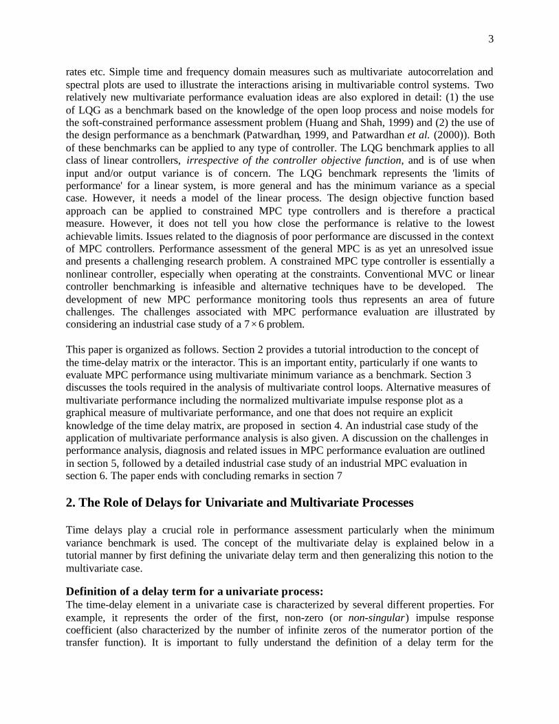
The increasing acceptance of the idea of process and performance monitoring has also grownfrom the awareness that control software, and therefore the applications that arise from it, shouldbe treated as capital assets and thus maintained, monitored and revisited routinely. Routinemonitoring of controller performance ensures optimal operation of regulatory control layers andthe higher level advanced process control (APC) applications. Model predictive control (MPC) iscurrently the main vehicle for implementing the higher level APC layer. The APC algorithmsinclude a class of model based controllers which compute future control actions by minimizing aperformance objective function over a finite prediction horizon. This family of controllers istruly multivariate in nature and has the ability to run the process close to its limits. It is for theabove reasons that MPC has been widely accepted by the process industry. Various commercialversions of MPC have become the norm in industry for processes where interactions are offoremost importance and constraints have to be taken into account. Most commercial MPCcontrollers also include a linear programming stage that deals with steady-state optimization andconstraint management. A schematic of a mature and advanced process control platform isshown in figure 1. It is important to note that the bottom regulatory layer consisting mainly ofPID loops forms the typical foundation of such a platform followed by the MPC layer. If thebottom layer does not perform and is not maintained regularly than it is futile to implementadvanced control. In the same vein, if the MPC layer does not perform then the benefits of thehigher level optimization layer, that may include real-time optimization, will not accrue.

The main contribution of this paper is in its generalization of the univariate impulse response(between the process output and the whitened disturbance variable) plot to the multivariate caseas the ‘Normalized Multivariate Impulse Response’ plot. A particular form of this plot, that doesnot require knowledge of the process time-delay matrix, is proposed here. Such a plot provides agraphical measure of the multivariate controller performance in terms of settling time, decay

Planning and Scheduling

Optimization

Model PredictiveControl

PID Loops

Days

Hours

Minutes

Seconds

Optimization

Model PredictiveControl

PID Loops

Subsystem 1 Subsystem 2

Figure 1. The Control Hierarchy

3

rates etc. Simple time and frequency domain measures such as multivariate autocorrelation andspectral plots are used to illustrate the interactions arising in multivariable control systems. Tworelatively new multivariate performance evaluation ideas are also explored in detail: (1) the useof LQG as a benchmark based on the knowledge of the open loop process and noise models forthe soft-constrained performance assessment problem (Huang and Shah, 1999) and (2) the use ofthe design performance as a benchmark (Patwardhan, 1999, and Patwardhan et al. (2000)). Bothof these benchmarks can be applied to any type of controller. The LQG benchmark applies to allclass of linear controllers, irrespective of the controller objective function, and is of use wheninput and/or output variance is of concern. The LQG benchmark represents the 'limits ofperformance' for a linear system, is more general and has the minimum variance as a specialcase. However, it needs a model of the linear process. The design objective function basedapproach can be applied to constrained MPC type controllers and is therefore a practicalmeasure. However, it does not tell you how close the performance is relative to the lowestachievable limits. Issues related to the diagnosis of poor performance are discussed in the contextof MPC controllers. Performance assessment of the general MPC is as yet an unresolved issueand presents a challenging research problem. A constrained MPC type controller is essentially anonlinear controller, especially when operating at the constraints. Conventional MVC or linearcontroller benchmarking is infeasible and alternative techniques have to be developed. Thedevelopment of new MPC performance monitoring tools thus represents an area of futurechallenges. The challenges associated with MPC performance evaluation are illustrated byconsidering an industrial case study of a 7× 6 problem.

This paper is organized as follows. Section 2 provides a tutorial introduction to the concept ofthe time-delay matrix or the interactor. This is an important entity, particularly if one wants toevaluate MPC performance using multivariate minimum variance as a benchmark. Section 3discusses the tools required in the analysis of multivariate control loops. Alternative measures ofmultivariate performance including the normalized multivariate impulse response plot as agraphical measure of multivariate performance, and one that does not require an explicitknowledge of the time delay matrix, are proposed in section 4. An industrial case study of theapplication of multivariate performance analysis is also given. A discussion on the challenges inperformance analysis, diagnosis and related issues in MPC performance evaluation are outlinedin section 5, followed by a detailed industrial case study of an industrial MPC evaluation insection 6. The paper ends with concluding remarks in section 7

2. The Role of Delays for Univariate and Multivariate Processes

Time delays play a crucial role in performance assessment particularly when the minimumvariance benchmark is used. The concept of the multivariate delay is explained below in atutorial manner by first defining the univariate delay term and then generalizing this notion to themultivariate case.

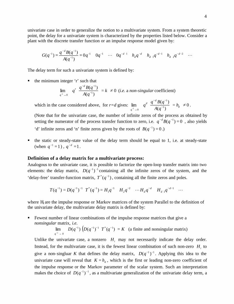
Definition of a delay term for a univariate process:The time-delay element in a univariate case is characterized by several different properties. Forexample, it represents the order of the first, non-zero (or non-singular) impulse responsecoefficient (also characterized by the number of infinite zeros of the numerator portion of thetransfer function). It is important to fully understand the definition of a delay term for the

4

univariate case in order to generalize the notion to a multivariate system. From a system theoreticpoint, the delay for a univariate system is characterized by the properties listed below. Consider aplant with the discrete transfer function or an impulse response model given by:

LL +++++++== −−+

−−+

−+−−−−

−−− 2

21

1111

1

11 000

)()(

)( dd

dd

dd

dd

qhqhqhqqqqA

qBqqG

The delay term for such a univariate system is defined by:

§ the minimum integer ‘r’ such that

0)(

)(lim 1

1

01≠=

−

−−

→−k

qAqBq

qd

r

q (i.e. a non-singular coefficient)

which in the case considered above, for r=d gives: 0)(

)(lim 1

1

01≠=

−

−−

→−d

dd

qh

qAqBq

q .

(Note that for the univariate case, the number of infinite zeros of the process as obtained bysetting the numerator of the process transfer function to zero, i.e. 0)( 1 =−− qBq d , also yields

‘d’ infinite zeros and ‘n’ finite zeros given by the roots of 0)( 1 =−qB .)

§ the static or steady-state value of the delay term should be equal to 1, i.e. at steady-state(when 11 =−q ) , 1=−dq .

Definition of a delay matrix for a multivariate process: Analogous to the univariate case, it is possible to factorize the open-loop transfer matrix into twoelements: the delay matrix, 11)( −−qD containing all the infinite zeros of the system, and the‘delay-free’ transfer-function matrix, )( 1* −qT , containing all the finite zeros and poles.

LL ++++=⋅= −−+

−−−−−−− 11

22

11

1*111 )()()( dd

dd qHqHqHqHqTqDqT

where Hi are the impulse response or Markov matrices of the system Parallel to the definition ofthe univariate delay, the multivariate delay matrix is defined by:

§ Fewest number of linear combinations of the impulse response matrices that give anonsingular matrix, i.e.

( ) KqTqDqDq

=⋅ −−−−

→−)()()(lim 1*111

01 (a finite and nonsingular matrix)

Unlike the univariate case, a nonzero iH may not necessarily indicate the delay order.Instead, for the multivariate case, it is the fewest linear combination of such non-zero iH to

give a non-singluar K that defines the delay matrix, 11 )( −−qD . Applying this idea to theunivariate case will reveal that dhK = , which is the first or leading non-zero coefficient ofthe impulse response or the Markov parameter of the scalar system. Such an interpretationmakes the choice of 11)( −−qD , as a multivariate generalization of the univariate delay term, a

5

very meaningful one. Note that det ( ( )) mD q cq= , where m is the number of infinite zeros ofthe system and c is a constant. For the multivariate case the number of infinite zeros may notbe related to the order ‘d’ of the time-delay matrix.

§ IqDqDT =− )()( 1 (As compared to the univariate case where 1=− qq d ). This is known as theunitary interactor matrix. This unitary property preserves the spectrum of the signal, whichleads us to the result that the variance of the actual output and the interactor filtered outputsare the same, i.e. )

~~()( t

Ttt

Tt YYEYYE = , where d

t tY q DY−=% (see Huang and Shah (1999)).

Example:Consider the following transfer function matrix and its impulse response or Markov parametermodel:

L+

+

+

+

=

−−

−−= −−−−

−

−

−

−

−

−

−

−

− 4321

1

3

1

2

1

3

1

2

1

25.0109.05.01

133.11

0101

0000

4131

211)( qqqq

qq

qq

qq

qq

qT

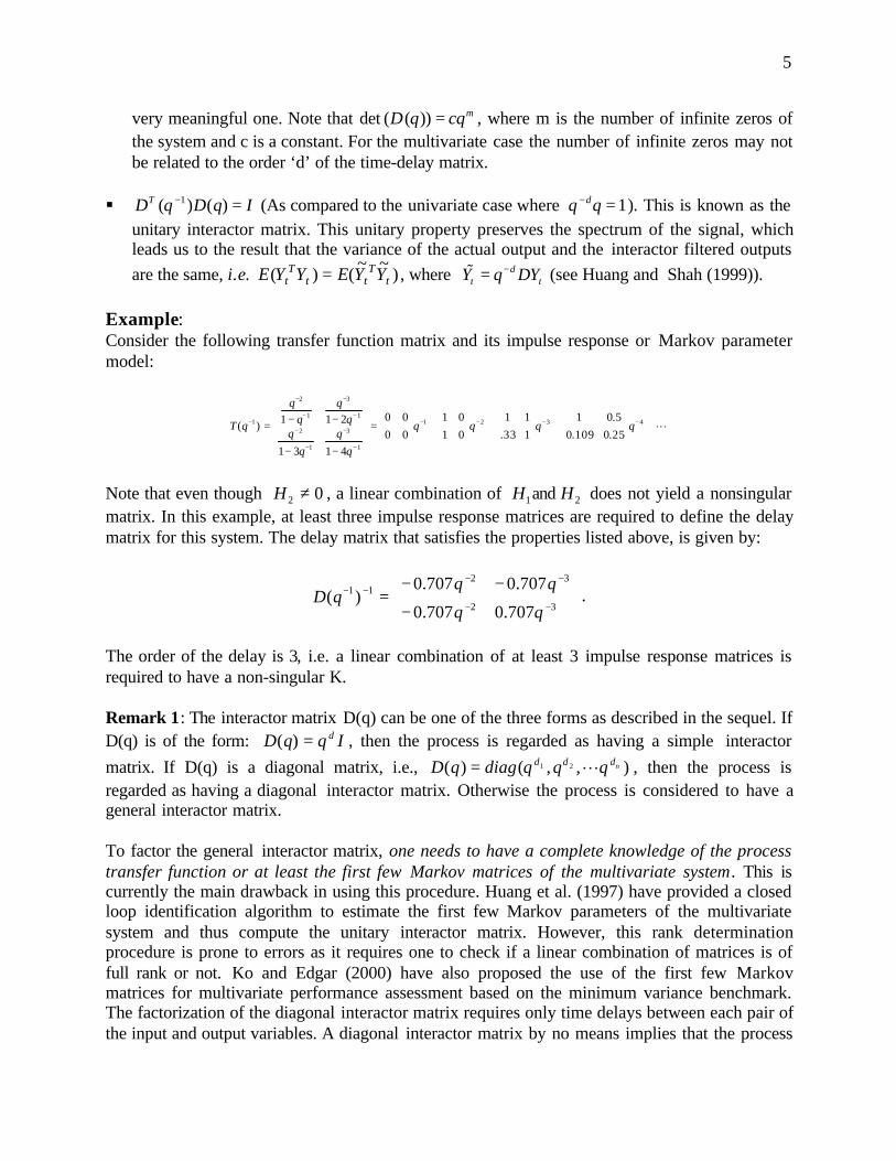
Note that even though 02 ≠H , a linear combination of 1H and 2H does not yield a nonsingularmatrix. In this example, at least three impulse response matrices are required to define the delaymatrix for this system. The delay matrix that satisfies the properties listed above, is given by:

−

−−=

−−

−−−−

32

3211

707.0707.0

707.0707.0)(

qq

qqqD .

The order of the delay is 3, i.e. a linear combination of at least 3 impulse response matrices isrequired to have a non-singular K.

Remark 1: The interactor matrix D(q) can be one of the three forms as described in the sequel. IfD(q) is of the form: D q q Id( ) = , then the process is regarded as having a simple interactormatrix. If D(q) is a diagonal matrix, i.e., D q diag q q qd d dn( ) ( , , )= 1 2 L , then the process isregarded as having a diagonal interactor matrix. Otherwise the process is considered to have ageneral interactor matrix.

To factor the general interactor matrix, one needs to have a complete knowledge of the processtransfer function or at least the first few Markov matrices of the multivariate system. This iscurrently the main drawback in using this procedure. Huang et al. (1997) have provided a closedloop identification algorithm to estimate the first few Markov parameters of the multivariatesystem and thus compute the unitary interactor matrix. However, this rank determinationprocedure is prone to errors as it requires one to check if a linear combination of matrices is offull rank or not. Ko and Edgar (2000) have also proposed the use of the first few Markovmatrices for multivariate performance assessment based on the minimum variance benchmark.The factorization of the diagonal interactor matrix requires only time delays between each pair ofthe input and output variables. A diagonal interactor matrix by no means implies that the process

6

has a diagonal transfer function matrix or that the process has no interaction. But the converse istrue, i.e. a diagonal process transfer function matrix or a system with weakly interactingmultivariate loops (a diagonally dominant system) does have a diagonal interactor matrix. Infact, experience has shown that many actual multivariable processes have the structure of thediagonal interactor, provided the input-output structuring has been done with proper engineeringinsight. This fact greatly simplifies performance assessment of the multivariate system.

3. The multivariate Minimum Variance Benchmark

In a univariate system, the first ‘d’ impulse response coefficients of the closed loop transferfunction between the control error and the white noise disturbance term determine the minimumvariance or the lowest achievable performance. In the same way, the first ‘d’ impulse responsematrices of the closed loop multivariate system are useful in determining the multivariate

minimum variance benchmark, where ‘d’ denotes the order of the interactor.

Performance assessment of univariate control loops is carried out, by comparing the actualoutput variance with the minimum achievable variance. The latter term is estimated by simpletime series analysis of routine closed-loop operating data and knowledge of the process timedelay. The estimation of the univariate minimum variance benchmark requires filtering andcorrelation analysis. This idea has been extended to multivariate control loop performanceassessment and the multivariate filtering and correlation (FCOR) analysis algorithm has beendeveloped as a natural extension of the univariate case, (Huang et. al., 1996, 1997, 1999). Harriset al. (1996) have also proposed a multivariate extension to their univariate performanceassessment algorithm. Their extension requires a spectral factorization routine to compute the

a a

at

Y

at

controllercontroller processprocess-

disturbancedisturbance

Steps:1) time series analysis2) correlation3) obtain η

)ˆ~( ttaYcorr

)ˆ~( 1−ttaYcorr

)ˆ~( 1+−dttaYcorr

q −1

q −1

)1(ˆ~ −daYρ

)1(ˆ

~aYρ

)0(ˆ~aYρ

Inne

r Pr

oduc

t

η

time series analysistime series analysis

Interactor FilterInteractor Filter tY~

sptY

Figure 2: Schematic diagram of the multivariate FCOR algorithm

7

delay free part of the multivariate process and thus estimate the multivariate minimum varianceor the lowest achievable variance for the process. The FCOR algortihm of Huang et al. (1996),on the other hand, is a term for term generalization of the univariate case to the multivariate caseand also requires the knowledge of the multivariate time-delay or interactor matrix. Figure 2summarizes the steps required in computing the mutivariate performance index. A quadraticmeasure of multivariate control loop performance is defined as:

J E Y Y Y Yt tsp T

t tsp= − −( ) ( )

(where Yt represnts an ‘n’ dimensional output vector).The lower bound or the quadratic measureof the multivariate control performance under minimum variance control is defined as

J E Y Y Y Yt tsp T

t tsp

mvmin ( ) ( )|= − − .

It has been shown by Huang et al.(1997) that the lower bound of the performance measure Jmin

can be estimated from routine operating data. In Huang et al. (1997), the multivariateperformance index is defined as

η =J

Jmin

and is bounded by 0 1≤ ≤η . In practice, one may also be interested in knowing how eachindividual output (loop) of the multivariate system performs relative to multivariate minimumvariance control. Performance indices of each individual output are defined as

η

η

σ σ

σ σ

y

y

y y

y y

mv Y

n n n

diag1 1 1

2 2

2 2

1M M

=

= −

min( ) /

min( ) /(~ ~ )Σ Σ

where ~ ( )Σ Σmv mvdiag= and ~ ( )Σ ΣY Ydiag= ; Σ Y is the variance matrix of the output Yt andΣ Σmv Y= min( ) is the covariance matrix of the output Yt under multivariate minimum variancecontrol. It has been shown by Huang et al. (1997) that Σ mv can also be estimated using routineoperating data, and knowledge of the interactor matrix.

To summarize, a multivariate performance index is a single scalar measure of multivariatecontrol loop performance relative to multivariate minimum variance control. Individual outputperformance indices indicate performance of each output relative to the loop’s performanceunder multivariate minimum variance control. If a particular output index is smaller than otheroutput indices, then some of the other loops may have to be de-tuned in order to improve thispoorly tuned loop.

8

4. Alternative Methods for Performance Analysis of Multivariate ControlSystems

4.1 Autocorrelation Function:

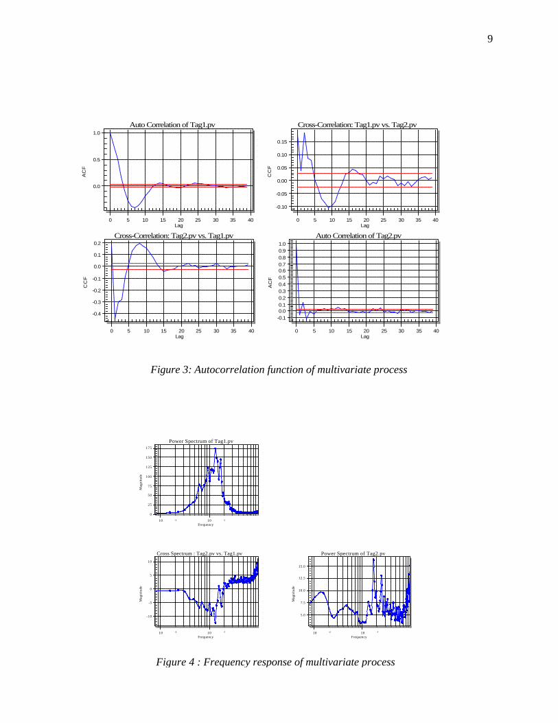
The autocorrelation function (ACF) plots may be used to analyze individual process variableperformance. A typical example of the ACF plots for the two output variables of the simulatedWood-Berry (Wood and Berry, 1973) column control system is shown in Fig. 3. A decentralizedcontrol system comprising two PI controllers was used on the Wood-Berry column. The diagonalplots are autocorrelations of each output variable, while the off-diagonal plots are cross-correlation plots. The diagonal plots typically indicate how well each loop is tuned. For example,a slowly decaying autocorrelation function implies an under-tuned loop, and an oscillatory ACFtypically implies an over-tuned loop. Off-diagonal plots can be used to trace the source ofdisturbance or the interaction between each process variables. Figure 3 clearly indicates that thefirst loop has relatively poor performance while the second loop has very fast decay dynamicsand thus good performance. Interaction between the two loops can also observed from the off-diagonal subplots. Note that the autocorrelation plot of the multivariate system is not necessarilysymmetric.

4.2 Spectral Analysis:

Frequency domain plots provide alternative indicators of control loop performance. They may beused to assess individual output dynamic behavior, interactions and effects of disturbances. Forexample, peaks in the diagonal plots typically imply oscillation of the variables due to an over-tuned controller or presence of oscillatory disturbances. Frequency domain plots also provideinformation on the frequency ranges over which the oscillations occur and the amplitude of theoscillations. Like time domain analysis, off-diagonal plots provide one with information on thecorrelation or interaction between the loops. Fig. 4 is the power spectrum and the cross-powerspectrum plot of the simulated Wood-Berry column. The first diagonal plot indicates that there isa clear mid-frequency harmonic in the 1st output. This could be due to an overtuned controller.Off-diagonal plots show a peak in the cross-spectrum at the same frequency. The poorperformance of loop 1 can then be attributed to significant interaction effects from loop 2 to loop1. In other words, the satisfactory or good performance of loop 2 could be at the expense oftransmitting disturbances or upsets to loop 1 via the interaction term.. The power spectrum plotsof a multivariate system are symmetric.

4.3 Normalized Multivariate Impulse Response (NMIR) Curve as analternative measure of performance:

As shown in figure 2, the evaluation of the multivariate controller performance has to beundertaken on the interactor filtered output and not on the actual output. The reason for this isthat the interactor filtered output vector, t

dt YDqY −=

~, is a special linear combination of the

actual output, lagged or otherwise, and this fictitious output preserves the spectral property ofthe system and facilitates simpler analysis of the multivariate minimum variance benchmark.

9

Figure 3: Autocorrelation function of multivariate process

0.0

0.5

1.0

0 5 10 15 20 25 30 35 40

Auto Correlation of Tag1.pv

AC

F

Lag

-0.10

-0.05

0.00

0.05

0.10

0.15

0 5 10 15 20 25 30 35 40

Cross-Correlation: Tag1.pv vs. Tag2.pv

CC

F

Lag

-0.4

-0.3

-0.2

-0.1

0.0

0.1

0.2

0 5 10 15 20 25 30 35 40

Cross-Correlation: Tag2.pv vs. Tag1.pv

CC

F

Lag

-0.10.00.10.20.30.40.50.60.70.80.91.0

0 5 10 15 20 25 30 35 40

Auto Correlation of Tag2.pv

AC

F

Lag

0

25

50

75

100

125

150

175

10 -2 10 -1

Power Spectrum of Tag1.pv

Mag

nitu

de

Frequency

-10

-5

0

5

10

10 -2 10 -1

Cross Spectrum : Tag2.pv vs. Tag1.pv

Mag

nitu

de

Frequency

5.0

7.5

10.0

12.5

15.0

10 -2 10 -1

Power Spectrum of Tag2.pv

Mag

nitu

de

Frequency

Figure 4 : Frequency response of multivariate process

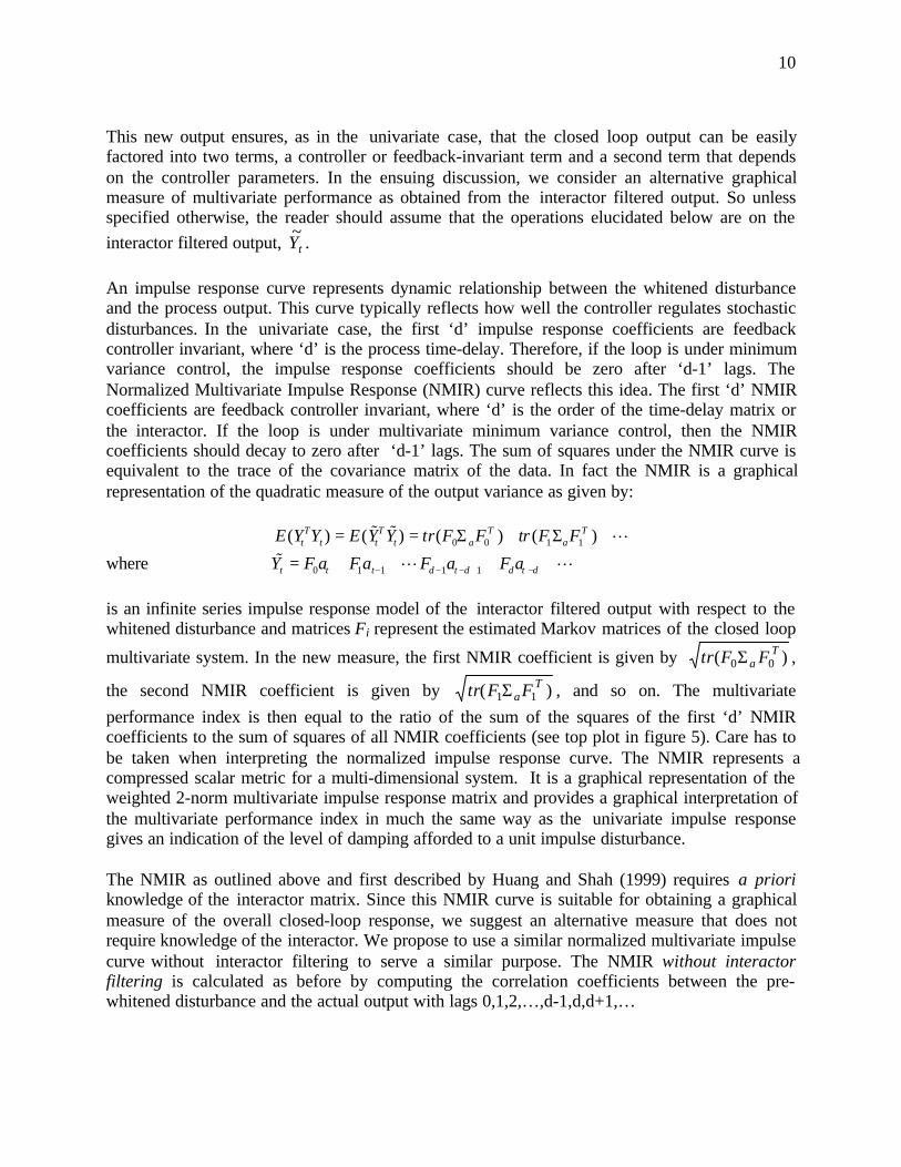
10

This new output ensures, as in the univariate case, that the closed loop output can be easilyfactored into two terms, a controller or feedback-invariant term and a second term that dependson the controller parameters. In the ensuing discussion, we consider an alternative graphicalmeasure of multivariate performance as obtained from the interactor filtered output. So unlessspecified otherwise, the reader should assume that the operations elucidated below are on theinteractor filtered output, tY

~.

An impulse response curve represents dynamic relationship between the whitened disturbanceand the process output. This curve typically reflects how well the controller regulates stochasticdisturbances. In the univariate case, the first ‘d’ impulse response coefficients are feedbackcontroller invariant, where ‘d’ is the process time-delay. Therefore, if the loop is under minimumvariance control, the impulse response coefficients should be zero after ‘d-1’ lags. TheNormalized Multivariate Impulse Response (NMIR) curve reflects this idea. The first ‘d’ NMIRcoefficients are feedback controller invariant, where ‘d’ is the order of the time-delay matrix orthe interactor. If the loop is under multivariate minimum variance control, then the NMIRcoefficients should decay to zero after ‘d-1’ lags. The sum of squares under the NMIR curve isequivalent to the trace of the covariance matrix of the data. In fact the NMIR is a graphicalrepresentation of the quadratic measure of the output variance as given by:

0 0 1 1( ) ( ) ( ) ( )T T T Tt t t t a aE Y Y E Y Y tr F F tr F F= = Σ + Σ +% % L

where 0 1 1 1 1t t t d t d d t dY F a F a F a F a− − − + −= + + + +% L L

is an infinite series impulse response model of the interactor filtered output with respect to thewhitened disturbance and matrices Fi represent the estimated Markov matrices of the closed loop

multivariate system. In the new measure, the first NMIR coefficient is given by )( 00T

a FFtr Σ ,

the second NMIR coefficient is given by )( 11T

aFFtr Σ , and so on. The multivariateperformance index is then equal to the ratio of the sum of the squares of the first ‘d’ NMIRcoefficients to the sum of squares of all NMIR coefficients (see top plot in figure 5). Care has tobe taken when interpreting the normalized impulse response curve. The NMIR represents acompressed scalar metric for a multi-dimensional system. It is a graphical representation of theweighted 2-norm multivariate impulse response matrix and provides a graphical interpretation ofthe multivariate performance index in much the same way as the univariate impulse responsegives an indication of the level of damping afforded to a unit impulse disturbance.

The NMIR as outlined above and first described by Huang and Shah (1999) requires a prioriknowledge of the interactor matrix. Since this NMIR curve is suitable for obtaining a graphicalmeasure of the overall closed-loop response, we suggest an alternative measure that does notrequire knowledge of the interactor. We propose to use a similar normalized multivariate impulsecurve without interactor filtering to serve a similar purpose. The NMIR without interactorfiltering is calculated as before by computing the correlation coefficients between the pre-whitened disturbance and the actual output with lags 0,1,2,…,d-1,d,d+1,…

11

L+Σ+Σ= )()()( 1100T

aT

tT

t EEtrEEtrYYEwhere LL ++++= −+−−− dtddtdttt aEaEaEaEY 11110

Note that unlike the original NMIR measure as proposed by Huang and Shah (1999), the newmeasure proposed here does not require interactor filtering of the output, i.e. an explicitknowledge of the interactor is not required in computing the new graphical and qualitativemeasure. From here onwards this new measure is denoted as NMIRwof.

In the new measure, the first NMIRwof coefficient is given by )( 00T

a EEtr Σ , the second

NMIRwofcoefficient is given by )( 11T

a EEtr Σ , and so on. Note that the NMIRwof measure(without interactor filtering) is similar to NMIR with interactor filtering in the sense that bothrepresent the closed-loop infinite series impulse response model of the output with respect to thewhitened disturbance, one for the actual output and the other one for the interactor filtered outputrespectively. The newly proposed NMIRwof is physically interpretable, but does not have theproperty that the first d coefficients are feedback control-invariant. The main rationale for usingthe newly proposed NMIRwof is that the following two terms are asymptotically equal:

{ }

Σ+

+Σ+Σ=Σ++Σ+Σ

∞→ )(

)()()()()( 1100

1100 Tnan

Ta

TaT

nanT

aT

an FFtr

FFtrFFtrEEtrEEtrEEtrLimit

LL

This follows from the equality: )~~

()( tT

ttT

t YYEYYE = (Huang and Shah, 1999). It is then clearthat the NMIR curves with and without filtering will coincide with each other for ‘n’ sufficientlylarge. Alternately, the cumulative sum of the square of the impulse response coefficients can alsobe plotted and as per the above asymptotic equality, one would expect that the two terms willcoincide for a sufficiently large ‘n’. These curves are reproduced here for the illustrative Wood-Berry column example. The ordinate in the bottom plot in figure 5 gives the actual outputvariance when the curves converge for a sufficiently large n. Note that, unlike the NMIR curvewith interactor filtering (solid line in figure 5), the NMIRwof curve (dashed line in figure 5) cannot be used to calculate a numerical value of the performance index. However, it has thefollowing important properties that are useful for assessment of multivariate processes:1. The new NMIRwof represents the normalized impulse response from the white noise to the

true output.2. The new NMIRwof curve reflects the predictability of the disturbance in the original output. If

the impulse response decays slowly, then this is clear indication of a highly predictabledisturbance (e.g. an integrated white noise type disturbance) and relatively poor control. Onthe other hand a fast decaying impulse response is a clear graphical indication of a well-tunedmultivariate system (Thornhill et al., 1999).

3. The new NMIRwof also provides a graphical measure of the overall multivariate systemperformance with information regarding settling time, oscillation, speed of response etc.

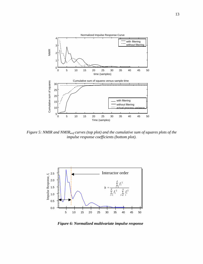
NMIRs with and without interactor filtering are calculated for the simulated Wood-Berrydistillation column with two multiloop PI controllers. With sampling period 0.5 second, theinteractor matrix of the process is found to have a diagonal structure and is given by

12

3

7

0( )

0q

D qq

=

Since the order of the interactor is 7 sample unit, the first 7 NMIR coefficients are feedbackcontrol invariant and depend solely on the disturbance dynamics and the interactor matrix. Thesum of squares of these 7 coefficients is the variance achieved under multivariate minimumvariance control. In fact as shown in figure 6, the scalar multivariate measure of performance isequal to the sum of squares of the first 7 NMIR coefficients divided by the total sum of squares.Notice that for sufficiently large ‘n’ or prediction horizon, the two curves, as expected, coincidewith each other. In this simulation example, observe that the NMIR and the NMIRwof curvesdecay to zero relatively quickly after 7 sample units, indicating relatively good controlperformance.

4.3.1 Industrial MIMO Case study 1: Capacitance Drum Control Loops at SyncrudeCanada Ltd.

Capacitance drum control loops of Plant AB in Syncrude Canada Ltd. were analyzed for thisstudy. The primary objective of Plant AB is to further reduce the water in the (Plant A) dilutedbitumen product prior to it reaching the next plant (Plant B) storage tanks. As the grade of thefeed entering plant A reduces, the water required to process the oilsands increasesproportionately. A large portion of this excess water ends up in the Plant A froth feed tank andultimately increases the % volume of water in the Plant A product. Aside from degrading thequality of the product, the increased volume of water means reduction in the amount of bitumenthat can be piped to the diluted bitumen tanks. In addition, the higher water content means moreof the chloride compound present in the oilsands is dissolved and finds its way to the dilutedbitumen tanks and eventually to plant B. The higher chloride concentration increases thecorrosion rate of equipment in the Upgrading units. Plant AB was developed as a means ofreducing the water content, and ultimately, the chlorides sent to Upgrading. This reduction isachieved by centrifuging the Plant A Product.All product from plant A is directed to the Plant AB feed storage tank. The IPS portion of theproduct is routed through 5 Cuno Filters prior to entering the Plant AB feed storage tank. Feedfrom the feed storage tank is then pumped through the feed pumps to the Alfa Laval centrifuges.The Alfa Laval centrifuges remove water and a small amount of solids from the feed. Eachcentrifuge has its own capacitance drum and product back pressure valve. This arrangementallows for individual centrifuge “E-Line” control and a greatly improved product quality. Heavyphase water from plant A is used as Process Water in plant AB.The cap drum pressure controller controls the capacitance drum pressure by adjusting thenitrogen flow into the drum. The Cap Drum Primary level controller maintains the cap drumwater level by adjusting water addition into the drum. Control of these two variables is essentialto maintain the E-Line in the centrifuges. Currently these two loops are controlled by multiloopPID controllers. The two process variables, pressure and level, are highly interacting. Theobjective of the performance assessment is to evaluate the existing multiloop PID controllers’performance, and to identify opportunities, if any, to improve performance by implementing amultivariate controller

13

Figure 5: NMIR and NMIRwof curves (top plot) and the cumulative sum of squares plots of theimpulse response coefficients (bottom plot).

0 5 10 15 20 25 30 35 40 45 500

1

2

3

4

time (samples)

NM

IR

Normalized Impulse Response Curve

with filteringwithout filtering

0 5 10 15 20 25 30 35 40 45 505

10

15

20

25

30

Time (samples)

Cum

ulat

ive

sum

of s

quar

es Cumulative sum of squares versus sample time

with filtering

actual process variancewithout filtering

Figure 6: Normalized multivariate impulse response

0.0

0.5

1.0

1.5

2.0

2.5

Impu

lse

Res

pons

e, f i

Lag

5 10 15 20 25 30 35 40 45 50

∑+∑

∑= ∞

+==

=

1

2

1

2

1

2

dii

d

ii

d

ii

ff

fη

Interactor order

14

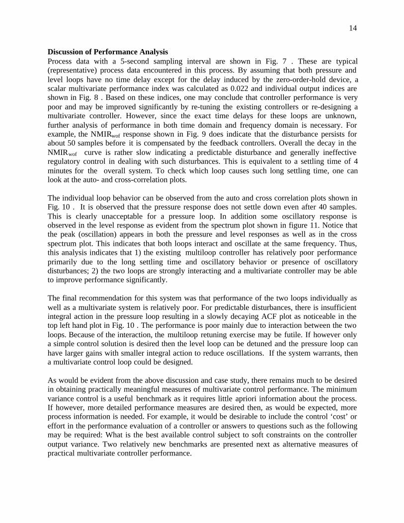
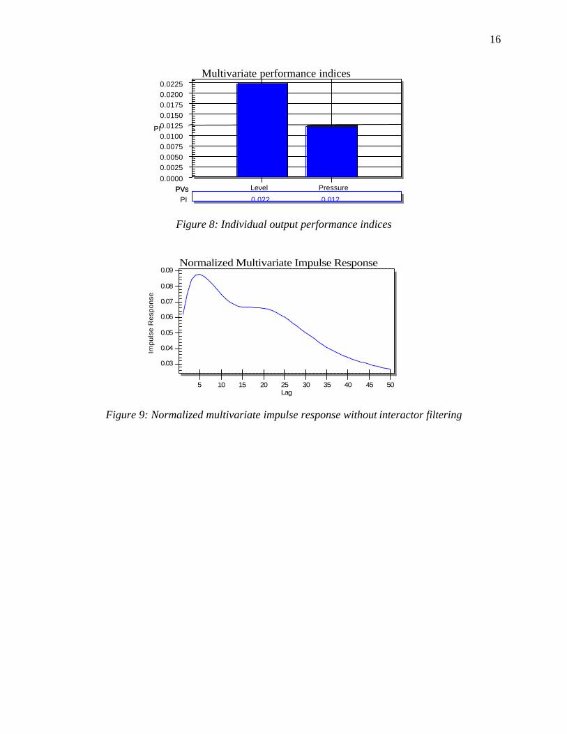
Discussion of Performance AnalysisProcess data with a 5-second sampling interval are shown in Fig. 7 . These are typical(representative) process data encountered in this process. By assuming that both pressure andlevel loops have no time delay except for the delay induced by the zero-order-hold device, ascalar multivariate performance index was calculated as 0.022 and individual output indices areshown in Fig. 8 . Based on these indices, one may conclude that controller performance is verypoor and may be improved significantly by re-tuning the existing controllers or re-designing amultivariate controller. However, since the exact time delays for these loops are unknown,further analysis of performance in both time domain and frequency domain is necessary. Forexample, the NMIRwof response shown in Fig. 9 does indicate that the disturbance persists forabout 50 samples before it is compensated by the feedback controllers. Overall the decay in theNMIRwof curve is rather slow indicating a predictable disturbance and generally ineffectiveregulatory control in dealing with such disturbances. This is equivalent to a settling time of 4minutes for the overall system. To check which loop causes such long settling time, one canlook at the auto- and cross-correlation plots.

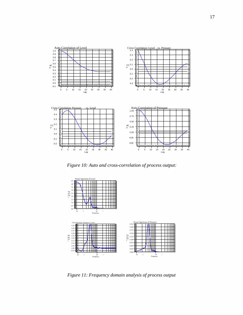
The individual loop behavior can be observed from the auto and cross correlation plots shown inFig. 10 . It is observed that the pressure response does not settle down even after 40 samples.This is clearly unacceptable for a pressure loop. In addition some oscillatory response isobserved in the level response as evident from the spectrum plot shown in figure 11. Notice thatthe peak (oscillation) appears in both the pressure and level responses as well as in the crossspectrum plot. This indicates that both loops interact and oscillate at the same frequency. Thus,this analysis indicates that 1) the existing multiloop controller has relatively poor performanceprimarily due to the long settling time and oscillatory behavior or presence of oscillatorydisturbances; 2) the two loops are strongly interacting and a multivariate controller may be ableto improve performance significantly.

The final recommendation for this system was that performance of the two loops individually aswell as a multivariate system is relatively poor. For predictable disturbances, there is insufficientintegral action in the pressure loop resulting in a slowly decaying ACF plot as noticeable in thetop left hand plot in Fig. 10 . The performance is poor mainly due to interaction between the twoloops. Because of the interaction, the multiloop retuning exercise may be futile. If however onlya simple control solution is desired then the level loop can be detuned and the pressure loop canhave larger gains with smaller integral action to reduce oscillations. If the system warrants, thena multivariate control loop could be designed.

As would be evident from the above discussion and case study, there remains much to be desiredin obtaining practically meaningful measures of multivariate control performance. The minimumvariance control is a useful benchmark as it requires little apriori information about the process.If however, more detailed performance measures are desired then, as would be expected, moreprocess information is needed. For example, it would be desirable to include the control ‘cost’ oreffort in the performance evaluation of a controller or answers to questions such as the followingmay be required: What is the best available control subject to soft constraints on the controlleroutput variance. Two relatively new benchmarks are presented next as alternative measures ofpractical multivariate controller performance.

15

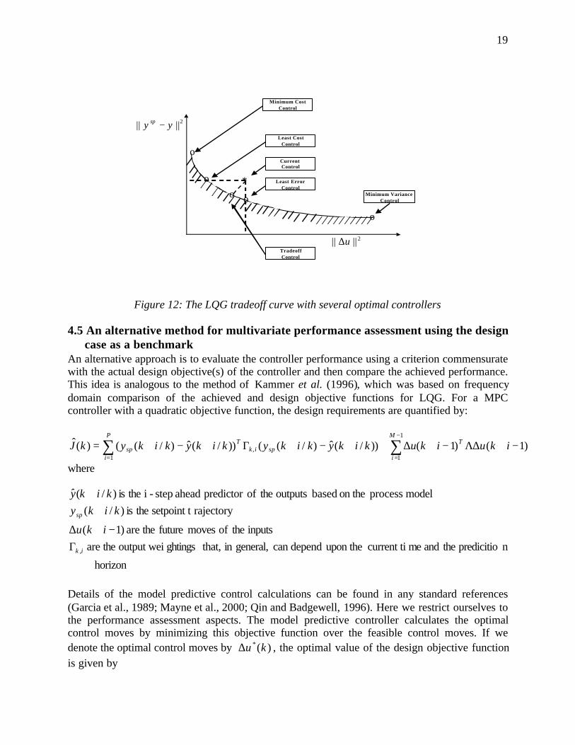
4.4 LQG benchmarkingPreliminary results on the LQG benchmark as an alternative to the minimum variancebenchmark were proposed in Huang and Shah (1999). These results are reviewed here and a newbenchmark that takes the control cost into account is proposed. The main advantage of theminimum variance benchmark is that other than the time-delay, it requires little processinformation. On the other hand if one requires more information on controller performance suchas how much can the output variance be reduced without significantly affecting the controlleroutput variance then one needs more information on the process. In short it is useful to have abenchmark that explicitly takes the control cost into account. The LQG cost function is one suchbenchmark. This benchmark does not require that an LQG controller be implemented for thegiven process. Rather the benchmark provides the 'limit of performance' for any linear controllerin terms of the input and output variance. As remarked earlier, it is a general benchmark with theminimum variance as a special case. The only disadvantage is that the computation of theperformance limit curve as shown in figure 12 requires knowledge of the process model. ForMPC type controllers these models may be readily available. Furthermore the benchmark cannothandle hard constraints, but it can be used to compare the performance of unconstrained andconstrained controllers (see figure 13).

In general, tighter quality specifications lead to smaller variations in the process output, buttypically require more control effort. Consequently one may be interested in knowing how faraway the control performance is from the "best" achievable performance with the same effort,i.e., in mathematical form the resolution of the following problem may be of interest:

Given that α≤)( 2uE , what is the lowest achievable )( 2yE ?

The solution is given by a tradeoff curve as shown in Fig. 12. This curve can be obtained bysolving the LQG problem (Kwakernaak and Sivan (1972)), where the LQG objective function isdefined by:

)()()( 22 uEyEJ λλ +=

120

125

130

135

140

117.5

120.0

122.5

125.0

127.5

Value

RightYAxis

Sample429 572 715 858 1001 1144 1287 1430 1573 1716 1859

Level Pressure

Figure 7: Pressure and level data with sampling interval 5 seconds

16

0.0000

0.00250.00500.00750.01000.01250.01500.01750.02000.0225

Multivariate performance indices

PI

PVs Level PressurePVsPI 0.022 0.012

Figure 8: Individual output performance indices

Figure 9: Normalized multivariate impulse response without interactor filtering

0.03

0.04

0.05

0.06

0.07

0.08

0.09 Normalized Multivariate Impulse Response

Impu

lse

Res

pons

e

Lag5 10 15 20 25 30 35 40 45 50

17

-0.1

0.0

0.10.2

0.3

0.4

0.5

0.6

0.70.8

0.9

1.0

0 5 10 15 20 25 30 35 40

Auto Correlation of Level

ACF

Lag

-0.2

-0.1

0.0

0.1

0.2

0.3

0.4

0.5

0 5 10 15 20 25 30 35 40

Cross-Correlation: Pressure . vs. Level

CCF

Lag

-0.50

-0.25

0.00

0.25

0.50

0.75

1.00

0 5 10 15 20 25 30 35 40

Auto Correlation of Pressure

ACF

Lag

-0.3

-0.2

-0.1

0.0

0.1

0.2

0.3

0.4

0 5 10 15 20 25 30 35 40

Cross-Correlation: Level . vs. Pressure

CCF

Lag

Figure 10: Auto and cross-correlation of process output:

0.0

0.5

1.0

1.5

2.0

2.5

3.0

3.5

4.0

4.5

10 -2 10 -1

Power Spectrum of Level

Magnitude

Frequency

-0.050.000.05

0.100.15

0.200.250.30

0.350.40

0.45

10 -2 10 -1

Cross Spectrum : Pressure vs. Level

Magnitude

Frequency

0.000

0.025

0.050

0.075

0.100

0.125

0.150

0.175

0.200

0.225

10 - 2 10 - 1

Power Spectrum of Pressure

Magnitude

Frequency

Figure 11: Frequency domain analysis of process output

18

By varying λ , various optimal solutions of E( )2y and E( )2u can be calculated. Thus a curvewith the optimal output variance as ordinate, and as the incremental manipulative variablevariance as the abscissa can be plotted from these calculations. Boyd and Barratt (1991) haveshown that any linear controller can only operate in the region above this curve. In this respectthis curve defines the limit of performance of all linear controllers, as applied to a linear time-invariant process, including the minimum variance control law. If the process is modelled as anARIMAX process then the resulting LQG benchmark curve due to the optimal controller willhave an integrator built into it to asymptotically track and reject step type setpoints anddisturbances respectively. Five optimal controllers may be identified from the tradeoff curveshown in Fig. 12. They are explained as follows:

• Minimum cost control: This is an optimal controller identified at the left end of the tradeoffcurve. The minimum cost controller is optimal in the sense that it offers an offset-free controlperformance with the minimum possible control effort. It is worthwhile pointing out that thiscontroller is different from the open-loop mode since an integral action is guaranteed to existin this controller.

• Least cost control: This optimal controller offers the same output error as the current orexisting controller but with the least control effort. So if the output variance is acceptable butactuator variance has to be reduced then this represents the lowest achievable manipulativeaction variance for the given output variance.

• Least error control: This optimal controller offers least output error for the same controleffort as the existing controller. If the input variance is acceptable but the output variance hasto be reduced then this represents the lowest achievable output variance for the given inputvariance.

• Tradeoff controller: This optimal controller can be identified by drawing the shortest line tothe tradeoff curve from the existing controller; the intersection is the tradeoff control.Clearly, this tradeoff controller has performance between the least cost control and the leasterror control. It offers a tradeoff between reductions of the output error and the control effort.

• Minimum error (variance) control: This is an optimal controller identified at the right end ofthe tradeoff curve. The minimum error controller is optimal in the sense that it offers theminimum possible error. Note that this controller may be different from the traditionalminimum variance controller due to the existence of integral action.

The challenges with respect to the LQG benchmark lie in the estimation of a reasonably accurateprocess model. The uncertainty in the estimated model then has to be 'mapped' onto the LQGcurve, in which case it would become a fuzzy trade-off curve. Alternately the uncertainty regioncan be mapped into a region around the current performance of the controller relative to the LQGcurve (see Patwardhan and Shah, 2000).

19

*o

o

o

o

Minimum Variance Control

Least Error Control

Current Control

Least CostControl

TradeoffControl

o

Minimum CostControl

2|||| yy sp −

2|||| u∆

Figure 12: The LQG tradeoff curve with several optimal controllers

4.5 An alternative method for multivariate performance assessment using the designcase as a benchmark

An alternative approach is to evaluate the controller performance using a criterion commensuratewith the actual design objective(s) of the controller and then compare the achieved performance.This idea is analogous to the method of Kammer et al. (1996), which was based on frequencydomain comparison of the achieved and design objective functions for LQG. For a MPCcontroller with a quadratic objective function, the design requirements are quantified by:

∑∑−

==

−+Λ∆−+∆++−+Γ+−+=1

11, )1()1())/(ˆ)/(())/(ˆ)/(()(ˆ

M

i

TP

ispik

Tsp ikuikukikykikykikykikykJ

where

horizon

npredicitio theand mecurrent ti upon the dependcan general,in that,ghtingsoutput wei theare inputs theof moves future theare )1(

rajectorysetpoint t theis )/(model process on the based outputs theofpredictor ahead step-i theis )/(ˆ

,ik

sp

iku

kikykiky

Γ−+∆

++

Details of the model predictive control calculations can be found in any standard references(Garcia et al., 1989; Mayne et al., 2000; Qin and Badgewell, 1996). Here we restrict ourselves tothe performance assessment aspects. The model predictive controller calculates the optimalcontrol moves by minimizing this objective function over the feasible control moves. If wedenote the optimal control moves by )(ku ∗∆ , the optimal value of the design objective functionis given by

20

))((ˆ)(ˆ kuJkJ ∗∗ ∆=

The actual output may differ significantly from the predicted output due to inadequacy of themodel structure, nonlinearities, modeling uncertainty etc. Thus the achieved objective function isgiven by:

∑∑−

==

−+Λ∆−+∆++−+Γ+−+=1

11, )1()1())/()/(())/()/(()(ˆ

M

i

TP

ispik

Tsp ikuikukikykikykikykikykJ

where )()( kuandky ∆ denote the measured values of the outputs and inputs at correspondingsampling instants appropriately vectorized. The inputs will differ from the design value in partdue to the receding horizon nature of the MPC control law. The value of the achieved objectivefunction cannot be known a priori, but only p sampling instants later. A simple measure ofperformance can then be obtained by taking a ratio of the design and the achieved objectivefunctions as:

)()(ˆ

)(kJkJ

k∗

=η

This performance index will be equal to one when the achieved performance meets the designrequirements. The advantage of using the design criterion for the purpose of performanceassessment is that it is a measure of the deviation of the controller performance from theexpected or design performance. Thus a low performance index truly indicates changes in theprocess or the presence of disturbances, resulting in sub-optimal control. The estimation of suchan index does not involve any time series analysis or identification. The design objective iscalculated by the controller at every instant and only the measured input and output data isneeded to find the achieved performance. The above performance measure represents aninstantaneous measure of performance and can be driven by the unmeasured disturbances. Inorder to get a better overall picture the following measure is recommended:

∑

∑

=

=

∗

=k

i

k

i

iJ

iJk

1

1

)(

)(ˆ

)(α

)(kα is the ratio of the average design performance to the average achieved performance up tothe current sampling instant. Thus 1)( =kα implies that the design performance is being achievedon an average. 1)( <kα means that the achieved performance is worse than the design. Thisalternative metric of multivariate controller performance has been applied towards the evaluationof a QDMC and another MPC controller. Further details on the evaluation of this algorithm canbe found in Patwardhan (1999).

The motivation for a lumped performance index is that the MPC controllers in the dynamicsense, attempt to minimize a lumped performance objective. The lumped objective function andsubsequently the performance index, therefore does reflect the true intentions of the controller.

21

The motivation for this idea was to have a performance statistic for MPC that is commensuratewith its constrained and time-varying nature. The idea of comparing design with achievedperformance has been common place in the area of control relevant identification (also known asiterative identification and control, identification for control)–see the survey by Van Den Hofand Schrama (1995). Performance degradation is measured as a deviation from designperformance and becomes the motivation for re-design/re-identification.

4.5.1 Simulation example: A Mixing ProcessThe above approach was applied to a simulation example. The system under consideration is a2x2 mixing process. The controlled variables are temperature (y1) and water level (y2) and themanipulated inputs are inlet hot water (u1) and inlet cold water (u2) flow rates. The followingmodel is available in discrete form,

=

−

−

−

−

−

−

−

−

−−

−−

−−

1

1

1

1

1

1

1

1

9827.012839.0

9827.012043.0

8607.011602.0

8607.01025.0

1)(z

zz

zzz

zz

zP

A MPC controller was used to control this process in the presence of unmeasured disturbances.The controller design parameters were:

])2,1([]),4,1([,2,10 diagdiagmp =Γ=== λ

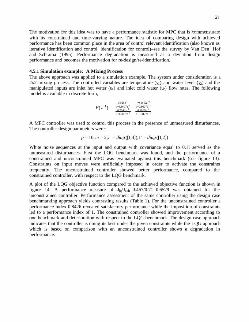
White noise sequences at the input and output with covariance equal to 0.1I served as theunmeasured disturbances. First the LQG benchmark was found, and the performance of aconstrained and unconstrained MPC was evaluated against this benchmark (see figure 13).Constraints on input moves were artificially imposed in order to activate the constraintsfrequently. The unconstrained controller showed better performance, compared to theconstrained controller, with respect to the LQG benchmark.

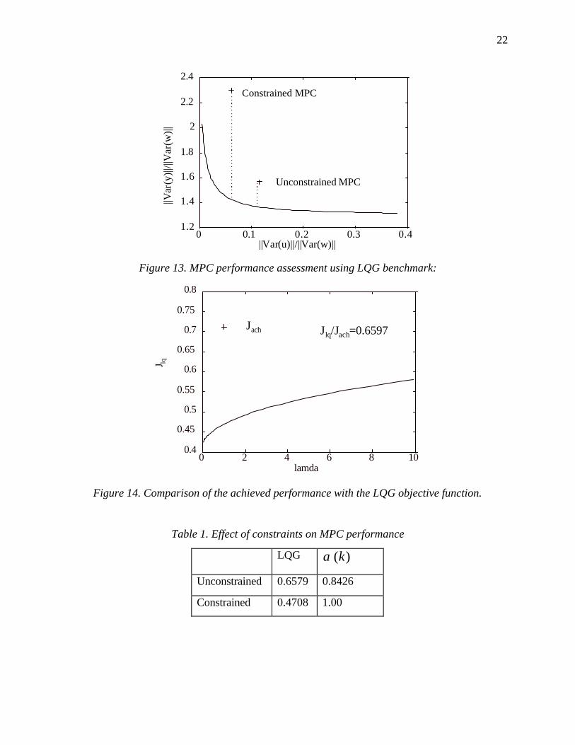
A plot of the LQG objective function compared to the achieved objective function is shown infigure 14. A performance measure of Jlq/Jach=0.467/0.71=0.6579 was obtained for theunconstrained controller. Performance assessment of the same controller using the design casebenchmarking approach yields contrasting results (Table 1). For the unconstrained controller aperformance index 0.8426 revealed satisfactory performance while the imposition of constraintsled to a performance index of 1. The constrained controller showed improvement according toone benchmark and deterioration with respect to the LQG benchmark. The design case approachindicates that the controller is doing its best under the given constraints while the LQG approachwhich is based on comparison with an unconstrained controller shows a degradation inperformance.

22

0 0.1 0.2 0.3 0.41.2

1.4

1.6

1.8

2

2.2

2.4

||Var(u)||/||Var(w)||

||Var

(y)||

/||V

ar(w

)||

Constrained MPC

Unconstrained MPC

Figure 13. MPC performance assessment using LQG benchmark:

J lq

Jach Jlq/Jach=0.6597

0 2 4 6 8 100.4

0.45

0.5

0.55

0.6

0.65

0.7

0.75

0.8

lamda

Figure 14. Comparison of the achieved performance with the LQG objective function.

Table 1. Effect of constraints on MPC performance

LQG )(kα

Unconstrained 0.6579 0.8426

Constrained 0.4708 1.00

23

-0.02-0.01 0 0.01 0.02

-0.01

0

0.01

du2

du1

Figure 15. The input moves for the constrained controller during the regulatory run

Figure 15 shows the input moves during the regulatory run for the constrained controller. Theconstraints are active for a large portion of the run and are limiting the performance of thecontroller in an absolute sense (LQG). On the other hand the controller cannot do any better dueto design constraints as indicated by the design case benchmark.

5. Challenges in Performance Analysis and Diagnosis: General Comments andIssues in MPC Performance Evaluation

A single index or metric by itself may not provide all the information required to diagnose thecause of poor performance. Considerable insight can be obtained by carefully interpreting all theperformance indices. For example, in addition to the minimum variance benchmark performanceindex, one should also look at the cross-correlation plots, normalized multivariate impulseresponse plots, spectrum analysis etc to determine causes of poor performance. As an example, ifthe process data is 'white' then the performance index will always be close to 1 irrespective ofhow large the variance is. On the other hand, if the data is highly correlated (highly predictable),then the performance index will be low irrespective of how small the output variance is. In thisrespect the performance index plus the impulse response or the auto-correlation plot wouldprovide a complete picture of the root cause of the problem. (The auto-correlation plot wouldhave yielded information on the predictability of the disturbance). In summary then, each indexhas its merits and its limitations. Therefore, one should not just rely on any one specific index. Itwould be more appropriate to check all relevant indices that reflect performance measures fromdifferent aspects.As mentioned earlier, the multivariate extension of the minimum variance benchmark requires aknowledge of the time-delay or the interactor matrix. This requirement of apriori information onthe interactor has been regarded by many as impractical. However, from our experience thisbenchmark, when applied with care, can yield meaningful measures of controller performance.Yet, many outstanding issues remain open before once can confidently apply MIMO assessmenttechniques for a wide-class of MIMO systems. Some of the issues related to the evaluation ofmultivariate controllers are listed below:

24

1. To calculate a general interactor matrix, one needs to have more apriori information thanjust the time delays. However, experience has shown us that a significant number of MIMOprocesses do have the diagonal interactor structure. In fact, a properly designed MIMOcontrol structure will most likely have a diagonal interactor structure (Huang and Shah,1999). A diagonal interactor depends only on the time delays between the paired input andoutput variables.

2. Since models are available for all MPC based controllers, apriori knowledge of the timedelay matrix is surely not an issue at all.

3. A more important issue in the analysis and diagnosis of control loops is the accuracy of themodels and their variability over time. How does the model uncertainty affect the calculationof performance index? This question has not been answered so far. It is a common problemin both MIMO and SISO performance assessment. Therefore, one of the many outstandingissues remaining is the robustness of performance assessment, i.e. how to transfer the modeluncertainty onto the uncertainty in the calculation of the performance index? This issue hasbeen addressed to some extent in Patwardhan and Shah (2000, 1999), where SISO andMIMO examples, relating modeling uncertainty to uncertainty in performance measures, aregiven.

Industrial MPC is a combination of a dynamic part and a steady state part, which often comprisesa linear programming (LP) step. The dynamic component consists of unconstrained minimizationof a dynamic cost function, comprising of the predicted tracking errors and future input moves,familiar to academia. The steady state part focuses on obtaining economically optimal targets,which are then sent to the dynamic part for tracking as illustrated in figure 16. This combinationof the dynamic and steady state parts and constraint handling via the linear programming or theLP step renders the MPC system as a nonlinear multivariate system. Patwardhan et al (1998)have illustrated the difficulties caused by the LP step on an industrial case study involving ademethanzier MPC (see figure 17.). In that particular application as in a number of other MPCapplications, when the LP stage is activated fairly routinely, significant correlation existsbetween the LP targets and the measurements that the LP relies upon. In such instances when theLP stage is activated at the same frequencies as the control frequencies, the controller structure isno longer linear. Situations such as these preclude the use of conventional performanceassessment methods such the LQ or the minimum variance benchmark. We believe that thevariable structure nature of industrial MPC can be captured by the objective function methodsince it takes into account the time varying nature of the MPC objective. Patwardhan (1999) hasapplied this method successfully on an industrial QDMC application. Even though one mayargue that QDMC is devoid of the LP step, it is a variable structure MIMO controller that allowsdifferent inputs and outputs to swap into active and inactive states relative to the active constraintset. In this respect, the lumped objective function and subsequently the performance indexproposed here does ‘measure’ the true intentions of the controller relative to the design case. Itthus provides a useful performance metric. The only limitation being that the access to the actualdesign control objective has to be available in the MPC vendor software.

Establishing the root causes of performance degradation in industrial MPCs is indeed achallenging task. Potential factors include models, inadequately designed LP in that the LPoperates at the control frequencies, inappropriate choice of weightings, ill-posed constraints,steady-state bias updates etc. In practice, these factors combine in varying degrees to give poorperformance. Thus the issues and challenges related to the diagnosis aspects of MPC

25

y

+

+

d

Dynamic Control uProcess

P

ModelP

+

-

desJMin

u

y

+

-

Steady StateModel

Steady StateOptimization

K

ssy

ssyJ

ss

max,u ss

ssu

Figure 16. Schematic of a typical commercial MPC with a blended linear programming module that setstargets for the controlled and manipulative variables

0 20 40 60 80 100 120

0.242

0.244

0.246

Pre

ssu

re

0 10 20 30 40 50 60 70 80 90 100-2

-1

0

1

2

Lev

el

Figure 17. An example of the interaction between the steady state optimization and the dynamiclayer in industrial MPC. Note that setpoints have higher variation compared to controlled

variables!

performance assessment are many. Some of these issues are listed below and one ‘quantifiable’diagnosis issue related to model-plant mismatch is discussed. The diagnosis stage for poorperformance involves a trial and error approach (Kesavan and Lee, 1997). For example, thediagnosis or the decision support system has to investigate the cause of poor performance asbeing due to:

• Poor or incorrect tuning.

26

• Incorrect controller configuration, e.g. choice of MVs may not be correct.• Large disturbances, in which case the sources of measured disturbances have to be identified

and potential feedforward control benefits should be investigated.• Engineering redesign , e.g. is it possible to reduce process time delays.• Model-plant mismatch in the case of MPC controllers and how does model uncertainity

affect the calculation of the performance index (e.g. if the index has been obtained from anuncertain interactor).

• Poor choice of constraint variables and constrained values.

Some of the above referenced issues have been already dealt with in the literature, e.g. (ANOVAanalysis to investigate the need for feedforward control by Desborough and Harris (1993),Vishnubhotla et al. (1997), and Stanfejl et al. (1993); others are open problems. The diagnosisissues related to the model-plant mismatch is briefly discussed below in a theoretical frameworkand illustrated on an industrial MPC evaluation case study that follows. A discussion of the poorperformance diagnosis steps leading to guidelines for tuning and controller design issues isbeyond the scope of this paper.

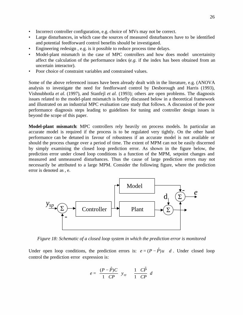
Model-plant mismatch: MPC controllers rely heavily on process models. In particular anaccurate model is required if the process is to be regulated very tightly. On the other handperformance can be detuned in favour of robustness if an accurate model is not available orshould the process change over a period of time. The extent of MPM can not be easily discernedby simply examining the closed loop prediction error. As shown in the figure below, theprediction error under closed loop conditions is a function of the MPM, setpoint changes andmeasured and unmeasured disturbances. Thus the cause of large prediction errors may notnecessarily be attributed to a large MPM. Consider the following figure, where the predictionerror is denoted as , e.

Controller Plant

Model

dysp

e

-

-

Σ Σ

Σ

Figure 18: Schematic of a closed loop system in which the prediction error is monitored

Under open loop conditions, the prediction errors is: duPPe +−= )ˆ( . Under closed loopcontrol the prediction error expression is:

dCP

PCy

CPCPP

e sp

++

+

+−

=1

ˆ11

)ˆ(

27

It is clear from the above expression that a large prediction error signal could be due to a largeMPM term, or a large disturbance term or setpoint changes. Thus the question of attributing alarge prediction error as being due to model-plant-mismatch needs careful scrutiny. Huang(2000) has studied the problem of detecting significant model plant mismatch or processparameter changes in the presence of disturbances.

6. Industrial MIMO Case study 2: Analysis of cracking Furnace under MPCcontrol

This section documents the results of the controller performance analysis carried out on anethane cracking furnace. The control systems comprises of (1) a regulatory layer and (2) anadvanced MPC control layer. The first pass of performance assessment revealed some poorlyperforming loops. Further analysis revealed that these loops were in fact well tuned but werebeing affected by high frequency disturbances and setpoint changes. The furnace MPCapplication considered here, however, is unlike conventional MPC applications. The steady statelimits were set in such a way that the setpoints for the controlled variables were held constant,i.e. the focus of the evaluation was on the models and the tuning of the dynamic part.

The MPC layer displays satisfactory performance levels when there are no rate changes. Duringrate changes, the MPC model over predicts thus causing poor performance. Re-identification ofthe model gains was found to be necessary to improve MPC performance.

Control Strategy OverviewThe purpose of the Furnace MPC controllers is to maintain smooth operation, maximizethroughput and minimize energy consumption to the furnaces while simultaneously honoring allconstraints. There is one MPC controller per furnace. The conversions, the total dry feed, the wetfeed bias, the steam/feed ratio and the oxygen to fuel ratio is controlled by MPC. These variablesare manipulated by moving the north and south fuel gas duty setpoints, the north and south wetfeed flow setpoints, the steam pressure setpoint, the fan speed controller setpoint and the inducedfan draft. Thus there are 6 primary controlled variables and 7 manipulated variables. There are anumber of secondary controlled variables, which MPC is required to maintain within a constraintregion. These secondary CVs include valve constraints, constraints on critical constraints such asthe coil average temperatures (COTS). Considering the degrees of freedom (MVs) available, itmay not always be possible to satisfy all the constraints. In such cases, a ranking mechanismdecides what constraints are least important and could be let go.

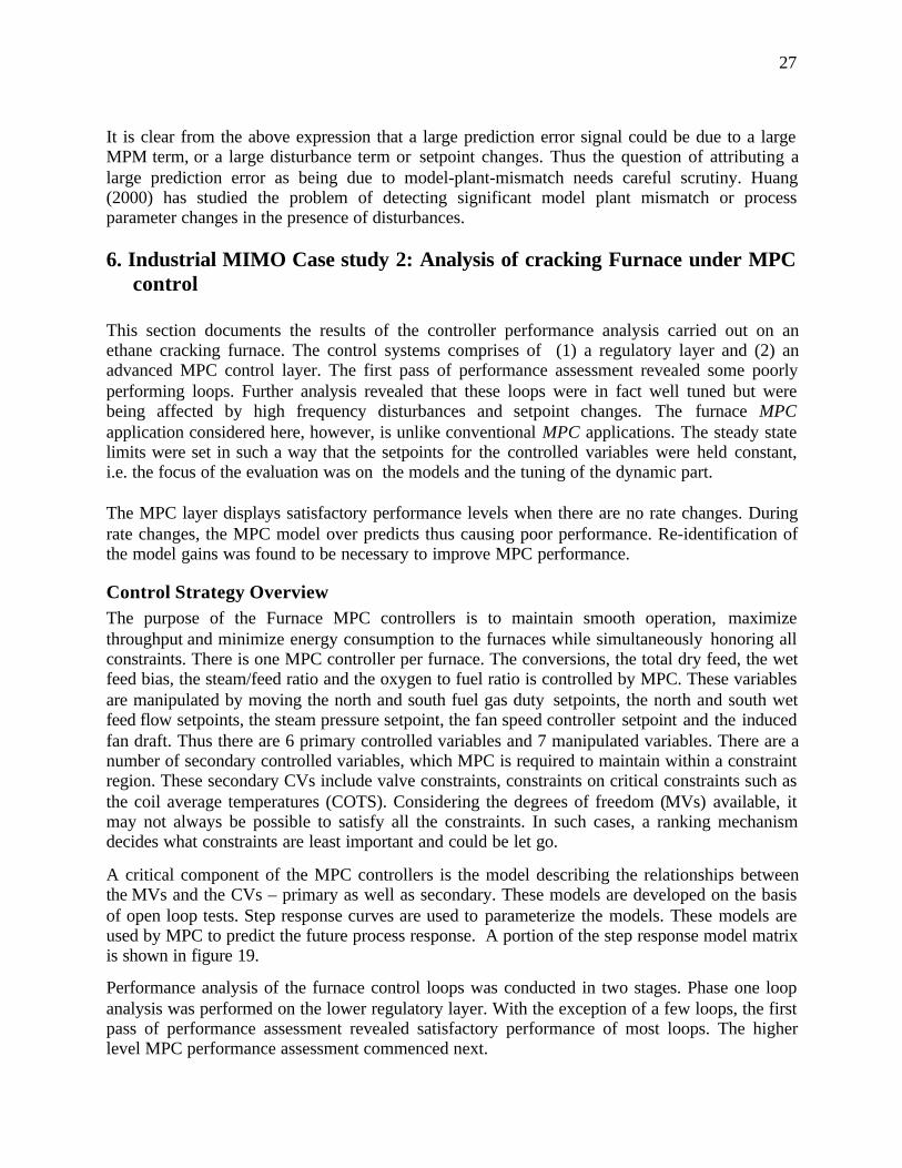
A critical component of the MPC controllers is the model describing the relationships betweenthe MVs and the CVs – primary as well as secondary. These models are developed on the basisof open loop tests. Step response curves are used to parameterize the models. These models areused by MPC to predict the future process response. A portion of the step response model matrixis shown in figure 19.

Performance analysis of the furnace control loops was conducted in two stages. Phase one loopanalysis was performed on the lower regulatory layer. With the exception of a few loops, the firstpass of performance assessment revealed satisfactory performance of most loops. The higherlevel MPC performance assessment commenced next.

28

0 500123

x 10-3

0 500246

x 10- 4

0 50

-15-10

-5

0 500

0.1

0.2

0 500246

x 10-4

0 500123

x 10- 3

0 50

-15-10

-5

0 500

0.1

0.2

0 500.20.40.60.8

0 500.20.40.60.8

0 50-0.02

-0.01

0 50

0.5

1

0 50

-1

-0.5

0 50-14-12-10

-8-6-4-2

x 10-3

0 50-14-12-10

-8-6-4-2

x 10-3

0 50

0.51

1.52

2.5

x 10-3

Figure 19 . A portion of the step response models used by MPC.

Multivariable Performance Assessment for MPC

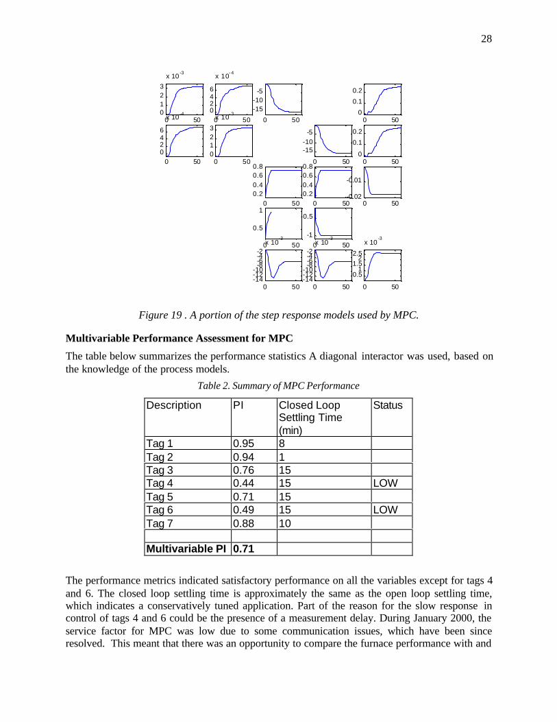
The table below summarizes the performance statistics A diagonal interactor was used, based onthe knowledge of the process models.

Table 2. Summary of MPC Performance

Description PI Closed LoopSettling Time(min)

Status

Tag 1 0.95 8Tag 2 0.94 1Tag 3 0.76 15Tag 4 0.44 15 LOWTag 5 0.71 15Tag 6 0.49 15 LOWTag 7 0.88 10

Multivariable PI 0.71

The performance metrics indicated satisfactory performance on all the variables except for tags 4and 6. The closed loop settling time is approximately the same as the open loop settling time,which indicates a conservatively tuned application. Part of the reason for the slow response incontrol of tags 4 and 6 could be the presence of a measurement delay. During January 2000, theservice factor for MPC was low due to some communication issues, which have been sinceresolved. This meant that there was an opportunity to compare the furnace performance with and

29

without MPC. Based on data from Jan 14-16 when MPC was shut off for part of the time,performance metrics were obtained to compare the two control systems – MPC and conventionalPID controls. The statistics indicate that the overall control is only slightly better with MPCturned on.

0

0.2

0.4

0.6

0.8

1

1.2

Tag 1 Tag 2 Tag 3.

Tag 4 Tag 5 Tag 6 Tag 7

MPC ON

MPC OFF

Figure 20. Comparison of performance, with and without MPC.

MPC Diagnostics

Is MPC doing its best? Can we improve the current performance levels of the furnace MPCcontroller? These questions lead us to two issues that are closely related to each other:

(i) How good are the models used for predicting the process response?

(ii) How well tuned is the multivariable controller? “Tuning” includes a whole range ofdifferent of parameters – weightings, horizons, constraints, rankings …

We will try to illustrate a case where the model predictions can mislead the controller and hencecause poor performance. This Furnace was showing poor MPC performance, especially duringrate changes. This motivated us to look more closely at the model prediction accuracy.

Before evaluating the current predictions, we establish a baseline when the open loop tests wereconducted. The following graphs compare the conversion predictions for the open loop case asconducted before commissioning the MPC. The model accuracy is reasonable. The averageprediction error, for this data set was 3.18.

∑∑= =

+−+=N

k

n

iii kkyky

N

y

1

2

1

)}/1(ˆ)1({1

Error Prediction Average

The predictions for other variables – COTs, Feed Flow and Bias, S/F ratio also fared well. Theremaining variables are not shown for the sake of brevity.

30

0 200 400 600 800 1000 1200 1400 1600 1800-6

-4

-2

0

2

4

0 200 400 600 800 1000 1200 1400 1600 18002.4

2.5

2.6

2.7

2.8

2.9

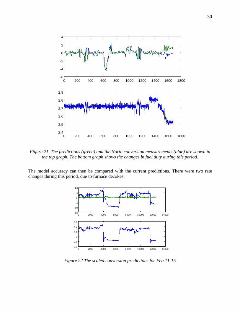
Figure 21. The predictions (green) and the North conversion measurements (blue) are shown inthe top graph. The bottom graph shows the changes in fuel duty during this period.

The model accuracy can then be compared with the current predictions. There were two ratechanges during this period, due to furnace decokes.

0 2000 4000 6000 8000 10000 12000 14000-1.5

-1.0

-.5

0

.5

1.0

0 2000 4000 6000 8000 10000 12000 140002.6

2.8

3

3.2

3.4

3.6

Figure 22 The scaled conversion predictions for Feb 11-15

31

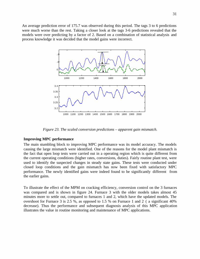
An average prediction error of 175.7 was observed during this period. The tags 3 to 6 predictionswere much worse than the rest. Taking a closer look at the tags 3-6 predictions revealed that themodels were over predicting by a factor of 2. Based on a combination of statistical analysis andprocess knowledge it was decided that the model gains were incorrect.

1000 1200 1400 1600 1800 2000

0

.4

..8

1000 1100 1200 1300 1400 1500 1600 1700 1800 1900 2000

3.2

3.25

3.3

3.35

3.4

Figure 23. The scaled conversion predictions – apparent gain mismatch.

Improving MPC performanceThe main stumbling block to improving MPC performance was its model accuracy. The modelscausing the large mismatch were identified. One of the reasons for the model plant mismatch isthe fact that open loop tests were carried out in a operating region which is quite different fromthe current operating conditions (higher rates, conversions, duties). Fairly routine plant test, wereused to identify the suspected changes in steady state gains. These tests were conducted underclosed loop conditions and the gain mismatch has now been fixed with satisfactory MPCperformance. The newly identified gains were indeed found to be significantly different fromthe earlier gains.

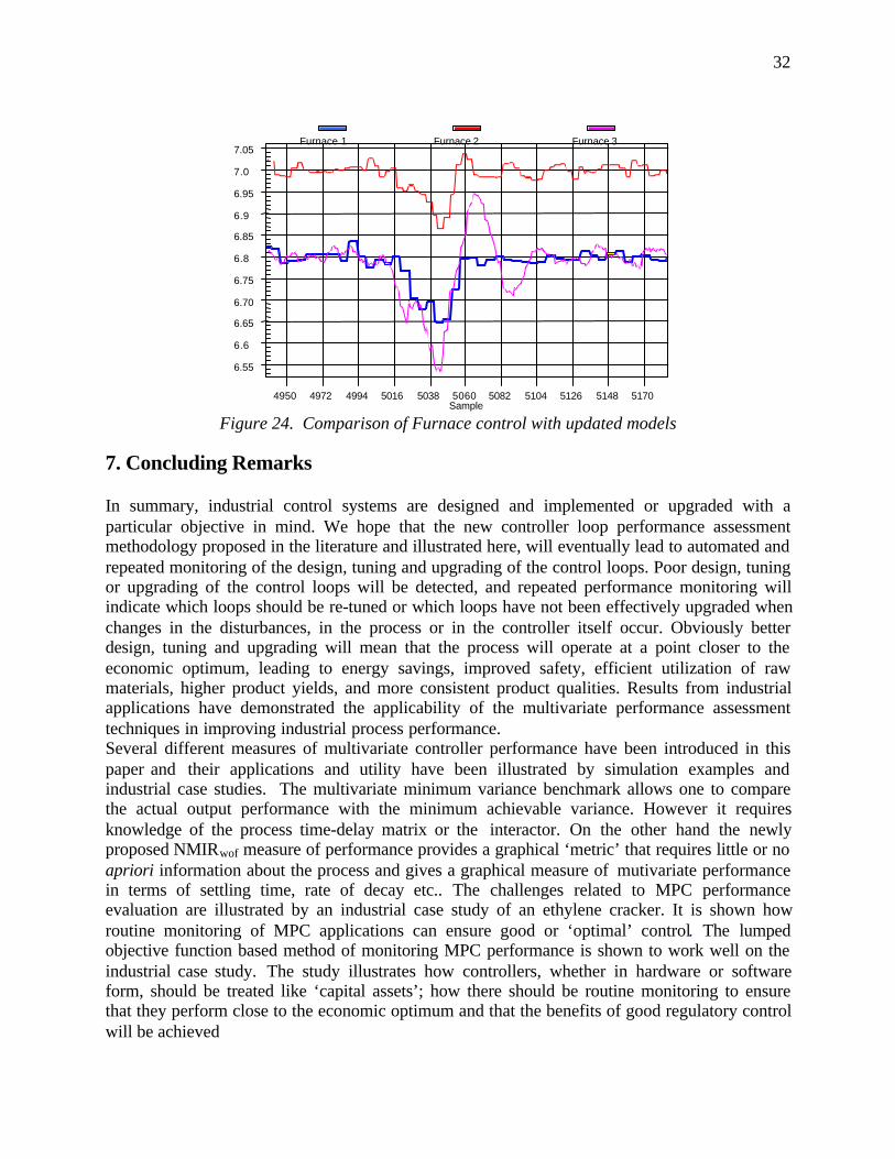
To illustrate the effect of the MPM on cracking efficiency, conversion control on the 3 furnaceswas compared and is shown in figure 24. Furnace 3 with the older models takes almost 45minutes more to settle out, compared to furnaces 1 and 2, which have the updated models. Theovershoot for Furnace 3 is 2.5 %, as opposed to 1.5 % on Furnace 1 and 2 ( a significant 40%decrease). Thus the performance and subsequent diagnosis analysis of this MPC applicationillustrates the value in routine monitoring and maintenance of MPC applications.

32

6.55

6.6

6.65

6.70

6.75

6.8

6.85

6.9

6.95

7.0

7.05

Sample4950 4972 4994 5016 5038 5060 5082 5104 5126 5148 5170

Furnace 1 Furnace 2 Furnace 3

Figure 24. Comparison of Furnace control with updated models

7. Concluding Remarks

In summary, industrial control systems are designed and implemented or upgraded with aparticular objective in mind. We hope that the new controller loop performance assessmentmethodology proposed in the literature and illustrated here, will eventually lead to automated andrepeated monitoring of the design, tuning and upgrading of the control loops. Poor design, tuningor upgrading of the control loops will be detected, and repeated performance monitoring willindicate which loops should be re-tuned or which loops have not been effectively upgraded whenchanges in the disturbances, in the process or in the controller itself occur. Obviously betterdesign, tuning and upgrading will mean that the process will operate at a point closer to theeconomic optimum, leading to energy savings, improved safety, efficient utilization of rawmaterials, higher product yields, and more consistent product qualities. Results from industrialapplications have demonstrated the applicability of the multivariate performance assessmenttechniques in improving industrial process performance.Several different measures of multivariate controller performance have been introduced in thispaper and their applications and utility have been illustrated by simulation examples andindustrial case studies. The multivariate minimum variance benchmark allows one to comparethe actual output performance with the minimum achievable variance. However it requiresknowledge of the process time-delay matrix or the interactor. On the other hand the newlyproposed NMIRwof measure of performance provides a graphical ‘metric’ that requires little or noapriori information about the process and gives a graphical measure of mutivariate performancein terms of settling time, rate of decay etc.. The challenges related to MPC performanceevaluation are illustrated by an industrial case study of an ethylene cracker. It is shown howroutine monitoring of MPC applications can ensure good or ‘optimal’ control. The lumpedobjective function based method of monitoring MPC performance is shown to work well on theindustrial case study. The study illustrates how controllers, whether in hardware or softwareform, should be treated like ‘capital assets’; how there should be routine monitoring to ensurethat they perform close to the economic optimum and that the benefits of good regulatory controlwill be achieved

33

AcknowledgementsThe authors of this paper wish to express sincere gratitude andappreciation to the following persons who have provided assistance by participating in industrialevaluation studies at their respective work sites: Jim Kresta and Henry Tse (Syncrude Research),Janice Vegh-Morin and Harry Frangogiannopoulus (both of TDCC), Genichi Emoto (MitsubishiChemical Corporation,Japan) andAnand Vishnubhotla (Matrikon Consulting) Their feedbackand industrial insight were helpful in enhancing the practicality and utility of the proposedmethods to make it better suited to the process industry.

Financial support in the form of research grants from the Natural Science and EngineeringResearch Council of Canada and Equilon Enterprises (Shell-USA) is gratefully acknowledged.

References

Boyd, S. and Barratt, C. (1991), Linear Control Design, Prentice Hall, Englewood Cliffs, NewJersey

Desborough, L. and Harris, T.(1992), Performance Assessment Measures for UnivariateFeedback Control, Can. J. Chem. Eng., 70, 1186-1197.

Desborough, L. and Harris, T. (1993), Performance Assessment Measures for UnivariteFeedforward/feedback Control, Can. J. Chem. Eng. 71, 605-616.

Garcia, C. E., Prett, D. M. and Morari, M., (1989), Model Predictive Control: Theory andPractice – A Survey, Automatica, 25, 335-348

Harris, T (1989), Assessment of Closed-loop Performance, Can. J. Chem. Eng. 67, 856-861

Harris, T., Seppala, C. and Desborough, L. (1999), A Review of Performance Monitoring andassessment Techniques for Univariate and Multivariate Control Systems, J. of Process Control,9, 1-17.

Harris, T. Boudreau, F. and MacGregor (1996), Performance Assessment of MultivariateFeedback Controllers, Automatica 32(11), 1505-1518

Huang, B., Shah, S.L. and Kwok K. (1996), How Good Is Your Controller? Application ofControl Loop Performance Assessment Techniques to MIMO Processes, In Proc. 13th IFACWorld Congress, Vol M, San Francisco, 229-234

Huang, B., Shah, S.L. and Kwok K. (1997), Good, Bad or Optimal? Performance Assessment ofMultivariable Processes, 33, 1175-1183, Automatica

Huang,B, Shah,S.L. and Fujii,H., “The Unitary Interactor Matrix and Its Estimation fromClosed-loop Data”, Journal of Process Control, 7, 6, 195-207, 1997

Huang, B. and Shah, S.L. (1999), Performance Assessment of Control Loops: Theory andApplications, Springer Verlag

Huang, B., Model Validation in the Presence of Time-variant Disturbance Dynamics, ChemicalEngineering Science, 55, 4583-4595, 2000.

Ko, B.S. and Edgar, T.F., "Performance Assessment of Multivariable Feedback ControlSystems", Submitted for publication. 2000

Kozub, D. and Garcia, C. (1993), Monitoring and Diagnosis of Automated Controllers in theChemical Process Industries, AIChE Annual Meeting, St. Louis

34

Kozub, D. (1996), Controller Performance Monitoring and Diagnosis Experiences andChallenges, In Proceedings of CPC-V, Lake Tahoe, CA

Kwakernaak, H. and Sivan, R. (1972), Linear Optimal Control System, John Wiley & Sons

Kammer, L. C. , Bitmead, R. R. and Barlett, P. L., 1996, Signal-based testing of LQ-optimalityof controllers , Proc. of the 35th IEEE_CDC, Kobe, Japan, pp 3620-3624.

Kesavan, P. and Lee, J.H., (1997), Diagnostic tools for multivariable model-based controlsystems, Ind. Eng. Chem. Res., 36, 2725

Ljung, L. (1987) System Identification, Prentice-Hall

Mayne, D. Q., Rawlings, J. B., Rao, C. V. and Scokaert, P. O. M, (2000), Constrained modelpredictive control: Stability and optimality, Automatica, 36(6) 789-814.

Patwardhan, R. S., Studies in the Synthesis and Analysis of Model Predictive Controllers, PhDThesis, Department of Chemical and Materials Engineering, University of Alberta, 1999

Patwardhan, R. S., and Shah, S. L., (2000), The Effect of Uncertainty on Controller Performance,Submitted to J. Proc. Control.

Patwardhan, R., Shah, S.L. and Emoto, G., "Experiences in Performance Annalysis of Industrial ModelPredictive Controllers", Submitted for publication, 2000

Patwardhan, R., Shah, S.L. and Qi, K., "Techniques for Assessment of Model PredictiveControllers", Submitted for publication

Qin, J. S.,(1998) , Control performance monitoring-a review and assessment, Computers andChemical Engineering, 23, pp 173-186

Qin, J. S. and Badgewell, T. A., (1996), An Overview of Industrial Model Predictive ControlTechnology, In Proceedings of CPC-V, Lake Tahoe, CA.

Stanfelj, N., Marlin, T. and MacGregor, J.(1993), Monitoring and Diagnosing Process ControlPerformance: the single-loop case, Ind. Eng. Chem. Res. 32, 301-314

Swanda, A. and Seborg, D.E., "Controller Performance Assessment based on Setpoint ResponseData", Proc. of 1999 ACC, San Diego, CA

N.F. Thornhill, M. Oettinger, and P. Fedenczuk, Refinery-wide control loop performanceassessment, Journal of Process Control, 9(2), 109-124, 1999.

Vishnubhotla, A., Shah, S., and Huang, B. (1997) Feedback and Feedforward PerformanceAnalysis of the Shell Industrial Closed-loop Data Set, In Proc. Of ADCHEM, Banff, 295-300.

Wood and Berry, 1973, Terminal Composition Control of a binary distillation column, Chem.Eng. Science, 29, 1808

Van Den Hof, P. M. J. and Schrama, R. J. P, (1995), Identification and Control – Closed LoopIssues, Automatica, 31, 1751-1770