
Multiscale structures in solutal Marangoni convection: Three-dimensional simulations and supporting...
32
Multiscale structures in solutal Marangoni convection: Three-dimensional simulations and supporting experiments Thomas Köllner, Karin Schwarzenberger, Kerstin Eckert, and Thomas Boeck Citation: Physics of Fluids (1994-present) 25, 092109 (2013); doi: 10.1063/1.4821536 View online: http://dx.doi.org/10.1063/1.4821536 View Table of Contents: http://scitation.aip.org/content/aip/journal/pof2/25/9?ver=pdfcov Published by the AIP Publishing This article is copyrighted as indicated in the article. Reuse of AIP content is subject to the terms at: http://scitation.aip.org/termsconditions. Downloaded to IP: 141.30.106.164 On: Fri, 21 Mar 2014 12:03:53
-
Upload
tu-dresden -
Category
Documents
-
view
1 -
download
0
Transcript of Multiscale structures in solutal Marangoni convection: Three-dimensional simulations and supporting...

Multiscale structures in solutal Marangoni convection: Three-dimensional simulationsand supporting experimentsThomas Köllner, Karin Schwarzenberger, Kerstin Eckert, and Thomas Boeck Citation: Physics of Fluids (1994-present) 25, 092109 (2013); doi: 10.1063/1.4821536 View online: http://dx.doi.org/10.1063/1.4821536 View Table of Contents: http://scitation.aip.org/content/aip/journal/pof2/25/9?ver=pdfcov Published by the AIP Publishing
This article is copyrighted as indicated in the article. Reuse of AIP content is subject to the terms at: http://scitation.aip.org/termsconditions. Downloaded to IP:
141.30.106.164 On: Fri, 21 Mar 2014 12:03:53
PHYSICS OF FLUIDS 25, 092109 (2013)
Multiscale structures in solutal Marangoni convection:Three-dimensional simulations and supportingexperiments
Thomas Kollner,1 Karin Schwarzenberger,2 Kerstin Eckert,2
and Thomas Boeck1
1Institute of Thermodynamics and Fluid Mechanics, Technische Universitat Ilmenau, P.O.Box 100565, D-98684 Ilmenau, Germany2Institute of Fluid Mechanics, Chair of Magnetofluiddynamics, Measuring and AutomationTechnology, TU Dresden, D-01062 Dresden, Germany
(Received 16 January 2013; accepted 14 July 2013; published online 25 September 2013)
Transient solutal Marangoni convection in a closed two-layer system is studied bya combination of numerical simulations and supplementary validation experiments.The initially quiescent, equally sized liquid layers are the phases of a cyclohexanol/water mixture. Butanol is additionally dissolved in the upper organic layer. Its dif-fusion across the interface is sensitive to the Marangoni instability. Complex con-vective patterns emerge that develop a hierarchical cellular structure in the courseof the mass transfer. Our highly resolved simulations based on a pseudospectralmethod are the first to successfully reproduce the multiscale flow observed in theexperiments. We solve the three-dimensional Navier-Stokes-Boussinesq equationswith an undeformable interface, which is modeled using the linear Henry relation forthe partition of the weakly surface-active butanol. Length scales in the concentrationand velocity fields associated with the small and large-scale cells agree well withour experimental data from shadowgraph images. Moreover, the simulations providedetailed information on the local properties of the flow by which the evolution ofthe patterns and their vertical structure are analyzed. Apart from relatively weakinfluences due to buoyancy, the evolution of the convective structures is self-similarbetween different initial butanol concentrations when length and time are appropri-ately rescaled. C© 2013 AIP Publishing LLC. [http://dx.doi.org/10.1063/1.4821536]
I. INTRODUCTION
Solutal Marangoni convection is of high relevance for mass transfer processes across liquidinterfaces. It is driven by gradients in the interfacial tension due to variations of the interfacial soluteconcentration. Its impact on various fields of application is reflected in the widespread scientificwork on this topic published recently. Current activities on Marangoni convection are associatedwith evaporation-driven flows1–3 and the resulting pattern formation by deposition of dissolved ordispersed substances.4–8 In some systems, amazing processes such as the self-propulsion of liquiddroplets9, 10 or solid bodies11 driven by inhomogeneities in the surface tension, periodic large-scale interfacial deformations,12 kicking pendant drops,13, 14 and intriguing forms of spreading anddissolving droplets15–17 occur. Nonlinear Marangoni-driven oscillations18, 19 were observed duringthe mass transfer of surfactants and further investigated by numerical simulation. Moreover, ongoingresearch still emerges from the classical aspect of Marangoni convection in chemical engineeringconcerning the determination of mass transfer rates.20, 21
These references show that recent research on Marangoni convection predominantly focuseson droplet geometries, which is due to its high technological relevance. However, this configurationinherently includes complicating effects of curvature, density convection, and geometric asymmetryof the solvent phases. Hence, to unravel the complex phenomena induced by Marangoni convection,a simpler model system is preferable. This approach was already pursued in the seminal work of
1070-6631/2013/25(9)/092109/31/$30.00 C©2013 AIP Publishing LLC25, 092109-1
This article is copyrighted as indicated in the article. Reuse of AIP content is subject to the terms at: http://scitation.aip.org/termsconditions. Downloaded to IP:
141.30.106.164 On: Fri, 21 Mar 2014 12:03:53
092109-2 Kollner et al. Phys. Fluids 25, 092109 (2013)
Sternling and Scriven,22 who considered a system with a plane interface. According to their linearstability analysis, solutal Marangoni convection can set in either via an oscillatory or a stationarymode. The current study focuses on the stationary mode. This instability mode can appear ifinterfacial tension lowering solute is transferred out of the phase with the higher kinematic viscosityand the lower solute diffusivity.
Stationary solutal Marangoni instability forms the mass-transfer-driven analog to the heat-transfer-driven Benard convection.23–26 Both configurations show significant differences in the dif-fusivities as well as in the initial and boundary conditions, i.e., usually the temperature is fixed attwo outer walls, while we study the redistribution of a prescribed amount of solute. Despite this fact,the primary instability occurs in both types in the form of simple roll cells. In particular, the solutalMarangoni cells can undergo a nonlinear evolution toward complex multiscale flow patterns.27–30
For such systems, Linde et al.31 proposed a classification of the highly complex and unsteadypatterns in the form of a few hypotheses based on a wide range of experiments examined. The mostrelevant hypotheses shall briefly be repeated:
1. Interfacial convection is built up of three basic structures: (a) Marangoni roll cells, (b) relaxationoscillations, and (c) synchronized relaxation oscillation waves.
2. Each of these structures may occur in n different hierarchy steps of different size, which wecall nth order, referring to the number of substructures which are embedded. Substructure(s)of all three types can occur in any of the three patterns.
3. Driving force of all these structures is the Marangoni shear stress operating on different lengthscales.
At present, only the simplest Marangoni roll cells of the primary pattern have been thoroughlyinvestigated by experiments and two-dimensional simulations, including very recent work.12, 32–36
By contrast, neither the details of the hierarchic multiscale patterns nor the mechanisms of hierarchyformation have been characterized up to now. These open issues are addressed by the current studyof a Marangoni roll cell pattern that incorporates two hierarchy levels through a combination ofhighly resolved three-dimensional simulations and specifically designed validation experiments.Specifically, we examine the full structure of velocity and concentration fields during the differentstages and processes of pattern evolution.
The paper is organized as follows. The material properties of the system under study,(cyclohexanol+butanol)/water, are discussed in Sec. II A. The experimental setup consists oftwo equally sized vessels that are brought into contact as detailed in Sec. II B. Section II Cpresents the mathematical model based on the Navier-Stokes-Boussinesq equations along with aclassical model with a partition coefficient for the weakly surface-active solute. The equations aresolved by a pseudospectral method as detailed in Sec. II E. The large Sec. III is dedicated to theanalysis of the hierarchical cellular patterns and their underlying flow structures. To begin with,Sec. III A overviews the temporal development of the arising multiscale structures in accordancewith the concept of Linde et al.31 Next, the velocity and surfactant distribution of the genericstructures are shown in Sec. III B and further quantified by length scales of momentum and solutetransport in Sec. III C. Typical mechanisms underlying the pattern formation are illustrated in detailin Sec. III D. Finally, we provide conclusions and indicate directions for further work in Sec. IV.
II. METHODS
A. System under study
We study solutal Marangoni convection at the planar interface between an aqueous phase asbottom layer (1) and a lighter organic phase as top layer (2). These layers are the phases of a water andcyclohexanol (C6H11OH) mixture. Both binary phases are in equilibrium due to mutual saturation.On top of this, a third species 1-butanol (C4H9OH), lowering interfacial tension, is dissolved in theorganic phase. It causes stationary convective instability according to Sternling and Scriven22 whentransferred out of the organic, cyclohexanol-rich phase. The diffusion of low amounts of butanol intothe lower phase is buoyantly stable since butanol lowers the density. This ensures that the Marangoni
This article is copyrighted as indicated in the article. Reuse of AIP content is subject to the terms at: http://scitation.aip.org/termsconditions. Downloaded to IP:
141.30.106.164 On: Fri, 21 Mar 2014 12:03:53
092109-3 Kollner et al. Phys. Fluids 25, 092109 (2013)
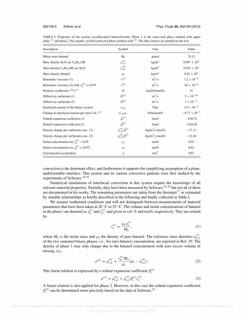
TABLE I. Properties of the system (cyclohexanol+butanol)/water. Phase 1 is the water-rich phase marked with upperindex (1) and phase 2 the organic cyclohexanol-rich phase marked with (2). The data sources are detailed in the text.
Description Symbol Unit Value
Molar mass butanol Mb g/mol 74.12
Mass density H2O sat. C6H11OH ρ(1)re f kg/m3 0.997 × 10³
Mass density C6H11OH sat. H2O ρ(2)re f kg/m3 0.955 × 10³
Mass density butanol ρb kg/m3 0.81 × 10³
Kinematic viscosity (1) ν(1) m2/s 1.2 × 10⁻⁶
Kinematic viscosity (2) with y(2)b = 0.075 ν(2) m2/s 20 × 10−6
Partition coefficient c(2)/c(1) H (mol/l)/(mol/l) 31
Diffusivity surfactant (1) D(1) m2/s 5 × 10⁻¹⁰
Diffusivity surfactant (2) D(2) m2/s 7 × 10⁻¹¹
Interfacial tension of the binary system σ ref N/m 3.4 × 10⁻³
Change in interfacial tension per mol/l of c(1) σ ref αc N/m/(mol/l) −8.77 × 10⁻³
Solutal expansion coefficient (1) β(1)c l/mol −0.0172
Solutal expansion coefficient (2) β(2)c l/mol −0.0128
Density change per surfactant conc. (1) ρ(1)re f β
(1)c (kg/m3)/(mol/l) −17.11
Density change per surfactant conc. (2) ρ(2)re f β
(2)c (kg/m3)/(mol/l) −12.26
Initial concentration for y(2)b = 0.05 c0 mol/l 0.55
Initial concentration for y(2)b = 0.075 c0 mol/l 0.82
Gravitational acceleration g m/s2 9.81
convection is the dominant effect, and furthermore it supports the simplifying assumption of a plane,undeformable interface. This system and its various convective patterns were first studied by theexperiments of Schwarz.29, 30
Numerical simulations of interfacial convection in this system require the knowledge of allrelevant material properties. Partially, they have been measured by Schwarz,29, 30 but not all of themare documented in his works. The remaining parameters are taken from the literature37 or estimatedby suitable relationships as briefly described in the following and finally collected in Table I.
We assume isothermal conditions and will not distinguish between measurements of materialparameters that have been taken at 20 ◦C or 25 ◦C. The volume and molar concentrations of butanolin the phase i are denoted as y(i)
b and c(i)b , and given in vol. % and mol/l, respectively. They are related
by
c(i)b = ρb y(i)
b
Mb, (1)
where Mb is the molar mass and ρb the density of pure butanol. The reference mass densities ρ(i)re f
of the two saturated binary phases, i.e., for zero butanol concentration, are reported in Ref. 29. Thedensity of phase 1 may only change due to the butanol concentration with zero excess volume ofmixing, i.e.,
ρ(1) = ρ(1)re f + c(1)
b Mb
ρb(ρb − ρ
(1)re f ). (2)
This linear relation is expressed by a solutal expansion coefficient β(1)c
ρ(1) = ρ(1)re f + ρ
(1)re f β
(1)c c(1)
b . (3)
A linear relation is also applied for phase 2. However, in this case the solutal expansion coefficientβ(2)
c can be determined more precisely based on the data of Schwarz.29
This article is copyrighted as indicated in the article. Reuse of AIP content is subject to the terms at: http://scitation.aip.org/termsconditions. Downloaded to IP:
141.30.106.164 On: Fri, 21 Mar 2014 12:03:53

092109-4 Kollner et al. Phys. Fluids 25, 092109 (2013)
The concentration at the interface is assumed to be in thermodynamic equilibrium with thelocal excess concentration of the interface �. Furthermore, we apply Henry’s model, stating thatthe excess concentration depends linearly on the concentrations adjacent to the interface � = K1c(1)
b
and � = K2c(2)b . Both relations yield the concentration partition coefficient or Henry’s constant H,
c(1)b = K2/K1c(2)
b = c(2)b /H. (4)
H is approximated by means of a correlation method,38 which relies on the partition coefficientof 1-butanol in an octanol-water system HOW = 6.92.37 This correlation method estimates theequilibrium concentration of butanol to be 31 times higher in the upper organic phase compared tothe aqueous phase, i.e., H = 31. Thus, the absolute concentration of butanol in both layers changesonly slightly for our configuration, making the applied linearizations and the further assumption ofconstant material properties more robust.
General thermodynamic considerations39 imply that the excess concentration of the interface isrelated to the interfacial tension σ by the Gibbs adsorption isotherm. For Henry’s model, this yieldsa linear relationship between the interfacial tension and the concentration,
σ = σre f + σre f αcc(1)b . (5)
This solutal surface tension coefficient αc is determined from the measurements of Schwarz.29 Healso listed the kinematic viscosity of phase 2 for different butanol concentrations. We use the value ν(2)
= 20 × 10−6 m2/s corresponding to a volume concentration of y(2)b = 0.075. For the lower aqueous
phase 1, ν(1) = 1.2 × 10⁻⁶ m2/s was measured29 at zero butanol concentration. The diffusivity ofbutanol in the aqueous phase is approximated by the value in pure water37 D(1) = 5 × 10⁻¹⁰ m2/s.To estimate the diffusivity in the organic phase, we use several methods discussed in Ref. 40. Weapply four different formulas (corresponding to the Scheibel, Reddy-Doraiswamy, Lusis-Ratcliff,and Wilke-Chang correlations) to the organic phase, which yields D(2) = 7 × 10⁻¹¹ m2/s as a meanvalue. The lower diffusivity in layer 2 is mainly due to the higher viscosity, since all correlationscontain the relation D∝1/μ.
B. Experimental setup
Cyclohexanol and water are mutually presaturated by gently stirring the superposed fluids eachwith the same volume for at least 24 h. Then the desired solution of butanol in the cyclohexanol-rich phase with a molar concentration of c0 is prepared and stirred well to distribute the solutehomogeneously. As the experimental conditions have to agree with the simulations as far as possible,the preparation of the two-phase system demands an appropriate setup. On the one hand, disturbancesof the Marangoni flow by the superposition of the phases should be minimized. On the other hand,the procedure of superposition should be completed quickly so that the desired step-like initialconcentration profile can be maintained. These requirements are mostly realized by the assemblyshown in Fig. 1. A similar experimental setup has already been used by Linde and co-workers.29, 30, 41
At the beginning, each phase is filled in a glass cuvette (A, B) with an inner size of L × W × H= 60 mm × 60 mm × 20 mm. The box height H corresponds to the parameters d(1), d(2) that areused in the mathematical model, discussed in Sec. II C. The cuvette (A), which contains the loweraqueous phase, is placed over a cutout for the optical path in the ground plate (C) and covered witha glass plate (D). The cuvette (B) with the upper organic phase is covered with stand (E) and turned
FIG. 1. Experimental setup to superimpose the two phases.
This article is copyrighted as indicated in the article. Reuse of AIP content is subject to the terms at: http://scitation.aip.org/termsconditions. Downloaded to IP:
141.30.106.164 On: Fri, 21 Mar 2014 12:03:53
092109-5 Kollner et al. Phys. Fluids 25, 092109 (2013)
over, so that the cuvette is now placed on its top. After that, the stand (E) is fit into the groundplate as shown in Fig. 1. As indicated by the gray (blue) horizontal block arrow, we slide the uppercuvette over the lower one along the guide plate (F). Thereby, the cover plate (D) is pushed asideso that the two phases come into contact. After this procedure of superposition, the whole apparatusis carefully introduced into the shadowgraph optics (beam path sketched by the vertical gray (red)line arrows) to follow the evolution of the flow patterns and their length scales. The employed high-resolution shadowgraph system (construction by TSO, Pulsnitz, Germany) operates in transmission.The recording unit consists of a CCD camera (Dalsa DS-21-02M30, 1600 × 1200 pixels), whichis run with 2 × 2 binning and a frame rate between 1 and 3 Hz. Based on the high viscosity of theorganic phase, the development of the system can be captured continuously with these settings. InRef. 29, only a few images are available while our experiments provide the possibility to evaluatethe pattern dynamics in more depth (cf. Fig. 13). Furthermore, the larger field of view (diameter45 mm) allows us to monitor the growth of the higher-order patterns which cannot be extractedfrom the data of Schwarz.29, 30 In this way, the multi-scale nature of the interfacial convection in thepresent system can be further substantiated.
C. Mathematical model
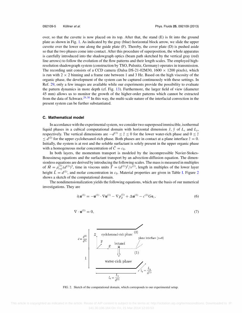
In accordance with the experimental system, we consider two superposed immiscible, isothermalliquid phases in a cubical computational domain with horizontal dimension x, y of Lx and Ly,respectively. The vertical dimensions are −d (1) ≤ z ≤ 0 for the lower water-rich phase and 0 ≤ z≤ d (2) for the upper cyclohexanol-rich phase. Both phases are in contact at a plane interface z = 0.Initially, the system is at rest and the soluble surfactant is solely present in the upper organic phasewith a homogeneous molar concentration of C = c0.
In both layers, the momentum transport is modeled by the incompressible Navier-Stokes-Boussinesq equations and the surfactant transport by an advection-diffusion equation. The dimen-sionless equations are derived by introducing the following scales. The mass is measured in multiplesof M = ρ
(1)re f (d (1))3, time in viscous units T = (d (1))2/ν(1), length in multiples of the lower layer
height L = d (1), and molar concentration in c0. Material properties are given in Table I. Figure 2shows a sketch of the computational domain.
The nondimensionalization yields the following equations, which are the basis of our numericalinvestigations. They are
∂t u(1) = −u(1) · ∇u(1) − ∇ p(1)d + u(1) − c(1)Gez, (6)
∇ · u(1) = 0, (7)
FIG. 2. Sketch of the computational domain, which corresponds to our experimental setup.
This article is copyrighted as indicated in the article. Reuse of AIP content is subject to the terms at: http://scitation.aip.org/termsconditions. Downloaded to IP:
141.30.106.164 On: Fri, 21 Mar 2014 12:03:53
092109-6 Kollner et al. Phys. Fluids 25, 092109 (2013)
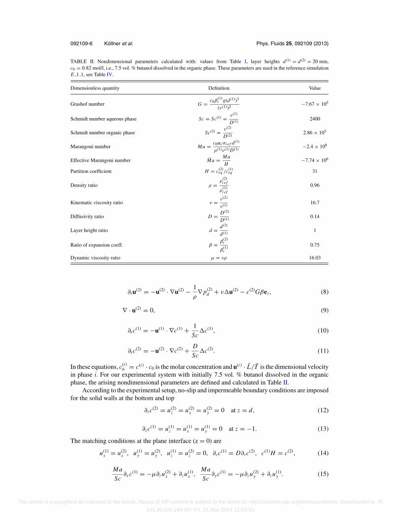
TABLE II. Nondimensional parameters calculated with: values from Table I, layer heights d(1) = d(2) = 20 mm,c0 = 0.82 mol/l, i.e., 7.5 vol. % butanol dissolved in the organic phase. These parameters are used in the reference simulationE 1 1, see Table IV.
Dimensionless quantity Definition Value
Grashof number G = c0β(1)c g(d(1))3
(ν(1))2−7.67 × 10⁵
Schmidt number aqueous phase Sc = Sc(1) = ν(1)
D(1)2400
Schmidt number organic phase Sc(2) = ν(2)
D(2)2.86 × 10⁵
Marangoni number Ma = c0αcσre f d(1)
ρ(1)ν(1) D(1)−2.4 × 10⁸
Effective Marangoni number Ma = Ma
H−7.74 × 10⁶
Partition coefficient H = c(2)eq /c(1)
eq 31
Density ratio ρ =ρ
(2)re f
ρ(1)re f
0.96
Kinematic viscosity ratio ν = ν(2)
ν(1)16.7
Diffusivity ratio D = D(2)
D(1)0.14
Layer height ratio d = d(2)
d(1)1
Ratio of expansion coeff. β = β(2)c
β(1)c
0.75
Dynamic viscosity ratio μ = νρ 16.03
∂t u(2) = −u(2) · ∇u(2) − 1
ρ∇ p(2)
d + νu(2) − c(2)Gβez, (8)
∇ · u(2) = 0, (9)
∂t c(1) = −u(1) · ∇c(1) + 1
Scc(1), (10)
∂t c(2) = −u(2) · ∇c(2) + D
Scc(2). (11)
In these equations, c(i)b = c(i) · c0 is the molar concentration and u(i) · L/T is the dimensional velocity
in phase i. For our experimental system with initially 7.5 vol. % butanol dissolved in the organicphase, the arising nondimensional parameters are defined and calculated in Table II.
According to the experimental setup, no-slip and impermeable boundary conditions are imposedfor the solid walls at the bottom and top
∂zc(2) = u(2)
z = u(2)x = u(2)
y = 0 at z = d, (12)
∂zc(1) = u(1)
z = u(1)x = u(1)
y = 0 at z = −1. (13)
The matching conditions at the plane interface (z = 0) are
u(1)x = u(2)
x , u(1)y = u(2)
y , u(1)z = u(2)
z = 0, ∂zc(1) = D∂zc
(2), c(1) H = c(2), (14)
Ma
Sc∂x c(1) = −μ∂zu(2)
x + ∂zu(1)x ,
Ma
Sc∂yc(1) = −μ∂zu(2)
y + ∂zu(1)y . (15)
This article is copyrighted as indicated in the article. Reuse of AIP content is subject to the terms at: http://scitation.aip.org/termsconditions. Downloaded to IP:
141.30.106.164 On: Fri, 21 Mar 2014 12:03:53
092109-7 Kollner et al. Phys. Fluids 25, 092109 (2013)
These relations arise from the continuity of velocity, the conservation of surfactant in the bulk,Henry’s model, and the stress balance at the interface. The normal stress balance is replaced by thezero vertical velocity condition at the interface. The boundary conditions in the x-y directions areperiodic. These equations are derived comprehensively in Ref. 42.
The shadowgraph technique used in the experiments is mimicked by averaging the horizontalLaplacian of the concentration distribution over both layers,43
s(x, y) = −∫
[−1,d](∂2
x + ∂2y )c(x, t)dz. (16)
The quantity s(x, y) permits a visual comparison of the emerging structures with the experiments.Locations with low values of s(x, y) correspond to a gain of surfactant by horizontal diffusion, thesepoints are usually areas of low concentration. Thus, s(x, y) primarily displays the horizontal surfactantdistribution in the close proximity to the interface, since surfactant gradients are mainly producedthere by interfacial convection. In the later stages of mass transfer, it also includes information furtheraway from the interface. However, note that the experimental shadowgraph records are affected byslight deflections of the interface and nonlinearities of the refractive index as well as of the opticaldevices.
In Sec. III C 3, it is shown that the convection is in the creeping flow regime. For this regime,the momentum balance may be modeled by the time-independent Stokes equations. By additionallyneglecting buoyancy terms, i.e., G = 0 they read
0 = −∇ p(1)d + u(1), (17)
0 = ∇ · u(1), (18)
0 = −∇ p(2)d + μu(2), (19)
0 = ∇ · u(2). (20)
The analysis of Eqs. (17)–(20) reveals that the flow governed by these equations possesses a mirrorsymmetry at the interface for equally sized layers d = 1. Since we use d = 1 in the present study, adeparture from this symmetry can only be due to the action of inertial or buoyancy forces.
D. Initial conditions and self-similarity
In the ideal initial state, the concentration of butanol is uniform in the top layer and zero inthe bottom layer. Therefore, the concentration distribution has no intrinsic length scale apart fromthe layer thickness. This outer length scale does not play any role as long as Marangoni convectionremains localized near the interface. In the present system, this assumption may be valid for timesthat are much shorter than the vertical diffusion time (d(1))2/D(1), which is on the order of 100 h.For such times, we have an effectively unbounded system in the vertical direction. It is thereforeappropriate to choose reference units based on the characteristic interfacial tension difference σ
= |σ refαcc0| computed with the butanol concentration c0. These interface units are independent ofthe layer height. We define them by
Lint = μ(1)ν(1)
σ, (21)
Tint = μ(1)μ(1)ν(1)
(σ )2, (22)
Uint = Lint/Tint = σ
μ(1), (23)
for length, time, and velocity. Mass and the molar concentration are measured in ρ(1)re f · L3
int andc0, respectively. In these units, the non-dimensional equations take a different form compared with
This article is copyrighted as indicated in the article. Reuse of AIP content is subject to the terms at: http://scitation.aip.org/termsconditions. Downloaded to IP:
141.30.106.164 On: Fri, 21 Mar 2014 12:03:53
092109-8 Kollner et al. Phys. Fluids 25, 092109 (2013)
Eqs. (6)–(15) in viscous units. The solute transport equations (10) and (11) and the incompressibilityconstraints remain unchanged. The momentum equations (6) and (8) become
∂t u(1) = −u(1) · ∇u(1) − ∇ p(1)d + u(1) − c(1) Moez, (24)
∂t u(2) = −u(2) · ∇u(2) − ∇ p(2)d
ρ+ νu(2) − c(2) Moβez, (25)
where we have introduced the Morton number
Mo = GSc3
|Ma|3 = c0β(1)c (μ(1))3ν(1)g
(σ )3. (26)
The tangential stress balance (15) becomes
sgn(Ma)∂x c(1) = −μ∂zu(2)x + ∂zu
(1)x , (27)
sgn(Ma)∂yc(1) = −μ∂zu(2)y + ∂zu
(1)y . (28)
It does no longer contain the absolute value of Ma. The other continuity conditions (14) at theinterface retain their form. The remaining boundary conditions (12) and (13) are replaced by
c(2)(z → ∞) = 1, c(1)(z → −∞) = 0, u(±z → ∞) = 0. (29)
The ideal initial conditions are
c(2)(z > 0, t = 0) = 1, c(1)(z < 0, t = 0) = 0, u(z, t = 0) = 0. (30)
When buoyancy effects are absent (Mo = 0), these equations together with their boundary and initialconditions are independent of the initial concentration c0. As a result, the dynamics are invariantwith respect to a change of σ provided length and time are measured in interface units. This exactscaling symmetry is not present with buoyancy. However, for short times buoyancy effects should benegligible, and one should obtain the same evolution for different values of c0. Deviations betweentwo different initial c0 will appear after a certain time on account of the different Morton numbers.
Because of this scaling symmetry, we shall later use interface units when results for differ-ent concentrations are presented and compared. Length, time, or velocity have to be transformedaccording to
lvis · |Ma|Sc
= lint , (31)
tvis · |Ma|2Sc2
= tint , (32)
uvis · Sc
|Ma| = uint . (33)
For convenience, we use a relative Marangoni number
Mar = Ma/(−2.4 × 108), (34)
for the transformation. The reference value −2.4 × 10⁸ in Eq. (34) corresponds to the referencesimulation E_1_1 from Table IV. Times and lengths in viscous units will therefore be multipliedwith Ma2
r and Mar, respectively. These results are then based on what we shall call relative interfaceunits.
Finally, we remark that for Mo = 0 and when σ refαcc0 does not change sign, the problemcontains the parameters Sc, H, ρ, ν, D. These property ratios are essential.
This article is copyrighted as indicated in the article. Reuse of AIP content is subject to the terms at: http://scitation.aip.org/termsconditions. Downloaded to IP:
141.30.106.164 On: Fri, 21 Mar 2014 12:03:53
092109-9 Kollner et al. Phys. Fluids 25, 092109 (2013)
E. Numerical method
The numerical method is pseudospectral. Both planar layers are treated as separate computa-tional domains that are coupled at the interface. In each layer, the fields are expanded in truncatedFourier series in the two periodic horizontal directions x, y. The vertical direction z is expandedin Chebyshev polynomials Tp of order p. The smallest wavenumbers for the x,y directions arekx0 = 2π /lx, ky0 = 2π /ly. For example, the expansion of the vertical velocity in the upper layer,where (x, y, z) ∈ [0, lx] × [0, ly] × [0, d], reads
u(2)z (x, y, z, t) =
Nx /2−1∑m=−Nx /2
Ny/2−1∑n=−Ny/2
Nz∑p=0
eimkx0x+inky0 y Tp(2z/d − 1)u(2);mnpz . (35)
The data output in physical space and the calculation of the nonlinear terms is done on the collocationpoints, e.g., for layer (2) they are(
xi , y j , zk
)=
(i · lx/Nx , j · ly/Ny, d · 0.5(1 + cos(kπ/N (2)
z ))), (36)
with i ∈ {0, 1, . . . , Nx }, j ∈ {0, 1, . . . , Ny}, k ∈ {0, 1, . . . , N (2)z }. The velocity field is represented
through the poloidal-toroidal decomposition, whereby incompressibility is automatically satisfied.Parallelization with message passing interface (MPI) is based on a domain decomposition in onehorizontal direction. The number of grid points in each direction is a power of two because onlybase two FFTs are used.
The numerical code has been used in previous investigations of thermal interfacial convectionin two-layer systems and is described in Ref. 44. For the present study, temperature is replaced bythe concentration field, and the respective boundary conditions for this field are modified. We haveincluded dealiasing in the horizontal directions for kx or ky bigger than three fourth of their maximumabsolute value. The time step is adjusted according to the current grid CFL number,
Cg = max
{uxδt
x,
uyδt
y,
uzδt
z
}. (37)
This number is calculated every time step by dividing the local displacement uαδt by the collocationgrid sizes x, y, z. We force Cg to be smaller than a constant Cb and to be larger than Cb/2, i.e.,
Cb/2 ≤ Cg ≤ Cb. (38)
Specifically, if Cg > Cb the next time step δt is set such that Cg = Cb/2 and if Cg < Cb/2 the nexttime step δt is set such that Cg = Cb. Additionally, we require the time step δt to be smaller thanδtmax.
The standard initial conditions are set as follows. The velocity field is initialized (t = 0) withpseudorandom numbers for uz ; (∇ × u) · ez , which are uniformly distributed between [0, 1 × 10⁻³],and zero mean flow. The surfactant is initialized with a homogeneous concentration of unity forlayer 2, i.e., c(2) = 1, and zero for layer 1, i.e., c(1) = 0. For the simulation with the lowest soluteconcentration S_3_1 (for notation see Table IV), we used stronger noise to lower the onset time ofconvection. In particular, uz ; (∇ × u) · ez is initialized with values in [0, 1 × 10⁻²] and the soluteis initialized by c(1) ∈ [0, 1 × 10⁻³], c(2) ∈ 1 + [0, 1 × 10⁻³]. The reference simulation E_1_1consumed approximately 650 GB main memory. On 512 processors, it took 1.24 × 10⁵ core hoursfor the simulation to be advanced until t = 2.07 with 17 800 time steps. They are governed by theCourant-Friedrichs-Lewy (CFL) restriction given in Eq. (37) except before the onset of convection.
The numerical resolution requirements turned out to be quite severe. A very high verticalresolution near the interface was required to properly capture the vertical structures, cf. the profilesin Fig. 6. The horizontal resolutions (Nx, Ny) are set to resolve the similar fine solute structures in thehorizontal directions. We verified grid convergence for selected test cases, cf. Table III, by changingthe number of expansion coefficients in the horizontal Nx, Ny and vertical direction N (1)
z , N (2)z .
Furthermore, we changed the maximum time step δtmax and the bound for the grid CFL number Cb.To provide comparability, all test simulations are based on exactly the same initial conditions. Forthat purpose, the standard random initial conditions are generated for the case of lowest resolution,
This article is copyrighted as indicated in the article. Reuse of AIP content is subject to the terms at: http://scitation.aip.org/termsconditions. Downloaded to IP:
141.30.106.164 On: Fri, 21 Mar 2014 12:03:53
092109-10 Kollner et al. Phys. Fluids 25, 092109 (2013)
TABLE III. Overview of test simulations with exactly the same initial conditions but changed numerical parameters. Forthese test simulations, we use the physical parameters from Table II, i.e., corresponding to E_1_1, E_1_2 of Table IV.
# Cb δtmax lx(Ny) ly(Ny) N (1)z N (2)
z Num. stability Vis. oscill.
N_0 0.3 5 × 10⁻⁴ 0.3(256) 0.3(256) 64 64 Unstable . . .N_1 0.3 5 × 10⁻⁴ 0.3(256) 0.3(256) 512 256 Unstable . . .N_2 0.3 5 × 10⁻⁴ 0.3(512) 0.3(512) 512 256 Stable YesN_3 0.3 5 × 10⁻⁴ 0.3(1024) 0.3(1024) 512 256 Stable NoN_4 0.3 5 × 10⁻⁴ 0.3(2048) 0.3(2048) 512 256 Stable NoN_5 0.3 5 × 10⁻⁴ 0.3(1024) 0.3(1024) 64 64 Unstable . . .N_6 0.3 5 × 10⁻⁴ 0.3(1024) 0.3(1024) 128 128 Unstable . . .N_7 0.3 5 × 10⁻⁴ 0.3(1024) 0.3(1024) 256 256 Stable NoN_3 0.3 5 × 10⁻⁴ 0.3(1024) 0.3(1024) 512 256 Stable NoN_8 0.3 5 × 10⁻⁴ 0.3(1024) 0.3(1024) 512 512 Stable NoN_9 0.3 1 × 10⁻² 0.3(1024) 0.3(1024) 512 256 Stable/no convection . . .N_10 0.3 1 × 10⁻³ 0.3(1024) 0.3(1024) 512 256 Stable NoN_3 0.3 5 × 10⁻⁴ 0.3(1024) 0.3(1024) 512 256 Stable NoN_11 0.3 1 × 10⁻⁴ 0.3(1024) 0.3(1024) 512 256 Stable NoN_12 0.3 5 × 10⁻⁵ 0.3(1024) 0.3(1024) 512 256 Stable NoN_13 0.1 5 × 10⁻⁴ 0.3(1024) 0.3(1024) 512 256 Stable NoN_3 0.3 5 × 10⁻⁴ 0.3(1024) 0.3(1024) 512 256 Stable NoN_14 0.6 5 × 10⁻⁴ 0.3(1024) 0.3(1024) 512 256 Stable NoN_15 1 5 × 10⁻⁴ 0.3(1024) 0.3(1024) 512 256 Stable Early phase
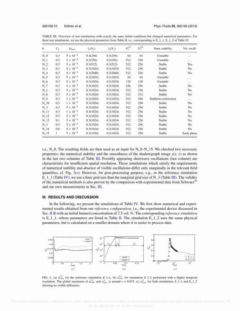
i.e., N_0. The resulting fields are then used as an input for N_0–N_15. We checked two necessaryproperties: the numerical stability and the smoothness of the shadowgraph image s(x, y) as shownin the last two columns of Table III. Possibly appearing shortwave oscillations (last column) arecharacteristic for insufficient spatial resolution. Those simulations which satisfy the requirementsof numerical stability and absence of visible oscillations differ only marginally in the relevant fieldquantities, cf. Fig. 3(c). However, for post-processing purpose, e.g., in the reference simulationE_1_1 (Table IV), we use a finer grid size than the marginal grid size of N_3 (Table III). The validityof the numerical methods is also proven by the comparison with experimental data from Schwarz29
and our own measurements in Sec. III.
III. RESULTS AND DISCUSSION
In the following, we present the simulations of Table IV. We first show numerical and experi-mental results obtained from our reference configuration, i.e., the experimental device discussed inSec. II B with an initial butanol concentration of 7.5 vol. %. The corresponding reference simulationis E_1_1, whose parameters are listed in Table II. The simulation E_1_2 uses the same physicalparameters, but is calculated on a smaller domain where it is easier to process data.
0 0.5 1 1.5 20
0.005
0.01
0.015
0.02
0.025
Time
u rms
(i)
Layer 1Layer 2
(a)
0 0.05 0.1 0.1510
−10
10−8
10−6
10−4
10−2
Time
u rms
(i)
Layer 1Layer 2
Ia Ib II
(b)
10−2
10−1
100
0
0.2
0.4
0.6
0.8
1
Time
urm
sS
E_1_1E_1_2
(c)
FIG. 3. (a) u(i)rms for the reference simulation E 1 1, (b) u(i)
rms for simulation E 1 2 performed with a higher temporalresolution. The global maximum of u(i)
rms and uSrms is around t = 0.053. (c) uS
rms for both simulations E 1 1 and E_1_2showing no visible difference.
This article is copyrighted as indicated in the article. Reuse of AIP content is subject to the terms at: http://scitation.aip.org/termsconditions. Downloaded to IP:
141.30.106.164 On: Fri, 21 Mar 2014 12:03:53
092109-11 Kollner et al. Phys. Fluids 25, 092109 (2013)
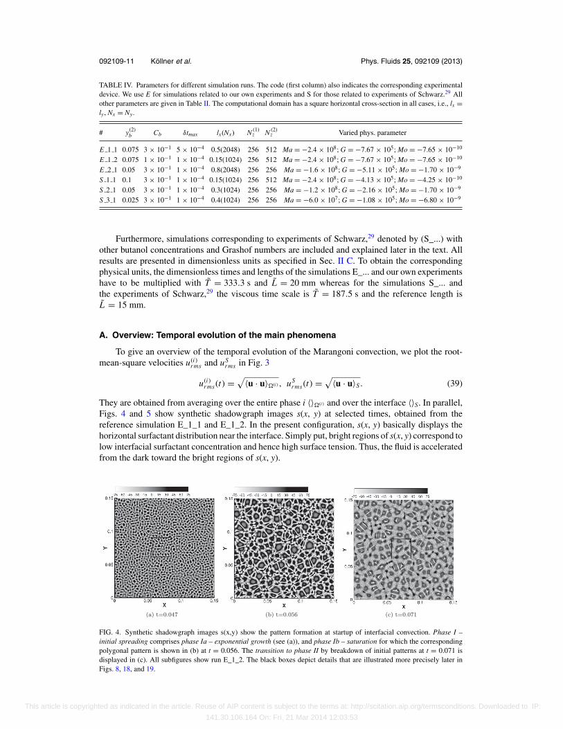
TABLE IV. Parameters for different simulation runs. The code (first column) also indicates the corresponding experimentaldevice. We use E for simulations related to our own experiments and S for those related to experiments of Schwarz.29 Allother parameters are given in Table II. The computational domain has a square horizontal cross-section in all cases, i.e., lx =ly, Nx = Ny.
# y(2)b Cb δtmax lx(Nx) N (1)
z N (2)z Varied phys. parameter
E 1 1 0.075 3 × 10⁻¹ 5 × 10⁻⁴ 0.5(2048) 256 512 Ma = −2.4 × 10⁸; G = −7.67 × 10⁵; Mo = −7.65 × 10⁻¹⁰
E 1 2 0.075 1 × 10⁻¹ 1 × 10⁻⁴ 0.15(1024) 256 512 Ma = −2.4 × 10⁸; G = −7.67 × 10⁵; Mo = −7.65 × 10⁻¹⁰
E 2 1 0.05 3 × 10⁻¹ 1 × 10⁻⁴ 0.8(2048) 256 256 Ma = −1.6 × 10⁸; G = −5.11 × 10⁵; Mo = −1.70 × 10⁻⁹
S 1 1 0.1 3 × 10⁻¹ 1 × 10⁻⁴ 0.15(1024) 256 512 Ma = −2.4 × 10⁸; G = −4.13 × 10⁵; Mo = −4.25 × 10⁻¹⁰
S 2 1 0.05 3 × 10⁻¹ 1 × 10⁻⁴ 0.3(1024) 256 256 Ma = −1.2 × 10⁸; G = −2.16 × 10⁵; Mo = −1.70 × 10⁻⁹
S 3 1 0.025 3 × 10⁻¹ 1 × 10⁻⁴ 0.4(1024) 256 256 Ma = −6.0 × 10⁷; G = −1.08 × 10⁵; Mo = −6.80 × 10⁻⁹
Furthermore, simulations corresponding to experiments of Schwarz,29 denoted by (S_...) withother butanol concentrations and Grashof numbers are included and explained later in the text. Allresults are presented in dimensionless units as specified in Sec. II C. To obtain the correspondingphysical units, the dimensionless times and lengths of the simulations E_... and our own experimentshave to be multiplied with T = 333.3 s and L = 20 mm whereas for the simulations S_... andthe experiments of Schwarz,29 the viscous time scale is T = 187.5 s and the reference length isL = 15 mm.
A. Overview: Temporal evolution of the main phenomena
To give an overview of the temporal evolution of the Marangoni convection, we plot the root-mean-square velocities u(i)
rms and uSrms in Fig. 3
u(i)rms(t) =
√〈u · u〉�(i) , uS
rms(t) =√
〈u · u〉S. (39)
They are obtained from averaging over the entire phase i 〈〉�(i) and over the interface 〈〉S. In parallel,Figs. 4 and 5 show synthetic shadowgraph images s(x, y) at selected times, obtained from thereference simulation E_1_1 and E_1_2. In the present configuration, s(x, y) basically displays thehorizontal surfactant distribution near the interface. Simply put, bright regions of s(x, y) correspond tolow interfacial surfactant concentration and hence high surface tension. Thus, the fluid is acceleratedfrom the dark toward the bright regions of s(x, y).
(a) t=0.047 (b) t=0.056 (c) t=0.071
FIG. 4. Synthetic shadowgraph images s(x,y) show the pattern formation at startup of interfacial convection. Phase I –initial spreading comprises phase Ia – exponential growth (see (a)), and phase Ib – saturation for which the correspondingpolygonal pattern is shown in (b) at t = 0.056. The transition to phase II by breakdown of initial patterns at t = 0.071 isdisplayed in (c). All subfigures show run E_1_2. The black boxes depict details that are illustrated more precisely later inFigs. 8, 18, and 19.
This article is copyrighted as indicated in the article. Reuse of AIP content is subject to the terms at: http://scitation.aip.org/termsconditions. Downloaded to IP:
141.30.106.164 On: Fri, 21 Mar 2014 12:03:53
092109-12 Kollner et al. Phys. Fluids 25, 092109 (2013)
(a) t=0.16 (b) t=0.51
(c) t=1.44 (d) t=2.092
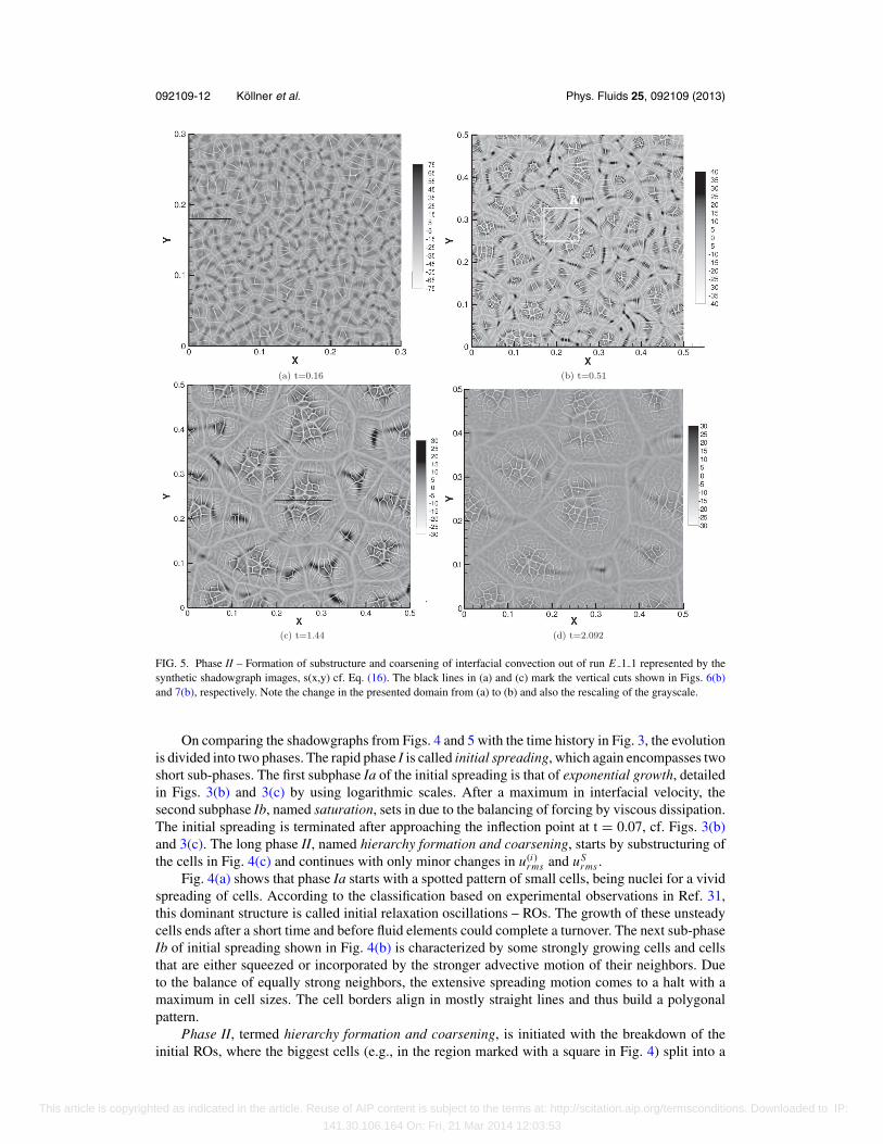
FIG. 5. Phase II – Formation of substructure and coarsening of interfacial convection out of run E 1 1 represented by thesynthetic shadowgraph images, s(x,y) cf. Eq. (16). The black lines in (a) and (c) mark the vertical cuts shown in Figs. 6(b)and 7(b), respectively. Note the change in the presented domain from (a) to (b) and also the rescaling of the grayscale.
On comparing the shadowgraphs from Figs. 4 and 5 with the time history in Fig. 3, the evolutionis divided into two phases. The rapid phase I is called initial spreading, which again encompasses twoshort sub-phases. The first subphase Ia of the initial spreading is that of exponential growth, detailedin Figs. 3(b) and 3(c) by using logarithmic scales. After a maximum in interfacial velocity, thesecond subphase Ib, named saturation, sets in due to the balancing of forcing by viscous dissipation.The initial spreading is terminated after approaching the inflection point at t = 0.07, cf. Figs. 3(b)and 3(c). The long phase II, named hierarchy formation and coarsening, starts by substructuring ofthe cells in Fig. 4(c) and continues with only minor changes in u(i)
rms and uSrms .
Fig. 4(a) shows that phase Ia starts with a spotted pattern of small cells, being nuclei for a vividspreading of cells. According to the classification based on experimental observations in Ref. 31,this dominant structure is called initial relaxation oscillations – ROs. The growth of these unsteadycells ends after a short time and before fluid elements could complete a turnover. The next sub-phaseIb of initial spreading shown in Fig. 4(b) is characterized by some strongly growing cells and cellsthat are either squeezed or incorporated by the stronger advective motion of their neighbors. Dueto the balance of equally strong neighbors, the extensive spreading motion comes to a halt with amaximum in cell sizes. The cell borders align in mostly straight lines and thus build a polygonalpattern.
Phase II, termed hierarchy formation and coarsening, is initiated with the breakdown of theinitial ROs, where the biggest cells (e.g., in the region marked with a square in Fig. 4) split into a
This article is copyrighted as indicated in the article. Reuse of AIP content is subject to the terms at: http://scitation.aip.org/termsconditions. Downloaded to IP:
141.30.106.164 On: Fri, 21 Mar 2014 12:03:53
092109-13 Kollner et al. Phys. Fluids 25, 092109 (2013)
network of smaller polygonal, more persistent cells, cf. Fig. 4(c). Typically, this pattern is the firstone visible in experiments. The initial spreading phase I is hidden in the experiments due to its shortduration and the overlap with superposing the layers.
In Figs. 5(a) and 5(b), the more vigorous cells grow and develop an internal substructure ofsmaller Marangoni cells. In line with Ref. 31, we term these large-scale patterns Marangoni rollcells of second order, i.e., RC-IIs. The enclosed cellular substructures and the individual cellswithout substructure are called Marangoni roll cells of first order, RC-Is.31 They constitute thelowest level of hierarchy. In the early stage, presented in Fig. 5(a), an unambiguous assignment ofthe individual cells to a hierarchy order is hardly possible due to the continuous evolution in lengthscales. However, from Fig. 5(b)–5(d) the beginning spatial hierarchy formation is clearly discerniblebecause the RC-IIs steadily increase in size and the separation of scales between RC-Is and RC-IIsgrows.
In the thesis of Schwarz,29 two experimental images (Figs. 16 and 18 in Ref. 29) correspondingto parameters of (S_1_1) and the time of Figs. 5(a) and 5(c) can be found. They agree remarkablygood regarding the visual nature and the general development of the structures, which demonstratesthat the simulated patterns are not restricted to our set-up. Fig. 13 shows corresponding images fromour own experiments.
Another, different type of pattern can be identified in Figs. 5(b)–5(d) and Figs. 13(b) and 13(c).Particularly in those RC-IIs that are about to shrink and disappear, e.g., white A mark in Fig. 5(b),arrays of aligned, straight surfactant fronts are visible. According to its wavelike appearance, thispattern is referred to as relaxation oscillation waves – ROWs.31 A preliminary characterization ofROWs is given in Ref. 45. It will be extended in future work.
B. Velocity and surfactant distribution of the generic structures
We study the generic structures RO, RC-I, and RC-II, identified in Sec. III A, by the examinationof the tightly coupled surfactant and velocity distributions. For this purpose, both vertical andhorizontal cuts through the patterns are used, which are hardly accessible in the experiment.
1. Vertical sections
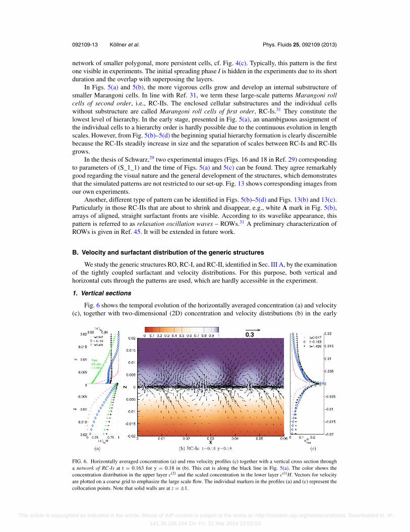
Fig. 6 shows the temporal evolution of the horizontally averaged concentration (a) and velocity(c), together with two-dimensional (2D) concentration and velocity distributions (b) in the early
FIG. 6. Horizontally averaged concentration (a) and rms velocity profiles (c) together with a vertical cross section througha network of RC-Is at t = 0.163 for y = 0.18 in (b). This cut is along the black line in Fig. 5(a). The color shows theconcentration distribution in the upper layer c(2) and the scaled concentration in the lower layer c(1)H. Vectors for velocityare plotted on a coarse grid to emphasize the large scale flow. The individual markers in the profiles (a) and (c) represent thecollocation points. Note that solid walls are at z = ±1.
This article is copyrighted as indicated in the article. Reuse of AIP content is subject to the terms at: http://scitation.aip.org/termsconditions. Downloaded to IP:
141.30.106.164 On: Fri, 21 Mar 2014 12:03:53
092109-14 Kollner et al. Phys. Fluids 25, 092109 (2013)
phase II. The velocity field of the three-dimensional (3D) polygonal cells is of a toroidal-likestructure,53 manifesting itself as a double vortex in the 2D section. The concentration profiles inFig. 6(a) correspond to characteristic states of run E_1_1, namely, (i) the state of emerging initialROs at t = 0.047, cf. Fig. 4(a), (ii) a polygonal network of RC-Is at t = 0.163, cf. Fig. 5(a), wheresome of the cells already begin to develop irregular small substructures, and (iii) large RC-II att = 1.436, cf. Fig. 5(c). Note that the profiles are the horizontal averages over the whole x-y plane.The curves with light gray plus signs (+) depict a purely diffusive evolution, i.e., starting with idealinitial conditions without noise. The individual data points in the 1D profiles correspond to thecollocation points in z-direction, cf. Eq. (36).
In both domains, the initially thin concentration boundary layers grow with time as the masstransfer proceeds and the convection patterns increase in size. The interface concentration rises, andthe lower phase is progressively saturated with solute. In the upper phase, the bulk concentrationis necessarily lowered, which leads to intersecting concentration profiles at different times there.Furthermore, the graphs illustrate the influence of the diffusivity ratio on the concentration profiles.Due to the distinctly higher diffusivity in the lower phase (D(2)/D(1) = 0.14), Marangoni convectiononly marginally affects the shape of the concentration profiles there, but additional convectionintensifies mixing of solute. This is exemplified by the difference between the light gray (+) curvefor pure diffusion and the black (+) curve with convection at z < 0 in Fig. 6(a).
In the upper phase (z > 0) in Figs. 6(a) and 7(a), the concentration profiles (t = 0.163, t =1.436) have two characteristic gradients separated by inflection points. The first gradient near theinterface is formed by the combined action of small-scale flow of RC-Is, large-scale advection byRC-IIs, and pure diffusive transport near the interface. The second gradient connects the mixed fluidnear the interface with almost unchanged bulk fluid. This situation is visualized by the vertical crosssection of the RC-Is pattern in Fig. 6(b) and the large-scale RC-II in Fig. 7(b). In both of these 2Dconcentration distributions, the mixed fluid appears in light gray in the upper phase. It extends up toz ≈ 0.01 for t = 0.163 in Fig. 6(a) and z ≈ 0.04 for t = 1.436 in Fig. 7(a).
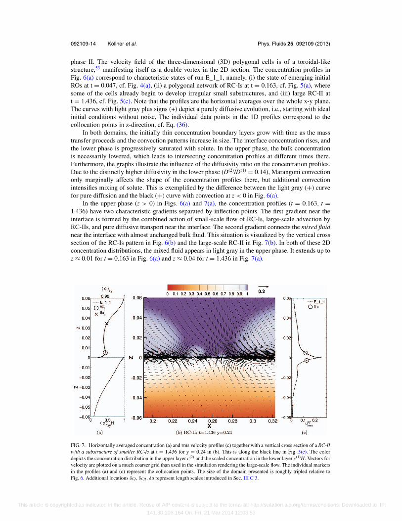
FIG. 7. Horizontally averaged concentration (a) and rms velocity profiles (c) together with a vertical cross section of a RC-IIwith a substructure of smaller RC-Is at t = 1.436 for y = 0.24 in (b). This is along the black line in Fig. 5(c). The colordepicts the concentration distribution in the upper layer c(2) and the scaled concentration in the lower layer c(1)H. Vectors forvelocity are plotted on a much coarser grid than used in the simulation rendering the large-scale flow. The individual markersin the profiles (a) and (c) represent the collocation points. The size of the domain presented is roughly tripled relative toFig. 6. Additional locations δcI, δcII, δu represent length scales introduced in Sec. III C 3.
This article is copyrighted as indicated in the article. Reuse of AIP content is subject to the terms at: http://scitation.aip.org/termsconditions. Downloaded to IP:
141.30.106.164 On: Fri, 21 Mar 2014 12:03:53
092109-15 Kollner et al. Phys. Fluids 25, 092109 (2013)
The cross-section in Fig. 7(b) explains the local maximum in the concentration profile ofFig. 7(a) at z ≈ 0.005, which results from the general flow structure of the RC-IIs in this system.The jet-like inflow in the center carries surfactant-rich fluid from the deeper bulk regions toward theinterface, where the flow is diverted parallel to the interface. The fluid depleted of butanol howeveraccumulates in the rather flat vortices at the cell boundaries forming the surfactant-poor plumes witha local minimum of concentration at z ≈ 0.02.
The velocity profiles
uxyrms(z) = √〈u · u〉xy (40)
for the same states as the concentration profiles are shown in Figs. 6(c) and 7(c). In line with theconcentration profiles, the zone influenced by the interfacial convection reaches farther into the bulkphases as time advances. For large times (t = 1.436), the rms velocity reaches a local maximum atsome distance from the interface, clearly visible only in the lower aqueous phase at z ≈ −0.015 inFig. 7(c). This maximum can be assigned to the flow of the large RC-II-vortex in Fig. 7(b). The shapeof the presented velocity profile with the global maximum at the interface and the local maximumof the RC-II vortex qualitatively agrees with measured velocity profiles of substructured Marangonicells in a Hele-Shaw geometry.46
The mirror symmetry of the flow, discussed at the end of Sec. II C, is disturbed by the actionof buoyancy arising in the course of mass transfer. This was already made visible by the differencebetween rms velocity of both layers in Fig. 3(a). From Ref. 47, it is expected that the increasingstabilizing density stratification confines the roll cell convection to a more narrow zone adjacent tothe interface. Because the velocity distribution in Figs. 7(b) and 7(c) reaches further into the upperorganic bulk phase, the confining effect seems to be more pronounced in the lower aqueous phase.This might be a result of the higher density change in the aqueous phase ρ
(1)re f β
(1)c , see Table I. We
shall investigate these questions in future work.
2. Horizontal sections
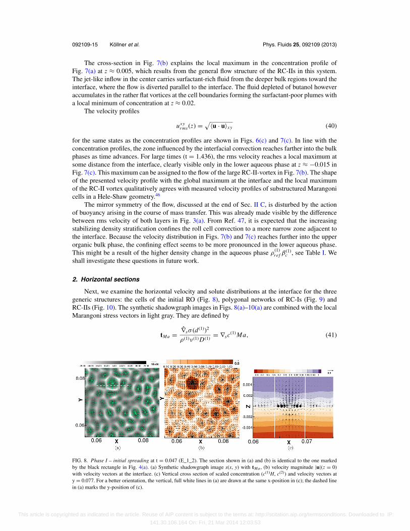
Next, we examine the horizontal velocity and solute distributions at the interface for the threegeneric structures: the cells of the initial RO (Fig. 8), polygonal networks of RC-Is (Fig. 9) andRC-IIs (Fig. 10). The synthetic shadowgraph images in Figs. 8(a)–10(a) are combined with the localMarangoni stress vectors in light gray. They are defined by
tMa = ∇sσ (d (1))2
ρ(1)ν(1) D(1)= ∇sc(1) Ma, (41)
FIG. 8. Phase I – initial spreading at t = 0.047 (E_1_2). The section shown in (a) and (b) is identical to the one markedby the black rectangle in Fig. 4(a). (a) Synthetic shadowgraph image s(x, y) with tMa , (b) velocity magnitude |u|(z = 0)with velocity vectors at the interface. (c) Vertical cross section of scaled concentration (c(1)H, c(2)) and velocity vectors aty = 0.077. For a better orientation, the vertical, full white lines in (a) are drawn at the same x-position in (c); the dashed linein (a) marks the y-position of (c).
This article is copyrighted as indicated in the article. Reuse of AIP content is subject to the terms at: http://scitation.aip.org/termsconditions. Downloaded to IP:
141.30.106.164 On: Fri, 21 Mar 2014 12:03:53
092109-16 Kollner et al. Phys. Fluids 25, 092109 (2013)
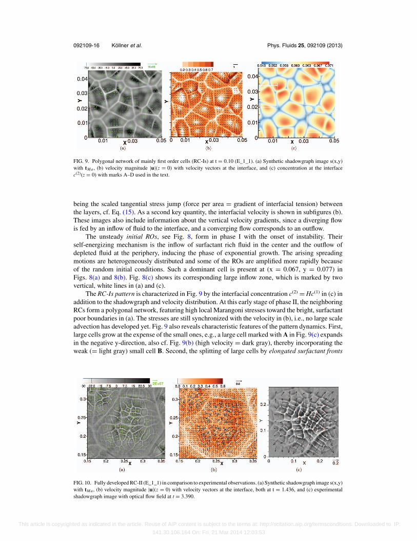
FIG. 9. Polygonal network of mainly first order cells (RC-Is) at t = 0.10 (E_1_1). (a) Synthetic shadowgraph image s(x,y)with tMa , (b) velocity magnitude |u|(z = 0) with velocity vectors at the interface, and (c) concentration at the interfacec(2)(z = 0) with marks A–D used in the text.
being the scaled tangential stress jump (force per area = gradient of interfacial tension) betweenthe layers, cf. Eq. (15). As a second key quantity, the interfacial velocity is shown in subfigures (b).These images also include information about the vertical velocity gradients, since a diverging flowis fed by an inflow of fluid to the interface, and a converging flow corresponds to an outflow.
The unsteady initial ROs, see Fig. 8, form in phase I with the onset of instability. Theirself-energizing mechanism is the inflow of surfactant rich fluid in the center and the outflow ofdepleted fluid at the periphery, inducing the phase of exponential growth. The arising spreadingmotions are heterogeneously distributed and some of the ROs are amplified more rapidly becauseof the random initial conditions. Such a dominant cell is present at (x = 0.067, y = 0.077) inFigs. 8(a) and 8(b). Fig. 8(c) shows its corresponding large inflow zone, which is marked by twovertical, white lines in (a) and (c).
The RC-Is pattern is characterized in Fig. 9 by the interfacial concentration c(2) = Hc(1) in (c) inaddition to the shadowgraph and velocity distribution. At this early stage of phase II, the neighboringRCs form a polygonal network, featuring high local Marangoni stresses toward the bright, surfactantpoor boundaries in (a). The stresses are still synchronized with the velocity in (b), i.e., no large scaleadvection has developed yet. Fig. 9 also reveals characteristic features of the pattern dynamics. First,large cells grow at the expense of the small ones, e.g., a large cell marked with A in Fig. 9(c) expandsin the negative y-direction, also cf. Fig. 9(b) (high velocity = dark gray), thereby incorporating theweak (= light gray) small cell B. Second, the splitting of large cells by elongated surfactant fronts
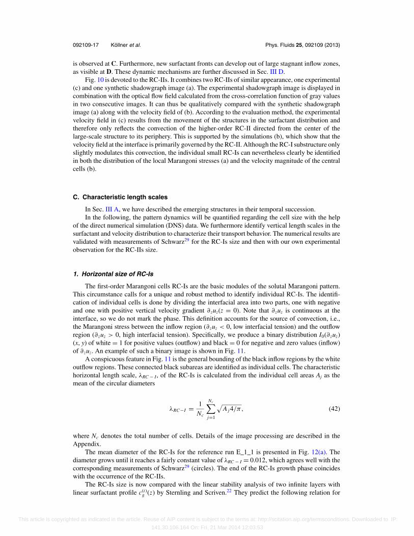
FIG. 10. Fully developed RC-II (E_1_1) in comparison to experimental observations. (a) Synthetic shadowgraph image s(x,y)with tMa , (b) velocity magnitude |u|(z = 0) with velocity vectors at the interface, both at t = 1.436, and (c) experimentalshadowgraph image with optical flow field at t = 3.390.
This article is copyrighted as indicated in the article. Reuse of AIP content is subject to the terms at: http://scitation.aip.org/termsconditions. Downloaded to IP:
141.30.106.164 On: Fri, 21 Mar 2014 12:03:53
092109-17 Kollner et al. Phys. Fluids 25, 092109 (2013)
is observed at C. Furthermore, new surfactant fronts can develop out of large stagnant inflow zones,as visible at D. These dynamic mechanisms are further discussed in Sec. III D.
Fig. 10 is devoted to the RC-IIs. It combines two RC-IIs of similar appearance, one experimental(c) and one synthetic shadowgraph image (a). The experimental shadowgraph image is displayed incombination with the optical flow field calculated from the cross-correlation function of gray valuesin two consecutive images. It can thus be qualitatively compared with the synthetic shadowgraphimage (a) along with the velocity field of (b). According to the evaluation method, the experimentalvelocity field in (c) results from the movement of the structures in the surfactant distribution andtherefore only reflects the convection of the higher-order RC-II directed from the center of thelarge-scale structure to its periphery. This is supported by the simulations (b), which show that thevelocity field at the interface is primarily governed by the RC-II. Although the RC-I substructure onlyslightly modulates this convection, the individual small RC-Is can nevertheless clearly be identifiedin both the distribution of the local Marangoni stresses (a) and the velocity magnitude of the centralcells (b).
C. Characteristic length scales
In Sec. III A, we have described the emerging structures in their temporal succession.In the following, the pattern dynamics will be quantified regarding the cell size with the help
of the direct numerical simulation (DNS) data. We furthermore identify vertical length scales in thesurfactant and velocity distribution to characterize their transport behavior. The numerical results arevalidated with measurements of Schwarz29 for the RC-Is size and then with our own experimentalobservation for the RC-IIs size.
1. Horizontal size of RC-Is
The first-order Marangoni cells RC-Is are the basic modules of the solutal Marangoni pattern.This circumstance calls for a unique and robust method to identify individual RC-Is. The identifi-cation of individual cells is done by dividing the interfacial area into two parts, one with negativeand one with positive vertical velocity gradient ∂zuz(z = 0). Note that ∂zuz is continuous at theinterface, so we do not mark the phase. This definition accounts for the source of convection, i.e.,the Marangoni stress between the inflow region (∂zuz < 0, low interfacial tension) and the outflowregion (∂zuz > 0, high interfacial tension). Specifically, we produce a binary distribution I0(∂zuz)(x, y) of white = 1 for positive values (outflow) and black = 0 for negative and zero values (inflow)of ∂zuz. An example of such a binary image is shown in Fig. 11.
A conspicuous feature in Fig. 11 is the general bounding of the black inflow regions by the whiteoutflow regions. These connected black subareas are identified as individual cells. The characteristichorizontal length scale, λRC − I, of the RC-Is is calculated from the individual cell areas Aj as themean of the circular diameters
λRC−I = 1
Nc
Nc∑j=1
√A j 4/π, (42)
where Nc denotes the total number of cells. Details of the image processing are described in theAppendix.
The mean diameter of the RC-Is for the reference run E_1_1 is presented in Fig. 12(a). Thediameter grows until it reaches a fairly constant value of λRC − I = 0.012, which agrees well with thecorresponding measurements of Schwarz29 (circles). The end of the RC-Is growth phase coincideswith the occurrence of the RC-IIs.
The RC-Is size is now compared with the linear stability analysis of two infinite layers withlinear surfactant profile c(i)
g (z) by Sternling and Scriven.22 They predict the following relation for
This article is copyrighted as indicated in the article. Reuse of AIP content is subject to the terms at: http://scitation.aip.org/termsconditions. Downloaded to IP:
141.30.106.164 On: Fri, 21 Mar 2014 12:03:53
092109-18 Kollner et al. Phys. Fluids 25, 092109 (2013)
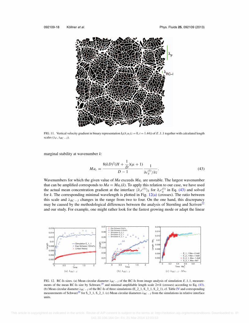
FIG. 11. Vertical velocity gradient in binary representation I0(∂zuz(z = 0, t = 1.44)) of E 1 1 together with calculated lengthscales (λF, λRC − I).
marginal stability at wavenumber k:
Mac =8(k D)2(H + 1
D)(μ + 1)
D − 1
1
∂c(1)g /∂z
. (43)
Wavenumbers for which the given value of Ma exceeds Mac are unstable. The largest wavenumberthat can be amplified corresponds to Ma = Mac(k). To apply this relation to our case, we have usedthe actual mean concentration gradient at the interface 〈∂zc(1)〉S for ∂zc(1)
g in Eq. (43) and solvedfor k. The corresponding minimal wavelength is plotted in Fig. 12(a) (crosses). The ratio betweenthis scale and λRC − I changes in the range from two to four. On the one hand, this discrepancymay be caused by the methodological differences between the analysis of Sternling and Scriven22
and our study. For example, one might rather look for the fastest growing mode or adapt the linear
0 0.5 1 1.5 20
0.002
0.004
0.006
0.008
0.01
0.012
0.014
0.016
Time
Leng
th
Simulation E_1_1Exp Schwarz 10Vol%Linear theory
(a) λRC−I
0 0.5 1 1.5 20
0.01
0.02
0.03
0.04
0.05
0.06
0.07
Time
Leng
th
Exp Schwarz 5Vol%Exp Schwarz 2.5Vol%Simulation S_3_1Simulation S_2_1Simulation E_2_1
(b) λRC−I
0 0.2 0.4 0.6 0.8 10
0.002
0.004
0.006
0.008
0.01
0.012
0.014
0.016
Time ⋅ Mar2
Leng
th ⋅
Ma r
E_1_1 Ma=−2.4e8E_2_1 Ma=−1.6e8S_2_1, Ma=−1.2e8S_3_1, Ma=−6e7
(c) λRC−I · Mar
FIG. 12. RC-Is sizes. (a) Mean circular diameter λRC − I of the RC-Is from image analysis of simulation E 1 1, measure-ments of the mean RC-Is size by Schwarz,29 and minimal amplifiable length scale 2π /k (crosses) according to Eq. (43).(b) Mean circular diameter λRC − I of the RC-Is of three simulations (E_2_1, S_3_1, S_2_1), cf. Table IV and correspondingmeasurements of Schwarz29 for S_3_1, S_2_1. (c) Mean circular diameters λRC − I from the simulations in relative interfaceunits.
This article is copyrighted as indicated in the article. Reuse of AIP content is subject to the terms at: http://scitation.aip.org/termsconditions. Downloaded to IP:
141.30.106.164 On: Fri, 21 Mar 2014 12:03:53
092109-19 Kollner et al. Phys. Fluids 25, 092109 (2013)
diffusive profile to a more realistic one. On the other hand, a part of this deviation might be due tothe transient substructuring that is manifested in the white spots in the middle of several RC-Is inFig. 11. Nevertheless, relation (43) provides a useful lower bound for the smallest length scale.
For a further comparison of the RC-I sizes, we have performed simulations corresponding toexperiments of Schwarz29 with lower butanol concentrations y(2)
b = 0.025 (S_3_1) and y(2)b = 0.05
(S_2_1), cf. Table IV. There is a clear trend toward larger RC-Is with decreasing |Ma|, which isreflected both in the experiment29 and simulation when considering Fig. 12(b) with Fig. 12(a).Note that simulation S_3_1 had to be conducted with stronger initial perturbations to match thetime for the onset of interfacial convection according to the experiments for this low butanolconcentration. However, even under these conditions, the simulation S_3_1 shows a significantlyretarded growth phase, see (+) curve in Fig. 12(b). The data from simulation S_2_1 (dotted curvegray) and experiment (circles) for y(2)
b = 0.05 again agree fairly well. Also, the simulation E_2_1with |Ma| = 1.6 × 10⁸ between the values of E_1_1 and S_3_1 corroborates the continuous trendto smaller RC-Is with increasing |Ma|. These observations are also in line with the self-similarevolution for different initial concentrations. Fig. 12(c) shows an effectively identical behavior ofthe RC-I sizes for different concentrations when relative interface units are used. This includessimulation S_3_1. For this reason, the differences in the early evolution between our simulationsand experiments by Schwarz29, 30 cannot be explained in a straightforward way. They may be causedby the superposition procedure for creating the initial state in the experiments.
2. Horizontal size of RC-IIs
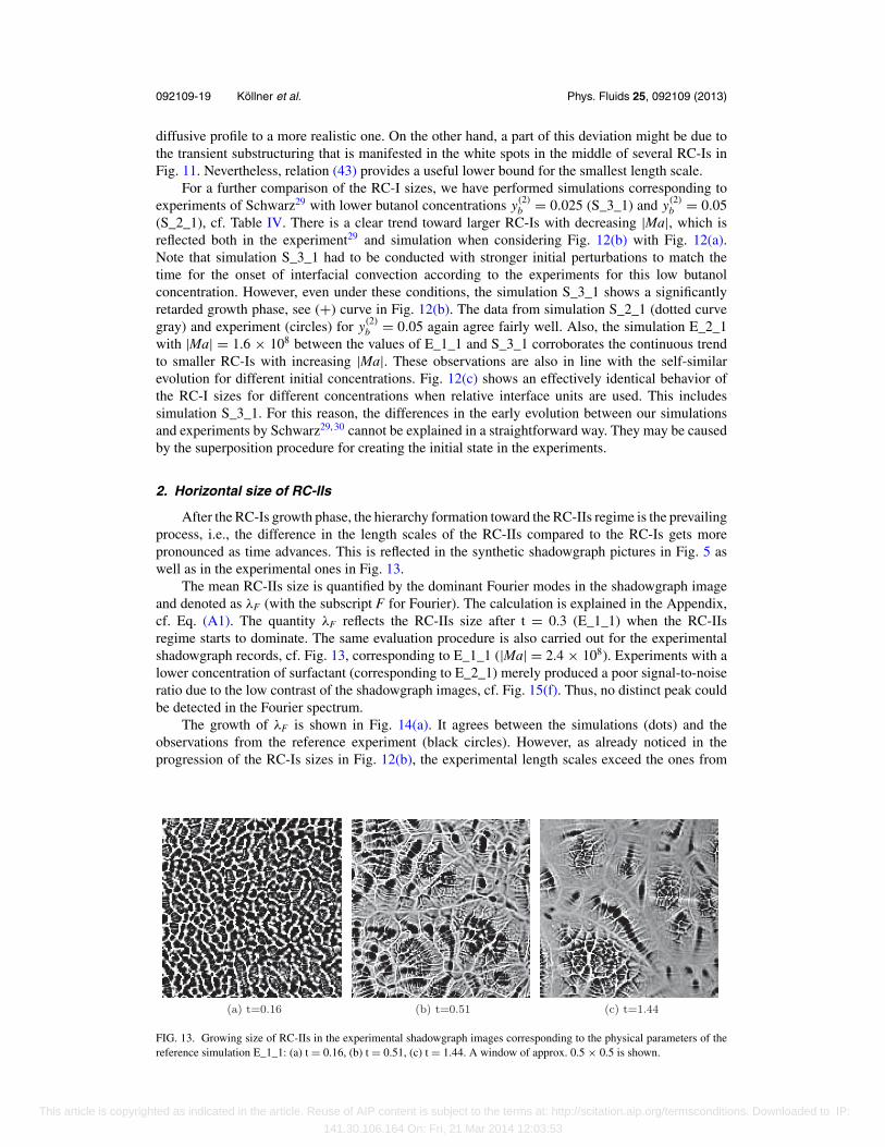
After the RC-Is growth phase, the hierarchy formation toward the RC-IIs regime is the prevailingprocess, i.e., the difference in the length scales of the RC-IIs compared to the RC-Is gets morepronounced as time advances. This is reflected in the synthetic shadowgraph pictures in Fig. 5 aswell as in the experimental ones in Fig. 13.
The mean RC-IIs size is quantified by the dominant Fourier modes in the shadowgraph imageand denoted as λF (with the subscript F for Fourier). The calculation is explained in the Appendix,cf. Eq. (A1). The quantity λF reflects the RC-IIs size after t = 0.3 (E_1_1) when the RC-IIsregime starts to dominate. The same evaluation procedure is also carried out for the experimentalshadowgraph records, cf. Fig. 13, corresponding to E_1_1 (|Ma| = 2.4 × 10⁸). Experiments with alower concentration of surfactant (corresponding to E_2_1) merely produced a poor signal-to-noiseratio due to the low contrast of the shadowgraph images, cf. Fig. 15(f). Thus, no distinct peak couldbe detected in the Fourier spectrum.
The growth of λF is shown in Fig. 14(a). It agrees between the simulations (dots) and theobservations from the reference experiment (black circles). However, as already noticed in theprogression of the RC-Is sizes in Fig. 12(b), the experimental length scales exceed the ones from
(a) t=0.16 (b) t=0.51 (c) t=1.44
FIG. 13. Growing size of RC-IIs in the experimental shadowgraph images corresponding to the physical parameters of thereference simulation E_1_1: (a) t = 0.16, (b) t = 0.51, (c) t = 1.44. A window of approx. 0.5 × 0.5 is shown.
This article is copyrighted as indicated in the article. Reuse of AIP content is subject to the terms at: http://scitation.aip.org/termsconditions. Downloaded to IP:
141.30.106.164 On: Fri, 21 Mar 2014 12:03:53
092109-20 Kollner et al. Phys. Fluids 25, 092109 (2013)
0 0.5 1 1.5 20
0.05
0.1
0.15
0.2
Time
Leng
th
E_1_1 Ma=−2.4e8Experiment Ma=−2.4e8
(a) λF
0 0.5 1 1.5 20
2
4
6
8
10
Time ⋅ Mar2
Leng
th r
atio
S_3_1, Ma=−6e7 S_2_1 Ma=−1.2e8E_2_1 Ma=−1.6e8E_1_1 Ma=−2.4e8
(b) λF /λRC−I
FIG. 14. (a) Evolution of λF from the radially averaged spectrum of s(x, y) in relative interface units. The discrete natureoriginates from averaging the spectrum around wavelength lx/i for i ∈ (1, 2, 3, . . . , Nx/2). (b) Ratio of λF and the RC-Is size,λF/λRC − I as function of time in relative interface units.
the simulations in the early phase. Fig. 14(b) illustrates the degree of hierarchy formation, whichis manifested in the ratio of λF to the formerly calculated RC-Is size λRC − I. This length ratioλF/λRC − I is related to the number of subcells in a RC-II and increases with time. The comparison ofthe λF/λRC − I evolution in Fig. 14(b) confirms the validity of the self-similar evolution for differentinitial concentrations.
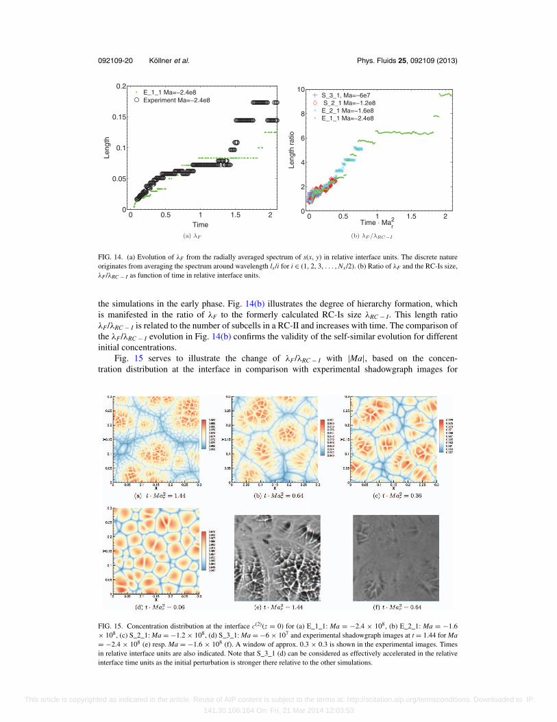
Fig. 15 serves to illustrate the change of λF/λRC − I with |Ma|, based on the concen-tration distribution at the interface in comparison with experimental shadowgraph images for
FIG. 15. Concentration distribution at the interface c(2)(z = 0) for (a) E_1_1: Ma = −2.4 × 10⁸, (b) E_2_1: Ma = −1.6× 10⁸, (c) S_2_1: Ma = −1.2 × 10⁸, (d) S_3_1: Ma = −6 × 10⁷ and experimental shadowgraph images at t = 1.44 for Ma= −2.4 × 10⁸ (e) resp. Ma = −1.6 × 10⁸ (f). A window of approx. 0.3 × 0.3 is shown in the experimental images. Timesin relative interface units are also indicated. Note that S_3_1 (d) can be considered as effectively accelerated in the relativeinterface time units as the initial perturbation is stronger there relative to the other simulations.
This article is copyrighted as indicated in the article. Reuse of AIP content is subject to the terms at: http://scitation.aip.org/termsconditions. Downloaded to IP:
141.30.106.164 On: Fri, 21 Mar 2014 12:03:53
092109-21 Kollner et al. Phys. Fluids 25, 092109 (2013)
t = 1.44 (in viscous units). These results explain the observations of Schwarz29 regarding thepositive correlation of |Ma| and the degree of the hierarchy. On the other hand, one can also regardthe different distributions in Fig. 15 as different stages of pattern evolution in time provided thatthe approximate scaling symmetry with respect to concentration c0 holds. The appropriate units arethen the relative interface units, i.e., length and time have to be multiplied by Mar and Ma2
r . Therespective times are indicated in the captions of the subfigures. Accordingly, the effective area ininterface units is decreasing from Figs. 15(a)–15(d).
Moreover, Figs. 15(a)–15(d) visualize the concentration gradient between the cell centers (highconcentration = dark gray) and their periphery, which generates the large-scale flow structure of theRC-IIs. Interestingly, the scale bars indicate that the difference of the nondimensional concentrationbetween the in- and outflow is approximately constant at about 0.02, although the mean concentrationincreases with |Ma|.
3. Vertical length scales of concentration and velocity
In the vertical dimension, the concentration distribution can be divided into two domainscharacterized by the varying transport mechanisms of advection and diffusion. In the lower, aqueousphase, cf. Fig. 6(a), this division is less pronounced due to the higher diffusive transport. Therefore,we only discuss the upper phase concerning concentration.
The first domain, basically the organic bulk fluid, extends from the solid wall at z = 1 toapproximately z = 0.08 (E_1_1 at t = 1.44). In this domain, the fluid is effectively at rest, cf.Fig. 7(c), and the surfactant is solely transported by diffusion. The second domain is the regionof interfacial convection which covers the space between the bulk fluid and the interface. It againembeds two subregions, the concentration boundary layer and the larger mixing zone, extendingover the length scales
δc(2)I = 1 − 〈c(2)〉S
|〈∂zc(2)〉S| , δc(2)I I = 1 − 〈c(2)〉�(2)
1 − 〈c(2)〉S, (44)
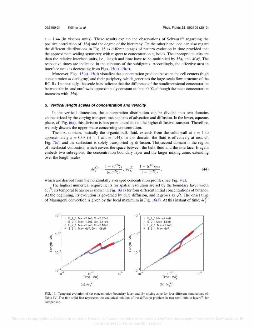
which are derived from the horizontally averaged concentration profiles, see Fig. 7(a).The highest numerical requirements for spatial resolution are set by the boundary layer width
δc(2)I . Its temporal behavior is shown in Fig. 16(a) for four different initial concentrations of butanol.
At the beginning, its evolution is governed by pure diffusion, and it grows as√
t . The onset timeof Marangoni convection is given by the local maximum in Fig. 16(a). At this instant of time, δc(2)
I
10−4
10−2
100
10−4
10−3
10−2
10−1
Time ⋅ Mar2
Leng
th ⋅
Ma r
E_1_1, Ma=−2.4e8, G=−7.67e5E_2_1, Ma=−1.6e8, G=−5.11e5S_2_1, Ma=−1.2e8, G=−2.16e5S_3_1, Ma=−6e7, G=−1.08e5
(a) δc(2)I
10−4
10−2
100
10−4
10−3
10−2
10−1
Time ⋅ Mar2
Leng
th ⋅
Ma r
E_1_1 Ma=−2.4e8E_2_1 Ma=−1.6e8S_2_1, Ma=−1.2e8S_3_1, Ma=−6e7
(b) δc(2)II
FIG. 16. Temporal evolution of (a) concentration boundary layer and (b) mixing zone for four different simulations, cf.Table IV. The thin solid line represents the analytical solution of the diffusion problem in two semi-infinite layers48 forcomparison.
This article is copyrighted as indicated in the article. Reuse of AIP content is subject to the terms at: http://scitation.aip.org/termsconditions. Downloaded to IP:
141.30.106.164 On: Fri, 21 Mar 2014 12:03:53
092109-22 Kollner et al. Phys. Fluids 25, 092109 (2013)
10−3
10−2
10−1
100
10−4
10−3
Time ⋅ Mar2
Leng
th ⋅
Ma r
E_1_1 Ma=−2.4e8E_2_1 Ma=−1.6e8S_2_1, Ma=−1.2e8S_3_1, Ma=−6e7
δ u(2)
δ u(1)
(a) δu(i)
0 0.5 1 1.5 20
0.2
0.4
0.6
0.8
1
1.2
1.4
1.6
Time ⋅ Mar2
Re
⋅ 103
E_1_1 Ma=−2.4e8E_2_1 Ma=−1.6e8S_2_1, Ma=−1.2e8S_3_1, Ma=−6e7
(b) Re
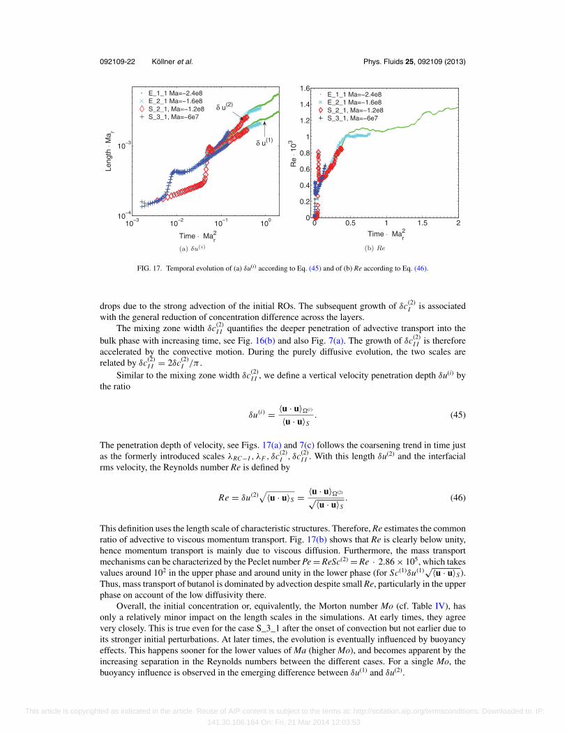
FIG. 17. Temporal evolution of (a) δu(i) according to Eq. (45) and of (b) Re according to Eq. (46).
drops due to the strong advection of the initial ROs. The subsequent growth of δc(2)I is associated
with the general reduction of concentration difference across the layers.The mixing zone width δc(2)
I I quantifies the deeper penetration of advective transport into thebulk phase with increasing time, see Fig. 16(b) and also Fig. 7(a). The growth of δc(2)
I I is thereforeaccelerated by the convective motion. During the purely diffusive evolution, the two scales arerelated by δc(2)
I I = 2δc(2)I /π .
Similar to the mixing zone width δc(2)I I , we define a vertical velocity penetration depth δu(i) by
the ratio
δu(i) = 〈u · u〉�(i)
〈u · u〉S. (45)
The penetration depth of velocity, see Figs. 17(a) and 7(c) follows the coarsening trend in time justas the formerly introduced scales λRC−I , λF , δc(2)
I , δc(2)I I . With this length δu(2) and the interfacial
rms velocity, the Reynolds number Re is defined by
Re = δu(2)√
〈u · u〉S = 〈u · u〉�(2)√〈u · u〉S. (46)
This definition uses the length scale of characteristic structures. Therefore, Re estimates the commonratio of advective to viscous momentum transport. Fig. 17(b) shows that Re is clearly below unity,hence momentum transport is mainly due to viscous diffusion. Furthermore, the mass transportmechanisms can be characterized by the Peclet number Pe = ReSc(2) = Re · 2.86 × 10⁵, which takesvalues around 102 in the upper phase and around unity in the lower phase (for Sc(1)δu(1)√〈u · u〉S).Thus, mass transport of butanol is dominated by advection despite small Re, particularly in the upperphase on account of the low diffusivity there.
Overall, the initial concentration or, equivalently, the Morton number Mo (cf. Table IV), hasonly a relatively minor impact on the length scales in the simulations. At early times, they agreevery closely. This is true even for the case S_3_1 after the onset of convection but not earlier due toits stronger initial perturbations. At later times, the evolution is eventually influenced by buoyancyeffects. This happens sooner for the lower values of Ma (higher Mo), and becomes apparent by theincreasing separation in the Reynolds numbers between the different cases. For a single Mo, thebuoyancy influence is observed in the emerging difference between δu(1) and δu(2).
This article is copyrighted as indicated in the article. Reuse of AIP content is subject to the terms at: http://scitation.aip.org/termsconditions. Downloaded to IP:
141.30.106.164 On: Fri, 21 Mar 2014 12:03:53
092109-23 Kollner et al. Phys. Fluids 25, 092109 (2013)
D. Pattern forming mechanisms
Sections III A–III C illustrated the main evolution and generic structures of solutal Marangoniconvection. Finally, the question of how the structures change and transform locally, remains tobe addressed. To classify the pattern evolution, we identified two main mechanisms. The first oneis the coarsening of convection units, measured by the length scales λRC − I and later by λF. Thecoarsening is caused by the continuing equilibration of surfactant differences between the phases.Therefore, cells with large vertical dimensions are favored as they are more efficient at transportingsurfactant over the mixing zone length δcII. This competition between individual cells leads to agrowing velocity penetration depth δu, which in turn causes an increase of the horizontal lengthscales as both quantities are coupled by the cellular flow structure.
The second mechanism is the local instability that leads to a subdivision of the inflow regions. Itappears clearly visible as the creation of surfactant fronts in the shadowgraph images. Furthermore,it limits the maximum size of RC-Is, since the probability of splitting seems to increase with the sizeof a contiguous inflow region and with the local concentration gradient.
The two mechanisms are present in both the very early phase of Marangoni convection, deter-mined by the initial ROs, discussed next in Secs. III D 1 and III D 2, and in the later evolution of thehierarchical cellular patterns, discussed in Secs. III D 3 and III D 4.
1. Growth and saturation of initial ROs
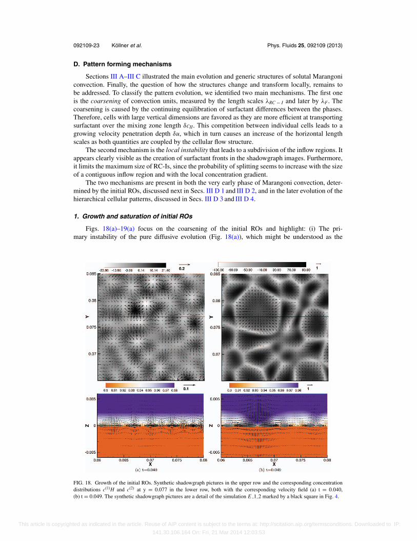
Figs. 18(a)–19(a) focus on the coarsening of the initial ROs and highlight: (i) The pri-mary instability of the pure diffusive evolution (Fig. 18(a)), which might be understood as the
FIG. 18. Growth of the initial ROs. Synthetic shadowgraph pictures in the upper row and the corresponding concentrationdistributions c(1)H and c(2) at y = 0.077 in the lower row, both with the corresponding velocity field (a) t = 0.040,(b) t = 0.049. The synthetic shadowgraph pictures are a detail of the simulation E 1 2 marked by a black square in Fig. 4.
This article is copyrighted as indicated in the article. Reuse of AIP content is subject to the terms at: http://scitation.aip.org/termsconditions. Downloaded to IP:
141.30.106.164 On: Fri, 21 Mar 2014 12:03:53
092109-24 Kollner et al. Phys. Fluids 25, 092109 (2013)
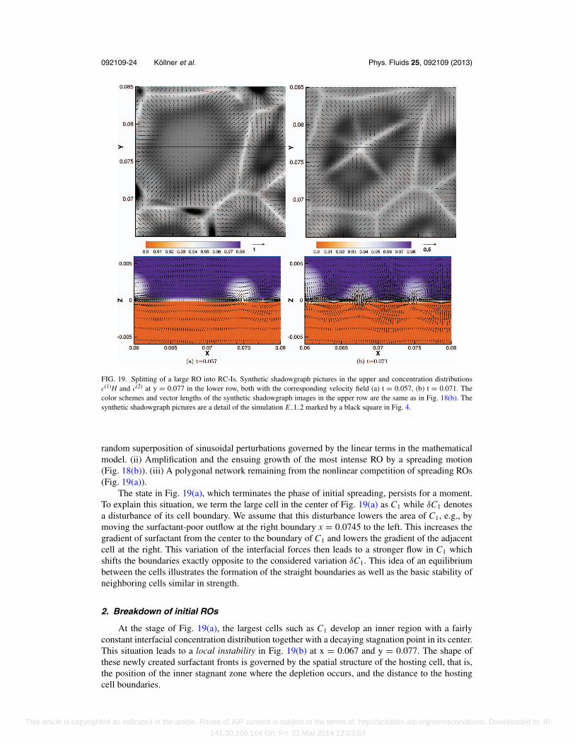
FIG. 19. Splitting of a large RO into RC-Is. Synthetic shadowgraph pictures in the upper and concentration distributionsc(1)H and c(2) at y = 0.077 in the lower row, both with the corresponding velocity field (a) t = 0.057, (b) t = 0.071. Thecolor schemes and vector lengths of the synthetic shadowgraph images in the upper row are the same as in Fig. 18(b). Thesynthetic shadowgraph pictures are a detail of the simulation E 1 2 marked by a black square in Fig. 4.
random superposition of sinusoidal perturbations governed by the linear terms in the mathematicalmodel. (ii) Amplification and the ensuing growth of the most intense RO by a spreading motion(Fig. 18(b)). (iii) A polygonal network remaining from the nonlinear competition of spreading ROs(Fig. 19(a)).
The state in Fig. 19(a), which terminates the phase of initial spreading, persists for a moment.To explain this situation, we term the large cell in the center of Fig. 19(a) as C1 while δC1 denotesa disturbance of its cell boundary. We assume that this disturbance lowers the area of C1, e.g., bymoving the surfactant-poor outflow at the right boundary x = 0.0745 to the left. This increases thegradient of surfactant from the center to the boundary of C1 and lowers the gradient of the adjacentcell at the right. This variation of the interfacial forces then leads to a stronger flow in C1 whichshifts the boundaries exactly opposite to the considered variation δC1. This idea of an equilibriumbetween the cells illustrates the formation of the straight boundaries as well as the basic stability ofneighboring cells similar in strength.
2. Breakdown of initial ROs
At the stage of Fig. 19(a), the largest cells such as C1 develop an inner region with a fairlyconstant interfacial concentration distribution together with a decaying stagnation point in its center.This situation leads to a local instability in Fig. 19(b) at x = 0.067 and y = 0.077. The shape ofthese newly created surfactant fronts is governed by the spatial structure of the hosting cell, that is,the position of the inner stagnant zone where the depletion occurs, and the distance to the hostingcell boundaries.
This article is copyrighted as indicated in the article. Reuse of AIP content is subject to the terms at: http://scitation.aip.org/termsconditions. Downloaded to IP:
141.30.106.164 On: Fri, 21 Mar 2014 12:03:53
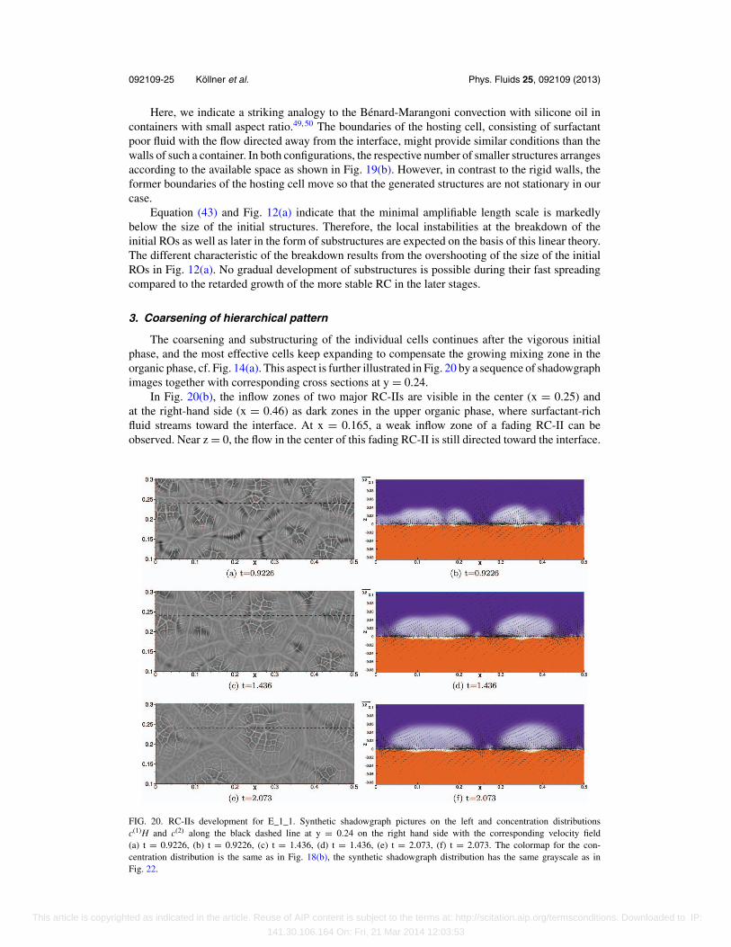
092109-25 Kollner et al. Phys. Fluids 25, 092109 (2013)
Here, we indicate a striking analogy to the Benard-Marangoni convection with silicone oil incontainers with small aspect ratio.49, 50 The boundaries of the hosting cell, consisting of surfactantpoor fluid with the flow directed away from the interface, might provide similar conditions than thewalls of such a container. In both configurations, the respective number of smaller structures arrangesaccording to the available space as shown in Fig. 19(b). However, in contrast to the rigid walls, theformer boundaries of the hosting cell move so that the generated structures are not stationary in ourcase.
Equation (43) and Fig. 12(a) indicate that the minimal amplifiable length scale is markedlybelow the size of the initial structures. Therefore, the local instabilities at the breakdown of theinitial ROs as well as later in the form of substructures are expected on the basis of this linear theory.The different characteristic of the breakdown results from the overshooting of the size of the initialROs in Fig. 12(a). No gradual development of substructures is possible during their fast spreadingcompared to the retarded growth of the more stable RC in the later stages.
3. Coarsening of hierarchical pattern
The coarsening and substructuring of the individual cells continues after the vigorous initialphase, and the most effective cells keep expanding to compensate the growing mixing zone in theorganic phase, cf. Fig. 14(a). This aspect is further illustrated in Fig. 20 by a sequence of shadowgraphimages together with corresponding cross sections at y = 0.24.
In Fig. 20(b), the inflow zones of two major RC-IIs are visible in the center (x = 0.25) andat the right-hand side (x = 0.46) as dark zones in the upper organic phase, where surfactant-richfluid streams toward the interface. At x = 0.165, a weak inflow zone of a fading RC-II can beobserved. Near z = 0, the flow in the center of this fading RC-II is still directed toward the interface.
FIG. 20. RC-IIs development for E_1_1. Synthetic shadowgraph pictures on the left and concentration distributionsc(1)H and c(2) along the black dashed line at y = 0.24 on the right hand side with the corresponding velocity field(a) t = 0.9226, (b) t = 0.9226, (c) t = 1.436, (d) t = 1.436, (e) t = 2.073, (f) t = 2.073. The colormap for the con-centration distribution is the same as in Fig. 18(b), the synthetic shadowgraph distribution has the same grayscale as inFig. 22.
This article is copyrighted as indicated in the article. Reuse of AIP content is subject to the terms at: http://scitation.aip.org/termsconditions. Downloaded to IP:
141.30.106.164 On: Fri, 21 Mar 2014 12:03:53
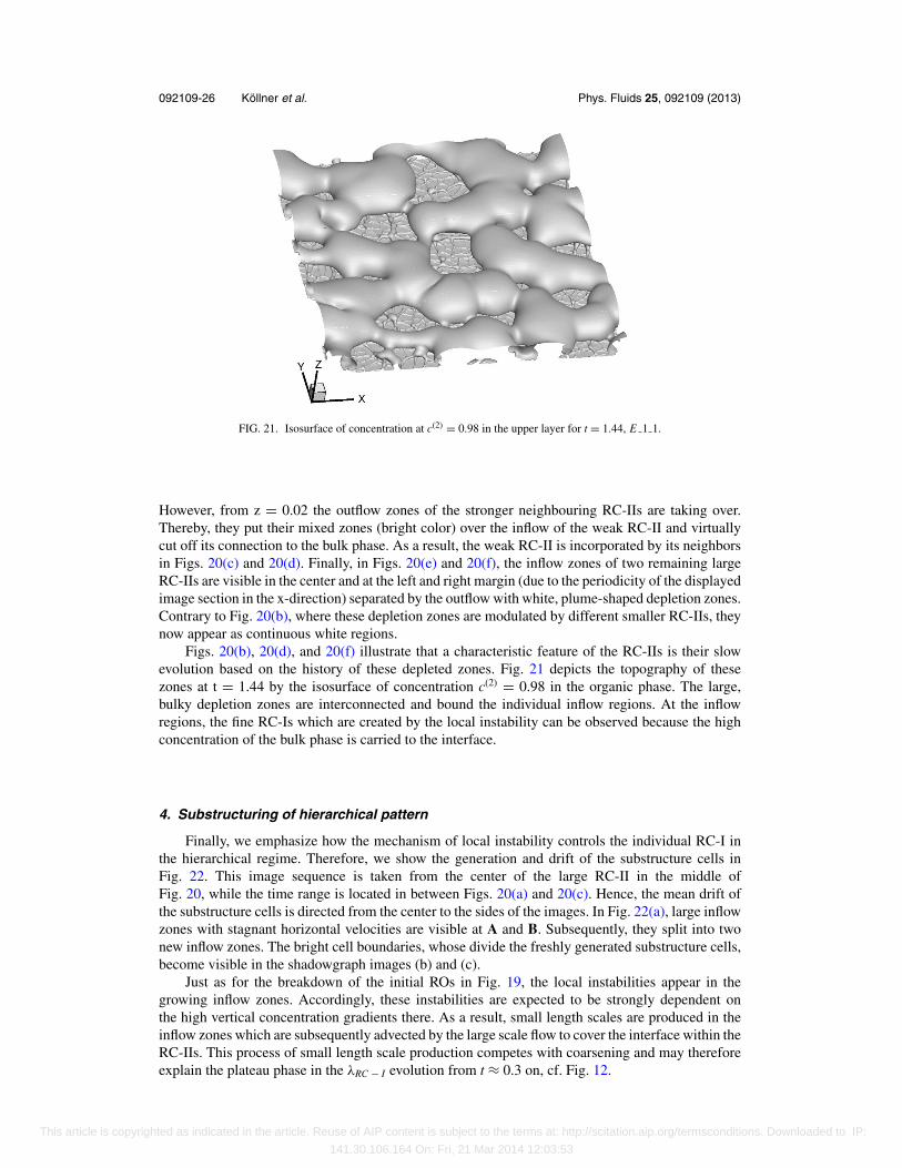
092109-26 Kollner et al. Phys. Fluids 25, 092109 (2013)
FIG. 21. Isosurface of concentration at c(2) = 0.98 in the upper layer for t = 1.44, E 1 1.
However, from z = 0.02 the outflow zones of the stronger neighbouring RC-IIs are taking over.Thereby, they put their mixed zones (bright color) over the inflow of the weak RC-II and virtuallycut off its connection to the bulk phase. As a result, the weak RC-II is incorporated by its neighborsin Figs. 20(c) and 20(d). Finally, in Figs. 20(e) and 20(f), the inflow zones of two remaining largeRC-IIs are visible in the center and at the left and right margin (due to the periodicity of the displayedimage section in the x-direction) separated by the outflow with white, plume-shaped depletion zones.Contrary to Fig. 20(b), where these depletion zones are modulated by different smaller RC-IIs, theynow appear as continuous white regions.
Figs. 20(b), 20(d), and 20(f) illustrate that a characteristic feature of the RC-IIs is their slowevolution based on the history of these depleted zones. Fig. 21 depicts the topography of thesezones at t = 1.44 by the isosurface of concentration c(2) = 0.98 in the organic phase. The large,bulky depletion zones are interconnected and bound the individual inflow regions. At the inflowregions, the fine RC-Is which are created by the local instability can be observed because the highconcentration of the bulk phase is carried to the interface.
4. Substructuring of hierarchical pattern
Finally, we emphasize how the mechanism of local instability controls the individual RC-I inthe hierarchical regime. Therefore, we show the generation and drift of the substructure cells inFig. 22. This image sequence is taken from the center of the large RC-II in the middle ofFig. 20, while the time range is located in between Figs. 20(a) and 20(c). Hence, the mean drift ofthe substructure cells is directed from the center to the sides of the images. In Fig. 22(a), large inflowzones with stagnant horizontal velocities are visible at A and B. Subsequently, they split into twonew inflow zones. The bright cell boundaries, whose divide the freshly generated substructure cells,become visible in the shadowgraph images (b) and (c).
Just as for the breakdown of the initial ROs in Fig. 19, the local instabilities appear in thegrowing inflow zones. Accordingly, these instabilities are expected to be strongly dependent onthe high vertical concentration gradients there. As a result, small length scales are produced in theinflow zones which are subsequently advected by the large scale flow to cover the interface within theRC-IIs. This process of small length scale production competes with coarsening and may thereforeexplain the plateau phase in the λRC − I evolution from t ≈ 0.3 on, cf. Fig. 12.
This article is copyrighted as indicated in the article. Reuse of AIP content is subject to the terms at: http://scitation.aip.org/termsconditions. Downloaded to IP:
141.30.106.164 On: Fri, 21 Mar 2014 12:03:53
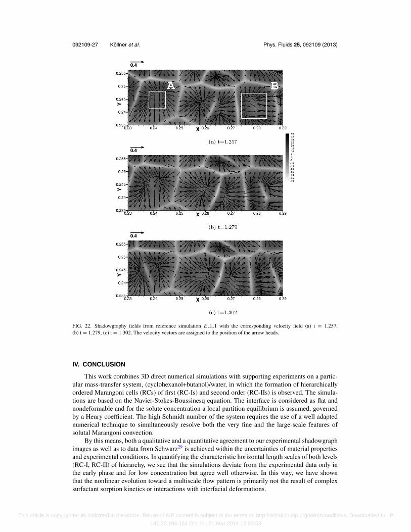
092109-27 Kollner et al. Phys. Fluids 25, 092109 (2013)
FIG. 22. Shadowgraphy fields from reference simulation E 1 1 with the corresponding velocity field (a) t = 1.257,(b) t = 1.279, (c) t = 1.302. The velocity vectors are assigned to the position of the arrow heads.
IV. CONCLUSION
This work combines 3D direct numerical simulations with supporting experiments on a partic-ular mass-transfer system, (cyclohexanol+butanol)/water, in which the formation of hierarchicallyordered Marangoni cells (RCs) of first (RC-Is) and second order (RC-IIs) is observed. The simula-tions are based on the Navier-Stokes-Boussinesq equation. The interface is considered as flat andnondeformable and for the solute concentration a local partition equilibrium is assumed, governedby a Henry coefficient. The high Schmidt number of the system requires the use of a well adaptednumerical technique to simultaneously resolve both the very fine and the large-scale features ofsolutal Marangoni convection.
By this means, both a qualitative and a quantitative agreement to our experimental shadowgraphimages as well as to data from Schwarz29 is achieved within the uncertainties of material propertiesand experimental conditions. In quantifying the characteristic horizontal length scales of both levels(RC-I, RC-II) of hierarchy, we see that the simulations deviate from the experimental data only inthe early phase and for low concentration but agree well otherwise. In this way, we have shownthat the nonlinear evolution toward a multiscale flow pattern is primarily not the result of complexsurfactant sorption kinetics or interactions with interfacial deformations.
This article is copyrighted as indicated in the article. Reuse of AIP content is subject to the terms at: http://scitation.aip.org/termsconditions. Downloaded to IP:
141.30.106.164 On: Fri, 21 Mar 2014 12:03:53
092109-28 Kollner et al. Phys. Fluids 25, 092109 (2013)
The simulated velocity and concentration distribution of the arising patterns, which are hardlyaccessible in the experiments, illustrate how the hierarchical planforms are organized. A classificationof the length scales deduced from the vertical concentration and velocity distribution is presented.The knowledge of these scales not only improves the understanding of the canonical problem itself.It also supports further numerical studies by estimating the relevant time and length scales to beresolved. Especially, we see that the interfacial convection in our reference system is limited to azone smaller than 1/10 and the concentration boundary layer to an even smaller zone of 1/100 of thewhole fluid layer height.
The parameter study of different initial butanol concentrations shows that the change in interfa-cial tension difference σ could be accounted for by a transformation of scales since the vertical andhorizontal geometrical constraints could be disregarded. This indicates that the hierarchical patternis an intrinsic feature, whose occurrence depends on time and space available for an unperturbedevolution. However, for systems with considerably smaller length scales the mathematical modelshould be extended from zero to a finite capacity of solute (excess concentration �) at the interface.
The growing influence of the buoyancy forces with decreasing butanol concentration, measuredby the Morton number, appeared to be insignificant in the studied parameter and time range.However, preliminary studies with a vanishing Morton number show a distinct change in the lengthscale progression, but no qualitative change of the observed structures.
The coupling of the hierarchy levels and their steady evolution leads, at first glance, to aquasi-chaotic dynamics. To shed light upon these complex processes, we identify the governingmechanisms that are interdependent causes and effects of coarsening and local instability. Theprediction of the classical linear instability analysis of Sternling and Scriven22 is related to the fullynonlinear simulation by means of the actual mean concentration gradient. It is consistent with thesteady production of new concentration fronts by the local instability.
In this respect, extended numerical studies with a separate variation of the buoyancy andinterfacial tension influences seem valuable to support further development of scaling theories,51
which up to now are mainly based on simple models or experiments. Moreover, we aim to investigateeven higher-level hierarchies and other types of patterns, which were observed in experiments onother chemical systems.31 In this regard, the question arises if these more complex patterns can bedetected by an approach based on the assumption of creeping flow which is surely valid for ourpresent simulations. This would help to simplify the corresponding computations, which are quiteexpensive even in the creeping flow approximation. Another important issue concerns the impact ofthe supposed plane, undeformable interface. This will be addressed in a future study by modelingweakly deformable interfaces to quantify the influence on Marangoni pattern formation. Additionally,a more detailed quantitative description of the complex patterns calls for an enhancement of existingmethods,52 which are mainly designed for stationary patterns.
ACKNOWLEDGMENTS
Financial support by the Deutsche Forschungsgemeinschaft (DFG) in the framework of thePriority Program 1506 (Grant Nos. Ec201/2-1 and Bo1668/6-1) is gratefully acknowledged. Fur-thermore, we thank the computing centers (UniRZ) of TU Ilmenau and FZ Julich (NIC) for access totheir parallel computing resources. We are also grateful to Professor H. Linde for numerous fruitfuldiscussions.
APPENDIX: IMAGE PROCESSING
Here, we provide the details of the image analysis. After mapping the raw data ∂zuz into thebinary representation I0(∂zuz)(x, y), we erase all connected inflow regions at the image boundary.This is apparent in Fig. 11. Otherwise, all cells at the boundary have to be merged with their periodiccontinuation, which is avoided for simplicity. The connected black subareas in Fig. 11 are determinedas individual cells Cj with j ∈ [1, . . . , Nc]. Some of the RC-Is exhibit a completely enclosed whitespot in their middle, corresponding to surfactant fronts. They are included into the individual setsCj. This identification of individual cells disregards the area of the white outflow zones, which
This article is copyrighted as indicated in the article. Reuse of AIP content is subject to the terms at: http://scitation.aip.org/termsconditions. Downloaded to IP:
141.30.106.164 On: Fri, 21 Mar 2014 12:03:53
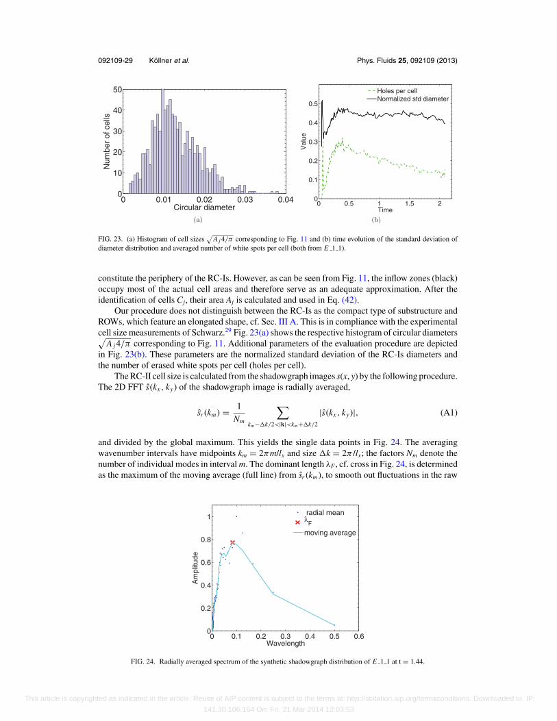
092109-29 Kollner et al. Phys. Fluids 25, 092109 (2013)
0 0.01 0.02 0.03 0.040
10
20
30
40
50
Circular diameter
Num
ber
of c
ells
(a)
0 0.5 1 1.5 20
0.1
0.2
0.3
0.4
0.5
Time
Val
ue
Holes per cellNormalized std diameter
(b)
FIG. 23. (a) Histogram of cell sizes√
A j 4/π corresponding to Fig. 11 and (b) time evolution of the standard deviation ofdiameter distribution and averaged number of white spots per cell (both from E 1 1).
constitute the periphery of the RC-Is. However, as can be seen from Fig. 11, the inflow zones (black)occupy most of the actual cell areas and therefore serve as an adequate approximation. After theidentification of cells Cj, their area Aj is calculated and used in Eq. (42).
Our procedure does not distinguish between the RC-Is as the compact type of substructure andROWs, which feature an elongated shape, cf. Sec. III A. This is in compliance with the experimentalcell size measurements of Schwarz.29 Fig. 23(a) shows the respective histogram of circular diameters√
A j 4/π corresponding to Fig. 11. Additional parameters of the evaluation procedure are depictedin Fig. 23(b). These parameters are the normalized standard deviation of the RC-Is diameters andthe number of erased white spots per cell (holes per cell).
The RC-II cell size is calculated from the shadowgraph images s(x, y) by the following procedure.The 2D FFT s(kx , ky) of the shadowgraph image is radially averaged,
sr (km) = 1
Nm
∑km−k/2<|k|<km+k/2
|s(kx , ky)|, (A1)
and divided by the global maximum. This yields the single data points in Fig. 24. The averagingwavenumber intervals have midpoints km = 2πm/lx and size k = 2π /lx; the factors Nm denote thenumber of individual modes in interval m. The dominant length λF, cf. cross in Fig. 24, is determinedas the maximum of the moving average (full line) from sr (km), to smooth out fluctuations in the raw
0 0.1 0.2 0.3 0.4 0.5 0.60
0.2
0.4
0.6
0.8
1
Wavelength
Am
plitu
de
radial meanλ
F
moving average
FIG. 24. Radially averaged spectrum of the synthetic shadowgraph distribution of E 1 1 at t = 1.44.
This article is copyrighted as indicated in the article. Reuse of AIP content is subject to the terms at: http://scitation.aip.org/termsconditions. Downloaded to IP:
141.30.106.164 On: Fri, 21 Mar 2014 12:03:53
092109-30 Kollner et al. Phys. Fluids 25, 092109 (2013)
data. As can be seen from Fig. 24, the large-scale structures in their fully developed state govern thesignal of the averaged spectrum.
1 K. E. Uguz and R. Narayanan, “Instability in evaporative binary mixtures. I. The effect of solutal Marangoni convection,”Phys. Fluids 24, 094101 (2012).
2 J. Zhang, A. Oron, and R. P. Behringer, “Novel pattern forming states for Marangoni convection in volatile binary liquids,”Phys. Fluids 23, 072102 (2011).
3 B. D. MacDonald and C. A. Ward, “Onset of Marangoni convection for evaporating liquids with spherical interfaces andfinite boundaries,” Phys. Rev. E 84(4), 046319 (2011).
4 H. Hu and R. G. Larson, “Marangoni effect reverses coffee-ring depositions,” J. Phys. Chem. B 110, 7090–7094 (2006).5 D. J. Harris and J. A. Lewis, “Marangoni effects on evaporative lithographic patterning of colloidal films,” Langmuir 24,
3681–3685 (2008).6 W. Bi, X. Wu, and E. K. L. Yeow, “Unconventional multiple ring structure formation from evaporation-induced self-
assembly of polymers,” Langmuir 28, 11056–11063 (2012).7 T. Still, P. J. Yunker, and A. G. Yodh, “Surfactant-induced Marangoni eddies alter the coffee-rings of evaporating colloidal
drops,” Langmuir 28(11), 4984–4988 (2012).8 S. G. Yiantsios and B. G. Higgins, “Marangoni flows during drying of colloidal films,” Phys. Fluids 18, 082103 (2006).9 H. Kitahata, N. Yoshinaga, K. H. Nagai, and Y. Sumino, “Spontaneous motion of a droplet coupled with a chemical wave,”
Phys. Rev. E 84, 015101(R) (2011).10 Z. Yin, L. Chang, W. Hu, Q. Li, and H. Wang, “Numerical simulations on thermocapillary migrations of nondeformable
droplets with large Marangoni numbers,” Phys. Fluids 24(9), 092101 (2012).11 E. Lauga and A. M. J. Davis, “Viscous Marangoni propulsion,” J. Fluid Mech. 705, 120–133 (2012).12 K. Eckert, M. Acker, R. Tadmouri, and V. Pimienta, “Chemo-Marangoni convection driven by an interfacial reaction:
Pattern formation and kinetics,” Chaos 22(3), 037112 (2012).13 A. Javadi, D. Bastani, J. Kragel, and R. Miller, “Interfacial instability of growing drop: Experimental study and conceptual
analysis,” Colloids Surf., A 347, 167–174 (2009).14 Y. Sutjiadi-Sia, P. Jaeger, and R. Eggers, “Interfacial phenomena of aqueous systems in dense carbon dioxide,” J. Supercrit.
Fluids 46, 272–279 (2008).15 V. Pimienta, M. Brost, N. Kovalchuk, S. Bresch, and O. Steinbock, “Complex shapes and dynamics of dissolving drops of
dichloromethane,” Angew. Chem., Int. Ed. 50, 10728–10731 (2011).16 S. Berg, “Marangoni-driven spreading along liquid-liquid interfaces,” Phys. Fluids 21, 032105 (2009).17 K. S. Lee, N. Ivanova, V. M. Starov, N. Hilal, and V. Dutschk, “Kinetics of wetting and spreading by aqueous surfactant
solutions,” Adv. Colloid Interface Sci. 144, 54–65 (2008).18 N. M. Kovalchuk and D. Vollhardt, “Oscillation of interfacial tension produced by transfer of nonionic surfactant through
the liquid/liquid interface,” J. Phys. Chem. C 112, 9016–9022 (2008).19 R. Tadmouri, N. M. Kovalchuk, V. Pimienta, D. Vollhardt, and J. C. Micheau, “Transfer of oxyethylated alcohols
through water/heptane interface: Transition from non-oscillatory to oscillatory behaviour,” Colloids Surf., A 354, 134–142(2010).
20 M. Wegener and A. R. Paschedag, “Mass transfer enhancement at deformable droplets due to Marangoni convection,” Int.J. Multiphase Flow 37, 76–83 (2011).
21 Z. F. Sun, K. T. Yu, S. Y. Wang, and Y. Z. Miao, “Absorption and desorption of carbon dioxide into and from organicsolvents: Effects of Rayleigh and Marangoni instability,” Ind. Eng. Chem. Res. 41, 1905–1913 (2002).
22 C. V. Sternling and L. E. Scriven, “Interfacial turbulence: Hydrodynamic instability and the Marangoni effect,” AIChE J.5(4), 514–523 (1959).
23 E. L. Koschmieder and M. I. Biggerstaff, “Onset of surface-tension-driven Benard convection,” J. Fluid Mech. 167, 49–64(1986).
24 A. Thess and S. A. Orszag, “Surface-tension-driven Benard convection at infinite Prandtl number,” J. Fluid Mech. 283,201–230 (1995).
25 K. Eckert, M. Bestehorn, and A. Thess, “Square cells in surface-tension-driven Benard convection: Experiment and theory,”J. Fluid Mech. 356, 155–197 (1998).
26 M. F. Schatz, S. J. VanHook, W. D. McCormick, J. B. Swift, and H. L. Swinney, “Time-independent square patterns insurface-tension-driven Benard convection,” Phys. Fluids 11, 2577 (1999).
27 A. Orell and J. W. Westwater, “Spontaneous interfacial cellular convection accompanying mass transfer: Ethylene glycol-acetic acid-ethyl acetate,” AIChE J. 8(3), 350–356 (1962).
28 H. Linde and E. Schwarz, “Untersuchungen zur Charakteristik der freien Grenzflachenkonvektion beim Stoffubergang anfluiden Grenzen,” Z. Phys. Chem. 224, 331–352 (1963).
29 E. Schwarz, “Hydrodynamische Regime der Marangoni-Instabilitat beim Stoffubergang uber eine fluide Phasengrenze,”Ph.D. thesis, Humboldt-Universitat, Berlin, 1968.
30 E. Schwarz, “On the occurrence of Marangoni instability,” Heat Mass Transfer 3(3), 131–133 (1970).31 H. Linde, K. Schwarzenberger, and K. Eckert, “Pattern formation emerging from stationary solutal Marangoni instability:
A roadmap through the underlying hierarchic structures,” in Without Bounds: A Scientific Canvas of Nonlinearity andComplex Dynamics, edited by R. G. Rubio, Y. S. Ryazantsev, V. M. Starov, G.-X. Huang, A. P. Chetverikov, P. Arena, A.A. Nepomnyashchy, A. Ferrus, and E. G. Morozov (Springer, Berlin, 2013).
32 S. Chen, B. Fu, X. Yuan, H. Zhang, W. Chen, and K. Yu, “Lattice Boltzmann method for simulation of solutal interfacialconvection in gas-liquid system,” Ind. Eng. Chem. Res. 51, 10955–10967 (2012).
33 Y. Sha, H. Chen, Y. Yin, S. Tu, L. Ye, and Y. Zheng, “Characteristics of the Marangoni convection induced in initialquiescent water,” Ind. Eng. Chem. Res. 49, 8770–8777 (2010).
This article is copyrighted as indicated in the article. Reuse of AIP content is subject to the terms at: http://scitation.aip.org/termsconditions. Downloaded to IP:
141.30.106.164 On: Fri, 21 Mar 2014 12:03:53
092109-31 Kollner et al. Phys. Fluids 25, 092109 (2013)
34 Z. Mao, P. Lu, G. Zhang, and C. Yang, “Numerical simulation of the Marangoni effect with interphase mass transferbetween two planar liquid layers,” Chin. J. Chem. Eng. 16(2), 161–170 (2008).
35 A. Grahn, “Two-dimensional numerical simulations of Marangoni-Benard instabilities during liquid-liquid mass transferin a vertical gap,” Chem. Eng. Sci. 61, 3586–3592 (2006).
36 D. A. Bratsun and A. De Wit, “On Marangoni convective patterns driven by an exothermic chemical reaction in two-layersystems,” Phys. Fluids 16, 1082–1096 (2004).
37 D. R. Lide, CRC Handbook of Chemistry and Physics: A Ready-Reference Book of Chemical and Physical Data (CRCPress, Boca Raton, FL, 2004).
38 A. J. Leo and C. Hansch, “Linear free energy relations between partitioning solvent systems,” J. Org. Chem. 36(11),1539–1544 (1971).
39 D. A. Edwards, H. Brenner, and D. T. Wasan, Interfacial Transport Processes and Rheology (Butterworth-Heinemann,Stoneham, MA, 1991).
40 J. Li and P. W. Carr, “Accuracy of empirical correlations for estimating diffusion coefficients in aqueous organic mixtures,”Anal. Chem. 69(13), 2530–2536 (1997).
41 H. Linde, E. Schwarz, and K. Groger, “Zum Auftreten des oszillatorischen Regimes der Marangoni-Instabilitat beimStoffubergang,” Chem. Eng. Sci. 22, 823–836 (1967).
42 A. Nepomnyashchy, I. Simanovskii, and J. C. Legros, Interfacial Convection in Multilayer Systems (Springer Science +Business Media, New York, 2006).
43 W. Merzkirch, Flow Visualization (Academic Press, London, 1987).44 T. Boeck, A. Nepomnyashchy, I. Simanovskii, A. Golovin, L. Braverman, and A. Thess, “Three-dimensional convection
in a two-layer system with anomalous thermocapillary effect,” Phys. Fluids 14, 3899 (2002).45 K. Schwarzenberger, T. Kollner, H. Linde, S. Odenbach, T. Boeck, and K. Eckert, “On the transition from cellular to
wavelike patterns during solutal Marangoni convection,” Eur. Phys. J. Spec. Top. 219(1), 121–130 (2013).46 K. Schwarzenberger, K. Eckert, and S. Odenbach, “Relaxation oscillations between Marangoni cells and double diffusive
fingers in a reactive liquid-liquid system,” Chem. Eng. Sci. 68, 530–540 (2012).47 J. C. Berg and C. R. Morig, “Density effects in interfacial convection,” Chem. Eng. Sci. 24, 937–946 (1969).48 J. Crank, The Mathematics of Diffusion (Oxford University Press, Oxford, 1975).49 E. L. Koschmieder and S. A. Prahl, “Surface-tension-driven Benard convection in small containers,” J. Fluid Mech. 215(1),
571–583 (1990).50 M. Medale and P. Cerisier, “Numerical simulation of Benard-Marangoni convection in small aspect ratio containers,”
Numer. Heat Transfer, Part A 42(1–2), 55–72 (2002).51 A. A. Golovin, “Mass transfer under interfacial turbulence: Kinetic regularities,” Chem. Eng. Sci. 47(8), 2069–2080 (1992).52 U. Thiele and K. Eckert, “Stochastic geometry of polygonal networks: An alternative approach to the hexagon-square
transition in Benard convection,” Phys. Rev. E 58(3), 3458 (1998).53 The velocity field is partly directed in poloidal direction of a suitable located coordinate system and therefore an isosurface
of the velocity magnitude maybe viewed as a torus.
This article is copyrighted as indicated in the article. Reuse of AIP content is subject to the terms at: http://scitation.aip.org/termsconditions. Downloaded to IP:
141.30.106.164 On: Fri, 21 Mar 2014 12:03:53