Forced Convection
29
Chapter 9 Forced Convection INTRODUCTION When a pot of water is heated on a stove, the portion of water adjacent to the bottom of the pot is the first to experience an increase in temperature. Eventually, the water at the top will also become hotter. Although some of the heat transfer from bottom to top is explainable by conduction through the water, most of the heat transfer is due to a second mechanism of heat transfer, convection. Agitation produced by a mixer, or the equivalent, adds to the convective effect. As the water at the bottom is heated, its density becomes lower. This results in convection currents as gravity causes the low density water to move upwards while being replaced by the higher density, cooler water from above. This macroscopic mixing is occasionally a far more effective mechanism for transferring heat energy through fluids than conduction. This process is called natural or free convection because no external forces, other than gravity, need be applied to move the energy in the form of heat. In most industrial applications, how- ever, it is more economical to speed up the mixing action by artificially generating a current by the use of a pump, agitator, or some other mechanical device. This is referred to as forced convection and practicing engineers are primarily interested in this mode of heat transfer (i.e., most industrial applications involve heat transfer by convection). Convective effects described above as forced convection are due to the bulk motion of the fluid. The bulk motion is caused by external forces, such as that provided by pumps, fans, compressors, etc., and is essentially independent of “thermal” effects. Free convection is the other effect that occasionally develops and was also briefly dis- cussed above. This convective effect is attributed to buoyant forces that arise due to density differences within a system. It is treated analytically as another external force term in the momentum equation. The momentum (velocity) and energy (temp- erature) effects are therefore interdependent; consequently, both equations must be solved simultaneously. This treatment is beyond the scope of this text, but is available in the literature. (1) Also note that both forced and free convection may exist in some applications. In order to circumvent the difficulties encountered in the analytical solution of microscopic heat-transfer problems, it is common practice in engineering to write Heat Transfer Applications for the Practicing Engineer. Louis Theodore # 2011 John Wiley & Sons, Inc. Published 2011 by John Wiley & Sons, Inc. 131
-
Upload
khangminh22 -
Category
Documents
-
view
1 -
download
0
Transcript of Forced Convection

Chapter 9
Forced Convection
INTRODUCTION
When a pot of water is heated on a stove, the portion of water adjacent to the bottom ofthe pot is the first to experience an increase in temperature. Eventually, the water at thetop will also become hotter. Although some of the heat transfer from bottom to top isexplainable by conduction through the water, most of the heat transfer is due to asecond mechanism of heat transfer, convection. Agitation produced by a mixer, orthe equivalent, adds to the convective effect. As the water at the bottom is heated,its density becomes lower. This results in convection currents as gravity causes thelow density water to move upwards while being replaced by the higher density,cooler water from above. This macroscopic mixing is occasionally a far more effectivemechanism for transferring heat energy through fluids than conduction. This process iscalled natural or free convection because no external forces, other than gravity, needbe applied to move the energy in the form of heat. In most industrial applications, how-ever, it is more economical to speed up the mixing action by artificially generating acurrent by the use of a pump, agitator, or some other mechanical device. This isreferred to as forced convection and practicing engineers are primarily interested inthis mode of heat transfer (i.e., most industrial applications involve heat transfer byconvection).
Convective effects described above as forced convection are due to the bulkmotion of the fluid. The bulk motion is caused by external forces, such as that providedby pumps, fans, compressors, etc., and is essentially independent of “thermal” effects.Free convection is the other effect that occasionally develops and was also briefly dis-cussed above. This convective effect is attributed to buoyant forces that arise due todensity differences within a system. It is treated analytically as another externalforce term in the momentum equation. The momentum (velocity) and energy (temp-erature) effects are therefore interdependent; consequently, both equations must besolved simultaneously. This treatment is beyond the scope of this text, but is availablein the literature.(1) Also note that both forced and free convection may exist in someapplications.
In order to circumvent the difficulties encountered in the analytical solution ofmicroscopic heat-transfer problems, it is common practice in engineering to write
Heat Transfer Applications for the Practicing Engineer. Louis Theodore# 2011 John Wiley & Sons, Inc. Published 2011 by John Wiley & Sons, Inc.
131

the rate of heat transfer in terms of a heat transfer coefficient h, a topic that will receiveextensive treatment in Part Three. If a surface temperature is TS, and TM represents thetemperature of a fluid medium at some distance from the surface, one may write that
_Q ¼ hA(TS � TM) (9:1)
Since h and TS are usually functions of the area A, the above equation may be rewrittenin differential equation form
d _Q ¼ h(TS � TM) dA (9:2)
Integrating for the area gives
ð _Q
0
d _Q
h(TS � TM)¼
ðA
0dA (9:3)
This concept of a heat-transfer coefficient is an important concept in heat transfer, andis often referred to in the engineering literature as the individual film coefficient.
The expression in Equation (9.1) may be better understood by referring to heattransfer to a fluid flowing in a conduit. For example, if the resistance to heat transferis thought of as existing only in a laminar film(2) adjacent to the wall of the conduit,the coefficient h may then be viewed as equivalent to h/Dxe, where Dxe is the equiv-alent thickness of a stationary film that offers the same resistance corresponding to theobserved value of h. This is represented pictorially in Figure 9.1. In effect, this simplyreplaces the real resistance with a hypothetical one.
The reader should note that for flow past a surface, the velocity at the surface (s) iszero (no slip). The only mechanism for heat transfer at the surface is therefore conduc-tion. One may therefore write
_Q ¼ �kAdT
dx
����s
(9:4)
TS
T
x L
Solid Fluid
Q = hA (TS –TM)
TM
≡
≡Δxe Δxe
Q = k A (Ts –Tf) = k A (Ts –Tf)
Q Q
Δxe Fluid
TS
Tf
Solid
TMQ Q
Figure 9.1 Convection temperature profile.
132 Chapter 9 Forced Convection

If the temperature profile in the fluid can be determined (i.e., T ¼ T(x)), the gradient,dT=dx, can be evaluated at all points in the system including the surface, dT=dx
��s.
The heat transfer coefficient, h, was previously defined by
_Q ¼ hA(TS � TM) (9:1)
Therefore, combining Equations (9.1) and (9.4) leads to
�kAdT
dx
����s
¼ hA(TS � TM) (9:5)
Since the thermal conductivity, k, of the fluid is usually known, information on h maybe obtained. This information is provided later in this chapter.
To summarize, the transfer of energy by convection is governed by Equation (9.1)and is referred to as Newton’s Law of Cooling,
_Q ¼ hA(TS � TM) (9:1)
where Q is the convective heat transfer rate (Btu/h); A, the surface area availablefor heat transfer (ft2); TS, the surface temperature (8F); TM, the bulk fluid temperature(8F); and h is the aforementioned convection heat transfer coefficient, also termed thefilm coefficient or film conductance (Btu/h . ft2 . 8F or W/m2 . K). Note that 1 Btu/h . ft2 . 8F ¼ 5.6782 W/m2 . K.
The magnitude of h depends on whether the transfer of heat between the surfaceand the fluid is by forced convection or by free convection, radiation, boiling, or con-densation (to be discussed in later chapters). Typical values of h are given in Tables 9.1and 9.2.
Topics covered in this chapter include:
Convective Resistances
Heat Transfer Coefficients: Qualitative Information
Heat Transfer Coefficients: Quantitative Information
Microscopic Approach
Table 9.1 Typical Film Coefficients
Mode
h
Btu/h . ft2 . 8F W/m . K
Forced convectionGases 5–50 25–250Liquids 10–4000 50–20,000
Free convection (see next chapter)Gases 1–5 5–25Liquids 10–200 50–1000
Boiling/condensation 500–20,000 2500–100,000
Introduction 133

CONVECTIVE RESISTANCES
Consider heat transfer across a flat plate, as pictured in Figure 9.2. The total resistance(Rt) may be divided into three contributions: the inside film (Ri), the wall (Rw), and theoutside film (Ro),
XR ¼ Rt ¼ Ri þ Rw þ Ro (9:6)
Table 9.2 Film Coefficients in Pipesa
h, Inside pipes h, Outside pipesb,c
Gases 10–50 1–3 (n), 5–20 ( f )Water (liquid) 200–2000 20–200 (n), 100–1000 ( f )
Boiling waterd 500–5000 300–9000Condensing steamd 1000–10,000
Nonviscous fluids 50–500 50–200 ( f )Boiling liquidsd 200–2000Condensing vapord 200–400
Viscous fluids 10–100 20–50 (n), 10–100 ( f )Condensing vapord 50–100
ah ¼ Btu/h . ft2 . 8F.b(n) ¼ natural convection (see next chapter).c( f ) ¼ forced convection.dAdditional details in Chapter 12.
Q
Hot fluid
Cold fluid
TH
T1
TC
T2
Δx
Q
Figure 9.2 Flow past a flat plate.
134 Chapter 9 Forced Convection

where the individual resistances are defined by
Rt ¼1
hiAþDx
kAþ
1hoA
(9:7)
The term hi is the inside film coefficient (Btu/h . ft2 . 8F); ho, the outside film coeffi-cient (Btu/h . ft2 . 8F); A, the surface area (ft2); Dx, the thickness (ft); and, k, the ther-mal conductivity (Btu/h . ft . 8F).
ILLUSTRATIVE EXAMPLE 9.1
Consider a closed cylindrical reactor vessel of diameter D ¼ 1 ft, and length L ¼ 1.5 ft. The sur-face temperature of the vessel, T1, and the surrounding temperature, T2, are 3908F and 508F,respectively. The convective heat transfer coefficient, h, between the vessel wall and surround-ing fluid is 4.0 Btu/h . ft . 8F. Calculate the thermal resistance in 8F . h/Btu.
SOLUTION: Write the heat transfer rate equation:
_Q ¼ hA(T1 � T2) (9:1)
Since D ¼ 1 ft and L ¼ 1.5 ft, the total heat transfer area may be determined.
A ¼ p (1)(1:5)þ(2)p (1)2
4¼ 6:28 ft2
Calculate the rate of heat transfer.
_Q ¼ (4:0)(6:28)(390� 50) ¼ 8545 Btu=h
Finally, calculate the thermal resistance associated with the film coefficient (see Equation 9.7).
R ¼1
hA¼
1(4:0)(6:28)
¼ 0:03988F � h=BtuB
ILLUSTRATIVE EXAMPLE 9.2
Referring to the previous example, convert the resistance to K/W and 8C/W.
SOLUTION: First note that
1 W ¼ 3:412 Btu=h
and a 18C change corresponds to a 1.88F change. Therefore,
R ¼ (0:0398)(3:412)=1:8
¼ 0:0758C=W
¼ 0:075 K=W B
Convective Resistances 135

ILLUSTRATIVE EXAMPLE 9.3
Hot gas at 5308F flows over a flat plate of dimensions 2 ft by 1.5 ft. The convection heat transfercoefficient between the plate and the gas is 48 Btu/ft2 . h . 8F. Determine the heat transfer rate inBtu/h and kW from the air to one side of the plate when the plate is maintained at 1058F.
SOLUTION: Assume steady-state conditions and constant properties. Write Newton’s law ofcooling to evaluate the heat transfer rate. Note that the gas is hotter than the plate. Therefore, Qwill be transferred from the gas to the plate,
_Q ¼ hA(TS � TM) (9:1)
Substituting
_Q ¼ (48)(3)(530� 105) ¼ 61,200 Btu/h
¼ 61,200=3:4123 ¼ 17,935 W
¼ 17:94 kW B
ILLUSTRATIVE EXAMPLE 9.4
The glass window shown in Figure 9.3 of area 3.0 m2 has a temperature at the outer surface of108C. The glass has conductivity of 1.4 W/m . K. The convection coefficient (heat transfercoefficient) of the air is 100 W/m2 . K. The heat transfer is 3.0 kW. Calculate the bulk tempera-ture of the fluid.
SOLUTION: Write the equation for heat convection. Equation (9.1) is given by
_Q ¼ hA(TS � TM)
Glass Air at TM
TS = 10°C
Figure 9.3 Convective glass.
136 Chapter 9 Forced Convection

where TS ¼ surface temperature at the wall and TM ¼ temperature of the bulk fluid. Solving forthe unknown, the air temperature TM, and substituting values yields
TM ¼ TS �_Q
hA
TM ¼ (273þ 10)�3000
(100)(3)¼ 273 K ¼ 08C
B
ILLUSTRATIVE EXAMPLE 9.5
Refer to Illustrative Example 9.1. If the convective heat transfer coefficient, h, between thevessel wall and the surrounding fluid is constant at 4.0 Btu/h . ft2 . 8F and the plant operates24 h/day, 350 days/yr, calculate the steady-state energy loss in Btu/yr.
SOLUTION: The operating hours per year, N, are
N ¼ (24)(350) ¼ 8400 h=yr
The yearly energy loss, Q, is therefore
_Q ¼ (8545)(8400) ¼ 7:18� 107 Btu=yr B
Returning to Newton’s law, the above development is now expanded and applied tothe system pictured in Figure 9.2. Based on Newton’s law of cooling,
_Q1 ¼ h1A(TH � T1) (9:8)
_Q2 ¼kA
Dx(T1 � T2) (9:9)
_Q3 ¼ h2A(T2 � TC) (9:10)
Assuming steady-state ð _Q ¼ _Q1 ¼_Q2 ¼
_Q3Þ, and combining the above in a mannersimilar to the development provided in Chapter 7 yields:
_Q ¼TH � TC
(1=h1A)þ (Dx=kA)þ (1=h2A)(9:11)
¼TH � TC
Ri þ Rw þ Ro¼
TH � TC
Rt(9:12)
HEAT TRANSFER COEFFICIENTS: QUALITATIVEINFORMATION
The heat transfer coefficient h is a function of the properties of the flowing fluid, thegeometry and roughness of the surface, and the flow pattern of the fluid. Severalmethods are available for evaluating h: analytical methods, integral methods, anddimensional analyses. Only the results of these methods are provided in the next
Heat Transfer Coefficients: Qualitative Information 137
section. These may take the form of local and/or average values. Their derivation isnot included. As will be demonstrated in the next Part, it is convenient to knowthese values for design purposes.
As one might suppose, heat transfer coefficients are higher for turbulent flow thanwith laminar flow, and heat transfer equipment are usually designed to take advantageof this fact. The heat transferred in most turbulent streams occurs primarily bythe movement of numerous microscopic elements of fluid (usually referred toas eddies) in the system. Although one cannot theoretically predict the behavior ofthese eddies quantitatively with time, empirical equations are available for the practi-cing engineer.
Surface roughness can also have an effect on the heat transfer coefficient.However, the effect in laminar flow is, as one might expect, negligible. Except for aslight increase in the heat transfer area, the roughness has little to no effect on heattransfer with laminar flow. When the flow is turbulent, the roughness may have a sig-nificant effect. In general, the coefficient will not be affected if the rough “elements”do not protrude through the laminar sub-layer.
The heat transfer problems most frequently encountered have to do with the heat-ing and cooling of fluids in pipes. Although the entrance effects can significantly affectoverall performance in short pipes and conduits, this is normally neglected.
Before proceeding to a quantitative review of the equations that can be employedto calculate heat transfer film coefficients, it should be noted that a serious errorcan arise if the viscosity of the fluid is strongly dependent on temperature. Thetemperature gradient is normally greatest near the surface wall of the conduit and itis in this region that the velocity gradient is also greatest. The effect of temperatureon the viscosity of the fluid at or near the wall may therefore have a pronouncedeffect on both the viscosity and temperature profiles. This effect is reflected in theheat transfer coefficient equations. If m and ms represent the fluid viscosity at the aver-age bulk fluid temperature and the viscosity at the wall temperature, respectively, thedimensionless term m/ms is an empirical correction factor for the distortion of thevelocity profile that results from the effect of temperature on viscosity.
A summary of the describing equations employed to predict convective heattransfer coefficients is presented in the next section. Most of the correlations containdimensionless numbers, many of which were introduced in Chapter 3; some areredefined and reviewed again in this section. A host of illustrative examples comp-lement the presentation.
HEAT TRANSFER COEFFICIENTS: QUANTITATIVEINFORMATION
Many heat transfer film coefficients have been determined experimentally. Typicalranges of film coefficients are provided in Tables 9.3–9.5. Explanatory details are pro-vided in the subsections that follow. In addition to those provided in Tables 9.3–9.5,many empirical correlations can be found in the literature for a wide variety of fluidsand flow geometries.(1)
138 Chapter 9 Forced Convection

Tab
le9.
3S
umm
ary
ofFo
rced
Con
vect
ion
Hea
tT
rans
fer
Cor
rela
tions
for
Ext
erna
lF
low
Geo
met
ryC
orre
latio
nC
ondi
tions
Fla
tpl
ate:
lam
inar
Hyd
rody
nam
icbo
unda
ryla
yer,d=x¼
5R
e�0:
5x
Lam
inar
flow
,pr
oper
ties
atth
efl
uid
film
tem
pera
ture
,Tf
Loc
alfr
ictio
nfa
ctor
,fx¼
0:66
4R
e�0:
5x
Lam
inar
,lo
cal,
Tf
Loc
alN
usse
ltnu
mbe
rN
u x¼
0:33
2R
e0:5
xP
r0:33
3L
amin
ar,
loca
l,T
f,0.
6�
Pr�
50T
herm
albo
unda
ryla
yer
thic
knes
s,d
t¼
dP
r�0:
333
Lam
inar
,T
f
Ave
rage
fric
tion
fact
or,
f¼
1:32
8R
e�0:
5x
Lam
inar
,av
erag
e,T
f
Ave
rage
Nus
selt
num
ber,
Nu x¼
0:64
4R
e0:5
xP
r0:33
3L
amin
ar,
aver
age,
Tf,
0.6�
Pr�
50F
lat
plat
e:liq
uid
met
alL
iqui
dm
etal
,Nu x¼
0:56
5P
r0:5
xL
amin
ar,
loca
l,T
f,P
r�
0.05
Fla
tpl
ate:
turb
ulen
tfl
owL
ocal
fric
tion
fact
or,f
x¼
0:05
92R
e�0:
2x
Tur
bule
nt,
loca
l,T
f,R
e x�
108
Hyd
rody
nam
icbo
unda
ryla
yer,d=x¼
0:37
Re0:
2x
Tur
bule
nt,
loca
l,T
f,R
e x�
108
Loc
alN
usse
ltnu
mbe
r,N
u x¼
0:02
96R
e0:8
xP
r0:33
3T
urbu
lent
,lo
cal,
Tf,
Re x�
108,
0.6�
Pr�
60A
vera
geN
usse
ltnu
mbe
r,N
u¼
0:03
7R
e4=5
LP
r1=3
Tur
bule
nt,
aver
age,
Tf,
Re
.R
e x,c¼
5�
105,
0.6
,P
r,
60,L�
x cA
vera
gefr
ictio
nfa
ctor
,f¼
2j H¼
0:06
4R
e�0:
2x
Tur
bule
nt,
aver
age,
Tf
Fla
tpl
ate:
mix
edfl
owA
vera
gefr
ictio
nfa
ctor
,f¼
0:07
4R
e�0:
2L�
1472
Re�
1L
Mix
edav
erag
e,T
f,R
e x,c¼
5�
105,R
e L�
108
Ave
rage
Nus
selt
num
ber,
Nu¼
(0:0
37R
e4=5
L�
871)
Pr1=
3M
ixed
aver
age,
Tf,
Re x
,c¼
5�
105,R
e L�
108,
0.6
,P
r,
60C
ylin
der
Kun
dsen
and
Kat
zeq
uatio
nof
aver
age
Nus
selt
num
ber
Nu D¼
CR
em DP
r1=3
(Tab
le9.
4pr
ovid
esC
and
min
form
atio
n)
Ave
rage
,Tf,
0.4
,R
e d,
4�
105,P
r�
0.7
(Con
tinue
d)
139

Tab
le9.
3C
ontin
ued
Geo
met
ryC
orre
latio
nC
ondi
tions
Sph
ere
Whi
take
req
uatio
nfo
rth
eav
erag
eN
usse
ltnu
mbe
r,
Nu D¼
2þ
(0:4
Re1=
2Dþ
0:06
Re2=
3D
)Pr0:
4(m=m
s)1=
4
Ave
rage
,pro
pert
ies
atT
1,
3.5
,R
e D,
7.6�
104,
0.71
,P
r,
380,
1.0
,( m
/ms)
,3.
2
Falli
ngdr
opN
u¼
2þ
0:6
Re1=
2D
Pr1=
3[2
5(x=
D)�
0:7]
Ave
rage
,T1
Pack
edbe
dof
sphe
res
1j H¼
1j m¼
2:06
Re�
0:57
5D
Ave
rage
,T,9
0�
Re D�
4000
,Pr�
0.7
Not
es:
The
seco
rrel
atio
nsas
sum
eis
othe
rmal
surf
aces
.
j H¼
Col
burn
j Hfa
ctor¼
StP
r2=3¼
Nu
Pr�
1=3
1¼
void
frac
tion
orpo
rosi
ty
For
pack
edbe
ds,p
rope
rtie
sar
eev
alua
ted
atth
eav
erag
efl
uid
tem
pera
ture
,T¼
(Tiþ
T o)/
2,or
the
aver
age
film
tem
pera
ture
,Tf¼ðT
sþ
TÞ=
2:
140

One of the more critical steps in solving a problem involving convection heattransfer is the estimation of the convective heat transfer coefficient. Cases consideredin this section involve forced convection, while natural convection is considered in thenext chapter. During forced convection heat transfer, the fluid flow may be eitherexternal to the surface (e.g., flow over a flat plate, flow across a cylindrical tube, oracross a spherical object) or inside a closed surface (e.g., flow inside a circular pipeor a duct).
When a fluid flows over a flat plate maintained at a different temperature, heat trans-mission takes place by forced convection. The nature of the flow (laminar or turbulent)influences the forced convection heat transfer rate. The correlations used to calculatethe heat transfer coefficient between the plate surface and the fluid are usually presentedin terms of the average Nusselt number, Nux, the average Stanton number, St, (or,equivalently, the Colburn jH factor), the local Reynolds number, Rex, and the Prandtlnumber, Pr. In some cases, the Peclet number, Pe, is also used.
Correlation details as presented in Tables 9.3 and 9.4, apply in this section for:
1. Convection from a plane surface
2. Convection in circular pipes
a. laminar flowb. turbulent flow
3. Convection in non-circular conduits
4. Convection normal to a cylinder
5. Convection normal to a number of circular tubes
6. Convection for spheres
7. Convection between a fluid and a packed bed
Topics 1 and 2 receives the bulk of the treatment. In addition, heat transfer to liquidmetals is also discussed.
Flow Past a Flat Plate
For external flow, the fluid is assumed to approach the surface with a uniform constantvelocity, V, and a uniform temperature, T1. The stagnant surface has a constant
Table 9.4 Constants of Knudsen and Katz for HeatTransfer to Cylinders in Cross Flow
Re C m
0.04–4 0.989 0.3304–40 0.911 0.38540–4000 0.683 0.4664000–40,000 0.193 0.61840,000–400,000 0.027 0.805
Heat Transfer Coefficients: Quantitative Information 141

Tab
le9.
5S
umm
ary
ofFo
rced
Con
vect
ion
Cor
rela
tions
for
Inte
rnal
Flo
w
Cor
rela
tion
Con
ditio
ns
Dar
cyfr
ictio
nfa
ctor
:(2)
f¼
64=R
e¼
64=R
e(1
)L
amin
ar,f
ully
deve
lope
d
Nu¼
4:36
4(2
)L
amin
ar,f
ully
deve
lope
d,co
nsta
ntQ0 ,
UH
F,P
r�
0.6
Nu D¼
3:65
8(3
)L
amin
ar,f
ully
deve
lope
d,co
nsta
ntT
s,U
WT
,Pr�
0.6
Sei
der
and
Tat
eeq
uatio
n:
Nu¼
1:86
Re D
PrD L
�� 1=3
m ms�� 0:14
¼1:
86G
z0:33
3m m
s�� 0:14
(4)
Lam
inar
,com
bine
den
try
leng
th,p
rope
rtie
sat
mea
nbu
lkte
mpe
ratu
reof
the
flui
d
Re
Pr
L D
�� 1=3
m ms�� 0:14
"# �
2
Con
stan
tw
all
tem
pera
ture
,T
s,0.
48,
Pr
,16
,700
,0.
0044
,( m
/ms)
,9.
75
f¼
0:31
6R
e�0:
25D
(5)
Tur
bule
nt,f
ully
deve
lope
d,sm
ooth
tube
s,R
e�
2�
104
f¼
0:18
4R
e�0:
2D
(6)
Tur
bule
nt,f
ully
deve
lope
d,sm
ooth
tube
s,R
e�
2�
104
Ditt
us–
Boe
lter
equa
tion:
Nu¼
0:02
3R
e0:8
DP
rn(7
)
Tur
bule
nt,f
ully
deve
lope
d,0.
6�
Pr�
160,
Re�
10,0
00,
L/D�
10n¼
0.4
for
Ts
.T
man
dn¼
0.3
for
Ts
,T
m
(Con
tinue
d)
142

Tab
le9.
5C
ontin
ued
Cor
rela
tion
Con
ditio
ns
Sei
der
and
Tat
etu
rbul
ent
equa
tion:
Nu¼
0:02
7R
e0:8
DP
r0:33
3m m
s�� 0:1
4
(8)
Tur
bule
nt,f
ully
deve
lope
d,0.
7�
Pr�
16,7
00,R
e D�
10,0
00,
L/D
�10
,lar
gech
ange
infl
uid
prop
ertie
sbe
twee
nth
ew
allo
fth
etu
bean
dth
ebu
lkfl
ow
Nus
selt
turb
ulen
ten
tran
cere
gion
equa
tion:
Nu D¼
0:03
6R
e0:8
DP
r0:33
3D L��
0:05
5m m
s�� 0:14
(9)
Tur
bule
nt,e
ntra
nce
regi
on,1
0,
L/D
,40
0,0.
7�
Pr�
16,7
00
Chi
lton
–C
olbu
rnan
alog
y:
j H¼
StP
r2=3¼
Nu
Re�
1P
r�1=
3¼
f=8
(10)
Rou
ghtu
bes,
turb
ulen
tfl
ow,S
tis
base
don
the
flui
dbu
lkte
mpe
ratu
re,
whi
leP
ran
df
are
base
don
the
film
tem
pera
ture
Sku
pins
kieq
uatio
nfo
rliq
uid
met
als:
Nu D¼
4:82þ
0:01
85(R
e DP
r)0:
827
¼4:
82þ
0:01
85P
e0:82
7D
(11)
Liq
uid
met
als,
0.00
3,
Pr
,0.
05,t
urbu
lent
,ful
lyde
velo
ped,
cons
tant
QS,3
.6�
103
,R
e D,
9.05�
105,1
02,
PeD
(Pec
let
num
ber
base
don
diam
eter
),
104
Seb
anan
dS
him
azak
ieq
uatio
nfo
rliq
uid
met
als:
Nu D¼
5:0þ
0:02
5(R
e DP
r)0:
8
¼5:
0þ
0:02
5P
e0:8
D
(12)
Liq
uid
met
als,
turb
ulen
t,fu
llyde
velo
ped,
cons
tant
TS,P
e D.
100,
prop
ertie
sat
the
aver
age
bulk
tem
pera
ture
Not
es:P
rope
rtie
sin
Equ
atio
ns2,
3,7,
8,11
and
12ar
eba
sed
onth
em
ean
flui
dte
mpe
ratu
reT
m;p
rope
rtie
sin
Equ
atio
ns1,
5,an
d6
are
base
don
the
aver
age
film
tem
pera
ture
,T
f;
(Tsþ
Tm
)/2;
prop
ertie
sin
Equ
atio
n4
are
base
don
the
aver
age
ofth
em
ean
tem
pera
ture
offl
uids
ente
ring
and
leav
ing
T;
(Tm
,iþ
Tm
,o)/
2.
Re D
;D
hV
/n;
Dh¼
hydr
aulic
diam
eter
;4A
/Pw
;V
;m
/rA
.
UH
F;
unif
orm
heat
flow
;UW
T;
unif
orm
wal
ltem
pera
ture
.
143

temperature of TS. Since a fluid is a material that cannot slip, the velocity of the fluid incontact with the surface is zero. A retardation layer forms near the stagnant surface.This layer is termed the “boundary-layer”, or “hydrodynamic boundary layer”. Itsthickness, d, increases as the fluid moves down the surface.
The dimensionless Reynolds number for flow over a flat plate depends on the dis-tance, x, from the leading edge of the plate. It is termed the local Reynolds number,Rex, and is defined by
Rex ¼ xV=n ¼ xVr=m (9:13)
A value of Rex less than 500,000 indicates that the boundary layer is in laminar flow.Critical Reynolds numbers above 500,000 indicate that most of the boundary layer isin turbulent flow. (Note that, even when the boundary layer is turbulent, the thin layeradjacent to the plate must still be in laminar flow.)
For laminar flow, the thickness of the laminar boundary layer, d, is given by theBlasius equation,
d
x¼
5ffiffiffiffiffiffiffiffiRexp , or d ¼ 5
ffiffiffiffiffinx
V
r(9:14)
where
d
n
m
r
V
¼ boundary layer thickness¼ kinematic viscosity of the fluid ¼ m/r¼ dynamic or absolute viscosity of the fluid¼ fluid density¼ free stream velocity of the fluid (outside the boundary layer)
Similar correlations for other types of external flow are listed in Table 9.3 with thecoefficients for the Knudsen and Katz equation given in Table 9.4. When the fluid is agas, the correlations are based on the assumption of incompressible flow, an assump-tion that is valid for Mach numbers less than 0.3. The Mach number is defined by theequation,
Ma ¼ V=c (9:15)
where
ck
cp
cv
RMW
¼ speed of sound in the gas ¼ffiffiffiffiffiffiffiffiffiffiffiffiffiffiffiffiffiffiffiffiffiffikRT=(MW)p
¼ ratio of gas heat capacities ¼ cp/cv
¼ constant pressure heat capacity¼ constant volume heat capacity¼ universal (ideal) gas constant¼ molecular weight of the gas
144 Chapter 9 Forced Convection

For air, k ¼ 1.4, MW ¼ 28.9, R ¼ 8314.4 m2/s2 . K; the speed of sound in air fromEquation (9.15) is therefore,
cair ¼ 20ffiffiffiffiffiffiffiffiffiffiffiffiffiffiffiffiffiT (in K)
p; m=s
¼ 49ffiffiffiffiffiffiffiffiffiffiffiffiffiffiffiffiffiffiffiT (in 8R)
p; ft=s
(9:16)
The heat transfer between the surface and the fluid is by convection. The heattransfer coefficient, h, will vary with position and is termed the local heat transfer coef-ficient, hx. At any distance, x, on the plate surface, the heat flux, Q0 (i.e., the heat flowrate through a unit cross-section, Q/A) is
_Q0¼
_Q
A¼ hx(TS � T1) (9:17)
Since the fluid is stagnant at the plate surface, then (from a conduction heat transferpoint-of-view)
_Q0¼ �k
dT
dy
� �S
(9:18)
where k is the thermal conductivity of the fluid and y is the coordinate perpendicular tothe direction of flow.
For a small area of the surface, dA, the heat transfer rate, dQ, is
d _Q ¼ hx(TS � T1) dA (9:19)
Integration of Equation (9.19) yields
_Q ¼ (TS � T1)ð
hx dA ¼ �hA(TS � T1) (9:20)
where �h is now the average heat transfer coefficient.For flow over a flat plate of width, b, with the distance x measured from the leading
edge of the plate, the surface area for heat transfer, A, is A ¼ bx so that dA ¼ b dx.Combining this result and noting that the plate length, L, is
L ¼
ðL
0dx (9:21)
yields the following relation for the average heat transfer coefficient over the wholelength, L, of the plate:
h ¼1L
ðL
0hx dx (9:22)
Heat Transfer Coefficients: Quantitative Information 145

For the entire plate, then,
_Q 0 ¼_Q
A¼ h(TS � T1) (9:23)
The local coefficient hx for laminar flow is
Nux ¼hxx
k¼ (0:332)Re1=2
x Pr1=3 (9:24)
The average coefficient over the interval 0 , x , L can be shown to be
h ¼ 2hxjx¼L
so that
NuL ¼hL
k¼ (0:664)Re1=2
L Pr1=3 (9:25)
Flow in a Circular Tube
Many industrial applications involve the flow of a fluid in a conduit (e.g., fluid flow ina circular tube). When the Reynolds number exceeds 2100, the flow is turbulent. Threecases are considered below. For commercial (rough) pipes, the friction factor is a func-tion of the Reynolds number and the relative roughness of the pipe, 1/D.(2) In theregion of complete turbulence (high Re and/or large 1/D ), the friction factor dependsmainly on the relative roughness.(2) Typical values of the roughness, 1, for variouskinds of new commercial piping are available in the literature.(2)
1. Fully Developed Turbulent Flow in a Smooth PipeWhen the temperature difference is moderate, the Dittus and Boelter(3)
equation may be used
Nu ¼ 0:023 Re0:8 Prn (9:26)
where Nu ¼ Nusselt number ¼ hD/k, Re ¼ DV/n ¼ DVr/m, and Pr ¼cpm/k. The properties in this equation are evaluated at the average (ormean) fluid bulk temperature, Tm, and the exponent n is 0.4 for heating (i.e.,T1 , Ts1, T2 , Ts2) and 0.3 for cooling (i.e., T1 . Ts1, Ts . Ts2). Theequation is valid for fluids with Prandtl numbers, Pr, ranging from about 0.6to 100.
If wide temperature differences are present in the flow, there may be anappreciable change in the fluid properties between the wall of the tube andthe central flow. To take into account the property variations, the Seider and
146 Chapter 9 Forced Convection

Tate(1,4) equation should be used:
Nu ¼ 0:027 Re0:8 Pr1=3(m=ms)0:14 (9:27)
All properties are evaluated at bulk temperature conditions, except ms which isevaluated at the wall surface temperature, TS.
2. Turbulent Flow in Rough PipesThe recommended equation is the Chilton–Colburn jH analogy between heattransfer and fluid flow. It relates the jH factor (¼St Pr2/3) to the Darcy frictionfactor, f :
jH ¼ St Pr2=3 ¼ Nu Re�1 Pr�1=3 ¼ f =8
or
Nu ¼ ( f =8) Re Pr1=3 (9:28)
where f is obtained from the Moody chart.(1– 4) The average Stanton number(St) is based on the fluid bulk temperature, Tm, while Pr and f are evaluatedat the film temperature, i.e., (TS þ Tav)/2.
Internal flow film coefficients are provided in Table 9.5. Special conditions thatapply are provided in the note at the bottom of the Table.
Liquid Metal Flow in a Circular Tube
Liquid metals have small Prandtl numbers because they possess large thermal conduc-tivities. This makes it possible for liquid metals to remove larger heat fluxes than otherfluids. These fluids remain liquid at much higher temperatures than water or other sub-stances. On the down side, liquid metals are difficult to handle, corrosive, and reactviolently with water. Despite their disadvantages, liquid metals are used in highheat flux systems. For example, they are commonly used to cool the cores of nuclearreactors.
For liquid metals, the Nusselt number has been found to depend on the productof the Reynolds and Prandtl numbers. This product is termed the aforementionedPeclet number:
(Re)(Pr) ¼ Pe ¼ DV=a ¼ DVr cp=k (9:29)
Table 9.5 lists the equations to use for predicting the heat transfer in liquid metals insmooth pipes. The Seban and Shimazaki equation is used for uniform wall temperature(UWT), or constant surface temperature, Ts, fully developed flow (L/D . 60) and aPeclet number, Pe . 100.
Nu ¼ hD=k ¼ 5:0þ 0:025 Pe0:8 (9:30)
Heat Transfer Coefficients: Quantitative Information 147

All properties are evaluated at the the average bulk temperature. The correlation ofSrupinski is used for a uniform heat flux (UHF), Q0s, turbulent flow, fully developedflow, 0.003 , Pr , 0.05, 3.6 � 103, Re , 9.05 � 105, and 100 , Pe , 10,000.
Nu ¼ 4:82þ 0:0185(Re Pr)0:827 ¼ 4:82þ 0:0185 Pe0:827 (9:31)
Convection Across Cylinders
Forced air coolers and heaters, forced air condensers, and cross-flow heat exchangers(to be discussed in Part Three) are examples of equipment that transfer heat primarilyby the forced convection of a fluid flowing across a cylinder. For engineering calcu-lations, the average heat transfer coefficient between a cylinder (at temperature Ts)and a fluid flowing across the cylinder (at a temperature T1) is calculated from theKnudsen and Katz equation (see Table 9.4)
NuD ¼ hD=k ¼ C Rem Pr1=3 (9:32)
All the fluid physical properties are evaluated at the mean film temperature (the arith-metic average temperature of the cylinder surface temperature and the bulk fluid temp-erature). The constants C and m depend on the Reynolds number of the flow and aregiven in Table 9.4.
ILLUSTRATIVE EXAMPLE 9.6
Identify the following three dimensionless groups:
1. hf L/kf (subscript f refers to fluid)
2. hf L/ks (subscript s refers to solid surface)
3. (Reynolds number)(Prandtl number), i.e., (Re)(Pr)
SOLUTION: As noted above,
1. hf L/kf ¼ Nusselt number ¼ Nu
2. hf L/ks ¼ Biot number ¼ Bi (see also Table 3.5 and Equation 9.35 later in Chapter)
3. (Re)(Pr) ¼LVr
m
� �cpm
k
� �¼
LVr cp
k¼ Peclet number ¼ Pe B
ILLUSTRATIVE EXAMPLE 9.7
For a flow of air over a horizontal flat plate, the local heat transfer coefficient, hx, is given by theequation
hx ¼25x0:4
, W=m2 � K
148 Chapter 9 Forced Convection

where hx is the local heat transfer coefficient at a distance x from the leading edge of the plate andx is the distance in meters. The critical Reynolds number, Recr, which is the Reynolds number atwhich the flow is no longer laminar, is 500,000.
Consider the flow of air at T1 ¼ 218C (cp ¼ 1004.8 J/kg . K, n ¼ 1.5 � 1025 m2/s, k ¼0.025 W/m . K, Pr ¼ 0.7), at a velocity of 3 m/s, over a flat plate. The plate has a thermalconductivity k ¼ 33 W/m . K, surface temperature, TS ¼ 588C, width, b ¼ 1 m, and length,L ¼ 1.2 m. Calculate
1. the heat flux at 0.3 m from the leading edge of the plate
2. the local heat transfer coefficient at the end of the plate
3. the ratio �h/hx at the end of the plate
SOLUTION:
1. Calculate the local heat transfer coefficient, hx, at x ¼ 0.3 m:
hx ¼ 25=x0:4 ¼ 25=(0:3)0:4
¼ 40:5 W=m2 � K
Calculate the heat flux, _Q0, at x ¼ 0.3 m:
_Q0 ¼ hx¼0:3(TS � T1)
¼ 40:5(58� 21)
¼ 1497 W=m2
2. Calculate hx at the end of the plate. Since x ¼ L,
hL ¼ 25=(1:2)0:4
¼ 23:2 W=m2 � K
3. Calculate the average heat transfer coefficient, �h. Apply Equation (9.22).
h ¼ (1=L)ðL
0hx dx
¼ (1=L)ðL
0(25=x0:4) dx
¼ (25=L)(1=0:6)(x0:6)jL0
¼ 41:67L0:6=L ¼ 41:67=L0:4 ¼ 41:67=(1:2)0:4
¼ 38:7 W=m2 � K
Calculate the ratio h/hx at the end of the plate:
h=hL ¼ 38:7=23:2 ¼ 1:668 B
Heat Transfer Coefficients: Quantitative Information 149

ILLUSTRATIVE EXAMPLE 9.8
Refer to the previous example. Calculate the rate of heat transfer over the whole length of theplate.
SOLUTION: Calculate the area for heat transfer for the entire plate
A ¼ bL ¼ (1)(1:2) ¼ 1:2 m2
Apply Equation (9.23).
_Q ¼ hA(Ts � T1)
¼ (38:7)(1:2)(58� 21)
¼ 1720 W B
ILLUSTRATIVE EXAMPLE 9.9
Air with a mass rate of 0.075 kg/s flows through a tube of diameter D ¼ 0.225 m. The air entersat 1008C and, after a distance of L ¼ 5 m, cools to 708C. Determine the heat transfer coefficientof the air. The properties of air at 858C are approximately, cp ¼ 1010 J/kg . K, k ¼ 0.030W/m . K, m ¼ 208 � 1027 N . s/m2, and Pr ¼ 0.71.
SOLUTION: The Reynolds number is
Re ¼4 _m
pDm¼
(4)(0:075)(p)(0:225)(208� 10�7 N)
¼ 20,400
Apply either Equation (7) in Tables 9.5 and/or Equation (9.26), with n ¼ 0.3 for heating,
Nu ¼ hD=k ¼ 0:023 Re0:8 Pr0:3 ¼ 0:023(20,400)0:8(0:71)0:3 ¼ 58:0
Thus
h ¼k
D
� �Nu ¼ (0:03=0:225)58:0
¼ 7:73 W=m2 � K B
ILLUSTRATIVE EXAMPLE 9.10
Calculate the average film heat transfer coefficient (Btu/h . ft2 . 8F) on the water side of a singlepass steam condenser. The tubes are 0.902 inch inside diameter, and the cooling water entersat 608F and leaves at 708F. Employ the Dittus–Boelter equation and assume the averagewater velocity is 7 ft/s. Pertinent physical properties of water at an average temperature of658F are:
r ¼ 62.3 lb/ft3
m ¼ 2.51 lb/ft . h
150 Chapter 9 Forced Convection

cp ¼ 1.0 Btu/lb . 8F
k ¼ 0.340 Btu/h . ft . 8F
SOLUTION: For heating, Equation (9.26) applies:
Nu ¼ 0:023 Re0:8 Pr0:4
or
h ¼k
D0:023
DVe
m
� �0:8 cpm
k
� �0:4
The terms Re0.8 and Pr0.4 are given by
Re0:8 ¼ [(0:902=12)(7)(62:4)=(2:51=3600)]0:8
¼ (47,091)0:8 ¼ 5475
Pr0:4 ¼ [(1:0)(2:51)=(0:340)]0:4
¼ (7:38)0:4
¼ 2:224
Therefore,
h ¼0:3400:0752
� �(0:023)(5475)(2:224)
¼ 1266 Btu=h � ft2 � 8F B
ILLUSTRATIVE EXAMPLE 9.11
Air at 1 atm and 3008C is cooled as it flows at a velocity 5.0 m/s through a tube with a diameterof 2.54 cm. Calculate the heat transfer coefficient if a constant heat flux condition is maintainedat the wall and the wall temperature is 208C above the temperature along the entire length ofthe tube.
SOLUTION: The density is first calculated using the ideal gas law in order to obtain theReynolds number. Apply the appropriate value of R for air on a mass basis.
r ¼P
RT¼
1(1:0132� 105)(287)(573)
¼ 0:6161 kg=m3
Heat Transfer Coefficients: Quantitative Information 151
The following data is obtained from the Appendix assuming air to have the properties ofnitrogen:
Pr ¼ 0:713
m ¼ 1:784� 10�5 kg=m � s
k ¼ 0:0262 W=m � K
c p ¼ 1:041 kJ=kg � K
Thus,
Re ¼DVr
m¼
(0:0254)(5)(0:6161)1:784� 10�5
¼ 4386
Since the flow is turbulent, Equation (7) in Table 9.5 and/or Equation (9.26) applies:
Nu ¼hDk¼ 0:023 Re0:8Pr0:3 ¼ 0:023(4386)0:8(0:713)0:3 ¼ 17:03
Thus,
h ¼k
D
� �Nu ¼
0:02620:0254
� �(17:03) ¼ 17:57 W=m2 � K
B
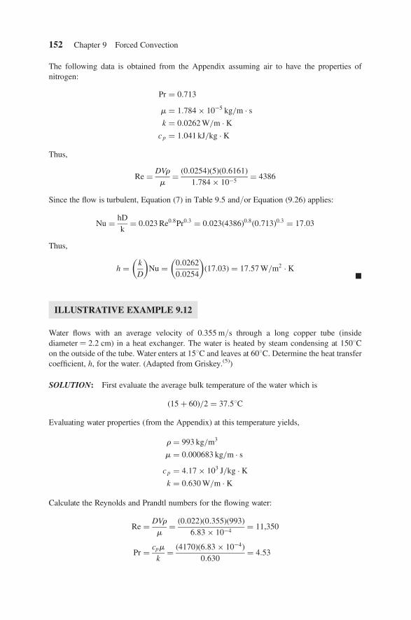
ILLUSTRATIVE EXAMPLE 9.12
Water flows with an average velocity of 0.355 m/s through a long copper tube (insidediameter ¼ 2.2 cm) in a heat exchanger. The water is heated by steam condensing at 1508Con the outside of the tube. Water enters at 158C and leaves at 608C. Determine the heat transfercoefficient, h, for the water. (Adapted from Griskey.(5))
SOLUTION: First evaluate the average bulk temperature of the water which is
(15þ 60)=2 ¼ 37:58C
Evaluating water properties (from the Appendix) at this temperature yields,
r ¼ 993 kg=m3
m ¼ 0:000683 kg=m � s
c p ¼ 4:17� 103 J=kg � K
k ¼ 0:630 W=m � K
Calculate the Reynolds and Prandtl numbers for the flowing water:
Re ¼DVr
m¼
(0:022)(0:355)(993)6:83� 10�4
¼ 11,350
Pr ¼cpm
k¼
(4170)(6:83� 10�4)0:630
¼ 4:53
152 Chapter 9 Forced Convection

The flow is turbulent and, since the tube is a long one (i.e., no L/D effect), one may use theSeider and Tate turbulent relation [Equation (8) in Table 9.5 and/or Equation (9.25)] for internalflow:
hD
k¼ 0:027 Re0:8 Pr0:33 m
mw
� �0:14
All of the quantities in the above equation are known except mw. To obtain this value, the fluids’average wall temperature must be determined. This temperature is between the fluid’s bulk aver-age temperature of 37.58C and the outside wall temperature of 1508C. Once again, use a value of93.758C (the average of the two). At this temperature (see Appendix)
mw ¼ 0:000306 kg=m � s
Then
h ¼0:6300:022
(0:027)(11,350)0:8(4:53)0:33 0:0006830:000306
� �0:14
¼ 2498:1 W=m2 � KB
An important dimensionless number that arises in some heat transfer studies andcalculations is the Biot number, Bi. It plays a role in conduction calculations thatalso involve convection effects, and provides a measure of the temperature changewithin a solid relative to the temperature change between the surface of the solidand a fluid.
Consider once again the heat transfer process described in Figure 9.1. Understeady-state conditions, one may express the heat transfer rate as
_Q ¼kA
L(T � TS) ¼ hA(TS � TM) (9:33)
The above equation may be rearranged to give
T � TS
TS � TM¼
hA
kA=L¼
L=kA
1=hA¼
Rcond
Rconv¼ Bi ¼
hL
k(9:34)
The above equation indicates that, for small values of Bi, one may assume that thetemperature across the solid is (relatively speaking) constant. If Bi ¼ 1.0, the resist-ances are approximately equal. If Bi 1.0, the resistance to conduction within thesolid is much less than the resistance to convection across the fluid boundary layer.The reverse applies if Bi �1.0. Generally, if Bi , 2.0, one may assume that for thescenario provided in Figure 9.1, the temperature profile in the solid is constant.
ILLUSTRATIVE EXAMPLE 9.13
Refer to Illustrative Example 9.7. Calculate the average Biot number.
Heat Transfer Coefficients: Quantitative Information 153
SOLUTION: Since the thickness of the flat plate is specified, the Biot number can becalculated.
Bi ¼hL
k¼
(38:7)(1:2)0:025
¼ 1858B
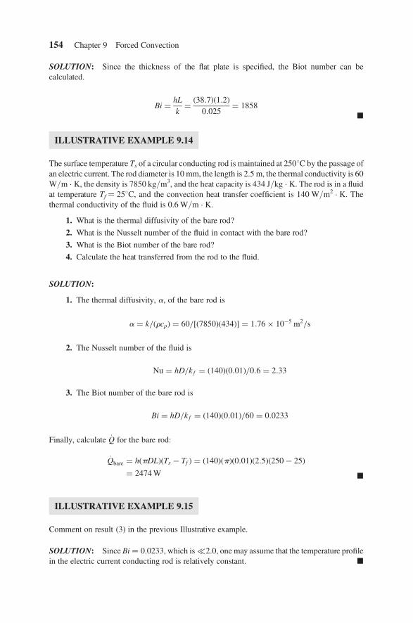
ILLUSTRATIVE EXAMPLE 9.14
The surface temperature Ts of a circular conducting rod is maintained at 2508C by the passage ofan electric current. The rod diameter is 10 mm, the length is 2.5 m, the thermal conductivity is 60W/m . K, the density is 7850 kg/m3, and the heat capacity is 434 J/kg . K. The rod is in a fluidat temperature Tf ¼ 258C, and the convection heat transfer coefficient is 140 W/m2 . K. Thethermal conductivity of the fluid is 0.6 W/m . K.
1. What is the thermal diffusivity of the bare rod?
2. What is the Nusselt number of the fluid in contact with the bare rod?
3. What is the Biot number of the bare rod?
4. Calculate the heat transferred from the rod to the fluid.
SOLUTION:
1. The thermal diffusivity, a, of the bare rod is
a ¼ k=(rcp) ¼ 60=[(7850)(434)] ¼ 1:76� 10�5 m2=s
2. The Nusselt number of the fluid is
Nu ¼ hD=k f ¼ (140)(0:01)=0:6 ¼ 2:33
3. The Biot number of the bare rod is
Bi ¼ hD=k f ¼ (140)(0:01)=60 ¼ 0:0233
Finally, calculate _Q for the bare rod:
_Qbare ¼ h(pDL)(Ts � Tf ) ¼ (140)(p)(0:01)(2:5)(250� 25)
¼ 2474 W B
ILLUSTRATIVE EXAMPLE 9.15
Comment on result (3) in the previous Illustrative example.
SOLUTION: Since Bi ¼ 0.0233, which is2.0, one may assume that the temperature profilein the electric current conducting rod is relatively constant. B
154 Chapter 9 Forced Convection

MICROSCOPIC APPROACH
The microscopic (transport) equations employed to describe heat transfer in a flowingfluid are presented in Table 9.6.(6,7) The equations describe the temperature profile in amoving fluid. Note that this table is essentially an extension of the microscopicmaterial presented in the previous two chapters. The six illustrative examples thatfollow, drawn from the work of Theodore,(7) involve the application of this table.
ILLUSTRATIVE EXAMPLE 9.16
An incompressible fluid enters the reaction zone of an insulated tubular (cylindrical) reactor attemperature T0. The chemical reaction occurring in the zone causes a rate of energy per unitvolume to be liberated. This rate is proportional to the temperature and is given by
(S)(T)
where S is a constant. Obtain the steady-state equations describing the temperature in the reactorzone if the flow is laminar. Neglect axial diffusion.
SOLUTION: This problem is solved in cylindrical coordinates. The pertinent equation is“extracted” from Table 9.6. Based on the problem statement, the temperature is a function ofboth z and r, and the only velocity component is vz:
vz@T
@z¼ a
1r
@
@rr@T
@r
� �þ@2T
@z2
� þ
A
rcp
Table 9.6 Energy-Transfer Equation for Incompressible Fluids(7)
Rectangular coordinates:
@T
@tþ vx
@T
@xþ vy
@T
@yþ vz
@T
@z¼ a
@2T
@x2þ@2T
@y2þ@2T
@z2
� þ
A
rcp(1)
Cylindrical coordinates:
@T
@tþ vr
@T
@rþ
vf
r
@T
@fþ vz
@T
@z¼ a
1r
@
@rr@T
@r
� �þ
1r2
@2T
@f2 þ@2T
@z2
� þ
A
rcp(2)
Spherical coordinates:
@T
@tþ vr
@T
@rþ
vu
r
@T
@uþ
vf
r sin u@T
@f
¼ a1r2
@
@rr2 @T
@r
� �þ
1r2 sin u
@
@usin u
@T
@u
� �þ
1
r2 sin2 u
@2T
@f2
� þ
A
rcp
(3)
Note. Lowercase v employed for velocity.
Microscopic Approach 155

If one neglects axial diffusion
@2T
@z2¼ 0
The source term A is given by
A ¼ (S)(T)
The resulting equation is
vz@T
@z¼ a
1r
@
@rr@T
@r
� �� þ
S
rcp
� �T (1)
If the flow is laminar(2),
vz ¼ V 1�r
a
� �2�
where a ¼ radius of cylinder and V ¼ maximum velocity, located at r ¼ 0. Equation (1) nowtakes the form
V 1�r
a
� �2�
@T
@z¼ a
1r
@
@rr@T
@r
� �� þ
S
rcp
� �T
B
ILLUSTRATIVE EXAMPLE 9.17
Refer to the previous example. Obtain the describing equation if the flow is plug.
SOLUTION: If the flow is plug, vz is constant(2) across the area of the reactor. Based on phys-ical grounds, the radial-diffusion term is zero and T is solely a function of z. Equation (1) thenbecomes
vzdT
dz¼
S
rcp
� �T
B
ILLUSTRATIVE EXAMPLE 9.18
Obtain the temperature profile in the reactor of Illustrative Example 9.17 if the flow is plug.
SOLUTION: The describing DE is obtained from Illustrative Example 9.17,
vzdT
dz¼
S
rcp
� �T
The equation is rewritten as
dT
T¼
S
rcpvz
� �dz
156 Chapter 9 Forced Convection

Integrating the above equation gives
ln T ¼S
rcpvz
� �zþ B
The BC is
T ¼ T0 at z ¼ 0
so that
B ¼ ln T0
Therefore
lnT
T0
� �¼
S
rcpvz
� �z
or
T ¼ T0e(S=rcpvz)z
If energy is absorbed due to chemical reaction, the above solution becomes
T ¼ T0e�(S=rcpvz)z
B
ILLUSTRATIVE EXAMPLE 9.19
A fluid is flowing (in the y direction) through the reaction zone of a rectangular parallelepipedreactor. Chemical reaction is occurring in the zone and energy is liberated at a constant rate.Obtain the equation(s) describing the steady-state temperature in the reaction zone if the flowis laminar. Assume the height (in the z direction) of the reactor h to be very small comparedto its width w. Do not neglect diffusion effects.
SOLUTION: For laminar flow,
T ¼ T( y, z)
vy ¼ vy(z)
From Table 9.6, Equation (1),
vy@T
@y¼ a
@2T
@y2þ@2T
@z2
� þ
A
rcp
In addition, Theodore(7) has shown that for this application,
vy ¼6q
wh3(zh� z2)
where q ¼ volumetric flow rate. B
Microscopic Approach 157

ILLUSTRATIVE EXAMPLE 9.20
Refer to Illustrative Example 9.19. Obtain the describing equation if the flow is plug.
SOLUTION: For plug flow,
T ¼ T(y)
vy ¼ constant
From Table 9.6, Equation (1),
vydT
dy¼ a
d2T
dy2þ
A
rcp B
ILLUSTRATIVE EXAMPLE 9.21
Consider the motion of a fluid past a thin flat plate as pictured in Figure 9.4. The boundary-layerthickness for energy transfer dT is arbitrarily defined at the points where T ¼ 0.99T0. The temp-erature of the fluid upstream from the plate is T0. The temperature at every point on the plate ismaintained at zero. Obtain the steady-state equations describing the temperature in and outsidethe boundary layer.
SOLUTION: The describing DE is obtained from Equation (1) in Table 9.6. Since the flow istwo-dimensional,
vx ¼ 0
vy = 0
vz = 0
T0
V0
T0
z
y
z = δT
T0 T0
Figure 9.4 Boundary layers.
158 Chapter 9 Forced Convection

Based on the problem statement
T ¼ T(y, z)
Since the flow is “primarily” in the y-direction, neglect thermal diffusion effects in thatdirection, i.e.,
d2T
dy2¼ 0
The following equation results from Table 9.6:
vy@T
@yþ vz
@T
@z¼ a
@2T
@z2(1)
The equation of continuity in rectangular coordinates for this application is(2,7)
@vy
@yþ@vz
@z¼ 0 (2)
The BC are
T ¼ 0 , vy ¼ 0 at z ¼ 0T ¼ T0, vy ¼ V0 at z ¼ 1
Equations (1) and (2) can now be solved to give the temperature profile in the system. The com-plete solution is not presented. However, the profile outside the boundary layer is (naturally)
T ¼ T0B
REFERENCES
1. D. GREEN and R. PERRY (editors), Perry’s Chemical Engineers’ Handbook, 8th edition, McGraw-Hill,New York City, NY, 2008.
2. P. ABULENCIA and L. THEODORE, Fluid Flow for the Practicing Engineer, John Wiley & Sons, Hoboken,NJ, 2009.
3. F. DITTUS and L. BOELTER, University of California at Berkeley, Pub. Eng., Vol. 2, 1930.4. I. FARAG and J. REYNOLDS, Heat Transfer, A Theodore Tutorial, Theodore Tutorials, East Williston,
NY, 1996.5. R. GRISKEY, Transport Phenomena and Unit Operations, John Wiley & Sons, Hoboken, NJ, 2002.6. R. BIRD, W. STEWART, and E. LIGHTFOOT, Transport Phenomena, 2nd edition, John Wiley & Sons,
Hoboken, NJ, 2002.7. L. THEODORE, Transport Phenomena for Engineers, International Textbook Co., Scranton, PA, 1971.
References 159