Multimodel Combination Techniques for Analysis of Hydrological Simulations:Application to Distributed Model Intercomparison Project Results

NEWSHA K. AJAMI

University of California, Irvine, Irvine, California

QINGYUN DUAN

Lawrence Livermore National Laboratory, Livermore, California

XIAOGANG GAO AND SOROOSH SOROOSHIAN

University of California, Irvine, Irvine, California

(Manuscript received 15 April 2005, in final form 17 November 2005)

ABSTRACT

This paper examines several multimodel combination techniques that are used for streamflow forecasting:the simple model average (SMA), the multimodel superensemble (MMSE), modified multimodel super-ensemble (M3SE), and the weighted average method (WAM). These model combination techniques wereevaluated using the results from the Distributed Model Intercomparison Project (DMIP), an internationalproject sponsored by the National Weather Service (NWS) Office of Hydrologic Development (OHD). Allof the multimodel combination results were obtained using uncalibrated DMIP model simulations and werecompared against the best-uncalibrated as well as the best-calibrated individual model results. The purposeof this study is to understand how different combination techniques affect the accuracy levels of themultimodel simulations. This study revealed that the multimodel simulations obtained from uncalibratedsingle-model simulations are generally better than any single-member model simulations, even the best-calibrated single-model simulations. Furthermore, more sophisticated multimodel combination techniquesthat incorporated bias correction step work better than simple multimodel average simulations or multi-model simulations without bias correction.

1. Introduction

Many hydrologists have been working to developnew hydrologic models or to try improving the existingones. Consequently, a plethora of hydrologic modelsare in existence today, with many more likely to emergein the future (Singh 1995; Singh and Frevert 2002a,b).With the advancement of the geographic informationsystem (GIS), a class of models, known as distributedhydrologic models, has become popular (Russo et al.1994; Vieux 2001; Ajami et al. 2004). These modelsexplicitly account for spatial variations in topography,meteorological inputs, and water movement.

The National Weather Service Hydrology Labora-

tory (NWS-HL) has recently conducted the DistributedModel Intercomparison Project (DMIP; http://www.nws.noaa.gov/oh/hrl/dmip), which showcased state-of-the-art distributed hydrologic models from differentmodeling groups (Smith et al. 2004). It was found thatthere is a large disparity in the performance of theDMIP models (Reed et al. 2004). The more interestingfindings were that multimodel ensemble averages per-form better than any single-model simulations, includ-ing the best-calibrated single-model simulations, andthe multimodel ensemble averages are more skillfuland reliable than the single-model ensemble averages(Georgakakos et al. 2004). Georgakakos et al. (2004)attributed the superior skill of the multimodel en-sembles to the fact that model structural uncertainty isaccounted for in the multimodel approach. They wenton to suggest that multimodel ensemble simulationsshould be considered as an operational forecasting tool.The fact that the simple multimodel averaging ap-

Corresponding author address: Newsha K. Ajami, Dept. of Civiland Environmental Engineering, University of California, Irvine,E/4130 Engineering Gateway, Irvine, CA 82697-2175.E-mail: nkhodata@uci.edu

AUGUST 2006 A J A M I E T A L . 755

© 2006 American Meteorological Society

JHM519

proach such as the one used by Georgakakos et al.(2004) has led to more skillful and reliable simulationsmotivated us to examine whether more sophisticatedmultimodel combination techniques can result in con-sensus simulations of even better skill.

Most hydrologists are used to the traditional contruc-tionist approach, in which the goal of the modeler is tobuild a perfect model that can capture the real worldprocesses as much as possible. The evolution of simpleconceptual models to more physically based distributedmodels is a manifestation of this approach. The multi-model combination approach, on the other hand, worksin essentially a different paradigm in which the modeleraims to extract as much information as possible fromthe existing models. The rationale behind multimodelcombination lies in the fact that predictions from indi-vidual models invariably contain errors from varioussources, including model input data, model state andparameter estimation, and model structural deficiencies(Beven and Freer 2001). With independently con-structed models, these errors tend to be mutually inde-pendent in statistical property. Through model averag-ing, these errors would act to cancel each other out,resulting in better overall predictions.

The idea of combining predictions from multiplemodels was explored more than 30 years ago in econo-metrics and statistics (see Bates and Granger 1969;Dickinson 1973, 1975; Newbold and Granger 1974).Thompson (1976) applied the model combination con-cept in weather forecasting. He showed that the meansquare error of forecasts generated by combining twoindependent model outputs is less than that of the in-dividual predictions. Based on the study done byClemen (1989), the concept of the combination fore-casts from different models were applied in diversefields ranging from management to weather prediction.Fraedrich and Smith (1989) presented a linear regres-sion technique to combine two statistical forecast meth-ods for long-range forecasting of the monthly tropicalPacific sea surface temperatures (SSTs). Krishnamurtiet al. (1999) explored the model combination techniqueby using a number of forecasts from a selection of dif-ferent weather and climate models. They called theirtechnique multimodel superensemble (MMSE) andcompared it to the simple model average (SMA)method. Krishnamurti and his group applied theMMSE technique to forecast various weather and cli-matological variables (e.g., precipitation, tropical cy-clones, seasonal climate) and all of these studies agreedthat consensus forecast outperforms any single-membermodel as well as the SMA technique (e.g., Krishna-murti et al. 1999, 2000a,b, 2001, 2002; Mayers et al.2001; Yun et al. 2003). Kharin and Zwiers (2002) re-

ported that for small sample size data the MMSE doesnot perform as well as simple ensemble mean or theregression-improved ensemble mean.

Shamseldin et al. (1997) first applied the model com-bination technique in the context of rainfall–runoffmodeling. They studied three methods of combiningmodel outputs, the SMA method, the weighted averagemethod (WAM), and the artificial neural network(ANN) method. They applied these methods to com-bine outputs of five rainfall–runoff models for 11 wa-tersheds. For all these cases they reported that themodel combination simulation is superior to that of anysingle-model simulations. Later Shamseldin andO’Connor (1999) developed a real-time model outputcombination method (RTMOCM), based on the syn-thesis of the linear transfer function model (LTFM) andthe WAM and tested it using three rainfall–runoffmodels on five watersheds. Their results indicated thatthe combined streamflow forecasts produced byRTMOCM were superior to those from the individualrainfall–runoff models. Xiong et al. (2001) refined theRTMOCM method by introducing the concept of Tak-agi–Sugeno fuzzy system as a new combination tech-nique. Abrahart and See (2002) compared six differentmodel combination techniques: the SMA; a probabilis-tic method in which the best model from the last timestep is used to create the current forecast; two differentneural network operations; and two different soft com-puting methodologies. They found that neural networkcombination techniques perform the best for a stablehydroclimate regime, while the fuzzy probabilisticmechanism generates superior outputs for a more vola-tile environment (flashier catchments with extremeevents). Butts et al. (2004a,b) proposed a frameworkthat allowed a variety of alternative distributed hydro-logical models (model structures) to be used to gener-ate multimodel ensembles. They found exploring dif-ferent model structures and using SMA or WMA mul-timodel combinations very beneficial as part of theoverall modeling approach for operational hydrologicalprediction since it decreases model structural uncer-tainty.

This paper extends the work of Georgakakos et al.(2004) and Shamseldin et al. (1997) by examining sev-eral multimodel combination techniques, includingSMA, MMSE, WAM, and modified multimodel aver-age (M3SE) a variant of MMSE. As in Georgakakos etal. (2004), we will use the simulation results from theDMIP to evaluate various multimodel combinationtechniques. Through this study, we would like to an-swer this basic question, “Does it matter which multi-model combination techniques are used to obtain con-sensus simulation?” We will also investigate how the

756 J O U R N A L O F H Y D R O M E T E O R O L O G Y VOLUME 7

accuracy of the multimodel simulations are influencedby different factors, including 1) the seasonal variationsof hydrological processes, 2) number of independentmodels considered, and 3) accuracy levels of individualmember models.

The paper is organized as follows: Section 2 over-views different model combination techniques. Section3 describes the data used in this study. Section 4 pre-sents the results and analysis. Section 5 provides a sum-mary of major lessons and conclusions.

2. A brief description of the multimodelcombination techniques

a. Simple model average

The SMA method is the multimodel ensemble tech-nique used by Georgakakos et al. (2004). This is thesimplest technique and is used as a benchmark forevaluating more sophisticated techniques in this work.SMA can be expressed by the following equation:

�QSMA�t � Qobs � �i�1

N�Qsim�i,t � �Qsim�i

N, �1�

where (QSMA)t is the multimodel streamflow simulationobtained through SMA at time t, (Qsim)i,t is the ithmodel streamflow simulation for time t, (Qsim)i is thetime average of the ith model streamflow simulation,(Qobs) is the corresponding observed average stream-flow, and N is the number of models under consider-ation.

b. Weighted average method

WAM is one of the model combination techniquesspecifically developed for rainfall–runoff modeling byShamseldin et al. (1997). This method utilizes the mul-tiple linear regression (MLR) technique to combine themodel simulations. The model weights are constrainedto be always positive and to sum to unity. If we havemodel simulations from N models, WAM can be ex-pressed as

�QWAM�t � �i�1

N

xi�Qsim�i,t �2�

S.t. � xi � 0

�xi � 1 i � 1 . . . N,

where (QWAM)t is the multimodel simulation obtainedthrough WAM at time t. Equation (2) presents a simplemultiple linear regression. The multiregression method

is a tool for exploiting linear tendencies that may existbetween dependent variable (here observed stream-flow) and a set of independent variables (the simulatedstreamflow by various models contributing in multi-model ensemble). Shamseldin et al. (1997) used theconstrained least squares technique to solve this mul-tiple linear regression equation and estimate theweights. In the constrained least squares technique, theweights are restrained to be positive and to sum tounity. The available dataset is divided into two periods:training and validation. Over the training period theweights are estimated for the each model contributingin the multimodel combination. Subsequently the esti-mated weights are tested over the validation period.For more details about this method the reader shouldrefer to Shamseldin et al. (1997).

c. Multimodel superensemble

The MMSE is a multimodel forecasting approachpopular in meteorological forecasting. Here we applythis approach for hydrological forecasting. The MMSEuses the following logic (Krishnamurti et al. 2000b):

�QMMSE�t � Qobs � �i�1

N

xi��Qsim�i,t � �Qsim�i�, �3�

where (QMMSE)t is the multimodel streamflow simula-tion obtained through MMSE at time t, and {xi, i � 1,2, . . . , N} are the regression coefficients (weights) com-puted over the training period. The weights (regressioncoefficients) are estimated through the unconstrainedleast squares technique where they can be assigned toany real numbers. As in the WAM multimodel combi-nation technique, weights are estimated over the train-ing period and validated over the forecast period.

Equation (3) comprises two main terms. The firstterm, (Qobs), which replaces the MMSE simulation av-erage streamflow with the observed average stream-flow, serves to reduce the forecast bias. The secondterm, �xi[(Qsim)i,t � (Qsim)i], reduces the variance ofthe combination of simulations using multiple regres-sions. Therefore, the logic behind this methodology is asimple idea of bias correction along with variance re-duction. We also note that when a multimodel combi-nation technique such as MMSE is used to predict hy-drologic variables like streamflow, it is important thatthe average streamflow during the training period overwhich the model weights are computed is close to theaverage streamflow of the validation period (i.e., thestationarity assumption). In section 4, we will show thatbias removal and stationarity assumption are importantfactors in multimodel simulation accuracy.

AUGUST 2006 A J A M I E T A L . 757

d. Modified multimodel superensemble

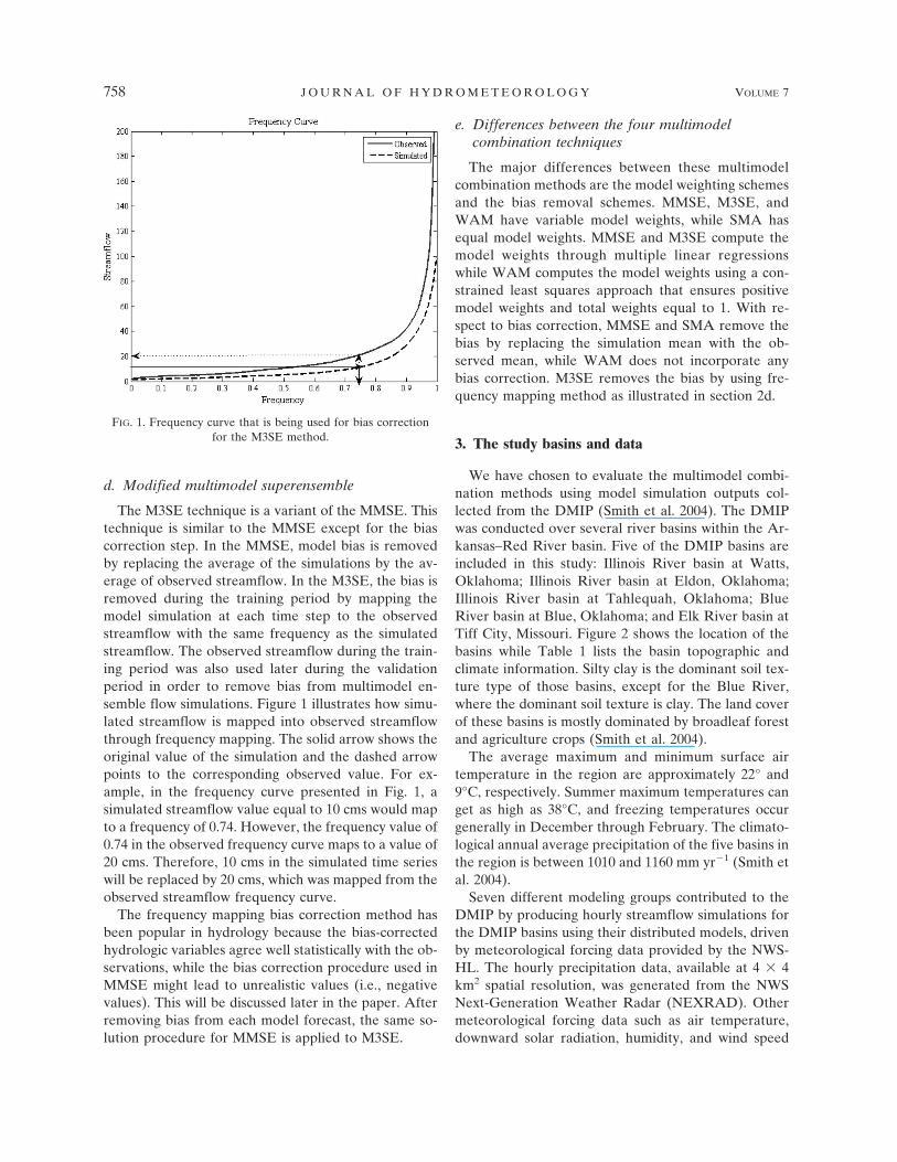
The M3SE technique is a variant of the MMSE. Thistechnique is similar to the MMSE except for the biascorrection step. In the MMSE, model bias is removedby replacing the average of the simulations by the av-erage of observed streamflow. In the M3SE, the bias isremoved during the training period by mapping themodel simulation at each time step to the observedstreamflow with the same frequency as the simulatedstreamflow. The observed streamflow during the train-ing period was also used later during the validationperiod in order to remove bias from multimodel en-semble flow simulations. Figure 1 illustrates how simu-lated streamflow is mapped into observed streamflowthrough frequency mapping. The solid arrow shows theoriginal value of the simulation and the dashed arrowpoints to the corresponding observed value. For ex-ample, in the frequency curve presented in Fig. 1, asimulated streamflow value equal to 10 cms would mapto a frequency of 0.74. However, the frequency value of0.74 in the observed frequency curve maps to a value of20 cms. Therefore, 10 cms in the simulated time serieswill be replaced by 20 cms, which was mapped from theobserved streamflow frequency curve.

The frequency mapping bias correction method hasbeen popular in hydrology because the bias-correctedhydrologic variables agree well statistically with the ob-servations, while the bias correction procedure used inMMSE might lead to unrealistic values (i.e., negativevalues). This will be discussed later in the paper. Afterremoving bias from each model forecast, the same so-lution procedure for MMSE is applied to M3SE.

e. Differences between the four multimodelcombination techniques

The major differences between these multimodelcombination methods are the model weighting schemesand the bias removal schemes. MMSE, M3SE, andWAM have variable model weights, while SMA hasequal model weights. MMSE and M3SE compute themodel weights through multiple linear regressionswhile WAM computes the model weights using a con-strained least squares approach that ensures positivemodel weights and total weights equal to 1. With re-spect to bias correction, MMSE and SMA remove thebias by replacing the simulation mean with the ob-served mean, while WAM does not incorporate anybias correction. M3SE removes the bias by using fre-quency mapping method as illustrated in section 2d.

3. The study basins and data

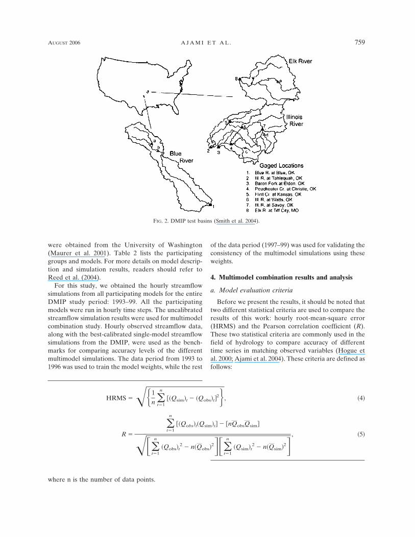
We have chosen to evaluate the multimodel combi-nation methods using model simulation outputs col-lected from the DMIP (Smith et al. 2004). The DMIPwas conducted over several river basins within the Ar-kansas–Red River basin. Five of the DMIP basins areincluded in this study: Illinois River basin at Watts,Oklahoma; Illinois River basin at Eldon, Oklahoma;Illinois River basin at Tahlequah, Oklahoma; BlueRiver basin at Blue, Oklahoma; and Elk River basin atTiff City, Missouri. Figure 2 shows the location of thebasins while Table 1 lists the basin topographic andclimate information. Silty clay is the dominant soil tex-ture type of those basins, except for the Blue River,where the dominant soil texture is clay. The land coverof these basins is mostly dominated by broadleaf forestand agriculture crops (Smith et al. 2004).

The average maximum and minimum surface airtemperature in the region are approximately 22° and9°C, respectively. Summer maximum temperatures canget as high as 38°C, and freezing temperatures occurgenerally in December through February. The climato-logical annual average precipitation of the five basins inthe region is between 1010 and 1160 mm yr�1 (Smith etal. 2004).

Seven different modeling groups contributed to theDMIP by producing hourly streamflow simulations forthe DMIP basins using their distributed models, drivenby meteorological forcing data provided by the NWS-HL. The hourly precipitation data, available at 4 4km2 spatial resolution, was generated from the NWSNext-Generation Weather Radar (NEXRAD). Othermeteorological forcing data such as air temperature,downward solar radiation, humidity, and wind speed

FIG. 1. Frequency curve that is being used for bias correctionfor the M3SE method.

758 J O U R N A L O F H Y D R O M E T E O R O L O G Y VOLUME 7

were obtained from the University of Washington(Maurer et al. 2001). Table 2 lists the participatinggroups and models. For more details on model descrip-tion and simulation results, readers should refer toReed et al. (2004).

For this study, we obtained the hourly streamflowsimulations from all participating models for the entireDMIP study period: 1993–99. All the participatingmodels were run in hourly time steps. The uncalibratedstreamflow simulation results were used for multimodelcombination study. Hourly observed streamflow data,along with the best-calibrated single-model streamflowsimulations from the DMIP, were used as the bench-marks for comparing accuracy levels of the differentmultimodel simulations. The data period from 1993 to1996 was used to train the model weights, while the rest

of the data period (1997–99) was used for validating theconsistency of the multimodel simulations using theseweights.

4. Multimodel combination results and analysis

a. Model evaluation criteria

Before we present the results, it should be noted thattwo different statistical criteria are used to compare theresults of this work: hourly root-mean-square error(HRMS) and the Pearson correlation coefficient (R).These two statistical criteria are commonly used in thefield of hydrology to compare accuracy of differenttime series in matching observed variables (Hogue etal. 2000; Ajami et al. 2004). These criteria are defined asfollows:

HRMS ���1n �

t�1

n

��Qsim�t � �Qobs�t�2� , �4�

R �

�t�1

n

��Qobs�t�Qsim�t� � �nQobsQsim�

���t�1

n

�Qobs�t2 � n�Qobs�

2���t�1

n

�Qsim�t2 � n�Qsim�2�

, �5�

where n is the number of data points.

FIG. 2. DMIP test basins (Smith et al. 2004).

AUGUST 2006 A J A M I E T A L . 759

b. Comparison of the multimodel consensuspredictions and the uncalibrated individualmodel predictions

In the first set of numerical experiments, the multi-model simulations were computed from the uncali-brated individual model simulations using the differentmultimodel combination techniques described in sec-tion 2. Figures 3a–j present the scatterplots of theHRMS versus R values of the individual model simu-lations and those of the SMA simulations. The horizon-tal axis in these figures denotes the Pearson coefficientfrom the individual models and SMA, while the verticalaxis denotes HRMS of these simulations. Note that themost desired accuracy value set in matching observedstreamflow is located at the lower-right corner of thefigures. Figures 3a, 3c, 3e, 3g, and 3i show the results forthe training period, while Figs. 3b, 3d, 3f, 3h, and 3jshow the results over validation period. These figuresclearly show that the statistics from the individualmodel simulations are almost always worse than thoseof the SMA simulations. These results confirm the factthat just simply averaging the individual model simula-tions would lead to improved accuracy levels, which isconsistent with the conclusions from the paper byGeorgakakos et al. (2004).

Figures 4a–j show the scatterplots of the HRMS andR for all multimodel combination techniques as well asfor the best-uncalibrated and the best-calibrated indi-vidual model simulations during the training and vali-dation periods. Clearly shown in these figures is that allmultimodel simulations have superior performance sta-tistics compared to the best-uncalibrated individualmodel simulation (best-uncal). More interestingly, themultimodel simulations generated by MMSE andM3SE show noticeably better performance statisticsthan those by SMA. This implies that there are benefitsin using more sophisticated multimodel combinationtechniques. The simulations generated by WAM showworse performance statistics than the simulations gen-erated by other multimodel combination techniques.This suggests that the bias removal step incorporated

by other multimodel combination techniques is impor-tant in improving simulation accuracy especially duringthe validation period. It was found that reducing thevariance solely improves the R and HRMS compared tothe best-performing uncalibrated member model be-tween 3%–12% and 13%–30% over the training periodand 0%–3% and 8%–16% over the validation period,respectively. Adding the bias removal step to the pro-cedure improves the R and HRMS compared to thecombination methods with just variance reduction step(WAM combination technique), between 2%–4% and10%–16% over the training period and 0%–5% and0%–10% over the validation period. These results high-light two interesting observations. First, the bias re-moval step improves the HRMS statistics more signifi-cantly than R. The second observation is that the majorprogress during model combination methods happensover the variance reduction step, even though it is hardto disregard the improvement gained during the biasremoval step. It is noteworthy that adding the bias re-moval step to the multimodel combination techniquedoes not significantly increase the complexity and com-putation time of the combination process. Figure 5 de-picts an excerpt of streamflow simulation results fromM3SE and MMSE during the forecast period. The ad-vantage of the bias removal technique in the M3SEover that of the MMSE is indicated by the fact thatnegative streamflow values were generated by theMMSE for some parts of the hydrograph (over the lowflow periods) while the M3SE does not suffer from thisproblem.

The advantage of multimodel simulations from thetraining period carries into the validation period in al-most all cases except for Blue River basin, where theperformance statistics of the multimodel simulationsare equal to or slightly worse than the best-uncalibratedindividual model simulation. The reason for the relativepoor performance in Blue River basin is that a notice-able change in streamflow characteristics is observedfrom the training period to the validation period (i.e.,the average streamflow changes from 10.8 cms in the

TABLE 1. Basin information.

Basin name

U.S. Geological Survey(USGS) gauge location

Area(km2)

Annualrainfall(mm)

Annualrunoff(mm)

Dominantsoil texture

VegetationcoverLat Lon

Illinois River basin at Eldon 35°5516� 94°5018� 795 1175 340 Silty clay Broadleaf forestBlue River basin at Blue 33°5949� 96°1427� 1233 1036 176 Clay Woody savannahIllinois River basin at Watts 36°0748� 94°3419� 1645 1160 302 Silty clay Broadleaf forestElk River basin at Tiff City 36°3753� 94°3512� 2251 1120 286 Silty clay Broadleaf forestIllinois River basin at Tahlequah 35°5522� 94°5524� 2484 1157 300 Silty clay Broadleaf forest

760 J O U R N A L O F H Y D R O M E T E O R O L O G Y VOLUME 7

training period to 7.17 cms in the validation period;standard deviation from 27.6 to 16.8 cms). This mightbe the indication that the stationarity assumption forstreamflow was violated. Consequently, the accuracylevels of the simulations during validation period wereadversely affected. Future work could include a morediagnostic analysis of the data to identify the causes forthe poor validation results. If the stationarity assump-tion holds, the mean and variance of the streamflowfrom one period to another should be similar or veryclose (the closeness of these values is a subjective judg-ment made by the modeler or forecaster). Thereforethe accuracy level during the validation period will notdeteriorate significantly. To use this technique in theoperational mode so as to decrease the deterioration inthe forecast, the forecaster (modeler) should constantlycompare the mean and variance of recently availablereal-time observations against the mean of the histori-cal observations for the same period. Statistical mea-sures could be included in the procedure to identifywhen the mean and variance of the new observationsare such that the condition of data stationarity is vio-lated. In some cases the modeler may decide to use justsome specific years to remove the bias and train themultimodel scheme to facilitate a more accurate real-time forecast (e.g., if the current year seems to be a wetyear, the modeler could use historical data from otherwet years).

To get a measure of how multimodel simulations fareagainst the best-calibrated single-model simulations, wealso included them in Figs. 4a–j. As revealed in thesefigures, MMSE and M3SE outperform the best-calibrated models (best-cal) for all the basins exceptBlue River basin during the training period. Duringvalidation period, however, the best-calibrated single-model simulations have shown a slight advantage inperformance statistics over the multimodel simulations.MMSE and M3SE are shown to be the best-performingcombination technique during validation period andhave statistics comparable to those of the best-calibrated case, while WAM and SMA have worse per-formance statistics.

c. Application of multimodel combinationtechniques to river flow predictions fromindividual months

Hydrological variables such as streamflow are knownto have a distinct annual cycle. The simulation accuracyof hydrologic models for different months often mimicthis annual cycle, as shown in Fig. 6, which displays theperformance statistics of the individual model simula-tions for Illinois River basin at Eldon during the train-

TA

BL

E2.

DM

IPpa

rtic

ipan

tm

odel

ing

grou

psan

dch

arac

teri

stic

sof

thei

rdi

stri

bute

dhy

drol

ogic

alm

odel

s(R

eed

etal

. 200

4).

Par

tici

pant

Mod

elP

rim

ary

appl

icat

ion

Spat

ial

unit

for

rain

fall–

runo

ffca

lcul

atio

nR

ainf

all–

runo

ffsc

hem

eC

hann

elro

utin

gsc

hem

e

Agr

icul

tura

lR

esea

rch

Serv

ices

(AR

S)SW

AT

Lan

dm

anag

emen

t/ag

ricu

ltur

alH

ydro

logi

cR

espo

nse

Uni

t(H

RU

)M

ulti

laye

rso

ilw

ater

bala

nce

Mus

king

umor

vari

able

stor

age

Uni

vers

ity

ofA

rizo

na(A

RZ

)SA

C-S

MA

Stre

amfl

owfo

reca

stin

gSu

bbas

ins

SAC

-SM

AK

inem

atic

wav

eE

nvir

onm

enta

lM

odel

ing

Cen

ter

(EM

C)

Noa

hla

ndsu

rfac

em

odel

Lan

d–at

mos

pher

ein

tera

ctio

ns1/

8°gr

ids

Mul

tila

yer

soil

wat

eran

den

ergy

bala

nce

—

Hyd

rolo

gic

Res

earc

hC

ente

r(H

RC

)H

RC

DH

MSt

ream

flow

fore

cast

ing

Subb

asin

sSA

C-S

MA

Kin

emat

icw

ave

Off

ice

ofH

ydro

logi

cD

evel

opm

ent

(OH

D)

HL

-RM

SSt

ream

flow

fore

cast

ing

16km

2gr

idce

llsSA

C-S

MA

Kin

emat

icw

ave

Uta

hSt

ate

Uni

vers

ity

(UT

S)T

OP

NE

TSt

ream

flow

fore

cast

ing

Subb

asin

sT

OP

MO

DE

L—

Uni

vers

ity

ofW

ater

loo

(UW

O)

WA

TF

LO

OD

Stre

amfl

owfo

reca

stin

g1-

kmgr

idL

inea

rst

orag

ero

utin

g

AUGUST 2006 A J A M I E T A L . 761

ing period. Figure 5 reveals that a model might performwell in some months, but poorly in other months, whencompared to other models. This led us to hypothesizethat the weights for different months should take ondifferent sets of values to obtain consistently skillfulsimulations for all months. To test this hypothesis,model weights for each calendar month were computedseparately for all basins and all multimodel combina-tion techniques.

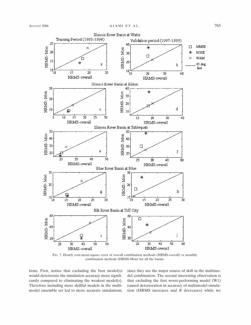
Figures 7a–j show the scatterplots of the HRMS val-ues when a single set of model weights were computedfor overall training period versus the HRMS valueswhen monthly weights were computed. Figures7a,c,e,g,i were for the training period and Figs. 7b,d,f,h,jwere for the validation period. From these figures, it isclear that the performance of MMSE and M3SE withmonthly weights is generally better than that with singlesets of weights for the entire training period. Applying

FIG. 3. Hourly root-mean-square error vs Pearson coefficient for SMA and uncalibrated member models for allof the basins.

762 J O U R N A L O F H Y D R O M E T E O R O L O G Y VOLUME 7

monthly weights for WAM does not improve the re-sults, and in some cases the results worsen over thetraining period. During the validation period, however,the performance statistics using single sets of weights

are generally better than those using monthly weights.This is because the stationarity assumptions are moreeasily violated when the multimodel techniques are ap-plied monthly.

FIG. 4. Hourly root-mean-square error vs Pearson coefficient for all model combinations (MMSE, M3SE, WAM,and SMA) against the best-performing uncalibrated and calibrated model for all the basins (the closer to thebottom-right corner, the better the model).

AUGUST 2006 A J A M I E T A L . 763

d. The effect of different number of models usedfor model combination on the skill levels ofmultimodel predictions

The use of multimodel simulations leads to the ques-tion of how many models are needed to ensure highaccuracy from multimodel simulations. To address thisquestion, we performed a series of experiments by se-quentially removing a different number of models fromconsideration. Figure 8 displays the test results forMMSE. Shown in the figure are the average HRMS andR values when a different number of models was in-cluded in model combination. The figure suggests thatthe inclusion of at least four models is necessary for theMMSE to obtain consistently good skillful results. Thefigure also shows that including over five models wouldactually slightly deteriorate the results. This indicates

that the accuracy levels of the individual member mod-els may affect the overall accuracy levels of the combi-nation results. To illustrate how important the accuracyof individual models is on the accuracy of the multi-model simulations, we experimented with removing thebest-performing models and the worst-performingmodels from consideration. The effects of removing thebest and worst models on the HRMS and R values areshown in Figs. 9a–d. The immediate left point from thecenter in the figures corresponds to the case in whichthe worst-performing model (w1) was removed and thenext point with the two worst models (w1 and w2) re-moved. The immediate right point from the center inthe figure corresponds to the case in which the best-performing model (b1) was removed and the next pointwith two best models (b1 and b2) removed. The resultspresented in Fig. 9 highlight two interesting observa-

FIG. 6. Monthly HRMS of uncalibrated member models for Illinois River basin at Eldon.

FIG. 5. An excerpt of streamflow simulation results for the Illinois River basin at Wattsduring the forecast period, illustrating the performance of MMSE and M3SE combinationtechniques against the observed and best-calibrated model. As can be seen M3SE has feasiblestreamflow values when MMSE produces negative streamflow values.

764 J O U R N A L O F H Y D R O M E T E O R O L O G Y VOLUME 7

tions. First, notice that excluding the best model(s)would deteriorate the simulation accuracy more signifi-cantly compared to eliminating the weakest model(s).Therefore including more skillful models in the multi-model ensemble set led to more accurate simulations,

since they are the major source of skill in the multimo-del combination. The second interesting observation isthat excluding the first worst-performing model (W1)caused deterioration in accuracy of multimodel simula-tion (HRMS increases and R decreases) while we

FIG. 7. Hourly root-mean-square error of overall combination methods (HRMS-overall) vs monthlycombination methods (HRMS-Mon) for all the basins.

AUGUST 2006 A J A M I E T A L . 765

would expect a monotonic improvement of statistic(not deterioration). This reveals that even the worstmodel(s) can capture some processes within the water-shed that has been ignored by other models. This char-acteristic can make them relatively useful in the multi-model combination strategy.

5. Conclusions and future direction

We have tested four different multimodel combina-tion techniques to the streamflow simulation resultsfrom the DMIP, an international project sponsored bythe NWS Office of Hydrologic Development, to inter-

FIG. 9. Goodness-of-fit statistics for various model combinations.

FIG. 8. Average HRMS and R statistics for MMSE when a different number of models was included in modelcombination.

766 J O U R N A L O F H Y D R O M E T E O R O L O G Y VOLUME 7

compare seven state-of-the-art distributed hydrologicmodels in use today (Smith et al. 2004). The DMIPresults show that there is a large disparity in the per-formance of the participating models in representingthe streamflow. While developing more sophisticatedmodels may lead to more agreement among models inthe future, this work has been motivated by the premisethat the accuracy of the existing models is not fullyrealized. Multimodel combination techniques are vi-able tools to extract the strengths from different modelswhile avoiding the weaknesses.

Through a series of numerical experiments, we havelearned several valuable lessons. First, simply averagingthe individual model simulations would result in con-sensus multimodel simulations that are superior to anysingle-member model simulations. More sophisticatedmultimodel combination approaches such as MMSEand M3SE can improve the simulation accuracy evenfurther. The multimodel simulations generated by theMMSE and M3SE can be better than or at least com-parable to the best-calibrated single-model simulations.This suggests that future operational hydrologic simu-lations should incorporate a multimodel combinationstrategy.

Second, in examining the different multimodel com-bination techniques, it was found that bias removal is animportant step in improving the simulation accuracy ofthe multimodel simulations. MMSE and M3SE simula-tions, which incorporated bias correction steps, performnoticeably better than WAM simulations, which did notincorporate bias removal. The M3SE has the advantageof generating consistent streamflow results over theMMSE because its bias removal technique is morecompatible with hydrologic variables such as stream-flow. Also important is the stationarity assumptionwhen using multimodel combination techniques forsimulating streamflow. In the Blue River basin wherethe average streamflow values are significantly differ-ent between the training and validation periods, theadvantages of multimodel simulations were lost duringthe validation period. This finding was also confirmedwhen the multimodel combination techniques were ap-plied to streamflow from individual months.

Third, we attempted to address how many modelsare needed to ensure the good accuracy of multimodelsimulations. We found that at least four models arerequired to obtain consistent multimodel simulations.We also found that the multimodel simulation accuracyis related to the accuracy of the individual membermodels. If the simulation accuracy from an individualmodel is poor in matching observations, removing thatmodel from consideration does not affect the accuracyof the multimodel simulations very much. On the other

hand, removing the best-performing model from con-sideration does adversely affect the multimodel simu-lation accuracy. This conclusion supports the need for abetter understanding of hydrological processes and todevelop well-performing hydrological models that willbe included in the multimodel ensemble set. Thesemodels are a major source of skill and their contribu-tion in the multimodel combination can advance accu-racy and skill of the final results.

This work was based on a limited dataset. There areonly seven models and a total of seven years of hourlystreamflow data. The findings are necessarily subject tothese limitations. Longer dataset and more models (es-pecially skillful models) might improve the multimodelcombination results especially during the verificationperiod; however, this needs to be investigated. Further,the regression-based techniques used here (i.e., MMSE,M3SE, and WAM) are vulnerable to a multicolinearityproblem, which may result in unstable or unreasonableestimates of the weights (Winkler 1989). This, in turn,would reduce the substantial advantages achieved em-ploying these combination strategies. There are rem-edies available to deal with a colinearity problem(Shamseldin et al. 1997; Yun et al. 2003). This mayentail more independent models to be included in themodel combination. It is recommended that a set ofhydrologic forecast experiments be conducted usingforecasted input forcings (such as forecasted precipita-tion and temperature) to evaluate performance of mul-timodel combinations as a real-time forecasting tool.

The multilinear-regression-based approach pre-sented here is only one type of the multimodel combi-nation approach. Over recent years, other model com-bination approaches have been developed in fieldsother than hydrology, such as the Bayesian model av-erage (BMA) method, in which model weights are pro-portional to the individual model accuracy and can becomputed recursively as more observation informationbecomes available (Hoeting et al. 1999). Model combi-nation techniques are still young in hydrology. The re-sults presented in this paper and others (e.g., Butts et al.2004a,b; Georgakakos et al. 2004) show promise thatmultimodel simulations will be a superior alternative tocurrent single-model simulation.

Acknowledgments. This work was supported by NSFSustainability of Semi-Arid Hydrology and RiparianAreas (SAHRA) Science and Technology Center (NSFEAR-9876800) and HyDIS project (NASA GrantNAG5-8503). The work of the second author was per-formed under the auspices of the U.S. Department ofEnergy by University of California, Lawrence Liver-more National Laboratory, under Contract W-7405-

AUGUST 2006 A J A M I E T A L . 767

Eng-48. The authors greatly acknowledge detailed andconclusive comments by Dr. Michael Smith and twoanonymous reviewers on the original manuscript.

REFERENCES

Abrahart, R. J., and L. See, 2002: Multi-model data fusion forriver flow forecasting: An evaluation of six alternative meth-ods based on two contrasting catchments. Hydrol. Earth Syst.Sci., 6, 655–670.

Ajami, N. K., H. Gupta, T. Wagener, and S. Sorooshian, 2004:Calibration of a semi-distributed hydrologic model forstreamflow estimation along a river system. J. Hydrol., 298,112–135.

Bates, J. M., and C. W. J. Granger, 1969: The combination offorecasts. Oper. Res. Quart., 20, 451–468.

Beven, K. J., and J. Freer, 2001: Equifinality, data assimilation,and uncertainty estimation in mechanistic modelling of com-plex environmental systems using the GLUE methodology. J.Hydrol., 249, 11–29.

Butts, M. B., J. T. Payne, M. Kristensen, and H. Madsen, 2004a:An evaluation of the impact of model structure on hydrologi-cal modelling uncertainty for streamflow prediction. J. Hy-drol., 298, 242–266.

——, ——, and J. Overgaard, 2004b: Improving streamflow simu-lations and flood forecasts with multi-model ensembles. Pro-ceedings of the 6th International Conference on Hydroinfor-matics, S. Y. Liong, K. K. Phoon, and V. Babovic, Eds.,World Scientific, 1189–1196.

Clemen, R. T., 1989: Combining forecasts: A review and anno-tated bibliography. Int. J. Forecasting, 5, 559–583.

Dickinson, J. P., 1973: Some statistical results in the combinationof forecast. Oper. Res. Quart., 24, 253–260.

——, 1975: Some comments on the combination of forecasts.Oper. Res. Quart., 26, 205–210.

Fraedrich, K., and N. R. Smith, 1989: Combining predictiveschemes in long-range forecasting. J. Climate, 2, 291–294.

Georgakakos, K. P., D. J. Seo, H. Gupta, J. Schake, and M. B.Butts, 2004: Characterizing streamflow simulation uncer-tainty through multimodel ensembles. J. Hydrol., 298, 222–241.

Hoeting, J. A., D. Madigan, A. E. Raftery, and C. T. Volinsky,1999: Bayesian model averaging: A tutorial. Stat. Sci., 14,382–417.

Hogue, T. S., S. Sorooshian, V. K. Gupta, A. Holz, and D. Braatz,2000: A multistep automatic calibration scheme for riverforecasting models. J. Hydrometeor., 1, 524–542.

Kharin, V. V., and F. W. Zwiers, 2002: Climate predictions withmultimodel ensembles. J. Climate, 15, 793–799.

Krishnamurti, T. N., C. M. Kishtawal, T. LaRow, D. Bachiochi, Z.Zhang, C. E. Williford, S. Gadgil, and S. Surendran, 1999:Improved skill of weather and seasonal climate forecastsfrom multimodel superensemble. Science, 285, 1548–1550.

——, ——, D. W. Shin, and C. E. Williford, 2000a: Improvingtropical precipitation forecasts from a multianalysis superen-semble. J. Climate, 13, 4217–4227.

——, ——, Z. Zhang, T. LaRow, D. Bachiochi, and C. E. Willi-

ford, 2000b: Multimodel ensemble forecasts for weather andseasonal climate. J. Climate, 13, 4196–4216.

——, and Coauthors, 2001: Real-time multianalysis-multimodelsuperensemble forecasts of precipitation using TRMM andSMM/I products. Mon. Wea. Rev., 129, 2861–2883.

——, and Coauthors, 2002: Superensemble forecasts for weatherand climate. Proc. ECMWF Seminar on Predictability ofWeather and Climate, Reading, United Kingdom, ECMWF.

Maurer, E. P., G. M. O’Donnell, D. P. Lettenmaier, and J. O.Roads, 2001: Evaluation of the land surface water budget inNCEP/NCAR and NCEP/DOE reanalyses using an off-linehydrologic model. J. Geophys. Res., 106 (D16), 17 841–17 862.

Mayers, M., T. N. Krishnamurti, C. Depradine, and L. Moseley,2001: Numerical weather prediction over the eastern Carib-bean using Florida State University (FSU) global and re-gional spectral models and multi-model/multi-analysis super-ensemble. Meteor. Atmos. Phys., 78, 75–88.

Newbold, P., and C. W. J. Granger, 1974: Experience with fore-casting univariate time series and the combination of fore-casts. J. Roy. Stat. Soc., 137A, 131–146.

Reed, S., V. Koren, M. Smith, Z. Zhang, F. Moreda, D. J. Seo, andDMIP Participants, 2004: Overall distributed model inter-comparison project results. J. Hydrol., 298, 27–60.

Russo, R., A. Peano, I. Becchi, and G. A. Bemporad, Eds., 1994:Advances in Distributed Hydrology. Water Resources Publi-cations, 416 pp.

Shamseldin, A. Y., and K. M. O’Connor, 1999: A real-time com-bination method for the outputs of different rainfall–runoffmodels. Hydrol. Sci. J., 44, 895–912.

——, ——, and G. C. Liang, 1997: Methods for combining theoutputs of different rainfall–runoff models. J. Hydrol., 197,203–229.

Singh, V. P., Ed., 1995: Computer Models of Watershed Hydrol-ogy. Water Resources Publications, 1144 pp.

——, and D. K. Frevert, Eds., 2002a: Mathematical Models ofLarge Watershed Hydrology. Water Resources Publications,914 pp.

——, and ——, Eds., 2002b: Mathematical Modeling of Small Wa-tershed Hydrology and Applications. Water Resources Pub-lications, 972 pp.

Smith, M. B., D.-J. Seo, V. I. Koren, S. Reed, Z. Zhang, Q. Duan,F. Moreda, and S. Cong, 2004: The distributed model inter-comparison project (DMIP): Motivation and experiment de-sign. J. Hydrol., 298, 4–26.

Thompson, P. D., 1976: How to improve accuracy by combiningindependent forecasts. Mon. Wea. Rev., 105, 228–229.

Vieux, B. E., 2001: Distributed Hydrologic Modeling Using GIS.Kluwer Academic, 294 pp.

Winkler, R. L., 1989: Combining forecasts: A philosophical basisand some current issues. Int. J. Forecasting, 5, 605–609.

Xiong, L. H., A. Y. Shamseldin, and K. M. O’Connor, 2001: Anon-linear combination of the forecasts of rainfall–runoffmodels by the first-order Takagi–Sugeno fuzzy system. J. Hy-drol., 245, 196–217.

Yun, W. T., L. Stefanova, and T. N. Krishnamurti, 2003: Improve-ment of the multimodel superensemble technique for sea-sonal forecasts. J. Climate, 16, 3834–3840.

768 J O U R N A L O F H Y D R O M E T E O R O L O G Y VOLUME 7