Multidimensional Dynamic Programming for Homology Search on Distributed Systems

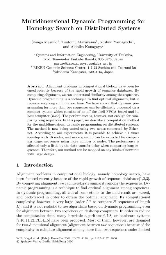
Multidimensional Dynamic Programming forHomology Search on Distributed Systems

Shingo Masuno1, Tsutomu Maruyama1, Yoshiki Yamaguchi1,and Akihiko Konagaya2

1 Systems and Information Engineering, University of Tsukuba,1-1-1 Ten-ou-dai Tsukuba Ibaraki, 305-8573, Japan

[email protected] RIKEN Genomic Sciences Center, 1-7-22 Suehiro-cho Tsurumi-ku

Yokohama Kanagawa, 230-0045, Japan

Abstract. Alignment problems in computational biology have been fo-cused recently because of the rapid growth of sequence databases. Bycomputing alignment, we can understand similarity among the sequences.Dynamic programming is a technique to find optimal alignment, but itrequires very long computation time. We have shown that dynamic pro-gramming for more than two sequences can be efficiently processed on acompact system which consists of an off-the-shelf FPGA board and itshost computer (node). The performance is, however, not enough for com-paring long sequences. In this paper, we describe a computation methodfor the multidimensional dynamic programming on distributed systems.The method is now being tested using two nodes connected by Ether-net. According to our experiments, it is possible to achieve 5.1 timesspeedup with 16 nodes, and more speedup can be expected for compar-ing longer sequences using more number of nodes. The performance isaffected only a little by the data transfer delay when comparing long se-quences. Therefore, our method can be mapped on any kinds of networkswith large delays.

1 Introduction

Alignment problems in computational biology, namely homology search, havebeen focused recently because of the rapid growth of sequence databases[1,2,3].By computing alignment, we can investigate similarity among the sequences. Dy-namic programming is a technique to find optimal alignment among sequences.In dynamic programming, all causal connections to the final result are stored,and back-traced in order to obtain the optimal alignment. Its computationalcomplexity, however, is very large (order LN to compare N sequences of lengthL), and it is not realistic to use algorithms based on dynamic programming evenfor alignment between two sequences on desk-top computers. In order to reducethe computation time, many heuristic algorithms[6,7,8] or hardware systems[9,10,11,12,13,14,15] have been proposed. Most of them, however, are designedfor two-dimensional alignment (alignment between two sequences) because of thecomplexity to calculate alignment among more than two sequences under limited

W.E. Nagel et al. (Eds.): Euro-Par 2006, LNCS 4128, pp. 1127–1137, 2006.c© Springer-Verlag Berlin Heidelberg 2006

1128 S. Masuno et al.

hardware resources. We have already proposed computational methods for morethan two sequences [16,17], and shown that high performance can be achievedon a compact system which consists of an off-the-shelf FPGA board and its hostcomputer (node). The performance is, however, not enough for comparing longsequences.

In this paper, we describe a computation method for the multidimensionaldynamic programming on distributed systems, which consist of the nodes con-nected as a ring. The communication pattern between the nodes in our approachis very simple and regular. Each node receives data from its predecessor, andsends its results to its successor. This data transfer can be overlapped with thecomputation of the dynamic programming. The method is now being testedusing two nodes connected by Ethernet.

This paper is organized as follows. Section 2 introduces the outline of dynamicprogramming for homology search, and our computation method for more thantwo sequences are described in Section 3. The parallel computation method ondistributed systems are given in Section 4, and the estimated performance basedon the experimental results is given in Section 5. The current status and futureworks are given in Section 6.

2 Dynamic Programming for Homology Search

In the dynamic programming for homology search, sequences are compared in-serting gaps with extra costs. Figure 1 shows an example of alignment of twosequences by dynamic programming (two-dimensional). In Figure 1(A), scoreson each node on the search space (M × N) are calculated using the equationin Figure 2. Scores for each matching between two elements (Ms[a[x], b[y]]) andinserting gaps (GC()) are given by score matrices [4,5]. In each node, there arethree candidates of its score (from the left-upper node, upper node and left node)in two-dimensional search, and the maximum of them is chosen. The paths whichgive the maximum values are stored, and after calculating scores of all nodes,the paths are back-traced from the last node to the start node to obtain thealignment of the two sequences (Figure 1(B)).

To obtain an alignment of more than two sequences, the same procedure is ap-plied to the sequences. The search space of N -dimensional dynamic programming

b[0] b[1] b[2] ...................... b[N-1]

a[0]

a[1]

a[M-1]

..........

Start Node

Last Node

y

x

b[0] b[1] b[2] ...................... b[N-1]

a[0]

a[1]

a[M-1]

..........

Start Node

Last Node

y

x

(A) computation of scores of each node (B) backtracing from Last Node

Fig. 1. Two Dimensional Dynamic Programming

Multidimensional Dynamic Programming for Homology Search 1129

Two-Dimensional Search:score(x, y) =

max

⎧⎨

⎩

score(x-1, y-1)+Ms[a[x], b[y]]score(x, y-1)+GC(x, -)score(x-1, y)+GC(-, y)

⎫⎬

⎭

Three-Dimensional Search:score(x, y, z) =

max

⎧⎪⎪⎪⎪⎪⎪⎪⎨

⎪⎪⎪⎪⎪⎪⎪⎩

score(x-1, y-1, z-1)+Ms[a[x], b[y], c[z]]score(x, y-1, z-1)+Ms[-, b[y], c[z]]+GC(x, -, -)score(x-1, y, z-1)+Ms[a[x], -, c[z]]+GC(-, y, -)score(x-1, y-1, z)+Ms[a[x], b[y], -]+GC(-, -, z)score(x-1, y, z)+GC(-, y, z)score(x, y-1, z)+GC(x, -, z)score(x, y, z-1)+GC(x, y, -)

⎫⎪⎪⎪⎪⎪⎪⎪⎬

⎪⎪⎪⎪⎪⎪⎪⎭

Fig. 2. Equations to calculate Scores

becomes LN (when N sequences have length L). As indicated by the equationsin Figure 2,

1. the number of candidates of the score for each node is 2N−1 in N -dimensionaldynamic programming, and

2. the size of score matrices is kN (k is the number of type of elements in thesequences), which becomes very large for larger N .

Figure 3 shows the maximum parallelism in dynamic programming. As shownin Figure 3, nodes on a diagonal line (plane) can be processed in parallel. Themaximum parallelism in N -dimensional search is the product of the size of N -1sequences (in the maximum case). When N=2, the maximum parallelism is Y ,and it takes X × Y - 1 steps to calculate the alignment.

3 Multidimensional Dynamic Programming on an FPGA

In the dynamic programming, we need to store paths to each node to back-trace. The total size of the paths becomes LN(the number of the nodes in thesearch space) ×N(data bit width of a path), which becomes very large for largerN . However, if the given sequences are not apparently similar, we do not needthe alignment. Therefore, in our approach, two types of circuits are configuredon FPGA[15,17]. With the first type circuits, the similarity among sequencesare checked by computing only the scores. Then, the second type circuits are

t=1

t=2

t=X t=X+1 .......................... t=X+Y-1

............

X

Y

(A) Parallel Processing of two dimensional dynamic programming

(B) Parallel Processing of three dimensional dynamic programming

Z

t=X+Y+ k’

Y

X

Fig. 3. Parallelism in Dynamic Programming


configured on the FPGA, and the alignments are calculated for the sequenceswith high similarity (score) by storing all causal connections. In the followingdiscussion, we focus on the first type circuits.

In our approach, N -dimensional dynamic programming is achieved by re-peating two-dimensional dynamic programming along other dimensions in or-der to reduce the size of the score matrices which have to be cached on theFPGA (for the protein sequences (k=24), the total size of the score matrix be-comes 324K words when N=4). Suppose that we repeat the following procedurefor four-dimensional dynamic programming (a four-dimensional score matrixMs[a[x], b[y], c[z], d[t]] is used).

1. Calculate the alignment between two sequences (a and b) without changingother two sequences (c[z] = Ck and d[t] = Dl; Ck and Dl are constants).

2. Increment z, and then t (c[z] or(and) d[t] is changed).

Then, we need only a part of the four-dimensional matrix, which is a two-dimensional score matrix (Ms[a[x], b[y], Ck, Dl]) in the first step of the proce-dure. However, we need different two-dimensional score matrix when the valueof c[z] or d[t] is changed. In our implementation, two-dimensional score matricesare implemented using dual-port RAMs in FPGA, and score matrices for nextb[z] or/and d[t] (namely next parts of the four-dimensional score matrix) aredownloaded from external RAMs on the FPGA board in parallel with the com-putation of scores. The number of score matrices which are download duringthe computation becomes 2N−2. Thus, with a certain value of N , the down-loading time of the next score matrices exceeds the time of the computation ofthe two-dimensional dynamic programming, and becomes the bottleneck of thisapproach.

In the following discussion, suppose that X , Y , Z and T are length of se-quences placed along x, y, z and t axes, and Wx, Wy, Wz and Wt are part ofsequences which can be processed continuously without extra input/output forboundary data. Figure 4 shows how three-dimensional dynamic programmingis executed by the repetition of the two-dimensional dynamic programming. InFigure 4, processing of Wx ×Wy nodes (two-dimensional dynamic programming)in the scan window (gray square in the figure) is scanned along z axis (the blackarrow shows the scan line). When the scan window reaches at the end of z axis,

Step0 ........... StepK ....

Z

Y

X

Wx

Step(Z*m+0) ..... Step (Z*m+K) ....

Z

Y

Step(Z+ 0) .....Step(Z+K) ....

Z

Y

X

Wx

WyWy

X Wx

Wy

ScanWindow

ScanLine

Fig. 4. Three-Dimensional Dynamic Programming


Z

X

Z

Y

Current Scan Window

Output to thenext scan line

Output to thescan line below

Input from thescan line above

Input from the previous

scan line

X

Y

Previous Scan Window

Current Scan Window

scan line

(A) (B)

Fig. 5. Boundary Data for Three-Dimensional Dynamic Programming

it is shifted along y axis by Wy , and is scanned along z axis again. After pro-cessing Wx ×Y ×Z nodes, the scan window is shifted down along x axis by Wx,and the same procedure is repeated.

Figure 5 shows the data input/output for the three-dimensional dynamic pro-gramming. In Figure 5(A), two dark gray rectangles show the inputs to the scanwindow (light gray square), and two rectangles with slanted lines show the out-put by the scan window. The outputs are stored, and used for the computationof other scan lines. In Figure 5(B), in order to calculate scores in the currentscan window, data in previous scan window are also necessary (those data arenot necessary in Figure 5(A), because the scan window is placed at the boundaryon the search space, and boundary conditions are given instead of those data).Therefore, the data in previous scan window are held on FPGA.

Figure 6 shows the scan cube for four-dimensional dynamic programming (acube is used instead of the window). Processing of nodes in the cube (size isWx × Wy × Wz) is scanned along t axis, changing positions of the scan line.In order to calculate scores of the nodes in the cube, the scan window in thecube (light gray square in Figure 6(A)) is scanned along z axis. Suppose thatcurrent cube is on (x, y, z, t=Ck). In order to start the calculation of the scanwindow (Figure 6(B)(1)), we need scores in dark gray parts and scores in theprevious cube along t axis ((x, y, z, t=Ck-1) which are temporally held on theFPGA (not shown in the figure) as boundary data. Among these data, twodark gray rectangles in the figure can be obtained while calculating the scoresof the nodes in the scan window. However, data in the dark gray square (the

Wz

Wx

Wy

Start node

End node

(A) Scan Cube (B) Boundary Data Given to the Currnet Search Cube and Stored for other Cubes

previous scancubeon x-axis

previous scan cubeon y-axis

previous scan cubeon z-axis Outputs to next scan cubes on x and y axes

Outputs to next scan cubeson z axis

(1) (2) (3)

Fig. 6. Four-Dimensional Dynamic Programming


last scan window in the previous scan cube along z axis) need to be loadedbefore starting the calculation, because the size of data is large, and can notbe loaded in parallel with the computation. The outputs by the scan windoware two rectangles with slanted lines. When the scan window is in the cube(figure 6(B)(2)), scores calculated in the previous scan window are held on theFPGA, and used for the calculation of the current scan window (the scores inthe previous cube along t axis which are held on the FPGA are also used). Whenthe scan window reaches at the end of the cube, scores in the current window arestored for later processing (figure 6(B)(3)). In this processing of the scan cube,there are two types of data;

1. data which can be loaded, and output in parallel with the computation ofthe scores of the nodes in the scan window (two dark rectangles in Figure6(B)(1,2,3)), and

2. data which have to be loaded before the computation (dark gray square inFigure 6(B)(1)) and which have to be stored after the computation (darkgray square in Figure 6(B)(3)).

The total clock cycles by our approach can be estimated as follows, when thedata width of each element in score matrices is 16 bits, and the external memorybanks run at the same speed as the circuit on the FPGA. In the following equa-tions, the first term chooses the maximum of the computation time of the scanwindow (Wx + Wy) and the time to update score matrices which is executed inparallel with the computation. In other terms, constant values show the timeto download score matrices, and other values show the time to input/outputboundary data (some matrices can not be loaded in parallel with the computa-tion, and we need to download them when c[z], d[t] and so on are changed).Three-Dimensional:

max{

Wx + Wy

242/4

}

× XY Z

WxWy

Four-Dimensional:max

{Wx + Wy

242/8 × 2

}

× XY ZT

WxWy

+ max{

242/2WxWy × 2/5

}

× XY ZT

WxWyWz

Five-Dimensional:max

{Wx + Wy

242/16 × 4

}

× XY ZTU

WxWy

+ max{

242/4 × 2WxWy × 2/5

}

× XY ZTU

WxWyWz

+

max{

242/2WxWyWz × 2/5

}

× XY ZTU

WxWyWzWt

Six-Dimensional:max

{Wx + Wy

242/32 × 8

}

× XY ZTUV

WxWy

+ max{

242/5 × 4WxWy × 2/5

}

× XY ZTUV

WxWyWz

+

max{

242/5 × 8WxWyWz × 2/5

}

× XY ZTUV

WxWyWzWt

+ max{

242/5 × 7WxWyWzWt × 2/5

}

× XY ZTUV

WxWyWzWtWu

In the equations above, {Wx, Wy , Wz, Wt, Wu} are parameters which decidethe performance, and have to be chosen so that the maximum performance canbe realized under given hardware resources (the size of the FPGA, and the mem-ory bandwitdh). For example, in our current implementation on ADM-XRC-II(FPGA board byits Alpha Data) with one Xilinx XC2V6000, {Wx, Wy, Wz , Wt}are {10,64,6,3} for five-dimensional dynamic programming, and it takes about1.35 × 104 seconds to calculate the alignment, when the length of the sequences


......

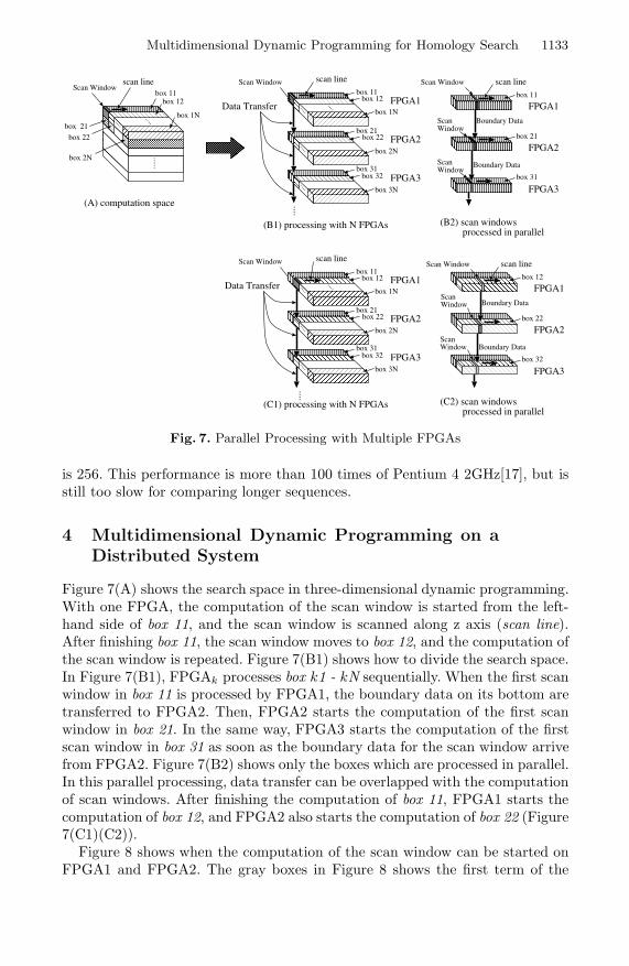
.... ....box 21

box 22

box 2N

(A) computation space

box 11box 12

box 1N

Scan Windowscan line

box 31

....

....box 22

box 2N

box 21

box 32

box 3N

....

.... ....box 12

box 1NFPGA1

FPGA2

FPGA3

Data Transfer

(B1) processing with N FPGAs

Scan Windowbox 11

box 21

box 31

box 11

Scan Window

ScanWindow

Boundary Data

Boundary Data

(B2) scan windows processed in parallel

FPGA1

FPGA2

FPGA3

scan line scan lineScan Window

box 31

....

....box 22

box 2N

box 21

box 32

box 3N

....

.... ....box 12

box 1NFPGA1

FPGA2

FPGA3

(C1) processing with N FPGAs

Scan Windowbox 11

box 22

box 32

box 12

Scan Window

ScanWindow

Boundary Data

Boundary Data

(C2) scan windows processed in parallel

FPGA1

FPGA2

FPGA3

scan linescan lineScan Window

Data Transfer

Fig. 7. Parallel Processing with Multiple FPGAs

is 256. This performance is more than 100 times of Pentium 4 2GHz[17], but isstill too slow for comparing longer sequences.

4 Multidimensional Dynamic Programming on aDistributed System

Figure 7(A) shows the search space in three-dimensional dynamic programming.With one FPGA, the computation of the scan window is started from the left-hand side of box 11, and the scan window is scanned along z axis (scan line).After finishing box 11, the scan window moves to box 12, and the computation ofthe scan window is repeated. Figure 7(B1) shows how to divide the search space.In Figure 7(B1), FPGAk processes box k1 - kN sequentially. When the first scanwindow in box 11 is processed by FPGA1, the boundary data on its bottom aretransferred to FPGA2. Then, FPGA2 starts the computation of the first scanwindow in box 21. In the same way, FPGA3 starts the computation of the firstscan window in box 31 as soon as the boundary data for the scan window arrivefrom FPGA2. Figure 7(B2) shows only the boxes which are processed in parallel.In this parallel processing, data transfer can be overlapped with the computationof scan windows. After finishing the computation of box 11, FPGA1 starts thecomputation of box 12, and FPGA2 also starts the computation of box 22 (Figure7(C1)(C2)).

Figure 8 shows when the computation of the scan window can be started onFPGA1 and FPGA2. The gray boxes in Figure 8 shows the first term of the


computation

loading scorematrices

sending boundary data

receiving boundary data

FPGA1

FPGA2

.......

.......

.......

.......

.......

.......

.......

.......

.......

.......

FPGA1

FPGA2

(A) data sending/receiving < max(comp. , loading) (B) data sending/receiving > max(comp. , loading)

idle timeone scan window

Fig. 8. Flow of the computation on FPGA1 and FPGA2

equation in Section 3. During the computation of a scan window in FPGA1,its boundary data are sent to FPGA2, and FPGA2 starts the computation ofits scan window using the boundary data. Figure 8(A) shows the flow of thecomputation when the data transfer is faster than the computation of the scanwindow, and Figure 8(B) shows the flow when it is slower. In Figure 8(B), eachFPGA becomes idle to wait for sending its boundary data to its successor, andfor the arrival of the boundary data from its predecessor.

Data transfer delay is not important in our computation method. The reasonis as follows. FPGA1 can continue its computation until it finishes all the com-putation assigned to FPGA1, and the data transfer can be overlapped with thecomputation of the scan windows. FPGA2 becomes idle when waiting for thefirst arrival of the boundary data because of the data transfer delay, but afterthat, FPGA2 can continue its computation as far as the boundary data arrivewithin a certain delay. Therefore, the increase of the computation time by thedata transfer delay is only

the data transfer delay × (the number of FPGAs - 1)in the total computation time.

Figure 9 shows a distributed system for our computation method. In ourapproach, the search space is divided along x axis as shown in Figure 7(B1).When the number of FPGAs(N) is smaller than the number of the dividedsearch spaces, some FPGAs have to process several of them sequentially (forexample, FPGAi processes the i-th, (N+i)-th, (2N+i)-th spaces, and so on).Therefore, the nodes are connected as a ring. Each node on the system consists

.......

FPGA

Processor

NIF NIF

node node node node

Fig. 9. A distributed system


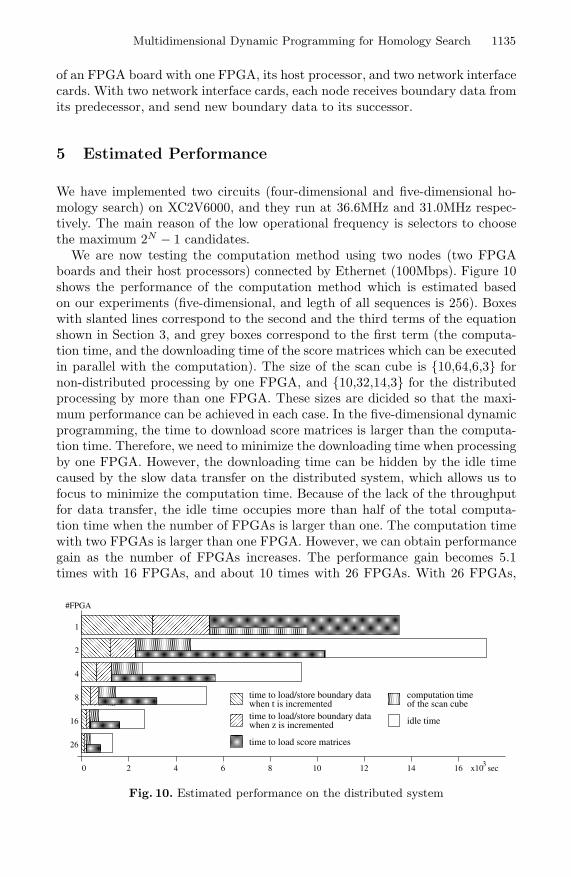
of an FPGA board with one FPGA, its host processor, and two network interfacecards. With two network interface cards, each node receives boundary data fromits predecessor, and send new boundary data to its successor.

5 Estimated Performance

We have implemented two circuits (four-dimensional and five-dimensional ho-mology search) on XC2V6000, and they run at 36.6MHz and 31.0MHz respec-tively. The main reason of the low operational frequency is selectors to choosethe maximum 2N − 1 candidates.

We are now testing the computation method using two nodes (two FPGAboards and their host processors) connected by Ethernet (100Mbps). Figure 10shows the performance of the computation method which is estimated basedon our experiments (five-dimensional, and legth of all sequences is 256). Boxeswith slanted lines correspond to the second and the third terms of the equationshown in Section 3, and grey boxes correspond to the first term (the computa-tion time, and the downloading time of the score matrices which can be executedin parallel with the computation). The size of the scan cube is {10,64,6,3} fornon-distributed processing by one FPGA, and {10,32,14,3} for the distributedprocessing by more than one FPGA. These sizes are dicided so that the maxi-mum performance can be achieved in each case. In the five-dimensional dynamicprogramming, the time to download score matrices is larger than the computa-tion time. Therefore, we need to minimize the downloading time when processingby one FPGA. However, the downloading time can be hidden by the idle timecaused by the slow data transfer on the distributed system, which allows us tofocus to minimize the computation time. Because of the lack of the throughputfor data transfer, the idle time occupies more than half of the total computa-tion time when the number of FPGAs is larger than one. The computation timewith two FPGAs is larger than one FPGA. However, we can obtain performancegain as the number of FPGAs increases. The performance gain becomes 5.1times with 16 FPGAs, and about 10 times with 26 FPGAs. With 26 FPGAs,

1

2

4

8

16

26

#FPGA

0 2 4 6 8 10 12 14 16 x10 sec3

time to load/store boundary datawhen t is incrementedtime to load/store boundary datawhen z is incremented

time to load score matrices

computation time of the scan cube

idle time

Fig. 10. Estimated performance on the distributed system


each FPGA processes only one divided search space, because the search space isdivided to 26 sub-spaces (X/Wx = 256/10).

The data transfer delay is not important in our computation method as de-scribed in Section 4, when the computation time by each FPGA is large enough.When the number of FPGAs is N , the increase of the total computation time isabount N × d seconds if the data transfer daley becomes d second longer. Thisincrease is very small compared with the total computation time.

6 Conclusions and Future Works

In this paper, we described a computation method for the multidimensionaldynamic programming on distributed systems. The method is now being testedusing two nodes connected by Ethernet. The data transfer speed of Ethernet(100 Mbps) is not enough, but according to our experiments, it is possible toachieve 5.1 times speedup with 16 nodes. The performance is affected only alittle by the data transfer delay when comparing long sequences. Therefore, ourmethod can be mapped on any kinds of networks with large delays.

We still have two major works. First, we need to evaluate the method usingmore FPGA boards, and then using more FPGA boards placed at distant places.Second, the size of boundary data can be compressed less than half, because twocontinuous data on the boundary have same values with high probability. Weneed to implement circuits to compress and uncompress the boundary data onFPGAs.

References

1. National Center for Biotechnology Information (NCBI), “NCBI-GenBank Flat FileRelease 137.0”, http://www.ncbi.nlm.nih.gov/, Aug 2003.

2. European Molecular Biology Laboratory (EMBL), http://www.ebi.ac.uk/embl/.3. DNA Data Bank of Japan (DDBJ), http://www.ddbj.nig.ac.jp/.4. Henikoff, S. and Henikoff, J.G.: “Amino Acid Substitution Matrices from Protein

Block”, Proc. Natl. Acad. Sci. 89, pp.10915-10919, 1992.5. Jones, D. T. et. al: “The Rapid Generation of Mutation DataMatrices from Proten

Sequences”, CABIOS 8, pp.275-282, 1992.6. Stephen F. Altschula, Warren Gisha, Webb Millerb, Eugene W. Meyersc, and David

J. Lipman, “Basic Local Alignment Search Tool”, Journal of Molecular Biology,Vol.215, Issue 3, pp.403-410, 1990.

7. Stephen F. et al, “Gapped BLAST and PSI-BLAST: a new generation of proteindatabase search programs”, Nucleic Acids Research, Vol.25, No.17, pp.3389-3402,1997.

8. William R. Pearson and David J. Lipman “Improved tools for biological sequencecomparison”, Proceedings of the National Academy of Sciences of the USA, Vol.85,pp.2444-2448, 1988.

9. PARACEL, “GeneMatcher2”, http://www.paracel.com/.10. Dominique Lavenier, “SAMBA Systolic Accelerators For Molecular Biological Ap-

plications”, Technical Report RR-2845, 1996.


11. C. Thomas White, et al, “BioSCAN: A VLSI-Based System for Biosequence Anal-ysis”, IEEE International Conference on Computer Design: VLSI in Computer &Processors, Vol.147, pp.504-509, (1991).

12. TimeLogic Corporation, “Decypher bioinformaticsacceleration solution”,http://www.timelogic.com/products.html, 2002.

13. Kiran Puttegowda, William Worek, Nicholas Pappas, Anusha Dandapani, and Pe-ter Athanas, “A Run-Time Reconfigurable System for Gene-Sequence Searching”,International VLSI Design Conference, pp.(to appear), 2003.

14. Steven A. Guccione and Eric Keller, “Gene Matching Using JBits”, InternationalConferenece on Field-Programmable Logic and Applications, pp.1168-1171, 2002.

15. Yoshiki Yamaguchi, Yosuke Miyajima, Tsutomu Maruyama, Akihiko Konagaya,“High Speed Homology Search with Run-time Reconfiguration”, InternationalConferenece on Field-Programmable Logic and Applications, pp.281-291, 2002.

16. Yoshiki Yamaguchi, Tsutomu Maruyama, Akihiko Konagaya, “Three-DimensionalDynamic Programming for Homology Search”, International Conferenece on Field-Programmable Logic and Applications, pp.505-514, 2004.

17. S. Masuno, T. Maruyama, Y. Yoshiki and A. Konagaya, “Multidimensional Dy-namic Programming for Homology Search”, International Conferenece on Field-Programmable Logic and Applications, pp.173-178, 2005.

Multidimensional Dynamic Programming for Homology Search on Distributed Systems

Documents

Transcript of Multidimensional Dynamic Programming for Homology Search on Distributed Systems