
Multicriteria optimization with a multiobjective golden section line search
31
Math. Program., Ser. A (2012) 131:131–161 DOI 10.1007/s10107-010-0347-9 FULL LENGTH PAPER Multicriteria optimization with a multiobjective golden section line search Douglas A. G. Vieira · Ricardo H. C. Takahashi · Rodney R. Saldanha Received: 6 November 2006 / Accepted: 3 March 2010 / Published online: 17 April 2010 © Springer and Mathematical Programming Society 2010 Abstract This work presents an algorithm for multiobjective optimization that is structured as: (i) a descent direction is calculated, within the cone of descent and fea- sible directions, and (ii) a multiobjective line search is conducted over such direction, with a new multiobjective golden section segment partitioning scheme that directly finds line-constrained efficient points that dominate the current one. This multiobjec- tive line search procedure exploits the structure of the line-constrained efficient set, presenting a faster compression rate of the search segment than single-objective golden section line search. The proposed multiobjective optimization algorithm converges to points that satisfy the Kuhn-Tucker first-order necessary conditions for efficiency (the Pareto-critical points). Numerical results on two antenna design problems support the conclusion that the proposed method can solve robustly difficult nonlinear multiob- jective problems defined in terms of computationally expensive black-box objective functions. Keywords Multiobjective optimization · Feasible directions · Line search · Golden section Mathematics Subject Classification (2000) 90C29 · 90C30 · 65K05 D. A. G. Vieira · R. R. Saldanha Departamento de Engenharia Elétrica, Universidade Federal de Minas Gerais, Minas Gerais, Brazil R. H. C. Takahashi (B ) Departamento de Matemática, Universidade Federal de Minas Gerais, Minas Gerais, Brazil e-mail: [email protected] 123
-
Upload
independent -
Category
Documents
-
view
5 -
download
0
Transcript of Multicriteria optimization with a multiobjective golden section line search

Math. Program., Ser. A (2012) 131:131–161DOI 10.1007/s10107-010-0347-9
FULL LENGTH PAPER
Multicriteria optimization with a multiobjective goldensection line search
Douglas A. G. Vieira · Ricardo H. C. Takahashi ·Rodney R. Saldanha
Received: 6 November 2006 / Accepted: 3 March 2010 / Published online: 17 April 2010© Springer and Mathematical Programming Society 2010
Abstract This work presents an algorithm for multiobjective optimization that isstructured as: (i) a descent direction is calculated, within the cone of descent and fea-sible directions, and (ii) a multiobjective line search is conducted over such direction,with a new multiobjective golden section segment partitioning scheme that directlyfinds line-constrained efficient points that dominate the current one. This multiobjec-tive line search procedure exploits the structure of the line-constrained efficient set,presenting a faster compression rate of the search segment than single-objective goldensection line search. The proposed multiobjective optimization algorithm converges topoints that satisfy the Kuhn-Tucker first-order necessary conditions for efficiency (thePareto-critical points). Numerical results on two antenna design problems support theconclusion that the proposed method can solve robustly difficult nonlinear multiob-jective problems defined in terms of computationally expensive black-box objectivefunctions.
Keywords Multiobjective optimization · Feasible directions · Line search ·Golden section
Mathematics Subject Classification (2000) 90C29 · 90C30 · 65K05
D. A. G. Vieira · R. R. SaldanhaDepartamento de Engenharia Elétrica, Universidade Federal de Minas Gerais,Minas Gerais, Brazil
R. H. C. Takahashi (B)Departamento de Matemática, Universidade Federal de Minas Gerais, Minas Gerais, Brazile-mail: [email protected]
123

132 D. A. G. Vieira et al.
1 Introduction
At the end of the XIX century, the study of economic equilibrium phenomena sug-gested the idea of the simultaneous maximization of several functions, which lead tothe concept of efficient solutions. In the words of Vilfredo Pareto [24]:
“We will say that the members of a collectivity enjoy maximum ophelimity1 in acertain position when it is impossible to find a way of moving from that positionvery slightly in such a manner that the ophelimity enjoyed by each of the indi-viduals of that collectivity increases. That is to say, any small displacement indeparting from that position necessarily has the effect of increasing the ophel-imity which certain individuals enjoy, and decreasing that which others enjoy,of being agreeable to some, and disagreeable to others.”
This idea, transposed to the context-free general setting of finding the efficient solu-tions of minimization or maximization problems with conflicting objective functionshas given rise to the multiobjective optimization [4]. A further generalization, intro-duced by Yu [32], based on the observation of an equivalence between partial ordersand certain convex cones, has given rise to the vector optimization [10]. In the contem-porary terms, a multiobjective optimization problem is a vector optimization problemin which the partial order is induced by the cone of the non-negative orthant. This paperdeals with an instance of the problem of finding the efficient solutions of multiobjectiveoptimization problems (the Pareto-optimal solutions).
This general problem can be instantiated in a number of different formulations,depending on the purpose of the analysis in each case. A group of approaches thatcan be considered “classical” rely on some scalarization procedure, i.e., they definean equivalent single objective problem leading to an efficient solution [3,4,9,27,31].These techniques are employed usually in two situations:
(i) A single efficient solution should be generated, in order to be implemented. In thiscase, the scalarization procedure should provide either the possibility of definingsome “goal” for guiding the optimization procedure, or some indication of the“relative importances” of the objectives in order to generate a meaningful solu-tion. As an instance of the first case, there is the goal programming procedure,and of the second case, the weighted sum procedure [4].
(ii) A solution set should be generated, in order to provide a description of the Pareto-set. The main concerns, for such applications, are: the ability of the algorithmto generate any point within the Pareto-set (the weighted sum procedure, forinstance, is unable to generate samples in some regions of the Pareto-set whenthe problem is non-convex); and the easiness of manipulation of the algorithmparameters in order to generate an approximately regular sample of the Pareto-set. The epsilon-constraint method, for instance, is likely to conduct a largenumber of unfeasible searches when the number of objectives is greater thantwo, while the goal programming method is likely to generate points that are
1 V. Pareto employed the term ophelimity instead of utility, in order to avoid the common-sense meaningof this last word that could be in conflict with its economic meaning.
123

Multicriteria optimization with a multiobjective golden section line search 133
more concentrated in some regions than in other ones when the goal vector ismoved uniformly.
In any case, with the exception of the approach of weighted sum of the objectives, thescalarized problems lead to scalar optimization problems that are more complicatedthan the individual optimization of the original objectives. For instance, the constraintstructure of the resulting single objective optimization problem becomes usually morecomplicated than in the original multiobjective optimization problem [3,4,9,27,31].
In recent years, it has been recognized that the availability of a sample set esti-mate that describes the whole Pareto set, as obtained in situation (ii) above, can beimportant for the development of computer aided design and computer aided decisionsystems. However, it has also become established that the application of scalarizationtechniques for the task of generating such sample set is inconvenient due to two rea-sons. First, the design of the sequence of scalar optimization problems with differentparameterizations, such that the Pareto-set is covered with a well-distributed sampledensity, is not a trivial task (see a discussion in [11]). Second, the scalarization pro-cedures are intrinsically more computationally costly than would be necessary, sincethey do not take profit of the peculiar structure of the multiobjective problems.
An important class of algorithms for dealing with such problem is the set of evolu-tionary multiobjective optimization techniques. Such algorithms, which perform ran-domized searches, are characterized by the simultaneous processing of an entire set oftentative solutions (a “population”). This parallel search allows the usage of the infor-mation about the partial order relation between such tentative solutions, for enhancingthe search for the non-dominated solutions, and also the usage of the relative distancesbetween solutions, for enhancing the solution distribution along the Pareto-set. Thefirst approach that fits this description has been presented in [14,15]. Two algorithmsthat are currently part of the state-of-the-art are described in [7,33]. A comprehensivediscussion on the topic can be found in [5,6]. Recent studies in the field include, forinstance, the choice of strategies for archiving the Pareto-set estimates found by thealgorithm [29].
More recently, some hybrid approaches have been proposed. The reference [2] haspresented an evolutionary algorithm that employs local searches using gradient infor-mation. The descent cone is reformulated such that for every direction in image spacean associated descent direction in parameter space can be computed, allowing thedetermination of directions for line searches that reach points that locally dominate acurrent solution. The paper [30] has employed a scalarization procedure over surrogateapproximated functions, for the purpose of correcting solutions within an evolutionarymultiobjective algorithm, in this way enhancing both the solution precision and thealgorithm computational effort.
Another randomized search approach has been proposed recently, based on the ideaof constructing stochastic differential equations which have the efficient solution setsas attractors [28]. A set of solutions is obtained in a single run of the algorithm. A simi-lar idea has been developed in [8], with the construction of a discrete dynamical systemfor which the efficient solution set is an attractor. Set-oriented numerical methods areemployed, coupled with a branch-and-bound procedure, in order to generate a tightbox-covering of the Pareto-set. The reference [19] presents a procedure for generating
123

134 D. A. G. Vieira et al.
polyhedral inner and outer approximations of the Pareto-set. This algorithm, whichrelies on a sequence of scalarized sub-problems, has an auto-adaptive mechanism thatautomatically balances the distribution of the Pareto-set samples. A related approach,based on the numeric resolution of a differential equation using continuation meth-ods, is presented in [25]. Yet another approach, based on homotopy methods, has beenproposed for the special case of equality-constrained problems [17].
There is yet another situation, however, in which Pareto-optimal points should begenerated:
(iii) A non-efficient solution is already available, and a non-dominated solution thatdominates the current solution should be generated.
This situation may appear, for instance, as a formal statement of the problem of enhanc-ing the characteristics of an existing technological apparatus. Other contexts for thesituation (iii) arise as sub-problems within algorithms of efficient solution generation,in the case of the algorithm outer loop being able to find only approximate non-dom-inated solutions that should be “corrected” in order to find the final solutions. Thismay be the case of evolutionary algorithms, as in [2,30].
The first versions of algorithms for situation (iii) were developed within the frame-work of scalarization methods, see for instance [1]. A key observation about situation(iii) is: since there is no need to find a specific point of the Pareto set, the multiplicityof the possible solutions can be used in order to tail more efficient search proceduresthat find any non-dominated solution that dominates the initial point. This peculiarstructure of the multiobjective optimization problems is not used by the scalarizationmethods, that perform searches for finding specific points of the Pareto-set.
The paper [13] seems to be the first one that employs such problem structure. Ithas proposed a line search method for multiobjective problems that does not rely ona scalarization procedure. That work follows the reasoning: (i) a direction in whichthere are feasible solutions that dominate the current point is chosen; (ii) a line searchbased on the Armijo’s rule is conducted on this direction, in order to find some pointthat dominates the current one. That work shows that such procedure converges to aPareto-critical point (a point that satisfies first-order conditions for Pareto-optimality,see [4,9]). Although no comparison has been performed in [13], it is shown here thatsuch procedure allows a significant reduction in the computational cost of generat-ing non-dominated solutions, in comparison with traditional scalarization methods.A generalization of those ideas, presenting a Newton’s method for the computation ofthe search direction, has been proposed recently in [12].
This paper further exploits the same principle, in order to enhance the computationalgains that are achieved. A golden section interval partitioning procedure is proposedhere, instead of the Armijo’s rule, for performing the multiobjective line search. Thefinal point that is delivered by the proposed procedure is Pareto-critical for the one-dimensional multiobjective problem obtained when constraining the original problemto the line of search: this is a stronger property than the one that is assured by theArmijo’s rule employed in [13], which guarantees only that the final point obtainedby the line search dominates the current one.
In the field of single-objective non-linear programming, the construction of line-search-based methods involves a choice of a line search procedure. The Armijo’s rule
123

Multicriteria optimization with a multiobjective golden section line search 135
and the golden section procedure are situated among the main available alternatives,and the choice between them involves a trade-off between the fast convergence of theArmijo’s rule procedure to a point that is better than the current one (also providingthat it is situated reasonably “far from” the current one) and the precise determinationof the line-constrained minimum of the objective function provided by the goldensection procedure.
The single-objective golden section line search procedure is known to be optimal,among the derivative-free and function-approximation-free line search procedures, inthe sense that it requires the minimal number of function evaluations for finding theline-constrained function minimum within a pre-defined ε-tolerance [23]. The goldensection multiobjective line search procedure proposed here not only inherits this opti-mality of the segment compression rate of the single-objective golden section proce-dure: it leads to a faster interval compressing rate than in the single-objective case,because the multiobjective problem allows simultaneously discarding two segmentparts in some steps. Also, as the constrained Pareto-set over a line is a non-zero mea-sure segment (except in very rare situations), the proposed procedure can be adjustedto find such Pareto-critical points in a number of steps that is not only finite, butusually small. Due to these reasons, the trade-off mentioned above between the fastconvergence of the Armijo’s rule and the precision of the golden section procedurebecomes more favorable to the golden section method in the multiobjective case thanin the single-objective case.
In addition to the new golden section multiobjective line search procedure, thispaper also proposes a modified procedure for finding a direction for performing thesearch. Employing the same basic procedure of [13] for guaranteeing that the directionis descent, such direction is also constrained to lie inside the cone of convex combina-tions of the negative gradients of the objective functions and of the active constraints.This has the advantage of directing the search toward the central portion of the coneof locally dominating solutions.
The proposed procedures are joined into a method that is somewhat simple, relyingonly on (i) the computation of function and constraint gradients, followed by (ii) thesolution of an auxiliary linear optimization, for finding the search direction, and by (iii)a golden-section multiobjective line search. The problem is solved with the originalstructure of constraints and objectives. This method has the same basic structure of theone proposed in [13]. The convergence of this method to a first-order Pareto-criticalpoint can be established in the same way as in that reference.
The paper is structured as follows. Firstly, the multiobjective golden section linesearch is presented. Afterward, a procedure for selecting a descent direction for linesearch is established. Using these procedures, an algorithm with monotonic converge tothe Pareto-critical solution set is built. Some results for real-world engineering designproblems are finally presented to highlight the usability of the proposed approach.
Some notations employed here are: X denotes the complement of the binary vari-able X ∈ {0, 1}; X ·Y denotes the and operation between the binary variables X, Y ∈{0, 1}; (·)′ denotes the transpose of the matrix argument. The following line segmentsbounded by the points a ∈ R
n and b ∈ Rn , are denoted as:
[a, b] � {x |x = λa + (1− λ)b, λ ∈ [0, 1]}
123

136 D. A. G. Vieira et al.
(a, b) � {x |x = λa + (1− λ)b, λ ∈ (0, 1)}(a, b] � {x |x = λa + (1− λ)b, λ ∈ (0, 1]}[a, b) � {x |x = λa + (1− λ)b, λ ∈ [0, 1)}
2 Preliminary definitions
Let B(·, ·) denote a binary relation in Rm defined by the set B ⊂ R
m×Rm . This means
that for any x1 ∈ Rm and x2 ∈ R
m, B (x1, x2) is true if and only if (x1, x2) ∈ B. Abinary relation that satisfies the following properties is called a partial order:
(i) Transitivity: B (x1, x2) and B(x2, x3) imply B(x1, x3);(ii) Reflexivity: B(x, x) for any x ∈ R
m ;(iii) Antisymmetry: B (x1, x2) and B(x2, x1) imply x1 = x2.
A partial order B(·, ·) is linear if, in addition, it satisfies:
(iv) B (x1, x2) and t ≥ 0 imply B (t x1, t x2);(v) B (x1, x2) and B (x3, x4) imply B (x1 + x3, x2 + x4).
The following characterization for a linear partial order is useful:
Proposition 1 Suppose that B(·, ·) is a linear partial order in Rm. Then the set
C0 �{
x ∈ Rm |B(x, 0)
}
is a convex and pointed cone. Conversely, if C ⊆ Rm is a convex and pointed cone,
then the relation B(·, ·) defined by
B (x1, x2)⇔ (x1 − x2) ∈ C
is a linear partial order in Rm.
Proof See [18]. �A point x1 ∈ R
m is a predecessor of x2 ∈ Rm if x1 = x2 and B (x1, x2) is true. The
concept of minimum, which is defined ordinarily for sets of scalars, can be generalizedfor sets of vectors by using partial orders. A vector x∗ ∈ � ⊂ R
m is a minimal elementof � if ∃x ∈ �, x = x∗, such that B (x, x∗), i.e., x∗ has no predecessor in � w.r.t. thepartial order B(·, ·). Differently from the scalar case, a set � ⊂ R
m can have multipledifferent minimal elements w.r.t. a given partial order B(·, ·).
The optimization with multiple criteria deals with the problem of minimization of avector of objective functions, and can be stated using any partial order for defining theinstances of the objective vector which constitute minimal elements of the image ofthe feasible set. If the partial order is linear, the problem is called a vector optimizationproblem (VOP). In the particular case of a vector optimization problem in which thepartial order is associated to the cone of the non-negative combinations of the basisvectors of the coordinate system (the columns of the identity matrix I), the problembecomes a Multiobjective Optimization Problem (MOP) – which is studied in thispaper.
123

Multicriteria optimization with a multiobjective golden section line search 137
In order to establish a compact notation to deal with MOPs, the relational operators<, = and ≤ are defined for vectors w, v ∈ R
m as:
w < v ⇔ wi < vi , ∀ i = 1, . . . , m
w ≤ v ⇔ wi ≤ vi , ∀ i = 1, . . . , m (1)
w = v ⇔ ∃ j such that w j = v j
It should be noticed that the operator ≤ defined in this way is the linear partial orderinduced by the cone of positive combinations of the columns of I. The operator ≺ isdefined, for the same vectors, as:
w≺v ⇔ (wi ≤ vi∀i=1, . . . , m) and(∃ j ∈ {1, . . . , m} such that w j < v j
)(2)
The relation w ≺ v, which means that w is a predecessor of v in the partial order ≤,is read as w dominates v. The relation v � w means the same as w ≺ v.
Consider the multiobjective optimization problem (MOP) defined by the min-imization (w.r.t. the partial order ≤) of a vector of objective functions F(x) =(F1(x), F2(x), . . . , Fm(x)):
min F(x)
subject to x ∈ � (3)
where Fi (x) : Rn �→ R are differentiable functions, for i = 1, . . . , m, and � ⊂ Rn is
the feasible set, defined by
� �{
x ∈ Rn|g(x) ≤ 0
}, (4)
with g(·) : Rn �→ Rp a vector of differentiable functions. Associated to the minimi-
zation of F(·), the efficient solution set, �∗, is defined as:
�∗ �{
x∗ ∈ �| ∃x ∈ � such that F(x) ≺ F(x∗
)}(5)
The multiobjective optimization problem is defined as the problem of finding vectorsx∗ ∈ �∗. This set of solutions is also called the Pareto-set of the problem.
3 Problem statement
This paper is concerned with the problem of finding vectors that satisfy certain con-ditions for belonging to �∗. The following matrices are defined:
⎧⎪⎨
⎪⎩
H(x) = [∇F1(x) ∇F2(x) . . . ∇Fm(x)]
G(x) = [∇gJ (1)(x) ∇gJ (2)(x) . . . ∇gJ (r)(x)]
W (x) = [H(x) G(x)]
(6)
in which J denotes the set of indices of the active constraints, with r elements. Then,gi (x) = 0⇔ i ∈ J .
123

138 D. A. G. Vieira et al.
The linearized feasible cone at a point x , denoted by G(x), is defined as:
G(x) �{ω ∈ R
n|G ′(x) · ω ≤ 0}
(7)
Given x ∈ �, a vector ω ∈ Rn is a tangent direction of � at x if there exists a sequence
[xk]k ⊂ � and a scalar η > 0 such that:
limk→∞ xk = x, and lim
k→∞ ηxk − x
‖xk − x‖ = ω (8)
The set of all tangent directions is called the contingent cone of � at x , and is denotedby T (�, x). In this paper, the following constraint qualification (see reference [16])is assumed to hold:
T (�, x) = G(x) (9)
Theorem 1 Consider the multiobjective optimization problem defined by (3) and (4),and assume that the constraint qualification (9) holds. Under such assumption, a nec-essary condition for x∗ ∈ �∗ is that there exist vectors λ ∈ R
m and μ ∈ Rr , with
λ � 0 and μ ≥ 0, such that:
H(x∗
) · λ+ G(x∗
) · μ = 0 (10)
This theorem is a matrix formulation of the Kuhn–Tucker necessary conditions forefficiency (KTE), that become also sufficient in the case of convex problems (see, forinstance, [4]). The points x∗ which satisfy the conditions of Theorem 1 are said tobe first-order Pareto-critical points. This paper is concerned with the search for suchpoints.
4 Golden section multiobjective line search
Consider, in first place, a version of problem (3) in which the feasible set � is containedin a line. This can be expressed by including the constraint
x = xk + αv (11)
in the set of problem constraints. In this case, the parameter α becomes the line searchoptimization variable. Before presenting a formal solution for this problem, a graphicalinterpretation is sketched.
4.1 Multiobjective line search graphical interpretation
A two-variable bi-objective example is employed for illustrating the issues a linesearch procedure must tackle. Figure 1 shows, in R
2, the contour curves of two qua-dratic functions with positive-definite Hessian matrices. xk is the current point and v
is the search direction vector. P1 and P3 are the constrained minima of F1 and F2,respectively, along the line xk + αv. The values of the objectives F1 and F2 over thisline are shown in Fig. 2. The Pareto-front (the image of the Pareto-set in the space ofobjectives) of this line-constrained problem is shown in Fig. 3.
123

Multicriteria optimization with a multiobjective golden section line search 139
0 0.5 1 1.5 2 2.5 3 3.5 4 4.5 5−1
−0.5
0
0.5
1
1.5
2
2.5
3
Xk
P1
P2
P3
PO Front
Search Direction
Fig. 1 A bi-objective problem where the point xk and the direction v are defined. The aim of this problemis to optimize α
0 0.1 0.2 0.3 0.4 0.5 0.6 0.7 0.8 0.9 10
1
2
3
4
5
6
7
8
9
10f1f2
Xk
P1
P2
P3
Fig. 2 The values (F1(x), F2(x)) , x ∈ (xk + αv)
Using the information presented in Fig. 3, the following considerations are estab-lished. Firstly, all the points in the segment (xk, P1] dominate xk . Also, any pointx ∈ [xk, P1) is dominated by at least one point in the segment [P1, P2]. This means
123

140 D. A. G. Vieira et al.
0 1 2 3 4 5 6 7 8 9 100
1
2
3
4
5
6
7
8
9
10
Xk
P1
P2
P3
Fig. 3 The image of the line x ∈ (xk + αv), in the objective space. The Pareto front constrained to thisline is represented by the points on the path from P1 to P3
that, even though all points x ∈ (xk, P1] dominate xk , it is more interesting to finda solution x ∈ [P1, P2]. The solutions x ∈ (P2, P3] do not dominate and are neitherdominated by xk although they belong to the one-dimensional constrained Pareto setof the problem of minimizing (F1(x), F2(x)) |x ∈ (xk + αv).
It should be noticed that the Armijo’s rule procedure, as presented in [13], wouldlead to any point in the segment (xk, P2]. The golden section line search procedure,as proposed here, is intended to deliver a point in the segment [P1, P2].
4.2 Some definitions
Given the vectors v and xk , consider the line segment parameterized in α, defined by:
{x ∈ �|x = xk + αv, 0 ≤ α ≤ 1} (12)
With this parametrization, the vector function F(x) : Rn �→ R
m is replaced byf (α) : R �→ R
m :
f (α) = F (xk + αv) (13)
The feasible set � constrained by (12) corresponds to the segment R defined by:
R � {α|α ∈ [0, 1]} (14)
123

Multicriteria optimization with a multiobjective golden section line search 141
The line search will be conducted within R. The multiobjective optimization problemconstrained to this line becomes the problem of finding R∗ such that:
R∗ �{α∗ ∈ R| ∃α ∈ R such that f (α) ≺ f
(α∗
)}(15)
Define the subsets Rd ⊆ R and R∗d ⊆ R∗ that contain the feasible solutions thatdominate the point α = 0 respectively in the set R and in the set R∗:
Rd � {α ∈ R| f (α) ≺ f (0)}R∗d � {α ∈ R∗| f (α) ≺ f (0)} (16)
Define, also, the closures of these sets, represented respectively by Rd and R∗d .The individual minima of the objective functions constrained to R are:
ρi = argα minα
fi (α)
subject to: α ∈ R (17)
Assume, provisionally, that the functions fi are strictly unimodal over R. This meansthat fi has monotonic behavior for both α < ρi and α > ρi :
fi (α1) < fi (α2)∀α1, α2 ∈ (ρi , 1], α1 < α2(18)
fi (α1) > fi (α2)∀α1, α2 ∈ [0, ρi ), α1 < α2
Lemma 1 below characterizes the structure of the efficient solution set R∗:
Lemma 1 Consider the multiobjective optimization problem defined by (15). Con-sider also the points ρi given by (17), and assume (provisionally) that the func-tions fi are unimodal over the line R, as stated in (18). Under these conditions,the efficient solution set R∗ is the smallest closed segment of R that contains the set{ρ1, ρ2, . . . , ρm}.Proof Define ρa as the smallest value in {ρ1, ρ2, . . . , ρm}, and ρb as the largest one.The unimodality of functions fi guarantees their monotonic increasing behavior inα ∈ (ρb, 1). This leads to the conclusion: f (ρb) ≺ f (α)∀α ∈ (ρb, 1]. The mono-tonic decreasing behavior of all functions fi in the segment α ∈ (0, ρa) similarlyleads to f (ρa) ≺ f (α)∀α ∈ [0, ρa). Therefore, R∗ ⊂ [ρa, ρb]. Consider now anyα ∈ [ρa, ρb]. All points over the segment [ρa, α) have value of function fb greater thanfb(α), due to the monotonic decreasing behavior of fb in [ρa, ρb), what means that α
is not dominated by any point in such interval. Using the same reasoning, employingthe monotonic increasing behavior of fa in the segment (α, ρb], it can be shown thatα is not dominated by any point in this interval too. Therefore, R∗ = [ρa, ρb]. �
It should be noticed that quasi-convex functions, for instance, satisfy the assump-tion of unimodality over any line. Lemma 2 constitutes the basis for building a linesearch procedure for finding a point in the set R∗:
123

142 D. A. G. Vieira et al.
Lemma 2 Consider α1, α2 ∈ R, such that: 0 < α1 < α2 < 1. Then:
(i)
{f (α1) ≺ f (α2)⇒ R∗ ∩ [α2, 1] = ∅f (α2) ≺ f (α1)⇒ R∗ ∩ [0, α1] = ∅
(ii) f (α1) ≺ f (α2) and f (α2) ≺ f (α1)⇒ R∗ ∩ [α1, α2] = ∅
Proof
(i) This comes directly from Lemma 1.(ii) Defining ρa and ρb as in the proof of Lemma 1; it comes that R∗ = [ρa, ρb].
Consider α1 > ρb. This means that f (α1) ≺ f (α2), due to the monotonicincreasing of all functions fi in the interval (ρb, 1). In such case, [α1, α2] ∩[ρa, ρb] = ∅. Adding the same reasoning for the case of α2 < ρa , the conclusionis that f (α1) ≺ f (α2) and f (α2) ≺ f (α1) implies that either α1 ∈ [ρa, ρb]or α2 ∈ [ρa, ρb] must occur, q.e.d. �
Lemma 3 presents a useful characterization of the set Rd . This characterizationidentifies its closure, the set Rd .
Lemma 3 Let αd be the supremum of the set of the scalars α ∈ (0, 1] such thatf (α) ≺ f (0). Then: αd ≥ ρa and Rd = [0, αd ].Proof Any point α ∈ (0, ρa] is such that f (α) ≺ f (0), due to the monotonic decreas-ing behavior of all functions fi in the interval (0, ρa). Therefore:
(i) (0, ρa] ⊂ Rd ,
and the scalar αd must be such that αd ≥ ρa .Define now a point of transition α as a point for which holds:
⎧⎨
⎩
α ∈ [ρa, 1]∃ε > 0 such that:
{f (α − δ) ≺ f (0) ∀δ ∈ (0, ε)
f (α + δ) ≺ f (0) ∀δ ∈ (0, ε)
Notice that at least one such α exists if αd < 1, since such αd satisfies such relations.Associated to any point of transition α, there is a set of indices I ⊂ {1, . . . , m} such
that the functions fi , with i ∈ I, satisfy fi (α − δ) < fi (0) and fi (α + δ) > fi (0),for all δ ∈ (0, ε). The other functions f j , with j ∈ {1, . . . , m} and j ∈ I are suchthat f j (α − δ) < f j (0) and f j (α + δ) ≤ f j (0). Therefore, the functions fi withi ∈ I are increasing in the point α = α. Let ρi = maxi∈I(ρi ). Since any func-tion fi is monotonically increasing for α ∈ (ρi , 1) and monotonically decreasing forα ∈ (0, ρi ), it can be concluded that, if α exists, it is such that α ∈ (ρi , 1). Therefore,fi (α) > fi (α) ≥ fi (0) for all α ∈ (α, 1]. This leads to the conclusion that there isnot an α ∈ (α, 1] such that f (α) ≺ f (0). Therefore, if α exists:
(ii) αd = α;(iii) The same argument leads to the impossibility of existence of another point of
transition smaller than αd .
123

Multicriteria optimization with a multiobjective golden section line search 143
Notice that if αd = 1, the results above imply that there is no point of transition in theinterval (0, αd ]. Joining (i), (ii) and (iii), it becomes established that Rd = [0, αd ].
�These definitions are illustrated, transposed back to the R
n space, in Figs. 1, 2 and 3.The line segment R represents the direction in which the search should be held. Thesegment R∗, which is the segment [P1, P3] in this case, contains the efficient solutionsof the multiobjective problem constrained to the segment R. The segment (xk, P2]contains all the points that dominate xk , thus, it is Rd . The segment R∗d , in this case,becomes [P1, P2].
4.3 The multiobjective line search algorithm
Consider the points α = 0 and α = 1, such that R = [0, 1]. Consider also thepoints α = ρa and α = ρb such that R∗ = [ρa, ρb], and the point α = αd such thatRd = [0, αd ]. The combination of Lemmas 1 and 3 leads to the fact that these fivepoints must lie in R either according the ordering [0, ρa, αd , ρb, 1] (as in Figs. 1, 2and 3) or according the ordering [0, ρa, ρb, αd , 1]. Note that in the first case holdsR∗d = [ρa, αd ], while in the second case holds R∗d = [ρa, ρb].
The possible relative positions of two other points αA ∈ (0, 1) and αB ∈ (αA, 1)
to these five points are shown in Fig. 4. It is assumed here that αA, αB /∈ {ρa, ρb, αd}.The information that is available to be used in a line search procedure is the set of
evaluations of the vector function f (·) in points α = 0, α = αA and α = αB . Forthe purpose of space saving, denote: f0 = f (0), f A = f (αA) and fB = f (αB). Thevector function C(·, ·, ·) : Rm×3 �→ {0, 1}6 of the vector comparison results is definedas:
C( f0, f A, fB) = [C1( f0, f A, fB) . . . C6( f0, f A, fB)]
= [( f0� f A) ( f0� fB) ( f A � fB) ( f0 ≺ f A) ( f0 ≺ fB) ( f A ≺ fB)]
(19)
with each Ci a binary number, with 1 meaning “true” and 0 meaning “false”for the result of each comparison. For instance f0 � f A makes C1 = 1, otherwise,C1 = 0( f0 � f A).
The application of lemmas 2 and 3 to the instances listed in Fig. 4 leads to thetruth-table for the vector function C( f0, f A, fB) that is shown in Table 1, where Xmeans “sometimes true and sometimes false”. For instance, in situa-tion II sometimes f A � fB , sometimes not. This table can be used for the purposeof determining what are the possible relative dispositions of the points αA and αB inrelation to the points ρa, ρb and αd , whose locations are not known. By matching thebinary vector C with one or more rows of this table, the possible relative positions ofthe points are determined.
There are three possible operations for contracting the current trust-segment (i.e.,the segment in which it is known that there exists some point that belongs to R∗) ina line search that is based on the function evaluation on points α = 0, α = αA and
123

144 D. A. G. Vieira et al.
Fig. 4 The 20 possible positions of the points αA and αB in relation to [0, ρa , αd , ρd , 1] (upper figure)and [0, ρa , ρd , αd , 1] (lower figure). Note that in the first case R∗d = [ρa , αd ], while in the second case
R∗d = [ρa , ρb] (which means that R∗d is the second segment in both cases). Note also that there are only14 distinct cases, since there are 6 cases that are equivalent in the upper and lower figures
α = αB . Let a current trust-segment be [α1, α2] ⊂ [0, 1]. These operations are namedD1, D2 and D3, as indicated in Table 2.
In order to find some point inside the segment R∗d , a maximal contraction of thetrust-segment should be performed at each step of the line-search algorithm, whilekeeping a non-null intersection between the current trust-segment and R∗d . In Table 3,each contraction operation is associated to a set of cases in which such operation couldbe applied without leading to the possibility of loss of the solution. The cases that arenot listed as indicated for the operation should be interpreted as “forbidden cases” forthat operation, that is, the application of the operation in such cases would lead to theloss of solution, i.e, discarding R∗d .
If, at each moment, the information about what is the correct relative positionbetween the points αA, αB, ρa, ρb and αd were available, the operations listed inTable 3 would indicate the maximal contraction policy for each case. However, ascan be seen in Table 1, there are situations in which the information of the binary
123

Multicriteria optimization with a multiobjective golden section line search 145
Table 1 The truth-table forcomparison betweenf (0), f (αA) and f (αB ),for the cases listed in Fig. 4
In the table, 1 means “true”, 0means “false” and X means“sometimes true andsometimes false”. Notethat: f0 = f (0), f A = f (αA)
and fB = f (αB )
C1 C2 C3 C4 C5 C6
f0 � f A f0 � fB f A � fB f0 ≺ f A f0 ≺ fB f A ≺ fB
I 1 1 1 0 0 0
II 1 1 X 0 0 0
III 1 0 X 0 0 0
IV 1 0 X 0 X X
V 1 1 0 0 0 0
VI 1 0 0 0 0 0
VII 1 0 0 0 X X
VIII 0 0 0 0 0 0
IX 0 0 0 0 X X
X 0 0 0 X X 1
XI 1 1 1 0 0 0
XII 1 1 X 0 0 0
XIII 1 1 X 0 0 X
XIV 1 0 X 0 X X
XV 1 1 0 0 0 0
XVI 1 1 0 0 0 X
XVII 1 0 0 0 X X
XVIII 1 1 0 0 0 1
XIX 1 0 0 0 X 1
XX 0 0 0 X X 1
Table 2 The contractionoperations on the trust segment[α1, α2] ⊂ [0, 1]
Contraction operation
D1 Discard [0, αA] ∩ [α1, α2]D2 Discard [αA, αB ] ∩ [α1, α2]D3 Discard [αB , 1] ∩ [α1, α2]
Table 3 The operations thatwould perform the maximalcontraction of the trust region ineach case, if the information fordetecting what is the currentcase were available
Contraction operation Cases
D1 Cases I–VII and XI–XVII
D2 All cases except III, IV and XIII, XIV
D3 All cases except I and XI
vector C (concerning the comparisons between f A, fB and f0) leads to the undecid-ability between some cases of possible point relative positions. For instance, whenC = [ 1 1 1 0 0 0 ], the relative positions can be either: I, II, XI, XII or XIII. Thecontraction operation to be performed, therefore, must be compatible with all possi-ble relative positions that can underly the value of the binary vector C that has been
123

146 D. A. G. Vieira et al.
Table 4 The operations thatwould perform the maximalcontraction of the trust region ineach case
Condition Operation
C1 · C6 D1
C1 D2
C1 · C2 · C3 · C4 · C5 · C6 D3
Table 5 Association of casesI–XX to the trust-segmentcontraction operations D1–D3,that is obtained by theapplication of the decision tableof Table 4
Case Always on Sometimes on
I D1
II D1 D3
III D1, D3
IV D3 D1
V D1, D3
VI D1, D3
VII D3 D1
VIII D2, D3
IX D2, D3
X D2, D3
XI D1
XII D1 D3
XIII D3 D1
XIV D3 D1
XV D1, D3
XVI D3 D1
XVII D3 D1
XVIII D3
XIX D3
XX D2, D3
obtained from the evaluation and comparison of f A, fB and f0. This means that anoperation that is incompatible with a case that is possible for the current C cannot beapplied. For the case of C = [ 1 1 1 0 0 0 ], the operation D2 cannot be applied, sinceit is “forbidden” for case XIII, although it is “allowed” for the cases I, II, XI and XII.
A decision table that “turns on” each contraction operation is shown in Table 4. Thisdecision table is built in order to maximize the matching of Table 3, using the vectorC( f0, f A, fB) through the truth-table of Table 1, without “turning on” an operation inany “forbidden case”. This decision table has been synthesized in order to deal withthe undecidability in C , choosing the maximal possible contraction that cannot causethe loss of solution.
The association of cases I–XX to the operations D1–D3, that is obtained by theapplication of the decision table of Table 4 is shown in Table 5. Table 5 shows that,under the decision prescribed by Table 4: (i) in all cases, at least one contraction oper-ation is performed on the trust segment; (ii) in 8 cases, two contraction operations are
123

Multicriteria optimization with a multiobjective golden section line search 147
always simultaneously applied; (iii) in 8 cases, two contraction operations are some-times simultaneously applied, although only one contraction operation is applied othertimes; (iv) in only 4 cases there is only one contraction operation being applied always.The procedure describing these operations, E(·, ·, ·), is shown on Algorithm 1.
Algorithm 1 Segment elimination algorithmInput: The set of objective function values f0, f A and fB .
Output: The binary numbers D1, D2 and D3.
1: function [D1, D2, D3] = E( f0, f A , fB )2: C1 ← ( f0 � f A)
3: C2 ← ( f0 � fB )
4: C3 ← ( f A � fB )
5: C4 ← ( f0 ≺ f A)
6: C5 ← ( f0 ≺ fB )
7: C6 ← ( f A ≺ fB )
8: D1 ← (C1 · C6)
9: D2 ← (C1)
10: D3 ← (C1 · C2 · C3 · C4 · C5 · C6)
11: end function
This section finishes with the Golden Section Multiobjective Line Search algorithm,Algorithm 2, that is intended to find a point α∗ ∈ R∗d . Of course, a Fibonacci searchscheme could be employed instead of the golden section one. The constant γ = 0.618,which is the inverse of the golden reason, is employed here for contracting the trustsegment.
For the purpose of making reference to Algorithm 2, define the function L(·, ·):
α∗ = L( f (·), ε) (20)
in which f (·) is the function to be minimized and ε is the tolerance on the resultprecision.
Theorem 2 The algorithm output α∗ = L( f (·), ε) is such that[α∗ − ε
2 , α∗ + ε2
] ∩R∗ = ∅, for a problem defined by (15). The algorithm stops in a number N of iterationsthat is bounded by: N ≤ log ε
log 0.618 .
Proof The proof of this Theorem is a straightforward result of Lemmas 3, 2 and 1,and the fact that at least one segment (usually more than one) is discarded at eachiteration, plus the fact that the compression rate is 0.618 when only one segment isdiscarded. �
Notice that the algorithm contracts the segment faster than the mono-objectivegolden section method, since there are some steps in which the contraction factorbecomes 0.236 (when two segments are discarded as shown in Table 5), at the costof two function evaluations, instead of 0.6182 = 0.382 for the conventional single-objective golden section algorithm.
123

148 D. A. G. Vieira et al.
Algorithm 2 Golden Section multiobjective line searchInput: f (·) : R �→ R
m , ε > 0
Output: α∗.1: function α∗ = L( f (·), ε)2: γ ← 0.6183: α1 ← 04: α2 ← 15: αA ← α1 + γ (α2 − α1)
6: αB ← α2 + γ (α1 − α2)
7: f0 ← f (0)
8: f A ← f (αA)
9: fB ← f (αB )
10: while ‖αA − αB‖ > ε do11: [D1, D2, D3] ← E( f0, f A , fB )
12: if (D2 · D3) then13: α2 ← αA14: αA ← α2 + γ (α1 − α2)
15: αB ← α1 + γ (α2 − α1)
16: f A ← f (αA)
17: fB ← f (αB )
18: else if (D1 · D3) then19: α2 ← αB20: α1 ← αA21: αA ← α2 + γ (α1 − α2)
22: αB ← α1 + γ (α2 − α1)
23: f A ← f (αA)
24: fB ← f (αB )
25: else if D1 then26: α1 ← αA27: αA ← αB28: αB ← α2 + γ (α1 − α2)
29: f A ← fB30: fB ← f (αB )
31: else if D3 then32: α2 ← αB33: αB ← αA34: αA ← α2 + γ (α1 − α2)
35: fB ← f A36: f A ← f (αA)
37: end if38: end while39: α∗ ← (αA + αB )/240: end function
NOTE 1 All the developments presented in this section have assumed that a feasibleend point (corresponding to α = 1) is readily available. If this is not the case, the issueof feasibility should be treated by the line search algorithm. This can be performed,assuming the convexity of feasible set �, by simply adding the following contractionoperations:
• αA infeasible: operations D2 and D3.• αB infeasible: operation D3.
123
Multicriteria optimization with a multiobjective golden section line search 149
NOTE 2 It is straightforward to conclude that, in the case of multimodal functions,the proposed line search algorithm may terminate in a point that is not locally Pareto-critical w.r.t. R. However, the algorithm output point still dominates the current point,and the algorithm also still terminates within a finite number of steps. This is sufficientfor establishing the conditions for the convergence of the multiobjective optimizationalgorithm, that will be presented in the next sections, to a first-order Pareto-criticalpoint.
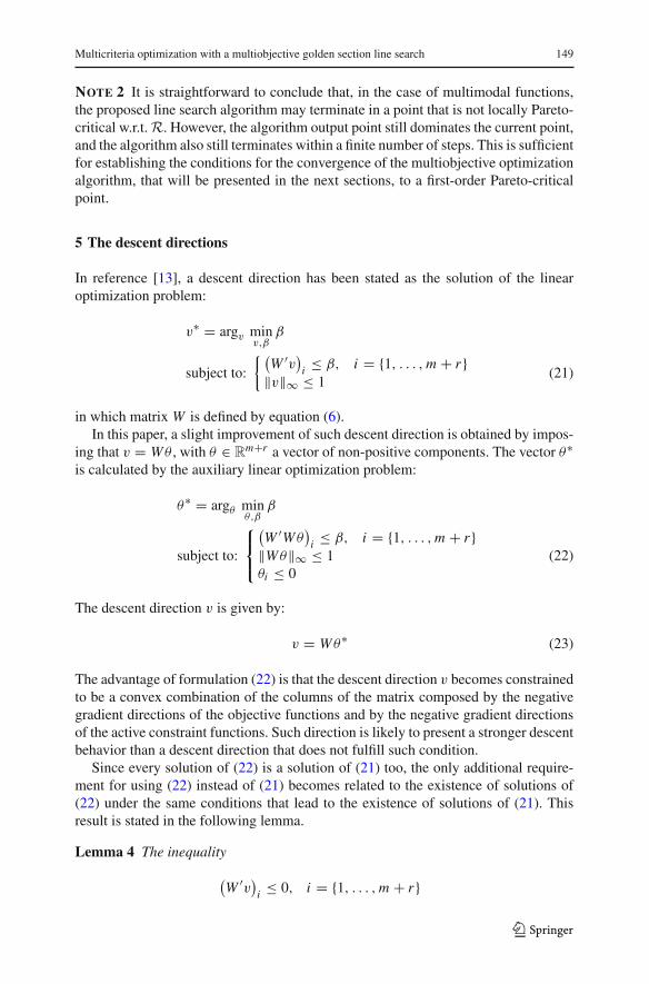
5 The descent directions
In reference [13], a descent direction has been stated as the solution of the linearoptimization problem:
v∗ = argv minv,β
β
subject to:
{(W ′v
)i ≤ β, i = {1, . . . , m + r}
‖v‖∞ ≤ 1(21)
in which matrix W is defined by equation (6).In this paper, a slight improvement of such descent direction is obtained by impos-
ing that v = Wθ , with θ ∈ Rm+r a vector of non-positive components. The vector θ∗
is calculated by the auxiliary linear optimization problem:
θ∗ = argθ minθ,β
β
subject to:
⎧⎨
⎩
(W ′Wθ
)i ≤ β, i = {1, . . . , m + r}
‖Wθ‖∞ ≤ 1θi ≤ 0
(22)
The descent direction v is given by:
v = Wθ∗ (23)
The advantage of formulation (22) is that the descent direction v becomes constrainedto be a convex combination of the columns of the matrix composed by the negativegradient directions of the objective functions and by the negative gradient directionsof the active constraint functions. Such direction is likely to present a stronger descentbehavior than a descent direction that does not fulfill such condition.
Since every solution of (22) is a solution of (21) too, the only additional require-ment for using (22) instead of (21) becomes related to the existence of solutions of(22) under the same conditions that lead to the existence of solutions of (21). Thisresult is stated in the following lemma.
Lemma 4 The inequality
(W ′v
)i ≤ 0, i = {1, . . . , m + r}
123

150 D. A. G. Vieira et al.
has a solution v if and only if the inequality
(W ′Wθ
)i ≤ 0, i = {1, . . . , m + r}
has a solution θ with θi ≤ 0.
Proof The proof is a direct application of Farkas’ lemma. �Concerning the generation of a descent direction v, it should be noticed that:
• Any direction v satisfying(W ′v
)i < 0, i = {1, . . . , m+r} is a descent direction.
In a single-objective unconstrained problem, this condition would be satisfied byany vector v whose projection over the function gradient is negative.
• The additional condition v = Wθ, θi ≤ 0 is analogous to a “steepest descent”condition. In a single-objective unconstrained problem, this condition would besatisfied only by v in the opposite direction to the gradient.
• Instead of using the directions given by the optimization problems (21) or (22), itis also possible to perform a randomized search, using a random v that satisfiesboth
(W ′v
)i < 0, i = {1, . . . , m + r} and v = Wθ, θi ≤ 0.
• It should be noticed that such random search should not be performed without the“steepest descent” condition v = Wθ, θi ≤ 0, because the convergence rate couldbecome degraded. This degradation does not occur in [13] because the minimi-zation of β in the condition
(W ′v
)i ≤ β, i = {1, . . . , m + r} nearly induces a
“steepest descent” property in the resulting v.• A steered search can be performed if the automatic choice of the descent direction,
which is performed via (21) or via (22), or still via a randomized procedure asdiscussed above, is replaced by an interactive choice involving a query to a deci-sion-maker. For instance, the decision-maker could be asked to choose θ such thatv = Wθ, θi ≤ 0, and
(W ′v
)i < 0, i = {1, . . . , m + r}, with an instruction for
assigning larger values of |θi | to the objectives which should have priority.
6 The dominating cone line search method
With the descent direction v given by (23), and with the multiobjective line searchalgorithm L( f (·), ε), a line-search-based procedure for determining first order Pa-reto-critical points can be stated. Another version of the algorithm can be built using adescent direction given by (21). An iteration of such procedure is depicted in algorithm3.
Define the function D(·, ·, ·) such that:
xk+1 = D(F(·), xk, ε) (24)
in which F(·) : Rn �→ R
m is the vector function, xk ∈ Rn is the output the k-th
iteration that becomes the initial point of (k + 1)-th iteration, ε is the tolerance of theline search procedure, and xk+1 ∈ R
n is the output of (k + 1)-th iteration.This algorithm obeys the same convergence properties than the one presented in
[13], as stated in the following theorem.
123

Multicriteria optimization with a multiobjective golden section line search 151
Algorithm 3 Iteration of dominating cone line search method (DCLS)Input: F(·) : Rn �→ R
m and xk ∈ � and ε ∈ R+Output: xk+1
1: function xk+1 = D(F(·),xk ,ε)2: Compute W using (6)3: Compute v using either (23) or (21)4: f (α)← F(xk + αv)
5: α∗k ← L( f (·), ε)6: xk+1 ← xk + α∗k v
7: end function
Theorem 3 Every accumulation point of the sequence [xk]∞k=0 generated by xk+1 =D(F(·), xk, ε) with search direction provided by (21) is a Pareto-critical point. Ifthe function F(·) has bounded level sets in the sense that {x ∈ R
n|F(x) ≤ F(x0)} isbounded, then the sequence [xk]∞k=0 stays bounded and has at least one accumulationpoint.
Proof For a descent direction v given by (21), there exists a β(x, v) > 0 such that
F(x + αv) ≤ F(x)+ βαH ′(x)v (25)
holds for all (x + αv) ∈ R∗d , provided that x /∈ R∗, with the following strict equalityvalid for a point (x + αv) in the relative boundary of R∗d (denoted by ∂r
(R∗d
)):
∃α| (x + αv) ∈ ∂r
(R∗d
), Fi
(x + αv
) = Fi (x)+ βα(H ′(x)
)i v, Fj (x + αv)
≤ Fj (x)+ βα(H ′(x)
)j v (26)
for some i ∈ {1, . . . , m} and all j ∈ {1, . . . , m}. As long as (x + αv) ∈ R∗d is validat the end point of the golden section multiobjective line search, defining β accordingto (26) allows to state that (25) is a necessary condition for the acceptance of the steplength α in the golden section multiobjective line search rule. In our case, the value ofα which performs the transition from xk to xk+1 after q golden section multiobjectiveline search steps is bounded by:
α ≥ 0.382q
2
in which q ∈ N is the index of the golden section line search iteration. After replacingthe Armijo acceptance condition F(x+αv) < F(x)+βαH ′(x)v by (25) and stating aq that does not reach the acceptance condition for 0.382q/2 > α instead of 1/2q > α,a straightforward adaptation of the convergence proof of [13] can be performed forthis theorem. �NOTE 3 This proof holds for the version of the algorithm with the descent directiongiven by (21). An essentially similar proof can be stated for the case of a descentdirection given by (23).
123

152 D. A. G. Vieira et al.
NOTE 4 The algorithm 3 has been presented in an unconstrained version, for sim-plicity. The adaptation to the constrained case is straightforward.
7 Results
7.1 Simple problem
Firstly, a simple problem is used for the purpose of illustrating the algorithm perfor-mance. The comparison is performed with two other methods: a simple weighted sumscalarization and the steepest descent method proposed in [13].
Consider the bi-objective problem:
minx
F(x) (27)
with x ∈ R2 and
F(x) =[
F1(x)
F2(x)
]
F1(x) = (x − c1)′ Q1(x − c1)
F2(x) = 1− exp(− (x − c2)
′ Q2 (x − c2))
(28)
Q1 =[
1 0
0 2
]
Q2 =[
5 1
1 3
]
c1 =[
5
0
]
c2 =[
5
3
]
Note that function F1(·) is convex, and function F2(·) is quasi-convex. This problemwas solved by the proposed dominating cone line search method (DCLS) with descentdirection (23), by the method proposed in [13] with β = 0.5 and β = 1.0 (denotedrespectively by FS0.5 and FS1.0) and also by the weighting method of scalarization,with the scalarized function Fw(·) : R2 �→ R defined by:
Fw(x) = wF1(x)+ (1− w)F2(x)
0 < w < 1 (29)
and solved by the BFGS Quasi-Newton method2 using golden section line search [23],denoted here by W-BFGS. A total of 200 executions of each method were computed,with random initial point (every initial point was used for each method) and randomweighting w in the interval 0 < w < 1 for W-BFGS. The average number of gradient
2 The acronym BFGS comes from the initials of the authors: Broyden–Fletcher–Goldfarb–Shanno.
123
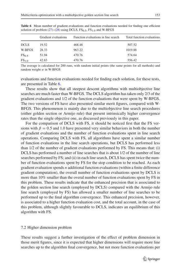
Multicriteria optimization with a multiobjective golden section line search 153
Table 6 Mean number of gradient evaluations and function evaluations needed for finding one efficientsolution of problem (27)–(28) using DCLS, FS0.5, FS1.0 and W-BFGS
Gradient evaluations Function evaluations in line search Total function evaluations
DCLS 19.52 468.48 507.52
W-BFGS 28.33 963.22 1019.88
FS0.5 51.94 470.76 574.64
FS1.0 42.83 470.76 556.42
The average is calculated for 200 runs, with random initial points (the same points for all methods) andrandom weight w in W-BFGS
evaluations and function evaluations needed for finding each solution, for these tests,are presented in Table 6.
These results show that all steepest descent algorithms with multiobjective linesearches are much faster than W-BFGS. The DCLS algorithm has taken only 2/3 of thegradient evaluations and 1/2 of the function evaluations that were spent by W-BFGS.The two versions of FS have also presented similar merit figures, compared with W-BFGS. This phenomenon is mainly due to the multiobjective line search procedures(either golden section or Armijo rule) that present intrinsically higher convergencerates than the single objective one, as discussed previously in this paper.
For the comparison of DCLS with FS, it should be noticed first that the FS ver-sions with β = 0.5 and 1.0 have presented very similar behaviors in both the numberof gradient evaluations and the number of function evaluations spent in line searchoperations. Comparing DCLS with FS, all algorithms have spent a similar numberof function evaluations in the line search operations, but DCLS has performed lessthan 1/2 of the number of gradient evaluations performed by FS. This means that: (i)DCLS has performed a number of line searches that is about 1/2 of the number of linesearches performed by FS; and (ii) in each line search, DCLS has spent twice the num-ber of function evaluations spent by FS for the stop condition to be reached. As eachgradient evaluation spends n additional function evaluations (within a finite differencegradient computation), the overall number of function evaluations spent by DCLS ismore than 10% smaller than the overal number of function evaluations spent by FS inthis problem. These results indicate that the enhanced precision that is associated tothe golden section line search (employed by DCLS) compared with the Armijo ruleline search (employed by FS) has allowed a smaller number of line searches to beperformed up to the final algorithm convergence. This enhanced precision, however,is associated to a higher function evaluation cost, and the total account, in the case ofthis problem, although slightly favourable to DCLS, indicates an equilibrium of thisalgorithm with FS.
7.2 Higher dimension problem
These results suggest a further investigation of the effect of problem dimension inthose merit figures, since it is expected that higher dimensions will require more linesearches up to the algorithm final convergence, but not more function evaluations per
123

154 D. A. G. Vieira et al.
10 20 30 40 50 60 70 80 90 1000
2000
4000
6000
8000
10000
12000
14000
16000
Problem Dimension
Fun
ctio
n C
alls
Golden SectionArmijo’s Rule
Fig. 5 The average overall number of function evaluations spent by DCLS and by FS0.5 up to the conver-gence to a Pareto-critical point versus the dimension n of problem (30)
line search. A series of tests has been conducted, for functions with the form:
minx
F(x) (30)
with x ∈ Rn , n = {10, 20, 30, . . . , 100}, and
F(x) =[
F1(x)
F2(x)
]
F1(x) = (x − c1)′Q1(x − c1)
F2(x) = (x − c2)′Q2(x − c2)
c1 = [1 1+ δ 1+ 2δ . . . 10] (31)
c2 = [10 10− δ 10− 2δ . . . 1]
Q1 = diag(c2)
Q2 = diag(c1)
δ = 9
n − 1
The tests have been performed for DCLS and for FS0.5. The resulting average over-all number of function evaluations for reaching a Pareto-critical point, starting fromrandom initial points (the same for both methods), for each method and each problemdimension is represented in Fig. 5. The golden section line search of DCLS providesmore precise and more costly line searches, compared with the Armijo rule line searchof FS0.5. The results presented in Fig. 5 show that, as the problem dimension increases,the balance between these two conflicting effects is favorable to DCLS, compared toFS0.5, under the viewpoint of the overall number of function evaluations requiredfor convergence to a Pareto-critical point. The advantage of DCLS grows more thanlinearly with the problem dimension.
123

Multicriteria optimization with a multiobjective golden section line search 155
10 20 30 40 50 60 70 80 90 100600
800
1000
1200
1400
1600
1800
2000
2200
Problem Dimension
Fun
ctio
n C
alls
Direction Eq. (23)
Direction Eq. (21)
Fig. 6 The average overall number of function evaluations spent up to the convergence to a Pareto-criticalpoint versus the dimension n of problem (30), using the original DCLS algorithm with descent direction(23) and using the DCLS algorithm modified with the descent direction (21)
Fig. 7 A 6-element Yagi-Udaantenna configuration
7.3 Evaluating the search direction
Another experiment has been conducted in order to evaluate the effect of employingthe descent direction proposed in this paper, given by equation (23), versus employingthe descent direction proposed in [13], given by the equation (21). The experimentemploys the same set of functions (30) and (31) that have been used in the formerexperiment. Now, only the multiobjective golden section line search is employed, andthe only difference between the algorithms is in the descent direction. The results arepresented in Fig. 6.
It can be noticed that the number of function calls of the DCLS algorithm whenthe descent direction (23) is employed becomes 10 to 20% lower than the number offunction calls when the descent direction (21) is employed. This experiment supportsthe conjecture that direction (23) is better than direction (21), although, as expected,the difference is not that remarkable.
7.4 Yagi-Uda antenna design
For the purpose of validating DCLS algorithm in a high-dimensional hard problem, itwas applied to the design of a 6-element wire Yagi-Uda antenna, illustrated in Fig. 7.The formulation of this problem, that was described in detail in [26], is as follows.
123

156 D. A. G. Vieira et al.
The element centered at the origin is the reflector, followed by the centered-feddriven element and the 4 directors. The distances d between consecutive elements(5 different distances) and the lengths L of each element are the parameters to be opti-mized (11 optimization parameters in total). The cross-section radius a is the same forall elements and is set equal to 0.003377 wavelengths at 859 MHz. The computationalsimulation of the antenna behavior follows the formulation described in [26].
The objective functions are set upon the antenna specifications, aiming the maxi-mization of the directivity, the front-to-back ratio, and the impedance matching, overthree different frequencies through the antenna bandwidth, resulting in nine differentobjectives. The design specifications upon the antenna radiation pattern are the high-est possible directivity and front-to-back ratio. The impedance matching is attainedby requesting an input resistance close to 50 � (or a voltage standing wave ratioclose to 1). Such requirements are imposed for three different frequencies (the lower,middle, and upper frequencies) over a 3.5% bandwidth centered at 859 MHz (828.935–889.065 MHz). All dimensions are given in wavelengths (λ) at 859 MHz. It should benoted that the objective functions, in this problem, are not guaranteed to be quasi-con-vex and differentiable.
The results of one typical run of DCLS algorithm on this problem are presented inTables 8 and 9 and in Fig. 8. DCLS was initialized, in this case, in the center point ofthe box constraints of the problem, shown in Table 7, and the optimization has taken39 algorithm iterations, with 706 function evaluations.
The monotonic behavior of the nine objective functions is illustrated in Fig. 8. Onlythe first 40 iterations are shown (after this, the objectives become almost constant).
An entire set of efficient solutions has been generated by DCLS, by starting thealgorithm at several randomly-generated initial points. The complete results of theapplication of DCLS to this problem have been published by the authors in [21], withmore details and a careful physical analysis. Up to the of the authors’ knowledge,there is no report in literature of any Yagi-Uda antenna with such performance. Forinstance, antennas with similar voltage standing wave ratio (VSWR) and input imped-ances (Zin) usually attain a directivity of less than 10 dB, and a front-to-back ratio ofless than 16 dB; see [26] and references therein.
The objective gradients have been calculated using the finite difference method.The average number of function evaluations for designing one antenna was of theorder of 2,000. However, a much smaller number could be reached if a more relaxedstop condition were applied.
This amount of computational effort is very competitive, for this class of problems.For instance, similar results have been presented by the NASA Ames Research Centerusing a dedicated Genetic Algorithm which required 600,000 evaluations per designedantenna [22].
7.5 Shape optimization of broad-band reflector antennas
Another real-world engineering problem solved using the proposed algorithm is theShape Optimization of Broad-band Reflector Antennas [20]. As a main objective,a specified region � must be illuminated uniformly. To accomplish this, a set of
123

Multicriteria optimization with a multiobjective golden section line search 157
Fig. 8 Evolution of antennadirectivity (Do), antennafront-to-back ratio (FB) andantenna voltage standing waveratio (VSWR), in the frequencies828.935 MHz (f1), 859 MHz(f2) and 889.065 MHz (f3)
0 5 10 15 20 25 30 35 406.5
7
7.5
8
8.5
9
9.5
10
10.5
11D(f1)D(f2)D(f3)
Iteration number
Do
0 5 10 15 20 25 30 35 408
10
12
14
16
18
20FBR(f1)FBR(f2)FBR(f3)
Iteration number
FB
0 5 10 15 20 25 30 35 401
1.5
2
2.5
3
3.5
4SWR(f1)SWR(f2)SWR(f3)
Iteration number
VSW
R
ns sample points, named P = {p1, . . . , pns
}, are spread over �, where the gain
G(p),∀p ∈ P is evaluated in relation to an isotropic radiation. This problem wasalso evaluated in three different frequencies to give broadband characteristics to theantenna (Table 10).
123

158 D. A. G. Vieira et al.
Table 7 Initial antennageometry, of the starting point ofDCLS
The dimensions are given inwavelengths (λ) at 859 MHz
L p dp−1,p
0.50000000000000
0.50000000000000 0.32375000000000
0.32375000000000 0.32375000000000
0.32375000000000 0.32375000000000
0.32375000000000 0.32375000000000
0.32375000000000 0.32375000000000
Table 8 Geometry of oneantenna obtained by DCLS, after39 algorithm iterations and 706function evaluations
The dimensions are given inwavelengths (λ) at 859 MHz
L p dp−1,p
0.50610055719041
0.44931282950414 0.25261747043376
0.38538718601364 0.25749579953324
0.39882084142996 0.37863536374455
0.38238790972033 0.38214346551819
0.38405677554186 0.33115644157639
Table 9 Electrical characteristics of the antenna of Table 8
Freq. MHz Do (dB) FB (dB) VSWR
828.935 9.715465 15.450613 1.335141
859 10.356968 18.961185 1.099307
889.065 10.918225 16.028036 1.798306
The variables shown in the table are: antenna directivity (Do), front-to-back ratio (FB), voltage standingwave ratio (VSWR)
Table 10 Gain distribution(mean μ and standard deviationσ at matching frequencies)considering the illumination ofthe Brazilian territory
Objective Initial Optimized
μL , (dBi) 17.46 31.77
μC , (dBi) 17.07 31.82
μU , (dBi) 16.58 31.82
σ L , (dB) 12.36 1.93
σC , (dB) 11.96 2.00
σU , (dB) 11.64 2.10
The result when a standard parabolic antenna is used is presented in Fig. 9(a), andthe optimized one in Fig. 9(b) that shows a pattern of illumination much closer to theBrazilian territory shape. Further details can be found in a paper by the authors [20].
123

Multicriteria optimization with a multiobjective golden section line search 159
−4 −3 −2 −1 0 1 2 3 4−4
−3
−2
−1
0
1
2
3
410
10
1010
10
10
1010
1010
1010
15
1515
1515
20
25
30
3540
44
CO−POL
AZ (º)
EL
(º)
−4 −3 −2 −1 0 1 2 3 4−4
−3
−2
−1
0
1
2
3
4
10
10
10
10
115
15
15
20
20
25
30
30
31
31
32
32
33
3333
34
34
35
CO−POL
AZ (º)E
L (º
)
(a) (b)
Fig. 9 Optimal radiation patterns (dBi) for the coverage of the Brazilian territory. In (a) the radiationpattern when the classical parabolic format is used. The algorithm has asymptotically converged to (b) thatis a better pattern to the coverage of the Brazilian territory
7.6 Remarks on the simulation results
The second and the third examples presented here are real world black box engineeringproblems, one with 11 variables and 9 objectives and the other with 6 objectives and38 variables. The gradients in both problems were extracted using the finite differencemethod. The exact natures of these problems are unknown; however, it is believed thatthey are multimodal and differentiable problems. The results obtained and publishedusing the algorithm presented in this paper have outperformed all the results for sim-ilar problems that appear in the current literature, in terms of the number of functionevaluations and design quality. Often, in engineering problems, a sub-optimal solutionis available, as the classical paraboloid solution in the third example. Therefore, analgorithm capable of a fast local search, with the aim of enhancing such solution, isvery useful for this type of design.
8 Final remarks
A new algorithm for generating first-order Pareto-critical solutions in multiobjectiveoptimization problems (called DCLS) has been proposed here, as a reformulation ofa former algorithm presented in [13].
DCLS has two basic functional blocks: (i) the computation of a direction in whichthere are points that dominate the current one; and (ii) the computation of a step-sizethat leads to a line-constrained efficient point. The iterative application of these stepsultimately leads to a Pareto-critical point under an assumption of bounded set-lev-els of the objective functions in the feasible set. The algorithm terminates when step(i) cannot be executed, which means that the first-order Kuhn–Tucker conditions for
123

160 D. A. G. Vieira et al.
efficiency hold in the current point. This basic structure is the same that has beenemployed in [13].
The main differences of DCLS in relation to the algorithm presented in [13] are: (i)the line search method is performed here with a new golden section line search multi-objective procedure, that takes advantage of the structure of the Pareto-set constrainedto a line, in order to further reduce the required number of function evaluations, whencompared with the single-variable golden section procedure, and (ii) the descent direc-tion is constrained, here, to belong to the set of convex combinations of the negativefunction gradients and negative active constraint gradients—this enhances the descentproperty of the chosen direction.
The performance of DCLS has been tested in the design of electromagnetic devices.The difficulties to solve this type of problems have been, in fact, the primary motiva-tion to develop the algorithm presented here. Both problems present high sensitivitythat makes the convergence rate of other algorithms very slow, as discussed in [21]and [20]. The tests presented here suggest that DCLS can be the basis for buildingpowerful engineering design tools. The proposed algorithm is currently being testedin other real-world problems.
Acknowledgments The authors acknowledge the support by the Brazilian agencies CAPES, CNPq andFAPEMIG.
References
1. Benson, H.P.: Existence of efficient solutions for vector maximization problems. J. Optim. TheoryAppl. 26(4), 569–580 (1978)
2. Bosman, P.A.N., de Jong, E.D.: Exploiting gradient information in numerical multi-objective evolu-tionary optimization. In: Proceedings of the 2005 Genetic and Evolutionary Computation Conference(GECCO’05), pp. 755–762. ACM, Washington June (2005)
3. Chankong, V., Haimes, Y.Y.: On the characterization of noninferior solutions of the vector optimizationproblem. Automatica 18(6), 697–707 (1982)
4. Chankong, V., Haimes, Y.Y.: Multiobjective decision making: theory and methodology. Elsevier,Amsterdam (1983)
5. Coello Coello, C.A., Van Veldhuizen, D.A., Lamont, G.B.: Evolutionary algorithms for solving multi-objective Problems. Kluwer Academic Publishers, Dordrecht (2001)
6. Deb, K.: Multi-objective optimization using evolutionary algorithms. Wiley, London (2001)7. Deb, K., Pratap, A., Agarwal, S., Meyarivan, T.: A fast and elitist multiobjective genetic algorithm:
NSGA II. IEEE Trans. Evol. Comput. 6(2), 182–197 (2002)8. Dellnitz, M., Schutze, O., Hestermeyer, T.: Covering Pareto sets by multilevel subdivision techniques.
J. Optim. Theory Appl. 124(1), 113–136 (2005)9. Ehrgott, M.: Multicriteria optimization, volume 491 of lecture notes in economics and mathematical
systems. Springer Verlag, Berlin (2000)10. Engau, A., Wiecek, M.M.: Cone characterizations of approximate solutions in real vector optimiza-
tion. J. Optim. Theory Appl. 134(3), 499–513 (2007)11. Fliege, J.: Gap-free computation of Pareto-points by quadratic scalarizations. Math. Methods Oper.
Res. 59, 69–89 (2004)12. Fliege, J., Grana-Drummond, L.M., Svaiter, B.F.: Newton’s method for multiobjective optimiza-
tion. SIAM J. Optim. 20(2), 602–626 (2009)13. Fliege, J., Svaiter, B.F.: Steepest descent methods for multicriteria optimization. Math. Methods Oper.
Res. 51, 479–494 (2000)14. Fonseca, C.M., Fleming, P.: Genetic algorithms for multiobjective optimization: formulation, discus-
sion and generalization. In: Proceedings of the 5th International Conference: Genetic Algorithms,pp. 416–427. San Mateo (1993)
123

Multicriteria optimization with a multiobjective golden section line search 161
15. Fonseca, C.M., Fleming, P.J.: An overview of evolutionary algorithms in multiobjective optimiza-tion. Evol. Comput. 7(3), 205–230 (1995)
16. Gould, F.J., Tolle, J.W.: A necessary and sufficient qualification for constrained optimization. SIAMJ. Appl. Math. 20(2), 164–172 (1971)
17. Hillermeier, C.: Generalized homotopy approach to multiobjective optimization. J. Optim. TheoryAppl. 110(3), 557–583 (2001)
18. Jeyakumar, V., Luc, D.T.: Nonsmooth vector functions and continuous optimization. Springer, Berlin(2008)
19. Klamroth, K., Tind, J., Wiecek, M.M.: Unbiased approximation in multicriteria optimization. Math.Methods Oper. Res. 56, 413–437 (2002)
20. Lisboa, A.C., Vieira, D.A.G., Vasconcelos, J.A., Saldanha, R.R., Takahashi, R.H.C.: Multi-objectiveshape optimization of broad-band reflector antennas using the cone of efficient directions algorithm.IEEE Transactions on Magnetics, pp. 1223–1226 (2006)
21. Lisboa, A.C., Vieira, D.A.G., Vasconcelos, J.A., Saldanha, R.R., Takahashi, R.H.C.: Monotonicallyimproving Yagi-Uda conflicting specifications using the dominating cone line search method. IEEETrans. Magn. 45(3), 1494–1497 (2009)
22. Lohn, J.D., Kraus, W.F., Colombano, S.P. Evolutionary optimization of Yagi-Uda antennas. In Pro-ceedings of the Fourth International Conference on Evolvable Systems, pp. 236–243 (2001)
23. Luenberger, D.G.: Linear and nonlinear programming. Addison-Wesley, Reading (1984)24. Pareto, V.: Manual of political economy. Augustus M. Kelley, New York (1906). (1971 translation of
1927 Italian edition)25. Pereyra, V.: Fast computation of equispaced Pareto manifolds and Pareto fronts for multiobjective
optimization problems. Math. Comput. Simulat. 79(6), 1935–1947 (2009)26. Ramos, R.M., Saldanha, R.R., Takahashi, R.H.C., Moreira, F.J.S.: The real-biased multiobjective
genetic algorithm and its application to the design of wire antennas. IEEE Trans. Magn. 39(3), 1329–1332 (2003)
27. Romero, C.: A survey of generalized goal programming (1970–1982). Eur. J. Oper. Res. 25, 183–191(1986)
28. Schaffler, S., Schultz, R., Weinzierl, K.: Stochastic method for the solution of unconstrained vectoroptimization problems. J. Optim. Theory Appl. 114(1), 209–222 (2002)
29. Schütze, O., Laumanns, M., Coello-Coello, C.A., Dellnitz, M.l., Talbi, E.G.: Convergence of stochasticsearch algorithms to finite size Pareto set approximations. J. Global Optim. 41, 559–577 (2008)
30. Wanner, E.F., Guimaraes, F.G., Takahashi, R.H.C., Fleming, P.J.: Local search with quadratic approxi-mations into memetic algorithms for optimization with multiple criteria. Evol. Comput. 16(2), 185–224(2008)
31. Yano, H., Sakawa, M.: A unified approach for characterizing Pareto optimal solutions of multiobjectiveoptimization problems: the hyperplane method. Eur. J. Oper. Res. 39, 61–70 (1989)
32. Yu, P.L.: Cone convexity, cone extreme points, and nondominated solutions in decision problems withmultiobjectives. J. Optim. Theory Appl. 14, 319–377 (1974)
33. Zitzler, E., Laumanns, M., Thiele, L.: SPEA2: improving the strength pareto evolutionary algorithm.Technical report 103, Computer Engineering and Networks Laboratory (TIK), Swiss Federal Instituteof Technology (ETH) Zurich (2001)
123