Supply Chain Networks

with

Multicriteria Decision-Makers

June Dong and Ding Zhang

Department of Marketing and Management

School of Business

State University of New York at Oswego

Oswego, New York 13126

Anna Nagurney

Department of Finance and Operations Management

Isenberg School of Management

University of Massachusetts

Amherst, Massachusetts 01003

September, 2001

Presented at the 15th International Symposium on Transportation and Traffic Theory, Ade-

laide, Australia, July 2002

Appears in revised form in Transportation and Traffic Theory in the 21st Century,

M. A. P. Taylor, Editor, Pergamon (2002) pp. 179-196.

Abstract: This paper presents a theoretical framework for supply chain network modeling,

analysis, and computation in the presence of competition, in which all the decision-makers,

who are located at distinct tiers of the network, are multicriteria decision-makers. In partic-

ular, in this framework, transportation time and transportation cost are explicit criteria and

these can depend on the service level provided. The optimality conditions of the different

tiers of decision-makers, consisting of manufacturers, retailers, and consumers are derived,

as well as the equilibrium conditions of the integrated model. The variational inequality

formulation of the governing equilibrium conditions is then utilized to obtain qualitative

properties as well as a computational procedure for the determination of the equilibrium

product shipments between the tiers of the network, the prices, as well as the service levels.

1

1. Introduction

In this paper, we develop a theoretical framework for multicriteria decision-making in

multitiered supply chain networks. The framework handles competition among the decision-

makers who consist of manufacturers, retailers, and consumers. The endogenous variables

include the product shipments between the network tiers, the prices of the product at the

various nodes of the supply chain network, as well as the service levels provided. The work

signficantly generalizes the model of Nagurney, Zhang, and Dong (2001) by introducing

another tier of decision-makers in the form of retailers and by allowing all tiers to be mul-

ticriteria decision-makers. Furthermore, it generalizes the model of Nagurney, Dong, and

Zhang (2001), which considered three tiers of decision-makers but the decision-makers were

exclusively faced with single criteria to optimize. Moreover, it formalizes the incorporation

of service levels.

We emphasize that the topic of supply chain analysis is interdisciplinary by nature since

it involves manufacturing, transportation and logistics, as well as retailing/marketing. It

has been the subject of a growing body of literature (cf. Stadtler and Kilger (2000) and the

references therein) with the associated research being both conceptual in nature (see, e.g.,

Poirier (1996, 1999), Mentzer (2000), Bovet (2000)), due to the complexity of the problem

and the numerous agents, such as manufacturers, retailers, or consumers involved in the

transactions, as well as analytical (cf. Bramel and Simchi-Levi (1997) and Miller (2001)

and the references therein). Daganzo (1999), for example, examined logistics systems in

an integrated way and showed how to find rational structures for such systems. Indeed,

many researchers, in addition to, practitioners, have described the various networks that

underly supply chain analysis. However, the framework considered has been primarily that

of single objective optimization. In this paper, in contrast, we focus on both the multicriteria

and the multitiered aspects of supply chain analysis with an eye towards understanding the

underlying behavior of the various decision-makers and the ultimate equilibrium patterns.

In particular, in this paper, we consider a comprehensive supply chain network for a homo-

geneous product that is comprised of competitive manufacturers, retailers, and consumers.

It should be noted that, although manufacturers, retailers, and consumers are selected here

to be the focal decision-makers, the framework of the model presented in this paper is suf-

2

ficiently general to include other levels of decision-makers such as owners of distribution

centers, for example. Moreover, the model formulates multicriteria decision-making as re-

gards the manufacturers, the retailers, as well as the consumers. To-date, except for the

recent work of Nagurney, Zhang, and Dong (2001), the subject and theory of multicriteria

decision-making in a supply chain context has focused exclusively on either the production

side or on the consumption side, and, typically, has considered only a single decision-maker

(see, e.g., Chankong and Haimes (1983), Yu (1985), Keeney and Raiffa (1993) and the refer-

ences therein). For references on multicriteria decision-making in transportation networks,

in general, see Nagurney and Dong (2001) and the references therein.

Specifically, we assume that the manufacturers are involved in the production of a ho-

mogeneous product which is then shipped to the retailers. The manufacturers seek to de-

termine their optimal production and shipment quantities, given the production costs and

the transaction costs associated with conducting business with the different retailers as well

as the prices that the retailers are willing to pay for the product and shipment alternative

combinations. The manufacturers are assumed to have two objectives and these are profit

maximization and market share maximization with the weight associated with the latter

criterion being distinct for each manufacturer.

The retailers, in turn, seek to determine the “optimal” quantity of the product to obtain

from each of the manufacturers, that is, the “most-economic” shipment pattern in terms of

both the amount and the shipment means selected, as well as the “optimal” service level. In

particular, the retailers have three criteria and these are: the maximization of profit, the min-

imization of transportation time, and the maximization of service level. Each of the retailers

can weight these criteria in a different manner. The shipment alternatives are represented by

links characterized by specific transportation cost and transportation time functions. Hence,

a specific shipment option or link may have a low associated transportation time but a high

transportation cost, whereas another may have a high associated transportation time and a

low cost. A higher price may be charged to have the products shipped faster to the retailers

or, in contrast, manufacturers may accept a lower price if they select a slower and, presum-

ably, cheaper, shipping mode. The service level indicates the percentage of time that the

product is not out of stock. Usually, a higher service level implies a greater stock size on

average, and thus, larger order quantities and less frequent order times. In other words, with

3

a higher service level, the stock (inventory) holding cost goes up, and the transportation

time and cost go down. Therefore, the service level set by each retailer significantly impacts

his holding cost as well as his transportation time and cost.

Finally, in this supply chain network model, the consumers provide the “pull” in that,

given the demand functions at the various demand markets, they determine their optimal

consumption levels from the various retailers subject to the prices charged for the product as

well as the transportation time and transportation cost associated with obtaining the prod-

uct. The consumers are classified into different classes according to various characteristics

that may include, for example: geographic location, consumption behavior, travel pattern,

profession or business type, and income level. Different classes of consumers may weight time

and cost associated with obtaining the product in an individual manner. It is worth noting

that the service level at a retailer may affect the transportation time and transportation cost

of the consumers who purchase at the retailer outlet. This is because when customers come

to shop at a store and the product they wish to purchase is out of stock, they have, in effect,

wasted their time and have incurred an associated cost.

We establish that the equilibrium conditions governing the state at which the manufac-

turers, the retailers, as well as the consumers, have reached optimality can be formulated as

a variational inequality. We then utilize the derived variational inequality to obtain qualita-

tive properties of the equilibrium product shipment, price, and service level pattern. We also

propose an algorithm for the computation of the equilibrium pattern and give conditions for

convergence.

The paper is organized as follows. In Section 2, we present the supply chain network model

with competition, derive the optimality conditions for the distinct tiers of decision-makers,

and provide the equilibrium conditions, which are then shown to be equivalent to a finite-

dimensional variational inequality problem. In Section 3, we establish certain qualitative

properties of the multicriteria, multitiered supply chain network model, in particular, the

existence and uniqueness of an equilibrium, under reasonable assumptions. In Section 4,

we describe the computational procedure, along with convergence results. In Section 5, we

summarize our results and present the conclusions.

4

2. The Multicriteria, Multitiered Supply Chain Network Model

In this Section, we develop the supply chain network model with manufacturers, retailers,

and consumers located at the demand markets. As mentioned in the Introduction, these

decision-makers are multicriteria ones. We first focus on the manufacturers. We then turn to

the retailers and, subsequently, to the consumers. The integrated model is then constructed

along with the variational inequality formulation of the governing equilibrium conditions.

The Manufacturers

We assume that a homogeneous product is produced by m manufacturers, is shipped to

n retailers, and is consumed by o different classes of consumers as represented by distinct

demand markets. We denote a typical manufacturer by i, a typical retailer by j, and a

typical consumer class by k. Each manufacturer can ship the product to each retailer using

one (or more) of r possible shipment alternatives, which can represent mode/route alterna-

tives. We denote a typical shipment alternative by l. Let qijl denote the quantity of the

product produced by manufacturer i and shipped to retailer j via shipment alternative l.

For simplicity of presentation, we now define certain vectors. Let qi =∑n

j=1

∑rl=1 qijl be the

total production of manufacturer i and let q be the m-dimensional vector with components:

{q1, . . . , qm}. Let qj =∑m

i=1

∑rl=1 qijl denote the product shipments to retailer j from all

the manufacturers. Finally, let Q1 denote the mnr-dimensional vector of all the product

shipments from all the manufacturers to all the retailers, with components: {q111, . . . , qmnr}.We assume that all the vectors are column vectors.

Each manufacturer i is assumed to be faced with a production cost function fi, which

may depend, in general, on the entire vector of production outputs, that is,

fi = fi(q), ∀i. (1)

We associate with manufacturer i, who is transacting with retailer j and using shipment

alternative l, a transaction cost c1ijl, where

c1ijl = c1ijl(qijl), ∀j, l. (2)

To help fix ideas, and in order to facilitate the ultimate construction of the supply chain

5

ShipmentAlternatives

� ��1 � ��· · · · · ·

· · · j · · · � ��n

Retailers

� ��i

� � j

ShipmentAlternatives

Manufacturer

Figure 1: Network Structure of Manufacturer i’s Transactions

network in equilibrium, we depict the manufacturers and the retailers as nodes and the

shipment alternatives between the manufacturers and the retailers as links, where recall that

since we assume that there are r shipment alternatives available, there are r links joining

each pair of nodes (i, j). See Figure 1 for the graphical depiction for a specific manufacturer

i.

The total costs incurred by a manufacturer i, thus, are equal to the sum of the manu-

facturer’s production cost plus his transaction costs. His revenue, in turn, is equal to the

sum over all the retailers and shipment alternatives of the price of the product charged to

each retailer and associated with a particular shipment alternative times the quantity. If

we let ρ∗1ijl denote the (endogenous) price charged for the product by manufacturer i to

retailer j and associated with shipment alternative l, we can express the criterion of profit

maximization for manufacturer i as:

Maximizen∑

j=1

r∑

l=1

ρ∗1ijlqijl − fi(q) −

n∑

j=1

r∑

l=1

c1ijl(qijl), (3)

subject to qijl ≥ 0, for all j, l. We discuss how the supply price ρ∗1ijl is determined later in

this Section.

In addition to the criterion of profit maximization, we also assume that each manufacturer

seeks to maximize his production output in an endeavor to gain market share. Therefore,

6

the second criterion of each manufacturer i can be expressed mathematically as:

Maximizen∑

j=1

r∑

l=1

qijl (4)

subject to qijl ≥ 0, for all j, l.

A Manufacturer i’s Multicriteria Decision-Making Problem

We now describe how we construct a value function associated with the two criteria

facing each manufacturer, that is, profit maximization and output maximization. Each

manufacturer i associates a nonnegative weight αi with the output maximization criterion,

with the weight associated with the profit maximization criterion serving as the numeraire

and being set equal to 1. Hence, we can construct a value function for each manufacturer (cf.

Fishburn (1970), Chankong and Haimes (1983), Yu (1985), Keeney and Raiffa (1993)) using

a constant additive weight value function. Consequently, the multicriteria decision-making

problem for manufacturer i is transformed into:

Maximizen∑

j=1

r∑

l=1

ρ∗1ijlqijl − fi(q) −

n∑

j=1

r∑

l=1

c1ijl(qijl) + αi

n∑

j=1

r∑

l=1

qijl, (5)

subject to:

qijl ≥ 0, ∀j, l.

The Retailers

The retailers, in turn, are positioned in the supply chain so as to have transactions with

both their suppliers, that is, with the m manufacturers as well as with their customers,

that is, the o classes of consumers. Hence, the network structure of a particular retailer’s

transactions is as depicted in Figure 2.

Let Qjk denote the amount of the product purchased by the kth class of consumer at the

retail outlet j. Let the vector Q2 consist of all the consumption quantities of the product

by the consumers and be the no-dimensional vector with components: {Q11, . . . , Qno}. Let

ρ∗2j denote the retail price of retailer j. This price, as we will show, will be endogenously

7

����1 ����

· · · i · · · ����m

Shipment

Alternatives ����j

Shipment

AlternativesRetailer

����1 · · · ����

k · · · ����o

HHHHHHHHHHHj

@@

@@

@@R

������������

������������

��

��

��

HHHHHHHHHHHj

Manufacturers

Consumers at the Demand Markets

Figure 2: Network Structure of Retailer j’s Transactions

determined in the integrated model. Then, the total revenue of retailer j is given by the

expression

ρ∗2j

o∑

k=1

Qjk. (6)

The costs that a typical retailer j is faced with include the price of obtaining the product

from the manufacturers, the transaction cost, which includes the transportation cost and

which is denoted by c2ijl, and the holding cost, hj, for carrying, displaying, and maintaining

the product stock. Since a retailer must decide upon an ordering system in terms of the order

quantity and the order time (order point), the service level, denoted by sj, is one of the main

factors, financially, in addition to the ordering cost and carrying cost. Here we define the

service level to be the percentage of time that the product is in stock when consumers come

to buy it (cf. Arnold (2000)). Usually, a higher service level implies a greater stock size,

on the average, and, thus, larger order quantities and less frequent order times (Beamon

(1998)).

We assume that the holding cost depends, in general, on j’s shipment pattern qj, and his

8

service level sj, that is,

hj = hj(sj, qj). (7)

Retailer j’s transaction cost associated with obtaining the product from manufacturer i

via transportation alternative l, in turn, is given by

c2ijl = c2ijl(sj, qj). (8)

We denote the transportation time of shipping the product from manufacturer i to retailer

j via alternative l by tijl, which, in general, may depend upon qj as well as on the service

level sj as discussed above. Therefore, we have that

tijl = tijl(sj, qj). (9)

A Retailer j’s Multicriteria Decision-Making Problem

In a multicriteria decision-making setting, we assume that retailer j has three criteria.

They are: to maximize the profit, to minimize the total transportation time in getting the

product from the manufacturers, and to maximize the service level. As mentioned earlier, by

increasing his service level sj, retailer j is, indeed, in a sense, improving his service reputation,

since the customers shopping at retail outlet j have a lower chance of experiencing a stockout

of the product when retailer j adopts a higher service level. The model assumes that retailer

j associates with his value function a weight of 1 to his profit attribute in dollar value, a

weight of β1j to his transportation time attribute, as the conversion rate of time to dollar

value, and a weight of β2j to his service level attribute, as the conversion rate of service

reputation to dollar value.

Therefore, the multicriteria decision-making problem for retailer j; j = 1, ..., n, can be

transformed into:

Maximize ρ∗2j

o∑

k=1

Qjk − β1j

m∑

i=1

r∑

l=1

tijl(sj, qj) + β2jsj

−m∑

i=1

r∑

l=1

ρ∗1ijlqijl −

m∑

i=1

r∑

l=1

c2ijl(sj, qj) − hj(sj, qj) (10)

9

subject too∑

k=1

Qjk ≤m∑

i=1

r∑

l=1

qijl, (γj) (11)

sj ≤ 1, (ηj) (12)

and

qijl ≥ 0, Qjk ≥ 0, sj ≥ 0, ∀i, l, k,

where γj is the Lagrange multiplier associated with inequality (11) and ηj is the Lagrange

multiplier associated with inequality (12).

The objective function (10) represents a value function for retailer j, with β1j having

the interpretation as the conversion rate of time into dollar value and β2j having the inter-

pretation as the conversion rate of service level into dollar value. Constraint (11) expresses

that consumers cannot purchase more from a retailer than is held in stock. Constraint (12)

and the nonnegativity constraint on the level of service specify that the service level is set

between 0 to 100 percent.

Subsequently, we derive the optimality conditions for this problem.

The Consumers at the Demand Markets

We now describe the consumers located at the demand markets. We assume that there

are o classes of consumers, with a typical class denoted by k. The consumers are classified

into different classes according to such characteristics as geographic location, consumption

behavior, travel pattern, profession and income level, etc. As such, each class of consumer

takes into account in making his consumption decision not only the different retail prices at

the retail stores, but also the transportation time and the transportation cost required to

obtain the product, as well as the service levels provided at the retail stores. Therefore, the

consumers in this model are multiclass and multicriteria decision-makers. Let Cjk denote the

transportation cost incurred to class k consumers for purchasing the product from retailer j,

and let Tjk denote the corresponding transportation time. In general, these functions may

depend upon the quantity of the product purchased at retailer j by consumer class k, as well

as upon the service level at retailer j. Indeed, one can expect that the higher the service

10

level at retailer j, the lower the procurement effort needed to obtain the product, and, thus,

the lower the associated time and cost.

We assume that the transportation cost and transportation time are in the following form:

Cjk = Cjk(sj, Qjk), ∀j, k (13)

Tjk = Tjk(sj, Qjk), ∀j, k. (14)

In addition, we assume that each class of consumer perceives the transportation cost and

the transportation time associated with obtaining the product in an individual manner, and

weights these three criteria accordingly. Let λ1k and λ2k denote, respectively, the nonnegative

weights associated with transportation cost and transportation time by class k consumers.

Therefore, their value function for the generalized retail price associated with the kth class

of consumer to obtain the product at retailer j is expressed as

ρ∗2j + λ1kCjk(sj, Qjk) + λ2kTjk(sj, Qjk), (15)

that is, the true price of the product from the perspective of consumers of class k is the price

charged for the product at the particular retail outlet plus the “effective” price associated

with obtaining the product which is composed of the weighted transportation cost plus the

weighted transportation time.

Let now ρ3k denote the generalized price of the product as perceived by class k and group

the generalized demand prices into the vector ρ3 ∈ Ro+. Further, denote the demand of class

k by dk, and assume continuous demand functions given by:

dk = dk(ρ3), ∀k. (16)

The Multicriteria Equilibrium Conditions for Consumers of Class k

We now present the multicriteria equilibrium conditions for consumers of class k. In

particular, in equilibrium, we must have the following conditions holding:

ρ∗2j + λ1kCjk(s

∗j , Q

∗jk) + λ2kTjk(s

∗j , Q

∗jk)

{= ρ∗

3k, if Q∗jk > 0

≥ ρ∗3k, if Q∗

jk = 0,(17)

11

����1 ����

· · · j · · · ����n

Retailers

����k

z

QQ

QQ

QQ

QQs

AAAAAAU

��

��

��

��+

Demand Market

Figure 3: Network Structure of Consumers’ Transactions at Demand Market k

and

dk(ρ∗3)

=n∑

j=1

Q∗jk, if ρ∗

3k > 0

≤n∑

j=1

Q∗jk, if ρ∗

3k = 0.(18)

Conditions (17) state that a member of consumer class k will purchase the product from

retailer j, if the generalized retail price at retailer j as perceived by consumers of class k does

not exceed the demand price that consumers of class k are willing to pay for the product.

Conditions (18) state, in turn, that if the demand price that consumers of class k are willing

to pay for the product is positive, then the quantities purchased of the product from the

retailers will be precisely equal to the demand of consumers of class k for the product. These

conditions correspond to the well-known spatial price equilibrium conditions (cf. Samuelson

(1952), Takayama and Judge (1971) and Nagurney (1999) and the references therein).

In Figure 3, the network of transactions between the retailers and the consumers at

demand market k is depicted. Each demand market is represented by a node and the

transactions, as previously, by links.

12

The Integrated Model

We now present the integrated supply chain network model with multicriteria manu-

facturers, retailers, and consumers, which synthesizes the optimality conditions of all the

manufacturers and all the retailers, and the equilibrium conditions of the consumers at all

the demand markets. In order to obtain an equilibrium of the multicriteria supply chain

network system, we must have that the optimality conditions of the manufacturers and the

retailers as well as the equilibrium conditions of the consumers are satisfied simultaneously .

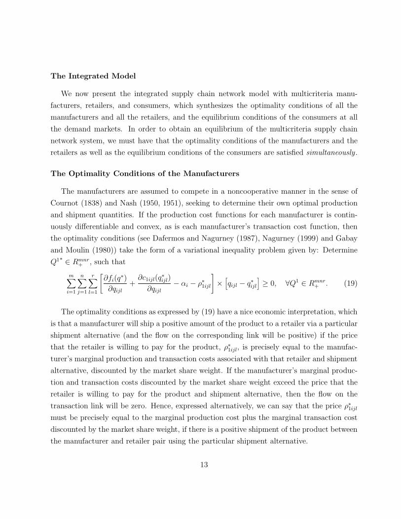
The Optimality Conditions of the Manufacturers

The manufacturers are assumed to compete in a noncooperative manner in the sense of

Cournot (1838) and Nash (1950, 1951), seeking to determine their own optimal production

and shipment quantities. If the production cost functions for each manufacturer is contin-

uously differentiable and convex, as is each manufacturer’s transaction cost function, then

the optimality conditions (see Dafermos and Nagurney (1987), Nagurney (1999) and Gabay

and Moulin (1980)) take the form of a variational inequality problem given by: Determine

Q1∗ ∈ Rmnr+ , such that

m∑

i=1

n∑

j=1

r∑

l=1

[∂fi(q

∗)

∂qijl

+∂c1ijl(q

∗ijl)

∂qijl

− αi − ρ∗1ijl

]×[qijl − q∗ijl

]≥ 0, ∀Q1 ∈ Rmnr

+ . (19)

The optimality conditions as expressed by (19) have a nice economic interpretation, which

is that a manufacturer will ship a positive amount of the product to a retailer via a particular

shipment alternative (and the flow on the corresponding link will be positive) if the price

that the retailer is willing to pay for the product, ρ∗1ijl, is precisely equal to the manufac-

turer’s marginal production and transaction costs associated with that retailer and shipment

alternative, discounted by the market share weight. If the manufacturer’s marginal produc-

tion and transaction costs discounted by the market share weight exceed the price that the

retailer is willing to pay for the product and shipment alternative, then the flow on the

transaction link will be zero. Hence, expressed alternatively, we can say that the price ρ∗1ijl

must be precisely equal to the marginal production cost plus the marginal transaction cost

discounted by the market share weight, if there is a positive shipment of the product between

the manufacturer and retailer pair using the particular shipment alternative.

13

The Optimality Conditions of the Retailers

We now consider the optimality conditions of the retailers assuming that each retailer

is faced with the optimization problem (10), (11) and (12). Here, we also assume that the

retailers compete in a noncooperative manner so that each maximizes his profits, given the

actions of the other retailers. Note that, at this point, we consider that retailers seek to

determine not only the optimal amounts purchased by the consumers from their specific

retail outlet but, also, the amount that they wish to obtain from the manufacturers, their

shipment pattern via the alternatives, as well as their service levels. In equilibrium, all the

shipments between the tiers of decision-makers will have to coincide.

Assuming that all the holding costs (7), the retailer transaction costs (8), and the trans-

portation times for shipping the product from the manufacturers to the retailers (9) are

all continuous and convex, then the optimality conditions for all the retailers satisfy the

variational inequality: Determine nonnegative (Q1∗, Q2∗, γ∗, η∗, s∗) satisfying (12) such that:

n∑

j=1

o∑

k=1

[γ∗

j − ρ∗2j

]×[Qjk − Q∗

jk

]

+m∑

i=1

n∑

j=1

r∑

l=1

[∂hj(s

∗j , q

∗j )

∂qijl+ ρ∗

1ijl +∂c2ijl(s

∗j , q

∗j )

∂qijl+ β1j

∂tijl(s∗j , q

∗j )

∂qijl− γ∗

j

]×[qijl − q∗ijl

]

+n∑

j=1

[m∑

i=1

r∑

l=1

q∗ijl −o∑

k=1

Q∗jk

]×[γj − γ∗

j

]+

n∑

j=1

[1 − s∗j

]×[ηj − η∗

j

]

+n∑

j=1

[∂hj(s

∗j , q

∗j )

∂sj

+m∑

i=1

r∑

l=1

∂c2ijl(s∗j , q

∗j )

∂sj

+m∑

i=1

r∑

l=1

β1j

∂tijl(s∗j , q

∗j )

∂sj

+ η∗j − β2j

]×[sj − s∗j

]≥ 0,

(20)

for all nonnegative Q1, Q2, s, γ, η satisfying (12), where recall that γj is the Lagrange mul-

tiplier for (11) and ηj is the Lagrange multiplier for (12). For further background on such

a derivation, see Bertsekas and Tsitsiklis (1992). In this derivation, as in the derivation of

inequality (19), we have not had the prices charged be variables. They become endogenous

variables in the integrated model.

We now highlight the economic interpretation of the retailers’ optimality conditions. The

third term in inequality (20) reveals that the Lagrange multiplier γ∗j can be interpreted as

14

the market clearing price at retailer j’s outlet, that is, if γ∗j is positive, then, at equilibrium,

the total inflow of the product should equal the total outflow at retailer j. We now turn

to the first term in inequality (20). The first term implies that, if consumers of class k

purchase the product at retailer j, that is, Q∗jk > 0, then the price charged by retailer j, ρ∗

2j,

should be equal to γ∗j , which is the price to clear the market at retailer j. From the second

term in (20), in turn, we see that if retailer j adopts transportation alternative l to ship the

product from manufacturer i, that is, q∗ijl > 0, then the total marginal cost for obtaining

the product from manufacturer i via alternative l should be equal to γ∗j , the price to clear

market at retailer j. On the other hand, if this marginal cost for obtaining the product from

manufacturer i via alternative l is greater than the market clearing price at retailer j, then

retailer j will not use alternative l to ship the product from manufacturer i. The fourth term

in (20) suggests that η∗j is the equilibrium shadow price for the deviation of the service level,

s∗j , from one hundred percent, since ηj is defined to be the Lagrange multiplier for constraint

(12). Finally, the fifth term in (20) argues that in order to have a positive service level s∗j at

retailer j, the sum of the generalized marginal handling cost, which includes the marginal

holding cost, the marginal transaction cost, the weighted transportation time (converted

to its dollar value), and the shadow price for the deviation of service level from being one

hundred percent, should be equal to the weight β2j assigned to the service level. This is

because this term should economically measure the importance of increasing service level

against other marginal costs.

The Equilibrium Conditions of the Consumers

The equilibrium conditions associated with the consumers at the demand markets are that

the systems of equalities and inequalities (17) and (18) must hold for all pairs of retailers and

consumer classes. This is equivalent to the satisfaction of the variational inequality given

by: (Q2∗, ρ∗3) ∈ Rno+o

+ must satisfy:

n∑

j=1

o∑

k=1

[ρ∗

2j + λ1kCjk(s∗j , Q

∗jk) + λ2kTjk(s

∗j , Q

∗jk) − ρ∗

3k

]×[Qjk − Q∗

jk

]

+o∑

k=1

n∑

j=1

Q∗jk − dk(ρ

∗3k)

× [ρ3k − ρ∗

3k] ≥ 0, ∀(Q2, ρ3) ∈ Rno+o+ . (21)

15

Note that, in the context of the consumption decisions, we have utilized demand functions,

rather than utility functions, as was the case for the manufacturers and the retailers. Of

course, demand functions can be derived from utility functions (cf. Arrow and Intrilligator

(1982)). We assume that the number of consumers to be much greater than that of the

manufacturers and retailers and, hence, it is not appropriate to treat them individually.

The Equilibrium Conditions of the Supply Chain

In equilibrium, we must have that the optimality conditions for all manufacturers, as

expressed by inequality (19), the optimality conditions for all retailers, as expressed by

inequality (20), and the equilibrium conditions of the consumers, as expressed by inequality

(21) must hold simultaneously.

Hence, the shipments that the manufacturers ship to the retailers must, in turn, be the

shipments that the retailers accept from the manufacturers. In addition, the amounts of the

product purchased by the consumers must be equal to the amounts sold by the retailers.

Thus, we have the following definition:

Definition 1: Supply Chain Equilibrium

A product shipment, price, and service level pattern (Q1∗, Q2∗, γ∗, ρ∗3, s

∗, η∗) ∈ K, where K ≡Rmnr

+ × Rno+ ×Rn

+×Ro+× [0, 1]n×Rn

+ is said to be a supply chain equilibrium if it satisfies the

optimality conditions for all manufacturers, for all retailers, and for all consumers, given,

respectively, by (19), (20), and (21), simultaneously.

We then, immediately, through the summation of the inequalities (19), (20), and (21),

after algebraic simplification, have the following:

Theorem 1: Variational Inequality Formulation

A supply chain network is in equilibrium, according to Definition 1 if and only if it satisfies

the variational inequality problem: Determine Q1∗, Q2∗, γ∗, ρ∗3, s

∗, η∗) ∈ K, such that:

m∑

i=1

n∑

j=1

r∑

l=1

[∂fi(q

∗)

∂qijl+

∂c1ijl(q∗ijl)

∂qijl− αi +

∂hj(s∗j , q

∗j )

∂qijl+

∂c2ijl(s∗j , q

∗j )

∂qijl+ β1j

∂tijl(s∗j , q

∗j )

∂qijl− γ∗

j

]

16

×[qijl − q∗ijl

]

+n∑

j=1

o∑

k=1

[γ∗

j + λ1kCjk(s∗j , Q

∗jk) + λ2kTjk(s

∗j , Q

∗jk) − ρ∗

3k

]×[Qjk − Q∗

jk

]

+n∑

j=1

[m∑

i=1

r∑

l=1

q∗ijl −o∑

k=1

Q∗jk

]×[γj − γ∗

j

]+

o∑

k=1

n∑

j=1

Q∗jk − dk(ρ

∗3k)

× [ρ3k − ρ∗

3k]

+n∑

j=1

[∂hj(s

∗j , q

∗j )

∂sj+

m∑

i=1

r∑

l=1

∂c2ijl(s∗j , q

∗j )

∂sj+

m∑

i=1

r∑

l=1

β1j

∂tijl(s∗j , q

∗j )

∂sj+ η∗

j − β2j

]×[sj − s∗j

]

+n∑

j=1

[1 − s∗j

]×[ηj − η∗

j

]≥ 0, ∀(Q1, Q2, γ, ρ3, s, η) ∈ K, (22a)

where γ is the n-dimensional column vector with component j given by γj.

For easy reference in the subsequent sections, variational inequality problem (22a) can be

rewritten in standard variational inequality form (cf. Nagurney (1999)) as follows:

〈F (X∗)T , X − X∗〉 ≥ 0, ∀X ∈ K, (22b)

where X ≡ (Q1, Q2, γ, ρ3, s, η) and

F (X) ≡ (F 1ijl, F

2jk, F

3j , F 4

k , F 5j , F 6

j )i=1,...,m,j=1,...,n,k=1,...,o,l=1,...,r,

where the terms of F correspond to the terms preceding the multiplication signs in inequality

(22a), and 〈·, ·〉 denotes the inner product in N Euclidean dimensional space.

In Figure 4, we present the multitiered network structure of the supply chain in equilib-

rium. The network consists of all the manufacturers, all the retailers, and all the demand

markets as depicted, respectively, by the top tier of nodes, the middle tier of nodes, and,

finally, the bottom tier of nodes in Figure 4. In order to construct this network, Figure 1

was replicated for all the manufacturers; Figure 2 for all the retailers, and Figure 3 for all

the demand markets. The supply chain network, hence, represents all the possible transac-

tions that can take place. In addition, since there must be agreement between/among the

transactors at equilibrium, the analogous links and the corresponding flows on them must

coincide.

17

����1 ����

· · · j · · · ����n Retailers

����1 ����

· · · i · · · ����m

Shipment Alternatives

����1 ����

· · · k · · · ����o

?

@@

@@

@@R

PPPPPPPPPPPPPPPPq

��

��

�� ?

HHHHHHHHHHHj

���������������������9

����������������)

��

��

��

?

@@

@@

@@R

XXXXXXXXXXXXXXXXXXXXXz

��

��

�� ?

PPPPPPPPPPPPPPPPq

����������������)

������������

@@

@@

@@R

· · ·

Manufacturers

Demand Markets

Figure 4: The Multitiered Network Structure of the Supply Chain with MulticriteriaDecision-Makers

The vectors of prices ρ∗1, γ∗, and ρ∗

3 are associated with the respective tiers of nodes on

the network, whereas the components of the vector of the equilibrium product shipments

Q1∗ correspond to the flows on the links joining the manufacturer nodes with the retailer

nodes. The components of ρ∗1 and ρ∗

2 can be determined as discussed following (19) and (20),

respectively, whereas the components of ρ∗3 are explicit in the solution of the variational

inequality (22a). The components of the vector of equilibrium product shipments Q2∗, in

turn, correspond to the flows on the links joining the retailer nodes with the demand market

nodes.

18

3. Qualitative Properties

In this Section, we provide some qualitative properties of the solution to variational

inequality (22). In particular, we derive existence and uniqueness results. We also investigate

properties of the function F (cf. (22b)) that enters the variational inequality of interest here.

Since the feasible set is not compact, we cannot derive existence simply from the assump-

tion of the continuity of the functions. Nevertheless, we can impose a rather weak condition

to guarantee existence of a solution pattern. Let

Kb ≡ {(Q1, Q2, γ, ρ3, s, η)

|0 ≤ Q1 ≤ b1; 0 ≤ Q2 ≤ b2; 0 ≤ γ ≤ b3; 0 ≤ ρ3 ≤ b4; 0 ≤ s ≤ 1; 0 ≤ η ≤ b6}, (23)

where b = (b1, b2, b3, b4, 1, b6) ≥ 0 and Q1 ≤ b1; Q2 ≤ b2; γ ≤ b3; ρ3 ≤ b4; s ≤ 1; η ≤ b6, mean

that each of the right-hand sides is a uniform upper bound for all the components of the

corresponding vectors. Then Kb is a bounded closed convex subset of K = Rmnr+ × Rno

+ ×Rn

+ × Ro+ × [0, 1]n × Rn

+. Thus, the following variational inequality

〈F (Xb)T , X − Xb〉 ≥ 0, ∀Xb ∈ Kb, (24)

admits at least one solution Xb ∈ Kb, from the standard theory of variational inequalities,

since Kb is compact and F is continuous. Following Kinderlehrer and Stampacchia (1980)

(see also Theorem 1.5 in Nagurney (1999)), we then have:

Theorem 2

Variational inequality (22) admits a solution if and only if there exists a b > 0, such that

variational inequality (24) admits a solution in Kb with

Q1 < b1; Q2 < b2; γ < b3; ρ3 < b4; s ≤ 1; η < b6. (25)

19

Theorem 3: Existence

Suppose that there exist positive constants M , N , R with R > 0, such that:

∂fi(q)

∂qijl

+∂c1ijl(qijl)

∂qijl

+∂hj(sj, qj)

∂qijl

+∂c2ijl(sj, qj)

∂qijl

+ β1j∂tijl(sj, qj)

∂qijl

≥ M,

∀qijl with qijl ≥ N, ∀i, j, l, (26)

λ1kCjk(sj, Qjk) + λ2kTjk(sj, Qjk) ≥ M, ∀Q2 with Qjk ≥ N, ∀j, k, (27)

dk(ρ3) ≤ N, ∀ρ3 with ρ3k > R, ∀k. (28)

Then, variational inequality (22) admits at least one solution.

Proof: Follows using analogous arguments as the proof of existence for Proposition 1 in

Nagurney and Zhao (1993) (see also existence proof in Nagurney, Zhang and Dong (2001)).

2

Assumptions (26), (27), and (28) are reasonable from an economics perspective. In par-

ticular, according to (26), when the product shipment between a manufacturer and a retailer

via a certain shipment alternative is large, we can expect the corresponding sum of the mar-

ginal costs associated with the production, the shipment, and the holding of the product

and the marginal time to exceed a positive lower bound. The rationale of assumption (27),

in turn, can be seen through the following: if the amount of the product purchased by class

k consumers at retailer j is large, the transportation cost and the transportation time asso-

ciated with obtaining the the product at the retailer can also be expected to exceed a lower

bound. Moreover, according to assumption (28), if the generalized price of the product as

perceived by a consumer class is high, we can expect that the demand for the product by

that class will be bounded from aove at that market.

We now recall the concept of additive production cost, which was introduced by Zhang

and Nagurney (1996) in the stability analysis of dynamic spatial oligopolies, and has also

been employed in the qualitative analysis by Nagurney, Zhang and Dong (2001) for the study

of spatial economic networks with multicriteria tiers of producers and consumers. Additive

production costs will be assumed in Theorems 4, 5, and 6.

20

Definition 2: Additive Production Cost

Suppose that for each manufacturer i, the production cost fi is additive, that is

fi(q) = f 1i (qi) + f 2

i (q̄i), (29)

where f 1i (qi) is the internal production cost that depends solely on the manufacturer’s own

output level qi, which may include the production operation and the facility maintenance,

etc., and f 2i (q̄i) is the interdependent part of the production cost that is a function of all

the other manufacturer’ output levels q̄i = (q1, · · · , qi−1, qi+1, · · · , qm) and reflects the impact

of the other manufacturers’ production patterns on manufacturer i’s production cost. This

interdependent part of the production cost may describe the competition for the resources,

the cost of the raw materials, etc.

We now establish additional qualitative properties of the function F that enters the varia-

tional inequality problem, as well as uniqueness of the equilibrium pattern. Monotonicity and

Lipschitz continuity of F will be utilized in the subsequent section for proving convergence

of the algorithmic scheme.

Theorem 4: Monotonicity

Suppose that the production cost functions fi; i = 1, ..., m, are additive, as defined in Defini-

tion 2, and that the f 1i ; i = 1, ..., m, are convex functions. In addition, suppose that

(i). the c1ijl, hj, c2ijl and tijl are all convex functions in the shipment qijl, forall i, j, l;

(ii). the Cjk, Tjk are monotone increasing functions with respect to Qjk, ∀j, k;

(iii). the dk are monotone decreasing functions of the prices ρ3k, for all k; and, finally,

(iv). the hj, is a family of increasing convex function of the service levels sj, ∀j, while the

retailer transaction costs c2ijl and the transportation times tijl are a family of decreasing and

concave functions of the service levels sj for all i, j, l.

Then the vector function F that enters the variational inequality (22b) is monotone, that is,

〈(F (X ′)− F (X ′′))T , X ′ −X ′′〉 ≥ 0, ∀X ′, X ′′ ∈ K ≡ Rmnr+ ×Rno

+ ×Rn+ ×Ro

+ × [0, 1]n ×Rn+.

(30)

21

Proof: Let X ′ = (q′, Q′, γ′, ρ′3, s

′, η′), X ′′ = (q′′, Q′′, γ′′, ρ′′3, s

′′, η′′). Then, inequality (30) can

been seen in the following deduction:

〈(F (X1) − F (X2))T , X1 − X2〉

=m∑

i=1

n∑

j=1

r∑

l=1

[∂f 1

i (q′)

∂qijl

− ∂f 1i (q′′)

∂qijl

]×[q′ijl − q′′ijl

]

+m∑

i=1

n∑

j=1

r∑

l=1

[∂c1ijl(q

′ijl)

∂qijl−

∂c1ijl(q′′ijl)

∂qijl

]×[q′ijl − q′′ijl

]

+m∑

i=1

n∑

j=1

r∑

l=1

[∂hj(s

′j, q

′j)

∂qijl−

∂hj(s′′j , q

′′j )

∂qijl

]×[q′ijl − q′′ijl

]

+m∑

i=1

n∑

j=1

r∑

l=1

[∂c2ijl(s

′j, q

′j)

∂qijl−

∂c2ijl(s′′j , q

′′j )

∂qijl

]×[q′ijl − q′′ijl

]

+m∑

i=1

n∑

j=1

r∑

l=1

[β1j

∂tijl(s′j, q

′j)

∂qijl− β1j

∂tijl(s′′j , q

′′j )

∂qijl

]×[q′ijl − q′′ijl

]

+n∑

j=1

o∑

k=1

[λ1kCjk(s

′j, Q

′jk) − λ1kCjk(s

′′j , Q

′′jk)]×[Q′

jk − Q′′jk

]

+n∑

j=1

o∑

k=1

[λ2kTjk(s

′j, Q

′jk) − λ2kTjk(s

′′j , Q

′′jk)]×[Q′

jk − Q′′jk

]

+o∑

k=1

[−dk(ρ′3k) + dk(ρ

′′3k)] × [ρ′

3k − ρ′′3k]

+n∑

j=1

[∂hj(s

′j, q

′j)

∂sj

−∂hj(s

′′j , q

′′j )

∂sj

]×[s′j − s′′j

]

+m∑

i=1

r∑

l=1

[∂c2ijl(s

′j, q

′j)

∂sj

−∂c2ijl(s

′′j , q

′′j )

∂sj

+ β1j

∂tijl(s′j, q

′j)

∂sj

− β1j

∂tijl(s′′j , q

′′j )

∂sj

]×[s′j − s′′j

]

= (I) + (II) + (III) + (IV ) + (V ) + (V I) + (V II) + (V III) + (IX) + (X). (31)

Since the fi; i = 1, ..., m, are additive, and the f 1i ; i = 1, ..., m, are convex functions, one

has

(I) =m∑

i=1

n∑

j=1

r∑

l=1

[∂f 1

i (q1′)

∂qijl− ∂f 1

i (q1′′)

∂qijl

]×[q′ijl − q′′ijl

]≥ 0. (32)

22

The nonnegativity of (II), (III), (IV), and (V) follows directly from assumption (i) that the

corresponding functions are convex in qijl. Assumption (ii) implies that terms (VI) and

(VII) are nonnegative. As assumed in (iii), since the demand functions are decreasing in

consumption price, we have that term (VIII) is nonnegative. Finally, the nonnegativity of

terms (IX) follows from asssumption (iv) that hj is convex with respect to the service level

sj, and nonnegativity of (X) can been seen through this assumption that c2ijl, tijl are concave

in sj.

Therefore, we see that under the conditions of the theorem, the right-hand side of (31) is

nonnegative. The proof is complete. 2

The strict monotonicity of the vector function F can be ensured with a slightly stronger

condition than assumed in Theorem 4.

Theorem 5: Strict Monotonicity

Assume all the conditions of Theorem 4. In addition, suppose that

(i). one of the families of the vector functions c1ijl, hj, c2ijl, or tijl is strictly convex in ship-

ment qijl;

(ii). either Cjk or Tjk is strictly monotone increasing with respect to Qjk;

(iii). the dk functions are strictly monotone decreasing functions of the prices ρ3k, for all

j, k; and, finally,

(iv). either the holding costs, hj, ∀j, are increasing and strictly convex functions of the ser-

vice levels sj, ∀j, or one of the transaction cost functions c2ijl, ∀i, j, l, and tijl, ∀i, j, l, is a

family of decreasing and strictly concave functions of the service levels sj, ∀j.

Then the vector function F that enters the variational inequality (22b) is strictly monotone,

with respect to (Q1, Q2, ρ3, s), that is, for any two X ′, X ′′ with (Q1′, Q2′, ρ′3, s

′) 6= (Q1′′, Q2′′, ρ′′3, s

′′):

〈(F (X ′) − F (X ′′))T , X ′ − X ′′〉 > 0. (33)

Proof: For any two X ′, X ′′ with (Q1′, Q2′, ρ′3, s

′) 6= (Q1′′, Q2′′, ρ′′3, s

′′), we must have at least

one of the following four cases:

23

(i). Q1′ 6= Q1′′,

(ii). Q2′ 6= Q2′′,

(iii). ρ′3 6= ρ′′

3,

(iv). s′ 6= s′′.

Under the condition of the theorem, if (i) holds true, then, at the right-hand side of (31),

at least one of (I), (II), (III), (IV) and (V) is positive. If (ii) is true, then either (VI) or (VII)

is positive. In the case of (iii), (VIII) is positive. Finally, in the case of (iv), then either (IX)

or (X) is positive. Hence, we can conclude that the right-hand side of (31) is greater than

zero. The proof is complete. 2

Theorem 5 has an important implication for the uniqueness of equilibrium production

shipments, Q1∗, the retailer shipments, Q2∗, the prices at the demand markets, ρ∗3, and the

service levels, s∗, set at the retailer stores, s. We note also that no guarantee of a unique γ∗

and η∗ can be generally expected at the equilibrium.

Theorem 6: Uniqueness

Assuming the condition of Theorem 5, there must be a unique production shipment pattern

Q1∗, a unique retail shipment (consumption) pattern Q2∗, a unique generalized price vector

ρ∗3, and a unique service vector s∗ satisfying the equilibrium conditions of the multitiered,

multicriteria supply chain network. In other words, if the variational inequality (22) admits

a solution, that should be the only solution in Q1, Q2, ρ3, s.

Proof: Under the strict monotonicity result of Theorem 5, uniqueness follows from the

standard variational inequality theory (cf. Kinderlehrer and Stampacchia (1980)). 2

Theorem 7: Lipschitz Continuity

The function that enters the variational inequality problem (22) is Lipschitz continuous, that

is,

‖F (X ′) − F (X ′′)‖ ≤ L‖X ′ − X ′′‖, ∀X ′, X ′′ ∈ K, (34)

24

under the following conditions:

(i). c1ijl, hj, c2ijl and tijl have bounded second-order derivatives, for all i, j, l, with respect to

q;

(ii). Cjk, Tjk, ∀j, k, have bounded second-order derivatives, with respect to Qjk.

(iii). dk have bounded second-order derivatives, for all k;

(iv). hj, ∀j; c2ijl, ∀i, j, k; tijl, ∀i, j, k, have bounded second-order partial derivatives with re-

spect to s.

Proof: The result is direct by applying a mid-value theorem from calculus to the vector

function F that enters the variational inequality problem (22). 2

25

4. The Algorithm

In this Section, we present the modified projection method of Korpelevich (1977) which

can be applied to solve the variational inequality problem in standard form (see (22b)), that

is:

Determine X∗ ∈ K, satisfying:

〈F (X∗)T , X − X∗〉 ≥ 0, ∀X ∈ K.

The algorithm is guaranteed to converge provided that the function F that enters the vari-

ational inequality is monotone and Lipschitz continuous (and that a solution exists).

The statement of the modified projection method applied to the solution of our variational

inequality problem is as follows, where T denotes an iteration counter:

Step 0: Initialization

Set (Q10, Q20

, γ0, ρ03, s

0, η0) ∈ K. Let T = 1 and let ξ be a scalar such that 0 < ξ ≤ 1L, where

L is the Lipschitz continuity constant (cf. Korpelevich (1977)) (see (34)).

Step 1: Computation

Compute (Q̄1T , Q̄2T , γ̄T , ρ̄T3 , s̄T , η̄T ) by solving the variational inequality subproblem:

m∑

i=1

n∑

j=1

r∑

l=1

[q̄Tijl + ξ

(∂fi(q

T −1)

∂qijl+

∂c1ijl(qT −1ijl )

∂qijl− αi +

∂hj(sT −1j , qT −1

j )

∂qijl

+∂c2ijl(s

T −1j , qT −1

j )

∂qijl+ β1j

∂tijl(sT −1j , qT −1

j )

∂qijl− γT −1

j

)− qT −1

ijl

]×[qijl − q̄Tijl

]

+n∑

j=1

o∑

k=1

[Q̄T

jk + ξ(γT −1

j + λ1kCjk(sT −1j , QT −1

jk )

+λ2kTjk(sT −1j , QT −1

jk ) − ρT −13k

)− QT −1

jk

]×[Qjk − Q̄T

jk

]

+n∑

j=1

[γ̄T

j + ξ

(m∑

i=1

r∑

l=1

qT −1ijl −

o∑

k=1

QT −1jk

)− γTj−1

]×[γj − γ̄T

j

]

26

+o∑

k=1

ρ̄T

3k + ξ

n∑

j=1

QT −1jk − dk(ρ

T −13k )

− ρT −1

3k

×

[ρ3k − ρ̄T

3k

]

+n∑

j=1

[s̄Tj + ξ

(∂hj(s

T −1j , qT −1

j )

∂sj+

m∑

i=1

r∑

l=1

∂c2ijl(sT −1j , qT −1

j )

∂sj

+m∑

i=1

r∑

l=1

β1j

∂tijl(sT −1j , qT −1

j )

∂sj+ ηT −1

j − β2j

)− sT −1

j

]×[sj − s̄Tj

]

+n∑

j=1

[η̄T

j + ξ(1 − sT −1j ) − ηT −1

j

]×[ηj − η̄T

j

]≥ 0, ∀(Q1, Q2, γ, ρ3, s, η) ∈ K. (35)

Step 2: Adaptation

Compute (Q1T , Q2T , γT , ρT3 , sT , ηT ) by solving the variational inequality subproblem:

m∑

i=1

n∑

j=1

r∑

l=1

[qTijl + ξ

(∂fi(q̄

T )

∂qijl+

c1ijl(q̄Tijl)

∂qijl+

∂hj(s̄Tj , q̄Tj )

∂qij− αi +

∂c2ijl(s̄Tj , q̄Tj )

∂qijl

+β1j

∂tijl(s̄Tj , q̄Tj )

∂qijl− γ̄T

j

)− qT −1

ijl

]×[qijl − qTijl

]

+n∑

j=1

o∑

k=1

[QT

jk + ξ(γ̄T

j + λ1kCjk(s̄Tj , Q̄T

jk) + λ2kTjk(s̄Tj , Q̄T

jk) − ρ̄T3k

)− QT −1

jk

]×[Qjk − QT

jk

]

+n∑

j=1

[γT

j + ξ

(m∑

i=1

r∑

l=1

q̄Tijl −o∑

k=1

Q̄Tjk

)− γT −1

j

]×[γj − γT

j

]

+o∑

k=1

ρT

3k + ξ

n∑

j=1

Q̄Tjk − dk(ρ̄

T3k)

− ρT −1

3k

×

[ρ3k − ρT

3k

]

+n∑

j=1

[sTj + ξ

(∂hj(s̄

Tj , q̄Tj )

∂sj+

m∑

i=1

r∑

l=1

∂c2ijl(s̄Tj , q̄Tj )

∂sj

+m∑

i=1

r∑

l=1

β1j

∂tijl(s̄Tj , q̄Tj )

∂sj

+ η̄Tj − β2j

)− sT −1

j

]×[sj − sTj

]

+n∑

j=1

[ηT

j + ξ(1 − s̄Tj

)− ηT

j

]×[ηj − ηT

j

]≥ 0, ∀(Q1, Q2, γ, ρ3, s, η) ∈ K. (36)

27

Note that the variational inequality subproblems (35) and (36) can be solved explicitly and

in closed form since the feasible set is that of the nonnegative orthant and a box constraints.

We now state the convergence result for the modified projection method for this model.

Theorem 8: Convergence

Assume that the function that enters the variational inequality (22) has at least one solution

and satisfies the conditions in Theorem 4 and in Theorem 7. Then the modified projection

method described above converges to the solution of the variational inequality.

Proof: According to Korpelevich (1977), the modified projection method converges to the

solution of the variational inequality problem of the form (23), provided that the function

F that enters the variational inequality is monotone and Lipschitz continuous and that

a solution exists. Existence of a solution follows from Theorem 3. Monotonicity follows

Theorem 4. Lipschitz continuity, in turn, follows from Theorem 7. 2

28

5. Summary and Conclusions

This paper develops a mathematical model for the study of multitiered supply chain

networks with multicriteria decision-makers in the presence of competition. The model

accommodates manufacturers, retailers, and consumers in different tiers of the supply chain

network. The manufacturers or suppliers are the first-tier decision-makers in the network and

are faced with a bicriterion objective function consisting of profit maximization and market

share maximization. They compete with one another in the production and the shipment of

the homogeneous product to the retailers in an oligopolistic manner.

The retailers are located in the second tier of the supply chain network and seek to procure

the product from the various manufacturers at the lowest possible prices and to have the

product shipped in a timely manner by selecting the appropriate shipment alternatives. The

retailers then sell the product to the consumers at the retail prices and manage their inventory

stock according to the service levels they set. The retailers are faced with threee criteria

which are: the maximization of profit, the minimization of transportation time needed to

procure the product, and the maximization of service level. Each retailer assigns weights to

each of these criteria.

At the bottom tier of the supply chain network are the multiple classes of consumers.

Each class of consumer takes into account in making the consumption decisions not only the

different retail prices at the retail stores, but also the transportation time and transportation

cost required to obtain the product.

The optimality conditions for the decision-makers at each tier of the network are derived

and are interpreted economically. These conditions are then integrated into a single vari-

ational inequality formulation that governs the equilibrium conditions of the entire supply

chain network. The analytic properties of the variational inequality formulation are inves-

tigated. In particular, we show that, under reasonable conditions, there exists a unique

production and shipment pattern for the manufacturers, a unique set of service levels for the

retailers, a unique consumption pattern of the multiclass consumers, and a unique demand

price pattern. A computational procedure is also proposed for the determination of the

equilibrium shipment, price, and service level pattern, along with convergence results.

29

Acknowledgments

The research of the first and third authors was supported by NSF Grant No.: IIS-0002647.

The research of the third author was supported also by NSF Grant No.: CMS 0085720. This

support is gratefully appreciated.

30

References

J. R. T. Arnold, Introduction to Materials Management, 3rd Edition, Prentice Hall,

Upper Saddle River, New Jersey, 2000.

K. J. Arrow and M. D. Intrilligator, editors, Handbook of Mathematical Economics,

Elsevier Science Publishers, New York, 1982.

B. M. Beamon, “Supply Chain Design and Analysis: Models and Methods,” International

Journal of Production Economics 55 (1998), 281-294.

D. P. Bertsekas and J. N. Tsitsiklis, Parallel and Distributed Computation - Numer-

ical Methods, Prentice Hall, Englewood Cliffs, New Jersey, 1989.

D. Bovet, Value Nets: Breaking the Supply Chain to Unlock Hidden Profits, John

Wiley & Sons, New York, 2000.

J. Bramel and D. Simchi-Levi, The Logic of Logistics: Theory, Algorithms and Ap-

plications for Logistics Management, Springer-Verlag, New York, 1997.

V. Chankong and Y. Y. Haimes, Multiobjective Decision Making: Theory and Method-

ology, North-Holland, New York, 1983.

A. A. Cournot, Researches into the Mathematical Principles of the Theory of

Wealth, English translation, MacMillan, England, 1838.

S. Dafermos and A. Nagurney, “Oligopolistic and Competitive Behavior of Spatially Sepa-

rated Markets.” Regional Science and Urban Economics 17 (1987), 245-254.

C. Daganzo, Logistics Systems Analysis, Springer-Verlag, Heidelberg, Germany, 1999.

P. C. Fishburn, Utility Theory for Decision Making, John Wiley & Son, New York,

1970.

D. Gabay and H. Moulin, “On the Uniqueness and Stability of Nash Equilibria in Nonco-

operative Games,” in A. Bensoussan, P. Kleindorfer, and C. S. Tapiero, editors, Applied

31

Stochastic Control of Econometrics and Management Science, North-Holland, Am-

sterdam, The Netherlands, 1980.

R. L. Keeney and H. Raiffa, Decisions with Multiple Objectives: Preferences and

Value Tradeoffs, Cambridge University Press, Cambridge, England, 1993.

D. Kinderlehrer and G. Stampacchia, An Introduction to Variational Inequalities and

Their Application, Academic Press, New York, 1980.

G. M. Korpelevich, “The Extragradient Method for Finding Saddle Points and Other Prob-

lems,” Matekon, 13 (1977), 35 – 49.

J. T. Mentzer, editor, Supply Chain Management, Sage Publishers, Thousand Oaks,

California, 2001.

T. C. Miller, Hierarchical Operations and Supply Chain Planning, Springer-Verlag,

London, England, 2001.

A. Nagurney, Network Economics: A Variational Inequality Approach, second and

revised edition, Kluwer Academic Publishers, Dordrecht, The Netherlands, 1999.

A. Nagurney and J. Dong, “A Multiclass, Multicriteria Traffic Network Equilibrium Model

with Elastic Demand,” to appear in Transportation Research B (2001).

A. Nagurney, J. Dong, and D. Zhang, “Decentralized Decision-Making in Supply Chain Net-

works with Competition: An Equilibrium Perspective,” revised and resubmitted to Trans-

portation Research E (2001).

A. Nagurney, D. Zhang, and J. Dong, “Spatial Economic Networks with Multicriteria Pro-

ducers and Consumers: Static and Dynamics,” to appear in Annals of Regional Science

(2001).

A. Nagurney and L. Zhao, “Networks and Variational Inequalities in the Formulation and

Computation of Market Disequilibria: The Case of Direct Demand Functions, Transportation

Science 27 (1993), 4-15.

32

J. F. Nash, “Equilibrium Points in N-Person Games,” in Proceedings of the National Academy

of Sciences, USA 36 (1950), 48-49.

J. F. Nash, “Noncooperative Games,” Annals of Mathematics 54 (1951), 286-298.

C. C. Poirier, Supply Chain Optimization: Building a Total Business Network,

Berrett-Kochler Publishers, San Francisco, California, 1996.

C. C. Poirier, Advanced Supply Chain Management: How to Build a Sustained

Competitive Advantage, Berrett-Kochler Publishers, San Francisco, California, 1999.

P. A. Samuelson, “Spatial Price Equilibrium and Linear Programming,” American Economic

Review 42 (1952), 293-303.

H. Stadtler and C. Kilger, editors, Supply Chain Management and Advanced Plan-

ning, Springer-Verlag, Berlin, Germany, 2000.

T. Takayama and G. G. Judge, Spatial and Temporal Price and Allocation Models,

North-Holland, Amsterdam, The Netherlands, 1971.

P. L. Yu, Multiple Criteria Decision Making – Concepts, Techniques, and Exten-

sions, Plenum Press, New York, 1985.

D. Zhang and A. Nagurney, “Stability Analysis of an Adjustment Process for Oligopolistic

Market Equilibrium Modeled as a Projected Dynamical System,” Optimization 36 (1996),

263-285.

33