Makers: Earth Science Case Studies - Strathprints
72
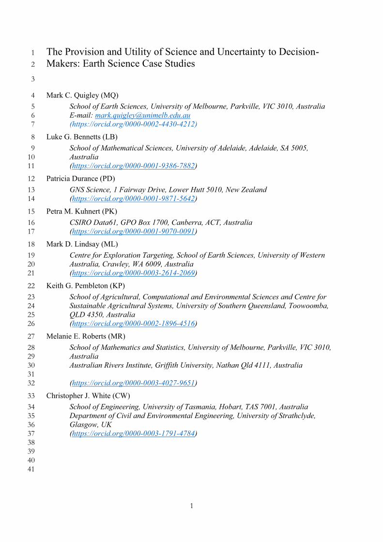
1 The Provision and Utility of Science and Uncertainty to Decision- 1 Makers: Earth Science Case Studies 2 3 Mark C. Quigley (MQ) 4 School of Earth Sciences, University of Melbourne, Parkville, VIC 3010, Australia 5 E-mail: [email protected] 6 (https://orcid.org/0000-0002-4430-4212) 7 Luke G. Bennetts (LB) 8 School of Mathematical Sciences, University of Adelaide, Adelaide, SA 5005, 9 Australia 10 (https://orcid.org/0000-0001-9386-7882) 11 Patricia Durance (PD) 12 GNS Science, 1 Fairway Drive, Lower Hutt 5010, New Zealand 13 (https://orcid.org/0000-0001-9871-5642) 14 Petra M. Kuhnert (PK) 15 CSIRO Data61, GPO Box 1700, Canberra, ACT, Australia 16 (https://orcid.org/0000-0001-9070-0091) 17 Mark D. Lindsay (ML) 18 Centre for Exploration Targeting, School of Earth Sciences, University of Western 19 Australia, Crawley, WA 6009, Australia 20 (https://orcid.org/0000-0003-2614-2069) 21 Keith G. Pembleton (KP) 22 School of Agricultural, Computational and Environmental Sciences and Centre for 23 Sustainable Agricultural Systems, University of Southern Queensland, Toowoomba, 24 QLD 4350, Australia 25 (https://orcid.org/0000-0002-1896-4516) 26 Melanie E. Roberts (MR) 27 School of Mathematics and Statistics, University of Melbourne, Parkville, VIC 3010, 28 Australia 29 Australian Rivers Institute, Griffith University, Nathan Qld 4111, Australia 30 31 (https://orcid.org/0000-0003-4027-9651) 32 Christopher J. White (CW) 33 School of Engineering, University of Tasmania, Hobart, TAS 7001, Australia 34 Department of Civil and Environmental Engineering, University of Strathclyde, 35 Glasgow, UK 36 (https://orcid.org/0000-0003-1791-4784) 37 38 39 40 41
-
Upload
khangminh22 -
Category
Documents
-
view
1 -
download
0
Transcript of Makers: Earth Science Case Studies - Strathprints
1
The Provision and Utility of Science and Uncertainty to Decision-1
Makers: Earth Science Case Studies 2
3
Mark C. Quigley (MQ) 4
School of Earth Sciences, University of Melbourne, Parkville, VIC 3010, Australia 5
E-mail: [email protected] 6
(https://orcid.org/0000-0002-4430-4212) 7
Luke G. Bennetts (LB) 8
School of Mathematical Sciences, University of Adelaide, Adelaide, SA 5005, 9
Australia 10
(https://orcid.org/0000-0001-9386-7882) 11
Patricia Durance (PD) 12
GNS Science, 1 Fairway Drive, Lower Hutt 5010, New Zealand 13
(https://orcid.org/0000-0001-9871-5642) 14
Petra M. Kuhnert (PK) 15
CSIRO Data61, GPO Box 1700, Canberra, ACT, Australia 16
(https://orcid.org/0000-0001-9070-0091) 17
Mark D. Lindsay (ML) 18
Centre for Exploration Targeting, School of Earth Sciences, University of Western 19
Australia, Crawley, WA 6009, Australia 20
(https://orcid.org/0000-0003-2614-2069) 21
Keith G. Pembleton (KP) 22
School of Agricultural, Computational and Environmental Sciences and Centre for 23
Sustainable Agricultural Systems, University of Southern Queensland, Toowoomba, 24
QLD 4350, Australia 25
(https://orcid.org/0000-0002-1896-4516) 26
Melanie E. Roberts (MR) 27
School of Mathematics and Statistics, University of Melbourne, Parkville, VIC 3010, 28
Australia 29
Australian Rivers Institute, Griffith University, Nathan Qld 4111, Australia 30
31
(https://orcid.org/0000-0003-4027-9651) 32
Christopher J. White (CW) 33
School of Engineering, University of Tasmania, Hobart, TAS 7001, Australia 34
Department of Civil and Environmental Engineering, University of Strathclyde, 35
Glasgow, UK 36
(https://orcid.org/0000-0003-1791-4784) 37
38
39
40
41

2
1 Abstract 42
43
This paper investigates how scientific information and expertise was provided to decision-44
makers for consideration in situations involving risk and uncertainty. Seven case studies from 45
the earth sciences were used as a medium for this exposition: (1) the 2010-2011 Canterbury 46
earthquake sequence in New Zealand, (2) agricultural farming system development in North 47
West Queensland, (3) operational flood models, (4) natural disaster risk assessment for 48
Tasmania, (5) deep sea mining in New Zealand, (6) 3-D modelling of geological resource 49
deposits, and (7) land-based pollutant loads to Australia’s Great Barrier Reef. Case studies 50
are lead-authored by a diverse range of scientists, based either in universities, industry, or 51
government science agencies, with diverse roles, experiences, and perspectives on the events 52
discussed. The context and mechanisms by which scientific information was obtained, 53
presented to decision-makers, and utilized in decision-making is presented. Sources of 54
scientific uncertainties and how they were communicated to and considered in decision-55
making processes are discussed. Decisions enacted in each case study are considered in terms 56
of whether they were scientifically informed, aligned with prevailing scientific evidence, 57
considered scientific uncertainty, were informed by models, and were (or were not) 58
precautionary in nature. The roles of other relevant inputs (e.g., political, socioeconomic 59
considerations) in decision-making are also described. Here we demonstrate that scientific 60
evidence may enter decision-making processes through diverse pathways, ranging from direct 61
solicitations by decision-makers to independent requests from stake-holders following media 62
coverage of relevant research. If immediately relevant scientific data cannot be provided with 63
sufficient expediency to meet the demands of decision-makers, decision-makers may (i) seek 64
expert scientific advice and judgement (to assist with decision-making under conditions of 65
high epistemic uncertainty), (ii) delay decision-making (until sufficient evidence is obtained), 66
and / or (iii) provide opportunities for adjustment of decisions as additional information 67
becomes available. If the likelihood of occurrence of potentially adverse future risks is 68
perceived by decision-makers to exceed acceptable thresholds and/or be highly uncertain, 69
precautionary decisions with adaptive capacity may be favoured, even if some scientific 70
evidence suggests lower levels of risk. The efficacy with which relevant scientific data, 71
models, and uncertainties contribute to decision-making may relate to factors including the 72
expediency with which this information can be obtained, the perceived strength and relevance 73
of the information presented, the extent to which relevant experts have participated and 74
collaborated in scientific communications to decision-makers and stake-holders, and the 75
perceived risks to decision-makers of favouring earth science information above other, 76
potentially conflicting, scientific and non-scientific inputs. This paper provides detailed 77
Australian and New Zealand case studies showcasing how science actions and provision 78
pathways contribute to decision-making processes. We outline key learnings from these case 79
studies and encourage more empirical evidence through documented examples to help guide 80
decision-making practices in the future. 81

3
Keywords: earth science, environmental science, decision-making, policy, natural 82
disasters, risk, uncertainty 83
84
2 Introduction 85
86
Earth science has much to offer decision-makers in situations involving risk and uncertainty. 87
Risks may result from the exposure of vulnerable elements to earth science hazards and/or 88
other forms of risk inherent to decision-making with uncertain outcomes. Risks discussed in 89
this paper include human fatality, physical, social or psychological injury, damage to 90
property and infrastructure, economic loss (or non-maximization of potential profit), 91
environmentally adverse effects such as pollution and habitat loss, and risks to decision-92
makers (e.g., political and/or job security risks, including those that might amplify in 93
complex ways throughout the decision-making process). These risks are further described and 94
analysed using decision trees in a companion paper (Quigley et al., Minerva, in review). 95
All science, and thus all scientifically-informed decision-making, is inherently uncertain 96
(Fischoff and Davis, 2014). Uncertainty may arise from incomplete scientific knowledge (i.e., 97
epistemic uncertainty), intrinsic variability in the system(s) or processes under consideration 98
(i.e., aleatoric uncertainty), vagueness, ambiguity and under-specificity in communications 99
between science providers, decision-makers, and affected parties (i.e., linguistic 100
uncertainties), and ambiguity or controversy about how decision-makers quantify, compare, 101
and value social goals, objectives, and trade-offs in decision-making processes (i.e., value 102
uncertainties) (Regan et al., 2002; Ascough II et al., 2008; Morgan and Henrion, 1990; 103
Finkel, 1990). Decision-makers tasked with developing and implementing policy, issuing 104
evacuations in emergency situations, deciding whether to approve mining consents, or 105
selecting amongst distinct approaches for resource extraction, may all draw on earth science 106
inputs to assist in characterising and reducing various forms of uncertainty. Decision-makers 107
may be individuals or collectives that are operating in their own self-interest or on behalf of 108
others. Decision-makers may ask the earth science community to provide forecasts of the 109
occurrence, magnitude, and likely impacts of natural and human-induced environmental 110
phenomena, ranging from earthquakes, to floods, to land-use practises, to climate change 111
(e.g., Sarewitz and Pielke Jr., 1999; Pielke Jr. and Conant, 2003). Some risks may be reduced 112
through mitigation against and/or avoidance of potential hazards. 113
Governments around the world spend billions of dollars each year on obtaining relevant earth 114
science that might assist in decision-making. However, many issues are complex with highly 115
uncertain outcomes, and may be strongly influenced by inputs that reside outside of the 116
immediate earth science domain, such as cost-benefit analyses, political considerations, and 117
other socioeconomic factors. Enacted decisions may not align with prevailing science and 118
4
because these issues are often informed by scientific, socioeconomic, and/or political models 119
of the future, the potential outcomes of enacted decisions are not known with certainty. 120
This contribution is presented in response to the Recommendations from the 2016 Theo 121
Murphy High Flyers Think Tank: An interdisciplinary approach to living in a risky world 122
(2017). The event brought together a group of Australian- and New Zealand-based, early- and 123
mid-career researchers form a broad range of disciplines across science, social science and 124
the humanities (including the authors of this paper), who were tasked with developing 125
recommendations for scientists, the public and decision-makers regarding how to understand, 126
communicate, and assess risk in conditions of uncertainty, ignorance and partial knowledge 127
(Colyvan et al. 2017). In many earth science disciplines, the scientific contributions to 128
decision-makers aim to describe and communicate uncertainty by quantifying the probability 129
of risks occurring if a decision is taken related to a specific action that would create exposure 130
to a hazard. Among the diverse expertise represented in the Think Tank, we found there was 131
an overarching lack of awareness and an absence of critical assessment of the utility of the 132
provision of science in decision-making under conditions of high uncertainty and risk. This 133
lack of appraisal by scientists on the utility of their evidence-based contributions creates an 134
obstacle that prohibits science providers from understanding of how their science was used 135
(or not) by decision-makers. 136
Our findings led to the creation of two key recommendations (Colyvan et al. 2017): 1) 137
Develop a better understanding of how uncertainty affects decision-making, and 2) Facilitate 138
improved communication of risk and uncertainty between scientists, decision-makers and the 139
general public. To address the first recommendation, we suggested that more empirical 140
evidence is needed on how scientific uncertainties contribute to the decision-making process. 141
To achieve this, we have called for contributions from scientists and decision-makers that 142
describe how scientific uncertainty of all forms is considered within the decision-making 143
scenarios, interdisciplinary research priority should be placed on understanding how 144
decision-makers, media, and public respond to uncertainty in the dissemination of scientific 145
research, including the trustworthiness of science, scientists and communicators, and lastly, 146
that decision-makers are provided with training to recognise the conventions and inherent 147
frailties of their scientific advisors. The second recommendation may be achieved by creating 148
a set of guidelines for reporting risk and uncertainty, methods for communicating the need or 149
value in supplying more information to decision-makers, standardised pathways for direct 150
and open communication between science experts and decision-makers, and communication 151
training for scientists to communicate scientific uncertainties to the media and public. This 152
paper represents a partial response to Recommendation 1, drawing together contributions 153
from members of the workshop that describe their experiences on how scientific uncertainty 154
has contributed to the decision-making process. To generalise these experiences, 155
contributions from a broader international audience are required. 156

5
Due to the high level of complexity and variance in the general field of earth science and 157
decision-making, we adopt a case-study approach aimed at establishing a body of empirical 158
evidence on how scientific uncertainties contribute to the decision-making process 159
(Recommendation 1 above). This descriptive research approach provides a means to 160
document successful and unsuccessful strategies in science provision to, and utility by, 161
decision-makers. Our work builds upon lessons learned from prior analyses of case studies 162
(e.g., Gluckman, 2004; Pielke Jr. and Conant, 2003) including (1) science provides only one 163
of many relevant components in the process of decision-making, (2) predictions drawn from 164
science inputs should not be conflated with policy, and (3) many scientific products are 165
difficult to evaluate and easy to misuse; scientific inputs may have varying levels of 166
accuracy, sophistication, and experience that are not always well described and considered in 167
decision-making (Pielke 2003). The importance of using statistical approaches and 168
quantitative risk evaluation approaches in decision-making has been extensively described 169
(e.g., Clark, 2005; Linkov et al. 2014). 170
Here, we provide case-studies that highlight how variable and complex decision-making 171
processes often are, including how science and associated uncertainties were provided to and 172
used by decision-makers, and how enacted decisions aligned or did not align with the science 173
and uncertainties provided. Each study presents the context and mechanisms by which 174
scientific information was obtained, presented to decision-makers, and utilized in decision-175
making. Sources of scientific uncertainties, and how they were communicated to and 176
considered in decision-making processes are also discussed. Decisions enacted in each case 177
study are considered in terms of whether they (i) were scientifically informed, (ii) aligned 178
with prevailing scientific evidence, (iii) considered scientific uncertainty, (iv) were informed 179
by models, and (v) were (or were not) precautionary in nature. The importance of other 180
relevant inputs (e.g., political, socioeconomic considerations) in decision-making is also 181
briefly described. This paper provides explicit accounts of science utility in diverse forms of 182
decision-making that may be beneficial towards improving communal knowledge of both 183
scientists and decision-makers operating in this highly complex environment. 184
3 Case study 1: Geoscience communications to decision makers 185
during the 2010-2011 Canterbury earthquake sequence in New 186
Zealand (Author: MQ) 187
3.1 Overview 188
The 2010 – 2011 Canterbury earthquake sequence (CES) occurred proximal to and beneath 189
New Zealand’s South Island city of Christchurch (2013 census pop. 366,000) (Fig.1). The 190
CES is New Zealand’s most fatal (185 fatalities) and most expensive natural disaster to date. 191
Rebuild costs (2012 estimate) are approximately NZ$20 Billion (US$15 billion) excluding 192
disruption costs (10% of GDP) and insured losses are estimated at around NZ$30 billion 193
(US$25 billion) (Parker and Steenkamp 2012). 194

6
The CES began with the magnitude (Mw) 7.1 Darfield earthquake in September 2010 and 195
was followed by strong damaging aftershocks in February 2011 (including the fatal Mw 6.2 196
Christchurch earthquake), June 2011, and December 2011, and more than 400 ML ≥ 4.0 197
earthquakes between September 2010 and September 2012 (Quigley et al. 2016). A national 198
state of emergency was declared following both the 2010 Darfield and 2011 February 199
Christchurch earthquakes. The protracted nature of the sequence including repeated episodes 200
of land and infrastructural damage (Berryman 2012; Hughes et al. 2015), and the fatalities, 201
injuries, and severe social and professional disruptions caused adverse economic and mental 202
health impacts throughout the affected region (Fergusson et al. 2014; Spittlehouse et al. 203
2014). Communication of a large and diverse amount of geoscientific (geological, 204
seismological, geospatial), engineering, economic, and sociological information to a variety 205
of decision-makers was undertaken during the response and recovery phases of the CES 206
(Becker et al. 2015; Berryman 2012; Wein et al. 2016). In this contribution we address only 207
the geoscientific communications to decision-makers that are known to MQ and / or 208
accessible in the public domain. A complete description of all science communications for 209
this prolonged, multi-phased, and complex disaster is well beyond the scope of this 210
contribution. 211
Geoscience communications were conducted by individuals and collectives from 212
government-funded Crown Research Institutes (“CRIs”, e.g., GNS Science, National Institute 213
of Water and Atmospheric Research), universities, and industry. Communication methods 214
included publications of scientific research (Cubrinovski et al. 2010; Gerstenberger et al. 215
2011; Quigley et al. 2010; Villamor et al. 2012), commentary on science websites1 (Quigley 216
and Forte 2017), solicited interviews across all forms of media, communications on social 217
media (Bruns and Burgess 2012; Gledhill et al. 2010), public presentations to large audiences 218
of diverse decision makers2, publicly-released government white papers3, and private and 219
public communications with specific decision-makers (e.g., informal communications, email 220
exchanges, and presentations to decision-making entities such as the New Zealand Ministry 221
of Civil Defence & Emergency Management (MCDEM); Urban Search and Rescue; 222
Canterbury Earthquake Recovery Authority (CERA); Christchurch City Council (CCC); 223
Royal Commission panels, independent hearings panels, insurance providers, banks). 224
1 www.geonet.org ; www.drquigs.com 2 http://www.stuff.co.nz/the-press/news/christchurch-earthquake-2011/5248119/Free-public-quake-lectures ; http://www.stuff.co.nz/the-press/news/christchurch-earthquake-2011/canterbury-earthquake-2010/4255970/Thirst-for-quake-info-at-lecture 3 https://royalsociety.org.nz/assets/documents/Information-paperThe-Canterbury-Earthquakes.pdf
7
225
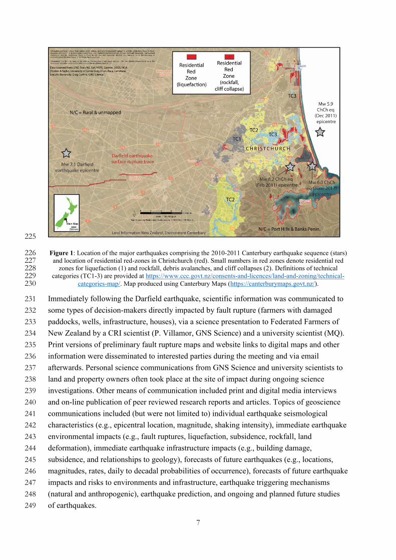
Figure 1: Location of the major earthquakes comprising the 2010-2011 Canterbury earthquake sequence (stars) 226 and location of residential red-zones in Christchurch (red). Small numbers in red zones denote residential red 227
zones for liquefaction (1) and rockfall, debris avalanches, and cliff collapses (2). Definitions of technical 228 categories (TC1-3) are provided at https://www.ccc.govt.nz/consents-and-licences/land-and-zoning/technical-229
categories-map/. Map produced using Canterbury Maps (https://canterburymaps.govt.nz/). 230
Immediately following the Darfield earthquake, scientific information was communicated to 231
some types of decision-makers directly impacted by fault rupture (farmers with damaged 232
paddocks, wells, infrastructure, houses), via a science presentation to Federated Farmers of 233
New Zealand by a CRI scientist (P. Villamor, GNS Science) and a university scientist (MQ). 234
Print versions of preliminary fault rupture maps and website links to digital maps and other 235
information were disseminated to interested parties during the meeting and via email 236
afterwards. Personal science communications from GNS Science and university scientists to 237
land and property owners often took place at the site of impact during ongoing science 238
investigations. Other means of communication included print and digital media interviews 239
and on-line publication of peer reviewed research reports and articles. Topics of geoscience 240
communications included (but were not limited to) individual earthquake seismological 241
characteristics (e.g., epicentral location, magnitude, shaking intensity), immediate earthquake 242
environmental impacts (e.g., fault ruptures, liquefaction, subsidence, rockfall, land 243
deformation), immediate earthquake infrastructure impacts (e.g., building damage, 244
subsidence, and relationships to geology), forecasts of future earthquakes (e.g., locations, 245
magnitudes, rates, daily to decadal probabilities of occurrence), forecasts of future earthquake 246
impacts and risks to environments and infrastructure, earthquake triggering mechanisms 247
(natural and anthropogenic), earthquake prediction, and ongoing and planned future studies 248
of earthquakes. 249
8
Some decision-makers sought information directly from science providers and some obtained 250
information from other sectors, including the media or other decision-making entities (Becker 251
et al. 2015). Aspects such as whether the decision required urgent action (e.g., immediate 252
evacuations from buildings and other areas of high life safety risk), or could be delayed until 253
further scientific and other inputs became available (e.g., revisions to land-use plans and 254
building codes), may have influenced where the decision-maker sourced the information 255
(Becker et al. 2015). Decisions that needed to be made and that could be informed by 256
geoscience information included whether to continue to reside in and/or utilize damaged 257
buildings, whether to rebuild new infrastructure within hazard zones or relocate new 258
infrastructure outside of these zones (Van Dissen et al. 2015), and what remediation 259
techniques might be most effective in reducing hazards and risks. The large volume and 260
diversity of CES decisions and decision-makers resulted in large variance in which science 261
providers were consulted, the methods by which the science was solicited, provided to, and 262
considered against other inputs by decision makers, and the ultimate decisions chosen. An 263
inclusive summary of all CES-related decisions is outside the scope of this article. Rather, we 264
present a diverse suite of decision-making processes that include documented 265
communications between scientists and decision makers and / or contain undocumented 266
aspects that are known to MQ. 267
3.2 Governmental policy decisions on land use in areas subjected to liquefaction 268
hazards 269
The NZ Government responded to the Darfield earthquake by appointing a Minister for 270
Canterbury Earthquake Recovery (Hon. G. Brownlee) on 7 September 2010. The Canterbury 271
Earthquake Response and Recovery Act 2010 was introduced on 14 September 2010 and 272
came into force on 15 September 2010. Following the February 2011 earthquake, Canterbury 273
Earthquake Recovery Authority (CERA) was established as a new Government Department 274
(29 March 2011). The 2010 Act was replaced by the Canterbury Earthquake Recovery Act 275
2011 on 18 April 2011. Extensive details on the 2011 Earthquake Recovery Act4 and related 276
cases in the NZ Supreme court5 and High Court6 are available on-line. 277
From April 2011, officials from the national insurer against natural hazards (The NZ 278
Earthquake Commission: EQC), CERA and the NZ Treasury began assessing the impact of 279
land and property damage in the greater Christchurch area and identifying the worst affected 280
areas. Tonkin & Taylor (an international firm of environmental and engineering consultants) 281
was commissioned by the government to assess the land damage caused by the 2010 and 282
2011 earthquakes. In identifying the land damage, Tonkin & Taylor (T&T) collected their 283
own extensive observations and geotechnical data and obtained further data from sources 284
4 http://legislation.govt.nz/act/public/2011/0012/latest/DLM3653522.html 5 https://www.courtsofnz.govt.nz/cases/quake-outcasts-and-fowler-v-minister-for-canterbury-earthquake-recovery/@@images/fileDecision 6 http://www.stuff.co.nz/national/83446819/High-Court-denies-uninsured-Quake-Outcasts-appeal

9
such as Land Information New Zealand, land data from local councils, engineering teams, 285
private surveyors, CRI and university scientists, and other engineering resources. CRI and 286
university scientists, and industry groups participated in data collection, commonly in a co-287
ordinated collaborative manner. Many of these science research efforts were organized 288
through the New Zealand Natural Hazards Research Platform (NHRP), established in 2009 to 289
foster networking across disciplines, organizations, and sectors in order to pursue the policy 290
goal of “a New Zealand society that is more resilient to natural hazards”7 (NHRP 2009, p. 291
5). A review of the performance of the NHRP throughout the CES is provided by (Beaven et 292
al. 2016). Property data was also collected from EQC and private insurers. Open access to 293
some scientific information was provided to the general public throughout the CES, in reports 294
from CCC, GNS Science, Tonkin & Taylor, NHRP, EQC and other entities, in reports across 295
all media streams, and from research publications made available through science websites. 296
The most extensive forms of land and property damage that required a series of decision-297
making processes at levels ranging from governmental policy to personal decisions by 298
individuals concerned the effects of liquefaction and mass movements on the city of 299
Christchurch. Multiple episodes of liquefaction (i.e., the process where transient shear 300
stresses exerted on soils during strong ground shaking in earthquakes increases pore fluid 301
pressures, reduces soil strength and stiffness, and causes ground deformations and surface 302
ejections of liquefied material and ground water) resulted in extensive and repeated land and 303
infrastructure damage in Christchurch during the CES (Cubrinovski et al. 2010; Hughes et al. 304
2015; Quigley et al. 2013). Liquefaction affected ~51,000 residential properties and severely 305
damaged ~15,000 residential houses in the Christchurch region. Mass movements included 306
collapse of cliffs (and associated cliff-top recession and cliff-bottom burial by debris) and the 307
detachment of subsequent downslope transport of individual rocks (rockfall and boulder roll) 308
into urban areas (Massey et al. 2014). Mass movements caused five fatalities and damaged 309
approximately 200 houses. 310
After a major liquefaction-inducing earthquake on 13 June 2011, the New Zealand Cabinet 311
authorised a committee of senior Ministers to make decisions on land damage and 312
remediation issues. On 22 June 2011, the decision-making criteria were recorded in a 313
confidential memorandum for Cabinet (“the Brownlee paper”)8,9 signed by the Hon. G. 314
Brownlee (signature dated 24 June 2011). The decisions were announced to the public by the 315
then Prime Minister Hon. John Key and G. Brownlee on 23 June 2011. The Cabinet 316
committee categorised greater Christchurch into four zones (red, white, green, orange) 317
according to the extent of land damage and the timeliness and economics of remediation8. In 318
7https://www.naturalhazards.org.nz/content/download/9099/49062/file/Hazards_Platform_Partnership_Agreement.pdf 8 https://ceraarchive.dpmc.govt.nz/sites/default/files/Documents/memorandum-for-cabinet-land-damage-june-2011_0.pdf
10
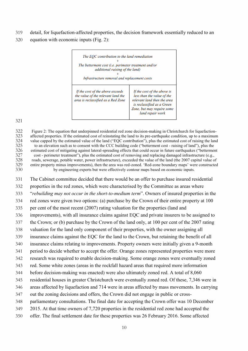
detail, for liquefaction-affected properties, the decision framework essentially reduced to an 319
equation with economic inputs (Fig. 2): 320
321
Figure 2: The equation that underpinned residential red zone decision-making in Christchurch for liquefaction-322 affected properties. If the estimated cost of reinstating the land to its pre-earthquake condition, up to a maximum 323 value capped by the estimated value of the land (“EQC contribution”), plus the estimated cost of raising the land 324
to an elevation such as to consent with the CCC building code (“betterment cost - raising of land”), plus the 325 estimated cost of mitigating against lateral-spreading effects that could occur in future earthquakes (“betterment 326
cost - perimeter treatment”), plus the estimated cost of removing and replacing damaged infrastructure (e.g., 327 roads, sewerage, potable water, power infrastructure), exceeded the value of the land (the 2007 capital value of 328
entire property minus improvements), then the area was red-zoned. ‘Red-zone boundary maps’ were constructed 329 by engineering experts but were effectively contour maps based on economic inputs. 330
The Cabinet committee decided that there would be an offer to purchase insured residential 331
properties in the red zones, which were characterised by the Committee as areas where 332
“rebuilding may not occur in the short-to-medium term”. Owners of insured properties in the 333
red zones were given two options: (a) purchase by the Crown of their entire property at 100 334
per cent of the most recent (2007) rating valuation for the properties (land and 335
improvements), with all insurance claims against EQC and private insurers to be assigned to 336
the Crown; or (b) purchase by the Crown of the land only, at 100 per cent of the 2007 rating 337
valuation for the land only component of their properties, with the owner assigning all 338
insurance claims against the EQC for the land to the Crown, but retaining the benefit of all 339
insurance claims relating to improvements. Property owners were initially given a 9-month 340
period to decide whether to accept the offer. Orange zones represented properties were more 341
research was required to enable decision-making. Some orange zones were eventually zoned 342
red. Some white zones (areas in the rockfall hazard areas that required more information 343
before decision-making was enacted) were also ultimately zoned red. A total of 8,060 344
residential houses in greater Christchurch were eventually zoned red. Of these, 7,346 were in 345
areas affected by liquefaction and 714 were in areas affected by mass movements. In carrying 346
out the zoning decisions and offers, the Crown did not engage in public or cross-347
parliamentary consultations. The final date for accepting the Crown offer was 10 December 348
2015. At that time owners of 7,720 properties in the residential red zone had accepted the 349
offer. The final settlement date for these properties was 26 February 2016. Some affected 350
11
property owners that have not accepted the offer remain engaged in legal action against the 351
Crown9. 352
Scientific inputs are stated to have influenced policy development and decision-making in the 353
Brownlee paper8. These include data on the extent and severity of the land damage caused by 354
the earthquakes, particularly where it affected properties over a wide area, and the risk of 355
additional damage to the land and buildings from further aftershocks. For example, the paper8 356
states “The ground accelerations recorded from this earthquake [Feb 2011 Christchurch 357
earthquake] are among some of the highest recorded anywhere in the world. Damage from 358
the recent 13 June 2011 5.6 and 6.3 magnitude earthquakes has added to the damage. The 359
seismic factor has recently been increased for Christchurch from 0.22 to 0.3, and after the 360
large aftershocks on Monday 13 June, work is being undertaken to consider if it should be 361
further revised upwards. In any case, there is a reasonable chance of continued large 362
aftershocks and this must be factored into recovery. After the aftershocks on Monday 13 June 363
GNS has indicated the chance of a quake of magnitude between 6 and 6.9 in the region over 364
the coming year being around 34 per cent. If no significant aftershocks or triggering events 365
occur in the next month that likelihood will fall to around 17%.”8 A detailed report authored 366
by GNS Science and university scientists on probabilistic assessments of future liquefaction 367
potential for Christchurch was commissioned by Tonkin and Taylor (Gerstenberger et al. 368
2011). The report concluded that “liquefaction probabilities for the next 50 years are high for 369
the most severely affected suburbs of the city, and are well in excess of the probabilities 370
associated with the ground-shaking design levels defined in the New Zealand structural 371
design standard NZS1170…”(Gerstenberger et al. 2011). The Brownlee paper8 stated that, 372
“The strength-depth profiles under some parts of Christchurch indicate typically up to 10 373
metres of 'liquefiable' material. Although some ground settlement may occur, the large 374
reservoir of liquefiable material and these examples suggest that similar characteristics of 375
ground shaking are likely to result in similar amounts of liquefaction in the future”8. The 376
Brownlee paper referenced the Canterbury earthquakes white paper3 as the source of this 377
information, although the statement was probably more directly informed by geotechnical 378
data and reports from Tonkin and Taylor and the results of the Gerstenberger et al. (2011) 379
paper. 380
Ultimately, for areas of Christchurch affected by liquefaction, the exact role of each science 381
provision to land zone policy is challenging to determine. It is likely that the observations of 382
recurrent liquefaction and land damage, and the assessments suggesting a relatively high 383
probability of future occurrence, may have influenced governmental decision-makers to 384
recognize the need to develop a land policy in the first place. However, the red-zone equation 385
as stated in the Brownlee paper does not explicitly account for these science and engineering 386
inputs. Instead, the most prominently featured motivation for policy decisions appears to have 387
9https://www.courtsofnz.govt.nz/cases/quake-outcasts-and-fowler-v-minister-for-canterbury-earthquake-recovery/@@images/fileDecision
12
been “the urgent need to provide a reasonable degree of certainty to residents in these areas 388
in order to support the recovery process. Speeding up the process of decision-making is 389
crucial for recovery and in order to give confidence to residents, businesses, insurers and 390
investors. This is particularly the case in the worst affected suburbs, where the most severe 391
damage has repeatedly occurred.”8 392
In this context, the sources of epistemic scientific uncertainty (e.g., will future liquefaction-393
triggering earthquakes occur in the short-to-medium term and what will their characteristics 394
be?), engineering uncertainty (e.g., what exact designs for residential properties and lateral-395
spreading perimeters would be most effective in terms of mitigating against future 396
liquefaction-triggering earthquakes?), and economic uncertainty (e.g., what are the precise 397
fiscal values of the three components of the economic equation in Figure 2 and what fiscal 398
uncertainty resides within each?) are likely to have been overridden by the decision-makers’ 399
(G. Brownlee, CERA, and other key central Government agents) desire to make expedient 400
decisions that could be (at least coarsely) justified by economic, scientific, and engineering 401
criteria, even if parameters sourced from the latter two criteria were not directly used to 402
define boundaries on the red-zone maps (Fig.1). While the incrementation of some decision-403
making (e.g., ‘orange zones’) frustrated both decision-makers and affected land owners, this 404
enabled more science and engineering information to be obtained in marginal cases where 405
reduction of epistemic uncertainty was viewed to be valuable. An Independent Hearings 406
process also enabled affected parties to challenge decisions if evidence of sufficient strength 407
to was able to be acquired and presented. 408
3.3 Risk-based land decisions and independent hearings pertaining to 409
residential properties subjected to rockfall hazards 410
Immediately following the 22 February 2011 Canterbury earthquakes, people were evacuated 411
from over 200 homes affected by rockfall and cliff collapse, as preliminary observations of 412
precariously fractured rockfall source areas, cliff-top cracks and relatively high estimated 413
probabilities of future strong earthquakes were considered to pose imminent life-safety risks 414
(see Massey et al. (2014) and references therein). In response to the recognition of the threat 415
of future rockfall events, and CCC and NZ Government’s priority to give the affected people 416
a timely decision over the future of their properties, the CCC (with additional funding from 417
the NZHRP) commissioned investigations to quantify the rockfalls triggered by the 418
earthquake sequence and to determine the risk posed by future rockfall (e.g., see Massey et 419
al. (2014) and references therein). Massey et al. (2014) adapted the Australian Geomechanics 420
Society framework for landslide risk management (Australian Geomechanics Society 2007) 421
to estimate the annual individual fatality risk (AIFR) for about 1,450 properties in the Port 422
Hills: 423
AIFR = P(H) x P (S:H) x P(T:S) x V (D:T) (1) 424
13
where P(H) is the annual probability of a rockfall-initiating event; P(S:H) is the probability of 425
a person, if present, being in the path of one or more boulders at a given location; P(T:S) is 426
the probability that a person is present at that location when the event occurs; V(D:T) is the 427
probability of a person being killed if present and in the path of one or more boulders (i.e., 428
vulnerability). Earth science inputs to P(H) and P (S:H) included seismicity forecasts 429
(incorporating both national seismic hazard models and aftershock-based, regional forecast 430
models to estimate the temporal probability of future strong earthquakes) (Gerstenberger et 431
al. 2011; Stirling et al. 2012), coupled seismic and geologic observations (to quantify the 432
relationship between ground motion parameters such as PGA and peak ground velocities with 433
the occurrence or non-occurrence of rockfall), geospatial analyses using LiDAR data (to map 434
boulder locations, rockfall source-slope angles and heights, and boulder travel distances), and 435
field studies (to measure boulder dimensions). Non-seismic rockfall triggers were also 436
considered but found to be a minimal short-term contributor to rockfall production when 437
compared to seismic triggering (Massey et al. 2014). Rockfall risk maps (i.e. AIFR contour 438
maps for the residential areas of the Port Hills) were generated for different future time 439
intervals, starting from the elevated first 1-year rate of seismicity (starting 1 January 2012) 440
(Massey et al. 2014). 441
Given a suite of epistemic uncertainties in model parameters, including probability-density 442
distributions of the earthquake ground motions that caused past rockfalls and could cause 443
future rockfalls (due to lack of instrumentation on source slopes for past events and lack of 444
knowledge of the future state of the rock mass in future events), Massey et al. (2014) 445
estimated an order of magnitude (higher or lower) uncertainty range in AIFR estimates 446
presented on the risk maps. A discussion of uncertainties is presented in Massey et al. (2014). 447
Addressing these uncertainties was not a priority in reducing the long-term safety risk in the 448
immediate aftermath of the earthquakes. 449
Within this context, in 2011, Mr. Brownlee stated that, “…the decisions that need to be made 450
here are very, very dependent upon research about the condition of the land in 451
Christchurch…”10. In 2012, he told the Christchurch Press that “…I'd love to be able to fix 452
all of that [earthquake land issues] for people immediately, [but] we've got to get the science 453
and engineering right on how to progress…”11. In 2013, he told the Christchurch Press that 454
“We know from the extensive ground-truthing and area-wide modelling that the risk of rock 455
roll in this part of the Port Hills is high; hence the need to zone the land red…”12. 456
10 https://www.courtsofnz.govt.nz/cases/quake-outcasts-and-fowler-v-minister-for-canterbury-earthquake-recovery/@@images/fileDecision 11 http://www.stuff.co.nz/the-press/news/christchurch-earthquake-2011/7656654/Brownlee-fed-up-with-moaning-residents 12 http://www.stuff.co.nz/the-press/news/christchurch-earthquake-2011/8220906/I-told-you-so-says-Brownlee-on-rockfall

14
The changes to land use designations described above required development of a new 457
Christchurch City Replacement District Plan, which provided a process for the review of the 458
previous district plans and preparation of a comprehensive replacement district plan for the 459
Christchurch district. The proposed framework for the plan included a Statement of 460
Expectations outlined by both the Minister for Canterbury Earthquake Recovery and Minister 461
for the Environment. One stated expectation was that the plan would “avoid or mitigate 462
natural hazards”13. The proposed plan was prepared by CCC in consultation with CRI, 463
university, and industry scientists and engineers14 and notified in three stages in 2014 and 464
2015. It was formally acknowledged by the CCC and the Crown that the proposed plan “is 465
based on complex technical modelling and outputs” that rely on “geotechnical and scientific 466
background research” and that the “most effective approach” for “refining the issues” that 467
could arise from submitters wishing to challenge decisions within the plan was “for relevant 468
experts to enter into technical caucusing on the modelling approach and methodology” prior 469
to “evidence exchange” in hearings15. Caucusing involved CRI, university and industry 470
scientists and engineers acting on behalf of the CCC and The Crown, and university and 471
industry scientists that were invited to participate in caucusing due to their likely future 472
involvement in hearings as expert witnesses acting on behalf of submitters. 473
Concurrent with the CCC commissioned research, independent researchers began to study the 474
prehistoric record of rockfalls at a specific site in the Port Hills using a variety of mapping 475
and dating methods (Borella et al. 2016a; Borella et al. 2016b; Mackey and Quigley 2014). 476
This research was neither funded by, nor undertaken for the purposes of, contributing to land 477
policy decision making. Two key conclusions arose from this work; (1) the penultimate (pre-478
CES) major rockfall event(s) at this site occurred sometime in the middle Holocene (ca. 3-8 479
ka), with a possible predecessor event at ca. 12-14 ka, interpreted to suggest recurrence 480
intervals of several 1000s of years for rockfall-triggering seismic ground motions (Borella et 481
al. 2016a; Mackey and Quigley 2014), and (2) that finite rockfall travel distances in the pre-482
CES Holocene events were reduced due to the presence of native vegetation on the currently 483
deforested slopes, which reduced boulder travel velocities through collisions and impedance 484
(Borella et al. 2016b). The results of this research were not available at the time of land-485
zoning decision-making, but became available via media coverage shortly thereafter, and 486
were considered of relevance by some affected property owners that were challenging zoning 487
decisions through the Independent Hearings Committee process. 488
MQ was invited to participate in the Independent Hearings Committee process by a submitter 489
wanting to challenge aspects of the CCC rockfall risk decision on her property after the 490
13 http://proposeddistrictplan1.ccc.govt.nz/ 14http://proposeddistrictplan1.ccc.govt.nz/ 15 http://www.chchplan.ihp.govt.nz/wp-content/uploads/2015/03/310_495-CCC-and-Crown-Joint-Memorandum-re-Preparations-for-Hearing-of-Natural-Hazards-8-12-14.pdf
15
submitter read a newspaper article published in the Christchurch Press16 that discussed the 491
authors recently published research on prehistoric rockfall frequencies at a nearby location 492
(Mackey and Quigley 2014). The submitter told MQ that “Your new research MUST be 493
incorporated in their general model and CERA’s submission seems to indicate that they 494
would support it…”. Mackey and Quigley (2014) was ultimately submitted into evidence by 495
the submitter and subsequently considered in the hearings17. Another submission group also 496
consulted MQ for advice relating to their claims in rockfall affected coastal holiday 497
properties upon learning of his research through the media. 498
In caucusing, the experts discussed the research methods and scientific evidence relevant to 499
the proposed plan and prepared a joint statement. The joint statement acknowledged that “the 500
risk-based modelling approach undertaken by GNS Science acknowledges key uncertainties 501
and is an appropriate method for assessing risk…” but that “the area-wide mapping and 502
modelling is not always sufficient to determine risk on a site-specific basis” and so “the 503
opportunity to undertake individual site assessment must be provided for in the plan…”18. A 504
separate signed document by three experts (including MQ) stated that “future earthquakes 505
have the potential to cause additional rockfall and cliff collapse” and that “published, 506
peerreviewed geologic data do not exclude the possibility of future rockfall triggering events 507
from the ongoing sequence or other seismic events. Available site-specific geologic data 508
suggest that clusters of severe rockfall events may be separated by hiatuses spanning 1000s 509
of years but further analysis from additional sites is required to test this hypothesis. The 510
seismicity model was developed by an international expert panel using international best 511
practice and has undergone peer review. Given the recent and modelled earthquake 512
clustering activity and the large uncertainties on predicted ground-motion for an individual 513
earthquake, we agree that the level of conservatism is appropriate”19. Full transcripts from 514
the panel hearings and decisions are available20. 515
In the context of rockfall risk, the results of Mackey and Quigley (2014) and other relevant 516
scientific evidence (Borella et al. 2016b) and bearings on the CCC district plan were 517
discussed. MQ delivered a statement, was cross-examined by council acting on behalf of 518
CCC and the Crown, re-examined by the submitter, and asked questions by the decision-519
making panel. In response to questions from the cross-examiner, MQ stated that “…there are 520
limitations to any dataset and uncertainties and I think that we have completely adopted that 521
16 http://www.stuff.co.nz/national/10574099/Alpine-Fault-unlikely-to-trigger-Port-Hills-rockfall 17 http://www.chchplan.ihp.govt.nz/wp-content/uploads/2015/03/IHP_Natural-Hazards-PART_180315.pdf 18 http://www.chchplan.ihp.govt.nz/wp-content/uploads/2015/03/Technical-expert-witness-caucusing-report-Natural-Hazards-full-signed.pdf) 19 http://www.chchplan.ihp.govt.nz/wp-content/uploads/2015/03/Technical-expert-witness-caucusing-report-Natural-Hazards-full-signed.pdf 20 http://www.chchplan.ihp.govt.nz/hearings/

16
statistical model, and I think that that statistical model needs to be also informed by geology, 522
whilst acknowledging the uncertainties therein….”, and “…site specific investigations need 523
to be better informed by geology…”. He stated that “…we cannot dismiss the possibility 524
outright of future strong earthquakes, and even though we find very little evidence for that 525
from a geologic perspective we cannot completely discount that possibility. [However] if 526
someone uses statistical seismology to say that there is a six percent chance of a magnitude 527
six earthquake somewhere over a broad region in the next year, an important question to ask 528
is if that event actually happens are they correct or are they incorrect in that statement. What 529
I am finding is there is a tension between source-based geological approaches, where I am 530
forced into somewhat of a binary position, where I have to either say there are active faults in 531
the area close enough to cause rock fall, or there are not, therefore I can be right or I can be 532
wrong. Whereas from a strictly probabilistic approach using overall low bulk probabilities, 533
like say for instance six percent, I think that you, at some level you are correct irrespective of 534
the outcome, although I know more sophisticated analysis can be done to validate those 535
claims and test those claims….” MQ concluded that “…my professional opinion is that we 536
are very unlikely to experience any future earthquakes in the short to medium and possibly 537
even to the long term that generate peak ground velocities and peak ground accelerations 538
analogous to those experienced in the February and June earthquakes [that caused severe 539
rockfall] in the Port Hills Region” but that “I cannot completely dismiss that possibility, and 540
it would be unprofessional of me to say we are out of the woods and there is no possibility of 541
anything similar to those going forward….”. 542
Under direct questioning from the panel, MQ was asked, “given that notwithstanding that this 543
District Plan has a 10-year life, some of the decisions made during that 10 year period will 544
endure for a long period of time, for example, if you build structures in certain locations, they 545
are not going to be taken away after 10 years. Given that, do you think it is wise from a 546
scientific point of view to exercise a degree of caution when delineating where hazards may 547
or may not occur, and how we manage them?” to which he replied, “I absolutely do agree 548
with that statement, yes”. MQ was asked, “So a regime that allowed lines to be adjusted as 549
better information became available, provided that we set the lines conservatively in the first 550
place, that would be a good outcome from your point of view?” to which he replied, 551
“Yes…from a strictly geological point of view conservativism is a great thing...”. MQ stated 552
to the panel that “there is very little in science in general that can be said with 100 percent 553
certainty” to which a panel member replied, “I understand that and that is really the point. 554
We are dealing with probabilities on one hand, whereas on the other hand, we and the 555
Council have the responsibility of trying to protect peoples’ lives. So doing nothing until 556
further work is carried out would not seem to be an option then…”. Regarding the scientific 557
evidence presented that regenerating the region with native forest could reduce the travel 558
distances of future rockfalls, the panel asked MQ, “if you wanted to protect from that hazard 559
now with vegetation, it is going to be quite a few years before the trees are substantial 560
enough to be of any value?” to which he replied, “That is completely correct. There will be a 561
17
lag time for the trees to grow to the point where they are actually able to effectively mitigate 562
that hazard, yes.” He was asked, “…have you given any thought of the level of regulation 563
that would be needed to prevent the cutting down of trees, to prevent fires in trees, all of 564
those sorts of things?” to which he replied, “that is a… valid question ..I have no easy answer 565
to that…”. 566
Ultimately, the decision-making panel decided that they were “quite satisfied that the 567
evidence of Dr Quigley is not a basis for taking a less cautious approach”. They stated that 568
“Dr Quigley’s evidence was of assistance to the Panel” and they “urge[d] that Dr Quigley 569
and his team’s work continue to further the current level of understanding” but noted that 570
“Dr Quigley accepted a cautionary approach was appropriate”. In some cases, Panel-571
directed mediations between the CCC and particular submitters (often with input from 572
experts) resulted in agreement that properties could be released in part, or completely, from 573
particular natural hazard areas; in other cases, the panel did not support the removal or 574
relaxation of hazard area controls from properties as sought by submitters. In the case of the 575
submitter that called MQ as an expert witness, the panel stated that “…Dr Quigley was 576
supportive of a regime that would allow hazard lines to be adjusted when better information 577
becomes available…” and after further site-specific investigations and consultation with the 578
CCC expert witness, that “…relief should be granted to the extent that the hazard lines are 579
moved as specified…”. 580
In this sense, relevant but initially unsolicited research ultimately entered into formal 581
considerations on land use planning, through submission of research papers as evidence to the 582
hearings panel, via an indirect, stake-holder-driven pathway. On balance, the strength of this 583
evidence was ultimately not considered sufficiently relevant to change the magnitude or 584
position of AIFR contours, nor to invalidate the CCCs precautionary approach towards 585
minimizing AIFR to Christchurch residents. 586
3.4 Individual decisions pertaining to earthquake risks 587
When considering whether to accept the red zone offer and which option to accept, affected 588
individuals consulted a diverse range of sources (e.g., lawyers, banks, the media, CERA, 589
surveyors, insurance companies, etc.)21. Detailed accounts including surveys of people who 590
chose to accept red zone offers22 and decline red zone offers23 have been published by CERA 591
and the New Zealand Human Rights Commission, respectively. For those who decided to 592
accept the Crown’s red zone offer to relocate, property affordability (47%) and relocating 593
into an area that had little physical damage (34%) and was perceived to be safe from natural 594
21 http://www.eqrecoverylearning.org/assets/downloads/2016-02-01-rec3020-cera-residential-red-zone-survey-report.pdf 22 http://www.eqrecoverylearning.org/assets/downloads/2016-02-01-rec3020-cera-residential-red-zone-survey-report.pdf 23 https://www.hrc.co.nz/red-zones-report/

18
disasters (29%) were the most highly cited reasons for relocating. In contrast, when asked 595
why the owners initially chose their (now red-zoned) properties, convenience to the natural 596
environment (56%) was the most highly cited reason, while only 6% cited safety from natural 597
disasters as a priority24. Given that the perception of safety from natural disasters relies in 598
part on publicly-communicated scientific information relating to natural disasters, we suggest 599
that geoscience played a role in informing decision-making in this context. 600
Some individuals and collectives chose to dispute the liquefaction and mass movement 601
hazard maps, and/or corresponding risk classifications estimated for their properties, and/or 602
policy decisions related to the above. The reasons for disputing these classifications included 603
challengers’ perceptions that characterisation of hazards at their site was inadequate or 604
inaccurate (e.g., inadequate or inaccurate documentation of CES rockfalls, floods, land 605
movement, and/or liquefaction effects), modelling of exposure to future hazards was 606
inadequate or inaccurate (e.g., under- or over-estimated exposure to falling rocks and/or cliff 607
collapse), modelling of future life safety and property risks was inadequate or inaccurate 608
(e.g., inaccurate inputs into calculations of building occupancy rates), and/or consideration of 609
other inputs was inadequate (e.g., social considerations, community health considerations, 610
insurance considerations, human rights considerations). It is beyond the scope of this article 611
to address each of these in detail. However, the most cited reasons for remaining in red zone 612
properties (financial, attachment to property, attachment to neighbourhood) are not informed 613
by geoscience information. Some individuals (19% of surveyed) indicated that they believed 614
their property to be ‘safe’ on the basis of their personal perceptions of risk, risk mitigations, 615
and independently obtained geoscience data25. The utilization of science evidence in this 616
instance is difficult to assess, as some of the individuals undoubtedly consider their 617
independent observations, risk assessments, and mitigation approaches to be equally if not 618
more scientific than the science evidence available to the New Zealand government and CCC 619
in the land use decision-making. 620
A large number of other decisions regarding personal safety and risk were made throughout 621
the CES. These include decisions related to safety in homes and workplaces, such as fixing 622
televisions and bookshelves to walls, stocking emergency supplies, and avoiding areas with 623
higher perceived risks. Given the well-reported scientific consensus that the probability of 624
strong earthquakes in the region was higher than average, decision-makers that opted for 625
additional safety measures in these instances are viewed as scientifically informed and 626
precautionary. In response to scientifically unjustified but highly publicized earthquake 627
predictions in the region following the 22 February 2011 Christchurch earthquake26, some 628
residents evacuated the city on the date at which a large earthquake was proposed by a non-629
24 http://www.eqrecoverylearning.org/assets/downloads/2016-02-01-rec3020-cera-residential-red-zone-survey-report.pdf 25 https://www.hrc.co.nz/red-zones-report/ 26 https://www.nbr.co.nz/article/scientists-side-campbell-moon-man-quake-prediction-dispute-ck-87208

19
scientist based on lunar cycles. Several trusted scientists discussed the scientifically 630
unjustified nature of this earthquake prediction through a variety of different media channels. 631
The decision to evacuate the city can be perceived as precautionary, but not scientifically 632
informed. 633
3.5 Summary 634
This case study summarizes communications between scientists and decision-makers, 635
including those responsible for policy decisions, and those who made other types of 636
decisions, in relation to the 2010-2011 Canterbury earthquake sequence in New Zealand. The 637
involvement of science evidence, and scientists themselves, in policy deliberations occurred 638
through a diverse range of channels. More traditional channels of delivering science advice to 639
policy makers, such as delivery of scientific research (e.g., maps, reports, research articles) to 640
end users in response to solicitation from these users, were complemented by commentary on 641
science websites, media communications, public presentations, government white papers, and 642
private and public communications with specific decision-makers. Scientific research 643
occasionally entered policy deliberations in unexpected ways, including at the bequest of 644
individuals who became aware of the research through the popular media, and who wanted to 645
see it considered by decision-makers. 646
The primary two hazards that affected property owners in Christchurch were either related to 647
liquefaction (which posed urban infrastructure risks and personal health risks) and rockfall / 648
cliff collapse (which posed fatality risks, in addition to urban infrastructure risks). A large 649
volume of scientific and engineering information was available to decision-makers 650
(government agencies), who sought to make economically sensible, expedient, pragmatic, 651
and defensible decisions with an overall goal of reducing risks to, and promoting recovery of, 652
the people, economy and infrastructure of Christchurch. It is unclear at the time of writing, 653
and may never be known, exactly how each form of available earth and engineering science 654
information underpinned the red-zone decision-making for liquefaction-affected areas. In the 655
Brownlee paper, the justification of need for expedient land zone policy making and decision-656
making, to give certainty to Christchurch residents, explicitly mentions knowledge derived 657
from science and engineering provisions. On the other hand, the economic equation used to 658
define red zone areas does not mention how any science and engineering provisions were 659
specifically utilized. Any uncertainty relating to the economic parameters in these inputs, and 660
possibly any of the science and engineering data, is not clearly reflected in the red or green 661
zone decisions. It is possible that the intermediate stage (orange zone) reflects aspects of 662
these uncertainties in a somewhat opaque way. In contrast, the land zone decisions ultimately 663
enacted for the initially-declared white zone (rockfall and cliff collapse areas) were made 664
quite differently; the science utility in constructing these maps is quite clearly defined, and 665
both solicited and initially unsolicited science was considered in subsequent Independent 666
Hearings processes. One of the biggest challenges in this example is to unpick how different 667

20
forms of uncertainty, for example, statistical uncertainty in earthquake forecasts versus 668
epistemic uncertainty in the paleoseismic data, ultimately influenced decision-makers. In the 669
example presented herein, it appears that uncertainties collectively were used to justify a 670
precautionary approach that could be adapted as more relevant scientific information became 671
available. 672
Decisions enacted in this case study (i) were scientifically informed, although the extent to 673
which science was actually used in some cases is more explicitly evident than others, (ii) 674
aligned with prevailing scientific evidence, although the extent to which this was because 675
prevailing science at the time of decision-making (or obtained after) supported a decision that 676
was actually enacted using different criteria remains a possibility for the liquefaction scenario 677
example, (iii) considered some scientific uncertainty in at least one case, although the 678
treatment of some uncertainties was more rigorous than others, and uncertainty was used to 679
justify a precautionary approach, (iv) were informed by models (of a variety of types, but 680
most ubiquitously, models of future earthquake occurrence), (v) were incremental, where 681
further scientific and engineering analysis was considered to be required to increase the 682
robustness of decision-making, although it appears that at least in some cases, the incremental 683
nature of this process was driven by the science providers rather than decision-makers, and 684
(v) were precautionary in nature. In the case of rockfall land-zoning, precautionary decisions 685
were informed by both science directly solicited for zoning purposes and independently 686
collected by other parties, evaluated by independent hearings panels, and allowed for 687
adaptive capacity as more scientific information was obtained. These aspects are viewed as 688
positive attributes of that decision-making process. The multi-institutional, diverse, 689
collaborative, pre-prepared, and sustained effort of science providers to communicate science 690
to both decision-makers and stake-holders is, in our opinion, one of the strongest reasons why 691
the CES provides excellent examples of effective science communication for decision-692
making. 693
694
4 Case study 2: Communicating uncertainty to farmers at the 695
forefront of developing irrigated broad acre agricultural 696
farming systems in North West Queensland (Author: KP) 697
4.1 Overview 698
North West Queensland represents a new frontier for broad acre crop production. Currently, 699
this region is almost exclusively used for extensive grazing of beef cattle but has over 10 700
million ha of soils suitable for cropping. The major Flinders and Gilbert river systems have 701
potentially 425 GL of water that could be sustainably extracted for irrigation purposes27. 702
27 https://publications.csiro.au/rpr/pub?pid=csiro:EP1313098
21
Developing broad acre cropping industries in this region is a priority for the Australian and 703
Queensland governments28. To facilitate the development, the Queensland Government is 704
releasing water to land holders and graziers for use in large scale agricultural activities. While 705
this is eagerly welcomed by the local community, the availability of irrigation water is only 706
one key element for successful agricultural production. 707
Farming systems are extremely complex with interactions between the components of 708
soil/land, plants, animals, management and the farm business along with ever present 709
variations in weather and climate leading to considerable uncertainty. Due to these 710
complexity and uncertainty, the inherent knowledge and learned experience needed for 711
successful farm management takes considerable time and effort to develop. In the already 712
established agricultural regions of Australia, farmers have collectively developed this 713
knowledge over the past 150 years, as evidenced by a 1.8 times improvement in crop yields 714
compared to what was achieved soon after European settlement (Fischer 2009). In these 715
regions, new entrants to the agricultural industries can learn from established farmers with 716
greater levels of experience. However, as broad acre crop production is new to North West 717
Queensland, such opportunities are not available to those graziers and land holders that wish 718
to transition to irrigated broad acre cropping. Consequently, for these farmers there is 719
considerable risk and uncertainty as they develop their cropping systems. The lack of 720
definition surrounding risks involved in crop production leads to uncertainty in decision 721
making and limits the availability of finance and capital to develop enterprises further and 722
fully capture the agricultural opportunities that north Queensland presents. Clearly, 723
developing learned experiences over 150 years is not a viable option for this region so an 724
alternative approach must be sought. 725
4.2 Agricultural systems modelling and simulation to understand the risks 726
within cropping systems and develop learned experience 727
Biophysical modelling of farming systems as a research discipline was established in the 728
1950s (Jones J.W. 2016). The models combine physical and biological principles in a 729
mechanistic way to represent components of a farming system (e.g. crop growth, soil water 730
dynamics). As computation power has increased, the models have become increasingly 731
detailed and complex, addressing more aspects of the system simultaneously (e.g. crop and 732
soil processes). These advances mean models can now be used to explore and make sense of 733
the complex interactions between farming-system components and the environment the 734
system operates within (Holzworth et al. 2014). Whilst these models are often considered 735
research tools, their mechanistic basis means they are also ideally suited to building farmers 736
learned experience rapidly when such experience is not readily available (e.g. in North West 737
Queensland). In North West Queensland, a key issue for farmers is the potential sowing dates 738
28 https://www.industry.gov.au/data-and-publications/our-north-our-future-white-paper-on-developing-northern-australia

22
and irrigation water requirements for their planned cropping program. Figure 3 gives example 739
model results for a chickpea crop grown at Richmond in North West Queensland. The model 740
analysis was undertaken in response to an enquiry by a farmer who was growing chickpeas 741
for the first time and wanted to know if they would have enough water stored on farm in 742
dams to grow the crop successfully, and would he be prepared for the crops sowing window. 743
The enquiry was first made to an industry development officer tasked by the state with 744
assisting new farmers in this region, and the development officer subsequently engaged an 745
academically employed agricultural scientist to assist. 746
Experimentation in more southern growing areas (New South Wales), along with learned 747
farmer experience in southern Australia, suggests that early sowing is key to growing a 748
successful chickpea crop (Jenkins and Brill 2012). However, there is no field experimental 749
data or learned experience for North West Queensland around this issue. Consequently the 750
biophysical farming systems model APSIM (Holzworth et al. 2014) was used by the 751
agricultural scientist to represent four different crop management scenarios using a locally 752
relevant soil description from the APSoil database (Dalgliesh et al. 2012), and a 115 year 753
daily weather record29 (Jeffrey et al. 2001) for the location of interest. The modelling results, 754
presented as a probability of exceedance plot in Figure 3, show that earlier sowing of 755
chickpeas improved crop yields, and irrigation increased yields. The modelling showed that 756
in relative terms, irrigation was key to consistently high (>2 t/ha) chickpea yields and the 757
positive impact of irrigation on crop yield was considerably greater compared to the impact 758
from sowing date. Further, irrigation all but ensures the crops achieve a high yield, 759
irrespective of the sowing date. The results were communicated to the farmer as a series of 760
probabilities derived from Figure 3, and the farmer was able to identify that irrigation water 761
availability, rather than sowing date, was the key driver for achieving a high yield. He 762
consequently shifted his management focus to irrigation practices that ensured adequate 763
water was available for irrigation of the chickpea crop, rather than working towards an early 764
sowing date. The crop was sown later than what would be considered optimal in more 765
southern production regions, however, ample irrigation water was available in farm storage to 766
ensure the crop could be fully irrigated. 767
29 www.longpaddock.qld.gov.au/silo/

23
768
Figure 3: A probability of exceedance plot for the yield of Chickpeas grown at Richmond in north west 769 Queensland when sown on either May 1 or June 1 and receiving either no irrigation or 4ML/ha of irrigation. 770
These results were generated from the APSIM model using a 115 year daily weather record. 771
4.3 Conveying risks and uncertainty, from one on one to mass communication 772
The above example involved direct communications between a farmer, agricultural systems 773
modellers and an industry development officer, to define the scope of the modelling analysis 774
and then interpret and present the results in the form of probabilities that informed the 775
decision making. Whilst this strategy was effective in conveying the risks and uncertainties in 776
on-farm decision making, it has limited reach relative to the 150,000 farm businesses in 777
Australia. To gain broad reach, tools and apps30 are being developed by both public and 778
private sector agricultural scientists and farm advisors, which will enable farmers to 779
undertake the analysis directly from a limited number of inputs and simple interfaces and 780
explore the data themselves using graphical presentations. In particular, the tools and apps 781
aim to provide farmers with understanding of the risks and uncertainties of a particular farm 782
management decision. The tools and apps are not a new concept, with such aims being a key 783
focus of agricultural systems modellers since the discipline was established that underpin 784
them, are iterative in their development and build on each other. For example the tools and 785
apps on www.armonline.com.au build on the very successful ‘Whopper Cropper’ software 786
package (Cox et al. 2004). 787
30 www.armonline.com.au
Chickpea Yield (kg/ha)
Pro
babili
ty o
f E
xceedance
0.0
0.1
0.2
0.3
0.4
0.5
0.6
0.7
0.8
0.9
1.0
0 500 1000 1500 2000 2500 3000 3500 4000
No irrigation, sown on 1 May
No irrigation, sown on 1 June
4ML/ha irrigation, sown on 1 May
4ML/ha irrigation, sown on 1 June
24
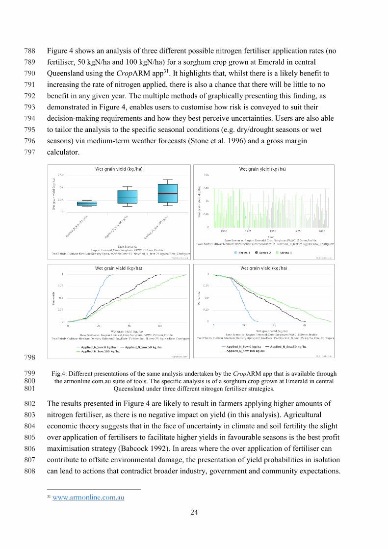
Figure 4 shows an analysis of three different possible nitrogen fertiliser application rates (no 788
fertiliser, 50 kgN/ha and 100 kgN/ha) for a sorghum crop grown at Emerald in central 789
Queensland using the CropARM app31. It highlights that, whilst there is a likely benefit to 790
increasing the rate of nitrogen applied, there is also a chance that there will be little to no 791
benefit in any given year. The multiple methods of graphically presenting this finding, as 792
demonstrated in Figure 4, enables users to customise how risk is conveyed to suit their 793
decision-making requirements and how they best perceive uncertainties. Users are also able 794
to tailor the analysis to the specific seasonal conditions (e.g. dry/drought seasons or wet 795
seasons) via medium-term weather forecasts (Stone et al. 1996) and a gross margin 796
calculator. 797
798
Fig.4: Different presentations of the same analysis undertaken by the CropARM app that is available through 799 the armonline.com.au suite of tools. The specific analysis is of a sorghum crop grown at Emerald in central 800
Queensland under three different nitrogen fertiliser strategies. 801
The results presented in Figure 4 are likely to result in farmers applying higher amounts of 802
nitrogen fertiliser, as there is no negative impact on yield (in this analysis). Agricultural 803
economic theory suggests that in the face of uncertainty in climate and soil fertility the slight 804
over application of fertilisers to facilitate higher yields in favourable seasons is the best profit 805
maximisation strategy (Babcock 1992). In areas where the over application of fertiliser can 806
contribute to offsite environmental damage, the presentation of yield probabilities in isolation 807
can lead to actions that contradict broader industry, government and community expectations. 808
31 www.armonline.com.au

25
In these cases, conveying specific information regarding the environmental risk of nutrient 809
loss is the best way to influence farming practices. SafeGuage for nutrients is one such 810
application that does this (Moody et al. 2013). It was originally developed for Queensland 811
sugar cane growers and is now extended for use by dairy farmers and crop growers in high 812
rainfall regions (Barlow et al. 2016; Thayalakumaran et al. 2015). The SafeGuage tool 813
presents results as a set of unitless discrete risk profiles, rather than a series of continuous 814
probabilities (Figure 5). Uncertainty is not directly acknowledged in this tool, as it is 815
minimised through the use of very specific scenarios that require a high level of user inputs 816
and engagement. 817
818
Figure 5: How the environmental risk associated with fertiliser practices of a northern Queensland sugar cane 819 farm is displayed to farmers in the SafeGuage for nutrients tool. 820
4.4 Summary 821
This case study highlights how agricultural systems modelling and simulation can be used to 822
guide crop production decisions in the face of uncertainty around climate and soils 823
performance. The example used was crop management (specifically sowing date and 824
irrigation) in a new agricultural region that has a shortage of learned experience around 825
appropriate cropping practices. It demonstrates that modelling is an effective alternative to 826
field experimentation and that the presentation of modelling results to the decision-maker was 827
effective in facilitating and informing decision-making. The case study then examines how 828
this direct approach can be extended through the use of decision support systems so it 829
efficiently reaches a broader audience of farmers and decision-makers. It highlights that the 830
26
decision support systems focus and how information is conveyed can influence the use of 831
scientific information in decision making. It also highlights that, in the case of decisions that 832
relate to environmental and social impact, potentially sound economic behaviour in the face 833
of uncertainty may mean the decisions supported by scientific evidence are not undertaken. 834
Decisions enacted in this case study (i) were informed by models, (ii) considered prevailing 835
scientific evidence, (iii) considered scientific uncertainty, (iv) and were precautionary in 836
nature. The communication of uncertainty (through the presentation of probability 837
distributions) was key to providing utility to the decision maker. 838
839
Case study 3: Communicating uncertainty in operational flood 840
models to decision makers: challenges from the field (Author: 841
MR) 842
4.5 Overview 843
Globally, floods are estimated to have claimed the lives of 500,000 people between 1980 and 844
200932. Floods are the most common natural disaster in Australia, with the highest fatality 845
rate after extreme heat events (Coates et al. 2014) and an average annual cost reported at 846
$377 million (Wenger et al. 2013), with fatal and non-fatal drowning incidents continuing to 847
occur regularly33. Flooding is a significant risk for Australia, and flood events will continue 848
to occur; finding a balanced approach between flood mitigation and the cost of mitigation 849
continues to challenge individuals and governments. Flood modelling is an integral part of 850
flood mitigation and response activities. The role of flood modelling, and the interpretation of 851
flood model outputs, is highlighted by reports such as the Queensland Floods Commission of 852
Inquiry34 and the Victorian Floods Review (Comrie 2011). 853
In 2013, the federal government announced the Bushfire and Natural Hazards Cooperative 854
Research Centre (BNHCRC), which expanded the work of the Bushfire CRC to include other 855
hazards, including floods. One focus of the BNHCRC is the scientific diversity, scientific 856
uncertainty and risk mitigation policy and planning project, which considers the impact of 857
uncertainty on decision making. Their investigations highlight that while “uncertainty is a 858
necessary element of scientific methods”, “being able to describe scientific uncertainty is a 859
vital aspect of internal and external risk communication” (Neale 2015). 860
32 http://www.who.int/violence_injury_prevention/global_report_drowning/en/ 33 http://www.watersafety.com.au/Portals/0/AWSC%20Strategy%202016-20/RLS_AWSS2016_Report_2016LR.pdf 34 http://www.floodcommission.qld.gov.au/publications/final-report

27
Challenges that individuals in operational flood response had experienced relating to 861
communicating uncertainty were discussed with one of the authors (MR). This case study, 862
rather than focussing on any specific event or series of events, captures these personal 863
communications. Two perspectives are discussed: the analyst’s or provider of scientific 864
advice, and the decision-makers, who acts as a result of the advice. 865
Advice that informs flood response is provided by people in many different roles, for 866
example weather forecasters and flood modellers from the Bureau of Meteorology who 867
predict future rain and flood levels; dam operators and river catchment managers who 868
provide advice on current water storage and the expected impact of additional inflows; 869
council engineers who understand the storm response capability of storm drains and other 870
local infrastructure; community groups and NGOs who have information on vulnerable 871
people and local resources etc. Decision-makers, or the recipients of advice, include the 872
above-mentioned groups, as well as emergency managers, responders, business operators, 873
and community members. In this case study, our analysts are flood modellers who have been 874
called upon during disasters to provide flood predictions, and the decision-makers are people 875
with an emergency management role in local council. 876
4.6 The Victorian Total Flood Warning System 877
The Victorian Total Flood Warning System highlights the fundamental role of prediction in 878
any flood warning system. As shown in Figure 6, the flood warning system is predicated on 879
the interpretation of data and predictions. Predictions of flood impacts are fundamentally 880
reliant on modelling, which is inherently uncertain. While the Total Flood Warning System 881
relates specifically to the external communication of flood risks, internal communications are 882
equally relevant to other planning and response activities. Uncertainty must be a key 883
consideration in the interpretation of flood predictions, and hence in the communication of 884
these risks to aid in identifying an appropriate response to flood risks and flood events. 885
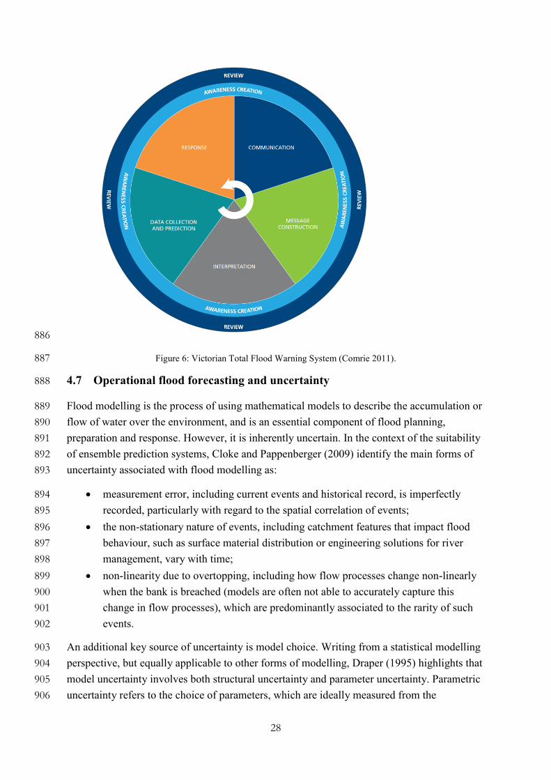
28
886
Figure 6: Victorian Total Flood Warning System (Comrie 2011). 887
4.7 Operational flood forecasting and uncertainty 888
Flood modelling is the process of using mathematical models to describe the accumulation or 889
flow of water over the environment, and is an essential component of flood planning, 890
preparation and response. However, it is inherently uncertain. In the context of the suitability 891
of ensemble prediction systems, Cloke and Pappenberger (2009) identify the main forms of 892
uncertainty associated with flood modelling as: 893
measurement error, including current events and historical record, is imperfectly 894
recorded, particularly with regard to the spatial correlation of events; 895
the non-stationary nature of events, including catchment features that impact flood 896
behaviour, such as surface material distribution or engineering solutions for river 897
management, vary with time; 898
non-linearity due to overtopping, including how flow processes change non-linearly 899
when the bank is breached (models are often not able to accurately capture this 900
change in flow processes), which are predominantly associated to the rarity of such 901
events. 902
An additional key source of uncertainty is model choice. Writing from a statistical modelling 903
perspective, but equally applicable to other forms of modelling, Draper (1995) highlights that 904
model uncertainty involves both structural uncertainty and parameter uncertainty. Parametric 905
uncertainty refers to the choice of parameters, which are ideally measured from the 906

29
environment or fitted to data. In the context of flood modelling, with high spatio-temporal 907
variation, model parameters usually contain a high degree of uncertainty. One example of 908
parametric uncertainty is soil saturation, i.e. the degree to which the soil is wet. A high degree 909
of saturation means that additional rainfall will lead to rain accumulating on the ground 910
(flooding) rather than soaking in. As opposed to parametric uncertainty, structural uncertainty 911
refers to the uncertainty arising from assumptions that are incorporated within the model 912
itself. Such assumptions cover the inclusion or exclusion of different factors (e.g. time, 913
spatial dimensions, or physical properties such as buoyancy), how different terms are 914
assumed to relate to each other, and even the resolution used in numerical solution methods. 915
Models require a number of simplifying assumptions of real-world processes in order to be 916
tractable. While necessary, these simplifying assumptions nonetheless introduce uncertainty 917
as the real-world is assumed to behave as per the model. An example of structural uncertainty 918
is adopting the 1D Saint-Venant equation under the assumption that the vertical velocity of 919
the flood water is small. A second example is the choice of mesh resolution for the 920
computational solution, as this limits the physical features that are able to be resolved. 921
Options to address model uncertainty include scientific advancement (e.g., improved 922
understanding of the processes that lead to flooding), data advances (e.g. improved spatio-923
temporal resolution, reduced or quantified measurement error), and model improvements 924
(e.g. ensemble methods, numerical solution techniques). There have been many recent 925
advances in knowledge of flood processes, climate change, and hydroinformatics, and 926
increased computational capacity available to engineering hydrologists35 (Pechlivanidis et al. 927
2011). 928
However, during an event, flood analysts are rarely in a position to incorporate new 929
techniques or data sources to help address model uncertainty. From an operational 930
perspective, a flood modeller must balance uncertainty quantification and reduction with the 931
pressures of time and available resources. For example, a modeller may trade the spatial 932
resolution of a model for computational speed, or use readily available (but less accurate) 933
data rather than wait for more useful data to become available. During flood operations, the 934
key role of a flood modeller or flood analyst is to provide insight into the expected behaviour 935
of flood waters, such as the magnitude, location and timings of key events, within the 936
intelligence function of Australasian Inter-Service Incident Management System (AIIMS). 937
Insight is gained by interpreting outputs of flood predictions and other knowledge, including 938
knowledge of vulnerable communities, critical businesses, and the distribution of resources 939
(human and physical) for mitigation and response. In the next section, we address issues that 940
arise in the communication of flood insight in an operational setting given the ever-present 941
uncertainty within the models and other data sources. 942
35 http://book.arr.org.au.s3-website-ap-southeast-2.amazonaws.com/
30
4.8 Providing flood insights: Challenges in communicating uncertainty 943
In preparation or response to a flooding event, the intelligence function within AIIMS 944
provides insights on the predicted flood behaviour to other functions within the Incident 945
Management Team (IMT). These insights are used to identify and trigger actions by the 946
responders such as building a levee, releasing dam water, evacuating an area, or advising 947
people to shelter in place. Effective communication between analysts and decision makers is 948
essential for an appropriate, risk-balanced response to a flooding event. We discuss three 949
situations where flood insights have been provided or received, and challenges have arisen in 950
effectively communicating the uncertainty associated with those insights. The first example 951
deals with challenges in communicating the relative uncertainties between high and low 952
fidelity models, the second with compounding errors between linked models, and the third 953
with how to communicate uncertain flood models. 954
4.8.1 Low vs high fidelity models 955
Model selection involves a trade-off between the cost of a model and the accuracy of the 956
results obtained for a particular scenario. Typically, a flood modeller can select different 957
flood models (or model options) for different scenarios, trading the accuracy of the results 958
obtained with the cost of the model given the flood behaviour of concern (for example, flash 959
flooding vs riverine flooding). Model cost is a combination of the data requirements for 960
running the model and the time it takes for the model to produce a meaningful result 961
(computational run-time). A low-fidelity model generally runs quickly and has minimal data 962
requirements, providing only a general indicator of the flooding event, while a high-fidelity 963
model is generally data intensive and takes longer to run, providing detailed and accurate 964
indicators of the flood behaviour. Thus, while a high-fidelity model may be available, the 965
run-time may make its use prohibitive. For example, the ANUGA open source flood model36 966
provides detailed flood models, including flow around buildings; however their case study of 967
the Towradgi Creek Catchment takes tens of hours to run (Roberts et al. 2015). Thus, the 968
ANUGA configuration is more suited to planning or post-event analysis, rather than 969
operational forecasting. 970
An analyst may choose to use a combination of low and higher fidelity models, with low 971
fidelity models providing rapid insight to inform future modelling and immediate decision 972
making. For analysts experienced in operational flood modelling, this is routine. However, 973
downstream decision-makers may be unfamiliar with the specifics of the different models and 974
importantly, limitations on the applicability of the models in different circumstances and the 975
associated uncertainty in the results. Therefore, it is essential that the analyst is able to clearly 976
communicate the contextual information, the uncertainty and model limitations, together with 977
the predicted flood levels in a way that is meaningful to downstream decision-makers. As an 978
example, a low fidelity model may indicate that a nursing home is at risk of flooding. The 979
36 https://anuga.anu.edu.au/
31
IMT may decide to contact the nursing home and have them initiate preparations for an 980
evacuation, in accordance with the nursing home’s emergency management plans. While 981
evacuation preparations are underway, this provides time for additional evidence to be 982
collected to determine the likelihood of inundation or isolation for the nursing home, and 983
therefore whether residents should be evacuated. Evacuations, particularly of vulnerable 984
people, are complex events that come with their own risks to the life and safety of the 985
evacuees. Information that would be useful for the IMT to make an informed decision about 986
the evacuation of the nursing home includes when additional predictions will be available, 987
how uncertain is the current prediction and what about the prediction is uncertain, and how 988
likely new information will change the decision being made (that is, to evacuate the nursing 989
home). Such information requires a dialogue between the decision-maker and the analyst, to 990
ensure that the analyst can provide a prediction that is meaningful for the intended use (here, 991
determining whether to evacuate a nursing home), and so that relevant contextual information 992
is communicated. How common such dialogues between analyst and decision-maker are is 993
unknown. 994
Where that dialogue is absent, challenges can arise. This was highlighted to MR in a 995
discussion with a flood modeller. During an event with localised flooding, the flood analyst 996
was called upon to provide predictions of the flood behaviour for decision-makers in the local 997
IMT and council. The flood modeller decided to use a low-fidelity model to provide a quick 998
overview of the event while awaiting the output of their more detailed high-fidelity model. 999
The analyst was asked for their latest forecast and provided the low-fidelity model (the high-1000
fidelity model was not yet available), being unaware of the intended use of this forecast. This 1001
forecast was subsequently passed on to senior decision-makers and communicated to groups 1002
outside of the IMT, but without any caveats on the results obtained. The contextual 1003
information of the forecast, including the uncertainty, was not shared, and decisions were 1004
made without that information. The analyst felt that the forecast was used inappropriately, 1005
given the high uncertainty associated with the result. The analyst recognised that they had not 1006
been effective in communicating the uncertainty associated with their result, but expressed a 1007
lack of knowledge in how to provide this information to people outside of their technical 1008
field. While it is not known whether the high-fidelity model would have resulted in different 1009
decisions being made at that stage, this example highlights the importance of providing tools 1010
to scientists to aid them in communicating the uncertainty associated with their results. 1011
4.8.2 Cascading margins of error 1012
During or in preparation for a flooding event, flood modelling is used to inform many 1013
decisions including evacuations, the allocation of resources, and communications to the 1014
public. Such modelling may be dependent on observations or measurements from the field 1015
(e.g. river heights, rainfall), other forecasts (e.g. weather forecasts), or a combination of both. 1016
These inputs are all subject to uncertainty, that may or may not be well quantified. Moreover, 1017

32
the outputs of flood models (typically water heights as a function of space and time) may be 1018
inputs to other models. 1019
Under the pressures of an unfolding natural disaster including the likelihood of having to 1020
account for the evidence provided to official enquiries37 (Comrie 2011), courts38 news 1021
media39 and other forums, the expected uncertainty in model outputs may be accounted for 1022
through the inclusion of a ‘margin of error’. Formally, the margin of error refers to the 1023
observational error in measured quantities. However, colloquially, this term is also used to 1024
describe an extra amount allowed for because of mistakes or uncertainty in a calculation. As 1025
an example, a forecast may indicate a maximum river height of 4.1m, however a margin of 1026
error of 0.2m is added to this forecast to account for any under prediction. Where multiple 1027
models or decision processes are linked, these margins of error may compound, impacting the 1028
decisions made. 1029
One decision-maker expressed frustration with this situation regarding the need to make 1030
decisions without a clear understanding of the likelihood of the scenario presented. A lack of 1031
clarity as to how uncertainty has been accounted for limits the ability of a decision-maker to 1032
take appropriate actions. Such a risk-adverse approach enacted at each link in the chain could 1033
potentially result in decisions that are more dangerous for residents. For example, the 1034
significant over-prediction of flooding in an area may result in an evacuation being 1035
recommended, which may be more dangerous than sheltering in place for a less severe flood. 1036
The decision to evacuate relies on information from many different sources. A key piece of 1037
information is whether or not the area is likely to be inundated or isolated by the flood. The 1038
flood forecast uses information about the terrain (e.g. slope, soil saturation, and surface 1039
roughness), the current state of the catchment (e.g. river heights and storage capacity) and the 1040
weather forecast as key inputs. This input information is itself uncertain. The decision-maker 1041
described an example scenario where a margin of error is added to the current river height 1042
data and to the forecast rainfall before being used by the flood model. The flood analyst then 1043
adds a margin of error to the predicted flood heights to account for error in their forecast and 1044
possible errors in the input data. This information is then passed to another person who 1045
identifies the area to be evacuated, adding their own margin of error. The decision-maker 1046
described being potentially faced with advice that will bear little resemblance to the actual 1047
event, as each link in the information chain adds their own buffer because of uncertainty, but 1048
without communicating this information along the chain. In the decision-maker’s experience, 1049
37 http://www.floodcommission.qld.gov.au/publications/final-report/ 38 http://www.courts.qld.gov.au/__data/assets/pdf_file/0019%2F152362%2Fcif-seq-floods-20120605.pdf 39 http://www.couriermail.com.au/news/queensland/bureau-of-meteorology-under-fire-after-a-weekend-of-wild-weather-and-storms-in-queensland-left-many-unprepared/news-story/d9cc7f437770f3dc22fe95a45516e0d9 ; http://www.abc.net.au/news/2017-03-22/locals-query-why-no-warning-was-given-for-heavy-rain/8377698

33
how error was accounted for and the magnitude of any ‘corrections’ was not something 1050
routinely communicated. 1051
The operation of the Wivenhoe Dam during the Queensland Floods is a high-profile example 1052
of the consequences of under-prediction. The manner in which the dam operators dealt with 1053
uncertainty in the rain forecasts resulted in a forecast dam lake level that remained below the 1054
threshold for dam water releases (Van den Honert and McAneney 2011). Had the forecast 1055
indicated the threshold would likely be exceeded, it is reasonable to presume that different 1056
decisions would have been made in dam management. 1057
A significant over prediction of a flooding event can also have negative consequences; 1058
impacting resourcing decisions and response options, as well as the risk to both responders 1059
and the community during an evacuation. Emergency managers continue to have concerns 1060
over the impact of ‘false alarms’ on future response, which is known as the ‘cry-wolf effect’. 1061
In laboratory experiments, Breznitz (1984) identified a cry wolf effect where false warnings 1062
lead to the alarm system losing credibility; however, these results have been questioned in a 1063
natural hazard context (Barnes et al. 2007). For example, research by Dow and Cutter (1998) 1064
on hurricane warnings in South Carolina did not find that previous false alarms were a 1065
significant factor in the decision-making process for whether to evacuate. 1066
In relating these stories on cascading uncertainties, the decision-maker not only identified a 1067
need for scientific methods to handle uncertainty between linked data and models, but also 1068
for ways to communicate this information to decision-makers. The need for improved 1069
scientific methods to handle uncertainty in the decision-making process for flood events was 1070
highlighted by the Queensland Flood Commission of Inquiry, who recommended using a 1071
stochastic, Monte Carlo or probabilistic approach in the determination of the design 1072
hydrology40 in a specific response to how uncertain rainfall forecasts were incorporated into 1073
the decision-making process at Wivenhoe Dam (Van den Honert and McAneney 2011). Such 1074
methods will assist in quantifying the uncertainty. However, the communication of this 1075
uncertainty through to decision makers, who may not be familiar with such techniques, must 1076
be addressed. 1077
4.9 Standardised approaches for communicating uncertainty 1078
The above two concerns raised by individuals involved in operational flood modelling, as 1079
either a decision-maker or provider of scientific advice, are ultimately centred on 1080
communication in the context of uncertainty. These examples highlight the need for tools to 1081
assist analysts in communicating with decision-makers under uncertainty. Both the analyst 1082
and decision-maker expressed a desire for more meaningful communication of the 1083
uncertainty within a forecast or result. In the first case, the analyst needed a way to explain 1084
the limitations of their low-fidelity model, while in the second case the decision-maker was 1085
40 http://book.arr.org.au.s3-website-ap-southeast-2.amazonaws.com/

34
looking for a way to know how likely a particular scenario is, and how uncertainty has been 1086
accounted for in a forecast. 1087
Knowing how to communicate forecasts under uncertainty was a key issue raised by one 1088
flood analyst. The analyst expressed that they did not know how to communicate the outputs 1089
of their models in a way that would ensure the information was appropriately re-1090
communicated to decision-makers within the IMT or externally, for example to residents or 1091
local businesses. They described an incident where flood forecasts with high uncertainty were 1092
communicated to the public by a non-technical person. The analyst expressed frustration 1093
with the loss of information that occurred, as details of the uncertainty associated with the 1094
flood model was not included in that communication. They expressed concern that the 1095
forecast would cause confusion for the public or a loss of confidence in the emergency 1096
management team due to a high error rate (cry-wolf concern). In this case, the analyst 1097
explained that they were asked for the output of a model. However, they were not aware of 1098
the intended use of the forecast and there was no opportunity for dialogue to interpret the 1099
results. The uncertainties associated with this forecast were not clearly communicated, and 1100
the forecast output was used by a third party (to communicate a warning to the public) 1101
without any of the context of the forecast. 1102
Whether the communication made to the public was appropriate involves many other highly 1103
relevant factors. However, the analyst’s comments highlight that they did not believe that the 1104
science was best represented in that instance. This concern was not due to a pedantic interest 1105
in technical accuracy, but came from a belief that this information was essential for 1106
identifying an appropriate emergency response. The analyst and their colleagues lacked the 1107
tools and training to provide information about forecast uncertainty to other functions of the 1108
IMT in a way that aids decision making. 1109
Standardised methods to communicate uncertainty in flood forecasts would aid both analysts 1110
and decision makers. Options for standardisation could include mapping methodologies, or 1111
pro forma documents, that explicitly address uncertainty. Figure 7 provides two examples of 1112
probabilistic flood maps, where the uncertainty in the forecast is expressed in terms of the 1113
inundation probability. A high probability (near 1, or 100%), indicates that the area will most 1114
likely flood, while a low probability (near 0 or 0%) indicates that flooding is highly unlikely. 1115
Such an approach would however require the use of probabilistic flood modelling 1116
techniques41 (Apel et al. 2006; Nathan et al. 2003), which may not always be practical. 1117
41 http://www.watersafety.com.au/Portals/0/AWSC%20Strategy%202016-20/RLS_AWSS2016_Report_2016LR.pdf

35
(a)
Adapted from Taylor (2017)42.
(b)
Adapted from Figure 1b of
(Alfonso et al. 2016).
Figure 7: Examples of probabilistic flood maps adapted from the literature: (a) shows a flood map for a city 1118 region with the inundation probability separated into three criteria; (b) shows a hypothetical flood map with five 1119 graduations. Probabilistic flood maps capture the uncertainty in flood modelling by providing information about 1120
the calculated likelihood of flooding, as opposed to a single predicted water height. 1121
To ensure consistency between events and personnel in IMTs, it is essential that any 1122
standards adopted for use in operational flood modelling are documented and training is 1123
provided. Before adopting any one standard, the effect of the visualisation on decision 1124
making should be investigated. Cheong et al. (Cheong et al. 2016) considered this question in 1125
a laboratory review of the effect of visualisation on decisions to stay or go (evacuate or stay 1126
and defend from a bushfire) under time pressures, and found that the choice of visualisation 1127
affected the decisions made. 1128
4.10 Summary 1129
This case study reports a number of issues that have arisen in the context of communicating 1130
scientific outputs with significant uncertainty during flood preparation and response. The 1131
experiences shared with one of the authors (MR) reinforces the need for scientists and 1132
decision-makers to have standardised ways to communicate the uncertainty associated with 1133
their results, and the limitations of their work. Standardised methods of communicating 1134
forecasts, even within a single discipline such as operational flood response, will greatly 1135
assist both analysts and decision-makers in their roles. 1136
Decisions enacted in this case study (i) were scientifically informed, (ii) aligned with 1137
prevailing scientific evidence, (iii) were informed by models, and (iv) were precautionary in 1138
nature. The absence of uncertainty in the communication of scientific results is 1139
acknowledged as a limitation in the decision-making process, and a key motivating factor for 1140
42 http://slideplayer.com/slide/4943891/

36
the scientists and decision makers featured in this case study. The absence of uncertainty in 1141
the communication motivated a precautionary approach for some of the decision makers. 1142
5 Case study 4: Developing a state-wide natural disaster risk 1143
assessment for Tasmania, Australia (Author: CW) 1144
5.1 Overview 1145
The 2016 Tasmanian State Natural Disaster Risk Assessment (TSNDRA)43 is the first state-1146
level assessment in Australia that adheres to the recently updated National Emergency Risk 1147
Assessment Guidelines (NERAG)44. It was undertaken to provide the emergency services 1148
with key information to help prepare for and reduce the impact of disasters, including 1149
bushfires, floods, severe storms, earthquakes, landslides, coastal inundations, heatwaves and 1150
influenza pandemics. It contributes to disaster resilience by delivering an increased 1151
understanding and awareness of natural disaster risks affecting Tasmania, and informs 1152
decision-making across the Tasmanian emergency management sector, particularly in relation 1153
to disaster risk reduction and mitigation activity priorities. The TSNDRA report (White et al. 1154
2016a) and its accompanying summary report (White et al. 2016b) are primarily aimed at 1155
informing the State Emergency Management Committee, but their findings are also relevant 1156
to a range of authorities, agencies and individuals with responsibilities for emergency risk 1157
management. 1158
5.2 Effective communication = collaboration 1159
Unusually, the risk assessment process was not led by State Government agencies, but by 1160
natural hazard and risk assessment researchers led by author CW from the University of 1161
Tasmania, along with researchers at RMIT University and the Antarctic Climate and 1162
Ecosystems Cooperative Research Centre. The team of researchers worked in close 1163
collaboration with hazard experts, emergency managers and decision-makers from the 1164
Tasmania State Emergency Service, Tasmania Fire Service and related Government agencies, 1165
and other stakeholders including the Bureau of Meteorology, the Australian Red Cross and 1166
Engineers Australia. This interdisciplinary, academia-led approach allowed a diverse range of 1167
expert voices to come together in an open and unbiased workshop setting to inform the 1168
identification and assessment of Tasmania’s ‘state level’ priority emergency risks across the 1169
consequences categories of People, Economic, Environmental, Public Administration and 1170
Social Setting (each with their own sub-categories). 1171
The risk assessment process took place over 12 months beginning in March 2015 and 1172
consisting of a series of online surveys and workshops involving stakeholders, experts and 1173
43 http://www.ses.tas.gov.au/h/em/risk-mgmt/tsndra 44 https://knowledge.aidr.org.au/resources/handbook-10-national-emergency-risk-assessment-guidelines/

37
decision-makers with responsibility within each natural hazard. Each hazard workshop 1174
considered the underlying risk of different natural hazards, as well as considering the 1175
consequences of worst-case, large-scale scenarios for each hazard, such as the 1967 bushfires 1176
or the 1929 Launceston floods. A separate workshop developed a portfolio of potential 1177
treatment options for the most at-risk sectors to enable issues to be communicated effectively 1178
and to help prioritise new risk-reduction actions across Tasmania. 1179
The hazard specific workshops, led by the TSNDRA project team, consisted of four key 1180
stages: 1) initial collation of current controls; 2) confirmation and assessment of current 1181
controls; 3) scenario consequence rating; and 4) subsequent likelihood rating of those 1182
consequences on any given day (not in the instance of an event, i.e. residual risk). Crucially, 1183
following on from initial breakout discussions of both hazards and consequences categories, 1184
including communicating details of a consensus on the thresholds for consequence categories 1185
(from ‘insignificant’ to ‘catastrophic’), each group was asked to identify who would be best 1186
suited as expert representatives (beyond those present in the room) for assessing each 1187
hazard’s probable consequences and the likelihood of these consequences occurring. This 1188
included: 1) the key experts or expert organisations related to each priority natural hazard; 1189
and 2) organisations or individuals that would be familiar with or able to qualitatively 1190
consider the consequence categories in relation to these hazards. With multiple breakout 1191
groups, the potential to have differing results was introduced, therefore, an average value for 1192
the ‘consequence’, ‘likelihood’ and ‘confidence’ ratings of each sub-category was required 1193
from the values provided by the different working groups. 1194
The risk assessment process determined bushfire to be the greatest aggregated natural hazard 1195
risk to Tasmania (Figure 8). It is a ‘high’ or ‘extreme’ risk across all sectors of society, often 1196
with catastrophic consequences expected every 30 years. However, bushfires are expected to 1197
become more frequent with climate change, based on evidence from experts and the most 1198
recent climate projections presented to the decision-makers in the workshop settings, 1199
transitioning at least into the ‘likely’ category by the end of the 21st Century, and potentially 1200
into ‘almost certain’ category. 1201
Earthquakes are the lowest risk hazard due to their ‘extremely rare’ likelihood and the 1202
‘moderate’ level consequences across the sectors, given the anticipated magnitude of an 1203
event. The most catastrophic impacts were determined to be dependent on an earthquake-1204
induced major dam failure that was deemed by experts even less likely than the earthquake 1205
itself. Interestingly, workshop participants perceived that if the seismic monitoring system 1206
throughout Tasmania were decommissioned, all consequence and likelihood estimates would 1207
be substantially increased due to increased uncertainty in the knowledge of the hazard. It was 1208
identified that the Tasmanian seismic monitoring system is in urgent need of review and 1209
management, as it is mostly operated by the private sector with no obligation to continue. 1210
This system ensures high confidence surrounding the likelihood of geological events, and the 1211
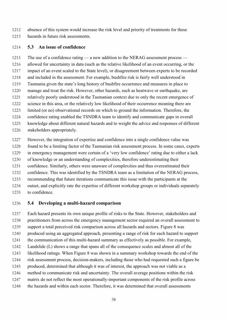
38
absence of this system would increase the risk level and priority of treatments for these 1212
hazards in future risk assessments. 1213
5.3 An issue of confidence 1214
The use of a confidence rating — a new addition to the NERAG assessment process — 1215
allowed for uncertainty in data (such as the relative likelihood of an event occurring, or the 1216
impact of an event scaled to the State level), or disagreement between experts to be recorded 1217
and included in the assessment. For example, bushfire risk is fairly well understood in 1218
Tasmania given the state’s long history of bushfire occurrence and measures in place to 1219
manage and treat the risk. However, other hazards, such as heatwave or earthquake, are 1220
relatively poorly understood in the Tasmanian context due to only the recent emergence of 1221
science in this area, or the relatively low likelihood of their occurrence meaning there are 1222
limited (or no) observational records on which to ground the information. Therefore, the 1223
confidence rating enabled the TSNDRA team to identify and communicate gaps in overall 1224
knowledge about different natural hazards and to weight the advice and responses of different 1225
stakeholders appropriately. 1226
However, the integration of expertise and confidence into a single confidence value was 1227
found to be a limiting factor of the Tasmanian risk assessment process. In some cases, experts 1228
in emergency management were certain of a ‘very low confidence’ rating due to either a lack 1229
of knowledge or an understanding of complexities, therefore underestimating their 1230
confidence. Similarly, others were unaware of complexities and thus overestimated their 1231
confidence. This was identified by the TSNDRA team as a limitation of the NERAG process, 1232
recommending that future iterations communicate this issue with the participants at the 1233
outset, and explicitly rate the expertise of different workshop groups or individuals separately 1234
to confidence. 1235
5.4 Developing a multi-hazard comparison 1236
Each hazard presents its own unique profile of risks to the State. However, stakeholders and 1237
practitioners from across the emergency management sector required an overall assessment to 1238
support a total perceived risk comparison across all hazards and sectors. Figure 8 was 1239
produced using an aggregated approach, presenting a range of risk for each hazard to support 1240
the communication of this multi-hazard summary as effectively as possible. For example, 1241
Landslide (L) shows a range that spans all of the consequence scales and almost all of the 1242
likelihood ratings. When Figure 8 was shown in a summary workshop towards the end of the 1243
risk assessment process, decision-makers, including those who had requested such a figure be 1244
produced, determined that although it was of interest, the approach was not viable as a 1245
method to communicate risk and uncertainty. The overall average positions within the risk 1246
matrix do not reflect the most operationally-important components of the risk profile across 1247
the hazards and within each sector. Therefore, it was determined that overall assessments 1248
39
require reference to a particular sector (people, economic, etc.) to provide context. 1249
Subsequently, although Figure 8 was included in the final report, the remainder of the risk 1250
assessment presented its findings by sector. 1251
1252
Figure 8: Summary of the risk posed by each hazard as assessed in the 2016 TSNDRA. The central position is 1253 the average across sectors for both consequence and likelihood, and the whiskers represent the minimum and 1254
maximum ratings across all sectors for each hazard. Figure reproduced from (White et al. 2016b). 1255
5.5 Identifying knowledge gaps 1256
Complementary to the multi-hazard comparison, the frequency and severity of multi-hazard 1257
coincident or ‘compound’ events (Leonard et al. 2014; Wahl et al. 2015) were identified as a 1258
knowledge gap in the NERAG process, as it was designed for single hazard assessment only. 1259
For example, the occurrence of heatwaves and bushfires are known to be linked, but this 1260
interaction is not currently incorporated into existing emergency management exercise 1261
scenarios. Other links, such as bushfire and flood (such as the devastating bushfires in the 1262
Tasmanian Wilderness World Heritage Area occurring simultaneously with floods on the east 1263
coast of the State in January 2016, stretching the emergency services to their limits), are 1264
perhaps less obvious, with the expected likelihood of such a co-occurrence poorly 1265
understood, especially when the influence of climate change is taken into account (White et 1266
al. 2010; White et al. 2013). Whilst it was identified that hazards can co-occur, the combined 1267
uncertainty of their causes, likelihood and consequences, meant that communicating the 1268
complexity of these types of events to decision-makers was not achievable within the 1269
Tasmanian risk assessment process. It was recommended by the TSNDRA team that 1270
Average Risk of Each Hazard
Insignificant Minor Moderate Major Catastrophic
Consequence
Extremely
Rare
Very
Rare
Rare
Unlikely
Likely
Almost
Certain
Lik
elih
oo
d
B
H
S
F
T
C
E
LP
Risk Level
Very Low
Low
Medium
High
Extreme
Results Range Hazard
Bushfire (B)
Coastal Inundation (C)
Earthquake (E)
Flood (F)
Heatwave (H)
Landslide (L)
Pandemic (P)
Severe Storm (S)
Tsunami (T)

40
compound events should be incorporated into a cross-agency risk assessment process to 1271
ensure state-wide capacity is assessed under different multi-hazard situations to identify areas 1272
for improvement. A multi-hazard approach to exercises and business continuity planning 1273
within Government was also agreed to be important, with training recommended for key 1274
incident management personnel (e.g. incident controllers) as well as formalising 1275
arrangements to guide decision-makers in times of crisis to ensure rapid decision-making. 1276
5.6 Summary and key messages 1277
Overall, the TSNDRA team felt that the report significantly benefitted from its basis on 1278
interdisciplinary cooperation and collaboration, as opposed to science communication only. 1279
The use of a ‘confidence’ rating in the report allowed for uncertainty in data or disagreement 1280
between experts to be accounted for. However, the lack of provision to be able to combine 1281
expertise with confidence into a single value was found to be a limiting factor. It was found 1282
that use of a cross-sector multi-hazard likelihood–consequence risk matrix provided 1283
interesting insights, but that it was limited by uncertainties in the science and the existing 1284
single-hazard risk assessment approaches. 1285
Decisions enacted in this case study (i) were scientifically informed, (ii) aligned with 1286
prevailing scientific evidence, (iii) considered some estimations of uncertainty, (iv) were 1287
partially informed by models, and (v) were precautionary in nature. The risk assessment 1288
process considered estimates of uncertainty using a workshop-based approach for the 1289
determination of consequence categories (ranging from ‘insignificant’ to ‘catastrophic’), 1290
enabling decision-makers to understand value of a consensus-based approach. 1291
6 Case study 5: Science contributions to decision making related 1292
to deep sea mining in New Zealand’s Exclusive Economic Zone 1293
and continental shelf (Author: PD) 1294
6.1 Overview 1295
This case study examines the contribution from science in the decision-making process for 1296
the Chatham Rock Phosphate (CRP) mining consent application for seabed mining along the 1297
Chatham Rise in the New Zealand’s Exclusive Economic Zone (EEZ). We review how 1298
science was used to describe and understand the marine environment, the resources under 1299
question (phosphate nodules) and the effects of the mining process on the environment. The 1300
CRP mining consent application was submitted to the Environmental Protection Authority of 1301
New Zealand (EPANZ) in May 2014. Significantly, this was the second time an exploration 1302
and mining company had applied for marine mining consent in New Zealand’s EEZ, and the 1303
second time such an application was refused by an EPANZ, board-appointed decision-1304
making committee (DMC) within a 5-month timeframe (June 2014—Feb 2015). 1305
41
6.2 The Quest for Seabed Mining in New Zealand’s EEZ 1306
The first marine consent application for seabed mining in New Zealand’s EEZ was submitted 1307
by Trans-Tasman Resources (TTR) in November 2013 to mine iron sands off the Taranaki 1308
coast45. The TTR application was refused because the DMC was ‘not satisfied that the life-1309
supporting capacity of the environment would be safeguarded or that the adverse effects of 1310
the proposal could be avoided, remedied or mitigated, nor do we consider that the proposed 1311
conditions (including the adaptive management approach) are sufficiently certain or robust 1312
for this application to be approved, given the uncertainty and inadequacy of the information 1313
presented to us about the potential adverse effects’46. The DMC’s overall impression was that 1314
the application was submitted prematurely and more work was warranted to better understand 1315
the mining process and impacts on the environment and to ‘engage more constructively’ with 1316
relevant third parties47. 1317
On 23 August 2016, TTR lodged a second, revised marine consent application with the 1318
EPANZ after undertaking more than two years of ‘additional science and engineering work’ 1319
programmes and ‘extensive engagement and consultation with a wide range of stakeholders, 1320
regulators and interest groups, as well as the EPA…’ to address the previous DMC’s 1321
concerns 48,49. The Hearing took place over 27 days from 16 February 2017 under a new 1322
EPANZ appointed DMC. On 10 August 2017 the new DMC reversed the decision made in 1323
the first application and granted a 35-year mining consent, on the condition that TTR carry 1324
out an additional two years of environmental monitoring and present the results to the EPA 1325
before mining activities commence (Environmental Protection Authority NZ 2017)50. The 1326
EPANZ DMC decision was appealed by 11 parties on eight different grounds and was 1327
referred to the High Court of New Zealand in: The appeal of The Taranaki-Whanganui 1328
Conservation Board versus the EPZNZ51. The High Court upheld only one of the grounds of 1329
appeal; that relating to the legal meaning of the term ‘adaptive management’ and held that the 1330
DMC’s ‘narrow interpretation’ was inconsistent with the meaning of that term derived from 1331
s61 of the EEZ Act and found this ‘error was material and may well have influenced the 1332
outcome of the consent application’. The DMC decision was quashed and referred back to the 1333
DMC ‘for reconsideration, applying the correct legal test in relation to the concept of adaptive 1334
management approach’. As of 21 September 2018, TTR have lodged a notice to the Court of 1335
45 https://www.epa.govt.nz/database-search/eez-applications/view/EEZ000004 46 https://www.epa.govt.nz/assets/FileAPI/proposal/EEZ000004/Boards-Decision/EEZ000004-Trans-Tasman-Resources-decision-17June2014.pdf 47 https://www.epa.govt.nz/assets/FileAPI/proposal/EEZ000004/Boards-Decision/EEZ000004-Trans-Tasman-Resources-decision-17June2014.pdf 48https://www.ttrl.co.nz/fileadmin/user_upload/TTR_Media_Statement_Marine_Consent_Application_23Aug16_-_updated.pdf 49 https://www.epa.govt.nz/public-consultations/decided/trans-tasman-resources-limited-2016/ 50 https://www.ttrl.co.nz/fileadmin/user_upload/TTR_Media_Statement_DMC_Decision_10Aug17.pdf 51 https://www.courtsofnz.govt.nz/cases/the-taranaki-whanganui-conservation-board-v-the-environmental-protection-authority/@@images/fileDecision?r=222.009077804

42
Appeal to seek leave to appeal the High Court judgement on the grounds that the EPANZ did 1336
follow a legally correct approach in granting a marine discharge consent52. 1337
TTR’s pursuit for seabed mining consent is ongoing and both pre- and post-dates the CRP 1338
case study presented here. TTR’s experience significantly foreshadows the hurdles CRP will 1339
have to overcome to counter the initial findings of the DMC in any subsequent applications. 1340
The overwhelming perception that there was inadequate information, and unacceptable risks 1341
and uncertainties associated with seabed mining was pervasive among external interested 1342
parties and the DMC in the CRP application. CRP’s adaptive management plan, which 1343
sought to avoid, mitigate and minimise impacts on the environment associated with the 1344
mining operations was viewed as inadequate due to knowledge gaps with respect to baseline 1345
data and environmental impacts. These findings strongly mirror many aspects of the TTR 1346
case and in both instances these perceived knowledge gaps are intended to be filled by 1347
additional and ongoing science programmes. The implicit assumption is that the collection of 1348
more data can address and sufficiently reduce the perception of the risks and uncertainties 1349
related to seabed mining to allow mining activities to occur. This puts a premium on the role 1350
of science in decision making but does not guarantee that science will be prioritised in the 1351
decision-making process. 1352
6.3 Chatham Rock Phosphate’s application to mine phosphorite nodules 1353
In May 2014 a New Zealand-based company Chatham Rock Phosphate (CRP) applied for a 1354
marine consent to mine phosphorite nodules from the crest of the Chatham Rise, based on an 1355
inferred resource of 80 million tonnes of phosphorite nodules, averaging 290 kg m-3 and 1356
containing 23.4 million tonnes of phosphorite (Figure 9) (Golder Associates Ltd 2014b; 1357
Golder Associates Ltd 2014c; Sterk 2014)53. Mining would occur at water depths from 250 m 1358
to 450 m in an area located about 400 km east of Christchurch and would initially take place 1359
within an 820 km2 area for which it holds a mining permit (Golder Associates Ltd 2014b). 1360
Mining was proposed to extend to parts of the prospecting licence area of 5,207 km2 if further 1361
resources could be identified and another marine consent obtained (Environmental Protection 1362
Authority NZ 2015; Golder Associates Ltd 2014b). Mining phosphorite nodules would 1363
involve the use of conventional trailing suction hopper dredger or drag-head to capture the 1364
nodules off the seafloor (Golder Associates Ltd 2014b). After extraction of the phosphate 1365
nodules the remaining sediment would be returned to the seafloor via a sinker pipe equipped 1366
with a diffuser positioned 10 m above the seafloor (Golder Associates Ltd 2014b). CRP 1367
aimed to produce 1.5 million tonnes of phosphorate nodules per year from a sequence of 1368
mining blocks. Over the proposed 15-year life of the mining operations approximately 450 1369
km2 of the seafloor would be mined (Golder Associates Ltd 2014b). By CRP’s accounts, an 1370
area equivalent to 0.1% of the entire Chatham Rise would be directly impacted by mining. 1371
52 https://www.ttrl.co.nz/fileadmin/user_upload/TTR_Seeks_Leave_to_Appeal_21_September_2018.pdf 53 https://www.epa.govt.nz/database-search/eez-applications/view/EEZ000006
43
6.3.1 Why mine the seabed for rock phosphate in New Zealand? 1372
New Zealand imports about one million tonnes of rock phosphate per year as a source of 1373
phosphorous, a primary component of commercial fertilisers. The use of commercial 1374
fertilisers has greatly contributed to a growth economy due to increased agricultural 1375
productivity globally including New Zealand (Golder Associates Ltd 2014b). 1376
Phosphate is considered a moderate risk industrial mineral (Behnam and Visbeck 2014) that 1377
is currently sourced from only a small number of countries in West Africa, Tunisia and in 1378
particular, Morocco, which controls 85% of the global rock phosphate supply. CRP argues in 1379
the interests of national security, and economic and environmental benefits that New Zealand 1380
should move towards developing its own source of phosphatic fertiliser (superphosphate and 1381
other phosphate fertilisers) on which it depends for over 40% of fertiliser used for agricultural 1382
productivity (Golder Associates Ltd 2014b). Further, the rock phosphate from the Chatham 1383
Rise has an extremely low level of cadmium and field trials have shown it is less likely to 1384
leach into waterways because reactive rock phosphate is less soluble than superphosphate 1385
(McDowell et al. 2010; Syers et al. 1986; Wood and Falconer 2016). 1386
Mining reactive rock phosphate in New Zealand waters would increase the security of supply 1387
of a strategic resource, decrease the rate of accumulation of cadmium in soils, improve soil 1388
resilience, reduce phosphate runoff to waterways, and reduce the carbon footprint of New 1389
Zealand’s phosphate usage (Wood and Falconer 2016). 1390
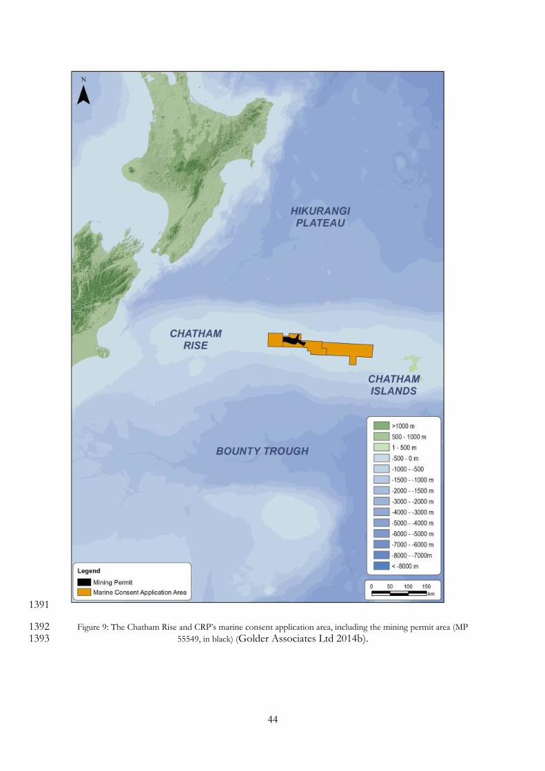
44
1391
Figure 9: The Chatham Rise and CRP’s marine consent application area, including the mining permit area (MP 1392 55549, in black) (Golder Associates Ltd 2014b). 1393

45
6.4 Science Evidence in CRP’s EPANZ Mining Consent Application 1394
CRP was required to demonstrate that it understood the current state of the environment, 1395
scope the potential environmental issues associated with seabed mining activities and prepare 1396
environmental impact assessments (EIAs) for these issues54 (Golder Associates Ltd 2014b; 1397
Golder Associates Ltd 2014c). The EIAs document the impacts of seabed mining on the 1398
following key areas: oceanography/hydrodynamics; sediment plume dynamics and 1399
sedimentation; species’ trophic relationships; operational noise propagation and marine 1400
mammals; benthic species’ distribution; commercial fish species distribution and population; 1401
habitat prediction and spatial planning; benefits to the New Zealand economy; ecotoxicology 1402
and human health, and the mining operation itself at depth. The proposal and EIAs were 1403
based on numerous scientific studies relating to geology, biology, oceanography, chemistry 1404
and physics. The studies required input from experts across many scientific disciplines to 1405
compile, collect and analyse data, and present the findings. Presenting information on all the 1406
EIAs, which consisted of 36 appendices to the application, and the specific details of the 1407
models that were created is beyond the scope of this case study but can be viewed and 1408
downloaded at the EPA website55. 1409
Lastly, CRP was required to consider and present the activities that it would undertake to 1410
ensure any negative impacts on any of the key areas and existing interests are avoided, 1411
mitigate and/or remedy. The EIAs revealed the potential impacts on benthic habitat and fauna 1412
loss within the mining blocks was serious, and sedimentation impacts on benthic habitats 1413
from mining would create high environmental risks. Their potential likelihoods were deemed 1414
‘almost certain’ even after applying strategies of avoidance, remediation and mitigation 1415
measures outlined in their Environment Management and Monitoring Plan (EMMP) (Golder 1416
Associates Ltd 2014a). These potential impacts generated much attention and had the largest 1417
effect on the final DMC decision. 1418
6.5 Modelling the Unknown 1419
The Chatham Rise is one of the most comprehensively studied parts of New Zealand’s EEZ 1420
(Boskalis Offshore 2014a; Boskalis Offshore 2014b; Chiswell 2014; CRP 2014; Hughes-1421
Allan et al. 2014; Wood 2014; Wood and Falconer 2016), but one of the main challenges 1422
CRP faced was a perceived dearth of environmental baseline data and indicators of how the 1423
environment would respond to mining operations. In the absence of additional baseline data 1424
sets and empirical observations, the use of various types of models became one of the main 1425
methods for conducting impact assessments in the following areas: oceanography and 1426
hydrodynamics; sediment plume dynamics and sedimentation; species’ trophic relationships; 1427
54 See applicant proposal documents at https://www.epa.govt.nz/database-search/eez-applications/view/EEZ000006 55 See Applicant proposal documents at https://www.epa.govt.nz/database-search/eez-applications/view/EEZ000006

46
operational noise propagation and marine mammals; benthic species’ distribution; 1428
commercial fish species distribution and population; habitat prediction and spatial planning; 1429
economic benefits; ecotoxicology and human health; and the mining operation itself at depth 1430
(Environmental Protection Authority NZ 2015). 1431
Models based on knowledge of physical and biological systems were used to predict the 1432
marine environment and the likely effects of disturbances on it (Wood 2014). The behaviour 1433
of these systems is not predictable in detail, but because they are based on physics, chemistry 1434
and biology and are not random (i.e. there are limits to current velocities and factors 1435
controlling the health and distribution of organisms, etc.), their general range of behaviour 1436
can be predicted (Golder Associates Ltd 2014b; Wood 2014). In some cases, the models are 1437
robust (e.g., oceanography) and in others they contain significant gaps (e.g., natural turbidity) 1438
that made it more difficult to assess the significance of the mining operations (Golder 1439
Associates Ltd 2014b). CRP proposed to address the uncertainties inherent in any marine 1440
development proposal through an adaptive management process that initially focused on 1441
gathering background environmental data, followed by extensive environmental monitoring 1442
and a requirement to stop mining if the target level of environmental effects could not be met 1443
(Golder Associates Ltd 2014a; Wood 2014). The consequences of uncertainties in the models 1444
were significant. The uncertainty about the modelled distribution of coral thickets, for 1445
example, led the DMC to conclude that the potential impacts of mining were too great to 1446
grant a consent (Environmental Protection Authority NZ 2015). 1447
The DMC showed considerable discomfort with the degree to which the EIAs depended on 1448
modelling and monitoring, in lieu of more comprehensive, pre-existing or new baseline data, 1449
or empirical observations collected by conducting in situ trials and surveys, even going so far 1450
as to call this aspect of the CRP application `unusual’. According to a CRP representative, 1451
some of this criticism may have been warranted (e.g., a lack of calibrated measurements of 1452
background turbidity) but expectations of in situ trials to assess sediment plume behaviour 1453
may not have been consistent with section 61, part (5) of the EEZ Act, which describes “best 1454
available information” as that which, “…in the particular circumstances, is available without 1455
unreasonable cost, effort, or time” (pers. comm. R Wood 2017). Likewise, science and 1456
models can help predict the likely outcomes of an activity but this is only part of the 1457
discussion that underpins the decision about whether the activity is acceptable to society 1458
(Environmental Protection Authority NZ 2015). 1459
It is difficult to understand what the DMC may have considered ‘usual’ when the proposed 1460
activity has no national or international predecessor and cannot be directly compared to 1461
consent applications for similar onshore activities. Most significantly, the DMC stated 1462
“…there were other uncertainties stemming from the fact that this would be the first seabed 1463
mining project ever undertaken at such depths anywhere in the world…” (Environmental 1464
Protection Authority NZ 2015). The DMC and CRP could not look elsewhere for direct 1465
reassurances, confirmation, or validation regarding any of the modelled scenarios and likely 1466
47
outcomes. However, other activities including offshore diamond mining and non-mining 1467
related activities such as port dredging, may serve as analogues for understanding the 1468
disturbance of seafloor sediments, the generation of sediment plumes and how they behave 1469
(Grogan 2017). Being the first to attempt to mine phosphorite nodules from depths of 250 – 1470
400 m in a marine setting was, in the end, too much to overcome, even in instances when the 1471
CRP experts and the DMC experts, as documented in most of the joint-witness statements, 1472
were in agreement about the degree to which there would be negative outcomes in the short-1473
term but that would likely be reversible in the long-term56. 1474
6.6 Uncertainty, Ignorance and Partial knowledge – In a Marine Setting 1475
The 2014 CRP mining consent application, and others like it, face an ongoing problem. 1476
Despite how well traversed our oceans are on the surface, various types and degrees of 1477
uncertainty, ignorance and partial knowledge (and the perceptions thereof) of the deep marine 1478
environment persists in hampering the ability to make decisions about how to manage, 1479
regulate, and responsibly (i.e. sustainably) extract the natural mineral resources within it 1480
(Behnam and Visbeck 2014; Durden et al. 2016; Gjerde et al. 2016; Grogan 2017; Halfar and 1481
Fujita 2002; Tremlett 2015; Wedding et al. 2015). It should be acknowledged that scientists 1482
do, in fact, have a reasonable and rapidly growing understanding of a wide range of deep 1483
marine environments, from both models, field samples and empirical data, but this is 1484
typically at a lower spatial resolution when compared to our knowledge of terrestrial 1485
environments (Tremlett 2015). By comparison to land-based research, our oceans, even 1486
within EEZs, are vast and inaccessible (Moritz Bollmann et al. 2010). The collection of 1487
marine data is orders of magnitude costlier, more time consuming to collect, and relies to a 1488
much larger degree on remote sensing and sampling that can only statistically represent the 1489
complexity of a natural marine system (pers. comm. R Wood 2017) (Tremlett 2015). In this 1490
respect, and to put it in perspective, the challenges faced in building our knowledge of the 1491
deep marine environments and ecosystems is, in many respects, more similar to challenges 1492
faced in exploring outer space than it is for any terrestrial environment. It is erroneous to 1493
apply standards of knowledge derived from analogous land-based activities to define what 1494
constitutes adequate information (i.e. the amount of available baseline data) and acceptable 1495
measures of risk and uncertainty in a marine setting. 1496
Further, these challenges have not hindered our ability or willingness to permit and regulate 1497
how other types of resources, such as fish, sand, diamonds, petroleum and gas hydrates are 1498
mined from a diverse range of marine environments globally (Behnam and Visbeck 2013; 1499
Behnam and Visbeck 2014; Moritz Bollmann et al. 2010). In relation to the EPANZ EEZ 1500
Act, the implications of these challenges should be understood and translated into context-1501
focused policy guidelines for decision-making criteria pertaining and relevant to marine 1502
56 See Boards decision at https://www.epa.govt.nz/database-search/eez-applications/view/EEZ000006
48
mining activities, and associated uncertainties and risks (Gluckman 2014; Grogan 2017). 1503
Scientists and other experts who understand the inherent uncertainty of science data in a 1504
marine setting should assist in providing clearer guidance in applying the decision-making 1505
criteria, outlined in section 61 of the EEZ Act, in these unique and pioneering applications for 1506
deep sea mining. It is not reasonable to rely on pre-existing understandings of what 1507
constitutes “best available information” (available without unreasonable cost, effort or time), 1508
how to “take into account any uncertainty or inadequacy in the information available”, how 1509
to “favour caution and environmental protection”, and how to “first consider whether taking 1510
an adaptive management approach would allow the activity to be undertaken” as stated in 1511
section 61 of the EEZ Act (Environmental Protection Authority NZ 2012). 1512
6.7 Science Communication 1513
Scientific evidence was not the only type of evidence presented by CRP or other expert and 1514
non-expert submitters, but science underpinned the majority of topics under consideration by 1515
the DMC (Golder Associates Ltd 2014b). How the science was communicated to the DMC 1516
and other parties with existing interests and how various opinions on the science were 1517
weighed by the DMC had a strong bearing on the final decision, which was to refuse the 1518
mining consent (Environmental Protection Authority NZ 2015). Complex scientific issues 1519
and the associated risks and uncertainty that constrain our understanding of the deep marine 1520
environment and the impacts of deep sea exploration and mining can either be exacerbated or 1521
reduced depending on how the science is communicated to its target audiences. 1522
During the hearing, CRP representatives admitted they sometimes found it difficult to present 1523
spatially and temporally varying data, for example in relation to the plume model results, in a 1524
way that could be easily understood (Lescinski 2014) and could have been presented in a 1525
more streamlined way (Gluckman 2014). CRP have also acknowledged that the descriptions 1526
of the project, the environment and the likely effects were complex and could have been 1527
presented more clearly (pers. comm. R Wood 2017). To compound matters, the hearing 1528
process is designed to allow additional data to be presented to the DMC in a piecemeal 1529
manner beyond what is put in the application. This data can lead to conflicting opinions 1530
and/or can be used to over-emphasise the uncertainty associated with science presented by 1531
the applicant (pers. comm. R Grogan 2017). Finally, the Crown appeared to make a balanced 1532
submission at the start of the consultation process for the project, which included comments 1533
on environmental concerns and economic benefits. However, during the hearing the Crown’s 1534
interest was entirely represented by the Department of Conservation (DoC), who emphasised 1535
their environmental concerns (pers. comm. R Wood 2017). 1536
Importantly, the choice of terms, specific wording and phrases used, are not likely to be 1537
universally understood (by all parties) and can have different meanings to different people. 1538
This can lead to a build-up of linguistic uncertainty if these word choices are presented 1539
without explicitly defining what they mean and the context in which they are being used. 1540
49
Language used in the application and subsequent hearing process contributed to a build-up of 1541
linguistic uncertainty related to the science and descriptions of the mining process. This had a 1542
negative impact on the likelihood of the application being approved (pers. comm. R Grogan 1543
2017). A good example of this was the use of the words/phrases “tailings”, “mine tailings”, 1544
and “processed waste materials” by CRP and others to describe the sediment that was being 1545
returned to the seafloor after the removal of the phosphate nodules (Environmental Protection 1546
Authority NZ 2015; Golder Associates Ltd 2014b; Lescinski 2014). Each of these words and 1547
phrases connote an overwhelmingly negative image of pending toxicity or pollution as they 1548
are typically used to describe an unusable mining by-product that has undergone intense 1549
refining processes involving chemical additives to aid in the separation of gangue (waste 1550
material) from the economic portion of the ore. However, according to Renee Grogan (an 1551
environmental consultant contracted by CRP), the CRP project doesn’t actually have a 1552
tailings stream because what is being returned to the seafloor is the same unaltered sediment 1553
(minus the phosphate nodules) that was picked up from the seabed along with the phosphate 1554
nodules (pers. comm. R Grogan 2017). 1555
6.8 Decision-making for Deep Sea Mining Under the EEZ Act 1556
The final decision was to refuse CRP’s application for mining consent. The main concerns 1557
cited by the DMC were related to the impact of the drag-head on the seabed, and the benthic 1558
fauna in and on the seabed. The DMC concluded that there was likely to be: significant and 1559
permanent damage to the benthic environment; modest economic benefits compared to 1560
environmental effects; and significant effect on the Benthic Protection Area (BPA) 1561
(Environmental Protection Authority NZ 2015). This was undoubtedly a complex application 1562
and resulted in a complicated decision-making strategy (Quigley et al., Minerva, in review; 1563
Figure 3). The jobs of CRP and DMC were possibly made more difficult by a number of 1564
features of the EEZ Act including the details of the decision-making criteria (Sections 59 and 1565
60), and clarity on how to apply the information principles (Section 61) (Environmental 1566
Protection Authority NZ 2012). 1567
The application was assessed as being complete; however, there were a subsequent 44 1568
requests for further information on many topics, which speaks to three salient issues. First, it 1569
was perceived that the science wasn’t comprehensive enough. Second, it pointed to a missed 1570
opportunity, by CRP, to present its application in a better, more understandable and 1571
streamlined way. Third, it suggested there was a lack of expertise within the DMC to be able 1572
to understand the complexities of the deep marine environment in general, and to be able to 1573
judge the value and context of the type of data they were expected to assess and base their 1574
decisions on, which led to a type of decision uncertainty. 1575
Uncertainty, primarily associated with the models, contributed to DMC’s decision. The 1576
consent process included caucusing by scientists representing all interested parties. These 1577
were especially valuable as they identified areas of consensus and highlighted areas of 1578

50
concern. Significant concerns were not expressed for most issues, and, overall, joint-witness 1579
conference results showed a consensus that the methods used to characterise the environment 1580
and the impacts from mining were adequate and modelling parameters were reasonable 1581
and/or sound (Environmental Protection Authority NZ 2015). Even though the reviewing 1582
experts agreed that CRP’s models were sound and reasonable, the DMC strongly expressed 1583
almost unanimous critique that the results carried an inherent uncertainty because the models 1584
were not calibrated and lacked validation through ground-truthing via trial surveys. 1585
As pointed out in point 155 on page 51 of the decision document, “The hearing produced two 1586
main schools of thought on the matter of field validation: those who thought that this could 1587
reasonably be accomplished as part of operational mining with the necessary review loops, 1588
and those who thought it must be done prior to operational mining so that the activity would 1589
avoid unanticipated adverse consequences and not have to resort to reactive management of 1590
those consequences”. CRP thought the uncertainties were minor and could be addressed by 1591
conditions on the consent, including surveys prior to mining and modifications to the mining 1592
process (including stopping mining if necessary) (pers. comm. R Wood 2017) (Wood 2014). 1593
The DMC thought they were fundamental and must be addressed before consent could be 1594
granted (Environmental Protection Authority NZ 2015). This divergence in viewpoints may 1595
point to a need for a more explicit dialogue between science contributors and decision-1596
makers, regarding the knowledge and assumption that are used in modelling scenarios for 1597
which there are risks and uncertainties (Colyvan et al. 2017). 1598
In the EEZ Act, the DMC was required to favour caution and environmental protection and 1599
the impacts were viewed as unavoidable and could not be remedied or mitigated by the 1600
proposed adaptive management measures in the EMMP. However, adaptive management is 1601
set up to regulate the process, which is becoming an outdated approach and is increasingly 1602
being abandoned in favour of performance or outcome-based regulations (Grogan 2017) . 1603
This means CRP had little to gain from their EMMP because the prescriptive tone of the act 1604
prohibits the type of flexibility needed to react to the full range of potential impacts identified 1605
as risks (Grogan 2017). 1606
The EEZ Act also requires the DMC to consider the economic aspects of a project. This can 1607
be difficult to quantify, and uncertainties can make decisions more difficult (pers. comm. R 1608
Grogan 2017). The assessment of economic viability and benefits of a mining project is more 1609
directly the concern of other legislation, such as the Crown Minerals act, which is 1610
administered by New Zealand Petroleum and Minerals (NZP&M) as part of the Ministry of 1611
Business, Innovation and Employment and whose primary purpose is to maximise the 1612
utilisation and return on the State’s mineral wealth. The DMC focussed on assessing the 1613
direct economic benefits (profitability and job creation), which were deemed to be not very 1614
significant. During the hearing both the DMC, CRP and NZP&M missed the opportunity to 1615
link the direct economic benefits of the project to indirect benefits such as securing a 1616

51
nationally significant strategic resource, environmental benefits and contributions to 1617
sustainable farming practices (Wood and Falconer 2016). 1618
Importantly, science was only one component of decision making, and did not necessarily 1619
address society’s values-based concerns. The DMC had to weigh the existing interests of 1620
other parties. The environmental (and economic) assessments were judged not only by the 1621
DMC and EPA but also by the community at large and other groups including representatives 1622
of: Treaty of Waitangi settlements; commercial fishing; marine eco-tourism, and; customary 1623
fishing and other vessels traversing the area. The DMC also considered the effects of the 1624
proposed mining activities on the Chatham Islanders and Maori and Moriori cultural 1625
interests. Public notification was delivered to a further 1,037 parties including 10 1626
Government Ministers, Maritime New Zealand, 98 New Zealand authorities and others such 1627
as the Chatham Island groups, commercial fishers, the Deepwater Group, Seafood New 1628
Zealand, the Department of Conservation and Environment Canterbury, all of whom were 1629
invited to make submissions. NGOs — including Greenpeace, Kiwis Against Seabed Mining 1630
(KASM) and The Royal Forest and Bird Protection Society of New Zealand — were also 1631
involved in the hearing. Many of these non-expert submitters were vocal and expressed their 1632
own opinions and concerns about the science presented in the application. 1633
Finally, the EEZ Act requires the DMC to consider relevant regulations and any other 1634
applicable law. For this project, the Mid Chatham Rise Benthic Protection Area (BPA), 1635
established under the Fisheries Act, was considered relevant by the DMC (Environmental 1636
Protection Authority NZ 2015). Under the Fisheries Act, bottom trawling is forbidden in a 1637
BPA but other activities such as mining are not excluded. BPAs were established to include 1638
regions of the seafloor representative of the Marine Environmental Classification areas, a 1639
regional classification scheme of the marine environment in New Zealand’s EEZ (Golder 1640
Associates Ltd 2014b). 1641
The BPAs were not established to protect sensitive environments such as the stony coral 1642
communities identified in the region of the proposed mining area (Golder Associates Ltd 1643
2014b). Models predicted that habitat suitable for those stony coral communities were likely 1644
to be widespread on the crest of the Chatham Rise, but those models were not validated 1645
before the consent application was submitted. As a result, the DMC concluded these stony 1646
coral communities were rare and vulnerable ecosystems and that if mining were to occur then 1647
the hard substrate habitat offered by the phosphorite nodules would irreversibly “be 1648
transformed wholly into soft sediment habitat” (Environmental Protection Authority NZ 1649
2015). The science submitted by CRP indicated that the significance of the impact on the 1650
stony coral communities was likely to be small, but the uncertainty arising from the lack of 1651
verification was sufficient to make this a significant factor in the DMC’s decision to decline 1652
the application. 1653
52
6.9 Summary 1654
New Zealand is not the only country grappling with the implications of extracting mineral 1655
resources from the seabed, as global demand is forecast to climb for a number of metals and 1656
industrial minerals that are known to exist on continental shelves, in EEZs and in 1657
international waters (Hannington et al. 2017; Wedding et al. 2015). Science evidence plays a 1658
critical role in understanding marine environments and the potential impacts from the mining 1659
process and should, therefore, be instrumental in the decision-making process. This case 1660
study demonstrates what happens when the decision-making is: 1) hindered by uncertainty, 1661
ignorance and partial knowledge related to the baseline data (i.e. science evidence), science-1662
based models and potential environmental impacts; 2) hampered by a science communication 1663
process that contributes to linguistic uncertainty and a piecemeal accumulation of scientific 1664
information; 3) restricted by a legislative framework that favours a precautionary approach 1665
over adaptive management, and does not provide guidelines for understanding the meaning of 1666
the criteria in the EEZ Act in relation to the type of activity proposed, or for weighing 1667
different types of evidence related to the activity. 1668
In relation to CRP’s 2014 EPANZ mining consent application, these issues led to the 1669
reprioritisation of the science in favour of precaution to ensure the preservation of the 1670
existing interests of other stakeholders. Decisions enacted in this case study (i) were informed 1671
by legislative framework of the EEZ Act, science, and existing third-party interests, (ii) were 1672
strongly aligned with the EPANZ DMC’s interpretation of the legislative framework of the 1673
EEZ Act, (iii) strongly relied on estimations of scientific uncertainty, (iv) were informed by a 1674
wide range of models in the absence of empirical, in situ data, and (v) were precautionary in 1675
nature due to perceptions of science knowledge gaps. 1676
7 Case Study 6: Locating and assessing sources of uncertainty in 1677
3D geological models (Author: ML) 1678
7.1 Overview 1679
Three-dimensional (3D) models are important tools within the geosciences and frequently 1680
used for prediction, communication and decision-making. Predictions are made to determine 1681
the location or value of a resource for a given commodity, or to locate geotechnical hazards 1682
during engineering and construction projects. These predictions are communicated to 1683
decision-makers who then determine whether, e.g., a mine will continue to operate, a 1684
reservoir can be developed, a bridge can be built or building commenced. The predictions are 1685
typically communicated to the decision-maker in the forms of reports, often with 1686
sophisticated 3D visualisation to aid assessment of the issue at hand. 1687
An aspect of 3D geological models (and models in general) that is often not communicated is 1688
the inherent uncertainty they contain. The source of this uncertainty is varied and primarily 1689

53
concerns epistemic and aleatoric uncertainty. Measurement errors, data inconsistencies and 1690
assumptions necessary when dealing with sparse data are considerations not just particular to 1691
geosciences, but many other disciplines (economics, astronomy, biology, medicine, etc.) that 1692
attempt to generate models to explain complex natural phenomena. The concepts which drive 1693
the initial assumptions are also subject to epistemic uncertainty. The geological structure of a 1694
particular region can often be explained by differing hypotheses, and the older the region 1695
(with correspondingly less data) the more controversy ensues. For example, much debate 1696
surrounds whether modern-day plate tectonic models apply to the Archean Eon (Martin 1697
1999), or do we need to consider other models (Taylor and McLennan 1995). 1698
A useful classification scheme is offered by Mann (1993) who defines three types of 1699
uncertainty specific to geoscientific modelling (Figure 10). Type 1 concerns error, bias and 1700
imprecision (aleatoric uncertainty), such as error in locating a boundary between rock types 1701
(possibly due to GPS inaccuracy or depth mis-estimation), or only collecting the location of a 1702
particular rock type, and not others, which would otherwise produce a more accurate model. 1703
Type 2 uncertainty concerns interpolation and extrapolation, i.e. making predictions between 1704
and away from data points, respectively. Type 3 uncertainty (epistemic uncertainty) concerns 1705
imprecise or incomplete knowledge and ambiguities in general, such as whether the 1706
unforeseen presence of a geological structure will change the nature of model prediction. 1707
7.2 “New geological model decimates resource” 1708
The recent resource revision of a gold deposit in Ontario’s Red Lake district is an example of 1709
the detrimental effects of uncertainty. The “F2” deposit, owned by Rubicon Minerals, was 1710
originally assessed to have indicated resources of 4.12 million tonnes grading at 8.52 grams 1711
of gold for 1.13 million contained ounces of gold. “F2” was subsequently modelled to have 1712
492,000 tonnes of gold grading at 6.73 grams per tonne for 106,000 contained ounces of 1713
gold, effectively a resource downgrade of 91%. The stated issues leading to this significant 1714
downgrade are an incomplete understanding of the controls on gold mineralisation (Type 3 or 1715
epistemic uncertainty), inadequate drill spacing (Type 2 uncertainty) and an ill-defined 1716
drilling strategy that failed to detect the continuity of gold mineralisation (Type 1 or aleatoric 1717
uncertainty). The model-based downgrade has had negative effects on the financial position 1718
of investors, including the Canada Pension Plan Investment Board, and has resulted in an 1719
overall distrust of model utility in estimating resource potential. Part of the “tag” line 1720
accompanying the article describing these events (Saywell, 2016) has been used as the title 1721
for this section and indicates where some think the blame could be placed. While it is clear 1722
that the assumptions and data used in the preliminary 2013 assessment were insufficient, the 1723
new 2016 model is touted as “decimating the resource”. Rather, it was the 2013 model that 1724
inadequately represented the state of data, knowledge and uncertainty, and over-estimated the 1725
resource volume. Without properly representing these aspects of the data and the model, the 1726
model can end up being the scapegoat in similar scenarios, and the real problem of 1727
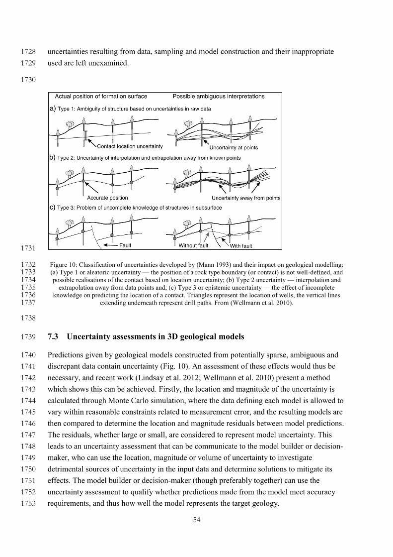
54
uncertainties resulting from data, sampling and model construction and their inappropriate 1728
used are left unexamined. 1729
1730
1731
Figure 10: Classification of uncertainties developed by (Mann 1993) and their impact on geological modelling: 1732 (a) Type 1 or aleatoric uncertainty — the position of a rock type boundary (or contact) is not well-defined, and 1733 possible realisations of the contact based on location uncertainty; (b) Type 2 uncertainty — interpolation and 1734
extrapolation away from data points and; (c) Type 3 or epistemic uncertainty — the effect of incomplete 1735 knowledge on predicting the location of a contact. Triangles represent the location of wells, the vertical lines 1736
extending underneath represent drill paths. From (Wellmann et al. 2010). 1737
1738
7.3 Uncertainty assessments in 3D geological models 1739
Predictions given by geological models constructed from potentially sparse, ambiguous and 1740
discrepant data contain uncertainty (Fig. 10). An assessment of these effects would thus be 1741
necessary, and recent work (Lindsay et al. 2012; Wellmann et al. 2010) present a method 1742
which shows this can be achieved. Firstly, the location and magnitude of the uncertainty is 1743
calculated through Monte Carlo simulation, where the data defining each model is allowed to 1744
vary within reasonable constraints related to measurement error, and the resulting models are 1745
then compared to determine the location and magnitude residuals between model predictions. 1746
The residuals, whether large or small, are considered to represent model uncertainty. This 1747
leads to an uncertainty assessment that can be communicate to the model builder or decision-1748
maker, who can use the location, magnitude or volume of uncertainty to investigate 1749
detrimental sources of uncertainty in the input data and determine solutions to mitigate its 1750
effects. The model builder or decision-maker (though preferably together) can use the 1751
uncertainty assessment to qualify whether predictions made from the model meet accuracy 1752
requirements, and thus how well the model represents the target geology. 1753

55
While this general procedure is not novel, and is performed in many workflows across 1754
disciplines, uncertainty assessments of 3D geological models typically involve a statistical 1755
summary of error directly obtained from the input data. This may be in the form of a mean 1756
error or standard deviation, possibly normalised when comparing datasets with different 1757
scales or units of measurement. Interpolation error can also be obtained if stochastic methods 1758
such as kriging are used. The estimates do not provide insight into geometrical or topological 1759
variability (Thiele et al. 2016) in the 3D model which may be due to interactions between 1760
inconsistent input data in order to answer the question “should resource exploration an 1761
extraction strategies, volume estimates and value assessments use this model? (Quigley et al., 1762
Minerva, in review) ” 1763
7.4 Combining geological modelling and uncertainty assessments 1764
The Gippsland Basin is a Mesozoic to Cenozoic oil and gas field in south-eastern Australia 1765
(Rahmanian et al. 1990). The 3D model in Figure 11 represents a basement of Ordovician 1766
rocks and covers sequences of Oligocene Seaspray and Pliocene Angler formations. The 1767
Palaeocene to Late Miocene Latrobe Group, which includes the Cobia, Golden Beach and 1768
Emperor Subgroups are prospective for oil and gas (Bernecker et al. 2001), but have also 1769
been considered as carbon sequestration sites (Swierczek et al. 2015). The geological 1770
structure of the basin is displaced by the NNE to NE-trending Lucas Point Fault, Spinnaker 1771
Fault and Cape Everard Fault System, and the E–W trending Wron Wron/Rosedale Fault 1772
Systems. The purpose of building this model was to try to understand the structure of the 1773
basin and where rock formations are located. Some of the data used to build this model were 1774
measured from outcrop, but the majority were derived from geophysical interpretation as 1775
much of the basin is submerged in Bass Strait. 1776
Geophysical interpretation is a technique commonly used in the geosciences, where different 1777
physical fields are measured from a region of interest and processed so that they reveal the 1778
spatial distribution of rock properties, which then can reveal geologic structure. Seismic data 1779
records energy as it travels through the earth. Where this energy is reflected, appropriate 1780
processing can translate these reflections into images, which a geologist can interpret in order 1781
to locate and estimate geometry of rock boundaries and faults (Herron 2011). Similarly, the 1782
magnetic and density properties of rocks can be measured and processed to produce images 1783
that geologists use to understand the structure of the subsurface. These techniques are 1784
necessary when the rocks of interest are covered by sand, vegetation, or in this case, water. 1785
Imprecision is inherent in the process and can creep in during each of the stages of surveying, 1786
processing and interpretation. The imprecisions have a compounding effect on the accuracy 1787
of the model, and thus the accuracy of the 3D model to represent what is known about the 1788
location and geometry of the petroleum target. 1789
That models contain uncertainty is widely accepted and forms a central assumption of 1790
Lindsay et al. (2012). This is based on the presence of input data errors and that models are a 1791

56
simplification of the natural world. As models are uncertain, it follows that to generate 1792
multiple model realisations from a given dataset is a reasonable approach. The 3D modelling 1793
approach used the input geological data to interpolate rock boundaries and faults within the 1794
volume. From there, a Monte Carlo process was employed where the input data was varied 1795
within acceptable constraints simulating aleatoric uncertainty. The varied input data was then 1796
used to calculate a new set (or ‘suite’) of models. Each of the members of this suite of models 1797
looked similar, but, when compared with each other, differences could be observed in the 1798
location and geometry of rock boundaries and faults. The magnitude of difference (or 1799
residual) between the models was calculated and used to visualise and communicate 1800
uncertainty. As an example, Figure 11 shows are the Golden Beach and Cobia subgroups 1801
(green and red respectively). The prisms represent uncertain locations in the model and are 1802
colour-coded according to the magnitude of the residual, and thus uncertainty (lighter blues 1803
are low, and darker blues are high). Seismic sections are also shown to highlight the position 1804
of model inputs used to construct the model. Such sections provide important data that is 1805
interpreted to offer depth constraints for the modelled geology. These data and interpretations 1806
are subject to aleatoric and epistemic uncertainty. 1807
1808
Figure 11: Oblique view looking southwest of the Gippsland Basin model constructed by (Lindsay et al. 2012), 1809 showing Golden Beach and Cobia subgroups (green and red respectively) as transparent to aid visualisation. The 1810
prisms indicate the location of uncertainty and are colour-coded to represent magnitude (light blue indicates 1811 lower uncertainty; dark blue indicates high uncertainty). The location of seismic sections (also transparent for 1812
visualisation) are shown as these were important sources of data. 1813
Assessment of Figure 11 clearly shows that a significant amount of uncertainty is located 1814
near to or within the boundaries of the modelled Golden Beach and Cobia subgroups. This 1815
was initially surprising given the proximity of the modelled rock units to data constraints 1816
provided by the seismic sections. Moore and Wong (2002) describes the seismic data and 1817
57
highlights potential issues with an inadequate velocity model that was used in seismic data 1818
processing. The velocity model is a critical component in seismic processing, as it defines the 1819
velocity a given rock unit will transmit energy from a seismic event and largely determines at 1820
what depth a seismic reflection will be placed on an image used for interpretation. Velocity is 1821
often measured with a high degree of precision from drill core, however these velocities can 1822
vary away from the measured location properties due to heterogeneities within the rock 1823
volume. If the estimate within the velocity model is wrong, then the location of a seismic 1824
reflection will also be incorrect. 1825
7.4.1 Sources of uncertainty in the Gippsland Basin model and a path to mitigation 1826
Deeper analysis revealed that the depth of the Cobia and Golden Beach subgroups interpreted 1827
from the seismic section disagreed with the depths of the same subgroups measured from 1828
logged drill core obtained from exploration and production wells. This disparity resulted in 1829
greater variability in the location of these units, which was shown as greater uncertainty. The 1830
disparity between the seismic and drill core data was compounded in the southern and eastern 1831
parts of the model by a lack of data constraints away from the seismic section due to it being 1832
a deeper part of the basin. Accurate data is more difficult to obtain in deep locations, wells 1833
that would extend to the appropriate depth to sample rocks are very expensive. A lack of 1834
geophysical data in the south and eastern regions compounds the sparsity of data. Hope for 1835
reducing uncertainty has come in the form of an improved velocity model produced by the 1836
Geological Survey of Victoria (McLean and Blackburn 2013). The initial velocity model 1837
assumed the velocity structure of the region could be categorised into four rock types with an 1838
additional category representing sea water. Each of the four rock types were represented by 1839
an average velocity, which assumes no heterogeneity in the rock volume: an assumption 1840
likely to be false. The newer edition provides velocities for eight rock units and also allows 1841
for heterogeneities within a rock unit to be present. Re-processing of the seismic sections 1842
used in this model with the new velocity data would certainly reduce uncertainties in 1843
accurately locating seismic reflections on the images used to build the model, and thus rock 1844
unit boundaries represented in the 3D model. As these rock boundaries are more accurately 1845
imaged, they would likely have less misfit with the depths measured from the well logs, 1846
reduce uncertainty in the 3D model and improve confidence in its predictions. 1847
7.5 Summary 1848
That models are uncertain is well-known to anyone who generates or constructs them. The 1849
real challenge is appropriately communicating this uncertainty to those who are not 1850
intimately familiar with data or modelling methods. The model builder will probably know, 1851
purely through familiarity with the project and its data, where the untrustworthy parts of the 1852
model are, and can point them out to those who need to know. The extent and magnitude of 1853
this uncertainty is much harder to convey and when stakes are high, such as deep-water oil 1854
and gas exploration or construction of public infrastructure (tunnels and bridges) a 1855
58
quantifiable uncertainty assessment is needed. In this case study, previous workers had 1856
already acknowledged inadequacies in the data and models used in the region, but what effect 1857
they had on the accurately predicting 3D structure of the region was not well described. The 1858
type of visualisation shown here is simple enough that a lay-person can understand it, and 1859
thus could make a more informed decision based on required predictions. The quantification 1860
of uncertainty serves other useful purposes. When additional or reprocessed data is added 1861
during remodelling, changes in the magnitude of uncertainty can then inform whether the 1862
new data was effective. Cost–benefit analysis can follow where the reduction of uncertainty 1863
was deemed appropriate for the costs associated with acquiring the new data. 1864
Decision-making, while not enacted by stakeholders in Gippsland Basin oil and gas 1865
exploration or carbon sequestration, was simulated in this case study as a proof-of-concept. 1866
Potential decisions relating to a reliable representation of the subsurface and thus exploration 1867
risk (i) were informed by models, (ii) considered prevailing scientific evidence, (iii) 1868
considered scientific uncertainty, (iv) and advocate taking a precautionary approach to 1869
uncertainty in resource exploration. The F2 deposit example describes the detrimental 1870
economic impact of not taking a precautionary approach to epistemic and aleatoric 1871
uncertainty. The method shown in the Gippsland Basin example provides an example of how 1872
the effects of uncertainty can be simulated, identified and mitigated if a precautionary 1873
approach is taken prior to making exploration decisions. The communication of uncertainty 1874
via visualisation of with a 3D geological model was key to providing insight to the source 1875
and magnitude of input data errors. 1876
8 Case Study 7: Loads estimation and reporting in the Great 1877
Barrier Reef: communication and challenges (Author: PK) 1878
8.1 Overview 1879
The Great Barrier Reef (GBR) is one of the seven natural wonders of the world, but is 1880
undergoing significant changes due to global warming, land based pollutant discharge and the 1881
recent attacks of the crown of thorns starfish (Brodie 2012; De'Ath et al. 2012; Kroon et al. 1882
2016). A recent publication by Hughes et al. (2017) highlights the main challenges for coral 1883
reefs as we move through the Anthropocene era. As stated in Hughes et al. (2017) and 1884
Hughes and Cinner (2017), the challenge is to sustain coral reefs for future generations and 1885
not just provide temporary fixes to ongoing problems. While the GBR and others like it are in 1886
trouble, we cannot “give up” – we need better ways to manage the changes and challenges 1887
presented. Solutions need to encompass a broader approach that not only includes the biology 1888
but considers the social implications of decision-making. With that comes uncertainty and a 1889
need for better approaches and demonstrated examples to communicate these uncertainties 1890
that can actively guide governance processes for clearer outcomes and decisions. 1891
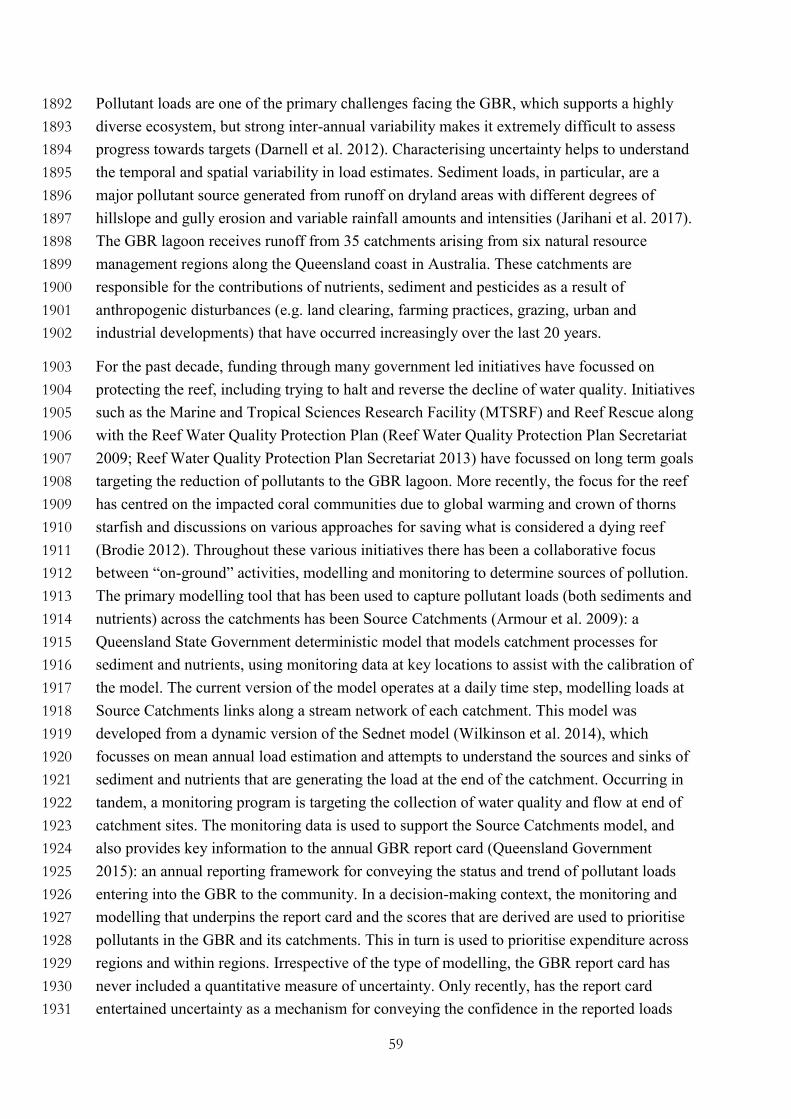
59
Pollutant loads are one of the primary challenges facing the GBR, which supports a highly 1892
diverse ecosystem, but strong inter-annual variability makes it extremely difficult to assess 1893
progress towards targets (Darnell et al. 2012). Characterising uncertainty helps to understand 1894
the temporal and spatial variability in load estimates. Sediment loads, in particular, are a 1895
major pollutant source generated from runoff on dryland areas with different degrees of 1896
hillslope and gully erosion and variable rainfall amounts and intensities (Jarihani et al. 2017). 1897
The GBR lagoon receives runoff from 35 catchments arising from six natural resource 1898
management regions along the Queensland coast in Australia. These catchments are 1899
responsible for the contributions of nutrients, sediment and pesticides as a result of 1900
anthropogenic disturbances (e.g. land clearing, farming practices, grazing, urban and 1901
industrial developments) that have occurred increasingly over the last 20 years. 1902
For the past decade, funding through many government led initiatives have focussed on 1903
protecting the reef, including trying to halt and reverse the decline of water quality. Initiatives 1904
such as the Marine and Tropical Sciences Research Facility (MTSRF) and Reef Rescue along 1905
with the Reef Water Quality Protection Plan (Reef Water Quality Protection Plan Secretariat 1906
2009; Reef Water Quality Protection Plan Secretariat 2013) have focussed on long term goals 1907
targeting the reduction of pollutants to the GBR lagoon. More recently, the focus for the reef 1908
has centred on the impacted coral communities due to global warming and crown of thorns 1909
starfish and discussions on various approaches for saving what is considered a dying reef 1910
(Brodie 2012). Throughout these various initiatives there has been a collaborative focus 1911
between “on-ground” activities, modelling and monitoring to determine sources of pollution. 1912
The primary modelling tool that has been used to capture pollutant loads (both sediments and 1913
nutrients) across the catchments has been Source Catchments (Armour et al. 2009): a 1914
Queensland State Government deterministic model that models catchment processes for 1915
sediment and nutrients, using monitoring data at key locations to assist with the calibration of 1916
the model. The current version of the model operates at a daily time step, modelling loads at 1917
Source Catchments links along a stream network of each catchment. This model was 1918
developed from a dynamic version of the Sednet model (Wilkinson et al. 2014), which 1919
focusses on mean annual load estimation and attempts to understand the sources and sinks of 1920
sediment and nutrients that are generating the load at the end of the catchment. Occurring in 1921
tandem, a monitoring program is targeting the collection of water quality and flow at end of 1922
catchment sites. The monitoring data is used to support the Source Catchments model, and 1923
also provides key information to the annual GBR report card (Queensland Government 1924
2015): an annual reporting framework for conveying the status and trend of pollutant loads 1925
entering into the GBR to the community. In a decision-making context, the monitoring and 1926
modelling that underpins the report card and the scores that are derived are used to prioritise 1927
pollutants in the GBR and its catchments. This in turn is used to prioritise expenditure across 1928
regions and within regions. Irrespective of the type of modelling, the GBR report card has 1929
never included a quantitative measure of uncertainty. Only recently, has the report card 1930
entertained uncertainty as a mechanism for conveying the confidence in the reported loads 1931

60
(Queensland Government 2015), however this has appeared as a qualitative assessment with 1932
no detail in terms of how the measure was obtained, what it means or how the loads can be 1933
interpreted in light of the uncertainty. The recent focus on uncertainty has stemmed from two 1934
independent reports of the paddock to reef monitoring and modelling program (Bosomworth 1935
and Cowie 2016; QAO 2015), where the quantification of uncertainty has been highlighted as 1936
a necessary component to reporting. For reporting, load estimates have tended to focus on 1937
“end-of-catchment” loads rather than “whole-of-catchment” loads to determine the sources of 1938
pollution. For this case study, we focus on whole-of-catchment loads and how information 1939
has been both solicited and offered up to decision-makers for the purpose of reporting and 1940
decision-making prior to the recent reviews. We discuss how information was disseminated, 1941
how it was received and how it could be used more effectively in the future. 1942
8.2 Communication of uncertainty in GBR loads reporting 1943
The communication of uncertainty in GBR loads reporting has failed miserably in recent 1944
times despite it being considered an important part of a report card framework (Bosomworth 1945
and Cowie 2016; QAO 2015). The often unrealistic timelines imposed on reporting 1946
frameworks to demonstrate progress that are heavily weighted by political constraints, makes 1947
the process challenging in terms of being able to quantify the uncertainty as well as to 1948
communicate it. 1949
The first attempt at quantifying uncertainty in loads arose from a MTSRF funded project, 1950
where a statistical methodology was proposed for the quantification of loads (sediment, 1951
nutrients and pesticides) with uncertainties using monitoring data. The Loads Regression 1952
Estimator (LRE) is a generalized additive model implemented in the R programming 1953
language that attempts to mimic the hydrological process of flow at sites that are responsible 1954
for the generation of a load (Kuhnert et al. 2012). The method quantifies the uncertainty of 1955
the load by considering the uncertainty in the concentration and the flow, where the latter 1956
considered uncertainty in the positioning of the flow gauge as well as uncertainty in the flow 1957
rate. This modelling approach was used to provide load estimates for the very first GBR 1958
report card for end of catchment sites where it was deemed through workshop consultation 1959
that Source Catchments could not provide an accurate load estimate alone (Queensland 1960
Government 2009). In this exercise, uncertainties from LRE were expressed as 80% 1961
confidence intervals and were compared with Source Catchment estimates in an expert 1962
setting. Kroon et al. (2012) published the LRE estimates of loads to explore the impact of 1963
sediment, nutrient and pesticide loads since human intervention. While load estimates with 1964
uncertainties in the form of standard deviations and 80% confidence intervals were conveyed 1965
in this paper and offered up for reporting, these uncertainties did not make it into the first 1966
GBR report card and subsequent report cards that followed. Why? Put simply, water quality 1967
managers found it difficult to understand a standard deviation or a confidence interval. 1968
61
Further, wide confidence intervals resulted in ambiguity around the estimates and managers 1969
were anxious around their potential miscommunication to a non-scientific audience. 1970
Figure 12 compares some of the results shown by Kroon et al. (2012) and compares them to 1971
the information used in the 2009 GBR report card. Note, the report card only showed loads 1972
for total nitrogen (TN), dissolved nitrogen (DIN + DON), total phosphorous (TP), dissolved 1973
phosphorous (DIP + DOP) and total suspended sediment (TSS). This figure shows the 80% 1974
confidence interval for the mean annual loads for the Burdekin end of catchment site as 1975
estimated by the LRE package and compares this with “current” estimates extracted from 1976
Kroon et al. (2012) and used in the 2009 GBR report card (Queensland Government 2009). 1977
Without the estimates of uncertainty, we really do not have complete information that 1978
provides some certainty around the estimates. For example, take the TSS loads estimate for 1979
the Burdekin (right hand panel of Figure 12). The single estimate provided in the 2009 GBR 1980
report card was 4.7 million tonnes (Mt) per year (blue square in right panel of Figure 12). 1981
However, the 80% confidence interval provided for the LRE estimate of the mean annual 1982
TSS load ranged between 1.1 and 15 million tonnes. The wide confidence interval may 1983
reflect the amount of data, n, used to generate the interval (n=36) in addition to the complex 1984
processes being modelled and their inherent variability associated with it. A decision based 1985
on the single number of 4.7 Mt per year could be perceived quite differently to a decision 1986
based on an interval [1.1 – 15 Mt], especially if the estimate for the year was closer to the 1987
upper bound of that 80% confidence interval. For instance, a wide confidence interval may 1988
warrant closer inspection of the site being monitored to understand the cause of the variability 1989
in the TSS estimate. Why is the interval so wide? Are there sufficient samples being taken to 1990
understand the variability at that site? Should more samples be taken or is this a “hotspot” site 1991
and should we look at specific management regimes that may reduce the mean annual TSS 1992
load at this site over time? 1993
While an uncertainty measure in the form of 80% confidence intervals was offered up for the 1994
2009 GBR Report card, these intervals never made it into the technical report and instead, 1995
histograms showing the mean annual loads were produced to compare pre-European loads 1996
with “current” best estimates from Kroon et al. (2012). It was understood that the concept of 1997
an 80% confidence interval for a report card was challenging in terms of how it might be 1998
perceived by the public, particularly for constituents and sites where confidence intervals 1999
were wide. 2000
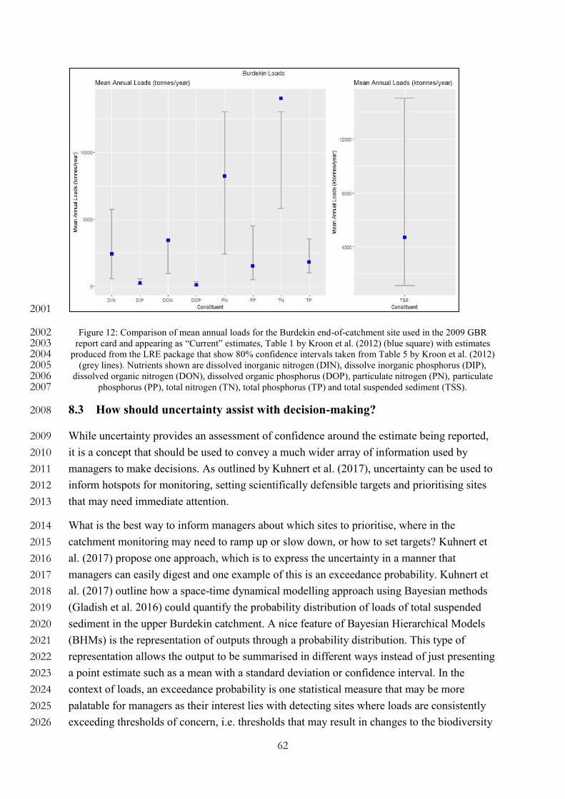
62
2001
Figure 12: Comparison of mean annual loads for the Burdekin end-of-catchment site used in the 2009 GBR 2002 report card and appearing as “Current” estimates, Table 1 by Kroon et al. (2012) (blue square) with estimates 2003
produced from the LRE package that show 80% confidence intervals taken from Table 5 by Kroon et al. (2012) 2004 (grey lines). Nutrients shown are dissolved inorganic nitrogen (DIN), dissolve inorganic phosphorus (DIP), 2005
dissolved organic nitrogen (DON), dissolved organic phosphorus (DOP), particulate nitrogen (PN), particulate 2006 phosphorus (PP), total nitrogen (TN), total phosphorus (TP) and total suspended sediment (TSS). 2007
8.3 How should uncertainty assist with decision-making? 2008
While uncertainty provides an assessment of confidence around the estimate being reported, 2009
it is a concept that should be used to convey a much wider array of information used by 2010
managers to make decisions. As outlined by Kuhnert et al. (2017), uncertainty can be used to 2011
inform hotspots for monitoring, setting scientifically defensible targets and prioritising sites 2012
that may need immediate attention. 2013
What is the best way to inform managers about which sites to prioritise, where in the 2014
catchment monitoring may need to ramp up or slow down, or how to set targets? Kuhnert et 2015
al. (2017) propose one approach, which is to express the uncertainty in a manner that 2016
managers can easily digest and one example of this is an exceedance probability. Kuhnert et 2017
al. (2017) outline how a space-time dynamical modelling approach using Bayesian methods 2018
(Gladish et al. 2016) could quantify the probability distribution of loads of total suspended 2019
sediment in the upper Burdekin catchment. A nice feature of Bayesian Hierarchical Models 2020
(BHMs) is the representation of outputs through a probability distribution. This type of 2021
representation allows the output to be summarised in different ways instead of just presenting 2022
a point estimate such as a mean with a standard deviation or confidence interval. In the 2023
context of loads, an exceedance probability is one statistical measure that may be more 2024
palatable for managers as their interest lies with detecting sites where loads are consistently 2025
exceeding thresholds of concern, i.e. thresholds that may result in changes to the biodiversity 2026
63
of the reef or increased toxicity levels in the water quality. Again, in the context of loads, 2027
exceedance probabilities were calculated for sites within the Burdekin catchment using 2028
published concentration thresholds given by Bartley et al. (2012). Once calculated, the 2029
exceedance probabilities could be expressed in different ways: spatially, through an 2030
exceedance probability map for a specific time period (Figure 7.2a); or a site-based 2031
exceedance probability calculated through time (Figure 7.2b). Kuhnert et al. (2017) also show 2032
how exceedance probabilities could be used to inform target setting by constructing 2033
exceedance probability curves that could be used in an expert setting to determine spatially 2034
referenced targets for example. 2035
Why is this information not being used for GBR reporting? The concept of exceedance 2036
probabilities is fairly new in the GBR and methods like the one proposed by Kuhnert et al. 2037
(2017) are only just appearing in the literature. For this type of approach to be adopted, there 2038
is a period of knowledge acquisition followed by a demonstration of the approach to end 2039
users to see how this information could be used in practice, not only for reporting but how it 2040
impacts on decision making. Further, implementing this approach in practice requires model 2041
runs of Source Catchments (Armour et al. 2009), the Queensland State Government 2042
catchment model, which then need to be assimilated with monitoring data using approaches 2043
such as Gladish et al. (2016) . Finding the time to implement these changes also becomes 2044
challenging with changing political environments and priorities. 2045
(a) (b)
Figure 13: Examples of exceedance probabilities calculated for (a) the Upper Burdekin Catchment in 1992/1993 2046 and (b) a Source Catchments link (248) that showcases exceedance probabilities from 1988 to 2008. 2047
8.4 Summary 2048
Uncertainty plays a significant role in the quantification and communication of loads in the 2049
GBR. Although the demonstrated need for uncertainties first appeared in 2012 with the 2050
development of the LRE approach to loads quantification and more recently, through the 2051
review of the P2R modelling and monitoring review, it still has not become an integral part of 2052
GBR reporting. Moreover, it has not been considered as a tool for decision-making. 2053
Therefore, better approaches are required for communicating uncertainties to decision-makers 2054
64
and be much clearer on what the term “uncertainty” covers. It is easy for managers to look at 2055
all the sources of uncertainty and lump them together. However, the reality is that some will 2056
incorporate sources of uncertainty that others do not. Improving predictive uncertainty is the 2057
key to model improvement as it helps to identify where we need to instigate change and 2058
reduce the uncertainty and width of the predictive intervals, thereby improving a manager’s 2059
ability to make more informed decisions. 2060
The decisions enacted in this case study are (i) largely informed by science and (ii) align with 2061
the prevailing scientific evidence. However, the current framework for reporting and 2062
decision-making does not consider scientific uncertainty. Decisions about priority load “hot 2063
spots” in the GBR region are informed by models, however these have been deterministic in 2064
nature and when model estimates have been accompanied with uncertainty estimates, these 2065
have been removed due to the difficulty in their interpretation or the concern about what large 2066
standard errors (or wide confidence intervals) actually mean. This has led to decisions that 2067
are precautionary in nature and often not useful for mitigating the effects of pollutant loads. 2068
2069
9 Summary of findings 2070
This study presents detailed descriptions of case studies in the earth and environmental 2071
sciences, pertaining to the communication of scientific evidence (data, models, expert 2072
opinions) to decision-makers in cases involving risk and uncertainty. Scientific evidence may 2073
enter decision-making processes via diverse pathways, ranging from direct solicitations by 2074
decision-makers to scientists (e.g., case studies 1, 2, 5, 7) to requests from stake-holders to 2075
intermediate agents tasked to engage science communities (case study 2) to independent 2076
requests from stake-holders directly to scientists (e.g., case studies 1). The latter is evidenced 2077
to be stimulated by external factors, such as media coverage of research that affected parties 2078
perceived to be relevant to their circumstances (e.g. case study 1, 5). Acquiring highly 2079
specialized, pertinent scientific data of direct relevance to specific aspects of decision-making 2080
may not always meet the expedient demands of decision-makers (case studies 1, 3, 4, 5, 7); in 2081
these cases, decision-making may be incremented (e.g., case study 1) or delayed (e.g., case 2082
study 1), use scientific expertise and judgement to assist in decision-making with large 2083
epistemic (case study 1, 3, 4, 5, 6) or aleatoric uncertainty (case study 6), and provide 2084
opportunities for adjustment of decisions as additional information becomes available (case 2085
study 1, 5). If the likelihood of occurrence of potentially adverse future risks is perceived by 2086
decision-makers to exceed acceptable thresholds and/or be highly uncertain, precautionary 2087
decisions with adaptive capacity may be favoured, even if some scientific evidence suggests 2088
lower levels of risk (e.g., case study 1, 3, 5, 7). The efficacy with which relevant scientific 2089
data, models, and uncertainties contribute to decision-making may relate to factors including 2090
the expediency with which this information can be obtained (case study 1, 2, 3, 7), the 2091
perceived strength and relevance of the information presented (case study 1, 5, 7), the extent 2092

65
to which relevant experts have participated and collaborated in scientific messaging to 2093
decision-makers and stake-holders (case study 1, 5, 7), and the perceived risks to decision-2094
makers of favouring earth science information above other, potentially conflicting, scientific 2095
and non-scientific inputs (case study 7, 5). The establishment of science provision teams and 2096
mechanisms that enable researchers with sufficient expertise and knowledge to collaborate 2097
and communicate internally, and with decision-makers and stakeholders, is viewed as a 2098
highly favourable aspect that should be further promoted. 2099
To exemplify parallel findings and differentiations between the case studies in relation to the 2100
decisions enacted, we summarize the results from each case study in Figure 14 in terms of 2101
whether decision-making was (i) scientifically informed, (ii) aligned with the prevailing 2102
scientific evidence, (iii) considered the available knowledge on scientific uncertainty, (iv) 2103
informed by models, and (v) precautionary in nature. All decision-making was informed by 2104
science, but the utility of relevant and available models in decision-making varies. These case 2105
studies, drawn from scientists working across the earth sciences on topics as diverse as 2106
natural disasters, agriculture and the environmental impacts of mining, demonstrate many 2107
similarities in the communication of uncertainty to decision makers. Despite the different 2108
motivations for seeking scientific input, uncertainty was a factor for consideration at least 2109
partially in all cases. In contrast, the adoption of a precautionary approach and the use of 2110
models differed between case studies due to the different requirements of the decision-2111
making process. Science is inherently uncertain, we anticipate that consideration of 2112
uncertainty will be increasingly part of the communication of scientific knowledge to 2113
decision makers. These case studies also demonstrate that systematic and standardised 2114
approaches to communicating uncertainty will benefit scientists and decision makers. 2115
2116
2117
2118
2119
Case
Study
Criteria (i)
Informed
by Science
Criteria (ii)
Aligned with
Prevailing
Science
Criteria (iii)
Considered
Uncertainty
Criteria (iv)
Informed
by Models
Criteria (v)
Precautionary
1 yes yes partially yes yes
2 yes yes yes yes yes
3 yes yes no yes yes
4 yes yes partially partially yes
5 yes no yes yes yes
6 yes yes partially yes partially
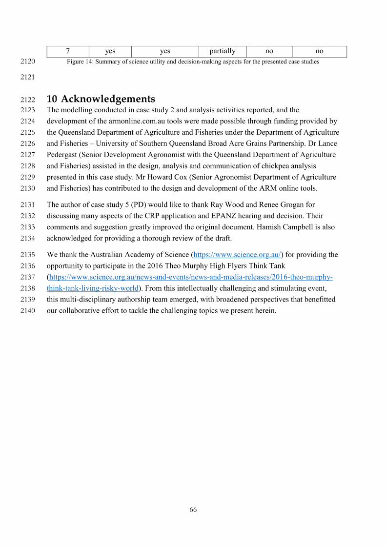
66
7 yes yes partially no no
Figure 14: Summary of science utility and decision-making aspects for the presented case studies 2120
2121
10 Acknowledgements 2122
The modelling conducted in case study 2 and analysis activities reported, and the 2123
development of the armonline.com.au tools were made possible through funding provided by 2124
the Queensland Department of Agriculture and Fisheries under the Department of Agriculture 2125
and Fisheries – University of Southern Queensland Broad Acre Grains Partnership. Dr Lance 2126
Pedergast (Senior Development Agronomist with the Queensland Department of Agriculture 2127
and Fisheries) assisted in the design, analysis and communication of chickpea analysis 2128
presented in this case study. Mr Howard Cox (Senior Agronomist Department of Agriculture 2129
and Fisheries) has contributed to the design and development of the ARM online tools. 2130
The author of case study 5 (PD) would like to thank Ray Wood and Renee Grogan for 2131
discussing many aspects of the CRP application and EPANZ hearing and decision. Their 2132
comments and suggestion greatly improved the original document. Hamish Campbell is also 2133
acknowledged for providing a thorough review of the draft. 2134
We thank the Australian Academy of Science (https://www.science.org.au/) for providing the 2135
opportunity to participate in the 2016 Theo Murphy High Flyers Think Tank 2136
(https://www.science.org.au/news-and-events/news-and-media-releases/2016-theo-murphy-2137
think-tank-living-risky-world). From this intellectually challenging and stimulating event, 2138
this multi-disciplinary authorship team emerged, with broadened perspectives that benefitted 2139
our collaborative effort to tackle the challenging topics we present herein. 2140

67
References 2141 Alfonso L, Mukolwe M, Di Baldassarre D (2016) Probabilistic Flood Maps to support decision-2142
making: Mapping the Value of Information Water Resour Res 52:1026–1043 2143 doi:doi:10.1002/2015WR017378 2144
Apel H, Thieken A, Merz B (2006) A Probabilistic Modelling System for Assessing Flood Risks Nat 2145 Hazards 38 doi:doi:10.1007/s11069-005-8603-7 2146
Armour JD, Hateley LR, Pitt GL (2009) Catchment modelling of sediment, nitrogen and phosphorus 2147 nutrient loads with SedNet/ANNEX in the Tully-Murray basin Marine and Freshwater 2148 Reserach 60:1091-1096 2149
Ascough II, J., Maierb, H., Ravalico, J., Strudley, M. (2008) Future research challenges for 2150 incorporation of uncertainty in environmental and ecological decision-making. Ecol. Model. 2151 219, 383–399 2152
Australian Geomechanics Society (2007) Practice note guidelines for landslide risk management 2153 Journal and News of the Australian Geomechanics Society 42:155-114 2154
Babcock B (1992) The effects of uncertainty on optimal nitrogen applications Appl Econ Perpect 2155 Policy 14:271–280 doi:doi: 10.2307/1349506 2156
Barlow K, Thayalakumaran T, Moody P Extending “SafeGauge for Nutrients” to high rainfall 2157 cropping in Australia. In: 7th International Nitrogen Imitative Conference, Melbourne, 2158 Australia, 2016. 2159
Barnes L, Gruntfest E, Hayden M, Schultz D, Benight C (2007) False Alarms and Close Calls: A 2160 Conceptual Model of Warning Accuracy Weather Forecast 22:1140–1147 2161 doi:https://doi.org/10.1175/WAF1031.1 2162
Bartley R, Speirs WJ, Ellis TW, Waters DK (2012) A review of sediment and nutrient concentration 2163 data from Australia for use in catchment water quality models. Marine Pollution Bulletin 2164 65:101-116 2165
Beaven S, Wilson T, Johnston L, Johnston D, Smith R (2016) Role of Boundary Organization after a 2166 Disaster: New Zealand’s Natural Hazards Research Platform and the 2010–2011 Canterbury 2167 Earthquake Sequence Nat Hazards Rev 18:05016003 2168
Becker J, Potter S, Wein A, Doyle E, Ratliff J Aftershock communication during the Canterbury 2169 earthquakes, New Zealand: Implications for response and recovery in the built environment. 2170 In: New Zealand Society of Earthquake Engineering, 2015. 2171
Behnam A, Visbeck M (2013) The Future of Fish –The Fisheries ofthe Future. Hamburg, Germany 2172 Behnam A, Visbeck M (2014) Marine Resources – Opportunities and Risks. Hamburg, Germany 2173 Bernecker T, Woollands M, Wong D, Moore D, Smith M (2001) Hydrocarbon prospectivity of the 2174
deep water Gippsland Basin, Victoria, Australia APPEA J 41:91–113 2175 Berryman K (2012) Geoscience as a component of response and recovery from the Canterbury 2176
earthquake sequence of 2010–2011 N Z J Geol Geophys 55:313–319 2177 Borella J, Quigley M, Sohbati R, Almond P, Gravley DM, Murray A (2016a) Chronology and 2178
processes of late Quaternary hillslope sedimentation in the eastern South Island, New Zealand 2179 Journal of Quaternary Science 31:691-712 2180
Borella J, Quigley M, Vick L (2016b) Anthropocene rockfalls travel farther than prehistoric 2181 predecessors Science Advances 2:e1600969 doi:10.1126/sciadv.1600969 2182
Boskalis Offshore (2014a) Appendix 3: Compilation of literature on the Chatham Rise phosphorite 2183 deposit. 2184
Boskalis Offshore (2014b) Appendix 4: Summary and analysis of site investigation data. 2185 Bosomworth B, Cowie B (2016) Response to the independent reviews of DNRM activities under 2186
Action 8 & 9 of Reef Plan 2013. Land and Water Science, Department of Natural Resources 2187 and Mines, State of Queensland 2188
Breznitz S (1984) Cry Wolf: The Psychology of False Alarms. Lawrence Erlbaum Associates, 2189 Brodie J (2012) Great Barrier Reef dying beneath its crown of thorns. The Conversation 2190 Bruns A, Burgess J Local and global responses to disaster: #eqnz and the Christchurch earthquake. In: 2191
Disaster and Emergency Management Conference, Brisbane Exhibition and Convention 2192 Centre, Brisbane, QLD, 2012. AST Management Pty Ltd, pp 86–103 2193
68
Cheong L, Bleisch S, Kealy A, Tolhurst K, Wilkening T, Duckham M (2016) Evaluating the impact 2194 of visualization of wildfire hazard upon decision-making under uncertainty Int J Geogg Inf 2195 Sci 30 2196
Chiswell SM (2014) Appendix 8: Physical oceanographic data available on the Chatham Ris. 2197 Clark, J. S. (2005). Why environmental scientists are becoming Bayesians. Ecology letters, 8(1), 2-14. 2198 Cloke H, Pappenberger F (2009) Ensemble Flood Forecasting: A Review J Hydrol 375:613–626 2199
doi:http://dx.doi.org/10.1016/j.jhydrol.2009.06.005 2200 Coates L, Haynes K, O’Brien J, McAneney J, de Oliveira F (2014) Exploring 167 years of 2201
vulnerability: An examination of extreme heat events in Australia 1844–2010 Environ Sci 2202 Policy 42:33–44 doi:doi: 10.1016/j.envsci.2014.05.003 2203
Colyvan M et al. (2017) Addressing Risk in Conditions of Uncertainty, Ignorance, and Partial 2204 Knowledge. In An interdisciplinary approach to living in a risky world. Recommendations 2205 from the Theo Murphy High Flyers Workshop (pp. 5–7). Australian Academy of Science, 2206 Canberra, ACT 2207
Comrie N (2011) Review of the 2010–11 flood warnings and response. Victorian Government, 2208 Australia, 2209
Cox H, Hammer G, McLean G, King C National WhopperCropper – risk management discussion 2210 support software. In 'New directions for a diverse planet. In: Fischer T, Turner N, Angus J, 2211 Mcintyre L, Robertson M, Borrell A, Lloyd D (eds) Proceedings for the 4th International 2212 Crop Science Congress, Brisbane, Australia, 2004. 2213
CRP (2014) Appendix 7: Other Voyages Overview. 2214 Cubrinovski M et al. (2010) Geotechnical reconnaissance of the 2010 Darfield (Canterbury) 2215
earthquake Bull N Z Soc Earthq Eng 43:243–320 2216 Dalgliesh N, Cocks B, Horan H APSoil-providing soils information to consultants, farmers and 2217
researchers. In: Capturing Opportunities and Overcoming Obstacles in Australian Agronomy" 2218 Proceedings of the 16th ASA Conference, Armidale, NSW Australia, 2012. 2219
Darnell R, Henderson BL, Kroon FJ, Kuhnert PM (2012) Statistical power of detecting trends in total 2220 suspended sediment loads to the Great Barrier Reef Marine Pollution Bulletin 65:203-209 2221
De'Ath G, Fabricius KE, Sweatman H, Puotinen M (2012) The 27-year decline of coral cover on the 2222 Great Barrier Reef and its causes Proceedings of the National Academy of Sciences of the 2223 United States of America 109:17995-17999 2224
Dow K, Cutter S (1998) Crying wolf: Repeat responses to hurricane evacuation orders Coast Manage 2225 26:237–252 2226
Draper D (1995) Assessment and propagation of model uncertainty J R Stat Soc 57:45–97 2227 Durden J et al. (2016) Report on the Managing Impacts of Deep-seA reSource exploitation (MIDAS) 2228
workshop on environmental management of deep-sea mining vol 2. 2229 Environmental Protection Authority NZ (2012) Exclusive Economic Zone and Continental Shelf 2230
Environmental Effects Act 2012. The New Zealand Federal Government, New Zealand 2231 Environmental Protection Authority NZ (2015) Decision on marine consent application by Chatham 2232
Rock Phosphate Limited to mine phosphorite nodules on the Chatham Rise. Environmental 2233 Protection Authority, Wellington 2234
Environmental Protection Authority NZ (2017) Decision on marine consents and marine discharge 2235 consents application: EEZ000011, Trans-Tasman Resources Limited. Extracting and 2236 processing ireon sand within the South Taranaki Bight. Wellington 2237
Fergusson D, Horwood L, Boden J, Mulder R (2014) Impact of a major disaster on the mental health 2238 of a well-studied cohort JAMA Psychiatry 71:1025–1031 2239
Finkel, A. (1990) Confronting Uncertainty in Risk Management: A Guide for Decision Makers. 2240 Center for Risk Management, Resources for the Future. 2241
Fischer R (2009) Exploiting the synergy between genetic improvement and agronomy of crops in 2242 rainfed farming systems of Australia. In: Sadras V, Calderini D (eds) Crop physiology: 2243 applications for genetic improvement and agronomy. Elsevier, Amsterdam, 2244
Fischhoff, B. and Davis, A.L. (2014) Communicating scientific uncertainty. Proceedings of the 2245 National Academy of Sciences, 111(Supplement 4): 13664-13671. 2246
Gerstenberger M et al. (2011) Probabilistic assessment of liquefaction potential for Christchurch in 2247 the next 50 years. vol 2011/15. GNS Science, Lower Hutt, NZ 2248

69
Gjerde KM et al. (2016) Report on the implications of MIDAS results for policy makers with 2249 recommendations for future regulations to be adopted by the EU and the ISA 2250
Gladish DW et al. (2016) Spatio-temporal assimilation of modelled catchment loads with monitoring 2251 data in the Great Barrier Reef Annals of Applied Statistics 10:1590-1618 2252
Gledhill K, Ristau J, Reyners M, Fry B, Holden C (2010) The Darfield (Canterbury) Mw 7.1 2253 earthquake of September 2010: Preliminary seismological report Bull N Z Soc Earthq Eng 2254 43:215–221 2255
Gluckman P (2014) The art of science advice to government Nature 507 2256 Golder Associates Ltd (2014a) Appendix 35(i): Draft Environmental Management and Monitoring 2257
Plan. 2258 Golder Associates Ltd (2014b) Marine Consent Application and Environmental Impact Assessment. 2259 Golder Associates Ltd (2014c) Marine Consent Application and Environmental Impact Assessment: 2260
Non-technical Summary. 2261 Grogan R (2017) Regulating extractive industries: what works in practice?, Practitioners’ perspectives 2262
on the effective implementation of environmental legislation. 2263 Halfar J, Fujita RM (2002) Precautionary management of deep-sea mining Marine Policy 26:103-106 2264
doi:https://doi.org/10.1016/S0308-597X(01)00041-0 2265 Hannington M, Petersen S, Kratschell A (2017) Subsea mining moves closer to shore Nature Geosci 2266
10:158-159 doi:10.1038/ngeo2897 2267 Herron DA (2011) First steps in seismic interpretation. Geophysical monograph series number 16. 2268
Society of Exploration Geophysicists, 2269 Holzworth D et al. (2014) APSIM — Evolution towards a new generation of agricultural systems 2270
simulation Environ Modell Softw 62:327–350 2271 Hughes-Allan S, Peters K, O’Donnell R (2014) Appendix 2: Genesis of the Chatham Rise Deposit: A 2272
synthesis of current literature (Kenex 2010). 2273 Hughes M, Quigley M, van Ballegooy S, Deam B, Bradley B, Hart D (2015) The sinking city: 2274
earthquakes increase flood hazard in Christchurch, New Zealand GSA Today 25:4–10 2275 Hughes T et al. (2017) Coral reefs in the Anthropocene Nature 546:82-90 2276 Hughes T, Cinner J (2017) The world's coral reefs. The Conversation 2277 Jarihani B, Sidle RC, Bartley R, Roth CH, Wilkinson S (2017) Characterisation of hydrological 2278
response to rainfall at multi spatio-temporal scales in savannas of semi-arid Australia Water 2279 In Press 2280
Jeffrey S, Carter J, Moodie K, Beswick A (2001) Using spatial interpolation to construct a 2281 comprehensive archive of Australian climate data Environ Modell Softw 16:309–330 2282
Jenkins L, Brill R The effect of time of sowing on phenology and yield of chickpeas at Trangie 2283 Central West, NSW, 2011. In: Capturing Opportunities and Overcoming Obstacles in 2284 Australian Agronomy, Proceedings of the 16th ASA Conference, Armidale, Australia, 2012. 2285
Jones J.W. AJM, Basso B., et al., Boote K.J., Conant R.T., Foster I., Godfray H.C.J., Herrero M., 2286 Howitt R.E., Janssen S., Keating B.A, Munoz R.M., Porter C.H, Rosenzweig C., Wheeler T.R 2287 (2016) Brief history of agricultural systems modeling Agr Syst 155:240–254 2288 doi:http://dx.doi.org/10.1016/j.agsy.2016.05.014 2289
Kroon FJ et al. (2012) River loads of suspended solids, nitrogen, phosphorus and herbicides delivered 2290 to the Great Barrier Reef lagoon Marine Pollution Bulletin 65:167-181 2291
Kroon FJ, Thorburn P, Schaffelke B, Whitten S (2016) Towards protecting the Great Barrier Reef 2292 from land-based pollution Global Change Biology doi: 10.1111/gcb.13262 2293
Kuhnert PM, Henderson BL, Lewis SE, Bainbridge ZT, Wilkinson SN, Brodie JE (2012) Quantifying 2294 total suspended sediment export from the Burdekin River catchment using the loads 2295 regression estimator tool Water Resources Research 48:10.1029/2011WR011080 2296
Kuhnert PM, Pagendam DE, Bartley R, Gladish DW, Lewis SE, Bainbridge ZT (2017) Making 2297 management decisions in the face of uncertainty: a case study using the Burdekin catchment 2298 in the Great Barrier Reef Marine and Freshwater Research Submitted 2299
Leonard M et al. (2014) A compound event framework for understanding extreme impacts WIREs 2300 Clim Change 5:113–128 doi:doi:10.1002/wcc.252 2301
Lescinski J (2014) Statement of Evidence of Jamie Lescinski for Chatham Rock Phosphate Limited. 2302 EPANZ, Welllington 2303

70
Linkov I, Anklam E, Collier ZA, DiMase D, Renn O (2014) Risk-based standards: integrating top–2304 down and bottom–up approaches. Environ Syst Decis 34:134–137 2305
Lindsay M, Aillères L, Jessell M, de Kemp E, Betts P (2012) Locating and quantifying geological 2306 uncertainty in three-dimensional models: Analysis of the Gippsland Basin, southeastern 2307 Australia Tectonophysics 546–547:10–27 2308
Mackey B, Quigley M (2014) Strong proximal earthquakes revealed by cosmogenic 3He dating of 2309 prehistoric rockfalls, Christchurch, New Zealand Geology 42:975–978 2310
Mann J (1993) Computers in Geology — 25 Years of Progress. In: Uncertainty in geology. Oxford 2311 University Press, pp 241–254 2312
Martin H (1999) Adakitic magmas: Modern analogues of Archaean granitoids Lithos 46:411–429 2313 Massey C et al. (2014) Determining Rockfall Risk in Christchurch Using Rockfalls Triggered by the 2314
2010–2011 Canterbury Earthquake Sequence Earthq Spectra 30:155–181 2315 McDowell RW, Littlejohn RP, Blennerhassett JD (2010) Phosphorus fertilizer form affects 2316
phosphorus loss to waterways: a paired catchment study Soil Use and Management 26:365-2317 373 doi:10.1111/j.1475-2743.2010.00289.x 2318
McLean M, Blackburn G (2013) A new regional velocity model for the Gippsland Basin. Department 2319 of Primary Industries, 2320
Moody P, Agustina L, Robinson B, McHugh A, Dang Y (2013) Safegauge: A web-based decision 2321 support tool for informing nutrient management in the Queensland sugar industry vol??? 2322
Moore D, Wong D (2002) Eastern and Central Gippsland Basin, Southeast Australia; Basement 2323 Interpretation and Basin Links. Department of Natural Resources and Environment, Australia, 2324
Morgan, M., Henrion, M. (1990) Uncertainty. A guide to dealing with uncertainty in quantitative risk 2325 and policy analysis. Cambridge University Press: 346 pgs. 2326
Moritz Bollmann et al. (2010) Living with the oceans. Hamburg, Germany 2327 Nathan R, Weinmann E, Hill P Use of Monte Carlo Simulation to Estimate the Expected Probability 2328
of Large to Extreme Floods. In: Boyd M, Ball J, Babister M, Green J (eds) 28th International 2329 Hydrology and Water Resources Symposium: About Water, Barton, ACT, Australia, 2003. 2330 Institution of Engineers, Australia, 2331
Neale T (2015) Scientific knowledge and scientific uncertainty in bushfire and flood risk mitigation. 2332 Literature Review. Bushfire and Natural Hazards Cooperative Research Centre, 2333
Parker M, Steenkamp D (2012) The economic impact of the Canterbury earthquakes Reserve Bank of 2334 New Zealand Bulletin 75:13-25 2335
Pechlivanidis I, Jackson B, McIntyre N, Wheater H (2011) Catchment scale hydrological modelling: a 2336 review of model types, calibration approaches and uncertainty analysis methods In the context 2337 of recent developments in technology and applications Global NEST Journal 13:193–214 2338
Pielke Jr, R. A. (2003). The role of models in prediction for decision. Models in ecosystem science, 2339 111-135. 2340
Pielke Jr, R. A., & Conant, R. T. (2003). Best practices in prediction for decision‐making: lessons 2341 from the atmospheric and earth sciences. Ecology, 84(6), 1351-1358. 2342
QAO (2015) Managing water quality in Great Barrier Reef catchments vol Report 20: 2015-2015. 2343 Queensland Audit Office, The State of Queensland 2344
Queensland Government (2009) Great Barrier Reef First Report Card 2009 Baseline. Reef Water 2345 Quality Protection Plan, Queensland Government, Brisbane Australia 2346
Queensland Government (2015) Great Barrier Reef Report Card 2014. Reef Water Quality Protection 2347 Plan, Queensland Government, Brisbane, Australia 2348
Quigley M, Bastin S, Bradley B (2013) Recurrent liquefaction in Christchurch, New Zealand, during 2349 the Canterbury earthquake sequence Geology 41:419–422 2350
Quigley M, Forte A (2017) Science website traffic in earthquakes Seismol Res Lett 88 doi:doi: 2351 10.1785/0220160172 2352
Quigley M et al. (2016) The 2010–2011 Canterbury Earthquake Sequence: Environmental effects, 2353 seismic triggering thresholds and geologic legacy Tectonophysics 672–673:228–274 2354
Quigley M et al. (2010) Surface rupture of the Greendale fault during the Darfield (Canterbury) 2355 earthquake, New Zealand: Initial findings Bull N Z Soc Earthq Eng 43:236–243 2356
Quigley, M et al. (in review at Minerva) The provision and utility of earth science to decision-makers 2357

71
Rahmanian V, Moore P, Mudge W, Spring D (1990) Sequence stratigraphy and the habitat of 2358 hydrocarbons, Gippsland Basin, Australia vol 50. Geological Society, London, 2359
Recommendations from the 2016 Theo Murphy High Flyers Think Tank. An interdisciplinary 2360 approach to living in a risky world. (2017). Canberra: Australian Academy of Science. 2361 https://www.science.org.au/files/userfiles/events/documents/think-tank-risk-2362 recommendations-1.pdf 2363
Regan, H., Colyvan, M., Burgman, M. (2002) A taxonomy and treatment of uncertainty for ecology 2364 and conservation biology. Ecol. Appl. 12, 618–628. 2365
Reef Water Quality Protection Plan Secretariat (2009) Reef Water Quality Protection Plan 2009. For 2366 the Great Barrier Reef World Heritage Area and Adjacent Catchments. vol 2367 http://www.reefplan.qld.gov.au/about/assets/reefplan-2009.pdf. Reef Water Quality 2368 Protection Plan Secretariat, Brisbane, Australia 2369
Reef Water Quality Protection Plan Secretariat (2013) Reef Water Quality Protection Plan 2013. 2370 Securing the Health and Resilience of the Great Barrier Reef World Heritage Area and 2371 Adjacent Catchments. vol http://www.reefplan.qld.gov.au/resources/assets/reef-plan-2372 2013.pdf. Reef Water Quality Protection Plan Secretariat, Brisbane, Australia 2373
Roberts S, Nielsen O, Gray D, Sexton J, Davies G (2015) Anuga User Manual Release 2.0. 2374 Sarewitz, D., & Pielke Jr, R. (1999). Prediction in science and policy. Technology in Society, 21(2), 2375
121-133. 2376 Spittlehouse J, Joyce P, Vierck E, Schluter P, Pearson J (2014) Ongoing adverse mental health impact 2377
of the earthquake sequence in Christchurch, New Zealand Aust New Zeal J Psychiatry 2378 48:756–763 2379
Sterk R (2014) Independent JORC (2012) Technical Report and Mineral Resource Estimate on the 2380 Chatham Rise Project in New Zealand. 2381
Stirling M et al. (2012) National seismic hazard model for New Zealand: 2010 update Bulletin of the 2382 Seismological Society of America 102:1514-1542 2383
Stone R, Hammer G, Marcussen T (1996) Prediction of global rainfall probabilities using phases of 2384 the Southern Oscillation Index Nature 384:252–255 2385
Swierczek E, Backe G, Holford S, Tenthorey E, Mitchell A (2015) 3D seismic analysis of complex 2386 faulting patterns above the Snapper Field, Gippsland Basin: implications for CO2 storage 2387 Aust J Earth Sci 62:77–94 2388
Syers JK, Mackay AD, Brown MW, Currie LD (1986) Chemical and physical characteristics of 2389 phosphate rock materials of varying reactivity Journal of the Science of Food and Agriculture 2390 37:1057-1064 doi:10.1002/jsfa.2740371102 2391
Taylor S, McLennan S (1995) The geochemical evolution of the continental crust Rev Geophys 2392 33:241–265 2393
Thayalakumaran T, Barlow K, Moody P Extending “SafeGauge for Nutrients” to rainfed dairy 2394 systems in Victoria, Australia. In: 21st International Congress on Modelling and Simulation, 2395 Gold Coast, Australia, 2015. 2396
Thiele S, Jessell M, Lindsay M, Wellmann J, Pakyuz-Charrier E (2016) The topology of geology 2: 2397 Topological uncertainty J Struct Geol 91:74–87 2398
Tremlett J (2015) Project 2058, One Ocean: Principles for the stewardship of a healthy and productive 2399 ocean. The McGuinness Institute, as part of Project 2058, Wellington, New Zealand 2400
Van den Honert R, McAneney J (2011) The 2011 Brisbane Floods: Causes, Impacts and Implications 2401 Water 3:1149–1173 doi:doi: 10.3390/w3041149 2402
Van Dissen R, Hornblow S, Villamor P, Quigley M, Litchfield N, Nicol A, Barrell D Greendale Fault 2403 rupture of 2010 (Darfield Earthquake, New Zealand): An Example of Recurrence Interval and 2404 Ground surface Displacement Characterisation for Land-use Planning and Engineering 2405 Design Purposes. In: 6th International Conference on Earthquake Geotechnical Engineering, 2406 Christchurch, New Zealand, 2015. 2407
Villamor P et al. (2012) Map of the 2010 Greendale Fault surface rupture, Canterbury, New Zealand: 2408 Application to land use planning N Z J Geol Geophys 55 2409
Wahl T, Jain S, Bender J, Meyers S, Luther M (2015) Increasing risk of compound flooding from 2410 storm surge and rainfall for major US cities Nature Clim Change 5:1093–1097 2411 doi:doi:10.1038/nclimate2736 2412

72
Wedding LM et al. (2015) Managing mining of the deep seabed Science 349:144-145 2413 doi:10.1126/science.aac6647 2414
Wein A, Potter S, Johal S, Doyle E, Becker J (2016) Communicating with the Public during an 2415 Earthquake Sequence: Improving Communication of Geoscience by Coordinating Roles 2416 Seismol Res Lett 87:112–118 doi:https://doi.org/10.1785/0220150113 2417
Wellmann J, Horowitz F, Schill E, Regenauer-Lieb K (2010) Towards incorporating uncertainty of 2418 structural data in 3D geological inversion Tectonophysics 490:141–151 2419
Wenger C, Hussey K, Pittock J (2013) Living with floods: key lessons from Australia and abroad. 2420 National Climate Change Adaptation Research Facility, QLD, Australia 2421
White C et al. (2010) Climate Futures for Tasmania: extreme events technical report. Antarctic 2422 Climate and Ecosystems Cooperative Research Centre, Hobart, 2423
White C et al. (2013) On regional dynamical downscaling for the assessment and projection of 2424 temperature and precipitation extremes across Tasmania, Australia Clim Dyn 41:3145–3165 2425 doi:doi: 10.1007/s00382-013-1718-8 2426
White C, Remenyi T, McEvoy D, Trundle A, Corney S (2016a) 2016 Tasmanian State Natural 2427 Disaster Risk Assessment. University of Tasmania, 2428
White C, Remenyi T, McEvoy D, Trundle A, Corney S (2016b) 2016 Tasmanian State Natural 2429 Disaster Risk Assessment: All Hazard Summary. University of Tasmania, 2430
Wilkinson SN, Dougall C, Kinsey-Henderson A, Searle RD, Ellis RJ, Bartley R (2014) Development 2431 of a time-stepping sediment budget model for assessing land use impacts in large river basins 2432 Science of the Total Environment 468-469:1210-1224 2433
Wood RA (2014) Statement of Evidence of Raymond Allen Wood for Chatham Rock Phosphate 2434 Limited. 2435
Wood RA, Falconer R (2016) Chatham Phosphate – a Strategic Resource. In: Christie AB (ed) 2436 Mineral Deposits of New Zealand Exploration and Research vol 31. vol AusIMM Monograph 2437 31. The Australasian Institute of Mining and Metallurgy, , Melbourne, pp 517-522 2438
2439