
STAB2015 - Strathprints
621
12 th INTERNATIONAL CONFERENCE ON THE STABILITY OF SHIPS AND OCEAN VEHICLES STAB2015 UNIVERSITY OF STRATHCLYDE, GLASGOW, 19-24 JUNE 2015 PROCEEDINGS Volume 1
-
Upload
khangminh22 -
Category
Documents
-
view
0 -
download
0
Transcript of STAB2015 - Strathprints

12th INTERNATIONAL CONFERENCE ON THE STABILITY OF SHIPS AND OCEAN VEHICLES
STAB2015
UNIVERSITY OF STRATHCLYDE,
GLASGOW, 19-24 JUNE 2015
PROCEEDINGS Volume 1


STAB2015
12th INTERNATIONAL CONFERENCE ON THE STABILITY OF SHIPS AND OCEAN VEHICLES
JUNE 14-19, 2015
GLASGOW, SCOTLAND
PROCEEDINGS
Edited by
Prof. Dracos Vassalos
Dr. Evangelos Boulougouris
The Department of Naval Architecture, Ocean and Marine
Engineering
University of Strathclyde

Published and distributed by:
University of Strathclyde Publishing Henry Dyer Building, 100 Montrose Street
Glasgow, G4 0LZ, UK
Telephone: +44 (0)141 548 4094
ISBN-13: 978-1-909522-13-8 (print)
ISBN-13: 978-1-909522-14-5 (ebook)

TABLE OF CONTENTS
PREFACE ............................................................................................................. i
STAB/STAB2015 COMMITTEES ................................................................... v
STAB2015 SPONSORS .....................................................................................vi
KEYNOTE ADDRESS ....................................................................................... 1
Safety & Stability through Innovation in Cruise Ship Design...................... 3
Harri Kulovaara, Royal Caribbean International
Design for Safety and Stability ........................................................................ 15
Henning Luhmann, MEYER WERFT
Stability Barrier Management for Large Passenger Ships ........................... 23
Dr Tor Svensen, DNVGL
Offshore Caring - Safety Management ........................................................... 37
Professor Chengi Kuo, for Keppel Singapore
Direct Assessment Will Require Accreditation – What this Means ............ 49
Dr Arthur Reed, ONRG
A Classification Society Perspective for Ship Stability.................................79
Prof. Fai Cheng, LR
Ship Stability in Practice .................................................................................. 81
Ross Ballantyne, Sea-Transport Solutions
ClassNK Activities Related to Stability in Collaboration with NAPA........... 89
Taise Takamoto, ClassNK and Jun Furustam, NAPA Ltd
Ship stability, Dynamics and Safety: Status and Perspectives ..................... 97
Dr. Gabriele Bulian, University of Trieste
Session 2-Work shop 1 Plenary ( Veterans of Stability).............................143
Contributions from the Class of 1975...........................................................145
Chengi Kuo

Session 3-Work shop 2 Plenary ( SRDC)......................................................157
Ship Stability & Safety in Intact Condition through Operational Measures..........................................................................................................159
Igor Bačkalov, Gabriele Bulian, Anders Rosén, Vladimir Shigunov, Nikolaos Themelis
Ship Stability & Safety in Damage Condition through Operational Measures .........................................................................................................173
Evangelos Boulougouris, Jakub Cichowicz, Andrzej Jasionowski, Dimitris Konovessis
Session 5.1 – 2nd GENERATION IS .............................................................. 181
A Numerical Study for Level 1 Second Generation Intact Stability Criteria ........................................................................................................................... 183
Arman Ariffin, Shuhaimi Mansor, Jean-Marc Laurens
Study on the Second Generation Intact Stability Criteria of Broaching Failure Mode ................................................................................................... 195
Peiyuan Feng, Sheming Fan, Xiaojian Liu
CALCOQUE: a Fully 3D Ship Hydrostatic Solver .................................... 203
François Grinnaert, Jean-Yves Billard, Jean-Marc Laurens
Session 5.2 – DAMAGE STABILITY ........................................................... 213
A New Approach for the Water- on- Deck- Problem of RoRo- Passenger Ships ................................................................................................................. 215
Stefan Krueger, Oussama Nafouti, Christian Mains
The Impact of the Inflow Momentum on the Transient Roll Response of a Damaged Ship ..................................................................................................227
Teemu Manderbacka, Pekka Ruponen
Safety of Ships in Icing Conditions................................................................239
Lech Kobylinski
Session 5.3 – DYNAMIC STABILITY..........................................................249
An Investigation of a Safety Level in Terms of Excessive Acceleration in Rough Seas .......................................................................................................251
Yoshitaka Ogawa
Application of IMO Second Generation Intact Stability Criteria for Dead Ship Condition to Small Fishing Vessels....................................................... 261
Francisco Mata-Álvarez-Santullano, Luis Pérez-Rojas
Investigation of the Intact Stability Accident of the Multipurpose Vessel MS ROSEBURG .............................................................................................271
Adele Lübcke
Session 6 – EMSA III PLENARY WORKSHOP ........................................ 281
Risk Acceptance and Cost-Benefit Criteria Applied in the Maritime Industry in Comparison with Other Transport Modes and Industries .... 283
John Spouge, Rolf Skjong, Odd Olufsen
Probabilistic Assessment of Survivability in Case of Grounding: Development and Testing of a Direct Non-Zonal Approach ...................... 293
Gabriele Bulian, Daniel Lindroth, Pekka Ruponen, George Zaraphonitis
Damage Stability Requirements for Passenger Ships – Collision Risk-Based Cost-Benefit Assessment .................................................................................307
Rainer Hamann, Odd Olufsen, Henning Luhmann, Apostolos Papanikolaou, Eleftheria Eliopoulou, Dracos Vassalos
Session 7.1 – 2nd GENERATION IS .............................................................. 317
An Investigation into the Factors Affecting Probabilistic Criterion for Surf-Riding ............................................................................................................... 319
Naoya Umeda, Toru Ihara, Satoshi Usada
Numerical Prediction of Parametric Roll Resonance in Oblique Waves .. 331
Naoya Umeda, Naoki Fujita, Ayumi Morimoto, Masahiro Sakai, Daisuke Terada, Akihiko Matsuda,
Numerical Simulation of the Ship Roll Damping ....................................... 341
Min Gu, Jiang Lu, Shuxia Bu, Chengsheng Wu, Gengyao Qiu,

Investigation of the Applicability of the IMO Second Generation Intact Stability Criteria to Fishing Vessels .............................................................349
Marcos Miguez González, Vicente DÃ-az Casás, Luis Pérez Rojas, Daniel Pena Agras, Fernando Junco Ocampo,
Session 7.2 – DAMAGE STABILITY ........................................................... 361
A Concept about Strengthening of Ship Side Structures Verified by Quasi-Static Collision Experiments .........................................................................363
Schöttelndreyer Martin, Lehmann Eike
A Numerical and Experimental Analysis of the Dynamic Water Propagation in Ship-Like Structures..............................................................373
Oliver Lorkowski, Florian Kluwe, Hendrik Dankowski
Dynamic Extension of a Numerical Flooding Simulation in the Time-Domain .............................................................................................................383
Hendrik Dankowski, Stefan Kruger
URANS Simulations for a Flooded Ship in Calm Water and Regular Beam Waves ...............................................................................................................393
Hamid Sadat-Hosseini, Dong-Hwan Kim, Pablo Carrica, Shin Hyung Rhee, Frederick Stern,
Session 7.3 – DYNAMIC STABILITY .........................................................409
Modified Dynamic Stability Criteria for Offshore Vessel .......................... 411
Govinder Singh, Chopra
On Aerodynamic Roll Damping .................................................................... 425
Carl-Johan Söder, Erik Ovegård, Anders Rosén
SPH Simulation of Ship Behaviour in Severe Water Shipping Situations ........................................................................................................................ ...433
Kouki Kawamura, Hirotada Hashimoto, Akihiko Matsuda, Daisuke Terada,
A Reassessment of Wind Speeds used for Intact Stability Analysis..........441
Peter Hayes, Warren Smith, Martin Renilson, Stuart Cannon
Session 8.1 – 2nd GENERATION IS ..............................................................451

On the Application of the 2nd Generation Intact Stability Criteria to Ro-Pax Vessels and Container Vessels ................................................................453
Stefan Krueger, Hannes Hatecke, Paola Gualeni, Luca Di Donato
A Study on Applicability of CFD Approach for Predicting Ship Parametric Rolling .............................................................................................................. 465
Yao-hua Zhou, Ning Ma, Jiang Lu, Xie-chong Gu
Estimation of Ship Roll Damping – a Comparison of the Decay and the Harmonic Excited Roll Motion Technique for a Post Panamax Container Ship ...................................................................................................................475
Sven Handschel, Dag-Frederik Feder, Moustafa Abdel-Maksoud
Assessing the Stability of Ships under the Effect of Realistic Wave Groups ........................................................................................................................... 489
Panayiotis A. Anastopoulos, Kostas J. Spyrou
Session 8.2 – DAMAGE STABILITY ........................................................... 499
Roll Damping Assessment of Intact and Damaged Ship by CFD and EFD Methods ............................................................................................................501
Ermina Begovic, Alexander H. Day, Atilla Incecik, Simone Mancini, Domenica Pizzirusso
Investigation of the Impact of the Amended S-Factor Formulation on ROPAX Ships ..................................................................................................513
Sotiris Skoupas
Stability Upgrade of a Typical Philippine Ferry.........................................521
Dracos Vassalos, Sokratis Stoumpos, Evangelos Boulougouris
The Evolution of the Formulae for Estimating the Longitudinal Extent of Damage for the Hull of a Small Ship of the Translational Mode ..............529
O.O. Kanifolskyi
Parametric Rolling of Tumblehome Hulls using CFD Tools ...................... 535
Alistair Galbraith, Evangelos Boulougouris
Session 8.3 – DYNAMIC STABILITY ......................................................... 545

Influence of Rudder Emersion on Ship Broaching Prediction ................... 547
Liwei Yu, Ning Ma, Xiechong Gu
Offshore Inclining Test ................................................................................... 557
Mauro Costa de Oliveira, Rodrigo Augusto Barreira, Ivan Neves Porciúncula
Lifecycle Aspects of Stability – Beyond Pure Technical Thinking ............ 575
Henrique M. Gaspar, Per Olaf Brett, Ali Ebrahimi, Andre Keane
An Experimental Study on the Characteristics of Vertical Acceleration on Small High Speed Craft in Head Waves ....................................................... 587
Toru Katayama, Ryosuke Amano
Session 9.1 – 2nd GENERATION IS .............................................................. 599
An Approach to Assess the Excessive Acceleration based on Defining Roll Amplitude by Weather Criterion Formula with Modified Applicability Range ................................................................................................................ 601
Rudolf Borisov, Alexander Luzyanin, Michael Kuteynikov, Vladimir Samoylov
A Simplified Simulation Model for a Ship Steering in Regular Waves ..... 613
Xiechong Gu, Ning Ma, Jing Xu, Dongjian Zhu
Prediction of Wave-Induced Surge Force Using Overset Grid RANS Solver ........................................................................................................................... 623
Hirotada Hashimoto, Shota Yoneda, Yusuke Tahara, Eiichi Kobayashi
Session 9.2 – DAMAGE STABILITY ........................................................... 633
Life-Cycle Risk (Damage Stability) Management of Passenger Ships ...... 635
Dracos Vassalos, Yu Bi
Free- Running Model Tests of a Damaged Ship in Head and Following Seas ........................................................................................................................... 643
Taegu Lim, Jeonghwa Seo, Sung Taek Park, Shin Hyung, Rhee
Main Contributing Factors to the Stability Accidents in the Spanish Fishing Fleet ..................................................................................................... 653
Francisco Mata-Álvarez-Santullano

Session 9.3 – EXTREME BEHAVIOUR ...................................................... 661
A Time-Efficient Approach for Nonlinear Hydrostatic and Froude-Krylov Forces for Parametric Roll Assessment in Irregular Seas .......................... 663
Claudio A. Rodríguez, Marcelo A. S. Neves, Julio César F. Polo
Non-Stationary Ship Motion Analysis Using Discrete Wavelet Transform ........................................................................................................................... 673
Toshio, ISEKI
A Study on the Effect of Parametric Rolling on Added Resistance in Regular Head Seas .......................................................................................... 681
Jiang Lu, Min Gu, Naoya Umeda
Session 10.1 – 2nd GENERATION IS ............................................................ 689
A Study on Roll Damping Time Domain Estimation for Non Periodic Motion .............................................................................................................. 691
Toru KATAYAMA, Jun UMEDA
Investigation of the 2nd Generation of Intact Stability Criteria in Parametric Rolling and Pure Loss of Stability ............................................ 701
Haipeng Liu, Osman Turan, Evangelos Boulougouris
Requirements for Computational Methods to be Used for the IMO Second Generation Intact Stability Criteria .............................................................. 711
William Peters, Vadim Belenky, Sotirios Chouliaras, Kostas Spyrou
Session 10.2 – NAVAL SHIP STABILITY ................................................... 723
Analytical Study of the Capsize Probability of a Frigate ............................ 725
Fre´de´ric Le Pivert, Abdelkader Tizaoui, Radjesvarane Alexandre, ean-Yves Billard
Aerodynamics Loads on a Heeled Ship ......................................................... 735
Romain LUQUET, Pierre VONIER, Andrew PRIOR, Jean-François LEGUEN
Validation of Time Domain Panel Codes for Prediction of Large Amplitude Motions of Ships .............................................................................................. 745
Erik Verboom, Frans van Walree

Session 10.3 – EXTREME BEHAVIOUR .................................................... 755
Surf-Riding in Multi-Chromatic Seas: “High-Runs” and the Role of Instantaneous Celerity .................................................................................... 757
Nikos Themelis, Kostas J. Spyrou, Vadim Belenky
Stability and Roll Motion of a Ship with an Air Circulating Tank in Its Bottom .............................................................................................................. 769
Ikko Watanabe, Satowa Ibata, Seijiro Miyake, Yoshiho Ikeda
A Study on the Effects of Bilge Keels on Roll Damping Coefficient .......... 775
Yue Gu, Sandy Day, Evangelos Boulougouris
Session 11.1 – RISK-BASED STABILITY ................................................... 785
Some Remarks on Stochastic Dynamic Analysis of Nonlinear Ship Rolling in Random Seas ............................................................................................... 787
Wei Chai, Arvid Naess, Bernt J. Leira
Risk Analysis of a Stability Failure for the Dead Ship Condition.............. 799
Tomasz Hinz
Application of the Envelope Peaks over Threshold (EPOT) Method for Probabilistic Assessment of Dynamic Stability ............................................ 809
Bradley Campbell, Vadim Belenky, Vladas Pipiras
Split-Time Method for Estimation of Probability of Capsizing Caused by Pure Loss of Stability ...................................................................................... 821
Vadim Belenky, Kenneth Weems, Woei-Min Lin
Session 11.2 – NAVAL SHIP STABILITY ................................................... 841
Beyond the Wall .............................................................................................. 843
Richard Dunworth
Exploration of the Probabilities of Extreme Roll of Naval Vessels ............ 855
Douglas Perrault
Comparative Stability Analysis of a Frigate According to the Different Navy Rules in Waves....................................................................................... 869

Emre Kahramanoğlu, Hüseyin Yılmaz, Burak Yıldız
Towing Test and Motion Analysis of a Motion-Controlled Ship - Based on an Application of Skyhook Theory ................................................................ 879
Jialin Han, Teruo Maeda, Takeshi Kinoshita, Daisuke Kitazawa
Session 11.3 – EXTREME BEHAVIOUR .................................................... 889
Statistical Uncertainty of Ship Motion Data ................................................ 891
Vadim Belenky, Vladas Pipiras, Kenneth Weems
An Investigation into the Capsizing Accident of a Pusher Tug Boat ......... 903
Harukuni Taguchi, Tomihiro Haraguchi, Makiko Minami, Hidetaka Houtani
Rapid Ship Motion Simulations for Investigating Rare Stability Failures in Irregular Seas .................................................................................................. 911
Kenneth Weems, Vadim Belenky
Dynamic Instability of Taut Mooring Lines Subjected to Parametric Excitation ......................................................................................................... 923
Aijun Wang, Hezhen Yang, Nigel Barltrop, Shan Huang
Session 12.1 – DAMAGE STABILITY ......................................................... 929
Flow Model for Flooding Simulation of a Damaged Ship ........................... 931
Gyeong Joong Lee
An Overview of Warships Damage Data from 1967 to 2013 ...................... 953
Andrea Ungaro, Paola Gualeni
Advanced Damaged Stability Assessment for Surface Combatants .......... 967
Evangelos Boulougouris, Stuart Winnie, Apostolos Papanikolaou
Dynamic Stability Assessment of Naval Ships in Early-Stage Design ....... 979
Heather A. Tomaszek, Christopher C. Bassler
Session 12.2 – DECISION SUPPORT ........................................................... 962
Prediction of Survivability for Decision Support in Ship Flooding Emergency ....................................................................................................... 962
Pekka Ruponen, Daniel Lindroth, Petri Pennanen

Crew Comfort Investigation for Vertical and Lateral Responses of a Container Ship ................................................................................................ 999
Ferdi Çakıcı, Burak Yıldız, Ahmet Dursun Alkan
Novel Statistical prediction on parametric roll resonance by using onboard monitoring data for officers…………………………………………….....1007
Daisuke Terada, Hirotada Hashimoto, Akihiko Matsuda
Target Ship Design and Features of Navigation for Motion Stabilization and High Propulsion in Strong Storms and Icing ...................................... 1017
Vasily N. Khramushin
Session 12.3 – INSTABILITY OTHER THAN ROLL MOTION ........... 1027
Prediction of Parametric Rolling of Ships in Single Frequency Regular and Group Waves ................................................................................................. 1029
Shukui Liu, Apostolos Papanikolaou
Probabilistic Response of Mathieu Equation Excited by Correlated Parametric Excitation ................................................................................... 1041
Mustafa A. Mohamad, Themistoklis P. Sapsis
Coupled Simulation of Nonlinear Ship Motions and Free Surface Tanks ......................................................................................................................... 1049
Jose Luis Cercos-Pita, Gabriele Bulian, Luis Pérez-Rojas, Alberto Francescutto
Modelling Sailing Yachts Course Instabilities Considering Sail Shape Deformations .................................................................................................1063
Emmanouil Angelou, Kostas J. Spyrou
Session 13.1 – STABILITY IN ASTERN SEAS ........................................ 1075
Coherent Phase-Space Structures Governing Surge Dynamics in Astern Seas ................................................................................................................. 1077
Ioannis Kontolefas, Kostas J. Spyrou
Toward a Split-Time Method for Estimation of Probability of Surf-Riding in Irregular Seas ............................................................................................ 1087
Vadim Belenky, Kenneth Weems, Kostas Spyrou

The Effect of Ship Speed, Heading Angle and Wave Steepness on the Likelihood of Broaching-To in Astern Quartering Seas ........................... 1103
Pepijn de Jong, Martin. R. Renilson, Frans van Walree
Session 13.2 – LIQUEFACTION ................................................................. 1115
Computation of Pressures in Inverse Problem in Hydrodynamics of Potential Flow ................................................................................................ 1117
Ivan Gankevich, Alexander Degtyarev
Potential Assessment of Cargo Liquefaction Based on an UBC3D-PLM Model .............................................................................................................. 1123
Lei Ju, Dracos Vassalos
Coupled Granular Material and Vessel Motion in Regular Beam Seas .. 1133
Christos C. Spandonidis, Kostas J. Spyrou
Session 13.3 – EXTREME BEHAVIOUR .................................................. 1143
Numerical Simulation of Ship Parametric Roll Motion in Regular Waves Using Consistent Strip Theory in Time Domain ........................................ 1145
Shan Ma, Rui Wang, Wenyang Duan, Jie Zhang
Validation of Statistical Extrapolation Methods for Large Motion Prediction ....................................................................................................... 1157
Timothy Smith, Aurore Zuzick
Coupled Hydro – Aero – Elastic Analysis of a Multi – Purpose Floating
Structure for Offshore Wind and Wave Energy Sources Exploitation ... 1171
Thomas P., Mazarakos, Dimitrios N., Konispoliatis, Dimitris I., Manolas, Spyros A., Mavrakos, Spyros G., Voutsinas
Session 14 – 40 Years of Stability ................................................................ 1183
SOTA on Damage Stability of Cruise Ships – Evidence and Conjecture ........................................................................................................................ .1185
Dracos Vassalos
SOTA on Dynamic stability of ships Design and Operation...................1197
Jan Otto de Kat

SOTA on Intact Stability Criteria of Ships – Past, Present and Future ..................................................................................................................... …1199
Alberto Francescutto

PREFACE
Dear delegates, colleagues and friends
1975 – 2015: the best 40 years of stability!
Welcome to Glasgow, the cradle of modern Naval Architecture and shipbuilding, the place where all came together to shine for over a century and shape our profession. Now the sound of bells and horns and clutter is all but gone but the spirit leaves on, if not in the few surviving yards in the Clyde, certainly in the classrooms at the Department of Naval Architecture, Ocean and Marine Engineering (NAOME) at the University of Strathclyde where such legacy still moulds, inspires and guides the young minds that flock the classrooms every year from around the world.
With artefacts on human endeavours at sea dated as far back as 6500 B.C., it is mind boggling to think that it was not until 250 B.C. when the first recorded steps to establish the foundation of Naval Architecture, floatability and stability, were made by Archimedes. It is even more astonishing that practical pertinence and function of these two very basic principles remained dormant for nearly two millennia after this (probably lack of recorded history), before the first attempts to convey the meaning of stability to men of practice took place in the 18th century by Hoste and Bouguer. Regulations, especially addressing accidents that involve water ingress and flooding, were introduced even much later. Notably, the first specific criterion on residual static stability standards was introduced at the 1960 SOLAS (Safety Of Life At Sea) Convention. This “tortoise” pace of developments gave way to the steepest learning curve in the history of Naval Architecture with the introduction of the probabilistic damage stability rules in SOLAS 1974 as an alternative to the deterministic requirements. Prompting and motivating the adoption of a more rational approach to stability and survivability, this necessitated the development of appropriate methods, tools and techniques capable of meaningfully addressing the physical phenomena involved. The UK Department of Transport sought help from NAOME in understanding the underlying concepts. This was the start of a close collaboration between UK Government and NAOME that is going strong to this day. With funding from the UK Government and industry NAOME established a strong international group on the stability of ships and ocean vehicles that served as one of the incubators for the development of the modern subject of ship stability. This, in turn, attracted similarly-minded scholars and industry leaders from around the globe to lay the foundations for international collaboration on the subject and to STAB 1975 – the first Conference on the Stability of Ships and Ocean Vehicles. Within 40 years, this new impetus has climaxed to the “zero tolerance” concept of Safe Return to Port for damaged passenger ships and to the Second Generation Intact Stability Criteria, all goal-based, all performance-inspired, using first-principles tools with strong scientific foundation to guide the way forward.
i

What is most impressive is that irrespective of these astonishing developments and despite unrelenting effort institutionally, country-wide and world scale the field remains relevant and of high focus, combining deep scientific basis with practical and ethical concerns stemming from a continually changing industry and society. Stability represents a prime driver for naval architects whilst the form and consequences of intact and damage stability regulations remain at the forefront of interest at IMO. Many ship stability problems remain “unsolved” as manifested by unacceptable loss in human lives in accidents that continue to happen too frequently for comfort. With rising societal regard for human life and the environment and with technology driving innovation in complex and safety-critical ship concepts, such as the giants of the cruise ships being built today, the subject will remain a central focus for as long as there is human activity at sea. Some of the younger members of our small fraternity will have the opportunity to reflect on this, 40 years on!
Organising a large Conference as most of you will know is not a mean task. But, we have been blessed with a superb Local Organising Committee whose help, advice and support made all the difference. We would like to express our gratitude to Dr Evangelos Boulougouris, Caroline McLellan and Lin Lin who have given their all to the Conference with admirable dedication, inspiration and zest. A vote of thanks goes to all our colleagues at NAOME and all the students who offered enthusiastically and unreservedly their support in all the vast array of preparatory work leading to the Conference.
We are indebted, of course, to the international Standing Committee for entrusting this prestigious Conference to the University of Strathclyde and NAOME, especially so to the current Chair, Professor Alberto Francescutto. The help, advice and support received by everyone are gratefully acknowledged.
This is also a good opportunity to express our gratitude and thanks to all the delegates of the STAB 2015 Conference, the keynote speakers, the authors, reviewers and presenters. Special thanks goes to the University of Strathclyde and NAOME for their support and to the City Council and Tourist Board of Glasgow for being so forthcoming and helpful. Last, but not least, the STAB 2015 sponsors: Lloyds Register of Shipping, Royal Caribbean Cruise Lines, DNVGL, ONR Global, Class NK, Keppel Offshore and Marine and Sea Transport Solutions. Their support is gratefully appreciated.
The past forty years have been challenging but rewarding and enjoyable. We have attended the STAB Conferences and Workshops in many parts of the world and were impressed by the enthusiasm for the subject by the participants, old and new, and the great effort expended by the organisers to provide a nurturing and stimulating environment. The most treasured experience of all has been the opportunity to meet similarly-minded people and to develop long-lasting friendships. We hope you will find STAB 2015 would offer the same environment to you.
ii

We do not expect to be attending STAB 2055 but stability is now in our blood and we will continue to give our support to the subject and share our experience with our younger colleagues. We know the subject is in good hands and we wish everyone success.
Professors Chengi Kuo and Dracos VassalosChairmen, STAB 2015Department of Naval Architecture, Ocean and Marine Engineering The University of StrathclydeGlasgow, Scotland, UKJune 2015
iii

This page is intentionally left blank
iv

STAB INTERNATIONAL STANDING COMMITTEE
Professor Alberto Francescutto (Chairman)
Dr. Vadim Belenky
Hendrik Bruhns
Professor Alexander Degtyarev
Dr. De Kat, Jan
Professor Marcelo Neves
Professor Apostolos Papanikolaou
Professor Luis Perez-Rojas
Professor Konstantinos Spyrou
Dr. Naoya Umeda
Professor Dracos Vassalos
Dr. Frans van Walree
Mr. William Peters
University of Trieste, Italy
David Taylor Model Basin, USA
Herbert-ABS, USA
University of St. Petersburg, Russia
ABS, Denmark
Federal University of Rio de Janeiro,
Brazil
National Technical University of
Athens, Greece
University of Madrid, Spain
National Technical University of
Athens, Greece
Osaka University, Japan
University of Strathclyde, United
Kingdom
Maritime Research Institute, Netherlands
U.S. Coast Guard, Office of Design and
Engineering Standards
STAB2015 LOCAL ORGANISING COMMITTEE
Professor Dracos Vassalos (Chair)
Professor Chengi Kuo (Chair)
Professor Sandy Day
Professor Osman Turan
Professor Panagiotis Kaklis
Dr Evangelos Boulougouris
Dr Cantekin Tuzcu,
Dr Dimitris Konovessis
Dr Andrzej Jasionowski
Dr Luis Guarin
Carolyn McLellan
Pamela Leckenby
Lin Lin
Renyou Yang
University of Strathclyde, NAOME
University of Strathclyde, NAOME
University of Strathclyde, NAOME
University of Strathclyde, NAOME
University of Strathclyde, NAOME
University of Strathclyde, NAOME
Maritime and Coastguard Agency
Nanyang Technological University
Safety at Sea Brookes Bell
Safety at Sea Brookes Bell
University of Strathclyde, NAOME
University of Strathclyde, NAOME
University of Strathclyde, NAOME
University of Strathclyde, NAOME

STAB2015 SPONSORS
Lloyd’s Register
DNV-GL
Royal Caribbean International
Office of Naval Research-Global
Keppel Corporation
Class NK
Sea-Transport Solutions
vi

KEYNOTE ADDRESS
Harri Kulovaara, Royal Caribbean International
1

This page is intentionally left blank
2

Proceedings of the 12th International Conference on the Stability of Ships and Ocean Vehicles, 14-19 June 2015, Glasgow, UK.
Safety & Stability through Innovation inCruise Ship Design
Harri Kulovaara, Executive Vice President, Maritime and Newbuildings,Design and Technology, RCCL [email protected]
ABSTRACT
The guests see one aspect of the operations, which may be the size of the vessel, the features of a restaurant, comfortable staterooms or the amazing architecture of the vessel. But what they do not necessarily see is everything behind this, making it work. Still, it is always there. It is about culture, it is about focus, it is about continuous improvement and it is about working together with the best minds; above all, it is about competence and knowledge – people!
Elevating the expectations, setting the goals and being true to them – every newbuilding project at Royal Caribbean Cruises starts by setting goals towards improving the guest experience. The same process that has created innovative vessels on the guest side has also been applied to the technical side. The result is the most technologically advanced cruise vessels in the world today with the highest levels of stability and safety, a strong focus on the environment and continual energy efficiency improvements.
Keywords: cruise ship design, safety and innovation, safety culture, life-cycle stability and safety
1. INTRODUCTION1
The organisation of Royal Caribbean Cruises Ltd is built around a fleet of 44 cruise vessels, operated by 7 strong brands. The combined capacity of the existing fleet is about 102,000 berths. In addition to that, 8 vessels are on order, boosting the capacity further by 10 per cent during the next few years. The itineraries include more than 480 destinations worldwide. A fleet of innovative and trendsetting vessels is turned into a winning concept by over 60,000 dedicated employees involved in all kinds of different tasks both ashore and onboard – from the chairman, to the naval architects designing the vessels, to the
Compiled by Par-Henrik Sjostrom based on discussions with the author and additional interviews with Kevin Douglas, Janne Lietzen, Mika Heiskanen, Clayton Van Welter, and Thomas McKenney
cabin stewards ensuring that the guests get a good night’s sleep in a tidy stateroom.
2. DESIGN TRENDS
Economies of scale have driven the development towards larger and larger cruise vessels. A large vessel opens up new possibilities. When Project Genesis was initiated, eventually resulting in the Oasis class, the design team looked at the advantages of many different sizes, from 150,000 to 250,000 GT. They decided to go for a record-breaking 220,000 GT design. The size was not a means in itself; they just needed an outstanding product, taking the guests’ vacation experience to the next level. A large vessel offers more real estate and extended width, allowing new architectural possibilities. It became possible to open up the ship even more and create a substantially wider promenade, which again was regarded as a giant leap.
3

Proceedings of the 12th International Conference on the Stability of Ships and Ocean Vehicles, 14-19 June 2015, Glasgow, UK.
A driving thought throughout the development of Genesis was the concept of neighborhoods – to offer distinct and separate areas for people with different lifestyles, needs and priorities. Step by step over two years of systematic development work the Genesis solution grew up and the contract was signed in February 2006. Now the ”MkII”-version of the successful Oasis-class is being built, with delivery of the Harmony of the Seas scheduled for 2016. At about the same time the third vessel of the Quantum-class, Ovation of the Seas, will be handed over. Although somewhat smaller than the Oasis-class, the Quantum-class is said to be the most technologically advanced cruise vessel design in the world. By taking all of the latest collective knowledge and experience across the company and industry, Royal Caribbean has further developed holistic safety and stability elements. For example, the size of Oasis class provided the opportunity to improve the design from the safety perspective as well.
The development towards improved safety on cruise vessels has been driven by the industry. In many cases new, innovative vessel designs have been challenging the existing regulations. As old rules are often not applicable to new designs, the ship designers push the envelope, challenging existing ”truths”. The result is that new technology is utilized in a much larger extension than before in all areas, including safety. It is no exaggeration to state that the cruise vessel design of today provides a better and safer platform for the operators. Beyond safety, the cruise vessel of today is also more environmentally friendly and fuel efficient. These improvements have been – and continue to be – possible due to hundreds of ongoing initiatives that target not only meeting current rules and regulations, but going above and beyond them.
However, Royal Caribbean and the cruise industry have come a long, and occasionally rocky, way before reaching the status as a major player in the multi-billion dollar vacation
market. The first purpose-built cruise vessel, designed for leisure cruises in warm waters, was developed in the late 1960s. It originated from a Norwegian project for the expanding Caribbean cruise market. It also materialized the dream of Edwin W Stephan, a multi-talented American visionary, who first came up with the idea of a cruise line operating a fleet of high-class, purpose-built new buildings instead of old ocean liners, which were common in those days.
In 1968 Edwin W Stephan travelled to Oslo to meet with Norwegian owners. He presented his idea and got the support of I M Skaugen and Anders Wilhelmsen. Together with a third partner, Gotaas-Larsen, they established Royal Caribbean Cruise Line A/S in 1969, and the rest is history. Edwin W Stephan was the cruise line’s president from 1969 to 1996, when he became vice chairman of the board of directors. At various times he had served as general manager, CEO, president and vice chairman.
Edwin W Stephan had a vision and was extremely focused on materializing it. This pioneering spirit has been present in the company ever since. It began with a total of three sister vessels being ordered from Wärtsilä Helsinki shipyard. It is said that it was a bargain for the owner, as the shipyard was desperately searching for a way to enter the cruise market.
These references could not have been better ones. The vessels to be named Song of Norway, Nordic Prince and Sun Viking are still today regarded as exceptionally innovative in their technical design and layout. Introducing many interesting features, the Song of Norway drew much attention. The vessel had a large pool deck and was the first ship in the world designed specifically for warm-weather cruising. It is not an understatement to say that she revolutionized the cruise industry, as previous ships were usually built with far less open space on deck.
4

Proceedings of the 12th International Conference on the Stability of Ships and Ocean Vehicles, 14-19 June 2015, Glasgow, UK.
Edwin W Stephan’s vision also included what was to become a distinctive feature on Royal Caribbean’s ships – the glass-walled cocktail lounge cantilevered from the funnel. Had he not been quite headstrong this might not have been the case today. When he first told the naval architects he wanted something like the Space Needle in Seattle, they were skeptical. A rival cruise line even predicted such a construction would shake right off the funnel.
The 18,000 GT Song of Norway made her maiden voyage from Miami on November 7, 1970 and became an instant success. She also made most of the existing cruise fleet feel old fashioned overnight. The Song of Norway was a purpose-built cruise ship, while the bulk of the cruise fleet was formed by former ocean liners, built in the 1950s, made obsolete on their original routes by the booming transcontinental air traffic.
The development since Song of Norway has been amazing. The Song of Norway class was followed by the twice as big Song of America in 1982. Just five years later the 73,192 GT Sovereign of the Seas entered service. Under Richard Fain’s leadership and vision, who became the cruise line’s Chairman and CEO in 1988, the culture of innovation and transformational ship design continued. Royal Caribbean has taken a place in the forefront of cruise ship development, introducing a row of trendsetting vessels, each generation with new features, of which many have been adapted by the whole industry.
Perhaps the most transformational and influential ship in the entire cruise industry is the 137,276 GT Post-Panamax cruise vessel Voyager of the Seas, originally known as Project Eagle. Delivered in 1999 by Kvaerner Masa-Yards in Turku, Finland (which after several changes of ownerships is now working under the name Meyer Turku), Voyager of the Seas became the lead vessel of the Voyager class, totalling five ships.
In 1995 Project Eagle took a new course when Harri Kulovaara joined Royal Caribbean. His experience from innovative ship design work in the ferry company Silja Line influenced the project in a positive manner, which in that stage more resembled a much larger version of the Sovereign class than something really ground breaking.
A unique feature was the huge horizontal atrium Royal Promenade, which was for the first time introduced on a cruise vessel. The ”prototype” for the Royal Promenade can still be seen onboard Silja Line’s cruise ferries Silja Serenade and Silja Symphony, built in 1990 and 1991.
The Voyager class marked a real turning point for Royal Caribbean, placing the company in a league of its own with respect to creativity and new innovations.
One such innovation was introducing the first ice rink at sea, another entertainment medium that further solidified Royal Caribbean’s place at the forefront of cruise entertainment. Its integration into the ship design, placed amidships on the neutral axis with minimum motions, further emphasized the focus on safety, not just for guests, but also for the crew.
Voyager of the Seas was regarded as a unique cruise vessel that mixed elements from the US cruise industry and Scandinavian ferry technology. But there was more to come. Probably the most amazing floating structure built so far is the Oasis class, a record-breaker in almost every aspect. Project Genesis was the largest commercial shipbuilding design effort ever undertaken, breaking totally new ground. The vessels were built with a larger Royal Promenade than the Voyager class and the updated Freedom class. The width of the vessel enables two parallel superstructures between which is a park with over 12,000 living plants and trees, Central Park, and the Boardwalk, inspired by Atlantic City.
5

Proceedings of the 12th International Conference on the Stability of Ships and Ocean Vehicles, 14-19 June 2015, Glasgow, UK.
The latest class of Royal Caribbean ships, the Quantum class, is not only a technological masterpiece; it once more introduces new experiences for the guests. A unique feature is North Star, an observation capsule, which is telescopically lifted to a height of 90 metres. Even the inside cabins have a view as they are fitted with an 82 inch video wall, serving as a virtual balcony with real-time images of the sea, offering the same view as the outside cabins.
After the turn of the millennium the trend towards a lower average age of cruise passengers has accelerated. A new market is formed by families travelling with children. The latest generations of cruise vessels are designed to fit the expectations of a much more heterogeneous market than 45 years ago when the Song of Norway-class was delivered. Now there are cruise passengers of all ages and with many different social backgrounds.
Today Royal Caribbean Cruises is the second largest cruise company in the world. The cruise industry has evolved from a niche to a major player in the vacation market. As it all started in the Caribbean, this area has maintained its position as the most important cruise market in the world. However, the Caribbean has become a mature market. The growth has moved to Europe and during the last years there are huge growth expectations for the Far East with China as the driving force.
Key features for the cruise industry of today are very high guest satisfaction and great value for money. As a product on the vacation market a cruise is superior. Innovation has been driving the experience and service level far above what you can expect ashore. The convenience of a cruise is outstanding: a high-standard floating hotel, providing excellent service and entertainment, moves along with the guest and offers interesting new destinations almost every day along the cruise.
The cruise industry is about a never-ending quest to provide the best vacation to the guests.
It is driven by consumer demands while economies of scale provide cost advantages and opportunities. Royal Caribbean has been in the business since the beginning of the modern era of the cruise industry. The lesson learnt during the past decades is that there is no shortcut to success. There is no silver bullet; it is all about culture and process. The success is built upon an innovative mind-set and the cornerstones for Royal Caribbean’s activities are guest experience, environment, energy efficiency, and most importantly safety.
Everyone is asking: ’what is the one thing going on?’ The answer is that there are several hundreds of initiatives going on. It is not just one thing, it is a mass of things, it is a way of thinking, a process.
3. SAFETY IS THE CORE
In the same way Royal Caribbean is pushing the cruise vessel architecture to its limit the company is driving the technical design, always with highest priority on the extremely important sectors of safety and environment. The foundation of the cruise industry is to ensure the safety of the guests in all conditions, including possible emergency situations.
Safety is indeed the core of all activities within the company. The guests shall feel the safety culture onboard and feel that they are well taken care of – even if something exceptional would occur. Knowing this, everything is set for an enjoyable and relaxing holiday onboard.
In general, safety is no doubt the most important issue at sea, no matter what kind of vessel we are talking about. On a cruise vessel, with several thousand passengers and crew onboard, it is absolutely crucial. The policy of Royal Caribbean has, for decades, been a proactive one – to take safety to a limit far above and beyond compliance. The vessel should remain floating as a priority and new
6

Proceedings of the 12th International Conference on the Stability of Ships and Ocean Vehicles, 14-19 June 2015, Glasgow, UK.
technology and design tools have contributed to great progress, driving better and safer rules for damage stability. Ultimately it is about just that. If the design cannot withstand extensive damage, the game is over when an accident occurs – as was the case with the Titanic in 1912.
Safety is a complex and vast field, containing much more than built-in damage stability requirements. Redundancy, for example, is essential in the modern way of thinking, where the ship should be the safe haven even if a serious accident should occur.
Royal Caribbean has pioneered redundancy. In 1995 the so called half ship concept was implemented with the Vision class, based upon separate engine rooms mainly for fire division. In practice this means, that in case of an engine room fire the vessel would still have capacity left to generate enough power not only for propulsion, but also for all the vital functions in the hotel part of the ship.
In 1999 double hulls in engine rooms and two totally independent engine rooms were introduced in the Voyager class to reduce the risks of flooding of these vital spaces if the hull would be penetrated by grounding or collision. Since 2007 Royal Caribbean has built its ships by the principles of Safe Return to Port along with enhanced guest comfort requirements. In 2013, additional divisions were included between engine rooms to improve damage stability in addition to building them within the double hull. Extensive 3D-topographic simulations have been completed to verify configurations, along with consequence studies and safe return to port simulations.
Royal Caribbean has been pioneering many other sectors for enhanced safety and security as well. In an early stage the company took a robust approach towards the adoption of paperless navigation, including an internal approval process above and beyond that of regulation. An enhanced bridge layout, focusing on human-centred design, was
introduced with the Voyager class. The utilization of electronic mustering systems was taken to the next level in the Oasis class, leveraging this technology to further enhance evacuation and accountability.
An essential part of safety is also good manoeuvrability. Manoeuvring calculations, simulations and model tests have been incorporated both onboard and in shore-based training. The result is that every new generation of vessels has presented improved manoeuvrability, regardless of size. There are also innovative utilization practices for dynamic positioning systems within operation.
Project Eagle, resulting in the Voyager class, is a good example of ground breaking thinking regarding safety. The dramatic increase in size was driven by experience, also leading to giant leaps in safety. The alternative design principle was extensively used for the development of the horizontal atrium, the Royal Promenade. Such a large space as the Royal Promenade presented a real challenge for fire safety, not only for the designers, but also for the shipyard and the classification society.
In the Voyager-class, double engine rooms and advanced safety simulations were also adapted. The advanced integrated navigation systems, originally developed for demanding navigation of large cruise ferries in narrow archipelago fairways, soon found their way to Royal Caribbean’s cruise vessels. Equipment and ergonomics of the bridge on Voyager of the Seas was state-of-the-art, and probably the most advanced on a cruise vessel at the time.
The Oasis of the Seas was the first ship designed with a known safety level, based upon the Risk-Based Design methodology. For crisis management an Onboard Decision Support System was adopted.
Technology made it possible to take such huge leaps in ship design without compromising safety. It had become possible
7

Proceedings of the 12th International Conference on the Stability of Ships and Ocean Vehicles, 14-19 June 2015, Glasgow, UK.
to simulate virtually everything on a cruise vessel during the very early phases of design: strength, stability, logistics, passenger flows, evacuation routes, damage stability, obstructed views in the theatre, manoeuvring in port, etc. It was now also possible to visualize the interiors of the vessel during the early stages. Simulation technology made it possible to design vessels that are progressive in all areas regarding customer satisfaction, operational advantages, energy efficiency and overall safety.
A main goal during the project was to design a vessel with improved levels of safety. The latest technology was utilized in all areas. The large number of passengers provided an opportunity to improve new evacuation routines and routes, including on-line registering of passengers at assembly stations.
Computational fluid dynamics calculations were used for optimizing the hull and its details. This process improved detail design and eventually created substantial energy savings. The machinery solution was adapted from Voyager and Freedom with two totally independent engine rooms and doubled systems.
The Solstice and Oasis class did in advance fulfil the principles of the coming regulations for “safe return to port”. In addition, the design of both classes helped shape the Safe Return to Port regulations by being used as examples during detailed analyses. Based upon a Casualty Threshold concept, where this defines the amount of damage the vessel is able to sustain and still safely return to port, a large 3D-computer model was created, including all channels, valves, cables and components. Numerous simulations took place, testing what would happen if a section was lost, analysing optimal routing for cables, etc. Part of the tools and the technology was developed exclusively for the Oasis-class and used for the first time to a greater extent.
Mainly due to the increased size of Oasis, there was a requirement to develop novel concepts in multiple areas including life-saving. Without compromising the design and safety of the vessel, several innovative designs were developed including optimized evacuation of the 8,500 passengers and crew, the largest lifeboats installed on a ship so far with a capacity of 370 persons each, and a large Marine Evacuation System (MES) for 450 persons each, designed for boarding through chutes.
Due to the configuration and novel design an alternative design process was extensively applied, including extensive fire simulations as per SOLAS Alternative Design and Arrangements. Alternative means of fire division was carried through in the form of roller shutters, enabling longitudinal and transversal fire breaks.
Royal Caribbean also pioneered a feature called the Safety Command Centre on the Solstice and Oasis class. Since the 1990s Royal Caribbean vessels were equipped with a safety desk on the bridge, evolving into the separate space on Celebrity Solstice in 2008 and Oasis of the Seas in 2009.
If a serious accident occurred the Safety Command Centre is manned, acting as a centre for resource allocation. Command, communication, evacuation and incident management all have dedicated resources that are specialized. The true power of the space is the potential to leverage the allocated resources through design and technology. Committing to a larger footprint allows objective-oriented teams to focus on their work stream. The team leader supports the command more effectively due to optimal span of control, thereby having a more ideal number of responsibilities and resources to manage.
This concept was further developed on the Quantum-class by dividing the Safety Command Centre into three pods. On the port side is the Evacuation & Command Pod, on the
8

Proceedings of the 12th International Conference on the Stability of Ships and Ocean Vehicles, 14-19 June 2015, Glasgow, UK.
starboard side the Incident Pod and amidships the Command Pod.
4. SAFETY LIFECYCLE
The philosophy of Royal Caribbean is that safety is not only about how a newbuilding is designed but also concerning virtually everything that takes place over the life cycle of the vessel. One important issue is how to train the ship operators and how to set the standards for the operations. The operators have to know exactly which tools are provided to monitor the stability in operations and also how to understand them. They have to understand a possible damage situation in a very complex manner, using the technological tools provided.
Training is essential in the safety lifecycle. The operational standards and levels of training are enhanced to fit for purpose and rigorous technology qualification. The company has a safety culture program that stresses the necessity of efficient emergency response procedures and training.
Royal Caribbean talks about the safety life-cycle of a ship, containing four phases: Ship Design (Design and NB phase), Strategic Stability Management (operational life cycle), Operational Stability Management (per voyage) and Emergency Stability Management (emergency situations).
The design of the ship is setting the bar. Over the life cycle of the ship several modifications are done. They can either impact the construction negatively or positively. With deeper knowledge of the vessel it is possible during a refit to enhance the stability by applying new types of watertight doors, adding ducktails, removing weight up high or splitting tanks. Through this process it is possible to improve the vessel stability, despite the fact that the original design has been modified. If no measures are taken, the ship will gain weight and the stability will be impacted.
Already in the design and newbuilding phase there is greater collaboration between partners such as the Cruise Ship Safety Forum (CSSF), the world’s leading shipbuilders and designers, academic institutions, authorities, technology suppliers and the Cruise Lines International Association (CLIA).
The CSSF has become a very active unit, where the majority of cruise lines, shipyards and classifications societies are represented. The forum is collectively working on several topics and has been pushing the envelope in a positive manner. Developing thoughts and giving recommendations to cruise lines, shipyards and even to the International Maritime Organization (IMO).
In the design phase the regulations are to a great extent providing the basis. But it is of course, as in the case of Royal Caribbean, possible to go above and beyond that.
The stability, and hence the safety of the vessel, does not remain unchanged through the entire operational life cycle. It is therefore important that it is constantly monitored to make sure that the vessel lives up to the initial design aspects and elements. This is called Strategic Stability Management. It starts with stability analytics that utilizes a shore-side stability analytics program for tracking and trending fleet stability parameters.
This process also includes a deadweight management system to better optimize both hull efficiency and stability. The potential exists for more robust policies and procedures, which can result in positive change with minimal cost.
Operational Safety Management is how a vessel is operated during each voyage. It is about how all the technological tools are applied and used to determine the stability and loading conditions. It includes control of water tight doors and deadweight management.
9

Proceedings of the 12th International Conference on the Stability of Ships and Ocean Vehicles, 14-19 June 2015, Glasgow, UK.
For example watertight door exemptions have been objectively assessed in an effort to strategically reduce opening times and thereby increase vessel survivability. These experiences are encouraging. Going beyond the requirements laid out by Class and authorities on two different ship classes, watertight door opening hours have been reduced from 40 to 80 percent.
Emergency Stability Management aims to prepare the operators for a critical situation. The key is training – it has to be the best training with the best procedures if the ship is damaged.
Royal Caribbean is also a step ahead in this field. For example, SOLAS has mandated fire and life boat drills on a weekly and monthly basis. But SOLAS has not mandated any damage control drills. Royal Caribbean started mandating damage control drills a couple of years ago on a few ships and now they have adapted the practice fleet-wide. Their ships do not only have fire drills and lifeboat drills, but they also have proposed through IMO that damage control drills be completed on a regular basis. For all RCCL brands there is a monthly damage control drill frequency in policy. The two newbuildings of Quantum class have also been delivered with Damage Control Plans updated to incorporate Damage Response.
The life cycle of a cruise vessel is like a journey itself. The trick is to make sure that all the competence and knowledge is transferred in a meaningful manner to the operators via training and tools. When new knowledge and new competence is found, there becomes ways to improve existing ships with relatively small modifications.
An important issue is the impact of Stability Management on Safety. Compliance serves as the clear baseline for safety while the actual ship design sets the bar. Stability management systems and procedures for a vessel in operation can raise, maintain or lower that bar.
Royal Caribbean continues towards enhanced Stability Management. Based upon a holistic approach, linking Strategic, Operational, and Emergency Stability Management, the aim is to ensure better understanding of existing ships as well as the impacts of lightship growth and reduction of stability.
The measures taken should initiate actions to improve both physical changes and operational practices. These measures will increase knowledge and understanding of specific ships, creating possibilities to develop even more efficient training processes and procedures to reduce risk of progressive flooding. An important part of the follow-up process is benchmarking and sharing best practices with the industry through the CSSF and to develop an industry-wide approach.
There are several issues on the agenda: Damage Control Response Plans (along with stability computers), damage consequences, decision identification and simulation support tool, attained index live on bridge based on watertight door status and linking/improving communication between the Engine Control Room and Safety Command Centre. The vision is to provide a further benchmark in the passenger ship and maritime industry, not just for cruise ships.
The CSSF continues working very actively on these improvements and even developed papers and practices for IMO, with recommendations such as damage control drills.
5. PROBABILISTIC DAMAGESTABILITY
When designing the Oasis- and Solstice-class vessels Royal Caribbean made a decision to utilize the probabilistic damage stability requirements ahead of time for safety. At that time the deterministic calculation model was still in use, calculating if the ship survives damage to any two of its compartments.
10

Proceedings of the 12th International Conference on the Stability of Ships and Ocean Vehicles, 14-19 June 2015, Glasgow, UK.
The probabilistic damage calculation methods were developed more than 10 years ago, supported by an ever increasing level of computing power.
The index required by SOLAS for the Oasis of the Seas is approximately 0.88. This means that Oasis could survive 88 per cent of the defined damage situations deriving from accident statistics without losing the ship. The actual calculated index for Oasis of the Seas, the attained index, is 0.91. When calculated in the project stage, Royal Caribbean was already informed that due to the simulations made they had a reason to believe the actual capability of the ship was much better. The simulations indicated that Oasis of the Seas could actually survive 98 per cent of all damages.
By then it had become clear that the calculation methods, which are demanded by SOLAS are conservative thus giving a very conservative view of the ship safety level. Since then a lot of work and research has been completed by the company and its associates that has verified that the presented calculations for the Oasis of the Seas were correct.
We feel strongly that the cruise ship industry, academia and regulators now urgently need to start focusing on improving the calculation methods to better indicate the true safety levels of a vessel. The rules are simplified and give a very conservative estimate of the situation. For example, longitudinal bulkheads in engine rooms protect better against raking side damage, but do not impact the attained index (meaning you don’t get credit for it). This is why designing to a standard above the rules is desired, especially in areas that the rules do not directly address. Royal Caribbean is also working towards improving safety in this field. Simulations are used to enable a much higher standard of safety to the ships, making these simulations exceptionally important.
The use of the simulations allows us to better understand the likely consequences for
the myriad of different damage scenarios. With that knowledge the ship’s operating team can be trained and educated so that they are more likely guided to a successful outcome in the event of progressive flooding.
Once more, this reiterates the need to go beyond the current rules while also identifying the conservative nature of the simplifications made in the rule calculations. Simulations are critical for training and understanding. These findings will be shared with the industry and the ship designers so that they collectively, as an industry, can work towards better regulations.
We have always had a gut feeling that the actual safety levels of our cruise ships exceeded the results of the calculated methods. The simplified calculation method does not give credit to the actual built-in safety. The probabilistic regulations have been very important; they have helped us to improve the safety of ships. However, through simulations and model scale work we have found out that they give a conservative look and now we hope that the industry starts really working on putting down research in order to get even better results in this respect to redefine the regulations.
Today there is a wide spread opinion in the industry that it is necessary to further enhance the probabilistic damage stability regulations to more accurately reflect the actual improved safety levels. Having all this information, it is asked if the probabilistic method really does advance safety. There is a great opportunity to advance and improve safety, along with more realistic regulations, by looking for long-term solutions and benchmarking cruise industry practices to all passenger vessels and the maritime industry as a whole. Continuing research on the entire life-cycle and on existing ships as well as further development of advisory, support and training tools is critical for the success of continual improvement in safety and specifically damage stability for all vessels.
11

Proceedings of the 12th International Conference on the Stability of Ships and Ocean Vehicles, 14-19 June 2015, Glasgow, UK.
6. THE FUTURE AND NEED FORINNOVATION
The tremendous success behind cruising is the sum of a number of factors, such as high service, innovative ships offering many activities and experiences for the guests, a pristine environment, interesting destinations and cost effective operations.
Effective operations through economies of scale have enabled large scale cruising. In the early days it was a vacation form for the wealthy. Today cruising is available for a large spectrum of consumers in a large number of countries.
Future trends in cruise ship design and operations show a continuing growth in the average ship size as larger vessels replace smaller aging vessels. Still, it is unlikely that the maximum size will increase significantly in the foreseeable future compared to the largest vessels of today. When talking about the super large ships, like the Oasis class, we believe that it will be some time before going beyond that size. The reason for the ultra large size of these vessels is, to a great extent, architectural, they were designed wide enough to really be opened up in the centre.
Future development is to a great extent a question about features, activities, experiences onboard and the ability to deliver unique destinations. The designers will continue to develop novelty in architectural design solutions, such as open spaces, large atriums and indoor-outdoor areas. Every new generation of Royal Caribbean’s ships have more new attractions and features. The guests want even more diversification regarding activities, features and options onboard. As a target group on the market, families become more and more important, which has to be taken into consideration even more when designing new ships.
The cruise vessels of today reflect the design trends in the land-based leisure industry.
This is especially true regarding restaurants onboard. Cruise ships are cutting edge on the culinary side today, offering many different choices and specialty restaurants. The trends of dining ashore are also the trends of dining on cruise ships.
Furthermore, there is still a focus on smaller ships, which are being designed to satisfy niche markets and deliver smaller and more remote destinations.
The focus will remain strong on safety. Regarding the environment, it will most likely become even stronger. For example, focus will be on advanced emission purification systems, both regarding water and air, as well as improved efficiencies with focus on alternative fuels.
Again, technology is the enabler in every respect. Technology and computing power is helping to design ships in a totally different manner than has been possible before. It is also enabling them to be operated in a totally different manner than in the past.
The design loop for all of the learnings across guest experience, energy, safety is a continuous cycle for newbuilds and the existing fleet, taking lessons learned from each and applying them to the other. For ships that can’t be changed from a design perspective, operational aspects are emphasized to better understand the current state of the vessel. All of the challenges that currently face our current and future fleet are very complex and require a structured and innovative process to make continual advancements and improvements. The end result will hopefully be a buried success for safety, as the types of situations that are being protected against are never desired. It is important that complacency is avoided and that innovation is the driver that keeps us moving forward in the direction of continuous improvement.
7. INNOVATION IS THE DRIVER
12

Proceedings of the 12th International Conference on the Stability of Ships and Ocean Vehicles, 14-19 June 2015, Glasgow, UK.
Designing and operating a fleet of cruise vessels demands a holistic view from every perspective. Key factors during cruise operations, such as guest experience, impacts on the sensitive marine environment, energy efficiency and safety do not live a life of their own, as they are all tightly connected to each other.
It is of utmost importance to understand that one thing does not rule out another. In modern cruise ship design and operation they support each other, from the launching of a newbuilding project to recycling at the end of the life cycle. Technology has become an integral part of design and ship features. Royal Caribbean Cruises has, during all of its existence, been known to be an innovator in the industry. The company has by designing and building ten generations of innovative cruise ships, become trendsetters. This has been made possible by a specific culture, set of values and capabilities and a way of working with the greatest minds of the industry. There is a constant drive to make innovation part of the culture to make it everyone’s responsibility and everyone’s desire. Sustainability of innovation comes from culture.
The company has strong in-house leadership that collaborates with the best expertise available to nurture innovative solutions. Without this knowledge and experience it would be impossible to innovate. The cornerstone for the approach towards safety is a rigorous risk assessment process and risk centrality, utilizing state of the art technical and design technology. It is a never-ending loop of continuous improvement and feedback. There is always something that can be done better. Royal Caribbean works with the experts in the damage stability field to build better competence and better tools, improving processes and sharing this knowledge with the shipping industry.
This vast competence is applied in every new and existing ship in the Royal Caribbean fleet, aiming at safer designs and safer
operation of existing ships. Technology and tools have been, and will continue to be, a tremendous player in this work.
The goal of continuous improvement in all areas is a journey, and we as an industry are part of driving the technology and tools that facilitate achieving this goal. A successful journey or outcome can be characterized using the simple formula of adding a restless desire, ambition, technology and tools, and the best competence in the industry.
Safety is not just for Royal Caribbean, but the industry as one unified body. There should be no competition when it comes to safety. Sharing and developing passion with others, as we are doing within the CSSF, remains a primary focus for us. Our presence at this Stability Conference exemplifies our willingness to share this point with all the key players.
8. CONCLUDING REMARKS
We will finish this keynote address by using two quotes:
“There is no such thing as perfect Safety, but there is perfect dedication to continuous improvement and Safety, and Royal Caribbean is fully committed to both of them.”
(Richard Fain – Chairman and CEO, RCCL)
”We are constantly working together in order to learn from the operational procedures, how we can apply better thinking, better training and better technical tools into that. We always think about how the use of advanced technology can help the crews to operate the ships more efficiently with less impact on the environment and with the highest possible safety standards.”
(Harri Kulovaara – EVP Maritime and Newbuildings, RCCL)
13

This page is intentionally left blank
14

KEYNOTE ADDRESS
Design for Safety and Stability
Henning Luhmann, MEYER WERFT
15

This page is intentionally left blank
16

Proceedings of the 12th International Conference on the Stability of Ships and Ocean Vehicles, 14-19 June 2015, Glasgow, UK
Design for Safety and Stability
Henning Luhmann, MEYER WERFT [email protected]
Jörg Pöttgen, MEYER WERFT [email protected]
ABSTRACT
Safety and stability are two key aspects for the successful design of ships while keeping the bal-ance between efficiency and performance of the ship. In the past the main drivers for safety im-provements have been catastrophic accidents but a change of mind is needed to enhance safety and stability within the given envelope of design constraints. This can only be achieved when beside comprehensive calculation tools basic design methods will be developed and used in the daily de-sign work. A method to predict the attained subdivision index has been developed and has been shown here as an example for a simplified design method.
Keywords: design, safety, cruise ships, stability index
1. INTRODUCTION
The design of complex ships, like cruiseships, is an everlasting quest to find the right balance between the performance of the ship, for cruise ships this is the satisfaction of the guests on board, efficiency of operation and safety and environmental protection. Obviously the compliance with rules and regulations are the basis for each design, but the development of technologies and new design ideas challeng-ing the application of regulations.
2. DESIGN TO SAFETY
Shipbuilding and design of ships has a verylong tradition and is mainly built on experi-ence. Main drivers for design changes towards a safer ship have been in the past mainly acci-dents or near-accidents and experiences of the designers as well as operational feedback. Very popular examples are the capsize of the VASA, the sinking of TITANIC or the foundering of ESTONIA. In the past such kind of accidents also influenced the rule making process and based on the IMO rules the current state-of-the-art has been defined.
Merchant ships are designed, built and op-erated to be part of an enterprise to generate profit. This main objective together with the challenge to find the right balance with rules and regulations is usually the motivation not to design to safety but to squeeze the rules and their interpretation to the limits and maximiz-ing the profit for shipbuilder and operator. By maximising the nominal capacity of a ship and designing the ship for the date of delivery only by ignoring the life time of the ship and the op-erational needs the strategy for design will fail on the long run. A change of mind is needed for the whole industry to maximize the safety within the given envelope in close cooperation with the operator and for the life-time of the ship.
Another important factor for the design process is the available time. Decisions influ-encing the global safety of a ship, like the wa-tertight subdivision, are defined at an very ear-ly stage of design and needs to be kept un-changed until delivery. Hence, the methods you may apply to determine the safety needs to be fast and robust. Complex tools like parametric optimizations may be used from time to time to expand the level of experience but they are un-
17

Proceedings of the 12th International Conference on the Stability of Ships and Ocean Vehicles, 14-19 June 2015, Glasgow, UK
suitable for the daily design work. The indus-trialization of outcome of research projects is very important to take new technologies into use, but it also worth to reconsider experiences and knowledge from the old days.
3. STABILITY RELATED TOPICS FORDESIGNERS
There are many different topics which mayinfluence the stability or general safety of a ship which needs to be considered during the design. The following figure illustrates a possi-ble accident scenario.
Figure 1 Accident Scenario
Although the best way to improve the safe-ty is the prevention of any accident the focus of most of the designers and researchers is the mitigation of any accident. In particular the ex-tensive discussion about stability after flooding during the recent years, which is still ongoing, is leading somehow in the wrong direction.
In the daily work of ship designs some basic elements like a accurate estimation of light weight and centre of gravity is much more important than a fancy flooding simulation. Proper weight and COG estimations together with the reasonable account for future growth and service based loading conditions form the basis for the hull form and thus the stability behaviour of the ship during its life time. The constant verification of weight and intact sta-bility, including dynamic stability behaviour,
ensures that the ship will meet the requirements from the regulations as well as for the perfor-mance.
The detailed investigation for stability after flooding is the second focus during the design. To find the best subdivision is again a huge it-erative process to align the different demands of space requirements, operability and surviva-bility after damage. Also other safety rules, like escape routes are challenging parameters in this process.
As explained before this needs to take place within a very short time frame and the follow-ing presentation of a method to judge on the damage stability capabilities for different hull forms in an easy way is a good example how modern first-principle tools together with basic knowledge can be combined to form a power-ful design tool. During the development of a new hull form it was recognized, that the normally used hard points for the hull form designer will not reflect all different demands a hull form has to fulfil. Therefore an algorithm has been developed to compare different hull forms under special in-terest of the demands of the damage stability calculation.
4. DESIGN OF A NEW HULL FORM
During the design process different hull forms are developed to find the best for the given de-sign. Hard points for the hull designer are de-fined to reflect any constraints, which are the following:
Geometryo Lppo Bmaxo Design draught
Hydrostaticso Minimum KM on design
draughto LCBo Displacement
18

Proceedings of the 12th International Conference on the Stability of Ships and Ocean Vehicles, 14-19 June 2015, Glasgow, UK
A new kind of hard point has been searched for the hull designer that guarantees the same level of the attained index.
4.1The Stability Energy Index
The fundamental idea was formulated by RAHOLA already in 1923. He invented the stability energy of a vessel which was used for the stability rating of different vessels. Based on these principles the following algorithm was developed.
Contributing Factors The area under the righting lever arm curve is calculated from the upright to a certain range of heel. This area is been called Ephi.
To reflect the influence of the damage stability calculation Ephi is only calculated for the design draught of a vessel but for all three draughts relevant for the calculation of the attained sub-division index:
Light service draught (Dl)Deepest subdivision draught (Ds)Partial subdivision draught (Dp)
Basic Calculations A variation of different hull forms with the same KG on the different draughts is calculated according the above mentioned principles. The watertight subdivision for the calculation of the attained index has been the same for all four hull forms. The below diagram show the resulting attained index in comparison with the computed area under the GZ-curve from upright to 22° of list.
Figure 1 Area under the GZ curve com-pared with the Attained Index Ai
As the ship is not floating on the three initial draughts after damage anymore, an additional draught has been considered to reflect the situa-tion of the vessel after flooding. This ‘over’ draught (Do) is the deepest subdivision draught Ds plus 40% of the difference between Ds and Dl. In addition a weight factor 0.5 for Dl is used to adjust for the minor influence of this draught. Figure 2 show the improvement driv-en by these decisions.
Figure 2 Area under the GZ curve com-pared with the Attained Index Ai with an addi-tional draught Do
Calculation Rule for the Stability Energy Index Based on the findings an easy algorithm for the hull form designer has been developed to verify if his hull form will reach the Stability Energy
19

Proceedings of the 12th International Conference on the Stability of Ships and Ocean Vehicles, 14-19 June 2015, Glasgow, UK
Index and to calculate the Required Stability Energy Index as a hard point for the hull for designer based on a given Attained Index reached in the damage stability calculation
The hull form designer will get the draughts Dl,Dp, Ds and Do with their corresponding KG values. For each draught the corresponding ar-ea under the GZ curve has to be calculated from 0° to 22° list and summed up according the following formulae.
)220;;(
)220;;(
)220;;(
)220;;(:
5.0
oophiophi
SSphisphi
ppphipphi
llphilphi
ophisphipphilphiphi
KGDEEKGDEEKGDEE
KGDEEwith
EEEESE
[1]
Stability Energy Index versus given Attained IndexBased on further calculations a simple calcula-tion rule for SEphi at a given Attained Index could be derived statistically.
shipphi seRAIRAISE 2)( [2]
with: RAI = Required Attained Index and seship = correction factor for different
ships [approx. 0.96-1.061]
The following diagram shows the results by using the above introduced formula. For the same KGs and watertight subdivision the at-tained index has been calculated as well as the SEphi indicated as the Real SEphi in the diagram. A very good correlation has been found and with this prove this method has been used dur-ing parametric optimizations of hull forms re-sulting in the optimum compromise between hydrodynamic performance, space require-ments and sufficient stability after flooding.
1 To be further investigated
Figure 3 congurence between the real and the calculated SEphi
5. EXAMPLE DESIGN TO SAFETY
One other example for design to safety isthe arrangement of watertight doors in a pas-senger ship. The space below the bulkhead deck is subdivided into watertight compart-ments and on cruise ships, each square meter is used for the accommodation of the crew and technical spaces like workshops and laundries or storage areas. Each of the watertight com-partments requires two means of escape, one of them needs to be a vertical stair or escape lead-ing to the embarkation deck, the second one is usually a watertight door leading into the adja-cent compartment.
If operational needs are not considered in the right way at an early design stage the pur-pose of the spaces may cause that watertight doors are required to be open during normal service and not only as an emergency escape. Typical examples are the laundry and the con-nected linen stores. In the past laundry and lin-en stores have been located in adjacent water-tight compartments, but recent designs have shown that this can also be placed on top of each other. With this vertical flow the water-tight doors may be kept closed during normal operation and this really increases the safety level.
0,600,620,640,660,680,700,720,740,760,78
A B C D E F
Real Sephi Calculated Sephi
Sample Ship B(seship=1.00)
Sample Ship B(seship=0.98)
20

Proceedings of the 12th International Conference on the Stability of Ships and Ocean Vehicles, 14-19 June 2015, Glasgow, UK
6. RISK MANAGEMENT AND FUTURECHALLENGES
The safety related design process requires ahigh degree of transparency and close coopera-tion between the stake holders. Not only ship-yard and operator are required to cooperate, also the regulatory bodies, like flag administra-tion and classification societies, and technical experts need to be part of the team.
This approach has a number of positive ef-fects. One is of course that the design is of out-standing quality, usually with a proven higher safety level than required by the rules and regu-lations, on the other hand the lack of knowledge about the special challenges for large cruise ships can be communicated in a better way to a wider audience.
A basic challenge however remains new de-signs and also new rules and regulations im-prove the safety of new ships significantly in a continuous way, however it takes about 30 to 40 years to get a whole fleet renewal. The question how to upgrade the safety of the exist-ing fleet is one of the major tasks for the indus-try and the regulatory bodies in the coming years. Otherwise the gap in safety level be-tween old and new ships will become unac-ceptable. The introduction and quantification of active safety measures may be one possible way to solve this problem.
7. CONCLUSIONS
Ship design always focus on safety and stabil-ity, however instead of interpreting gien rules and regulations to their limits a change of mind is needed to maximize safety within the given design constraints. A proper holistic approach based on close cooperation between regulators, designers and operators is the way ahead, while using highly sophisticated calculation tools to-gether with experience and traditional simple design methods to avoid the repetition of mis-takes which have happened in the past. A method has been shown how this combination
of modern tools with old experiences can be used in the daily design process.
21

This page is intentionally left blank
22

KEYNOTE ADDRESS
Dr Tor Svensen, DNVGL
23

This page is intentionally left blank
24

Proceedings of the 12th International Conference on the Stability of Ships and Ocean Vehicles, 14-19 June 2015, Glasgow, UK.
Stability Barrier Management forShips
Tobias King, DNV GL, [email protected]
Clayton Van Welter, Royal Caribbean Cruises, Ltd., [email protected]
Tor E. Svensen, DNV GL, [email protected]
ABSTRACT
This paper deals with major accident risk related to stability on large passenger ships. The main scope of work is to investigate the impact stability related risk has on the total risk picture, and introduce barrier management as an approach to control stability related risk. The paper also addresses some main elements in stability management, highlights critical barriers and presents a case study on how stability barrier management may function in practise.
Keywords: Stability barrier management, barrier management, stability management, safety management, passenger ships, cruiseships, bowtie
1. MAJOR ACCIDENT RISK FOR
PASSENGER VESSELS
Several definitions of major accident exist,as described by DNV GL and the Norwegian Ship-owners Association in the report “Good Practices - Barrier Management in Operation for the Rig Industry” [1]. Although somewhat different, they all have in common that they refer to large scale consequences, in terms of impact on life, property and the environment. They also indicate that the consequences may be immediate or delayed, suggesting that there is a potential for escalation. Further, major accidents are complicated by nature and hard to predict. They involve a complex risk picture,
multi-linear chain of events, failure in several safety features, and with a potential for uncontrolled escalation.
Accidents related to ship damage stability have been shown to be a major risk contributor for passenger ships through the joint industry project Risk Acceptance Criteria and Risk-Based Damage Stability [2] and the Goal-Based Damage Stability project (GOALDS) [3] where annual accident frequencies for passenger ships were determined based on the IHS Fairplay. To increase the accuracy, the data was filtered according to several criteria and the following accident categories were selected for analysis: Collision, contact, grounding, (also designated wrecked/stranded) and fire/explosion
25

Proceedings of the 12th International Conference on the Stability of Ships and Ocean Vehicles, 14-19 June 2015, Glasgow, UK.
Figure 1: Annual accident frequencies for passenger ships (excluding ropax) [2] [3]
Explanation to figure: CN: CollisionCT: ContactGR: Grounding (incl. Wrecked/Stranded)FX: Fire/explosion
The accident frequency statistics show thatthe main risk contributors for cruise ships are stability related. From 2000 to 2012, there were a total of 59 cruise ship casualties related to grounding, contact and collision and 21 to fire.
The events in the accident statistics above are all initial events considered to be serious, and could lead to a major accident with significant loss of life. For major accidents such as capsizing or sinking the risk is uncertain - we are still dependent on our perceptions to determine the risk. Exposure to some risk is unavoidable when operating a large passenger vessel in a seaway and it is not feasible for the industry to contemplate building and operating risk-free ships. The alternative would be a passenger ship never leaving port. The purpose of managing major accident risks is therefore not to eliminate the risk itself but to understand and control it so that risk can be managed in the most effective way.
2. INTRODUCTION TO BARRIERMANAGEMENT
The purpose of the barrier managementapproach to safety is to take into account the low frequency and high consequence major accidents by addressing the complexity of these scenarios. If a risk analysis predicts a major accident to occur once in a hundred years, it is hard to tell whether this happens tomorrow, in fifty years or in a hundred. Consequently, management of major accident risk requires good systems, which captures this complexity and reduces uncertainty. This is the main objective, or rationale, behind barrier management[1].
2.1 Bowties – the Foundation for Barrier Management
A common way to illustrate barriers is by James Reason’s Swiss Cheese Model [4]:
26

Proceedings of the 12th International Conference on the Stability of Ships and Ocean Vehicles, 14-19 June 2015, Glasgow, UK.
Figure 2: Swiss cheese model
As revealed by its name, the Swiss Cheese model illustrates an event sequence in which barriers are presented as cheese slices. The holes in the cheese slices represent barrier failure. Throughout the lifetime of a ship, holes in this model are expected to constantly move and change sizes depending on a multitude of causes, such as type of operation, condition of the ship, crew competence, to name but a few. For a major accident to happen, holes in the Swiss Cheese Model need to align, allowing for an accident trajectory.
Safety barriers are defined by making bowties, as has been defined by DNV GL and the Norwegian Shipowner’s Association [1] to consist of the following elements:
Hazard/Threat: Potential for human injury,damage to the environment, damage toproperty, or a combination of these (ISO13702).Hazardous event: Incident which occurswhen a hazard is realised (NORSOK Z-013; ISO 13702).Barriers: Barriers refer to measuresestablished with an explicit purpose to (1)prevent a hazard from being realised, or(2) to mitigate the effects of a hazardousevent.
A simplified presentation of the elements in the bowtie diagram is as follows:
Figure 3: Simplified bowtie diagram [5]
An example for stability could be a ship sailing in a busy waterway in heavy fog (threat) leading to collision (hazardous event) that may lead, in turn, directly to loss of life (consequences).
The bowtie tool is flexible and standards vary between different companies depending on their needs and what the bowtie structure is used for. As an example, bowties for accident analysis may differ from bowties used to define barriers in a safety management system or bowties used for the purpose of regulatory development. DNV GL typically uses major accidents as defined in chapter 1 as hazardous events in the centre of the bowties [1]. Examples of such hazardous events are fire/explosion, capsizing, collision/grounding, loss of power generation, loss of propulsion /manoeuvring, terrorism and pollution to air/sea.
These hazardous events are selected to best capture the complexity of major accidents. The bowties are naturally interlinked, meaning that the same incident may be a hazardous event, consequence or a threat depending on how the operator decides to set up the bowtie. Likewise, the same incident may be a threat in one bowtie, and a consequence in another. As an example, a collision may lead to fire/explosion, capsizing, loss of power generation or pollution to sea. Likewise loss of power generation may lead to collision.
From a safety management perspective, the purpose of the bowtie is to define barriers that are the foundation of the management system.
27

Proceedings of the 12th International Conference on the Stability of Ships and Ocean Vehicles, 14-19 June 2015, Glasgow, UK.
The only way to control a major accident risk is by controlling the integrity of the barriers at all times. By spotting degradation of a barrier at an early stage, one can take necessary action before an accident trajectory opens in the Swiss cheese model. Further, there is a need to have a process in place that continuously analyses the barriers for improvement potential, either by strengthening the existing barriers or adding new ones.
Using the bowtie structure as a basis for barrier management also contributes to the understanding of major accident risk. If one understands the bowtie, one will also improve the understanding of the complexity of accident risk and the purpose of the different safety functions. For every item that is sorted and managed under a barrier, be it e.g., a job in a maintenance system, a procedure or a rule, the function and purpose of the item is self-explanatory - the bow-tie structure explains why the item is there. Likewise, the bowtie structure explains how we manage our barriers. A certain barrier is managed by the totalities of items beneath it in the structure. As the complexity of the passenger ship industry develops, the bowtie concept may be useful for handling a novel design, which requires a different approach to managing safety barriers than what is stipulated through regulation and conventional design processes, which more often than not lack structure and rationale.
2.2 Moving Beyond Compliance
Given the severe consequences of a major accident on a large passenger vessel, it is the opinion of the authors that a compliance- based safety culture is not sufficient. History has proven that the current international structure for rules and regulations cannot keep up with the pace in which the industry is developing. The aftermath of the Estonia and the Herald of Free Enterprise accidents are two examples where update of international regulations first came as a consequence of a major accident.
Weaknesses in safety barriers must be addressed before an accident happens and this is one of the main purposes of a barrier management system. By systematically seeking improvements to barriers, the target goes from being in compliance to continuous improvement.
Figure 4: Targeting continuous improvement vs targeting compliance
Some operators of large passenger ships have taken steps beyond compliance on some aspects relating to stability. Examples are cruise ships designed to withstand more than three compartment damage, double skin at the engine room region of cruise ships, larger GM than the required value for compliance, enhanced damage response procedures, shore side training in damage control, increased drill frequencies, etc.
The next step for such companies could be to introduce a barrier management system that systemizes these initiatives and ensures that the improvements continue. However, simply placing a modern approach upon aging foundations will lead to increased long-term workload, frustration and a general hesitation towards acceptance of the modern approach. The transformation must not be done by adding work, but rather by working smarter, and it must be seen and understood as a means of delivering higher value.
28

Proceedings of the 12th International Conference on the Stability of Ships and Ocean Vehicles, 14-19 June 2015, Glasgow, UK.
3. STABILITY BARRIERMANAGEMENT
In 2012 Royal Caribbean Cruises Ltd andDNV GL worked together in defining a framework for enhanced stability management [6]. The focus on stability has continued and can be seen in the light of the following trends:
Increasing size of passenger ships, whichboth increases the severity of the worstcase consequences and increases thecomplexity of barriers related to e.g.evacuation.Manning and training. Finding competentcrew is an increasing challenge, whichmakes training ever more important.Workload onboard ships.
Operation in new areas and continualshifts in deployment strategy.New operators entering the market withlittle passenger ship experience.Ship revitalization projects andconversions whose scope impacts stability.Complexity of new approaches to shipstability: shift from deterministic toprobabilistic stability regulationsIncreased level of automation.
3.1 Stability Bowties
The following bowtie for Capsizing was created as a prototype by DNV GL in 2014:
Figure 5: High level bowtie diagram, only showing threats and consequences.
To account for the complexity of the major accident, the bowtie diagram can be broken down into a number of elements. The following
example is for the sub-function Detect Leakage.
29

Proceedings of the 12th International Conference on the Stability of Ships and Ocean Vehicles, 14-19 June 2015, Glasgow, UK.
Figure 6: Elements in bowtie diagram
The bowtie diagram will typically consist of dozens of different barrier elements that all need to be considered in the barrier management system. While the full detail bowtie serves its purpose for designing the barrier management system and barrier analysis, it may be beneficial to simplify it for the purpose of day-to-day management. In the following example, four preventive barriers against capsizing have been designed for use in a stability barrier management system.
Figure 7: Example of preventive barriers against capsizing, for use in a stability management system.
Besides the four barriers above, there are several other barriers that may be relevant for stability barrier management. A bowtie with Collision/Grounding as the Hazardous Event is interesting with regards to the accident statistics, which highlights this as the major risk contributor for passenger vessels. The
Collision/grounding and Capsizing bowties would be interlinked, as they can be seen as threats/causes and consequences for each other (collision can be a cause for capsizing, and capsizing a consequence in collision). In the bowtie above, collision/grounding is included in the threat “Major external leakage”. Having Collision/grounding and Capsizing as hazardous events in separate bowties, will allow for a better risk presentation as it will capture the other threats for capsizing and the other consequences of collision/grounding.
The following main areas are seeing the most attention in the industry:
Barriers related to Navigation, i.epreventing collision/grounding/contact.Watertight doors, which is a part of thebarrier Internal Watertight Integrity, i.epreventing capsizing or sinking.Damage response: Detection, assessmentand mitigation of a damage.
And as with most barriers, the challenges with ensuring the integrity are all related to people, processes and technical systems.
Navigation is an important barrier as it is far most to the left in the accident scenario described above. Controlling this barrier and preventing an accident from happening in an early stage is of course preferable to mitigation after e.g., grounding. At the same time it is a complicated barrier, involving management of people, processes and advanced systems. There have been significant investments into
30

Proceedings of the 12th International Conference on the Stability of Ships and Ocean Vehicles, 14-19 June 2015, Glasgow, UK.
navigation systems and training over the last years, but still the shipping industry as a whole has not seen a reduction of navigational accidents.
Figure 8: Distribution of navigational vs non-navigational accidents, 1990-2012 (All vessels, excluding fishing and miscellaneous categories). Source: IHS Fairplay
Watertight doors are a critical system for maintaining internal watertight integrity of the ship. The watertight doors stand out from other watertight bulkhead penetrations because of the following:
The size of the opening. The bilge systems on dry side of the bulkhead may handle small leaks but not the flow rate through an open watertight door.The possibility that the door is open at the time of the accident and will depend on the combination people, processes and technical systems in order to be closed. The water tight doors may frequently be in use and thereby over time be prone to failure.
Watertight doors are used as a case study in chapter 4.
3.2 Main Elements of Stability Barrier Management
The total robustness of a safety barrier can be seen as the sum of the inherent robustness, which is latent in the ship design and the robustness, which needs to be managed during operation. Therefore, the ship design sets the bar and the operation of the vessel can be seen
as the ability to keep the bar as close to the design intent. Having said this, interventional or active measures (e.g., counterballast post damage, use of inflatable devices, active foam, etc.), may with time and technological innovation change this norm. This is outlined further in the following.
The operational part can further be broken down into strategic, operational and emergency stability management [6]
Figure 9: Main Elements of Stability Management
Ship design and new building: The management process ensuring that the ship is designed and built with an inherent level of safety and sufficient margins as a result of current regulation and a company’s safety culture, addressing aspects such as layout constraints, number of bulkheads, tank arrangement, steel weight, centre of gravity, WTD arrangement and deck openings. Strategic stability management - operational life cycle perspective: shore side barrier management processes that ensure fleet-wide control over barriers, continuous improvement and allows for long term planning of stability enhancing measures based on data and operator feedback.Operational stability management - per voyage perspective: On board barrier management processes that control barriers and react to important factors and parameters to ensure that the voyage is safe, efficient, in compliance and according to company policy. The operational level of stability management is strongly linked to strategic management
31

Proceedings of the 12th International Conference on the Stability of Ships and Ocean Vehicles, 14-19 June 2015, Glasgow, UK.
and is a key predicator for effective strategic management. Emergency stability management –emergency situations: Both on board andshore side emergency response proceduresthat give a structured and clear response toensure full barrier integrity and therebypreventing loss of stability.
The inherent robustness in passenger ship design with regards to stability has developed significantly in the last decade, in particular with the transition from deterministic to probabilistic rules for stability. In addition some ship owners have introduced own standards, such as designing ships with double skin.
However, for the industry as a whole, it is the claim of the authors that the traditionally design focused culture for stability management must be shifted to one where the operation is seen as integral player to maintaining barrier integrity. Examples on how stability management in operations can be improved have been demonstrated by Royal Caribbean Cruises Ltd who since 2012 have enhanced their damage response procedures, increased the shore side training on damage control, introduced data tracking of opening hours of watertight doors and increased damage response drill frequencies [6] to name but a few of the many initiatives.
4. CASE STUDY: WATERTIGHTDOORS
In this chapter we are using a barrierdefined as Internal Watertight Integrity and the sub-function Watertight Doors as an example on how barrier management may function in practice. The chapter exemplifies how the barrier can be managed by cooperation between the shore side and ship side of an organization.
The following figure shows how watertight doors can be represented as a sub-function in a simplified bowtie.
Figure 10: Simplified bowtie, including internal watertight integrity and watertight doors.
With a barrier management system, the operator knows why watertight doors are important, knows the condition and takes necessary action to ensure maximum integrity to the safety barrier. A person with knowledge about the bowtie structure will also know why watertight doors are important, so the chapter focuses on how a company could know the condition of the watertight doors and take necessary action.
While watertight doors are chosen as an example in this paper, it is important to highlight the need for also managing the other sub-functions in the barrier to ensure that there are no holes in the Swiss cheese. Time and resources should be distributed according to the importance of the sub-functions, and with the bowtie as a basis there are possibilities to do a risk calculation for each barrier, which can be used as input for concentrating resources to the most critical areas.
Besides being an important function, watertight doors are interesting as an example for the following reasons:
It is possible to measure data which maybe available via the watertight door controlsystem or the VDR. Further, the data canbe aggregated to ship class and fleet leveland be used for analytics. This is already
32

Proceedings of the 12th International Conference on the Stability of Ships and Ocean Vehicles, 14-19 June 2015, Glasgow, UK.
being done by some operators. There is also a possibility of live data streaming of this data from ship to shore and provide shore side with a live feed on the status of the barrier.There is a certain degree of complexity tothe watertight doors as a sub-function. Ithas elements related to the people,processes and technical systems.Watertight doors must be managed in allelements of stability management: Design,strategic, operational and emergency. Itthereby also requires active participationfrom both ship side and shore side.
Figure 11: Example: Trending of opening hours for watertight doors
4.1 Ship side barrier management, watertight doors
Ship side will perform a barrier analysis for their ship, and their input for determining the status of the watertight doors will typically be the following:
Tests and inspectionsMaintenanceDrillsData monitoring of opening hours of theship’s watertight doors over time. Thisdata may be measured against pre-definedtargets.Partners or third party inspections,typically class, port state control or makerof systems. Ideally the partners report inthe same barrier management structure asthe operator.The ‘last barrier analysis’. How has thestatus progressed since last time?
A combination of colour coding and pre-defined acceptance criteria is a common method for reporting the status.
Based on the barrier assessment, the officers will perform the following actions:
Report the status of the safety barriers toshore side for further analysis in a shipclass and fleet perspectiveIf needed, perform any necessary actionon the ship’s watertight doors. Theseactions may be related to people,processes or technical systems.
4.2 Shore side barrier management, watertight doors
Shore side personnel will perform a barrier analysis for the fleet and for different ship classes. The barrier structure will be identical as the on-board analysis, but the perspective and number of units will differ. Their input for determining the status of the watertight doors will typically be the following:
Barrier analysis for individual ships,reported by each ship. Are the reporteddeficiencies systematic in their nature, oris it a one-off?Maintenance records aggregated to fleetlevelData monitoring of opening hours of thefleet’s watertight doors over time. Thisdata may be measured against pre-definedtargets.Partners or third party inspections,typically class, port state control or makerof systems.The last barrier analysis. How has thestatus progressed over time?
Based on the barrier assessment, the shore side personnel may perform actions toward the ships related to people, processes or the technical systems. They may take immediate action against individual ships if needed, but the main task of the shore side management is to provide instructions, guidance and training
33

Proceedings of the 12th International Conference on the Stability of Ships and Ocean Vehicles, 14-19 June 2015, Glasgow, UK.
to enable the ship’s crew and officers to manage the watertight doors in operation and emergency situations.
Another important task of shore side management is to assess the confidence of the barrier assessment, asking if enough information is available in order to confidently set a status on a barrier, or if more sources of information are needed. This may for instance lead to changes in maintenance/test/inspection intervals for watertight doors or setting up systems for tracking and trending opening hours. Likewise, the acceptance criteria for the barrier assessment should be reviewed at regular intervals; this is where both shore side and ship side has the opportunity of raising the bar by setting new targets and thereby ensuring continuous improvement and concentrate resources on the most critical elements.
Shore side management will also be responsible for bringing relevant findings from the barrier analysis to the design phase, ensuring that the next generations of passenger ships are modified to strengthen the barrier. If a flooding situation occurs and one or more watertight doors are open, the survivability of the ship is most likely significantly reduced as expressed by the attained index A calculated in accordance with SOLAS. The designers must find solutions to reach an equivalent level of safety. In such a setting, input from strategic and operational stability management may be valuable, as has already been proven by some operators. By tracking and trending opening hours of watertight doors, one can pinpoint which doors have the biggest effect on survivability and the operation, and redesign accordingly.
5. CONCLUSIONS
Collision or grounding leading to water ingress and capsizing or sinking have been shown to be a major risk contributor for passenger ships. Given the severe consequences of a major accident on a large
passenger vessel, it is the opinion of the authors that a compliance based safety culture is not sufficient. Moving beyond compliance means explicitly addressing risks and risk mitigation.
The introduction of barrier management can be an effective way of systemizing both prevention and mitigation in order to reduce risk and ensure continuous improvement. Barrier management must address people, processes and technological systems. Whilst the ship is designed and built with an inherent level of safety, it is necessary to address the important elements of stability in holistic view and over time. Watertight doors represent a good example of barrier management addressing all elements of stability management: Design, strategic, operational and emergency.
Proper stability management addressing all four phases of stability management using a barrier management system will in the opinion of the authors contribute to reducing the risk of large scale accidents involving major loss of life.
6. ACKNOWLEDMENTS
The authors would like to thank Tom Allan, Ole Christian Astrup, Kevin Douglas, Helge Hermundsgård, Andrzej Jasionowski, Harri Kulovaara, Odd Olufsen, Trond Schiestad, Dracos Vassalos and Anne Marie Wahlstrøm for their valuable input which has been essential for writing this paper.
7. REFERENCES
S. Øie, A. M. Wahlstrøm, H. Fløtaker and S. Rørkjær, "Good Practices - Barrier Management in Operation for the Rig Industry," DNV GL, 2014.
DNV GL, "DNV GL Report No. PP092633/1-
34

Proceedings of the 12th International Conference on the Stability of Ships and Ocean Vehicles, 14-19 June 2015, Glasgow, UK.
1/1, Risk level and Acceptance Criteria for Passenger Ships. First interim report, part 1: Risk level of current fleet.," Høvik, Norway.
SLF 55/INF.9, "The GOAL based Damage Stability project (GOALDS) ‒Development of a new risk-based damage stability requirement for passenger ships," IMO, 2012.
J. Reason, "Managing the Risks ofOrganizational Accidents," Burlington:Ashgate Publishing Company, 1997.
O. C. Astrup, A. M. Wahlstrøm and T. King,"A Framework Addressing Major AccidentRisk in the Maritime Industry," DNV GL,2015.
C. Van Weter and T. King, "Proposed BestPractices in Stability Management,"RCCL, DNV, 2012.
35

This page is intentionally left blank
36

KEYNOTE ADDRESS
Offshore Caring Safety Management
Professor Chengi Kuo, for Keppel Singapore
37

This page is intentionally left blank
38

Proceedings of the 12th International Conference on the Stability of Ships and Ocean Vehicles, 14-19 June 2015, Glasgow, UK,
Offshore Caring - Safety Management Chengi, Kuo, Department of naval architecture, ocean and marine engineering
University of Strathclyde, Glasgow, [email protected]
ABSTRACT
The paper is concerned with integrating the management of caring and safety in an offshore project in order that a pro-active method would be available. It is aimed at minimising any adverse effects of the project activities on the environment. After introducing the background, a brief review of safety management is performed before examining the influences of major disasters. Major disasters relating to Piper Alpha and Deepwater Horizon are discussed. Treatments of environmental impact are considered before proposing the Offshore Caring-Safety Management (OCSM) approach. The main conclusion is that pro-active attitude will assist in caring the environment and be safer while minimising reactive thinking.
Keywords: Caring and safety management, hazard, risk, offshore
1. INTRODUCTION
In the early days of offshore hydrocarbonexploration and exploitation, the safety of offshore instillations was addressed by following the experience ship safety approach. This is not surprising as searching and producing of oil was taking a new step in going from onshore operations to working in the waters. In practice, this was not a direct adaptation as there were some key differences, such as ships float and used mainly for transportation while offshore instillations were attached to the ground and did work. As offshore hydrocarbon activities progressed from shallow waters to deep waters , the drilling and production were being done by “rigs” under the names of jack ups, semi submersibles and FPSO (Floating Production Storage Offloading) vessels, see for example Rendal (2010). Little attention was paid to the adverse effects of these activities. The paper will highlight treatment of ship safety, influence of offshore disasters, consider how environmental impact is being tackled and examine possible approaches before proposing
the Offshore Caring -Safety Management (OCSM) approach for offshore application.
2. HIGHLIGHT OF SHIP SAFETYMANAGEMENT
The treatment of ship safety is based onevolutionary approach which makes minor changes to existing regulations using the lessons learnt from failures or accidents which have occurred in practical operations. Once the failure information is examined and analysed, the recommended agreed decisions would be responded by the relevant authorities and the practical implementation is achieved using fresh prescriptive regulations. It should be noted that this regulatory approach assumes that safety is absolute and this is a fundamental weakness which will be discussed later.
Significant changes have been made in ship safety when major disasters occurred and most influential ones include:
39

Proceedings of the 12th International Conference on the Stability of Ships and Ocean Vehicles, 14-19 June 2015, Glasgow, UK,
• Sinking of passenger ship Titanic,leading to SOLAS (Safety Of Life At Sea) regulations, IMO (2004).
• Capsizing of Ro Ro ferry the Herald ofFree Enterprise, DTp (1987)
• Grounding of Exxon Vadis in Alaskaleading to OPA 90 (Oil Pollution Act) which require tankers to have double hull if the operators plan to ship oil into USA, US Coast Guard (1990).
In the light of these disasters, many research studies have been performed by operators, classification societies, industry and academics. The more important maritime ones involve greater use of risk based methods, Vassalos (2009), Formal Safety Assessment (FSA), IMO (1996) and Goal Based Standard (GBS), IMO (2004). These methods are focused on ship safety and have had little direct influence on offshore oil and gas operations.
In recent years great attention is being paid to safety management that is putting greater emphasis on management, see Kuo (1998) for details on various aspects of maritime safety management.
3. APPROACH TO OFFSHORE SAFETY
In the early days of offshore hydrocarbonexploration and exploitation, the safety of offshore instillations was addressed by following the experience ship safety approach. This is not surprising as searching and producing of oil was taking a new step in going from onshore operations to working in the waters. In practice, this was not a direct adaptation as there were some key differences, such as ships float and used mainly for transportation while offshore instillations were attached to the ground and did work. As offshore hydrocarbon activities progressed from shallow waters to deep waters, the drilling and production were being done by Mobile
Offshore Drilling Unit (MODU) that include semi - submersibles and later FPSOs.
Deficiencies were noted in applying ship approach but no significant changes made until the explosion of jacket structure Piper Alpha in the North Sea in 1988, HSE (1990). More recently explosion and fire of semi- submersible Deepwater Horizon and followed by oil spillage from the Macondo well in the Gulf of Mexico in 2010, US Coast Guard (2012). Further discussion of their impact will be summarised in the next two sections.
4. IMPACT OF PIPER ALPHADISASTER IN 1988
In spite of incompatibilities the adaptedship safety approach it was continued to be used with minor modifications. It was only the major disaster of Piper Alpha in the North Sea and subsequent Public Inquiry of Lord Cullen that enabled the introduction of alternative approach, see HSE (1992). The Cullen report made 106 recommendations and the most significant being the approach based on the goal setting concept which is applied in other industries such as nuclear power industry. The offshore hydrocarbon industry adopted the name safety case approach. The principal aim was to make the operator think about safety and share responsibility for safety. In the practical implementation of the safety case approach, the operator defines the safety goal to be achieved and how the goal will be met to a national authority, in the UK it is Health and Safety Executive (HSE). HSE accepts the safety case but do not give its approval. To verify the operator is doing what has been written in the report, the HSE inspectors will make regular inspection visits and they can stop the instillation’s production if they find the operators are not doing what has been given in the submitted report.
The most significant outcomes of using the safety case approach have been to change the operator’s safety attitude and culture and have
40

Proceedings of the 12th International Conference on the Stability of Ships and Ocean Vehicles, 14-19 June 2015, Glasgow, UK,
great responsibility. Although the safety case approach has been in existence for nearly 27 years there is scope for improvement when the environmental impact is taken into account.
5. EFFECT OF DEEPWATERHORIZON DISASTER IN 2010
The Deepwater Horizon was a MODUworking in the Macondo field off the coast of Louisiana in the Gulf of Mexico. The operator was BP and the main contractors were Transocean and Halliburton who had various responsibilities. The former owned and operated the MODU and the latter on drilling activities.
There was a blow out at the wellhead and the equipment known as BOP (Blow Out Preventer) did not stop the surging oil and gas. A major explosion and fire occurred on Deepwater Horizon in April 2010 leading to death to 11 of 126 people working on board. Oil was spilling into ocean to a record quantity until July 2010 before the well was re-capped.
Figure.1 Explosion and fire of Deepwater Horizon
The effect of the explosion and oil spillage shock the oil and gas industry as well as the nation. As oil spillage continued, event was on top of America’s media agenda and a number of committees were set up or re-organised to investigate this incident, a key one is given by
National Commission (2012). A good discussion of the event can be found in the book by Sutton (2014). The outcome of the major oil spillage is more regulations that require the operators to implement a SEMS (Safety and Environmental Management System) program, see Sutton (2014) for a summary of key steps involved.
There are many reasons for this failure and the main reason is understood to be the failures of the management in the wider sense. These range from pressure to minimise cost though ineffective communication arrangement to sound decision making.
6. ADDRESSING OFFSHOREENVIRONMENTAL IMPACT
The methods of addressing environmentalimpact are at present based on prescriptive regulatory principle and the level of their implementation depend on the countries having the rights to the continental shelves There are two popular methods used in both the maritime and offshore industries. One method focuses on controlling pollution and discharges by regulations. The other covers broader scope and comes under the name of Environmental Impact Assessment (EIA). These will now be briefly considered
a) Pollution related regulations
Similar to the use of prescriptive regulations to address safety, there are now well- established prescriptive regulations for dealing with pollution. The high profile ones are concerned with oil pollution caused by crude oil tankers, e.g. MARPOL, IMO (2006) and Oil Pollution Act 1990, OPA 90 (1990) and US Coast Guard (1990). There are also regulations concerned with other types of pollution, e.g. discharges into the atmosphere. In the offshore hydrocarbon activities, for example, there are regulations associated with disposal of drilling cuttings, flair of gas and decommissioning of offshore installations.
41

Proceedings of the 12th International Conference on the Stability of Ships and Ocean Vehicles, 14-19 June 2015, Glasgow, UK,
The merits and drawbacks concerning the use of these regulations for addressing environmental impact are basically the same as those outlined for safety. The exception is that there are more maritime safety experience and data than what are available to address offshore environmental impacts. This in turn can be difficult in devising balanced EI regulations.
b) EIA and its usage
With growing interest in environmental issues in the past four decades and recognition that all development activities need to achieve sustainability, fresh legislations have been formulated in attempt to reach a proper balance between industrial developments and their effects on the environment. The outcome has been that large projects have to perform an EIA, e.g. a new building and how it will affect the environment.
An EIA assesses the possible positive or negative impacts a proposed project may have on the environment that include physical, social and economic effects. The EIA use is particularly valuable to decision makers regarding the viability of the project. The EIA process can be represented by a flow diagram with blocks such as project background, identifying key impacts, evaluating their significance, consulting the public, communicating findings in the form of environmental statements and decision making. There has been extensive work in EIA and further information can be found for examples in Therivel & Morris (2009) and Glasson et al (2009).
For oil and gas activities in the UKCS, DECC (2014) gives information including a concise summary on the EIA legislations, guidance on how to meet the requirements and the aspects needing interaction with the UK Department of Energy and Climate Change (DECC). In general it is DECC which considers environmental impact and when safety issues arise, the UK Health and Safety Executive would be involved.
7. POSSIBLE OPTIONS FORWARD
Main possible options forward forintegrating offshore environmental impact with safety management include:
a) Introducing more stringent regulations
Since prescriptive regulatory approach has played a very important role and it is continuingly being applied, the authorities can introduce more stringent regulations to control the EI of offshore hydrocarbon activities. The key merit of this option is that it can show to the public that “something has been firmly done”. The main drawback is that EI, like safety, is not an absolute entity. It is most unlikely that this option would not be fully effective. In addition all weaknesses of prescriptive regulatory approach would be present, see Kuo (2007).
b) Performing an EIA
Introduce EIA to offshore hydrocarbon activities would enable many aspects of environmental impact to be examined more fully. The key merits include: EI would receive full attention at an early stage and effort to minimise its effects could be incorporated; the process would assist in educating everyone on how EI can be treated. The main drawback is that existing EIA covers a huge number of factors ranging from economic and political to social and culture that technological aspects receive limited attention. For this reason EIA, in the existing form, may be too “global” for interface with safety management and this in turn leads to the danger for EI and safety management being treated separately. Other drawbacks include: difficulties in obtaining reliable input data for the assessment, time needed to do an EIA for an offshore activity and the need to train more people in applying EIA methodology from an engineering stand point.
c) Preparing an environmental impact case
42

Proceedings of the 12th International Conference on the Stability of Ships and Ocean Vehicles, 14-19 June 2015, Glasgow, UK,
The safety management of offshore installations in UKCS has evolved from implementing prescriptive regulatory approach to using safety case concept, and it is possible to ask the operators to prepare an Environmental Impact Case in a similar way to a safety case.
The main merit is that environmental impact would be given focused attention like safety and this ensures that the various critical issues are examined more closely and in greater depth. This is turn would increase greater awareness of potential adverse effects of specific operations on the offshore environment. The main drawback is the danger that safety management and EI could go by different routes due to many different angles the issues can be addressed and this is undesirable as it is only when they are considered together that the true benefits can be achieved. Other drawbacks include: duplication of effort and conflict between the two entities.
8. WHICH WAY FORWARD?
It can be seen from the previous section thatall the options have merits and drawbacks. For these reasons, none of three methods, in the present form, would justify the development efforts in integrating environment impact with safety management. Furthermore, to reduce environmental impact tends to be a responsive mind set.
For an approach that can take into account the integration of safety management and impact on the offshore environment, there is a need to explore fresh and innovative treatments. In addition, the successful approach must meet, as best as possible, the following criteria:
• Be pro-active in addressing offshoreenvironment
• Can take into account non-absolutenature of safety and caring
• The role of human action, attitude,behaviour must be transparent
• Able to integrate caring managementand safety management
• Would be usable in practical situations
9. PROPOSING AN OCSM APPROACH
The approach is called Offshore Caring -Safety Management (OSCM) and it is developed from the use the Generic Management System Circuit (GMSC) unit to generate a standard safety case, Kuo (2007). The basic GMSC unit is made up of two principal parts as shown in Figure 2. One is a common management system circuit and the other is a specific process scheme. present form, would justify the development efforts in integrating environment impact with safety management. Furthermore, to reduce environmental impact tends to be a responsive mind set.
The management system circuit has five elements. It begins by defining the goals and performance criteria before organising resources and activities to ensure the goals can be met. The process scheme is then implemented. The results obtained are measured against the performance criteria before reviewing the feedback and lessons learnt as well as documenting the experience gained. These five elements are placed on a revolving circuit so as to ensure improvement is continuous and iteration is introduced via feedback from the review element to the define element.
Management System Circuit
ProcessScheme
Figure 2 Basic unit of Generic ManagementSystem Circuit (GSMC)
43

Proceedings of the 12th International Conference on the Stability of Ships and Ocean Vehicles, 14-19 June 2015, Glasgow, UK,
The process scheme can take any form depending on the situation in question. For the caring- safety management method the two schemes are caring and safety, see Figure 3.
The scheme has four main steps of: identifying hazards, assess the risk level of the hazards, reduce the intolerable risk levels of hazards and prepare for emergencies. The resulting arrangement for GMSC for safety and environmental impact is shown in Figure 4.
The next section highlights how caring is integrated with safety management.
10. INTEGRATING CARING ANDSAFETY MANAGEMENT
There are five main elements in the GMSC
Element 1: DEFINE
There are two tasks to be performed in thiselement.
• Define the goals for caring and safety.
• Define a set of performance criteria thatinvolve technological and human factors
Element 2: ORGANISE
A number of activities are involved and include for example
• Planning and scheduling of activities
• Identify sources of information
Element 3: IMPLEMENT
This element is concerned with the implementation of the caring-safety scheme. This scheme involves identify options, opportunities and hazards. Their risk levels are then assessed and reduced as appropriate. This is followed by preparing for special situations and generation of results.
Element 4: MEASURE
The results obtained should be measured against the performance criteria defined in Element 1.
Element 5: REVIEW
Following from the previous elements the review would cover analysis of the lessons learnt, exploring scope for improvement and
MEASURE
IMPLEMENT
ORGANISE
DEFINE
REVIEW
Step 2: Assess Risk of options/hazards
Step 3: Reduce risk as appropriate
Step 4: Prepare for special circumstances
Step 1: IdentifyOptions/Hazards
CaringSchem
Safety Schem
Figure 4 Sketch showing GMSC for caring – safety schemes
GenericManagement
System Circuit Caring
Scheme Safety Scheme
Figure 3 GMSC with caring and safety schemes
44

Proceedings of the 12th International Conference on the Stability of Ships and Ocean Vehicles, 14-19 June 2015, Glasgow, UK,
benchmarking. On completion of review information would be feedback to Element 1 for further iteration if required.
A mind map for OCSM approach is given in Figure 5.
11. DISCUSSION
The following items deserve briefdiscussion.
• Integrating caring and safety
Safety is generally treated as a single entity and with demands to prevent pollution from offshore operations the efforts are devoted to minimising environmental impact. This means a responsive attitude is adopted. There is a need to change the way we think by integrating caring with safety. Caring is a pro-active response. There a number of ways in achieving the integration and this can be done through a
combined caring and safety management approach. Caring task can be implemented at concept and initial design phases of a product’s life cycle. This would lead to savings in time and costs.
• The roles of education and training
When a new procedure or working practice is being introduced in many activities it is quite common to hear people express opinions like: “We need to give the staff or team training”. The word education is never mentioned. One would question why this is the case? There are many reasons and some examples include: They associate training with doing something practical; they think education is going to school, college or university; they have given little thought about the roles of education and training. Education and training have many similarities but also differences. A key difference is on the emphasis. Education focuses on achieving competence and involves developing and changing attitudes and behaviours of those concerned. Training
Figure.5 A mind map of an Offshore Caring-Safety Management approach
45

Proceedings of the 12th International Conference on the Stability of Ships and Ocean Vehicles, 14-19 June 2015, Glasgow, UK,
concentrates on improving a person’s efficiency in doing a specific tasks, see Kuo (1998).
In practice, education and training go together. E & T has a dual role of generating a positive safety culture & enhancing capability. Indeed, training alone has several serious weaknesses. The key ones include: no insight into the task being trained to do; lack of ability to correct minor deviation from routine.
12. CONCLUSIONS
There are three main conclusions to bedraw:
Firstly, caring and safety are non- absolute entities in that there are no right or wrong answer to a situation so long as the goals are met and a generic management system is needed to ensure consistent and effective solutions are obtained in its usage.
Secondly, there is a tendency to put emphasis on reducing environment impact which is a responsive approach and it would be better to use a pro-active approach via integrating caring management with safety management.
Thirdly, successful practical application of technological advances require the active support of a positive caring and safety culture coupled continuing focused efforts in education and training.
13. ACKNOWLEDGEMENTS
I wish to thank the following for theirvaluable help in the preparation of this paper: Saishuai Dai, Shan Huang and Oleg Sukovoy.
14. REFERENCE
DECC, 2014, “Environmental legislation”, Website of UK Department of Energy and Climate Change.
DTp, 1987, “MV Herald of Free Enterprise-Fatal Accident Investigation (The Sheen report).”, HMSO Report of Court No.8074, UK Department of Transport.
Glasson, J, et all, 2009, “Introduction to environmental impact assessment”, SPON Press, London, 1999
HSE, 1990, “The Public Inquiry into the Piper Alpha disaster (The Cullen report)”, HSMO Cm1310.
HSE, 1992, “A Guide to Offshore Installation (Safety Case) Regulations”, UK Health and Safety Executive, HMSO, L30. 110E. ISBN: 9-280141-83-X.
IMO, 1995, “Formal Safety Assessment (FSA)” Submitted by the UK Government to the 65th Session of IMO’s Maritime Safety Committee, Agenda Item24.
IMO, 2006, “MARPOL (Marine Pollution regulations)”,International Maritime Organisation Publication IC520C. ISBN: 9-280142-16-X 200.
IMO, 2004, “Goal based standards (GBS)”. Submitted by the IMO council (89) to the 79th Session of IMO’s Maritime Safety Committee.
IMO, 2004, “SOLAS (Safety Of Life At Sea)” International Maritime Organisation Publication ID 1110E, ISBN: 9-280141-83-X.
Kuo, C 1998 “Managing ship safety”, LLP Ltd, ISBN: 1 85978 841 6.
46

Proceedings of the 12th International Conference on the Stability of Ships and Ocean Vehicles, 14-19 June 2015, Glasgow, UK,
Kuo, C, 2007, “Safety management and its maritime application”, The Nautical Institute, ISBN: 1 870077 83 0.
National commission, 2011, “National commission on BP Deepwater Horizon oil spill and offshore drilling”, Report for President.
Randall, R, 2010, “Elements of Ocean engineering”, SNAME publication, ISBN: 978-0-939773-77-0.
Sutton, I, 2014, “Offshore safety management”, Elsevier 2014, ISBN: 978-0-323-26206-4.
Therivel, R & Morris, P, 2009, “Methods of environmental impact assessment”, Routledge-Taylor & Francis Group, London.
US Coast Guard, 1990, “Oil Pollution Act 90”, US Coast Guard, Washington DC.
Vassalos, D, 2009, “Risk-based ship design”, Springer 2009. ISBN: 978-3-540-89041-6.
47

This page is intentionally left blank
48

KEYNOTE ADDRESS
Direct Assessment Will Require Accreditation – What this Means
Dr Arthur Reed, ONRG
49

This page is intentionally left blank
50

Proceedings of the 12th International Conference on the Stability ofShips and Ocean Vehicles, 14–19 June 2015, Glasgow, UK
Arthur M. Reed, ,[email protected]
Aurore V. Zuzick, ,[email protected]
ABSTRACT
With the advent of the second-generation intact stability criteria, IMO has initiated a two-tier performance-based stability assessment process for unconventional hulls. If the design fails the first tier evaluations, it progresses to the second tier, where direct assessment criteria are applied. The design is considered satisfactory if the direct assessment criteria are passed. If these criteria are not passed, operator guidance is needed to provide vessel operators with the information needed to safely operate the vessel in dangerous conditions. Ship motion simulation tools are needed to apply the direct assessment criteria and generate operator guidance, if necessary.
A framework is presented for certification that simulation tools used for direct assessment of stability failures and generation of operator guidance are sufficiently accurate for these purposes. Based on US Navy experience, guidance is provided on the Verification, Validation and Accreditation (VV&A) pro-cess, structure, and participation, and acceptance criteria are given for both quantitative and qualita-tive accreditation approaches. Accreditation acceptance criteria are tailorable to ship-specific VV&A efforts, particularly with regards to definition of critical motions and physical limits.
1 INTRODUCTION
For commercial vessels, the classical intact sta-
bility criteria is based on the work of Rahola
(1939) and is incorporated in the International
Code on Intact Stability, the 2008 IS Code (MSC
85/26/Add.11). Similar criteria for naval ves-
sels is provide by Sarchin & Goldberg (1962)
and codified in the NATO Naval Ship Code
1References to IMO documents such as “MSC
85/26/Add.1” appear in the list of references with an
“IMO” prefix, i.e. as: IMO MSC 85/26/Add.1. As there is
no ambiguity in the names of the IMO citations, the year
will be omitted from the citations.
(NATO, 2007a,b) and by a US Navy Design
Data Sheet (Rosborough, 2007). These criteria
are prescriptive—that is they are a set of criteria,
defined based on empirical data, which are as-sumed to ensure that a vessel meeting the criteria
will have adequate static stability. The history
of development and the background of the IMO
criteria are described by Kobylinski & Kastner
(2003); a summary of the origin of these criteria
is also available in chapter 3 of the Explanatory
Notes to the International Code on Intact Stabil-
ity (MSC.1/Circ.1281).
The deficiency of these prescriptive ap-
51

Proceedings of the 12th International Conference on the Stability ofShips and Ocean Vehicles, 14–19 June 2015, Glasgow, UK
proaches is that their adequacy is contingent
upon vessels and their modes of operation ly-
ing within the “design space” of the vessels that
define the empirical data used to derive the crite-
ria. However, the design space is not necessarily
well defined and modern vessels are more and
more tending to lie outside of the traditional de-
sign space—the classical intact stability criteria
do not apply to these latter vessels.
Beginning in the early 2000’s efforts were
initiated to develop performance based stabil-
ity criteria for commercial vessels with the
re-establishment of the intact-stability working
group by IMO’s Subcommittee on Stability and
Load Lines and on Fishing Vessels Safety (SLF)
(cf. Francescutto, 2004, 2007). Over time, the
terminology to describe the new intact stabil-
ity criteria evolved from “performance based” to
“next generation” to “2nd generation,” the ter-
minology in use today. This entire evolution
is described in the introduction to Peters, et al.(2011).
The SLF Working Group decided that the
second-generation intact stability criteria should
be performance-based and address three modes
of stability failure (SLF 48/21, paragraph 4.18):
• Restoring arm variation problems, such as
parametric roll and pure loss of stability;
• Stability under dead ship condition, as de-
fined by SOLAS regulation II-1/3-8; and
• Maneuvering related problems in waves,
such as surf-riding and broaching-to.
Ultimately, a fourth mode of stability failure was
added:
• Excessive accelerations.
The deliberations of the Working Group led
to the formulation of the framework for the sec-
ond generation intact stability criteria, which is
described in SLF 50/4/4 and was discussed at the
50th session of SLF in May 2007. The key ele-
ments of this framework were the distinction be-
tween parametric criteria (the 2008 IS Code) and
performance-based criteria, and between proba-
bilistic and deterministic criteria. Special atten-
tion was paid to probabilistic criteria; the exis-
tence of the problem of rarity was recognized for
the first time and a definition was offered. Also,
due to the rarity of stability failures, the evalua-
tion of the probability of failure with numerical
tools was recognized as a significant challenge.
“Second-generation intact-stability crite-
ria” are based on a multi-tiered assessment ap-
proach: for a given ship design, each stability-
failure mode is evaluated using two levels of vul-
nerability assessment. The two tiers or levels of
vulnerability assessment criteria are character-
ized by different levels of accuracy and compu-
tational effort, with the first level being simpler
and more conservative than the second.
A ship which fails to comply with the first
level is assessed by the second-level criteria. In
a case of unacceptable results, the vessel must
then be examined by means of a direct assess-
ment procedure based on tools and methodolo-
gies corresponding to the best state-of-the-art
prediction methods in the field of ship-capsizing
prediction. This third-level criteria should be as
close to the physics of capsizing as practically
possible.
The framework and the concept of vulnera-
bility criteria were first introduced in Belenky,
et al. (2008a). The state-of-the-art in the as-
sessment of vulnerability is presented in detail
in Peters, et al. (2011). Criteria for pure loss
of stability, parametric roll, and surf riding and
broaching were codified in February of this year
in SDC 2-WP.4 Annexes 1, 2 and 3, respectively.
Direct assessment procedures for stability
failure are intended to employ the most ad-
vanced technology available, yet be sufficiently
practical so as to be uniformly applied, verified,
validated, and approved using currently avail-
able infrastructure. Ship motions in waves, used
for assessment on stability performance, can be
reproduced by means of numerical simulations
or model tests (SLF 55/3/11). The process of ap-
proval, which we will call accreditation will be
the major focus of the remainder of this paper.
The structure of this paper will consist of
a definition of Verification, Validation and Ac-
creditation (VV&A), a description of the VV&A
process, and accreditation criteria. The VV&A
process will be subdivided into the process
structure, documentation, specific intended uses,
52

Proceedings of the 12th International Conference on the Stability ofShips and Ocean Vehicles, 14–19 June 2015, Glasgow, UK
and a description of Verification and Validation
(V&V). The acceptance criteria will be split be-
tween quantitative and qualitative criteria, where
quantitative is the more rigorous and thus more
difficult.
2 DEFINITION OF VV&A
If decisions regarding the design and construc-
tion of ships, each costing hundreds of millions
of dollars, if not a few billion dollars (in the case
of naval vessels), are going to be made based
on the stability predictions of a simulation tool,
there must be a reasonable assurance that the
tool provides acceptably accurate results. The
process by which a tool may be determined to
be sufficiently accurate is known as verification,
validation and accreditation.
Quoting from a US Navy VV&A presen-
tation, “Verification, Validation, and Accredita-
tion are three interrelated but distinct processes
that gather and evaluate evidence to determine,
based on the simulation’s intended use, the sim-
ulation’s capabilities, limitations, and perfor-
mance relative to the real-world objects it sim-
ulates.” Beck, et al. (1996), AIAA (1998), DoD
(1998, 2003, 2007, 2012), McCue, et al. (2008),
ASME (2009), and Reed (2009) provide differ-
ent, although consistent, definitions of the three
components of VV&A. The U.S. DoD defini-
tions for these three terms are provided below,
each followed by a practical commentary rel-
evant to computational tools for predicting dy-
namic stability.
1. Verification—the process of determin-
ing that a model or simulation implementation
accurately represents the developer’s conceptual
description and specification, i.e., does the code
accurately implement the theory that is proposed
to model the problem at hand?
2. Validation—the process of determining
the degree to which a model or simulation is an
accurate representation of the real world from
the perspective of the intended uses of the model
or simulation, i.e., does the theory and the code
that implements the theory accurately model the
relevant physical problem of interest?
3. Accreditation—the official determina-
tion that a model or simulation, . . . is accept-
able for use for a specific purpose, i.e., is the the-
ory and the code that implements it adequate for
modeling the physics relevant to a specific plat-
form? In other words, are the theory and code
relevant to the type of vessel and failure mode
for which it is being accredited?
2.1 Verification
Experience with attempting to verify ship-
dynamics software has been that the documen-
tation for many hydrodynamic codes, particu-
larly the theoretical basis, is neither complete
nor rigorous enough for the verification process
to be separated from the validation process. Un-
der these circumstances, when one finds that
the computations do not adequately model the
physical reality, one is left to ponder whether
the code is not accurately modeling the intended
physics or whether the intended physics are not
adequate for the problem. In this case, the
dilemma becomes: should one attempt to debug
the code or should one abandon use of the code
because its underlying physics model is not ad-
equate? Attempting to resolve this dilemma can
be expensive, in terms of both time and money.
Another issue related to verification of soft-
ware is the actual quality of the code and the
documentation of the code itself. Often the cod-
ing does not follow any consistent standard and
there is often insufficient guidance to link the ac-
tual code back to its theoretical basis.
As for the actual verification of the code,
this is best done by means of unit tests, where
each module and block of modules is exercised
against known or expected solutions. When
properly constructed, these unit tests will not
only test the module against normal execution,
but also against unexpected or unanticipated in-
puts, to determine if the code handles error ex-
ceptions correctly via error traps or error returns.
Many codes are not designed robustly enough
so as to deal with anomalous inputs—they ex-
pect that the input will always be correct and that
all modules output that is input to other modules
provide correct input. Rationally, this is a rather53

Proceedings of the 12th International Conference on the Stability ofShips and Ocean Vehicles, 14–19 June 2015, Glasgow, UK
naıve assumption.
2.2 Validation
Validation commences with a series of El-
emental Tests (or comparisons to model data),
which provide insight into a simulation’s ability
to capture the overall physics of the ship motions
in waves problem. Elemental tests consider such
quantities as roll decays, calm water turning cir-
cles, calm water zig-zag maneuvers, turning cir-
cles in regular waves, and acceleration from rest
in calm water. The results of the elemental tests
provide evidence that the computational tool is
capturing the physics of the problem of a ship
maneuvering in waves. They also provide con-
fidence that the quantitative comparison results
obtained with available model data may be as-
sumed characteristic of the code and applicable
for similar conditions for which model data is
not available.
It is reasonable to assume that if a predic-
tive tool is capable of predicting responses in
extreme seas, it should be capable of making
reasonable predictions of motions in moderate
seas. The motions problem in small and mod-
erate seas can be characterized as the seakeep-
ing problem. In the seakeeping problem, the
ship’s control system should have no difficulty
in maintaining the ordered speed and heading—
on the average the vessel will maintain a con-
stant heading at a constant speed. These are the
standard assumptions of seakeeping theory.
Thus, as a first order validation, the com-
putational tool should be capable of reproduc-
ing the single significant amplitude motions that
are measured during a model test in moderate
seas, where we interpret the term motions in a
most liberal way as motions, velocities and/or
accelerations—this can also be considered an
Elemental Test. This liberal interpretation is ne-
cessitated by the fact that, depending on how the
experiment is run, it can be very difficult to mea-
sure linear (as opposed to rotational) displace-
ments. The major challenge here is that exper-
imental data is required, and the experimental
data must be of sufficient duration in irregular
seas to have sufficiently small confidence bands
for the comparisons to be meaningful (cf. ITTC,
2011, Sect. 5; 2014, Sect. 5). The Acceptance
Criteria section to follow will discuss some pos-
sible statistical means of comparison.
In order to accommodate the validation of
simulations for predicting motions in extreme
seas and stability failures, situations must be ex-
amined that are not easily characterized using
techniques that are routinely used for seakeeping
validation. Nonlinear dynamics methods appear
to show significant promise. There are two as-
pects of nonlinear dynamics that appear to apply
to validation. The first is nonlinear time-seriesanalysis and the second is bifurcation analysis,
these methods are discussed in detail in Reed
(2009), summarized here. A third issue is that of
the problem of rarity, which is also briefly dis-
cussed below.
Nonlinear Time-Series Analysis—In
nonlinear time-series analysis (cf. Kantz &
Schreiber, 2004), the same time-series analysis
is applied to motions measured on a physical
model (or ship) and to simulations of the same
vessel, in the same environment, as observed
during the measurements. The results of the
two sets of analysis are compared to each other,
often graphically, to determine whether they
have produced similar results.
McCue, et al. (2008) provides examples
of nonlinear time-series analysis, applied as it
might be for validation of simulations. Both
qualitative and quantitative metrics that may ap-
ply were examined. Some qualitative measures
include: reconstructed attractors, correlation in-
tegrals, recurrence plots, and Poincare sam-
pling; possible quantitative measures are: corre-
lation dimension, Lyapunov exponent compari-
son, system entropy, and approximations to the
equations of motion (EoM).
While nonlinear time-series analysis tech-
niques can easily illustrate differences between
measurements and predictions, there is still
much to be investigated. The range of time-
series analysis techniques, which may be appli-
cable to dynamic-stability failure prediction cer-
tainly has not been exhausted. However, these
comparisons are at best qualitative; quantitative
54

Proceedings of the 12th International Conference on the Stability ofShips and Ocean Vehicles, 14–19 June 2015, Glasgow, UK
methods, particularly for physical understanding
and for comparing experimental and computed
results, are needed. Bifurcation analysis tech-
niques may provide this necessary additional in-
sight.
Bifurcation Analysis—There are at least
four bifurcations that have been observed in
ship dynamics which could be used to ana-
lyze whether or not a dynamic-stability code is
producing the correct dynamic behavior: Fold
bifurcation (Spyrou, 1997; Belenky & Sevas-
tianov, 2007: Sect. 4.5.2 for roll, Sect. 6.5.6
for yaw; Francescutto, et al., 1994), Flip bi-
furcation (Spyrpou, 1997; Belenky & Sevas-
tianov, 2007: Sect. 4.5.3 for roll, Sect. 6.5.6
for yaw), Hopf bifurcation (Spyrou, 1996; Be-
lenky & Sevastianov, 2007: Sect. 6.5.2; Kan,
1990a,b), and Homoclinic bifurcation (Belenky
& Sevastianov, 2007: Sect. 6.3.5). Bifurcation
analysis (Spyrou, et al., 2009) would appear
to be appropriate for application to the lateral-
plane aspects of dynamic stability.
The Problem of Rarity—Another issue for
the VV&A of simulations for dynamic stability
is the “problem of rarity,” where the time be-
tween events is long compared to the wave pe-
riod (Belenky, et al., 2008a,b). Large numbers
of realizations may be required to observe dy-
namic stability failures, either in a simulation or
experimentally.
Even if these events are observed, di-
rect comparison between realizations is diffi-
cult due to the stochastic nature of the fail-
ure event. One method that may help to re-
solve this problem is the use of deterministic
critical-wave groups. This would enable direct
comparison of realizations, while also captur-
ing the worst-case conditions of the stochastic
environment necessary to assess the ship’s sta-
bility performance. Themelis & Spyrou (2007,
2008) demonstrated the production of determin-
istic critical-wave groups using simulation tools,
and Clauss (2008) and others have done so ex-
perimentally.
2.3 AccreditationAccreditation is the process by which a
computational tool is certified as being suffi-
ciently accurate and thus acceptable for use in
a particular case for a particular vessel of class
of vessels. In the IMO context, this would be a
vessel of a particular size and proportions, which
will have a particular mode of operation. In
practice this would also be tied to a particular
mode of stability failure, and would be defined
as a particular Specific Intended Use (SIU).
As much of the rest of this paper will be
focused on accreditation, accreditation will not
be discussed further here except to state that ac-
creditation can be thought of as validation with
acceptance criteria. Depending on the druthers
of the Flag Administration, accreditation may
require more model data than validation, but this
is a detail—albeit a potentially expensive one,
that does not affect the process.
3 DESCRIPTION OF THE VV&A PRO-CESS
The VV&A in the process leading to accredita-
tion by a Flag Administration must be a formal
process with structure that is prescribed. The
process and structure that will be described is
that employed by the US Navy (Navy, 1999,
2002, 2004, 2005). However, some commentary
will be provided as to how this process might be
modified without compromising the integrity of
the process.
3.1 Accreditation Responsibilities and Or-ganizations
This structure includes the identification of
an Accreditation Authority (AA) and the estab-
lishment of three panels: the Accreditation Re-
view Panel (ARP), the Simulation Control Panel
(SCP) and the Modeling and Simulation Propo-
nent (MSP). There are four documents that are
produced during this formal process: an Accred-
itation Plan (AP), a Verification and Validation
(V&V) Plan, a V&V Report, and an Accredi-
tation Report, The first three of these are pro-
duced by the MSP under the guidance of the55

Proceedings of the 12th International Conference on the Stability ofShips and Ocean Vehicles, 14–19 June 2015, Glasgow, UK
SCP, and the latter is produced by the SCP. All
of the VV&A efforts are centered about a state-
ment or set of statements that define what the
vessel is that will be assessed, its mode of op-
eration and the stability failures that are consid-
ered critical for this type of vessel—these are the
Specific Intended Uses. Finally, the process in-
cludes verification and validation of the model-
ing and simulation (M&S) tool.
The AA is the individual representing the
Flag Administration who will actually accredit
the modeling and simulation tool for use with
a particular specific intended use (SIU). The
ARP is the panel which recommends to the AA
whether or not he should accredit the simulation
tool. The group in the middle of this process is
the SCP who guide the VV&A process, provid-
ing guidance to the MSP review the MSP prod-
ucts and prepare a report based on the result-
ing simulations for the ARP. The SCP is com-
posed of the individuals who will actually per-
form most of the work, preparing plans, running
the simulations, and preparing the V&V report.
The following material based on “Best
Practices Guide for Verification, Validation, and
Accreditation of Legacy Modeling and Simula-
tion” (Navy, 2005), describes the role and re-
sponsibilities of the AA, ARP, SCP and MSP.
Accreditation Authority—The AA is the se-
nior management level individual directly re-
sponsible to approve the use of an M&S capa-
bility for a particular application or set of appli-
cations. The AA will:
a. Resource the VV&A effortb. Develop the accreditation processc. Establish the ARP, approve the chairman
and its charterd. Designate models and/or simulations for
VV&Ae. Approve the M&S Accreditation Planf. Accredit the models and/or simulations
(Approve/Disapprove/Resolve ARP M&S
accreditation recommendations and assess-
ment reports)g. Maintain and disseminate gathered VV&A
information
Accreditation Review Panel—The ARP is
composed of AA representatives and Subject
Matter Experts (SMEs) as needed, and the ARP
will include a Flag Administration representa-
tive(s). The Flag Administration will reconvene
the ARP for each M&S milestone effort and
should allow tailoring of approaches and par-
ticipants to the specific models and simulations
under consideration. The AA or his designated
representative chairs the ARP. The ARP will:
a. Develop M&S Accreditation Plans with
MSP assistance
b. Establish Simulation Control Panels
(SCPs) (Report all resource requirements
for VV&A activities to the AA prior to
execution of tasking)
c. Approve the V&V Assessment Report
d. Review V&V information
e. Prepare the Accreditation Recommenda-
tion Letters
The ARP Chair shall:
a. Approve the SCP Charter, establish the
SCP, designate the Chair, and approve SCP
membership
b. Coordinate development of the Accredita-
tion Plan for the designated M&S
c. Oversee SCP activities
d. Approve the VV&A Assessment Report
Simulation Control Panel—The SCP(s)
should consist of technical SMEs from the rel-
evant Flag Administration and supporting orga-
nizations. The SCP is not a permanent body. An
SCP will be chartered for each model or sim-
ulation designated for accreditation. The SCP
chairman is designated by and reports directly
to the ARP chairman. The SCP will:
a. Provide guidelines for V&V Plan develop-
ment to the MSP
b. Approve the V&V Plan
c. Guide the gathering of V&V information
d. Provide guidelines for the V&V Report to
the MSP
e. Approve the V&V Report
f. Prepare the Accreditation Report and de-
liver it to the ARP
M&S Proponent—An MSP is a developer,
maintainer, modifier, or user of a model or sim-
ulation designated for VV&A. The MSP will:56

Proceedings of the 12th International Conference on the Stability ofShips and Ocean Vehicles, 14–19 June 2015, Glasgow, UK
a. Provide a Point of Contact (POC) to the
ARP Chairmanb. Assist the ARP in drafting the M&S Ac-
creditation Planc. Develop a Configuration Management
(CM) Plan for the M&Sd. Develop a V&V Plan and deliver to the
SCPe. Execute the V&V Plan upon approval by
the SCPf. Develop the V&V Report and deliver to the
SCP, along with supporting documentationg. Assist the SCP in determining model capa-
bilities versus requirementsh. Provide VV&A Status to the Flag Admin-
istration M&S
With the assistance of the MSP, the SCP
will identify model test data that is appropriate
for use in the VV&A process and also define the
acceptance criteria that the MSP will use in its
comparison of computed results to experimental
results. There are two substantial challenges re-
lated to this, the first and potentially most expen-
sive of these will be identifying sufficient data
of acceptable quality for use in the validation
effort. As identified in ITTC (2011, Sect. 5;
2014, Sect. 5), this is not something that can be
done with a single run of a model in a single sea
state. It is conceivable that 10’s of runs will be
required at each speed and heading in each rele-
vant sea state. If sufficient data is not available,
the confidence intervals for the results will be so
large as to render the comparisons meaningless.
The second challenge is that of decid-
ing what constitutes an acceptable comparison
between experimental results and simulations.
This is an area in which there is substantial
experience and in which there is significant
guidance—see the last section of this paper.
An issue that is often overlooked in the
VV&A process is Configuration Management
(CM). Because software is seldom static—it
tends to change over time. If software changes
after it has been accredited, there is no assur-
ance that it is still capable of simulating what it
was accredited for correctly. Thus, the neces-
sity of a Configuration Management Plan; the
development of a CM Plan is one of the MSP’s
responsibilities. Although a CM Plan does not
contribute directly to the VV&A of a M&S tool,
its proper development and implementation as-
sures that the M&S can and will remain accred-
ited over time, quoting from Navy (1999) “A
strong CM plan is one of the critical ingredients
in ensuring the continued credibility of models
and simulations.”
The process outlined above has three pan-
els performing the work of the VV&A. This
is intended to isolate the panel recommending
whether or not the simulation tool should be ac-
credited or not, the ARP, from the individuals
performing the computations, the MSP. If it is
not felt hat this level of isolation is required, then
the process can be simplified by eliminating the
SCP. The functions of the SCP would need to be
distributed between the ARP and the MSP. As it
is unlikely that the AA will have the expertise to
make an informed judgment as to the adequacy
of an M&S tool, there will need to be an inde-
pendent panel of subject mater experts between
the AA and the MSP, who can advise and make
recommendations to the AA. By definition the
MSP is not composed of independent individu-
als, they are experts on the M&S tool being eval-
uated.
3.2 Formal Accreditation Process
It should be noted that the Flag Admin-
istration formal accreditation process for M&S
VV&A includes three phases: designation, exe-cution, and accreditation. Preceding these three
phases is a designation process The designationprocess and designation phase are separate ac-
tivities. The designation process is that process
that leads to the selection and formal designa-
tion of M&S for accreditation. The designation
phase is the initial activity that takes place after
the selected model or simulation has been iden-
tified for accreditation.
Designation Process
The purpose of M&S VV&A designation
is for the user and the owner/developer to agree
that the model or simulation selected is capa-
ble of satisfying the specified need and that57

Proceedings of the 12th International Conference on the Stability ofShips and Ocean Vehicles, 14–19 June 2015, Glasgow, UK
there are sufficient resources to complete ac-
creditation. Each Flag Administration will have
specific variations on designating M&S—these
guidelines are intended to provide a basic un-
derstanding. An external organization, such as a
classification society or consulting group, iden-
tifies the need to accredit a model or simulation
and requests accreditation from the Flag Admin-
istration.
The Flag Administration should ensure that
an “M&S Accreditation Designation Request
Form” be completed and submitted to that Flag
Administration. This form will provide the in-
formation that is necessary to process the desig-
nation request.
Figure 1 provides a process flow diagram
for the formal accreditation process, showing
the designation, execution, and accreditation
phases and their interactions with the Accred-
itation Authority, Accreditation Review Panel,
Simulation Control Panel, and the Modeling and
Simulations Proponent. A description of the
phases follows.
Designation PhaseDuring the designation phase, the AA es-
tablishes the ARP. The ARP establishes the
SCP and documents information from the pre-
ceding designation process in an Accreditation
Plan. This document will consist of a descrip-
tion of the M&S, an overview of its intended
use, M&S requirements and acceptability cri-
teria, the V&V techniques to be used, and the
AA’s Plan of Action and Milestones (POA&M)
for the accreditation effort.
The designation phase is completed when
the Accreditation Plan receives AA approval.
Execution PhaseThe execution phase of the VV&A process
begins with the development of the V&V Plan.
The plan should contain the specific qualitative
and/or quantitative testing requirements to sat-
isfy the acceptance criteria of the accreditation
plan. The SCP provides V&V Plan guidelines
to the MSP. These guidelines should consist of
an outline, schedule for the execution phase,
and clarification of any questions regarding the
accreditation plan requirements. V&V Plans
may vary greatly based upon previous V&V ef-
forts, the complexity of simulation functional-
ity, length of usage, scope of intended use, and
M&S application requirements.
Once the V&V Plan is approved by the
SCP, the MSP is tasked with executing that plan.
According to the length and complexity of the
required V&V, the SCP may have one or more
In-Progress Reviews to ensure that the schedule
and product development is progressing accord-
ing to schedule. Prior to completion of V&V
testing, the SCP should provide the MSP with
guidance for the V&V Report. This guidance
should include an outline, inputs on desired for-
mats of information, and distribution formats.
When all required V&V efforts and documen-
tation are complete, the MSP provides a final
V&V Report to the SCP for evaluation and ap-
proval.
The V&V Report should summarize all
V&V efforts in accordance with the require-
ments set forth in the V&V Plan. The SCP can
decide to approve the V&V Report with or with-
out modification. As the V&V Report is a criti-
cal document in the accreditation process, mod-
ification to the report might be necessary to clar-
ify V&V results or to correct deficiencies. Once
the V&V Report is approved, the SCP must pre-
pare an Accreditation Report.
The Accreditation Report summarizes the
overall V&V execution, provides an assessment
of the demonstrated functionality’s support of
the specific intended use, and makes a recom-
mendation to the ARP for action on the results.
This recommendation could be any one of the
following:
a. he model or simulation can be used as is for
the specific intended use
b. The model or simulation can be used for the
specific intended use with recommended
modifications
c. The model or simulation requires addi-
tional V&V to be considered suitable for
accreditation
d. The model or simulation should not be used58

Proceedings of the 12th International Conference on the Stability ofShips and Ocean Vehicles, 14–19 June 2015, Glasgow, UK
Fig. 1 M&S VV&A Process (Navy, 2005)
for the specific intended use
A major challenge of the VV&A process
for a dynamic stability code is that of deter-
mining acceptable V&V techniques. The DoD
VV&A Recommended Practices Guide provides
information and guidance on many V&V tech-
niques and statistical methods. However, they
do not seem to be tailored to dealing with the
predictions from stochastic processes. Thus the
section on Acceptance Criteria that follows.
Accreditation PhaseUpon completion of the Accreditation Re-
port, the ARP evaluates the report for consis-
tency, correctness, and completeness. Once
the ARP is satisfied that the V&V information
provided meets the stated accreditation require-
ments, the ARP prepares an M&S Accreditation
Recommendation Letter.
This recommendation provides all the
M&S information required to support accredi-
tation, such as version and intended use. The
AA can approve the recommendation, deny the
recommendation, or request additional informa-
tion. Upon approval by the AA, an M&S Ac-
creditation Decision Letter is sent to the MSP
and the ARP. The SCP is dissolved at this time.
If the recommendation is denied or if additional
information is required, the AA should provide
written notification to the ARP and MSP. The
SCP may be retained if the ARP decides that fur-
ther V&V is required for accreditation.
The accreditation remains in effect as long
as the intended use or limitations/assumptions of
the model or simulation do not change, or until
revoked by the AA. If the functionality or the in-
tended use of the model or simulation defined in
the M&S Accreditation Decision Letter change,
the AA must submit the model or simulation for
re-accreditation.
Governing Principles of Accreditation
One governing principal of the accredita-
tion process is to leverage from other VV&A59

Proceedings of the 12th International Conference on the Stability ofShips and Ocean Vehicles, 14–19 June 2015, Glasgow, UK
effort of the Flag Administration (and other
Flag Administrations) to the greatest degree pos-
sible. Therefore the group seeking accredi-
tation should strive to capture and use other
VV&A efforts performed by the Flag Admin-
istration. The group seeking accreditation at
a minimum should request information about
existing VV&A from the applicable Flag Ad-
ministration(s) and should invite representatives
from the Flag Administration to participate in
the ARP and/or SCP of the new accreditation ef-
fort.
Another governing principle of this process
is to place authority in M&S matters consis-
tent with the accountability for the proper use
of M&S. M&S is accredited for a specific pur-
pose or a specific use. This specific use or spe-
cific purpose drive M&S requirements, which
have to be demonstrated by proper V&V tech-
niques before the M&S can be accredited. M&S
requirements should be levied on the MSP by
the Accreditation Authority. M&S requirements
should be imposed on the Flag Administration
by IMO.
3.3 Documentation
There are four core documents that are pro-
duced during the VV&A process. They are the
Accreditation Plan, the V&V Plan, the V&V Re-
port and the Accreditation Report. These docu-
ments are produced over time, used at different
times by different groups. Thus they must all
be complete and independent. As much of the
information included in each document is com-
mon, it should be shared for consistency and ef-
ficiency.
The following material describes the four
core reports, it is based on information extracted
from: Department of Defense Standard Practice:
Documentation of Verification, Validation, and
Accreditation (VV&A) for Models and Simula-
tions (DoD, 2012).
The Accreditation Plan focuses on: defin-
ing the criteria to be used during the accredi-
tation assessment; defining the methodology to
conduct the accreditation assessment; defining
the resources needed to perform the accredita-
tion assessment; and identifying issues associ-
ated with performing the accreditation assess-
ment.
The V&V Plan focuses on defining the
methodology for scoping the V&V effort to the
application and the acceptability criteria; defin-
ing the V&V tasks that will produce information
to support the accreditation assessment; defin-
ing the resources needed to perform the V&V;
and identifying issues associated with perform-
ing the V&V.
The V&V Report focuses on documenting
the results of the V&V tasks; documenting M&S
assumptions, capabilities, limitations, risks, and
impacts; identifying unresolved issues associ-
ated with V&V implementation; and document-
ing lessons learned during V&V.
The Accreditation Report focuses on doc-
umenting the results of the accreditation as-
sessment; documenting the recommendations in
support of the accreditation decision; and docu-
menting lessons learned during accreditation.
Table 1, from DoD (2012), shows the out-
lines of the four core VV&A documents. The
appendices of DoD (2012) provide detailed tem-
plates for these four documents.
3.4 Specific Intended UsesSIUs are the statements that define the
scope of the problem or simulation that is to be
modeled, and for which the M&S will be accred-
ited. In the context of direct assessment under
second-generation intact stability, this will need
to include a definition of the vessel for which
the M&S tool is to be accredited—accreditation
for small fishing vessels may well not apply to a
RO/PAX vessel; as well as the mode of stability
failure that is anticipated to be an issue. There
can, and in fact would likely be multiple SIUs
for the same VV&A activity.
The SUIs are used to determine what needs
to be characterized and analyzed from the per-
spective of the V&V process. This is ac-
complished by the development of a Require-ments Flow-Down Table. In the Requirements
Flow-Down Table, each SIU is decomposed
in to several high level requirements (HLRs),60

Proceedings of the 12th International Conference on the Stability ofShips and Ocean Vehicles, 14–19 June 2015, Glasgow, UK
Table 1 Outlines of four core VV&A documents, report sections in italic text are common and
shared across all four documents. (DoD, 2012)Accreditation Plan V&V Plan V&V Report Accreditation ReportExecutive Summary Executive Summary Executive Summary Executive Summary
1 Problem Statement 1 Problem Statement 1 Problem Statement 1 Problem Statement2 M&S Requirementsand Acceptability Cri-teria
2 M&S Requirementsand Acceptability Cri-teria
2 M&S Requirementsand Acceptability Cri-teria
2 M&S Requirementsand Acceptability Cri-teria
3 M&S Assumptions,Capabilities, Limita-tions & Risks/Impacts
3 M&S Assumptions,Capabilities, Limita-tions & Risks/Impacts
3 M&S Assumptions,Capabilities, Limita-tions & Risks/Impacts
3 M&S Assumptions,Capabilities, Limita-tions & Risks/Impacts
4 Accreditation
Methodology
4 V&V Methodology 4 V&V Task Analysis 4 Accreditation Assess-
ment
5 Accreditation Issues 5 V&V Issues 5 V&V Recommenda-
tions
5 Accreditation Recom-
mendations
6 Key Participants 6 Key Participants 6 Key Participants 6 Key Participants7 Planned Accreditation
Resources
7 Planned V&V Re-
sources
7 Actual V&V Re-
sources Expended
7 Actual Accreditation
Resources Expended
8 V&V Lessons
Learned
8 Accreditation
Lessons Learned
Suggested Appendices
A M&S DescriptionB M&S RequirementsTraceability MatrixC Basis of ComparisonD ReferencesE AcronymsF GlossaryG Accreditation Pro-
grammatics
H Distribution List
Suggested Appendices
A M&S DescriptionB M&S RequirementsTraceability MatrixC Basis of ComparisonD ReferencesE AcronymsF GlossaryG V&V Programmatics
H Distribution List
I Accreditation Plan
Suggested Appendices
A M&S DescriptionB M&S RequirementsTraceability MatrixC Basis of ComparisonD ReferencesE AcronymsF GlossaryG V&V Programmatics
H Distribution List
I V&V Plan
J Test Information
Suggested Appendices
A M&S DescriptionB M&S RequirementsTraceability MatrixC Basis of ComparisonD ReferencesE AcronymsF GlossaryG Accreditation Pro-
grammatics
H Distribution List
I Accreditation Plan
J V&V Report
which characterize important aspects of the SIU.
The HLRs are each further mapped into sev-
eral detailed-functional requirements (DFRs). A
comparison metric and acceptance criteria are
then identified for each DFR.
The SUIs are used to determine what needs
to be characterized and analyzed from the per-
spective of the V&V process. This is ac-
complished by the development of a Require-
ments Flow-Down Table. In the Requirements
Flow-Down Table, each SIU is decomposed
in to several high level requirements (HLRs),
which characterize important aspects of the SIU.
The HLRs are each further mapped into sev-
eral detailed-functional requirements (DFRs). A
comparison metric and an acceptance criterion
are identified for each DFR. Additional clarifica-
tion is provided by the definition of the compar-
ison metrics and their associated acceptance cri-
teria. High-level requirements reflect the tech-
nical specifications provided by SME-opinion.
Detailed-functional requirements provide addi-
tional specifications as necessary to more fully-
describe each HLR. Requirements Flow-Down
Tables are useful tools in high-level assessment
of the appropriateness of the proposed accredi-
tation criteria as well as required components of
the Accreditation Plan (DoD, 2012).
To clarify this, an example of an SIU and its
accompanying Requirements Flow-Down Table,
61

Proceedings of the 12th International Conference on the Stability ofShips and Ocean Vehicles, 14–19 June 2015, Glasgow, UK
Table 2, are provided. The prototype SIU is:
“The XYZ simulation tool will be used to
generate operator guidance polar plots for all ap-
plicable speeds and headings against pure loss
of stability for RO/PAX vessels in the 11,000–
13,000 t displacement range, lengths of 130–150
m, and with beam-to-draft ratios of 4.5 to 5.5.
These polar plots will enable the vessel opera-
tors to avoid situations where pure loss of stabil-
ity could be an intact stability issue. The infor-
mation used to generate the operator guidance
polar plots will be developed using numerical
data generated by the XYZ simulation tool.”
4 VALIDATION APPROACH AND AC-CEPTANCE CRITERIA
Following are proposed validation acceptance
criteria, which could be applied when seeking
accreditation for a numerical simulation tool to
be used for direct assessment of stability failure.
Two types of accreditation are examined: Quan-titative Accreditation and Qualitative Accredi-tation. Quantitative Accreditation is achieved
only if the simulation tool successfully passes
all elemental tests and quantitative validation
criteria. Qualitative Accreditation results from
quantified measures of simulation tool accuracy
being assessed as “good enough” and is only
achieved if the tool passes all elemental tests.
For the purpose of this discussion, we treat each
type of accreditation as a separate SIU.
The code accreditation is based on compar-
ison to non-rare and rare model-scale data rep-
resentative of the conditions the vessel would
be expected to operate in. It is generally con-
sidered that model-scale data captures the rele-
vant physics and scale effects can be accounted
for through accepted scaling laws. Utilizing
data from multiple scales of models will help
to demonstrate the validity of this assumption.
Correlation with full-scale trials data will occur
prior to certification of the Quantitative Accred-
itation. Model-scale motion data are collected
for a set speed, relative wave heading, and sea-
way using a model that matches the geometry
and anticipated mass properties of the full-scale
ship.
Validation is accomplished by comparing
statistical properties calculated from model test
and simulation data sets for a given speed-
heading-seaway combination; these properties
are known as condition statistics. Methods for
calculating a desired condition statistic from the
available data vary depending on the lengths of
the motion time histories.
In the case of scale-model test data, run
lengths are limited by the size of experimental
facilities and statistical properties are calculated
from a series of repeated shorter runs. Multi-
ple runs are collected for each speed-heading-
seaway combination to form an ensemble of
data. The ensemble of data provides enough ex-
posure time (data samples) to accurately repre-
sent the statistics of the ship motion at the given
speed-heading-seaway combination. Multiple
simulation realizations are made at the model-
scale test conditions to generate an ensemble of
simulation data with the same number of runs
and exposure time as the model test.
Non-rare motions will be compared using
the motion standard deviation and its uncertainty
interval. Rare motions will be compared us-
ing the 90th percentile of peak amplitudes and
its uncertainty interval. Rather than compare
statistically-extrapolated motions for rare mo-
tion comparison, the proposed acceptance crite-
ria utilize the most rare motion characteristics
of the available model test data which are con-
sidered repeatable and not subject to significant
variation due to sampling.
62

Proceedings of the 12th International Conference on the Stability ofShips and Ocean Vehicles, 14–19 June 2015, Glasgow, UK
Tabl
e2
Exam
ple
Req
uir
emen
tsF
low
-Dow
nT
able
.H
igh
Lev
elR
equi
rem
ents
Det
aile
dFu
nctio
nalR
equi
rem
ent
Com
pari
son
Met
ric
Acc
epta
nce
Cri
teri
aH
LR
1.a
Sim
ula
tion
must
dem
-
onst
rate
good
corr
elat
ion
tom
odel
dat
afo
rsh
ipre
-
sponse
sto
elem
enta
lte
sts
tosu
gges
tth
atunder
lyin
g
physi
csar
eso
und.
DF
R1.a
.1
Sim
ula
tion
must
dem
onst
rate
the
abil
ity
to
succ
essf
ull
ypre
dic
tcr
itic
alm
oti
on
val
ues
ina
larg
enum
ber
of
Quan
tita
tive
Acc
redit
a-
tion
condit
ions
for
whic
hm
odel
test
dat
ais
avai
lable
for
com
par
ison.
CM
1.a
.1
Chec
k-l
ist
of
quan
tifi
able
met
rics
defi
nin
g
“rea
sonab
le”
corr
elat
ion
for
elem
enta
l
test
suse
dto
info
rmS
ME
opin
ion
AC
1.a
AR
Pw
ill
vote
usi
ng
SM
E
opin
ion
info
rmed
by
elem
enta
l
test
com
par
isons
whet
her
to
asse
sssu
bse
quen
tac
cepta
nce
crit
eria
.D
FR
1.a
.2
Coll
ecti
ve
SM
Eju
dgm
ent
shal
lult
imat
ely
dec
ide
whet
her
or
not
this
requir
emen
tis
met
(reg
ardle
ssof
the
code’
sab
ilit
yto
mee
tth
e
sugges
ted
quan
tifi
able
met
rics
).
CM
1.a
.2
SM
Eopin
ion/j
udgm
ent
HL
R1.b
The
sim
ula
tion
and
model
-
scal
edat
am
ust
show
con-
sist
entl
ygood
corr
elat
ion
rangin
gfr
om
the
more
sim
ple
condit
ions
toth
e
more
com
ple
xco
ndit
ions.
Good
corr
elat
ion
must
be
dem
onst
rate
dfo
rth
era
nge
of
oper
atio
nal
,en
vir
onm
en-
tal,
and
load
ing
condit
ions
defi
ned
inth
eQ
uan
tita
tive
Acc
redit
atio
nsc
ope
for
whic
hco
mpar
ison
model
dat
aar
eav
aila
ble
.
DF
R1.b
.1
Par
amet
ers
whic
hch
arac
teri
zeth
esh
ip’s
op-
erat
ing
condit
ion
rela
tive
toth
ese
away
,an
d
iden
tify
the
corr
espondin
gcr
itic
alm
oti
on,
must
be
asse
ssed
.
CM
1.b
.1
Mea
nval
ues
,μ
,of
achie
ved
spee
dan
d
hea
din
g
AC
1.b
.1
Dif
fere
nce
sbet
wee
nm
ean
achie
ved
spee
dan
dm
ean
achie
ved
hea
din
gfo
rea
ch
val
idat
ion
condit
ion
must
be
less
than
spec
ified
amounts
.D
FR
1.b
.2
All
com
par
isons
must
take
into
acco
unt
all
know
nso
urc
esof
unce
rtai
nty
(sam
pli
ng,
inst
rum
ent,
condit
ion,et
c.).
CM
1.b
.2
90%
unce
rtai
nty
inte
rval
son
the
each
par
amet
er(m
odel
and
sim
ula
tion)
AC
1.b
.2
The
90%
confi
den
cein
terv
als
on
each
par
amet
erval
ue
(an
d
A90%
)fo
ra
giv
enm
oti
on
and
condit
ion
must
over
lap
inord
erto
sugges
tth
atth
e
under
lyin
gpopula
tions
(model
and
sim
ula
tion)
may
be
the
sam
e.
DF
R1.b
.3
Par
amet
ers
that
are
use
dto
defi
ne
Quan
tita
-
tive
Acc
redit
atio
npola
rplo
tsri
skval
ues
and
life
tim
eri
skca
lcula
tion
must
be
asse
ssed
.
Ifdir
ect
val
idat
ion
of
thes
equan
titi
esis
not
achie
vab
le,a
suffi
cien
tsu
bst
itute
quan
tity
shal
lin
stea
dbe
asse
ssed
.(r
are
moti
on
met
-
rics
)
CM
1.b
.3
The
90th
per
centi
leof
pea
kam
pli
tudes
,
A90%
,of
moti
ons
(in
lieu
of
exce
edan
ce
rate
sof
physi
cal
lim
itth
resh
old
sw
hic
h
are
not
expec
ted
tobe
avai
lable
for
val
ida-
tion)
DF
R1.b
.4
Par
amet
ers
that
are
use
dto
eval
uat
eth
e
Quan
tita
tive
Acc
redit
atio
nsy
stem
hea
lth
must
be
asse
ssed
.(n
on-r
are
moti
on
met
rics
)
CM
1.b
.4
Mea
nst
andar
ddev
iati
on,σ
,of
moti
ons
63

Proceedings of the 12th International Conference on the Stability ofShips and Ocean Vehicles, 14–19 June 2015, Glasgow, UK
Tabl
e2
(Con
t’d)
Exam
ple
Req
uir
emen
tsF
low
-Dow
nT
able
.H
igh
Lev
elR
equi
rem
ents
Det
aile
dFu
nctio
nalR
equi
rem
ent
Com
pari
son
Met
ric
Acc
epta
nce
Cri
teri
aH
LR
1.c
Nec
essa
ryac
-
cura
cyof
the
sim
ula
tion
shal
lbe
infl
uen
ceby
anap
-
pro
pri
ate
bal
ance
bet
wee
n
tech
nic
alex
cell
ence
and
judic
iousn
ess
DF
R1.c
Thoughtf
ul
engin
eeri
ng
judgm
ent
shal
lbe
appli
edin
the
det
erm
inat
ion
of
per
mis
sible
dif
fere
nce
sbet
wee
nsi
mula
tion
and
model
test
resu
lts.
CM
1.c
Mar
gin
appli
edto
obse
rved
sam
ple
pa-
ram
eter
val
ues
(defi
ned
inC
M1.b
.2an
d
CM
1.b
.3)
AC
1.c
The
obse
rved
val
ues
of
com
-
par
edsa
mple
dpar
amet
ers
may
be
dee
med
acce
pta
ble
ifth
e
dif
fere
nce
bet
wee
nth
eval
ues
isle
ssth
ana
spec
ified
amount.
(mar
gin
)H
LR
1.d
The
safe
tyof
the
ship
and
sail
or
must
be
pri
ori
tize
d
and
refl
ecte
din
the
crit
eria
esta
bli
shed
for
val
idat
ion.
DF
R1.d
.1
Rea
sonab
leco
nse
rvat
ism
on
the
par
tof
the
sim
ula
tion
solu
tion
should
be
endors
edto
pro
mote
the
over
all
safe
tyof
the
sail
or.
CM
1.d
.1
Mar
gin
appli
edto
obse
rved
sam
ple
pa-
ram
eter
val
ues
(defi
ned
inC
M1.b
.2an
d
CM
1.b
.3)
AC
1.d
.1
The
mar
gin
allo
wed
by
AC
1.c
shal
lbe
incr
ease
dby
50%
inth
eca
seof
over
-pre
dic
tion
on
the
par
tof
the
sim
ula
tion
toal
low
for
addit
ional
con-
serv
atis
mon
the
par
tof
the
sim
ula
tion.
(addit
ional
conse
r-
vat
ive
mar
gin
)D
FR
1.d
.2
Det
erm
inat
ion
of
sim
ula
tion
tool
succ
ess
must
only
be
reac
hed
usi
ng
reas
onab
lyhig
h-
fidel
ity
val
idat
ion
dat
ase
ts.
CM
1.d
.2
Com
bin
edunce
rtai
nty
inth
eco
mpar
ison,
calc
ula
ted
asa
funct
ion
of
the
90%
unce
r-
tain
tyin
terv
als
(CM
1.b
.2)
on
both
dat
a
sets
,m
odel
and
sim
ula
tion
AC
1.d
.2
Succ
essf
ul
val
idat
ion
com
-
par
isons
for
both
rare
and
non-r
are
moti
ons
(an
dA
90%
)
may
only
be
acce
pte
dif
the
com
bin
edunce
rtai
nty
inboth
dat
ase
tsis
suffi
cien
tly
smal
l.H
LR
1.e
Sim
ula
tion
must
be
dee
med
usa
ble
for
condit
ions
wit
hin
the
curr
ent
scope
of
the
Quan
tita
tive
Acc
redit
a-
tion
for
whic
hco
mpar
ison
model
test
dat
ais
not
avai
l-
able
.
DF
R1.e
.1
Sim
ula
tion
must
dem
onst
rate
the
abil
ity
to
succ
essf
ull
ypro
duce
crit
ical
moti
on
val
ues
ina
larg
enum
ber
of
Quan
tita
tive
Acc
redit
a-
tion
condit
ions
for
whic
hm
odel
test
dat
ais
avai
lable
for
com
par
ison.
CM
1.e
.1
Num
ber
of
condit
ions
whic
hsu
cces
s-
full
ypas
sth
efo
llow
ing
crit
eria
:A
C.1
.b.1
thro
ugh
AC
1.d
.
AC
1.e
70%
of
Quan
tita
tive
Acc
red-
itat
ion
condit
ions
for
whic
h
model
dat
aar
eav
aila
ble
for
com
par
ison
must
pas
scr
ite-
ria
(AC
1.a
thro
ugh
AC
1.d
)
for
100%
of
crit
ical
moti
on
par
amet
erval
ues
.(r
are
and
non-r
are
moti
on
asse
ssm
ents
calc
ula
ted
indep
enden
tly)
64

Proceedings of the 12th International Conference on the Stability ofShips and Ocean Vehicles, 14–19 June 2015, Glasgow, UK
4.1 Elemental TestsElemental tests (or comparisons to model
data) provide insight into the code’s ability to
capture the overall physics of the ship motion
problem. They also provide confidence that the
quantitative comparison results obtained with
available model data may be assumed character-
istic of the code and applicable for similar condi-
tions for which model data is not available. The
results of the elemental tests provide evidence to
the ARP to inform their final decision making.
Subject matter experts on the SCP will provide
the ARP with general guidelines about the com-
parisons; this guidance will include both qualita-
tive and quantitative characteristics of good cor-
relation.
The code will simulate the following ele-
mental tests in support of validation:
• Roll decays• Zig-zag maneuvers• Calm water turning circles• Turning circles in regular waves• Acceleration from rest tests• Generation of response amplitude opera-
tors (RAO) for comparison with model data
(if available)• Integrity values
Standard maneuvering and seakeeping
analyses of the time histories will be performed
on the code and model data time histories in or-
der to provide comparison quantities for SCP
guidance. Integrity values will be plotted on po-
lar and surface plots to investigate the code’s
ability to capture the ship’s capsize boundary.
An integrity value is a ratio between the num-
ber of runs which did not include a dynamic sta-
bility event divided by the total number of runs
examined. This metric allows for comparisons
between model test and simulation in which the
ship response is highly sensitive to initial con-
ditions. Since the initial conditions under which
each model test was performed cannot be known
precisely, a range of simulations is performed in
an attempt to cover the range of possibilities.
This elemental test is included on the list
above to specifically address the known dynamic
stability concerns associated with a ship oper-
ating in stern quartering seas. Characterization
Fig. 2 Notional Integrity Value Polar Plot
(top) and Surface Plot (bottom)
of the ship’s response in these conditions from
irregular seas model data is challenging, so in-
tegrity value plots (using regular waves model
test results) provide the necessary additional in-
sight into the code’s ability to capture this aspect
of the physics. Figure 2 shows an example of in-
tegrity value surface and polar plots.
4.2 Quantitative ValidationBeyond successful demonstration that the
general ship motion physics are captured by the
code, it will be assessed for its suitability for
each of the specific intended uses. These as-
sessments are quantitative in nature, although
ARP opinion will ultimately be included in all
final accreditation recommendations. Following
are recommended quantitative acceptance crite-
ria for Quantitative Accreditation and Qualita-
tive Accreditation.65

Proceedings of the 12th International Conference on the Stability ofShips and Ocean Vehicles, 14–19 June 2015, Glasgow, UK
Definitions
The acceptance criteria described in this
section for Quantitative Accreditation utilize
statistical quantities and their uncertainty inter-
vals calculated for a single motion and con-
dition (speed, heading, wave height, wave pe-
riod); these quantities are referred to as condi-
tion statistics.
Scale-model tests are characterized by mul-
tiple repeated runs of short run lengths. For each
comparison to model data, an equivalent number
of runs and run durations will be performed by
the code. The condition statistics will be cal-
culated from the model data time histories and
the code time histories in the same manner. The
condition statistic varies by SIU and rare or non-
rare motion. The statistical quantities examined
are: condition standard deviation (non-rare mo-
tion), condition 90th percentile amplitude (rare
motions), and condition mean.
Mean values of speed and heading are used
to compare the results of achieved speed and
heading in a seaway. Standard deviation values
are used to compare non-rare motion responses.
90th percentile of peaks values are used to com-
pare rare motion ship responses. Direct assess-
ment of very rare ship motions is typically pro-
hibited by the limitations of available model test
data, and this condition statistic was selected
as the peak amplitude threshold for compari-
son because analysis has suggested that it is the
highest motion magnitude (most rare quantity)
that is statistically stable for typical model data
sets. Higher percentiles of the peaks showed
great variation in repeated simulations, suggest-
ing that statistical sampling combined with the
non-linear system led to instability in the values
above the 90th percentile provides the analysis
used to determine this threshold. Figure 3 il-
lustrates relationship between peak distributions
and percentiles of peaks for two data sets.
Uncertainty associated with the value of the
condition statistic (mean, standard deviation, or
percentile) is captured by intervals applied about
the condition statistic. The size of these intervals
is influenced by sampling statistics, instrumen-
tation uncertainties, and variations in the condi-
tions under which the model was tested.
Uncertainty due to statistical sampling is
captured by a confidence interval. The confi-
dence interval is a conventional mathematical
quantity which NIST (2014) defines as a range
of values which is likely to contain the popula-
tion parameter of interest. Its purpose is to ac-
count for the possible difference between a dis-
creet value derived from limited population sam-
ples from the underlying population value. The
level of confidence associated with the interval
defines its length and corresponds to the prob-
ability that the sampled value and intervals en-
compass the true population value. When de-
fined relative to a mean value and assuming a
large sample size, the confidence interval is de-
fined as
CIμ = z1−α/2
σ√N
where σ is the sample standard deviation, N is
the number of samples, α is the desired signif-
icance level (corresponds to confidence level),
and z is the two-tailed Gaussian distribution fac-
tor with significance level, α . The upper and
lower bounds of the confidence intervals applied
to the sample mean are defined as
μsample ±CIμ
where μsample is the sample mean. Belenky, etal. (2013) provides an extension of this theory to
calculate the confidence interval on the ensem-
ble mean standard deviation value from a set of
time histories of ship motions for one parameter
and one condition. Calculation of the confidence
interval for a quantile or percentile is a standard
statistical process, which utilizes the binominal
distribution.
It should be noted that the terms “confi-
dence” and “uncertainty” are often used inter-
changeably. This document uses the term uncer-
tainty to include all sources of uncertainty. The
confidence level is 90-percent for comparisons
involving confidence intervals. Figure 4 shows
the relationship between the condition statistic
value, intervals and uncertainty limits used in
motion comparisons.
The difference between condition statistics66

Proceedings of the 12th International Conference on the Stability ofShips and Ocean Vehicles, 14–19 June 2015, Glasgow, UK
Fig. 3 Sorted Peak Amplitudes for Two Data Sets [by number (left), by percentile (center), per-
centiles plotted against one another (right)]
Fig. 4 Metric Nomenclature (condition statistic, interval, and limit)
is the primary metric used for quantitative val-
idation and is defined as the model test value
subtracted from the simulation value. A pos-
itive value is associated with simulation over-
prediction, and a negative value denotes sim-
ulation under-prediction. This concept is cer-
tainly not new to the field of validation, but its
use is often associated with largely determinis-
tic processes. The use of the difference between
data sets as a foundation for validation accep-
tance criteria is consistent with industry prac-
tice. (cf. Oberkampf & Barone, 2006; AIAA,
1998; ASME, 2009; Eca & Hoekstra, 2012).
Both Oberkampf & Barone (2006) and ASME
(2009) refer to this quantity as the error between
model and experimental results, noting that the
experimental results are only an estimated mea-
sure of the “true” parameter value.
The confidence interval on the difference
between condition statistic values of a model
and simulation result can be formulated as a
function of the confidence intervals on each set.
The confidence interval on the difference be-
tween mean values is defined as
CIΔμ = z1−α/2
√σ2
1
N1+
σ22
N2(1)
67

Proceedings of the 12th International Conference on the Stability ofShips and Ocean Vehicles, 14–19 June 2015, Glasgow, UK
where the subscripts 1 and 2 distinguish between
data sets.
Additional sources of uncertainty may be
applicable to the sample value, including uncer-
tainty due to instrumentation limitations and un-
certainty due to variability of the conditions un-
der which the data was generated. Combined
uncertainty intervals constructed from multiple
sources of uncertainty are typically the root sum
of squared intervals calculated separately for
each source. While confidence intervals (based
only on sampling characteristics) are symmetric,
combined uncertainty intervals may be asym-
metric.
To compare two data sets with equal num-
ber of samples (i.e. N1 = N2) and symmetric
confidence intervals, (1) can be rearranged and
described in terms of the confidence intervals as-
sociated with each data set value as
CIΔμ = z1−α/2
√√√√(CIμ 1
z1−α∗/2
)2
+
(CIμ 2
z1−α∗/2
)2
(2)
where α∗ refers to the level of significance as-
sociated with the sample intervals and α refers
to the level of significance associated with the
uncertainty in the difference.
Equation (2) lends itself to a definition of
the combined uncertainty (e.g. statistical, instru-
ment, etc.) in the difference between samples
which is agnostic to the methods used to de-
fine the combined uncertainty intervals associ-
ated with each data set, assuming the uncertain-
ties of each set are Gaussian distributed. Further,
(2) can be adapted to account for asymmetric in-
tervals by distinguishing between the upper and
lower intervals associated with each set.
For validation purposes, consider the def-
inition of the difference (simulation minus
benchmark) to compare two ensemble mean
standard deviation quantities. Given combined
uncertainty intervals associated with each data
set of significance level α∗, the upper and lower
combined uncertainty intervals on the difference
Fig. 5 Uncertainty Intervals On Two Data Sets
and On the Difference Between Data Sets
can be calculated as
CIΔ = z1−α/2
√√√√(CI−bench
z1−α∗/2
)2
+
(CIsim+
z1−α∗/2
)2
and
CIΔ = z1−α/2
√√√√(CI+bench
z1−α∗/2
)2
+
(CIsim−
z1−α∗/2
)2
where the subscripts “bench” and “sim” refer to
the benchmark (or model test) and simulation
data sets, respectively. Figure 5 illustrates the
relationships between the uncertainty intervals
on both data sets and the uncertainty interval
on the difference. The formulation of the con-
fidence interval on the difference based on the
confidence intervals on both samples is applica-
ble to comparisons of mean, standard deviation,
and amplitude percentile quantities.
The combined uncertainty intervals sur-
rounding a difference between simulation and
benchmark statistics enclose the region within
which the “true” difference between populations
is found. The level of confidence associated with
interval calculations corresponds to the proba-
bility that the true difference is within the inter-
val limit. For a 90-percent level of confidence,
there is a 90-percent probability that the differ-
ence between the simulation and benchmark re-68

Proceedings of the 12th International Conference on the Stability ofShips and Ocean Vehicles, 14–19 June 2015, Glasgow, UK
sults is between the lower and the upper interval
extents.
Positive values denote a simulation value
which is greater than the benchmark (over-
prediction) while negative values denote under-
prediction. A zero-crossing of an interval de-
notes the possibility that there is no difference
between the underlying. It should be noted,
however, that the confidence level associated
with the interval does not equal the probability
that the difference is zero. In fact, there is equal
likelihood that the true difference falls anywhere
else within the interval extents.
As noted above, when the uncertainty in-
terval on the difference crosses zero, there may
be no difference between the two populations.
A zero-crossing of difference intervals is most
analogous to an overlap of uncertainty intervals
associated with two data sets. Note, however,
that zero-crossing is a more “strict” measure of
similitude than interval overlap. For the same
level of significance, it is mathematically pos-
sible for the intervals to slightly overlap with-
out the corresponding interval on the difference
crossing through zero.
A particularly useful attribute of the differ-
ence between statistics is its ability to convey
information about the simulation’s accuracy for
a given parameter across a range of conditions.
This utility forms the foundation of acceptance
criteria for quantitative validation.
4.3 Quantitative Accreditation (AcceptanceCriteria)
The Quantitative Accreditation acceptance
criteria are a tiered series of channel, condition,
and code criteria. An evaluation of each criti-
cal motion is made to assess a speed-heading-
seaway condition. The channel criteria are ap-
plied to the statistical properties calculated from
model test and simulation time histories. The
condition criteria are applied to the results of the
channel criteria for each unique environmental
and operational condition combination within
the validation data domain space. Finally, the
code criteria are applied to the results from the
condition criteria to determine the final accred-
itation outcomes. The code acceptance is based
on passing over 70-percent of the conditions.
Figures 6 and 7 provide an overview of ac-
ceptance criteria for Quantitative Accreditation
of non-rare motions and rare motions, respec-
tively.
Channel CriteriaCondition statistics (standard deviation and
90th percentile values) calculated from model
and simulation time histories are used (with their
associated uncertainty intervals) to assess the
code’s ability to provide the required non-rare
and rare motion ship response. The motions
listed in Figures 6 and 7 are considered “criti-
cal channels” for assessment of intact stability-
related motions. Channel criteria are defined rel-
ative to a physical limit value for each motion.
Physical limit definitions may be tailored to ad-
dress ship-specific hull and machinery require-
ments. Yaw and yaw rate physical limits are de-
fined relative to the definition of a broach.
Condition statics and uncertainty intervals
for both model and simulation data sets are cal-
culated for a single motion and condition from
the respective sets of time histories of the mo-
tion. The difference between condition statistics
(including uncertainty) is then calculating from
the results of both data sets
Ordered values of ship speed and heading
identify the ship’s operational environment for
each condition. The average (mean) achieved
values of speed and heading resulting from the
ordered values and the ship’s response to the
seaway influence the ship’s motions response.
Condition mean values are determined from
time histories of both simulation and model tests
and are represented by the variable, μ .
The channel criteria are applied to the criti-
cal motions as four tests (referred to as Four Box
criteria) which result in a “pass,” “fail,” or “null”
conclusion. Figure 8 illustrates the relationship
between the Four Box criteria and the determi-
nation of the motion comparison for both non-
rare and rare channel criteria. Figure 9 shows
an example (roll standard deviation) of the re-
lationship between condition statistic difference69

Proceedings of the 12th International Conference on the Stability ofShips and Ocean Vehicles, 14–19 June 2015, Glasgow, UK
Fig. 6 Acceptance Criteria for Quantitative Accreditation Support (Non-Rare Motions)
Fig. 7 Acceptance Criteria for Quantitative Accreditation Support (Rare Motions)
70

Proceedings of the 12th International Conference on the Stability ofShips and Ocean Vehicles, 14–19 June 2015, Glasgow, UK
Fig. 8 Overview of Channel Criteria for
Quantitative Accreditation for Non-Rare (top)
and Rare (bottom) Motions
values and the four-box channel criteria.
Box 1: Very Small MotionsThe Box 1 criterion is met if both the model
and simulation condition σ -values are less than
5-percent of the physical limit. Passing the Box
1 criterion indicates that the motions are suffi-
ciently small to pose no significant risk to ship
operations.
Box 2: Zero Crossing of the Difference Uncer-tainty Interval
The Box 2 criterion is met if the uncertainty
intervals about the difference between condition
statistics passes through zero. Demonstration of
a zero-crossing indicates a non-negligible sta-
tistical probability that the two condition statis-
tics (model and simulation) may come from the
same distribution and may be statistically the
same (i.e. zero difference).
Box 3: Samples Within Margins
The Box 3 criterion is met if the model and
simulation condition statistics differ by a per-
missibly small amount, or margin. The sam-
ple margins are conservatively biased; greater
differences are allowed for over-prediction than
for under-prediction. The margin values for
non-rare motion comparisons are 3-percent of
the physical limit for simulation over-prediction
and 2-percent of the physical limit for simula-
tion under-prediction. The margin values for
rare motion comparisons are 6.5-percent of the
physical limit for simulation over-prediction and
4.3-percent of the physical limit for simulation
under-prediction. The margin values applied to
the condition 90th percentile values are the non-
rare motion margins multiplied by 2.15. This
factor is based on the relationship between stan-
dard deviation and the 90th percentile of peaks
for the Rayleigh distribution. Passing the Box 3
criterion addresses cases where the uncertainty
intervals are small, but the condition statistic
values are sufficiently similar to one another for
practical purposes.
Box 4: Limitations on UncertaintyThe Box 4 criterion is met if the overall un-
certainty in a comparison is less than a specified
amount based on statistical Type II error (accept-
ing what should be rejected due to too much
uncertainty). The following equation presents
the simplified numerical criterion for this test in
terms of the confidence intervals on each data
set.
√(CIσmodel
)2 +(CIσcode)2
< 5% of the physical limit
Note that the characteristic interval length for
each data set should be taken as the average of
the upper and lower intervals if the intervals are
asymmetric.
Failure of the Box 4 criterion does not sig-
nify a deficiency on the part of the simulation.
Rather, failure of the Box 4 criterion denotes a
comparison of poor quality from which no posi-
tive conclusions may be drawn.71

Proceedings of the 12th International Conference on the Stability ofShips and Ocean Vehicles, 14–19 June 2015, Glasgow, UK
Fig. 9 Illustration of Channel Criteria for Quantitative Accreditation
Condition Criteria
Three outcomes are possible for the condi-
tion criteria: “pass,” “fail,” and “null.” The con-
dition criteria are passed if the differences be-
tween mean speed and heading are permissibly
small and 100-percent of the critical channels
pass the channel criteria. The condition criteria
are failed if the mean speed or heading differ-
ences are excessively large or one or more chan-
nels within a condition fail the channel criteria.
The condition criteria results in a null conclu-
sion if all of the following criteria are met: 1)
mean speed and heading differences are permis-
sibly small, 2) no motions fail the channel crite-
ria, and 3) one or more motions result in a null
conclusion of the channel criteria. Figure 10 il-
lustrates the relationship between the condition
criteria and the possible outcomes.
The simulation must demonstrate the abil-
ity to sufficiently model the mean speed and
heading of the condition. The condition mean
achieved model and simulation values of speed
over ground and heading must fall within 2 knots
full-scale and 4 degrees, respectively. Note that
these limits should be tailored (based on ship
speed and natural pitch and roll periods) to limit
permissible deviation from wave encounter fre-
quency.
Fig. 10 Condition Criteria for Quantitative
Accreditation (Rare and Non-Rare Motions)
Code CriteriaThe code will pass the quantitative criteria
for either rare or non-rare motions if at least 70-
percent of conditions pass the respective quan-
titative condition criteria. The code will fail the
code criteria for either rare or non-rare motions
if more than 30-percent of the conditions fail the
respective quantitative condition criteria. Other-
wise, further review by the SCP is required due
to the influence of null conditions on pass/fail
outcomes. Further, the ARP must be satisfied
with the percentage and locations within the
domain space of non-null conditions ultimately
available for the code comparison. Table 3 sum-
marizes the quantitative code criteria, which are72

Proceedings of the 12th International Conference on the Stability ofShips and Ocean Vehicles, 14–19 June 2015, Glasgow, UK
applied separately for rare and non-rare results.
The ARP must also be satisfied by the ac-
curacy reports for the non-critical rare and non-
rare motions (not included in the channel com-
parisons). A description of the accuracy reports
calculated for these channels is given below in
the Qualitative Accreditation section.
The 70-percent criterion will be applied,
and accreditation recommendations determined
by the ARP, for non-rare motions across the fol-
lowing domain spaces:
• Across domain space
• Across defined operational conditions
(speed and heading combinations)
• Across defined environmental conditions
(wave height and period combinations)
4.4 Qualitative AccreditationQualitative Accreditation recommenda-
tions for the code’s ability to simulate non-rare
and rare motions is accomplished by gener-
ating accuracy reports (indicating differences
between simulation and model results) for each
channel across the relevant domain spaces,
following the methodology presented in Zuzick,
et al. (2014). Figures 11 and 12 provide an
overview of the non-rare motion and rare
motion, respectively, Quantitative Accreditation
validation process. Statistical properties and the
differences between these values are calculated
from model test and simulation time histories.
These values are calculated for each motion and
unique environmental and operational condition
combination within the validation data domain
space. Finally, measures of overall accuracy are
calculated from the observed difference values
and provided to the ARP in the accuracy report.
The main difference between Qualitative
and Quantitative Accreditation is the result of
the effort. While Quantitative Accreditation pro-
vides “pass”, “fail”, or “null” outcomes to com-
parisons, Quantitative Accreditation provides
statements about the simulation tool’s accuracy
(e.g. “The simulation over-predicts roll by 1.5
degrees across the validation domain.”). These
quantified measures of accuracy are contained
in accuracy reports and can be used to establish
margins on simulation results for ship-specific
operator guidance generation.
Accuracy ReportsQualitative Accreditation results in quanti-
fied measures of accuracy of critical and non-
critical rare and non-rare motions results pro-
duced by the simulation tool across the domain
and for subsets of the domain. For Qualitative
Accreditation accuracy reporting, the 90-, 95-
and 99-percent confidence intervals will each
be calculated on the difference. The condition
statistics examined through accuracy reports are
standard deviation (for non-rare motions), 90th-
percentile of amplitude peak (for rare motions),
and mean values (for achieved speed and head-
ing).
In addition to calculating the difference be-
tween condition statistics, the percent difference
between values (difference divided by the model
data condition statistic) will be calculated for
each motion and condition. Within the maneu-
vering and seakeeping simulation community, a
20-percent difference (or smaller) is a generally-
accepted measure of good correlation of stan-
dard deviation. The ARP will be provided with
the percentage of channels compared whose per-
cent difference was less than or equal to 20-
percent as an additional measure of the code’s
overall accuracy.
To quantify the code’s overall ability to
capture rare and non-rare motions, generalized
accuracy reports will be generated for each mo-
tion using the differences (and associated uncer-
tainties) between the code and model test condi-
tion statistics over a range of conditions.
Figure 13 provides a notional representa-
tion of a non-rare and rare motion accuracy re-
port for one mode of motion. Each accuracy re-
port will contain the following quantities:
• Arithmetic mean of the difference (includ-
ing arithmetic means of upper and lower
uncertainty limits)
• Weighted mean of the difference (including
weighted means of upper and lower uncer-
tainty limits)73

Proceedings of the 12th International Conference on the Stability ofShips and Ocean Vehicles, 14–19 June 2015, Glasgow, UK
Table 3 Quantitative Code CriteriaPASS FAIL NULL Comment70% N/A N/A Code Passes
N/A > 30% N/A Code Fails
< 70% < 30% > 0% Further examination of null conditions
Fig. 11 Acceptance Criteria (Accuracy Reports) for Qualitative Accreditation Support (Non-Rare
Motions)
– Weighting of each comparison con-
dition is determined by the inverse
of the combined length of the uncer-
tainty intervals
• Range of observed sample differences
• Range of observed upper and lower uncer-
tainty limits for 90%, 95%, and 99% confi-
dence intervals
• Plot of sample differences (including 90-
percent uncertainty limits) sorted from
smallest to largest sample differences
• Histogram of sample difference magni-
tudes
• Quantile-quantile plot of motion peak am-
plitudes showing all conditions in the do-
main
A non-rare and rare motion accuracy report
will be generated for each motion using indi-
vidual comparison results from conditions cat-
egorized by several domain spaces. Quantified
measures of accuracy will be calculated for each
motion for the following domains:
• Across domain space
• Across defined operational conditions
(speed and heading combinations)
• Across defined environmental conditions
(wave height and period combinations)
5 CONCLUSIONS
With the advent of the second-generation intact
stability criteria, IMO has initiated a two-tier74

Proceedings of the 12th International Conference on the Stability ofShips and Ocean Vehicles, 14–19 June 2015, Glasgow, UK
Fig. 12 Acceptance Criteria (Accuracy Reports) for Qualitative Accreditation Support (Rare Mo-
tions)
performance-based stability assessment process
for unconventional hulls with a risk of intact sta-
bility failure. The first tier has two levels where
simplified physics-based algorithms are used to
assess a design. If the design fails the first level
test, which is very simple but quite conservative,
the design is then assessed using the second level
criteria. The second level test is also simple, but
it is more involved and less conservative than the
first level method. If the design fails these first
tier evaluations, it then progresses to the second
tier, where direct assessment criteria are applied.
The design is considered satisfactory if the
direct assessment criteria are passed. If these
criteria are not passed, operator guidance is
needed to provide vessel operators with the in-
formation needed to safely operate the vessel in
dangerous conditions. Ship motion simulation
tools are needed to apply the direct assessment
criteria and generate operator guidance, if nec-
essary.
A framework is presented for certification
that simulation tools used for direct assessment
of stability failures and generation of operator
guidance are sufficiently accurate for these pur-
poses. Based on US Navy experience, guidance
is provided on the VV&A process, structure, and
participation, and acceptance criteria are given
for both quantitative and qualitative accredita-
tion approaches. Accreditation acceptance crite-
ria are tailorable to ship-specific VV&A efforts,
particularly with regards to definition of critical
motions and physical limits.
ACKNOWLEDGMENTS
The authors wish to express their appreciation to
Philip Alman of NAVSEA, and David Drazen,
Christopher Kent, Joel Park and Timothy Smith
of DTMB for their many hours of discussion
and contributions relating to acceptance crite-
ria. We would also like to thank Vadim Belenky,
William Belknap and Brad Campbell of DTMB
for their discussions on the VV&A process—
from both a Navy and IMO perspective, during75

Proceedings of the 12th International Conference on the Stability ofShips and Ocean Vehicles, 14–19 June 2015, Glasgow, UK
Fig. 13 Notional Non-Rare (top) and Rare
(bottom) Motion Accuracy Report for Roll
(NOTE: Data presented is notional)
the preparation of this paper. Finally, we would
like to thank Joe Gorski of DTMB for his thor-
ough review of the paper.
REFERENCES
AIAA (1998) Guide for the Verification and Val-
idation of Computational Fluid Dynamics
Simulations. AIAA G-077-1998 Guide,
Reston, VA: American Institute of Aero-
nautics and Astronautics, viii+19 p.
ASME (2009) V&V 20-2009, Standard for Ver-
ification and Validation in Computational
Fluid Dynamics and Heat Transfer. New
York, NY: American Society of Mechani-
cal Engineers, x+87 p.
Beck, R. F., A. M. Reed & E. P. Rood (1996)
Application of modern numerical methods
in marine hydrodynamics. Trans. SNAME,
104:519–37, Jersey City, NJ.
Belenky, V., J. O. de Kat & N. Umeda (2008a)
Towards Performance-Based Criteria for
Intact Stability. Marine Tech., 45(2):101–
123.
Belenky, V., V. Pipiras, C. Kent, M. Hughes, B.
Campbell, T. Smith (2013) On the Statis-
tical Uncertainties of Time-domain-based
Assessment of Stability Failures: Confi-
dence Interval for the Mean and Variance
of a Time Series. Proc. 13th Int’l Ship Sta-bility Workshop, Brest, France, 8 p.
Belenky, V. L. & N. B. Sevastianov (2007) Sta-bility and Safety of Ships: Risk of Capsiz-ing (2nd ed.). SNAME, Jersey City, NJ,
xx+435 p.
Belenky, V., K. M. Weems, W-M. Lin (2008b)
Numerical Procedure for Evaluation of
Capsizing Probability with Split Time
Method, Proc. 27th Symp. Naval Hydro.,Seoul, Korea, 25 p.
Clauss, G. (2008) The Taming of the Shrew:
Tailoring Freak Wave Sequences for Sea-
keeping Tests. J. Ship Res., 52(3):194–226.
DoD (1998) DoD Modeling and Simulation
(M&S) Glossary. DoD 5000.59-M, U. S.
Department of Defense, 175 p.
DoD (2003) DoD Modeling and Simula-
tion (M&S) Verification, Validation, and
Accreditation (VV&A). DoD Instruction
5000.61, U. S. Department of Defense,
10 p.
DoD (2007) DoD Modeling and Simulation
(M&S) Management. DoD Directive
5000.59, U. S. Department of Defense, 7 p.
DoD (2012) Department of Defense, USD
(AT&L) MIL-STD-3022 w/Change 1: De-
partment of Defense Standard Practice:
Documentation of Verification, Validation,
and Accreditation (VV&A) for Models and
Simulations, 55 p.
76

Proceedings of the 12th International Conference on the Stability ofShips and Ocean Vehicles, 14–19 June 2015, Glasgow, UK
Eca, L. & M. Hoekstra (2012) Verification
and Validation for Marine Applications of
CFD, Gothenburg, Sweden: Proc. 29thSymp Naval Hydro.
Francescutto, A. (2004) Intact Ship Stability—
The Way Ahead. Marine Tech., 41:31–37.
Francescutto, A. (2007) Intact Stability of
Ships-Recent Developments and Trends.
Proc. 10th Int’l Symp. Practical Design ofShips and Other Floating Struct (PRADS
’07). Houston, TX, Vol. 1, pp. 487–496.
Francescutto, A., G. Contento & R. Penna
(1994) Experimental Evidence of Strong
Nonlinear Effects in the Rolling Motion of
a Destroyer in Beam Seas. Proc. 5th Int’lConference of Stability of Ships & OceanVehicles (STAB 94), Florida Institute of
Technology, Melbourne, FL, Vol. 1, 13 p.
IMO MSC 85/26/Add.1 (2008) International
Code on Intact Stability, 2008 (2008 IS
Code). London, 96 p
IMO MSC.1/Circ.1281 (2008) Explanatory
Notes to the International Code on Intact
Stability, 2008, London, 30 p.
IMO SDC 2-WP.4 (2015) Development of Sec-
ond Generation Intact Stability Criteria,
Development of Amendments to Part B of
the 2008 IS Code on Towing, Lifting and
Anchor Handling Operations, Report of the
working group (Part 1), London, UK, 48 p.
IMO SLF 48/21 (2005) Report to Maritime
Safety Committee, London, UK, 65 p.
IMO SLF 50/4/4 (2007) Framework for the De-
velopment of New Generation Criteria for
Intact Stability, submitted by Japan, the
Netherlands and the United States, London,
UK, 6 p.
IMO SLF 55/3/11 (2013) Development of
second generation intact stability criteria,
comparison study of draft level 2 vulner-
ability criteria for stability under dead ship
condition. Submitted by Italy and Japan.
London, UK, 4 p.
ITTC (2011) The Specialist Committee on Sta-
bility in Waves: Final Report and Recom-
mendations to the 26th ITTC. Proc. 26th
ITTC, Rio de Janeiro, Brazil, 36 p.
ITTC (2014) The Committee on Stability in
Waves: Final Report and Recommenda-
tions to the 27th ITTC. Proc. 27th ITTC,
Copenhagen, Denmark, 67 p.
Kan, M. (1990a) Surging of large-amplitude
and surf-riding of ships in following seas.
Naval Arch. & Ocean Engin., 28:49–62.
Kan, M. (1990b) A Guideline to Avoid the Dan-
gerous Surf-riding. Proc. 4th Int’l Conf.Stability of Ships & Ocean Vehicles, Uni-
versity Federico II of Naples, Naples, Italy,
pp. 90–97.
Kantz, H. & T. Schreiber (2004) Nonlineartime series analysis. Cambridge University
Press, Cambridge, UK, xvi+369 p.
Kobylinski, L. K. & S. Kastner (2003) Stabilityand Safety of Ships: Regulation and Oper-ation. Elsevier, Amsterdam, 454 p.
McCue, L. S., W. R. Story & A. M. Reed (2008)
Nonlinear Dynamics Applied to the Valida-
tion of Computational Methods. Proc. 27thSymp. on Naval Hydro, Seoul, South Ko-
rea., 10 p.
NATO (2007a) Buoyancy, Stability and Control-
lability. Chapter III of Naval Ship Code,
NATO Naval Armaments Group, Maritime
Capability Group 6, Specialist Team on
Naval Ship Safety and Classification, Al-
lied Naval Engineering Publication ANEP-
77, vii+121 p.
NATO (2007b) Guidance on NSC Chapter III
Buoyancy and Stability, Part B: Applica-
tion. Chapter 3, Guide to the Naval Ship
Code, NATO Naval Armaments Group,
Maritime Capability Group 6, Specialist
Team on Naval Ship Safety and Classifica-
tion, 91 p.
Navy (1999) SECNAV Instruction 5200.40:
Verification, Validation, and Accreditation
(VV&A) of Models and Simulations, 21 p.
Navy (2002) SECNAV Instruction 5200.38A:
Department of the Navy Modeling and
Simulation Management, 8 p.
Navy (2004) Department of the Navy, Model-
77

ing and Simulation Verification, Validation,
and Accreditation Implementation Hand-
book, Volume I, VV&A Framework, 39 p.
Navy (2005) Approved Navy Modeling and
Simulation Standard: Best Practices Guide
for Verification, Validation, and Accredita-
tion of Legacy Modeling and Simulation.
Navy Modeling and Simulation Standards
Project, 48 p.
NIST (2014) National Institute of Standards
and Technology, ”NIST/SEMATECH e-
Handbook of Statistical Methods,” [On-
line]. Available: http://www.itl.
nist.gov/div898/handbook/. [Ac-
cessed 1/2/2014]
Oberkampf, W. L., & M. F. Barone (2006) Mea-
sures of agreement between computation
and experiment: Validation metrics. J.Comp. Physics, 217, 5–36.
Peters, W., V. Belenky, C. Bassler, K. Spyrou, N.
Umeda, G. Bulian, B. Altmayer (2011) The
Second Generation Intact Stability Crite-
ria: An Overview of Development. Trans.SNAME, 119:225–264.
Rahola, J. (1939) The judging of the stability
of ships and the determination of the mini-
mum amount of stability especially consid-
ering the vessel navigating Finnish waters.
PhD Thesis, Technical University of Fin-
land, Helsinki, viii+232 p.
Reed, A. M. (2009) A Naval Perspective on Ship
Stability. Proc. 10th Int’l Conf. Stabilityof Ships & Ocean Vehicles (STAB ’09), St.
Petersburg, Russia, pp. 21–44.
Rosborough, J. M. (2007) Stability and buoy-
ancy of U.S. Naval surface ships. Design
Data Sheet DDS 079-1, Version: 2.01, 30
Jan 2008, Carderock Division, Naval Sur-
face Warfare Center Report NSWCCD-20-
TR–2007/05, 107 p.
Sarchin, T. H. & L. L. Goldberg (1962) Stability
and buoyancy criteria for U. S. Naval sur-
face ships. Trans. SNAME, 72:418–58.
Spyrou, K. J. (1996) Dynamic Instability in
Quartering Seas: The Behavior of a Ship
During Broaching. J. Ship Res., 40(1):46–59.
Spyrou, K. J. (1997) Dynamic Instability in
Quartering Seas—Part III: Nonlinear Ef-
fectson Periodic Motions. J. Ship Res.,41(3):210–223.
Spyrou, K. J., K. M. Weems & V. Be-
lenky (2009) Patterns of Surf-Riding and
Broaching-to Captured by Advanced Hy-
drodynamic Modelling. Proc. 10th Int’lConf. Stability of Ships and Ocean Vehicles(STAB 09), St. Petersburg, Russia, 15 p.
Themelis, N. & K. J. Spyrou (2007) Probabilis-
tic Assessment of Ship Stability. Trans.SNAME, 117:181–206.
Themelis, N. & K. J. Spyrou (2008) Probabilis-
tic Assessment of Ship Stability Based on
the Concept of Critical Wave Groups. Proc.10th Int’l Ship Stability Workshop, Dae-
jeon, S. Korea, 11 p.
Zuzick, A. V., A. M. Reed, W. F. Belknap
& B. L. Campbell (2014) Applicability of
the Difference Between Population Statis-
tics as an Acceptance Criteria Metric for
Seakeeping Validation. Proc. 14th Int’lShip Stability Workshop, Kuala Lumpur,
Indonesia, 9 p.
Proceedings of the 12th International Conference on the Stability ofShips and Ocean Vehicles, 14–19 June 2015, Glasgow, UK
78

KEYNOTE ADDRESS
A Classification Society Perspective for Ship Stability
Prof. Fai Cheng, LR
79

This page is intentionally left blank
80

KEYNOTE ADDRESS
Ship Stability in Practice
Ross Ballantyne, Sea Transport Solutions
81

This page is intentionally left blank
82

Proceedings of the 12th International Conference on the Stability of Ships and Ocean Vehicles, 14-19 June 2015, Glasgow, UK.
Ship Stability in Practice
Ross Ballantyne/Stuart Ballantyne, ansport Solutions
ABSTRACT
Designing outside the box but inside the rules – a challenge for any Naval Architect. Modern ship designs are advancing at a faster pace than what the regulators can capture within a code of rules and guidelines.
Ship stability, in particular, is an aspect of naval architecture where a framework of prescriptive rules makes it difficult in practice to achieve an economically and operationally viable solution for unique ship designs.
This paper draws from the experience of an established international marine design firm and brings to attention various issues that are emerging as designs evolve, whilst proposing a way forward for establishing a foundation for practical safe stability assessments in the maritime sector and for future developments on the subject.
INTRODUCTION
Ship to Shore. Sea Transport Solutions (STS) CEO, Stuart Ballantyne, fascinated with ship design, left his job at sea as a navigator/deck officer after 7 years and returned to Glasgow to start studying for a career change in Ship Design. It was this foundation of seagoing experience at an early stage where practical, out of the box thinking ship design solutions were established with the Australian Marine Design Firm in 1976. A family based company where employees are a mixture of both Naval Architects and Seafarers, has proven to be a recipe for success with a series of Award Winning designs. This combination of theoretical and practical know-how has provided connections and close working relationships with the maritime regulators for on-going advice and direction for developing and refining the codes of practical ship design. With more and more regulating authorities and their college graduate personnel coming onto the maritime scene, ship stability has always been cause for great debate between
designers, operators and authorities. This paper endeavours to briefly highlight the problems, issues, gaps and interactions with ship stability rules in practice.
DAMAGE STABILITY LEGISLATION
Queensland, Australia, which is home to over 9,000 commercial vessels and around 260,000 recreational vessels, is a good place to set the scene of the where the maritime industry is globally. For it is here where decisions on ship selection were always bottom line driven. It is also where the STS design firm was established.
The Queensland Maritime regulators at the time were restructuring the Australian Domestic Code into a “Uniform Shipping Laws Code”, which was strongly influenced by unions and the GRT and NRT based
83

Proceedings of the 12th International Conference on the Stability of Ships and Ocean Vehicles, 14-19 June 2015, Glasgow, UK.
code was changed to a length basis, but not fairly. Stability rules were also tightened and this meant that operators of a 36 metre charter vessel had to have extra crew for fewer passengers. The operators came looking for a solution to reduce the crew back to original manning size and increase the passenger numbers, but there was to only be one immediate answer: a catamaran.
Catamarans in those days had a poor reputation for sea handling, so it was in the tank test facilities in Strathclyde where a series of tests with symmetric and partial asymmetric catamaran hulls with bulbous bows was carried out.
Figure 1 - Shangri La 20m Catamaran, hull centrelines toe out, asymmetric hulls with bulbs. Strathclyde Ph D. Student Apostolis Tsanticos standing in photo.
As ex seafarers, the company established a series of minimum tunnel clearances forward and amidships to avoid slamming loads. 20 years later these became compulsory in class rules.
STS also worked with Lloyds Register (LR) as the guinea pig in the establishment of the Special Service Craft (SSC) rules which had been purchased from the Russians. These very
sensible rules were first principles based, instead of the old empirical rules, which allowed room to minimise the weight with high tensile steel hulls and aluminium superstructured catamarans and sensibly attack the subdivision requirement rules.
Like most coastal regions, Australia is home to a number of Landing Craft designs which consistently capsize with loss of lives and cargoes as per the below table. A combination of a shallow deck immersion (typically 4-5 degrees in a stern trim configuration) and a bit of movement of deck cargo, a vessel is upside down within 3 to 5 seconds.
Table 1 - Capsized Landing Craft
STS addressed this lack of stability with side buoyancy, whilst at the same time also addressing the Landing Craft’s poor performance in head seas by designing a ship shape high bow, ultimately leading to the development and patent of the “Stern Landing Vessel” (SLV). The SLV, in other words, is a back to front landing craft which there are now 24 in operation and several currently under construction.
84

Proceedings of the 12th International Conference on the Stability of Ships and Ocean Vehicles, 14-19 June 2015, Glasgow, UK.
Figure 2 - SLV on the beach
Part of the hull design also incorporated a ‘V hull’ shape which birthed the first “no ballast” bulk carrier the “MV Deepwater” in 1990.
Figure 3 – SLV “MV Deepwater”
The company clashed heavily with the Australian Maritime Safety Authority (AMSA) regulators who said these well-deck novel designs were not compliant with the definition of “Freeboard Deck” -the uppermost continuous deck. AMSA were insisting on freeing ports from the well deck which is impossible with toxic cargoes such as lead zinc, or any other cargo for that instance. The design of these small bulk carriers was so to withstand total swamping in any loaded condition, however this common sense was only accepted after lengthy discussions and
model test experiments. A well deck configuration is far more robust in a heavy seaway.
Figure 4 - Well Deck, Flat Deck and 'effective' deck level
RESILIENCE
In the case of the small 5300dwt self-discharging bulk carrier, MV Wunma, with a well deck configuration, she was abandoned fully loaded in a cyclone in the Gulf of Carpentaria in November 2007. This is the ultimate test for any ship and generally bulk carriers would be overwhelmed in such a situation.
Despite some very bad press at the time, the vessel survived intact, with no loss of life or injuries or pollution and, under her own power, entered the port of Weipa 3 days later. The Australian Government, spent AU$6m on a marine court of enquiry. With no injuries, pollution or damages, this was an enquiry into being nearly pregnant! As a result of this incident and the press coverage of an unsinkable ship, STS secured a contract for a 14,000dwt SLV from the Middle East.
85

Proceedings of the 12th International Conference on the Stability of Ships and Ocean Vehicles, 14-19 June 2015, Glasgow, UK.
Figure 5 - MV Wunma, with a well deck configuration
FORWARD THINKING
The fact that 99% of all clients are after avessel which makes a profit, ship designers often have to think outside the box. In the case of a client who was after an SLV with a 10 vehicle 65 tonne deck load within a very limited space of time, a second-hand 30 metre length, narrow-beamed, 15 knot small patrol boat with a 3 tonne deck load was purchased and converted.
Figure 6 - LARA V, before alteration.
Without touching the vessel’s engineering or electrical system, gull wings either side of the vessel were fabricated and attached. With buoyancy of the added shape equal to the weight added including a 5 metre SLV stern section, the vessel ended up carrying the required 65 tonnes as well as gaining another knot in speed.
Figure 7 - LARA V, after alteration.
The Lara V alteration of course caused concern with the regulators at the time who insisted this could not be done. The vessel however was compliant in all aspects of ship design but not all stability criteria at the time, with one example, the requirement to have the GZmax occur after 20° heeling angle. With this new trimaran hull configuration, this obsolete rule could not be met. The regulators could not see the ‘intent’ of the rules and although the stability criteria on face value had not passed 100%, the vessel’s significant increase in stability safety was surprisingly not an easy argument, but ultimately an argument that was won. Basically it was taking the exceptionally low GM and raising it considerably with the aid of a trimaran shape that was really the core solution. The commercial risk was taken by our design office and had a happy ending technically, operationally and commercially.
GRT ISSUES
When addressing the problems of theSouth Pacific nations, numerous capsizes were occurring predominantly with vessels
86

Proceedings of the 12th International Conference on the Stability of Ships and Ocean Vehicles, 14-19 June 2015, Glasgow, UK.
that were under 500GRT. It was conclusive that the bottom dollar ship selection of vessels below 500GRT was to escape from an “IMO convention vessel benchmark”, at which point the extra expense it incurs. The unfortunate part of this is that the resultant sub 500GRT vessels are only 40-45m in waterline length and the predominant trade winds generate a wave height and frequency only suitable for a minimum 60m LWL vessel, instead these small waterline vessels fall into the troughs of the oncoming waves. Survivors of these tragedies such as the, Rabaul Queen, reported that “three large waves overcame the vessel” prior to capsize. The local regulators then finger-pointed to passenger overloading, where in fact the water on deck captured within the bulwarks is believed to be the major offending contribution to the capsize and loss of 142 lives. Marine operators have continued to push for the 500GRT benchmark to be replaced with 60m LWL without success.
The Dutch Naval Architect, Ernst Vossnack, also concluded that the pursuit of a lower GRT by eliminating forecastle and aftercastle buoyancy was the primary reason for the capsize of small Mediterranean 999GRT and 1499grt vessels in heavy weather, where their dynamic stability reserves were overwhelmed by the harsh reality of big waves.
This issue of GRT should be seriously addressed with the IMO to avoid further loss of life with naval architects creating ships that are fundamentally unseaworthy. It appears IMO are no longer interested in Safety of Life at Sea and have for the last decade, in this author’s opinion, had a myopic view on environmental
issues and very little or no interest in the ongoing capsizes of landing craft and the demise of sub paragraph GRT vessels.
ASSESSING UNCONVENTIONALSHIPS
Addressing the major problems ofworldwide transhipping (restrictions of a 2m wave height and 20 knot wind speeds and transportable moisture limits (TML)), the Floating Harbour Transhipper (FHT) was developed. This innovation incorporates exports of bulk commodities from remote small shallow draft harbours with shallow draft SLV’s to an FHT which has a wet dock to offload these small feeder barges.
Two interlinked vessels, one loading, one discharging creates its own problems, but stability in the end was not one of them. The ‘ship within a ship’ concept was beyond standard ship stability criteria, so a series of model test basin experiments were required to evaluate safety of the vessels at sea, which for now, have satisfied the local marine regulators.
Model test facilities are a great tool for assessing ship safety and stability, but unfortunately access to these resources are not always available in a timely manner or at bargain prices. Computational fluid dynamics (CFD) software is becoming more powerful, so perhaps one day the regulatory bodies may embrace the results of these tools with greater confidence, thereby allowing for a greater quantity of unique vessel designs to be designed, assessed and built.
87

Proceedings of the 12th International Conference on the Stability of Ships and Ocean Vehicles, 14-19 June 2015, Glasgow, UK.
Figure 8 - Floating Harbour Transhipper (FHT)
CONCLUDING REMARKS
So how does a Design Office focus onout-of-the-box practical solutions deal with stability regulations during the design phase: problems, issues, gaps, interactions, recommendations?
As a ship design company that have expanded into owning and operating ports and vessels, we prefer to find experienced ex mariners with current seagoing qualifications in amongst the regulators. This is getting more difficult and with this difficulty comes frustration, as the pure academic regulator will hide not only in the prescriptiveness of the regulations as opposed to the intent, but sometimes his or her own misguided interpretation of the regulations.
We would encourage the regulators to employ seafarers who do not only have deepsea experience, but rather more importantly have sea time on smaller, modern coastal vessels.
Innovation has a long way to go with commercial vessels and there is a strong future for the industry if we do not constrain the thinking.
------------------------------------ Ross Ballantyne/ Stuart Ballantyne
88

KEYNOTE ADDRESS
ClassNK Activities Related to Stability in Collaboration
with NAPA
Taise Takamoto, ClassNK and Jun Furustam, NAPA Ltd
89

This page is intentionally left blank
90

Proceedings of the 12th International Conference on the Stability of Ships and Ocean Vehicles, 14-19 June 2015, Glasgow, UK.
ClassNK Activities Related to Stability in Collaboration with NAPA
Mitsuhiko Kidogawa, General Manager of Hull Department, ClassNK [email protected]
Taise Takamoto, Manager of Hull Department, ClassNK [email protected]
Jan Furustam, Product Manager, Naval Architecture, NAPA Ltd. [email protected]
ABSTRACT
ClassNK has developed an application called “ClassNK Manager” in collaboration with NAPA Group. The application is designed to support ship designers carry out stability calculation based on NAPA 3D model and create the relevant booklets in compliance with statutory rules. The primary objective of the cooperation is to assist the naval architect in performing regulatory engineering calculations in a way that makes designs safer and makes the classification process faster.
1. . INTRODUCTION
Designing market competitive ships in a short period of time with minimal resources is a. demanding task in the current situation of shipbuilding industry. In order to add higher values to new building ships, more detailed studies are required in the design phase while design conditions.
Regarding statutory rules, regulations are becoming more complicated, e.g. SOLAS 2009, and they require accurate treatment of 3D geometries. Therefore, there is also a strong need of 3D systems from the viewpoints of statutory calculations and class approval.
For classification societies, it is important to support shipyards. ClassNK has been developing an application called “ClassNK Manager” based on the NAPA 3D model for stability calculation collaborating with NAPA group.
2. HISTORY OF COLLABORATIONBETWEEN CLASSNK AND NAPA
ClassNK began using NAPA System in2005. In order to improve customer service, from 2008, ClassNK started to collaborate with NAPA group to develop a new concept application which assist designer to prepare the stability booklet in accordance with rules. The fundaments of the project lied in designing the application to be so user friendly that no specific training would be needed.
From 2011, ClassNK also start to collaborate with NAPA group to develop the interface system to achieve Data Linkage between the ClassNK software for Harmonised CSR and NAPA Steel using the NAPA 3D model.
Furthermore, ClassNK and NAPA group developed “ClassNK-NAPA Green” which helps owners and operators better monitor and optimize the efficiency of vessel operations.
91
Keywords: Stability Booklet, Application, ClassNK, NAPA

Proceedings of the 12th International Conference on the Stability of Ships and Ocean Vehicles, 14-19 June 2015, Glasgow, UK.
In 2014, ClassNK acquired NAPA in order to ensure that innovation in software benefits the entire maritime industry and make new innovations available to everyone.
3. OUTLINE OF THE APPLICATION
The developed application, “ClassNK Manager”, is based on the NAPA Manager concept which comprises a framework for modelling a work process on top of the NAPA 3D model bringing the accuracy and efficiency of the ship design package into an easy-to-use and practical form. The NAPA Manager concept is widely used in the design work at world’s leading shipyards and design consultancies.
The key function of ClassNK Manager associated with stability is outlined below.
2.1 Intact Stability
The GM limit curve in accordance with 2008 IS Code can be created easily. The output of calculation results related to the Stability Information and Loading Manual for approval can be issued easily with a good and useful format. In general, very short time will be available to make the Stability Information and Loading Manual loaded onboard, because those cannot be made without the result of inclining experiment or lightweight measurement and they should be prepared to comply with the convention rule before the ship’s delivery. This tool will be useful to issue these documents within a short period of time.
Figure 1 Loading Condition View
GM limit curve in accordance with 2008 IS Code can be created easily. The output of calculation results related to the Stability Information and Loading Manual for approval can be issued easily with a good and useful format. In general, very short time will be available to make the Stability Information and Loading Manual loaded onboard, because those cannot be made without the result of inclining experiment or lightweight measurement and they should be prepared to comply with the convention rule before the ship’s delivery. This tool will be useful to issue these documents within a short period of time.
When timber deck cargoes are loaded, the buoyancy of the timber deck cargo can be taken into account in accordance with Paragraph 3.5.3 “Calculation of stability curves for ships carrying timber deck cargoes” in 2008 IS Code. The shape of timber deck cargo can be easily defined and used to calculate stability taking the reserve buoyancy of the timber deck cargo into account. The alternative stability criteria for timber deck cargo can be selected for each loading condition for stability calculation.
Figure 2 Input of Timber Deck Cargo
2.2 Damage Stability
The calculation results of Deterministic Damage Stability can be printed in a good and useful format easily. The permeability of the flooded compartments can be easily defined in
92

Proceedings of the 12th International Conference on the Stability of Ships and Ocean Vehicles, 14-19 June 2015, Glasgow, UK.
accordance with the convention rules, and the damage cases can be generated.
Figure 3 Input of ICLL Damage Case
2.3 2009 SOLAS Damage Stability
Probabilistic damage stability regulated in SOLAS II-1, Part B-1 and double bottom damage stability regulated in SOLAS II-1, Part B-2 can be calculated in accordance with the requirements. Zone damages can be created automatically based on the subdivision table defined by the user.
The buoyancy of timber deck cargo can be justifiably credited in damage stability calculations required by SOLAS II-1, when the integrity of the lashed timber deck cargo complies with the provisions of Chapters 3 and 4 of the CODE OF SAFE PRACTICE FOR SHIPS CARRYING TIMBER DECK CARGOES, 1991 (Resolution A.715(17)).
Figure 4 SOLAS 2009 multi-zone Damage
2.4 Creation of Grain Loading Booklet
Grain Heeling Moment can be calculated in accordance with International Grain Code by easy input. The output of calculation related Grain Loading Booklet for approval can be issued easily with a good and useful format in accordance with International Grain Code. In general, very short time will be available to make the Grain Loading Booklet loaded onboard, because those cannot be made without the result of inclining experiment or lightweight measurement and they should be prepared to comply with the convention rule before the ship’s delivery. This tool will be useful to issue Grain Loading Booklet within a short period of time.
Figure 5 Creation of Grain Loading Booklet
2.5 Compliance Check of Statutory requirements
New loading conditions are often created by the owner’s request before ship’s delivery. However, the compliance of statutory requirements for these conditions are not checked at designed stage.
We created the function which is used for easy checking of the compliance of stability requirements for new loading conditions. After creating new loading conditions, the end-users can find the compliance of stability requirements visually.
93

Proceedings of the 12th International Conference on the Stability of Ships and Ocean Vehicles, 14-19 June 2015, Glasgow, UK.
Figure6 Compliance check of intact stability
4. CONTINUOUS IMPROVEMENT OF THE CLASSIFICATION PROCESS
The further development of the application is aligned to making the classification process between the naval architect and the approving body as smooth as possible. Key elements in realizing these requirements are,
Understanding the ship design process and the needs of the different stakeholders involved in the shipbuilding project
Implementing new features through a market driven approach when designing the user experience to ensure that the tools provided fit the need of the user community as a whole
Ensuring that the engineering methods comply with the existing domain of rules and modern computation models
Serving naval architecture in practice
While the application today covers the needed regulatory domain, creation of the geometry model has so far been assumed to be pre-existing. With the exception of some domain specific modelling for objects such as down flooding openings, deck edges the product model is assumed to be existing prior to using the application. Current development is ongoing for making the creation of the geometry model easier and faster by creating a new workflow for the statutory compliance domain using the NAPA Designer.
Figure 7 NAPA Designer offers intuitive tools for modelling
The loading computer of the vessel is based on the same data as used in basic design of the vessel. Analogically to stability calculations for basic design, classification work is needed for the loading computer. Today, the loading computer is often created from scratch in the detail design stage of the vessel and is based on the final (‘as built’) calculations done at the delivery stage of the vessel. As the relevant information is already available in a standard format hosted by the product model of the vessel, the creation of the loading computer can be made significantly more efficient than it currently is using a single product model of the vessel.
The mission of both the cooperating companies is to provide excellent tools and services to the marine industry in the field of regulatory analysis of ships. The development of the tools and services is tightly connected with changing rules and new methodologies constantly developing in the IMO and in research globally, for example second generation intact stability criteria and amendments to the SOLAS Chapter II – 1 Subdivision and Damage Stability Regulation to name a few.
5. CONCLUSIONS
Ship design is getting into higher levels year by year while the design cycle is getting shorter and requirements such as statutory rules and design conditions are getting more complicated. In this circumstance, the
94

Proceedings of the 12th International Conference on the Stability of Ships and Ocean Vehicles, 14-19 June 2015, Glasgow, UK.
enhancement of efficiency of ship design and its approval have becoming more important.
ClassNK and NAPA group have developed “ClassNK Manager” based on the NAPA System. The application will support ship designers to carry out stability calculations based on NAPA 3D model in accordance with statutory rules.
“ClassNK Manager” is integrated into “Statutory Compliance Manager” in order to contribute to improve efficiency of ship design and to speed the classification approval process.
Authors expect that “Statutory Compliance Manager” will contribute to enhance the efficiency of stability calculation in accordance with the complicated statutory rules.
6. REFERENCES
K. Mizutani, 2005, “Application of NAPA Manager to Ship Initial Design, Proceedings”, Conference Paper, ICCAS.
N. Ueda and S. Takeda, 2007, “Integrated 3D Design Environment for Early Design Stage, Proceedings”, Conference Paper, ICCAS.
T. Takamoto, 2010, “Development of 3D model based application for creating stability documents supporting statutory rules”, Conference Paper, INMARCO.
M. Kidogawa, T. Takamoto, J. Furustam and T. Masui, 2011, “3D model based User-Friendly & Practical application for creating stability documents supporting statutory rules”, Conference Paper, ICCAS.
95

This page is intentionally left blank
96

KEYNOTE ADDRESS
Ship tability, Dynamics and Safety: Status and Perspectives
Dr. Gabriele Bulian, University of Trieste
97

This page is intentionally left blank
98

Proceedings of the 12th International Conference on the Stability of Ships and Ocean Vehicles, 14-19 June 2015, Glasgow, UK.
Ship Stability, Dynamics and Safety:Status and Perspectives
Igor Bačkalov, University of Belgrade, Serbia, [email protected]
Gabriele Bulian, University of Trieste, Italy, [email protected]
Jakub Cichowicz, Brookes Bell LLP, Scotland (UK), [email protected]
Eleftheria Eliopoulou, National Technical University of Athens, Greece, [email protected]
Dimitris Konovessis, Nanyang Technological University, Singapore, [email protected]
Jean-François Leguen, DGA Hydrodynamics, France, [email protected]
Anders Rosén, KTH Royal Institute of Technology, Sweden, [email protected]
Nikolaos Themelis, National Technical University of Athens, Greece, [email protected]
ABSTRACT
With the aim of analysing the current status and possible future perspectives of research in the field of ship stability, dynamics and safety, this paper deals with an extensive review of the research work presented at the International Conferences on Stability of Ships and Ocean Vehicles (STAB Conferences) and the International Ship Stability Workshops (ISSW) held during the period 2009-2014. The reviewed material is organised in different sections, corresponding to a set of identified main typical focal macro-topics of research. On the basis of the reviewed material, consolidated research topics are highlighted together with emerging topics, and ideas for possible future research and its needs and focus are provided. Discussion is also provided regarding the link between research and educational aspects.
Keywords: ship stability; ship dynamics; ship safety; STAB; ISSW; review
1. INTRODUCTION
Ship stability is undoubtedly a subject ofparamount importance in the field of Naval Architecture, its fundamentals having wider implications for the design and operation of ships and floating units. Moreover, “stability” is a concept which, in Naval Architecture, has a very wide meaning, embracing ship stability fundamentals with ship dynamics and ultimately ship safety. In this respect, research in the field has received considerable attention within the whole maritime community, resulting in the contemporary evolution of the
subject to the integrated notion of “ship stability, dynamics and safety” as it is being currently appreciated.
Although, due to its wide implications for the design, regulatory development and operation of ships, the subject receives attention in almost all the Naval Architecture scientific forums, the series of the International Conferences on Stability of Ships and Ocean Vehicles (STAB Conferences) and the International Ship Stability Workshops (ISSW) are certainly the venues where expertise and contemporary developments tend to be
99

Proceedings of the 12th International Conference on the Stability of Ships and Ocean Vehicles, 14-19 June 2015, Glasgow, UK.
collected and thoroughly debated. Therefore, a review of the status and perspectives of research and contemporary developments in “ship stability, dynamics and safety”, the subject of this paper, can certainly be considered as representative of the field when based on work presented in these series of international conferences and workshops. Following these considerations, herein a review has been carried out considering the series of the International Conferences on Stability of Ships and Ocean Vehicles (STAB Conferences) and the International Ship Stability Workshops (ISSW) organised during the period 2009-2014. This period was chosen since some of the contributions from earlier events have been reported in the “Contemporary Ideas on Ship Stability” series of two books [1.1, 1.11], in special issues of International Shipbuilding Progress [1.4, 1.9] and in some issues of Marine Technology [1.3, 1.5, 1.6]. It should be noted, however, that the work carried out in this review is to a very large extent exhaustive of the research included in the two STAB and four ISSW events covered in the review period (2009-2014), as compared to the selective earlier reporting, and this approach is in line with some reviews carried out in the past regarding single STAB events [1.2, 1.7, 1.8, 1.10]. For completeness of the review, some linked references presented elsewhere have also been included.
In order to provide an organised review, firstly, a set of main typical focal macro-topics of research related to the subject of ship stability, dynamics and safety have been identified. The paper has been organised in a series of sections corresponding to such topics, namely:
Intact stabilityDamage stabilityStability for specific types of vessels andfloating objects (fishing vessels, navalvessels, inland vessels, other types ofvessels and floating objects)Roll damping & anti-rolling devices, CFDfor ship stability, and modelling ofgranular materials
Ship stability in operationModelling of environment
As a result, for each topic, a structuredreview is herein provided of the research carried out, organised in the appropriate sub-topics constituting the macro-topic covered in each section of the paper. The review is then followed by an elaboration of ideas for possible future research and its needs and focus.
Furthermore, the additional topic of “education” is also considered. In this context, some considerations are provided on aspects related to the transferring of present evolution of knowledge in the field of ship stability, dynamics and safety, to future Naval Architects during their university education.
2. INTACT STABILITY
Nonlinear ship dynamics in intact conditionis one of the fundamental research topics when dealing with ship safety. Indeed, when comfort or operability are of concern, linear (or weakly nonlinear) approaches are typically sufficient. Instead, when the goal is to address the safety of the vessel in adverse weather conditions, large amplitude motions (particularly roll) are to be taken into account, with the consequent need of properly accounting for, and modelling of, (often strongly) nonlinear effects. In the past, nonlinear ship dynamics was often considered as an almost purely-research topic. However, with the increase of the computing capabilities and the advances of the research, this topic has transferred knowledge and tools also to the design and operation of vessels, as well as to the regulatory framework.
In the period of time considered in this review, an important topic has grown and has attracted attention, i.e. the IMO development of so-called “Second Generation Intact Stability Criteria (SGISC)”. In this framework, a specific set of failure modes associated with potentially dangerous dynamic stability phenomena in waves are considered, namely:
100

Proceedings of the 12th International Conference on the Stability of Ships and Ocean Vehicles, 14-19 June 2015, Glasgow, UK.
parametric roll, pure loss of stability, surf-riding and broaching and excessive accelerations. Such failure modes are strictly connected with nonlinear phenomena. As such, criteria aimed at guaranteeing sufficient safety with respect to these failure modes, need to embed the main features of the underlying nonlinear dynamics. Furthermore, the 3+1 tiers structure of SGISC allows accommodating methodologies at different levels of sophistication, from simple approaches up to the use of more complex nonlinear ship motions time domain tools. The development of SGISC has therefore represented a direct or indirect attractor for a significant amount of papers investigating the dynamics of the various failure modes and/or presenting possible methodologies for addressing such failure modes at design (or operational) stage.
With regard to SGISC, continuously updating overviews of development and general discussions have been provided over time [2.1, 2.2, 2.3, 2.23 2.62, 2.81, 2.85], showing the evolution of the framework. The more advanced status of development has been achieved, so far, with respect to Level 1 and Level 2 vulnerability criteria for the various failure modes. In this respect, in the observed time period, proposals have been put forward for addressing parametric roll [2.24, 2.37, 2.38], pure loss of stability [2.24], surf riding and broaching [2.25, 2.37], dead-ship condition [2.38], and excessive accelerations [2.40]. Also, test applications, sample calculations and consistency checks of the available Level 1&2 proposals have been presented [2.84, 2.101]. Some specific experiments have also been carried out to validate the mathematical models proposed for being implemented in Level 1 and Level 2 criteria [2.39, 2.59, 2.94], and importance was also given to a designers-oriented clarification of the underlying dynamics of surf-riding [2.92]. A more specific attention is yet to be given to the topic of regulatory application of direct stability assessment and associated development of operational guidance, although the interest is growing over time. A specific general
discussion on tools and methodologies for regulatory direct stability assessment was presented in [2.64], while a discussion on the development of appropriate ship-specific operational guidance for increasing ship safety was given in [2.26]. Direct assessment procedures for surf-riding and broaching assessment have been proposed in [2.25].
In parallel to the implementation of concepts and methods from nonlinear dynamics into design through SGISC, research has of course progressed on fundamental aspects of nonlinear ship motions. In the following, an attempt is made to report the identified contributions by dividing them according to failure modes considered by SGISC. However, this sharp separation, although pragmatic, is clearly an oversimplified scheme for categorizing stability-related research in the field on nonlinear dynamics in intact condition. A number of contributions indeed span among different failure modes, or touches diverse topics. Therefore, other subjects will also be considered in the following.
The first nonlinear phenomenon to be addressed is surely parametric roll. Indeed, among various potentially dangerous dynamic stability phenomena in waves, parametric roll has clearly gathered the majority of the attention. Specific benchmark studies have been organised in order to assess the prediction capabilities of existing simulations tools [2.18, 2.47]. An evolution in addressing the phenomenon could clearly be noticed. Indeed, while in the past parametric roll was mostly studied by means of 1-DOF uncoupled roll models, more recent research has clearly shifted towards the use of more advanced mathematical models, where more degrees of freedom are taken into account, at different levels of sophistication. The 1-DOF modelling, with roll restoring variations calculated assuming quasi-static heave and pitch, can nowadays be considered as a consolidated tool for sufficiently simple applications at the (early) design stage. Such model has also been
101

Proceedings of the 12th International Conference on the Stability of Ships and Ocean Vehicles, 14-19 June 2015, Glasgow, UK.
used, explicitly or implicitly, in developing parametric roll Level 1 & Level 2 vulnerability criteria in the framework of SGISC. For more advanced applications, models with more DOFs have been developed and used, i.e. 3-DOF [2.10, 2.12, 2.35, 2.66, 2.67, 2.97], 4-DOF [2.12], 6-DOF [2.11, 2.50, 2.67, 2.72]. With the increase in the complexity of the simulation tools, also the computational effort tends to increase. In view of this, simple indications for identifying potentially dangerous conditions of speed/heading have been presented in [2.11], with the intention of providing means for reducing the computational efforts in determining the inception and amplitude of parametric roll. Regarding the convergence of modelling techniques, it is to be noted that still there exists a significant variety of modelling when more than 1-DOF is considered: single time scale vs double (slow-manoeuvring and fast-seakeeping) time scale, consideration of memory effects or constant hydrodynamic coefficients, modelling details of damping, modelling of manoeuvring forces, etc. From the point of view of the peculiar nonlinear characteristics of parametric rolling, detailed studies have been carried out in some cases. The extent and shape of instability regions in regular waves, as well as the amplitude of roll within the instability regions was numerically studied in [2.10] through time domain simulations of a 3-DOF model, while a semi-analytical approach based on direct application of Floquet theory was used in [2.16] for the identification of instability regions in longitudinal regular waves. Results from such studies also relate with the observation that parametric roll can have a non-monotonic relation between amplitude of forcing and amplitude of roll motion [2.15, 2.51]. Although the majority of studies regarding parametric roll have dealt with conventional vessels, some studies have also been presented for unconventional hull forms, such as trimarans [2.13, 2.16]. Some attention has also been given to roll reduction means, intended to mitigate parametrically excited roll, such as passive anti-rolling tanks [2.34, 2.77] and
active rudder stabilization [2.67, 2.90]. In the context of parametric roll, it is also worth mentioning the book in [2.82], where different authors have dealt with some of the mentioned topics, and also with other aspects of parametric roll resonance.
Studies on the dynamics of loss of stability have, instead, been more limited in number. In [2.36] a probabilistic approach was presented for dealing with pure loss of stability in irregular longitudinal waves. Comparisons between experimental results and numerical simulations have been instead reported in [2.39, 2.94].
In parallel to the already mentioned contributions regarding the development of SGISC, additional fundamental research studies have also been carried out with respect to surf-riding and broaching. In [2.5], a 6-DOF blended code (LAMP) was used to study the ship behaviour in following/quartering waves and an approach based on continuation analysis was also implemented which allows tracing equilibria and periodic motions. With the same goal, a continuation analysis approach was also used in [2.75]. A detailed investigation of yaw motion and low-speed-broaching in following/quartering waves was instead presented in [2.9], where rudder control was used in order to reduce undesired yaw motions. In [2.76] an approach based on an extended Melnikov method was presented for improving the semi-analytical determination of the (second) surf-riding threshold. While most of the studies are based on regular waves, research progressed also on two open points: the issue of providing a proper definition of surf-riding in case of irregular waves and the problem of providing proper tools for the identification of surf-riding occurrence from simulated time series. To this end, ideas and proposals have been provided in [2.39, 2.74, 2.91, 2.102].
Fundamental aspects of nonlinear roll dynamics in beam waves have also been subject of specific investigation, also in this
102

Proceedings of the 12th International Conference on the Stability of Ships and Ocean Vehicles, 14-19 June 2015, Glasgow, UK.
case in parallel to the already mentioned contributions specifically targeting SGISC. In [2.68] the inception of sub-harmonic roll motion was studied experimentally and also numerically with 1-DOF and 6-DOF models in the particular cases of bi-chromatic waves. Sub-harmonic motions in irregular beam waves have been experimentally observed and numerically simulated in [2.89]. In [2.73] the Melnikov method was used for determining the critical wave forcing leading to capsize using a 1-DOF approach, while in [2.41] the extended Melnikov method was used for the same purpose considering a 3-DOF mathematical model. An interesting and uncommon set of experiments and comparison with numerical simulations (1-DOF and 4-DOF) of roll motion in irregular beam waves and fluctuating wind have been carried out and reported in [2.59]. In [2.4] the beam sea condition was instead addressed from a more regulatory perspective, by proposing a procedure combining model tests and numerical simulations for the determination of a Weather Criterion GM limit curve.
A notable amount of research efforts was also observed regarding the development, tuning and use of blended codes for the simulation of large amplitude ship motions and manoeuvring in waves. Herein, the wording blended (or hybrid) codes is intended to identify advanced systems-based tools having the necessary characteristics for efficient time domain simulation of nonlinear large amplitude ship motions in waves. Due to the high level of semi-empiricism which is present in such codes, a variety of blended codes exist, in a variety of different “flavours”. However, in general, blended codes are typically embedding (or at least are expected to embed) nonlinear rigid body dynamics, Froude-Krylov pressure calculation on the instantaneous wetted surface of the hull, radiation and diffraction effects based on linear (or partially nonlinear) hydrodynamics, and, when necessary, appropriate models for manoeuvring forces, steering means, propulsors, mooring lines, wind effects, etc. Such codes can also be
considered, in most cases, as suitable tools for direct stability assessment in the framework of SGISC. In this respect, some general considerations have been provided in [2.70] regarding the characteristics of codes intended to be used for direct stability assessment in the framework of SGISC. In [2.86] an approximate technique was presented for speeding up the calculation of Froude-Krylov forces in blended codes. In [2.17] a blended 6-DOF code for the simulation of ship motions and manoeuvring in waves was presented, designed to determine, in addition to ship motions, also instantaneous loads on the vessel, and discussion was provided regarding the difficulties involved in creating a consistent and still numerically efficient model. A methodology was presented in [2.32] for improving the capabilities of the 6-DOF blended code FREDYN of taking into account water on deck by improving the estimation of the free surface elevation around the vessel. In [2.33] the main theoretical aspects at the basis of the development of the 6-DOF blended code TEMPEST have been described, and some comparison between numerically computed and experimentally measured forces have been reported. A detailed description of the modelling of hull lift and cross flow drag forces used in TEMPEST, together with some sample calculations, has been presented in [2.54]. The blended code NLOAD3D was used in [2.69] and an interesting conceptual link with EEDI related issues has been provided together with a series of useful information regarding the process of software tuning. In [2.71] simulations in following quartering long crested irregular waves were carried out using the blended code LAIDYN in conditions characterised by strong narrowing of the spectrum due to Doppler effect, leading to large rolling, and simulations in following quartering waves were also carried out in [2.100] using a two-time-scales mathematical model. In [2.14] the blended code NLOAD3D was used for the simulation of parametrically excited rolling motion in irregular sea, and a methodology, based on the use of coherence function, has been proposed for trying to discriminate between
103

Proceedings of the 12th International Conference on the Stability of Ships and Ocean Vehicles, 14-19 June 2015, Glasgow, UK.
parametrically excited roll and 1:1 direct roll resonance on the basis of the analysis of time histories from numerical simulation. Such methodology has later been used also in [2.52]. Other examples of use of blended 6-DOF codes can be found in, e.g.: [2.12] (NMRIW, phenomenon: parametric roll), [2.5] (LAMP, phenomenon: surf-riding & broaching), [2.68] (SHIXDOF, phenomenon: nonlinear roll in beam sea), [2.79] (phenomena: parametric roll, surf-riding and broaching).
With the increased possibility of using advanced nonlinear ship motions simulation tools for the assessment of safety in intact condition, and with the foreseeable possibility that such tool can be used within the approval process (e.g. through Direct Assessment in SGISC, or through SOLAS provisions for alternative design) or for defining ship-specific operational guidance, the issue of a proper validation has become of significant practical importance. However, the validation process (or actually, the verification, validation and accreditation process) of such complex, usually modular and partially semi-empirical, tools is not a straightforward task. This is especially true when considering strongly nonlinear behaviours (coexisting solutions, strong dependence on initial conditions, possibility of chaotic motions, etc.) and/or nonlinear motions in irregular waves (convergence of statistical estimates, non-Gaussian distributions, etc.). Proposal of general procedures and/or frameworks for the validation of modular codes for the purpose of large amplitude ship motions simulation have been described in [2.7, 2.42], while attention to metrics and acceptance criteria was given in [2.63, 2.65, 2.93]. Connected with the process of validation, is also the problem of uncertainty assessment/propagation in experiments and simulations, and of sensitivity analysis. Such topics have, unfortunately, received limited attention in the field of nonlinear ship dynamics. In this context, an uncertainty propagation study in case of simplified mathematical models for parametric roll was carried out in [2.53] and a sensitivity analysis
was carried out in [2.35] with respect to damping coefficient in a 3-DOF nonlinear mathematical model for parametric roll prediction.
In addition to the above, other specific topics related with nonlinear ship dynamics in intact condition have been addressed by a more limited number of contributions. Measurement and modelling of forces due to deck in water was the subject of the study in [2.6]. The use of artificial neural networks, as physics-free adaptable models, has received some attention as a tool for the very short term prediction of motions [2.78] and for parameter identification in physics-based mathematical models [2.8]. A database of experimental results from (semi-)captive model tests carried out on a fishing vessel in following waves has been described in [2.96], with the intention of providing reference data for the tuning of blended 6-DOF codes. Experimental equipment and techniques for ship motions tests in following waves, targeting specifically the case of small models were described in [2.95]. In [2.87], the problem of yaw instability of a turret moored FSRU in waves was addressed experimentally and numerically.
Ship intact stability has been well studied within a deterministic context, due to the nonlinear character that spans the extreme ship motions, especially the rolling motion, which could jeopardize ship safety. Nevertheless, the weather environment a ship operates is actually a random field. At the same time uncertainty covers other operational parameters. Therefore, a issue that stability researchers had to consider was the incorporation of random sea and wind in the nonlinear ship motion problem, something that it is not straightforward due to the nonlinear relation between excitation and response. Moreover, the next step was the integration of the associated hazards into a risk-based framework. Studies related to the abovementioned context are reviewed in the following.
104

Proceedings of the 12th International Conference on the Stability of Ships and Ocean Vehicles, 14-19 June 2015, Glasgow, UK.
Using numerical simulations to predict extreme events is often a popular choice to directly attack to the problem, however the are some issues related with the statistical treatment of the results, the, hopefully, rare character of capsize events and the respective validation of the models and methods of prediction. In [2.29] the “Envelope Peaks over Threshold” (EPOT) was used, comprised by a statistical extrapolation, allowing explicit account of influence of nonlinearity of GZ curve on roll distribution. From a similar viewpoint in [2.56] the EPOT method was used, combined with the FREDYN code, in order to produce the targeted Generalised Pareto Distribution. The authors suggest that the EPOT method requires the least number of simulations for reliable results of a rare event. A discussion on the EPOT method can also be found in [2.80]. Moreover direct counting and Poisson distribution fitting techniques have been examined in [2.43]. In this context, dangerous wave conditions that produce rare events through hydrodynamic simulations were defined. In addition, direct counting was used in [2.91] for the statistical analysis of surf-riding realisations observed as high-runs. A high-run was defined as the time segment in which ship’s speed is maintained higher than her expected one, and mean time durations of high-runs were calculated. An approach to generate the distribution of extreme values of parametric roll was presented in [2.44], by using a Design Load Generator (DLG), a process to approximate the extreme value distribution of a Gaussian random variable. Moreover, in [2.48] several alternatives were examined for the modelling the distribution of parametric roll including a Gram-Charlier series, the Pearson type IV distribution, and an approximation based on a moving average. It is also worth mentioning that probabilistic methods for the assessment of parametric rolling can also be found in some of the contributions in [2.82].
As mentioned before, the problem of rarity represents a challenge to be addressed. One possible method to deal with it is the statistical
extrapolation. In such method one aims to use data where the targeted event (e.g. a specified, large, roll amplitude) has not occurred and then appropriately extrapolate the data for carrying out predicting regarding the target event. In [2.99], features of the modelling of the tail of the distribution of peaks as a Generalized Pareto Distribution (GPD), which can be derived from the Generalized Extreme Value distribution, have been examined. The key issue of this method is the appropriate selection of the threshold limit. Moreover, in [2.98] a multi-tier validation study for the statistical extrapolation method based on the Generalised Pareto Distribution was presented. The comparison was carried out considering the “true” values derived from numerical simulations by a direct counting method. The determination of confidence intervals for estimates of mean and variance from a time series, taking into account the correlation structure of the process, was examined in [2.88], with particular emphasis on simulations of roll motion. Another approach to the rarity issue of capsize is the so-called split time method [2.80]. For example, in [2.45] the split-time method for the evaluation of the time-dependent probability of broaching-to has been implemented, describing the development of a simple model of nonlinear surging and surf-riding response in following irregular seas. Furthermore, in [2.83], the split-time method has been utilised for the evaluation of the probability of capsizing for the case of variation of righting arm in waves, as in case of pure loss of stability. The threshold in roll angle was fixed and then the critical roll rate at the instant of up-crossing was calculated. On the other hand, the problem of nonlinearity has been attempted to be treated by the piece-wise method. In [2.19], capsizing has been considered as a sequence of two random events, up-crossing through a certain threshold and capsizing after up-crossing. A critical roll rate was introduced as a stochastic process defined at any instant of time. From a similar viewpoint, in [2.20], the capsizing probability of a Ro-Pax in dead-ship condition has been calculated by using the piece-wise linear
105

Proceedings of the 12th International Conference on the Stability of Ships and Ocean Vehicles, 14-19 June 2015, Glasgow, UK.
approach, and the correlation between winds and waves on the capsizing probability has been examined.
The concept of wave groups has been also utilised as they can constitute the critical wave episodes for the assessment of dynamic stability. In [2.22] experiments were described which have been performed in a model basin to generate groups of large-amplitude waves in irregular seas. Generation of asymmetric wave groups is the first step in the development of an experimental test technique that ensures a model will be exposed to multiple realistic extreme wave events. Furthermore, in [2.27], a method using wave groups to evaluate ship response in heavy seas was presented. Wave groups critical to ship response were defined, separating the complexity of the nonlinear dynamics of ship response from the complexities of a probabilistic description for the response. Finally, in [2.57] a comparison of two different methodologies for the calculation of exceedance rates utilising the same seakeeping code for the modelling of ship motion was presented. The first method refers to the critical wave groups approach and the second to direct Monte Carlo simulations. A discussion on the method of critical wave groups can also be found in [2.80].
Using stochastic differential equations represents another approach for the probabilistic treatment of nonlinear rolling motion. However closed-form solutions cannot always be derived in manageable form. In [2.21], new equations were derived governing the joint, response-excitation, pdf of roll motion, roll velocity and excitation, without any simplifying assumptions concerning the correlation and probabilistic structure of the excitation. Furthermore, in [2.61], the probabilistic characteristics of the long-time steady-state response of a half oscillator, subject to a coloured, asymptotically stationary, Gaussian or non-Gaussian (cubic Gaussian) excitation, are derived by means of the Response-Excitation theory. On the other hand, in [2.46], Gaussian and non-Gaussian
response of nonlinear ship rolling in random beam waves has been studied by moment equations. An automatic neglect tool was developed to handle the complex and untraceable higher order cumulant neglect method and capture the non-Gaussian effect of the nonlinear rolling phenomena. The developed tool was also used in [2.58], where dynamical systems forced by filtered Gaussian coloured noise were studied using Gaussian and non-Gaussian cumulant neglect methods, and, numerically, using the path integral method.
Finally, as mentioned previously, risk-based frameworks for the assessment of intact stability have been developed. For example, in [2.28], inland container vessel rolling due to the influence of beam gusting winds was investigated, and a critical analysis was given of the requirements of the European Directive for Technical Requirements for Inland Waterway Vessels. In [2.60], an overview and a critical analysis of the regulations for river-sea ships were given, and some of the existing regulations were evaluated from the probabilistic point of view. Moreover, in [2.30] a discussion was provided on the tolerable risk associated with the loss of a naval vessel due to the weather conditions. A review of tolerable risk and potential methodologies for calculating an annual probability of loss of the vessel using time domain simulations and statistics of observed weather conditions aboard naval ships was also presented. On the other hand, in [2.31], different intact dynamic stability methodologies that can be employed to naval ship design addressing dynamic stability in such a way as to minimize technical and safety risks in an economical manner have been discussed. Finally, in [2.55], a proper risk analysis and management framework was presented that can be brought into the process of stability control of naval ships by quantifying uncertainties, identifying and calculating consequences, and by developing status metrics that are based on risk-based calculations.
106

Proceedings of the 12th International Conference on the Stability of Ships and Ocean Vehicles, 14-19 June 2015, Glasgow, UK.
Based on the observed status, some directions could be suggested for future research. In case of research in the field of SGISC, two topics are likely to become of significant importance and require further research: direct stability assessment on one side, and associated development of ship-specific operational guidance on the other side. These two topics require development: of appropriate mathematical models, of verification, validation and accreditation procedures, and of appropriate application guidance. So far, most of the available experience regarding ship dynamics is based on the use of linear seakeeping tools, which are however not typically intended for being used in a regulatory framework. Bringing nonlinear time domain simulations of ship motions into the regulatory framework is going to be a challenging activity. With respect to parametric roll, nowadays it seems that the fundamental aspects of such phenomenon in regular longitudinal waves are quite well established. However, research is still needed in following/bow quartering waves and in irregular waves. In case of parametric roll in irregular waves, research is still necessary on more accurate estimations of the inception threshold, and on how to effectively model and handle the strong non-Gaussianity of the motion. In case of loss of stability in following waves, not much research efforts have been noticed in the analysed period. However, research would be useful regarding loss of stability in following waves, particularly in terms of characterization of roll motion in irregular sea. In case of surf-riding and broaching, two main topics could benefit from further research, namely: control/mitigation of the phenomenon, and description/definition of the phenomenon in irregular sea. In case of roll dynamics in dead-ship condition, it seems that a lack of information is present regarding the vessel behaviour in non-beam waves, since the beam-sea case is often considered as a reference condition for experiments and simulations. As a result, additional research on the topic of nonlinear rolling in quartering waves (where direct excitation and parametric
excitation combine) would be useful. For all these phenomena, and, in addition, for the increasingly important topic of assessment of ship motions and manoeuvring in adverse weather conditions, blended 6-DOF codes will likely show their usefulness. However, for a proper application of such tools, it would be useful to more thoroughly investigate uncertainty and error propagation, and to perform sensitivity analyses. Indeed, estimation of confidence on predictions, and identification of the most sensible parameters could help in identifying those blocks of the experimental/simulation chain where efforts are to be put to reduce uncertainty. In this respect, it is expectable that, roll damping modelling will play a key role. These aspects seem to have been given limited attention so far. Regarding the modelling of environment, in practice, most of the reviewed research has been carried out considering either regular waves or irregular long crested waves. Short crested irregular waves have been very seldom considered. This is understandable in case of experiments, due to intrinsic limitations of most facilities. However, this also reflects in most of the presented numerical investigations, since they are often compared with experimental data. As a result, information associated with short crested waves is rarely available. Also, detailed information associated with nonlinear ship motions in sea states characterised by non-idealised, more realistic sea spectra are largely missing. It is therefore useful that additional research efforts are put in the experimental and numerical assessment of nonlinear ship motions in more realistic sea conditions. This also means improving, when necessary, the modelling of wind actions, in addition to the modelling of action of waves. With reference to probabilistic approaches in intact stability, possible forthcoming studies could be envisioned. For example, one concerns the incorporation of CFD models into probabilistic methods and how the massive incurred computational cost could be appropriately decreased. Thus, the utilisation of critical realistic wave groups could be introduced in such assessments. On the other
107

Proceedings of the 12th International Conference on the Stability of Ships and Ocean Vehicles, 14-19 June 2015, Glasgow, UK.
hand, the work related with statistical extrapolation could pave the way in order to properly minimise the required data for the prediction of rare events within reasonable confidence intervals, keeping in mind that these models should appropriately reproduce the governing physics of the targeted problem. Furthermore, stochastic differential mathematical models that capture the nonlinear behaviour of rolling motions is also another worthwhile direction, however it should be reminded that up to now only primitive models of rolling motion have been used, thus questioning the practicality of this approach when advanced models are needed. Finally, one of the goals of the research in the field of nonlinear ship dynamics should always be to better understand the complex phenomena associated with the motions of a vessel at sea. However, in addition to this, one of the goals should also be to eventually transfer knowledge and tools from the level of research to the level of application (design/operation). According to the observed status of research and development, this goal is definitely achievable.
3. DAMAGE STABILITY
The subject of damage stability has arguably been in the forefront of developments relating to stability and safety research for the period of the last 30 years, with concerted large-scale initiatives taking place involving the research community, regulatory authorities and industry. During the review period considered in this paper research on damage stability has evolved in a number of diverse but interrelated directions, including direct simulations of motions in the damaged condition, research on the prediction of ship behaviour following progressive flooding and on experimental techniques, development of rules and regulations, probabilistic and risk-based methods and frameworks, integration of damage stability into ship design, research on safe return to port as well as on the importance of active operational measures for damage
mitigation and containment, and last but not least, accident investigations.
A number of studies for validation of codes for the direct simulation of ship motions in the damaged condition, including in most cases experimental validation, were carried out during the review period.
Numerical simulations and benchmarking against data from physical experiments of a generic RoPax ship have been performed, investigating how parametric variations can lead to establishing of survival limits outside which capsize will not occur or certainly occur and addressing ship's survival as a time-independent problem, [3.16]. In order to validate a dynamical model accounting for coupling in ship motions and floodwater dynamics (coupling of flooding module with MARIN’s software FREDYN), model tests were carried out on a generic destroyer model (1:40) with floodable internal compartments, [3.19]. The study reported in [3.20] focused on the validation of results of numerical simulations using the software tool (Shipsurv) which calculates motions, internal loads and survivability of damaged naval ships in seaways. Validation results for flooding case of a barge and cross-flooding case of a RoPax ship as reported during ITTC benchmark study were also presented. Numerical and scale model tests of a damaged cruise vessel were presented in [3.21]. Simulations and model tests were performed in calm seas and in regular and irregular waves whereas experiments were conducted at MOERI’s ocean engineering basin. The numerical studies were performed with use of a quasi-dynamic CFD code. In [3.22] an application of the DoE (Design of Experiments) methodology in building a model for transient flooding was presented, which was tested through physical experiments on a model of damaged ship section (PRR02) subjected to 6-DOF forced oscillations. In [3.29] a methodology for coupling of a seakeeping solver (PROTEUS3) with a volume-of-fluid (VOF) solver was presented in assessing the behaviour of a
108

Proceedings of the 12th International Conference on the Stability of Ships and Ocean Vehicles, 14-19 June 2015, Glasgow, UK.
damaged ship in waves. Flooding and internal water dynamics was simulated by the VOF solver, while the seakeeping solver addressed the external fluid-structure interaction. Numerical simulations were then compared with experiments (originating from ITTC tests) in case of a Ro-Ro ferry in regular beam waves. The presence of floodwater onboard a vessel was simulated within the LAIDYN software using the lump-mass method [3.30]. The time varying mass of floodwater was pre-calculated through the NAPA Flooding Simulation tool in calm water. An example application for a passenger vessel was considered in the simulations carried out in calm water and in irregular waves. In [3.36] an investigation on the time to capsize for a RoPax vessel (M.S. Estonia) using both physical model experiments and computer based time domain simulations was presented. The computer model also included a two-dimensional multi-model sloshing model, composed by a non-linear near-resonance pendulum model and an acceleration ratio model at non-resonance used for calculating the transverse centre of gravity of ingresses water in the damaged compartment and on car deck. In [3.37] a study on the evaluation of the performance of cross-flooding arrangements using Computational Fluid Dynamics (CFD) was reported. Computations for a simple arrangement including scaling effects were first carried out with model experiments performed for the validation of the computational results. Comparisons with the factors evaluated by the IMO simplified regression formulae were carried out. Computations for a complex arrangement was also carried out and compared with results from existing studies. A flooding extent prediction decision-support method including the intermediate phases of flooding was presented in [3.38]. The simplified, but reasonably accurate, algorithm was evaluated on the basis of test cases featuring comparisons to experimental data and time accurate flooding simulation results. In [3.39] simulation results addressing the probability to capsize and the flooding of ships in collision damages were presented. The results were discussed in the
context of the IMO regulatory concept for orderly abandonment for damaged passenger ships (in addition to the safe return to port regulatory provisions). Timely identification of the damage and the enhancement of survivability requirements were suggested as rational measures for improved survivability and safety of people onboard passenger ships. In [3.40] a numerical model for progressive flooding simulation was presented. The model utilises a direct approach in which the flow between the compartments is computed based on the Bernoulli equation and the current pressure heads at each intermediate step. The implemented approach makes use of graph theory in modelling the flooding paths. The developed method was validated by investigating the accident of the S.S. Heraklion occurred in 1966 and the results of the simulation method were compared with model tests of a barge performed at the Helsinki University of Technology in 2006. In [3.41] a CFD study for the flooding process of a fully constrained damaged compartment was presented, which was then extended to the flooding scenario of a damaged cruiser in calm water with 6-DOF motions. In [3.59], the Stability in Waves Committee of the 27th ITTC reported their investigation on how to deal with the ship inertia contributions due to floodwater mass from three points of view: (1) floodwater domain, (2) floodwater inertia itself, (3) floodwater entering the ship. The Committee suggested three criteria for accounting on floodwater dynamics in damage stability.
In many cases, progressive flooding is the determinant factor of ship capsizing or sinking. A number of investigations and research initiatives were reported on the subject of progressive flooding, including verification through experiments. In [3.5], the application of the pressure-correction technique for analysis of progressive flooding in a damaged large passenger ship was studied through a case study focusing on the efficient convergence of the pressure-correction iterations. In addition, a simple method for estimation of increased
109

Proceedings of the 12th International Conference on the Stability of Ships and Ocean Vehicles, 14-19 June 2015, Glasgow, UK.
flooding due to waves and implementation of pumping and closing of open doors into the pressure-correction equation were discussed. Αnumerical method capable of describing the progressive flooding of ships, accounting for complex subdivision arrangements, was presented in [3.6]. Numerical results were shown for the progressive flooding of the ITTC box-shaped barge. Comparison was made with experimental results aiming at validating the numerical simulation method and conclusions are drawn. In [3.7] the flooding phenomena with emphasis on transient and progressive flooding stages of damaged Ro-Ro ships were analysed and recommendations were proposed for an alternative assessment of the flooding process.
Research has also been reported on the use of experimental data for damage stability and survivability performance verification. A direct link of the s-factor with the time to capsize was discussed in [3.4] showing how to utilise experimental data from 30-minute test runs for the s-factor based on longer duration of tests. In [3.11] a series of experiments performed in calm water and in waves in order to study the motions and flooding process of a damaged cruise vessel were reported. The in-waves effects of inflow and outflow through opening and internal water motion were investigated in [3.12]. In [3.59] the work carried out by “The Stability in Waves” Committee of the 27th ITTC was presented, concerning the investigation of the significance of scale effects related to air pressure on flooding model tests under atmospheric conditions. Particular attention was given to effects associated with trapped air. The results were employed to update ITTC model test procedure for damage stability experiments.
Research on probabilistic and risk-based methods for the development of rules and regulations, and comparisons between different regulatory provisions has received great attention during the review period. A review and historical background of damage stability regulations with respect to Ro-Ro passenger
ships was presented in [3.14]. Some vulnerabilities of the probabilistic framework based on HARDER EU-funded project were highlighted in terms of specific modes of flooding and modes of loss typical to RoPax ships (low residual freeboard, flooding to car deck and presence of long-lower holds). The EU-funded project GOALDS was presented in [3.15] which is considered as the next step forward following HARDER project. Inconsistencies in predicting survivability of large and small passenger vessels, issues related to accumulation of water on deck (RoPax) and omission of grounding in the probabilistic framework were pointed out in this particular research work. In [3.24] issues related to evaluating probability of collision and subsequent hull breach leading to flooding of internal spaces of the ship were addressed. From this perspective, discussion focused on aspects of models used in evaluating risk from ship to ship collision. A comparison on the survivability assessment between SOLAS’s s-factor and Static Equivalent Method (SEM) was presented in [3.17] by two case studies of a RoPax ship Polonia and a box-shaped barge, identifying large discrepancies between SOLAS and SEM. In [3.18], middle-sized RoPax vessels were considered and comparisons were carried out regarding the level of safety achieved by SOLAS 2009 compliant vessels and ships compliant with SOLAS 90+SA (Stockholm Agreement). To this end limiting GM curves were compared. Limiting GM was also sought by means of model test. In [3.23] concepts related to capsize band were addressed and simple regression models were presented allowing for linking probability of capsize with sea state. In [3.25], a probabilistic model was presented for grounding damage characteristics (separately for full, non-full and all vessels) based on an updated accidents database proposed by the EU-funded GOALDS project. Also, an analysis was reported regarding the probability of breaching double bottom shells designed in marginal compliance with SOLAS Reg. 9 requirements. In [3.26] the importance of wave statistics in the survivability assessment
110

Proceedings of the 12th International Conference on the Stability of Ships and Ocean Vehicles, 14-19 June 2015, Glasgow, UK.
through “s-factor” within SOLAS2009 was assessed. The concept of “critical significant wave height” was discussed with particular attention to its dispersion for a given set of residual stability parameters as well as the importance of considering the “operational wave profile” of the vessel for obtaining more appropriate measures of survivability. The IMO work on SOLAS2009 requirements in the context of RoPax vessels was analysed in [3.27]. Open issues in SOLAS2009 regarding the accounting for water on deck were reported. The need for specific requirements for RoPax vessels, which could be vulnerable to fast capsize in case of water accumulated on large undivided spaces was also discussed there. A historical overview regarding SOLAS regulations associated with watertight doors and discussed whether this regulatory treatment is still appropriate for passenger ships of the future was provided in [3.28].
Research on the development of probabilistic and risk-based methods for new regulatory and design frameworks extending the capabilities of current provisions was also a focal area during the review period. In [3.31], the sequence of ship collision, flooding and loss of stability within given time has been investigated on the basis of an interdisciplinary calculation procedure. The method looked at the interaction between structural and damage stability computations and has been used to study the significance of various parameters, such as significant wave height and size of damage. A direct comparison of probabilistic and deterministic regulatory frameworks for damage stability on a selection of Ro-Ro passenger vessels of various sizes has been undertaken in [3.32]. Both numerical and analytical performance-based assessment methods were utilised, highlighting inherent inconsistency in each framework. The study constituted an attempt to present state-of-the-art methodology for damage stability assessment appropriate even for non-standard designs. In [3.34], the development of an alternative formulation for the assessment of the survivability of a damaged ship in waves
was presented. The authors discussed briefly concerns related to the current survivability model and present the process of development that led to the re-engineered formulation. The proposed formula based on simple and rational model accounted well for size of the ship and floodwater dynamics. In [3.35], established numerical methods for the measurement of performance-based survivability have been utilized and used as benchmark against available analytical methods in an attempt to define a rational requirement for the level of survivability. Survivability analysis results on representative cruise and Ro-Pax ships were related to design and operational parameters with a view to define and quantify the relationships between damage survivability characteristics following a collision and time available for evacuation with potential outcomes in terms of people potentially at risk. In [3.42], a new methodology for probabilistic bottom damage stability requirements following grounding has been developed, which takes into account also the probability of safe beaching. The analysis of the probability of safe beaching was based on historical data (indicating about 80%) and a specifically developed methodology, also indicating large values. An alternative formulation for the probability of a compartment flooding following grounding (the p factor) based on the GOALDS database on grounding damage was proposed in [3.43]. To this end, original GOALDS formulations for the probability density functions of damage characteristics, which employed rational functions, were substituted by alternative ones based on exponential or triangular distributions, and this made it possible to arrive at a closed form for the p factor. In [3.47] the results of a study about the influence of the longitudinal subdivision in the lower cargo hold of a Ro-Pax vessel on the attained subdivision index calculated according to MSC.216(82) were presented.
Developments on the use, implications and application of probabilistic and risk-based frameworks for design and operational
111

Proceedings of the 12th International Conference on the Stability of Ships and Ocean Vehicles, 14-19 June 2015, Glasgow, UK.
purposes also received attention. A way forward for establishing a stronger foundation to safety assurance in the maritime sector and for future developments on the subject of damage stability of passenger ships was proposed in [3.48]. In [3.49], the implications of the GOALDS revision of the regulatory requirements for the damage stability of passenger ships upon ship design were investigated. In particular, the study addressed impact of differences between the SOLAS 2009 and GOALDS formulations of the s-factor. In [3.52], the impact of the SOLAS 2009 formulation on the design and operational characteristics of ROPAX vessels was investigated. An in-depth review of the adopted formulation were analysed and applied within a multi-objective optimisation procedure developed and tested on RoPax ships. The practical design implications of SOLAS 2009 were discussed from a shipyard perspective in [3.54], where attention was given to the problem of rules’ interpretation on the attained A-indices and the consequent perception of the safety level, and attention was also given to the importance of a true safety culture during the design phase. In [3.62] a historical overview of regulatory framework from HARDER project up to SOLAS 2009 was given. The research work proposed a re-assessment of existing large passenger vessels, with retrospective application for vessels with attained index A significantly lower than the required index R. Furthermore, some interesting considerations were provided regarding the impact of the new regulations on the safety level of certain types of vessels. The safety level of pre-SOLAS90 and SOLAS90 vessels was examined in [3.60]. In this study, SOLAS2009 vessels were assumed to have the same safety level with vessels complying with the deterministic SOLAS90 standards. The study focussed on Cruise ships and RoPax vessels of 1,000GT and above. Casualties and associated data regarding fatalities were extracted from IHSF database. Potential Loss of Life (PLL) values were calculated for both categories. F-N curves were also determined and assessed against the ALARP region.
A final area of developments of probabilistic and risk-based methods can be found in the development and testing of contemporary approaches for advanced tools for risk-based assessment. Α systematic approach in constructing risk models using Bayesian Networks was presented in [3.3]. An approach also based on Bayes Networks was presented in [3.53], where a risk model for assessing risk associated with the occurrence of a collision accident was described. In [3.33] a data mining framework for ship safety management was presented. The approach utilised Bayesian Networks as a risk modelling technique, and provides means for systematic extraction of information stored in available data. Particular emphasis was placed on the integration of aspects of damage stability into such a framework for an overall management of ship lifecycle safety. The Goal Based Design, as an alternative to Risk-Based Design, was discussed in [3.9]. A case study was presented in order to demonstrate integration and advantages of Goal Based Design within the design process. In [3.10] the SAFEDOR design platform, a stand-alone multi-disciplinary design tool, was presented. In addition to the feature of regular optimisation platforms, the tool brought in an innovative functionally allowing for capturing the dynamics of the design process. As a result, incremental improvements through design optimisation became a secondary purpose of the platform, while the primary one was design from scratch towards trade-offs and cost-effective concepts. Experimental tests and numerical studies, carried out in relation to the progress of flooding, were described in [3.51] in the framework of FLOODSTAND project. A new approach to flooding simulation for onboard use has been developed. The authors discussed application of stochastic modelling to ship capsizes and uncertainties related to the “time-to-capsize” have been analysed. In [3.55] a benchmarking study addressing survivability assessment of a small RoPax ship was performed according to three different probabilistic frameworks – SOLAS 2009, GOALDS and SLF 55. The results showed that
112

Proceedings of the 12th International Conference on the Stability of Ships and Ocean Vehicles, 14-19 June 2015, Glasgow, UK.
all three regulations results in comparable values of A-index and that there was considerable room for cost-effective design solutions resulting in attained safety levels well above the requirements for damage stability. In [3.56] the notion of vulnerability was used to present a concept of emergency response and crisis management in flooding casualties. Based on real catastrophic accidents (e.g. M.S. Estonia) they discussed inherent vulnerabilities in ship design and operation. This led to the concept of vulnerability management (identification, screening, reducing, mitigation and emergency responses).
Implications of contemporary issues such as safe return to port and the need for operational and emergency response measures has received great attention during the review period. A classification society’s perspective on the Safe Return to Port requirements was discussed in [3.13], addressing residual operability of safety-critical systems onboard passenger vessels. The philosophy that the “ship is its best lifeboat” was highlighted by referring to potential issues relating to interpretation of the regulations, presenting relevant information to the master and its harmonization with the damage stability framework. In [3.50] the survivability assessment of damaged ships with respect to the coupled effects of structural degradation and damage stability in the context of the Safe Return to Port (SRtP) framework for passenger ship safety was assessed. The survivability was evaluated in the time domain with varying wave loads. An approach to safety in damaged condition for RoPax vessels was described in [3.61], embracing the full spectrum of measures (regulatory, design, operational and emergency response). A thorough and detailed discussion was presented regarding possible means and methodologies for the increase of safety of the vessels, using an holistic perspective, going from design to operation and, if necessary, emergency response.
Accident investigations are intended to determine the main and root cause of an
incident, to identify possible unsafe conditions and recommend actions to mitigate or ideally eliminate similar cases in the future. In this context, the capsize of a 12,000 DWT bulk carrier which suffered heavy storm weather, when sailing in South-West Black Sea, was presented in [3.1]. The analysis focused on the circumstances of the accident as well as the sequence of events leading to loss of stability, capsize and sinking. The catastrophic loss of Ro-Ro passenger ship M.S. Estonia who sank rapidly between Estonia and Finland was presented in [3.2]. The analysis focused on the use of a combined simulation and model test approach for analysing ship's sinking sequence. An accident investigation of the dredger Rozgwiazda which capsized and sank while being towed was discussed in [3.44]. The reason of the capsizing was sea water inflow to one hold and locker through opening of the hawse hole which had not been closed and properly secured on departure. The study presented most probable sequence of events and was accompanied with stability calculations performed for each major stage. In [3.46] the results of the accident investigation for S.S. Heraklion was presented including the reconstruction of the accident data available from a variety of original investigation reports, ship files and legal evidence. Ship’s loading and post-damage behaviour was re-investigated and the flooding/ sinking of the ship were simulated in time domain. The same accident was investigated in [3.45]. The loss sequence was studied with use of an advanced numerical method. The study revealed interesting aspects of the earlier phase of the accident (before and during the flooding of the main garage deck). In [3.58], the capsizing of the French pre-dreadnought Bouvet during World War One (WWI) was investigated. The aim was to clarify hypotheses associated with the accident and to test modern tools against the well documented event. For that purpose both numerical computations and experiments were carried out. The investigation pointed to the presence of longitudinal bulkheads which, in case of breach in the compartment, allow off-centre flooding to induce a large heel angle and
113

Proceedings of the 12th International Conference on the Stability of Ships and Ocean Vehicles, 14-19 June 2015, Glasgow, UK.
the correctness of a recommendation for the installation of cross-flooding ducts, which was not followed during construction.
Following the review of the current status of research on the topics relating to damage stability as addressed above, some insight and suggestions can be provided for directions future research could take.
Regarding the assessment of damage stability, direct simulations of the flooding process is a topic which will continue to receive attention. Benchmarking studies of the various codes developed is still required as well as research on progressive flooding and the development of experimental techniques and procedures. Research on the development of simplified methods suitable for design and regulatory purposes, e.g. p-factors and s-factors, would eventually evolve to the development of integrated methods, for example, to include treatment of consequences from collision and grounding incidents. With the increase of computational capabilities, and with the dissemination of information for in-house development of tools for dynamic flooding simulations, it seems there is space for advances in this respect, moving little by little the use simulations from research to design, or some detailed aspects of design. Also, it is worth noticing that the introduction of SOLAS 2009, and subsequent current research, has changed the perspective regarding damage stability assessment from a design and a regulatory perspective.
On the associated topic of development of rules for damage stability, the research of project HARDER and other initiatives world-wide, lead to the introduction of SOLAS 2009 and subsequent developments at IMO. Recent developments in project GOALDS and projects led by EMSA will lead the way for possible future regulatory developments. Research has progressed regarding the possibility of improving the s-factor. Furthermore, research is ongoing regarding the introduction of a probabilistic regulatory framework dealing
with grounding damages. It is therefore likely that some attention will be given, in the near-medium future, to this topic. Furthermore, the introduction of the requirements for safe return to port by IMO, is directing additional research focus in the area of post-damage availability of essential ship systems.
The development of probabilistic and risk-based methods for damage stability and safety has received considerable attention. Risk assessment is extensively used for rule development purposes, cost-effectiveness analysis and the proposal of adequate safety thresholds. Simplified tools are developed for capturing the time-domain behaviour of the ship by means of simplified formulae (simplified time-to-capsize approaches). Different approaches are used for risk analysis, for example, fault and event trees, Bayesian networks, etc. There is a variety of research issues still to be adequately addressed, namely the availability and representativeness of the selected accident datasets used, integration of considerations of the effects of the human element, research on formal data mining methods to achieve proper filtering and clustering of the dataset used, the integration of simplified probabilistic models of the flooding process within current practice in developing risk models, the consideration of the full chain of events starting from pro-active measures aiming to reduce the frequency of collision or grounding incidents occurring, to the direct association with structural degradation leading to flooding and the assessment of mitigating the consequences of flooding, the treatment of uncertainties in the data used and uncertainty propagation within the chain of events considered, and finally, the assumptions made and parameters considered in developing representative frameworks for cost-effectiveness assessment which should include costs and benefits expected from the reduction of the frequency and consequences of the accidents to the society and the environment.
The area of design implications due to advancements in damage stability research is
114

Proceedings of the 12th International Conference on the Stability of Ships and Ocean Vehicles, 14-19 June 2015, Glasgow, UK.
set to receive considerable attention in the future. Current contributions relate to the development of design concepts and methodologies and multi-objective and multi-criteria optimisation techniques. This trend is to continue developing, particularly as research on design parameterisation and concept development and their integration within contemporary design practices. Associated areas of research which will definitely play a significant role are developments in post-damage availability of essential ship systems, and the consideration of active design and operational measures for accident prevention and mitigation of consequences.
Finally, regarding accident investigation, even though being pro-active is the appropriate approach for ensuring safety, it is a fact that, unfortunately, accidents still happen and will likely still happen in the future. Therefore best use should be made of the process of learning from accidents, for increasing the level of safety of the relevant engineering field in general, and the field ship stability in this particular context. Accidents data can therefore provide valuable information for software development, application and for a better understanding of the physical phenomena. The research carried out in this area during the reporting period, highlights the further need for use of advanced scientific methods for accident investigations. In addition, further efforts should be spent in promoting a better reporting of stability-related data (loading conditions, damage characteristics, openings, etc.) in all those accidents reports associated with stability-related accidents. Such data are indeed very important for a technical assessment of the accident and, possibly, for having at disposal quantitative information for historical data analysis.
4. STABILITY FOR SPECIFIC TYPESOF VESSELS AND FLOATINGOBJECTS
4.1 Fishing Vessels
From the stability point of view, fishing vessels may be treated as special due to a number of design features related to their operational requirements. Fishing vessels are also specific because of a well-known regulatory paradox: despite the fact that fishing is recognized as one of the most hazardous occupations, the major international regulations addressing various aspects of stability and safety are not mandatory for this type of ships.
The problem is particularly evident in case of small fishing vessels whose length does not exceed 24 m. A group of papers dealing with practical measures on how to tackle the safety of such vessels could be distinguished. The safety of small fishing vessels is the subject of [4.1.10] where the Safety Recommendations for decked fishing vessels of less than 12 metres in length and undecked fishing vessels, jointly developed by IMO, ILO and FAO, have been presented. In [4.1.4] a government-supported educational and advisory program was presented, that does not directly deal with the stability, but primarily addresses the safety-related habits of the crew (the Safest Catch program). On the other hand, the contribution [4.1.7] presented a cost-efficient iOS-based solution (an app) SCraMP, that supplies the fishing boat crew with a “safety index” (calculated upon measured roll, heave and pitch motions), roll period and metacentric height and warns of risks associated with large amplitude motions.
Another group of papers concerns the model tests performed either to investigate the accidents of fishing vessels or to gain a better insight into dynamic behaviour of vessels in seaway. The results of investigations into three accidents that occurred in Spanish waters were given in [4.1.1]. Again, the stability of the
115

Proceedings of the 12th International Conference on the Stability of Ships and Ocean Vehicles, 14-19 June 2015, Glasgow, UK.
small vessels is addressed: all the examined ships (two purse seiners that capsized in following/quartering waves and a trawler that capsized in – most probably – beam seas) were below 24 m in length. The paper deals with a number of practical aspects of model testing. Experimental analysis of foundering of two Japanese fishing vessels was the subject of [4.1.9]. A purse seiner capsized in head waves and foundered due to a combination of improper loading and inadequate drainage of green water from the exposed deck. The examined stern trawler sank in matter of minutes in adverse weather conditions, after flooding of the engine room through watertight doors that were supposed to be closed. Both accidents pointed out the importance of proper stability management that seems to be often lacking on fishing vessels.
Model experiments are also used to validate mathematical models and numerical tools used in simulation of fishing vessel dynamics. In [4.1.3, 4.1.5] experiments with both physical and numerical models were used in order to test the decision-support system, based on artificial neural networks (ANN), that warns the skipper of the parametric roll resonance risk. Further research on this topic was presented in [4.1.8], where model tests were used for validation of a mathematical model that was later used in training of ANN for parametric roll prediction. The contribution in [4.1.6] reported on an in-depth research campaign, that made use of both model tests and sea trials carried out on a 23 m long trawler in order to validate a numerical simulator, developed within the scope of the study with an ultimate goal to gain understanding of the small fishing vessels behaviour in extreme seas.
In some papers, fishing vessels were not of the primary concern of the research carried out but were used in case studies or as sample ships. In [4.1.2] several capsizing accidents associated with freak waves were investigated, three of which involved fishing vessels.
Based on the reported papers it may be concluded that, presently, the research advances towards short- and mid-term solutions that would enable crew to gain an insight into dynamic behaviour of the vessel and take a more active role in risk avoidance. Small craft (below 24 m in length) were in the focus of the most of the studies. If some trend can be established, it appears that the research in this area moves away from the studies done in the past which mostly dealt with, conditionally speaking, a long-term approach to the safety of fishing vessels (e.g. development of the regulations).
It also seems that not many studies focus on specific design and operational features that pose a source of hazards for fishing vessels safety. In that respect, the dynamics of a vessel in case of the fishing gear malfunction or the loss of a paravane could be interesting topics. Similarly, the risks associated with the operation in ice conditions have not received any attention in the reviewed period. In past, some studies concerned with the effects of water trapped on deck were presented as well; it seems that this topic is not exhausted either. Finally, another valuable research direction was already reported in the section dedicated to the Nonlinear Dynamics: the stability of fishing vessels in light of the present framework of the Second Generation of Intact Stability Criteria [4.1.11].
4.2 Naval Vessels
Naval ships can also be considered as a special type of ships. At STAB 2009, Arthur Reed gave a keynote [4.2.1] about a naval perspective on ship stability and wrote: “Anavy has the same concerns relative to stability failures that all ship owners, designers and operators have. The significant differences arise from the fact that a navy is not governed by IMO regulations ; that the naval vessel is often much more costly than a commercial vessel; and that the naval vessel may not have the luxury of avoiding dangerous weather
116

Proceedings of the 12th International Conference on the Stability of Ships and Ocean Vehicles, 14-19 June 2015, Glasgow, UK.
conditions when performing its missions, while a commercial vessel may be able to choose an alternate route. In addition to these differences, a navy often has access to more research and development funds to investigate these issues than the commercial builder and operator”.Since this date there was a naval session during every STAB or ISSW. About four papers were presented each year, with the exception of ISWW2011 when there was no naval session, but nevertheless still some papers were presented addressing naval vessels.
As mentioned in [4.2.1], naval ships are governed by different rules than commercial vessel. Many regulations for naval vessels (e.g. those from United States, United Kingdom, Canada, Australia and France) are coming from the original studies of Sarchin and Goldberg in 1962, as mentioned in [4.2.9]. Suggested criteria were based on the experience of two destroyers who sank during COBRA typhoon in December 1944. The two mentioned papers demonstrated the need for improvements in stability assessment methodologies, connected with the appearance of modern hull forms and the need for a higher level of safety. Several navies work on this subject by participating to the NSWG (Naval Stability Standards Working Group). The methodology described in [4.2.9] was based on two main parts: determination ship hydrostatics, on one side, and estimation of probability of capsizing through direct simulation, on the other side. Then an analysis was carried to find a correlation between the two, concluding that parameters related to GZ curve are more correlated with the simulated probability of capsize than form parameters, and that stronger results are obtained when considering GZ curves in waves. The last step for such an analysis would be to define a “tolerable risk level”, and a justified choice for it was discussed in [4.2.8]. From setting the tolerable risk level, it could then be possible to set the corresponding limiting values of the stability parameters. Such a methodology is defined in [4.2.10] as “rules based on probabilistic dynamic approaches”. Furthermore, in [4.2.10], other possible
approaches for rule-development are also described, that can be employed to naval ship design and that address dynamic stability in such a way as to minimize technical and safety risks in an economical manner, namely: empirically based rules, direct probabilistic assessment and relative probabilistic assessment. A global view of risk assessment method for naval ship design is presented in [4.2.18]. After a definition of risk (the etymology of the word “risk” is complex and, among various possible origins, it includes also a link with the concept of collision with rocks at sea) the paper introduces the Naval Ship Code (NSC) prepared by NATO with the objective to provide rules for naval ship design. Similarly to the process undergone at IMO, also NATO has followed the “Goal Based Standards” (GBS) approach, but taking into account the specific aspects associated with naval ships. In [4.2.19] an approach is described which is meant to include risk into the overall weight and stability control process, taking into account the uncertainty in weights and position of centre of gravity. Within this framework, it is proposed to add error bands on ship KG values, and to add multiple (colour coded) KG limit curves associated with known consequences (e.g. increase of heeling angles, margin line immersion, etc. ).
Studies performed on a series of French frigates have been reported in [4.2.20, 4.2.26]. In [4.2.20] parameters related with the GZ curve are correlated to annual probability to capsize calculated by direct simulations using FREDYN. In [4.2.26], instead, results from direct simulations are compared with approaches based on simplified mathematical modelling. In this context, Melnikov method and measurement of the erosion of the attraction basin are used as tools for the analysis.
Dedicated numerical codes for simulation of ships in severe sea states are nowadays used for, and in some cases are necessary for quantifying the level of safety of naval vessels in intact condition. The US Navy has embarked
117

Proceedings of the 12th International Conference on the Stability of Ships and Ocean Vehicles, 14-19 June 2015, Glasgow, UK.
upon the development of a new blended (hybrid) computational tool, named TEMPEST, for simulating the nonlinear response of a ship in severe sea states, and the theoretical background of TEMPEST has been described in [4.2.15]. Another numerical code which has been used for investigating large amplitude motions for naval ship is FREDYN, developed by the CRNAV. With reference to FREDYN, in [4.2.13] an improvement of the code was described which was aimed at introducing the possibility of taking into account water on deck in an efficient way. Model experiments have been used to validate the code. A more comprehensive validation study of the code against experimental data is also presented in [4.2.21]. The validation was carried out by deterministically reproducing ship motions in experimentally measured wave trains. Also the progressive flooding module of FREDYN has been subject to validation, as reported in [4.2.14]. In particular, in [4.2.14] the simulation methodology was described (fluid considered with horizontal free surface at each time step and Bernoulli equation used for determining the flow through compartments), and simulations have been compared with dedicated model experiments. FREDYN was also used in [4.2.27], where results from a large number of direct simulations have been analysed using different techniques, and attention was given on how to report the outcomes using relatively simple and easily understandable visual indications.
As for commercial ships, operator guidance and training using shiphandling simulators are more and more used by navies and have encouraging potential for the future, as mentioned in [4.2.17]. Indeed, according to [4.2.17], the use of simulators for training in heavy weather can compensate the fact that mariners historically receive minimal initial formation on the topic of shiphandling in heavy weather (mostly relying on mentoring and hands on experience), and the fact that, in many present cases, the time actually spent at sea may represent a smaller portion of the mariner’s career in comparison with the past.
In [4.2.16], a description was given regarding the interfacing of a state-of-the-art bridge simulator with the state-of-the-art numerical code FREDYN for the evaluation in real time of ship motions. A series of Naval Operator Ship Handling Workshops were held at the Royal Netherlands Naval College bridge simulator facility considering different simulation scenarios, and the feedback from different officers of the watch was clearly positive. Essential and desirable additional improvements for the simulator have also been identified.
An important subtype of naval ships is represented by landing craft. These ships are relatively small and they could be subject to stability-related problems, in particular due to the open vehicles deck. Moreover, as pointed out in [4.2.12], these ships present different characteristics compared with those more standard warships around which naval stability standards have been originally designed. As a result of this difference, specific rules for landing craft have to be designed, and progress made by Royal Navy in this direction have been described in [4.2.12] in accordance with the performance requirements of the Naval Ship Code. Similarly, a study by the Royal Australian Navy regarding motions and stability of landing craft was presented in [4.2.24]. Ship motions were investigated with and without water on deck using FREDYN. Also, the authors stressed the importance of a proper prediction of the roll damping, which is a critical factor for properly predicting ship motions and, for landing craft, it cannot be determined by usual tools. In [4.2.11] an example of instrumentation installed on a French mine hunter was described. The system was intended to help the crew in checking the stability of the ship, by using a traditional loads calculator but also a sea states estimator and a roll period measurement.
The tumblehome special naval ship hull form proposed by ONR has been the subject of several investigations. Although it constitutes a typology of scarce interest for commercial
118

Proceedings of the 12th International Conference on the Stability of Ships and Ocean Vehicles, 14-19 June 2015, Glasgow, UK.
shipping, this special hull form has been proposed, in some cases, to validate the IMO Second Generation Intact Stability Criteria, due to its possible vulnerability to certain failure modes. For the ONR tumblehome vessel, parametric roll was investigated in [4.2.25], while dead-ship condition was investigated in [4.2.22, 4.2.29]. For these papers, the approach was the same: development of numerical tools, comparison with Second Generation Intact Stability Criteria and, finally, determination of safe zone (KG and/or speed) and suggestion of improvement on numerical codes. CFD calculations, system-based prediction methods and experiments have been instead presented in [4.2.6]. Then, in [4.2.28] the tumblehome hull form was used to present an approach where few CFD calculations are carried out in order to tune a manoeuvrability model. Use of the ONR tumblehome hull form for addressing the following sea condition can be found in [4.2.7, 4.2.30].
Also in damaged condition approaches are used for naval ships which are different in comparison with commercial vessels. In [4.2.5] a very useful database of Polish naval ship accidents was referenced. A simplified approach was also proposed for the on board estimation of the time to sink due to flooding. This approach was validated against model test and indications were given regarding the need of tuning of permeability. Although there could debate on whether historical damage data from commercial ships can also be used for naval ships, in [4.2.3] data from the HARDER database have been used to derive deterministic damage extent for naval vessels. The proposed solution was to set the deterministic damage extent that naval ships should be capable of withstanding on the basis of the 50th, 80th and 95th percentile of damage extents as obtained from the available historical data, depending on a specified category of damage severity (limited/moderate/severe). In [4.2.32] the determination of the optimum number of watertight compartments was instead addressed from an original cost-benefit analysis point of view. The more usual approach for intact
stability analysis, based on comparison of rule’s criteria with the risk evaluated by a direct time domain numerical code, has been used in [4.2.2] but for the more complex case of a damaged ship. The evaluation of ship performance was based on the use of an innovative index, referred to as the Relative Damage Loss Index (RDLI). In the contributions [4.2.4, 4.2.31] an interesting experience on the evolution of rules was proposed. As mentioned before, most of naval rules came from Sarchin & Goldberg studies in 1962. This is the case of Royal Navy rules, and in particular for damage stability criteria. One criterion in particular includes a dynamic allowance for heave and roll in waves. This aspect is taken into account by the so-called V-lines criterion. In [4.2.4, 4.2.31] an alternative methodology was proposed where numerical estimation of motions in waves was used in order to possibly extend the original approach to vessels of different type compared with those used by Sarchin and Goldberg.
With the exception of the previously mentioned Polish naval ships accident database, well documented naval ship accidents are rarely published. One very old event, namely the dramatic capsizing of the pre dreadnought ironclad Bouvet during World War One, has however been reported and discussed in [4.2.33].
In the considered review period, only one paper [4.2.23] was dedicated to submarines. In particular, the contribution in [4.2.23] dealt with the very special topic of Mathieu instability of surfacing submarines.
Some comments can then be provided regarding possible topics for further research. Behaviour of submarines, including the surfacing time, seems to be a complex problem which has unfortunately not very much investigated (or published). Therefore, further published analysis on this topic would be welcome. Then, as naval rules are based on quite old standards based on old hull forms, work is required in order to check if some
119

Proceedings of the 12th International Conference on the Stability of Ships and Ocean Vehicles, 14-19 June 2015, Glasgow, UK.
modifications are needed in order to take into account new hull form (including, for instance, tumblehome vessels or even multihulls). In this context, it would also be worth to collect and critically re-analyse the justification which was originally given for existing (old) rules. In the process of updating stability regulations, there is a need for determining the tolerable risk associated with rules, and to this aim it would be preferable to use advanced numerical codes. In this context, existing general codes could therefore need to be improved or adapted in order to deal with the particular features of naval ships. With respect to nonlinear ship motions in waves, one important mode of stability failure for naval ships is broaching. Research in this domain is therefore needed for naval ships, which could be required to safely operate at high speed in very severe sea states.
4.3 Inland Vessels
Although research in the field of inland navigation is active within various conferences and journals, the safety and stability of inland vessels has so far not received much attention in the STAB conferences and workshops. In recent years, only two papers dealing with the stability of inland vessels were presented in STAB/ISSW events. In [4.3.1] a probabilistic safety assessment of inland container vessels exposed to gusting beam wind was presented (see [4.3.2] also). A review and a probabilistic analysis of the ship stability regulations intended for the river-sea ships was given in [4.3.3].
What makes inland vessels special from the stability point of view? Even though the wind-generated waves, due to a limited fetch, could be disregarded in the analysis of dynamic stability of ships in inland waterways, there are other, quite specific environmental loads and potential hazards that ought to be taken into account. The strong, gusting winds, in particular in combination with other heeling moments and effects may induce both partial and total stability failures. On the other hand,
shallow-water sectors and periods of low water levels may cause grounding and contact. Some typical features of inland vessels, such as exceptionally low freeboards (some rules allow navigation with practically no freeboard) and carriage of non-fixed containers, are particularly important from the stability viewpoint. The river-sea navigation implies basically inland vessels (with few modifications) that operate in the coastal maritime stretches. Clearly, in such cases, the stability in waves should be assessed as well, having in mind the specific form and design features of river-sea ships.
Focusing on Europe only, perhaps the most important task of the future research is the improvement and harmonization of stability regulations. Both intact and damage stability rules intended for inland vessels are deterministic. In addition, the regulations imposed by the Directive 2006/87/EC (stemming from the Rhine Commission rules and valid on most of the waterways of European Union) are merely static stability requirements. Moreover, unlike in maritime transport, there is no common set of safety rules applicable to inland ships worldwide.
To carry out the aforementioned task efficiently, proper mathematical modelling of safety phenomena typical for inland vessels is required. Recent accidents on inland waterways in Europe warn against the oversimplified treatment of stability. The understanding and accurate modelling of weather phenomena (wind in particular) is of equal importance.
The notion of risk in inland navigation is a challenging topic too. Besides human casualties, environmental damage, loss of cargo and ship damage, accidents in inland navigation often yield an additional consequence: the suspension of navigation due to the waterway blockage. For instance, the tanker Waldhof that capsized in intact condition disrupted the navigation on the Rhine for 32 days in 2011, causing financial loss that amounted to EUR 50 million.
120

Proceedings of the 12th International Conference on the Stability of Ships and Ocean Vehicles, 14-19 June 2015, Glasgow, UK.
Finally, it is interesting to point out that the first practical implementation of the probabilistic approach to intact stability was realized in innovative rules for river-sea navigation, applied in Belgium and France. This seems to be a very promising track.
4.4 Other Types of Vessels and Floating Objects
Some contributions have also addressed some specific topics related with floating offshore structures. From a geometrical point of view, floating offshore structures are often characterised by shapes which are not elongated, as in the case of conventional vessels. This marked three-dimensionality can require reconsideration of, and/or elaboration on, concepts and calculation techniques for static stability and dynamics which are instead well consolidated for the case of conventional vessels. Contributions concerning static stability of floating offshore structures can be found in [4.4.2, 4.4.4, 4.4.13], where the issue of a proper calculation of the calm water righting lever for floating structures of generic shape has been discussed. More specifically, the potential energy of the floating structure was used in [4.4.2, 4.4.4, 4.4.13] as a fundamental tool to directly or indirectly determine the most critical ship restoring, and calculation methodologies have been proposed. Floating offshore structures have also been addressed from the point of view of nonlinear dynamics, since their shape and their possible mooring configurations can lead to the inception of ship motions governed by nonlinear phenomena. The behaviour of a long vertical cylindrical structure, representative of a spar platform, has been numerically investigated in [4.4.8] by means of an analytical nonlinear 3-DOF (heave/roll/pitch) mathematical model, indicating the potential occurrence of sub-harmonic roll motions for certain wave periods and height in regular waves. A long vertical cylindrical structure (mono-column), with different mooring configurations, has later been studied
experimentally and numerically in [4.4.14]. Sub-harmonic motions (pitch and roll) have been observed, both in regular and in irregular waves, with different response patterns depending on the mooring arrangement. Still remaining in the field of nonlinear motions, in [4.4.9] large amplitude sub-harmonic yaw motions have been observed, both experimentally and by using a 7-DOF nonlinear mathematical model, in regular waves for a system comprising a TLWP (Tension Leg Wellhead Platform) connected to a nearby moored FPSO (Floating Production Storage and Offloading vessel). The study presented in [4.4.1] was instead more related with design and rules assessment, presenting an analysis of the effect of uncertainty of some parameters (most notably the position of centre of gravity) on the overall assessment of static stability criteria for an FPSO.
Nonlinear ship dynamics in the particular case of multi-hull vessels has also been considered. Roll restoring variations and parametric roll in case of trimaran vessels have been addressed experimentally in [4.4.6], by measuring roll restoring in waves and identifying conditions of occurrence of parametrically excited roll motion. The topic of parametric roll for a trimaran vessel was also investigated in [4.4.7], where instability regions and roll response curves were experimentally determined and compared with predictions based on a 1-DOF mathematical model. Another type of multi-hull, a semi-SWATH, was considered in [4.4.11] in case of following waves. In the study, a 3-DOF (heave/pitch/surge) mathematical model was developed and used to investigate the occurrence of the phenomenon of bow-diving and to assess the possibility of its reduction through active or fixed fin stabilizers.
Phenomena specifically relevant to mono-hull high-speed craft have also been subject of some contributions. In [4.4.12], the roll restoring moment of a planning craft operating at planning speeds was investigated experimentally and by means of two different
121

Proceedings of the 12th International Conference on the Stability of Ships and Ocean Vehicles, 14-19 June 2015, Glasgow, UK.
mathematical models. In [4.4.19] an experimental investigation has been reported regarding the occurrence of the spinout phenomenon for a radio controlled high-speed craft model.
Furthermore, specific aspects of other special vessels/units have been addressed. A discussion has been provided in [4.4.12] regarding operational aspects and specific static stability issues of float on/float off (FLO/FLO) heavy-lift semi-submersible vessels during the de-ballasting phases. In [4.4.15] a numerical study was presented regarding second order forces for a series of variants of a semi-submersible floating structure. The second order drift roll moment was investigated because it was considered relevant to the observed possible occurrence, for this type of floating objects, of steady heel angles in head sea. In [4.4.18] the same phenomenon was investigated experimentally by considering three configurations of a semi-submersible (bare hull, with vertical barriers, and with sponge damping layers) in head waves. A weathervane turret moored floating storage and regasification unit (FSRU) was instead the subject of the study presented in [4.4.16]. The study provided an experimental investigation on the behaviour of yaw motion in regular and irregular waves, identifying regions of wave periods associated with the inception of yaw motions with large non-zero mean. Such regions have been linked with regions of instability of low-frequency yaw under second order forces, and numerical/analytical calculations have been carried out to predict such regions. Interestingly, the observed behaviour shows similarities with yaw instability during towing operations as presented in [4.4.17, 4.4.21].
Sailing yachts have been considered in [4.4.5]. The effects of size on the stability and safety of very large sailing yachts have been discussed from a design perspective, also in view of a reported series of wind tunnel experiments addressing wind heeling moment.
In addition to floating objects, also helicopters and Wing-In-Ground (WIG) craft have been given some attention. In [4.4.3], a study has been presented on anti-capsize floatation devices fitted on a helicopter. Two technical solutions have been considered, and results of static stability calculations and capsize model tests in irregular waves have been presented to assess the effectiveness of the solutions. The topic of WIG craft has instead been addressed in [4.4.20], where the take-off phase of a WIG craft has been numerically studied by means of a 3-DOF mathematical model (surge/heave/pitch).
Particular static and dynamic characteristics of floating offshore structures undoubtedly represent an opportunity for continuous research. However, the observed quantity of contributions within STAB/ISSW indicates that this opportunity seems not to have been fully exploited in the observed period of time, and possibility for improvements is clearly available. The strong three-dimensionality of (most) floating offshore structures represents a challenge for research on the development of new specific approaches or for the extension of tools and concepts originally developed for static and dynamic analysis of conventional ships. In fact such concepts/tools/methodologies of analysis often embed, implicitly or explicitly, assumptions and/or simplifications based on the elongated shape of conventional vessels, and can therefore become unsuitable if naively used. Moreover, the frequent presence of mooring lines in the configuration/operation of offshore floating structures add a further degree of complexity (also for ship-shaped floating objects) which is typically not considered for conventional freely floating vessels. Multi-bodies interaction, with associated increased system complexity, is another distinctive feature of offshore applications which is not considered in the typical analysis of freely floating/free running vessels. These general aspects, combined with the reported evidence of specific stability-related issues pertinent to floating offshore structures, provide sufficient
122

Proceedings of the 12th International Conference on the Stability of Ships and Ocean Vehicles, 14-19 June 2015, Glasgow, UK.
ground to suggest an increase of interest and efforts on this topic in the future. It should also be considered that floating offshore structures are, typically, high-budget designs. As a result, high-end technologies, tools and concepts can be more easily accommodated within the design flow compared with conventional vessels. This aspect could be seen as a facilitator in the process of transferring research outcomes to practice.
Somewhat similarly to offshore floating structures, multihull vessels would also be worth additional attention in the future, with the aim of addressing stability-related design aspects and developing and/or improving specific models for prediction of ship motions and manoeuvring in waves, which can better take into account the hydrodynamic interaction between hulls.
High-speed craft are also associated with specific technical issues and specific dynamic phenomena. High-speed craft have been traditionally handled, mostly, outside STAB/ISSW framework. However, the high speed of such vessels has consequences on many stability-related aspects: stability is no longer governed by hydrostatics and hydrodynamics plays a fundamental role also in calm water, damage stability safety is governed by damage dimensions not in line with conventional low-speed vessels, dynamic phenomena occurring on high-speed craft are often so specific that they cannot be observed in conventional low-speed vessels, methodologies for ship motions and manoeuvring in waves for high-speed craft require significant re-thinking and re-modelling compared with those used for low-speed conventional vessels, etc. , Therefore, it seems there could be justification for trying, in the future, to increase the attention on this topic from the perspective of stability and (nonlinear) dynamics also within STAB/ISSW.
In general, what is clear from the analysis of the available STAB/ISSW literature on special types of vessels/floating objects, within
the considered time period, is that, as expectable, peculiarities of the design eventually reflect on peculiarities of associated issues and phenomena. This fact should therefore be seen, and exploited, as an opportunity stimulating curiosity, research and development.
5. ROLL DAMPING & ANTI-ROLLING DEVICES, CFD FOR SHIP STABILITY, AND MODELLING OF GRANULAR MATERIALS
An accurate prediction of roll motion is of fundamental importance when ship safety is assessed. In case of an intact ship, the accuracy in the prediction of roll motion is, for a large set of dynamic phenomena, strongly dependent on the accuracy in the prediction of roll damping. In parallel to this, the fact that roll damping is, for conventional ships, governed by viscous effects, makes accurate roll damping prediction a very difficult task. Roll damping estimation and modelling have therefore represented important topics of research in the field of ship stability. In the considered review period, the subject of roll damping has been addressed from different perspectives and using different approaches.
The most commonly used approach for the estimation of roll damping has been in the past, and still is, based on semi-empirical methods. In this context, a simplified version of the well-known Ikeda’s method was presented in [5.5], where regression formulae, derived from systematic application of original Ikeda’s method, were proposed for the estimation of the various roll damping components. The approach has also been implemented within the framework of IMO Second Generation Intact Stability Criteria. In [5.4], following application examples, warnings have been given regarding the application of Ikeda’s method to vessels with characteristics not in line with the original sample used for the development of the method. Proposals for improvements in estimation of bilge keel roll
123

Proceedings of the 12th International Conference on the Stability of Ships and Ocean Vehicles, 14-19 June 2015, Glasgow, UK.
damping in case of shallow draught vessels, large rolling amplitude and non-uniform flow can be found in [5.10], while proposals for improvement of bilge keels roll damping modelling within time domain simulations have been presented in [5.18, 5.34]. The issue of proper modelling of roll damping in time domain simulations, in particular in case of large amplitude roll motions, has also been addressed in [5.9]. In [5.9] it was proposed to use different roll damping models at different rolling amplitudes, i.e. for regions assumed to be associated with substantially different physical phenomena (e.g. bilge keels or deck in water/out of water). The necessity of improvements in the modelling of bilge keels effects was also claimed and discussed in [5.16], with particular attention to the application in time domain simulation of large amplitude ship motions in waves, with or without forward speed.
Although semi-empirical methods still remain a reference tool for the prediction of roll damping, in the considered review period a significant number of studies have been presented where CFD techniques have been used with the intention of analysing roll damping (herein the short wording “CFD” is intended to refer to computational fluid dynamics techniques aimed at solving Navier-Stokes equations including viscous effects). In [5.17], forced roll motions (1-DOF - fixed roll axis) in calm water and beam waves have been simulated with CFDShip-Iowa. Large amplitude rolling motions up to 35deg and forward speed have been considered, with attention given to forces acting on bilge keels. CFD simulations using the commercial code Fluent have been used in [5.33] to study possible interaction effects between bilge keels plates. Such effects were considered to be the possible source of disagreement between experimental results and semi-empirical predictions based on Ikeda’s method for a vessel with round cross sections fitted with bilge keels. Comparisons between experiments, semi-empirical predictions based on Ikeda’s method, and CFD simulations using Fluent,
have also been reported in [5.38] in the study of shallow water effects on roll damping for 2D sections. 1-DOF roll decay and forced roll motion of DTMB5415 have been simulated in [5.39] using the code SURF, and an analysis of flow field and pressure distributions with and without bilge keels has been reported. The same hull form was also used in [5.26], where roll decays (see also [5.15]) and forced roll motions have been simulated using the commercial code Fluent. This study also showed some forced roll simulations which are reported to have been carried out at full scale. A numerical study on roll damping, with simulations reported to have been carried out at full scale using the commercial code STAR-CCM+, was presented in [5.31] for a twin-screw RoPax ship, allowed to rotate around a fixed axis through sliding meshes. The influence of roll amplitude (up to 35deg), ship speed, vertical position of the roll axis, presence of bilge keels (with possible emergence/re-entrance) and presence of rudder have been thoroughly investigated, and comparisons have been reported with semi-empirical predictions based on methods of Ikeda and of Blume. The influence of degrees of freedom (sway/heave/roll) left free in roll decay has been addressed in [5.19]. Numerical simulations have been carried out using the solver ICARE for DTMB5512 at model scale, and then compared with experiments. Results confirmed a known characteristic, i.e. the fact that roll decays with prescribed fixed axis are often not representative of the actual ship behaviour, due to lack of coupling of roll with, mainly, sway, which should then be left free.
For practical limitations, the large majority of data regarding roll damping are available from model scale experiments. CFD techniques have been used in some cases to try predicting full scale roll damping, although corresponding validation is typically missing. However, in [5.30] a unique set of results have been presented regarding roll decays with forward speed carried out at full scale (through rudder action) for a modern Panamax Pure Car and Truck Carrier (PCTC). Full scale data were
124

Proceedings of the 12th International Conference on the Stability of Ships and Ocean Vehicles, 14-19 June 2015, Glasgow, UK.
then compared with experimental results at model scale and with predictions based on Ikeda’s method. For the extraction of full scale roll damping coefficients, a method of analysis of full scale roll decays was also presented combining the classical 1-DOF model with a polynomial function aimed at removing low-frequency experimental disturbances. Different analysis methods for determining roll damping from roll-decay experiments have also been discussed in [5.11, 5.19, 5.20].
Anti-rolling tanks have also been given attention in a series of contributions, and they have been studied using analytical methods or by means of CFD approaches. In this latter case, preference was given to meshless methods such as MPS (Moving Particle Semi-implicit) and SPH (Smoothed Particle Hydrodynamics), thanks to their capabilities of handling violent sloshing flows which often occur in free surface anti-rolling tanks. An analytical model for a (passive/active) U-tube anti-rolling tank has been coupled in [5.12] with a nonlinear 3-DOF model (roll/heave/pitch) for parametric roll assessment. In [5.27], MPS has been used to simulate 2D flow and resulting forces in a U-tube tank and in a rectangular free surface tank, coupling the tank with a 1-DOF roll model for parametric roll, and comparing simulations with experiments. In [5.1], SPH has been used to simulate 2D flow and resulting forces in a free surface rectangular tank, free to rotate around a fixed axis, and forced by a sliding mass (an archetypal 1-DOF mechanical model for roll motion). Experimental results with fluids having different viscosity have been compared with simulations. The SPH approach has later been extended to 3D simulations, taking advantage of parallelization on graphical processing units (GPUs), see [5.28].
As an active anti-rolling means, rudder-roll stabilization has also been considered. The use of active rudder-roll stabilization to mitigate parametric rolling has been studied in [5.21] with a blended 6-DOF code (in 6-DOF and in 3-DOF configuration), and in [5.36] with a 4-
DOF model. In [5.23], instead, an unusual active anti-rolling device, based on a controlled wing assumed to be placed beneath the hull, has been proposed and studied numerically. An extensive control-oriented review of the development of, and challenges associated with, some active anti-rolling means (fin stabilizers, rudder, gyrostabilisers) can be found in [5.32].
As described above, an increasing application of CFD techniques has been observed in the fields of roll damping prediction and anti-rolling tanks performance assessment. CFD techniques have increasingly been used also for more general purposes in various additional contributions. Direct CFD simulation of free running ship motions in waves are still a too time consuming task for systematic application. However, a series of contributions combining simulations using CFDShip-Iowa, experiments and systems-based simulations for the ONR Tumblehome, have shown that, on one side, CFD techniques are becoming a reliable surrogate for model experiments and, on the basis of this, CFD simulation can be used as reference data for tuning more classical system-based approaches. For example, in [5.3] free running and semi-captive conditions in waves have been considered, giving attention to following waves, and to the occurrence of surf-riding, broaching and periodic motions. Semi-captive conditions have also been addressed in [5.6] for the HTC container vessel in bow and head waves. Further, in [5.13] ship motions and manoeuvring in calm water and in waves (turning circle and zig-zag) have been considered and a 4-DOF system-based model has been tuned making use of CFD results. A similar approach was also used in [5.22], considering manoeuvrability in following waves (straight running, course keeping, zig-zag) (see also [5.35]).
CFD techniques have been used not only for the case of intact vessel, but also for the case of damaged vessel. In this case, together with the inherent complexity in simulating the
125

Proceedings of the 12th International Conference on the Stability of Ships and Ocean Vehicles, 14-19 June 2015, Glasgow, UK.
fluid within the ship internal layout, one of the most challenging difficulties is the simulation of the fluid motion considering both internal and external hydrodynamics. In [5.2] a volume-of-fluid (VOF) approach was used, among other applications (dam break and tank sloshing), to simulate the progressive flooding of a compartment. The free flooding of a compartment, as well as the flooding of a freely floating 2D box and an internal sloshing problem, have been addressed in [5.7] by means of a 3D parallel SPH approach. The commercial code Fluent was instead used in [5.8] to simulate the progressive flooding due to side damage, and the consequent motions, of a freely floating 3D barge. Air compressibility was taken into account and dynamic meshing was used. CFD simulations of flooding process in calm water (with and without ship motions), roll decays (intact & damaged condition) and motions in regular beam waves (intact and damage), have been carried out in [5.25] with CFDShip-Iowa for the SSRC cruiser. In the simulations 6-DOF have been considered, and results have been compared with experimental data. Roll decays in damaged condition have also been simulated in [5.15] assessing also the influence of free or fixed sway. A mixed (blended) computational approach has instead been used in [5.14] to simulate ship roll motion in beam waves. In the proposed approach, external hydrodynamics has been addressed by the blended 6-DOF code PROTEUS3, while internal flooding has been addressed by means of a VOF approach. In [5.24], the SURF code has been used to simulate the flow behaviour through cross-flooding arrangements, and outcomes have been compared with experiments and with IMO guidelines as given in MSC.245(83).
An important aspect to be borne in mind when addressing ship stability, dynamics and safety, is that not all the cargoes onboard can be categorised as single rigid blocks, or as standard fluid cargoes. This is the case of granular materials, which are made of a huge number of interactive constituent small bodies, with their own specific behaviour and specific
interaction characteristics, depending on the material. As a result, granular materials behave differently from both a single rigid body and from a Newtonian fluid. As such, they pose risk to the safety of the vessel, and require special treatment in simulations. In this respect, contributions have been given in [5.29] regarding the direct simulation of granular materials (see also [5.37] for an extension of the analysis). In [5.29, 5.37], different available simulation approaches have been described and a soft sphere molecular dynamics approach was eventually detailed and used in a series of example calculations.
Considering the observed status of the research in the addressed topics, it is eventually possible to provide some comments and suggestions for possible directions of future research.
Roll damping is clearly a fundamental subject in the field of ship motions and stability. Indeed, an inaccurate prediction of roll damping can render useless even the most accurate ship motions model, if this is intended for roll motion prediction and ship safety assessment. Despite this is a very well known situation, it is evident that semi-empirical methodologies, i.e. the type of methods which are more likely to have a more widespread use, are still today showing difficulties in providing predictions systematically agreeing with experimental data. It is therefore of utmost importance that such methodologies are improved and/or updated, in order to give to designers and researchers, more precise, and still fast and easy to use, tools for roll damping prediction. Accurate predictions of roll damping are not only relevant when direct ship motions simulations are carried out. They are also relevant when roll damping becomes a factor within intact stability regulations (as it is the case, for instance, of the Weather Criterion and in some methodologies within the Second Generation Intact Stability Criteria). In this context imprecise roll damping estimations can lead, eventually, to uneven levels of safety for vessels complying with the criteria. More
126

Proceedings of the 12th International Conference on the Stability of Ships and Ocean Vehicles, 14-19 June 2015, Glasgow, UK.
accurate prediction tools could also promote a virtuous design practice aimed at increasing the ship roll damping. Improvement of roll damping estimation should also be pursued at the level of modelling. While the concept of amplitude/frequency dependent linear equivalent roll damping as a substitute for nonlinear roll damping is suitable for frequency domain approaches, this is not the case when time domain large amplitude simulations are to be carried out. In this case, reliable time domain models need to be used. There is space, in this context, for improving present modelling of roll damping moment (which is mostly based on a nonlinear roll damping depending on roll velocity) in order to better account for phenomena occurring at large rolling amplitudes. Also, efforts should be spent in improving the modelling of roll damping when the ship is at forward speed and when the vessel is free running in waves, and in order to better understand to what extent information from roll decays in calm water can be considered appropriate for large amplitude ship motions in waves. Such type of improvements would largely benefit the accuracy of prediction of blended large amplitude ship motions codes. Scale effects in roll damping represent another topic which would benefit from further elaboration. Full scale experiments have been limited, and considering the associated difficulties, this is understandable. However, examples have been shown that carrying out full scale experiments is feasible not only for naval ships, but also for civil vessels. Additional, possibly systematic (e.g. at sea trials), efforts in this respect could therefore be recommended, with the aim of considering cargo, and possibly passenger, vessels. Together with the improvement in the predictions of roll damping, also prediction method for rolling period should be improved. Indeed, the rolling period represents a key aspect governing the dynamics of the vessel. Inaccurate predictions of such quantity inevitably lead to imprecise dynamic simulations. Since the added mass/inertia affecting the actual roll period is typically well predicted by nowadays standard linear
seakeeping codes, it means that efforts should be spent in improving the methodologies for predicting dry radii of inertia.
Direct CFD approaches have gained increasing attention, especially thanks to the more widespread availability of suitable computational resources. Although some research has been carried out on using CFD approaches for directly simulating the motions of an intact free running ship in waves, the associated computational time is still prohibitive. However, such tools can be used in a virtuous combination with existing systems-based approaches (which are typical of blended ship motions codes). Useful research could therefore be directed into a more extensive validation of CFD tools, and on the use of such tools for tuning, or developing, appropriate, simpler and faster, mathematical models. This could typically include roll damping from decays, manoeuvring forces, forces due to appendages, wind effects, etc. Some use of direct CFD computations has been reported also for the damaged ship condition. Also in this context complete direct simulations are still prohibitively time consuming. However, similarly to the case of intact vessels, direct CFD simulations could be used to better tune semi-empirical progressive flooding tools (e.g. tuning of discharge coefficients). CFD approaches, in both intact and damaged condition, after proper validation, could be used not only for tuning, but also for producing surrogate (with respect to experiments) validation data for checking more simplified, semi-empirical, approaches.
With reference to anti-rolling devices, contributions have been provided for different types of system. Anti-rolling tanks (U-tube and free surface) continue, as in the past, to be a topic of interest. Additional interest was given to rudder-roll stabilization. With the increased availability of computational resources, anti-rolling tanks could be targeted for more in depth studies on the, possibly nonlinear, characteristics of the coupled tank-ship system. This could help in providing better tools at the
127

Proceedings of the 12th International Conference on the Stability of Ships and Ocean Vehicles, 14-19 June 2015, Glasgow, UK.
design stage, and better information to the masters for operating vessels with such devices. Also, interest should be given to understanding whether, for passive devices, present knowledge and calculation and experimentation capabilities could allow to take such systems into account within intact stability regulations dealing with ship dynamics. Going to rudder-roll stabilization, the observed interest could benefit from a virtuous link with the field of controls, combining existing knowledge in such field, with more advanced dynamical models typical of the field of ship stability. In terms of active systems, it would be beneficial to dedicate more efforts to the modelling and assessment of active anti-rolling tanks, especially in case of large amplitude nonlinear motions.
A limited number of contributions have been provided on the interesting emerging topic of granular materials, which is relevant to certain types of cargo. Being such materials different from a perfectly solid or a perfectly Newtonian fluid cargo, a better understanding is necessary regarding the impact of granular cargoes in dynamic conditions. Also, this topic of research could be linked with the issues associated with the inception of liquefaction. Considering the limited availability of research in this specific context, the interest and complexity of the phenomenon, and its importance for the safety of certain types of vessels, it is expectable, and desirable, that further experimental and numerical studies will be carried out in the future.
6. SHIP STABILITY IN OPERATION
Enhancing the stability of ships during their operation could be a challenging task considering the uncertainty that spans the various operational parameters such as the weather and loading conditions as well as the human reactions in critical situations. On the other hand, the large amplitude response of a ship in random seas and the various instabilities that may appear have been well
studied, while probabilistic methods and numerical simulation tools have been already incorporated in the design process. Moreover, it should not be disregarded that operational guidance is also considered as an important element in the second generation intact stability criteria. However, stability failures, either affecting ship’s safety or cargo’s integrity still occurring, and thus, it becomes obvious how all the knowledge gained from the above fields could be appropriately utilised in the operation of a ship.
One of the available methods is through the operational guidance to ship’s master based on numerical simulation tools. A respective study was presented in [6.1], where polar diagrams of maximum acceptable significant wave height versus the seaway period and wave direction for different speeds and load cases were shown for the cases of excessive motions and accelerations for containerships in heavy seaways. In [6.8, 6.12] another approach was considered where stability limits for pure loss of stability and parametric rolling were derived from GM variation spectra calculated from stability variation RAO’s and arbitrary seaway spectra based on linear response theory. The approach was evaluated in comparison to real stability incidents and time-domain simulations, and the importance of proper representation of the wave environment was highlighted.
From another viewpoint, one could take advantage of the direct measurements of ship motions in order to predict, and subsequently advice on stability in order to avoid possible forthcoming undesiring events. In [6.6], an approach for assessing parametric roll resonance based on roll motion time series was presented. The approach utilized the time varying autoregressive modelling procedure and parametric roll was detected by studying the characteristic roots of the time varying autoregressive operator. Additionally, in [6.14] an alternative autoregressive modelling procedure for parametric roll detection based on time series analysis was examined in order
128

Proceedings of the 12th International Conference on the Stability of Ships and Ocean Vehicles, 14-19 June 2015, Glasgow, UK.
to decrease the required computational cost. In this case, an exponential autoregressive modelling procedure was applied. On the other hand, in [6.10] it was demonstrated that influential parameters of the encountered wave pattern, such as peak frequency and amplitude, can be detected through the monitoring of heave and pitch motions, which were considered as signals with time-dependent spectral content. In [6.9] an application was described for implementation in mobile phones and similar devices. Utilizing built-in accelerometers and gyroscopes, the application can provide low budget operators, like fishermen, with ship motion recordings, information about natural roll period and GM, and a safety index reflecting the severity of the motions.
In a similar manner, on-board tools can be utilised in order to optimise, in real time stability and provide the appropriate guidance to the crew. In [6.7] a 1-DOF simulation model was proposed as a candidate to use for generation of real time on-board guidance in terms of parametric rolling. Typical results were in the form of polar plots of roll amplitudes that could be presented to the crew to indicate dangerous zones with respect to parametric rolling. Furthermore in [6.13] a description was given of the practical implementation methodology of an artificial neural network (ANN) system for parametric roll prediction, which can be integrated in a fishing vessel for onboard stability guidance. A 1-DOF mathematical rolling model was used instead of expensive and time consuming towing tank tests for the training of the ANN.
On-board safety assessments can significantly enhance operational guidance to the crew also in critical conditions. From the viewpoint of damage stability, the contribution in [6.4] highlighted the challenges in real-time simulations of complex physical processes and/or evaluation of random scenarios by presenting real flooding scenarios leading to significant loss of life. The importance of time
in crises management and consequences mitigation was therefore illustrated.
Various methodologies have been presented for the accurate prediction of sea conditions. In [6.5] a method for on-board sea state estimation was explored and validated. Based on the wave buoy analogy the method builds on comparison between measured and calculated ship motion response spectra and minimization of the error to obtain the parameters of a sea state spectrum formulation. Besides, in [6.11] computational issues associated with the identification process of the wave spectrum on the basis of indirect dynamic measurements of oscillation motion of the dynamic object in a seaway were examined, specifically the parametric identification based on the adaptive model that can be carried out in the on-board intelligent system.
Providing the right information to the crew will not ensure safe operation if crew’s training in critical weather conditions is not sufficient. A discussion was offered in [6.3] on the growing trend of turning to new technologies in heavy weather ship-handling training, which complements the traditional education relying on mentoring and experience. The importance of fidelity (virtual reality) in simulators was mentioned, in terms of real time 6-DOF large amplitude motions. This issue was also discussed in [6.2] where a benchmark study for the coupling between a bridge simulator with a nonlinear blended sea-keeping code (FREDYN) was presented. The incorporation of advanced numerical tools in bridge simulator could enhance the training of the heavy weather ship-handling.
Operational guidance has revealed, without doubt, its importance in preventing ship accidents associated with stability failures. Polar plots based on extensive time-domain simulations for all sea states and loading conditions stand as one of the strategies, so the validation and the capability of the numerical tools to capture the related phenomena are necessary. Real time on-board guidance based
129

Proceedings of the 12th International Conference on the Stability of Ships and Ocean Vehicles, 14-19 June 2015, Glasgow, UK.
on the measurement of ship motions is a also a promising direction but the implemented mathematical modelling can adequately and promptly predict the forthcoming events keeping in mind the short time window that is available after the initiation of an instability. The techniques of artificial neural network could help on this direction. Besides, safety assessments aiming at the capturing of the basic stability failures could improve route planning given that the prevailing weather conditions could be sufficiently predicted. Last, but not least, crew performance in safety critical conditions should be enhanced, either by utilising crisis management on-board tools or by training in advanced bridge simulators capable of reproducing extreme ship response in rough weather.
7. MODELLING OF ENVIRONMENT
A proper modelling of the environment (typically waves and, in some cases, wind) is fundamental in obtaining accurate estimations of ship motions. Therefore, the modelling of the environment plays a crucial role in the evaluation of ship safety. In this context, in [7.1], analytical expressions of typical sea spectra used in Naval Architecture were analysed, showing that, with proper renormalization, such shapes can be approximated by families of functions usually used for describing probability density functions. The topic of extreme (freak) waves has instead been the subject of investigation in [7.2], where non-Gaussian behaviours in case of generation of short crested waves were reported, and a series of accidents are reviewed in view of the possible occurrence of freak waves, considering weather forecasting/hindcasting information. The experimental modelling of extreme waves was investigated in [7.4], where different approaches were described for experimental modelling of extreme waves and nonlinear effects on wave crests distributions have been investigated, showing that, for a given sea state steepness, the directional wave spreading
reduces the probability of occurrence of extreme wave crest heights. A direct specific link between environmental modelling and nonlinear ship motions assessment was instead provided in [7.3]. In [7.3], idealised spectra and spectra coming from forecasting/hindcasting were both used together with simplified semi-analytical spectral methods for assessing risk of pure loss of stability and parametric rolling, showing that spectral representation can have a significant influence on the final assessment.
Considering the mentioned importance of environment modelling for ship motions predictions, it is evident that future developments in this context should aim at guaranteeing that more realistic environmental models are used in the field of ship stability. Although detailed information on realistic environment are nowadays potentially available (thanks to wave measurements through buoys and/or wave radars, numerical wind&waves forecasting/hindcasting tools, etc.), their use within the ship stability framework is still limited and requires developments and/or transferring of information from other fields. The availability of area specific probabilistic models of directional sea and associated wind spectra could provide an important resource for improving the accuracy of ship safety assessment compared with the presently common use of standard reference environmental conditions. Also, virtuous links could be created between nonlinear ship motions assessment tools and onboard measurement of environmental conditions (wind and waves), in order to provide accurate and relevant real-time measures of ship safety.
8. EDUCATION
Beyond doubt, four decades of ship stability conferences and workshops brought numerous scientific achievements and considerably increased the level of knowledge and the understanding of phenomena related to the ship safety in real operational conditions. Even if
130

Proceedings of the 12th International Conference on the Stability of Ships and Ocean Vehicles, 14-19 June 2015, Glasgow, UK.
limited to a much shorter time window, the present paper clearly demonstrates this fact. From the educational point of view, the questions is, however, to what extent this “newly” acquired knowledge can be/is actually transferred to the present generations of undergraduate naval architecture students, or, more importantly, to what extent this knowledge is supposed to be transferred.
Although the concept of the university education varies across the globe, the objective of the engineering studies is principally the same: to nurture an individual capable of coping with daily tasks and challenges of a particular engineering field. From the naval architecture perspective, the question arises whether this goal is still attainable with the present state of teaching on ship stability, based on classical, mostly deterministic approach that was common in the past. Maintaining its historic role as one of the most important generators of progress, the maritime trade keeps on evolving. New ships, unconventional in terms of size, hull form and powering represent the milestones in this evolutionary process. With new ships, however, new safety and stability problems emerge, while some old problems resurface in a different form. There is a possibility that, if the educational process does not evolve as well, we may end up in educating the engineers of yesterday that are to be struggling with the challenges of tomorrow.
There are some warning signs already. A recent conversation with a young naval architect, employed in a shipyard of a considerable size, who stated that “the ship stability is solved” and that “the seakeeping is the next big thing”, indicated that there is a false impression on what ship stability is in the first place. It is reasonable to assume that the organization of the educational practice was one of the factors that contributed to this misleading image.
So, what is the ship stability about? The idea that the metacentric height represents the stability of a vessel sufficiently well was
gradually superseded by the understanding that the characteristics of the righting arm provide a better insight into the problem, which ultimately led to the founding of the statistical criteria. Further progress resulted in the stability criteria based on the assessment of static and dynamic heel of the ships exposed to external loads, including the “severe wind and rolling criterion” better known as the Weather Criterion. Forty-year history of STAB conferences and workshops was instrumental in shaping the contemporary notion of stability as dynamics of ships (and other floating structures) exposed to the environmental loads (waves, wind and current) where (nonlinear) roll is not the only motion of interest. As a result, modern notion of ship stability in intact condition has become a subject closely related to seakeeping and manoeuvring, whereby the term “intact ship stability” is often used to refer to “large amplitude ship motions and manoeuvring in waves”. The associated phenomena are dealt with methods “borrowed” from nonlinear dynamics and/or are analysed in a probabilistic manner. Of course, the “basic” ship stability problems have not vanished in the meantime. According to some statistics a considerable number of stability failures of small container vessels happen in port, i.e. in calm water conditions.
The assessment of stability in damaged condition evolved from the deterministic approach to a probabilistic one, through at the times turbulent process, triggered by a series of catastrophic accidents involving large number of fatalities. In addition, the knowledge gained through model experiments and numerical simulations performed over the years revealed the importance of flooding dynamics (progressive flooding, sloshing in internal flooded compartments, water accumulation on deck, etc.).
Within the academic community, there is a dilemma whether (and to what extent) these developments are addressed in the classrooms, at least at the undergraduate / M.Sc. level. Therefore, herein, an effort is made to identify
131

Proceedings of the 12th International Conference on the Stability of Ships and Ocean Vehicles, 14-19 June 2015, Glasgow, UK.
the factors that could hamper the implementation of contemporary concepts of ship stability in the teaching process. Is there a need for an additional, “advanced” course on ship stability and what are the obstacles to the introduction of such a course?
In order to efficiently carry out an “advanced” course on ship stability, a number of conditions are to be met. Due to the fact that it deals with genuinely nonlinear phenomena, ship stability has an inherent “deficiency”: it is complex. The students should be familiar with a list of topics, some of which fall out of the scope of the traditional undergraduate naval architecture courses. Regarding the standard naval architecture subjects, in addition to the knowledge of intact and damage stability in calm water, the comprehension of seakeeping and manoeuvring, beyond the basic level, would be necessary as well. Other desirable “skills” include the understanding of fundamental probability concepts, statistical analysis and stochastic processes. A brief survey of the curricula of several European universities revealed that the courses on probability and statistics are more often than not elective ones and, as such, sometimes in collision with other, equally important engineering subjects. The use of methods of nonlinear dynamics in ship stability problems has become widely accepted. Nonlinear dynamics, however, is normally taught at the postgraduate level. As a result, does it mean that one should obtain a Ph.D. in order to become a “stability engineer”?
The limited availability of appropriate literature is also evident. The available books on the subject either deal with the basic problems of static and dynamic stability in calm water, suitable for introductory courses on ship buoyancy and stability, or discuss much more advanced topics, better fitting for the postgraduate level. Finding an appropriate balance between these two extremes presents a considerable challenge for the lecturer. It should be added, however, that some books that could be used in the ship stability
education of young naval architects were authored by well known researchers within the stability field [8.2, 8.3, 8.4]. Furthermore, the Contemporary ideas on ship stability series [8.1, 8.5] could also be considered as reference material for providing students with a modern approach to ship stability-related issues.
The problem is, however, that although we may refer to such a course as to an advanced one in comparison to the present programs (which inevitably generates a sense that it could be an “elective” subject intended for those that are more research-inclined) the topics discussed are either becoming or have already become a part of everyday engineering practice. Such is the case with, e.g. present probabilistic damage stability regulations; while the floodable lengths curve was a straightforward and an easily understandable tool, that could be incorporated without difficulty in the students’ exercises, the current probabilistic rules are not effortlessly explained (let alone applied in the classroom) whereby the lack of sufficient previously-acquired knowledge of the probability concepts is just a part of the problem. The application of the methodologies embedded in present proposals for “Second Generation Intact Stability Criteria” requires the knowledge of a considerable amount of all the aforementioned subjects. Some experiences indicate that this could be the next “bottleneck” of the engineering practice. Given that the naval architect’s work is guided by the regulatory regime, it sounds reasonable to reiterate the dilemma whether future engineers will be appropriately “armed” under present state of undergraduate education. Without a proper understanding of theoretical foundations of present and future stability criteria, the increase of ship safety may not be proportional to the evident rise of the level of knowledge.
How to introduce these new topics efficiently, without producing a sense of saturation with the ship stability issues and also having in mind that the available time is limited? From the pedagogical point of view,
132

Proceedings of the 12th International Conference on the Stability of Ships and Ocean Vehicles, 14-19 June 2015, Glasgow, UK.
the evident complexity of the contemporary ship stability topics underlines the need for a “wise” approach to the teacher-student interaction. Such an approach, if based on the understanding of modern perception, may capitalize on the present day tools. The importance of the experimental work can never be overestimated, but it should be noted that complex phenomena are not easily reproduced when resources are limited. Video recordings of successful experiments (nowadays available more than ever) may seem to be a feasible alternative. Indeed, the effect of visually-aided lessons on students’ attention is undisputed. Some believe, however, that the extensive use of videos may oversimplify the teaching process and limit (or even replace) the ability of abstract thinking, very much needed in engineering disciplines. That said, we should be reminded that teaching is about the development of: conceptual understanding; engineering design skills including creativity and judgment; personal and interpersonal skills such as communication and team work; abilities to identify own limitations; active approach to continuous learning throughout lifetime, etc.
The topic is far from being exhausted. The intention herein is merely to put the observed issues on the table and hopefully initiate a wide-ranging discussion on the matter. There isn’t a more competent forum to start such a debate than the STAB conference. In relation to that, the following should be noted. The ship stability as an academic discipline may considerably benefit from an inherent quality of the ship stability as a scientific field: it has a distinct international dimension. In the end, this contribution is an example of collaboration at the international level. International cooperation in the education, including exchange of students and lecturers (i.e. the experts in various areas) cannot solve the problem, but could be a good step towards the understanding of its proportions. Within the framework of the Stability Research & Development Committee several activities in that direction have been already facilitated.
9. FINAL REMARKS
In this paper, a review has been presentedof recent developments and elaborated on ideas for future directions on the subject of ship stability, dynamics and safety. The added-value for such an undertaking is explained by the need of a clear and structured overview of past research and results available, before proceeding with future research and the directions and focus it should take.
It is hoped that this work will be useful to both young and experienced researchers in providing a concise reference of the research undertaken in the past six years, and in driving forward with improvements in our knowledge of ship stability and ship dynamics, and on how to improve ship safety through new, innovative and more efficient concepts. This work could be stimulating for identifying lines of research, having a more immediate evidence of the efforts spent in the considered period by many different researchers and institutions.
As a final suggestion, it could be recommended that this massive review exercise is carried out on a regular basis by covering a shorter period than the six years covered herein. A suggestion is that future similar contributions could be done covering the period between two subsequent STAB conferences, in a way that there is some overlap between subsequent reviews. In this way, this effort can become systematic and would provide the means for continuous monitoring of research on the subject of ship stability, dynamics and safety.
10. ACKNOWLEDGMENTS
This collaborative effort has beenundertaken by a group of members of the “Stability R&D Committee”(www.shipstab.org/stability-r-d-committee-srdc/). The authors would like to express their sincere thanks to the organisers of the 12th International Conference on Stability of Ships
133

Proceedings of the 12th International Conference on the Stability of Ships and Ocean Vehicles, 14-19 June 2015, Glasgow, UK.
and Ocean Vehicles (STAB 2015, Glasgow, UK) for the opportunity given to present this work.
11. REFERENCES
Due to the resulting large number of reviewed papers, for the benefit of the reader, the list of references is presented in accordance with the section of the paper each reference has been reviewed in. A limited number of papers appear in more than one sub-list.
Introduction
1.1 Vassalos, D., Hamamoto, M., Papanikolaou, A., Molyneux, D., (Editors), 2000, “Contemporary Ideas on Ship Stability”, Elsevier, Oxford.
1.2 Belenky, V.L., 2001, “Seventh international conference on the stability of ships and ocean vehicles (STAB' 2000) - A review”, Marine Technology, Vol. 38, No. 1, pp. 1-8.
1.3 Marine Technology, 2003, Sixth International Stability Workshop Papers Reviewed by the SNAME Stability Panel SD-3, in Vol. 40, No. 3.
1.4 International Shipbuilding Progress, 2004, Special issue: Selected Papers from the 8th International Conference on Stability of Ships and Ocean Vehicles (STAB 2003), Vol. 51, No. 2/3.
1.5 Marine Technology, 2004, Sixth International Stability Workshop Papers Reviewed by the SNAME Stability Panel SD-3, in Vol. 41, No. 1.
1.6 Marine Technology, 2004, Sixth International Stability Workshop Papers Reviewed by the SNAME Stability Panel SD-3, in Vol. 41, No. 2.
1.7 Pérez Rojas, L., Fernández Gutiérrez, D., “Sobre la Estabilidad de Buques y Vehículos Oceánicos. Una visión de la Conferencia "STAB 2003" ”, Ingegneria Naval, Junio 2004, pp. 101-110.
1.8 Pérez Rojas, L.P., Belenky, V.L., 2005, “A review of the 8th International Conference on the Stability of Ship and Ocean Vehicles (STAB 2003)”, Marine Technology, Vol. 42, No. 1, pp. 21-30.
1.9 International Shipbuilding Progress, 2007, Special issue: Selected Papers from the 9th International Conference on Stability of Ships and Ocean Vehicles (STAB 2006), Vol. 54, No. 4.
1.10 Neves, M.A.S., Belenky, V., 2008, “A review of the ninth international conference on the stability of ships and ocean vehicles (STAB 2006)”, Marine Technology, Vol.45, No. 3, pp. 147-156.
1.11 Neves, M.A.S., Belenky, V., de Kat, J.O., Spyrou, K., Umeda, N., (Editors), 2011, “Contemporary Ideas on Ship Stability and Capsizing in Waves”, Springer, Dordrecht, Heidelberg, London, New York.
Intact Stability
2.1 Kobyliński, L., 2009, “Future Generation Stability Criteria – Prospects and Possibilities”, Proc. STAB2009, pp.101-110.
2.2 Bassler, C. C., Belenky, V., Bulian, G., Francescutto, A., Spyrou, K., Umeda, N., 2009, “A Review of Available Methods for Application to Second Level Vulnerability Criteria”, Proc. STAB2009, pp. 111-128.
2.3 Belenky, V., Bassler, C.C., Spyrou, K., 2009, “Dynamic Stability Assessment in Early-Stage Ship Design”, Proc. STAB2009, pp.141-153.
2.4 Larsson, A., Ribbe, G., Routi, A.-L., 2009, “A Procedure for Determining a GM Limit Curve Based on an Alternative Model Test and Numerical Simulations”, Proc. STAB2009, pp. 181-189.
2.5 Spyrou, K., Weems, K., Belenky, V., 2009, “Patterns of Surf-Riding and Broaching-To captured by Advanced Hydrodynamic Modelling”, Proc. STAB2009, pp.331-345.
2.6 Grochowalski, S., 2009, “Investigation of The Hydrodynamic Forces Generated on Submerged Part of a Deck During Ship Large Motions In Waves”, Proc. STAB2009, pp. 399-408.
2.7 Grochowalski, S., Jankowski, J., 2009, “Validation Methodology for Simulation Software of Ship Behaviour in Extreme Seas”, Proc. STAB2009, pp. 409-420.
2.8 Xing, Z., McCue, L., 2009, “Parameter Identification for Two Nonlinear Models of Ship Rolling Using Neural Networks”, Proc. STAB2009, pp. 421-428.
2.9 Maki, A., Umeda, N., 2009, “Bifurcation and Chaos in Yaw Motion of a Ship at Lower Speed in Waves and its Prevention Using Optimal Control”, Proc. STAB2009, pp. 429-440.
2.10 Neves, M.A.S., Vivanco, J.E.M., Rodríguez, C.A., 2009, “Nonlinear Dynamics on Parametric Rolling of Ships in Head Seas”, Proc. STAB2009, pp. 509-520.
2.11 Shigunov, V., El Moctar, O., Rathje, H., 2009, “Conditions of Parametric Rolling”, Proc. STAB2009, pp. 521-532.
2.12 Ogawa, Y., 2009, “A Study on Numerical Modelling for the Parametric Rolling”, Proc. STAB2009, pp. 533-540.
2.13 Katayama, T., Taniguchi, T., Umeda, N., 2009, “An Experimental Study on Parametric Rolling of A High Speed Trimaran In Head Sea”, Proc. STAB2009, pp. 541-548.
2.14 Hong, S.Y., Yu, H.C., Kim, S., Sung, H.G., 2009, “Investigation of Parametric Roll of a Container Ship in Irregular Seas by Numerical Simulation”, Proc. STAB2009, pp. 549-558.
2.15 Spanos, D., Papanikolaou, A., 2009, “On the Decay and Disappearance of Parametric Roll of Ships in Steep Head Waves”, Proc. STAB2009, pp. 559-566.
2.16 Bulian, G., Francescutto, A., Fucile, F., 2009, “Numerical and Experimental Investigation on the Parametric Rolling of a Trimaran Ship in Longitudinal Regular Waves”, Proc. STAB2009, pp. 567-582.
2.17 Sutulo, S., Guedes Soares, C., 2009, “Computation of Hydrodynamic Loads on a Ship Manoeuvring In Regular Waves”, Proc. STAB2009, pp. 609-620.
2.18 Spanos, D., Papanikolaou, A., 2009, “Benchmark Study on Numerical Simulation Methods for the Prediction of Parametric Roll of Ships in Waves”, Proc. STAB2009, pp. 627-635.
2.19 Belenky, V., Reed, A.M., Weems, K.M, 2009. “Probability of Capsizing in Beam Seas with Piecewise Linear Stochastic GZ Curve”, Proc. STAB 2009, pp. 637-650.
2.20 Ogawa, Y., 2009, “A Study for the Effect of Correlation between Winds and Waves on the Capsizing Probability under Dead Ship Condition”, Proc. STAB 2009, pp. 651-660.
2.21 Athanassoulis, G., Tsantili,I., Sapsis, T., 2009, “New Equations for the Probabilistic Prediction of Ship Roll Motion in a Realistic Stochastic Seaway”, Proc. STAB 2009, pp. 661-672.
2.22 Bassler, C., Dipper, M., Lang, G., 2009, “Formation of Large-Amplitude Wave Groups in an Experimental Model Basin”, Proc. STAB 2009, pp. 673-686.
2.23 Francescutto, A., Umeda, N., 2010, “Current Status of New Generation Intact Stability Criteria Development”, Proc. ISSW2010, pp.1-5.
2.24 Peters, W. S., Belenky, V., Bassler, C. C., 2010, “On Vulnerability Criteria for Righting Lever Variations in Waves”, Proc. ISSW2010, pp. 6-16.
2.25 Umeda, N., Yamamura, S., 2010, “Designing New Generation Intact Stability Criteria on Broaching Associated with Surf-Riding”, Proc. ISSW2010, p. 17-25.
2.26 Shigunov, V., El Moctar, O., Rathje, H., 2010, “Research towards Goal-Based Standards for Container Shipping”, Proc. ISSW2010, pp. 26-31.
134

Proceedings of the 12th International Conference on the Stability of Ships and Ocean Vehicles, 14-19 June 2015, Glasgow, UK.
2.27 Bassler, C., Belenky, V., Dipper, M., 2010, “Application of Wave Groups to Assess Ship Response in Irregular Seas”, Proc. ISSW2010, pp. 58-66.
2.28 Hofman, M., Bačkalov, I., 2010, “Risk-Based Analysis of Inland Vessel Stability”, Proc. ISSW2010, pp. 67-72.
2.29 Campbell, B., Belenky, V., 2010, “Assessment of Short-Term Risk with Monte-Carlo Method”, Proc. ISSW2010, pp. 85-92.
2.30 Peters, A. ,2010, “Tolerable Capsize Risk of a Naval Vessel”, Proc. ISSW2010, pp. 93-107.
2.31 Alman, P., 2010, “Approaches for Evaluating Dynamic Stability in Design”, Proc. ISSW2010, pp. 121-128.
2.32 Carette, N. F. A. J., Walree, F. van, 2010, “Calculation method to include water on deck effects”, Proc. ISSW2010, pp. 166-172.
2.33 Belknap, W.F., Reed, A.M., “TEMPEST — A New Computationally Efficient Dynamic Stability Prediction Tool”, Proc. ISSW2010, pp. 185-197.
2.34 Neves, M.A.S., Rodríguez, C.A., Vivanco, J.E.M., Villagómez Rosales, J.C., Agarwal, R., 2010, “Integrity Diagrams of the Ship/U-Tank System Undergoing Parametric Rolling”, Proc. ISSW2010, pp. 288-294.
2.35 Hashimoto, H., Umeda, N., 2010, “A study on Quantitative Prediction of Parametric Roll in Regular Waves”, Proc. ISSW2010, pp. 295-301.
2.36 Bulian, G., 2010, "Checking vulnerability to pure loss of stability in long crested following waves: a probabilistic approach", Ocean Engineering, Vol. 37, pp. 1007-1026.
2.37 Peters, W.S., Belenky, V., Bassler, C.C., Spyrou, K., 2011, “On Vulnerability Criteria for Parametric Roll and Surf-riding”, Proc. ISSW2011, pp.1-6.
2.38 Bulian, G., Francescutto, A., 2011, “Considerations on Parametric Roll and Dead Ship Conditions for the Development of Second Generation Intact Stability Criteria”, Proc. ISSW2011, pp. 7-18.
2.39 Umeda, N., Izawa, S., Sano, H., Kubo, H., Yamane K., Matsuda, A., 2011, “Validation Attempts on Draft New Generation Intact Stability Criteria”, Proc. ISSW2011, pp. 19-26.
2.40 Shigunov, V., Rathje, H., El Moctar, O., Altmayer, B., 2011, “On the Consideration of Lateral Accelerations in Ship Design Rules”, Proc. ISSW2011, pp. 27-35.
2.41 Wu, W., McCue, L., 2011, “Melnikov’s Method Applied to a Multi-DOF Ship Model”, Proc. ISSW2011, pp. 73-78.
2.42 Belknap, W.F., Smith, T.C., Campbell, B.L., 2011, “Addressing Challenges in the Validation of Dynamic Stability Simulation Tools”, Proc. ISSW2011, pp. 81-89.
2.43 Leadbetter, M., Rychlik, I., Stambaugh, K., 2011, “Estimating Dynamic Stability Event Probabilities from Simulation and Wave Modeling Methods”, Proc. ISSW2011, pp. 147-154.
2.44 Kim, D., Troesch, A., 2011, “Stochastic Wave Inputs for Extreme Roll in Near Head Seas”, Proc. ISSW2011 , pp. 155-161.
2.45 Belenky, V., Spyrou, K., Weems, K., 2011, “Split-Time Methods for Surf-Riding and Broaching-To”, Proc. ISSW2011, pp. 163-168.
2.46 Su, Z., Falzarano, J., 2011, “Gaussian and Non-Gaussian Response of Ship Rolling in Random Beam Waves”, Proc. ISSW2011, pp. 189-193.
2.47 Reed, A.M., 2011, “26th ITTC Parametric Roll Benchmark Study”, Proc. ISSW2011, pp. 195-204
2.48 Belenky, V., Weems, K., 2011, “On the Distribution of Parametric Roll”, Proc. ISSW2011 , pp. 205-212.
2.49 Míguez González, M., López Peña, F., Díaz Casás, V., Neves, M.A.S., 2011, “Large Amplitude Roll Motion Forecasting through an Artificial Neural Network System”, Proc. ISSW2011, pp. 219-224.
2.50 Song, K.H., Kim , Y., 2011, “Quantitative Analysis of Parametric Roll and Operational Guidance”, Proc. ISSW2011, pp. 225-232.
2.51 Schreuder, M., 2011, “Parameter Study of Numerical Simulation of Parametric Rolling of Ships”, Proc. ISSW2011, pp. 233-240.
2.52 Hong, S.H., Nam, B.W., Yu, H.-C., Kim, S., 2011,
“Investigation of Susceptibility of Parametric Roll in Regular and Irregular Waves”, Proc. ISSW2011, pp. 241-248.
2.53 Wu, W., Bulian, G., McCue, L., 2011, “Uncertainty Analysis for Parametric Roll Using Non-intrusive Polynomial Chaos”, Proc. ISSW2011, pp. 249-255.
2.54 Hughes, M.J., Kopp, P.J., Miller, R.W., “Modelling of Hull Lift and Cross Flow Drag Forces in Large Waves in a Computationally Efficient Dynamic Stability Prediction Tool”, Proc. ISSW2011, pp. 331-339.
2.55 Tellet, D., 2011, “Incorporating Risk into Naval Ship Weight and Stability Control”, Proc. ISSW2011, pp. 369-374.
2.56 Ypma, E., Harmsen, E., 2012, "Development of a New Methodology to Predict the Capsize Risk of Ships", Proc. STAB2012, pp.1-10.
2.57 Shigunov, V., Themelis, N., Spyrou, K., 2012, “Critical wave groups vs. direct Monte-Carlo simulations for typical stability failure modes of a containership”, Proc. STAB2012, pp. 11-21.
2.58 Falzarano, J., Su, Z., Jamnongpipatkul, A., 2012 “Application of Stochastic Dynamical System to Nonlinear Ship Rolling Problems, Proc. STAB2012, pp. 21-29.
2.59 Kubo, T., Umeda, N., Izawa, S., Matsuda, A., “Total Stability Failure Probability of a Ship in Irregular Beam Wind and Waves: Model Experiment and Numerical Simulation”, Proc. STAB2012, pp. 39-46.
2.60 Bačkalov, I., 2012, “A Probabilistic Analysis of Stability Regulations for River-Sea Ships”, Proc. STAB2012, pp. 67-78.
2.61 Athanassoulis, G., Tsantili, I., Kapelonis, Z., 2012, “Steady State Probabilistic Response of a Half Oscillator Under Colored, Gaussian or non-Gaussian Excitation”, Proc. STAB2012, pp. 79-90.
2.62 Kobylinski, L., 2012, “Stability Criteria - 50 Years of Experience and Future Prospects”, Proc. STAB2012, pp. 91-100.
2.63 Smith, T., 2012, “Approaches to Ship Motion Simulation Acceptance Criteria”, Proc. STAB2012, pp. 101-114.
2.64 Peters, W.S., Belenky, V.B., Reed, A.M., 2012, “On Regulatory Framework of Direct Stability Assessment”, Proc. STAB2012, pp.115-128.
2.65 Cooper, M., McCue, L., 2012, “Effectiveness of Chaotic System Measures for the Validation of Ship Dynamics Simulations”, Proc. STAB2012, pp. 363-372.
2.66 Hashimoto, H., Umeda, N., 2012, “Validation of a Numerical Simulation Model for Parametric Rolling Prediction Using a PCTC”, Proc. STAB2012, pp. 141-149.
2.67 Yu, L., Ma, N., Gu, X., 2012, “Study on Parametric Roll and Its Rudder Stabilization Based on Unified Seakeeping and Maneuvering Model”, Proc. STAB2012, pp. 159-169.
2.68 Bulian, G., Sinibaldi, M., Francescutto, A., 2012, “Roll Motion of a Ship with Low Metacentric Height in Bi-chromatic Beam Waves”, Proc. STAB2012, pp. 187-200.
2.69 Kim, S., Sung, Y.J., 2012, “Numerical Simulations of Maneuvering and Dynamic Stability of a Containership in Waves”, Proc. STAB2012, pp. 215-225.
2.70 Belknap, W.F., Reed, A.M., Hughes, M.J., 2012, “Model Characteristics and Validation Approach for a Simulation Tool Supporting Direct Stability Assessment”, Proc. STAB2012, pp. 227-242.
2.71 Matusiak, J., Stigler, C., 2012, “Ship Roll Motion in Irregular Waves During a Turning Circle Maneuver”, Proc. STAB2012, pp 291-297.
2.72 Breu, D., Holden, C., Fossen, T., 2012, “Stability of Ships in Parametric Roll Resonance Under Time-Varying Heading and Speed”, Proc. STAB2012, pp. 305-313.
2.73 Fan, J., Zhu, R., Miao, G., Huang, X., 2012, “The Unstable Boundary of Large Amplitude Rolling of a Ship in Waves”, Proc. STAB2012, pp. 315-321.
2.74 Spyrou, K., Belenky, V., Themelis, N., Weems, K., 2012, “Conditions for Surf-riding in an Irregular Seaway”, Proc. STAB2012, pp. 323-336.
2.75 Tigkas, J., Spyrou, K., 2012, “Continuation Analysis of Surf-riding and Periodic Responses of a Ship in Steep
135

Proceedings of the 12th International Conference on the Stability of Ships and Ocean Vehicles, 14-19 June 2015, Glasgow, UK.
Quartering Seas”, Proc. STAB2012, pp. 337-349. 2.76 Wu, W., Spyrou, K., 2012, “Technical Note: Prediction of
the Threshold of Global Surf-Riding by an Extended Melnikov Method”, Proc. STAB2012, pp. 441-445.
2.77 Hashimoto, H., Ito, Y., Kawakami, N., Sueyoshi, M., 2010, “Numerical Simulation Method for Coupling of Tank Fluid and Ship Roll Motions”, Proc. STAB2012, pp. 477-485.
2.78 Míguez González, M., Díaz Casás, V., López Peña, F., Pérez Rojas, L., 2012, “Experimental Parametric Roll Resonance Characterization of a Stern Trawler in Head Seas”, Proc. STAB2012, pp. 625-634.
2.79 Pagès, A., Maisonneuve, J.-J., Wandji, C., Corrignan, P., Vincent, B., 2012, “Small Fishing Vessels Study and Modelling for the Improvement of the Behaviour in Extreme Seas”, Proc. STAB2012, pp. 643-653.
2.80 Belenky, V., Weems, K., Bassler, C. C., Dipper, M., Campbell, B., Spyrou, K. J., 2012, “Approaches to rare events in stochastic dynamics of ships”, Probabilistic Engineering Mechanics, Vol. 28, pp. 30-38.
2.81 Peters, W., Belenky, V., Bassler, C., Spyrou, K., Umeda, N., Bulian, G., Altmayer, B., 2012, "The Second Generation Intact Stability Criteria: An Overview of Development", Trans. SNAME, Vol. 119 (2011), pp. 225-264.
2.82 Fossen, T.I, Nijmeijer, H., (Editors) 2012, “Parametric Resonance in dynamical systems”, contributing authors: Belenky, V., Blanke, M., Breu, D., A., Bulian, G., Feng, L., Fey, R.H.B, Fossen, T.H., Francescutto, A., Galeazzi, R., Hashimoto, H., Holden, C., Huss, M., Jensen, J.J., Kraaij, C.S., Mallon, N.J., Neves, M.A.S., Nijmeijer, H., Palmquist, M., Pettersen, K.Y., Poulsen, N.K., Pena-Ramirez, Rodriguez, C.A., Rosen, A., Sogawa, Y., Tsukamoto, I., Umeda, N., Weems, K., - Springer
2.83 Belenky, V., Weems, K., Pipiras, V., 2013, "Split-time Method for Calculation of Probability of Capsizing Due to Pure Loss of Stability", Proc. ISSW2013, pp.70-78.
2.84 Wandji, C., Corrignan, P., 2013, “Sample Application of Second Generation IMO Intact Stability Vulnerability Criteria as Updated during SLF 55”, Proc. ISSW2013, pp. 121-129.
2.85 Umeda, N., 2013, “Current Status of Second Generation Intact Stability Criteria Development and Some Recent Efforts”, Proc. ISSW2013, pp. 138-157.
2.86 Weems, K., Wundrow, D., 2013, “Hybrid Models for Fast Time-Domain Simulation of Stability Failures in Irregular Waves With Volume-Based Calculations for Froude-Krylov and Hydrostatic Forces”, Proc. ISSW2013, pp. 130-137.
2.87 Cho, S.K., S., H.G., Hong, S.Y., Kim, Y.H., 2013, “Study of the Stability of Turret moored Floating Body”, Proc. ISSW2013, pp.199-206.
2.88 Belenky, V., Pipiras, V., Kent, C., Hughes, M., Campbell, B., Smith, T., 2013, "On the Statistical Uncertainties of Time-domain-based Assessment of Stability Failures: Confidence Interval for the Mean and Variance of Time Series", Proc. ISSW2013, pp. 251-258.
2.89 Bulian, G., Francescutto, A., 2013, “Second Generation Intact Stability Criteria: on the validation of codes for direct stability assessment in the framework of an example application”, Polish Maritime Research, No.4/2013, pp. 52-61.
2.90 Söder, C.-J., Rosén, A., Ovegård, E., Kuttenkeuler, J., Huss, M., 2013, “Parametric roll mitigation using rudder control”, Journal of Marine Science and Technology, Vol. 18, pp. 395-403.
2.91 Spyrou, K., Themelis, S., Kontolefas, L., 2014, “What is Surf-Riding in Irregular Seas?”, Proc. ISSW2014, pp. 12-18.
2.92 Peters, W.S., Belenky, V., Spyrou, K., 2014, “Regulatory Use of Nonlinear Dynamics: an Overview”, Proc. ISSW2014, pp.28-35.
2.93 Zuzick, A.V., Reed, A.M., Belknap, W.F., Campbell, B.L., 2014, “Applicability of the Difference between Population Statistics as an Acceptance Criteria Metric for Seakeeping Validation”, Proc. ISSW2014, pp. 36-43.
2.94 Umeda, N., Kawaida, D., Ito, Y., Tsutsumi, Y., Matsuda, A., Terada, D., 2014, “Remarks on Experimental Validation Procedures for Numerical Intact Stability Assessment with
Latest Examples”, Proc. ISSW2014, pp. 77-83. 2.95 Nakamura, M., Yoshimura, Y., Shiken, D., 2014, “Model
Experiments in Following and Quartering Seas using a Small Size Ship Model”, Proc. ISSW2014, pp. 85-92.
2.96 Horel, B., Guillerm, P.-E., Rousset, J.-M., Alessandrini, B., 2014, “Experimental Database for Surf-Riding and Broaching-to Quantification based on Captive Model Tests in Waves”, Proc. ISSW2014, pp. 94-104.
2.97 Lu, J., Gu, M., Umeda, N., 2014, “Experimental and Numerical Study on Predicting Method of Parametric Rolling in Regular Head Seas”, Proc. ISSW2014, pp.117-125.
2.98 Smith, T., 2014, “Example of Validation of Statistical Extrapolation”, Proc. ISSW2014, pp. 140-143.
2.99 Campbell, B., Belenky, V., Pipiras, V., 2014, “On the Application of the Generalized Pareto Distribution for Statistical Extrapolation in the Assessment of Dynamic Stability in Irregular Waves”, Proc. ISSW2014, pp. 149-156.
2.100 Yu, L., Ma, N., Gu, X., 2014, “Numerical Investigation into Ship Stability Failure Events in Quartering Seas Based on Time Domain Weakly Nonlinear Unified Model”, Proc. ISSW2014, pp. 229-235.
2.101 González, M.M., Casás, V.D., Pérez-Rojas, L., Ocampo, F.J., Pena, D., 2014, “Application of Second Generation IMO Intact Stability Criteria to Medium – Sized Fishing Vessels”, Proc. ISSW2014, pp. 269-277.
2.102 Spyrou, K.J., Belenky, V., Themelis, N., Weems, K., 2013, “Detection of surf-riding behavior of ships in irregular seas”, Nonlinear Dynamics, Vol. 78, 2014, pp. 649-667
Damage Stability
3.1 Kishev, R., Rakitin, V., Kirilova, S., 2009, “Analysis of the Capsize and Loss of a 12000 Dwt Bulk Carrier”, Proc. STAB2009, pp. 191-198.
3.2 Källström, C., Allenström, B., Ottosson P., 2009, “Analysis of the Sinking Sequence of MV Estonia Using a Combined Simulation and Model Test Approach”, Proc. STAB2009, pp. 199-208.
3.3 Vassalos, D., Cai, W., Konovessis, D., 2009, “Data Mining of Marine Accident/Incident Database for use in Risk-Based Ship Design”, Proc. STAB2009, pp. 209-218.
3.4 Pawłowski, M., 2009, “Developing the S Factor”, Proc. STAB2009, pp. 245-252.
3.5 Ruponen, P., 2009, “On the Application of Pressure-Correction Method for Simulation of Progressive Flooding”, Proc. STAB2009, pp. 271-279.
3.6 Santos, T.A., Dupla, P., Soares C.G., 2009, “Numerical Simulation of the Progressive Flooding of a Box-Shaped Barge”, Proc. STAB2009, pp. 281-294.
3.7 Mallat, C.K., Rousset, J.M., Ferrant P., 2009, “On Factors Affecting the Transient and Progressive Flooding Stages of Damaged Ro-Ro Vessels”, Proc. STAB2009, pp. 295-305.
3.8 Cichowicz, J., Vassalos, D., Logan J., 2009, “Probabilistic Assessment of Post-Casualty Availability of Ship Systems”, Proc. STAB2009, pp. 453-462.
3.9 Tsakalakis, N., Vassalos, D., Puisa R., 2009, “Goal-Based Ship Subdivision and Layout”, Proc. STAB2009, pp. 687-696.
3.10 Puisa, R., Vassalos, D., Guarin L., 2009, “Design for Safety with Minimum Life-Cycle Cost”, Proc. STAB2009, pp. 697-706.
3.11 Lee, D., Choi, J., Kang, H.J., 2009, “Improvement of Survivability by Behaviour Simulation of a Damaged Ship”, Proc. STAB2009, pp. 741-746.
3.12 Cho, S.K., Sung, H.G., Nam, B.W., Hong, S.Y., Kim K.S., 2009, “Experimental Study on Flooding of a Cruiser in Waves”, Proc. STAB2009, pp. 747-753.
3.13 Dodman, J., 2010, “Going Forward with Safer Return to Port”, Proc. ISSW2010, pp. 32-37.
3.14 Scott, A.L., 2010, “Damage Stability of Ro-Pax Ships with Water on Deck”, Proc. ISSW2010, pp. 38‐45.
3.15 Papanikolaou, A., Mains, C., Russas, S., Szalek, R., Tsakalakis, N., Vassalos, D., Zaraphonitis, G., 2010,
136

Proceedings of the 12th International Conference on the Stability of Ships and Ocean Vehicles, 14-19 June 2015, Glasgow, UK.
“GOALDS – Goal Based Damage Stability”, Proc. ISSW2010, pp. 46-57.
3.16 Spanos, D., Papanikolaou, A., 2010, “On the Time-Dependent Survivability of RoPax Ships”, Proc. ISSW2010, pp. 143-147.
3.17 Pawłowski, M., 2010, “Comparison of s-Factor According to SOLAS and SEM for Ro-Pax Vessels”, Proc. ISSW2010, pp. 148-152.
3.18 Ogawa, Y., Takeda, S., 2010, “A Study on the Damage Stability Requirements for Ro-Ro Passenger Ships”, Proc. ISSW2010, pp. 153-158.
3.19 Ypma, E.L., Turner, T., 2010, “An Approach to the Validation of Ship Flooding Simulation Models”, Proc. ISSW2010, pp. 173-184.
3.20 Corrigan, P., Arias, A., 2010, “Flooding Simulations of ITTC and SAFEDOR Benchmark Test Cases using CRV Shipsurv Software”, Proc. ISSW2010, pp. 238-245.
3.21 Cho, S.K., Sung, H.G., Hong, S.Y., Nam, B.W., Kim, Y.S., 2010, “Study on the Motions and Flooding Process of a Damaged Ship in Waves”, Proc. ISSW2010, pp. 246-254.
3.22 Khaddaj-Mallat, C., Rousset, J.M., Alessandrini, B., Delhommeau, G.,2010, “An Application of the DOE Methodology in Damage Survivability”, Proc. ISSW2010, pp. 255-261.
3.23 Tsakalakis, N., Cichowicz, J., Vassalos, D., 2010, “The Capsize Band Concept Revisited”, Proc. ISSW2010, pp. 262-271.
3.24 Mermiris, G., Vassalos, D., 2010, “Damage Stability Making Sense”, Proc. ISSW2010, pp. 302-309.
3.25 Papanikolaou, A., Bulian, G., Mains, C., 2011, “GOALDS – Goal Based Damaged Stability: Collision and Grounding Damages”, Proc. ISSW2011, pp. 37-44.
3.26 Spanos, D., Papanikolaou, A., 2011, “Considerations on the Survivability Assessment of Damaged Ships”, Proc. ISSW2011, pp. 45-52.
3.27 Scott, A., 2011, “IMO Developments on RoPax Safety”, Proc. ISSW2011, pp. 53-56.
3.28 Pearson, J., 2011, “Impact of Watertight Door Regulations on Ship Survivability”, Proc. ISSW2011, pp. 57-59.
3.29 Gao, Z., Gao, Q., Vassalos, D., 2011, “Numerical Study of Damaged Ship Motion in Waves”, Proc. ISSW2011, pp. 257-261.
3.30 Manderbacka, T.L., Matusiak, J.E., Ruponen, P., 2011, “Ship Motions Caused by Time-Varying Extra Mass on Board”, Proc. ISSW2011, pp. 263-269.
3.31 Schreuder, M., 2011, “A Method for Assessment of the Survival Time of a Ship after Collision”, Proc. ISSW2011, pp. 375-390.
3.32 Tsakalakis, N., Puisa, R., Mohamed, K., Vassalos, D., Tuzcu, C., 2011, “A Performance-Based Survivability Assessment of Regulatory Frameworks”, Proc. ISSW2011, pp. 391-397.
3.33 Cai, W., Konovessis, D., Vassalos, D., 2011, “Integration of Damage Stability into a Risk Management Framework”, Proc. ISSW2011, pp. 399-404.
3.34 Cichowicz, J., Tsakalakis, N., Vassalos, D., Jasionowski, A., 2011, “Survivability of Passenger Vessels – Re-engineering of the S-Factor”, Proc. ISSW2011, pp. 405-414.
3.35 Tsakalakis, N., Konovessis, K., Vassalos, D., 2011, “Defining Rational Damage Stability Requirements”, Proc. ISSW2011, pp. 415-420.
3.36 Ran, H., Rask, I., Janson, C. E., 2012, “Damaged Ro-Pax Vessel Time to Capsize”, Proc. STAB2012, pp. 373-379.
3.37 Ohashi, K., Ogawa, Y., Shiraishi, K., 2012, “Study on the Evaluation for Performance of the Cross Flooding Arrangements by means of the Computational Fluid Dynamics”, Proc. STAB2012, pp. 381-389.
3.38 Ruponen, P., Larmela, M., Pennane, P., 2012, “Flooding Prediction Onboard a Damaged Ship”, Proc. STAB2012, pp. 391-400.
3.39 Spanos, D., Papanikolaou, A., 2012, “Time Dependent Survivability against Flooding of Passenger Ships in Collision Damages”, Proc. STAB2012, pp. 401-409.
3.40 Dankowski, H., 2012, “An Explicit Progressive Flooding Simulation Method”, Proc. STAB2012, pp. 411-423.
3.41 Sadat-Hosseini, H., Kim, D. H., Lee, S. K., Rhee, S. H., Carrica, P., Stern, F., Rhee, K. P., 2012, “CFD and EFD Study of Damaged Ship Stability in Calm Water and Regular Waves”, Proc. STAB2012, pp. 425-452.
3.42 Shiraishi, K., Ogawa, Y., 2012, “A Study for the Harmonised Probabilistic Approach for Damage Stability Taking Account of the Difference Between Collision and Grounding”, Proc. STAB2012, pp. 453-460.
3.43 Pawlowski, M., Glowacka, D., 2012, “Developing the p-Factor for Grounding”, Proc. STAB2012, pp. 461-470.
3.44 Szozda, Z., 2012, “Capsizing and Sinking of the Dredger Rozgwiazda”, Proc. STAB2012, pp. 735-741.
3.45 Kruger, S., Dankowski, H., Teuscher, C., 2012, “Numerical Investigations of the Capsizing Sequence of SS HERAKLION”, Proc. STAB2012, pp. 743-753.
3.46 Papanikolaou, A., Boulougouris, E., Sklavenitis, A., 2012, “Investigation into the Sinking of the RO-RO Passenger Ferry S.S HERAKLION”, Proc. STAB2012, pp. 755-766.
3.47 Junco, F., Marcote, J. M., Dia, V. and Miguez, M., 2012, “Influence of Lower Cargo Deck Longitudinal Subdivision of SOLAS 90/2004 on Ro-Pax Vessels over Attained Damage Stability Indices as 2006 Amendments SOLAS per MSC 216(82)”, Proc. STAB2012, pp. 767-773.
3.48 Vassalos, D., 2012, “Damage Stability of Passenger Ships – Notions and Truths”, Proc. STAB2012, pp. 775-789.
3.49 Puisa, R., Zagorski, P., Vassalos, D., 2012, “Effect of Revised Damage Survivability Formulation upon Ship Design”, Proc. STAB2012, pp. 791-806.
3.50 Kwon, S., Chen, Q., Mermiris, G., Vassalos, D., 2012, “Coupling of Progressive Structural Failure and Loss of Stability in the Safe Return to Port Framework”, Proc. STAB2012, pp. 807-818.
3.51 Jalonen, R., Ruponen, P., Jasionowski, A., Maurier, P., Kajosaari, M., Papanikolaou, A., 2012, “FLOODSTAND – Overview of Achievements”, Proc. STAB2012, pp. 819-829.
3.52 Zaraphonitis, G., Skoupas, S., Papanikolaou, A., Cardinale, M., 2012, “Multiobjective Optimisation of ROPAX Ships Considering the SOLAS 2009 and GOALDS Damage Stability Formulations”, Proc. STAB2012, pp. 831-840.
3.53 Montewka, J., Goerlandt, F., Ehlers, S., Hinz, T., Kujala, P., 2013, “A risk framework for maritime transportation systems” , Proc. ISSW2013, pp. 58-69.
3.54 Lemoine, L., Mahé, F., Morisset, N., Bertin, R., 2013, “Interpretation and Design Implications of Probabilistic Damage Stability Regulation”, Proc. ISSW2013, pp. 214-227.
3.55 Zaraphonitis, G., Papanikolaou, A., Roussou, C., Kanelopoulou, A., 2013, “Comparative Study of Damage Stability Regulations and Their Impact on the Design and Safety of Modern RoPax Ships”, Proc. ISSW2013, pp. 235-242.
3.56 Vassalos, D., Jasionowski, A., 2013, “Emergency Response in Ship Flooding Casualties”, Proc. ISSW2013, pp. 259-263.
3.57 Lee, G.J., Walree, F. van, Reed, A.M., Peters, A., Gualeni, P., Katayama, T., Duan, W.Y., 2014, “Air Pressure Scale Effects during Damage Model Tests”, Proc. ISSW2014, pp. 105-109.
3.58 Billard, J.Y., Grinnaert, F., Delumeau, I., Vonier, P., Creismeas, P., Leguen, J.F., Ferreiro, L.D., 2014, “Forensic Study of BOUVET Capsizing”, Proc. ISSW2014, pp. 110-116.
3.59 Lee, G.J., Reed, A.M., Van Walree, F., Peters, A., Gualeni, P., Katayama, T., Duan, W., 2014, “The Inertia Contributions due to Floodwater Mass”, Proc. ISSW2014, pp. 199-203.
3.60 Yuzui, T., Ogawa, Y., 2014, “Consideration of Risk Level in Terms of Damage Stability of Old Ship”, Proc. ISSW2014, pp. 278-285.
3.61 Vassalos, D., Boulougouris, E., Guarin, L., Jasionowski, A., Garner, J., 2014, “Regulatory, Design, Operational and Emergency Response Measures for Improving the Damage Survivability of Existing RoPax”, Proc. ISSW2014, pp. 292-300.
3.62 Tagg, R., 2014, “Comparison of Survivability between
137

Proceedings of the 12th International Conference on the Stability of Ships and Ocean Vehicles, 14-19 June 2015, Glasgow, UK.
SOLAS 90/95 and SOLAS 2009 Ships - A Retrospective View 10 Years on from Project HARDER”, Proc. ISSW2014, 8 pp.
Stability for Specific Types of Vessels and Floating Objects
Fishing Vessels
4.1.1 Marón, A., Carrillo, E., Prieto, M.E., Gutiérrez, C., Carmona, J.C., Miguel, F., 2009, “Investigation on the Causes of Fishing Vessel Capsizes by Means of Model Tests. The CEHIPAR Experience”, Proc. STAB 2009, pp. 219-228.
4.1.2 Waseda, T., Kinoshita, T., 2010, “Freak waves and capsizing accidents”, Proc. ISSW 2010, pp. 79-84.
4.1.3 Míguez González, M., López Peña, F., Díaz Casás, V., Neves, M.A.S., 2011, “Large Amplitude Roll Motion Forecasting through an Artificial Neural Network System”, Proc. ISSW 2011, pp. 219-224.
4.1.4 McKay, G., Krgovich, J., Howe, B., 2012, “The Safest Catch Program – Fishermen Taking Ownership of Safety”, Proc. STAB 2012, pp. 635-642.
4.1.5 Míguez González, M., Díaz Casás, V., López Peña, F., Pérez Rojas, L., 2012, Experimental Parametric Roll Resonance Characterization of a Stern Trawler in Head Seas, Proc. STAB 2012, pp. 625-634.
4.1.6 Pagès, A., Maisonneuve, J-J., Wandji, C., Corrignan, P., Vincent, B., “Small Fishing Vessels Study and Modelling for the Improvement of the Behaviour in Extreme Seas”, Proc. STAB 2012, pp. 643-653.
4.1.7 McCue, L., 2012, “Putting Vessel Motion Research into the Hands of Operators”, Proc. STAB 2012, pp. 679-687.
4.1.8 Míguez González, M., Díaz Casás, V., López Peña, F., Pérez Rojas, L., 2013, “Experimental Analysis of Roll Damping in Small Fishing Vessels for Large Amplitude Roll Forecasting”, Proc. ISSW 2013, pp. 95-103.
4.1.9 Taguchi, H., Matsuda, A., Shoji, K., 2013, “Experimental Investigations into Accidents of Two Japanese Fishing Vessels”, Proc. ISSW 2013, pp. 104-111.
4.1.10 Gudmundsson, A., 2013, “The FAO/ILO/IMO Safety Recommendations for Decked Fishing Vessels of Less than 12 metres in Length and Undecked Fishing Vessels – a major milestone to improve safety for small fishing vessels”, Proc. ISSW 2013, pp. 112-120.
4.1.11 González, M.M., Casás, V.D., Pérez-Rojas, L., Ocampo, F.J., Pena, D., 2014, “Application of Second Generation IMO Intact Stability Criteria to Medium – Sized Fishing Vessels”, Proc. ISSW2014, pp. 269-277.
Naval Vessels
4.2.1 Reed, A.M., 2009, “A Naval Perspective on Ship Stability”, Proc. STAB2009, pp. 21-44.
4.2.2 Peters, A. J., Wing, D., 2009, “Stability Evaluation and Performance Based Criteria Development for Damaged Naval Vessels”, Proc. STAB2009, pp. 155-170.
4.2.3 Smith, D., Heywood, M., 2009, “Accidental Damage Templates (ADTS). A Basis for the Future of Naval Ship Safety Certification?”, Proc. STAB2009, pp. 229-234.
4.2.4 Heywood, M., Smith, D., 2009, “Application of Dynamic V-Lines to Naval Vessels”, Proc. STAB2009, pp. 235-244.
4.2.5 Mironiuk, W., 2009, “The Research on the Flooding Time and Stability Parameter of the Warship after Compartments Damage”, Proc. STAB2009, pp. 253-260.
4.2.6 Sadat-Hosseini, H., Carrica, P., Stern, F., Umeda, N., Hashimoto, H., Yamamura, S., Matsuda, A., “Comparison CFD and System-Based Methods and EFD for Surf-Riding, Periodic Motion, and Broaching of ONR Tumblehome”, Proc. STAB2009, pp. 317-329.
4.2.7 Maki, A., Umeda, N., 2009, “Bifurcation and Chaos in Yaw Motion of a Ship at Lower Speed in Waves and its Prevention Using Optimal Control”, Proc. STAB2009, pp. 429-440.
4.2.8 Peters, A., 2010, “Tolerable Capsize Risk of a Naval Vessel”, Proc. ISSW2010, pp. 93-107.
4.2.9 Perrault, D., Hughes, T., Marshall S., 2010, “Developing a Shared Vision for Naval Stability Assessment”, Proc. ISSW2010, pp. 115-120
4.2.10 Alman, P.R., 2010, “Approaches for Evaluating Dynamic Stability in Design”, Proc. ISSW2010, pp. 121-128.
4.2.11 Leguen, J.-F., Caquineau, C., Mogicato, E., Dupau, T., Régnier, E., Vonier, P., Dispa, H., Lorin, F., 2010, “Operator Guidance for French Mine Hunters”, Proc. ISSW2010, pp. 129-133.
4.2.12 Atkins, J., Marshall, S., 2010, Noel-Johnson, N., 2010, “Landing Craft Stability Standard”, Proc. ISSW2010, pp. 134-142.
4.2.13 Carette, N.F.A.J., van Walree, F., 2010, “Calculation Method to Include Water on Deck Effects”, Proc. ISSW2010, pp. 166-172.
4.2.14 Ypma, E., Turner, T., 2010, “An Approach to the Validation of Ship Flooding Simulation Models”, Proc. ISSW2010, pp. 173-184.
4.2.15 Belknap, W.F., Reed, A.M., 2010, “TEMPEST – A New Computationally Efficient Dynamic Stability Prediction Tool”, Proc. ISSW2010, pp. 185-197.
4.2.16 Marshall, S., 2010, “Heavy Weather Ship-Handling Bridge Simulation”, Proc. ISSW2010, pp. 198-201.
4.2.17 Van Buskirk, L.J., Alman, P.R., McTigue, J.J., 2010, “Further Perspectives on Operator Guidance and Training for Heavy Weather Shiphandling”, Proc. ISSW2010, pp. 202-208.
4.2.18 Alman, P.R., 2011, “Thoughts on Integrating Stability into Risk Based Methods for Naval Ship Design”, Proc. ISSW2011, pp. 359-368.
4.2.19 Tellet, D., 2011, “Incorporating Risk into Naval Ship Weight and Stability Control”, Proc. ISSW2011, pp. 369-374.
4.2.20 Beaupuy, B., Stachelhausen, N., Billard, J.-Y., Mogicato, E., Vonier, P., Leguen, J.-F., 2012, “Operability of French Naval Ships over 50 Years”, Proc. STAB2012, pp. 575-581.
4.2.21 Walree, F. van, 2012, “Development and Validation of a Time Domain Seakeeping Code for a Destroyer Hull Form Operating in Extreme Sea States”, Proc. STAB2012, pp. 583-591.
4.2.22 Gu, M., Lu, J., Wang T., 2012, “An Investigation on Stability under Dead Ship Condition of a Tumblehome Hull”, Proc. STAB2012, pp. 593-598.
4.2.23 Karlinskiy, S., Efimov, A., 2012, “Mathieu Instability of Surfacing Submarine”, Proc. STAB2012, pp. 599-605.
4.2.24 Hayes, P., Smith, W., Renilson, M., Cannon, S., 2012, “Naval Landing Craft Stability – Simulation of Extreme Roll Motions and Shipping of Water into the Well Deck”, Proc. STAB2012, pp. 607-616.
4.2.25 Lu, J., Gu, M., 2012, “An Investigation on Parametric Rolling of a Tumblehome Hull”, Proc. STAB2012, pp. 617-623.
4.2.26 Brodu, A., Mauger, E., Billard, J.-Y., 2013, “Comparison of Global Technique and Direct Evaluation of Capsizing Probability on French Frigates”, Proc. ISSW20013, pp. 158-164.
4.2.27 Perrault, D., 2013, “Examination of the Probability Results for Extreme Roll of Naval Vessels”, Proc. ISSW20013, pp. 178-184.
4.2.28 Araki, M., Sadat-Hosseini, H., Sanada, Y., Umeda, N., Stern, F., 2013, “System Identification using CFD Captive and Free Running Tests in Severe Stern Waves”, Proc. ISSW2013, pp. 165-177.
4.2.29 Gu, M., Lu, J., Wang, T., 2013, “Experimental and Numerical Study on Stability under Dead Ship Condition of a Tumblehome Hull”, Proc. ISSW2013, pp. 192-198.
4.2.30 Spyrou, K., Themelis, S., Kontolefas, L., 2014, “What is Surf-Riding in Irregular Seas?”, Proc. ISSW2014, pp. 12-18.
4.2.31 Peters, A., Goddard, R., Dawson, N., 2014, “A New Approach to the Derivation of V-Line Criteria for a Range of Naval Vessels”, Proc. ISSW2014, pp. 58-66.
4.2.32 Marshall, S., Goddard, R., Horner, D., Randles, I., 2014, “Small Combatant Accidental Damage Extents”, Proc. ISSW2014, pp. 67-74
4.2.33 Billard, J.-Y., Grinaert, F., Delumeau, I., Vonier, P.,
138

Proceedings of the 12th International Conference on the Stability of Ships and Ocean Vehicles, 14-19 June 2015, Glasgow, UK.
Creismeas, P., Leguen, J.-F., Ferreiro, L.D., 2014, “Forensic Study of BOUVET Capsizing”, Proc. ISSW2014, pp. 110-116.
Inland Vessels
4.3.1 Hofman, M., Bačkalov, I., 2010, “Risk-Based Analysis of Inland Vessel Stability”, Proc. ISSW2010, pp. 67-72.
4.3.2 Bačkalov, I., Kalajdžić, M., Hofman, M., 2010, Inland vessel rolling due to severe beam wind: a step towards a realistic model, Probabilistic Engineering Mechanics, Vol. 25, No. 1, pp. 18-25.
4.3.3 Bačkalov, I., 2012, “A probabilistic analysis of stability regulations for river-sea ships”, Proc. STAB2012, pp. 67-77.
Other types of vessels and floating objects
4.4.1 Vasconcellos, J. M. , Guimarães, N., 2009, "Risk Evaluation in Floating Offshore Structures", Proc. STAB2009, pp. 53-64
4.4.2 Santen, J. van, 2009, "The Use of Energy Build up to Identify the Most Critical Heeling Axis Direction for Stability Calculations for Floating Offshore Structures", Proc. STAB2009, pp. 65-76
4.4.3 Delorme, L., Denante, M., Santucci, P., De-Gelas, A., 2009, “New Floatation Devices to Avoid Helicopters’ Total Inversion After Capsize”, Proc. STAB2009, pp. 77-86
4.4.4 Breuer, J. A., Sjölund, K.-G., 2009, “Steepest Descent Method. Resolving an Old Problem”, Proc. STAB2009, pp. 87-99.
4.4.5 Deakin , B., 2009, “Stability Regulation of Very Large Sailing Yachts”, Proc. STAB2009, pp. 171-180.
4.4.6 Katayama, T., Taniguchi, T., Umeda, N., 2009, “An Experimental Study on Parametric Rolling of A High Speed Trimaran In Head Sea”, Proc. STAB2009, pp. 541-548.
4.4.7 Bulian, G., Francescutto, A., Fucile, F., 2009, “Numerical and Experimental Investigation on the Parametric Rolling of a Trimaran Ship in Longitudinal Regular Waves”, Proc. STAB2009, pp. 567-582.
4.4.8 Rodriguez, C.A., Neves, M.A.S., 2012, "Investigation on parametrically excited motions of Spar platforms in waves", Proc. STAB2012, pp. 509-517.
4.4.9 Rivera, L.A., Neves, M.A.S., Cruz, R.E., Esperança, P.d.T., 2012, "A study on unstable motions of a tension leg platform in close proximity to a large FPSO", Proc. STAB2012, pp. 519-532
4.4.10 Judge, C.Q., 2012, “Dynamic Transverse Stability for High Speed Craft”, Proc. STAB2012, pp. 545-556.
4.4.11 Maimun, A., Rahimuddin, Abdul Ghani, M.P., Muhammad, A.H., 2012, “Bow Diving of Semi-Swath Vessel in Following Seas and Fins Stabilizer Effect”, Proc. STAB2012, pp. 557-568.
4.4.12 Handler, P., Jarecki, V., Bruhns, H., 2012, “FLO/FLO Heavy Lift Critical Stability Phases”, Proc. STAB2012, pp. 569-574.
4.4.13 Santen, J. van, 2013, “Problems met in stability calculations of offshore rigs and how to deal with them”, Proc. ISSW2013, pp. 9-17.
4.4.14 Polo, J.C., Rodríguez, C., Neves, M.A.S., 2013, “Experimental and Numerical Investigation on the Stability in Waves of a Mono-column Platform”, Proc. ISSW2013, pp. 18-27.
4.4.15 Hong, S.Y., Nam, B.W., Kim, N.W., Cho, Y.S., 2013, “Investigation of Nonlinear Roll Motion Characteristics of a Shallow Draft Semi-submersible”, Proc. ISSW2013, pp. 28-35.
4.4.16 Cho, S.K., Sung, H.G., Hong, S.Y., Kim, Y.H., 2013, “Study of the Stability of Turret moored Floating Body”, Proc. ISSW2013, pp. 199-206.
4.4.17 Fitriadhy, A., Yasukawa, H., Koh, K.K., 2013, “Course stability of a ship towing system in wind”, Ocean Engineering, Vol. 64, pp. 135–145.
4.4.18 Kim, N.W., Nam, B.W., Choi, Y.M., Hong, S.Y., 2014, “An Experimental Investigation on Reduction of List Angle of a Semi-submersible Platform in Head Sea”, Proc. ISSW2014, pp. 157-164.
4.4.19 Katayama, T., Ohashi, S., 2014, “A Study on Spinout Phenomena of Planing Craft in High Speed Turning with Radio Control Small Model”, Proc. ISSW2014, pp. 249-253.
4.4.20 Rahimuddin, Maimun, A., Mobassher Tofa, M., Jamei, S., Tarmizi, 2014, “Stability Analysis of a Wing in Ground Effect Craft”, Proc. ISSW2014, 8 pp.
4.4.21 Sinibaldi, M., Bulian, G., 2014, “Towing simulation in wind through a nonlinear 4-DOF model: Bifurcation analysis and occurrence of fishtailing”, Ocean Engineering, Vol. 88, pp. 366-392.
Roll Damping & Anti-rolling Devices, CFD for Ship Stability, and Modelling of Granular Materials
5.1 Pérez-Rojas, L., Bulian, G., Botia-Vera, E., Cercos-Pita, J.L., Souto-Iglesias, A., Delorme, L., 2009, “A Combined Experimental and SPH Approach to Sloshing and Ship Roll Motions”, Proc. STAB2009, pp. 261-270.
5.2 Gao, Z., Vassalos, D., Gao, Q., 2009, “A Multiphase CFD Method For Prediction Of Floodwater Dynamics”, Proc. STAB2009, pp. 307-316.
5.3 Sadat-Hosseini, H., Carrica, P., Stern, F., Umeda, N., Hashimoto, H., Yamamura, S., Matsuda, A., 2009, “Comparison CFD and System-Based Methods and EFD for Surf-Riding, Periodic Motion, and Broaching of ONR Tumblehome”, Proc. STAB2009, pp. 317-329.
5.4 Bassler, C.C., Reed, A.M., 2009, “An Analysis of the Bilge Keel Roll Damping Component Model”, Proc. STAB2009, pp. 369-385.
5.5 Kawahara, Y., Maekawa, K., Ikeda, Y., 2009, “A Simple Prediction Formula of Roll Damping of Conventional Cargo Ships on the Basis of Ikeda’s Method and Its Limitation”, Proc. STAB2009, pp. 387-398.
5.6 Gao, Q., Vassalos, D., 2009, “Simulation of Wave Effect on Ship Hydrodynamics by RANSE”, Proc. STAB2009, pp. 591-596.
5.7 Shen, L., Vassalos, D., 2009, “Applications of 3D Parallel SPH for Sloshing and Flooding”, Proc. STAB2009, pp. 723-732.
5.8 Strasser, C., Jasionowski, A., Vassalos, D., 2009, “Calculation of the Time-to-Flood of A Box-Shaped Barge by Using CFD”, Proc. STAB2009, pp. 733-733.
5.9 Bassler, C.C., Reed, A.M., Brown, A.J., 2010, “A Method to Model Large Amplitude Ship Roll Damping”, Proc. ISSW2010, pp. 217-224.
5.10 Katayama, T., Yoshioka, Y., Kakinoki, T., Ikeda, Y., 2010, “Some Topics for Estimation of Bilge-Keel Component of Roll Damping”, Proc. ISSW2010, pp. 225-230.
5.11 Pawlowski, M., 2010, “Approximation of the Non-Linear Roll Damping”, Proc. ISSW2010, pp. 231-237.
5.12 Neves, M.A.S., Rodríguez, C.A., Vivanco, J.E.M., Villagómez Rosales, J.C., Agarwal, R., 2010, “Integrity Diagrams of the Ship/U-Tank System Undergoing Parametric Rolling”, Proc. ISSW2010, pp. 288-294.
5.13 Sadat-Hosseni, H., Araki, M., Umeda, N., Sano, M., Yeo, D.J., Toda, Y., Carrica, P.M., Stern, F., 2011, "CFD, System-Based, and EFD Preliminary Investigation Of ONR Tumblehome Instability and Capsize with Evaluation of the Mathematical Model", Proc. ISSW2011, pp. 135-145.
5.14 Gao, Z., Gao, Q., Vassalos, D., 2011, "Numerical Study of Damaged Ship Motion in Waves", Proc. ISSW2011, pp. 257-261.
5.15 Gao, G., Vassalos, D., 2011, "Numerical Study of the Roll Decay of Intact and Damaged Ships", Proc. ISSW2011, pp. 277-282.
5.16 Greeley, D.S., 2001, "Some Results from a New Time-Domain Bilge Keel Force Model", Proc. ISSW2011, pp. 283-289.
5.17 Bassler, C., Miller, R., Reed, A., Brown, A., "Considerations for Bilge Keel Force Models in Potential Flow Simulations of Ship Maneuvering in Waves", Proc. ISSW2011, pp. 291-307.
5.18 Katayama, T., Yoshioka, Y., Kakinoki, T., Miyamoto, S., 2001, "A Study on Estimation Method of Bilge-Keel
139

Proceedings of the 12th International Conference on the Stability of Ships and Ocean Vehicles, 14-19 June 2015, Glasgow, UK.
Component of Roll Damping for Time Domain Simulation", Proc. ISSW2011, pp. 309-315.
5.19 Hua, M.T., Régnier, E., Mélice, M., Leguen, J.-F., 2011, "Approximation of Roll Damping by a Second Order Oscillator for Experiments at Different Scales and Numerical Calculations", Proc. ISSW2011, pp. 317-323.
5.20 Lewandowski, E.M., 2011, "Comparison of Some Analysis Methods for Ship Roll Decay Data", Proc. ISSW2011, pp. 325-330.
5.21 Yu, L., Ma, N., Gu, X., 2012, “Study on Parametric Roll and Its Rudder Stabilization Based on Unified Seakeeping and Maneuvering Model”, Proc. STAB2012, pp. 159-169.
5.22 Araki, M., Sadat-Hosseini, H., Sanada, Y., Umeda, N., Stern, F., 2012, “Study of System-based Mathematical Model Using System Identification Technique with Experimental, CFD, and System-Based Free Running Trials in Following Waves”, Proc. STAB2012, pp. 171-185.
5.23 Belibassakis, K.A., Politis, G.K., 2012, “Roll Stabilization by Vertical Thrust-Producing Flapping Wings Using Active Pitch Control”, Proc. STAB2012, pp. 201-213.
5.24 Ohashi, K., Ogawa, Y., Shiraishi, K., 2012, “Study on the Evaluation for Performance of the Cross-Flooding Arrangements by means of the Computational Fluid Dynamics”, Proc. STAB2012, pp. 381-389.
5.25 Sadat-Hosseini, H., Kim, D.H., Lee, S.K., Rhee, S.H., Carrica, P., Stern, F., Rhee, K.-P., 2012, “CFD and EFD Study of Damaged Ship Stability in Calm Water and Regular Waves”, Proc. STAB2012, pp. 425-452.
5.26 Gao, Q., Vassalos, D., 2012, “The Numerical Study of Hydrodynamic Coefficients by RANS”, Proc. STAB2012, pp. 471-476.
5.27 Hashimoto, H., Ito, Y., Kawakami, N., Sueyoshi, M., 2012, “Numerical Simulation Method for Coupling of Tank Fluid and Ship Roll Motions”, Proc. STAB2012, pp. 477-485.
5.28 Pérez-Rojas, L., Cercós-Pita, J.L., “3D GPU SPH Analysis of Coupled Sloshing and Roll Motion”, Proc. STAB2012, pp. 487-496.
5.29 Spandonidis, C.C., Spyrou, K.J., 2012, “Use of Granular Material Dynamics Simulation for the Study of Cargo Shift of Ships”, Proc. STAB2012, pp. 497-507.
5.30 Söder, C.-J., Rosén, A., Werner, S., Huss, M., Kuttenkeuler, J., 2012, “Assessment of Ship Roll Damping through Full Scale and Model Scale Experiments and Semi-Empirical Methods”, Proc. STAB2012, pp. 877-886.
5.31 Handschel, S., Köllisch, N., Abdel-Maksoud, M., 2012, “Roll Damping of Twin-Screw Vessels: Comparison of RANSE with Established Methods”, Proc. STAB2012, pp. 887-898.
5.32 Perez, T., Blanke, M., 2012, “Ship Roll Damping Control”, Annual Reviews in Control, Vol. 36, pp. 129-147.
5.33 Miyake, T., Ikeda, Y., 2013, "A Study on Roll Damping of Bilge Keels for New Non-Ballast Ship with Rounder Cross Section", Proc. ISSW2013, pp. 36-43.
5.34 Katayama, T., Umeda, J., Hashimoto, H., Yildiz, B., 2013, "A Study on Roll Damping Estimation for Non Periodic Motion", Proc. ISSW2013, pp. 44-49.
5.35 Araki, M., Sadat-Hosseini, H., Sanada, Y., Umeda, N., Stern, F., 2013, "System Identification Using CFD Captive and Free Running Tests in Severe Stern Waves", Proc. ISSW2013, pp. 165-177.
5.36 Söder, C.-J., Rosén, A., Ovegård, E., Kuttenkeuler, J., Huss, M., 2013, “Parametric roll mitigation using rudder control”, Journal of Marine Science and Technology, Vol. 18, pp. 395–403.
5.37 Spandonidis, C.C., Spyrou, K.J., 2013, “Μicro-scale modeling of excited granular ship cargos: A numerical approach”, Ocean Engineering, Vol. 74, pp. 22–36.
5.38 Katayama, T., Yildiz, B., Umeda, J., 2014, “Numerical Estimation and Validation of Shallow Draft Effect on Roll Damping”, Proc. ISSW2014, pp. 204-209.
5.39 Araki, M., Ohashi, K., Hirata, N., 2014, “An Analysis of Bilge Keel Effects using RANS with Overset Grids Method”, Proc. ISSW2014, pp. 216-228.
Ship Stability in Operation
6.1 Shigunov, V., 2009, "Operational Guidance for Prevention of Container Loss", Proc. STAB2009, pp. 473-482.
6.2 Marshall, S., 2010, “Heavy Weather Ship-Handling Bridge Simulation”, Proc. ISSW2010, pp. 198-201.
6.3 Buskirk, L.J. van, Alman, P.R., McTigue, J.J., 2010, “Further Perspectives on Operator Guidance and Training for Heavy Weather Shiphandling”, Proc. ISSW2010, pp. 202-208.
6.4 Jasionowski, A., 2010, “Decision Support for Crisis Management and Emergency Response”, Proc. ISSW2010, pp. 209-216.
6.5 Nielsen, U., Stredulinsky, D.C., 2011, "Onboard Sea State Estimation Based on Measured Ship Motions", Proc. ISSW2011, pp. 61-67.
6.6 Terada, D., Matsuda, A., 2011, "Onboard Analysis of Ship Stability Based on Time-Varying Autoregressive Modeling Procedure", Proc. ISSW2011, pp. 69-74.
6.7 Song, K.H., Kim, Y., 2011, "Quantitative Analysis of Parametric Roll and Operational Guidance", Proc. ISSW2011, pp. 225-232.
6.8 Ovegård, E., Rosén, A., Palmquist, M., Huss, M., 2012, “Operational Guidance with Respect to Pure Loss of Stability and Parametric Rolling”, Proc. STAB2012, pp. 655-668.
6.9 McCue, L., 2012, “Putting Vessel Motion Research into the Hands of Operators”, Proc. STAB2012, pp. 679-687.
6.10 Enshaei, H., Birmingham, R., 2012, “Monitoring of Dynamic Stability via Ship’s Motion Responses, Proc. STAB2012, pp. 707-718.
6.11 Degtyarev, A., Busko, I., Nechaev, Y., 2012, “System Identification for Wave Measurements Using Ship as a Buoy, Proc. STAB2012, pp. 725-734.
6.12 Rosén, A., Björnsson, L., Palmquist, M., Ovegård, E., 2013, "On the Influence of Sea State Idealizations and Wave Directionality in Dynamic Stability Assessments", Proc. ISSW2013, pp. 50-57.
6.13 González, M.M., Casás, V.D., Peña, F.L., Rojas, L.P., 2013, "Experimental Analysis of Roll Damping in Small Fishing Vessels for Large Amplitude Roll Forecasting", Proc. ISSW2013, pp. 95-103.
6.14 Terada, D., Matsuda, A., 2013, "Onboard Evaluation of the Transverse Stability for Officers", Proc. ISSW2013,pp. 207-213.
Modelling of Environment
7.1 Pawłowski, M., 2009, “Sea Spectra Revisited”, Proc. STAB2009, pp. 463-472.
7.2 Waseda, T., Kinoshita, T., 2010, “Freak Waves and Capsizing Accidents”, Proc. ISSW2010, pp. 79-84.
7.3 Rosén, A., Björnsson, L., 2013, “On the influence of sea state idealizations and wave directionality in dynamic stability assessments”, Proc. ISSW2013, pp. 50-57.
7.4 Hennig, J., Walree, F. van, 2014, “Modelling of Extreme Waves Related to Stability Research”, Proc. ISSW2014, pp. 210-215.
Education
8.1 Vassalos, D., Hamamoto, M., Papanikolaou, A., Molyneux, D., (Editors), 2000, “Contemporary Ideas on Ship Stability”, Elsevier, Oxford.
8.2 Kobylinski, L.K., Kastner, S., 2003, “Stability and Safety of Ships, Volume I: Regulation and Operation”, Elsevier, Oxford.
8.3 Pawlowski, M., 2004, "Subdivision and damage stability of ships", Euro-MTEC Series, Technical University of Gdansk
8.4 Belenky, V.L., Sevastianov, N.B., 2007, “Stability and Safety of Ships: Risk of Capsizing”, The Society of Naval Architect and Marine Engineers.
8.5 Neves, M.A.S., Belenky, V., de Kat, J.O., Spyrou, K., Umeda, N., (Editors), 2011, “Contemporary Ideas on Ship Stability and Capsizing in Waves”, Springer, Dordrecht, Heidelberg, London, New York.
140

Proceedings of the 12th International Conference on the Stability of Ships and Ocean Vehicles, 14-19 June 2015, Glasgow, UK.
Description of abbreviations used in the list of references:
Proc. STAB2009 – Proceeding of 10th International Conference on Stability of Ships and Ocean Vehicles, 22-26 June 2009, St. Petersburg, Russia
Proc. ISSW2010 - Proceeding of 11th International Ship Stability Workshop, 21-23 June 2010, Wageningen, The Netherlands
Proc. ISSW2011 - Proceeding of 12th International Ship Stability Workshop, 12-15 June 2011, Washington D.C., USA
Proc. STAB2012 - Proceeding of 11th International Conference on the Stability of Ships and Ocean Vehicles, 23-28 September 2012, Athens, Greece
Proc. ISSW2013 - Proceeding of 13th International Ship Stability Workshop, 23-26 September 2013, Brest, France
Proc. ISSW2014 - Proceeding of 14th International Ship Stability Workshop, 29 September - 01 October 2014, Kuala Lumpur, Malaysia
141

This page is intentionally left blank
142

Session 2–Workshop 1 Plenary (Veterans of Stability)
Contributions from the Class of 1975
143

This page is intentionally left blank
144

Proceedings of the 12th International Conference on the Stability of Ships and Ocean Vehicles, 14-19 June 2015, Glasgow, UK.
STAB 2015, GLASGOW 14-19 JUNE 2015
CONTRIBUTIONSFROM THE CLASS OF 1975
145

Proceedings of the 12th International Conference on the Stability of Ships and Ocean Vehicles, 14-19 June 2015, Glasgow, UK.
Representatives of the Class of 1975
1 Chengi Kuo (University of Strathclyde)
2 Hartmut Hormann (Formerly of Germanischer Lloyd)
3 Anthony Morrall (BMT Group)
4 John Martin (Formerly of University of Edinburgh)
5 Allan Gilfillan (Formerly of Maritime Coastguard Agency)
6 Alan Graham (Formerly of YARD Limited)
7 Sigi Kastner (Formerly of University of Bremen)
146

Proceedings of the 12th International Conference on the Stability of Ships and Ocean Vehicles, 14-19 June 2015, Glasgow, UK.
Contributions
1. Chengi Kuo (University of Strathclyde)
Reasons for organising the first conference in 1975
I met Mr Harry Bird of UK Board of Trade in 1968 and he was the UK representative at IMCO (Inter-governmental Maritime Consultative Organisation). He told me at IMCO most countries were supported by senior academics and in UK no one was interested in ship stability. Would I be interested in helping him. I said yes and became involved in devising criteria for assessing computer programs for calculating ship stability. Later I got to know various delegates to IMCO which became IMO. In 1972 I won a major research contract for three years to explore how theoretical methods can be incorporated into assessing ship stability. As we came near to the end of the contract, we wanted to share our work with people working on ship stability. The idea of having an international conference was our choice.
Aspects of particular personal interest in the 1975 Conference
There were a number of items of interest:
a) Static stability: Most of the interests were on static or quasi-static ship stability. The area under the GZ curve got a lot of debate. Generally it was about the quantities of areas up to certain angle of heel. It did not seem logical.
b) Theoretical solutions: Our team’s attempts to introduce some theoretical solutions were not receiving much enthusiasm. The feedbacks we received were that the stage had not been reached for complicated equations; few understood the equations.
c) Ocean vehicles: Little special attention
was given to the stability of ocean vehicles. These vehicles were shape and responses to ships, yet modified ship stability rules were in use. For example, semisubmersibles were being used for exploring drilling in the North Sea.
d) Meeting people: It was a valuable experience in meeting some of the people whose studies we were familiar with, and since it was the first biggish marine international conference to be held in Glasgow we were very well supported by the Glasgow City Council and the University.
Research priorities for the next 10-20 years
I would like to see more emphasis put on fundamental issues and their links to present approaches. Two examples are given here:
a) Non absolute nature of safety: Safety is dominated by personal perceptions as can be illustrated by two persons trying to cross a busy road. One thinks it is unsafe and the other thinks it is safe. Both of them are correct because judgement of safe or not safe is based on personal perception. By accepting safety is non absolute, a management system would be needed to address safety issues. The regulatory efforts such as FSA (Formal Safety Assessment) and GBS (Goal Based Standard) assume safety is absolute. It is necessary to link them to management systems if they are to yield consistent results such as the sketch for GBS.
b) Influence of human factors: Considerable advances have been made in technological aspects of safety but insufficient
GenericManagement
System Circuit GBS
Scheme
147

Proceedings of the 12th International Conference on the Stability of Ships and Ocean Vehicles, 14-19 June 2015, Glasgow, UK.
efforts are being made to ensure improved methods are available for addressing human factors. For example, when defining a project goal and performance criteria both technological and human criteria should be included. The latter will ensure features such as human attitudes and behaviour are measured. By having this facility it may help in reducing maritime accidents
2. Hartmut Hormann (Formerly of Germanischer Lloyd)
Reasons for attending the first conference in 1975
It was something thrilling, this Stability Conference at Strathclyde University! I then was exactly 10 years within my professional life, in hindsight still a youngster, though I did not feel so at the time. – From the onset of my employment with GERMANISCHER LLOYD I had been dealing with intact and damage stability problems, including lots of routine work in approving respective design features and the stability booklets required to be put on board – and used there.
Stability was only one of my areas of activities, but my then boss decided I should attend the Conference. I was particularly pleased to be there together with my admired teacher Prof Kurt Wendel. – Again in hindsight this experience has played its part in developing my lifelong interest in stability; as my career developed, of course, dealing with stability problems represented less and less of my time; in later years it felt like a relief from daily pressures, once I had the chance to engage in a true technical stability issue.
In a classification society one is automatically at a hinge or joint between R&D, regulatory requirements, and on-board application. I treasured this position and I had lots of opportunities to work with researchers on one side, in regulatory bodies (chiefly IMO, where I had the privilege to chair the STAB-
Subcommittee for six years), and on the other end to learn about all the related practical problems on board.
Aspects of particular personal interest in the 1975 Conference
I am supposed to think back to the 1975 Conference and I would offer just a few and certainly non-representative thoughts. For the majority of the attendees here today it might sound strange that then the accuracy of cross curves of stability was still a problem. Less strange, because it went on for many years if not for decades, is the fact that the Rahola-criteria in essence were the only tool which could be applied in practice. (It was not called so, but the stability values given in both international and national recommendations for application on board were simple derivatives of Rahola`s findings).
In 1975 the profession had just begun to apply the mathematics ruling ship motions, and the capacity of computers – rather still “electric calculation machines” at the time – was a problem with respect to the volume of data needed to adequately define the hull forms. We then remembered still the time, when another German professor, Georg Weinblum, had managed to describe ship lines by mathematical functions. (Prof Weinblum had just passed away in 1974).
In listening to the presentations at the conference, I got confirmed, what I roughly knew before: the scientists had made significant progress in understanding ship motions and their repercussions on the risk of capsizing; however, I could clearly see that there was a big gap between their results and an application in practice. Since then the profession has gone a long way.
Quite naturally, having spent almost my entire professional life in a classification society (with a short intermission at a yard), my main interest concerning stability focussed on the practicability of what research brought
148

Proceedings of the 12th International Conference on the Stability of Ships and Ocean Vehicles, 14-19 June 2015, Glasgow, UK.
about. The two areas towards which the mentioned gap had to be closed were, and are still, to formulate the regulations defining sufficient stability and to see to it that these requirements can be applied in on-board practice.
Research priorities for the next 10-20 years
And these sentences bring me to formulate my expectations for work to be done has the safety factor to be chosen to avoid a ship capsizing with a sufficiently high probability. I know, the discussion of this issue has not only technical aspects, it has also to take into account the acceptance of accident rates by the general public – not an easy task! The other area to be addressed is the big field of human errors; there are multiple “opportunities” to individually fail in assessing the actual stability while the ship is in service and to draw the right conclusions.
I am retired since 13 years now, and I have not any longer really followed the developments in my former profession, but I am reasonably sure that these aspects need attention also in future.
3. Anthony Morrall (BMT Group)
Reasons for attending the first conference in 1975
My reasons for attending the first conference in 1975 can be traced back to the UK’s Holland Martin Committee Inquiry into Trawler Safety following the loss of three trawlers in 1968 in which a total of 58 crew members died, with just one survivor. My Director at this time was James Paffett, a member of this Committee, and he asked me to assist the UK Department of Transport with the drafting of new fishing vessel safety regulations, following the recommendations of the Inquiry. My first task was to help with the technical aspects through the “Freeboard
Committee”, now renamed as the Fishing Industry Safety Group (FISG), which led to the introduction of the UK’s Fishing Vessels (Safety Provisions) Rules 1975. This new legislation introduced IMO’s (IMCO’s) intact stability criteria A168 for the first time and was one of recommendations of the Holland Martin Inquiry, which influenced subsequent UK legislation on maritime safety.
My role as a technical advisor to the Department of Transport continued for many years and in addition I attended numerous IMO meetings on fishing vessel safety as well as the Torremolinos International Convention for the Safety of Fishing Vessels in 1977. Prior to attending the first International Conference on Stability of Ships and Ocean Vehicles in 1975 I had therefore become heavily involved in fishing vessel stability and safety, although this was additional to my other responsibilities at the NPL Ship Division.
My paper at the first conference reported on an experimental and analytical investigation of capsizing of a side trawler in irregular beam seas. The results of this investigation gave an indication of the conditions in which capsize would occur. A time-domain analysis using an analogue simulator program was employed to model capsize and this approach was considered “a realistic proposition, providing roll damping coefficients for the ship, rather than for the model were used”. The question of adequate safety for these vessels was more problematical, but the best criterion for survival was considered to be through “a simplified dynamic approach”, “without forgetting good seamanship”.
My interest in fishing vessel stability and safety continued long after the first conference and over the years I have been responsible for several experimental investigations into the losses of fishing vessel, such as the Gaul, Trident, and Solway Harvester. I was also involved in model experiments and computer flooding simulations investigating the sudden and catastrophic capsizing of the passenger/car
149

Proceedings of the 12th International Conference on the Stability of Ships and Ocean Vehicles, 14-19 June 2015, Glasgow, UK.
ferries the Herald of Free Enterprise and the European Gateway and the sail-training ship Marques.
Aspects of particular personal interest in the 1975 Conference
I found the first conference rather daunting even though many of the delegates were known to me at the time, particularly Prof Chengi Kuo and the late Harry Bird, Prof. Yucel Odabasi and Bill Cleary. Subsequently, many others became known to me through my work on stability, such as Professors Paulling and Motoro, or through IMO stability working groups with distinguished delegates such as Dorin, Dudziak, Kastner, Kobylinski, Kure, Rakhmanin, Takahashi, and Tsuchiya etc., all of whom attended the first conference.
Looking back on this conference many of the papers were attempting to produce a better understanding of specific aspects of stability, including dynamic considerations in irregular seas, as well as considering ways in which future stability criteria might be addressed. All of the presentations reinforced the need for further research on this topic in order to progress the state-of-the-art. This has become the lasting legacy of the first conference, thanks mainly to the efforts of Prof Kuo and the support given to him by Harry Bird and others. All subsequent work and progress made on intact stability criteria can therefore in my view be traced back to the first conference in 1975.
The most interesting aspect of the conference was the enthusiasm expressed by most of the delegates not only to understand the physics of all the phenomena related to ship stability in a seaway, but to question the status quo, and to consider how future stability criteria might include dynamic aspects. The phenomena of parametric rolling and the Mathieu instability are of course not new; for example the stability variations experiences by a ship moving in longitudinal waves have been studied by a number of eminent people in the
past e.g.: Froude (1861), Kempf (1938), Graff & Heckscher (1941) and Pauling (1959, 1961, 1974, 2001), but at the conference these and other phenomena were being reconsidered, in the context of intact stability criteria and ship safety.
Research priorities for the next 10-20 years
Since the first conference in 1975 significant progress has been made in the field of ship stability, not only at subsequent conferences but at IMO. For example, IMO has undertaken the development of so-called “Second Generation Intact Stability Criteria” (SGISC) with the intention of providing a new set of rules covering the different phenomena. This development is in recognition of the fact that traditional intact stability criteria does not adequately address all intact stability phenomena and cannot give any indication of safety margins in any sea state except still water. However, despite its limitations IMO’s stability criteria A167 and A168, which are based on a statistical analysis of casualty data, have proven very effective since their introduction in 1968; this is mainly because of their relation to hull form geometry and obvious physical meaning to naval architects and ship’s officers.
The intact stability phenomena of particular interest include Parametric Rolling, Broaching, and Dead Ship etc. However, despite of the progress made, accurate prediction of extreme motion leading to capsize from these phenomena remains outstanding. More accurate modelling of the physics, including non-linear roll damping, rudder action, and the effect of stabilisers is therefore needed before these new criteria can provide reliable and practical guidance to designers and ship operators. A container ship after experiencing parametric rolling is shown in the picture.
150

Proceedings of the 12th International Conference on the Stability of Ships and Ocean Vehicles, 14-19 June 2015, Glasgow, UK.
At the moment the prediction of these stability phenomena remain a challenging task. The new generation of intact stability criteria may therefore only be able to provide an approximate guide for these phenomena, unless advances are made in the modelling. Although intact stability phenomena have been known for some time a database of incidents has to my knowledge, not been compiled. This would have allowed a risk assessment to have been made on these phenomena.
Most of IMO’s work on the Second Generation Intact Stability Criteria has been supported by theoretical calculations and model tests, but very little emphasis appears to have been given to providing guidance to the master for avoiding dangerous situations. In contrast, MSC Circular 1329 for High Speed Craft provides guidance to the master for avoiding dangerous situations in following seas.
The survival of a vessel in heavy sea as a result of extreme motions, and of roll in particular, is one of the most fundamental requirements considered by a naval architect when designing a ship. New design and operational criteria for all intact stability phenomena will ultimately depend upon more accurate modelling of the physics involved, as well as making use of advanced simulation and virtual reality techniques. Education is also needed to improve the general understanding of the safety implications of extreme dynamic behaviour and how this relates to design and operational considerations. Guidance to masters for avoiding dangerous situations for vessel most at risk, perhaps by the use simulators, should also be a higher priority than at present.
In summary, my views on the current and future developments of new intact stability criteria are as follows:
i. Despite recent progress there is still some way to go before the Second Generation Intact Stability Criteria are introduced as regulatory design tools with more advanced guidance for avoiding dangerous situations.
ii. Future stability criteria must undoubtedly take into account all physical phenomena likely to occur during a vessel’s service. The advancement of this aim through more advanced modelling and realistic simulation should be the main emphasis for stability and safety over the next decade.
iii. The prediction of capsize for all physical phenomena with an acceptable degree of certainty is an extremely difficult task; these phenomena are non-linear and extremely rare events of seakeeping behaviour that can be affected by both rudder and fin stabiliser action.
iv. Future intact stability criteria and the related safety of ships in critical sea conditions should ideally be quantified in terms of risk or loss or of exceeding certain bounds of motion, as a result of environmental forces.
v. The above approach is more appropriate to the seakeeping assessment of a ship’s likely behaviour, and this approach could also help establish broad margins of safety.
vi. The emphasis of any new stability and safety research should be on ship design and operational criteria for all intact stability phenomena, including excessive roll motion and accelerations.
4. John Martin (Formerly of University of Edinburgh, Department of Mathematics)
Reasons for attending the first conference in 1975
151

Proceedings of the 12th International Conference on the Stability of Ships and Ocean Vehicles, 14-19 June 2015, Glasgow, UK.
At the time of the 1975 conference, I had recently become involved with the Strathclyde Ship Stability Group through my former research supervisor, the late Professor Fritz Ursell. My role was to help out with mathematical matters, such as advising them on their forays into the stability theory of differential equations and dynamical systems. I subsequently participated in workshops for naval architects and regulators to help them understand these ideas. I also undertook some personal research in nonlinear aspects of wave-body interactions such as the steady tilting of semi-submersibles in regular waves – a problem flagged at the 1975 conference. My involvement in ship stability work ceased during the 1980’s so I am very far from up-to-date with more recent developments.
Aspects of particular personal interest in the 1975 Conference
As an applied mathematician, with experience in the linear theory of water waves and floating bodies, my overwhelming impression at the conference was that the real issues of ship stability and capsize far exceeded the scope of small amplitude approximations or perturbation expansions; it was fully nonlinear, involving large, highly nonlinear waves and extreme motions, whether leading to capsize or survival. This, therefore, called into question much of the classical modelling, whether deterministic or statistical, based on small amplitudes and superposition of various effects. It appeared that physical understanding of capsize mechanisms was limited at quite a basic qualitative level, with questions being raised such as: what forces are critical in the “ultimate half roll”; is coupling important e.g. between roll and yaw; is parametric resonance significant – a long list!
Systems of nonlinear differential equations were proposed, largely of the kind obtained in linear theory with additional hypothesised nonlinearities, and some of their qualitative predictions compared with observations of full scale events or model tank experiments. With
many of these systems there seemed to be a huge problem with proliferation of parameters and near impossibility of measuring most of them. Indeed, even some of the most basic parameters in the linear theory (damping, added mass, etc) are only really defined in time-harmonic situations where they are frequency-dependent and really represent history effects in the time domain (i.e. needing integro-differential equations).
Wrapping all this up into usable stability criteria was the final challenge; something which, like the GZ curve, can be measured or calculated and simple criteria applied. There is a paradox here: that the better a theoretical model replicates the physics (even going to the “ideal” of a full numerical simulation) the more it replicates the difficulties of identifying dangerous situations, key parameters and stability criteria. High quality simulation may be useful as a cheaper alternative to tank testing (maybe offering the possibility of basing regulations on survival testing in defined “dangerous” conditions), but it does not lead to simple quantifiable criteria based on system parameters. Ironically this requires a simplification of the full physics – one which reliably captures all the key effects (if such a simplification actually exists).
Towards the end of the conference, there was optimism that the large body of work on stability for differential equations (phase space analysis and Lyapunov theory in particular) would translate directly to ship stability and deliver the required criteria. These theories, however, were mostly “local”, i.e. giving conditions for an equilibrium position or some other particular solution to be stable to sufficiently small perturbations. I could not see how the forces leading to capsize could be regarded as “sufficiently small”! The mathematicians only demand existence of a Lyapunov function for local stability; it needn’t be a particularly efficient one, often leading to unrealistically harsh stability conditions. The real challenge is the “global” problem of defining and using practical stability
152

Proceedings of the 12th International Conference on the Stability of Ships and Ocean Vehicles, 14-19 June 2015, Glasgow, UK.
boundaries (in whatever parameter space is found relevant), not over-pessimistic and expressed in terms which can be measured and applied for actual vessels.
Research priorities for the next 10-20 years
Most, if not all, of the above qualms were discussed in some form or other at the 1975 conference which did a wonderful job of agenda setting. Given that I ceased to work in ship stability during the 1980’s, I would not presume to set any newer agenda for the next 10-20 years. However, it will be extremely interesting to discover what has been achieved on these matters in the past 40 years, which of the original agenda items are still open and relevant, and what new priorities have emerged.
5. Allan Gilfillan (Formerly of Maritime Coastguard Agency)
Reasons for attending the first conference in 1975
In 1975 I was still involved in the investigations in the loss of the trawler Gaul in February 1974. As you know the Gaul was lost in a very heavy storm off the north of Norway – the only clue being a lifebelt washed ashore in a Norwegian Fjord. The Gaul and her sister vessels had recently been acquired by Hellyer Brothers as part of their purchase of Ranger Fishing from P&O, and the owners were concerned for safety of the ships which they had bought. In the absence of any clues all we could do was to carry out a review of their stability and the impact that various fittings might have had on the safe operation of the vessels. Various scenarios for the loss were postulated, but it was not possible to agree on the most likely cause. After the Formal Inquiry had made its judgement, the Department of Transport (or whatever name it went under at that time) arranged for a series of model tests to be carried out at NMI and made the Gaul data
available for academic study – but I can’t remember whether the results from these studies were available in time for the stability conference – my copy of the proceedings was lodged in YARD’s library.
Aspects of particular personal interest in the 1975 Conference
I think that I found most of the papers at the 1975 Conference interesting – but can’t really remember many details. After 1975, my role in the company changed to a more general project management and administrative functions and this lasted until I retired from YARD/BAeSYSTEMS in 1999. This undoubtedly explains my loss of memory.
Research priorities for the next 10-20 years
Since 1975 a lot of work has been done both experimentally and through simulations to better understand flooding and stability in a dynamic domain, rather than the classical static approach taken previously. I don’t believe it is feasible, or cost effective, to undertake these detailed simulations to every ship design and the challenge to the academic community is to turn the results into a practical set of rules which can be applied by naval architects working in ship design offices. After I retired I participated in using the results from the “Derbyshire” investigations into an amendment to the load line rules on hatch loading. One further point concerns probabilistic damage stability, which as you know involves calculating an “Attained index” of survivability against a “required index”. (incidentally, when I worked in John Browns, I gathered the data for your exercise for the Swedish Authorities on the probabilistic stability of the “Kungsholm”) I have long thought that the whole probabilistic method needs to be turned round so that the historic damage probability data is used to define the lengths and penetration at various locations along the length of the vessel which any ship design has to survive.
153

Proceedings of the 12th International Conference on the Stability of Ships and Ocean Vehicles, 14-19 June 2015, Glasgow, UK.
6. Alan Graham (Formerly of YARD Limited)
Reasons for attending the first conference in 1975
My keen interest in stability matters really began when I joined the Marine Division of the Department of Trade and Industry, (now the Maritime Coastguard Agency), in 1968.
Within a few days of joining the Department, I was invited to attend a meeting in London at the headquarters of the Inter-Governmental Consultative Organisation (IMCO) that is the present-day Inter-Governmental Organisation (IMO). The meeting was composed of a special group experienced in ship stability matters and were representative of the major maritime nations. The group had been commissioned by the Sub-Committee on Subdivision, Stability and Load Lines to investigate the manner in which Part B, Chapter II of SOLAS, (the regulations governing the minimum standards of subdivision and stability for passenger ships), might be improved. These anachronistic regulations were to be replaced by regulations based upon the concept of the probability of survival. This change was long overdue since they had barely been changed since the 1920’s. From that time onwards, until my retirement from full time employment, a great proportion of my work was to attend IMO sessions as a member of that group. In the latter years, I became Chairman of the group.
Aspects of particular personal interest in the 1975 Conference
When I was invited to attend the STAB 75 conference in Glasgow, it gave me an opportunity to gauge what progress had been made in the research efforts in developing reliable stability criteria. As I recall, the majority of the papers presented at STAB 75 related to intact stability, rather than residual stability after assumed damage. However, effective subdivision regulations need to be
underpinned by reliable intact stability criteria to be meaningful, so I was anxious to learn what research effort was being made at that time.
I had the rather optimistic impression that within a reasonably short timeframe such criteria might be developed, enabling them to be introduced into safety regulations. I did not appreciate how difficult a task it would prove to be.
Research priorities for the next 10-20 years
Safety regulations were becoming increasingly risk–based. Regulations of a highly deterministic nature will be phased out. Future research will take account of this.
Human behaviour in an emergency may significantly exacerbate a potentially hazardous situation. Regulations in the future will need to take care of this to discourage the use of an ‘active’ device in an emergency situation, where the use of a ‘passive’ device would be preferable.
There is a strong possibility that passenger ships carrying very large numbers may, in the future, be required to remain afloat for a minimum time after assumed damage. Clearly, urgent research is required if such a ‘time to stay afloat’ criterion is ever to become a reality.
Now that a revised text for the outdated Part B, Chapter II of SOLAS has been approved, I would like to see a similar procedure adopted - initially for cargo ships and later to other ship types, including high speed craft and multi-hulls. At each stage, extensive research effort would be needed.
7. Sigi Kastner (Formerly of University of Bremen)
Reasons for attending the first conference in 1975
154

Proceedings of the 12th International Conference on the Stability of Ships and Ocean Vehicles, 14-19 June 2015, Glasgow, UK.
I attended the conference because it offered an opportunity to meet other researchers who were working on ship stability from other organisations. It also enabled me to publish a paper at the conference.
Aspects of particular personal interest in the 1975 Conference
Personally, I found it very interesting to meet colleagues from other countries working in the same field of ship design and research on the improvement of ship safety at sea.
I remember discussions at and after STAB 1975 on whether further Conferences should be organized by IMO. However, it was decided that solely scientific bodies and not governments should organize the STAB Conferences. It turned out to be a big success: Since then, every three years the next STAB has been organized in another part of the world.
Research priorities for the next 10-20 years
Future emphases should be placed on problems of the environmental impact of fuel consumption and type of fuel, considering the growing number of large container ships and passenger vessels. However, safety with respect to the particular ship type, the human factor in ship operation, connection of ship and harbour, and modern computer technology, will play an important role further on.
155

This page is intentionally left blank
156

Session 3– Workshop 2 Plenary (SRDC)
Ship Stability & Safety in Intact Condition through
Operation Measures
Ship Stability & Safety in Damage Condition throughOperation Measures
157

This page is intentionally left blank
158

Proceedings of the 12th International Conference on the Stability of Ships and Ocean Vehicles, 14-19 June 2015, Glasgow, UK.
Ship Stability & Satety in Intact Condition through Operation Measures
Igor Bačkalov, University of Belgrade, Serbia, [email protected] Bulian, University of Trieste, Italy, [email protected]
Anders Rosén, KTH Royal Institute of Technology, Sweden, [email protected] Shigunov, DNV GL, Germany, [email protected]
Nikolaos Themelis, National Technical University of Athens, Greece, [email protected]
ABSTRACT
Guaranteeing a sufficient level of safety from the point of view of stability is typically considered to be a matter of design. However, it is impossible to ensure safety only by design measures, and operational measures can then represent a complementary tool for efficiently and cost-effectively increasing the overall safety of the vessel. Time could therefore be coming for systematically considering operational measures as a recognised and normed integral part of a holistic approach to ship safety from the point of view of stability. In this respect, the scope of this paper is to identify open challenges and to provide, in general, food for thoughts for stimulating a discussion on the topic of operational measures, with specific attention to the intact ship condition. The aim of the discussion should be to provide ground for further proceeding towards the goal of implementing a virtuous integrated approach to ship stability safety which gives due credit to effective and robust operational risk control options.
Keywords: ship stability; ship dynamics; ship safety; operational measures; intact condition
1. INTRODUCTION
Guaranteeing a sufficient level of safetyfrom the point of view of stability is typically considered to be a matter of design. It is indeed often assumed that the required level of safety is to be guaranteed by implementing proper passive measures at the design stage, in the form of design characteristics (hull shape, subdivision, systems redundancy, etc.) and in the form of limitations on the acceptable loading conditions.
The matter of safety-by-design, both in intact and damaged condition, has been, and of course still is on top of the agenda, especially regarding the rule-making process. However, it is impossible to ensure safety only by design measures, and design rules implicitly assume a
certain level of knowledge, skills, experience and prudence of ship masters and crew. These human factors, which are commonly referred to as “good/prudent seamanship”, represent, therefore, a crucial aspect in determining the ship level of safety. The skills of existing officers are however challenged by rapid development of unconventional ship types and shipping solutions. In some dangerous, or potentially dangerous, operational situations, it can therefore be a great challenge for the ship officers to take the most appropriate decisions for reducing the risk level. Such situations can be effectively addressed by operational measures aimed at providing a decision support for the crew. The implementation of operational risk control options can represent a valid tool for efficiently and cost-effectively increasing the overall level of safety of the
159

Proceedings of the 12th International Conference on the Stability of Ships and Ocean Vehicles, 14-19 June 2015, Glasgow, UK.
vessel, both in intact and in damaged condition, also in those cases for which design variations would not be cost-effective. This is typically the case with issues associated with dangerous dynamic stability phenomena in intact condition.
In fact, looking at numerous accidents reports it can be easily understood that several accidents could have been avoided, or at least mitigated, by implementing appropriate operational countermeasures. Depending on the case, such operational risk control options could be aimed at the prevention of the occurrence of the accident (measures aimed at the reduction of accident frequency/likelihood) or at the mitigation of its consequences.
Although operational measures become effective during the actual life at sea of the vessel, the combination of planning and implementation of such measures involves both the design and the operation phases of the vessel. It is therefore needed to properly “design operational safety measures”, both for intact and for damaged condition. Indeed, operational measures are expected to be of different nature and to follow different approaches when considering an intact condition (a “normal state” of the vessel) and a damaged condition (an “abnormal state” of the vessel).
As a result, guaranteeing safety through operational measures is linked with various aspects of the vessel (hull shape, ship handling, subdivision, cargo handling, systems design, etc. etc.), with different phases of the vessel’s life (from concept design to actual operation at sea), and with different stakeholders (ship officers, ship owner, cargo owner, shipyards & designers, class, administration).
It can therefore be understood that the concept of “ship stability & safety through operational measures” embraces a variety of conceptual, theoretical, technical, regulatory and educational challenges, with consequent opportunities for research and development.
The combination of passive design measures, with active operational measures, can therefore represent a virtuous holistic approach for increasing, in a cost-effective way, the overall level of safety of the vessel, and this concept is further elaborated in this paper with specific attention to the intact condition.
Present intact stability IMO/SOLAS regulations and class rules are mostly “design oriented” and based on an implicit “passive safety” concept. In this context, operational aspects are given a limited attention, often in the form of qualitative, more than quantitative, indications. As a result, operational measures aimed at increasing the overall safety level of the vessel are put in place by ship owners and operators on the basis of a mostly voluntary, and not harmonised, approach.
This situation, where operational safety measures are neither facilitated nor sufficiently normed by the regulators, does not promote the implementation of approaches aimed at increasing safety through proper and cost-effective operational measures. The eventual result is a lack of promotion of holistic approaches to safety, with consequent missing of opportunities for a potential increase of the fleet safety level.
An example of what the shipping system is possibly missing in terms of potential increase of safety can be found by looking at the experience from a European PCTC operator. In such case, the occurrence of large amplitude motions, associated with phenomena driven by variations of restoring in waves, have been significantly decreased by implementing a holistic pro-active framework including a chain of activities: design optimization to ascertain ships’ hull forms which are sufficiently robust for their intended service (using extensive numerical simulations and model experiments); continuous recording of ship motions and wave measurements with associated analysis and follow up (particularly in case of occurrence of dangerous events); education of all officers (with particular reference to the dangerous
160

Proceedings of the 12th International Conference on the Stability of Ships and Ocean Vehicles, 14-19 June 2015, Glasgow, UK.
phenomena the vessel can be prone to); and onboard installation of operational guidance systems. As can be noticed, such activities embrace all the phases of the life of the vessel, and are targeting the vessel design, the vessel operation, and the education of the crew. The implementation of such a risk management framework was eventually successful, leading to a reduction of parametric rolling events to a very low rate (of the order of about one per five ship-years for the latest generation of vessels).
There are therefore many opportunities for research and development associated with the idea of giving a more systematic and quantifiable importance to operational measures. At the same time, however, there are also numerous challenges. Some ideas regarding opportunities and challenges have been collected in the following, where the discussion is split in three sections, namely: design, regulatory and classification aspects; tools and methodologies; implementation in operation. However, a sharp separation proved to be very difficult since several of the given considerations are actually conceptually spanning more than one, and in some cases, all the three sections. As a result, some topics appear in more than one section taking, however, a different flavour depending on the perspective they are looked from.
2. DESIGN, REGULATORY AND CLASSIFICATION ASPECTS
Presently, ship stability safety in intact condition is normed by “design oriented” IMO/SOLAS regulations or class rules. The design approach is typically aimed at verifying specific loading conditions and at determining limitations in terms of acceptable KG values, to guarantee a “sufficient static roll restoring” according to specific requirements. Fulfilment of such requirements is implicitly assumed to guarantee a “sufficient level of safety”.
Some general indications are given by regulations regarding the risk involved in
having too large static restoring, since this can lead to excessive accelerations. However, such indications do not typically translate into quantitative limitations on GM. Some quantitative indications regarding too large metacentric heights can be applied in the preparation of the cargo securing manual, for those vessels for which this relevant.
The main weakness of such approach is that the criteria used for the determination of acceptable/unacceptable loading conditions are mostly semi-empirical in nature, and do not provide explicit information regarding the possibly dangerous phenomena a vessel could be prone to in a specific loading condition. Furthermore, in some cases, existing regulations do not sufficiently or properly cover certain dangerous phenomena, which are typically associated with large amplitude ship motions under the action of wind and waves.
As a result of this situation, it might happen that a vessel may undergo crew injuries or cargo loss or damage in heavy sea despite fulfilling existing regulations. Conversely, it might happen that a vessel, marginally complying with existing regulations, still has a sufficient level of safety potentially allowing for a further increase of payload and, thus, profitability. In addition to this, the strongly semi-empirical and statistical nature of present regulations does not provide the master with any information regarding the expected behaviour of the vessel at sea. The lack of information, in turn, can lead the master to take wrong decisions in case of a dangerous situation (e.g. selecting speed and/or heading in facing harsh environmental conditions). Also, the present regulatory framework is not designed for incorporating active operational measures as a means for guaranteeing the required level of safety in certain specific, potentially dangerous, conditions.
The mentioned limitations in the prevailing regulatory framework have recently been tackled, conceptually, in the development of the IMO Second Generation Intact Stability
161

Proceedings of the 12th International Conference on the Stability of Ships and Ocean Vehicles, 14-19 June 2015, Glasgow, UK.
Criteria (SGISC). Indeed, in the framework of SGISC, specific criteria are developed for specific dangerous stability phenomena in waves. This allows identifying, at the design stage, the type of phenomena the particular vessel is prone to. The identification of such phenomena becomes clear with the determination of the governing criteria, and associated failure mode, in the definition of acceptable/unacceptable loading conditions. It is worth noting that, because these criteria are based on a dynamic approach, the usual concept of “limiting GM” is, in principle, abandoned, and this can potentially lead to problems on how to treat this situation from an approval (Administration, or Class on behalf of the Administration) perspective.
In addition, the framework of SGISC allows guaranteeing, in principle, a sufficient level of safety by means of a combination of design requirements and of properly developed ship-specific operational guidance. Alternatively, it is also possible, in principle, to approve the vessel, in the specific loading condition, subject to the fulfilment of some specific operational limitations. “Operational limitations” are herein intended as limitations on the overall operability of the vessel in specific loading conditions (e.g. operations allowed only in certain geographical areas/sheltered waters, or up to a certain significant wave height). On the other hand, ship-specific “operational guidance” is intended as a detailed recommendation to the master on how to handle the vessel, in a specific environmental condition, to reduce the likelihood of inception of “stability failures” to an acceptable level.
It can therefore be seen that the envisioned framework of SGISC gives significant importance to ship-specific operational measures (operational guidance, or operational limitations). Actually, the framework of the SGISC can be seen as shift of paradigm, going from the current situation where ships are regarded as safe when designed and loaded in accordance with the current stability criteria
assuming they are just operated on the basis of generic good seamanship, to a situation where ships would be designed considering the possibility of also developing ship-specific operational guidance contributing at keeping the likelihood of stability failures below an acceptable limit. The present target date for addressing “guidelines for direct stability assessment” and “requirements for development of ship specific operational guidance” within SGISC has been set to 2017. The SGISC framework is then supposed to be initially implemented as non-mandatory regulations through the 2008 IS Code, and a possible mandatory application is therefore likely far away in time. Under such a situation, a series of questions arise. To what extent will these new voluntary criteria actually be used if they are not forced by a mandatory framework? How many shipping companies/shipowners will dedicate resources to fulfill these criteria if they are non-mandatory? Will the owners/designers be interested in a pro-active verification of non-mandatory criteria, in view of a possible future mandatory application, or in view of having a better understanding of the dynamic characteristics of the vessel? Will this lead to a wider, more informed, introduction of operational-oriented measures? And how could operational measures be used to increase the safety of some of existing ships that obviously would benefit from stability and safety improvements, but which will not be affected by the new criteria?
However, irrespective of the specific regulatory framework, it is clear that efforts should be spent, in general, to introduce operational measures in the design process, as viable and accepted risk control options. Indeed, implementing operational measures can represent a cost-effective way for increasing safety and, also, competitiveness. An example in this respect can be found in case of inland navigation, where suspension of navigation is sometime introduced in case of too harsh weather conditions (typically wind). In some cases, navigational limitations based on weather conditions are also introduced, on a
162

Proceedings of the 12th International Conference on the Stability of Ships and Ocean Vehicles, 14-19 June 2015, Glasgow, UK.
local basis, for sea-going vessels (to avoid, e.g., port entrance problems). However, a vessel able to operate safely in such harsh conditions could become more competitive, if the cost-effectiveness analysis indicates so. Similar considerations could also apply to vessels operating in sheltered waters, on specific routes, etc.
Implementing such an approach is not free from technical and regulatory challenges, which, at this moment, have not really been sufficiently addressed. As a result, several questions are open and more are likely to come.
Operational limitations could be introduced by changing the reference environmental conditions for the evaluation of intact stability criteria, when this is feasible according to the structure and background of the criterion (this is doable, for instance, at Level 2 vulnerability assessment in the framework of SGISC). The vessel should then be approved with such limitations noted. Operational aspects are presently under responsibility of the Administrations. In presence of operational limitation, it could be necessary for the master to demonstrate the compliance of the planned travel (loading condition, route and associated weather forecasts) before leaving the port, and such plan should be approved by the Administration. It is worth noting at this stage that operational limitations are well-known in rules for classification of vessels for combined river-sea or sea-river navigation, and therefore some experience could be gathered from that context. In the same context, approaches have also been developed in order to allow the operation of inland vessels (with few modifications) in the coastal maritime stretches up to a certain, pre-computed, significant wave height. It is however evident that having this procedure in place for a large number of sea-going vessels would require significant procedural efforts.
In case of development of ship-specific operational guidance, three main possible means can be envisaged for providing such
guidance to the master: pre-computation at the design stage, real-time computations on board during operation, real-time computations onshore during operation. In addition, a combination of these three approaches could also be considered as an option. Each of these approaches presents pros and cons from the technical and the regulatory perspective, which so far have not yet been deeply investigated.
From a regulatory perspective, one fundamental issue is the definition of the type software, and associated underlying mathematical model, which can be accepted for preparing ship-specific operational guidance. This aspect has to do with the verification, validation and accreditation process, which should be expected to eventually end up in an approval. At this moment, different options are on the table regarding possibly applicable mathematical models, ranging from simplified 1-DOF models intended for being used for single specific failure modes, up to 6-DOF hybrid tools simulating a vessel free running in wind and waves. Of course this wide spectrum of possibilities needs to be standardised to obtain a uniform application of the regulations.
Regarding how to prepare ship-specific operational guidance, on the one hand, one could be tempted to think that a large number of pre-computations should be carried at the design phase. Results of such computations should then be processed in order to give information to the master on how to safely handle the vessel in dangerous environmental conditions. Such information could then be provided in terms of, e.g. polar diagrams (or any other type of relevant representation) reporting some measure of stability failure. On one side, an advantage of such pre-computed operational guidance is that they could be approved, likely by the Class on behalf of the Administration, already in the design stage. On the other side, however, this could be a difficult approach, for a series of reasons. The first problem is the large number of computations to be carried out, because the set of scenarios to be checked could become huge: different
163

Proceedings of the 12th International Conference on the Stability of Ships and Ocean Vehicles, 14-19 June 2015, Glasgow, UK.
loading conditions, different wave conditions (separating at least swell and wind waves, considering different significant wave heights and characteristics spectral periods), different wind conditions (in terms of mean wind, gustiness spectrum, relative direction with respect to waves), different wave headings, different ship speeds, etc. All these combinations would eventually lead to a very large matrix of simulation scenarios. Another issue to be taken into account when considering the preparation of pre-computed ship-specific operational guidance has to do with the modelling of the environment. Indeed, although typical spectral models can be introduced in the pre-computation phase for both wind and waves, it is also known that the actual environmental conditions can differ significantly from the idealised models. As a result, wind and wave spectra encountered at sea will not correspond, in general, to the ones assumed in the pre-computations. How to use, then, data obtained from pre-computations in such cases? And how to “approve” an instrument, with associated methodology, intended for carrying out this inference? Connected to this, there is also another open question: what level of approximation can be accepted in the representation of the actual environment through simplified idealised parameterised models (with a reduced number of parameters), while still keeping the ability of reasonably identifying the possibility of occurrence of dangerous situations? In short, how much can the description of the environment be simplified, while still keeping a sufficiently accurate prediction of ship motions for identifying dangerous scenarios?
If, alternatively, ship-specific operational guidance would be designed to be potentially based on real-time calculations using the environmental conditions locally encountered by the vessel, this approach could ideally solve some of the issues associated with pre-computations at the design stage. At the same time, the real-time approach would lead to several challenges from the point of view of the approval process, depending on how the
computations are carried out. Indeed, real-time computations could be carried out, in general, onboard or onshore. These two alternatives are associated with different levels of available computational resources and information. As a result, a real-time system based onboard (characterised by limited computational resources and limited data access due to satellite bandwidth limitations) would likely be significantly different from a real-time system based onshore (where computational resources and data access are no longer an issue). Such difference in the system would reflect, on one side, on the type of tools and methodologies which can be applicable. On the other side, such difference in the computational system and associated approaches would also reflect in differences in the approval process.
Another issue to be addressed is the definition of “stability failure” for a proper integration within a regulatory framework. When speaking about operation, there could be different types of “failures” with escalating levels of severity, ranging from passengers’ severe discomfort, to cargo shifting/loss/collapsing, up to ship capsize. Such types of failures are typically defined by appropriate limits of angles (usually roll, but also pitch) and/or accelerations. In addition, it could be necessary to provide specific “failure conditions” for different types of vessels and/or different types of cargo onboard. For instance, in case of cargo vessels, “failure conditions” need to be defined to avoid the occurrence of cargo shift, cargo loss, or possible cargo collapsing, taking into account the specific vessel, transported cargo and associated lashing arrangement. Then, the most critical mode of cargo failure will depend on the specific case. For instance, in case of inland navigation, the sliding, with possible loss, of non-secured containers can become the governing cargo-related failure condition, while this is typically not the case for sea-going vessels which transport secured containers.
A further challenge for a proper application of ship-specific operational guidance is
164

Proceedings of the 12th International Conference on the Stability of Ships and Ocean Vehicles, 14-19 June 2015, Glasgow, UK.
associated with a sufficiently accurate determination of the parameters of the actual ship loading conditions, which are relevant for dynamic stability computations. From the perspective of “classical” intact stability criteria, a check of the compliance of the loading condition can be carried out by knowing the position of the (solid) centre of gravity and free surface effects (e.g. by tanks’ sounding). Accurate knowledge of these parameters is already a challenge, and in many occasions the crew only has an estimation (in some cases a rough estimation) of the actual loading condition. This is a typical case for, e.g., container vessels, where the loading condition cannot be accurately determined using only the declared containers’ weight (the situation will however improve by the introduction of the mandatory weighting of containers expected in 2016). In case of methodologies intended to determine the dynamic behaviour of the vessel at sea, in addition to the knowledge of KG/GM, it is necessary to know also the characteristic vessel periods (particularly roll period). An inaccurate evaluation of the roll period (or, equivalently, of the roll inertia) can lead to inaccuracies in the application of ship-specific operational guidance. It is therefore a challenge, from a regulatory perspective, to put in place uniform procedures which can guarantee that the guidance to the master is provided on the basis of accurate enough input data for the underlying computational tool.
A challenge which is also likely to be faced in the approval process, is associated with the uncertainty in the estimation of the parameters (e.g. roll damping, radii of inertia, wind coefficients, etc.) for carrying out the simulations aimed at providing ship-specific operational guidance. Indeed, many of the parameters used in the simulations will be affected by some level of uncertainty. Such uncertainty will then propagate to the final results, which, then, will also be uncertain. Therefore, the challenge for the approval process will be how to address this inherent level of uncertainty.
Another interesting aspect which is likely necessary to be properly taken into account in respect to the development and approval of ship-specific operational guidance is the use of active means for motion reduction (typically roll). When assessing present intact stability criteria, it is typical to neglect the effect of active anti-rolling means. However, neglecting active means when preparing ship-specific operational guidance can produce misleading guidance. A typical example is represented by active anti-rolling fins for certain vessels (e.g. cruise ships). Such anti-rolling devices tend to have a significant beneficial effect on roll motion at sufficiently high forward ship speed. Neglecting the additional damping effect of anti-rolling fins could lead to issuing operational recommendations to the master which are not properly exploiting the increase of forward speed (and thus damping) as a risk control option. Of course, taking into account active anti-rolling devices (e.g. stabilizing fins, anti-rolling tanks, etc.) introduces further complexity in the mathematical modelling which is to be used for developing operational guidance.
Another global challenge from a design and regulatory perspective is associated with the decision on when/how to accept a ship-specific operational guidance, instead of requiring a design modification or flagging the considered loading condition as “not seagoing”. Indeed, there will be a region of high “safety level” where the vessel, in the considered loading condition, will comply without additional requirements. There will likely be a region of low “safety level” where the vessel, in the considered loading condition, will not comply at all. As a result, the loading condition will either be considered as “unacceptable” or design modifications will be required to increase the passive safety. However, there will be an intermediate region where it will be possible to ensure the required safety level by providing ship-specific operational guidance. How to measure the “safety level” and where to put the “boundaries” is a significant
165

Proceedings of the 12th International Conference on the Stability of Ships and Ocean Vehicles, 14-19 June 2015, Glasgow, UK.
challenge from the technical and from the rule-development/approval perspectives.
Furthermore, in all these considerations, it was implicitly assumed that, given “ideally perfect operational guidance”, the crew would respond appropriately by following them. The reality, however, is clearly fuzzier. Ship-specific operational guidance cannot be perfect for different reasons: approximation of the underlying mathematical modelling, inaccurate knowledge of environmental conditions, inaccurate knowledge of loading condition, etc. On top of this, the human factor becomes crucial, because, when dealing with operational guidance, the type of risk control option is active, and no longer passive, and typically, in intact condition, it could require human intervention (unless an automatic system is introduced). However, the human action is intrinsically uncertain, and the question arises of whether and how to take this uncertainty into account for the approval of procedures and tools for ship-specific operational guidance.
3. TOOLS AND METHODOLOGIES
To guarantee safety through operational measures, it is necessary to be able to predict large amplitude ship motions under the action of wind and waves. This requires using tools which are able to address nonlinear ship motions, and classical linear seakeeping tools are, in general, not appropriate for this purpose.
Simulation tools addressing nonlinear ship motions are, in the vast majority of cases, based on time-domain simulations. This makes the required computational time a challenging problem. In order for such tools to be viable in the framework of providing ship-specific operational guidance to the master it is therefore necessary to have at disposal tools which are fast enough, as well as application methodologies which reduces the required time for the computation of motions and subsequent provision/development of the operational guidance to an acceptable level. The acceptability level with respect to
computational time depends on whether the tools and procedures are to be used in the design phase or in the operation phase.
As already said, in fact, three main categories of approaches can be envisioned for ship-specific operational guidance: pre-computation at the design stage, real-time computations on board during operation, and real-time computations onshore during operation. Different types of mathematical models can better suit different approaches. Indeed, tools and methods at various levels of detail can be utilised for nonlinear ship motions assessment.
Nowadays, the highest level of simulation complexity which is still compatible with the need for extensive series of simulations is represented by hybrid 6-DOF tools simulating the vessel freely manoeuvring in waves. The typically required computational time makes these tools more suitable for an application within a procedure targeting the design phase. However, under proper design of the methodology, they could also be implemented in a framework based on onshore real-time calculations using forecast weather data. In this moment, these tools are hardly applicable for real-time approaches using locally measured wind and sea conditions (e.g. through anemometers and wave radars, or using vessel motions to infer the sea spectrum). Nevertheless, such tools could ideally be implemented in frameworks intended for deterministic prediction of ship motions in a short time-horizon (of the order of minutes), provided the associated methodologies would prove to be robust enough and the prediction time-horizon would prove to be long enough to allow the actual implementation of some risk control option.
At reduced level of complexity there are several possible approaches, based on nonlinear models, typically with a reduced number of degrees of freedom. Such models are much faster, and therefore, in principle, more appealing, especially if the aim is the implementation of real-time, or near real-time
166
Proceedings of the 12th International Conference on the Stability of Ships and Ocean Vehicles, 14-19 June 2015, Glasgow, UK.
approaches. However, the reduction in the model complexity is often achieved by targeting the model to certain specific failure modes (e.g. resonant roll, variations of stability in waves, manoeuvring-related problems such as surf-riding and broaching). As a result, such models should be used very carefully, with a clear understanding of the modelling limitations. Indeed, such specific dynamical models, targeted to specific failure modes, typically provide wrong operational indications if misused, i.e. if used outside their region of applicability.
Irrespective of the used dynamical model for the prediction of ship motions and/or for the identification of potentially dangerous conditions, there are a series of common challenges impacting tools and methodologies.
A challenge which was already anticipated in the previous section has to do with the description of the environment (wind and waves). Indeed, it is known that the actual environmental conditions can differ significantly from the idealised simplified and parameterised spectral models which are commonly used for simulation purposes. Sea and wind spectra encountered in operation shows larger shape variability than that which can be modelled by superimposing the classical two wave systems: wind waves (with spreading) and swell (with or without spreading). Also, more than two systems can coexist, with a significant potential variability in terms of relative direction. In this respect the question then arises of whether and, if so, to what extent, the differences between the actual environment and the parameterised simplified environmental conditions actually impact the capability of providing relevant operational guidance. In addition to this, questions are also open regarding the impact, on the relevance of the prediction, of introducing or neglecting nonlinear effects such as a nonlinear description of the wave field, breaking waves, rogue waves, etc.
With respect to environmental modelling, it is also necessary to bear in mind some other
aspects. First of all, not all mathematical models are capable of taking into account multi-directional waves. This is the typical case for some 1-DOF models which were developed only for the long-crested sea case. As a result, environmental modelling limitations can be implicitly introduced by the used mathematical model, and the consequent impact on the prediction capabilities should be assessed. Furthermore, practical limitations exist regarding the modelling of the environment, depending on whether the operational guidance are developed through pre-computations at design stage, or whether the operational guidance are linked with real-time computations in operation. Indeed, taking into account the actual variability of the environmental conditions in a framework based on pre-computations at design stage is likely to be not viable due to the corresponding too large matrix of simulation scenarios. As a result, in such a framework, simplifications in terms of number of parameters for the modelling of the environment are necessary. Alternatively, calculations should be carried out on reduced sets of scenarios, assuming the other scenarios to be “safe” (e.g. avoiding unnecessary calculations in small significant wave heights). On the other hand, in a framework based on real-time computations, the actual environment could be exactly taken into account, at least in principle, provided that the information regarding wind and waves spectra are available (from measurement or forecast) and provided the tool and the procedure for issuing the guidance is able to appropriately use such information. There are also special situations where getting information regarding the environmental conditions can be difficult. It is the case, for instance, of inland navigation, where microclimate effects can be difficult to be captured in a real-time framework based on weather forecast.
An important point to be taken into account when considering tools and procedures to be used for operational guidance, is the fact that the framework, in general, has to be based on a probabilistic approach where the likelihood of an intact stability failure is typically required to
167

Proceedings of the 12th International Conference on the Stability of Ships and Ocean Vehicles, 14-19 June 2015, Glasgow, UK.
be at acceptable probability levels, which can be very low. This means that failure events to be “discovered” (and for which guidance should be issued) can become rare events. This poses significant challenges in terms of procedure for assessing the risk level of a specific scenario. Indeed, direct Monte Carlo approaches require a large number of realizations to be able to quantify the likelihood of occurrence of rare events with sufficient accuracy. In some cases a direct Monte Carlo approach can become unfeasible, without introducing some more advanced calculation procedures. Procedures have been proposed making use of split-time approaches, wave-groups approaches, approaches based on first-order reliability methods, or approaches relying on extrapolation based on significant wave height. In most cases such approaches were proposed for the use in a design-level pre-computation framework, but potential could exist for their use also in a real-time calculation framework. In some cases such approaches have been designed for application in a route-optimization framework. In such case, translating them to an operational-guidance framework could be mostly a matter of computational speed.
Another important aspect to be taken into account when generating operational guidance relates to the manoeuvring behaviour of the vessel in wind and waves. In numerous mathematical models the (average) ship speed and the (average) heading angle are kept fixed. Although this is a useful assumption for assessing the behaviour of the vessel in the nominally defined conditions, such an approach misses a series of important characteristics. First of all this approach does not take into account the effect of active rudder control. There are phenomena, such as broaching, where the modelling of the rudder control has a significant effect on the outcomes of the assessment. Other phenomena which are not considered by constant (average) speed models are the involuntary speed reduction and the ship ability to keep the commanded course. These phenomena can make some combinations of speed and course not realistic
because they would be practically not achievable by the vessel. Furthermore, neglecting speed variations can miss the speed reduction in high groups in head sea, as well as the typical prolonged staying of the vessel on the wave crest in following waves due to asymmetric surging, and this can influence certain phenomena (e.g. parametric roll, pure loss of stability, surf-riding and broaching). Whether taking into account all these aspects is something to be done directly by the ship motions simulation model, or whether this can be done by intermediate approaches mixing different mathematical models, is, presently, a matter of investigation. A matter of investigation is also the understanding of the extent to which the mentioned modelling aspects are affecting the issuing of operational guidance.
A further matter connected with tools and methodologies for operational guidance is the definition of “stability failure”, because such definition cannot be considered to be totally independent of the tool used for the computations. The definition of “stability failure” needs to be consistent with, and needs to properly account for, the capabilities and limitations of the tool which will eventually be used for the evaluation of the ship behaviour. For instance, while a 6-DOF tool is able to provide the full kinematics of the vessel, the same cannot be said, in general, for models with reduced number of degrees of freedom (e.g. 1-DOF models). In this latter case additional assumptions and approximations need to be introduced to try taking into account the missing degrees of freedom, when this is needed. This eventually reflects in the overall capability and accuracy of different tools to take into account stability failures associated with, e.g., accelerations. Such situation needs therefore to be properly accounted for when defining the “failure conditions” to be used.
Other types of less conventional approaches have been proposed, or can be envisaged, for issuing operational guidance in a real-time framework, where use is made of specifically designed and trained Artificial Neural
168

Proceedings of the 12th International Conference on the Stability of Ships and Ocean Vehicles, 14-19 June 2015, Glasgow, UK.
Networks (ANN). Although such approach is appealing, thanks to the associated computational speed and adaptability, some challenges for its use are evident. The model needs to be properly and extensively trained at the design stage (with possible update during the operation), through appropriate simulations. In addition, and connected with the training phase, attention must be paid to the use of ANN outside the training range, since such approaches typically lack extrapolation capabilities.
When considering approaches for a real-time calculation framework, two options have been mentioned: onboard computations and onshore computations (through an onshore support team). These two approaches significantly differ in terms of availability of computational resources and expertise of users, and this, in turn, reflects on the fact that significantly different models and/or procedures are expected to be used in the two cases. In case computations are carried out onboard, fast and simple models are expected to be employed, whereas more complex and computationally intensive models can be used for calculations carried out onshore. The same is valid for the calculation procedures to be used. Indeed, even fast simulation models can result in slow computations if the application procedure requires too many calculations for the available resources. In case calculations are carried out onboard, such procedures shall therefore be fast and simple (possibly based on simplified nonlinear frequency domain approaches). On the other hand calculation procedures based onshore can benefit, and therefore be allowed to require, significantly larger computational resources.
Formulating ship specific operational guidance is hence a trade-off between accuracy and simulation time, and also between accuracy in the ship dynamics modelling and the accuracy in the sea state representation. In his context, on one extreme there are 6-DOF simulation tools having the potential for providing a higher level of accuracy, which is however paid at the cost of the increased
simulation time. On the other extreme, simplified frequency domain methods exist, for example, for the determination of stability limits for parametric rolling and pure loss of stability from estimated spectra of GM variation, which are determined from GM variation transfer functions and wave spectra according to linear response theory. Such methods require very small computational effort, making them applicable for real-time computations. However the reduced computation time is paid by the likely reduction in the prediction accuracy. Where the optimum trade-off is positioned is a matter, on the one hand, of goals and, on the other hand, of technological and theoretical evolutions. This means that the optimum trade-off is something moving with time, experience and research & development.
4. IMPLEMENTATION IN OPERATION
The onboard implementation of means for providing operational guidance to the master is, evidently, the final goal. It is also evident, from the discussion so far, that a series of technological challenges are associated with the actual implementation of such a system. While some of such challenges are of general nature, some others, again, depend on how operational guidance is assumed to be provided: on the basis of pre-calculations at design stage, on the basis of real-time onboard calculations, on the basis of real-time onshore calculations, or a mixture of the three. Challenges associated with theoretical and technological aspects, however, are only one part of the picture. Aspects associated with ergonomics (human factors) are also important for a successful implementation of an onboard operational guidance system, which, in essence, is (part of) a decision support system. Indeed, in a system development phase, the attention is typically focussed on calculation methods. However, moving from such phase to the later phase of the implementation, clearly requires taking the matter of interaction with crew in due account.
169

Proceedings of the 12th International Conference on the Stability of Ships and Ocean Vehicles, 14-19 June 2015, Glasgow, UK.
Two fundamental aspects are directly linked with onboard implementation: loading condition on one side, and prevailing weather conditions on the other side. Indeed, irrespective of how the operational guidance is actually determined (pre-calculations or real-time calculations), for an onboard implementation, it is clearly necessary for the system to know the present (or future, in case of forecasts) loading condition and the present (or future, in case of forecasts) weather conditions. It is therefore necessary that an actual onboard implementation will be able to get information regarding the loading condition and weather conditions.
Regarding the loading condition, the starting point is evidently the loading condition as known (estimated) at the departure, combined with the sounding of the tanks during the voyage (or an estimation of consumptions), and/or combined with the information on loaded/unloaded cargo weights in case this is relevant to the vessel operation. However, such an approach is limited with respect to two aspects. First, it gives an estimation of the actual loading condition which can be affected by uncertainty. Second, typically, it does not give information regarding the inertia, which needs therefore to be estimated, introducing, again, uncertainty. In order to provide accurate operational guidance, it is therefore necessary to try implementing approaches which can increase the accuracy in the knowledge of the relevant mechanical characteristics of the vessel. For instance, to increase the accuracy in the knowledge of GM, it could be envisioned to systematically perform some kind of simplified inclining test at the departure, something which some vessels/operators are already doing. Alternatively, methods could be devised for carrying out an approximate GM determination while at sea. Clearly, appropriate approaches should also be implemented in order to have also a sufficiently accurate knowledge of the trim and displacement. To this end, the common procedure of direct reading of draught marks in port can be supplemented by, e.g., approaches making use of data from automatic
draught measuring systems which, following proper processing, could be used to provide a real-time estimation of trim and displacement during navigation (at least in time windows of sufficiently mild weather conditions). However, the knowledge of GM, for a given trim and displacement, is not sufficient for predictions addressing ship dynamics for safety purposes. In such case the rolling period (or rolling inertia) is one of the parameters which need to be properly known. To this end it could be envisaged to implement procedures for systematically carrying out small roll decays, at least at the departure, for estimating the roll period. Alternatively, real-time monitoring systems could be used to estimate the natural roll period of the vessel during operation. Other parameters could also be necessary such as, e.g., the pitch inertia. For the determination of the pitch inertia, real-time monitoring of the pitch motion, possibly linked with knowledge of local weather conditions, could be of help. Of course, none of these approaches can be considered more than an estimation of the actual quantity of interest. However, trying to increase the accuracy of the estimation represents a means for increasing the accuracy of the overall decision support system.
Once the actual loading condition is assumed to be known with a sufficient accuracy, the other big challenge is the knowledge of the weather conditions, i.e. wind and waves (and possibly current). Two main approaches can be implemented onboard in this respect: use of forecast data, or use of data from real-time measurements. A combination of the two can also be envisaged, where, for instance, forecast data could be corrected by an analysis of systematic comparison of forecast and actual measurements. In general, however, the type of measuring system could be tied to the type of procedure which is used for issuing the operational guidance. Indeed, guidance based on pre-computations could in principle make use of real-time estimation/measurements of weather conditions. However, a challenge in this case is faced: how to use pre-computed data in nominal weather conditions for issuing guidance associated with the presently
170

Proceedings of the 12th International Conference on the Stability of Ships and Ocean Vehicles, 14-19 June 2015, Glasgow, UK.
measured ones? Such challenge actually occurs also with forecast data, whenever the forecasted weather condition does not (sufficiently) match any one in the set of those originally used in pre-calculations. Real-time measurement, as well as forecasted data, can be used, instead, at least in principle, without difficulties, whenever sufficiently fast algorithms are used for the issuing of operational guidance. However, this requires algorithms able to account for the complexity of the environment (directional sea spectra, wind spectrum, etc.). On the other hand, real-time monitoring is typically of no use if operational guidance approaches are based on relatively slow computations (onboard, but more likely onshore). In such case the only viable option for issuing operational guidance based on motions statistics is the use of forecast data. Alternatively, deterministic short-time horizon (of the order of minutes) guidance could be potentially based on real-time measurements. In this case, however, wave radars should be used.
Also connected with the monitoring of weather conditions, it is worth mentioning a relevant fact, providing some associated brief considerations. Presently, the IMO MSC.1/Circ.1228, which basically represents the prototype of ship-independent (i.e. generic) operational guidance, assumes that a monitoring of the weather conditions based on observations by the crew is sufficient. The question, then, is weather this assumption can be considered valid for a modern ship-specific operational guidance system. It is indeed known that the level of accuracy of visual observations is limited, and the example case of (basically impossible) estimation of weather conditions by visual observations at night should serve as a sufficient example to show the limitation of the approach. Therefore, considering that the accuracy of the predictions of ship motions is typically limited by the element of the prediction chain with the higher combination of inaccuracy and sensitivity coefficient, it is very likely that environmental conditions estimated on the basis of visual observations cannot be considered compatible
with a robust ship-specific operational guidance system.
The other mentioned challenge for a practical successful onboard implementation is associated with human factors and, in details, with the relation between the system and the crew. One important aspect to be taken into account is the usability and understanding by the crew of the information given by the support system. In this respect it is important that the post-processing of the data is made with the aim of providing immediately and clearly understandable information regarding the potential danger level of the conditions. Polar diagrams (speed and course for the present weather scenario) are a typical way of presenting results based on the analysis of, for instance, some statistical quantity relevant to the ship safety (e.g. expected mean roll amplitude, or maximum roll amplitude for a given nominal exposure time, or similar data regarding the acceleration, or quantities associated with cargo failure). Guidance information, based on the processing of such data, should be provided using appropriate colour coding for immediate understanding, and the parsimonious use of audio alarms could also be considered. Similar polar representations can also be used to report regions of speed and course leading to specific problems (e.g. parametric roll, pure loss of stability, manoeuvring and course keeping problems, etc.).
With reference to the interaction of the system with the crew, it is also important to be sure that the system is accurate enough (and not, for instance, too conservative) for the crew to rely on it when taking decisions. Experience has shown that the trust of the crew in operational guidance and decision support information is very much dependent on how well the information corresponds to their own experience of the operational situation.
Another important aspect for a successful holistic approach to safety through operational measures is associated with the training/education of the crew. The crew is
171

Proceedings of the 12th International Conference on the Stability of Ships and Ocean Vehicles, 14-19 June 2015, Glasgow, UK.
indeed likely to take in low consideration guidance information received from a system that is not sufficiently well understood in terms of underlying theoretical and/or technical background. Also, not all crews are fully aware of the more complex stability failure modes. Enhancing the crew education and awareness is hence of utmost importance. Such education should consider general stability aspects as well as certain aspects regarding the specific vulnerabilities of their ships. As an example, just informing crews about the outcomes of SGISC Level 2 assessment for their particular ship, would already imply a significant safety improvement compared to the current situation, since it would give a better awareness of the susceptibility of the vessel to different phenomena in a transparent way. Part of the process of education could also be based on follow up from accidents, or near-accidents. In this case, the recording, and following analysis together with the crew, of the actual weather conditions and ship motions at the moment of the (near-)accident, could prove being of great help and impact.
Furthermore, education and training of crew could also be enhanced by increasing the use of virtual reality simulators embedding also operational guidance systems. This would have two main benefits. On the one side it could help the crew in familiarising with the operational guidance system. On the other side, it could help in improving and updating the operational guidance system on the basis of the experience made during the virtual simulations and on the basis of the feedback gathered from the users.
5. FINAL REMARKS
Although the overall ship safety in intact condition is the result of a combination of design and operational measures, operational safety measures are presently neither facilitated nor sufficiently normed by the regulators. This situation does not promote the implementation of approaches aimed at increasing safety through proper and cost-effective operational
measures. At the same time, however, clear and large potentialities exist for increasing the fleet safety level by properly combining passive design measures with active operational risk control options. It seems, therefore, that time could be coming for systematically considering operational measures as a recognised and normed integral part of a holistic approach to ship safety from the point of view of stability. However, several challenges are to be faced, requiring efforts from the point of view of research & development and from the point of view of the rule-making process. In this context, the scope of this paper has been to identify such open challenges and to provide, in general, food for thoughts for stimulating a discussion on this topic, with specific attention to the intact condition. The aim of the discussion should be to provide ground for further proceeding towards the goal of implementing a virtuous integrated approach to ship stability safety which gives due credit to effective and robust operational risk control options.
6. ACKNOWLEDGEMENTS
This collaborative effort has been undertaken by a group of members of the “Stability R&D Committee” (www.shipstab.org/stability-r-d-committee-srdc/).The authors would like to express their sincere thanks to the organisers of the 12th
International Conference on Stability of Ships and Ocean Vehicles (STAB 2015, Glasgow, UK) for the opportunity given to present this work.
7. REFERENCES
Bačkalov, I., Bulian, G., Cichowicz, J., Eliopoulou, E., Konovessis, D., Leguen, J.-F., Rosén, A., Themelis, N., 2015, “Ship stability, dynamics and safety: status and perspectives”, Proc. 12th International Conference on the Stability of Ships and Ocean Vehicles (STAB2015), 14-19 June 2015, Glasgow, Scotland, UK
172

Proceedings of the 12th International Conference on the Stability of Ships and Ocean Vehicles, 14-19 June 2015, Glasgow, UK.
Ship Stability & Satety in Damage Condition through Operation Measures
Evangelos Boulougouris, University of Strathclyde, UK, [email protected] Cichowicz, Brookes Bell, UK, [email protected]
Andrzej Jasionowski, Brookes Bell, Singapore, andrzej.jasionowski@ brookesbell.comDimitris Konovessis, Nanyang Technological University, Singapore, [email protected]
ABSTRACT
Guaranteeing a sufficient level of safety from the point of view of stability is typically considered to be a matter of design. However, it is impossible to ensure safety only by design measures, and operational measures can then represent a complementary tool for efficiently and cost-effectively increasing the overall safety of the vessel. Time could therefore be coming for systematically considering operational measures as a recognised and normedintegral part of a holistic approach to ship safety from the point of view of stability. In this respect, the scope of this paper is to identify open challenges and to provide, in general, food for thought for stimulating a discussion on the topic of operational measures, with specific attention to the damaged ship condition. The aim of the discussion should be to provide ground for further proceeding towards the goal of implementing a virtuous integrated approach to ship stability safety which gives due credit to effective and robust operational risk control options.
Keywords: ship stability; ship dynamics; ship safety; operational measures; damaged condition.
1. INTRODUCTION
Required levels of safety with respect todamage ship stability are typically guaranteed by the consideration and evaluation of the effectiveness of proper passive measures at the design stage against applicable regulatory provisions. These measures are in the form of potential design alternatives (hull shape, subdivision, systems redundancy and availability, etc.) and for acceptable loading conditions.
Concerted research and development efforts in the period of the last 20 or so years have mobilised the international maritimecommunity to research on the theoretical understanding of the flooding process and to focus and act on the development of new probabilistic rules for damage stability for all ship types, new ship designs extending and
challenging known design limitations, and the Safe Return to Port (SRtP) regulations. Risk-based approaches and cost-effectiveness considerations have been extensively used in this process. A major finding is that the overall level of safety of a ship can only be guaranteed when considering passive design measures in conjunction with active operational measures, in a holistic, balanced and cost-effective manner.
The concepts of time to flood and time to evacuate and how they interrelate are fundamental notions in determining safety thresholds with respect to ship stability and flooding. In principle, vulnerability to flooding relates to the cumulative probability for time to capsize within a given time in the operational environment of the vessel, accounting either for all statistical damages or for a given damage scenario. This also provides the key input for
173

Proceedings of the 12th International Conference on the Stability of Ships and Ocean Vehicles, 14-19 June 2015, Glasgow, UK.
vulnerability monitoring, which in turn offers all the essential information for damage control and emergency response.
There are therefore many further opportunities for research and development associated with the idea of giving a more systematic and quantifiable importance to operational measures. At the same time, however, there are also numerous challenges. Some ideas regarding opportunities and challenges have been collected in the following, where the discussion is split in three sections, namely: operational guidance and procedures; systems availability post-damage; active measures for damage containment. In this paper, we provide elaborations on open challenges and food for thought for stimulating a discussion on the topic of operational measures, with specific attention to the damaged ship condition.
2. OPERATIONAL GUIDANCE AND PROCEDURES
Technological advances in computing hardware over the last decades have facilitated solution of many problems in ever decreasing amount of time. However, the progress in technical calculus, involving modelling based on the fundamental physical laws, has been just as significant, and despite the availability of ever grater processing power, many cases of numerical approximations to reality remain impractical to compute. It is for this reason that advanced prognosis have only had limited success in proliferating the field of instantaneous decision support.
Although highly advanced computerised safety management systems (SMS), have found accelerated support, their advisory functionality are mostly limited to detection only, with more sophisticated prognosis and advisory capabilities remaining at prototyping and development stages.
Such prototype simulation approaches available for use in prognosis comprise a range of phenomena such as (a) ship response to flooding progression, modelled through various but direct solution to conservation of momentum laws, or through quasi-static iterative approximations, (b) structural stress evolution under flooding, (c) the mustering process, (d) fire and smoke spread, and possibly many other.
Some of the reasons inhibiting their more wide use for decision support arise due to a series of practical problems in addition to sheer computational effort, such as the following:
• Each of these processes may vary at any instant of time due to changing conditions.
• The input is subject to considerable uncertainty.
• For any set of input information the outcome is random due to computational and modelling uncertainties as well as due to random nature of environmental or process conditions themselves.
• Each may be seriously influenced by decision choices.
The nature as well as inseparable combination of these engineering challenges imply that the projection functionality would need to be iterated for a range of uncertain conditions of either of the scenarios occurring as well as for a range of decision options, so that the best choice can be identified with controllable degree of confidence. This, in turn, implies that the computational task of scenario projection in real time in support of decision making will likely remain a serious challenge, as most of these analyses require substantial amount of processing time, at present accounted in hours.
Vulnerability Log, or VLog for short, has been proposed to be the functionality to inform the crew at all times on the instantaneous
174

Proceedings of the 12th International Conference on the Stability of Ships and Ocean Vehicles, 14-19 June 2015, Glasgow, UK.
vulnerability to flooding of the vessel, considering its actual loading conditions, the environmental conditions and the actual watertight integrity architecture (Jasionwoski, A, 2011). The vulnerability is proposed to be measured in terms of the probability that a vessel might capsize within given time when subject to any feasible flooding scenario. Figure 1 demonstrates the distribution of vulnerability logged on a demonstration ship.
0%
10%
20%
30%
40%
50%
60%
70%
80%
90%
100%
0% 10% 20% 30% 40% 50% 60% 70%Vulnerabiliy [%]
Perc
enta
ge o
f tim
e op
erat
ed a
t[%
] vul
nera
bilit
y or
less
Week7
Week6
Week5
Week4
Week3
Week2
Week1
med
ian
med
ian
Figure 1: Distribution of vulnerability logged on a demonstration ship. The actual vulnerability values are undisclosed. The impact of the awareness of the crew on the day-to-day management of watertight integrity, and hence crew and ship preparedness, can be seen in Week 7, when explanation and training on use of VLog had been given
Since until a casualty occurs it is impossible to anticipate any specifics of a flooding case a ship might suffer and therefore let the crew prepare for it, it seems plausible that instead the crew is made aware of the range of such flooding specifics together with projected impact these can have on the ship state. The crew would be able to infer the criticality of the situation evolving immediately, based on their own awareness, and hence decide instinctively of the best possible actions to follow. Ship vulnerability to flooding will naturally vary significantly from a flooding case to a flooding case, and subject to what condition the vessel operates at, at which environment and what is the watertight integrity status. All these must, therefore, be considered.
The framework for vulnerability assessment given in the source (Jasionwoski, A, Vassalos,
D, 2006) can serve as a very informative model for use in the context of decision making. It reflects fundamentals of physical processes governing ship stability in waves and explicitly acknowledges uncertainty of such predictions by exploiting probability theory.
Therefore, further research efforts should be expanded to establish and verify practicalities of the principles of the proposed functionality, as well as to assess impact of all engineering approximations that are used in application of the proposed model. Many such aspects should be considered, with key focus on uncertainty in the widest sense, pertaining to its both aleatory as well as epistemic types. Example impact of treatment of actual tank loads in assessing stability, effects of damage character, relative importance of transient flooding stages, accuracy of physical experimentation used as basis data, or simple elements such as effect of computational speed on functionality of the whole proposition, or ergonomics of the conveying techniques used. The prime objective is to find solution acceptable for wider industrial application.
3. SYSTEMS AVAILABILITY POST-ACCIDENT
Formally, the safe return to port regulations adopted at 82nd session of MSC and subsequent amendments to SOLAS are not linked to damage stability and although it makes little sense to speculate about the reasons behind the separation, the formal disengagement by IMO seem to be utterly intentional. Nevertheless, the separation does not undermine the strong and authentic interrelation between the damage stability framework and SRtP, at least in part of the latter referring to flooding casualties (in short: all SRtP-compliant vessels need to demonstrate that their safety-critical systems remain operational outside the casualty area following single-compartment flooding). That is, SRtP capability is to be demonstrated for specific subset of all possible flooding scenarios.
175

Proceedings of the 12th International Conference on the Stability of Ships and Ocean Vehicles, 14-19 June 2015, Glasgow, UK.
As a matter of fact, it is the way the subset of flooding scenarios is being defined that prevents harmonisation of SRtP with damage stability framework. The SRtP subset is deterministic while the damage stability calculations draw from probabilistic domain (Cichowicz, J, Vassalos, D, Logan, J, 2009, Dodman, J., 2010). Notwithstanding the lack of harmonisation the SRtP is an important concept that transposes concept of survivability from that of the hull to that of the ship. In essence, the SRtP require the assessment to be performed on system models embedded within the vessel arrangement including both WT subdivision and A-class boundaries. Such modelling and evaluation philosophy was adopted during the development of iSys – an FMEA and SRtP-compliance assessment tool.
Figure 2: The iSys package allows for rapid modelling of complex systems embedded in ship’s arrangement. The tool allows for assessing post-casualty availability of the systems and is capable of generating recommendations for restoring functionality
The most difficult aspect of post-casualty availability assessment derives from complexity of interconnected system models with time needed for evaluation by traditional calculators linked exponentially to the model size. Furthermore, as experience shows identification of design flaws in typical onboard plant requires high-resolution models able to capture fine details of the functionality. The design principles of ship systems are robust and backed by long experience hence in principle the onboard system are equally robust
and have acceptable level of built-in redundancy. Yet, the complex system often suffer from well-hidden deficiencies resulting in serious vulnerabilities to even minor flooding or fire accidents (as observed during some quite-recent incidents on cruise ships). The problem of such concealed vulnerabilities is particularly important for passenger ships (ever-growing in capacity and sailing to the most remote corners of the oceans) and the off-shore production plants (where again the isolation and accessibility of remote assistance becomes a serious issue).
Finally, the concept of post-casualty availability has an additional flavour in the context of active means of reducing a risk of rapid capsize. In particular, although the project GOALDS demonstrated clearly that accuracy of survivability assessment can be greatly improved by adopting the rational and design-friendly s-factor formulation. This allows for safer designs and cheaper designs but still the “mythical” requirements for the required index R to be equal to 1 remains commercially unattainable without use of active stability-enhancing devices. These, in turn would have to comply with “enhanced” (probabilistic) SRtP requirements. This highlights how strong the link between damage stability and systems’ availability is.
4. ACTIVE MEASURES FOR DAMAGE CONTAINMENT
Traditionally, in order to reduce the severity of the consequences of a flooding event, we have been relying on passive risk control measures, for example, enhanced internal watertight subdivision arrangements. This has received considerable focus and research over the last 30 years, and it seems that we may have reached a stage that no further vulnerability enhancements may be expected from passive design measures.
In this respect, there are measures that may reduce the severity of consequences of a
176

Proceedings of the 12th International Conference on the Stability of Ships and Ocean Vehicles, 14-19 June 2015, Glasgow, UK.
flooding event, measures of operational nature and/or active measures and as such less amenable to statutory verification unless an alternative method is applied.
Therefore, new measures for risk reduction (operational and in emergencies) should be considered in addition to design (passive) measures. What needs to be demonstrated and justified is the level of risk reduction and a way to account for it, the latter by adopting a formal process and taking requisite steps to institutionalise it. IMO Circular 1455 on Alternatives and Equivalents offers the means but we still have to overcome the philosophical and practical problems of “summing up” risk reduction from design and operational means.
For risk control measure in damage stability the rules are focusing on design solutions, normally referred to as passive measures (category 1 measures) shown in Figure 3 (Vassalos, D, 2013). Operational/active measures (category 2 measures) whilst abundant in SOLAS Ch. II-2 (e.g. damage control), have not been validated to the same level of rigour as category 1 measures. Finally, measures/systems focusing on emergency response (category 3 measures), such as Decision Support Systems for Crisis Management, Evacuation, LSA, Escape and Rescue, whilst fuelling debates on being effective risk control measures or not, the cost-effectiveness of their risk reduction potential has never been measured nor verified.
Figure 3: Vulnerability Management
It is also evident that survivability following a serious incident such as hull breach due to collision or grounding, resulting in water ingress, is still relatively low. Deriving from the foregoing, the following arguments may be put forward:
• Design (passive) measures are saturated. Hence, any such measures to improve damage stability severely erode the ship earning potential and are being resisted by industry.
• Traditionally, the industry is averse to operational (active) measures and it takes perseverance and nurturing to change this norm.
• Up until recently, there was no legislative instrument to assign credit for safety improvement by active means. It is IMO Circular 1455 that opened the door to such innovation.
• Key industry stakeholders are keen to explore this route.
Inspired by these considerations, a system that can be fitted to new or retrofitted to existing RoPax in order to reduce the
177

Proceedings of the 12th International Conference on the Stability of Ships and Ocean Vehicles, 14-19 June 2015, Glasgow, UK.
likelihood of capsize/sinking and further water ingress following a major incident / accident (Vassalos, D, 2015). The proposed system utilises standard units comprising containers of polyurethane foaming agents, pumps and piping, distributed to safety-critical ship compartments and delivered through dedicated nozzles either directly into the compartment or in a flexible membrane, which is pre-inflated in an emergency and then filled under pressure. The system is able to withstand the ingress water pressure and provides a void filling mechanism to reduce flooding and thus enhance the buoyancy and stability of the vessel. The use of the system is under the full control of the crew, with a decision support system available to help the ship officers decide where and when the system will act as well as inform them of the ensuing effect. The system complies with identified requirements for the timely delivery of the foam in the damaged compartments to prevent progressive flooding and stability loss.
The foam itself meets all the environmental and health criteria, it is not toxic to humans and its release does not pose any danger to the people onboard or the environment. The system is illustrated in Figure 4.
Key characteristics of the system include:
Modular/Standardised design:
• System of (standard) parts • Raw foam stored in sealed containers • Dedicated pump per container • Piping system running along the centre of
the vessel • Nozzles located in each of the primary
spaces.
Non-intrusive:
• Optimum location in vessel – “void”, “out of the way” spaces.
Figure 4: Damage Stability Recovery System (DSRS)
5. FINAL REMARKS
In this paper, we provided some elaborations on the current state-of-affairs with regards to operational measures relating to damage stability and safety. The aim is to stimulate discussion and provide ground for further proceeding towards the goal of implementing a virtuous integrated approach to ship stability safety which gives due credit to effective and robust operational risk control options.
178

Proceedings of the 12th International Conference on the Stability of Ships and Ocean Vehicles, 14-19 June 2015, Glasgow, UK.
6. ACKNOWLEDGEMENTS
This collaborative effort has been undertaken by members of the “Stability R&D Committee” (www.shipstab.org/stability-r-d-committee-srdc/). The authors would like to express their sincere thanks to the organisers of the 12th International Conference on Stability of Ships and Ocean Vehicles (STAB 2015, Glasgow, UK) for the opportunity given to present this work.
7. REFERENCES
Jasionwoski, A., 2011, “Decision Support for Ship Flooding Crisis Management”, Ocean Engineering, Volume 38, pp. 1568–1581.
Jasionwoski, A., Vassalos, D., 2006, “Conceptualising Risk”, Proceedings of the 9th International Conference on Stability of Ships and Ocean Vehicles (STAB 2006), Rio de Janeiro, Brazil.
Cichowicz, J., Vassalos, D., Logan, J., 2009, “Probabilistic Assessment of Post-Casualty Availability of Ship Systems”, Proceedings of the 10th International Conference on Stability of Ships and Ocean Vehicles (STAB 2009), St. Petersburg, Russia.
Dodman, J., 2010, “Going Forward with Safe Return to Port”, Proceedings of the 11th International Ship Stability Workshop, Wageningen, The Netherlands.
Vassalos, D: “Emergency Response in Flooding Casualties”, 13th International Ship Stability Workshop, Brest, France, 21-26 September 2013.
Vassalos, D: “Life-Cycle Vulnerability Management of RoRo Passenger Ships”, Damaged Ship III, RINA International Conference, London, UK, March 2015.
179

This page is intentionally left blank
180

Session 5.1 – 2nd GENERATION I
A Numerical Study for Level 1 Second Generation Intact StabilityCriteria
Study on the Second Generation Intact Stability Criteria of BroachingFailure Mode
CALCOQUE: a Fully 3D Ship Hydrostatic Solver
181

This page is intentionally left blank
182

Proceedings of the 12th International Conference on the Stability of Ships and Ocean Vehicles, 15-19June 2015, Glasgow, UK.
A Numerical Study for Level 1 Second Generation
Intact Stability Criteria
Arman Ariffin, ENSTA Bretagne, LBMS EA 4325, Brest, France
Shuhaimi Mansor, Faculty of Mechanical Engineering, University Teknologi Malaysia, Malaysia
Jean-Marc Laurens, ENSTA Bretagne, LBMS EA 4325, Brest, France
ABSTRACT
During the last International Ship Stability Workshop held in Brest last September, several questions were raised concerning the existing IMO intact stability rules and the new proposed regulations. The lower level (level 1) criteria are conservative but should be easily implemented in stability codes. In this particular study it was investigated if and how an existing and extensively used commercial computer code, in the present case GHS©, could handle level 1 criteria. For simple and realistic cases it was found that a relatively small angle of trim can cause the capsizing of the vessel. These clearly unsafe examples indicate that the existing rules are insufficient. The new intact stability rules aim to deal with failure modes generally associated with extreme weather conditions such as parametric rolling, broaching or pure loss of stability in astern waves but they may also prevent capsizing due to environmental loading. Some of the difficulties encountered with the computation are presented to assess the extent of the necessary development. Finally an illustrative example is presented to verify whether the existing and future regulations can prevent certain obviously dangerous situations.
Keywords: second generation intact stability, weather criterion, GZ curve
1. INTRODUCTION
Intact stability is a basic requirement to minimise the risk of the capsizing of vessels. It is a guideline for the ship designer, ship operator and classification society to design, build and commission the ship before it start its service life at sea. A comprehensive background study of intact stability development was written by Kuo & Welaya (Welaya & Kuo, 1981). Their paper "A review of intact stability research and criteria", stated
that the first righting arm curve was proposed by Reedin 1868, but the application was presented by Denny in 1887. In addition, in 1935, Pierrottet tried to rationally establish the forces which tend to capsize a ship and proposed a limiting angle at which the dynamic level of the ship must be equal to or greater than the sum of work done by the inclining moments. However, Pierrottet's proposal was too restrictive in the design process and it was not accepted.
183

Proceedings of the 12th International Conference on the Stability of Ships and Ocean Vehicles, 15-19June 2015, Glasgow, UK.
Kuo and Welaya also mentioned the famous doctoral thesis written by Jaakko Rahola in 1939. Rohola's thesis evoked widespread interest throughout the world at that time because it was the first comprehensive study and proposed method to evaluate the intact stability which did not require complex calculations.
The First International Conference for ship stability which was held at the University of Strathclyde in 1975, Tsuchiya presented a new method for treating the stability of fishing vessels (Tsuchiya, 1975). He introduced a list of coefficient to define the weather stability criteria. He disregarded the idea of a stability assessment using simple geometrical stability standards such as metacentric height and freeboard, or the shape of the righting arm curve. He proposed a number of factors which, in his opinion, are crucial. He introduced a certain coefficient which should be calculated and plotted on a diagram as a function of metacentric height and the freeboard for every stability assessment. He concluded that his proposed method should be confirmed by a comparison with actual data on fishing boat activities and empirical stability standards.
The first generation intact stability criteria was originally codified at IMO in 1993 as a set of recommendations in Res A.749(18) by taking into account the former Res.A.167 (ES.IV) ("Recommendation on intact stability of passenger and cargo ships under 100 meters in length" which contained statistical criteria, heeling due to passenger crowding, and heeling due to high speed turning, 1968) and Res A.562.(14) ("Recommendation on a severewind and rolling criterion (Weather Criterion)for the intact stability of passenger and cargoships of 24 meters in length and over," 1985).These criteria were codified in the 2008 ISCode and became effective as part of bothSOLAS and the International Load LineConvention in 2010 in IMO Res MSC.269(85)and MSC.207(85) (Peters et al., 2012).
The actual work to review IS Code 2008 was highlighted during the 48th session of the
SLF in Sept. 2005 (IMO, 2005). The work group decided to address three modes of stability failure:
a. Restoring arm variation.b. Stability under dead ship condition.c. Manoeuvring-related problems in waves.
There are two conferences that address the development of second generation intact stability criteria. These are the International Conference on Stability of Ship Ocean Vehicles (STAB) and the International Ship Stability Workshop (ISSW). An experimental evaluation of weather criteria was carried out at the National Maritime Research Institute, in Japan. They conducted a wind tunnel test with wind speeds varying from 5m/s to 15 m/s. The results showed some differences compared to the current estimation. For example the wind heeling moment depended on the heel angle and the centre of drift force was higher than half draft (Ishida, Taguchi, & Sawada, 2006). The experimental validation procedures for numerical intact stability assessment with the latest examples was presented by Umeda and his research members in 2014 (Umeda et al., 2014). They equipped the seakeeping and manoeuvring basin of the National Research Institute of Fisheries Engineering in Japan with a wind blower to examine dead ship stability assessment.
A review of available methods for application to second level vulnerability criteria was presented at STAB 2009 (Bassler, Belenky, Bulian, Spyrou, & Umeda, 2009). They concluded that the choice of environmental conditions for vulnerability criteria is at least as important as the criteria themselves. A test application of second generation IMO intact stability criteria on a large sample of ships was presented during STAB 2012. Additional work remains to be carried out to determine a possible standard for the criteria and environment conditions before finalising the second generation intact stability criteria (Wandji & Corrignan, 2012).
184

Proceedings of the 12th International Conference on the Stability of Ships and Ocean Vehicles, 15-19June 2015, Glasgow, UK.
During the ISSW 2013, Umeda presented the current status of the development of second generation intact stability criteria and some recent efforts (Umeda, 2013). The discussion covered the five failures modes: pure loss of stability, parametric rolling, broaching, harmonic resonance under dead ship condition and excessive acceleration.
2. BACKGROUND OF IS CODE 2008
The Intact Stability Code 2008 is the document in force. The code is based on the best "state-of-the-art" concept (IMO, 2008). It was developed based on the contribution of design and engineering principles and experience gained from operating ships. In conjunction with the rapid development of modern naval architecture technology, the IS Code will not remain unchanged. It must be re-evaluated and revised as necessary with the contribution of the IMO Committees all around the globe (IMO, 2008).
The IS Code 2008 is divided into 2 parts. Part A consists of the mandatory criteria and Part B contains the recommendation for certain types of ships and additional guidelines. As stated in Part A, the IS Code applies to marine vehicles of 24 metres in length and more. Paragraph 2.2 of Part A lists the criteria regarding the righting arm curve properties and Paragraph 2.3 describes the severe wind and rolling criteria (weather criterion).
The IS Code 2008 Part A 2.2 sets four requirements for righting arm (GZ) curve properties (Grinnaert and Laurens 2013):
a. Area under the righting lever curve,
i. not less than 0.055 meter-radian up to a 30˚ heel angle.
ii. not less than 0.09 meter-radians up to a 40˚ heel angle, or downflooding angle.
iii. not less than 0.03 meter-radians from a 30˚ to 40˚ heel angle or between 30˚ to the downflooding angle.
b. The righting lever GZ shall be at least 0.2m for a heel angle greater than 30˚.
c. The maximum righting lever shall occur at a heel angle not less than 25˚.
d. The initial GM shall not be less than 0.15 meters.
The additional requirement for passenger ships is stated in Part A, Paragraph 3.1. It states that:
a. The angle of heel due to passenger crowding shall not be more than 10˚.
b. A minimum weight of 75kg for each passenger and the distribution of luggage shall be approved by the Administration.
c. The centre of gravity for a passenger standing upright is 1 m and for a seated passenger 0.3 m above the seat.
The IS Code 2008 Part A 2.3 concerns the weather criterion. The ship must be able to withstand the combined effects of beam wind and rolling at the same time. The conditions are:
a. the ship is subjected to a steady wind pressure acting perpendicular to the ship's centreline which results in a steady wind heeling lever (lw1).
b. from the resultant angle of equilibrium (φ0), the ship is assumed to present an angle of roll (φ1) to windward due to wave action. The angle of heel under action of steady wind (φ0) should not exceed 16˚or 80% of the angle of deck edge immersion, whichever is less.
185

Proceedings of the 12th International Conference on the Stability of Ships and Ocean Vehicles, 15-19June 2015, Glasgow, UK.
c. the ship is then subjected to a gust wind pressure which results in a gust wind heeling lever (lw2); and under these circumstances, area b shall be equal to or greater than area a, as indicated in Figure 1:
The heeling lever shall be calculated using formula:
lw1 = (1)
lw2 = 1.5 lw1 (2)Figure 1 Severe wind and rolling
where lw1 = steady wind heeling angle, lw2= gust wind heeling lever, P = wind pressure of 504 Pa, A = projected lateral area (m2), Z = vertical distance from the centre of A to the centre of the underwater lateral area or approximately to a point at one half of the mean draught (m), =displacement (t) and g = gravitational acceleration of 9.81 m/s2).
Part 3.1 of the IS Code 2008 only concerns passenger ships. Passenger ships have to also pass the criteria of Part 2.2 and 2.3. The heeling angle on account of turning should not exceed 10˚, when calculated using the following formula:
MR = 0.200 * * * (KG - ) (2)
where: MR= heeling moment (kNm), v0 = service speed (m/s), VWL = length of ship at waterline (m), = displacement (tons), d = mean draught (m), KG = height of centre of gravity above baseline (m).
The centrifugal force Fc is equal to V02/2
where R is the radius of gyration. The smaller R, the higher Fc. But the formula proposed in the code is R = 5Lwl which is the maximum value R can take according to manoeuvring code (Veritas, 2011). The formula is therefore not conservative.
3. DEVELOPMENT OF A SECOND GENERATION IS CODE
The Sub-Committee on Stability and Load Lines and on Fishing Vessels Safety 48th Session IMO (2005) emphasized the requirement of revising the current IS Code. The importance of the work on the comprehensive review of the current IS Code 2008 would significantly affect the design and ultimately enhance the safety of ships (Mata-Álvarez-Santullano & Souto-Iglesias, 2014).
Intact Stability is a crucial criterion that concerns most of naval architects in the design stage. The current Intact Stability (IS) Code 2008 is in force. Except for the weather criterion the IS Code 2008 only concerns the hydrostatics of the ship. It does not cover the seakeeping behaviour of the ship and first and foremost, it always considers a ship with negligible trim angle. In head seas, the ship can take some significant angle of trim which may affect the righting arm. Van Santen, 2009 also presents an example of a vessel capsizing because of the small angle of trim. For the enhancement and improvement of intact stability criteria, the International Maritime Organisation (IMO) introduced the new generation intact stability criteria in 2008 (Francescutto, 2007).
Figure 2 presents the procedure to apply to the second generation intact stability rule.
186

Proceedings of the 12th International Conference on the Stability of Ships and Ocean Vehicles, 15-19June 2015, Glasgow, UK.
Once the basic criteria described in Section 2 have been satisfied, each failure mode is verified to satisfaction at the most conservative level.
The development of the second generation intact stability criteria focuses on five dynamical stability failure modes. Performing such a complete calculation of time-depending dynamical phenomena would require well-trained engineers as well as advanced tools (IMO, 2013a). The aim of level 1 is to devise a simple computational method, but the criteria are very conservative. Level 2 criteria are more realistic since wave shape is taken into account but the computation remains static. Level 3 involves seakeeping simulations.
Figure 2 Structure of Second Generation Intact Stability Criteria IMO (2008)
The formula used in this paper is based on SDC1/INF.8 (IMO, 2013b). 1. Parametric rolling stability failure criteria mode as stated in SDC/1 INF.8 Annex 1 (submitted by correspondence group). 2. Pure loss of stability failure mode as stated in SDC/1 INF.8 Annex 2 (submitted by correspondence group). 3. Dead ship stability failure mode as stated inSDC/1 INF.8 Annex 16 (submitted by Italy andJapan). 4. Broaching stability failure mode asstated in SDC/1 INF.8 Annex 15 (submitted byUnited States and Japan).
3.1 Dead Ship Condition for Level 1
Based on SDC/1 INF.8 Annex 16, for level 1 vulnerability criteria for the dead ship stability failure mode, a ship is considered not to be vulnerable to the dead ship stability failure mode if:
b ≥ a (3)
where a and b should be calculated according to the "Severe wind and rolling criterion (weather criterion)" in Part A – 2.3 of the Code12, and substituting the steepness factor s in Table 2.3.4-4 in Part A – 2.3, by the steepness factor s specified in Table 4.5.1 in MSC.1/Circ.1200.
3.2 Pure Loss of Stability for Level 1
Based on SDC/1 INF.8 Annex 2, for level 1 vulnerability criteria for the pure loss of stability failure mode, a ship is considered not to be vulnerable to the pure loss of stability failure mode if:
GMmin ˃ RPLA (4)
where RPLA = [min(1,83 d (Fn)2, 0.05]m and GMmin = the minimum value of the metacentric height [on level trim and without taking free surface effects into consideration] as a longitudinal wave passes the ship calculated as provided in 2.10.2.2 (ref SDC/1 INF.8 Annex 2 ),or
GMmin = KB + IL/V –KG (5)
only if [(VD – V)/AW (D-d)] ≥1.0 (6)
d = draft corresponding to the loading condition under consideration; IL = moment of inertia of the waterplane at the draft dL;
dL = d - δdL (7)
KB = height of the vertical centre of buoyancy corresponding to the loading condition under consideration; KG = height of
187

Proceedings of the 12th International Conference on the Stability of Ships and Ocean Vehicles, 15-19June 2015, Glasgow, UK.
the vertical centre of gravity corresponding to the loading condition under consideration; V = volume of displacement corresponding to the loading condition under consideration;
[δdL= min(d – 0.25dfull, (L.SW/2) ] (8)
SW= 0.0334, D = Depth, VD= volume of displacement at waterline equal to D, AW=waterplane area of the draft equal to d.
3.3 Parametric Rolling for Level 1
Based on SDC/1 INF.8 Annex 1 for level 1 vulnerability criteria for the parametric rolling failure mode, a ship is considered not to be vulnerable to the parametric roll failure mode if:
ΔGM/ GM ˃ RPR (9)
ΔGM = (IH – IL)/2V (10)
where ΔGM = amplitude of the variation of the metacentric height when a longitudinal wave passes the ship, GM = metacentric height, RPR= 0.5, IH = moment inertia of the waterplane at the draft dH, IL= moment inertia of the waterplane at the draft dL,and V = volume of displacement corresponding to the loading condition under consideration.
3.4 Surf-riding/Broaching for Level 1
Based on SDC/1 INF.8 Annex 15 for level 1 vulnerability criterion for the surf-riding (Spyrou, Themelis, & Kontolefas, 2013)/broaching stability failure mode, a ship is considered not to be vulnerable to the broaching stability failure mode if:
Fn<0.3 or LBP > 200m (11)
where Fn = Vmax/ (LBP.g)0.5, Vmax = maximum service speed in calm water (m/s), LBP = the length between perpendicular (m), and g = gravitational acceleration (m/s).
4. PROPOSAL FOR EXPERIMENTAL WORK ON WEATHER CRITERIA
The highest level criterion for the second generation intact stability code is the direct stability assessment using a time-domain numerical simulation. The tools should be validated by experimental results. The guideline of direct stability assessment was produced at the initiative of the United States and Japan as in SDC1/INF.8 in Annex 27(IMO, 2013b).
Recent experiments carried out by Umeda and his research members (Umeda et al., 2014) presented during the ISSW 2014 provide examples of comparisons between model experiments and numerical simulations for stability under dead ship condition and for pure loss of stability in astern waves. The experiment using a model 1/70 CEHIPAR2792 vessel was conducted in a seakeeping and manoeuvring basin. A wind blower consisting of axial flow fans and controlled by inverters with a v/f control law was used to provide the wind input. The experimental setup is shown in Figure 3 and 4. They concluded that for the dead ship condition, an adequate selection of representative wind velocities generated by wind fans is crucial and for the pure loss of stability, an accurate Fourier transform and the reverse transformation of incident irregular waves are important.
Figure 3 Overview of experimental setup (Umeda et al., 2014).
188

Proceedings of the 12th International Conference on the Stability of Ships and Ocean Vehicles, 15-19June 2015, Glasgow, UK.
Figure 4 Lateral view of experimental setup (Umeda et al., 2014).
An experimental study will be carried out at the Low-Speed Wind Tunnel of the Aeronautics Laboratory at the University Teknologi Malaysia in 2016. The aim of the study is to validate the weather criterion in the IS Code 2008 using the wind tunnel results. For the dead ship condition, the study will consist of two layered vulnerability criteria and a direct assessment of each failure mode and a ship is requested to comply with at least one of them. This is because the use of expensive numerical simulations for a direct assessment should be minimised in order to realise a feasible application of the new scheme. It is also essential that the numerical simulations used for the direct assessment should be validated by physical model experiments (Kubo, Umeda, Izawa, & Matsuda, 2012).
4.1 Wind Tunnel Specifications
This wind tunnel has a test section of 2 m (width) x 1.5 m (height) x 5.8 m (length). The maximum test velocity is 80m/s (160 knots or 288 km/h). The wind tunnel has a flow uniformity of less than 0.15%, a temperature uniformity of less than 0.2˚C, a flow angularity uniformity of less than 0.15˚ and a turbulence level of less than 0.06% (Mansor, 2008).
The wind tunnel is equipped with a six component balance for load measurements. The balance is a pyramid type with the virtual balance moment at the centre of the test section. The balance has the capacity to measure the aerodynamic forces and moments in 3-D. The aerodynamic loads can be tested as a function
of the various wind directions by rotating the model using the turntable. The accuracy of the balance is within 0.04% based on 1 standard deviation. The maximum load range is ±1200N for axial and side loads. It also has the capacity to measure surface pressure using electronic pressure scanners. The balance load range for the wind tunnel is presented in Table 1.
5. STABILITY EVALUATION
A naval ship is used for the stability calculation. The ship is a patrol vessel (Ariffin, 2014) with a cruising speed of 12 knots, and a maximum speed of 22 knots. Its overall length is 91.1 metres, the design draft is 3.4 metres and the maximum draft is 3.6 metres for a displacement of 1800 tons. Finally the vessel’s block coefficient, Cb, is 0.448 and the prismatic coefficient, Cp, is 0.695.
The body plan of the ship is shown in Figure 4.
Table 1 Balance load range (Noor & Mansor, 2013)
189

Proceedings of the 12th International Conference on the Stability of Ships and Ocean Vehicles, 15-19June 2015, Glasgow, UK.
Figure 4 Body plan of the vessel
The level calculations in the present paper are based on a formula in SDC 1/INF.8. Only criteria for level 1 were verified. The results were obtained using the GHS software for the level 1 verification of pure loss of stability and parametric rolling. The VCG for the vessel was varied from 3.0 to 7.0 meters for analysis purposes. Direct calculation was used for the dead ship condition and the surf-riding/broaching.
5.1 Dead Ship Condition for Level 1
Based on SDC/1 INF.8 Annex 16, proposed by Italy and Japan, the steepness factor, s in Part A – 2.3 Table 2.3.4-4 was changed to the steepness factor s in Table 4.5.1 in MSC.1/Circ.1200. In GHS, the steepness factor is defined by s = 0.0992364 + 0.0058416T - 0.0011127T2 + 0.0000331T3with0.035 ≤ s ≤ 0.1. Table 4.5.1 in MSC.1/Circ.1200 is the extension of Table 2.3.4.4. The graft of steepness factor, s vs roll period, T in Table 4.5.1 can be computed with the 5th order polynomial s = 0.016 + 0.0385T - 0.0058T2 + 0.0003T3 – 0.000009T4+0.00000009T5with 0.02 ≤ s ≤ 0.1.
The vessel passed the level 1 dead ship condition using the proposed amended criteria.
5.2 Pure Loss of Stability for Level 1
As in SDC/1 INF.8 Annex 2, the GMmin is calculated based on a range of VCG from 3 to 7m. The result shows that the change of VCG will affect the GMmin significantly. With the
increment of VCG, the max VCG to pass the IS Code 2008 is 5.46 m and the max. VCG to pass the level 1 pure loss of stability is 6.6 m. The result is shown in Figure 5.
Figure 5 Result of Level 1 Pure loss of stability
It appears that the level 1 pure loss of stability criterion is less restrictive than the existing IS Code 2008 for conventional ships.
5.3 Parametric Rolling for Level 1
The ΔGM/GM is calculated based on a range of VCG from 3 to 7 m in SDC/1 INF.8 Annex 1. The result shows that the change of VCG affects the ΔGM/GM significantly. With the increment of VCG, the max VCG to pass the IS Code 2008 is 5.46 m and the max. VCG to pass the level 1 pure loss of stability is 5.56 m. The results are shown in Figure 6.
Figure 6 Result of Level 1 Parametric rolling
In this case, the level 1 parametric rolling criterion is less restrictive than the IS Code 2008.
190

Proceedings of the 12th International Conference on the Stability of Ships and Ocean Vehicles, 15-19June 2015, Glasgow, UK.
5.4 Surf-riding/Broaching for Level 1
In SDC/1 INF.8 Annex 12, proposed by United Stated and Japan, the criterion is based on ship dimension and maximum speed. The vessel is tested with various speeds. The results show that the maximum speed (22 knots) is vulnerable to broaching and the cruising speed (12 knots) is not vulnerable to broaching. The results are shown in Figure 7. The maximum speed at which the ship is not vulnerable to broaching is 17.4 knots.
Figure 7 Result of Level 1 Broaching
6. DISCUSSION
The patrol boat whose body plan is presented in Figure 4, passes the level 1 criteria for the dead ship condition, the pure loss of stability and the parametric rolling. But it failed to meet the criteria for broaching at maximum speed.
The GHS© code can currently handle the level 1 verification for pure loss of stability, and parametric rolling. The level 1 verification for broaching does not require GHS© output. The level 1 verification for dead ship condition requires a change of the wave steepness value, s whereas the current code has a range of 0.035 ≤ s ≤ 0.1 but the proposed change for level 1 broaching required a range of 0.02 ≤ s ≤ 0.1.
7. CONCLUSIONS
This paper presents the results for a naval ship for a level 1 verification based on a proposed change of second generation intact
stability criteria as outlined in the current state of development by the International Maritime Organisation (IMO).
The vessel which already complied with the existing IS Code 2008, easily passes the level 1 criteria for pure loss of stability and parametric rolling but does not meet the broaching criterion at maximum speed.
The dead ship condition is based on weather criteria and there is no proposed change to the current regulations except for the wave steepness value. The wind tunnel experimental facility will be used to investigate the possibility of proposing some new or amended rules for the weather criterion.
8. ACKNOWLEDGEMENT
The authors would like to acknowledge the support of the Government of Malaysia, the Government of the French Republic and the Direction des Constructions Navales (DCNS).
9. REFERENCES
Ariffin, A. (2014). Air Flow and Superstructure Interaction on a Model of a Naval Ship. Master Thesis, Universiti Teknologi Malaysia.
Bassler, C. C., Belenky, V., Bulian, G., Spyrou, K. J., & Umeda, N. (2009). A Review of Available Methods for Application to Second Level Vulnerability Criteria. In International Conference on Stability of Ships and Ocean Vehicles (pp. 111–128).
Francescutto, A. (2007). The Intact Ship Stability Code: Present Status and Future. In Proceedings of the 2nd International Conference on Marine Research and Transportation, Naples, Italy, Session A (pp. 199–208).
IMO. (2005). SLF 48/21 Report to the Maritime Safety Committee.
191

Proceedings of the 12th International Conference on the Stability of Ships and Ocean Vehicles, 15-19June 2015, Glasgow, UK.
IMO. (2008). International Code of Intact Stability.
IMO. (2013a). SDC 1/5/1 - Development of Second Generation Intact Stability Criteria. Remarks on the Development of the Second Generation Intact Stability Criteria Submitted by Germany.
IMO. (2013b). SDC 1/INF.8 - Development of Second Generation Intact Stability Criteria.
Ishida, S., Taguchi, H., & Sawada, H. (2006). Evaluation of the Weather Criterion by Experiments and its Effect to the Design of a RoPax Ferry. International Conference on Stability of Ships and Ocean Vehicles, 9–16.
Kubo, T., Umeda, N., Izawa, S., & Matsuda, A. (2012). Total Stability Failure Probability of a Ship in Irregular Beam Wind and Waves: Model Experiment and Numerical Simulation. In 11th International Conference on Stability of Ships and Ocean Vehicles.
Laurens, J.-M., & François, G. (2013). Stabilité Du Navire: Théorie, Réglementation, Méthodes De Calcul (Cours Et Exercices Corrigés). Ellipses, Paris.
Mansor, S. (2008). Low Speed Wind Tunnel Univeristi Teknologi Malaysia.
Mata-Álvarez-Santullano, F., & Souto-Iglesias, A. (2014). Stability, Safety andOperability of Small Fishing Vessels.Ocean Engineering, 79, 81–91. doi:10.1016/j.oceaneng.2014.01.011
Noor, A. M., & Mansor, S. (2013). Measuring Aerodynamic Characteristics Using High Performance Low Speed Wind Tunnel at Universiti Teknologi Malaysia. Journal of Applied Mechanical Engineering, 03(01), 1–7. doi:10.4172/2168-9873.1000132
Peters, W. M., Belenky, V. M., Bassler, C. M., Spyrou, K. M., Umeda, N. M., Bulian, G. V, & Altmayer, B. V. (2012). The Second Generation Intact Stability Criteria : An Overview of Development. Transactions - The Society of Naval Architects and Marine Engineers, 119(225-264).
Spyrou, K. J., Themelis, N., & Kontolefas, I. (2013). What is Surf-Riding in Irregular Seas? In International Conference on Marine Safety and Environment.
Tsuchiya, T. (1975). An Approach for Treating the Stability of Fishing Boats. In International Conference on Stability of Ships and Ocean Vehicles.
Umeda, N. (2013). Current Status of Second Generation Intact Stability Criteria Development and Some Recent Efforts. In International Ship Stability Workshop.
Umeda, N., Daichi Kawaida, Ito, Y., Tsutsumi, Y., Matsuda, A., & Daisuke Terada. (2014). Remarks on Experimental Validation Procedures for Numerical Intact Stability Assessment with Latest Examples. In International Ship Stability Workshop (pp. 77–84).
Van Santen, J. (2009). The Use of Energy Build Up to Identify the Most Critical Heeling Axis Direction for Stability Calculation for Floaring Offshore Structures. In 10th International Conference on Stability of Ship and Ocean Vehicles (pp. 65–76).
Veritas, B. (2011). Rules for the Classification of Steel Ship.
Wandji, C., & Corrignan, P. (2012). Test Application of Second Generation IMO Intact Stability Criteria on a Large Sample Ships. In International Conference on Stability of Ships and Ocean Vehicles (pp. 129–139).
192

Proceedings of the 12th International Conference on the Stability of Ships and Ocean Vehicles, 15-19June 2015, Glasgow, UK.
Welaya, Y., & Kuo, C. (1981). A Review of Intact Ship Stability Research and Criteria. Ocean Engineering, 8, 65–84.
193

This page is intentionally left blank
194

Proceedings of the 12th International Conference on the Stability of Ships and Ocean Vehicles, 14-19 June 2015, Glasgow, UK.
Study on the Second Generation Intact Stability Criteria of Broaching Failure Mode
Peiyuan Feng, Marine Design & Research Institute of China (MARIC), [email protected]
Sheming Fan, Marine Design & Research Institute of China (MARIC), [email protected]
Xiaojian Liu, Marine Design & Research Institute of China (MARIC), [email protected]
ABSTRACT
This paper evaluates the vulnerability of sample ships to the broaching stability failure mode according to the current proposal submitted to IMO’s Subcommittee on Ship Design and Construction (SDC). Sensitivity analysis is performed to study the influence of input parameters on the assessment result. Sample calculations are then performed and the results are analyzed with an emphasis on the appropriateness of the current proposal. Consequently, some comments concerning the potential impact of the broaching stability criteria on ship design is proposed.
Keywords: surf-riding, broaching, stability assessment, sample calculations, ship design
1. INTRODUCTION
The International Maritime Organization (IMO) is currently working on the second generation intact stability criteria of five failure modes to ensure the safety of ships in waves more effectively. Broaching is among the five and is considered to be the most complicated one due to its highly nonlinear and chaotic nature. Broaching occurs when a ship cannot keep a constant course despite the maximum steering effort typically in following and quartering waves. Surf-riding is usually regarded as the prerequisite of broaching, which occurs when a ship is captured by the wave approaching from the stern that accelerates the ship to the wave celerity. Small-size high-speed ships such as fishing vessels are most vulnerable to this stability failure mode.
To investigate the mechanism behind this hazardous phenomenon, significant theoretical and experimental efforts have been made by researchers in the recent decades (Umeda et al., 1999, Spyrou, 2001, Umeda &
Vassalos, 1996, Hashimoto et al., 2004, Hashimoto & Stern, 2007, Maki et al., 2010), which form a good foundation for the development of broaching stability assessment criteria.
According to IMO, a three-tiered approach is applied for assessing the five stability failure modes. Level 1 is meant to be simple and conservative, whose purpose is to distinguish ships that are clearly not vulnerable. If found vulnerable, the ship is then required for Level 2 evaluation which is less conservative. The method adopted for Level 2 evaluation is meant to be based on simplified physics and involve calculations with reduced computational efforts. If the ship is found vulnerable again, direct stability assessment using the most advanced state-of-the art technology has to be performed.
The current proposal from U.S. and Japan (SDC 2/INF.X, 2014) follows the three-tiered framework: Level 1 evaluation only needs the ship length and speed information; Level 2 evaluation is based on a simplified surf-riding
195

Proceedings of the 12th International Conference on the Stability of Ships and Ocean Vehicles, 14-19 June 2015, Glasgow, UK.
model, the probability of surf-riding occurrence in irregular seaway is chosen as the criteria for assessment; Level 3 direct stability assessment procedures are still under discussion, the draft guidelines can be found in SDC1/INF.8 (2013).
This study focuses on the Level 2 evaluation. The main purpose is to analyze and verify the current proposal through sensitivity analysis and sample calculations. Concerns towards the appropriateness of the Level 2 criteria such as the threshold value are raised. Consequently, the potential impact of the broaching stability criteria on ship design is discussed.
This study can help designers better understand the second generation intact stability criteria of broaching failure mode and the establishing of the regulation.
2. CURRENT BROACHINGSTABILITY FAILURE ASSESSMENTPROPOSAL
The following introduction of the current proposal to assess the Level 1 and Level 2 broaching stability failure mode is based on the contents of Annex 32 and Annex 35 in SDC 2/INF.X (2014).
2.1 Level 1 Vulnerability Criteria
A ship is considered not to be vulnerable to the broaching stability failure mode if:
200 or 0.3L m Fn (1)
where, SFn V Lg is the Froude number; Vs is ship service speed in calm water; L is the length of ship.
If the ship fails to pass Level 1 criteria, Level 2 assessment is needed.
2.2 Level 2 Vulnerability Criteria
For a ship to pass Level 2 assessment, it is required that:
SRC R (2)
where, C represents the probability of surf-riding occurrence; RSR is the standard value. Two opinions exist for the value of RSR, with 1e-4 by Japan and 5e-3 by U.S.
C is estimated by:
1 1
1 1
22 ,
a
aS Z
N N
ij iji j
S Z N NH T
iji j
W CC W H T
W (3)
where, W2(Hs,Tz) is the weighting factor of short-term sea state according to long-term wave statistics; Hs is the significant wave height; Tz is the zero-crossing wave period; Wij is a statistical weight of a wave with steepness sj=(H/ )j varying from 0.03 to 0.15; and wave length to ship length ratio ri=( /L)ivarying from 1.0 to 3.0. Details concerning these factors are specified in SDC 2/INF.X (2014).
C2ij is the key element which represents whether surf-riding/broaching occurs for each wave case, which is defined as follows:
1 if ,2
0 if ,
cr j i
ij
cr j i
Fn Fn r sC
Fn Fn r s (4)
where, cr crFn u Lg is the critical Froude number corresponding to the threshold of surf-riding (surf-riding occurs under any initial condition); ucr is the critical ship speed determined by solving the following equation:
; 0e cr cr crT u n R u (5)
196

Proceedings of the 12th International Conference on the Stability of Ships and Ocean Vehicles, 14-19 June 2015, Glasgow, UK.
where, R(u) is the calm water resistance of the ship approximated by Nth order polynomial:
20 1 2
0
Ni
ii
R u ru r ru r u (6)
Te(ucr; ncr) is the propulsor thrust in calm water:
2 4; 1e cr cr P cr P TT u n t n D K J (7)
20 1 2
0
Ni
T ii
K J J J J (8)
where, ncr is number of propeller revolutions corresponding to the threshold of surf-riding, which is estimated based on Melnikov method by solving the following equation:
1 1
;2 2
N ije w cr w
ij ji j
T c n R cC I
f(9)
where,
2
2!
! !
ji ji
ij wjjx
fkc iC cfk j i j m m
(10)
2 4
1 1 iP P i
i ii iP
t wc r
n D (11)
1 222 2j
j jI (12)
1 !N N (13)
1 2 1 !!2 2NN N (14)
In the above equations, cw is the wave celerity; k is the wave number; tP is the thrust deduction factor; wP is the wake fraction; DPis the propeller diameter.
The amplitude of wave surging force f in equation (9) is calculated as:
2 2
2 C SHf gk F F (15)
where,
1exp 0.5 sin
SN
C i i i ii
F S x kd x kx x (16)
1exp 0.5 cos
SN
S i i i ii
F S x kd x kx x (17)
where, d(xi) and S(xi) are the draft and the submerged area of the ship at station i in calm water, respectively.
3 SENSITIVITY ANALYSIS
Level 2 assessment involves many parameters which might be hard to obtain at the early design stage. Usually, empirical formula and/or model experiment results are used as the initial estimation. Therefore, it is meaningful to perform the sensitivity analysis to evaluate the influence of input parameter variation on the assessment result.
A purse seiner (LPP=42.5m, B=7.8m, d=3.2m, CB=0.6721) is chosen as the target ship for the sensitivity analysis. The service speed of the ship is 6.5m/s (Fn=0.32),therefore the ship cannot pass Level 1 assessment.
197

Proceedings of the 12th International Conference on the Stability of Ships and Ocean Vehicles, 14-19 June 2015, Glasgow, UK.
Figure 1 Lines of the purse seiner.
3.1 Influence of Resistance Estimation
Two aspects are studied, one is the influence of the order of polynomials for resistance curve approximation, and the other is the influence of resistance estimation error. The propeller thrust coefficients are approximated by 2nd order polynomials.
Figure 2 demonstrates the influence of order of polynomials for curve fitting. As can be seen, the curve fitting results in low and middle speed region (Fn<0.35) have small differences. However, the differences increase between NFit=3 and NFit=4 or 5 in the high speed region.
The results are listed in Table 1. As expected, there is a 29.5% difference of Cvalue between NFit=3 and NFit=5. Therefore, proper choice of the order of polynomials for resistance curve fitting is important for the assessment.
Figure 2 Resistance curve approximation.
The influence of estimation error is also listed in Table 1. According to the results, if there is 1% uncertainty in the estimated data, there will be about 1% difference in the attained C value. Moreover, with the increase of estimation uncertainty, the differences in
the attained C values grow rapidly. Typically, if there is 5% uncertainty in the resistance estimation, which is quite likely in terms of RANS based CFD computations, the resulting difference in the attained C value can be up to 16%.
However, it should be pointed out that the lack of data in high speed region (Fn around 0.45) may have some influence on the obtained result, which implies that accurate estimation of ship resistance at high speeds is also important.
Table 1 Resistance Estimation Influence
Case Uncertainty(%) NFit C
C (%) 1 0 5 1.90E-022 0 4 1.82E-02 4.23 0 3 2.46E-02 29.54 1 5 1.88E-02 1.15 3 5 1.79E-02 6.06 5 5 1.59E-02 16.3
3.2 Influence of Propulsion Estimation
Similar studies are performed to investigate the influence of propulsion input data uncertainty, where the resistance curve is approximated by 5th order polynomials.
Figure 3 demonstrates the influence of order of polynomials for KT curve approximation, and very small differences can be noticed. As shown by the results listed in Table 2, this will cause roughly 2% difference in the attained C value. Moreover, it is demonstrated that the result is not very sensitive to the KT coefficient estimation error. If the uncertainty is within 2%, the final difference can be kept within 1%.
198

Proceedings of the 12th International Conference on the Stability of Ships and Ocean Vehicles, 14-19 June 2015, Glasgow, UK.
Figure 3 Thrust coefficient approximation.
Table 2 Propulsion Estimation Influence
Case Uncertainty(%) NFit C
C (%) 1 0.0 2 1.90E-022 0.0 3 1.94E-02 2.1 3 0.0 4 1.94E-02 2.1 4 1.0 2 1.91E-02 0.5 5 1.5 2 1.90E-02 0.2 6 2.0 2 1.91E-02 0.7
Table 3 Influence of wP and tP Estimation
Case wP tP CC (%)
1 0.287 0.287 1.90E-02 2 0.316 0.287 1.84E-02 3.2 3 0.258 0.287 1.94E-02 2.1 4 0.287 0.316 1.88E-02 1.1 5 0.287 0.258 1.92E-02 1.1
The influence of wP and tP are also studied by varying them either 10% larger or smaller. The results are listed in Table 3. As can be seen, both parameters have small influence on the final C value. Comparatively speaking, the result is more sensitive to wP than tP.
3.3 Influence of Wave Force Calculation
As pointed out by Japan (SDC 2/INF.X, 2014), the wave-induced surge force could often be over-estimated because only the Froude-Krylov component is considered in
current procedure. Japan thus proposed an empirical correction factor for the diffraction effect as follows:
2 2
2x C SHf gk F F (18)
1.46 0.05 0.86
5.76 5 0.05 0.86 0.94
1.06 0.05 0.94
b m
x m b m
b m
C C
C C C
C C
(19)
where, x is the empirical correction factor; Cm is the midship section coefficient.
Figure 4 Surf-riding occurrence boundary.
The change of critical surf-riding boundary after correcting for the diffraction effect is illustrated in Figure 4, where the safe region corresponds to C2ij=0. As can be seen, the safe region is increased, and correspondingly, the attained C value decreases from 1.90E-02 to 9.40E-03, which is 50.5% smaller. Therefore, the wave force calculation has significant influence on the assessment. Investigations on more accurate wave force estimation methods are crucial in subsequent researches.
199

Proceedings of the 12th International Conference on the Stability of Ships and Ocean Vehicles, 14-19 June 2015, Glasgow, UK.
4 SAMPLE CALCULATIONS
Based on the sensitivity analysis result, sample calculations are performed to 10 ships. The calm water resistance curve and the propeller thrust coefficient are approximated by the 5th and 2nd order polynomials, respectively. The correction for the diffraction effect is not considered since it has not yet been included in the standard procedure. The results of the sample calculations are analyzed to verify the appropriateness of the current proposal.
4.1 Sample Ships
The main particulars of the 10 sample ships are listed in Table 4.
Table 4 Main Particulars of Sample Ships
NO. Ship Type Fn LPP (m) B (m) d (m) CB
1 Purse Seiner 0.320 42.5 7.8 3.2 0.6721 2 Purse Seiner 0.285 43.0 8.5 3.7 0.8011 3 Purse Seiner 0.268 54.0 10.0 4.1 0.7396 4 Fishing Boat 0.364 29.5 6.0 1.8 0.4796 5 Fishing Boat 0.290 41.0 7.0 2.8 0.5800 6 Traffic Boat 0.496 16.0 6.0 1.8 0.5277 7 Traffic Boat 0.553 19.5 5.0 1.4 0.4925 8 Gillnet Boat 0.332 27.1 5.4 2.0 0.5610 9 Trawler 0.316 36.8 7.2 2.8 0.5850
10 Crab Boat 0.285 39.0 6.6 2.7 0.5940
Fishing boats and small-size high-speed boats are chosen intentionally because they are most vulnerable to the broaching stability failure. Moreover, the Froude numbers of the sample ships are around 0.3, with four below 0.3 and six over 0.3. However, none of the ship length is over 200m.
The offset data, calm water resistances and propeller open water data of the sample ships are provided by the design institutes, while wPand tP are estimated by:
3 0.063P Bw C (20)
P Pt w (21)
4.2 Assessment Results
The results are shown in Table 5. Four ships can pass the Level 1 assessment because their Froude numbers are below 0.3. When it comes to Level 2 assessment, the setting of the standard value RSR plays an important role. If RSR =1e-4, only two of the four remaining ships (NO.2 and NO.3) can further pass Level 2 assessment while inconsistency occurs to NO.5 and NO.10, even when the diffraction effect is included (NO.5- x and NO.10- x); however, if RSR =5e-3, all the four remaining ships can further pass Level 2 assessment, and the consistency can be guaranteed.
Since Level 2 assessment is meant to be less conservative than Level 1 assessment, the occurrence of inconsistency should be avoided. Therefore, based on the current sample calculation results, RSR =5e-3 seems to be a more proper standard value.
Table 5 Assessment Results
NO. Level 1 Level 2
CConclusion
RSR=1e-4 RSR=5e-31 Fail 1.90E-02 Fail Fail 2 Pass 0.00E+00 Pass Pass 3 Pass 0.00E+00 Pass Pass 4 Fail 3.26E-01 Fail Fail 5
Pass3.40E-03 Fail Pass
5- x 5.43E-04 Fail Pass6 Fail 9.68E-01 Fail Fail 7 Fail 1.00E+00 Fail Fail 8 Fail 1.11E-01 Fail Fail 9 Fail 1.97E-02 Fail Fail
10 Pass
1.70E-03 Fail Pass 10- x 3.30E-04 Fail Pass
200

Proceedings of the 12th International Conference on the Stability of Ships and Ocean Vehicles, 14-19 June 2015, Glasgow, UK.
4.3 Impact on Ship Design
Some insights concerning the potential impact of the broaching stability criteria on ship design can be obtained through further investigation into the sample ship calculation results.
Taking the NO.10 crab boat as the example, the Fn—C relation curve is shown in Figure 5. As can be seen, the slope of the curve around Fn=0.3 is very steep, which implies that a slight change of Fn will cause a significant change in the attained C. Therefore, a slight increase of ship length or decrease of ship speed might be helpful for meeting the criteria requirement.
Furthermore, we can see from Table 4 and 5 that NO.6 and NO.7 traffic boats are most vulnerable to the broaching stability failure mode due to their small lengths. The same situation might happen to most ships with small lengths and thus high Froude numbers. If the second generation intact stability criteria come into force, the existing small-size high-speed ships may have to increase their lengths in order to comply with the regulation. Otherwise, they can only operate under much slower speeds, which do not seem to be very feasible for these task-oriented vessels.
Figure 5 Fn—C relation curve.
5 CONCLUSIONS
This study tries to identify the most crucial parameters of the broaching stability criteria assessment through sensitivity analysis, and to verify the current proposal based on sample calculations. The main conclusions are summarized as follows:
1) Resistance estimation accuracy has biginfluence on the attained index value C.Calm water resistance estimation at highship speeds is important for curve fitting.The result is also quite sensitive to theuncertainty level of resistance estimation.A 5% uncertainty in the resistance datamay cause a significant difference on theattained C value. However, prediction ofresistance at large Froude numbers is verydifficult and error prone. CFD results forFroude numbers over 0.4 are consideredto be unreliable, so the estimation of theresistance at high speeds should bestudied.
2) The result of attained C value is not verysensitive to the KT coefficient estimationerror, so as the wake fraction wP andthrust deduction coefficient tP. The resultsseem to justify the use of roughapproximations for the propeller thrustcoefficient as well as wP and tP in theinitial design stage.
3) The wave force calculation has significantinfluence on the assessment result. Theattained C value can be halved if thediffraction effect is taken into accountthrough an empirical correction model.Further studies on this aspect are crucialand definitely necessary.
4) Based on the sample calculation results,RSR =5e-3 seems to be a more properstandard value than RSR =1e-4. To betterjustify the choice of the standard value,more sample calculations that cover awider range of ship types are preferable.
201

Proceedings of the 12th International Conference on the Stability of Ships and Ocean Vehicles, 14-19 June 2015, Glasgow, UK.
6. REFERENCES
Hashimoto, M. and Stern, F., 2007, “An Application of CFD for Advanced Broaching Prediction”, Proceedings of the Japan Society of Naval Architects and Ocean Engineers, Vol. 5E, pp. 51-52.
Hashimoto, M., Umeda, N. and Matsuda, A., 2004, “Importance of Several Nonlinear Factors on Broaching Prediction”, Journal of Marine Science and Technology, Vol. 9, pp. 80-93.
Maki, A., Umeda, N. et al., 2010, “Analytical Formulae for Predicting the Surf-riding Threshold for a Ship in Following Seas”, Journal of Marine Science and Technology, Vol. 15, pp. 218-229.
SDC 1/INF.8, 2013, “Development of Second Generation Intact Stability Criteria”, Sub-committee on Ship Design and Construction, 1st session, Agenda item 5, Annex 27.
SDC 2/INF.X, 2014, “Development of Second Generation Intact Stability Criteria”, Sub-committee on Ship Design and Construction, 2nd session, Agenda item 5, Annex 32.
Spyrou, K. J., 2001, “Exact Analytical Solutions for Asymmetric Surging and Surf-riding”, Proceedings of the 5th
International Workshop on Stability and Operational Safety of Ships, University of Trieste, pp. 4.4.1-3.
Umeda, N. and Vassalos, D., 1996, “Non-linear Periodic Motions of a Ship Running in Following and Quartering Seas”, Journal of the Society of Naval Architects of Japan, Vol. 179, pp. 89-101.
Umeda, N., Matsuda, A. et al., 1999, “Stability Assessment for Intact Ships in the Light of Model Exeriments”, Journal of Marine Science and Technology, Vol. 4, pp. 16-26.
202

Proceedings of the 12th International Conference on the Stability of Ships and Ocean Vehicles, 14-19 June 2015, Glasgow, UK.
Calcoque: a Fully 3 Ship Hydrostatic Solver
François Grinnaert, French Naval Academy Research Institute, [email protected]
Jean-Yves Billard, French Naval Academy Research Institute, [email protected]
Jean-Marc Laurens, ENSTA Bretagne, [email protected]
ABSTRACT
Calcoque is a 3D hydrostatic computer code developed at the French Naval Academy. It computes equilibrium, stability and bending moment. A matrix algorithm transforms the classical representation of the ship by stations into a volume mesh made of tetrahedrons, prisms and hexahedrons, which can have large dimensions without degradation of the numerical result. At present the codes can handle the existing IMO intact stability criteria. It can also compute damage stability. The software code has a geometric equilibrium algorithm compatible with a strong coupling between the heel and trim. The balance position is determined on calm water and on static waves with two or three degrees of freedom. These characteristics make the code fully compatible with the second generation intact stability criteria. After some particularities of the code are presented, the paper shows a sample of computation applied to the pure loss of stability failure mode.
Keywords: Equilibrium, algorithm, volume mesh, second generation intact stability criteria, pure loss of stability
1. INTRODUCTION
Calcoque is a 3D hydrostatic computercode developed at the French Naval Academy for academic and research use. It computes equilibrium, stability (intact and damage) and bending moment and can handle the existing IMO intact stability criteria. It uses an unusual 3D volume method for hydrostatic computa-tions based on meshes made of tetrahedrons, prisms and hexahedrons.
The goal of this study is to use this 3D hydrostatic volume method to compute first and second level pure loss of stability criteria for a passenger ship. These criteria are extracted from IMO second generation intact stability regulation currently under develop-ment and validation (Bassler, et al., 2009, Francescutto, et. al., 2010, Wandji, et al., 2012). In order to avoid any assumption about the height of the centre of gravity, the criteria
are evaluated through KGmax curves they generate.
This paper presents the 3D hydrostatic volume method and its application on pure loss of stability criteria.
2. VOLUME HYDROSTATICCOMPUTATION
The hydrostatic solver consists of threemain algorithms. The first one transforms a classical representation of the ship by sections into a volume mesh. The second algorithm is cutting the volume mesh by a plane, generating two volume sub-meshes (one on each side of the plane) and a surface mesh at the intersection. The third one searches the balance position of the ship on calm water and on static waves with three degrees of freedom (sinkage, heel, trim) or two degrees of freedom (fixed heel). These algorithms are partially described
203

Proceedings of the 12th International Conference on the Stability of Ships and Ocean Vehicles, 14-19 June 2015, Glasgow, UK.
in a handbook (Grinnaert & Laurens, 2013) but have never been introduced in open literature. They are described below.
2.1 Generation of Volume Mesh
The ship is designed with stations, which are a list of (Y, Z) points with the same longitudinal coordinate X. Stations must be ordered from aft to forward. They are symmetrical, defined on port side only. The first point of each station is on the ship’s centreline (Y=0). Vertical coordinate of the points are increasing (Zi+1>Zi).
Lines defined by the user connect some points of stations in order to represent the main edges of the hull. A line starts at any station and ends at any other one located forward. It has a unique point on each station it intersects and cannot miss out any station. Two lines can intersect only at a station point.
Figure 1 Stations and lines of an offshore patrol vessel.
Stations and lines (Figure 1) are used to generate a volume mesh of the ship through a “matrix” algorithm which builds the N-1 strips defined by the N stations. For each strip between stations indexed i and i+1, the process is organized in two steps.
First step. The first step consists of the generation of a matrix defining the links between all the points of the station i and all the points of station i+1. Let us consider a strip defined by a aft station with 5 points (port side only) and a forward station with 4 points. Let us consider 3 user lines. The first one links point 1 of the rear station to point 1 of the forward station (keel line). The second links point 2 (rear) to point 3 (forward). The third links point 5 (rear) to point 4 (forward). The
strip and its links can be represented by Figure 2 (stations in black, lines in grey).
Figure 2 Strip defined by two stations and three lines.
Thus, a link matrix is defined with 5 rows associated with the 5 points of the rear station, and 4 columns associated with the 4 points of the forward station. The three user lines are represented in this matrix by three black dots in the appropriate cells (Figure 3).
Figure 3 Link matrix associated with the strip.
Each link in the matrix defines two restricted zones which are the upper right cells and the lower left cells. This avoids considering a line which crosses another. In the current sample, the restricted zones defined by the second link (2-3) appear in grey in Figure 3. Both other links (1-1 and 5-4) define no restricted zone.
Thus, the matrix filled with user links is automatically completed with other links by going from the upper left corner to the lower right corner without missing out any cells
204

Proceedings of the 12th International Conference on the Stability of Ships and Ocean Vehicles, 14-19 June 2015, Glasgow, UK.
while passing by all cells associated with user links. Diagonal path is favoured (link 1-1 to link 2-2). If not possible, the path is horizontal (2-2 to 2-3) or vertical (3-4 to 4-4). These added links are grey dots in the left part of Figure 4. They can be added on the strip diagram (right).
Figure 4 Completed link matrix (left) and associated strip diagram (right).
Second step. The second step consists of the generation of the volume and surface meshes defined by the completed link matrix. A diagonal path (1-1 to 2-2 and 2-3 to 3-4) generates a tetragon on each side of the hull and a hexahedron which connects both together. A horizontal path (2-2 to 2-3) generates a triangle on each side of the hull and a prism, whose bases are on the forward station. A vertical path (3-4 to 4-4 and 4-4 to 4-5) also generates two triangles and one prism, but their bases are on the rear station. The surface mesh associated with the current sample is shown in Figure 5.
Figure 5 3D wireframe view of the strip and its surface mesh.
Flat volumes should be eliminated (same Z coordinate of the points). Some volumes may be simplified: in the sample, the first
hexahedron is a prism because the Y coordinate of the first point of each station is null.
The volume mesh of the entire ship is created by concatenating all strips (Figure 6). The volume mesh may be corrected to represent the real hull. It may be cut at the watertight deck and the void spaces (bow thruster tunnel, water inlets, flooded rooms for damage stability …) may be extracted. Both operations need a routine which cuts the mesh by a plane, described below. Volume meshes of appendages and propellers may be added.
Figure 6 Wireframe view of the volume mesh of an offshore patrol vessel.
2.2 Cutting the Volume Mesh by a Plane
Cutting a volume mesh by a plane is necessary to define the waterplane. It also permits to extract some volumes from the hull (void spaces or flooded rooms) and to define volume meshes of the compartments and surface meshes of the decks. The volume mesh is made of prisms and hexahedrons. The former can be divided in three tetrahedrons and the latter in two prisms or six tetrahedrons. The cutting routine of prisms and hexahedrons only handles simple cases: volume entirely on one side or the other of the plane, a face contained in the plane or face “parallel” to the plane. In other cases, the volume being cut is previously decomposed into three or six tetrahedrons. Each point of the tetrahedron can be located on one side of the plane, included in the plane, or on the other side. Then, we have 34=81possibilities. However, the order of points having no importance (unlike the necessary orientation of the vertices of a surface mesh) the number of possibilities is reduced to 15 and may be simplified to 8 (see Table 1).
205

Proceedings of the 12th International Conference on the Stability of Ships and Ocean Vehicles, 14-19 June 2015, Glasgow, UK.
Case Topology
ANo point on the upper side 1 tetrahedron on the lower side 1 intersecting triangle if 3 points in the plane
B No point on the lower side 1 tetrahedron on the upper side
C
2 points on the upper side 2 points on the lower side 1 prism on the upper side 1 prism on the lower side 1 intersecting tetragon
D
1 point on the upper side 3 points on the lower side 1 tetrahedron on the upper side 1 prism on the lower side 1 intersecting triangle
E
3 points on the upper side 1 point on the lower side 1 prism on the upper side 1 tetrahedron on the lower side 1 intersecting triangle
F
1 point on the upper side 1 point in the plane 2 points on the lower side 1 tetrahedron on the upper side 1 tetrahedron on the lower side 1 intersecting triangle
G
2 points on the upper side 1 point in the plane 1 point on the lower side 1 tetrahedron on the upper side 1 tetrahedron on the lower side 1 intersecting triangle
H
1 point on the upper side 2 points in the plane 1 point on the lower side 1 tetrahedron on the upper side 1 tetrahedron on the lower side 1 intersecting triangle
Table 1 Cut cases of a tetrahedron with a plane.
2.3 Research of the Balance Position
The research algorithm for the balance position is partially presented in a handbook (Grinnaert & Laurens, 2013). A second method has since been implemented in the Calcoque software.
Definition of the Balance Position. The three degrees of freedom are sinkage (e, metre), heel ( , radian) and trim ( , radian). Sinkage
replaces draught which has no sense while heel approaches 90 degrees. Sinkage is defined as the algebraic distance between a ship fixed point Q (coordinates LPP/2, 0, Z of the reference waterline 10H) and its projected point P on the calm water waterplane (even for computation on static waves). See Figure 7.
Figure 7 Sinkage.
Balance is achieved if the three following conditions are met: ε 0 1.1 0 1.2 0 1.3
With: Computed displacement volume (m3)0 Ship displacement volume (m3) Volume gap (m3)
X Longitudinal gap (m, defined below) Y Transverse gap (m, defined below)
Heel can be free (research of the balance position) or fixed (GZ curve computation). In that case, the third condition is ignored and the transverse gap Y is the righting arm lever GZ.
Inclined Ship Planes. X and Y gaps are respectively the algebraic longitudinal and transverse distances between the centre of gravity (G) and the Earth vertical through the centre of buoyancy (B). Two “inclined ship planes” are defined to compute these gaps. Their line of intersection is the Earth vertical whose director vector is n1.
206

Proceedings of the 12th International Conference on the Stability of Ships and Ocean Vehicles, 14-19 June 2015, Glasgow, UK.
The transverse plane of inclined ship also contains vector n2 defined as: ∧‖ ∧ ‖ 2
The longitudinal plane of inclined ship contains n1 and n3 vectors with: ∧ 3
In the ship fixed coordinates system, the three vectors are:
. sin. sin. cos cos 4.1 0. cos. sin 4.2
cos. sin sin. cos sin 4.3 Thus, X and Y gaps are respectively the
algebraic distances between G and the transverse and longitudinal planes of the inclined ship. They are computed as follows: . 5.1 . 5.2
Gaps and planes are shown in Figure 8.
Figure 8 Gaps and inclined ship planes.
This expression of the longitudinal gap is more accurate than the simplified strip method proposed by the SLF 52/INF.2 (annex 6) which consists in: 6
Hydrostatic computation on calm water. The waterplane, depending on sinkage (e), heel ( ) and trim ( ), is defined with a point P (see Figure 7) and the vector n1 with: . 7
When searching for the balance position, the displacement volume ( ) and its centre (B) are computed by cutting the watertight volume mesh by the waterplane.
Hydrostatic computation on waves. Water-tight volume is previously divided in strips by cutting with transverse planes. SLF 52/INF.2 (annex 6) recommends at least 20 strips. In each strip, the following are defined (see Figure 9):
Plane P1: strip’s rear plane. Plane P2: strip’s forward plane. Line D3: through point P with director vector n3 (longitudinal line included in the calm waterplane). Point I1: intersection of P1 and D3.Point I2: intersection of P2 and D3.
Three points (A, B and C) define the strip’s local waterplane. They are defined as follows (see Figure 9): . 8.1 . 8.2 . 8.3
With:
2 cos . Φ 9.1 2 cos . Φ 9.2
207

Proceedings of the 12th International Conference on the Stability of Ships and Ocean Vehicles, 14-19 June 2015, Glasgow, UK.
Φ ∈ 0,2 h Wave height (m) k Wave number (m-1)x1 Longitudinal position of the rear plane of
the strip x2 Longitudinal position of the forward
plane of the strip
Figure 9 Strip wave waterplane.
Balance - First Method. The process is iterative. At each step, three gaps (two if fixed heel) are computed as explained above. Sinkage, heel and trim are corrected as follows before being used in the next step: 10.1
| | 10.2 | | 10.3
With: ei sinkage at step i (m) ei+1 sinkage at step i+1 (m)
i heel at step i (rad) i+1 heel at step i+1 (rad) i trim at step i (rad) i+1 trim at step i+1 (rad)
Absolute values of the metacentric heights permit to let the process diverge in case of transverse or longitudinal instability. At first step, the waterplane area (AWP) and metacentric heights (GMT, GML) may be calculated with the hydrostatic table or by direct computation on the waterplane surface mesh, which must be
projected on an Earth-horizontal plane in case of computation on waves. At next steps, they are computed as follows:
11.1 . . 11.2 . . 11.3
When the three gaps ( , , ) are small enough, the balance position is considered reached. This method is compatible with a strong coupling between the heel and trim (unconventional floating structures). However, it is fragile if the coupling between the trim and sinkage is strong because the corrections of trim and sinkage may conflict.
Balance - Second Method. This method is also iterative and has been developed after the publication of the handbook (Grinnaert & Laurens, 2013). Before the iterative process, an initial hydrostatic computation gives the three gaps for initial values of e, and . At each step of the iterative process, three hydrostatic computations (two if fixed heel) are performed. They permit to evaluate separately the influence of a small increment of sinkage, heel and trim on the values of the three gaps. These computations are listed in Table 2.
Input data Output data 1 e+ e e xe ye
2 e + x y
3 e + x y
Table 2 Hydrostatic computations.
With: e dfull/100 small sinkage increment 0.1 degree small trim increment
e 1.0 degree small heel increment dfull (m) full loaded ship draught
Then, still in the same iteration, the following system of three equations with three unknowns (2x2 if fixed heel) is solved:
208

Proceedings of the 12th International Conference on the Stability of Ships and Ocean Vehicles, 14-19 June 2015, Glasgow, UK.
Unknowns are de, d and d , which are increments of sinkage, trim and heel to be added at current values to cancel the gaps. The second and third terms of the diagonal are respectively the longitudinal and transverse metacentric heights. Their sign may be used to detect instability and invert the sign of the trim and heel increments.
At the end of the iteration, a last hydrostatic computation is done using corrected values of sinkage, trim and heel. If the three gaps are small enough, the balance position is considered reached.
This second method is as suitable as the first for a strong coupling between the heel and trim. It is more robust in case of strong coupling between the trim and sinkage. The number of iterations is very small (1 or 2, see Table 3) but the number of hydrostatic computations is similar. If n is the number of iterations, the number of hydrostatic compu-tations is 3n + 1 if the heel is fixed and 4n + 1 if it’s free.
Comparison of Methods. Table 3 shows the GZ computed for a 13,000-ton ferry (length 160 m) using both methods. It also shows numbers of iterations and hydrostatic computations to reach each balance position with fixed heel. The maximum allowed gaps are 1 m3 in volume and 1 millimetre for x. The maximum difference between both GZ is lower than 0.02 millimetres.
Heel(deg.)
First method Second method
GZ (m) Nb.iter.
Nb.calc. GZ (m) Nb.
iter.Nb.calc.
0 0.000 8 8 0.000 2 7 1 0.042 6 6 0.042 1 4 2 0.085 7 7 0.085 1 4 3 0.130 11 11 0.130 1 4 4 0.176 7 7 0.176 1 4 5 0.224 7 7 0.224 1 4
10 0.484 8 8 0.484 2 7 15 0.774 8 8 0.774 2 7 20 1.103 8 8 1.103 2 7 25 1.441 7 7 1.441 2 7 30 1.737 8 8 1.737 2 7 35 1.984 5 5 1.984 2 7 40 2.179 5 5 2.179 2 7 45 2.252 6 6 2.252 2 7 50 2.189 6 6 2.189 2 7 Sum 107 Sum 90
Table 3 Comparison of both balance methods.
Transverse metacentric height computation. The transverse metacentric height is computed using two first points of the GZ curve (0 and 1 degree).
13 In the case of the hydrostatic computation
on waves, the inertia of the projected waterplane is not used as recommended in the simplified strip method proposed by the IMO (see SLF 52/INF.2 annex 6).
3. APPLICATION TO THE PURE LOSS OF STABILITY FAILURE MODE
3.1 Goal and Ship Presentation
The volume method is applied to compute the first and the second level of pure loss of stability criteria for a ferry whose characteristics are shown in Table 4. These criteria are extracted from second generation intact stability criteria, which are currently under development and validation at the IMO.
209

Proceedings of the 12th International Conference on the Stability of Ships and Ocean Vehicles, 14-19 June 2015, Glasgow, UK.
They are thoroughly presented by Umeda (2013). Two methods are proposed for the level one criterion. The first method considers a parallel waterplane with lowest draught (dL).The second method consists in minimum GMTcomputation on a static sinusoidal wave which has the same length as the ship. Both methods are tested. No assumption of centre of gravity position is made. KGmax curves are computed for several displacements with zero trim. Two watertight volumes are considered, respectively limited at 14 m and 9 m above base line. Their meshes include appendages. Void spaces are truncated (bow thruster’s tunnel and retractable stabilizers’ housings).
Length overall LOA 175 m Length between perpendiculars LPP 160 m Breadth B 24 mFull load displacement 13147 tons Draught dfull 6.00 m Froude number @ 25 knots Fn 0.325 Table 4 Ship main characteristics.
3.2 Watertight volume limited at 14 m
KGmax curves for the first and the second level of pure loss of stability criteria are shown in Figure 10.
First level. Both methods proposed for the first level give significantly different results. The first is quite more conservative than the second. The curve associated with first method has a hook at a draught of 5.67 m, which is the consequence of a loss of inertia on the parallel waterplane due to the stabilizers housings (see dark grey waterplane in Figure 11). Using the theoretical hull would mask this phenomenon.
Recommendation: Regulation should specify the hull to use (real or bare). It should be noted that the simplified strip method proposed by the SLF 52/INF.2 annex 6 is not compatible with a real hull. This simplified method has been used by Wandji and Corrignan to apply the second generation criteria on a large sample of ships (Wandji, et al., 2012).
Figure 10 KGmax curves associated with 1st and 2nd level pure loss of stability criteria.
Figure 11 Parallel waterplanes for d=6.00 m (light grey) and dL=3.33 m (dark grey).
Second level. We observe that the second level criterion is less conservative than both first level methods (except for one point below light ship displacement).
Comparison with first generation criteria. KGmax curves associated with first and second generation criteria are compared in Figure 12. We observe that the pure stability loss criteria do not introduce a higher requirement for this ship. The existing ship will comply with the new regulation but the architect will need to compute the second level criterion to prove it.
Figure 12 Comparison of 1st and 2nd generation criteria KGmax curves.
210

Proceedings of the 12th International Conference on the Stability of Ships and Ocean Vehicles, 14-19 June 2015, Glasgow, UK.
3.3 Influence of watertight deck height
The watertight deck is lowered from 14 to 9 metres.
First level. Lowering the watertight deck has normally no influence on the first level criterion which considers only metacentric height (hence small inclinations). For the first method (parallel waterplane at lowest draught), this is evident. For the second method (GM computation on wave), the wave crest should pass over the watertight deck, reducing the waterplane and its inertia. This situation does not occur with the watertight deck at 9 m (free-board at full load is 3 m, to be compared with wave half-height which is 2.67 m). However, it appears at a draught over 6 m if the watertight deck is lowered at 8 m (in this case the ship does not comply with the current regulation). See KGmax curves in Figure 13.
Figure 13 KGmax curves for 1st level criterion (2nd method) for watertight deck at 9 and 8 m.
The situation for the last point of the curve “Watertight deck @ 8 m” in Figure 13 (d=6.25 m) is shown in Figure 14. The waterplane is truncated on a quarter of its length. This situation should not occur in reality because the wave crest should not flood the garage deck even if its volume is considered as not watertight.
Figure 14 Truncated waterplane.
Recommendation: Regulation should specify the watertight volume to use. French military regulation (IG6018A) considers two different watertight volumes. The “bulkhead deck” is its upper limit which is tight to prolonged immersion. This watertight volume is considered in damage stability. In this sample, this deck should be the garage deck at 8 or 9 m above baseline. The “weather deck” is the upper limit which is tight to non-prolonged immersion. It may be the bulkhead deck or above. The increased watertight volume associated with this deck is considered in intact stability. In this sample, this deck should be located at 14 m above baseline (first passenger deck).
Second level. KGmax curves associated with the second level criterion for the lowered watertight volume height are shown in Figure 15. They are compared to those associated with the first level (independent from the watertight volume height) and those associated with the first generation criteria recalculated for the same watertight volume. As before, we observe that the pure loss of stability criteria do not introduce any additional requirement compared to first generation criteria. However, we note that the second level criterion is more demanding than the first level criterion calculated by the second method (GM compu-tation on wave). This is a paradoxical situation.
Figure 15 KGmax curves for a watertight volume limited at 9 m.
211

Proceedings of the 12th International Conference on the Stability of Ships and Ocean Vehicles, 14-19 June 2015, Glasgow, UK.
Figure 16 compares the KGmax curves associated with pure loss of stability criteria first and second level computed for both watertight decks located at 9 m and 14 m from baseline.
Figure 16 Influence of the watertight volume height on pure loss of stability KGmax curves.
4. CONCLUSION
The 3D hydrostatic volume code imple-mented in the Calcoque software is fully compatible with the first and second level pure loss of stability criteria. It can handle the real hull of the ship, with its appendages and void spaces. Use of this code to compute KGmaxcurves of a passenger ship showed:
New requirements regarding pure loss ofstability criteria are similar to those of thefirst generation criteria.The importance of a rigorous definition ofthe watertight volume to be considered(real or bare hull, upper limit).A paradoxical situation when the water-tight deck is lowered (first level requiresmore than second level).
The study should be continued with other civilian and military ships of different geometries and extended to parametric roll, whose hydrostatic computations are similar to those of pure loss of stability.
5. REFERENCES
Bassler, C., Belenky, V., Bulian, G., Francescutto, A., Spyrou, K., Umeda, N., “A Review of Available Methods for Application to Second Level Vulnerability Criteria”, Proceedings of the 10th International Conference on Stability of Ships and Ocean Vehicles, pp. 111-128, 2009.
Direction Générale de l’Armement, “Stabilité des bâtiments de surfaces de la Marine Nationale”, IG6018A, 1999, Restricted diffusion.
Francescutto, A., Umeda, N., “Current Status of New Generation Intact Stability Criteria Development”, Proceedings of the 11th International Ship Stability Workshop, pp 1-5, 2010.
Grinnaert, F., Laurens, J.-M., Stabilité du navire – Théorie, réglementation, méthodes de calcul – Cours et exercices corrigés, ISBN 978-2-7298-80644, Ellipses, 2013.
SLF 52/INF.2, “Information collected by the intersectional Correspondence Group on Intact Stability”, Submitted by USA, IMO, London, 2009.
Umeda. N., “Current Status of Second Generation Intact Stability Criteria Development and Some Recent Efforts”, Proceedings of the 13th International Ship Stability Workshop, pp 138-157, 2013.
Wandji. C., Corrignan. P., “Test Application of Second Generation IMO Intact Stability Criteria on a Large Sample of Ships”, Proceedings of the 11th International Conference on the Stability of Ships and Ocean Vehicles, pp 129-139, 2012.
212

Session 5.2 – DAMAGE STABILITY
A New Approach for the Water n Deck Problem ofRoRo Passenger Ships
The Impact of the Inflow Momentum on the Transient Roll Responseof a Damaged Ship
Safety of Ships in Ic Conditions
213

This page is intentionally left blank
214

Proceedings of the 12th International Conference on the Stability of Ships and Ocean Vehicles, 14-19 June 2015, Glasgow, UK.
A New Approach for the Water - On - Deck - Problem of RoRo - Passenger Ships
Stefan Krueger, Oussama Nafouti Hamburg University of Technology, Germany
Christian Mains DNV GL Hamburg, Germany
ABSTRACT
Since the ESTONIA accident in 1994, the so called water on deck problem for RoRo-Passenger Ships has been subject to many investigations. Being the central part of the Stockholm-Agreement (MSC Circ.1891 and EU directive), the water on deck problem was included in the damage stability calculations in addition to SOLAS 74/90 II-1/8. Although some of theassumptions are not physical sound, it is obvious that the safety level of RoRo- Passenger Ships has significantly been improved by including the water on deck problem in the safety regime. Unfortunately, the SOLAS 2009 does not explicitly address this problem, and there have been indications that the present safety level of the SOLAS 2009 seems not to cover the Stockholm Agreement for most of the smaller RoRo- Passenger Ships/ Ferries. However, when accidentsof ships are analysed where water on the vehicle deck plays the dominating role, one finds that in most cases the problem is more related to intact stability. This is due to the fact that the involved ships were not damaged below the waterline, and this does especially hold for all problems related to firefighting on the vehicle deck.
Therefore we tried to formulate the water on deck problem as an intact stability criterion. In a first step, the stability limiting amount of water on deck needs to be determined. Then, in a second step, righting levers for the intact condition including this amount of water on deck can be computed, and some defined intact stability criteria can be applied. When determining the amount of water on deck which shall be used as design value, it is useful to analyse the relevant accidents. As a matter of fact, the ships accumulated water on deck due to various reasons, and the crew continued their operation until the situation became irreversible. They were not aware that they had run into a dangerous situation. This led to the idea to use the alteration of the roll period with water on deck as a suitable design criterion) and as an indicator for dangerous situation which easily can be measured by the crew). Consequently, we performed numerical roll decay tests with several RoRo-Passenger ships, where we varied the amount of water on deck. As an interesting result, we found that when increasing the amount of water on deck, the roll period first increases slightly and then changes drastically with a steep gradient. As a good rule of thumb we found that when the roll period doubles, a significant amount of water hasaccumulated on deck, but the ship still has a significant remaining stability margin against capsizing. Thus we used this approach to come to a reasonable design value for the minimum amount of water to be considered on deck. We also found a significant influence from centrecasings on the amount of water on deck, which has to be considered. The proposed stabilitycriteria have to be complied with for the intact condition including a dedicated amount of water on deck. These loading conditions were defined in such a way that all ships which are fully compliant to Stockholm Agreement do also fulfil our new approach, which is quite robust.Keywords: RoRo-Passenger Vessel, Water on Deck Problem, GM required curves, safety level.
215

Proceedings of the 12th International Conference on the Stability of Ships and Ocean Vehicles, 14-19 June 2015, Glasgow, UK.
1. INTRODUCTION
One of the critical design characteristics of RoRo-Passenger Vessels is the large vehicle deck. In case of water ingress into the vehicle deck, the water is flowing freely on the deck and substantial heeling moments can be built up. If the amount of accumulated water on such a vehicle deck is increasing up to a critical value, the (initial) stability of the ship is going to vanish and the ship rapidly capsizes or takes a substantial heeling angle which extends the evacuation time significantly. Due to the nature of capsizing, accidents with water on deck often lead to a large number of casualties that might be reduced if one can set up a simple rule for crew and officers when the amount of accumulated water would become dangerous. Water may accumulate on deck due to opened vehicle compartments (Heraklion, Estonia), or by faulty operations (Herald of Free Enterprise, Jan Hewliuscz) or due to firefighting measures (Al SALAM BOCCACIO). The ESTONIA disaster has made the water on deck problem obvious, and after this accident the damage stability regulations for RoRo-Passenger ships operating in European waters have been updated by explicitly taking into account accumulated water on deck. These regulations are known as “Stockholm-Agreement”. The basic design philosophy behind this stability standard is to reduce the amount of possible floodwater on the vehicle deck by sufficient residual freeboard between the vehicle deck and the damaged waterline. If this criterion cannot be complied with, the stability of the ship must be increased in such a way that the ship can withstand the assumed amount of floodwater which led to an increase vehicle deck for post ESTONIA RoRo-Passenger ship designs. Despite the fact that the physical background of the Stockholm- Agreement was subject to many discussions in the past, there is no doubt that the application of this regulation to RoRo- Passenger vessels has significantly improved the overall safety level of this ship type.
When the stability code for Passenger Vessels was updated with the enforcement of the SOLAS 2009, the damage stability regime for Passenger Vessels became a probabilistic one. In SOLAS 2009, water on deck is not explicitly addressed, but the Stockholm Agreement remains in force for all RoRo-Passenger vessels calling a European Port. As the Stockholm- Agreement is a local stability standard only, there are many discussions and research projects dealing with the question if in the framework of the SOLAS 2009 the Stockholm- Agreement is still needed or not. The results were quite controversial: Some researches came to the conclusion that the SOLAS 2009 would provide a higher safety level compared to the Stockholm- Agreement, and others pointed out that there might be still a deficiency even in the new SOALS 2009. As a consequence of this discussion, a modification of the s-factor of the SOLAS 2009 for RoRo-Passenger ships has been suggested during the last SDC- session at IMO with a future option to skip the Stockholm agreement. It is still an option (and presently under discussion) to modify the required index R of the SOLAS 2009. However this poses the difficulty that a modified R-index would also affect all vessels designed according to the SPS code, as the SPS code refers to the SOLAS 2009. In fact, the situation is quite complex. To come to possible solutions, the following two questions need to be answered:
Is there still a need for considering water on deck for RoRo-Passenger vessels even in the frame work of the SOLAS 2009?
If the first question is answered with “yes”, which possible options exist to improve the design of RoRo passenger ships?
Consequently, the present paper will deal with these two questions.
216

Proceedings of the 12th International Conference on the Stability of Ships and Ocean Vehicles, 14-19 June 2015, Glasgow, UK.
2. STABILITY OVERVIEW
In this chapter, we will discuss the influence of the existing different regulations on the design of RoRo-Passenger ships. This is necessary to understand if there is a need for the explicit treatment of water on deck or not.
2.1 Before 2009
Before 2009, the situation was quite clear: A RoRo- Passenger ship had to fulfil SOLAS 74/90 II-1/8 (deterministic approach) including permissible floodable lengths. If the ship was operated in Europe, it had also to fulfil Stockholm- Agreement, where the full compliance was obtained if the ship was designed for a significant wave height of 4m. Depending on the number of passengers, the ship had to withstand one or two compartment flooding. The damage length was defined as 0.03L+3m, and the penetration depth was maximum B/5. The ship had to survive all possible damages within the prescribed damage extents. Due to the deterministic nature of the stability standard, not all possible damages could be included. Otherwise it would not have been possible to design a ship. Krueger and Dankowski [1] have analysed the amount of damages covered by the SOLAS 74/90 II-1/8, depending on the ship length L (see Fig. 1, green curve).
SOLAS 2009
SOLAS 04 B1
SOLAS 74/90
Figure 1: Percentage of possible damages covered by several damage stability standards. Green: SOLAS 74/90 II-1/8, 2- Compartment- Flooding.
If we assume that the HARDER- statistics represents all possible damages (100%), we can obtain from Monte- Carlo- Simulations the percentage of damages which are covered by e.g. SOLAS 74/90 II-1/8. Fig. 1 shows that for a 200m RoRo-Passenger ship, only abt. 35% of all possible damages are included, but the ship has to survive them all. Due to this circumstance, the ship has a hidden safety reserve, because it is well possible that the ship survives damages which are not in the scope of SOLAS 74/90 II-1/8. Despite these considerations, the situation was in principle quite clear for the designer, but there remained the following practical difficulties:
The floodable length calculation was challenging when the ship was equipped with a long lower hold.
The safety philosophy targeted on sufficient residual freeboard, at the same time it was not allowed to submerge the Margin Line. This made double hull designs/side casings (on the vehicle deck) not attractive, and the increased residual freeboard resulted in increased VCGs and all the related problems.
But as already pointed out, the overall safety level seemed to be sufficient.
2.2 Since 2009
The SOLAS 2009 has put forward a probabilistic damage stability assessment. As a consequence, more possible damages have to be investigated (blue curve in Fig. 1) compared to the previous deterministic standard, but not all of these damages have to be survived. The amount of damages which has to be survived strongly depends on the number of passengers on board, and slightly on the ship length (exactly: The required R- index). Now the number of passengers on board determines the safety level of the ship. It is well known that if a ship is only designed according to probabilistic principles, designs may be created
217

Proceedings of the 12th International Conference on the Stability of Ships and Ocean Vehicles, 14-19 June 2015, Glasgow, UK.
where a minor damage can lead to the total loss of the ship. Therefore, the SOLAS 2009 also contains a deterministic addendum which prohibits such designs. The damage assumptions of this deterministic addendum have been taken from SOLAS 74/90 II-1/8, but with a reduced maximum penetration of B/10 instead of B/5. If the ship has less than 400 persons, one compartment damage is assumed. This requirement must also be fulfilled by each ship complying with SOLAS 2009. If the ship shall operate in European waters, the Stockholm- Agreement must be additionally applied which results in B/5 damage penetration and the additional water on deck. This makes the design consideration more complicated and reduces the designer’s flexibility. In the following we will discuss the problem further.
If we look at the SOLAS 2009 only, we have to fulfil two requirements: The probabilistic part and the deterministic addendum. The safety level of the probabilistic part strongly depends on the number of passengers, the deterministic part does not (except for the decision of one or two compartment flooding). It is now of utmost importance to understand which of the two elements of the SOLAS 2009 is the governing stability criterion: If the number of passengers is sufficiently high, the probabilistic part determines the safety level. On the other hand, if the number of passengers is small enough, the deterministic part of the SOLAS 2009 determines the stability. From some sample calculations we have made [1], one can roughlysay that this number of passengers is about 1500. That means that for all RoRo-Passenger- Vessels with about 1500 or less passengers, the stability limit of the SOLAS 2009 is defined by the deterministic addendum (SOLAS 74/90 II-1/8, but B/10 penetration).
If such a design now needs to comply with the Stockholm- Agreement, the situation becomes at least challenging as this standard prescribes to survive all B/5 damages according to SOLAS 74/90 II-1/8. In such a
case, the safety of the ship is determined by the Stockholm- Agreement. In [1] we have developed a method to quantify the difference of the absolute safety levels of different damage stability standards, as an example see Fig. 2. Concerning the ship design this simply means that if a RoRo-Passenger ship with about 1500 Pax or less shall be designed to operate in European Waters, the designer simply needs to fulfil the Stockholm- Agreement. The SOLAS 2009 is then also fulfilled, maybe with small design changes.
Figure 2: Determination of safety levels of different damage stability standards. Here: 1500 Pax, 200m RoPax with B/10 Lower Hold [1].
It has been in principle understood that there remains a problem in the SOLAS 2009 with passenger ships carrying a smaller number of passengers. This holds for all passenger vessels. Consequently there are ongoing discussions to possibly modify the R- index for smaller number of passengers. But thedifficulty remains that all SPS ships might also be affected by such a modification.
On the other hand it became obvious that at least a rough treatment of the large vehicle decks of RoRo-Passenger should be included in the damage stability. A modification of the s- factor has been suggested, where the required righting lever h and the range of positive righting levers have been increased. However, one needs to remember that the s- factor is determined from a power of ¼, and thus small alterations of the required values are not effective. It is therefore questionable whether
218

Proceedings of the 12th International Conference on the Stability of Ships and Ocean Vehicles, 14-19 June 2015, Glasgow, UK.
this approach is a full compensation of the water on deck problem.
From all these findings, we can draw the following conclusions:
There seems to be a necessity to improve the R- index for passenger ships with smaller number of passengers. This problem affects all passenger ships.
It is not yet clear whether the modification of the s- factor is sufficient. This problem affects only RoRo- passenger ships.
What makes a solution extremely challenging is that both conclusions are coupled together: It may turn out that if a possible future R-value is conservative enough, there may be no need to explicitly include water on deck in the damage stability assessment. On the other hand one has to remember that a critical amount water on deck leads to a rapid capsize of the ship, and it is not certain in how far this failure mode is still in the scope of a possibly revised SOLAS 2009. Therefore, according to the opinion of the authors it makes sense to look for alternative possibilities to include a possible rapid capsize scenario due to a critical amount of water on deck in a stability regime. This could also help to separate problems which are only related to RoRo-Passenger ships from problems which are relevant for all types of passenger vessels.
2.3 General considerations
When we deal with the water ingress on a RoRo-Passenger ship vehicle deck, we automatically consider it as a damage stability problem. But is that really true? As a matter of fact, the bulkhead deck is the upper limit of the water tight subdivision, and all watertight bulkheads must be extended to this deck (with an exception of moveable bow ramps). Above the vehicle deck, the ship is typically weathertight, and it needs to be weathertight to fulfil the intact stability requirements. From a pure damage stability point of view, the
accumulation of water on deck could simply be avoided by arranging freeing ports, but then, the ship cannot fulfil the intact stability requirements. Consequently, the ingress of water on a vehicle deck means water ingress above the watertight subdivision on the freeboard deck (which is the bulkhead deck for a RoRo-Passenger vessel). Regardless how the water has entered into the vehicle compartment, we put forward the argument that we can formally treat water on the freeboard deck as a green water problem on the freeboard deck. This becomes more obvious if we take into account one event which can lead to a substantial accumulation of water on the vehicle deck, namely firefighting. In these cases (like AL SALAM BOCACCIO) the ship did not have a structural damage which lead to a water ingress. Although in other cases water entered on the vehicle deck due to structural damages (ESTONIA and HERAKLION), these damages were always above the watertight subdivision, affecting a weathertight superstructure. The same holds for the accidents of JAN HEWELIUSZ and HERALD OF FREE ENTERPRISE. These ships did also not experience a damage of the watertight subdivision. The same holds for the RoRo- Ferry investigated by Ikeda et. Al. during model experiments, where water was allowed to enter the vehicle deck through the open bowdoor [6]. The only exemption known to the authors is the EUROPEAN GATEWAY accident. This ship experienced a damage below the bulkhead deck. A large heel during an intermediate stage of flooding occurred, which resulted in progressive flooding of the vehicle deck and finally the ship capsized. This is indeed a typical damage stability accident, and the failure is well covered by the existing damage stability regime.
From these findings we can conclude that most of the accidents where water ingress on the vehicle deck played a major role are actually accidents where the ship did not formally experience damage to the watertight subdivision, but water entered on the freeboard deck of an intact ship. Due to the unique design
219

Proceedings of the 12th International Conference on the Stability of Ships and Ocean Vehicles, 14-19 June 2015, Glasgow, UK.
boundary condition of RoRo-Passenger vessels, no freeing ports can be arranged on the freeboard deck to allow the water to leave the deck. Consequently, this circumstance allows water to accumulate on the freeboard deck which is a potential threat to the safety of the ship. This situation is unique for RoRo- Passenger vessels, and needs according to our opinion a unique treatment. From these findings, the following arguments can be put forward:
Due to the fact that most accidents with water on deck happened in an intact ship condition with respect to the watertight subdivision, this problem should be regulated by the intact stability regulations.
Due to the unique design boundary condition of RoRo-Passenger vessels, the problem must be dealt with only for this specific ship type.
If once the argument is put forward to formulate an intact stability criterion for RoRo- Passenger ships, this has also the advantage that the water on deck problem can be completely decoupled from the current developments of the damage stability code.
With the above mentioned findings it becomes clear that there is always the risk that a critical amount of water may enter the vehicle deck on an intact RoRo- Passenger ship and will accumulate there. Consequently, a RoRo-passenger vessel must have the ability to withstand a certain amount of water on the vehicle in the intact condition. If this is once put forward, the following questions have to be answered:
How much floodwater shall be assumed on the vehicle deck?
How shall the stability requirements be validated?
If the first point has successfully been treated, the stability requirements could then simply be solved by taking into account the
stability reduction due to the free surface of the floodwater in the vehicle deck.
These questions will be answered in the following sections.
3. AMOUNT OF DESIGN WATER ON DECK
The first step of a possible intact stability criterion covering water on the vehicle deck must be the determination of a reasonable amount of water which is to be assumed on the vehicle deck. The Stockholm-Agreement relates this amount of floodwater to the residual freeboard to the bulkhead deck. The design philosophy behind this approach is that any water ingress into the vehicle compartment should be avoided as far as possible. This approach neglects the fact water ingress due to firefighting is independent from the position of vehicle deck. The same holds for the development of the so called “static equivalent method” (SEM), which was developed by Vassalos [2] as an improvement of the Stockholm- Agreement. To cover also the firefighting problem, an alternative approach needs to be developed.
In this context it helps to analyse the most important accidents where water on deck played a major role. All these accidents followed a comparable scheme: Due to different circumstances, water entered on the vehicle deck and started to accumulate there. The crew was not aware of the fact that the situation became dangerous, and they continued their operation. When the amount of water increased to a critical value, the crew detected that there was something wrong, but then it was already too late: The ship experienced a large heel, all the water on deck flew to one side and the situation was irreversible. Consequently, a criterion for a critical amount of water on deck shall try to avoid that the stability situation leads to an irreversible condition. The irreversibility of such conditions lies in the fact that the water
220

Proceedings of the 12th International Conference on the Stability of Ships and Ocean Vehicles, 14-19 June 2015, Glasgow, UK.
which has been accumulated in a quasi upright condition suddenly flows to one side when the initial stability becomes small or even negative. This circumstance has brought up the idea to analyse the roll period with water on deck. This can be done by a numerical roll decay test. We have used the nonlinear time domain seakeeping code E4ROLLS [3] to perform such calculations. Nafouti [4] has used this technique to analyse the alteration of the roll period of several RoRo-Passenger vessels where he has systematically varied the amount of water on deck. In the computations, the water on the vehicle deck is modelled by shallow water equations according to Glimm´s method [5] and it is allowed to flow freely on the vehicle deck. The method is also able to take into account the blockage of the flow due to a centre casing. The roll motion can be initiated by a non-zero roll speed at the upright condition. From the computed time series, the roll period can be determined.
Fig. 3: Numerical roll decay test with 900m3 water on deck of the RoPax Ferry EMSA2 [4],[1].
The principle is shown in Fig. 3. The figure shows the time plot of the roll angle of the RoPax- Ferry EMSA2 [1] with 900m3 water on the vehicle deck. When the roll motion is excited by an initial disturbance, the ship gradually oscillates around the final static equilibrium. The roll period with water on deck can then simply be determined by counting the peaks. When the amount of water on deck is systematically varied, the alteration of the roll period can be determined as a function of the amount of water on deck. This has been done
for twelve different RoRo-Passenger ship configurations. In the beginning, a centre casing was not considered. The results were quite interesting, and two of them are presented in figures 4 and 5.
Figure 4: Alteration of the roll period as a function of the amount of water on the vehicle deck for the RoPax EMSA1 [1].
Figure 5: Alteration of the roll period as a function of the amount of water on deck, for the RoPax EMSA2.
The figures show the development of the roll period of two RoRo-Passenger vessels as a function of the water volume on deck. This has been increased until the ship reached a large heel of 30 Degree or more during the computation. This critical volume is also indicated in the figures. For smaller volumes the results show that the roll period changes slightly, and the gradient of the curve becomes steeper towards the final capsize. This can be nicely observed in Fig. 4. This general trend was found for all ships analysed. Fig. 4 leads to the idea that a doubling of the roll period due to
221

Proceedings of the 12th International Conference on the Stability of Ships and Ocean Vehicles, 14-19 June 2015, Glasgow, UK.
the influence of water on deck can be taken as a first idea to determine the minimum amount of water on deck the ship has to withstand: There is still a good safety margin from the doubling of the roll period to the final capsize, and a substantial amount of water is required to actually double the roll period. Therefore we have chosen the doubling of the roll period in a numerical roll decay test to determine an amount of water which could be used for the stability evaluation in a later step (such change of the roll period can also be observed by officers and crew). We have checked this relation for other RoRo-Passenger ship designs and came to similar conclusions.
But this criterion alone is not sufficient: If for example a wide double hull would be fitted onto the vehicle deck, it will not be possible to double the roll period with reasonable amounts of water on deck. Therefore, we need a second criterion which limits the design amount of water on deck in case a doubling of the roll period cannot be achieved. From our investigations (with indeed a limited number of designs) it seemed to be most promising to limit the amount of water on deck to 6% of the total displacement. This gave the best agreement with the numerical computations. Then it finally boils down to the following procedure to determine the design amount of water on deck:
Determine the amount of water on deck which leads to a doubling of the roll period.
Determine 6% of the total displacement and take the smaller value of both evaluations.
A special consideration is required for centre casings: A centre casing has no influence on the hydrostatics of the floodwater, but it prohibits the free flow on the vehicle deck. Consequently, a larger amount of water is required to double the roll period when a centre casing is fitted. From a safety point of view, this is correct, because according to the authors’ opinion, the centre casing bears an additional risk: If the water accumulates on a
vehicle deck with a centre casing, the floodwater dynamics lead to a less severe alteration of the ship`s motion, and the crew has reduced chances to detect that the situation is potentially dangerous. According to our basic assumptions this means that more water on the deck will be accumulated as without a centre casing. When the ship then begins to list, all the floodwater flows irreversibly to one side and the centre casing becomes irrelevant. Consequently, long centre casings could make the situation potentially more dangerous, and this would require a larger amount of water on deck to be considered during the design. Such behaviour is exactly demonstrated by the computations of the numerical roll decay tests. But this means that also the limiting value of the amount of water on deck needs to be corrected for the presence of a centre casing. We have performed all calculations for configurations with and without centre casing, and the length of the casings was systematically varied [4]. From the comparison of the different numerical results we suggest the following relation for the minimum amount of water which should be considered on the vehicle deck:
V (T=2T0) [%] = 6 [%]+ 3.75 (LCasing/LDeck) [%]
Here, V is the design volume of water on deck as percentage of the total displacement, LCasing denotes the overall length of the centre casing and LDeck is the length of the vehicle deck. However, one needs to take into account that due to the limited number of designs we have analyzed, this relationship may be seen as a first rough guess.
This design amount of water on deck is now used to carry out calculations of the static lever arm curves.
4. STABILITY CRITERIA
The design amount of water on the vehicle deck which has been determined by a.m.
222

Proceedings of the 12th International Conference on the Stability of Ships and Ocean Vehicles, 14-19 June 2015, Glasgow, UK.
procedure is now used to carry out computations of the static righting lever. The volume is kept constant and the ship (including the water) is allowed to trim freely. The principal shape of such a righting lever curve is shown in Fig. 6.
Figure 6: Righting lever curves of the intact condition (red) and with the design volume of water on deck (black) according to section 4.
Figure 6 shows the comparison of the righting lever curve for the intact condition (red) and the remaining stability when the design amount of water on deck is applied. For this particular righting lever curve stability criteria need to be developed. These criteriashould be close to criteria which are already in use. They should be of the following type:
The static equilibrium should be limited to a certain value (taking into account limitations for possible evacuation).
The negative area under the righting lever curve should be limited in relation to the positive residual area under the righting lever curve to avoid capsizing when the ship swings over to the other side.
There should be a requirement for the maximum lever and for the area below the righting lever curve.
These kinds of criteria are principally known from other IMO- instruments. The question is now to find reasonable minimum values.
One possible approach to set up the limiting values is that the safety level of a RoRo- Passenger ship according to the newly proposed criterion shall be equivalent to the existing safety level. For most of the ships we have analyzed, the safety level was determined by the Stockholm- Agreement. Only the two ships EMSA1 and EMSA2 did not comply with the Stockholm Agreement. For our investigations, they were additionally fitted with a double hull on the vehicle deck until they were compliant with the Stockholm Agreement. All our ships were then evaluated by the described procedure. If all Stockholm Agreement - compliant ships should pass the newly developed criterion, the following stability values need to be obtained including the design amount of water on the vehicle deck:
The static heel should be limited to 12 Degree.
The area under the righting lever curve from the equilibrium to the angle of no return or possible progressive flooding must be three times larger compared to the (negative) area under the righting lever curve from 0 to the equilibrium.
The maximum righting lever should be 0.2m or more.
The area under the righting lever curve from the equilibrium to 30 Degree should be 55mmrad or more.
These are reasonable values which are close to those used by the Intact Stability Code 2008. According to our investigations, a RoRo- passenger ship which fulfils these requirements including the design amount of water on the vehicle deck has an equivalent level of safety with respect to water ingress on the vehicle deck as a ship which fulfils the Stockholm- Agreement damage stability standard. Therefore our approach seems to offer a reasonable alternative to cover water on vehicle decks by keeping the existing safety level without the necessity of including this problem in the damage stability regulations.
223

Proceedings of the 12th International Conference on the Stability of Ships and Ocean Vehicles, 14-19 June 2015, Glasgow, UK.
5. SHIPS INVESTIGATED
The following table summarizes the most important data of the RoRo- Passenger ships. Design alternatives of the basic designs were created by adding additional double hulls and/or center casings of different lengths.
Ship L
Pax
LowerHold
Doub.Hull
1 80
300
No No
2 200
600
Yes No
3 150
600
No No
4 160
1600
No No
5 115
650
No Yes
6 165
1500
No No
The ships 3,4,5 and 6 fulfill the Stockholm- Agreement Standard, the Ships 1 and 2 did not. In our investigations they were made with the Stockholm- Agreement by fitting a double hull on the vehicle deck.
6. CONCLUSIONS
An alternative method was presented which covers the effect of entrapped water in the vehicle deck of a RoRo- Passenger ship on the stability. In contrary to the existing stability standards, our method treats the problem as an intact stability problem. This is justified by the fact that in the relevant accidents, no damage below the bulkhead deck occurred. Further, the newly proposed method covers water
accumulation due to fire fighting. As a first step of the analysis, a design amount of water on the vehicle deck needs to be determined. This can be obtained by the calculation of the roll period, and the design water volume is reached when the roll period takes twice its initial value. If this cannot be achieved, the design water volume is limited. A centre casing is accounted for by an increased design water volume. Static lever arm curves can be calculated including this amount of water on deck, and stability criteria have been proposed which ensure a lever of safety which is equivalent to the Stockholm Agreement. The method is in principle straight forward and quite simple. But it should be further developed: Instead of performing numerical roll decay tests, it could also be possible to establish a relation between hydrostatic parameters of the righting lever curve including water on deck and the resulting roll period, although this might be challenging for the centre casings. And the proposed criteria need further evaluation due to the fact that we investigated a limited number of designs only.
7. ACKNOWLEDGEMENTS
Part of this research has been funded by the German Federal Ministry of Economics and Energy in the framework of the research project LESSEO. Without this funding, this project would not have been possible.
8. REFERENCES
Valanto, P., Krüger, S., Dankowski, H.: Research for the Parameters of the Damage Stability Calculation including the Calculation of Water on Deck of Ro-Ro Passenger Vessels for the amendment of the Directives, 2003/25/EC and 98/18/EC. HSVA- Report No. 1669, Hamburg, 2009
Vassalos, D. et al: SEM- Static Equivalent Method- Background and Application. The Ship Stability Research Centre, University
224
Proceedings of the 12th International Conference on the Stability of Ships and Ocean Vehicles, 14-19 June 2015, Glasgow, UK.
of Strahclyde, Glasgow, UK, June 2000.
Kröger, P.: Simulation der Rollbewegung von Schiffen im Seegang. Report 473, Hamburg University of Technology, Hamburg, Germany, February 1987.
Nafouti, O.: Development of an Intact Stability Criterion for RoRo-Passenger Ships against Capsizing due to Trapped Water on Vehicle Deck. Hamburg University of Technology, Report A-55. June 2014
Glimm, J.: Solutions in the Large for Nonlinear Hyperbolic Systems of Equations. Commun. Pure Appl. Math, 18:697-715,1965
Shimizu, N., Roby, K., Ikeda, Y.: An experimental study on Flooding into the Car Deck of a RORO Ferry through Damaged Bow Door. J. Kansai N.A., Japan, No. 225, March 1996
225

This page is intentionally left blank
226

Proceedings of the 12th International Conference on the Stability of Ships and Ocean Vehicles, 14-19 June 2015, Glasgow, UK.
The Impact of the Inflow Momentum on the Transient Roll Response of a Damaged Ship
Teemu Manderbacka, Aalto University, School of Engineering, Department of Applied Mechanics
Pekka Ruponen, Napa Ltd [email protected]
ABSTRACT
Dynamics of an abrupt flooding case are studied by comparing fully dynamic and quasi-static flooding simulation methods. Transient asymmetric flooding is traditionally modelled by dividing the compartment into smaller parts with bulkheads representing different obstructions in the flooded compartment. The implications of this assumption are studied by varying the size of the opening on the dividing bulkhead. The importance of the inflooding jet to the response is shown. The jet i.e. the inflooding momentum flux is modelled as force acting on the lumped mass. When the flooded compartment does not have significant obstructions it is important to account for the inflooding momentum flux.
Keywords: damage stability; dynamic simulation; transient flooding 1. INTRODUCTION
Collision or grounding can cause a large opening on the ship hull. An abrupt flooding may lead to ship capsize at the intermediate stages of flooding (Spouge, 1985). The roll response to an abrupt flooding is a complex problem. The geometry of the flooded compartment and the damage affect the flooding. The flooding process consists of the inflow, floodwater motions and its progression (Khaddaj-Mallat et al., 2011). These, in turn, are all affected by the ship motions. The ship response and the flooding process are coupled.
The inflow phenomenon is governed by the inflooding jet. The obstructions in the flooded compartment affect the propagation floodwater and the ship response (de Kat and van’t Veer, 2001; Ikeda et al., 2003). As shown for example in the experiments of Manderbacka et al., (2015b). In the beginning of the flooding a dam-breaking type jet ingress the damaged compartment. When the opening is relatively
large, the jet can push floodwater to the opposite side of the opening. As the jet meets the opposite wall in the compartment a water run-up on the wall takes place. This run-up creates a breaking wave on the wall. The jet is partly reflected from the wall and can create a reflected wave propagating back towards the opening side. As a consequence, the sloshing of the floodwater is created.
The inflow jet had been observed to play an important role in case of an undivided compartment. The ship can roll to the opposite side of the damage. In this case, the opening can be lifted above the sea surface and the inflow can be stopped (Ikeda and Ma, 2000; Ikeda and Kamo, 2001). The inflooding jet can be slowed down in case of a compartment with obstructions. In these cases, a quasi-static modelling of the flooding may be sufficient. The transient asymmetric flooding of symmetrical compartments has traditionally been modelled by dividing the compartment into smaller parts with bulkheads representing
227

Proceedings of the 12th International Conference on the Stability of Ships and Ocean Vehicles, 14-19 June 2015, Glasgow, UK.
different obstructions e.g. the main engines in the flooded compartment, Santos et al. (2002) and Ruponen et al. (2009). If the size of the connecting opening between the parts is large, the dynamics of the floodwater may still be significant. In this paper the implications of this assumption are studied by varying the size of the opening on the dividing bulkhead.
This work aims to study the impact of the inflow momentum on the roll response for different damaged compartment layouts. Here a calculation method described in Manderbacka et al., (2015a) based on the lumped mass motions is applied (Spanos and Papanikolaou, 2001; Jasionowski, 2001; Valanto, 2008) The ship and flooded water motions are fully coupled and simulated in the time domain. The rate of change of the momentum due to the inflooding water (inflow momentum) is accounted for.
The impact of the inflow momentum is studied for different damaged compartment layouts for an abrupt large flooding. The response to transient flooding is simulated for undivided and divided compartments. The divided compartments have non-watertight divisions allowing but limiting the cross-flooding. A systematic variation of flooded space arrangements is realized. Size of the damage and internal opening in the divided compartment are varied. The limits of the flooded compartment geometry (size and divisions) where the inflow momentum should be accounted for and where the quasi-static simulation is sufficient are studied.
2. METHODS
Ship motions are modelled as a rigid 6 d.o.f motions. Hydrostatic forces acting on the ship hull are integrated over the actual wetted surface. Hull surface is presented with triangular panels.
Radiation forces are divided on the added mass and potential damping parts. The added
mass and damping matrices are assumed to be constant, they are pre-calculated for the ship with the potential theory based strip method code (Frank 1967).
All the equations of motion are written in the ship fixed coordinate system xyz, which is fixed to the intact ship center of gravity cog. Ship angular position is expressed in modified Euler angles. The inertial XYZ and ship fixed coordinate system and its orientation is shown in Figure 1.
Flooded water is modelled in each flooded room as a lumped mass concentrated on its center of gravity. The floodwater surface is assumed to stay plane but is free to move (Jasionowski, 2001; Spanos and Papanikolaou, 2001; Valanto, 2008). Position of the lumped mass in ship fixed coordinate system ri is a function of the lumped mass mi and the angle of the free surface i Figure 2. The flow through the opening is modelled with the hydraulic model based on Bernoulli equation (Dillingham, 1981; Ruponen, 2007). In/outflow jet i.e. the inflow momentum flux is accounted for as a force acting on the lumped mass (Manderbacka2015a). Energy dissipation in the motion of the floodwater due to the viscous effects is modelled as a friction force acting on the lumped mass (Manderbacka et al., 2014).
Equations of motion for the ship and the lumped mass are combined into one system with 6 + n d.o.f, where n is number of flooded rooms. Position of the ship and floodwater are solved time integration applying fourth order Runge-Kutta scheme. Simulations performed with the presented method are denoted as sim. The impact of the inflow momentum on the roll response was studied by simulating the cases also without accounting for it. The simulations where the inflow momentum flux is eliminated are denoted as sim no fdm.
In order to compare different methods of predicting the ship response to an abrupt flooding quasi-static flooding simulation was also performed. In addition to the dynamic
228

Proceedings of the 12th International Conference on the Stability of Ships and Ocean Vehicles, 14-19 June 2015, Glasgow, UK.
simulation described above (where the flooded water sloshing is simulated by a lumped mass with a moving free surface method) the ship response was simulated with NAPA software quasi-static flooding simulation (Ruponen et al., 2007). Quasi-static NAPA simulations are denoted as NAPAsta. One degree of freedom model, where the roll motion is modelled is added to NAPA quasi-static flooding simulation. This model is denoted as NAPAdyn, where the linear equation of roll motion is solved. Linear roll damping is applied. Draft and trim are treated as quasi-static.
2.1 Validation
The lumped mass with a free moving surface method was validated against the measurement data (Manderbacka et al., 2015a). Transient flooding of the Box shaped barge model was measured by (Manderbacka et al., 2015b). The same model was used for the ITTC benchmark study on the progressive
flooding (van Walree and Papanikolaou, 2007). Load case and damage opening was modified compared to the progressive flooding tests. Two different compartments were flooded separately, undivided and divided compartment Figure 3. Both compartments were of same size. The divided compartment had two longitudinal bulkheads with narrow and tall openings (20 mm wide and 200 mm high). The breach on the starboard side was 200 mm x 200 mm square opening. In the measurements for the undivided compartment, the model experiences largest roll on the opposite side of the breach, on portside, while for the divided compartment flooding the
Figure 1. Ship coordinate system.
Figure 2. Model for the motions of the lumped mass with a moving free surface (Manderbacka et al., 2015a).
Figure 3. Box shape barge flooded undividedcompartment (on left) and dividedcompartment (on right).
Figure 4. Measured and simulated rollresponse to abrupt flooding of Box shapedbarge. Undivided compartment (above) anddivided compartment (below) (Manderbacka etal., 2015a).
229

Proceedings of the 12th International Conference on the Stability of Ships and Ocean Vehicles, 14-19 June 2015, Glasgow, UK.
model rolled on the breach side, on starboard. The maximum roll angles are well predicted by the presented simulation method Figure 4.
3. CASE STUDY
Case study was performed on the Floodstand Concept Ship A. The ship is a Post Panamax cruise ship with size of 125 000 GT. It is designed for world-wide cruises with capacity of total 5600 persons on board. The design of the vessel shall fulfil relevant international rules and regulations (Kujanpää and Routi, 2009). Main particulars of intact Concept Ship A are presented in Table 1. In this flooding case study engine rooms 1 and 2 are flooded, Figure 5. Hull is presented by 6508 triangular panels, Figure 6. Water density in the simulations was 1025.0 kg/m3 and gravitational acceleration 9.807 m/s2.
Table 1: Ship main particulars. Length Loa 327.0 m Length Lpp 300.7 m Breadth B 37.4 m Draft T 8.1 m Displacement Δ 63823 t Initial stability GM0 1.9 m Height of CoG KG 19.2 m Roll radius of gyration kxx (= 0.42B) 15.708 m Pitch and yaw radii of gyration kyy = kzz (= 0.26Lpp) 78.182 m Roll natural period T 26.2 s Roll damping factor 0.027
3.1 Damage Case
The layout of the damaged compartments is simplified. Compartments are prismatic tanks with permeability of 1.0 each. The locations of the center of the compartment bottom and compartment dimensions are listed in Table 2. The engine blocks are not included in the compartments in the simulations. Instead the obstructing effect of the engine blocks is modelled by a non-watertight longitudinal bulkhead in the middle.
External hull breach height ranged over the height of the compartment. Four different breach widths LB are introduced. The breach width for the biggest breach is equal to the compartment length LB=LR. Then the breach width is reduced to half LB=LR/2, then LB=LR/4 and finally smallest breach width LB=LR/8 is used. The breach is located on the starboard side. The simulation is performed in calm water. Initially ship is at even keel. The hull breach is introduced in the beginning of the simulation. Hull breach is presented as a line opening shown in Figure 6.
The undivided compartment cases were simulated with above mentioned four different breach widths. In addition to the undivided cases, simulations were performed for divided engine room compartments, Figure 7. The engine room compartments were divided by a non-watertight longitudinal bulkhead. The opening height on the longitudinal bulkhead was equal to the compartment height. The opening width LO was varied. Four different opening widths were used; largest opening width was equal to the compartment length LO=LR, then LO=LR/2, LO=LR/4 and the smallest opening width was LO=LR/8 of the compartment length. Largest opening on the bulkhead corresponds to the undivided compartment case. The difference in the simulation in comparison to the undivided case is that the engine room compartment is divided into two spaces with an opening between the starboard and portside space ranging over the entire compartment height and length.
Figure 5. Ship general arrangement and engine room compartments.
230

Proceedings of the 12th International Conference on the Stability of Ships and Ocean Vehicles, 14-19 June 2015, Glasgow, UK.
Altogether 16 different configurations of the flooded compartments with four different breach and four different opening widths were simulated Figure 7. Breach and the opening had discharge coefficient Cd=0.6. The case LO=LR, where the divided compartment had the largest opening, was also simulated with the discharge coefficient value Cd=1.0.
Table 2. Flooded compartments. compartment 1, engine room closer to aft x1, from aft PP 70.115 m y1, from CL 0.0 m z1, bottom height from keel 3.2 m room 1 length 13.65 m room 1 breadth 37.4 m room 1 height 8.4 m compartment 2, engine room closer to bow x2, from aft PP 83.89 m y2, from CL 0.0 m z2, bottom height from keel 3.2 m room 2 lenght 13.9 m room 2 breadth 37.4 m room 2 height 8.4 m
Table 3. Damage opening. breach to room 1 discharge coeff. Cd 0.6 opening height 8.4 m breach to room 2 discharge coeff. Cd 0.6 opening height 8.4 m
4. RESULTS
4.1 Undivided Compartment
Total floodwater volume in the undivided compartments is calculated with simulation where the inflow is taken into account, sim in Figure 8. and without taking the inflow momentum into account with presented simulation method and with NAPA quasi-static flooding simulation, sim no fdm and NAPAsta in Figure 8. The compartment is symmetrical and the ship initial metacentric height stays positive in flooded case so no roll motion occurs when in-flooding momentum is not taken into account. Total floodwater volume is simulated with NAPA until the equilibrium stage is reached.
With simulations accounting for the inflow momentum, the ship experiences roll on the portside i.e. the opposite side of the damage. At biggest opening, the ship experiences smallest transient roll (approx. 6 degrees) The transient roll is increased when the opening size is reduced to half (approx. 8 degrees). Highest transient roll (approx. 9 degrees) is experienced at the opening width 1/4 of room length, Figure 9.
Figure 6. Hull panels. 6508 triangular panels and a 2D representation of the flooded engine room compartments with breach on starboard side.
231

Proceedings of the 12th International Conference on the Stability of Ships and Ocean Vehicles, 14-19 June 2015, Glasgow, UK.
The maximum floodwater volume is attained fastest with the biggest opening, around 15 seconds after the damage. The time to attain the maximum floodwater volume is roughly doubled always when the opening size is halved.
The transversal y position (positive towards starboard) of the floodwater center of gravity is shown in Figure 10. With the biggest opening the motion of the floodwater center of gravity is more limited due to bigger volume than in case of smaller openings.
4.2 Divided Compartment
The biggest roll in case of the undivided compartment flooding was reached when the breach width was one fourth of the compartment length. Here both engine compartments are divided in the middle by the longitudinal non-watertight bulkhead. Four different opening widths were introduced to the dividing longitudinal bulkhead in the center line. Opening width was varied from compartment length to one eight of the compartment length. The biggest opening corresponds to a situation where the whole longitudinal bulkhead is open i.e. the division
into two rooms in this case is virtual. This case is simulated with two different discharge coefficient values, one for no pressure loss Cd=1.0 and the other with same discharge coefficient as in the breach Cd=0.6. Other opening widths were simulated with the discharge coefficient Cd =0.6, the same value
Figure 7. Configurations of floodedcompartments (viewed from above) at differentbreach LB and opening LO widths. Breach is onthe starboard side.
Figure 8. Total floodwater volume. Undividedcompartment flooding case at four differentbreach widths.
232

Proceedings of the 12th International Conference on the Stability of Ships and Ocean Vehicles, 14-19 June 2015, Glasgow, UK.
was used for the breach. These cases with breach width LB=LR/4 were simulated with presented simulation method including sim the inflow momentum flux, without the impact of the inflow momentum flux sim no fdm and with NAPA quasi-static and dynamic roll motion models, NAPAsta and NAPAdyn, respectively. The total floodwater volume for these cases is shown in Figure 11 and roll response in Figure 12. When the opening width of the dividing bulkhead is biggest the results between the methods vary the most. At biggest opening LO=LR with the discharge coefficient Cd=1.0 the result of the simulation with undivided compartment is also shown in the figures of volume and roll time histories. In this case the presented simulation method with inflow momentum flux predicts approximately 5 degree roll on the opposite side of the damage. The simulation with undivided compartment predicts even bigger roll angle. The flooding is also slower with sim calculation due to the roll on the opposite side of the damage.
When the opening width is reduced the presented simulation method predicts the first roll on the damage side. Reducing the opening width increases the roll angle on the damage side with all the simulation methods. When the opening width is smallest LO=LR/8 the results between different methods correspond quite well to each other. Results of the fully quasi-static simulation NAPAsta differ the most from the other methods.
4.3 First Maximum Roll Angle
A summary of the first maximum roll angle for four different breach widths is shown as a function of the opening width in Figure 13. The opening width LO is made proportional to the breach width LB. In most of the cases ship experiences the first roll angle on the damage side. In fact the quasi-static simulations and the simulations where the inflow momentum flux is not accounted for predict the first roll on the damage side in all cases. The dynamic simulation for divided compartments with the inflow momentum flux accounted for predict first maximum roll on the opposite side or close to zero when the opening is four times wider than the breach. When the opening width is reduced, the first roll on the damage side increases and its value predicted by all the methods gets closer.
The case where the opening reached over the whole compartment was calculated as one undivided compartment. The simulations with undivided compartment predict the first roll on the opposite side of the damage at all breach widths Figure 9. When the breach side is reduced the simulation sim with divided compartment gets closer to the results of the undivided compartment simulations Figure 13.
Figure 10. Transversal position of thefloodwater center of gravity wih differentbreach widths.
Figure 9. Roll in the undivided compartment flooding case at four different breach widths.
233

Proceedings of the 12th International Conference on the Stability of Ships and Ocean Vehicles, 14-19 June 2015, Glasgow, UK.
Figure 11. Total floodwater volume. Divided compartment with five different bulkhead openings. . Breach width is LR/4.
Figure 12. Roll motion. Divided compartment with five different bulkhead openings. Breach width is LR/4.
234

Proceedings of the 12th International Conference on the Stability of Ships and Ocean Vehicles, 14-19 June 2015, Glasgow, UK.
5. DISCUSSION
For divided compartments, where the opening on the dividing wall is small, all the methods give quite similar results. The flooding is asymmetric and the cross flooding is slow. The water motion inside the smaller compartment does not affect the roll response and it is sufficient to simulate the flooding with a quasi-static simulation method. When the width of the opening on the dividing longitudinal bulkhead is increased, the results between the methods start to deviate from each other. Different methods do not even agree on the direction of the initial roll angle. The inflooding water can be pushed fast on the opposite side of the breach when the compartment is undivided or the opening on the dividing bulkhead is sufficiently wide. In this case the quasi-static methods or calculation, which do not account for the inflooding momentum flux and thus are not
modelling the inflooding jet, cannot predict the initial roll on the opposite side.
6. CONCLUSIONS
Abrupt flooding cases to an undivided compartment with four different breach sizes and flooding cases to divided compartment at one breach size were simulated with four different methods; Dynamic flooding simulation with lumped mass method with a moving free surface with and without the inflow momentum flux and a totally quasi-static simulation and quasi-static simulation with one degree of freedom were applied.
Presented case and simulations give insight to the significance of the assumptions when predicting the transient flooding response. The importance of the inflooding jet to the response is shown. When the opening on the dividing bulkhead is small compared to the breach, i.e. the obstructions in the compartment are significant, the assumption of quasi-static simulation is sufficient. Conversely, the bigger the opening is on the bulkhead compared to the breach i.e. there are not significant obstructions in the compartment, accounting for the inflow momentum flux becomes more important.
7. ACKNOWLEDMENTS
Aalto University, School of Engineering and City of Turku, MERIDIEM Maritime Innovation Hub are greatly appreciated for the financial support.
8. REFERENCES
de Kat, J. O., van’t Veer, R., 2001.Mechanisms and physics leading to the capsize of damaged ships. In: Proceedings of the 5th International Ship Stability Workshop. Trieste, Italy.
Dillingham, J., 1981. Motion studies of a
Figure 13. First roll angle for different breach widths as a function of opening width per breach width. Filled red square and filled green circle are sim and sim no fdm with opening Cd=1.0.
235

Proceedings of the 12th International Conference on the Stability of Ships and Ocean Vehicles, 14-19 June 2015, Glasgow, UK.
vessel with water on deck. Marine Technology 18 (1), 38–50.
Frank, W., 1967. Oscillation of cylinders in or below the free surface of deep fluids. Tech. Rep. 2375, Naval Ship Research and Development Center, Washington, DC.
Ikeda, Y., Kamo, T., 2001. Effects of transient motion in intermediate stages of flooding on the final condition of a damaged PCC. In: Proceedings of the 5th International Ship Stability Workshop. Trieste, Italy.
Ikeda, Y., Ma, Y., 2000. An experimental study on large roll motion in intermediate stage of flooding due to sudden ingress water. In: Proceedings of the 7th International Conference on Stability of Ships and Ocean Vehicles. Launceston, Australia, 270–285.
Ikeda, Y., Shimoda, S., Takeuchi, Y., 2003. Experimental studies on transient motion and time to sink of a damaged large passenger ship. In: Proceedings of the 8th International Conference on Stability of Ships and Ocean Vehicles. Madrid, Spain, pp. 243–252.
Jasionowski, A., 2001. An integrated approach to damage ship survivability assessment. Ph.D. thesis, University of Strathclyde.
Khaddaj-Mallat, C., Rousset, J.-M., Ferrant, P., 2011. The transient and progressive flooding stages of damaged ro-ro vessels: A systematic review of entailed factors. Journal of Offshore Mechanics and Arctic Engineering, 133 (3).
Kujanpää, J., Routi, A.-L., 2009. WP1: Concept Ship Design A. Tech. Rep. Deliverable 1.1a, STX Europe, Finland, FLOODSTAND, EU FP7.
Manderbacka, T., Mikkola, T., Ruponen, P.,Matusiak, J. E., 2015a. Transient response of a ship to an abrupt flooding accounting for the momentum flux.
Accepted for publication in J. of Fluids and Structures, June 2, 2015.
Manderbacka, T., Ruponen, P., Kulovesi, J., Matusiak, J. E., 2015b. Model experiments of the transient response to flooding of the box shaped barge. Accepted for publication in J. of Fluids and Structures, June 2, 2015.
Manderbacka, T. L., Jacob, V., Carriot, T., Mikkola, T., Matusiak, J. E., 2014. Sloshing forces on a tank with two compartments, application of the pendulum model and CFD. In: Proceedings of the ASME 2014 33nd International Conference on Ocean, Offshore and Arctic Engineering. San Francisco, California, USA.
Ruponen, P., 2007. Progressive flooding of a damaged passenger ship. Ph.D. thesis, Helsinki University of Technology, Ship Laboratory.
Ruponen, P., Metsä, A., Ridgewell, C., Mustonen, P., 2009. Flooding Simulation as a Practical Design Tool, Schifstechnik – Ship Technology Research, Vol. 56, 3-12.
Ruponen, P., Sundell, T., Larmela, M., 2007. Validation of a simulation method for progressive flooding. International Shipbuilding Progress 54 (4), 305–321.
Santos, T. A., Winkle, I. E., Guedes Soares, C., 2002. Time domain modelling of the transient asymmetric flooding of ro-ro ships. Ocean Engineering 29 (6), 667–688.
Spanos, D., Papanikolaou, A., 2001. On the stability of fishing vessels with trapped water on deck. Ship Technology Research-Schiffstechnik 48, 124–133.
Spouge, J. R., 1985. The Technical Investigation of the Sinking of the Ro-Ro Ferry European Gateway. Transactions of RINA 127, 49–72.
Valanto, P., 2008. Research study on the
236

Proceedings of the 12th International Conference on the Stability of Ships and Ocean Vehicles, 14-19 June 2015, Glasgow, UK.
sinking sequence and evacuation of the MV Estonia - final report. Tech. Rep. 1663, HSVA, Hamburg, Germany.
237

This page is intentionally left blank
238

Proceedings of the 12th International Conference on the Stability of Ships and Ocean Vehicles, 14-19 June 2015, Glasgow, UK.
Safety of Ships in Icing Conditions
Lech Kobylinski, Foundation for Safety of Navigation and Environment Protection, Poland
ABSTRACT
Icing of the above water part of ship poses serious hazard to stability. Icing may occur in high latitudes but also sometimes in other sea routes in adverse weather conditions. Present stability requirement as, for example, in 2008 IS Code, include certain provisions related to icing, but they seam to be inadequate, in particular in view of opening northern sea routes and trends to exploit arctic waters where possibility of icing and its effect on stability must be seriously considered. In the paper physical phenomena related to formation of icing and available data on amount of icing in various areas are considered. Possibility of application of risk analysis to the effect of icing on stability is also discussed
Keywords: safety of ships, icing, risk analysis
1. INTRODUCTION
Few years ago within a project sponsored by the Polish Committee for Scientific Research the group of ten experts was assembled consisting of seven ship masters having at least 20 years of service at sea on different types of ships, two scientist involved in stability matters and one experienced naval architects having wide experience in designing different types of ships. The group was charged with the task of assessing the importance of different hazards to stability for different types of ships. The Delphic method was used and the game was arranged. The game did show that the group of experts attached rather high priority (index 4 of the range 0 to 5) to hazard of icing in particular to fishing vessels and smaller passenger ships.
One of the masters having served many years on board passenger ships, produced photos of severe icing that happened during one particular voyage in North Atlantic. One of those photos reproduced below shows how serious threat to stability icing may pose.
At the same time about 300 stability accidents, the data on which were collected from many various sources, including IMO data bank, [IMO 1985] and book of Aksiutin and Blagoveschensky [1975] were analysed and it was discovered that in about 26 cases from the above number of accidents icing was considered as a main cause of capsizing.
Fig.1. Severe icing on m/s Stefan Batory in North Atlantic. (Courtesy of Captain H.Majek)
239

Proceedings of the 12th International Conference on the Stability of Ships and Ocean Vehicles, 14-19 June 2015, Glasgow, UK.
It is also difficult to imagine, that icing may cause capsizing of ships even in Black Sea, where two fishing vessels capsized because of severe icing in 2002 [Sukhanov et al 2003]. It is clear, that icing is creating severe hazard to stability and must be taken into consideration for ships operating in the areas where icing may occur.
2. STRUCTURAL MODEL OF ICE ACCRETION
Usual way of taking into account the effect of ice accretion on stability is based on very simple and deterministic structural model. It is assumed that certain amount of additional mass of accrued ice is taken on board. The centre of gravity of the ice is assumed to be in the centre of this mass. Because the mass of accrued ice usually is smaller than 10 per cent of the mass of the ship, simplified method of calculation of the new metacentric height and stability levers curve may be used. This is shown in the attached sketch (fig. 2)
Fig.2. Structural model of the effect of ice accretion
New metacentric height could be calculated by the formula:
000 2Δ GMKATT
mmGM'M'G
Because when ice is accrued always:
02Δ GMTTKA
then the new metacentric height would be always smaller than the original one without icing.
New stability levers could be calculated with the formula (Fig.3):
sin'KGBNGZ
Fig. 3. Reduction of stability levers with icing
Accrued ice will also affect ship motion characteristics in rough sea, particularly rolling periods and deck wetness characteristics but these factors are rarely taken into account when considering problem of icing. The main problem is, however, proper estimation of the mass and centre of gravity of the accrued ice.
3. PHYSICS OF ICE ACCRETION
The physics of ice accretion is very complex and unpredictable phenomenon. Ice accretion depends on many factors as for example on:
Temperature of air
(GM)
GZ
57.30
φ0
GM
G’G
T
IT’IT
GM0
G’M0’
M0’M0
B’B
K
ΔT
WL
WL
A
Ic
240

Proceedings of the 12th International Conference on the Stability of Ships and Ocean Vehicles, 14-19 June 2015, Glasgow, UK.
Temperature of the upper layer of water
Wind velocity and direction
Sea surface condition (waves, current etc)
Ship speed, course in relation to wind and waves
Ship characteristics (freeboard, deck and superstructures arrangement, ship motions etc)
Ice may accumulate basically in three different ways
Freezing rain or drizzle cause thin layer of ice distributed almost evenly over decks, superstructures and rigging including high positioned objects like masts, antennas etc. Layer of accumulated ice increases quite slow, therefore dangerous increase of the position of centre of gravity occurs only when the ship is long time exposed to those effects. Generally this way of accumulating ice is not very dangerous for the ship.
The second way of accumulating ice occurs when the temperature is at least 90 C less than the temperature of water. Freezing fog in contact with cold metal creates thin layer of ice. This usually is close to the waterline and is not very dangerous to the ship.
The third way of icing is most dangerous. This type of ice accretion occurs when the temperature of air is very low and there is stormy wind and waves. In such situation sprays of water freeze in contact with the hull, decks, superstructures and rigging. It is less likely that sprays are cause icing higher above the water, however. But if at the same time there is heavy freezing rain, then large amount of ice may accumulate high above the water. This is the most dangerous case. The photo in fig. 1 shows how large amount of ice may accumulate on board The photo shows ice
accrued on the deck of m.s Stefan Batory in North Atlantic.
In some publications information could be found that at very low air temperatures (below – 180C) this type of ice accretion is not present, because water sprays freeze in air and do not stick to the ship construction. Other observations do not agree with this, however. Four Russian fishing vessels capsized in Bering Sea in 1965 at temperatures between – 200 and -220 C. On “Norilsk” ship heavy icing was observed at temperature -280 C [Aksiutin 1975].
Usually icing does not occur at temperatures of water above +60, but in some cases icing was observed even at water temperature +80C.
The third type of icing occurs most often and when in conjunction with freezing rain is most dangerous. According to data collected by Borisenko [Aksiutin 1986], who analysed about 2000 cases of icing on ships of Russian fleet, frequency of different kinds of icing was as shown in the table 1.
Table 1. Frequency of different types of icing (percent)
Sprays Sprays plus rain
Snow Fog, rain drizzle
Northern hemisphere
89.9 6.4 1.1 2.7
Southern hemisphere
50.0 41.0 9.0
Obviously heavy icing occurs usually only in certain areas. Chart where heavy icing may be expected is included in the IMO IS Code [IMO 2008]. The other chart showing areas in North Atlantic and North Pacific Oceans is reproduced in fig. 4. [Sechrist et al 1989]. However there are known incidents where heavy icing occurred in other areas, even in Black Sea.
241

Proceedings of the 12th International Conference on the Stability of Ships and Ocean Vehicles, 14-19 June 2015, Glasgow, UK.
For example extreme icing was observed on two Russian fishing vessels in Black Sea on 9th December 2002. Both ships capsized and foundered. Synoptic situation at that time was as follows: because of suddenly changing air circulation over eastern part of Black Sea, layer of cold air came over this part and air temperature drops down from +100C to −180C in 24 hours. Strong wind of about 35 m/s velocity called “Bora” occurred. Icing on both vessels started fast increasing and as all attempts to remove it failed, it was not possible to save the vessels [Sukhanov et al 2003]. According to data provided by Aksiutin (1986) heavy icing may be expected in periods and areas as shown in the table 2.
Fig. 4. Chart of areas where icing may be expected [Sechrist et al 1989].
Table 2. Areas and periods where heavy icing may be expected [Aksiutin 1975]
Area Period North-west Atlantic Ocean, 15 Dec-15 March Norway and Greenland Sea 15 Dec-31 March
Northern Atlantic Ocean 15 Dec-15 April Barents Sea 1 Jan - 15 March Baltic Sea 15 Dec- Baffin Sea 1 Dec-31 March New Foundland area 1 Jan - 15 March Bering Sea and Okhock Sea 1 Dec- 29 Feb Japan Sea 1 Dec- 29 Feb North-West Pacific Ocean 15 Dec-31 March Karsk and , Laptiev Sea 15 June -15 Nov Chukock Sea 15 June -15 Nov East Siberian Sea 15 June -15 Nov
As icing depends on air temperature and wind velocity some data were published showing how fast layer of ice accumulates with increasing wind velocity and decreasing temperature. The diagram showing icing dependence on air temperature and wind velocity developed in Japan is reproduced in fig. 5 [Sawada 1962].
Similar diagrams were developed by Overland et al [1986] and also by the US Navy [1988]. Rate of ice accretion depends on the water and air temperature and on the wind velocity. According to Mertins [1968] who on the basis of 4000 observations in North Atlantic area, with the temperature of water 00C and air temperature -60C discovered that the ice accumulation may be 7 to 14cm in 24 hours.
Fig.5.Icing dependence on air temperature and wind velocity.[Sawada 1962]
Air temp 0C
0 10 20 30 40 Wind velocity m/s
3
ICING1 –heavy 2- moderate3- small
2
1
0
- 5
-10
-15
242

Proceedings of the 12th International Conference on the Stability of Ships and Ocean Vehicles, 14-19 June 2015, Glasgow, UK.
Fig 6. Nomogram for estimation of icing in North Atlantic for wind force 9-100B [Mertins
1968]
Mertins [1968] produced also diagrams for prediction of icing in relation on air and water temperatures and on wind force. One of these diagrams for wind force 9 -100B is reproduced in fig.6.
4. CURRENT CRITERIA OF ICING
Problem of icing is considered currently in several IMO instruments, for example in the IS Code, Polar Code, Torremolinos Protocol and in some other documents. The requirements and recommendations included there are not repeated here; they may be easily found in those documents, in particular in the 2008 IS Code, Chapter 6 and Annex 2 [IMO 2009] and they are not very different in other IMO documents.
The basic requirements for fishing vessels consist of specification of certain amount of accrued ice on exposed surfaces of weather decks and on projected lateral areas on each side of the vessel above the waterplane.
In most IMO instruments the recommended amount of accrued ice is:
30 kg/m2 of open weather decks, and gangways;
7.5 kg/m2for projected lateral area of each side of the vessel above the water plane.
In several national recommendations different values of accrued ice per square meter of open decks and projected lateral areas are recommended, but in general those values are not very different from the above.
In mid-eighties of the last century at the time when first edition of the IS Code was considered at IMO, many delegations pointed out that the above values are underestimated because 30 kg/m2 practically means 3 cm thick layer of ice. After discussion, however, it was decided that adoption of higher values in certain regions was left to the decision of national Administrations.
Aksyutin and Blagoveschensky [1975] pointed out that thickness of layer of ice as recommended in the IS Code was widely different from values observed in different regions. In 1000 observed cases of icing they analysed, thickness of accrued ice was greater than recommended by IS Code for fishing vessels:
In Baltic Sea by 76% In Bering Sea by 71% In Okhock and Japan Sea by 60%
The actual mass of accrued ice exceeded the mass calculated according to the recommendation of IS Code
In Barents Sea by 270% In Okhock Sea by 200% In Bering Sea by 360% In Baltic Sea by 1000%
According to the same observations calculated position of the centre of gravity of accrued ice was usually 20 to 60 % higher than calculated according to IS Code recommendation which had important effect on stability characteristics of the vessel. There are many similar data available showing that ice accretion in certain conditions may by much larger than recommended by IS Code. This was duly noticed by the IMO Subcommittee, however finally it was decided to leave the
243

Proceedings of the 12th International Conference on the Stability of Ships and Ocean Vehicles, 14-19 June 2015, Glasgow, UK.
decision in respect of the amount of accrued ice in hands of the national administrations.
5. OPERATIONAL FACTORS
Safety of ships in situations where icing occurs depends greatly on operational factors, first of all on possibility to remove accrued ice. In several IMO recommendations in this respect included, for example, in the IS Code, there is operational guidance on how to behave in situations when icing occurs, on how to prepare the vessel and what kind of equipment for removal of accumulated ice should be on board. Such operational guidance is essential for safety of the vessel but in real life quite often in cannot be observed.
Removal of excessive ice accumulating very fast in in bad weather, particularly if the vessel is weathering against the wind, cannot be accomplished because access to the forward part of the ship is too dangerous. Moreover in modern ships the number of crew members who could be employed in this work is much
smaller than it was in older times. This particularly applies to small container ships and ships carrying deck load of timber. In fishing vessels having low freeboard in stormy weather deck is constantly flooded by the waves and if covered with ice, slippery. Therefore access there is risky. According to current requirements in relation to icing, assessment of safety in icing condition was left to the judgement of national Administrations. The requirements concerning values of accrued ice as, for example in the IS Code, seem to be roughly applicable to icing at comparatively mild weather conditions. There is nowhere, however, guidance on how to perform risk analysis for ships sailing in areas where heavy icing might occur.
6. EVENT TREE AND FAULT TREE FOR DANGEROUS ICING
Branches of event tree and fault tree for dangerous icing are shown in figs 7 and 8.
Fig.7. Branch of event tree for heavy icing
Sufficient stability
Not successful
Turn with the wind for removing of ice− successful
Weather improving
Critical stability
Removed
Dangerous icing
Not removed
survivingg
capsing
244

Proceedings of the 12th International Conference on the Stability of Ships and Ocean Vehicles, 14-19 June 2015, Glasgow, UK.
Fig.8. Branch of fault tree for dangerous icing
They may help national Administrations when performing risk analysis in order to assess safety of a ship intended to operate in areas where heavy icing might occur. Risk analysis should include scenarios that may cause loss of stability and in all cases reduction of metacentric height and stability levers due to ice accumulated should be taken into account.
In the risk analysis scenarios of ship motions in areas where icing is possible should apart from hazards from icing take into account hazards from wind and waves. Scenarios where human error is taken into account should be also considered. Ice accumulated should be removed as fast as possible. However it is not always possible. As mentioned above there are many situations when ice removal is risky or not possible at all. For example, if in stormy weather ship is weathering against the wind and ice is accumulated in the front part of the ship, manoeuvre to turn the ship with the wind in order to make access to front part possible is too dangerous. This is taken into account in fault tree shown in fig. 8.
Obviously two factors should be present if icing would be possible: firstly vessel should operate in area where icing is possible and
secondly weather conditions must be such, that formation of icing may occur. Both factors are taken into account in the fault tree shown in fig. 8. The situation that the vessel would be in the area where icing occurs depends on the route, therefore on the decision of shipowner but it may depend on the decision of the master who ignored danger and decided not to avoid area where icing may occur.
The difficult part of the risk analysis is attribution of probabilities to particular events in the fault tree and assessment of the probability of top event which is dangerous icing. Probably the only method would be assessment by experts having enough experience in operating ships in areas where icing occurs. In the example shown in fig. 9 probabilities were taken as example values. In the exercise performed that was mentioned in the introduction and where Delphic method was used the conclusion was that the probability of dangerous icing that may lead to capsizing was of the order of 10-7 (hourly) or 10-3 (ship and year). It seems, however, that this probability is underestimated and based mainly on the experience of one ship master who served on large passenger ship operating on North Atlantic route.
Captain error
Wind Frost Weathering against wind
Removing ice not possible
Captain error
Outside influence Shipowner order
DANGEROUS ICING
Icing Ice not removed
Area Weather cond.
245

Proceedings of the 12th International Conference on the Stability of Ships and Ocean Vehicles, 14-19 June 2015, Glasgow, UK.
Fig. 9. Simplified fault tree for calculation of probabilities
Estimation of the probabilities in the fault tree in order to assess the top event probability is rather difficult and probably should be made by experts having sufficient experience of navigating in areas where icing might occur It is doubtful if general accessible data on icing in areas in question are available, although national Administrations may have their own data. However with expanding navigation in arctic routes international recommendations are certainly needed.
7. CONCLUSIONS AND RISK CONTROL OPTIONS
From the point of view calculation of stability characteristics in icing condition poses no problems. For the majority of ships navigating around the world hazard of icing does not exist at all or may appear with such small probability that it is not taken into account. It is essential, however, for ships navigating in northern or southern seas, especially important for fishing vessels. For those vessels risk control options should be considered. Those options include preventive options as well as mitigation options. (Fig.10).
Fig. 10 Risk control options
Prevention options are mainly related to ship design including stability and suitable design of decks and superstructures intended to reduce possibility of accumulation of ice. Mitigation options are related to the possibility of removing ice and safe manoeuvring in stormy weather.
Current requirements of the IS Code related to icing include mostly recommendations and guidance for skippers of fishing vessels for ensuring survival of icing that may be valid also for other types of ships. However recommended values of ice accretion seem to be underestimated. Risk analysis performed should allow adoption of more diversified values of ice accretion in different areas. Also it may allow to take into considerations risk control options
8. REFERENCES
Aksyutin, L.R (1986): Fighting casualties of sea-going ships due to loss of stability. Sudostroyenye, Leningrad
Area
p1
Weather conditions
DANGEROUS ICING
p5=p3p4=p1p2
Icing
p3=p1p2
Ice not removed
p4
8
RISK CONTROL OPTIONS
Prevention options
Design - stability - design directet to reduction of icing
Operation- weather forecast - avoiding areas where icing may occur
Mitigation options
Operation-equipment for removing ice - instructions for removing ice –-proper manoeuvres (e,g) with the wind)
246

Proceedings of the 12th International Conference on the Stability of Ships and Ocean Vehicles, 14-19 June 2015, Glasgow, UK.
Aksyutin, L.R., Blagoveschensky S.N. (1975): Avarii sudov ot potery ostoichivosti. Sudostroyenye, Leningrad (in Russian)
IMO (1985): Analysis of intact stability casualty records. Submitted by Poland. Documents SLF 30/4/4/ and SLF /38
IMO (2009): International Code on Intact Stability, 2008. London
Mertins H.O. (1968): Icing on fishing vessels due to spray. Maritime Observations, Vol. 38, No. 221, London
Overland J. E., , Pease C.H., Preisendorfer R. W. Comisky A. L. (1986): Prediction of vessel icing. Journal of climate and Applied Meteorology. , Vol 25 pp. 1793-1806
Savada T. (1962): Icing on ships and its forecasting. Japan Society of Snow and Ice, Vol 24, Tokyo
Sukhanov S.I., Panov V. V., Lavrenov I. V. (2003): Extreme ship’s icing in the Black Sea. Arctic and Atlantic Research Institure , Russia
SechristF.S., Fett R.W., Perryman D.C. (1989) Forecast handbook for the Arctic. Chapter 10: Icing. Naval Environmental Prediction Research Facility. Technical Report TR89-12
U.S. Navy (1988): Cold weather handbook for surface ships. OPNAV P-03C-01-89. Chief of Naval Operations, Washington DC
247

This page is intentionally left blank
248

Session 5.3 – DYNAMIC STABILITY
An Investigation of a Safety Level in Terms of Excessive Accelerationin Rough Seas
Application of IMO Second Generation Intact Stability Criteria forDead Ship Condition to Small Fishing Vessels
Investigation of the Intact Stability Accident of the MultipurposeVessel MS ROSEBURG
249

This page is intentionally left blank
250

Proceedings of the 12h International Conference on the Stability of Ships and Ocean Vehicles, 14-19 June 2015, Glasgow, UK.
An Investigation of a Safety Level in Terms of
Excessive Acceleration in Rough Seas
Yoshitaka Ogawa, National Maritime Research Institute, Japan [email protected]
ABSTRACT
A probability of occurrence of lateral acceleration owing to the rolling motion was evaluated to investigate a safety level for a prevention of the situation that excessive acceleration occurs. Firstly, sea state in the sea area of excessive acceleration accident was examined by means of hindcast wave data. Through the comparison of the long term prediction of lateral acceleration, the correlation between loading condition, sea state and long term probability was examined. It is clarified that threshold probability of excessive lateral acceleration depends on loading condition and sea state. Consequently, the safety level of excessive lateral acceleration was discussed.
Keywords: new generation intact stability criteria, lateral acceleration, container vessel, long term prediction
1. INTRODUCTION
Currently, the construction of a reliablemethodology for estimating a capsizing probability is an urgent issue for the proper provision of the safety because the International Maritime Organization (IMO) started to develop the new-generation intact stability criteria for five major capsizing modes, which contains the stability under excessive acceleration, dead ship conditions, parametric rolling, broaching and pure loss of stability with performance based approaches.
With regard to the excessive acceleration, accidents of ballast loading container vessels due to excessive acceleration were the trigger for the new-generation intact stability criteria. In accordance with the casualty report of CHICAGO EXPRESS (Federal Bureau of Maritime Casualty Investigation of Germany, 2009), a very serious marine casualty occurred on board the 8749 TEU2 containervessel CHICAGO EXPRESS in the morning on 24 September 2008.
The vessel navigated in South China Sea from Hong Kong to Ningbo following instructions to shipping from the local port authority because of the approaching Typhoon “HAGUPIT”. After reaching the open sea, the CHICAGO EXPRESS encountered heavy winds and swell from a south-easterly direction; this exposed the vessel to rolling motions of up to approximately 32 degrees. The vessel was suddenly hit by a particularly violent wave coming from starboard just as she rolled to starboard. Following that, the CHICAGO EXPRESS keeled over severely several times, at which the inclinometer registered a maximum roll angle of 44 degrees for an estimated period of 10 seconds.
It is remarkable that requirement for the prevention of excessive lateral acceleration has the possibility to restrict GM and to be the opposite side of ensuring sufficient stability because current large vessel generally has sufficient GM to ensure the adequate safety for damage stability. On the other hand, if the ship has sufficient (or excessive) stability, large rolling angles can occur which then result in large lateral accelerations and cargo damage.
251

Proceedings of the 12h International Conference on the Stability of Ships and Ocean Vehicles, 14-19 June 2015, Glasgow, UK.
Typically, this situation occurs if the encounter frequency of the waves is in resonance to the natural roll frequency of the ship. This means that all types of ship have certain possibility to meet large acceleration. This also means that it is rational to prevent such a phenomenon that occurs frequently not only by the design criteria but also by the operational guidance or limitation.
Therefore, it is important to assess the probability of occurrence of excessive lateral acceleration and to provide the adequate information for adequate safety and operation.
Based on the background, first, a database of world wave and wind is constructed by means of the hindcast data, which can provide worldwide wind and wave data synchronized in space and time. Sea state in the sea area where accident of excessive acceleration occurred was examined by the comparison of a probability of occurrence of wave height. It is found that sea state in the sea area of accident was not necessarily severe compared with that of North Atlantic and North Pacific. This indicates that large lateral acceleration can occur in other sea areas.
Second, the correlation between realistic loading condition, sea state and probability of occurrence was examined by computation of the long term prediction of lateral acceleration. It is clarified that threshold probability of excessive lateral acceleration depends on the combination of loading condition and sea state. It is also clarified that excessive lateral acceleration occurs in a relatively high probability owing to the roll resonance. Finally, the safety level of excessive lateral acceleration is discussed.
2. CONSIDERATION OF SEA STATEAT THE SEA AREA OF ACCIDENTOWING TO EXCESSIVEACCLERATION
2.1 Source Data of Wave and Wind
For the examination of correlation between winds and waves, it is preferable that wind data synchronizes with wave data in space and time. Based on this background, the wave and wind statistics are composed by the wave hindcasti data. The present hindcasting data is computed by means of the third generation wave hindcasting model of Global Climate by Japan Weather Association (JWA3G model). Grid point value (GPV) of sea winds, provided by the Meteorological Agency of Japan, is used as an input of this model. Significant wave height, wave period and peak direction of waves, mean wind speed and wind direction are computed. These are composed by lattice of 2.5 degree interval (all area from 70 degrees of North latitude to 70 degrees of South latitude). In the present study, data of the 10-year span from January 1997 to December 2006 are used.
The third generation wave hindcasting models basically adopt not conservative methods such as SMB (Sverdrup, Munk and Bretschneider) method or PNJ (Pierson, Neumann and James) method (e.g. British Maritime Technology Limited, 1985) but the spectral method, which is the mainstream of the ocean waves forecasting/hindcasting model. In a spectral method, individual growth and attenuation of each component wave was computed. Prior to the application, the validity of numerical computation of JWA3G model was verified (Japan Weather Association, 1993) through the numerical simulation in accordance with the SWAMP (Sea WAve Modeling Project) method (The SWAMP group, 1985), which is constructed as a verification method of the numerical computation of ocean wave in the world meteorological community.
252

Proceedings of the 12h International Conference on the Stability of Ships and Ocean Vehicles, 14-19 June 2015, Glasgow, UK.
2.2 Spatial Distribution of Wave Height
Figures 1 to 5 show the contour of average of significant wave height in annual and four seasons. It is found that wave in Southeast Asia is relatively calmer than that in North Pacific because wave of Southeast Asia is affected by weather from South Pole to the south Indian Ocean. On the other hand, it is also found that wave height in South China Sea is relatively higher than that in around South China Sea. It is remarkable in autumn and winter owing to low pressure and typhoon. It is clarified that these findings are consistent with existing findings.
Figure 1 Contour of average of significant wave height (annual).
Figure 2 Contour of average of significant wave height (spring: March - May).
Figure 3 Contour of average of wave height (summer: June - August).
Figure 4 Contour of average of significant wave height (autumn: September - November).
Figure 5 Contour of average of wave height (winter: December - February).
253

Proceedings of the 12h International Conference on the Stability of Ships and Ocean Vehicles, 14-19 June 2015, Glasgow, UK.
2.3 Statistical Characteristic of Wave Height
Probability of exceedance of wave height is evaluated based on the statistical analysis of wave and wind data. For the comparison of wave height between South China Sea, North Pacific and North Atlantic, the sea area in statistical analysis shown in Figure 6 is defined.
It is found that wave in South China Sea is relatively calmer than that in North Pacific and North Atlantic because wave of Southeast Asia is affected by weather from South Pole to the south Indian Ocean. On the other hand, in autumn, severe sea state in the area close to Hong Kong is similar to that in North Pacific and North Atlantic owing to typhoon in low pressure.
It is found that occurrence probability of sever sea state in North Atlantic and North Pacific is about 10 or 102 times higher than that in South China Sea. This means that large acceleration can occur in other sea area such as North Atlantic and North Pacific. Therefore, it is rational that long term prediction for the determination of safety level of lateral acceleration should be evaluated based on the long term probability in North Atlantic or North Pacific.
Figure 6 The sea area as the object of the present study
1.E 07
1.E 06
1.E 05
1.E 04
1.E 03
1.E 02
1.E 01
1.E+000 5 10 15 20
Prob
.
Hw(m)
Probability of exceedance of wave height (Annual)
AREA7(North Atlantic)
AREA:6(North Atlantic)
AREA:5(North Pacific)
AREA:4(North Pacific)
AREA:3(East Taiwan)
AREA:2(South China Sea )
AREA:1(Off shore of Hong Kong)
1.E 07
1.E 06
1.E 05
1.E 04
1.E 03
1.E 02
1.E 01
1.E+000 5 10 15 20
Prob
.
Hw(m)
Probability of exceedance of wave height (Spring)
AREA7(North Atlantic)
AREA:6(North Atlantic)
AREA:5(North Pacific)
AREA:4(North Pacific)
AREA:3(East Taiwan)
AREA:2(South China Sea )
AREA:1(Off shore of Hong Kong)
1.E 07
1.E 06
1.E 05
1.E 04
1.E 03
1.E 02
1.E 01
1.E+000 5 10 15 20
Prob
.
Hw(m)
Probability of exceedance of wave height (Summer)
AREA7(North Atlantic)AREA:6(North Atlantic)AREA:5(North Pacific)AREA:4(North Pacific)AREA:3(East Taiwan)AREA:2(South China Sea )AREA:1(Off shore of Hong Kong)
1.E 07
1.E 06
1.E 05
1.E 04
1.E 03
1.E 02
1.E 01
1.E+000 5 10 15 20
Prob
.
Hw(m)
Probability of exceedance of wave height (Winter)
AREA7(North Atlantic)
AREA:6(North Atlantic)
AREA:5(North Pacific)
AREA:4(North Pacific)
AREA:3(East Taiwan)
AREA:2(South China Sea )
AREA:1(Off shore of Hong Kong)
254

Proceedings of the 12h International Conference on the Stability of Ships and Ocean Vehicles, 14-19 June 2015, Glasgow, UK.
Figure 7 Probability of exceedance of wave height.
3. EVALUATION OF OCCURRENCEOF PROBABILITY OF EXCESSIVEACCLERATION
3.1 Computation of Long term Probability
Short term and long term probability of lateral acceleration is computed based on the superposition of linear response amplitude operator (Price, W. G. and Bishop, R.E.D., 1974). Container ship and crude tanker were used for object ships in the present study. Table 1 indicates loading conditions of object ships. Loading conditions of them were assumed based on the loading manual of the same ship type.
Response amplitude operator of ship motion and acceleration was computed by means of linear strip method (NSM). ISSC Spectrum was used as a wave spectrum. Cosine square distribution was assumed as a wave directional spectrum. Ship speed in the computation was assumed as 3 knots.
Scatter diagrams of wave height and wave period in North Atlantic, North Pacific and South China Sea were made by means of hindcast data. Tables 2, 3 and 4 show these scatter diagrams. Area of North Atlantic, North Pacific and South China Sea corresponds to areas, which is shown in Figure 4, respectively.
Table 1 Loading conditions of object ships in the present study.
Ship type Lpp (m)
Loadingcondition
draught (m)
GM(m)
Containership
283.8 Full 14.0 1.0 Partial 11.0 5.0 Ballast 8.8 7.0
Crude tanker
307.0 Full 19.5 12.0 Ballast 8.0 28.0
3.2 Short Term Probability of Lateral Acceleration
Standard deviation of lateral acceleration at bridge as a function of mean wave period is shown in Figures 8 to 12. It is found that standard deviation becomes larger in the case of large GM. In the accident of CHICAGO EXPRESS (Federal Bureau of Maritime Casualty Investigation of Germany, 2009), significant wave height and acceleration in the bridge were estimated to be 7.5m and 1G (=9.8m/s2). In the case of ballast condition of object container ship, it is found that maximum acceleration exceeds 1G when wave height exceeds about 8m.
With regard to the object ships in the present study, it is important to examine long term probability of ballast condition because having sufficient stability could induce large rolling angles and resulting in large lateral accelerations.
Figure 8 Standard deviation of lateral acceleration at bridge (Container ship, Full loading).
1.E 07
1.E 06
1.E 05
1.E 04
1.E 03
1.E 02
1.E 01
1.E+000 5 10 15 20
Prob
.
Hw(m)
Probability of exceedance of wave height (Autumn)
AREA7(North Atlantic)
AREA:6(North Atlantic)
AREA:5(North Pacific)
AREA:4(North Pacific)
AREA:3(East Taiwan)
AREA:2(South China Sea )
AREA:1(Off shore of Hong Kong)
00.10.20.30.40.50.60.70.8
0 5 10 15 20
a()
T(sec.)
Standard Deviation of lateral acceleration(Container ship, d=14.0m, H1/3=5m)
χ=30(deg.)χ=90(deg.)χ=150(deg.)
255

Proceedings of the 12h International Conference on the Stability of Ships and Ocean Vehicles, 14-19 June 2015, Glasgow, UK.
Figure 9 Standard deviation of lateral acceleration at bridge (Container ship, Partial condition).
Figure 10 Standard deviation of lateral acceleration at bridge (Container ship, Ballast condition).
Figure 11 Standard deviation of lateral acceleration at bridge (Crude tanker, Full loading).
Figure 12 Standard deviation of lateral acceleration at bridge (Crude tanker, Ballast condition).
3.3 Long Term Probability of Lateral Acceleration
Figures from 13 to 15 show long term prediction of lateral acceleration of container ship using wave scatter diagram of North Atlantic, North Pacific and South China Sea, respectively. Figures from 16 to 18 show long term prediction of lateral acceleration at bridge of crude tanker.
It is found that long term probability in beam seas is higher than that in other wave direction because large lateral acceleration is caused by the rolling resonance. In the present computation, long term probability of 1G corresponds to about from 102.5 to 101.5 in beam seas. It is clarified that large acceleration can occur with high probability because large lateral acceleration is caused by the rolling resonance.
Figure 19 and Figure 20 show long term prediction of rolling of container ship and crude tanker, respectively. It is found that probability of occurrence of rolling corresponds to about from 25 to 30 at the same probability of acceleration of 1G. This is the same level as that in the casualty report of CHICAGO EXPRESS (Federal Bureau of Maritime Casualty Investigation of Germany, 2009).
It is clarified that probability of excessive lateral acceleration largely depends on the loading condition. It is also clarified that excessive lateral acceleration occurs in a relatively high probability owing to the roll resonance. This means that all types of ship have certain possibility to meet large acceleration. Therefore, it is basically difficult to exclude all risk of excessive lateral acceleration only based on the design criteria. It is essential to prevent such a phenomenon that occurs frequently by the combination of design criteria and operational limitation.
00.10.20.30.40.50.60.70.8
0 5 10 15 20
a()
T(sec.)
Standard Deviation of lateral acceleration(Container ship, d=11.0m, H1/3=5m)
χ=30(deg.)χ=90(deg.)χ=150(deg.)
00.10.20.30.40.50.60.70.8
0 5 10 15 20
a()
T(sec.)
Standard Deviation of lateral acceleration(Container ship, d=8.8m, H1/3=5m)
χ=30(deg.)χ=90(deg.)χ=150(deg.)
00.10.20.30.40.50.60.70.8
0 5 10 15 20
a()
T(sec.)
Standard Deviation of lateral acceleration(Crude Tanker, d=19.5m, H1/3=5m)
χ=30(deg.)χ=90(deg.)χ=150(deg.)
00.10.20.30.40.50.60.70.8
0 5 10 15 20
a()
T(sec.)
Standard Deviation of lateral acceleration(Crude Tanker, d=8.0m, H1/3=5m)
χ=30(deg.)χ=90(deg.)χ=150(deg.)
256

Proceedings of the 12h International Conference on the Stability of Ships and Ocean Vehicles, 14-19 June 2015, Glasgow, UK.
Table 2 Scatter diagram of wave height and wave period (South China Sea).
Table 3 Scatter diagram of wave height and wave period (North Atlantic).
Table 4 Scatter diagram of wave height and wave period (North Pacific).
257

Proceedings of the 12th International Conference on the Stability of Ships and Ocean Vehicles, 14-19 June 2015, Glasgow, UK.
Figure 13 Long term prediction of lateral acceleration at bridge of container ship (Ballast condition, wave scatter diagram: South China Sea).
Figure 14 Long term prediction of lateral acceleration at bridge of container ship (Ballast condition, wave scatter diagram: North Atlantic).
Figure 15 Long term prediction of lateral acceleration at bridge of container ship (Ballast condition, wave scatter diagram: North Pacific).
Figure 16 Long term prediction of lateral acceleration at bridge of crude tanker (Ballast condition, wave scatter diagram: South China Sea).
Figure 17 Long term prediction of lateral acceleration at bridge of crude tanker (Ballast condition, wave scatter diagram: North Atlantic).
Figure 18 Long term prediction of lateral acceleration at bridge of crude tanker (Ballast condition, wave scatter diagram: North Pacific).
0
0.5
1
1.5
2
2.5
3
-8 -7 -6 -5 -4 -3 -2 -1 0
a/g
log10Q
Long term prediction of lateral acceleration(Crude tanker, d=8.0m)
χ=30(deg.)χ=90(deg.)χ=150(deg.)All headings
0
0.5
1
1.5
2
2.5
3
-8 -7 -6 -5 -4 -3 -2 -1 0
a/g
log10Q
Long term prediction of lateral acceleration(Container ship, d=8.8m)
χ=30(deg.)χ=90(deg.)χ=150(deg.)All headings
0
0.5
1
1.5
2
2.5
3
-8 -7 -6 -5 -4 -3 -2 -1 0
a/g
log10Q
Long term prediction of lateral acceleration(Crude tanker, d=8.0m)
χ=30(deg.)χ=90(deg.)χ=150(deg.)All headings
0
0.5
1
1.5
2
2.5
3
-8 -7 -6 -5 -4 -3 -2 -1 0
a/g
log10Q
Long term prediction of lateral acceleration(Container ship, d=8.8m)
χ=30(deg.)χ=90(deg.)χ=150(deg.)All headings
258

Proceedings of the 12th International Conference on the Stability of Ships and Ocean Vehicles, 14-19 June 2015, Glasgow, UK.
Figure 19 Long term prediction of rolling of container ship (Ballast condition, wave scatter diagram: South China Sea).
Figure 20 Long term prediction of rolling of crude tanker (Ballast condition, wave scatter diagram: South China Sea).
4. CONCLUSIONS
For the assessment of the correlationbetween loading condition, sea state and probability of occurrence of lateral acceleration, the short term and long term probability of lateral acceleration was computed. Conclusions are as follows:
1) Sea state in North Atlantic and NorthPacific is severer than that in South China Sea although wave becomes severer in the area close to Hong Kong.
2) Lateral acceleration of the object shipsin this study becomes larger in the ballast condition.
3) Excessive lateral acceleration occurs in arelatively high probability owing to the roll resonance.
4) It is rational to prevent such aphenomenon that occurs frequently not only by the design criteria but also by the operational guidance or limitation.
5. ACKNOWLEDMENTS
The present study was carried out incooperation with the Japan Ship Technology Research Association through the Japanese project for the stability safety in the fiscal year of 2014 that is supported by the Nippon Foundation.
6. REFERENCES
Federal Bureau of Maritime Casualty Investigation of Germany, 2009, “Fatal accident on board the CMV CHICAGO EXPRESS during Typhoon “HAGUPIT” 24 September 2008 off the coast of Hong Kong”, Investigation Report 510/08.
British Maritime Technology Limited, 1985, “Global Wave Statistics”.
Price, W. G. and Bishop, R.E.D., 1974, “Probabilistic Theory of Ship Dynamics”, London: Chapman and Hall Ltd.
The SWAMP group, 1985, “Ocean wave modelling”, Plenum Press.
Japan Weather Association, 1993, “Research and development of the ocean-waves prediction model and waves information service system by means of a spherical-surface coordinate system”.
00.10.20.30.40.50.60.70.80.9
1
-8 -7 -6 -5 -4 -3 -2 -1 0
(rad
)
log10Q
Long term prediction of rolling(Container ship, d=8.8m)
χ=30(deg.)χ=90(deg.)χ=150(deg.)All headings
00.10.20.30.40.50.60.70.80.9
1
-8 -7 -6 -5 -4 -3 -2 -1 0
(rad
)
log10Q
Long term prediction of rolling (Crude tanker, d=8.0m)
χ=30(deg.)χ=90(deg.)χ=150(deg.)All headings
259

This page is intentionally left blank
260

Proceedings of the 12th International Conference on the Stability of Ships and Ocean Vehicles, 14-19 June 2015, Glasgow, UK.
Application of IMO Second Generation Intact Stability Criteria for Dead Ship Condition to
Small Fishin VesselsFrancisco Mata-Álvarez-Santullano, Maritime Accident and Incident Investigations Standing
Commission, Government of Spain, [email protected]
Luis Pérez-Rojas, ETSIN UPM, Madrid, Spain. [email protected]
ABSTRACT
This work analyses the applicability of the Second Generation Intact Stability Criteria (SGISC) to small fishing vessels. The stability performance of a set of ten small fishing vessels in dead ship condition is analysed in relation with the degree of fulfilment of the same vessels of the IMO Weather Criterion. The results obtained show that the vessels which present better stability regarding the SGISC in general show less stability margin under the IMO Weather Criterion. These inconsistencies suggest that SGISC in dead ship condition could require further development for its application to small fishing vessels.
Keywords: Second generation intact stability criteria, dead ship condition, small vessel, fishing vessel, weather criterion
1. INTRODUCTION
It is widely recognized that the currentstability framework can be improved, being necessary to explore new approaches to develop new intact stability criteria which could capture the complexity of the dynamics experienced by seagoing vessels. The IMO Sub-Committee on Stability and Load Lines and Fishing Vessels at its 45th meeting in 2002 (SLF 45) established a working group with the long-term aim to redefine the Intact Stability Code according to a performance standards approach (Francescutto, 2004). In its current status, the Second Generation Intact Stability Criteria (SGISC) framework contemplates five failure modes: Pure loss of stability, parametric roll, surf-riding / broaching, dead-ship condition; and excessive accelerations. This SGISC is intended to substitute or at least complement to some extent the current stability framework. Regarding the current status of the SGISC in dead ship condition, the IMO
weather criterion is proposed to be the 1st tier criterion for the dead ship condition. The 2nd
tier criterion is based on the calculation of the probability of capsizing in certain conditions. Therefore, homogeneity in the trends observed by the application of both stability standards to the same vessels would be expectable.
Focusing in the application of the SGISC for dead ship condition to small fishing vessels, the authors have undertaken a research to study the influence of a specific fishing effort control regulations on the accident rates of part of the Spanish fishing fleet (Mata-Álvarez-Santullano and Souto-Iglesias, 2014, 2012). In the course of this investigation the stability performance in rough weather of ten small fishing vessels under IMO weather criterion and SGISC for dead ship condition was studied.
The current work presents the results of this part of the investigation: the comparison of the stability performance of ten small fishing
261

Proceedings of the 12th International Conference on the Stability of Ships and Ocean Vehicles, 14-19 June 2015, Glasgow, UK.
vessels under these two mentioned stability criteria.
2. VESSELS STUDIED
Ten small fishing vessels have been studied. They are grouped in two sets: five fishing vessels which were lost in stability
related accidents, and the five vessels which where decommissioned for building the lost ones. These two sets of vessels are referred to as “lost vessels” and “predecessors”, and are given the codes F1 to F5 and P1 to P5, respectively. The ten vessels are presented in Table 1.
Boat SFFR1
codeGear
typeYear
of build Length
overall (m) Tonna
ge (GT) Notes
F1 25057 Seines 2001 17 34.18 Lost vessel
F2 24593 Hookand lines 1999 16.02 29.97 Lost vessel
F3 24391 Seines 1999 18 44.83 Lost vessel
F4 24358
Gilnets/entanglingnets
1999 20.5 87.03 Lost vessel
F5 24199 Seines 1999 19.4 59.01 Lost vessel
P1 16060 Seines 1989 15 17.11 Predecessor to 25057
P2 11830 Hookand lines 1963 11.3 5.86 Predecessor to 24593
P3 5969 Seines 1978 14.1 28.7 Predecessor to 24391
P4 251
Gilnets/entanglingnets
1983 16 47 Predecessor to 24358
P5 5154 Seines 1959 15.75 29 Predecessor to 24199
Table 1 Fishing vessel case studies
1 SFFR: Spanish fishing fleet register
262

Proceedings of the 12th International Conference on the Stability of Ships and Ocean Vehicles, 14-19 June 2015, Glasgow, UK.
The ships in this table are referred to using the SFFR code. The European equivalent to such code is obtained adding to it the country code (ESP). This database may be accessed at http://ec.europa.eu/fisheries/fleet/index.cfm?lg=en.
Images of the ten vessels are included in Figure 1.
Vessels Lost vessel Predecessor
F1-P1
F2-P2 No photography available
F3-P3
F4-P4
263

Proceedings of the 12th International Conference on the Stability of Ships and Ocean Vehicles, 14-19 June 2015, Glasgow, UK.
F5-P5
Figure 1. Images of the ten vessels studied
It has not been possible to obtain precise information about all predecessors, for the following reasons:
• Some documents are missing in the ship file or there is not ship file in the Spanish Maritime Administration, as some vessels are quite old.
• Some documents were not compulsory by the regulation that was in force when some of the predecessors were built (e.g. hullform plan, stability book…)
• The shipyards where some boats were built do not exist nowadays or do not keep files of those boats.
Due to these reasons, not all the main dimensions and characteristics of these are available. Some of them have been estimated according to the following procedures:
• Hullforms were obtained by affine transformation of known similar fishing vessels. The vessels from which the studied ones were obtained had similar dimensions, the same type of fishing gear, hull material, and hull type (stern and bow). When possible, ships built in close years and from the same areas of operation were chosen.
• Unknown main dimensions were estimated by linear regression of databases of fishing vessels, similar in size, type of fishing gear, year of built, hull material and area of operation.
For each of the ten fishing studied a characteristic loading condition is established. Each vessel has been studied in one loading condition only, chosen from the information available, normally the full load condition. In the case of vessels for which no stability booklets were available (most predecessors) a loading condition close to the full load is estimated, with the best information available.
3. METHODOLOGY FOR THE ANALYSES
The Weather Criterion is one of general provisions of the IMO 2008 Intact Stability Code. This criterion was originally developed to guarantee the safety against capsizing for a ship losing all propulsive and steering power in severe wind and waves, which is known as a dead ship condition. This criterion is well known and explanatory notes have been developed by IMO explaining the fundamentals behind the criterion (IMO, 2008), the underlying physical laws and the implicit assumptions.
A graphical representation of this criterion is shown in Figure 2.
264

Proceedings of the 12th International Conference on the Stability of Ships and Ocean Vehicles, 14-19 June 2015, Glasgow, UK.
Figure 2 Graphical representation of the weather criterion
The basic principle of the weather criterion is an energy balance between the beam wind heeling and righting moments with a roll motion taken into account. The underlying physical ideas behind the criterion are:
• The ship is assumed to be heeled under the action of a steady beam wind providing a constant, heel independent, heeling moment;
• In addition, the ship is assumed to roll (mainly due to the action of waves) around the equilibrium angle under the action of constant beam wind with amplitude determined according to the criterion.
• When the ship is at the maximum heel to the windward side, a gust occurs leading to a wind heeling moment that is 50% higher than the heeling moment due to the steady wind.
• The ship is required to have sufficient dynamic stability to survive the considered scenario. This will occur if ‘b’ (Figure 2) is larger than ‘a’. Otherwise the vessel will reach the capsizing angle.
It is worth to mention that, under the Spanish regulations, Weather Criterion is not required to be complied with if the area below the stability curve up to a heel angle of 30º is over 0.065 rad x m.
The Weather Criterion is based on partially semi-empirical approaches. To overcome the inherent limitations to this criterion, a Second Generation Intact Stability Criteria (SGISC) for dead ship condition is under development by IMO. Some authors (Bulian and Francescutto, 2006) have proposed a methodology to assess the ship vulnerability to the failure mode “dead ship condition”. Under this approach vulnerability is assessed by estimating the short term probability of capsizing by calculating the roll motion under the combined action of stochastic wind and waves. This is the basis of the methodology agreed by the IMO SLF sub-committee for the 2nd tier vulnerability criteria for the dead ship condition (IMO, 2013).
In this paper the probability of capsizing is estimated following the methodology by Bulian and Francescutto with some modifications which are explained hereinafter. Most of the text and formulae included in this section is taken directly from these references. This section is not intended to be a thorough description of the methodology, and further details and explanations may be found in the referenced documents by Bulian and Francescutto (Bulian and Francescutto, 2006, 2004) and IMO.
3.1 Roll model
The objective of this analysis is obtaining a short-term capsize index Cs by means of a simplified calculation methodology which takes into account the roll dynamics in given environmental conditions. The roll motion of the ship can be described by the following 1-dof non-linear model: ∙ ∆ ∙ =, , (1)
where
• Jxx is the ship dry moment of inertia
• Jadd is the added moment of inertia
265

Proceedings of the 12th International Conference on the Stability of Ships and Ocean Vehicles, 14-19 June 2015, Glasgow, UK.
• D(ϕ’) is the general damping moment
• Δ is the ship displacement
• GZ(ϕ) is the restoring lever
• Mwind,tot(ϕ,t) is the total instantaneous moment due to wind taking
• Mwaves(t) is the total instantaneous moment due to waves
For simplicity, a linear roll damping model is chosen, therefore D(ϕ’) = 2•μ•ϕ’, with ∙ ∙ ∙ ∆ (2)
where GM is the transversal metacentric height and k a non-dimensional damping coefficient. Following Tello et al. (Tello et al., 2011) the coefficient k may be taken constant for fishing vessels similar to the studied, equal to 0.12.
The spectrum of wave moment is estimated according to the methodology by Bulian and Francescutto. Under this assumption, the excitation moment due to waves Mwaves is assumed to be a Gaussian process, whose spectrum, SMwaves(ω) is estimated from the sea wave slope spectrum Sαα(ω):
∆ ∙ ∙ ,∙ (3)
Where fr,waves(ω) is the effective wave slope function and the spectrum of the wave slope Sαα is to be calculated as ∙ (4)
3.2 Wave moment spectrum
Spectrum of wave moment has been obtained by two different methods:
1. Moment of waves is directly computed by state‐of‐the‐art linear seakeeping software that calculates wave loads and vessel motions in regular waves, on the basis of three dimensional potential theory. To avoid problems associated with roll‐sway‐yawcoupling in the 1‐dof roll model only Froude‐Krylov moments are considered for the calculations.
Figure 3 Simplified effective wave slope function
2. A very simplified form for fr,waves(w) is used (Figure 3): a step function that takes value 1 for frequencies lower than wlim, and takes value 0 for values higher than wlim, being wlimthe frequency corresponding to a wave having a length equal to one half of the ship breadth: 2 ∙2⁄ (1)
3.3 Roll spectrum
Assuming wind and waves moments to be Gaussian processes, locally uncorrelated, the spectrum of the total roll moment can be computed as the sum of the non-dimensional wind and waves moment spectra.
(6)
The final roll spectrum Sx(ω) can be obtained as follows: 2 ∙ ∙ (7)
266

Proceedings of the 12th International Conference on the Stability of Ships and Ocean Vehicles, 14-19 June 2015, Glasgow, UK.
Where ϕs is the static equilibrium heel angle under the action of the static wind with velocity Vw and ωe is the modified roll natural frequency close to the equilibrium angle ϕs,given by the equation ∙ (8)
Where GMres(ϕs) is the derivative of the righting lever curve at ϕs.
The linear roll damping model chosen allows us to compute directly the spectrum as all terms in the right side of the above equation are known.
3.4 Capsize index and mean capsize time
The capsizing event is defined as the up-crossing of a certain “equivalent area virtual capsize” angle. In order to take into account the actual shape of the righting lever, two virtual capsize angles to leeward and windward are defined, in such a way that the area under the actual residual righting lever and under the linearized residual righting lever are the same. Such “equivalent area” virtual capsize angles are to be calculated by equations 9 and 10.
windward:
leeward:
, 2 ∙ ,, 2 ∙ ,
(9)
(10)
1 exp ∙1⁄1, ∙ exp 12 ∙ exp 12 ∙(11)(12)
(13)
∆ , ; ∆ , ,∆ , ; ∆ , ,
(14)
(15)
Where GZφ = GZ(φ)-lwind,tot and lwind,tot is the heeling moment lever due to the action of the mean wind.
From this point, the mean capsize time Tcap and the capsize index CI can be estimated. These magnitudes are given by the expressions in equations 11 and 12.
The exposure time Texp is taken equal to 3600 s, and the quantities σCs and Tz,Cs are to be determined:
, 2 ∙ ∙ (16)
(17)
For a more complete description of the methodology and the process to obtain CI and Tcap, the work under development by IMO (IMO, 2013) should be consulted.
267

Proceedings of the 12th International Conference on the Stability of Ships and Ocean Vehicles, 14-19 June 2015, Glasgow, UK.
3.5 Conditions of the analysis
For the ten vessels studied, Tcap and CI have been calculated in two sea states defined by the significant wave height and modal wave period according to the standardized scale adopted by NATO (Military Agency for Standarization, NATO, 1983). For all vessels, SSN4 and SSN5 have been studied, corresponding to significant wave heights of 1.88m and 3.25m with modal periods of 8.8s and 9.7 s respectively. The Bretschneider wave spectrum and exposure time of 1 hour have been considered.
4. RESULTS
4.1 Weather Criterion
Table 2 presents the degree of compliance of the ten vessels studied with the Weather Criterion. Only two vessels (F1 and F2) fail to comply with the criterion, although it must be remarked that none of the case studies had to comply with Weather Criterion, as in all cases the area under the GZ curve up to 30º is larger than 0.065 m.rad.
Vessel b / a (%) Heel angle due to steady wind moment (deg)
F1 15.1 9.8 F2 63.2 6.3 F3 143.1 7.1 F4 348.0 5.1 F5 125.6 5.9 P1 147.7 6.6 P2 193.4 5.9 P3 293.0 3.0 P4 306.9 3.4 P5 337.2 1.7
Table 2 Summary of the weather criterion results for the ten vessels studied
4.2 SGISC. Vulnerability in dead ship condition
For the ten vessels studied, Capsize Index (CI) and Mean Capsize Time (Tcap) have been obtained according to the methodology explained previously. Results of the analyses are presented in tables 3 to 6.
Vessel
SSN4 – wave moment calculated by linear seakeeping program
Static heel angle (º) CI Tcap (hours)
F1 0.8 5.33E-04 1875 F2 0.6 3.96E-07 2526427 F3 0.7 8.07E-08 12393879 F4 0.5 8.11E-12 1.23E+11 F5 0.6 5.43E-05 18407 P1 0.8 4.14E-03 241 P2 0.6 1.59E-05 63087 P3 0.3 8.06E-09 124132802 P4 0.4 5.60E-10 1.78E+09 P5 0.2 1.46E-07 6847793
Table 3 CI and Tcap in SSN4. Wave moment calculated by linear seakeeping program
Vessel
SSN5 – wave moment calculated by linear seakeeping program
Static heel angle (º) CI Tcap (hours)
F1 1.7 0.898827 0.44 F2 1.3 0.060066 16.14 F3 1.5 0.034321 28.63 F4 1.1 0.000404 2477.51 F5 1.3 0.498709 1.45 P1 1.6 0.986700 0.23 P2 1.2 0.271029 3.16 P3 0.6 0.008210 121.30 P4 0.7 0.002221 449.67 P5 0.4 0.030468 32.32
Table 4 CI and Tcap in SSN5. Wave moment calculated by linear seakeeping program
268

Proceedings of the 12th International Conference on the Stability of Ships and Ocean Vehicles, 14-19 June 2015, Glasgow, UK.
Vessel
SSN4 – wave moment calculated by simplified effective wave slope function
Static heel angle (º) CI Tcap (hours)
F1 0.8 0.012652 78.5 F2 0.6 0.000141 7105.5 F3 0.7 0.000098 10170.0 F4 0.5 0.000002 464736.8 F5 0.6 0.011733 84.7 P1 0.8 0.075432 12.8 P2 0.6 0.007261 137.2 P3 0.3 0.001136 879.9 P4 0.4 0.000049 20328.1 P5 0.2 0.019307 51.3
Table 5 CI and Tcap in SSN4. Wave moment calculated by simplified effective wave slope function
Vessel
SSN5 – wave moment calculated by simplified effective wave slope function
Static heel angle (º) CI Tcap (hours)
F1 1.7 1.00 0.119 F2 1.3 0.5790 1.155 F3 1.5 0.5464 1.265 F4 1.1 0.1099 8.586 F5 1.3 0.9992 0.140 P1 1.6 1 0.060 P2 1.2 0.9949 0.189 P3 0.6 0.8766 0.478 P4 0.7 0.3702 2.163 P5 0.4 0.9997 0.125
Table 6 CI and Tcap in SSN5. Wave moment calculated by simplified effective wave slope function
5. RESULTS ANALYSIS
Regarding the Weather Criterion, it is interesting that, while under the Spanish stability regulations in force, Weather Criterion was not required to be checked for F1 and F2, these two vessels failed to pass it.
It is to be noted a very low b/a ratio of about 15% for F1. When comparing the lost vessels with their predecessors, it can be seen that, in general, predecessors have more margin with respect to the criterion limits. Except F4, all the lost vessels have lower b/a ratio than any of the predecessors. Regarding the heel angle due to steady wind, in all cases predecessors have lower values, which is indicative of better stability.
The main result of the SGISC analysis is that in general predecessors present worst stability in dead ship condition, except for the pair F3-P3 and F5-P5, for which the trend is not so clear.
One outcome observed looking at tables 3 to 6 is that in general higher CI’s are obtained when using the simplified effective wave slope function for estimating the wave moments than the CIs obtained using the linear seakeeping Froude-Krylov roll moments. This is an expectable result, as in general the simplified effective wave slope function reaches higher values in the frequency calculation domain than the effective wave slope estimated by the seakeeping program.
The comparisons between F3-P3 and F5-P5 provide different results depending on which roll moment calculation method is chosen. For instance, comparing vessels F3 and P3 in SSN5, if roll moment is obtained by linear seakeeping calculations, P3 results to have lower CI (that is to say, better stability performance). On the contrary, if the wave roll moment is estimated by the simplified effective wave slope, F3 results with better stability. This suggests that in some cases the simplified effective wave slope may not provide the needed accuracy at estimating wave roll moment for the intended regulatory use.
Except for the pairs of vessels F3-P3 and F5-P5, in general, the lost vessels seem to
269

Proceedings of the 12th International Conference on the Stability of Ships and Ocean Vehicles, 14-19 June 2015, Glasgow, UK.
have better behaviour in dead ship condition than the predecessors.
According to the results obtained, it seems the two methods used for comparing the stability in rough weather (IMO standard Weather Criterion, and 2nd Generation Stability Criteria dead ship condition) does not correlate. While according to Weather Criterion predecessors show in general better performance, in dead ship condition the lost vessels tend to have smaller capsize indexes.
6. CONCLUSIONS
The analysis conducted has not thrown consistent results in regards to pointing to the lost vessels as less secure from the point of view of these rough weather criteria.
Considering the variability in the results obtained, it is guessed that further validation work might be needed for ensuring that Second generation intact stability criteria (SGISC) in dead ship condition is providing a robust methodology to quantitatively determine capsizing probabilities for regulatory purposes. The large sensibility of short term capsize index CI and capsize time Tcap formulation to small input parameters variations may indicate that further validation is needed in order to ensure the methodology it suitable for early design stability assessment or regulatory purposes, as in design stages many vessel parameters are still uncertain or may have a large variability which would affect the values of CI and Tcap.
At this stage, this methodology is believed to provide good guidance at design stages when comparing different design options or comparing vessels.
7. REFERENCES
Bulian, G., Francescutto, A., 2004, “A simplified modular approach for the
prediction of the roll motion due to the combined action of wind and waves”, Proceedings of The Institution of Mechanical Engineers Part M-journal of Engineering for The Maritime Environment 218, 189–212. doi:10.1243/1475090041737958
Bulian, G., Francescutto, A., 2006, “Safety and operability of fishing vessels in beam and longitudinal waves”, International Journal of Small Craft Technology.
Francescutto, A., 2004, “Intact Ship Stability: The Way Ahead”, Marine Technology Vol. 41, pp. 31–37.
IMO, 2008. Circular MSC.1/Circ.1281. Explanatory notes to the international code on intact stability, 2008.
IMO, 2013. Development of second generation intact stability criteria. Vulnerability assessment for dead-ship stability failure mode. Submitted by Italy and Japan (No. SC 1/INF.6), Sub-committee on ship design and construction. International Maritime Organization, London.
Mata-Álvarez-Santullano, F., Souto-Iglesias, A., 2012, “Fishing effort control policies and ship stability: Analysis of a string of accidents in Spain in the period 2004–2007”. Marine Policy, Vol. 40, pp. 10–17. doi:10.1016/j.marpol.2012.12.027
Mata-Álvarez-Santullano, F., Souto-Iglesias, A., 2014, “Stability, safety and operability of small fishing vessels”, Ocean Engineering Vol. 79, pp. 81–91.doi:10.1016/j.oceaneng.2014.01.011
Military Agency for Standarization, NATO, 1983, “Standardized wave and wind environments and shipboard reporting of sea conditions (No. 4194)”, STANAG.
Tello, M., Ribeiro e Silva, S., Guedes Soares, C., 2011, “Seakeeping performance of fishing vessels in irregular waves”, Ocean Engineering Vol. 38, pp. 763–773.doi:10.1016/j.oceaneng.2010.12.020
270

Proceedings of the 12th International Conference on the Stability of Ships and Ocean Vehicles, 14-19 June 2015, Glasgow, UK.
Investigation of the Intact Stability Accident of the Multipurpose Vessel MS ROSEBURG
Adele Lübcke, Institute of Ship Design and Ship Safety, Hamburg University of Technology
German Federal Bureau of Maritime Casualty Investigation (Hamburg)
ABSTRACT
This paper presents the results of the accident of the multipurpose vessel MS ROSEBURG. On the voyage from Riga to Barrow Haven the ship was laden with timber cargo on the deck and in the hold. In the Bay of Kiel the ship was caught by a gust of wind and reached a heeling angle of 10 to 15 degrees. The deck cargo began to slip and lashing straps for cargo securing broke. The ship reached a heeling angle of 40 degrees. About 75 percent of the deck cargo was lost. Afterwards the ship rested at a stable equilibrium.
Keywords: Intact Stability; Ship Accident; Accident Investigation; Ship Safety; MS ROSEBURG
1. INTRODUCTION
The investigation of accidents is useful tobetter understand the casualty roots. In this paper the accident of MS ROSEBURG is investigated which happened in an intact condition of the vessel. Hence conclusions can be made, whether the applicable intact stability criteria are sufficient.
MS ROSEBURG was built in 1990 as a combined freighter for timber and grain cargo. On the relevant voyage the vessel was laden with timber cargo in the hold and on deck and a few cable reels in the hold. The ship started in Riga on the evening of 02 November 2013. Three days later, on 05 November 2013, MS ROSEBURG reached the Bay of Kiel, where the accident occurred.
The sequence of events leading to the accident is reconstructed by the witness statements. The crew of the vessel, the harbour police and the company for the recovery of the timber cargo were asked to
comment on the accident. According to this the accident happens as follows:
Figure 1 Consequences of the accident
At five o'clock the captain asked for the permission of anchoring to perform small repairs. Shortly afterwards the ship began to heel and reached a heeling angle of 10 to 15 degree caused by a gust of wind. As a result of the heeling angle and the related accelerations the timber cargo on deck slipped and the load securing failed. Hence the ship reached a heeling angle of 40 degree and the
271

Proceedings of the 12h International Conference on the Stability of Ships and Ocean Vehicles, 14-19 June 2015, Glasgow, UK.
main part of timber cargo on deck went overboard. Following the stability of MS ROSEBURG was increased and the vessel reached a stable position of equilibrium. In Figure 1 the consequences of the accident are shown. People were not injured in the accident.
In this paper the questions will be answered, which stability condition resulted in the accident and why it occurred in the Bay of Kiel. Therefore, the paper begins with the presentation of MS ROSEBURG and the according calculation model. Afterwards the documents of the loading condition are analysed checking the consistency. In addition it is analysed why the voyage from Riga to the Bay of Kiel was without an accident. This is done by the calculation of the accelerations of the deck cargo taking into account realistic environmental conditions during the voyage. Finally the process of the accident and all related information are summarized in the conclusion.
All calculations are executed within the ship design environment E4 which is developed by the Institute of Ship Design and Ship Safety at the Hamburg University of Technology and partners.
2. SHIP AND CALCULATION MODEL
2.1 MS ROSEBURG
The multipurpose vessel MS ROSEBURG was originally built in 1990 as MV BALTIC BORG by the shipyard FERUS SMIT BV Hoogezand as Hull No. 257. The call sign of the vessel is V2PS2. MS ROSEBURG is classified at Lloyd's Register in Rotterdam. The ship is designed for timber and grain cargo with a maximum permissible deadweight of 3005 t. A side view of the vessel is presented in figure 2. At the time of the accident, the ship was registered in St.
John's, Canada. In table 1 the main dimensions of MS ROSEBURG can be found.
Figure 2 Side view of MS ROSEBURG
Table 1 Main dimension of MS ROSEBURG
According to the stability booklet the safety requirements of the Intact Stability Code are applied. In the following investigation these rules are considered for the evaluation of the stability condition in the different loading conditions which means:
GM0 ≥ 0.15 m h(30°) ≥ 0.20 m hmax at f ≥ 25° Area(0°,30°) ≥ 0.055 m·rad Area(0°,40°) ≥ 0.090 m·rad Area(30°,40°) ≥ 0.030 m·rad Weather Criteria
2.2 Calculation Model
The calculation model of MS ROSEBURG is presented in figure 3. For the investigation the buoyancy body is composed of the forecastle (green) and the stern geometry (red) up to the height of 8.8 m which corresponds to the height of the hatch cover (blue). The sheer strake is not taken into account as a part of the buoyancy body. Furthermore the deckhouse is not modelled due to the fact that it is only relevant at a
Length over all 78.00 m Breadth 12.50 mDraft at summer freeboard 4.95 m Depth to main deck 6.60 m
272

Proceedings of the 12h International Conference on the Stability of Ships and Ocean Vehicles, 14-19 June 2015, Glasgow, UK.
heeling angle of more than 45 degrees which did not occur during the accident.
Figure 3 Calculation model
To control the calculation model, a comparison of a standard loading condition of the stability booklet ("Timber length packages Departure") is made between the given and calculated hydrostatic characteristics and the weight distribution. The values of the weight, the draft, the stability etc. are approximately similar. The comparison is shown in table 2 in detail. Therefore it can be assumed that the calculation model represents the real behaviour of MS ROSEBURG.
Table 2 Comparison of the calculated and given values
3. THE DECISIVE VOYAGE
On the second of November 2013 MS ROSEBURG was laden with timber cargo and cable reels and left the port of Riga at 20.00 o'clock. The destination of the voyage was the harbour of Barrow Haven, UK. On the fifth of November 2013, the vessel reached the Bay of Kiel where the accident occurred. The track of the vessel is displayed in figure 4.
Following the documents of the loading conditions of the voyage are analysed at the departure and the arrival time. The stability condition must be significantly changed at the Bay of Kiel. Otherwise the accidents would already take place during the voyage.
Figure 4 AIS Data of MS ROSEBURG
3.1 Departure Condition
Based on the documentation of the on board computer, the ship has an deadweight of 2886 t with a draft of 5.00 m forward, 4.90 m aft and a mean draft of 4.95 m. Furthermore, the lever arm curve is calculated which is presented in figure 5.
Figure 5 Lever arm curve during the departure time
From this, it can be said, the deadweight and the draft do not exceed the maximum values. Also the intact stability criteria are fulfilled by this loading condition.
It was recognized that the printout from the on board computer has a discrepancy
Calc. Stab. Booklet Displacement 4037.0 t 4037.070 t Draft at AP 4.923 m 4.928 m Draft at FP 4.949 m 4.950 m LCG from AP 39.742 m 39.739 m VCG a. BL 4.922 m 4.931 m GM0 0.449 m 0.454 m GG’ 0.030 m 0.038 m
273

Proceedings of the 12h International Conference on the Stability of Ships and Ocean Vehicles, 14-19 June 2015, Glasgow, UK.
regarding the cargo on deck. The timber packages on deck are specified with a volume of 609 m³, but without a mass and a centre of gravity. From further documents it is clear that the mass of the hold cargo must include the mass of the timber packages on the hatch covers/ on deck.
Therefore, a new calculation is performed with a corrected centre of gravity for the load of the timber cargo on deck. It is assumed that the mass of the cargo is 1845 t in the hold and 300 t on deck. This corresponds to the loading condition of comparison from the stability booklet. As a result the initial stability of the ship is reduced from 0.891 m to 0.412 m, also the lever arm for greater heeling angles. In figure 6 the lever arm curve with a corrected centre of gravity is presented. In this case MS ROSEBURG do not comply the applicable intact stability criteria.
Figure 6 Lever arm curve during the departure time with corrected centre of gravity
3.2 Arrival Condition according to Shipping Company
Furthermore the shipping company created an additional loading condition, which must describe the loading condition at arrival time in the Bay of Kiel. This document was ensured by an inspector at the office of the shipping company.
In comparison to the corrected on board document (departure condition, corrected) the information about the mass of the cargo load and the water ballast differ partly. The total mass of the timber cargo is 2555 t in this case, which is 323 t greater than the given value of the on board computer with 2232 t. Looking at the mass of the timber cargo in hold the values are practically equal. But the mass of the decks cargo is increased by 323 t in case of the information by the shipping company. Additionally the mass of the ballast water is reduced from previous 563 t (departure condition, corrected) to 250 t. Therefore the double bottom tanks are empty. Figure 7 shows the regarding lever arm curve. In this condition MS ROSEBURG has a significant reduced stability based on the additional weight on deck and the missing water ballast in the double bottom tanks.
Figure 7 Lever arm curve according to shipping company
It has to be mentioned the draft with 4.90 m forward, 5.18 m aft and a mean draft of 5.04 m exceeds the limit of 4.95 m. Accordingly the vessel is formally overloaded. In this condition the intact stability criteria are not fulfilled. From this it is not clear, why the shipping company did not noticed that the stability condition is insufficient.
274

Proceedings of the 12h International Conference on the Stability of Ships and Ocean Vehicles, 14-19 June 2015, Glasgow, UK.
3.3 Consideration about the Cargo Plan
Due to the disagreement about the timber cargo (difference of 323 t) further documents and information are analysed to find the true loading condition during the voyage. In figure 8 the cargo plan of MS ROSEBURG can be found. From this it can be said that there are no deviations between the data of the on board computer and the cargo plan. The mass of the cargo on deck is also included in the mass of the cargo in hold which does not represent the centre of gravity correctly.
Figure 8 Cargo Plan
The company, which recovered the lost timber packages, specifies the cargo with 700 packages of timber. According to evidence up to 75 percent of the on deck cargo went overboard. Thereby the total number of timber packages on deck can be calculated with a result of at least 933 packages. The cargo plan gives a value of only 733 timber packages. Hence the information of the cargo plan and the printout of the on board computer are doubtful.
Furthermore timber packages with a mass of around 750 to 800 t were recovered from the water. Taking into account wet wood has a 1.7 times major mass density than dry wood, the loss of cargo is determined to 440 to 470 t. This corresponds to the loss of 75 percent deck cargo. Hence the cargo on deck is assumed to 587 to 626 t. The range of the calculated deck cargo fits to the given value by the shipping company.
But how is the difference of the deck cargo between the information of the on board
document and the shipping company explainable? Firstly, it was established that the loading condition at departure time does not include a mass of a deck cargo but a volume with 609 m³ of timber packages. Hence the assumption is made the mass of this cargo is considered in the value of the cargo in hold. However this hypothesis seems to be incorrect. Such a volume is approximately equivalent to a mass of 300 t which corresponds to the difference between the cargo plan and the information of the shipping company. From this and the above considerations it follows immediately that the printout of the on board computer does not include the mass of the deck cargo with the given volume of 609 m³.
3.4 Most Likely Loading Condition at Departure Time
Following from the previous considerations the cargo on deck was not correctly declared regarding the mass and the centre of gravity in the printout of the on board computer. Hence the loading condition at departure time is corrected in accordance to the previous investigations. This loading condition is considered to be the most likely loading condition at departure time in Riga. In figure 9 the corrected lever arm curve is presented.
Figure 9 Lever arm curve at departure time in Riga with corrected centre of gravity and cargo load
275

Proceedings of the 12h International Conference on the Stability of Ships and Ocean Vehicles, 14-19 June 2015, Glasgow, UK.
The corrections take into account the centre of gravity of the timber cargo on deck and the missing mass. The additional deck cargo is estimated with 320 t. This value is calculated from the difference between the information s of the timber cargo from the on board computer and the shipping company. The centre of gravity is assumed with the value of the loading condition of comparison of the stability booklet.
In consideration of this the deadweight is determined to 3206 t in the loading condition on departure from Riga. Thus the maximum value of 3005 t is exceeded. Furthermore the intact stability criteria are not complied.
3.5 Summary of the Loading Condition during the Voyage
From the analysis of the documents and all information MS ROSEBURG is overloaded at departure. At this time it is not possible that some ballast water tanks were empty because that results in a stability condition according to the lever arm curve in figure 7 which is with high probability the accident condition. Based on the departure loading case the accident condition is produced by draining the ballast water tanks. Consequently it is most likely that the accident at the Bay of Kiel was a result of the intention to comply with the load lines because the maximum draft was checked before entering the Kiel Canal. Otherwise the accident would have happened much earlier during the voyage. In section 4 the assumption of the loading conditions is investigated in detail.
4. ANALYSIS OF THE ROLL MOTION AND THE HEELING MOMENTS
Following, dynamic investigations of the roll motion and the heeling moments are made for the validation of the stability condition at accident time. Furthermore it is
check whether the vessel could have achieved the Bay of Kiel in the most likely loading condition without any loss of cargo and further stability problems.
4.1 Accident Condition
At the accident time it is assumed that MS ROSEBURG has the stability condition according to the loading condition of the shipping company. In figure 7 the related lever arm is already presented. It shows the vessel has an equilibrium position at zero degree without a resulting moment. But small heeling moments result in a roll motion around the equilibrium position. Thereby there is a limit for the moment which has the effect that the vessel has the new equilibrium position of approximately 25 degree.
For the investigation the roll motion is calculated for defined heeling moments acting on the vessel in still water. The heeling moment Mheel is determined by the shift of the transverse centre of gravity dyG which is incrementally increased. Thereby the calculation is made for the determination of the maximum roll angle fmax the static angle of the equilibrium fstat and the maximum transverse acceleration ay on deck during the roll motion. In table 3 the results are summarized.
dyG Mheel fmax fstat ay
[mm] [mt] [°] [°] [m/s²] 1 4 9.5 3.8 1.6 2 8 10.7 5.1 1.8 3 12 12.1 5.9 2.0 4 16 13.6 6.6 2.2 5 20 15.4 7.0 2.5 6 24 19.0 7.8 3.2 7 28 28.2 8.4 4.5 8 32 29.5 9.0 5.0 9 36 30.4 9.8 5.1 10 40 31.1 25.5 5.3 11 44 31.8 25.8 5.5
276

Proceedings of the 12h International Conference on the Stability of Ships and Ocean Vehicles, 14-19 June 2015, Glasgow, UK.
Table 3 Results of the calculation of the roll motion for different heeling moments
The results correspond to the previous assumptions. Small heeling moments cause small static and maximum heeling angles and moderate accelerations in transverse direction. From a heeling moment of 28 mt (see table 3, printed in bold type) the ship reached a maximum heeling angle of 28 degree because the first stability level is passed. The equilibrium position is found at a heeling angle of 8.4 degree providing the cargo on deck does not slip. In figure 10 the roll angle is shown in time domain. The related maximum acceleration is 4.5 m/s².
Figure 10 Roll angle for a heeling moment of 28 mt
In case of a heeling moment of 40 mt (see table 3, printed in bold type) the equilibrium position is at a heeling angle of 25 degree, but the transverse acceleration is slightly larger in comparison to the previous calculation. In figure 11 the heeling angle in time can be found. Hence it is assumed the lashings of the timber packages on deck fail not later than in case of a resulting acceleration of 4 to 5 m/s². But it is also possible the cargo securing breaks down earlier because from the described sequence of events leading to the accident the heeling angle is 10 to 15 degree caused by the gust of wind. With high probability it can be assumed that the acceleration of 4.5 m/s² is sufficient to trigger the failure of the load securing. Hence the
value is used for the following calculation in section 4.2.
According to the calculations the accident takes place in the assumed stability condition (loading condition of the shipping company) as a result of a heeling moment of 28 mt. Using equation 1 the wind speed can be calculated for a given heeling moment. The wind lateral area Alat is determined with 600 m² and a wind lever zw of 6.5 m. The density of air rair is 1.226 kg/m³. Thereby the influence of waves and others is not taken into account.
Mheel = ½ · rair · vw² · Alat · zw (1)
The assumed heeling moment of 28 mt corresponds to a wind speed of 10.7 m/s which is equivalent to 5.5 Beaufort. In addition the calculation is made for a heeling moment of 40 mt which is caused by a wind speed of 12.8 m/s or 6.0 Beaufort.
Figure 11 Roll angle for a heeling moment of 40 mt
The information about the weather condition is given by the German Weather service, which based on measurements and observations of surrounding stations. At the accident time the significant wave height is specified with 0.5 m and wind strength of 4 to 5 Beaufort, in gusts 6 to 7 Beaufort. Following it can be said the wind heeling moment caused the accident with a high probability of occurring.
277

Proceedings of the 12h International Conference on the Stability of Ships and Ocean Vehicles, 14-19 June 2015, Glasgow, UK.
The investigation confirms the accident progresses in this stability condition. Furthermore it is clear the voyage of MS ROSEBURG would not occur without a critical incident in this loading condition.
4.2 Most Likely Loading Condition at Departure Time
In addition the most likely loading condition at departure time has to be investigated to proof that the voyage would happen without a loss of cargo. Therefore a polar diagram is calculated which presents the significant wave height for the transverse acceleration of 4.5 m/s² in real sea condition. This acceleration is determined from the previous considerations which have to occur to cause the loss of the cargo on deck during the voyage. In figure 12 the polar diagram is exemplarily shown for a wave period of 7.5 s and 8.5 s. The sea condition is generated by a JONSWAP-spectrum.
Figure 12 Polar diagram for a wave period of 7.5 s (left) and 8.5 s (right)
The significant wave height has to be not less than 5.0 m to cause a loss of cargo on deck. That is not occurred with high probability. The sea state and weather information confirm this assumption. Hence the vessel has started the voyage with ballast
water which corresponds to the reconstructed loading condition. Otherwise the accident would have happened during the voyage.
5. CONCLUSIONS
The paper presents the intact stability accident of MS ROSEBURG. Therefore the investigations are carried out based on the documents found by the competent authorities during the recovery of the lost cargo of the vessel, the description of the weather conditions and the given evidence.
MS ROSEBURG left the port of Riga with a sufficient stability but without the compliance of the established intact stability criteria. Also the permitted deadweight was exceeded caused by the timber load and additional ballast water to have a sufficient stability. The analysis of the roll motion in natural seaway shows the voyage could take place without a loss of cargo in this loading condition.
As a result of the presented investigation the ballast water was pumped out in the Bay of Kiel. Hence the maximum draft was complied, but the stability of the vessel was reduced significantly. Consequently a small gust of wind caused the accident of MS ROSEBURG.
Such an investigation of an intact stability accident shows that the existing intact stability criteria are sufficient. The compliance of the applicable regulations would have avoided this accident.
6. ACKNOWLEDMENTS
The author would like to thank for the support of the German Federal Bureau of Maritime Casualty Investigation (Hamburg) and the permission to use the information of MS ROSEBURG.
278

Proceedings of the 12h International Conference on the Stability of Ships and Ocean Vehicles, 14-19 June 2015, Glasgow, UK.
7. REFERENCES
Bundesamt für Schiffahrt und Hydrografie. Unpublished, 2013.
German Federal Bureau of Maritime Casualty Investigation(Hamburg)Untersuchungsbericht. 342/13, 2013.
German Weather Service. Unpublished, 2013.
Wasserschutzpolizei Kiel. Unpublished, 2013.
279

This page is intentionally left blank
280

Session 6 – EMSA III WORKSHOP
Risk Acceptance and Cost Benefit Criteria pplied in the aritimendustry in omparison with ther ransport odes and ndustries
Probabilistic Assessment of Survivability in Case of Grounding:Development and Testing of a Direct Non Zonal Approach
Damage Stability Requirements for Passenger Ships – Collision RiskBased Cost Benefit Assessment
281

This page is intentionally left blank
282

Proceedings of the 12th International Conference on the Stability of Ships and Ocean Vehicles, 14-19 June 2015, Glasgow, UK
Risk Acceptance and Cost Benefit Criteria Applied in the Maritime Industry in Comparison with Other
Transport Modes and Industries
John Spouge, DNV GL [email protected]
Rolf Skjong, DNV GL [email protected]
Odd Olufsen, DNV GL [email protected]
ABSTRACT
This paper identifies the risk acceptance and cost-benefit criteria of various transport modes and industries, and compares them with those currently applied to the maritime industry.
The current maritime criteria are in general within the range of criteria used in other industries and transport modes, and in most cases in line with good practice elsewhere, so far as this can be determined. In the light of this, the paper considers whether there are any opportunities for improvements of the maritime criteria.
Keywords: Risk Criteria, Cost-Benefit, Transport
1. INTRODUCTION
This paper presents results from the third study commissioned by the European Maritime Safety Agency (EMSA) related to the damage stability of passenger ships. The study aims at further investigating the damage stability in a formal safety assessment (FSA) framework in order to cover the knowledge gaps that have been identified after the finalisation of the previous EMSA studies and the GOALDS project. Part of this study focussed on risk acceptance and cost-benefit criteria (DNV GL 2015), and that work is summarised in the present paper.
The objectives of this work were to identify the risk acceptance and cost-benefit criteria of various transport modes and industries, and to compare them with those currently applied to the maritime industry (IMO 2013).
The following transport modes and industries were reviewed:
Aviation transport (EASA 2013, ICAO2001, EUROCONTROL 2001, DfT 2007).Road transport (SafetyNet 2009a, 2009b,DoT 2013, ACDS 1991, Diernhofer et al2010, PIARC 2012).Rail transport (European Commission2012, RSSB 2009, LU 2012).Nuclear industry (ICRP 1997, EURATOM1996).Onshore process (HSE 2001, BEVI 2004,Duijm 2009, HKPD 2011).Offshore oil & gas (ISO 2000).Healthcare (USEPA 2010).
The review concentrated on criteria for risks of fatalities, but it also covered criteria for risks of injuries and ill health.
283

Proceedings of the 12th International Conference on the Stability of Ships and Ocean Vehicles, 14-19 June 2015, Glasgow, UK
2. DECISION-MAKING IN THEMARITIME INDUSTRY
When designing, managing or regulating ships, decisions sometimes have to be made about questions such as:
Does the ship have adequate safety to beapproved for operation?Are restrictions or other safety measuresnecessary to reduce its risks?How much risk reduction is required?What level of safety should be achievedby new rules?
To answer questions such as these, the decision-maker must decide when the ship or the maritime operation is safe enough, i.e. when the risks are so low that further safety measures are not necessary. Risk criteria are intended to guide this decision-making process in a systematic way.
In a quantitative risk assessment (QRA), risk criteria can be used to translate numerical risk estimates (e.g. 10-7 per year) into value judgements (e.g. “negligible risk”) which can be set against other value judgements (e.g. “beneficial transport of goods”) in a decision-making process, and presented to the public to justify a decision.
Risk criteria are also useful where risks are to be compared or ranked. Such comparisons are sometimes complicated by the multi-dimensional nature of risk, e.g. rare high-consequence accidents may be exchanged for more likely low-consequence ones. Risk criteria can help the ranking of such options.
Risk assessment is often a qualitative process, based on expert judgement. In this case, risk criteria may be qualitative standards that help decide whether further action is needed.
The risks of accidents on a ship are not the only consideration when making decisions about safety standards. Operational, economic, social, political and environmental factors may
be important too. As a result, decisions about safety levels on ships are complex judgements, which cannot be reduced to simple rules or criteria. Nevertheless, it is possible to provide guidance on some of the most critical risk issues, and this is what risk criteria attempt to do.
3. TERMINOLOGY
The term “risk criteria” is defined by ISO (2009) as “terms of reference against which the significance of a risk is evaluated”. Despite the existence of this standard term, different industries use varying terminology for this concept, as shown in Table 1.
Terminology Equivalent to Risk Table 1.Criteria in Different Industries
INDUSTRY TERMINOLOGYAviation transport Target level of safetyRoad transport Safety targetsRoad transport of dangerous goods
Risk criteria
Rail transport Risk acceptance criteria (RAC)
Nuclear industry Dose limitsOnshore process industry
Risk criteria
Maritime industry Risk evaluation criteria
The current guidelines on FSA (IMO 2013) define “risk evaluation criteria” as the term to describe “criteria used to evaluate the acceptability/tolerability of risk”. Despite this, the annex containing the criteria also uses the terms “risk criteria” and “risk acceptance criteria”. It might therefore be appropriate to follow ISO by standardising on the term “risk criteria”. However, the term “risk acceptance criteria” could be considered clearer for people unfamiliar with the ISO definition, and its abbreviation (RAC) is also useful.
It is generally considered impractical to divide risks simply into “acceptable” and
284

Proceedings of the 12th International Conference on the Stability of Ships and Ocean Vehicles, 14-19 June 2015, Glasgow, UK
“unacceptable”. In reality, there is a spectrum, in which higher risks need more stringent control. Risk criteria therefore typically divide the risk spectrum into regions, each calling for different types of response and usually give qualitative terms to each. The different terms used by decision-makers can be sorted into the following groups:
Unacceptable/Intolerable/De manifestis
Highest risk
Tolerable/Risk reduction desirable/ALARP/ALARA
Intermediate risk
Acceptable/Negligible/De minimis
Lowest risk
In this paper, the terms within each group are treated as interchangeable.
4. TYPES OF RISK CRITERIA
Risks can be measured in many ways, and for every metric that can be used to describe a risk, there are corresponding risk criteria. In this paper the following types of risk criteria are distinguished:
Risk matrix criteria – evaluating theregions on a matrix of accident frequency(or probability) and consequence (orseverity) – e.g. Figure 1.
Figure 1 Example Risk Matrix Criteria
Individual risk criteria – evaluating therisk of death to an individual – e.g. Figure2.
Figure 2 Example Individual Risk Criteria
Societal risk criteria - evaluating the riskof death to the whole exposed population.These often apply to frequency-fatality(FN) curves – e.g. Figure 3.
Figure 3 Example Societal Risk Criteria
Cost-benefit criteria - evaluating the costof risk reduction measures in a cost-benefit analysis (CBA). Although these donot evaluate the significance of risksdirectly, and hence are not strictly riskcriteria at all, they do evaluate the need forrisk reduction, and are closely connectedto risk criteria.
285

Proceedings of the 12th International Conference on the Stability of Ships and Ocean Vehicles, 14-19 June 2015, Glasgow, UK
Application of Types of Risk Criteria in Different IndustriesTable 2.
INDUSTRY RISK MATRIX
INDIVIDUAL RISK
SOCIETAL RISK
ALARP/ COST-BENEFIT
Aircraft design (EASA)Air Traffic Management (EUROCONTROL)Airports (UK)Road transport (EU MS)Road transport of DG (ACDS)Road transport of DG (Switzerland)Road tunnels (Austria)Rail transport (ERA)Rail transport/LU (UK)Nuclear (ICRP)Onshore process (UK)Onshore process (Netherlands)Onshore process (Flanders)Onshore process (France)Offshore (ISO)HealthcareMaritime
Table 2 shows the metrics that are used for risk criteria in various transport modes and industries. Many industries make use of individual and societal risk criteria, and cost-benefit or qualitative criteria defining when risks are as low as reasonably practicable (ALARP). Risk matrix criteria are also widely used, but the table shows only those industries using them as their primary metric for decision-making on risk.
5. PRINCIPLES FOR RISK CRITERIA
Most risk criteria have developed through a process of expert judgement and political compromise. Nevertheless, it is worthwhile to consider the fundamental principles that could be used to develop and justify risk criteria.
The following principles have been suggested in different industries, but have been expressed here in a way that would be valid for any activity that involves risks of accidents: 1. Justification of activity – the risks of
the activity should be justified by its benefits (in terms of people transported, value of leisure activities, jobs etc) for the society as a whole. 2. Optimisation of protection – the risksshould be minimised by appropriate safetymeasures, taking account of their benefits (interms of risk reduction) and costs, and also ofestablished good practice.3. Equity – the risks should not be undulyconcentrated on particular individuals orcommunities.4. Aversion to catastrophes – the risks ofmajor accidents (involving multiple-fatalities,high cost or widespread impacts) should be asmall proportion of the total.5. Proportionality – the detail in the riskassessment should be proportionate to the levelof risk, and negligible risks should beexempted from detailed assessment.6. Continuous improvement – overall risksshould not increase, and preferably shouldreduce.
Table 3 indicates where these principles are applied in other transport modes and industries.
286

Proceedings of the 12th International Conference on the Stability of Ships and Ocean Vehicles, 14-19 June 2015, Glasgow, UK
Application of Principles for Risk Criteria in Different IndustriesTable 3.
INDUSTRYJUSTIF-ICATION OFACTIVITY
OPTIMIS-ATION OF PRO-TECTION
EQUITY
AVERSION TO CATAS-TROPHES
PROPOR-TIONALITY
CONTIN-UOUSIMPROVE-MENT
Aircraft design (EASA)ATM (EUROCONTROL)Airports (UK)Road transport (EU MS)Road transport (USA, Norway)Road transport of DG (ACDS)Road transport of DG (Switz)Road tunnels (Austria)Rail transport (ERA)Rail transport (UK)Nuclear (ICRP)Onshore process (UK)Onshore process (Netherlands)Onshore process (Flanders)Onshore process (France)Onshore process (HK)Offshore oil & gasHealthcareMaritime
The current maritime criteria (IMO 2013) apply all the principles except continuous improvement. The only enhancement that might be considered, based on the principles used in other industries, might therefore be to include an element to ensure continuous improvement. This could, for example, consist of a requirement that fatality risks or total loss rates in the maritime fleet as a whole, or in the fleets of specific ship types, should decline at a rate no less than that achieved over the previous decade.
6. INDIVIDUAL RISK CRITERIA
Individual risk criteria are intended to ensure that individual people are not exposed to excessive risk. This implements the equity principle, giving all individuals the same protection. Individual risk criteria can also
define a negligible risk level, below which further risk reduction is not required. This implements the proportionality principle, allowing simpler assessment for smaller risks.
Individual risks are relatively easy to calculate in a risk analysis, and most approaches to risk criteria include limits on individual risks, so they are sometimes seen as the most important type of risk criteria. However, modern risk assessment practice is typically to use individual risk criteria as outer limits on a process that tries to make the risks ALARP, and therefore cost-benefit criteria (or qualitative equivalents) are usually more important. Furthermore, experience suggests that most ships would comply with standard individual risk criteria. However, individual risk criteria are still important when demonstrating to the public, who may distrust cost-benefit calculations, that acceptable safety levels have been achieved.
287

Proceedings of the 12th International Conference on the Stability of Ships and Ocean Vehicles, 14-19 June 2015, Glasgow, UK
Individual Risk Criteria in Different IndustriesTable 4.
INDUSTRY MAXIMUM INDIVIDUAL RISK (per year)
NEGLIGIBLE INDIVIDUAL RISK (per year)
Airports (UK) 10-4 (public) 10-5
Road transport of DG (ACDS) 10-3 (workers),10-4 (public) 10-6
Rail transport (ERA) Various FWSI per pass km -Rail transport (UK) 1.038 FWI per 108 pass km -London Underground 10-3 (workers),10-4 (public) 10-6
Nuclear (ICRP) 10-3 (workers),10-4 (public) -Onshore process (UK) 10-3 (workers),10-4 (public) 10-6
Onshore process (Netherlands) 10-6 (public LSIR) -Onshore process (Flanders) 10-5 (public LSIR) 10-7
Onshore process (HK) 10-5 (public LSIR) -Offshore oil & gas (UK) 10-3 (workers)Maritime 10-3 (crew),10-4 (passengers) 10-6
Table 4 shows the individual risk criteria that are in use in other transport modes and industries. In the UK the individual risk criteria from HSE (2001) are used in all industries, and these are also used in the maritime industry criteria. When the values of the criteria are different, this partly reflects the different approaches to ALARP in the national legal systems. In the rail industry, individual risk criteria are expressed as fatalities and weighted serious injuries (FWSI) per passenger km, which cannot be compared to the other metrics
7. SOCIETAL RISK CRITERIA
Societal risk criteria are intended to limit the risks from the ship to the society as a whole, and to local communities who may be affected by it. One purpose is to implement the equity principle, giving all communities the same protection. Societal risk criteria can also define a negligible risk level, below which further risk reduction is not required. This implements the proportionality principle, allowing simpler assessment for smaller risks. Societal risk criteria expressed as FN curves can also implement the principle of aversion to catastrophes.
Societal risk criteria are particularly important for transport activities, which spread their risks over a constantly changing population of passengers and people near to their ports. Compared to fixed installations, this tends to produce relatively high societal risks despite relatively low individual risks.
Societal risk criteria are also important where there is potential for catastrophic accidents. These are a particular concern for passenger ships and liquefied gas carriers, which have the potential to affect large numbers of people in a single accident, although the likelihood is very low.
Table 5 shows the societal risk criteria that are in use in other transport modes and industries. It shows both the maximum and negligible criteria for FN curves, and the applicable range of fatalities (N). Some of the criteria depend on tunnel or road length (L) in km. The table also shows fatality rate criteria where used.
Despite their attractiveness, there are many theoretical and practical challenges in understanding and using FN criteria, especially when comparing activities with different societal benefits (such as ships whose size or cargo is much larger than average).
288

Proceedings of the 12th International Conference on the Stability of Ships and Ocean Vehicles, 14-19 June 2015, Glasgow, UK
Societal Risk Criteria in Different IndustriesTable 5.
INDUSTRY RANGEMAXIMUM
FN(per year)
NEGLIGIBLEFN
(per year)
FATALITY RATE(per year)
Road transport of DG (ACDS) 1 0.1/N 10-4/N -Road transport of DG (NL) 10 10-2L/N2 - -Road tunnels (Austria) 10 - 0.1L0.5/N2 10-3 per tunnel yearRoad tunnels (Czech Republic) 1 - 1000 0.1/N 10-4/N -Road tunnels (Denmark) 1 0.4/N2 0.004/N2 -Road tunnels (France) - - - 10-3 per tunnel yearRoad tunnels (Germany) 10 - 1000 - 0.01L/N2 6.2 x 10⁻³ per tunnel km
per yearRoad tunnels (Italy) 1 0.1/N 10-3/N -Rail transport (ERA) - - - Value per train km for
each MSRail transport (UK) - - - 1.9 x 10⁻⁷ per train kmOnshore process (Netherlands) 10 10-3/N2 - -Onshore process (Flanders) 10 - 1000 10-2/N2 - -Onshore process (HK) 1 – 1000 10-3/N 10-5/N -Maritime (tanker) 1 0.02/N 2 x 10⁻⁴/NMaritime (dry cargo) 1 0.01/N 10-4/NMaritime (passenger ro/ro) 1 0.1/N 0.001/N
As a result, there are at present no widely accepted societal risk criteria, and FN criteria that have been developed are often not used in practice, or are treated as guidelines that indicate where risk reduction might be cost-effective. Because cost-benefit criteria make use of integrated measures of fatality risk, some authorities consider these automatically take account of quantifiable societal risks. Societal concerns, including concern about catastrophe risks, are better addressed through qualitative decision making rather than embedded in the risk criteria.
The current maritime criteria are unusual in having a consistent methodology to take account of societal benefit (Norway 2000). They may therefore be considered more advanced than the criteria in other industries. Nevertheless, given the difficulties with societal risk criteria, it is recommended that they are treated as guidelines rather than rigid rules. If exceeded, they indicate opportunities
for risk reduction, and should not be considered to demonstrate that risks are unacceptable.
8. COST-BENEFIT CRITERIA
Cost-benefit criteria define the point at which the benefits of a risk reduction measure just outweigh its costs. This implements the principle of optimisation of protection. By systematically evaluating a range of measures, it is possible to show whether the risks are ALARP.
One of the most important issues in a cost-benefit analysis (CBA) of safety measures is the value assigned to reductions in fatality risks. The critical parameter is the “value of preventing a fatality” (VPF). It should be emphasised that this does not refer to any individual fatality, but to a small change in risk to many lives, equivalent to a single statistical fatality. The VPF is an input to the CBA, but it
289

Proceedings of the 12th International Conference on the Stability of Ships and Ocean Vehicles, 14-19 June 2015, Glasgow, UK
is often very critical to the evaluation of safety measures.
Several types of cost-benefit criteria are in use:
Cost of averting a fatality (CAF) - the costof a measure divided by the expectednumber of fatalities averted. A measure isnormally recommended if its CAF is lessthe VPF Hence the VPF can be seen as atype of cost-benefit criterion.Cost per quality-adjusted life year(QALY) - the cost of a measure divided bythe life-years saved, standardised toequivalent years of healthy life. This issimilar to the VPF but refers to healthrisks.Net present value (NPV) - the differencebetween the discounted benefits and thediscounted costs of a measure. A measureis normally recommended if its NPV ispositive.Benefit/cost ratio (BCR) - the discountedbenefits of a measure divided by thediscounted costs. A measure is normallyrecommended if its BCR is greater than 1.Internal rate of return (IRR) - the discountrate that makes the discounted benefits ofa measure equal to the discounted costs,and hence would make its NPV equal tozero. A measure is recommended if itsIRR is greater than the usual discount rate.
The VPF can be set through techniques such as:
Human capital approaches. These estimatethe VPF in terms of the future economicoutput that is lost when a person is killed.Willingness to pay (WTP) approaches.These estimate the amount that people insociety would be prepared to pay to avoida statistical fatality.Life quality approaches. These are basedon social indicators of quality of life thatreflect life expectancy and gross domesticproduct (GDP). By relating the costs of ameasure to the GDP and the risk benefitsto life expectancy, it is possible to identifythe point at which further safety measures
have a negative overall impact on the quality of life.
Table 6 shows the cost-benefit criteria that are in use in other transport modes and industries. Some industries do not use CBA at all. Some countries, notably the UK, have standardised on VPFs across all industries and transport modes. Others vary because of differences in national income and the VPF setting technique used.
The VPF of $3m in the maritime criteria (IMO 2013) was derived from 1998 statistics. New calculations in the present study (DNV GL 2015) indicate an appropriate VPF would be approximately $7m. This uses the life quality approach, based on 2012 GDP data and updated life expectancies and fractions of time in economic activity, with the results averaged over all OECD members.
The maritime criteria are unique in taking account of injuries by adjusting the criterion for studies that do not model injury costs explicitly. It would be clearer to value injury risks separately following approaches in the road and nuclear industries. For sensitivity tests, a range of VPF from $4m to $8m is considered appropriate.
The maritime criteria are also unique in distinguishing gross and net costs of averting a fatality (GCAF and NCAF). The need for this arises because decisions on risk reduction measures can sometimes be sensitive to the inclusion of non-fatality economic benefits. The two separate criteria make clear whether this is so, but because both are compared to the same criterion, GCAF appears redundant since NCAF is always lower. However, GCAF is simpler to calculate, and NCAF sometimes becomes negative, which has no clear meaning. The distinction is logical but somewhat confusing. Other industries address this issue by using the criterion of NPV instead, and it may be possible to do the same in future developments of the maritime criteria.
290

Proceedings of the 12th International Conference on the Stability of Ships and Ocean Vehicles, 14-19 June 2015, Glasgow, UK
Cost-Benefit Criteria in Different IndustriesTable 6.
INDUSTRY CRITERIA USED VPF(Original units)
VPF($m 2012)
Airports (UK) Qualitative - -Road transport (EU MS) NPV, BCR and IRR €0.056 to 2.1m $0.1m to $4.3mRoad transport (UK) NPV, BCR £1.7m $2.8mRoad transport (USA) NPV $9.1m $9.1mRoad transport (Norway) NPV NOK26.5m $4.5mRoad transport of DG (ACDS) CAF £2m $5.3mRoad tunnels (Austria and others) Qualitative - -Rail transport (UK) NPV £1.7m $2.8mLondon Underground Qualitative - -Nuclear (UK) NPV £1.7m $2.8mOnshore process (UK) Qualitative - -Onshore process (Netherlands) Qualitative - -Onshore process (France/HK) Qualitative - -Offshore oil & gas CAF Various VariousHealthcare (USA) NPV $7.4m $7.4mHealthcare (WHO/UK/Spain) Cost per QALY - -Maritime GCAF and NCAF $3m $4m to $8m
9. CONCLUSIONS
The overall conclusion from the review of risk criteria used in different industries and transport modes is that each application differs in terms of the types of criteria used, the principles for their development, and the specific values adopted. In some countries, the same approaches are used in different industries and transport modes, but overall the pattern is one of difference rather than commonality.
The current maritime criteria are in general within the range of criteria used in other industries and transport modes, and in most cases are in line with good practice elsewhere, so far as this can be determined. Only a few minor improvements have been suggested.
10. REFERENCES
ACDS (1991), “Major Hazard Aspects of the
Transport of Dangerous Substances”, Health and Safety Commission, Advisory Committee on Dangerous Substances, HMSO.
BEVI (2004), “Decree on External Safety of Installations”, Ministry of Housing, Physical Planning and Environment.
DfT (2007), “Control of Development in Airport Public Safety Zones”, DfT Circular 01/2010, Department for Transport, London.
DoT (2013), “Guidance on Treatment of the Economic Value of a Statistical Life in US Department of Transportation Analyses”, Department of Transportation, Washington.
Diernhofer, F., Kohl,B. & Hörhan, R. (2010), “New Austrian Guideline for the Transport of Dangerous Goods through Road Tunnels”, 5th International Conference on Tunnel Safety and Ventilation, Graz.
DNV GL (2015), “Risk Acceptance Criteria
291

Proceedings of the 12th International Conference on the Stability of Ships and Ocean Vehicles, 14-19 June 2015, Glasgow, UK
and Risk Based Damage Stability. Final Report, part 1: Risk Acceptance Criteria”, Report EMSA/OP/10/2013 for European Maritime Safety Agency.
Duijm, N.J. (2009), “Acceptance Criteria in Denmark and the EU”, Danish Ministry of the Environment, project 1269.
EASA (2013), “Certification Specifications and Acceptable Means of Compliance for Large Aeroplanes (CS-25)”, (Annex to ED Decision 2013/010/R) European Aviation Safety Agency, Amendment 13, June 2013.
EURATOM (1996), “Basic Safety Standards for the Protection of the Health of Workers and the General Public against the Dangers Arising from Ionising Radiation”, Directive 96/26/EURATOM, Council of the European Union.
EUROCONTROL (2001), “Risk Assessment and Mitigation in ATM”, Eurocontrol Safety Regulatory Requirement ESARR4, April 2001.
European Commission (2012), “Decision 2012/226/EU of the European Commission of 23 April 2012 on the second set of common safety targets as regards the rail system”.
HKPD (2011), “Hong Kong Planning Standards and Guidelines, Chapter 12 : Miscellaneous Planning Standards and Guidelines”, Planning Department, The Government of Hong Kong Special Administrative Region.
HSE (2001), “Reducing Risks, Protecting People. HSE’s Decision-Making Process”, Health & Safety Executive, HSE Books.
ICAO (2001), “Air Traffic Services”, Annex 11 to the Convention on International Civil Aviation, 13th edition, International Civil Aviation Organization, Montreal, Canada.
ICRP (1977), “Recommendations of the ICRP”, International Commission on Radiological Protection, Publication 26.
IMO (2013), “Revised Guidelines for Formal Safety Assessment (FSA) for Use in the IMO Rule-Making Process”, MSC-MEPC.2/Circ.12, International Maritime Organization.
ISO (2000), “Petroleum and natural gas industries - Offshore production installations - Guidelines on tools and techniques for hazard identification and risk assessment”, International Standard ISO 17776:2000.
ISO (2009), “Risk Management - Vocabulary”, Guide 73:2009, International Organization for Standardization.
LU (2012), “London Underground Safety Certificate and Safety Authorisation Document”, v2, January 2012.
Norway (2000), “Formal Safety Assessment: Decision Parameters Including Risk Acceptance Criteria”, MSC 72/16, International Maritime Organization.
PIARC (2012), “Current Practice for Risk Evaluation for Road Tunnels”, World Road Association.
RSSB (2009), “Railway Strategic Safety Plan 2009-2014”, Rail Safety & Standards Board, London.
Safety Net (2009a), “Quantitative Road Safety Targets”, European Commission Directorate-General Transport and Energy.
Safety Net (2009b), “Cost-benefit analysis”, European Commission Directorate-General Transport and Energy.
USEPA (2010), “Guidelines for Preparing Economic Analysis”, US Environmental Protection Agency.
292

Proceedings of the 12th International Conference on the Stability of Ships and Ocean Vehicles, 14-19 June 2015, Glasgow, UK
Probabilistic Assessment of Survivability in Case of Grounding: Development and Testing of a
Direct Non-Zonal Approach
Gabriele Bulian, University of Trieste, [email protected]
Daniel Lindroth, NAPA Ltd, [email protected]
Pekka Ruponen, NAPA Ltd, [email protected]
George Zaraphonitis, National Technical University of Athens, [email protected]
ABSTRACT
This paper presents the results of ongoing research efforts aimed at the theoretical development and practical implementation of a probabilistic framework for regulatory assessment of ship survivability following grounding accidents, with particular attention to passenger vessels. In the envisioned framework, the probabilities of flooding of a compartment, or a group of compartments, i.e. the so-called “p-factors”, are determined using a flexible and easily updatable direct non-zonalapproach. The assessment of the conditional ship survivability, on the other hand, is based on theSOLAS “s-factor”. The general framework is described, together with implementation details in thespecific case of bottom grounding. Testing results, carried out using a specifically developedsoftware tool, are also reported.
Keywords: ship stability; grounding; p-factors; non-zonal approach; bottom damage
1. INTRODUCTION
Past and more recent accidents have shownthat grounding can potentially have catastrophic consequences. This is particularly true when speaking of passenger vessels, for which the risk to be accounted for is thepotential loss of lives. Express Samina in 2000, Sea Diamond in 2007, Princess of the Stars in 2008 and Costa Concordia in 2012, are some examples of such accidents.
From a regulatory point of view, present SOLAS damage stability regulations for passenger and (dry) cargo vessels (IMO, 2014a) address ship survivability following a flooding due to collision in a probabilistic framework, with some additional deterministic requirement on top of the basic probabilistic
ones. The underlying distributions of damage characteristics were originally developed in the framework of the EU-funded HARDER project (Lützen, 2002), and have then been adapted as a result of discussion at IMO (IMO, 2003a,b, 2004a, 2005).
On the other hand, SOLAS regulations for passenger and cargo ships do not specifically address the case of grounding damages within the probabilistic framework. Safety with respect to bottom grounding is instead addressed deterministically through Chapter II-1 - Regulation 9 “Double bottoms in passenger ships and cargo ships other than tankers”. Regulation 9 (IMO, 2014a), which was developed using historical data of grounding damages (IMO, 2004b), sets minimum double bottom requirements and specifies
293

Proceedings of the 12th International Conference on the Stability of Ships and Ocean Vehicles, 14-19 June 2015, Glasgow, UK
deterministic bottom grounding damage characteristics to be used for survivability assessment in case of vessels with unusual bottom arrangements. An analysis of the effectiveness of the deterministic requirements in Reg.9 in light of the statistics of grounding damage characteristics collected in the GOALDS project can be found in (IMO, 2012; Papanikolaou et al., 2011).
It should also be reminded that SOLAS Reg.9 only deals with grounding damages assumed to penetrate the vessel vertically, from the ship bottom (i.e. bottom grounding damages). However, as both historical data and more recent accidents show, grounding damages can also result in breaches on the side of the vessel, extending partially or totally above the double bottom. Side damages can also be the result of the contact with fixed or floating objects. However, such type of damages is presently not considered by Reg.9.
Therefore, a lack of harmonization exists in present SOLAS regulations, between the applied probabilistic framework for collision-related survivability, and the applied deterministic framework for bottom grounding-related survivability. Such situation could benefit from a harmonization towards a fully probabilistic framework for both collision and grounding damages. Indeed, with particular reference to stability-related regulations, the present evolution of knowledge and practice regarding rule-development, taking into account risk-assessment, indicates that the more rational way to address the problem of survivability following an accident is by trying to develop a regulatory framework based on probabilistic concepts. Probabilistic frameworks, in addition of being more strictly related with reality, also allow more design flexibility, which, instead, is in some cases impaired by deterministic prescriptions. Moreover, in the grounding framework, it would also be necessary to introduce damages occurring on the side of the vessel, in addition to bottom damages.
In order to develop a probabilistic framework for survivability assessment in damaged condition, two elements are needed. Firstly, it is necessary to specify an appropriate geometrical and probabilistic model for the damage shape, position and extent. Secondly, it is necessary to have at disposal a means for assessing the conditional ship survivability following a damage. With a view towards a harmonization with existing SOLAS damage stability regulations dealing with collision accidents, these two elements can be used to determine, respectively, the so-called “p-factors” (i.e. the probability of flooding a compartment, or group of compartments) and the consequent “s-factors”.
In present SOLAS regulations, “p-factors” for collision damages can be calculated by means of analytical formulae which have been derived starting from the underlying distributions of damage characteristics (Lützen, 2002). Following the “zonification” process, such formulae are applied to ships having compartments of generic shape. However, this is just an approximation, and the formulae are strictly valid only for box-shaped vessels having box-shaped compartments.
Studies carried out within the GOALDS project (Bulian & Francescutto, 2010) indicated that, in case of bottom grounding, the development of analytical, or semi-analytical, “p-factors”, although it was technically possible, would have been hardly applicable to realistic ships and subdivision layouts. To overcome this difficulty, it was therefore suggested to address the determination of “p-factors” using a direct approach, based Monte Carlo generation of breaches, starting from the underlying probabilistic model.
In the past, a direct approach for the determination of “p-factors”, in case of collision damages, was also explored by Koelman (2005). In this study, a methodology based on direct deterministic integration of the underlying probability density functions of damage characteristics was used. Moreover, a
294

Proceedings of the 12th International Conference on the Stability of Ships and Ocean Vehicles, 14-19 June 2015, Glasgow, UK
direct, non-analytical determination of the probability of flooding of (group of) compartments, starting from the underlying distributions of damage characteristics, is implicit in the alternative assessment of accidental oil outflow performance or of double hull and double bottom requirements within MARPOL (IMO, 2003c, 2014b). For MARPOL oil outflow assessment, a direct approach of the Monte Carlo type was used by Kehren, & Krüger (2007) for the determination of the probabilities of damaging a compartment (or group of compartments) following bottom damages. Furthermore, Kehren, & Krüger (2007) also correctly pointed out that the same philosophy could have been used also for survivability assessment.
It is therefore the scope of this paper to present the results of ongoing research efforts aimed at the theoretical development and practical implementation of a probabilistic framework for regulatory assessment of ship survivability following grounding accidents, with particular attention to the case of passenger vessels. In the envisioned framework, “p-factors” are determined using a flexible and easily updatable direct non-zonal approach, while the assessment of the conditional ship survivability is based on the SOLAS “s-factor”. In the following, the general framework is described. Although the framework has been developed for both bottom and side grounding damages, and it could be extended to collision damages (and also to, e.g., accidental oil outflow performance),herein implementation details are given onlyfor the specific case of bottom grounding. Anexample testing application, carried out using aspecifically developed software tool, is alsoreported.
2. OUTLINE OF THE APPROACH
Scope of the assessment is to determine anattained subdivision index, which is meant to be representative of the survivability of the vessel following a bottom grounding accident
leading to hull breach. Furthermore, in order to allow a possible harmonization with existing regulations, the approach is designed to be formally in line with present SOLAS probabilistic assessment of survivability following a collision accident (hereinafter, briefly, SOLAS2009).
Considering bottom grounding damages, an attained subdivision index ,GR BA is defined in line with SOLAS2009, considering three calculation draughts sd (deepest subdivision draught), pd (partial subdivision draught) and
ld (light service draught), as follows:
, , , , , , ,0.4 0.4 0.2GR B GR B s GR B p GR B lA A A (1)
Each partial index is given by the summation of contributions from all damage cases taken into consideration:
, , with , ,c c
c
GR B c i ii
A p s c s p l (2)
where ci represents each compartment or group of compartments under consideration,
cip accounts for the probability that only the
compartment or group of compartments under consideration may be flooded, and
cis accounts
for the probability of survival after flooding the compartment or group of compartments under consideration.
In the considered methodology, the “s-factors” are assumed to be determined in accordance with the GZ-based methodology in SOLAS2009. On the other hand, factors
cip
are determined by means of a direct, non-zonal approach. In this approach, on the basis of the probabilistic model for the damagecharacteristics, a sufficiently large number of breaches, each one with an associated probability of occurrence, are generated by a Monte Carlo procedure. For each breach, the corresponding compartments which become open to the sea are identified. Then, all
295

Proceedings of the 12th International Conference on the Stability of Ships and Ocean Vehicles, 14-19 June 2015, Glasgow, UK
breaches leading to the flooding of the same compartment, or group of compartments, are grouped into what are commonly referred to as “damage cases”, and the probability contributions of each breach in each “damage case” are summed up to obtain estimates of
cip . “Non-contact cases” are disregarded and
the remaining “p-factors” are renormalized in such a way that they sum up to unity. This renormalization is assumed to be acceptable as long as the fraction of generated non-contact breaches is small enough, which is achievable by a careful definition of the probabilistic model of the considered damage (Bulian & Francescutto, 2012).
It is to be noted that the described direct procedure leads to an automatic determination of damage cases. Also, this fully automatic procedure does not need the preliminary “zonification” process, which is instead required when using analytical “p-factors”, as in case of SOLAS2009. For such reason, this procedure can be referred to as “non-zonal”. Furthermore, this procedure does not have any limitation regarding the actual shape of the compartments. Since the outcome from this procedure is affected by sampling uncertainty, the number of generated breaches must be large enough to achieve an acceptable convergence of the attained subdivision index. The general logic of the proposed direct non-zonal approach is shown in Figure 1.
Figure 1: General logic of the proposed direct non-zonal approach for damaged ship
survivability assessment.
It should be highlighted that the proposed approach is a simplified one, intended to be in line with the SOLAS2009 framework. In particular, the approach is simplified in terms of survivability assessment (“s-factors”), which is assumed to be performed on the basis of a GZ-based static stability assessment. In case survivability is to be assessed by means of more advanced tools, such as time domain dynamic flooding simulations, then a survivability assessment should be carried out for each individual breach, and grouping in terms of “damage cases” is no longer possible. This latter approach, which was followed in the past by, e.g., Vassalos et al. (2008) (for grounding and collision) and by Spanos & Papanikolaou (2014) (for collision), is, however, much more time consuming, and more challenging to be applied in a regulatory framework. Furthermore, in case of dynamic flooding simulations, probabilistic models of damage characteristics which are specifically intended for such purpose should be used.
It is also worth noticing that, for consistency with SOLAS2009, the attained subdivision index in (1), which is then expected to be compared with a properly defined required subdivision index R , has been defined using three draughts. However, specifying requirements of the type A R ,provided separately for each draught, would allow removing the well-known arbitrariness in the identification of the limiting GM curve. Indeed, specifying requirements of the type A R for each draught, would lead to a unique identification of the limiting GM for each ship draught.
In principle, different “p-factors” should be calculated for each of the three draughts (subdivision, partial and lightest draught). However, since the generation of the damage cases might be quite time consuming, particularly in case a very large number of hull breaches is to be generated, it was decided at this stage to generate the damage cases and calculate the corresponding “p-factors” only for the deepest subdivision draught sd , and use the
296

Proceedings of the 12th International Conference on the Stability of Ships and Ocean Vehicles, 14-19 June 2015, Glasgow, UK
same “p-factors” and damage cases also for the partial subdivision draught pd and the light service draught ld . The methodology, however, can also be applied, without any problem, by considering draught dependent “p-factors”.
3. GEOMETRICALCHARACTERISATION OF DAMAGE
In order to apply the described direct non-zonal approach, it is first necessary to provide a clearly defined, unambiguous geometrical model for the type of damage to be considered. Herein, bottom damages, i.e. damages penetrating the bottom of the vessel in vertical direction, are considered. Such type of damages is conventionally referred to as “type B00”. A sketch of this type of damages is shown in Figure 2, while a detailed representation of the damage geometry, and defining parameters, is shown in Figure 3. In Figure 3 and in the following, the ship-fixed coordinate system is assumed to be right handed.
Figure 2: Sketch of bottom damage.
The damage is assumed to be box-shaped. Moreover, the damage is assumed to be a “potential damage”, i.e. a damage which can also partially extend, in some cases, outside the vessel. There are some main reasons for the selection of a box as shape of the damage. The first reason is that significantly more complex modelling could not have been supported by the limited available information from accidents. Then, a box-shaped damage has favourable geometrical characteristics from the computational perspective. Finally, a box-shaped damage is more conservative, from the
point of view of stability assessment, compared with other possible typical choices, such as, e.g. triangular or parabolic penetrations. Withreference to Figure 3, the defining parametersfor a damage of type B00 are:
Longitudinal position of forward end ofdamage: [m]FX ;
Transversal dimensionless position ofcentre of measured damage:
*/ , [-]dam dam FY b X z ;
Longitudinal extent of potentialdamage, i.e. potential damage length:
, [m]x pL ;
Transversal extent of potential damage,i.e. potential damage width: , [m]y pL ;
Vertical extent of potential damage, i.e.potential damage penetration: , [m]z pL ;
Vertical position to be used for thetransversal positioning of damage:
* [m]z ;
In the definition of dam , the quantity damY[m] is the dimensional transversal position ofthe centre of the measured damage (not to beconfused with the transversal position of thecentre of potential damage, ,dam pY [m]). The quantity *,Fb X z [m] is the breadth of the vessel at a longitudinal position corresponding to the forward end of damage, FX , and vertical position *z . For the positioning of the damage, given the characterising variables, it is necessary that the software tool is able to determine the intersection between the section at FX and a waterplane at *z z . Defining
*,SB Fy X z and *,PS Fy X z as, respectively, the coordinates of the starboard and portside limits of *,Fb X z , the quantity damY is determined as:
297

Proceedings of the 12th International Conference on the Stability of Ships and Ocean Vehicles, 14-19 June 2015, Glasgow, UK
* *
* **
* * *
, ,
, ,,
2, , ,
dam c F dam F
PS F SB Fc F
F PS F SB F
Y y X z b X z
y X z y X zy X z
b X z y X z y X z
(3)
On the other hand, the quantity ,dam pY is defined as:
,
*
*
*
max ; 02
where
,
2 , ; min
2 ,
Note: 0 1 ; 0 0 ;
0 1
dam P dam
y,p y,lim
dam c F
PS F dam
y,lim
dam SB F
Y Y
signL L
Y y X z
y X z YL
Y y X z
sign sign
sign
(4)
If an intersection with the hull at Fx Xand *z z is not obtained, as could happen, for instance, for FX in the very forward or very aft part of the vessel, and for small values of *z ,then *,SB Fy X z and *,PS Fy X z are to be set equal to 0. In case multiple intersections are found, then *,PS Fy X z is set as the maximum y-coordinate among the intersections, and
*,SB Fy X z is set as the minimum y-coordinate among the intersections, in such a way that *,Fb X z represents the maximum breadth at Fx X and *z z .
The above mentioned geometrical characterisation (in particular the transversal positioning of the damage) has been devised with the intention of reducing the occurrence of “non-contact damages”, i.e. generated damages which, eventually, do not get in contact with the hull of the vessel.
Figure 3: Geometrical parameters characterising bottom damages (type B00).
4. PROBABILISTIC MODEL OFDAMAGE CHARACTERISTICS
In order to develop a probabilistic modelfor the damage, it is necessary to introduce a probabilistic characterisation for the variables,
described in the previous section, which are used to specify the generic breach.
The primary interest of this study is to provide a methodology suitable, in particular, for the survivability assessment of passenger vessels. To this end, herein reference is made to the distribution of bottom damage characteristics as determined in the GOALDS
298

Proceedings of the 12th International Conference on the Stability of Ships and Ocean Vehicles, 14-19 June 2015, Glasgow, UK
project for the category of non-full vessels (Bulian & Francescutto, 2011; Papanikolaou et al., 2011). Such distributions have been derived from the analysis of the GOALDS database of grounding damage characteristics. It is to be noted that, in case of accidents resulting in multiple breaches, as it is common in case of grounding, the damage characteristics as analysed in GOALDS refer to an “equivalent damage” (Papanikolaou et al., 2011; IMO, 2012). An “equivalent damage” is a single box-shaped breach which is meant to represent, only for the purpose of static stability calculations, the region of the vessel actually damaged by multiple breaches.
The considered distributions are reported analytically in Table 1-Table 5. Graphical representations of the corresponding cumulative distributions are reported in Figure 4- Figure 8. Damages are assumed to begenerated such that the forward end of thedamage, FX , is distributed between MINX and
MAX MIN shipX X L . For application to real vessels, and in order to reduce the fraction of non-contact cases, it is suggested, at this stage, to set MINX and MAXX at the extremities of the freeboard length of the vessel as specified by the International Convention on Load Lines (IMO, 2014c). For simplicity of notation, in specifying the distribution for FX (see Table 1), it is assumed that 0MINX . In addition, for simplicity of notation, in specifying the distribution for the damage penetration (see Table 5), the vertical position of the ship bottom is assumed to be at 0bottomz . It is also noted that, while in GOALDS the distribution of damY (see Table 2) was assumed to be uniform in / 2 , / 2B B (with B the shipbreadth), herein the ship breadth B is substituted by the local ship breadth
*,Fb X z , and damY is assumed to beuniformly distributed, according to the local breadth, in * *, / 2 , , / 2F Fb X z b X z .Moreover, in the actual generation of the damages, the vertical position for the transversal positioning of damage, i.e. *z , is assumed to coincide with the top of the potential damage box, i.e. *
,bottom z pz z L .
All damage characteristics are assumed to be independent random variables. In the framework of a regulatory assessment this is considered to be an acceptable approximation, although it can lead, with low probability, to the occurrence of damage boxes with high aspect ratios. It is however easy to introduce limitations in this respect, if deemed necessary.
Table 1: Distribution of dimensionless longitudinal position of forward end of
damage. Dimensionless longitudinal position of
forward end of damage , /F dam F shipX L , , 0,1F dam
( )CDF x 21 11x x
( )PDF x 2 11 2 11 x
1 0.325
2 3.104
Note: here FX is intended to be measured starting with 0FX at
MINX , and ship MAX MINL X X .
Table 2: Distribution of dimensionless transversal position of centre of measured
damage. Dimensionless transversal position of centre of
measured damage */ ,dam dam FY b X z , 0.5,0.5dam
( )CDF x 0.5x
( )PDF x 1
Note: ship centreplane is assumed to be at 0y
299

Proceedings of the 12th International Conference on the Stability of Ships and Ocean Vehicles, 14-19 June 2015, Glasgow, UK
Table 3: Distribution of dimensionless longitudinal extent of potential damage
(potential damage length). Dimensionless potential damage length
, , /x p x p shipL L , , 0,1x p
( )CDF x2
1 2
1 2 1x x
x
( )PDF x2
1 1 2 1 22
1 2
1 2
1
x x
x
1 0.231
2 0.845
Table 4: Distribution of dimensionless transversal extent of potential damage
(potential damage width). Dimensionless potential damage width
, , /y p y pL B , , 0,1y p
( )CDF x2
1 2
1 2 1x x
x
( )PDF x2
1 1 2 1 22
1 2
1 2
1
x x
x
1 0.110
2 0.926
Table 5: Distribution of dimensional vertical extent of potential damage (potential damage penetration), measured from baseline. Ship-
size-dependent model. Dimensional potential damage penetration
,z pL [m] , , , ,max0,z p z pL L
( )CDF x 1
, ,max 1 1z p
xx L
( )PDF x, ,max 1 1
2
, ,max 1
1
1z p
z p
L
x L
Parameters
1
, ,max
1.170 ; 0.636 ;0.503 ;
min ,
with in [ ]
B
B
MB
z p MB
k
L B k B T
B m
Note: this is the distribution of the damage penetration measured from the bottom,
fixing the vertical position of the bottom, conventionally, at 0bottomz
Figure 4: Plot of cumulative distribution dimensionless longitudinal position of forward end of damage.
Figure 5: Plot of cumulative distribution of dimensionless transversal position of centre of measured damage.
Figure 6: Plot of cumulative distribution of dimensionless longitudinal extent of potential damage (potential damage length).
300

Proceedings of the 12th International Conference on the Stability of Ships and Ocean Vehicles, 14-19 June 2015, Glasgow, UK
Figure 7: Plot of cumulative distribution of dimensionless transversal extent of potential damage (potential damage width).
Figure 8: Plot of cumulative distribution of dimensional vertical extent of potential damage (potential damage penetration), measured from baseline. Ship-size-dependent model.
5. IMPLEMENTATION AND EXAMPLERESULTS
The described approach has beenimplemented in a dedicated software tool within the NAPA software environment. A series of successful initial verification cross-checks of the NAPA tool have been carried out regarding the generation of damages and the determination of “p-factors” using an in-house tool available at University of Trieste. The developed tool within the NAPA software environment was designed to be easy to use for
practical application purposes, still retaining a sufficient flexibility for research applications. With reference to practical (design) applications, the developed tool allows a user, in a fully automated way, to generate breaches, to determine damage cases and associated “p-factors” and, eventually, to calculate the attained subdivision index. Furthermore, batch processing is possible, in order to more easily handle repeated or multiple calculations. Presently the tool allows to handle bottom damages (“type B00”), as well as side grounding damages (“type S00”). This latter type of damage is however not discussed in this paper.
Herein the developed approach has been applied through the NAPA tool on a simplified example case. The scope of the example calculations was, firstly, to provide a reference example for comparative purposes, and, secondly, to assess the typical level of dispersion which can be expected for the A-index when applying the described procedure.
To this end, a notional vessel was developed which is simple enough for software verification purposes, and which can be easily and freely reproduced. The considered test vessel is a barge having a box-shaped hull and box-shaped internal compartments. The main characteristics of the barge are reported in Table 6, while a view of the general arrangement is shown in Figure 9. Table 6: Main characteristics of the test barge. Length 100m ds 4.0mBreadth 16m dp 3.6m
Totalheight 10m dl 3.0m
Assumed number of passengers
750 Height of double bottom 1.6m
The barge has a total length of 100m (starting from 4x m up to 96x m ), a breadth of 16m and a total height of 10m. The barge has a double bottom with height equal to 1.6m. A horizontal deck (the bulkhead deck) is
301

Proceedings of the 12th International Conference on the Stability of Ships and Ocean Vehicles, 14-19 June 2015, Glasgow, UK
positioned 6m above the ship bottom. The deepest subdivision draught is set to 4m, while the light draught is set to 3m, this leading to a partial subdivision draught according to SOLAS of 3.6m. A series of transversal bulkheads are fitted, which extend from the ship bottom up to the bulkhead deck. The transversal bulkheads are uniformly spaced at a distance of 10m from each other, leading to a total of 10 zones. With the exception of the extreme aft and forward zones, the double bottom is longitudinally subdivided, leading to central compartments of 6m in width and wing compartments of 5m in width on each side. In the extreme aft and forward zones the double bottom extends from side to side. Eventually, this leads to a total of 26 rooms in the double bottom, 10 rooms immediately above the double bottom and a single room above the deck up to the maximum height, summing up to a total of 37 rooms.
Each room in the double bottom is associated with an unprotected opening, which becomes relevant in the s-factor calculation whenever the associated compartment belong
to the considered damage case. Such openings are meant to represent overflow vents, and are modelled in NAPA as one-way connections from the associated double bottom room to the uppermost room. Unprotected openings are all vertically positioned at 7.5m above the ship bottom, and longitudinally positioned at the centre of the associated room. For the central double bottom rooms, and for double bottom rooms extending from side to side, the opening is also transversally positioned at the centre of the room, which coincides with the ship centreline. On the other hand, for wing compartments, the openings are positioned at 0.5m from the ship side, i.e. at 7.5y m or
7.5y m , for port or starboard side double bottom wing compartments, respectively. Unprotected openings are reported in Figure 9 as small red squares. It is worth recalling that unprotected openings have an effect on the attained subdivision index, through the s-factor, since the GZ curve contributes in the s-factor calculation until the relevant openings(if any) are immersed.
Figure 9: Layout of the test barge. Red squares marks the position of one way unprotected openings.
302

Proceedings of the 12th International Conference on the Stability of Ships and Ocean Vehicles, 14-19 June 2015, Glasgow, UK
For the considered test vessel, the attained subdivision index ,GR B has been calculated according to (1). Damages have been generated considering a length of the ship equal to the overall length of the barge ( 4MINX m ,
96MAXX m , 100shipL m - See Table 1 and Table 3). An increasing number of generated breaches have been considered, namely: 103,104 and 105. For each case, a series of 20 different repetitions have been run, and for each repetition the index ,GR B has been determined.
In the determination of ,GR B , the “s-factor” has been calculated according to SOLAS Regulation 7-2 (IMO, 2014a), considering only the final stage of flooding. Heeling moments due to passengers on one side and due to wind have been considered in the determination of the “s-factor”. On the other hand, considering the absence of information for this simplified test case, the moment due to the launching of survival craft has been neglected. For the sake of the present testing, the same metacentric height, 2.0GM m , has been used for the three calculation draughts.
Results from the described example calculations are shown in Figure 10. Black squares represent the attained subdivision index ,GR BA as obtained from each single repetition, for the different numbers of generated breaches. Superimposed, the curve of the average index among the available repetitions is also reported. Around the average index, an approximate simplified Gaussian confidence band is shown, which extend for
2 A , with A being the standard deviation of ,GR BA as estimated from the available
repetitions, for each number of breaches. This band is to be interpreted as a simplified approximate region within which the outcome from a single run will lie, with approximately 95% probability. If the A-index is averaged among different repetitions, the confidence band for the averaged index decreases by the square root of the number of repetitions.
From a practical point of view, the results in Figure 10 provide indications regarding the number of breaches to be used in order to obtain a given accuracy for ,GR B .Alternatively, they provide information regarding the confidence in the estimated A-index. For instance, when 104 breaches are used for the example case, A is estimated as
31.65 10 . This means that, if a single repetition is considered, then, with approximately 95% confidence, the true attained index is in an interval of 33.30 10around the obtained ,GR B . In case the index is obtained by averaging, e.g., five repetitions, then the expected 95% confidence interval around the obtained average reduces to 3 33.30 10 / 5 1.48 10 . From the perspective of practical applications, the obtained results indicate that calculations based on the generation of 104 breaches can be considered to provide an acceptable level of accuracy, particularly when using multiple repetitions. It can therefore be preliminary suggested to carry out a series of five repetitions, with 104 breaches for each repetition.
Figure 10: Example calculations for ,GR BA .
6. FINAL REMARKS
In this paper, a probabilistic approach hasbeen presented for the regulatory assessment of damaged ship survivability following a grounding accident. The presented approach is flexible and easily updatable. Furthermore, the essence of the described approach was
303

Proceedings of the 12th International Conference on the Stability of Ships and Ocean Vehicles, 14-19 June 2015, Glasgow, UK
designed to be in line with existing SOLAS2009 probabilistic regulations dealing with survivability following a collision. As a result, this potentially allows for a harmonization within the existing SOLAS framework.
The main difference between the described approach and present SOLAS2009 regulations resides in the way the “p-factors” are determined.
Indeed, SOLAS2009 uses analytical expressions for the determination of “p-factors”. Such expressions have been developed, and are strictly valid, only in case of box-shaped vessels with orthogonal subdivision, which is clearly not the case for most real vessels. Their practical application to real vessels is hence approximate, and it requires, in addition, the so-called “zonification” of the vessel, combined with explanatory notes aimed at specifying how to address compartments having complex (non-box-shaped) layouts. Furthermore, the analytical expressions for the determination of “p-factors” are strongly tied with the underlying distributions for the assumed damage characteristics, which do not appear explicitly in the regulations. As a result, although the “zonal approach” is fast and practical, it is inherently approximate and difficult to update. While its application in case of collision has been considered sufficiently accurate, the same cannot be said in case of damages due to grounding.
To take a step forward with respect to the present situation, the approach presented herein is based on the idea of determining the “p-factors” using a direct non-zonal approach. In such an approach, as a first step, the geometrical model of the damage is clearly described. Then, appropriate distributions are specified for the damage characteristics. These two elements lead to a fully characterised, transparent and easily updatable probabilistic model for the position and extent of the damage. This explicit model is then used to
generate a sufficiently large number of breaches on the vessel. Collecting breaches leading to the same set of damaged compartments allow to automatically determine what are commonly called “damage cases” together with their associated “p-factors” (probability of occurrence). The occurrence of non-contact cases is addressed by proper renormalization of “p-factors”. Combining the obtained “p-factors” with the “s-factor” calculated, for instance, according to SOLAS, for each “damage case”, and for each calculation draught, it is eventually possible to arrive at an attained survivability index. This index is intended to represent the survivability of the vessel following a grounding accident. The number of generated breaches needs to be large enough to achieve sufficient convergence of the attained index.
Once the geometrical model of the damage is clearly and properly described, hopefully limited explanatory notes regarding the application of the methodology are necessary, and the methodology is able to handle any compartment shape. Moreover, this approach can be easily updated in terms of underlying geometrical damage model and associated probability distributions, since no explicit analytical expressions, which in the general case cannot be obtained without essential simplifications, are to be developed for the determination of “p-factors”. When new, or better, probabilistic damage models, or new, or better, probability distributions for the characteristics of existing damage types become available, they can simply substitute the existing ones in the calculation code, together with the generation procedure for the breaches (if this is needs to be modified). The software tool and its underlying logic (which is actually very simple) remain exactly the same. Such flexibility and ease of update can be exploited in a number of ways: periodic update of the regulations, alternative design assessment taking into account structural effects, ship-specific damage models, model tuning based on direct structural calculations, specific damage models for implementation
304

Proceedings of the 12th International Conference on the Stability of Ships and Ocean Vehicles, 14-19 June 2015, Glasgow, UK
into dynamic flooding simulations, just to mention a few possibilities.
In this paper, an example has been reported for the case of bottom grounding damages. However, the same procedure and software tool can be used, and have been developed, also for the case of grounding damages to the side of the vessel, extending partially or totally above the double bottom. In addition, the same procedure and software tool could be applied also to the case of collision, provided some updates are introduced in the current SOLAS framework. It is also important to note that this procedure is not totally new for the IMO regulatory framework. In fact, a procedure very close to the one reported herein, is already at the basis of the alternative assessment of accidental oil outflow performance or of double hull and double bottom requirements within MARPOL. As a result, almost the same software tool and logic could be applied also to such cases.
Preliminary testing of the described framework have shown that the number of breaches to be generated in order to achieve a sufficient convergence of the attained subdivision index is reasonable enough to render the approach practical for engineering purposes.
7. ACKNOWLEDGEMENTS
The financial support from the EuropeanMaritime Safety Agency (EMSA), in the framework of project EMSA/OP/10/2013 “Study assessing the acceptable and practicable risk level of passenger ships related to damage stability”, is acknowledged. The information and views set out in this paper are those of the authors and do not necessarily reflect the official opinion of EMSA.
8. REFERENCES
Bulian, G., Francescutto, A., 2010, “Probability of flooding due to grounding damage using a p-factor formulation”, GOALDS Project
Bulian, G., Francescutto, A., 2011, “Probabilistic modelling of grounding damage characteristics”, GOALDS Project
Bulian, G., Francescutto, A., 2012, “Bottom damages: possible ways to reduce the occurrence and/or influence of non-contact cases in view of practical applications”, GOALDS Project
IMO, 2003a, “SLF46/3/3 - Final recommendations from the research project HARDER”, Submitted by Norway and the United Kingdom, 6 June
IMO, 2003b, “SLF46/INF.5 - Evaluation of Required Subdivision Index R for Passenger and Dry Cargo Ships - Report from the research project HARDER”, Submitted by Norway and the United Kingdom, 6 June
IMO, 2003c, “MEPC.110(49) - Revised Interim Guidelines for the Approval of Alternative Methods of Design and Construction of Oil Tankers under Regulation 13F(5) of Annex I of MARPOL 73/78”, Adopted on 18 July
IMO, 2004a, “SLF47/INF.4 - Bottom damage statistics for draft regulation 9”, Submitted by Germany and Norway, London, UK, 9 June
IMO, 2004b, “SLF47/17 - Report to the Maritime Safety Committee”, 27 September
IMO, 2005, “MSC80/3/5 - Report of the Intersessional Working Group on Subdivision and Damage Stability (SDS)”, 21 January 2005
305

Proceedings of the 12th International Conference on the Stability of Ships and Ocean Vehicles, 14-19 June 2015, Glasgow, UK
IMO, 2006, “MSC.216(82) - Adoption of Amendments to the International Convention for the Safety Of Life At Sea, 1974, as amended”, 8 December
IMO, 2012, “SLF55/INF.7 - The GOAL based Damage Stability project (GOALDS) – Derivation of updated probability distributions of collision and grounding damage characteristics for passenger ships”, Submitted by Denmark and the United Kingdom, 14 December
IMO, 2014a, “International Convention for the Safety of Life at Sea (SOLAS)”
IMO, 2014b, “International Convention for the Prevention of Pollution from Ships, 1973, as modified by the Protocol of 1978 - Annex I”
IMO, 2014c, “International Convention on Load Lines, 1966, as amended by the 1988 Protocol by res. MSC.143(77) in 2003”
Kehren, F.-I., Krüger S., 2007, “Development of a Probabilistic Methodology for Damage Stability Regarding Bottom Damages”, Proc. 10th International Symposium on Practical Design of Ships and Other Floating Structures (PRADS2007), Houston, Texas, USA
Koelman, H.J., 2005, “On the procedure for the determination of the probability of collision damage”, International Shipbuilding Progress, Vol. 52, pp. 129–148
Lützen, M., 2002, “Damage Distributions”, HARDER Document 2-22-D-2001-01-4 (version:4 , date: 2002-07-29). See also Lützen, M., 2001, “Ship Collision Damage”, PhD thesis, Department of Mechanical Engineering, Maritime Engineering, Technical University of Denmark, Lyngby
Papanikolaou, A., Bulian, G., Mains, C., 2011, “GOALDS – Goal Based Damaged Stability: Collision and Grounding Damages”, Proc. 12th International Ship Stability Workshop, 12-15 June, pp. 37-44
Spanos, D., Papanikolaou, A., 2014, “On the time for the abandonment of flooded passenger ships due to collision damages”, Journal of Marine Science and Technology, Vol. 19, pp. 327–337
Vassalos, D., Jasionowski, A., Guarin, L., 2008, “Risk-Based Design: a Bridge too Far?”, Proc. 6th Osaka Colloquium on Seakeeping and Stability of Ships, 26-29 March, Osaka, Japan, pp. 201-212
306

Proceedings of the 12th International Conference on the Stability of Ships and Ocean Vehicles, 14-19 June 2015, Glasgow, UK.
Damage tability equirements for assenger hips – Collision isk ased ost enefit ssessment
Rainer Hamann, DNV GL [email protected]
Odd Olufsen, DNV GL [email protected]
Henning Luhmann, Meyer Werft [email protected]
Apostolos Papanikolaou, National Technical University Athens [email protected]
Eleftheria Eliopoulou, National Technical University Athens [email protected]
Dracos Vassalos, University of Strathclyde [email protected]
ABSTRACT
Currently built passenger ships have to comply with SOLAS 2009 probabilistic damage stability requirements. There are, however, serious concerns regarding the sufficiency of these requirements with respect to the Required Subdivision Index R, which should properly account for the risk of People On Board (POB) and ship’s inherent survivability in case of loss of her watertight integrity. In recent years extensive research on determining the appropriate level of R using risk-based methods has been carried out. The urgency of the matter was reinforced by the quite recent Costa Concordia(2012) accident, even though this accident was not related to a collision event. This paper outlines the objectives, the methodology of work and first results of the ongoing studies funded by EMSA (EMSA III project) focusing on risk-based damage stability requirements for passenger ships. In compliance with IMO Formal Safety Assessment process a collision risk model is further developed based on the results of EU GOALDS project and a new required index shall be suggested by means of cost-benefit assessment. The updated collision risk model uses information from the most recent analysis of casualty reports of databases considering the period 1990 to 2012.
Keywords: Collision, Risk Model, Damage Stability, Passenger Ship Safety, Formal Safety Assessment, Cost Benefit Analys
1. INTRODUCTION
In January 2009 the SOLAS 90 deterministic damage stability requirements for passenger ships were replaced by the new harmonised SOLAS 2009 probabilistic requirements, which were to a great extent based on research work of the HARDER project. However, that time when IMO Sub-Committee SLF was in the process of developing SOLAS 2009, it was mandated by IMO Marine Safety Committee not to raise the safety level. At that time this was considered satisfactory, except for the Ro-Ro cargo and
car carriers ships in general, for which the required survivability level was significantly raised. Therefore, for the majority of ship types, including the passenger ships, the required damage stability index (R-Index) was adjusted to represent on average the safety level of a representative sample of ships of the particular ship type with satisfactory survivability regarding the likely collision damages. A review of related developments can be found in Papanikolaou and Eliopoulou (2008).
307

Proceedings of the 12th International Conference on the Stability of Ships and Ocean Vehicles, 14-19 June 2015, Glasgow, UK.
Since then, extensive research on determining the appropriate level of R using risk-based methods has been carried out in particular in the projects funded by EMSA, e.g. EMSA study on specific damage stability parameters of Ro-Pax vessels (2011) and the partially EU funded project GOALDS (Papanikolaou et al., 2013). One of the key contributions of GOALDS (2009 – 2012) was the risk-based derivation of a new damage stability requirement for passenger ships, which was supported by conducting a series of concept design studies for sample RoPax and cruise ships, including their formal optimisation with respect to technical, economic and safety (risk) criteria. Key results of this project were submitted to IMO for consideration in the rule-making process (SLF 55/INF.7, SLF 55/INF.8, SLF 55/INF.9) and were positively reviewed by IMO FSA expert group (MSC 93/6/3, 2013).
Despite of all the above research efforts there were still some unanswered questions and the objectives of the EMSA III study are to cover the specific knowledge gaps that were identified after the finalisation of the previous EMSA projects and GOALDS. These knowledge gaps are the effect of (open left) watertight doors, the consideration of grounding and raking damages the in damage stability evaluation as well as the consolidation of the collision risk model. This paper is focusing on the consolidated collision risk model.
The EMSA III study uses a risk-based cost-benefit assessment for derivation of new damage stability requirements. In context of IMO rule making procedures this process is specified in the Guidelines for Formal Safety Assessment (FSA, MSC-MEPC.2/Circ.12 2013). In risk-based cost-benefit assessment the impact of risk reducing measures in relation to their costs and monetary benefits (Cost of Averting a Fatality, CAF) is quantitatively compared to well specified thresholds (value of preventing a fatality). These thresholds are
accepted by regulator and in accordance with the FSA Guidelines, and were based on a Life Quality approach. Therefore, this assessment requires the development of a risk model and a cost model for the aspect under consideration.
The focus of the work outlined in this paper is on damage stability requirements as covered by current regulations of SOLAS 2009. Accordingly, the collision risk model is particularly developed for this purpose and consequences focus on damage stability related casualties (fatalities due to sinking).
2. FLEET ATRISK
The risk model developed in section 0 wasquantified using initial accident frequencies that were calculated determining accidents and fleet at risk for a sample complying with the characteristics specified already in GOALDS project:
Ship types: cruise, passenger ships,Ro-Pax and RoPaxRail;
GT ≥ 1,000 – most ships below GT1,000 operate on non-internationalvoyages;
≥ 80 m length (LOA) - most shipsbelow 80 m in length operate onnon-international voyages;
Built ≥ 1982;
Accidents in the period 1994-01-01and 2012-12-31;
IACS class at time of accident – toreduce the potential effect of underreporting;
IACS class for determination of shipyears;
308

Proceedings of the 12th International Conference on the Stability of Ships and Ocean Vehicles, 14-19 June 2015, Glasgow, UK.
Froude No. ≤ 0.5 – to eliminateHigh Speed Craft (HSC) from thestudy.
For the further analysis two basic ship categories were considered and the different samples merged accordingly:
Cruise, comprising cruise andpassenger ships with accommodation for more than 12passengers in cabins;
RoPax, comprising Ro-Pax and Ro-Pax-Rail vessel with accommodation for more than 12passengers.
The development of fleet size in terms of ship years for both categories and the period 1994 to 2012 is shown in
Figure 1. For the samples the number of ship years was 3,290 for Cruise and 6,738 for RoPax.
Figure 1 Fleet size per year for ship categories Cruise and RoPax
3. COLLISION CASUALTIES
Initial raw casualty data were retrievedfrom the IHS Fairplay database. The particular records were inserted in the newly developed database allowing for more detailed statistical investigation. Before inserted records were
reviewed and enhanced by additional information to the extent available; the data in hand were re-analysed and post-processed in the way to produce input to the pre-developed collision risk model.
All captured accidents occurred during the ship's operational phase and were assigned to one of the predefined main incident categories according to the last “accidental event”. Regarding the definition of each accident event, the relevant IMO descriptions were adopted (MSC/Circ.953, 2000).
In the post 2000 period, a total of 67 serious collision events occurred involving IACS classed Cruise and RoPax ships, see Table 1.
Focusing on Cruise ships, 17 accidents were assigned as collision events (Table 1); the vast majority of them; 88% (15 accidents out of 17) occurred in terminal areas. Heavy weatherconditions were reported in 7 cases, goodweather in 2 cases whereas there was noweather report concerning the remainingaccidents.
In 43% of the collision accidents, the Cruise vessel was the struck one. In cases where the Cruise ship was the struck one, striking ships are: another Cruise ship (2 cases), a barge (1 case), a Chemical/Oil Tanker (1 case), a Bulk Carrier (1 case) and a Containership (1 case). Finally, no ship total loss and no fatalities were reported within the study period.
Regarding RoPax ships, in total 50 serious collision events occurred involving IACS classed RoPax ships, ref. Table 1. About 57% of the particular collision events occurred in Terminal areas, 39% in limited waters and 2% in Open Sea during en-route operation. Heavy weather conditions were reported in 9 cases, good weather in 3 cases, under poor visibility in 5 cases, under freezing conditions in 2 cases whereas there was no weather report concerning the remaining accidents.
309

Proceedings of the 12th International Conference on the Stability of Ships and Ocean Vehicles, 14-19 June 2015, Glasgow, UK.
In 58% of the collision accidents, the RoPax ship was the struck vessel. In cases where the RoPax ship was the struck one, striking ships are: another RoPax ship (9 cases), a Ro-Ro Cargo ship (3 cases), a General Cargo (3 cases), a Bulk Carrier (2 cases), a Chemical/Oil Tanker (1 case), a Containership (1 case), a tug (1 case) and a Fishing vessel (1 case). Finally, no ship total loss and no fatalities were reported within the study period.
Table 1: Number of casualties for ship categories Cruise and RoPax as well as related initial accident frequencies for periods 1994 to 2012 and 2000 to 2012
Table 2 presents the calculated frequencies used for input to the collision risk model. The previous analysis carried out in GOALDS project started with year 1994 and therefore the focus for collecting and investigating casualty reports was put on the period 1994 to 2012. For the current analysis the time period covers year 2000 to 2012 due to higher annual accident frequencies compared to 1994 to 2000. Anyway, the same constrains with GOALDS project are adopted as described in the previous section.
4. COLLISION RISK MODEL
The collision risk model in EMSA IIIproject was developed on basis of the risk
1 serious cases, IACS ships at the time of incident 2 Calculated considering IACS classed ships and the selection criteria specified: 3290 ship years 3 Calculated considering IACS classed ships and the selection criteria specified: 2673 ship years
model developed for GOALDS incorporating newly available information. Starting point for the risk model was the high-level collision event sequence considering main influences on the development of consequences (Figure 2),i.e. considering whether the ship was struck orstriking (initiator), the location of the accident(operational area), the possibility of wateringress and in case of water ingress thepossibility of sinking including the velocity.
Collision Initiator
Water Ingress
Consequences
Operational Area
Level 1 Level 2 Level 3 Level 4 Level 5
Sinking
Figure 2 High-level event sequence for collision casualties of passenger ship
The developed collision risk model is shown in Figure 7 for the example of ship type Cruise. The main differences to the GOALDS collision risk models are:
Merging scenarios “en route” and“limited waters” because in bothbranches the same dependentprobabilities were used;
Reduced fatality rate for sinking interminal area of 5% considering theeffects of limited water depth and goodSAR;
Estimate dependent probabilities for theevents “initiator”, “operational area”and “water ingress” on basis of asample received by merging the reportsfor Cruise and RoPax.
Initial accident frequencies are summarised in Table 2 above. Dependent probabilities for initiator (struck/striking), operational area (terminal/limited waters-en route) and water
Time Period
1994 - 2012 2000 - 2012 No of casualties1
1/ship year2 No of casualties1
1/ship year3
Cruise19 5.78E-03 17 6.36E-03
RoPax52 7.72E-03 50 9.38E-03
310

Proceedings of the 12th International Conference on the Stability of Ships and Ocean Vehicles, 14-19 June 2015, Glasgow, UK.
ingress were estimated on basis of the casualty reports collected for the period 1994 to 2013. As this risk model is dedicated to damage stability the probability of sinking was estimated on basis of SOLAS 2009 damage stability requirements. Hence, the probability of sinking is equal to 1-A.
For consider the uncertainty in the initial accident frequencies, the dependent probabilities as well as the consequences with respect to Person On Board distributions were estimated for the nodes in the risk model and risk was calculated in terms of PLL by means of Monte Carlo simulation. Distributions were estimated on basis of the confidence intervals that were calculated using the approach suggested by Engelhardt (1994). Figure 3shows exemplarily the used log-normal distribution for a Cruise ship being struck
Figure 3 Log-normal distribution for Cruise ship being struck with 90% confidence interval.
The collision risk for Cruise ships and RoPax were calculated considering typical occupancy rates. For Cruise ships the occupancy rate was 90%, i.e. 90% of certified passenger and crew capacity. For RoPax three different occupancy rates for passengers were defined approximating seasonal variation of people on board over the year:
100% for 12.5% of the year (highseason);
75% for 25% of the year (mediumseason); and,
50% for 62.5% of the year (lowseason).
Number of crew was kept constant using nominal value.
Table 2 summarises the collision risk in terms of PLL for six reference ships. These collision risk values were calculated for the damage stability index attained for the original design.
Table 2 Collision risk in terms of Potential Loss of Lives (mean values) calculated for ship types considered in cost benefit analysis
Ship type and size
PLL (fatalities per ship year)
Number of Persons
(POB) large cruise 6.32E-02 6730 small cruise 9.67E-03 478 ropax baltic 1.04E-01 3280 ropax Med 6.80E-02 1700 ropax ferry 2.95E-02 625 double end 2.71E-02 610
As shown, risk in terms of PLL increased with number of persons on board which is quite obvious because the risk model considers the ship size only via the attained index and corresponding POB when estimating the probability of sinking.
5. COST-BENEFIT ANALYSIS
The main objective of the cost-benefitassessment (CBA) is the evaluation of risk control options with respect to their economic impact, i.e. compare related costs with monetary threshold CAF (Cost of Averting a Fatality). The basic assumption for design work was to keep the business model and the transport task constant during the design variations. In particular the defined capacities
311

Proceedings of the 12th International Conference on the Stability of Ships and Ocean Vehicles, 14-19 June 2015, Glasgow, UK.
like number of cabins, lane metres and deadweight, operational profiles with regard to speed and turnaround times, as well as specific demands for the ship, e.g. restrictions of main dimensions, have been preserved.
For the different design variants a cost-benefit calculation has been done, based on the same method as applied in GOALDS. For all cost elements only the change compared to the reference design has been calculated.
All values are calculated on 2014 levels and the life-cycle costs are assessed using a discount factor of 5% over the 30 year lifetime of the ship.
The change of three main cost elements has been evaluated in the cost benefit analysis (CBA):
Change of production costs, forstructure, outfitting and equipment,including also design costs and othercosts such as insurance, financing etc.;
Change of operational costs, mainly thechange of fuel costs due to modifiedmain dimensions or hull form;
Change of revenue – theoreticalrevenues arising from the designmodification were not investigatedsince the transportation task / businessmodel of the owner was kept constant;therefore only the change of scrap valuedue to the reduced probability of totalloss (sinking of ship) due to an increaseof A was calculated.
The future fuel price development is connected to a high degree of uncertainty; the fuel costs may, however, have significant influence on the cost effectiveness of the risk control options. In order to achieve comparable results, the same approach as in the GOALDS project has been used where the development of fuel prices is based on the estimations of the Annual Energy Outlook 2012 prepared by the
U.S. Energy Information Administration (EIA), as shown in the following graph (Figure 4).
Figure 4 Average annual oil prices for the three scenarios ‘low’, ‘reference’ and ‘high’, 1990-20354 (2010 US$ per bbl)
In respect to the coming environmental regulations and the use of low sulphur fuels, a fuel mix has been defined for the life time of each of the sample ships. For each design variant a calculation of the annual fuel consumption has been made based on the given operational profile which considers different percentages of port time, as well as the distribution of different operational speeds.
As the business model is kept constant, e.g. the same number of cabins or amount of deadweight and cargo capacity, the only change in the revenue is calculated based on small variations of the business model and on the reduced probability of total loss due to the changed attained index A.
This small contribution to the revenue is based on the GOALDS investigations, in which published newbuilding and scrapping prices from IHS Fairplay database have been analysed to achieve a coarse relation between ship size and the price for design and construction.
Secondary effects costs which may be faced by the operator or the society following a large
4 Remarkably with respect to the volatility of prices: early 2015 oil prices are well below the 2010 predicted Low Price Level
312

Proceedings of the 12th International Conference on the Stability of Ships and Ocean Vehicles, 14-19 June 2015, Glasgow, UK.
accident has not been accounted for due to limited available data.
6. NEW PASSENGER SHIP DESIGNS
New designs of six passenger ships havebeen developed to form the basis for the optimization and benchmark for the subdivision index, as well as for grounding and the effect of open water tight doors.
All designs comply with the current statutory rules and regulations, e.g. SOLAS 2009 including ‘Safe Return to Port’ where applicable. Some of the RoPAx designs also comply with the EU directive for RoRo passenger ships, known as Stockholm Agreement.
The designs have been selected in close cooperation between the designers and ship operators in such a way that the world fleet will be well represented and as a complement to the designs investigated in GOALDS. Figure 5shows a plot of the actual world fleet of XY ships in terms of length and person on board, and the sample ships. The main characteristics of the sample ships are summarised in Table 3.
Figure 5 Selection of sample ships with regard to length and POB (RoPax and Cruise)
For all ships a number of risk control options have been executed mainly due to the moderate variation of breadth and freeboard as well as changes to the internal watertight subdivision. The focus was laid on practical feasible design variations which results in a
workable ship but with highest increase of the attained subdivision index according to SOLAS 2009. For the RoPax designs the new defined s-factor has been used, while the Stockholm Agreement has not been considered. Also the effect of any large lower hold has been investigated for two of the RoPax sample ships, as cargo capacity is the main design target and source of revenue for some ferry routes.
To allow an effective design the new defined CAF limits of 4 to 8 mill USD have been converted for each of the sample ships into graphs showing the maximum allowable costs to stay with the limits of cost effectiveness ( Figure 6 shows the results for ‘large Cruise’). The 5% and 95% confidence intervals are also shown.
Table 3 Overview of sample ships
Type
Length bp
GT Number of persons
Largecruise
294.6 153400 6730
Small cruise
113.7 11800 478
BalticRoPax
232.0 60000 3280
MedRoPax
172.4 43000 1700
Small cruise
113.7 11800 478
Small RoPax
95.5 7900 625
Doubleender
96.8 6245 610
313

Proceedings of the 12th International Conference on the Stability of Ships and Ocean Vehicles, 14-19 June 2015, Glasgow, UK.
Figure 6 Diagram of cost effectiveness for large cruise ship
As explained in section 5 the costs and possible benefits for each Risk Control Option will be determined. Costs spread over the lifetime of the vessel will be transferred to a Net Present Value, i.e. future costs are transferred to a reference year (2014) using interest rate.
As seen in the risk model in Figure 7 the level of Attained Index (A) is directly used parameter in the risk model indicating whether the ship will sink or not. For an improvement in A there is a corresponding reduction in Potential Loss of Lives. This is what can be directly plotted in the Figure 6 to visualise whether the investigated RCO is within CAF limits of 4 or 8 mill USD. Additionally, corresponding confidence intervals are plotted allowing consideration of uncertainty in the risk model.
The results of the investigation of the sample ships will be used in the further work of this project to suggest a new level of R
7. SUMMARY AND CONCLUSIONS
The FSA on cruise ships demonstratedimpressively that collision and grounding accidents are major risk contributors in particular due to water ingress leading to loss of stability.
The determination of an appropriate level of required damage stability (R-Index) for passenger ships has been a matter of extensive research. For instance the project GOALDS dealt with the quantification of damage stability related risk and identification of design options for mitigating the risk of collision and grounding accidents. However, despite of all research efforts some issues related to damage stability remain. One of the current key topics in this context is related to the update of damage stability requirements.
In IMO FSA Guidelines the ALARP process is recommended for determining new requirements respectively updating them. This process focuses on making the risk “as low as reasonable practical”, which comprises the development of a risk model for quantifying risk reduction and performing cost-benefit assessment. By cost-benefit assessment the economic impact of risk mitigating measures is evaluated by means of monetary thresholds.
In this paper the investigations focusing on a reduction of damage stability related risk, and following the procedures of the IMO FSA Guidelines were described, i.e. development of the risk model and design modification followed by cost-benefit assessment. The purpose was to be able to recommend the level of the required index R covering collision damages. An updated risk model has been developed which was further used in the cost-benefit assessment of six sample ships (two cruise and four RoPax ships). These sample ships were representative for the world fleet with respect to size, capacity and type. For each sample ship a number of risk control options have been executed mainly due to the moderate variation of breadth and freeboard as well as changes to the internal watertight subdivision. The work focused on obtaining practical feasible design variations with highest possible level of attained index A according to SOLAS 2009.
For each design modification a cost-benefit assessment has been carried out giving the
314

Proceedings of the 12th International Conference on the Stability of Ships and Ocean Vehicles, 14-19 June 2015, Glasgow, UK.
related Cost of Averting a Fatality (CAF). For modified designs where a CAF value less than the threshold of 4 and 8 mill USD is found the corresponding attained index A is taken into consideration for suggesting the level of R. The work carried out so far provided design variations with increased damage stability and in compliance with set CAF threshold, i.e. cost-beneficial designs.
8. ACKNOLEDGEMENTS
The authors would like to express gratitudeto EMSA for providing funding to the study.
The information and views set out in this paper are those of the authors and do not necessarily reflect the official opinion of EMSA.
9. REFERENCES
Engelhardt, M.E., 1994: Events in Time: Basic Analysis of Poisson Data. Idaho National Engineering Laboratory, Idaho 83415.
MSC-MEPC.2/Circ.12, 2013: Revised Guidelines for Formal Safety Assessment (FSA) for Use in the IMO Rule-Making Process. IMO London, 2007.
MSC 93/6/3, 2013: Report of the intersessional meeting of the Experts Group on Formal Safety Assessment (FSA). Submitted by IMO Secretariat, IMO London.
MSC/Circ.953, 2000: Reports on marine casualties and incidents. Revised harmonized reporting procedures - Reports required under SOLAS regulation I/21 and MARPOL 73/78 articles 8 and 12, December 2000, IMO London.
Papanikolaou, A., Hamann, R., Lee, B-S, Mains, C., Olufsen, O, Tvedt, E., Vassalos, D., Zaraphonitis, G., 2013: GOALDS - Goal Based Damage Stability of Passenger
Ships, Transactions of the 2013 Annual Conference of the Society of Naval Architect and Marine Engineers (SNAME), Seattle.
Papanikolaou, A., Eliopoulou, E., 2008: On the Development of the New Harmonised Damage Stability Regulations for Dry Cargo and Passenger Ships, Journal of Reliability Engineering and System Safety (RESS), Elsevier Science, Vol. 93, 1305-1316.
SLF 55/INF.7, 2012: The GOAL based Damage Stability project (GOALDS) – Derivation of updated probability distributions of collision and grounding damage characteristics for passenger ships. Submitted by Denmark and United Kingdom, IMO London.
SLF 55/INF.8, 2012: The GOAL based Damage Stability project (GOALDS) - Derivation of updated probability of survival for passenger ships. Submitted by Denmark and United Kingdom, IMO London.
SLF 55/INF.9, 2012: The GOAL based Damage Stability project (GOALDS) ‒Development of a new risk-based damage stability requirement for passenger ships based on Cost-Benefit Assessment. Submitted by Denmark and United Kingdom, IMO London.
U.S. Energy Information Administration, 2012: Annual Energy Outlook – 2012
315

Proceedings of the 12th International Conference on the Stability of Ships and Ocean Vehicles, 14-19 June 2015, Glasgow, UK.
Figure 7 CN risk model for cruise ship
Table 4: Main particulars of ship designs optimised
No Type Length bp Breadth Draught Gross Tonnage
Number of Persons
m m m tonnes1 large cruise 300.00 40.80 8.75 153400 67302 small cruise 113.70 30.00 5.30 11800 478 3 PoPax Baltic 232.00 29.00 7.20 60000 3280 4 RoPax Med 172.40 31.00 6.60 43000 1700 5 RoPax ferry 95.95 20.20 4.90 7900 625 6 RoPax double end 96.80 17.60 4.00 6245 600
50.00% 6.238E-05
22.23% Velocity
50.00% 6.238E-05
33.33% Sinking (A-Index)
77.77% 4.364E-04
33.33% Water ingress
66.67% 1.122E-03
50.77% Operational area
22.23% 5.347E-05
7.14% Sinking (A-Index)
77.77% 1.870E-04
66.67% Water ingress
92.86% 3.126E-03
0.99% Initiator
49.23% 4.897E-03
CN
99.01% 9.901E-01
CN Risk model
No
Yes
Striking
Struck
LimitedWaters / En Route
No
Yes
No
Yes
Fast
Slow
Terminal
Yes
No
No
Yes
Based on merged casualty reports
Ship category dependent
SOLAS 2009 1-A
316

Session 7.1 – 2nd GENERATION I
An Investigation into the Factors Affecting Probabilistic Criterion forSurf Riding
Numerical Prediction of Parametric Roll Resonance in Oblique Waves
Numerical Simulation of the Ship Roll Damping
Investigation of the Applicability of the IMO Second Generation IntactStability Criteria to Fishing Vessels
317

This page is intentionally left blank
318

Proceedings of the 12th International Conference on the Stability of Ships and Ocean Vehicles, 14-19 June 2015, Glasgow, UK.
An Investigation into the Factors AffectingProbabilistic Criterion for Surf-Riding
Naoya Umeda, Osaka University [email protected]
Toru Ihara, Osaka University [email protected]
Satoshi Usada, Osaka University [email protected]
ABSTRACT
The second generation intact stability criteria for broaching are now under development. In this process, several elements should be investigated with nonlinear ship dynamics and stochastic theories for regulatory application. First, the effect of diffraction effects on surf-riding probability was investigated so that the effect is essential for reasonable operational limitation. Second, the effect of estimation of calm-water resistance was examined so that reasonably good fitting of resistance curve is proposed. Third, the effect of different stochastic wave theories was also investigated. These results could provide a base of discussion at the IMO.
Keywords: Broaching, diffraction effect, IMO, Second generation intact stability criteria, stochastic wave theory
1. INTRODUCTION
When surf-riding occurs, a ship occasionallysuffers broaching, which could results in capsizing. Therefore, the International Maritime Organisation (IMO) circulated its operational guidance for preventing surf-riding (IMO, 1995) and drafted its design criteria for surf-riding (Japan, 2014) as a part of the second generation intact stability criteria. These operational and design requirements are based on global bifurcation analyses, i.e. phase plane analysis and the Melnikov analysis, because surf-riding can be regarded as a global bifurcation of uncoupled surge motion in regular following waves.
Although these approaches were well validated with model experiments, some additional elements should be developed for regulatory criteria. Firstly wave-induced surge force, which induces surf-riding, should be accurately estimated. Secondly, ship calm-water resistance, which could prevent surf-riding, should be practically modelled. Thirdly, a gap between the global bifurcation of periodically excited system and realistic irregular waves should be resolved. Finally the relationship be-
tween the surf-riding and capsizing should be established for proper use of direct stability assessment in future. Thus, this paper attempts to provide some guides for these elements for establishing operational and design criteria, fol-lowing outline of the draft surf-riding criteria at the IMO.
2. OUTLINE OF PROBABILISTIC SURF-RIDING CRITERION
2.1 Surf-riding threshold in regular waves
The draft criterion utilises calculation of surf- riding probability for a given ship in the North Atlantic or its operational area. Firstly, the surf- riding threshold in various regular waves is systematically calculated with the wave- induced surge force, calm-water ship resistance, propeller thrust and displacement. Here the Melnikov analysis is used to determine the bifurcation point where a trajectory starting from one unstable surf-riding equilibrium point coincides with a trajectory from another unstable surf-riding threshold. This means that such trajectory is definitely a periodic orbit but its period is infinite
319
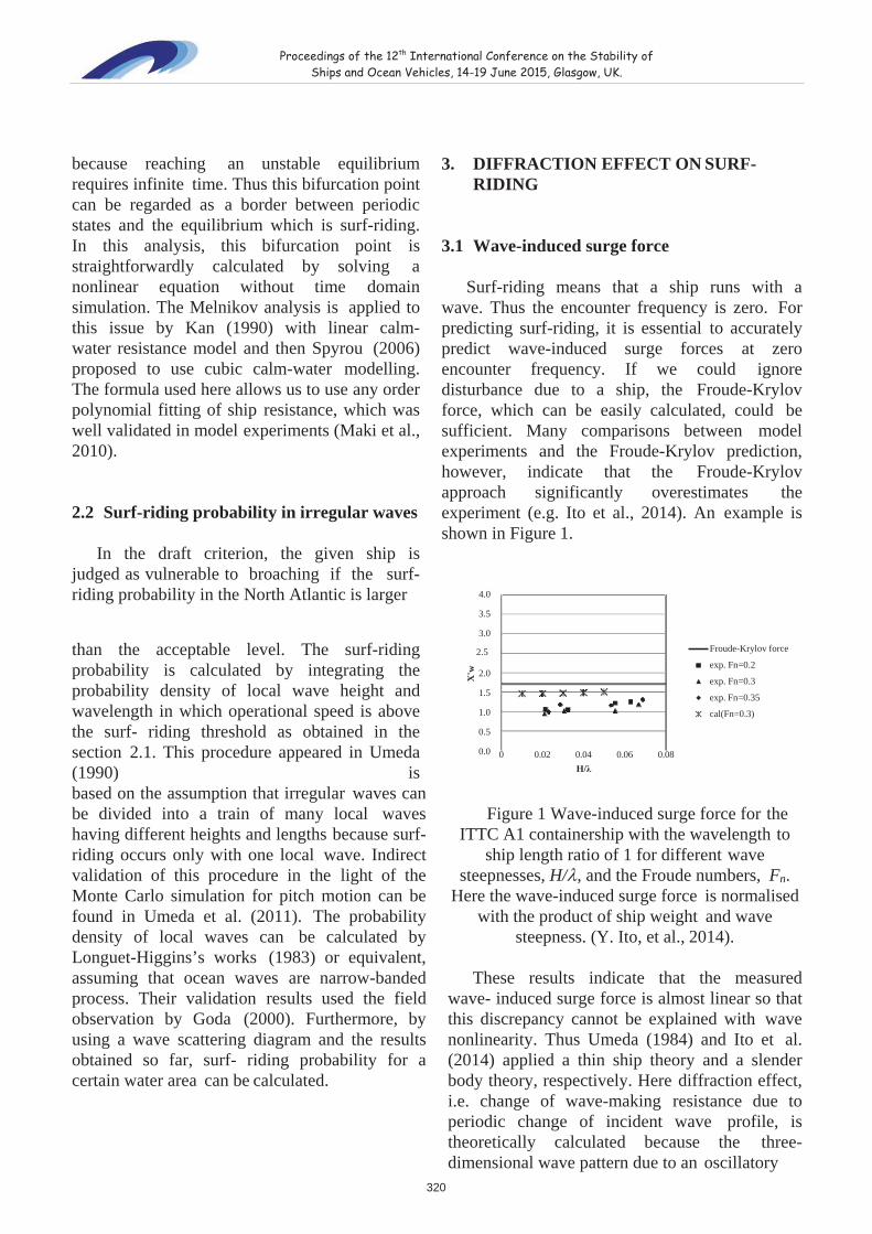
Proceedings of the 12th International Conference on the Stability of Ships and Ocean Vehicles, 14-19 June 2015, Glasgow, UK.
because reaching an unstable equilibrium requires infinite time. Thus this bifurcation point can be regarded as a border between periodic states and the equilibrium which is surf-riding. In this analysis, this bifurcation point is straightforwardly calculated by solving a nonlinear equation without time domain simulation. The Melnikov analysis is applied to this issue by Kan (1990) with linear calm- water resistance model and then Spyrou (2006) proposed to use cubic calm-water modelling. The formula used here allows us to use any order polynomial fitting of ship resistance, which was well validated in model experiments (Maki et al., 2010).
2.2 Surf-riding probability in irregular waves
In the draft criterion, the given ship is judged as vulnerable to broaching if the surf-riding probability in the North Atlantic is larger
3. DIFFRACTION EFFECT ON SURF- RIDING
3.1 Wave-induced surge force
Surf-riding means that a ship runs with a wave. Thus the encounter frequency is zero. For predicting surf-riding, it is essential to accurately predict wave-induced surge forces at zero encounter frequency. If we could ignore disturbance due to a ship, the Froude-Krylov force, which can be easily calculated, could be sufficient. Many comparisons between model experiments and the Froude-Krylov prediction, however, indicate that the Froude-Krylov approach significantly overestimates the experiment (e.g. Ito et al., 2014). An example is shown in Figure 1.
4.0
3.5
3.0
than the acceptable level. The surf-riding probability is calculated by integrating the probability density of local wave height and wavelength in which operational speed is above the surf- riding threshold as obtained in the section 2.1. This procedure appeared in Umeda (1990) is
2.5
2.0
1.5
1.0
0.5
0.0 0 0.02 0.04 0.06 0.08 H/
Froude-Krylov force
exp. Fn=0.2
exp. Fn=0.3
exp. Fn=0.35
cal(Fn=0.3)
based on the assumption that irregular waves can be divided into a train of many local waves having different heights and lengths because surf-riding occurs only with one local wave. Indirect validation of this procedure in the light of the Monte Carlo simulation for pitch motion can be found in Umeda et al. (2011). The probability density of local waves can be calculated by Longuet-Higgins’s works (1983) or equivalent, assuming that ocean waves are narrow-banded process. Their validation results used the field observation by Goda (2000). Furthermore, by using a wave scattering diagram and the results obtained so far, surf- riding probability for a certain water area can be calculated.
Figure 1 Wave-induced surge force for the ITTC A1 containership with the wavelength to
ship length ratio of 1 for different wave steepnesses, H/ , and the Froude numbers, Fn.
Here the wave-induced surge force is normalised with the product of ship weight and wave
steepness. (Y. Ito, et al., 2014).
These results indicate that the measured wave- induced surge force is almost linear so that this discrepancy cannot be explained with wave nonlinearity. Thus Umeda (1984) and Ito et al. (2014) applied a thin ship theory and a slender body theory, respectively. Here diffraction effect, i.e. change of wave-making resistance due toperiodic change of incident wave profile, istheoretically calculated because the three-dimensional wave pattern due to an oscillatory
X'w
320

Proceedings of the 12th International Conference on the Stability of Ships and Ocean Vehicles, 14-19 June 2015, Glasgow, UK.
point source at the zero encounter frequency tends to that due to the Kelvin source. The strength of source distribution can be determined with the hull surface condition with water particle velocity due to waves taken into account. As shown in Figure 1, this diffraction effects explain the discrepancy between the model experiment and the Froude-Krylov prediction to some extent. More quantitative agreement can be achieved with the CFD simulation (Sadat-Hosseini et al., 2011.)
3.2 Diffraction effect on surf-ridingprobability
It was already published that diffraction effect on surf-riding threshold in regular waves is indispensable to avoid inconsistency between
the IMO operational guidance and the draft criteria (Umeda et al., 2011). The critical nominal Froude number for surf-riding estimated with the Froude-Krylov force on its own could be smaller than 0.3, which is requirement of the IMO operational guidance, while that with the measured wave force is larger than 0.3.
As a next step, it is necessary to quantify the diffraction effect on surf-riding probability as the final output of the draft criterion. The comparisons of surf-riding probability with and without diffraction force are conducted as shown in Figures 2-7. The subject ships used here are two containerships, a pure car carrier (PCC), a RoRO ship and two hypothetical war ships. Their principal particulars are shown in Table 1.
Table 1 Principal particulars of the subject ships C11container-ship
ITTC A1 container-ship
RoRo PCC ONR- flare ONR- tumblehome
Length : LBP(m) 262.0 150.0 187.7 192.0 154.0 154.0
Breadth:B(m) 40.0 27.2 24.5 32.26 18.78 18.78 Mean Draught: d(m)
11.5 8.5 6.9 8.18 5.494 5.494
Block coefficient: Cb
0.560 0.667 N/A 0.537 0.536 0.536
Metacentric height: GM (m)
0.56 0.739 1.00 1.25 0.755 2.07
Figure 2 Surf-riding probability for the modified C11 containership with and without diffraction effect.
321

Proceedings of the 12th International Conference on the Stability of Ships and Ocean Vehicles, 14-19 June 2015, Glasgow, UK.
Figure 3 Surf-riding probability for the ITTC A1 containership with and without diffraction effect.
Figure 4 Surf-riding probability for a RoRo ship with and without diffraction effect.
Figure 5 Surf-riding probability for a car carrier with and without diffraction effect.
322

Proceedings of the 12th International Conference on the Stability of Ships and Ocean Vehicles, 14-19 June 2015, Glasgow, UK.
Figure 6 Surf-riding probability for the ONR flare topside vessel with and without diffraction effect.
Figure 7 Surf-riding probability for the ONR tumblehome topside vessel with and without diffraction effect.
These comparisons demonstrate that surf-riding probability without diffraction effect issignificantly larger than that with diffraction effect. As a result, for avoiding inconsistency with the operational requirement, the acceptable probability level is 10-4 with diffraction force and 5 x 10⁻³ without diffraction effect (Japan, 2015).
where P: probability of surf-riding within the time interval of T, p: conditional probability of surf-riding when the ship meets a wave and Te: average of encounter wave period. By using Equation (1), the time interval of non-surf- riding, Ts, can be calculated with Equation (2).
Then a question could arise: this difference in acceptable probability is crucial or not. It can
Ts Te log(1 p) / log(1 P) (2).
be quantify with Equation (1).
P(T ) 1 (1 p)T /Te
(1)
Thus, if we assume Te=10 s and the confidence level of 5 per cent, p=10-4 and 5 x 10⁻³ could result in Te=1.4 hours and 1.7 minutes,
323

Proceedings of the 12th International Conference on the Stability of Ships and Ocean Vehicles, 14-19 June 2015, Glasgow, UK.
respectively. This result clearly indicates that an estimation without diffraction effect is not practical.
4. EFFECT OF CALM-WATERRESISTANCE SAMPLING ON SURF- RIDING
Other than the wave-induced surge force,calm- water ship resistance is an important factor for estimating surf-riding. Prediction of calm-water ship resistance itself is rather a routine for naval architects for guaranteeing ship speed and for complying with the EEDI (Energy Efficiency Design Index) requirement. Modeltest for these purposes, however, is not alwaysexecuted for a given ship design. Thus, it is appropriate to allow the use of speed/power trial. In this case we should examine whether the estimation with only limited number of ship speed is sufficient or not. For providing an answer for this question, the authors attempt to verify the use of speed/power trial in place of model test.
For the sample ships in this paper, we already completed model tests in calm-water up to the Froude number of 0.6. Firstly all available test
data was fitted with a quintic curve. Secondly, to simulate speed/power trial we sampled three conditions, i.e. service speed, maximum service speed and maximum speed, from the model test data. We assumed here that the service speed corresponds to 85 per cent of the MCR (Maximum Continuous Rating), the maximum service speed does 100 per cent of the MCR and the maximum speed does 110 per cent of the MCR. Then the speed/resistance curve is fitted with a quadratic model, which requires three unknown parameters.
Figures 8 and 9 show examples of comparisons of fitted calm-water resistances. As a whole, quintic modelling with all experimental data is quite satisfactory. For the ONR tumblehome topside vessel as shown in Figure 8, the sampled speeds coincides with wave celerity range for wavelength to ship length ratio from 1.0 to 1.2 so that quadratic modelling well agrees with the quintic modelling for higher speed range. For the PCC, the sampled speeds are slower but the agreement with the quintic modelling is not so unsatisfactory. This might be because quadratic modelling, which has only one trough, is more robust than cubic modelling or higher order polynomial modelling.
Figure 8 Calm-water resistance of the ONR tumblehome topside vessel
7000000
6000000
5000000
4000000experiment
3000000
2000000
quadraticapproximationsample points
C(1.0 / 1.21000000 quintic curve
00 5 10 15 20 25
-1000000
-2000000U(m/s)
R(N
)
324

Proceedings of the 12th International Conference on the Stability of Ships and Ocean Vehicles, 14-19 June 2015, Glasgow, UK.
1.00E+00
1.00E-01
1.00E-02
1.00E-03
1.00E-04
1.00E-05
1.00E-06
1.00E-070.28 0.3 0.32 0.34 0.36 0.38 0.4
Froude numberthree sampling full range sampling
Prob
abili
ty
Figure 9 Calm-water resistance of the PCC
Furthermore, surf-riding probabilities of the sample ships are calculated with different calm-water modelling. The results shown in Figures 10-15 demonstrate that surf-riding probabilitieswith three speed sampling well agree with thosewith full range sampling. This could be becausegood agreement of calm- water resistance in thewave celerity range for wavelength to shiplength ratio from 1.0 to 1.2, which is responsiblefor surf-riding prediction.
1.00E+00
1.00E-01
1.00E-02
Figure 11 Effect of calm-water resistance modellng nn surf-riding probability of the PCC
1.00E-03
1.00E-04
1.00E-05
1.00E-06
1.00E-070.28 0.3 0.32 0.34 0.36 0.38 0.4
Froude numberthree sampling full range sampling
Figure 10 Effect of calm-water resistance modellng on surf-riding probability of the
RoRo ship
5. EFFECT OF STOCHASTIC WAVETHEORIE
In the draft criterion, it is necessary tocalculate the joint probability density function of wave height and wavelength in a stationary seaway specified as a wave spectrum with Longuet- Higgins’s work (1983) or equivalent. In 1957 Longuet-Higgins derived the formula by using the joint probability density of amplitude and phase of wave envelope. Here the relationship between the local wave period,
25000000
20000000
experiment15000000
quadraticapproximation
sample points10000000
C(1.0 /L 1.2 quintic curve
5000000
00 5 10 15
U(m/s)20 25 30
R(N
)
Prob
abili
ty
325

Proceedings of the 12th International Conference on the Stability of Ships and Ocean Vehicles, 14-19 June 2015, Glasgow, UK.
1.00E+00
1.00E-01
1.00E-02
1.00E-03
1.00E-04
1.00E-05
1.00E-06
1.00E-070.28 0.3 0.32 0.34 0.36 0.38 0.4
Froude numberthree sampling full range sampling
1.00E+00
1.00E-01
1.00E-02
1.00E-03
1.00E-04
1.00E-05
1.00E-06
1.00E-070.28 0.3 0.32 0.34 0.36 0.38 0.4
Froude numberthree sampling full range sampling
Prob
abili
ty
T, and wave envelope phase, , was simplified as
was pointed out that this formula cannot explain the physically observed fact that short local waves have smaller wave local height.
T 2 /( )
T01 (1 )
(3)
(4)
Then, in 1983, Longuet-Higgins revised his own formula with more precise relationship between the local wave period and wave envelope phase, i.e. Equation (3) in place of Equation (4). As a result, he resolved the draw back of his original formula.
Figure 12 Effect of calm-water resistance modellng on surf-riding probability of the C11
class containership Figure 14 Effect of calm-water resistance modellng on surf-riding probability of the ONR
flare topside vessel
1.00E+00
1.00E-01
1.00E-02
1.00E-03
1.00E-04
1.00E-05
1.00E-06
Figure 13 Effect of calm-water resistance modellng on surf-riding probability of the
ITTC A1 containership
where T01 is the mean wave period, is the mean wave circular frequency and a dot indicates differentiation with time. Later on it
1.00E-070.28 0.3 0.32 0.34 0.36 0.38 0.4
Froude numberthree sampling full range sampling
Figure 15 Effect of calm-water resistance modellng on surf-riding probability of the ONR
tumblehome topside vessel
1.00E+00
1.00E-01
1.00E-02
1.00E-03
1.00E-04
1.00E-05
1.00E-06
1.00E-070.28 0.3 0.32 0.34 0.36 0.38 0.4
Froude numberthree sampling full range sampling
Prob
abili
tyPr
obab
ility
Prob
abili
ty
326

Proceedings of the 12th International Conference on the Stability of Ships and Ocean Vehicles, 14-19 June 2015, Glasgow, UK.
1.E+00
1.E-01
1.E-02
1.E-03
1.E-04
1.E-05
1.E-06
1.E-07 0.28 0.32 0.36 0.4
Fn
Longuet-Higgins(1983)Longuet-Higgins(1957)
validated with the Monte Carlo simulation by Umeda et al. (2007). The failure probability is calculated by integrating the probability density of local wave height and wavelength on the region in which capsizing due to broaching occurs in systematic time domain simulation using a coupled surge-sway-yaw-roll model with an autopilot in periodic waves. Here capsizing is defined as the roll angle of 90 degrees or over and the rudder gain is 1.
Figure 16 Effect of the wave probability formulae on surf-riding probability of the
RoRo ship
It is indispensable for practical application of them to quantify effect of these two different formulae on surf-riding probability. Thus the authors executed comparison studies using the subject ships. The result shown in figure 16 as an example indicates the difference in surf- riding probability is negligibly small. This could be partly because the subject ships are longer so that they do not respond to smaller waves. Thus it can be presumed that at least the use of the formula in Longuet-Higgins (1983) is recommended although a similar study using a smaller ship is desirable.
6. RELATIONSHIPS WITH BROACHING
If a ship does not comply with the draft criterion for surf-riding, it is expected that her safety against capsizing due to surf- riding/broaching is examined with the direct stability assessment, in which failure probability in irregular seaways is directly estimated with a numerical time-domain simulation. This is because surf-riding is only a prerequisite for broaching or capsizing.
For verifying this approach, the authors calculate also probability of capsizing due to broaching in the North Atlantic. The calculation method used here was proposed and
1.E+00
1.E-01
1.E-02
1.E-03
1.E-04
1.E-05
1.E-06
1.E-070.28 0.3 0.32 0.34 0.36 0.38 0.4
Froude number
Figure 17 Comparisons between surf-riding probability and probability of capsizing due to broaching for the ONR tumblehome topside
vessel.
The results shown in Figure 17 indicate that the probability of capsizing due to broaching is smaller than the surf-riding probability. Thus we can conclude that the draft criterion for surf-riding guarantees safety against capsizing due to broaching. It is noteworthy here that in critical speed range around the Froude number of 0.3 the difference between the two is rather small. This means that the safety margin is not so large.
7. CONCLUSIONS
For reasonably evaluating surf-riding probability to be used for design and operational criteria, diffraction effect on wave- induced surge force is indispensable, calm- water resistance can be modelled with model tests covering the Froude number up to 0.6 or standard speed/power trials and choice of stochastic wave theory is not crucial. The evaluated surf-riding probability is a conserva-
SurfRiding Probability
prpbability of capsizing due to broach
Prob
abili
ty
Prob
abili
ty
327

Proceedings of the 12th International Conference on the Stability of Ships and Ocean Vehicles, 14-19 June 2015, Glasgow, UK.
tive index for capsizing due to broach.
ACKNOWLEDGEMENTS
This work was supported by JSPS (JapanSociety for Promotion of Science) KAKENHI Grant Number 24360355 and 15H02327. It was partly carried out as a research activity of Goal-based Stability Criteria Project of Japan Ship Technology Research Association in the fiscal year of 2013, funded by the Nippon Foundation. The authors appreciate Mr. William Peters from United States Coast Guard and Dr. Vadim Belenky from David Taylor Model Basin for their usefuldiscussion.
REFERENCES
Goda Y., 2000, “Random seas and design of maritime structures”, Advanced Series on Ocean Engineering, Vol. 15.World Scientific Pub Co Inc, Singapore.
IMO, 1995, “Guidance to the Master for Avoiding Dangerous Situations in Following and Quartering Seas, MSC/Circ. 707.
Ito, Y., N. Umeda and H. Kubo, 2014, “Hydrodynamic Aspects on Vulnerability Criteria for Surf-Riding of Ships”, Jurnal Teknologi, Vol. 66, No. 2, pp. 127-132.
Japan, 2014, “Information collected by the Correspondence Group on Intact Stability”, IMO, SDC 2/INF.10.
Kan, M. 1990, “A Guideline to Avoid the Dangerous Surf-riding”, Proceedings of the 4th International Conference on Stability of Ships and Ocean Vehicles, University Federico II of Naples (Naples), pp.90-97.
Longuet-Higgins, M.S., 1983, “On the joint distribution of wave periods and amplitudes in a random wave field”, Proc. Roy., Soc.
London, Ser. A, Vol. 389, pp. 241-258.
Longuet-Higgins, M.S., 1957, “The statistical
analysis of a random, moving surface”, Phil. Trans. Roy., Soc. London, Ser. A (966), Vol. 249, pp. 321-387.
Maki, A., N. Umeda, M. Renilson and T. Ueta, 2010, “Analytical Formulae for Predicting the Surf- Riding Threshold for a Ship in Following Seas”, Journal of MarineScience and Technology, Vol.,15, No.3, pp.218-229.
Sadat-Hosseini, H., P. Carrica, F. Stern, N.
Umeda et al., 2011, “CFD, system-based and EFD study of ship dynamic instability events:Surf-riding, periodic motion,and broaching”,OceanEngineering, Vol. 38, pp. 88-110.
Spyrou, K.J., 2006, “Asymmetric Surging of Ships in Following Seas and its Repercussion for Safety”, Nonlinear Dynamics, Vol.43, pp.149-172.
Umeda, N., 1984, “Resistance Variation and Surf- riding of a Fishing Boat in Following Sea”, Bulletin of National Research Institute of Fisheries Engineering, No. 5, pp. 185-205.
Umeda, N. , 1990, “Probabilistic Study on Surf-riding of a Ship in Irregular Following Seas”, Proceedings of the 4thInternational Conference on Stability ofShips and Ocean Vehicle, Naples, pp.336-343.
Umeda, N., Shuto, M. and Maki, A., 2007, “Theoretical Prediction of Broaching Probability for a Ship in Irregular Astern Seas“, Proceedings of the 9th International Ship Stability Workshop, Hamburg, pp. 1.5.1-1.5.7.
Umeda, N., S. Izawa, H. Sano, H. Kubo and K. Yamane, 2011, “Validation Attempts on Draft New Generation Intact Stability Criteria”, Proceedings of the 12th 328

Proceedings of the 12th International Conference on the Stability of Ships and Ocean Vehicles, 14-19 June 2015, Glasgow, UK.
International Ship Stability Workshop, Washington D.C., pp.19-26.
Umeda N., Yamamura S., Matsuda, A., Maki, A. and Hashimoto, H., 2008, “Model Experiments on Extreme Motions of a Wave-Piercing Tumblehome Vessel in Following and Quartering Waves”, Journal of the Japan Society of Naval Architects and Ocean Engineers ,Vol. 8, pp. 123-129.
329

This page is intentionally left blank
330

Proceedings of the 12th International Conference on the Stability of Ships and Ocean Vehicles, 15-19 June 2015, Glasgow, UK.
Numerical Prediction of Parametric Roll Resonance in Oblique Waves
Naoya Umeda, Osaka University [email protected]
Naoki Fujita, Osaka University [email protected]
Ayumi Morimoto, Osaka University [email protected]
Masahiro Sakai, Osaka University [email protected]
Daisuke Terada, National Research Institute of Fisheries Engineering, [email protected]
Akihiko Matsuda, National Research Institute of Fisheries Engineering, [email protected]
ABSTRACT
Numerical prediction of parametric roll in head and following waves has been intensively investigated so that requirements for reasonably good prediction are almost revealed. On the other hand, prediction of parametric roll in oblique waves has not yet been sufficiently established. This is because coupling with sway and yaw motions are unavoidable. Since parametric roll for actual ships occurs with very low forward velocity, even accurate prediction of lee ways in waves is not so easy. Therefore, in this study, the authors present a numerical model of parametric roll in oblique waves with low-speed manoeuvring forces taken into account. Then the numerical prediction was compared with newly executed free-running model experiments of a hypothetical ship. Its results demonstrate the present model shows reasonably good agreement with the experiment. This information could be used for identifying minimum requirements for good prediction of parametric roll in oblique waves. Keywords: parametric rolling, IMO, Second generation intact stability criteria, direct stability assessment, operational guidance
1. INTRODUCTION
Although danger of parametric rolling had been well known among scientists (e.g. Watanabe, 1934), the accident of a C11 class post Panamax containership (France, 2003) induced extensive studies on this phenomenon. As a result, several numerical models for parametric rolling were developed and some of them were well validated with model experiments in head and following waves (Reed, 2011). These models deal with coupled heave-pitch-roll motions by using simultaneous nonlinear differential equations and the hydrodynamic coefficients used in the equations are calculated with potential theories
and empirical viscos force estimation. Time dependence of roll restoring coefficient, including coupling from other modes and diffraction moment depending on heel angle, is indispensable.
Based on such progress in research for parametric rolling, at the International Maritime Organisation (IMO), stability criteria for preventing parametric roll is now under development (Umeda, 2013). They consist of three layers: the first and second layers use simplified estimation of occurrence and magnitude of parametric roll in head and following waves with averaging method applied to uncoupled roll model with restoring variation; the third layer means direct use of numerical simulation in time domain of
331

Proceedings of the 12th International Conference on the Stability of Ships and Ocean Vehicles, 15-19 June 2015, Glasgow, UK.
coupled roll model in irregular waves. For the latter case, the numerical models mentioned before could be used. It is noteworthy here that the third layer requires not only calculation in head and following waves but also in oblique waves. This is because we have to evaluate safety for all ship courses. For oblique waves, validation efforts for existing numerical models Sanchez & Nayfeh, 1990; Neves & Valerio, 2000) were not sufficient so far partly because a model experiment requires a seakeeping and manoeuvring basin and partly because coupling with manoeuvring motion including rudder actions are unavoidable.
Based on this understanding, the authors attempted to validate a numerical simulation model taking low-speed manoeuvring model in oblique waves with a newly executed model experiment in a seakeeping and manoeuvring basin. This numerical model is an extension of the model published in Hashimoto and Umeda (2011) for head and following waves, which were well validated with model experiments of containerships and a car carrier in the towing tank of Osaka University. The ship used in this paper is a typical ship having large flare and transom stern, i.e. a hypothetical ship known as the ONR flare topside vessel, of which hull form is open for public. At this stage comparisons in regular oblique waves are ready to be published. Comparisons in irregular oblique waves are a task for future. In this paper, details of the numerical model are described for facilitating development of the guidelines for the direct assessment at the IMO.
2. NUMERICAL MODEL FOR PARAMETRIC ROLL IN OBLIQUE WAVES
2.1 Coordinate systems and equations of coupled motions
The coordinate systems used here are shown in Figure 1. The space-fixed coordinate system is O1- the coordinate system
moving with a constant speed of U and course of is O2-XYZ and the body-fixed coordinate system is G-xyz. Here we assume that a wave propagates in the direction of O1 axis. The ship oscillates around the O2-XYZ. G indicates the centre of ship mass and O1G0 indicates initial depth of centre of ship mass. The ship motions around the O2-XYZ are denoted by xi:surge (i=1), sway (i=2), heave (i=3), roll (i=4), pitch (i=5) and yaw (i=6).
Figure 1 Coordinate systems
The coupled sway-heave-roll-pitch-yaw motions are modelled as follows:
x4
O1 O2, Y
Gx3+O1G0x2
Z
z
y
x6
Wave
O1
O2
Gx1
x2
Y
x
U
y
X
Wave
O1 O2 , X
Gx
z
x3+O1G0
Z
x5
332

Proceedings of the 12th International Conference on the Stability of Ships and Ocean Vehicles, 15-19 June 2015, Glasgow, UK.
),,,,,,,,,,,,,,,(
),,,,,,,,,,,,,,,(),,,,,,,,,,,,,,,(
),,,,,,,,,,,,,,,(),,,,,,,,,,,,,,,(
65432654326543266
65432654326543255
65432654326543244
65432654326543233
65432654326543222
txxxxxxxxxxxxxxxFxI
txxxxxxxxxxxxxxxFxItxxxxxxxxxxxxxxxFxI
txxxxxxxxxxxxxxxFxmtxxxxxxxxxxxxxxxFxm
zz
yy
xx
(1)
where m: ship mass, Ixx: moment of inertia of ship mass in roll, Iyy: moment of inertia of ship mass in pitch, Izz: moment of inertia of ship mass in yaw, t: time and Fj: force or moment in the j direction. A dot denotes differentiation with time. Here we assume that the surge motion x1 is zero, for avoiding estimation of added mass, so that the ship runs with a constant velocity and a straight course. The forces are modelled with Equation (2).
DELj
MLSj
EGj
Dj
FKj
Bj
Rjj FFFFFFFF (2)
where the superscript R indicates the radiation component, B the component due to hydrostatic pressure, FK the component due to incident wave pressure, D the diffraction component, EG component due to gravity, MLS the hull force due to manoeuvring motion and DEL the force due to rudder action.
2.2 Buoyancy and Froude-Krylov Forces
If we assume incident waves are sinusoidal, their profile, w, and wave pressure, p, are given by Equations (3-4).
tg kk
aw
2
cos (3)
tgg
gp kk
wk
a
22
cosexp (4)
where : water density, a: wave amplitude, g:gravitational acceleration, k: wave circular frequency and t: time. Here water pressure is adjusted to be zero at the wave surface
although this is a higher order correction under the assumption of small wave steepness.
Then submerged hull surface, SH, can be determined with Equation (5).
),,,,( 543 xxxSS wGHH (5)
By integrating the water pressure on the wetted hull surface, the buoyancy, Fj
B, and Froude-Krylov forces, Fj
FK, can be calculated as follows:
L S jBj
H
dsndxgF (6)
L S jFKj
H
dsdxpnF (7)
where L indicates the range of hull in x direction. The gravitational force, F3
EG, in the vertical direction are given by
3EGF mg (8).
2.3 Radiation and Diffraction Forces
The radiation force, FiR, can be calculated
as follows:
6
2444 ))()((
jjijjijjij
Ri xxCxxBxxAF (9)
where the added mass, Aij, the wave damping coefficient, Bij, and the restoring coefficient, Cij,are given by
L HL HL H dxAAdxAAdxAA 242423232222 ,,
L HL H dxxAAdxxAA 22262325 ,
L HL HL H dxAAdxAAdxAA 343433333232 ,,
L HL H dxxAAdxxAA 32363335 ,
L HL H dxAAdxAA 43434242 ,
333

Proceedings of the 12th International Conference on the Stability of Ships and Ocean Vehicles, 15-19 June 2015, Glasgow, UK.
L HL H dxxAAdxxAA 42464345 ,
L HL H dxxAAdxxAA 33533252 ,
L H dxxAA 3454
L HL H dxAxAdxAxA 322
56332
55 ,
L HL HL H dxxAAdxxAAdxxAA 246423632262 ,,
L HL H dxAxAdxAxA 222
66232
65 ,
L HL HL H dxBBdxBBdxBB 242423232222 ,,
L HL H dxAUdxxBB 232325
L HL H dxAUdxxBB 222226
L HL HL H dxBBdxBBdxBB 343433333232 ,,
L HL H dxAUdxxBB 333335
L HL H dxAUdxxBB 323236
,, 43434242 L HL H dxBBdxBB
L HL H dxAUdxxBB 434345
L HL H dxAUdxxBB 424246
L HL H dxAUdxxBB 323252
L HL H dxAUdxxBB 333353
L HL H dxAUdxxBB 343454
L HL HL H dxxAUdxBxBdxBxB 32322
56332
55 ,
L HL H dxAUdxxBB 222262
L HL H dxAUdxxBB 232363
L HL H dxAUdxxBB 242464
L HL H dxBxBdxBxB 222
66232
65 ,
L HL H dxBUCdxBUC 22262325 ,
L H dxBUC 3335
L H dxBUC 4345
L H dxBUC 2446
L HL H dxAUdxxBUC 332
3355
L HL H dxAUdxxBUC 322
3256
L HL H dxAUdxxBUC 232
2365
L HL H dxAUdxxBUC 222
2266
HS ijHij
Hij dsnB
iA.
Here j and ni are the velocity potential of two-dimensional flow with hull and linear free surface condition and normal vector to the hull surface. The added mass and damping in roll are estimated as follows:
2
44 2T
GMWAI xx (10)
34444444 xxxxxB (11).
The and T can be estimated with roll decay test of a ship model.
The diffraction force, FjD, can be calculated
as follows (Salvesen et al., 1970):
))(cos()( 44 xtxFF Dkje
Dkja
Dj (12)
where
Dkj
Dkj EF
334

Proceedings of the 12th International Conference on the Stability of Ships and Ocean Vehicles, 15-19 June 2015, Glasgow, UK.
Dkj
Dkj Earg
dsnx
UidxigE jDS kL
aDkj
H
)(
cos)/( 2 Ugkke
And D is the diffraction velocity potential of two-dimensional flow with hull and linear free surface condition in incident waves.
2.4 Manoeuvring Forces
Since parametric roll occurs at low speed, it is desirable to estimate manoeuvring forces with a mathematical model suitable for such situation where ship forward velocity is comparable to ship lateral velocity (Umeda & Yamakoshi, 1989). The hull manoeuvring forces, Fi
MLS, can be estimated as the sum of linear lift components, YL and NL, and nonlinear cross-flow drag components, YC and NC, as follows:
LCMLS YYF2
LCMLS NNF6 (13)
where
2/
2/21 L
LDC dxrxvrxvCdY
2/
2/21 L
LDC xdxrxvrxvCdN
rYvYY rvL
rNvNN rvL
6261 sincos xxxxUu
6261 cos sin xxxxUv
6xr
'21
vppv YudLY
'21 2
vppv NudLN
'21 2
rppr YudLY
'21 3
rppr NudLN
Here u and v are the surge and sway velocity defined with the body-fixed coordinate system G-xyz, respectively. CD is the cross-flow drag coefficient when the ship is laterally towed.
The rudder-induced forces, FiDEL, are
calculated as follows:
fuAaF RRHDEL 2
2 211
fuAxaxF RRHHRDEL 2
6 21
(14)
where
6xK P
281
JKuu T
pR
Uwu pp )1(
p
p
nDu
J
cbJaJK T2
281
Jc
Jbauu pR
2
2281pp
p uDcn
ubnDau
2222 8 DcnbnDuauuu pppp
Here : rudder angle, aH: the interaction factor for rudder force between hull and rudder, xH:the longitudinal position of rudder force due to
335

Proceedings of the 12th International Conference on the Stability of Ships and Ocean Vehicles, 15-19 June 2015, Glasgow, UK.
interaction between hull and rudder, xR: the longitudinal rudder position, AR: the rudder area, f : the hydrodynamic rudder lift slope, KP:the rudder gain, n: the propeller revolution number, DP: the propeller diameter, KT: the rudder gain, : the wake ratio between propeller and rudder. The flow straightening effect is ignored.
The system parameters for manoeuvring forces and moments, such as CD and Yv, can be estimated with captive model experiment of a ship. In this paper, we used the coefficients measured in the circular motion tests of the C11 class post Panamax containership, whose hull form is similar to the ONR flare topside vessel.
3. MODEL EXPERIMENTS
For validating a numerical model for parametric rolling in oblique waves, experiments using a 1/48.8 scaled model of the 154m-long ONR flare topside vessel were executed at the seakeeping and manoeuvring basin of National Research Institute of Fisheries Engineering, based on the ITTC recommended procedure on intact stability model test (ITTC, 2008). The ship was propelled with an electric motor and two propellers and steered with two rudders. The propeller RPM was controlled to be a constant and the auto pilot was used with the rudder gain of 1.0. The roll, pitch and yaw angles were measured by a fibre optical gyroscope.
Table1 Principal Particulars of the ONR Flare topside vessel
Length : L pp 154.0 [m] 3.158 [m]
Breath : B 19.65 [m] 0.403 [m]
Depth : D 15.2 [m] 0.312 [m]Draught : d 5.753 [m] 0.118 [m]
Displacement : W 9733 [ton] 83.93 [kg]Longitudinal position of center of
buoyancy from the midship : LCB6.45 [m]
aft0.132 [m]
aft
Radius of gyration in pitch : K yy /L pp 0.272 0.272
Block coefficient : C b 0.536 0.536
Metacentric height : GM 0.8095 [m] 0.0166 [m]
Natural roll period : T 21.11[s] 3.023 [s]
Figure 2 Body plan of the the ONR Flare topside vessel
Figure 3 GZ variations of the ONR flare topside vessel in longitudinal waves whose wavelength to ship length ratio is 1.25 and the wave steepness is 0.03.
Figure 4 Steady amplitude of parametric roll in oblique waves.
0
5
10
15
20
25
-60-50-40-30-20-100
Para
met
ric
Rol
l Am
plitu
de (d
egre
es)
Heading Angle (degrees)
Calculation
Experiment
calculated scattered range
wave trough amidship wave crest amidship
336

Proceedings of the 12th International Conference on the Stability of Ships and Ocean Vehicles, 15-19 June 2015, Glasgow, UK.
The principal particulars and body plan of the subject ship are shown in Table 1 and Figure 2, respectively.
The experiment shown here is executed for regular astern waves. The wavelength to ship length ratio is 1.25 and the wave steepness is 0.03. Under this wave condition, the GZ curve of this vessel definitely changes due to longitudinal waves as shown in Figure 3. The auto pilot course ranges from 0 degrees from the wave direction to 70 degrees but no parametric roll occurred for the auto pilot course of 70 degrees. The propeller RPS is set to be 72, which corresponds to the Froude number of 0.05 in calm water. In addition, speed trials, roll decay tests and propeller open test were executed for this ship model.
4. RESULTS AND DISCUDSSION
The numerical results are compared with the experimental results as shown in Figure 4. Here the steady amplitude for each condition is plotted. An example of numerical runs is shown in Figure 5. In this case the roll motion is settled to a steady periodic state. The roll period is twice the pitch period, and is nearly equal to the ship natural roll period. Thus this can be judged as a typical parametric rolling. Similarly, in the auto pilot course of -30 degrees the steady periodic state was simulated as shown in Figure 6. However, in case of the auto pilot course of -40 degrees as shown in Figure 7, the calculated roll angle does not settled to a periodic state. Similar complicate response was reported by Hashimoto & Umeda (2004) with an uncoupled roll model with parametric and direct excitation. Thus this could be a future task with nonlinear dynamics.
The calculated values slightly overestimate the measured values. Good agreement between the two can be found at the heading angle of 0 degrees but some discrepancies can be found in case of oblique waves. The heading angle is rather different from the specified autopilot course. This could indicate that steady wave
forces and manoeuvring forces could have some roles.
Figure 5 Time series of roll and pitch angles with the auto pilot course of -10 degrees.
Figure 6 Time series of roll angle with the auto pilot course of -30 degrees.
Figure 7 Time series of roll angle with the auto pilot course of -40 degrees.
The largest roll amplitude occurs at the heading angle different from head waves both
337

Proceedings of the 12th International Conference on the Stability of Ships and Ocean Vehicles, 15-19 June 2015, Glasgow, UK.
in experiment and calculation. However, when the heading angle further increases, the roll amplitude decreases. This is due to the shift of encounter frequency together with the reduction of roll restoring variation.
5. CONCLUSIONS
Parametric roll in regular oblique waves was realised in free-running model experiments. The 5 degrees-of-freedom numerical model slightly overestimates the experimental results. The numerical model used here includes nonlinear Froude-Krylov components, radiation / diffraction components as functions of roll angle and manoeuvring forces. The roll amplitude decreases with the increasing heading angle but the largest roll occurs with non-head waves. Non periodic roll response was found in one case of numerical simulation. Following this preliminary validation, wider validation studies in oblique waves will be executed with different ships and different wave heading in the near future.
6. ACKNOWLEDGEMENTS
This work was supported by JSPS (Japan Society for Promotion of Science) KAKENHI Grant Number 24360355 and 15H02327. It was partly carried out as a research activity of Goal-based Stability Criteria Project of Japan Ship Technology Research Association in the fiscal year of 2013, funded by the Nippon Foundation. The authors thank Prof. H. Hashimoto, Mses. F. Yoshiyama and N. Yamashita for their effective assistance during the work described here.
7. REFERENCES
France, W.N., Levadou, M., Treakle, T.W. et al., 2003, “An Investigation of Head-Sea Parametric Roll and Its Influence on Container Lashing System”, Marine Technology, 40(1), pp.1-19.
Hashimoto, H. and N. Umeda, 2004, “Nonlinear analysis of parametric rolling in longitudinal and quartering seas with realistic modeling of roll-restoring moment”, Journal of Marine Science and Technology, Vol. 9, pp. 117-126.
Hashimoto, H. and Umeda, N., 2010, “A Study on Qualitative Prediction of Parametric Roll in Regular Head Wave”, Proceedings of the 10th International Ship Stability Workshop, Wageningen, pp.295-301.
ITTC, 2008: Recommended Procedures, Model Tests on Intact Stability, 7.5-02-07-04.
Neves, M.A.S. and Valerio, L. 2000, “Parametric Resonance in Waves of Arbitrary Heading”, Proceedings of the 7th International Conference on Stability and Operational Safety of Ships and Ocean Vehicles, Launceston, B, pp. 680-687.
Reed, A.M., 2011, "26th ITTC Parametric Roll Benchmark Study", Proceedings of the 12th International Ship Stability Workshop, Washington D.C., pp. 195-204.
Salvesen, N., Tuck, E.O. and O. Faltinsen, 1970, “Ship Motions and Sea Loads”, Transaction of the Society of Naval Architects and Marine Engineers.
Sanchez, N.E. and Nayfeh, A.H. 1990, “Rolling of Biased Ships in Quartering Seas”, Proceedings of the 18th Symposium on Naval Hydrodynamics, Michigan.
Umeda, N. and Y. Yamakoshi, 1989, “Hydrodynamic Forces Acting on a Longitudinally Non-symmetric Ship Under Manoeuvring at Low Speed”, Journal of the Kansai Society of Naval Architects, No. 211, 127-137, (in Japanese.)
Umeda, N. 2013, "Current Status of Second Generation Intact Stability Criteria", Proceedings of the 13th International Ship Stability Workshop, Brest, pp. 138-157.
338

Proceedings of the 12th International Conference on the Stability of Ships and Ocean Vehicles, 15-19 June 2015, Glasgow, UK.
Watanabe, Y., 1934, “On the Dynamical Properties of the Transverse Instability of a Ship due to Pitching”, Journal of the Society of Naval Architects, Vol. 53, pp. 51- 70 (in Japanese)
339

This page is intentionally left blank
340

Proceedings of the 12th International Conference on the Stability of Ships and Ocean Vehicles, 14-19 June 2015, Glasgow, UK.
Numerical Simulation of the Ship Roll Damping
Min Gu, China Ship Scientific Research Center, Wuxi, China [email protected]
Jiang Lu, China Ship Scientific Research Center, Wuxi, China [email protected]
Shuxia Bu, China Ship Scientific Research Center, Wuxi, China [email protected]
Chengsheng Wu, China Ship Scientific Research Center, Wuxi, China [email protected]
Gengyao Qiu, China Ship Scientific Research Center, Wuxi, China [email protected]
ABSTRACT
The roll damping is a critical hydrodynamic coefficient for predicting roll motion. In this paper, the forced roll motion of a 2-dimensional ship section and free roll motion of a 3-dimensioinal hull are simulated based on the RANS model in calm water. For the forced rolling, firstly, the influences of different calculation parameters are investigated through the methods of orthogonal design and variance analysis. Then the simulations about different roll amplitudes are carried out based on the selected parameters. For the free rolling, the free decay experiments and numerical simulations are performed. These calculated results are agreed well with experimental data, which validate the presented method can yield satisfactory results for roll damping coefficients.
Keywords: roll damping; RANS; forced rolling; free rolling
1. INTRODUCTIONThe roll damping is a critical hydrodynamic
coefficient for predicting roll motion, such as parametric rolling and stability under dead ship condition. The roll damping coefficient should be predicted with high accuracy. The vulnerability criteria are under development by the International Organization (IMO) of the second generation of intact stability criteria, in which the roll damping have been calculated by Ikeda`s (1977, 1978, 1979, 2000, 2004) simplified method. These formulas can be used quite well for the conventional ship, but the predicted results are sometimes conservative or underestimated for unconventional ships (Japan, 2011a, Japan, 2011b, Sweden, 2011). This is because the roll damping is strongly nonlinear, which has some direct relationships with fluid viscosity and flow characteristics, such as the flow separation and vortex shedding. So the experience or semi-experience formulas can`t
take the full consideration of different characteristics for different objects. The calculated results of most traditional ships by Ikeda’ method can fit experimental data well at the same order magnitude. However, if the size is outside the application range of Ikeda’ method, or for the large amplitude roll motion in some phenomena, such as parametric rolling, the accuracy will be low in these conditions, which limit the scope of application of Ikeda’ method.
The corresponding group of IMO proposed that the roll damping could be calculated by roll decay / forced roll test or CFD (United States & Japan, 2014). Although the model tests can predict the roll damping very well, but it is costly and time-consuming as well as most of experimental data are limited to a certain frequency range and particular geometry, which is impossible for the large-scale
341

Proceedings of the 12th International Conference on the Stability of Ships and Ocean Vehicles, 14-19 June 2015, Glasgow, UK.
expansion of the application (Blok & Aalbers, 1991, Haddara & Bass, 1988).
The influence of viscosity should be considered during the calculation of roll damping. The CFD numerical simulation can consider different objects and its characteristic, which can also reduce the cost. With the development of CFD technology, the turbulent models have been improved, such as RANS model, discrete vortex method. In addition, the fine structure of the flow field can also be analyzed by CFD, so CFD could be widely used to predict roll damping. Forced roll method and free decay method are two main methods for calculation of the roll damping.
K.B.Salui et al. (2000), Ronald et al. (2002), Miller&Stern (2002), Salui & Vassalos (2003), Frederick Jaouen et al.(2011) simulated forced roll motions for different kinds of ship or two-dimensional ship sections using the RANS model. Wilson et al. (2006) predicted the roll decay of a DTMB Model 5512 hull based on the RANS technique. Miller et al. (2008) conducted roll decay and forced roll simulations using DTMB Model 5415 based on the RANS approach. Sun kyun Lee et al. (2011) performed CFD simulations for the roll damping of a damaged passenger ship by solving RANS equations. These results are in good agreement with the experimental data. The above analysis proved that the roll damping coefficients can be accurately solved using RANS approach.
In this paper, firstly the forced motions of two dimensional ship section of Series 60 based on the orthogonal design and variance analysis are carried out, in which different calculation parameters for roll damping are analyzed. Secondly, the free motions of a three dimensional 4250TEU containership have been simulated. The comparisons between the computed results and the experimental results proved that the roll damping can be predicted by RANS-based method. These can provide
technical support for the development of second generation intact stability criteria.
2. FORCED ROLLING
For the forced roll motion, the section of Series 60 is chosen, as experimental tests on its forced roll have been conducted by Ikeda (Ikeda et al. 1977). The same principles are used in the simulations, as shown in table 1. During the calculation, the roll center is located in the intersection between waterline and mid-perpendicular. The formula (1) is used for the roll motion. Then formula (2) is used to get the dynamic moment. Finally, formulas (3) are used to get the roll damping coefficients and non-dimensional coefficients.
Table 1 Principal particulars of S.S.5.
Section B T KG
S.S.5 0.237m 0.096m 0.096m
Where B is the width of model; T is the draught; KG is the vertical height of center of gravity.
)sin( to (1)
( ) ( )
( )
d y zs
d z ys
M t z y ds
p n y n z ds (2)
gB
BBBMRB
2ˆ
244
440
44 (3)
Where 0 is the initial roll amplitude, is the initial phase, is the shear stress on the surface of the hull, pd is the dynamic pressure on the surface of the hull, Md is the instant roll moment at the maximum rolling angular velocity, is the volume for the model.
342

Proceedings of the 12th International Conference on the Stability of Ships and Ocean Vehicles, 14-19 June 2015, Glasgow, UK.
Table 2 Calculation conditions
Cases 0 (rad)
1 0.58 0.1 2 0.58 0.15 3 0.58 0.175
The calculation conditions are shown in table 2. Where 2B g , is the frequency of rolling. We can see that the non-dimensional frequency ( ) is equal to 0.58, and the initial roll amplitudes are 0.1rad, 0.15rad, 0.175rad, 0.22rad respectively.
2.1 Orthogonal design
The simulation results can be affected by different parameters, such as the mesh quantity, mesh quality(y+), turbulent mode, boundary condition and discretization method. In order to find out the best combination of these parameters, we choose the initial roll amplitude 0 =0.175rad to analyze these influencing factors based on the orthogonal design and variance analysis. According to the previous studies, the values of y+ are always very small during the forced roll motion, especially for ships with bilge keels, so the enhance wall function is used, in which y+ is approximately 1. The discretization method is SIMPLE which has a wide application. Finally, we focus our attentions on the following factors: mesh quantity, turbulent model and boundary condition.
The ship section is 16m, so we chose a circular section as the calculating domain, whose diameter is approximately 12.5 times of the model`s width (D ≈ 12.5B), and the boundary conditions including 3 parts: (1) the upper boundary of the circular domain; (2) the bottom boundary of circular domain; (3) the section surface, as shown in figure 1.
For the part of mesh quantity, we choose 10 thousands mesh as a benchmark. Three
different kinds of mesh quantities are 10 thousands, 20 thousands and 40 thousands based on the geometric proportion increasing and decreasing design, as shown in figure 2. The selection of turbulent model should consider the practicality and efficiency. In this paper, we studied standard k-ω model (s k-ω), SST k-ω and RNG k-ε. The boundary conditions are all walls, all velocity-inlet, the bottom boundary of circular domains wall and the upper boundary of circular domains pressure-outlet, respectively.
Fig.1 The boundary conditions
Fig.2 The part of the calculating domain (mesh quantity=40 thousands)
According to above analysis, we can get the table of factors and levels, as shown in table 3. The orthogonal layout and the two columns interaction layout L27(313) are selected after considering the columns and degrees (Wei & Wu, 2013), and the layout is shown in table 4, in which the 9,10,12,13 are blank columns (error columns).
Table 3 Factors and levels
343

Proceedings of the 12th International Conference on the Stability of Ships and Ocean Vehicles, 14-19 June 2015, Glasgow, UK.
LevelFactor
A:Meshquantity
B:Meshquality
C:Boundarycondition
1 A1: 10t B1:sst k-ω C1: 2 walls
2 A2: 20t B2: s k-ω C2: 2 vel
3 A3: 40t B3:RNG k-ε C3: 1wall+1pre
Table 4 Top design of the calculation program
Factor A B (A×B)1 (A×B)2 C (A×C)1 (A×C)2 (B×C)1 (B×C)2
Num 1 2 3 4 5 6 7 8 9 10 11 12 13
2.2 Variance analysis
The numerical simulations for the combination of different parameters have been conducted based on RANS model. The VOF method is used for the free surface modeling. The pressure-correction algorithm of SIMPLE type is used for the pressure-velocity coupling. The modified HRIC is used for the discretization of VOF equation, and the dynamic mesh technique is used by UDF. The non-dimensional roll damping coefficients can be got by formula (3). We selected several y+ values from two calculating cases, and the results show that the enhanced wall function was appropriate, as shown in figure 3.
The non-dimensional coefficients were got for different computational schemes. Then the
significance of the test was investigated through the table of variance analysis, as shown in table 5. During the variance analysis, the relative errors between simulation results and experimental results were adopted as the analyze benchmark.
Case -1Case -2
Fig. 3 The value of y+
Table 5 Variance analysis
Soruce of variation
Quadraticsum-S
Degree of freedom-f
Meansquare-V F Significance Fa
A0.61 2 0.30 10.64 **
F0.05(2,12)=3.89B 0.47 2 0.23 8.18 ** C 0.34 2 0.17 5.86 * F0.01(2,12)=6.93A×B 0.52 4 0.13 4.52 * A×C 0.17 4 0.04 1.45 F0.05(4,12)=3.26B×C 2.12 4 0.53 18.50 ** e 0.61 2 0.30 F0.01(4,12)=5.41
344

Proceedings of the 12th International Conference on the Stability of Ships and Ocean Vehicles, 14-19 June 2015, Glasgow, UK.
The values of F showed that the factor B×C (the interaction between turbulent model and boundary condition), the factor A (mesh quantity) and the factor B (turbulent model) have large influence on the results. The factor A×B (the interaction between mesh quantity and turbulent model) and the factor C (boundary condition) also have effects on the results, but the effects are not obvious compared with the above three factors.
The collocation table of B and C was listed to seek the best combination, as shown in table 6. The results showed that the combination of B1and C1, B1 and C2 were both available. However, we find that the combination of B1 and C1 was easier to convergence and the computational process was more stable during the calculation, so we choose the combination of B1 and C1 as the best combination.
Table 6 The match of B and C
B1 B2 B3C1 0.33 1.76 1.23C2 1.35 2.79 2.26C3 0.25 1.69 1.16
Statistical hypothesis: the influence of controlled and control factors on results have no significant difference.
This hypothesis can be proved by formula (4). The results showed that the factors are significant differences, which meanings other factors which have not been taken into consideration have little effect on the results during our numerical simulation. Therefore the appropriate turbulent model and boundary condition as well as the mesh quantity can get good results on forced roll simulations. We should note that the enhanced wall function is adopted during the calculation. Otherwise, the results were not consistent with the actual situation. This means the mesh quality (y+) has the most important effect on the results. The current results can only be adopted on the premise of the guarantee of y+.
(4)
From the above analysis we see that: on the guarantee of y+, the design of A2 (40 thousands mesh), B1 (SST k-ω), C1 (all boundary conditions are walls) is the best combination.
2.3 The calculation results and analysis
Based on the above combination, more research about other conditions were conducted, and the results are shown in figure 4. This figure shows a comparison between the numerical simulation results and experimental results, we can see that the results are in good accordance with the experimental results, so the combination is feasible.
Fig.4 The non-dimensional damping coefficients for different roll amplitudes
3. THE FREE ROLLING
For the free roll decay motion, the object is a 4250TEU containership due to the availability of experimental data for validation. The free roll decay simulations were performed based on the unsteady RANS model and compared to experimental data.
173818
415818188
050
010
.),(
.),(.
//
.
.
FF
fSfSF
ee
345

Proceedings of the 12th International Conference on the Stability of Ships and Ocean Vehicles, 14-19 June 2015, Glasgow, UK.
3.1 Experiment
The principal particulars and body plan of this containership are shown in table 7 and figure 5, respectively. Roll decay experiments were performed with a 1/62.97 scaled model at the seakeeping basin (length: 69m, breadth: 46m, height: 4m) of CSSRC (China Ship Scientific Research Center), as shown in figure 6. The initial roll angle was 25 degrees in calm water.
Fig. 5 Lines of 4250TEU containership
Table 7 Principal particulars of the 4250TEU Containership
Items Ship Model Length: L 251.88m 4.0m
Draft: T 12.6m 0.2m
Breadth: B 32.2m 0.511m
Depth: D 19.3m 0.3065m
GM 1.62m 0.0257m
Tφ 21.19s 2.7s
Kyy 0.3L 0.3L
Fig.6 The ship model in free decay test
3.2 Simulation
In this paper, the simulations of roll decay at 25 degrees initial roll angle in calm water were performed. During the simulation, the VOF method is used for the free surface modeling. A pressure-correction algorithm of SIMPLE type is used for the pressure-velocity coupling. The SST k-ω model is incorporated for turbulence modeling. The solution domain is formed in two parts: the first part (S1) moves with the body, and the second part (S2) is fixed, as shown in figure 7. For the purpose of wave absorption, two artificial damping zones were located at the second part (S2), which is far away from the hull.
3.3 Comparison
The results of numerical simulations of roll decay histories were compared with the experimental results, as shown in figure 8. It shows that the period agrees well with the experimental data with the growth of the time. However, the amplitude of CFD becomes a little larger than the experiment. The future calculations are needed to verify these phenomena.
346

Proceedings of the 12th International Conference on the Stability of Ships and Ocean Vehicles, 14-19 June 2015, Glasgow, UK.
Fig. 7 The solution domain in free decay
Fig. 8 The comparison of experimental results and numerical simulation of free decay
4. CONCLUSIONS
As a result of experimental and numerical study on roll damping by the forced rolling with two dimensional ship sections of Series 60 and by the free rolling with a 3-dimensioinal hull based on the RANS model, the following remarks are noted:
1) For the forced motion, an applicable results of roll damping can be got based on the combination of enhance wall function, SST k-ωmodel, the wall boundary conditions as well as the appropriate mesh quantity.
2) For the free roll motion, the roll motion of a 3-dimensioinal hull based on the RANS model in calm water was simulated, and the results were in reasonable agreement with the experimental results.
3) Both the forced rolling and free rolling based on RANS approach have the abilities to predict the roll damping.
4) More works should be made in future to improve calculating accuracy of roll damping, especially for free roll motion condition.
5. ACKNOWLEDGEMENTS
This research is supported by Ministry of Industry and Information Technology of China (No. [2012] 533). The authors sincerely thank the above organization.
6. REFERENCES
Blok, J.J. and Aalbers. A.B., 1991, “Roll Damping Due to Lift Effects on High Speed Monohulls”, FAST`91.
Frederick Jaouen, Arjen Koop, Guilherme Vaz, 2011, “Predicting Roll Added Mass and Damping of a Ship Hull Section Using CFD”, Proceedings of the ASME 2011 30th
International conference on ocean, offshore and arctic engineering, Netherlands.
Haddara, M.R. BASS, D.W., 1988, “Non-linear Models of Ship Roll Damping”,International Shipbuilding Progress, 35/401, pp. 5-24.
Japan, 2011a, “Interim Verification and Validation Report on Simplified Roll Damping”, IMO SLF 54/INF 12, Annex 7.
Japan, 2011b, “Additional Validation Data on Simplified Roll Damping Estimation for Vulnerability Criteria on Parametric Rolling”, IMO SLF 54/INF 12, Annex 11.
K.B.Salui and D.Vassalos, 2003, “A RANS Based Technique to Compute Forced Rolling Responses in Three-Dimensional Flows”, Computational Fluid Dynamic Technology in Ship Hydrodynamic, UK, pp. 13-18.
347

Proceedings of the 12th International Conference on the Stability of Ships and Ocean Vehicles, 14-19 June 2015, Glasgow, UK.
K.B.Salui, Tanmay Sarkar and Dracos Vassalos, 2000, “An Improved Method for Determining Hydrodynamic Coefficients in Roll Motion Using CFD Techniques”, Ship Technology Research, Vol. 47, pp.161-174.
Robet Wilson and Fred Stern, 2002, “Unsteady RANS Simulation of a Surface Combatant with Roll Motion”, 24th Symposium on Naval Hydrodynamics Fukuoka, Japan.
Miller,R., W. Gorski J.J., and Fry, D.J. 2002, “Viscous Roll Predictions of a Circular Cylinder with Bilge Keels”, 24th Symposium on Naval Hydrodynamics Fukuoka, Japan.
Miller, R., W. Bassler C.C., ec al.. 2008, “Viscous Roll Predictions for Naval Surface Ships Appended with Bilge Keels using URANS”, 27th Symposium on Naval Hydrodynamics, Seoul, Korea.
Sungkyun Lee, Ji-Myoung You, 2011, “Free Roll Decay Study of a Damaged Ship for CFD Validation”, Proceedings of the ASME 2011 30th International conference on ocean, offshore and arctic engineering, Netherlands.
Sweden, 2011, “Evaluation of Ikeda's simplified method for prediction of roll damping”, IMO SLF 54/3/6.
United States and Japan, 2014, “Draft Guidelines of Direct Stability Assessment Procedures as a Part of the Second Generation Intact Stability Criteria, IMO SDC1/INF.8, Annex 27.
Wei Ze, Wu Chengsheng, Ni Yang, 2013, “Optimum Hydrodynamic Design of Helical Strake on Spar Platforms Based on Orthogonal Design and CFD Method”, Journal of Ship Mechanics, Vol. 17, PP.
1133-1139.
Wilson, R.V. and Fred Stern, 2002, “Unsteady RANS Simulation of a Surface Combatant with Roll Motion”, 24th Symposium on Naval Hydrodynamics Fukuoka, Japan.
Wilson, R.V., Carrica, P.M., and Stern, F, 2006, “Unsteady RANS method for ship motions with application to roll for a surface combatant”, Computers and Fluids, Vol. 35(5), pp. 501-524.
Yoshiho Ikeda, Yoji Himeno and Norio Tanaka, 1977, “On Eddy Making Component of Roll Damping Force on Naked Hull”, Journal of the society of Naval Architects of Japan. Vol. 142.
Yoshiho Ikeda, Yoji Himeno and Norio Tanaka, 1978, “Components of Roll Damping of Ship at Forward Speed”, Journal of the society of Naval Architects of Japan, Vol. 143.
Yoshiho Ikeda, Yoji Himeno and Norio Tanaka, 1979, “On Roll Damping Force of Ship-Effect of Hull Surface Pressure Created by Bilge Keels”, Journal of the society of Naval Architects of Japan, Vol. 165
Yoshiho Ikeda and Katayama,T., 2000, “Roll Damping Prediction Method for a High-Speed Planning Craft”, Proceedings of the 7th International Conference of Ships and Ocean Vehicles (STAB’2000),Vol. 2, PP. 532-541.
Yoshiho Ikeda, 2004, “Prediction Methods of Roll Damping of Ships and Their Application to Determine Optimum Stabilization Devices”, Marine Technology.
348

Proceedings of the 12th International Conference on the Stability of Ships and Ocean Vehicles, 14-19 June 2015, Glasgow, UK.
Investigation of the Applicability of the IMO SecondGeneration Intact Stability Criteria to Fishing Vessels
Marcos Míguez González, GII, University of A Coruña, Spain [email protected]
Vicente Díaz Casás, GII, University of A Coruña, Spain [email protected]
Luis Pérez Rojas, Model Basin, ETSIN, Technical University of Madrid [email protected]
Daniel Pena Agras, GII, University of A Coruña, Spain [email protected]
Fernando Junco Ocampo, GII, University of A Coruña, Spain [email protected]
ABSTRACT
In this work, the vulnerability of seven fishing vessels of mid and small size, representative of the Spanish fleet, to some of the failure modes covered by the IMO Second Generation Intact Stability Criteria, has been studied. The latest draft proposals for Level 1 and 2 checks for parametric roll, pure loss of stability and dead-ship condition, as presented in the IMO SDC 1 (2013), have been applied to the aforementioned sample vessels. The results are commented, and some notes regarding the applicability of this criteria a as a design tool are also included.
Keywords: Second generation intact stability criteria, parametric roll, pure loss of stability, dead ship condition, fishing vessels stability
1. INTRODUCTION
The Second Generation Intact StabilityCriteria have been under development by the IMO SLF Sub-Committee for the last ten years, beginning in the 48th session of the SLF (Peters et al., 2011). The main aim of these criteria is to increase the ship safety by quantifying its tendency to experiencing one of the so called failure modes. These are basically dynamic instabilities derived from the interaction while sailing between the ship and the waves and wind, and which are not covered by the traditional intact stability requirements. These failure modes include five phenomena: parametric roll resonance, loss of stability in stern waves, broaching, dead-ship condition and excessive accelerations.
The structure of the criteria is the same for all the aforementioned failure modes. They
follow a three level arrangement: the Level 1 represents the easiest method of evaluation, and also the most conservative one. If the vessel fails to comply with Level 1, a Level 2 check has to be carried out, where a more detailed evaluation, also more complicated, is proposed. Finally, if the vessel is also find to be vulnerable under Level 2 criteria, a direct assessment has to be done, where stability operational guidelines have to be developed from the detailed analysis of more realistic sailing situations.
Regarding the development of the criteria, their current status can be found in the report of the Correspondence Group on Intact Stability to the SDC 1. Parametric roll and loss of stability draft criteria have been already agreed and draft explanatory notes developed, broaching and dead-ship condition draft criteria and explanatory notes are also available and
349

Proceedings of the 12th International Conference on the Stability of Ships and Ocean Vehicles, 14-19 June 2015, Glasgow, UK.
excessive acceleration criteria are still under discussion (IMO SDC 1/5/3, 2013).
Second generation intact stability criteria are mainly focused on cargo and passenger ships; although some fishing vessels have been considered in the different applicability analysis of the criteria (three vessels in IMO SLF55/Inf.15 (2012a) and IMO SDC 1/Inf.8 (2013) and two in IMO SLF55/Inf.15 (2012b)), they´re very few compared to the rest of the typologies.
The fleet of fishing vessels is the largest worldwide. Moreover, the fishing activity is known for being one of the most dangerous industrial activities in many countries, such as Spain (MIT, 2014), U.K. (Roberts, 2010) or the U.S. (BLS, 2013).
Most of the effort spent on increasing the safety of fishing vessels has been directed at improving the crew training in the fields of static stability (cargo stowage, post- construction modifications, overloading and reduction in freeboard) and ship operation (flooding prevention) (Míguez-González et al.,2012a). In fact, fishing vessel stability criteria, with the exception of the IMO Weather Criterion (which is not mandatory for all of them), are based on static stability principles. However, dynamical instabilities (parametric roll, loss of stability, broaching, dead ship condition) are also known to affect fishing vessels and to be the possible cause of many accidents (Mata-Alvarez-Santullano & Souto- Iglesias, 2014). And neither of them are analysed during the vessel design process or included within crew training programs.
Related to this fact, and in addition to their possible implementation as mandatory requirements, the application of second generation intact stability criteria as complementary design tools, could lead to very important increases in the safety of this type of vessels. So, the main objective of this work is to evaluate the suitability of the proposed second generation intact stability criteria to
fishing vessels, and their application as a design tool to improve their safety levels from the dynamic stability point of view.
In order to do this, the draft second generation intact stability criteria proposed in IMO SDC 1/Inf.8 (2013), including parametric roll, pure loss of stability and dead-ship condition failure modes, have been applied to a sample of seven fishing vessels. These are representative of the different typologies present on the Spanish fleet of mid-sized fishing vessels, including trawlers, longliners and purse seiners, with lengths ranging from 20 to 70 meters. From the obtained results, the vulnerability of the different vessels to the aforementioned failure modes and the suitability of these draft criteria as a first stage design tool have been analysed.
2. TEST VESSELS
One of the main characteristics of thefishing vessel fleet is its vast heterogeneity; the arrangement of the different ships depends on the used fishing gear, on tradition and regional factors or on regulatory issues. This fact makes it very difficult to analyse fishing vessels as a whole. In our case, the mid-sized Spanish fishing fleet, which is the largest in Europe in terms of tonnage, has been selected (EU Commission, 2014). From this, we focused on the vessels of more than 20 m long (usually operating in open seas), which in the Spanish case, are more than 1400 units (MAGRAMA, 2013).
The selected ships try to cover all the main typologies present on the aforementioned fleet, and two medium sized stern trawlers (named Trawler 1 and 2), one large stern trawler (Large Trawler), one longliner (Longliner), one medium size purse seiner (Purse Seiner) and one large tuna purse seiner (Tuna Purse Seiner), were chosen. Experimental head sea data of the Trawler 2, is available in Míguez- González et al. (2012b).
350

Proceedings of the 12th International Conference on the Stability of Ships and Ocean Vehicles, 14-19 June 2015, Glasgow, UK.
Table 1: Vessel characteristics (1). Table 4: Tested Conditions. Vessel LPp (m) B (m) d (m)
Trawler 1 25.70 8.50 3.25 Trawler 2 29.00 8.00 3.30 Large Trawler 60.60 12.50 4.60 Longliner 24.00 8.20 3.20 Purse Seiner 21.00 7.00 2.70 Tuna Purse Seiner 67.60 14.00 4.80 TS Trawler (d1) 22.00 6.90 2.30 TS Trawler (d2) 22.00 6.90 2.46
Table 2: Vessel characteristics (2).
Table 3: Vessel characteristics (3). Vessel AL (m2) Z (m) fl (deg)
Trawler 1 145 4.47 64.3 Trawler 2 162 4.38 65.4 Large Trawler 415 5.57 53.6 Longliner 120 4.09 68.6Purse Seiner 83 3.50 54.3 Tuna Purse Seiner 361 7.60 69.1 TS Trawler (d1) 95 3.37 57.2 TS Trawler (d2) 91 3.37 57.2
Moreover, and for comparison purposes, a typical U.K. beam trawler (named TS Trawler), which has been broadly studied (Neves & Rodríguez, 2006), has also been selected.
The main characteristics of the analysed vessels are included in Tables 1 and 2. In Table 3, some of the parameters needed for the evaluation of the IMO Weather Criterion are presented, where AL is the projected lateral area over the waterline, Z is the distance from the centre of AL to the half of the mean draft and fl is the first downflooding angle.
Regarding the tested loading conditions, in all cases the design draft has been selected; in the case of the TS Trawler, two different drafts, for which experimental data are available (Paffet, 1976), have been chosen. When the real GM was available for the selected draft, that was the applied value; in addition, another condition with the minimum GM according to the Torremolinos Protocol (350 mm), was also defined for these cases. When no data was available, the minimum GM of 350 mm was selected.
The natural roll frequency for all cases was computed by using a roll radius of gyration (including added inertia) of 0.43·B, estimated from the experimental data in Míguez- González et al. (2012b). In all cases, no bilge keels were considered (ABK = 0), and the design speed was chosen to compute the reference ship speed (VPR).
3. CRITERIA DESCRIPTION
In this work, the vulnerability of theselected vessels to parametric roll, pure loss of stability and dead-ship condition failure modes have been analysed by applying the proposals contained in the different annexes of IMO SDC 1/Inf.8 (2013). Parametric roll criteria and their explanatory notes are contained in Annexes 1 and 3; pure loss of stability criteria and their explanatory notes in Annexes 2 and 4; and
Vessel LPp/B B/D D/d Cb Cm
Trawler 1 3.02 1.51 1.73 0.56 0.85 Trawler 2 3.63 1.38 1.76 0.57 0.86 Large Trawler 4.85 1.63 1.66 0.54 0.88 Longliner 2.93 1.41 1.81 0.68 0.90 Purse Seiner 3.00 2.19 1.19 0.67 0.89 Tuna Purse Seiner 4.83 1.54 1.90 0.53 0.93 TS Trawler (d1) 3.19 2.06 1.46 0.47 0.74 TS Trawler (d2) 3.19 2.06 1.36 0.48 0.75
Vessel Fn d(m)
GMT
(m) 0
(rad/s) Trawler 1 LC1 0.32 3.25 0.653 0.692 Trawler 1 LC2 0.32 3.25 0.350 0.507 Trawler 2 0.31 3.30 0.350 0.539 Large Trawler 0.31 4.60 0.350 0.345 Longliner LC1 0.34 3.20 0.495 0.625 Longliner LC2 0.34 3.20 0.350 0.526 Purse Seiner 0.36 2.70 0.350 0.616 Tuna Purse Seiner LC1 0.34 4.80 0.916 0.498 Tuna Purse Seiner LC2 0.34 4.80 0.350 0.308 TS Trawler LC1 0.32 2.30 0.730 0.902
TS Trawler LC2 0.32 2.46 0.436 0.697
351

Proceedings of the 12th International Conference on the Stability of Ships and Ocean Vehicles, 14-19 June 2015, Glasgow, UK.
dead-ship condition criteria in Annex 16. The draft explanatory notes of dead-ship condition are included in IMO SDC 1/Inf.6 (2013).
3.1 Parametric roll
The phenomenon of parametric roll is generated by the variation of the roll restoring term due to the wave passing along the hull. Its effects are more intense in longitudinal waves, when the wave encounter frequency approximates the double of the ship roll natural frequency. Under these conditions, roll motion can reach very large amplitudes.
The parametric roll vulnerability criteria are divided into two levels, both based on the analysis of the GM variation in longitudinal waves. In the Level 1, the GM in calm water is compared to the amplitude of GM variation(ΔGM) in a longitudinal wave of wavelength equal to ship length and a constant steepness of SW = 0.0167. The ship is considered vulnerable if:
Where RPR represents roll linear damping, that may be taken as 0.5 or a value dependant on bilge keel area and midship coefficient.
The Level 2 presents two checks. The first one is similar to that of Level 1, but computations have to be made for a set of 16 waves, with different lengths and steepness’s, and the results of each wave case have to be weighted and summed up. Moreover, an additional requirement that takes into account the vessel forward speed has to be also considered. According to this first check, the ship will be considered vulnerable if:
Where RPR0 is 0.06 or 0.1, Wi is the wave case weight and Ci is a coefficient equal to 1 if the ship is vulnerable under GM and speed checks, and 0 if not. GM vulnerability checks are the same as those of the first level criterion, but computed for each of the wave parameters. The ship is considered as vulnerable if:
GM (Hi , i ) 0 (3)
G M (Hi , i ) RPRGM (Hi , i )
(4)
The speed requirement consists on comparing the design speed of the ship (VD)and a reference speed for parametric roll appearance (VPRi), which depends on the metacentric height on waves and calm water, on wave conditions and on natural roll period. Although not specified in the rules, for a ship with two very different sailing conditions (such as trawlers), it could be important, in order to accurately evaluate this requirement, to take into account the two possible sailing speeds. In any case, the ship is considered vulnerable if:
VPRi VD (5)
If the ship is found to be vulnerable under the first check, a second check has to be done. This has a similar structure to the previous one; the ship will be considered vulnerable if:
GM RGM PR
(1)
N
C1 WiCi RPR0i 1
(2)
N
C2 WiCi RPR1i 1
(6)
352

Proceedings of the 12th International Conference on the Stability of Ships and Ocean Vehicles, 14-19 June 2015, Glasgow, UK.
In this case, Wi is again the wave case weight (which are obtained from a wave scatter diagram with 306 wave cases) and Ci is a coefficient equal to 1 if the roll motion of the ship, computed by using an uncoupled equation of roll motion, is over 25 degrees, and 0 if it is not.
3.2 Pure loss of stability
The reduction of the transverse stability of the ship, when it sails in stern seas and wave crest persists for a long time near amidships, is the cause of this failure mode. In waves of wavelength similar to ship length, and in low stability conditions, it could lead to large roll and even capsizing.
Pure loss of stability criteria are only of application to ships of length of more than 24 m and speeds of Froude over 0.2, 0.26 or 0.31 (to be decided), and are also divided into two levels. Level 1 is similar to that of the parametric roll failure mode, and consists on evaluating the minimum GM (GMmin) when a wave of wavelength equal to ship length and a constant steepness of SW = 0.0334 passes the ship. The vessel would be considered as vulnerable if:
where RPLA is the minimum value between0.05 m and a speed and draft dependant factor.
The second level check consists of three criteria (CRj), computed for two possible set of waves (16 or 306 cases).
Each CRj is obtained by weighting the coefficients Cji, which are evaluated for each wave condition; C1i is equal to 1 if the angle of vanishing stability ( v) is over 30 degrees or the angle of steady heel in waves ( s) is over15 or 20 degrees; C2i is equal to 1 if the maximum loll angle ( loll) is over 25 degrees; and C3i is equal to 1 if the maximum GZ value is under 8 (H / ) d Fn2 .
So, the ship is considered vulnerable if:
max(CR1,CR2 ,CR3 ) RPL0 (9)
Where RPL0 is 0.06 for the first set of waves and 0.15 if the second option is adopted.
3.3 Dead-ship condition
The dead ship condition of a ship takes place when all of its machinery becomes out of operation, disabling its propulsive and manoeuvring capabilities. Under these conditions, the vessel may be affected by severe beam wind and waves, not being able to escape this dangerous situation. The objective of the dead ship stability criteria, is to ensure that the ship is able to withstand the effect of the aforementioned beam excitations for a given amount of time.
As in the case of the previous two failure modes, they are divided into two levels. The Level 1 check corresponds to the well-known IMO Weather Criterion (Severe Wind and Rolling Criterion), included in the IMO 2008 Intact Stability Code, but with a modification on the wave steepness’s for large draft vessels.
The Level 2 assessment proposes a probabilistic approach for evaluating the vessel vulnerability to the analysed failure mode. The procedure consists on determining the long term vulnerability of the ship by computing the coefficient C; if it is under the reference value
GM min RPLA (7)
N
CR j 1:3 WiCjii 1
(8)
353

Proceedings of the 12th International Conference on the Stability of Ships and Ocean Vehicles, 14-19 June 2015, Glasgow, UK.
of 10-3, the ship is considered as non- vulnerable.
To obtain this long term coefficient, a short term vulnerability index CS is computed for different wave and wind conditions, characterized by the significant wave height (HS), the zero crossing period (TZ) and the wind speed (UW). Once computed, the C index is obtained as a weighted average of the CS
values:
The short term environmental conditions, together with the probability weighting factors (W (HS, TZ)), are obtained by applying the North Atlantic scatter diagram (IACS Recommendation 34), although other wave cases may be accepted.
The short term vulnerability index is obtained by considering the ship as a 1 d.o.f. linear system which rolls under the action of beam irregular waves and gusty winds, which spectra are obtained from the corresponding short term wave characteristics (HS, TZ). After obtaining some parameters from the residual righting lever curve under the effect of steady wind moment, the roll standard deviation and zero crossing frequency corresponding to the wave and wind moment spectra are obtained by solving the roll equation in frequency domain.
The short term vulnerability index represents the probability of capsizing in the analysed conditions in a given exposure time (3600 s in this case), and is computed from the vessel roll characteristics defined above and two virtual capsizing angles, obtained by equalling the area under the residual righting lever curves and a linearized (in the equilibrium heel angle due to steady wind), residual righting lever curve.
In the method draft explanatory notes (IMO SDC 1/Inf.6, 2013), in addition to the
description of the applied methodology, a procedure for computing the effective wave slope coefficient and an alternative methodology for computing the CS index are also included. Moreover, a method for estimating the necessary roll damping coefficients is presented, based on the least squares fitting of the equivalent linear roll damping coefficient obtained by the Ikeda method for different roll amplitudes.
4. RESULTS AND DISCUSSION
In this section, the results obtained from theapplication of parametric roll, pure loss of stability and dead-ship condition criteria are presented and commented. The ones corresponding to the first two failure modes, have been already presented in Míguez- González et al. (2014), where draft requirements described in IMO SLF 55/WP.3 (2013) for parametric roll, loss of stability and broaching, were applied to the same sample vessels.
4.1 Parametric roll
In this case, Level 1 and Level 2 first check have been carried out. The Level 1 results are shown in Table 5, where ΔGM is the GMvariation on the specified waves and ΔGMalt isthe alternative GM variation in waves computed considering the waterplane inertias at drafts dh and dl. The Level 2 first check results are shown in Table 6. There, ΔGMmax is the maximum GM variation for all the 16 wave cases, GMavg is the corresponding average GMfor that wave case and VPR is the reference ship speed for resonance in that conditions.
According to the results, all ships, excepting the Large Trawler and the Tuna Purse Seiner in the low GM condition, pass Level 1 check.
C (W (HS ,TZ ) CS (HS ,TZ ,UW ))HS TZ
(10)
354

Proceedings of the 12th International Conference on the Stability of Ships and Ocean Vehicles, 14-19 June 2015, Glasgow, UK.
Table 5: Parametric roll. Level 1 results.
Table 6: Parametric roll. Level 2 results. 1st check.
obtained. So, both of them have been considered as non-vulnerable, while experimental data have shown their large tendency to developing parametric roll. However, the small wave heights and probabilities (weighting factors, which represent a small probability for the ship facing them in real sailing), associated with the waves of small wavelength that correspond to these ships length, is the cause of this consideration. Moreover, the results obtained for the Tuna Purse Seiner were also compared to experimental data available, showing a good consistency.
From the different typologies of vessels studied, it can be seen that those ships with larger bow flares and hanging sterns, such us trawlers and the tuna purse seiner, are the most vulnerable to this failure modes, presenting the largest GM variations from all the sample.
4.2 Pure loss of stability
Pure loss of stability criteria are of application to all the sample ships, as their speeds are, in all cases, equal or over Fn =0.31. Level 1 and Level 2 (Option A, 16 reference wave cases) checks have been carried out. The results of the Level 1 check are presented in Table 7, where GMmin is the minimum GM as the specified wave passes the ship, and GMmin_alt is the alternative minimum
Regarding Level 2 check, all ships pass the criteria for all wave cases (C1 = 0). The criteria, for these vessels, are consistent, as no vessel is found to be non-vulnerable under Level 1 and vulnerable under Level 2.
In Míguez-González et al. (2014) and references therein, these results were analysed and compared to experimental data present in the literature, in order to analyse the suitability of the criteria to these small vessels. In the cases of the Trawler 2 and the TS Trawler, small variation of GM in waves has been
GM computed considering the waterplane inertia at draft dL. The Level 2 results are presented in Table 8, where GZmax is the minimum smallest GZ curve maximum for all the 16 wave cases, v , s and loll arerespectively the vanishing stability, the steady heel and the loll angles for that condition and RPL3 is the vulnerability limit for the presented GZmax.
As can be seen, the largest vessels (Large Trawler and Tuna Purse Seiner in the two loading conditions), together with the TS Trawler in the low GM condition, are found to be vulnerable under Level 1 check.
Vessel GM(m)
GMalt(m) GM/GM Level
1Trawler 1 LC1 0.090 0.164 0.251 Pass Trawler 1 LC2 0.090 0.164 0.468 Pass
Trawler 2 0.102 0.133 0.379 Pass Large Trawler 0.109 0.251 0.718 Fail Longliner LC1 0.051 0.062 0.126 Pass Longliner LC2 0.051 0.062 0.178 Pass Purse Seiner 0.035 0.046 0.130 Pass
Tuna Purse Seiner LC1 0.154 0.295 0.322 Pass
Tuna Purse Seiner LC2 0.153 0.295 0.843 Fail
TS Trawler LC1 0.095 0.205 0.281 Pass TS Trawler LC2 0.107 0.181 0.414 Pass
Vessel GMmax (m)
GMavg (m)
GMmax/GMavg
VPR
(m/s)Level
2Trawler 1
LC1 0.075 0.650 0.115 1.186 Pass
Trawler 1 LC2 0073 0.347 0.211 2.040 Pass
Trawler 2 0.085 0.353 0.241 0.728 Pass Large
Trawler 0.104 0.360 0.287 1.707 Pass
Longliner LC1 0.044 0.495 0.089 1.110 Pass
Longliner LC2 0.045 0.349 0.128 0.935 Pass
Purse Seiner 0.034 0.352 0.097 1.171 Pass
Tuna Purse Seiner LC1 0.152 0.895 0.169 2.090 Pass
Tuna Purse Seiner LC2 0.152 0.330 0.460 3.069 Pass
TS Trawler LC1 0.090 0.719 0.125 1.019 Pass
TS Trawler LC2 0.100 0.444 0.225 0.473 Pass
355

Proceedings of the 12th International Conference on the Stability of Ships and Ocean Vehicles, 14-19 June 2015, Glasgow, UK.
Table 7: Pure loss of stability. Level 1 results.
Table 8: Pure loss of stability. Level 2 results. Option A.
Trawler 2, and although some reduction of stability in stern seas has been shown in the literature, no capsizing occurred in any of the tested conditions. So, results seem to be consistent also for this vessel. Again, the vessels with larger bow flares and hanging sterns (trawlers and tuna purse seiner), are shown to be more vulnerable than the others.
4.3 Dead-ship condition
As have been already mentioned, the Level 1 and Level 2 dead-ship condition checks have been carried out. In Table 9, the intact stability characteristics of the different vessels are shown (all GM values are over the minimum, as shown in Table 4). As it can be seen, there are two vessels, the Trawler 1 and the TS Trawler in the low GM conditions, which do not fulfil the minimum requirements stated by the Torremolinos Protocol.
Regarding the Level 1 check, in Table 10 the obtained results are presented. There, 0 isthe angle of equilibrium under the steady wind heel lever, 1 is the windward roll angle and 2
Regarding Level 2 check, all vessels were found to be non-vulnerable (all criteria were fulfilled in all wave cases), and criteria are consistent for this set of vessels.
Like in the case of parametric roll failure mode, in Míguez-González et al. (2014) and references therein, the obtained results were compared with available experimental data. Regarding both the TS Trawler and the Tuna Purse Seiner, a large tendency to capsizing in stern seas has been described, showing a good agreement between the vulnerability analysis and the towing tank test data. In the case of the
is the minimum between the downflooding angle and 50 degrees. a and b are the areas under the GZ and wind heeling lever curves stated in the IMO Weather Criterion. It can be appreciated that all ships, with the exception of the TS Trawler, but including the Trawler 1 in the low GM condition (LC2), pass the Level 1 check.
In Table 11, the results of the Level 2 check are presented. In there, Smax is the maximum steady heel angle for all the wave conditions tested, σ Smax is the maximum roll standard deviation, TZ max is the maximum roll zero crossing period and C, is the long term probability failure index.
Vessel GMmin (m)
GMmin_alt (m) Level 1
Trawler 1 LC1 0.452 0.488 Pass Trawler 1 LC2 0.148 0.184 Pass
Trawler 2 0.172 0.075 Pass Large Trawler 0.193 -0.147 Fail Longliner LC1 0.391 0.342 Pass Longliner LC2 0.246 0.197 Pass Purse Seiner 0.276 0.231 Pass
Tuna Purse Seiner LC1 0.626 0.028 Fail Tuna Purse Seiner LC2 0.060 -0.540 Fail
TS Trawler LC1 0.520 0.105 Pass TS Trawler LC2 0.271 -0.113 Fail
Vessel GZmax (m)
v(deg)
s(deg)
loll(deg) RPL3
Level 2
Trawler 1 LC1 0.422 90 0 0 0.084 Pass
Trawler 1 LC2 0.199 70 0 0 0.085 Pass
Trawler 2 0.746 125 0 0 0.075 Pass Large
Trawler 0.187 51 0 0 0.115 Pass
Longliner LC1 0.392 82 0 0 0.088 Pass
Longliner LC2 0.293 73 0 0 0.089 Pass
Purse Seiner 0.269 78 0 0 0.086 Pass Tuna Purse Seiner LC1 0.995 111 0 0 0.148 Pass
Tuna Purse Seiner LC2 0.451 95 0 0 0.136 Pass
TS Trawler LC1 0.254 70 0 0 0.056 Pass
TS Trawler LC2 0.144 58 0 0 0.060 Pass
356

Proceedings of the 12th International Conference on the Stability of Ships and Ocean Vehicles, 14-19 June 2015, Glasgow, UK.
Table 9: Intact stability results. Table 11: Dead ship condition. Level 2 results. No Bilge Keels.
Table 10: Dead ship condition. Level 1 results.
Vessel Smax
(deg) max
(deg) Tz max
(s) C Level 2 Trawler 1
LC1 18.0 10.1 10.7 2.38E-03 Fail
Trawler 1 LC2 32.0 12.4 11.8 2.97E-03 Fail
Trawler 2 25.0 11.7 9.4 4.60E-04 Pass Large
Trawler 18.0 11.3 14.0 1.46E-05 Pass
LonglinerLC1 14.0 12.5 9.8 1.28E-02 Fail
LonglinerLC2 19.0 14.6 10.2 9.24E-03 Fail
PurseSeiner 19.0 13.5 9.4 2.02E-02 Fail
Tuna Purse Seiner LC1 8.0 9.0 13.5 5.53E-05 Pass
Tuna Purse Seiner LC2 20.0 11.1 18.2 3.02E-07 Pass
TS Trawler LC1 24.0 12.1 12.5 1.11E-02 Fail
TS Trawler LC2 34.0 20.1 16.6 1.60E-02 Fail
Table 12: Dead ship condition. Level 2 results. Bilge keel effect included.
The roll damping coefficients of the different vessels, were obtained from the experimental data of a stern trawler with no bilge keels (Trawler 2), described in Míguez- González et al. (2013).
It can be seen that all the small vessels (with the exception of the Trawler 2), fail the Level 2 criteria.
In order to investigate the influence of the damping coefficients on the obtained results, a new computation including a 40 % increase in damping was carried out. This increase could reflect the effect of bilge keels (Chun et al.,2001), which are installed in all of these vessels in the reality.
Vessel Area
0 – 30(m.rad)
Area 0-40
(m.rad)
Area 30 -40(m.rad)
Max. GZ(m)
Max. GZAngle (deg)
Trawler 1 LC1 0.0833 0.1506 0.0673 0.489 47.3
Trawler 1 LC2 0.0426 0.0795 0.0369 0.271 44.5
Trawler 2 0.0560 0.1093 0.0532 0.863 75.5 Large Trawler 0.0642 0.1189 0.0547 0.321 35.5
Longliner LC1 0.0759 0.1434 0.0675 0.461 45.0
Longliner LC2 0.0565 0.1095 0.0530 0.360 43.6
Purse Seiner 0.0550 0.0960 0.0435 0.301 45.8 Tuna Purse Seiner LC1 0.1282 0.2366 0.1084 1.079 64.5
Tuna Purse Seiner LC2 0.0550 0.1036 0.0515 0.575 60.0
TS Trawler LC1 0.078 0.1277 0.0497 0.304 41.4
TS Trawler LC2 0.0507 0.0850 0.0341 0.203 37.7
Vessel 0
(deg) 1
(deg) 2
(deg) b
(m.rad) a
(m.rad) Level
1Trawler 1
LC1 7.4 24.2 50 0.1396 0.0743 Pass
Trawler 1 LC2 15.3 21.5 50 0.0432 0.0392 Pass
Trawler 2 12.6 22.8 50 0.1029 0.0474 Pass Large
Trawler 9.4 12.4 50 0.0919 0.0166 Pass
Longliner LC1 6.6 25.7 50 0.1549 0.0651 Pass
Longliner LC2 9.2 23.9 50 0.1059 0.0447 Pass
Purse Seiner 8.8 25.5 50 0.0855 0.0489 Pass Tuna Purse Seiner LC1 3.6 17.3 50 0.3114 0.0505 Pass
Tuna Purse Seiner LC2 9.5 13.4 50 0.1148 0.0172 Pass
TS Trawler LC1 8.3 23.4 50 0.0672 0.0777 Fail
TS Trawler LC2 12.2 22.6 50 0.025 0.0507 Fail
Vessel Smax
(deg)max
(deg)Tz max
(s) C Level 2 Trawler 1
LC1 18.0 8.9 11.0 4.37E-04 Pass
Trawler 1 LC2 32.0 11.1 12.0 9.91E-04 Pass
Trawler 2 25.0 10.5 9.5 8.61E-05 Pass Large
Trawler 18.0 10.1 14.1 1.58E-06 Pass
Longliner LC1 14.0 10.9 9.9 3.20E-03 Fail
Longliner LC2 19.0 12.9 10.3 2.43E-03 Fail
Purse Seiner 19.0 11.9 9.5 5.94E-03 Fail
Tuna Purse Seiner LC1 8.0 7.9 13.6 3.84E-06 Pass
Tuna Purse Seiner LC2 20.0 9.9 18.3 1.59E-08 Pass
TS Trawler LC1 24.0 10.7 13.1 3.12E-03 Fail
TS Trawler LC2 34.0 17.9 17.2 5.44E-03 Fail
357

Proceedings of the 12th International Conference on the Stability of Ships and Ocean Vehicles, 14-19 June 2015, Glasgow, UK.
In this new case (Table 12), the Trawler 1 is found to be non-vulnerable in all conditions, while the small vessels are again found vulnerable. However, a very significant decrease of the probability index (C) is shown.
In all cases, a very high tendency to capsizing could be seen in the small vessels, while larger vessels seem to be safer from the dead-ship condition point of view. Regarding the consistency of the criteria, and considering the large effect of roll damping, the only relevant ship for analysis is that of Trawler 2, as experimental data of roll damping were available. According to it, criteria seem to be consistent. However, further analysis is necessary applying realistic values of damping coefficients.
5. CONCLUSIONS
In this work, the application of the draftsecond generation intact stability criteria for parametric roll, pure loss of stability and dead- ship condition, as presented in IMO SDC 1/5/3 to a sample of seven vessels representative of the Spanish fishing fleet, has been done. The objective of this study was to analyse their applicability to this fleet, in order to use them as a design tool to reduce the high number of accidents due to dynamic stability issues which usually affect this type of ships.
In order to do this, Level 1 and Level 2 checks were carried out for the three failure modes mentioned above, checking the consistency of the criteria and analysing the results to determine their suitability to a fleet to which, in principle, they were not focused to.
Regarding the pure loss of stability failure, a very good agreement between the results and
available experimental data has been found, showing a very good consistence of the criteria.
In the case of parametric roll resonance, some discrepancies, mainly due to the environmental conditions under consideration
in the criteria, have been found, especially for the small ships.
Finally, from the analysis of the dead–ship failure mode, it has been observed that small ships fail Level 2 criteria after passing Level 1, which shows some inconsistency of the criteria; however, and considering the observed large sensibility of the Level 2 check to the roll damping, a more precise estimation of the damping coefficients is needed to make a conclusion on this matter.
In any case, the proposed methodology look like a set of simple and easy to use set of tools that could be straightforwardly applied during the design stage, to analyse the vulnerability of the studied vessels to those failure modes.
6. ACKNOWLEDGEMENTS
The present work was supported by theSpanish Ministry of Economy and Competitiveness A-TEMPO contract with EDF funding.
7. REFERENCES
BLS, 2013, “National Census of Fatal Occupational Injuries in 2013 (Preliminary Results)”, News Release of the Bureau of Labor Statistics, U.S. Dept. of Labor, US.
Chun, H. H., Chun, S. H., & Kim, S. Y., 2001, “Roll damping characteristics of a small fishing vessel with a central wing”, Ocean Engineering, Vol. 28(12), pp. 1601-1619.
EU Commission, 2014, Facts and figures on the Common Fisheries Policy – Basic statistical data – 2014 Edition, Publications Office of the EU, Luxembourg.
IMO SDC 1/5/3, 2013, “Development of Second Generation Intact Stability Criteria. Rpt. of the correspondence group on Intact Stability. Submitted by Japan”, London.
358

Proceedings of the 12th International Conference on the Stability of Ships and Ocean Vehicles, 14-19 June 2015, Glasgow, UK.
IMO SDC 1/Inf.6, 2013, “Vulnerability assessment for dead-ship stability failure mode. Submitted by Italy and Japan”, London.
IMO SDC 1/Inf.8, 2013, “Information Collected by the Correspondence Group on Intact Stability. Submitted by Japan, Annex 7, Sample calculation results of draft vulnerability criteria for parametric rolling, pure loss of stability and excessive accelerations”, London.
IMO SLF 55/Inf.15, 2012a, “Information Collected by the Correspondence Group on Intact Stability. Submitted by Japan. Annex6, Application and comments of vulnerability criteria on a large ship sample”, London.
IMO SLF 55/Inf.15, 2012b, “Information Collected by the Correspondence Group on Intact Stability. Submitted by Japan, Annex 22, Sample calculations for vulnerability criteria on pure loss of stability, Level 2”, London.
IMO SLF 55/WP.3, 2013, “Report of the Working Group (Part 1)”, London.
MAGRAMA, 2013, Estadísticas pesqueras: Flota pesquera de pesca marítima. Número de buques pesqueros y eslora media, por tipo de pesca y caladero, MAGRAMA, Madrid.
Mata-Álvarez-Santullano, F., Souto-Iglesias, A., 2014, “Stability, safety and operability of small fishing vessels”, Ocean Engineering, vol. 79, 81–91.
Míguez-González, M., Díaz-Casás, V., Pérez- Rojas, L., Junco, F., Pena, D., 2014, “Application of Second Generation IMO Intact Stability Criteria to Medium–Sized Fishing Vessels”, Proceedings of the 2014 International Ship Stability Workshop, Kuala Lumpur.
Míguez-González, M., Díaz-Casás, V., Lopez- Peña, F., Pérez-Rojas, L., 2013, “Experimental analysis of roll damping in small fishing vessels for large amplitude roll forecasting”, Proceedings of the 13th Int. Ship Stability Workshop, Brest.
Míguez-González, M., Caamaño-Sobrino, P., Tedín-Álvarez, R., Díaz-Casás, V.,Martínez-López, A., López-Peña, F., 2012a, “Fishing vessel stability assessment system”, Ocean Engineering, vol.41, 67-78.
Míguez-González, M., Díaz-Casás, V., Lopez- Peña, F., Pérez-Rojas, L., 2012b, “Experimental parametric roll resonance characterization of a stern trawler in head seas”, Proceedings of the 11th International Conference on the Stability of Ships and Ocean Vehicles, Athens.
MIT, 2014, Estadística de Accidentes de Trabajo, Ministerio de Empleo y Seguridad Social, Madrid.
Neves, M. A. S., Rodríguez, C. A., 2006, “On unstable ship motions resulting from strong non-linear coupling”, Ocean Engineering, Vol. 33, pp. 1853-1883.
Paffett, J.A.H., 1976, Experiments with a model of MFV Trident and an alternative round-stern design, National Maritime Institute (NMI), UK.
Peters, W., Belenky, V. Bassler, C., Spyrou, K., Umeda, N., Bulian, G., Altmayer, B., 2011, “The second generation intact stability criteria: an overview of development”, Transactions of the Society of Naval Architects and Marine Engineers, 119, 225- 264.
Roberts, S. E., 2010, “Britain's most hazardous occupation: Commercial fishing”, Accident Analysis & Prevention, vol. 42(1), p.44-49.
359

This page is intentionally left blank
360

Session 7.2 – DAMAGE STABILITY
A Concept about Strengthening of Ship Side Structures Verified by Quasi Static Collision Experiments
A Numerical and Experimental Analysis of the Dynamic Water Propagation in Ship-Like Structures
Dynamic Extension of a Numerical Flooding Simulation in the Time Domain
URANS Simulations for a Flooded Ship in Calm Water and Regular Beam Waves
361

This page is intentionally left blank
362

Proceedings of the 12th International Conference on the Stability of Ships and Ocean Vehicles, 14-19 June 2015, Glasgow, UK.
A Concept about Strengthening of Ship Side Structures Verified by Quasi-Static Collision Experiments
Schöttelndreyer, Martin, Institute for Ship Structural Design and Analysis of TUHH,
Lehmann, Eike, Institute for Ship Structural Design and Analysis of TUHH,
ABSTRACT
The present work is dealing with the question, how to improve local parts of ship constructions to increase the safety of life at sea as well as environmental protection. Local parts which have to be strengthened are on the one hand selected parts of ship side structures and they are on the other hand constructions to protect tanks filled with highly explosive or flammable liquids like LNG. The strengthening is achieved by filling void spaces with granulate material. To investigate their effects on the failure mechanism, several quasi-static and large-scaled experiments were conducted on the test facility of TUHH.
KEYWORDS: collision-test, side structure, strengthening, granulate material
1. INTRODUCTION
This paper is based on a research workcarried out in a collaborative joint research project. The project ELKOS started in 2009 and was finished in 2013. ELKOS stands for: „Improving collision safety by integrating effects of structural arrangements in damage stability calculations“. The scope of the project was divided in three sub-projects:
validating collision calculations by large scale experiments using design variants of side structures development of a method to predict the damage stability of ship designs on the basis of the collision mechanics close to realitydevelopment of collision-mechanical analysis method for double-hull alternatives to identify damage calculation parameters
The superior research objective was to develop a method that allows adequate consideration of structural arrangements which significantly increase collision safety in damage stability calculations for new products. TUHH was engaged in this project with its institutes „Ship Structural Design and Analysis“- responsible for the first sub-project and „Ship Design and Ship Safety“- responsible for the second sub-project. The experimental structures were built at the German shipyard Flensburger Schiffbau-Gesellschaft (FSG) which was the industrial partner and also responsible for the third sub-project.
The Institute of Ship Design and Ship Safety determined the statistical distribution of the collision energy with a Monte-Carlo-Simulation. With this method the probability of the double hull failure of specific side structure constructions was predicted. The determined probability of the double hull failure
363

Proceedings of the 12th International Conference on the Stability of Ships and Ocean Vehicles, 14-19 June 2015, Glasgow, UK.
corresponds well with the regulation of the SOLAS 2009 B1. For side structures which increase the collision resistance significantly the probability of the double hull failure was determined and could have been integrated in the damage calculation in form of a probability distribution. Thus the damage calculation index according to SOLAS 2009 B1 could be calculated. Thereby it was found that a side structure being locally improved to increase the collision resistance has a marginal influence on the leakage safety index. The reason therefore is based on the fact that the improved structures only prevent leakage of compartments for low-energy-collisions. The statistical part for low-energy-collision appears rarely for the examined RoRo-ferry. For that reason an economic benefit according to SOLAS 2009 B1 could not be realized. Finally the results show that it is not advantageous in respect of the leakage safety index to shift the inner hull towards the outer hull by realizing an equivalent absorption of energy regarding the SOLAS 2009 B1. For more details see Krüger et al. (2014).
However, the authors like to mention that in reality a lot of sailors lost their lives due to collisions in coastal areas. In the period of the years 2002-2012 sixty-six ship collisions were registered by the German Federal Bureau of Maritime Casualty Investigation (BSU). Most of them happened in the Kiel-Canal (12 cases), Port of Hamburg (10 cases), river Elbe (6 cases), river Weser (4 cases) and Kiel (3 cases). Thereby three sailors lost their lives in the Kiel-Canal and one sailor on the river Elbe. Furthermore the society's attitude towards environmental protection has changed severely during the last decades. The demand for safer transports of chemicals and fuels especially in coastal areas has become a very important matter with high priority. Thereby it is justified that also low-energy-collisions have to be investigated to prevent human lives and to avoid environmental damage.
In addition to this fact the authors note that the safety level of cars due to crash according
to the European New Car Assessment Programme (EURO NCAP) is done for velocities of 29 km/h for side pole and 50 km/h for side mobile barrier and frontal impacts. Generating a speed range out of the EURO NCAP crash tests with an upper and a lower bound by taking a Cayenne (Porsche) and a Mini (BMW Group) the range of 13-27% can be determined. This range covers 3.2-5.5 kn regarding a large container ship (187 625 tdw, vmax=24.3 kn) and the range 2.9-4.9 kn for a smaller container ship (11 500 tdw , vmax=18.3 kn). However, structural improvements for higher safety are restricted by physical bound. Up to this bound engineers have the possibility to work preventively and to evaluate this work. Furthermore, the authors present the results of the first sub-project for a reinforced side structure.
After several disasters of tank ships causing enormous environmental pollution due to oil spills, new IMO construction requirements for oil tankers had been established. These requirements are addressed to all tank ships ordered after 6 July 1993 had to be built with a double hull or an alternative design. The possibility of an alternative design poses a new challenge on engineers.
One obvious disadvantage of all presented structures is that they are very expensive in manufacturing and owners have to modify the common and approved structure. This leads to an additional risk in operation for example fatigue.
The idea of filling foamed material or concrete in void spaces of ship side structures is not new. The already realised designs served as additional safety in case of flooding regarding the hydrostatic of ships. At the beginning of the 20th century the double bottoms of lifeboats were filled with cork and in 1994/1995 the void spaces of the ferry SIER were packed with blocks of EPS, see Kulzep (2001). The first design of a 171.8 m long ship for the transport of radioactive waste was published in Hutchison (1987). This design was
364

Proceedings of the 12th International Conference on the Stability of Ships and Ocean Vehicles, 14-19 June 2015, Glasgow, UK.
provided with blocks of urethane with a density of 101.9 kg/m3 to increase the safety in case of a collision. Collision experiments with side structures equipped with filling material are not known.
The only known experiment related to collision experiments is published in Nagasawa et al. (1981) who investigated ship structures which struck a bridge pier. The aim was to protect the bridge pier. Therefore a composite-type consisting of outer hull and polyurethane filled inside and a grid-composite type also packed with polyurethane were investigated in collision experiments with a rigid bow model. Next to the already mentioned collision experiments in the Netherlands one grounding experiment was conducted, see Kulzep (2001). A double bottom structure was packed also with blocks of polystyrol with a density of 22 kg/m3 and driven against a synthetic rock in a real grounding experiment.
Finally, a current draft International Code of Safety for Ships using Gases or other Low flashpoint Fuels (IGF Code) by IMO shows certain parallels to the construction requirements for tank ships in the future. In case of an external damage caused by collision the suggested regulation 5.3.4 demands that the fuel storage tanks shall be placed as close as possible to the centreline. Minimum is the lesser of B/5 and 11.5 m from the ship side at right angles to the centreline at the level of summer load line. In the IGF Code an alternative design is also in the discussion and moves a strengthened side structure in the focus of engineering.
Concluding all presented concepts one major disadvantage is that the steel-core or the filling material will make inspections for class renewal in periodical time difficult. For an alternative design to protect e.g. LNG storage tanks a potential filling material must be easy to remove and to refill after inspection.
2. EXPERIMENTAL CONDITIONS
2.1 Test model of the side structure
In two collision tests the protective effects of the investigated granulate material could have been determined. Hence a conventional side structure derived by a RoRo-vessel (designed and built on the German shipyard FSG) was scaled approximately 1:3 except the stiffeners and the frames. The conventional side structure was used for both experiments, except of minor modifications in applying different kinds of collar plates.
The complete test model has a length over all of 5788 mm, a breadth of 3490 mm and a height of 900 mm as presented in Figure 1. The investigated area within the surrounding support-constructions measured a length of 3400 mm and a breadth of 2260 mm. The wall thickness of the four web frames amounts to 5 mm and the two shell plates amount to 4 mm. The frames of the side structure consist of eight bulb profiles HP 140x7.
Figure 1 Side structure without shell plate
Both collision tests were enforced with a cylindrical rigid bulbous bow. The construction measured a diameter of 813 mm and a length over all of 1700 mm. The collision angle was 90°. With a collision speed of 0.2 mm/sec the whole test procedure is quasi-static, see Tautz et al. (2010).
365

Proceedings of the 12th International Conference on the Stability of Ships and Ocean Vehicles, 14-19 June 2015, Glasgow, UK.
2.2 Granulate material
For the determination of the granulate material following aspects were considered: Environmental harmlessness, hydrolyse and heat resistance as well as less mass density. The choice of an eligible material enables inspections of the structure.
Hence the filled side structure was equipped with multicellular hollow spheres made out of glass which exhibit the specification of Table 1.
Table 1 Specification of glass multicellular hollow spheres grain size distribution >2.0 mmbulk density 190-250 kg/m3
grain density 380-480 kg/m3
This mineral material has the following useful characteristics: fire-proof, good thermal insulation, heat resistant up to ca. 900 °, hydrophobic, acoustical absorption, high adhesion, environmental friendly production and 100% recyclable. It is very light for granulate material, has good characteristics under compressive load and is easy to remove/ refill with the use of an industrial hover.
2.3 Test plant and configuration
Both collision tests are carried out on the existing test-plant of the Institute of Ship Structural Design and Analysis of TUHH, see Figure 2.
1 1 11
2
3
4
5 5
5 5
6 6
Figure 2 Test plant and configuration
Collision forces are applied by four hydraulic cylinders (1) which are connected with a cross-beam (2). The test model of the bulbous bow (3) is located underneath the middle of the cross-beam and is driven against the side structure (4).
Collision forces are measured at the hydraulic cylinders as well as at the pressure load cells (5) between side structure and support (6). The hydraulic cylinders are limited to 400 mm regarding the maximum range of displacement. Thus larger displacements are implemented by using appropriate interim pieces between the bulbous bow and the cross-beam.
2.4 Experimental results
In Figure 3 the measured results of both experiments are compared with each other. The measured results of the collision test with the conventional side structure are represented by the grey curve and the results of the collision test with the filled side structure by the black graph.
0 200 400 600 800 1000 1200 140
Kollisionsweg [mm]
0
500
1000
1500
2000
Kra
ft[ k
N]
KV 3 (gefüllte Seitenhülle)
KV 1 (konv. Seitenhülle)
filled structureconv. structure
0 200 400 600 800 1000 1200
displacement [mm]
500
0
2000
1500
reac
tion
forc
e [k
N]
1000
46,5
%
Figure 3 Measured reaction forces
The meaningful characteristics of the reaction forces are described in Schöttelndreyer et al. (2013). The cracks in the inner shell occur at the two marked points in Figure 3 and are chosen for comparison of the absorbed energy plotted in Figure 4. In total a significant increase of the reaction force of 46.5 % was achieved by the side structure filled with multicellular glass hollow spheres.
366

Proceedings of the 12th International Conference on the Stability of Ships and Ocean Vehicles, 14-19 June 2015, Glasgow, UK.
The integration of the reaction forces in Figure 3 leads to the absorbed energies of the side structures. The filled side structure has got the ability to absorb 70.5% more energy than the conventional side structure at the time of the inner hull failure.
0 200 400 600 800 1000 1200 1400
Kollisionsweg [mm]
0
0.4
0.8
1.2
Ene
rgie
[ MJ]
KV 3 (gefüllte Seitenhülle)
KV 1 (konv. Seitenhülle)
70,5
%
0 200 400 600 800 1000 1200
displacement [mm]
0.4
0
1.2
0.8
abso
rbed
ene
rgy
[MJ]
filled structureconv. structure
Figure 4 Absorbed energies of conventional and filled side structure
This significant enhancement of absorbed energy is generated by two effects. The primary effect is the compression and the collapse of the multicellular glass hollow spheres. At the beginning the material exhibits a crushable behaviour. Under high compression the material changes its constitutional characteristics and becomes a hard mass with a nearly incompressible behaviour. The secondary effect is the transfer of the reaction force to the inner hull construction which arises from the constitutional change of the multicellular glass hollow spheres of the primary effect.
3. VERFICATION OF SIMULATION
The properties of the steel structure weredetermined by numerous specimen in the form of tensile tests in accordance to the Norm DIN EN ISO 6892–1 (2009) and the choice of one numerical optimization tool as well as one validated power law hardening approach, see Schöttelndreyer (2015). For highly non-linear simulations a failure criteria must be determined which deletes finite elements by reaching e.g. a critical rupture strain. The criteria developed by Scharrer et al. (2002) in
charge for the German classification society Germanischer Lloyd (since 2013: DNV GL) is quite simple in appliance and generates good results in simulations for ship collisions which was confirmed within the project ELKOS. The critical rupture strain εc represents the first principal strain and can be calculated for the uniaxial stress state by equation (1)
(1)
and for the biaxial stress state by equation (2).
(2)
The parameters t and le describe the shell thickness and the element length. To determine the properties of the multicellular glass hollow spheres several different tests had to be accomplished. The deviatoric perfect plastic yield function for the chosen material “Soil and Foam” developed by Krieg (1972) is given in equation (3):
(3)
The parameter J2 is the second invariant of the stress deviator and the constants a0, a1, a2characterise the deviatoric plane and must be calculated. The hydrostatic pressure p can be evaluated with the principal stresses measured in triaxial compression tests in accordance to the Norm DIN 18137 – 2 (2011) known in the geotechnical engineering to predict the behaviour of soils. The volumetric part of the yield function as well as the plastical deformability was achieved by using uniaxial compression tests. Further details are published in Schöttelndreyer et al. (2013).
22102 papaaJ
ec l
t76.0079.0
ec l
t54.0056.0
367

Proceedings of the 12th International Conference on the Stability of Ships and Ocean Vehicles, 14-19 June 2015, Glasgow, UK.
3.1 Comparison between Experiment and Simulation
For all collision simulations the programme LS-DYNA version 971/ R6.1.0 is used. Therefore the geometry of the side structure was simplified. The stiffeners of the outer and inner hull are modelled with beam elements in order to avoid geometric disturbances for solid elements. They only have a different breadth but the same height and cross section like the bulb profiles. With this modification the granulate material could be modelled with five blocks of solid elements using a mapped mesh.
Figure 5 Half of the FE-model without outer shell
The outer and inner shell are modelled with four-noded quadrilateral shell elements using five integration points through their thickness and their critical rupture strain which is calculated by equation (2). Caused by the different scale rates for the stiffeners (more than 1:2), the equation (1) cannot be used for the test model of the side structure. In Schöttelndreyer et al. (2013) a critical rupture strain was determined by simulations. In Figure 6 the reaction forces of the experiment and the appendant simulation are presented.
0 200 400 600 800 1000 1200 140
Kollisionsweg [mm]
0
500
1000
1500
2000
2500
Kra
ft[k
N]
experiment
simulation
0 200 400 600 800 1000 1200
displacement [mm]
500
0
2500
1500
reac
tion
forc
e [k
N]
1000
2000
Figure 6 Comparison of the reaction forces
The simulation underestimates the reaction force with 5%. The displacement is 1% deeper as measured in the experiment when the first crack in the inner shell occurs. Only the failure of the frames is overestimated at a displacement between 1000 mm and 1200 mm.
Thus a transfer to real structures is justified and delivers furthermore conservative results.
4. NUMERICAL EXAMPLE OF USE
On 3rd of Mai 2013 a collision occurredbetween the ferries NILS HOLGERSSON and URD in the port of Lübeck-Travemünde. During a turning-manoeuvre the NILS HOLGERSSON struck the parallel middle body of the URD which was fastened to the pier. This collision leads to the structural damage of the URD above and underwater and to a minor damage of the bow structure. The damage of both vessels is shown in Figure 7.
photo: Volker Schimonek
Figure 7 Collision between the ferries NILS HOLGERSSON and URD in the port of Travemünde
Using the experience of this accident, the benefit of the granulate material in a real ship structure is quite simple to investigate. The dissipated energies as well as the ship motions are not difficult to calculate. Almost the whole kinetic energy of the NILS HOLGERSSON is dissipated by the structure of the URD. The kinetic energy can be determined with the known equation (4).
368

Proceedings of the 12th International Conference on the Stability of Ships and Ocean Vehicles, 14-19 June 2015, Glasgow, UK.
(4)
The required data like displacement Δ,draft, trim of the NILS HOLGERSSON are published in the report of the Bundesstelle für Seeunfalluntersuchung (2013). All the other values like AIS-data, geometry of the NILS HOLGERSSON, main frame as well as several photos of the damage of the URD were given by diverse institutions.
The struck ferry URD was built in 1981 on the Italian shipyard Nuovi Cantieri Apuania. In 2001 the ship was extended with a 20.25 m long mid-part-section which was struck. She has got a length and a breadth over all of 171.05 m and 20.82 m and a maximal depth of 5.43 m. The design of the main frame with all characteristic dimensions is presented in Figure 8.
1370
0
6600
6000
10100
main deck
weather deck
tank top
1025
0
1820
unit: mm
Figure 8 Main frame of the URD
The frame spacing and the arrangement of web plates are plotted in Figure 9 and amounts 750 mm and 1500/2250 mm.
BL 1820
weather deck
main deck
tank top
6600
1370
0
frame spacing 750 unit: mm
damage
Figure 9 Side view (10100 mm) of the modelled section with the projected damage of the URD
The striking ferry NILS HOLGERSSON was built in 2001 on the German shipyard SSW Fähr-und Spezialschiffbau GmbH. She has got a length and a breadth over all of 190.77 m and 35.87 m and a maximal depth of 6.20 m. She struck the URD with a displacement of 20500 t in a collision angle of 82° with a speed of 6.52 kn. Caused by the minor damage her bow structure is discretised as a rigid part.
To confirm the benefit of the multicellular glass hollow spheres in the structure of the URD a FE-model validated by Martens (2014) is taken and modified analogical to the filled side structure model of the experiment. The size of the four-noded quadrilateral shell elements of the outer and inner shells amounts to 100 mm. In the model of Martens (2014) the stiffeners of the conventional structure are modelled as L- profiles with nearly the same section modulus like the original bulb profiles. Therefore the rapture strain is calculated by equation (2). Comparative simulations of the conventional structure with shell elements and beam elements for the stiffeners deliver comparable results. The rupture strain for the beam elements is determined by equation (1). The blocks of solid elements to describe the behaviour of the multicellular glass hollow spheres range from baseline to main deck and from inner hull (6000 mm) to outer hull (10100 mm), see Figure 8. The movement of the model is prohibited in all translational directions at mid ship and only in longitudinal direction of the ship at the two ends of the section. The rigid bow structure of the NILS HOLGERSSON is driven against the structure of the URD with the above mentioned velocity of 6.52 nm at the beginning of the simulation.
4.1 Benefit of the multicellular glass hollow spheres
For the evaluation of this analysis the calculated energies are separated in one part which is absorbed by the steel structure above the water surface and one part which is absorbed by the steel structure beneath the
2v21
kinE
369

Proceedings of the 12th International Conference on the Stability of Ships and Ocean Vehicles, 14-19 June 2015, Glasgow, UK.
Figure 10 Results of simulation of the conventional and the filled side structure
water surface. In order to realise further analysis of the filled structure, the granulate material is separated in addition. In Figure 10 the black curves represent the energies of the conventional structure and the grey curves of the filled structure.
Before the outer shell fails there is no benefit to observe in Figure 10. The outer shell
fails in both simulations at a penetration of 3.5 m with almost the same energy level. At a penetration of 4.0 m the multicellular glass hollow spheres start to act.
The energy absorption of the underwater hull increases significant at a penetration of 4.5 m. Also in these simulations the two mentioned effects of the multicellular glass hollow spheres are confirmed. At the maximal penetration of 6.5 m in the simulation of the filled side structure the multicellular glass hollow spheres absorbed 24 MJ which is the
primary effect. In addition 28 MJ are dissipated of the steel structure beneath the water surface. The steel structure beneath the water surface of the conventional side structure exhibits the absorption of 17 MJ at a penetration of 6.5 m. That demonstrates 11 MJ less than the structure of the filled model. This 11 MJ are dissipated because the collapsed multicellular glass hollow spheres also change their constitutional
characteristics and become incompressible in a real ship structure. This behaviour enables the transfer of the collision force to a large area of the inner hull construction with its stiffeners and web frames. The stiffeners and web frames deflect the collision force to the main deck and tank top as well as to the bulkheads.
Using multicellular glass hollow spheres in the structure of the URD shows that the rupture of the inner hull could have been avoided and therefore the flooding of the investigated compartment would have been prevented.
0 0.5 1 1.5 2 2.5 3 3.5 4 4.5 5 5.5 6 6.5 7 7.50
10
20
30
40
50
60Konvent ionellmit Füllstoff
0 0.5 1 1.5 2 2.5 3 3.5 4 4.5 5 5.5 6 6.5 7 7.5Eindringt iefe [m]
0
20
40
60
80
100
120Konvent ionell - GesamtKonvent ionell - ÜberwasserKonvent ionell - Unterwassermit Füllstoff - Gesamtmit Füllstoff - Überwassermit Füllstoff - UnterwasserFüllstoff einzeln
120
100
80
60
40
20
0
60
50
40
30
20
10
0
forc
e[M
N]
diss
ipat
ed e
nerg
y [M
J]
60
50
40
30
20
10
0
120
100
80
60
40
20
0
filled structureconventional structure
conventional – above waterconventional – underwater hull
conventional – total
filled structure– totalsteel structure – above watersteel structure – underwatermulticellular glass hollow spheres
penetration [m]0 0.5 1.0 1.5 2.0 2.5 3.0 3.5 4.0 4.5 5.0 5.5 6.0 6.5 7.0 7.5
0 0.5 1.0 1.5 2.0 2.5 3.0 3.5 4.0 4.5 5.0 5.5 6.0 6.5 7.0 7.5
370

Proceedings of the 12th International Conference on the Stability of Ships and Ocean Vehicles, 14-19 June 2015, Glasgow, UK.
4.2 Additional benefit of the multicellular glass hollow spheres
The determined benefit leads to the following question: What is the advantage for owners?
First at all they can protect their sailors/ goods with a strengthened ship structure and prevent environmental damage for low-energy-collision. In reality owners are still in a hard competition. Therefore they normally tend to comply with the existing regulations. If the regulations give benefits for safer and strengthened ships in future, owners will modify the structure of their existing ships or order new ships which will increase safety at sea.
Regarding the already introduced draft IGF Code with an estimated allowance of alternative designs, owners will have a justification for reducing the distance (less than B/5) between storage tanks and ship side which might increase the loading capacity of their cargo holds.
This advantage can be illustrated with a simulation where the inner hull of the ferry URD is shifted, see Figure 11.
4,10 3,35
conventional filled structure filled structure + shifted inner hull
unit: mfloodedFigure 11 Failure mode of the conventional, filled and filled structure with shifted inner hull
Her double bottom construction is designed with longitudinal stiffeners with a spacing of 750 mm. In this simulation the inner hull of the URD is shifted one stiffener towards the outer shell and the void is filled with multicellular glass hollow spheres. Also with
this arrangement the flooding of the compartment could have been avoided.
5. CONCLUSIONS
This paper presents a simple but extremelyeffective concept to strengthen ship side structure. The concept with a granulate material inside of void spaces enables inspections without complications in a periodical time. Therefore a conventional side structure and a side structure equipped with multicellular glass hollow spheres enhanced with a rigid bulbous bow were conducted. The results showed that the filled side structure absorbed 70.5% more energy than the conventional one. With the knowledge of the experiments and the appendant and validated simulations the protecting effects of the granulate materials can be transferred to real ship structures.
Therefore one collision scenario is chosen which happened on the German maritime waterways in Lübeck-Travemünde. Without regarding the SOLAS 2009 B1 the concept enables the possibility to strengthen the side structure according to the conventional design on the one hand and on the other hand to reduce the distance of inner hull and outer shell to get larger cargo holds which generates an economic benefit for the owners.
This gives designers more possibilities for modification of existing ships e.g. to protect a LNG power unit as well as for the general structure arrangement of new ships. This concept does not touch the conventional and approved construction and owners do not take an additional risk by using a new strengthened ship construction.
6. ACKNOWLEDMENTS
The work was performed within theresearch Project ELKOS, funded by German Federal Ministry of Economics and Technology (BMWi) carrying the project no. 03SX284B.
371

Proceedings of the 12th International Conference on the Stability of Ships and Ocean Vehicles, 14-19 June 2015, Glasgow, UK.
The authors are responsible for the content of this paper and wish to thank those who supported this project. The authors’ gratitude is particularly addressed to the German shipyard Flensburger Schiffbau-Gesellschaft which delivered the cross-beam, the two supports for the test-plant and the test models.
7. REFERENCES
Bundesstelle für Seeunfalluntersuchung, 2013, “Kollision der Ro/Pax-Fähre NILS HOLGERSSON mit der Ro/Pax-Fähre URD im Hafen von Lübeck-Travemünde am 3. Mai 2012“, (Untersuchungsbericht 154/12)
DIN 18137–2, 2011, “Soil, investigation and testing – Determination of shear strength – Part 2: Triaxial test”, Berlin, Beuth Verlag GmbH.
DIN EN ISO 6892–1, 2009, “Metallic materials - Tensile testing – Part 1: Method of test at room temperature“, Berlin, Beuth Verlag GmbH
Hutchison, B.L., Laible, D.H., Kristensen, D.H. and Jagannathan, S., 1987, “Conceptual design and probablistic safety assessment for a nuclear waste transport and emplacement ship”. SNAME Transactions, Vol. 95, pp.283-317
Kulzep, A., 2001, “Verhalten von ausgeschäumten Schiffsstrukturen bei Kollisionen und Grundberührungen“,Diss., Hamburg University of Technology TUHH, Hamburg
Krieg, R.D., 1972, “A simple constitutive description for cellular concrete”, (Report - SC-DR-72-0883)
Krüger, S., Dankowski, H., 2014, “Integration von strukturellen Maßnahmen zur Verbesserung der Kollisionssicherheit von RoRo-Fahrgastschiffen in die
Leckstabilitätsberechnung”, (Report – BMWI -03SX284A)
Nagasawa, H.; Masaaki, T., 1981; "A study on the Collapse of Ship Structure in Collision with Bridge Piers". In: Naval Architecture and Ocean Engineering, VOL. 19, p. 102-116
Scharrer, M. ; Zhang, L. ; Egge, E. D. ; Jamarillo, D., 2002, “Wettbewerbsvorteile durch informationstechnisch unterstützte Produktsimulation im Schiffbau- WIPS” Technical Report MTK0614 Kollisionsberechnungen in schiffbaulichen Entwurfssystemen, Germanischer Lloyd, Hamburg
Schöttelndreyer, M. ; Tautz, I. ; Fricke, W. ; Lehmann, E., 2013, "Side structure filled with multicellular glass hollow spheres in a quasi-static collision test". In: Collision and Grounding of Ships and Offshore Structures - Proc. of the 6th International Conferenceon Collision and Grounding of Ships andOffshore Structures (ICCGS), pp. 101-108
Schöttelndreyer, M., 2015, „Füllstoffe in der Konstruktion: Ein Konzept zur Verstärkung von Schiffsseitenhüllen“,Diss., Hamburg University of Technology TUHH , published prospectively in 2015, Hamburg
Tautz, I., Schöttelndreyer, M., Fricke, W., Lehmann, E., 2010, „Experimental investigations on collision behaviour of bow structures”, In: Proc. of 5th
International Conference on Collision and Grounding of Ships, Espoo, pp. 179-183
Martens, I., 2014, „Konstruktive Aspekte beim Entwurf von Bugwülsten zur Verbesserung des Energieaufnahmevermögens bei Schiffskollisionen“, Diss., Hamburg University of Technology TUHH , Hamburg
372

Proceedings of the 12th International Conference on the Stability of Ships and Ocean Vehicles, 14-19 June 2015, Glasgow, UK.
A Numerical and Experimental Analysis of the Dynamic Water Propagation in Ship-Like Structures
Oliver Lorkowski, Flensburger Schiffbau-Gesellschaft mbH & Co. KG, [email protected]
Florian Kluwe, Flensburger Schiffbau-Gesellschaft mbH & Co. KG, [email protected]
Hendrik Dankowski, Hamburg University of Technology, [email protected]
ABSTRACT
Current damage stability rules for ships are based on the evaluation of a ship’s residual stability in the final flooding stage. Up to the stage of this report, the dynamic water propagation within the inner subdivision as well as intermediate flooding stages and their influence on the resulting stability are considered on a very basic level in the damage stability regulations and may thus lead to an inappropriate evaluation of the safety level in damaged condition.
The investigation of accidents like the one of the Estonia or the European Gateway reveals that intermediate stages of flooding and the dynamic flooding sequence result in significant fluid shifting moments which have a major influence on the dependent stability of damaged ships. Consequently, the critical intermediate stages should be considered when evaluating designs with large cargo decks like RoRo vessels, RoPax vessels and car carriers.
Within this report, an enhanced numerical flooding calculation method is validated by a series of model tests with the aim to investigate its capabilities and limitations and to improve the understanding of a ship's time dependent damage stability. The model tests haven been carried out with a ship-like test body which comprises a typical subdivision. In this respect, emphasis has been given on the evaluation of critical intermediate stages of flooding which are characterised by large roll angles and roll velocities.
By the end of this report, the results of the model test campaign and the calculation method are compared and discussed in the context of the observed influencing factors on the flooding process to evaluate its' prediction accuracy for intermediate stages of flooding.
Keywords: intermediate stages of flooding, ship design, damage stability
1. INTRODUCTION
The recent introduction of the harmonized,probabilistic damage stability regulations in 2009 [SOLAS II-I, Part B-1] let to a new assessment of the damage stability of RoPax and Pax vessels where the time dependent evaluation of the ships damage stability has
become more important. This damage stability regulation requires for passenger ships the evaluation of intermediate stages of flooding with respect to the maximum righting lever, its range, cross flooding time and the equilibrium heel angle. The damage stability assessment of contemporary RoPax and Pax vessels may comprise several hundred leak cases, so that
373

Proceedings of the 12th International Conference on the Stability of Ships and Ocean Vehicles, 14-19 June 2015, Glasgow, UK.
the evaluation of these intermediate stages of flooding can be very time consuming if carried out by use of the available methods.
Furthermore, the results of the first study of the European Maritime Safety Agency (EMSA) has indicated, that the attained safety level of RoPax vessels can be significantly lower according to the harmonized damage stability regulations (SOLAS 2009) in comparison to the old deterministic damage stability regulations (SOLAS 90) in combination with the Stockholm agreement (EC-Directive 2003/25/EC).
This is due to the fact that the SOLAS 2009 regulations do not require considering accumulated water on vehicle decks for the stability assessment (compare Valanto, 2009).
For this reason, a research project called LESSEO had been introduced in 2011 with the aim to develop new calculation methods for the evaluation of a ship's time dependent damage stability and to propose a new approach for assessment large free surfaces on vehicle decks within the current regulation frame work.
This report focuses on the validation of a quasi-static calculation method which has been developed by Dankowski 2013 to evaluate a ship's time dependent damage stability. This calculation method has already applied for accident investigations (e.g. in Krueger et al. 2012, Dankowski 2013) and its' basic functionality has been tested with the model test results of (Ruponen 2007). In the investigations of this report, emphasis has been given on the validation by damage scenarios with initial flooding prevention. These damage scenarios are of particular interest with respect to their intermediate stages of flooding and are derived from a model test campaign with a test body, which has been conducted within the LESSEO research project. The comparison between measured and calculated results illustrates the potential and limitations of the calculation method and enhances the
understanding of such complex flooding scenarios.
The following sections give a brief overview about the theoretical background of the calculation method and the conducted the model test campaign. Within the validation section, the model test results are described and compared to results from the calculation method.
At the end of this report, a summary of results of the validation is given and put into the context of further research and possible areas of improvement.
2. NUMERICAL METHOD
This section comprises a brief overviewabout the theoretical background of the quasi-static calculation method. For further reading please refer to Krüger et al. 2012, Dankowski 2013, Dankowski 2012, Dankowski & Krüger 2012, Dankowski et al. 2014.
Within the quasi-static approach, the sinking sequence is estimated by a finite number of consecutive quasi-static changes of the floating position. The floating position in the respective time step is determined under equilibrium condition of the hydrostatic and gravity forces. These forces change within the flooding process due to the propagation of water volumes through internal and external openings. The water volume within a compartment is determined via the integral of the inflow and outflow fluxes (mass balance). The governing equation for the determination of the fluxes is the Bernoulli equation, formulated for a streamline between the points a and b:
(1)
The term ab accounts for energy dissipation along the stream line which is
abbababa zz
guu
gppdz
2²²
374

Proceedings of the 12th International Conference on the Stability of Ships and Ocean Vehicles, 14-19 June 2015, Glasgow, UK.
mainly caused by the jet expansion behind the opening (Dankowski 2013). This energy loss is assumed to be proportional to a semi-empirical discharge coefficient Cd, which reduces the flux velocity u:
(2)
The discharge coefficient has been determined from outflow experiments for the applied opening types in the model test campaign (compare Dankowski et al. 2014) and depends on the shape and size of the discharge opening. The applicability of such determined model scale discharge coefficients to full-scale ships has been investigated e.g. in (Stening 2010), (Ruponen, 2010) and (Ikeda et al. 2004). The results of the FLOODSTAND research project in (Stening 2010) indicate that full-scale openings show larger discharge coefficients than corresponding model-scale openings. Anyhow, full-scale measurements in (Ruponen 2010) have revealed that the general course of the flooding sequence can be predicted with satisfactory accuracy even if a rough estimation for the discharge coefficient is used in the calculation method.
From the given brief overview about the theoretical background, the following assumptions can be summarized for the quasi-static calculation method:
The flooding process is assumed to besufficiently slow e.g. as a consequenceof small
leaks and large compartments so thatthe change in the ship's floating positioncan be regarded as quasi-static
Water propagation is exclusively drivenby the static pressure differences at theopenings.
Besides the energy loss at the openings,no further energy loss is accounted for.Thus, frictional losses e.g. due to wallfriction, flow separation, circulation orwave breaking are assumed the play aminor roll in the flooding process.
The free surface of the water is assumedto be flat so that no waves or sloshingforces are accounted for.
3. MODEL TEST CAMPAIGN
The model test campaign of the LESSEOresearch project comprises roll damping experiments for the determination of the effective roll damping coefficients, inclining experiments for the determination of the vertical centre of gravity, outflow experiments for the determination of the empirical discharge coefficients and sinking experiments with symmetrical and asymmetrical subdivision. While a brief overview about the model test campaign has already been given in Dankowski et al. 2014 this section summarises the main particulars of the developed test body. The main dimensions of the test body are given in Table 1:
Length over all 2.02 m
Breadth 0.42 m
Depth 0.42 m
Draft 0.20 m
Displacement 159 kg
Vertical Centre of Gravity
0.178
m
Table 1: Main dimensions of the test body
The test body is depicted in Figure 1.
dzgCu d 2
375

Proceedings of the 12th International Conference on the Stability of Ships and Ocean Vehicles, 14-19 June 2015, Glasgow, UK.
The test body consists of three parts: A yellow coloured aft body, a transparent mid ship section and a yellow coloured fore body (compare left hand side of Figure 1). The floodable compartments are located in the mid ship section. The internal subdivision is shown on the left hand side of Figure 1 and has been derived from contemporary RoRo and RoPax ships. The main deck (compartment 22) e.g. represents a typical vehicle deck with centre and side casing, compartment 11 represents an engine room compartment and compartment 15 has been derived from a void space around a bunker tank compartment. Compartment 14 comprises an adjustable bulkhead which can be located at the position B/5, 2B/5 or B/2. The test body can be flooded through 10 external openings: One at the bottom of compartment 1, three at the side of the compartments 11, 14, 15, four freeing ports and a stern and bow door in compartment 22 (compare left hand side of Figure 1). The external openings are either closed or dynamically opened by pulling a plug. Furthermore, the test body is equipped with 18 internal openings which are either open or statically closed by a tape to generate the respective leak case.
4. MEASUREMENT DEVICES
Within the test campaign, the following quantities have been measured:
Angular velocities and longitudinal accelerations in 3D (ship fixed coordinates),
Translation and rotation on of the test body in 3D (earth fixed coordinates),
Filling level in the flooded compartments (ship fixed coordinates)
Pressure in the double bottom compartment.
The measurement devices are located in the fore and aftbody and are powered by three Lithium-Polymer rechargeable battery packs. The accumulated, measured data are transferred via a local WiFi connection the data processor, which is located next to the test facility. Through the chosen measurement device set-up it is ensured that the test body's motion is not influenced by any cable connections. Anyhow, some uncertainty considerations with respect to applied measurement devices have to be taken into account when evaluating the measured signal. The uncertainty of the measured signal depends on the measurement device and is given in this case for the 95% confidence interval.
The angular velocities and longitudinal accelerations are measured by an inertial measurement unit (IMU), which is placed in the forward compartment of the test body. The uncertainty of the measured values is +- 1E-3 rad/s for the angular velocities and +- 1E-2 m/s² for the accelerations. The angles and translations are measured by a stereo camera system. These magnitudes are measured with an uncertainty of 1E-3 deg and 1E-4 m respectively. The filling levels are measured via resistive wave probes. The uncertainty of the filling level has been determined to +- 1 mm. In this respect it is worth to mention that these sensors are sensible to the environmental conditions such as tank water quality, gas content of the water, ambient temperature and manufacturing imperfections on the wire distance of surface quality. Thus, these factors have to be taken into account within the calibration of these sensors to obtain a sufficient accuracy of the measure signal. The pressure of the double bottom compartments is measured by two piezo resistive pressure transducers. The uncertainty of the measured signal is +- 0.2 mbar.
Figure 1: Test body 1
376

Proceedings of the 12th International Conference on the Stability of Ships and Ocean Vehicles, 14-19 June 2015, Glasgow, UK.
More details about the measurement devices are given in (Dankowski et al. 2014) and (Pick 2009).
5. VALIDATION
For the validation of the quasi-staticcalculation method, test cases with initial flooding obstruction e.g. through longitudinal bulkheads, engine casings and girders have been selected to quantify their influence on the course of flooding. Within the following evaluation, emphasis has been given on the evaluation of the roll angle, since this quantity is also of interest of the evaluation of the intermediate flood stages within the current damage stability regulation framework. At the following leak cases, the test body has been tested at its' design condition (compare Table 1).
5.1 Leak Case 1
The first leak case presented here is a damage scenario with initial flooding prevention through a longitudinal bulkhead. The leak case is shown in Figure 2. The model is flooded through a side damage opening (16) and a door opening (18) in the longitudinal bulkhead at B/5. The initial flooding prevention is caused by the longitudinal offset of these two openings.
The measured roll motion and filling level is shown in Figure 3. The filling level sensor 27 is located in compartment 14 close to the shell, sensor 28 is located in compartment 13 at mid ships. The plug has been pulled at time
instant 0s. After opening the leak, the test body starts rolling to starboard after 1s at a nearly constant roll velocity of 9 deg/s. The water propagation in the compartment is characterized by an inhomogeneous water distribution, caused by the jet and spray in compartment 14.
This fact is also visible in the difference of the filling level signals for sensor 28 and 27 in Figure 3. After about 3s, the inner side of the leak opening becomes submerged so that the incoming water flux starts to decrease continuously as a consequence of the rising hydrostatic pressure in the compartment (compare Figure 4 at 3s).
The change in the water flux causes a lower roll velocity so that the test body starts to decelerate. Due to the inertia of the test body, an overshoot angle of 18 deg is reached after 3.5s. Form the comparison with the static righting lever curves including fluid shifting moments shown in Figure 5 follows, that the dynamic roll angle is about twice as high as it would be in the ideal static case with an equal filling level distribution (compare curve for 20% average filling level).
Figure 2: Side damage and long. bulkhead at B/5 with door opening
Figure 3: Roll motion (left) and filling level (right) of leak case 1.
Figure 4: Video sequence at time steps 3s, 6s and 20s for leak case 1.
377

Proceedings of the 12th International Conference on the Stability of Ships and Ocean Vehicles, 14-19 June 2015, Glasgow, UK.
Figure 5: Static righting lever curve (left) and level difference in the compartments 13&14 at 3s (right)
Since the restoring and inclining moments are at this angle not in equilibrium, the vessel starts to roll back to port side. This dynamic process induces a natural roll motion to the test body of about 4 deg amplitude. After about 6s, the inner opening (18) becomes completely immersed and the water level raises quasi-static within the two compartments (see Figure 4 at 6s). At the time instant of 20s, the test body reaches it final floating condition at an average roll angle of 19 deg. The two compartments are almost completely flooded (compare time instant 20s in Figure 4).
From Figure 3 follows, that the basic effect of the initial flooding prevention is the increased roll velocity and large overshoot angle at the beginning of the flooding process. The increased roll velocity is in general well represented by the quasi-static method, as the comparison in Figure 3 illustrates. The quasi-static method shows also a change in the roll velocity where the inner side of leak opening becomes immersed, but the induced roll motion including its' overshoot angle cannot be resolved. The magnitude of the roll velocity has been slightly underestimated by the calculation method which is assumed to be caused by the more inhomogeneous water distribution at the model test and the inertia of the model. Furthermore, the course of the measured and calculated roll motion reveals that the immersion of the leak opening results also in a balancing process of the water levels at the longitudinal bulkhead. At the previous time steps, the water level had been significant higher in the wink tank compartment due to the larger pressure difference at the leak opening
(compare Figure 5 (right) and Figure 4 at 3s). As the mass flux through the leak opening decreases, the pressure difference at the longitudinal bulkhead is sufficient to raise the water level up to the values of the wink tank compartment. This balancing of the water levels equalizes the whole flooding process so that roll velocity decreases further between the time instants 5-8s. Finally, both the numerical model and test body reach their final floating position after about 20s. The comparison of the final calculated and measured roll angle indicates that calculated value is slightly lower. This fact is assumed to be related to the accuracy of to the determined vertical centre of gravity. The vertical centre of gravity had been determined from an inclining experiment and turns out to be slightly underestimated for the considered leak case.
5.2 Leak Case 2
This leak case has been selected according to the findings from the European Gateway accident in 1974 (compare Dankowski 2013). A principal sketch of the involved compartments is shown in Figure 6.
The test body is flooded through a small side damage in the auxiliary engine room compartment (11) and progressive flooding is taking place though the door openings in the transversal and longitudinal bulkheads. The measured roll angle and filling level are shown in Figure 7. Level sensor 25 had not been connected during this leak case. Level sensor 26 is located in the auxiliary engine room compartment at starboard, near the leak, sensor 27 is located in the forward compartment close
Figure 6: Side damage in the auxiliary engine room compartment and open bulkhead door
378

Proceedings of the 12th International Conference on the Stability of Ships and Ocean Vehicles, 14-19 June 2015, Glasgow, UK.
to the bulkhead door and sensor 28 is located in the starboard wing compartment. The plug has been again pulled at time instant 0s. The test body comprises a slight initial heel to portside.
After the leak had been opened, the water starts to flow to portside as a consequence of the initial heel angle. This process induces a corresponding roll motion to the test body. After about 2s, the water level in front of the engine box has increased significantly so that a roll motion is initiated towards the opposite direction, which is characterized by a sudden shift of the water volume to starboard (compare time instant 2s in Figure 7 and Figure 8) and results in a roll velocity of 3 deg/s. After about 5s, the test body reaches an intermediated flood stage at a roll angle of 10 deg.
At this time instant, the inner side of the
leak opening becomes fully immersed so that the mass flux, driven by the pressure head difference in and outside the compartment, is reduced. While the inclining moment through the free water surface remains nearly constant at this time step, the additional water volume causes a reduction of the test body's vertical centre of gravity, similar to the effect of a ballast water tank, which gives in turn a reduction of the roll motion at time instant 5-7s.
After 7s flooding time, the opening in the transverse bulkhead becomes immersed and progressive flooding is taking place in the forward compartments (compare time step 7s in Figure 9 and filling level sensor 27 in Figure 7).
This flooding process yields to a more more asymmetric water distribution within the test body and increases the roll angle up 20 deg after 15s. The test body’s motion at the time instants up to 20s is characterized by an oscillatory roll motion which is assumed to be caused by the sudden immersion and emergence of the door opening in the transverse bulkhead and the inertia of the model. At time instant 20s, the door opening in the longitudinal bulkhead at portside becomes immersed so that the portside wing compartment is flooded correspondingly. This flooding process reduces the roll moment and induces consequently a slow up righting movement of the test body. The up righting process takes about 40s and is assumed to be influenced by the fluid damping within the compartments. This thesis is also supported by the fact that induced roll motion declines rapidly after time step 20s. After about 65s, the test body reaches its' final equilibrium position at a roll angle of 7 deg.
The numerical model has been tested with two configurations, shown in Figure 10. The first configuration considers the compartmentation according to the general
Figure 8: Video screen shots of compartment 11 at 1s, 2s und 17s.
Figure 7: Roll motion (left) and filling level (right) of leak case 2.
Figure 9: Video screen shots of compartment 12,13 and 14 at 6s, 15s and 30s.
Figure 10: Numerical model without coaming (left) and with coaming (right).
379

Proceedings of the 12th International Conference on the Stability of Ships and Ocean Vehicles, 14-19 June 2015, Glasgow, UK.
arrangement of the test body. The engine casings are modelled as void spaces to cover their displacement effect.
In the second configuration, additional openings with coamings have been added at the starboard engine box to account for the corresponding water accumulation within the first time instants. A similar modelling strategy had been applied at the accident investigation of the European Gateway (compare Dankowski 2013). The comparison of the measured and calculated roll motion in Figure 7 indicates that the course of flooding has been predicted by both numerical models with a satisfactory accuracy since the up righting and rolling characteristic is very similar. However, the intermediate roll angle at time instant 15s is slightly underestimated which is assumed to be also related to the a difference the vertical centre of gravity (compare also roll angle differences at the final floating condition). In terms of the initial heel angle, it had been observed that an initial heel to portside cannot be correctly covered by the quasi-static method, since this heel angle would also result in a final heel angle to portside (at 65s).
The effect of the coaming and thus initial flooding prevention of the engine box can be identified from the comparison of the two calculated roll motion curves: The initial flooding prevention increase the intermediate roll angle but does not affect the course of flooding in the later time steps. Nevertheless, if it is considered, that the intermediate measured roll angle at time instant 5s comprises a dynamic contribution due to the inertia of the test body, the degree of flooding prevention is well represented by the second numerical model (with coaming).
Finally, the comparison between measured and calculated roll motion indicates, that the up righting process after 20s is significantly slower at the model test than predicted by the numerical calculation. This fact confirms the previous made assumption that up righting process is possibly influenced by the fluid
damping of the water e.g. at the longitudinal bulkheads which may have a similar effect as nozzle plates of passive roll damping tank.
6. CONCLUSIONS
The results for above presented leak casesindicate that the course of flooding is well represented by the calculated values of the quasi-static calculation method. Thus, the comparison between the estimated and measured flooding process allows drawing the conclusion that the quasi-static water propagation proves to be the main driver for the flooding of enclosed spaces. Further effects such as additional energy dissipation or the dynamic elevation of the free surface are of minor importance for the considered leak cases. Furthermore, the results of leak case with initial flooding prevention at the engine boxes indicate, that such dynamic water accumulation can be modelled with sufficient accuracy by introducing some virtual coamings at the engine casing. This finding is also in line with accident investigation of the European Gateway in Dankowski 2013.
Nevertheless, the comparison between measured and calculated flooding sequence indicates also an area of improvement with respect to the consideration of water and body dynamics.
These quantities may not be disregarded for cases where the vessels exact motion is of interest. Such cases may comprise a dynamic immersion of non water tight openings which can lead to the progressive flooding of further compartments. The body dynamics could be approximated by dynamic model to solve the corresponding equation of motion. This dynamic model could be connected to the quasi-static method to increase its' prediction accuracy in terms of the roll angle magnitude.
With respect to the evaluation of the full-scale time dependent damage stability of ships, it has to be mentioned that the accuracy of the
380

Proceedings of the 12th International Conference on the Stability of Ships and Ocean Vehicles, 14-19 June 2015, Glasgow, UK.
prognosis depends on the available input data and the level of detail of the numerical model. Chadi et al. 2009 have summarised possible influencing factors on the time dependent damage stability such as scale effects on the fluid flow, geometric similarity (e.g. permeability of the compartments, representation the buoyancy body and weight items, consideration of internal structures etc.) as well as the consideration of the time dependent structural integrity of openings such as windows, doors etc. The presented quasi-static calculation method can account for most of these factors but requires in turn a sufficient accuracy of the input values (e.g. pressure height of collapsing windows, discharge coefficients etc.) which are sometimes not available. Thus, the numerical model may compromise in the level of detail and the respective input data is often subject to assumptions. However, the accident investigations of Dankowski 2013 and full-scale measurements Ruponen 2010 indicate, that the general course of flooding of full-scale ships is well represented by the quasi-static method, even if assumptions regarding the discharge coefficient or time-dependent openings are made.
Summarising the findings above, the quasi-static calculation method is in the view of the authors an appropriate tool for the estimation of a ship's time dependent damage stability and can enhance the identification of critical intermediate stages of flooding.
7. ACKNOWLEDMENTS
Special thanks go to the Federal Ministry ofEconomics and Technology (BMWi) for funding and supporting this research project.
Furthermore, special thanks go to the Institute of Mechanics and Ocean Technology for providing the towing tank and work shop facilities. In particular, the authors would like to thank Marc-André Pick (Hamburg University of Technology), who supported this
research with his ideas, thoughts and expertise regarding the measurement device setup, the integration into the model and the data processing. Finally, the authors would like to thank Prof. Andrés Cura Hochbaum (TU Berlin) for supporting us with the motion exciter.
8. REFERENCES
Chadi, Khaddaj-Mallat, Jean Marc Rousset, & Pierre, Ferrant. 2009. On factors affecting the transient and progressive flooding stages of damaged Ro-Ro vessels. In: Proceedings of 10th International Ship Stability Workshop. Ecole Centrale de Nantes, equipe hydrodynamique et genie oceanique, laboratoire de mecanique des fluides.
Dankowski, H. 2012 (September). An Explicit Progressive Flooding Simulation Method.In: Spyrou, K. J., Themelis, N., & Papanikolaou, A. D. (eds), 11th InternationalConference on the Stability of Ships and Ocean Vehicles.
Dankowski, H. 2013 (August). A Fast and Explicit Method for the Simulation of Flooding and Sinkage Scenarios on Ships. Ph.D. Thesis, Hamburg University of Technology, Institute of Ship Design and Ship Safety. ISBN 978-3-89220-668-2.
Dankowski, H., & Krüger, S. 2012 (June). A Fast, Direct Approach for the Simulation of Damage Scenarios in the Time Domain. In: 11th International Marine Design Conference. University of Strathclyde, Glasgow, UK.
Dankowski, H., Lorkowski O. Kluwe F. 2014. An Experimental Study on Progressive and Dynamic Damage Stability Scenarios. In: Proceedings of the ASME 2014 33rd International Conference on Ocean, Offshore and Arctic Engineering,
381

Proceedings of the 12th International Conference on the Stability of Ships and Ocean Vehicles, 14-19 June 2015, Glasgow, UK.
OMAE2014, June 8-13, San Francisco, USA.
Ikeda, Y., Ishida, S., Katayama, T., & Takeuchi, Y. 2004. Experimental and Numerical Studies on Roll Motion of a Damaged Large Passenger Ship in Intermediate Stages of Flooding. In: Proceedings of the 7th International Ship Stability Workshop.
Krüger, S., Dankowski, H., & Teuscher, C. 2012. Numerical Investigations of the Capsizing Sequence of SS HERAKLION. In: Proceedings of the 11th International Conference on Stability of Ships and Ocean Vehicles.
Pick, M., A. 2009 (September). Ein Beitrag zur numerischen und experimentellen Untersuchung extremerSchiffsbewegungen. Ph.D. Thesis, Hamburg University of Technology, Institute of Mechanics and Ocean Dynamics. ISBN 978-3-18-333911-2.
Ruponen, Pekka. 2007. Progressive Flooding of a Damaged Passenger Ship. Ph.D. thesis, Helsinki University of Technology.
Ruponen, Pekka, Kurvinen, P., Saisto, I., & Harras, J. 2010. Experimental and Numerical Study on Progressive Flooding in Full-Scale. In: RINA Transactions 2010 Part A - International Journal of Maritime Engineering. RINA. Stening, Mikael. 2010. Pressure losses and flow velocities in flow through manholes and cross-ducts. In: FLOODSTAND project. Floodstand Deliverable, no. D2.3. Aalto University (TKK).
Valanto, P. 2009 (July). Research for the Parameters of the Damage Stability Rules including the Calculation of Water on Deck of Ro-Ro Passenger Vessels for the amendment of the Directives 2003/25/EC and 98/18/EC. Final Report 1663. European Maritime Safety Agency (EMSA).
382

Proceedings of the 12th International Conference on the Stability ofShips and Ocean Vehicles, 14-19 June 2015, Glasgow, UK
Dynamic Extension of a Numerical FloodingSimulation in the Time-Domain
Hendrik Dankowski, [email protected]
Stefan Krüger, [email protected]
Institute of Ship Design and Ship Safety, Hamburg University of Technology
ABSTRACT
A fast and explicit numerical flooding s imulation h as a lready b een v alidated w ith t he h elp of results from model tests and successfully applied to the investigation of several severe ship accidents like the one of the Costa Concordia. The progressive flooding method in the time-domain computes the flux b etween t he c ompartments b ased o n t he B ernoulli e quation c ombined w ith a quasi-static approach for the evaluation of the current floating position.
The numerical method is now extended to take into account the effects of the dynamic motion of the vessel during the flooding. As it has been observed by recent model tests, the dynamic motion of the vessel might play an important role for the flooding process especially during the initial transient phase after the damage occurred. To take this into account, the hydrostatic evaluation during each time step is replaced by an integration of the equation of motions in the time-domain.
The extended method will be validated with results from the model tests to demonstrate the in-fluence of the dynamic motion of the vessel on the flooding pr ocess. In addition, the new model test campaign of various flooding cases are d escribed. The enhanced method allows to give an in-depth view on the dynamic propagation of the flood water after a damage to the watertight integrity of a ship occurred. Effects like the acceleration or delay of the flooding by the dynamic motion of the vessel itself are investigated. In addition, the dynamic extension is compared with the results obtained from the quasi-static approach to demonstrate the applicability of both methods.
The extension of the already very powerful numerical flooding method will not only better resolve the initial phase of flooding. It will also accelerate the existing method, since the search for a new hydrostatic equilibrium is replaced by fewer volumetric calculations for the integration of the equation of motions. Applications of such a fast numerical flooding simulation in the time-domain are complex accident investigations and next generation damage stability tools to be used on-board for decision support. A reliable and fast prediction of the flooding sequence after a damage occurred assist the crew to decide whether an evacuation of the vessel is required or not.
Keywords: Progressive Flooding; Sinking; Dynamic Flooding; Ship Design; Accident Investiga-tion; Ship Safety
1. INTRODUCTION
In the past, a numerical flooding simula-tion has been developed and presented in sev-
eral publications (Dankowski, 2012; Dankowskiand Dilger, 2013; Dankowski, 2013; Dankowskiet al., 2014). To further extend and validate themethod, a research project called LESSEO has
383

Proceedings of the 12th International Conference on the Stability ofShips and Ocean Vehicles, 14-19 June 2015, Glasgow, UK
been initiated. Within this project, a model testcampaign has been conducted and the numericalmethods to compute the time-dependent damagestability of ships were extended or newly devel-oped.
First results of this research project werepresented in Lorkowski et al. (2014). Addi-tional test cases and new results are also givenin Lorkowski et al. (2015). The focus of this pa-per is on the dynamic extension of the numericalflooding simulation. The underlying physicalmodel is described together with the validationon two test cases from the model test campaign.
The numerical methods are implemented inthe ship design environment E4, a first-principalship design software used and developed at ourinstitute together with partners from the Germanshipbuilding industry. In doing so, direct accessto the whole ship data model and already im-plemented computational algorithms like hydro-static evaluations is granted.
2. NUMERICAL METHODS
First, the quasi-static method is summarized.A more detailed description including valida-tion test cases can be found in Dankowski andKrüger (2012; 2013). Second, the dynamic ex-tension of this method is described, which takesinto account the dynamic movement of the shipand its influence on the flooding process. This isaccomplished by the solution of the non-lineardifferential equation of motions of the vessel.
2.1 Quasi-Static Method
The quasi-static method has been developedto estimate the time dependent damage stabilityof ships. It is assumed that most flooding inci-dents are mainly driven by the relatively slowprogressive flooding of the ship and dynamiceffects can be neglected. Its focus is on thefast and accurate computation of different sce-narios to investigate full scale accidents. Sev-eral accident investigations have already been
successfully performed, while the last investiga-tion was on the accident of the Costa Concordia(Dankowski et al., 2014).
The method is in general capable to considertime dependent openings by a pressure heightcriterion and defined closure/opening times forwatertight doors. Furthermore, an air compres-sion model according to Boyles law has beenimplemented to account the effect of trapped airwithin the compartments.
The floodwater ingress and the spreading ofthe floodwater inside the vessel are computed bya hydraulic model for the water fluxes. For eachtime step, the new distribution of the floodwaterinside the complex inner subdivision of the shipis computed and a new floating equilibrium po-sition is determined based on the new resultinghydrostatic moments caused by the floodwater.
Details of the method will roughly besketched in the following. The pressure headdifferences at the openings lead to a water in-or egress to the watertight integrity of the shipor between two inner compartments:
dz =pa − pbρ g
+u2a − u2
b
2 g+ za − zb, (1)
u =√
2 g · dz. (2)
By integrating the velocity u over the areaof the opening, the volume flux is determinedassuming a perpendicular flow direction to theopening. Any dissipative losses are taken intoaccount by a semi-empirical discharge coeffi-cient Cd:
∂V
∂t= Q =
∫A
u · dA =
∫A
u · n dA. (3)
The solution of this integral becomes morecomplicated if the opening is large and of ar-bitrary shape and orientation. Therefore, largeropenings are discretized in smaller, elementaryparts for which an analytical solution of the vol-ume flux can be determined.
The connection of all compartments byopenings can be modelled by directed graphs.
384

Proceedings of the 12th International Conference on the Stability ofShips and Ocean Vehicles, 14-19 June 2015, Glasgow, UK
Each compartment is represented by a node andthe openings are the corresponding edges.
2.2 Dynamic Flooding Simulation
Especially during the initial phase of flood-ing, the dynamic motion of the ship can havea significant influence on the flooding process.Larger roll oscillations are also observed duringthe model tests. To better study the influence ofthe dynamic motions of the vessel, the existingflooding model is extended by means of the nu-merical solution of a non-linear ordinary differ-ential equation of motions of all six degrees offreedom. The general structure of this equationwith x as the state vector writes as follows:
M · x+ B · x+ C · x = F (4)
where M is the generalized mass matrix includ-ing added masses, B is the damping matrix andC is the stiffness matrix together with the exter-nal forces F as the right hand side. All of thecomponents of this equation are strongly non-linear, since these depend on the changing massproperties of the vessel by the ingressing floodwater and the right hand side is evaluated by adirect computation of the hydrostatic propertiesfor the current floating position.
Since the focus on this method is on a firststudy of the influence of the dynamic motionson the flooding process and to even improve thecomputational runtime of the method, the fol-lowing simplification is applied: The dampingmatrix is assumed to be a percentage of the massmatrix, as so for the hydrodynamic masses.
On the other hand, the stiffness matrix is di-rectly derived from the current hydrostatic stiff-ness matrix and no linearization is done here.The external forces on the right hand side aredefined by the resulting hydrostatic forces dueto gravitation and buoancy for the current massproperties and the floating condition at each timestep.
During the flooding process, it is supposedthat especially the changing mass distribution
has a large impact on the motions. The cur-rent fluid masses in the different compartmentsare known at each time step, such that these canbe compiled to update the mass matrix concur-rrently.
In practice, this is done by initially comput-ing the overall mass matrix of dry and wet (fill-ing in tanks and the flood water) componentsfrom the current loading condition, then sub-tracting again the wet part at the beginning andby updating the current wet part of the mass ma-trix from the distribution of the flood water ateach time step.
The numerical solution of the differentialequation is performed by the adaptive 4-5th or-der Runge-Kutta method by Fehlberg (1969).Due to the fact that the search for a new hydro-static equilibrium is now replaced by the numer-ical efficient integration of the differential equa-tion, less costly hydrostatic evaluations are re-quired and the computational runtime is signif-icantly reduced. In addition, it is in most casessufficient to update the mass matrix only at eachouter time step and not in between the Runge-Kutta steps, which further reduces the requiredcomputational effort.
This model will be compared to the test casesto identify if it is appropriate to compute suchphysical problems with this numerical method.The validation will also be used to identify im-portant effects which play an important role inthis scope to further improve the model.
3. MODEL TESTS
Before coming to the results from the val-idation, the model test setup will briefly bedescribed. Further details can be found inLorkowski et al. (2014; 2015).
The model is shown in Figure 1 togetherwith its main dimensions in Table 2. The wholemodel is build out of acrylic glass. Around onethird of the model around the mid section canbe flooded including the main deck. Most of themeasurement equipment is located in the aft and
385

Proceedings of the 12th International Conference on the Stability ofShips and Ocean Vehicles, 14-19 June 2015, Glasgow, UK
Figure 1 The inclined model in the test basin af-
ter flooding
fore part of the model below the main deck.
Table 1 Main Dimensions of the Model
Length over all L 2.02 m
Breadth B 0.42 m
Depth D 0.42 m
Draught T 0.18 m
Displacement Δ 144 kg
The following quantities are measured dur-ing the model test campaign:
1. Filling levels in the flooded compartments
2. Model’s motions in six degrees of freedom
3. Air pressure in the double bottom
The measurement setup has been developedat the Institute of Mechanics and Ocean Tech-nology of the Hamburg University of Technol-ogy. In the following, a brief overview aboutthe measurement setup is given. Further de-tails about the measurement setup are given inLorkowski et al. (2014); Pick (2008).
3.1 Filling Levels
The filling levels in the flooded compart-ments are measured by filling level sensors. Thephysical principle of these sensors is based onOhm’s law: The water changes the electrical re-sistance and thus the voltage between the wires.The change in voltage is proportional to the fill-
ing level. The relationship between voltage andfilling is derived from the calibration of the sen-sors (see also Figure 2). The data of each fillinglevel sensor is stored continuously on it’s ownmemory card with 228 Hz and written to a file.Through this procedure, it is ensured that the fill-ing level data is at any time step synchronouslywith the other measurement devices.
Figure 2 The level sensors during calibration
Furthermore, the water level in the compart-ments is recorded by three high speed cameras.These cameras are capable to capture the fillinglevel of the flooded compartment with a rate upto 240 frames per second. The video data ofthe cameras is used to verify the measured fill-ing levels of the filling level sensors and to pro-vide some background information on the flood-ing process.
3.2 Motion Tracking
The vessel’s motion is measured by a com-bination of an inertial measurement unit (IMU)with an optical stereo camera system. The dataof both measurement devices is combined via aKalman filter to obtain the overall highest accu-racy in terms of acceleration, velocity and alti-tude in all six degrees of freedom. The accu-racy for the translational degrees of freedom isless than 0.1 mm and for the rotational degreesof freedom less than 0.01 degree (Pick, 2008).
386

Proceedings of the 12th International Conference on the Stability ofShips and Ocean Vehicles, 14-19 June 2015, Glasgow, UK
3.3 Inner Subdivision
The subdivision of the model is shown inFigure 3. The subdivision of the mid ship sec-tion has been designed according to a typicalsubdivision layout of a RoRo vessel. The flood-able compartments are indicated by the lightblue color.
bowdoor
sterndoor
adjust. longit. bulkhead
freeing port
Main Deck
Above Tank Top
Below Tank Topy
zx
Figure 3 General arrangement sketch of the test
body
In horizontal direction, the model consists ofthe main and the tank top deck. In longitudi-nal direction, the model is subdivided throughthe side and center casing on the main deck, thecenter line girder in the double bottom and thetwo longitudinal bulkheads above the tank top.The longitudinal bulkhead at starboard can beadjusted to the positions 0.2 B, 0.35 B and 0.5 B.
The compartment in the aft of the mid sec-tion above the tank represents a typical engineroom compartment. The displacement of the en-gines has been considered through three water-tight boxes. The C-shaped fore compartment issimilar to a typical bunker tank compartment.The large cargo hold compartment above themain deck comprises a closeable bow and sterndoor and four freeing ports. Every floodablecompartment is equipped with an air pipe toavoid incomplete flooding events as a result ofcompressed air pockets.
3.4 Openings
The four different geometric shapes of theopenings has been derived from typical open-ings on board of ships such as stair cases, bulk-head doors, man holes, holes for pipes in thedouble bottom etc.
The openings are indicated by the coloredboxes in Figure 3: Openings through bulkheadsare marked with a crossed box, openings indecks are marked with a blank box. The externalopenings are indicated by the green color, inter-nal openings are indicated by the yellow color.
The model can be flooded through ten exter-nal openings: One in the bottom below tank top,three side openings above tank top, two doorsand four freeing ports on the main deck.
The external bottom and side openings arelocated below the water surface and can beopened by pulling a plug, which is connected toa thin rope. The surface of the plug has been ma-nipulated with fabric-tape, to ensure satisfactorysealing characteristics. Compared to other seal-ing materials such as rubber or foam, the cho-sen material offers the advantage that the sur-face of the plug can be accurately adjusted tothe opening dimensions by adding very thin lay-ers of tape. In addition, some grease were ap-plied to further improve the sealing. This pro-cedure allows to keep the required pulling forceto a minimum to avoid any induced side or rollmotion of the vessel while opening the plug.
3.5 Motion Exciter
The model can be excited via a motion ex-citer, which has initially been developed by Ot-ten (2008). The original exciter were newly con-structed for the model tests and is shown in Fig-ure 4.
The motion exciter consists of two masses,which are driven by an electrical motor. Themasses rotate about the vertical axis in contrarydirection and at the same speed. Depending onthe orientation of the motion exciter, the masses
387

Proceedings of the 12th International Conference on the Stability ofShips and Ocean Vehicles, 14-19 June 2015, Glasgow, UK
Figure 4 The top view of the used motion exciter
overlap either in longitudinal or transverse direc-tion in such a way that a roll or pitch moment isinduced to the model. The frequency of the mo-tion exciter can be varied by adjusting the volt-age of the electric motor via an transformer.
4. THE INVESTIGATED TEST CASES
From the comprehensive model test cam-paign two test case are selected to compare themeasured results with the computed values fromthe quasi-static method and the dynamic flood-ing computation.
The validation test cases are selected to havea significant dynamic roll motion, where onlythe average mean values can be reproduced bythe quasi-static method. Both cases have a sym-metric layout but result in a final equilibriumheeling angle of around 5 degrees, while heel-ing angles up to 20 degrees occur during the in-termediate stages of flooding.
The following computational setup for thetwo test cases are used:
Table 2 Computational setup in full scale
Testcase A B
Outer time step dt 0.5 0.5 s
Damping factor fB 2 5 %
Initial roll velocity ϕ0 -0.4 0.5 ◦/s
Initial stability GM 0.52 0.51 m
The computations are performed in full scalewith a model scale of λ = 100 resulting for ex-
ample in a time step of dt = 0.05 s in modelscale. The typical computational time for oneof the model test cases, which lasted around 100seconds, is approximately 3-5 seconds.
4.1 Damage Case A
The setup of the first test case is shown inFigure 5. The model is flooded through a sidedamage below the water line. The water furtherspreads to the other side through a longitudinalbulkhead and from the center through a door tothe compartment located further aft in model.
y z
13
15
16
18
(a) Section View
xz
16
13
18
(b) Side View
Figure 5 Setup Case A
The roll angle of the model observed duringthe model tests together with the computed onesare shown in the plot in Figure 6.
Since the water is first prevented by the lon-gitudinal bulkhead, the roll angle increases veryfast at the beginning. After around one second,this increase slows down before the maximumroll angle of a little more than 20 degrees isreached after 20 seconds. After this point, themodel uprights again before it comes to rest ataround 5 degrees of heel.
Even though the damage case has a symmet-ric layout, the final equilibrium is not upright.This can be explained by the fact, that the final
388

Proceedings of the 12th International Conference on the Stability ofShips and Ocean Vehicles, 14-19 June 2015, Glasgow, UK
-5
0
5
10
15
20
25
0 20 40 60 80 100
Time [s]
MeasuredDynamicStatic
Figure 6 Case A: Roll motion measured and
computed
equilibrium would not be stable at an heel angleof zero, but the model finds its new and stableequilibrium at around 5 degrees.
The motion of the vessel highly oscillatesat the beginning until the maximum heel angleis reached. After this point, the flooding slowsdown, the motion is highly damped by the addi-tional flood water and the progressive floodingphase continues.
The quasi-static computation can only pre-dict the mean average motion of the vessel.However, this general mean motion is quite wellreproduced.
The results obtained from the dynamic flood-ing method match all phases of flooding of thistest case very well. At the start, the initialsmall roll velocity leads first to a small angleto port side before the very unsteady phase fol-lows. Even though, only a very simplified damp-ing model is assumed, the computed motionmatches quite well with the measured one. Thiscan be explained by the fact that most of thedamping simply comes from the additional floodwater.
4.2 Damage Case B
The layout of the second test case is moresimple as shown in Figure 7. Only one com-partment is flooded through a side damage. Thiscompartment is of C-shape kind if looking from
above. This shape leads to a quite complexflooding behaviour since the small channel at thefront prevents an immediate symmetric floodingof the whole compartment.
y z
24
(a) Section View
xz
24
(b) Side View
Figure 7 Setup Case B
To better illustrate the complex and irregu-lar flooding, two snapshots from the video takenduring the model test is shown in Figure 8. Thecamera is located in front of the flooded com-partment and looks to the aft in direction of theleak.
(a) After around 2 seconds
(b) After around 4 seconds
Figure 8 Case B: Snapshots from the flooding
389

Proceedings of the 12th International Conference on the Stability ofShips and Ocean Vehicles, 14-19 June 2015, Glasgow, UK
It can be depicted from the snapshots thatat the beginning the incoming water jet hits thewall opposite to the leak and the water propa-gates with an uneven and irregular surface fur-ther through the channel to the other side.
The measured roll angle is compared to thevalues obtained from the numerical methods asshown in Figure 9.
-5
0
5
10
15
20
0 10 20 30 40 50 60 70
Time [s]
MeasuredDynamicStatic
Figure 9 Case B: Roll motion measured and
computed
First, the heel angle increases quite fast toaround 15 degrees. A strongly damped roll os-cillation follows before the model comes to restat around 3.5 degrees. The final equilibrium isagain not at zero degrees, because the initial sta-bility would not be sufficient.
The quasi-static method finds the same finalequilibrium but it reaches this point after only10 seconds. The measured time and the timecomputed with the dynamic method is around 5times larger.
The roll oscillation and the movement of themodel is again quite well reproduced by the dy-namic simulation. However, the damping whichis observed during the model is higher and morenon-linear. The roll period is faster stretchedcompared to the computed values. But the gen-eral dynamic motion behaviour is also shown bythe numerical method, since around the samemaximum heel angle is reached and also theoverall flooding time is very similar.
5. CONCLUSIONS AND OUTLOOK
An existing powerful flooding simulationmethod has been successfully extended by a dy-namic model. This does not only reproduces thereal flooding behaviour better, it is also more ef-ficient by means that the computational time isreduced.
The dynamic extension has been validatedwith the help of two model tests of a large testcampaign. The results and the comparison fromthese tests are very valueable, since it allows tobetter understand such complex flooding phe-nomenons.
The dynamic motions computed with thenew dynamic model matches quite well the ob-served behaviour during the model tests. Thiscould be further improved by a more com-plex and better computation of the real dampingforces and the added masses.
The numerical flooding simulation is im-proved by its applicability and its performance,which is a very important step to bring such sys-tems also on board of ships. Only an approriateaccurate and sufficient fast numerical methodto compute the dynamic flooding behaviour ofships in the time domain would help and assistthe crew on board to make the correct decisionafter a severe damage to watertight integrity ofthe ship happened.
A further extension to include also the in-fluence of waves is possible, but several acci-dents in the past have shown that many of theseaccidents mainly caused by a damage to thehull followed by flooding happend in calm wa-ter. Vessels like the Costa Concordia or the Ex-press Samina suffered an underwater damage incoastal regions at a moderate or quiet sea state.
In addition, the extended method could alsobe used to re-evaluate already investigated ac-cidents or to apply it to new accident investi-gations to learn from these and to improve theoverall safety of ships.
390

Proceedings of the 12th International Conference on the Stability ofShips and Ocean Vehicles, 14-19 June 2015, Glasgow, UK
6. ACKNOWLEDGMENT
Special thanks go to the Federal Ministry ofEconomics and Technology (BMWi) for fund-ing and supporting this research project. In ad-dition, special thanks go to our partner in thisresearch project, the Flensburger Shipyard. Fur-thermore, thanks go to the Institute of Mechan-ics and Ocean Technology for providing thetowing tank and work shop facilities. In particu-lar, the authors would like to thank Marc-AndréPick, who supported this research with his ideas,thoughts and expertise regarding the measure-ment device setup, the integration into the modeland the data processing.
7. REFERENCES
The ASME 2014 33rd International Conferenceon Ocean, Offshore and Arctic Engineering,number 33, San Francisco, California, USA,6 2014. ASME, ASME. geplant.
H. Dankowski. An Explicit Progressive Flood-ing Simulation Method. In K. J. Spyrou,N. Themelis, and A. D. Papanikolaou, editors,11th International Conference on the Stabilityof Ships and Ocean Vehicles, Athens, Greece,9 2012.
H. Dankowski. A Fast and Explicit Methodfor the Simulation of Flooding and SinkageScenarios on Ships. Ph.D. Thesis, Ham-burg University of Technology, Instituteof Ship Design and Ship Safety, 8 2013.URL http://doku.b.tu-harburg.de/
volltexte/2013/1222/. ISBN 978-3-89220-668-2.
H. Dankowski and H. Dilger. Investigation ofthe Mighty Servant 3 Accident by a Progres-sive Flooding Method. In Proceedings of theASME 2013 32nd International Conferenceon Ocean, Offshore and Arctic Engineering,number ISBN 978-0-7918-4492-2, Nantes,France, 7 2013. ASME, ASME.
H. Dankowski and S. Krüger. A Fast, Direct Ap-proach for the Simulation of Damage Scenar-ios in the Time Domain. In 11th International
Marine Design Conference, Glasgow, UK, 62012. University of Strathclyde.
H. Dankowski and S. Krüger. Progres-sive Flooding Assessment of the Inter-mediate Damage Cases as an Extensionof a Monte-Carlo based Damage StabilityMethod. In Chang-Sup Lee and Suak HoVan,editors, 12th International Symposium onPractical Design of Ships and Other FloatingStructures, number ISBN 978-89-950016-0-8, Changwon City, Gyeongnam Province, Ko-rea, October 2013. The Society of Naval Ar-chitects of Korea.
H. Dankowski, P. Russell, and S. Krüger. NewInsights into the Flooding Sequence of theCosta Concordia Accident. In Proceedingsof the ASME 2014 33rd InternationalConference on Ocean, Offshore and ArcticEngineering ASM (2014). geplant.
Erwin Fehlberg. Low-order classical Runge-Kutta formulas with step size control and theirapplication to some heat transfer problems.NASA Technical Report 315, NASA, 1969.
O. Lorkowski, H. Dankowski, and F. Kluwe.An Experimental Study on Progressiveand Dynamic Damage Stability Scenarios.In Proceedings of the ASME 2014 33rdInternational Conference on Ocean, Offshoreand Arctic Engineering ASM (2014). geplant.
O. Lorkowski, F. Kluwe, and H. Dankowski.A Numerical and Experimental Analysis ofthe Dynamic Water propagation in Ship-LikeStructures. In K. J. Spyrou, N. Themelis,and A. D. Papanikolaou, editors, 12thInternational Conference on the Stability ofShips and Ocean Vehicles, Athens, Greece, 92015.
N. Otten. Rolldämpfung von Schiffsmodellenmit und ohne Schlingerkiel. Diploma thesis,TU Berlin, 2008.
Marc-André Pick. Ein Beitrag zur numerischenund experimentellen Untersuchung extremerSchiffsbewegungen. Dissertation, TechnischeUniversität Hamburg-Harburg, Denickestr.22, 21071 Hamburg, Oct 2008.
391

This page is intentionally left blank
392

Proceedings of the 12th International Conference on the Stability of Ships and Ocean Vehicles, 14-19 June 2015, Glasgow, UK
URANS Simulations for a Flooded Ship in Calm Water and Regular Beam Waves
Hamid Sadat-Hosseini, IIHR – Hydroscience & Engineering, [email protected]
Dong-Hwan Kim, IIHR – Hydroscience & Engineering, [email protected]
Pablo Carrica, IIHR – Hydroscience & Engineering, [email protected]
Shin Hyung Rhee, Seoul National University Towing Tank, [email protected]
Frederick Stern, IIHR – Hydroscience & Engineering, [email protected]
ABSTRACT
CFD simulations are conducted for zero-speed damaged passenger ship SSRC in calm water and waves with 6DOF motions including flooding procedure in calm water, roll decay in calm water and motions in regular beam waves for various wavelengths. The simulations model the 6DOF soft spring experimental mount, the one- and two-room flooding compartment configurations, including both intact and damaged conditions. For flooding and roll decay, simulations show ability predict the trend of increases in roll period and damping due to flooding, as reported in ITTC (2002). The damping magnitudes were often under-predicted with large errors while the roll period and compartment water height were well predicted. Two-room compartment simulation showed three times larger damping than one-room compartment cases whereas the roll period was similar for both conditions. For wave cases, all motions show primarily 1st order response, except for parametric roll condition which shows large ½ harmonic response for the intact ship. The 2nd order responses are small for both damaged and intact ship. The larger roll period and damping for thedamaged ship shift the peak of responses to smaller wave frequency and reduce the amplitude of responses. The average error is often large for 1st order intact ship pitch and damaged ship surge and pitch and for most ½ and 2nd order responses. Large errors could be partially due to the complex mounting system in the experiment. Overall, current CFD results show better predictions than those reported for potential flow solvers even though the computational cost is larger.
Keywords: CFD, Damage Ship Stability, Calm Water, Beam Waves
1. INTRODUCTION
Safety is of high priority in ship design butpoorly understood and often in conflict other important requirements such as powering, seakeeping and maneuvering. To meet new energy efficiency IMO guidelines requires a reduction in the main engine output. However,lowering output may result in diminished seakeeping and maneuvering performance.Finalization of the guidelines for minimum power requirement is in progress.Intact/damaged and static/dynamic stability are all major concerns.
Damaged dynamic stability is most complex and been research focus as summarized by the last several ITTC Stability in Waves Committee and Specialist Committee Reports. Flooding process, floodwater dynamics and ship motions are studied. Passenger and ferry ships are specified as benchmarks for experimental and simulation studies. For the zero-speed calm water damaged condition, the roll period and damping are larger than for the damaged condition. Increasing KG showed larger roll period and smaller damping and increasing floodwater height showed both larger roll period and damping. Tests for regular and
393

Proceedings of the 12th International Conference on the Stability of Ships and Ocean Vehicles, 14-19 June 2015, Glasgow, UK
irregular waves indicated second harmonic roll motion and capsize, respectively. Recent focus is on time to flood and safe return to port and survival boundaries in irregular waves.
Potential flow methods are the common numerical approach to study the damaged ship stability (Papanikolaou et al., 2000; Palazzi and De Kat, 2004). The 6DOF damaged ship motions in waves are solved by various strip theory or panel based methods. The viscous effects are treated by semi-empirical approaches. The inflow and outflow of water through the openings is computed by the Bernoulli based equations including orifice, sluice gate and weir equations. The non-linear sloshing effect inside the compartment is often neglected, and the internal water surface is assumed to be either horizontal or a freelymovable plane. The capability of potential flow methods for a damaged passenger ship (PRR1) with zero-speed was evaluated in 23rd ITTCSpecialist Committee on Prediction Methods of Extreme Ship Motions and Capsize using several benchmark experimental data for free roll decay in calm water, motion in regular waves and survivability boundaries in irregular waves (ITTC, 2002). The potential flow predictions were only assessed for motions and not evaluated for floodwater height. The results from several potential flow tools showed overestimation of the damped roll frequency (E=-22%D) and underestimation of logarithmic roll damping coefficient (E=62%D) for roll decay, scattered results for regular waves with large over prediction for roll frequency (E=-15%D) and amplitude (E=-91%D), and only qualitative agreement with experimental data in irregular waves. Note that the comparison errors were not given in ITTC report and calculated by authors as E=(D-S)%D between the experimental data (D) and simulation (S) values.
The CFD study of the damaged ship is performed for very limited cases. Few studies only used CFD to predict the dynamic effect of floodwater and then coupled with the potential flow solvers for ship motion prediction (Strasser et al., 2009; Gao et al., 2013).
Therefore, the accuracy of the predicted motions was still associated with the level of nonlinearity implemented in the potential flow solver. The complete physics-based CFD simulations are conducted only for the ship in calm water with semi-captive condition. Gao and Vassalos (2011) demonstrated the capability of CFD prediction for roll decay prediction of a damaged ship for initial angle ±5°. The simulations were conducted for 1DOF and 2DOF conditions with free roll motion w/ or w/o sway motion. Gao et al. (2011) validated motions and floodwater heights for 3DOF damaged barge in calm water free to heave, roll and pitch. The time history of roll motion showed quite large error (E~200%D) during the initial part of the flooding procedure while it is predicted well after the compartment is fully flooded. Additionally, the heave and pitch motions were well predicted with E<5%D. The trends of computed floodwater heights were generally consistent with the experimental measurements. However, there were differences between numerical simulation and experiment which could not be quantified.
Herein, the capabilities of physics-based CFD simulations are assessed for zero-speed ship flooding and roll decay in calm water and regular beam waves with 6DOF motions using the experimental data provided by Lee et al. (2015). The simulations model the soft spring experimental mount, the one- and two–roomflooding compartment configurations, including both intact and damaged conditions. The errors are evaluated for floodwater and motions using the experimental data. The level of the errors is compared with that from previous potential flow studies and the cost and benefit for the current approach is described.
2. EXPERIMENTAL VALIDATIONDATA
2.1 Facility, model, mount, measurement systems
The tests are conducted in the Seoul National University (SNU) towing tank, which
394

Proceedings of the 12th International Conference on the Stability of Ships and Ocean Vehicles, 14-19 June 2015, Glasgow, UK
is 110 m long, 8 m wide and 3.5 m deep. A 1:82.75 scale, L=3.0 m geosim of the SSRC passenger ship is used for the experiments. Model-scale geometric parameters are summarized in Table 1. The model is appended with a compartment installed at the mid-ship as shown in Fig. 1a. The compartment is divided by a side wall into two rooms connected through a small hole, so that there is a cross-flooding between the rooms. Both compartment rooms have ventilation holes on their roof to have atmosphere pressure inside the rooms during flooding. The flooding occurs through a gate located on the starboard side of the compartment. The compartment layout is shown in Fig. 1b. Table 1 The main particulars of SSRC Description ParticularsShip ModelLength between perpendiculars [m] 3Beam (B/L) [-] 0.143Draft (T/L) [-] 0.034Damage length [m] 0.150LCG/L [-] 0.520KG/L [-] 0.032Radius of gyration along x-axis [-] 0.053 (0.0501*)Radius of gyration along y-axis [-] 0.250Radius of gyration along z-axis [-] 0.250Heave and pitch frequency 1.003 HzRoll frequency 0.487 HzDamaged CompartmentNumber of Rooms TwoCompartment shape BoxVentilation hole YesOpening door shape RectangularOpening door length 0.0727Opening door height 0.061*adjusted kxx
In the experiments, the ship was located in the mid-tank, free to all degree of motions. For wave cases, the aft and fore of the model were attached to the stationary carriage using four springs to compensate the drift motion of the ship in the experiment. All springs were initially installed to be parallel and close to the free surface. A simple mass-spring measurement showed that the spring force has linear behavior within the range of possible spring length during the experiment. The
effective spring stiffness is shown to be 5.946 N/m and the spring forces are off by 6.8148 N from the one estimated by F=kx. For flooding of the compartment, its gate was opened using an air cylinder that pulled up the gate in the vertical direction. The opening time was approximately 0.09 second in model scale and it was confirmed that the induced roll motion due to the opening mechanism was negligible.
Table 2 The EFD and CFD test matrix for SSRC
Type i(deg)
# of comp. room
sea condition validation variables
Flooding 0.0 - Calm water ,Intact roll decay
-13.7 - Calm water-20.5
Damaged roll decay
-15.6 1
Calm water
15.9 1-25.5 1 ,26.7 1
-28.62 ,
Intact beam waves* - 2
L=0.52,1.17,1.99,2.20,2.42
H/ =1/60,1/100
x,y,z, , ,
Damagedbeam waves* - 2
L=0.52,1.17,1.99,2.20,2.42
H/ =1/60,1/100
x,y,z, , ,
*CFD simulations in waves are only conducted forH/l=1/60.
Two measurement systems were used for the experiments: flooding water and ship motion measurement systems. The height of the flooding water was measured by five capacitance type wave probes at locations A, B, C, D, E in the compartment ( i i A,B,C,D,E as shown in Fig. 1b. The6DOF motion responses (x,y,z, , , ) weremeasured with a combination of theaccelerometers and inertial measurement unit(IMU). The IMU was mainly used for the rollmotion measurement in the free roll decay test.The accelerometers were used to obtain 6DOFmotion responses from the test results inregular waves. From the measuredaccelerations, the 6DOF motion responses ofthe model were obtained using the strap-downmethod. It should be noted that theaccelerations were first filtered using band-passfiltering in Matlab and then numerically
395

Proceedings of the 12th International Conference on the Stability of Ships and Ocean Vehicles, 14-19 June 2015, Glasgow, UK
integrated to get velocities. The velocity data were filtered again and numerically integrated to produce displacement. Thus the experimental data reduction technique might have influence on the accuracy of the data. More details of the experimental setup and measurement system are reported in Lee et al. (2012, 2014) and Lim et al. (2015).
2.2 Conditions and validation variables
The experimental test matrices are provided in Table 2. The tests include flooding procedure in calm water for damaged SSRC, roll decay in calm water for intact and damaged SSRC, and motions in regular waves for intact and damaged SSRC. All tests were performed for zero Fr with free motions. Roll decay test were conducted by imposing different initial roll angle including i=-13.7° and -20.5° for intact ship and about i=±16° and ±26° (+15.9° and -15.6°; +26.7° and -25.5°) for the damaged ship with one-room compartment and i=-28.6° with two-room compartment. The negative initial roll angle represents rolling toward the damaged side. The regular waves tests were conducted for two wave steepness conditions H/ =1/100 and 1/60 as shown in Table 2. The wave periods were 1, 1.5, 1.995, 2.055, 2.155 sec, chosen to be distributed around the natural roll period of the intact SSRC which is 2.055 second (see Table 1). The wave periods correspond to /L=0.52, 1.17, 1.99, 2.2, 2.42. The wave heading was 270 deg (beam waves), approaching the ship from the damaged side. Both rooms were included in the damaged ship tests in waves.
As shown in Tables 2, the validation variables for calm water cases include and
A,B,C for flooding and for all roll decay casesplus A,B,C and A,B,C,D,E for i=-25.5° and -28.6°, respectively. For waves, the validationvariables include x,y,z, and A,B,C,D,E.
3. COMPUTATIONAL METHODS
The code CFDShip-Iowa v4.5 (Huang etal., 2008) is used for the CFD computations.
The simulations are conducted in absolute inertial earth-fixed coordinates. k- /k- with no wall function is used for turbulence model. A single-phase level-set method is used for free-surface capturing. The 6DOF rigid body equations of motion are solved to predict the ship motions. Dynamic overset grid technique is used to allow motions for the ship. The governing equations are discretized using finite difference schemes on body-fitted curvilinear grids. The time derivatives in the turbulence and momentum equations are discretized using second order finite Euler backward difference.Convection terms in the turbulence and momentum equations are discretized with higher order upwind formula. The viscous term in momentum and turbulent equations are computed with similar considerations using a second order difference scheme. Projection method, a two-stage fractional step scheme, is employed to couple pressure field and velocity effectively. In order to solve the system of discretized governing equations, between three and five inner iterations are used in each time step and solutions are considered to be converged once the error for velocities, pressure, and level set reach to less than 10-5, 10-8, and 10-5 respectively.
Figure 1 The damaged SSRC model: (a) SSRC hull geometry; (b) compartment layout.
3.1 Soft spring mount modeling
Similar to the experimental setup, springs were included in the regular wave simulations to counteract the wave drift forces while the
(a)
(b)
396

Proceedings of the 12th International Conference on the Stability of Ships and Ocean Vehicles, 14-19 June 2015, Glasgow, UK
ship model is still free to all modes of motion. The spring forces for all 6DOF were computed in earth coordinate system and then transformed to ship-fixed coordinate system with origin at the center of gravity (G) to be considered in the equations of motion. The spring moments in ship-fixed coordinate were calculated by cross product of the moments’ arm and forces described in ship-fixed coordinate.
The displacement of each spring was found in earth coordinate system based on the position of the two ends of that spring. For spring i, one end is attached to the ship at point Pi and another is attached to the carriage at point Ci. The location of Pi changes during simulation as it is located on the ship. The location of Pi in earth coordinate system was found based on:
(1)Here, rPi and dPi are the displacement
vector of Pi in earth and ship coordinate system, rG is the displacement vector of G in earth coordinate system, and R is the rotational matrix from ship to earth coordinate system.
The force for the ith spring attached to theship at point Pi and the carriage at Ci was calculated as follows:
(2)
where, Fi is the force vector in earth coordinate system and f is the spring force function which is dependent on the spring displacement. In this study, the formula found from experiment is used.
The total spring induced forces in earth coordinate system ( F ) are sum of the forces induced by each spring as shown in Eq. (3). Then the total forces were transformed into ship coordinate system (Eq. (4)).
(3)
(4)
where F is the total spring induced forces in ship coordinate system.
For the spring moments, each spring force was transformed to ship coordinate system first and then the moment induced by each spring was calculated by cross product of the moments’ arm and forces:
(5)
(6)
(7)
After calculating the spring forces and moments in ship-fixed coordinates, they were added to the total forces and moments applied on the right hand side of the equations of motion. The total forces and moments are the fluid forces and moments integrated at each time step not only on the ship hull but also inside the flooded compartment. This means that the change of the ship mass and/or center of gravity due to the flooding are already included in the integrated forces and moments. Therefore, there's no need to modify the ship mass, moment of inertia or center of the gravity unlike the traditional methods. In the traditional methods, the flooded compartments are treated often as an additional weight to the ship. The added weight then changes the center of gravity and moments of inertia of the ship and consequently the equations of motion have to be solved for the ship with the new properties.
Figure 2 Grid topology for damaged SSRC and compartment.
1F R F
M r ri Ci Pi iF4
1M Mi
i
r r R dPi G Pi
F Ci Pii Ci Pi
Ci Pi
r r f r rr r
4
1F Fi
i
1F R Fi i
397

Proceedings of the 12th International Conference on the Stability of Ships and Ocean Vehicles, 14-19 June 2015, Glasgow, UK
3.2 Domain, boundary conditions, grids,conditions, and analysis method
The computational domain extends from -1.5<x<1.5, -1.2<y<1.2, -1<z<0.25 for roll decay and flooding procedure simulation and -1.5<x<1.5, -2<y<1, -1<z<0.25 for regular wave simulations of intact/damaged SSRC in dimensionless coordinates based on ship length. The ship axis is aligned with x with the bow at x=0 and the stern at x=1. The y axis is positive to starboard with z pointing upward. The free surface at rest lies at z=0.
Several types of boundary condition are used in this CFD study. The far field boundary conditions are imposed on the top and bottom of background. The no-slip condition is applied on the solid surfaces on the hull or inside the compartment. On the sides, the zero gradient boundary condition is applied. For calm water simulation, the inlet and exit boundaryconditions are used for inlet and outlet of the domain. For waves, the inlet and outlet boundary conditions are calculated from the linear potential flow solution of waves.
Table 3 CFD and EFD comparison of roll motion for calm water cases
Type EFD/CFDAve.
Ave. Ave. Ave. Ave.
Flooding EFD 0.452 0.439 0.446 0.083 0.201 0.142 0.037 0.088 0.063 -2.489 0.93 0.81 0.87CFD 0.436 0.433 0.435 0.042 0.122 0.082 0.018 0.053 0.036 -2.472 2.68 2.58 2.63E%D 3.54 1.37 2.47 49.40 39.30 42.25 51.35 39.77 43.20 0.68 -188.17 -218.52 -202.30 65.78
Intact Roll Decay
-13.7 EFD 0.489 0.488 0.489 0.181 0.193 0.187 0.089 0.094 0.092 0 8.24 9.25 8.75CFD 0.486 0.487 0.487 0.120 0.096 0.108 0.058 0.057 0.058 0 9.14 9.1 9.12E%D 0.61 0.20 0.41 33.70 50.26 42.25 34.83 39.36 37.16 0.00 -10.92 1.62 -4.29 19.04
-20.5 EFD 0.493 0.492 0.493 0.267 0.241 0.254 0.132 0.119 0.126 0 12.48 11.81 12.15CFD 0.490 0.488 0.489 0.242 0.187 0.215 0.119 0.091 0.105 0 13.18 11.73 12.46E%D 0.61 0.81 0.71 9.36 22.41 15.55 9.85 23.53 16.33 0.00 -5.61 0.68 -2.55 8.16
Ave. E%D 0.61 0.51 0.56 21.53 36.33 28.90 22.34 31.45 26.75 0.00 8.27 1.15 110.19 13.60
Damaged Roll Decay
-15.7 EFD 0.438 0.441 0.440 0.391 0.159 0.275 0.171 0.070 0.121 -2.897 5.74 10.39 8.07CFD 0.444 0.442 0.443 0.255 0.128 0.192 0.114 0.057 0.086 -2.480 7.17 11.01 9.09E%D -1.37 -0.23 -0.80 34.78 19.50 30.36 33.33 18.57 29.05 14.39 -24.91 -5.97 -12.71 17.13
15.9 EFD 0.438 0.437 0.438 0.336 0.193 0.265 0.147 0.084 0.116 -2.628 7.68 14.29 10.99CFD 0.445 0.445 0.445 0.241 0.170 0.206 0.107 0.076 0.092 -2.354 8.08 13.93 11.01E%D -1.60 -1.83 -1.71 28.27 11.92 22.31 27.21 9.52 20.78 10.43 -5.21 2.52 -0.18 11.04
-25.5 EFD 0.444 0.440 0.442 0.385 0.188 0.287 0.171 0.083 0.127 -2.932 11.07 14.61 12.84CFD 0.432 0.444 0.438 0.363 0.233 0.298 0.157 0.103 0.130 -2.351 11.07 16.61 13.84E%D 2.70 -0.91 0.90 5.71 -23.94 -4.01 8.19 -24.10 -2.36 19.82 0.00 -13.69 -7.79 11.07
26.7 EFD 0.443 0.444 0.444 0.356 0.268 0.312 0.157 0.119 0.138 -2.474 9.87 17.24 13.56CFD 0.445 0.431 0.438 0.285 0.164 0.225 0.127 0.071 0.099 -2.373 9.96 13.61 11.79E%D -0.45 2.93 1.24 19.94 38.81 28.04 19.11 40.34 28.26 4.08 -0.91 21.06 13.06 16.46
-28.6 EFD 0.434 0.432 0.433 0.542 0.183 0.363 0.235 0.079 0.157 -5.843 8.04 17.37 12.71CFD 0.402 0.416 0.409 0.439 0.184 0.312 0.176 0.077 0.127 -4.995 9.66 16.95 13.31E%D 7.37 3.70 5.54 19.00 -0.55 14.07 25.11 2.53 19.43 14.51 -20.15 2.42 -4.72 10.67
Ave. E%D 2.70 1.92 2.04 21.54 18.94 19.76 22.59 19.01 19.97 12.65 10.24 9.13 7.69 13.28
Table 4 CFD and EFD comparison of water height inside the compartment for calm water cases
Type EFD/CFDAve. Ave. Ave.
Flooding 0 EFD 0.080 0.465 0.071 0.441 0.064 0.465
no comp. #2 no comp. #2 CFD 0.078 0.444 0.071 0.435 0.064 0.424 E%D 2.55 4.47 0.81 1.33 -0.39 8.74 1.25 4.85 3.05
Damaged Roll Decay
-25.5EFD 0.073 0.428 0.064
N/A 0.055 0.437
no comp. #2 no comp. #2 CFD 0.074 0.415 0.068 0.063 0.430 E%D -1.89 2.96 -6.49 -13.44 1.62 7.27 1.53 4.40
-28.6EFD 0.089 0.446 0.062
N/A 0.059 0.426 0.089 0.440 0.077
N/A CFD 0.086 0.402 0.072 0.061 0.419 0.083 0.413 0.075 E%D 3.67 9.99 -16.27 -4.47 1.44 6.62 6.14 2.46 6.70 3.51 5.11
398

Proceedings of the 12th International Conference on the Stability of Ships and Ocean Vehicles, 14-19 June 2015, Glasgow, UK
The computational grids are overset, with independent grids assembled together to generate the total grid. The grid includes the ship hull boundary layer, compartment room 1 and 2, ventilation hole, connection grids, refinements, and background. The boundary layer grids are small enough (y+<1) to capture the boundary layer. Because the ship hull is symmetric respect to center-plane, the grid for one side of the ship was generated and then mirrored respect to center-plane. Two Cartesian grids are used for the inside of the rooms 1 and 2 of the compartment. Two connection grids are also used; one at the opening door located between the two rooms and another one located at the compartment door. A circular cylinder grid was designed for ventilation hole. Cartesian grids are used for several refinements around the ship. In addition, a Cartesian grid for background is used to impose the far-field boundary conditions. The grid size ranges from 2.4M to 28.5M depending on the damage/intact and calm water/wave conditions of the simulations. For calm water cases, the grid size is 6.3M for the intact ship and 19.8M and 28.5M for the damaged ship with one- and two-room compartment, respectively. For wave cases, the grid size for the intact ship is 7.09M-12.2M, finer for short wave cases. The grid size for the damaged ship is within 24.1M-27.1M grid points. For verification study, a fine grid with 19.9M and a coarse grid with 2.4M points are generated from the medium grid with 7.09M points using refinement/coarsen ratio of 2.The details of grid system for damaged SSRC with the two-room compartment are shown in Fig. 2.
For the coarse grid (2.4M), 32 CPUs have been employed in parallel running for 72 hours wall cock time with computational cost of 2300 CPUh. The computational cost increases with the increase of the grid size reaching to 97000 CPUh for the finest grid (28.5 M) as it requires 288 CPUs running for about 14 days. Compared to the presumably negligible computational cost for potential flow solvers, the computational cost for current CFD study is
large but it is a complete physics-based method which can be used for much more complex conditions compared to potential flow.
Figure 3 Flooding procedure for damaged SSRC in calm water: (a) roll; (b) floodwater height; (c) a snap shot of the predicted compartment flooding
The simulations are carried out in calm water and in waves, as shown in Table 2. The simulations are performed for the ship at zero Fr and free to all motions. For calm water, the flooding and intact/damaged roll decay cases with all different initial roll angles are simulated. For beam waves, the intact/damaged ship simulations are conducted only for the largest wave slope (H/ =1/60) for /L=0.52, 1.17, 1.99, 2.2, 2.42. For all CFD simulations, kxx value is adjusted to 0.0501L (see Table 1), found from preliminary roll decay simulation compared with the experimental data. It should be noted that experimental setup usually has difficulties to fix kxx of the model to the desired value.
The validation variables are motions and water height as listed in Table 2. For flooding and roll decay, validation study is also conducted for the roll decay variables including mean roll angle ( mk), damping frequency (fdk),logarithmic decrement ( k) and linear damping coefficient ( k), and their averages over k roll
time [s]
[deg
]
0 1 2 3 4 5 6 7 8 9-6
-4
-2
0
2
4DS
time [s]
[m]
0 1 2 3 4 5 6 7 8 90.000.020.040.060.080.10
D; AD; BD; CS; AS; BS; C
(a)
(c)
(b)
399

Proceedings of the 12th International Conference on the Stability of Ships and Ocean Vehicles, 14-19 June 2015, Glasgow, UK
cycles ( m, fd, following roll decay analysis method described in Irvine et al. (2013). Harmonic analysis are conducted forthe cases in beam waves.
4. VERIFICATION STUDY
Iterative UI and grid UG and time UT sizeuncertainties were evaluated following Stern et al. (2001) and Xing and Stern (2010) for the intact configuration regular beam waves
=2.4L and H/ =1/60 conditions. The verification variables included the 1st harmonicamplitude of 6DOF motions (x1,y1,z1, 1, 1, 1 and corresponding phases (x 1,y 1,z 1, 1, 1, 1 .
Figure 4 Variation of mk with respect to i and fdk, k, with respect to mk for flooding
The verification study showed UI<2%S1 for both 1st harmonic amplitudes and phases withaverage values 0.75 and 1.22, respectively. The largest UI was for surge and heave motions i.e.
x1, z1 and x 1, z 1. UG/UT were mostly MC and OC with small/large P values thus far from asymptotic range with average values 1.28/0.18 and 9.64/3.49 for amplitudes and phases, respectively. Similar to UI, the largest UG/UTwere for surge and heave motions. Average USN is 1.05 and 8.30 for amplitudes and phases, respectively. Further studies are needed for improved convergence and flooded conditions.
5. FLOODING
Fig. 3 shows a comparison of theexperimental and computational roll and flooded compartment wave elevations along with a snap shot of the predicted compartment flooding.
Figure 5 Variation of mk with respect to i and fdk, k, with respect to mk for intact roll decay
Fig. 4 shows comparison of the experimental and computational mk vs. initial roll angle ( i and fdk, k and k vs. mk.
mk [deg]
f dk
0 1 2 3 4 5
0.44
0.46
0.48
mk [deg]
k
0 1 2 3 4 50
0.2
0.4
0.6
mk [deg]
k
0 1 2 3 4 50
0.05
0.1
0.15
0.2
0.25
D; flooding (p)D; flooding (s)S; flooding (p)S; flooding (s)D; curvefit (p)D; curvefit (s)S; curvefit (p)S; curvefit (s)
i [deg]
mk
[deg
]
0 40
1
2
3
4
i [deg]
mk
[deg
]
12 16 20 240
5
10
15
20
25
mk [deg]
f dk
4 8 12 160.46
0.48
0.5
mk [deg]
k
4 8 12 160
0.2
0.4
0.6
mk [deg]
k
4 8 12 160
0.05
0.1
0.15
0.2
0.25
D; i=13.7 deg (p)D; i=13.7 deg (s)D; i=20.5 deg (p)D; i=20.5 deg (s)
S; i=13.7 deg (p)S; i=13.7 deg (s)S; i=20.5 deg (p)S; i=20.5 deg (s)
iD; curvefit (p)D; curvefit (s)S; curvefit (p)S; curvefit (s)
400

Proceedings of the 12th International Conference on the Stability of Ships and Ocean Vehicles, 14-19 June 2015, Glasgow, UK
Values are shown for both the port and starboard sides since the damaged roll response is asymmetric.
t/T [-]
/i[-]
0 1 2 3 4-1.2-0.8-0.40.00.40.81.2
DS
t/T [-]
[m]
0 1 2 3 40
0.04
0.08
0.12
0.16D; AD; BD; CS; AS; BS; C
t/T [-]
/i[-
]
0 1 2 3 4-1.2-0.8-0.40.00.40.8
DS
t/T [-]
[m]
0 1 2 3 40.00
0.04
0.08
0.12
0.16D; AD; BD; CS; AS; BS; C
t/T [-]
[m]
0 1 2 3 40.00
0.04
0.08
0.12
0.16D; DD; ES; DS; E
Figure 6 Results for damaged roll decay: (a) roll for i=-25.5°; (b) floodwater height for i=-25.5°; (c) roll for i=-28.6°; (d) floodwater height in room#1for i=-28.6°; (e) floodwater height in room #2for i=-28.6°; (f) a snap shot of the predicted two-room compartment flooding
Table 3 and 4 summarizes the values and comparison error for the validation variables which are averaged over roll cycles. For fd,CFD shows similar values for the intact and damaged side (~0.43) while EFD shows slightly larger value for the intact side. The error for fd is 3.5%D for the intact side and 1.37%D for the damaged side, showing that CFD can predict the damaged ship roll
frequency quite well unlike the potential flow tools (ITTC, 2002). CFD results also show good agreement for heel angle E<1%D, and compartment wave elevation frequency/mean E<9%/3%D, but the linear damping are under predicted by E=43%D and consequently mean roll angle are predicted three times larger than EFD. The damped roll frequency is about 10% less than the one available for the intact ship roll decay, due to the lower GM value. Fig. 3c snap shot of the flooding compartment shows water entry with sloshing. The sloshing frequency is close to the damped roll frequency as shown in Table 4.
Figure 7 Variation of mk with respect to i and fdk, k, with respect to mk for damaged roll decay
6. INTACT AND DAMAGED ROLLDECAY
Fig. 5 shows the comparison of theexperimental and computational intact condition roll decay mk vs. i and fdk, k and
(a)
(b)
(c)
(d)
(e)
i [deg]
mk
[deg
]
12 16 20 24 28 320
5
10
15
20
25
mk [deg]
f dk
0 4 8 12 16 20 240.4
0.42
0.44
0.46
mk [deg]
k
0 4 8 12 16 20 240
0.2
0.4
0.6
mk [deg]
k
0 4 8 12 16 20 240
0.05
0.1
0.15
0.2
0.25
D; i=15.9 deg (p)D; i=15.9 deg (s)D; i=15.7 deg (p)D; i=15.7 deg (s)D; i=26.7 deg (p)D; i=26.7 deg (s)D; i=25.5 deg (p)D; i=25.5 deg (s)
iS; i=15.9 deg (p)S; i=15.9 deg (s)S; i=15.7 deg (p)S; i=15.7 deg (s)S; i=26.7 deg (p)S; i=26.7 deg (s)S; i=25.5 deg (p)S; i=25.5 deg (s)
iD; curvefit (p)D; curvefit (s)S; curvefit (p)S; curvefit (s)
(f)
401

Proceedings of the 12th International Conference on the Stability of Ships and Ocean Vehicles, 14-19 June 2015, Glasgow, UK
k vs. mk. fdk changes slightly during rolldecay confirming that the restoring moment ofthe ship is fairly linear. The damped rollfrequency is close to roll natural frequency (seeTable 1) and about 10% larger than the dampedroll frequency in flooding, as explained earlier.Table 3 summarize the values and errors for thevalidation variables. For fd, E is <1%D for bothintact roll decay cases, showing very goodagreement with the experimental data. The E
values for linear damping is about 37%D for the intact case with smaller initial roll angle iwhile the error decreases to 16%D for the case with larger i. Nonetheless, the results show close agreement with the experimental data as the error for m is 4% for the case with smaller
i, dropping to 2.5% for the case with larger i.The simulations display strong roll, sway andyaw coupling for which validation data is notavailable.
Table 5 CFD and EFD comparison of 1/2, 1st and 2nd harmonic amplitudes for intact SSRC in beam waves with H/ =1/60
/L 0.52 1.17 1.99 2.2 2.42Ave E%DEFD CFD E%D EFD CFD E%D EFD CFD E%D EFD CFD E%D EFD CFD E%D
1st
x/A 0.030 0.034 -13 0.021 0.029 -42 0.017 0.010 39 0.025 0.016 35 0.013 0.015 -14 29y/A 0.533 0.525 1 0.673 0.843 -25 1.253 0.864 31 1.349 0.935 31 0.994 0.965 3 18z/A 0.936 1.530 -63 1.030 1.081 -5 0.853 0.893 -5 0.772 0.987 -28 0.728 0.978 -34 27
/Ak 0.121 0.201 -66 0.548 0.354 35 4.786 4.720 1 6.297 5.543 12 5.643 5.038 11 25/Ak 0.022 0.011 49 0.007 0.030 -306 0.049 0.016 67 0.074 0.014 82 0.063 0.014 78 116/Ak 0.005 0.005 -1 0.009 0.019 -101 0.029 0.047 -61 0.046 0.056 -21 0.034 0.050 -48 46
Avg. E%D 32 86 34 35 31 44
2nd
x/A 0.002 0.000 92 0.001 0.000 77 0.004 0.021 -458 0.011 0.000 95 0.008 0.000 95 163y/A 0.003 0.011 -225 0.006 0.012 -121 0.027 0.057 -111 0.119 0.009 92 0.109 0.006 94 129z/A 0.001 0.024 -3895 0.007 0.010 -47 0.201 0.059 71 0.150 0.017 89 0.168 0.006 96 840
/Ak 0.003 0.027 -846 0.018 0.017 2 0.045 0.102 -128 0.027 0.057 -110 0.114 0.073 36 224/Ak 0.000 0.002 -1300 0.002 0.000 94 0.016 0.011 32 0.015 0.002 89 0.007 0.004 41 311/Ak 0.001 0.000 92 0.001 0.000 71 0.010 0.009 11 0.009 0.001 94 0.002 0.001 16 57
Avg. E%D 1075 69 135 95 63 287
1/2
x/A 0.032 0.010 67 0.013 0.001 91 0.005 0.001 86 0.012 0.000 97 0.005 0.002 53 79y/A 5.602 0.565 90 0.004 0.036 -785 0.007 0.007 0 0.012 0.033 -178 0.117 0.007 94 229z/A 0.599 0.047 92 0.022 0.020 9 0.029 0.005 83 0.100 0.015 85 0.053 0.008 84 71
/Ak 5.777 7.186 -24 0.007 0.148 -2016 0.044 0.184 -319 0.056 0.092 -64 0.719 0.073 90 503/Ak 0.069 0.002 97 0.007 0.002 75 0.002 0.001 48 0.010 0.000 96 0.009 0.001 91 81/Ak 0.058 0.044 23 0.001 0.005 -327 0.002 0.009 -475 0.003 0.002 50 0.002 0.004 -96 194
Avg. E%D 66 550 169 95 85 193Avg. E%D 391 235 113 75 60 175
Table 6 CFD and EFD comparison of 1/2, 1st and 2nd harmonic amplitudes for damaged SSRC in beam waves with H/ =1/60
/L 0.52 1.17 1.99 2.2 2.42Ave E%DEFD CFD E%D EFD CFD E%D EFD CFD E%D EFD CFD E%D EFD CFD E%D
1st
x/A 0.027 0.040 -49 0.022 0.023 -7 0.015 0.021 -40 0.011 0.017 -55 0.004 0.015 -298 90y/A 0.399 0.646 -62 0.573 0.832 -45 0.731 0.852 -17 1.017 0.903 11 1.094 1.053 4 28z/A 1.069 1.416 -32 0.966 1.016 -5 0.856 1.032 -21 0.810 1.088 -34 0.859 1.085 -26 24
/Ak 0.140 0.288 -106 0.391 0.572 -46 2.033 1.092 46 4.520 4.388 3 5.539 5.162 7 42/Ak 0.025 0.033 -31 0.013 0.021 -60 0.013 0.021 -66 0.045 0.013 71 0.065 0.008 87 63/Ak 0.010 0.010 -3 0.009 0.009 -1 0.019 0.022 -15 0.029 0.042 -45 0.038 0.053 -40 21
Avg. E%D 47 27 34 37 77 44
2nd
x/A 0.005 0.000 93 0.002 0.001 65 0.009 0.002 75 0.003 0.000 91 0.007 0.001 91 83y/A 0.004 0.004 10 0.011 0.019 -73 0.049 0.059 -20 0.070 0.018 75 0.119 0.005 96 55z/A 0.009 0.013 -36 0.011 0.017 -49 0.126 0.008 94 0.176 0.023 87 0.229 0.054 76 68
/Ak 0.000 0.038 -9263 0.015 0.109 -603 0.066 0.083 -26 0.276 0.161 42 0.036 0.253 -603 2107/Ak 0.001 0.000 35 0.000 0.003 -809 0.000 0.000 -49 0.013 0.001 89 0.007 0.002 71 211/Ak 0.000 0.000 -35 0.001 0.002 -24 0.004 0.003 23 0.014 0.000 97 0.004 0.004 1 36
Avg. E%D 1579 271 48 80 156 427
1/2
x/A 0.034 0.001 97 0.021 0.001 96 0.009 0.012 -29 0.002 0.000 78 0.003 0.001 78 76y/A 0.505 0.016 97 0.053 0.046 13 0.035 0.065 -84 0.070 0.085 -22 0.006 0.016 -188 81z/A 0.116 0.045 61 0.064 0.038 40 0.030 0.018 40 0.066 0.035 48 0.063 0.013 80 54
/Ak 0.558 0.245 56 0.126 0.699 -456 0.143 0.425 -196 0.326 0.491 -51 0.027 0.301 -1019 356/Ak 0.008 0.001 86 0.004 0.002 40 0.004 0.000 89 0.007 0.001 79 0.002 0.001 23 63/Ak 0.010 0.000 98 0.005 0.009 -72 0.002 0.024 -1391 0.004 0.005 -10 0.002 0.018 -665 447
Avg. E%D 82 120 305 48 342 179Avg. E%D 569 139 129 55 192 217
402

Proceedings of the 12th International Conference on the Stability of Ships and Ocean Vehicles, 14-19 June 2015, Glasgow, UK
Fig. 6 shows the comparison of the experimental and computational damaged condition roll decay and two compartment wave elevations along with a snap shot of the predicted two compartment flooding. The roll decay and floodwater height time histories show good agreement between the experimental data and CFD.
Figure 8 RAO of intact ship motions in beam waves with H/ =1/60 for different wave frequency
Figure 9 Time history of damaged ship motions in beam waves with = 2.42L and H/ =1/60
fw [Hz]
y/A
[-]
0.4 0.5 0.6 0.7 0.8 0.9 1 1.1 1.20123456
fw [Hz]
z/A
[-]
0.4 0.5 0.6 0.7 0.8 0.9 1 1.1 1.200.20.40.60.8
11.21.41.61.8
fw [Hz]
x/A
[-]
0.4 0.5 0.6 0.7 0.8 0.9 1 1.1 1.20
0.02
0.04
0.06 EFD x1CFD x1EFD x1/2CFD x1/2EFD x2CFD x2
fw [Hz]
/Ak
[-]
0.4 0.5 0.6 0.7 0.8 0.9 1 1.1 1.20
0.02
0.04
0.06
0.08
0.1
fw [Hz]
/Ak
[-]
0.4 0.5 0.6 0.7 0.8 0.9 1 1.1 1.2012345678
fw [Hz]
/Ak
[-]
0.4 0.5 0.6 0.7 0.8 0.9 1 1.1 1.20
0.02
0.04
0.06
0.08
0.1
t/T [-]
x[m
]
0 1 2 3 4 5 6 7 8 9 10-0.003-0.002-0.001
00.0010.0020.003 D
S
t/T [-]
y[m
]
0 1 2 3 4 5 6 7 8 9 10-0.08-0.06-0.04-0.02
00.020.040.060.08 D
S
t/T [-]
z[m
]
0 1 2 3 4 5 6 7 8 9 10-0.1
-0.05
0
0.05
0.1 DS
t/T [-]
[deg
]
0 1 2 3 4 5 6 7 8 9 10-25-20-15-10-505
10152025 D
S
t/T [-]
[deg
]
0 1 2 3 4 5 6 7 8 9 10-0.3-0.2-0.1
00.10.20.3 D
S
t/T [-]
[deg
]
0 1 2 3 4 5 6 7 8 9 10-0.3-0.2-0.1
00.10.20.3 D
S
t/T [-]
[m]
0 1 2 3 4 5 6 7 8 9 100
0.020.040.060.08
0.10.120.14 A
D; BD; CS; AS; BS; C
t/T [-]
[m]
0 1 2 3 4 5 6 7 8 9 100
0.020.040.060.08
0.10.120.140.16
D; DD; ES; DS; E
Wave direction
403

Proceedings of the 12th International Conference on the Stability of Ships and Ocean Vehicles, 14-19 June 2015, Glasgow, UK
Fig. 7 shows the comparison of the experimental and computational damaged condition roll decay mk vs. i and fdk, k and
k vs. mk. The experiments and simulationsshow scatter for the roll decay variablescompared to the intact condition. The valuesare more scattered for portside. Tables 3 and 4summarize the values and errors for thevalidation variables. Similarly as for flooding(and intact roll decay) the error for fd is quitesmall for all damaged roll decay cases. Theerror is <2% for the cases with one-roomcompartment and <6% for the case with two-room compartment, showing much betterprediction for current CFD studies compared tothe potential flow studies (E~22%D), reportedin ITTC (2002). is mostly under predicted forcurrent CFD simulations, same as for potentialflow studies. However, the error values arewithin 2.4-29%D which is less than thosereported for potential flow studies (E~62%D).The current results also show E=10.7-17%Dfor m, E=1.4-10%D for wave frequency andE=1.9-16%D for mean wave elevation.Overall, the simulations are in both qualitativeand quantitative agreement with theexperiments. The simulations display strongroll, sway and yaw coupling for whichvalidation data is not available. Fig. 6f snapshot of the two compartment flooding showswater entry with sloshing. The sloshingfrequency is close to the damped roll frequencyas shown in Table 4.
Comparison of the intact and damaged roll decay shows the damped roll frequency is 10%/11% smaller and damping is 15%/45%larger for the damaged ship with one /two -room compartment, which follows the stated trends in ITTC Stability in Waves Committee report (2002). Since the water height in both rooms are quite same, it was expected to have similar effect on the damped roll frequency for both one- and two–roomcompartment cases. However, the flooding water acts as an anti-rolling tank and damps the roll motion more quickly for the case with larger volume of flooded water. Additionally, the results showed average heel angle of -2.7
deg for one-room compartment and -5.84 deg for two-room compartment cases. The heel angle for one room compartment cases are comparable with the one for the flooding (-2.5 deg).
Figure 10 RAO of damaged ship motions in beam waves with H/ =1/60 for different wave frequency
fw [Hz]
x/A
[-]
0.4 0.5 0.6 0.7 0.8 0.9 1 1.1 1.20
0.02
0.04
0.06EFD x1CFD x1EFD x1/2CFD x1/2EFD x2CFD x2
fw [Hz]y/
A[-
]0.4 0.5 0.6 0.7 0.8 0.9 1 1.1 1.20
0.5
1
1.5
2
fw [Hz]
z/A
[-]
0.4 0.5 0.6 0.7 0.8 0.9 1 1.1 1.200.20.40.60.8
11.21.41.61.8
fw [Hz]
/Ak
[-]
0.4 0.5 0.6 0.7 0.8 0.9 1 1.1 1.2012345678
fw [Hz]
/Ak
[-]
0.4 0.5 0.6 0.7 0.8 0.9 1 1.1 1.20
0.02
0.04
0.06
0.08
0.1
fw [Hz]
/Ak
[-]
0.4 0.5 0.6 0.7 0.8 0.9 1 1.1 1.20
0.02
0.04
0.06
0.08
0.1
404

Proceedings of the 12th International Conference on the Stability of Ships and Ocean Vehicles, 14-19 June 2015, Glasgow, UK
7. INTACT AND DAMAGED BEAMWAVES
Fig. 8 shows the comparison of theexperimental and computational intact beam waves 6DOF 1st order (RAO), ½ and 2nd orderresponses. Table 5 summarizes the validation variable and E values. All motions show primarily 1st order response, except forparametric roll condition which shows large ½ harmonic response. The peak for roll, sway and yaw responses are at same wave frequency showing strong roll, sway and yaw coupling. The 1st order response for sway, roll and yaw isnear the roll resonance condition while their large ½ harmonic response is where the wave frequency is nearly twice of the roll frequency.
The heave 1st order response is quite largez/A=1.0, causing 1st order response for pitchand surge in beam waves due to surge, heave and pitch coupling. The 2nd order responses aresmall. The E value for 1st order responses isoften larger for pitch motion with maximum error for /L=1.17, as the EFD value is surprisingly too small for that wavelength condition. Overall, the averaged errors for 1st
order responses are quite similar for different wavelength conditions (E~31-35%D) without considering /L= 1.17 test case. For ½ and 2nd
order responses, the average errors are 63-135%D and 66-169%D, respectively, excluding the large errors often shown for
/L=0.52 and 1.17. Large E values could bedue to the complex mounting system in theexperiment. Nonetheless, the simulations are inboth qualitative and quantitative agreementwith the experiments.
Fig 9 shows the comparison of the experimental and computational damaged ship beam waves roll and flooded compartment wave elevations along with a snap shot of the predicted compartment flooding. Fig. 10 shows the comparison of the experimental and computational damaged beam waves 6DOF 1st
order (RAO), ½ and 2nd order responses. Table6 and 7 summarizes the validation variable E
values. All motions show primarily 1st orderresponse. Similarly as for the intact condition, the peaks for roll, sway and yaw responses are located at same wave frequency. Parametric roll (½ harmonic response) is not shown. The 2nd order responses are small. The average Evalue for 1st harmonic responses is within 27-77%D for different wavelength conditions. Among all motions, the largest errors are often for surge and pitch motions. Even though the average error for 1st harmonic roll amplitudefor all the wavelength cases (E=42%D) is quite large, it is still much smaller than the value report for potential flow studies in ITTC report (E~91%D) since the viscous effects are more accurately predicted. Similarly as for the intact condition, ½ and 2nd order variables showlarger errors. Large error values could be due to the complex mounting system in the experiment. As shown in Table 7, the mean value of the compartment water height is well predicted with E<6.5%D while ½, 1st and 2nd
harmonic amplitudes of the compartment water height show large errors. Nonetheless, the water heights are in both qualitative and quantitative agreement with the experiments, as shown in Fig. 9.
Comparing the intact and damaged ship shows that larger roll damping for the damaged ship reduces the amplitude of 1st orderresponses. Additionally, the peak for 1st orderresponses for the damaged ship (roll resonance) occurs at smaller wave frequency (longer wavelength) confirming larger roll period for the damaged ship. Similarly, the peak for ½ order responses (parametric roll) should occur at longer wavelength due to flooding and thus more simulations between /L=0.52 and 1.17 are required to resolve the peak for ½ order responses. Unlike the beam wave results for damaged passenger Ro-Ro ship reported in 23rd
ITTC report (2002), 2nd order responses weresmall for SSRC damaged ship.
405

Proceedings of the 12th International Conference on the Stability of Ships and Ocean Vehicles, 14-19 June 2015, Glasgow, UK
Table 7 CFD and EFD comparison of water height inside the compartment for beam wave cases
Type /L EFD/CFDAve. Ave. Ave. Ave. Ave.
Damaged beam waves
0.52 EFD 0.079 0.017 0.007 0.005 0.069 0.002 0.006 0.001 0.065 0.016 0.006 0.007
CFD 0.076 0.023 0.008 0.002 0.069 0.002 0.009 0.000 0.067 0.022 0.008 0.002
E%D 3.05 -34.74 -10.63 63.96 -0.31 -64.75 -50.07 62.16 -3.22 -39.41 -24.89 63.71 2.20 46.30 28.53 63.28 35.08
2.20 EFD 0.077 0.050 0.003 0.007 0.067 0.002 0.005 0.000 0.060 0.052 0.007 0.006
CFD 0.086 0.047 0.008 0.005 0.069 0.006 0.002 0.001 0.063 0.051 0.007 0.005
E%D -10.45 4.28 -189.37 26.95 -4.06 -261.22 61.63 -53.63 -5.08 3.41 6.34 29.23 6.53 89.63 85.78 36.60 54.64
2.42 EFD 0.074 0.055 0.002 0.003 0.066 0.004 0.006 0.000 0.064 0.057 0.008 0.004
CFD 0.078 0.060 0.009 0.000 0.066 0.011 0.004 0.001 0.067 0.056 0.011 0.001
E%D -5.38 -8.35 -377.56 92.59 -0.31 -189.50 38.89 -119.14 -4.55 1.93 -36.41 82.16 3.41 66.59 150.95 97.96 79.73
8. CONCLUSIONS AND FUTURERESEARCH
URANS capabilities are assessed for zero-speed ship flooding using experimental validation data for flooding and roll decay in calm water and regular beam waves at zero speed.
For flooding and roll decay, the simulations show the ability to predict the trend of increases in roll period and damping due to flooding, as reported in ITTC (2002). The damping magnitudes were often under-predicted similar to potential flow studies reported in ITTC (2002). However, the errors are smaller for current CFD studies (E<43%D) compared to those reported for potential flow (E~62%D) even thought the computational cost is larger. The damped roll frequency and floodwater heights were well predicted with E<5.5%D and E<7%D, respectively.Therefore, CFD could predict the hydrodynamic added moment of inertia due to the flooding unlike the potential flow asreported in ITTC (2002). Two-room compartment simulation showed three times larger damping than one-room compartment cases whereas the roll period was similar for both conditions. The simulations display strong roll, sway and yaw coupling for which validation data is not available. The compartment showed sloshing with a frequency close to the damped roll frequency for all calm water cases.
For the beam wave cases, all motions show primarily 1st order response, except for theparametric roll condition which shows large ½ harmonic response for the intact ship. The 2nd
order responses are small for both the damaged and intact ship, unlike ITTC (2002). The average error for 1st order responses is 44%Dwith large errors for the intact ship pitch motion and damaged ship surge and pitch motions. The results show that the average error for 1st harmonic roll amplitude (E=42%D)is much smaller than that for potential flow studies in ITTC (2002) (E~91%D) since the viscous effects are more accurately predicted. ½ and 2nd order variables show also largeerrors. Large error values could be due to the complex mounting system in the experiment. The compartment water height mean value was predicted very well (E<6.5%D) while ½, 1st
and 2nd order water height amplitude showlarge errors. The trend of responses against the wave frequency is similar for sway, roll and yaw motions and also for surge, heave and pitch motions due to the strong coupling between them. For the damaged ship, the larger roll period and damping shift the peak of responses to smaller wave frequency and also reduce the amplitude of responses.
In future, the damaged ship behavior in beam waves approaching the ship from the intact side will be studied. Additionally, damaged stability for the self-propelled free running ship in following or head waves will be investigated.
406

9. ACKNOWLEDGEMENTS
The research was sponsored by the USOffice of Naval Research (ONR) grant 000141-41-04-6-5 and ONR Global as part of the NavalInternational Cooperative Opportunities inScience and Technology Program (NICOP)under the supervisions of Drs. Ki-Han Kim andWoei-Min Lin. The CFD simulations wereconducted utilizing DoD HPC.
10. REFERENCES
Gao, Q., Vassalos, D., 2011, Numerical study of the roll decay of intact and damaged ships. In: 12th STAB workshop, Washington, US.
Gao, Z., Gao, Q., Vassalos, D., 2011, Numerical simulation of flooding of a damaged ship, Ocean Engineering, Volume 38, Issues 14–15, Pages 1649–1662.
Gao, Z., Gao, Q., Vassalos, D., 2013,Numerical study of damaged ship flooding in beam seas. Ocean Eng. 61, 77-87.
Huang J., Carrica P., Stern F., 2008, ,Semi-coupled air/water immersed boundary approach for curvilinear dynamic overset grids with application to ship hydrodynamics,, International Journal Numerical Methods Fluids, Vol. 58, pp. 591-624.
Irvine, M., Longo, J., Stern, F., 2013, Forward Speed Calm Water Roll Decay for Surface Combatant 5415: Global and Local Flow Measurements, Journal of Ship Research,Vol. 57, 2013.
ITTC, 2002, The Specialist Committee on Prediction of Extreme Ship Motions and Capsizing, Proceedings of 23rd International Towing Tank Conference, Venice, 2002.
Lee S., You J.M, Lee H.H., Lim T., Park S.T.,
Seo J., Rhee S.H., and Rhee K.P., 2015,Experimental Study on the Six Degree-of-Freedom Motions of a Damaged Ship Floating in Regular Waves, IEEE Journal of Oceanic Engineering,DOI:10.1109/JOE.2015.2390751.
Lee S., You J.M, Lee H.H., Lim T., Rhee S.H., and Rhee K.P., 2012, Preliminary Tests of a Damaged Ship for CFD Validation, International Journal of Naval Architecture and Ocean Engineering, Vol. 4, No. 2, pp.172-181.
Lim, T., Seo, J., Park, S.T., Rhee, S.H., 2014, Experimental Study on the Safe-Return-to-Port of a Damaged Ship in Head Seas, 30th
SNH, Hobart, Australia.
Palazzi, L., De Kat, J. O., (2004). “Model experiments and simulations of a damaged ship with air flow taken into account”, Marine Technology, 41 (1), 38-44.
Papanikolaou, A., Zaraphonitis, G., Spanos, D., Boulougouris, E., Eliopoulou, E., (2000). “Investigation into the capsizing of damaged Ro- Ro passenger ships in waves”, Proc. of the 7th Intl Conf on Stability of Ships and Ocean Vehicles, STAB2000, Tasmania, pp. 351-362.
Stern, F., Wilson, R. V., Coleman, H. W., and Paterson, E. G., 2001, Comprehensive Approach to Verification and Validation of CFD Simulations—Part 1: Methodology and Procedures, ASME J. Fluids Eng.,123(4), pp. 793–802.
Strasser, C., Jasionowski, A., Vassalos, D., 2009, Calculation of the time-to-flood of a box shaped barge by using CFD. In: 10th STAB conference, St. Petersburg, Russia.
Xing, T. and Stern, F., 2010, Factors of Safety for Richardson Extrapolation, ASME Journal of fluids engineering, Vol. 132, No. 6, DOI: 061403.
407

This page is intentionally left blank
408

Session 7.3 – DYNAMIC STABILITY
Modified Dynamic Stability Criteria for Offshore Vessel
On Aerodynamic Roll Damping
SPH Simulation of Ship Behaviour in Severe Water Shipping Situations
A Reassessment of Wind Speeds Used for Intact Stability Analysis
409

This page is intentionally left blank
410

Proceedings of the 12th International Conference on the Stability of Ships and Ocean Vehicles, 14-19 June 2015, Glasgow, UK.
Modified Dynamic Stability Criteria forOffshore Vessels
Govinder Singh, Chopra, Director, SeaTech Solutions International (S) Pte Ltd
ABSTRACT
Stability has always been the biggest concern of vessels owners, operators and naval architects. Stability defines the safety and operability of a vessel, and for any activities to take place, these two points have to be fulfilled. The stability of offshore vessels has become an issue with the trend of increasing roles and unpredictable operations that one offshore vessel has throughout its lifespan.
This paper attempts to provide a ship designer's perspective on the stability issues based on our own experience and suggests a modified dynamic stability criteria more suitable for these offshore vessel operations.
KEYWORDS: Stability of offshore vessels; Offshore operating environment; Crane operations; Towing; Anchor handling.
1. INTRODUCTION
There is a well-known Chinese saying“Water can support the ship and it can also capsize it”. Every vessel is capable of capsizing; the only question is under which conditions. The International Maritime Organization’s (IMO) Maritime Safety Committee agreed in principle that “ships are to be designed and constructed for a specific design life to be safe and environmentally friendly, when properly operated and maintained under specified operating and environmental conditions, in intact and specified damaged conditions throughout their life” (IMO, 2009).
The IMO Criteria for stability has been developed for commercial vessels and has proven to be reasonably safe. How relevant is this criteria for other types of vessels such as offshore support vessels or workboats?
The number of Offshore Support Vessels (OSV) has increased over the years (see Fig 1). To date, approximately 30 per cent of world’s oil and gas production comes from offshore. As the search for oil moves to deeper waters the challenges increase and the operating sea conditions get harsher. As a result, offshore vessels have evolved to keep pace with the ever changing demands. Today offshore vessels support a variety of duties e.g. for search and rescue, diving support, well intervention, maintenance support, hotel service etc.; either as specialist vessels or as multi-purpose vessels. Further, offshore vessels are no more limited for oil and gas industry; we see increasing use in industries such as offshore wind farms and deep sea mining.
1.1 Offshore Support Vessels Operations
There are many differences between OSVs and commercial vessels, in terms of their operating profiles, operating environment vulnerability and the risks faced. The roles of
411

Proceedings of the 12th International Conference on the Stability of Ships and Ocean Vehicles, 14-19 June 2015, Glasgow, UK.
OSVs are more diverse as compared to commercial vessels, e.g. transportation of goods and personnel, towing; diving support, search and rescue, well intervention, oceanographic surveys and deep sea mining etc (see Table 1). Unlike commercial vessels which are primarily used to carry cargo or passengers from one port to another, OSVs are built as workboats and they carry out different operations, as and when required to support the offshore industry. The duties these vessels may be asked to perform are unpredictable.
Offshore Vessels / Workboats
Commercial Vessels
Typ
es o
f Ves
sels
-Tugs-AHTS (Anchor HandlingTowing Vessels)-PSV (Platform SupplyVessels)-DSV (Diving SupportVessels)-Survey-Well intervention-Fire fighting vessel-Deep sea mining
-Bulk carriers-Container ships-Tankers-Ocean liners-Cargo ships-Passenger Ships
Size Length < 100m Length > 100m
Cha
ract
eris
tics
-Power horses-Very manoeuvrable-GM approx. 1m-Lower freeboards-Higher vulnerability tocapsize-Unpredictable operations
-Optimisedpower for sailing-Do not requirehighmanoeuvrability-GM > 2m-High freeboards-Predictableoperations
Mod
es o
f Ope
ratio
n
-Sailing-Standby-Harbour-DP(Dynamic Positioning)-Anchor handling-Towing-Crane operations-Deck Cargo-Fire fighting
-To carry cargo,or passengersfrom point A topoint B-Sailing-Harbour
Ope
ratin
g E
nvir
onm
ent
-Wind – 35 knots-Currents – 1.5 knots-Waves – 6m-Not only when sailing,but also when stationaryas in DP.
-As activity movedfurther and furtheroffshore, harsheroperating sea conditions.
-Commercialvessels canreduce speed orchange course.-Operators willtry to avoidseasons wherethe conditions ofthe sea are harsh;some operatorsmay have a fixedoperating monthswhere they canpredict the seaconditions
Table 1: Main difference of OSVs and Commercial Vessels
5000
6000
7000
8000
9000
10000
11000
2005
2006
2007
2008
2009
2010
2011
2012
2013
2014
Num
bero
fOffs
hore
Vessels
Fig 1: Number of offshore vessels by year (Clarkson Service Limited 2015)
1.2 Operating Environment
As operations move further offshore, the greater the environmental uncertainties, hence, the larger the number of safety factors that need to be applied to achieve a target level of structural adequacy and reliability. (Paik and Thayamballi 2007) The OSV is required to operate and work in this harsh environment. Anchor handling operations, Towing, Crane Operations etc. need to be carried out under these conditions. Most OSVs are required to remain in a particular position in Dynamic Positioning mode over a long period of time to
412

Proceedings of the 12th International Conference on the Stability of Ships and Ocean Vehicles, 14-19 June 2015, Glasgow, UK.
support the offshore operations. For example a Diving Support Vessel (DSV) which supports diving operations need to have its position unchanged as the lives of the divers are dependent on the vessel. Therefore, unlike commercial vessels which can choose to make a detour to avoid extreme weathers, OSVs need to withstand harsh weather conditions while remaining stationary at a particular position.
1.3 Stability for Operations
As the OSV is a different form of vessel, and the operating conditions are different, the relevance of the IMO stability criteria to such operations is studied and a possible modified criterion is proposed which may more realistically take into consideration the operations as well as the operating conditions under which OSVs need to operate.
Designers know how to make ships safer but safety always comes at a cost. In practice, therefore, there is a compromise between safety and the economies of operations, and the vessel is designed to regulatory minima, because that gives the most economical solution with acceptable safety. Traditionally, regulations and stability information booklets provide limited safety guidance to the master of the ship but they do give the operator the full confidence to go to sea in the false belief that the ship is safe. It may not be safe though, particularly if it is a small vessel in big seas, and would depend on how the vessel is operated in these conditions. For OSVs which may have unpredictable operating conditions, it becomes crucial to develop a limiting envelope together with practical methods of assessing the level of safety of a ship in the range of sea states in which a ship might remain safe from capsize. Regulators have the greatest responsibility but sometimes they may be intimidated by industrial, commercial and political pressures. We should use what we learn to improve safety for all, by developing
simple formulae which may offer operators means of safety assessment.
2. EVOLUTION OF IMO STABILITYREQUIREMENTS
The first IMCO (IMO) Resolutionsconcerning stability criteria were adopted in 1968 by Assembly resolutions A167(ES.IV) for passenger and cargo ships under 100 meters in length and in A.168(ES.IV) for fishing vessels, the Resolutions are based on the analysis of statistical data on casualties and on ships considered safe from the point of view of stability. (Kobylinski and Kastner 2003)
Recognising that the stability criteria may not be “rational” since resolution A.167 was applicable only to small ships (length of not more than 100 meters), the committee decided to develop a “weather criteria” requirement for the situation where the ship is exposed to beam wind when rolling on the wave hence aiming to improve safety against capsize. Weather criterion was then introduced and adopted by resolutions A.562(14) for passenger and cargo vessels and A.685(17) for fishing vessels and its application was not limited to ships under 100 meters in length.
In dead ship condition with severe wind and corresponding roll, the ship must comply with the “weather criterion”. The main scope of this criterion is to determine the ability of a ship to withstand severe wind and rolling from a beam sea by comparing heeling and righting moments.
However the criterion is for dead ship and still not related to the wind force that the ship may encounter, in service, while operating.
Intact Stability (IS) Code, a harmonisation of the existing stability requirements and weather criterion, was initially adopted in 1993 by resolution A.749(18). Current version of the IS Code 2008 was adopted about 15 years later by resolution MSC.267(85). IS Code preserved
413

Proceedings of the 12th International Conference on the Stability of Ships and Ocean Vehicles, 14-19 June 2015, Glasgow, UK.
basic stability criteria, statistical as well as weather criterion virtually unchanged. The basic statistical criteria and weather criteria were now made compulsory by way of reference in the SOLAS Convention to part A of the IS Code 2008.
Recognising the fact that the design and normal operation of offshore supply vessels are different compared to conventional cargo ships, IMO came up with “Guidelines for the Design and Construction of Offshore Supply Vessels”, A.469(XII) adopted on November 1981 andsuperseded by Res.MSC.235(82). For offshorevessels, the same criteria used for merchantvessels have been passed on. Classificationsociety have prescribed criteria for certainoperating modes of OSV such as: towing; firefighting; anchor handling; and craneoperations.
In February 2015, the sub-committee for Ship Design and Construction (SDC) agreed on draft amendments pertaining to vessels that engage in anchor handling operations (SDC-2 2015). These changes to part B of the International Code on Intact Stability, 2008 (2008 IS Code) are slated for submission to MSC 95 for approval. Vulnerability criteria and standards (level 1 and 2) related to ‘parametric roll, pure loss or stability and surf-riding / broaching; and to ice accretion in timber deck cargo’ were some of the other amendments the sub-committee has agreed in principle to draft.
A correspondence group has been set up to assist with these amendments concerning towing and lifting operations. They are expected to report their findings to the next session of SDC.
3. LIMITATIONS OF PRESENTSTABILITY CRITERIA
Regardless of the particular situation beingevaluated, however, the conventional approach to stability evaluation still remains valid. The
goal is to ensure that there is sufficient righting energy along with adequate freeboard to the downflooding points.
The criteria included currently in the IS Code is a design criteria, addressed mainly to ship designers. However, it is well known that about 80% of all casualties at sea are due to operational factors and the human factor. Resolution A.167(ES.IV) in the preamble acknowledges this, stressing the importance of good seamanship. It is to be noted that many stability casualties still happen every year, and most of these with small ships. Such accidents may not create strong reaction or public opinion as the casualties with large ships do.
Casualties for Merchant Vessels have been reducing significantly over the last 5 years. However, the casualties for OSVs do not show a similar decrease (see Fig 2).
0102030405060708090
Num
bero
fVessels
MerchantVessels
PassengerShips
OffshoreVessels
Fig 2: Losses & Casualties of Merchant Vessels, Passenger Ships & Offshore Vessels (Clarkson Services Limited 2015)
At its core, the afloat stability of the vessel is a function of:
Adequate buoyancy and stability of the hull form; Preventing water from ingress into the buoyant body Limiting the movement of any water which does manage to enter the buoyant body
414

Proceedings of the 12th International Conference on the Stability of Ships and Ocean Vehicles, 14-19 June 2015, Glasgow, UK.
Based on the geometry and hull form, the vessels stability characteristics get fixed at the design stage, such as KM, KN etc. Each hull form being unique, the stability characteristics will be different, however for a given set of fixed dimensions, there is little room for designers to drastically improve these stability characteristics.
3.1 Watertight Integrity
The other major aspect of capsizing is the watertight integrity.
3.1.1 External Watertight Integrity
As noted earlier, one of the most important parts of ensuring adequate stability involves providing external watertight and weathertight integrity so that the hull boundary remains effective in providing buoyant force and righting energy. This is most often expressed as the location of the downflooding points into the hull. (Rousseau and Breuer, 2007)
3.1.2 Downflooding Point
“Downflooding point” is the point at which water could enter the hull envelope which was providing buoyancy and stability. From an external integrity standpoint, it is important to note that intact stability is an expression of an intermittent phenomenon, so that the vessel is presumed to incline under the effect of the environment and then return upright when that effect is removed. This has implications for the types of closures that can be considered to eliminate downflooding.
There are generally two types of downflooding points assumed in the calculation of stability: unprotected openings and weathertight openings. Openings which may be closed watertight may be ignored as downflooding points, but the types of these are limited.
3.1.3 Unprotected Openings
The most common unprotected opening is the ventilator, since provision of air to combustion machinery is necessary for operations. The possibility exists that in certain conditions, however, some of the unprotected openings may be closed such as during the preparation for severe storm or for the duration of the tow and when the hull is unmanned and not in an operational condition
Unprotected openings are important in both intact and damage stability, since water can enter the hull even during intermittent immersion of the opening.
3.1.4 Weathertight Openings
Providing weathertight closures on openings into the buoyant envelope removes them from consideration in intact stability because they are assumed to be effective in preventing the ingress of water during intermittent immersion.
There are two facts to remember regarding such closures, however: they must be manually or automatically engaged to be effective, and they will not prevent water ingress if they remain submerged, under water pressure.
In order that engagement is assured, a closure must either be automatically closing (like a ball or float check closure on a tank vent pipe) or must be specifically closed as part of a procedure such activating a screw-down ventilator closure during storm preparation.
Since they serve such a vital role in maintaining the external boundaries, it is important that closures are periodically inspected and are maintained in proper working condition.
415

Proceedings of the 12th International Conference on the Stability of Ships and Ocean Vehicles, 14-19 June 2015, Glasgow, UK.
When it is possible for an opening to be submerged for long periods, as in the case of openings below the final damage waterline, it is necessary to provide positive closure and maximum degree of confidence of the effectiveness of the closing means in preventing entry of water when subject to the same pressure head of water as the surrounding structure. In general, this involves bolted manholes or positive closing valves which are as effective as the surrounding boundary. These openings are therefore excluded from the list of downflooding points in al analyses of stability.
Penetrations in the shell for wire rope have been accepted based on a dual “pinch valve” assembly, which fails in the closed position and can be tested with applied pressure. In addition to such testing during construction of the unit, proper inspection and maintenance is also critical to ensure that the valve materials are not worn and rendered ineffective.
Ventilation closures are specifically excluded from consideration as watertight, due to the typically large size of ventilation openings and the concern over the provision of a truly watertight seal to the appropriate pressure head.
No less important than the ability to keep water outside of the buoyant envelope is the ability to limit the extent to which it can progress in the event that damage has occurred. The subdivision of a floating vessel is the means by which the final inclination or parallel sinkage is limited, which in turn helps keep the downflooding openings above the waterline, after damage.
3.1.5 Automatic Closing Openings
All tank vents and overflows are required to have automatic closures, not just the ones which might be subject to intermittent immersion.
3.2 Dynamic Positioning (DP) Mode
The present stability criteria have not dealt with such conditions of operations which take place with simultaneous wind, waves and currents. The “weather criteria” considers a dead ship or a stationary ship. However, all offshore vessels operations are carried out often under harsh sea conditions. In the DP mode, the reaction or forces from the thrusters to counter the environmental forces/moments resulting in heeling moments needed to be added in the “weather criteria”, along with crane operations. In actual operations, “worst” downflooding point may need to be considered.
4. LIMITING ENVELOPE
For safe operations, a limiting envelope could be provided for the operator’s guidance.
4.1 Limiting KG
The limiting KG is the maximum KG complying with prescribed and applicable set of criteria at a given draft.
4.2 Limiting Heel
This is another useful guidance for operators. The heel cycle needs to be less than the angle of which water may flood the vessel through opening left without weathertight closures.
4.3 Limiting Sea Conditions during Different Modes of Operations
Perhaps, this is the most critical guidance for the operator - limiting sea conditions i.e. the wind, wave, and current limitations.
416

Proceedings of the 12th International Conference on the Stability of Ships and Ocean Vehicles, 14-19 June 2015, Glasgow, UK.
5. CASE STUDIES
Stability investigations were carried out on existing designs of offshore vessels, in order to have a better perception of the limitations of the present stability criteria as applied to offshore vessels and then identify areas where the criteria may be modified to take better account of the actual operations.
The types of vessels investigated were as follows (see Tables 2-5):
1. Anchor Handling Tugs / SupplyVessels (AHTS) – 3 Nos.
2. Tugs – 3 Nos.3. Platform Supply Vessels (PSV) – 3
Nos.4. Diving Support Vessels (DSV) – 3 Nos.
Table 2: Dimensions of three unique AHTS
AHTS
AHTS1 AHTS2 AHTS3Length B.P. 44.4m 63.1m 62.5mBeam (Mld) 12.6m 14.8m 17.0mDepth (Mld) 5.5m 6.5m 8.5mDesign Draft 4.5m 4.8m 6mBollard Pull 50MT 80MT 130MT
Table 3: Dimensions of three unique Tugs
TUG
Tug1 Tug2 Tug3Length B.P. 25.5m 25.2m 27.0mBeam (Mld) 10.5m 9.5m 12.0mDepth (Mld) 4.5m 5.0m 5.3mDesign Draft 3.0m 4.0m 4.5mBollard Pull 35MT 40MT 50MT
Table 4: Dimensions of three unique PSV
PSV
PSV1 PSV2 PSV3Length B.P. 73.6m 48.2m 57.4mBeam (Mld) 17.0m 12.6m 18.0mDepth (Mld) 8.0m 5.0m 5.0mDesign Draft 6.3m 3.5m 2.5m
Table 5: Dimensions of three unique DSV
DSV
DSV1 DSV2 DSV3Length B.P. 55.0m 55.2m 83.4mBeam (Mld) 13.3m 13.8m 18.2mDepth (Mld) 5.0m 5.0m 7.8mDesign Draft 4m 3.6m 4.2m
417

Proceedings of the 12th International Conference on the Stability of Ships and Ocean Vehicles, 14-19 June 2015, Glasgow, UK.
Intact Stability Criteria• ‘A’ – Area under the GZ curve
up to 30o ≥ 0.055 m-rad • ‘B’ – Area under the GZ curve
up to θ2 ≥ 0.090 m-rad • ‘C’ – Area under the GZ curve
between 30o and θ2 ≥ 0.030 m-rad • ‘E’ – Max GZ to occur at an
angle ≥ 25o • ‘F’ – Max GZ ≥ 0.20 m (at
angle of heel, θ ≥ 30o ) • ‘G’ – Initial GM ≥ 0.15 m
Weather Criteria • (i) θ0 ≤ 0.80 x θde or 16° whichever is
less.• (ii) S2 ≥ S1
ABS Towing Criteria & Fire Fighting Criteria
• S2 > 0.09 m-radFig 3: Intact Stability, Weather, Towing and Fire Fighting Criterion
5.1 Dominant Criteria
Limiting KG values were calculated under different draft conditions for all the criteria as defined in Figs 3-4.
1. Intact stability criteria (Fig 3)2. Weather criteria (Fig 3)3. Towing & Fire fighting criteria (Fig 3)4. Crane criteria (Fig 4)
Fig 4: Stability with loss of Crane load
Investigations revealed a certain pattern in the criteria which was most dominating at different draft loading conditions (see Table 6).
Table 6: Dominant criteria under four different loading conditions
Dominant Criteria
AHTS TUG PSV DSV
Light Draft Weather Towing Weather WeatherLight DraftMid OperatingDraft Towing Towing Weather Crane
Mid operatingdraft Normalopertaing draft Towing Towing
Max 92 °angle Crane
NormaloperatingMax draft
Max 92 °angle
Max 92 °angle
Max 92 °angle
Max 92 °angle
418

Proceedings of the 12th International Conference on the Stability of Ships and Ocean Vehicles, 14-19 June 2015, Glasgow, UK.
5.2 Operational Stability
Offshore vessels provide support for the offshore industry and perform these operations under harsh sea conditions.
A series of operations to deploy and retrieve anchors for oil rigs or floating platform is called anchor handling. The AHTS should be equipped with high bollard pull, stern roller and high handling capacity winches on board.
Two accidents have already been reported in the history of this industry, and these operations are indeed considered hazardous.
The reduction of dynamic transverse stability of anchor handling vessels due to the additional overturning moment induced by the lifting anchor load is to be considered (Gunnu and Moon, 2012). Along with this the wind and wave forces can lead the vessel into capsize situation.
The present criteria provides for downflooding from unprotected openings which are normally the Engine Room Ventilator openings/louvers as it is assumed all other openings can be closed weathertight and will so be closed. However in offshore vessels
and tugs, this is not the case. There may be other openings such as steering gear compartments ventilators or sometimes even doors to accommodation spaces may not be closed tight. We would rightly term this as bad seamanship or mishandling, but this makes the ship more vulnerable to capsizing. A case is made for considering such downflooding points which are not considered in the present criteria and these are termed as “worst” downflooding points.
Limiting KG curves were plotted (Fig 6 to 9) during operations for each type of vessel and for the following cases:
1. Without wind2. With wind3. With wind and “worst” downflooding
(DF) point (see Fig 5)4. With wind, “worst” downflooding
(DF) point and aft trim 1% L
In cases of the DSV Crane Operations, the classification society Det Norske Veritas (DNV) requirement already considers the effect of wind during crane operations. However as the DSV operations are in DP mode, the additional heeling moment of the thrusters must be considered. This also has a significant impact on reducing the limiting KG (see Fig 9)
419

Proceedings of the 12th International Conference on the Stability of Ships and Ocean Vehicles, 14-19 June 2015, Glasgow, UK.
Fig
5: D
ownf
lood
ing
Poin
ts
420

Proceedings of the 12th International Conference on the Stability of Ships and Ocean Vehicles, 14-19 June 2015, Glasgow, UK.
Fig 6: AHTS – Limiting KG Draft (m)
Lim
iting
KG
Fig 6: AHTS – Limiting KG
Displacement (T)
Lim
iting
KG
Fig 7: Tug – Limiting KG
421

Proceedings of the 12th International Conference on the Stability of Ships and Ocean Vehicles, 14-19 June 2015, Glasgow, UK.
Fig 8: PSV – Limiting KG
Displacement (T)
Lim
iting
KG
Fig 9: DSV – Limiting KG
Draft (m)
Lim
iting
KG
422

Proceedings of the 12th International Conference on the Stability of Ships and Ocean Vehicles, 14-19 June 2015, Glasgow, UK.
There is a significant impact of downflooding point and aft trim on the reduction in the limiting KG. (Shown in Table 7)
Table 7: Percentage Reduction in Limiting KG Type ofVessel
LowerDownflooding Point With Aft Trim
AHTS 28% 4%
TUG 44% 7%
PSV 89% 7%
DSV 7% 3%
6. CONCLUSION
From the results of the case studies, thereappears a strong case for modifying the existing criteria to include the following:
Wind, wave and current forces superimposed on the existing criteria for towing, anchor handling, fire fighting operations etc. More fail safe means to ensure external watertight integrity Effect of worst downflooding point to be considered coupled with the effect of aft trim Effect of thruster forces to be considered as additional heeling moments during DP mode.
Presently, stability is a shared responsibility (see Table 8).
Table 8: Roles and Responsibilities (Rohr, 2003)
Responsible Accountable Consulted InformedDesignforStability
PrincipalNavalArchitect
Design Firm Regulatory/ VesselOperations
Owner
ProduceforStability
BuildingYard
Owner’sAgent
Regulatory/ VesselOperationsMaster
VesselOperations/ Owner
OperateforStability
LoadPlanner /Crew
Ship Master VesselOperations
VesselOperations/ Owner
A gradual shift of mindset is required from this shared responsibility for stability. Stability is the sole responsibility of the operator. It is
the responsibility of the designer, regulatory bodies and other stakeholders to provide accurate and limiting envelope for operations and provide simple user friendly guidance to the operator.
Additionally, the operators deserve quality and intense training not only in “basic stability” but in “operations stability”.
For operators guidance in decision making, easy to use stability advisory tools (software) should be made available with built-in limits from the limiting envelope.
Further detailed research would be required to analyse further existing designs with inputs from operators on their operational requirements and finally provide a basis to develop a modified stability criteria for offshore vessels.
7. REFERENCES
Clarkson Services Limited, 2015, World Fleet Register Online – Timeseries.
IMO, 1967, “Report of the Sub-Committee on Subdivision and Stability”. STAB VII/11.
IMO, 1984, “Intact Stability, Report of the ad hoc working group”, SLF29/WP.7.
IMO, 1985, “Analysis of intact stability casualty records”. Submitted by Poland. SLF
IMO, 2002, “Guidelines for Formal Safety Assessment (FSA) for use in the IMO rulemaking process”, MSC/Circ.1023; MEPC/Circ.392.
IMO, 2009, Report of the Maritime Safety Committee on its eighty-sixth session.
IMO, 2015, Sub-Committee on Ship Design
423

Proceedings of the 12th International Conference on the Stability of Ships and Ocean Vehicles, 14-19 June 2015, Glasgow, UK.
and Construction (SDC), 2nd Session, 16-20 February 2015.
Gunnu G.R.S., and Moon, T., 2012, “Stability Assessment of Anchor Handling Vessel during Operation Considering Wind Loads and Wave Induced Roll Motions”, Proceedings of the Twenty-second (2012) International Offshore and Polar Engineering Conference, Centre for Ships and Ocean Structures, Norwegian University of Science and Technology, Norway
Kobylinski, L., and Kastner, S., 2003, “Safety and Stability of Ships”, Vol. 1, Elsevier.
Paik, J.K. and Thayamballi, A.K., 2007, “Ship-Shaped Offshore Installations: Design, Building and Operations”, Chapter 4 – Environmental Phenomena and Application to Design, Cambridge University Press
Rohr, J., 2003, “Stability Management for DP Platform Supply Vessels”, Dynamic Positioning Committee, Dynamic Positioning Conference Paper, Houston, Texas.
Rousseau J.H., and Breuer, J.A., 2007, “Developments in Watertight Integrity on Floating Offshore Installations”, ABS Technical Papers 2007, Offshore Technology Conference Vol. Houston, Texas.
424

Proceedings of the 12th International Conference on the Stability of Ships and Ocean Vehicles, 14-19 June 2015, Glasgow, UK.
On Aerodynamic Roll Damping Carl-Johan Söder, Wallenius Marine AB & KTH Royal Institute of Technology, [email protected]
Erik Ovegård, Seaware AB & KTH Royal Institute of Technology, [email protected]
Anders Rosén, KTH Royal Institute of Technology, [email protected]
ABSTRACT
In this paper an approach for estimating aerodynamic roll damping is formulated. The approach utilizes wind tunnel tests and the concept of effective levers to relate roll induced apparent wind to a damping moment. Evaluation of the approach on a typical PCTC demonstrates that the aerodynamic damping in certain conditions can be of similar magnitude as the hydrodynamic damping when the weather is rough. The importance of considering this component in the formulation of operational guidance with respect to parametric roll is highlighted using analysis of a real incident and simplistic simulations.
Keywords: Roll damping, Parametric roll, Roll decay, Wind damping, Aerodynamic damping, Wind tunnel tests
1. INTRODUCTION
In November 25 2011, a Panamax Pure Car and Truck Carrier (PCTC), was passing south of a heavy low pressure in the North Atlantic outside of Newfoundland. Wind speeds over 22 m/s were measured onboard and a combined significant wave height of about 5 meter was registered. The vessel was traveling in bow waves and the speed was reduced to about 10 knots to avoid bow slamming. A recorded roll motion sequence from this day is given in Figure 1. The wind came initially in from the same direction as the waves and gave the vessel a static wind list of some 3 degrees to starboard. The roll motion was limited. As the vessel was passing the low pressure the wind rapidly shifted in direction and dropped in speed. As a consequence, the wind list diminished and shortly afterwards the vessel started to roll heavily. During this sequence the course was kept un-changed while the apparent wind direction went from at the bow to straight heading. Minutes later the Master decided to alter the course to port to regain the bow wind
effect. After the rolling diminished the vessel was listing to port due to the new apparent wind direction.
Figure 1: Heavy rolling event in the North Atlantic with a Pure Car and Truck Carrier. Initially small roll angles were experienced onboard but as the wind shifted the wind list diminishes and large roll angles were developed.
When the rolling occurred the vessel was pitching heavily with a period of half the roll
425

Proceedings of the 12th International Conference on the Stability of Ships and Ocean Vehicles, 14-19 June 2015, Glasgow, UK.
period, which indicates that this was a typical case of parametric roll. In case of parametric resonance the roll damping is decisive for the roll amplitude. As long as the damping is sufficiently high the parametric excitation will not result in any amplified roll motions, while if the damping is too low large roll angles can develop rapidly.
Captains of PCTC’s generally prefer bow wind in rough weather as the wind is claimed to have a “stabilizing effect” on the roll motions. The here described event gives credibility to this claim and indicates that the changing aerodynamic damping during the turn of first the wind then the ship, had a significant influence on the development of parametric roll.
Today, roll decay model tests are considered the most accurate way to estimate the roll damping for a certain ship (IMO 2006). Due to associated costs, model tests are however normally limited to a few, often hypothetical design load cases. Alternatively, semi-empirical methods such Ikeda (1978) may be used to estimate the damping. In common for both these approaches is that they only consider the hydrodynamic damping. In Söder et al. (2012) it was discussed whether the wind could make any significant contribution to the total damping. Otherwise, very limited work has been done on aerodynamic roll damping.
In this paper an approach for estimating the aerodynamic roll damping is formulated. The approach is applied on m/v Fidelio, a PCTC similar to the one in the event 2011. The significance of aerodynamic damping is assessed relative to the hydrodynamic damping and the importance of considering this component in operational guidance is discussed.
2. AERODYNAMIC DAMPING
An approach for estimating theaerodynamic roll damping is here developed based on similar principles as used to estimate the hydrodynamic lift induced damping in Ikeda (1978).
As illustrated in figure 2 the air flow past the vessel, the apparent wind, Va and ψ, is determined by the ship speedVs, the true wind speed Vt and the true wind direction γ.Aerodynamic drag DA is generated in the flow direction and if ψ differs from zero, an aerodynamic lift force LA is induced perpendicular to the flow. The sum of the projected transversal components of DA and LAdecides the transversal force Y. The centre of effort of this force is typically some distance zYabove the centre of gravity. A heeling moment is hereby generated that is fairly constant if the ship and wind speeds are steady.
Figure 2: Illustration of velocity and force components that are decisive for the generation of aerodynamic roll damping.
If the vessel is rolling the roll velocity induces a transversal velocity field, linearly increasing from the centre of roll, that also contributes to the apparent wind. This results in variations in heeling moment over the roll cycle which can be interpreted as aerodynamic roll damping,
426

Proceedings of the 12th International Conference on the Stability of Ships and Ocean Vehicles, 14-19 June 2015, Glasgow, UK.
, , . (1)
where Y is the transversal force including the apparent wind effect from the roll induced velocity field
cos sin (2)
ψ (3)
The lever is here estimated as half the distance from the centre of roll to the bridge deck while is estimated as 4/3based on the concept of effective levers similarly as in Ikeda (1978). These estimations are obviously rough and should be assessed in future work.
3. EVALUATION
The methodology is evaluated on m/vFidelio which is a modern Panamax PCTC, built in 2011 with cargo capacity of 8000 cars. A picture of the vessel is seen in figure 3 with main particulars according to table 1.
Figure 3: M/v Fidelio, a Pure Car and Truck Carrier
Table 1: Main particulars of m/v Fidelio in the design load condition
Length [m] 220Beam [m] 32.3Draft [m] 9.5GM [m] 1.1Displacement [m3] 41000Air draft [m] 40
The hydrodynamic roll damping was estimated using towing tank model tests in Söder et al. (2012). The tests were performed at SSPA in Sweden with a 1:30 scaled model and the results are shown in figure 4 for non-dimensional linear equivalent damping at 5° roll angle.
Figure 4: Non-dimensional linear equivalent hydrodynamic roll damping at 5°
roll angle vs. speed.
The aerodynamic forces are determined using static wind tunnel tests with a 1:100 scaled model pictured in figure 5.
Figure 5: Wind tunnel model of PCTC Fidelio
The tests were performed at STARCS in Sweden. A closed circuit low speed tunnel was used with a test section measuring Ø 3.6m x 7 m. The measured transversal lift coefficientas function of ψ is given in figure 6, relating tothe transversal force Y as
427

Proceedings of the 12th International Conference on the Stability of Ships and Ocean Vehicles, 14-19 June 2015, Glasgow, UK.
ψ (4)
where is the air density and is the reference area which here is set to the projected side area of the vessel. The tests were performed in Reynolds numbers in the order of 5 ∙ 10 . A sensitivity study showed a slight increase of lift with Reynolds number which indicates that the force coefficients in full scale, with a Reynolds number up to 100 times higher could be somewhat higher.
Figure 6: Non-dimensional transversal force coefficient as function of apparent wind angle for PCTC Fidelio.
Figure 7 shows the resulting aerodynamic roll damping for the design load condition at vessel speeds from 0-20kn, true wind directions 0-360° and a true wind speed of 20m/s.
Figure 7: Predicted aerodynamic roll damping at 20m/s true wind speed as function of true wind direction and speed of the vessel.
The aerodynamic damping is practically linear with the roll velocity. At zero ship speed the damping reaches its maximum in bow wind, at a true wind direction of around 35°. At 20kn ship speed the maximum damping is found around 50° true wind direction. That is because the apparent wind direction is decisive and for the given condition a true wind direction of 50° corresponds to an apparent wind direction close to 35°.
The damping increases fairly linearly with the apparent wind speed as a consequence of that the wind pressure increase with the square of the apparent wind speed while the angle of attack ψ decreases with the apparent wind speed (equation 3). As a consequence, when the true wind is strong the ship speed dependence is modest.
In figure 8 the ratio between aerodynamic and hydrodynamic damping is shown for different ship speeds and headings for the design load case and a true wind speed of 20m/s.
Figure 8: The ratio between aerodynamic damping and hydrodynamic damping for different ship speeds and headings at a true wind speed of 20m/s.
Notably, at bow winds and reduced ship speed the aerodynamic damping is of similar magnitude as the hydrodynamic damping. This implies that the typical roll amplitudes in those conditions will be reduced by half, which
418428

Proceedings of the 12th International Conference on the Stability of Ships and Ocean Vehicles, 14-19 June 2015, Glasgow, UK.
supports the Captains preference for bow wind in rough weather to gain a “stabilizing effect”.
In figure 9 time series of roll, speed, heading, true wind angle (TWA) and true wind speed (TWS) from the event in 2011 are plotted. The lowest diagram is the aerodynamic damping estimated based on the presented approach. As seen the decreased wind speed and shift in direction causes a sudden drop in aerodynamic damping and after that the vessel starts to roll heavily. There appears to be a strong correlation between the reduction of roll damping and initiation of large roll motions.
Figure 9: Time series of Fidelio’s roll motions, speed, heading, true wind angle (TWA), true wind speed (TWS) and estimated aerodynamic damping from the event in 2011.
4. OPERATIONAL GUIDANCE
The effect of considering or not consideringthe aerodynamic roll damping in the formulation of operational guidance with respect to parametric rolling, will here be studied in a simplistic manner using the Parametric Roll Failure Index (PRFI) introduced in Ovegård et al (2012). According to Dunwoody (1989a) the GM-variation in waves produces an effect analogous to a roll damping reduction. Based on this the PRFI was in Ovegård et al (2012) formulated as ∗ / (6)
where is the linear roll damping expressed as a fraction of the critical damping, while ∗ is the expected value of the GM-variation related roll damping reduction. ∗is calculated according to Dunwoody (1989b) based on the GM-variation spectrum, which in turn is calculated from the wave spectrum and the GM-variation transfer function. Theoretically parametric roll will occur in conditions where there is a 2:1 relation between the GM-variation and roll natural frequencies and where the GM-variation related roll damping reduction is larger than the actual roll damping, i.e. where PRFI>1. In Ovegård et al (2012) it was however concluded that PRFI=4 is a more appropriate limit to be used in operational guidance.
Two cases are here studied. The first is a hypothetical case with Fidelio in design load condition, with a ship speed of between 0 and 12 knots, a true wind speed of 20 m/s, and a sea state with a significant wave height of 5m and a mean period of 8s represented by a Jonswap wave spectrum with the shape factor set to 3.3. The two diagrams in Figure 10 could be advisory plots presented to the ship crew in
429

Proceedings of the 12th International Conference on the Stability of Ships and Ocean Vehicles, 14-19 June 2015, Glasgow, UK.
these conditions, with wind and waves coming from 0°. The grey zones indicate ship speeds and headings where PRFI ≥ 4, which hence should be considered unsafe with respect to parametric rolling. In the upper diagram the aerodynamic roll damping is included while only the hydrodynamic damping is taken into account in the lower diagram. As seen the aerodynamic damping has a large influence in these conditions and the crew is advised very differently depending on if the aerodynamic effects are considered or not.
The second case represents the incident in 2011 described in the introduction. The ship speed is here between 6 and 10 knots and the true wind speed is 19 m/s. The sea state is based on analysis of weather data from the ECMWF Wave Atmospheric Model with a significant wind wave height of 5.14 m, a mean wind wave period of 9.81s, a significant swell height of 3.76 m and a mean swell period of 12.0 s. The wind waves are modeled as a Jonswap spectrum and the swell as an Ochi3 spectrum, both with shape parameters of 3.3 (Michel 1999). Figure 11 shows the corresponding advisory plots, with and without aerodynamic roll damping. As seen the difference between the unsafe zones is not as large as in the previous hypothetical case. Nevertheless, the circle that marks the approximate speed and heading during the incident is just at the boundary of the unsafe zone in the case with aerodynamic damping representing the conditions before the wind shift, while it is well inside the unsafe zone in the case without aerodynamic damping representing the conditions after the wind shift when the vessel started rolling.
5. CONCLUSIONS
Captains of PCTC’s generally prefer bowwind in rough weather as the wind is claimed to have a “stabilizing effect” on the roll motions. This paper presents a simple approach for estimating the aerodynamic damping of volume carriers. The approach utilizes the
concept of effective levers to relate roll induced transversal velocity to relative wind variations which causes angle of attack and wind pressure variations that generates a damping moment.
Figure 10: Advisory plots regarding parametric rolling with PRFI ≥ 4 in the grey zones for Fidelio in design load condition, ship speed between 0 and 12 knots, true wind 20m/s, significant wave height 5m, mean period of 8s, wind and waves coming from 0°, with (top) and without (bottom) aerodynamic roll damping.
430

Proceedings of the 12th International Conference on the Stability of Ships and Ocean Vehicles, 14-19 June 2015, Glasgow, UK.
Figure 11: Advisory plots regarding parametric rolling with PRFI ≥ 4 in the grey zones in conditions corresponding to the incident in 2011, with (top) and without (bottom) aerodynamic roll damping representing before and after the wind shift. Head wind is set to 0°.
Evaluation of the approach on a typical PCTC demonstrates that the damping can be considerable in rough weather. For the considered vessel the largest damping is generated at apparent wind angles at the bow. For that heading combined with reduced speed the magnitude of the aerodynamic damping is actually in parity with the hydrodynamic damping. This means that ordinary roll motions will be reduced by half which well supports the captains’ preferences for bow wind angles in rough weather.
Critical roll events of PCTC’s are normally related to parametric excitation and in case of parametric resonance the roll damping is the limiting factor. For operational guidance systems providing in-situ ship-specific decision support a proper consideration of aerodynamic damping will increase the operability of the vessels. When creating, or validating, a decision support system for roll motions the wind damping is an important component to avoid unnecessary warnings to the crew and unnecessary cost for the owner or operator.
Future work should aim at assessing the effective levers that are used to couple roll velocity to an equivalent (mean) transversal velocity and a subsequent angle of attack and induced lift of the superstructure. These levers have a large influence on the results and were estimated using rough assumptions for this work.
6. ACKNOWLEDMENTS
This research has been financiallysupported by the Swedish Mercantile Marine Foundation (Stiftelsen Sveriges Sjömanshus) and the Swedish Maritime Administration
(Sjöfartsverket) which are both gratefully acknowledged.
7. REFERENCES
Dunwoody A.B., 1989a, “Roll of a Ship in Astern Seas –Response to GM Fluctuations”, Jour. of Ship Research, 33(4), pp. 284-290.
Dunwoody A.B., 1989b, “Roll of a Ship in Astern Seas – Metacentric Height Spectra”, Jour. of Ship Research, 33(3), pp. 221-228.
IMO 2006, Interim Guidelines For Alternative Assessment Of The Weather Criterion, MSC.1/Circ.1200.
Ikeda, Y., Himeno, Y. & Tanaka, N., 1978, “Components of roll damping of ship at forward speed”, Journal of the Society of Naval Architects of Japan, Vol. 143.
Michel W.H, 1999, “Sea Spectra Revisited”, Marine Technology, Vol 36, No. 4, Winter, pp. 211-227.
Ovegård E., Rosén A., Palmquist M., Huss M., 2012, ”Operational Guidance with Respect to Pure Loss of Stability and Parametric Rolling”, 11th Intl Conf on the Stability of Ships and Ocean Vehicles (STAB 2012), Greece.
Soder C-J., Rosén A., Werner S., Huss M. & Kuttenkeuler J., 2012,”Assessment of Ship Roll Damping Through Full Scale and Model Scale Experiments and Semi-Empirical Methods”, 11th Intl Conf on the Stability of Ships and Ocean Vehicles (STAB 2012), Greece.
431

This page is intentionally left blank
432

Proceedings of the 12th International Conference on the Stability of Ships and Ocean Vehicles, 14-19 June 2015, Glasgow, UK.
SPH Simulation of Ship Behaviourin Severe Water-Shipping Situations
Kouki Kawamura, , [email protected]
Hirotada Hashimoto, [email protected]
Akihiko Matsuda, [email protected]
Daisuke Terada, , [email protected]
ABSTRACT
Fishing vessels, having relatively small freeboard, are prone to suffer water-shipping in severe sea state. The water impact and the accumulated water effect could make fishing vessels be unstable and capsize in the worst situation. Therefore to secure the safety of fishing vessel under water-shipping condition is important, but it is not easy to numerically predict the water behaviour/influence associated with the violent water-shipping where the water impact, the large free-surface deformation, and the strong coupling with the ship motion appear compositely. In thispaper, SPH simulation using GPU is performed to predict the 6DoF ship motion in water-shipping situations. Then the prediction accuracy of the SPH method is investigated through comparisons with dedicated captive and free-motion tests.
Keywords: Water-shipping, SPH, 6DoF motion, Experiment, GPU
1. INTRODUCTION
Since most of Japanese fishing vessels haverelatively small freeboard to increase the efficiency of fishery operation/fishery regulation using gross tonnage, they occasionally suffer water-shipping in severe sea state. The shipped water is easily accumulated on deck because of the existence of large bulwark, so the water-shipping event has potential danger resulting in large heeling/capsizing in the worst situation. Since there have been many accident reports in which fishing vessels capsized due to most likely the water-shipping, there is a strong demand to develop a numerical simulation method for ship dynamic behaviours when suffering serious water-shipping. However, water-shipping problems contain several difficulties; how to deal highly nonlinear free-surface flows
and their impacts and to estimate the coupling effect with ship motions. Therefore, advanced numerical approaches are required for the quantitative assessment of ship stability/safety against the severe water-shipping. Analytical approaches are very limited for this event because the nonlinear free-surface flows are to be dealt, and CFD (Computational Fluid Dynamics) has good ability to overcome the difficulties. Among CFDs, mesh-based CFD is well developed and evaluated so far but still have difficulties/complexity to precisely capture the largely-deformed free surface flows with the fragmentation and the reconnection, and particle methods have an advantage in terms of the capturing of non-diffusive nonlinear free-surface flows.
In this paper, the SPH (Smoothed Particle Hydrodynamics) method, which is a truly mesh-free CFD and is fully Lagrangian method, is applied to a water-shipping problem. In order
433

Proceedings of the 12th International Conference on the Stability of Ships and Ocean Vehicles, 14-19 June 2015, Glasgow, UK.
to investigate the applicability of the SPH method, a captive model test in steep waves is firstly conducted to observe the water on deck situation and to measure the hydrodynamic force acting on the ship model in water-shipping condition. Then the SPH result is compared with the experiment to confirm the prediction accuracy. Secondly ship motion measurement in steep wave trains is executed for the same ship model. Then a SPH simulation of 6DoF (Degrees of Freedom) motions, including the water-shipping event in in regular steep waves, is executed and compared with the measurement. Through the comparisons with the captive and free-motion tests, it is demonstrated that the SPH method provides a promising result for realizing the quantitative safety assessment of fishing vessels in severe water-shipping condition.
2. NUMERICAL METHOD
SPH
The SPH method derives from astrophysical field and was developed by Monaghan (1994) for free-surface flows of weak-compressible fluid. The SPH governing equations dealing with compressible fluids are shown in Eqs.1-2. The momentum conservation equation can be written in SPH notation as Eq.3 and the viscous term ij iscalculated using the artificial viscosity proposed by Monaghan (1992) given as Eqs.4-5. The pressure of weakly compressible fluid isdetermined by solving an equation of stateexpressed as Eq.6 (Monagan and Kos, 1999).The quintic form kernel (Wendland, 1995),Eq.7, is used as the SPH interpolator. Timeforwarding is explicit for all equations, so theSPH method is suitable for parallel computingusing GPU (Graphics Processing Unit). Furtherexplanation and references can be found inliteratures, e.g. SPHysics user guid by Gesteiraet al. (2010).
0DDt
u (1)
1D PDt
u g (2)
2 2
2 2j i
j ij i ijj j i
P Pd m Wdtu g (3)
0
0 0
ij
ij
ijj
ij
j
cu ri
u ri(4)
2 2 2(0.01 )ij ij
ijij
hh
u rr
(5)
720 0
0
17
cP (6)
4
3
21( , ) 1 2 116 20 ( / ) 2
qW r h qhq r h
(7)
SPH solver
An open source code of DualSPHysics (http://dual.sphysics.org/) that combines CUDA and OpenMP, based on the SPH method is used. DualSPHysics can utilise GPUs for arithmetic processing, so that over 3,000 threads parallelization can be performed on CUDA platform. Because of difficulties in implementation of several algorithms into GPU-based code, the basic SPH algorithms, not the latest ones, are available in the current DualSPHysics code. However DualSPHysics can deal with much large number of particles as compared to the ParallelSPH code, so that the global analysis of ship motions, incident waves and their interactions as well as the local water-shipping phenomenon can be solved in the same framework.
In this study, TeslaC2050 developed for GPU computing and GTXTITAN done for gaming are used. The numerical models and conditions used for the SPH simulation are shown in Table 1. The reduced speed of sound is used to avoid the excessive CPU load and is decided not to exceed the certain Mach number. The variable time step is determined to satisfy the CFL (Courant-Friedrichs-Lewy) condition in each step.
434

Proceedings of the 12th International Conference on the Stability of Ships and Ocean Vehicles, 14-19 June 2015, Glasgow, UK.
Table 1 Numerical conditionTime step marching Verlet
Viscosity parameter: 0.08Kernel compact support: 2h [m] 0.225
Speed of sound: C [m/s] 26.7Particle distance: dx [m] 0.075
CFL number 0.3
3. MODEL EXPERIMENT
In order to investigate the applicability/accuracy of the SPH method for water-shipping problems, a model experiment for validation is conducted. The model ship is an 80 tonnage Japanese purse seiner because she could suffer the water-shipping in stormy wave condition due to the relatively small freeboard. As a first step towards quantitative safety assessment of the fishing vessel against the water on deck, a simplified ship model, in which the ship profile along the centre line is uniformly projected in width direction, is used as shown in Fig.1. The principal dimension of the model is shown in Table 2. The heights of freeboard and forecastle, L/B, and L/D are set to keep the original value of the subject fishing vessel. For the simplicity, the bulwark is neglected in this study.
With use of the simplified ship model, a captive test and free-motion measurement are conducted to validate the SPH simulation using a GPU.
Figure 1 Simplified purse-seiner model
Table 2 Particulars of the model
Length LOA [m] 1.6Breadth B [m] 0.33Depth D [m] 0.126Draught: d [m] 0.12mass M [kg] 55.2
Metacentric height: GM [m] 0.00922 Gyro radius in roll: kxx/B 0.40
Gyro radius in pitch: kyy/L 0.30 Gyro radius in yaw: kzz/L 0.30
Captive test
A captive model experiment is conducted at the towing tank of Osaka University. The ship model is fixed in 6 degrees of freedom, and hydrodynamic forces of surge, sway, roll and yaw are measured by a dynamometer located at the centre of ship gravity. Regular wave trains are generated by a plunger-type wave generator. The wave condition used in the captive test is shown in Table 3. The encounter angle to the incident waves is set to be zero (following wave) and sixty (stern quartering wave) degrees.
Table 3 Wave condition [m] H [m] H/ /L1.75 0.1575 0.090 1.094
Free-motion test
Ship motion measurement is conducted at the seakeeping and manoeuvring basin of National Maritime Research Institute of Fisheries Engineering. The ship model is completely free in the experiment and all the 6 DoF component of surge, sway, heave, roll, pitch, and yaw are measured by an on-board optical gyro scope and a total station system, and are stored in an on-board computer. The instantaneous position of the centre of ship gravity in the earth-fixed coordinate system can be measured by the total station system. (Umeda et al., 2014) The total station system uses two prisms attached to the ship model with the different position. The theodolite
435

Proceedings of the 12th International Conference on the Stability of Ships and Ocean Vehicles, 14-19 June 2015, Glasgow, UK.
emits light to the prisms and measures the phases of lights reflected by the prisms, so the instantaneous position of each prism in the earth-fixed coordinate can be calculated. By combining the positions of the two prisms and roll, yaw, and pitch angles measured by the gyro scope, instantaneous position of the centre of ship gravity can be determined. The prisms and the theodolite used in the experiment are shown in Fig.2.
Figure 2 Two prisms (left) and theodolite (right)
Regular steep waves are generated by a plunger-type wave generator and the tested wave condition is shown in Table 4. The initial encounter angle to the wave is 0 degrees (following wave). Firstly a vertical motion is excited by wave-ship interaction and a lateral motion is also excited after a while, and then the fully combined 6 DoF motion is excited. During the measurement, the shipping water on both the fore and aft upper decks is recorded by a water-proof camera of GoPro hero3.
Table 4 Wave condition [m] H [m] H/ /L1.75 0.1945 0.111 1.094
4. RESULTS AND DISCUSSION
Numerical simulations using theDualSPHysics code are performed for the same conditions as the captive test and free-motion measurement to discuss the applicability/accuracy of the SPH method in the prediction of 6 DoF motions under water-
shipping situations. Regular waves are generated by a flap-type wave generator realized by imposing the moving wall boundary condition.
Captive test
In the simulation of captive test, different sizes of numerical wave tanks are used depending on the encounter angle to reduce CPU costs as shown in Table 5. The comparisons of hydrodynamic force acting on the ship between the experiment and the SPH simulation are shown in Figs.3-4. Here t=0means the time when a wave crest is passing the centre of ship gravity. Figs.5-6 show the water-shipping situation.
Table 5 Numerical wave tank Encounterangle [deg]
Length[m]
Width [m]
Depth[m]
0.0
7.5 1.5 1.2 No. of fluid
particles [million]
No. of wall
particles[million]
TotalNo. of
particles[million]
12.30 1.37 13.67 Encounterangle [deg]
Length[m]
Width [m]
Depth[m]
-60.0
7.5 3.0 1.2 No. of fluid
particles [million]
No. of wall
particles[million]
TotalNo. of
particles[million]
25.18 1.76 26.94
60
30
0
30
60
0 0.25 0.5 0.75 1 1.25 1.5 1.75 2surge[N]
non dimensional time (t/T)
120
60
0
60
120
0 0.25 0.5 0.75 1 1.25 1.5 1.75 2
pitch[Nm]
non dimensional time (t/T)
Figure 3 Comparison of wave-induced surge force and pitch moment ( =0deg)
436
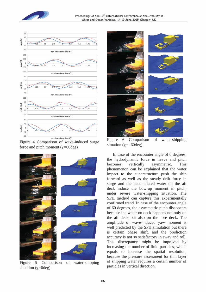
Proceedings of the 12th International Conference on the Stability of Ships and Ocean Vehicles, 14-19 June 2015, Glasgow, UK.
80
40
0
40
80
0 0.25 0.5 0.75 1 1.25 1.5 1.75 2surge[N]
non dimensional time (t/T)
300
150
0
150
300
0 0.25 0.5 0.75 1 1.25 1.5 1.75 2sway
[N]
non dimensional time (t/T)
40
20
0
20
40
0 0.25 0.5 0.75 1 1.25 1.5 1.75 2roll[Nm]
non dimensional time (t/T)
120
60
0
60
120
0 0.25 0.5 0.75 1 1.25 1.5 1.75 2
pitch[Nm]
non dimensional time (t/T)
80
40
0
40
80
0 0.25 0.5 0.75 1 1.25 1.5 1.75 2
yaw[Nm]
non dimensional time (t/T)
Figure 4 Comparison of wave-induced surge force and pitch moment ( =60deg)
Figure 5 Comparison of water-shipping situation ( =0deg)
Figure 6 Comparison of water-shipping situation ( = -60deg)
In case of the encounter angle of 0 degrees, the hydrodynamic force in heave and pitch becomes vertically asymmetric. This phenomenon can be explained that the water impact to the superstructure push the ship forward as well as the steady drift force in surge and the accumulated water on the aft deck induce the bow-up moment in pitch, under severe water-shipping situation. The SPH method can capture this experimentally confirmed trend. In case of the encounter angle of 60 degrees, the asymmetric pitch disappears because the water on deck happens not only on the aft deck but also on the fore deck. The amplitude of wave-induced yaw moment is well predicted by the SPH simulation but there is certain phase shift, and the prediction accuracy is not so satisfactory in sway and roll. This discrepancy might be improved by increasing the number of fluid particles, which equals to increase the spatial resolution, because the pressure assessment for thin layer of shipping water requires a certain number of particles in vertical direction.
437

Proceedings of the 12th International Conference on the Stability of Ships and Ocean Vehicles, 14-19 June 2015, Glasgow, UK.
4.2 Free-motion test
The SPH simulation with the same condition of the ship motion measurement is executed. The size of numerical tank, the numbers of fluid and wall particles are shown in Table 6, respectively. Numerical test is performed with the initial angles of -3 degrees and 60 degrees for the comparison of transient and steady motions, respectively. The comparisons of the x- and y-positions, heave, roll, pitch and yaw motions between the model experiment and the SPH simulation are shown in Figs.7-8.
Table 6 Numerical wave tank Length
[m] Width
[m] Depth[m]
10.0 3.0 0.5No. of fluid
particles [million]
No. of wall particles [million]
Total No. of particles [million]
23.22 1.34 24.56
Exp. SPH
1.5
0
1.5
3
0 1 2 3 4 5 6 7
xpo
sitio
n[m
]
time [sec]
0.5
0
0.5
1
0 1 2 3 4 5 6 7
ypo
sitio
n[m
]
time [sec]
0.1
0.05
0
0.05
0.1
0 1 2 3 4 5 6 7
heave[m
]
time [sec]
10
0
10
20
30
0 1 2 3 4 5 6 7
roll[deg]
time [sec]
15
7.5
0
7.5
15
0 1 2 3 4 5 6 7
pitch[deg]
time [sec]
10
5
0
5
10
0 1 2 3 4 5 6 7
yaw[deg]
time [sec]
Figure 7 Comparison of transient motion in following waves
Exp. SPH
1.5
0
1.5
3
0 1 2 3 4 5 6 7
xpo
sitio
n[m
]
time [sec]
0.5
0
0.5
1
0 1 2 3 4 5 6 7
ypo
sitio
n[m
]
time [sec]
0.1
0.05
0
0.05
0.1
0 1 2 3 4 5 6 7
heave[m
]
time [sec]
30
20
10
0
10
0 1 2 3 4 5 6 7
roll[deg]
time [sec]
15
7.5
0
7.5
15
0 1 2 3 4 5 6 7
pitch[deg]
time [sec]
60
70
80
0 1 2 3 4 5 6 7
yaw[deg]
time [sec]
Figure 8 Comparison of steady periodic motion in stern quartering waves
Both in the experimental and numerical results for a transient motion, the lateral motions are almost negligible because of the small encounter angle, except for the heeling due to accumulated water on deck. The drift in longitudinal-direction (surge), heave and pitch motions are dominant in this situation, and the SPH well reproduces the experimental result. In case of a periodic steady state, the SPH result agrees with the experimental one qualitatively in all the 6 DoF motions. The agreement in sway and roll motions are slightly worse than other 4 motions, as presumed from Fig.4. The numerical simulation of the ship motion in steep waves shows the consistent result with the captive test results. To summarize, the prediction accuracy of the ship behaviour in severe water-shipping condition is reasonable and acceptable for practical uses.
Comparisons of the ship behaviour and the shipping water situation on the aft deck are shown in Figs.9-10 and Figs.11-12, respectively. In the experimental result of the
438

Proceedings of the 12th International Conference on the Stability of Ships and Ocean Vehicles, 14-19 June 2015, Glasgow, UK.
transient motion, severe water-shipping on the aft deck happens and hits the vertical wall of the superstructure with the significant water splashing. The SPH result well reproduces the ship-wave interaction with the violent shipping water flows in following seas. In the periodic steady state, the water-shipping happens much less compared to the transient motion both in the experiment and the simulation. Regarding the water on deck situation, the experimental result is more violent in the transient motion and the amount of the water on deck is larger in the steady state than the SPH results. For the first discrepancy, it might be because that water flows tend to over-damp due to the energy dissipation when the artificial viscosity is used. For the second discrepancy, the predicted amplitude of pitch moment is smaller than the experiment as shown in Fig.8, so the amount of water on deck becomes smaller because the water-shipping mainly happens when the ship stern is going down.
Figure 9 Comparison of ship transient motion
Figure 10 Comparison of ship steady motion
Figure 11 Comparison of shipping water on the aft deck in transient state
439

Proceedings of the 12th International Conference on the Stability of Ships and Ocean Vehicles, 14-19 June 2015, Glasgow, UK.
Figure 12 Comparison of shipping water on the aft deck in steady state
5. CONCLUSIONS
SPH simulation using GPU is performed topredict the 6DoF ship motion in water-shipping condition. The applicability and the prediction accuracy are investigated through comparisons with dedicated captive and free-motion tests in very steep waves using a simplified model of a fishing vessel. The calculated wave-induced hydrodynamic force agrees with the captive test qualitatively and the SPH method well reproduces the ship dynamic behaviour, in severe water-shipping situations. From the comparison results, it is demonstrated that the SPH simulation using GPU has good potential for the quantitative safety assessment of fishing vessels in water-shipping situation. Similar investigation using more realistic 3-D hull geometries is expected as a next step.
6. ACKNOWLEDMENTS
This work was supported by JSPSKAKENHI Grant Number 26630454.
7. REFERENCES
Gesteira, M.G., Rogers, B.D., Dalrymple, R.A., Crespo, A.J.C. and Narayanaswamy, M., 2010, “User Guide for the SPHysics code”, https://wiki.manchester.ac.uk/sphysics/index.php/Documentation
Monaghan, J.J., 1992, “Smoothed particle hydrodynamics”, Annual Rev. Astron. Appl., 30: pp. 543-574.
Monaghan, J.J., 1994, “Simulating free surface flows with SPH”, Journal Computational Physics, 110: pp. 543-574.
Monaghan, J.J. and Kos, A., 1999, “Solitary waves on a Cretan beach”, J. Wtrwy. Port, Coastal and Ocean Eng., 125: pp. 145-154.
Umeda, N., Furukawa, T., Matsuda, A. and Usada, S., 2014, “Rudder Normal Force during Broaching of a Ship in Stern Quartering Waves”, Proceedings of the 30th Symposium on Naval Hydrodynamics, Tasmania.
Wendland, H., 1995, “Piecewise polynomial, positive definite and compactly supported radial functions of minimal degree”, Advances in Computational Mathematics, 4(1): pp. 389-396.
8. NOMENCLATURES
density t time u velocity vector P pressure g gravity vector
diffusion term m mass W weight function
tuning parameter c speed of sound r position vector
wave lengthH wave height
440

Proceedings of the 12th International Conference on the Stability
of Ships and Ocean Vehicles, 14-19 June 2015, Glasgow, UK.
A Reassessment of Wind Speeds used for Intact Stability Analysis
Peter Hayes, DNPS, Department of Defence, Australia, [email protected]
Warren Smith, University of New South Wales Canberra, Australia, [email protected]
Martin Renilson, Higher College of Technology, UAE, [email protected]
and Australian Maritime College, Australia, [email protected]
Stuart Cannon, DSTO, Department of Defence, Australia, [email protected]
The views expressed in this paper are those of the authors and not necessarily endorsed by the Department of Defence, Australia.
ABSTRACT
The intact stability of maritime surface vessels (ships, boats, landing craft, etc.) should be as-sessed for the most extreme environment that they are designed for or limited to operate in: namely the nominal and gust wind speeds and associated wave height and wave frequency profile.
The IMO and naval weather criteria apply to ocean going vessels but each use different wind speeds. The IMO criterion uses a single nominal wind speed (26 ms-1) and a small gust factor (√1.5 = 1.225) for all assessed vessels, irrespective of operational environment or expectations. The naval weather criteria uses different gust wind speeds for different operational expectations, with most significantly higher than the IMO gust wind speed. Yet these criteria are intended to assess the suit-ability of vessels for essentially similar operational expectations.
This paper revisits the basis of the wind speeds used for stability analysis. A range of standard-ized wind speeds for different types of operational service is proposed.
Keywords: Stability, Wind Speed,
NOMENCLATURE
t time interval, in sec
avgV average or nominal wind speed at 10
m height, in ms-1
gustV gust wind speed at 10 m height, in
ms-1
ZV wind speed at height z , in ms-1
refV reference wind speed at height refz ,
in ms-1
600WSR wind speed ratio based on an average
over 600 seconds (10 minutes)
3600WSR wind speed ratio based on an average
over 3600 seconds (1 hour)
z height above the surface, in m
refz reference height, in m
α exponent
1. INTRODUCTION
Ship stability knowledge and practise hasdeveloped over the centuries much as other branches of engineering have, starting with trial and error, progressing to rules of thumb and then, relatively recently, introducing and de-
441

Proceedings of the 12th International Conference on the Stability
of Ships and Ocean Vehicles, 14-19 June 2015, Glasgow, UK.
veloping analysis based on more rigorous ap-plication of scientific principles. Unlike other branches of engineering such as structural analysis, the ‘science’ of ship stability has not progressed much beyond the beginnings of sci-entific principles. Empirical relationships and heuristic information are heavily relied upon in developing criteria. In the main only still water characteristics are used to assess transverse stability in extreme environments. The use of seakeeping and manoeuvring characteristics in an extreme seaway to simulate and predict ship behaviour, such as broaching, that could lead to capsize has only in recent decades been active-ly explored.
Existing stability criteria are based on the still water characteristics of the vessel, incorpo-rating various factors to account for operation in severe environments. Some, such as the basic IMO criteria, require nominated charac-teristics of the righting arm curve, including minimum areas under the GZ curve and mini-mum GM values. These were based on early work, such as that of Rahola (1939). This type of criteria that have been derived empirically are strictly only valid for the data set and the environments used in their derivation. However these criteria have been extended to many ves-sel types and sizes not in the original data set, and to environments markedly different than those original environments.
Weather criteria have been introduced in more recent decades that attempt to include the effects of wind and waves as overturning forces to be resisted. In these criteria, wave effects are usually introduced to the still-water righting moment curve by a ‘roll-back’ angle. Wind ef-fects are introduced by a wind heeling mo-ment/lever function, generally based on the up-right wind heeling moment.
There are a number of different factors that contribute to a stability criterion, wind speed being one. Especially important are the hidden factors and cause/effect mechanisms that drive how the criteria actually works (e.g. different wind/heel relationships, how much of the
buoyant structure is considered, roll back from nominal or gust equilibrium). The easiest ex-ample is probably the area ratio (refer to Figure 1): the naval criteria (DDS079, 1975) uses a cos2 relationship for the wind moment/lever with ship heel, requiring A1/A2 ≥ 1.40, whereas the IMO criterion (IMO2008, 2009) uses a constant wind moment/lever relationship, re-quiring A1/A2 ≥ 1.00.
The IMO wind speed (and wave age part of the roll back formulation) are intended to be an "average" between the height of a tornado (high winds, young, steep developing seas) and the aftermath (lower winds, more fully devel-oped seas). So the criterion coefficients some-how relate this average environment to both the height of the tornado and the environment in its aftermath. What is actually being modelled here has become clouded, with wind speed used as a tuning factor.
Adopted in this paper is the premise that inputs (especially wind and wave effects) should be treated in as rigorous and realistic a manner as possible and then any criterion rela-tionship coefficients tuned to give results that match experimental and real life data. This ap-proach has the following advantages: � Inputs can be investigated generally in iso-
lation without hidden factors clouding re-sults, allowing for better treatments over time.
� Criteria can be developed from established engineering principles largely independent of the inputs. Over time this could allow for better criteria to be developed.
� Inputs can be varied to allow for different environments in a logical and transparent manner.
The treatment of wind, particularly devel-oping a standardised set of wind speeds for sta-bility analyses, is the subject of this paper.
442

Proceedings of the 12th International Conference on the Stability
of Ships and Ocean Vehicles, 14-19 June 2015, Glasgow, UK.
Figure 1 Wind speed ratio for 1 hour, 10 minute and 1 minute averaging periods
2. WIND CHARACTERISTICS
2.1 Wind Velocity Profile
The average or nominal wind does not have the same wind speed at all heights above the earth surface. Near the surface, friction and sur-face roughness affect the strength or speed of the wind. This is the ‘constant shear’ region, which extends to about 100 m above the sur-face. Within this region the variation in wind speed over the ocean is commonly approximat-ed by (e.g. McTaggart and Savage, 1994, EM 1110-2-1100, 2002):
α
=
refrefZ z
zVV ( 1 )
The value of α varies from 0.1 to 0.4 de-pending on surface roughness. McTaggart and Savage (1994) reported that α varies from 0.12 to 0.14 for stormy ocean conditions. A common value for α is 0.13 (≈ 1/7.5).
The international meteorological communi-ty has standardized on reporting wind speeds at a 10 m height above the surface. Historically, this height was not always used and measure-ments of opportunity, such as ship’s anemome-ters, could be at any height. When comparing wind speeds from different sources, conversion to a common baseline height (10 m) using equation (1) may be necessary.
2.2 Wind Gusts
The long term average wind speed is used in wave growth models and is usually the nom-inal wind speed reported by the local weather bureau. In Australia, and generally internation-ally, the 10-minute maximum sustained wind speed average, at 10 meters height, is used as the nominal wind speed.
The spatial distribution of packets of wind blowing in a particular direction with a rela-
tively constant wind speed is seemingly ran-dom in nature. A time history at a particular point will provide various statistics about the wind, such as the average and standard devia-tions of wind speed and direction, and so on. Unlike ocean waves, which can be viewed in an analogous manner, the wind statistics can quickly change, and there is a need to take sta-tistics over limited time intervals. Durst (1960) established a relationship for gust wind speeds for different durations based on analysis of winds over open and flat terrain.
For a 1-hour (3600-seconds) average max-imum sustained wind speed, the Durst wind speed ratio for winds of smaller duration is given by (EM 1110-2-1100 2002):
( )
+=t
tWSR45
log9.0tanh296.0277.1 103600
( 2 )
If the wind speed ratio for a different return period, say 10-minutes (600-seconds), is calcu-lated, it is a simple matter to obtain the wind speed ratio relative to that new return period:
( ) ( )( )6003600
3600600 WSR
tWSRtWSR = ( 3 )
The wind speed ratios based on 1-hour, 10-minute and 1-minute average maximum sus-tained wind speeds are plotted in Figure 1. The gust ratio for a 5-sec gust duration when com-
443

Proceedings of the 12th International Conference on the Stability
of Ships and Ocean Vehicles, 14-19 June 2015, Glasgow, UK.
Figure 2 Comparison of the ESDU model to gust data, adapted from Vickery et al.
(2007)
pared to the 10-min average is 1.4122, very close to 4142.12= .
In more recent years there have been many studies of wind gustiness, especially in hurri-canes, each arriving at different gust factors. One example is the gust model developed by the Engineering Sciences Data Unit, ESDU. Vickery and Skerlj (2005) presented data indi-cating that the ESDU gust model, using a roughness of 0.03m, gave the best fit to availa-ble data, though the Durst model also gave a fit close to this preferred ESDU model. Limited data indicated that gust factors at sea are a little lower than over land by an average factor of 0.95, Vickery and Skerlj (2005). A later analy-sis by Vickery et al. (2007) presented a com-parison of the ESDU gust model to available data, this time based on a 1-minute nominal period, reproduced as Figure 2. Overlaid on this figure (dashed line) is the Durst model for 1-minute nominal wind speeds. The Durstmodel appears to give better predictions forgusts longer than 3 seconds. Also, convertingto 10-minute nominal winds would result in15-20% higher gust factors.
The ESDU model is somewhat complicated to apply, whereas the Durst model is relatively simple. Noting that the two give fairly similar results and that the Durst model dates from the 1960s when wind speeds for stability analysis
were selected, the Durst model is adopted for this paper.
2.3 Tropical Cyclone Scales
There are a number of schemes for catego-rising the severity of tropical cyclones. A summary of the various scales used throughout the world as given by Tropical Cyclone Scales (2013) is: � Atlantic Ocean and East Pacific Ocean -
characterised by the United States devel-oped Saffir-Simpson Hurricane Scale, which is based on 1-minute maximum sus-tained wind speeds.
� West Pacific Ocean, Northern Hemisphere monitored by the Japan Meteorological Agency's Regional Specialized Meteoro-logical Centre (RSMC). The typhoon in-tensity scale is based on 10-minute maxi-mum sustained wind speed.
� North Indian Ocean - monitored by the In-dia Meteorological Department's Regional Specialized Meteorological Centre in New Delhi, India. The cyclonic storm scale is based on a 3-minute averaging period to determine sustained wind speeds.
� South-Western Indian Ocean - monitored by Météo-France which runs the Regional Specialized Meteorological Centre in La Reunion. The tropical cyclone scale is based on a 10-minute average maximum sustained winds.
� South Pacific Ocean and South-Eastern Indian Ocean - monitored by either the Australian Bureau of Meteorology and/or the Regional Specialized Meteorological Centre in Nadi, Fiji. Both warning centres use the Australian tropical cyclone intensi-ty scale, which is based on 10-minute maximum sustained wind speed combined with estimated maximum wind gusts, which are a further 30-40% stronger.
It can be seen that there are a number of dif-ferent scales used to characterise tropical cy-clones, potentially making comparisons erro-neous.
444

Proceedings of the 12th International Conference on the Stability
of Ships and Ocean Vehicles, 14-19 June 2015, Glasgow, UK.
The Beaufort wind scale is used to catego-rize wind speed and, in the absence of reliable instrumentation, is often used to report wind speed. Wind speeds used in the Beaufort scale reflect the standard 10-minute average at 10-metres height. The Beaufort Scale is typically defined to Beaufort 12. It was extended to Beaufort 17 in 1944, intended for special cases, such as tropical cyclones (Met Office, 2010).
The tropical cyclone scales of interest are the US Saffir-Simpson scale and the Japanese scale, as they have been influential on wind speed selection used in stability analyses, and, for the authors, the Australian tropical cyclone scale. These tropical cyclone scales have been compared to the Beaufort scale in Table 1, us-ing the Durst relationship to convert US 1-minute sustained wind speed to 10-minute sus-
tained wind speeds. This illustrates the differ-ences between the tropical cyclone scales. Of note is that the US hurricane categories start at Beaufort 11 and the Japanese typhoon category (which is subdivided for internal use) starts at Beaufort 12.
3. WIND SPEEDS
3.1 IMO
The IMO uses a wind speed of 26 ms-1 (50.5 knots) as the nominal wind speed in its weather criterion, with a gust factor (GF) of 1.225 ( 5.1 ) to give a gust wind speed of 31.8 ms-1 (61.9 knots). The nominal wind speed is equivalent to a mid Beaufort 10 wind. Noting
Table 1 Beaufort wind scale, adapted from Tropical Cyclone Scales (2010)
445

Proceedings of the 12th International Conference on the Stability
of Ships and Ocean Vehicles, 14-19 June 2015, Glasgow, UK .
Figure 3 Wind gustiness, from Yamagata (1959)
that the gust heeling lever governs the weather criterion, using the 5-second gust factor of 1.412 equates the IMO gust wind of 31.8 ms-1 to a nominal wind speed of 22.5 ms-1 (43.8 knots), which is mid Beaufort 9. For vessels expected to avoid the worst weather and that can use weather routing to do so, mid Beaufort 9 represents fairly severe weather - but it is cer-tainly not the worst that could be encountered. Not all vessels, whether or not they are using weather routing, can successfully avoid the worst weather.
According to Yamagata (1959), the selec-tion of 26 ms-1 was an average between the maximum winds of a tropical cyclone (called a typhoon by the Japanese) and the more steady winds in the immediate aftermath. This also made allowance for wave age—waves tend to be younger and therefore steeper in short dura-tion winds compared to the more fully devel-oped waves that occur with time. However, an examination of the actual data presented, espe-cially Table III of Yamagata (1959) (adapted as Table 2 here), would suggest a higher value.
Comparing Table 1 with Table 2, the max-imum wind speeds of Table 2 could possibly be gust wind speeds. The question then is what gust ratio to apply.
Yamagata (1959) provided data, reproduced as Figure 3 here, that showed gust factors ranged from 1.0 to 1.7 with an average of 1.23 (≈ √1.5). At higher wind speeds, above about
30 ms-1, the maximum gust factor was 1.3. The average value was adopted, taken as √1.5 (= 1.225).
The variation of wind speed with location from the peak of a tropical cyclone through to the trailing wind was simplified (Yamagata, 1959). This simplification was similar to Fig-ure 4 (the bottom line is the Yamagata simpli-fication, apparently using the data from Table 2, though how this was effected is not immedi-ately apparent). The maximum wind speed adopted was about 32 ms-1. From Table 2, this is the maximum wind velocity for a low pres-sure system. If the value of 50 ms-1 from Table 2 is taken as a gust wind speed, using a gust factor of 1.225 (the gust factor assumed by the Japanese) gives a nominal wind speed of 40.8 ms-1. Alternatively, using a gust factor of 1.412 (the gust factor from Durst) gives a nominal wind speed of 35.4 ms-1. Neither matches the 32 ms-1 that was used.
Taking the data of Table 2 as the intended values, a number of different analyses can be performed. Assuming that the typhoon maxi-mum wind speed is a gust wind speed and the gust factor of 1.225 applies, the average and gust wind speeds of the central or tropical cy-clone zone should have been calculated as:
1
1
ms2.37
4.30225.1
ms4.30
2
20225.1
50
−
−
=
×==
+=
gust
avg
V
V
( 4 )
Table 2 Nominal wind environments, adapted from Yamagata (1959)
446

Proceedings of the 12th International Conference on the Stability
of Ships and Ocean Vehicles, 14-19 June 2015, Glasgow, UK.
If the 5-second gust factor of 1.412 was used instead, the respective wind speeds would be:
1
1
ms1.39
4.30412.1
ms7.272
20412.1
50
−
−
=
×==
+=
gust
avg
V
V
( 5 )
This second result is close to the top of Beaufort 10 (nominal to 28.3 ms-1, gusts to ap-proximately 40.0 ms-1). This suggests that Beaufort 10 is a more realistic wind definition for vessels intended for unlimited operation at sea, though still avoiding centres of severe tropical disturbance.
Figure 4 shows the result when applying different gust factors (GF) to the specified maximum wind speed at the centre of a ty-phoon of 50.0 ms-1.
Applying the same method and the 5-second gust factor of 1.412, the respective wind speeds for a low pressure system would be:
1
1
ms5.26
8.18412.1
ms8.182
15412.1
32
−
−
=
×==
+=
gust
avg
V
V
( 6 )
This last result is the middle of Beaufort 8 (nominal to 20.6 ms-1, gusts to approximately 29.1 ms-1). This suggests that Beaufort 8 is more appropriate for vessels that must avoid the worst weather. Such vessels would need ready access to refuge.
3.2 Naval
There is no actual historical evidence avail-able for the development of the naval criteria wind speeds. The likely rationale for their se-lection can be deduced once the different tropi-cal cyclone scales employed by different au-thorities are considered.
The defining event for formulating USN in-tact stability, Typhoon Cobra in 1944 (also known as Halsey's Typhoon), was described as Force 12 with average winds 50 to 75 knots and gusts as high as 120 knots. Brown and Deybach (1998) reported that the USN identi-fied 100 knots as a reasonable wind velocity for ship survival in tropical storms. DDS 079-1 (1975) specified wind speeds for various ser-vice categories as: � Ocean and Coastwise:
o 100 knots - Ships which must be ex-pected to weather the full force of tropi-cal cyclones.
o 80 knots - Ships which will be expectedto avoid centres of tropical disturbance;and
� Coastwise: o 60 knots - Vessels which will be re-
called to protected anchorages if windsover Force 8 are expected.
A number of observations can be made about the USN categories: � 100 knots is the 5-second gust speed for
Beaufort 12. It seems reasonable to as-sume that, for this service category, a gust
Figure 4 Simplified typhoon wind veloci-ty, adapted from Yamagata (1959)
447

Proceedings of the 12th International Conference on the Stability
of Ships and Ocean Vehicles, 14-19 June 2015, Glasgow, UK.
factor of about 1.5, rounded to a neat re-sult, was applied to a nominal wind of Beaufort 12.
� 80 knots is close to the 5-second gust speed for Beaufort 10 - refer to Table 1. Under the US system, this is the strongest Beaufort wind not categorized as a hurri-cane and 80 knots applies to ships ex-pected to avoid centres of tropical disturb-ance. It seems reasonable to assume that, for this service category, a gust factor of about 1.5, rounded to a neat result, was applied to a nominal wind of Beaufort 10.
� Beaufort 8 has a nominal wind speed to 40 knots. 60 knots is 1.5 times the nominal wind speed. It seems reasonable to assume that a gust factor of about 1.5, rounded to a neat result, was applied.
� The USN categories are essentially for ocean voyaging ships (100 and 80 knots wind speed) and for limited range vessels (60 knots) able to return easily to shelter. The latter category could include ship's boats which would not operate in severe environments and which could return to the parent ship.
3.3 NSCV
The Australian National Standard for Commercial Vessels (NSCV, 2002) defined environments deemed suitable for domestic operations. The wind environments were pre-sented as Beaufort wind speeds and gust pres-sures, with a formula to convert pressures to equivalent wind speeds. Using this formula re-vealed a wide range of gust factors, ranging from 1.3 for the ocean going categories to 1.76 for a protected waters category.
In the Australian context, it is desirable to use the NSCV categories where possible as most vessels available commercially in Aus-tralia would have been assessed against the NSCV. This can best be done by matching gusting wind pressures, which are used for analysis in the NSCV.
4. STANDARD WIND SPEEDS
The reanalysis of the original Japanese datapresented in Yamagata (1959), the interpreta-tion of the naval wind speeds presented in DDS 079-1 (1975) and inclusion of the NSCV cate-gories strongly suggest the wind speeds definedin Table 3 for a range of service categoriesshould apply. The wind speeds prescribed arenominal or average wind speeds. A gust factorof around 1.4 is recommended to derive thegust or design wind speed typically used inquasi-static analyses. This would most easilybe arranged by doubling the nominal windheeling moment (equivalent to a gust factor of
414.12= ).
This paper developed the wind speeds rec-ommended for offshore and ocean-going ves-sels. Table 3 also presents recommended wind speeds for operation of limited duration off-shore (coastal) and in more protected areas. These were developed by Hayes (2014) and are appropriate for the Australian context. Other jurisdictions will possibly need to vary from these suggestions to suit local conditions.
Associated wave heights have been shown in Table 3 for completeness. They were derived from basic wind/wave relationships (Hayes, 2014) and are not intended to be definitive.
It is useful to define a number of service categories for the purposes of setting the envi-ronments (and any other pertinent parameters) applicable to the intended uses of a vessel. A vessel intended to stay in position except in the most severe weather should clearly be assessed using a more severe environment to that for a vessel intended to coastal hop only when suita-ble weather presents itself. The service catego-ries, once defined, would be applied to most vessels, selecting the most appropriate category for the intended service of the vessel. This al-lows for clear definitions that can be applied and understood across the fleet.
448

Proceedings of the 12th International Conference on the Stability
of Ships and Ocean Vehicles, 14-19 June 2015, Glasgow,UK.
Suggested descriptions of the service categories are presented in Table 4. Note that in the naval context, a safe haven can include the parent ship and that the size of the environment and
range from the safe haven, not geographical limits, are the important parameters. This could also apply in the commercial context.
Table 3 Suggested standard environments
Table 4 Suggested service categories
449

Proceedings of the 12th International Conference on the Stability
of Ships and Ocean Vehicles, 14-19 June 2015, Glasgow,UK.
The suggested service categories would ap-ply to a majority of cases. Special purpose ves-sels, intended for very specific roles, environ-ments and survival probabilities, could require very specific operational profiles and environ-ments to be defined.
5. CONCLUSIONS
Reiterating, inputs to stability criteria (es-pecially wind and wave effects) should be treated in as rigorous and realistic a manner as possible. Any criterion relationship coefficients should then be developed such that the results of applying the criteria match experimental and real life data – i.e. they are realistic predictors of safe vessels for the intended extreme envi-ronment.
A standardised set of wind speeds for sta-bility analyses would mean that the use of wind speed becomes more transparent, with less op-portunity to cloud how it shapes the criteria coefficients. How the criteria would then be developed to accommodate these standardised wind speeds is a different question to be an-swered by more research.
Wind speeds appropriate for general stabil-ity analyses have been developed and defined in terms of different service categories. Adopt-ing these, or similar, wind speeds and service categories allows for stability analyses appro-priate to the actual use of and operational limi-tations of different vessels and is encouraged.
6. REFERENCES
Brown, A.J. and Deybach, F., 1998. Towards a Ra-tional Intact Stability Criteria for Naval Ships, Naval Engineers Journal, 110 (1), pp. 65–77.
DDS 079-1, 1975. Stability and Buoyancy of U.S. Naval Surface Ships. United States, Department of the Navy, Naval Ship Engi-neering Centre.
Durst, C. S., “Wind Speed Over Short Periods of Time,” Meteorological Magazine, 89, 181-187, 1960.
EM 1110-2-1100, 2002. Coastal Engineering Manual – Part II – Chapter 2: Meteorology and Wave Climate, US Army Corps of En-gineers.
Hayes, P., 2014, Naval Landing Craft Stability, Masters Thesis, University of New South Wales, Australia.
McTaggart, K. and Savage, M., 1994. Wind Heeling Loads on a Naval Frigate, 5th Inter-national Conference on Stability of Ships and Ocean Vehicles, Melbourne, Florida, USA
Met Office, 2010. National Meteorological Li-brary and Archive Fact Sheet 6 The Beau-fort Scale, URL: http://www.metoffice. gov. uk/corporate/library
NSCV, 2002. National Standard for Commer-cial Vessels (NSCV), URL: http://www. amsa.gov.au/domestic/standards/
Rahola, J. 1939, The Judging of the Stability of Ships and the Determination of the Mini-mum Amount of Stability, Ph.D. Thesis, The University of Finland, Helsinki, Fin-land.
Tropical Cyclone Scales, 2013. Wikipedia arti-cle, URL: http://en.wikipedia.org/wiki/ Tropical_cyclone_scales
Vickery, P.J., Masters, F.J., Powell, M.D. and Wadhers, D., 2007. Hurricane Hazard Mod-elling: The Past, Present and Future, 12th In-ternational Conference on Wind Engineer-ing, Cairns, Australia.
Vickery, P.J. and Skerlj, P.F., 2005. Hurricane Gust Factors Revisited, Journal of Structur-al Engineering, pp. 825–837.
Yamagata, M. (1959). Standard of Stability Adopted in Japan, Transactions Royal Insti-tution of Naval Architects 101: 27. 417.
450

Session 8.1 – 2nd GENERATION I
On the Application of the 2nd Generation Intact Stability Criteria toRo Pax Vessels
A Study on Applicability of CFD Approach for Predicting ShipParametric Rolling
Estimation of Ship Roll Damping – a Comparison of the Decay and theHarmonic Excited Roll Motion Technique
Assessing the Stability of Ships under the Effect of Realistic WaveGroups
451

This page is intentionally left blank
452

Proceedings of the 12th International Conference on the Stability of Ships and Ocean Vehicles, 14-19 June 2015, Glasgow, UK
On the application of the 2nd Generation Intact Stability Criteria to Ro-Pax and Container Vessels
Stefan Krueger, Hannes Hatecke
Hamburg University of Technology, Germany
Paola Gualeni, Luca Di Donato
University of Genoa, Italy
ABSTRACT
A new set of intact stability criteria is under development at IMO with the aim to address the stability failures of a ship in a seaway. These criteria are structured in a three level approach. The first two levels consist of calculations characterized by different levels of accuracy. The third level is named “direct assessment” and typically a numerical tool for hydrodynamics calculations is envisaged for the assessment. However, at present no criteria or procedures have been developed for this third level.
In the various scenarios of modern merchant ships, Ro Ro-Passenger vessels represent a very interesting field of investigation for intact stability vulnerability assessment especially for the righting lever variations in waves. For the specific stability failures of parametric roll and pure loss of stability, in the present paper, we apply the 2nd Generation of Intact Stability Criteria to some typical Ro Ro-Passenger ferries and results are presented in terms of computed curves of minimum required GM. We have also carried out a direct assessment of the stability using the “Insufficient Stability Event Index” (ISEI- concept) and compared the obtained GMReq – curves.
This comprehensive investigation has the purpose to assess the reliability of the newly proposed criteria as technically consistent and harmonized safety rules.
To this aim the investigation domain has been enhanced to the cargo ships field, in particular considering three selected containerships that have suffered serious accidents in a heavy seaway.
Keywords: Intact stability failure modes, direct assessment, GM required curves, safety level.
1. INTRODUCTION
In the latest years, under the specific agendaitem named “second-generation intact-stability criteria,” IMO has been active on the development of vulnerability criteria for the assessment of ship behaviour in a seaway. The importance of this issues is already pointed out in the Preamble of the Intact Stability code (2008): “It was recognized that in view of a
wide variety of types, sizes of ships and their operating and environmental conditions, problems of safety against accidents related to stability have generally not yet been solved. In particular, the safety of a ship in a seaway involves complex hydrodynamic phenomena which up to now have not been fully investigated and understood”
453

Proceedings of the 12th International Conference on the Stability of Ships and Ocean Vehicles, 14-19 June 2015, Glasgow, UK
Among the failure modes recognised by the IMO are:
-Pure loss of stability-Parametric roll-Dead ship condition in beam seas-Surf-riding and broaching-to
Only the first two are faced in the present investigation, in the specific field of Ro-Pax ships. For a larger perspective on the subject, also three Container vessels` behaviour has been analysed.
If a ship is susceptible to a stability failure that is neither explicitly nor properly covered by the existing intact stability regulations, the ship is regarded as an “unconventional ship” in terms of that particular stability failure mode.
“Second-generation intact-stability criteria” are based on a multi-tiered assessment approach: for a given ship design, each stability failure mode is evaluated relying on two levels of vulnerability assessment, characterized by different levels of accuracy and computational effort.
A ship which fails to comply with the first level is assessed at the second-level criteria. In turn, if unacceptable results are found again, the vessel must then be examined by means of a direct assessment procedure based on tools and methodologies corresponding to the best state-of-the-art prediction methods in the field of ship-capsizing prediction. This third-level criteria should be as close to the physics of capsizing as practically possible.
Direct assessment procedures for stability failure are intended to employ the most advanced technology available, ant to be sufficiently practical to be uniformly applied, verified, validated, and approved using currently available infrastructure. Ship motions in waves, used for assessment on stability performance, can be reproduced by means of numerical simulations or model tests.
Where model tests have the disadvantage that investigations in short crested, irregular seas are hardly possible.
Calculations performed in the current work are structured in three phases.
First, all the ships are judged with the mandatory intact stability regulation (IS Code, 2008), in order to define the safety level at present. Then a direct assessment is performed by means of non-linear time domain, computations, able to compute the so called “insufficient stability event index” (ISEI). A more thorough description of ISEI is given in the next paragraphs. Following the above mentioned calculations, GMReq sets of values are obtained from both the IS code criteria (usually for Ro-Pax corresponds to the Weather Criterion) and the direct assessment method. A gap, in terms of GMReq , between the two approaches is the obtained result, as it could be expected.
At this point the Second Generation Intact Stability Criteria are introduced to complete the outline of the situation.
The aim of this work is to show how suitably the new stability requirements apply in addressing parametric roll and pure loss problems, filling the range between the mandatory and the numerically simulated stability safety level. In the following the structure of the new criteria is explained, as well as a description of the direct assessment methodology. Finally, results for the case studies are presented and properly discussed.
2. 2ND GENERATION INTACTSTABILITY CRITERIA
In this work the IMO document used for thecalculations is the SDC 1 Inf. 8 with the updates of the SDC/ISCG of the latest months. All the amendments have been implemented in the ship design software package E4 of the
454

Proceedings of the 12th International Conference on the Stability of Ships and Ocean Vehicles, 14-19 June 2015, Glasgow, UK
Hamburg University of Technology, developed in Fortran90 language.
In the following the first two levels of vulnerability criteria, for the specific failure modes of Parametric roll and Pure Loss of stability, are briefly explained.
2.1 Level 1 Vulnerability Criteria
The first level consists of simple formulae based on the ship hydrostatics and regards the GM sensitiveness to waterline variation due to wave profile. In fact, as an effect of a wave passing the ship, the lever arm as well as the metacentric height will face a change due to the modification of the water plane area and the immersed volume distribution, considering the ship to be balanced in sinkage and trim. It is recognized that most of the times the worse situation in terms of stability is represented by the wave crest situated amidships.
Figure 1: Wave with the length of the ship with crest and trough located at amidships.
Parametric Roll: A ship is vulnerable to parametric roll, according to level 1, if the ratio between the amplitude of the GM variation in waves and the GM in still water is less than a certain value. The formula reads as follows:
Where Rpr is taken as 0.5 or as a value function of the midship section coefficient Cm and the bilge keel area, whichever is the less.
Longitudinal sinusoidal waves with a length λand steepness Sw of 0.0167 are taken for the calculation of the ΔGM. The wave crest is centred at the longitudinal centre of gravity at each 0.1 forward and aft thereof.
Pure loss of stability: For cases with speed corresponding to Froude number of significantly high values (in the draft proposal threshold value for example 0.31), a ship is considered potentially dangerous to this phenomenon. In such case the criterion reads as follows:
GMMIN is the minimum value of the metacentric height as a longitudinal wave passes the ship. It has been observed that the most critical situation is quite often presenting the wave crest in the surrounding of the amidships longitudinal position. RPLA is defined as: min( 1.83 d (Fn)2 , 0.05) , with d the draft of the loading condition under consideration. The wave length considered to compute the GM is the same of the ship length and the steepness in this case is 0.0334 (the double of the one applied for parametric roll).
2.2 Level 2 Vulnerability Criteria
The compliance with the first level is in principle always possible provided that the sufficient (usually high) level of stability (for example in terms of GM) is met. One of the reasons for that could be also the conservative approach of the described formulae (i.e. the high safety margin implied). To this regard it is worth mentioning that a very high GM value might imply also some shortcomings and recently at IMO attention has also been given to the issue of excessive accelerations. It should also be mentioned that unrealistically high values of GM pose a severe burden to the design of the ship.
455

Proceedings of the 12th International Conference on the Stability of Ships and Ocean Vehicles, 14-19 June 2015, Glasgow, UK
Therefore for both parametric roll and pure loss more complex formulations are needed in order to get a more realistic stability level. The way to gain this target consists basically of developing an averaged assessment on a larger set of environment conditions. For the purpose of this paper a series of longitudinal sinusoidal waves (proposed as an option in the draft rule text) from a length λ of 22m to 630m are used for the computation of a weighted average.
Parametric Roll: The first check the ship has to pass requires that the weighted average among all the wave cases is less than a certain value RPR (in our case 0.1).
At the same time it is also requested that:
Therefore, besides that check on GM also the design speed VD of the ship shall not exceed the resonance speed VPRI.
Moreover, if this check is not overcome, the roll motion has to be assessed in head and following seas for a range of operational speeds. Different options are possible for this computation: a numerical transient solution, an analytical steady state solution or a numerical steady state solution. In this work the second option has been attempted using the updated formula of the working group when the 5th degree polynomial fitting of the righting lever curve was not precise enough. No satisfactory results have been obtained with this approach, therefore we considered the first check as the only possible requirement in the evaluation of the GM required curves. It should in this context be mentioned that if the criteria will be
made mandatory, it must be guaranteed that they are numerically stable.
Pure loss of stability: The same wave cases, with double of the steepness are applied for this second level. Three criteria have to be assessed, addressing the issues of a limit for the vanishing stability angle, for the maximum loll angle and for the maximum value of the righting arm. For the angle parameters we applied the proposed standards of 30 degrees, 25 degrees respectively. The standard value for the criterion addressing the maximum righting arm is expressed as a function of wave steepness, Fn, and ship draft.
3. DIRECT ASSESSMENT
As already mentioned, if the ship is foundto be vulnerable under the first two levels (or more realistically, if the GMReq in order to comply with is too high), a direct assessment is required, possibly related with the quantification of a capsizing risk. No rules are actually available for this procedure, therefore the numerical tool E4ROLLS, developed by Söding Kroeger and Petey provided by the Hamburg University of Technology, has been applied. With this tool, the 6-DOF motion of the ship is computed in an irregular short-crested seaways. While heave, pitch, sway and yaw are computed by means of strip theory in the frequency domain, roll and surge, due to their nonlinear nature, are determined in the time domain.
For the roll motion the following equation has been used (Kröger 1987):
here Mwind , Msy, Mwave and Mtank are the moments due to wind, sway, waves and fluid in tanks respectively. The damping is
∆GM H , λGM H , λ R
ζ hs-
456

Proceedings of the 12th International Conference on the Stability of Ships and Ocean Vehicles, 14-19 June 2015, Glasgow, UK
considered in Md and the restoring moment in the term hs, representing the restoring arm in the seaway according to the Grim’s concept of the equivalent wave modified by Söding. Ixx and Ixz are the moments of inertia around the longitudinal axis and the product of inertia, respectively, calculated for the actual mass distribution, introduced for the yaw moment influence. As a result of the calculations, a polar plot produced by a computation can be represented for example in figure 2. The diagram is characterized by representative wave length (and period as well), different speed on each circle, different encounter angles and wave height (coloured). All calculations are carried out for short crested irregular seas. The limiting significant wave height which identifies a situation as dangerous derives either from the Blume criterion or from a maximum roll angle of 50 degrees, whichever is the less:
Figure 2: Polar Plot for a single significant wave period Each colour represents the limiting significant wave height.
To determine if the loading condition under analysis is safe or not, the direct assessment makes use of the ISEI concept. The Insufficient Stability Event Index, developed by Krueger and Kluwe , gives a failure index in terms of long term prediction:
Here psea represents the environmental context by means of a two dimensional probability density function for a sea-state characterized by significant height H1/3 and period T1, whereas pdang denotes the probability that the stability condition under consideration is dangerous in the current seastate, using the two failure criteria mentioned before.
Psea is taken from the North Atlantic Area according to the Global Seaway Statistics by Söding.
The limit between the safe and the unsafe situation is defined by the threshold value of the index 1·10-3 . Six wave periods are typically used for each calculation which should be arranged around the period representing a wave length corresponding to ship length.
4. APPLICATION CASES
For the investigation, four Ro-Pax ofsignificantly different geometry are analysed. For each ship the main dimensions are shown below.
RoPax 1 Lpp [m] 171 B [m] 27 T [m] 6.6 V [kn] 23
Table 1: Main dimensions of RoPax1
/ ,/ ∙∙ / , , , ∙ ∙ ∙ / ∙Figure 3: Body plan of the RoPax1
457

Proceedings of the 12th International Conference on the Stability of Ships and Ocean Vehicles, 14-19 June 2015, Glasgow, UK
RoPax 2
Lpp [m] 186 B [m] 30T [m] 7.8V [kn] 25
Table 2: Main dimensions of RoPax2
Figure 4: Bodyplan of the RoPax 2
RoPax 3 Lpp [m] 110 B [m] 15T [m] 6V [kn] 25
Table 3: Main dimensions of RoPax3
Figure 5: Body plan of the RoPax 3
RoPax 4 Lpp [m] 156 B [m] 19T [m] 6.86V [kn] 17GM accident [m] 1.691
Table 4: Main dimensions of RoPax4
Figure 6: Bodyplan of RoPax4
This last Ropax4 ship has a geometry which has experienced a capsizing due to the dynamic phenomena studied by the new criteria. It has been analysed in order to check if the two levels of parametric roll and pure loss of stability recognize a stability problem at the loading condition of the accident.
5. CALCULATIONS AND RESULTS
General procedure
As mentioned before, three calculation phases are covered to obtain all the final results useful for the comparison purposes, aim of this paper:
458

Proceedings of the 12th International Conference on the Stability of Ships and Ocean Vehicles, 14-19 June 2015, Glasgow, UK
Figure 7: Procedure adopted
As a general comment, it is worth mentioning that usually the limiting GM for a RoRo passenger ferry, neglecting the damage condition, is represented by the weather criterion. With E4ROLLS this GMReq- value is compared with the results obtained by the ISEI concept. Beyond the level 1 of Parametric Roll and Pure Loss of Stability, very conservative, the level 2 is the one in charge to smoothly converge to the direct assessment GM requirements.
RoPax 1
As already mentioned, at first the limiting GM curve with reference to IS Code has been identified. At the design draft this ferry fulfils the weather criterion, with a GM of 0.8m. At this loading condition the direct assessment has been applied, showing an insufficient stability in following seas. This is evident from the polar plot representation and quantitatively by the ISEI value higher than the 10-3.
Figure 8 Two polar plots for limiting capsizing wave height for a wave length of 172m. Left: GM=0.8m Right: GM=1.9m
After few iterations, a value of ISEI of 1·10-3 is found at a GM of 1.9m, more than one meter increment compared to the present regulations. In figure 8 results are reported for calculations performed at both GM values (GM= 0.8 m left, GM= 1.9 m right). It can be observed that the ship faces already several problems in following seas with wave heights of 3m for the GM required by the weather criterion ( 0.8m). From a direct assessment, there isn’t any sharp boundary between a parametric roll and a pure loss of stability failure; each dangerous situation is often a combination of both. The GMReq curves read as follows:
Figure 9 : GMReq curves for the RoPax 1
In figure 9, results derived by the direct assessment are represented by straight horizontal line, as an extrapolation of the calculation carried out at draft 6.6 m and GM= 1.9 m. The second levels of parametric roll and pure loss of stability criteria seem to work properly in the range of the GM limiting values,
Intact stability Code: Evaluation of
the limiting criterion
Application of the Direct Assessment with different GM
GM required curves for IS Code2nd Generation ISCriteriaDirect assessment(1·103)
459

Proceedings of the 12th International Conference on the Stability of Ships and Ocean Vehicles, 14-19 June 2015, Glasgow, UK
between the IS Code and the Direct Assessment curves. For the design draft of 6.6m, the first levels requires a GM up to three meters, not so high considering the conservative approach of these two criteria. For the second level it is evident that the limiting criterion is the one relevant to the parametric roll, in this case very close to the direct assessment requirements.
RoPax 2
The second Ro-Pax, larger in size than the first one, requires a GM of 1.1m at the design draft in accordance with the weather criterion. Applying the direct assessment, E4ROLLS shows again more the need of more than one meter increment between the IS Code requirement and the GM corresponding to the ISEI of 1·10-3. The results with the two different GM values are reported in figure 10.
Curve trends in figure 11 for RoPax2 represent nearly the same behaviour of RoPax1. It is possible again to identify the conservative nature of levels 1 criteria and, as far as level 2 is concerned, the strong difference in terms of GM requirements between pure loss and parametric roll criteria.
Figure 10: Two polar plots for limiting capsizing wave height for a wave length of 172m. Left: GM=1.1m Right: GM=2.179m
Figure 11: GM req curves for the RoPax 2
RoPax 3
This high speed ferry was designed to meet the ISEI- standard. The limiting GM resulting from the IS Code therefore corresponds more or less to the one computed by the direct assessment i.e. 3.2m. The second level assessments requires values identifying even lower curves. On the other hand, the first levels are extremely conservative, leading to 5-7 m of required GM. Compared to the other two examples, it can be observed an inversion of the level 2 between parametric roll and pure loss of stability; the last one for high drafts requires more stability. As the righting lever curve of this particular ship strongly deviates from the linear representation by GM (fig 12), the example clearly shows that the proposed criteria have problems to cope with such kind of ships.
Figure 12: GZ curve for RoPax3
460

Proceedings of the 12th International Conference on the Stability of Ships and Ocean Vehicles, 14-19 June 2015, Glasgow, UK
Figure 13: GM required curves for the RoPax 3
RoPax 4
As introduced before, for this ferry the conditions of the accident have been reproduced in the direct assessment computational tool, in order to analyse if the 2nd generation criteria could have prevented that situation. The ship was sailing at a draft of 6.86m with a GM of 1.691m; the direct assessment has been already applied by Kluwe and Krueger resulting in a required metacentric height of 1.89m to fulfil the usual ISEI of 10-3. Considering only the level 2, it is evident for a range of realistic drafts, that criteria show GM results differing (in positive and negative gap) of nearly 0.2 from the IS Code requirements. Actually, a not negligible detail is to be mentioned, i.e. the ship was sailing with a threshold GM value (exactly on the IS Code curve). At the same time, it appears how the criterion for the second level-parametric roll for that draft requires a lower GM value in comparison with the one at the time of the accident (fig.14).
Figure 14: GM required curves for the RoPax 4
Further Cases
So far only problems related to minimum stability requirements have been addressed. It is well known anyway, that an excessive stability can produce problems as well, resulting in excessive accelerations. In figures 11-13-14-15, the level 1 criteria point out apossible problem of this kind, with GMrequired up sometimes to 7 or 8 meters.Therefore to conclude this investigation, threeContainer ships are analysed. All these threeexamples have experienced problems ofexcessive acceleration as a consequence ofsailing with high GM in ballast condition. Inthe following, the computed curves for thenew criteria are presented.
Container 1
This ship was sailing with 8.1 m of draft with a GM of 7.712 m. The limiting criterion for low drafts in this case is the maximum GZ arm position at 25°. The condition of the accident lies in the middle of parametric roll and pure loss limiting curves derived from level 1, leaving space for discussion about the excessive stability requirements (fig. 15).
Container 2
For this ship the accident occurred at a draft of 5.59m and a GM of 4.52m From the curves, it appears that the accident condition is moderately above any present and future rules (fig.16).
Container 3
The ship experienced the accident at a draft of 5.72m and a GM of 5.67. In this example the accident condition is well above the level 1 criteria for both parametric roll and pure loss of stability (fig. 17).
461

Proceedings of the 12th International Conference on the Stability of Ships and Ocean Vehicles, 14-19 June 2015, Glasgow, UK
Figure 15: GM required curves for the Container 1
Figure 16: GM required curves for the Container 2
Figure 17: GM required curves for the Container 3
4. CONCLUSIONS
The second generation intact stabilitycriteria, as at present proposed in draft by IMO,
have been applied to a selected set of ships for the specific stability failure modes of parametric roll and loss of stability in waves.
In particular the interest has been focused on the Ro-Ro passenger ship typology and four vessels have been investigated.
Nevertheless, some other special cases have been analysed as well, for the discussion of possible shortcomings due to excessive accelerations. With this purpose, the attention has shifted to the field of containers ships referring to three ships that suffered serious incident.
For the above mentioned ships, comprehensive calculations have been carried out, starting from the present Intact Stability Code requirements, addressing the two lower vulnerability levels up to the direct assessment approach. For this final level, a specified tool is not described by the IMO draft rules text and, for the purpose of this paper, a computational tool available at Hamburg University of Technology has been applied.
Results shows a rather satisfactory consistency among the different assessment levels that has been ascertained by means of the minimum GM curves for a range of drafts.
However, criteria show some difficulties to cope with ships where the righting lever curve strongly deviates from the linear representation by the initial GM. This is a consequence of the approach the criteria are based on. This deficiency clearly points out the necessity for establishing a direct assessment.
An important issue is represented by the high level of GM required in some occasions to comply with the second generation intact stability criteria: From the analysis of the accidents reports it appears how in any case this has not prevented the ship to suffer stability failures in waves, with the further negative implication of high accelerations. This
462

Proceedings of the 12th International Conference on the Stability of Ships and Ocean Vehicles, 14-19 June 2015, Glasgow, UK
finding also points out the necessity for establishing a direct assessment.
5. REFERENCES
Blume, P., (1987) “Development of new Stability criteria for Dry Cargo Vessels”. In Proc. PRADS ,Vol.3
Grim,O.,(1961). “Beitrag zu dem Problem der Sicherheit des Schiffes im Seegang”. Schiff und Hafen,61(8)
Hatecke,,Krueger (2013), “The Impact of the second generation intact stability criteria on RoRo-Ship Design” . Proceedings for PRADS2013
Kluwe,F., (2009) “Development of a minimum stability criterion to prevent large amplitude roll motions in following seas “ .PhD Thesis, Hamburg
Krueger S., Kluwe F. (2010) “Development of threshold values minimum stability criterion based of full scale accidents “
IMO SDC 1/INF.8 (2013) Information collected by the Correspondence Group on Intact Stability regarding the second generation intact stability criteria development. Submitted by Japan 13 November 2013.
IMO SDC 1 /Annex XX Draft explanatory notes on the vulnerability of ships to the parametric rolling stability failure mode. Working version for sample calculation in the correspondence group established at the SDC 1
Soeding,H, and Tonguc, E., (1986). “computing capsizing frequencies in a seaway”. In Proc. STAB, Vol. 2
Kröger, P. (1987) :”Simulation der Rollbewegung von Schiffen im Seegang. Report 473, TU Hamburg-Harburg,
Hamburg,
463

This page is intentionally left blank
464

Proceedings of the 12th International Conference on the Stability of Ships and Ocean Vehicles, 14-19 June 2015, Glasgow, UK.
A Study on Applicability of CFD Approach for Predicting Ship Parametric Rolling
Yao-hua, Zhou, School of Naval Architecture, Ocean and Civil Engineering, Shanghai Jiao Tong
University, Shanghai 200240, China, E-mail: [email protected], Ma, State Key Laboratory of Ocean Engineering, Shanghai Jiao Tong University, Shanghai
200240, China, E-mail: [email protected]
Jiang, Lu, China Ship Scientific Research Center, Wuxi 214082, ChinaXie-chong, Gu, State Key Laboratory of Ocean Engineering, Shanghai Jiao Tong University,
Shanghai 200240, China
ABSTRACT
New criteria for Parametric Rolling (PR) are considered in the development of 2nd generation intact stability criterion, by the International Maritime Organization (IMO). As it is well known, estimation methods of the roll damping affect the prediction of parametric rolling significantly, and most estimation approaches for roll damping are based on experiment data or Ikeda's empirical formula. When the new criteria are applied in the design stage of ship, the accuracy of estimation approach for roll damping will be a key aspect of the validity of prediction. In this research, a hybrid method is proposed that 3D CFD approach is utilized to calculate the roll damping, while potential theory method is adopted for predicting parametric rolling motion. Furthermore, direct simulation is also investigated for PR of containership based on CFD approach. Comparative study is carried out for these two methods and potential method whose roll damping is estimated by simplified Ikeda’s method and experimental data. According to the results, the CFD approach could achieve satisfactory agreements with the experiment for both roll damping and roll amplitude of PR. Therefore, CFD approach may be suitable to be utilized for PR analysis especially at the early design stage when lack of experiment data.
Keywords: Parametric rolling; Roll damping; CFD;
1. INTRODUCTION
Due to the lack of experiment data in theinitial design stage, the roll damping is usually obtained by semi-empirical method such as simplified Ikeda’s method, so the prediction of PR will be doubtful, because the roll damping has not yet been determined. Considering the significant effect of roll damping on parametric rolling, the estimation method of roll damping needs further investigation.
Fully nonlinear CFD approach could be a good choice for this purpose, and it is preferable to directly obtain the roll damping by CFD approach for numerical prediction model of PR. In this study, a hybrid method is developed based on 3D CFD approach and potential method. The parametric rolling is simulated and validated for containership C11. Good agreement has been achieved. Furthermore, numerical study also has been
465

Proceedings of the 12th International Conference on the Stability of Ships and Ocean Vehicles, 14-19 June 2015, Glasgow, UK.
carried out to investigate the applicability of direct CFD prediction for parametric rolling.
2. HYBRID METHOD FORPREDICTING PARAMETRICROLLING
Figure 1 Conceptual scheme of hybrid method
for assessment
The hybrid method is developed based on non-linear 3D CFD approach and 3D potential method. CFD approach is utilized for calculation of roll damping and potential method is adopted for calculation of radiation and diffraction forces. The method follows process shown in Figure 1.
2.1 Numerical models
The hybrid method adopts a 3 D.O.F weakly nonlinear model (roll, heave and pitch) for the simulation of ship motion. Such kind of models that considering the time delay effect
and nonlinearity of Froude-Krylov forces has been successfully applied for the simulation of parametric rolling (Turan, 2008, Chang, 2008. ). Motion equations are shown in Eqn (1) (Zhou, 2010).
33 3 33 3 35 50
35 5 35 5 3 30
44 4 44 40
4 4 4
55 5 55 5 55 50
53 3 53 3 53 3 5 50
( ) ( )
( )
( ) ( )
( ) ( )
( )
t
t IS D
t
xx
IS D v
t
yy
t IS D
M K t d
b K t d F F Mg
I K t d
F F F
I K t d c
b K t d F F
(1)
Where ISF is the composition force of Froude-Krylov force and restore force which are calculated based 3D pressure integration method for the instantaneous wetted hull; diffraction forces DF are predicted by 3D frequency domain potential method; radiation forces are calculated based on impulse response theory in the motion equation to considering the memory effect (as shown in Eqn (2)).
0
2( ) ( ( ) )cosjk jk e jk e eK B w b w dw (2)
Where ( )jk eB is wave making damping that calculated by frequency domain potential theory method.
jk is added mass or moment of
inertia, which is calculated for mean wetted surface by solving boundary problem.
4vF is moment due to roll damping, and is
simplified as shown in Eqn (3).3
4 4 4( )vF A C (3)
Where A and C are roll damping
coefficients that calculated by CFD approach.
The Roll damping coefficients are calculated based on motion or moment data of numerical simulations for free decay or forced roll of scaled model. The simulation is carried out by 3D RANSE solver ISIS-CFD (Deng, 2010). This flow solver uses the incompressible unsteady Reynolds-averaged
466

Proceedings of the 12th International Conference on the Stability of Ships and Ocean Vehicles, 14-19 June 2015, Glasgow, UK.
Navier Stokes equations (RANSE), which is based on the finite volume method to build the spatial discretization of the transport equations. The face-based method is generalized to three-dimensional unstructured meshes for which non-overlapping control volumes are bounded by an arbitrary number of constitutive faces. The flow solver deals with multi-phase flows and moving grids.
2.2 Validation and Discussions
The well-known Container ship C11 (Lu, 2011) is utilized for numerical simulation to validate the hybrid method.
2.2.1 Estimation of roll damping by CFD simulation
First, four ship models of different types are utilized for validating numerical simulation method, including S175, 3100TEU container ship, Warship and Concept Trimaran. S175 is a public experimental model, without bilge keel or rudder. 3100TEU is commercial ship that still in service, with bilge keels and rudder installed in the model. The experiments of these container ships are conducted by Shanghai Jiao Tong University. Warship is a model of combatant published by RINA (RINA, 1980), and installed with bilge keels, rudders and stabilizer fins. The Concept Trimaran is a Concept ship for research purposes that developed by Harbin Engineering University (Zhou, 2010). Table 1 shows the principal dimensions of the four models. Figure 2 shows the model of 3100TEU.
Figure 2 the model of 3100TEU container ship
Table.1 Principal Dimensions S175 3100TEU Warship
Length Lpp (m) 3.034 3.120 6.000 Breadth B (m) 0.440 0.469 0.654
Draft T (m) 0.165 0.173 0.204 GM (m) 0.017 0.013 0.028
TrimaranLength LWL (main hull) (m) 3.120
BreadthBWL
(main hull) (m) 0.240
Draft T(main hull) (m) 0.116
GM (m) 0.140
All of the predictions are procured on 0.79~1.2M grid. Figure 3 shows the free surface around 3100TEU model in free decay test simulation. The generation and propagation of wave trough and crest in wide area due to radiation could be observed obviously.
(a) T=8.1s
(b) T=8.7s
467

Proceedings of the 12th International Conference on the Stability of Ships and Ocean Vehicles, 14-19 June 2015, Glasgow, UK.
(c) T=9.0s
Figure 3 Free surface height around 3100TEU
model
Figure 4 shows the roll decay curves of S175 and 3100TEU, including the comparisons between the experimental data and simulations. Figure 5 shows the CFD simulation results of Warship and Trimaran.
As shown in Figure 4 and Table 2(a), good accuracy could be achieved for the natural roll period. Moreover, with the increase in the number of rolling cycles, errors of the time history due to cumulative error are inevitable. By fitting the extinction curve, it could be found that, the CFD method is able to ensure the simulation of roll damping to achieve a satisfactory accuracy, even if there are certain errors for the amplitude and phase of roll. The comparisons of B44 and 2μ show that (Table 2(b)), the CFD method proposed by this study could achieve good agreement for the simulation of free decay in calm water at zero velocity, and the errors are acceptable.
(a) S175
(b) 3100TEU
Figure 4 The time histories of free rolling of
S175 and 3100TEU (Fn=0)
(a)Warship
(b)Trimaran
Figure 5 the time histories of free rolling of
Warship and Trimaran (Fn=0)
Table 2 (a) The natural roll periods Troll
CFD (s) EXP (s)
S175 1.635 1.600
3100TEU with rudder no rudder
3.610 3.570
3.600
Warship 2.735 2.66
468

Proceedings of the 12th International Conference on the Stability of Ships and Ocean Vehicles, 14-19 June 2015, Glasgow, UK.
Trimaran 1.108 1.100
Table 2 (b) The extinction/damping coefficients
44B(0~15degs) /
2μCFD EXP
S175 44B 4.34E-4~3.59E-3 4.86E-4~4.25E-3
3100TEU
44B (with rudder)
44B (no rudder)
2.03E-3~8.13E-3
2.05E-3~6.10E-3
2.27E-3~7.32E-3
Warship 2μ 0.0878 0.094
Trimaran 2μ 0.117 0.123
For the estimation of roll damping for C11, the scale of CFD simulation is taken as the same scale of model test. All of the predictions are procured on 1.44M grid (as shown in Figure 6).
Figure 6 Meshes of typical section of C11
For blind simulation of parametric rolling, the initial heel angle or forced roll amplitude is difficult to determine for estimation of roll damping. Therefore, these two values are taken as 20 degrees for both CFD simulations. Figure 7 and Figure 8 show the simulations of forced roll and free decay at Fn=0.0, 0.05 and 0.1. Then roll damping coefficients A and C are estimated for further parametric rolling prediction.
Figure 7 Time history of roll moment for
forced roll simulation of C11
Figure 8 Time history of free decay
simulation of C11
Table 3 The damping coefficients of C11 (full scale)
Fn A C
Free decay
0.0 3.68E+08 5.59E+10
0.05 2.82E+08 4.28E+10
469

Proceedings of the 12th International Conference on the Stability of Ships and Ocean Vehicles, 14-19 June 2015, Glasgow, UK.
0.1 2.53E+08 8.25E+10
Forcedroll
0.0 6.22E+08 6.92E+10
0.05 3.18E+08 2.99E+10
0.1 2.60E+08 3.63E+10
2.2.2 Validation and analysis of parametric rolling results
Figure 9 shows the predictions of parametric rolling for C11 by hybrid method. Two options of estimating roll damping coefficients were compared with experiment data. According to prediction results, the hybrid method (with forced roll damping) could successfully predict parametric roll for different speeds and wave-steepness. For cases those amplitudes around and less than 27~33 degrees could achieve satisfactory accuracy.
a) Fn=0.0
b) Fn=0.05
c) Fn=0.1
Figure 9 Roll amplitudes prediction for PR
The initial heel angle or forced roll amplitude plays an important role on obtaining the roll damping characteristic such as equivalent damping coefficients (Hashimoto, 2010). In this study, the initial heel angle and forced roll amplitude are both taken as 20 degrees for estimation of roll damping coefficients. Thus, the agreement is not good for cases with large amplitudes. Therefore, how to determine the initial heel angle or forced roll amplitude for blind simulation of PR by hybrid method still needs further study in the future. These values could be taken as 20 degrees temporarily to be consistent with IMO’s Level 2 criteria.
According to the president results of C11, it is appropriate to adopt the hybrid method (forced roll), and this method could bring great advantage in the initial design stage especially in the lack of experiment data for a new design.
3. STUDY ON APPLICABILITY OFDIRECT CFD METHOD FORPREDICTING PARAMETRICROLLING
In order to improve the forecastingprecision of PR for optimal design, in theory the best way is to carry out good simulation for encountered wave surface accounting the action of ship, highly nonlinear restoring forces and hydrodynamic forces, and large roll-heave-
470

Proceedings of the 12th International Conference on the Stability of Ships and Ocean Vehicles, 14-19 June 2015, Glasgow, UK.
pitch resonance. Different from traditional potential methods, fully nonlinear CFD approach could be a good choice for state of the art method for this purpose. Thus, it is also necessary to carry out comparative study for hybrid method with “state of the art” methods such as 3D direct CFD approach.
The direct CFD prediction method utilizes the same RANS solver as in the estimation of roll damping. Most of parameter settings and mesh generation also follow the same principles. All of the predictions are procured on 2.77M grid. As shown in Figure 10, cylindrical computational domain is created with sliding grid for simulating near filed flow of ship.
Figure 10 Refined meshes of typical section
of C11
3 D.O.F motions (roll, pitch and heave) are free for simulation of PR. Sway and yaw are limited and neglected.
a) Time history of motion responses
b) Simulation of PR (t=16.704s)
c) Simulation of PR (t=17.052s)
d) Simulation of PR (t=17.4s)
Figure 11 Simulations of Parametric Rolling (Fn=0, wave-steepness 0.03)
Figure 11 shows the time histories of motion responses and interactions between fluid field and ship at Fn=0. Figure 12 shows the comparisons of roll amplitudes predicted by different methods, including Hybrid method, direct CFD method and potential theory method whose roll damping is estimated by simplified Ikeda’s method and experimental data (3 D.O.F(Ikeda) and 3 D.O.F(EXP-damping)).
471

Proceedings of the 12th International Conference on the Stability of Ships and Ocean Vehicles, 14-19 June 2015, Glasgow, UK.
a) Fn=0.0
b) Fn=0.05
c) Fn=0.1
Figure 12 Comparisons of roll amplitudes for
PR
In Figure 12, results show the influence of four estimating methods of roll damping on PR amplitudes. Roll amplitudes of hybrid method (Free decay) is very close to 3 D.O.F (EXP-damping), It indicates roll damping estimated by free decay based on CFD simulation achieved good accuracy for prediction of PR,
and can be a good option to replace free decay tests which are currently carried out in initial design stage.
On the whole, Hybrid method and direct CFD prediction method could achieve good accuracy for prediction of PR. These two methods are considered to be more appropriate as options for numerical models of direct stability assessment of PR.
4. CONCLUSIONS
The research results show that, the CFDapproach has good applicability in simulating parametric rolling, and has positive significance for the development of direct stability assessment criteria of PR. Overall, hybrid method needs less computational resource, and is more suitable for engineering application comparing to direct CFD method. It is suggested to pay enough attentions to the application of CFD approach in the study and development of guideline of direct stability assessment criteria in the future.
5. ACKNOWLEDMENTS
This work was supported by Ministry ofIndustry and Information Technology of the People's Republic of China No. [2012]533, and the Chinese Government Key Research Project KSHIP-II Project (Knowledge-based Ship Design Hyper-Integrated Platform) No.201335.
6. REFERENCES
G.B. Deng, P. Queutey, M. Visonneau. Seakeeping Prediction for a Container Ship with RANS Computation [C]. The 9th International Conference on Hydrodynamics, 2010.
Hirotada Hashimoto, Naoya Umeda. A study on Quantitative Prediction of Parametric
472

Proceedings of the 12th International Conference on the Stability of Ships and Ocean Vehicles, 14-19 June 2015, Glasgow, UK.
Roll in Regular Waves [C]. Proceedings of the 11th International Ship Stability Workshop, 2010.
Jiang Lu, Naoya Umeda, Kun Ma, Predicting parametric rolling in irregular head seas with added resistance taken into account [J]. Journal of Marine Science and Technology, (2011) 16:462–471.
Osman Turan, Zafer Ayaz. Parametric rolling behaviour of azimuthing propulsion-driven ships [J]. Ocean Engineering 35 (2008) 1339–1356.
RINA. Wave Induced Motions and Loads on a Model Warship [R]. 1980.
Yong-quan Chang, Fan Ju. et al. Analysis of ship parametric rolling in head sea [J]. Chinese Journal of Hydrodynamics, Vol.23, No.2, 2008 (in Chinese).
Yao-hua Zhou. The Prediction of Roll Damping and Nonlinear Motion of Trimaran [D]. Harbin Engineering University, 2010(in Chinese).
473

474

Proceedings of the 12th International Conference on the Stability of Ships and Ocean Vehicles, 14-19 June 2015, Glasgow, UK.
Estimation of Ship Roll Damping - a Comparison of the Decay and the Harmonic Excited
Roll Motion Technique for a Post PanamaxContainer Ship
Sven Handschel, TU Hamburg-Harburg, [email protected]
Dag-Frederik Feder, TU Hamburg-Harburg, [email protected]
Moustafa Abdel-Maksoud, TU Hamburg-Harburg, [email protected]
ABSTRACT
The decay motion as well as the harmonic excited roll motion are established techniques to estimate roll damping for ships. This paper compares the advantages and disadvantages of both techniques and focuses on their applicability. Different analysis methods for both techniques to determine the nonlinear roll damping moment are investigated with the aim ofdeveloping an exact estimation approach without additional filtering, curve fitting and offset manipulation of the recorded time series. Damping coefficients of both techniques are compared for available experiments of the benchmarking post panamax container ship model Duisburg Test Case (DTC). Reasons for deviations are investigated, and the influence of an accurate estimation of the current nonlinear hydrostatic moment will be shown. In this context, the experimental estimation is more convenient than an additional calculation. A method forthe determination of the nonlinear hydrostatic moment during a harmonic excited rollmotion test is presented. Different approximations of roll damping based on series expansion are investigated. Disadvantages of a widely used approach are discussed based on the results.
Keywords: roll damping, decay technique, harmonic excited roll motion technique
1. INTRODUCTION
Boundary element methods (BEM) basedon the potential theory can, in most cases, simulate ship motions with sufficient accuracy. They are accurate enough for many applications, and compared to finite volume methods (FVM), they are computationally efficient. Ship motions are mainly damped by the generation of surface waves which radiate from the ship. This is not valid for the roll motion. The roll motion is influenced by additional damping effects which cannot be predicted by BEMs. To consider these effects,
roll damping is often estimated separately. Hence different techniques exist. Common techniques are (I) the roll decay (see e.g. Spouge, 1988), (II) the harmonic excited roll motion (called HERM, see Sugai et al., 1963, Blume, 1979 and Handschel et al., 2014a) and (III) the harmonic forced roll motion (Bassleret al., 2010 and Handschel et al. 2014b), seealso Figure 1. Techniques (I) and (II) estimatethe roll damping moment from the roll anglerecording. In technique (III) the roll moment isdirectly determined on a fixed predefined rollaxis.
475

Proceedings of the 12th International Conference on the Stability of Ships and Ocean Vehicles, 14-19 June 2015, Glasgow, UK.
Applicability of the techniques: Table 1 shows a comparison of the properties of all three techniques. Only with the decay (I) and the harmonic excited roll motion technique (II) does the ship roll with a natural free motion axis. In fact, the fixed roll axis of technique (III) and the direct determination of themoment enable an easy validation process fornumerical simulation methods (see alsoHandschel et al., 2014b), but the natural motioncoupling of the degrees of freedom issuppressed. In this paper, technique (III) willnot be further investigated.
* less/small *** high/large (I) (II) (III)Real motion coupling yes yes no Steady roll motion no possible possible Large roll amplitudes * *** *** Forward speed * *** *** Time and cost * ** ***
In contrast to the harmonic excited roll motion technique (II), no roll damping for large roll amplitudes and forward velocities can be estimated by the decay technique (I). Large forward velocities are associated with large damping moments. The high roll damping
prevents the realisation of sufficient numbers of roll periods with the decay technique, which are necessary to analyse roll damping with high accuracy. Nevertheless, the decay technique is a low cost technique and does not require much towing tank testing time.
Post panamax container ship: In the present paper model tests are included for the post panamax container ship Duisburg Test Case (DTC, Table 2, see el Moctar et al., 2012). The model is equipped with bilge keels, a propeller and a full spade rudder. The bilge keels are separated in five parts with a breadth of 0.008 WLB . Especially the huge bow flare areaas well as the transom stern is typical for this type of ship. The model tests were carried out for DTC with a full scale length of mLWL 361
in full loading condition at Hamburg ship model basin (HSVA, Schumacher, 2010). A scale factor of 59.467 is applied.
full loading ballast
WLL 6.0691 m 5.9391 m
WLB 0.8576 m 0.8576 m
D 0.2354 m 0.2018 m
KG 0.3992 m 0.235 m
BC 0.6544 0.62880.7887 m3 0.6496 m3
xxi 0.3967 WLB 0.3801 WLB
zzyy ii , 0.2447 WLL 0.2713 WLL
The paper presents results for both measurement techniques (I) and (II). Three different analysis methods based on a one degree of freedom, namely the roll motion equation, are investigated. The focus is set on identifying a method which determines roll damping without additional filtering 1 and curve fitting. The analysis methods should also work with typical measurement offsets which could be observed in the available roll angle
1 It is assumed that the prior filtering of the signals with a measurement amplifier is weak.
Figure 1 Techniques to estimate roll damping
Table 1 Advantages and disadvantages of techniques to estimate roll damping
Table 2 Main dimensions Duisburg Test Case (DTC) for full loading and ballast condition – scale factor 1:59.467
476

Proceedings of the 12th International Conference on the Stability of Ships and Ocean Vehicles, 14-19 June 2015, Glasgow, UK.
measurements. Furthermore, it will be shown that a comparison of the results for both techniques depends on an exact determination of the hydrostatic moment. For the application in ship motion simulations, damping coefficients are usually formulated as a linear, quadratic or as a cubic function of the roll velocity. The applicability of these approximations will be discussed. It will be shown that each approach can lead to certain deviations.
2. ROLL MOTION OF SHIPS
2.1 Equation of Roll Motion
Considering one degree of freedom, the roll equation can be formulated based on Newton’s second law. The coefficients of the inertia moment of the ship M , damping moment N ,restoring moment S and the external momentF are usually formulated with a balancebetween the rigid body moments and external moments:
(1)
The )( heelGZ -curve, the change of the lever arm over the heel angle, characterises the hydrostatic moment
(2)
It can be determined by static or dynamic measurements (see Section 4). Figure 2 includes the )( heelGZ -curves for both load cases. The undamped natural frequency of the ship can be described by the ratio of the hydrostatic and inertia moment coefficients:
(3)
From this equation, the total inertia, the sum of the ship inertia and the virtual inertia due to the acceleration of the fluid, can be determined exactly at the undamped natural frequency by
(4)
2.2 Roll Damping
The roll damping moment N is generated by wave radiation, vortex generation and the lift and friction on the hull (see Himeno, 1981 and
.)(2
2
tF=S+t
N+t
M
.)()( GZg=S
.0 MS
=
.)(2
0
GZg=M
Figure 2 GZ curve DTC: full loading (red) and ballastcondition (blue) / dotted line: linearization of hydrostaticmoment
Figure 3 Separation of roll damping phenomena
477

Proceedings of the 12th International Conference on the Stability of Ships and Ocean Vehicles, 14-19 June 2015, Glasgow, UK.
Figure 32). In addition, ship appendages can have a noticeable effect on roll damping.
For the consideration of the total roll damping, additional damping terms are embedded in BEM simulation methods. These were usually estimated by the decay (I) or harmonic excited roll motion (HERM, II) technique via experiments or numerical simulations (see Sarkar, 2000, Salui, 2004, Röös, 2009, el Moctar et al., 2010, Gao et al., 2010, Handschel et al., 2012a).
Using an energy approach over one period,
(5)
the damping moment can be expressed as an equivalent damping coefficient eN which depends on the roll frequency and the roll amplitude assuming harmonic behaviour
)sin( ta . The equivalent non-
2 Figures are retraced from Llyod, A.R.J.M, 1998, “Seakeeping: Ship Behaviour in Rough Weather”.
dimensional roll damping coefficient Bis formulated according to the ITTC as
. (6)
2.3
The rolling of ships in irregular waves can be divided in four scenarios, see Figure 4: a roll motion with (1) a decreasing roll amplitude, (2) an increasing roll amplitude, (3) a constant roll amplitude and (4) an alternation of increasingand decreasing amplitudes. The variation of the roll amplitude depends mainly on the wave period and wave height.
A problem of the discussed techniques is that each of them considers only one of four scenarios. The decay motion (I) corresponds to the first case, HERMs (II) to case (3).
3. ESTIMATION OF ROLL DAMPING
3.1 Roll Decay Motion
Roll decay measurements are straight forward and can be easily realised. The ship is excited once and decayed to the rest position. The measured time series of the roll angle are analysed to estimate roll damping. Carried out in towing tanks, they are less expensive than other techniques.
gB
BN
=B WL
WL
aea 2
)()( 2
,40
2a
aeE NdNE
Figure 4 Rolling of ships in irregular waves
Figure 5 Comparison unfiltered and filtered signal Figure 6 Comparison unfiltered and filtered results forlogarithmic decrement – full loading condition, Fn=0.10
478

Proceedings of the 12th International Conference on the Stability of Ships and Ocean Vehicles, 14-19 June 2015, Glasgow, UK.
Three methods (A, B and C) are investigated for the (D)ecay technique. Methods based on the logarithmic roll decrement (D.A) and energy conservation (D.B and D.C) are analysed. The roll motion occurs in the damped natural frequency
(7)
which is evaluated for every half period. The influence of low-pass filtering is investigated. The measurement window in Figure 5 shows an example of the filter application. The influence of noise on determining double amplitudes D is not significant for the presented results, see Figure 6. Improvements can mainly be observed for determining the roll period DT /2 from peak to peak (Figure 7).
Method (D.A): Four variations of the logarithmic decrement method
(8)
are tested: with all extrema, only maxima or minima as well as double amplitudes, see Figure 8. Only the application of double amplitudes compensates for possible measurement offsets. The damping coefficient is defined as
(9)
for
(10)
Method (D.B): The ‘Froude’-energy method (see Spouge, 1988) is based on the energy conservation of the dissipated energy EE andthe – hydrostatic – potential energy BDE . in the roll maximum ( 0 ):
(11)
|)2(|
|)(|ln1
jt
tj
=
||||
ln)(
)(32
1
rr
rraDae
MN
.)(1
.D
D
dGZgE BD
.4
|||| 321 rrrra
Figure 7 Comparison unfiltered (upper diagram) andfiltered resonance roll period for full loading condition
2
00 2
1M
N= e
D
Figure 8 Decay test
479

Proceedings of the 12th International Conference on the Stability of Ships and Ocean Vehicles, 14-19 June 2015, Glasgow, UK.
Instead of using only extrema, it is more useful to formulate the method for double amplitudes D to compensate for possiblemeasurement offsets. Both energy formulationsare equated ( BDE EE . ), which results to
(12)
Method (D.C): This method (see Roberts, 1985 and Spouge, 1988) is also based on energy conservation, but for the sum of potential and kinetic energy. Instead of using an integral term as method (D.B), Roberts recommends a differential term to estimate theenergy loss rate dtdE CD /. . The energyequation is given by:
(13)
In contrast to Spouge, 1988, who fitted thefunction CDE . by a cubic spline curve, in thisinvestigation exponential functions are used, see Figure 9. The roll damping follows to
(14)
Applicability of method (A), (B) and (C): The methods presented can be used in the resonance frequency D and for ships withlinear or nonlinear righting arm curves. Table 3
shows an overview of advantages and disadvantages of each analysis method in the case of a decay motion. The focus was set on three points: (i) if a filtering of the roll angle time series is required, (ii) if a curve fitting is necessary for the analysis method and (iii) if a measurement offset of the roll angle leads to deviations of the results. The information given in Table 3 has been verified in a comparative study for an analytical decay function in the Appendix, Figure 17.
Unfortunately, with all methods, the time series have to be filtered3 to achieve satisfied results. Double amplitudes compensate for deviations due to measurement offsets in methods (D.A) and (D.B). Method (D.C) is able to estimate roll damping for larger amplitudes based on a curve fitting of the energy. It has to be mentioned that an approximation by curve fitting is a compromise between exactness and the possibility to estimate roll damping over a wider range of roll amplitudes.
(D.A)4 (D.B) (D.C) Filter required yes yes yes Curve fit required no no yes Sensitive to measurement offset
weak weak yes
# of peaks at start for which no result of N can be estimated
2 2 0
3.2 Harmonic Excited Roll Motion
The (H)armonic roll motion corresponds to the third scenario (constant amplitude) of the roll motion in irregular waves, see Figure 4. The motion is excited by two contrary rotating weights (Blume, 1979) or by flying wheels
3 Butterworth lowpass filter 8th-order with cuttoff frequency DC 5 .4 Logarithmic roll decrement method with double amplitudes.
.)( 2,
aD
BDa
EN
.21
21)( 222
. DCD tE
./)( ..
CDCD
a Edt
dEMN
Figure 9 Curve fit (dotted, pink) of energy function (blue), Eq. (13) – full loading condition, Fn=0.10
Table 3 Advantages and disadvantages of the presented analysis methods for technique (I)
480

Proceedings of the 12th International Conference on the Stability of Ships and Ocean Vehicles, 14-19 June 2015, Glasgow, UK.
(Sugai et al., 1963). Three different analysis methods are known which are independent from the roll resonance frequency. Details can be found in Handschel et al., 2014a.
The methods are all based on energy conservation over one roll period, see Eq. (5). The maximum roll amplitude, the peak, occurs at the frequency (see also Spouge, 1988)
(15)
for harmonic motion with sinusoidal excitation.
Method (H.A): The roll angle
(16)
is phase-shifted by with respect to the initiated roll moment, see Figure 10,
(17)
The work done by the exciting moment in one roll period is
(18)
The dissipated damping energy and the work done by the exciting moment over one roll period should be the same. With the relation
AHE EE . the equivalent roll damping can be calculated by:
(19)
Method (H.B): The roll moment and roll angle span a closed trajectory in phase-space, a Lissajous curve (Figure 10). The area inside the
trajectory is the energy which dissipates over a roll period
(20)
(21)
Method (H.C): The analysis with the Fourier transform is based on the condition that only the damping moment is phase-shifted by 90° to the roll angle. A Fourier polynomial approximates the roll moment:
(22)
which will be inserted in Equation (20).
(23)
(24)
Applicability of method (A), (B) and (C): The methods presented can be used for all frequencies and for ships with linear or nonlinear curves of righting arm. Table 4 shows an overview of advantages and disadvantages of each analysis method in the
)sin()( tt a
).sin()( , tFtF a
T
aaAH FdtFE0 ,. .sin
.sin
)( ,
a
aa
FN
.)( 2a
Ba
EN
dFE BH .
a
BaBaCH
CNCE 1,
1,. )(
dtktk
CC
Ek
kB
kACH 1
,
,. )cos(
)sin(
,)cos()sin(
)(1
,
,
kkB
kA
tktk
CC
tF
2
00 2
11M
N= e
P
Figure 10 phase plot of the roll moment (here 4EF ) and the excited roll angle, Lissajous curve
481

Proceedings of the 12th International Conference on the Stability of Ships and Ocean Vehicles, 14-19 June 2015, Glasgow, UK.
case of a harmonic roll motion with constant roll amplitude. As an example a comparison of the non-dimensional damping coefficient for an
(H.A) (H.B) (H.C) Filter required/used no no no Curve fit required no no no Sensitive to Measurement offset
weak weak weak
Sensitive to )(nn
yes no no
analytical test case is given in Table 5 of the Appendix. It can be summarised that all three methods are very robust. A low-pass filter was not used for the presented case. Correct results can be obtained by method (H.A) for
)(nn when high sampling rate can be achieved. If the signal is overlapped by a strong background noise or has a low sampling rate, method (H.C) is recommended due to the robustness of the Fourier transform approach.
3.3 Comparison of both techniques
For a comparison of both techniques
Table 4 Advantages and disadvantages of the presented analysis methods for technique (II)
Figure 11 and 12 Comparison of data points with technique I (D.B) and technique II (H.C) for ballast (upper figure) and full loading condition (lower figure) - Fn=0.00 (black), Fn=0.10 (light grey), Fn=0.19 (grey)
Fn=0.19
Fn=0.00
Fn=0.10
Fn=0.19
Fn=0.00
Fn=0.10
482

Proceedings of the 12th International Conference on the Stability of Ships and Ocean Vehicles, 14-19 June 2015, Glasgow, UK.
methods (D.B) and (H.C) are selected. The decay measurement results have partially an offset. For this reason method (D.C) cannot be applied. To compare both experimental results,the non-dimensional formulation B (see Eq.6) is chosen. Compared to technique (II) wherethe moment is forced and known, a moment fortechnique (I) must be calculated. Therefore,besides the time series of the roll angle, theestimation of the roll inertia or roll hydrostaticmoment is necessary to calculate the dampingmoment. In the present roll resonancefrequency D , the inertia and hydrostaticmoment are equal. Because of the complexityin estimating the roll inertia moment, it isrecommended to estimate the hydrostaticmoment. Method (D.B) is based on thisrecommendation. The results for ballast andfull loading conditions at Froude numbers 0.00,0.10 and 0.19 are presented in Figures 11 and12.
Deviations between both techniques (I) and (II) are mainly based on the differentapproaches to estimate damping and theirrealisation or uncertainties of the model testsand analysis errors.
Deviations can be based on the different approaches. Technique (I) is similar to scenario case (1), technique (II) similar to case (3). These deviations cannot be prevented and are physically-based.
Technique (II) is carried out with a steering rudder which holds the model on course in the narrow towing tank. Unfortunately, the influence of the rudder was not investigated. It should be expected that the rudder has an influence on the roll motion.
To estimate roll damping by the decay technique (I), the righting arm curve has to be determined with high accuracy. To prevent deviations due to uncertainties of additional model tests or computations, it is recommended to determine the hydrostatic moment
based on the existing decay or HERM measurements. Different aspects can influence the GZ-values compared to computational estimated values, e.g. the manufacturing accuracy of the model as well as the correct model setup due to large scale factors. Unfortunately, an effective approach to estimate the hydrostatic roll moment based on HERM model tests was developed after carrying out the tests with the DTC, see Section 4. For this reason, GZ-values can be evaluated for only a few roll amplitudes, see Figure 14.
4. DYNAMIC ESTIMATION OFHYDROSTATIC ROLL MOMENT
Two experimental techniques can beapplied to estimate the lever arm GZ:
A static technique – inclining tests with different weights and distances.
A dynamic technique using HERM measurements.
Nearly all roll amplitudes occur twice: once in the frequency range dominated by the hydrostatic moment ( 1 ) and once in the frequency range dominated by the inertia moment ( 2 ), see Fig. 13 and Handschel et al., 2014a.
If the virtual added inertias of both frequencies are equated, this results to
Figure 13 Sample Response Amplitude Operator (RAO) for the roll motion and virtual added inertia
483

Proceedings of the 12th International Conference on the Stability of Ships and Ocean Vehicles, 14-19 June 2015, Glasgow, UK.
(25)
with
(26)
and 1,2, / AAc the ratio of both virtual added inertia. If the virtual added inertia is equal for both frequencies, Equation (25) simplifies to
(27)
Figure 14 shows the differences between calculated GZ-values and measured values. Differences are up to 7% in the present case, see Handschel et al., 2014a.
5. IMPLEMENTATION OFESTIMATED DAMPING MOMENTSIN SHIP MOTION SIMULATIONS
5.1 Frequency Domain
Although results of both techniques look similar, the estimation with the HERM (II) technique is recommended. In frequency
domain, the roll motion is also simulated as a steady-state harmonic motion, scenario case (3), see Figure 4.
5.2 Time Domain – Series Expansion
Regardless of which technique is selected to estimate roll damping, usually a polynomial expansion of the roll velocity with linear, quadratic or cubic terms is used to approximate roll damping over various roll amplitudes (Spouge, 1988 and 26th ITTC, 2011).
(28)3
321 || NNNN
22
21
1,2
22
1 cos)(
cgFcX
GZ aa
2222, )1(cos xxaa icFX
.coscos
)( 22
21
1,2
22,2
1
gFF
GZ aaa
Figure 14 Estimation of the righting arms based onmeasurement results and calculated GZ-values (full scale)
Figure 16 Different polynomials for data points of decay measurements with Fn=0.00 (upper), 0.10 and 0.19 (lowest)
484

Proceedings of the 12th International Conference on the Stability of Ships and Ocean Vehicles, 14-19 June 2015, Glasgow, UK.
A widley used approach is that different combinations of order of the polynomial expansions are included directly in the analysis methods (D) and (H), see Figure 15 - upper chart.
As an example, results for the full loading condition of the container ship DTC are fitted to a
linear:eNN ,
linear+quadratic:||21 NNN ,
linear+cubic:3
31 NNN
and linear+quadratic+cubic:3
321 || NNNN
function, see Figure 16. It can be clearly seen for the investigated ship that for each Froude number a different polynomial fits more suitable to the estimated equivalent damping coefficients (data points). For the smallest Froude number Fn=0.00, a linear+cubic polynomial seems to be the best choice. The damping results for a Froude number of 0.10 can be fitted with a linear+quadratic approach, whereas the largest Froude number 0.19 needs at least a linear+quadratic+cubic polynomial for the estimated data points. The selection of the right polynomial is different for every case and cannot be generalized at least for the presented model. Furthermore, extrapolations should be omitted.
It is recommended to select an approximation by series expansion or interpolation after the analysis of the time series, see Figure 15 – lower chart. A control plot helps to indentify mismatches. Data points can be summarised and averaged before an approximation. This also leads to discrete
distances between data points for a correct approximation.
6. CONCLUSIONS
Different analysis methods for the decay (I)and harmonic excited roll motion (HERM, II) techniques are compared. The focus is set on the accurate estimation of roll damping without additional low-pass filtering and curve fitting. Recommended analysis methods are identified regarding the sensitivity of measurement offsets. These methods are:
for the decay technique: method (D.B),based on the determination of thepotential energy in the roll maximum( 0 )
and for the HERM technique: method(H.C), based on the determination ofthe first Fourier coefficient in phasewith the roll velocity.
All analysis methods consider non-linear GZ curves of the ship geometry. For a comparison of the damping results for both techniques, a correct estimation of the hydrostatic moment is needed. Therefore, a possibility of using the dynamic test results to estimate the GZ curve during HERM measurements is presented.
Series expansions are often used for time domain simulations to approximate equivalent damping results. The form of series expansion should not be generalized over all Froude numbers, at least for the presented test case.
Figure 15 Flow chart of roll damping estimation fromtime series – general procedure (upper picture),recommended procedure (lower)
485

Proceedings of the 12th International Conference on the Stability of Ships and Ocean Vehicles, 14-19 June 2015, Glasgow, UK.
7. ACKNOWLEDGEMENT
The project was funded by the GermanFederal Ministry of Economics and Technology under the aegis of the BMWi-project “Best-Rolldämpfung” within the framework program “Schifffahrt und Meerestechnik für das 21. Jahrhundert”. The authors would like to thank the cooperation partners in the project: University Duisburg-Essen, Potsdam Model Basin and the DNV-GL. The authors thank also the HSVA for the support during the evaluation of the test results.
8. REFERENCES
26th ITTC, Specialist Committee on Stability in Waves, 2011, “Recommended Procedures – Numerical Estimation of Roll Damping”, International Towing Tank Conference, URL January 2015: http://ittc.sname.org.
Bassler, C.C., Reed, A.M. and Brown, A.J., 2010, “Characterization of Energy Dissipation Phenomena for Large Amplitude Ship Roll Motions”, Proceedings of the 29th American Towing Tank Conference, Annapolis, MD, USA.
Blume, P., 1979, “Experimentelle Bestimmung von Koeffizienten der wirksamen Rolldämpfung und ihrer Anwendung zur Abschätzung extremer Rollwinkel”, Ship Technology Research / Schiffstechnik, Vol. 26, pp. 3-23 (in German).
el Moctar, B., Shigunov, V. and Zorn, T., 2012, “Duisburg Test Case: Post-Panamax Containership for Benchmarking”, Ship Technology Research / Schiffstechnik, Vol. 59/3.
el Moctar, B., Kaufmann, J., Ley, J., Oberhagemann, J., Shigunov, V. and Zorn, T., 2010, “Prediction of ship resistance and ship motion using RANSE”, A Workshop on Numerical Ship Hydrodynamics, Proceedings, Vol. II, Gothenburg, Sweden.
Gao, Q., Jin, W. and Vassalos, D., 2010, “Simulation of Roll Decay by RANS Approach”, A Workshop on Numerical Ship Hydrodynamics, Proceedings, Vol. II, Gothenburg, Sweden.
Handschel, S., Köllisch, N., Soproni, J.P. and Abdel-Maksoud, M., 2012a, “A Numerical Method for the Estimation of Ship Roll Damping for Large Amplitudes”, 29th
Symposium on Naval Hydrodynamics, Gothenburg, Sweden.
Handschel, S. and Abdel-Maksoud, M., 2014a, “Improvement of the Harmonic Excited Roll Motion Technique for Estimating Roll Damping”, Ship Technology Research / Schiffstechnik, Vol. 61/3, pp. 116-130.
Handschel, S., Fröhlich, M., and Abdel-Maksoud, M., 2014b, “Experimental and Numerical Investigation of Ship Roll Damping by Applying the Harmonic Forced Roll Motion Technique”, 30th Symposium on Naval Hydrodynamics, Hobart, Tasmania, Australia.
Himeno, Y., 1981, “Prediction of Ship Roll Damping – State of the Art”, Report at Univ. of Michigan – Nav. Arch. And Mar. ENgr., USA.
Roberts, J.B., 1985, “Estimation of Nonlinear Ship Roll Damping from Free-Decay Data”, Journal of Ship Research, Vol. 29/2, pp. 127-138.
Röös, B., 2009, “Numerische Untersuchung der Rolldämpfung”, Diploma Thesis, University Duisburg-Essen (in German).
Salui, K.B., 2004, “A RANS Based Prediction Method of Ship Roll Damping Moment”, University Research Presentation Day, University of Glasgow and Strathclyde.
Sarkar, T. and Vassalos, D., 2000, “A RANS-
486

Proceedings of the 12th International Conference on the Stability of Ships and Ocean Vehicles, 14-19 June 2015, Glasgow, UK.
based technique for simulation of the flow near a rolling cylinder at the free surface”, Journal of Marine Science and Technology, Vol. 5.
Schumacher, A., 2010, “Rolldämpfungs-versuche mit dem Modell eines großen Containerschiffes – Teilvorhaben Mat-Roll”, Report at Hamburgische Schiffbau-Versuchsanstalt (HSVA), Germany (in German).
Spouge, J.R., 1988, “Non-Linear Analysis of Large Rolling Experiments”, Int. Shipbuild. Progr., Vol. 35/403, pp. 271-320.
Sugai, K. and Yamanouchi, Y., 1963, “A Study on the Rolling Characteristics of Ship by Forced Oscillation Model Experiments”, Journal of Society of Naval Architects of Japan, pp. 54-66 (in Japanese).
9. APPENDIX
487

Proceedings of the 12th International Conference on the Stability of Ships and Ocean Vehicles, 14-19 June 2015, Glasgow, UK.
Figure 17 Comparison of methods (D.A), (D.B) and (D.C) – D is labelled as I in the legends, left column: signal, rightcolumn: damping value, dotted line: target damping value – an undisturbed signal (first picture), signal with whiteGaussian noise (second), signal with a large offset (third) and a signal with a lower sampling rate (fourth)
Table 5 Comparison of methods (H.A), (H.B) and (H.C) – target damping value is 0.5 – for an undisturbed signal,signal with white Gaussian noise, signal with a large offset and a signal with a lower sampling rate
488

Proceedings of the 12th International Conference on the Stability of Ships and Ocean Vehicles, 14-19 June 2015, Glasgow, UK
Assessing the tability of hips under the ffect of ealistic ave roups
Panayiotis A. Anastopoulos, Department of Naval Architecture and Marine Engineering, National
Technical University of Athens, Greece, [email protected]
Kostas J. Spyrou, Department of Naval Architecture and Marine Engineering, National Technical
University of Athens, Greece, [email protected]
ABSTRACT
Ship propensity for stability failure in random beam seas is addressed. A novel method based on the systematic construction of realistic wave groups is proposed. Derived waveforms are sequences of varying heights and periods with high probability of occurrence. To demonstrate the approach, stability analysis is performed on a modern container vessel using an uncoupled equation of roll motion. The effects of height and period variations on the system’s transient response and on the integrity of its safe basin are discussed against the context of a “regular sea” investigation.
Keywords: irregular seas, wave groups, transient capsize, safe basin erosion, integrity curves, Karhunen-Loève theorem
1. INTRODUCTION
The study of large amplitude ship motionsin a stochastic sea is one of the most challenging computational tasks in naval architecture. On the one hand, advanced methods of nonlinear dynamics are indispensable for yielding insights into the mechanisms of capsizing. At the same time, however, such methods have not been so practical for providing estimates of capsizing tendency, especially when employing computationally expensive numerical techniques. This is compounded by the fact that, for quantitative accuracy in dynamic stability predictions, detailed hydrodynamic modelling is highly desirable. For rare phenomena like capsizing, the efficiency of long-time simulations on heavy models is disputed since most of the time is idly expended on simulating innocuous ship-wave encounters. This has motivated the development of a number of techniques for directly extracting those time intervals when hazardous wave episodes occur.
A relevant phenomenon, often observed in wind-generated seas, is wave grouping. Wave groups are sequences of high waves with periods varying within a potentially small range (Masson & Chandler, 1993, Ochi, 1998). Notably, the occurrence of dangerous wave group events, leading to motion augmentation, does not necessarily imply exceptionally high waves. Resonant phenomena, often “felt” in the first few cycles of wave group excitation, are crucial for the integrity of a marine system. The manifestation of ship instability under the effect of wave groups was the objective of three recent studies, reviewed, in brief, next.
Reaping the benefits coming from the separation of dynamics from randomness, the “critical wave groups” approach disassembles the problem in a deterministic and a probabilistic part (Themelis & Spyrou, 2007). In the former, critical combinations of heights, periods and run lengths, related to regular wave groups that incur unacceptably large dynamic
489

Proceedings of the 12th International Conference on the Stability of Ships and Ocean Vehicles, 14-19 June 2015, Glasgow, UK
response, are identified. The critical, in terms of ship stability, waveforms represent basically thresholds, defined by regular wave trains. Statistical analysis of the seaway is included in the probabilistic part of the approach. The propensity for ship stability failure is quantified by calculating the probability of encountering any train higher than the determined critical threshold.
A statistical approach for the prediction of extreme parametric roll responses was presented in the study of Kim & Troesch (2013). The method is based on the assumption that the fluctuation of instantaneous GM is a Gaussian random process. The “Design Loads Generator” was employed to generate an ensemble of irregular wave groups, associated with the extreme value distribution of a surrogate process, representing time-varying metacentric height groups (Kim, 2012). The derived wave trains, realized as a lower bound of the “true” excitation, were, eventually, utilized as input to a high fidelity hydrodynamic system for simulating the actual nonlinear response of a C11 containership.
Malara et al. (2014) proposed an approach for the estimation of the maximum roll angle, induced by spectrum compatible wave group excitation. Representation of the load process in the vicinity of an exceptionally high wave was formulated within the context of the “Quasi-Determinism” theory (Boccotti, 2000). The approach is asymptotically valid in the limit of infinitely high waves and its use is possibly suitable for heights at least twice the significant wave height of the considered sea state (Boccotti, 2000).
In the following section, a new, spectrum compatible, method of wave group loads is proposed. The method expands upon Themelis & Spyrou (2007) on the one hand, by considering realistic wave group profiles; and on Malara at al. (2014) by removing the “extreme waves” assumption imposed by the theory of Quasi-Determinism. The objective is an in-depth investigation of the effects of short
duration irregular seaways on the transient response and engineering integrity of a modern container vessel.
2. MODELLING OF WAVE GROUPLOADS
9.1 Stochastic treatment of wave successions
The assumption of height sequences which fulfil the Markov property has been employed with remarkable success in a number of studies for the derivation of wave groupiness measures (Kimura, 1980, Battjes & van Vledder, 1984, Longuet-Higgins, 1984). On the other hand, the application of straightforward spectral techniques, targeting the statistical elaboration of wave period groupings, is full of inherent limitations.
Recently, an extended Markov-chain model, allowing for cross-correlations between successive heights and periods, was proposed (Anastopoulos et al., 2014). A computational method, based on envelope analysis in conjunction with the theory of copula distributions, produced explicit formulas for the transition probabilities of the process. The joint expectations of consecutive heights ihand periods it were expressed by the following set of coupled equations:
(1a)
(1b)
where H and T are the height and period random variables at time step i, with state variables h and t, respectively. The “most expected” wave sequence can iteratively be constructed using equations (1a)-(1b). The whole waveform becomes explicitly dependent
1 11 1,
0
,i i i
i i i i i iH H Th h f h h t dh
1 11 1,
0
,i i i
i i i i i iT H Tt t f t h t dt
490

Proceedings of the 12th International Conference on the Stability of Ships and Ocean Vehicles, 14-19 June 2015, Glasgow, UK
on the wave occupying the centre of the group if the key characteristics of the highest wave are selected as initial conditions for the iteration process.
2.1 Estimating transition kernels via Monte Carlo simulations
Comprehensive description of the analysis associated with the theoretical estimation of the transition kernels, given by equations (1a) and (1b), can be found in Anastopoulos et al. (2014). In this study, a JONSWAP spectrum (Hasselmann et al., 1973), with peak period Tp= 13.6s and significant wave height Hs = 10m, was considered in order to simulate time series of water surface elevation. The main idea is to arrange the generated data in the following vector sets and proceed to regression analysis.
(2)
Then, the transition mechanisms can be expressed through a best-model-fit method. Figure 1 explains the concept of a “correlation surface”, which fits data of vector A. In the same figure, the (h1-t1) plane corresponds to the total population of joint height-period realizations. The smoothened bivariate height and joint height-period distributions for successive waves are also provided.
2.2 The Karhunen-Loève representation
The Karhunen-Loève theorem is employed in order to construct continuous-time analogues of wave sequences, related to the predictions of the Markov-chain model described before (Karhunen, 1947, Loève, 1978). The main advantage of the specific approach over the traditional Fourier series representation is that it ensures the minimum total mean-square error resulting out of its truncation. In other words,
all the information provided by the auto-covariance function of the original process, can efficiently be integrated within the few waves of a group sequence. The theorem states that the water surface displacement admits the following decomposition:
(3)
In the case of a Gaussian random process, the coefficients, an (n = 0,1,…), are random independent variables. An efficient computational procedure for the basis functions fn is described in Sclavounos (2012).
Figure 1: Correlation surface for the prediction of the “most expected” wave heights.
Spectrum compatible wave loads can directly be constructed if appropriate geometric constraints are imposed on equation (3). The key is to formulate a well-defined interpolation problem for the values of water surface displacement at time instants when crests, troughs and zero-crossings occur. To this end, the truncation of the series expansion (3) should be explicitly dependent on the number of waves j participating in the group formation. In this case, the space-time expansion of the original process is reformulated as:
1 1
1 1
, i i
i i
i i
h th ht t
A B
0, , ,n n
nx t a f x t T t T
491

Proceedings of the 12th International Conference on the Stability of Ships and Ocean Vehicles, 14-19 June 2015, Glasgow, UK
(4)
The Markov-chain/Karhunen-Loève (MC-KL) model was employed to generate the family of irregular wave groups, shown in Figure 2. The derived waveforms are comprised of j = 5 waves and correspond to the same central wave period Tc. The root-mean-square value (Hrms) of the simulated sea state heights was the assumed threshold that individual wave heights should exceed. As demonstrated, groups of different durations arise when changing the value of the central wave height Hc. Furthermore, the convergence rate of the approach is tested in Figure 3. The vertical axis denotes the absolute relative error with respect to the estimation of the spectral variance; and the horizontal axis, the corresponding number of stochastic components kept in equation (3). Considering a run length of j = 5 waves would result in a small truncation error of approximately 2%.
Figure 2: Wave groups of increasing Hc = 14m, 16m, 18m and 20m. Tc = Tp.
Figure 3: Error in spectral variance for various truncation orders.
2.3 Roll motion in long-crested irregular wave groups
A 4800 TEU panamax containership was selected for a preliminary application of the method. The main particulars and the considered loading condition are shown in Table 1. No information about the existence of bilge keels was provided; thus, the bare hull of the ship, shown in Figure 4, was only considered.
Table1: Ship main paticulars
Displacement (Δ) 68199 Tons
Length between perpendiculars (LBP) 238.35 m
Breadth (B) 37.30 m
Drought (T) 11.52 m
Depth (D) 19.60 m
Service speed (Vs) 21 kn
Metacentric height (GM) 2.85 m
Natural period (T0) 15.25 s
6
0, , ,
j
n nn
x t a f x t T t T
492

Proceedings of the 12th International Conference on the Stability of Ships and Ocean Vehicles, 14-19 June 2015, Glasgow, UK
Figure 4: The hull of the containership modelled with Mathematica®.
In the presence of long incident waves, ship motion is studied under the Froude-Krylov assumption. In this case, the following uncoupled equation, written in terms of the relative roll angle , is employed:
(5)
where I44 and A44 are the roll moment of inertia and the added moment, respectively. Customary quadratic damping moment D is assumed:
(6)
The damping coefficients were calculated according to the hydrodynamic component moment analysis, described in Ikeda et al. (1978). To the GZ-curve was fitted a 9th degree polynomial. The wave induced moment was modelled as (Wright & Marshfield, 1980):
(7)
with being the instantaneous wave slope at the middle of the ship.
3. TRANSIENT CAPSIZE DIAGRAMS
The “transient capsize diagram” is a plot ofwave period against the steepness ratio associated with critical, from ship dynamics perspective, roll angles (Rainey & Thompson, 1991). Ship motion in real seas is inherently transient and the use of steady-state analysis can be only indicative (Spyrou & Thompson, 2000). Below we shall extent the idea of the transient capsize using the MC-KL model in order to identify thresholds of unsafe behaviour under the “most expected” wave group loads. This can offer a rational treatment to problem of quantifying low-probability wave encounters.
Calculating transient capsize diagrams in the case of regular wave groups is a straightforward procedure, commonly advocated in the literature. On the other hand, analysis of the system’s transient response in irregular seas can turn into a complicated task, mostly due to the lack of necessary definitions. The appropriate selection of wave group characteristics, to be labelled on the stability diagram, is the greatest concern in the specific approach. In order to provide satisfactory answers to this issue, separation of height from period variations was attempted. Transient capsize diagrams were eventually calculated for the three cases shown in Table 2.
Table 2: Wave group case studies
Case Description
01 Regular wave groups
02 Regular wave groups with varying heights
03 MC-KL wave groups
The construction algorithm of wave sequences related to Case 02 is based on simple manipulations of the MC-KL model. Firstly, joint height-period successions were calculated according to the original formulation of the method. Cross-correlations between consecutive heights and periods were fully
44 44 waveI A D GZ M t
1 2D B B
44waveM t I t
493

Proceedings of the 12th International Conference on the Stability of Ships and Ocean Vehicles, 14-19 June 2015, Glasgow, UK
considered. In the end, however, the predicted periods were discarded and the derived height sequences were associated with constant periods. The Karhunen-Loève theorem was applied again to construct continuous counterparts.
In all three cases of Table 2 the produced wave groups were comprised of j = 5 individual waves with heights greater than Hrms.Moreover, without loss of generality, zero initial conditions at the moment of encounter were assumed. According to the Weather Criterion ship capsize was considered the exceedance of the down-flooding angle f = 40degrees.
3.1 The effect of height variations
In Figure 5 the transient capsize diagrams of Cases 01 and 02 are superimposed. The “mean wave steepness” curve, denoted by Hm/ ,was calculated from the average wave height Hm of groupings derived for Case 02. The steepness ratio of the respective highest wave is given by the Hc/ - curve. The horizontal axis is the non-dimensional wave period T with respect to the ship natural period T0.
Figure 5: Transient capsize diagrams for Cases 01 (dashed line) and 02 (solid lines).
Figure 5 reveals the existence of three regions with qualitatively different stability features. In region A (T/T0 ≤ 0.85) the critical steepness
ratio of the regular wave trains was found very close to that of the maximum wave, calculated in Case 02. Rapid exceedance of f was encountered, in both cases, within the first three wave cycles. In region B (0.85 < T/T0 ≤1.10), which is the region of resonant response, the two methods are totally equivalent. Since jwas constantly fixed, the produced wave groups were of exactly the same duration. Moreover, height variations were found to have little influence on the performance of the vessel considering that the mean critical steepness Hm/ was approximately the same for both methods. Stability failure was experienced after the third wave cycle. Finally, in region C (T/T0> 1.10) the two methods exhibit substantialdiscrepancies. The key finding is that rollmotion is build-up during the developing stageof non-periodic wave groups. The position ofthe highest wave plays a crucial role for themanifestation of instability, leading tomoderate critical steepness predictions.
3.2 The effects of period variations
In the same spirit, the transient capsize diagrams of Cases 01 and 03 are shown in Figure 6. The period of the highest wave of a single run is Tc. In Figure 7 critical wave groups of Case 03 are represented in terms of the average period (Tavg) and shortest period (Tmin) in a non-dimensional form with respect to Tc.
Figure 6: Transient capsize diagram for Cases 01 (dashed line) and 03 (solid lines).
494

Proceedings of the 12th International Conference on the Stability of Ships and Ocean Vehicles, 14-19 June 2015, Glasgow, UK
Figure 7: Period variations for Case 03; solid line: Tavg/Tc, dashed line: Tmin/Tc.
Figure 6 indicates that modelling of realistic period successions results in a wider instability area, shifted to the region of long waves. In a typical MC-KL wave group the highest wave is surrounded by two waves with only slightly different periods. This fact, also reported in the experimental study of Su (1986), implies an “almost regular” waveform in the vicinity of the high central wave. In Figure 7 such phenomena are mostly associated with region A. However, motion augmentation is still possible in regions B and C if estimated periods vary within a sufficiently small range.
In Figure 8 short time histories of simulated roll motion are displayed. Ship responses that exceed plot boundaries are related to capsizing events, included in Figures 5 and 6. Dashed, thin and thick lines denote Cases 01, 02 and 03, respectively. The upper panel is associated with region A, where quick violation of the capsizing criterion is experienced in all case studies. In region B resonant phenomena dominate resulting in dangerous build-up of roll motion (middle panel). Finally, in region C, exceptionally high regular wave trains led to immediate capsizing (bottom panel). On the other hand, Cases 02 and 03 produced progressively increasing roll amplitudes.
Figure 8: Roll response time-histories; upper panel: Tc/T0 = 0.789, middle panel: Tc/T0 = 1.049, lower panel: Tc/T0 = 1.246.
4. SAFE BASIN EROSION ANDINTEGRITY CURVES
In this section the non-linear response ofthe system is investigated up to the limiting angle of vanishing stability v = 66degrees. Basins of attraction are constructed after repeated simulations of ship motion with different initial conditions. The short duration of wave group excitation allows for a considerable reduction of the computational burden. In the study of Thompson (1989) rapid erosion and stratification of the safe basin was observed to take place under small variations of the wave parameters. The same logic is applied below using the MC-KL approach.
In Figure 9 the “integrity curves” of the vessel are illustrated. The probability of capsizing is quantified by the ratio of the actual safe basin area over the estimated area in free decay. The horizontal axis is the non-dimensional central wave height Hc with respect to Airy breaking limit H0. Analysis was performed for a fixed central wave period Tc =
495

Proceedings of the 12th International Conference on the Stability of Ships and Ocean Vehicles, 14-19 June 2015, Glasgow, UK
Tp. Rapid loss of engineering integrity is observed when modelling successions of realistic wave periods.
Figure 9: Integrity curves; left panel: Cases 01 (dashed line) & 02 (solid line); right panel: Cases 01 (dashed line) & 03 (solid line).
Basins of attraction, indicating 10% and 40% loss of the originally safe area appear in Figure 10. The graphs correspond to a 400x400 grid of initial conditions. Black colour implies initial conditions that led to quick capsize, practically within the first wave cycle. Purple and blue regions indicate capsizing during the second and third wave cycles, respectively. Safe regions remained uncoloured. In the case of regular group excitation, striations arise close to the basin boundary. At later stages of the erosion process these striations expand rapidly to the internal of the initially safe basin. On the other hand, for Cases 02 and 03 the basins start to erode “from within”. In most cases capsizing is experienced when encountering the highest wave of the train.
Figure 10: Transient basin erosion. Left column: 10% integrity loss; right column: 40% integrity loss; from top to bottom: Cases 01, 02, 03.
5. CONCLUSIONS
A new model for the systematicconstruction of spectrum-compatible wave group loads was presented. The effects of wave grouping phenomena on the performance of a modern containership were investigated. Stability analysis was performed in terms of transient capsize diagrams. The idea was to simulate wave induced moments with high probability of occurrence and study separately the effects of height from period variations within the group formations. The results indicate that realistic wave groups yield a wide instability region, yet shifted with respect to the regular case. In some cases, lower capsize
496

Proceedings of the 12th International Conference on the Stability of Ships and Ocean Vehicles, 14-19 June 2015, Glasgow, UK
thresholds were defined by wave successions of gradually increasing heights rather than common regular trains. Finally, the concept of quantifying safe operational conditions through integrity curves was discussed. The conclusion is that the sudden erosion of the safe basin caused by irregular wave group excitation is a qualitatively different process from the typical regular approach.
6. ACKNOWLEDMENTS
This work has been supported by the GreekGeneral Secretariat of Research and Technology under the General Program “ARISTEIA I” (contract reference number GSRT-252).
7. REFERENCES
Anastopoulos, P.A., Spyrou, K.J., Bassler, C.C., and Belenky, V., 2014, “Towards an improved critical wave groups method for the assessment of large ship motions in irregular seas”, Proceedings of the 7th International Computational Stochastic Mechanics Conference, Santorini, Greece (to be published).
Battjes, J.A., and van Vledder, G.P., 1984, “Verification of Kimura’s theory for wave group statistics”, Proceedings of the 19th International Coastal Engineering Conference, ASCE, Houston, TX, pp. 642-648.
Boccotti, P., 2000, “Wave Mechanics for Ocean Engineering”, Elsevier, Oxford, England, ISBN: 978-0-444-50380-0.
Hasselmann, K. et al, 1973, “Measurements of wind-wave growth and swell decay during the Joint North Sea Wave Project (JONSWAP)”, Deutschen Hydrographischen Zeitschrift, A.12, pp. 1-95.
Ikeda, Y., Himeno, Y., and Tanaka, N., 1978, “A prediction method for ship roll damping”, Report No. 00405 of Department of Naval Architecture, University of Osaka Prefecture.
Karhunen, K., 1947, “Über lineare Methoden in der Wahrscheinlichkeitsrechnung”, Annales, Academiae Scientiarum Fennicae. Ser. A. I. Math.-Phys., Vol. 37, pp. 1–79.
Kim, D-H., 2012, “Design loads generator: Estimation of extreme environmental loadings for ship and offshore applications”, PhD thesis, The University of Michigan.
Kim, D-H., and Troesch, A.W., 2013, “Statistical estimation of extreme roll response in short crested irregular head seas”, SNAME Transactions.
Kimura, A., 1980, “Statistical properties of random wave groups”, Proceedings of the 17th International Coastal Engineering Conference, ASCE, Sydney, Australia, pp. 2955-2973.
Loève, M., 1978, “Probability theory”, Vol. II, 4th ed., Graduate Texts in Mathematics, Springer-Verlag, London, England, ISBN: 0-387-90262-7.
Longuet-Higgins, M.S., 1984, “Statistical properties of wave groups in a random sea state”, Philosophical Transactions of the Royal Society of London A, Vol. 312(1521), pp. 219-250.
Malara, G., Spanos, P.D., and Arena, F., 2014, “Maximum roll angle estimation of a ship in confused sea waves via a quasi-deterministic approach”, Elsevier Probabilistic Engineering Mechanics, Vol. 35, pp. 75-81.
Masson, D., and Chandler, P., 1993, “Wave groups: A closer look at spectral methods”, Elsevier Coastal Engineering, Vol. 20(3-4), pp. 249-275.
497

Proceedings of the 12th International Conference on the Stability of Ships and Ocean Vehicles, 14-19 June 2015, Glasgow, UK
Ochi, M., 1998, “Ocean Waves: The Stochastic Approach”, Cambridge University Press, Cambridge, England, ISBN: 978-0-521-01767-1.
Rainey, R.C.T., and Thompson J.M.T., 1991, “The transient capsize diagram – a new method of quantifying stability in waves”, Journal of Ship Research, Vol. 35(1), pp. 58-62.
Sclavounos, P.D., 2012, “Karhunen-Loève representation of stochastic ocean waves”, Proceedings of Royal Society of London A, Vol. 468(2145), pp. 2574-2594.
Spyrou, K.J., and Thompson, J.M.T., 2000, “The nonlinear dynamics of ship motions: a field overview and some recent developments”, Philosophical Transactions of the Royal Society A, Vol. 358 (1771), pp. 1735-1760.
Su, M.Y., 1986, “Extreme wave group in storm seas near coastal water”, Proceedings of the 20th International Coastal Engineering Conference, ASCE, Taipei, Taiwan, pp. 767-779.
Themelis, N., and Spyrou, K.J., 2007, “Probabilistic Assessment of Ship Stability”, SNAME Transactions, Vol. 115, pp. 181-206.
Thompson, J.M.T., 1989, “Chaotic phenomena triggering the escape from a potential well”, Proceedings of Royal Society of London A, Vol. 421(1861), pp. 195-225.
Wright, J.H.G., and Marshfield, W.B., 1980, “Ship roll response and capsize behaviour in beam seas”, RINA Transactions, Vol. 122, pp. 129-148.
498

Session 8.2 – DAMAGE STABILITY
Roll Damping Assessment of Intact and Damaged Ship by CFD and EFDMethods
Investigation of the Impact of the Amended S Factor Formulation onROPAX Ships
The Evolution of the Formulae for Estimating the Longitudinal Extentof Damage for the Hull of a Small Ship of the Translational Mode
Parametric Rolling of Tumblehome Hulls using CFD Tools
499

This page is intentionally left blank
500

Proceedings of the 12th International Conference on the Stability of Ships and Ocean Vehicles, 14-19 June 2015, Glasgow, UK.
Roll amping ssessment of ntact and amagedhip by CFD and EFD ethods
Ermina Begovic, University of Naples Federico II, [email protected]
Alexander H. Day, University of Strathclyde, Glasgow, [email protected]
Atilla Incecik, University of Strathclyde, Glasgow, [email protected]
Simone Mancini, University of Naples Federico II, [email protected]
Domenica Pizzirusso, postgraduate student EniCorporate University, [email protected]
ABSTRACT
This paper presents an assessment of the roll damping of DTMB 5415 naval ship model in both intact and two compartments symmetric damaged scenarios. An experimental assessment of roll decay is performed at zero speed at different initial heel angles at the University of Strathclyde, Glasgow. Reported experimental results are decay curves, natural frequency and period of roll for intact and damaged ship. CFD calculations are performed by CDAdapco StarCCM+ software investigating the accuracy and efficiency of the numerical approach. In the numerical procedure the sensitivity analysis on mesh refinement for damaged ship was performed. Furthermore, a sensitivity analysis on time step and turbulence models was performed for the intact ship. Numerical results are plotted against experimental to verify the precision of the numerical simulations. Obtained numerical results are shown to be reasonably accurate although the calculation time still precludes the use of CFD analysis as a standard design procedure.
Keywords: DTMB 5415 navy ship, intact ship, damaged ship, CFD, EFD, roll decay
1. INTRODUCTION
Although most vessel responses can becalculated with acceptable accuracy by potential theories in the frequency domain, this is more difficult for roll response due to the viscous damping effects which are not negligible in roll. Roll damping plays an important role in the vessel seakeeping, which is the basis for the precise prediction of vessel motions in waves. The most common approach adopted is based on the Ikeda (1976) empirical method in which the equivalent total damping coefficient is calculated as a sum of potential, friction, eddy-making, appendages and lift contributions. The roll damping coefficient can be also be obtained through a ship model roll
decay tank test but there is evident lack of this approach in typical design procedures.
Very recently use of CFD methods in calculating roll damping has become possible due to developments in computing power. Numerical simulation based on CFD offers the advantage of considering viscous flow, although calculations are still very time consuming and experience of the modeling of this phenomenon is still very limited. A major problem in roll decay simulation, common to any problem of transient ship motion, is the necessity of special computational techniques such as deforming mesh, moving mesh and grid interface.
501

Proceedings of the 12th International Conference on the Stability of Ships and Ocean Vehicles, 14-19 June 2015, Glasgow, UK.
One of the first CFD assessments of roll decay is by Wilson (2006) who performed simulations for a bare hull and bilge-keel-appended surface combatant model (referred as DTMB 5512) using the software CFDShip-IOWA. Roll decay simulations are performed for three cases: the bare hull at Fr = 0.138 and 0.28 and the hull with bilge keels at Fr = 0.138. Comparisons of EFD and CFD damping coefficients for the low speed case with bilge keels showed very small differences, generally less than 0.4%, while comparisons for the bare hull cases at both speeds showed larger differences for damping coefficients (up to 20%) even though the difference in time histories for the roll motion showed reasonable agreement (<4.5%).
Yang et al. (2012) presented simulation performed using the commercial software package Fluent of roll decay for the same vessel, DTMB 5512, with initial heel angles: 5, 10 and 15 degrees at Fr = 0.28. The authors reported very good results in terms of damping coefficient and two examples of decay curve but no details on the method and calculation procedure are given. Yang et al. (2013) performed numerical simulations of free decay and forced rolling at various forward speeds and amplitudes for DTMB 5512 and S60 hulls to predict ship roll damping, using a RANS solver using a dynamic mesh technique. The influences of forward speed, roll amplitude and frequency on the ship roll damping are evaluated. The authors report the difference between numerical and experimental results as 1.3 to 2.5%.
Handschel et al. (2012) applied RANS simulations to calculate roll damping coefficients of a RoPax vessel in full scale. The influence of the roll amplitude up to 35 degrees, three ship speeds, the vertical position of the roll axis, and the interaction between the bilge keels and the ship hull are analysed. Detailed validation data for a RoPax ship was not available but authors compared the numerical results with Ikeda’s method. Avalos et al. (2014) investigated a roll decay test of the
middle section of an FPSO with bilge keels by the numerical solution of the incompressible two-dimensional Navier–Stokes equations. The simulations indicated the strong influence of the bilge radius on the damping coefficient of the FPSO section. Very good results were generally obtained for cases with bilge keels, although sometimes the agreement for the oscillation period was not so good in the case with the larger bilge keel. The worst results in terms of damping and oscillation period were obtained for the section without bilge keels. The authors highlighted that the numerical simulation confirmed the occurrence of the so-called damping coefficient saturation: i.e. the phenomenon in which the damping coefficient does not increase with amplitude as predicted by conventional quadratic theory.
Gao & Vassalos (2011) presented results of numerical simulations of roll decay of DTMB 5415 with bilge keel in both intact and damage conditions by RANS. The comparison shows that the agreements between calculation and model test are acceptable with slightly larger period and smaller damping obtained from the calculation. Gao et al. (2013) presented an integrated numerical method that couples a seakeeping solver based on the potential flow theory and a Navier–Stokes (NS) solver with the volume of fluid (VOF), developed to study the behaviour of a damaged ship in beam seas. The integrated method was used to simulate the roll decay of a damaged Ro–Ro ferry and the ferry’s motion in regular beam seas. Validation against experimental data showed that the proposed method can yield satisfactory results with acceptable computational costs.
This work continues the stream of investigation on the applicability of CFD methods for roll damping determination. The commercial software CD Adapco StarCCM+ is used for roll decay simulation of an intact and damaged bare hull DTMB 5415 model, tested by authors at the University of Strathclyde.
502

Proceedings of the 12th International Conference on the Stability of Ships and Ocean Vehicles, 14-19 June 2015, Glasgow, UK.
2. MODEL DTMB 5415 GEOMETRYAND DATA
2.1 DTMB 5415
Roll damping was studied for the well-known benchmark naval hull form DTMB 5415, constructed in fibreglass as 1/51 scale model used in experimental campaign in Begovic et al. (2013). The main particulars of the DTMB 5415 model are given in Table 1.
Table 1. Main Particulars DTMB 5415 Particulars Ship Model 51
LOA (m) 153.300 3.0
LPP (m) 142.200 2.788
BWL (m) 19.082 0.374
BOA (m) 20.540 0.403
D (m) 12.470 0.244
T (m) 6.150 0.120
V( m3) 8424.4 0.0635
(t, kg) 8635 63.5
CB 0.505 0.505
CP 0.616 0.616
CM 0.815 0.815
KM (m) 9.493 0.186
KG (m) 7.555 0.148
GM (m) 1.938 0.038
LCG (m) 70.137 1.375
kxx-WATER (m) 6.932 0.136
kyy-AIR (m) 36.802 0.696
kzz-AIR (m) 36.802 0.696
Figure 1 DTMB 5415
The internal geometry of the 1:51 model was identical to that presented by Lee et al.(2012). The model has been fitted with the 5 watertight bulkheads located as shown in Figure 1. The damage opening shown in Fig. 2 leads to two compartment (3 and 4) symmetric flooding. The flooded length extended from x1= 65.66 m (ship scale) to x2 = 90.02 m, corresponding to 17% of the length between perpendiculars. This extension seemed reasonable for a destroyer type of ship, as it is expected that this type of ships have to preserve all functionality with two compartments damage. Both compartments were fitted with the small tube to assure the air-flow during tests, visible on the port side of model at Fig.2.
Figure 2 Damage opening of DTMB 5415
The exact amount of flooded water is determined from hydrostatic calculations, i.e. for the measured immersion and trim angle, the displaced volume was found. All characteristics of damaged ship are reported in Table 2.
503

Proceedings of the 12th International Conference on the Stability of Ships and Ocean Vehicles, 14-19 June 2015, Glasgow, UK.
Table 2. Damaged case principalcharacteristicsParticulars SHIP MODELLflooded compartments (m) 24.36 0.478 BWL (m) 19.458 0.382 Tmean (m) 7.41 0.145 Trim [+ aft] (deg) -0.656 -0.656
(t) 11273.8 0.083 Mass of flooded water (t/kg) 2638.9 0.019
LCG (m) 71.622 1.404 KM (m) 9.427 0.185 KG (m) 6.654 0.130 GM (m) 2.773 0.054
2.2 Experimental results for intact ship
The tests have been performed at the Kelvin Hydrodynamics Lab, University of Strathclyde. The model motion has been tracked using a Qualisys optical system at frequency of 137.36 Hz. In Figure 3, four decay cases are reported for the bare hull intact ship, with different initial heel angles of: 4.00, 13.43, 19.38 and 28.00 deg.
-30
-20
-10
0
10
20
30
40
0 5 10 15 20
Roll angle (deg)
Time (s)
INTACT SHIP EXPERIMENTAL ROLL DECAYData_4deg
Data_13deg
Data_20deg
Data_28deg
Figure 3 Roll decays of intact DTMB 5415
Results of simple analysis of roll damping coefficient for all tested decays according to ITTC (2011) nomenclature and standard logarithmic decay are natural period and damping coefficients: linear and quadratic
reported in Table 3. The trends of measured decays reported in Fig.3 indicate very small damping for small initial heel: in 15 roll cycles
the roll amplitude decreased from initial 4.0 deg heel to 1.1 degree. It can be further noted that the 20 and 13 deg decay curves converge for amplitudes lower than 5 degrees indicating that the roll damping mechanism at large amplitude heel angles is different to that at small angles and that the damping formulations proposed by Fernandes & Oliveira (2009) and Bessler (2010) are suitable for both small and large angles.
2.3 Experimental results for damaged ship
For the damaged ship only cases with initial amplitudes higher than 10 deg have been considered due to the much higher damping of the damaged ship with respect to the intact case. Two cases with initial amplitudes of 13.5 and 19.1 deg are given in Figure 4. It can be noted that in 10 cycles the roll amplitude is reduced to 1deg. It can be further noted from Figs. 3 and 4 that the natural period of the damaged ship (1.518s) is significantly higher than that of the intact ship (1.368s).
-20
-15
-10
-5
0
5
10
15
20
25
0 5 10 15 20
Roll angle (deg)
Time (s)
DAMAGED SHIP EXPERIMENTAL ROLL DECAY
Data_13deg
Data_20deg
Figure 4 Roll decays of damaged DTMB 5415
Table 3. Roll decay analysis summary Intact Damaged
4 (1/rad) 4.593 4.135
T4 (s) 1.368 1.518
(1/s) 0.0604 0.1358
(1/rad) 0.1237 0.2628
504

Proceedings of the 12th International Conference on the Stability of Ships and Ocean Vehicles, 14-19 June 2015, Glasgow, UK.
From Table 3 it can be seen that the damaged ship exhibits a higher natural roll period as well as much higher linear and quadratic damping coefficients and than those for the intact ship. This difference is mainly due to the flood water dynamics, inside and outside the compartment, generating some waves and some vortices. It can be noted that both linear and quadratic damping coefficients have increased by more than double.
3. NUMERICAL SET UP
In this work the commercial software CDAdapco StarCCM+ V.8.04. has been used for the calculations of roll decay curves. It is well known that the accuracy of CFD results and the calculation time strongly depends on the type of the mesh and number of cells used, and therefore meshing is optimized for the “most challenging” case, i.e. damaged ship with 19.1 deg initial heel. In present work, a moving mesh and grid interface have been used for modelling the roll decay phenomenon. For the interaction between the moving body and the free surface a Chimera grid or overset mesh technique is used. To solve the time-marching equations, an implicit solver has been used to find the field of all hydrodynamic unknown quantities, in conjunction with an iterative solver to solve each time step. The software uses a Semi Implicit Method for Pressure Linked Equations to conjugate pressure field and velocity field, and an Algebraic Multi-Gridsolver to accelerate the convergence of the solution. The free surface is modelled with the two phase volume of fluid technique (VoF). A segregated flow solver approach is used for all simulations. The Reynolds stress problem is solved by means of k- turbulence model.
3.1 Mesh generation and sensitivity analysis
A trimmed mesh of hexahedral type is used, shown in Fig. 5. In order to optimize the
discretization of each region and to avoid large computational costs, the region around the hull is finer than the far field regions.
Figure 5 Hexahedral trimmed mesh
The mesh shown in Fig.5 is the result of the sensitivity analysis performed with two trimmed meshes and two hybrid meshes (polyhedral and trimmed) running 5 seconds of model roll decay simulation. A summary of cell numbers and CPU time for 32 processors is given in Table 4. The obtained roll decay histories are shown in Fig.6 indicating that the Hybrid_1 mesh gives completely incorrect results, and it was thus stopped after 3 seconds. It can be noted how the refinement of the free surface VoF (Hybrid_1 vs. all others) in the range of the complete hull model height (not only the “seakeeping” free surface) yields significant improvement in roll decay
505

Proceedings of the 12th International Conference on the Stability of Ships and Ocean Vehicles, 14-19 June 2015, Glasgow, UK.
simulation. From Fig.6 very small difference can be noted between Trim_2 and Hybrid_2 meshes in quality of results while the computational time is extremely prohibitive for the Hybrid_2 case.
Table 4. Mesh sensitivity analysis summary
GridType
No.Cells
CPUTime
*106 (h)
Hybrid_1
1.194
90
Trim_1 0.709
40
Trim_2 1.476
90
Hybrid_2
2.590
192
Figure 5a Mesh Hybrid_1
Figure 5b Mesh Trim_1
Figure 5c Mesh Trim_2
Figure 5d Mesh Hybrid_2
-20
-15
-10
-5
0
5
10
15
20
25
0 1 2 3 4 5
Roll angle (deg)
Time (s)
MESH SENSITIVITY ANALYSIS
Hybrid_1Trim_1Hybrid_2Trim_2Experiment
Figure 6. Mesh sensitivity results
3.2 Boundary Conditions and solver settings
All the boundaries, as defined in the numerical set up, are shown in Fig. 7.
506

Proceedings of the 12th International Conference on the Stability of Ships and Ocean Vehicles, 14-19 June 2015, Glasgow, UK.
Figure 7 Domain and Boundary representation
The conditions applied to each of them are summarised in Table 5. For each simulation, the hull is heeled at the initial angle of the roll decay curve. The origin of the coordinate system is at the model CG. For the intact case the calculations have been performed with k-
and k- turbulence models All properties of the numerical solver are reported in Table 6.
Table 5 Boundary conditions summary Inlet Velocity inlet conditionOutlet Velocity inlet conditionBottom/Top Velocity inlet condition Sides Pressure outletHull Wall with no-slip condition Symmetry plane Not existing Overset Boundary Interface
Once all the boundary conditions have been imposed, the last step is defining the numerical set up. The ITTC “Practical Guidelines for Ship CFD Applications” recommendation for
time step choice for periodic phenomena such as roll decay and vortex shedding is at least 1/100 of phenomenon period. The measured roll period varies from 1.37 to 1.52 seconds resulting in recommended minimum of 0.015s. Sensitivity analysis has been performed for time steps equal to 0.002s and 0.001s. The simulations have been performed for intact ship at 19.43 deg initial heel and results are given in Fig. 8.
-20
-15
-10
-5
0
5
10
15
20
25
0 1 2 3 4 5 6 7 8
Roll angle (deg)
time (s)
Time step sensitivity_Intact DTMB 5415
Experimental_Data
Time step_0.001s
Time step_0.002s
Figure 8 Time step sensitivity
Although the initial step of 0.002s is one order of magnitude lower that ITTC recommended time step, it can be seen that the simulation results is not stable with this time step. Both: decay curve and roll period are improved in simulation with 0.001s time step. Trying lower time step has been considered too expensive in terms of calculations costs.
Results of simulations with k- and k-turbulence models are given in Fig. 9. Numerical results are within 1% difference although it is not possible to appreciate the difference between two numerical curves.
507

Proceedings of the 12th International Conference on the Stability of Ships and Ocean Vehicles, 14-19 June 2015, Glasgow, UK.
-20
-15
-10
-5
0
5
10
15
20
25
0 2 4 6 8
Roll angle (deg)
time (s)
Turbulence model sensitivity_Intact DTMB 5415
Exp_19.38deg
Numerical_k-epsilon
Numerical_k-omega
Figure 9 Turbulence models sensitivity
Final numerical set up used for the simulations is reported in Table 6.
Table 6 Solver settings summary Convection Term 2nd order Temporal Discretization 2nd order
Time-step (s) 0.001 Iteration per time step 12 Turbulence Model k- k-
4. NUMERICAL RESULTS
4.1 Intact ship
The final simulations for the intact ship have been performed for 4.00 and 28.00 degrees initial heel. The larger angle represents a limit for mesh functionality. The lower angle gives the part of extinction curve common to all experimental decays reported in Fig. 3, where none of the simulations arrived due to the necessary computing time. The mesh scene is given in Fig. 10 for both simulations. The total number of cells is 1.24M. The calculation time depends on the turbulence model and the initial heel angle; for the k- model using 32 processors, 1s of simulation takes about 13 hours for 4.00 deg and about 8 hours for 28.00 deg initial heel.
Results compared with the experimental data are given in Figs. 11 and 12.
Figure 10 Mesh Scene for Intact model
-30
-20
-10
0
10
20
30
40
0 5 10 15
Roll angle (deg)
time (s)
Intact DTMB 5415 model roll decay
Experimental_data
Numerical_k-epsilon
Figure 11 Comparison of experimental and numerical results
-5
-4
-3
-2
-1
0
1
2
3
4
5
0 5 10 15
Roll angle (deg)
time (s)
Intact DTMB 5415 model roll decay
Experimental data
Numerical_k-epsilon
Numerical_k-omega
Figure 12 Comparison of numerical and experimental results
In both simulations a good trend of magnitude of decay curves with higher roll period can be observed. Roll oscillation period in all simulations is 1.443 seconds, and does not show dependence on roll angle. With respect to experimental result of 1.369s, this gives a difference of 5.4%.
508

Proceedings of the 12th International Conference on the Stability of Ships and Ocean Vehicles, 14-19 June 2015, Glasgow, UK.
4.2 Damaged ship
The final simulation for the damaged ship is performed for 15 seconds model time. Details of the mesh in the flooded compartments is shown in Fig. 12. The numerical roll decay curve compared with the experimental data for the damaged ship is given in Fig. 13.
Figure 12 Damage detail
-20
-15
-10
-5
0
5
10
15
20
25
0 5 10 15 20
Roll angle (deg)
time (s)
Damaged DTMB 5415 model roll decay
Data_19deg
Numerical_k-epsilon
Figure 13 Numerical vs Experimental Roll Decay
It can be seen that oscillation period of numerical results 1.56 s is longer than of experimental, 1.518s, leading to the difference of 2.8%.
4.3 Damping coefficients comparison
Assessment of damping coefficients in experimental procedure generally is done analysing more than five decay curves. Results presented in Table 4 are calculated for 10 decays, including large and small initial angles. Due to required CPU time, it is not possible to use the same number of decays within numerical procedure; therefore the comparison of damping coefficients is done for two numerical cases vs. respective experimental results. Decay coefficient analysis is given in Fig. 14.
eq_numerical= 0.4744 + 0.0601
eq_experimental = 0.2617 + 0.0597
0.00
0.05
0.10
0.15
0.20
0.25
0.30
0.00 0.05 0.10 0.15 0.20 0.25 0.30 0.35 0.40 0.45
Mean Amplitude (rad)
log(Ai - Ai+1 ) / (ti+1 - ti )(rad/s)
Numerical roll decay
Experimental roll decay
DAMPING COEFFICIENTS ANALYSIS
Figure 14 Damping coefficient determination
The linear coefficient obtained for numerical and experimental results can be considered equal (0.0601 vs. 0.0597). The quadratic coefficient is obtained by multiplying the angular coefficient of trend line by 0.75· / . The values obtained are 0.243 and 0.124 for numerical and experimental results, respectively. Looking at the numerical data in Figs. 11 and 14, two problems for simulation at very high initial heel are evident. The first one is the higher predicted damping, which depends upon calculation settings (mesh, time step, solver, etc). The second problem, which presents a serious challenge, is that the time required for simulation to arrive at small angles is too long and without this part of the extinction curve the damping coefficient prediction will not be realistic.
509

Proceedings of the 12th International Conference on the Stability of Ships and Ocean Vehicles, 14-19 June 2015, Glasgow, UK.
5. CONCLUSIONS
This work focuses on the use of commercialsoftware CD Adapco StarCCM+ RANS solver for the analysis of roll damping properties of the bare hull naval ship DTMB 5415.
Roll damping is considered through the roll decay curve prediction, which is the beginning for any further analysis of roll damping coefficients and it is directly compared with the decay curves obtained from experiments performed by the authors. Experimental results concern intact and damaged ship behaviour in free roll decay starting from different angles ranging from 4 to 28 degrees and damaged ship data can be added to Gothenburg CFD workshop (2010).
Mesh sensitivity in numerical simulations is optimised for the damaged ship case considering hexahedral trimmed and hybrid meshes with different refinements, sizes and shapes. The trimmed mesh is chosen as it has the same accuracy of fine hybrid but significantly lower computational time. Obtained numerical results have reasonable damping coefficient prediction but the period of oscillations differ from experiments by up to 4%. These results are in line with those presented by Gao (2011, 2013) and Avalos (2014). It has to be commented that numerical predictions are highly determined by the quality rather than the quantity of the mesh
The serious challenge for the use of CFD method for damping prediction lies in the extremely high computational time required. Without considering the time necessary for the mesh generation, the calculation time of 5-6 days on 32 computers is impractical for common design practice. However there is great potential to use these simulations to generate damping coefficients numerically for flooded compartments of different geometry and to use these results to improve those semi-empirical formulae typically used in design practice, such as those based on experiments by Katayama (2009).
6. ACKNOWLEDMENTS
The authors gratefully acknowledge theavailability of 32 processors at Calculation Centre SCoPE, University of Naples and thanks to SCoPE academic staff for the given support.
7. REFERENCES
Avalos, G. O.G., Wanderley J. B.V., Fernandes A.C., Oliveira, A.C, 2014, “Roll dampingdecay of a FPSO with bilge keel”, OceanEngineering 87 , pp. 111– 120
Begovic, E., Mortola, G., Incecik, A., and Day, A.H., 2013, “Experimental assessment ofintact and damaged ship motions in head,beam and quartering seas”, OceanEngineering, 72, pp. 209 - 226.
Fernandes A.C., Oliveira A.C., 2009, The roll damping assessment via decay model testing (new ideas about an old subject), J.Marine Science Application (2009),8:144-150,
Gao, Z., Gao, Q., Vassalos, D., 2013, “Numerical study of damaged ship flooding in beam seas”, Ocean Engineering 61 , pp. 77 – 87.
Gao, Q., Vassalos, D., 2011, “Numerical study of the roll decay of intact and damaged ships”, Proceedings of the 12th International Ship Stability Workshop, Washington D.C., pp. 277–282.
Katayama T., Kotaki M., Katsui T., Matsuda A., 2009, “A Study on Roll Motion Estimation of Fishing Vessels with Water on Deck”, Journal of the Japan Society of Naval Architects and Ocean Engineers, Vol.9, pp.115-125 (in Japanese)
Lee Y., Chan H.S, Pu Y., Incecik A., Dow R.S., 2012, “Global Wave Loads on a Damaged Ship”, Ships and Offshore Structures 7(3),
510

Proceedings of the 12th International Conference on the Stability of Ships and Ocean Vehicles, 14-19 June 2015, Glasgow, UK.
pp. 237-268
Lewandowsky E.M., 2004, “The Dynamics of Marine Craft: Maneuvering and Seakeeping”, World Scientific Publishing Co. Pte Ltd, Advanced Series on Ocean Engineering, Vol. 22
Sadat-Hosseini H., Kim D.H, Lee S.K, Rhee S.H., Carrica P., Stern F., Rhee K.P., 2012,“CFD and EFD Study of Damaged Stabilityin Calm Water and Regular Waves”,Proceedings of the 11th InternationalConference on the Stability of the Ships andOcean Vehicles, Greece, pp. 425 – 452
Wilson, R.,V., Carrica, P.M., Stern F., 2006, “Unsteady RANS method for ship motions with application to roll for a surface combatant”, Computers & Fluids 35, pp. 501–524
Yang, B., Wang, Z.C., Wu, M., 2012, “Numerical Simulation of Naval Ship’s Roll Damping Based on CFD”, Procedia Engineering 37, pp. 14 – 18
Yang, C. L., Zhu, R.C., Miao G.P., Fan J., 2013, “Numerical simulation of rolling for 3-D ship with forward speed and nonlinear damping analysis”, Journal of Hydrodynamics, 25(1), pp. 148-155
ITTC Recommended Procedures and Guidelines., 2011, “Practical Guidelines for Ship CFD Applications”, 7.5-03-02-03
511

This page is intentionally left blank
512

Proceedings of the 12th International Conference on the Stability of Ships and Ocean Vehicles, 14-19 June 2015, Glasgow, UK.
Investigation of the mpact of the mended - actorormulation on ROPAX hips
Sotiris Skoupas, Lloyd’s Register (LR) [email protected]
ABSTRACT
The adoption of the probabilistic framework in the 2009 Amendments to SOLAS, was a major change against the deterministic approach used for the damage stability assessment of passenger and dry cargo ships. Over the last years, a number of serious concerns have been raised regarding the survivability of SOLAS 2009 ships in comparison with the requirements of Stockholm Agreement (Directive 2003/25/EC). A number of studies and discussions exist along the marine industry and IMO of how the water on deck effect could be incorporated under the SOLAS regulations. Recently, the SDC Sub-Committee at its first session has agreed in principle to the proposed amendments to SOLAS chapter II-1, including the survivability assessment of ROPAX ships. The main objective of this paper is to investigate the impact of the revised s-factor formulation on existing designs.
Keywords: damaged ship stability, ROPAX ship, probabilistic assessment
1. INTRODUCTION
The 2009 amendments to SOLAS and theadoption of the harmonized probabilistic damage stability regulations for dry cargo and passenger ships (SOLAS 2009), was a significant step towards a more rational approach for the assessment of ship’s survivability after damage. The EU-funded research project HARDER (1999-2003) investigated all elements of the existing approach and proposed new formulations for the damage and survival probabilities and for the maximum acceptable risk level (minimum safety requirements) taking into consideration enhanced probabilistic data. The final recommendations submitted to SLF 46 and the new harmonized regulations adopted by Marine Safety Committee on May 2005 (Resolution MSC.194(80)) and entered into force on 1 January 2009.
Since the harmonised probabilistic damage stability regulations became mandatory there isa continuous process in the international and national maritime regulatory bodies of developing amendments to SOLAS chapter II-1 and of the associated explanatory notes (resolution MSC.281(85)). A number of regulations have been identified as needing for improvement as realised over the years that the new SOLAS could not cater for the expeditious developments in the design of large passenger ships. Moreover, concerns were expressed by EU member states and the Maritime Safety Agency (EMSA), regarding the safety equivalence between SOLAS 2009 and the provisions of Stockholm Agreement (Directive 2003/25/EC) for RoRo passenger ships. It is noted that SOLAS 2009 was not aiming to include water-on-deck (WoD) effects on RoPax ships because the Stockholm Agreement was not part of the SOLAS 90 standard then in force [Papanikolaou, 2013].
513

Proceedings of the 12th International Conference on the Stability of Ships and Ocean Vehicles, 14-19 June 2015, Glasgow, UK.
Last year IMO SDC Sub-Committee at its first session (SDC 1) has agreed in principle to the proposed amendments to SOLAS chapter II-1, including a revised formulation for thesurvivability assessment of ROPAX ships. Thispaper aims to identify the impact of the reviseds-factor formulation on existing designs.
2. REGULATORY FRAMEWORK
2.1 The current s-factor formulation
The s-factor represents the probability of survival after flooding a compartment or group of compartments after collision damage and itscurrent formulation as found in SOLAS II-1Reg.7-2 is based on the concept of critical significant wave height HScrit, as derived from the original HARDER project:
= 4 ( , . ). ( , ) = 4 (1)
In order to account transient capsize phenomena in the calculation of the survival probability and prevent asymmetric flooding, a factor is applied to the final stage of flooding as a function of the final heeling angle at the equilibrium ( = 1 if 7° , 0 if 15°and [(15 ) (15 7)] / elsewhere).
Therefore, the s-factor at the final stage of flooding is determined as:
= K . / (2)
where: 0.12 and 16°For passenger ships, SOLAS 2009 requires
the calculation of at the final equilibrium,which is the survival probability considering the maximum transverse moment at the
damaged condition resulted by the wind force and the evacuation of the ship (passengers movement to one side and lifeboats lunching).In addition, for passenger ships only, where the intermediate stages of flooding may be critical,it is required the calculation of the ship’s survival probability ( ) before the final equilibrium is reached. Where cross-flooding fittings are required, the time for equalization shall not exceed 10 min. When the heel angle at any intermediate stage exceeds 15° the value of is zero. In any other case it is calculated as follow:
= . /(3)
where: 0.05 , 7° The s-factor for any damage case is then
obtained from the formula:
= minimum , (4)
The value of s-factor is also depending onthe floatability of the ship at the final equilibrium and the immersion of critical points like horizontal evacuation routes, vertical escapes, control stations, etc. The immersion of any of the critical points result s=0.
2.2 The Stockholm Agreement
The Stockholm Agreement (SA) applies to RoRo passenger ships operating on regular scheduled voyages or visiting designated ports in North West Europe and Baltic Sea. The requirements of SA aim to increase ship’ssafety by accounting the risk of accumulation of water on the RoRo deck; water on deck (WoD) effect. The regulatory framework is based on a deterministic approach having as
514

Proceedings of the 12th International Conference on the Stability of Ships and Ocean Vehicles, 14-19 June 2015, Glasgow, UK.
main parameters the residual freeboard ( ) in the way of damage and the sea state, by means of significant wave height ( ). The ship shall meet the survival criteria as described in SOLAS 90 Ch.II-1 Reg.8 paragraphs 2.3 to 2.3.4 when a hypothetical amount of water accumulated on the RoRo deck. If 2.0mno water is assumed while if 0.3m the height ( ) of water on deck is taken as= 0.5m. Intermediate heights of water are obtained by linear interpolation. With respect to the sea conditions, if the significant wave height in the voyage area is 1.5m then no water is assumed to be accumulated on theRoRo deck due to damage while if 4.0m the height of the water is based on the residual freeboard and calculated as above. Intermediate values are determined by linear interpolation. It is noted that, as an alternative to the above compliance with SA requirements can be demonstrated by carrying out model tests based on the specific method described in Directive 2003/25/EC.
2.3 The amended s-factor formulation
The SDC sub-committee at its first session on January 2014 finalized the draft amendments to SOLAS Ch. II-1 based on the report of the working group at SLF55 and of the correspondence group (SDC 1/WP.5/Add.1). According to the agreed amendments the survival probability for ROPAX ships is calculated using the formula:
= K / (5)
where: and = 0.20 and = 20°for each damage case that involves a RoRo space,
or = 0.12 and = 16° otherwise
3. APPLICATION OF THE AMENDEDFORMULATION
Two existing ROPAX designs are used inorder to investigate the impact of the amended survival probability on the stability characteristics, with respect to the attained subdivision index (A), and damage stability requirements, in terms of the minimumrequired intact metacentric height (GM). It is noted that for both ships the requirements of Reg.7 were more onerous than those of Reg.8 and Reg.9 when either the existing or the amended s-factor formula was used. All ships have been designed according to SOLAS 2009 and SA stability requirements.
3.1 Ship 1
The first ship is a large sized RoRo passenger day/night ferry which can accommodate 1900 passengers, is fitted with one lower hold and is divided into 18 watertight zones along the subdivision length of 200.8m.
In total 1146 damaged conditions are investigated for the three intact draughts (light, partial and deepest) with the damages to extend up to four zones. At 840 cases, at least one RoRo space is involved in the damage scenario Figure 1. For the most of them the vessel has sufficient GZ and Range in order to achieve s=1 or not enough stability and/or floatability leading to s=0 when both the existing and the revised s-factor formulation is considered.
Figure 1: Damaged conditions studied, Ship 1
515

Proceedings of the 12th International Conference on the Stability of Ships and Ocean Vehicles, 14-19 June 2015, Glasgow, UK.
For the rest 355 cases a mean reduction 8.7% occurred in the survival probability. If all 840 cases where a RoRo space is involved are accounted then the mean reduction to the s-factor is 2.5%. The Figure 2 shows the differences in the s-factor values for alldamages where a RoRo space is involved when the existing and amended formula is used. It is also noted that for 88 or 10% of these cases the survival probability was one when calculated with the existing formula but reduced after theEquation 3 is used.
The required subdivision index according to SOLAS II-1 Reg.6, is R=0.79108. The calculations show that when the revised s-factor formulation is used, the attained index is reduced per 1.6%, decreased from =0.79164 to =0.77915, where and are the attained subdivision index according to the existing and amended Reg.7, respectively. As can be seen from Table 1, the minimum GM values need to be increased per 7cm in order the vessel to achieve compliance with Reg.6. For the calculation of the new GM, the values at partial(DP) and deepest subdivision draught (DS) equally increased while the GM value at the light service draught (DL) remained constant.
According to the approved stability information, the ship complies with the requirements of Stockholm Agreement (WoD) for a significant wave height of 4.0m at the light, partial and deepest draughts when the metacentric height values are at least those shown on the Table 1. It can be seen that the amended s-factor formulation for ROPAX ships, which leads to more onerous requirements, is able to draw up the water on deck effect, in terms of minimum required GM.
Table 1: Minimum required GM values, Ship 1
Existings-factor
Amended s-factor WoD
Initial Condition GM(m)
GMS (m)
GMW(m)
DL 5.10m, TR-0.3m 5.180 5.180 2.440
DP 6.00m 1.760 1.830 1.850
DS 6.60m 1.760 1.830 1.850
A 0.79164 0.79169 -
R 0.79108 -
Figure 2: Survival probability of RoRo damages based on the existing and amended formula, Ship 1
516

Proceedings of the 12th International Conference on the Stability of Ships and Ocean Vehicles, 14-19 June 2015, Glasgow, UK.
3.2 Ship 2
The second ship is a large sized RoRo passenger day ferry with the capability to accommodate 300 passengers and transport vehicles on the main and upper garage decks and in one lower hold. The subdivision length of 211.9m is divided into 18 watertight zones while the required subdivision index is lower in comparison with the first ship (R=0.70036) because of the significantly smaller number of passengers.
The total number of the damage conditions investigated for the light, partial and deepest draughts was 1353 assuming the ship damagedup to four zones. As can be seen on Figure 3, the 81% of the examined cases involve a RoRo space. More than half of them did not have sufficient stability or enough floatability and result a zero survival probability regardless of the formulation used. On the other hand, 18% of them result s=1 based on both the existing and revised s-factor formula. For the rest 262cases a mean reduction of 10.2% occurred in the s-factor values. If all 1098 cases involving aRoRo space are considered, then the mean reduction to the s-factor is 2.4%. It is also noted that 79 or 7% of the cases with a damaged RoRo space had a unitary probability of survival when calculated with the existing
formula but reduced after the amended formula used.
Figure 4: Damaged conditions studied, Ship 2
The impact of the amended s-factor formulation on the survival probabilities for all damages involving a RoRo space can be seen on Figure 4. The subdivision index of the ship has been reduced from =0.70245 to
=0.68265 or 2.8%, where and are the attained subdivision indices according to the existing and the amended s-factor formulation, respectively. In order the vessel to achieve A=R the intact GM values need to be increased per 11cm equally for both the partial (DP) and deepest subdivision conditions (DS). As per the first ship, the GM value corresponding to thelight service condition (DL) remains constant(Table 2).
Figure 3: Survival probability of RoRo damages based on the existing and amended formula, Ship 2
517

Proceedings of the 12th International Conference on the Stability of Ships and Ocean Vehicles, 14-19 June 2015, Glasgow, UK.
Table 2: Minimum required GM values, Ship 2
4. CONCLUSIONS
Following many discussions within themaritime community, last year the SDC subcommittee finalised the draft amendments to SOLAS Ch.II-1. A brief study for the effect of the amended survival probability for ROPAX ships has been presented in this paper.
The results show that, with respect to the requirements of Stockholm Agreement, the amended SOLAS Ch.II-1 was able, in terms of minimum required GM, to draw up the water on deck effect for the vessels under investigation. On the other hand, and due to the nature of the probabilistic approach, it is recognised that it is difficult to figure out possible critical damage cases and identify potential vulnerabilities in design with regard to damage cases involve a RoRo space. It is important to note that as the number of the vessels investigated is rather small the generalisation of the above outcomes is not possible.
5. ACKNOWLEDMENTS
The author(s) acknowledge the support ofLloyd’s Register Strategic Research & Technology Policy.
Lloyd’s Register Group Limited, its affiliates and subsidiaries and their respective officers, employees or agents are, individually and collectively, referred to in this clause as the ‘Lloyd’s Register'. Lloyd’s Register assumes no responsibility and shall not be liable to any person for any loss, damage or expense caused by reliance on the information or advice in this document or howsoever provided, unless that person has signed a contract with the relevant Lloyd’s Register entity for the provision of this information or advice and in that case any responsibility or liability is exclusively on the terms and conditions set out in that contract.
6. REFERENCES
EU, Directive 2003/25/EC of the European Parliament and the Council of 14 April 2013 on Specific Stability Requirements for Ro-Ro Passenger Ships, Official Journal of the European Union, May 2003
HARDER, 1999-2003, “Harmonisation of Rules and Design Rationale”. EC funded project, DG XIIBRITE.
HSVA, 2009, “Research for the Parameters of the Damage Stability Rules including the Calculation of Water on Deck of Ro-Ro Passenger Vessels, for the amendment of the Directives 2003/25/EC and 98/18/EC”, Final Report Part I-II, funded by EMSA, July 2009, http://www.emsa.europa.eu.
Papanikolaou, A., Bulian, G. and Mains, C., 2011, “GOALDS – Goal Based Ship Stability: Collision and Grounding Damages”, Proceedings of the 12th
International Ship Stability Workshop,Washington D.C.
Papanikolaou, A. (ed.), Guedes Soares, C., Jasionowski, A., Jensen, J., Mc George, D., Papanikolaou, A., Poylio, E., Sames, P., Skjong, R., Skovbakke-Juhl, J. and Vassalos, D. “Risk-based Ship Design – Methods, Tools and Applications”
Existings-factor
Amended s-factor WoD
Initial Condition GM(m)
GMS (m)
GMW(m)
DL 5.01m, TR-0.2m 4.610 4.610 2.141
DP 5.79m 1.500 1.610 1.611
DS 6.30m 1.900 2.010 2.024
A 0.70245 0.70213 -
R 0.70036 -
518

Proceedings of the 12th International Conference on the Stability of Ships and Ocean Vehicles, 14-19 June 2015, Glasgow, UK.
SPRINGER, ISBN 978-3-540-89041-6, February 2009.
Papanikolaou, A., Hamann, R., Lee, B.S., Mains, C., Olufsen, O., Tvedt, E., Vassalos, D. and Zaraphonitis, G., “GOALDS - GoalBased Damage Stability of PassengerShips” Proc. 2013 Annual Meeting & Expo& Ship Production Symposium - SNAME,Washington D.C., 6-8 November 2013.
IMO MSC 80/24, 80/24/Add.1, “Report of the Maritime Safety Committee on its Eightieth Session”, May 2005.
IMO SDC 1/7, 1/7/Add.1, “Revision of SOLAS Chapter II-1 Subdivision and Damage Stability Regulations”, Report of the SDS Correspondence Group, Submitted by the United Kingdom, October 2013.
IMO SDC 1/WP.5/Add.1., “Revision of SOLAS Chapter II-1 Subdivision and Damage Stability Regulations, “Development of Guidelines on Safe Return to Port for Passenger Ships, Any other Business, Report of the Stability Working Group”, January 2014.
IMO SLF 46/INF.6, “Development of Revised SOLAS Chapter II-1 Parts A, B and B-1, Development of generalized s-factor”, Final recommendations from the research project HARDER, Submitted by Norway and theUnited Kingdom, June 2003.
IMO SLF 55/8/2. “Revision of SOLAS Chapter II-1 Subdivision and Damage Stability Regulations”, Report of the SDS Correspondence Group, Submitted by the United Kingdom, November 2012.
Jasionowski, A. “Study of the specific damagestability parameters of Ro-Ro passenger ships according to SOLAS 2009 including water on deck calculation”, Project No. EMSA/OP/08/2009, Ship Stability Research Centre (SSRC), Final Report, November 2011.
Zaraphonitis, G., Skoupas, S., Papanikolaou, A., Cardinale, M. “Multi-Objective Optimization of RoPax Ships Considering the SOALS 2009 and GOALDS Damage Stability Formulations”,Proc. 11th International Conference on Stability of Ships and Ocean Vehicles (STAB2012), Athens, 23-28 September 2012.
519

This page is intentionally left blank
520

Proceedings of the 12th International Conference on the Stability of Ships and Ocean Vehicles, 14-19 June 2015, Glasgow, UK.
Stability Upgrade of a Typical Philippine Ferry
Dracos Vassalos, Sokratis Stoumpos, Evangelos Boulougouris
Naval Architecture, Ocean and Marine Engineering, University of Strathclyde, Glasgow G4 0LZ, Scotland
ABSTRACT
The waterborne transport in the Philippines has been a sensitive subject amplified by the lack of rules and regulations to restrict ship-owners profit-driven decisions, leading to overloading, with significant impact on ship stability. Most of the Tier-II vessels are using solid ballast to balance trim and increase static stability at the expense of freeboard. To improve matters whilst facilitating the currently adopted process, solutions are required that offer additional buoyancy with increased stability. To this end, a solution is proposed here through the addition of sponsons, providing the required level of intact stability and residual floatability/stability, using a typical Ro-Pax. In this paper, a case study is presented to demonstrate the validity of the proposed solution.
Keywords: damage stability, freeboard, load line, conversion, sponsons
1. INTRODUCTION
In the Philippines, it has become commonpractice to overload passenger ferries with additional people carried, leading to a significantly low freeboard, below the ICLL’66 levels. This increases the risk for the people on-board. In order to keep in operation the vessels concerned without compromising safety severely, an immediate solution is required. One of the obvious solutions identified is the addition of buoyancy by increasing the volume of the hull with sponsons. There are three categories of ships used in the region, namely: old vessels about to be withdrawn from service; the second-hand IMO Tier-II compliant ships (with solid ballast); and the new-built IMO Tier-III compliant vessels (IMO, 2015). This paper focuses on the second category and a case study of the stability upgrade process, using an existing Ro-Pax as a basis, which has already undergone modifications involving the addition of partial decks and other items, aiming at increasing her payload. The extent of modification required to restore vessel floatability and residual stability to satisfactory levels is indicative of
the level of risk of these vessels and of the need to take action.
2. CURRENT SITUATION
There are currently approximately 7,000islands in the Philippines. They are served by ferries providing vital links for trade, communities and tourism. Nearly a billion ferry passenger journeys were conducted in 2013 in South East Asia, according to INTERFERRY. The reason for the concern being raised about domestic ferries is the thousands of lives lost at sea on a yearly basis because of the level of risk inherent in these vessels and the ignorance of people on how unsafe they really are. An overview of the situation is given by the Worldwide Ferry Safety Association reported over the last 14 years, 163 accidents leading to 17,000 fatalities (from which 50% occurred in China, Philippines, Indonesia and Bangladesh) were recorded. This contradicts with IMO’s aim to continuously improve the safety of ships and reduce to acceptable levels the risk to people on board. The latter is the main reason why the regulations in this area must come in line with
521

Proceedings of the 12th International Conference on the Stability of Ships and Ocean Vehicles, 14-19 June 2015, Glasgow, UK.
the rest of the international shipping (Adamson, 2015).
2.1 Operational Issues
The major issues of the IMO Tier-II compliant vessels used in this area derives from the wish of ship-owners to increase the capacity of their vessels without considering the limiting criteria set at the design stage. The conversion commences as soon as the vessels are bought in order to increase the passenger carrying capacity with the addition of decks. This results to a change of the longitudinal and vertical distribution of weights and therefore solid ballast (concrete in most cases) is added to adjust the trim and improve the upright static stability. This results in an additional increase of the draught, leading to an increased displacement and resistance but most importantly to a significantly reduced freeboard, impacting the reserved buoyancy and the damage stability of the vessel. The extent of this problem is of such magnitude that demands drastic measures and one such measure is proposed here, as described next.
3. CONCEPT DESCRIPTION
The additional structural parts that areconsidered for the enhancement of buoyancy and stability are sponsons located at each side of the vessel with a ducktail formation at the aft end. Both modifications will affect buoyancy as well as hydrodynamic properties, which with proper consideration could lead to an increase of the propulsive efficiency and, potentially, to a reduction of fuel consumption or to an increase of service speed. The geometry of these appendages is illustrated in figures 1 and 2. Such a solution will allow the removal of the solid ballast. The resulting hull form has sufficient stability as indicated in the following.
Figure 1 Sponsons with ducktail fitted on the existing hull.
Figure 2 Body plan view of upgraded vessel.
4. REGULATORY FRAMEWORK
4.1 Intact stability
For the present case study the regulations of IMO IS Code 2008 concerning the intact stability of passenger ferry ships (IMO, 2008) is used. Full load departure condition is used.
4.2 Damage stability
Regarding damage stability, an investigation is carried out to assess whether the design will comply with the stability requirements of Regulation 8, Chapter II-1 of SOLAS 1974, SOLAS 88 Amended / II-1 / Reg. 8, for Ships Constructed from 29-4-1990 to 1-10-1994 (IMO, 1988).
522

Proceedings of the 12th International Conference on the Stability of Ships and Ocean Vehicles, 14-19 June 2015, Glasgow, UK.
The damage case particulars (size) are determined in accordance with the extent of damage in SOLAS 1974. Thus, the worst case 1-compartment damage scenario is considered,involving the engine room and the RoRo deckflooded in full-loaded departure.
5. CASE STUDY
For the calculations performed, a second-hand Ro-Pax ship operating in the Philippines that complies with IMO Tier-II was selected as sample for the comparison before/after the upgrade proposed in this paper.
5.1 Existing ship
This vessel has undergone a number of modifications, as described next:
1) Reinforcements to the freeboard deck toaccommodate the new stowage layoutand installation/relocation of new fixedcargo securing device;
2) Re-plating of the opening of the upperdeck (mid-portion in way of ramp) toaccommodate additional passengers.Installation of additional side structuresP/S. Installation of additional comfortrooms between frames 15-25 P/S.Cropping out dining tables (inside andoutside) and replacement with doublebed bunks. Cropping out of seatsbetween frames 90-100 andreplacement with double bed bunks;
3) “A Deck” was extended from frame 30going aft and relocation of inflatablelife raft. The conversion of the openspace in passenger area was made byinstalling double bed bunks as well asaddition of new cabins on both sides ofthe vessel. Passenger walkways werecreated from frame 10-60 P/S alongwith a passenger ramp (aft) P/S.
4) The navigation bridge deck wasextended aftwards from frame 72 toframe 30 and tables and chairs wereinstalled as well as re-installation oflifeboat and davits.
5) Solid ballast was added in the doublebottom at the fore end (in Void No. 3 &Void No. 4 to reduce the trim toacceptable levels and reduce the verticalcentre of gravity.
5.2 Upgraded ship
The proposed upgrades according to the present proposal are as follows:
1) Removal of the solid ballast from thedouble bottom.
2) Installation of sponsons. Both the addedbuoyancy and their structural weightwere taken into account
3) Extension of the sponsons to the aft endin order to form a ducktail, helping theadjustment of the trim, the increase ofbuoyancy and stability.
5.3 Ship particulars
The main vessel’s particulars before and after the proposed changes are illustrated in table 1 below:
Table 1 Ship’s particulars
ExistingShip
Upgraded Ship
Length (O.A.) 86.90 m 86.90 m
Length (P.P.) 74.00 m 74.00 m
Breadth (mld) 14.00 m 17.18 m
Depth (mld) 10.20/5.50 m 10.20/5.50 m
Draught (designed) 4.35 m 4.02 m
Main engine 3,500 x 2 PS 3,500 x 2 PS
523

Proceedings of the 12th International Conference on the Stability of Ships and Ocean Vehicles, 14-19 June 2015, Glasgow, UK.
ExistingShip
Upgraded Ship
Speed (trial max) 15 knots (average)
>15 knots(average)
Passenger Capacity 516 P 516 P
Crew 53 P 53 P
Container Capacity 30 units – 10 ft. van
30 units – 10 ft. van
As seen in table 1, the increase of breadth resulted in draught reduction. The number of passengers is the same for both cases, which is an attractive feature for the ship-owner.
5.4 Lightship calculations of the upgraded ship
The authors examined a number of different sponson sizes before deciding on the configuration presented here. The lightship weight is acquired from the existing stability booklet and the data from the inclined experiment performed following the initial conversion of the sample vessel.
Table 2 Lightship calculations
Mass (t) LCG(m)
LCGMOM(tm)
VCG(m)
VCGMOM(tm)
Lightship 1805.72 -5.89 -10632.1 7.16 12936.2
Permanent Ballast Void No.3
-53.00 19.37 -1026.61 2.08 -110.24
Permanent Ballast Void No.4
-38.31 14.98 -573.88 0.74 -28.35
Sponsons 76 -12.72 -966.72 3.67 278.92
Total 1881.72 -6.164 -11599 7.023 13215
5.5 Stability analysis
The initial ship hullform was modelled in Maxsurf© (Bentley, 2014) and the resulting
hydrostatics properties were compared with the original, showing only minor differences. Following this, the geometry of the sponsons was attended to and the resulting hull form was analysed.
The results indicate that the intact stability of the vessel following the installation of sponsons is improved. However, due to the removal of the permanent ballast from the forward part of the vessel, the trim increases. On the other hand, the damage stability of the vessel is significantly improved with the volume acquired from the sponsons contributing to the buoyancy, especially at the aft end. The increased waterplane area leads to an increase of the metacentric height, resulting to compliance with all the required stability regulations. The data for intact and damage stability at the full load condition are shown in table 3.
Table 3 Intact full load condition calculations
ExistingShip
Upgraded Ship
Draught amidships, m 4.348 4.021
Displacement, t 2739 2723
Volume (displaced) m^3 2671.87 2656.95
Trim (+ve by stern), m 0.434 0.592
LCB from amidsh.(+ve aft), m 3.492 4.462
LCF from amidsh.(+ve aft), m 7.282 8.468
KG fluid m 6.207 6.293
GMt corrected m 0.939 4.372
Immersion (TPc) tonne/cm 9.060 10.769
As seen in table 3, the displacement for the upgraded ship is reduced as the weight of the sponsons is smaller than the weight of the solid ballast removed. The trim shows a minor increase but the draught amidships reduces. Noticeable changes are the increase of the TPC and the shift of LCF and LCB towards the aft end. There is, obviously, a marked improvement in GM.
524

Proceedings of the 12th International Conference on the Stability of Ships and Ocean Vehicles, 14-19 June 2015, Glasgow, UK.
In table 4 below the respective results are presented for damage of the engine room at full load condition according to Regulation 8, Chapter II-1 of SOLAS 1974, SOLAS 88 Amended / II-1 / Reg. 8, for Ships Constructed from 29-4-1990 to 1-10-1994 (IMO, 1988):
Table 4 Damage full load calculations
ExistingShip
Upgraded Ship
Draught Amidships, m 5.264 4.712
Displacement, t 2739 2723
Volume (displaced), m^3 2671.888 2656.948
Trim (+ve by stern), m 0.688 0.627
LCB from amidsh.(+ve aft), m 3.501 4.463
LCF from amidsh.(+ve aft), m 5.852 7.752
KG fluid, m 6.207 6.293
GMt corrected, m 0.768 3.662
Immersion (TPc), tonne/cm 7.533 8.870
In the intact stability calculations performed, both designs comply with the regulations. However, the damage stability of the existing vessel fails to comply with the SOLAS requirements. The results from the upgraded vessel are promising seen on table 5 below albeit an extensive modification. A major impact on the margin line and deck line can be observed.
Table 5 Damage freeboard
Key points Existing ship Upgraded shipFreeboard, m Freeboard, m
Margin Line (freeboard pos = -24.03 m) 0.013 0.584
Deck Edge (freeboard pos = -24.03 m) 0.089 0.66
DF point Vent. Head 1 5.698 6.235DF point Vent. Head 2 5.698 6.235
Table 5 presents a comparison of the damage stability results for both vessels. It is clear that the upgraded vessel meets the criteria
whilst the existing fails to comply with. This is also apparent comparing figures 3 and 4.
Figure 3: GZ curve existing ship
Figure 4: GZ curve upgraded ship
The results demonstrate that the existing ship loses stability in the scenario considered, which involves one-compartment damage. In a real scenario the existing ship will capsize almost instantly following one-compartment damage.
In contrast to the existing ship, the upgraded vessel has a range of positive stability of about 20 degrees. This meets the minimum requirements of damage stability set by SOLAS, namely angle at equilibrium post damage area under the GZ curve as well as residual GM as seen in Tables 5, 6 and 7.
Table 6 Residual freeboard criteria Criteria Value Units Actual StatusHeel angle at equilibriumfor unsymmetrical flooding
Equil based7.0 deg 0.0 Pass
Margin line immersionEquil based 0.000 m 0.584 Pass
525

Proceedings of the 12th International Conference on the Stability of Ships and Ocean Vehicles, 14-19 June 2015, Glasgow, UK.
Table 7 Damage stability criteria Criteria Value Units Actual Status Range of residual positive stability 15.0 deg 22.4 Pass
Area under residual GZ curve 0.8594 m.deg 5.7613 Pass
Maximum residual GZ (method 2 - manual calc.)
0.100 m 0.417 Pass
Maximum GZ (intermediate stages) 0.050 m 0.417 Pass
Range of positive stability (intermediate stages)
7.0 deg 22.4 Pass
Residual GM with symmetrical flooding 0.050 m 3.662 Pass
6. CONCLUDING REMARKS
From the results presented in this paper thefollowing conclusions may be drawn:
The condition of the existing fleet as represented by the sample ship examined herein is unacceptable, as the vessel has no stability in case of damage. The present study shows that a medium cost conversion could provide a basic level of safety. Similar solutions have been used in Europe to upgrade existing ships in the late 80s and 90s.
Regarding the intact stability of the existing ship, it is clear that the conversion process leading to increased capacity focuses on satisfying stability and freeboard requirements for intact ships and as such it meets pertinent requirements. This is encouraging, as the process adopted, meets the requirements laid down by the Philippine Administration.
For the damage stability, equally interesting and worth noting is that freeboard requirements are also satisfied for the converted ship, even though the Philippines Merchant Marine Rules and Regulations (PMMRR) are not explicit enough when it comes to damaged ships. However, the ship has no damage stability whatsoever and this is the heart of the whole problem.
On the contrary, for the upgraded ship following the addition of sponsons the vessel intact stability has been further enhanced, meeting the requisite criteria with considerable margin.
Regarding damage stability, the addition of sponsons and ducktail bring the required effect on damage stability, perhaps with some further adjustment on the trim still required, which will be easily achieved with a more in-depth study following due optimization process. The size of the sponsons is indicative of the degree of non-compliance and the perilous situation resulting from the conversion process of the RoRo tonnage imported in Philippines and then converted to increase carrying capacity.
The key problem leading to this situation is lack of damage stability regulations in PMMRR, which should be attended to with immediate effect to apply to all existing and any newly imported or constructed ships.
Sponsons are not a panacea. They provide the additional buoyancy required for the sought out increase in payload whilst providing the platform to meet damage stability requirements as apply in international regulations. Should this solution proved to be infeasible due to financial or other reasons there are alternative solutions that could be considered. However, leaving the current fleet in the situation that it currently is, is not an option that should be accommodated any longer.
7. REFERENCES
Adamson, L. (2015). Domestic Ferry Safety in S.E. Asia [Recorded by ΙΜΟ Podcast].
Bentley. (2014). Maxsurf Suite Enterprise. IMO. (1988). SOLAS 88 Amended / II-1.IMO. (2008). IS CODE 2008 Annex II RES.
MSC.267(85).IMO. (2015). Enhancement of Safety of
Passenger Ships Engaged in Domestic Services in Philippines. Manila and Cebu: ΙΜΟ.
526

Proceedings of the 12th International Conference on the Stability of Ships and Ocean Vehicles, 14-19 June 2015, Glasgow, UK.
8. APPENDIX I
NOMENCLATURE
Units The metric system is used
Shellplating
The shell plate thickness used in the calculations
Keel The thickness of the keel plate
Draught The draught T used in the calculations is measured from the baseline at Lpp/2.
BaseLine
The base line of the ship is the upper side of the keel plate
DISP Tabulated displacements are measured on the outside of the shell plating
AP Aft Perpendicular
FP Forward Perpendicular
Lpp Length between perpendiculars
KMT Transverse metacentric height at zero angle of heel measured from the baseline
LCB Longitudinal position of centre of buoyancy measured from midship
LCF Longitudinal position of centre of floatation measured from midship
TPC Tonnes Per Centimetre. i.e., weight which when added or subtracted will change the draught by one centimetre.
MCT Longitudinal moment required to change trim by one centimetre
T Draught amidships, measured from the upper side of the keel plate at Lpp/2.
Taft Moulded draught measured at AP
Tfwd Moulded draught measured at FP
TRIM TRIM aft is positive when taft is larger than tfwd i.e. the ship has an aft trim; TRIM is negative when tfwd is larger than taft i.e. the ship has a forward trim.
527

This page is intentionally left blank
528

Proceedings of the 12th International Conference on the Stability of Ships and Ocean Vehicles, 14-19 June 2015, Glasgow, UK.
The Evolution of the Formula for Estimating the Longitudinal Extent of Damage for the Hull of a Small Ship of the Transitional Mode
[O.O.] [Kanifolskyi], [Odessa National Maritime University], [Ukraine]
SUMMARY
Old and new requirements of the High Speed Craft Code, and the methods of some researchers for calculating the damage length for a ship’s hull, are considered in this article. Damage occurs more often in small vessels than in large vessels. Collisions between ships and ship’s grounding are two of the main reasons for the loss of ships. The damage to the vessel is determined, for the worst case scenario. Long and narrow damage ("raking"), which absorbs the kinetic energy of the vessel, is the worst case scenario. Small high speed craft were selected for analysis. This article describes the requirements of the High Speed Craft Code related to high-speed vessels. Small vessels of the transitional mode are a category of high-speed vessels, as operated at relative velocities1 FrV 3 ,where FrV
v - the Froude number based on volume. The formula for calculating the length ofthe possible dag3mVage of hull should take into account data on the material, the thickness of the plating, the width of the damage, the vessel's speed and its displacement. This paper proposes a comparative analysis of the size of the possible length of the hull damage, which has been calculated using different methods. The formula for calculating damages is proposed for small high speed vessels, but is possible to use this formula to other types of ships.
1. INTRODUCTION
Ships of the transitional mode belong to the category of high-speed vessels, because they are operated at relative velocities 1 FrV 3 . In the High Speed Craft Code 1994 [1]: “High speed craft” is defined as a craft capable of maximum speed (m/s) equal to or exceeding: vmax 3,7V 0,1667 , where V is the displacement corresponding to the design waterline (m3). After the transformation of the Froude number, velocity is v 3,13FrVV 0,1667 .From this inequality and the equation, it can be concluded that the vessel is at high speed at FrV 1,18 . The term "small" ship of the transitional mode is defined in article 2 and in accordance with the data of this
work such vessels have lengths less than 40 m and a displacement less than 190 t. These data were
©201: The Royal Institution of Naval Architects
obtained on the basis of the requirements of the strength of the vessel, vertical accelerations, the optimal relative dimensions of the high-speed vessel and the comparison of two energies: the energy of the moving ship and the energy of the sea wave. The causes of the loss of ships remain steady over the years 3 . In this paper, several types of the
collisions are considered: collisions between ships and the ship’s grounding. These are the two main causes of loss of ships; accounting for 10.3% and 33.1% of annual losses respectively. For small ships, the probability of damage is three times more, than for large ships. It is necessary to consider the data and methods, which are offered by different researchers, for calculation of the length of the possible damage of the hull of small high speed ship, as a result of collisions with an undersea object.
529

©201: The Royal Institution of Naval Architects
Proceedings of the 12th International Conference on the Stability of Ships and Ocean Vehicles, 14-19 June 2015, Glasgow, UK.
2. THE DATA ON POSSIBLEEXTENT OF DAMAGE
One of the variants in calculating the extent of damage was offered by W. Hovgaard [4]. He noted that the length of damage, caused by blast of the torpedo, ranges from 8 to 17 m. The average length of the damage is taken as 11 m. According to the IMO data the average length of damage is: for vessels less than 70 m. - 2.5 m; for vessels (70-108 m.) - 6.2 m; forvessels (109-131 m.) - 7.8 m; for vessels (132-145 m.) - 9.5 m; for vessels with a length over145 m. - 11.8 m. This information does nottake into account the speed of the vessel [5].
The HSC Code 1 proposes a possible length of bottom or side damage equal to 10% of the length of the vessel, L , or L03,0m3 , or 11 meters, whichever is the least. For a large passenger vessel (category “B” craft), which, after the flooding of one compartment retains the capability to navigate safely, there is a requirement to increase the possible length of the bottom damage by 50%, in the case of damage to the bow of the vessel.
This Code 1 defines two types of vessels. These categories are listed below in a short form. “Category A craft” is high-speed passenger craft operating on a route with high probability of the evacuation at any points of the route all passengers and crew. They can be rescued with the time to prevent persons in survival craft from exposure causing hypothermia or 4 hours and carrying not more than 450 passengers. “Category B craft” is any high-speed passenger craft other than a category “A” craft.
The length of the damage, according to the formula L03,0m3ld , for a vessel with length 145 m, is equal to 7.4 m. This value corresponds to the Hovgaard’s assumptions. Information about the speed of the ship, hull material, thickness of the plating and the width of the damage is absent in these data.
Some of the accidents which occurred with the high-speed vessels have shown that damage equal to 10% of the length of the ship did not give a good picture of the damage. The paper 6 demonstrated more probability of full
length damage, for craft with length about 60 m, than for craft with length about 30 m. In this paper, the researchers took into account the material of the hull, the speed of the ship and others parameters. The proposals for predicting the extent of the damage to the hull in a collision with an underwater object have been developed. It is noted that the main difficulty in the theoretical analysis of the probable collision is the choice of scenario for the events. It is shown that the length of the relative damage for high-speed vessels is several times greater than for conventional vessels.
Some variants of the characteristics of possible damage are described below [6]. The long and narrow damage (“raking”) is driven by the kinetic energy of the ship. The wide damage after collision with a rock is driven by the kinetic energy of the ship also. After this type of damage the ship may be lifted vertically. Side damage will occur after incorrect maneuvering. The driving energies for this damage process are the wind and the waves. The greatest length of the damage will be in the first variant. In this paper, a formula for determining the length of possible damage, which includes the kinetic energy of the vessel and the "raking" force, is proposed, but this proposition does not contain practical guidance for calculating the length of the damage based on different hull materials, plating thickness and damage width.
In the HSC Code 7 there is a new assumption about the possible length of the side damage equal to 3/1
d V75,0l or (3 m + 3/1V225,0 ), or 11 m, whichever is the least. V -
volume of displacement corresponding to the design waterline (m3). The main difference between new and old rules is the use in calculating formulas of volume of displacement instead of the length.
530

©201: The Royal Institution of Naval Architects
Proceedings of the 12th International Conference on the Stability of Ships and Ocean Vehicles, 14-19 June 2015, Glasgow, UK.
Any part of the hull is considered to be vulnerable to raking damage if it’s in contact with the water at speed in smooth water and it also lies below two planes which are perpendicular to the craft middle line plane and at heights as shown in figure 1.
Figure 1. The area vulnerable to “raking”.
Two different longitudinal extents are considered. The first is 55% of the length, measured from the forward point of the underwater volume. The second is a percentage of the length, applied anywhere in the length of the craft, equal to 35%. For craft with length less than 50 m the extent equal to (L/2 + 10) %. In areas not vulnerable to “raking”, the damage must be taken to be the same as for the sides.
V.U.Minorsky, in work [8], suggests thatthe length of the damage can be calculated by the formula, dEald , a - the coefficient of the local strength of the damaged vessel, dE -the energy of the collision. These calculations using this formula are based on the collision with two ships. In an accident that occurs due to contact with an underwater object and ship, calculations with these formulas are difficult.
3. THE METHOD FORCALCULATING THE LENGTH OFPOSSIBLE DAMAGE FOR THE HULLOF A HIGH-SPEED VESSEL
The force of the resistance of the hull material can be written as:
btLl
ER d
(1)
where E - Young's modulus, kN/m2; b -the width of the damage, m; t - the thickness
of the plating, m; dl - the length of the damage, m.
The kinetic energy of the vessel is equal to the work of the resistance of the hull’s material, at the part of the vessel.
d
2Rl
2mv (2)
Some ship’s hull can not be damaged, after collision, but it is better to consider a more dangerous case, with damage. The case of cutting the plating of the vessel, without the effect of frames, has more dangerous, because it would lead to greater damage length. In these calculations it is assumed that the engine is stopped and the speed of the vessel at the end of the process equals to zero. A variant of the collision is contact with an underwater object, “raking”.
Ebt2Lmvl
2
d (3)
where m - the mass of the ship, t; v - the speed, m/sec; L - the length of the ship, m.
For example, the calculation of the possible length of the damage of high-speed vessel, with relative speed = 1.6, the width of
the damage is 0,01 m; length of ship 40 and 60 m were made, Figure 2 (formula). The results of calculations by different methods are presented, Figure 2.
Figure 2. The relative length of the damage
Ll
l d and the ship length.
The proposed scheme, for calculating the length of the damage, can be applied to vessels of various designs: with a double bottom and without it. Vessels may have restrictions
3VVg
vFr
531

©201: The Royal Institution of Naval Architects
Proceedings of the 12th International Conference on the Stability of Ships and Ocean Vehicles, 14-19 June 2015, Glasgow, UK.
navigation area, and may not have [9]. Proposed formula makes it possible to determine the length of damage to ships with different materials and different Froude number based on volume. The following tables show the calculations for the vessel, which has steel, aluminum alloy or wood hull. The athwartships girth of damage are 7 m [10], 3/1V2,0 [7] и0.01 m. The last value corresponds approximately to the average thickness of the shell plating of the ship and in the case of landing on an underwater obstacle, which has the same width; this obstacle will be damaged rather than the vessel's hull. For example, the calculations of possible length of the damage for vessel with length 60 m, at the relative speeds 1.6 and 3, with different hull’s materials (steel, aluminium alloy, wood) were made, figures 3 and 4.
Figure 3. The length of the damage, 6.1
Vg
vFr3V .
Figure 4. The length of the damage, 3
Vg
vFr3V .
The formula (3) can be used for small high speed vessels, but is possible to use this formula to other types of ships.
4. CONCLUSIONS
The length of damage significantly depends on the hull’s material and the width of the damage. For a high speed vessel collision with an underwater object is the most probable. The formula for calculating the length of the possible damage, that takes into account data on the material, the thickness of the plating and the width of the damage, can give more accurate data on the extent of the damage. Until now, such a differentiated method for the determination of the extent of the ship's hull damage have not been used.
5. REFERENCES
“International Code of Safety for High-Speed Craft, 1994” International Maritime Organisation, London.
Kanifolskyi O.O. The term "high-speed small craft of the coastal navigation". Bulletin of the Odessa National Maritime University. - Odessa: ONMU, 2010. - № 29. - P. 17-25
Aleksandrov M.N. Safety of life at sea. – L.: Shipbuilding, 1983 – 208 p.
Hovgaard W. Structural design of warship. – M., 1947 – 367 p.
Volkov B.N. The study of the flooding of the ships, with the help of the theory of probability. L.: Shipbuilding, 1963.
Cerup Simonsen. Det Norske Veritas “Raking Damage to High Speed Craft: Proposal for the High Speed Code”. Conference RINA “High speed craft”, 2004.
“International Code of Safety for High-Speed Craft, 2000” International Maritime Organisation, London.
Minorsky V.U. Eine Studie über Schiffscollisionen mit Bezug auf schiffbauliche Schutzmaβnahmen für Kernenergieantriebsanlagen /
532

©201: The Royal Institution of Naval Architects
Proceedings of the 12th International Conference on the Stability of Ships and Ocean Vehicles, 14-19 June 2015, Glasgow, UK.
V. U. Minorsky // Shiff und Hafen.- 1960.-№2.- P. 21.
MSC 71/7/1. Revision of the HSC Code. -3 p.
Germanischer Lloyd. High Speed Craft. Rules for Classification and Construction. - Humburg: Gebrüder Braasch, 1996.-300 р.
533

This page is intentionally left blank
534

Proceedings of the 12th International Conference on the Stability of Ships and Ocean Vehicles, 14-19 June 2015, Glasgow, UK.
Parametric Rolling of the Tumblehome Hull using CFD
Alistair Galbraith, University of Strathclyde, [email protected]
Evangelos Boulougouris, University of Strathclyde, [email protected]
ABSTRACT
Parametric rolling is one of the five failure modes introduced by the draft amendments to IMO’s 2008 IS Code. The aim of this paper is to study the use of CFD for the detection of parametric rolling. The ONR Tumblehome model 5613 was utilised and the simulation was set up using an overset mesh to allow motions to all 6 degrees of freedom. The results were validated against results presented from previous research. A number of different simulations were run and the results are presented and discussed herein.
Keywords: parametric rolling, tumblehome hull, computational fluid dynamics
1. INTRODUCTION
The tumblehome hulls main feature is the inward sloping freeboard. This is where the ships beam is wider at the waterline and becomes narrower towards the deck. This is in contrast to conventional flared and wall-sided hull designs.
The design was used heavily in warship design for the French and Russian navies in the early 20th century, the most notable being the Russian cruiser Aurora. However due to the hulls disadvantage in stability compared to other vessels, the hull design was eventually discontinued from mainstream vessels.
However with recent developments and a greater knowledge of ship stability and behaviour in certain sea environments, the Tumblehome Hull has returned to development in the form of a Naval Combatant.
The main reason for its return to service is due to its stealth capability and its wave-piercing bow. Though there has been a huge development of ship behaviour in different sea-types, for stability it has been noted that the Tumblehome is still at a disadvantage (Hashimoto, 2009).
2. BACKGROUND
2.1 Stability Issues
As the Tumblehome hull heels over, the waterplane area decreases resulting in the metacentric height decreasing. Therefore, though the GZ curve increases initially with heel angle, it very quickly begins to decrease reaching the angle of vanishing stability. Additionally with a lower metacentric height, the righting arm will be smaller, taking it longer for the hull to recover to its upright position (Hashimoto, 2009).
2.2 Parametric Rolling
A symmetrical ship moving in head seas is expected to have pitch, heave and surge motions according to the linear theory, but no roll. However due to non-linear effects, roll motions can occur at certain encounter frequencies due to a combination of external and internal factors. This phenomenon is called “auto parametrically excited motion” or “parametric motion” in short to indicate that the motion is the result the periodic variation of certain parameters of the oscillating system
535

Proceedings of the 12th International Conference on the Stability of Ships and Ocean Vehicles, 14-19 June 2015, Glasgow, UK.
rather than the outcome of a time-varying external force (France, 2001). Once this roll motion has commenced, it can grow to large amplitudes (see Figure 1) and in extreme cases, may result in the loss of the vessel.
Figure 1. Parametric roll resonance (ABS, 2004)
Due to the restoring force of the tumblehome being smaller than comparable ships, it is therefore more susceptible to parametric rolling.
2.3 Criteria for Parametric Rolling
For Parametric Rolling to occur, the following conditions should be satisfied with the ship moving in pure head or following long-crested seas (France, 2001): The wave encounter period is
approximately one-half the ships naturalroll period
The wave length is in the order of ship’slength (0.8 to 2 times of LBP)
The wave damping is below a certainthreshold
The wave height is above a certainthreshold level
As the wave moves along the ship, the mean GM is smaller than conventional hullforms. Due to the relationship n=√(*GM/(I+A)), the effective natural frequency for parametric rolling to occur is smaller. Therefore the ship will encounter parametric rolling at low forward speeds. This is important, as roll damping is smaller at slower forward speeds, therefore the best course of action to avoid the phenomenon is to increase speed (McCue, 2007).
The IMO Second Generation Intact Stability criteria are developed in order to take into account stability failures that are not sufficiently covered in the 2008 Intact Stability code. The second generation criteria assess the vulnerability of the ship to parametric rolling as well as pure loss of stability on the wave crest, excessive accelerations, dead ship condition and Surfriding and broaching (Kruger, 2013).
There are various levels to investigate if a ship is vulnerable to parametric rolling resulting in a loss of stability. The Level 1 criterion is a conservative approach and involves a relatively simple calculation that the ship has to meet to show it is not vulnerable to the parametric rolling stability failure mode. It involves the variation of GM as the wave moves along the ship. If the criterion is not met in level 1, the ship in question should then be subjected to a more detailed assessment where it is required to meet the criteria for Level 2 criteria (Liu, 2014). If the ship fails to satisfy these criteria, then methods for the direct assessment of the stability of the vessels should be applied (Level 3).
2.4 Computer Fluid Dynamics (CFD)
Computational Fluid Dynamics approach can be a very useful tool for the study of the parametric rolling susceptibility of ships and a valid direct stability assessment (Level 3) method (Hosseini, 2011; IMO-SDC 2/INF.7, 2014). The software Star-CCM+ (CD-Adapco, 2015) was the tool used in the present study. The domain definition is shown in Figure 2.
It has had a positive response and is accredited for its ease of use by clients from across the industry. It has a user-friendly interface due to the automation of many functions and has many features that enable the program to tackle problems with complex shapes, such as the Tumblehome hull with its inward shaped bow.
536

Proceedings of the 12th International Conference on the Stability of Ships and Ocean Vehicles, 14-19 June 2015, Glasgow, UK.
It is capable of modelling Eulerian Multiphase, required for the interaction of the fluids air and water due to waves. It is also capable of simulating fifth order waves that are more representative of a real-life wave-pattern (CD-Adapco, 2015).
2.5 Overset mesh
In order to allow the ship to roll while encountering head waves, an overset mesh was required (see Figure 2).
The domain (see Figure 3), where the simulation would take place was split in two; the fixed background was fixed and contained the freesurface and the overset containing the ship and was able to move as required in 6DOF. Both these meshes were able to interact allowing realistic waves and ship movements.
2.6 ONR Tumblehome model
The model used for the study was the ONR Tumblehome Hull model 5613 that was
developed by Naval Surface Warfare Center, Carderock Division (NSWCCD) for ONR. (Bishop, 2005, Bassler, 2007)
The model used was based off the hull DDG-51, which is approximately half the size of the DDG-1000 Zumwalt Class. The tumblehome freeboard is angled inward 10 degrees from the vertical (Bishop, 2005).
Figure 4. ONR Tumblehome Model without Bilge Keels
The dimensions used for the ONR Tumblehome hull are given in Table 1. For the
simulation, the 1/32 model scale was utilised.
For the numerical simulations, the bilge keels were removed as can be seen in Figure 4. This was because they would produce a damping force that would prevent the occurance of parametric rolling and it will also increase the meshing requirements around them.
3. METHODOLOGY
3.1 Initial assessment
The full scale model was imported into the Maxsurf Stability software, (Bentely, 2014) where the position of the centre of gravity was
Figure 2. Rotated Overset Mesh
Figure 3. Domain definition
Table 1. Main Particulars of ship and model
537

Proceedings of the 12th International Conference on the Stability of Ships and Ocean Vehicles, 14-19 June 2015, Glasgow, UK.
inputted along with the parameters of the wave. The program was used in order to calculate the change in GM as the wave passes by the hullform. This change in GM (ΔGM) was used for the calculation of the Level 1 Vulnerability Criteria for Parametric Rolling. A ship was considered not to be vulnerable to the parametric rolling stability failure mode if (IMO SDC 2/WP.4, 2014):
(ΔGM)/GM ≤ Rpr (1)
The result was (ΔGM)/GM=0.37 and Rpr =0.17, demonstrating the tumblehome hull without its bilge keels is failling the first criteria, making that the ship vulnerable to parametric rolling.
3.2 Simulation Setup
The simulation was run using an allocated 36 cores over two cycles taking approximately 48.3 hrs for a simulation time of 70 seconds. Therefore 1738.8 CPU hrs were required with each of the 35,000 iterations taking 2.98 minutes per iteration to complete. The ARCHIE-WeSt state-of-the art High Performance Computer was used for the runs (ARCHIE-WeSt, 2015) The hardware used includes Dell C6100 servers with Dual Intel Xeon X5650 2.66 GHz CPU’s (6 cores each), having a RAM of 48 GB, linked by 4xQDR Infiniband Internconnect.
In total about 5 million cells were required to build up the simulation with 1.8 million cells required for the background domain and 2.9 million cells for the overset mesh. The file size was 2GB.
3.3 Wave Conditions and Ship’s speed
The conditions used in the simulation were known to result in parametric rolling. They were set up as follows; the full scale wave encounter frequency was 0.8 rad/s, 4.6 rad/s in model scale. The waveheight in full scale of was 7.5m and 0.234m in model scale. The full
scale wavelength was 154m, which resulted in 4.8125m in model scale. Finally, the Froude Number was 0.106.
3.4 Initiating roll
Due to the ship travelling in headwaves, rolling will not occur unless there is an initiating event. Two methods were used to initiate the roll motions of the ship. The first method involved the ship positioned in its upright position with an initial angular velocity of 0.1 rad/s exerted onto the model.
The second method again involved the ship in its upright position but involved a small shift of the transverse centre of gravity by 0.00156m to starboard.
When the model was released within the simulation after 0.5 seconds, both these methods would result in the ship rolling and parametric rolling would commence if the criteria for it to occur were met.
4. PARAMETRIC ROLLING WITHANGULAR VELOCITY METHOD
4.1 Roll Motion
It was found that the period between oscillations was 2.7s. This is double the wave encounter period of 1.35s, thus demonstrating that the ships motions meets the first criteria of parametric rolling as described in the above literature review (see Figure 5).
Figure 5. Parametric Rolling Pitch
30
20
10
0
-10
-20
-30
Rol
l Ang
le, d
egre
es
Time, seconds
0 10 20 30 40 50 60 70
538

Proceedings of the 12th International Conference on the Stability of Ships and Ocean Vehicles, 14-19 June 2015, Glasgow, UK.
The first oscillation reached a peak heel angle of 1.75 degrees due to the initial angular velocity of 0.1 rad/s. The roll motion damped slightly with the following roll amplitude being ±1 degree. Over the next 20 seconds the roll amplitude for the following 6 oscillations remained relatively steady, increasing gradually over that time to an amplitude of ±2 degrees. The roll amplitude began to increase substantially with the 9th oscillation plotting a peak roll angle of 2.75 degrees, 10th – 3.5 degrees, 11th – 5.25 degrees, 12th – 7.5 degrees, 13th – 10.8 degrees, 14th – 14.75 degrees, 15th – 21.5 degrees and 16th – 23.5 degrees. For the 17th oscillation onwards, the roll amplitude damped down to an average of 20 degrees where it remained constant for the remainder of the simulation.
This demonstrated that after 45 seconds from the initial angular velocity, the ship encountered steady parametric rolling.
It is noted that with a GM of 1.5m, the vanishing angle of the Tumblehome hull is 64 degrees, therefore these parametric roll motions alone will not result in the loss of the vessel.
4.2 Pitch Motion
The values of pitch are initially large. However this can be explained by the simulation converging and the shock of the model being released as the subsequent pitch angles after 7.5 seconds had an average amplitude of 2.57 degrees (see Figure 6).
It was noted that the average peak pitch was 2.548 degrees while the average trough pitch was -2.587 degrees. Though the difference is 1.5% it does suggest the Tumblehome is following the pattern of diving rather than being lifted over the wave.
The large angles of pitch are coupled with the large angles of roll encountered during the parametric motion.
It is also noted that the pitch period was 1.36s, which is 4.61rad/s or 0.8 rad/s in full scale. This is identical to the encounter period of the wave, suggesting that pitch is dependent on the period of the wave.
4.3 Heave Motion
The heave amplitude of the model was 0.0275m, 0.88m in full scale. The ship heaved around a position of 0 to 0.02m throughout the simulation reaching an average value of 0.02m after 15s before stabilising at 0.01m (see Figure 7).
This motion suggests that the ship is being lifted out the water during the motions of parametric rolling. The heave period was noted to be identical to the pitch and wave encounter period.
Figure 7. Parametric Rolling - Heave
Figure 6. Parametric Rolling - Pitch
4 3 2 1 0 -1-2-3-4
Pitc
h A
ngle
, deg
rees
0 10 20 30 40 50 60 70
Time, seconds
Hea
ve m
otio
n, m
etre
s
0.05 0.04 0.03 0.02 0.01 0 -0.01-0.02-0.03-0.04-0.05
0 10 20 30 40 50 60 70
Time, seconds
539

Proceedings of the 12th International Conference on the Stability of Ships and Ocean Vehicles, 14-19 June 2015, Glasgow, UK.
5. PARAMETRIC ROLLING WITHDISPLACED TRANSVERSE CENTREOF GRAVITY
An additional method used to initiate roll in order to promote parametric rolling was moving the centre of gravity off the centreline and to starboard by 0.001486m, 0.0475m in full scale. It would also allow the motions of the ship to be compared with the motions resulted from the previous method.
5.1 Roll
It was again found that the natural roll period of 2.7 seconds was double that of the wave encounter period of 1.35s, confirming that parametric rolling is being detected. (see Figure 8). Parametric rolling became apparent as soon as the ship was released, with the roll amplitude increasing significantly for the first 7 oscillations. After the 8th oscillation, the roll stabilised indicating that the ship had reached its natural roll period with sufficient restoring.
It was noted that steady parametric rolling is detected 20 seconds quicker in this method with the mass off the centreline than compared to the method with the mass on the centreline and angular velocity used to initiate roll.
The first oscillation rolled around the heel angle of -2.5 degrees and had an amplitude of 2.93deg. This amplitude increased to 4.43deg for the 2nd oscillation, 6.73 degrees - 3rd, 9.27 degrees - 4th, 13.36 degrees - 5th, 18.29 degrees - 6th and 21.35 degrees 7th oscillation.
For the 8th oscillation the roll amplitude decreased to 20.06 degrees and then 18.37 degrees where it remained for the continuation of the simulation.
It was noted that the asymmetry of the roll increased from around -2.27 degrees to an average of -4.3 degrees when the rolling became constant.
The Angular Velocity of roll varies between 9 and -7 rads/s. As the roll velocity is at its maximum, the ship is at its upright position. When the velocity is at 0, the ship is at its maximum heeled angles.
5.2 Pitch
The values of pitch are initially large however this could be put down to the simulation converging and the shock of the model being released as the subsequent pitch angles after 7.5 seconds had an average amplitude of 2.57 degrees (see Figure 9).
Figure 8. Asymmetric Parametric Motion - Roll Figure 9. Asymmetric Parametric Motion -
Pitch
Figure 10. Asymmetric Parametric Motion -Heave
20
10
0
-10
-20
-30
Rol
l Ang
le, d
egre
es
0 10 20 30 40 50 Time, seconds
0 10 20 30 40 50
4
3
2
1
0
-1
-2
-3
-4
Pitc
h A
ngle
, deg
rees
Time, seconds
Hea
ve m
otio
n, m
etre
s
0.05 0.04 0.03 0.02 0.01 0 -0.01-0.02-0.03-0.04-0.05
Time, seconds 0 10 20 30 40 50
540

Proceedings of the 12th International Conference on the Stability of Ships and Ocean Vehicles, 14-19 June 2015, Glasgow, UK.
It was noted that the average peak pitch was 2.548 degrees while average trough pitch is -2.587 degrees. Though the difference is 1.5%it does suggest the Tumblehome is againfollowing the pattern of diving rather thanbeing lifted over the wave. The pitch periodwas noted to be 1.36s, which is 4.61rad/s.
5.3 Heave
The heave amplitude follows the same small values as the previous simulation and is again coupled with pitch. It is also noted that the heave motions are once more oscillating around a moving average that varies between -0.005m and 0.015m again showing that the ship is lifted out of the water (see Figure 10).
5.4 Comparison with Angular Velocity Method
It is noted that the motions of pitch and heave are very similar, regardless to the method used to initiate the roll. It was noted that in the mass off centre method, the parametric rolling was detected 20 seconds sooner, with the amplitude being slightly smaller at 18.37 degrees instead of the 20 degrees. Additionally with the mass off centre, the roll was subsequently asymmetric.
6. INCREASED SHIP SPEED
To investigate the change in parametric rolling and related motions, the ships velocity was increased to a Froude number of 0.145579, 11 knots in full scale. The wave encounter frequency was subsequently increased to 0.87 rad/s in full scale and 4.97 rad/s in model scale. The roll in this simulation was initiated with the mass off centre method.
6.1 Roll
The average period between oscillations was noted through tabulation to be 2.52 seconds,
double the wave encounter period of 1.265s again demonstrating that the ship motion is meeting the criteria of parametric rolling. (see Figure 11)
The first oscillation rolled around the angle of -2.6 degrees and had an amplitude of 2.26 degrees. This amplitude increased to 2.51 degrees for the 2nd oscillation, 2.92 degrees - 3rd, 3.64 degrees - 4th and 4.69 degrees - 5th oscillation. Though the simulation was only run for 15 seconds, it was apparent that the increase in amplitude was significantly smaller with the amplitude only increasing by 107.5% by the 5th oscillation compared to 355.97% when the ship was travelling at a slower speed.
This corresponds with the literature, indicating that the faster the ship speed, the intensity of parametric rolling is reduced. Therefore, a solution to recover from the motion is to increase the speed of the vessel.
It was noted that the asymmetry of the roll for the first oscillation was -2.60 degrees. This increased to -2.65 degrees for the 2nd oscillation, but for the following oscillations, the asymmetry decreased progressively to -2.25 degrees.
Figure 11. Parametric Motion, Increased Velocity, Roll
Figure 12. Parametric Motion, Increased Velocity Pitching
Rol
l Ang
le, d
egre
es
0 1 2 3 4 5 6 7 8 9 10 11 12 13 14 15 Time, seconds
3
0
-3
-6
-9
5 4 3 2 1 0
-1-2-3-4-5
Pitc
h A
ngle
, deg
rees
0 1 2 3 4 5 6 7 8 9 10 11 12 13 14 15 Time, seconds
541

Proceedings of the 12th International Conference on the Stability of Ships and Ocean Vehicles, 14-19 June 2015, Glasgow, UK.
6.2 Pitch
It was noted that the pitch amplitude is 15.95% larger than the previous simulation with an amplitude of 2.98 degrees. This suggests that at faster velocities the tumblehome encounters its natural pitch period (see Figure 12).
6.3 Heave
The heave motion amplitude was found to be 0.037m, 1.184m in full scale. This is an increase in amplitude of 48% compared to parametric rolling at a lower speed.
It was noted that the heave motions are oscillating around a moving average that varies between 0.004m and -0.004m for the first 12s before increasing significantly (see Figure 13).
It was noted that though the coupled motion of pitch is larger due to the non-linear motions of roll being reduced, the heave motion is also larger.
7. CONCLUSION
The aims of the stydy were met whereby using the CFD application Star-CCM+, the non-linear motion of parametric rolling was detected and analysed.
The simulation to find the motion was set-up from scratch using the ONR Tumblehome Model with the bilge keels removed and required an Overset Mesh to allow the essential movements of pitch, heave and roll. The GM for these simulations was set to 1.5m or 0.047m in model scale.
Parametric Rolling was detected at the model scale wave encounter frequency of 4.6 rad/s, Froude number 0.105 and a wave height of 0.234m. It took approximately 45 seconds for steady rolling to occur with an amplitude of 20 degrees. This motion was accompanied with high pitch angles and small heave motions.
It was found that steady parametric rolling occurred 20 seconds quicker when the centre of mass was displaced slightly to starboard than when the mass is above the centreline of the ship, though the roll was asymmetric and the amplitude was smaller at 18.37 degrees.
It was confirmed that when the ships velocity was increased from 8kn to 11kn, the intensity of parametric rolling decreased substantially with the roll amplitude increasing at a slower rate. This corresponds with other research involving parametric rolling, where a means of avoiding the non-linear phenomenon is to increase speed.
The study has proven that CFD can be a valuable tool for the investigation of this interesting and complex phenomenon and may assist the designers to develop ships “immune” to the risk of parametric rolling.
8. ACKNOWLEDGEMENTS
Results were obtained using the EPSRC funded ARCHIE-WeSt High Performance Computer (www.archie-west.ac.uk). EPSRC grant no. EP/K000586/1.
Figure 13. Parametric Motion, Increased Velocity Heaving
Hea
ve m
otio
n, m
etre
s
0.06 0.05 0.04 0.03 0.02 0.01 0 -0.01-0.02-0.03-0.04-0.05-0.06
0 1 2 3 4 5 6 7 8 9 10 11 12 13 14 15 Time, seconds
542

Proceedings of the 12th International Conference on the Stability of Ships and Ocean Vehicles, 14-19 June 2015, Glasgow, UK.
9. REFERENCES
ABS, 2004 - “Assessment of Parametric Roll Resonance in the Design of Container Carriers”, American Bureau of Shipping September 2004 pp. 2-3.
ARCHIE-WeSt, 2015, http://www.archie-west.ac.uk/.
Bassler C., Peters A., Belknap W. and McCue L., 2007, “Dynamic Stability of Flared and Tumblehome Hull Forms in Waves”, 9th International Ship Stability Workshop, Hamburg, Germany, August 2007, pp. 2-13.
Bentley, Maxsurf, 2014, http://www.bentley.com/en-US/.
Bishop R.C., Belknap W., Turner C., Simon B. and Joseph H. Kim, 2005, “Parametric Investigation on the Influence of GM, Roll Damping, and Above-Water Form on the Roll Response of Model 5613”, Naval Surface Warfare Center NSWCCD-50-TR-2005/027, Hydromechanics Department Report, August 2005.
CD-Adapco, 2015, Star-CCM+, Website -http://www.cd-adapco.com/products/star-ccm%C2%AE
France W.N., Levadou M., Treakle T.W., Paulling J.R., Michel R.K. and Moore C., 2001, “An Investigation of Head-Sea Parametric Rolling and its Influence on Container Lashing Systems”, SNAME Annual Meeting 2001 Presentation, pp. 1-24.
Hashimoto H., 2009, “Pure loss of Stability of a Tumblehome Hull in Following Seas”, Proc. of the 9th Int. Offshore and Polar Engineering Conference (ISOPE 09), 21-26 July, Osaka, Japan, Osaka, Japan, 2009, pp. 626-631.
Hosseini H.S., Carrica P., Stern F., Umeda N., Hashimoto H., Yamamura S. and Mastuda
A., 2011, “CFD, system-based and EFD study of ship dynamic instability events: Surf-riding, periodic motion, and broaching”, Ocean Engineering, Volume 38 (1), 2011, pp. 88-110
IMO Sub-Committee on Ship Design and Construction (SDC), 2014, “Development of Second Generation Intact Stability Criteria - Research on CFD approach application in direct stability assessment criteria of parametric rolling”, SDC 2/INF.7, December 2014.
IMO Sub-Committee on Ship Design and Construction (SDC), 2014, “Draft amendments to Part B of the IS Code with regard to vulnerability criteria of levels 1 and 2 for the parametric rolling failure model”, SDC 2/WP.4 Annex 2, December 2014.
Kruger S., Hatecke H., Billerbeck H., Bruns A. and Kluwe F., 2013, “Investigation of the 2nd Generation of Intact Stability Criteria for Ships Vulnerable to Parametric Rolling in Following Seas” Hamburg University of Technology, Flensburger Schiffbau-Gesellschaft pp. 1-2.
Liu H., Turan O. and Boulougouris E., 2014, “Sample Calculation on Vulnerability Criteria for Parametric Roll”, Monday, 25 August 2014
McCue L.S., Campbell B.L. and Belknap W.F., 2007, “On the Parametric Resonance of Tumblehome Hullforms in a Longitudinal Seaway”, 2007, American Society of Naval Engineers pp. 38-43.
543

This page is intentionally left blank
544

Session 8.3 – DYNAMIC STABILITY
Influence of Rudder Emersion on Ship Broaching Prediction
Offshore Inclining Test
Lifecycle Aspects of Stability – Beyond Pure Technical Thinking
An Experimental Study on the Characteristics of Vertical Accelerationon Small High Speed Craft in Head Waves
545

This page is intentionally left blank
546

Proceedings of the 12th International Conference on the Stability of Ships and Ocean Vehicles, 14-19 June 2015, Glasgow, UK.
Influence of Rudder Emersion on Ship Broaching Prediction
Liwei Yu, School of Naval Architecture and Ocean Engineering, Shanghai Jiao Tong University
(SJTU), [email protected]
Ning Ma*, State Key Laboratory of Ocean Engineering, SJTU, [email protected]
Xiechong Gu, State Key Laboratory of Ocean Engineering, SJTU, [email protected]
ABSTRACT
Broaching is recognized as one of the major causes of ship capsizing in adverse quartering seas. Loss of rudder effectiveness due to rudder emersion is believed to be very important for broaching. Therefore in the paper, a 6-DOF unified model considering sea-keeping motion at low frequency, manoeuvring motion and rudder propeller hydrodynamics is developed for the numerical analysis ofbroaching of the ITTC ship A2. A modified model of rudder is proposed to account for the effect of wave orbital velocity and the variation of rudder area and aspect ratio. The modified model of rudder is compared with the original model. Then numerical simulations are conducted in differentship speeds and wave heights, and the influence of rudder emersion on broaching motion is investigated. Results show that rudder immersed depth decreases dramatically and rudder inflowvelocity is reduced by wave orbital velocity when surf-riding happens. It is also concluded that rudder emersion is the key factor for the emergence of broaching motion. Moreover the influence ofrudder emersion seems to take effect only when Froude number is high.
Keywords: Broaching, Surf-riding, Unified model, Rudder emersion
1. INTRODUCTION
Ships have much higher possibility ofcapsizing when sailing in adverse following and quartering seas comparing to head sea condition. Broaching is one of the major causes of capsizing in following and quartering seas. When sailing in astern seas, ship may encounter large wave induced yaw moment and rudder may lose its course-keeping capability. These will cause ship heading to change suddenly and broaching occurs. Broaching often occurs on small ship and naval vessel with high speed. According to IMO Sub-Committee on Ship Design and Construction (SDC), ship is considered to be vulnerable to broaching if Fn 0.3 or LBP<200m (IMO SDC, 2014).
Since the pioneering work of Grim (1951) based on analytical formula, researches on surf-riding and broaching are conducted through theoretical analyses (Umeda, 1999; Makov, 1969; Spyrou, 1996), numerical simulations (Umeda & Hamamoto, 2000; Umeda & Hashimoto, 2002; Yu, Ma, & Gu, 2014) and model experiments (Umeda et al., 1999). As an output of these continuous efforts, the amendments to Part B of the 2008 IS code to assess broaching are proposed recently in IMO (IMO SDC, 2014). However as a strongly nonlinear phenomenon, broaching is influenced by various factors and detailed investigation needs to be conducted.
547

Proceedings of the 12th International Conference on the Stability of Ships and Ocean Vehicles, 14-19 June 2015, Glasgow, UK.
Loss of rudder effectiveness due to rudder and propeller emersion is believed to be an important factor for the occurrence of broaching. Rudder and propeller emersion is observed in free running model experiment when broaching happens (Araki et al., 2012). Renilson (1982) conducted numerical and experimental study on broaching for ship with standard rudder and rudder with 1/2 depth. Rudder force derivatives in wave were considered in a simplified way. Results showed that loss in rudder effectiveness caused by emersion had an important influence on broaching. Furthermore, Umeda & Kohyama (1990) pointed out that propeller thrust coefficient dropped dramatically when surf-riding happened due to high advance coefficients in wave. This could reduce rudder inflow velocity induced by propeller, in turn weakening rudder force. They also mentioned the possible influence of wave orbital velocity and rudder emersion on surf-riding and broaching. Tigkas & Spyrou (2012) conducted steady-state analysis and bifurcation analysis with a 6 DOF model. In the model, loss of rudder effectiveness was considered by changing rudder area and aspect ratio according to its instantaneous draught. However the influence of rudder on broaching was not further discussed in the paper. Araki et al. (2012) proposed a 6-DOF model with a full consideration of rudder and propeller emersion for the broaching prediction of a tumblehome vessel. In the model the unexpected yaw moment caused by the emersion of twin propellers was also taken into account. Through comparison with experiment and 4-DOF numerical simulation results, it showed that rudder and propeller emersions could be a crucial factor for broaching.
However improvements on the modeling of rudder and propeller are still needed for a better understanding of rudder’s influence on broaching. Critical factors such as wave orbital velocity, rudder inflow velocity, propeller and rudder wake near free surface and vortex shedding at rudder edge should be considered in the numerical model. Although very few
data is available for loss of rudder effectiveness caused by rudder and propeller emersion, one can be inspired from researches on reduction of rudder performance in ship ballast condition. Experiments show that rudder force coefficients are reduced due to air bubble and wave making on free surface when rudder is out of water (Lu et al., 1981). Flow straightening coefficient and rudder wake differ significantly with different trims (Liu, Huang, & Deng, 2010) while the hull-rudder interaction coefficients differ slightly for different drafts and trims (Nagarajan et al., 2008).
Therefore in order to investigate rudder’s influence on broaching, the 6-DOF weakly nonlinear model proposed by Yu, Ma, & Gu (2012) is adopted for the simulation of broaching motion of the ITTC ship A2 in following and quartering seas. The model couples the manoeuvring and seakeeping motion based on the unified theory. Additionally, modelling of rudder and propeller is modified to account for the effect of wave orbital velocity, change of rudder area and aspect ratio and reduction of rudder inflow velocity. Through the analysis of the numerical results, the reduction of rudder steering capability in adverse following and quartering seas and its influence on broaching motion is investigated.
2. MATHEMATICAL MODEL
In the present numerical model, a combinedseakeeping and manoeuvring analysis is carried out based on the unified theory. The modelling of rudder is modified to take the effect of rudder emersion into account.
2.1 6-DOF Weakly Nonlinear Model
In the unified model, the manoeuvring motion is simulated using a 3-DOF surge-sway-yaw MMG model:
548

Proceedings of the 12th International Conference on the Stability of Ships and Ocean Vehicles, 14-19 June 2015, Glasgow, UK.
( )(1 ) ( )
0
0
0 000
0 000
U
GV R
G zV R
HO
V R HO
V G R HO
R Ut T U
m X um Y mx Y v
mx N I N R
mR u X XY mU Y v Y YN mx U N R N N
(1)
where m and I represent the ship mass and moment of inertia. u, v, R denote surge, sway and yaw velocity. (Xδ, Yδ, Nδ), R(U) and T(U)are defined as rudder force, ship resistance and propeller thrust respectively. t is the propeller thrust deduction factor. (XHO, YHO, NHO) is higher order hull hydrodynamic force:
2 2
2 2 3 3
2 2 3 3
HO vv vr rr
HO vvr vrr vvv rrr
HO vvr vrr vvv rrr
X X v X vr X r
Y Y v r Y vr Y v Y r
N N v r N vr N v N r(2)
The sea-keeping motion is simulated by a 6-DOF model based on the IRF approach. Theequation of motion can be written as:
6
01
( ) ( ) ( ) ( )
( ) ( ) ( , 4) ( 1,...,6)
t resij ij j ij j i
j
FK difi i
m a t R t d F t
F t F t K when i i
(3)
where mij and aij(∞) stand for the ship mass and the infinite-frequency added mass. The nonlinear restoring forces, F-K forces and diffraction forces are denoted as
( ), ( ), ( )res FK difi i iF t F t F t respectively.
According to the IRF approach, the radiation and diffraction forces are calculated in frequency domain by the strip theory and transferred into time domain using the retardation function Rij( ). The nonlinear restoring and Froude-Kriloff forces are calculated through pressure integration on instantaneous wetted surfaces. The hull and upper deck consist of several NURBS surfaces are demonstrated in Figure 1.
Figure 1 Hull NURBS surface of ITTC ship A2
In the unified model, the manoeuvring and seakeeping models described above are solved in different time scale. The total ship motion is calculated by combining the two motions referring to different coordinate system together:
0 0 0 0 0 0
0 0 0 0 0 0
, , , , , , , , , ,
, , , , ,
T T T T T T
t t t t t t
T T T T T T
X Y Z x y z
U dt V dt W dt P dt Q dt R dt(4)
where the subscript T indicates the total motion, and superscript 0 means the initial value for the time t=0.
2.2 Modelling of Rudder and Propeller
The rudder forces and propeller thrust are calculated as follows:
2
2
2
4 2
0.5(1 ) sin sin
0.5(1 ) sin cos
0.5( ) sin cos
( )
R R R N R
H R R N R
L H H R R N R
T P
X t A U C
Y a A U CN GR a x A U CK GRY
T U K D n
(5)
where Kδ denotes rudder roll moment. AR,UR, GR, GRL indicate the rudder area, the inflow velocity, the vertical and longitudinal distance between center of gravity and point of rudder force. n, Dp, KT represent the propeller rotation rate, diameter and thrust coefficient.
In order to account for the effect of rudder emersion, the model for rudder forces and moments need to be modified. Firstly rudder
549

Proceedings of the 12th International Conference on the Stability of Ships and Ocean Vehicles, 14-19 June 2015, Glasgow, UK.
inflow velocity and propeller advance coefficient are modified to incorporate wave orbital velocity:
2 2
20 1 2
( )(1 ) cos
R r w r
p ww
P
Tw w w
U u u vU u
JnD
K a a J a J
(6)
where ur, vr denote the longitudinal and transversal rudder inflow velocity. p, denote the propeller wake fraction, and ship drift angle.
wu is the longitudinal component of mean value wave orbital velocity around rudder as shown in Figure 2:
cos( )kzw w wu C kA e kx t (7)
where Cw, Aw, k, stand for the wave celerity, wave amplitude, wave number and frequency.
Furthermore, the variation of rudder area ARw, and aspect ratio λw due to rudder emersion are obtained from instantaneous wetted surfaces. The rudder force coefficient CN is still determined by Fujii’s prediction formula (Ogawa & Kasai, 1978):
/6.13 / (2.25 )
w w
N w w
h bC
(8)
where b denotes rudder width. hw is rudder immersed depth which is calculated from the distance between free surface and rudder bottom considering 6-DOF ship motion as shown in Figure 2.
Due to the limitation of present model, the variation of other factors including hull-rudder interaction coefficients, flow straightening coefficient and rudder wake are not yet taken into account.
3. MODEL VERIFICATION
3.1 Ship Model
The subject ship used for the verification of the weakly nonlinear numerical model accounting for rudder emersion is the ITTC ship A2 fishing vessel(NAOE Osaka University, 2015). Main particulars of the ship and its model are shown in Table 1.
The autopilot system are modeled as follows:
( )E p cT K (9)
Where the time constant TE is 0.63s, is the rudder angle, is rudder rate, is the yaw angle, and c is the desired course.
All other data needed for the numerical simulation including hull geometry, hydrodynamic derivatives, rudder and propeller characteristics, roll viscous damping can be found in NAOE Osaka University (2015).
Figure 2 Wave oribital velocity around rudder
550

Proceedings of the 12th International Conference on the Stability of Ships and Ocean Vehicles, 14-19 June 2015, Glasgow, UK.
Table 1 Main particulars of ITTC ship A2
Ship 1/15model
Length between per-pendiculars, Lpp(m) 34.5 2.3
Breadth, B(m) 7.60 0.507Depth, D(m) 3.07 0.205Fore draught, df(m) 2.5 0.166 Aft draught, da(m) 2.8 0.176Mean draught, d(m) 2.65 0.186 Block coefficient, CB 0.597 0.597 Radius of gyration, roll, kxx/Lpp
0.108 0.108
Radius of gyration, pitch yaw, kyy/Lpp, kzz/Lpp
0.302 0.302
Longitudinal position of Buoyancy, LCB(m)
1.31m aft
0.087m aft
Longitudinal position of Floatation, LCF(m)
3.94m aft
0.263m aft
Metacentric height, GM(m) 1.00 0.0667
Natural roll period,TR(s) 7.4 1.9 Rudder Area, AR(m2) 3.49 0.0155 Rudder aspect ratio, 1.84 1.84 Rudder height, h(m) 2.57 0.171
3.2 Validation of rudder modelling
The 6-DOF weakly nonlinear model for the simulation of surf-riding and broaching in astern seas are validated qualitatively based on experiment results of ITTC ship A2 in Yu, Ma, & Gu, (2014). In this paper, the model is further modified based on the method in section 2.2 to account for the effect of rudder emersion. However there is no experimental data for rudder emersion such as rudder immersed depth, wave orbital velocity around rudder and rudder forces and moments. Thus in this paper, the modified model accounting for rudder emersion is only validated through comparison with the original model without rudder emersion. The results of comparison are demonstrated in Figure 3
In Figure 3, (a), (b), (c) and (d) are time history of ship yaw, roll, pitch and heave
motion. (e) and (f) are the time history of wave orbital velocity uw and rudder immersed depth hw. The dashed line is results for the original model without rudder emersion, while the solid line is results for the modified model with rudder emersion.
From Figure 3, it can be identified that ship is doing periodic motion in astern sea with and without rudder emersion. However the differences on ship motion between with and without rudder emersion can be easily found. This can be explained by the rudder emersion in astern sea. As shown in Figure 3(a)(b)(c), yaw, roll and pitch motion of the two model are almost the same before 20s. While the time is around 20-30s, rudder emersion starts, rudder immersed depth decreases and rudder inflow velocity is reduced by wave orbital velocity as shown in Figure 3(e)(f). At the same time, there is an overshot on yaw angle for the modified model (solid line) compared to the original model (dashed line) as shown in Figure 3(a). This overshoot proves that rudder emersion can cause loss of rudder effectiveness and steering capability in astern sea.
Figure 3 Comparison of ship motions between with and without rudder emersion (Hw=4m,/Lpp=1.637, Fn=0.40 and =-10 deg)
551

Proceedings of the 12th International Conference on the Stability of Ships and Ocean Vehicles, 14-19 June 2015, Glasgow, UK.
Therefore through comparison between results of the original model without rudder emersion and the modified model with rudder emersion, the modified model is verified to be able to account for the effect of rudder emersion. Its influence on broaching motion will be investigated in the next chapter.
4. SIMULATION RESULTS
4.1 Calculation Cases
Numerical simulations using the modified 6-DOF weakly nonlinear model accounting forrudder emersion are conducted to investigatethe influence of rudder behaviour on broachingmotion. The subject ship is ITTC ship A2, andcalculation cases including 5 ship speeds and11 wave heights are shown in Table 2.
Table 2 Cases for numerical simulation No. Fn V(m/s) Hw(m) /Lpp Cwx(m/s) e
1-# 0.3 5.52 3.6~6 1.637 -30 8.13 0.563
2-# 0.33 6.07 3.6~6 1.637 -30 8.13 0.516
3-# 0.36 6.62 3.6~6 1.637 -10 9.25 0.453
4-# 0.40 7.36 3.6~6 1.637 -10 9.25 0.295
5-# 0.43 7.91 3.6~6 1.637 -10 9.25 0.228 Where “#” denotes numbers for different wave height Hw. Fn stands for Froude number. Hw, ,
are wave height, length and angle, e is encounter frequency taking into account the nonlinearity caused by high wave amplitudes (see Eqn.(10), Umeda et al., 1999). V, Cwxdenotes ship nominal speed and wave celerity in x direction. They satisfy the followings:
2 2 2(1 / 4)
2 / , cos( ), Fn ,
/ 2 , cos( )
w
e pp
w wx w
gk k H
k kU U gL
C gk C C
(10)
In order to evaluate the influence of rudder emersion, simulations using the original model without rudder emersion with the same cases are also conducted for comparison.
4.2 Result Analysis
The simulation results obtained from the modified model and the original model are demonstrated in Figure 4, 5 and 6. In Figure 4 and 5, results of the case No. 4-5 and 5-4 are shown. The left figure shows the result of the original model, while the right one shows result of the modified model. (a)-(g) represents the time history of yaw & rudder angle, roll angle, pitch & heave, ship velocity, ship relative position in wave, wave orbital velocity around rudder uw and rudder immersed depth hw. Ship relative position in wave is the distance of ship centre of buoyancy to wave though multiplied with wave number k leading to a value within [0, 2 ].
From Figure 4, it can be found that ship relative position in wave keeps almost constant within the time range 45-85s for the original and modified model. Meanwhile, the pitch angle stays almost unchanged and the ship is accelerated to wave celerity as shown in Figure 4(c) and (d). This indicates that surf-riding occurs for both models. Because ship relative position in wave is constant when surf-riding happens, wave orbital velocity also keeps constant as presented in Figure 4 right (f). Moreover as shown in Figure 4 right (f)(g), for the modified model rudder immersed depth decreases dramatically even to zero and rudder inflow velocity is reduced by wave orbital velocity when surf-riding happens. Thus the rudder effectiveness is significantly reduced and loss its course keeping capability, which are confirmed by the sudden increase of ship yaw angle despite hard turning of rudder to the opposite side as shown in Figure 4 right (a) within the time range 45-85s. Broaching almost happens. However after 85s, ship escapes from surf-riding, rudder retain its steering capability and ship turns back to original course. That is to say, ship motion by the modified model is further categorized as surf-riding and nearly broaching due to the influence of rudder emersion, while ship motion by the original model can only be categorized as surf-riding.
552

Proceedings of the 12th International Conference on the Stability of Ships and Ocean Vehicles, 14-19 June 2015, Glasgow, UK.
Figure 4 Simulation results of case 4-5 (Hw=4.6m, /Lpp=1.637, Fn=0.40 and =-10 deg) Left: the original model; Right: the modified model
Figure 5 Simulation results of case 5-4 (Hw=4.8m, /Lpp=1.637, Fn=0.43 and =-10 deg) Left: the original model; Right: the modified model
553

Proceedings of the 12th International Conference on the Stability of Ships and Ocean Vehicles, 14-19 June 2015, Glasgow, UK.
Furthermore in Figure 5, the difference between the original and modified model becomes more obvious. The ship motion by the original model is categorized as surf-riding. Meanwhile, the motion by the modified model is categorized as capsize due to broaching after surf-riding. As shown in Figure 5 right, ship velocity is accelerated to wave celerity after 50s and rudder lose its steering capability due to emersion. Yaw angle increases suddenly despite max rudder control is applied. Roll angle also starts to raise and eventually causes ship to capsize. Thus capsize due to broaching after surf-riding has been demonstrated by the modified model. However in Figure 5 left, only surf-riding occurs due to the underestimate on the influence of rudder emersion in the original model.
According to the results presented in Figure 4 and 5, rudder emersion occurs and rudder immersed depth and inflow velocity decrease when surf-riding happens. If these effects are considered in the numerical model, loss of rudder effectiveness can cause sudden increase of yaw angle and even broaching. Therefore rudder emersion is the key factor for the emergence of broaching motion. This conclusion is confirmed by the results shown in Figure 6.
In Figure 6, the results of all the calculation cases including 5 ship speeds and 11 wave heights are presented. The ship motions response are categorized into 6 types: 1 Periodic Motion, 2 Surf-riding, 3 Surf-riding and nearly broaching, 4 Capsize on the wave crest, 5 Capsize due to Broaching after Surf-riding and 6 Capsize due to Broaching. From Figure 6, it is found that for the modified model with rudder emersion, non-periodic motion especially broaching is more likely to be aroused than for the original model. Additionally it is found that the difference between the two models exists mainly in Fn 0.36. That is to say, the influence of rudder emersion mainly takes effect in Fn 0.36.
5. CONCLUSIONS
In this paper, the 6-DOF weakly nonlinearmodel proposed by Yu, Ma, & Gu (2012) is adopted for the simulation of broaching motion of the ITTC ship A2 in following and quartering seas. Modelling of rudder and propeller is modified to account for change of rudder area and aspect ratio and reduction of rudder inflow velocity due to wave orbital velocity. Then numerical simulations are conducted in different ship speeds and wave heights. Through analysis of the results, the influence of rudder emersion on broaching
Figure 6 Comparison on simulation results of different cases (Left: the original model; Right: the modified model. The heading angle of cases with Fn=0.30 and 0.33 is -30 deg, while the heading
angle of cases with Fn=0.36, 0.40 and 0.43 is -10 deg which are chosen based on the model experiments of Umeda et al., 1999)
554

Proceedings of the 12th International Conference on the Stability of Ships and Ocean Vehicles, 14-19 June 2015, Glasgow, UK.
motion is investigated. The following conclusions are drawn:
1. During periodic motion, waveorbital velocity is oscillating, which has no effect on rudder inflow velocity. However when surf-riding happens, wave orbital velocity on rudder keeps almost constant, and the reduction on rudder inflow velocity cannot be neglected.
2. When surf-riding happens,rudder immersed depth decreases dramatically and rudder emersion effect is significant.
3. The loss of rudder effectivenesscaused by rudder emersion and wave orbital velocity is the key factor for the emergence of broaching motion in quartering seas.
4. The influence of rudderemersion seems to take effect when Froude number is high and surf-riding is expect to occur.
However modelling of rudder still needs to be verified through experiments. Factors like variation of hull-rudder interaction coefficients, flow straightening coefficient and the thrust reduction due to propeller emersion should also be considered in the model.
6. REFERENCE
Araki, M., Umeda, N., Hashimoto, H., & Matsuda, A. (2012). An Improvement of Broaching Prediction with a Nonlinear 6 Degrees of Freedom Model. Journal of the Japan Society of Naval Architects and Ocean Engineers, 14, 85–96.
Grim, O. (1951). Das Schiff in von achtern auflaufender. Schiffbau-Versuchsanstalt.
IMO SDC1/INF.8 ANNEX 15. (2014). Proposed Amendments to Part B of the
2008 IS CODE to Assess the Vulnerability of Ships to the Broaching Stability Failure Mode. London, UK.
Liu, X., Huang, G., & Deng, D. (2010). Research of interaction force coefficients based on model test in loading condition. Journal of Shanghai Jiaotong University (Science), 15(2), 168–171. doi:10.1007/s12204-010-8033-x
Lu, N., Zhu, H., Fei, W., & Wang, W. (1981). Experimental Study on Open Rudders. Journal of Shanghai Jiaotong University, 2,1.
Makov, Y. (1969). Some results of theoretical analysis of surf-riding in following seas. T Krylov Soc, (126), 4.
Nagarajan, V., Kang, D. H., Hasegawa, K., & Nabeshima, K. (2008). Comparison of the mariner Schilling rudder and the mariner rudder for VLCCs in strong winds. Journal of Marine Science and Technology, 13(1), 24–39.
NAOE Osaka University. (2015). Sample ship data sheet: ITTC A2 fishing vessel. Retrieved fromhttp://www.naoe.eng.osaka-u.ac.jp/imo/a2
Ogawa, A., & Kasai, H. (1978). On the mathematical model of manoeuvring motion of ships. International Shipbuilding Progress, 25(292).
Renilson, M. R. (1982). An investigation into the factors affecting the likelihood of broaching-to in following seas. In Proceedings of the 2nd International Conference on Stability of Ships and Ocean Vehicles.
Spyrou, K. J. (1996). Dynamic instability in quartering seas : The behavior of a ship during broaching. Journal of Ship Research, 40(1).
555

Proceedings of the 12th International Conference on the Stability of Ships and Ocean Vehicles, 14-19 June 2015, Glasgow, UK.
Tigkas, I., & Spyrou, K. J. (2012). Continuation Analysis of Surf-riding and Periodic Responses of a Ship in Steep Quartering Seas. In Proceedings of the 11th International Conference on the Stability of Ships and Ocean Vehicles (pp. 337–349).
Umeda, N. (1999). Nonlinear dynamics of ship capsizing due to broaching in following and quartering seas. Journal of Marine Science and Technology, 4(1), 16–26. doi:10.1007/s007730050003
Umeda, N., & Hamamoto, M. (2000). Capsize of ship models in following/quartering waves: physical experiments and nonlinear dynamics. PhilosophicalTransactions of the Royal Society of London. Series A: Mathematical, Physical and Engineering Sciences, 358(1771), 1883–1904. doi:10.1098/rsta.2000.0619
Umeda, N., & Hashimoto, H. (2002). Qualitative aspects of nonlinear ship motions in following and quartering seas with high forward velocity. Journal of Marine Science and Technology, 6(3), 111–121. doi:10.1007/s007730200000
Umeda, N., & Kohyama, T. (1990). Surf-riding of a ship in regular seas. Journal of Kansai Society of Naval Architects, 11.
Umeda, N., Matsuda, A., Hamamoto, M., & Suzuki, S. (1999). Stability assessment for intact ships in the light of model experiments. Journal of Marine Science and Technology, 4(2), 45–57. doi:10.1007/s007730050006
Yu, L., Ma, N., & Gu, X. (2012). Study on Parametric Roll and Its Rudder Stabilization Based on Unified Seakeeping and Maneuvering Model. In 11th Internationalconference on the Stability of Ships and Ocean Vehicles. Greece.
Yu, L., Ma, N., & Gu, X. (2014). Numerical Investigation into Ship Stability Failure Events in Quartering Seas Based on Time Domain Weakly Nonlinear Unified Model. In Proceedings of the 14th International Ship Stability Workshop (pp. 229–235). Kuala Lumpur, Malaysia.
556

Proceedings of the 12th International Conference on the Stability of Ships and Ocean Vehicles, 14-19 June 2015, Glasgow, UK.
Offshore Inclining Test
Mauro Costa de Oliveira, Petrobras [email protected]
Rodrigo Augusto Barreira, Petrobras [email protected]
Ivan Neves Porciúncula Petrobras [email protected]
ABSTRACT
The stability test that includes the Lightweight Survey and the Inclining Experiment is the traditional way to determine the light ship and the centre of gravity of a vessel. It is normally conducted in sheltered waters in calm weather conditions and usually requires the vessel to be taken out of service to prepare for and to conduct the test. The motivation to this work began with the application of semisubmersible units (SS) in the oil and gas production activity. These units are planned and installed for long term operation, typically 25 years. Throughout their operational life a SS unit usually requires modifications, basically due to the natural reservoir changes or due to safety or regulatory issues that lead to changes in lightweight. The option of demobilizing a Floating Production System (FPS) to calm waters to execute the Inclining Experiment is neither economical nor technically feasible, due to the impacts to the mooring system, risers system andreservoir management plus the associated costs to tow the unit close to coastal areas. Bearing inmind this scenario, an alternative method to carry out the test with the unit in operation offshore with wind, waves and current and under the influence of the mooring lines and risers could be applied as previously proposed. This paper addresses the main technical issues to be overcome in order to validate and produce reliable results in these new conditions.
Keywords: inclining test, IMO MODU Code, Centre of Gravity
1. INTRODUCTION
The stability test that includes theLightweight Survey and the Inclining Experiment is the traditional way to determine the light ship and the centre of gravity of a vessel. The stability test is required for most vessels upon their completion and is the worldwide recommended and approved method to determine the light vessel characteristics and the Centre of Gravity coordinates. It is normally conducted in sheltered waters in calm weather conditions and usually requires the vessel to be taken out of service to prepare for and conduct the test [1], [2].
The motivation to this work began with the application of semisubmersible units (SS) in the production activity. These units are planned and installed for long term operation, typically 25 years. Throughout their operational life a SS unit requires modifications, basically due to the natural reservoir changes or due to safety or regulatory issues. These changes lead to adjustments in the process plant, typically with the introduction of new equipment to carry out the new processing activities. Safety and legal requirements can also pose the necessity of additional equipment and its structural support.
557

Proceedings of the 12th International Conference on the Stability of Ships and Ocean Vehicles, 14-19 June 2015, Glasgow, UK.
Once the weight control procedures may not be effective the regulatory bodies and classification societies impose the execution of a new Inclining Test every time the summation of the weight changes surpasses a certain limit.
The option of demobilizing a FPS to calm waters is neither economical nor technically feasible, due to the impacts to the mooring system, risers system and reservoir management plus the associated costs to tow the unit close to the coast. Therefore, instead of the Inclining Test, the classification societies opt to apply penalties to the units, prescribing VCG values above the ones calculated in the weight control reports. Bearing in mind this scenario, this paper evaluates an alternative method to carry out the Inclining Test with the unit in operation offshore, with wind, waves and current and under the influence of the mooring lines and risers, as described in previous studies addressing the same problem [3], [4], [5], [6] and [7].
In order to validate the method an inclining test of a moored semi-submersible with risers and under the action of waves has been carried out in Laboceano ocean basin. The results were analysed and discussed and the error margins were also determined and compared with the traditional approach. After this stage the procedure was applied to a full scale unit of the Petrobras fleet. Ballast transfer was executed to incline the unit and the wave induced motions recorded through a MRU (Motion Recording Unit) equipment. The mooring and risers were carefully modelled in numerical simulation programs and included in the VCG determination. After these two phases, the paper presents the main conclusions and validation of this alternative procedure using only proven measuring equipment and numerical methods to calculate the Centre of Gravity coordinates.
2. SEMISUBMERSIBLE UNIT
Figure 1 – Typical SS production unit
The hull selected to perform the model test is a typical semi-submersible platform. The main characteristics of this unit are shown below:
Table 1 – Platform Main Dimensions
3. MODEL TESTS
3.1 Description
The model tests were conducted at LABOCEANO’s ocean basin from UFRJ in Brazil from August to September 2013 with a typical SS to evaluate the proposed procedures to carry out the inclining tests offshore [8].
The main objective of the tests was to evaluate a procedure to perform inclining tests with a moored SS with risers installed at site in the presence of waves and wind mean load. The results from the inclining tests would then be compared with model dry calibration and with still water conventional tests.
Particular Value
Length Over All (m) 116.0
Beam (m) 72.0 Depth Main Deck (m) 41.6
Pontoon Width 13.5 Deck length 77.0 Deck width 63.3 Draft (m) 23.47
Displacement (t) 33562
558

Proceedings of the 12th International Conference on the Stability of Ships and Ocean Vehicles, 14-19 June 2015, Glasgow, UK.
A SS hull was constructed at scale of 1:50 and due to basin dimensions limitations, and in order to keep a simplified test, a truncated and simplified mooring and risers system was designed to mimic the influence of such systems on the platform behaviour. The measurements included platform motions, line tensions, local wave heights and waves run-up at four columns.
The structure was firstly tested free floating and then the mooring and risers system was installed. The moored structure was then tested in still water (different draft of free floating condition), and finally wave tests were performed. A set of regular and irregular waves were simulated, and inclining tests in waves were performed using weights in different positions at the deck. A test matrix was defined in a way that the inclining tests in waves could be compared to static inclining tests so that the mean equilibrium angles could be compared. Also, the main parameter to be measured – the vertical centre of gravity, should be well known for both cases. This last requirement was fulfilled by measuring the KG of the instrumented and ballasted model on dry condition before and after the tests.
The environmental conditions chosen for the tests included both regular and irregular waves, with different heights and periods, and two directions (waves from stern and quarter stern).
For the procedure itself, the model deck was prepared with high precision machining so that the weight used to impose the known inclining moment would be precisely positioned at required distances to minimize uncertainty on the results.
On the instrumentation side, a high accuracy visual tracking system was used to measure the model 6 DOF motions, in order to obtain high quality measurements in waves. As additional measurements, the relative wave heights were also measured at four columns, in order to simulate the measured draft at draft
marks. Mooring lines and risers dynamic tensions were also measured, and so were the wave heights at certain points at the basin. The water depth in full scale is 600 m.
3.2 Model Calibration
Figure 2 illustrates the model used in Laboceano basin:
Figure 2 – SS Model in Laboceano Basin
The results at dry "LEVE" condition obtained are summarized below:
Table 2 – Platform Mass Data Model Scale Prototype scale
Mass 233.450 kg 30091.329 ton XG 0 mm 0
YG 0 mm 0 m
ZG 428 mm 21.4 m
IXX 8.90E+07 kg.mm2 2.87E+07 ton.m2
IYY 8.86E+07 kg.mm2 2.86E+07 ton.m2
IZZ 1.05E+08 kg.mm2 3.38E+07 ton.m2
The mass of the model considers the inclining weight (2.32 kg in model scale), positioned at the center of the deck X=0mm, Y=0mm, Z=871mm. The weight and center of gravity coordinates of “LEVE” or LIGHT condition without inclining test mass are shown below as these values will be used later in the proposed procedures to determine the KG.
559

Proceedings of the 12th International Conference on the Stability of Ships and Ocean Vehicles, 14-19 June 2015, Glasgow, UK.
Table 3 – Mass measured in Dry Conditions Prototype scale (light without
inclining test mass)
Mass 29836.11 ton
XG 0 m
YG 0 m
ZG 21.182 m
3.3 Mooring and Riser System Design
A mooring system was designed and constructed using eight (8) lines. Also, six (6) risers representing groups were designed and constructed to simulate the influence of such lines.
Figure 3 – Mooring and Risers Model
3.4 Environmental Conditions
Both regular (4) and irregular (4) waves have been tested using the JONSWAP spectrum.
Table 4 – Model Test Wave Data
WAVEFILE SPEC HEIGTH (m) PERIOD (s) DIR
W01_10101 - 1.0 8.0 180
W01_102010 - 1.5 8.0 180
W01_10301 REG 2.0 9.0 180
W01_20100 REG 1.5 8.0 225
W02_10102 JS 1.0 8.0 180
W02_10201 JS 1.5 8.0 180
WAVEFILE SPEC HEIGTH (m) PERIOD (s) DIR
W02_10304 JS 2.0 9.0 180
W02_20100 JS 1.5 8.0 225
3.5 Test Matrix
All tests were grouped into five (5) batteries. The following groups describe the naming convention.
GROUP PT100 – PRE-TESTS - "LEVE" CONDITION, FREE FLOATING: Model freely floating (no mooring, no risers) was tested for equilibrium and inclining test measurements.
GROUP PT120 – PRE-TESTS - "LEVE" CONDITION, MOORED W RISERS: Model moored with risers installed
GROUP T120 – "LEVE" CONDITION, MOORED W RISERS: Same as Group PT120
In all groups the Inclining Weight was placed in 8 different positions from Starboard to Portside in order to incline the platform.
Figure 4 – Test Weight Positions
560

Proceedings of the 12th International Conference on the Stability of Ships and Ocean Vehicles, 14-19 June 2015, Glasgow, UK.
3.6 Model Test Results
As a sample of the model test results the irregular waves roll motion time trace, mean values and standard deviation for all groups and for the 8 Test Weight positions are shown in Figures 5, 6 and 7:
Figure 5 Time traces of roll motion for all irregular waves and test weight positions
Figure 6 Mean Roll angle for all irregular waves and test weight positions
Figure 7 – Standard Deviation of Roll angle for all irregular waves and test weight positions
4. KG CALCULATION PROCEDURE
In order to determine the KG based on themodel test results, two approaches were selected:
1- Uncoupled Direct Method procedure
2- Coupled Iterative Method
Both procedures will use the data generated in the model scale inclining experiment carried out at LabOceano. However to use the model test data it is first necessary to generate numerical models and to calibrated them to obtain the same behaviour as the physical models employed in LabOceano. Two models will be required: the hydrostatic one and the mooring and risers.
4.1 Numerical Hydrostatic Model
The hydrostatic data model was prepared using the in-house hydrostatic and stabilityprogram SSTAB, as can be seen below:
561

Proceedings of the 12th International Conference on the Stability of Ships and Ocean Vehicles, 14-19 June 2015, Glasgow, UK.
Figure 8 – SSTAB Numerical Model
Table 5 – Test Conditions # Cond. Displac.
(t) Heel
(Deg.) Trim
(Deg.) Draft (m)
KG(m)
KMt(m)
GMt(m)
1 LIGHT 30087.46 0.0 0.0 17.85 21.40 22.76 1.32
2LIGHT
M-RLOADS
34029.00 0.0 0.0 24.87 19.66 22.29 2.63
3LIGHT
M-RCAT
34028.98 0.0 0.0 24.87 19.66 22.29 2.63
LIGHT condition refers to the platform model, plus ballasts, plus the inclining weight, plus the required instrumentation.
LIGHT M-R LOADS: This condition is the same as the LIGHT condition plus the addition of the vertical component of the mooring and risers tensions as point loads.
LIGHT M-R CAT: This condition adds the mooring and risers tensions calculated using a catenary model included in the SSTAB program.
With this model one can calculate the displacement and KM in the mean draft obtained in the model test.
4.2 Mooring and Riser Model
The mooring and risers system was modelled in DYNASIM program using eight (8) mooring lines and six (6) riser
representative groups. The mooring lines in DYNASIM were modelled as close as possible to the LabOceano configuration, using segments of steel wire, steel chains, floaters and stainless steel springs.
Figure 9 – M&R Numerical Model
As all segments but the springs were highly stiff, all the stiffness was considered to be characterized by the springs. However the main requirement of the numerical model was to match the total stiffness obtained in the pull-out tests PT-120-101000 and PT-120-102000 and the Frame tests with force plate.
Figure 10 – Restoring Force Calibration
4.3 Uncoupled Direct Method Procedure
A final derivation of GM was performed based on Hydrostatic data and Mooring lines and Risers Moments calculated from Calibrated numerical model. So, for each mean position achieved for the model during wave tests, the Mooring lines and risers moments were
562

Proceedings of the 12th International Conference on the Stability of Ships and Ocean Vehicles, 14-19 June 2015, Glasgow, UK.
subtracted to allow GM and KG calculations, using the following equation:
1
where:
w - Inclining weight
d - Inclining distance
θ - Inclining angle
Disp - Displacement
Mmris - Total moment for mooring lines and risers calculated for achieved equilibrium position, i.e., mean position for each test. The KG was then calculated by:
2
The results of KG were then obtained for each test using the conventional expressions [1] and [2]. Implicit in this approach is that it is only valid for small inclination angles due to the change in KM for larger angles.
Figure 11 – Uncoupled Procedure Results
KG calculated values are presented in pink lines for free floating test results, brown lines moored static w/o wave results, green lines moored regular waves results (1 REG, 2 REG, 3 REG and 4 REG) and blue lines moored irregular waves results (1 IRR, 2 IRR, 3 IRR and 4 IRR).
4.4 Coupled Iterative Method Procedure
In this item a numerical procedure to determine the KG using the in-house programs SSTAB, for hydrostatic and stability calculations, and DYNASIM for mooring analysis is described. This procedure is based in an iterative search calculation where KG values are input and the equilibrium of the platform is calculated and checked with the model test mean values of heel and trim. When the calculated heel equates the model test heel result the associated KG is the target KG. The procedure is repeated for the 6 positions and the mean KG will be the resultant KG of the platform.
This procedure is fully based in the SSTAB equilibrium algorithm, which does not use any hypothesis of small angle or fixed Metacenter, but determines the coordinate of the Center of Gravity that reproduces the model heel, trim and draft. Therefore the inclining moment is imposed through the change of position of the inclining weight and the platform attains the equilibrium that is dependent of hydrostatic properties and the mooring and risers moments in the inclined position. The forces and moments due to the lines are determined through a catenary model included in the search for equilibrium.
Figure 12 – SSTAB Program
. . cos . sin
563

Proceedings of the 12th International Conference on the Stability of Ships and Ocean Vehicles, 14-19 June 2015, Glasgow, UK.
Figure 13 Iterative Coupled procedure
The X and Y displacements can also be considered and input to SSTAB with the objective of including the effect of the offset caused by waves, current and wind in the forces/moments induced by the mooring and risers systems.
Figure 14 – SSTAB Program mixing hydrostatic and lines static calculations
Figure 15 – SSTAB Program based iterative equilibrium calculations mixing hydrostatic and lines static calculations
4.5 Results for Model Test Verification
A KG analysis was performed by using calibrated numerical models leading to the following results:
Table 6 – Test KG results
KG Mean % Diff toref
% Diff tofree
floatingm
reference value 21.40
Conv
.M
etho
d free floating small angle 21.01
free floating all angles 20.73
Unc
oupl
edDi
rect
Met
hod
free floating 20.87 2.48% 0.67%
moored static 21.06 1.61% 0.22%
moored in regular waves 21.10 1.42% 0.41%
moored in irregularwaves 21.16 1.12% 0.72%
Coup
led
Itera
ctiv
eM
etho
d
SSTAB free floating static 21.02 1.78% 0.05%
SSTAB moored static 20.70 3.27% 1.48%
SSTAB irregular wave 3 20.73 3.13% 1.33%
Comparing the differences to the free floating condition small angles value (KG = 21.01 m), that represents the conventional procedure currently accepted KG determination practice with the other calculation methods, that include different approaches, we can verify an error from -1.96% to 1.65%, that is reasonable considering all the uncertainties involved by the inclining tests.
It can be observed that even the conventional inshore inclining test procedure works with some tolerance ranges, once it is difficult to define precisely some variables, like hull displacement, external weights and variable loads in the platform, draft and angle measurements, etc. Though, the sensitivity analysis performed in this report showed that the error are within an adequate margin of tolerance.
We conclude that this increase in the error is acceptable and within the tolerances of the current practice of inclining tests as performed by the industry and certified by regulatory institutions, therefore we consider that the
564

Proceedings of the 12th International Conference on the Stability of Ships and Ocean Vehicles, 14-19 June 2015, Glasgow, UK.
inclining test can be performed offshore with the effects of mooring lines and risers and waves consistently taken into account.
5. APPLICATION OF THE OFFSHOREINCLINING TEST PROCEDURE TOAN ACTUAL UNIT
The objective of this item is to apply theprocedure to execute the Inclining Experiment offshore in the location as described in the previous items, without removing the unit or stopping the production. This procedure has been approved in principle by ABS.
The proposed procedures have been applied initially in model scale in order to check their feasibility. In this way a model test has been carried out at LabOceano aiming at producing data that has been used to execute all the steps required for the offshore inclining experiment. LabOceano has issued a report [12] and also time series results of all tests in MATLAB format.
As the feasibility of the Model Scale Inclining Experiment has been confirmed and approved in principle, these tests were then performed in a typical semisubmersible unit in order to determine the lightweight and Centre of Gravity with the modifications carried out since the last Stability Experiment, executed in sheltered waters after the construction.
Based on the results of the full test with the SS unit, reported in this document, an official test will be carried out aiming at obtaining the approval of the classification societies and regulatory bodies in order to update the KG of the units in operation after eventual lightweight modifications carried out in the last years. Therefore the penalties imposed could be lifted in a safe and correct way enabling the execution of the required improvements within the safety standards.
The test has been carried out on the 6th of June 2014 from 13:00 to 16:00 (Brasilia Time
Zone) or 16:00 to 19:00 (GMT). The ballast was transferred between tanks S05WBT and S11WBT. There was no admission or discharge of ballast to the sea. In this way only the trim was changed.
Figure 16 – Tanks used in the experimental test
The following manoeuvers have been executed:
Table 7 Ballast Manoeuvers Manoeuvers
Time Ballast transfer
NominalTrim
POS01 Reference Parallel Draft 0
13:00
POS02 1 11BE==>5BE 2.5 13:20
POS03 2 5BE==>11BE 2 13:49
POS04 3 5BE==>11BE 1.5 14:04
POS05 4
5BE==>11BE 1 14:24
POS06 5 5BE==>11BE 0.5 14:48
POS07 6 5BE==>11BE 0 15:07
POS08 7
5BE==>11BE -0.515:31
POS09 8 5BE==>11BE -115:56
POS10 9 5BE==>11BE -1.516:16
POS11 10 5BE==>11BE -216:38
POS12 11
5BE==>11BE -2.517:02
POS13 12
11BE==>5BE 0 17:23
During the test the consumption of fresh water and of fuel oil was reduced to a
565

Proceedings of the 12th International Conference on the Stability of Ships and Ocean Vehicles, 14-19 June 2015, Glasgow, UK.
minimum, however it is not possible to eliminate it completely in a producing unit. Therefore the alternative was to carefully register the level of these tanks in order to take this reduction into account.
Figure 17 – Tanks with consumption during the test
Figure 18 – Heel and Trim Positions
Figure 19 – WBT 5 Tank Ballast Transfers
Figure 20 WBT 11 Ballast Transfers
Due to the non-linearities inherent to this method the more general approach of the Coupled Iterative Method has been applied to determine the KG.
5.1 Numerical Hydrostatic Data
The hydrostatic data model was adjusted using the in-house hydrostatic and stabilityprogram SSTAB, as can be seen in Figure 21. The SSTAB program has a special feature characterized by the inclusion of a catenary model within the equilibrium calculations taking into account the non-linear behaviour of the mooring and risers system.
Figure 21 – Initial Position
Table 8 – Initial Position Condition # Condition. Displac.
(t) Heel (Deg.)
Trim (Deg.)
Draft (m)
1 POS01 - 13:00 33350 -0.21 -0.07 23.31
Fuel Oil Tanks P08FOT and S08FOT
Fresh Water Tanks P01PWT and P02PWT
566

Proceedings of the 12th International Conference on the Stability of Ships and Ocean Vehicles, 14-19 June 2015, Glasgow, UK.
Table 9 – Target Draft, Heel and Trim for All Positions
Draft Origin
(m)
Required Required
HeelTest(deg)
Trim Test(deg)
POS01 - 13:00 23.31 -0.21 -0.07
POS02 - 13:20 23.30 -0.02 2.56
POS03 - 13:49 23.30 -0.04 1.99
POS04 - 14:04 23.31 0.05 1.55
POS05 - 14:24 23.30 0.1 0.97
POS06 - 14:48 23.29 0.07 0.48
POS07 - 15:07 23.29 0.06 0
POS08 - 15:31 23.28 0.18 -0.63
POS09 - 15:56 23.28 0.22 -1.09
POS10 - 16:16 23.28 0.32 -1.54
POS11 - 16:38 23.27 0.44 -2.07
POS12 - 17:02 23.25 0.49 -2.58
POS13 - 17:23 23.26 0.61 0.04
Averages 23.29
5.2 Mooring and Riser Model
The mooring and risers systems were modelled in DYNASIM program with 12 mooring lines and 36 risers.
Figure 22 – M&R model as inspected in the field
The mooring lines in DYNASIM were modelled as the AS-LAID configuration [15], using segments of steel wire and steel chains. This model is imported in SSTAB program.
Table 10 – Mooring Line Composition
Bottom Chain (m)
Interm. Wire Rope (m)
Chain Connection (m)
Top Chain (m)
1 950 600 10 148
2 1120 600 10 143
3 1135 600 10 202
4 1380 600 10 152
5 1510 600 10 137
6 1410 600 10 130
7 1220 600 10 105
8 1220 600 10 160
9 1130 600 10 160
10 965 600 10 145
11 950 600 10 165
12 840 600 10 173
Table 11 – Mooring Line Properties Diam (mm)
MBL (kN)
EA (kN)
Weight in
Air (kN/m)
Weight in
Water (kN/m) R3_Stud_Chain 0.084 5550 5.84E+05 1.516 1.315
EIPS_Steel_WireRope 0.096 5740 5.04E+05 0.38 0.315
R4_Stud_Chain 0.078 6295 5.17E+05 1.34 1.17
R4_Stud_Chain 0.078 6295 5.17E+05 1.34 1.17
5.3 KG Calculation – Coupled Iterative Method Procedure
In this item a numerical procedure to determine the KG using the in-house program SSTAB, for hydrostatic and stability calculations, that includes the catenary model imported from DYNASIM program for mooring analysis is described. This procedure is based in an iterative search calculation where KG values are input and the equilibrium of the platform is calculated and checked with the measured offshore test mean values of heel and trim. When the calculated trim equates the measured trim results the current KG is the target KG. The procedure is repeated for the 13 positions and the mean KG will be the resultant KG of the platform.
This procedure is fully based in the SSTAB equilibrium algorithm, which does not use any hypothesis of small angle or fixed Metacentre, but determines the coordinate of the Centre of Gravity that reproduces the model heel, trim
567

Proceedings of the 12th International Conference on the Stability of Ships and Ocean Vehicles, 14-19 June 2015, Glasgow, UK.
and draft. Therefore the inclining moment is imposed through the change of the ballast level in the test tanks (5SB and 11SB) and the platform attains the equilibrium that is dependent of hydrostatic properties and the mooring and risers moments in the inclined position. The forces and moments due to the lines are determined through a catenary model included in the search for equilibrium. The X and Y displacements can also be considered and input to SSTAB with the objective of including the effect of the offset caused by waves, current and wind in the forces/moments induced by the mooring and risers systems.
In order to determine the overall KG of the condition, all weight items, but liquid cargos in tanks, have been added to the so called Calibration item. The Calibration item is initially comprised by all items described below based on estimates of the current loading condition.
Table 12 – All Weight Items Summation Item Weight (t) LCG (m) TCG (m) VCG (m)
Calibration Item (All weight items
Except variable loads) 20093.94 -2.46 1.14 28.41
The Calibration item obtained above is a reference once the actual weight value and X and Y coordinates of the centre of gravity´s item has been obtained to attain the equilibrium with the Heel and Trim measured in POSITION01. Four KG calculations have been carried out: One without considering the displacement of the unit in the X and Y directions (offset) due to the environmental actions, other one considering this displacement, another removing the catenary model of the mooring and risers, thus considering them as fixed vertical loads and the last one modelling the tanks cargoes as fixed loads.
5.4 KG Calculation Without Offset Consideration
Table 13 show the weight items considered to assemble the Loading Condition. The Calibration Item comprises, as described above, the Lightweight, consumables, crew, etc. The remaining weight items of the platform are the liquid contained in the tanks, which have been measured through the PI control system and the mooring and risers systems, which are included in the model based on the As-Laid system.
Table 13 – Condition Weight Items Weight Class Weight
(t) % of Total LCG TCG VCG
Calibracao 19953.89 59.83 -2.52 1.17 0.00
Mooring Lines 1020.13 3.06 1.03 0.34 16.80
Risers 924.18 2.77 -9.12 2.65 21.06
Ballast_Tanks 8974.40 26.91 3.87 -3.92 3.89
Fresh_Water 1015.32 3.04 17.80 28.08 7.95
Drill Water 323.88 0.97 39.16 -26.22 2.21
Fuel_Oil 1138.21 3.41 -4.35 -7.38 3.10
Total Weight 33350.01 100.00 0.09 0.08 2.51
The procedure described in Figure 13 is applied for the 13 positions beginning with POSITION01. As the trim angle is 0 it is not possible to iterate to determine the KG, this is only possible when the trim is different from 0. The procedure is applied for the remaining 13 positions.
Figure 23 – SSTAB model with lines as catenaries in Position 02 (POS02)
568

Proceedings of the 12th International Conference on the Stability of Ships and Ocean Vehicles, 14-19 June 2015, Glasgow, UK.
Figure 24 – Trim angle measurement POS02
Table 14 – VCG Coord. Calculated for Inclining Test Positions without Offset
Displ (t) Draft Origin
(m)
ResultantHeel
SSTAB(deg)
ResultantTrim
SSTAB(deg)
LCG TCG VCG
(m) (m) (m)
POS01 - 13:00 33350.01 23.31 -0.21 -0.07 0.056 0.08
POS02 - 13:20 33343.87 23.3 0 2.57 0.29 0 20.63
POS03 - 13:49 33350.6 23.31 0.13 2 0.24 0 20.7
POS04 - 14:04 33349.96 23.31 0.13 1.56 0.2 0 20.87
POS05 - 14:24 33349.07 23.31 0.15 0.97 0.15 0 21.22
POS06 - 14:48 33350.13 23.31 0.59 0.38 0.1 -0.01 22.44
POS07 - 15:07 33347.34 23.31 0.02 -0.05 0.06 0
POS08 - 15:31 33344.79 23.3 0.05 -0.65 0 0 18.31
POS09 - 15:56 33349.3 23.31 0.13 -1.12 -0.04 -0.01 19.14
POS10 - 16:16 33347.07 23.31 0.12 -1.54 -0.08 -0.01 19.38
POS11 - 16:38 33343.79 23.3 0.11 -2.1 -0.13 -0.01 19.56
POS12 - 17:02 33342.9 23.3 0.13 -2.61 -0.17 -0.01 19.65
POS13 - 17:23 33342.09 23.3 0.02 -0.04 0.06 -0.01
Averages 33346.99 23.31 0.06 0.00 20.19
Figure 25 – Balance of ballast between tanks during transfers
5.5 KG Calculation With Offset Consideration
In this chapter the results considering the offset measured through the SMO (Offshore Monitoring System) system are presented. The offsets are calculated based on the GPS data stored in the SMO system from Petrobras.
Table 15 – Offsets X and Y in relation to the Neutral position during the Inclining Test
Offset X (m) Offset Y (m)
POS01 - 13:00 3.15 -1.98
POS02 - 13:20 3.49 -1.66
POS03 - 13:49 3.09 -1.71
POS04 - 14:04 2.80 -1.37
POS05 - 14:24 2.80 -1.16
POS06 - 14:48 2.89 -0.70
POS07 - 15:07 2.55 -0.92
POS08 - 15:31 2.64 -0.38
POS09 - 15:56 2.07 -0.43
POS10 - 16:16 1.90 -0.28
POS11 - 16:38 1.69 0.07
POS12 - 17:02 1.53 0.31
POS13 - 17:23 2.17 -0.27
Figure 26 – Planar displacements measured by GPS during Position02 inclination
569

Proceedings of the 12th International Conference on the Stability of Ships and Ocean Vehicles, 14-19 June 2015, Glasgow, UK.
Table 16 – Calculation of Offsets in relation to the Neutral Position
Neutral Position without environmental loads East (m) North (m)
Neutral Position 405421.32 7554774.95
Average of POSITION02 405424.81 7554773.29
Offset 3.49 -1.66
Table 17 – Weight Items for POS02 Summary of Loading Condition for POS02 - 13:20 Offset
Weight Class Weight % of Total LCG TCG VCG
Calibracao 19963.26 59.86 -2.45 1.03 30.04
Mooring Lines 1016.44 3.05 0.03 0.50 16.80
Risers 925.64 2.78 -9.25 2.69 21.12
Ballast_Tanks 8967.29 26.89 4.77 -3.92 3.93
Fresh_Water 1015.56 3.05 17.83 28.08 7.95
Drill Water 323.88 0.97 39.29 -26.25 2.21
Fuel_Oil 1138.21 3.41 -4.24 -7.40 3.10
Total Weight 33350.28 100.00 0.34 0.00 20.51
Table 18 – VCG Coord. Calculated for Inclining Test Positions with Offset
Displ (t) Draft Origin
(m)
ResultantHeel
SSTAB(deg)
ResultantTrim
SSTAB(deg)
LCG TCG VCG
(m) (m) (m)
POS01 - 13:00 33350.51 23.31 -0.21 -0.07 0.01 0.08
POS02 - 13:20 33350.28 23.31 0 2.57 0.34 0 20.51
POS03 - 13:49 33351.76 23.32 0.17 2 0.3 -0.01 20.41
POS04 - 14:04 33351.1 23.31 0.22 1.55 0.26 -0.01 20.46
POS05 - 14:24 33350.44 23.31 0.09 0.97 0.21 -0.01 20.53
POS06 - 14:48 33351.37 23.32 0.62 0.49 0.16 -0.01 21.3
POS07 - 15:07 33346.55 23.31 -0.17 -0.03 0.06 -0.01
POS08 - 15:31 33351.23 23.32 0.27 -0.64 0.03 -0.02 19.98
POS09 - 15:56 33349.22 23.31 0.4 -1.1 -0.02 -0.02 20.22
POS10 - 16:16 33346.1 23.31 0.46 -1.55 -0.01 -0.02 20.35
POS11 - 16:38 33344.14 23.3 0.46 -2.08 -0.06 -0.02 20.28
POS12 - 17:02 33347.94 23.31 0.26 -2.59 -0.11 -0.01 19.93
POS13 - 17:23 33343.17 23.3 -0.15 0 0.06 -0.01
Averages 33348.75 23.31 0.09 -0.01 20.40
5.6 KG Calculation with the Mooring and Risers Modelled as Constant Vertical Weights
This item presents the calculation of the KG for the Calibration Item and for the overall KG of the condition for each Position considering the mooring and riser loads as constant vertical loads applied in the respective fairleads or connection points. It should be noted that this approach is the recommended way by the rules and regulations to take into account the mooring and risers loads. In this type of method the horizontal component (Th) of the mooring loads is not considered and also the variation due to the change in position of the connection points is also not included in the calculations. Only the vertical component (Tv) as a constant load is considered.
Figure 27 – Mooring Line Catenary
Figure 28 – Mooring line tension components
570

Proceedings of the 12th International Conference on the Stability of Ships and Ocean Vehicles, 14-19 June 2015, Glasgow, UK.
Table 19 – Vertical Component of Tension Vertical
Constant Load (t) X(m) Y(m) Z(m)
L1 88.85 39.5 35 16.8
L2 90.07 35.2 36 16.8
L3 86.47 30.6 34.8 16.8
L4 83.69 -30.6 34.8 16.8
L5 83.58 -35.2 36 16.8
L6 82.48 -39.5 35 16.8
L7 81.65 -39.5 -35 16.8
L8 86.83 -35.2 -36 16.8
L9 77.39 -30.6 -34.8 16.8
L10 79.37 30.6 -34.8 16.8
L11 91.55 35.2 -36 16.8
L12 88.20 39.5 -35 16.8
Table 20 – VCG Coord. Calculated for Inclining Test Positions without Offset and
with Constant Vertical Tension
Displ (t) Draft Origin
(m)
ResultantHeel
SSTAB(deg)
ResultantTrim
SSTAB(deg)
LCG TCG VCG
(m) (m) (m)
POS01 - 13:00 33350.01 23.31 -0.23 0.01 0.056 0.08
POS02 - 13:20 33342.52 23.3 -0.02 2.58 0.33 0 18.92
POS03 - 13:49 33349.72 23.31 0.07 2 0.28 0 18.76
POS04 - 14:04 33349.26 23.31 0.06 1.56 0.24 0 18.67
POS05 - 14:24 33348.61 23.31 0.06 0.97 0.19 0 18.34
POS06 - 14:48 33349.9 23.31 0.08 0.49 0.14 -0.01 18.37
POS07 - 15:07 33347.32 23.31 0.01 0.03
POS08 - 15:31 33345 23.3 0.07 -0.63 0.03 0 19.92
POS09 - 15:56 33349.71 23.31 0.17 -1.09 -0.01 -0.01 19.62
POS10 - 16:16 33347.66 23.31 0.14 -1.56 -0.05 -0.01 19.56
POS11 - 16:38 33344.59 23.3 0.1 -2.08 -0.1 -0.01 19.34
POS12 - 17:02 33343.91 23.3 0.13 -2.58 -0.15 -0.01 19.27
POS13 - 17:23 33342.09 23.3 0.02 0.04
Averages 33346.95 23.31 0.09 0.00 19.08
5.7 KG Calculation with the Mooring and Risers Modelled as Constant Vertical Weights and with Liquid Cargoes as Solid Weights
In this item the objective is to consider the liquid cargo as a fixed item, without variation due to the inclination of the platform. This is the usual way to perform the hydrostatic calculations, without including the effect of the change in the coordinates of the center of gravity of the liquid cargo inside the tank. The SSTAB program automatically calculates the change in the liquid form of the cargo due to the inclination and the consequent moment that is produced by this change. Usually this effect is taken into account by the correction of the free surface effect by the elevation of the vertical coordinate of the tank center of gravity. The purpose of this item is to investigate the free surface correction in tanks with shapes different from the parallel walls assumption used to determine the increase in the vertical coordinate of the overall KG of the condition. In this way the liquid cargo was considered as fixed and the free surface correction would have to be applied and a comparison with the option with the liquid cargo equilibrium within the tank is performed.
The tanks used to incline the platform, as already mentioned are the tanks S05WBT and S11WBT. The shape of the tanks are the same and as the inclinations are around the Y axis (trim), the resultant shapes of the water line can be seen below.
Figure 29 – Pontoon Ballast Tanks Level
571

Proceedings of the 12th International Conference on the Stability of Ships and Ocean Vehicles, 14-19 June 2015, Glasgow, UK.
Figure 30 – Three ballast levels of Tank S05WBT showing the complex shape (Level 1, 2 and 5 m)
Table 21 – VCG Coord. Calculated for Inclining Test Positions without Offset with Constant Vertical Tension and with Ballast
Tanks as Solid Weights
Displ (t) Draft Origin
(m)
ResultantHeel
SSTAB(deg)
ResultantTrim
SSTAB(deg)
LCG TCG VCG
(m) (m) (m)
POS01 - 13:00 33350.01 23.31 -0.23 0.01 0.056 0.08
POS02 - 13:20 33343.14 23.3 -0.06 2.57 0.31 0 19.33
POS03 - 13:49 33350.48 23.31 -0.01 1.99 0.27 0 19.24
POS04 - 14:04 33350.54 23.31 -0.01 1.55 0.23 0 19.14
POS05 - 14:24 33350.61 23.31 -0.01 0.97 0.18 0 18.76
POS06 - 14:48 33352.64 23.32 0.01 0.48 0.13 0 18.44
POS07 - 15:07
POS08 - 15:31 33344.69 23.3 0.05 -0.63 0.04 0 20.48
POS09 - 15:56 33349.27 23.31 0.15 -1.09 0 -0.01 20.19
POS10 - 16:16 33346.99 23.31 0.12 -1.54 -0.03 0 20.06
POS11 - 16:38 33343.63 23.3 0.08 -2.07 -0.08 0 19.85
POS12 - 17:02 33342.66 23.3 0.08 -2.58 -0.13 0 19.76
POS13 - 17:23
Averages 33347.70 23.31 0.09 0.01 19.53
5.8 Preliminary Verification of Results of the Experimental Offshore Inclining Test
Based on the results obtained above one can verify on Table 22 the estimated KG of the Calibration Item (including all items except the tanks and lines) and the overall condition KG of the typical SS Unit following the 4 different approaches:
Table 22 – Final KG
Option LiquidsCargoes
Mooring& Riser Offset
KGCalibrated Item(m)
KGSolid All Items(m)
GMT(m)
1 Fluid Catenary Yes 29.89 20.4 2.05
2 Fluid Catenary No 29.54 20.19 2.26
3 Fluid Constant No 27.68 19.08 3.37
4 Solid Constant No 28.43 19.53 2.92
In Table 22 one can see clearly the effect of the Mooring and Risers in the calculation of the KG and hence in the stability. In Option 2 the KG was calculated considering the exact effect of the mooring and risers calculated with the catenary formulation, therefore increasing the Condition KG, whereas in Option 3 this effect was not considered resulting in a smaller KG (19.08 m). In this way the current approach of not considering the mooring and riser contribution results in a difference of 1.11 m in the Condition KG, i.e. with the mooring and riser contribution considered correctly the platform would have a KG of 20.19 m. The conclusion is that the effect of mooring and risers is beneficial for the stability introducing a restoring moment that is not considered in the conventional analysis including the effect of tension as constant weights.
Another aspect that should be considered is the influence of the moment induced by the liquids inside the tanks. In this particular case the comparison of Option 3 and Option 4 leads to a KG increase of 0.45 m. The use of the conventional free surface correction (calculated as Transversal FS = 0.24 m and Longitudinal Free Surface = 0.335) is smaller than 0.45, showing an inadequate correction of the effect
572

Proceedings of the 12th International Conference on the Stability of Ships and Ocean Vehicles, 14-19 June 2015, Glasgow, UK.
of the inclination of the liquids due to the complex shape of the tanks.
The final KG of the test condition considering the effect of the mooring and risers and the offset is 20.4 m and the KG of all items except the mooring and risers and liquid cargoes is 29.89 m. That leads to a GMT of 2.05 m and a GML of 4.04 m. Without considering the exact catenary effects and the correct effect of the liquids inclination inside complex tanks the Condition KG would be 19.53 m and the Calibration Item KG would be 28.43 m. The latter values are the ones that are used to verify the IMO and Classification Societies rules.
Figure 31 – GZ Curve with Mooring Lines defined as Catenary Model (black) and with Fixed Weights (blue)
Figure 31 shows the GZ curve for inclination around the Y axis (trim) for the SS with the same KG for the Calibration Item (29.89 m) and the Condition of POS01, showing the influence of the Mooring and Risers modelled as catenaries increasing the GZ.
6. CONCLUSIONS
It has been shown, firstly in model testscale and secondly in full scale, that an offshore inclining test is a feasible procedure.
The IMO Rules and Regulations were developed aiming at ships and mobile offshore units, without taking into account permanent
offshore moored units that remain in the field for 25 to 30 years. In this way alternative procedures and regulations shall be implemented in order to consider the special nature of this type of unit.
The offshore test is a sound and robust way to assess and to guarantee the safety of offshore units throughout their operational lives. All procedures are based on proven measurement devices and engineering methodologies.
The mooring and risers effect is beneficial for the stability, introducing an additional restoring moment that is not considered in the current calculations of stability.
7. ACKNOWLEDMENTS
We acknowledge the great contribution ofthe TECGRAF Institute from PUC-Rio Pontifical Catholic University of Rio de Janeiro) in the development of the programs MG, SSTAB and DYNASIM.
8. REFERENCES
ASTM International, 2004, “Standard Guide for Conducting a Stability Test (Lightweight Survey and Inclining Experiment) to Determine the Light Ship Displacement and Centers of Gravity of a Vessel”
International Maritime Organization IMO, 1989, “Code for The Construction And Equipment Of Mobile Offshore Drilling Units 1989 (Modu Code - 89)”.
Bradley, M.S. and MacFarlane C.J. Inclining Tests in Service, 1986, “Advances in Underwater Technology”
MOSIS System MacFarlane C.J. Internet Description
Brown D.T. and Witz J.A. RINA, 1996,
573

Proceedings of the 12th International Conference on the Stability of Ships and Ocean Vehicles, 14-19 June 2015, Glasgow, UK.
“Estimation of Vessel Stability at Sea Using Roll Motion Records”
Nogueira, S., 2009, “Development of a Inclining Test Procedure Applicable to Semi Floating Production Units Moored on Location”, OMAE2009-79184, Honolulu, Hawaii, USA, 31 may – 5 June.
Nogueira, S., 2010, “Sistemática para Executar Teste de Inclinação em Unidades Semissubmersíveis de Produção Operando na Locação” in Portuguese, Dissertação de Mestrado (MSc Dissertation), COPPE/UFRJ
LABOCEANO COPPE/UFRJ, 2013, “Model Tests for Verification of Inclining Tests Offshore Procedure” Draft Report - 006_12_RELPRJ03_01A 2013
574

Proceedings of the 12th International Conference on the Stability of Ships and Ocean Vehicles, 14-19 June 2015, Glasgow, UK.
Lifecycle Properties of Stability – beyond PureTechnical Thinking
Henrique M. Gaspar, Aalesund University College, Norway - [email protected]
Per Olaf Brett, Ulstein International AS, Norway - [email protected]
Ali Ebrahimi, Ulstein International AS, Norway - [email protected]
Andre Keane, Ulstein International AS, Norway - [email protected]
ABSTRACT
This paper addresses the importance of understanding a stable ship through its lifecycle, which goes beyond purely technical thinking. Not only is it sufficient to address under what circumstances the vessel is operating during its life cycle, but the vessel needs to be stability wise, prepared to handle safely any likely operational condition. Binary decision-making, such as a Ship A complies with the norm, therefore Ship A is stable throughout its life cycle, is only valid for a specific set of scenarios and pre-defined operational conditions, usually involving most advanced and precise engineering methods on the technical aspect, but not necessarily taking into account accurately other important ship-as-a-complex-system aspects being used for different operational scenarios over its life cycle. Our proposition is that stability is, after all, a system lifecycle property, and should be treated as such. How this proposition is observed by a systems engineering classification, both technically and operationally, is discussed in the paper. Stability as a system lifecycle property is observed via change enabled paths, with its agents, effects and mechanisms. The implications for design of five change related lifecycle properties (ilities) are discussed, namely flexibility, adaptability, robustness, scalability and modifiability. We also reflect upon the use of a complex system engineering five-aspect taxonomy. Structural and behavioural aspects are briefly commented based on classical stability formulation, on how internal (e.g. cargo) and external (e.g. environment) stimulus influence the stability. External factors that influence the concept of stability in a certain scenario, such as mission type, location of the mission and market behaviour, are also considered on the contextual aspect. Uncertainties over time, and how it affects the ship stability, are considered from a temporal perspective. The perceptual aspect presents the understanding of stability as a valuable lifecycle property after the ship is put into initial use. A prescriptive semantic basis for stability is proposed as an extension of this work, applying a general change-related ility pattern introduced by recent systems engineering research.
Keywords: Lifecycle Properties, Stability and Systems Engineering, Ship as a Complex System.
1. INTRODUCTION – ON THE VALUEOF STABILITY
Stability is such a fundamental property ofthe vessel that it is inherently connected to every kind of its operation and design approach. Design for safety, for instance,
would treat stability as the most uncertain aspect of the vessel design solution to be always feared, with designers being asked right on the first meeting: What is the worst case scenario that this vessel can operate and yet be considered stable, sound safe? Design
575

Proceedings of the 12th International Conference on the Stability of Ships and Ocean Vehicles, 14-19 June 2015, Glasgow, UK.
for maximum vessel performance would observe stability as a key constraint for modifications in a current design process, Wecould have a bigger crane if the stability criteria did not played such a strong role, one may say, when designing a new offshore construction vessel. The extension of such an exercise would find stability mentioning in pretty much every X at the Design for X studies (Andrews, 2009; IMDC 2012).
On the other side of the spectre we find new trends on observing qualities of a complex system, such as operability, modularity, maintainability, sustainability and robustness. These new trends and drivers are influencing shipowners’ businesses a great deal, shifting perception from the delivery of goods by a ship with a size X and power Y to providing service A and B within safety, economic, and
environmental constraints. As Bodénes describes (2013), a decade ago, a shipowner would sit with the designer and discuss hull and propulsion; Today, the meetings are steered by factors such as safety, fuel consumption, capability, and reliability, necessitating documenting this kind of information as precisely as possible. There is, however, no consensus on how this precision can be achieved, especially since this required knowledge is not easy to access due to the abstract (one may say humanistic or non-metric) nature of these factors. Given that there is a clear shift from purely technical to knowledge-oriented factors, we can ask how then the traditional idea of stability fits on it? How is stability connected to a conception of value that includes not only immediate economic return, but also robustness toward uncertain lifecycle scenarios?
Figure1‐ilitiesco‐occurrenceinengineeringliterature(basedondeWecket al., 2012)576

Proceedings of the 12th International Conference on the Stability of Ships and Ocean Vehicles, 14-19 June 2015, Glasgow, UK.
This paper observes and discusses the stability as a system lifecycle property (ilities), connecting it to other ilities and its implications for vessel design. Section 2 proposes key ship design ilities categorized in top requirements, constraints and change related properties. Stability as a lifecycle property is investigated in Section 3, with its agents, effects and mechanisms, as well as implication for design. A five-aspect taxonomy is used to understand the factors that influence value (Section 4).
Extension of this work using system engineering prescriptive semantic basis is briefly investigated in Section 5. A discussion on the desire for proper stability and its value during the vessel lifecycle appears in the conclusion (Section 6).
2. KEY SHIP DESIGN ILITIES
The traditional understanding of lifecycleproperties relates to the satisfactory performance from a quality perspective, over the full lifespan of the vessel system. They describe some essential property of the system connected (or resulted from) the form and function mapping of the system. Ilities typically relates to qualities above and beyond cost/schedule and performance expectations for the system development and operation. In other words, requirements that are not necessarily part of the fundamental set of requirements or constraints, but that act as a response to uncertain factors, such as threats (perturbations) and constraints (limitations) (Ross, 2008, 2014).
Many systems engineering authors are giving emphasis to the study of system lifecycle properties in complex systems during the last decade (Hastings et al. 2012). Croudsource approaches, for instance, gathered in 2012 identified more than 80 ilities that can be used to evaluate the performance of a system (Ross and Rhodes, 2015). Descriptive surveys based on occurrence of ilities in written media attempted to illustrate the occurance and
dependence of these properties in journal Articles (Figure 1, based on de Weck et al.,2012).
Expressing wishes or expectations for a proper clarification of a property seems essential but, as noted by Rhodes and Ross (2015), tracing and mapping these wishes/expectations remains an ambiguous task. Therefore, selecting and filtering such ilities to the most relevant ones within a specific field is then a necessary challenge.
Table 1 – Key Ship Design Ilitiesproperty definition category
QUALITY The ship is well made to achieve its desired functions (missions) throughout its lifecycle
Top
RELIABILITY The ship operates throughout its lifecycle without need ofunplanned repair or intensive maintenance
Top
SAFETY The ship operates in a state ofacceptable risk, minimizing danger, injury or loss
Top
RESILIENCY The ship can continue to provide required capabilities in the face ofcritical failures, such as subsystems malfunctions andenvironmental challenges
Constraint
AFFORDABILITY The ship remains delivering value to the stakeholders (e.g. owner, operator, customer) in face ofcontext shifts throughout its lifecycle
Constraint
SURVIVABILITY The ship minimizes the impact ofa finite duration disturbance on overall performance
Constraint
FLEXIBILITY The ship’s dynamic ability to take advantage of external opportunity, mitigating risk by enabling the ship to respond to context shifts in order to retain or increase performance
Change
ADAPTABILITY The ship’s dynamic ability to take advantage of internal opportunity, mitigating risk by enabling the ship to respond to context shifts in order to retain or increase performance
Change
SCALABILITY A ship parameter can be scaled (e.g. increased/decreased) in orderto retain or increase performance
Change
MODIFIABILITY A ship can modify its form/ essence/ configuration in order to retain or increase performance
Change
ROBUSTNESS The ship maintains an acceptable level of performance through context shifts with no change in its parameters
Change
(based on Hastings et al., 2012; Ross, 2008; de Weck et al.,2012; Jasionowski and Vassalos, 2010).
Approaching ship design as a complex system problem (Gaspar et al., 2012), we
577

Proceedings of the 12th International Conference on the Stability of Ships and Ocean Vehicles, 14-19 June 2015, Glasgow, UK.
propose in Table 1 eleven key ilities connected to ship design. A general definition is presented, withihn three main categories. Quality, Reliability and Safety are considered top requirements the “Design for X” concept, meaning that every stakeholder desires a high quality ship (for instance better among peers), with safety (lower risk) and reliable (higher trust). Resiliency, Affordability and Survivability are considered constraints requirements, defined by price (afford) and how much it can survive disturbances (survivability) and critical failures (resiliency), in which the vessels stops to deliver value if not considered resilient, affordable and survivable at any point of its lifespan.
Change related ilities are connected to the changeability concept presented by Ross (2008), where changes can be considered as the transition over time of a parameter of the ship to an altered state (e.g. of stability). For the rest of this work we will use the terms of this last category to situate and compare stability among other lifecycle properties, pointing out how it influences the perception of an “-able” vessel during its lifecycle (e.g. stable, flexible, affordable, adaptable).
3. STABILITY AS A SYSTEMLIFECYCLE PROPERTY
3.1 Changes in Stability as Enabled Paths
Many lifecycle properties can be understood as how good the system reacts to changes in its form and function. Our assumption is thus that stability is a change-related ility (Ross and Rhodes, 2015), and shoud be treated as such, since stability crosses between technical and operational system’s metrics. On the initial phases of the value chain, such as concept and basic design, stability is strongly technical, connected to the system form and architecture. It is measured using a structural/behavioural metric, such as criteria
for GM, GZ curves and classification society rules.
Later, during operation, changes in the form are not an immediate option, and operational metrics gain in relevance. The performance is then measured based on the mission and environment factors that the ship is subjected to. Operational metrics thus are connected to the relation between stability and other attributes of the ship, such as rolling, pitch and heave acceleration, as well as survivability when perturbed/damaged (Neves et al., 2010).
In this context, it is possible to consider changes in the events of a vessel as paths between different situations/states (Ross, 2014), for instance from stable to unstable as well as to more operable due to moderate rolling to less operable due to heavy rolling. This path is affected by external and internal agents, as well as mechanisms to balance/infer the effects of these agents.
To exemplify, consider stability having two essential binary states: stable and unstable. A change event in these conditions can be characterized with three elements: i) the agents of change; ii) the mechanism of change; and iii) the effect of change (Figure 2).
Consider A the actual state of a ship (for instance stable). An external active change agent α, such as a wave, wind, cargo displacement or damage, acts on the system (ship), affecting its stability. These disturbances accept two paths. First, without
Figure 2 - Changes in stability as pathsbetween states (Ross, 2008)
578
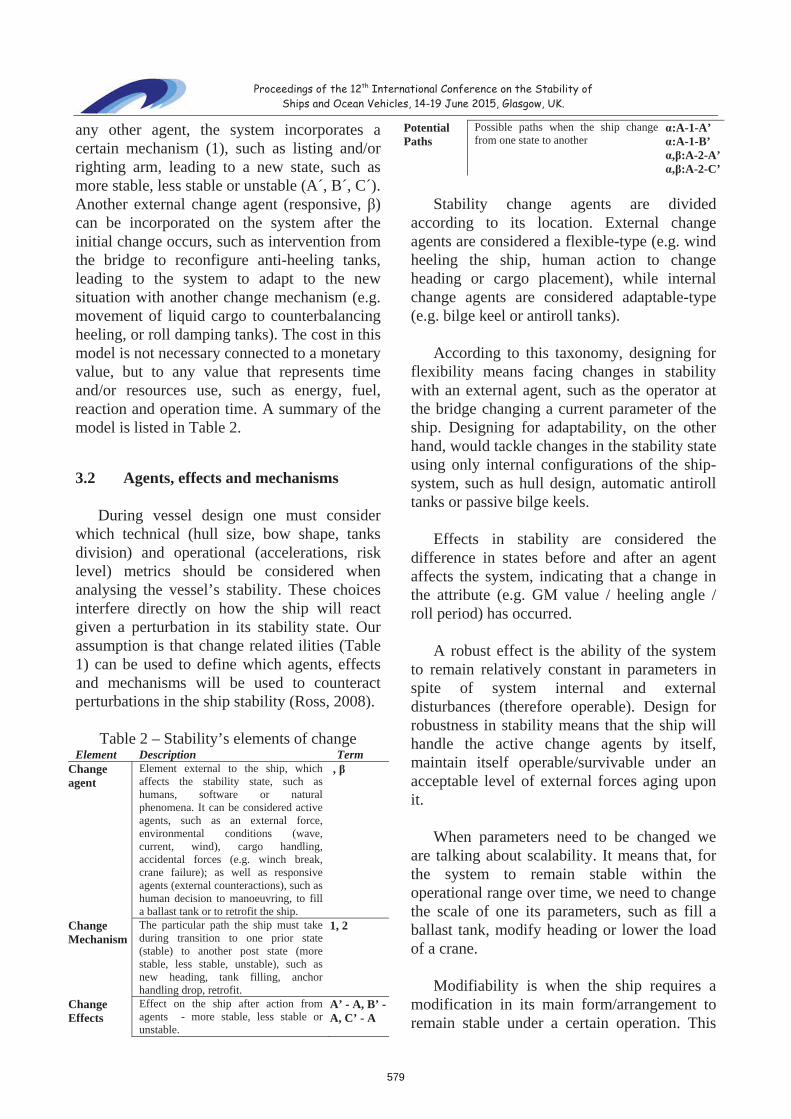
Proceedings of the 12th International Conference on the Stability of Ships and Ocean Vehicles, 14-19 June 2015, Glasgow, UK.
any other agent, the system incorporates a certain mechanism (1), such as listing and/or righting arm, leading to a new state, such as more stable, less stable or unstable (A´, B´, C´). Another external change agent (responsive, β)can be incorporated on the system after the initial change occurs, such as intervention from the bridge to reconfigure anti-heeling tanks, leading to the system to adapt to the new situation with another change mechanism (e.g. movement of liquid cargo to counterbalancing heeling, or roll damping tanks). The cost in this model is not necessary connected to a monetary value, but to any value that represents time and/or resources use, such as energy, fuel, reaction and operation time. A summary of the model is listed in Table 2.
3.2 Agents, effects and mechanisms
During vessel design one must consider which technical (hull size, bow shape, tanks division) and operational (accelerations, risk level) metrics should be considered when analysing the vessel’s stability. These choices interfere directly on how the ship will react given a perturbation in its stability state. Our assumption is that change related ilities (Table 1) can be used to define which agents, effectsand mechanisms will be used to counteractperturbations in the ship stability (Ross, 2008).
Table 2 – Stability’s elements of change Element Description Term
Changeagent
Element external to the ship, which affects the stability state, such as humans, software or natural phenomena. It can be considered active agents, such as an external force, environmental conditions (wave, current, wind), cargo handling, accidental forces (e.g. winch break, crane failure); as well as responsive agents (external counteractions), such as human decision to manoeuvring, to fill a ballast tank or to retrofit the ship.
,
ChangeMechanism
The particular path the ship must take during transition to one prior state (stable) to another post state (more stable, less stable, unstable), such as new heading, tank filling, anchor handling drop, retrofit.
1, 2
ChangeEffects
Effect on the ship after action from agents - more stable, less stable or unstable.
A’ - A, B’ - A, C’ - A
Potential Paths
Possible paths when the ship change from one state to another
:A-1-A’:A-1-B’, :A-2-A’, :A-2-C’
Stability change agents are divided according to its location. External change agents are considered a flexible-type (e.g. wind heeling the ship, human action to change heading or cargo placement), while internal change agents are considered adaptable-type (e.g. bilge keel or antiroll tanks).
According to this taxonomy, designing for flexibility means facing changes in stability with an external agent, such as the operator at the bridge changing a current parameter of the ship. Designing for adaptability, on the other hand, would tackle changes in the stability state using only internal configurations of the ship-system, such as hull design, automatic antiroll tanks or passive bilge keels.
Effects in stability are considered the difference in states before and after an agent affects the system, indicating that a change in the attribute (e.g. GM value / heeling angle / roll period) has occurred.
A robust effect is the ability of the system to remain relatively constant in parameters in spite of system internal and external disturbances (therefore operable). Design for robustness in stability means that the ship will handle the active change agents by itself, maintain itself operable/survivable under an acceptable level of external forces aging upon it.
When parameters need to be changed we are talking about scalability. It means that, for the system to remain stable within the operational range over time, we need to change the scale of one its parameters, such as fill a ballast tank, modify heading or lower the load of a crane.
Modifiability is when the ship requires a modification in its main form/arrangement to remain stable under a certain operation. This
579

Proceedings of the 12th International Conference on the Stability of Ships and Ocean Vehicles, 14-19 June 2015, Glasgow, UK.
requires usually a redesign or retrofit of the vessel to incorporate new structural aspects, such as new antiroll tanks and/or structural reinforcement.
Mechanisms can be understood as the paths that the ship must take to transit between states. It includes elements inherent to the ship design process, such as necessary subsystems, components, resources, conditions and constraints that allows a path between two situations, such as less stable to more stable,higher roll acceleration to lower roll accelerations.
For the sake of exemplification, lets consider a crane operation with heavy cargo. The change agent is the crane, and the change effect is the GM value and heeling angle of the ship. Many possible paths (mechanisms) can be taken to minimize heeling angle and keeping safe GM values. The active agent (crane) can modify its arm length and height or even drop the cargo. The ship operator (responsive agent) can turn on dynamic positioning (DP) or roll compensation mechanism. Each action, thus, is connected to a cost in terms of time and resources to correct the effect caused by the crane.
When taking these definitions in the initial design process, design for many potential change mechanisms means design for different costs, with potential costs for a given path in a given condition. Over time, not only the cost of a mechanism may change, but also more paths can be added to the ship via new capabilities on board or retrofit of the ship. Table 3 summarizes the Stability’s implications for design in terms of flexibility, adaptability robustness, scalability and modularity
Table 3 – Change related properties in Stability Design for Description Flexibility The stability change agent is external to the
ship-system. Change mechanisms are possible under external (human, computer) actions
Adaptability The stability change agent is internal to the ship-system.
Robustness Design a vessel that keeps stable under conditions’ change. Change mechanisms are inherent to the design
Scalability Design a vessel able to be stable under a set of conditions when its parameters are scalable. For instance activate anti-heeling tanks or move deck cargo.
Modifiability Vessel is only able to be stable after modifications are incorporated in its form, via re-design or retrofit. It may be the case for a low initial capital cost, with option for a retrofit and more stability in the long-term, if future contracts require it.
3.3 Lifecycle implications for ilities in stability during initial design
Our assumption is that designers should no longer only consider stability properties that meet today’s regulations and requirements, but rather consider the implications and consequences of the lifecycle technical, operational and commercial context changes early in the design process (Ulstein and Brett, 2012; 2015), including change related mechanisms into the ship, which allow cost-effective reactions on how it behaves to disturbances in its stability related attributes. In order to explicit address the desire of a shipowner to have flexibility, it is necessary to gather more information about the desired responsive change agent, change effect and mechanisms, as desiring flexibility alone is an imprecise request. In this sense, we build on Ross (2008) proposition of analysing and evaluating stability related in five basic steps:
i) Specify the origin of the active changeagents (perturbances, disturbances), and in which operational conditions they occur. For instance, finite duration active agents such as wave, wind, short operation loads (hanging, moving) or even chaotic motions; as well as long term shifts (likely to last), such as cargo placement/shift, long operation (towing, crane),
580

Proceedings of the 12th International Conference on the Stability of Ships and Ocean Vehicles, 14-19 June 2015, Glasgow, UK.
damage, free-surface, flooding, collision, grounding should be specified.
ii) Determine the acceptable cost threshold,that is, response time and resource uses when disturbed, as well as determining the shipowner willingness to pay for a more stable vessel, such as wider breadth, faster antiroll system, stronger hull or higher dynamic position capability.
iii) Specify if the origin of responsive agent,that is, internal (adaptable and incorporate in the ship as a system) of external (acting on the ship but external to its boundaries).
iv) Consider which effect is expected foreach of the responsive agents selected in iii). Robust effects will change no parameter, being inherent to the form/arrangement of the ship. Changes in the level of a vessel parameter creates scalable effects, such as modification of the tension in a towing line, as well as filling up the antiroll tank or activating the DP system. Modifiable effects require changes in the nature of a certain parameter of the ship, such as the installation of a more powerful anti-heeling pump, a new crane or rearrangement of the ship load distribution.
v) Analysis and evaluation of the vesseldesign space is done in the last phase, considering, which capabilities should be inherent or installed on board the ship, in terms of disturbances (active agents), reactions (responsive agents), and effects on stability related attributes. For example, if the shipowner requires the ship to be adaptable and robust regarding supply operation in North Sea high wave conditions, while flexible when performing anchor-handling operation in more extreme conditions, then response mechanisms that are able to be flexible and adaptable must be considered when evaluating the design space. In this way, the specific adaptability (in terms of low accelerations while supplying) and flexibility (in terms of controlling safe GM and low acceleration while anchor-handling in extreme conditions) can be weighed against
cost (time/resource) requirements and rules constraints. At the end, we should converge towards a set of quantified lifecycle properties, that is, a value gain versus cost when talking about robustness or scalability.
4. HANDLING VESSEL STABILITYCOMPLEXITY IN A LIFECYCLECONTEXT VIA A FIVE-ASPECTSTAXONOMY
A systemic approach for definingcomplexity in ship design is presented by Gaspar et al. (2012a, 2012b), where the complexity of a system is captured through five main aspects, namely: Structural (structure and relationships), Behavioural (performance), Contextual (circumstances),Temporal (changes in context and uncertainties) and Perceptual (stakeholders’ viewpoint). Here we use these taxonomy to clarify, organize and handle the information necessary to proper identify and build up the elements necessary to understand stability as a lifecycle property.
Structural and behavioural aspects connect to the traditional technical understanding that stability depends on the ship main dimensions, the shape of the submerged hull and tanks/ cargo arrangement, as well as location of unprotected openings such as engine room air intakes and the actual location of centre of gravity KG. Well-known trade-offs analysis, when determining the main dimensions and hull form, should be conducted among some major design disciplines, such as sea keeping, stability, manoeuvrability, sufficient cargo hold volume and payload capacity. Considering a ship with large GM, for instance, where the righting arm developed at small angles of heel is also large. Such a ship is usually considered stiff and will resist roll. However, if the metacentric height of this ship is small, with smaller righting arm, the vessel may be considered tender, rolling slowly. Practical offshore support vessel (OSV) design experience shows the necessity of balance between generating stiff or tender design, since
581

Proceedings of the 12th International Conference on the Stability of Ships and Ocean Vehicles, 14-19 June 2015, Glasgow, UK.
they have opposite influences on stability of vessel and convenience of crew during site operation. A design for safety thus will be contradictory to a design for operability. Therefore, if a shipowner invests in robustness for the reason that his or her vessel may be considered safe for a wide range of conditions, the same investment may lead to a loss in contracts due to limited cargo capacity or smaller crew comfort. What the designer should consider then is the nature of the reaction of the vessel, for instance, by changing one of its change effects, for instance a tank installed in a higher deck (modifiability) that can be filled during site operation (scalability). The initial robust solution is unable to proper consider the extension of the stability complexity, while the modifiable / scalable solution is.
The contextual aspect pertains to the external circumstances to which the vessel is subject to during operation and how its behaviour is affected accordingly. The applied contextual factors in traditional ship design are often dominated by various technical and economic factors during exploration of the technical design space such as meteorological conditions, rules and regulations, supply and demand, breakeven rates and so forth. Such factors will impose a range of requirements and restrictions, the resulting solution space will be significantly delimited, inherently affecting the shape of the vessel and consequently narrowing the diversification of potential stability characteristics. In order to move beyond pure technical thinking, stability as a lifecycle property, which must also be included as input when considering the boundaries of the design space. In other words, stability must be perceived as something more than just metacentric height, a GZ-curve and a characteristic of operational performance. It should also be considered an attribute of value creation across contextual factors, i.e. diversifying the categories of which stability value is commonly quantified by. Exemplifying, a remarkably stable vessel could be considered technically superior, but at the
same time, it may also require compensatory investments leading to an increased capital cost. Viewing this in a contextual lifecycle perspective the value of this increased robustness should also be considered in terms of factors such as flexibility, adaptability, and current and presumed market developments.
When considering a vessel from a temporal perspective, changes in the system’s lifespan occurring at disparate points in time, in conjunction with a highly scattered degree of uncertainty, together constitute the fourth taxonomy aspect. When viewing stability as a lifecycle property, a method of quantifying contextual shifts is necessary. The technical perspective would take into account the probable spectre of applicable mission types and operational modes by utilizing a traditional set of analyses, and conclude based on input parameters such as wave height and direction, currents, mass distribution, and hull shape. These types of analyses unquestionably provide excellent sources of information regarding a vessel’s stability characteristics; however, they do not take into account contextual variations in an uncertain temporal perspective. One possible method of quantifying such complex information is Epoch Era Analysis (EEA) (Ross and Rhodes, 2008, Gaspar et al., 2012b, Keane et al., 2015),which captures future expectations by encapsulating each factor-variant in a fixed (epoch) and dynamic (era) time-constrained context setting that should be further analysed in terms of probability, optimality, performance, value, and utility, to name a few. This enables the incorporation of multi- values, attributes and assumptions that previously may have been side-lined, generating data for the perceptual aspect.
The overall lifecycle property connected to the perceptual aspect is value robustness, which is used, including but not limited to aspects presented above, to define in multi-perspective a better vessel among a design set. Value robustness is the ability of a system to continue to deliver stakeholder value in face of shifts in
582

Proceedings of the 12th International Conference on the Stability of Ships and Ocean Vehicles, 14-19 June 2015, Glasgow, UK.
context and needs (Ross and Rhodes, 2008). In ship design, this means a ship perceived successful by stakeholders throughout the lifetime of the vessel. Rather than maximizing value delivered by a ship in one situation, we need to maximize it over a range of situations and preferences of the owner (or other constituents). This might reduce the maximum possible reward but also minimize the maximum possible loss, with relevance increasing as uncertainty grows and investors become more risk aware (Gaspar et al., 2015).
In this context, how to perceive stability as a lifecycle property, and make benefit of it to bring more value to the vessel? How to really decompose the multi-perspective perception of what a stakeholder would understand as a valuable ility? Ebrahimi et al. (2015) notes that the perception of a better (therefore stable) vessel relies in a middle term perspective, between the pure satisficing and maximizing the goodness of fit of all stakeholders’ expectations. On one hand, we would like to select the best solution, by creating and analysing all possible risk situations and alternatives, and choose the best. Our limitation as human beings, however, allow us to only compare and contrast a very limited set of variables and alternatives when trying to find the good enough stability. Ulstein and Brett (2015) propose the application of different perspectives to overcome these limitations. Technical, Operational and Commercial perspective for instance, links to the vessel skills and level of efficiency needed for a particular operation, while Smarter, Safer and Greener perspective connects to a more fashionable idea of effectiveness, increasing the overall effect of the combined technical, operational and commercial performance. The change related ilities are tackled in their approach for design for efficiency, whereflexibility, agility and robustness are observed in terms of the ability of the vessel to perform different operation, move and upgrading itself quickly and not likely to fail.
5. TOWARDS A PRESCRIPTIVESEMANTIC BASIS FOR STABILITY
We are aware of the challenges whenextending the concept of stability, connecting it to less technical lifecycle properties. While stability is traditionally a well-defined and quantified term in ship design, the informal meaning, ambiguity, synonymy and lack of scientific precision (and therefore standard) for the pre-mentioned ilities raise a yellow flag. This concern does not relate solely to the stability issue, but to the assessment and quantification of all ilities in general.Flexibility, for instance, may be connected to the ability to change as well as to the ability to satisfy multiple needs.
Therefore, to assume that stability can be defined and measured in terms of properties such as flexibility, adaptability, modifiability, scalability and robustness, we need to have a more precise understanding of these terms. Ross and Rhodes (2015) address this issue by proposing a generalization of the change related properties, via a prescriptive semantic basis for these ilities. Starting from the same principle of change agent, effect and mechanism, the authors propose a larger set of twenty categories (elements) for defining a larger set of possible changes in a system. This semantic basis aims to capture the essential difference among change-related ilities, in the following proposed general statement (categories emphasized): “in response to perturbation in context during phase, desireagent to make some nature impetus to the system parameter from origin(s) todestination(s) in the aspect using mechanism in order to have an effect to the outcome parameter from origin(s) to destination(s) inthe aspect of the abstraction that are valuable with respect to the thresholds in reaction, span, cost and benefit”.
For the illustrative purposes, we can use the aforementioned general pattern to create a statement that intends to capture a more precise meaning to which kind of lifecycle property in
583

Proceedings of the 12th International Conference on the Stability of Ships and Ocean Vehicles, 14-19 June 2015, Glasgow, UK.
stability are we talking about. When talking to scalability, for instance, one could state: “In response to a crane failure (perturbation) during heavy lift operation (phase) in the North Sea (context), desire operator (agent) to be able to decrease (nature) the heeling angle of the ship (parameter) from a less stable (origin) to more stable (destination) position (aspect)trough turning on the pumps that feeds the anti-heeling tanks (mechanism) in less than ten seconds (reaction) that results in the increasing of the volume of the tanks (effect), decreasing the heeling angle (aspect) to an acceptable value (destination) in the ship (abstraction) taking less than 30 seconds (span), with a energy use (cost) inferior than the actual installed system (benefit)”.
The basis allow then the parsing and decomposition of what one may understand as lifecycle property. When applied to stability, however, this basis can be a bit overwhelming, and simplifications can be done according to phase of the lifecycle studied. When evaluating different mechanisms to overcome unstable conditions, for instance, we may fix the other elements, while leaving the mechanism option open, allowing designer to propose and evaluate different alternative paths for meeting the criteria. In this case, considering the example from the last paragraph, rather than proposing the use of anti-heeling tank, one could suggest a second crane to compensate, or adaptations at hull form or at the anti-roll system. In other case, we case vary the causes of failure, investigating which cases of perturbation require robust, scalable and modifiable solutions.
Note also that the concept of costintroduced in Section 3.1 is also extended, incorporating common trade-offs that can be used to judge the goodness of a stability performance of a ship, such as reaction(timing), span (duration), cost (resources) and benefit (utility).
6. CONCLUDING REMARKS
Much research is currently being developedon the topic of less technical lifecycle properties, and yet many open questions require a more deep study until some consensus is reached as to what this set of agreed upon properties should be like. As for the case described in this paper, our intention was to show that a ship-owner may require a robust vessel system, but in real life situations he or she wants a ship system that can be changed in the future. Market conditions are changing over time and therefore, vessels have to change their capacity and capabilities (internalities) with such externalities. Thus, the way we normally handle the stability of ships from a naval architectural standpoint is not having the process quality of being able to deal with all internalities and externalities to the extent necessary for future flexible/adaptable ship design. Why do people desire higher stability for common initial load cases, while at the same time they know that the vessel over time will be subject to new operational situations not really catered for in the initial design solution space? Stability, may not have a value in and of itself, but rather may represent a significant boundary condition limitation for future adaptability and changeability of the ship at hand. Better prepared for and thought through, in the context of an epoch-era concept framework, stability can be allocated higher value in the future of ship design, than a strict boundary condition, normally,
For the sake of example, let us analyse the main stakeholder and needs of an OSV. It is assumed that the concept of safety considers the protection of human life and environment, and efficiency connects primarily to fuel and the cost (or savings) connected to it. Considering increasingly harsher operating conditions is a necessary precaution in order to reveal adequate stability characteristics when quantifying from a value robustness perspective. The increase of significant wave height, wind speed, and current, all contribute
584

Proceedings of the 12th International Conference on the Stability of Ships and Ocean Vehicles, 14-19 June 2015, Glasgow, UK.
towards a heightened range of loads and motions, consequentially increasing the risk of destabilizing the vessel, minimizing operational windows, and, inherently, depreciating value from a lifecycle perspective. Creating a vessel with sufficient capabilities to counter these effects increases the operational window, but traditionally will also widen the vessel resulting in increased hull resistance and a need for more power to uphold the same speed during transit and on site DP operations. It will also facilitate a higher payload capacity as well as a larger crane capability, again, enabling a wider range of mission profiles. On the extreme case, even if technically and theoretically science and technology are able to design and construct a vessel that does not capsize, such vessel would end up being unfit to operation or, most commonly, unaffordable. Thus, depending on the viewer’s perspective regarding the value of stability, certain trade-offs will be virtually inescapable, e.g. payload capacity versus fuel consumption, or level of acceleration (crew comfort) versus operational utilization (up to allowed level of excitation). Using the concept of ilities can then facilitate the understanding and quantification of these stability trade-offs in future vessel design. In other words, a design can be better perceived as more valuable if stability is observed as a lifecycle system property.
7. REFERENCESAndrews, D. IMDC 2009 “State of the Art
Report on Design Methodology” in 10th International Marine Design Conference 2009 Proceedings Vol 2, Tapir Academic Press, Trondheim, Norway, 2009.
Bodénes, G. “Bourbon into the future. Norwegian Maritime Centre of Expertise”, NCE Annual Conference, Alesund, 2013
de Weck, O.L., Ross, A.M., and Rhodes, D.H., "Investigating Relationships and Semantic Sets amongst System Lifecycle Properties (Ilities)," 3rd International Conference on Engineering Systems, TU Delft, the Netherlands, June 2012.
Gaspar, H., Erikstad, S.O., and Ross, A.M., "Handling Temporal Complexity in the Design of Non-Transport Ships Using Epoch-Era Analysis," Transactions RINA, Vol. 154, Part A3, International Journal of Maritime Engineering, Jul-Sep, pp. A109-A120, 2012a
Gaspar, H., Rhodes, D.H., Ross, A.M., and Erikstad, S.O., "Handling Complexity Aspects in Conceptual Ship Design: A Systems Engineering Approach," Journal of Ship Production and Design, Vol. 28, No. 4, November, pp. 145-159, 2012b
Gaspar, H. M.; P. O. Brett; S. O. Erikstad and A. M. Ross. 2015. “Quantifying valuerobustness of OSV designs taking intoconsideration medium to long termstakeholders’ expectations”. In Proceedings12th IMDC, Tokyo, 2015.
Hastings, D.E., La Tour, P., and Putbrese, B., "Value-Driven Analysis of New Paradigms in Space Architectures: An Ilities-Based Approach," AIAA Space 2014, San Diego, CA, August 2014
IMDC Secretariat. 11th International Marine Design Conference, Proceedings Vol 1&2- IMDC Glasgow, UK, 2012.
Jasionowski, A., Vassalos, D. “Conceptualizing Risk”, University of Strathclyde, in “Contemporary Ideas on Ship Stability and Capsizing Waves”, Springer, 2010.
Keane, A., Brett, P. O., Gaspar, H. M., “Epoch-Era Analysis in the Design of the Next Generation Offshore Subsea Construction Vessels”, in 10th International Conference on System of Systems Engineering (SoSE), San Antonio, USA, 2015.
Neves, M. A. S., Belenky, V. L., de Kat, J. O., Spyrou, K., Umeda, N. “Contemporary Ideas on Ship Stability and Capsizing Waves”, Springer, 2010.
Ross, A. M. “Contributing toward a prescriptive ‘Theory of Ilities’, SEAri-MIT, Missiouri University of Science and Tech. April 2014
Ross, A. M. “Defining and Using new ‘ilities’”, SEAri Working Paper Series, MIT, 2008
585

Proceedings of the 12th International Conference on the Stability of Ships and Ocean Vehicles, 14-19 June 2015, Glasgow, UK.
Ross, A. M., and Rhodes, D. H. “Architecting systems for value robustness: Research motivations and progress”. SysCon 2008 – IEEE International Systems Conference 2008.
Ross, A.M., and Rhodes, D.H., “Towards a Prescriptive Semantic Basis for Change-type Ilities,” 13th Conf. on Systems Engin. Research, Hoboken, NJ, March 2015.
Ulstein, T., and Brett, P. O. “Critical systems thinking in ship design approaches” 11th
IMDC, Glasgow, UK, 2012. Ulstein, T., and Brett, P. O. “What is a better
ship? – It all depends…” (accepted) keynote speaker, 12th International Maritime Design Conference – Tokyo, 2015
586

Proceedings of the 12nd International Conference on the Stability of Ships and Ocean Vehicles, 14-19 June 2015, Glasgow, UK.
An Experimental Study on the Characteristics ofVertical Acceleration on Small High Speed Craft in
Head Waves
Toru, Katayama, Graduate School of Engineering, Osaka Prefecture University
Ryosuke, Amano, Graduate Student, Graduate School of Engineering, Osaka Prefecture University
ABSTRACT
In this study, the characteristics of vertical acceleration on small high speed passenger craft in head waves are investigated experimentally, an empirical method to estimate it is proposed. First, how to decide the sampling frequency and the test duration (total number of waves encounters) is discussed to measure acceleration accurately. Next, the vertical acceleration on a hull is measured in regular and irregular waves, and the characteristics of the vertical acceleration for wave height, wave period and forward speed are investigated. And its probability density function is also investigated for the results in irregular waves. Moreover, the same measurements for two different hulls are carried out, and the effects of hull form is investigated.
Keywords: vertical acceleration, small high craft, irregular waves
1. INTRODUCTION
Recently, the maximum forward speed ofsmall passenger craft is increasing. In case of the craft, the encounter wave period becomes shorter with increase of forward speed, and very large upward vertical acceleration is caused when its bow goes into the water surface. It is known that it cause not only bad ride comfort but also failure of hull or injury of passengers in some cases.
For development hull form, it is necessary to estimate the response of acceleration for its forward speeds and sea conditions. And for safety navigation management, it is important to estimate statistical short-term prediction of
occurrence of un-desired large vertical acceleration.
The purpose of this study is to investigate the above-mentioned characteristics of vertical acceleration of small high speed passenger craft. First, in order to measure accurate vertical acceleration by a partly captive model test, data sampling and data analysis methods are discussed. Next, the vertical acceleration on a hull is measured in regular and irregular waves, and the characteristics of the vertical acceleration for wave height, wave period and forward speed are investigated. And its probability density function is also investigated for the results in irregular waves. Moreover, the same measurements for two additional
587

Proceedings of the 12nd International Conference on the Stability of Ships and Ocean Vehicles, 14-19 June 2015, Glasgow, UK.
different hulls are carried out, and the effects of hull form is investigated.
2. OBJECT SHIP
Table 1 and Fig.1 show the principleparticulars of models and their photographs. Fig.2 shows the body plan of Ship A. Their loading condition is full load. They are fast semi-planing craft with warped V and their draft is shallower and Lpp/B is larger than typical planing hulls. In the comparisons among the models, Lpp/B of Ship B is smaller than others and dead rise angle of Ship B is larger than others.
Table 1 Principal particulars of the models in real scale.
Ship A Ship B Ship C
Scale: 1/S 1/23.4 1/21.0 1/21.0
Length between perpendiculars: Lpp [m] 23.4 14.95 18.1
Breadth: B [m] 4.5 4.5 4.4.
Deadrise angle at s.s.=5.0: [deg] 18 18 24
Displacement: W [tonf] 36.76 25.91 31.51
Draft: d [m] 0.760 0.751 0.953
Fig.1 Photographs of the models (Ship A, B and C)
−2 0 20
1
2
[m][m]
[m][m]
Fig.2 Body plan of the model (ship A).
3. MEASUREMENT AND ANALYSIS
3.1 Measuring device and coordinate system
Fig.2 show a schematic view of experiment and its coordinate system. Fig.3 shows its picture. A model is towed at constant speed with heaving and pitching free condition. And heaving (up: +), pitching (bow up: +) and normal acceleration on the base line of the hull (upward: +) are measured. Three acceleration sensors are installed on bow, midship and stern. Wave height is also measured with a servo type wave height meter attached to the towing carriage.
Fig.2 Schematic view of the experiment to measure vertical acceleration on hull
588

Proceedings of the 12nd International Conference on the Stability of Ships and Ocean Vehicles, 14-19 June 2015, Glasgow, UK.
Fig.3 Photograph of the experiment.
3.2 Sampling frequencies
The sampling frequencies fs [Hz] in the measurement is decided by eq.(1).
st
nfs ss (1)
where s is the denominator of scale of model, t [sec] is the shortest duration of impact accelerations acting on hull in irregular waves in real scale, ns is the number of sampling data in the impact acceleration. According to the reference (National Maritime Research Institute, 2007 and Takemoto et al., 1981), t is about 120msec in real scale. To express the peak of the impact acceleration, if ns = 4 or 5 (Seakeeping Committee of ITTC, 2011) is assumed, an adequate fs = 200Hz is obtained. Fig.4 shows the convergency of average amplitude of vertical acceleration measured for different sampling frequencies (100, 200, 500, 1000Hz). The number of encounter waves is more than 400.
The upper figure shows the average of upward peak value of the acceleration and the under one shows the average of downward peak value of the acceleration, and the horizontal axis is sampling frequency. As a result, it is noted that the margin of error is smaller than 5% when the number of sampling frequencies is more than 200Hz. Therefore, the number of sampling frequencies in the measurement is decided for 200Hz.
Fig.5 shows a time history of measured accleration at FP. In the measurement, the impact acceleration shown at t = 0.7seconds in Fig.5 is observed commonly in each measured data. The acceleration occurs when its bow goes down into the water surface. In order to obtain the peak to peak values of the acceleration, zero-down crossing method is used in the analysis. As seen in Fig.5, time history of measured acceleration has noise. To take zero cross points, the data filtered with a central moving average method of 10 datum is used. On the other hand, to take accurate peak value of the acceleration, the data filtered with a central moving average method of 2 datum is used.
0 500 10000
20
Sumpling Frequency [ Hz]Acc
eler
atio
n [ m
/sec
.2 ]
0 500 1000
10
0Sumpling Frequency [ Hz]
Acc
eler
atio
n [ m
/sec
.2 ]
Fig.4 Variation of average of amplitude of vertical acceleration measured for different sampling frequencies. (upper figure: upward acceleration, lower figure: downward acceleration)
589

Proceedings of the 12nd International Conference on the Stability of Ships and Ocean Vehicles, 14-19 June 2015, Glasgow, UK.
0 0.5 1
−20
0
20
40
0 0.5 1
−20
0
20
40
t[sec.]
af [m/sec.2]
moving average(2 datas)measuerd data
moving average(10 datas)measuerd data
= 0.045sec.
zero crossing point
t√s
one period
Fig.5 Time histories of measured data in irregular waves. (upper figure: a central moving average method of 2 datum, lower figure: a central moving average method of 10 datum)
3.3 Sampling number of encounter waves
Fig.6 shows the convergency of average amplitude of vertical acceleration measured for different sampling number of encounter waves. The upper figure shows the average of upward peak value of the acceleration and the under one shows the average of downward peak value of the acceleration, and the horizontal axis is sampling number of encounter waves. As a result, it is noted that the margin of error is smaller than ±4% when the sampling number of encounter waves is more than 200. Therefore, measurement in irregular waves is carried out with more than 200 encounter waves.
0 200 4000
2
4
Acce
lera
tion
[m/s
ec.2 ]
The number of wave encounters
0 200 400
6
4
2
0
Acce
lera
tion
[m/s
ec.2 ] The number of wave encounters
Fig.6 Variation of average of amplitude of measured vertical acceleration for numbers of amplitude data.(upper figure: upward peak value, lower figure: downward peak value)
3.4 Longitudinal distribution of vertical acceleration
The instantaneous acceleration aX on longitudinal position X on hull is expressed as Eq.(2) with heaving and pitching of an arbitrary position.
glza XX cos1cos (2)
Where z is heave displacement (upward: +), is pitch angle (bow up: +), lX is distance
(forward:+) from the position of motionmeasuring and g is the gravitationalacceleration (downward: +). Furthermore theheave and pitch accelerations are calculatedwith numerical differentiation of their data ofdisplacement.
The accelerations measured on two different position on hull (aA and aF) are expressed as eq.(3) and eq.(4) by using eq.(2).
glza AA cos1cos (3)
590

Proceedings of the 12nd International Conference on the Stability of Ships and Ocean Vehicles, 14-19 June 2015, Glasgow, UK.
glza FF cos1cos (4)
By using eq.(3) and eq.(4), heave and pitch terms in eq.(2) can be erased. Then eq.(5) is obtained.
AF
AFFXFX ll
aallaa )(
(5)
where lX-lF is the distance from F to X,lF-lA is the distance from A to F. Eq.(5) indicated that the instantaneous acceleration aXis calculated by Eq.(5) with the measured instantaneous accelerations aA and aF.
Fig.7 shows the comparison between the calculated acceleration on midship by Eq.(5) using accelerations measured on the stem and stern and the acceleration measured on the midship position. From the results, it is confirmed that the calculated result is good agreement with the measured results.
0 1 2 3-15
0
15
30
45
t[sec.]
ac[m/sec.2]
mesured datacalculated data
Fig.7 Time histories of measured and calculated results at s.s.5.0 in irregular wave. (sea state 4, Fn=0.51, Ship A)
3.5 Making irregular waves
Eq.(6) is ISSC spectrum, and Eq.(7) is the relations between significant wave height H1/3[m] and average wave period T1 [sec].
41
51
12
31 244.0exp
2211.0)( TT
THS
(6)
3/11 86.3 HT (7)
where [rad/sec] is circular frequency of wave, S( ) [m2 sec]is energy density function of wave. To make irregular waves, the spectrum is divided into 100 equally in 0.2~2.5Hz, and a sine wave of each frequency component is superposed. In addition, the phase difference of each frequency component is given as random numbers for each measurement. Table 2 shows the range of wave height for sea state in real scale, and the wave height in this study. The towing speeds in the measurement are 0, 10, 15, 20, 25, 40kts in real scale.
Table 2 Wave conditions of the experiment.
4. CHARACTRISTICS OFACCELERATION
4.1 Effects of Type of Ship
As an estimation method of vertical acceleration on hull, Osumi’s chart (Osumi, 1992) and Savitsky’s empirical formula (Savitsky et al., 1976) are known. Fig.8 shows the comparisons between the measured results (Ship A) and Osumi’s results. The measured results are larger than Osumi’s results. It is supposed that Osumis’ results does not include the impact acceleration shown in Fig.5, because the object ship is the high speed patrol boat. Fig.9 shows the comparisons between the measured results and Savitsky’s results. The measured results are smaller than Savitsky’s results. It is supposed that Savitsky’s results include large impact acceleration, because the object ships is typical planing hulls which is hard chine straight deep V monohedron without bow flare.
sea statewave height
for seastate [m]typical wave height
for a sea stateaverage wave period
: T1 [sec.]0.70 3.21.00 3.9
4 1.25~2.50 2.00 5.55 2.50~4.00 3.00 6.7
3 0.50~1.25
591

Proceedings of the 12nd International Conference on the Stability of Ships and Ocean Vehicles, 14-19 June 2015, Glasgow, UK.
Fn=0.34Fn=0.51Fn=0.68Fn=0.85Fn=1.36
Fn=0.4 by Osumi's resultFn=0.5 by Osumi's resultFn=0.7 by Osumi's resultFn=0.9 by Osumi's resultFn=1.2 by Osumi's result
0 2 40
50
A FP(
1/3)
*LPP
/(g*H
W)
/ LPP
Fig.8 Comparison of non-dimensional significant peak to peak amplitude of acceleration between the measured results and Osumi’s results.
10knotSavitsky 10knot
15knot 25knot20knot 40knotSavitsky 15knot
Savitsky 20knot Savitsky 25knotSavitsky 40knot
0 2 40
10
20
30
/L
A(+
) FP[
m/s
2 ]
0 2 40
10
20
30
/L
A(−
) FP[
m/s2 ]
Fig.9 Comparison of average peak value of vertical acceleration between the measured results and Savitsky’s results. (upper figure: upward peak value, lower figure: downward peak value)
4.2 Effects of wave length and height
Fig.10 shows non-dimensional average upward or downward peak value of measured
vertical acceleration on hull. In the figure, the horizontal axis is the ratio of wavelength to ship length /LPP. The wavelength is calculated from =g/(2 )×T1. Eq.(8) is proposed to fit to the measured results, and the fitted curves are shown the figure.
CxexBy (8)
To investigate the effect of wave height on the vertical acceleration, the measurement with different wave height, constant forward speed and constant average wave period for Ship A is carried out. Fig.11 shows average upward and downward peak values of vertical acceleration at FP. The horizontal axis is H1/3/LPP. From the figure, it is noted that the non-dimension values of upward and downward acceleration are linearly increased with increase of wave height. The same tendency can be seen in the upward acceleration in the regular wave shown in Fig.12 in the condition where the impact acceleration shown in Fig.5 occurs because of increase of wave height or/and forward speed.
0 2 40
20
40
Fn=0.00Fn=0.51Fn=1.36
A(+
) FP(
ave)
*LPP
/ H
W(1
/3)
T12*g / 2 *LPP
0 2 40
20
40Fn=0.00Fn=0.51Fn=1.36
A() F
P(av
e)*L
PP /
HW
(1/3
)
T12*g / 2 *LPP
Fig.10 Non-dimensional average peak value of measured vertical acceleration obtained by Eq.(8) for Ship A. (upper figure: upward peak value, lower figure: downward peak value)
592

Proceedings of the 12nd International Conference on the Stability of Ships and Ocean Vehicles, 14-19 June 2015, Glasgow, UK.
0 0.1
20
0
20
A FP(
1/3)
*LPP
/(g*H
w)[
G]
HW(1/3)/LPP
Average upward accelerationAverage downward acceleration
Fig.11 Average upward and downward peak values of vertical acceleration at FP measured for several wave height. (Ship A) In this figure, the black solid line shows the free fall whose acceleration is 1.0 G.
0 0.02 0.04 0.060
50
A f(+
)*L p
p/(g*
Hw
) [G
]
HW/LPP
30knot25knot20knot15knot
0 0.02 0.04 0.06
40
20
0
A f(−
)*L p
p/(g*
Hw
) [G
] HW/LPP
30knot25knot20knot15knot
Fig.12 Measured upward and downward peak value of vertical acceleration for wave heights at s.s. 10.39 (Tw=1.0 sec) (Ship A). (upper figure: upward peak value, lower figure: downward peak value)
4.3 Longitudinal Distribution
Fig.13 shows longitudinal distribution of peak to peak amplitude and peak values of vertical acceleration which is calculated by Eq.(5) with vertical acceleration measured at FP and at AP. The horizontal axis is the square station number (AP=0 and FP=10). The vertical acceleration increases with increase of forward speed, and it linearly increase with
moving forward of longitudinal position from about s.s.=4.0. From the lower figure, it is found that upward peak value is larger than downward peak value, because upward acceleration occurs when bow of ship goes into the water surface. Fig.14 shows the longitudinal position of minimum vertical acceleration. The position is different according to forward speeds or wave periods and moves backward with increase of forward speed or/and wave period.
0 5 100
20
40
S.S
A ss(
ave)
*LPP
/(g*H
)
Fn=0.00
Fn=0.51
Fn=0.85
Fn=0.34
Fn=0.68
0 5 100
20
S.SA(+
,) ss
(ave
)*L P
P/(g
*H)
Fig.13 Longitudinal distribution of significant peak to peak value and upward and downward of vertical acceleration on hull. (upper figure: peak to peak value, lower figure, upward and downward of acceleration)
0 0.5 10
2
4
S.S.
Fn
sea state 3sea state 4sea state 5
Lcg[S.S.number]
Fig.14 Longitudinal position where amplitude of vertical acceleration is minimum. (Ship A)
Fig.15 shows the non-dimensional value of acceleration shown in Fig.13. Value at arbitrary longitudinal position is divided by the value at FP. To estimate longitudinal
593

Proceedings of the 12nd International Conference on the Stability of Ships and Ocean Vehicles, 14-19 June 2015, Glasgow, UK.
distribution of the acceleration except at Fn=0,Eq.(9), (10) and (11) are proposed as empirical formula.
)0.3..(10
.).6(
.).0.3(10
..
)(
)(
ssss
ssss
AA
aveFP
avess (9)
)0.3..(28
.).10(
.).0.3(28
)2..3(
)()(
)(
)(
ssss
ssss
AA
aveFP
avess (10
)
)0.3..(12
.).314(
.).0.3(12
.).2(
)()(
)(
)(
ssss
ssss
AA
aveFP
avess (
11)
0 5 100
1
S.S
A ss(
ave)
/AFP
(ave
)
Fn=0.00Fn=0.34Fn=0.51Fn=0.68Fn=0.85
0 5 100
1
S.S
A(+
) ss(a
ve)/A
(+) F
P(av
e)
0 5 100
1
S.S
A() ss
(ave
)/A(
) FP(
ave)
Fig.15 Form of longitudinal distribution of peak to peak value, upward peak value and downward peak value of vertical acceleration on hull in irregular waves. (upper figure: peak to peak value, middle figure: upward peak value, lower figure: downward peak value)
4.4 Effects of Hull Form
Fig.16 shows significant peak to peak value of upward and downward of vertical acceleration on hull with Ship A, B and C. Its horizontal axis is LPP. The extent is different from hull form and vertical acceleration becomes small when deadrise angle becomes large or LPP/B becomes small.
Kihara's line 15knotKihara's line 20knotKihara's line 25knotKihara's line 30knotKihara's line 35knot
10knot15knot20knot25knot
Ship A Ship BShip C
LPP = 14.95 [m]LPP = 23.4 [m]LPP = 18.1 [m]
0 20 400
1
2Ac
cele
ratio
n [G
]
LPP [m]
Seastate 3
0 20 400
2
4
Acce
lera
tion
[G]
LPP [m]
Seastate 4
0 20 400
2
4
Acce
lera
tion
[G]
LPP [m]
Seastate 5
Fig.16 Measured significant amplitude of vertical acceleration on hull at FP vs ship length speed in real scale. (Ship A, B and C) (upper figure: Seastate 3, middle figure: Seastate 4, lower figure: Seastate 5)
594

Proceedings of the 12nd International Conference on the Stability of Ships and Ocean Vehicles, 14-19 June 2015, Glasgow, UK.
4.5 Statistic property
It is well known that the probability density function of amplitudes of acceleration of a displacement type ship in irregular waves can be expressed with Rayleigh distribution of Eq.(12). Rayleigh law describes distribution of the envelope of nomal process. In the case of narrow band spectrum, the envelope can be used as a reasonable approximation of the amplitudes. The maximum likelihood estimate if parameter is expressed as Eq.(13).
)2
exp()( 2
2
2xxxp (12)
n
iiX
n 1
2
21ˆ (13)
where Xi is measured datum in time step and n is the number of total datum. The relation among parameter , average value, significant value and average 1/10 maximum value of Rayleigh distribution is expressed as Eq.(14).
10/131 04.21
6.11
2XXX
(14)
Fig.17 shows the comparison of parameter , significant value, average 1/10 maximum
value obtained from measured results and estimated results by Eq.(14) with the average amplitude of measured data. From upward acceleration in the upper side Fig.17, measured results are larger than estimated results when the average amplitude is larger than 1.0G. On the other hand, downward acceleration in the lower side Fig.17, measured results smaller than estimated results when the average amplitude lager than 0.5G.
Savitsky proposes a probability density function p(x) (Savitsky et al., 1976) as Eq.(15) with exponential distribution.
)exp(1)(XX
XXp (15)
where X is average amplitude of acceleration. The average 1/N maximum amplitude of acceleration is proposed as Eq.(16).
NXX eN log1/1 (16)
Fig.18 shows comparisons of probability distributions of amplitude of acceleration. The results of Eq.(15) is good agreement with measured results. Fig.19 shows the results of Eq.(16) drowned on the left side Fig.17, and the results is good agreement with the measured results when the average amplitude is larger than 1.0G.
Xave (measuresd result)X1/3 (measuresd result)X1/10 (measuresd result)
(measuresd result)
Xave (estimated result)X1/3 (estimated result)X1/10 (estimated result)
(estimated result)
0 50 1000
20
40
[m/sec.2]
X ave
[m/s
ec.2 ]
0 10 200
5
10
[m/sec.2]
X ave
[m/s
ec.2 ]
Fig.17 Comparison between measured results and estimated results based on Rayleigh distribution with average value of measured data. (Ship A) (upper figure: upward acceleration, lower figure: downward acceleration)
Fig.20 shows probability distribution of downward peak value of vertical acceleration at FP. The upper figure shows the results when
595

Proceedings of the 12nd International Conference on the Stability of Ships and Ocean Vehicles, 14-19 June 2015, Glasgow, UK.
the average amplitude smaller than 0.5G, and the lower figure shows the results when the average amplitude lager than 0.5G. If average amplitude becomes larger, the mode of amplitude is close to about 1.0G. However when the average is over 0.5G, the mode of amplitude does not becomes much larger than 1.0G and the average amplitude does no becomes larger. Because downward acceleration occurs when ship bow turns rising into falling, bow moves close to free fall when the average is over 0.5G.
0 50 100 1500
2
4
AFP (+) [m/sec.2]
Seastate 4:HW(1/3)=2.11mTAve=4.83secFn=0.85
Rayleigh distribution ( =27.9)
XAve=28.1 m/sec.2
by Savitsky
Fig.18 Measured probability distribution of upward peak value of vertical acceleration at FP in irregular wave.
0 50 1000
20
40
[m/sec.2]
X ave
[m/s
ec.2 ]
Fig.19 Comparison between measured result and exponential distribution proposed by Savitsky.
0 5 10 150
10
20
30
AFP (−) [m/sec.2]
Seastate 3 :HW(1/3)=0.93mTAve=3.25secFn=0.85
Rayleigh distribution ( =2.77)
XAve=−3.40 m/sec.2
−−
0 10 200
10
20
AFP (−) [m/sec.2]
Seastate 4:HW(1/3)=2.11mTAve=4.83secFn=0.85
Rayleigh distribution ( =27.9)
XAve=−8.05 m/sec.2
−
Fig.20 Probability distributions of downward peak value of vertical acceleration at FP in irregular wave. (Ship A)
5. CONCLUSIONS
In this study, the characteristics of verticalacceleration in irregular waves for high speed semi-planing hull is investigated experimentally. The following conclusions are obtained.
1. To measure peak value of impactacceleration accurately, a measurement andanalysis procedure is proposed.
2. Based on the measured results, the effectsof wave length, wave height and forwardspeed are indicated and a fitting curve toexplain the characteristics of RAO of theacceleration is proposed.
3. Form of longitudinal distribution of theacceleration is discuss, and an empiricalequation to express the form expecting atFn = 0 is propose.
4. The vertical acceleration on hull inirregular waves is different with that of
596

Proceedings of the 12nd International Conference on the Stability of Ships and Ocean Vehicles, 14-19 June 2015, Glasgow, UK.
upward and downward acceleration. When impact acceleration doesn’t occur, upward acceleration follows Rayleigh distribution and upward acceleration follows that Savitsky’s empirical formula. On the other hand, when the average is not over about 0.5G, downward acceleration follows Rayleigh distribution, when over 0.5G, its mode is larger than that of Rayleigh distribution.
Based on the above-mentioned results, the characteristics of the vertical acceleration of a hull can be formulated. It can be possible to estimate vertical on a hull if database of the vertical acceleration for typical hulls are prepared.
6. ACKNOWLEDGEMENT
This work, which was sponsored by JCI (;Japan Craft Inspection Organization), was carried out by Osaka Prefecture University, who is a member of the "Research Committee about the safety of the small high-speed passenger craft of Japan Craft Inspection Organization" which was initiated by JCI.
7. REFERENCES
National Maritime Research Institute, 2007, “Report of research committee of the safety of seat and it equipment for high speed passenger ship”.
Osumi, M., 1992, “A design method of a medium-speed boat (continued) (1)”, Ship Technology, Vol.45, (in Japanese).
Savitsky, D. and Brown. P. W., 1976, “Procedures for Hydrodynamic Evaluation of Planing Hulls in Smooth and Rough Water”, Marine Technology, pp.381-400.
Seakeeping Committee of ITTC, 2011, “Seakeeping Experiments”, ITTC
Recommended Procedures and Guidelines 7.5-02-07-02.1, p. 6.
Takemoto, H., Naoi, T., Hashizume, Y., Watanabe, I., Nose, Y. and Osumi, M., 1981, “On the Full Scale Measurement of Motions and Impact Loads of a High Speed Patrol Boat in Waves”, Transaction of the west-japan society of naval architects, No.61, (in Japanese).
597

This page is intentionally left blank
598

ISBN-13: 978-1-909522-13-8 (print)
ISBN-13: 978-1-909522-14-5 (ebook)