ISSN 0280-5316 ISRN LUTFD2/TFRT--5891--SE

Multi-Cylinder Valve Control FPGA-controlled Pneumatic

Variable Valve Actuation

Niklas Everitt

Department of Automatic Control Lund University

January 2012

Lund University Department of Automatic Control Box 118 SE-221 00 Lund Sweden

Document name

MASTER THESIS Date of issue

January 2012 Document Number

ISRN LUTFD2/TFRT--5891--SE Author(s)

Niklas Everitt Supervisor

Maria Henningsson Automatic Control, Lund Sweden. Kent Ekholm Combustion Engines, Lund Sweden Rolf Johansson Automatic Control LTH, Lund Sweden (Examiner) Sponsoring organization

Title and subtitle

Multi-Cylinder Valve Control – FPGA-controlled Pneumatic Variable Valve Actuation. (Flercylindring pneumatisk ventilaktuation)

Abstract The society of today relies heavily on transportation. Goods and people are transported across the globe at an unpreceded scale and volume and the internal combustion engine is an integral part of the world’s transportation systems. Combustion engines emit greenhouse gases that contribute to global warming, one of the most serious global threats today. One of several ways to increase efficiency and reduce exhaust emissions of ICEs is the use of variable valve actuation. The purpose of this thesis is to implement a control system for a variable valve actuation system from Cargine in a Volvo D12 cylinder head, a 12-liter heavyduty engine with six cylinders and 24 valves. The cylinder head is to be used in a laboratory engine at Lund University. The task consisted of two parts. Investigation of relationship between control pulse sent to the actuators, actuator pressure and valve displacement. The second part is to create a Field Programmable Gate Array (FPGA) based feedback control system in Labview to obtain desired valve open time, valve close time and lift. A second order model of the exhaust valve was identified. An FPGA based feedback control was implemented for all 24 valves in Labview. Satisfactory control of valve open timing and valve close timing and lift for a fixed engine condition was obtained. A Kalman filter was implemented on one valve, leading to a small increase in performance. Implementing a Kalman filtering in the controller on all valves would either require, optimization of the Kalman filter implementation, some kind of signal condition, or additional computational resources. The system defined and implemented in this thesis can serve as the basis of further experiments for modeling the effect of cylinder pressure and actuator pressure on valve open timing, valve close timing and lift.

Keywords

Classification system and/or index terms (if any)

Supplementary bibliographical information

ISSN and key title

0280-5316 ISBN

Language

English Number of pages

36 Recipient’s notes

Security classification

http://www.control.lth.se/publications/

Acknowledgements

I would like to express my gratitude to everyone who has helped me along the courseof this project.

I would like to thank my supervisors Maria Henningsson and Kent Ekholm for theircontinuous guidance and support throughout the project.

Urban Carlson and Anders Hoglund, CEO and combustion engine expert at CargineEngineering AB, for their time, effort and making this thesis possible.

Tommy Petersen for his help in designing and building the measurement system.Kjell Jonholm for the lift sensor calibration and help with the pnuematics and theother technicians for always being there to help when needed.

Hjalmar Arvidsson, Olivian Marku, Patrik Svensson for all the fun times in our office.

Everybody at the Division of Combustion Engines for their support and making mytime at the departement a pleasant experience.

ii

Contents

1 Background 11.1 Introduction . . . . . . . . . . . . . . . . . . . . . . . . . . . . . . 11.2 Task . . . . . . . . . . . . . . . . . . . . . . . . . . . . . . . . . . 11.3 Variable Valve Actuation . . . . . . . . . . . . . . . . . . . . . . . 11.4 Camshaft-based VVA Strategies . . . . . . . . . . . . . . . . . . . 21.5 Camless-based VVA Strategies . . . . . . . . . . . . . . . . . . . . 3

2 Experimental Setup 62.1 Actuators and Sensors . . . . . . . . . . . . . . . . . . . . . . . . 62.2 Electro Pneumatic Valve Actuators . . . . . . . . . . . . . . . . . . 72.3 Analog Lift Sensor . . . . . . . . . . . . . . . . . . . . . . . . . . 7

3 Implementation 93.1 Labview . . . . . . . . . . . . . . . . . . . . . . . . . . . . . . . . 103.2 Field Programmable Gate Array . . . . . . . . . . . . . . . . . . . 10

3.2.1 Communication to Host . . . . . . . . . . . . . . . . . . . 113.2.2 Analog Lift Signal . . . . . . . . . . . . . . . . . . . . . . . 123.2.3 Moving Average Filter and Downsampling . . . . . . . . . . 12

3.3 Sensor Mapping . . . . . . . . . . . . . . . . . . . . . . . . . . . . 133.4 Labview Implementation . . . . . . . . . . . . . . . . . . . . . . . 14

4 Modeling 164.1 ARMAX Modeling . . . . . . . . . . . . . . . . . . . . . . . . . . . 164.2 State Space Modeling . . . . . . . . . . . . . . . . . . . . . . . . . 164.3 Model Evaluation . . . . . . . . . . . . . . . . . . . . . . . . . . . 17

5 Results 185.1 Lift Sensor Noise . . . . . . . . . . . . . . . . . . . . . . . . . . . 185.2 Model Evaluation . . . . . . . . . . . . . . . . . . . . . . . . . . . 185.3 Controller . . . . . . . . . . . . . . . . . . . . . . . . . . . . . . . 21

5.3.1 Constant Input . . . . . . . . . . . . . . . . . . . . . . . . 215.3.2 Stochastic Input . . . . . . . . . . . . . . . . . . . . . . . 21

6 Discussion 266.1 Lift Signal Noise . . . . . . . . . . . . . . . . . . . . . . . . . . . . 266.2 Implementation Issues . . . . . . . . . . . . . . . . . . . . . . . . . 276.3 Future Work . . . . . . . . . . . . . . . . . . . . . . . . . . . . . . 27

7 Conclusion 28

iii

List of Figures

1 Porsche VarioCam Plus lift curves . . . . . . . . . . . . . . . . . . 32 Electromagnetic valve actuation system . . . . . . . . . . . . . . . 43 Electrohydraulic valve actuation system . . . . . . . . . . . . . . . 44 Experimental setup . . . . . . . . . . . . . . . . . . . . . . . . . . 65 Actuator setup . . . . . . . . . . . . . . . . . . . . . . . . . . . . 86 Control program structure . . . . . . . . . . . . . . . . . . . . . . 97 Labview control program . . . . . . . . . . . . . . . . . . . . . . . 108 Analog lift signal . . . . . . . . . . . . . . . . . . . . . . . . . . . 129 Raw lift sensor readings . . . . . . . . . . . . . . . . . . . . . . . . 1310 Filtered lift sensor readings . . . . . . . . . . . . . . . . . . . . . . 1411 Lift calibration using two sensors . . . . . . . . . . . . . . . . . . . 1412 Noise power spectrum . . . . . . . . . . . . . . . . . . . . . . . . . 1813 Exhaust valve model evaluation . . . . . . . . . . . . . . . . . . . . 1914 Correlation of Residuals State Space Models . . . . . . . . . . . . . 2015 Control of VO and VC, with Kalman filter, 1 mm trigger . . . . . . 2216 Control of VO and VC, with Kalman filter, 4 mm trigger . . . . . . 2317 Control of VO and VC, no Kalman filter, 1 mm trigger . . . . . . . 2418 Control of VO and VC, no Kalman filter, 4 mm trigger . . . . . . . 25

List of Tables

1 FPGA specifications . . . . . . . . . . . . . . . . . . . . . . . . . . 112 Exhaust valve models . . . . . . . . . . . . . . . . . . . . . . . . . 193 Exhaust valve model evaluation data . . . . . . . . . . . . . . . . . 204 Variance of steady state VO and VC with and without Kalman filter 215 Mean and variance of error sequences . . . . . . . . . . . . . . . . 22

iv

Nomenclature

AIC Akaike’s Information Criterion

ARMAX Autoregressive moving average with exogenous input

CAD Crank Angle Degree

DIO Digital Input/Output

DMA Direct Memory Access

EGR Exhaust Gas Recirculation

EHV Electro Hydraulic Valve actuation

EMV ElectroMagnetic Valve actuation

EPV Electro Pneumatic Valve actuation

FIFO First In First Out

FPE Akaike Final Prediction Error

FPGA Field Programmable Gate Array

GUI Graphical User Interface

HCCI Homogeneous Charge Compression Ignition

ICE Internal Combustion Engine

LUT Lookup table

MIVEC Mitshubishi Innovative Valve timing and lift Electronic Control

PC Personal Computer

PI Proportional Integral

RAM Random Access Memory

RPM Revolutions Per Minute

SISO Single Input Single Output

VAF Variance Accounted For

VC Valve Closing

VO Valve Opening

VVA Variable Valve Actuation

v

1 Background

The society of today relies heavily on transportation. Goods and people are trans-ported across the globe at an unpreceded scale and volume. The Internal CombustionEngine (ICE) is today an integral part of the world’s transportation systems. Com-bustion engines emit greenhouse gases that contribute to global warming, one of themost serious global threats today. Although the extent and the urgency of takingaction are debated, there is no doubt that we have to drastically reduce our car-bon emissions. Rising fuel prices is another concern for engine manufacturers andtheir consumers. Growing environmental concerns coupled with increasing fuel pricesare driving the development of cleaner and more efficient engines. One of severalways to increase efficiency and reduce exhaust emissions is the use of variable valveactuation.

1.1 Introduction

This thesis is part of a Homogeneous Charge Compression Ignition (HCCI) projectthat is a cooperation of Volvo Powertrain, Cargine, the department of CombustionEngines and the Department of Automatic Control at Lund University (SwedishEnergy Agency, Diesel Combustion with Low Environmental Impact, Ref FFI-LV,project nbr 32067-1). The cylinder head of the target Volvo D12 engine, a 12-litersix cylinder heavy-duty engine with six cylinders and 24 valves, has been outfitted withpneumatic valve actuators from Cargine [1] that enables Variable Valve Actuation(VVA). VVA essentially gives full control of valve lift, lift duration and timing at allengine speeds and loads. Free valve control gives control of swirl and internal ExhaustGas Recirculation (EGR). It can also be used for pneumatic hybridization, capturingenergy usually lost from braking and storing it as pressurized air. This thesis aimsat implementing a control strategy that minimizes cylinder-to-cylinder variations andcycle to cycle variations. Black-box modeling was used to develop a suitable valvemodel and a feedback controller was implemented.

1.2 Task

The aim of this thesis is to implement a control system of Cargine valves in a VolvoD12 cylinder head, a 12-liter heavy-duty engine with six cylinders and 24 valves.The cylinder head is to be used in a laboratory engine at Lund University. The taskconsisted of two parts. Investigation of relationship between control sequence ud andvalve displacement yd . The second part is to create a feedback controller to obtaindesired Valve Opening (VO) timing yV O, Valve Closing (VC) timing yV C and lift yLthrough the control parameters: start of control pulse uV O, end of control pulse uV Cand actuator pressure uP .

1.3 Variable Valve Actuation

Valves are the standard option for facilitating gas-exchange in an ICE. Gas-exchangeis the process in which burnt gases are removed from the combustion chamber and

1

exchanged with fresh air (direct injected ICE) or a mix of air and fuel (port injectedICE). Conventional valve actuation is done through camshafts with a fixed valveprofile. However, the optimal valve profile is dependent on engine speed and load,whereby the valve profile is bound to be a compromise. VVA gives the opportunityto have specific lift profiles for every operating condition. Optimal VO and VC tim-ings are dependent on load and speed conditions. For example, a spark ignition raceengine operating at high engine speeds keeps the inlet valve and exhaust valve openlonger to facilitate a quick gas exchange. However this setup will produce roughidling and poor performance at low engine speeds since unburned fuel will exit theopen valves. Variable valve time thus gives greater efficiency and power across awider range of engine speeds [2, p. 215].

Variable valve actuation is fundamental for concepts yet to be commercialized; pneu-matic hybrids, cylinder deactivation and it’s beneficial for HCCI. Pneumatic Hybridsare a hybridization that has the potential of regenerating a substantial amount ofbraking energy and reuse it for acceleration. A simulation study has shown the poten-tial benefits of the pneumatic hybrid bus. A fuel consumption reduction of between8 % and 58% was achieved, highly dependent on driving patterns [3]. Deactivatingcylinders enables the engine to run more efficiently at low loads because the stillactive cylinders operates more efficiently at higher load. HCCI is an ICE in whichwell-mixed fuel and oxidizer are compressed to the point of auto-ignition and promisesgreatly increased fuel efficiency and lower emissions.

1.4 Camshaft-based VVA Strategies

Camshaft-based strategies have some extra components that enables the changeof timing, lift or a combination of the two. Camshaft phasing system rotates thecamshaft in relation to the crankshaft. The valve timing are changed but the dura-tion and lift remain the same. A simple system offer the possibility to switch betweena set of profiles while a more complex system can change the timings continuously.

Cam profile switching is a way to change the duration and lift by switching the camprofile. There are several different implementations of this, one being theMitshubishiInnovative Valve timing and lift Electronic Control (MIVEC) [4]. The MIVEC systemhas one low speed cam, one high speed cam and two rocker arms. The system usesone rocker arm at a time or none, in other words the system offers valve deactivation.There are also systems combining cam phasing with cam profile switching. Porsche’sVarioCam Plus is such a system which has three cam profiles that offers 4 differentlift curves for the intake valves, all can be seen in Figure [5].

Combining both variable lift and timing can be done in cam-based systems in sev-eral ways. See for example [6] for a description of the BMW Double Vanos systemthat is the foundation for the BMW Valvetronic system that offer fully variable valveactuation [7].

2

Figure 1: VarioCam Plus valve lift curves [5]

1.5 Camless-based VVA Strategies

Camless-based VVA strategies offer great adjustability of valve timing and lift. Thedrawback is that these systems are often complex and expensive and mainly used inlaboratory settings. Several different approaches has been proposed including elec-tromagnetic, electro hydraulic and electro pneumatic systems.

ElectroMagnetic Valve actuation (EMV) systems uses a series of solenoids, springs,a permanent magnet and an electromagnet to actuate the valve. Besides the flexi-bility, the benefit with the EMV systems compared to a conventional camshaft-basedsystem is the steep VO and VC. One critical problem with an EMV system is thecontrol of valve seating velocity, a high seating velocity leads to high noise levels. Ithas been shown that to mitigate this problem closed-loop feedback is needed [8]. Asuccessful solution is to have feedback from a measurement of the location of thearmature inside the actuator, see Figure 2.

Electro Hydraulic Valve actuation (EHV) systems use the elastic properties of acompressed hydraulic fluid. The fluid acts as a liquid spring, accelerating each valveduring its opening motion and decelerating it during the closing motion. Ford hasdeveloped an EHV system [9], which has been illustrated in Figure 3a. The seatingvelocity is also a challenge with this system but can be solved by a practical solution,a hydraulic snubbing action illustrated in Figure 3b.

Electro Pneumatic Valve actuation (EPV) system is a promising alternative to theaforementioned EHV and EMV system. Both EHV and EMV systems perform well inresearch settings, but have issues making them less suitable for production engines.The EMV system suffers from high noise and packaging issues, while the EHV systemhave problems with temperature variations and is expensive. EPV system are com-paratively cheap, have the characteristics of a fully variable valve actuation systemand low seating velocity. Additionally the system is more robust since to air leaks areless hazardous than oil leaks in an hydraulic system [10].

3

Figure 2: Electromagnetic valve actuation system [8]

(a) Illustration of EHV system (b) Lift profile

Figure 3: Ford’s electrohydraulic valve actuation system [9]

4

In this project, the EPV system used has been developed by Cargine EngineeringAB. A previous version of the system has been evaluated in [11] and a mathematicalmodel of the same system can be found in [12]. The current version used in thisproject has been partially redesigned and only use one solenoid in the actuator, butthe fundamental dynamics of the actuation remain the same. This project is the firstmulti-cylinder laboratory setting in which the system is used and the first time thesystem is used in a diesel engine.

5

2 Experimental Setup

The test rig is a Volvo D12 cylinder head, from a 12-liter heavy-duty engine with sixcylinders and 24 valves controlled by 24 Cargine actuators. A dummy cylinder hasbeen added beneath the second cylinder head as seen in Figure 4 in order to havethe exhaust valves open against a variable pressure.

Figure 4: Experimental setup

2.1 Actuators and Sensors

The control system setup consists of a target Personal Computer (PC) equippedwith a NI PCIe-7842R FPGA card [13]. The FPGA has programmable logic utilizedfor sensor data acquisition, preprocessing and control signal generation. The sensorsand actuators consists of 24 Cargine EPV actuators, 24 analog lift sensors and threeair pressure regulators, two of which are electronically controlled Rexroth ED05 [14]and one is a Norgren R07-200-RNKG [15]. The Rexroth pressure regulator controlsthe intake valve air pressure and the exhaust valve air pressure and can be seenmounted on the back wall in Figure 4. The Norgren pressure regulator is used tochange the pressure in the dummy cylinder. A mock engine is attached to the FPGAcard, sending a pulse each 1/5 Crank Angle Degree (CAD) to simulate a movingpiston, and another pulse at the start of each cycle, running at 1200 Revolutions

6

Per Minute (RPM). The valve control system was built in Labview, a graphicalprogramming language developed by National Instruments.

2.2 Electro Pneumatic Valve Actuators

Cargine EPV actuators use pressurized air to push the valves into the open positionwhen the control signal is sent. Once in place, a hydraulic latch mechanism holdsthe valves in place until the control signal is driven low; thereafter the valves dislodgeand close. The actuators have three parameters by which they can be controlled:the air pressure uP , the VO timing uV O and the VC timing uV C. The actual signalsent to the actuators u is given by

u(k) =

{1, if uV O ≤ k ≤ uV C0, otherwise

(2.1)

and uP is sent to the air pressure controller. The actuators are fed oil with 6bar pressure and air with a pressure between 0-10 bar. The building’s commonair compressor provides a 50 liter tank with pressurized air at about 7 bar. The tankis coupled with an air pressure amplifier that raises the pressure to 11 bars, whichis fed to the air pressure regulators seen on the back wall in Figure 4 that regulatesthe pressure of the air fed to the Cargine EPV actuators.

2.3 Analog Lift Sensor

The analog lift sensor was used to measure valve lift. The lift sensor is mountedas seen in Figure 5. The lift sensor outputs a square-wave with a frequency thatdepends on the valve lift. As the frequency was not a linear function of the lift, asecond order mapping was obtained.

7

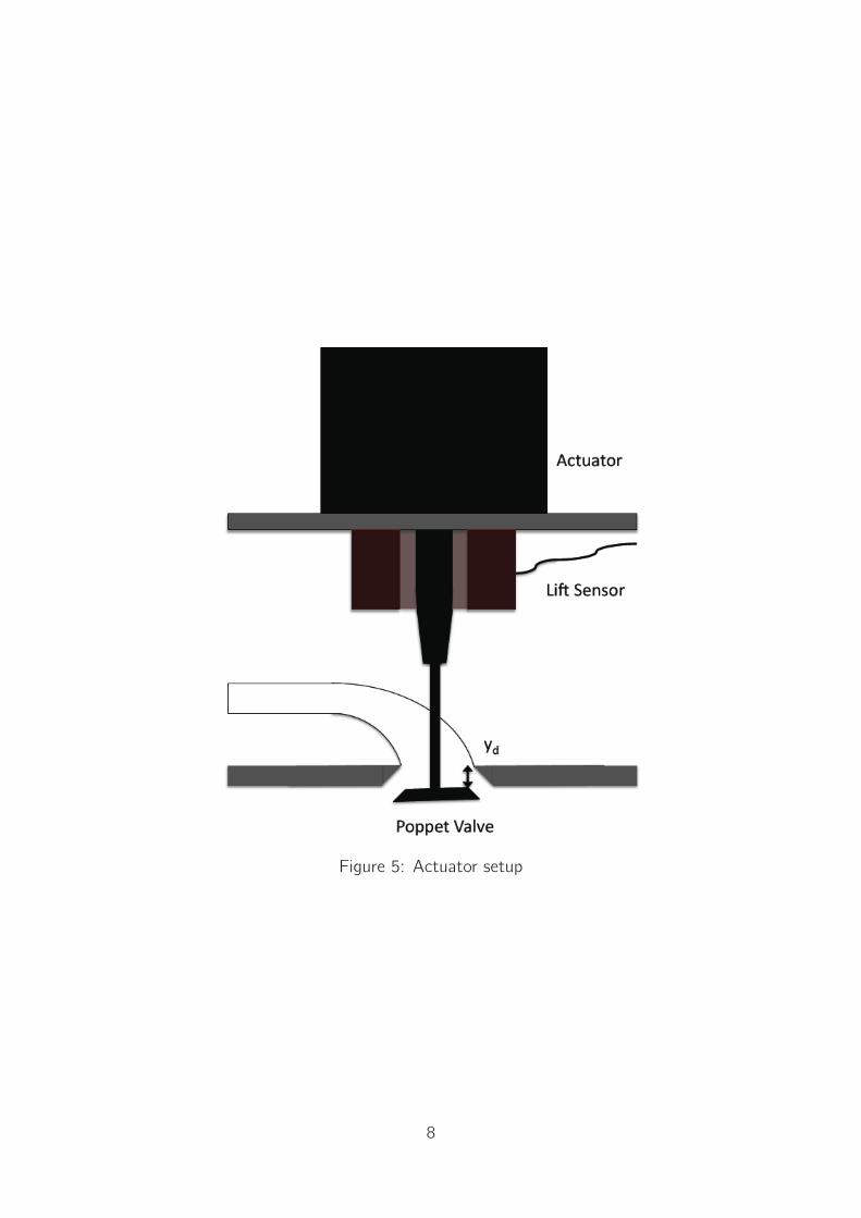
Figure 5: Actuator setup

8

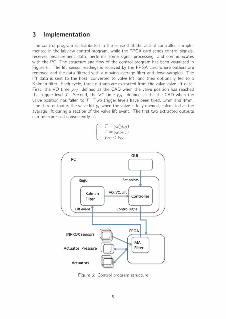
3 Implementation

The control program is distributed in the sense that the actual controller is imple-mented in the labview control program, while the FPGA card sends control signals,receives measurement data, performs some signal processing, and communicateswith the PC. The structure and flow of the control program has been visualized inFigure 6. The lift sensor readings is received by the FPGA card where outliers areremoved and the data filtered with a moving average filter and down-sampled. Thelift data is sent to the host, converted to valve lift, and then optionally fed to aKalman filter. Each cycle, three outputs are extracted from the valve valve lift data.First, the VO time yV O, defined as the CAD when the valve position has reachedthe trigger level T . Second, the VC time yV C, defined as the the CAD when thevalve position has fallen to T . Two trigger levels have been tried, 1mm and 4mm.The third output is the valve lift yL when the valve is fully opened, calculated as theaverage lift during a section of the valve lift event. The first two extracted outputscan be expressed conveniently as⎧⎨

⎩T = yd(yV O)T = yd(yV C)yV O < yV C

Figure 6: Control program structure

9

3.1 Labview

Labview is a graphical programming language where an application is constructed bywiring together provided building blocks. The Labview application has two sides, thefront panel and the block diagram. The block diagram is where functional blocks arewired together and the controls and indicators of the front panel are connected. Foran introduction to Labview programming and a reference manual see the LabviewUser Manual [16]. The front panel is the Graphical User Interface (GUI), designedto simulate the interface of a real hardware. The GUI of the control program canbe seen in Figure 7. To the left, there are toggles to activate the control of VO andVC, in the center, the VO and VC times can be set, and to the right the valve lift isshown.

Figure 7: Labview control program

3.2 Field Programmable Gate Array

The FPGA can be reconfigured after manufacture, which gives the programmeropportunity to change the function of the FPGA card as the requirements of theapplication changes. The drawback is that the design is less optimized, leading togreater use of area, reduced execution speed and increased power consumption [17].The FPGA card used, NI PCIe-7842R, has 96 digital Digital Input/Output (DIO)lines, 8 analog inputs, 8 analog outputs and a built in clock that runs at a frequency of40 MHz. The FPGA card enables simultaneous execution of parallel task. In Table 1The programmable logic blocks of the FPGA is the flip-flop, Lookup table (LUT),embedded block Random Access Memory (RAM) and DSP48 slices. The n-inputLUT can implement any n-input boolean function as a truth table. Flip-flops arecircuits that have two stable states and can be used as data storage elements. Theflip-flop circuit change state when the control input signals change. Block RAM can

10

be used to store datasets or pass values between parallel loops and thereby reducethe number of flip flops used. Multiplication is resource intensive in the number ofLUTs and flip-flops used. DSP48 slices integrate a 25-bit by 18-bit multiplier withadder circuitry. Please see the documentation for further details [18]. On the FPGA,data acquisition and some rudimentary signal processing take place. Each rising edgeof each lift sensor triggers a FPGA DIO channel and the time between rising edgesis measured. The time measurements are in clock ticks of the built-in clock, runningat 40MHz .

Table 1: FPGA specifications

NI 7842R

FPGA type Virtex-5 LX50

Number of flip-flops 28,800

Number of 6-input LUTs 28,800

Number of DSP48 slices (25 ∗ 18 multipliers) 48Embedded block RAM 1,728 kbits

Analog Input Channels

Number of Analog Input channels 8

Maximum sampling rate 200 kS/s (per channel)

Analog Voltage Input Range ±10 V

Analog Output Channels

Number of Analog Output channels 8

Maximum update rate 1 MS/s

Analog Voltage Output Range ±10 V

Digital I/O channels

Number of Digital I/O channels 96

Minimum sampling period 5 ns

Digital Voltage Input Range -20.0 to 20.0 V, single line

3.2.1 Communication to Host

The FPGA Communicates with the host PC, through a Direct Memory Access(DMA) First In First Out (FIFO) queue. The DMA FIFO queue allows the FPGAto directly access the RAM of the host for increased throughput compared to trans-ferring the data between two local FIFO queues. The FPGA FIFO queue consist ofblock RAMs on the FPGA side, RAM memory on the host side, and an DMA enginethat automatically transfers data between the two. The DMA FIFO is setup to write6 unsigned 64 bit integers every 6th sample. The 64 bit unsigned integer consistof four valve lift readings, the CAD value and the cylinder pressure. The valve liftreading is a 8 bit unsigned integer, the CAD value is a 16 bit integer and the cylinder

11

pressure reading is also a 16 bit integer. Each 64 bit unsigned integer contain thevalve lift readings from one cylinder. Each write cycle, one valve lift reading from eachvalve is sent to the host PC, which receives 600 valve lift readings per valve and cycle.

3.2.2 Analog Lift Signal

The analog lift sensor output a square-wave with a frequency depending on valve lift.The time between two rising flanks is measured on the FPGA card in clock ticks ofthe built in clock. In Figure 8 100 samples from an analog lift signal is presented, thesignal was acquired by an oscilloscope. The signal is subject to noise which resultsin outliers and noise when handled by the FPGA. See section 6.1 for a discussion of

Figure 8: Analog lift signal

outliers and noise. The raw sensor data acquired by the FPGA are plotted during alift event in Figure 9a. The unit clock ticks refers to the FPGA clock and the samplerate is 1800 samples per revolution or 3600 samples per cycle, or 5 samples per CAD.Using a simple heuristic algorithm, the outliers is easily identified and removed. Theimplemented solution compares the difference between two consecutive samples, yiand yi+1 , and if

yi+1 − yi = Δy < Δminwhere Δmin = 5, then the sample is replaced by the previous sample. A solution thatwas chosen for simplicity, causality and low logical requirements when implementedon the FPGA. The signal without outliers can be seen in Figure 9b.

3.2.3 Moving Average Filter and Downsampling

Since only one valve position can be sent every 6th sample, an average of the sixmost recent samples is calculated and subsequently sent. In general, it is advisable

12

to use unfiltered data in the identification procedure and then come up with a filter.The necessity to use one here is due to the fact that otherwise only one sixth of thedata could be sent to the PC because of limitations in the amount of data that canbe sent from the FPGA.

The valve position calculated on the FPGA is in clock ticks, where a lift has aresolution of about 25 clock ticks, varying between approximately 180 clock tickswhen the valve is closed to approximately 205 when the valve is fully opened. Tominimize the use of FPGA resources and to fit the averaged valve position readinginto an 8 bit unsigned integer the built in overflow behavior is used. An 8 bit unsignedinteger can represent a value between 0 and 255. A value above 255 rolls over, e.g.260 rolls over to 4 = 260− 256. Thus simply adding the six lift values together willcause rollover to occur four times. The lift resolution is amplified six times, with arange of 150 ticks, but can still fit in an 8 bit unsigned integer. A closed valve willgenerate a value of approximately 56 to be sent to the host, and a fully open valvewill generate a value of 206. Values that are translated into frequencies and then tovalve lifts on the host side. In total, the averaging operation only requires five addoperations per valve on the FPGA card. A comparison between the lift curve onlyfiltered by the moving averaging filter and also Kalman filtered is seen in Figure 10.

3.3 Sensor Mapping

Due to the analog lift sensor being nonlinear, a second order mapping was done,using sensor readings from two different sensors. In Figure 11a the frequency of thesquare-wave from the lift sensor is shown at different positions. It can be seen thatthere is a significant frequency discrepancy between the two sensors, however thediscrepancy predominantly being a constant offset in frequency, which can be seenmore clearly in Figure 11b, where the mean frequency difference has been removedfrom the second sensor. It is assumed that all sensors can be normalized by removingthe mean frequency difference when the valves are closed. With the relative position

(a) Raw lift sensor lift curve (b) Raw lift sensor lift curve with outliersremoved

Figure 9: Raw lift sensor readings

13

(a) MA filtered lift curve (b) MA and Kalman filtered lift curve

Figure 10: Filtered lift sensor readings

available with sufficient accuracy, the absolute position profile can be obtained byobserving that the position of the valve is known when the valve is closed, thus thefrequency offset and the absolute valve position can be calculated.

(a) Calibration measurement (b) Calibration measurement with frequencyoffset removed

Figure 11: Lift calibration using two sensors

3.4 Labview Implementation

To implement feedback from the previous cycle, start and stop timings of the con-trol pulse need to be set at several different times because there is basically alwaysvalves open. Therefor one cycle was split into 6 parts, and in each part, outputsare calculated for two exhaust valves and two intake valves and control pulse timingssent to the FPGA. The duration of a valve lift event has an absolute constraint inthat it can not open for roughly more than 360 CAD, since otherwise the pistonwould hit the open valves. In practice, the valves are open far shorter periods. Thisgives ample time to calculate the control signal with the implemented solution. For

14

details on Labview programming see the reference manual or [19], one of the manybooks available on the subject.

Due to time constraints due to the scope of the thesis, a set of simple controllerswhere implemented. The controller setup consists of three Single Input Single Out-put (SISO) systems [20], where the lift height is controlled by the actuator pressure,the start of the control pulse controls the VO time, and VC time is controlled bythe end timing of the control pulse. All controllers are Proportional Integral (PI)controllers [20] with very conservative controller gains.

15

4 Modeling

The purpose of the identified model is to facilitate filtering of the lift sensor signal, inan attempt to get more consistent lift data. For a general treatment of system iden-tification and modeling see [21]. Two types of discrete time models where evaluated,Autoregressive moving average with exogenous input (ARMAX) models and state-space models. The model was the used to filter the output sequence to get a betterVO and VC signals. The state-space models were developed using the n4sid Matlabcommand, see the Matlab documentation [22], or Ljung [23] for algorithm details.The input sequence was defined as the pulse sent to the actuators multiplied by theactuator pressure, and the output sequence is just the filtered and down-sampled liftmeasurement. The control sequence ud is defined as

ud = up · u (4.1)

where up is the actuator pressure and u is the generated physical control pulsesent to the actuators, defined in Equation (2.1). For successful identification itis necessary to have enough variability in the input [21], which is why the controlsignals were generated by the following procedure. The control parameters, up, uV Oand uV C were only changed if the realization of a binary random variable Xu wasone. The binary random variable had a probability of P (Xu = 1) = 0.15. Each inputthat was to be changed was then drawn from a range of valid control signals withconstant probability density function. The Input-output data were subdivided into anestimation part of 80% of the data and a evaluation part of 20% of the data. Themodels were estimated using the estimation data and evaluated on the validationdata based on the criteria introduced in section 4.3.

4.1 ARMAX Modeling

ARMAX models have the following structure:

A(z−1)yk = z−dB(z−1)uk + C(z−1)wk (4.2)

where the A polynomial is the autoregressive part, the B polynomial is a movingaverage of the input signal and the C polynomial is a moving average part of noiseterms. The input uk ∈ �m is modeled affecting the output yk ∈ �p with a delayd time steps and the noise process {wk} is assumed to be a white-noise stochasticprocess. The A,B and C polynomials have the structure

A(z−1) = 1 + a1z−1 · · ·+ anaz−na

B(z−1) = b0 + b1z−1 · · ·+ bnbz−nbC(z−1) = 1 + c1z

−1 · · ·+ cncz−nc(4.3)

4.2 State Space Modeling

The state-space equations for system with m inputs and p outputs is given by theequations

xk+1 = Axk + Buk + wkyk = Cxk +Duk + ek

(4.4)

16

with state vector xk ∈ �n and noise sequences wk ∈ �n, ek ∈ �p affecting thedynamics of the system and the output respectively.

4.3 Model Evaluation

The developed models were evaluated on the evaluation data set by three evaluationstatistics based on the prediction errors and residual tests.

The Variance Accounted For (VAF) statistic defined as

τV AF =

(1− (yN − yN)

T (yN − yN)yTN yN

)× 100%

where yN is the N point vector containing the output data and yN is the estimatedoutput. The Akaike Final Prediction Error (FPE) defined as

FPE(p) =N + p

N − pV

where p is the identified number of parameters and V is the loss function defined as

V = det

(1

N

N∑i=1

ε(i , θN)ε(i , θN)T

)

Akaike’s Information Criterion (AIC) is defined as

AIC(p) = log(V ) +2p

N

where V is the loss function defined earlier.

The transfer function of both the ARMAX models and the state space models canbe expressed as Y (z−1) = Hu(z−1) +Hw(z−1)W (z−1). The residuals ε(z−1), of theevaluated models are obtained by

ε(z−1) = H−1w (z−1)(Y (z−1)− Hu(z−1)U(z−1)) (4.5)

The residuals can be considered a disturbance input that would explain the disparitybetween the observed data and data from the estimated model. If the model is correctthe residuals should not contain any structure, especially they should be uncorrelatedto inputs and outputs [21].

17

5 Results

In this section results from the sensor calibration, model identification and the im-plemented controller are presented.

5.1 Lift Sensor Noise

The lift sensor readings are subject to noise. The noise is concluded to be whitenoise and the estimated power spectrum is shown in Figure 12, the power spectrumis calculated for 64 frequencies, logarithmically spaced. The power spectrum hasbeen calculated for a valve turned off, all 3600 data points are used without theaverage filter, using the Matlab psd command and a Kaiser window, see Matlabdocumentation for details [22].

Figure 12: Power spectrum estimate of the noise affecting the lift sensor using aperiodogram with Kaiser window

5.2 Model Evaluation

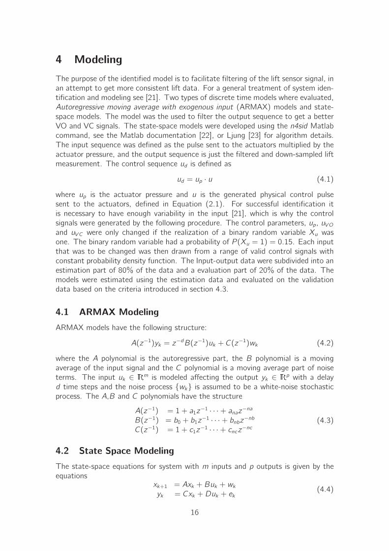
The statistics for the identified models are presented in Figure 13. For easier com-parison, an offset of 2.5 has been added to the AIC statistic and the VAF statistichas ben replace by 1-VAF. The raw statistics can be found in Table 3 and the modelparameters in Table 2. A filter based was implemented in Labview based on the bestmodel, the third order n4s3 model, however the Labview program could not finishexecution in time consistently. The n4s2 model was then chosen as a compromisebetween performance and implementation requirements. Figure 14 show the crosscorrelation of the residuals and correlation between the input and the residuals forthe three state space models. The residuals of the first order model clearly contain

18

structure, but to a lesser extent this is also true for the models of order 2 and threeas well. All three models exhibit cross correlation between input and output, thatmanifests itself in that the models predict too low lift with lower than average valuesof up and too high lift with higher than average values of up. The n4s2 state spacemodel is given by equation (4.4) and the matrices

A =

[0.9682 −0.041260.08114 0.8981

], B = 10−5

[2.81439.75

],

C =[0571.1 12.47

], D = 0

(5.1)

Figure 13: Exhaust valve model evaluation. Smaller values imply a better fit. Anoffset has been added to the AIC statistic

Table 2: Exhaust valve models

Name Type na nb nc n (n4sid only) delay

arx1 ARX 2 1 - - 23

arx2 ARX 3 2 - - 23

arx3 ARX 4 3 - - 23

amx1 ARMAX 2 1 1 - 23

amx2 ARMAX 3 2 2 - 23

amx3 ARMAX 4 3 3 - 23

n4s1 n4sid - - - 1 18

n4s2 n4sid - - - 2 18

n4s3 n4sid - - - 3 18

19

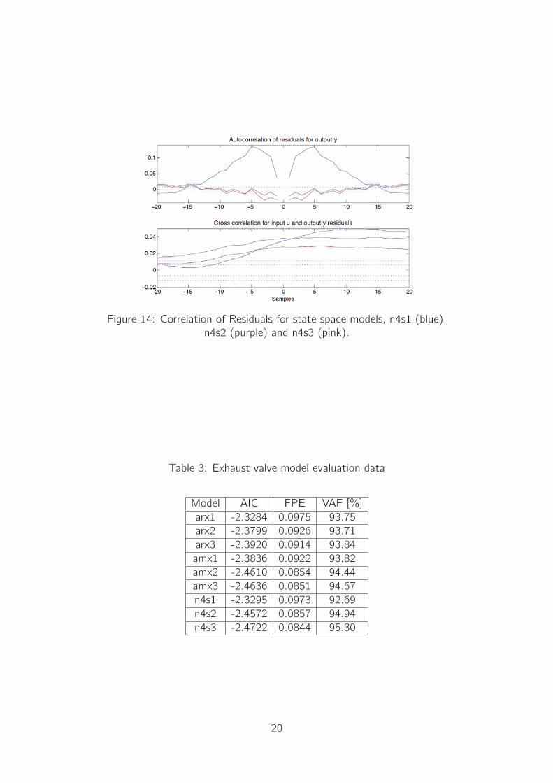
Figure 14: Correlation of Residuals for state space models, n4s1 (blue),n4s2 (purple) and n4s3 (pink).

Table 3: Exhaust valve model evaluation data

Model AIC FPE VAF [%]

arx1 -2.3284 0.0975 93.75

arx2 -2.3799 0.0926 93.71

arx3 -2.3920 0.0914 93.84

amx1 -2.3836 0.0922 93.82

amx2 -2.4610 0.0854 94.44

amx3 -2.4636 0.0851 94.67

n4s1 -2.3295 0.0973 92.69

n4s2 -2.4572 0.0857 94.94

n4s3 -2.4722 0.0844 95.30

20

5.3 Controller

A Kalman filter based on the n4s2 system model was implemented in the controllerfor one valve. The Kalman gain K is

K = 10−4[5.24318.02

](5.2)

To evaluate the controller with and without the use of the Kalman filter two kinds ofinput signal were used. The first signal used was a constant signal of 5 bar actuatorpressure and the signal sent to the actuator chosen according to Equation (2.1) withuV O = −200 CAD BTDC and uV C = 0 CAD BTDC. The second signal was the sametype of signal as the one used in the modeling part, but with constant air pressureat 5 bar. For both input signals a trigger level of 1 mm and 4 mm was tested andthe length of the input sequences was 200 cycles.

5.3.1 Constant Input

The variance of the first input sequence, the constant input sequence, is presentedin Table 4.

Table 4: Variance of steady state VO and VC with and without Kalman filter

With Kalman Filter w/o Kalman filter

VO 1 mm trigger level 0.1447 0.5364

VC 1 mm trigger level 0.7494 0.4790

VO 4 mm trigger level 0.0921 0.1573

VC 4 mm trigger level 0.1913 0.3297

5.3.2 Stochastic Input

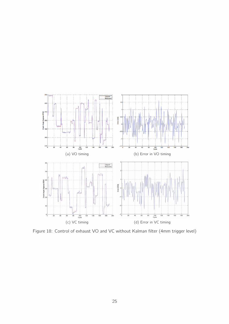
The controller with Kalman filter response to a stochastic VO and VC input signalsimilar to the signal used in identification can be seen in Figure 15 for 1 mm triggerlevel and in Figure 16 for 4 mm trigger level. The response for the controller withoutthe Kalman filter can be seen in Figure 17 for 1 mm trigger level and in Figure 18for 4 mm trigger level. The variance and mean of the error in the just mentionedexperiments are presented in Table 5.

21

Table 5: Mean and variance of error sequences

With Kalman filter w/o Kalman filtervariance mean variance mean

1 mm TriggerVO error 0.23 0.02 0.53 -2.72×10−4VC error 0.79 -0.10 0.72 -0.08

4 mm TriggerVO error 0.85 0.08 0.28 -0.0039VC error 0.3126 -0.2575 0.7984 -0.0792

(a) VO timing (b) Error in VO timing

(c) VC timing (d) Error in VC timing

Figure 15: Control of exhaust VO and VC with Kalman filter (1mm trigger level)

22

(a) VO timing (b) Error in VO timing

(c) VC timing (d) Error in VC timing

Figure 16: Control of exhaust VO and VC with Kalman filter (4mm trigger level)

23

(a) VO timing (b) Error in VO timing

(c) VC timing (d) Error in VC timing

Figure 17: Control of exhaust VO and VC without Kalman filter (1mm trigger level)

24

(a) VO timing (b) Error in VO timing

(c) VC timing (d) Error in VC timing

Figure 18: Control of exhaust VO and VC without Kalman filter (4mm trigger level)

25

6 Discussion

A second order model of the exhaust valve was identified. A Kalman filter and a sim-ple feedback was implemented on one valve. Both with and without the Kalman filterthe feedback control achieved variances beneath 1 CAD. From the results, there issome support to conclude that the Kalman filter did improve the performance, how-ever not by much and not consistently. The valve used for both model identificationand the control experiments was the one least susceptible to noise. It is reasonableto believe that the Kalman filter would give stronger benefit on valves affected moreby noise.

There is some remaining structure in the auto correlation of output residuals andcross correlation between input and output residuals as seen in Figure 14. The crosscorrelation between input and output residuals suggest some dynamics that the modelfails to capture and that model complexity is insufficient. Increased model complex-ity, maybe in the form of a nonlinear model, might be needed since increased modelorder was not sufficient remove the cross correlation. There are several sources tothe remaining variance. The resolution of the FPGA is one fifth CAD and possi-bly give a quantization error of one tenth CAD. Variations in supplied air pressureprobably have an effect on the variance. The model that the Kalman filter is wasbased on, does not describe the system satisfactory as can be seen by the correlationanalysis and Figure 14.

Having access to whole lift curve each cycle gives endless possibilities in what data toextract and use for the cycle-to-cycle feedback. It is interesting to note that there isnot that much difference in variance between the two trigger levels 1 mm and 4 mm.It would be interesting to investigate the cross-correlation between the two, becauseif the added noise is uncorrelated, better information can be obtained by combiningseveral points on each flank of the lift curve.

6.1 Lift Signal Noise

The outliers seen in Figure 9a have a certain regularity to them, the measured timeseem to be approximately half the clock ticks of the valid data points. The probablecause of this is that the analog lift signal seen in Figure 8 triggers a second timeon the zero-crossing on the falling flank when the signal is only supposed to triggeron the rising flank. This would explain the characteristics of the outliers. However,an occasional faulty trigger event would result in two consecutive samples of halfthe number of clock ticks, but in Figure 8 there is often several correct samples inbetween two faulty samples. This implies that the FPGA triggers only on the fallingflank for several samples, a behavior that lacks explanation.

26

6.2 Implementation Issues

Given the timing requirements of feedback from the previous cycle, the PC was unableto run more than one Kalman filter in the control program, and even with one Kalmanfilter the computations was not finished in time or not deterministic enough, resultingin missed deadlines. There are at least thee possible ways to mitigate this problem.Implementing the Kalman filter on the FPGA would lead to a reduced load on thecomputer’s CPU. It would require a fixed-point implementation of the Kalman filterwhich is not feasible to implement for all 24 valves on the current FPGA card. Whenattempting a fixed-point low-pass filter of first order, the FPGA requirements scaledup nicely when used on 12 lift signals, utilizing less than 50% of the FPGA resourcesin terms of both LUTs and flip-flops. But when attempting to use it on all 24 valves,the utilization reached above 200%. Further investigation is needed to determine thereason for this behavior and if a second FPGA card or an improved one would sufficeto solve the issue. The second possible solution would be to optimize the Kalmanfilter on the PC, removing features of the built-in Labview version and neglectingsmall terms. The third would be to remove the need for Kalman filtering by reducingthe noise level which seem possible since with only one sensor attached, the signaldid not contain noise. The noise origin is unknown, however it is likely to be commonground related, since all lift input share the same power source and have the sameground signal on the FPGA card. Furthermore, filtering one of the lift signals throughan analog low-pass filter did not lead to any visually detectable reduction in noiselevel on the raw analog lift sensor signal observed in an oscilloscope, the signal stillhad the noise as in Figure 8.

6.3 Future Work

The next step would be to model and implement model based control of lift, VO andVC timings with the additional input parameter of cylinder pressure. Such modelingwas attempted during the course of this project, but it turned out hard to fit amodel. One of the reasons was that the length of the datasets were limited. Ifthe whole lift curve was to be saved, the data acquisition and processing became tocumbersome. During the acquisition of data, the disk could not write fast enoughto have more than a couple of hundred cycles of data at a time and the processingof datasets with a large number of samples became time-consuming. Now, whenthe preprocessing is done during execution, only a small number of values need tobe saved each cycle, which should make it possible to have larger data sets and abetter chance of developing models. There also need to be some way to change thespeed of the mock engine to cover that aspect. One way would be to implement themock engine on the FPGA instead. The overarching final goal would be to integratethe valve control with the existing engine control platform, implemented in C++,Matlab and Real-time Workshop.

27

7 Conclusion

The main result of this project is that a FPGA based feedback controller was imple-mented for all 24 valves in Labview. A second order model of the exhaust valve wasidentified. A Kalman filter and a simple feedback was implemented on one valve.Satisfactory control of VO and VC and Lift for a fixed engine condition was obtained.The Kalman filtering in the controller had only small effect on the controller per-formance. In order to have a Kalman filter on all valves, optimization of the filterimplementation, some kind of signal condition, or additional computational resourcesis needed.

28

References

[1] Cargine Engineering AB, 2011, http://www.cargine.com [25-11-2011].

[2] B. Johansson, Forbranningsmotorer, Faculty of Engineering, Lund University,2006.

[3] S. Trajkovic, P. Tunestal, and B. Johansson, “A simulation study quantifyingthe effects of drive cycle characteristics on the performance of a pneumatichybrid bus,” in Proceedings of the ASME 2010 Internal Combustion EngineDivision Fall Technical Conference, San Antonio, TX, 2010.

[4] K. Hatano, K. lida, H. Higashi, and S. Murata, “Development of a new multi-mode variable valve timing engine,” in SAE Technical Paper 930878, 1993.

[5] C. Brustle and D. Schwarzenthal, “Variocam plus - a highlight of the porsche911 turbo engine,” in SAE Technical Paper 2001-01-0245, 2001.

[6] R. Flierl and M. Kluting, “The third generation of valvetrains – new fully variablevalvetrains for throttle-free load control,” in SAE Technical Paper 2000-01-1227, 2000.

[7] R. Hofmann, J. Liebl, M. Klueting, and R. Flierl, “The new BMW 4-cylindergasoline engine-reduction of fuel consumption without compromise,” in Pro-ceedings. JSAE Annual Congress, 2001.

[8] C. Tai and T. Tsao, “Control of an electromechanical camless valve actuatuor,”in Proceedings of the American Control Conference, Anchorage, AK May 8-10,2002.

[9] M. M. Schechter and M. B. Levin, “Camless engine,” in SAE Technical Paper960581, 1996.

[10] S. Trajkovic, “The pneumatic hybrid vehicle,” Ph.D. dissertation, Lund Univer-sity, 2010.

[11] A. Milosavljevic and S. Trajkovic, “Fpga controlled pneumatic variable valveactuation,” in SAE Technical Paper 2006-01-0041, 2006.

[12] J. Ma, H. Schock, U. Carlson, A. Hoglund, and M. Hedman, “Analysis and mod-eling of an electronically controlled pneumatic hydraulic valve for an automotiveengine,” in SAE Technical Paper 2006-01-0042, 2006.

[13] National Instruments Corporation, NI R Series Multifunction RIO Specifications,2009, http://www.ni.com/pdf/manuals/372492c.pdf [23-11-2011].

[14] Data Sheet, BoshRexroth E/P pressure regulator, Series ED05,http://www.boschrexroth.com/pneumatics-catalog/Pdf.cfm?Language=EN&file=en/pdf/PDF p58395 en.pdf.

29

[15] Norgren Ltd, 2011, http://www.norgren.com/document resources/usa/R07.pdf [28-11-2011].

[16] National Instruments Corporation, LabVIEW User Manual, 2003, http://www.ni.com/pdf/manuals/320999e.pdf.

[17] I. Kuon and J. Rose, “Measuring the gap between FPGAs and ASICs,” in Pro-ceedings of the FPGA ’06 Proceedings of the 2006 ACM/SIGDA 14th inter-

national symposium on Field programmable gate arrays, ACM New York, NY,USA, 2006.

[18] National Instruments Corporation, NI PCIe-7842R multifunction RIO Docu-mentation, 2008, http://sine.ni.com/ds/app/doc/p/id/ds-98/lang/en [23-11-2011].

[19] J. Travis and J. Kring, LabVIEW for Everyone: Graphical Programming MadeEasy and Fun, 3rd ed. Prentice Hall, 2006.

[20] K. J. Astrom and R. M. Murray, Feedback Systems: An Introduction for Scien-tists and Engineers. Princeton University Press, NJ, 2008.

[21] R. Johansson, System Modeling and Identification, 2nd ed. Dept. AutomaticControl, Lund University: Prentice Hall, Englewood Cliffs, 2011.

[22] The MathWorks Incorporation, Matlab Documentation, 2011, http://www.mathworks.se/help/techdoc/ [23-11-2011].

[23] L. Ljung, System Identification: Theory for the User. Prentice-Hall, UpperSaddle River, NJ, 1999.

30