Multi-Classification of Breast Cancer Lesions in ... - MDPI

Diagnostics 2022, 12, 1152. https://doi.org/10.3390/diagnostics12051152 www.mdpi.com/journal/diagnostics

Article

Multi-Classification of Breast Cancer Lesions in

Histopathological Images Using DEEP_Pachi: Multiple

Self-Attention Head

Chiagoziem C. Ukwuoma 1,*, Md Altab Hossain 2, Jehoiada K. Jackson 1, Grace U. Nneji 1, Happy N. Monday 3

and Zhiguang Qin 1,*

1 School of Information and Software Engineering, University of Electronic Science and Technology of China,

Chengdu 610054, China; [email protected] (J.K.J.); [email protected] (G.U.N.) 2 School of Management and Economics, University of Electronic Science and Technology of China,

Chengdu 610054, China; [email protected] 3 School of Computer Science and Engineering, University of Electronic Science and Technology of China,

Chengdu 610054, China; [email protected]

* Correspondence: [email protected] (C.C.U.); [email protected] (Z.Q.)

Abstract: Introduction and Background: Despite fast developments in the medical field, histological

diagnosis is still regarded as the benchmark in cancer diagnosis. However, the input image feature

extraction that is used to determine the severity of cancer at various magnifications is harrowing

since manual procedures are biased, time consuming, labor intensive, and error-prone. Current

state-of-the-art deep learning approaches for breast histopathology image classification take fea-

tures from entire images (generic features). Thus, they are likely to overlook the essential image

features for the unnecessary features, resulting in an incorrect diagnosis of breast histopathology

imaging and leading to mortality. Methods: This discrepancy prompted us to develop DEEP_Pachi

for classifying breast histopathology images at various magnifications. The suggested DEEP_Pachi

collects global and regional features that are essential for effective breast histopathology image clas-

sification. The proposed model backbone is an ensemble of DenseNet201 and VGG16 architecture.

The ensemble model extracts global features (generic image information), whereas DEEP_Pachi ex-

tracts spatial information (regions of interest). Statistically, the evaluation of the proposed model

was performed on publicly available dataset: BreakHis and ICIAR 2018 Challenge datasets. Result:

A detailed evaluation of the proposed model’s accuracy, sensitivity, precision, specificity, and f1-

score metrics revealed the usefulness of the backbone model and the DEEP_Pachi model for image

classifying. The suggested technique outperformed state-of-the-art classifiers, achieving an accu-

racy of 1.0 for the benign class and 0.99 for the malignant class in all magnifications of BreakHis

datasets and an accuracy of 1.0 on the ICIAR 2018 Challenge dataset. Conclusion: The acquired

findings were significantly resilient and proved helpful for the suggested system to assist experts

at big medical institutions, resulting in early breast cancer diagnosis and a reduction in the death

rate.

Keywords: histopathological images; breast cancer; medical images; transfer learning;

multi-head self-attention; image classification

1. Introduction

Cancer is among the majority of deadly diseases, claiming the lives of millions of

people each year. Breast Cancer (BC) is the most common cancer and the leading cause of

death among women [1]. As per World Health Organization (WHO) data, 460,000 people

die annually from BC out of 1,350,000 cases [2]. The United States (US) alone recorded

Citation: Ukwuoma, C.C.; Hossain,

M.A.; Jackson, J.K.; Nneji, G.U.;

Monday, H.N.; Qin, Z. Multi-

Classification of Breast Cancer

Lesions in Histopathological Images

Using DEEP_Pachi: Multiple

Self-Attention Head. Diagnostics

2022, 12, 1152.

https://doi.org/10.3390/

diagnostics12051152

Academic Editor: Antonio Barile

Received: 1 April 2022

Accepted: 28 April 2022

Published: 5 May 2022

Publisher’s Note: MDPI stays neu-

tral with regard to jurisdictional

claims in published maps and institu-

tional affiliations.

Copyright: © 2022 by the authors. Li-

censee MDPI, Basel, Switzerland.

This article is an open access article

distributed under the terms and con-

ditions of the Creative Commons At-

tribution (CC BY) license (https://cre-

ativecommons.org/licenses/by/4.0/).

Diagnostics 2022, 12, 1152 2 of 33

about 268,600 instances of BC in 2019, setting a new record [3,4]. BC develops due to ab-

errant cell proliferation inside the breast [5]. The breast anatomy comprises several blood

arteries, tendons and ligaments, milk ducts, lacrimal gland, and lymph ducts [6]. Benign

carcinoma is squamous cell carcinoma that forms due to minor anomalies in the breast.

Malignant carcinoma, in contrast, is classed as melanoma and further characterized as

invasive carcinoma or in situ carcinoma [7]. Invasive BC expands to nearby organs and

causes difficulties [8,9], whereas in situ carcinoma stays limited to its territory and does

not affect surrounding tissues. To avoid future progression and problems, BC must be

identified earlier and correctly classified as benign or malignant carcinoma. As a result, a

prompt and accurate therapy may be devised, lowering the disease’s fatality rate. Diverse

imaging techniques are used to identify BC, such as Histopathology (HP) [10], Computed

Tomography (CT) [11], Magnetic Resonance Imaging (MRI) [12], Ultrasound (US) [13],

Mammograms (MGs) [14], and Positron Emission Tomography (PET). Statistics reported

in recently published studies on imaging methods [15] reveal that 50% of datasets utilized

in BC-related research are MGs, 20% are US, 18% are MRI and 8% are HP. The remaining

percentage includes commercial records and data from different forms [6,12,16]. Further

studies prove that HP images do not offer binary identification and classifications but

support the multiclass identification and classification of BC subtypes [17–19]. In this pa-

per, a BHI dataset at various magnifications (40×, 100×, 200×, 400×) is studied. The prepro-

cessing of various magnification varies. For instance, with 100× magnification, a specialist

examines squamous development, mesenchymal involvement, and tumor localization to

determine the carcinoma. Nevertheless, developing an accurate and fast model to evalu-

ate BHI at various magnifications is difficult due to multiple factors such as variable pixel

intensity, microscopic size nucleus, diverse image characteristics, a wide variation of nu-

clei, the existence of distortions, and so on. The current effort aims to create a deep learn-

ing-based attention model to categorize BHIs in various magnifications.

Several strategies have been studied for classifying BHIs under 100× magnification

[20,21]. Conventional approaches are always focused on feature extraction. On the other

hand, finding relevant handmade characteristics necessitates experience and expertise but

these might fail to grasp all permutations in the dataset. Deep learning-based approaches

have recently gained prominence as processing computing capacity has improved. Their

ability to analyze end-to-end provides it a better choice for BHI classification. Convolu-

tional layers are used in deep learning algorithms to extract input image features. These

convolutional layers often extract unwanted features alongside the needed parts or over-

look the essential features. However, the extracted features influence the result and choice

of malignancy; thus, disregarding these aspects may result in incorrect image evaluation.

As a result, the extracted characteristics by the convolutional layers of CNN are insuffi-

cient for classifying BHIs. We present an attention-based deep learning framework that

employs global and local features to determine tumor malignancy. The mechanism of the

human brain to interpret visual data while still analyzing the significance of input ele-

ments is known as attention. This neurological mechanism enables exclusive focus on a

single piece of information while ignoring other discernible details. Nevertheless, in op-

position to the competency of attention, the conventional and commonly used CNN clas-

sifier examines characteristics more broadly. It is not assured of extracting relevant clinical

knowledge subconsciously comparable to trained networks [22]. Self-attention is a signif-

icant advancement of computer vision [23–28]. These advancements focus exclusively on

essential features in an informal m with no external guidance. The CNN models serve as

the backbone of the self-attention models. They are trained end-to-end, with no modifica-

tions in the training phase. Thus, employing self-attention processes inside conventional

CNN yields several advantages in accuracy, comprehensibility, and robustness on clinical

vision tasks.

Diagnostics 2022, 12, 1152 3 of 33

1.1. Diagnostic Medical Methods Used in the Investigation of BC

Having mentioned several medical imaging methods used in diagnosing BC, this pa-

per describes the imaging methods related to our task and why we chose histopathologi-

cal images in this section. PET is an accepted imaging method that might provide handy

information regarding BC; nonetheless, it is usually utilized for early grading of advanced

or metastatic invasive and reactive breast cancers, assessing progress to therapies and de-

tecting and localizing family history of the disease [29]. As a result, we did not include it

in our discussion.

The most often and extensively used technique is MGs [30–32], as they are easily ac-

cessible as public datasets. MGs are small breast X-rays [33] that are simple and frequently

employed as the initial test for BC identification [34]. Regrettably, because of the vast dis-

crepancies in shape, the surface area of breast tissues and morphological form, these are

not reliable as they are associated with health effects, including radiation exposure risks

for carriers and radiologists and overdose of radiation effects for carriers [35]. Moreover,

due to inadequate specificity, these techniques subject a considerable proportion of the

population (65–85%) to unnecessary biopsy procedures [36,37]. Such unnecessary biopsies

increase the hospitalization cost for individuals and cause mental stress. Due to such lim-

itations, US imaging is considered a much better option for breast cancer diagnosis and

detection [38,39].

US imaging can significantly boost detection accuracy by 17% while decreasing over-

all needless biopsy procedures by 40% [39] compared with MGs. Sonograms are another

title for breast US in clinical medicine. US might be a superior option to MGs for BC as-

sessment and diagnosis due to its adaptability, reliability, sensitivity, and selectivity [40].

On the other hand, BC lesion identification and classification with US imaging need radi-

ologists’ experience and knowledge due to its complexity and speckle [41]. Aside from the

complicated imaging form, US image-based assessment in female patients produces un-

satisfactory false detection results and misclassification [42]. As a result, there is insuffi-

cient evidence to recommend the use of US in the diagnosis and treatment of BC.

MRI breast images yield better sensitivity for detecting BC in dense tissue [43]. MRI

images provide a more thorough overview of breast tendons than CT, US, or MGs images

because multiple samples from different angles constitute a patient’s breast image sample

[44]. Since MRI scans are more comprehensive than other alternative imaging techniques,

they may uncover tumors not apparent on different imaging techniques or be deemed

malignant [45]. Despite MRI’s high sensitivity [46], its adoption for BC diagnosis is limited

due to its expensive cost [47]. Conversely, newer MRI methods, such as DWI (Diffusion-

Weighted Imaging) and UFMRI (Ultrafast Breast MRI), provide much improved diagnos-

tic precision with faster processing efficiency and lower expenses [48,49].

HP is the process of removing a heap from a questionable anatomical and physiolog-

ical spot for screening and extensive investigation by specialists [50]. In clinical medicine,

this procedure is commonly referred to as a biopsy. Biopsy specimens are mounted over

a microscope slide clouded with Hematoxylin and Eosin (H&E) for examination [51]. HP

images come in two types: (i) Whole Slide Images (WS), which are computerized color

imaging, and (ii) image patches derived from WSI. Several researchers have effectively

employed HP images in the multiclassification of BC due to tissue level examination [17–

19]. BC identification and classification with HP images has several benefits over MGs and

other imaging alternatives such as MRI and US. In particular, HP images do not offer only

binary identification and classifications but support multiclass identification and classifi-

cation of BC subtypes. Table 1 illustrates the summary of the discussed Breast cancer mo-

dalities, its robustness, constraints and available datasets.

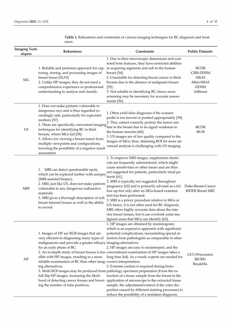
Diagnostics 2022, 12, 1152 4 of 33

Table 1. Robustness and constraints of various imaging techniques for BC diagnosis and treat-

ment.

Imaging Tech-

niques Robustness Constraints Public Datasets

MG

1. Reliable and premium approach for cap-

turing, storing, and processing images of

breast tissue [52,53]

2. Unlike HP images, they do not need a

comprehensive experience or professional

understanding to analyze and classify.

1. Due to their microscopic dimensions and scat-

tered form features, they have restricted abilities

in acquiring segments and sub in the human

breast [54].

2. Unsuitable for detecting breast cancer in thick

breasts due to the absence of malignant tissues

[55].

3. Not reliable in identifying BC; hence more

screening may be necessary for accurate assess-

ments [56].

-BCDR

-CBIS-DDSM

-MIAS

-Mini-MIAS

-DDSM

-InBreast

US

1. Does not make patients vulnerable to

dangerous rays and is thus regarded ex-

ceedingly safe, particularly for expectant

mothers [57].

2. These are specifically convenient imaging

techniques for identifying BC in thick

breasts, where MGs fail [58].

3. Allows for viewing a breast tumor from

multiple viewpoints and configurations,

lowering the possibility of a negative result

assessment.

1. Often yield false diagnoses if the scanner

probe is not moved or pushed appropriately [59].

2. They cannot correctly portray the tumor out-

line in the breast due to its signal weakness to

the human muscles [60].

3. US images are of low quality compared to the

images of MGs; thus, obtaining ROI for more ad-

vanced analysis is challenging with US imaging.

-BCDR

-BUSI

MRI

1. MRI can detect questionable spots,

which can be explored further with autopsy

(MRI-assisted biopsy).

2. MRI, just like US, does not make patients

vulnerable to any dangerous radioactive

materials.

3. MRI gives a thorough description of soft

breast internal tissues as well as the ability

to record

1. To improve MRI images, supplement chemi-

cals are frequently administered, which might

cause sensitivities or other issues and are thus

not suggested for patients, particularly renal pa-

tients [61].

2. MRI is typically not suggested throughout

pregnancy [62] and is primarily advised as a fol-

low-up test only after an MGs-based examina-

tion has been performed.

3. MRI is a pricey procedure relative to MGs or

US; hence, it is not often used for BC diagnosis.

MRI offers highly accurate data about the inte-

rior breast tissues, but it can overlook some ma-

lignant areas that MGs can identify [63].

Duke-Breast-Cancer

RIDER Breast MRI

HP

1. Images of HP are RGB images that are

very efficient in diagnosing many types of

malignancies and provide a greater efficacy

for an early phase of BC.

2. An in-depth study of breast tissues is fea-

sible with HP images, resulting in a more

reliable examination of BC than other imag-

ing alternatives.

3. Multi ROI images may be produced from

full flip HP images, increasing the likeli-

hood of detecting cancer tissues and lower-

ing the number of false positives.

1. HP images are obtained by mammogram,

which is an expensive approach with significant

potential complications, necessitating special at-

tention from pathologists as comparable to other

imaging alternatives

2. HP images are easy to misinterpret, and the

conventional examination of HP images takes a

long time [64]. As a result, experts are needed for

correct interpretation.

3. Extreme caution is required during histo-

pathology specimen preparation (From the ex-

traction of a tissue sample from the breast to the

application of microscope to the extracted tissue

sample, the adjustment/control of the color dis-

parities caused by different staining processes) to

reduce the possibility of a mistaken diagnosis.

UCI (Wisconsin)

BICBH

BreakHis

Diagnostics 2022, 12, 1152 5 of 33

Identified Pub-

lic site for BC

Dataset

http://peipa.essex.ac.uk/info/mias.html, http://marathon.csee.usf.edu/Mammography/Database.html, https://bio-

keanos.com/source/INBreast, https://bcdr.ceta-ciemat.es/information/about

https://wiki.cancerimagingarchive.net/display/Public/, https://www.repository.cam.ac.uk/handle/1810/250394, ac-

cessed on 20 March 2022.

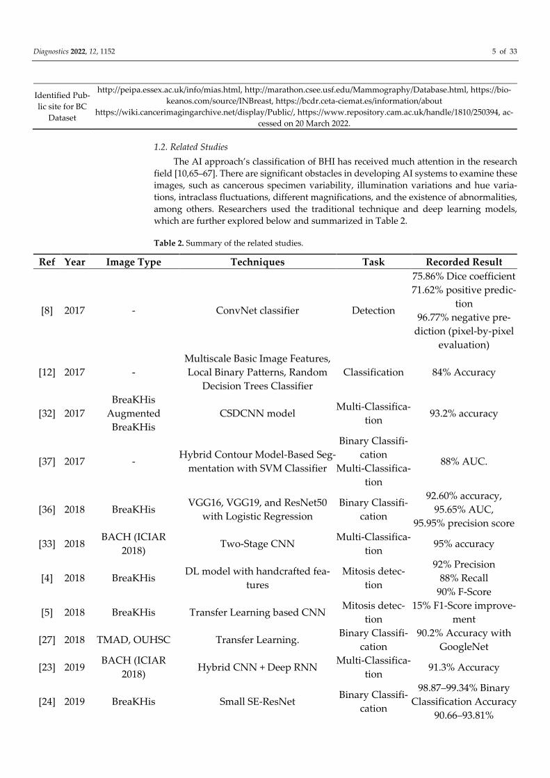
1.2. Related Studies

The AI approach’s classification of BHI has received much attention in the research

field [10,65–67]. There are significant obstacles in developing AI systems to examine these

images, such as cancerous specimen variability, illumination variations and hue varia-

tions, intraclass fluctuations, different magnifications, and the existence of abnormalities,

among others. Researchers used the traditional technique and deep learning models,

which are further explored below and summarized in Table 2.

Table 2. Summary of the related studies.

Ref Year Image Type Techniques Task Recorded Result

[8] 2017 - ConvNet classifier Detection

75.86% Dice coefficient

71.62% positive predic-

tion

96.77% negative pre-

diction (pixel-by-pixel

evaluation)

[12] 2017 -

Multiscale Basic Image Features,

Local Binary Patterns, Random

Decision Trees Classifier

Classification 84% Accuracy

[32] 2017

BreaKHis

Augmented

BreaKHis

CSDCNN model Multi-Classifica-

tion 93.2% accuracy

[37] 2017 - Hybrid Contour Model-Based Seg-

mentation with SVM Classifier

Binary Classifi-

cation

Multi-Classifica-

tion

88% AUC.

[36] 2018 BreaKHis VGG16, VGG19, and ResNet50

with Logistic Regression

Binary Classifi-

cation

92.60% accuracy,

95.65% AUC,

95.95% precision score

[33] 2018 BACH (ICIAR

2018) Two-Stage CNN

Multi-Classifica-

tion 95% accuracy

[4] 2018 BreaKHis DL model with handcrafted fea-

tures

Mitosis detec-

tion

92% Precision

88% Recall

90% F-Score

[5] 2018 BreaKHis Transfer Learning based CNN Mitosis detec-

tion

15% F1-Score improve-

ment

[27] 2018 TMAD, OUHSC Transfer Learning. Binary Classifi-

cation

90.2% Accuracy with

GoogleNet


2018) Hybrid CNN + Deep RNN

Multi-Classifica-

tion 91.3% Accuracy

[24] 2019 BreaKHis Small SE-ResNet Binary Classifi-

cation

98.87–99.34% Binary

Classification Accuracy

90.66–93.81%

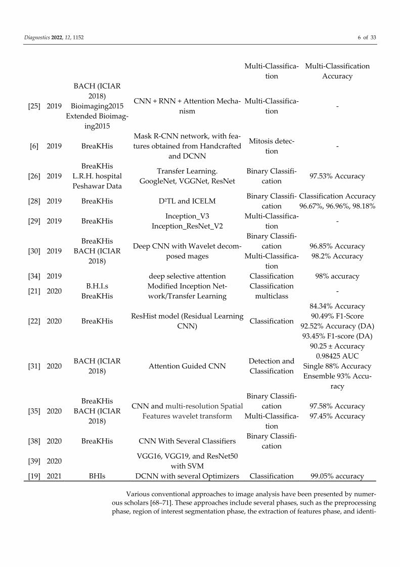
Diagnostics 2022, 12, 1152 6 of 33

Multi-Classifica-

tion

Multi-Classification

Accuracy

[25] 2019

BACH (ICIAR

2018)

Bioimaging2015

Extended Bioimag-

ing2015

CNN + RNN + Attention Mecha-

nism

Multi-Classifica-

tion -

[6] 2019 BreaKHis

Mask R-CNN network, with fea-

tures obtained from Handcrafted

and DCNN

Mitosis detec-

tion -

[26] 2019

BreaKHis

L.R.H. hospital

Peshawar Data

Transfer Learning.

GoogleNet, VGGNet, ResNet

Binary Classifi-

cation 97.53% Accuracy

[28] 2019 BreaKHis D2TL and ICELM Binary Classifi-

cation

Classification Accuracy

96.67%, 96.96%, 98.18%

[29] 2019 BreaKHis Inception_V3

Inception_ResNet_V2

Multi-Classifica-

tion -

[30] 2019

BreaKHis

BACH (ICIAR

2018)

Deep CNN with Wavelet decom-

posed mages

Binary Classifi-

cation

Multi-Classifica-

tion

96.85% Accuracy

98.2% Accuracy

[34] 2019 deep selective attention Classification 98% accuracy

[21] 2020 B.H.I.s

BreaKHis

Modified Inception Net-

work/Transfer Learning

Classification

multiclass -

[22] 2020 BreaKHis ResHist model (Residual Learning

CNN) Classification

84.34% Accuracy

90.49% F1-Score

92.52% Accuracy (DA)

93.45% F1-score (DA)


2018) Attention Guided CNN

Detection and

Classification

90.25 ± Accuracy

0.98425 AUC

Single 88% Accuracy

Ensemble 93% Accu-

racy

[35] 2020

BreaKHis

BACH (ICIAR

2018)

CNN and multi-resolution Spatial

Features wavelet transform

Binary Classifi-

cation

Multi-Classifica-

tion

97.58% Accuracy

97.45% Accuracy

[38] 2020 BreaKHis CNN With Several Classifiers Binary Classifi-

cation

[39] 2020 VGG16, VGG19, and ResNet50

with SVM

[19] 2021 BHIs DCNN with several Optimizers Classification 99.05% accuracy

Various conventional approaches to image analysis have been presented by numer-

ous scholars [68–71]. These approaches include several phases, such as the preprocessing

phase, region of interest segmentation phase, the extraction of features phase, and identi-

Diagnostics 2022, 12, 1152 7 of 33

fication phase. In Refs. [71,72], Local Binary Patterns (LBP) were used for BHI categoriza-

tion, while the authors of Ref. [73] used the frequency distribution index, in conjunction

with contours, to identify meiosis. Unfortunately, due to the varied properties of cancer-

ous images, appearance alone will be inadequate for effective image classification. Fur-

thermore, support vector machines (SVM) [71] and decision trees (DT) [74,75] have been

widely investigated for image classification. These strategies focused on data prepro-

cessing since it significantly influenced the recognition rate. Such techniques depend on

characteristics that have been handcrafted. Furthermore, detecting these handcrafted

traits necessitates technical knowledge and expertise. Moreover, these characteristics

might not perfectly capture all variabilities in the sample, resulting in poorer predictive

performance.

The ability of Deep Learning models to represent complicated patterns has made

them a common approach for image processing. Several CNN-based methods such as

ResNet, VGG-16, Inception, VGG-19, and others were proposed for image classification

tasks. Ref. [76] authors employed Deep CNN for BHI classification. The authors of Ref. [8]

used CNN to detect invasive BC. In contrast, the author of Ref. [77] used the same CNN

approach to address the sample class imbalance and extractions of input image features

at various BHIs Magnification. The authors of Ref. [78] employed the Residual neural net-

work for automated BHI assessment. The authors of Ref. [79] combined CNN and Resid-

ual neural network for multi-level feature extraction. The authors of Ref. [80] argued for

the integration of squeeze and excitation blocks and residual neural network yields com-

pared to Ref [79] for this classification. The authors of Ref. [81] suggested that the combi-

nation of Ref. [79] and Ref. [80] yields a better result. They used Ref. [80]’s approach to

extract the input image features in Latent space and used an attention mechanism [80] for

classification. Transfer learning [82–84] has been widely investigated as it provides room

for better model performance where there are few training samples. Ref [85] used Incep-

tion with a residual connection model via transfer learning for more feature extraction.

Ref. [86] entails using CNN’s wavelet decomposition for image classification. Ref. [87] in-

tegrated a soft attention network to its architecture to focus entirely on the region of inter-

est alone. At the same time, the author of Ref. [88] designed a class-specific Deep CNN

network for BHIs multiclass classification. To tackle the computational cost of processing

huge images, the authors of Ref. [89] developed a dual-stage CNN. The authors of Ref [90]

integrated the idea of Refs. [76,86]. They used adaptive spectral composition and an atten-

tion technique [90] for classification.

Several researchers have employed the hybrid technique to seek a better and more

accurate BHI classification model. The authors of Ref. [91] used the ensemble of ResNet50,

VGG19 and VGG16 as feature extractors for a logistic regressor classifier. The authors of

Ref. [92] suggested that a cascaded ensemble model with an SVM classifier yields better

and more accurate results. The cascaded ensemble is seen at the feature extraction (multi-

lateral and syntactic feature) by the CNN model. Ref. [92] created an ensemble of Dense-

Net121, InceptionV3, ResNet50, and VGG-16 as feature extractors. Ref. [93] investigated

several Deep learning pre-trained models as feature extractors and used SVM as classifi-

ers. Unfortunately, CNN-based techniques require a substantial amount of labeled train-

ing samples. Much research that focused on patch level [94] feature extraction and image-

level [95] feature extraction for BHIs classification has been performed. The author of Ref.

[95] used a voting principle for the classification after extracting input image features via

image and patch levels. In contrast, the authors of Ref [94] employed pre-trained models

(ResNet and Inception architecture) for input image feature extraction via images and

patch level. Notwithstanding, there are chances where the input images analyzed for

patch features fail to contain RIO, thus yielding false malignancy results as they might not

adequately depict the input image.

Research has proposed numerous convolutional neural network-based classification

architectures for BHIs to extract features from the entire input image. This approach

Diagnostics 2022, 12, 1152 8 of 33

mostly fails as the network might overlook the essential features. The identified proper-

ties/regions of the input images that might be overlooked are the cores, proliferative cells,

and ducts, which are critical in determining the tumor’s malignancy. As a result, neglect-

ing certain traits may impact outcomes. Furthermore, extracting distinctive features at dif-

ferent magnifications is difficult due to the tiny size of cores. To address these constraints

of multiclassification of BC using the BHI dataset, this article proposes “DEEP_Pachi,” an

end-to-end deep learning model incorporating multiple self-attention network heads and

Multilayer Perceptron. The input images are processed as a series of patches. Each patch

is squished into a single feature vector by merging the layers of all pixels in a patch and

then exponentially extending it to the appropriate input dimension. Even though the pro-

posed architectures require more training samples than CNN architectures, the most typ-

ical approach is to use a pre-trained network and then to finetune it on a smaller task

sample. This paper used the option of pre-trained networks to mitigate the issues of more

training sample requirements of the proposed model. To select the pre-trained networks,

we first examine four pre-trained deep learning models (DensetNet201, VGG16, Incep-

tionResNetV2, and Xception network) on BHIs images using a transfer learning tech-

nique. Afterward, an ensemble of pre-trained models functioned as feature extractors for

the DEEP_Pachi network. We propose an automated method to distinguish between be-

nign breast tumors such as Adenosis, Fibroadenoma, Phyllodes_tumor, and Tubular_ad-

enoma and malignant breast tumors Ductal_carcinoma, Lobular_Carcinoma, Mucin-

ous_Cancinoma, and Papillary_carcinoma to help medical diagnosis even when profes-

sional radiologists are not accessible. Furthermore, to provide a point of comparison for

our findings, the proposed method is compared to other baseline models and recently

published research.

The significant contribution of this paper is summarized as follows:

This research reviews several Medical BC imaging techniques, their robustness and

limitation, and associated public dataset.

This paper proposed a fine-tuned approach termed “DEEP_Pachi,” an end-to-end

deep learning model incorporating multiple self-attention network heads and Multi-

layer Perceptron for the multiclassification of Breast cancer diseases using histo-

pathological images.

According to the comprehensive study via transfer learning experiment, the sug-

gested feature extractor discriminates remarkably between benign breast tumors

such as Adenosis, Fibroadenoma, Phyllodes_tumor and Tubular_adenoma malig-

nant breast tumors Ductal_carcinoma, Lobular_Carcinoma, Mucinous_Cancinoma,

and Papillary_carcinoma to help medical diagnosis even when professional radiolo-

gists are not accessible.

We reported a well robust deep learning method in Accuracy, Specificity, Sensitivity,

Precision, F1 Score, Confusion matrix, and AUC using receiver operating character-

istics (ROC) for the multiclassification of Breast cancer diseases using histopatholog-

ical images based on the detailed experimental evaluation of the proposed model and

comparison with state-of-the-art results.

Finally, this research suggests that the proposed model “DEEP_Pachi” can also be

used to increase ensemble deep learning models’ detection and classification accura-

cies.

The remainder of this article is organized as follows; Section 1 is devoted to the in-

troduction and relevant studies of this research. Section 2 outlines the materials, the pro-

posed approach, and the evaluation measures. Section 3 introduces the experimental

setup and outcomes, whereas Section 4 explains the results. Section 5 discusses the con-

clusion and future studies.

Diagnostics 2022, 12, 1152 9 of 33

2. Materials and Methods

This section examines the suggested architecture and materials in depth. The imple-

mentation structure of this research is depicted in Figure 1. First, this paper argues that

data preprocessing should only be applied to the training set because when test set data

are preprocessed, there is every likelihood that the training model will perform poorly in

real-time; thus, the first step in this paper was to split the dataset downloaded from the

database. After splitting the dataset into train and test sets, data preparation procedures

such as scaling, rotation, cropping, and normalization are performed in the train set. To

make our model robust enough, transfer learning was used as the network backbone’s

(feature extraction). While selecting the optimum network backbone for the proposed

model, this paper conducted an experimental examination on four deep learning pre-

trained models. On the other hand, researchers have argued that ensemble models pro-

vide more generalized results than single models; hence, we adopted the ensemble archi-

tecture for the proposed network backbone. The ensemble network now serves as the in-

put to the proposed model (DEEP_Pach). The proposed model comprises a self-attention

network and an MLP block, as seen in Figure 2. The self-attention network receives the

input in two forms: patch embedding and position embedding. This helps the self-atten-

tion network differentiate between the various symptoms in the fed images. The multi-

layer perceptron (MLP) block improves the self-attention network’s outcomes in false

symptom detection in the fed dataset. The input evaluated by the self-attention network

is transferred to the multilayer perceptron layer for extraction before being passed to the

classification/detection layer for prediction. We go over the following stages for putting

our suggested approach into action.

Figure 1. Proposed methodology block diagram.

Diagnostics 2022, 12, 1152 10 of 33

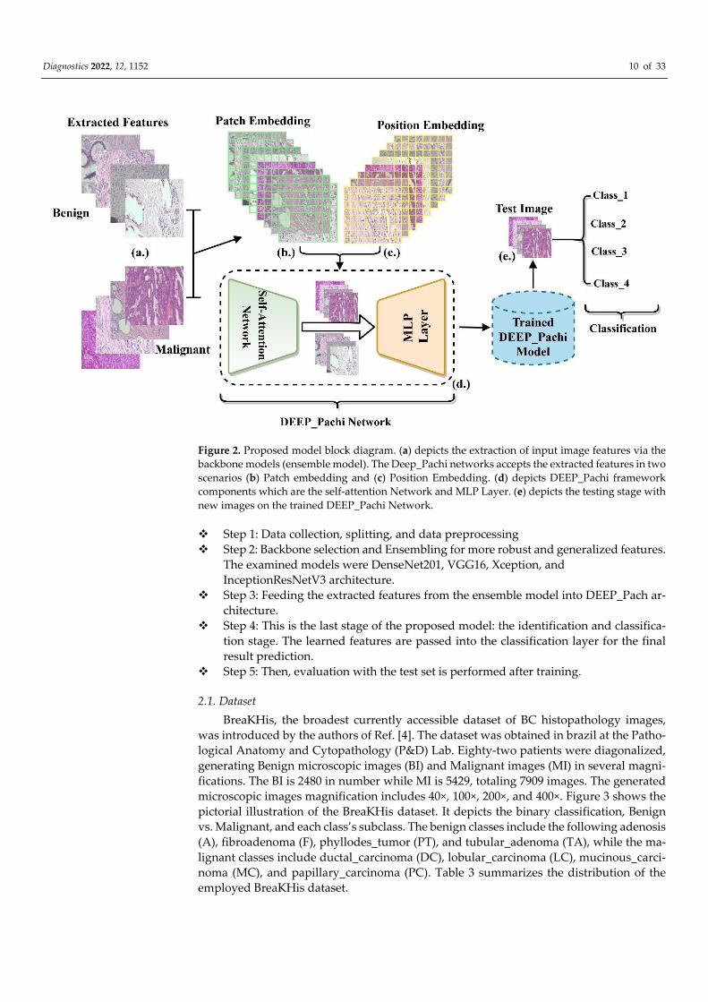
Figure 2. Proposed model block diagram. (a) depicts the extraction of input image features via the

backbone models (ensemble model). The Deep_Pachi networks accepts the extracted features in two

scenarios (b) Patch embedding and (c) Position Embedding. (d) depicts DEEP_Pachi framework

components which are the self-attention Network and MLP Layer. (e) depicts the testing stage with

new images on the trained DEEP_Pachi Network.

Step 1: Data collection, splitting, and data preprocessing

Step 2: Backbone selection and Ensembling for more robust and generalized features.

The examined models were DenseNet201, VGG16, Xception, and

InceptionResNetV3 architecture.

Step 3: Feeding the extracted features from the ensemble model into DEEP_Pach ar-

chitecture.

Step 4: This is the last stage of the proposed model: the identification and classifica-

tion stage. The learned features are passed into the classification layer for the final

result prediction.

Step 5: Then, evaluation with the test set is performed after training.

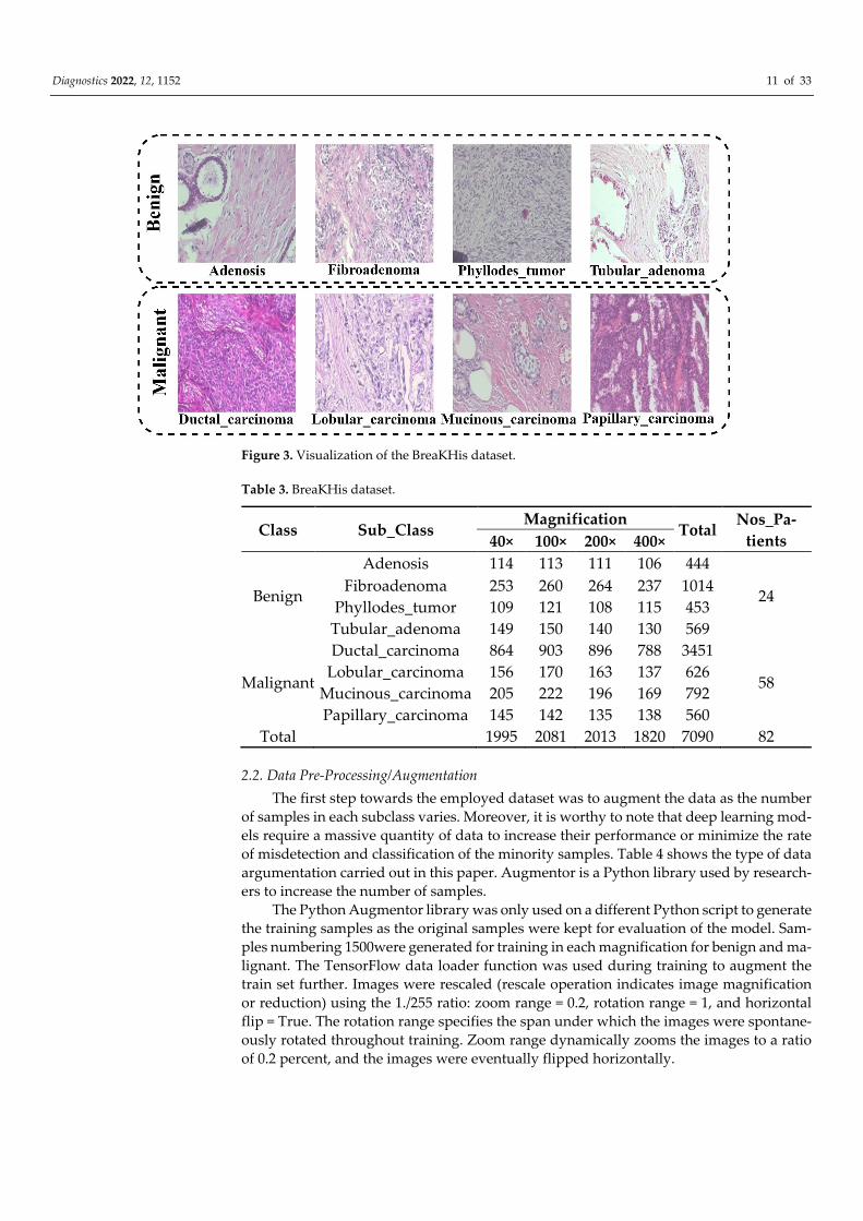
2.1. Dataset

BreaKHis, the broadest currently accessible dataset of BC histopathology images,

was introduced by the authors of Ref. [4]. The dataset was obtained in brazil at the Patho-

logical Anatomy and Cytopathology (P&D) Lab. Eighty-two patients were diagonalized,

generating Benign microscopic images (BI) and Malignant images (MI) in several magni-

fications. The BI is 2480 in number while MI is 5429, totaling 7909 images. The generated

microscopic images magnification includes 40×, 100×, 200×, and 400×. Figure 3 shows the

pictorial illustration of the BreaKHis dataset. It depicts the binary classification, Benign

vs. Malignant, and each class’s subclass. The benign classes include the following adenosis

(A), fibroadenoma (F), phyllodes_tumor (PT), and tubular_adenoma (TA), while the ma-

lignant classes include ductal_carcinoma (DC), lobular_carcinoma (LC), mucinous_carci-

noma (MC), and papillary_carcinoma (PC). Table 3 summarizes the distribution of the

employed BreaKHis dataset.

Diagnostics 2022, 12, 1152 11 of 33

Figure 3. Visualization of the BreaKHis dataset.

Table 3. BreaKHis dataset.

Class Sub_Class Magnification

Total Nos_Pa-

tients 40× 100× 200× 400×

Benign

Adenosis 114 113 111 106 444

24 Fibroadenoma 253 260 264 237 1014

Phyllodes_tumor 109 121 108 115 453

Tubular_adenoma 149 150 140 130 569

Malignant

Ductal_carcinoma 864 903 896 788 3451

58 Lobular_carcinoma 156 170 163 137 626

Mucinous_carcinoma 205 222 196 169 792

Papillary_carcinoma 145 142 135 138 560

Total 1995 2081 2013 1820 7090 82

2.2. Data Pre-Processing/Augmentation

The first step towards the employed dataset was to augment the data as the number

of samples in each subclass varies. Moreover, it is worthy to note that deep learning mod-

els require a massive quantity of data to increase their performance or minimize the rate

of misdetection and classification of the minority samples. Table 4 shows the type of data

argumentation carried out in this paper. Augmentor is a Python library used by research-

ers to increase the number of samples.

The Python Augmentor library was only used on a different Python script to generate

the training samples as the original samples were kept for evaluation of the model. Sam-

ples numbering 1500were generated for training in each magnification for benign and ma-

lignant. The TensorFlow data loader function was used during training to augment the

train set further. Images were rescaled (rescale operation indicates image magnification

or reduction) using the 1./255 ratio: zoom range = 0.2, rotation range = 1, and horizontal

flip = True. The rotation range specifies the span under which the images were spontane-

ously rotated throughout training. Zoom range dynamically zooms the images to a ratio

of 0.2 percent, and the images were eventually flipped horizontally.

Diagnostics 2022, 12, 1152 12 of 33

Table 4. Data augmentation Python algorithm.

Import Augmentor

def upsample(dir, num_samples):

p = Augmentor.Pipeline(dir)

p.rotate(probability = 1, max_left_rotation = 5, max_right_rotation = 5)

p.zoom(probability = 0.2, min_factor = 1.1, max_factor = 1.2)

p.skew(probability = 0.2)

p.shear(probability = 0.2, max_shear_left = 2, max_shear_right = 2)

p.crop_random(probability = 0.5, percentage_area = 0.8)

p.flip_random(probability = 0.2)

p.sample(num_samples)

p.random_distortion(probability = 1, grid_width = 4, grid_height = 4, magni-

tude = 8)

p.flip_left_right(probability = 0.8)

p.flip_top_bottom(probability = 0.3)

p.rotate90(probability = 0.5)

p.rotate270(probability = 0.5)

src_dir = ‘D:/Pachigo/Breast_Cancer/Train/Benign/40




upsample(src_dir, 1500)

2.3. Network Backbone

The proposed network backbone in this study is the ensemble of two deep-learning

models via the transfer learning approach. Four deep learning pretrained models were

first examined using the malignant subclass magnification of the BreaKHis dataset: the

DenseNet201 and the VGG16 architecture produced a better classification performance

among the four examined models. Hence, we used both as the network backbone via the

ensemble approach. Ensembling is the capacity to combine several learning algorithms to

obtain their collective performance, i.e., to improve the performance of existing models

by integrating many models into a single trustworthy model. The network backbone

serves as feature extractors to the proposed model DEEP_Pachi, as seen in Figure 4.

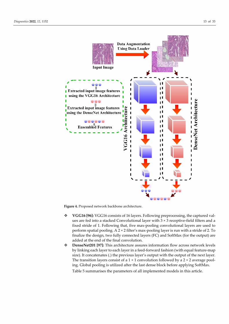
Diagnostics 2022, 12, 1152 13 of 33

Figure 4. Proposed network backbone architecture.

VGG16 [96]: VGG16 consists of 16 layers. Following preprocessing, the captured val-

ues are fed into a stacked Convolutional layer with 3 × 3 receptive-field filters and a

fixed stride of 1. Following that, five max-pooling convolutional layers are used to

perform spatial pooling. A 2 × 2 filter’s max-pooling layer is run with a stride of 2. To

finalize the design, two fully connected layers (FC) and SoftMax (for the output) are

added at the end of the final convolution.

DenseNet201 [97]: This architecture assures information flow across network levels

by linking each layer to each layer in a feed-forward fashion (with equal feature-map

size). It concatenates (.) the previous layer’s output with the output of the next layer.

The transition layers consist of a 1 × 1 convolution followed by a 2 × 2 average pool-

ing. Global pooling is utilized after the last dense block before applying SoftMax.

Table 5 summarises the parameters of all implemented models in this article.

Diagnostics 2022, 12, 1152 14 of 33

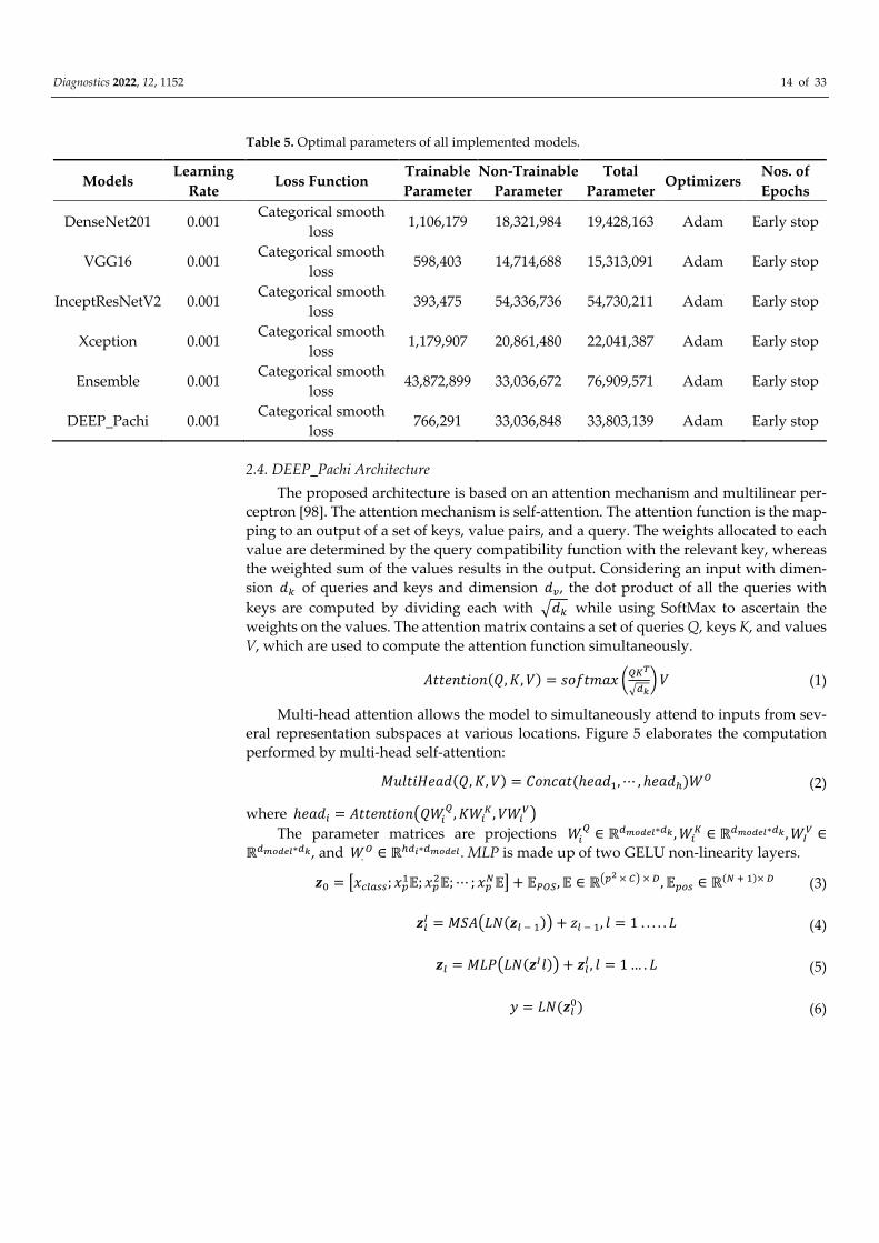
Table 5. Optimal parameters of all implemented models.

Models Learning

Rate Loss Function

Trainable

Parameter

Non-Trainable

Parameter

Total

Parameter Optimizers

Nos. of

Epochs

DenseNet201 0.001 Categorical smooth

loss 1,106,179 18,321,984 19,428,163 Adam Early stop

VGG16 0.001 Categorical smooth

loss 598,403 14,714,688 15,313,091 Adam Early stop

InceptResNetV2 0.001 Categorical smooth


Xception 0.001 Categorical smooth


Ensemble 0.001 Categorical smooth


DEEP_Pachi 0.001 Categorical smooth


2.4. DEEP_Pachi Architecture

The proposed architecture is based on an attention mechanism and multilinear per-

ceptron [98]. The attention mechanism is self-attention. The attention function is the map-

ping to an output of a set of keys, value pairs, and a query. The weights allocated to each

value are determined by the query compatibility function with the relevant key, whereas

the weighted sum of the values results in the output. Considering an input with dimen-

sion �� of queries and keys and dimension ��, the dot product of all the queries with

keys are computed by dividing each with �� while using SoftMax to ascertain the

weights on the values. The attention matrix contains a set of queries Q, keys K, and values

V, which are used to compute the attention function simultaneously.

��(�, �, �) = ��

�� (1)

Multi-head attention allows the model to simultaneously attend to inputs from sev-

eral representation subspaces at various locations. Figure 5 elaborates the computation

performed by multi-head self-attention:

��(�, �, �) = ��(ℎ��, ⋯ , ℎ��)�� (2)

where ℎ�� = ��, ��

�, ��

The parameter matrices are projections �� ∈ ℝ��∗��, ��

� ∈ ℝ��∗��, �� ∈

ℝ��∗��, and �.� ∈ ℝ��∗��. MLP is made up of two GELU non-linearity layers.

�� = ��; ��; ��

��; ⋯ ; �� + ��, � ∈ ℝ�� × �� × �, �� ∈ ℝ(� � �)× � (3)

�� = ��(�� )� + �� , � = 1 . . . . . � (4)

�� = ��(��)� + ��, � = 1 … . � (5)

� = ��(��) (6)

Diagnostics 2022, 12, 1152 15 of 33

.

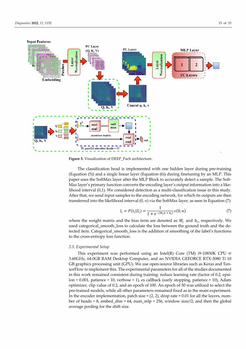
Figure 5. Visualization of DEEP_Pach architecture.

The classification head is implemented with one hidden layer during pre-training

(Equation (5)) and a single linear layer (Equation (6)) during finetuning by an MLP. This

paper uses the SoftMax layer after the MLP Block to accurately detect a sample. The Soft-

Max layer’s primary function converts the encoding layer’s output information into a like-

lihood interval (0,1). We considered detection as a multi-classification issue in this study.

After that, we send input samples to the encoding network, for which its outputs are then

transferred into the likelihood interval (0, n) via the SoftMax layer, as seen in Equation (7):

�� = �(��|��) =1

1 + ��(�� )�(0, �) (7)

where the weight matrix and the bias term are denoted as �� and ��, respectively. We

used categorical_smooth_loss to calculate the loss between the ground truth and the de-

tected item. Categorical_smooth_loss is the addition of smoothing of the label’s functions

to the cross-entropy loss function.

2.5. Experimental Setup

This experiment was performed using an Intel(R) Core (TM) i9-10850K CPU @

3.60GHz, 64.0GB RAM Desktop Computer, and an NVIDIA GEFORCE RTX-3080 Ti 10

GB graphics processing unit (GPU). We use open-source libraries such as Keras and Ten-

sorFlow to implement this. The experimental parameters for all of the studies documented

in this work remained consistent during training: reduce learning rate (factor of 0.2, epsi-

lon = 0.001, patience = 10, verbose = 1), es callback (early stopping, patience = 10), Adam

optimizer, clip value of 0.2, and an epoch of 100. An epoch of 50 was utilized to select the

pre-trained models, while all other parameters remained fixed as in the main experiment.

In the encoder implementation, patch size = (2, 2), drop rate = 0.01 for all the layers, num-

ber of heads = 8, embed_dim = 64, num_mlp = 256, window size//2, and then the global

average pooling for the shift size.

Diagnostics 2022, 12, 1152 16 of 33

2.6. Evaluation

The proposed model used various evaluation metrics to evaluate the robustness of

the model. The metrics include Accuracy, Precision, Specificity, F1-score, Sensitivity, and

area under a receiver operating characteristic curve (AUC). The predefined notations are

TP = True Positive, FP = False Positive, TN = True Negative, and FN = False Negative. We

defined classification Accuracy (ACC) as follows.

�� = �� + ��

(�� + ��) + (�� + ��)× 100 (8)

Precision (PRE) is defined as follows.

�� = ��

�� + ��× 100 (9)

Specificity (��) is defined as follows.

�� = ��

�× 100 =

��

�� + ��× 100 (10)

Sensitivity (SEN) is mathematically formulated as follows.

�� = ��

�× 100 =

��

�� + ��× 100 (11)

The Precision and Sensitivity harmonic means are referred to as the �� , math-

ematically represented as thus.

�� = �� + ��

2�

��

=2 × ��

2 × �� + �� + �� (12)

The AUC measures a classifier’s performance, while the probability curve is obtained

from plotting at different threshold settings, the FP rate is referred to as the ROC (Receiver

Operating Characteristic). The AUC indicates how well the model distinguishes between

the given instances. The higher the AUC, the better. AUC = 1 implies a perfect classifier,

whereas AUC = 0.5 suggests a classifier randomizing class observation. To determine the

area under the ROC curve, AUC is calculated using trapezoidal integration.

3. Results

This section describes the results of the experiment. The parameter sensitivity exper-

iment was first presented in this section to guide readers on how the proposed model

parameter was selected for optimal performance. The transfer learning, binary, and mul-

ticlass experimental results were discussed using the employed evaluation metrics and

compared with the state-of-the-art results.

3.1. Parameter Sensitivity Analysis of the Proposed Method

This paper carried out a parameter sensitivity analysis of the optimal number of

heads and feature extractors to ascertain the parameter setting for the proposed model’s

best and worst performance scenario. The number of epochs and learning rate is kept con-

stant during this experiment. The evaluation metrics used here include accuracy, preci-

sion, and F1_score. The obtained result is recorded in Table 6. The computational cost was

considered during the parameter sensitivity analysis; hence, only two, four, and eight

numbers of self-attention heads and one, two, and three backbones were set up in the

analysis. The backbone models used for this analysis were DenseNet201, VGG16, and

Xception architecture. It was observed that using only one pre-trained network as the pro-

posed model backbone with different numbers of self-attention heads does not have any

significant result enhancement; thus, we focused on using only two and three pre-trained

networks for the optimal feature selection approach. The best accuracy, F-1 score, and

precision were obtained when the number of self-attention network heads is set from four

Diagnostics 2022, 12, 1152 17 of 33

using two pre-trained networks. The optimal best parameter setting of the proposed

model is seen while using three pre-trained models as network backbone and setting the

number of self-attention heads = 16. Although there was a minimal difference from using

two pre-trained models and four self-attention heads, this paper used two pretrained

model backbones and set the number of self-attention heads to be eight in all experiments

to reduce the computational cost of the proposed model. The malignant class of the

BreaKHis dataset was used in this evaluation. We combined all the malignant magnifica-

tion subclasses into a binary classification task. We combined the 40× and the 100× mag-

nification for low-quality image resolution while combining 200× and 400× magnification

for the high-quality image resolution. We used 80 percent for training and 20% for the test

during this analysis.

Table 6. Parameter sensitivity analysis of DEEP_Pachi.

Nos. of

Pre-Trained

Network

Nos. of

Self-Atten-

tion Heads

Learning

Rate

Nos. Of

Epoch

Accuracy

(%)

Precision

(%)

F1_Score

(%)

1 2 3 × 10−3 50 0.96 0.96 0.96

2 2 3 × 10−3 50 0.96 0.97 0.96

3 2 3 × 10−3 50 0.97 0.97 0.97

1 4 3 × 10−3 50 0.96 0.97 0.96

2 4 3 × 10−3 50 0.97 0.98 0.97

3 4 3 × 10−3 50 0.98 0.97 0.97

1 8 3 × 10−3 50 0.96 0.97 0.97

2 8 3 × 10−3 50 0.97 0.99 0.98

3 8 3 × 10−3 50 0.98 0.98 0.98

1 16 3 × 10−3 50 0.98 0.98 0.98

2 16 3 × 10−3 50 0.99 1.0 0.98

3 16 3 × 10−3 50 1.0 0.98 0.99

3.2. Transfer Learning Experiment for Backbone Network Selection

Having first obtaining the optimal best performance using the number of self-atten-

tion networks and number of pre-trained models for the backbone, we carried out a de-

tailed experiment using both the Benign class and the Malignant class on various magni-

fications, as recorded in Table 7. From the recorded results, the transfer learning models

performed very well in the benign class; hence, we focused our attention on the malignant

class for backbone network selection. The excellent results of the models using the Benign

class can be traced to the data preprocessing technique employed in this paper. The

DenseNet201 architecture had the best result in all magnification (40×, 100×, 200×, and

400×). By comparing the recorded results, the malignant class’s results in all magnifica-

tions are lower than the benign class. VGG16 results show how robust the model is on

both low and high-image resolutions compared to the Xception model. However, they

recorded almost the same results in this experiment. The InceptionResNet is the least per-

forming model; hence, DenseNet and the VGG16 were selected for the network backbone.

Table 7. Transfer learning classification result. The experiment was performed specifically for the

selection of the proposed model backbone.

Models ACC (%) SEN (%) SPE (%) PRE (%) F1_Score (%) AUC (%)

40× Magnification-Benign

DenseNet201 1.0 1.0 1.0 1.0 1.0 1.0

InceptionResNet 0.99 0.99 0.99 0.98 0.98 0.99

VGG16 1.0 1.0 1.0 1.0 1.0 1.0

Diagnostics 2022, 12, 1152 18 of 33

Xception 1.0 1.0 1.0 1.0 1.0 1.0


DenseNet201 1.0 1.0 1.0 1.0 1.0 1.0


VGG16 0.99 0.99 0.99 0.98 0.98 0.99

Xception 0.99 0.99 0.99 0.98 0.98 0.99


DenseNet201 1.0 1.0 1.0 1.0 1.0 1.0


VGG16 1.0 1.0 1.0 1.0 1.0 1.0

Xception 1.0 1.0 1.0 1.0 1.0 1.0

400× Magnification Benign

DenseNet201 1.0 1.0 1.0 1.0 1.0 1.0


VGG16 0.99 0.98 0.99 0.99 0.98 0.98

Xception 0.99 0.98 0.99 0.99 0.98 0.98

40× Magnification Malignant

DenseNet201 0.98 0.99 0.99 0.95 0.97 0.99


VGG16 0.94 0.93 0.96 0.82 0.86 0.94

Xception 0.94 0.93 0.96 0.82 0.86 0.94


DenseNet201 0.97 0.98 0.98 0.91 0.94 0.98


VGG16 0.94 0.94 0.96 0.83 0.87 0.95

Xception 0.96 0.96 0.97 0.86 0.90 0.97


DenseNet201 0.98 0.97 0.98 0.94 0.95 0.98


VGG16 0.92 0.93 0.95 0.79 0.84 0.94

Xception 0.95 0.95 0.97 0.85 0.89 0.96


DenseNet201 0.98 0.98 0.98 0.92 0.95 0.98


VGG16 0.97 0.96 0.98 0.90 0.93 0.97

Xception - - - - - - ACC denotes Accuracy; SEN = Sensitivity; SPE = Specificity; PRE = Precision; AUC = Area under the

ROC Curve.

3.3. DEEP_Pachi Architecture Classification Result

For ideal and well-detailed microscopic image analysis, the magnification factor

plays a significant role; hence, this paper experimented on all BreaKHis dataset magnifi-

cation (40×, 100×, 200×, and 400×). However, before then, a Binary classification was car-

ried out on the BreaKHis dataset combing all 100× and 400× magnifications for the benign

and malignant class. The reason behind selecting only the 100× and the 400× magnification

was to analyze the robustness of the model in low and high-quality image resolution and

have a neutral experiment without data augmentation. The binary classification is shown

in Table 8. The evaluation was between the backbone network, the Ensemble of DenseNet

Diagnostics 2022, 12, 1152 19 of 33

architecture and VGG16 and the DEEP_Pachi model (Proposed model). We can see a sig-

nificant contribution of the proposed model with 0.1% improvements in the Benign class

and +0.1–+0.3% improvements in the Malignant class. Figure 6 visualizes the class perfor-

mance of each model using the Precision–Recall curve and the Reciever Operating Char-

acteristics (ROC) Curve.

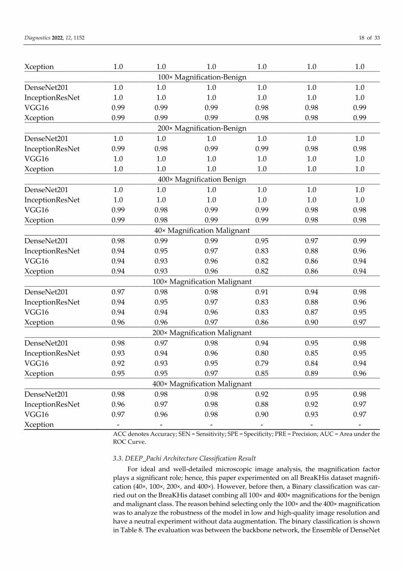
Table 8. Binary classification using DEEP_Pachi.

Models ACC (%) SEN (%) SPE (%) PRE (%) F1_Score AUC

100× Magnification

Backbone Net-

work 0.99 0.99 0.99 0.99 0.99 0.99

DEEP_Pachi 1.0 1.0 1.0 1.0 1.0 1.0

400× Magnification

Network Back-

bone 0.95 0.93 0.93 0.95 0.94 0.93

DEEP_Pachi 0.96 0.96 0.96 0.97 0.95 0.96

(a) (b)

(c) (d)

Figure 6. Binary Classification between Benign and Malignant. (a) depicts the PR Curve using the

100×, (b) depicts PR Curve @400× (c) depicts ROC curve @ 100×, and (d) depicts ROC curve @ 400×.

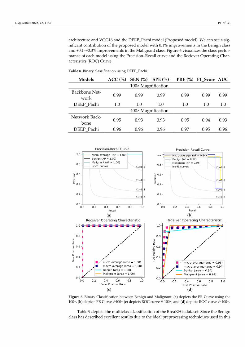
Table 9 depicts the multiclass classification of the BreaKHis dataset. Since the Benign

class has described excellent results due to the ideal preprocessing techniques used in this

Diagnostics 2022, 12, 1152 20 of 33

paper, we focused our discussion more on the Malignant class. Comparing the network

backbone classification performance using the Accuracy, Sensitivity, Specificity, Preci-

sion, F1-score and AUC evaluation metrics, the DEEP_Pachi architecture significantly im-

proved by +0.1–+0.3% classification performance. Figure 7 visualized the Benign individ-

ual class performance using the Precision-Recall (PR) curve and the Reciever Operating

Characteristics (ROC) Curve while Figure 8 visualized the Benign individual class perfor-

mance using the Precision-Recall (PR) curve and the Reciever Operating Characteristics

(ROC) Curve.

Table 9. Multiclass classification using DEEP_Pachi vs. the network backbone.

Models ACC (%) SEN (%) SPE (%) PRE (%) F1_Score (%) AUC (%)


Network Backbone 1.0 1.0 1.0 1.0 1.0 1.0

DEEP_Pachi 1.0 1.0 1.0 1.0 1.0 1.0



DEEP_Pachi 1.0 1.0 1.0 1.0 1.0 1.0



DEEP_Pachi 1.0 1.0 1.0 1.0 1.0 1.0

400× Magnification Benign


DEEP_Pachi 1.0 1.0 1.0 1.0 1.0 1.0



DEEP_Pachi 0.99 1.0 1.0 0.96 0.98 0.98



DEEP_Pachi 0.99 1.0 1.0 0.94 0.98 0.98



DEEP_Pachi 0.99 0.99 0.99 0.95 0.98 0.98



DEEP_Pachi 1.0 1.0 1.0 0.97 0.99 0.99

(a) (b) (c)

Diagnostics 2022, 12, 1152 21 of 33

(d) (e) (f)

(g) (h)

Figure 7. Benign individual class performance using Receiver Operating Characteristics (ROC)

Curve and Precision–Recall (PR) Curve. (a) depicts the PR Curve @40×, (b) depicts PR Curve @100×

(c) depicts PR Curve @ 200×, (d) depicts PR Curve @ 400×, (e) depicts ROC curve @ 40×, (f) depicts

ROC curve @ 100×, (g) depicts ROC curve @ 200×, and (h) depicts ROC curve @ 400×.

(a) (b) (c)

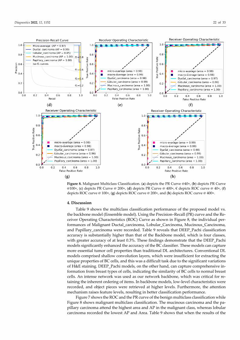
Diagnostics 2022, 12, 1152 22 of 33

(d) (e) (f)

(g) (h)

Figure 8. Malignant Multiclass Classification. (a) depicts the PR Curve @40×, (b) depicts PR Curve

@100×, (c) depicts PR Curve @ 200×, (d) depicts PR Curve @ 400×, € depicts ROC curve @ 40×, (f)

depicts ROC curve @ 100×, (g) depicts ROC curve @ 200×, and (h) depicts ROC curve @ 400×.

4. Discussion

Table 9 shows the multiclass classification performance of the proposed model vs.

the backbone model (Ensemble model). Using the Precision–Recall (PR) curve and the Re-

ceiver Operating Characteristics (ROC) Curve as shown in Figure 8, the individual per-

formances of Malignant Ductal_carcinoma, Lobular_Carcinoma, Mucinous_Cancinoma,

and Papillary_carcinoma were recorded. Table 9 reveals that DEEP_Pachi classification

accuracy is substantially higher than that of the Backbone model, which is four classes,

with greater accuracy of at least 0.3%. These findings demonstrate that the DEEP_Pachi

models significantly enhanced the accuracy of the BC classifier. These models can capture

more essential tumor cell properties than traditional DL architectures. Conventional DL

models comprised shallow convolution layers, which were insufficient for extracting the

unique properties of BC cells, and this was a difficult task due to the significant variations

of H&E staining. DEEP_Pachi models, on the other hand, can capture comprehensive in-

formation from breast types of cells, indicating the similarity of BC cells to normal breast

cells. An intense network was used as our network backbone, which was critical for re-

taining the inherent ordering of items. In backbone models, low-level characteristics were

recorded, and object pieces were retrieved at higher levels. Furthermore, the attention

mechanism raises feature levels, resulting in better classification performance.

Figure 7 shows the ROC and the PR curve of the benign multiclass classification while

Figure 8 shows malignant multiclass classification. The mucinous carcinoma and the pa-

pillary carcinoma attend the highest area and AP in the malignant class, whereas lobular

carcinoma recorded the lowest AP and Area. Table 9 shows that when the results of the

Diagnostics 2022, 12, 1152 23 of 33

DEEP_Pachi architecture are compared to the state-of-the-art results, the backbone model

alone achieves a higher accuracy for the multiclassification task. The accuracy of the back-

bone model alone was at least 3% greater than any of the state-of-the-art models. This

demonstrates that this model can use the deep network architecture of multi-resolution

input images to collect multi-scale relevant information and the benefits of its single mod-

els. The DEEP_Pachi model outperforms the multiclass classification by a margin for bi-

nary classification. This is because the various classes are not dissimilar and share many

characteristics. The findings show that the backbone model outperformed the other algo-

rithms in the binary classification task, with a total accuracy of 99%. Table 9 also shows

the backbone model’s sensitivity, Sensitivity, Precision, F1-Score, and AUC vs. the

DEEP_Pachi. Because our model can capture multi-level and multi-scale data and distin-

guish individual nucleus features and hierarchical organization, the DEEP_Pachi per-

formed well. DEEP_Pachi may also learn features at multiple sizes through its convolu-

tional layers. As a result, it can accurately distinguish individual nuclei and nuclei struc-

tures. The experimental findings reveal that the ensemble technique outperforms all other

approaches, achieving gains of at least 0.2–0.8% for images at 40×, 100×, 200×, and 400×

magnification due to its capacity to collect multi-scale contextual information. DEEP_Pa-

chi demonstrates that features derived from cross image inputs and then merged into a

boosting framework outperform standard deep learning architectures in object classifica-

tion tests. This also indicates that our enhancing approach exceeds deep learning net-

works when dealing with few training data samples.

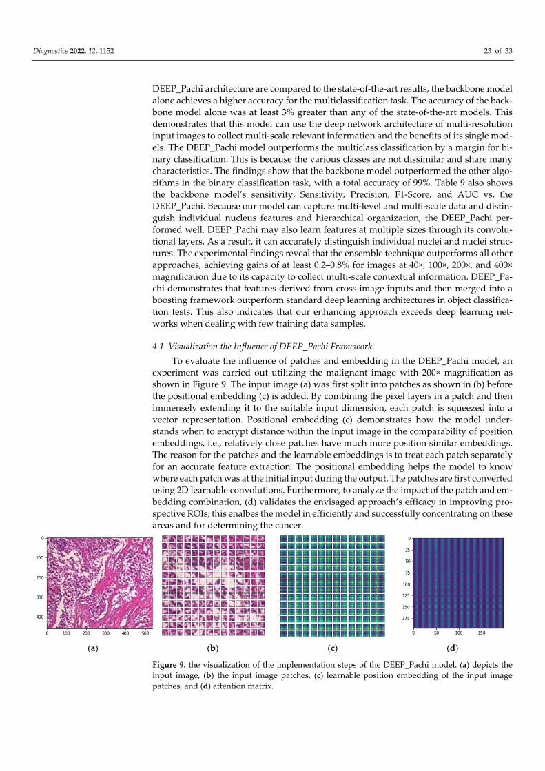
4.1. Visualization the Influence of DEEP_Pachi Framework

To evaluate the influence of patches and embedding in the DEEP_Pachi model, an

experiment was carried out utilizing the malignant image with 200× magnification as

shown in Figure 9. The input image (a) was first split into patches as shown in (b) before

the positional embedding (c) is added. By combining the pixel layers in a patch and then

immensely extending it to the suitable input dimension, each patch is squeezed into a

vector representation. Positional embedding (c) demonstrates how the model under-

stands when to encrypt distance within the input image in the comparability of position

embeddings, i.e., relatively close patches have much more position similar embeddings.

The reason for the patches and the learnable embeddings is to treat each patch separately

for an accurate feature extraction. The positional embedding helps the model to know

where each patch was at the initial input during the output. The patches are first converted

using 2D learnable convolutions. Furthermore, to analyze the impact of the patch and em-

bedding combination, (d) validates the envisaged approach’s efficacy in improving pro-

spective ROIs; this enalbes the model in efficiently and successfully concentrating on these

areas and for determining the cancer.

(a) (b) (c) (d)

Figure 9. the visualization of the implementation steps of the DEEP_Pachi model. (a) depicts the

input image, (b) the input image patches, (c) learnable position embedding of the input image

patches, and (d) attention matrix.

Diagnostics 2022, 12, 1152 24 of 33

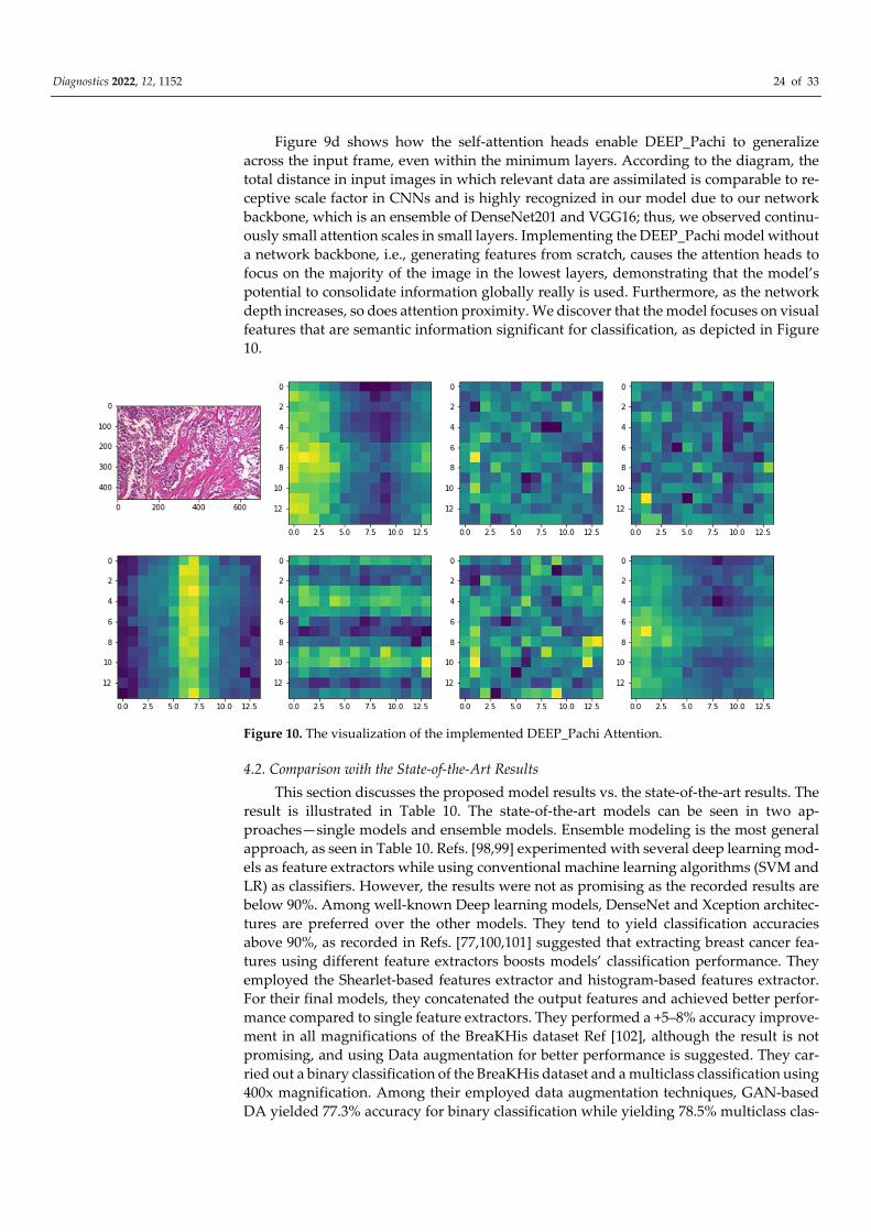
Figure 9d shows how the self-attention heads enable DEEP_Pachi to generalize

across the input frame, even within the minimum layers. According to the diagram, the

total distance in input images in which relevant data are assimilated is comparable to re-

ceptive scale factor in CNNs and is highly recognized in our model due to our network

backbone, which is an ensemble of DenseNet201 and VGG16; thus, we observed continu-

ously small attention scales in small layers. Implementing the DEEP_Pachi model without

a network backbone, i.e., generating features from scratch, causes the attention heads to

focus on the majority of the image in the lowest layers, demonstrating that the model’s

potential to consolidate information globally really is used. Furthermore, as the network

depth increases, so does attention proximity. We discover that the model focuses on visual

features that are semantic information significant for classification, as depicted in Figure

10.

Figure 10. The visualization of the implemented DEEP_Pachi Attention.

4.2. Comparison with the State-of-the-Art Results

This section discusses the proposed model results vs. the state-of-the-art results. The

result is illustrated in Table 10. The state-of-the-art models can be seen in two ap-

proaches—single models and ensemble models. Ensemble modeling is the most general

approach, as seen in Table 10. Refs. [98,99] experimented with several deep learning mod-

els as feature extractors while using conventional machine learning algorithms (SVM and

LR) as classifiers. However, the results were not as promising as the recorded results are

below 90%. Among well-known Deep learning models, DenseNet and Xception architec-

tures are preferred over the other models. They tend to yield classification accuracies

above 90%, as recorded in Refs. [77,100,101] suggested that extracting breast cancer fea-

tures using different feature extractors boosts models’ classification performance. They

employed the Shearlet-based features extractor and histogram-based features extractor.

For their final models, they concatenated the output features and achieved better perfor-

mance compared to single feature extractors. They performed a +5–8% accuracy improve-

ment in all magnifications of the BreaKHis dataset Ref [102], although the result is not

promising, and using Data augmentation for better performance is suggested. They car-

ried out a binary classification of the BreaKHis dataset and a multiclass classification using

400x magnification. Among their employed data augmentation techniques, GAN-based

DA yielded 77.3% accuracy for binary classification while yielding 78.5% multiclass clas-

Diagnostics 2022, 12, 1152 25 of 33

sification performance. Comparing the performance of the inception models, Incep-

tion_V3 and Inception_ResNet_V2 [93] produced a better performance as they extracted

more relevant information by running convolution operations with varied regions of in-

terest concurrently. The use of transfer learning is more evident in binary classification.

The authors of Refs. [103–107] based their work on binary classification by combining the

subclasses of the benign and the malignant. VGG is seen to be often used for feature ex-

traction as it has deeper layers able to identify conceptual features. Comparing our pro-

posed model DEEP_Pachi, which is a modification of the vison transformer self-attention

heads computation techniques, ensemble models, and a classification layer using the Mul-

tilinear perceptron block, we argue that extracting increased breast cancer features re-

quires an accurate vision system and, hence, and attention mechanism to focus on the

region of the disease instead of extracting entire image features. Refs. [108–111] proposed

an accurate and more unique approach for breast cancer classification. Ref. [108] em-

ployed the use of multi-view attention mechanism. Ref [109] proposed the deep attention

high order network, while Ref [110] proposed using a different branch of CNN for more

feature generation. Ref [111] proposed a three-channel feature low dimension model. All

these approaches were in line with better breast cancer feature extraction; thus, they

achieved the highest classification performance with +95% classification accuracy on all

magnifications of BreaKHis (40×, 100×, 200×, and 400× magnification). In line with the cur-

rent state-of-the-art results, our model achieved an accuracy of 99% for all magnifications

except 400%, where we achieved an accuracy of 1.0%. Our analyses demonstrate that our

proposed models significantly enhanced the efficiency of the BC classifier. Our models

can extract more critical breast cell features than CNN. CNN was made up of four thin

convolution layers, which were insufficient for extracting unique properties of BC tumors,

which was a difficult task due to the large variation of H&E smears.

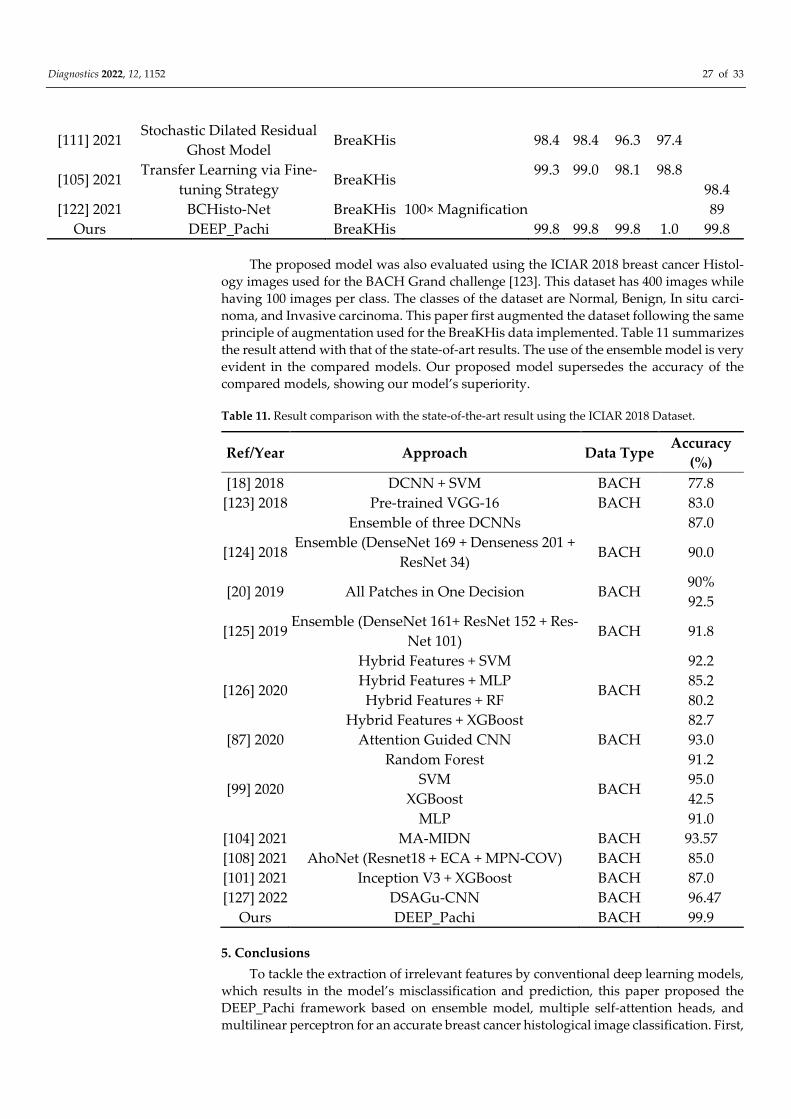
Table 10. Result comparison with the state-of-the-art result using the BreaKHis Dataset.

Ref/Year Approach Data Type Classification

Type

Accuracy (%)

40× 100× 200× 400× Binary

[112] 2018 Ensemble (CNN + LSTM) BreaKHis 88.7 85.3 88.6 88.4

[113] 2018 DenseNet CNN BreaKHis 93.6 97.4 95.9 94.7

[77] 2018 Xception BreaKHis 95.3 93.4 93.1 91.7

[114] 2018 KAZE features + Bag of Fea-

tures BreaKHis 85.9 80.4 78.1 71.1

[102] 2019

CNN

BreaKHis

77.2

CNN + DA 76.7

CGANs based DA 77.3

DA + CGANs based DA 75.2

CNN 75.4

CNN + DA 75.9

CGANs based DA 78.5

DA + CGANs based DA 78.7

[115] 2019 Deep ResNet + CBAM BreaKHis 91.2 91.7 92.6 88.9

[103] 2019 Transfer Learning (VGG16 +

VGG19 + CNN)

98.2 98.3 98.2 97.5

98.1

[116] 2019 IRRCNN BreaKHis 98.0 97.6 97.3 97.4

[85] 2019

Inception_V3

BreaKHis

Multiclass 90.3 85.4 84.0 82.1

Binary 97.7 94.2 87.2 96.7

Inception_ResNet_V2 Multiclass 98.4 98.7 97.9 97.4

Binary 99.9 99.9 1.0 99.9

Diagnostics 2022, 12, 1152 26 of 33

[80] 2019 BHCNet-6 + ERF

BreaKHis Multiclass 94.4 94.5 92.3 91.1

CNN +SE-ResNet Binary 98.9 99.0 99.3 99.0

[117] 2020 Deep CNN BreaKHis 73.4 76.8 83.2 75.8

[94] 2020

VGG16 + SVM

(Balanced + DA)

BreaKHis

94.0 92.9 91.2 91.8

Ensemble (VGG16 + VGG19 +

ResNet 50) + RF Classifier 90.3 90.1 87.4 86.6

Ensemble (VGG16 + VGG19 +

ResNet 50) + SVM Classifier 82.2 87.6 86.5 83.0

[78] 2020 ResHist (RL Based 152-layer

CNN) BreaKHis 86.4 87.3 91.4 86.3

[64] 2020 VGGNET16-RF

BreaKHis 92.2 93.4 95.2 92.8

VGGNET16-SVM 94.1 95.1 97.0 93.4

[118] 2020 CNN + spectral–spatial fea-

tures BreaKHis Malignant 97.6 97.4 97.3 97.0

[100] 2020 NucTraL+BCF BreaKHis 96.9

[119] 2020 ResNet50 + KWE LM BreaKHis Malignant 88.4 87.1 90.0 84.1

[93] 2020

AlexNet + SVM

BreaKHis

84.1 87.5 89.4 85.2

VGG16 + SVM 86.4 87.8 86.8 84.4

VGG19+SVM 86.6 88.1 85.8 81.7

GoogleNet + SVM 81.0 84.5 82.5 79.8

ResNet18 + SVM 84.0 84.3 82.5 79.8

ResNet50 + SVM 87.7 87.8 90.1 83.7

ResNet101 + SVM 86.4 88.9 90.1 83.2

ResNetInceptionV2 + SVM 86.3 86.3 87.1 81.4

InceptionV3 + SVM 85.8 84.7 86.8 82.9

SqueezeNet + SVM 81.2 83.7 84.2 77.5

[120] 2020 Optimized CNN BreaKHis 80.8 76.6 79.9 74.2

[110] 2020 InceptionV3 + BCNNs BreaKHis 95.7 94.7 94.8 94.5

96.1

[105] 2020

VGG16 + SVM

BreaKHis

78.6 85.2 82.0 79.6

VGG19 + SVM 77.3 79.1 83.0 79.1

Xception + SVM 81.6 82.9 78.4 76.1

ResNet50 + SVM 86.4 86.0 84.3 82.9

VGG16 + LR 78.8 85.2 81.2 79.1

VGG19 + LR 77.6 82.4 82.2 77.8

Xception + LR 82.4 79.6 79.4 83.1

ResNet50 + LR 83.1 86.7 84.0 80.1

[107] 2020

Shearlet-based features

BreaKHis

89.4 88.0 86.0 83.0

Histogram-based features. 92.6 93.9 95.0 94.7

Concatenating all features 98.2 97.2 97.8 97.3

[104] 2021 MA-MIDN BreaKHis 96.3 95.7 97.0 95.4

[108] 2021 AhoNet (Resnet18 + ECA +

MPN-COV) BreaKHis 97.5 97.3 99.2 97.1

[109] 2021 3PCNNB-Net BreaKHis 92.3 93.1 97.0 92.1

[121] 2021 APVEC BreaKHis 92.1 90.2 95.0 92.8

Diagnostics 2022, 12, 1152 27 of 33

[111] 2021 Stochastic Dilated Residual

Ghost Model BreaKHis 98.4 98.4 96.3 97.4

[105] 2021 Transfer Learning via Fine-

tuning Strategy BreaKHis

99.3 99.0 98.1 98.8

98.4

[122] 2021 BCHisto-Net BreaKHis 100× Magnification 89

Ours DEEP_Pachi BreaKHis 99.8 99.8 99.8 1.0 99.8

The proposed model was also evaluated using the ICIAR 2018 breast cancer Histol-

ogy images used for the BACH Grand challenge [123]. This dataset has 400 images while

having 100 images per class. The classes of the dataset are Normal, Benign, In situ carci-

noma, and Invasive carcinoma. This paper first augmented the dataset following the same

principle of augmentation used for the BreaKHis data implemented. Table 11 summarizes

the result attend with that of the state-of-art results. The use of the ensemble model is very

evident in the compared models. Our proposed model supersedes the accuracy of the

compared models, showing our model’s superiority.

Table 11. Result comparison with the state-of-the-art result using the ICIAR 2018 Dataset.

Ref/Year Approach Data Type Accuracy

(%)

[18] 2018 DCNN + SVM BACH 77.8

[123] 2018 Pre-trained VGG-16 BACH 83.0

Ensemble of three DCNNs 87.0

[124] 2018 Ensemble (DenseNet 169 + Denseness 201 +

ResNet 34) BACH 90.0

[20] 2019 All Patches in One Decision BACH 90%

92.5

[125] 2019 Ensemble (DenseNet 161+ ResNet 152 + Res-

Net 101) BACH 91.8

[126] 2020

Hybrid Features + SVM

BACH

92.2

Hybrid Features + MLP 85.2

Hybrid Features + RF 80.2

Hybrid Features + XGBoost 82.7

[87] 2020 Attention Guided CNN BACH 93.0

[99] 2020

Random Forest

BACH

91.2

SVM 95.0

XGBoost 42.5

MLP 91.0

[104] 2021 MA-MIDN BACH 93.57

[108] 2021 AhoNet (Resnet18 + ECA + MPN-COV) BACH 85.0

[101] 2021 Inception V3 + XGBoost BACH 87.0

[127] 2022 DSAGu-CNN BACH 96.47

Ours DEEP_Pachi BACH 99.9

5. Conclusions

To tackle the extraction of irrelevant features by conventional deep learning models,

which results in the model’s misclassification and prediction, this paper proposed the

DEEP_Pachi framework based on ensemble model, multiple self-attention heads, and

multilinear perceptron for an accurate breast cancer histological image classification. First,

Diagnostics 2022, 12, 1152 28 of 33

a thorough review of medical image modalities for breast cancer classification was carried

out with the related open access datasets. Secondly, we applied the Python augmentation

library to address the issues of limited raining data samples. The Python Augmentor was

used to generate the training image samples while utilizing the original image for testing.

The proposed model utilizes ensemble model (Densenet201 and VGG16) as the network

backbone for a more generalized feature extraction of the input images (global features),

whereas multiple self-attention heads extract spatial information (regions of interest). The

superiority of the proposed model was evaluated using two publicly available databases,

BreakHis and ICIAR2018, and using various evaluations metrics, and the result obtained

show that the proposed DEEP_Pachi outperforms the state-of-the-art results in histo-

pathological breast cancer image classification. The suggested technique achieved an ac-

curacy of 1.0 for the benign class and 0.99 for the malignant class in all magnifications of

the BreakHis datasets and an accuracy of 0.99 on the ICIAR 2018 Challenge dataset.

As much as the proposed framework exhibit high classification accuracy, there is still

room to evaluate DEEP_Pachi using other data augmentation techniques. Future work

will see the exploration of various data augmentation techniques such as GAN for increas-

ing training samples. We also intend on extending the DEEP_Pachi framework to other

disease classification using histopathological or microscopic images such as Oral cancer,

Skin Cancer, etc. On the other hand, this paper will investigate the replacement of the

MLP Block with SGTM neural-like structures to evaluate the possible best approach in

our model.

Author Contributions: Formal analysis, G.U.N.; funding acquisition, M.A.H.; methodology, C.C.U.;

project administration, H.N.M.; resources, M.A.H.; supervision, Z.Q.; validation, G.U.N.; visualiza-

tion, H.N.M.; writing—original draft, C.C.U.; writing—review and editing, J.K.J. All authors have

read and agreed to the published version of the manuscript.

Funding: This research was partially supported by the National Science Foundation of China

(NSFC) under the project “Development of fetal heart-oriented heart sound echocardiography mul-

timodal auxiliary diagnostic equipment” (62027827).

Ethical Approval: This article does not contain any studies with human participants or animals

performed by any of the authors.

Informed Consent Statement: Not applicable.

Data Availability Statement: The dataset used in this paper is public and can be obtained from

these repositories: https://www.kaggle.com/ambarish/breakhis (accessed: 12 March 2022) and

https://iciar2018-challenge.grand-challenge.org/Dataset/(accessed: 12 March 2022). The Tensor-

Flow/Keras code we used in our experiment is not yet publicly available and will be made so after

the publication of the work.

Ethical Approval This article does not contain any studies with human participants or animals per-

formed by any of the authors.

Conflicts of Interest: All authors declare that they have no conflict of interest.

References

1. Anastasiadi, Z.; Lianos, G.D.; Ignatiadou, E.; Harissis, H.V.; Mitsis, M. Breast Cancer in Young Women: An Overview. Updates

Surg. 2017, 69, 313–317.

2. Wang, K.; Franch-Expósito, S.; Li, L.; Xiang, T.; Wu, J.; Ren, G. 34P Comprehensive clinical and molecular portraits of grade 3

ER+ HER- breast cancer. Ann. Oncol. 2020, 31, S27.

3. DeSantis, C.E.; Ma, J.; Gaudet, M.M.; Newman, L.A.; Miller, K.D.; Sauer, A.G.; Jemal, A.; Siegel, R.L. Breast Cancer Statistics.

CA A Cancer J. Clin. 2019, 69, 438–451.

4. Man, R.; Yang, P.; Xu, B. Classification of Breast Cancer Histopathological Images Using Discriminative Patches Screened by

Generative Adversarial Networks. IEEE Access 2020, 8, 155362–155377.

5. Mambou, S.; Maresova, P.; Krejcar, O.; Selamat, A.; Kuca, K. Breast Cancer Detection Using Infrared Thermal Imaging and a

Deep Learning Model. Sensors 2018, 18, 2799.

6. Mahmood, T.; Li, J.; Pei, Y.; Akhtar, F.; Imran, A.; Rehman, K.U. A Brief Survey on Breast Cancer Diagnostic with Deep Learning

Schemes Using Multi-Image Modalities. IEEE Access 2020, 8, 165779–165809.

Diagnostics 2022, 12, 1152 29 of 33

7. Chiao, J.Y.; Chen, K.-Y.; Liao, K.Y.-K.; Hsieh, P.-H.; Zhang, G.; Huang, T.-C. Detection and Classification the Breast Tumors

Using Mask R-CNN On Sonograms. Medicine 2019, 98, e15200.

8. Cruz-Roa, A.; Gilmore, H.; Basavanhally, A.; Feldman, M.; Ganesan, S.; Shih, N.N.C.; Tomaszewski, J.; González, F.A.;

Madabhushi, A. Accurate and Reproducible Invasive Breast Cancer Detection in Whole-Slide Images: A Deep Learning Ap-

proach for Quantifying Tumor Extent. Sci. Rep. 2017, 7, 1–14.

9. Talbert, P.Y.; Frazier, M.D. Inflammatory Breast Cancer Disease: A Literature Review. Cancer Stud. 2019, 2.

https://doi.org/10.31532/cancerstud.2.1.004.

10. Saha, M.; Chakraborty, C.; Racoceanu, D. Efficient Deep Learning Model for Mitosis Detection Using Breast Histopathology

Images. Comput. Med. Imaging Graph. 2018, 64, 29–40.

11. Domingues, I.; Pereira, G.; Martins, P.; Duarte, H.; Santos, J.; Abreu, P.H. Using Deep Learning Techniques in Medical Imaging:

A Systematic Review of Applications on CT And PET. Artif. Intell. Rev. 2019, 53, 4093–4160.

12. Murtaza, G.; Shuib, L.; Wahab, A.W.A.; Mujtaba, G.; Mujtaba, G.; Nweke, H.F.; Al-garadi, M.A.; Zulfiqar, F.; Raza, G.; Azmi,

N.A. Deep Learning-Based Breast Cancer Classification Through Medical Imaging Modalities: State of The Art and Research

Challenges Artif. Intell. Rev. 2019, 53, 1655–1720.

13. Pavithra, S.; Vanithamani, R.; Justin, J. Computer-aided breast cancer detection using ultrasound images. Mater. Today Proc.

2020, 33, 4802–4807.

14. Moghbel, M.; Ooi, C.Y.; Ismail, N.; Hau, Y.W.; Memari, N. A Review of Breast Boundary and Pectoral Muscle Segmentation

Methods in Computer-Aided Detection/Diagnosis of Breast Mammography. Artif. Intell. Rev. 2019, 53, 1873–1918.

15. Prabha, S. Thermal Imaging Techniques for Breast Screening—A Survey. Curr. Med. Imaging Former. Curr. Med. Imaging Rev.

2020, 16, 855–862.

16. Hadadi, I.; Rae, W.; Clarke, J.; McEntee, M.; Ekpo, E. Diagnostic Performance of Adjunctive Imaging Modalities Compared to

Mammography Alone in Women with Non-Dense and Dense Breasts: A Systematic Review and Meta-Analysis. Clin. Breast

Cancer 2021, 21, 278–291.

17. Nahid, A.A.; Ali, F.B.; Kong, Y. Histopathological Breast-Image Classification with Image Enhancement by Convolutional Neu-

ral Network. In Proceedings of the 2017 20th International Conference of Computer and Information Technology (ICCIT),

Dhaka, Bangladesh, 22–24 December 2017.

18. Bardou, D.; Zhang, K.; Ahmad, S.M. Classification of Breast Cancer Based on Histology Images Using Convolutional Neural

Networks. IEEE Access 2018, 6, 24680–24693.

19. Araújo, T.; Aresta, G.; Castro, E.; Rouco, J.; Aguiar, P.; Eloy, C.; Polónia, A.; Campilho, A. Classification of Breast Cancer His-

tology Images Using Convolutional Neural Networks. PLoS ONE 2017, 12, e0177544.

20. Roy, K.; Banik, D.; Bhattacharjee, D.; Nasipuri, M. Patch-Based System for Classification of Breast Histology Images Using Deep

Learning. Comput. Med. Imaging Graph. 2019, 71, 90–103.

21. Kausar, T.; Wang, M.; Malik, M.S.S. Cancer Detection in Breast Histopathology with Convolution Neural Network Based Ap-

proach. In Proceedings of the 2019 IEEE/ACS 16th International Conference on Computer Systems and Applications (AICCSA),

Abu Dhabi, United Arab Emirates, 3–7 November 2019.

22. Albawi, S.; Mohammed, T.A.; Al-Zawi, S. Understanding of A Convolutional Neural Network. In Proceedings of the 2017 In-

ternational Conference on Engineering and Technology (ICET), Antalya, Turkey, 21–23 August 2017.

23. Perumal, V.; Narayanan, V.; Rajasekar, S.J.S. Detection of Brain Tumor with Magnetic Resonance Imaging using Deep Learning

Techniques. In Brain Tumor MRI Image Segmentation Using Deep Learning Techniques; Elsevier, Amsterdam, The Netherlands,

2022; pp. 183–196.

24. Hu, J.; Shen, L.; Sun, G. Squeeze-And-Excitation Networks. In Proceedings of the IEEE conference on computer vision and

pattern recognition, Salt Lake City, UT, USA, 18–23 June 2018; pp. 7132–7141.

25. Huang, Z.; Wang, X.; Huang, L.; Huang, C.; Wei, Y.; Liu, W. CCNET: Criss-Cross Attention for Semantic Segmentation. In

Proceedings of the IEEE/CVF International Conference on Computer Vision, Seoul, Korea, 27–28 October 2019; pp. 603–612.

26. Wang, F.; Jiang, M.; Qian, C.; Yang, S.; Li, C.; Zhang, H.; Wang, X.; Tang, X. Residual Attention Network for Image Classification.

In Proceedings of the IEEE conference on computer vision and pattern recognition, Honolulu, HI, USA, 21–26 July 2017; pp.

3156–3164.

27. Wang, X.; Girshick, R.; Gupta, A.; He, K. Non-Local Neural Networks. In Proceedings of the IEEE conference on computer

vision and pattern recognition, Salt Lake City, UT, USA, 18–23 June 2018; pp. 7794–7803.

28. Woo, S.; Park, J.; Lee, J.-Y.; Kweon, I.S. CBAM: Convolutional Block Attention Module. In Proceedings of The European Con-

ference on Computer Vision (ECCV), Munich, Germany, 8–14 September 2018; pp. 3–19.

29. Sarikaya, I. Breast Cancer and Pet Imaging. Nucl. Med. Rev. Cent. East. Eur. 2021, 24, 16–26.

30. Vaishnavi, J.; Devi, M.A.; Punitha, S.; Ravi, S. Computer-aided mammography techniques for detection and classification of

microcalcifications in digital mammograms. Int. J. Image Min. 2018, 3, 48.

31. Loizidou, K.; Skouroumouni, G.; Nikolaou, C.; Pitris, C. An Automated Breast Micro-Calcification Detection and Classification

Technique Using Temporal Subtraction of Mammograms. IEEE Access 2020, 8, 52785–52795.

32. Suh, Y.J.; Jung, J.; Cho, B.-J. Automated Breast Cancer Detection in Digital Mammograms of Various Densities Via Deep Learn-

ing. J. Pers. Med. 2020, 10, 211.

33. Mohamed, A.A.; Berg, W.A.; Peng, H.; Luo, Y.; Jankowitz, R.C.; Wu, S. A Deep Learning Method for Classifying Mammographic

Breast Density Categories. Med. Phys. 2018, 45, 314–321.

Diagnostics 2022, 12, 1152 30 of 33

34. Mehmood, M.; Ayub, E.; Ahmad, F.; Alruwaili, M.; Alrowaili, Z.A.; Alanazi, S.; Humayun, M.; Rizwan, M.; Naseem, S.; Alyas,

T. Machine Learning Enabled Early Detection of Breast Cancer by Structural Analysis of Mammograms. Comput. Mater. Contin.

2021, 67, 641–657.

35. Fiorica, J.V. Breast Cancer Screening, Mammography, And Other Modalities. Clin. Obstet. Gynecol. 2017, 59, 688–709.

36. Li, Q.; Shi, W.; Yang, H.; Zhang, H.; Li, G.; Chen, T.; Mori, K.; Jiang, Z. Computer-aided diagnosis of mammographic masses

using geometric verification-based image retrieval. Med. Imaging 2017 Comput. Aided Diagn. 2017, 10134, 746–753.

37. Kaur, P.; Singh, G.; Kaur, P. Intellectual detection and validation of automated mammogram breast cancer images by multi-

class SVM using deep learning classification. Inform. Med. Unlocked 2019, 16, 100151.

38. Tran, T.S.H.; Nguyen, H.M.T. Application of 2D Ultrasound, Elastography Arfi and Mammography for Diagnosis of solid tu-

mors in breast. J. Med. Pharm. 2019, 58–65. https://doi.org/10.34071/jmp.2019.4.8.

39. Han, J.; Li, F.; Peng, C.; Huang, Y.; Lin, Q.; Liu, Y.; Cao, L.; Zhou, J. Reducing Unnecessary Biopsy of Breast Lesions: Preliminary

Results with Combination of Strain and Shear-Wave Elastography. Ultrasound Med. Biol. 2019, 45, 2317–2327.

40. Ucar, H.; Kacar, E.; Karaca, R. The Contribution of a Solid Breast Mass Gray-Scale Histographic Analysis in Ascertaining a

Benign-Malignant Differentiation. J. Diagn. Med. Sonogr. 2022, 875647932210782. https://doi.org/10.1177/87564793221078205.

41. Yap, M.H.; Pons, G.; Marti, J.; Ganau, S.; Sentis, M.; Zwiggelaar, R.; Davison, A.K.; Marti, R. Automated Breast Ultrasound

Lesions Detection Using Convolutional Neural Networks. IEEE. J. Biomed. Health Inf. 2017, 22, 1218–1226.

42. Early Initiation of MRI-Based Breast Cancer Screening Predicted to Halve Breast Cancer Deaths in Childhood Cancer Survivor.

Default Digital Object Group. 2019. https://doi.org/10.1200/adn.19.190216.

43. Sriussadaporn, S.; Sriussadaporn, S.; Pak-art, R.; Kritayakirana, K.; Prichayudh, S.; Samorn, P. Ultrasonography increases sen-

sitivity of mammography for diagnosis of multifocal, multicentric breast cancer using 356 whole breast histopathology as a gold

standard. Surg. Pract. 2022. https://doi.org/10.1111/1744-1633.12543.

44. Pujara, A.C.; Kim, E.; Axelrod, D.; Melsaether, A.N. PET/MRI in Breast Cancer. J. Magn. Reson. Imaging 2018, 49, 328–342.

45. Mann, R.M.; Athanasiou, A.; Baltzer, P.A.T.; Camps-Herrero, J.; Clauser, P.; Fallenberg, E.M.; Forrai, G.; Fuchsjäger, M.H.; Hel-

bich, T.H.; Killburn-Toppin, F.; et al. Breast cancer screening in women with extremely dense breasts recommendations of the

European Society of Breast Imaging (EUSOBI). Eur. Radiol. 2022, 1–10. https://doi.org/10.1007/s00330-022-08617-6.

46. Houssami, N.; Cho, N. Screening Women with A Personal History of Breast Cancer: Overview of The Evidence on Breast Im-

aging Surveillance. Ultrasonography 2018, 37, 277.

47. Greenwood, H.I. Abbreviated Protocol Breast MRI: The Past, Present, And Future. Clin. Imag. 2019, 53, 169–173.

48. Zelst, J.C.V.; Vreemann, S.; Witt, H.-J.; Gubern-Merida, A.; Dorrius, M.D.; Duvivier, K.; Lardenoije-Broker, S.; Lobbes, M.B.;

Loo, C.; Veldhuis, W.; et al. Multireader Study on The Diagnostic Accuracy of Ultrafast Breast Magnetic Resonance Imaging for

Breast Cancer Screening. Investig. Radiol. 2018, 53, 579–586.

49. Heller, S.L.; Moy, L. MRI Breast Screening Revisited. J. Magn. Reson. Imag. 2019, 49, 1212–1221.

50. Aswathy, M.; Jagannath, M. Detection of Breast Cancer On Digital Histopathology Images: Present Status And Future Possibil-

ities. Inf. Med. Unlocked 2017, 8, 74–79.

51. Tellez, D.; Balkenhol, M.; Karssemeijer, N.; Litjens, G.; Laak, J.V.D.; Ciompi, F. H and E Stain Augmentation Improves General-

ization of Convolutional Networks for Histopathological Mitosis Detection. In Medical Imaging 2018: Digital Pathology; Interna-

tional Society for Optics and Photonics: Bellingham, WA, USA, 2018; p. 105810Z.

52. Jaglan, P.; Dass, R.; Duhan, M. Breast Cancer Detection Techniques: Issues and Challenges. J. Inst. Eng Ser. B 2019, 100, 379–386.

53. Posso, M.; Puig, T.; Carles, M.; Ru’e, M.; Canelo-Aybar, C.; Bonfill, X. Effectiveness and Cost-Effectiveness of Double Reading

in Digital Mammography Screening: A Systematic Review and Meta-Analysis Eur. J. Radiol. 2017, 96, 40–49.

54. Wilkinson, L.; Thomas, V.; Sharma, N. Microcalcification On Mammography: Approaches to Interpretation and Biopsy. Br. J.

Radiol. 2017, 90, 20160594.

55. Houssami, N. Evidence on Synthesized Two-dimensional Mammography Versus Digital Mammography When Using Tomo-

synthesis (Three-dimensional Mammography) for Population Breast Cancer Screening. Clin. Breast Cancer 2018, 18, 255–260.e1.

56. Fujimura, S.; Tamura, T.; Kawasaki, Y. The relationship between compressed breast thickness in mammography and other

factors that influence breast cancer. J. Jpn. Assoc. Breast Cancer Screen. 2021, 30, 177–181.

57. Rapelyea, J.A.; Marks, C.G. Breast Ultrasound Past, Present, And Future. In Breast Imaging; Intech Open: Rijeka, Croatia, 2018;

pp. 21–48.

58. Sood, R.; Rositch, A.F.; Shakoor, D.; Ambinder, E.; Pool, K.-L.; Pollack, E.; Mollura, D.J.; Mullen, L.A.; Harvey, S.C. Ultrasound

for Breast Cancer Detection Globally: A Systematic Review and Meta-Analysis. J. Global. Oncol. 2019, 5, 1–17.

59. Youk, J.H.; Gweon, H.M.; Son, E.J. Shear-Wave Elastography in Breast Ultrasonography: The State of the Art. Ultrasonography

2017, 36, 300.

60. R. S. of North America. Ultrasound Images. Available online: https://www.radiologyinfo.org/en/info/genus (accessed on 22

March 2022).

61. García, E.; Diez, Y.; Diaz, O.; Llado, X.; Martí, R.; Martí, J.; Oliver, A. A Step-By-Step Review on Patient-Specific Biomechanical

Finite Element Models for Breast M.R.I. To X-Ray Mammography Registration. Med. Phys. 2018, 45, e6–e31.

62. Kalantarova, A.; Zembol, N.J.; Kufel-Grabowska, J. Pregnancy-Associated Breast Cancer as A Screening and Diagnostic Chal-

lenge: A Case Report. Nowotwory 2021, 71, 162–164.

63. Reig, B.; Heacock, L.; Geras, K.J.; Moy, L. Machine Learning in Breast MRI. J. Magn. Reson. Imag. 2020, 52, 998–1018.

Diagnostics 2022, 12, 1152 31 of 33

64. Kumar, A.; Singh, S.K.; Saxena, S.; Lakshmanan, K.; Sangaiah, A.K.; Chauhan, H.; Shrivastava, S.; Singh, R.K. Deep Feature

Learning for Histopathological Image Classification of Canine Mammary Tumors and Human Breast Cancer. Inf. Sci. 2020, 508,

405–421.

65. Beevi, K.S.; Nair, M.S.; Bindu, G.R. Automatic Mitosis Detection In Breast Histopathology Images Using Convolutional Neural

Network Based Deep Transfer Learning. Biocybern. Biomed. Eng. 2019, 39, 214–223.

66. Dodballapur, V.; Song, Y.; Huang, H.; Chen, M.; Chrzanowski, W.; Cai, W. Mask-Driven Mitosis Detection in Histopathology

Images. In Proceedings of the 2019 IEEE 16th International Symposium on Biomedical Imaging (ISBI 2019), Venice, Italy, 8–11

April 2019.

67. Wang, Y.; Lei, B.; Elazab, A.; Tan, E.-L.; Wang, W.; Huang, F.; Gong, X.; Wang, T. Breast Cancer Image Classification via Multi-

Network Features and Dual-Network Orthogonal Low-Rank Learning. IEEE Access 2020, 8, 27779–27792.

68. Das, A.; Nair, M.S.; Peter, S.D. Sparse Representation Over Learned Dictionaries on the Riemannian Manifold for Automated

Grading of Nuclear Pleomorphism in Breast Cancer. IEEE Trans. Image Processing 2019, 28, 1248–1260.

69. Dimitropoulos, K.; Barmpoutis, P.; Zioga, C.; Kamas, A.; Patsiaoura, K.; Grammalidis, N. Grading of Invasive Breast Carcinoma

Through Grassmannian VLAD Encoding. PLoS ONE 2017, 12, e0185110.

70. Zheng, Y.; Jiang, Z.; Zhang, H.; Xie, F.; Ma, Y.; Shi, H.; Zhao, Y. Histopathological Whole Slide Image Analysis Using Context-

Based CBIR. IEEE Trans. Med. Imaging 2018, 37, 1641–1652.

71. Biswas, R.; Roy, S.; Biswas, A. Mammogram Classification using Curvelet Coefficients and Gray Level Co-Occurrence Matrix

for Detection of Breast Cancer. Int. J. Innov. Technol. Explor. Eng. 2019, 8, 4819–4824.

72. Reis, S.; Gazinska, P.; Hipwell, J.H.; Mertzanidou, T.; Naidoo, K.; Williams, N.; Pinder, S.; Hawkes, D.J. Automated Classifica-

tion of Breast Cancer Stroma Maturity from Histological Images. IEEE Trans. Biomed. Eng. 2017, 64, 2344–2352.

73. Vaiyapuri, S.; Mari, K.; Delphina, A.A. An Intelligent Framework for Detection and Classification of MRI Brain Tumour using

SIFT-SURF Features and K-nearest Neighbour Approach. Strad Res. 2020, 7, 1–10.

74. Krystel-Whittemore, M.; Wen, H.Y. Update on HER2 expression in breast cancer. Diagn. Histopathol. 2022, 28, 170–175.

75. Nateghi, R.; Danyali, H.; Helfroush, M.S. Maximized Inter-Class Weighted Mean for Fast and Accurate Mitosis Cells Detection

in Breast Cancer Histopathology Images. J. Med. Syst. 2017, 41, 1–15.

76. Burçak, K.C.; Baykan, Ö.K.; Uğuz, H. A New Deep Convolutional Neural Network Model for Classifying Breast Cancer Histo-

pathological Images and The Hyperparameter Optimization of The Proposed Model. J. Supercomput. 2020, 77, 973–989.

77. Li, L.; Pan, X.; Yang, H.; Liu, Z.; He, Y.; Li, Z.; Fan, Y.; Cao, Z.; Zhang, L. Multi-Task Deep Learning for Fine-Grained Classifica-

tion and Grading in Breast Cancer Histopathological Images. Multimed. Tools Appl. 2018, 79, 14509–14528.

78. Gour, M.; Jain, S.; Kumar, T.S. Residual Learning-Based CNN For Breast Cancer Histopathological Image Classification. Int. J.

Imaging Syst. Technol. 2020, 30, 621–635.

79. Yan, R.; Ren, F.; Wang, Z.; Wang, L.; Zhang, T.; Liu, Y.; Rao, X.; Zheng, C.; Zhang, F. Breast Cancer Histopathological Image

Classification Using A Hybrid Deep Neural Network. Methods 2020, 173, 52–60.

80. Jiang, Y.; Chen, L.; Zhang, H.; Xiao, X. Breast Cancer Histopathological Image Classification Using Convolutional Neural Net-

works with Small SE-Resnet Module. PLoS ONE 2019, 14, e0214587.

81. Yao, H.; Zhang, X.; Zhou, X.; Liu, S. Parallel Structure Deep Neural Network Using CNN and RNN with an Attention Mecha-

nism for Breast Cancer Histology Image Classification. Cancers 2019, 11, 1901.

82. Khan, S.; Islam, N.; Jan, Z.; Din, I.U.; Rodrigues, J.J.P.C. A Novel Deep Learning-Based Framework for The Detection and Clas-

sification of Breast Cancer Using Transfer Learning. Pattern Recognit. Lett. 2019, 125, 1–6.

83. Du, Y.; Zhang, R.; Zargari, A.; Thai, T.C.; Gunderson, C.C.; Moxley, K.M.; Liu, H.; Zheng, B.; Qiu, Y. Classification of Tumor

Epithelium and Stroma by Exploiting Image Features Learned by Deep Convolutional Neural Networks. Ann. Biomed. Eng.

2018, 46, 1988–1999.

84. Wang, P.; Song, Q.; Li, Y.; Lv, S.; Wang, J.; Li, L.; Zhang, H. Cross-Task Extreme Learning Machine for Breast Cancer Image

Classification with Deep Convolutional Features. Biomed. Signal Processing Control. 2020, 57, 101789.

85. Xie, J.; Liu, R.; Luttrell, J.; Zhang, C. Deep Learning-Based Analysis of Histopathological Images of Breast Cancer. Front. Genet.

2019, 10, 80.

86. Kausar, T.; Wang, M.; Idrees, M.; Lu, Y. HWDCNN: Multi-Class Recognition in Breast Histopathology with HAAR Wavelet

Decomposed Image-Based Convolution Neural Network. Biocybern. Biomed. Eng. 2019, 39, 967–982.

87. Yang, H.; Kim, J.-Y.; Kim, H.; Adhikari, S.P. Guided Soft Attention Network for Classification of Breast Cancer Histopathology

Images. IEEE Trans. Med. Imaging 2020, 39, 1306–1315.

88. Han, Z.; Wei, B.; Zheng, Y.; Yin, Y.; Li, K.; Li, S. Breast Cancer Multi-classification from Histopathological Images with Struc-

tured Deep Learning Model. Sci. Rep. 2017, 7, 1–10.

89. Nazeri, K.; Aminpour, A.; Ebrahimi, M. Two-Stage Convolutional Neural Network for Breast Cancer Histology Image Classifi-

cation. Image Anal. Recognit. 2018, 10882, 717–726.

90. Xu, B.; Liu, J.; Hou, X.; Liu, B.; Garibaldi, J.; Ellis, I.O.; Green, A.; Shen, L.; Qiu, G. Attention by Selection: A Deep Selective

Attention Approach to Breast Cancer Classification. IEEE Trans. Med. Imaging 2020, 39, 1930–1941.

91. Shallu; Mehra, R. Breast Cancer Histology Images Classification: Training from Scratch or Transfer Learning? ICT Express 2018,

4, 247–254.

92. Wan, T.; Cao, J.; Chen, J.; Qin, Z. Automated Grading of Breast Cancer Histopathology Using Cascaded Ensemble with Combi-

nation of Multi-Level Image Features. Neurocomputing 2017, 229, 34–44.

Diagnostics 2022, 12, 1152 32 of 33

93. Saxena, S.; Shukla, S.; Gyanchandani, M. Pre-Trained Convolutional Neural Networks as Feature Extractors for Diagnosis of

Breast Cancer Using Histopathology. Int. J. Imaging Syst. Technol. 2020, 30, 577–591.

94. Sharma, S.; Mehra, R. Conventional Machine Learning and Deep Learning Approach for Multi-Classification of Breast Cancer

Histopathology Images—A Comparative Insight. J. Digit. Imaging 2020, 33, 632–654.

95. Zhu, C.; Song, F.; Wang, Y.; Dong, H.; Guo, Y.; Liu, J. Breast Cancer Histopathology Image Classification Through Assembling

Multiple Compact CNNS. BMC Med. Inform. Decis. Mak. 2019, 19, 1–17.

96. Karen, S.; Zisserman, A. Very Deep Convolutional Networks for Large-Scale Image Recognition. arXiv 2015, arXiv:1409.1556.

97. Huang, G.; Liu, Z.; Maaten, L.V.D.; Weinberger, K.Q. Densely Connected Convolutional Networks. In Proceedings of the 2017

IEEE Conference on Computer Vision and Pattern Recognition (CVPR), Honolulu, HI, USA, 21–26 July 2017.

98. Dosovitskiy, A.; Beyer, L.; Kolesnikov, A.; Weissenborn, D.; Zhai, X.; Unterthiner, T.; Dehghani, M.; Minderer, M.; Heigold, G.;

Gelly, S.; et al. An image is worth 16 × 16 words: Transformers for image recognition at scale. arXiv 2020, arXiv:2010.11929.

99. Aresta, G.; Araújo, T.; Kwok, S.; Chennamsetty, S.S.; Safwan, M.; Alex, V.; Marami, B.; Prastawa, M.; Chan, M.; Donovan, M.; et

al. BACH: Grand challenge on breast cancer histology images. Med. Image Anal. 2019, 56, 122–139.

100. George, K.; Faziludeen, S.; Sankaran, P. Breast cancer detection from biopsy images using nucleus guided transfer learning and

belief-based fusion. Comput. Biol. Med. 2020, 124, 103954.

101. Kwok, S. Multiclass Classification of Breast Cancer in Whole-Slide Images. Image Anal. Recognit. 2018, 10882, 931–940.

102. Wong, W.S.; Amer, M.; Maul, T.; Liao, I.Y.; Ahmed, A. Conditional Generative Adversarial Networks for Data Augmentation

in Breast Cancer Classification. Recent Adv. Soft Comput. Data Min. 2019, 978, 392–402.

103. Thuy, M.B.H.; Hoang, V.T. Fusing of Deep Learning, Transfer Learning and GAN for Breast Cancer Histopathological Image

Classification. Adv. Intell. Syst. Comput. 2019, 1121, 255–266.

104. Li, G.; Li, C.; Wu, G.; Ji, D.; Zhang, H. Multi-View Attention-Guided Multiple Instance Detection Network for Interpretable

Breast Cancer Histopathological Image Diagnosis. IEEE Access 2021, 9, 79671–79684.

105. Boumaraf, S.; Liu, X.; Zheng, Z.; Ma, X.; Ferkous, C. A new transfer learning-based approach to magnification dependent and

independent classification of breast cancer in histopathological images. Biomed. Signal Processing Control. 2021, 63, 102192.

106. Gupta, K.; Chawla, N. Analysis of Histopathological Images for Prediction of Breast Cancer Using Traditional Classifiers with

Pre-Trained CNN. Procedia Comput. Sci. 2020, 167, 878–889.

107. Budak, Ü.; Güzel, A.B. Automatic Grading System for Diagnosis of Breast Cancer Exploiting Co-occurrence Shearlet Transform

and Histogram Features. IRBM 2020, 41, 106–114.

108. Zou, Y.; Zhang, J.; Huang, S.; Liu, B. Breast cancer histopathological image classification using attention high-order deep net-

work. Int. J. Imaging Syst. Technol. 2021, 32, 266–279.

109. Ibraheem, A.M.; Rahouma, K.H.; Hamed, H.F.A. 3PCNNB-Net: Three Parallel CNN Branches for Breast Cancer Classification

Through Histopathological Images. J. Med. Biol. Eng. 2021, 41, 494–503.

110. Liu, W.; Juhas, M.; Zhang, Y. Fine-Grained Breast Cancer Classification with Bilinear Convolutional Neural Networks (BCNNs).

Front. Genet. 2020, 11, 1061.

111. Kashyap, R. Evolution of histopathological breast cancer images classification using stochastic dilated residual ghost model.

Turk. J. Electr. Eng. Comput. Sci. 2021, 29, 2758–2779.

112. Nahid, A.A.; Mehrabi, M.A.; Kong, Y. Histopathological Breast Cancer Image Classification by Deep Neural Network Tech-

niques Guided by Local Clustering. BioMed Res. Int. 2018, 2018, 2362108.

113. Nawaz, M.; Sewissy, A.A.; Hassan, T. Multi-Class Breast Cancer Classification using Deep Learning Convolutional Neural Net-

work. Int. J. Adv. Comput. Sci. Appl. 2018, 9, 316–332.

114. Sanchez-Morillo, D.; González, J.; García-Rojo, M.; Ortega, J. Classification of Breast Cancer Histopathological Images Using

KAZE Features. Lect. Notes Comput. Sci. 2018, 10814, 276–286.

115. Zhang, X.; Zhang, Y.; Qian, B.; Liu, X.; Li, X.; Wang, X.; Yin, C.; Lv, X.; Song, L.; Wang, L. Classifying Breast Cancer Histopatho-

logical Images Using a Robust Artificial Neural Network Architecture. Lect. Notes Comput. Sci. 2019, 11465, 204–215.

116. Alom, M.Z.; Yakopcic, C.; Nasrin, M.S.; Taha, T.M.; Asari, V.K. Breast Cancer Classification from Histopathological Images with

Inception Recurrent Residual Convolutional Neural Network. J. Digit. Imaging 2019, 32, 605–617.

117. Spanhol, F.A.; Oliveira, L.S.; Petitjean, C.; Heutte, L. Breast Cancer Histopathological Image Classification using Deep Convo-

lutional Neural Network. In Proceedings of the 2016 International Joint Conference on Neural Networks (IJCNN), Vancouver,

BC, Canada, 24–29 July 2016, pp. 2560–2567.

118. Mewada, H.K.; Patel, A.V.; Hassaballah, M.; Alkinani, M.H.; Mahant, K. Spectral–Spatial Features Integrated Convolution Neu-

ral Network for Breast Cancer Classification. Sensors 2020, 20, 4747.

119. Saxena, S.; Shukla, S.; Gyanchandani, M. Breast cancer histopathology image classification using kernelized weighted extreme

learning machine. Int. J. Imaging Syst. Technol. 2020, 31, 168–179.

120. Sharma, S.; Mehra, R.; Kumar, S. Optimised CNN in conjunction with efficient pooling strategy for the multi-classification of

breast cancer. IET Image Processing 2020, 15, 936–946.

121. Hao, Y.; Qiao, S.; Zhang, L.; Xu, T.; Bai, Y.; Hu, H.; Zhang, W.; Zhang, G. Breast Cancer Histopathological Images Recognition

Based on Low Dimensional Three-Channel Features. Front. Oncol. 2021, 11, 657560. https://doi.org/10.3389/fonc.2021.657560.

122. Rashmi, R.; Prasad, K.; Udupa, C.B.K. BCHisto-Net: Breast histopathological image classification by global and local feature

aggregation. Artif. Intell. Med. 2021, 121, 102191.

Diagnostics 2022, 12, 1152 33 of 33

123. Carvalho, E.D.; Filho, A.O.C.; Silva, R.R.V.; Araújo, F.H.D.; Diniz, J.O.B.; Silva, A.C.; Paiva, A.C.; Gattass, M. Breast cancer

diagnosis from histopathological images using textural features and CBIR. Artif. Intell. Med. 2020, 105, 101845.

124. Pimkin, A.; Makarchuk, G.; Kondratenko, V.; Pisov, M.; Krivov, E.; Belyaev, M. Ensembling Neural Networks for Digital Pa-

thology Images Classification and Segmentation. Image Anal. Recognit. 2018, 10882, 877–886.

125. Yang, Z.; Ran, L.; Zhang, S.; Xia, Y.; Zhang, Y. EMS-Net: Ensemble of Multiscale Convolutional Neural Networks for Classifi-

cation of Breast Cancer Histology Images. Neurocomputing 2019, 366, 46–53.

126. Sitaula, C.; Aryal, S. Fusion of whole and part features for the classification of histopathological image of breast tissue. Health

Inf. Sci. Syst. 2020, 8, 38.

127. Zhong, Y.; Piao, Y.; Zhang, G. Dilated and soft attention-guided convolutional neural network for breast cancer histology im-

ages classification. Microsc. Res. Tech. 2022, 85, 1248–1257.

Multi-Classification of Breast Cancer Lesions in ... - MDPI

Documents

Transcript of Multi-Classification of Breast Cancer Lesions in ... - MDPI