High-Dimensional Classification *

Chapter 1

High-Dimensional Classification *

Jianqing Fant Yingying Fan+ and Yichao Wu§

Abstract

In this chapter, we give a comprehensive overview on high-dimensional classification, which is prominently featured in many contemporary statistical problems. Emphasis is given on the impact of dimensionality on implementation and statistical performance and on the feature selection to enhance statistical performance as well as scientific understanding between collected variables and the outcome. Penalized methods and independence learning are introduced for feature selection in ultrahigh dimensional feature space. Popular methods such as the Fisher linear discriminant, Bayes classifiers, independence rules, distance-based classifiers and loss-based classification rules are introduced and their merits are critically examined. Extensions to multi-class problems are also given.

Keywords: Bayes classifier, classification error rates, distanced-based classifier, feature selection, impact of dimensionality, independence learning, independence rule, loss-based classifier, penalized methods, variable screening.

1 Introduction

Classification is a supervised learning technique. It arises frequently from bioinformatics such as disease classifications using high throughput data like micorarrays or SNPs and machine learning such as document classification and image recognition. It tries to learn a function from training data consisting of pairs of input features and categorical output. This function will be used to predict a class label of any valid input feature. Well known classification methods include (multiple) logistic regression, Fisher discriminant analysis, k- th-nearest-neighbor classifier, support vector machines, and many others. When the dimensionality of the input

·The authors are partly supported by NSF grants DMS-0714554, DMS-0704337, DMS-0906784, and DMS-0905561 and NIH grants ROI-GM072611 and ROI-CA149569.

tDepartment of ORFE, Princeton University, Princeton, NJ 08544, USA, E-mail: jqfan@ princeton.edu

tlnformation and Operations Management Department, Marshall School of Business, University of Southern California, Los Angeles, CA 90089, USA, E-mail: [email protected]

§ Department of Statistics, North Carolina State University, Raleigh, NC 27695, USA, E-mail: [email protected]

3

4 Jianqing Fan, Yingying Fan and Yichao Wu

feature space is large, things become complicated. In this chapter we will try to investigate how the dimensionality impacts classification performance. Then we propose new methods to alleviate the impact of high dimensionality and reduce dimensionality.

We present some background on classification in Section 2. Section 3 is devoted to study the impact of high dimensionality on classification. We discuss distance-based classification rules in Section 4 and feature selection by independence rule in Section 5. Another family of classification algorithms based on different loss functions is presented in Section 6. Section 7 extends the iterative sure independent screening scheme to these loss-based classification algorithms. We conclude with Section 8 which summarizes some loss-based multicategory classification methods.

2 Elements of classifications

Suppose we have some input space X and some output space y. Assume that there are independent training data (Xi, li) E X x y, i = 1, ... , n coming from some unknown distribution P, where li is the i-th observation of the response variable and Xi is its associated feature or covariate vector. In classification problems, the response variable li is qualitative and the set Y has only finite values. For example, in the cancer classification using gene expression data, each feature vector Xi represents the gene expression level of a patient, and the response li indicates whether this patient has cancer or not. Note that the response categories can be coded by using indicator variables. Without loss of generality, we assume that there are K categories and Y = {I, 2, ... , K}. Given a new observation X, classification aims at finding a classification function g : X -> y, which can predict the unknown class label Y of this new observation using available training data as accurately as possible.

To access the accuracy of classification, a loss function is needed. A commonly used loss function for classification is the zero-one loss:

L(y,g(x)) = {a, g(x) = y, 1, g(x) -=I- y.

(2.1)

This loss function assigns a single unit to all misclassifications. Thus the risk of a classification function g, which is the expected classification error for an new observation X, takes the following form:

W(g) = E[L(Y,g(X))] = E [t,L(k,g(X))P(Y = kIX)]

= 1 - P(Y = g(x)IX = x), (2.2)

where Y is the class label of X. Therefore, the optimal classifier in terms of minimizing the misclassification rate is

g*(x) = arg max P(Y = klX = x) kEY

(2.3)

Chapter 1 High-Dimensional Classification 5

This classifier is known as the Bayes classifier in the literature. Intuitively, Bayes classifier assigns a new observation to the most possible class by using the posterior probability of the response. By definition, Bayes classifier achieves the minimum misclassification rate over all measurable functions:

W(g*) = min W(g). 9

(2.4)

This misclassification rate W (g*) is called the Bayes risk. The Bayes risk is the minimum misclassification rate when distribution is known and is usually set as the benchmark when solving classification problems.

Let fk(X) be the conditional density of an observation X being in class k,

and 7rk be the prior probability of being in class k with L:~l 7ri = 1. Then by Bayes theorem it can be derived that the posterior probability of an observation X being in class k is

(2.5)

Using the above notation, it is easy to see that the Bayes classifier becomes

g*(X) = argmaxJk(X)7rk. kEY

(2.6)

For the following of this chapter, if not specified we shall consider the classification between two classes, that is, K = 2. The extension of various classification methods to the case where K > 2 will be discussed in the last section.

The Fisher linear discriminant analysis approaches the classification problem by assuming that both class densities are multivariate Gaussian N(1L1' 1::) and N(1L2' 1::), respectively, where ILk' k = 1,2 are the class mean vectors, and 1:: is the common positive definite covariance matrix. If an observation X belongs to class k, then its density is

where p is the dimension of the feature vectors Xi. Under this assumption, the Bayes classifier assigns X to class 1 if

(2.8)

which is equivalent to

7rl ( )T -1 ( ) log - + X - IL 1:: IL 1 - 1L2 ;? 0, 7r2

(2.9)

where IL = ~ (ILl + 1L2)' In view of (2.6), it is easy to see that the classification rule defined in (2.8) is the same as the Bayes classifier. The function

(2.10)


is called the Fisher discriminant function. It assigns X to class 1 if 8 F (X) ;::::, log :~ ; otherwise to class 2. It can be seen that the Fisher discriminant function is linear in x. In general, a classifier is said to be linear if its discriminant function is a linear function of the feature vector. Knowing the discriminant function 8F , the classification function of Fisher discriminant analysis can be written as gF(X) = 2 - I(8F (x) ;::::, log :~) with 1(·) the indicator function. Thus the classification function is determined by the discriminant function. In the following, when we talk about a classification rule, it could be the classification function 9 or the corresponding discriminant function 8.

Denote by 0 = (J..L1, J..L2, ~) the parameters of the two Gaussian distributions N(J..L1'~) and N(J..L2, ~). Write W(8, 0) as the misclassification rate of a classifier with discriminant function 8. Then the discriminant function 8B of the Bayes classifier minimizes W(8,0). Let q,(t) be the distribution function of a univariate standard normal distribution. If 7r1 = 7r2 = ~, it can easily be calculated that the misclassification rate for Fisher discriminant function is

W(8F ,0) = q, ( _ d2~0)) , (2.11)

where d(O) = {(J..L1 - J..L2)T~-1(J..L1 - J..L2)}1/2 and is named as the Mahalanobis distance in the literature. It measures the distance between two classes and was introduced by Mahalanobis (1930). Since under the normality assumption the Fisher discriminant analysis is the Bayes classifier, the misclassification rate given in (2.11) is in fact the Bayes risk. It is easy to see from (2.11) that the Bayes risk is a decreasing function of the distance between two classes, which is consistent with our common sense.

Let f be some parameter space. With a slight abuse of the notation, we define the maximum misclassification rate of a discriminant function 8 over f as

Wr(8) = sup W(8, 0). (2.12) OEr

It measures the worst classification result of a classifier 8 over the parameter space f. In some cases, we are also interested in the minimax regret of a classifier, which is the difference between the maximum misclassification rate and the minimax misclassification rate, that is,

Rr(8) = Wr(8) - sup min W(8, 0). OEr 8

(2.13)

Since the Bayes classification rule 8B minimizes the misclassification rate W(8, 0), the minimax regret of 8 can be rewritten as

Rr(8) = Wr(8) - sup W(8B ,0). (2.14) OEr

From (2.11) it is easy to see that for classification between two Gaussian distributions with common covariance matrix, the minimax regret of 8 is

(2.15)


0 @

!IIIi

!IIIi@l @l - @

J fjil!llli '!IIIi @ 1!IIIi

01 J

-2 -1 0 2 3 4

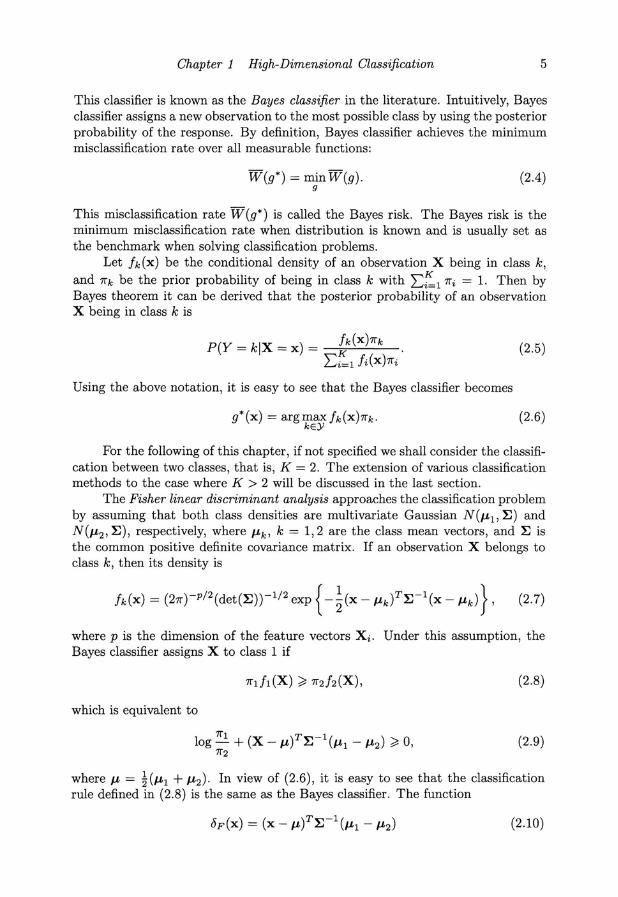
Figure 2.1 Illustration of distance-based classification. The centroid of each subsample in the training data is first computed by taking the sample mean or median. Then, for a future observation, indicated by query, it is classified according to its distances to the centroids.

The Fisher discriminant rule can be regarded as a specific method of distancebased classifiers, which have attracted much attention of researchers. Popularly used distance-based classifiers include support vector machine, naive Bayes classifier, and k- th-nearest-neighbor classifier. The distance-based classifier assigns a new observation X to class k if it is on average closer to the data in class k than to the data in any other classes. The "distance" and "average" are interpreted differently in different methods. Two widely used measures for distance are the Euclidean distance and the Mahalanobis distance. Assume that the center of class i distribution is J.£i and the common convariance matrix is :E. Here "center" could be the mean or the median of a distribution. We use dist(x, J.£i) to denote the distance of a feature vector x to the centriod of class i. Then if the Euclidean distance is used,

(2.16)

and the Mahalanobis distance between a feature vector x and class i is

(2.17)


Thus the distance-based classifier places a new observation X to class k if

argmindist(X, ILi) = k. iEY

Figure 2.1 illustrates the idea of distanced classifier classification.

(2.18)

When 7r1 = 7r2 = 1/2, the above defined Fisher discriminant analysis has the interpretation of distance-based classifier. To understand this, note that (2.9) is equivalent to

(2.19)

Thus DF assigns X to class 1 if its Mahalanobis distance to the center of class 1 is smaller than its Mahalanobis distance to the center of class 2. We will introduce in more details about distance-based classifiers in Section 4.

3 Impact of dimensionality on classification

A common feature of many contemporary classification problems is that the dimensionality p of the feature vector is much larger than the available training sample size n. Moreover, in most cases, only a fraction of these p features are important in classification. While the classical methods introduced in Section 2 are extremely useful, they no longer perform well or even break down in high dimensional setting. See Donoho (2000) and Fan and Li (2006) for challenges in high dimensional statistical inference. The impact of dimensionality is well understood for regression problems, but not as well understood for classification problems. In this section, we discuss the impact of high dimensionality on classification when the dimension p diverges with the sample size n. For illustration, we will consider discrimination between two Gaussian classes, and use the Fisher discriminant analysis and independence classification rule as examples. We assume in this section that 7r1 = 7r2 = ~ and n1 and n2 are comparable.

3.1 Fisher discriminant analysis in high dimensions

Bickel and Levina (2004) theoretically studied the asymptotical performance of the sample version of Fisher discriminant analysis defined in (2.10), when both the dimensionality p and sample size n goes to infinity with p much larger than n. The parameter space considered in their paper is

where c, C1 and C2 are positive constants, Amin(I::) and Amax(I::) are the minimum and maximum eigenvalues of I::, respectively, and B = Ba,d = {u : 2:;:1 ajuJ < d2 } with d some constant, and aj --t 00 as j --t 00. Here, the mean vectors ILk, k = 1,2 are viewed as points in l2 by adding zeros at the end. The condition on

eigenvalues ensures that Amaxt~? ~ ~ < 00, and thus both I:: and I::-1 are not Amm 1

ill-conditioned. The condition d2 (0) )! c2 is to make sure that the Mahalanobis

Chapter 1 High- Dimensional Classification 9

distance between two classes is at least c. Thus the smaller the value of c, the harder the classification problem is.

Given independent training data (Xi, Yi), i = 1, ... , n, the common covariance matrix can be estimated by using the sample covariance matrix

K

is = L L (Xi - fik)(X i - fik)T I(n - K). (3.2) k=l Yi=k

For the mean vectors, Bickel and Levina (2004) showed that there exist estimators Mk of J-Lk, k = 1,2 such that

(3.3)

Replacing the population parameters in the definition of 6F by the above estimators Mk and is, we obtain the sample version of Fisher discriminant function 8F .

It is well known that for fixed p, the worst case misclassification rate of 8 F

converges to the worst case Bayes risk over r 1, that is,

(3.4)

where <I?(t) = 1- <I>(t) is the tail probability of the standard Gaussian distribution. Hence, 8F is asymptotically optimal for this low dimensional problem. However, in high dimensional setting, the result is very different.

Bickel and Levina (2004) studied the worst case misclassification rate of 8F

when nl = n2 in high dimensional setting. Specifically they showed that under some regularity conditions, if pin ---4 00, then

(3.5)

where the Moore-Penrose generalized inverse is used in the definition of 8F . Note that 1/2 is the misclassification rate of random guessing. Thus although Fisher discriminant analysis is asymptotically optimal and has Bayes risk when dimension p is fixed and sample size n ---4 00, it performs asymptotically no better than random guessing when the dimensionality p is much larger than the sample size n. This shows the difficulty of high dimensional classification. As have been demonstrated by Bickel and Levina (2004) and pointed out by Fan and Fan (2008), the bad performance of Fisher discriminant analysis is due to the diverging spectra (e.g., the condition number goes to infinity as dimensionality diverges) frequently encountered in the estimation of high-dimensional covariance matrices. In fact, even if the true covariance matrix is not ill conditioned, the singularity of the sample covariance matrix will make the Fisher discrimination rule inapplicable when the dimensionality is larger than the sample size.

3.2 Impact of dimensionality on independence rule

Fan and Fan (2008) studied the impact of high dimensionality on classification. They pointed out that the difficulty of high dimensional classification is intrinsically caused by the existence of many noise features that do not contribute to the


reduction of classification error. For example, for the Fisher discriminant analysis discussed before, one needs to estimate the class mean vectors and covariance matrix. Although individually each parameter can be estimated accurately, aggregated estimation error over many features can be very large and this could significantly increase the misclassification rate. This is another important reason that causes the bad performance of Fisher discriminant analysis in high dimensional setting. Greenshtein and Ritov (2004) and Greenshtein (2006) introduced and studied the concept of persistence, which places more emphasis on misclassification rates or expected loss rather than the accuracy of estimated parameters. In high dimensional classification, since we care much more about the misclassification rate instead of the accuracy of the estimated parameters, estimating the full covariance matrix and the class mean vectors will result in very high accumulation error and thus low classification accuracy.

To formally demonstrate the impact of high dimensionality on classification, Fan and Fan (2008) theoretically studied the independence rule. The discriminant function of independence rule is

(3.6)

where D = diag{:E}. It assigns a new observation X to class 1 if 6I(X) ?: O. Compared to the Fisher discriminant function, the independence rule pretends that features were independent and use the diagonal matrix D instead of the full covariance matrix :E to scale the feature. Thus the aforementioned problems of diverging spectrum and singularity are avoided. Moreover, since there are far less parameters need to be estimated when implementing the independence rule, the error accumulation problem is much less serious when compared to the Fisher discriminant function.

Using the sample mean ilk = ,L l::Yi=k Xi, k = 1,2 and sample covariance

matrix is as estimators and letting jj = diag{iS}, we obtain the sample version of independence rule

(3.7)

Fan and Fan (2008) studied the theoretical performance of J1(x) in high dimensional setting.

Let R = D- l / 2:ED- l / 2 be the common correlation matrix and Amax(R) be its largest eigenvalue, and write a == (al," ., ap)T = 1-£1 - 1-£2' Fan and Fan (2008) considered the parameter space

where Cp is a deterministic positive sequence depending only on the dimensionality p, bo is a positive constant, and a} is the j-th diagonal element of :E. The condition aT Da ?: Cp is similar to the condition d(O) ?: c in Bickel and Levina (2004). In fact, a'D-la is the accumulated marginal signal strength of p individual features, and the condition a'D-la ?: Cp imposes a lower bound on it. Since there is no


restriction on the smallest eigenvalue, the condition number of R can diverge with sample size. The last condition minl~j~p a} > 0 ensures that there are no deterministic features that make classification trivial and the diagonal matrix D is always invertible. It is easy to see that f2 covers a large family of classification problems.

To access the impact of dimensionality, Fan and Fan (2008) studied the posterior misclassification rate and the worst case posterior misclassification rate of SI over the parameter space f 2 . Let X be a new observation from class 1. Define the posterior misclassification rate and the worst case posterior misclassification rate respectively as

W(SI,O) = P(SI(X) < O!(Xi , Yi), i = 1, ... , n),

Wr2 (SI) = max W(SI'O). OEr 2

(3.9)

(3.10)

Fan and Fan (2008) showed that when logp = o(n), n = o(p) and nCp -+ 00, the following inequality holds

This inequality gives an upper bound on the classification error. Since ¥(.) decreases with its argument, the right hand side decreases with the fraction inside ¥. The second term in the numerator of the fraction shows the influence of sample size on classification error. When there are more training data from class 1 than those from class 2, i.e., nl > n2, the fraction tends to be larger and thus the upper bound is smaller. This is in line with our common sense, as if there are more training data from class 1, then it is less likely that we misclassify X to class 2.

Fan and Fan (2008) further showed that if yinln2/(np)Cp -+ Co with Co some positive constant, then the worst case posterior classification error

A P -( Co ) Wr2 (6I) --+q? 2v'bo" . (3.12)

We make some remarks on the above result (3.12). First of all, the impact of dimensionality is shown as Cp / yip in the definition of Co. As dimensionality p increases, so does the aggregated signal Cp , but a price of the factor yip needs to be paid for using more features. Since nl and n2 are assumed to be comparable, nlnz!(np) = O(n/p). Thus one can see that asymptotically W r2 (SI) increases with yin/pCp' Note that yin/pCp measures the tradeoff between dimensionality p and the overall signal strength Cp . When the signal level is not strong enough

to balance out the increase of dimensionality, i.e., yin/pCp -+ 0 as n -+ 00, then

Wr2 (S I) ~ ~. This indicates that the independence rule S I would be no better than the random guessing due to noise accumulation, and using less features can be beneficial.

The inequality (3.11) is very useful. Observe that if we only include the first m features j = 1, ... , m in the independence rule, then (3.11) still holds with each


term replaced by its truncated version and p replaced by m. The contribution of the j feature is governed by its marginal utility a; I a} . Let us assume that the importance of the features is already ranked in the descending order of {a; I an. Then m-1 2:7=1 a;la; will most possibly first increase and then decrease as we include more and more features, and thus the right hand side of (3.11) first decreases and then increases with m. Minimizing the upper bound in (3.11) can help us to find the optimal number of features m .

3

2.5

2

1.5

0.5

o 1 -L

-0.5

-1

-1.5

-2 o

I ~ 1 I j I I II , I' I

I I I "

,

500 1000 1500 2000 2500 3000 3500 4000 4500

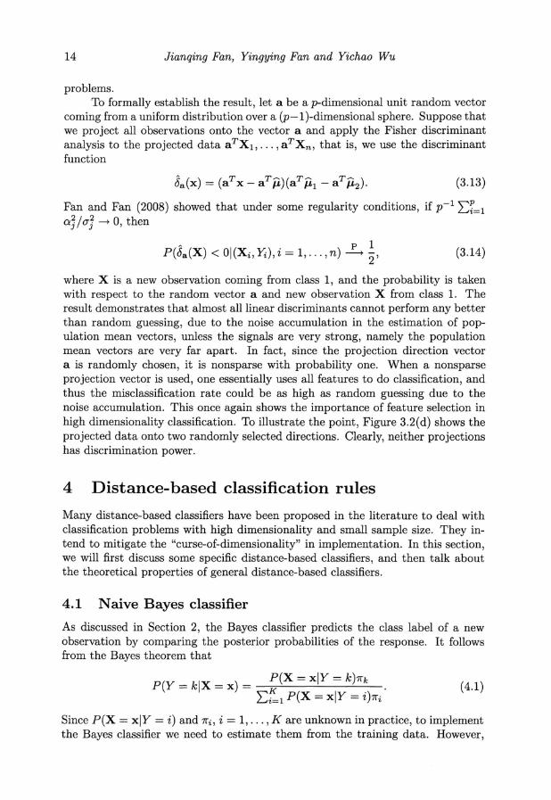
Figure 3.1 The centroid ILl of class 1. The heights indicate the values of non-vanishing elements.

To illustrate the impact of dimensionality, let us take p = 4500, ~ the identity matrix, and IL2 = 0 whereas ILl has 98% of coordinates zero and 2% non-zero, generated from the double exponential distribution. Figure 3.1 illustrates the vector ILl' in which the heights show the values of non-vanishing coordinates. Clearly, only about 2% of features have some discrimination power. The effective number of features that have reasonable discrimination power (excluding those with small values) is much smaller. If the best two features are used, it clearly has discrimination power, as shown in Figure 3.2(a), whereas when all 4500 features are used, they have little discrimination power (see Figure 3.2(d)) due to noise accumulation. When m = 100 (about 90 features are useful and 10 useless: the actual useful signals are less than 90 as many of them are weak) the signals are strong enough to overwhelm the noise accumulation, where as when m = 500 (at least 410 features are useless), the noise accumulation exceeds the strength of the signals so that there is no discrimination power.


(a) m=2 (b) m~1 00

4 10

2 5

0

0 - 2

- 4 5 0 5 lO -5 0

(c) m=SOO (d) m"04500

10 4

5 ,f 2 4-

0 +

-s + -2 +

- 10 -4 4 =1 0 0 10 20 -4 - 2 0 2

Figure 3.2 The plot of simulated data with "*" indicated the first class and "+" the second class. The best m features are selected and the first two principal components are computed based on the sample covariance matrix. The data are then projected onto these two principal components and are shown in (a), (b) and (c). In (d), the data are projected on two randomly selected directions in the 4500-dimensional space.

3.3 Linear discriminants in high dimensions

From discussions in the previous two subsections, we see that in high dimensional setting, the performance of classifiers is very different from their performance when dimension is fixed. As we have mentioned earlier, the bad performance is largely caused by the error accumulation when estimating too many noise features with little marginal utility oJ / a}. Thus dimension reduction and feature selection are very important in high dimensional classification.

A popular class of dimension reduction methods is projection. See, for example, principal component analysis in Ghosh (2002), Zou et al. (2004), and Bair et al. (2006); partial least squares in Nguyen and Rocke (2002), Huang and Pan (2003), and Boulesteix (2004); and sliced inverse regression in Li (1991), Zhu et al. (2006), and Bura and Pfeiffer (2003). As pointed out by Fan and Fan (2008), these projection methods attempt to find directions that can result in small classification errors. In fact, the directions found by these methods put much more weight on features that have large classification power. In general, however, linear projection methods are likely to perform poorly unless the projection vector is sparse, namely, the effective number of selected features is small. This is due to the aforementioned noise accumulation prominently featured in high-dimensional


problems. To formally establish the result, let a be a p-dimensional unit random vector

coming from a uniform distribution over a (p-1 )-dimensional sphere. Suppose that we project all observations onto the vector a and apply the Fisher discriminant analysis to the projected data aTX1 , ... ,aTXn , that is, we use the discriminant function

(3.13)

Fan and Fan (2008) showed that under some regularity conditions, if p-l L:f=l oj / a} ---> 0, then

- . P 1 P(ba(X) < OI(Xi , Yi), z = 1, ... , n) ----+ 2' (3.14)

where X is a new observation coming from class 1, and the probability is taken with respect to the random vector a and new observation X from class 1. The result demonstrates that almost all linear discriminants cannot perform any better than random guessing, due to the noise accumulation in the estimation of population mean vectors, unless the signals are very strong, namely the population mean vectors are very far apart. In fact, since the projection direction vector a is randomly chosen, it is nonsparse with probability one. When a nonsparse projection vector is used, one essentially uses all features to do classification, and thus the misclassification rate could be as high as random guessing due to the noise accumulation. This once again shows the importance of feature selection in high dimensionality classification. To illustrate the point, Figure 3.2(d) shows the projected data onto two randomly selected directions. Clearly, neither projections has discrimination power.

4 Distance-based classification rules

Many distance-based classifiers have been proposed in the literature to deal with classification problems with high dimensionality and small sample size. They intend to mitigate the "curse-of-dimensionality" in implementation. In this section, we will first discuss some specific distance-based classifiers, and then talk about the theoretical properties of general distance-based classifiers.

4.1 Naive Bayes classifier

As discussed in Section 2, the Bayes classifier predicts the class label of a new observation by comparing the posterior probabilities of the response. It follows from the Bayes theorem that

P(Y = klX = x) = P(X = xlY = k)7rk L:~l P(X = xlY = i)7ri

( 4.1)

Since P(X = xlY = i) and 7ri, i = 1, ... , K are unknown in practice, to implement the Bayes classifier we need to estimate them from the training data. However,


this method is impractical in high dimensional setting due to the curse of dimensionality and noise accumulation when estimating the distribution P(XIY), as discussed in Section 3. The naive Bayes classifier, on the other hand, overcomes this difficulty by making a conditional independence assumption that dramatically reduces the number of parameters to be estimated when modeling P(XIY). More specifically, the naive Bayes classifier uses the following calculation:

p

P(X = xlY = k) = II P(Xj = xjlY = k), (4.2) j=l

where Xj and Xj are the j-th components of X and x, respectively. Thus the conditional joint distribution of the p features depends only on the marginal distributions of them. So the naive Bayes rule utilizes the marginal information of features to do classification, which mitigates the "curse-of-dimensionality" in implementation. But, the dimensionality does have an impact on the performance of the classifier, as shown in the previous section. Combining (2.6), (4.1) and (4.2) we obtain that the predicted class label by naive Bayes classifier for a new observation is

p

g(x) = argmax1Tk II P(Xj = xjlY = k). kEY j=l

(4.3)

In the case of classification between two normal distributions N(J.L1'~) and N(J.Lz'~) with 1T1 = 1TZ = ~, it can be derived that the naive Bayes classifier has the discriminant function

( 4.4)

where D = diag(~), the same as the independence rule (3.7), which assigns a new observation X to class 1 if bJ(X) ~ 0; otherwise to class 2. It is easy to see that bJ(x) is a distance-based classifier with distance measure chosen to be the weighted Lz-distance: distJ (x, J.Li) = (x - J.Li) T D-1 (x - J.Li)'

Although in deriving the naive Bayes classifier, it is assumed that the features are conditionally independent, in practice it is widely used even when this assumption is violated. In other words, the naive Bayes classifier pretends that the features were conditionally independent with each other even if they are actually not. For this reason, the naive Bayes classifier is also called independence rule in the literature. In this chapter, we will interchangeably use the name "naive Bayes classifier" and "independence rule" .

As pointed out by Bickel and Levina (2004), even when J.L and ~ are assumed known, the corresponding independence rule does not lose much in terms of classification power when compared to the Bayes rule defined in (2.10). To understand this, Bickel and Levina (2004) consider the errors of Bayes rule and independence rule, which can be derived to be

e1 = P(bB(X) (0) = <$ (~{o?~-la}l/Z) and

ez = P(bJ(X) ( 0) = <$ (~{ aT D~:~~l_~aP/z) ,


respectively. Since the errors ek, k = 1,2 are both decreasing functions of the arguments of <1>, the efficiency of the independence rule relative to the Bayes rule is determined by the ratio r of the arguments of <1>. Bickel and Levina (2004) showed that the ratio r can be bounded as

a.T D-1a 2$0

{(aT:E-1a)(aT D-1:ED-1a)} 1/2 ~ 1 + Ko' (4.5)

where Ko = maXr AmaxCR) with R the common correlation matrix defined in 1 Am;nCR)

Section 3.2. Thus the error e2 of the independence rule can be bounded as

(4.6)

It can be seen that for moderate K o, the performance of independence rule is comparable to that of the Fisher discriminant analysis. Note that the bounds in (4.6) represents the worst case performance. The actual performance of independence rule could be better. In fact, in practice when a and :E both need to be estimated, the performance of independence rule is much better than that of the Fisher discriminant analysis.

We use the same notation as that in Section 3, that is, we use 5F to denote the sample version of Fisher discriminant function, and use 51 to denote the sample version of the independence rule. Bickel and Levina (2004) theoretically compared the asymptotical performance of 5 F and 51. The asymptotic performance of Fisher discriminant analysis is given in (3.5). As for the independence rule, under some regularity conditions, Bickel and Levina (2004) showed that if logp/n ~ 0, then

(4.7)

where f1 is the parameter set defined in Section 3.1. Recall that (3.5) shows that the Fisher discriminant analysis asymptotically performs no better than random guessing when the dimensionality p is much larger than the sample size n. While the above result (4.7) demonstrates that for the independence rule, the worst case classification error is better than that of the random guessing, as long as the dimensionality p does not grow exponentially faster than the sample size nand Ko < 00. This shows the advantage of independence rule in high dimensional classification. Note that the impact of dimensionality can not be seen in (4.7) whereas it can be seen from (3.12). This is due to the difference of f2 from fl.

On the practical side, Dudoit et al. (2002) compared the performance of various classification methods, including the Fisher discriminant analysis and the independence rule, for the classification of tumors based on gene expression data. Their results show that the independence rule outperforms the Fisher discriminant analysis.

Bickel and Levina (2004) also introduced a spectrum of classification rules which interpolate between 5F and 51 under the Gaussian coloured noise model assumption. They showed that the minimax regret of their classifier has asymptotic


rate O(n- K logn) with /'i, some positive number defined in their paper. See Bickel and Levina (2004) for more details.

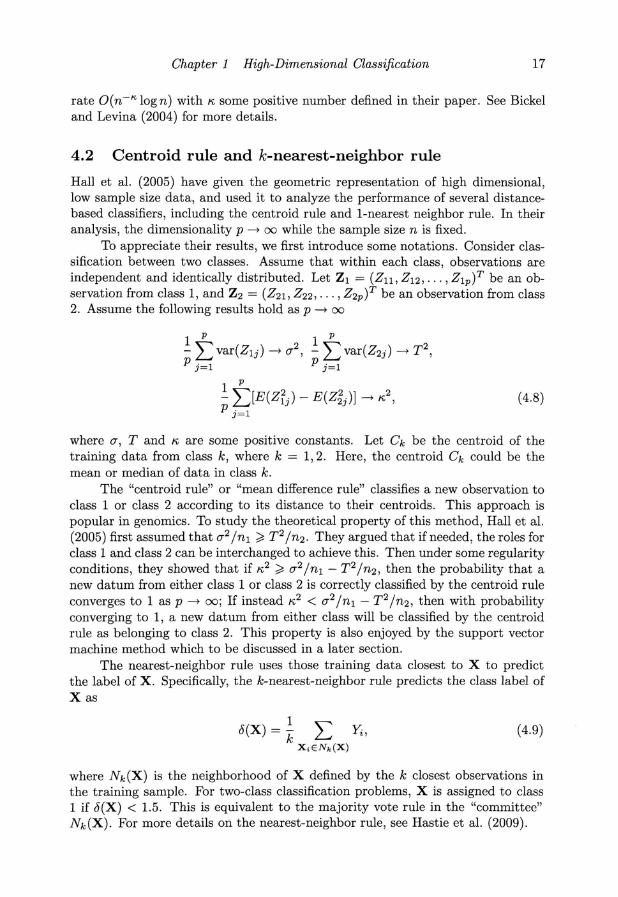
4.2 Centroid rule and k-nearest-neighbor rule

Hall et al. (2005) have given the geometric representation of high dimensional, low sample size data, and used it to analyze the performance of several distancebased classifiers, including the centroid rule and I-nearest neighbor rule. In their analysis, the dimensionality p ----t 00 while the sample size n is fixed.

To appreciate their results, we first introduce some notations. Consider classification between two classes. Assume that within each class, observations are independent and identically distributed. Let Zl = (Zll' Z12," ., Zlp)T be an observation from class 1, and Z2 = (Z2l' Z22,"" Z2p)T be an observation from class 2. Assume the following results hold as p ----t 00

(4.8)

where (J', T and /'i, are some positive constants. Let Ck be the centroid of the training data from class k, where k = 1,2. Here, the centroid Ck could be the mean or median of data in class k.

The "centroid rule" or "mean difference rule" classifies a new observation to class 1 or class 2 according to its distance to their centroids. This approach is popular in genomics. To study the theoretical property of this method, Hall et al. (2005) first assumed that (J'2 I nl ~ T2 I n2. They argued that if needed, the roles for class 1 and class 2 can be interchanged to achieve this. Then under some regularity conditions, they showed that if /'i,2 ~ (J'2/nl - T2/n2, then the probability that a new datum from either class 1 or class 2 is correctly classified by the centroid rule converges to 1 as p ----t 00; If instead /'i,2 < (J'2/nl - T2/n2, then with probability converging to 1, a new datum from either class will be classified by the centroid rule as belonging to class 2. This property is also enjoyed by the support vector machine method which to be discussed in a later section.

The nearest-neighbor rule uses those training data closest to X to predict the label of X. Specifically, the k-nearest-neighbor rule predicts the class label of X as

8(X) = ~ 2:: Yi, (4.9) X;ENk(X)

where Nk(X) is the neighborhood of X defined by the k closest observations in the training sample. For two-class classification problems, X is assigned to class 1 if 8(X) < 1.5. This is equivalent to the majority vote rule in the "committee" Nk(X), For more details on the nearest-neighbor rule, see Hastie et al. (2009).


Hall et al. (2005) also considered the I-nearest-neighbor rule. They first assumed that 0'2 ;? T2. The same as before, the roles of class 1 and class 2 can be interchanged to achieve this. They showed that if ",2 > 0'2 - T2, then the probability that a new datum from either class 1 or class 2 is correctly classified by the I-nearest-neighbor rule converges to 1 as p --+ 00; if instead ",2 < 0'2 - T2, then with probability converging to 1, a new datum from either class will be classified by the 1-nearest-neighbor rule as belonging to class 2.

Hall et al. (2005) further discussed the contrasts between the centroid rule and the I-nearest-neighbor rule. For simplicity, they assumed that nl = n2. They pointed out that asymptotically, the centroid rule misclassifies data from at least one of the classes only when ",2 < 10'2 - T 21/nl, whereas the I-nearest-neighbor rule leads to misclassification for data from at least one of the classes both in the range ",2 < 10'2 - T21/nl and when 10'2 - T21/nl :( ",2 < 10'2 - T21. This quantifies the inefficiency that might be expected from basing inference only on a single nearest neighbor. For the choice of k in the nearest neighbor, see Hall, Park and Samworth (2008).

For the properties of both classifiers discussed in this subsection, it can be seen that their performances are greatly determined by the value of ",2. However, in view of (4.8), ",2 could be very small or even 0 in high dimensional setting due the the existence of many noise features that have very little or no classification power (i.e. those with EZrj ~ EZ?j)' This once again shows the difficulty of classification in high dimensional setting.

4.3 Theoretical properties of distance-based classifiers

Hall, Pittelkow and Ghosh (2008) suggested an approach to accessing the theoretical performance of general distance-based classifiers. This technique is related to the concept of "detection boundary" developed by Ingster and Donoho and Jin. See, for example, Donoho and Jin (2004); Hall and Jin (2008). Ingster (2002); and Jin (2006); Hall, Pittelkow and Ghosh (2008) studied the theoretical performance of a variety distance-based classifiers constructed from high dimensional data, and obtain the classification boundaries for them. We discuss their study in this subsection.

Let gO = g(-I(Xi,Yi),i = I, ... ,n) be a distanced-based classifier which assigns a new observation X to either class 1 or class 2. Hall, Pittelkow and Ghosh (2008) argued that any plausible, distance-based classifier 9 should enjoy the following two properties:

(a) 9 assigns X to class 1 if it is closer to each of the X~s in class 1 than it is to any of the Xjs in class 2;

(b) If 9 assigns X to class 1 then at least one of the X~s in class 1 is closer to X than X is closer to the most distant Xjs in class 2.

These two properties together imply that

(4.10)

where Pk denotes the probability measure when assuming that X is from class k


with k = 1,2, and 7rkl and 7rk2 are defined as

7rkl = Pk (max IIXi - XII ~ min IIXj - XII) and 'Eg, ]Eg2

(4 .11)

7rk2 = Pk (min IIXi - XII ~ max IIXj - XII) 'Eg, ]Eg2

(4.12)

with ~h = {i : 1 ~ i ~ n, Vi = I} and 92 = {i : 1 ~ i ~ n , Vi = 2}. Hall, Pittelkow and Ghosh (2008) considered a family of distance-based classifiers satisfying condition (4.10).

To study the theoretical property of these distance-based classifiers, Hall, Pittelkow and Ghosh (2008) considered the following model

Xij = ILkj + Eij, for i E 9k , k = 1,2, (4.13)

where Xij denotes the j-th component of Xi, ILkj represents the j-th component of mean vector I-£k> and Ei/S are independent and identically distributed with mean 0 and finite fourth moment. Without loss of generality, they assumed that the class 1 population mean vector 1-£1 = O. Under this model assumption, they showed that if some mild conditions are satisfied, 7rkl --> 0 and 7rk2 --> 0 if and only if p = 0(111-£2114). Then using inequality (4.10), they obtained that the probability of the classifier 9 correctly classifying a new observation from class 1 or class 2 converges to 1 if and only if p = 0(111-£2114) as p --> 00. This result tells us just how fast the norm of the two class mean difference vector 1-£2 must grow for it to be possible to distinguish perfectly the two classes using the distance-based classifier. Note that the above result is independent of the sample size n. The result is consistent with (a specific case of) (3.12) for independent rule in which Cp = 111-£211 2 in the current setting and misclassification rate goes to zero when the signal is so strong that C;/p --> 00 (if n is fixed) or 111-£211 4/p --> 00. The impact of dimensionality is implied by the quantity 111-£211 2/ yiP.

It is well known that the thresholding methods can improve the sensitivity of distance-based classifiers. The thresholding in this setting is a feature selection method, using only features with distant away from the other. Denote by XfJ = XijI(Xij > t) the thresholded data, i = 1, ... , n , j = 1, ... ,p , with t the thresholding level. Let Xr' = (X;I) be the thresholded vector and gtr be the version of the classifier g based on thresholded data. The case where the absolute values IXij I are thresholded is very similar. Hall, Pittelkow and Ghosh (2008) studied the properties of the threshold-based classifier IT. For simplicity, they assumed that IL2j = v for q distinct indices j , and IL2j = 0 for the remaining p - q indices, where

(a) v ~ t, (b) t = t(p) --> 00 as p increases, (c) q = q(p) satisfies q --> 00 and 1 ~ q ~ cp with 0 < c < 1 fixed, and (d) the errors Eij has a distribution that is unbounded to the right.

With the above assumptions and some regularity conditions, they proved that the general thresholded distance-based classifier lr has a property that is analogue to the standard distance-based classifier, that is, the probability that the classifier


gtT correctly classifies a new observation from class 1 or class 2 tending to 1 if and only if p = o(T) as p ~ 00, where T = (qv2)2 / E[EtjI(Eij > t)]. Compared to the property of standard distance-based classifier, the thresholded classifier allows for higher dimensionality if E[EtjI(Eij > t)] ~ 0 as p ~ 00.

Hall, Pittelkow and Ghosh (2008) further compared the theoretical performance of standard distanced-based classifiers and thresholded distance-based classifiers by using the classification boundaries. To obtain the explicit form of classification boundaries, they assumed that for j-th feature, the class 1 distribution is GN,(O, 1) and the class 2 distribution is GN,(/-L2j, 1), respectively. Here GN,(/-L, 0"2) denotes the Subbotin, or generalized normal distribution with probability density

(4.14)

where ,,(,0" > 0 and C, is some normalization constant depending only on "(. It is easy to see that the standard normal distribution is just the standard Subbotin distribution with "( = 2. By assuming that q = O(pl-{3), t = brlogp)lh, and v = bs logp)lh with ~ < (3 < 1 and 0 < r < s ~ 1, they derived that the sufficient and necessary conditions for the classifiers g and IT to produce asymptotically correct classification results are

1 - 2(3 > 0 and

1 - 2(3 + s > 0,

(4.15)

(4.16)

respectively. Thus the classification boundary of gtT is lower than that of g, indicating that the distance-based classifier using truncated data are more sensible.

The classification boundaries for distance-based classifiers and for their thresholded versions are both independent of the training sample size. As pointed out by Hall, Pittelkow and Ghosh (2008), this conclusion is obtained from the fact that for fixed sample size n and for distance-based classifiers, the probability of correct classification converges to 1 if and only if the differences between distances among data have a certain extremal property, and that this property holds for one difference if and only if it holds for all of them. Hall, Pittelkow and Ghosh (2008) further compared the classification boundary of distance-based classifiers with that of the classifiers based on higher criticism. See their paper for more comparison results.

5 Feature selection by independence rule

As has been discussed in Section 3, classification methods using all features do not necessarily perform well due to the noise accumulation when estimating a large number of noise features. Thus, feature selection is very important in high dimensional classification. This has been advocated by Fan and Fan (2008) and many other researchers. In fact, the thresholding methods discussed in Hall, Pittelkow and Ghosh (2008) are also a type of feature selection.


5.1 Features annealed independence rule

Fan and Fan (2008) proposed the Features Annealed Independence Rule (FAIR) for feature selection and classification in high dimensional setting. We discuss their method in this subsection.

There is a huge literature on the feature selection in high dimensional setting. See, for example, Efron et al. (2004); Fan and Li (2001); Fan and Lv (2008, 2009); Fan et al. (2008); Lv and Fan (2009); Tibshirani (1996). Two sample t tests are frequently used to select important features in classification problems. Let X kj = L,Yi=k Xijlnk and S~j = L,Yi=k(Xkj - Xkj)2 I(nk -1) be the sample mean and sample variance of j-th feature in class k, respectively, where k = 1,2 and j = 1, ... ,p. Then the two-sample t statistic for feature j is defined as

(5.1)

Fan and Fan (2008) studied the feature selection property of two-sample t statistic. They considered the model (3.14) and assumed that the error Cij satisfies the Cramer's condition and that the population mean difference vector JL = JLl - JL2 = (/ll, ... , /lp) T is sparse with only the first s entries nonzero. Here, s is allowed to diverge to 00 with the sample size n. They showed that if

log(p - s) = o(nl'), logs = o(n!-f3n), and minl';:;Ks ~ = o(n-I'!3n) with 0"1j+a2j

some !3n ---+ 00 and I E (0,1), then with x chosen in the order of O(nl'/2), the following result holds:

P(minlTjl > x,maxlTjl < x) ---+ 1. J';:;S J>S

(5.2)

This result allows the lowest signal level minl';:;j';:;s ~ to decay with sample (J Ij +0' 2j

size n. As long as the rate of decay is not too fast and the dimensionality p does not grow exponentially faster than n, the two-sample t-test can select all important features with probability tending to 1.

Although the theoretical result (5.2) shows that the t-test can successfully select features if the threshold is appropriately chosen, in practice it is usually very hard to choose a good threshold value. Moreover, even all revelent features are correctly selected by the two-sample t test, it may not necessarily be the best to use all of them, due to the possible existence of many faint features. Therefore, it is necessary to further single out the most important ones. To address this issue, Fan and Fan (2008) proposed the features annealed independence rule. Instead of constructing independence rule using all features, FAIR selects the most important ones and use them to construct independence rule. To appreciate the idea of FAIR, first note that the relative importance of features can be measured by the ranking of {Iaj II OJ}. If such oracle ranking information is available, then one can construct the independence rule using m features with the largest {lajI/O"j}. The optimal


value of m is to be determined. In this case, FAIR takes the following form:

p

o(x) = I>:l!j(Xj - J.Lj)/O'Jl{ !aj!/aj>b}, (5.3) j=l

where b is a positive constant chosen in a way such that there are m features with laj l/O'j > b. Thus choosing the optimal m is equivalent to selecting the optimal b. Since in practice such oracle information is unavailable, we need to learn it from the data. Observe that lajl/O'j can be estimated by 100jl/o-j. Thus the sample version of FAIR is

p

J(x) = L O:j(Xj - j),j)/o-Jl{ !aj!/&j>b} ' j=l

(5 .4)

In the case where the two population covariance matrices are the same, we have

Thus the sample version of the discriminant function of FAIR can be rewritten as

p

JFAIR(X) = LOj(Xj - j),j)/o-Jl{y'n/(nln2) !Tj !>b}' j=l

(5.5)

It is clear from (5.5) that FAIR works the same way as that we first sort the features by the absolute values of their t-statistics in the descending order, and then take out the first m features to construct the classifier. The number of features m can be selected by minimizing the upper bound of the classification error given in (3.11). To understand this, note that the upper bound on the right hand side of (3.11) is a function of the number of features. If the features are sorted in the descending order of lajl/O'j, then this upper bound will first increase and then decrease as we include more and more features. The optimal m in the sense of minimizing the upper bound takes the form

1 [2::;:1 a;/O'J + m(1/n2 - 1/ndl2 mopt = arg max -- /() ~m 2/ 2

l~m~p >'~ax nm n1 n2 + 6j=1 a j O'j

where >'~ax is the largest eigenvalue of the correlation matrix R m of the truncated observations. It can be estimated from the training data as

Note that the above t-statistics are the sorted ones. Fan and Fan (2008) used simulation study and real data analysis to demonstrate the performance of FAIR. See their paper for the numerical results .


5.2 Nearest shrunken centroids method

In this section, we will discuss the nearest shrunken centroids (NSC) method proposed by Tibshirani et al. (2002). This method is used to identify a subset of features that best characterize each class and do classification. Compared to the centroid rule discussed in Section 3.2, it takes into account the feature selection. Moreover, it is general and can be applied to high-dimensional multi-class classification.

Define X kj = L:iEQk Xij Ink as the j-th component of the centroid for class k, and Xj = L:~1 Xij In as the j-th component of the overall centroid. The basic idea of NSC is to shrink the class centroids to the overall centroid. Tibshirani et al. (2002) first normalized the centroids by the within class standard deviation for each feature, i.e.,

(5.7)

where So is a positive constant, and Sj is the pooled within class standard deviation for j-th feature with

and mk = y'l/nk - lin the normalization constant. As pointed out by Tibshirani et al. (2002), dkj defined in (5.7) is a t-statistic for feature j comparing the k-th class to the average. The constant So is included to guard against the possibility of large dkj simply caused by very small value of Sj. Then (5.7) can be rewritten as

(5.8)

Tibshirani et al. (2002) proposed to shrink each dkj toward zero by using soft thresholding. More specifically, they define

(5.9)

where sgn(·) is the sign function, and t+ = t if t > 0 and t+ = 0 otherwise. This yields the new shrunken centroids

(5.10)

As argued in their paper, since many of Xkj are noisy and close to the overall mean X j , using soft thresholding produces more reliable estimates of the true means. If the shrinkage level D. is large enough, many of the dkj will be shrunken to zero and the corresponding shrunken centroid X~j for feature j will be equal to the overall centroid for feature j. Thus these features do not contribute to the nearest centroid computation.


To choose the amount of shrinkage .6., Tibshirani et al. (2002) proposed to use the cross validation method. For example, if lO-fold cross validation is used, then the training data set is randomly split into 10 approximately equal-size subsamples. We first fit the model by using 90% of the training data, and then predict the class labels of the remaining 10% of the training data. This procedure is repeated 10 times for a fixed .6., with each of the 10 sub-samples of the data used as the test sample to calculate the prediction error. The prediction errors on all 10 parts are then added together as the overall prediction error. The optimal .6. is then chosen to be the one that minimizes the overall prediction error.

After obtaining the shrunken centroids, Tibshirani et al. (2002) proposed to classify a new observation X to the class whose shrunken centroid is closest to this new observation. They define the discriminant score for class k as

(5.11)

The first term is the standardized squared distance of X to the k-th shrunken centroid, and the second term is a correction based on the prior probability 7fk.

Then the classification rule is

g(X) = argmin8k(X), k

It is clear that NSC is a type of distance-based classification method.

(5.12)

Compared to FAIR introduced in Section 5.1, NSC shares the same idea of using marginal information of features to do classification. Both methods conduct feature selection by t-statistic. But FAIR selects the number of features by using mathematical formula that is derived to minimize the upper bound of classification error, while NSC obtains the number of features by using cross validation. Practical implementation shows that FAIR is more stable in terms of the number of selected features and classification error. See Fan and Fan (2008).

6 Loss-based classification

Another popular class of classification methods is based on different (marginbased) loss functions. It includes many well known classification methods such as the support vector machine (SVM, Cristianini and Shawe-Taylor, 2000; Vapnik, 1998).

6.1 Support vector machine

As mentioned in Section 2, the zero-one loss is typically used to access the accuracy of a classification rule. Thus, based on the training data, one may ideally minimize ~7=1 Ig(xi)o/-Yi with respect to gO over a function space to obtain an estimated classification rule §(.). However the indicator function is neither convex nor smooth. The corresponding optimization is difficult, if not impossible, to


solve. Alternatively, several convex surrogate loss functions have been proposed to replace the zero-one loss.

For binary classification, we may equivalently code the categorical response Y as either -1 or + 1. The SVM replaces the zero-one loss by the hinge loss H(u) = [1 - ul+, where [ul+ = max{O, u} denotes the positive part of u. Note that the hinge loss is convex. Replacing the zero-one loss with the hinge loss, the SVM minimizes

n

L H(Y;J(X i )) + )"J(f) (6.1) i=l

with respect to f, where the first term quantifies the data fitting, J(f) is some roughness (complexity) penalty of f, and ).. is a tuning parameter balancing the data fit measured by the hinge loss and the roughness of fe) measured by J(f). Denote the minimizer by ie). Then the SVM classification rule is given by g(x) = sign(j(x)). Note that the hinge loss is non-increasing. While minimizing the hinge loss, the SVM encourages positive Y f(X) which corresponds to correct classification.

For linear SVM with f(x) = b + x T /3, the standard SVM uses the 2-norm penalty J(f) = ~ L:~=1 /3;. While in this exposition, we are formulating the SVM in the regularization framework. However it is worthwhile to point out that the SVM was originally introduced by V. Vapnik and his colleagues with the idea of searching for the optimal separating hyperplane. Interested readers may consult Boser, Guyon and Vapnik (1992) and Vapnik (1998) for more details. It was shown by Wahba (1998) that the SVM can be equivalently fit into the regularization framework by solving (6.1) as presented in the previous paragraph. Different from those methods that focus on conditional probabilities P(YIX = x), the SVM targets at estimating the decision boundary {x: P(Y = llX = x) = 1/2} directly.

A general loss function £ (.) is called Fisher consistent if the minimizer of E[£(Yf(X)IX = x)] has the same sign as P(Y = +IIX = x) - 1/2 (Lin, 2004). Fisher consistency is also known as classification-calibration (Bartlett, Jordan, and McAuliffe, 2006) and infinite-sample consistency (Zhang, 2004). It is a desirable property for a loss function.

Lin (2002) showed that the minimizer of E[H(Y f(X)IX = x)l is exactly sign(P(Y = +IIX = x) - 1/2), the decision-theoretically optimal classification rule with the smallest risk, which is also known as the Bayes classification rule. Thus the hinge loss is Fisher consistent for binary classification.

When dealing with problems with many predictor variables, Zhu, Rosset, Hastie, and Tibshirani (2003) proposed the I-norm SVM by using the L1 penalty J(f) = L:~=1 l/3jl to achieve variable selection; Zhang, Ahn, Lin and Park (2006) proposed the SCAD SVM by using the SCAD penalty (Fan and Li, 2001); Liu and Wu (2007) proposed to regularize the SVM with a combination of the Lo and L1 penalties; and many others.

Either basis expansion or kernel mapping (Cristianini and Shawe-Taylor, 2000) may be used to accomplish nonlinear SVM. For the case of kernel learning, a bivariate kernel function K (-, .), which maps from X x X to R, is employed. Then f(x) = b+ L:~=1 K(x, Xi) by the theory of reproducing kernel Hilbert spaces


(RKSH), see Wahba (1990). In this case, the 2-norm of f(x) - b in RKHS with K (', .) is typically used as J (f). Using the representor theorem (Kimeldorf and Wahba, 1971), J(f) can be represented as J(f) = ~ I:~=l I:j=l ciK(Xi,Xj)Cj.

6.2 1j;-learning

The hinge loss H(u) is unbounded and shoots to infinity when t goes to negative infinity. This characteristic makes the SVM tend to be sensitive to noisy training data. When there exist points far away from their own classes (namely, "outliers" in the training data), the SVM classifier tends to be strongly affected by such points due to the unboundedness of the hinge loss. In order to improve over the SVM, Shen, Tseng, Zhang, and Wong (2003) proposed to replace the convex hinge loss by a nonconvex 1,b-loss function. The 1,b-loss function 1,b( u) satisfies

u ~ 1,b(u) > 0 ifu E [O,T]; 1,b(u) = 1 - sign(u) otherwise,

where 0 < U ::::;; 2 and T > 0 are constants. The positive values of 1,b( u) for u E [0, T] eliminate the scaling issue of the sign function and avoid too many points piling around the decision boundary. Their method was named the 1,b-learning. They showed that the 1,b-learning can achieve more accurate class prediction.

Similarly motivated, Wu and Liu (2007a) proposed to truncate the hinge loss function by defining Hs(u) = min(H(s),H(u)) for s ::::;; 0 and worked on the more general multi-category classification. According to their Proposition 1, the truncated hinge loss is also Fisher consistent for binary classification.

6.3 AdaBoost

Boosting is another very successful algorithm for solving binary classification. The basic idea of boosting is to combine weaker learners to improve performance (Freund, 1995; Schapire, 1990). The AdaBoost algorithm, a special boosting algorithm, was first introduced by Freund and Schapire (1996). It constructs a "strong" classifier as a linear combination

T

f(x) = L atht(x) t=l

of "simple", "weak" classifiers ht(x). The "weak" classifiers ht(x)'s can be thought of as features and H(x) = sign(f(x)) is called "strong" or final classifier. It works by sequentially reweighing the training data, applying a classification algorithm (weaker learner) to the reweighed training data, and then taking a weighted majority vote of the thus-obtained classifier sequence. This simple reweighing strategy improves performance of many weaker learners. Freund and Schapire (1996) and Breiman (1997) tried to provide a theoretic understanding based on game theory. Another attempt to investigate its behavior was made by Breiman (1998) using bias and variance tradeoff. Later Friedman, Hastie, and Tibshirani (2000) provided


a new statistical perspective, namely using additively modeling and maximum likelihood, to understand why this seemingly mysterious AdaBoost algorithm works so well. They showed that AdaBoost is equivalent to using the exponential loss £(u) = e-U •

6.4 Other loss functions

There are many other loss functions in this regularization framework. Examples include the squared loss £(u) = (1 - u)2 used in the proximal SVM (Fung and Mangasarian, 2001) and the least square SVM (Suykens and Vandewalle, 1999), the logistic loss £(u) = 10g(1+e-U ) of the logistic regression, and the modified least squared loss £(u) = ([1- ul+)2 proposed by Zhang and Oles (2001). In particular, the logistic loss is motivated by assuming that the probability of Y = + 1 given X = x is given by efex ) /(1 +efex )). Consequently the logistic regression is capable of estimating the conditional probability.

7 Feature selection in loss-based classification

As mentioned above, variable selection-capable penalty functions such as the L1 and SCAD can be applied to the regularization framework to achieve variable selection when dealing with data with many predictor variables. Examples include the L1 SVM (Zhu, Rosset, Hastie, and Tibshirani, 2003), SCAD SVM (Zhang, Ahn, Lin and Park, 2006), SCAD logistic regression (Fan and Peng, 2004). These methods work fine for the case with a fair number of predictor variables. However the remarkable recent development of computing power and other technology has allowed scientists to collect data of unprecedented size and complexity. Examples include data from microarrays, proteomics, functional MRI, SNPs and others. When dealing with such high or ultra-high dimensional data, the usefulness of these methods becomes limited.

In order to handle linear regression with ultra-high dimensional data, Fan and Lv (2008) proposed the sure independence screening (SIS) to reduce the dimensionality from ultra-high p to a fairly high d. It works by ranking predictor variables according to the absolute value of the marginal correlation between the response variable and each individual predictor variable and selecting the top ranked d predictor variables. This screening step is followed by applying a refined method such as the SCAD to these d predictor variables that have been selected. In a fairly general asymptotic framework, this simple but effective correlation learning is shown to have the sure screening property even for the case of exponentially growing dimensionality, that is, the screening retains the true important predictor variables with probability tending to one exponentially fast.

The SIS methodology may break down if a predictor variable is marginally unrelated, but jointly related with the response, or if a predictor variable is jointly uncorrelated with the response but has higher marginal correlation with the response than some important predictors. In the former case, the important feature has already been screened out at the first stage, whereas in the latter case, the unimportant feature is ranked too high by the independent screening technique.

28 Jianging Fan, Yingying Fan and Yichao Wu

Iterative SIS (ISIS) was proposed to overcome these difficulties by using more fully the joint covariate information while retaining computational expedience and stability as in SIS. Basically, ISIS works by iteratively applying SIS to recruit a small number of predictors, computing residuals based on the model fitted using these recruited variables, and then using the working residuals as the response variable to continue recruiting new predictors. Numerical examples in Fan and Lv (2008) have demonstrated the improvement of ISIS. The crucial step is to compute the working residuals, which is easy for the least-squares regression problem but not obvious for other problems. By sidestepping the computation of working residuals, Fan et al. (2008) has extended (I)SIS to a general pseudo-likelihood framework, which includes generalized linear models as a special case. Roughly they use the additional contribution of each predictor variable given the variables that have been recruited to rank and recruit new predictors.

In this section, we will elaborate (I) SIS in the context of binary classification using loss functions presented in the previous section. While presenting the (I)SIS methodology, we use a general loss function £(.). The R-code is publicly available at cran.r-project.org.

7.1 Feature ranking by marginal utilities

By assuming a linear model f(x) = b + xT (3, the corresponding model fitting amounts to minimizing

Q(b, (3) = ~ t £(Yi(b + X[ (3)) + )'J(f) , i=l

where J(f) can be the 2-norm or some other penalties that are capable of variable selection. The marginal utility of the j-th feature is

n

For some loss functions such as the hinge loss, another term ~f3; + ~ I: 13m2 mEMl

may be required to avoid possible identifiability issue. In that case

(7.1)

The idea of SIS is to compute the vector of marginal utilities .e = (£1, £2, ... , £p)T and rank predictor variables according to their corresponding marginal utilities. The smaller the marginal utility is the more important the corresponding predictor variable is. We select d variables corresponding to the d smallest components of .e. Namely, variable j is selected if £j is one of the d smallest components of .e. A typical choice of d is l n/ log n J. Fan and Song (2009) provided an extensive account on the sure screening property of the independence learning and on the capacity of the model size reduction.


7.2 Penalization

With the d variables crudely selected by SIS, parameter estimation and variable selection can be further carried out simultaneously using a more refined penalization method. This step takes joint information into consideration. By reordering the variables if necessary, we may assume without loss of generality that Xl, X 2 ,

... , Xd are the variables that have been recruited by SIS. In the regularization framework, we use a penalty that is capable of variable selection and minimize

(7.2)

where p>.(-) denotes a general penalty function and>' > 0 is a regularization parameter. For example, p>.(-) can be chosen to be the Ll (Tibshirani, 1996), SCAD (Fan and Li, 2001), adaptive Ll (Zhang and Lu, 2007; Zou, 2006), or some other penalty.

7.3 Iterative feature selection

As mentioned before, the SIS methodology may break down if a predictor is marginally unrelated, but jointly related with the response, or if a predictor is jointly uncorrelated with the response but has higher marginal correlation with the response than some important predictors. To handle such difficult scenario, iterative SIS may be required. ISIS seeks to overcome these difficulties by using more fully the joint covariate information.

The first step is to apply SIS to select a set Al of indices of size d, and then employ (7.2) with the L1 or SCAD penalty to select a subset M1 of these indices. This is our initial estimate of the set of indices of important variables.

Next, we compute the conditional marginal utility

(7.3)

for any j E Ml = {I, 2, ... ,p}\M1 , where Xi,Ml is the sub-vector of Xi consisting of those elements in M1. If necessary, the term of ~j3J may be added in (7.3) to avoid identifiability issue just as the case of defining the marginal utilities in (7.1). The conditional marginal utility £)2) measures the additional contribution of variable Xj given that the variables in M 1 have been included. We then rank variables in Ml according to their corresponding conditional marginal utilities and form the set A2 consisting of the indices corresponding to the smallest d - 1M 11 elements.

The above prescreening step using the conditional utility is followed by solv-ing


The penalty p>- (.) leads to a sparse solution. The indices in M1 U A2 that have non-zero /3j yield a new estimate M2 of the active indices.

This process of iteratively recruiting and deleting variables may be repeated until we obtain a set of indices Mk which either reaches the prescribed size d or satisfies convergence criterion Mk = Mk-1.

7.4 Reducing false discovery rate

Sure independence screening is a simple but effective method to screen out irrelevant variables. They are usually conservative and include many unimportant variables. Next we present two possible variants of (I) SIS that have some attractive theoretical properties in terms of reducing the false discovery rate (FDR).

Denote A to be the set of active indices, namely the set containing those indices j for which /3j =I- 0 in the true model. Denote XA = {Xj,j E A} and XAc = {Xj,j E AC} to be the corresponding sets of active and inactive variables respectively.

Assume for simplicity that n is even. We randomly split the sample into two halves. Apply SIS separately to each half with d = L n/ log n J or larger, yielding two estimates )(1) and )(2) of the set of active indices A. Both )(1) and )(2) may have large FDRs because they are constructed by SIS, a crude screening method. Assume that both )(1) and )(2) have the sure screening property, P(A c )(j)) --->

1, for j = 1 and 2. Then

P(A c )(1) n )(2)) ---> l.

Thus motivated, we define our first variant of SIS by estimating A with ) = )(1) n )(2).

To provide some theoretical support, we make the following assumption: Exchangeability Condition: Let r E IN, the set of natural numbers. The model satisfies the exchangeability condition at level r if the set of random vectors

is exchangeable. The Exchangeability Condition ensures that each inactive variable has the

same chance to be recruited by SIS. Then we have the following nonasymptotic probabilistic bound. .

Let r E IN, and assume that the model satisfies the Exchangeability Condition at level r . For) = )(1) n )(2) defined above, we have

where there second inequality requires d2 :::;: p - IAI· When r = 1, the above probabilistic bound implies that, when the number

of selected variables d :::;: n, we have with high probability) reports no 'false


positives' if the exchangeability condition is satisfied at levelland if P is large by comparison with n 2 . It means that it is very likely that any index in the estimated active set also belongs to the active set in the true model, which, together with sure screening assumption, implies the model selection consistency. The nature of this result is somehow unusual in that it suggests that a 'blessing of dimensionality' the probability bound one false positives decreases with p. However, this is only part of the full store, because the probability of missing elements of the true active set is expected to increase with p.

The iterative version of the first variant of SIS can be defined analogously. We apply SIS to each partition separately to get two estimates of the active index set AP) and Ai2), each having d elements. After forming the intersection Al = Ail) n Ai2), we carry out penalized estimation with all data to obtain a first approximation M 1 to the true active index set. We then perform a second stage of the ISIS procedure to each partition separately to obtain sets of indices Ml UA~l) and Ml UA~2). Take their intersection and re-estimate parameters using penalized estimation to get a second approximation M2 to the true active set. This process can be continued until convergence criterion is met as in the definition of ISIS.

8 Multi-category classification

Sections 6 and 7 focus on binary classifications. In this section, we will discuss how to handle classification problems with more than two classes.

When dealing with classification problems with a multi-category response, one typically label the response as Y E {I, 2, ... , K}, where K is the number of classes. Define conditional probabilities Pj(x) = P(Y = j!X = x) for j =

1,2, ... , K. The corresponding Bayes rule classifies a test sample with predictor vector x to the class with the largest Pj(x). Namely the Bayes rule is given by argmaxpj(x).

j

Existing methods for handling multi-category problems can be generally divided into two groups. One is to solve the multi-category classification by solving a series of binary classifications while the other considers all the classes simultaneously. Among the first group, both methods of constructing either pairwise classifiers (Krefsel, 1998; Schmidt and Gish, 1996) or one-versus-all classifiers (Hsu and Lin, 2002; Rifkin and Klautau, 2004) are popularly used. In the one-versus-all approach, one is required to train K distinct binary classifiers to separate one class from all others and each binary classifier uses all training samples. For the pairwise approach, there are K(K - 1)/2 binary classifier to be trained with one for each pair of classes. Comparing to the one-versus-all approach, the number of classifiers is much larger for the pairwise approach but each one involves only a subs ample of the training data and thus is easier to train. Next we will focus on the second group of methods.

Weston and Watkins (1999) proposed the k-class support vector machine. It


solves 1 n K

min ~ L L (2 - [fyi(Xi ) - fJ(Xi )])+ + A L II fj II . (8.1) i=l j#Yi j=l

The linear classifier takes the form fj (x) = bj + f3J x, whereas the penalty in (8.1)

can be taken as the L 2-norm IIfJll = wjllf3j l1 2 for some weight Wj. Let jj(x) be

the solution to (8.1). Then the classifier assigns a new observation x to class k = argmaxj jj(x). Zhang (2004) generalized this loss to L:k#Y ¢(fy(X) - fk(X)) and called it pairwise comparison method. Here ¢(.) can be any decreasing function so that a large value fy(X) - fk(X) for k =1= Y is favored while optimizing. In particular Weston and Watkins (1999) essentially used the hinge loss up to a scale offactor 2. By assuming the differentiability of ¢O, Zhang (2004) showed that the desirable property of order preserving. See Theorem 5 of Zhang (2004). However the differentiability condition on ¢(.) rules out the important case of hinge loss function.

Lee, Lin, and Wahba (2004) proposed a nonparametric multi-category SVM by minimizing

(8.2)

subject to the sum-to-zero constraint in the reproducing kernel Hilbert space. Their loss function works with the sum-to-zero constraint to encourage fy(X) = 1 and fk(X) = -l/(k - 1) for k =1= Y. For their loss function, they obtained Fisher consistency by proving that the minimizer of EL:#y(fJ(X) -l/(k -1))+ under the sum-to-zero constraint at X = x is given by fJ(x) = 1 if j = argmaxmPm(x) and -1/(k-1) otherwise. This formulation motivated the constrained comparison method in Zhang (2004). The constrained comparison method use the loss function L:k#Y ¢( - fk(X)), Zhang (2004) showed that this loss function in combination with the sum-to-zero constraint has the order preserving property as well (Theorem 7, Zhang 2004).

Liu and Shen (2006) proposed one formulation to extend the 'lj!-learning from binary to multicategory. Their loss performs multiple comparisons of class Y versus other classes in a more natural way by solving

(8.3)

subject to the sum-to-zero constraint. Note that the 'lj! loss function is nonincreasing. The minimization in (8.3) encourages fYi (Xi) to be larger than fJ (Xi) for all j =1= Yi thus leading to correct classification. They provided some statistical learning theory for the multicategory 'lj!-learning methodology and obtained fast convergence rates for both linear and nonlinear learning examples.

Similarly motivated as Liu and Shen (2006), Wu and Liu (2007a) proposed the robust truncated hinge loss support vector machines. They define the truncated


hinge loss function to be Hs(u) = min{H(u),H(s)} for some s ~ O. The robust truncated hinge loss support vector machine solves

Wu and Liu (2007a) used the idea of support vectors to show that the robust truncated hinge loss support vector machine is less sensitive to outliers than the SVM. Note that Hs(u) = H(u) - [s - u]+. This decomposition makes it possible to use the difference convex algorithm (An and Tao, 1997) to solve (8.4). In this way, they showed that the robust truncated hinge loss support vector machine removes some support vectors form the SVM and consequently its corresponding support vectors are a subset of the support vectors of the SVM. Fisher consistency is also established for the robust truncated hinge loss support vector machine when s E [-l/(K - 1),0]. Recall that K is the number of classes. This tells us that more truncation is needed to guarantee consistency for larger K.

The truncation idea is in fact very general. It can be applied to other loss functions such as the logistic loss in logistic regression and the exponential loss in AdaBoost. Corresponding Fisher consistency is also available. Wu and Liu (2007a) only used the hinge loss to demonstrate how the truncation works. In another work, Wu and Liu (2007b) studied the truncated hinge loss function using the formulation of Lee, Lin, and Wahba (2004) .

Other formulations of multicategory classification includes those of Vapnik (1998), Bredensteiner and Bennett (1999), Crammer and Singer (2001) among many others. Due to limited space, we cannot list all of them here. Interested readers may read those papers and references therein for more formulations.

In the aforementioned different formulations of multicategory classification with linear assumption that fk(X) = bk + f3r x for k = 1,2, ... , K, variable selection-capable penalty function can be used in place of II fk II to achieve variable selection. For example Wang and Shen (2007) studied the Ll norm multi-

class support vector machine by using penalty "L{;=l "L;=l l,8jk I· Note that the Ll norm treats all the coefficients equally. It ignores the fact that the group of ,8jl, ,8j2, ... ,,8jK corresponds to the same predictor variable X j . As a result the Ll norm SVM is not efficient in achieving variable selection. By including this group information into consideration, Zhang, Liu, Wu, and Zhu (2008) proposed the adaptive super norm penalty for multi-category SVM. They use the penalty "L;=l Wj max l,8jk I, where the adaptive weight Wj is based on a con-

k=1 ,2, ... ,K

sistent estimate in the same way as the adaptive Ll penalty (Zhang and Lu, 2007; Zou, 2006) does. Note that the super norm penalty encourages the entire group ,8jl, ,8j2, . .. , ,8jK to be exactly zero for any noise variable Xj and thus achieves more efficient variable selection.

Variable selection-capable penalty works effectively when the dimensionality is fairly high. However when it comes to ultrahigh dimensionality, things may get complicated. For example, the computational complexity grows with the dimensionality. In this case, the (I)SIS method may be extended to aforementioned


multi-category classifications as they are all given in loss function based formulations. Fan et al. (2008) considered (I) SIS for the formulation by Lee, Lin, and Wahba (2004). They used a couple of microarray datasets to demonstrated its practical utilities.

References

[1 ] An L. T . H. and Tao P. D. (1997). Solving a class of linearly constrained indefinite quadratic problems by D.C. algorithms. Journal of Global Optimization 11, 253-285.

[2] Bair E., Hastie T., Paul D. and Tibshirani R. (2006). Prediction by supervised principal components. J. Amer. Statist. Assoc. 101, 119-137.

[3] Bartlett P., Jordan M., and McAuliffe J. (2006). Convexity, classification, and risk bounds. Journal of the American Statistical Association 101, 138-156.

[4] Bickel P. J. and Levina E. (2004). Some theory for Fisher's linear discriminant function, "naive Bayes" , and some alternatives when there are many more variables than observations. Bernoulli 10, 989-1010.

[5] Boser B. , Guyon 1. and Vapnik V. N. (1992). A training algorithm for optimal margin classifiers. In Proceedings of the Fifth Annual Conference on Computational Learning Theory, 144-152. ACM Press, Pittsburgh, PA.

[6] Boulesteix A. L. (2004). PLS dimension reduction for classification with microarray data. Stat. Appl. Genet. Mol. Biol. 3, 1-33.

[7] Breiman L. (1997) . Prediction games and arcing algorithms. Technical Report 504, Dept. Statistics, Univ. California, Berkeley.

[8] Breiman L. (1998). Arcing classifiers (with discussion). Ann. Statist. 26, 801-849.

[9] Bura E. and Pfeiffer R. M. (2003). Graphical methods for class prediction using dimension reduction techniques on DNA micro array data. Bioinformatics 19, 1252-1258.

[10] Cristianini N. and Shawe-Taylor, J. (2000). An Introduction to Support Vector Machines. Cambridge University Press, Cambridge.

[11] Donoho D. L. (2000). High-dimensional data analysis: The curses and blessings of dimensionality. Aide-Memoire of a Lecture at AMS Conference on Math Challenges of the 21st Century.

[12] Donoho D. L. and Jin J. (2004). Feature Selection by Higher Criticism Thresholding: Optimal Phase Diagram. Manuscript.

[13] Dudoit S., Fridlyand J. and Speed T. P. (2002). Comparison of discrimination methods for the classification of tumors using gene expression data. J. Amer. Statist. Assoc. 97, 77-87.

[14] Efron B., Hastie T., Johnstone 1. and Tibshirani R. (2004). Least angle regression (with discussion). Ann. Statist. 32, 407-499.

[15] Fan J. and Fan Y. (2008). High-dimensional classification using features annealed independence rules. Ann. Statist. 36, 2605-2637.


[16] Fan J . and Li R. (2001). Variable selection via nonconcave penalized likelihood and its oracle properties. J. Amer. Statist. Assoc. 96, 1348-1360.

[17] Fan J. and Li R. (2006). Statistical challenges with high dimensionality: Feature selection in knowledge discovery. Proceedings of the International Congress of Mathematicians (M. Sanz-Sole, J. Soria, J.L. Varona, J. Verdera, eds.), Vol. III, 595-622. European Mathematical Society, Zurich.

[18] Fan J. and Lv J. (2008) . Sure independence screening for ultrahigh dimensional feature space (with discussion). J. Roy. Statist. Soc. Ser. B 70 , 849-911.

[19] Fan J. and Lv J. (2009) . Properties of Non-concave Penalized Likelihood with NP-dimensionality. Manuscript.

[20] Fan J. and Peng H. (2004). Nonconcave penalized likelihood with diverging number of parameters. Ann. Statist. 32, 928-96l.

[21] Fan J., Samworth R. and Wu Y. (2008). Ultrahigh dimensional variable selection: Beyond the linear model. Journal of Machine Learning Research. To appear.

[22] Fan J. and Song R. (2009) . Sure Independence Screening in Generalized Linear Models with NP-dimensionality. Manuscript.

[23] Freund Y. (1995) . Boosting a weak learning algorithm by majority. Inform. and Comput. 121, 256-285.

[24] Freund Y. and Schapire R. E . (1996). Experiments with a new boosting algorithm. In Machine Learning: Proceedings of the Thirteenth International Conference, 148-156. Morgan Kaufman, San Francisco.

[25] Friedman J., Hastie T. and Tibshirani R. (2000). Additive logistic regression: a statistical view of boosting. The Annals of Statistics 28, 337-407.

[26] Fung G. and Mangasarian O. L. (2001). Proximal support vector machine classifiers. In Proceedings KDD-2001: Knowledge Discovery and Data Mining (Provost F. and Srikant F., eds), 77-86. Asscociation for Computing Machinery.

[27] Ghosh D. (2002) . Singular value decomposition regression modeling for classification of tumors from microarray experiments. Proceedings of the Pacific Symposium on Biocomputing. 11462-11467.

[28] Greenshtein E. (2006). Best subset selection, persistence in high-dimensional statistical learning and optimization under 11 constraint. Ann. Statist. 34, 2367-2386.

[29] Greenshtein E. and Ritov Y. (2004). Persistence in high-dimensional linear predictor selection and the virtue of overparametrization. Bernoulli 10, 971-988.

[30] Hall P. and Jin J. (2008). Properties of higher criticism under strong dependence. Ann. Statist. 1, 381-402.

[31] Hall, P., Marron, J. S. and Neeman, A. (2005). Geometric representation of high dimension, low sample size data. J. R. Statist. Soc. B 67, 427-444.

[32] Hall P., Park B. and Samworth R. (2008). Choice of neighbor order in nearestneighbor classification. Ann. Statist. 5, 2135-2152.

[33] Hall P., Pittelkow Y. and Ghosh M. (2008). Theoretical measures of relative performance of classifiers for high dimensional data with small sample sizes. J. R. Statist. Soc. B 70, 159-173.


[34] Hastie T., Tibshirani R. and Friedman J. (2009). The Elements of Statistical Learning: Data Mining, Inference, and Prediction (2nd edition). SpringerVerlag, New York.

[35] Hsu C. and Lin C. (2002). A comparison of methods for multi-class support vector machines. IEEE Trans. Neural Netw. 13, 415-425.

[36] Huang X. and Pan W. (2003). Linear regression and two-class classification with gene expression data. Bioinformatics 19, 2072-2978.

[37] Ingster Yu. 1. (2002). Adaptive detection of a signal of growing dimension: II. Math. Meth. Statist. 11, 37-68.

[38] Jin J. (2006). Higher criticism statistic: theory and applications in nonGaussian detection. In Proc. PHYSTAT 2005: Statistical Problems in Particle Physics, Astrophysics and Cosmology ( L. Lyons and M. K linel, eds). World Scientific Publishing, Singapore.

[39] Kimeldorf G. and Wahba G. (1971). Some results on Tchebycheffian spline functions, J. Math. Anal. Applic. 33, 82-95.

[40] Krefsel U. (1998). Pairwise classification and support vector machines. In Advances in Kernel Methods - Support Vector Learning (B. Sch6lkopf, C. Burges, and A. Smola, eds.) MIT Press, Cambridge, MA.

[41] Lee Y, Lin Y and Wahba, G. (2004). Multicategory support vector machines, theory, and application to the classification of micro array data and satellite radiance data. Journal of the American Statistical Association 99, 67-8l.

[42] Li K-C. (1991). Sliced inverse regression for dimension reduction. Journal of the American Statistical Association 414, 316-327.

[43] Lin Y (2002). Support vector machines and the Bayes rule in classification. Data Mining and Knowledge Discovery 6, 259-275

[44] Lin Y (2004). A note on margin-based loss functions in classification. Statistics and Probability Letters 68, 73-82

[45] Liu Y and Shen X. (2006). Multicategory ~-learning. Journal of the American Statistical Association 101, 500-509.

[46] Liu Y and Wu Y (2007). Variable selection via a combination of the LO and L1 penalties. Journal of Computational and Graphical Statistics 16 (4), 782-798.

[47] Lv J. and Fan Y (2009). A unified approach to model selection and sparse recovery using regularized least squares. Ann. Statist. 37, 3498-3528.

[48] Mahalanobis P. C. (1930). On tests and measures of group divergence. Journal of the Asiatic Society of Bengal 26, 541-588.

[49] Nguyen D. V. and Rocke D. M. (2002). Tumor classification by partial least squares using microarray gene expression data. Bioinformatics 18, 39-50.

[50] Rifkin R. and Klautau A. (2004). In defence of one-versus-all classificaiton. Journal of Machine Learning Research 5, 101-141.

[51] Schapire R. E. (1990). The strength of weak learnability. Machine Learning 5, 197-227.

[52] Schmidt M. S. and Gish H. (1996). Speaker identification via support vector classifiers. In Proceedings of the 21st IEEE International Conference Conference on Acoustics, Speech, and Signal Processing (ICASSP-96) 105-108, Atlanta, GA.


[53] Shen X., Tseng G. C., Zhang X. and Wong W. H. (2003). On 7j'!-Learning. Journal of the American Statistical Association 98, 724-734.

[54] Suykens J. A. K. and Vandewalle J. (1999). Least squares support vector machine classifiers. Neural Processing Letters 9, 293-300.

[55] Tibshirani R (1996). Regression shrinkage and selection via the LASSO. J. Roy. Statist. Soc. Ser. B 58, 267-288.

[56] Tibshirani R, Hastie T., Narasimhan B. and Chu G. (2002). Diagnosis of multiple cancer types by shrunken centroids of gene expression. Proc. Natl. Acad. Sci. 99, 6567-6572.

[57] Vapnik V. (1998). Statistical Learning Theory. Wiley, New York. [58] Wahba G. (1990). Spline models for observational data. CBMS-NSF Regional

Conference Series in Applied Mathematics 59. SIAM, Philadelphia. [59] Wahba G. (1998). Support Vector Machines, Reproducing Kernel Hilbert

Spaces, and Randomized GACV. In Advances in Kernel Methods: Support Vector Learning (Schokopf, Burges, and Smola, eds.), 125-143. MIT Press, Cambridge, MA.

[60] Wang L. and Shen X. (2007). On Ll-norm multi-class support vector machines: methodology and theory. Journal of the American Statistical Association 102, 595-602.

[61] Weston J., and Watkins C. (1999). Support vector machines for multi-class pattern recognition. In Proceedings of the 7th European Symposium on Artificial Neural Networks (ESANN-99), 219-224.

[62] Wu Y. and Liu Y. (2007a). Robust truncated-hinge-loss support vector machines. Journal of the American Statistical Association 102 (479) 974-983.

[63] Wu Y. and Liu Y. (2007b). On multicategory truncated-hinge-loss support vector machines. Contemporary Mathematics 443, 49-58.

[64] Zhang T. (2004), Statistical analysis of some multi-category large margin classification methods. Journal of Machine Learning Research 5, 1225-125l.

[65] Zhang H. H., Ahn J., Lin X. and Park C. (2006). Gene selection using support vector machines with nonconvex penalty. Bioinformatics 22, 88-95.

[66] Zhang H. H., Liu Y., Wu. and Zhu J. (2008). Variable selection for the multicategory SVM via sup-norm regularization. Electronic Journal of Statistics 2, 149-167.

[67] Zhang H. H. and Lu W. (2007). Adaptive-LASSO for Cox's proportional hazard model. Biometrika 94, 691-703.

[68] Zhang T. and Oles F. J. (2001). Text categorization based on regularized linear classification methods. Information Retrieval 4, 5-3l.

[69] Zhu L., Miao B. and Peng H. (2006). On sliced inverse regression with highdimensional covariates . .Journal of the American Statistical Association. 101, 630-643.

[70] Zhu J., Rosset S., Hastie T. and Tibshirani R (2003). I-norm support vector machines. Neural Information Processing Systems 16.

[71] Zou H. (2006). The adaptive Lasso and its oracle properties. Journal of the American Statistical Association 101, 1418-1429.

[72] Zou H., Hastie T. and Tibshirani. R (2004). Sparse principal component analysis. Technical Report.

High-Dimensional Classification *

Documents

Transcript of High-Dimensional Classification *