Journal of Machine Learning Research 11 (2010) 2487-2531 Submitted 12/09; Revised 6/10; Published 9/10

Hubs in Space: Popular Nearest Neighbors in High-Dimensional Data∗

Milo s Radovanovic RADACHA@DMI .UNS.AC.RS

Department of Mathematics and InformaticsUniversity of Novi SadTrg D. Obradovica 4, 21000 Novi Sad, Serbia

Alexandros Nanopoulos NANOPOULOS@ISMLL .DE

Institute of Computer ScienceUniversity of HildesheimMarienburger Platz 22, D-31141 Hildesheim, Germany

Mirjana Ivanovi c MIRA @DMI .UNS.AC.RS

Department of Mathematics and InformaticsUniversity of Novi SadTrg D. Obradovica 4, 21000 Novi Sad, Serbia

Editor: Ulrike von Luxburg

AbstractDifferent aspects of the curse of dimensionality are known to present serious challenges to variousmachine-learning methods and tasks. This paper explores a new aspect of the dimensionality curse,referred to ashubness, that affects the distribution ofk-occurrences: the number of times a pointappears among thek nearest neighbors of other points in a data set. Through theoretical and empir-ical analysis involving synthetic and real data sets we showthat under commonly used assumptionsthis distribution becomes considerably skewed as dimensionality increases, causing the emergenceof hubs, that is, points with very highk-occurrences which effectively represent “popular” nearestneighbors. We examine the origins of this phenomenon, showing that it is an inherent propertyof data distributions in high-dimensional vector space, discuss its interaction with dimensionalityreduction, and explore its influence on a wide range of machine-learning tasks directly or indi-rectly based on measuring distances, belonging to supervised, semi-supervised, and unsupervisedlearning families.Keywords: nearest neighbors, curse of dimensionality, classification, semi-supervised learning,clustering

1. Introduction

The curse of dimensionality, a term originally introduced by Bellman (1961), isnowadays com-monly used in many fields to refer to challenges posed by high dimensionality of data space. In thefield of machine learning, affected methods and tasks include Bayesian modeling (Bishop, 2006),nearest-neighbor prediction (Hastie et al., 2009) and search (Korn etal., 2001), neural networks(Bishop, 1996), and many others. One aspect of the dimensionality curseis distance concentration,which denotes the tendency of distances between all pairs of points in high-dimensional data tobecome almost equal. Distance concentration and the meaningfulness of nearest neighbors in high

∗. A preliminary version of this paper appeared in the Proceedings of the 26th International Conference on MachineLearning (Radovanovic et al., 2009).

c©2010 Milos Radovanovic, Alexandros Nanopoulos and Mirjana Ivanovic.

RADOVANOVI C, NANOPOULOS AND IVANOVI C

dimensions has been thoroughly explored (Beyer et al., 1999; Hinneburg et al., 2000; Aggarwalet al., 2001; Francois et al., 2007). The effect of the phenomenon onmachine learning was demon-strated, for example, in studies of the behavior of kernels in the context ofsupport vector machines,lazy learning, and radial basis function networks (Evangelista et al., 2006; Francois, 2007).

There exists another aspect of the curse of dimensionality that is related to nearest neigh-bors (NNs), which we will refer to ashubness. Let D ⊂ R

d be a set ofd-dimensional pointsandNk(x) the number ofk-occurrencesof each pointx ∈ D, that is, the number of timesx occursamong thek nearest neighbors of all other points inD, according to some distance measure. Underwidely applicable conditions, as dimensionality increases, the distribution ofNk becomes consider-ably skewed to the right, resulting in the emergence ofhubs, that is, points which appear in manymorek-NN lists than other points, effectively making them “popular” nearest neighbors. Unlikedistance concentration, hubness and its influence on machine learning have not been explored indepth. In this paper we study the causes and implications of this aspect of thedimensionality curse.

As will be described in Section 4, the phenomena of distance concentration and hubness arerelated, but distinct. Traditionally, distance concentration is studied throughasymptotic behaviorof norms, that is, distances to the origin, with increasing dimensionality. The obtained resultstrivially extend to reference points other than the origin, and to pairwise distances between allpoints. However, the asymptotic tendencies of distances of all points to different reference pointsdo not necessarily occur at the samespeed, which will be shown for normally distributed data by ourmain theoretical result outlined in Section 4.2, and given with full details in Section 5.1. The mainconsequence of the analysis, which is further discussed in Section 5.2 and supported by theoreticalresults by Newman et al. (1983) and Newman and Rinott (1985), is that the hubness phenomenon isan inherent property of data distributions in high-dimensional space under widely used assumptions,and not an artefact of a finite sample or specific properties of a particulardata set.

The above result is relevant to machine learning because many families of MLalgorithms,regardless of whether they are supervised, semi-supervised, or unsupervised, directly or indirectlymake use of distances between data points (and, with them,k-NN graphs) in the process of buildinga model. Moreover, the hubness phenomenon recently started to be observed in application fieldslike music retrieval (Aucouturier and Pachet, 2007), speech recognition(Doddington et al., 1998),and fingerprint identification (Hicklin et al., 2005), where it is described as a problematic situation,but little or no insight is offered into the origins of the phenomenon. In this paper we presenta unifying view of the hubness phenomenon through theoretical analysis of data distributions, andempirical investigation including numerous synthetic and real data sets, explaining the origins of thephenomenon and the mechanism through which hubs emerge, discussing therole ofantihubs(pointswhich appear in very few, if any,k-NN lists of other points), and studying the effects on commonsupervised, semi-supervised, and unsupervised machine-learning algorithms.

After discussing related work in the next section, we make the following contributions. First,we demonstrate the emergence of hubness on synthetic and real data in Section 3. The followingsection provides a comprehensive explanation of the origins of the phenomenon, through empiricaland theoretical analysis of artificial data distributions, as well as observations on a large collectionof real data sets, linking hubness with theintrinsic dimensionality of data. Section 5 presents thedetails of our main theoretical result which describes the mechanism throughwhich hubs emerge asdimensionality increases, and provides discussion and further illustration of the behavior of nearest-neighbor relations in high dimensions, connecting our findings with existing theoretical results.The role of dimensionality reduction is discussed in Section 6, adding furthersupport to the previ-

2488

HUBS IN SPACE

ously established link between intrinsic dimensionality and hubness, and demonstrating that dimen-sionality reduction may not constitute an easy mitigation of the phenomenon. Section 7 exploresthe impact of hubness on common supervised, semi-supervised, and unsupervised machine-learningalgorithms, showing that the information provided by hubness can be used tosignificantly affect thesuccess of the generated models. Finally, Section 8 concludes the paper,and provides guidelinesfor future work.

2. Related Work

The hubness phenomenon has been recently observed in several application areas involving soundand image data (Aucouturier and Pachet, 2007; Doddington et al., 1998; Hicklin et al., 2005). Also,Jebara et al. (2009) briefly mention hubness in the context of graph construction for semi-supervisedlearning. In addition, there have been attempts to avoid the influence of hubsin 1-NN time-seriesclassification, apparently without clear awareness about the existence of the phenomenon (Islamet al., 2008), and to account for possible skewness of the distribution ofN1 in reverse nearest-neighbor search (Singh et al., 2003),1 whereNk(x) denotes the number of times pointx occursamong thek nearest neighbors of all other points in the data set. None of the mentioned papers,however, successfully analyze the causes of hubness or generalizeit to other applications. Onerecent work that makes the connection between hubness and dimensionalityis the thesis by Beren-zweig (2007), who observed the hubness phenomenon in the application area of music retrieval andidentified high dimensionality as a cause, but did not provide practical or theoretical support thatwould explain the mechanism through which high dimensionality causes hubness in music data.

The distribution ofN1 has been explicitly studied in the applied probability community (New-man et al., 1983; Maloney, 1983; Newman and Rinott, 1985; Yao and Simons,1996), and by math-ematical psychologists (Tversky et al., 1983; Tversky and Hutchinson,1986). In the vast majorityof studied settings (for example, Poisson process,d-dimensional torus), coupled with Euclideandistance, it was shown that the distribution ofN1 converges to the Poisson distribution with mean 1,as the number of pointsn and dimensionalityd go to infinity. Moreover, from the results by Yaoand Simons (1996) it immediately follows that, in the Poisson process case, the distribution ofNk

converges to the Poisson distribution with meank, for anyk ≥ 1. All these results imply that nohubness is to be expected within the settings in question. On the other hand, in the case of continu-ous distributions with i.i.d. components, for the following specific order of limits it was shown thatlimn→∞ limd→∞ Var(N1) = ∞, while limn→∞ limd→∞ N1 = 0, in distribution (Newman et al., 1983,p. 730, Theorem 7), with a more general result provided by Newman andRinott (1985). Accord-ing to the interpretation by Tversky et al. (1983), this suggests that if the number of dimensions islarge relative to the number of points one may expect a small proportion of points to become hubs.However, the importance of this finding was downplayed to a certain extent (Tversky et al., 1983;Newman and Rinott, 1985), citing empirically observed slow convergence (Maloney, 1983), withthe attention of the authors shifting more towards similarity measurements obtained directly frompsychological and cognitive experiments (Tversky et al., 1983; Tversky and Hutchinson, 1986) thatdo not involve vector-space data. In Section 5.2 we will discuss the aboveresults in more detail, aswell as their relations with our theoretical and empirical findings.

It is worth noting that inε-neighborhood graphs, that is, graphs where two points are connectedif the distancebetween them is less than a given limitε, the hubness phenomenon does not occur.

1. Reverse nearest-neighbor queries retrieve data points that have thequery pointq as their nearest neighbor.

2489

RADOVANOVI C, NANOPOULOS AND IVANOVI C

Settings involving randomly generated points formingε-neighborhood graphs are typically referredto as random geometric graphs, and are discussed in detail by Penrose (2003).

Concentration of distances, a phenomenon related to hubness, was studied for general distancemeasures (Beyer et al., 1999; Durrant and Kaban, 2009) and specifically for Minkowski and frac-tional distances (Demartines, 1994; Hinneburg et al., 2000; Aggarwal et al., 2001; Francois et al.,2007; Francois, 2007; Hsu and Chen, 2009). Concentration of cosine similarity was explored byNanopoulos et al. (2009).

In our recent work (Radovanovic et al., 2009), we performed an empirical analysis of hubness,its causes, and effects on techniques for classification, clustering, andinformation retrieval. In thispaper we extend our findings with additional theoretical and empirical insight, offering a unifiedview of the origins and mechanics of the phenomenon, and its significance to various machine-learning applications.

3. The Hubness Phenomenon

In Section 1 we gave a simple set-based deterministic definition ofNk. To complement this definitionand introduceNk into a probabilistic setting that will also be considered in this paper, letx,x1, . . . ,xn,be n+ 1 random vectors drawn from the same continuous probability distribution withsupportS ⊆R

d, d ∈ {1,2, . . .}, and letdist be a distance function defined onRd (not necessarily a metric).Let functionspi,k, wherei,k∈ {1,2, . . . ,n}, be defined as

pi,k(x) ={

1, if x is among thek nearest neighbors ofxi , according todist,0, otherwise.

In this setting, we defineNk(x) = ∑ni=1 pi,k(x), that is,Nk(x) is the random number of vectors from

Rd that havex included in their list ofk nearest neighbors. In this section we will empirically

demonstrate the emergence of hubness through increasing skewness ofthe distribution ofNk onsynthetic (Section 3.1) and real data (Section 3.2), relating the increase ofskewness with the di-mensionality of data sets, and motivating the subsequent study into the origins of the phenomenonin Section 4.

3.1 A Motivating Example

We start with an illustrative experiment which demonstrates the changes in the distribution of Nk

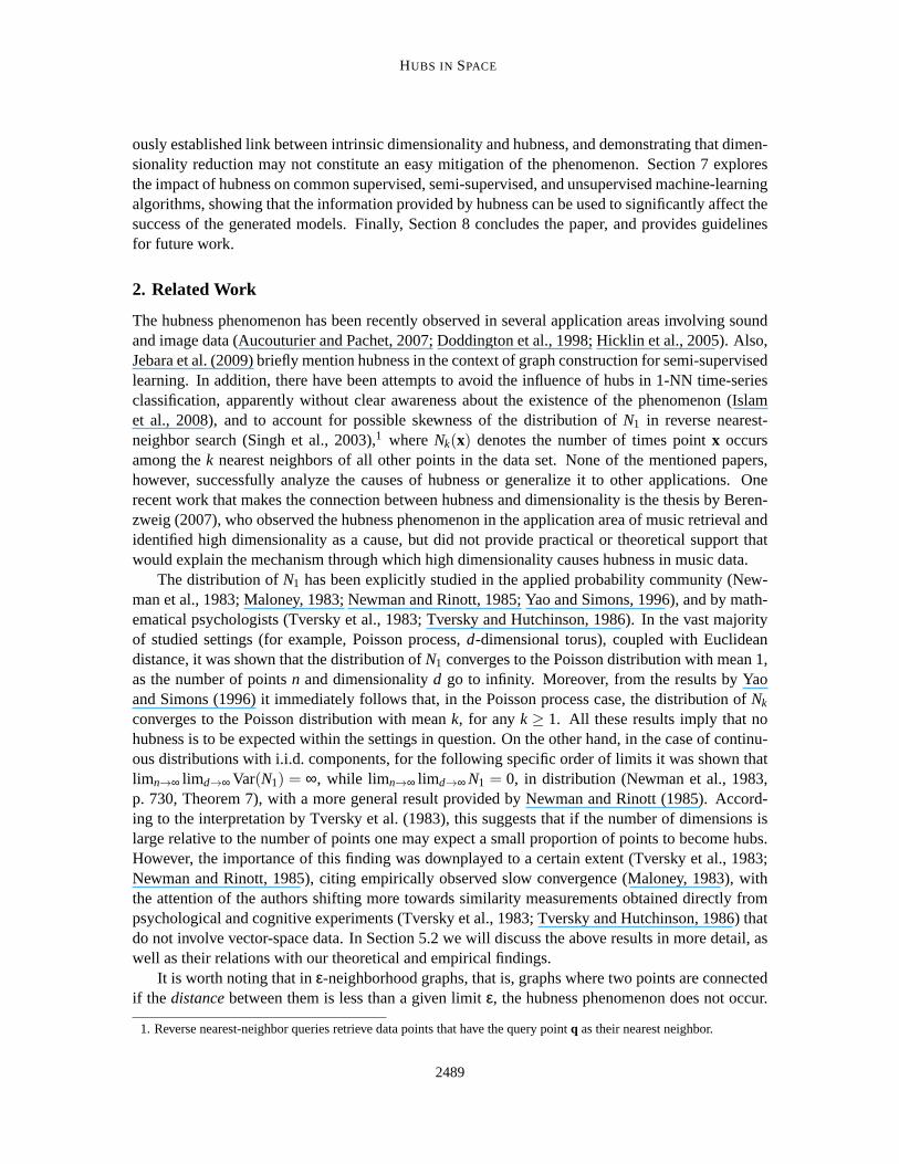
with varying dimensionality. Let us consider a random data set consisting of10000d-dimensionalpoints, whose components are independently drawn from the uniform distribution in range[0,1], andthe following distance functions: Euclidean (l2), fractionall0.5 (proposed for high-dimensional databy Aggarwal et al., 2001), and cosine. Figure 1(a–c) shows the empirically observed distributionsof Nk, with k= 5, for (a)d = 3, (b)d = 20, and (c)d = 100. In the same way, Figure 1(d–f) depictsthe empirically observedNk for points randomly drawn from the i.i.d. normal distribution.

For d = 3 the empirical distributions ofN5 for the three distance functions (Figure 1(a, d)) areconsistent with the binomial distribution. This is expected by consideringk-occurrences as node in-degrees in thek-nearest neighbor digraph. For randomly distributed points in low dimensions, thedegree distributions of the digraphs closely resemble the degree distributionof the Erdos-Renyi (ER)random graph model, which is is binomial and Poisson in the limit (Erdos and Renyi, 1959).

As dimensionality increases, the observed distributions ofN5 depart from the random graphmodel and become more skewed to the right (Figure 1(b, c), and Figure 1(e, f) for l2 and l0.5).

2490

HUBS IN SPACE

0 5 10 150

0.05

0.1

0.15

0.2

0.25iid uniform, d = 3

N5

p(N

5)

l2l0.5

cos

0 10 20 30 40 500

0.02

0.04

0.06

0.08

0.1

0.12

0.14

0.16iid uniform, d = 20

N5

p(N

5)

l2l0.5

cos

0 0.5 1 1.5 2 2.5−4

−3.5

−3

−2.5

−2

−1.5

−1

−0.5iid uniform, d = 100

log10

(N5)

log 10

( p(

N5))

l2l0.5

cos

(a) (b) (c)

0 5 10 150

0.05

0.1

0.15

0.2

0.25iid normal, d = 3

N5

p(N

5)

l2l0.5

cos

0 10 20 30 40 500

0.05

0.1

0.15

0.2iid normal, d = 20

N5

p(N

5)

l2l0.5

cos

0 0.5 1 1.5 2 2.5 3−4

−3

−2

−1

0iid normal, d = 100

log10

(N5)

log 10

( p(

N5))

l2l0.5

cos

(d) (e) (f)

Figure 1: Empirical distribution ofN5 for Euclidean,l0.5, and cosine distances on (a–c) i.i.d. uni-form, and (d–f) i.i.d. normal random data sets withn= 10000 points and dimensionality(a, d)d = 3, (b, e)d = 20, and (c, f)d = 100 (log-log plot).

We verified this by being able to fit major right portions (that is, tails) of the observed distributionswith the log-normal distribution, which is highly skewed.2 We made similar observations withvariousk values (generally focusing on the common casek ≪ n, wheren is the number of pointsin a data set), distance measures (lp-norm distances for bothp ≥ 1 and 0< p < 1, Bray-Curtis,normalized Euclidean, and Canberra), and data distributions. In virtually all these cases, skewnessexists and produces hubs, that is, points with highk-occurrences. One exception visible in Figure 1is the combination of cosine distance and normally distributed data. In most practical settings,however, such situations are not expected, and a thorough discussionof the necessary conditions forhubness to occur in high dimensions will be given in Section 5.2.

3.2 Hubness in Real Data

To illustrate the hubness phenomenon on real data, let us consider the empirical distribution ofNk

(k= 10) for three real data sets, given in Figure 2. As in the previous section, a considerable increasein the skewness of the distributions can be observed with increasing dimensionality.

In all, we examined 50 real data sets from well known sources, belongingto three categories:UCI multidimensional data, gene expression microarray data, and textual data in the bag-of-words

2. Fits were supported by theχ2 goodness-of-fit test at 0.05 significance level, where bins represent the number ofobservations of individualNk values. These empirical distributions were compared with the expected output of a(discretized) log-normal distribution, making sure that counts in the bins do not fall below 5 by pooling the rightmostbins together.

2491

RADOVANOVI C, NANOPOULOS AND IVANOVI C

0 5 10 15 200

0.05

0.1

0.15

0.2

0.25

N10

p(N

10)

haberman, d = 3

0 10 20 30 400

0.05

0.1

0.15

0.2

0.25mfeat−factors, d = 216

N10

p(N

10)

1 1.5 2 2.5 3

−3

−2

−1

0

log10

(N10

)

log 10

(p(N

10))

movie−reviews, d = 11885

(a) (b) (c)

Figure 2: Empirical distribution ofN10 for three real data sets of different dimensionalities.

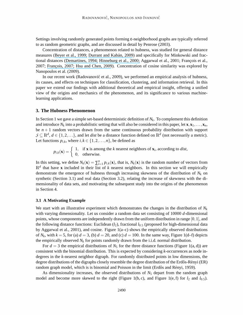
representation,3 listed in Table 1. The table includes columns that describe data-set sources(2nd col-umn), basic statistics (data transformation (3rd column): whether standardization was applied, or fortextual data the used bag-of-words document representation; the number of points (n, 4th column);dimensionality (d, 5th column); the number of classes (7th column)), and the distance measureused(Euclidean or cosine, 8th column). We took care to ensure that the choice of distance measure andpreprocessing (transformation) corresponds to a realistic scenario for the particular data set.

To characterize the asymmetry ofNk we use the standardized third moment of the distributionof k-occurrences,

SNk =E(Nk−µNk)

3

σ3Nk

,

whereµNk andσNk are the mean and standard deviation ofNk, respectively. The corresponding (9th)column of Table 1, which shows the empiricalSN10 values for the real data sets, indicates that thedistributions ofN10 for most examined data sets are skewed to the right.4 The value ofk is fixedat 10, but analogous observations can be made with other values ofk.

It can be observed that someSNk values in Table 1 are quite high, indicating strong hubness in thecorresponding data sets.5 Moreover, computing the Spearman correlation betweend andSNk overall 50 data sets reveals it to be strong (0.62), signifying that the relationshipbetween dimensionalityand hubness extends from synthetic to real data in general. On the other hand, careful scrutiny of thecharts in Figure 2 andSNk values in Table 1 reveals that for real data the impact of dimensionalityon hubness may not be as strong as could be expected after viewing hubness on synthetic data inFigure 1. Explanations for this observation will be given in the next section.

3. We used the movie review polarity data set v2.0 initially introduced by Pangand Lee (2004), while the computers andsports data sets were first used by Radovanovic and Ivanovic (2006). Preprocessing of all text data sets (except dexter,which is already preprocessed) involved stop-word removal and stemming using the Porter stemmer. Documentswere transformed into the bag-of-words representation with word weights being either term frequencies (tf), or termfrequencies multiplied by inverse document frequencies (tf-idf), with the choice based on independent experimentsinvolving several classifiers. All term frequency vectors were normalized to average document length.

4. If SNk = 0 there is no skewness, positive (negative) values signify skewness tothe right (left).5. For comparison, sample skewness values for i.i.d. uniform data and Euclidean distance, shown in Figure 1(a–c), are

0.121, 1.541, and 5.445 for dimensionalities 3, 20, and 100, respectively. The values for i.i.d. normal data fromFigure 1(d–f) are 0.118, 2.055, and 19.210.

2492

HUBS IN SPACE

Name Src. Trans. n d dmle Cls. Dist. SN10 SSN10

Clu. CN10dm CN10

cm BN10 CN10BN10

CAV

abalone UCI stan 4177 8 5.39 29l2 0.277 0.235 62−0.047−0.526 0.804 0.934 0.806arcene UCI stan 100 10000 22.85 2l2 0.634 2.639 2−0.559−0.684 0.367 0.810 0.455arrhythmia UCI stan 452 279 21.63 16l2 1.984 6.769 8−0.867−0.892 0.479 0.898 0.524breast-w UCI stan 699 9 5.97 2l2 1.020 0.667 7−0.062−0.240 0.052 0.021 0.048diabetes UCI stan 768 8 6.00 2l2 0.555 0.486 15−0.479−0.727 0.322 0.494 0.337dorothea UCI none 800 100000 201.11 2 cos 2.355 1.016 19−0.632−0.672 0.108 0.236 0.092echocardiogram UCI stan 131 7 4.92 2l2 0.735 0.438 5−0.722−0.811 0.372 0.623 0.337ecoli UCI stan 336 7 4.13 8l2 0.116 0.208 8−0.396−0.792 0.223 0.245 0.193gisette UCI none 6000 5000 149.35 2 cos 1.967 4.671 76−0.667−0.854 0.045 0.367 0.241glass UCI stan 214 9 4.37 7l2 0.154 0.853 11−0.430−0.622 0.414 0.542 0.462haberman UCI stan 306 3 2.89 2l2 0.087−0.316 11−0.330−0.573 0.348 0.305 0.360ionosphere UCI stan 351 34 13.57 2l2 1.717 2.051 18−0.639−0.832 0.185 0.464 0.259iris UCI stan 150 4 2.96 3 l2 0.126−0.068 4−0.275−0.681 0.087 0.127 0.147isolet1 UCI stan 1560 617 13.72 26l2 1.125 6.483 38−0.306−0.760 0.283 0.463 0.352mfeat-factors UCI stan 2000 216 8.47 10l2 0.826 5.493 44−0.113−0.688 0.063 0.001 0.145mfeat-fourier UCI stan 2000 76 11.48 10l2 1.277 4.001 44−0.350−0.596 0.272 0.436 0.415mfeat-karhunen UCI stan 2000 64 11.82 10l2 1.250 8.671 40−0.436−0.788 0.098 0.325 0.205mfeat-morph UCI stan 2000 6 3.22 10l2 −0.153 0.010 44−0.039−0.424 0.324 0.306 0.397mfeat-pixel UCI stan 2000 240 11.83 10l2 1.035 3.125 44−0.210−0.738 0.049 0.085 0.107mfeat-zernike UCI stan 2000 47 7.66 10l2 0.933 3.389 44−0.185−0.657 0.235 0.252 0.400musk1 UCI stan 476 166 6.74 2l2 1.327 3.845 17−0.376−0.752 0.237 0.621 0.474optdigits UCI stan 5620 64 9.62 10l2 1.095 3.789 74−0.223−0.601 0.044 0.097 0.168ozone-eighthr UCI stan 2534 72 12.92 2l2 2.251 4.443 49−0.216−0.655 0.086 0.300 0.138ozone-onehr UCI stan 2536 72 12.92 2l2 2.260 5.798 49−0.215−0.651 0.046 0.238 0.070page-blocks UCI stan 5473 10 3.73 5l2 −0.014 0.470 72−0.063−0.289 0.049−0.046 0.068parkinsons UCI stan 195 22 4.36 2l2 0.729 1.964 8−0.414−0.649 0.166 0.321 0.256pendigits UCI stan 10992 16 5.93 10l2 0.435 0.982 104−0.062−0.513 0.014−0.030 0.156segment UCI stan 2310 19 3.93 7l2 0.313 1.111 48−0.077−0.453 0.089 0.074 0.332sonar UCI stan 208 60 9.67 2l2 1.354 3.053 8−0.550−0.771 0.286 0.632 0.461spambase UCI stan 4601 57 11.45 2l2 1.916 2.292 49−0.376−0.448 0.139 0.401 0.271spectf UCI stan 267 44 13.83 2l2 1.895 2.098 11−0.616−0.729 0.300 0.595 0.366spectrometer UCI stan 531 100 8.04 10l2 0.591 3.123 17−0.269−0.670 0.200 0.225 0.242vehicle UCI stan 846 18 5.61 4l2 0.603 1.625 25−0.162−0.643 0.358 0.435 0.586vowel UCI stan 990 10 2.39 11l2 0.766 0.935 27−0.252−0.605 0.313 0.691 0.598wdbc UCI stan 569 30 8.26 2l2 0.815 3.101 16−0.449−0.708 0.065 0.170 0.129wine UCI stan 178 13 6.69 3l2 0.630 1.319 3−0.589−0.874 0.076 0.182 0.084wpbc UCI stan 198 33 8.69 2l2 0.863 2.603 6−0.688−0.878 0.340 0.675 0.360yeast UCI stan 1484 8 5.42 10l2 0.228 0.105 34−0.421−0.715 0.527 0.650 0.570AMLALL KR none 72 7129 31.92 2 l2 1.166 1.578 2−0.868−0.927 0.171 0.635 0.098colonTumor KR none 62 2000 11.22 2l2 1.055 1.869 3−0.815−0.781 0.305 0.779 0.359DLBCL KR none 47 4026 16.11 2l2 1.007 1.531 2−0.942−0.947 0.338 0.895 0.375lungCancer KR none 181 12533 59.66 2l2 1.248 3.073 6−0.537−0.673 0.052 0.262 0.136MLL KR none 72 12582 28.42 3l2 0.697 1.802 2−0.794−0.924 0.211 0.533 0.148ovarian-61902 KR none 253 15154 9.58 2l2 0.760 3.771 10−0.559−0.773 0.164 0.467 0.399computers dmoz tf 697 1168 190.33 2 cos 2.061 2.267 26−0.566−0.731 0.312 0.699 0.415dexter UCI none 300 20000 160.78 2 cos 3.977 4.639 13−0.760−0.781 0.301 0.688 0.423mini-newsgroups UCI tf-idf 1999 7827 3226.43 20 cos 1.980 1.765 44 −0.422−0.704 0.524 0.701 0.526movie-reviews PaBo tf 2000 11885 54.95 2 cos 8.796 7.247 44−0.604−0.739 0.398 0.790 0.481reuters-transcribed UCI tf-idf 201 3029 234.68 10 cos 1.1651.693 3−0.781−0.763 0.642 0.871 0.595sports dmoz tf 752 1185 250.24 2 cos 1.629 2.543 27−0.584−0.736 0.260 0.604 0.373

Table 1: Real data sets. Data sources are the University of California, Irvine (UCI) Machine Learn-ing Repository, Kent Ridge (KR) Bio-Medical Data Set Repository, dmoz Open Directory,and www.cs.cornell.edu/People/pabo/movie-review-data/ (PaBo).

2493

RADOVANOVI C, NANOPOULOS AND IVANOVI C

4. The Origins of Hubness

This section moves on to exploring the causes of hubness and the mechanismsthrough which hubsemerge. Section 4.1 investigates the relationship between the position of a pointin data spaceand hubness. Next, Section 4.2 explains the mechanism through which hubsemerge as points inhigh-dimensional space that become closer to other points than their low-dimensional counterparts,outlining our main theoretical result. The emergence of hubness in real datais studied in Section 4.3,while Section 4.4 discusses hubs and their opposites—antihubs—and the relationships betweenhubs, antihubs, and different notions of outliers.

4.1 The Position of Hubs

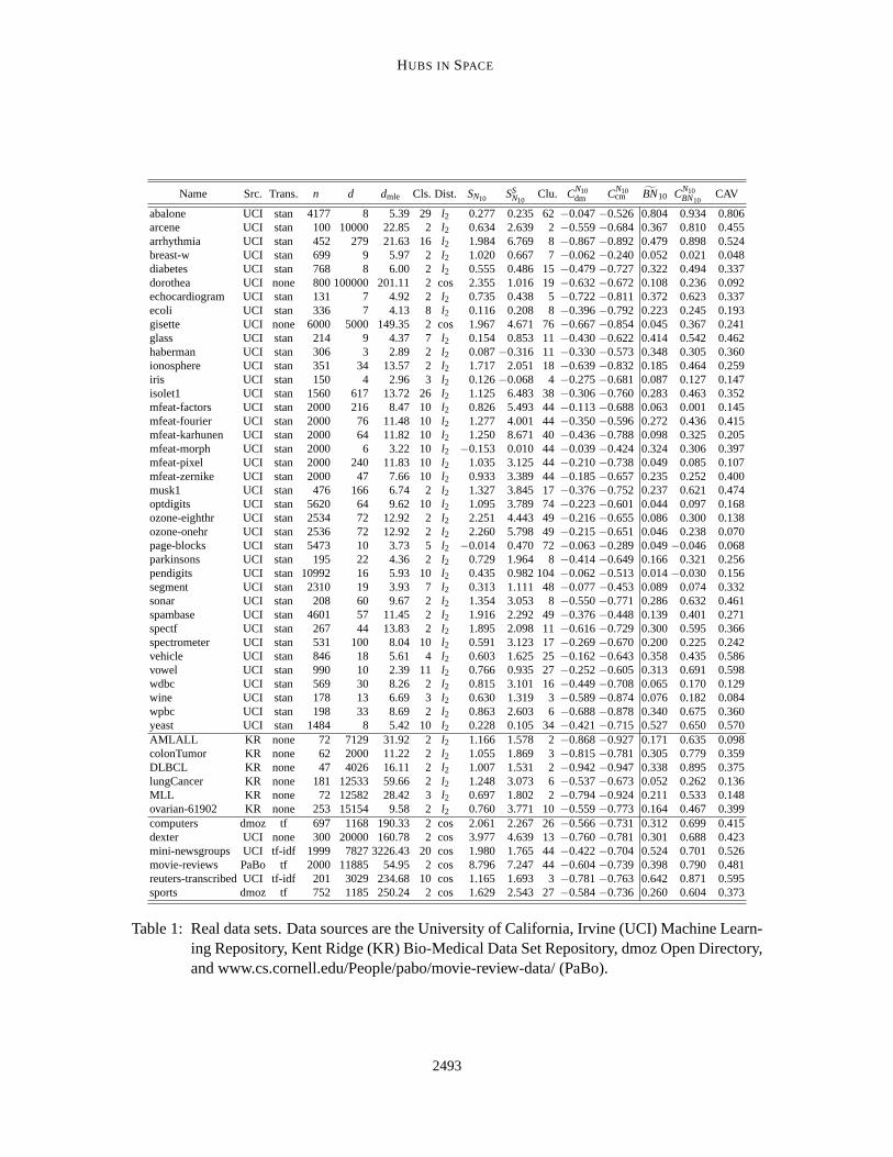
Let us consider again the i.i.d. uniform and i.i.d. normal random data examinedin the previoussection. We will demonstrate that the position of a point in data space has a significant effect on itsk-occurrences value, by observing the sample mean of the data distribution asa point of reference.Figure 3 plots, for each pointx, its N5(x) against its Euclidean distance from the empirical datamean, ford = 3, 20, 100. As dimensionality increases, stronger correlation emerges, implyingthat points closer to the mean tend to become hubs. We made analogous observations with othervalues ofk, and combinations of data distributions and distance measures for which hubness occurs.It is important to note that proximity to one global data-set mean correlates with hubness in highdimensions when the underlying data distribution isunimodal. For multimodal data distributions,for example those obtained through a mixture of unimodal distributions, hubs tend to appear closeto the means of individual component distributions of the mixture. In the discussion that followsin Section 4.2 we will assume a unimodal data distribution, and defer the analysisof multimodaldistributions until Section 4.3, which studies real data.

4.2 Mechanisms Behind Hubness

Although one may expect that some random points are closer to the data-setmean than others, inorder to explain the mechanism behind hub formation we need to (1) understand the geometricaland distributional setting in which some points tend to be closer to the mean than others, and then(2) understand why such points become hubs in higher dimensions.6

Hubness appears to be related to the phenomenon of distance concentration, which is usuallyexpressed as the ratio between some measure of spread (for example, standard deviation) and somemeasure of magnitude (for example, the mean) of distances of all points in a data set to some ar-bitrary reference point (Aggarwal et al., 2001; Francois et al., 2007). If this ratio converges to 0as dimensionality goes to infinity, it is said that the distances concentrate. Based on existing the-oretical results discussing distance concentration (Beyer et al., 1999; Aggarwal et al., 2001), high-dimensional points are approximately lying on a hypersphere centered at the data-set mean. More-over, the results by Demartines (1994) and Francois et al. (2007) specify that the distribution ofdistances to the data-set mean has a non-negligible variance for any finited.7 Hence, the existenceof a non-negligible number of points closer to the data-set mean isexpectedin high dimensions.

6. We will assume that random points originate from a unimodal data distribution. In the multimodal case, it can be saidthat the observations which follow are applicable around one of the “peaks” in the pdf of the data distribution.

7. These results apply tolp-norm distances, but our numerical simulations suggest that other distance functions men-tioned in Section 3.1 behave similarly. Moreover, any point can be used as a reference instead of the data mean, butwe observe the data mean since it plays a special role with respect to hubness.

2494

HUBS IN SPACE

0 0.2 0.4 0.6 0.8 10

2

4

6

8

10

12

iid uniform, d = 3, Cdm N

5 = −0.018

Distance from data set mean

N5

0.6 0.8 1 1.2 1.4 1.6 1.8 20

10

20

30

40

50

iid uniform, d = 20, Cdm N

5 = −0.803

Distance from data set mean

N5

2 2.5 3 3.5 40

20406080

100120140160

iid uniform, d = 100, Cdm N

5 = −0.865

Distance from data set mean

N5

(a) (b) (c)

0 1 2 3 4 50

2

4

6

8

10

12

iid normal, d = 3, Cdm N

5 = −0.053

Distance from data set mean

N5

1 2 3 4 5 6 7 80

10

20

30

40

50

iid normal, d = 20, Cdm N

5 = −0.877

Distance from data set mean

N5

5 6 7 8 9 10 11 12 13 14 150

100200300400500600700800

iid normal, d = 100, Cdm N

5 = −0.874

Distance from data set mean

N5

(d) (e) (f)

Figure 3: Scatter plots and Spearman correlation ofN5(x) against the Euclidean distance of pointxto the sample data-set mean for (a–c) i.i.d. uniform and (d–f) i.i.d. normal random datasets with (a, d)d = 3, (b, e)d = 20, and (c, f)d = 100.

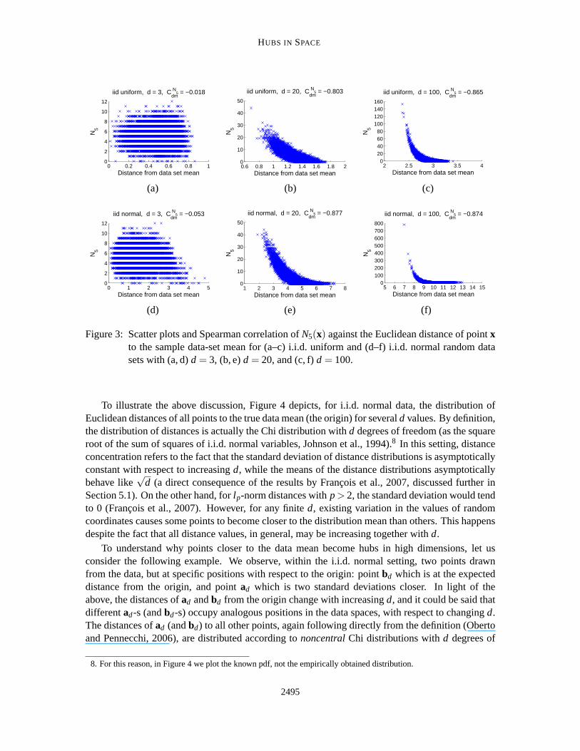
To illustrate the above discussion, Figure 4 depicts, for i.i.d. normal data, thedistribution ofEuclidean distances of all points to the true data mean (the origin) for several d values. By definition,the distribution of distances is actually the Chi distribution withd degrees of freedom (as the squareroot of the sum of squares of i.i.d. normal variables, Johnson et al., 1994).8 In this setting, distanceconcentration refers to the fact that the standard deviation of distance distributions is asymptoticallyconstant with respect to increasingd, while the means of the distance distributions asymptoticallybehave like

√d (a direct consequence of the results by Francois et al., 2007, discussed further in

Section 5.1). On the other hand, forlp-norm distances withp> 2, the standard deviation would tendto 0 (Francois et al., 2007). However, for any finited, existing variation in the values of randomcoordinates causes some points to become closer to the distribution mean than others. This happensdespite the fact that all distance values, in general, may be increasing together withd.

To understand why points closer to the data mean become hubs in high dimensions, let usconsider the following example. We observe, within the i.i.d. normal setting, two points drawnfrom the data, but at specific positions with respect to the origin: pointbd which is at the expecteddistance from the origin, and pointad which is two standard deviations closer. In light of theabove, the distances ofad andbd from the origin change with increasingd, and it could be said thatdifferentad-s (andbd-s) occupy analogous positions in the data spaces, with respect to changing d.The distances ofad (andbd) to all other points, again following directly from the definition (Obertoand Pennecchi, 2006), are distributed according tononcentralChi distributions withd degrees of

8. For this reason, in Figure 4 we plot the known pdf, not the empirically obtained distribution.

2495

RADOVANOVI C, NANOPOULOS AND IVANOVI C

0 2 4 6 8 10 12 140

0.2

0.4

0.6

0.8Distribution of distances from iid normal data mean

Distance from iid normal data mean (r)

p(r)

d = 1d = 3d = 20d = 100

Figure 4: Probability density function of observing a point at distancer from the mean of a multi-variated-dimensional normal distribution, ford = 1, 3, 20, 100.

0 2 4 6 8 10 12 14 16 180

0.2

0.4

0.6

0.8

Distance from other points (r)

p(r)

Distribution of distances from two points at analogous positions in iid normal data

d = 3d = 20d = 100

Dashed line: point at expected dist. from meanFull line: point two standard deviations closer

0 20 40 60 80 1000.2

0.4

0.6

0.8

d

Diff

eren

cebe

twee

nm

eans

(a) (b)

Figure 5: (a) Distribution of distances to other points from i.i.d. normal random data for a point atthe expected distance from the origin (dashed line), and a point two standard deviationscloser (full line). (b) Difference between the means of the two distributions, with respectto increasingd.

freedom and noncentrality parameterλ equaling the distance ofad (bd) to the origin. Figure 5(a)plots the probability density functions of these distributions for several values ofd. It can be seenthat, asd increases, the distance distributions forad and bd move away from each other. Thistendency is depicted more clearly in Figure 5(b) which plots the difference between the means ofthe two distributions with respect tod.

It is known, and expected, for points that are closer to the mean of the datadistribution to becloser, on average, to all other points, for any value ofd. However, the above analysis indicatesthat this tendency is amplified by high dimensionality, making points that reside in theproximityof the data mean become closer (in relative terms) to all other points than their low-dimensionalanalogues are. This tendency causes high-dimensional points that are closer to the mean to haveincreased inclusion probability intok-NN lists of other points, even for small values ofk. We willdiscuss this relationship further in Section 5.2.

In terms of the notion of nodecentrality typically used in network analysis (Scott, 2000), theabove discussion indicates that high dimensionality amplifies what we will call thespatial centrality

2496

HUBS IN SPACE

of a point (by increasing its proximity to other points), which, in turn, affectsthedegree centralityof the corresponding node in thek-NN graph (by increasing its degree, that is,Nk). Other notionsof node centrality, and the structure of thek-NN graph in general, will be studied in more detailin Section 5.2.1. The rest of this section will focus on describing the mechanism of the observedspatial centrality amplification.

In the preceding discussion we selected two points from i.i.d. normal data with specific distancesfrom the origin expressed in terms of expected distance and deviation fromit, and tracked theanalogues of the two points for increasing values of dimensionalityd. Generally, we can express thedistances of the two points to the origin in terms of “offsets” from the expecteddistance measuredby standard deviation, which in the case of i.i.d. normal random data would beλd,1 = µχ(d) +c1σχ(d) andλd,2 = µχ(d)+c2σχ(d), whereλd,1 andλd,2 are the distances of the first and second pointto the origin,µχ(d) andσχ(d) are the mean and standard deviation of the Chi distribution withddegrees of freedom, andc1 andc2 are selected constants (the offsets). In the preceding exampleinvolving pointsad andbd, we setc1 =−2 andc2 = 0, respectively. However, analogous behaviorcan be observed with arbitrary two points whose distance to the data mean is below the expecteddistance, that is, forc1,c2 ≤ 0. We describe this behavior by introducing the following notation:∆µd(λd,1,λd,2) = |µχ(d,λd,2)−µχ(d,λd,1)|, whereµχ(d,λd,i) is the mean of the noncentral Chi distributionwith d degrees of freedom and noncentrality parameterλd,i (i ∈ {1,2}). In the following theorem,which we prove in Section 5.1, we show that∆µd(λd,1,λd,2) increases with increasing values ofd.

Theorem 1 Letλd,1 = µχ(d)+c1σχ(d) andλd,2 = µχ(d)+c2σχ(d), where d∈N+, c1,c2 ≤ 0, c1 < c2,

and µχ(d) andσχ(d) are the mean and standard deviation of the Chi distribution with d degrees offreedom, respectively. Define

∆µd(λd,1,λd,2) = µχ(d,λd,2)−µχ(d,λd,1) ,

where µχ(d,λd,i) is the mean of the noncentral Chi distribution with d degrees of freedom andnon-centrality parameterλd,i (i ∈ {1,2}).

There exists d0 ∈N such that for every d> d0,

∆µd(λd,1,λd,2)> 0,

and∆µd+2(λd+2,1,λd+2,2)> ∆µd(λd,1,λd,2) . (1)

The main statement of the theorem is given by Equation 1, which expresses the tendency of thedifference between the means of the two distance distributions to increase withincreasing dimen-sionalityd. It is important to note that this tendency is obtained through analysis ofdistributionsofdata and distances, implying that the behavior is an inherent property of data distributions in high-dimensional space, rather than an artefact of other factors, such as finite sample size, etc. Throughsimulation involving randomly generated points we verified the behavior for i.i.d.normal data byreplicating very closely the chart shown in Figure 5(b). Furthermore, simulations suggest that thesame behavior emerges in i.i.d. uniform data,9 as well as numerous other unimodal random datadistributions, producing charts of the same shape as in Figure 5(b). Realdata, on the other hand,

9. The uniform cube setting will be discussed in more detail in Section 5.2, inthe context of results from related work(Newman and Rinott, 1985).

2497

RADOVANOVI C, NANOPOULOS AND IVANOVI C

tends to be clustered, and can be viewed as originating from amixtureof distributions resulting in amultimodal distribution of data. In this case, the behavior described by Theorem 1, and illustratedin Figure 5(b), is manifested primarily on the individual component distributions of the mixture,that is, on clusters of data points. The next section takes a closer look at the hubness phenomenonin real data sets.

4.3 Hubness in Real Data

Results describing the origins of hubness given in the previous sections were obtained by examiningdata sets that follow specific distributions and generated as i.i.d. samples fromthese distributions.To extend these results to real data, we need to take into account two additional factors: (1) realdata sets usually contain dependent attributes, and (2) real data sets areusually clustered, that is,points are organized into groups produced by a mixture of distributions instead of originating froma single (unimodal) distribution.

To examine the first factor (dependent attributes), we adopt the approach of Francois et al. (2007)used in the context of distance concentration. For each data set we randomly permute the elementswithin every attribute. This way, attributes preserve their individual distributions, but the dependen-cies between them are lost and theintrinsic dimensionalityof data sets increases, becoming equalto their embedding dimensionalityd (Francois et al., 2007). In Table 1 (10th column) we give theempirical skewness, denoted asSS

Nk, of the shuffled data. For the vast majority of high-dimensional

data sets,SSNk

is considerably higher thanSNk, indicating that hubness actually depends on the in-trinsic rather than embedding dimensionality. This provides an explanation forthe apparent weakerinfluence ofd on hubness in real data than in synthetic data sets, which was observed in Section 3.2.

To examine the second factor (many groups), for every data set we measured: (i) the Spearmancorrelation, denoted asCN10

dm (12th column), of the observedNk and distance from the data-set mean,and (ii) the correlation, denoted asCN10

cm (13th column), of the observedNk and distance to theclosest group mean. Groups are determined withK-means clustering, where the number of clustersfor each data set, given in column 11 of Table 1, was determined by exhaustive search of valuesbetween 2 and⌊√n⌋, to maximizeCN10

cm .10 In most cases,CN10cm is considerably stronger thanCN10

dm .Consequently, in real data, hubs tend to be closer than other points to their respective cluster centers(which we verified by examining the individual scatter plots).

To further support the above findings, we include the 6th column (dmle) to Table 1, correspondingto intrinsic dimensionality measured by the maximum likelihood estimator (Levina and Bickel,2005). Next, we compute Spearman correlations between various measurements from Table 1 overall 50 examined data sets, given in Table 2. The observed skewness ofNk, besides being stronglycorrelated withd, is even more strongly correlated with the intrinsic dimensionalitydmle. Moreover,intrinsic dimensionality positively affects the correlations betweenNk and the distance to the data-set mean / closest cluster mean, implying that in higher (intrinsic) dimensions thepositions of hubsbecome increasingly localized to the proximity of centers.

Section 6, which discusses the interaction of hubness with dimensionality reduction, will pro-vide even more support to the observation that hubness depends on intrinsic, rather than embeddingdimensionality.

10. We report averages ofCN10cm over 10 runs ofK-means clustering with different random seeding, in order to reduce the

effects of chance.

2498

HUBS IN SPACE

d dmle SN10 CN10dm CN10

cm BN10 CN10BN10

dmle 0.87

SN10 0.62 0.80

CN10dm −0.52 −0.60 −0.42

CN10cm −0.43 −0.48 −0.31 0.82

BN10 −0.05 0.03−0.08 −0.32 −0.18

CN10BN10

0.32 0.39 0.29−0.61 −0.46 0.82CAV 0.03 0.03 0.03−0.14 −0.05 0.85 0.76

Table 2: Spearman correlations over 50 real data sets.

0 2 4 6 8 10 120

20

40

60

Distance from k−th NN

Nk

ionosphere

4 6 8 10 12 14 160

20

40

60

Distance from k−th NN

Nk

sonar

(a) (b)

Figure 6: Correlation between lowNk and outlier score (k= 20).

4.4 Hubs and Outliers

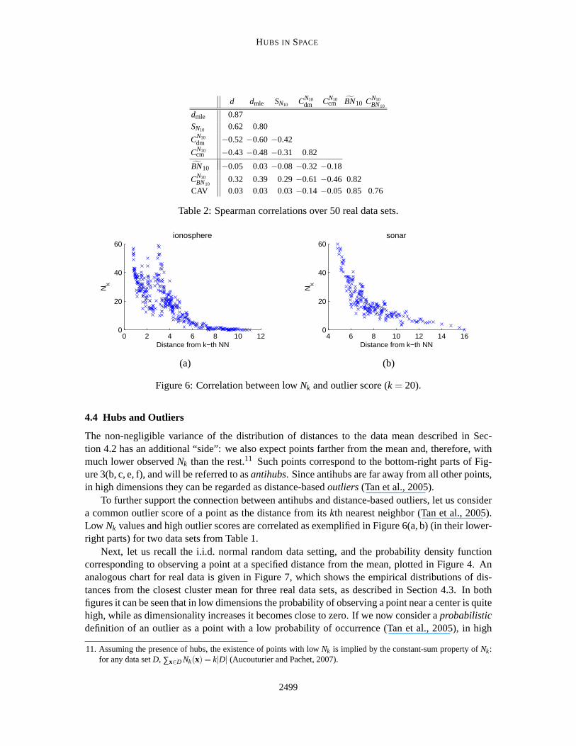
The non-negligible variance of the distribution of distances to the data mean described in Sec-tion 4.2 has an additional “side”: we also expect points farther from the mean and, therefore, withmuch lower observedNk than the rest.11 Such points correspond to the bottom-right parts of Fig-ure 3(b, c, e, f), and will be referred to asantihubs. Since antihubs are far away from all other points,in high dimensions they can be regarded as distance-basedoutliers(Tan et al., 2005).

To further support the connection between antihubs and distance-based outliers, let us considera common outlier score of a point as the distance from itskth nearest neighbor (Tan et al., 2005).Low Nk values and high outlier scores are correlated as exemplified in Figure 6(a,b) (in their lower-right parts) for two data sets from Table 1.

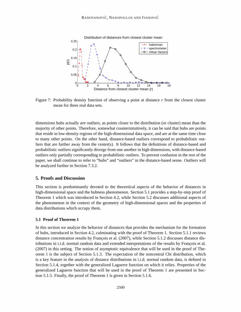
Next, let us recall the i.i.d. normal random data setting, and the probability density functioncorresponding to observing a point at a specified distance from the mean, plotted in Figure 4. Ananalogous chart for real data is given in Figure 7, which shows the empirical distributions of dis-tances from the closest cluster mean for three real data sets, as described in Section 4.3. In bothfigures it can be seen that in low dimensions the probability of observing a point near a center is quitehigh, while as dimensionality increases it becomes close to zero. If we now consider aprobabilisticdefinition of an outlier as a point with a low probability of occurrence (Tan etal., 2005), in high

11. Assuming the presence of hubs, the existence of points with lowNk is implied by the constant-sum property ofNk:for any data setD, ∑x∈D Nk(x) = k|D| (Aucouturier and Pachet, 2007).

2499

RADOVANOVI C, NANOPOULOS AND IVANOVI C

0 2 4 6 8 10 12 14 16 180

0.05

0.1

0.15

0.2

0.25Distribution of distances from closest cluster mean

Distance from closest cluster mean (r)

p(r)

habermanspectrometermfeat−factors

Figure 7: Probability density function of observing a point at distancer from the closest clustermean for three real data sets.

dimensions hubs actuallyare outliers, as points closer to the distribution (or cluster) mean than themajority of other points. Therefore, somewhat counterintuitively, it can besaid that hubs are pointsthat reside in low-density regions of the high-dimensional data space, andare at the same time closeto many other points. On the other hand, distance-based outliers correspond to probabilistic out-liers that are farther away from the center(s). It follows that the definitions of distance-based andprobabilistic outliers significantly diverge from one another in high dimensions, with distance-basedoutliers only partially corresponding to probabilistic outliers. To prevent confusion in the rest of thepaper, we shall continue to refer to “hubs” and “outliers” in the distance-based sense. Outliers willbe analyzed further in Section 7.3.2.

5. Proofs and Discussion

This section is predominantly devoted to the theoretical aspects of the behavior of distances inhigh-dimensional space and the hubness phenomenon. Section 5.1 provides a step-by-step proof ofTheorem 1 which was introduced in Section 4.2, while Section 5.2 discusses additional aspects ofthe phenomenon in the context of the geometry of high-dimensional spaces and the properties ofdata distributions which occupy them.

5.1 Proof of Theorem 1

In this section we analyze the behavior of distances that provides the mechanism for the formationof hubs, introduced in Section 4.2, culminating with the proof of Theorem 1. Section 5.1.1 reviewsdistance concentration results by Francois et al. (2007), while Section 5.1.2 discusses distance dis-tributions in i.i.d. normal random data and extended interpretations of the results by Francois et al.(2007) in this setting. The notion of asymptotic equivalence that will be used inthe proof of The-orem 1 is the subject of Section 5.1.3. The expectation of the noncentral Chi distribution, whichis a key feature in the analysis of distance distributions in i.i.d. normal random data, is defined inSection 5.1.4, together with the generalized Laguerre function on which it relies. Properties of thegeneralized Laguerre function that will be used in the proof of Theorem1 are presented in Sec-tion 5.1.5. Finally, the proof of Theorem 1 is given in Section 5.1.6.

2500

HUBS IN SPACE

5.1.1 DISTANCE CONCENTRATION RESULTS

We begin by reviewing the main results of Francois et al. (2007) regarding distance concentration.Let Xd = (X1,X2, . . . ,Xd) be a randomd-dimensional variable with i.i.d. components:Xi ∼ F , andlet ‖Xd‖ denote its Euclidean norm. For random variables|Xi |2, let µ|F |2 andσ2

|F |2 signify their

mean and variance, respectively. Francois et al. (2007) prove the following two lemmas.12

Lemma 2 (Francois et al., 2007, Equation 17, adapted)

limd→∞

E(‖Xd‖)√d

= µ|F |2 .

Lemma 3 (Francois et al., 2007, Equation 21, adapted)

limd→∞

Var(‖Xd‖) =σ2|F |2

4µ|F |2.

The above lemmas imply that, for i.i.d. random data, the expectation of the distribution of Eu-clidean distances to the origin (Euclidean norms) asymptotically behaves like

√d, while the stan-

dard deviation is asymptotically constant. From now on, we will denote the mean and variance ofrandom variables that are distributed according to some distributionF by µF andσ2

F , respectively.

5.1.2 DISTANCES IN I.I .D. NORMAL DATA

We now observe more closely the behavior of distances in i.i.d. normal random data. LetZd =(Z1,Z2, . . . ,Zd) be a randomd-dimensional vector whose components independently follow thestandard normal distribution:Zi ∼N (0;1), for everyi ∈ {1,2, . . . ,d}. Then, by definition, randomvariable‖Zd‖ follows the Chi distribution withd degrees of freedom:‖Zd‖ ∼ χ(d). In other words,χ(d) is the distribution of Euclidean distances of vectors drawn fromZd to the origin. If one wereto fix another reference vectorxd instead of the origin, the distribution of distances of vectors drawnfrom Zd to xd would be completely determined by‖xd‖ since, again by definition, random variable‖Zd − xd‖ follows the noncentral Chi distribution withd degrees of freedom and noncentralityparameterλ = ‖xd‖: ‖Zd −xd‖ ∼ χ(d,‖xd‖).

In light of the above, let us observe two points,xd,1 andxd,2, drawn fromZd, and express theirdistances from the origin in terms of offsets from the expected distance, withthe offsets describedusing standard deviations:‖xd,1‖ = µχ(d)+ c1σχ(d) and‖xd,2‖ = µχ(d)+ c2σχ(d), wherec1,c2 ≤ 0.We will assumec1 < c2, that is,xd,1 is closer to the data distribution mean (the origin) thanxd,2. Bytreatingc1 andc2 as constants, and varyingd, we observe analogues of two points in spaces of dif-ferent dimensionalities (roughly speaking, pointsxd,1 have identical “probability” of occurrence atthe specified distance from the origin for everyd, and the same holds forxd,2). Let λd,1 = ‖xd,1‖andλd,2 = ‖xd,2‖. Then, the distributions of distances of pointsxd,1 andxd,2 to all points from thedata distributionZd (that is, the distributions of random variables‖Zd −xd,1‖ and‖Zd −xd,2‖) arenoncentral Chi distributionsχ(d,λd,1) andχ(d,λd,2), respectively. We study the behavior of thesetwo distributions with increasing values ofd.

Lemmas 2 and 3, takingF to be the standard normal distributionN (0;1), and translating thespace so thatxd,1 or xd,2 become the origin, imply that bothµχ(d,λd,1) andµχ(d,λd,2) asymptotically

12. Francois et al. (2007) provide a more general result forlp norms with arbitraryp> 0.

2501

RADOVANOVI C, NANOPOULOS AND IVANOVI C

behave like√

d asd→∞, whileσ2χ(d,λd,1)

andσ2χ(d,λd,2)

are both asymptotically constant.13 However,

for xd,1 andxd,2 placed at different distances form the origin (λd,1 6= λd,2, that is,c1 6= c2), theseasymptotic tendencies do not occur at the samespeed. In particular, we will show that asd increases,the difference betweenµχ(d,λd,1) andµχ(d,λd,2) actuallyincreases. If we takexd,1 to be closer to theorigin thanxd,2 (c1 < c2), this means thatxd,1 becomes closer to all other points from the datadistributionZd thanxd,2, simply by virtue of increasing dimensionality, since for different valuesof d we place the two points at analogous positions in the data space with regards tothe distancefrom the origin.

5.1.3 ASYMPTOTIC EQUIVALENCE

Before describing our main theoretical result, we present several definitions and lemmas, beginningwith the notion of asymptotic equivalence that will be relied upon.

Definition 4 Two real-valued functions f(x) and g(x) areasymptotically equal, f (x)≈ g(x), iff foreveryε > 0 there exists x0 ∈R such that for every x> x0, | f (x)−g(x)|< ε.

Equivalently,f (x)≈ g(x) iff lim x→∞ | f (x)−g(x)|= 0. Note that the≈ relation is different fromthe divisive notion of asymptotic equivalence, wheref (x)∼ g(x) iff lim x→∞ f (x)/g(x) = 1.

The following two lemmas describe approximations that will be used in the proof of Theorem 1,based on the≈ relation.

Lemma 5 For any constant c∈R, let f(d) =√

d+c, and g(d) =√

d . Then, f(d)≈ g(d) .

Proof

limd→∞

∣∣∣√

d+c−√

d∣∣∣= lim

d→∞

∣∣∣∣∣(√

d+c−√

d)√d+c+

√d√

d+c+√

d

∣∣∣∣∣= limd→∞

∣∣∣∣c√

d+c+√

d

∣∣∣∣= 0.

Lemma 6 µχ(d) ≈√

d, andσχ(d) ≈ 1/√

2.

Proof Observe the expression for the mean of theχ(d) distribution,

µχ(d) =√

2Γ(

d+12

)

Γ(

d2

) .

The equalityxΓ(x) = Γ(x+1) and the convexity of logΓ(x) yield (Haagerup, 1982, p. 237):

Γ(

d+12

)2

≤ Γ(

d2

)Γ(

d+22

)=

d2

Γ(

d2

)2

,

13. More precisely, the lemmas can be applied only for pointsx′d,i that have equal values of all components, sinceafter translation data components need to be i.i.d. Because of the symmetry of the Gaussian distribution, the sameexpectations and variances of distance distributions are obtained, for everyd, with anyxd,i that has the same norm asx′d,i , thereby producing identical asymptotic results.

2502

HUBS IN SPACE

and

Γ(

d+12

)2

=d−1

2Γ(

d−12

)Γ(

d+12

)≥ d−1

2Γ(

d2

)2

,

from which we have√

d−1≤√

2Γ(

d+12

)

Γ(

d2

) ≤√

d .

From Lemma 5 it now follows thatµχ(d) ≈√

d .Regarding the standard deviation of theχ(d) distribution, from Lemma 3, takingF to be the

standard normal distribution, we obtain

limd→∞

σ2χ(d) =

σ2χ2(1)

4µχ2(1)=

12,

since the square of a standard normal random variable follows the chi-square distribution with onedegree of freedom,χ2(1), whose mean and variance are known:µχ2(1) = 1, σ2

χ2(1) = 2. It now di-

rectly follows thatσχ(d) ≈ 1/√

2.

5.1.4 EXPECTATION OF THENONCENTRAL CHI DISTRIBUTION

The central notion in Theorem 1 is the noncentral Chi distribution. To express the expectation ofthe noncentral Chi distribution, the following two definitions are needed, introducing the Kummerconfluent hypergeometric function1F1, and the generalized Laguerre function.

Definition 7 (Ito, 1993, p. 1799, Appendix A, Table 19.I)For a,b,z∈R, the Kummer confluent hypergeometric function1F1(a;b;z) is given by

1F1(a;b;z) =∞

∑k=0

(a)k

(b)k· zk

Γ(k+1),

where(·)k is the Pochhammer symbol,(x)k =Γ(x+k)

Γ(x) .

Definition 8 (Ito, 1993, p. 1811, Appendix A, Table 20.VI)For ν,α,z∈R, the generalized Laguerre function L(α)

ν (z) is given by

L(α)ν (z) =

Γ(ν+α+1)Γ(ν+1)

· 1F1(−ν;α+1;z)Γ(α+1)

.

The expectation of the noncentral Chi distribution withd degrees of freedom and noncentralityparameterλ, denoted byµχ(d,λ), can now be expressed via the generalized Laguerre function (Obertoand Pennecchi, 2006):

µχ(d,λ) =

√π2

L(d/2−1)1/2

(−λ2

2

). (2)

2503

RADOVANOVI C, NANOPOULOS AND IVANOVI C

5.1.5 PROPERTIES OF THEGENERALIZED LAGUERREFUNCTION

The proof of Theorem 1 will rely on several properties of the generalized Laguerre function. In thissection we will review two known properties and prove several additionalones as lemmas.

An important property of the generalized Laguerre function is its infinite differentiability inz,with the result of differentiation again being a generalized Laguerre function:

∂∂z

L(α)ν (z) =−L(α+1)

ν−1 (z) . (3)

Another useful property is the following recurrence relation:

L(α)ν (z) = L(α)

ν−1(z)+L(α−1)ν (z) . (4)

Lemma 9 For α > 0 and z< 0:(a)L(α)

−1/2(z) is a positive monotonically increasing function in z, while

(b) L(α)1/2(z) is a positive monotonically decreasing concave function in z.

Proof (a) From Definition 8,

L(α)−1/2(z) =

Γ(α+1/2)Γ(1/2)

· 1F1(1/2;α+1;z)Γ(α+1)

.

Sinceα > 0 all three terms involving the Gamma function are positive. We transform the remainingterm using the equality (Ito, 1993, p. 1799, Appendix A, Table 19.I):

1F1(a;b;z) = ez1F1(b−a;b;−z) , (5)

which holds arbitrarya,b,z∈R, obtaining

1F1(1/2;α+1;z) = ez1F1(α+1/2;α+1;−z) .

From Definition 7 it now directly follows thatL(α)−1/2(z) is positive forα > 0 andz< 0.

To show thatL(α)−1/2(z) is monotonically increasing inz, from Equation 3 and Definition 8

we have∂∂z

L(α)−1/2(z) =−L(α+1)

−3/2 (z) =−Γ(α+1/2)Γ(−1/2)

· 1F1(3/2;α+2;z)Γ(α+2)

.

Forα > 0 andz< 0, from Equation 5 it follows that1F1(3/2;α+2;z)> 0. SinceΓ(−1/2)< 0 and

all remaining terms are positive, it follows that−L(α+1)−3/2 (z) > 0. Thus,L(α)

−1/2(z) is monotonicallyincreasing inz.

(b) Proofs thatL(α)1/2(z) is positive and monotonically decreasing are very similar to the proofs in

part (a), and will be omitted. To address concavity, we observe the second derivative ofL(α)1/2(z):

∂2

∂zL(α)

1/2(z) = L(α+2)−3/2 (z) =

Γ(α+3/2)Γ(−1/2)

· 1F1(3/2;α+3;z)Γ(α+3)

.

Similarly to part (a), from Equation 5, Definition 7, and basic properties of the gamma function itfollows thatL(α+2)

−3/2 (z)< 0 for α > 0 andz< 0. Thus,L(α)1/2(z) is concave inz.

2504

HUBS IN SPACE

Lemma 10 For α > 0 and z< 0, L(α+1)1/2 (z)≈ L(α)

1/2(z) .

Proof From the recurrence relation in Equation 4 we obtain

L(α+1)1/2 (z) = L(α+1)

−1/2 (z)+L(α)1/2(z) .

Therefore, to prove the lemma it needs to be shown that forz< 0,

limα→∞

L(α)−1/2(z) = 0. (6)

From Definition 8 and Equation 5 we have

L(α)−1/2(z) =

e−z

Γ(1/2)· Γ(α+1/2)

Γ(α+1)· 1F1(α+1/2;α+1;−z) .

From the asymptotic expansion by Fujikoshi (2007, p. 16, adapted),

1F1

(12

n;12(n+b);x

)= ex(1+O(n−1)

), (7)

wheren is large andx ≥ 0, it follows that limα→∞ 1F1(α+ 1/2;α+ 1;−z) < ∞ . Thus, to proveEquation 6 and the lemma it remains to be shown that

limα→∞

Γ(α+1/2)Γ(α+1)

= 0. (8)

As in the proof of Lemma 6, from the inequalities derived by Haagerup (1982) we have

√β−1≤

√2

Γ(

β+12

)

Γ(

β2

) ≤√

β ,

whereβ > 1. Applying inversion and substitutingβ with 2α+1 yields the desired limit.

Lemma 11 For α > 1/2 and z< 0:

(a) limz→−∞ L(α)−3/2(z) = 0, and

(b) limα→∞ L(α)−3/2(z) = 0.

Proof (a) From Definition 8 we have

L(α)−3/2(z) =

Γ(α−1/2)Γ(−1/2)

· 1F1(3/2;α+1;z)Γ(α+1)

. (9)

The following property (Abramowitz and Stegun, 1964, p. 504, Equation 13.1.5),

1F1(a;b;z) =Γ(b)

Γ(b−a)(−z)a(1+O(|z|−1)

)(z< 0),

2505

RADOVANOVI C, NANOPOULOS AND IVANOVI C

when substituted into Equation 9, takinga= 3/2 andb= α+1, yields

L(α)−3/2(z) =

1Γ(−1/2)

(−z)−3/2(1+O(|z|−1)). (10)

From Equation 10 the desired limit directly follows.(b) The proof of part (b) is analogous to the proof of Lemma 10, that is, Equation 6. From

Definition 8 and Equation 5, after applying the expansion by Fujikoshi (2007) given in Equation 7,it remains to be shown that

limα→∞

Γ(α−1/2)Γ(α+1)

= 0. (11)

SinceΓ(α−1/2) < Γ(α+1/2) for everyα ≥ 2, the desired limit in Equation 11 follows directlyfrom Equation 8.

5.1.6 THE MAIN RESULT

This section restates and proves our main theoretical result.

Theorem 1 Letλd,1 = µχ(d)+c1σχ(d) andλd,2 = µχ(d)+c2σχ(d), where d∈N+, c1,c2 ≤ 0, c1 < c2,

and µχ(d) andσχ(d) are the mean and standard deviation of the Chi distribution with d degrees offreedom, respectively. Define

∆µd(λd,1,λd,2) = µχ(d,λd,2)−µχ(d,λd,1) ,

where µχ(d,λd,i) is the mean of the noncentral Chi distribution with d degrees of freedom andnon-centrality parameterλd,i (i ∈ {1,2}).

There exists d0 ∈N such that for every d> d0,

∆µd(λd,1,λd,2)> 0, (12)

and∆µd+2(λd+2,1,λd+2,2)> ∆µd(λd,1,λd,2) . (13)

Proof To prove Equation 12, we observe that ford > 2,

∆µd(λd,1,λd,2) = µχ(d,λd,2)−µχ(d,λd,1)

=

√π2

L( d

2−1)1/2

(−

λ2d,2

2

)−√

π2

L( d

2−1)1/2

(−

λ2d,1

2

)

> 0,

where the last inequality holds ford > 2 becauseλd,1 < λd,2, andL(d/2−1)1/2 (z) is a monotonically

decreasing function inz< 0 for d/2−1> 0 (Lemma 9).In order to prove Equation 13, we will use approximate values of noncentrality parametersλd,1

andλd,2. Let λd,1 =√

d+c1/√

2, andλd,2 =√

d+c2/√

2. From Lemma 6 it follows thatλd,1 ≈ λd,1

andλd,2 ≈ λd,2. Thus, by proving that there existsd2 ∈N such that for everyd > d2,

∆µd+2(λd+2,1, λd+2,2)> ∆µd(λd,1, λd,2) , (14)

2506

HUBS IN SPACE

we prove that there existsd1 ∈ N such that for everyd > d1 Equation 13 holds. The existence ofsuchd1, when approximations are used as function arguments, is ensured by the fact thatL(α)

1/2(z) isa monotonically decreasingconcavefunction inz (Lemma 9), and by the transition fromα to α+1having an insignificant impact on the value of the Laguerre function for large enoughα (Lemma 10).Once Equation 14 is proven, Equations 12 and 13 will hold for everyd> d0, whered0 =max(2,d1).

To prove Equation 14, from Equation 2 it follows we need to show that

L(d/2)1/2

(−1

2

(√d+2+c2/

√2)2)−L(d/2)

1/2

(−1

2

(√d+2+c1/

√2)2)

> L(d/2−1)1/2

(−1

2

(√d+c2/

√2)2)−L(d/2−1)

1/2

(−1

2

(√d+c1/

√2)2). (15)

We observe the second derivative ofL(α)1/2(z):

∂2

∂zL(α)

1/2(z) = L(α+2)−3/2 (z) .

SinceL(α+2)−3/2 (z) tends to 0 asz→−∞, and tends to 0 also asα → ∞ (Lemma 11), it follows that the

two Laguerre functions on the left side of Equation 15 can be approximatedby a linear function withan arbitrary degree of accuracy for large enoughd. More precisely, sinceL(α)

1/2(z) is monotonicallydecreasing inz (Lemma 9) there exista,b ∈ R, a > 0, such that the left side of Equation 15, forlarge enoughd, can be replaced by

−a

(−1

2

(√d+2+c2/

√2)2)+b −

(−a

(−1

2

(√d+2+c1/

√2)2)+b

)

=a2

(√d+2+c2/

√2)2

− a2

(√d+2+c1/

√2)2

. (16)

From Lemma 10 it follows that the same linear approximation can be used for the right side ofEquation 15, replacing it by

a2

(√d+c2/

√2)2

− a2

(√d+c1/

√2)2

. (17)

After substituting the left and right side of Equation 15 with Equations 16 and 17, respectively, itremains to be shown that

a2

(√d+2+c2/

√2)2

− a2

(√d+2+c1/

√2)2

>a2

(√d+c2/

√2)2

− a2

(√d+c1/

√2)2

. (18)

Multiplying both sides by√

2/a, moving the right side to the left, and applying algebraic simplifi-cation reduces Equation 18 to

(c2−c1

)(√d+2−

√d)> 0,

which holds forc1 < c2, thus concluding the proof.

2507

RADOVANOVI C, NANOPOULOS AND IVANOVI C

5.2 Discussion

This section will discuss several additional considerations and related work regarding the geometryof high-dimensional spaces and the behavior of data distributions within them.First, let us considerthe geometric upper limit to the number of points that pointx can be a nearest neighbor of, inEuclidean space. In one dimension, this number is 2, in two dimensions it is 5, while in 3 dimensionsit equals 11 (Tversky and Hutchinson, 1986). Generally, for Euclidean space of dimensionalitydthis number is equal to thekissing number, which is the maximal number of hyperspheres that canbe placed to touch a given hypersphere without overlapping, with all hyperspheres being of thesame size.14 Exact kissing numbers for arbitraryd are generally not known, however there existbounds which imply that they progress exponentially withd (Odlyzko and Sloane, 1979; Zeger andGersho, 1994). Furthermore, when consideringk nearest neighbors fork > 1, the bounds becomeeven larger. Therefore, only for very low values ofd geometrical constraints of vector space preventhubness. On the other hand, for higher values ofd hubness may or may not occur, and the geometricbounds, besides providing “room” for hubness (even for values ofk as low as 1) do not contributemuch in fully characterizing the hubness phenomenon. Therefore, in highdimensions the behaviorof data distributionsneeded to be studied.

We focus the rest of the discussion around the following important result,15 drawing parallelswith our results and analysis, and extending existing interpretations.

Theorem 12 (Newman and Rinott, 1985, p. 803, Theorem 3, adapted)

Let x(i) = (x(i)1 , . . . ,x(i)d ), i = 0, . . . ,n be a sample of n+1 i.i.d. points from distributionF(X),X = (X1, . . . ,Xd) ∈ R

d. Assume thatF is of the formF(X) = ∏dk=1F (Xk), that is, the coordinates

X1, . . . ,Xd are i.i.d. Let the distance measure be of the form D(x(i),x( j)) = ∑dk=1g(x(i)k ,x( j)

k ). Let Nn,d1

denote the number of points among{x(1), . . . ,x(n)} whose nearest neighbor isx(0).Suppose0< Var(g(X,Y))< ∞ and set

β = Correlation(g(X,Y),g(X,Z)) , (19)

where X,Y,Z are i.i.d. with common distributionF (the marginal distribution of Xk).(a) If β = 0 then

limn→∞

limd→∞

Nn,d1 = Poisson(λ = 1) in distribution (20)

and

limn→∞

limd→∞

Var(Nn,d1 ) = 1. (21)

(b) If β > 0 then

limn→∞

limd→∞

Nn,d1 = 0 in distribution (22)

while

limn→∞

limd→∞

Var(Nn,d1 ) = ∞ . (23)

14. If ties are disallowed, it may be necessary to subtract 1 from the kissing number to obtain the maximum ofN1.15. A theorem that is effectively a special case of this result was proven previously (Newman et al., 1983, Theorem 7)

for continuous distributions with finite kurtosis and Euclidean distance.

2508

HUBS IN SPACE

What is exceptional in this theorem are Equations 22 and 23. According to the interpretation byTversky et al. (1983), they suggest that if the number of dimensions is large relative to the numberof points, one may expect to have a large proportion of points withN1 equaling 0, and a smallproportion of points with highN1 values, that is, hubs.16 Trivially, Equation 23 also holds forNk

with k> 1, since for any pointx, Nk(x)≥ N1(x).The setting involving i.i.d. normal random data and Euclidean distance, used inour Theorem 1

(and, generally, any i.i.d. random data distribution with Euclidean distance),fulfills the conditionsof Theorem 12 for Equations 22 and 23 to be applied, since the correlationparameterβ > 0. Thiscorrelation exists because, for example, if we view vector component variableXj ( j ∈ {1,2, . . . ,d})and the distribution of data points within it, if a random point drawn fromXj is closer to the meanof Xj it is more likely to be close to other random points drawn fromXj , and vice versa, producingthe caseβ > 0.17 Therefore, Equations 22 and 23 from Theorem 12 directly apply to the settingstudied in Theorem 1, providing asymptotic evidence for hubness. However, since the proof ofEquations 22 and 23 in Theorem 12 relies on applying the central limit theoremto the (normalized)distributions of pairwise distances between vectorsx(i) andx( j) (0≤ i 6= j ≤ n) asd → ∞ (obtaininglimit distance distributions which are Gaussian), the results of Theorem 12 are inherently asymptoticin nature. Theorem 1, on the other hand, describes the behavior of distances in finite dimensionali-ties,18 providing the means to characterize the behavior ofNk in high, but finite-dimensional space.What remains to be done is to formally connect Theorem 1 with the skewness of Nk in finite dimen-sionalities, for example by observing pointx with a fixed position relative to the data distributionmean (the origin) across dimensionalities, in terms of being at distanceµχ(d)+cσχ(d) from the ori-gin, and expressing how the probability ofx to be the nearest neighbor (or among thek nearestneighbors) of a randomly drawn point changes with increasing dimensionality.19 We address thisinvestigation as a point of future work.

Returning to Theorem 12 and the value ofβ from Equation 19, as previously discussed,β > 0signifies that the position of a vector component value makes a difference when computing dis-tances between vectors, causing some component values to be more “special” than others. Anothercontribution of Theorem 1 is that it illustrates how the individual differences in component valuescombine to make positions of whole vectors more special (by being closer to thedata center). Onthe other hand, ifβ = 0 no point can have a special position with respect to all others. In this case,Equations 20 and 21 hold, which imply there is no hubness. This setting is relevant, for example, topoints being generated by a Poisson process which spreads the vectorsuniformly overRd, where allpositions within the space (both at component-level and globally) become basically equivalent. Al-though it does not directly fit into the framework of Theorem 12, the same principle can be used toexplain the absence of hubness for normally distributed data and cosine distance from Section 3.1:in this setting no vector is more spatially central than any other. Equations 20 and 21, which im-ply no hubness, hold for many more “centerless” settings, including random graphs, settings withexchangeable distances, andd-dimensional toruses (Newman and Rinott, 1985).

16. Reversing the order of limits, which corresponds to having a large number of points relative to the number of dimen-sions, produces the same asymptotic behavior as in Equations 20 and 21,that is, no hubness, in all studied settings.

17. Similarly to Section 4.2, this argument holds for unimodal distributions of component variables; for multimodaldistributions the driving force behind nonzeroβ is the proximity to a peak in the probability density function.

18. Although the statement of Theorem 1 relies on dimensionality being greater than somed0 which is finite, but can bearbitrarily high, empirical evidence suggests that actuald0 values are low, often equaling 0.

19. Forc< 0 we expect this probability to increase sincex is closer to the data distribution mean, and becomes closer toother points as dimensionality increases.

2509

RADOVANOVI C, NANOPOULOS AND IVANOVI C

0 2000 4000 6000 8000 100000

0.2

0.4

0.6

0.8

1Groups by decreasing N

5

No. of points

Out

−lin

k de

nsity

d = 3d = 20d = 100

0 1000 2000 3000 4000 50000

0.1

0.2

0.3

0.4

0.5

Groups by decreasing N5

No. of points

In−

link

dens

ity

d = 3d = 20d = 100

0 1000 2000 3000 4000 50000

0.2

0.4

0.6

0.8

1

1.2Groups by decreasing N

5

No. of points

In−

links

from

gro

up /

outs

ide

d = 3d = 20d = 100

(a) (b) (c)

Figure 8: (a) Out-link, and (b) in-link densities of groups of hubs with increasing size; (c) ratio ofthe number of in-links originating from points within the group and in-links originatingfrom outside points, for i.i.d. uniform random data with dimensionalityd = 3, 20, 100.

The following two subsections will address several additional issues concerning the interpreta-tion of Theorem 12.

5.2.1 NEAREST-NEIGHBOR GRAPH STRUCTURE

The interpretation of Theorem 12 by Tversky et al. (1983) may be understood in the sense that, withincreasing dimensionality,very fewexceptional points become hubs, while all others are relegatedto antihubs. In this section we will empirically examine the structural change of the k-NN graph asthe number of dimensions increases. We will also discuss and consolidate different notions nodecentrality in thek-NN graph, and their dependence on the (intrinsic) dimensionality of data.

First, as in Section 3.1, we considern = 10000 i.i.d. uniform random data points of differentdimensionality. Let us observe hubs, that is, points with highestN5, collected in groups of pro-gressively increasing size: 5,10,15, . . . ,10000. In analogy with the notion of network density fromsocial network analysis (Scott, 2000), we define groupout-link densityas the proportion of the num-ber of arcs that originate and end in nodes from the group, and the total number of arcs that originatefrom nodes in the group. Conversely, we define groupin-link densityas the proportion of the num-ber of arcs that originate and end in nodes from the group, and the total number of arcs thatend innodes from the group. Figure 8(a, b) shows the out-link and in-link densities of groups of strongesthubs in i.i.d. uniform random data (similar tendencies can be observed with other synthetic datadistributions). It can be seen in Figure 8(a) that hubs are more cohesive in high dimensions, withmore of their out-links leading to other hubs. On the other hand, Figure 8(b)suggests that hubs alsoreceive more in-links from non-hub points in high dimensions than in low dimensions. Moreover,Figure 8(c), which plots the ratio of the number of in-links that originate within the group, and thenumber of in-links which originate outside, shows that hubs receive a larger proportion of in-linksfrom non-hub points in high dimensions than in low dimensions. We have reported our findings fork= 5, however similar results are obtained with other values ofk.

Overall, it can be said that in high dimensions hubs receive more in-links thanin low dimen-sions from both hubs and non-hubs, and that the range of influence ofhubs gradually widens asdimensionality increases. We can therefore conclude that the transition of hubness from low to highdimensionalities is “smooth,” both in the sense of the change in the overall distribution of Nk, andthe change in the degree of influence of data points, as expressed by theabove analysis of links.

2510

HUBS IN SPACE

So far, we have viewed hubs primarily through their exhibited high values ofNk, that is, highdegree centrality in thek-NN directed graph. However, (scale-free) network analysis literatureoften attributes other properties to hubs (Albert and Barabasi, 2002), viewing them as nodes that areimportant for preserving network structure due to their central positions within thegraph, indicated,for example, by theirbetweenness centrality(Scott, 2000). On the other hand, as discussed by Liet al. (2005), in both synthetic and real-world networks high-degree nodes do not necessarily needto correspond to nodes that are central in the graph, that is, high-degree nodes can be concentratedat theperipheryof the network and bear little structural significance. For this reason, we computedthe betweenness centrality of nodes ink-NN graphs of synthetic and real data sets studied in thispaper, and calculated its Spearman correlation with node degree, denotingthe measure byCNk

BC. Fori.i.d. uniform data (k = 5), whend = 3 the measured correlation isCN5

BC = 0.311, whend = 20 thecorrelation isCN5

BC = 0.539, and finally whend = 100 the correlation rises toCN5BC = 0.647.20 This

suggests that with increasing dimensionality the centrality of nodes increasesnot only in the senseof higher node degree or spatial centrality of vectors (as discussed in Section 4.2), but also in thestructural graph-based sense. We support this observation furtherby computing, over the 50 realdata sets listed in Table 1, the correlation betweenCN10

BC andSN10, finding it to be significant: 0.548.21

This indicates that real data sets which exhibit strong skewness in the distribution of N10 also tendto have strong correlation betweenN10 and betweenness centrality of nodes, giving hubs a broadersignificance for the structure of thek-NN graphs.

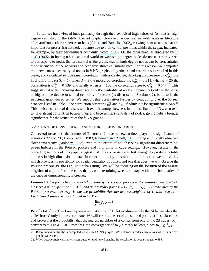
5.2.2 RATE OF CONVERGENCE AND THEROLE OF BOUNDARIES

On several occasions, the authors of Theorem 12 have somewhat downplayed the significance ofequations 22 and 23 (Tversky et al., 1983; Newman and Rinott, 1985), citing empirically observedslow convergence (Maloney, 1983), even to the extent of not observing significant differences be-tween hubness in the Poisson process and i.i.d. uniform cube settings. However, results in thepreceding sections of this paper suggest that this convergence is fastenough to produce notablehubness in high-dimensional data. In order to directly illustrate the difference between a settingwhich provides no possibility for spatial centrality of points, and one that does, we will observe thePoisson process vs. the i.i.d. unit cube setting. We will be focusing on the location of the nearestneighbor of a point from the cube, that is, on determining whether it stays within the boundaries ofthe cube as dimensionality increases.

Lemma 13 Let points be spread inRd according to a Poisson process with constant intensityλ > 1.Observe a unit hypercube C⊂R

d, and an arbitrary pointx = (x1,x2, . . . ,xd) ∈C, generated by thePoisson process. Let pλ,d denote the probability that the nearest neighbor ofx, with respect toEuclidean distance, is not situated in C. Then,

limd→∞

pλ,d = 1.

Proof Out of the 3d−1 unit hypercubes that surroundC, let us observe only the 2d hypercubes thatdiffer fromC only in one coordinate. We will restrict the set of considered points to these2d cubes,and prove that the probability that the nearest neighbor ofx comes from one of the 2d cubes,pλ,d,converges to 1 asd → ∞. From this, the convergence ofpλ,d directly follows, sincepλ,d ≥ pλ,d.

20. Betweenness centrality is computed on directedk-NN graphs. We obtained similar correlations when undirectedgraphs were used.

21. When betweenness centrality is computed on undirected graphs, the correlation is even stronger: 0.585.

2511

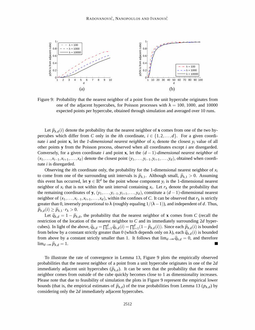
RADOVANOVI C, NANOPOULOS AND IVANOVI C

1 2 3 4 5 6 7 8 9 100

0.2

0.4

0.6

0.8

1

d

p(N

N is

from

adj

acen

t cub

e)

λ = 100λ = 1000λ = 10000

1 10 20 30 40 50 60 70 80 90 1000

0.2

0.4

0.6

0.8

1

d

p(N

N is

from

adj

acen

t cub

e)

λ = 100λ = 1000λ = 10000

(a) (b)

Figure 9: Probability that the nearest neighbor of a point from the unit hypercube originates fromone of the adjacent hypercubes, for Poisson processes withλ = 100, 1000, and 10000expected points per hypercube, obtained through simulation and averaged over 10 runs.

Let pλ,d(i) denote the probability that the nearest neighbor ofx comes from one of the two hy-percubes which differ fromC only in the ith coordinate,i ∈ {1,2, . . . ,d}. For a given coordi-natei and pointx, let the1-dimensional nearest neighborof xi denote the closestyi value of allother pointsy from the Poisson process, observed when all coordinates excepti are disregarded.Conversely, for a given coordinatei and pointx, let the(d− 1)-dimensional nearest neighborof(x1, . . . ,xi−1,xi+1, . . . ,xd) denote the closest point(y1, . . . ,yi−1,yi+1, . . . ,yd), obtained when coordi-natei is disregarded.

Observing theith coordinate only, the probability for the 1-dimensional nearest neighbor of xi

to come from one of the surrounding unit intervals ispλ,1. Although small,pλ,1 > 0. Assumingthis event has occurred, lety ∈ R

d be the point whose componentyi is the 1-dimensional nearestneighbor ofxi that is not within the unit interval containingxi . Let rλ denote the probability thatthe remaining coordinates ofy, (y1, . . . ,yi−1,yi+1, . . . ,yd), constitute a(d−1)-dimensional nearestneighbor of(x1, . . . ,xi−1,xi+1, . . . ,xd), within the confines ofC. It can be observed thatrλ is strictlygreater than 0, inversely proportional toλ (roughly equaling 1/(λ−1)), and independent ofd. Thus,pλ,d(i)≥ pλ,1 · rλ > 0.

Let qλ,d = 1− pλ,d, the probability that the nearest neighbor ofx comes fromC (recall therestriction of the location of the nearest neighbor toC and its immediately surrounding 2d hyper-cubes). In light of the above,qλ,d = ∏d

i=1 qλ,d(i) = ∏di=1(1− pλ,d(i)). Since eachpλ,d(i) is bounded

from below by a constant strictly greater than 0 (which depends only onλ), eachqλ,d(i) is boundedfrom above by a constant strictly smaller than 1. It follows that limd→∞ qλ,d = 0, and thereforelimd→∞ pλ,d = 1.

To illustrate the rate of convergence in Lemma 13, Figure 9 plots the empirically observedprobabilities that the nearest neighbor of a point from a unit hypercubeoriginates in one of the 2dimmediately adjacent unit hypercubes (pλ,d). It can be seen that the probability that the nearestneighbor comes from outside of the cube quickly becomes close to 1 as dimensionality increases.Please note that due to feasibility of simulation the plots in Figure 9 represent theempirical lowerbounds (that is, the empirical estimates ofpλ,d) of the true probabilities from Lemma 13 (pλ,d) byconsidering only the 2d immediately adjacent hypercubes.

2512

HUBS IN SPACE

The above indicates that when boundaries are introduced in high dimensions, the setting com-pletely changes, in the sense that new nearest neighbors need to be located inside the boundaries.Under such circumstances, points which are closer to the center have a better chance of becomingnearest neighbors, with the mechanism described in previous sections. Another implication of theabove observations, stemming from Figure 9, is that the number of dimensions does not need to bevery large compared to the number of points for the setting to change. As forboundaries, they canbe viewed as a dual notion to spatial centrality discussed earlier. With Poisson processes and cubesthis duality is rather straightforward, however for continuous distributionsin general there exist noboundaries in a strict mathematical sense. Nevertheless, since data sets contain a finite number ofpoints, it can be said that “practical” boundaries exist in this case as well.

6. Hubness and Dimensionality Reduction

In this section we elaborate further on the interplay of skewness ofNk and intrinsic dimensionalityby considering dimensionality-reduction (DR) techniques. The main questionmotivating the dis-cussion in this section is whether dimensionality reduction can alleviate the issue of the skewnessof k-occurrences altogether. We leave a more detailed and general investigation of the interactionbetween hubness and dimensionality reduction as a point of future work.

We examined the following methods: principal component analysis—PCA (Jolliffe, 2002), in-dependent component analysis—ICA (Hyvarinen and Oja, 2000), stochastic neighbor embedding—SNE (Hinton and Roweis, 2003), isomap (Tenenbaum et al., 2000), and diffusion maps (Lafon andLee, 2006; Nadler et al., 2006). Figure 10 depicts the relationship between the percentage of theoriginal number of features maintained by the DR methods andSNk, for several high-dimensionalreal data sets (musk1, mfeat-factors, and spectrometer; see Table 1) and i.i.d. uniform random data(with Euclidean distance,k= 10, and the same number of neighbors used for isomap and diffusionmaps). For PCA, ICA, SNE, and the real data sets, looking from right to left, SNk stays relativelyconstant until a small percentage of features is left, after which it suddenly drops (Figure 10(a–c)).It can be said that this is the point where the intrinsic dimensionality of data sets isreached, and fur-ther reduction of dimensionality may incur loss of valuable information. Such behavior is in contrastwith the case of i.i.d. uniform random data (full black line in Figure 10(a–c)), whereSNk steadilyand steeply reduces with the decreasing number of randomly selected features (dimensionality re-duction is not meaningful in this case), because intrinsic and embedded dimensionalities are equal.Since PCA is equivalent to metric multidimensional scaling (MDS) when Euclideandistances areused (Tenenbaum et al., 2000), and SNE is a variant of MDS which favors the preservation of dis-tances between nearby points, we can roughly regard the notion of intrinsic dimensionality used inthis paper as the minimal number of features needed to account for allpairwise distanceswithina data set. Although ICA does not attempt to explicitly preserve pairwise distances, combinationsof independent components produce skewness ofNk which behaves in a way that is similar to theskewness observed with PCA and SNE.

On the other hand, isomap and diffusion maps replace the original distanceswith distancesderived from a neighborhood graph. It can be observed in Figure 10(d, e) that such replacementgenerally reducesSNk, but in most cases does not alleviate it completely. With the decreasing numberof features, however,SNk of real data sets in Figure 10(d, e) still behaves in a manner more similarto SNk of real data sets for PCA, ICA, and SNE (Figure 10(a–c)) than i.i.d. random data (dash-dotblack line in Figure 10(d, e)).

2513

RADOVANOVI C, NANOPOULOS AND IVANOVI C

0 20 40 60 80 100−0.5

0

0.5

1

1.5

2PCA

Features (%)

SN

10

0 20 40 60 80 100−0.5

0

0.5

1

1.5

2ICA

Features (%)

SN

10

0 20 40 60 80 100−0.5

0

0.5

1

1.5

2SNE

Features (%)

SN

10

(a) (b) (c)

0 20 40 60 80 100−0.2

0

0.2

0.4

0.6Isomap

Features (%)

SN

10

0 20 40 60 80 100−0.5

0

0.5

1Diffusion Maps

Features (%)

SN

10

0 50100−10

12

musk1mfeat−factorsspectrometeriid uniform, d =15, no DRiid uniform, d = 9, no DR

(d) (e)

Figure 10: Skewness ofN10 in relation to the percentage of the original number of featuresmaintained by dimensionality reduction, for real and i.i.d. uniform random dataand(a) principal component analysis—PCA, (b) independent component analysis—ICA,(c) stochastic neighbor embedding—SNE, (d) isomap, and (e) diffusion maps.

The above observations signify that, if distances are not explicitly altered (as with isomap anddiffusion maps DR methods), that is, if one cares about preserving the original distances, dimension-ality reduction may not have a significant effect on hubness when the number of features is abovethe intrinsic dimensionality. This observation is useful in most practical casesbecause if dimension-ality is reduced below intrinsic dimensionality, loss of information can occur. Ifone still chooses toapply aggressive dimensionality reduction and let the resulting number of features fall below intrin-sic dimensionality, it can be expected of pairwise distances and nearest-neighbor relations betweenpoints in the data set to be altered, and hubness to be reduced or even lost.Whether these effectsshould be actively avoided or sought really depends on the application domain and task at hand, thatis, whether and to what degree the original pairwise distances represent valuable information, andhow useful are the new distances and neighborhoods after dimensionalityreduction.

7. The Impact of Hubness on Machine Learning

The impact of hubness on machine-learning applications has not been thoroughly investigated so far.In this section we examine a wide range of commonly used machine-learning methods for super-vised (Section 7.1), semi-supervised (Section 7.2), and unsupervised learning (Section 7.3), thateither directly or indirectly use distances in the process of building a model. Ourmain objective isto demonstrate that hubs (as well as their opposites, antihubs) can have a significant effect on thesemethods. The presented results highlight the need to take hubs into accountin a way equivalent toother factors, such as the existence of outliers, the role of which has been well studied.

2514

HUBS IN SPACE

7.1 Supervised Learning

To investigate possible implications of hubness on supervised learning, we first study the interactionof k-occurrences with information provided by labels (Section 7.1.1). We then move on to examinethe effects of hubness on several well-known classification algorithms in Section 7.1.2.

7.1.1 “GOOD” AND “B AD” k-OCCURRENCES

When labels are present,k-occurrences can be distinguished based on whether labels of neighborsmatch. We define the number of“bad” k-occurrencesof x, BNk(x), as the number of points fromdata setD for which x is among the firstk NNs, and the labels ofx and the points in questiondo not match. Conversely,GNk(x), the number of“good” k-occurrencesof x, is the number ofsuch points where labels do match. Naturally, for everyx ∈ D, Nk(x) = BNk(x)+GNk(x).

To account for labels, Table 1 includesBN10 (14th column), the sum of all observed “bad”k-occurrences of a data set normalized by∑x N10(x) = 10n. This measure is intended to express thetotal amount of “bad”k-occurrences within a data set. Also, to express the amount of informationthat “regular”k-occurrences contain about “bad”k-occurrences in a particular data set,CN10

BN10(15th

column) denotes the Spearman correlation betweenBN10 andN10 vectors. The motivation behindthis measure is to express the degree to whichBNk andNk follow a similar distribution.

“Bad” hubs, that is, points with highBNk, are of particular interest to supervised learning be-cause they carry more information about the location of the decision boundaries than other points,and affect classification algorithms in different ways (as will be described in Section 7.1.2). Tounderstand the origins of “bad” hubs in real data, we rely on the notion ofthecluster assumptionfrom semi-supervised learning (Chapelle et al., 2006), which roughly states that most pairs of pointsin a high density region (cluster) should be of the same class. To measure thedegree to which thecluster assumption is violated in a particular data set, we simply define thecluster assumption vi-olation (CAV) coefficient as follows. Leta be the number of pairs of points which are in differentclasses but in the same cluster, andb the number of pairs of points which are in the same class andcluster. Then, we define

CAV =a

a+b,

which gives a number in the[0,1] range, higher if there is more violation. To reduce the sensitivityof CAV to the number of clusters (too low and it will be overly pessimistic, too highand it willbe overly optimistic), we choose the number of clusters to be 3 times the number ofclasses of aparticular data set. Clustering is performed withK-means.

For all examined real data sets, we computed the Spearman correlation between the total amountof “bad” k-occurrences,BN10, and CAV (16th column of Table 1) and found it strong (0.85, see Ta-ble 2). Another significant correlation (0.39) is observed betweenCN10

BN10and intrinsic dimensionality.

In contrast,BN10 and CAV are not correlated with intrinsic dimensionality nor with the skewness ofN10. The latter fact indicates that high dimensionality and skewness ofNk are not sufficient to induce“bad” hubs. Instead, based on the former fact, we can argue that there are two, mostly independent,forces at work: violation of the cluster assumption on one hand, and high intrinsic dimensionality onthe other. “Bad” hubs originate from putting the two together; that is, the consequences of violatingthe cluster assumption can be more severe in high dimensions than in low dimensions, not in termsof the total amount of “bad”k-occurrences, but in terms of their distribution, since strong regularhubs are now more prone to “pick up” badk-occurrences than non-hub points. This is supported by

2515

RADOVANOVI C, NANOPOULOS AND IVANOVI C

the positive correlation betweenCN10BN10

and intrinsic dimensionality, meaning that in high dimensionsBNk tends to follow a more similar distribution toNk than in low dimensions.

7.1.2 INFLUENCE ONCLASSIFICATION ALGORITHMS

We now examine how skewness ofNk and the existence of (“bad”) hubs affects well-known clas-sification techniques, focusing on thek-nearest neighbor classifier (k-NN), support vector ma-chines (SVM), and AdaBoost. We demonstrate our findings on a selection of data sets from Table 1which have relatively high (intrinsic) dimensionality, and a non-negligible amount of “badness”(BNk) and cluster assumption violation (CAV). Generally, the examined classification algorithms(including semi-supervised learning from Section 7.2) exhibit similar behavior on other data setsfrom Table 1 with the aforementioned properties, and also with various different values ofk (in thegeneral range 1–50, as we focused on values ofk which are significantly smaller than the numberof points in a data set).

k-nearest neighbor classifier.The k-nearest neighbor classifier is negatively affected by thepresence of “bad” hubs, because they provide erroneous class information to many other points. Tovalidate this assumption, we devised a simple weighting scheme. For each pointx, we compute itsstandardized “bad” hubness score:

hB(x,k) =BNk(x)−µBNk

σBNk

,

whereµBNk andσBNk are the mean and standard deviation ofBNk, respectively. During majorityvoting in thek-NN classification phase, when pointx participates in thek-NN list of the point beingclassified, the vote ofx is weighted by

wk(x) = exp(−hB(x,k)),

thus lowering the influence of “bad” hubs on the classification decision. Figure 11 compares theresulting accuracy ofk-NN classifier with and without this weighting scheme for six data sets fromTable 1. Leave-one-out cross-validation is performed, with Euclidean distance being used for de-termining nearest neighbors. Thek value forNk is naturally set to thek value used by thek-NNclassifier, andhB(x,k) is recomputed for the training set of each fold. The reduced accuracy of theunweighted scheme signifies the negative influence of “bad” hubs.

Although “bad” hubs tend to carry more information about the location of class boundariesthan other points, the “model” created by thek-NN classifier places the emphasis on describingnon-borderline regions of the space occupied by each class. For this reason, it can be said that“bad” hubs are truly bad fork-NN classification, creating the need to penalize their influence onthe classification decision. On the other hand, for classifiers that explicitly model the borders be-tween classes, such as support vector machines, “bad” hubs can represent points which contributeinformation to the model in a positive way, as will be discussed next.

Support vector machines.We consider SVMs with the RBF (Gaussian) kernel of the form:

K(x,y) = exp(−γ‖x−y‖2) ,

whereγ is a data-dependent constant.K(x,y) is a smooth monotone function of Euclidean distancebetween points. Therefore,Nk values in the kernel space are exactly the same as in the original

2516

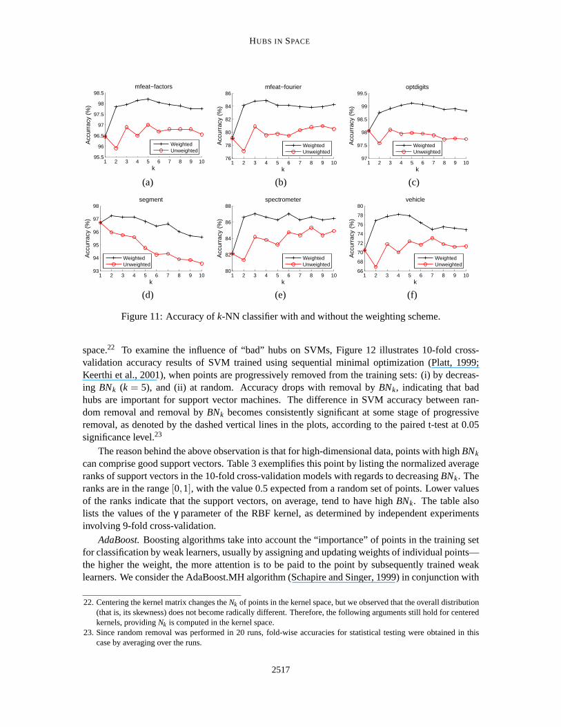
HUBS IN SPACE

1 2 3 4 5 6 7 8 9 1095.5

96

96.5

97

97.5

98

98.5mfeat−factors

k

Acc

urra

cy (

%)

WeightedUnweighted

1 2 3 4 5 6 7 8 9 1076

78

80

82

84

86mfeat−fourier

k

Acc

urra

cy (

%)

WeightedUnweighted

1 2 3 4 5 6 7 8 9 1097

97.5

98

98.5

99

99.5optdigits

k

Acc

urra

cy (

%)

WeightedUnweighted

(a) (b) (c)

1 2 3 4 5 6 7 8 9 1093

94

95

96

97

98segment

k

Acc

urra

cy (

%)

WeightedUnweighted

1 2 3 4 5 6 7 8 9 1080

82

84

86

88spectrometer

k

Acc

urra

cy (

%)

WeightedUnweighted

1 2 3 4 5 6 7 8 9 1066

68

70

72

74

76

78

80vehicle

k

Acc

urra

cy (

%)

WeightedUnweighted

(d) (e) (f)

Figure 11: Accuracy ofk-NN classifier with and without the weighting scheme.

space.22 To examine the influence of “bad” hubs on SVMs, Figure 12 illustrates 10-fold cross-validation accuracy results of SVM trained using sequential minimal optimization (Platt, 1999;Keerthi et al., 2001), when points are progressively removed from thetraining sets: (i) by decreas-ing BNk (k = 5), and (ii) at random. Accuracy drops with removal byBNk, indicating that badhubs are important for support vector machines. The difference in SVMaccuracy between ran-dom removal and removal byBNk becomes consistently significant at some stage of progressiveremoval, as denoted by the dashed vertical lines in the plots, according to thepaired t-test at 0.05significance level.23

The reason behind the above observation is that for high-dimensional data, points with highBNk

can comprise good support vectors. Table 3 exemplifies this point by listing the normalized averageranks of support vectors in the 10-fold cross-validation models with regards to decreasingBNk. Theranks are in the range[0,1], with the value 0.5 expected from a random set of points. Lower valuesof the ranks indicate that the support vectors, on average, tend to havehigh BNk. The table alsolists the values of theγ parameter of the RBF kernel, as determined by independent experimentsinvolving 9-fold cross-validation.

AdaBoost.Boosting algorithms take into account the “importance” of points in the training setfor classification by weak learners, usually by assigning and updating weights of individual points—the higher the weight, the more attention is to be paid to the point by subsequently trained weaklearners. We consider the AdaBoost.MH algorithm (Schapire and Singer,1999) in conjunction with

22. Centering the kernel matrix changes theNk of points in the kernel space, but we observed that the overall distribution(that is, its skewness) does not become radically different. Therefore, the following arguments still hold for centeredkernels, providingNk is computed in the kernel space.

23. Since random removal was performed in 20 runs, fold-wise accuracies for statistical testing were obtained in thiscase by averaging over the runs.

2517

RADOVANOVI C, NANOPOULOS AND IVANOVI C

0 10 20 30 40 50

96.8

97

97.2

97.4

97.6mfeat−factors

Points removed (%)

Acc

urra

cy (

%)

BN5 rem.

Rnd. rem

0 10 20 30 40 5074

76

78

80

82

84mfeat−fourier

Points removed (%)

Acc

urra

cy (

%)

BN5 rem.

Rnd. rem

0 10 20 30 40 50

97.6

97.8

98

98.2

98.4

98.6

98.8optdigits

Points removed (%)

Acc

urra

cy (

%)

BN5 rem.

Rnd. rem

(a) (b) (c)

0 10 20 30 40 5090

91

92

93

94

95

96segment

Points removed (%)

Acc

urra

cy (

%)

BN5 rem.

Rnd. rem

0 10 20 30 40 5083

84

85

86

87

88spectrometer

Points removed (%)

Acc

urra

cy (

%)

BN5 rem.

Rnd. rem

0 10 20 30 40 5068

70

72

74

76

78vehicle

Points removed (%)

Acc

urra

cy (

%)

BN5 rem.

Rnd. rem

(d) (e) (f)

Figure 12: Accuracy of SVM with RBF kernel and points being removed from the training sets bydecreasingBN5, and at random (averaged over 20 runs).

Data set γ SV rank Data set γ SV rankmfeat-factors 0.005 0.218 segment 0.3 0.272mfeat-fourier 0.02 0.381 spectrometer 0.005 0.383optdigits 0.02 0.189 vehicle 0.07 0.464

Table 3: Normalized average support vector ranks with regards to decreasingBN5.

CART trees (Breiman et al., 1984) with the maximal depth of three.24 We define for each pointx itsstandardized hubnessscore:

h(x,k) =Nk(x)−µNk

σNk

, (24)

whereµNk, σNk are the mean and standard deviation ofNk, respectively. We set the initial weight ofeach pointx in the training set to

wk(x) =1

1+ |h(x,k)| ,

normalized by the sum over all points, for an empirically determined value ofk. The motivationbehind the weighting scheme is to assign less importance to both hubs and outliersthan other points(this is why we take the absolute value ofh(x,k)).

Figure 13 illustrates on six classification problems from Table 1 how the weighting scheme helpsAdaBoost achieve better generalization in fewer iterations. The data sets were split into training,

24. More precisely, we use the binary “Real AdaBoost” algorithm and theone-vs-all scheme to handle multi-class prob-lems, which is equivalent to the original AdaBoost.MH (Friedman et al., 2000).

2518

HUBS IN SPACE

validation, and test sets with size ratio 2:1:1, parameterk was chosen based on classification ac-curacy on the validation sets, and accuracies on the test sets are reported. While it is known thatAdaBoost is sensitive to outliers (Ratsch et al., 2001), improved accuracy suggests that hubs shouldbe regarded in an analogous manner, that is, both hubs and antihubs areintrinsically more difficultto classify correctly, and the attention of the weak learners should initially be focused on “regu-lar” points. The discussion from Section 4.4, about hubs corresponding to probabilistic outliers inhigh-dimensional data, offers an explanation for the observed good performance of the weightingscheme, as both hubs and antihubs can be regarded as (probabilistic) outliers.

To provide further support, Figure 14 depicts binned accuracies of unweighted AdaBoost trainedin one fifth of the iterations shown in Figure 13, for points sorted by decreasing Nk. It illustrateshow in earlier phases of ensemble training the generalization power with hubsand/or antihubs isworse than with regular points. Moreover, for the considered data sets itis actually the hubs thatappear to cause more problems for AdaBoost than antihubs (that is, distance-based outliers).

7.2 Semi-Supervised Learning

Semi-supervised learning algorithms make use of data distribution information provided by unla-beled examples during the process of building a classifier model. An importantfamily of approachesare graph-based methods, which represent data as nodes of a graph, the edges of which are weightedby pairwise distances of incident nodes (Chapelle et al., 2006).

We consider the well-known algorithm by Zhu et al. (2003), whose strategy involves computinga real-valued functionf on graph nodes, and assign labels to nodes based on its values. Functionf ,which exhibits harmonic properties, is obtained by optimizing a quadratic energy function thatinvolves graph edge weights, with the probability distribution on the space of functions f formedusing Gaussian fields. For data pointsx,y ∈ R

d we consider edge weights assigned by the radialbasis function (RBF) of the following form:

W(x,y) = exp

(−‖x−y‖2

σ2

),

whereσ is a data-dependent constant. Therefore, large edge weights are assigned between nodesthat are close to one another with respect to Euclidean distance.

Taking into account the properties of hubs and antihubs discussed in previous sections, for high-dimensional data sets it can be expected of hubs to be closer to many other points than “regular”points are, and thus carry larger edge weights and be more influential in theprocess of determiningthe optimal functionf . Conversely, antihubs are positioned farther away from other points, andare expected to bear less influence on the computation off . Therefore, following an approach thatresembles active learning, selecting the initial labeled point set from hubs could be more beneficialin terms of classification accuracy than arbitrarily selecting the initial points to belabeled. On theother extreme, picking the initial labeled point set from the ranks of antihubs could be expected tohave a detrimental effect on accuracy.

To validate the above hypothesis, we evaluated the accuracy of the harmonic function algorithmby Zhu et al. (2003) on multiple high-dimensional data sets from Table 1, forlabeled set sizesranging from 1% to 10% of the original data set size, with the test set consisting of all remainingunlabeled points. Because the setting is semi-supervised, we compute theNk scores of points basedon complete data sets, instead of only training sets which was the case in Section7.1.2. Based on

2519

RADOVANOVI C, NANOPOULOS AND IVANOVI C

10 20 30 40 5090

92

94

96

98mfeat−factors

Iterations

Acc

urra

cy (

%)

WeightedUnweighted

10 20 30 40 50 6072

74

76

78

80

82mfeat−fourier

Iterations

Acc

urra

cy (

%)

WeightedUnweighted

20 40 60 80 10075

80

85

90

95

100optdigits

Iterations

Acc

urra

cy (

%)

WeightedUnweighted

(a) (b) (c)

10 20 30 4093.5

94

94.5

95

95.5

96

96.5segment

Iterations

Acc

urra

cy (

%)

WeightedUnweighted

10 20 30 40 50 60 7075

80

85

90spectrometer

Iterations

Acc

urra

cy (

%)

WeightedUnweighted

20 40 60 80 10068

70

72

74

76

78

80vehicle

Iterations

Acc

urra

cy (

%)

WeightedUnweighted

(d) (e) (f)

Figure 13: Accuracy of AdaBoost with and without the weighting scheme: (a) k = 20, (b)k = 15,(c) k= 10, (d)k= 20, (e)k= 20, (f) k= 40.

1 2 3 4 5 660

70

80

90

100mfeat−factors

(hubs) Bins by decreasing Nk (outliers)

Acc

urra

cy (

%)

1 2 3 4 5 660

65

70

75

80mfeat−fourier

(hubs) Bins by decreasing Nk (outliers)

Acc

urra

cy (

%)

1 2 3 4 5 660

70

80

90

100optdigits

(hubs) Bins by decreasing Nk (outliers)

Acc

urra

cy (

%)

(a) (b) (c)

1 2 3 4 5 680

85

90

95

100segment

(hubs) Bins by decreasing Nk (outliers)

Acc

urra

cy (

%)

1 2 3 4 5 660

70

80

90

100spectrometer

(hubs) Bins by decreasing Nk (outliers)

Acc

urra

cy (

%)

1 2 3 4 5 660

65

70

75

80vehicle

(hubs) Bins by decreasing Nk (outliers)

Acc

urra

cy (

%)

(d) (e) (f)

Figure 14: Binned accuracy of AdaBoost by decreasingNk, at one fifth of the iterations shown inFigure 13.

2520

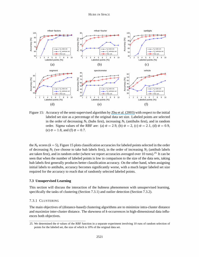
HUBS IN SPACE

1 2 3 4 5 6 7 8 9 1050

60

70

80

90

100mfeat−factors

Labeled points (%)

Acc

urra

cy (

%)

N5 hubs sel.

N5 antihubs sel.

Rnd. sel.

1 2 3 4 5 6 7 8 9 100

20

40

60

80mfeat−fourier

Labeled points (%)

Acc

urra

cy (

%)

N5 hubs sel.

N5 antihubs sel.

Rnd. sel.

1 2 3 4 5 6 7 8 9 1040

50

60

70

80

90

100optdigits

Labeled points (%)

Acc

urra

cy (

%)

N5 hubs sel.

N5 antihubs sel.

Rnd. sel.

(a) (b) (c)

1 2 3 4 5 6 7 8 9 10

50

60

70

80

segment

Labeled points (%)

Acc

urra

cy (

%)

N5 hubs sel.

N5 antihubs sel.

Rnd. sel.

1 2 3 4 5 6 7 8 9 1020

30

40

50

60

70

80

90spectrometer

Labeled points (%)

Acc

urra

cy (

%)

N5 hubs sel.

N5 antihubs sel.

Rnd. sel.

1 2 3 4 5 6 7 8 9 10

30

35

40

45

50

55

60

vehicle

Labeled points (%)

Acc

urra

cy (

%)

N5 hubs sel.

N5 antihubs sel.

Rnd. sel.

(d) (e) (f)

Figure 15: Accuracy of the semi-supervised algorithm by Zhu et al. (2003) with respect to the initiallabeled set size as a percentage of the original data set size. Labeled points are selectedin the order of decreasingN5 (hubs first), increasingN5 (antihubs first), and in randomorder. Sigma values of the RBF are: (a)σ = 2.9, (b) σ = 2, (c) σ = 2.1, (d) σ = 0.9,(e) σ = 1.8, and (f)σ = 0.7.

theNk scores (k= 5), Figure 15 plots classification accuracies for labeled points selected in the orderof decreasingN5 (we choose to take hub labels first), in the order of increasingN5 (antihub labelsare taken first), and in random order (where we report accuracies averaged over 10 runs).25 It can beseen that when the number of labeled points is low in comparison to the size of thedata sets, takinghub labels first generally produces better classification accuracy. On the other hand, when assigninginitial labels to antihubs, accuracy becomes significantly worse, with a much larger labeled set sizerequired for the accuracy to reach that of randomly selected labeled points.

7.3 Unsupervised Learning

This section will discuss the interaction of the hubness phenomenon with unsupervised learning,specifically the tasks of clustering (Section 7.3.1) and outlier detection (Section 7.3.2).

7.3.1 CLUSTERING

The main objectives of (distance-based) clustering algorithms are to minimize intra-cluster distanceand maximize inter-cluster distance. The skewness ofk-occurrences in high-dimensional data influ-ences both objectives.

25. We determined theσ values of the RBF function in a separate experiment involving 10 runs of random selection ofpoints for the labeled set, the size of which is 10% of the original data set.

2521

RADOVANOVI C, NANOPOULOS AND IVANOVI C

Intra-cluster distance may be increased due to points with lowk-occurrences. As discussedin Section 4.4, such points are far from all the rest, acting as distance-based outliers. Distance-based outliers and their influence on clustering are well-studied subjects (Tan et al., 2005): outliersdo not cluster well because they have high intra-cluster distance, thus they are often discoveredand eliminated beforehand. The existence of outliers is attributed to various reasons (for example,erroneous measurements). Nevertheless, the skewness ofNk suggests that in high-dimensional dataoutliers are also expected due to inherent properties of vector space. Section 7.3.2 will providefurther discussion on this point.

Inter-cluster distance, on the other hand, may be reduced due to points withhighk-occurrences,that is, hubs. Like outliers, hubs do not cluster well, but for a differentreason: they have lowinter-cluster distance, because they are close to many points, thus also to points from other clusters.In contrast to outliers, the influence of hubs on clustering has not attracted significant attention.

To examine the influence of both outliers and hubs, we used the popular silhouette coeffi-cients (SC) (Tan et al., 2005). For theith point, letai be the average distance to all points in its cluster(ai corresponds to intra-cluster distance), andbi the minimum average distance to points from otherclusters (bi corresponds to inter-cluster distance). The SC of theith point is(bi −ai)/max(ai ,bi),ranging between−1 and 1 (higher values are preferred). The SC of a set of points is obtained byaveraging the silhouette coefficients of the individual points.

We examined several clustering algorithms, and report results for the spectral algorithm of Meilaand Shi (2001) and Euclidean distance, with similar results obtained for classicalK-means, as wellas the spectral clustering algorithm by Ng et al. (2002) in conjunction withK-means and the algo-rithm by Meila and Shi (2001). For a given data set, we set the number of clusters,K, to the numberof classes (specified in Table 1). We select as hubs those pointsx with h(x,k) > 2, that is,Nk(x)more than two standard deviations higher than the mean (note thath(x,k), defined by Equation 24,ignores labels). Letnh be the number of hubs selected. Next, we select as outliers thenh pointswith the lowestk-occurrences. Finally, we randomly selectnh points from the remaining points (wereport averages for 100 different selections). To compare hubs and antihubs against random points,we measure therelative SCof hubs (antihubs): the mean SC of hubs (antihubs) divided by the meanSC of random points. For several data sets from Table 1, Figure 16 depicts with bars the relativesilhouette coefficients.26 As expected, outliers have relative SC lower than one, meaning that theycluster worse than random points. Notably, the same holds for hubs, too.27

To gain further insight, Figure 16 plots with lines (referring to the right vertical axes) the relativemean values ofai andbi for hubs and outliers (dividing with those of randomly selected points).Outliers have high relativeai values, indicating higher intra-cluster distance. Hubs, in contrast,have low relativebi values, indicating reduced inter-cluster distance. In conclusion, when clusteringhigh-dimensional data, hubs should receive analogous attention as outliers.

7.3.2 OUTLIER DETECTION

This section will briefly discuss possible implications of high dimensionality on distance-based out-lier detection, in light of the findings concerning the hubness phenomenon presented in previoussections. Section 4.4 already discussed the correspondence of antihubs with distance-based outliers

26. Data sets were selected due to their high (intrinsic) dimensionality—similar observations can be made with otherhigh-dimensional data sets from Table 1.

27. The statistical significance of differences between the SC of hubs and randomly selected points has been verified withthe paired t-test at 0.05 significance level.

2522

HUBS IN SPACE

Figure 16: Relative silhouette coefficients for hubs (gray filled bars) and outliers (empty bars). Rel-ative values fora andb coefficients are also plotted (referring to the right vertical axes).

in high dimensions, and demonstrated on real data the negative correlation betweenNk and a com-monly used outlier score—distance to thekth nearest neighbor. On the other hand, a prevailingview of the effect of high dimensionality on distance-based outlier detection isthat, due to distanceconcentration, every point seems to be an equally good outlier, thus hindering outlier-detection al-gorithms (Aggarwal and Yu, 2001). Based on the observations regarding hubness and the behaviorof distances discussed earlier, we believe that the true problem actually liesin the opposite extreme:high dimensionality induces antihubs that can represent “artificial” outliers.This is because, fromthe point of view of common distance-based outlier scoring schemes, antihubs may appear to bestronger outliers in high dimensions than in low dimensions, only due to the effects of increasingdimensionality of data.

To illustrate the above discussion, Figure 17(a) plots for i.i.d. uniform random data the highestand lowest outlier score (distance to thekth NN, k = 5) with respect to increasingd (n = 10000points, averages over 10 runs are reported). In accordance with theasymptotic behavior of all pair-wise distances discussed in previous sections, both scores increase withd. However, as Figure 17(b)shows, thedifferencebetween the two scores also increases. This implies that a point could be con-sidered a distance-based outlier only because of high dimensionality, sinceoutliers are not expectedfor any other reason in i.i.d. uniform data (we already demonstrated that such a point would mostlikely be an antihub). As a consequence, outlier-detection methods based on measuring distancesbetween points may need to be adjusted to account for the (intrinsic) dimensionality of data, in orderto prevent dimensionality-induced false positives.

8. Conclusion

In this paper we explored an aspect of the curse of dimensionality that is manifested through thephenomenon of hubness—the tendency of high-dimensional data sets to contain hubs, in the senseof popular nearest neighbors of other points. To the best of our knowledge, hubs and the effects they

2523

RADOVANOVI C, NANOPOULOS AND IVANOVI C

0 20 40 60 80 1000

1

2

3

4

d

Out

lier

scor

e

iid uniform: highest and lowest outlier score

Highest scoreLowest score

0 20 40 60 80 1000

0.1

0.2

0.3

0.4

0.5

0.6

0.7

d

Hig

hest

−lo

wes

t out

lier

scor

e

iid uniform: outlier score difference

(a) (b)

Figure 17: (a) Highest and lowest distance to the 5th nearest neighbor ini.i.d. uniform random data,with respect to increasingd. (b) The difference between the two distances.

have on machine-learning techniques have not been thoroughly studied subjects. Through theoret-ical and empirical analysis involving synthetic and real data sets we demonstrated the emergenceof the phenomenon and explained its origins, showing that it is an inherent property of data dis-tributions in high-dimensional vector space that depends on the intrinsic, rather than embeddingdimensionality of data. We also discussed the interaction of hubness with dimensionality reduction.Moreover, we explored the impact of hubness on a wide range of machine-learning tasks that di-rectly or indirectly make use of distances between points, belonging to supervised, semi-supervised,and unsupervised learning families, demonstrating the need to take hubnessinto account in an equiv-alent degree to other factors, like the existence of outliers.

Besides application areas that involve audio and image data (Aucouturier and Pachet, 2007;Doddington et al., 1998; Berenzweig, 2007; Hicklin et al., 2005), identifying hubness within dataand methods from other fields can be considered an important aspect of future work, as well as de-signing application-specific methods to mitigate or take advantage of the phenomenon. We alreadyestablished the existence of hubness and its dependence on data dimensionality on collaborativefiltering data with commonly used variants of cosine distance (Nanopoulos et al., 2009), time-seriesdata sets in the context ofk-NN classification involving dynamic time warping (DTW) distance(Radovanovic et al., 2010b), text data within several variations of the classical vectorspace modelfor information retrieval (Radovanovic et al., 2010a), and audio data for music information retrievalusing spectral similarity measures (Karydis et al., 2010). In the immediate future we plan to performa more detailed investigation of hubness in the fields of outlier detection and imagemining. An-other application area that could directly benefit from an investigation into hubness are reversek-NNqueries (which retrieve data points that have the query pointq as one of theirk nearest neighbors,Tao et al., 2007).

One concern we elected not to include into the scope of this paper is the efficiency of com-puting Nk. It would be interesting to explore the interaction between approximatek-NN graphs(Chen et al., 2009) and hubness, in both directions: to what degree do approximatek-NN graphspreserve hubness information, and can hubness information be used to enhance the computation ofapproximatek-NN graphs for high-dimensional data (in terms of both speed and accuracy).

Possible directions for future work within different aspects of machine learning include a moreformal and theoretical study of the interplay between hubness and various distance-based machine-

2524

HUBS IN SPACE

learning models, possibly leading to approaches that account for the phenomenon at a deeper level.Supervised learning methods may deserve special attention, as it was also observed in another study(Caruana et al., 2008) that thek-NN classifier and boosted decision trees can experience problems inhigh dimensions. Further directions of research may involve determining whether the phenomenonis applicable to probabilistic models, (unboosted) decision trees, and other techniques not explicitlybased on distances between points; and also to algorithms that operate within general metric spaces.Since we determined that forK-means clustering of high-dimensional data hubs tend to be closeto cluster centers, it would be interesting to explore whether this can be usedto improve iterativeclustering algorithms, likeK-means or self-organizing maps (Kohonen, 2001). Nearest-neighborclustering (Bubeck and von Luxburg, 2009) of high-dimensional data may also directly benefit fromhubness information. Topics that could also be worth further study are theinterplay of hubness withlearned metrics (Weinberger and Saul, 2009) and dimensionality reduction,including supervised(Vlassis et al., 2002; Geng et al., 2005), semi-supervised (Zhang et al.,2007), and unsupervisedapproaches (van der Maaten et al., 2009; Kumar, 2009). Finally, as wedetermined high correlationbetween intrinsic dimensionality and the skewness ofNk, it would be interesting to see whethersome measure of skewness of the distribution ofNk can be used for estimation of the intrinsicdimensionality of a data set.

Acknowledgments

We would like to thank the authors of all software packages, libraries, andresources used in thisresearch: Matlab with the Statistics Toolbox, Dimensionality Reduction Toolbox (van der Maaten,2007), the FastICA package (Gavert et al., 2005), GML AdaBoost Toolbox (Vezhnevets, 2006),code for semi-supervised learning with the basic harmonic function (Zhu etal., 2003), SpectraLIBpackage for symmetric spectral clustering (Verma, 2003; Meila and Shi, 2001), MatlabBGL graphlibrary (Gleich, 2008); the Weka machine-learning toolkit (Witten and Frank, 2005), and WolframMathematica with invaluable online resources MathWorld (mathworld.wolfram.com/)and the Wol-fram Functions Site (functions.wolfram.com/).

We would like to express our gratitude to the action editor, Ulrike von Luxburg, and the anony-mous reviewers, for helping to significantly improve the article with their detailed and thoughtfulcomments. We are also indebted to Zagorka Lozanov-Crvenkovic for helpful discussions and sug-gestions regarding the mathematical aspects of the paper.

Milo s Radovanovic and Mirjana Ivanovic thank the Serbian Ministry of Science for supportthrough projectAbstract Methods and Applications in Computer Science, no. 144017A. AlexandrosNanopoulos gratefully acknowledges the partial co-funding of his workthrough the European Com-mission FP7 projectMyMedia(www.mymediaproject.org/) under the grant agreement no. 215006.

References

Milton Abramowitz and Irene A. Stegun, editors.Handbook of Mathematical Functions With For-mulas, Graphs and Mathematical Tables. National Bureau of Standards, USA, 1964.

Charu C. Aggarwal and Philip S. Yu. Outlier detection for high dimensional data. InProceedings ofthe 27th ACM SIGMOD International Conference on Management of Data, pages 37–46, 2001.

2525

RADOVANOVI C, NANOPOULOS AND IVANOVI C

Charu C. Aggarwal, Alexander Hinneburg, and Daniel A. Keim. On the surprising behavior ofdistance metrics in high dimensional spaces. InProceedings of the 8th International Conferenceon Database Theory (ICDT), volume 1973 ofLecture Notes in Computer Science, pages 420–434. Springer, 2001.

Reka Albert and Albert-Laszlo Barabasi. Statistical mechanics of complex networks.Reviews ofModern Physics, 74(1):47–97, 2002.

Jean-Julien Aucouturier and Francois Pachet. A scale-free distributionof false positives for a largeclass of audio similarity measures.Pattern Recognition, 41(1):272–284, 2007.

Richard E. Bellman.Adaptive Control Processes: A Guided Tour. Princeton University Press, 1961.

Adam Berenzweig.Anchors and Hubs in Audio-based Music Similarity. PhD thesis, ColumbiaUniversity, New York, USA, 2007.

Kevin S. Beyer, Jonathan Goldstein, Raghu Ramakrishnan, and Uri Shaft. When is “nearest neigh-bor” meaningful? InProceedings of the 7th International Conference on Database Theory(ICDT), volume 1540 ofLecture Notes in Computer Science, pages 217–235. Springer, 1999.

Christopher M. Bishop.Neural Networks for Pattern Recognition. Oxford University Press, 1996.

Christopher M. Bishop.Pattern Recognition and Machine Learning. Springer, 2006.

Leo Breiman, Jerome H. Friedman, Richard A. Olshen, and Charles J. Stone. Classification andRegression Trees. Chapman & Hall, 1984.

Sebastien Bubeck and Ulrike von Luxburg. Nearest neighbor clustering: A baseline method forconsistent clustering with arbitrary objective functions.Journal of Machine Learning Research,10:657–698, 2009.

Rich Caruana, Nikos Karampatziakis, and Ainur Yessenalina. An empiricalevaluation of supervisedlearning in high dimensions. InProceedings of the 25th International Conference on MachineLearning (ICML), pages 96–103, 2008.

Olivier Chapelle, Bernhard Scholkopf, and Alexander Zien, editors.Semi-Supervised Learning.The MIT Press, 2006.

Jie Chen, Haw ren Fang, and Yousef Saad. Fast approximatekNN graph construction for highdimensional data via recursive Lanczos bisection.Journal of Machine Learning Research, 10:1989–2012, 2009.

Pierre Demartines.Analyse de Donnees par Reseaux de Neurones Auto-Organises. PhD thesis,Institut national polytechnique de Grenoble, Grenoble, France, 1994.

George Doddington, Walter Liggett, Alvin Martin, Mark Przybocki, and Douglas Reynolds.SHEEP, GOATS, LAMBS and WOLVES: A statistical analysis of speaker performance in theNIST 1998 speaker recognition evaluation. InProceedings of the 5th International Conferenceon Spoken Language Processing (ICSLP), 1998. Paper 0608.

2526

HUBS IN SPACE

Robert J. Durrant and Ata Kaban. When is ‘nearest neighbour’ meaningful: A converse theoremand implications.Journal of Complexity, 25(4):385–397, 2009.

Paul Erdos and Alfred Renyi. On random graphs.Publicationes Mathematicae Debrecen, 6:290–297, 1959.

Paul F. Evangelista, Mark J. Embrechts, and Boleslaw K. Szymanski. Taming the curse of dimen-sionality in kernels and novelty detection. In A. Abraham, B. Baets, M. Koppen, and B. Nickolay,editors,Applied Soft Computing Technologies: The Challenge of Complexity, volume 34 ofAd-vances in Soft Computing, pages 425–438. Springer, 2006.

Damien Francois.High-dimensional Data Analysis: Optimal Metrics and Feature Selection. PhDthesis, Universite catholique de Louvain, Louvain, Belgium, 2007.

Damien Francois, Vincent Wertz, and Michel Verleysen. The concentration of fractional distances.IEEE Transactions on Knowledge and Data Engineering, 19(7):873–886, 2007.

Jerome Friedman, Trevor Hastie, and Robert Tibshirani. Additive logistic regression: A statisticalview of boosting.The Annals of Statistics, 28(2):337–374, 2000.

Yasunori Fujikoshi. Computable error bounds for asymptotic expansionsof the hypergeometricfunction1F1 of matrix argument and their applications.Hiroshima Mathematical Journal, 37(1):13–23, 2007.

Hugo Gavert, Jarmo Hurri, Jaakko Sarela, and Aapo Hyvarinen. The FastICA package for Matlab.http://www.cis.hut.fi/projects/ica/fastica/, 2005.

Xin Geng, De-Chuan Zhan, and Zhi-Hua Zhou. Supervised nonlinear dimensionality reduction forvisualization and classification.IEEE Transactions on Systems, Man, and Cybernetics, Part B:Cybernetics, 35(6):1098–1107, 2005.

David Gleich. MatlabBGL: A Matlab graph library.http://www.stanford.edu/∼dgleich/programs/matlabbgl/, 2008.

Uffe Haagerup. The best constants in the Khintchine inequality.Studia Mathematica, 70:231–283,1982.

Trevor Hastie, Robert Tibshirani, and Jerome Friedman.The Elements of Statistical Learning: DataMining, Inference, and Prediction. Springer, 2nd edition, 2009.

Austin Hicklin, Craig Watson, and Brad Ulery. The myth of goats: How many people have fin-gerprints that are hard to match? Internal Report 7271, National Instituteof Standards andTechnology (NIST), USA, 2005.

Alexander Hinneburg, Charu C. Aggarwal, and Daniel A. Keim. What is the nearest neighbor inhigh dimensional spaces? InProceedings of the 26th International Conference on Very LargeData Bases (VLDB), pages 506–515, 2000.

Geoffrey Hinton and Sam Roweis. Stochastic neighbor embedding. InAdvances in Neural Infor-mation Processing Systems 15, pages 833–840, 2003.

2527

RADOVANOVI C, NANOPOULOS AND IVANOVI C

Chih-Ming Hsu and Ming-Syan Chen. On the design and applicability of distance functions inhigh-dimensional data space.IEEE Transactions on Knowledge and Data Engineering, 21(4):523–536, 2009.

Aapo Hyvarinen and Erkki Oja. Independent component analysis: Algorithms andapplications.Neural Networks, 13(4–5):411–430, 2000.

Khandoker Tarik-Ul Islam, Kamrul Hasan, Young-Koo Lee, and Sungyoung Lee. Enhanced 1-NNtime series classification using badness of records. InProceedings of the 2nd International Con-ference on Ubiquitous Information Management and Communication, pages 108–113, 2008.

Kiyosi Ito, editor.Encyclopedic Dictionary of Mathematics. The MIT Press, 2nd edition, 1993.

Tony Jebara, Jun Wang, and Shih-Fu Chang. Graph construction andb-matching for semi-supervised learning. InProceedings of the 26th International Conference on Machine Learning(ICML), pages 441–448, 2009.

Norman L. Johnson, Samuel Kotz, and N. Balakrishnan.Continuous Univariate Distributions,volume 1. Wiley, 2nd edition, 1994.

Ian T. Jolliffe. Principal Component Analysis. Springer, 2nd edition, 2002.

Ioannis Karydis, Milos Radovanovic, Alexandros Nanopoulos, and Mirjana Ivanovic. Lookingthrough the “glass ceiling”: A conceptual framework for the problems of spectral similarity.In Proceedings of the 11th International Society for Music Information Retrieval Conference(ISMIR), 2010.

S. Sathiya Keerthi, Shirish Krishnaj Shevade, Chiranjib Bhattacharyya,and K. R. Krishna Murthy.Improvements to Platt’s SMO algorithm for SVM classifier design.Neural Computation, 13(3):637–649, 2001.

Teuvo Kohonen.Self-Organizing Maps. Springer, 3rd edition, 2001.

Filip Korn, Bernd-Uwe Pagel, and Christos Faloutsos. On the “dimensionalitycurse” and the “self-similariy blessing”. IEEE Transactions on Knowledge and Data Engineering, 13(1):96–111,2001.

Ch. Aswani Kumar. Analysis of unsupervised dimensionality reduction techniques. ComputerScience and Information Systems, 6(2):217–227, 2009.

Stephane Lafon and Ann B. Lee. Diffusion maps and coarse-graining: Aunified framework fordimensionality reduction, graph partitioning, and data set parameterization.IEEE Transactionson Pattern Analysis and Machine Intelligence, 28(9):1393–1403, 2006.

Elizaveta Levina and Peter J. Bickel. Maximum likelihood estimation of intrinsic dimension. InAdvances in Neural Information Processing Systems 17, pages 777–784, 2005.

Lun Li, David Alderson, John C. Doyle, and Walter Willinger. Towards a theory of scale-freegraphs: Definition, properties, and implications.Internet Mathematics, 2(4):431–523, 2005.

2528

HUBS IN SPACE

Laurence T. Maloney. Nearest neighbor analysis of point processes: Simulations and evaluations.Journal of Mathematical Psychology, 27(3):251–260, 1983.

Marina Meila and Jianbo Shi. Learning segmentation by random walks. InAdvances in NeuralInformation Processing Systems 13, pages 873–879, 2001.

Boaz Nadler, Stephane Lafon, Ronald R. Coifman, and Ioannis G. Kevrekidis. Diffusion maps,spectral clustering and reaction coordinates of dynamical systems.Applied and ComputationalHarmonic Analysis, 21(1):113–127, 2006.

Alexandros Nanopoulos, Milos Radovanovic, and Mirjana Ivanovic. How does high dimensionalityaffect collaborative filtering? InProceedings of the 3rd ACM Conference on RecommenderSystems (RecSys), pages 293–296, 2009.

Charles M. Newman and Yosef Rinott. Nearest neighbors and Voronoi volumes in high-dimensionalpoint processes with various distance functions.Advances in Applied Probability, 17(4):794–809,1985.

Charles M. Newman, Yosef Rinott, and Amos Tversky. Nearest neighbors and Voronoi regions incertain point processes.Advances in Applied Probability, 15(4):726–751, 1983.

Andrew Y. Ng, Michael I. Jordan, and Yair Weiss. On spectral clustering: Analysis and an algo-rithm. In Advances in Neural Information Processing Systems 14, pages 849–856, 2002.

Luca Oberto and Francesca Pennecchi. Estimation of the modulus of a complex-valued quantity.Metrologia, 43(6):531–538, 2006.

Andrew M. Odlyzko and Neil J. A. Sloane. New bounds on the number of unit spheres that cantouch a unit sphere inn dimensions.Journal of Combinatorial Theory, Series A, 26(2):210–214,1979.

Bo Pang and Lillian Lee. A sentimental education: Sentiment analysis using subjectivity summa-rization based on minimum cuts. InProceedings of the 42nd Annual Meeting of the Associationfor Computational Linguistics (ACL), pages 271–278, 2004.

Mathew Penrose.Random Geometric Graphs. Oxford University Press, 2003.

John C. Platt. Fast training of support vector machines using sequential minimal optimization. InB. Scholkopf, C. J. C. Burges, and A. J. Smola, editors,Advances in Kernel Methods—SupportVector Learning, pages 185–208. MIT Press, 1999.

Milo s Radovanovic and Mirjana Ivanovic. Document representations for classification of shortWeb-page descriptions. InProceedings of the 8th International Conference on Data Warehousingand Knowledge Discovery (DaWaK), volume 4081 ofLecture Notes in Computer Science, pages544–553. Springer, 2006.

Milo s Radovanovic, Alexandros Nanopoulos, and Mirjana Ivanovic. Nearest neighbors in high-dimensional data: The emergence and influence of hubs. InProceedings of the 26th InternationalConference on Machine Learning (ICML), pages 865–872, 2009.

2529

RADOVANOVI C, NANOPOULOS AND IVANOVI C

Milo s Radovanovic, Alexandros Nanopoulos, and Mirjana Ivanovic. On the existence of obstinateresults in vector space models. InProceedings of the 33rd Annual International ACM SIGIRConference on Research and Development in Information Retrieval, pages 186–193, 2010a.

Milo s Radovanovic, Alexandros Nanopoulos, and Mirjana Ivanovic. Time-series classification inmany intrinsic dimensions. InProceedings of the 10th SIAM International Conference on DataMining (SDM), pages 677–688, 2010b.

Gunnar Ratsch, Takashi Onoda, and Klaus-Robert Muller. Soft margins for AdaBoost.MachineLearning, 42(3):287–320, 2001.

Robert E. Schapire and Yoram Singer. Improved boosting algorithms using confidence-rated pre-dictions.Machine Learning, 37(3):297–336, 1999.

John P. Scott.Social Network Analysis: A Handbook. Sage Publications, 2nd edition, 2000.

Amit Singh, Hakan Ferhatosmanoglu, and Ali Saman Tosun. High dimensional reverse nearestneighbor queries. InProceedings of the 12th International Conference on Information andKnowledge Management (CIKM), pages 91–98, 2003.

Pang-Ning Tan, Michael Steinbach, and Vipin Kumar.Introduction to Data Mining. AddisonWesley, 2005.

Yufei Tao, Dimitris Papadias, Xiang Lian, and Xiaokui Xiao. MultidimensionalreversekNN search.VLDB Journal, 16(3):293–316, 2007.

Joshua B. Tenenbaum, Vin de Silva, and John C. Langford. A global geometric framework fornonlinear dimensionality reduction.Science, 290(5500):2319–2323, 2000.

Amos Tversky and John Wesley Hutchinson. Nearest neighbor analysisof psychological spaces.Psychological Review, 93(1):3–22, 1986.

Amos Tversky, Yosef Rinott, and Charles M. Newman. Nearest neighbor analysis of point pro-cesses: Applications to multidimensional scaling.Journal of Mathematical Psychology, 27(3):235–250, 1983.

Laurens van der Maaten. An introduction to dimensionality reduction using Matlab. TechnicalReport MICC 07-07, Maastricht University, Maastricht, The Netherlands, 2007.

Laurens van der Maaten, Eric Postma, and Jaap van den Herik. Dimensionality reduction: A com-parative review. Technical Report TiCC-TR 2009-005, Tilburg University, Tilburg, The Nether-lands, 2009.

Deepak Verma. SpectraLIB – package for symmetric spectral clustering.http://www.stat.washington.edu/spectral/, 2003.

Alexander Vezhnevets. GML AdaBoost Matlab Toolbox. MSU Graphics &Media Lab, ComputerVision Group, http://graphics.cs.msu.ru/, 2006.

Nikos Vlassis, Yoichi Motomura, and Ben Krose. Supervised dimension reduction of intrinsicallylow-dimensional data.Neural Computation, 14(1):191–215, 2002.

2530

HUBS IN SPACE

Kilian Q. Weinberger and Lawrence K. Saul. Distance metric learning for large margin nearestneighbor classification.Journal of Machine Learning Research, 10:207–244, 2009.

Ian H. Witten and Eibe Frank.Data Mining: Practical Machine Learning Tools and Techniques.Morgan Kaufmann Publishers, 2nd edition, 2005.

Yi-Ching Yao and Gordon Simons. A large-dimensional independent and identically distributedproperty for nearest neighbor counts in Poisson processes.Annals of Applied Probability, 6(2):561–571, 1996.

Kenneth Zeger and Allen Gersho. Number of nearest neighbors in a Euclidean code.IEEE Trans-actions on Information Theory, 40(5):1647–1649, 1994.

Daoqiang Zhang, Zhi-Hua Zhou, and Songcan Chen. Semi-superviseddimensionality reduction. InProceedings of the 7th SIAM International Conference on Data Mining (SDM), pages 629–634,2007.

Xiaojin Zhu, Zoubin Ghahramani, and John Lafferty. Semi-supervised learning using Gaussianfields and harmonic functions. InProceedings of the 20th International Conference on MachineLearning (ICML), pages 912–919, 2003.

2531