
I learned from what you did: Retrieving visuomotor associations learned by observation
Towards Robust Performance Guarantees forModels Learned from High-Dimensional Data
Rui Henriques and Sara C. Madeira
Abstract Models learned from high-dimensional spaces, where the high number offeatures can exceed the number of observations, are susceptible to overfit since theselection of subspaces of interest for the learning task is prone to occur by chance.In these spaces, the performance of models is commonly highly variable and de-pendent on the target error estimators, data regularities and model properties. High-variable performance is a common problem in the analysis of omics data, health-care data, collaborative filtering data, and datasets composed by features extractedfrom unstructured data or mapped from multi-dimensional databases. In these con-texts, assessing the statistical significance of the performance guarantees of modelslearned from these high-dimensional spaces is critical to validate and weight the in-creasingly available scientific statements derived from the behavior of these models.Therefore, this chapter surveys the challenges and opportunities of evaluating mod-els learned from big data settings from the less-studied angle of big dimensionality.In particular, we propose a methodology to bound and compare the performance ofmultiple models. First, a set of prominent challenges is synthesized. Second, a set ofprinciples is proposed to answer the identified challenges. These principles providea roadmap with decisions to: i) select adequate statistical tests, loss functions andsampling schema, ii) infer performance guarantees from multiple settings, includ-ing varying data regularities and learning parameterizations, and iii) guarantee itsapplicability for different types of models, including classification and descriptivemodels. To our knowledge, this work is the first attempt to provide a robust and flex-ible assessment of distinct types of models sensitive to both the dimensionality andsize of data. Empirical evidence supports the relevance of these principles as theyoffer a coherent setting to bound and compare the performance of models learned inhigh-dimensional spaces, and to study and refine the behavior of these models.
Key words: high-dimensional data, performance guarantees, statistical significanceof learning models, error estimators, classification, biclustering
KDBIO, INESC-ID, Instituto Superior Tecnico, Universidade de Lisboa{rmch,sara.madeira}@ist.utl.pt
1
2 Rui Henriques and Sara C. Madeira
1 Introduction
High-dimensional data has been increasingly adopted to derive implications fromthe analysis of biomedical data, social networks or multi-dimensional databases.In high-dimensional spaces, it is critical to guarantee that the learned relations arestatistically significant, that is, they are not learned by chance. This is particularlyimportant when these relations are learned from subspaces of the original space andwhen the number of observations is not substantially larger than the number of fea-tures. Examples of data where the number of observations does not significantlyexceed the number of features include collaborative filtering data, omics data (suchas gene expression data, structural genomic variations and biological networks),clinical data (such as data integrated from health records, functional magnetic res-onances and physiological signals), and random fields (Amaratunga, Cabrera, andShkedy 2014). In order to bound or compare the performance of models composedby multiple relations, the impact of learning in these high-dimensional spaces onthe statistical assessment of these models needs to be properly considered.
Despite the large number of efforts to study the effects of dimensionality anddata size (number of instances) on the performance of learning models (Kanal andChandrasekaran 1971; Jain and Chandrasekaran 1982; Raudys and Jain 1991; Ad-cock 1997; Vapnik 1998; Mukherjee et al. 2003; Hua et al. 2005; Dobbin and Simon2007; Way et al. 2010; Guo et al. 2010), an integrative view of their potentialities andlimitations is still lacking. In this chapter, we identify a set of major requirements toassess the performance guarantees of models learned from high-dimensional spacesand survey critical principles for their adequate satisfaction. These principles canalso be applied to affect the learning methods and to estimate the minimum samplesize that guarantees the inference of statistical significant relations.
Some of the most prominent challenges for this task are the following. First, as-sessing the performance of models based on simulated surfaces and on fitted learn-ing curves often fail to provide robust statistical guarantees. Typically under thesesettings, the significance of the estimations is tested against loose models learnedfrom permuted data and the performance guarantees are not affected by the vari-ability of the observed errors (Mukherjee et al. 2003; Way et al. 2010). Second,many of the existing assessments assume independence among features (Dobbinand Simon 2005; Hua et al. 2005). This assumption does not hold for datasets inhigh-dimensional spaces where the values of few features can discriminate classesby chance. This is the reason why learning methods that rely on subsets of the orig-inal features, such as rule-based classifiers, have higher variance on the observederrors, degrading the target performance bounds. Third, error estimators are ofteninadequate since the common loss functions for modeling the error are inappropriateand the impact of test sample size is poorly studied leading to the collection errorestimates without statistical significance (Beleites et al. 2013). Fourth, assessmentmethods from synthetic data commonly rely on simplistic data distributions, suchas multivariate Gaussian class-conditional distributions (Dobbin and Simon 2007).However, features in real-world data (biomedical features such as proteins, metabo-lites, genes, physiological features, etc.) exhibit highly skewed mixtures of distri-
Title Suppressed Due to Excessive Length 3
butions (Guo et al. 2010). Finally, existing methods are hardly extensible towardsmore flexible settings, such as the performance evaluations of descriptive models(focus on a single class) and of classification models in the presence of multiple andunbalanced classes.
In this context, it is critical to define principles that are able to address thesedrawbacks. In this chapter, we rely on existing contributions and on additional em-pirical evidence to derive these structural principles. Additionally, their integrationthrough a new methodology is discussed. Understandably, even in the presence ofdatasets with identical sample size and dimensionality, the performance is highlydependent on data regularities and learning setting as they affect the underlying sig-nificance and composition of the learned relations. Thus, the proposed methodologyis intended to be able to establish both data-independent and data-dependent assess-ments. Additionally, it is suitable for distinct learning tasks in datasets with eithersingle or multiple classes. Illustrative tasks include classification of tumor samples,prediction of healthcare needs, biclustering of genes, proteomic mass spectral clas-sification, chemosensitivity prediction, survival analysis, or putative class discoveryusing clustering.
The proposed assessment methodology offers three new critical contributions tothe big data community:
• integration of statistical principles to provide a solid foundation for the defini-tion of robust estimators of the true performance of models learned in high-dimensional spaces, including adequate loss functions, sampling schema (orparametric estimators), statistical tests and strategies to adjust performance guar-antees in the presence of high variance and bias of performance;
• inference of general performance guarantees for models tested over multiplehigh-dimensional datasets with varying regularities;
• applicability for different types of models, including classification models withclass-imbalance, regression models, and local and global descriptive models.
This chapter is organized as follows. Below, we provide the background requiredfor the definition and comprehension of the target task – assessing models learnedfrom high-dimensional spaces. Section 2 surveys research streams with importantcontributions for this task, covering their major challenges. Section 3 introducesa set of key principles derived from existing contributions to address the identi-fied challenges. These are then coherently integrated within a simplistic assessmentmethodology. Section 4 discusses the relevance of these principles based on ex-perimental results and existing literature. Finally, concluding remarks and futureresearch directions are synthesized.
4 Rui Henriques and Sara C. Madeira
1.1 Problem Definition
Consider a dataset described by n pairs (xi,yi) from (X ,Y ), where xi ∈ Rm andY is either described by a set of labels yi ∈ Σ or numeric values yi ∈ R. A spacedescribed by n ∈ N observations and m ∈ N features is here referred as a (n,m)-space, Xn,m ⊆ X .
Assuming that data is characterized by a set of underlying stochastic regularities,PX |Y , a learning task aims to infer a model M from a (n,m)-space such that the errorover PX |Y is minimized.
The M model is a composition of relations (or abstractions) from the underlyingstochastic regularities. Two major types of models can be considered.
First, supervised models, including classification models (M : X→Y , where Y =Σ
is a set of categoric values) and regression models (M : X → Y , with Y =R), focuson the discriminative aspects of the conditional regularities PX |Y and their error isassessed recurring to loss functions (Toussaint 1974). Loss functions are typicallybased on accuracy, area under roc-curve or sensitivity metrics for classification mod-els, and on the normalized or root mean squared errors for regression models. Insupervised settings, there are two major types of learning paradigms with impacton the assessment of performance: i) learning a relation from all features, includingmultivariate learners based on discriminant functions (Ness and Simpson 1976), andii) learning a composition of relations inferred from specific subspaces Xq,p ⊆ Xn,m
of interest (e.g. rule-based learners such as decision trees and Bayesian networks).For the latter case, capturing the statistical impact of feature selection is criticalsince small subspaces are highly prone to be discriminative by chance (Iswandy andKoenig 2006).
To further clarify the impact of dimensionality when assessing the performanceof these models, consider a subset of original features, Xn,p ⊆ Xn,m, and a specificclass or real interval, y ∈ Y . Assuming that these discriminative models can be de-composed in mapping functions of the type M : Xn,p → y, comparing or boundingthe performance of these models needs to consider the fact that the (n,p)-space is notselected aleatory. Instead, this subspace is selected as a consequence of an improveddiscriminatory power. In high-dimensional spaces, it is highly probable that a smallsubset of the original features is able to discriminate a class by chance. When thestatistical assessment is based on error estimates, there is a resulting high-variabilityof values across estimates that needs to be considered. When the statistical assess-ment is derived from the properties of the model, the effect of mapping the original(n,m)-space into a (n,p)-space needs to be consider.
Second, descriptive models (|Y |=1) either globally or locally approximate PXregularities. The error is here measured either recurring to merit functions or matchscores when there is knowledge regarding the underlying regularities. In particular,a local descriptive model is a composition of learned relations from subspaces offeatures J=Xn,p ⊆ Xn,m, samples I=Xq,m ⊆ Xn,m, or both (I,J). Thus, local modelsdefine a set of k (bi)clusters such that each (bi)cluster (Ik,Jk) satisfies specific criteriaof homogeneity. Similarly to supervised models, it is important to guarantee a robustcollection and assessment of error estimates or, alternatively, that the selection of the
Title Suppressed Due to Excessive Length 5
(qk,pk)-space of each (bi)cluster (where qk=|Ik| and pk=|Jk|) is statistical significant,that is, the observed homogeneity levels for these subspaces do not occur by chance.
Consider that the asymptotic probability of misclassification of a particularmodel M is given by εtrue, and a non-biased estimator of the observed error in a(n,m)-space is given by θ(εtrue). The problem of computing the performance guar-antees for a specific model M in a (n,m)-space can either be given by its perfor-mance bounds or by the verification of its ability to perform better than other mod-els. The task of computing the (εmin,εmax) performance bounds for a M model in a(n,m)-space can be defined as:
[εmin,εmax] : P(εmin < θ(εtrue)< εmax | n,m,M,PX |Y ) = 1−δ , (1)
where the performance bounds are intervals of confidence tested with 1-δ statisticalpower.
The task of comparing a set of models {M1, ..,Ml} in a (n,m)-space can be de-fined as the discovery of significant differences in performance between groups ofmodels while controlling the family-wise error, the probability of making one ormore false comparisons among all the l× l comparisons.
Defining an adequate estimator of the true error θ(εtrue) for a target (n,m,M,PX |Y )setting is, thus, the central role of these assessments.
In literature, similar attempts have been made for testing the minimum number ofobservations, by comparing the estimated error for n observations with the true error,minn : P(θn(εtrue)<εtrue |m,M,PX |Y )> 1-δ rejected at α , or by allowing relaxationfactors θn(εtrue)<(1+ γ)εtrue when the observed error does not rapidly converge toεtrue, limn→∞ θn(εtrue) 6= εtrue. In this context, the εtrue can be theoretically derivedfrom assumptions regarding the regularity PX |Y or experimentally approximated us-ing the asymptotic behavior of learning curves estimated from data.
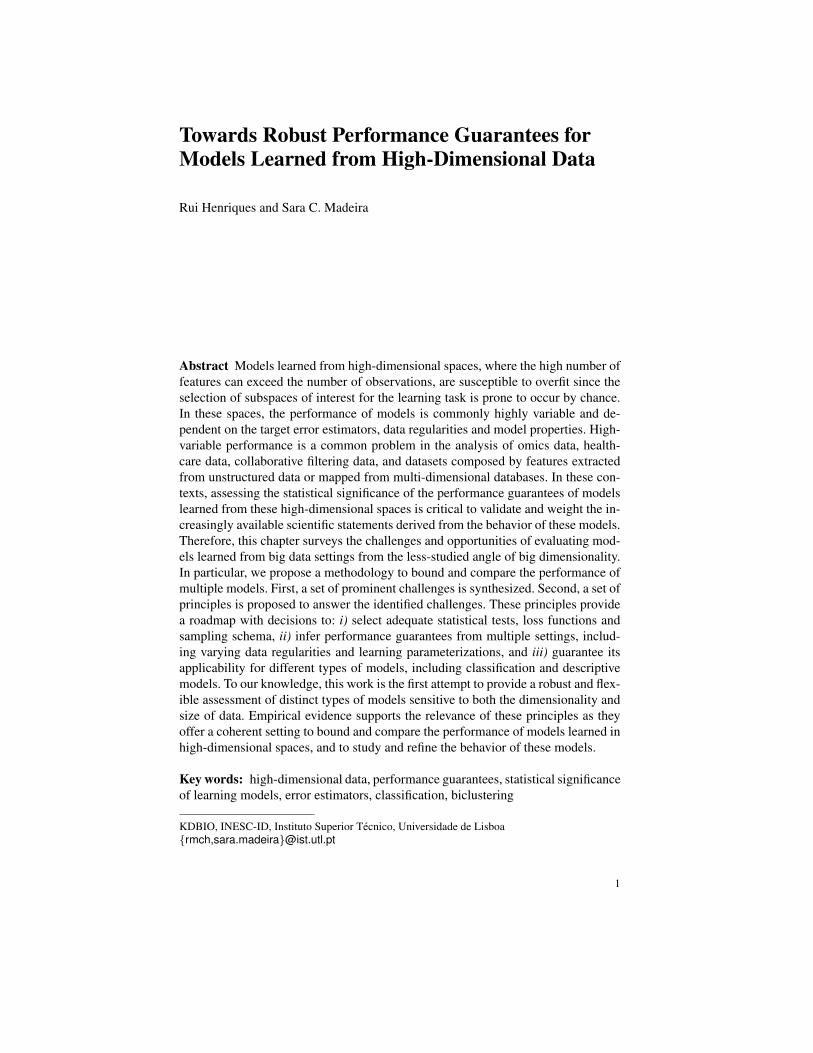
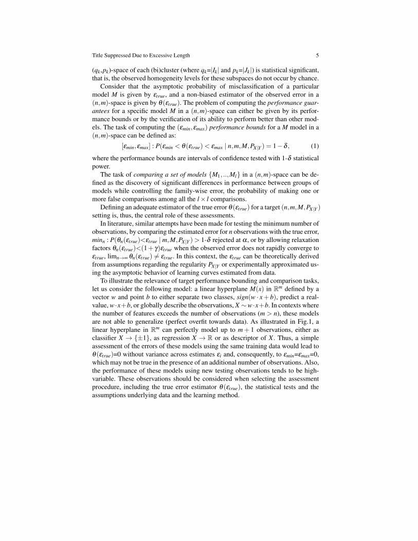
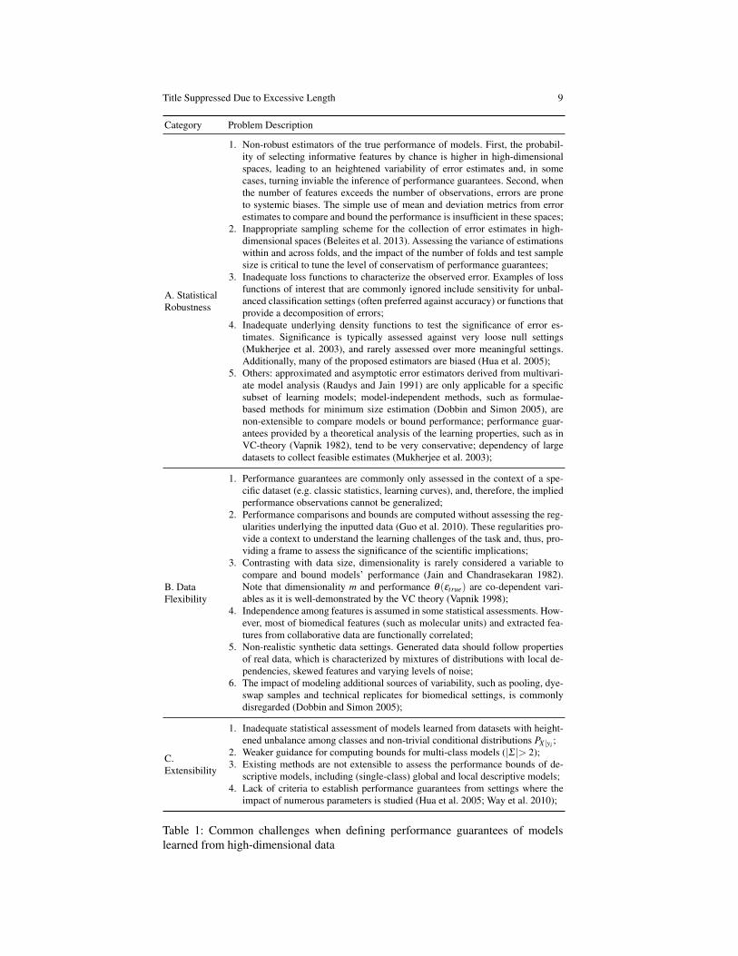
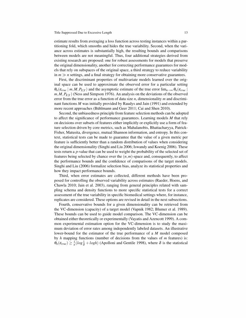
To illustrate the relevance of target performance bounding and comparison tasks,let us consider the following model: a linear hyperplane M(x) in Rm defined by avector w and point b to either separate two classes, sign(w · x+ b), predict a real-value, w ·x+b, or globally describe the observations, X ∼w ·x+b. In contexts wherethe number of features exceeds the number of observations (m > n), these modelsare not able to generalize (perfect overfit towards data). As illustrated in Fig.1, alinear hyperplane in Rm can perfectly model up to m+ 1 observations, either asclassifier X → {±1}, as regression X → R or as descriptor of X . Thus, a simpleassessment of the errors of these models using the same training data would lead toθ(εtrue)=0 without variance across estimates εi and, consequently, to εmin=εmax=0,which may not be true in the presence of an additional number of observations. Also,the performance of these models using new testing observations tends to be high-variable. These observations should be considered when selecting the assessmentprocedure, including the true error estimator θ(εtrue), the statistical tests and theassumptions underlying data and the learning method.
6 Rui Henriques and Sara C. Madeira
Fig. 1: Linear hyperplanes cannot generalize when dimensionality is larger than thenumber of observations (data size), m≥ n+1.
2 Related Work
Classic statistical methods to bound the performance of models as a function ofthe data size include power calculations based on frequentist and Bayesian methods(Adcock 1997), deviation bounds (Guyon et al. 1998), asymptotic estimates of thetrue error εtrue (Raudys and Jain 1991; Niyogi and Girosi 1996), among others (Jainand Chandrasekaran 1982). Here, the impact of the data size in the observed errors isessentially dependent on the entropy associated with the target (n,m)-space. Whenthe goal is the comparison of multiple models, Wilcoxon signed ranks test (twomodels) and the Friedman test with the corresponding post-hoc tests (more than twomodels) are still state-of-the-art methods to derive comparisons either from errorestimates or from the performance distributions given by classic statistical methods(Demsar 2006; Garcıa and Herrera 2009).
To generalize the assessment of performance guarantees for an unknown samplesize n, learning curves (Mukherjee et al. 2003; Figueroa et al. 2012), theoreticalanalysis (Vapnik 1998; Apolloni and Gentile 1998) and simulation studies (Hua etal. 2005; Way et al. 2010) have been proposed. A critical problem with these latterapproaches is that they either ignore the role of dimensionality in the statisticalassessment or the impact of learning from subsets of overall features.
We have grouped these existing efforts according to six major streams of re-search: 1) classic statistics, 2) risk minimization theory, 3) learning curves, 4) sim-ulation studies, 5) mutivariate model’s analysis, and 6) data-driven analysis. Exist-ing approaches have their roots on, at least, one of these research streams. Thesestreams of research assess the performance significance of a single learning modelas a function of the available data size, which is a key factor when learning fromhigh-dimensional spaces. Understandably, comparing multiple models is a matterof defining robust statistical tests from the assessed performance per model.
First, classic statistics cover a wide-range of methods. They are either centeredon power calculations (Adcock 1997) or on the asymptotic estimates of εtrue by us-ing approximation theory, information theory and statistical mechanics (Raudys andJain 1991; Opper et al. 1990; Niyogi and Girosi 1996). Power calculations provide
Title Suppressed Due to Excessive Length 7
a critical view on the model errors (performance) by controlling both sample sizen and statistical power 1-γ , P(θn(εtrue)< εtrue)=1-γ , where θn(εtrue) can either relyon a frequentist view, from counts to estimate the discriminative/descriptive abilityof subsets of features, or on a Bayesian view, more prone to deal with smaller andnoisy data (Adcock 1997).
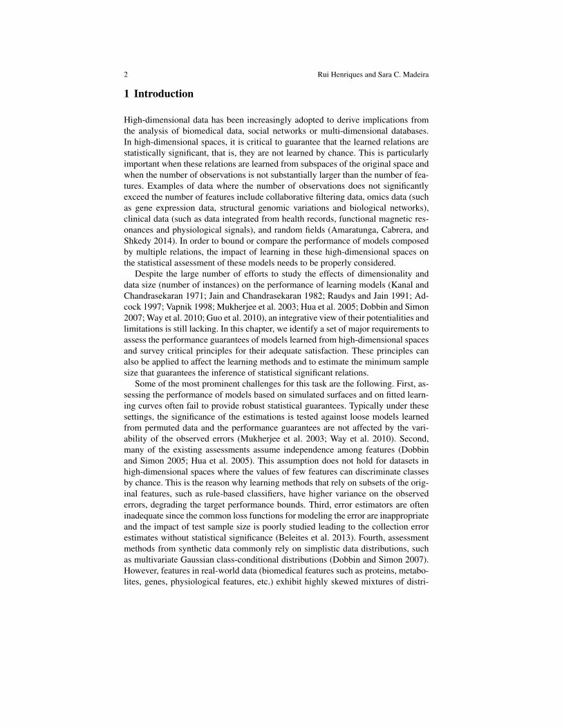
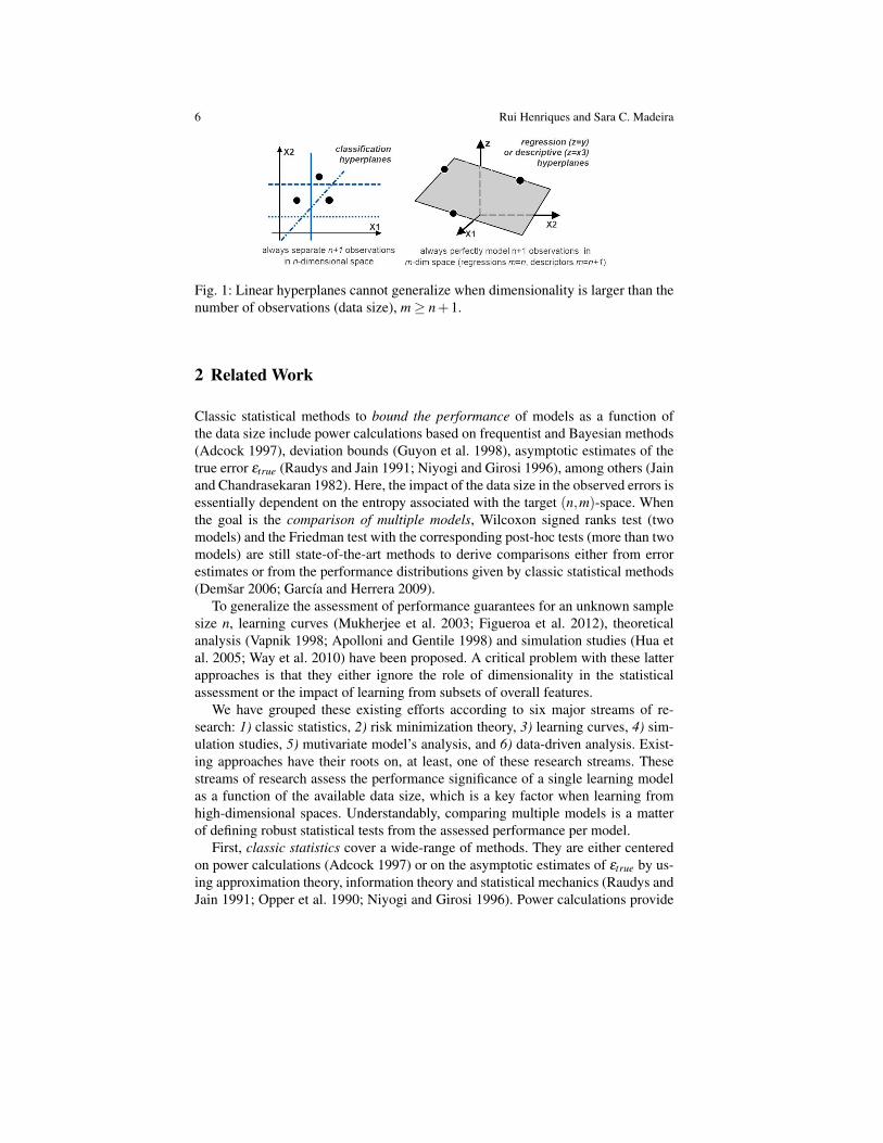
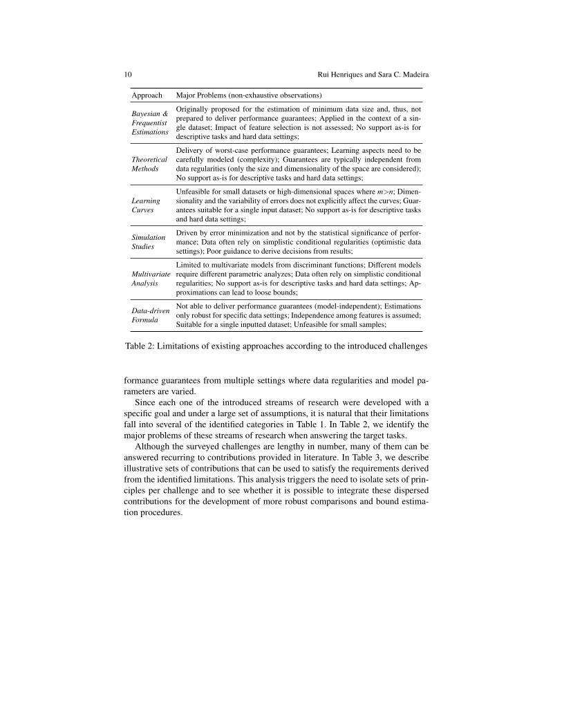
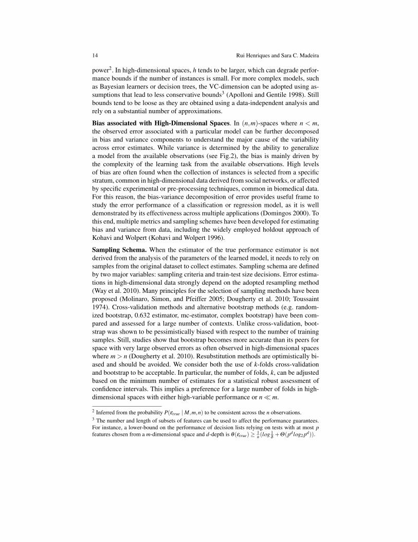
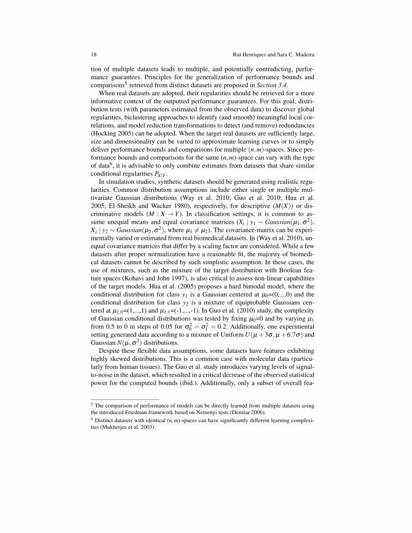
Second, theoretical analysis of empirical risk minimization (Vapnik 1982; Apol-loni and Gentile 1998). To understand the concept of risk minimization, considertwo distinct models: one simplistic model achieving good generalization but withhigh observed error, and a model able to minimize the observed error but overfittedto the available data. As illustrated in Fig.2, this analysis aims to minimize the riskby finding an optimal trade-off between the model capacity (or complexity term)and the observed error. Core contributions from this research stream comes fromVapnik-Chervonenkis (VC) theory (Vapnik 1998), where the sample size and thedimensionality is related through the VC-dimension (h), a measure of the modelcapacity that defines the minimum number of observations required to generalizethe learning in a m-dimensional space. As we illustrated in Fig.1, linear hyperplaneshave h=m+1. The VC-dimension can be theoretically or experimentally estimatedfor different models and used to compare the performance of models and approx-imate lower-bounds. Although under this stream the target overfitting problem isaddressed, the resulting assessment tends to be conservative.
Fig. 2: Capacity and training error impact on true error estimation for classificationand regression models
Third, learning curves use the observed performance of a model over a givendataset to fit inverse power-law functions that can extrapolate performance boundsas a function of the sample size or dimensionality (Mukherjee et al. 2003; Boonya-nunta and Zeephongsekul 2004). An extension that weights estimations accordingto their confidence has been applied for medical data (Figueroa et al. 2012). How-ever, the estimation of learning curves in high-dimensional spaces requires largedata (n>m), which are not always available, and does not consider the variabilityacross error estimates.
Fourth, simulation studies infer performance guarantees by studying the impactof multiple parameters on the learning performance (Hua et al. 2005; Way et al.2010; Guo et al. 2010). This is commonly accomplished through the adoption of
8 Rui Henriques and Sara C. Madeira
a large number of synthetic datasets with varying properties. Statistical assessmentand inference over the collected results can be absent. This is a typical case whenthe simulation study simply aims to assess major variations of performance acrosssettings.
Fifth, true performance estimators can be derived from a direct analysis of thelearning models (Ness and Simpson 1976; El-Sheikh and Wacker 1980; Raudys andJain 1991; Raudys 1997). This stream of research is mainly driven by the assessmentof multivariate models that preserve the dimensionality of space (whether describedby the original m features or by a subset of the original features after feature se-lection) when specific regularities underlying data are assumed. Illustrative mod-els include classifiers based on discriminant functions, such as Euclidean, Fisher,Quadratic or Multinomial. Unlike learning models based on tests over subsets offeatures selected from the original high-dimensional space, multivariate learnersconsider the values of all features. Despite the large attention given by the multi-variate analysis community, these models only represent a small subset of overalllearning models.
Finally, model-independent size decisions derived from data regularities are re-viewed and extended by Dobbin and Simon (2005; 2007). Data-driven formulasare defined from a set of approximations and assumptions based on dimensional-ity, class prevalence, standardized fold change, and on the modeling of non-trivialsources of errors. Although dimensionality is used to affect both the testing signifi-cance levels and the minimum number of features (i.e., the impact of selecting sub-spaces is considered), the formulas are independent from the selected models, for-bidding their extension for comparisons or the computation of performance bounds.
These six research streams are closely related and can be mapped through con-cepts of information theory. In fact, an initial attempt to bridge contributions fromstatistical physics, approximation theory, multivariate analysis and VC theory withina Bayesian framework was proposed by Haussler, Kearns, and Schapire (1991).
2.1 Challenges and Contributions
Although each of the introduced research streams offer unique perspectives to solvethe target task, they suffer from drawbacks as they were originally developed witha different goal – either minimum data size estimation or performance assessmentsin spaces where n� m. These drawbacks are either related with the underlyingapproximations, with the assessment of the impact of selecting subspaces (often re-lated with a non-adequate analysis of the variance of the observed errors) or withthe poor extensibility of existing approaches towards distinct types of models orflexible data settings. Table 1 details these drawbacks according to three major cat-egories that define the ability to: A) rely on robust statistical assessments, B) deliverperformance guarantees from multiple flexible data settings, and C) extend the tar-get assessment towards descriptive models, unbalanced data, and multi-parametersettings. The latter two categories trigger the additional challenge of inferring per-
Title Suppressed Due to Excessive Length 9
Category Problem Description
A. StatisticalRobustness
1. Non-robust estimators of the true performance of models. First, the probabil-ity of selecting informative features by chance is higher in high-dimensionalspaces, leading to an heightened variability of error estimates and, in somecases, turning inviable the inference of performance guarantees. Second, whenthe number of features exceeds the number of observations, errors are proneto systemic biases. The simple use of mean and deviation metrics from errorestimates to compare and bound the performance is insufficient in these spaces;
2. Inappropriate sampling scheme for the collection of error estimates in high-dimensional spaces (Beleites et al. 2013). Assessing the variance of estimationswithin and across folds, and the impact of the number of folds and test samplesize is critical to tune the level of conservatism of performance guarantees;
3. Inadequate loss functions to characterize the observed error. Examples of lossfunctions of interest that are commonly ignored include sensitivity for unbal-anced classification settings (often preferred against accuracy) or functions thatprovide a decomposition of errors;
4. Inadequate underlying density functions to test the significance of error es-timates. Significance is typically assessed against very loose null settings(Mukherjee et al. 2003), and rarely assessed over more meaningful settings.Additionally, many of the proposed estimators are biased (Hua et al. 2005);
5. Others: approximated and asymptotic error estimators derived from multivari-ate model analysis (Raudys and Jain 1991) are only applicable for a specificsubset of learning models; model-independent methods, such as formulae-based methods for minimum size estimation (Dobbin and Simon 2005), arenon-extensible to compare models or bound performance; performance guar-antees provided by a theoretical analysis of the learning properties, such as inVC-theory (Vapnik 1982), tend to be very conservative; dependency of largedatasets to collect feasible estimates (Mukherjee et al. 2003);
B. DataFlexibility
1. Performance guarantees are commonly only assessed in the context of a spe-cific dataset (e.g. classic statistics, learning curves), and, therefore, the impliedperformance observations cannot be generalized;
2. Performance comparisons and bounds are computed without assessing the reg-ularities underlying the inputted data (Guo et al. 2010). These regularities pro-vide a context to understand the learning challenges of the task and, thus, pro-viding a frame to assess the significance of the scientific implications;
3. Contrasting with data size, dimensionality is rarely considered a variable tocompare and bound models’ performance (Jain and Chandrasekaran 1982).Note that dimensionality m and performance θ(εtrue) are co-dependent vari-ables as it is well-demonstrated by the VC theory (Vapnik 1998);
4. Independence among features is assumed in some statistical assessments. How-ever, most of biomedical features (such as molecular units) and extracted fea-tures from collaborative data are functionally correlated;
5. Non-realistic synthetic data settings. Generated data should follow propertiesof real data, which is characterized by mixtures of distributions with local de-pendencies, skewed features and varying levels of noise;
6. The impact of modeling additional sources of variability, such as pooling, dye-swap samples and technical replicates for biomedical settings, is commonlydisregarded (Dobbin and Simon 2005);
C.Extensibility
1. Inadequate statistical assessment of models learned from datasets with height-ened unbalance among classes and non-trivial conditional distributions PX |yi ;
2. Weaker guidance for computing bounds for multi-class models (|Σ |> 2);3. Existing methods are not extensible to assess the performance bounds of de-
scriptive models, including (single-class) global and local descriptive models;4. Lack of criteria to establish performance guarantees from settings where the
impact of numerous parameters is studied (Hua et al. 2005; Way et al. 2010);
Table 1: Common challenges when defining performance guarantees of modelslearned from high-dimensional data
10 Rui Henriques and Sara C. Madeira
Approach Major Problems (non-exhaustive observations)
Bayesian·&FrequentistEstimations
Originally proposed for the estimation of minimum data size and, thus, notprepared to deliver performance guarantees; Applied in the context of a sin-gle dataset; Impact of feature selection is not assessed; No support as-is fordescriptive tasks and hard data settings;
TheoreticalMethods
Delivery of worst-case performance guarantees; Learning aspects need to becarefully modeled (complexity); Guarantees are typically independent fromdata regularities (only the size and dimensionality of the space are considered);No support as-is for descriptive tasks and hard data settings;
LearningCurves
Unfeasible for small datasets or high-dimensional spaces where m>n; Dimen-sionality and the variability of errors does not explicitly affect the curves; Guar-antees suitable for a single input dataset; No support as-is for descriptive tasksand hard data settings;
SimulationStudies
Driven by error minimization and not by the statistical significance of perfor-mance; Data often rely on simplistic conditional regularities (optimistic datasettings); Poor guidance to derive decisions from results;
MultivariateAnalysis
Limited to multivariate models from discriminant functions; Different modelsrequire different parametric analyzes; Data often rely on simplistic conditionalregularities; No support as-is for descriptive tasks and hard data settings; Ap-proximations can lead to loose bounds;
Data-drivenFormula
Not able to deliver performance guarantees (model-independent); Estimationsonly robust for specific data settings; Independence among features is assumed;Suitable for a single inputted dataset; Unfeasible for small samples;
Table 2: Limitations of existing approaches according to the introduced challenges
formance guarantees from multiple settings where data regularities and model pa-rameters are varied.
Since each one of the introduced streams of research were developed with aspecific goal and under a large set of assumptions, it is natural that their limitationsfall into several of the identified categories in Table 1. In Table 2, we identify themajor problems of these streams of research when answering the target tasks.
Although the surveyed challenges are lengthy in number, many of them can beanswered recurring to contributions provided in literature. In Table 3, we describeillustrative sets of contributions that can be used to satisfy the requirements derivedfrom the identified limitations. This analysis triggers the need to isolate sets of prin-ciples per challenge and to see whether it is possible to integrate these dispersedcontributions for the development of more robust comparisons and bound estima-tion procedures.
Title Suppressed Due to Excessive Length 11
Requirements Contributions
Guarantees fromHigh-VariablePerformance (A.1)
Statistical tests to bound and compare performance sensitive to error distri-butions and loss functions (Martin and Hirschberg 1996; Qin and Hotilovac2008; Demsar 2006);VC theory and discriminant-analysis (Vapnik 1982; Raudys and Jain 1991);Unbiasedness principles from feature selection (Singhi and Liu 2006;Iswandy and Koenig 2006);
Bias Effect (A.1) Bias-Variance decomposition of the error (Domingos 2000);
Adequate SamplingSchema (A.2)
Criteria for sampling decisions (Dougherty et al. 2010; Toussaint 1974);Test-train splitting impact (Beleites et al. 2013; Raudys and Jain 1991);
Expressive LossFunctions (A.3)
Error views in machine learning (Glick 1978; Lissack and Fu 1976; Pa-trikainen and Meila 2006);
Feasibility (A.4) Significance of estimates against baseline settings (Adcock 1997; Mukher-jee et al. 2003);
Flexible DataSettings (B.1/4/5)
Simulations with hard data assumptions: mixtures of distributions, localdependencies and noise (Way et al. 2010; Hua et al. 2005; Guo et al. 2010;Madeira and Oliveira 2004);
Retrieval of DataRegularities (B.2)
Data regularities to contextualize assessment (Dobbin and Simon 2007;Raudys and Jain 1991);
DimensionalityEffect (B.3)
Extrapolate guarantees by sub-sampling features (Mukherjee et al. 2003;Guo et al. 2010);
Advanced DataProperties (B.6) Modeling of additional sources of variability (Dobbin and Simon 2005);
Unbalanced/DifficultData (C.1)
Guarantees from unbalanced data and adequate loss functions (Guo et al.2010; Beleites et al. 2013);
Multi-class Tasks (C.2) Integration of class-centric performance bounds (Beleites et al. 2013);
DescriptiveModels (C.3)
Adequate loss functions and collection of error estimates for global and(bi)clustering models (Madeira and Oliveira 2004; Hand 1986);
Guidance Criteria (C.4) Weighted optimization methods for robust and compact multi-parameteranalysis (Deng 2007);
Table 3: Contributions with potential to satisfy the target set of requirements
3 Principles to Bound and Compare the Performance of Models
The solution space is proposed according to the target tasks of bounding or com-paring the performance of a model M learned from high-dimensional spaces. Theadequate definition of estimators of the true error is the central point of focus. Anillustrative simplistic estimator of the performance of classification model can be de-scribed by a collection of observed errors obtained under a k-fold cross-validation,with its expected value being their average:
E[θ(εtrue)]≈ 1k Σ k
i=1(εi |M,n,m,PX |Y ),
12 Rui Henriques and Sara C. Madeira
where εi is the observed error for the ith fold. When the number of observations isnot significantly large, the errors can be collected under a leave-one-out scheme,where k=n and the εi is, thus, simply given by a loss function L applied over a singletesting instance (xi,yi): L(M(xi)=yi,yi).
In the presence of a estimator for the true error, finding performance boundscan rely on non-biased estimators from the collected error estimates, such as themean and q-percentiles to provide a bar-envelope around the mean estimator (e.g.q∈{20%,80%}). However, such strategy does not robustly consider the variability ofthe observed errors. A simple and more robust alternative is to derive the confidenceintervals for the expected true performance based on the distribution underlying theobserved error estimates.
Although this estimator considers the variability across estimates, it still may notreflect the true performance bounds of the model due to poor sampling and lossfunction choices. Additionally, when the number of features exceeds the number ofobservations, the collected errors can be prone to systemic biases and even statisti-cally inviable for inferring performance guarantees. These observations need to becarefully considered to shape the statistical assessment.
The definition of good estimators is also critical for comparing models, as thesecomparisons can rely on their underlying error distributions. For this goal, either thetraditional t-Student, McNemar and Wilcoxon tests can be adopted to compare pairsof classifiers, and Friedman tests with the corresponding post-hoc tests (Demsar2006) or less conservative tests1 (Garcıa and Herrera 2009) can be adopted for eithercomparing distinct models, models learned from multiple datasets or models withdifferent parameterizations.
Motivated by the surveyed contributions to tackle the limitations of existing ap-proaches, this section derives a set of principles for a robust assessment of the per-formance guarantees of models learned from high-dimensional spaces. First, theseprinciples are incrementally provided according to the introduced major sets of chal-lenges. Second, we show that these principles can be consistently and coherentlycombined within a simplistic assessment methodology.
3.1 Robust Statistical Assessment
Variability of Performance Estimates. Increasing the dimensionality m for a fixednumber of observations n introduces variability in the performance of the learnedmodel that must be incorporated in the estimation of performance bounds for aspecific sample size. A simplistic principle is to compute the confidence intervalsfrom error estimates {ε1, ..,εk} obtained from k train-test partitions by fitting anunderlying distribution (e.g. Gaussian) that is able to model their variance.
However, this strategy two major problems. First, it assumes that the variabilityis well-measured for each error estimate. This is commonly not true as each error
1 Friedman tests rely on pairwise Nemenyi tests that are conservative and, therefore, may not reveala significant number of differences among models (Garcıa and Herrera 2009)
Title Suppressed Due to Excessive Length 13
estimate results from averaging a loss function across testing instances within a par-titioning fold, which smooths and hides the true variability. Second, when the vari-ance across estimates is substantially high, the resulting bounds and comparisonsbetween models are not meaningful. Thus, four additional strategies derived fromexisting research are proposed: one for robust assessments for models that preservethe original dimensionality, another for correcting performance guarantees for mod-els that rely on subspaces of the original space, a third strategy to reduce variabilityin m� n settings, and a final strategy for obtaining more conservative guarantees.
First, the discriminant properties of multivariate models learned over the orig-inal space can be used to approximate the observed error for a particular settingθn(εtrue | m,M,PX |Y ) and the asymptotic estimate of the true error limn→∞ θn(εtrue |m,M,PX |Y ) (Ness and Simpson 1976). An analysis on the deviations of the observederror from the true error as a function of data size n, dimensionality m and discrimi-nant functions M was initially provided by Raudys and Jain (1991) and extended bymore recent approaches (Buhlmann and Geer 2011; Cai and Shen 2010).
Second, the unbiasedness principle from feature selection methods can be adoptedto affect the significance of performance guarantees. Learning models M that relyon decisions over subsets of features either implicitly or explicitly use a form of fea-ture selection driven by core metrics, such as Mahalanobis, Bhattacharyya, Patrick-Fisher, Matusita, divergence, mutual Shannon information, and entropy. In this con-text, statistical tests can be made to guarantee that the value of a given metric perfeature is sufficiently better than a random distribution of values when consideringthe original dimensionality (Singhi and Liu 2006; Iswandy and Koenig 2006). Thesetests return a p-value that can be used to weight the probability of the selected set offeatures being selected by chance over the (n,m)-space and, consequently, to affectthe performance bounds and the confidence of comparisons of the target models.Singhi and Liu (2006) formalize selection bias, analyze its statistical properties andhow they impact performance bounds.
Third, when error estimates are collected, different methods have been pro-posed for controlling the observed variability across estimates (Raeder, Hoens, andChawla 2010; Jain et al. 2003), ranging from general principles related with sam-pling schema and density functions to more specific statistical tests for a correctassessment of the true variability in specific biomedical settings where, for instance,replicates are considered. These options are revised in detail in the next subsections.
Fourth, conservative bounds for a given dimensionality can be retrieved fromthe VC-dimension (capacity) of a target model (Vapnik 1982; Blumer et al. 1989).These bounds can be used to guide model comparison. The VC-dimension can beobtained either theoretically or experimentally (Vayatis and Azencott 1999). A com-mon experimental estimation option for the VC-dimension is to study the maxi-mum deviation of error rates among independently labeled datasets. An illustrativelower-bound for the estimator of the true performance of a M model composedby h mapping functions (number of decisions from the values of m features) is:θn(εtrue) ≥ 1
n (log 1δ+ logh) (Apolloni and Gentile 1998), where δ is the statistical
14 Rui Henriques and Sara C. Madeira
power2. In high-dimensional spaces, h tends to be larger, which can degrade perfor-mance bounds if the number of instances is small. For more complex models, suchas Bayesian learners or decision trees, the VC-dimension can be adopted using as-sumptions that lead to less conservative bounds3 (Apolloni and Gentile 1998). Stillbounds tend to be loose as they are obtained using a data-independent analysis andrely on a substantial number of approximations.
Bias associated with High-Dimensional Spaces. In (n,m)-spaces where n < m,the observed error associated with a particular model can be further decomposedin bias and variance components to understand the major cause of the variabilityacross error estimates. While variance is determined by the ability to generalizea model from the available observations (see Fig.2), the bias is mainly driven bythe complexity of the learning task from the available observations. High levelsof bias are often found when the collection of instances is selected from a specificstratum, common in high-dimensional data derived from social networks, or affectedby specific experimental or pre-processing techniques, common in biomedical data.For this reason, the bias-variance decomposition of error provides useful frame tostudy the error performance of a classification or regression model, as it is welldemonstrated by its effectiveness across multiple applications (Domingos 2000). Tothis end, multiple metrics and sampling schemes have been developed for estimatingbias and variance from data, including the widely employed holdout approach ofKohavi and Wolpert (Kohavi and Wolpert 1996).
Sampling Schema. When the estimator of the true performance estimator is notderived from the analysis of the parameters of the learned model, it needs to rely onsamples from the original dataset to collect estimates. Sampling schema are definedby two major variables: sampling criteria and train-test size decisions. Error estima-tions in high-dimensional data strongly depend on the adopted resampling method(Way et al. 2010). Many principles for the selection of sampling methods have beenproposed (Molinaro, Simon, and Pfeiffer 2005; Dougherty et al. 2010; Toussaint1974). Cross-validation methods and alternative bootstrap methods (e.g. random-ized bootstrap, 0.632 estimator, mc-estimator, complex bootstrap) have been com-pared and assessed for a large number of contexts. Unlike cross-validation, boot-strap was shown to be pessimistically biased with respect to the number of trainingsamples. Still, studies show that bootstrap becomes more accurate than its peers forspace with very large observed errors as often observed in high-dimensional spaceswhere m > n (Dougherty et al. 2010). Resubstitution methods are optimistically bi-ased and should be avoided. We consider both the use of k-folds cross-validationand bootstrap to be acceptable. In particular, the number of folds, k, can be adjustedbased on the minimum number of estimates for a statistical robust assessment ofconfidence intervals. This implies a preference for a large number of folds in high-dimensional spaces with either high-variable performance or n� m.
2 Inferred from the probability P(εtrue |M,m,n) to be consistent across the n observations.3 The number and length of subsets of features can be used to affect the performance guarantees.For instance, a lower-bound on the performance of decision lists relying on tests with at most pfeatures chosen from a m-dimensional space and d-depth is θ(εtrue)≥ 1
n (log 1δ+Θ(pd log2 pd)).
Title Suppressed Due to Excessive Length 15
An additional problem when assessing performance guarantees in (n,m)-spaceswhere n < m, is to guarantee that the number of test instances per fold offers a reli-able error estimate since the observed errors within a specific fold are also subjectedto systematic (bias) and random (variance) uncertainty. Two options can be adoptedto minimize this problem. First option is to find the best train-test split. Raudysand Jain (1991) propose a loss function to find a reasonable size of the test samplebased on the train sample size and on the estimate of the asymptotic error, whichessentially depends on the dimensionality of the dataset and on the properties of thelearned model M. A second option is to model the testing sample size independentlyfrom the number of training instances. This guarantees a robust performance assess-ment of the model, but the required number of testing instances can jeopardize thesample size and, thus, compromise the learning task. Error assessments are usuallydescribed as Bernoulli process: ntest instances are tested, t successes (or failures) areobserved and the true performance for a specific fold can be estimated, p=t/ntest ,as well as its variance p(1-p)/ntest . The estimation of ntest can rely on confidenceintervals for the true probability p under a pre-specified precision4 (Beleites et al.2013) or from the expected levels of type I and II errors using the statistical testsdescribed by Fleiss (1981).
Loss Functions. Different loss functions capture different performance views,which can result in radically different observed errors, {ε1, ...εk}. Three major viewscan be distinguish to compute each one of these errors for a particular fold fromthese loss functions. First, error counting, the commonly adopted view, is the rela-tive number of incorrectly classified/predicted/described testing instances. Second,smooth modification of error counting (Glick 1978) uses distance intervals, and it isapplicable for classification models with probabilistic outputs (correctly classifiedinstances can contribute to the error) and for regression models. Finally, posteriorprobability estimate (Lissack and Fu 1976) is often adequate in the presence ofthe class-conditional distributions. These two latter metrics provide a critical com-plementary view for models that deliver probabilistic outputs. Additionally, theirvariance is more realistic than the simple error counting. The problem with smoothmodification is its dependence on the error distance function, while posterior prob-abilities tend to be biased for small datasets.
Although error counting (and the two additional views) are commonly parame-terized with an accuracy-based loss function (incorrectly classified instances), othermetrics can be adopted to turn the analysis more expressive or to be extensibletowards regression models and descriptive models. For settings where the use ofconfusion matrices is of importance due to the difficulty of the task for someclasses/ranges of values, the observed errors can be further decomposed accordingto type-I and type-II errors.
4 For some biomedical experiments (Beleites et al. 2013), 75-100 test samples are commonlynecessary to achieve reasonable validation and 140 test samples (confidence interval widths 0.1)are necessary for an expected sensitivity of 90%. When this number is considerably higher than thenumber of available observations, there is the need to post-calibrate the test-train sizes accordingto the strategies depicted for the first option.
16 Rui Henriques and Sara C. Madeira
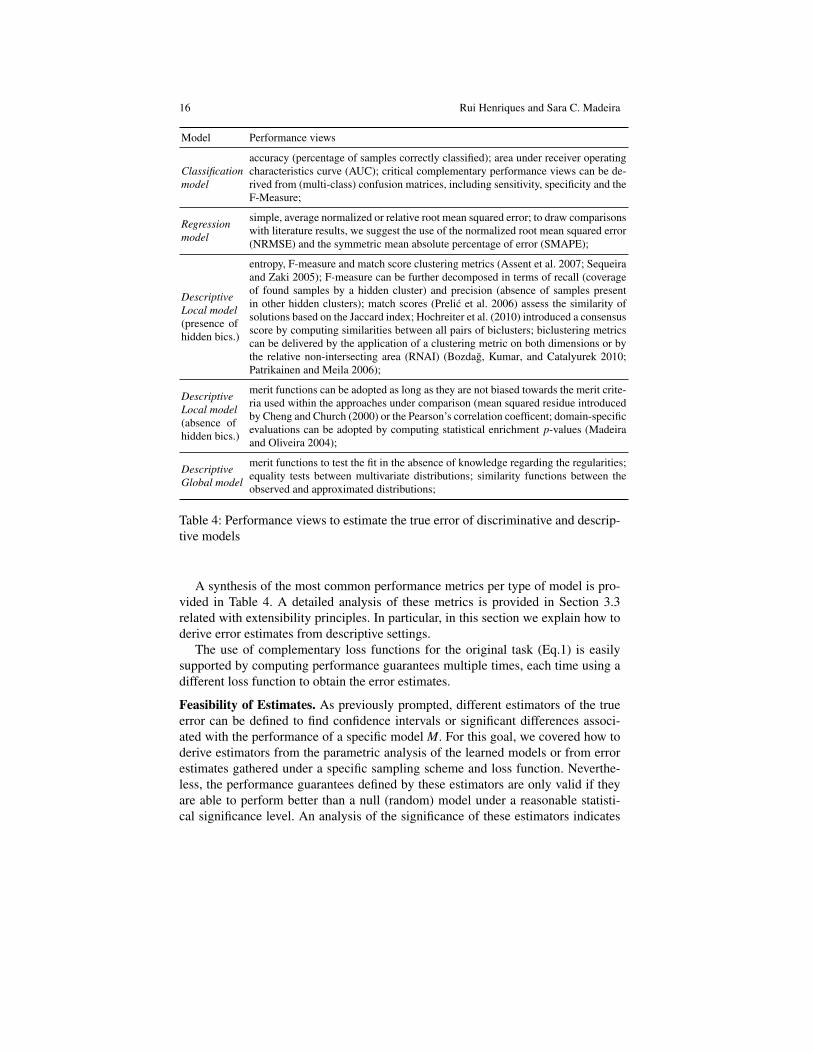
Model Performance views
Classificationmodel
accuracy (percentage of samples correctly classified); area under receiver operatingcharacteristics curve (AUC); critical complementary performance views can be de-rived from (multi-class) confusion matrices, including sensitivity, specificity and theF-Measure;
Regressionmodel
simple, average normalized or relative root mean squared error; to draw comparisonswith literature results, we suggest the use of the normalized root mean squared error(NRMSE) and the symmetric mean absolute percentage of error (SMAPE);
Descriptive ·Local model(presence of ·hidden bics.)
entropy, F-measure and match score clustering metrics (Assent et al. 2007; Sequeiraand Zaki 2005); F-measure can be further decomposed in terms of recall (coverageof found samples by a hidden cluster) and precision (absence of samples presentin other hidden clusters); match scores (Prelic et al. 2006) assess the similarity ofsolutions based on the Jaccard index; Hochreiter et al. (2010) introduced a consensusscore by computing similarities between all pairs of biclusters; biclustering metricscan be delivered by the application of a clustering metric on both dimensions or bythe relative non-intersecting area (RNAI) (Bozdag, Kumar, and Catalyurek 2010;Patrikainen and Meila 2006);
Descriptive ·Local model(absence of ·hidden bics.)
merit functions can be adopted as long as they are not biased towards the merit crite-ria used within the approaches under comparison (mean squared residue introducedby Cheng and Church (2000) or the Pearson’s correlation coefficent; domain-specificevaluations can be adopted by computing statistical enrichment p-values (Madeiraand Oliveira 2004);
DescriptiveGlobal model
merit functions to test the fit in the absence of knowledge regarding the regularities;equality tests between multivariate distributions; similarity functions between theobserved and approximated distributions;
Table 4: Performance views to estimate the true error of discriminative and descrip-tive models
A synthesis of the most common performance metrics per type of model is pro-vided in Table 4. A detailed analysis of these metrics is provided in Section 3.3related with extensibility principles. In particular, in this section we explain how toderive error estimates from descriptive settings.
The use of complementary loss functions for the original task (Eq.1) is easilysupported by computing performance guarantees multiple times, each time using adifferent loss function to obtain the error estimates.
Feasibility of Estimates. As previously prompted, different estimators of the trueerror can be defined to find confidence intervals or significant differences associ-ated with the performance of a specific model M. For this goal, we covered how toderive estimators from the parametric analysis of the learned models or from errorestimates gathered under a specific sampling scheme and loss function. Neverthe-less, the performance guarantees defined by these estimators are only valid if theyare able to perform better than a null (random) model under a reasonable statisti-cal significance level. An analysis of the significance of these estimators indicates
Title Suppressed Due to Excessive Length 17
whether we can estimate the performance guarantees of a model or, otherwise, wewould need a larger number of observations for the target dimensionality.
A simplistic validation option is to show the significant superiority of M againstpermutations made on the original dataset (Mukherjee et al. 2003). A possible per-mutation procedure is to construct for each of the k folds, t samples where the classes(discriminative models) or domain values (descriptive models) are randomly per-muted. From the errors computed for each permutation, different density functionscan be developed, such as:
Pn,m(x) =1kt
Σki=1Σ
tj=1θ(x− εi, j,n,m), (2)
where θ(z) = 1 if z ≥ 0 and 0 otherwise. The significance of the model is Pn,m(x),the percentage of random permutations with observed error smaller than x, where xcan be fixed using a estimator of the true error for the target model M. The averageestimator, εn,m = 1
k Σ ki=1(εi | n,m), or the θ th percentile of the sequence {e1, ...,ek}
can be used as an estimate of the true error. Both the average and θ th percentile oferror estimates are unbiased estimators. Different percentiles can be used to defineerror bar envelopes for the true error.
There are two major problems with this approach. First, variability of the ob-served errors does not affect the significance levels. To account for the variabilityof error estimates across the k×t permutations, more robust statistical tests can beused, such as one-tailed t-test with (k×t)-1 degrees of freedom to test the unilateralsuperiority of the target model. Second, the significance of the learned relations ofa model M is assessed against permuted data, which is a very loose setting. Instead,the same model should be assessed against data generated with similar global reg-ularities in order to guarantee that the observed superiority does not simply resultfrom an overfitting towards the available observations. Similarly, stastical t-tests aresuitable options for this scenario.
When this analysis reveals that error estimates cannot be collected with statisticalsignificance due to data size constraints, two additional strategies can be applied. Afirst strategy it to adopt complementary datasets by either: 1) relying on identicalreal data with more samples (note, however, that distinct datasets can lead to quitedifferent performance guarantees (ibid.)), or by 2) approximating the regularitiesof the original dataset and to generated larger synthetic data using the retrieveddistributions. A second strategy is to relax the significance levels for the inferenceof less conservative performance guarantees. In this case, results should be providedas indicative and exploratory.
3.2 Data Flexibility
Deriving performance guarantees from a single dataset is of limited interest. Evenin the context of a specific domain, the assessment of models from multiple datasetswith varying regularities of interest provides a more complete and generalize frameto validate their performance. However, in the absence of other principles, the adop-
18 Rui Henriques and Sara C. Madeira
tion of multiple datasets leads to multiple, and potentially contradicting, perfor-mance guarantees. Principles for the generalization of performance bounds andcomparisons5 retrieved from distinct datasets are proposed in Section 3.4.
When real datasets are adopted, their regularities should be retrieved for a moreinformative context of the outputted performance guarantees. For this goal, distri-bution tests (with parameters estimated from the observed data) to discover globalregularities, biclustering approaches to identify (and smooth) meaningful local cor-relations, and model reduction transformations to detect (and remove) redundancies(Hocking 2005) can be adopted. When the target real datasets are sufficiently large,size and dimensionality can be varied to approximate learning curves or to simplydeliver performance bounds and comparisons for multiple (n,m)-spaces. Since per-formance bounds and comparisons for the same (n,m)-space can vary with the typeof data6, it is advisable to only combine estimates from datasets that share similarconditional regularities PX |Y .
In simulation studies, synthetic datasets should be generated using realistic regu-larities. Common distribution assumptions include either single or multiple mul-tivariate Gaussian distributions (Way et al. 2010; Guo et al. 2010; Hua et al.2005; El-Sheikh and Wacker 1980), respectively, for descriptive (M(X)) or dis-criminative models (M : X → Y ). In classification settings, it is common to as-sume unequal means and equal covariance matrices (Xi | y1 ∼ Gaussian(µ1,σ
2),X j | y2 ∼ Gaussian(µ2,σ
2), where µ1 6= µ2). The covariance-matrix can be experi-mentally varied or estimated from real biomedical datasets. In (Way et al. 2010), un-equal covariance matrices that differ by a scaling factor are considered. While a fewdatasets after proper normalization have a reasonable fit, the majority of biomedi-cal datasets cannot be described by such simplistic assumption. In these cases, theuse of mixtures, such as the mixture of the target distribution with Boolean fea-ture spaces (Kohavi and John 1997), is also critical to assess non-linear capabilitiesof the target models. Hua et al. (2005) proposes a hard bimodal model, where theconditional distribution for class y1 is a Gaussian centered at µ0=(0,...,0) and theconditional distribution for class y2 is a mixture of equiprobable Gaussians cen-tered at µ1,0=(1,...,1) and µ1,1=(-1,...,-1). In Guo et al. (2010) study, the complexityof Gaussian conditional distributions was tested by fixing µ0=0 and by varying µ1from 0.5 to 0 in steps of 0.05 for σ2
0 = σ21 = 0.2. Additionally, one experimental
setting generated data according to a mixture of Uniform U(µ +3σ ,µ +6.7σ) andGaussian N(µ,σ2) distributions.
Despite these flexible data assumptions, some datasets have features exhibitinghighly skewed distributions. This is a common case with molecular data (particu-larly from human tissues). The Guo et al. study introduces varying levels of signal-to-noise in the dataset, which resulted in a critical decrease of the observed statisticalpower for the computed bounds (ibid.). Additionally, only a subset of overall fea-
5 The comparison of performance of models can be directly learned from multiple datasets usingthe introduced Friedman framework based on Nemenyi tests (Demsar 2006).6 Distinct datasets with identical (n,m)-spaces can have significantly different learning complexi-ties (Mukherjee et al. 2003).
Title Suppressed Due to Excessive Length 19
tures was generated according class-conditional distributions in order to simulatethe commonly observed compact set of discriminative biomarker features.
The majority of real-world data settings is also characterized by functionally cor-related features and, therefore, planting different forms of dependencies among them target features is of critical importance to infer performance guarantees. Hua etal. (2005) proposes the use of different covariance-matrices by dividing the overallfeatures into correlated subsets with varying number of features (p ∈ {1,5,10,30}),and by considering different correlation coefficients (ρ ∈ {0.125,0.25,0.5}). Theincrease in correlation among features, either by decreasing g or increasing ρ , in-creases the Bayes error for a fixed dimensionality. Guo et al. (2010) incorporates acorrelation factor just for a small portion of the original features. Other studies offeradditional conditional distributions tested using unequal covariance matrices (Wayet al. 2010). Finally, biclusters can be planted in data to capture flexible functionalrelations among subsets of features and observations. Such local dependencies arecommonly observed in biomedical data (Madeira and Oliveira 2004).
Additional sources of variability can be present, including technical biases fromthe collected sample of instances or replicates, pooling and dye-swaps in biologi-cal data. This knowledge can be used to shape the estimators of the true error or tofurther generate new synthetic data settings. Dobbin and Simon work (Dobbin andSimon 2005; Dobbin and Simon 2007) explore how such additional sources of vari-ability impact the observed errors. The variability added by these factors is estimatedfrom the available data. These factors are modeled for both discriminative (multi-class) and descriptive (single-class) settings where the number of independent obser-vations is often small. Formulas are defined for each setting by minimizing the dif-ference between the asymptotic and observed error, (limn→∞ εtrue|n)− εtrue|n, whereεtrue|n depends on these sources of variability. Although this work provides hintson how to address advanced data aspects with impact on the estimation of the trueerror, the proposed formulas provide loose bounds and have been only deduced inthe the scope of biological data under the independence assumption among features.The variation of statistical power using ANOVA methods has been also proposed toassess these effects on the performance of models (Surendiran and Vadivel 2011).
Synthesizing, flexible data assumptions allow the definition of more general,complete and robust performance guarantees. Beyond varying the size n and di-mensionality m, we can isolate six major principles. First, assessing models learnedfrom real and synthetic datasets with disclosed regularities provide complementaryviews for robust and framed performance guarantees. Second, when adopting mul-tivariate Gaussian distributions to generate data, one should adopt varying distancesbetween their means, use covariance-matrices characterized by varying number offeatures and correlation factors, and rely on mixtures to test non-linear learningproperties. Non-Gaussian distributions can be complementary considered. Third,varying degrees of noise should be planted by, for instance, selecting a percentageof features with skewed values. Fourth, impact of selecting a subset of overall fea-tures with more discriminative potential (e.g. lower variances) should be assessed.Fifth, other properties can be explored, such as the planting of local regularities withdifferent properties to assess the performance guarantees of descriptive models and
20 Rui Henriques and Sara C. Madeira
the creation of imbalance between classes to assess classification models. Finally,additional sources variability related with the specificities of the domains of interestcan be simulated for context-dependent estimations of performance guarantees.
3.3 Extensibility
Performance Guarantees from Unbalanced Data Settings. Imbalance in the rep-resentativity of classes (classification models), range of values (regression models)and among feature distributions affect the performance of models and, consequently,the resulting performance guarantees. In many high-dimensional contexts, such asbiomedical labeled data, case and control classes tend to be significantly unbalanced(access to rare conditions or diseases is scarce). In these contexts, it is importantto compute performance guarantees in (n,m)-spaces from unbalanced real data orfrom synthetic data with varying degrees of imbalance. Under such analysis, wecan frame the performance guarantees of a specific model M with more rigor. Simi-larly, for multi-class tasks, performance guarantees can be derived from real datasetsand/or synthetic datasets (generated with a varying number and imbalance amongthe classes) to frame the true performance of a target model M.
Additionally, an adequate selection of loss functions to compute the observederrors is required for these settings. Assuming the presence of c classes, one strategyis to estimate performance bounds c times, where each time the bounds are driven bya loss function based on the sensitivity of that particular class. The overall upper andlower bounds across the c estimations can be outputted. Such illustrative method iscritical to guarantee the robustness assessment of the performance of classificationmodels for each class.
Performance Guarantees of Descriptive Models. The introduced assessment prin-ciples to derive performance guarantees of discriminative models are applicable todescriptive models under a small set of assumptions. Local and global descriptivemodels can be easily adopted when considering one of the loss functions proposedin Table 4. The evaluation of local descriptive models can either be made in thepresence or absence of hidden (or planted) (bi)clusters, H. Similarly, global descrip-tive models that return a mixture of distributions that approximate the populationfrom which the sample was retrieved, X ∼ π , can be evaluated in the presence andabsence of the underlying true regularities.
However, both descriptive and global models cannot rely on traditional samplingschema to collect error estimates. Therefore, in order to have multiple error esti-mates for a particular (n,m)-space, which is required for a robust statistical assess-ment, these estimates should be computed from:
• alternative subsamples of a particular dataset (testing instances are discarded);• multiple synthetic datasets with fixed number of observations n and features m
generated under similar regularities.
Title Suppressed Due to Excessive Length 21
3.4 Inferring Performance Guarantees from Multiple Settings
In previous sections, we have been proposing alternative estimators of the true per-formance, and the use of datasets with varying regularities. Additionally, the per-formance of learning methods can significantly vary depending on their parameter-izations. Some of the variables that can be subject to variation include: data size,data dimensionality, loss function, sampling scheme, model parameters, distribu-tions underlying data, discriminative and skewed subsets of features, local corre-lations, degree of noise, among others. Understandably, the multiplicity of viewsrelated with different estimators, parameters and datasets results in a large numberof performance bounds and comparison-relations that can hamper the assessment ofa target model. Thus, inferring more general performance guarantees is critical andvalid for studies that either derive specific performance guarantees from collectionsof error estimates or from the direct analysis of the learned models.
Guiding criteria needs to be considered to frame the performance guarantees ofa particular model M based on the combinatorial explosion of hyper-surfaces thatassess performance guarantees from these parameters. When comparing models,simple statistics and hierarchical presentation of the inferred relations can be avail-able. An illustrative example is the delivery of the most significant pairs of valuesthat capture the percentage of settings where a particular model had a superior andinferior performance against another model.
When bounding performance, a simple strategy is to use the minimum and max-imum values over similar settings to define conservative lower and upper bounds.More robustly, error estimates can be gathered for the definition of more generalconfidence intervals. Other criteria based on weighted functions can be used toframe the bounds from estimates gathered from multiple estimations (Deng 2007).In order to avoid very distinct levels of difficulty across settings that penalized theinferred performance bounds, either a default parameterization can be made for allthe variables and only one variable be tested at a time or distinct settings can beclustered leading to a compact set of performance bounds.
3.5 Integrating the Proposed Principles
The retrieved principles can be consistently and coherently combined according toa simple methodology to enhance the assessment of the performance guaranteesof models learned from high-dimensional spaces. First, the decisions related withthe definition of the estimators, including the selection of adequate loss functionsand sampling scheme and the tests of the feasibility of error estimates, provide astructural basis to bound and compare the performance of models.
Second, to avoid biased performance guarantees towards a single dataset, we pro-pose the estimation of these bounds against synthetic datasets with varying proper-ties. In this context, we can easily evaluate the impact of assuming varying regulari-ties X |Y , planting feature dependencies, dealing with different sources of variability,
22 Rui Henriques and Sara C. Madeira
and of creating imbalance for discriminative models. Since the result of varying alarge number of parameters can result in large number of estimations, the identifiedstrategies to deal with the inference of performance guarantees from multiple set-tings should be adopted in order to collapse these estimations into a compact frameof performance guarantees.
Third, in the presence of a model that is able to preserve the original space (e.g.support vector machines, global descriptors, discriminant multivariate models), theimpact of dimensionality in the performance guarantees is present by default, andit can be further understood by varying the number of features. For models thatrely on subsets of overall features, as the variability of the error estimates may notreflect the true performance, performance guarantees should be adjusted throughthe unbiasedness principle of feature selection or conservative estimations shouldbe considered recurring to VC-theory.
Finally, for both of these models, the estimator of the true performance should befurther decomposed to account for the both the bias and variance underlying errorestimates. When performance is highly-variable (loose performance guarantees),this decomposition offers an informative context to understand how the model isable to deal with the risk of overfitting associated with high-dimensional spaces.
4 Results and Discussion
In this section we experimentally assess the relevance of the proposed methodol-ogy. First, we compare alternative estimators and provide initial evidence for theneed to consider the proposed principles when assessing performance over high-dimensional datasets when n<m. Second, we bound and compare the performanceof classification models learned over datasets with varying properties. Finally, weshow the importance of adopting alternative loss functions for unbalanced multi-class and single-class (descriptive) models.
For these experiments, we rely on both real and synthetic data. Two distinctgroups of real-world datasets were used: high-dimensional datasets with small num-ber of instances (n<m) and high-dimensional datasets with a large number of in-stances. For the first group we adopted microarrays for tumor classification col-lected from BIGS repository7: colon cancer data (m=2000, n=62, 2 labels), lym-phoma data (m=4026, n=96, 9 labels), and leukemia data (m=7129, n=72, 2 labels).For the second group we selected a random population from the healthcare heritageprize database8 (m=478, n=20000) which integrates claims across hospitals, phar-macies and laboratories. The original relational scheme was denormalized by map-ping each patient as an instance with features extracted from the collected claims(400 attributes), the monthly laboratory tests and taken drugs (72 attributes), and thepatient profile (6 attributes). We selected the tasks of classifying the need for upcom-
7 http://www.upo.es/eps/bigs/datasets.html8 http://www.heritagehealthprize.com/c/hhp/data (under a granted permission)
Title Suppressed Due to Excessive Length 23
ing interventions (2 labels) and the level of drug prescription ({low,moderate,high}labels), considered to be critical tasks for care prevention and drug management.
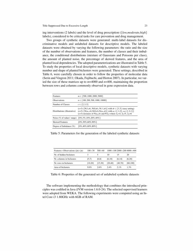
Two groups of synthetic datasets were generated: multi-label datasets for dis-criminative models and unlabeled datasets for descriptive models. The labeleddatasets were obtained by varying the following parameters: the ratio and the sizeof the number of observations and features, the number of classes and their imbal-ance, the conditional distributions (mixture of Gaussians and Poissons per class),the amount of planted noise, the percentage of skewed features, and the area ofplanted local dependencies. The adopted parameterizations are illustrated in Table 5.To study the properties of local descriptive models, synthetic datasets with varyingnumber and shape of planted biclusters were generated. These settings, described inTable 6, were carefully chosen in order to follow the properties of molecular data(Serin and Vingron 2011; Okada, Fujibuchi, and Horton 2007). In particular, we var-ied the size of these matrices up to m=4000 and n=400, maintaining the proportionbetween rows and columns commonly observed in gene expression data.
Features m ∈ {500,1000,2000,5000}
Observations n ∈ {100,200,500,1000,10000}
Number of Classes c ∈ {2,3,5}
Distributions (illustrative)(c=3) {N(1,σ ), N(0,σ ), N(-1,σ )} with σ ∈ {3,5} (easy setting)(c=3) {N(u1,σ ),N(0,σ ),N(u3,σ )} with u1∈{-1,2}, u2∈{-2,1}}(c=3) mixtures of N(ui,σ ) and P(λi) where λ1=4, λ2=5, λ3=6
Noise (% of values’ range) {0%,5%,10%,20%,40%}
Skewed Features {0%,30%,60%,90%}
Degree of Imbalance (%) {0%,40%,60%,80%}
Table 5: Parameters for the generation of the labeled synthetic datasets
Features×Observations (]m×]n) 100×30 500×60 1000×100 2000×200 4000×400
Nr. of hidden biclusters 3 5 10 15 20
Nr. columns in biclusters [5,7] [6,8] [6,10] [6,14] [6,20]
Nr. rows in biclusters [10,20] [15,30] [20,40] [40,70] [60,100]
Area of biclusters 9.0% 2.6% 2.4% 2.1% 1.3%
Table 6: Properties of the generated set of unlabeled synthetic datasets
The software implementing the methodology that combines the introduced prin-ciples was codified in Java (JVM version 1.6.0-24). The selected supervised learnerswere adopted from WEKA. The following experiments were computed using an In-tel Core i3 1.80GHz with 6GB of RAM.
24 Rui Henriques and Sara C. Madeira
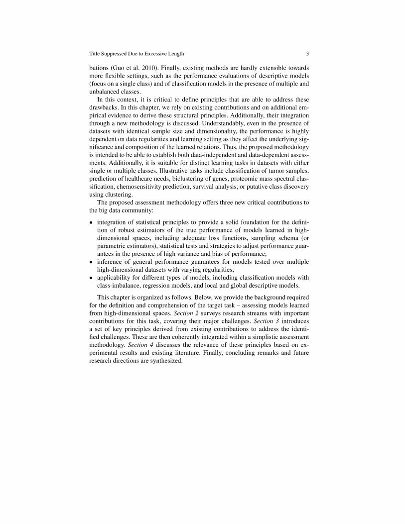
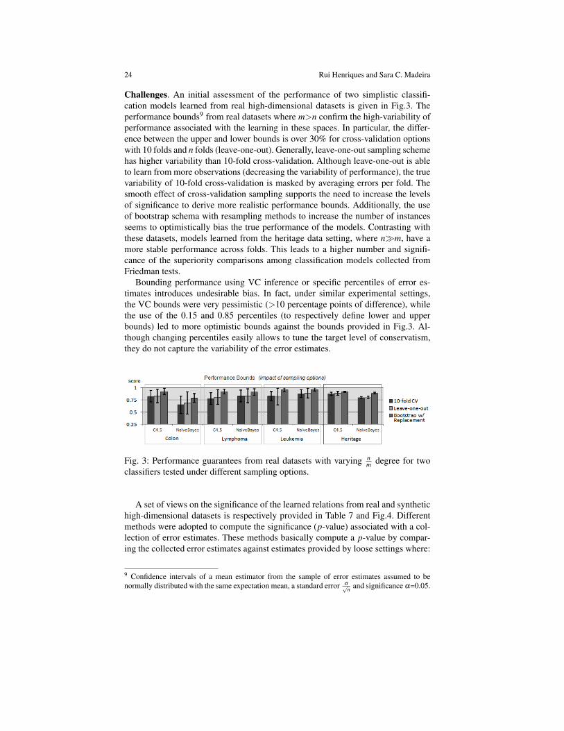
Challenges. An initial assessment of the performance of two simplistic classifi-cation models learned from real high-dimensional datasets is given in Fig.3. Theperformance bounds9 from real datasets where m>n confirm the high-variability ofperformance associated with the learning in these spaces. In particular, the differ-ence between the upper and lower bounds is over 30% for cross-validation optionswith 10 folds and n folds (leave-one-out). Generally, leave-one-out sampling schemehas higher variability than 10-fold cross-validation. Although leave-one-out is ableto learn from more observations (decreasing the variability of performance), the truevariability of 10-fold cross-validation is masked by averaging errors per fold. Thesmooth effect of cross-validation sampling supports the need to increase the levelsof significance to derive more realistic performance bounds. Additionally, the useof bootstrap schema with resampling methods to increase the number of instancesseems to optimistically bias the true performance of the models. Contrasting withthese datasets, models learned from the heritage data setting, where n�m, have amore stable performance across folds. This leads to a higher number and signifi-cance of the superiority comparisons among classification models collected fromFriedman tests.
Bounding performance using VC inference or specific percentiles of error es-timates introduces undesirable bias. In fact, under similar experimental settings,the VC bounds were very pessimistic (>10 percentage points of difference), whilethe use of the 0.15 and 0.85 percentiles (to respectively define lower and upperbounds) led to more optimistic bounds against the bounds provided in Fig.3. Al-though changing percentiles easily allows to tune the target level of conservatism,they do not capture the variability of the error estimates.
Fig. 3: Performance guarantees from real datasets with varying nm degree for two
classifiers tested under different sampling options.
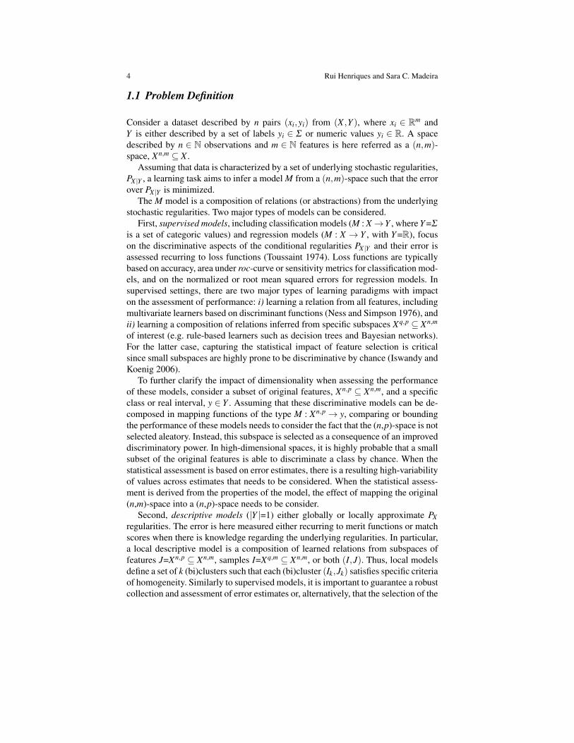
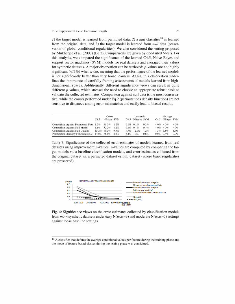
A set of views on the significance of the learned relations from real and synthetichigh-dimensional datasets is respectively provided in Table 7 and Fig.4. Differentmethods were adopted to compute the significance (p-value) associated with a col-lection of error estimates. These methods basically compute a p-value by compar-ing the collected error estimates against estimates provided by loose settings where:
9 Confidence intervals of a mean estimator from the sample of error estimates assumed to benormally distributed with the same expectation mean, a standard error σ√
n and significance α=0.05.
Title Suppressed Due to Excessive Length 25
1) the target model is learned from permuted data, 2) a null classifier10 is learnedfrom the original data, and 3) the target model is learned from null data (preser-vation of global conditional regularities). We also considered the setting proposedby Mukherjee et al. (2003) (Eq.2). Comparisons are given by one-tailed t-tests. Forthis analysis, we compared the significance of the learned C4.5, Naive Bayes andsupport vector machines (SVM) models for real datasets and averaged their valuesfor synthetic datasets. A major observation can be retrieved: p-values are not highlysignificant (�1%) when n<m, meaning that the performance of the learned modelsis not significantly better than very loose learners. Again, this observation under-lines the importance of carefully framing assessments of models learned from high-dimensional spaces. Additionally, different significance views can result in quitedifferent p-values, which stresses the need to choose an appropriate robust basis tovalidate the collected estimates. Comparison against null data is the most conserva-tive, while the counts performed under Eq.2 (permutations density function) are notsensitive to distances among error mismatches and easily lead to biased results.
Colon Leukemia HeritageC4.5 NBayes SVM C4.5 NBayes SVM C4.5 NBayes SVM
Comparison Against Permutated Data 1.5% 41.3% 1.2% 0.6% 0.1% 0.2% ∼0% ∼0% ∼0%Comparison Against Null Model 1.1% 32.2% 1.2% 0.1% 0.1% 0.1% ∼0% ∼0% ∼0%Comparison Against Null Dataset 15.2% 60.3% 9.3% 9.7% 12.0% 7.2% 1.3% 3.8% 1.7%Permutations Density Function (Eq.2) 14.0% 36.0% 8.4% 8.4% 1.2% 0.8% 0.0% 0.4% 0.0%
Table 7: Significance of the collected error estimates of models learned from realdatasets using improvement p-values. p-values are computed by comparing the tar-get models vs. a baseline classification models, and error estimates collected fromthe original dataset vs. a permuted dataset or null dataset (where basic regularitiesare preserved).
Fig. 4: Significance views on the error estimates collected by classification modelsfrom m>n synthetic datasets under easy N(ui,σ=3) and moderate N(ui,σ=5) settingsagainst loose baseline settings.
10 A classifier that defines the average conditional values per feature during the training phase andthe mode of feature-based classes during the testing phase was considered.
26 Rui Henriques and Sara C. Madeira
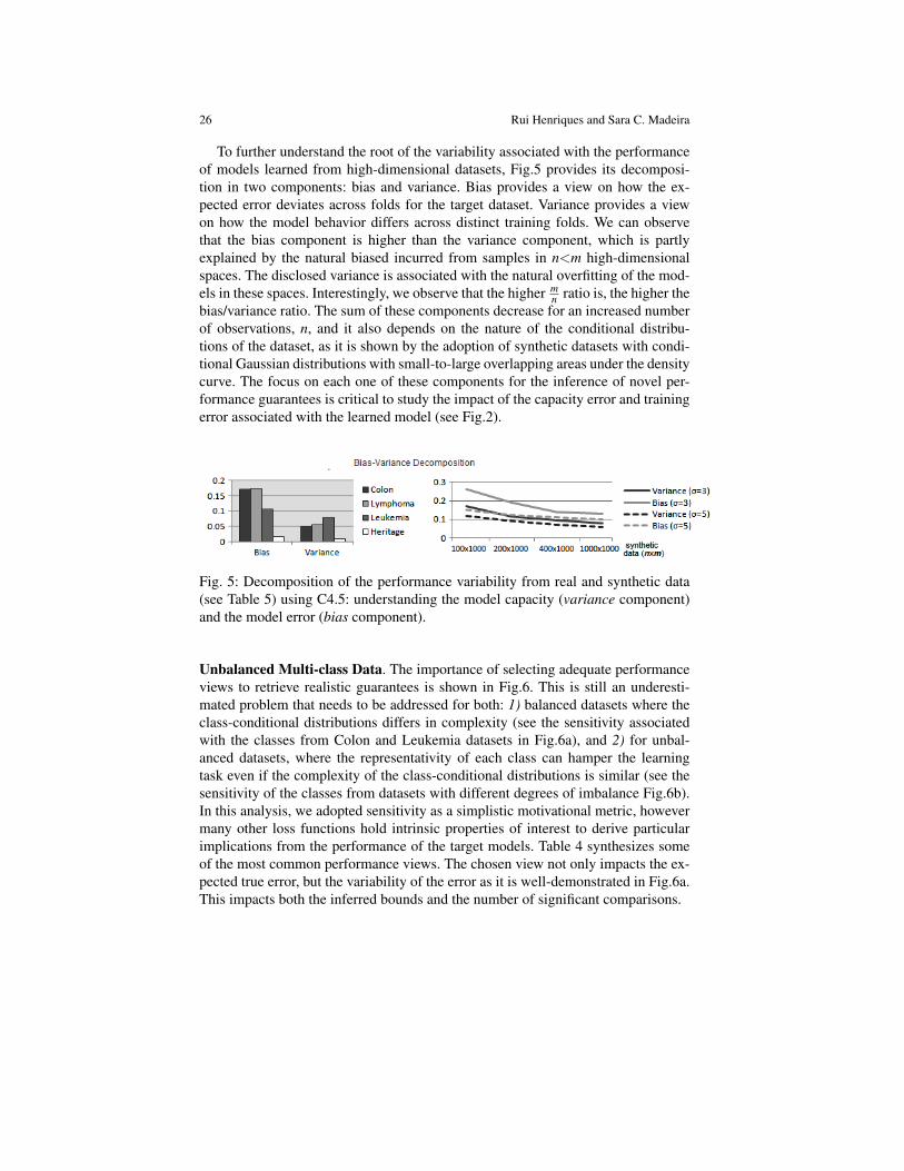
To further understand the root of the variability associated with the performanceof models learned from high-dimensional datasets, Fig.5 provides its decomposi-tion in two components: bias and variance. Bias provides a view on how the ex-pected error deviates across folds for the target dataset. Variance provides a viewon how the model behavior differs across distinct training folds. We can observethat the bias component is higher than the variance component, which is partlyexplained by the natural biased incurred from samples in n<m high-dimensionalspaces. The disclosed variance is associated with the natural overfitting of the mod-els in these spaces. Interestingly, we observe that the higher m
n ratio is, the higher thebias/variance ratio. The sum of these components decrease for an increased numberof observations, n, and it also depends on the nature of the conditional distribu-tions of the dataset, as it is shown by the adoption of synthetic datasets with condi-tional Gaussian distributions with small-to-large overlapping areas under the densitycurve. The focus on each one of these components for the inference of novel per-formance guarantees is critical to study the impact of the capacity error and trainingerror associated with the learned model (see Fig.2).
Fig. 5: Decomposition of the performance variability from real and synthetic data(see Table 5) using C4.5: understanding the model capacity (variance component)and the model error (bias component).
Unbalanced Multi-class Data. The importance of selecting adequate performanceviews to retrieve realistic guarantees is shown in Fig.6. This is still an underesti-mated problem that needs to be addressed for both: 1) balanced datasets where theclass-conditional distributions differs in complexity (see the sensitivity associatedwith the classes from Colon and Leukemia datasets in Fig.6a), and 2) for unbal-anced datasets, where the representativity of each class can hamper the learningtask even if the complexity of the class-conditional distributions is similar (see thesensitivity of the classes from datasets with different degrees of imbalance Fig.6b).In this analysis, we adopted sensitivity as a simplistic motivational metric, howevermany other loss functions hold intrinsic properties of interest to derive particularimplications from the performance of the target models. Table 4 synthesizes someof the most common performance views. The chosen view not only impacts the ex-pected true error, but the variability of the error as it is well-demonstrated in Fig.6a.This impacts both the inferred bounds and the number of significant comparisons.
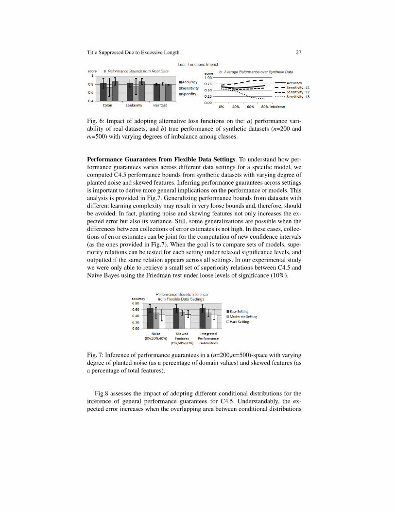
Title Suppressed Due to Excessive Length 27
Fig. 6: Impact of adopting alternative loss functions on the: a) performance vari-ability of real datasets, and b) true performance of synthetic datasets (n=200 andm=500) with varying degrees of imbalance among classes.
Performance Guarantees from Flexible Data Settings. To understand how per-formance guarantees varies across different data settings for a specific model, wecomputed C4.5 performance bounds from synthetic datasets with varying degree ofplanted noise and skewed features. Inferring performance guarantees across settingsis important to derive more general implications on the performance of models. Thisanalysis is provided in Fig.7. Generalizing performance bounds from datasets withdifferent learning complexity may result in very loose bounds and, therefore, shouldbe avoided. In fact, planting noise and skewing features not only increases the ex-pected error but also its variance. Still, some generalizations are possible when thedifferences between collections of error estimates is not high. In these cases, collec-tions of error estimates can be joint for the computation of new confidence intervals(as the ones provided in Fig.7). When the goal is to compare sets of models, supe-riority relations can be tested for each setting under relaxed significance levels, andoutputted if the same relation appears across all settings. In our experimental studywe were only able to retrieve a small set of superiority relations between C4.5 andNaive Bayes using the Friedman-test under loose levels of significance (10%).
Fig. 7: Inference of performance guarantees in a (n=200,m=500)-space with varyingdegree of planted noise (as a percentage of domain values) and skewed features (asa percentage of total features).
Fig.8 assesses the impact of adopting different conditional distributions for theinference of general performance guarantees for C4.5. Understandably, the ex-pected error increases when the overlapping area between conditional distributions
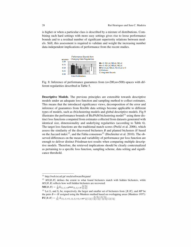
28 Rui Henriques and Sara C. Madeira
is higher or when a particular class is described by a mixture of distributions. Com-bining such hard settings with more easy settings gives rise to loose performancebounds and to a residual number of significant superiority relations between mod-els. Still, this assessment is required to validate and weight the increasing numberdata-independent implications of performance from the recent studies.
Fig. 8: Inference of performance guarantees from (n=200,m=500)-spaces with dif-ferent regularities described in Table 5.
Descriptive Models. The previous principles are extensible towards descriptivemodels under an adequate loss function and sampling method to collect estimates.This means that the introduced significance views, decomposition of the error andinference of guarantees from flexible data settings become applicable to differenttypes of models, such as (bi)clustering models and global descriptive models. Fig.9illustrates the performance bounds of BicPAM biclustering model11 using three dis-tinct loss functions computed from estimates collected from datasets generated withidentical size, dimensionality and underlying regularities (according to Table 6).The target loss functions are the traditional match scores (Prelic et al. 2006), whichassess the similarity of the discovered biclusters B and planted biclusters H basedon the Jaccard index12, and the Fabia consensus13 (Hochreiter et al. 2010). The ob-served differences on the mean and variability of performance per loss function areenough to deliver distinct Friedman-test results when comparing multiple descrip-tive models. Therefore, the retrieved implications should be clearly contextualizedas pertaining to a specific loss function, sampling scheme, data setting and signifi-cance threshold.
11 http://web.ist.utl.pt/ rmch/software/bicpam/12 MS(B,H) defines the extent to what found biclusters match with hidden biclusters, whileMS(H,B) reflects how well hidden biclusters are recovered:MS(B,H) = 1
|B|Σ(I1,J1)∈Bmax(I2,J2)∈H|I1∩I2||I1∪I2|
13 Let S1 and S2 be, respectively, the larger and smaller set of biclusters from {B,H}, and MP bethe pairs B↔ H assigned using the Munkres method based on overlapping areas (Munkres 1957):FC(B,H) = 1
|S1|Σ((I1,J1)∈S1,(I2,J2)∈S2)∈MP
|I1∩I2|×|J1∩J2||I1|×|J1|+|I2|×|J2|−|I1∩I2|×|J1∩J2|
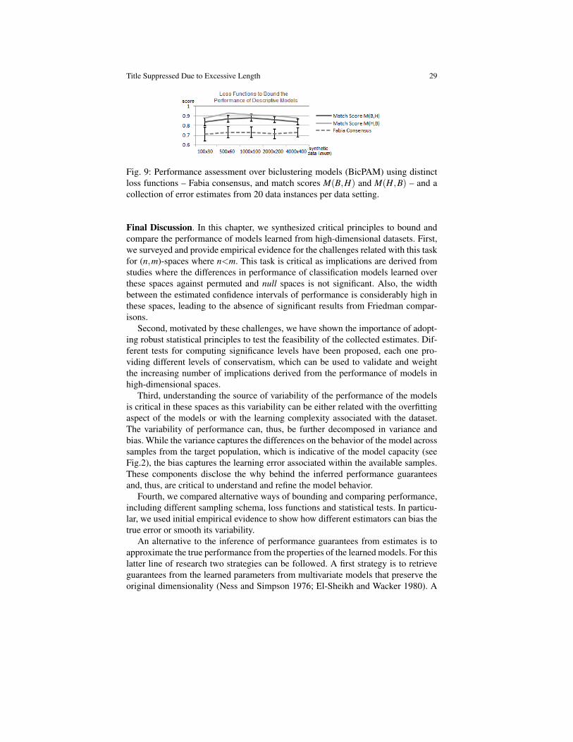
Title Suppressed Due to Excessive Length 29
Fig. 9: Performance assessment over biclustering models (BicPAM) using distinctloss functions – Fabia consensus, and match scores M(B,H) and M(H,B) – and acollection of error estimates from 20 data instances per data setting.
Final Discussion. In this chapter, we synthesized critical principles to bound andcompare the performance of models learned from high-dimensional datasets. First,we surveyed and provide empirical evidence for the challenges related with this taskfor (n,m)-spaces where n<m. This task is critical as implications are derived fromstudies where the differences in performance of classification models learned overthese spaces against permuted and null spaces is not significant. Also, the widthbetween the estimated confidence intervals of performance is considerably high inthese spaces, leading to the absence of significant results from Friedman compar-isons.
Second, motivated by these challenges, we have shown the importance of adopt-ing robust statistical principles to test the feasibility of the collected estimates. Dif-ferent tests for computing significance levels have been proposed, each one pro-viding different levels of conservatism, which can be used to validate and weightthe increasing number of implications derived from the performance of models inhigh-dimensional spaces.
Third, understanding the source of variability of the performance of the modelsis critical in these spaces as this variability can be either related with the overfittingaspect of the models or with the learning complexity associated with the dataset.The variability of performance can, thus, be further decomposed in variance andbias. While the variance captures the differences on the behavior of the model acrosssamples from the target population, which is indicative of the model capacity (seeFig.2), the bias captures the learning error associated within the available samples.These components disclose the why behind the inferred performance guaranteesand, thus, are critical to understand and refine the model behavior.
Fourth, we compared alternative ways of bounding and comparing performance,including different sampling schema, loss functions and statistical tests. In particu-lar, we used initial empirical evidence to show how different estimators can bias thetrue error or smooth its variability.
An alternative to the inference of performance guarantees from estimates is toapproximate the true performance from the properties of the learned models. For thislatter line of research two strategies can be followed. A first strategy is to retrieveguarantees from the learned parameters from multivariate models that preserve theoriginal dimensionality (Ness and Simpson 1976; El-Sheikh and Wacker 1980). A
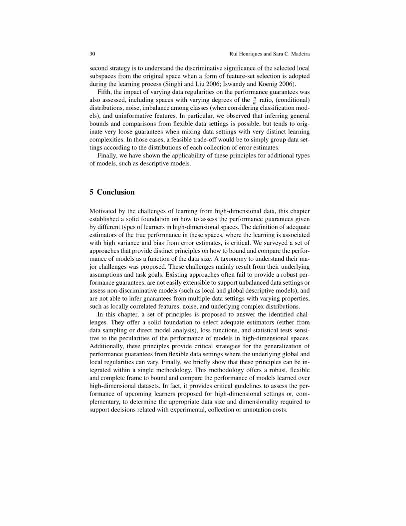
30 Rui Henriques and Sara C. Madeira
second strategy is to understand the discriminative significance of the selected localsubspaces from the original space when a form of feature-set selection is adoptedduring the learning process (Singhi and Liu 2006; Iswandy and Koenig 2006).
Fifth, the impact of varying data regularities on the performance guarantees wasalso assessed, including spaces with varying degrees of the n
m ratio, (conditional)distributions, noise, imbalance among classes (when considering classification mod-els), and uninformative features. In particular, we observed that inferring generalbounds and comparisons from flexible data settings is possible, but tends to orig-inate very loose guarantees when mixing data settings with very distinct learningcomplexities. In those cases, a feasible trade-off would be to simply group data set-tings according to the distributions of each collection of error estimates.
Finally, we have shown the applicability of these principles for additional typesof models, such as descriptive models.
5 Conclusion
Motivated by the challenges of learning from high-dimensional data, this chapterestablished a solid foundation on how to assess the performance guarantees givenby different types of learners in high-dimensional spaces. The definition of adequateestimators of the true performance in these spaces, where the learning is associatedwith high variance and bias from error estimates, is critical. We surveyed a set ofapproaches that provide distinct principles on how to bound and compare the perfor-mance of models as a function of the data size. A taxonomy to understand their ma-jor challenges was proposed. These challenges mainly result from their underlyingassumptions and task goals. Existing approaches often fail to provide a robust per-formance guarantees, are not easily extensible to support unbalanced data settings orassess non-discriminative models (such as local and global descriptive models), andare not able to infer guarantees from multiple data settings with varying properties,such as locally correlated features, noise, and underlying complex distributions.
In this chapter, a set of principles is proposed to answer the identified chal-lenges. They offer a solid foundation to select adequate estimators (either fromdata sampling or direct model analysis), loss functions, and statistical tests sensi-tive to the pecularities of the performance of models in high-dimensional spaces.Additionally, these principles provide critical strategies for the generalization ofperformance guarantees from flexible data settings where the underlying global andlocal regularities can vary. Finally, we briefly show that these principles can be in-tegrated within a single methodology. This methodology offers a robust, flexibleand complete frame to bound and compare the performance of models learned overhigh-dimensional datasets. In fact, it provides critical guidelines to assess the per-formance of upcoming learners proposed for high-dimensional settings or, com-plementary, to determine the appropriate data size and dimensionality required tosupport decisions related with experimental, collection or annotation costs.
REFERENCES 31
Experimental results support the relevance of these principles. We provided em-pirical evidence for the importance of computing adequate significance views toadjust the statistical power when bounding and comparing the performance of mod-els, of selecting adequate error estimators, of inferring guarantees from flexible datasettings, and of decomposing the error to gain further insights on the source of itsvariability. Additionally, we have experimentally shown the extensibility of thesedecisions for descriptive models under adequate performance views.
This work opens a new door for understanding, bounding and comparing theperformance of models in high-dimensional spaces. First, we expect the applicationof the proposed methodology to study the performance guarantees of new learners,parameterizations and feature selection methods. Additionally, these guarantees canbe used to weight and validate the increasing number of implications derived fromthe application of these models over high-dimensional data. Finally, we expect theextension of this assessment towards models learned from structured spaces, suchas high-dimensional time sequences.
Acknowledgments
This work was partially supported by FCT under the projects PTDC/EIA-EIA/111239/2009 (Neuroclinomics) and PEst-OE/ EEI/LA0021/2011, and under thePhD grant SFRH/BD/75924/2011.
Software Availability
The generated synthetic datasets and the software implementing the proposed sta-tistical tests are available in http://web.ist.utl.pt/rmch/software/bsize/.
References
Adcock, C. J. (1997). “Sample size determination: a review”. In: J. of the RoyalStatistical Society: Series D (The Statistician) 46.2, pp. 261–283.
Amaratunga, D., J. Cabrera, and Z. Shkedy (2014). Exploration and Analysis ofDNA Microarray and Other High-Dimensional Data. Wiley Series in Probabilityand Statistics. Wiley.
Apolloni, B. and C. Gentile (1998). “Sample size lower bounds in PAC learningby algorithmic complexity theory”. In: Theoretical Computer Science 209.1.2,pp. 141 –162.
Assent, I. et al. (2007). “DUSC: Dimensionality Unbiased Subspace Clustering”.In: ICDM.
32 REFERENCES
Beleites, C. et al. (2013). “Sample size planning for classification models”. In: An-alytica Chimica Acta 760.0, pp. 25 –33.
Blumer, A. et al. (1989). “Learnability and the Vapnik-Chervonenkis dimension”.In: J. ACM 36.4, pp. 929–965.
Boonyanunta, N. and P. Zeephongsekul (2004). “Predicting the Relationship Be-tween the Size of Training Sample and the Predictive Power of Classifiers”. In:Knowledge-Based Intelligent Information and Engineering Systems. Vol. 3215.LNCS. Springer Berlin Heidelberg, pp. 529–535.
Bozdag, D., A. S. Kumar, and U. V. Catalyurek (2010). “Comparative analysis ofbiclustering algorithms”. In: BCB. Niagara Falls, New York: ACM, pp. 265–274.
Buhlmann, P. and S. van de Geer (2011). Statistics for High-Dimensional Data:Methods, Theory and Applications. Springer Series in Statistics. Springer.
Cai, T. and X. Shen (2010). High-Dimensional Data Analysis (Frontiers of Statis-tics). World Scientific.
Cheng, Y. and G. M. Church (2000). “Biclustering of Expression Data”. In: Intelli-gent Systems for Molecular Biology. AAAI Press, pp. 93–103.
Demsar, J. (2006). “Statistical Comparisons of Classifiers over Multiple Data Sets”.In: J. Machine Learning Res. 7, pp. 1–30.
Deng, G. (2007). Simulation-based optimization. University of Wisconsin–Madison.Dobbin, K. and R. Simon (2005). “Sample size determination in microarray exper-
iments for class comparison and prognostic classification”. In: Biostatistics 6.1,pp. 27+.
Dobbin, K. K. and R. M. Simon (2007). “Sample size planning for developingclassifiers using high-dimensional DNA microarray data.” In: Biostatistics 8.1,pp. 101–117.
Domingos, P. (2000). “A Unified Bias-Variance Decomposition and its Applica-tions”. In: IC on Machine Learning. Morgan Kaufmann, pp. 231–238.
Dougherty, E. R. et al. (2010). “Performance of Error Estimators for Classification”.In: Current Bioinformatics 5.1, pp. 53–67.
El-Sheikh, T. S. and A. G. Wacker (1980). “Effect of dimensionality and estima-tion on the performance of gaussian classifiers.” In: Pattern Recognition 12.3,pp. 115–126.
Figueroa, R. L. et al. (2012). “Predicting sample size required for classification per-formance”. In: BMC Med. Inf. & Decision Making 12, p. 8.
Fleiss, J. L. (1981). Statistical Methods for Rates and Proportions. Wiley P. in Ap-plied Statistics. Wiley.
Garcıa, S. and F. Herrera (2009). “An Extension on ”Statistical Comparisons ofClassifiers over Multiple Data Sets” for all Pairwise Comparisons”. In: Journalof Machine Learning Research 9, pp. 2677–2694.
Glick, N. (1978). “Additive estimators for probabilities of correct classification”. In:Pattern Recognition 10.3, pp. 211 –222.
Guo, Y. et al. (2010). “Sample size and statistical power considerations in high-dimensionality data settings: a comparative study of classification algorithms”.English. In: BMC Bioinformatics 11.1, pp. 1–19.
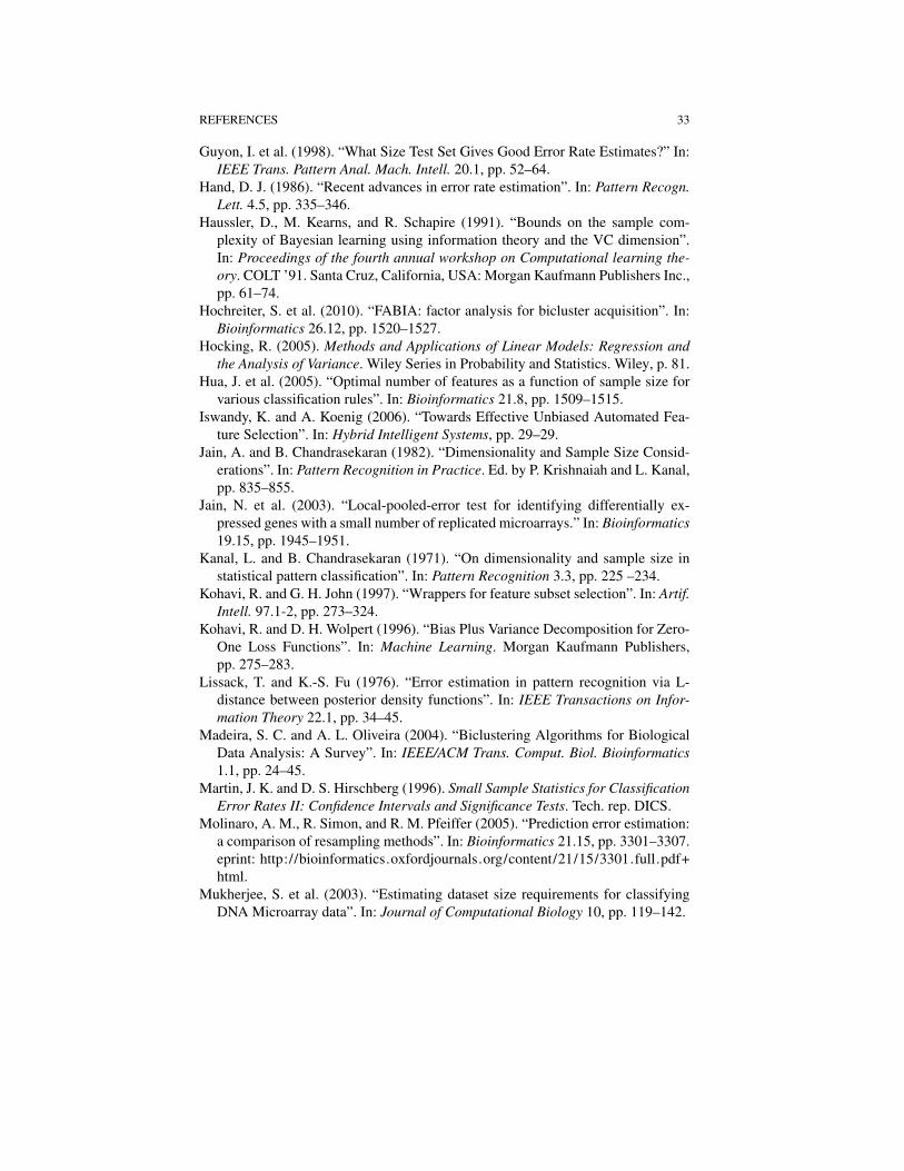
REFERENCES 33
Guyon, I. et al. (1998). “What Size Test Set Gives Good Error Rate Estimates?” In:IEEE Trans. Pattern Anal. Mach. Intell. 20.1, pp. 52–64.
Hand, D. J. (1986). “Recent advances in error rate estimation”. In: Pattern Recogn.Lett. 4.5, pp. 335–346.
Haussler, D., M. Kearns, and R. Schapire (1991). “Bounds on the sample com-plexity of Bayesian learning using information theory and the VC dimension”.In: Proceedings of the fourth annual workshop on Computational learning the-ory. COLT ’91. Santa Cruz, California, USA: Morgan Kaufmann Publishers Inc.,pp. 61–74.
Hochreiter, S. et al. (2010). “FABIA: factor analysis for bicluster acquisition”. In:Bioinformatics 26.12, pp. 1520–1527.
Hocking, R. (2005). Methods and Applications of Linear Models: Regression andthe Analysis of Variance. Wiley Series in Probability and Statistics. Wiley, p. 81.
Hua, J. et al. (2005). “Optimal number of features as a function of sample size forvarious classification rules”. In: Bioinformatics 21.8, pp. 1509–1515.
Iswandy, K. and A. Koenig (2006). “Towards Effective Unbiased Automated Fea-ture Selection”. In: Hybrid Intelligent Systems, pp. 29–29.
Jain, A. and B. Chandrasekaran (1982). “Dimensionality and Sample Size Consid-erations”. In: Pattern Recognition in Practice. Ed. by P. Krishnaiah and L. Kanal,pp. 835–855.
Jain, N. et al. (2003). “Local-pooled-error test for identifying differentially ex-pressed genes with a small number of replicated microarrays.” In: Bioinformatics19.15, pp. 1945–1951.
Kanal, L. and B. Chandrasekaran (1971). “On dimensionality and sample size instatistical pattern classification”. In: Pattern Recognition 3.3, pp. 225 –234.
Kohavi, R. and G. H. John (1997). “Wrappers for feature subset selection”. In: Artif.Intell. 97.1-2, pp. 273–324.
Kohavi, R. and D. H. Wolpert (1996). “Bias Plus Variance Decomposition for Zero-One Loss Functions”. In: Machine Learning. Morgan Kaufmann Publishers,pp. 275–283.
Lissack, T. and K.-S. Fu (1976). “Error estimation in pattern recognition via L-distance between posterior density functions”. In: IEEE Transactions on Infor-mation Theory 22.1, pp. 34–45.
Madeira, S. C. and A. L. Oliveira (2004). “Biclustering Algorithms for BiologicalData Analysis: A Survey”. In: IEEE/ACM Trans. Comput. Biol. Bioinformatics1.1, pp. 24–45.
Martin, J. K. and D. S. Hirschberg (1996). Small Sample Statistics for ClassificationError Rates II: Confidence Intervals and Significance Tests. Tech. rep. DICS.
Molinaro, A. M., R. Simon, and R. M. Pfeiffer (2005). “Prediction error estimation:a comparison of resampling methods”. In: Bioinformatics 21.15, pp. 3301–3307.eprint: http://bioinformatics.oxfordjournals.org/content/21/15/3301.full.pdf+html.
Mukherjee, S. et al. (2003). “Estimating dataset size requirements for classifyingDNA Microarray data”. In: Journal of Computational Biology 10, pp. 119–142.
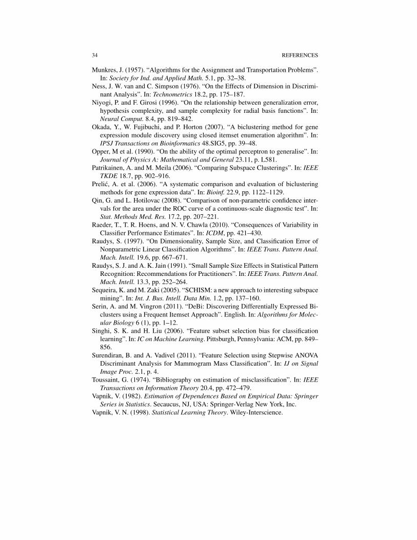
34 REFERENCES
Munkres, J. (1957). “Algorithms for the Assignment and Transportation Problems”.In: Society for Ind. and Applied Math. 5.1, pp. 32–38.
Ness, J. W. van and C. Simpson (1976). “On the Effects of Dimension in Discrimi-nant Analysis”. In: Technometrics 18.2, pp. 175–187.
Niyogi, P. and F. Girosi (1996). “On the relationship between generalization error,hypothesis complexity, and sample complexity for radial basis functions”. In:Neural Comput. 8.4, pp. 819–842.
Okada, Y., W. Fujibuchi, and P. Horton (2007). “A biclustering method for geneexpression module discovery using closed itemset enumeration algorithm”. In:IPSJ Transactions on Bioinformatics 48.SIG5, pp. 39–48.
Opper, M et al. (1990). “On the ability of the optimal perceptron to generalise”. In:Journal of Physics A: Mathematical and General 23.11, p. L581.
Patrikainen, A. and M. Meila (2006). “Comparing Subspace Clusterings”. In: IEEETKDE 18.7, pp. 902–916.
Prelic, A. et al. (2006). “A systematic comparison and evaluation of biclusteringmethods for gene expression data”. In: Bioinf. 22.9, pp. 1122–1129.
Qin, G. and L. Hotilovac (2008). “Comparison of non-parametric confidence inter-vals for the area under the ROC curve of a continuous-scale diagnostic test”. In:Stat. Methods Med. Res. 17.2, pp. 207–221.
Raeder, T., T. R. Hoens, and N. V. Chawla (2010). “Consequences of Variability inClassifier Performance Estimates”. In: ICDM, pp. 421–430.
Raudys, S. (1997). “On Dimensionality, Sample Size, and Classification Error ofNonparametric Linear Classification Algorithms”. In: IEEE Trans. Pattern Anal.Mach. Intell. 19.6, pp. 667–671.
Raudys, S. J. and A. K. Jain (1991). “Small Sample Size Effects in Statistical PatternRecognition: Recommendations for Practitioners”. In: IEEE Trans. Pattern Anal.Mach. Intell. 13.3, pp. 252–264.
Sequeira, K. and M. Zaki (2005). “SCHISM: a new approach to interesting subspacemining”. In: Int. J. Bus. Intell. Data Min. 1.2, pp. 137–160.
Serin, A. and M. Vingron (2011). “DeBi: Discovering Differentially Expressed Bi-clusters using a Frequent Itemset Approach”. English. In: Algorithms for Molec-ular Biology 6 (1), pp. 1–12.
Singhi, S. K. and H. Liu (2006). “Feature subset selection bias for classificationlearning”. In: IC on Machine Learning. Pittsburgh, Pennsylvania: ACM, pp. 849–856.
Surendiran, B. and A. Vadivel (2011). “Feature Selection using Stepwise ANOVADiscriminant Analysis for Mammogram Mass Classification”. In: IJ on SignalImage Proc. 2.1, p. 4.
Toussaint, G. (1974). “Bibliography on estimation of misclassification”. In: IEEETransactions on Information Theory 20.4, pp. 472–479.
Vapnik, V. (1982). Estimation of Dependences Based on Empirical Data: SpringerSeries in Statistics. Secaucus, NJ, USA: Springer-Verlag New York, Inc.
Vapnik, V. N. (1998). Statistical Learning Theory. Wiley-Interscience.

REFERENCES 35
Vayatis, N. and R. Azencott (1999). “Distribution-Dependent Vapnik-ChervonenkisBounds”. English. In: Computational Learning Theory. Ed. by P. Fischer and H.Simon. Vol. 1572. LNCS. Springer Berlin Heidelberg, pp. 230–240.
Way, T. et al. (2010). “Effect of finite sample size on feature selection and classifi-cation: A simulation study”. In: Medical Physics 37.2, pp. 907–920.
Copyright © 2022 FDOKUMEN