Optimal routing for end-to-end guarantees using Network Calculus

Optimal routing for end-to-end guarantees using

Network Calculus

Anne Bouillard, Bruno Gaujal, Sebastien Lagrange, Eric Thierry

To cite this version:

Anne Bouillard, Bruno Gaujal, Sebastien Lagrange, Eric Thierry. Optimal routing for end-to-end guarantees using Network Calculus. [Research Report] RR-6423, INRIA. 2008, pp.20.<inria-00214235v2>

HAL Id: inria-00214235

https://hal.inria.fr/inria-00214235v2

Submitted on 24 Jan 2008

HAL is a multi-disciplinary open accessarchive for the deposit and dissemination of sci-entific research documents, whether they are pub-lished or not. The documents may come fromteaching and research institutions in France orabroad, or from public or private research centers.

L’archive ouverte pluridisciplinaire HAL, estdestinee au depot et a la diffusion de documentsscientifiques de niveau recherche, publies ou non,emanant des etablissements d’enseignement et derecherche francais ou etrangers, des laboratoirespublics ou prives.

https://hal.archives-ouvertes.fr

https://hal.inria.fr/inria-00214235v2

appor t de r ech er ch e

ISS

N02

49-6

399

ISR

NIN

RIA

/RR

--64

23--

FR

+E

NG

Thème COM

INSTITUT NATIONAL DE RECHERCHE EN INFORMATIQUE ET EN AUTOMATIQUE

Optimal routing for end-to-end guaranteesusing Network Calculus

Anne.Bouillard and Bruno Gaujal and Sébastien Lagrange and Éric Thierry

N° 6423

Janvier 2008

Unité de recherche INRIA RennesIRISA, Campus universitaire de Beaulieu, 35042 Rennes Cedex (France)

Téléphone : +33 2 99 84 71 00 — Télécopie : +33 2 99 84 71 71

Optimal routing for end-to-end guarantees

using Network Calculus

Anne.Bouillard ∗ and Bruno Gaujal † and Sebastien Lagrange ‡ and Eric Thierry §

Theme COM — Systemes communicantsProjet Distribcom

Rapport de recherche n�

6423 — Janvier 2008 — 20 pages

Abstract: In this paper we show how Network Calculus can be used to compute the optimal route for a flow(w.r.t. end-to-end guarantees on the delay or the backlog) in a network in the presence of cross-traffic. Whencross-traffic is independent, the computation is shown to boild down to a functional shortest path problem.When cross-traffic perturbates the main flow over more than one node, then the “Pay Multiplexing Only Once”phenomenon makes the computation more involved. We provide an efficient algorithm to compute the servicecurve available for the main flow and show how to adapt the shortest path algorithm in this case.

Key-words: Network Calculus, multiplexing, shortest-path.

∗ [email protected]† [email protected]‡ [email protected]§ [email protected]

Routage optimal pour le calcul de garanties de performances de

bout en bout dans les reseaux

Resume : Dans ce rapport, nous montrons comment le Network Calculus peut etre utilise pour calculer uneroute optimale pour un flot, quant a ses garanties de performances pour le delai de bout en bout ou le nombre depaquets, dans un reseau en presence de trafic transverse. Quand le trafic transverse est independant, on peut seramener a un calcul de plus court chemin dans un graphe pondere par des fonctions. Quand le trafic transverseperturbe le flot principal sur plus d’un nœud, le phonomene pay multiplexing only once rend les calculs pluscomplexes. Nous fournissons un algorithme efficace pour calculer la courbe de service disponible pour le flotprincipal et montrons comment adapter l’algorithme de plus court chemin dans ce cas.

Mots-cles : Network Calculus, multiplexage, plus court chemins.

Optimal routing for end-to-end guarantees using Network Calculus 3

1 Introduction

Optimizing the route of a flow of packets through a network has been investigated in many directions and usingmany approaches depending on the assumptions made on the system as well as the performance objectives.When one wants to maximize the throughput of one connection, most recent results in deterministic contextsuse multi-flow or LP techniques [3, 4], or optimal control and/or game theory in a stochastic one as for examplein [1].

When the maximal delay over all packets in the flow is the performance index, fewer results are available inthe litterature. Under static assumptions on the flows and the network ressources, optimal bandwidth allocationhas been investigated in [8]. However, when the flows and the ressources have dynamic features, most focus ison simple systems such as single nodes where the issue becomes optimal scheduling.

Here we consider the problem of computing the route of a flow that provides the best delay guarantee Dmax

(no packet of the flow will ever spend more than Dmax seconds in the system) or backlog guarantee Bmax (thenumber of packets of the flow inside the network never tops Bmax), in the presence of cross-traffic. NetworkCalculus [7, 11] is a framework that allows us to formulate this problem as a mathematical program.

In the first part of this paper, we show how to compute the best route for one flow from source to destinationover an arbitrary network when the cross-traffic in each node is independent. Using the network calculusframework, we show that this boils down to solving a classical shortest path problem using appropriate costs ateach node, as soon as the service curves are piecewise affine and convex and arrival curves are concave, whichare classical assumptions in Network Calculus.

The second part of the paper considers the more realistic case where cross-traffic in each node is not inde-pendent. This happens when several flows follow the same sub-paths over more than two nodes or when themain flow crosses the same cross-traffic several times. This case is much harder to solve because of the “PayMultiplexing Only Once” (PMOO) phenomenon, which was first identified in [10]. When the main flow mergeswith a cross-traffic, its service might be strongly reduced in the first node. However, in the following nodes, theinterference due to the cross-traffic cannot be as severe since the competition for the ressource has already beenpartially resolved in the previous ones. The PMOO phenomenon can be quantified in the Network Calculuscontext. It does provide good bounds on performance guarantees but this comes with a price:

� In that case we only tackle efficiently networks with a strong acyclicity property (introduced in this paper).In fact, computing tight guarantees in cyclic networks is still open (the simpler problem of stability is alsoopen [2]).

� The algorithms involved have much higher complexities.

For single paths, the approach in [13] provides an example showing how to compute the global service curvefor a single path with 2 cross-traffic flows. When the service curve in each node is piecewise affine, then thealgorithm provided in [13] is based on a decompostion in affine functions. The complexity grows exponentiallywith the number of cross-traffic flows and the number of nodes in the path. Here, we provide an explicit generalformula for the PMOO phenomenon for arbitrary cross-traffic. The global service curve is written under theform of a multi-dimensional convolution which helps designing an algorithm to compute it with a sub-quadraticcomplexity. For routing problems, this single path computation can be applied to find the best route in anacyclic network, taking into account PMOO. Under stronger assumptions (affine functions, concentration ofthe cross-traffic), we show how to speed up the best route computation by reducing the problem once more toclassical shortest path algorithms.

This paper is a long version of [5], providing detailed proofs of all the results as well as several extensions.The most important one is the new algorithm provided in Section 3. It allows one to compute the best route forbacklog and delay minimization under concave/convex assumptions on the arrival/service curves. In [5] moredirect algorithms were provided, but they worked on more restricted types of curves: backlog minimizationassumed rate-latency service curves or affine arrival curves, and delay minimization assumed affine arrivalcurves. A detailed overview of the complexity of all these algorithms is provided in Table 3.3.

2 Performances guarantees

In this section, we recall the main definitions and the main properties of the Network Calculus functions andoperations. More precise insights can be found in [7, 11].

RR n�

6423

4 Bouillard, Gaujal, Lagrange & Thierry

2.1 Network Calculus functions

Network Calculus is based on the (min, +) algebra and models flows and services in a network with non-decreasing functions taking their values in the (min, +) semiring.

Formally, the (min, +) semiring, denoted by (Rmin,⊕,⊗) is defined on Rmin = R ∪ {+∞}, and is equippedwith two internal operations: ⊕, the minimum, and ⊗, the addition. The zero element is +∞, the unitaryelement is 0. The ⊕ and ⊗ operators are commutative and associative. Moreover ⊗ is distributive over ⊕.

Consider the set F of functions from R+ into Rmin. One can define as follows two operators on F , theminimum, denoted by ⊕, and the (min,+) convolution, denoted by ∗: for all f, g in F , ∀t ∈ R+,

� f ⊕ g(t) = f(t)⊕ g(t) and

� f ∗ g(t) = inf0≤s≤t(f(s) + g(t− s)).

The triple (F ,⊕, ∗) is also a semiring and the convolution can be seen as an analogue to the classical (+,×)convolution of filtering theory, transposed in the (min,+) algebra. Another important operator for NetworkCalculus is the (max, +) deconvolution, denoted by �: let f, g ∈ F , ∀t ≥ 0,

� f � g(t) = supu≥0(f(t + u)− g(u)).

2.2 Arrival and service curves

Arrival curves. Given a data flow traversing a system, let A be its cumulative arrival function, i.e. A(t) isthe number of packets that have arrived until time t. We say that α is an arrival curve for A (or that A isupper-constrained by α) if ∀ 0 ≤ s ≤ t ∈ R+, A(t) − A(s) ≤ α(t − s). This means that the number of packetsarriving between time s and t is at most α(t− s). An important particular case of arrival curves are the affinefunctions: α(t) = σ +ρt. Then σ represents the maximal number of packets that can arrive simultaneously (themaximal burst) and ρ the maximal long-term rate of arrivals.

Service curves. Consider B the cumulative departure function of the flow, defined similarly by the num-ber B(t) of packets that have left the system until time t. The system provides a (minimum) service curve βif B ≥ A ∗ β. Particular cases of service curves are the peak rate functions with rate r (the system can serve rpackets per unit of time and β(t) = rt) and the pure delay service curves with delay T : β(t) = 0 if t < T andβ(t) = +∞ otherwise. The combination of those two service curves gives a rate-latency function β(t) = r(t−T )+

where a+ denotes max(a, 0). A strict service curve β is a service curve such that for all t ∈ R+, let u < t be thelast instant before t when there is no packet in the system i.e. B(u) = A(u), then B(t) ≥ B(u) + β(t−u). Thisenforcement of the service curve notion is necessary to have refined bounds (e.g. positiveness of output servicecurves in Lemma 2 and Theorem 2). Note that contrary to a statement of [5], if a service curve is convex, it isnot necessarily a strict service curve. Consequently, all along the paper, we will detail whenever service curvesare assumed to be strict or not.

We also consider that for any service curve β, β(0) = 0: there is no instantaneous service.

2.3 Performance characteristics and bounds

The worst case backlog and the delay can be easily characterized with Network Calculus.

Definition 1. Let A be the arrival function of a flow through a system and B be its corresponding departurefunction. Then the backlog of the flow at time t is

b(t) = A(t)−B(t)

and the delay (assuming FIFO order for serving packets of the flow) at time t is

d(t) = inf{s ≥ 0 | A(t) ≤ B(t + s)}.

Given an arrival curve and a service curve, it is possible to compute with the Network Calculus operationsthe maximal backlog and delay. Moreover, one can also compute the arrival curve of the departure process.

Theorem 1 ([7, 11]). Let A be the arrival function with an arrival curve α for a flow entering a system withservice curve β. Let B be the departure function. Then,

INRIA


1. B has an arrival curve α� β.

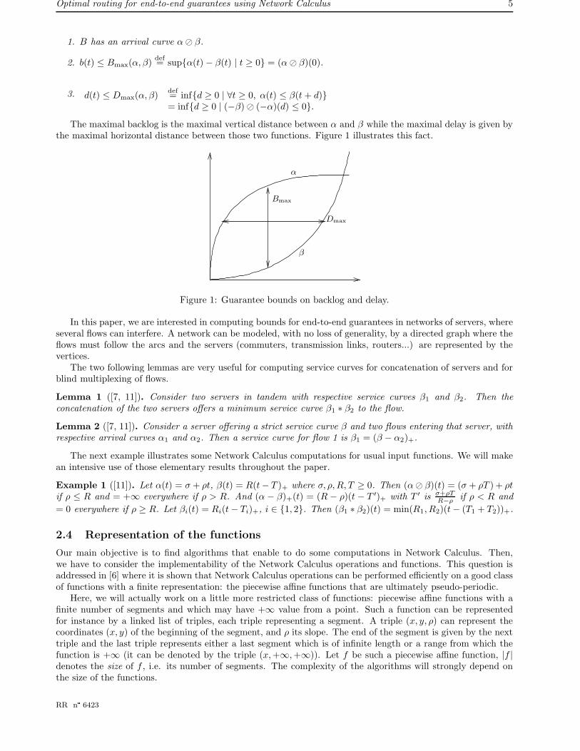
2. b(t) ≤ Bmax(α, β)def= sup{α(t)− β(t) | t ≥ 0} = (α� β)(0).

3. d(t) ≤ Dmax(α, β)def= inf{d ≥ 0 | ∀t ≥ 0, α(t) ≤ β(t + d)}= inf{d ≥ 0 | (−β)� (−α)(d) ≤ 0}.

The maximal backlog is the maximal vertical distance between α and β while the maximal delay is given bythe maximal horizontal distance between those two functions. Figure 1 illustrates this fact.

Dmax

Bmax

α

β

Figure 1: Guarantee bounds on backlog and delay.

In this paper, we are interested in computing bounds for end-to-end guarantees in networks of servers, whereseveral flows can interfere. A network can be modeled, with no loss of generality, by a directed graph where theflows must follow the arcs and the servers (commuters, transmission links, routers...) are represented by thevertices.

The two following lemmas are very useful for computing service curves for concatenation of servers and forblind multiplexing of flows.

Lemma 1 ([7, 11]). Consider two servers in tandem with respective service curves β1 and β2. Then theconcatenation of the two servers offers a minimum service curve β1 ∗ β2 to the flow.

Lemma 2 ([7, 11]). Consider a server offering a strict service curve β and two flows entering that server, withrespective arrival curves α1 and α2. Then a service curve for flow 1 is β1 = (β − α2)+.

The next example illustrates some Network Calculus computations for usual input functions. We will makean intensive use of those elementary results throughout the paper.

Example 1 ([11]). Let α(t) = σ + ρt, β(t) = R(t− T )+ where σ, ρ, R, T ≥ 0. Then (α� β)(t) = (σ + ρT ) + ρtif ρ ≤ R and = +∞ everywhere if ρ > R. And (α − β)+(t) = (R − ρ)(t − T ′)+ with T ′ is σ+ρT

R−ρ if ρ < R and

= 0 everywhere if ρ ≥ R. Let βi(t) = Ri(t− Ti)+, i ∈ {1, 2}. Then (β1 ∗ β2)(t) = min(R1, R2)(t− (T1 + T2))+.

2.4 Representation of the functions

Our main objective is to find algorithms that enable to do some computations in Network Calculus. Then,we have to consider the implementability of the Network Calculus operations and functions. This question isaddressed in [6] where it is shown that Network Calculus operations can be performed efficiently on a good classof functions with a finite representation: the piecewise affine functions that are ultimately pseudo-periodic.

Here, we will actually work on a little more restricted class of functions: piecewise affine functions with afinite number of segments and which may have +∞ value from a point. Such a function can be representedfor instance by a linked list of triples, each triple representing a segment. A triple (x, y, ρ) can represent thecoordinates (x, y) of the beginning of the segment, and ρ its slope. The end of the segment is given by the nexttriple and the last triple represents either a last segment which is of infinite length or a range from which thefunction is +∞ (it can be denoted by the triple (x, +∞, +∞)). Let f be such a piecewise affine function, |f |denotes the size of f , i.e. its number of segments. The complexity of the algorithms will strongly depend onthe size of the functions.

RR n�

6423


We will also always suppose that the networks are stable, that is the total number of packets in the serversnever grows to infinite. For the class of functions we use as arrival and service curves, checking the stability ofa network is easy if the directed graph is acyclic [11]: at each vertex, the long-term rate of arrivals must be lessthan the long-term service rate, i.e. the sum over the flows entering the vertex of the ultimate slopes of theirarrival curves must be less than the ultimate slope of the service curve. For general digraphs, the complexityof this decision problem is open [2].

3 Optimal routing with independent cross-traffic

In this section, we wish to route one flow over an arbitrary network. Each vertex may or may not be subject tointerference due to independent cross-traffic: the cross-traffic in any two vertices are not correlated. We wantto find a path from the source vin of the flow to its destination vout, that optimizes the end-to-end performanceguarantees for that flow, given the service curves at each vertex and the arrival curves of that flow and of thecross-traffic.

Here is a survey of the main assumptions we will consider. All functions are non-decreasing. We supposethat arrival curves are concave. It is an usual assumption. Even when it is not fullfilled, an arrival curve α canalways be replaced by its subadditive closure α∗ [11] for which α∗(t)/t converges to a finite value when t→ +∞(as any subadditive function). Then one can choose to use the concave envelope of α∗ as arrival curve for theflow. This is asymptotically tight with regard to α∗.

We suppose that the service curves are convex. It is also an usual assumption. Since we allow infinite values,note that a function which is convex over [0, T ] and equal to +∞ over ]T, +∞[ is convex over R+. If the servicecurves are also strict, we can take into account the cross-traffic with blind multiplexing: if vertex v offers aservice curve β0

v and the cross-traffic in vertex v has arrival curve αv, then we can use βv = (β0v − αv)+ as

a service curve for the main flow, as stated in Lemma 2, and if β0v is convex and αv is concave, then βv is

convex. Such a reduction is totally appropriate for independent cross-traffic. Once this is done, no mention ofthe cross-traffic is necessary any longer in this section.

The general routing problem we consider in this section is:

Given a directed graph G = (V, A) with a service curve βv for each v ∈ V andsome flow specifications, namely its source vin ∈ V , its destination vout ∈ Vand an arrival curve α, compute a path from vin to vout such that the worstcase delay (or backlog) for the flow is minimal.

In graph theory, one can mention two classical versions of optimal routing. With arcs and/or verticesweighted by numbers, the first one consists in finding a classical shortest path from one source to one destination(minimizing the sum of the weights of the path), and the latter one is to find a path with maximum bottleneckcapacity (maximizing the smallest weight of the path). Those two problems can be seen as special cases ofour problem, when respectively the service curves βv are all pure delays or are all peak rates (see Lemma 6explaining how these functions behave with regard to the convolution).

We first state some general lemmas about computing maximal backlog and delay for concave arrival curvesand convex service curves. Then we describe a polynomial algorithm to solve the optimal routing problem fordelays and backlogs

3.1 Concave arrival curves and convex service curves

Some specific results apply when arrival/service curves are concave/convex. The first one is a simple min-maxtheorem concerning the maximal delay or backlog.

We first define a notion of stripe. Let λ ∈ R+ ∪ {+∞}, a λ-stripe S is a subset of R2 of the form {(x, y) ∈

R2 | ymin + λx ≤ y ≤ ymax + λx} for ymin ≤ ymax (and of the form {(x, y) ∈ R

2 | xmin ≤ x ≤ xmax + λx} forxmin ≤ xmax if λ = +∞). In other words, a λ-stripe S is the stripe between two lines of slope λ. We denotehsize(S) (resp. vsize(S), and width(S)) the horizontal (resp. vertical, and euclidian) distance between thesetwo border lines. We set hsize(S) = +∞ (resp. vsize(S) = +∞) if λ = 0 (resp. λ = +∞), and we clearly have

vsize(S) = width(S)√

1 + λ2 and hsize(S) = width(S)√

1+λ2

λ .

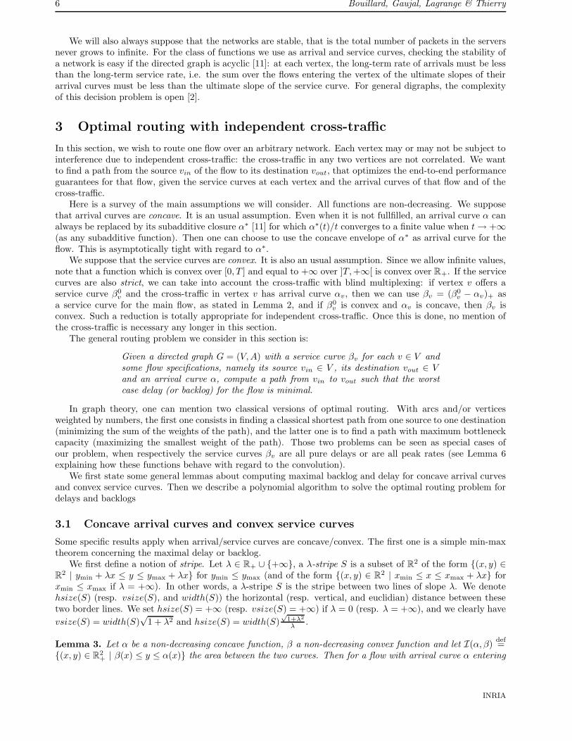
Lemma 3. Let α be a non-decreasing concave function, β a non-decreasing convex function and let I(α, β)def=

{(x, y) ∈ R2+ | β(x) ≤ y ≤ α(x)} the area between the two curves. Then for a flow with arrival curve α entering

INRIA


λ-stripe S

width(S)

Dmax(α, β)hsize(S)

α

Bmax(α, β)vsize(S)

β

I(α, β)

Figure 2: An arrival curve α, a sevice curve β and a stripe S containing the area I(α, β). The quantitieswidth(S), hsize(S), Dmax(α, β) and vsize(S), Dmax(α, β) are given in the figure.

a node with service curve β, the maximal delay and maximal backlog satisfy:

Dmax(α, β) = min{hsize(S) | S is a λ−stripe, λ ∈ R+ ∪ {+∞}, S ⊇ I(α, β)}

Bmax(α, β) = min{vsize(S) | S is a λ−stripe, λ ∈ R+ ∪ {+∞}, S ⊇ I(α, β)}

Proof. Since α is concave and β is convex, then α− β is concave with value 0 at 0.If α−β remains non-negative then I(α, β) is infinite and no stripe of finite width can contain it. By consideringthat min ∅ = +∞, one gets Dmax(α, β) = Bmax(α, β) =∞. This ends the proof in that case.If α is always smaller than β, then I(α, β) = {(0, 0)} and all stripes containing (0, 0) will do. In particular, astripe reduced to a line with an arbitrary slope and containing (0, 0) has a null width and provides the equalitiesDmax(α, β) = Bmax(α, β) = 0.The only interesting case is when α−β is larger than 0 up to some point t0 and is non-positive from that pointon. From the definitions of Dmax(α, β) and Bmax(α, β), the inequalities

Dmax(α, β) ≤ min{hsize(S) | S is a λ−stripe, , S ⊇ I(α, β)}Bmax(α, β) ≤ min{vsize(S) | S is a λ−stripe, , S ⊇ I(α, β)}.

are clearly true as seen on Figure 2.For the other inequality, let us first carry the proof for Bmax. By concavity, there exists a finite time t1 suchthat Bmax(α, β) = α(t1) − β(t1). Since the function α − β is piecewise affine, let us call by d+(α − β)(t1)(resp. d−(α − β)(t1)) its slope just after t1 (resp. just before t1). The function α − β being maximal at t1,then d+(α− β)(t1) = d+(α)(t1)− d+(β)(t1) ≤ 0 and d−(α− β)(t1) = d−(α)(t1)− d−(β)(t1) ≥ 0. Moreover byconvexity and concavity of β and α, d+(β)(t1) ≥ d−(β)(t1) and d−(α)(t1) ≥ d+(α)(t1). Combining all thoseinequalities says that d+(β)(t1) and d−(α)(t1) are both larger than d−(β)(t1) and d+(α)(t1). Consider anyslope λ such that

min(d+(β)(t1), d−(α)(t1)) ≥ λ ≥ max(d−(β)(t1), d+(α)(t1)).

Then, the stripe of slope λ containing the points (t1, α(t1)) and (t1, β(t1)) is of vertical size α(t1)−β(t1), equalto Bmax(α, β) by definition of t1 and contains I(α, β), because from point (t1, α(t1)) all the slopes of α and βcompare well with λ. This ends the proof for Bmax.As for horizontal distance Dmax, the proof is essentially the same by considering the vertical distance betweenα−1 and β−1.

Lemma 4. With the assumptions of Lemma 3, suppose that α (resp. β) is piecewise affine with a finite number

of segments of slopes r0 ≥ r1 ≥ · · · ≥ rp (resp. ρ1 ≤ · · · ≤ ρm) with r0def= +∞ corresponding to the segment

from (0, 0) to (0, f(0+)) and with ρmdef= +∞ if β = +∞ from a point. Then

Dmax(α, β) = minλ∈{r0,...,rp}∪{ρ1,...,ρm}

{hsize(S) | S is a λ−stripe, S ⊇ I(α, β)}

Bmax(α, β) = minλ∈{r0,...,rp}∪{ρ1,...,ρm}

{vsize(S) | S is a λ−stripe, S ⊇ I(α, β)}

RR n�

6423


Dmax(α, β)

α

SS′

β

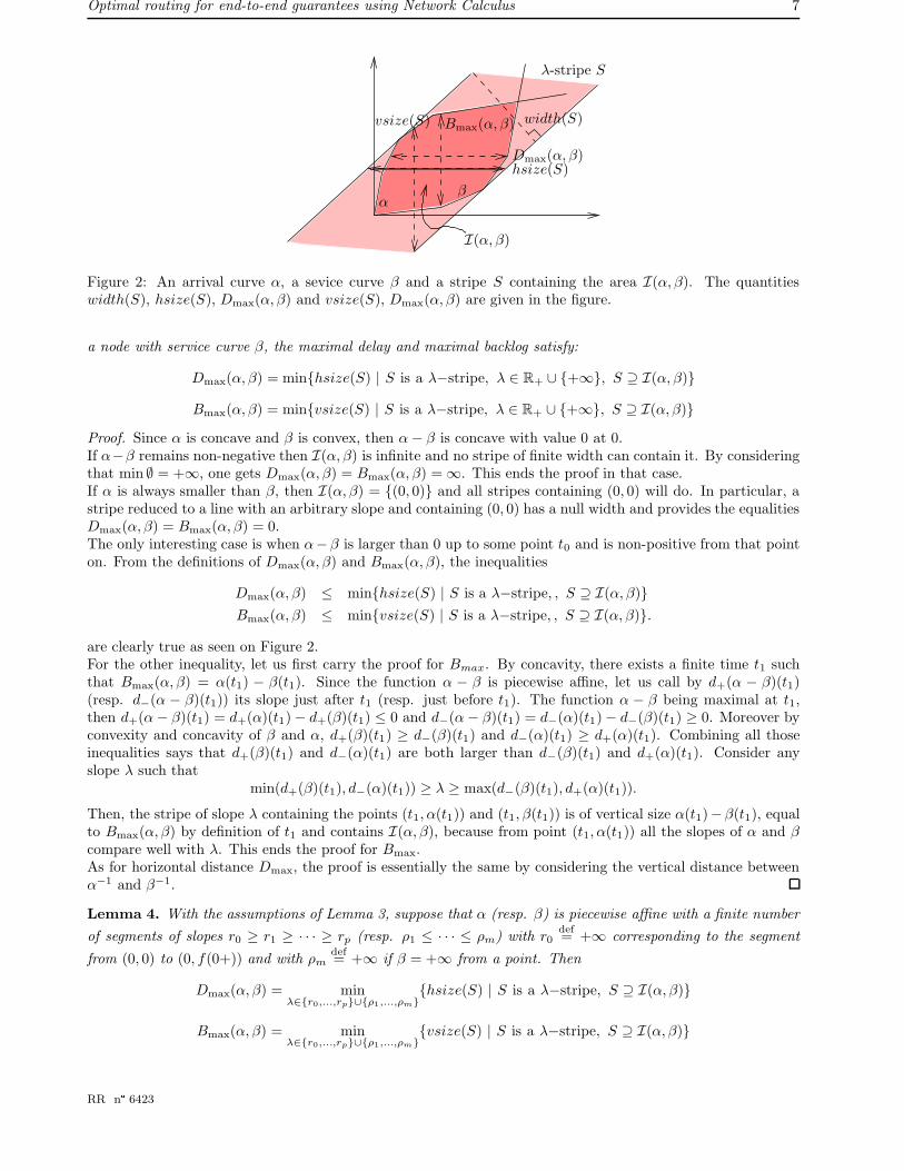
Figure 3: A stripe S with horizontal size equal to Dmax(α, β). By tilting S, one gets S ′ a stripe with the samesize as S whose slope is commum with α (or β).

Proof. We only provide the proof for Dmax(α, β). The same argument holds for Bmax(α, β). Assume thatDmax(α, β) is the horizontal size of a stripe S is Dmax(α, β). It should be clear that the stripe touches bothα and β (otherwise, a stripe with the same slope and a smaller horizontal size can be constructed). Figure 3displays such an example. From S let us construct a new stripe S ′ with the same horizontal size as S by fixingthe two contact points with α and β and letting λ increase as long as the stripe contains I(α, β). The slope ofthe new tilted stripe S′ must be the slope of one of the segments of α and β (see Figure 3).

If both α and β have a finite number of segments, and if the slope λ is fixed, then the minimum value ofwidth(S), hsize(S) and vsize(S) over λ-stripes is given by a simple formula involving projections along thedirection λ. Let λ ∈ R+ ∪ {+∞}, we denote

Wλ(α, β)def= min{width(S) | S is a λ−stripe, S ⊇ I(α, β)}

Hλ(α, β)def= min{hsize(S) | S is a λ−stripe, S ⊇ I(α, β)}

Vλ(α, β)def= min{vsize(S) | S is a λ−stripe, S ⊇ I(α, β)}.

We also define the orthogonal projection projλ parallel to the line y = λx (the line x = 0 if λ = +∞) whichassociates with each segment s of R

2 of slope r ∈ R+ ∪ {+∞} and length ` ∈ R+ ∪ {+∞} the value1:

projλ(s) =λ− r√

1 + λ2√

1 + r2`.

Lemma 5. With the assumptions of Lemma 4 and the notation above, let αi, 0 ≤ i ≤ p (resp. βj , 1 ≤ j ≤ m),be the segments composing α (resp. β). Let λ ∈ R+ ∪ {+∞}, then:

Hλ = Wλ

√1 + λ2

λ, Vλ = Wλ

√

1 + λ2,

Wλ =

p∑

i=0

(−projλ(αi))+ +

m∑

j=1

(projλ(βj))+

where x+ denotes max(x, 0).

Proof. The equalities linking Hλ, Vλ and Wλ, are direct consequences of the same equalities mentionned beforeand linking hsize(S), vsize(S) and width(S) for any λ-stripe S.

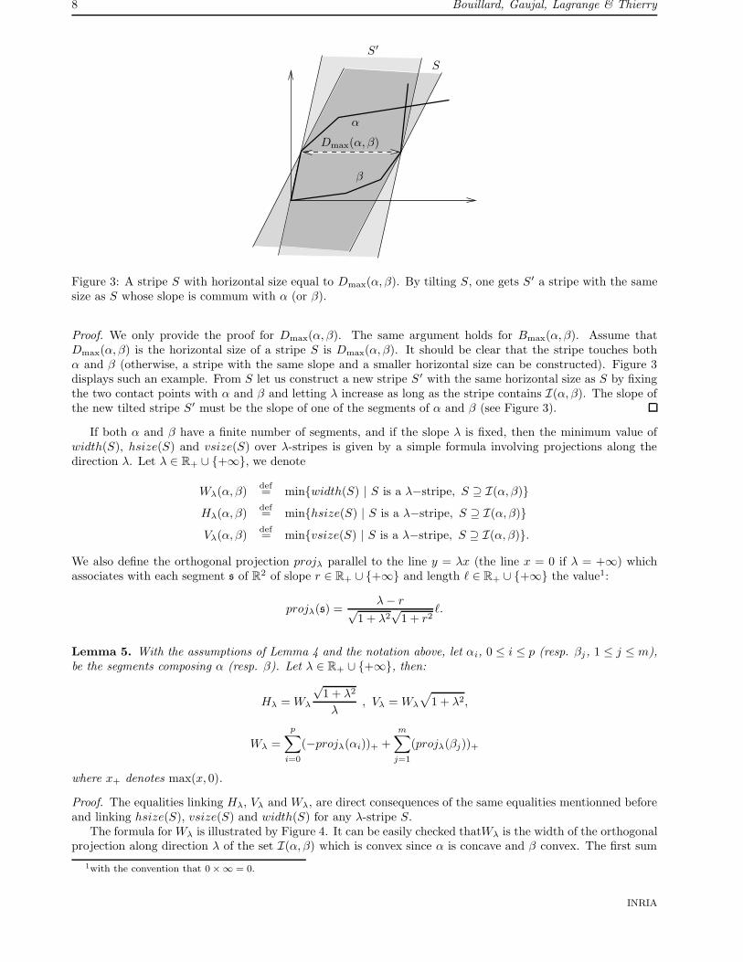
The formula for Wλ is illustrated by Figure 4. It can be easily checked thatWλ is the width of the orthogonalprojection along direction λ of the set I(α, β) which is convex since α is concave and β convex. The first sum

1with the convention that 0 ×∞ = 0.

INRIA


Wλ

b2

β1

β2

α1

α2

a1

b1

a2

b3

Figure 4: The projection along direction λ of the segments of α1 and α2 give the quantities a1(< 0) and a2(> 0)respectively. All the other segments of α have slopes smaller than λ so that they are projected on positivequantities. The projection of β1, β2, β3 are b1(> 0), b2(> 0), b3(< 0) respectively. All the other segments of βhave slopes larger than λ so that they are projected on negative quantities. One can verify on the figure thatWλ = (−a1)+ + (−a2)+ +

∑

i>2(−ai)+ + b1+ + b2+ + b3+ +∑

i>3(bi)+ = −a1 + b1 + b2.

corresponds to the concave curve α. Due to its shape, the projection of α only takes into account the firstpart of the curve where the segments have a slope at least λ (the maximum with 0 is used to retain only thecontribution of those segments). It is clearly additive with regard to the concatenation of the segments αi.Similarly the second sum represents the projection of the first part of the convex curve β where the segmentshave a slope at most λ.

Note that the formula of Lemma 5 is a sum. Due to commutativity, it means that it is not necessary to givethe list of the segments αi (resp. βj) ordered by non-increasing (resp. non-decreasing) slopes.

3.2 Transforming service curves into elementary service curves

Before presenting an algorithm which solves the optimal routing problem when the arrival curve of the routedflow is concave and the services curves are convex, we show how to transform the input network so that theservice curves we manipulate all have the same elementary shape, that is a single segment.

An elementary segment β is a finite or semi-infinite segment over R+ such that β(0) = 0. More precisely,either β(t) = rt when 0 ≤ t ≤ T and = +∞ when t > T for some r, T ∈ R+ (finite elementary segment) orβ(t) = rt on R+ for some r ∈ R+ (semi-infinite elementary segment).

Any non-decreasing, convex, piecewise affine function β over R+ such that β(0) = 0 and with a finitenumber of segments, is equal to the convolution of these segments all translated to point (0, 0) to be elementarysegments. This result is a direct consequence of the following well-known lemma describing the convolution oftwo convex piecewise affine functions.

Lemma 6 ([11]). Let β1 and β2 be two convex and piecewise affine functions over R+. Then, the convolutionβ1 ∗β2 consists in concatenating the segments of the service curves in the increasing order of the slopes, startingfrom β1(0)+β2(0) (if β1 and β2 both end by a semi-infinite segment, β1 ∗β2 keeps only the semi-infinite segmentwith minimum slope).

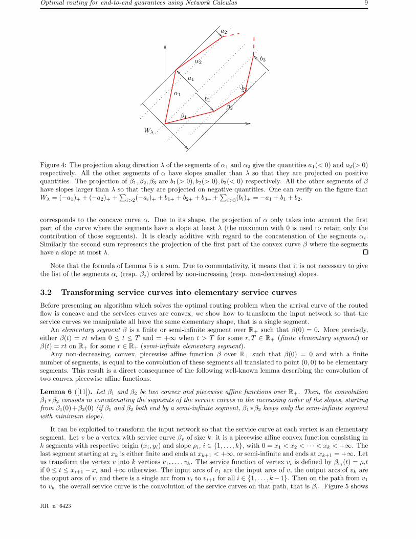
It can be exploited to transform the input network so that the service curve at each vertex is an elementarysegment. Let v be a vertex with service curve βv of size k: it is a piecewise affine convex function consisting ink segments with respective origin (xi, yi) and slope ρi, i ∈ {1, . . . , k}, with 0 = x1 < x2 < · · · < xk < +∞. Thelast segment starting at xk is either finite and ends at xk+1 < +∞, or semi-infinite and ends at xk+1 = +∞. Letus transform the vertex v into k vertices v1, . . . , vk. The service function of vertex vi is defined by βvi

(t) = ρitif 0 ≤ t ≤ xi+1 − xi and +∞ otherwise. The input arcs of v1 are the input arcs of v, the output arcs of vk arethe ouput arcs of v, and there is a single arc from vi to vi+1 for all i ∈ {1, . . . , k− 1}. Then on the path from v1

to vk, the overall service curve is the convolution of the service curves on that path, that is βv. Figure 5 shows

RR n�

6423


an example of the transformation. The service curve of the central vertex is composed of three segments. Thatvertex is replaced by three vertices, each of which has an elementary service curve corresponding to the threesegments (the last segment is of infinite length, so its associate service curve is an affine function).

Figure 5: Transformation of the graph.

Transforming all the vertices in this way gives a graph such that there is a one-to-one correspondancebetween the paths of the initial graph from v to w and the paths of transformed graph from v1 to w|βw|, for allv, w ∈ V , and such that for each path in this one-to-one correspondance, the overall service curve is the same.The transformation is linear in the size of the initial data: the number of vertices in the new graph is

∑

v∈V |βv|and the number of arcs is |A|+∑v∈V (|βv| − 1).

All these considerations can be summed up in the following proposition.

Proposition 1. Any instance of the initial routing problem where the graph is G = (V, A) and the servicescurves are (βv)v∈V can be transformed into an equivalent instance where the graph G′ = (V ′, A′) satifisfies|V ′| =∑v∈V |βv |, |A′| = |A|+∑v∈V (|βv | − 1), and the service curve at each vertex is an elementary segment.

In the next subsection, we describe algorithms solving the optimal routing problem for inputs where theservices curves are elementary segments. Thanks to the transformation, the algorithms apply to inputs whereservices curves have several segments. We could have directly presented our algorithms for this latter case.However the description and proof of the algorithms is more convenient when working with elementary segments.

3.3 Routing algorithms for concave arrival curves and convex service curves

Let G = (V, A) be the directed graph where one wish to route a flow from vin to vout. The flow has anarrival curve α non-decreasing, concave and piecewise affine with a finite number of concatenated segments αi

of respective slope ri ∈ R+ ∪ {+∞} and length li ∈ R+ ∪ {+∞}, 0 ≤ i ≤ p. Note that α0 corresponds tothe segment from (0, 0) to (0, α(0+)), thus r0 = +∞. Each vertex v ∈ V has a service curve βv which is anelementary segment of slope ρv ∈ R+ and length `v ∈ R+ ∪ {+∞}.

Let p be a path from vin to vout, we denote β(p) the service curve of the whole path. From Lemma 3,finding a path which minimizes the maximum delay with regard to α is equivalent to finding a path achievingthe minimum

Dmax(G) = minp path fromvin to vout

minλ∈R+∪{+∞}

Hλ(α, β(p)).

One only needs to replace Hλ by Vλ to minimize the maximum backlog. The service curve β(p) of path p is theconvolution of the elementary segments associated to its vertices. Due to Lemma 6, it is their concatenation bynon-decreasing slopes. Thus applying Lemma 4, we know that for any path p, the minimum over λ is alwaysreached for a slope λ ∈ {r0, r1, . . . , rp}∪ {ρv | v ∈ p} which is included in the set {r0, r1, . . . , rp}∪ {ρv | v ∈ V }.

Interverting the two minima yields

Dmax(G) = minλ∈{r0,r1,...,rp}∪{ρv|v∈V }

minp path fromvin to vout

Hλ(α, β(p)).

For each λ ∈ {r0, r1, . . . , rp} ∪ {ρv | v ∈ V }, from Lemma 5, Hλ(α, β(p)) =√

1+λ2

λ

(∑p

i=0(−projλ(αi))+ +∑

v∈p(projλ(βv))+

)

. The first sum does not depend on the path p. Only the second term is subject tooptimization. Minimizing this value over paths from vin to vout is equivalent to computing a classical shortestpath from vin to vout in the graph G = (V, A) where each vertex v ∈ V is weighted by the orthogonal projectionprojλ(βv)+ = max( λ−ρv√

1+λ2√

1+ρ2v

`v, 0). Since the weights are non-negative, one can use for instance Dijkstra’s

algorithm. These arguments lead to Algorithm 1 and ensure its correction.

INRIA


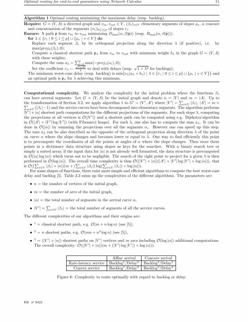
Algorithm 1 Optimal routing minimizing the maximum delay (resp. backlog).

Require: G = (V, A) a directed graph and vin, vout ∈ V , (βv)v∈V elementary segments of slopes ρv , α concaveand concatenation of the segments (αi)0≤i≤p of slopes ri.

Ensure: A path p from vin to vout minimizing Dmax(α, β(p)) (resp. Bmax(α, β(p))).for λ ∈ {ri | 0 ≤ i ≤ p} ∪ {ρv | v ∈ V } do

Replace each segment βv by its orthogonal projection along the direction λ (if positive), i.e. bymax(projλ(βv), 0);Compute a classical shortest path pλ from vin to vout with minimum weight bλ in the graph G = (V, A)with these weights;Compute the sum aλ =

∑pi=0 max(−projλ(αi), 0);

Set the coefficient cλ ←√

1+λ2

λ to deal with delays (resp.√

1 + λ2 for backlogs);The minimum worst-case delay (resp. backlog) is min{cλ(aλ + bλ) | λ ∈ {ri | 0 ≤ i ≤ p} ∪ {ρv | v ∈ V }} andan optimal path is pλ for λ achieving this minimum.

Computational complexity. We analyze the complexity for the initial problem where the functions βv

can have several segments. Let G = (V, A) be the initial graph and denote n = |V | and m = |A|. Up tothe transformation of Section 3.2, we apply algorithm 1 to G′ = (V ′, A′) where |V ′| = ∑

v∈V |βv|, |A′| = m +∑

v∈V (|βv|−1) and the service curves have been decomposed into elementary segments. The algorithm performs|V ′|+ |α| shortest path computations for the different projections of the segments. For each slope λ, computingthe projections at all vertices is O(|V ′|) and a shortest path can be computed using e.g. Dijskstra’algorithmin O(|A′| + |V ′| log |V ′|) (with Fibonacci heaps). For each λ, one also has to compute the sum aλ. It can bedone in O(|α|) by summing the projections over all the segments αi. However one can speed up this step.The sum aλ can be also described as the opposite of the orthogonal projection along direction λ of the pointon curve α where the slope changes and becomes lower or equal to λ. One way to find efficiently this pointis to precompute the coordinates of all the points at angles of α where the slope changes. Then store thesepoints in a dictionary data structure using slopes as keys for the searches. With a binary search tree orsimply a sorted array, if the input data for |α| is not already well formatted, the data structure is precomputedin O(|α| log |α|) which turns out to be negligible. The search of the right point to project for a given λ is thenperformed in O(log |α|). The overall time complexity is thus O((|V ′|+ |α|)(|A′| + |V ′| log |V ′|+ log |α|)), thatis O((

∑

v∈V |βv|+ |α|)(m + (∑

v∈V |βv|) log(∑

v∈V |βv |) + log |α|)).For some shapes of functions, there exist more simple and efficient algorithms to compute the best worst-case

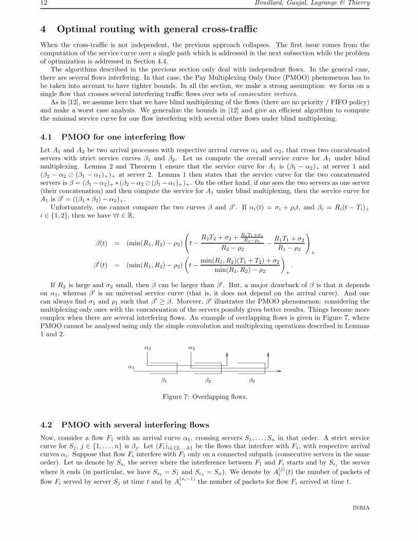
delay and backlog [5]. Table 3.3 sums up the complexities of the different algorithms. The parameters are:

� n = the number of vertices of the initial graph,

� m = the number of arcs of the initial graph,

� |α| = the total number of segments in the arrival curve α,

� |V ′| =∑v∈V |βv | = the total number of segments of all the service curves.

The different complexities of our algorithms and their origins are:

� 1 = classical shortest path, e.g. O(m + n log n) (see [5]),

� 2 = n shortest paths, e.g. O(mn + n2 log n) (see [5]),

� 3 = (|V ′| + |α|) shortest paths on |V ′| vertices and m arcs including O(log |α|) additional computations.The overall complexity: O((|V ′|+ |α|)(m + (|V ′| log |V ′|) + log |α|)).

Affine arrival Concave arrivalRate-latency service Backlog1/Delay2 Backlog2/Delay2

Convex service Backlog1/Delay3 Backlog3/Delay3

Figure 6: Complexity to route optimally with regard to backlog or delay.

RR n�

6423


4 Optimal routing with general cross-traffic

When the cross-traffic is not independent, the previous approach collapses. The first issue comes from thecomputation of the service curve over a single path which is addressed in the next subsection while the problemof optimization is addressed in Section 4.4.

The algorithms described in the previous section only deal with independent flows. In the general case,there are several flows interfering. In that case, the Pay Multiplexing Only Once (PMOO) phenomenon has tobe taken into account to have tighter bounds. In all the section, we make a strong assumption: we focus on asingle flow that crosses several interfering traffic flows over sets of consecutive vertices.

As in [12], we assume here that we have blind multiplexing of the flows (there are no priority / FIFO policy)and make a worst case analysis. We generalize the bounds in [12] and give an efficient algorithm to computethe minimal service curve for one flow interfering with several other flows under blind multiplexing.

4.1 PMOO for one interfering flow

Let A1 and A2 be two arrival processes with respective arrival curves α1 and α2, that cross two concatenatedservers with strict service curves β1 and β2. Let us compute the overall service curve for A1 under blindmultiplexing. Lemma 2 and Theorem 1 ensure that the service curve for A1 is (β1 − α2)+ at server 1 and(β2 − α2 � (β1 − α1)+)+ at server 2. Lemma 1 then states that the service curve for the two concatenatedservers is β = (β1−α2)+ ∗ (β2−α2� (β1−α1)+)+. On the other hand, if one sees the two servers as one server(their concatenation) and then compute the service for A1 under blind multiplexing, then the service curve forA1 is β′ = ((β1 ∗ β2)− α2)+.

Unfortunately, one cannot compare the two curves β and β ′. If αi(t) = σi + ρit, and βi = Ri(t − Ti)+i ∈ {1, 2}, then we have ∀t ∈ R,

β(t) = (min(R1, R2)− ρ2)

(

t−R2T2 + σ2 + R1T1+σ1

R1−ρ1

R2 − ρ2− R1T1 + σ2

R1 − ρ2

)

+

β′(t) = (min(R1, R2)− ρ2)

(

t− min(R1, R2)(T1 + T2) + σ2

min(R1, R2)− ρ2

)

+

.

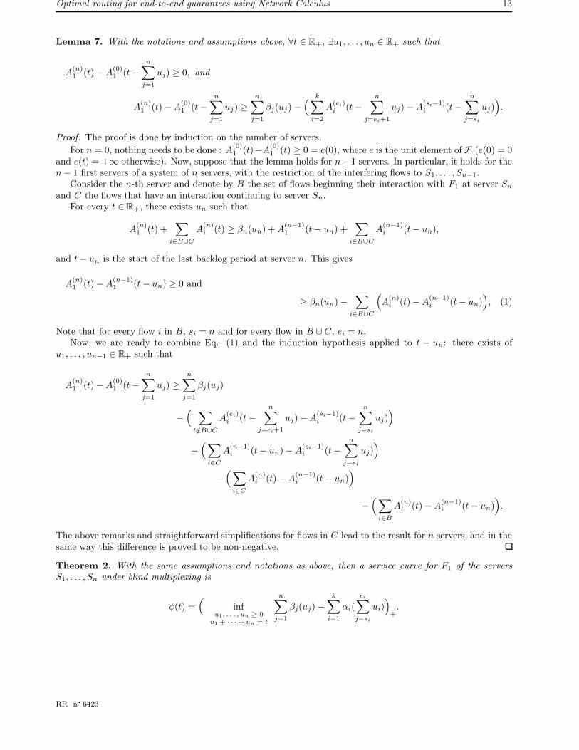
If R2 is large and σ2 small, then β can be larger than β′. But, a major drawback of β is that it dependson α1, whereas β′ is an universal service curve (that is, it does not depend on the arrival curve). And onecan always find σ1 and ρ1 such that β′ ≥ β. Morever, β′ illustrates the PMOO phenomenon: considering themultiplexing only once with the concatenation of the servers possibly gives better results. Things become morecomplex when there are several interfering flows. An example of overlapping flows is given in Figure 7, wherePMOO cannot be analysed using only the simple convolution and multiplexing operations described in Lemmas1 and 2.

α2 α3

α1

β2β1 β3

Figure 7: Overlapping flows.

4.2 PMOO with several interfering flows

Now, consider a flow F1 with an arrival curve α1, crossing servers S1, . . . , Sn in that order. A strict servicecurve for Sj , j ∈ {1, . . . , n} is βj . Let (Fi)i∈{2,...,k} be the flows that interfere with F1, with respective arrivalcurves αi. Suppose that flow Fi interfere with F1 only on a connected subpath (consecutive servers in the sameorder). Let us denote by Ssi

the server where the interference between F1 and Fi starts and by Seithe server

where it ends (in particular, we have Ss1= S1 and Se1

= Sn). We denote by A(j)i (t) the number of packets of

flow Fi served by server Sj at time t and by A(si−1)i the number of packets for flow Fi arrived at time t.

INRIA


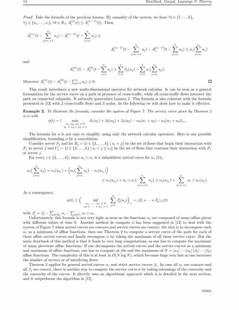
Lemma 7. With the notations and assumptions above, ∀t ∈ R+, ∃u1, . . . , un ∈ R+ such that

A(n)1 (t)−A

(0)1 (t−

n∑

j=1

uj) ≥ 0, and

A(n)1 (t)−A

(0)1 (t−

n∑

j=1

uj) ≥n∑

j=1

βj(uj)−(

k∑

i=2

A(ei)i (t−

n∑

j=ei+1

uj)−A(si−1)i (t−

n∑

j=si

uj))

.

Proof. The proof is done by induction on the number of servers.

For n = 0, nothing needs to be done : A(0)1 (t)−A

(0)1 (t) ≥ 0 = e(0), where e is the unit element of F (e(0) = 0

and e(t) = +∞ otherwise). Now, suppose that the lemma holds for n− 1 servers. In particular, it holds for then− 1 first servers of a system of n servers, with the restriction of the interfering flows to S1, . . . , Sn−1.

Consider the n-th server and denote by B the set of flows beginning their interaction with F1 at server Sn

and C the flows that have an interaction continuing to server Sn.For every t ∈ R+, there exists un such that

A(n)1 (t) +

∑

i∈B∪C

A(n)i (t) ≥ βn(un) + A

(n−1)1 (t− un) +

∑

i∈B∪C

A(n−1)i (t− un),

and t− un is the start of the last backlog period at server n. This gives

A(n)1 (t)−A

(n−1)1 (t− un) ≥ 0 and

≥ βn(un)−∑

i∈B∪C

(

A(n)i (t)−A

(n−1)i (t− un)

)

, (1)

Note that for every flow i in B, si = n and for every flow in B ∪ C, ei = n.Now, we are ready to combine Eq. (1) and the induction hypothesis applied to t − un: there exists of

u1, . . . , un−1 ∈ R+ such that

A(n)1 (t)−A

(0)1 (t−

n∑

j=1

uj) ≥n∑

j=1

βj(uj)

−(

∑

i/∈B∪C

A(ei)i (t−

n∑

j=ei+1


n∑

j=si

uj))

−(

∑

i∈C

A(n−1)i (t− un)−A

(si−1)i (t−

n∑

j=si

uj))

−(

∑

i∈C

A(n)i (t)−A

(n−1)i (t− un)

)

−(

∑

i∈B

A(n)i (t)−A

(n−1)i (t− un)

)

.

The above remarks and straightforward simplifications for flows in C lead to the result for n servers, and in thesame way this difference is proved to be non-negative.

Theorem 2. With the same assumptions and notations as above, then a service curve for F1 of the serversS1, . . . , Sn under blind multiplexing is

φ(t) =(

infu1, . . . , un ≥ 0

u1 + · · · + un = t

n∑

j=1

βj(uj)−k∑

i=1

αi(

ei∑

j=si

ui))

+.

RR n�

6423


Proof. Take the formula of the previous lemma. By causality of the system, we have ∀i ∈ {1 . . . , k},∀j ∈ {si, . . . , ei}, ∀t ∈ R+ A

(j)i (t) ≤ A

(si−1)i (t). Then,

A(ei)i (t−

n∑

j=ei+1


n∑

j=si

uj) ≤

A(si−1)i (t−

n∑

j=ei+1


n∑

j=si

uj) ≤ αi(

ei∑

j=si

uj)

and

A(n)1 (t)−A

(0)1 (t−

n∑

j=1

uj) ≥n∑

j=1

βj(uj)−k∑

i=1

αi(

ei∑

j=si

uj).

Moreover A(n)1 (t)−A

(0)1 (t−∑n

j=1 uj) ≥ 0.

This result introduces a new multi-dimensional operator for network calculus. It can be seen as a generalformulation for the service curve on a path in presence of cross-traffic, while all cross-traffic flows intersect thepath on connected subpaths. It naturally generalizes Lemma 2. This formula is also coherent with the formulapresented in [12] with 2 cross-traffic flows and 3 nodes. In the following we will show how to make it effective.

Example 2. To illustrate the formula, consider the system of Figure 7. The service curve given by Theorem 2is φ with

φ(t) = ( minu1, u2, u3 ≥ 0

u1 + u2 + u3 = t

β1(u1) + β2(u2) + β3(u3)− α2(u1 + u2)− α3(u2 + u3))+.

The formula for φ is not easy to simplify, using only the network calculus operators. Here is one possiblesimplification, bounding φ by a convolution.

Consider server Sj and let Bj = {i ∈ {2, . . . , k} | si = j} be the set of flows that begin their interaction withF1 at server j and Cj = {i ∈ {2, . . . , k} | si < j ≤ ei} be the set of flows that continue their interaction with F1

at server j.For every i ∈ {2, . . . , k}, since αi � αi is a subadditive arrival curve for αi [11],

αi

(

ei∑

j=si

uj

)

= αi(usi) +

(

αi

(

ei∑

j=si

uj

)

− αi(usi))

≤ αi(usi) + αi � αi

(

ei∑

j=si+1

uj

)

≤ αi(usi) +

ei∑

j=si+1

αi � αi(uj).

As a consequence,

φ(t) ≤(

infu1, . . . , un ≥ 0

u1 + · · · + un = t

n∑

j=1

β′j(uj)

)

+= (β′

1 ∗ · · · ∗ β′n)+(t)

with β′j = βj −

∑

i∈Bjαi −

∑

i∈Cjαi � αi.

Unfortunately, this formula is not very tight as soon as the functions αi are composed of many affine pieceswith different values at time 0. Another method de compute φ has been suggested in [12] to deal with thesystem of Figure 7 when arrival curves are concave and service curves are convex: the idea is to decompose eachαi as a minimum of affine functions, then use Theorem 2 to compute a service curve of the path for each ofthese affine arrival curves and finally recompose φ by taking the maximum of all those service curve. But themain drawback of this method is that it leads to very long computations, as one has to compute the maximumof many piecewise affine functions. If one decomposes the arrival curves and the service curves as a minimumand maximum of affine functions, one has to compute at the end the maximum of N = |α1| · · · |αk|.|β1| · · · |βn|affine functions. The complexity of this is at least in O(N log N), which becomes huge very fast as one increasesthe number of servers or of interfering flows.

Theorem 2 applies for general arrival curves αi and strict service curves βi. In case all αi are concave andall βj are convex, there is another way to compute the service curve φ by taking advantage of the convexity andthe concavity of the curves. It directly uses an algorithmic approach which is is detailed in the next section,and it outperforms the algorithm in [12].

INRIA


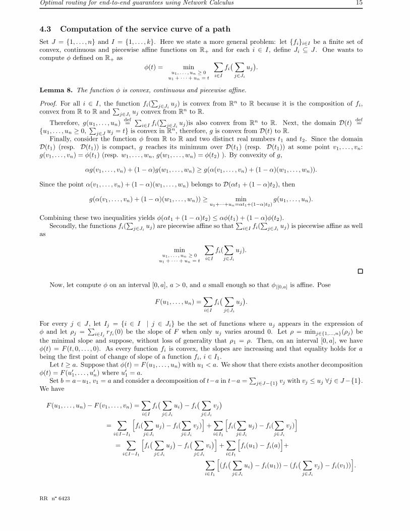
4.3 Computation of the service curve of a path

Set J = {1, . . . , n} and I = {1, . . . , k}. Here we state a more general problem: let {fi}i∈I be a finite set ofconvex, continuous and piecewise affine functions on R+ and for each i ∈ I , define Ji ⊆ J . One wants tocompute φ defined on R+ as

φ(t) = minu1, . . . , un ≥ 0

u1 + · · · + un = t

∑

i∈I

fi

(

∑

j∈Ji

uj

)

.

Lemma 8. The function φ is convex, continuous and piecewise affine.

Proof. For all i ∈ I , the function fi(∑

j∈Jiuj) is convex from R

n to R because it is the composition of fi,convex from R to R and

∑

j∈Jiuj convex from R

n to R.

Therefore, g(u1, . . . , un)def=∑

i∈I fi(∑

j∈Jiuj)is also convex from R

n to R. Next, the domain D(t)def=

{u1, . . . , un ≥ 0,∑

j∈J uj = t} is convex in Rn, therefore, g is convex from D(t) to R.

Finally, consider the function φ from R to R and two distinct real numbers t1 and t2. Since the domainD(t1) (resp. D(t1)) is compact, g reaches its minimum over D(t1) (resp. D(t1)) at some point v1, . . . , vn:g(v1, . . . , vn) = φ(t1) (resp. w1, . . . , wn, g(w1, . . . , wn) = φ(t2) ). By convexity of g,

αg(v1, . . . , vn) + (1− α)g(w1, . . . , wn) ≥ g(α(v1, . . . , vn) + (1− α)(w1, . . . , wn)).

Since the point α(v1, . . . , vn) + (1− α)(w1, . . . , wn) belongs to D(αt1 + (1− α)t2), then

g(α(v1, . . . , vn) + (1− α)(w1, . . . , wn)) ≥ minu1+···+un=αt1+(1−α)t2)

g(u1, . . . , un).

Combining these two inequalities yields φ(αt1 + (1− α)t2) ≤ αφ(t1) + (1− α)φ(t2).Secondly, the functions fi(

∑

j∈Jiuj) are piecewise affine so that

∑

i∈I fi(∑

j∈Jiuj) is piecewise affine as well

as

minu1, . . . , un ≥ 0

u1 + · · · + un = t

∑

i∈I

fi(∑

j∈Ji

uj).

Now, let compute φ on an interval [0, a], a > 0, and a small enough so that φ|[0,a] is affine. Pose

F (u1, . . . , un) =∑

i∈I

fi

(

∑

j∈Ji

uj

)

.

For every j ∈ J , let Ij = {i ∈ I | j ∈ Ji} be the set of functions where uj appears in the expression ofφ and let ρj =

∑

i∈Ijrfi

(0) be the slope of F when only uj varies around 0. Let ρ = minj∈{1,...,n}(ρj) be

the minimal slope and suppose, without loss of generality that ρ1 = ρ. Then, on an interval [0, a], we haveφ(t) = F (t, 0, . . . , 0). As every function fi is convex, the slopes are increasing and that equality holds for abeing the first point of change of slope of a function fi, i ∈ I1.

Let t ≥ a. Suppose that φ(t) = F (u1, . . . , un) with u1 < a. We show that there exists another decompositionφ(t) = F (u′

1, . . . , u′n) where u′

1 = a.Set b = a−u1, v1 = a and consider a decomposition of t−a in t−a =

∑

j∈J−{1} vj with vj ≤ uj ∀j ∈ J−{1}.We have

F (u1, . . . , un)− F (v1, . . . , vn) =∑

i∈I

fi

(

∑

j∈Ji

ui

)

− fi

(

∑

j∈Ji

vj

)

=∑

i∈I−I1

[

fi(∑

j∈Ji

uj)− fi(∑

j∈Ji

vj)]

+∑

i∈I1

[

fi(∑

j∈Ji

uj)− fi(∑

j∈Ji

vj)]

=∑

i∈I−I1

[

fi

(

∑

j∈Ji

uj

)

− fi

(

∑

j∈Ji

vi

)

]

+∑

i∈I1

[

fi(u1)− fi(a)]

+

∑

i∈I1

[

(fi

(

∑

j∈Ji

ui

)

− fi(u1))− (fi

(

∑

j∈Ji

vj

)

− fi(v1))]

.

RR n�

6423


For i ∈ I−I1, let us define hi by fi(∑

j∈Jiuj)−fi(

∑

j∈Jivj) = hi

∑

j∈Ji(uj−vj), the average slope for fi being

hi over I−I1 and for i ∈ I1, define hi by (fi(∑

j∈Jiuj)−fi(u1))−(fi(

∑

j∈Jivj)−fi(v1)) = hi

∑

j∈Ji−{1}(uj−vj).The equation above can be rewritten as

∑

i∈I

hi

∑

j∈Ji−{1}(uj − vj)− ρb =

∑

j∈J−{1}

(

∑

i∈Ji

hi

)

(uj − vj)− ρb.

But, because of the convexity of the functions and because ρ is the minimum of the slopes around 0, we have∑

i∈Ijhi ≥ ρ. Then F (u1, . . . , un)−F (v1, . . . , vn) ≥ 0 and a decomposition for φ(t) can be found where u1 ≥ a.

Set f ′i(t) = fi(t + a)− fi(a) if i ∈ I1 and f ′

i = f1 for i /∈ I1. For every t ≥ a, there exists u1, . . . , un ≥ 0 withu1 ≥ a such that

φ(t) =

k∑

i=1

fi(∑

j∈Ji

uj) =∑

i∈I1

f1(a) +

k∑

i=1

f ′i(∑

j∈Ji

u′j),

with u′1 = u1 − a and u′

j = uj for j ≥ 2. The functions f ′i are still convex, continuous and piecewise affine.

So one can compute φ on an interval [a, b] using the f ′i . Remark also that the total size of the functions f ′

i isstrictly less than that of the fi, because a corresponds to a change of slope of a function (so the first segmentof that function disappears in at least on of the f ′

i , i ∈ I1). The function φ can then be computed in finite time,repeating the computations above at most as many times as the total number of segments of the functions fi.

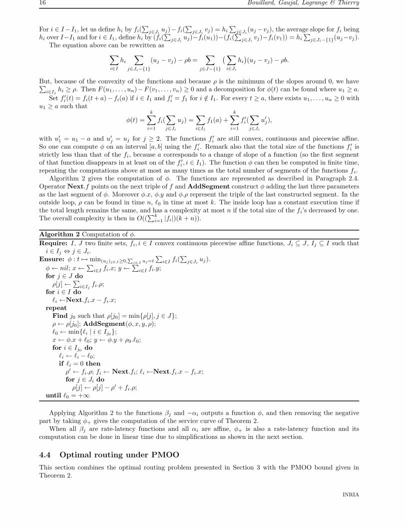
Algorithm 2 gives the computation of φ. The functions are represented as described in Paragraph 2.4.Operator Next.f points on the next triple of f and AddSegment construct φ adding the last three parametersas the last segment of φ. Moreover φ.x, φ.y and φ.ρ represent the triple of the last constructed segment. In theoutside loop, ρ can be found in time n, `0 in time at most k. The inside loop has a constant execution time ifthe total length remains the same, and has a complexity at most n if the total size of the fi’s decreased by one.The overall complexity is then in O((

∑ki=1 |fi|)(k + n)).

Algorithm 2 Computation of φ.

Require: I , J two finite sets, fi, i ∈ I convex continuous piecewise affine functions, Ji ⊆ J , Ij ⊆ I such thati ∈ Ij ⇔ j ∈ Ji.

Ensure: φ : t 7→ min(uj)j∈J≥0,P

j∈Juj=t

∑

i∈I fi(∑

j∈Jiuj).

φ← nil; x←∑

i∈I fi.x; y ←∑

i∈I fi.y;for j ∈ J do

ρ[j]←∑

i∈Ijfi.ρ;

for i ∈ I do

ì ←Next.fi.x− fi.x;repeat

Find j0 such that ρ[j0] = min{ρ[j], j ∈ J};ρ← ρ[j0]; AddSegment(φ, x, y, ρ);`0 ← min{ì | i ∈ Ij0};x← φ.x + `0; y ← φ.y + ρ0.`0;for i ∈ Ij0 do

ì ← ì − `0;if ì = 0 then

ρ′ ← fi.ρ; fi ← Next.fi; ì ←Next.fi.x− fi.x;for j ∈ Ji do

ρ[j]← ρ[j]− ρ′ + fi.ρ;until `0 = +∞

Applying Algorithm 2 to the functions βj and −αi outputs a function φ, and then removing the negativepart by taking φ+ gives the computation of the service curve of Theorem 2.

When all βj are rate-latency functions and all αi are affine, φ+ is also a rate-latency function and itscomputation can be done in linear time due to simplifications as shown in the next section.

4.4 Optimal routing under PMOO

This section combines the optimal routing problem presented in Section 3 with the PMOO bound given inTheorem 2.

INRIA


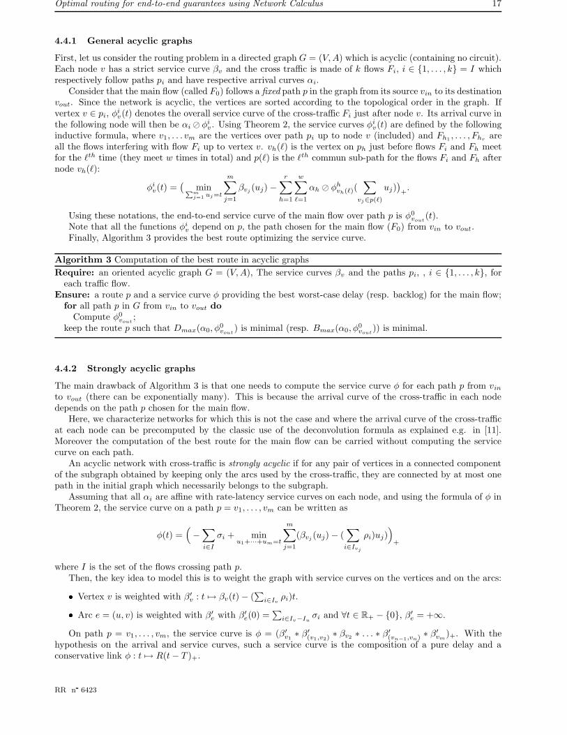
4.4.1 General acyclic graphs

First, let us consider the routing problem in a directed graph G = (V, A) which is acyclic (containing no circuit).Each node v has a strict service curve βv and the cross traffic is made of k flows Fi, i ∈ {1, . . . , k} = I whichrespectively follow paths pi and have respective arrival curves αi.

Consider that the main flow (called F0) follows a fixed path p in the graph from its source vin to its destinationvout. Since the network is acyclic, the vertices are sorted according to the topological order in the graph. Ifvertex v ∈ pi, φi

v(t) denotes the overall service curve of the cross-traffic Fi just after node v. Its arrival curve inthe following node will then be αi � φi

v . Using Theorem 2, the service curves φiv(t) are defined by the following

inductive formula, where v1, . . . vm are the vertices over path pi up to node v (included) and Fh1, . . . , Fhr

areall the flows interfering with flow Fi up to vertex v. vh(`) is the vertex on ph just before flows Fi and Fh meetfor the `th time (they meet w times in total) and p(`) is the `th commun sub-path for the flows Fi and Fh afternode vh(`):

φiv(t) =

(

minP

mj=1

uj=t

m∑

j=1

βvj(uj)−

r∑

h=1

w∑

`=1

αh � φhvh(`)(

∑

vj∈p(`)

uj))

+.

Using these notations, the end-to-end service curve of the main flow over path p is φ0vout

(t).Note that all the functions φi

v depend on p, the path chosen for the main flow (F0) from vin to vout.Finally, Algorithm 3 provides the best route optimizing the service curve.

Algorithm 3 Computation of the best route in acyclic graphs

Require: an oriented acyclic graph G = (V, A), The service curves βv and the paths pi, , i ∈ {1, . . . , k}, foreach traffic flow.

Ensure: a route p and a service curve φ providing the best worst-case delay (resp. backlog) for the main flow;for all path p in G from vin to vout do

Compute φ0vout

;keep the route p such that Dmax(α0, φ

0vout

) is minimal (resp. Bmax(α0, φ0vout

)) is minimal.

4.4.2 Strongly acyclic graphs

The main drawback of Algorithm 3 is that one needs to compute the service curve φ for each path p from vin

to vout (there can be exponentially many). This is because the arrival curve of the cross-traffic in each nodedepends on the path p chosen for the main flow.

Here, we characterize networks for which this is not the case and where the arrival curve of the cross-trafficat each node can be precomputed by the classic use of the deconvolution formula as explained e.g. in [11].Moreover the computation of the best route for the main flow can be carried without computing the servicecurve on each path.

An acyclic network with cross-traffic is strongly acyclic if for any pair of vertices in a connected componentof the subgraph obtained by keeping only the arcs used by the cross-traffic, they are connected by at most onepath in the initial graph which necessarily belongs to the subgraph.

Assuming that all αi are affine with rate-latency service curves on each node, and using the formula of φ inTheorem 2, the service curve on a path p = v1, . . . , vm can be written as

φ(t) =(

−∑

i∈I

σi + minu1+···+um=t

m∑

j=1

(βvj(uj)− (

∑

i∈Ivj

ρi)uj))

+

where I is the set of the flows crossing path p.Then, the key idea to model this is to weight the graph with service curves on the vertices and on the arcs:

� Vertex v is weighted with β′v : t 7→ βv(t)− (

∑

i∈Ivρi)t.

� Arc e = (u, v) is weighted with β′e with β′

e(0) =∑

i∈Iv−Iuσi and ∀t ∈ R+ − {0}, β′

e = +∞.

On path p = v1, . . . , vm, the service curve is φ = (β′v1∗ β′

(v1,v2)∗ βv2

∗ . . . ∗ β′(vn−1,vn) ∗ β′

vm)+. With the

hypothesis on the arrival and service curves, such a service curve is the composition of a pure delay and aconservative link φ : t 7→ R(t− T )+.

RR n�

6423


For a flow F on that path, with an affine arrival curve α(t) = σ + ρt, the maximal backlog is α(T ) = σ + ρTand the maximal delay is φ−1(σ) = T +σ/R. Due to the special shape of input functions, both R and T can beeasily computed. The rate R is the smallest number among the rates of the β ′

v: R = minv∈p(Rv − (∑

i∈Ivρi)).

Then T can be deduced:

T =∑

v∈p

Tv

(

1 +∑

i∈Iv

ρi

R

)

+∑

e∈p

β′e(0)

R.

The maximal delay and backlog strongly depend on R, and if R is fixed, following algorithm can be applied.In order to compute the maximal delay, for fixed R, the weight of a vertex v is Tv(1+

∑

i∈Iv

ρi

R ) and the weightof an arc e = (u, v) is

∑

i∈Iv−Iuσi/R. The maximal delay on a path is the sum of the weights on that path

plus σ/R. Any shortest-path algorithm can be applied (restricted to the vertices whose asymptotic service rateis greater than R).

In order to compute the maximal backlog, for fixed R, the weight of a vertex v is ρTv and the weight of anarc e = (u, v) is ρ

∑

i∈Iv−Iuσi/R. The maximal backlog on a path is the sum of the weights on that path plus

σ.Following that scheme, in the worst case, one has to execute one shortest path algorithm per vertex (it

covers all the possible rates R). All this results in the following proposition.

Proposition 2. For a strongly acyclic network (V, A), with affine arrival curves and rate-latency service curves,the optimal end-to-end service curve is a rate-latency service curve that can be computed using a shortest pathalgorithm with an overall complexity in O(|V |(|V |+ |A|)).

4.5 Implementation work

Following the algorithmic framework of [6], a software for worst case performance evaluation with NetworkCalculus is currently under development. The main Network Calculus operations have been implemented for alarge class of piecewise affine functions including the classical arrival and service curves of network calculus. Afirst version should be released soon for downloads (COINC Project [9]).

The new multi-dimensional operator, described in Algorithm 2 and corresponding to the service curve φ ona path with cross-traffic has been incorporated to the software. Routing algorithms presented in this paper havealso been implemented.

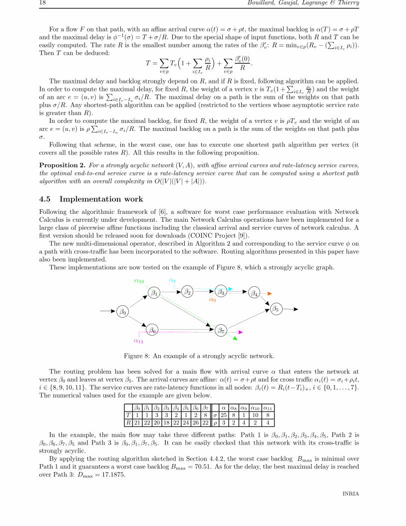
These implementations are now tested on the example of Figure 8, which a strongly acyclic graph.

Figure 8: An example of a strongly acyclic network.

The routing problem has been solved for a main flow with arrival curve α that enters the network atvertex β0 and leaves at vertex β5. The arrival curves are affine: α(t) = σ+ρt and for cross traffic αi(t) = σi+ρit,i ∈ {8, 9, 10, 11}. The service curves are rate-latency functions in all nodes: βi(t) = Ri(t−Ti)+, i ∈ {0, 1, . . . , 7}.The numerical values used for the example are given below.

β0 β1 β2 β3 β4 β5 β6 β7 α α8 α9 α10 α11

T 1 1 3 3 2 1 2 8 σ 25 8 1 10 8

R 21 22 20 18 22 24 26 22 ρ 3 2 4 2 4

In the example, the main flow may take three different paths: Path 1 is β0, β1, β2, β3, β4, β5, Path 2 isβ0, β6, β7, β5 and Path 3 is β0, β1, β7, β5. It can be easily checked that this network with its cross-traffic isstrongly acyclic.

By applying the routing algorithm sketched in Section 4.4.2, the worst case backlog Bmax is minimal overPath 1 and it guarantees a worst case backlog Bmax = 70.51. As for the delay, the best maximal delay is reachedover Path 3: Dmax = 17.1875.

INRIA


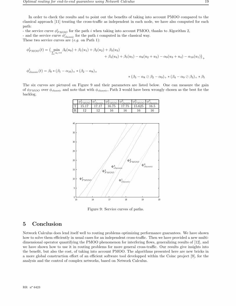
In order to check the results and to point out the benefits of taking into account PMOO compared to theclassical approach [11] treating the cross-traffic as independent in each node, we have also computed for eachpath:- the service curve φi

PMOO for the path i when taking into account PMOO, thanks to Algorithm 2,- and the service curve φi

classic for the path i computed in the classical way.These two service curves are (e.g. on Path 1):

φ1PMOO(t) =

(

minP

ui=tβ0(u0) + β1(u1) + β2(u2) + β3(u3)

+ β4(u4) + β5(u5)− α8(u2 + u3)− α9(u3 + u4)− α10(u1))

+

φ1classic(t) = β0 ∗ (β1 − α10)+ ∗ (β2 − α8)+

∗ (β3 − α8 � β2 − α9)+ ∗ (β4 − α9 � β3)+ ∗ β5

The six curves are pictured on Figure 9 and their parameters are listed below. One can measure the gainof φPMOO over φclassic and note that with φclassic, Path 3 would have been wrongly chosen as the best for thebacklog.

φ1

PMOO φ1

classic φ2

PMOO φ2

classic φ3

PMOO φ3

classic

T 15.17 17.17 16.75 17.75 15.625 16.5

R 12 12 16 16 16 16

0

5

10

15

20

25

30

35

40

15 16 17 18 19 20

Φ1

PMOO Φ1

classic

Φ3

PMOO

Φ3

classic

Φ2

PMOO

Φ2

classic

Figure 9: Service curves of paths.

5 Conclusion

Network Calculus does lend itself well to routing problems optimizing performance guarantees. We have shownhow to solve them efficiently in usual cases for an independent cross-traffic. Then we have provided a new multi-dimensional operator quantifying the PMOO phenomenon for interfering flows, generalizing results of [12], andwe have shown how to use it in routing problems for more general cross-traffic. Our results give insights intothe benefit, but also the cost, of taking into account PMOO. The algorithms presented here are new bricks ina more global construction effort of an efficient software tool developped within the Coinc project [9], for theanalysis and the control of complex networks, based on Network Calculus.

RR n�

6423


References

[1] E. Altman, T. Basar, and R. Srikant. Nash equilibria for combined flow control and routing in networks:Asymptotic behavior for a large number of users. IEEE Transctions on Automatic Control, 47(6):917–930,2002.

[2] M. Andrews. Instability of FIFO in the permanent sessions model at arbitrarily small network loads. InProceedings of SODA’07, 2007.

[3] B. Awerbuch and T. Leighton. A simple local-control approximation algorithm for multicommodity flow.In Proceedings of FOCS’93, pages 459–468, 1993.

[4] D. Bertsimas and D. Gamarnik. Asymptotically optimal algorithm for job shop scheduling and packetrouting. Journal of Algorithms, 33(2):296–318, 1999.

[5] A. Bouillard, B. Gaujal, S. Lagrange, and E. Thierry. Optimal routing for end-to-end guarantees: the priceof multiplexing. In VALUETOOLS, 2007.

[6] A. Bouillard and E. Thierry. An algorithmic toolbox for network calculus. Journal of Discrete EventDynamic Systems, 2007. To appear.

[7] C. S. Chang. Performance Guarantees in Communication Networks. TNCS, 2000.

[8] J. Cohen, E. Jeannot, N. Padoy, and F. Wagner. Messages scheduling for parallel data redistributionbetween clusters. IEEE Trans. Parallel Distrib. Syst., 17(10):1163–1175, 2006.

[9] COINC. Computational issues in network calculus. http://perso.bretagne.ens-cachan.fr/∼bouillar/coinc.

[10] M. Fidler. Extending the network calculus pay bursts only once principle to aggregate scheduling. InQoS-IP, pages 19–34, 2003.

[11] J.-Y. Le Boudec and P. Thiran. Network Calculus: A Theory of Deterministic Queuing Systems for theInternet, volume LNCS 2050. Springer-Verlag, 2001.

[12] J. B. Schmitt and F. A. Zdarsky. The disco network calculator: a toolbox for worst case analysis. InValuetools ’06: Proceedings of the 1st international conference on Performance evaluation methodolgiesand tools. ACM Press, 2006.

[13] J. B. Schmitt, F. A. Zdarsky, and I. Martinovic. Performance Bounds in Feed-Forward Networks underBlind Multiplexing. Technical Report 349/06, University of Kaiserslautern, Germany, April 2006.

INRIA

Unité de recherche INRIA RennesIRISA, Campus universitaire de Beaulieu - 35042 Rennes Cedex (France)

Unité de recherche INRIA Futurs : Parc Club Orsay Université - ZAC des Vignes4, rue Jacques Monod - 91893 ORSAY Cedex (France)

Unité de recherche INRIA Lorraine : LORIA, Technopôle de Nancy-Brabois - Campus scientifique615, rue du Jardin Botanique - BP 101 - 54602 Villers-lès-Nancy Cedex (France)

Unité de recherche INRIA Rhône-Alpes : 655, avenue de l’Europe - 38334 Montbonnot Saint-Ismier (France)Unité de recherche INRIA Rocquencourt : Domaine de Voluceau - Rocquencourt - BP 105 - 78153 Le Chesnay Cedex (France)

Unité de recherche INRIA Sophia Antipolis : 2004, route des Lucioles - BP 93 - 06902 Sophia Antipolis Cedex (France)

ÉditeurINRIA - Domaine de Voluceau - Rocquencourt, BP 105 - 78153 Le Chesnay Cedex (France)��

ISSN 0249-6399

Optimal routing for end-to-end guarantees using Network Calculus

Documents

Transcript of Optimal routing for end-to-end guarantees using Network Calculus