University of Central Florida University of Central Florida

STARS STARS

Electronic Theses and Dissertations, 2004-2019

2005

Decision Theory Classification Of High-dimensional Vectors Decision Theory Classification Of High-dimensional Vectors

Based On Small Samples Based On Small Samples

David Bradshaw University of Central Florida

Part of the Mathematics Commons

Find similar works at: https://stars.library.ucf.edu/etd

University of Central Florida Libraries http://library.ucf.edu

This Doctoral Dissertation (Open Access) is brought to you for free and open access by STARS. It has been accepted

for inclusion in Electronic Theses and Dissertations, 2004-2019 by an authorized administrator of STARS. For more

information, please contact STARS@ucf.edu.

STARS Citation STARS Citation Bradshaw, David, "Decision Theory Classification Of High-dimensional Vectors Based On Small Samples" (2005). Electronic Theses and Dissertations, 2004-2019. 533. https://stars.library.ucf.edu/etd/533

DECISION THEORY CLASSIFICATION OF HIGH-DIMENSIONALVECTORS BASED ON SMALL SAMPLES

by

DAVID J. BRADSHAW

A dissertation submitted in partial fulfillment of the requirementsfor the degree of Doctor of Philosophy in the Department of Mathematicsin the College of Arts and Sciences at the University of Central Florida

Orlando, Florida

Fall Term2005

Major Professor: Dr. Marianna Pensky

ABSTRACT

In this paper, we review existing classification techniques and suggest an entirely new proce-

dure for the classification of high-dimensional vectors on the basis of a few training samples.

The proposed method is based on the Bayesian paradigm and provides posterior probabilities

that a new vector belongs to each of the classes, therefore it adapts naturally to any number

of classes. Our classification technique is based on a small vector which is related to the pro-

jection of the observation onto the space spanned by the training samples. This is achieved

by employing matrix-variate distributions in classification, which is an entirely new idea. In

addition, our method mimics time-tested classification techniques based on the assumption

of normally distributed samples. By assuming that the samples have a matrix-variate normal

distribution, we are able to replace classification on the basis of a large covariance matrix

with classification on the basis of a smaller matrix that describes the relationship of sample

vectors to each other.

ii

TABLE OF CONTENTS

LIST OF FIGURES vi

LIST OF TABLES viii

1 INTRODUCTION AND FORMULATION OF THE PROBLEM 1

1.1 Introduction . . . . . . . . . . . . . . . . . . . . . . . . . . . . . . . . . . . . 1

2 BACKGROUND INFORMATION 6

2.1 Bayesian Classification Methods . . . . . . . . . . . . . . . . . . . . . . . . . 6

2.1.1 Bayesian decision rules . . . . . . . . . . . . . . . . . . . . . . . . . . 6

2.1.2 Minimum Risk Criterion . . . . . . . . . . . . . . . . . . . . . . . . . 7

2.1.3 Minimax criterion . . . . . . . . . . . . . . . . . . . . . . . . . . . . . 9

2.2 Linear Discriminating Functions . . . . . . . . . . . . . . . . . . . . . . . . . 10

2.2.1 Generalized Linear Discriminant Functions . . . . . . . . . . . . . . . 13

2.2.2 Criterion Functions . . . . . . . . . . . . . . . . . . . . . . . . . . . . 14

2.2.3 Minimum Squared Error Criterion . . . . . . . . . . . . . . . . . . . . 16

2.2.4 Support Vector Machines . . . . . . . . . . . . . . . . . . . . . . . . . 18

2.3 Dimensionality Considerations . . . . . . . . . . . . . . . . . . . . . . . . . . 23

2.3.1 Principle Component Analysis . . . . . . . . . . . . . . . . . . . . . . 24

iii

2.3.2 Discriminant Analysis . . . . . . . . . . . . . . . . . . . . . . . . . . 25

2.4 Matrix-Variate Normal Distribution . . . . . . . . . . . . . . . . . . . . . . . 27

3 CLASSIFICATION RULE BASED ON MATRIX DISTRIBUTIONS 31

3.1 Theory . . . . . . . . . . . . . . . . . . . . . . . . . . . . . . . . . . . . . . . 31

3.2 Delta Prior . . . . . . . . . . . . . . . . . . . . . . . . . . . . . . . . . . . . 38

3.2.1 Derivation . . . . . . . . . . . . . . . . . . . . . . . . . . . . . . . . . 38

3.2.2 Decision Rule . . . . . . . . . . . . . . . . . . . . . . . . . . . . . . . 38

3.3 Maximum Entropy Prior . . . . . . . . . . . . . . . . . . . . . . . . . . . . . 44

3.3.1 Derivation . . . . . . . . . . . . . . . . . . . . . . . . . . . . . . . . . 44

3.3.2 Decision Rule . . . . . . . . . . . . . . . . . . . . . . . . . . . . . . . 47

3.4 Hybrid Prior . . . . . . . . . . . . . . . . . . . . . . . . . . . . . . . . . . . . 49

3.4.1 Derivation . . . . . . . . . . . . . . . . . . . . . . . . . . . . . . . . . 49

3.4.2 Decision Rule . . . . . . . . . . . . . . . . . . . . . . . . . . . . . . . 52

3.4.3 Generalization . . . . . . . . . . . . . . . . . . . . . . . . . . . . . . . 54

3.5 Estimating Parameters . . . . . . . . . . . . . . . . . . . . . . . . . . . . . . 62

3.6 Relation to Linear SVMs . . . . . . . . . . . . . . . . . . . . . . . . . . . . . 65

3.7 Proofs . . . . . . . . . . . . . . . . . . . . . . . . . . . . . . . . . . . . . . . 67

4 SIMULATIONS AND RESULTS 72

4.1 Simulations with Normal Data . . . . . . . . . . . . . . . . . . . . . . . . . . 73

4.2 Simulations with Non-Normal Data . . . . . . . . . . . . . . . . . . . . . . . 78

4.3 Application to Target Detection and Recognition . . . . . . . . . . . . . . . 79

4.4 Remarks . . . . . . . . . . . . . . . . . . . . . . . . . . . . . . . . . . . . . . 82

iv

5 CONCLUSIONS AND FUTURE WORK 83

REFERENCES 85

v

LIST OF FIGURES

4.1 Percent Correct ME-MN vs. SVM (left) and H-MN vs. SVM (right) for

Normal Data (100 iterations): C = 2, n = 50, Ni = 5, N∗i = 100, σ2

1 = σ22 = 0.2 74

4.2 Percent Correct ME-MN vs. SVM (left) and H-MN vs. SVM (right) for

Normal Data (100 iterations): C = 2, n = 50, Ni = 5, N∗i = 100, σ2

1 =

0.2, σ22 = 0.3 . . . . . . . . . . . . . . . . . . . . . . . . . . . . . . . . . . . 75

4.3 Percent Correct ME-MN vs. SVM (left) and H-MN vs. SVM (right) for

Normal Data (100 iterations): C = 3, n = 50, Ni = 5, N∗i = 100, σ2

1 =

0.2, σ22 = 0.3, σ2

3 = 0.4 . . . . . . . . . . . . . . . . . . . . . . . . . . . . . . 76

4.4 Posteriors vs. Empirical Values, ME-MN (left) and H-MN (right) for Normal

Data (100 iterations): C = 2, n = 50, Ni = 5, N∗i = 100, σ2

1 = σ22 = 0.2 . . 77

4.5 Posteriors vs. Empirical Values, ME-MN (left) and H-MN (right) for Normal

Data (100 iterations): C = 2, n = 50, Ni = 5, N∗i = 100, σ2

1 = 0.2, σ22 = 0.3 78

4.6 Posteriors vs. Empirical Values, ME-MN (left) and H-MN (right) for Normal

Data (100 iterations): C = 3, n = 50, Ni = 5, N∗i = 100, σ2

1 = 0.2, σ22 =

0.3, σ23 = 0.4 . . . . . . . . . . . . . . . . . . . . . . . . . . . . . . . . . . . 78

4.7 MSTAR Images of Target (left) and Clutter (right) . . . . . . . . . . . . . . 80

vi

4.8 Percent Correct ME-MN vs. SVM for MSTAR Data (50 iterations): C =

2, n = 625, Ni = 5, N∗i = 50 . . . . . . . . . . . . . . . . . . . . . . . . . . 81

4.9 Posteriors vs. Empirical Values, ME-MN for MSTAR Data (50 iterations):

C = 2, n = 625, Ni = 5, N∗i = 50 . . . . . . . . . . . . . . . . . . . . . . . . 81

vii

LIST OF TABLES

4.1 Correct classification rates for Normal data averaged over M=100 iterations.

Simulations are conducted with Ni = 5, N∗i = 100 and n = 50. . . . . . . . . 76

4.2 Correct classification rates for Laplacian data averaged over M=100 iterations.

Simulations are conducted with Ni = 5, N∗i = 100 and n = 50. . . . . . . . . 79

viii

1

INTRODUCTION ANDFORMULATION OF THE

PROBLEM

1.1 Introduction

The problem of pattern classification has been around for almost a century, and with recent

technological developments, it is experiencing a renewed enthusiasm. The problem itself is

quite simple to describe: “What’s the difference between these and those?” Or, more to

the point, “is that more like one of these or one of those?” The problem is to construct

an algorithm, called a decision rule, which classifies future observations as coming from C

predetermined classes. In order to devise the decision rule, one is given a set of N observa-

tions, called training samples, which come from known classes. Using the training samples,

the classifier “learns” a distinctive description of each class. Depending on the design of

the classifier, the learning process can involve estimating probability distributions (decision

theoretic approach), finding coefficients of a separating hyperplane (linear discriminants),

or various other techniques. The rule is usually designed on the basis of some optimization

criterion, for example, minimizing the percentage of future misclassifications.

We can trace the origins of pattern classification to a 1936 study by Ronald Fisher of

1

the differences between various types of Iris plants, Iris versicolor and Iris setosa. In the

experiment, Fisher represented each plant by its feature vector x = (x1, ..., x4)T , where x1 =

sepal length, x2 = sepal width, x3 = petal length, and x4 = petal width, all in centimeters.

He sought a coefficient vector w = (w1, ..., w4)T such that the values of the linear function

wTx for each species would be widely separated. Fisher argued that the coefficient vector

w should be chosen to maximize the ratio of the square of the mean difference to the

within-group variance (see Section 2.3.2). If we denote the training samples from group i by

xi,1, . . . ,xi,Ni, i = 1, 2, and the sample means by mi, then the coefficients can be found by

maximizing

J =(wTm1 −wTm2)

2

wTSWw, (1.1)

where SW =∑2

i=1

∑Ni

j=1(xi,j −mi)(xi,j −mi)T is proportional to the within-group pooled

covariance matrix. The coefficients are then given by

w = S−1W (m1 −m2). (1.2)

(Note that the parameters wi of the classifier were “learned” from the training samples.

Classifiers that work in this way are often called learning machines, and setting the parame-

ters based on the samples is called training.) A natural decision rule here would be to pick

some suitable constant k (between wTm1 and wTm2) and classify a new vector x according

to whether wTx is greater than or less than k. This decision rule is known as Fisher’s Linear

Discriminant Function.

Fisher’s study was a two-class discrimination, where the dimension of the vector space n

was small compared to the number of available training samples N . In this paper, we are

interested in the opposite situation. That is, given C classes and N training samples in Rn

2

with N << n, determine an appropriate classification rule. This situation is becoming more

common as our technological capacity grows. For example, even a low resolution digital

photograph will have thousands of pixels, and most image classification applications have a

limited number of training images. In the medical field, several studies have demonstrated

great potential in classifying various types of tumors based on microarray measurements

for thousands of genes. These HDLSS (high dimension, low sample-size) problems do not

cooperate with the traditional classification methods.

The statistical methods of classification all rely on some sort of density estimation. Non-

parametric estimation will not work in HDLSS problems, because the number of training

samples needed grows exponentially with dimension. When a parametric form is assumed

(generally normal), the number of parameters to be estimated is O(n2). Linear discriminant

functions are less computationally complex, and hence do not suffer as much from the “curse

of dimensionality,” however they do not support the Bayesian paradigm (except in special

cases). In this paper, we propose a classification method designed for the HDLSS problem

that combines the Bayesian decision rules with linear discriminant functions

In Fisher’s study, a feature vector consisted of petal and sepal dimensions, but there

were other features that could have improved results, like height or mass or leaf-color. Our

intuition tells us that the more characteristics we use to distinguish, the more accurate our

classification will be. But this is not always the case. For example, adding height and mass

to the feature vector may have improved performance, but because of the strong statistical

dependence of the two, the additional information might have some redundancy, and the

performance increase could have been achieved with only one or the other. Hence care should

be given to feature selection, not only to keep the feature vector to a reasonable size, but also

3

to ensure that the chosen features separate the categories well. In classification applications,

the features are usually selected by a scientist or someone with intimate knowledge of the

area. This was the case in Fisher’s experiment, because he was an evolutionary biologist and

statistician, so he was familiar with the distinguishing characteristics of various Iris plants.

While we will be considering only a subset of the general theory of pattern classification,

we can mention some of the areas that fall outside of our scope. Our discussion will only

deal with supervised learning (where the category of each training sample is known), but

there are many reasons to study unsupervised learning. As an example, consider training

a speech-recognition classifier, where samples of recorded speech are free, but labeling each

word would be a time-consuming process. In this case, one might desire a classifier that can

learn from large amounts of unlabeled data, and perhaps be fine-tuned with a smaller amount

of labeled data. Or in data mining applications, the contents of a large database might be

unknown, and it is desired to analyze the data for groups of patterns whose members are

similar to each other but distinct from other groups. This type of classification, sometimes

called data clustering, has a wide range of applications, as does the area of reinforced learning,

where the machine is trained by labelling its decisions as right or wrong.

As in Fisher’s experiment, this paper will deal with classification of vectors in Euclidian

space. But there are also various non-metric methods, where the feature space (the space

containing the set of all feature vectors, R4 in Fisher’s experiment) lacks a natural notion of

distance, similarity, or ordering of its elements. This is usually the case when the problem

involves nominal data, such as word-based descriptions. In cases like these we can construct

decision trees and use a “twenty-questions” like approach to classification. There are even

rule-based and grammatical classifiers that can be used when there is an underlying structure

4

to the elements.

In what follows we shall denote vectors by boldface lowercase letters and matrices by

boldface capital letters. We shall keep the notations commonly used in matrix algebra, i.e.

|A| is the determinant of the matrix A, ‖x‖ is the Euclidean norm of the vector x, etc. Let

ω1, . . . , ωC represent the C states of nature, or classes. We will use xi,j ∈ Rn to denote the

jth training sample from class ωi, j = 1, . . . , Ni, where the total number of training samples

is N =∑C

i=1 Ni. The objective is to assign a new vector x ∈ Rn to one of the classes

ωi based on the training samples xi,j. We will summarize some of the current methods

of classification, including generalizations and shortcomings. We will then propose a new

method designed for classification of large-dimensional vectors on the basis of small number

of samples (n >> N).

5

2

BACKGROUND INFORMATION

2.1 Bayesian Classification Methods

2.1.1 Bayesian decision rules

Let us first introduce the Bayesian approach to classification. Since the classifier should

employ all of the prior knowledge of the problem, it naturally depends on what is known

beforehand. Consider the simplest case where we know only the a priori class probabilities

p(ωi). If our goal is to minimize the probability of error, then we would choose the class

with the highest value for p(ωi). While this would achieve the goal (based on the limited

information), the classification decision is independent of the measurement vector x. To

improve our chances, we should compute the posterior probability that the given vector is in

class ωi. If we know the class-conditional probabilities p(x|ωi) (or perhaps estimated them

from the training samples), then in order to minimize the error, we need to choose the class

with the highest posterior probability p(ωi|x). From Bayes theorem, we have

p(ωi|x) =p(x|ωi)p(ωi)

p(x)

=p(x|ωi)p(ωi)∑C

j=1 p(x|ωj)p(ωj).

6

Observe that the denominator is merely a scaling factor and is independent of i. Thus, Bayes

decision rule for minimum error is

p(x|ωj)p(ωj) ≥ p(x|ωk)p(ωk), ∀k =⇒ x ∈ ωj. (1.1)

In the event of equal posterior probabilities, the decision is made based on the class priors.

To see that the Bayes decision rule minimizes the probability of error, let Ωi denote the

set of points in Rn which are assigned to class ωi, i = 1, . . . , C. Then the probability of error

can be written

p(error) =C∑

i=1

p(ωi)p(error|ωi)

=C∑

i=1

p(ωi)

∫

Rn\Ωi

p(x|ωi) dx

=C∑

i=1

p(ωi)

(1−

∫

Ωi

p(x|ωi) dx

)

= 1−C∑

i=1

∫

Ωi

p(x|ωi)p(ωi) dx.

Therefore, minimizing the probability of error is achieved by choosing Ωi to be precisely the

region where p(x|ωi)p(ωi) is the largest out of all the classes. This leads to a convenient

representation for the minimum possible error rate, or Bayes error rate,

eB = 1−C∑

i=1

∫

Rn

maxi

[p(x|ωi)p(ωi)] dx.

2.1.2 Minimum Risk Criterion

Often the minimum error rate criterion is not appropriate in practice because certain mis-

classifications are more costly than others. For example, in a medical diagnosis problem it

is more dangerous to misclassify a sick patient as healthy than vice versa. In this situation,

7

rather than designing a classifier to achieve the minimum error rate, we should assign a cost

to each misclassification and design a classifier to minimize the expected cost, or risk. To

this end, we denote by λj,i the cost of misclassifying a pattern from class ωj into ωi. The

conditional risk of assigning a pattern x to ωi is then given by

li(x) =C∑

j=1

λj,ip(ωj|x).

As before, we let Ωi be the region in Rn that is classified as ωi. Then the average risk over

region Ωi is

ri =

∫

Ωi

li(x)p(x) dx

=

∫

Ωi

C∑j=1

λj,ip(ωj|x)p(x) dx.

Summing over all the regions, we get the overall risk,

r =C∑

i=1

∫

Ωi

C∑j=1

λj,ip(ωj|x)p(x) dx. (1.2)

The above expression for risk will be minimized if Ωi is exactly the set of points x where the

integrand is minimized. Thus, Bayes decision rule for minimum risk is

C∑j=1

λj,ip(ωj|x) ≤C∑

j=1

λj,kp(ωj|x), k = 1, . . . , C =⇒ x ∈ ωi, (1.3)

and the minimum possible risk is

r∗ =

∫

Rn

mini

[C∑

j=1

λj,ip(ωj|x)p(x) dx

].

As a special case, if we assign unit cost to misclassifications, and zero cost to correct clas-

sification, i.e. λj,i is the Kronecker delta δj,i, then the decision rule becomes the Bayes rule

for minimum error.

8

2.1.3 Minimax criterion

The Bayes classification rules depend on the prior class probabilities p(ωi) and the within-

class distributions p(x|ωi). But sometimes the situation calls for a decision rule that will

work well for a range of prior class probabilities, such as when the relative frequency of

new objects to be classified varies throughout the year. In this case, the Bayes minimum

risk classifier for one value of the priors might lead to an unacceptably high risk as the

priors fluctuate (assuming the decision regions Ωi remain fixed). In this case a minimax

criterion can be used to minimize the maximum possible risk over the range of prior class

probabilities. To illustrate, consider a two-class problem. From (1.2), and noting that

p(ωj|x)p(x) = p(x|ωj)p(ωj), the Bayes risk is

r =2∑

i=1

∫

Ωi

2∑j=1

λj,ip(x|ωj)p(ωj) dx

=

∫

Ω1

[λ1,1p(x|ω1)p(ω1) + λ2,1p(x|ω2)p(ω2)] dx

+

∫

Ω2

[λ1,2p(x|ω1)p(ω1) + λ2,2p(x|ω2)p(ω2)] dx.

Using the fact that p(ω2) = 1− p(ω1), we can write r as a function of p(ω1) alone

r =

∫

Ω1

λ2,1p(x|ω2) dx +

∫

Ω2

λ2,2p(x|ω2) dx

+ p(ω1)

[(∫

Ω1

λ1,1p(x|ω1)− λ2,1p(x|ω2) dx

)+

(∫

Ω2

λ1,2p(x|ω1)− λ2,2p(x|ω2) dx

)].

Since this is a two-category case, we can use∫

Ω2+

∫Ω1

= 1, obtaining

r = λ2,2 + (λ2,1 − λ2,2)

∫

Ω1

p(x|ω2) dx

+ p(ω1)

[(λ1,1 − λ2,2) + (λ1,2 − λ1,1)

∫

Ω2

p(x|ω1) dx− (λ2,1 − λ2,2)

∫

Ω1

p(x|ω2) dx

].

The latter shows that, for fixed decision regions Ωi, risk is linear in p(ω1). Note that Bayes

risk is not linear in p(ω1), because the Bayes decision regions would not remain fixed. Hence

9

fixing the decision regions according to (1.3) for some value of p(ω1), then varying p(ω1)

results in a linear change in risk. If we can find decision regions such that this constant of

proportionality is zero, i.e.

(λ1,2 − λ1,1)

∫

Ω2

p(x|ω1) dx− λ2,2 = (λ2,1 − λ2,2)

∫

Ω1

p(x|ω2) dx− λ1,1,

then we will achieve the minimax risk

rmm = λ2,2 + (λ2,1 − λ2,2)

∫

Ω1

p(x|ω2) dx,

which is the maximum value of the Bayes risk for p(ω1) ∈ [0, 1].

2.2 Linear Discriminating Functions

The discrimination methods described above (except Fisher’s Linear Discriminant) are all

based on the underlying class-conditional probability densities, and the training samples are

used to estimate these pdf’s. The decision rule was then determined by the appropriate

method (minimizing error, minimax criterion, etc). We will now introduce a different ap-

proach, called a linear discriminant function, which bypasses calculation of the pdf’s and

attempts to find an appropriate decision rule directly from the training samples. The funda-

mental assumption for these classifiers is that the decision rule can be expressed in terms of

discriminant functions which are linear in the components of x (or linear in some set of func-

tions of components of x). The problem is then to choose the coefficients of the functions to

provide a certain optimality in the training samples. As in the decision theoretic approach,

this is generally done by optimizing some criterion function. One problem, however, is that

it is difficult to derive minimum-risk or minimum-error criterion functions, so we generally

use functions that are easier to deal with, such as Jp or Jq (see below).

10

The main benefit of the linear discriminant function over the decision theoretic approach

is its simplicity. First, the learning process involves specifying far fewer parameters. A linear

function of a feature vector x ∈ Rn has only (n + 1) parameters, while estimating the mean

vector and covariance matrix of a Gaussian involves n(n + 3)/2 parameters. Second, many

efficient computer algorithms have been developed to minimize various criterion functions.

Hence, for applications with high dimensional feature spaces, such as image classification

and certain medical problems, linear discriminant functions are a good choice.

To illustrate this method, consider C = 2 classes. In the linear discriminant approach,

we seek a function of the form

g(x) = wTx + w0,

where w is called the weight vector, and w0 the threshold weight, such that g(x) > 0 for

ω1 and g(x) < 0 for ω2. Geometrically, this amounts to splitting the feature space with a

hyperplane wTx + w0 = 0, where w is the normal vector, and w0/‖w‖ is the distance from

the origin. Classifying a new vector is equivalent to deciding on which side of the hyperplane

the vector lies.

While the decision theoretic approach generalizes well to the C-class problem, the linear

discriminant function is inherently a binary classifier, because a hyperplane can only split

the feature space into two regions. However, there are various methods to generalize any

binary classifier to C classes. One method is to construct C(C − 1)/2 linear discriminants,

one for each pair of classes. Another is to reduce the problem to C two-class problems, where

the ith problem discriminates between ωi and not ωi. Unfortunately, both of these methods

can lead to ambiguously defined regions. What is often done for linear discriminants is a

11

variation of the latter: construct C linear discriminant functions

gi(x) = wTi x + wi0, i = 1, . . . , C, (2.4)

and assign x to the class with the largest value of gi(x) (ignoring ties). The resulting classifier

divides the feature space into C regions, where the border between two neighboring regions

Ωi and Ωj is a portion of the hyperplane

(wTi −wT

j )x = wj0 − wi0.

To illustrate the connection between the decision theoretic approach and the linear dis-

criminant function, consider the two-class problem where the class-conditional densities are

multivariate normal with different means but equal covariance matrices, i.e. P (x|ω1) ∼

N(µ1,Σ) and P (x|ω2) ∼ N(µ2,Σ), so that the pdf’s are of the form

P (x|ωi) = (2π)−n/2 |Σ|−1/2 e−12(x−µi)

T Σ−1(x−µi), i = 1, 2.

This model often appears in applications (such as signal detection) where the observed feature

vector x represents a class-prototype vector (µ1 or µ2) corrupted by noise (atmospheric

interference, instrumental error, etc.). If we use the Bayes decision rule for minimum error

given in (1.1), then we assign x to class ω1 if and only if

p(ω1)

(2π)n/2 |Σ|1/2e−

12(x−µ1)T Σ−1(x−µ1) >

p(ω2)

(2π)n/2 |Σ|1/2e−

12(x−µ2)T Σ−1(x−µ2).

Simplifying the last inequality and taking logarithms of both sides, we arrive at

−1

2(x− µ1)

TΣ−1(x− µ1) > lnp(ω2)

p(ω1)− 1

2(x− µ2)

TΣ−1(x− µ2).

Cancelling the quadratic term xTΣ−1x in both sides of the inequality and further simplifying,

we obtain a discrimination rule that is linear in x:

x ∈ ω1 ⇐⇒ wT (x− x0) > 0,

12

where

w = Σ−1(µ1 − µ2),

x0 =µ1 + µ2

2− ln[p(ω1)/p(ω2)]

(µ1 − µ2)TΣ−1(µ1 − µ2)

(µ1 − µ2)

Thus, under these fairly general assumptions, the Bayes minimum error rate can only be

achieved by a linear discriminant function. Note that when the priors are equal, the decision

surface will pass through the midpoint of the means. For unequal priors, the surface shifts

away from the more likely mean. For more extreme values of the priors, it may not even

pass between µ1 and µ2.

In this example, and in fact in any C-class linear discriminant function, the boundary

between two adjacent regions will be a portion of a hyperplane. In particular, each region will

be connected. This tends to make linear machines especially suited for problems where the

class-conditional densities are unimodal. However, for some multimodal densities, or even

Gaussians with equal means but different covariance matrices, the optimal Bayes regions are

not connected, so linear machines do not perform well in these circumstances.

2.2.1 Generalized Linear Discriminant Functions

When classes cannot be separated efficiently by hyperplanes, the linear machines can be

modified by adding additional terms involving products of pairs of components of x, so that

instead of (2.4), the discriminant functions take the form

g(x) = w0 +n∑

i=1

wixi +n∑

i=1

n∑j=1

wi,jxixj,

called a quadratic discriminant function. This gives the added flexibility of using various

quadratic surfaces to separate regions, but at a computational expense when n is large.

13

Higher degree terms can be added, which can be though of as truncated series expansions

of some arbitrary (nonlinear) g(x). While these function are not necessarily linear in com-

ponents of x, they are linear in the components of some vector-valued function y(x) ∈ Rn.

For example, when n = 2, the quadratic discriminant function above can be thought of as a

linear function of y = (1, x1, x2, x1x2) ∈ R4. For polynomial discriminants, the n functions

are all the possible monomials of the components of x, but for more general cases they may

be computed by some feature detecting system. The mapping from x to y merely reduces

the problem to finding a linear discriminant function. For true linear discriminant functions,

a common practice is to set yT = (1, x1, . . . , xn) so that (2.4) can be written as gi(x) = wTy

for some w ∈ Rn+1. The vectors y and w are often called the augmented feature vector and

augmented weight vector, respectively.

2.2.2 Criterion Functions

We now consider various methods to determine the parameters in linear discriminant func-

tions. Without loss of generality, we will consider the two-class problem where g(y) = wTy,

and y is the image of x in Rn. If the training samples yi,j, j = 1, . . . , Ni, i = 1, 2 are

linearly separable, i.e. they can be separated by a hyperplane without error, then the solution

vector w (which is usually not unique) should satisfy the inequalities

wTy1,j > 0, j = 1, . . . , N1,

wTy2,j < 0, j = 1, . . . , N2.

But rather than dealing with mixed inequalities, we can make the trivial transformation

y2,j → −y2,j, j = 1, . . . , N2, so that an error-free separation occurs if and only if

wTyi,j > 0, j = 1, . . . , Ni, i = 1, 2. (2.5)

14

Often, the training samples are not linearly separable, so a solution to (2.5) might not be

possible. In these cases, we can specify a criterion function J(w;y1,1, . . . ,y1,N1 ,y2,1, . . . ,y2,N2)

to be minimized (or maximized) with respect to w. The criterion function J(w) is usually

difficult to optimize analytically, so this process is done by computer calculations.

A natural choice for the criterion function J(w) is to set it equal to the number of samples

misclassified by w. However, this function is piecewise constant, so it is not a good choice for

optimization algorithms. A better function to work with is the Perceptron criterion function

Jp(w) =∑y∈Y

(−wTy),

where Y is the set of samples misclassified by w. Since wTy < 0 whenever y is misclassified,

then Jp is nonnegative. Geometrically, Jp is proportional to the sum of the distances from

the separating hyperplane to the misclassified training samples samples, so it is zero only

when it separates without error. This criterion function lends itself well to a gradient decent

procedure, because ∇Jp =∑

y∈Y(−y). Thus, a gradient decent algorithm for minimizing the

Perceptron criterion function can be summarized as follows: the new weight vector equals the

old weight vector plus some multiple (increment size) of the sum of the misclassified samples.

It is shown in Duda et al. [2001] that in the linearly separable case, a fixed-increment gradient

decent procedure will always terminate at a separating hyperplane for any initial choice of

w. However, in the linearly separable case, there is an entire wedge-shaped solution region

which gives error-free separation. To ensure that the solution vector lies near the middle

of this region (which we might expect would lead to better performance), we can introduce

a margin b > 0, so that y ∈ Y whenever wTy ≤ b. In that case, a vector y would be

“misclassified” whenever wTy does not exceed the margin.

15

An alternative to the Perceptron is the related function

Jq(w) =∑y∈Y

(wTy)2.

The main benefit is that Jq is smoother and has a continuous gradient. However, a seri-

ous disadvantage is that Jq is so smooth near the boundary of the solution region that the

sequence of weight vectors can converge to a point on the boundary, e.g. zero vector. Fur-

thermore, Jp and Jq can both be overly dominated by the largest sample vectors. The latter

can be corrected by using the criterion function

Jr(w) =1

2

∑y∈Y

(wTy − b)2

‖y‖2,

where Y is the set of samples for which wTy ≤ b.

2.2.3 Minimum Squared Error Criterion

The above methods deal with criterion functions that only use the misclassified samples. We

now consider a technique that uses all of the training samples. The main idea is to replace

the inequality constraints wTyi,j > 0 with the equalities wTyi,j = bi,j. Then the problem of

solving a set of inequalities becomes a more straightforward problem of solving a system of

linear equations.

In matrix form, the objective is to find a weight vector w ∈ Rn such that

Yw = b,

where Y is the N × n matrix whose rows are the training samples, and b is a vector which

we specify. Matrix Y is generally not square, so an exact solution is usually not possible.

Suppose N > n, so that w is over-determined. In this case, we can find the least squares

16

solution for w, i.e. the one which minimizes

Js(w) = ‖Yw − b‖2.

A necessary condition for minimization is obtained by setting the gradient∇Js = 2YT (Yw−

b) equal to zero, so that

YTYw = YTb. (2.6)

If YTY is invertible, then this gives us the Minimum Squared-Error (MSE) Solution because

it minimizes the norm of the error vector e = Yw − b.

To see a connection between the MSE solution and Fisher’s Linear Discriminant, suppose

we partition Y as

Y =

[1N1 X1

1N2 X2

],

where Xi is the Ni × n matrix whose rows are the training samples from class ωi, and

1Ni∈ RNi is a column vector of 1’s. We partition w and b accordingly, as

w =

[w0

wv

], b =

[N/N1 1N1

−N/N2 1N2

].

Thus we seek the least squares solution to the system of equations

wTy1,j = N/N1, j = 1, . . . , N1,

wTy2,j = −N/N2, j = 1, . . . , N2,

where yi,j is jth the augmented feature vector from class ωi. Plugging these block forms into

equation (2.6) and simplifying yields

[N (N1m1 + N2m2)

T

N1m1 + N2m2 SW + N1m1mT1 + N2m2m

T2

] [w0

wv

]=

[0

N(m1 −m2)

].

17

Here

mi =

Ni∑j=1

yi,j, i = 1, 2,

SW =2∑

i=1

Ni∑j=1

(yi,j −mi)(yi,j −mi)T ,

are the group means and within-class scatter matrix (which is just N − 2 times the sample

covariance matrix), respectively. The top equation leads to w0 = −mTwv, where m is the

mean of all the samples. Plugging this in to the bottom equation and simplifying, we get

[SW +

N1N2

N(m1 −m2)(m1 −m2)

T

]wv = N(m1 −m2).

Note that N1N2

N(m1 −m2)(m1 −m2)

Tw can be written as α(m1 −m2), where α is a scalar

that depends on w. Simplifying and solving, we get wv = S−1W (N −α)(m1−m2). But since

only the direction of wv is important, the separating hyperplane in Rn is determined by its

normal vector S−1W (m1−m2), which is the same as in Fisher’s Linear Discriminant, equation

(1.2).

2.2.4 Support Vector Machines

In the last several decades, a new type of linear classifier has been developed, called the

Support Vector Machine (SVM). It is similar to the ones mentioned above in that it searches

for an optimal hyperplane with respect to some criterion function. However, in this case is it

difficult to write explicitly. Furthermore, the separable and non-separable cases have slightly

different derivations. The basic idea is to map the vectors xi,j into a high-dimensional vector

space (which is done implicity, so the actual mapping need not be computed) and search for

a separating hyperplane which gives the largest margin between the two classes. The concept

of a margin was introduced with the Perceptron criterion function, where it is assumed that

18

a wider margin will result in better performance of the classifier. Like all linear classifiers,

SVMs are designed as binary classifiers. However, this relatively new area has been a popular

topic for research, including a formulation for the multicategory case [Lee et al., 2004].

We will start with the simple case where the training samples are linearly separable. For

notational convenience, let us temporarily drop the double subscripts and refer the sample

vectors simply as x1, . . . ,xN , where xi is the original n-dimensional vector. With each xi,

we shall associate a scalar yi, such that yi = 1 if xi ∈ ω1 and yi = −1 if xi ∈ ω2. A given

separating hyperplane consists of the points x such that wTx + b = 0. Define d1 and d2

to be the distances from the hyperplane to the closest training vector in class ω1 and ω2,

respectively. We define the margin m to be d1 +d2. The requirement that there is a nonzero

(equal) margin on either side of the hyperplane can be formulated as wTxi+b ≥ 1 for xi ∈ ω1

and wTxi + b ≤ −1 for xi ∈ ω2, or

yi(wTxi + b) ≥ 1, i = 1, . . . , N. (2.7)

For any point (on either side of the hyperplane) for which (2.7) achieves equality, the distance

from that point to the hyperplane is 1/‖w‖, so that the margin is equal to 2/‖w‖. The

maximum margin hyperplane is then found by minimizing ‖w‖ (or ‖w‖2) subject to (2.7).

The standard approach to constrained minimization problems is to use Lagrange multi-

pliers, which leads to the primal form of the objective function

LP =1

2wTw −

N∑i=1

αi[yi(wTxi + b)− 1] (2.8)

where αi ≥ 0, i = 1, . . . , N, are the Lagrange multipliers. We seek to minimize LP with

respect to w and b, and maximize it with respect to αi, subject to αi ≥ 0. The conditions

19

∂LP /∂w = 0 and ∂LP /∂b = 0 become

w =N∑

i=1

αiyixi, (2.9)

0 =N∑

i=1

αiyi. (2.10)

Substitution of (2.9) and (2.10) into equation (2.8) yields the dual form of the Lagrangian

LD =N∑

i=1

αi − 1

2

N∑i=1

N∑j=1

αiαjyiyjxTi xj, (2.11)

which we maximize subject to αi ≥ 0 and∑N

i=1 αiyi = 0.

The dual formulation makes the problem of finding the Lagrange multipliers αi more

manageable, but finding the solution usually requires a computer. Once these parameters

are found, we can use equation (2.9) to find w. The value for b can be obtained from the

Karush-Kuhn-Tucker (KKT) conditions, which are necessary and sufficient conditions for an

optimization problem with inequality and equality constraints. The KKT conditions for the

primary formulation (2.8) are

∂LP

∂w= 0,

∂LP

∂b= 0,

yi(wTxi + b)− 1 ≥ 0, i = 1, . . . , N, αi ≥ 0, i = 1, . . . , N,

αi[yi(wTxi + b)− 1] = 0, i = 1, . . . , N.

Note that (2.9) and (2.10) correspond to the first two. In particular, the last condition

αi[yi(wTxi+b)−1] = 0 is known as the KKT complementarity condition, and it distinguishes

between active and inactive constraints. The active constraints correspond to yi(wTxi +

b) = 1, so that αi ≥ 0. These xi’s are precisely those which define the margin. When

yi(wTxi + b) > 1, the vector xi is away from the margin, and αi = 0, so the constraint is

20

inactive. To find b, we can select a vector xi corresponding to an active constraint, so that

yi(wTxi + b) = 1, where w is given by (2.9). However, to minimize roundoff error and for a

simpler decision rule, b would be averaged over all the active constraints.

The set of vectors xi with active constraints are called support vectors, and they are the

ones for which equality holds in (2.7). They alone determine the values of w and b. If any

of the other training samples were moved (provided they do not cross over into the margin)

or deleted, it would not affect the solution for the separating hyperplane. If we denote the

set of support vectors by SV , then this fact becomes obvious by noting that

w =∑i∈SV

αiyixi, (2.12)

b =1

NSV

[∑i∈SV

yi −wT∑i∈SV

xi

],

=1

NSV

[∑i∈SV

yi −∑i∈SV

∑j∈SV

αiyixTi xj

](2.13)

where NSV is the number of support vectors. The actual decision rule for a new vector x is

given by the sign of wTx + b. Plugging in (2.12) and (2.13) gives us the rule: assign x to ω1

if and only if

∑i∈SV

αiyixTi x +

1

NSV

∑i∈SV

yi − 1

NSV

∑i∈SV

∑j∈SV

αiyixTi xj > 0.

We saw how any linear decision rule can be generalized by mapping the original space

Rn into Rn by some (possibly nonlinear) function y(x). This sort of generalization for the

support vector machines is accomplished by a simple trick. Note that in the dual formulation

(2.11), the data appears only in the forms of the inner products xTi xj. So if we first mapped

data into Rn, we would still use the data only in the form of inner products yTi yj. Hence,

if there were a “kernel function” K such that K(xi,xj) = yTi yj, then we would never even

21

need to know explicitly which mapping y : Rn → Rn was chosen. The SVM training (finding

αi) and decision rule would remain almost unchanged, except that all of the inner products

would be replaced by the values of the kernel function K. Popular kernel functions include

K(x1,x2) = (xT1 x2 + 1)p, which results in a classifier that is a polynomial of degree p in the

data, and K(x1,x2) = e‖x1−x2‖2/2σ2, which gives a Gaussian radial basis function classifier,

where the image space is infinite dimensional.

The above derivation works only if the training data is separable. To apply SVMs to non-

separable data, we need to introduce “slack” variables ξi, i = 1, . . . , N, so that constraints

(2.7) become

yi(wTxi + b) ≥ 1− ξi, i = 1, . . . , N, (2.14)

ξi ≥ 0, i = 1, . . . , N. (2.15)

Thus ξi = 0 if xi is correctly classified, 0 < ξi < 1 if xi is inside the margin, and ξi > 1 if xi is

misclassified. Therefore∑N

i=1 ξi can be used as an extra cost term in the primary formulation.

Hence we minimize 12wTw + C

∑Ni=1 ξi subject to (2.14) and (2.15). The primary form of

the Lagrangian becomes

LP =1

2wTw + C

N∑i=1

ξi −N∑

i=1

αi[yi(wTxi + b)− 1 + ξi]−

N∑i=1

βiξi,

where αi ≥ 0 and βi ≥ 0 are the Lagrange multipliers. Differentiating with respect to w, b,

and ξi, we obtain

w =N∑

i=1

αiyixi,

0 =N∑

i=1

αiyi,

C − αi − βi = 0, i = 1, . . . , N,

22

where the last equation implies that αi and βi are each bounded by C. Substituting these

into LP we obtain

LD =N∑

i=1

αi − 1

2

N∑i=1

N∑j=1

αiαjyiyjxTi xj.

This is maximized with respect to αi, subject to constraints

N∑i=1

αiyi = 0,

0 ≤ αi ≤ C, i = 1, . . . , N.

Note that the only difference in LD from the separable case is the upper bound on αi. The

KKT complementarity conditions become

αi[yi(wTxi + b)− 1 + ξi] = 0,

βiξi = (C − αi)ξi = 0.

Vectors for which αi > 0 are the support vectors, because this implies that ξi = 0, so these

vectors lie on the margin. Nonzero slack variables only occur when αi = C. The vector w

is obtained by setting ∂LP /∂w equal to zero, and b by choosing one of (or averaging over)

the samples for which 0 < αi < C.

2.3 Dimensionality Considerations

In this paper, we propose a method of classification which can be used when the dimension

of the feature vectors is much larger than the number of training samples, i.e. n >> N . In

situations like this, many of the existing classification techniques fall short. The decision

theoretic approach, for example, requires knowledge of the class-conditional pdfs. If there

is no prior information about their form, then they must be estimated non-parametrically.

However, this is not possible unless N >> n, because the number of data points needed

23

grows exponentially with n. If we assume some parametric form of the class-conditional

pdfs (usually normal), then we still have to estimate the O(n2) parameters in the covariance

matrix Σ. The maximum likelihood estimate would only have rank N , so Σ would not even

be invertible. If we use a hyperplane to separate the data (which is always possible in this

situation), we still have many degrees of freedom, and it is possible to overfit the data.

2.3.1 Principle Component Analysis

One way to deal with a high-dimensional feature space is to combine features. Principle

Component Analysis seeks to project high-dimensional data into a lower dimensional space

that best represents it in the least-squares sense. Consider the problem of representing

the vectors x1, . . . ,xN ∈ Rn by a single vector x0 such that the sum of the squares of the

distances from xi to x0 is as small as possible, i.e. J0(x0) =∑N

i=1 ‖xi−x0‖2 is minimized. It

is easy to show that x0 = m, where m is the mean of the N vectors. If we think of each xi

as being projected onto x0, then we have a zero-dimensional representation of all the data.

To find a one-dimensional representation, let e be a unit vector in a direction of our choice.

We wish to project each xi onto the line passing through m in the direction of e. This is

done by choosing the parameters ai to minimize

J1(a1, . . . , aN , e) =N∑

i=1

‖xi − (m + aie)‖2,

=N∑

i=1

(a2

i − 2aieT (xi −m) + ‖xi −m‖2

).

Setting ∂J1

∂ai= 0 gives ai = eT (xi −m). Plugging this into J1, we obtain

J1(a1, . . . , aN , e) =N∑

i=1

(−eT (xi −m)(xi −m)Te + ‖xi −m‖2),

= −eTSe +N∑

i=1

‖xi −m‖2,

24

where S =∑N

i=1(xi −m)(xi −m)T is the scatter matrix. The vector e that minimizes J1

must maximize eTSe, subject to ‖e‖ = 1. Therefore, we maximize L = eTSe− λ(eTe− 1),

where λ is the Lagrange multiplier. Setting ∂L∂e

= 0 gives 2Se− 2λe = 0, or

Se = λe,

so that e must be an eigenvector of the scatter matrix. In particular, since eTSe = λeTe = λ,

we must choose the eigenvector corresponding to the largest eigenvalue.

This result can also be obtained for a n-dimensional projection, where n < n. In this

case, we seek to minimize

Jn =N∑

i=1

‖xi −(

m +n∑

j=1

ai,jej

)‖2.

It can similarly be shown that the best choices for ej are the directions of the eigenvectors of S

corresponding to the n largest eigenvalues. Geometrically, if we can think of xi, i = 1, . . . , N,

as occupying a ellipsoidal cloud, then the best n dimensional representation (in the least

squares sense) of the data is to project it onto the principle axes of the ellipsoid. The

coefficients ai,j are called the principle components of xi.

2.3.2 Discriminant Analysis

While Principle Component Analysis deals with projecting a group of vectors onto a subspace

that best represents them as a group (in the least squares sense), the goal of Discriminant

Analysis is to project the data onto the subspace that best separates two groups (also in

the least squares sense). The is exactly the idea behind linear discriminant functions: to

project the n-dimensional vectors onto a one-dimensional subspace so that the two groups

are separated well. We have already seen a connection between the Least Squared Error

25

criterion function and Fisher’s Linear Discriminant. We will now see the motivation behind

(1.1). Suppose we wish to separate x1,j, j = 1, . . . , N1 from x2,j, j = 1, . . . , N2. Then

we need to choose w so that the scalar products yi,j = wTxi,j have y1,j well separated

from y2,j. Geometrically, yi,j represents the projection of xi,j onto w (assuming ‖w‖ = 1,

although the magnitude of w is unimportant). A measure of the separation between the

projected points is the square of the difference of the sample means (mi):

(m1 −m2)2 =

[1

N1

N1∑j=1

y1,j − 1

N2

N2∑j=1

y2,j

]2

,

=

[1

N1

N1∑j=1

wTx1,j − 1

N2

N2∑j=1

wTx2,j

]2

,

=[wT (m1 −m2)

]2,

= wTSBw,

where SB = (m1 − m2)(m1 − m2)T is called the between-class scatter matrix. We would

like the difference between the means to be large relative to the variances, so we define the

scatter for projected samples from class ωi to be

s2i =

Ni∑j=1

(yi,j −mi)2,

=

Ni∑j=1

(wTxi,j −wTmi)2,

= wT

[Ni∑j=1

(xi,j −mi)(xi,j −mi)T

]w,

= wTSiw.

where Si is the scatter matrix for class ωi. The sum of these scatters can be written as

s21 + s2

2 = wT (S1 + S2)w = wTSWw, where SW is the within-class scatter matrix. Fisher’s

26

linear discriminant is the vector w maximizing the ratio

J(w) =(m1 −m2)

2

s21 + s2

2

,

=wTSBw

wTSWw,

which coincides with (1.1).

2.4 Matrix-Variate Normal Distribution

Let us assume that, for class ωi, the class-conditional density p(x|ωi) is multivariate normal.

The training process would typically involve estimating the mean µi and covariance matrix

Σi. While this model works well for many applications (ignoring dimensionality consid-

erations), it is limited because it can only capture relationships within the feature vector

components (via the covariance matrix Σi). What if there are relationships not only within

these components, but also among vectors of the same class? And how would one capture

these relationships?

With these questions as motivation, we consider matrix-variate normal prior class-conditional

densities, which are a generalization of multivariate normal priors because it allows for corre-

lations between components of different vectors of the same class. We have not encountered

this in any of the literature except for classification on the basis of repeated measurements

[Choi, 1972, Gupta, 1986].

We now present definitions and some useful results for matrix-variate normal random

variables. Since they are defined in terms of multivariate normal variables, we will present a

more direct proof and forego some of the theory. The reader is directed to Gupta and Nagar

[2000] for a more elegant exposition.

27

Definition 2.4.1. Let A be an m×n matrix and B be p× q. Then we define the Kronecker

product A⊗B to be the mp× nq matrix which can be written in block form as

A⊗B =

a11B · · · a1nBa21B · · · a2nB

.... . .

...am1B · · · amnB

Definition 2.4.2. Let X be the m×n matrix (x1,x2, . . . ,xn), where xi ∈ Rm, i = 1, . . . , n.

Then we define vec(X) to be the mn× 1 matrix

vec(X) =

x1...

xn

Definition 2.4.3. The random p × n matrix X is said to have a matrix-variate normal

distribution with mean matrix M (p × n) and covariance matrix Σ ⊗Ψ, where Σ (p × p)

and Ψ (n × n) are positive definite, if vec(XT ) ∼ Npn(vec(MT ),Σ ⊗Ψ). We will use the

notation

X ∼ Np,n(M,Σ⊗Ψ).

It can be shown that the pdf of X is

f(X) = (2π)−np2 |Σ|−n

2 |Ψ|− p2 etr

−1

2Σ−1(X−M)Ψ−1(X−M)T

.

Theorem 2.4.4. Suppose X ∼ Np,n(M,Σ⊗Ψ). Let A and B be n×n and p× p matrices,

respectively. Then

E((X−M)A(X−M)T ) = tr(ΨA)Σ,

E((X−M)TB(X−M)) = tr(ΣB)Ψ,

Proof. Without loss of generality, let us assume M = 0. If we write y = vec(XT ), then by

definition we have E(yyT ) = Σ⊗Ψ. Identifying each component tells us that

E(xi,jxk,l) = σi,kψj,l, 1 ≤ i, k ≤ p, 1 ≤ j, l ≤ n.

28

To prove the first, note that the (k, l)th component of XAXT is∑n

s=1 xk,s

∑nr=1 as,rxl,r, for

1 ≤ k, l ≤ p. Hence, we have

(E(XAXT )

)k,l

= E

(n∑

s=1

xk,s

n∑r=1

as,rxl,r

),

=n∑

s=1

n∑r=1

as,rE(xk,sxl,r),

=n∑

s=1

n∑r=1

as,rσk,lψs,r,

= σk,l

n∑s=1

n∑r=1

as,rψs,r,

= σk,l tr(ΨA).

For the second, we have for 1 ≤ k, l ≤ n,

(E(XTBX)

)k,l

= E

(p∑

s=1

xs,k

p∑r=1

bs,rxr,l

),

=

p∑s=1

p∑r=1

bs,rE(xs,kxr,l),

=

p∑s=1

p∑r=1

bs,rσs,rψk,l,

= ψk,l

p∑s=1

p∑r=1

bs,rσs,r,

= ψk,l tr(ΣB).

Theorem 2.4.5. Let X ∼ Np,n(M,Σ⊗Ψ). Let D be and m× p matrix of rank m ≤ p, and

let C be n× t with rank t ≤ n. Then

DXC ∼ Nm,t

(DMC, (DΣDT )⊗ (CTΨC)

).

29

Corollary 2.4.6. Let X ∼ Np,n(M,Σ⊗Ψ) and let xi and mi be the ith columns of X and

M, respectively. Then

xi ∼ N(mi, ψi,iΣ), i = 1, . . . , n.

Proof. In Theorem 2.4.5, let D be the identity matrix and C the column vector with a 1 in

the ith place and zeros everywhere else.

30

3

CLASSIFICATION RULE BASEDON MATRIX DISTRIBUTIONS

3.1 Theory

In this chapter, we propose a new C-class classification rule based on training samples

xi,j, j = 1, . . . , Ni, i = 1, . . . , C, which is motivated by situations where the length of

vectors n is much larger than the total number of training samples N =∑C

i=1 Ni. We

will develop the theory behind the classification rule and propose several implementations –

based on different prior distributions p(a|ωi). We will then outline the calculations for each

method.

The most common decision theoretic approach is to assume that the vectors from class

ωi obey a multivariate normal distribution, i.e.

xi,j ∼ N(mi,Σi), j = 1, . . . , Ni, i = 1, . . . , C. (1.1)

Under this assumption, the covariance matrix Σi reflects relationships between components

of a vector from class ωi, but vectors from different classes are assumed to be independent.

However, in certain situations, there may be relationships between vectors of different classes.

For example, if xi,j are images of a certain human organ with or without a disease, then

we would expect the images from the two classes to be related. To model these kinds of

31

relationships, we make the additional assumption that the n×N matrix

X = [x1,1, . . . ,x1,N1 ,x2,1, . . . ,x2,N2 , . . . ,xC,1, . . . ,xC,NC] (1.2)

came from a matrix-variate normal distribution

X ∼ N(Θ,V ⊗Ψ),

for some Θ, V and Ψ. For notational convenience, we will define

si,j = N1 + . . . + Ni−1 + j,

so that xi,j is the sthi,j column of X. Further, let us denote the canonical vectors in RN as

νi = (0, . . . , 0︸ ︷︷ ︸i−1

, 1, 0, . . . , 0︸ ︷︷ ︸N−i

)T , i = 1, . . . , N,

and define the vectors ei ∈ RN , i = 1, . . . , C, such that ei has ones in the places correspond-

ing to class ωi (see (1.2) and zeros elsewhere. That is,

ei =

siNi∑j=si1

νj

= (0, . . . , 0, 1, . . . , 1︸ ︷︷ ︸si1,...,siNi

, 0, . . . , 0)T .

(Note: we will use νi to denote canonical basis vectors in spaces other than RN when there

is no ambiguity in the dimension.) Finally, we define the matrix E ∈ RN×C to be

E = [e1, . . . , eC ]. (1.3)

By Corollary 2.4.6 we have

xi,j ∼ N(θsij, ψsij ,sij

V),

32

where θsijis the appropriate column of Θ. In order for this to be consistent with (1.1), we

must choose θsij= mi and ψsij ,sij

V = Σi. In particular, we will assume that

Σi = σ2i Σ, (1.4)

for some common covariance matrix Σ. Hence we set V = Σ and ψsij ,sij= σ2

i , obtaining

X ∼ N(MET ,Σ⊗Ψ), (1.5)

where

M = [m1,m2, . . . ,mC ] ,

MET = [m1, . . . ,m1,m2, . . . ,m2, . . . ,mC , . . . ,mC ] ,

diag(Ψ) = (σ21, . . . , σ

21, σ

22, . . . , σ

22, . . . , σ

2C , . . . , σ2

C).

In what follows, we will assume that the vectors m1, . . . ,mC are linearly independent.

We now wish to classify a new vector z ∈ Rn. We would like to write z as a linear com-

bination of the training samples, but this will not be possible unless z ∈ L(X) ≡ spanxi,j.

Hence, we will write

z =∑i,j

xi,jai,j + δ,

where δ represents the random deviation of z from L(X). If we introduce the vector

a = (a1,1, . . . , a1,N1 , a2,1, . . . , a2,N2 , . . . , aC,1, . . . , aC,NC)T ∈ RN ,

then this can be written more compactly as

z = Xa + δ. (1.6)

The coefficient vector a can be interpreted as the coefficients of the projection of z onto L(X),

and classification based on these coefficients is similar to the idea of a linear SVM. We shall

33

discuss this relationship in more detail in Section 3.6. The vector δ can be interpreted as the

orthogonal component in L(X)⊥. However, since we will be applying the class-conditional

priors to the vector a, it will be convenient for the sake of the decision rule to assume that

δ is independent Gaussian noise, i.e.

δ ∼ N(0, σ2I). (1.7)

From (1.6) and (1.7), the pdf of z|a,X is then given by

p(z|a,X) =1

(2πσ2)n/2exp

− 1

2σ2(z−Xa)T (z−Xa)

. (1.8)

Since we treat the vector δ as a “deviation”, we will classify the new vector z on the basis

of Xa, where we will choose a so that z is classified into class ωi whenever Xa ∼ N(mi, σ2i Σ).

From the properties of matrix-variate normal distributions, we establish:

Theorem 3.1.1. For the matrix-variate random variable X given by (1.5), we have

E(Xa|a) = METa,

Cov(Xa|a) = (aTΨa)Σ.

Proof. The calculations are straightforward and follow from (1.5) and Theorem 2.4.4,

E(Xa|a) = METa,

Cov(Xa|a) = E[(Xa−METa)(Xa−METa)T

]

= E[(X−MET )aaT (X−MET )T

]

= tr(ΨaaT )Σ

= (aTΨa)Σ.

34

Recall from (1.1) and (1.4) that vectors from class ωi are normally distributed with mean

mi and covariance matrix σ2i Σ. Therefore, z belongs to class ωi whenever E(Xa|a) = mi

and Cov(Xa|a) = σ2i Σ, i.e. if and only if a satisfies the two relations

METa = mi, (aTΨa)Σ = σ2i Σ.

In the first equation, we note that mi is the ith column of M, and in the second we can drop

Σ. Therefore, these equations can be written

ETa = νi, aTΨa = σ2i , (1.9)

where νi is the canonical basis vector in RC , so that ETa = νi is equivalent to the C equations

eTk a = δi,k, k = 1, . . . , C, where δi,k is the Kronecker delta.

Let us consider the second term in (1.9). From (1.5) and the properties of matrix-normal

distributions, we have

Ψ =1

tr(Σ)

[E(XTX)− E(XT )E(X)

].

Plugging this in to (1.9), and using tr(Σ) = 1 (see Section 3.5), we obtain

σ2i = aTΨa

= aT [E(XTX)− E(XT )E(X)]a

= aT E(XTX)a− (METa)T (METa).

But for class ωi, we have METa = mi. Hence, the second equation in (1.9) becomes

σ2i = aT E(XTX)a− ‖mi‖2.

Thus, we have established the following:

35

Theorem 3.1.2. For z = Xa + δ, we have E(Xa|a) = mi and Cov(Xa|a) = σ2i Σ if and

only if

ETa = νi, (1.10)

aTΩa = κ2i , (1.11)

where we define

Ω = E(XTX), (1.12)

κ2i = σ2

i + ‖mi‖2. (1.13)

Note that (1.10) is equivalent to the C equations eTk a = δi,k, k = 1, . . . , C.

In this approach, we classify a new vector z into class ωi not on the basis of the relationship

between its components (how close z is to mi and Cov(z) to σ2i Σ), but on the basis of its

projection onto the linear space formed by the columns of matrix X, i.e. vector a. The

advantage of this approach is that vector a ∈ RN is of much smaller dimension than z ∈ Rn.

Hence, we avoid the “curse of dimensionality” by applying the class-conditional priors on the

small vector a instead of on the large vector z (i.e. p(a|ωi) replaces p(z|ωi)). From Theorem

3.1.2, we choose these class-conditional priors p(a|ωi) to be consistent with (1.10) and (1.11),

and we classify a new vector according to the posterior probability that it belongs to class

ωi, i = 1, . . . , C.

To compute the posterior probability that an observed vector z falls into class ωi, we use

Bayes rule and write

p(ωi|z,X) =p(ωi, z|X)

p(z|X). (1.14)

Denote by πi ≡ p(ωi) the prior probability that a new vector z falls into class ωi. Then the

36

numerator of (1.14) can be written as

p(ωi, z|X) = πi p(z|ωi,X)

= πi

∫· · ·

∫

RN

p(z, a|ωi,X) da

= πi

∫· · ·

∫

RN

p(a|ωi,X) p(z|a, ωi,X) da.

But since we will choose p(a|ωi,X) = p(a|ωi) according to conditions (1.10) and (1.11), and

since p(z|a, ωi,X) = p(z|a,X) is given in (1.8), then we have

p(ωi, z|X) = πi

∫· · ·

∫

RN

p(a|ωi) p(z|a,X) da.

Note that the denominator of (1.14) is just the scaling constant

p(z|X) =C∑

i=1

πi

∫· · ·

∫

RN

p(a|ωi) p(z|a,X) da,

which is independent of i. Therefore the posteriors p(ωi|z,X) are proportional to p(ωi, z|X),

i.e.

p(ωi|z,X) ∝ πi

∫· · ·

∫

RN

p(a|ωi) p(z|a,X) da. (1.15)

The (minimum error-rate) decision rule is determined by choosing the class ωi with the

highest posterior probability (1.14) – or equivalently (1.15). We must then consider the

problem of how to specify the prior pdfs p(a|ωi), i = 1, . . . , C, according to conditions (1.10)

and (1.11). Depending on how we interpret these conditions, this can be done in more than

one way. In this paper, we will propose several different interpretations of these conditions,

each resulting in a different set of priors on a|ωi. Naturally, different choices of the priors

yield different decision rules.

37

3.2 Delta Prior

3.2.1 Derivation

One possibility is to require that constraints (1.10) and (1.11) be satisfied with probability

one, i.e.

P (ETa = νi) = 1,

P (aTΩa = κ2i ) = 1.

In this case, the support of p(a|ωi) must be contained in the intersection of the C hyperplanes

eTk a = δi,k, k = 1, . . . , C, and the ellipsoid aTΩa = κ2

i . Formally, we can accomplish this by

setting

p(a|ωi) = Ci δ(ETa− νi) δ(aTΩa− κ2i ), (2.16)

where Ci is a scaling factor so that∫

RN p(a|ωi) da = 1, and δ(·) is the Dirac delta function.

Vector arguments to the delta function are interpreted as a termwise product of C delta

functions. We shall refer to (2.16) as the Delta prior.

One drawback of this approach is that when we substitute (2.16) into (1.15), the integral

becomes difficult to work out analytically. Fortunately, by choosing a convenient represen-

tation of the delta function, we can reduce the N -dimensional integral in (1.15) to a more

tractable one-dimensional integral.

3.2.2 Decision Rule

The decision rule for the classification of z is determined by evaluating (1.15) for i = 1, . . . , C.

Without loss of generality, we will consider the case i = 1. For this and the following sections,

we will use several results:

38

Definition 3.2.1. Let x = (x1, x2, . . . , xN)T ∈ RN . Then we will denote by xl the vector

(x1, x2, . . . , xN−1)T ∈ RN−1, where the subscript l indicates that the last element has been

dropped. Similarly, we will use xf to denote (x2, x3, . . . , xN)T ∈ RN−1, where the first

element has been dropped.

Lemma 3.2.2. Let b,v ∈ RN , c ∈ R, and let Ψ be a symmetric N × N matrix. If, in the

quadratic form xTΨx + 2bTx, we replace xN by 1vN

(c− x1v1 − . . .− xN−1vN−1) — perhaps

as a result of evaluating the integral∫

g(xTΨx + 2bTx) δ(vTx− c) dxN — we have

xTΨx + 2bTx|xN= 1vN

(c−x1v1−...−xN−1vN−1) = xTl Φxl + 2xT

l w + C, (2.17)

where

Φi,j = Ψi,j − viΨN,j + vjΨN,i

vN

+vivj

v2N

ΨN,N , i, j = 1, . . . , N − 1,

wi =c

vN

(ΨN,i − viΨN,N

vN

)+ bi − bN

vN

vi, i = 1, . . . , N − 1,

C =ΨN,N

v2N

c2 +2bN

vN

c.

Furthermore, if Ψ is positive definite, then Φ is positive definite.

In particular, if Ψ is the identity matrix IN , b = 0, and vN = 1, then we have the

following relations

Φ = IN−1 + vlvTl , (2.18)

w = −cvl, (2.19)

‖v‖2 = 1 + ‖vl‖2, (2.20)

Φ−1 = IN−1 − 1

|Φ|vlvTl , (2.21)

|Φ| = ‖v‖2. (2.22)

39

The proof of this and other statements are placed in Section 3.7

Lemma 3.2.3. If the A is positive definite, then

∫· · ·

∫

RN

exp

−1

2

(xTAx + 2bTx + c

)dx =

[(2π)N exp

bTA−1b− c

|A|

]1/2

.

Lemma 3.2.4. If Ψ is positive definite, then

∫· · ·

∫

RN

e−xT Ψx δ(vTx− c) dx =

√π

N−1

|Ψ|1/2√

vTΨ−1vexp

−c2

vTΨ−1v

.

Lemma 3.2.5. Let v = (v1, . . . , vN)T , c > 0, and d = (d1, . . . , dN)T where di > 0, i =

1, . . . , N . Let D = diagd and define the function

J ≡ J(d,v, c) =

∫· · ·

∫

RN

e−(xT Dx+2vT x) δ(xTx− c) dx.

Then

J = πN−2

2 ePN

j=1

v2j

dj

∫ ∞

0

(N∏

j=1

(d2j + u2)−1/4

)e

PNj=1

−v2j u2

dj(d2j+u2)

× cos

(−cu +

N∑j=1

v2j u

d2j + u2

+1

2tan−1 u

dj

)du.

To find p(ω1|z,X), we plug (2.16) and (1.8) into (1.15), giving

p(ω1|z,X) ∝ C1π1

(2πσ2)n/2

∫· · ·

∫

RN

δ(eT1 a− 1) δ(eT

2 a) δ(aTΩa− κ21)

× exp

− 1

2σ2(z−Xa)T (z−Xa)

da. (2.23)

Before we evaluate this integral, we compute C1. For notational convenience, we will use

40

e = e1 and ˆe = e2. From (2.16), we have

1

C1

=

∫· · ·

∫

RN

δ(eTa− 1) δ(aTΩa− κ21) δ(ˆeTa) da

=

∫

R

[∫· · ·

∫

RN−1

δ(eTa− 1) δ(aTΩa− κ21) δ(ˆeTa) dal

]daN .

By Lemma 3.2.2, this becomes

1

C1

=

∫· · ·

∫

RN−1

δ(eTl al − 1) δ(aT

l Φal − κ21) dal,

where

Φi,j = Ωi,j − (ˆeiΩN,j + ˆejΩN,i) + ˆeiˆejΩN,N , i, j = 1, . . . , N − 1.

We wish to apply Lemma 3.2.2 again, but the last element of el is zero. Hence, we will

integrate with respect to the first element of al, requiring an obvious modification of Lemma

3.2.2. Continuing, we have

1

C1

=

∫· · ·

∫

RN−1

δ(eTl al − 1) δ(aT

l Φal − κ21) dal

=

∫

R

[∫· · ·

∫

RN−2

δ(eTl al − 1) δ(aT

l Φal − κ21) dafl

]da1

=

∫· · ·

∫

RN−2

δ(aTflΥafl + 2aT

flw + D − κ21) dafl,

where

Υi−1,j−1 = Φi,j − (eiΦ1,j + ejΦ1,i) + eiejΦ1,1, i, j = 2, . . . , N − 1,

wi−1 = Φ1,i − eiΦ1,1, i = 2, . . . , N − 1,

D = Φ1,1.

41

In terms of the original matrix Ω, we have

Υi−1,j−1 = Ωi,j − (eiΩ1,j + ejΩ1,i)− (ˆeiΩN,j + ˆejΩN,i) + (eiˆej + ej

ˆei)Ω1,N

+ eiejκ21 + ˆei

ˆejκ22, i, j = 2, . . . , N − 1,

wi−1 = Ω1,i − ˆeiΩ1,N − eiκ21, i = 2, . . . , N − 1,

D = Ω1,1 = κ21.

This gives

1

C1

=

∫· · ·

∫

RN−2

δ(aTflΥafl + 2aT

flw) dafl

=

∫· · ·

∫

RN−2

δ((

afl + Υ−1w)T

Υ(afl + Υ−1w

)−wTΥ−1w)

dafl,

where we have completed the square on the last line. Since Υ is positive definite, we we can

write Υ =√

ΥT√

Υ , and perform the change of variables a =√

Υ (afl + Υ−1w), so that

we obtain

1

C1

= |Υ|−1/2

∫· · ·

∫

RN−2

δ(aT a−wTΥ−1w) da.

This integral can be found in Gradshteyn and Ryzhik [2000] as the surface area of an N − 2

dimensional sphere of radius r =√

wTΥ−1w , giving

C1 =|Υ|1/2 Γ(N−2

2)

2√

πN−2

(wTΥ−1w)(N−3)/2.

Having found C1, we now evaluate (2.23). We first write it as

p(ω1|z,X) ∝ C1π1

(2πσ2)n/2

∫· · ·

∫

RN

δ(eTa− 1) δ(ˆeTa) δ(aTΩa− κ21)

× exp

− 1

2σ2

(aT Xa− 2zTa + zTz

)da,

where we have used X = XTX and z = XTz. As in the calculation of C1, we apply Lemma

42

3.2.2 twice to get

p(ω1|z,X) ∝ C1π1

(2πσ2)n/2

∫· · ·

∫

RN−2

δ(aTflΥafl + 2aT

flw)

× exp

− 1

2σ2

(aT

fl∆afl − 2nTafl + G)

dafl,

where Υ and w are the same as before, and ∆, n, and G can be found from Lemma 3.2.2,

giving

∆i−1,j−1 = Xi,j − (eiX1,j + ejX1,i)− (ˆeiXN,j + ˆejXN,i) + (eiˆej + ej

ˆei)X1,N

+ eiejX1,1 + ˆeiˆejXN,N , i, j = 2, . . . , N − 1,

ni−1 = zi + eiX1,1 + ˆeiX1,N − X1,i, i = 2, . . . , N − 1,

G = zTz + X1,1.

We then make a similar substitution as before, setting y =√

Υ (afl + Υ−1w), which yields

p(ω1|z,X) ∝ C1π1

|Υ|1/2 (2πσ2)n/2

∫· · ·

∫

RN−2

δ(yTy −wTΥ−1w)

× exp

− 1

2σ2

(yT∆y − 2nTy + G

)dy,

where

∆ =√

Υ−T

∆√

Υ−1

,

n =√

Υ−T

n +√

Υ−T

∆Υ−1w,

G = G + wTΥ−T∆Υ−1w + 2nTΥ−1w.

In the two quadratic forms yTy and yT∆y, both IN−2 and ∆ are positive definite. Therefore,

there exists matrix that simultaneously diagonalizes both. In other words, there exists a

matrix Q ∈ R(N−2)×(N−2) such that QTQ = I and QT ∆Q = diag(λ1, . . . , λN−2) ≡ Λ. Let

43

y = Qx, then we have

p(ω1|z,X) ∝ |Q|C1π1

|Υ|1/2 (2πσ2)n/2

∫· · ·

∫

RN−2

δ(xTx−wTΥ−1w)

× exp

− 1

2σ2

(xTΛx− 2nTQx + G

)dx.

This integral can be expressed as a one-dimensional integral, according to Lemma 3.2.5.

However, the integrand is very complicated and highly oscillatory, so it is difficult to evaluate.

For this reason, we are not pursuing the decision rule based on the Delta prior in this paper.

3.3 Maximum Entropy Prior

3.3.1 Derivation

An alternate interpretation is to require that p(a|ωi) satisfy (1.10) and (1.11) on the average,

i.e.

Ea|ωi[ETa] = νi,

Ea|ωi[aTΩa] = κ2

i .

Under these conditions, we seek the prior which introduces as little new information as

possible. A useful way of addressing this problem is through the concept of entropy, which

measures the amount of uncertainty in a pdf [Berger, 1985]. For continuous random variables,

it is common to define the entropy of a pdf f as Ent(f) = −E[ln f ]. Therefore, we choose

p(a|ωi) to be the function fi(a) which maximizes

Ent(fi) = −E[ln fi(a)] = −∫· · ·

∫

RN

fi(a) ln fi(a) da,

44

subject to the constraints

δi,k =

∫· · ·

∫

RN

fi(a)eTk a da, k = 1, . . . , C, (3.24)

κ2i =

∫· · ·

∫

RN

fi(a)aTΩa da, (3.25)

1 =

∫· · ·

∫

RN

fi(a) da.

In other words, we need to maximize the functional

F (fi) = −∫· · ·

∫

RN

fi(a)[ln fi(a)] da−C∑

j=1

λj

[∫· · ·

∫

RN

fi(a)eTj a da− δi,j

]

− γ

[∫· · ·

∫

RN

fi(a)aTΩa da− κ2i

]− ρ

[∫· · ·

∫

RN

fi(a) da− 1

],

where λj, γ, and ρ are the Lagrange multipliers. The Euler-Lagrange equation becomes

0 = −1− ln fi(a)−C∑

j=1

λjeTj a− γaTΩa− ρ,

so that

fi(a) = exp

−γaTΩa−

C∑j=1

λjeTj a− ρ− 1

= C exp

−

1

2

[a +

∑Cj=1 λjΩ

−1ej

2γ

]T

2γΩ

[a +

∑Cj=1 λjΩ

−1ej

2γ

] ,

where C is a normalizing constant that does not depend on a. In this form, we recognize

that fi(a) is the pdf of a multivariate normal random variable

a|ωi ∼ N

(−

∑Cj=1 λjΩ

−1ej

2γ,Ω−1

2γ

). (3.26)

To find λj and γ, we use (3.24) and (3.25). From the properties of multivariate normal

variables, these constraints become

δi,k = −[∑C

j=1 λjeTk Ω−1ej

2γ

], k = 1, . . . , C,

κ2i = tr

(1

2γΩ−1Ω

)+

[∑Cj=1 λjΩ

−1ej

2γ

]T

Ω

[∑Cj=1 λjΩ

−1ej

2γ

].

45

Let us define the matrices

P = ETΩ−1E , Q = P−1, (3.27)

so that pk,l = eTk Ω−1el. We can then write the constraint equations as

0 =C∑

j=1

λjpk,j, k = 1, . . . , C, k 6= i, (3.28)

−2γ =C∑

j=1

λjpi,j, (3.29)

4γ2κ2i = 2γN +

C∑j=1

C∑

k=1

λjλkpj,k. (3.30)

To solve equations (3.28) – (3.30), we introduce the vectors λ and γ ∈ RC , where

λ = (λ1, . . . , λC)T ,

γ = (0, . . . , γ︸︷︷︸i

, . . . , 0)T .

Equations (3.28) and (3.29) can be written as Pλ = −2γ, so that

λ = −2P−1γ.

Equation (3.30) then becomes

0 = 4γ2κ2i − 2γN − λTPλ

= 4γ2κ2i − 2γN − 4γTP−1γ

= 4γ2κ2i − 2γN − 4qi,iγ

2

= 2γ[2γ(κ2

i − qi,i)−N],

so that

γ =N

2(κ2i − qi,i)

,

λj = − Nqj,i

(κ2i − qi,i)

.

46

Plugging in γ and λj into (3.26) yields

a|ωi ∼ N

(Ω−1

C∑j=1

qj,iej,(κ2

i − qi,i)

NΩ−1

). (3.31)

3.3.2 Decision Rule

To compute the decision rule using the Maximum Entropy prior, we only need to evaluate

p(ωi|z,X) in (1.15) using p(a|ωi) in (3.31) and p(z|a,X) in (1.8). For notational convenience,

we will use

ri =κ2

i − qi,i

N, ui = Ω−1

C∑j=1

qj,iej,

so that

a|ωi ∼ N(ui, riΩ−1).

Plugging in to (1.15) gives

p(ωi|z,X) ∝ πi

∫· · ·

∫

RN

p(a|ωi) p(z|a,X) da

=πi

(2πσ2)n/2(2π)N/2 |riΩ−1|1/2

∫· · ·

∫

RN

exp

− 1

2ri

(a− ui)TΩ(a− ui)

× exp

− 1

2σ2(z−Xa)T (z−Xa)

da.

Dropping the terms that are independent of i and rearranging the exponent, we can write

p(ωi|z,X) ∝ πi

|riΩ−1|1/2

∫· · ·

∫

RN

exp

−1

2

[(a− vi)

T Ωi(a− vi) + H]

da,

where

vi =

(1

ri

Ω +XTX

σ2

)−1 (1

ri

Ωui +XTz

σ2

)

Ωi =

(1

ri

Ω +XTX

σ2

)

H =

(1

ri

uTi Ωui +

zTz

σ2

)−

(1

ri

Ωui +XTz

σ2

)T (1

ri

Ω +XTX

σ2

)−1 (1

ri

Ωui +XTz

σ2

)

47

Now let

y =√

Ωi (a− vi),

so that the integral becomes

p(ωi|z,X) ∝ πi e−H/2

(2π)N/2 |riΩ−1|1/2∣∣Ωi

∣∣1/2

∫· · ·

∫

RN

e−12yT y dy,

=πi e−H/2

|riΩ−1|1/2∣∣∣ 1riΩ + XT X

σ2

∣∣∣1/2

=πi e−H/2

∣∣IN + ri

σ2Ω−1XTX∣∣1/2

.

This can be simplified further by noting that in the exponent H, we can write

uTi Ωui =

[Ω−1

C∑j=1

qj,iej

]T

Ω

[Ω−1

C∑

k=1

qk,iek

],

=C∑

j=1

qj,i

C∑

k=1

eTj Ω−1ekqk,i,

=C∑

j=1

qj,i

C∑

k=1

pj,kqk,i,

=C∑

j=1

qj,iδi,j,

= qi,i,

Ωui = ΩΩ−1

C∑j=1

qj,iej,

=C∑

j=1

qj,iej.

Therefore,

p(ωi|z,X) ∝ πi e−H/2

∣∣IN + ri

σ2Ω−1XTX∣∣1/2

,

48

where

H =qi,i

ri

+zTz

σ2−

(1

ri

C∑j=1

qj,iej +XTz

σ2

)T

M

(1

ri

C∑j=1

qj,iej +XTz

σ2

),

M =

(1

ri

Ω +XTX

σ2

)−1

,

ri =κ2

i − qi,i

N.

To get the decision rule for implementation, we plug in the estimates for for Ω, κ2i , and

σ2, given in (5.56) - (5.58). It then simplifies to

p(ωi|z,X) ∝ πi (σ2 + ri)−N/2 exp

−1

2

[qi,i

ri

+zTz

σ2

]

× exp

σ2ri

2(σ2 + ri)

(C∑

j=1

qj,i

ri

ej +XTz

σ2

)T

(XTX)−1

(C∑

j=1

qj,i

ri

ej +XTz

σ2

)

,

(3.32)

where Q = (ET (XTX)−1E)−1, ri = (κ2i − qi,i)/N , and κ2

i is given in (5.57).

3.4 Hybrid Prior

3.4.1 Derivation

Another way of treating restrictions (1.10) and (1.11) is to require that the first one be

satisfied with probability one, while the second is true only on the average, i.e.

P (ETa = νi) = 1,

Ea|ωi[aTΩa] = κ2

i .

This represents a mixture of the Delta and Maximum Entropy interpretations, hence we will

call it the Hybrid prior. The first condition is enforced by restricting the support of the prior

to the intersection of the N hyperplanes (as in the Delta prior). Of all restricted priors, we

choose the one with maximum entropy subject to Ea|ωi[aTΩa] = κ2

i .

49

To restrict the domain of definition, we consider the set a | a ∈ RN , ETa = νi. First

note that the nullspace of ET is spanned by the columns of the matrix

H =

B1 0 0

0. . . 0

0 0 BC

∈ RN×N−C , (4.33)

where

Bi =

( −INi−1

1T

)∈ RNi×Ni−1.

(Note that the columns of E and H form a basis for RN , and that ETH = 0.) Next we form

a particular solution to the equation ETa = νi, which is given by a = ei/Ni. We therefore

conclude that

a | a ∈ RN , ETa = νi

=

ei

Ni

+ Hy | y ∈ RN−C

. (4.34)

As a result, the problem of specifying a prior on a ∈ RN is reduced to finding a prior on

y ∈ RN−C . The Hybrid prior p(a|ωi) is therefore the function fi(y) which maximizes

Ent(fi) = −E[ln fi(y)] = −∫· · ·

∫

RN−C

fi(y) ln fi(y) dy,

subject to the constraints

κ2i =

∫· · ·

∫

RN−C

fi(y)

(ei

Ni

+ Hy

)T

Ω

(ei

Ni

+ Hy

)dy, (4.35)

1 =

∫· · ·

∫

RN−C

fi(y) dy.

We then seek to minimize the functional

F (fi) =

∫· · ·

∫

RN−C

fi(y) ln fi(y) dy − ρ

[∫· · ·

∫

RN−C

fi(y) dy − 1

]

− γ

[∫· · ·

∫

RN−C

fi(y)

(ei

Ni

+ Hy

)T

Ω

(ei

Ni

+ Hy

)da− κ2

i

],

where ρ and γ are the Lagrange multipliers. The Euler-Lagrange equation becomes

0 = ln fi(y) + 1− ρ− γ

(ei

Ni

+ Hy

)T

Ω

(ei

Ni

+ Hy

).

50

Then we have

fi(y) = C exp

(ei

Ni

+ Hy

)T

γΩ

(ei

Ni

+ Hy

),

where C does not depend on y. We can rewrite the exponent as

(ei

Ni

+ Hy

)T

γΩ

(ei

Ni

+ Hy

)=

[y + (HTΩH)−1HTΩei/Ni

]T

× γHTΩH[y + (HTΩH)−1HTΩei/Ni

]

+ D,

where D is independent of y. We then conclude that

y|ωi ∼ N

(−(HTΩH)−1HTΩei/Ni,

(HTΩH)−1

−2γ

). (4.36)

To find γ, we use (4.35):

κ2i =

∫· · ·

∫

RN−C

fi(y)

(ei

Ni

+ Hy

)T

Ω

(ei

Ni

+ Hy

)dy

= E

[1

N2i

eTi Ωei +

2

Ni

eTi ΩHy + yTHTΩHy

]

=1

N2i

eTi Ωei +

2

Ni

eTi ΩH E [y] + E

[yTHTΩHy

]. (4.37)

But from (4.36), we note that

E [y] = −(HTΩH)−1HTΩei/Ni,

E[yTHTΩHy

]= tr

[(HTΩH)−1

−2γ(HTΩH)

]

+1

N2i

eTi ΩH(HTΩH)−T (HTΩH)(HTΩH)−1HTΩei

=N − C

−2γ+

1

N2i

eTi ΩH(HTΩH)−THTΩei.

Plugging these into (4.37) and solving for γ yields

1

−2γ=

κ2i − 1

N2i

[eT

i Ωei − eTi ΩH(HTΩH)−1HTΩei

]

N − C.

51

With this value for γ, we write (4.36) as

y|ωi ∼ N(µyi,Ωyi

),

where we will use

µyi= −(HTΩH)−1HTΩei/Ni, (4.38)

αyi=

1

N − C

[κ2

i −1

N2i

(eT

i Ωei − eTi ΩH(HTΩH)−1HTΩei

)], (4.39)

Ωyi= (HTΩH)−1αyi

. (4.40)

The Hybrid prior (on the restricted vector y ∈ RN−C) is then

p(y|ωi) =1

(2π)(N−C)/2 |Ωyi|1/2

exp

−1

2(y − µyi

)TΩ−1yi

(y − µyi)

. (4.41)

Recall that this prior on y corresponds to the Hybrid prior on a|ωi according to set relation

(4.34).

3.4.2 Decision Rule

As before, to compute the decision rule using the Hybrid prior, we evaluate (1.15) using

p(y|ωi) in (4.41) and p(z|a,X) in (1.8). First, we write (1.8) in terms of the restricted vector

y:

p(z|a,X) =1

(2πσ2)n/2exp

− 1

2σ2(z−Xa)T (z−Xa)

=1

(2πσ2)n/2exp

− 1

2σ2

[z−X

(ei

Ni

+ Hy

)]T [z−X

(ei

Ni

+ Hy

)]

=1

(2πσ2)n/2exp

− 1

2σ2

[XHy −

(z− 1

Ni

Xei

)]T [XHy −

(z− 1

Ni

Xei

)]

=1

(2πσ2)n/2exp

− 1

2σ2

[yTHTXTXHy − 2yTHTXT (z− xi) + (z− xi)

T (z− xi)]

,

52

where

xi =1

Ni

Xei (4.42)

is the sample mean of the vectors from class ωi. Next we plug in the above into (1.15) and

integrate, giving

p(ωi|z,X) ∝ πi

∫· · ·

∫

RN

p(a|ωi) p(z|a,X) da

=πi

(2πσ2)n/2(2π)(N−C)/2 |Ωyi|1/2

∫· · ·

∫

RN−C

exp

−1

2

(yTAy − 2yTb + c

)dy,

where

A = Ω−1yi

+1

σ2HTXTXH,

b = Ω−1yi

µyi+

1

σ2HTXT (z− xi),

c = µTyiΩ−1

yiµyi

+1

σ2(z− xi)

T (z− xi).

The integral is evaluated from Lemma 3.2.3 and simplified, giving

p(ωi|z,X) ∝ πi

(2πσ2)n/2(2π)(N−C)/2 |Ωyi|1/2

[(2π)N−C exp

bTA−1b− c

|A|

]1/2

=πi

(2πσ2)n/2∣∣I + 1

σ2ΩyiHTXTXH

∣∣1/2

× exp

−1

2

[µT

yiΩ−1

yiµyi

+1

σ2(z− xi)

T (z− xi)

]

× exp

1

2µT

yiΩ−1

yiA−1Ω−1

yiµyi

× exp

1

σ2µT

yiΩ−1

yiA−1HTXT (z− xi)

× exp

1

2σ4(z− xi)

TXHA−1HTXT (z− xi)

, (4.43)

where

A = Ω−1yi

+1

σ2HTXTXH.

53

Equation (4.43) actually reduces to a much simpler form when we write it in terms of the

original parameters. But rather than deriving the final form here, we will consider a more

generalized setting in the next section.

3.4.3 Generalization

Recall that we have modeled the observed vector z as

z = Xa + δ,

where Xa represents the component of z in L(X), and δ was treated as independent Gaussian

noise. We will now consider alternate models for δ to more accurately model the component

of z in L(X)⊥, while still using the Hybrid prior for a|ωi. Specifically, we will replace the

assumption δ ∼ N(0, σ2I) from (1.7) with the more general form

δ ∼ N(0,Λ), (4.44)

where Λ will allow us to impose some degree of orthogonality between Xa and δ. Hence the

Hybrid prior on a will model the component of z in L(X), and δ will model the component

of z in L(X)⊥.

Perhaps the most straightforward approach is to require that δ ⊥ X. While this ensures

that the two components of z will be in orthogonal subspaces, the resulting decision rule

will not give true probabilities. However, this approach will give us insight into a more

appropriate choice for Λ. Therefore, let us write Λ = UUT so that δ ∼ N(0,UUT ). We

wish to find the form for U so δ ⊥ L(X). Next we note that, since X ∈ Rn×N , there exist

an orthogonal matrix OX ∈ Rn×n and a matrix BX ∈ Rn×N of the form

BX =

(B0

0

),

54

where B0 ∈ RN×N , such that X = OXBX. With this form for X, we can easily establish the

following:

Lemma 3.4.1. If δ ∼ N(0,Λ), with

Λ = OX

(0 00 L

)OT

X, (4.45)

for any (positive definite) L ∈ R(n−N)×(n−N), then δ ⊥ L(X).

Proof. Write L =√

LT√

L . Then for ξ ∼ N(0, I), we have

δ = OX

(0 0

0√

LT

)ξ.

Then

δTX = ξT

(0 0

0√

L

)OT

XOXBX

= ξT

(0 0

0√

L

)(B0

0

)

= 0.

Let us now assume that Λ is of the form (4.45), so that δ ⊥ X. But since δ = z −Xa,

then we have (z−Xa)TX = 0, so that a has a unique solution given by

a = (XTX)−1XTz.

This implies that

p(z|a,X) = δ(a− (XTX)−1XTz

).

Combining this with the Hybrid prior pa|ωi, and plugging into (1.15), we obtain

p(ωi|z,X) ∝ πi pa|ωi

((XTX)−1XTz

),

55

Now recall that in the Hybrid prior on class ωi, we require that ETa = νi with prob-

ability 1. As a result, pa|ωi

((XTX)−1XTz

)= 0 unless the observed vector z satisfies

ET (XTX)−1XTz = νi, which will – in general – not be true for any i.

Hence choosing Λ of the form (4.45) is too extreme, since it will not give posteriors for

each class. Therefore, to give meaningful posteriors, we will need a less restrictive choice.

One option is to set Λ = Λ0 + Λ1, where Λ0 is of the form (4.45), and Λ1 is chosen to avoid

a restricted distribution, i.e. allow Λ to be invertible. To do this, we will set

Λ = OX

(d1IN 00 d2In−N

)OT

X. (4.46)

Note that setting d1 = d2 = σ2 results in the original Hybrid posteriors, and setting d1 = 0

gives the degenerate case described above.

In this case, we can follow the derivation as in the original Hybrid posterior, where now

(4.44) implies that p(z|a,X) = p(z|a,X,Λ) ∼ N(Xa,Λ). To derive the decision rule with

the Hybrid prior on a|ωi, we first rewrite p(z|a,X,Λ) in terms of the restricted vector y (see

(4.34) and Section 3.4.2)

p(z|a,X,Λ) =1

(2π)n/2 |Λ|1/2exp

−1

2(z−Xa)T Λ−1 (z−Xa)

=1

(2π)n/2 |Λ|1/2exp

−1

2

[z−X

(ei

Ni

+ Hy

)]T

Λ−1

[z−X

(ei

Ni

+ Hy

)]

=1

(2π)n/2 |Λ|1/2exp

−1

2

[XHy −

(z− 1

Ni

Xei

)]T

Λ−1

[XHy −

(z− 1

Ni

Xei

)]

=1

(2π)n/2 |Λ|1/2exp

−1

2

[yTHTXTΛ−1XHy + (z− xi)

TΛ−1(z− xi)

−2yTHTXTΛ−1(z− xi)]

,

where xi was defined in (4.42). The decision rule is obtained by combining this with the

56

Hybrid prior p(y|ωi) in (4.41), giving

p(ωi|z,X) ∝ πi

∫· · ·

∫

RN

p(a|ωi) p(z|a,X,Λ) da

= C0

∫· · ·

∫

RN−C

exp

−1

2

(yTA0y − 2yTb0 + c0

)dy,

where

C0 =πi

(2π)(n+N−C)/2 |Λ|1/2 |Ωyi|1/2

,

A0 = Ω−1yi

+ HTXTΛ−1XH,

b0 = Ω−1yi

µyi+ HTXTΛ−1(z− xi),

c0 = µTyiΩ−1

yiµyi

+ (z− xi)TΛ−1(z− xi).

Using Lemma 3.2.3, we obtain

p(ωi|z,X) ∝ C0

[(2π)N exp

bT

0 A−10 b0 − c0

|A0|

]1/2

∝ πi e−(c0−bT0 A−1

0 b0)/2

|IN−C + ΩyiHTXTΛ−1XH|1/2

,

where in the last line we have substituted in for C0 and |A0|, and we dropped terms that

are independent of i. Plugging in for A0, b0, and c0, we obtain

p(ωi|z,X) ∝ πi

|IN−C + ΩyiHTXTΛ−1XH|1/2

expµT

yiΩ−1

yiµyi

+ (z− xi)TΛ−1(z− xi)

− 12

× exp(

Ω−1yi

µyi

)T (Ω−1

yi+ HTXTΛ−1XH

)−1 (Ω−1

yiµyi

)] 12

× exp(

HTXTΛ−1(z− xi))T (

Ω−1yi

+ HTXTΛ−1XH)−1 (

HTXTΛ−1(z− xi)) 1

2

× exp(

Ω−1yi

µyi

)T (Ω−1

yi+ HTXTΛ−1XH

)−1 (HTXTΛ−1(z− xi)

).

57

Next we substitute in for µyiand Ωyi

, using (4.38) - (4.40), giving

p(ωi|z,X) ∝ πi

|IN−C + αyi(HTΩH)−1HTXTΛ−1XH|1/2

× exp

1

αyiN2

i

eTi ΩH(HTΩH)−1HTΩei + (z− xi)

TΛ−1(z− xi)

− 12

× exp

1

α2yi

N2i

eTi ΩH

(HT

(α−1

yiΩ + XTΛ−1X

)H

)−1HTΩei

] 12

× exp(

HTXTΛ−1(z− xi))T (

HT(α−1

yiΩ + XTΛ−1X

)H

)−1 (HTXTΛ−1(z− xi)

) 12

× exp

−1

αyiNi

eTi ΩH

(HT

(α−1

yiΩ + XTΛ−1X

)H

)−1 (HTXTΛ−1(z− xi)

),

(4.47)

where αyiis given by (4.39). Note that (4.47) determines the posteriors in terms of the true

parameters Ω and κ2i (via αyi

). In practice, these parameters will be estimated from the

training samples, and as we shall see, this results in a much simpler expression.

Let us then plug in the estimates for Ω and κ2i from (5.56) and (5.57) into (4.47). Recalling

that Xei/Ni = xi, it becomes

p(ωi|z,X) ∝ πi

|IN−C + αyi(HTXTXH)−1HTXTΛ−1XH|1/2

× exp

1

αyi

xTi XH(HTXTXH)−1HTXT xi + (z− xi)

TΛ−1(z− xi)

− 12

× exp

1

α2yi

xTi XH

(HTXT

(α−1

yi+ Λ−1

)XH

)−1HTXT xT

i

] 12

× exp(

HTXTΛ−1(z− xi))T (

HTXT(α−1

yi+ Λ−1

)XH

)−1 (HTXTΛ−1(z− xi)

) 12

× exp

−1

αyi

xTi XH

(HTXT

(α−1

yi+ Λ−1

)XH

)−1 (HTXTΛ−1(z− xi)

),

58

where αyiis obtained from (4.39), giving

αyi=

1

N − C

[κ2

i −1

N2i

(eT

i Ωei − eTi ΩH(HT ΩH)−1HT Ωei

)]

=1

N − C

[σ2

i + ‖xi‖2 − ‖xi‖2 + xTi XH(HTXTXH)−1HTXT xi

]

=1

N − C

[σ2

i + xTi XH(HTXTXH)−1HTXT xi

].

Now we define the matrix

Y = XH, (4.48)

so that we can write is more compactly as

p(ωi|z,X) ∝ πi

|IN−C + αyi(YTY)−1YTΛ−1Y|1/2

× exp

(z− xi)T

(Λ−1 −Λ−1Y

[YT

(α−1

yiIn + Λ−1

)Y

]−1YTΛ−1

)(z− xi)

−1/2

× expxT

i

(α−1

yiY(YTY)−1YT − α−2

yiY

[YT

(α−1

yiIn + Λ−1

)Y

]−1YT

)xi

−1/2

× expxT

i

(2α−1

yiY

[YT

(α−1

yiIn + Λ−1

)Y

]−1YTΛ−1

)(z− xi)

−1/2

, (4.49)

where

αyi=

1

N − C

[σ2

i + xTi Y(YTY)−1YT xi

].

Next, we will use our choice for Λ given in (4.46). Note that since Y = XH, and

X = OXBX, we have the useful result

Λ−1Y = OX

(d−1

1 IN 00 d−1

2 In−N

)OT

XOXBXH

= d−11 OXBXH

= d−11 XH

= d−11 Y.

59

As a result, (4.49) becomes

p(ωi|z,X) ∝ πi(αyi+ d1)

−N−C2 exp

(z− xi)

T

(Λ−1 − αyi

/d1

αyi+ d1

Y(YTY)−1YT

)(z− xi)

−1/2

× exp

xT

i

(1

αyi+ d1

Y(YTY)−1YT

)xi

−1/2

× exp

xT

i

(2

αyi+ d1

Y(YTY)−1YT

)(z− xi)

−1/2

. (4.50)

Note that the exponent is a quadratic in (z − xi) and xi. We therefore seek a convenient

factorization in hopes of gaining insight into behavior of the classifier. This will require the

following Lemma:

Lemma 3.4.2. For any symmetric A,B,C ∈ Rn×n, we have

(z− xi)TA(z− xi) + xT

i Bxi + xTi C(z− xi) = (C′z− xi)

TA′(C′z− xi) + zTB′z,

if and only if

A′ = A + B−C

B′ = A− (A−C/2)(A + B−C)−1(A−C/2)

C′ = (A + B−C)−1(A−C/2).

Comparing Lemma 3.4.2 with the exponent in (4.50), and noting in this case that 2B = C,

we can easily obtain

A′ = Λ−1 − d−11 Y(YTY)−1YT

B′ =1

αyi+ d1

Y(YTY)−1YT

C′ = I.

60

We can then rewrite (4.50) as

p(ωi|z,X) ∝ πi(αyi+ d1)

−N−C2 exp

−1

2(z− xi)

T(Λ−1 − d−1

1 Y(YTY)−1YT)(z− xi)

× exp

− 1

2(αyi+ d1)

zTY(YTY)−1YTz

.

Now, observe that the matrix Y(YTY)−1YT projects onto the column space of Y, i.e.

projL(Y)z = Y(YTY)−1YTz. Hence we will define the matrix

PY = Y(YTY)−1YT .

This allows us to write the generalized Hybrid posteriors as

p(ωi|z,X) ∝ πi(αyi+ d1)

−N−C2 exp

−1

2(z− xi)

T(Λ−1 − d−1

1 PY

)(z− xi)

× exp

− 1

2(αyi+ d1)

zTPYz

, (4.51)

where now we can express αyias

αyi=

1

N − C

[σ2

i + ‖PYxi‖2].

The original Hybrid posteriors are obtained by setting Λ = σ2I in (4.51), which can be

accomplished by setting d1 = d2 = σ2 in (4.46). In this case, we obtain the original Hybrid

posteriors, which can now be written

p(ωi|z,X) ∝ πi(αyi+ σ2)−

N−C2 exp

− 1

2σ2(z− xi)

TPY⊥(z− xi)

× exp

− 1

2(αyi+ σ2)

zTPYz

,

where σ2 is given in (5.58), and PY⊥ = I − PY is the projection onto L(Y)⊥. But since

61

projections are self-adjoint and idempotent, then

zTPYz =< z,PYz >

=< z,PYPYz >

=< PYz,PYz >

= ‖PYz‖2.

Similarly, (z − xi)TPY⊥(z − xi) = ‖PY⊥(z − xi)‖2. Hence, the original Hybrid posteriors

have the convenient representation

p(ωi|z,X) ∝ πi(αyi+ σ2)−

N−C2 exp

−1

2

(‖PY⊥(z− xi)‖2

σ2+‖PYz‖2

αyi+ σ2

). (4.52)

3.5 Estimating Parameters

In this section, we consider how to estimate the parameters that were used in the decision

rules. Recall that

X ∼ N(MET ,Σ⊗Ψ),

diag(Ψ) = (σ21, . . . , σ

21, σ

22, . . . , σ

22, . . . , σ

2C , . . . , σ2

C),

where X is the matrix of training samples, M is the matrix of class-means, and E was defined

in (1.3). To obtain the parameters σ2i , we first estimate M in the usual way by setting

M = [x1, x2, . . . xC ]

= XED−1N ,

62

where xi is the sample mean from ωi given in (4.42), and DN = diag(N1, N2, . . . , NC). From

the properties of matrix-normal distributions, we have

E(XTX) = tr(Σ)Ψ + E(X)T E(X)

= tr(Σ)Ψ + (MET )T (MET ).

Therefore,

Ψ =1

tr(Σ)

[E(XTX)− EMTMET

].

But since (1.5) is invariant under the transformation Σ → kΣ,Ψ → k−1Ψ, we can assume

tr(Σ) = 1. Then based on the single observed matrix X, we estimate Ψ by

Ψ = XTX− EMTMET

= XTX− ED−1N ETXTXED−1

N ET (5.53)

Next, consider the problem of estimating σ2i , i = 1, . . . , C, given Ψ. Of course if Ψ has

appropriately sized blocks of constants along the diagonal, then we would choose σ2i to be

these constants, and there would be no problem. However, this will generally not be the case

because Ψ in (5.53) will not have the appropriately structured diagonal. Note, though, that

EMTMET is of the correct form, because

diag(EMTMET ) = (‖x1‖2, . . . , ‖x1‖2, ‖x2‖2, . . . , ‖x2‖2, . . . , ‖xC‖2, . . . , ‖xC‖2).

Therefore, if we can force XTX to have a block-constant diagonal, then we will be able to

obtain unambiguous estimates for the σ2i ’s.

To do this, let us preprocess all of the data (training and test) by normalizing each

vector to have a norm of 1. Then we will have diag(XTX) = (1, 1, . . . , 1) and Ψ will have

63

the desired form without affecting any of the calculations. This yields

σ2i = 1− ‖xi‖2, i = 1, . . . , C. (5.54)

The drawback to this technique is that it does affect our assumption that X ∼ N(MET ,Σ⊗

Ψ), because now the vectors in X would be projected onto the unit sphere, nullifying the

normality assumption. Despite this, the numerical simulations often have better results for

the normalized data, indicating that the improvement in the estimates for σ2i counteract the

deviation from normality. For simulations where the data is not normalized, it would be

natural to choose σ2i to be the average of the appropriate diagonal block of Ψ, i.e.

σ2i = diag(Ψ)Tei/Ni, i = 1, . . . , C. (5.55)

Note that (5.55) reduces to (5.54) when the data is normalized.

The decision rules implemented in this paper use the parameters Ω and κ2i , defined in

(1.12) and (1.13). Their estimates are given by

Ω = XTX, (5.56)

κ2i = σ2

i + ‖xi‖2. (5.57)

It is worth noting that when the data is normalized, κ2i = 1.

When a new vector z is observed, we estimate the unknown parameter σ2 in (1.8) with

the MLE

σ2 = ‖z−Xa‖2/n, (5.58)

where a = arg mina ‖z−Xa‖.

64

3.6 Relation to Linear SVMs

Note that formula (1.6) implies that the vector a can be viewed as the coefficients of the

projection of z onto L(X) = spanxi,j. Let us find these coefficients explicitly in the

deterministic paradigm. If u = projL(X)z = Xa, then XT (z− u) = 0, which leads to

a = (XTX)−1XTz. (6.59)

Now consider the two-class problem and construct a classification rule based on a linear

discriminant function

f(z) = wTz.

We classify a new vector z into class ω1 whenever f(z) > 0 (and ω2 otherwise). For the

training vectors, we want wTx1,j = y1 and wTx2,j = y2, which can be written

wTX = yT , yT = (y1, . . . , y1︸ ︷︷ ︸N1

, y2, . . . , y2︸ ︷︷ ︸N2

). (6.60)

We add the condition ‖w‖2 = min to minimize the length of the vector w (and therefore

maximize the margin). The optimization problem is therefore

‖w‖2 = min,

XTw = y.

Solving this using Lagrange multipliers, we wish to minimize

L =1

2wTw −

2∑i=1

2∑j=1

λi,j

(xT

i,jw − yi

). (6.61)

If we compare this to equation (2.8) from Chapter 2, we see that it is identical to the linear

SVM formulation with the additional requirement that all of the training samples must be

65

support vectors (i.e. they must all lie on the margin). And since we assume n >> N , the

separating hyperplane still has n−N degrees of freedom to maximize this margin.

If we write λT = (λ1,1, . . . , λ1,N1 , λ2,1, . . . , λ2,N2), then we can rewrite (6.61) as

La =1

2wTw − λT

(XTw − b

).

Taking the derivative with respect to w we obtain

w = Xλ.

Combining this with (6.60) gives λT = yT (XTX)−1, so we obtain

w = X(XTX

)−1y

and

f(z) = wTz

= yT(XTX

)−1XTz

= yTa,

where a is the vector of coefficients of the projection of z onto L(X) in (6.59). In SVMs,

usually y1 = 1 and y2 = −1. Hence f(z) = eT1 a − eT

2 a, and z is classified into class ω1 if

eT1 a > eT

2 a. Note that under our priors,

eT1 a = 1, eT

2 a = 0,

for class ω1, and

eT1 a = 0, eT

2 a = 1,

for class ω2. Hence, under the Delta and Hybrid priors, f(z) = 1 for class ω1, and f(z) = −1

for class ω2. This is consistent with the linear SVM classification method. The condition

aTΩa = κ2i has the role of normalizing the data in our case.

66

3.7 Proofs

Proof of Lemma 3.2.2

Proof. Define the matrix U to be

U =

[IN−1

−vTl /vN

]∈ RN×N−1.

Therefore, we have

x|xN= 1vN

(c−x1v1−...−xN−1vN−1) = Uxl +c

vN

νN ,

so that (2.17) becomes

xTΨx + 2bTx =

[Uxl +

c

vN

νN

]T

Ψ

[Uxl +

c

vN

νN

]+ 2bT

[Uxl +

c

vN

νN

]

= xTl

[UTΨU

]xl + 2xT

l

[c

vN

UTΨνN + UTb

]+

[c2

v2N

νTNΨνN + 2

c

vN

bT νN

].

By comparing this to the right-hand side of (2.17), we have

Φ = UTΨU,

w =c

vN

UTΨνN + UTb,

C =c2

v2N

νTNΨνN + 2

c

vN

bT νN .

If follows by direct calculation that

Φi,j = Ψi,j − viΨN,j + vjΨN,i

vN

+vivj

v2N

ΨN,N , i, j = 1, . . . , N − 1,

wi =c

vN

(ΨN,i − viΨN,N

vN

)+ bi − bN

vN

vi, i = 1, . . . , N − 1,

C =ΨN,N

v2N

c2 +2bN

vN

c.

Now let us assume that Ψ is positive definite. Let r = (r1, . . . , rN−1)T ∈ RN−1, r 6= 0.

Then rTΦr = sTΨs, where

s = (r1, r2, . . . , rN−1,−r1v1

vN

− . . . − rN−1vN−1

vN

)T ∈ RN .

67

But then s 6= 0 , so sTΦs > 0. Thus rTΦr > 0 for all r 6= 0.

Now consider the particular case where Ψ = IN , b = 0, and vN = 1. In this case, (2.18)

- (2.21) are easily checked. To see (2.22), note that Φ − IN−1 = vsvTs , which has rank 1.

Thus 1 is an eigenvalue of Φ with multiplicity N − 2. Furthermore, it is easy to check that

‖v‖2 is the remaining eigenvalue. Thus |Φ| = ‖v‖2.

Proof of Lemma 3.2.3

Proof.

∫· · ·

∫

RN

e−12(xT Ax+2bT x+c) dx = e−

12(c−bT A−1b)

∫· · ·

∫

RN

e− 1

2

h(x+A−1b)

TA(x+A−1b)

idx

=

[(2π)N exp

bTA−1b− c

|A|

]1/2

Proof of Lemma 3.2.4

Proof. To prove this Lemma, we first establish that for x,v ∈ RN , v 6= 0, c ∈ R,

∫· · ·

∫

RN

e−xT x δ(vTx− c) dx =

√π

N−1

‖v‖ exp

−c2

‖v‖2

. (7.62)

Without loss of generality, we will assume that vN = 1.

∫· · ·

∫

RN

e−xT x δ(vTx− c) dx =

∫ ∞

−∞

∫· · ·

∫

RN−1

e−xT x δ(vTx− c) dxl dxN

=

∫· · ·

∫

RN−1

e−(xTl Φxl+2xT

l w+c2) dxl,

from Lemma 3.2.2. Note that relations (2.18) – (2.22) are valid. Since Φ is positive definite

(Lemma 3.2.2), we can write Φ =√

ΦT√

Φ . Completing the square, and letting

y =√

Φ xl +√

Φ−T

w,

68

we obtain

∫· · ·

∫

RN−1

e−(xTl Φxl+2xT

l w+c2) dxl =1√|Φ| e−c2+wT Φ−1w

∫· · ·

∫

RN−1

e−yT y dy

=

√π

N−1

‖v‖ e−c2+wT Φ−1w.

Equation (7.62) follows by noting that, by (2.18) – (2.22), we have

−c2 + wTΦ−1w = c2(−1 + vTl Φ−1vl)

= c2(−1 + vTl (IN−1 − 1

‖v‖2vlvTl )vl)

= c2(−1 + ‖vl‖2 − ‖vl‖4

‖v‖2 )

= c2(−1 +‖vl‖2

‖v‖2)

=−c2

‖v‖2 .

We are now ready to prove the Lemma. Since Ψ is positive definite, write Ψ =

√Ψ

T√Ψ , and let y =

√Ψ x. Then we have

∫· · ·

∫

RN

e−xT Ψx δ(vTx− c) dx =1

|Ψ|1/2

∫· · ·

∫

RN

e−yT y δ((√

Ψ−T

v)Ty − c)

dx.

Noting that ‖(√Ψ−T

v)‖ =√

vTΨ−1v , the result follows from (7.62).

Proof of Lemma 3.2.5

Proof. It is well known that

∫ ∞

0

sin tu

udu =

−π/2, t < 0,0, t = 0,π/2, t > 0.

Thus, we can define the unit step function h(t) to be

h(t) =1

π

∫ ∞

0

sin tu

udu +

1

2

=

0, t < 0,1/2, t = 0,1, t > 0.

69

We can then represent the delta function as the derivative of the unit step function, or

δ(t) = lim∆→0

h(t + ∆2)− h(t− ∆

2)

∆

=

[lim∆→0

1

π∆

∫ ∞

0

sin(t + ∆2)u

u− sin(t− ∆

2)u

udu

].

Proceeding formally, we derive

J =

∫· · ·

∫

RN

e−(xT Dx+2vT x) δ(xTx− c) dx

=

∫· · ·

∫

RN

e−(xT Dx+2vT x)

[lim∆→0

1

π∆

∫ ∞

0

sin(xTx− c + ∆2)u

u− sin(xTx− c− ∆

2)u

udu

]dx.

Interchanging the limit and the integral, we obtain

J = lim∆→0

1

π∆

∫· · ·

∫

RN

∫ ∞

0

e−(xT Dx+2vT x)

[sin(xTx− c + ∆

2)u

u− sin(xTx− c− ∆

2)u

u

]du dx

= lim∆→0

1

π∆

∫ ∞

0

∫· · ·

∫

RN

e−(xT Dx+2vT x)

[sin(xTx− c + ∆

2)u

u− sin(xTx− c− ∆

2)u

u

]dx du

= lim∆→0

1

π∆

∫ ∞

0

1

u

∫· · ·

∫

RN

e−(xT Dx+2vT x)

[sin(xTx− c +

∆

2)u− sin(xTx− c− ∆

2)u

]dx du

= lim∆→0

1

π∆

∫ ∞

0

=

1

u

∫· · ·

∫

RN

e−(xT Dx+2vT x)[eiu(xT x−c+∆

2) − eiu(xT x−c−∆

2)]

dx du

,

where = (z) is the imaginary part of z. Combining the exponents in the integrand and

interchanging the order of integration, we arrive at

J = lim∆→0

1

π∆

∫ ∞

0

=

1

u

∫· · ·

∫

RN

e−(xT (D−iuI)x+2vT x)[e−iu(c−∆

2) − e−iu(c+∆

2)]

dx du

= lim∆→0

1

π∆

∫ ∞

0

=

1

u

[e−iu(c−∆

2) − e−iu(c+∆

2)] ∫

· · ·∫

RN

e−(xT Dx+2vT x) dx du.

Here D = D− iuI, so that∣∣∣D

∣∣∣ =∏N

j=1(dj − iu). Since dj > 0, the inner integral becomes

∫· · ·

∫

RN

e−(xT Dx+2vT x) dx =

√π

N

∣∣∣D∣∣∣1/2

evT D−1v

=√

πN e

PNj=1

v2j

dj−iu

∏Nj=1

√dj − iu

.

70

Plugging this into the expression for J , we obtain

I = πN−2

2 lim∆→0

1

∆

∫ ∞

0

1

u=

[e−iu(c−∆

2) − e−iu(c+∆

2)] e

PNj=1

v2j

dj−iu

∏Nj=1

√dj − iu

du

= −πN−2

2d

dc

∫ ∞

0

1

u=

e−iuc e

PNj=1

v2j

dj−iu

∏Nj=1

√dj − iu

du

= πN−2

2

∫ ∞

0

<

e−iuc e

PNj=1

v2j

dj−iu

∏Nj=1

√dj − iu

du

= πN−2

2

∫ ∞

0

<

e−iuc+

PNj=1

v2j (dj+iu)

d2j+u2

∏Nj=1

√dj − iu

du,

where <(z) is the real part of z. Now represent dj + iu = rjeiθj , so that rj =

√d2

j + u2 and

θj = tan−1 udj

. Consequently, J may be rewritten in the following form:

J = πN−2

2

∫ ∞

0

< e−iuc+

PNj=1

v2j (dj+iu)

r2j

∏Nj=1

√rj e

−iθj2

du

= πN−2

2

∫ ∞

0

(N∏

j=1

1√rj

)e

PNj=1

v2j dj

r2j cos

−cu +

N∑j=1

[v2

j u

r2j

+θj

2

]du

= πN−2

2

∫ ∞

0

(N∏

j=1

(d2j + u2)−1/4

)e

PNj=1

v2j dj

d2j+u2

cos

−cu +

N∑j=1

[v2

j u

d2j + u2

+1

2tan−1 u

dj

]du.

The result follows by writingv2

j dj

d2j+u2 =

v2j

dj+

v2j u2

dj(d2j+u2)

in the exponent.

71

4

SIMULATIONS AND RESULTS

In order to assess the precision of the approach proposed above, we analyze the performance

of the method using artificial and real data. In the artificial simulations, we test the method

against both a normal and non-normal dataset. We then conduct a study with the Moving

and Stationary Target Acquisition and Recognition (MSTAR) dataset, which consists of

high-dimensional radar images for a target/non-target classification.

For a given dataset, we compute the Maximum Entropy (3.32) and Hybrid (4.52) pos-

teriors for each test vector. Since these decision rules are derived from a matrix-normal

distribution, we will refer to them as the ME-MN (Maximum Entropy – Matrix Normal)

and H-MN (Hybrid– Matrix Normal) methods, respectively. We examine the common mea-

sure of performance of classification algorithms, namely the percent of correct classifications,

and we compare it with that of the linear SVM. As a decision rule for the approach consid-

ered in this paper, we assign the vector z to the class with the highest posterior probability.

For the linear SVM we use a “one versus the rest” rule whenever C > 2. Note that since

n >> N , the classes do not overlap and can be easily separated by a hyperplane.

72

4.1 Simulations with Normal Data

We first investigate how the proposed classification method works under ideal conditions,

using data that matches the assumptions exactly, i.e. where the matrix X of training samples

follows the matrix-variate normal distribution in (1.5) from Chapter 3. Using the definition

of a matrix-variate normal random variable in terms of multivariate normal,

X ∼ Nn,N(MET ,Σ⊗Ψ) ⇐⇒ vec(XT ) ∼ NnN(vec(EMT ),Σ⊗Ψ),

we generate the corresponding random vector and reshape it accordingly to generate the

matrix of training samples. In choosing parameters M, Σ and Ψ of (1.5), we note that the

decision rules are determined only by vectors mi, i = 1, . . . , C, matrix Ψ and the parameter

σ2. We choose the class means to be the canonical unit vectors in Rn, i.e. mi = νi. Since Σ

is not explicitly used in the decision rule, we choose Σ to be the identity matrix. In order to

define the matrix Ψ, recall that ideally it should have blocks of constants σ2i , i = 1, . . . , C

along its diagonal. To construct such a matrix, we generate N vectors (whose elements are

random uniformly distributed integers) vi,j, j = 1, . . . , Ni, i = 1, . . . , C, and scale each

vector so that ‖vi,j‖2 = σ2i . We then define

√Ψ = [v1,1 · · ·vC,NC

], so that Ψ =√

ΨT√

Ψ

is a positive definite matrix with the desired diagonal. With these values for M,Σ, and Λ,

we generate the random matrix of training samples. Each test vector is generated from the

N(mi, σ2i Σ) distribution. Also, in all simulations, we use the uniform priors: πi = 1/C, i =

1, . . . , C, so that N1 = N2 = · · ·NC .

In our simulation study we use Ni = 5 samples from each class available for training,

N∗i = 100 test vectors from each class to be classified, and the dimension of each vector

is n = 50. In our first set of simulations, we consider the simple case where C = 2 and

73

σ21 = σ2

2 = 0.2. This value of σ2i was chosen so that when the vectors are normalized and σ2

i

is estimated, it is close to the values for the MSTAR dataset. Figure 4.1 shows a comparison

of the correct classification rates for ME-MN vs. SVM (top) and H-MN vs. SVM (bottom)

for M = 100 simulation runs each.

0 0.1 0.2 0.3 0.4 0.5 0.6 0.7 0.8 0.9 10

0.1

0.2

0.3

0.4

0.5

0.6

0.7

0.8

0.9

1

0 0.1 0.2 0.3 0.4 0.5 0.6 0.7 0.8 0.9 10

0.1

0.2

0.3

0.4

0.5

0.6

0.7

0.8

0.9

1

Figure 4.1: Percent Correct ME-MN vs. SVM (left) and H-MN vs. SVM (right) for NormalData (100 iterations): C = 2, n = 50, Ni = 5, N∗

i = 100, σ21 = σ2

2 = 0.2

In Figure 4.1, each simulation run produces a point on the graph with coordinates (x, y) ∈

(0, 1)× (0, 1), where x is the percentage of vectors correctly classified using the new method,

and y is the percentages correctly classified from the linear SVM. Hence, the point lies below

the line y = x if the new method is more precise than SVM and vice versa. Here we see

that both methods yield classification rates that are very close to those of the linear SVM,

although in this case the ME-MN exhibits a slight improvement over SVM. Furthermore, we

notice that the H-MN method gives classification rates which are almost identical to SVM

on every iteration.

Figure 4.2 shows the results for another two-class case, but now we choose σ21 = 0.2 and

74

σ21 = 0.3, and the remaining parameters are as in Figure 4.1. Like Figure 4.1, the top graph

shows the classification rates of ME-MN vs. SVM, and the bottom H-MN vs. SVM. Once

again, we see that both methods give classification rates which are very close to those of the

linear SVM, with the H-MN method showing nearly identical rates for each iteration.

0 0.1 0.2 0.3 0.4 0.5 0.6 0.7 0.8 0.9 10

0.1

0.2

0.3

0.4

0.5

0.6

0.7

0.8

0.9

1

0 0.1 0.2 0.3 0.4 0.5 0.6 0.7 0.8 0.9 10

0.1

0.2

0.3

0.4

0.5

0.6

0.7

0.8

0.9

1

Figure 4.2: Percent Correct ME-MN vs. SVM (left) and H-MN vs. SVM (right) for NormalData (100 iterations): C = 2, n = 50, Ni = 5, N∗

i = 100, σ21 = 0.2, σ2

2 = 0.3

Figure 4.3 shows the results for the case C = 3, σ21 = 0.2, σ2

2 = 0.3, and σ23 = 0.4. The

remaining parameters are the same as in Figures 4.1 and 4.2. Again we see classification

rates for both methods that are very similar to SVM.

Note that Figures 4.1 – 4.3 do not show the actual correct classification percentages for

each method. This is the purpose of Table 4.1, which gives a comparison of the average

classification rates for the two methods vs. SVM for various parameters. Each row in

the table corresponds to M = 100 runs, and the columns under “% Correct” contain the

respective average correct classification rates over the M iterations.

One may also be interested in an accurate assessment of the posterior probabilities of

75

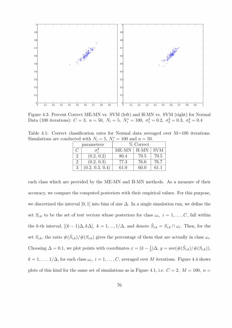
0 0.1 0.2 0.3 0.4 0.5 0.6 0.7 0.8 0.9 10

0.1

0.2

0.3

0.4

0.5

0.6

0.7

0.8

0.9

1

0 0.1 0.2 0.3 0.4 0.5 0.6 0.7 0.8 0.9 10

0.1

0.2

0.3

0.4

0.5

0.6

0.7

0.8

0.9

1

Figure 4.3: Percent Correct ME-MN vs. SVM (left) and H-MN vs. SVM (right) for NormalData (100 iterations): C = 3, n = 50, Ni = 5, N∗

i = 100, σ21 = 0.2, σ2

2 = 0.3, σ23 = 0.4

Table 4.1: Correct classification rates for Normal data averaged over M=100 iterations.Simulations are conducted with Ni = 5, N∗

i = 100 and n = 50.parameters % Correct

C σ2i ME-MN H-MN SVM

2 (0.2, 0.2) 80.4 79.5 79.52 (0.2, 0.3) 77.3 76.6 76.73 (0.2, 0.3, 0.4) 61.0 60.0 61.1

each class which are provided by the ME-MN and H-MN methods. As a measure of their

accuracy, we compare the computed posteriors with their empirical values. For this purpose,

we discretized the interval [0, 1] into bins of size ∆. In a single simulation run, we define the

set Si,k to be the set of test vectors whose posteriors for class ωi, i = 1, . . . , C, fall within

the k-th interval, [(k − 1)∆, k∆], k = 1, ..., 1/∆, and denote Si,k = Si,k ∩ ωi. Then, for the

set Si,k, the ratio #(Si,k)/#(Si,k) gives the percentage of them that are actually in class ωi.

Choosing ∆ = 0.1, we plot points with coordinates x = (k− 12)∆, y = ave(#(Si,k)/#(Si,k)),

k = 1, . . . , 1/∆, for each class ωi, i = 1, . . . , C, averaged over M iterations. Figure 4.4 shows

plots of this kind for the same set of simulations as in Figure 4.1, i.e. C = 2, M = 100, n =

76

50, Ni = 5, N∗i = 100, σ2

1 = σ22 = 0.2. If the performance of the method were perfect and

∆ were small enough, the graphs would coincide with the line y = x, indicating that the

computed posteriors matched the true percentage exactly.

0 0.1 0.2 0.3 0.4 0.5 0.6 0.7 0.8 0.9 10

0.1

0.2

0.3

0.4

0.5

0.6

0.7

0.8

0.9

1Class 1Class 2

0 0.1 0.2 0.3 0.4 0.5 0.6 0.7 0.8 0.9 10

0.1

0.2

0.3

0.4

0.5

0.6

0.7

0.8

0.9

1Class 1Class 2

Figure 4.4: Posteriors vs. Empirical Values, ME-MN (left) and H-MN (right) for NormalData (100 iterations): C = 2, n = 50, Ni = 5, N∗

i = 100, σ21 = σ2

2 = 0.2

In our example ∆ is relatively large, however one can see that the graphs tend to follow

the line y = x. Figure 4.5 demonstrates similar plots with the same parameter values as in

Figure 4.2, i.e. C = 2, M = 100, n = 50, Ni = 5, N∗i = 100, σ2

1 = 0.2, σ22 = 0.3.

In Figure 4.6, we show posteriors vs. their empirical values for C = 3, using the same

parameters as in Figure 4.3, i.e. M = 100, n = 50, Ni = 5, N∗i = 100, σ2

1 = 0.2, σ22 =

0.3, σ23 = 0.4.

Note that when each class has a different value of σ2i , both methods tend to favor (assign

more vectors to) the class with the smallest value of σ2i . Although it is not clear from the

figures, the H-MN method tends to perform slightly better in the case of different σ2i , so for

the MSTAR dataset we only study the H-MN method.

77

0 0.1 0.2 0.3 0.4 0.5 0.6 0.7 0.8 0.9 10

0.1

0.2

0.3

0.4

0.5

0.6

0.7

0.8

0.9

1Class 1Class 2

0 0.1 0.2 0.3 0.4 0.5 0.6 0.7 0.8 0.9 10

0.1

0.2

0.3

0.4

0.5

0.6

0.7

0.8

0.9

1Class 1Class 2

Figure 4.5: Posteriors vs. Empirical Values, ME-MN (left) and H-MN (right) for NormalData (100 iterations): C = 2, n = 50, Ni = 5, N∗

i = 100, σ21 = 0.2, σ2

2 = 0.3

0 0.1 0.2 0.3 0.4 0.5 0.6 0.7 0.8 0.9 10

0.1

0.2

0.3

0.4

0.5

0.6

0.7

0.8

0.9

1Class 1Class 2Class 3

0 0.1 0.2 0.3 0.4 0.5 0.6 0.7 0.8 0.9 10

0.1

0.2

0.3

0.4

0.5

0.6

0.7

0.8

0.9

1Class 1Class 2Class 3

Figure 4.6: Posteriors vs. Empirical Values, ME-MN (left) and H-MN (right) for NormalData (100 iterations): C = 3, n = 50, Ni = 5, N∗

i = 100, σ21 = 0.2, σ2

2 = 0.3, σ23 = 0.4

4.2 Simulations with Non-Normal Data

The decision rules derived in this paper assume that the data is normally distributed. Since

it is difficult to test the normality hypothesis in our setting (high-dimension, low sample

78

size), we instead test the ME-MN and ME-H methods against data which is not normally

distributed. To do this, we use the Laplace (double exponential) distribution, which we

denote by L(µ, σ2). The pdf is given by

f(x|µ, σ2) =1√2 σ

exp

√2 |x− µ|

σ

.

The vectors from class ωi are generated so that if ti,k is the kth element of a vector from

class ωi, then ti,k ∼ L(δik, σ2i ). Therefore, the class means are the canonical unit vectors, and

there is independence between and within vectors. The goal in this study is to test not only

deviations from normality, but also the affects of uncorrelated data. Table 4.2 shows the

results of these simulations in a format identical to Table 4.1. The results again show similar

classification rates as SVM, hence the methods do not appear to be sensitive to deviations

from the assumptions.

Table 4.2: Correct classification rates for Laplacian data averaged over M=100 iterations.Simulations are conducted with Ni = 5, N∗

i = 100 and n = 50.parameters % Correct

C σ2i ME-MN H-MN SVM

2 (0.2, 0.2) 80.0 80.4 79.82 (0.2, 0.3) 76.9 75.6 76.03 (0.2, 0.3, 0.4) 58.8 58.1 59.2

4.3 Application to Target Detection and Recognition

In real life situations one cannot expect that the assumptions of the model are satisfied

exactly. For this reason, we study the performance of the proposed method using the public

domain Moving and Stationary Target Acquisition and Recognition (MSTAR) dataset, which

is a collection of X-band synthetic aperture radar (SAR) images of 1 foot by 1 foot resolution.

The dataset contains 40×40 pixel images of the T72 battle tank, the BMP armored personnel

79

carrier (APC), the BTR70 APC, and clutter. Images from the target class and clutter class

are shown in Figure 4.7. For this dataset, we only show output for the ME-MN method,

since it gave the most meaningful posterior probabilities. However, the H-MN method did

provide classification rates nearly identical to SVM on every simulation run (like in Figures

4.1 and 4.2).

5 10 15 20 25 30 35 40

5

10

15

20

25

30

35

405 10 15 20 25 30 35 40

5

10

15

20

25

30

35

40

Figure 4.7: MSTAR Images of Target (left) and Clutter (right)

For the application of the ME-MN method, we cropped the images to 25× 25 and scaled

each vector to unit norm so that the estimate for Ψ has blocks of constants along the diagonal

corresponding to σ2i . For a comparison to SVM, we perform 50 runs of simulations. In each

of the runs, we pick up Ni = 5, i = 1, 2, images from each of the two classes as training

samples, and another N∗i = 50, i = 1, 2, vectors to be classified. In Figure 4.8, we represent

the results of each simulation run as a point, similar to Figures 4.1 - 4.3. As one can see,

the classification rates varied for both ME-MN and SVM, but on the average tended to be

near the line y = x, confirming that the ME-MN method achieves classification precision

similar to SVM – and in addition provides posterior probabilities for each class. A plot of

80

these posterior probabilities vs. their empirical values is given in Figure 4.9. In Figure 4.9,

we see that the ME-MN method does provide meaningful posterior probabilities, while still

achieving classification rates similar to the SVM.

0 0.1 0.2 0.3 0.4 0.5 0.6 0.7 0.8 0.9 10

0.1

0.2

0.3

0.4

0.5

0.6

0.7

0.8

0.9

1

Figure 4.8: Percent Correct ME-MN vs. SVM for MSTAR Data (50 iterations): C = 2, n =625, Ni = 5, N∗

i = 50

0 0.1 0.2 0.3 0.4 0.5 0.6 0.7 0.8 0.9 10

0.1

0.2

0.3

0.4

0.5

0.6

0.7

0.8

0.9

1Class 1Class 2

Figure 4.9: Posteriors vs. Empirical Values, ME-MN for MSTAR Data (50 iterations):C = 2, n = 625, Ni = 5, N∗

i = 50

81

4.4 Remarks

The method proposed in the paper is very efficient computationally and has very few limi-

tations. It does not require much storage space apart from original matrix X and the new

vector z to be classified, and all structures involved in the classification rule are of the small

size N × N . This distinguish our algorithm from classical decision rules which require the

evaluation of the n × n matrix Σ. In addition, both the Matrix Entropy and the Hybrid

priors lead to a very efficient computation algorithm. After XTX, XTz and zTz are evalu-

ated, the computational complexity of the method is O(N2) where N << n, so it is more

suitable than MCMC-based Bayesian classification [Mallick et al., 2005] in situations where

the decision must be made in real time.

Our simulations show that our methods have misclassification rates very similar to SVM,

but they also possesses convenient features of Bayesian approaches. In addition, we demon-

strated that the posterior probabilities of the classes provided by our algorithm are reason-

ably close to their empirical values, and hence provide useful information in many real life

situations.

82

5

CONCLUSIONS AND FUTUREWORK

In this dissertation, we introduced a new technique for the classification of high-dimensional

vectors based on a small number of training samples. The method is based on the small

vector a, which can be interpreted as the coefficients of the projection of the observation

z onto the space spanned by the training samples L(X). The purpose of this method was

to derive meaningful posterior probabilities while avoiding the “curse of dimensionality,”

which arises when trying to estimate the large covariance matrices in the decision theoretic

approach.

This method employed the use of matrix-variate normal distributions, which have previ-

ously been used in classification only in the context of repeated measurements. Our assump-

tion that the matrix of training samples follows a matrix-variate normal distribution can be

viewed as an restriction to the method, since we did not perform any validation that the

data was normally distributed. However, the normality assumption is difficult to test in this

situation, since the majority of available tests are only suitable when n is small and N →∞.

Even the normality tests which allow for N < n [Liang et al., 2000, Tan et al., 2005] are

not appropriate when N << n. Furthermore, they only test to reject normality, not confirm

it. In this paper, we studied the effects of deviations from normality via simulations, and

83

the results confirmed that deviations from normality do not have a critical effect. Moreover,

the normality assumption was only used to derive the conditions in Theorem 3.1.2, which

established class-conditional relations on the coefficient vector a.

Based on the conditions from Theorem 3.1.2, we chose the class-conditional distributions

on the coefficient vector a ∈ RN , where N << n = dim(z), thus avoiding the “curse

of dimensionality.” We proposed three different interpretations of the conditions – Delta,

Maximum Entropy, and Hybrid – resulting in three different priors on a, although the Delta

prior proved to be difficult to implement.

The results of the numerical simulations were promising. For the simulated data, we ob-

served that both the Maximum Entropy and Hybrid methods provided meaningful posterior

probabilities, as evidenced by comparing them with their empirical counterparts. Further-

more, both methods provided classification rates very similar to the Linear Support Vector

Machine. For the application to the target detection problem, we noticed that the Maximum

Entropy method was closer to the true posterior probabilities, and the Hybrid method had

a classification rate which matched the SVM rate almost exactly in every simulation run.

Furthermore, we noticed that both methods tended to favor (assign more vectors to) the

class with the smallest value of σ2i .

The work presented in this dissertation can be extended in several ways. First, classifica-

tion based on the matrix Ω = XTX can be extended to classification based on reproducing

kernels K(x,y) = φ(x)φ(y), for some function φ(x). Second, instead of arbitrary choices for

the components d1 and d2 in matrix Λ (see equation (4.46) in Chapter 3), we can develop

a meaningful algorithm which, for example, chooses d1 and d2 to maximize the marginal

likelihood. We would then need to conduct simulations for this Λ and compare the results

84

with simulations when Λ = σ2I. Finally, it would be a challenge to develop a fully Bayesian

model of the SVM which is suitable when not necessarily all the training samples are involved

in the classification process.

85

REFERENCES

J. O. Berger. Statistical Decision Theory and Bayesian Analysis. Springer-Verlag, New York,

1985.

C. Burges. A tutorial on support vector machines for pattern recognition. Data Mining and

Knowledge Discovery, 2:121–167, 1998.

G. Casella and R. L. Berger. Statistical Inference. Duxbury Press, Belmont, CA, 2001.

S. C. Choi. Classification of multiply observed data. Biometrical Journal, 14:8–11, 1972.

R. O. Duda, P. E. Hart, and D. G. Stork. Pattern Classification. John Wiley & Sons, Inc.,

New York, 2001.

I. S. Gradshteyn and I. M. Ryzhik. Table of Integrals, Series, and Products. Academic Press,

2000.

A. K. Gupta. On a classification rule for multiple measurements. Computer and Mathematics

with Applications, 12A:301–308, 1986.

A. K. Gupta and D. K. Nagar. Matrix Variate Distributions. Chapman and Hall CRC, Boca

Raton, 2000.

86

F. S. Hillier and G. J. Lieberman. Introduction to Operations Research. McGraw-Hill Pub-

lishing, New York, 1986.

K. Jajuga, A. Sokolowski, and H. Bock, editors. Classification, Clustering, and Data Analy-

sis. Springer, Berlin, 2001.

J. P. Keener. Principles of Applied Mathematics. Perseus Books, Cambridge, MA, 2000.

W. J. Krzanowski and F. H. Marriott. Multivariate Analysis: Part 2, Classification, Covari-

ance Structures & Repeated Measurements. Edward Arnold, London, 1995.

Y. Lee, Y. Lin, and G. Wahba. Multicategory support vector machines: Theory and appli-

cations to the classification of microarray data and satellite radiance data. Journal of the

American Statistical Association, 99(465):67–81, 2004.

J. Liang, R. Li, H. Fang, and K. Fang. Testing multinormality based on low-dimensional

projection. Journal of Statistical Planning and Inference, 86:129–141, 2000.

Y. Lin. Support vector machines and the bayes rule in classification. Data Mining and

Knowledge Discovery, 6:259–275, 2002.

B. K. Mallick, D. Ghosh, and M. Ghosh. Bayesian classification of tumors using gene

expression data. Journal of the Royal Statistical Society, 2005. to appear.

A. M. Mathai. Jacobians of Matrix Transformations and Functions of Matrix Argument.

World Scientific, Singapore, 1997.

K. S. Miller. Multidimensional Gaussian Distributions. John Wiley & Sons, Inc., New York,

1964.

87

B. Muise. Quadratic Filters for Automatic Pattern Recognition. PhD thesis, University of

Central Florida, Orlando, FL, 2003.

J. M. Ortega. Matrix Theory. Plenum Press, New York, 1987.

M. Tan, H. Fang, G. Tian, and G. Wei. Testing multivariate normality in incomplete data

of small sample size. Journal of Multivariate Analysis, 93:164179, 2005.

A. B. Tsybakov. Optimal aggregation of classifiers in statistical learning. Annals of Statistics,

32(1):135–166, 2004.

V. N. Vapnik. Statistical Learning Theory. John Wiley & Sons, Inc., New York, 1998.

G. Wahba. Soft and hard classification by reproducing kernel hilbert space methods. Proc-

cedings of the National Academy of Sciences, 99:14524–16530, 2002.

A. R. Webb. Statistical Pattern Recognition. John Wiley & Sons, Inc., West Sussex, England,

2002.

R. Yang and J. O. Berger. Estimation of a covariance matrix using the reference prior. The

Annals of Statistics, 22(3):1195–1211, 1994.

88