Unsupervised Linear Feature-Extraction Methods and Their Effects in the Classification of...

IEEE TRANSACTIONS ON GEOSCIENCE AND REMOTE SENSING, VOL. 45, NO. 2, FEBRUARY 2007 469

Unsupervised Linear Feature-Extraction Methodsand Their Effects in the Classification of

High-Dimensional DataLuis O. Jiménez-Rodríguez, Member, IEEE, Emmanuel Arzuaga-Cruz, Student Member, IEEE, and

Miguel Vélez-Reyes, Senior Member, IEEE

Abstract—This paper presents an analysis and a comparisonof different linear unsupervised feature-extraction methods ap-plied to hyperdimensional data and their impact on classifica-tion. The dimensionality reduction methods studied are underthe category of unsupervised linear transformations: principalcomponent analysis, projection pursuit (PP), and band subsetselection. Special attention is paid to an optimized version of thePP introduced in this paper: optimized information divergencePP, which is the maximization of the information divergencebetween the probability density function of the projected dataand the Gaussian distribution. This paper is particularly relevantwith current and the next generation of hyperspectral sensorsthat acquire more information in a higher number of spectralchannels or bands when compared to multispectral data. Theprocess to uncover these high-dimensional data patterns is not asimple one. Challenges such as the Hughes phenomenon and thecurse of dimensionality have an impact in high-dimensional dataanalysis. Unsupervised feature extraction, implemented as a linearprojection from a higher dimensional space to a lower dimen-sional subspace, is a relevant process necessary for hyperspectraldata analysis due to its capacity to overcome some difficultiesof high-dimensional data. An objective of unsupervised featureextraction in hyperspectral data analysis is to reduce the dimen-sionality of the data maintaining its capability to discriminate datapatterns of interest from unknown cluttered background that maybe present in the data set. This paper presents a study of theimpact these mechanisms have in the classification process. Theimpact is studied for supervised classification even on the con-ditions of a small number of training samples and unsupervisedclassification where unknown structures are to be uncovered anddetected.

Index Terms—Classification, dimensionality reduction, fea-ture extraction, feature selection, hyperspectral data, patternrecognition, principal component analysis (PCA), projectionpursuit (PP).

Manuscript received May 9, 2005; revised June 11, 2006. This work wassupported in part by the U.S. Army Corps of Engineers Topographic Engineer-ing Center under Grant DACA76-97-K-0007, in part by the National ScienceFoundation Engineering Research Center Program under Grant EEC-9986821,in part by the NASA University Research Centers Program under Grant NCC5-518, and in part by the National Imagery and Mapping Agency under ContractNMA2010112014.

L. O. Jiménez-Rodríguez and M. Vélez-Reyes are with the Electri-cal and Computer Engineering Department, University of Puerto Rico atMayagüez, Mayagüez 00681, Puerto Rico (e-mail: [email protected];[email protected]).

E. Arzuaga-Cruz is with the Department of Electrical and ComputerEngineering, Northeastern University, Boston, MA 02115 USA (e-mail:[email protected]).

Color versions of one or more of the figures in this paper are available onlineat http://ieeexplore.ieee.org.

Digital Object Identifier 10.1109/TGRS.2006.885412

I. INTRODUCTION

THIS PAPER presents an analysis and a comparison ofdifferent linear unsupervised feature-extraction methods

applied to hyperdimensional data and their impact on classifi-cation. Feature extraction is a process applied in multivariatepattern recognition to reduce the number of variables to beused in the classification process. The objective of featureextraction is to reduce the dimensionality of the data whilemaintaining its discrimination capability. This paper focuses onlinear projections due to a series of advantages [1]: 1) The linearmapping function is well defined. 2) The only requirementis to find the coefficient of the linear function which is doneby maximizing or minimizing a criterion. 3) Linear projectionuses well-developed techniques of linear algebra or well-knowniterative and numerical techniques. For features that are notlinear functions of original measurements, it is a challenge tofind suitable nonlinear projection functions and usually is a veryproblem dependent method.

Linear feature selection is a subset of linear feature-extraction process. It is a type of linear projection that choosesvariables instead of adding weighted variables that representnumerical features. The main purpose of this paper is tocompare and study different unsupervised linear methods fordimensionality reduction applied to hyperdimensional data andtheir impact on classification. The methods studied in this paperare: principal component analysis (PCA), projection pursuit(PP), and band subset selection.

PP techniques search for projections that optimize certainprojection indexes. The projection index we optimized in PP,named information divergence PP (IDPP), is the informationdivergence between the probability density function of theprojected data and the Gaussian distribution. To calculate theprojection, an optimization algorithm was used. The PP wasmodified to develop an unsupervised feature-selection versionof the information divergence measure. We named this versionas information divergence band subset selection (IDSS). Inorder to select the set of dsub-bands out of the original set ofd-bands, we measured the divergence between each band prob-ability density function and the Gaussian probability densityfunction. An unsupervised band subset selection mechanismalready developed by Vélez-Reyes [2] was implemented withthe purpose of further comparison. This method, named singu-lar value decomposition subset selection (SVDSS), selects thebest dsub-bands that better approximate to the dsub-principal

0196-2892/$25.00 © 2007 IEEE

470 IEEE TRANSACTIONS ON GEOSCIENCE AND REMOTE SENSING, VOL. 45, NO. 2, FEBRUARY 2007

components. The method uses a technique based on the SVDto select the best subset of dsub-bands over a total number ofd-bands.

These techniques are relevant for hyperspectral data analysis.As the number of spectral bands increases in hyperspectral sen-sors, there is a significant amount of information added to thehigh-dimensional feature space data. Previous work has shownthat hyperspectral data contains a redundant information interms of spectral features [3]. The relevant information contentof hyperspectral data can be represented in a lower dimensionalsubspace for specific applications [3]. Therefore, reducing thedimensionality of hyperspectral data without loosing importantinformation about objects of interest is a very important issuefor the remote sensing community.

The differences in terms of statistical properties anddifficulties in density parameter estimation between high- andlow-dimensional spaces cause that conventional super-vised classification methods originally developed for low-dimensional multispectral data to give unsatisfactory resultswhen managing hyperspectral data. These unsatisfactory resultsof hyperspectral data analysis are due to the characteristics ofhigh-dimensional spaces. Fukunaga shows that as the numberof dimensions increases, the number of samples needed to havehigh classification accuracy increases as well [1]. The increasein the number of samples is linear in the dimensionalityfor a linear classifier and proportional to the square of thedimensionality for a quadratic one. This problem is also knownas “the Hughes phenomenon” [4]. For density estimation, thesituation is more difficult. Local neighborhoods are almostsurely empty, requiring the bandwidth of estimation to be largeand producing the effect of losing detailed density estimation.As a consequence, the situation is even worst for nonparametricclassifiers based on density estimation. It has been estimatedthat as the number of dimensions increases, the sample sizeneeds to increase exponentially in order to have an effectiveestimate of multivariate densities [5], [6]. This also has beennamed “the curse of dimensionality” [3], [5].

A similar problem is found in supervised feature extraction.A number of techniques for case-specific feature extractionhave been developed to reduce the dimensionality withoutloss of class separability. Most of these techniques require theestimation of statistics at full dimensionality in order to extractrelevant features for classification. If the number of trainingsamples is not adequately large, the estimation of parametersin high-dimensional data will not be accurate enough. As aresult, the estimated features may not be as effective as theycould be. To avoid the Hughes phenomenon and the curseof dimensionality, dimensionality reduction methods used formultispectral data analysis must be modified in a way that takesinto consideration the high-dimensional characteristics of thehyperspectral data [7].

This paper presents different mechanisms that perform un-supervised linear dimensionality reduction in the hyperspectralimage analysis process. Special attention is paid to an opti-mized version of PP introduced in this paper: optimized IDPP(OIDPP), which is the optimization of the information diver-gence between the probability density function of the projecteddata and the Gaussian distribution. The objective is to present a

study of the impact these mechanisms have in the classificationprocess and how they handle the Hughes Phenomena. Section IIintroduces a different unsupervised feature-extraction mecha-nism. Section III introduces the PP using information diver-gence. Section IV presents our modification to this mechanism,named OIDPP. A subset selection process based on OIDPP ispresented in Section V. Experimental results with synthetic,multispectral, and hyperspectral data are shown in Section VI.For the purpose of comparison, the study is performed for bothtypes of classification processes: unsupervised and supervisedclassifications. The last experiment is performed and studied onthe supervised classification on the conditions of small numberof training samples. Finally, concluding remarks are presentedin Section VII.

II. DIMENSIONALITY REDUCTION TECHNIQUES

This section presents a summary of several dimensionalreduction techniques. Although the scope of this paper is onunsupervised techniques, one of the best known supervisedtechniques, Fisher discriminant analysis (DA), will be pre-sented. Its strengths and limitations are exemplary of othersupervised feature-extraction mechanism. Unsupervised tech-niques, such as PP, PCA, and SVDSS, will be summarizedwith its potentiality to address the Hughes phenomenon and thecurse of dimensionality.

A. Fisher DA

DA is a supervised feature-extraction technique that uses theinformation of the data distribution as an index to maximize.The index that maximizes is the ratio of the between-class andwithin-class variances as a measure of separability. This methodneeds a priori information in terms of labeled samples thatrepresents classes in the data set. This transformation is basedon the eigenvalue/vector decomposition. This transformation isbased on the Fisher criterion [8].

For mathematical clarity, let us define the within-class scattermatrix

Σω =1M

M∑i=1

Σi (1)

where Σi is the covariance matrix of the ith class.Let us define the between-class scatter matrix Σb

Σb =1M

M∑i=1

(mi − m)(mi − m)T (2)

where M is the number of spectral classes, mi is the samplemean vector of the ith class, and m is the sample mean vectorfor the whole labeled data set.

Finally, we compute the feature vector a by maximizing thefollowing function:

J(a) =aTΣba

aTΣωa. (3)

JIMÉNEZ-RODRÍGUEZ et al.: UNSUPERVISED LINEAR FEATURE-EXTRACTION METHODS 471

The feature vector a that maximizes (3) is the eigenvectorof ΣbΣ−1

ω associated to the largest eigenvalue and is used tolinearly project the data. One of the major drawbacks of FisherDA is that if the class-mean vectors are very close to each other,the method may select a projection that merges classes. DAalso requires a large amount of training samples per number offeatures, in order to avoid Hughes phenomenon. Kernel-basedmethods have been developed that include variants of FisherDA based on more general equations than (1)–(3). For example,(3) could be expressed as

J(a) =aTSia

aTSNa(4)

where Si is a symmetric matrix that measures desire informa-tion and SN measures undesired noise along the direction ofprojection. Solutions to this problem have been formulated asan optimization in some kernel feature space [9], [10], where ais expressed as

a =∑

k

αkφk, αk ∈ �. (5)

Feature vector a lies in the spanning of a set of functions φi.This method is called Kernel Fisher discriminant and resemblessupport vector machines classifiers. This mechanism has beenimplemented in hyperspectral data analysis [11]. Linear andnonlinear feature-extraction methods have been developed andimplemented based on kernel methods including the PCA [12].

Fisher DA as expressed in (1)–(3) was used for comparisonpurposes in terms of class separability in one experiment.

B. PP

PP is a mechanism that linearly projects data to a lowerdimensional subspace while retaining most of the informationin terms of optimizing a defined projection index. This tech-nique is able to reduce the dimensionality of hyperspectraldata bypassing many of the challenges that high-dimensionalspace introduces. For a mathematical definition, we defined thefollowing variables:X original data set (d × N);Y projected data (dsub × N);A orthonormal projection matrix (d × dsub) that satisfies

Y = ATX (6)

where N is the number of spectral samples, d is the originaldimensionality of the hyperspectral data, and dsub is the di-mensionality of the projected data y(dsub < d). PP computesmatrix A by optimizing the projection index that is a function ofY : f(Y) = f(ATX). Unless we state otherwise, bold upperletters will refer to matrices and bold lower letter will refer tovectors on the rest of this paper.

Friedman and Tukey were the first ones that introduced theterm PP [7]. Since then, many articles related to the topic haveappeared. All publications that followed Friedman and Tukey’swork are based on the same concept of optimizing a certainprojection index. Jiménez and Landgrebe [7] proposed a super-vised projection index based on the minimum Bhattacharyya

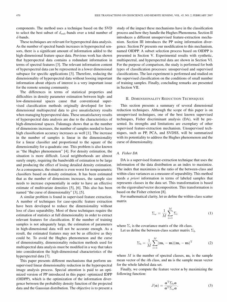
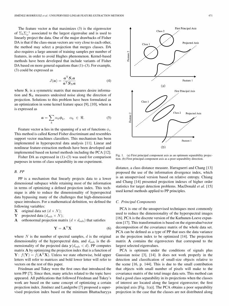
Fig. 1. (a) First principal component axis as an optimum separability projec-tion. (b) First principal component axis as a poor separability direction.

distance, a class distance measure. Ifarraguerri and Chang [13]proposed the use of the information divergence index, whichis an unsupervised version based on relative entropy. Chiangand Chang [14] presented projection indexes of higher orderstatistics for target detection problems. MacDonald et al. [15]used kernel methods applied to PP principles.

C. Principal Components

PCA is one of the unsupervised techniques most commonlyused to reduce the dimensionality of the hyperspectral images[16]. PCA is the discrete version of the Karhunen-Loeve expan-sion [17]. This transformation is based on the eigenvalue/vectordecomposition of the covariance matrix of the whole data set.PCA can be defined as a type of PP that uses the data varianceas the projection index to be optimized [14]. The projectionmatrix A contains the eigenvectors that correspond to thelargest selected eigenvalues.

PCA is optimum under the conditions of signals plusGaussian noise [3], [14]. It does not work properly in thedetection and classification of small-size objects relative tothe scene [16, p. 144]. This is due to the small contributionthat objects with small number of pixels will make to thecovariance matrix of the total image data sets. This method canfind a good class separability in its projections when the classesof interest are located along the largest eigenvector; the firstprincipal axis [Fig. 1(a)]. The PCA obtains a poor separabilityprojection in the case that the classes are not distributed along


the principal axis [Fig. 1(b)]. Another helpful characteristic ofthis mechanism is the fact that it uses the whole data set toestimate the parameters. This implies that the ratio of samplesper number of features is generally acceptable.

D. SVD Band Subset Selection

Another dimension-reduction problem of particular interestis the band subset selection where a subset of dsub-bands isselected from the set of d-bands in a way that some measureof information contained in the data subset is maximized (orinformation loss is minimized). Let x be a d-dimensionalrandom vector with zero mean and covariance matrix ΣX. Wewish to consider a linear dimension-reducing transformation ofx to a dsub-dimensional random vector y given by

y = ATx (7)

where A is a d × dsub projection matrix with dsub < d andATA = Idsub (orthonormal). Thus, y is a dsub-dimensionalrandom vector. Notice that y is a zero-mean random variablewith covariance

ΣY = ATΣXA. (8)

Suppose that we want to reconstruct the random vector x usingy. We denote the prediction of x by X̂. The best linear mean-squared estimator of x from y is given by

x̂ = ΣXYΣ−1Y y = (ΣXA)

(ATΣXA

)−1y. (9)

This estimate is the optimal mean-squared Bayes estimator forthe case that x is a Gaussian random vector. The covariance ofthe estimate is given by

ΣX̂ = ΣXA(ATΣXA

)−1ATΣX. (10)

Note that ΣX̂ is a d × d singular matrix of rank dsub < d.Therefore, the transformation from x to y and back to X̂involves a loss of information. Let e = X − X̂ be the recon-struction error, the error covariance is given by

Σe = ΣX − ΣXYΣ−1Y ΣT

XY

= ΣX − ΣXA(ATΣXA

)−1ATΣX

= ΣX − ΣX̂. (11)

From this result, it is clear that the difference between ΣX̂

and ΣX is a measure of the loss of information resulting fromthe dimension-reduction process. Therefore, we can think ofselecting the orthonormal projection matrix A to minimize theloss of information in dimension reduction by minimizing somemeasure of this difference [1]. The optimal solution to thisproblem for any unitary invariant norm is given by the first dsub

principal components of x. Although PCAs are optimal in themean-square sense, the resulting projection vector y is a linearcombination of the original bands. Therefore, computation ofthe principal components requires processing the full hyper-spectral data cube that will imply that most of the tradeoffsdiscussed previously will be difficult to achieve.

The band subset selection problem can be framed in theapproximation framework discussed previously by further re-stricting the projection matrix A as follows:

A = P[Idsub

0

](12)

where P is a permutation matrix. The net effect of this con-straint is that the dimension-reducing transformation A nowselects a subset of the original variables in the vector x asfollows:

y = ATx = [ Idsub 0 ]PTx =

xi1

xi2

···

xidsub

. (13)

The selection of a subset of bands has several interestingadvantages since we are retaining the physical meaning of thedata in order to: 1) maximize human understanding; 2) combinespectral data with other data types; and 3) exploit physicalmodeling/simulation.

The selection of the dsub-optimal bands is still a combi-natorial optimization problem with a very large dimensionsolution space. For instance, selecting ten out of 210 bands(as in HYDICE) results in searching approximately 3.7 × 1016

possibilities. This problem can be tackled using standard searchmechanisms for combinatorial optimization problems that arequite time consuming. We have implemented a heuristic al-gorithm for band selection that is based on approximating theprincipal components using subspace approximation methods,which give suboptimal solutions, but in significantly less time.This is because we use matrix decompositions that can becomputed in polynomial time. This approach is based on thesubset selection method described in [18].

The basic idea behind the approach of [19] is that, undera certain condition, the subspace spanned by a subset of dsub

sufficiently independent columns of a matrix will approximatethe subspace spanned by the first dsub principal components forthe same matrix. To search for a subset of sufficiently indepen-dent columns rank revealing decompositions such as the SVD[18] and rank revealing QR factorizations can be used. Here,we focus on using the SVD method that has been shown in thelinear algebra literature to produce the best approximation [19].

The SVD subset selection algorithm is summarized in thefollowing.

1) Construct a matrix representation of the hyperspectralcube as follows. Let X = [x1,x2, . . . ,xN ], where N isthe number of pixels in the image. Notice that each rowof the image corresponds to a band of the cube andeach column corresponds to a measured pixel spectralsignature.

2) Construct the normalized matrix Z = [z1, z2, . . . , zN ]which is obtained by subtracting the mean from each


pixel and normalizing each band to unit variance asfollows:

z = D1/2 (x − µx)

where D = diag{σ2x1

, σ2x2

, . . . , σ2xd} and σ2

xiis the vari-

ance of the ith band.3) Compute the SVD of Z and determine its rank dsub (you

can determine dsub in this form or use an a priori value).4) Compute the QR factorization with pivoting of the matrix

VT1 P = QR where V1 is formed by the first dsub left

singular vectors of X, P is the pivoting matrix of the QRfactorization and Q and R are the QR factors.

5) Compute X = PTX, where P is the pivoting matrixfrom the QR factorization in step 4).

6) Take the first dsub rows of X as the selected bands.

The impact of all the unsupervised feature-extraction methodsdiscussed previously on the unsupervised classification processwill be studied. In the rest of this paper, PP will refer to its useof the information divergence function, as it will be explainedin the next section. The DA, a supervised method, will only beused in one experiment to show the advantages of using the PP.

III. IDPP

Recently, Ifarraguerri and Chang [13] proposed a method thatuses the divergence between the estimated probability densityfunction of the projected data and the Gaussian distributionas a projection index. This method is unsupervised, and itextracts the required information, the estimated probabilitydensity function of the projected data, from the image itselfwithout any a priori information [13].

This method starts by sphering the whole data set X. Thesphering procedure is an orthogonal transformation that “stan-dardizes” the data by subtracting its mean (centering) andwhitening it. The sphering procedure is a preprocessing step.Let X be expressed as X = [x1,x2,x3, . . . ,xN ], where eachcolumn is a pixel vector, and matrix Z be expressed as Z =[z1, z2, z3, . . . , zN ], whose columns are the N sphered pixelvectors. For a mathematical definition, the sphered column zi

of Z is defined as

zi = D−1/2UT (xi − µx) (14)

where D is the diagonal matrix containing the eigenvaluesof the estimated covariance matrix of the image, U is thematrix containing the column eigenvectors associated with theeigenvalues, and µx is the mean of the columns of the imageX. Note that the resulting mean of Z columns is the vector0 = [0, 0, . . . , 0]T, and its covariance matrix is equal to theidentity matrix Id.

The projection index, the function to be optimized, usedin this method is known as the information divergence indexbecause it calculates the relative entropy between probabilitydensity functions. In information theory, entropy is defined as ameasure of the amount of “information” available in the data set[20]. To better understand this method let us use the notation in(6) Y = aTZ, where a is a dx1vector. The projected columns

data in Y will be one dimensional and represent the projecteddata. Let y be the random variable that generates the columns ofthe projected data Y. The projection index uses the estimatedcontinuous probability density function of the projected dataf(y) and the continuous probability density function g(y) of thedistribution that we desire the projection to diverge the most. Inorder to give the definition of this projection index, there areother measures we must introduce first. The continuous relativeentropy of f(y) with respect to g(y) is given by

d(f‖g) =

∞∫−∞

f(y) ln(f(y)

/g(y)

)dy. (15)

The continuous absolute information divergence betweenf(y) and g(y) is expressed by the following [20]:

i(f, g) = d(f‖g) + d(g‖f). (16)

This index is symmetric and nonnegative. When the value ofthe index increases, the two distributions are said to diverge themost. The minimum value is zero, and this value occurs whenboth distributions are the same; f(y) = g(y). If we define g(y)to be a normal Gaussian distribution, N(0, 1), we can computethe divergence of f(y) from that Gaussian probability densityfunction. We must estimate the distribution f(y) from theprojected image data in order to compute the divergence. Giventhe fact that we are using a discrete estimate of f(y), namedvector p obtained from the data, we can simplify the informa-tion divergence computation using a discrete approximation ofthe Gaussian distribution as well. Ifarragueri and Chang use aquantization technique for the discrete approximation of g(y).They select a number of bins n and a width ∆y to approximatethe integral of a standard normal distribution

qi = 1/√

2π

(i+1)∆y∫i∆y

e−t2/2dt. (17)

The vector q is the discrete approximation of g(y). Thevalues of q range from i = −n/2 to n/2. The discrete estimateof f(y), vector p, is created using a histogram of the projectionwith the same number of bins n.

The number of bins must be in the range of [−5σ, 5σ] (were σis the standard deviation) in order to cover most of the Gaussianshape. The authors stated that the optimal width ∆y is close to 1for 1000 samples and decreases with an increasing sample size.

Once vector q and vector p are generated, the relative en-tropy for discrete distributions can be used. The relative entropyfor discrete distributions is defined as [20]

D(p‖q) =∑

i

pi log(pi

/qi

)(18)

where qi and pi are the ith components of column vectors qand p, which are the discrete approximations of g(y) and f(y),respectively. The discrete absolute information divergence thatis implemented is defined by the following expression:

I(p,q) = D(p‖q) + D(q‖p). (19)


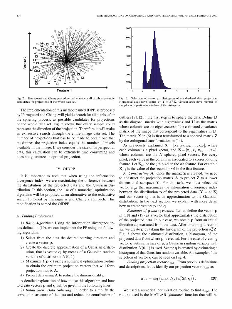
Fig. 2. Ifarraguerri and Chang procedure that considers all pixels as possiblecandidates for projections of the whole data set.

The implementation of this method named IDPP, as proposedby Ifarraguerri and Chang, will yield a search for all pixels, afterthe sphering process, as possible candidates for projectionsof the whole data set. Fig. 2 shows that every sample couldrepresent the direction of the projection. Therefore, it will makean exhaustive search through the entire image data set. Thenumber of projections that has to be made to obtain one thatmaximizes the projection index equals the number of pixelsavailable in the image. If we consider the size of hyperspectraldata, this calculation can be extremely time consuming anddoes not guarantee an optimal projection.

IV. OIDPP

It is important to note that when using the informationdivergence index, we are maximizing the difference betweenthe distribution of the projected data and the Gaussian dis-tribution. In this section, the use of a numerical optimizationalgorithm will be proposed as an alternative to the exhaustivesearch followed by Ifarraguerri and Chang’s approach. Thismodification is named the OIDPP.

A. Finding Projections

1) Basic Algorithm: Using the information divergence in-dex defined in (19), we can implement the PP using the follow-ing algorithm.

1) Select from the data the desired starting direction andcreate a vector p.

2) Create the discrete approximation of a Gaussian distrib-ution, that is vector q, by means of a Gaussian randomvariable of distribution N(0, 1).

3) Maximize I(p,q) using a numerical optimization routineto obtain the optimum projection vectors that will formprojection matrix A.

4) Project data using A to reduce the dimensionality.

A detailed explanation of how to use this algorithm and howto create vectors p and q will be given in the following lines.2) Initial Step: Data Sphering: In order to simplify the

correlation structure of the data and reduce the contribution of

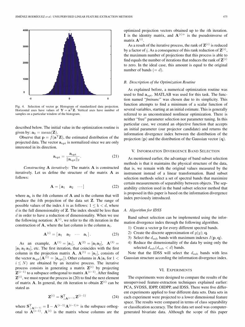
Fig. 3. Selection of vector p: Histogram of standardized data projection.Horizontal axes have values of Y = aTZ. Vertical axes have number ofsamples on a particular window of the histogram.

outliers [8], [21], the first step is to sphere the data. Define Das the diagonal matrix with eigenvalues and U as the matrixwhose columns are the eigenvectors of the estimated covariancematrix of the image that correspond to the eigenvalues in D.The matrix X in (6) is first transformed to a sphered matrix Zby the orthogonal transformation in (14).

As previously explained X = [x1,x2,x3, . . . ,xN ], whereeach column is a pixel vector, and Z = [z1, z2, z3, . . . , zN ],whose columns are the N sphered pixel vectors. For everypixel, each value in the column is associated to a correspondingfeature. Let Zi,j be the jth pixel in the ith feature. For exampleZ1,2 is the value of the second pixel in the first feature.3) Constructing A: Once the matrix Z is created, we need

to construct the projection matrix A to project Z to a lowerdimensional subspace Y. For this task, we must select thevector aopt that maximizes the information divergence indexbetween the distribution p of the projected data (Y = aTZ)and our vector q that is an approximation to the Gaussiandistribution. In the next section, we explain with more detailhow to create vectors p and q.

Estimates of p and q vectors: Let us define the vector pin (18) and (19) as a vector that approximates the distributionof the projected data. In our case, we obtain p from an initialdirection a0 extracted from the data. After obtaining directiona0, we create p by taking the histogram of the projection aT

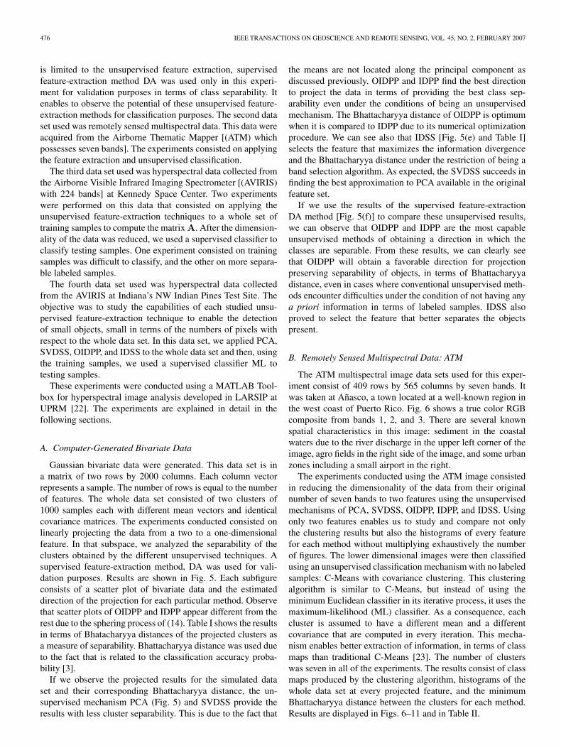
0 Z.Fig. 3 shows the estimated distribution, a histogram, of theprojected data from where p is created. For the case of creatingvector q with same size of p, a Gaussian random variable withdistribution N(0, 1) is used. Vector q is created by estimating ahistogram of that Gaussian random variable. An example of theselection of vector q can be seen on Fig. 4.

Finding projection vector aopt: From previous definitionsand descriptions, let us identify our projection vector aopt as

aopt = arg(max

iI(f(aT

i Z),q))

. (20)

We used a numerical optimization routine to find aopt. Theroutine used is the MATLAB “fminunc” function that will be


Fig. 4. Selection of vector p: Histogram of standardized data projection.Horizontal axes have values of Y = aTZ. Vertical axes have number ofsamples on a particular window of the histogram.

described below. The initial value in the optimization routine isgiven by: a0 = mean(Z).

Observe that p = f(aTZ), the estimated distribution of theprojected data. The vector aopt is normalized since we are onlyinterested in its direction.

aopt =aopt

‖aopt‖2. (21)

Constructing A iteratively: The matrix A is constructediteratively. Let us define the structure of the matrix A asfollows:

A = [a1 a2 · · · ] (22)

where ak is the kth columns of A and is the column that willproduce the kth projection of the data set Z. The range ofpossible values of the index k is as follows: 1 ≤ k < d, whered is the full dimensionality of Z. The index should be less thand in order to have a reduction of dimensionality. When we usethe following notation: A(i), we refer to the ith iteration in theconstruction of A, where the last column is the column ai.

A(i) = [a1 a2 · · · ai ] . (23)

As an example, A(1) = [a1], A(2) = [a1a2], A(3) =[a1 a2 a3], etc. The first iteration, that coincides with the firstcolumn in the projection matrix A, A(1) = [a1], consists ofthe vector aopt(A(1) = [aopt]). Other columns in A(ai for 1 <i ≤ N) are obtained by an iterative process. The iterativeprocess consists in generating a matrix Z(i) by projectingZ(i−1) to a subspace orthogonal to matrix A(i−1). After findingZ(i), we must repeat the process in (20) to find the next elementof matrix A. In general, the ith iteration to obtain Z(i) can bestated as

Z(i) = ST⊥A(i−1)Z(i−1) (24)

where ST⊥A(i−1) = I − A(i−1)A(i−1)+ is the subspace orthog-

onal to A(i−1). A(i) is the matrix whose columns are the

optimized projection vectors obtained up to the ith iteration.I is the identity matrix, and A(i)+ is the pseudoinverse ofmatrix A(i).

As a result of the iterative process, the rank of Z(i) is reducedby a factor of i. As a consequence of this rank reduction of Z(i),the maximum number of projections that this process is able tofind equals the number of iterations that reduces the rank of Z(i)

to zero. In the ideal case, this amount is equal to the originalnumber of bands (= d).

B. Description of the Optimization Routine

As explained before, a numerical optimization routine wasused to find aopt. MATLAB was used for this task. The func-tion named “fminunc” was chosen due to its simplicity. Thisfunction attempts to find a minimum of a scalar function ofseveral variables, starting at an initial estimate. This is generallyreferred to as unconstrained nonlinear optimization. There isneither “free” parameter selection nor parameter tuning. In thisparticular case, we created an objective function that acceptsan initial parameter (our projector candidate) and returns theinformation divergence index between the distribution of theprojection (p) and the distribution of the Gaussian vector (q).

V. INFORMATION DIVERGENCE BAND SELECTION

As mentioned earlier, the advantage of band subset selectionmethods is that it maintains the physical structure of the data,that is, we remain with the original values measured by theinstrument instead of a linear transformation. Band subsetselection methods select a set of spectral bands that maximizecertain measurements of separability between objects. The sep-arability criterion used in the band subset selector method thatis proposed in this paper is based on the information divergenceindex previously introduced.

A. Algorithm for IDSS

Band subset selection can be implemented using the infor-mation divergence index through the following algorithm.

1) Create a vector p for every different spectral bands.2) Create the discrete approximation of g(y); q.3) Select the dsub bands with maximum indexes I(p,q).4) Reduce the dimensionality of the data by using only the

selected dsub(dsub < d) bands.Note that the IDSS will select the dsub bands with less

Gaussian structure according the information divergence index.

VI. EXPERIMENTS

The experiments were designed to compare the results of theunsupervised feature-extraction techniques explained earlier:PCA, SVDSS, IDPP, OIDPP, and IDSS. There were five differ-ent experiments applied to four different data sets. Data sets ineach experiment were projected to a lower dimensional featurespace. The results were compared in terms of class separabilityor classification accuracy. The first data set used was computer-generated bivariate data. Although the scope of this paper


is limited to the unsupervised feature extraction, supervisedfeature-extraction method DA was used only in this experi-ment for validation purposes in terms of class separability. Itenables to observe the potential of these unsupervised feature-extraction methods for classification purposes. The second dataset used was remotely sensed multispectral data. This data wereacquired from the Airborne Thematic Mapper [(ATM) whichpossesses seven bands]. The experiments consisted on applyingthe feature extraction and unsupervised classification.

The third data set used was hyperspectral data collected fromthe Airborne Visible Infrared Imaging Spectrometer [(AVIRIS)with 224 bands] at Kennedy Space Center. Two experimentswere performed on this data that consisted on applying theunsupervised feature-extraction techniques to a whole set oftraining samples to compute the matrix A. After the dimension-ality of the data was reduced, we used a supervised classifier toclassify testing samples. One experiment consisted on trainingsamples was difficult to classify, and the other on more separa-ble labeled samples.

The fourth data set used was hyperspectral data collectedfrom the AVIRIS at Indiana’s NW Indian Pines Test Site. Theobjective was to study the capabilities of each studied unsu-pervised feature-extraction technique to enable the detectionof small objects, small in terms of the numbers of pixels withrespect to the whole data set. In this data set, we applied PCA,SVDSS, OIDPP, and IDSS to the whole data set and then, usingthe training samples, we used a supervised classifier ML totesting samples.

These experiments were conducted using a MATLAB Tool-box for hyperspectral image analysis developed in LARSIP atUPRM [22]. The experiments are explained in detail in thefollowing sections.

A. Computer-Generated Bivariate Data

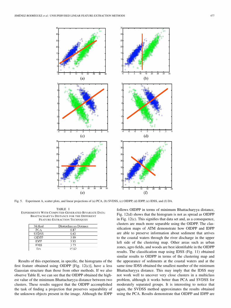
Gaussian bivariate data were generated. This data set is ina matrix of two rows by 2000 columns. Each column vectorrepresents a sample. The number of rows is equal to the numberof features. The whole data set consisted of two clusters of1000 samples each with different mean vectors and identicalcovariance matrices. The experiments conducted consisted onlinearly projecting the data from a two to a one-dimensionalfeature. In that subspace, we analyzed the separability of theclusters obtained by the different unsupervised techniques. Asupervised feature-extraction method, DA was used for vali-dation purposes. Results are shown in Fig. 5. Each subfigureconsists of a scatter plot of bivariate data and the estimateddirection of the projection for each particular method. Observethat scatter plots of OIDPP and IDPP appear different from therest due to the sphering process of (14). Table I shows the resultsin terms of Bhatacharyya distances of the projected clusters asa measure of separability. Bhattacharyya distance was used dueto the fact that is related to the classification accuracy proba-bility [3].

If we observe the projected results for the simulated dataset and their corresponding Bhattacharyya distance, the un-supervised mechanism PCA (Fig. 5) and SVDSS provide theresults with less cluster separability. This is due to the fact that

the means are not located along the principal component asdiscussed previously. OIDPP and IDPP find the best directionto project the data in terms of providing the best class sep-arability even under the conditions of being an unsupervisedmechanism. The Bhattacharyya distance of OIDPP is optimumwhen it is compared to IDPP due to its numerical optimizationprocedure. We can see also that IDSS [Fig. 5(e) and Table I]selects the feature that maximizes the information divergenceand the Bhattacharyya distance under the restriction of being aband selection algorithm. As expected, the SVDSS succeeds infinding the best approximation to PCA available in the originalfeature set.

If we use the results of the supervised feature-extractionDA method [Fig. 5(f)] to compare these unsupervised results,we can observe that OIDPP and IDPP are the most capableunsupervised methods of obtaining a direction in which theclasses are separable. From these results, we can clearly seethat OIDPP will obtain a favorable direction for projectionpreserving separability of objects, in terms of Bhattacharyyadistance, even in cases where conventional unsupervised meth-ods encounter difficulties under the condition of not having anya priori information in terms of labeled samples. IDSS alsoproved to select the feature that better separates the objectspresent.

B. Remotely Sensed Multispectral Data: ATM

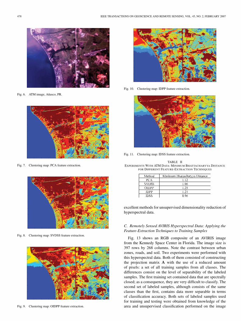
The ATM multispectral image data sets used for this exper-iment consist of 409 rows by 565 columns by seven bands. Itwas taken at Añasco, a town located at a well-known region inthe west coast of Puerto Rico. Fig. 6 shows a true color RGBcomposite from bands 1, 2, and 3. There are several knownspatial characteristics in this image: sediment in the coastalwaters due to the river discharge in the upper left corner of theimage, agro fields in the right side of the image, and some urbanzones including a small airport in the right.

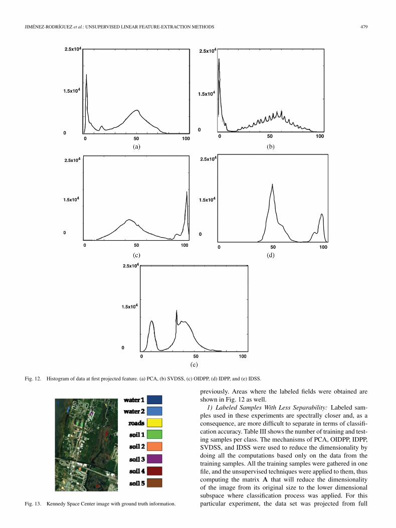
The experiments conducted using the ATM image consistedin reducing the dimensionality of the data from their originalnumber of seven bands to two features using the unsupervisedmechanisms of PCA, SVDSS, OIDPP, IDPP, and IDSS. Usingonly two features enables us to study and compare not onlythe clustering results but also the histograms of every featurefor each method without multiplying exhaustively the numberof figures. The lower dimensional images were then classifiedusing an unsupervised classification mechanism with no labeledsamples: C-Means with covariance clustering. This clusteringalgorithm is similar to C-Means, but instead of using theminimum Euclidean classifier in its iterative process, it uses themaximum-likelihood (ML) classifier. As a consequence, eachcluster is assumed to have a different mean and a differentcovariance that are computed in every iteration. This mecha-nism enables better extraction of information, in terms of classmaps than traditional C-Means [23]. The number of clusterswas seven in all of the experiments. The results consist of classmaps produced by the clustering algorithm, histograms of thewhole data set at every projected feature, and the minimumBhattacharyya distance between the clusters for each method.Results are displayed in Figs. 6–11 and in Table II.


Fig. 5. Experiment A, scatter plots, and linear projections of (a) PCA, (b) SVDSS, (c) OIDPP, (d) IDPP, (e) IDSS, and (f) DA.

TABLE IEXPERIMENTS WITH COMPUTER-GENERATED BIVARIATE DATA:

BHATTACHARYYA DISTANCE FOR THE DIFFERENT

FEATURE-EXTRACTION TECHNIQUES

Results of this experiment, in specific, the histograms of thefirst feature obtained using OIDPP [Fig. 12(c)], have a lessGaussian structure than those from other methods. If we alsoobserve Table II, we can see that the OIDPP obtained the high-est value of the minimum Bhattacharyya distance between twoclusters. These results suggest that the OIDPP accomplishedthe task of finding a projection that preserves separability ofthe unknown objects present in the image. Although the IDPP

follows OIDPP in terms of minimum Bhattacharyya distance,Fig. 12(d) shows that the histogram is not as spread as OIDPPin Fig. 12(c). This signifies that data set and, as a consequence,clusters are much more separable using the OIDPP. The clas-sification maps of ATM demonstrate how OIDPP and IDPPare able to preserve information about sediment that arrivesto the coastal waters through the river discharge in the upperleft side of the clustering map. Other areas such as urbanzones, agro fields, and woods are best identifiable in the OIDPPresults. The classification map using IDSS (Fig. 11) obtainedsimilar results to OIDPP in terms of the clustering map andthe appearance of sediments at the coastal waters and at thesame time IDSS obtained the smallest number of the minimumBhattacharyya distance. This may imply that the IDSS maynot work well to uncover very close clusters in a multiclassproblem, although it works better than PCA and SVDSS formoderately separated groups. It is interesting to notice thatagain, the SVDSS method approximates the results obtainedusing the PCA. Results demonstrate that OIDPP and IDPP are


Fig. 6. ATM image, Añasco, PR.

Fig. 7. Clustering map: PCA feature extraction.

Fig. 8. Clustering map: SVDSS feature extraction.

Fig. 9. Clustering map: OIDPP feature extraction.

Fig. 10. Clustering map: IDPP feature extraction.

Fig. 11. Clustering map: IDSS feature extraction.

TABLE IIEXPERIMENTS WITH ATM DATA: MINIMUM BHATTACHARYYA DISTANCE

FOR DIFFERENT FEATURE-EXTRACTION TECHNIQUES

excellent methods for unsupervised dimensionality reduction ofhyperspectral data.

C. Remotely Sensed AVIRIS Hyperspectral Data: Applying theFeature-Extraction Techniques to Training Samples

Fig. 13 shows an RGB composite of an AVIRIS imagefrom the Kennedy Space Center in Florida. The image size is397 rows by 268 columns. Note the contrast between urbanzones, roads, and soil. Two experiments were performed withthis hyperspectral data. Both of them consisted of constructingthe projection matrix A with the use of a reduced amountof pixels: a set of all training samples from all classes. Thedifferences consist on the level of separability of the labeledsamples. The first training set contained data that are spectrallyclosed; as a consequence, they are very difficult to classify. Thesecond set of labeled samples, although consists of the sameclasses than the first, contains data more separable in termsof classification accuracy. Both sets of labeled samples usedfor training and testing were obtained from knowledge of thearea and unsupervised classification performed on the image


Fig. 12. Histogram of data at first projected feature. (a) PCA, (b) SVDSS, (c) OIDPP, (d) IDPP, and (e) IDSS.

Fig. 13. Kennedy Space Center image with ground truth information.

previously. Areas where the labeled fields were obtained areshown in Fig. 12 as well.1) Labeled Samples With Less Separability: Labeled sam-

ples used in these experiments are spectrally closer and, as aconsequence, are more difficult to separate in terms of classifi-cation accuracy. Table III shows the number of training and test-ing samples per class. The mechanisms of PCA, OIDPP, IDPP,SVDSS, and IDSS were used to reduce the dimensionality bydoing all the computations based only on the data from thetraining samples. All the training samples were gathered in onefile, and the unsupervised techniques were applied to them, thuscomputing the matrix A that will reduce the dimensionalityof the image from its original size to the lower dimensionalsubspace where classification process was applied. For thisparticular experiment, the data set was projected from full


TABLE IIIEXPERIMENTS WITH AVIRIS KENNEDY SPACE CENTER DATA: CLASSES

AND NUMBER OF TRAINING AND TESTING SAMPLES

WITH LESS SEPARABILITY

TABLE IVEXPERIMENTS WITH AVIRIS KENNEDY SPACE CENTER DATA TESTING

SAMPLES: CONFUSION MATRICES AND OVERALL ACCURACIES

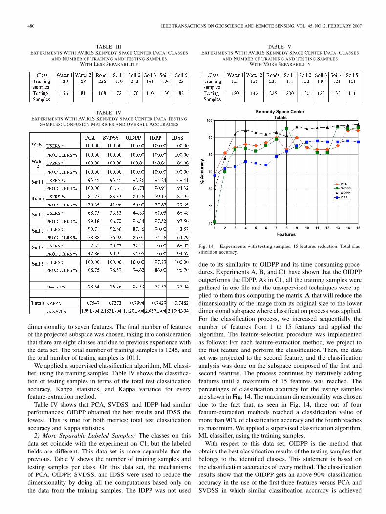
dimensionality to seven features. The final number of featuresof the projected subspace was chosen, taking into considerationthat there are eight classes and due to previous experience withthe data set. The total number of training samples is 1245, andthe total number of testing samples is 1011.

We applied a supervised classification algorithm, ML classi-fier, using the training samples. Table IV shows the classifica-tion of testing samples in terms of the total test classificationaccuracy, Kappa statistics, and Kappa variance for everyfeature-extraction method.

Table IV shows that PCA, SVDSS, and IDPP had similarperformances; OIDPP obtained the best results and IDSS thelowest. This is true for both metrics: total test classificationaccuracy and Kappa statistics.2) More Separable Labeled Samples: The classes on this

data set coincide with the experiment on C1, but the labeledfields are different. This data set is more separable that theprevious. Table V shows the number of training samples andtesting samples per class. On this data set, the mechanismsof PCA, OIDPP, SVDSS, and IDSS were used to reduce thedimensionality by doing all the computations based only onthe data from the training samples. The IDPP was not used

TABLE VEXPERIMENTS WITH AVIRIS KENNEDY SPACE CENTER DATA: CLASSES


WITH MORE SEPARABILITY

Fig. 14. Experiments with testing samples, 15 features reduction. Total clas-sification accuracy.

due to its similarity to OIDPP and its time consuming proce-dures. Experiments A, B, and C1 have shown that the OIDPPoutperforms the IDPP. As in C1, all the training samples weregathered in one file and the unsupervised techniques were ap-plied to them thus computing the matrix A that will reduce thedimensionality of the image from its original size to the lowerdimensional subspace where classification process was applied.For the classification process, we increased sequentially thenumber of features from 1 to 15 features and applied thealgorithm. The feature-selection procedure was implementedas follows: For each feature-extraction method, we project tothe first feature and perform the classification. Then, the dataset was projected to the second feature, and the classificationanalysis was done on the subspace composed of the first andsecond features. The process continues by iteratively addingfeatures until a maximum of 15 features was reached. Thepercentages of classification accuracy for the testing samplesare shown in Fig. 14. The maximum dimensionality was chosendue to the fact that, as seen in Fig. 14, three out of fourfeature-extraction methods reached a classification value ofmore than 90% of classification accuracy and the fourth reachesits maximum. We applied a supervised classification algorithm,ML classifier, using the training samples.

With respect to this data set, OIDPP is the method thatobtains the best classification results of the testing samples thatbelongs to the identified classes. This statement is based onthe classification accuracies of every method. The classificationresults show that the OIDPP gets an above 90% classificationaccuracy in the use of the first three features versus PCA andSVDSS in which similar classification accuracy is achieved


TABLE VIEXPERIMENTS WITH AVIRIS INDIAN TEST SITE DATA: CLASSES


only using the first 14 features for PCA and the first eightfeatures for SVDSS. These results suggest that the band subsetobtained using IDSS as proposed in this paper work will notobtain a suboptimum subset as SVDSS does for this data set.

The total number of training samples is 1082, and the totalnumber of testing samples is 1242.

D. Remotely Sensed AVIRIS Hyperspectral Data: SmallNumber of Training and Testing Samples and the Applicationof Feature-Extraction Techniques to the Whole Image

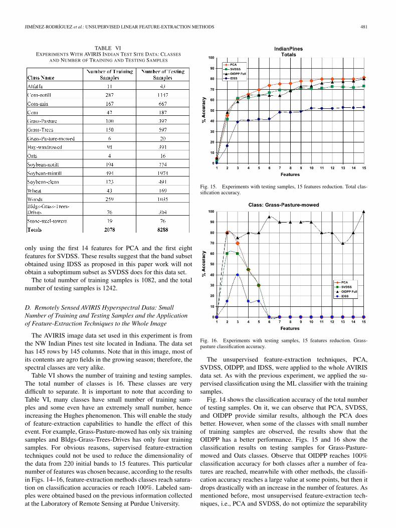
The AVIRIS image data set used in this experiment is fromthe NW Indian Pines test site located in Indiana. The data sethas 145 rows by 145 columns. Note that in this image, most ofits contents are agro fields in the growing season; therefore, thespectral classes are very alike.

Table VI shows the number of training and testing samples.The total number of classes is 16. These classes are verydifficult to separate. It is important to note that according toTable VI, many classes have small number of training sam-ples and some even have an extremely small number, henceincreasing the Hughes phenomenon. This will enable the studyof feature-extraction capabilities to handle the effect of thisevent. For example, Grass-Pasture-mowed has only six trainingsamples and Bldgs-Grass-Trees-Drives has only four trainingsamples. For obvious reasons, supervised feature-extractiontechniques could not be used to reduce the dimensionality ofthe data from 220 initial bands to 15 features. This particularnumber of features was chosen because, according to the resultsin Figs. 14–16, feature-extraction methods classes reach satura-tion on classification accuracies or reach 100%. Labeled sam-ples were obtained based on the previous information collectedat the Laboratory of Remote Sensing at Purdue University.

Fig. 15. Experiments with testing samples, 15 features reduction. Total clas-sification accuracy.

Fig. 16. Experiments with testing samples, 15 features reduction. Grass-pasture classification accuracy.

The unsupervised feature-extraction techniques, PCA,SVDSS, OIDPP, and IDSS, were applied to the whole AVIRISdata set. As with the previous experiment, we applied the su-pervised classification using the ML classifier with the trainingsamples.

Fig. 14 shows the classification accuracy of the total numberof testing samples. On it, we can observe that PCA, SVDSS,and OIDPP provide similar results, although the PCA doesbetter. However, when some of the classes with small numberof training samples are observed, the results show that theOIDPP has a better performance. Figs. 15 and 16 show theclassification results on testing samples for Grass-Pasture-mowed and Oats classes. Observe that OIDPP reaches 100%classification accuracy for both classes after a number of fea-tures are reached, meanwhile with other methods, the classifi-cation accuracy reaches a large value at some points, but then itdrops drastically with an increase in the number of features. Asmentioned before, most unsupervised feature-extraction tech-niques, i.e., PCA and SVDSS, do not optimize the separability


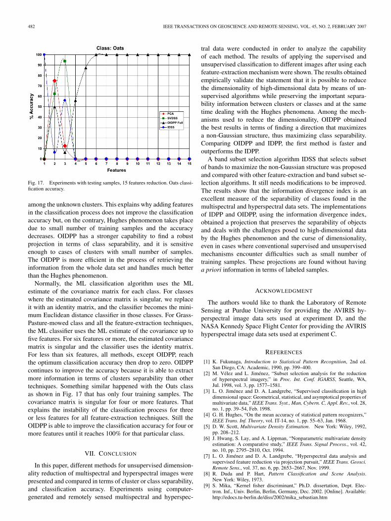
Fig. 17. Experiments with testing samples, 15 features reduction. Oats classi-fication accuracy.

among the unknown clusters. This explains why adding featuresin the classification process does not improve the classificationaccuracy but, on the contrary, Hughes phenomenon takes placedue to small number of training samples and the accuracydecreases. OIDPP has a stronger capability to find a robustprojection in terms of class separability, and it is sensitiveenough to cases of clusters with small number of samples.The OIDPP is more efficient in the process of retrieving theinformation from the whole data set and handles much betterthan the Hughes phenomenon.

Normally, the ML classification algorithm uses the MLestimate of the covariance matrix for each class. For classeswhere the estimated covariance matrix is singular, we replaceit with an identity matrix, and the classifier becomes the mini-mum Euclidean distance classifier in those classes. For Grass-Pasture-mowed class and all the feature-extraction techniques,the ML classifier uses the ML estimate of the covariance up tofive features. For six features or more, the estimated covariancematrix is singular and the classifier uses the identity matrix.For less than six features, all methods, except OIDPP, reachthe optimum classification accuracy then drop to zero. OIDPPcontinues to improve the accuracy because it is able to extractmore information in terms of clusters separability than othertechniques. Something similar happened with the Oats classas shown in Fig. 17 that has only four training samples. Thecovariance matrix is singular for four or more features. Thatexplains the instability of the classification process for threeor less features for all feature-extraction techniques. Still theOIDPP is able to improve the classification accuracy for four ormore features until it reaches 100% for that particular class.

VII. CONCLUSION

In this paper, different methods for unsupervised dimension-ality reduction of multispectral and hyperspectral images werepresented and compared in terms of cluster or class separability,and classification accuracy. Experiments using computer-generated and remotely sensed multispectral and hyperspec-

tral data were conducted in order to analyze the capabilityof each method. The results of applying the supervised andunsupervised classification to different images after using eachfeature-extraction mechanism were shown. The results obtainedempirically validate the statement that it is possible to reducethe dimensionality of high-dimensional data by means of un-supervised algorithms while preserving the important separa-bility information between clusters or classes and at the sametime dealing with the Hughes phenomena. Among the mech-anisms used to reduce the dimensionality, OIDPP obtainedthe best results in terms of finding a direction that maximizesa non-Gaussian structure, thus maximizing class separability.Comparing OIDPP and IDPP, the first method is faster andoutperforms the IDPP.

A band subset selection algorithm IDSS that selects subsetof bands to maximize the non-Gaussian structure was proposedand compared with other feature-extraction and band subset se-lection algorithms. It still needs modifications to be improved.The results show that the information divergence index is anexcellent measure of the separability of classes found in themultispectral and hyperspectral data sets. The implementationsof IDPP and OIDPP, using the information divergence index,obtained a projection that preserves the separability of objectsand deals with the challenges posed to high-dimensional databy the Hughes phenomenon and the curse of dimensionality,even in cases where conventional supervised and unsupervisedmechanisms encounter difficulties such as small number oftraining samples. These projections are found without havinga priori information in terms of labeled samples.

ACKNOWLEDGMENT

The authors would like to thank the Laboratory of RemoteSensing at Purdue University for providing the AVIRIS hy-perspectral image data sets used at experiment D, and theNASA Kennedy Space Flight Center for providing the AVIRIShyperspectral image data sets used at experiment C.

REFERENCES

[1] K. Fukunaga, Introduction to Statistical Pattern Recognition, 2nd ed.San Diego, CA: Academic, 1990, pp. 399–400.

[2] M. Vélez and L. Jiménez, “Subset selection analysis for the reductionof hyperspectral imagery,” in Proc. Int. Conf. IGARSS, Seattle, WA,Jul. 1998, vol. 3, pp. 1577–1581.

[3] L. O. Jiménez and D. A. Landgrebe, “Supervised classification in highdimensional space: Geometrical, statistical, and asymptotical properties ofmultivariate data,” IEEE Trans. Syst., Man, Cybern. C, Appl. Rev., vol. 28,no. 1, pp. 39–54, Feb. 1998.

[4] G. H. Hughes, “On the mean accuracy of statistical pattern recognizers,”IEEE Trans. Inf. Theory, vol. IT-14, no. 1, pp. 55–63, Jan. 1968.

[5] D. W. Scott, Multivariate Density Estimation. New York: Wiley, 1992,pp. 208–212.

[6] J. Hwang, S. Lay, and A. Lippman, “Nonparametric multivariate densityestimation: A comparative study,” IEEE Trans. Signal Process., vol. 42,no. 10, pp. 2795–2810, Oct. 1994.

[7] L. O. Jiménez and D. A. Landgrebe, “Hyperspectral data analysis andsupervised feature reduction via projection pursuit,” IEEE Trans. Geosci.Remote Sens., vol. 37, no. 6, pp. 2653–2667, Nov. 1999.

[8] R. Duda and P. Hart, Pattern Classification and Scene Analysis.New York: Wiley, 1973.

[9] S. Mika, “Kernel fisher discriminant,” Ph.D. dissertation, Dept. Elec-tron. Inf., Univ. Berlin, Berlin, Germany, Dec. 2002. [Online]. Available:http://edocs.tu-berlin.de/diss/2002/mika_sebastian.htm


[10] S. Mika, G. Rätsch, J. Weston, B. Schölkopf, and K.-R. Müller, “Fisherdiscriminant analysis with kernels,” in Neural Networks for SignalProcessing IX, Y.-H. Hu, J. Larsen, E. Wilson, and S. Douglas, Eds.Piscataway, NJ: IEEE Press, 1999, pp. 41–48.

[11] G. Camps-Valls and L. Bruzzone, “Kernel-based methods for hyperspec-tral image classification,” IEEE Trans. Geosci. Remote Sens., vol. 43,no. 6, pp. 1351–1362, Jun. 2005.

[12] B. Schölkopf, S. Mika, C. J. C. Burges, P. Knirsch, K.-R. Müller,G. Rätsch, and A. J. Smola, “Input space versus. feature space in kernel-based methods,” IEEE Trans. Neural Netw., vol. 10, no. 5, pp. 1000–1017,Sep. 1999.

[13] A. Ifarraguerri and C. Chang, “Unsupervised hyperspectral image analysiswith projection pursuit,” IEEE Trans. Geosci. Remote Sens., vol. 38, no. 6,pp. 2529–2538, Nov. 2000.

[14] S. Chiang and C. Chang, “Unsupervised target detection in hyperspectralimages using projection pursuit,” IEEE Trans. Geosci. Remote Sens.,vol. 39, no. 7, pp. 1380–1391, Jul. 2001.

[15] D. MacDonald, C. Fyfe, and D. Charles, “Kernel exploratory projectionpursuit,” in Proc. 4th Int. Conf. Knowledge-Based Intell. Eng. Syst. andAllied Technol., Brighton, U.K., Aug. 2000, pp. 193–196.

[16] J. A. Richards, “Remote sensing digital image analysis,” in An Introduc-tion, 3rd ed. New York: Springer-Verlag, 1999.

[17] D. A. Landgrebe, Signal Theory Methods in Multispectral RemoteSensing. Hoboken, NJ: Wiley, 2003, pp. 281–287.

[18] G. Golub and C. F. Van Loan, Matrix Computations. Baltimore, MD:The Johns Hopkins Univ. Press, 1997.

[19] T. F. Chan and P. C. Hansen, “Some applications of the rank revealing QRfactorization,” SIAM J. Sci. Stat. Comput., vol. 13, no. 3, pp. 727–741,May 1992.

[20] T. M. Cover and J. A. Thomas, Elements of Information Theory. NewYork: Wiley, 1991.

[21] J. Hwang, S. Lay, and A. Lippman, “Nonparametric multivariate densityestimation: A comparative study,” IEEE Trans. Signal Process., vol. 42,no. 10, pp. 2795–2810, Oct. 1994.

[22] E. Arzuaga-Cruz, L. O. Jiménez-Rodríguez, M. Vélez-Reyes, D. Kaeli,E. Rodriguez-Diaz, H. T. Velazquez-Santana, A. Castrodad-Carrau, L. E.Santos-Campis, and C. Santiago, “A MATLAB toolbox for hyperspectralimage analysis,” in Proc. Int. Conf. IGARSS, Anchorage, AK, Sep. 2004,vol. 7, pp. 4839–4842.

[23] L. O. Jiménez, M. Vélez-Reyes, Y. Chaar, F. Fontan, and C. Santiago,“Partially supervised detection using band subset selection in hyperspec-tral data,” in Proc. SPIE Conf., Orlando, FL, Apr. 1999, pp. 148–156.

Luis O. Jiménez-Rodríguez (M’96) received theB.S.E.E. degree from the University of Puerto Ricoat Mayagüez (UPRM), in 1989, the M.S.E.E. degreefrom the University of Maryland, College Park, in1991, and the Ph.D. degree from Purdue University,West Lafayette, IN, in 1996.

He is currently a Professor of electrical and com-puter engineering with the University of Puerto Ricoat Mayagüez. He was the Director of the Laboratoryof Applied Remote Sensing and Image Processing(LARSIP) and was with the UPRM component of

the Center for Subsurface Sensing and Imaging Systems, an NSF EngineeringResearch Center. During the academic year of 2000–2001, he was selected theOutstanding Professor with the Department of Electrical and Computer Engi-neering. During the same year, before his term, he was promoted by exceptionalmerit to Full Professor for his distinguished research and education work. ThePresident of the University of Puerto Rico selected him as a DistinguishedResearcher of the University of Puerto Rico. His research has been in the areaof hyperspectral image analysis, remote sensing, pattern recognition, imageprocessing, and subsurface sensing.

Dr. Jiménez-Rodríguez is a member of the IEEE Geoscience and RemoteSensing, the IEEE System, Man and Cybernetics, and SPIE Societies. He isalso a member of the Tau Beta Pi and Phi Kappa Phi honor societies.

Emmanuel Arzuaga-Cruz (S’99) received theBSCpE and MSCpE degrees from the Universityof Puerto Rico at Mayagüez (UPRM), in 2000and 2003, respectively. He is currently working to-ward the Ph.D. degree at Northeastern University,Boston, MA.

He worked with UPRM as a Software Developerfor the Laboratory for Applied Remote Sensing andImage Processing, where he worked in the devel-opment of remote sensing and pattern recognitionrelated software for the NSF-funded Engineering

Research Center for Subsurface Sensing and Imaging Systems and the TropicalCenter for Earth and Space Studies funded by the NASA University ResearchCenters Program.

Mr. Arzuaga-Cruz is a member of the ACM and the IEEE Computer Society.

Miguel Vélez-Reyes (S’81–M’92–SM’00) receivedthe B.S.E.E. degree from the University of PuertoRico at Mayagüez (UPRM), in 1985, and the M.S.and Ph.D. degrees from the Massachusetts Insti-tute of Technology, Cambridge, in 1988, and 1992,respectively.

In 1992, he joined the faculty with UPRM, wherehe is currently a Professor. He has held FacultyInternship Positions with AT&T Bell Laboratories,Air Force Research Laboratories, and the NASAGoddard Space Flight Center. His teaching and re-

search interests are in the areas of model-based signal processing, systemidentification, parameter estimation, and remote sensing using hyperspectralimaging. He has over 60 publications in journals and conference proceedings.He is the Director with the UPRM Tropical Center for Earth and Space Studies,a NASA University Research Center, and Associate Director of the Centerfor Subsurface Sensing and Imaging Systems, an NSF Engineering ResearchCenter led by Northeastern University.

Dr. Vélez-Reyes was one of the 60 recipients from across the United Statesand its territories of the Presidential Early Career Award for Scientists andEngineers from the White House in 1997. He is member of the Academy ofArts and Sciences of Puerto Rico and a member of the Tau Beta Pi, Sigma Xi,and Phi Kappa Phi honor societies.

Unsupervised Linear Feature-Extraction Methods and Their Effects in the Classification of...

Documents

Transcript of Unsupervised Linear Feature-Extraction Methods and Their Effects in the Classification of...