Unsupervised Feature Construction for Improving Data Representation and Semantics

Noname manuscript No.(will be inserted by the editor)

Unsupervised Feature Construction for Improving Data

Representation and Semantics

Marian-Andrei Rizoiu · Julien Velcin ·Stephane Lallich

Received: 27/01/2012 / Accepted: 29/01/2013

Abstract Feature-based format is the main data representation format used by machine

learning algorithms. When the features do not properly describe the initial data, perfor-

mance starts to degrade. Some algorithms address this problem by internally changing the

representation space, but the newly-constructed features are rarely comprehensible. We seek

to construct, in an unsupervised way, new features that are more appropriate for describing

a given dataset and, at the same time, comprehensible for a human user. We propose two

algorithms that construct the new features as conjunctions of the initial primitive features or

their negations. The generated feature sets have reduced correlations between features and

succeed in catching some of the hidden relations between individuals in a dataset. For ex-

ample, a feature like sky∧¬building∧ panorama would be true for non-urban images and

is more informative than simple features expressing the presence or the absence of an ob-

ject. The notion of Pareto optimality is used to evaluate feature sets and to obtain a balance

between total correlation and the complexity of the resulted feature set. Statistical hypoth-

esis testing is used in order to automatically determine the values of the parameters used

for constructing a data-dependent feature set. We experimentally show that our approaches

achieve the construction of informative feature sets for multiple datasets.

Keywords Unsupervised feature construction · Feature evaluation · Nonparametric

statistics · Data mining · Clustering · Representations · Algorithms for data and knowledge

management · Heuristic methods · Pattern analysis

Marian-Andrei Rizoiu · Julien Velcin · Stephane Lallich

ERIC Laboratory, University Lumiere Lyon 2

5, avenue Pierre Mendes France, 69676 Bron Cedex, France

Tel. +33 (0)4 78 77 31 54

Fax. +33 (0)4 78 77 23 75

Marian-Andrei Rizoiu

E-mail: [email protected]

Julien Velcin


Stephane Lallich


2 Marian-Andrei Rizoiu et al.

1 Introduction

Most machine learning algorithms use a representation space based on a feature-based for-

mat. This format is a simple way to describe an instance as a measurement vector on a set

of predefined features. In the case of supervised learning, a class label is also available. One

limitation of the feature-based format is that supplied features sometimes do not adequately

describe, in terms of classification, the semantics of the dataset. This happens, for exam-

ple, when general-purpose features are used to describe a collection that contains certain

relations between individuals.

In order to obtain good results in classification tasks, many algorithms and preprocessing

techniques (e.g., SVM (Cortes and Vapnik, 1995), PCA (Dunteman, 1989) etc.) deal with

non-adequate variables by internally changing the description space. The main drawback of

these approaches is that they function as a black box, where the new representation space

is either hidden (for SVM) or completely synthetic and incomprehensible to human readers

(PCA).

The purpose of our work is to construct a new feature set that is more descriptive for

both supervised and unsupervised classification tasks. In the same way that frequent item-

sets (Piatetsky-Shapiro, 1991) help users to understand the patterns in transactions, our goal

with the new features is to help understand relations between individuals of datasets. There-

fore, the new features should be easily comprehensible by a human reader. Literature pro-

poses algorithms that construct features based on the original user-supplied features (called

primitives). However, to our knowledge, all of these algorithms construct the feature set in

a supervised way, based on the class information, supplied a priori with the data.

In order to construct new features, we propose two algorithms that create new feature

sets in the absence of classified examples, in an unsupervised manner. The first algorithm is

an adaptation of an established supervised algorithm, making it unsupervised. For the second

algorithm, we have developed a completely new heuristic that selects, at each iteration, pairs

of highly correlated features and replaces them with conjunctions of literals that do not

co-occur. Therefore, the overall redundancy of the feature set is reduced. Later iterations

create more complex Boolean formulas, which can contain negations (meaning absence of

features). We use statistical considerations (hypothesis testing) to automatically determine

the value of parameters depending on the dataset, and a Pareto front (Sawaragi et al, 1985)-

inspired method for the evaluation. The main advantage of the proposed methods over PCA

or the kernel of the SVM is that the newly-created features are comprehensible to human

readers (features like people∧mani f estation∧ urban and people∧¬urban∧ f orest are

easily interpretable).

In Sections 2 and 3, we present our proposed algorithms and in Section 4 we describe

the evaluation metrics and the complexity measures. In Section 5, we perform a set of initial

experiments and outline some of the inconveniences of the algorithms. In Section 6, by

use of statistical hypothesis testing, we address these weak points, notably the choice of

the threshold parameter. In Section 7, a second set of experiments validates the proposed

improvements. Finally, Section 8 draws the conclusion and outlines future works.

1.1 Motivation: why construct a new feature set

In the context of classification (supervised or unsupervised), a useful feature needs to por-

tray new information. A feature p j, that is highly correlated with another feature pi, does

Unsupervised Feature Construction 3

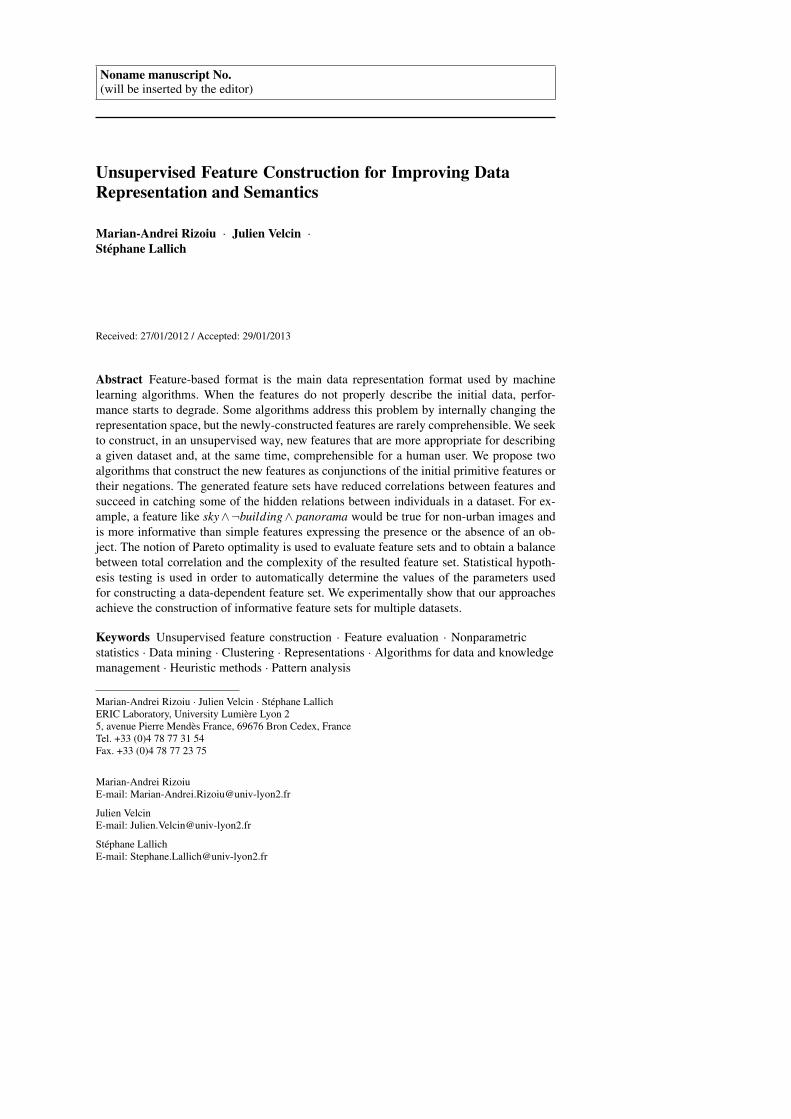
Fig. 1: Example of images tagged with {groups, road, building, interior}

not bring any new information, since the value of p j can be deduced from that of pi. Sub-

sequently, one could filter out “irrelevant” features before applying the classification algo-

rithm. But by simply removing certain features, one runs the risk of losing important infor-

mation of the hidden structure of the feature set, and this is the reason why we perform

feature construction. Feature construction attempts to increase the expressive power of the

original features by discovering missing information about relationships between features.

We deal primarily with datasets described with Boolean features. Any dataset described

by using the feature-value format can be converted to a binary format using discretization

and binarization. In real-life datasets, most binary features have specific meanings. Let us

consider the example of a set of images that are tagged using Boolean features. Each feature

marks the presence (true) or the absence (false) of a certain object in the image. These

objects could include: water, cascade, mani f estation, urban, groups or interior. In this

case, part of the semantic structure of the feature set can be guessed quite easily. Relations

like “is-a” and “part-of” are fairly intuitive: cascade is a sort of water, paw is part of animal

etc. But other relations might be induced by the semantics of the dataset (images in our

example). mani f estation will co-occur with urban, for they usually take place in the city.

Fig. 1 depicts a simple image dataset described using the feature set {groups, road, building,

interior}. The feature set is quite redundant and some of the features are non-informative

(e.g., feature groups is present for all individuals). Considering co-occurrences between

features, we could create the more eloquent features groups∧¬road ∧ interior (describing

the top row) and groups∧ road∧building (describing the bottom row).

The idea is to create a data-dependent feature set, so that the new features are as inde-

pendent as possible, limiting co-occurrences between the new features. At the same time

they should be comprehensible to the human reader.

1.2 Related work

The literature proposes methods for augmenting the descriptive power of features. Liu and

Motoda (1998) collects some of them and divides them into three categories: feature selec-

tion, feature extraction and feature construction.


Feature selection (Lallich and Rakotomalala, 2000; Mo and Huang, 2011) seeks to

filter the original feature set in order to remove redundant features. This results in a rep-

resentation space of lower dimensionality. Feature extraction is a process that extracts

a set of new features from the original features through functional mapping (Motoda and

Liu, 2002). For example, the SVM algorithm (Cortes and Vapnik, 1995) constructs a ker-

nel function that changes the description space into a new separable one. Supervised and

non-supervised algorithms can be boosted by pre-processing with principal component

analysis (PCA) (Dunteman, 1989). PCA is a mathematical procedure that uses an orthog-

onal transformation to convert a set of observations of possibly correlated variables into

a set of values of uncorrelated variables, called principal components. Manifold learn-

ing (Huo et al, 2005) can be seen as a classification approach where the representation

space is changed internally in order to boost the performances. Feature extraction mainly

seeks to reduce the description space and redundancy between features. Newly-created fea-

tures are rarely comprehensible and very difficult to interpret. Both feature selection and

feature extraction are inadequate for detecting relations between the original features.

Feature Construction is a process that discovers missing information about the rela-

tionships between features and augments the space of features by inferring or creating addi-

tional features (Motoda and Liu, 2002). This usually results in a representation space with a

larger dimension than the original space. Constructive induction (Michalski, 1983) is a pro-

cess of constructing new features using two intertwined searches (Bloedorn and Michalski,

1998): one in the representation space (modifying the feature set) and another in the hypoth-

esis space (using classical learning methods). The actual feature construction is done using

a set of constructing operators and the resulted features are often conjunctions of primitives,

therefore easily comprehensible to a human reader. Feature construction has mainly been

used with decision tree learning. New features served as hypotheses and were used as dis-

criminators in decision trees. Supervised feature construction can also be applied in other

domains, like decision rule learning (Zheng, 1995).

Algorithm 1 General feature construction schema.

Input: P – set of primitive user-given features

Input: I – the data expressed using P which will be used to construct features

Inner parameters: Op – set of operators for constructing features, M – machine learning algorithm to be

employed

Output: F – set of new (constructed and/or primitives) features.

F ← P

iter← 0

repeat

iter← iter+1

Iiter ← convert(Iiter−1,F)

out put← Run M(Iiter,F)

F ← F⋃

new feat. constructed with Op(F,out put)prune useless features in F

until stopping criteria are met.

Algorithm 1, presented in Gomez and Morales (2002); Yang et al (1991), represents

the general schema followed by most constructive induction algorithms. The general idea

is to start from I, the dataset described with the set of primitive features. Using a set of

constructors and the results of a machine learning algorithm, the algorithm constructs new

features that are added to the feature set. In the end, useless features are pruned. These


steps are iterated until some stopping criterion is met (e.g., a maximum number of iterations

performed or a maximum number of created features).

Most constructive induction systems construct features as conjunctions or disjunctions

of literals. Literals are the features or their negations. E.g., for the feature set {a,b} the literal

set is {a,¬a,b,¬b}. Operator sets {AND,Negation} and {OR,Negation} are both complete

sets for the Boolean space. Any Boolean function can be created using only operators from

one set. FRINGE (Pagallo and Haussler, 1990) creates new features using a decision tree

that it builds at each iteration. New features are conjunctions of the last two nodes in each

positive path (a positive path connects the root with a leaf having the class label true).

The newly-created features are added to the feature set and then used in the next iteration to

construct the decision tree. This first algorithm of feature construction was initially designed

to solve replication problems in decision trees.

Other algorithms have further improved this approach. CITRE (Matheus, 1990) adds

other search strategies like root (selects first two nodes in a positive path) or root-fringe

(selects the first and last node in the path). It also introduces domain-knowledge by apply-

ing filters to prune the constructed features. CAT (Zheng, 1998) is another example of a

hypothesis-driven constructive algorithm similar to FRINGE. It also constructs conjunctive

features based on the output of decision trees. It uses a dynamic-path based approach (the

conditions used to generate new features are chosen dynamically) and it includes a pruning

technique.

There are alternative representations, other than conjunctive and disjunctive. The M-of-

N and X-of-N representations use feature-value pairs. An feature-value pair AVk(Ai = Vi j)is true for an instance if and only if the feature Ai has the value Vi j for that instance. The

difference between M-of-N and X-of-N is that, while the second one counts the number of

true feature-value pairs, the first one uses a threshold parameter to assign a value of truth

for the entire representation. The algorithm ID2−o f −3 (Murphy and Pazzani, 1991) uses

M-of-N representations for the newly-created features. It has a specialization and a gener-

alization construction operator and it does not need to construct a new decision tree at each

step, but instead integrates the feature construction in the decision tree construction. The

Xo f N (Zheng, 1995) algorithm functions similarly, except that it uses the X-of-N represen-

tation. It also takes into account the complexity of the features generated.

Comparative studies like Zheng (1996) show that conjunctive and disjunctive repre-

sentations have very similar performances in terms of prediction accuracy and theoretical

complexity. M-of-N, while more complex, has a stronger representation power than the two

before. The X-of-N representation has the strongest representation power, but the same stud-

ies show that it suffers from data fragmenting more than the other three.

The problem with all of these algorithms is that they all work in a supervised envi-

ronment and they cannot function without a class label. In the following sections, we will

propose two approaches towards unsupervised feature construction.

2 uFRINGE - adapting FRINGE for unsupervised learning

We propose uFRINGE, an unsupervised version of FRINGE, one of the first feature con-

struction algorithms. FRINGE (Pagallo and Haussler, 1990) is a framework algorithm (see

Section 1.2), following the same general schema shown in Algorithm 1. It creates new fea-

tures using a logical decision tree, created using a traditional algorithm like ID3 (Quinlan,

1986) or C4.5 (Quinlan, 1993). Taking a closer look at FRINGE, one would observe that its

only component that is supervised is the decision tree construction. The actual construction


of features is independent of the existence of a class attribute. Hence, using an unsupervised

decision tree construction algorithm renders FRINGE unsupervised.

Clustering trees (Blockeel et al, 1998) were introduced as generalized logical deci-

sion trees. They are constructed using a top-down strategy. At each step, the cluster under

a node is split into two, seeking to maximize the intra-cluster variance. The authors argue

that supervised indicators, used in traditional decision trees algorithms, are special cases of

intra-cluster variance, as they measure intra-cluster class diversity. Following this interpre-

tation, clustering trees can be considered generalizations of decision trees and are suitable

candidates for replacing ID3 in uFRINGE.

Adapting FRINGE to use clustering trees is straightforward: it is enough to replace

M in Algorithm 1 with the clustering trees algorithm. At each step, uFRINGE constructs

a clustering tree using the dataset and the current feature set. Just like in FRINGE, new

features are created using the conditions under the last two nodes in each path connecting

the root to a leaf. FRINGE constructs new features starting only from positive leaves (leaves

labelled true). But unlike decision trees, in classification trees the leaves are not labelled

using class features. Therefore, uFRINGE constructs new features based on all paths from

root to a leaf.

Newly-constructed features are added to the feature set and used in the next classification

tree construction. The algorithm stops when either no more features can be constructed

from the clustering tree or when a maximum allowed number of features have already been

constructed.

Limitations. uFRINGE is capable of constructing new features in an unsupervised con-

text. It is also relatively simple to understand and implement, as it is based on the same

framework as FRINGE. However, it suffers from a couple of drawbacks. Constructed fea-

tures tend to be redundant and contain doubles. Newly-constructed features are added to

the feature set and are used, alongside old features, in later iterations. Older features are

never removed from the feature set and they can be combined multiple times, thus resulting

in doubles in the constructed feature set. What is more, old features can be combined with

new features in which they already participated, therefore constructing redundant features

(e.g., f2 and f1∧ f2∧ f3 resulting in f2∧ f1∧ f2∧ f3). Another limitation is controlling the

number of constructed features. The algorithm stops when a maximum number of features

are constructed. This is very inconvenient, as the dimension of the new feature set cannot

be known in advance and is highly dependent on the dataset. Furthermore, constructing too

many features leads to overfitting and an overly complex feature set. These shortcomings

could be corrected by refining the constructing operator and by introducing a filter operator.

3 uFC - a greedy heuristic

We address the limitations of uFRINGE by proposing a second, innovative approach. We

propose an iterative algorithm that reduces the overall correlation of features of a dataset

by iteratively replacing pairs of highly correlated features with conjunctions of literals. We

use a greedy search strategy to identify the features that are highly correlated, then use a

construction operator to create new features. From two correlated features fi and f j we

create three new features: fi ∧ f j, fi∧ f j and fi ∧ f j. In the end, both fi and f j are removed

from the feature set. The algorithm stops when no more new features are created or when

it has performed a maximum number of iterations. The formalization and the different key


(a) (b) (c)

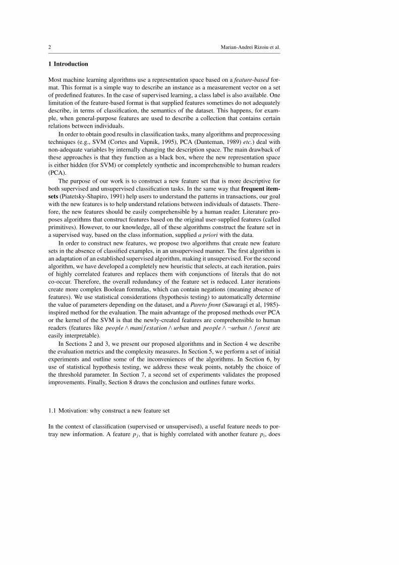
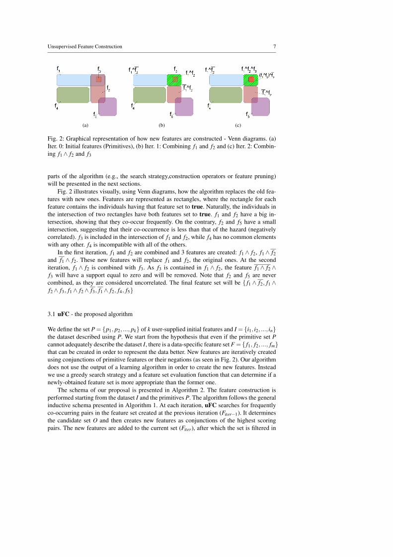
Fig. 2: Graphical representation of how new features are constructed - Venn diagrams. (a)

Iter. 0: Initial features (Primitives), (b) Iter. 1: Combining f1 and f2 and (c) Iter. 2: Combin-

ing f1∧ f2 and f3

parts of the algorithm (e.g., the search strategy,construction operators or feature pruning)

will be presented in the next sections.

Fig. 2 illustrates visually, using Venn diagrams, how the algorithm replaces the old fea-

tures with new ones. Features are represented as rectangles, where the rectangle for each

feature contains the individuals having that feature set to true. Naturally, the individuals in

the intersection of two rectangles have both features set to true. f1 and f2 have a big in-

tersection, showing that they co-occur frequently. On the contrary, f2 and f5 have a small

intersection, suggesting that their co-occurrence is less than that of the hazard (negatively

correlated). f3 is included in the intersection of f1 and f2, while f4 has no common elements

with any other. f4 is incompatible with all of the others.

In the first iteration, f1 and f2 are combined and 3 features are created: f1 ∧ f2, f1 ∧ f2

and f1 ∧ f2. These new features will replace f1 and f2, the original ones. At the second

iteration, f1 ∧ f2 is combined with f3. As f3 is contained in f1 ∧ f2, the feature f1∧ f2 ∧f3 will have a support equal to zero and will be removed. Note that f2 and f5 are never

combined, as they are considered uncorrelated. The final feature set will be { f1 ∧ f2, f1 ∧f2∧ f3, f1∧ f2∧ f3, f1∧ f2, f4, f5}

3.1 uFC - the proposed algorithm

We define the set P = {p1, p2, ..., pk} of k user-supplied initial features and I = {i1, i2, ..., in}the dataset described using P. We start from the hypothesis that even if the primitive set P

cannot adequately describe the dataset I, there is a data-specific feature set F = { f1, f2, ..., fm}that can be created in order to represent the data better. New features are iteratively created

using conjunctions of primitive features or their negations (as seen in Fig. 2). Our algorithm

does not use the output of a learning algorithm in order to create the new features. Instead

we use a greedy search strategy and a feature set evaluation function that can determine if a

newly-obtained feature set is more appropriate than the former one.

The schema of our proposal is presented in Algorithm 2. The feature construction is

performed starting from the dataset I and the primitives P. The algorithm follows the general

inductive schema presented in Algorithm 1. At each iteration, uFC searches for frequently

co-occurring pairs in the feature set created at the previous iteration (Fiter−1). It determines

the candidate set O and then creates new features as conjunctions of the highest scoring

pairs. The new features are added to the current set (Fiter), after which the set is filtered in


Algorithm 2 uFC - Unsupervised feature construction

Input: P – set of primitive user-given features

Input: I – the data expressed using P which will be used to construct features

Inner parameters: λ – correlation threshold for searching, limit iter – max no of iterations.

Output: F – set of newly-constructed features.

F0← P

iter← 0

repeat

iter← iter+1

O← search correlated pairs(Iiter,Fiter−1,λ )

Fiter ← Fiter−1

while O 6= /0 do

pair← highest scoring pair(O)

Fiter ← Fiter

⋃

construct new feat(pair)

remove candidate(O, pair)

end while

prune obsolete features(Fiter, Iiter)

Iiter+1← convert(Iiter,Fiter)

until Fiter = Fiter−1 OR iter = limit iter

F ← Fiter

order to remove obsolete features. At the end of each iteration, the dataset I is translated

to reflect the feature set Fiter. A new iteration is performed as long as new features were

generated in the current iteration and a maximum number of iterations have not yet been

reached (limit iter is a parameter for the algorithm).

3.2 Searching co-occurring pairs

The search correlated pairs function searches for frequently co-occurring pairs of features

in a feature set F . We start with an empty set O← /0 and we investigate all possible pairs

of features { fi, f j} ∈ F ×F . We use a function (r) to measure the co-occurrence of a pair

of features { fi, f j} and compare it to a threshold λ . If the value of the function is above the

threshold, then their co-occurrence is considered as significant and the pair is added to O.

Therefore, O will be

O = {{ fi, f j}|∀{ fi, f j} ∈ F×F sothat r({ fi, f j})> λ}

The r function is the empirical Pearson correlation coefficient, which is a measure of

the strength of the linear dependency between two variables. r ∈ [−1,1] and it is defined as

the covariance of the two variables divided by the product of their standard deviations. The

sign of the r function gives the direction of the correlation (inverse correlation for r < 0 and

positive correlation for r > 0), while the absolute value or the square gives the strength of

the correlation. A value of 0 implies that there is no linear correlation between the variables.

When applied to Boolean variables, having the contingency table as shown in Table 1, the r

function has the following formulation:

r({ fi, f j}) =a×d−b× c

√

(a+b)× (a+ c)× (b+d)× (c+d)

The λ threshold parameter will serve to fine-tune the number of selected pairs. Its impact

on the behaviour of the algorithm will be studied in Section 5.3. A method of automatic

choice of λ using statistical hypothesis testing is presented in Section 6.1.


Table 1: Contingency table for two Boolean features

f j ¬ f j

fi a b

¬ fi c d

3.3 Constructing and pruning features

Once O is constructed, uFC performs a greedy search. The function highest scoring pair

is iteratively used to extract from O the pair { fi, f j} that has the highest co-occurrence score.

The function construct new feat constructs three new features: fi∧ f j, fi∧ f j and fi∧f j. They represent, respectively, the intersection of the initial two features and the relative

complements of one feature in the other. The new features are guaranteed by construction

to be negatively correlated. If one of them is set to true for an individual, the other two

will surely be false. At each iteration, very simple features are constructed: conjunctions of

two literals. The creation of more complex and semantically rich features appears through

the iterative process. fi and f j can be either primitives or features constructed in previous

iterations.

After the construction of features, the remove candidate function removes from O the

pair { fi, f j}, as well as any other pair that contains fi of f j. When there are no more pairs in

O, prune obsolete features is used to remove from the feature set two types of features:

– features that are false for all individuals. These usually appear in the case of hierar-

chical relations. We consider that f1 and f2 have a hierarchical relation if all individuals

that have feature f1 true, automatically have feature f2 true (e.g., f1 “is a type of” f2 or

f1 “is a part of” f2). One of the generated features (in the example f1∧ f2) is false for all

individuals and, therefore, eliminated. In the example of water and cascade, we create

only water∧ cascade and water∧¬cascade, since there cannot exist a cascade without

water (considering that a value of false means the absence of a feature and not missing

data).

– features that participated in the creation of a new feature. Effectively, all { fi|{ fi, f j}∈O, f j ∈ F} are replaced by the newly-constructed features.

{ fi, f j| fi, f j ∈ F,{ fi, f j} ∈ O} repl.−−→ { fi∧ f j, fi∧ f j, fi∧ f j}

4 Evaluation of a feature set

To our knowledge, there are no widely accepted measures to evaluate the overall correlation

between the features of a feature set. We propose a measure inspired from the “inclusion-

exclusion” principle (Feller, 1950). In set theory, this principle permits to express the car-

dinality of the finite reunion of finite ensembles by considering the cardinality of those

ensembles and their intersections. In the Boolean form, it is used to estimate the probability

of a clause (disjunction of literals) as a function of its composing terms (conjunctions of

literals).

Given the feature set F = { f1, f2, ..., fm}, we have:

p( f1∨ f2∨ ...∨ fm) =m

∑k=1

(

(−1)k−1 ∑1≤i1<...<ik≤m

p( fi1 ∧ fi2 ∧ ...∧ fik)

)


which, by putting apart the first term, is equivalent to:

p( f1∨ f2∨ ...∨ fm) =m

∑i=1

p( fi)+m

∑k=2

(

(−1)k−1 ∑1≤i1<...<ik≤m

p( fi1 ∧ fi2 ∧ ...∧ fik)

)

Without loss of generality, we can consider that each individual has at least one feature

set to true. Otherwise, we can create an artificial feature “null” that is set to true when

all the others are false. Consequently, the left side of the equation is equal to 1. On the

right side, the second term is the probability of intersections of the features. Knowing that

1 ≤ ∑mi=1 p( fi) ≤ m, this probability of intersection has a value of zero when all features

are incompatible (no overlapping). It has a “worst case scenario” value of m− 1, when all

individuals have all the features set to true.

Based on these observations, we propose the Overlapping Index evaluation measure:

OI(F) =∑

mi=1 p( fi)−1

m−1

where OI(F) ∈ [0,1] and “better” towards zero. Hence, a feature set F1 describes a dataset

better than another feature set F2 when OI(F1)< OI(F2).

4.1 Complexity of the feature set.

Number of features Considering the case of the majority of machine learning datasets,

where the number of primitives is inferior to the number of individuals in the dataset, reduc-

ing correlations between features comes at the expense of increasing the number of features.

Consider the pair of features { fi, f j} judged correlated. Unless fi ⊇ f j or fi ⊆ f j, the algo-

rithm will replace { fi, f j} by { fi ∧ f j, fi ∧ f j, fi ∧ f j}, thus increasing the total number of

features. A feature set that contains too many features is no longer informative, nor compre-

hensible. The maximum number of features that can be constructed is mechanically limited

by the number of unique combinations of primitives in the dataset (the number of unique

individuals).

|F | ≤ unique(I)≤ |I|where F is the constructed feature set and I is the dataset.

To measure the complexity in terms of number of features, we use:

C0(F) =|F |− |P|

unique(I)−|P|

where P is the primitive feature set. C0 measures the ratio between how many extra features

are constructed and the maximum number of features that can be constructed. 0 ≤ C0 ≤ 1

and a value closer to 0 means a feature set less complex.

The average length of features At each iteration, simple conjunctions of two literals are

constructed. Complex Boolean formulas are created by combining features constructed in

previous iterations. Long and complicated expressions generate incomprehensible features,

which are more likely a random side-effect rather than a product of underlying semantics.

We define C1 as the average number of literals (a primitive or its negation) that appear

in a Boolean formula representing a new feature.

P = {pi|pi ∈ P}; L = P⋃

P


C1(F) =∑ fi∈F |{l j|l j ∈L , l j appears in fi}|

|F |where P is the primitive set and 1≤C1 < ∞.

As more iterations are performed, the feature set contains more features (C0 grows)

which are increasingly more complex (C1 grows). This suggests a correlation between the

two. What is more, since C1 can potentially double at each iteration and C0 can have at most

a linear increase, the correlation is exponential. For this reason, in the following sections we

shall use only C0 as the complexity measure.

Overfitting All algorithms that learn from data risk overfitting the solution to the learn-

ing set. There are two ways in which uFC can overfit the resulted feature set, corresponding

to the two complexity measures above: a) constructing too many features (measure C0) and

b) constructing features that are too long (measure C1). The worst overfitting of type a) is

when the algorithm constructs as many features as the maximum theoretical number (one

for each individual in the dataset). The worst overfitting of type b) appears in the same con-

ditions, where each constructed feature is a conjunction of all the primitives appearing for

the corresponding individual. The two complexity measures can be used to quantify the two

types of ovefitting. Since C0 and C1 are correlated, both types of overfitting appear simulta-

neously and can be considered as two sides of a single phenomenon.

4.2 The trade-off between two opposing criteria

C0 is a measure of how overfitted a feature set is. In order to avoid overfitting, feature set

complexity should be kept at low values, while the algorithm optimizes the co-occurrence

score of the feature set. Optimizing both the correlation score and the complexity at the same

time is not possible, as they are opposing criteria. A compromise between the two must be

achieved. This is equivalent to the optimization of two contrary criteria, which is a very

well-known problem in multi-objective optimization. To acquire a trade-off between the two

mutually contradicting objectives, we use the concept of Pareto optimality (Sawaragi et al,

1985), originally developed in economics. Given multiple feature sets, a set is considered to

be Pareto optimal if there is no other set that has both a better correlation score and a better

complexity for a given dataset. Pareto optimal feature sets will form the Pareto front. This

means that no single optimum can be constructed, but rather a class of optima, depending

on the ratio between the two criteria.

We plot the solutions in the plane defined by the complexity, as one axis, and the co-

occurrence score, as the other. Constructing the Pareto front in this plane makes a visual

evaluation of several characteristics of the uFC algorithm possible, based on the deviation

of solutions compared to the front. The distance between the different solutions and the

constructed Pareto front visually shows how stable the algorithm is. The convergence of

the algorithm can be visually evaluated by how fast (in number of performed iterations) the

algorithm transits the plane from the region of solutions with low complexity and high co-

occurrence score to solutions with high complexity and low co-occurrence. We can visually

evaluate overfitting, which corresponds to the region of the plane with high complexity and

low co-occurence score. Solutions found in this region are overfitted.

In order to avoid overfitting, we propose the “closest-point” heuristic for finding a com-

promise between OI and C0. We consider the two criteria to have equal importance. We con-

sider as a good compromise, the solution in which the gain in co-occurrence score and the

loss in complexity are fairly equal. If one of the indicators has a value considerably larger

than the other, the solution is considered to be unsuitable. Such solutions would have either


(a) (b) (c)

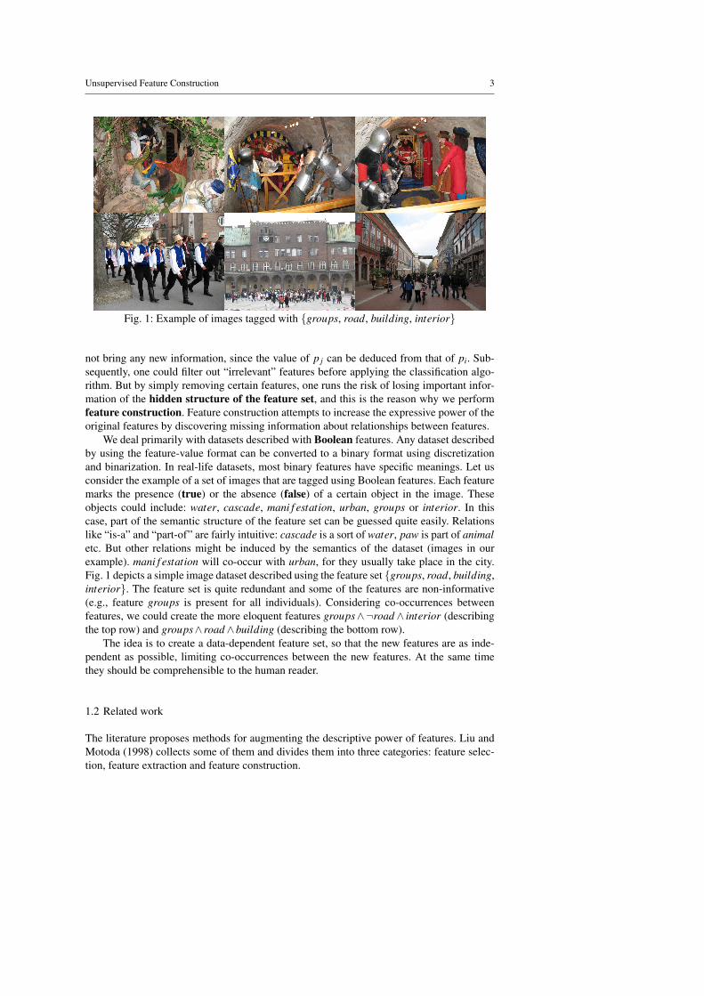
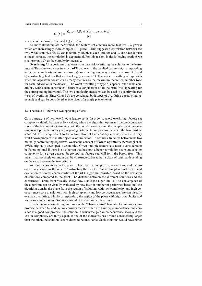
Fig. 3: Images related to the newly-constructed feature sky ∧ building ∧ panorama on

hungarian: (a) Hungarian puszta, (b)(c) Hungarian Matra mountains

a high correlation between features or a high complexity. Therefore, we perform a battery

of tests and we search a posteriori the Pareto front for solutions for which the two indica-

tors have essentially equal values. In the space of solutions, this translates into a minimal

Euclidian distance between the solution and the ideal point (the point (0;0)).

5 Initial Experiments

Throughout the experiments, uFC was executed by varying only the two parameters: λ and

limititer. We denote an execution with specific values for parameters as uFC(λ , limititer),whereas the execution where the parameters were determined a posteriori using the “closest-

point” strategy will be noted uFC*(λ , limititer). For uFRINGE, the maximum number of

features was set at 300. We perform a comparative evaluation of the two algorithms seen

from a qualitative and quantitative point of view, together with examples of typical execu-

tions. Finally, we study the impact of the two parameters of uFC.

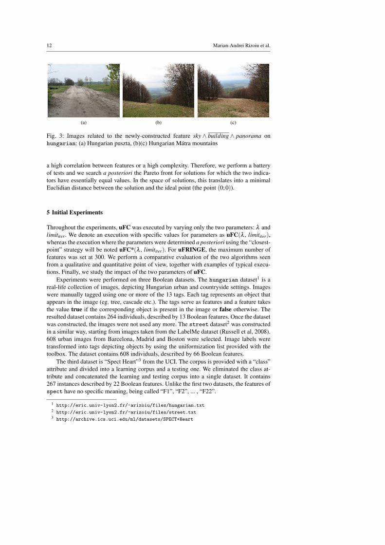
Experiments were performed on three Boolean datasets. The hungarian dataset1 is a

real-life collection of images, depicting Hungarian urban and countryside settings. Images

were manually tagged using one or more of the 13 tags. Each tag represents an object that

appears in the image (eg. tree, cascade etc.). The tags serve as features and a feature takes

the value true if the corresponding object is present in the image or false otherwise. The

resulted dataset contains 264 individuals, described by 13 Boolean features. Once the dataset

was constructed, the images were not used any more. The street dataset2 was constructed

in a similar way, starting from images taken from the LabelMe dataset (Russell et al, 2008).

608 urban images from Barcelona, Madrid and Boston were selected. Image labels were

transformed into tags depicting objects by using the uniformization list provided with the

toolbox. The dataset contains 608 individuals, described by 66 Boolean features.

The third dataset is “Spect Heart”3 from the UCI. The corpus is provided with a “class”

attribute and divided into a learning corpus and a testing one. We eliminated the class at-

tribute and concatenated the learning and testing corpus into a single dataset. It contains

267 instances described by 22 Boolean features. Unlike the first two datasets, the features of

spect have no specific meaning, being called “F1”, “F2”, ... , “F22”.

1 http://eric.univ-lyon2.fr/~arizoiu/files/hungarian.txt2 http://eric.univ-lyon2.fr/~arizoiu/files/street.txt3 http://archive.ics.uci.edu/ml/datasets/SPECT+Heart

http://eric.univ-lyon2.fr/~arizoiu/files/hungarian.txt

http://eric.univ-lyon2.fr/~arizoiu/files/street.txt

http://archive.ics.uci.edu/ml/datasets/SPECT+Heart


(a) (b) (c)

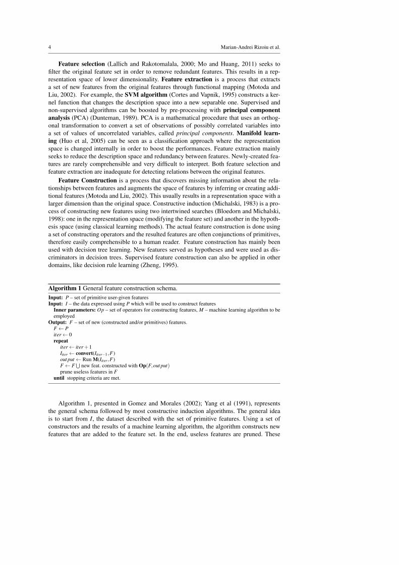
Fig. 4: Images related to the newly-constructed feature water∧ cascade∧ tree∧ f orest on

hungarian

(a) (b) (c)

Fig. 5: Images related to the newly-constructed feature headlight∧windshield∧arm∧head

on street

5.1 uFC and uFRINGE: Qualitative evaluation

For the human reader, it is quite obvious why water and cascade have the tendency to ap-

pear together or why road and interior have the tendency to appear separately. One would

expect, that based on a given dataset, the algorithms would succeed in making these associ-

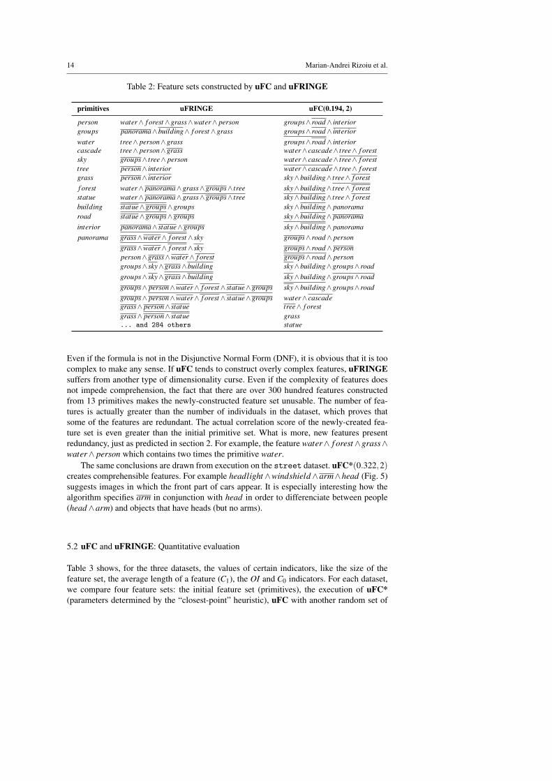
ations and catching the underlying semantics. Table 2 shows the features constructed with

uFRINGE and uFC*(0.194,2) on hungarian. A quick overview shows that constructed

features manage to make associations that seem “logical” to a human reader. For example,

one would expect the feature sky∧building∧ panorama to denote images where there is a

panoramic view and the sky, but no buildings, therefore suggesting images outside the city.

Fig. 3 supports this expectation. Similarly, the feature sky∧ building∧ groups∧ road cov-

ers urban images, where groups of people are present and water∧ cascade∧ tree∧ f orest

denotes a cascade in the forest (Fig. 4).

Comprehension quickly deteriorates when the constructed feature set is overfitted, when

the constructed features are too complex. The execution of uFC(0.184,5) reveals features

like:

sky∧building∧ tree∧building∧ f orest ∧ sky∧building∧groups∧ road∧sky∧building∧ panorama∧groups∧ road∧ person∧ sky∧groups∧ road


Table 2: Feature sets constructed by uFC and uFRINGE

primitives uFRINGE uFC(0.194, 2)

person water∧ f orest ∧grass∧water∧ person groups∧ road∧ interior

groups panorama∧building∧ f orest ∧grass groups∧ road∧ interior

water tree∧ person∧grass groups∧ road∧ interior

cascade tree∧ person∧grass water∧ cascade∧ tree∧ f orest

sky groups∧ tree∧ person water∧ cascade∧ tree∧ f orest

tree person∧ interior water∧ cascade∧ tree∧ f orest

grass person∧ interior sky∧building∧ tree∧ f orest

f orest water∧ panorama∧grass∧groups∧ tree sky∧building∧ tree∧ f orest

statue water∧ panorama∧grass∧groups∧ tree sky∧building∧ tree∧ f orest

building statue∧groups∧groups sky∧building∧ panorama

road statue∧groups∧groups sky∧building∧ panorama

interior panorama∧ statue∧groups sky∧building∧ panorama

panorama grass∧water∧ f orest ∧ sky groups∧ road∧ person

grass∧water∧ f orest ∧ sky groups∧ road∧ person

person∧grass∧water∧ f orest groups∧ road∧ person

groups∧ sky∧grass∧building sky∧building∧groups∧ road

groups∧ sky∧grass∧building sky∧building∧groups∧ road

groups∧ person∧water∧ f orest ∧ statue∧groups sky∧building∧groups∧ road

groups∧ person∧water∧ f orest ∧ statue∧groups water∧ cascade

grass∧ person∧ statue tree∧ f orest

grass∧ person∧ statue grass

... and 284 others statue

Even if the formula is not in the Disjunctive Normal Form (DNF), it is obvious that it is too

complex to make any sense. If uFC tends to construct overly complex features, uFRINGE

suffers from another type of dimensionality curse. Even if the complexity of features does

not impede comprehension, the fact that there are over 300 hundred features constructed

from 13 primitives makes the newly-constructed feature set unusable. The number of fea-

tures is actually greater than the number of individuals in the dataset, which proves that

some of the features are redundant. The actual correlation score of the newly-created fea-

ture set is even greater than the initial primitive set. What is more, new features present

redundancy, just as predicted in section 2. For example, the feature water∧ f orest∧grass∧water∧ person which contains two times the primitive water.

The same conclusions are drawn from execution on the street dataset. uFC*(0.322,2)creates comprehensible features. For example headlight∧windshield∧arm∧head (Fig. 5)

suggests images in which the front part of cars appear. It is especially interesting how the

algorithm specifies arm in conjunction with head in order to differenciate between people

(head∧arm) and objects that have heads (but no arms).

5.2 uFC and uFRINGE: Quantitative evaluation

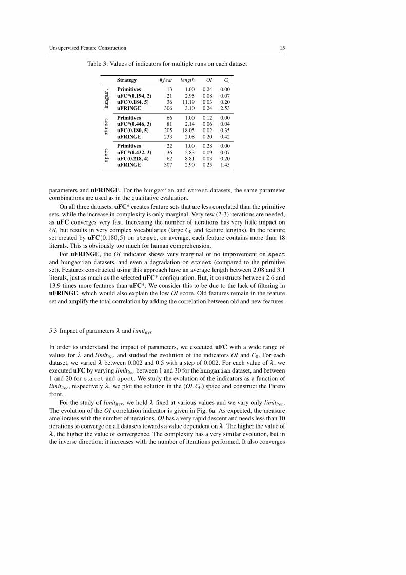
Table 3 shows, for the three datasets, the values of certain indicators, like the size of the

feature set, the average length of a feature (C1), the OI and C0 indicators. For each dataset,

we compare four feature sets: the initial feature set (primitives), the execution of uFC*

(parameters determined by the “closest-point” heuristic), uFC with another random set of


Table 3: Values of indicators for multiple runs on each dataset

Strategy # f eat length OI C0

hungar. Primitives 13 1.00 0.24 0.00

uFC*(0.194, 2) 21 2.95 0.08 0.07

uFC(0.184, 5) 36 11.19 0.03 0.20

uFRINGE 306 3.10 0.24 2.53street Primitives 66 1.00 0.12 0.00

uFC*(0.446, 3) 81 2.14 0.06 0.04

uFC(0.180, 5) 205 18.05 0.02 0.35

uFRINGE 233 2.08 0.20 0.42

spect

Primitives 22 1.00 0.28 0.00

uFC*(0.432, 3) 36 2.83 0.09 0.07

uFC(0.218, 4) 62 8.81 0.03 0.20

uFRINGE 307 2.90 0.25 1.45

parameters and uFRINGE. For the hungarian and street datasets, the same parameter

combinations are used as in the qualitative evaluation.

On all three datasets, uFC* creates feature sets that are less correlated than the primitive

sets, while the increase in complexity is only marginal. Very few (2-3) iterations are needed,

as uFC converges very fast. Increasing the number of iterations has very little impact on

OI, but results in very complex vocabularies (large C0 and feature lengths). In the feature

set created by uFC(0.180,5) on street, on average, each feature contains more than 18

literals. This is obviously too much for human comprehension.

For uFRINGE, the OI indicator shows very marginal or no improvement on spect

and hungarian datasets, and even a degradation on street (compared to the primitive

set). Features constructed using this approach have an average length between 2.08 and 3.1

literals, just as much as the selected uFC* configuration. But, it constructs between 2.6 and

13.9 times more features than uFC*. We consider this to be due to the lack of filtering in

uFRINGE, which would also explain the low OI score. Old features remain in the feature

set and amplify the total correlation by adding the correlation between old and new features.

5.3 Impact of parameters λ and limititer

In order to understand the impact of parameters, we executed uFC with a wide range of

values for λ and limititer and studied the evolution of the indicators OI and C0. For each

dataset, we varied λ between 0.002 and 0.5 with a step of 0.002. For each value of λ , we

executed uFC by varying limititer between 1 and 30 for the hungarian dataset, and between

1 and 20 for street and spect. We study the evolution of the indicators as a function of

limititer, respectively λ , we plot the solution in the (OI,C0) space and construct the Pareto

front.

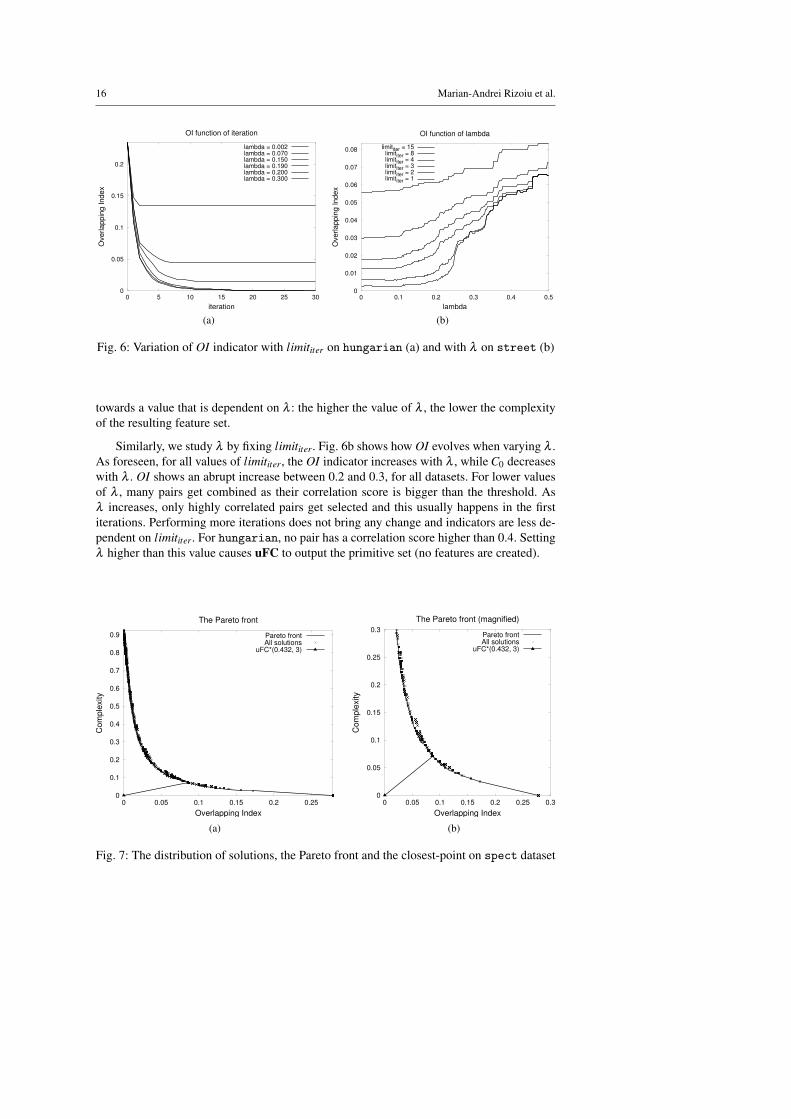
For the study of limititer, we hold λ fixed at various values and we vary only limititer.

The evolution of the OI correlation indicator is given in Fig. 6a. As expected, the measure

ameliorates with the number of iterations. OI has a very rapid descent and needs less than 10

iterations to converge on all datasets towards a value dependent on λ . The higher the value of

λ , the higher the value of convergence. The complexity has a very similar evolution, but in

the inverse direction: it increases with the number of iterations performed. It also converges


0

0.05

0.1

0.15

0.2

0 5 10 15 20 25 30

Ove

rla

pp

ing

In

de

x

iteration

OI function of iteration

lambda = 0.002lambda = 0.070lambda = 0.150lambda = 0.190lambda = 0.200lambda = 0.300

(a)

0

0.01

0.02

0.03

0.04

0.05

0.06

0.07

0.08

0 0.1 0.2 0.3 0.4 0.5

Ove

rla

pp

ing

In

de

x

lambda

OI function of lambda

limititer = 15limititer = 8limititer = 4limititer = 3limititer = 2limititer = 1

(b)

Fig. 6: Variation of OI indicator with limititer on hungarian (a) and with λ on street (b)

towards a value that is dependent on λ : the higher the value of λ , the lower the complexity

of the resulting feature set.

Similarly, we study λ by fixing limititer. Fig. 6b shows how OI evolves when varying λ .

As foreseen, for all values of limititer, the OI indicator increases with λ , while C0 decreases

with λ . OI shows an abrupt increase between 0.2 and 0.3, for all datasets. For lower values

of λ , many pairs get combined as their correlation score is bigger than the threshold. As

λ increases, only highly correlated pairs get selected and this usually happens in the first

iterations. Performing more iterations does not bring any change and indicators are less de-

pendent on limititer. For hungarian, no pair has a correlation score higher than 0.4. Setting

λ higher than this value causes uFC to output the primitive set (no features are created).

0

0.1

0.2

0.3

0.4

0.5

0.6

0.7

0.8

0.9

0 0.05 0.1 0.15 0.2 0.25

Co

mp

lexity

Overlapping Index

The Pareto front

Pareto frontAll solutions

uFC*(0.432, 3)

(a)

0

0.05

0.1

0.15

0.2

0.25

0.3

0 0.05 0.1 0.15 0.2 0.25 0.3

Co

mp

lexity

Overlapping Index

The Pareto front (magnified)

Pareto frontAll solutions

uFC*(0.432, 3)

(b)

Fig. 7: The distribution of solutions, the Pareto front and the closest-point on spect dataset


To study Pareto optimality, we plot the generated solutions in the (OI, C0) space. Fig. 7a

presents the distribution of solutions, the Pareto front and the solution chosen by the “closest-

point” heuristic. The solutions generated by uFC with a wide range of parameter values are

not dispersed in the solution space, but their distribution is rather close together. This shows

good algorithm stability. Even if not all the solutions are Pareto optimal, none of them are

too distant from the front and there are no outliers.

Most of the solutions densely populate the part of the curve corresponding to low OI and

high C0. As pointed out in the Section 4.2, the area of the front corresponding to high feature

set complexity (high C0) represents the overfitting area. This confirms that the algorithm

converges fast, then enters overfitting. Most of the improvement in quality is done in the

first 2-3 iterations, while further iterating improves quality only marginally with the cost

of an explosion of complexity. The “closest-point” heuristic keeps the constructing out of

overfitting, by stopping the algorithm at the point where the gain of co-occurence score and

the loss in complexity are fairly equal. Fig. 7b magnifies the region of the solution space

corresponding for low numbers of iterations.

5.4 Relation between number of features and feature length

Both the average length of a feature (C1) and the number of features (C0) increase with

the number of iterations. In Section 4.1 we have speculated that the two are correlated:

C1 = f (C0). For each λ in the batch of tests, we create the C0 and C1 series depending on the

limititer and we perform a statistical hypothesis test, using the Kendall rank coefficient as the

test statistic. The Kendall rank coefficient is particularly useful as it makes no assumptions

about the distributions of C0 and C1. For all values of λ , for all datasets, the statistical test

revealed a p-value of the order of 10−9. This is consistently lower than habitually used

significance levels and makes us reject the null independence hypothesis and conclude that

C0 and C1 are statistically dependent.

6 Improving the uFC algorithm

The major difficulty of uFC, shown by the initial experiments, is setting the values of pa-

rameters. An unfortunate choice would result in either an overly complex feature set or a

feature set where features are still correlated. But both parameters λ and limititer are depen-

dent on the dataset and finding the suitable values would prove to be a process of trial and

error for each new corpus. The “closest-point” heuristic achieves acceptable equilibrium be-

tween complexity and performance, but requires multiple executions with large choices of

values for parameters and the construction of the Pareto front, which might not always be

desirable or even possible.

We propose a new method for choosing λ based on statistical hypothesis testing and a

new stopping criterion inspired from the “closest-point” heuristic. These will be integrated

into a new “risk-based” heuristic that approximates the best solution while avoiding the time

consuming construction of multiple solutions and the Pareto front. The only parameter is the

significance level α , which is independent of the dataset, and makes the task of running uFC

on new, unseen datasets easy. A pruning technique is also proposed.


6.1 Automatic choice of λ

We propose replacing the user-supplied co-occurrence threshold λ with a technique that

selects only pairs of features for whom the positive linear correlation is statistically signif-

icant. These pairs are added to the set O of co-occurring pairs (defined in Section 3.2) and,

starting from O, new features are constructed. We use a statistical method: the hypothesis

testing. For each pair of candidate features, we test the independence hypothesis H0 against

the positive correlation hypothesis H1.

We use as a test statistic the Pearson correlation coefficient (calculated as defined in

Section 3.2) and test the following formally defined hypothesis: H0 : ρ = 0 and H1 : ρ > 0,

where ρ is the theoretical correlation coefficient between two candidate features. We can

show that in the case of Boolean variables, having the contingency table shown in Table 1,

the observed value of the χ2 of independence is χ2obs = nr2 (n is the size of the dataset).

Consequently, considering true the hypothesis H0, nr2 is approximately following a χ2 dis-

tribution with one degree of freedom (nr2 ∼ χ21 ), resulting in r

√n following a standard

normal distribution (r√

n∼ N(0,1)), given that n is large enough.

We reject the H0 hypothesis in favour of H1 if and only if r√

n ≥ u1−α , where u1−α is

the right critical value for the standard normal distribution. Two features will be considered

significantly correlated when r({ fi, f j}) ≥ u1−α√n

. The significance level α represents the

risk of rejecting the independence hypothesis when it was in fact true. It can be interpreted

as the false discovery risk in data mining. In the context of feature construction it is the

false construction risk, since this is the risk of constructing new features based on a pair of

features that are not really correlated. Statistical literature usually sets α at 0.05 or 0.01, but

levels of 0.001 or even 0.0001 are often used.

The proposed method repeats the independence test a great number of times, which in-

flates the number of type I errors. Ge et al (2003) presents several methods for controlling

the false discoveries. Setting aside the Bonferroni correction, often considered too simplis-

tic and too drastic, one has the option of using sequential rejection methods (Benjamini

and Liu, 1999; Holm, 1979), the q-value method of Storey (Storey, 2002) or making use

of bootstrap (Lallich et al, 2006). In our case, applying these methods is not clear-cut, as

tests performed at each iteration depend on the results of the tests performed at previous

iterations. It is noteworthy that a trade-off must be acquired between the inflation of false

discoveries and the inflation of missed discoveries. This makes us choose a risk between 5%

and 5%m

, where m is the theoretical number of tests to be performed.

6.2 Candidate pruning technique. Stopping criterion.

Pruning In order to apply the χ2 independence test, it is necessary that the expected frequen-

cies considering true the H0 hypothesis be greater or equal than 5. We add this constraint

to the new feature search strategy (subsection 3.2). Pairs for whom the values of(a+b)(a+c)

n,

(a+b)(b+c)n

,(a+c)(c+d)

nand

(b+d)(c+d)n

are not greater than 5, will be filtered from the set of

candidate pairs O. This will impede the algorithm from constructing features that are present

for very few individuals in the dataset.

Risk-based heuristic We introduced in Section 4.2 the “closest-point” for choosing the

values for parameters λ and limititer. It searches the solution on the Pareto front for which

the indicators are sensibly equal. We transform the heuristic into a stopping criterion: OI and

C0 are combined into a single formula, the root mean square (RMS). The algorithm will


0

0.1

0.2

0.3

0.4

0.5

0.6

0 5 10 15 20

Root

Square

Mean

iteration

RMS function of iteration

lambda = 0.002lambda = 0.200lambda = 0.240lambda = 0.300lambda = 0.400lambda = 0.500

Fig. 8: RMS vs. limititer on spect

stop iterating when RMS has reached a minimum. Using the generalized mean inequality,

we can prove that RMS(OI,C0) has only one global minimum, as with each iteration the

complexity increases and OI descends.

The limititer parameter, which is data-dependent, is replaced by the automatic RMS stop-

ping criterion. This stopping criterion together with the automatic λ choice strategy, pre-

sented in Section 6.1, form a data-independent heuristic for choosing parameters. We will

call the new heuristic risk-based heuristic. This new heuristic will make it possible to ap-

proximate the best parameter compromise and avoid the time consuming task of computing

a batch of solutions and constructing the Pareto front.

7 Further Experiments

We test the proposed ameliorations, similarly to what was shown in Section 5, on the same

three datasets: hungarian, spect and street. We execute uFC in two ways: the classical

uFC (Section 3) and the improved uFC (Section 6). The classical uFC needs to have param-

eters λ and limititer set (noted uFC(λ , limititer)). uFC*(λ , limititer) denotes the execution

with parameters which were determined a posteriori using the “closest-point” heuristic. The

improved uFC will be denoted as uFCα (risk). The “risk-based” heuristic will be used to de-

termine the parameters and control the execution.

7.1 Risk-based heuristic for choosing parameters

Root Mean Square In the first batch of experiments, we study the variation of the Root

Means Square aggregation function for a series of selected values of λ . We vary limititer

between 0 and 30, for hungarian, and between 0 and 20 for spect and street. The

evolution of RMS is presented in Fig. 8.

For all λ the RMS starts by decreasing, as OI descends more rapidly than the C0 in-

creases. In just 1-3 iterations, RMS reaches its minimum and afterwards its value starts to

increase. This is due to the fact that complexity increases rapidly, with only marginal im-

provement of quality. This behaviour is consistent with the results presented in Section 5. As


0

0.05

0.1

0.15

0.2

0.25

0 0.05 0.1 0.15 0.2 0.25

Com

ple

xity

Overlapping Index

Risk-based and closest-point (magnified)

Pareto frontuFC*(0.194, 2)

uFCalpha(0.001): (0.190,2)uFCalpha for multiple risks

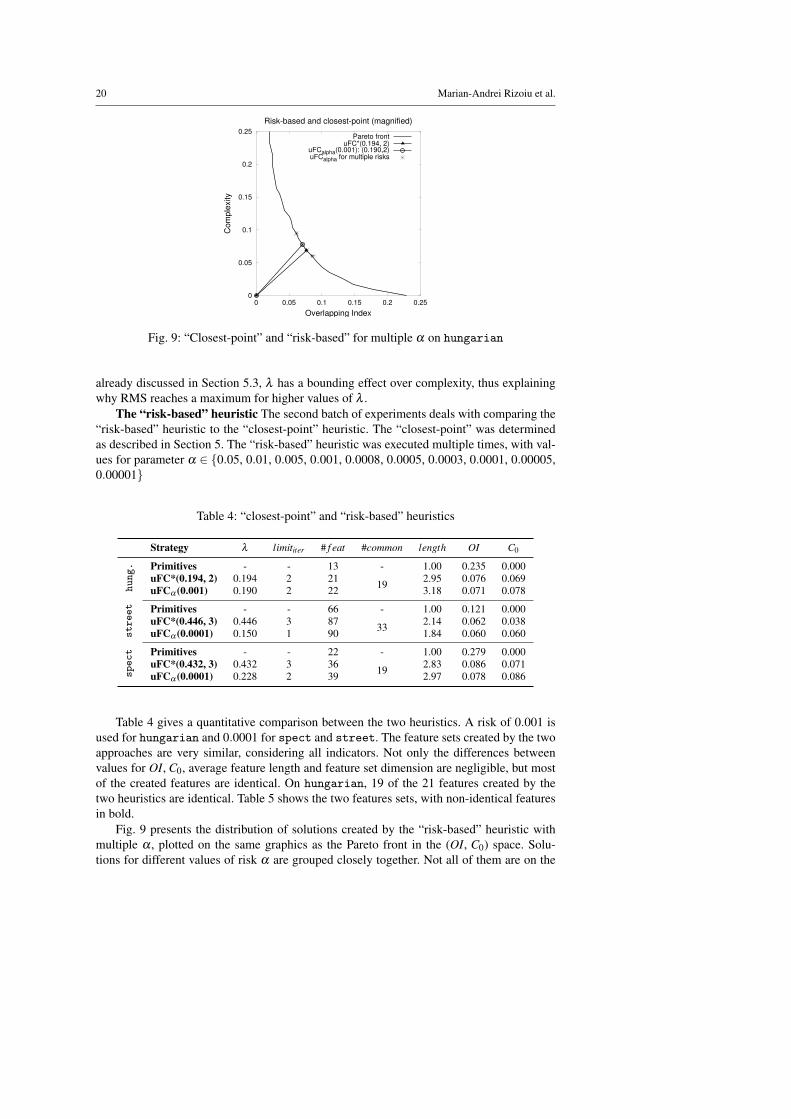
Fig. 9: “Closest-point” and “risk-based” for multiple α on hungarian

already discussed in Section 5.3, λ has a bounding effect over complexity, thus explaining

why RMS reaches a maximum for higher values of λ .

The “risk-based” heuristic The second batch of experiments deals with comparing the

“risk-based” heuristic to the “closest-point” heuristic. The “closest-point” was determined

as described in Section 5. The “risk-based” heuristic was executed multiple times, with val-

ues for parameter α ∈ {0.05, 0.01, 0.005, 0.001, 0.0008, 0.0005, 0.0003, 0.0001, 0.00005,

0.00001}

Table 4: “closest-point” and “risk-based” heuristics

Strategy λ limititer # f eat #common length OI C0

hung. Primitives - - 13 - 1.00 0.235 0.000

uFC*(0.194, 2) 0.194 2 2119

2.95 0.076 0.069

uFCα (0.001) 0.190 2 22 3.18 0.071 0.078

street Primitives - - 66 - 1.00 0.121 0.000

uFC*(0.446, 3) 0.446 3 8733

2.14 0.062 0.038

uFCα (0.0001) 0.150 1 90 1.84 0.060 0.060

spect Primitives - - 22 - 1.00 0.279 0.000

uFC*(0.432, 3) 0.432 3 3619

2.83 0.086 0.071

uFCα (0.0001) 0.228 2 39 2.97 0.078 0.086

Table 4 gives a quantitative comparison between the two heuristics. A risk of 0.001 is

used for hungarian and 0.0001 for spect and street. The feature sets created by the two

approaches are very similar, considering all indicators. Not only the differences between

values for OI, C0, average feature length and feature set dimension are negligible, but most

of the created features are identical. On hungarian, 19 of the 21 features created by the

two heuristics are identical. Table 5 shows the two features sets, with non-identical features

in bold.

Fig. 9 presents the distribution of solutions created by the “risk-based” heuristic with

multiple α , plotted on the same graphics as the Pareto front in the (OI, C0) space. Solu-

tions for different values of risk α are grouped closely together. Not all of them are on the


Table 5: Feature sets constructed by “closest-point” and “risk-based” heuristics on

hungarian

primitives uFC*(0.194, 2) uFCα (0.001)

person groups∧ road∧ interior groups∧ road∧ interior

groups groups∧ road∧ interior groups∧ road∧ interior

water groups∧ road∧ interior groups∧ road∧ interior

cascade water∧ cascade∧ tree∧ f orest water∧ cascade∧ tree∧ f orest

sky water∧ cascade∧ tree∧ f orest water∧ cascade∧ tree∧ f orest

tree water∧ cascade∧ tree∧ f orest water∧ cascade∧ tree∧ f orest

grass sky∧building∧ tree∧ f orest sky∧building∧ tree∧ f orest

f orest sky∧building∧ tree∧ f orest sky∧building∧ tree∧ f orest

statue sky∧building∧ tree∧ f orest sky∧building∧ tree∧ f orest

building sky∧building∧ panorama sky∧building∧ panorama

road sky∧building∧ panorama sky∧building∧ panorama

interior sky∧building∧ panorama sky∧building∧ panorama

panorama groups∧ road∧ person groups∧ road∧ person

groups∧ road∧ person groups∧ road∧ person

groups∧ road∧ person groups∧ road∧ person

water∧ cascade sky∧building∧groups∧ road

sky∧building sky∧building∧groups∧ road

tree∧ f orest sky∧building∧groups∧ road

groups∧ road water∧ cascade

grass tree∧ f orest

statue grass

statue

Pareto front, but they are never too far from the “closest-point” solution, providing a good

equilibrium between quality and complexity.

0

0.02

0.04

0.06

0.08

0.1

0.12

0.14

0 0.02 0.04 0.06 0.08 0.1 0.12 0.14

Co

mp

lexity

Overlapping Index




(a)

0

0.02

0.04

0.06

0.08

0.1

0.12

0.14

0 0.02 0.04 0.06 0.08 0.1 0.12 0.14

Co

mp

lexity

Overlapping Index




(b)

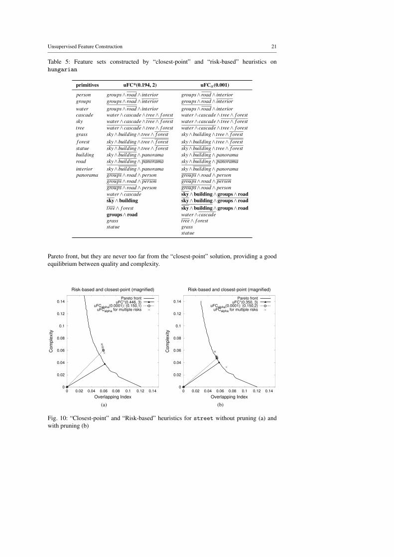
Fig. 10: “Closest-point” and “Risk-based” heuristics for street without pruning (a) and

with pruning (b)


On street, performances of the “risk-based” heuristic start to degrade compared to

uFC*. Table 4 shows differences in the resulted complexity and only 33% of the constructed

features are common for the two approaches. Fig. 10a shows that solutions found by the

“risk-based” approach are moving away from the “closest-point”. The cause is the large

size of the street dataset. As the sample size increases, the null hypothesis tends to be

rejected at lower levels of p-value. The auto-determined λ threshold is set too low and the

constructed feature sets are too complex. Pruning solves this problem as shown in Fig. 10b

and Section 7.2.

7.2 Pruning the candidates

The pruning technique is independent of the “risk-based” heuristic and can be applied in

conjunction with the classical uFC algorithm. An execution of this type will be denoted

uFCP(λ ,maxiter). We execute uFCP(λ ,maxiter) with the same parameters and on the same

datasets as described in Section 5.3.

0

0.1

0.2

0.3

0.4

0.5

0.6

0.7

0.8

0.9

0 0.05 0.1 0.15 0.2

Co

mp

lexity

Overlapping Index

Pruned and Non-pruned Pareto Fronts

Pareto front prunedPareto front non-pruned

(a)

0.05

0.06

0.07

0.08

0.09

0.1

0.11

0.12

0.13

0.14

0.15

0.03 0.04 0.05 0.06 0.07 0.08 0.09 0.1

Com

ple

xity

Overlapping Index

Pruned and Non-pruned Pareto Fronts (zoomed)

Pareto front prunedPareto front non-pruned

(b)

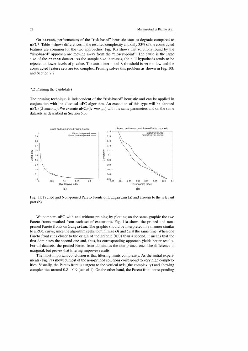
Fig. 11: Pruned and Non-pruned Pareto Fronts on hungarian (a) and a zoom to the relevant

part (b)

We compare uFC with and without pruning by plotting on the same graphic the two

Pareto fronts resulted from each set of executions. Fig. 11a shows the pruned and non-

pruned Pareto fronts on hungarian. The graphic should be interpreted in a manner similar

to a ROC curve, since the algorithm seeks to minimize OI and C0 at the same time. When one

Pareto front runs closer to the origin of the graphic (0,0) than a second, it means that the

first dominates the second one and, thus, its corresponding approach yields better results.

For all datasets, the pruned Pareto front dominates the non-pruned one. The difference is

marginal, but proves that filtering improves results.

The most important conclusion is that filtering limits complexity. As the initial experi-

ments (Fig. 7a) showed, most of the non-pruned solutions correspond to very high complex-

ities. Visually, the Pareto front is tangent to the vertical axis (the complexity) and showing

complexities around 0.8−0.9 (out of 1). On the other hand, the Pareto front corresponding


to the pruned approach stops, for all datasets, for complexities lower than 0.15. This proves

that filtering successfully discards solutions that are too complex to be interpretable.

Last, but not least, filtering corrects the problem of automatically choosing λ for the

“risk-based” heuristic on big datasets. We ran uFCP with risk α ∈ {0.05, 0.01, 0.005, 0.001,

0.0008, 0.0005, 0.0003, 0.0001, 0.00005, 0.00001}. Fig. 10b presents the distributions of

solutions found with the “risk-based pruned” heuristic on street. Unlike results without

pruning (Fig. 10a), solutions generated with pruning are distributed closely to those gener-

ated by “closest-point” and to the Pareto front.

7.3 Algorithm stability

In order to evaluate the stability of the uFCα algorithm, we introduce noise in the hungarian

dataset. The percentage of noise varied between 0% (no noise) and 30%. Introducing a cer-

tain percentage x% of noise means that x%× k× n random features in the datasets are in-

verted (false becomes true and true becomes false). k is the number of primitives and n is

the number of individuals. For each given noise percentage, 10 noised datasets are created

and only the averages are presented. uFCα is executed for all the noised datasets, with the

same combination of parameters (risk = 0.001 and no filtering).

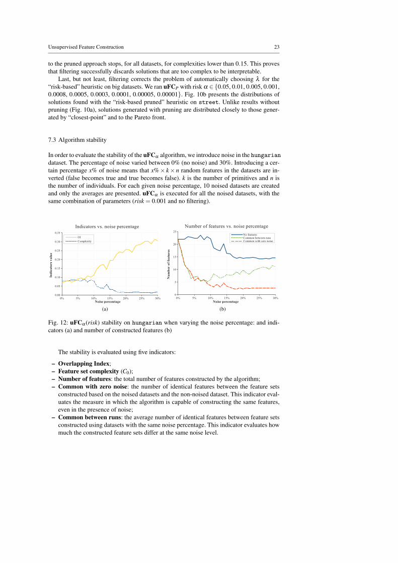
(a) (b)

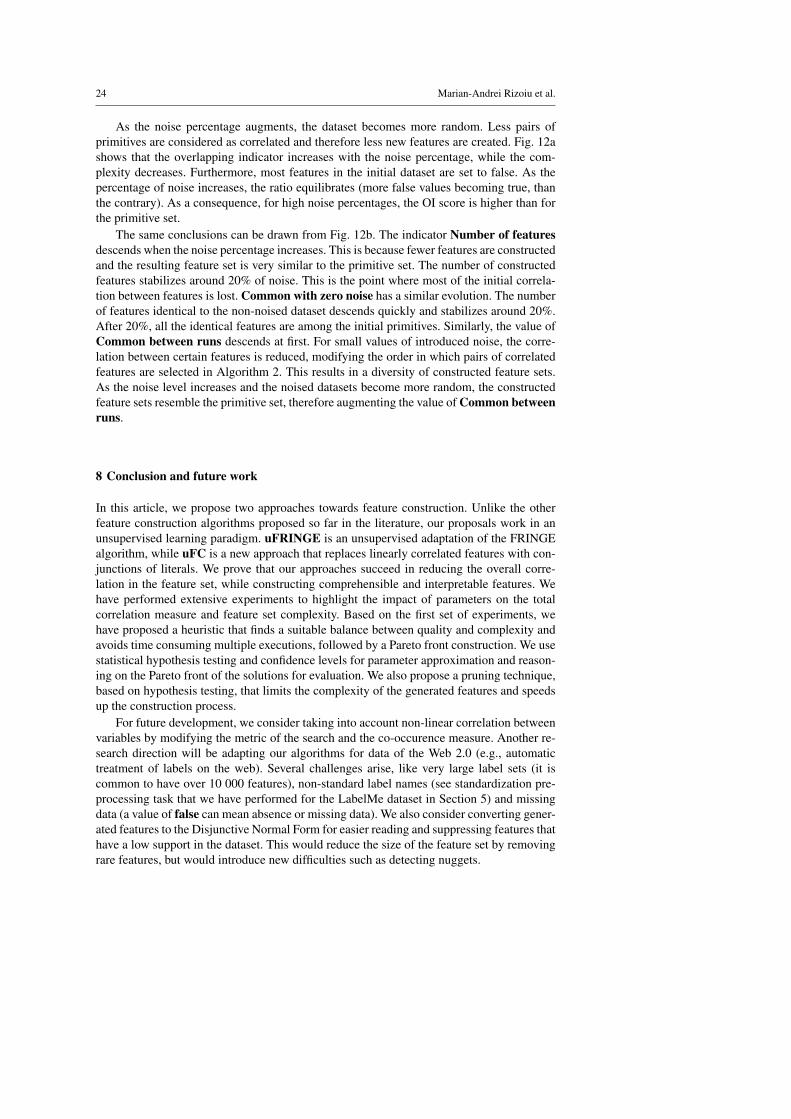
Fig. 12: uFCα (risk) stability on hungarian when varying the noise percentage: and indi-

cators (a) and number of constructed features (b)

The stability is evaluated using five indicators:

– Overlapping Index;

– Feature set complexity (C0);

– Number of features: the total number of features constructed by the algorithm;

– Common with zero noise: the number of identical features between the feature sets

constructed based on the noised datasets and the non-noised dataset. This indicator eval-

uates the measure in which the algorithm is capable of constructing the same features,

even in the presence of noise;

– Common between runs: the average number of identical features between feature sets

constructed using datasets with the same noise percentage. This indicator evaluates how

much the constructed feature sets differ at the same noise level.


As the noise percentage augments, the dataset becomes more random. Less pairs of

primitives are considered as correlated and therefore less new features are created. Fig. 12a

shows that the overlapping indicator increases with the noise percentage, while the com-

plexity decreases. Furthermore, most features in the initial dataset are set to false. As the

percentage of noise increases, the ratio equilibrates (more false values becoming true, than

the contrary). As a consequence, for high noise percentages, the OI score is higher than for

the primitive set.

The same conclusions can be drawn from Fig. 12b. The indicator Number of features

descends when the noise percentage increases. This is because fewer features are constructed

and the resulting feature set is very similar to the primitive set. The number of constructed

features stabilizes around 20% of noise. This is the point where most of the initial correla-

tion between features is lost. Common with zero noise has a similar evolution. The number

of features identical to the non-noised dataset descends quickly and stabilizes around 20%.

After 20%, all the identical features are among the initial primitives. Similarly, the value of

Common between runs descends at first. For small values of introduced noise, the corre-

lation between certain features is reduced, modifying the order in which pairs of correlated

features are selected in Algorithm 2. This results in a diversity of constructed feature sets.

As the noise level increases and the noised datasets become more random, the constructed

feature sets resemble the primitive set, therefore augmenting the value of Common between

runs.

8 Conclusion and future work

In this article, we propose two approaches towards feature construction. Unlike the other

feature construction algorithms proposed so far in the literature, our proposals work in an

unsupervised learning paradigm. uFRINGE is an unsupervised adaptation of the FRINGE

algorithm, while uFC is a new approach that replaces linearly correlated features with con-

junctions of literals. We prove that our approaches succeed in reducing the overall corre-

lation in the feature set, while constructing comprehensible and interpretable features. We

have performed extensive experiments to highlight the impact of parameters on the total

correlation measure and feature set complexity. Based on the first set of experiments, we

have proposed a heuristic that finds a suitable balance between quality and complexity and

avoids time consuming multiple executions, followed by a Pareto front construction. We use

statistical hypothesis testing and confidence levels for parameter approximation and reason-

ing on the Pareto front of the solutions for evaluation. We also propose a pruning technique,

based on hypothesis testing, that limits the complexity of the generated features and speeds

up the construction process.

For future development, we consider taking into account non-linear correlation between

variables by modifying the metric of the search and the co-occurence measure. Another re-

search direction will be adapting our algorithms for data of the Web 2.0 (e.g., automatic

treatment of labels on the web). Several challenges arise, like very large label sets (it is

common to have over 10 000 features), non-standard label names (see standardization pre-

processing task that we have performed for the LabelMe dataset in Section 5) and missing

data (a value of false can mean absence or missing data). We also consider converting gener-

ated features to the Disjunctive Normal Form for easier reading and suppressing features that

have a low support in the dataset. This would reduce the size of the feature set by removing

rare features, but would introduce new difficulties such as detecting nuggets.


References

Benjamini Y, Liu W (1999) A step-down multiple hypotheses testing procedure that controls

the false discovery rate under independence. Journal of Statistical Planning and Inference

82(1-2):163–170

Blockeel H, De Raedt L, Ramon J (1998) Top-down induction of clustering trees. In: Pro-

ceedings of the 15th International Conference on Machine Learning, pp 55–63

Bloedorn E, Michalski RS (1998) Data-driven constructive induction. Intelligent Systems

and their Applications 13(2):30–37

Cortes C, Vapnik V (1995) Support-vector networks. Machine learning 20(3):273–297

Dunteman GH (1989) Principal components analysis, vol 69. SAGE publications, Inc

Feller W (1950) An introduction to probability theory and its applications. Vol. I. Wiley

Ge Y, Dudoit S, Speed TP (2003) Resampling-based multiple testing for microarray data

analysis. Test 12(1):1–77

Gomez G, Morales E (2002) Automatic feature construction and a simple rule induction

algorithm for skin detection. In: Proc. of the ICML workshop on Machine Learning in

Computer Vision, pp 31–38

Holm S (1979) A simple sequentially rejective multiple test procedure. Scandinavian journal

of statistics pp 65–70

Huo X, Ni XS, Smith AK (2005) A survey of manifold-based learning methods. Mining of

Enterprise Data pp 06–10

Lallich S, Rakotomalala R (2000) Fast feature selection using partial correlation for multi-

valued attributes. In: Zighed DA, Komorowski J, Zytkow JM (eds) Proceedings of the

4th European Conference on Principles of Data Mining and Knowledge Discovery, LNAI

Springer-Verlag, pp 221–231

Lallich S, Teytaud O, Prudhomme E (2006) Statistical inference and data mining: false

discoveries control. In: COMPSTAT: proceedings in computational statistics: 17th sym-

posium, Springer, p 325

Liu H, Motoda H (1998) Feature extraction, construction and selection: A data mining per-

spective. Springer

Matheus CJ (1990) Adding domain knowledge to sbl through feature construction. In: Pro-

ceedings of the Eighth National Conference on Artificial Intelligence, pp 803–808

Michalski RS (1983) A theory and methodology of inductive learning. Artificial Intelligence

20(2):111–161

Mo D, Huang SH (2011) Feature selection based on inference correlation. Intelligent Data

Analysis 15(3):375–398

Motoda H, Liu H (2002) Feature selection, extraction and construction. Communication of

IICM (Institute of Information and Computing Machinery) 5:67–72

Murphy PM, Pazzani MJ (1991) Id2-of-3: Constructive induction of m-of-n concepts for

discriminators in decision trees. In: Proceedings of the Eighth International Workshop on

Machine Learning, pp 183–187

Pagallo G, Haussler D (1990) Boolean feature discovery in empirical learning. Machine

learning 5(1):71–99

Piatetsky-Shapiro G (1991) Discovery, analysis, and presentation of strong rules. Knowl-

edge discovery in databases 229:229–248

Quinlan JR (1986) Induction of decision trees. Machine learning 1(1):81–106

Quinlan JR (1993) C4.5: programs for machine learning. Morgan Kaufmann

Russell BC, Torralba A, Murphy KP, Freeman WT (2008) Labelme: a database and web-

based tool for image annotation. International Journal of Computer Vision 77(1):157–173


Sawaragi Y, Nakayama H, Tanino T (1985) Theory of multiobjective optimization, vol 176.

Academic Press New York

Storey JD (2002) A direct approach to false discovery rates. Journal of the Royal Statistical

Society: Series B (Statistical Methodology) 64(3):479–498

Yang DS, Rendell L, Blix G (1991) A scheme for feature construction and a comparison

of empirical methods. In: Proceedings of the Twelfth International Joint Conference on

Artificial Intelligence, pp 699–704

Zheng Z (1995) Constructing nominal x-of-n attributes. In: Proceedings of International

Joint Conference On Artificial Intelligence, vol 14, pp 1064–1070

Zheng Z (1996) A comparison of constructive induction with different types of new attribute.

Tech. rep., School of Computing and Mathematics, Deakin University, Geelong

Zheng Z (1998) Constructing conjunctions using systematic search on decision trees.

Knowledge-Based Systems 10(7):421–430

Unsupervised Feature Construction for Improving Data Representation and Semantics

Documents

Transcript of Unsupervised Feature Construction for Improving Data Representation and Semantics