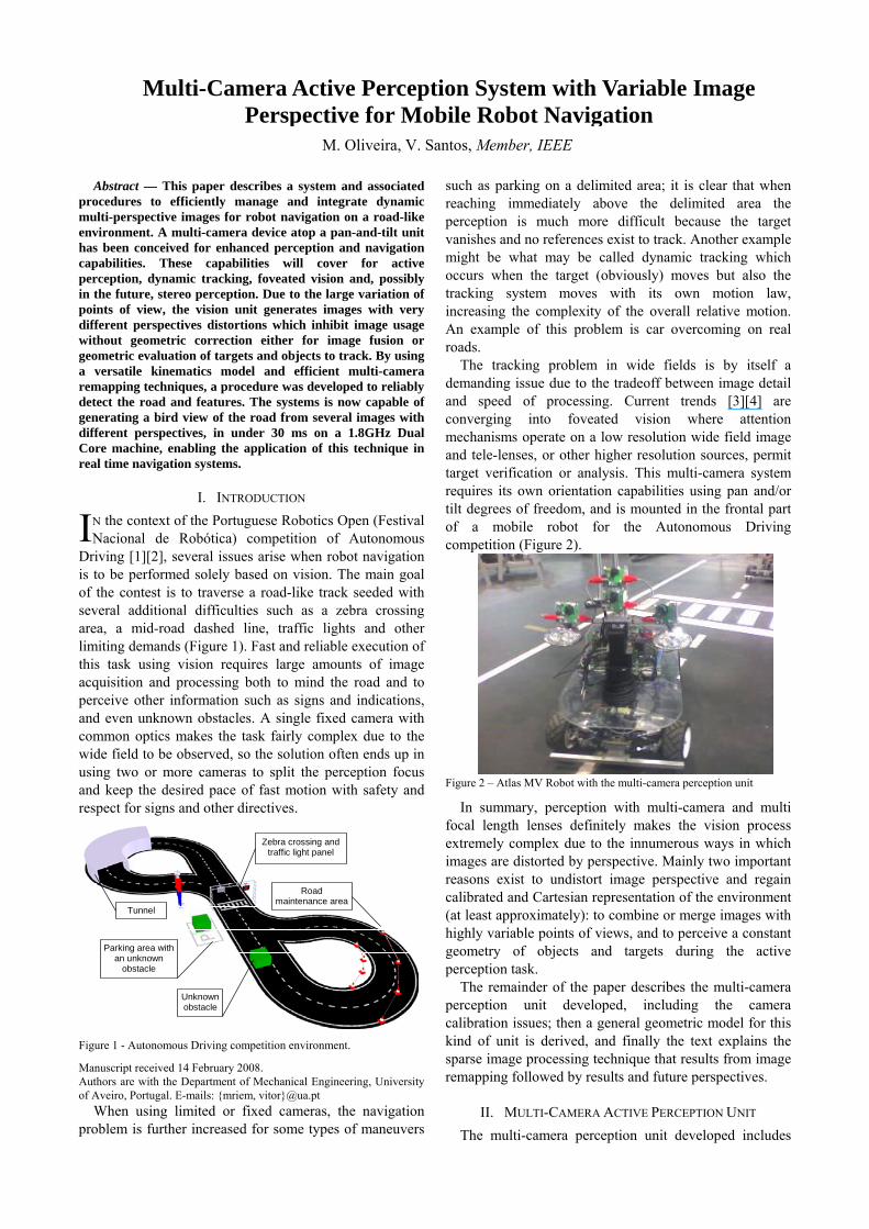
Multi-Camera Active Perception System with Variable Image Perspective for Mobile Robot Navigation

M. Oliveira, V. Santos, Member, IEEE

Abstract — This paper describes a system and associated procedures to efficiently manage and integrate dynamic multi-perspective images for robot navigation on a road-like environment. A multi-camera device atop a pan-and-tilt unit has been conceived for enhanced perception and navigation capabilities. These capabilities will cover for active perception, dynamic tracking, foveated vision and, possibly in the future, stereo perception. Due to the large variation of points of view, the vision unit generates images with very different perspectives distortions which inhibit image usage without geometric correction either for image fusion or geometric evaluation of targets and objects to track. By using a versatile kinematics model and efficient multi-camera remapping techniques, a procedure was developed to reliably detect the road and features. The systems is now capable of generating a bird view of the road from several images with different perspectives, in under 30 ms on a 1.8GHz Dual Core machine, enabling the application of this technique in real time navigation systems.

I. INTRODUCTION N the context of the Portuguese Robotics Open (Festival Nacional de Robótica) competition of Autonomous

Driving [1][2], several issues arise when robot navigation is to be performed solely based on vision. The main goal of the contest is to traverse a road-like track seeded with several additional difficulties such as a zebra crossing area, a mid-road dashed line, traffic lights and other limiting demands (Figure 1). Fast and reliable execution of this task using vision requires large amounts of image acquisition and processing both to mind the road and to perceive other information such as signs and indications, and even unknown obstacles. A single fixed camera with common optics makes the task fairly complex due to the wide field to be observed, so the solution often ends up in using two or more cameras to split the perception focus and keep the desired pace of fast motion with safety and respect for signs and other directives.

Parking area with an unknown

obstacle

Unknown obstacle

Tunnel

Road maintenance area

Zebra crossing and traffic light panel

Figure 1 - Autonomous Driving competition environment.

Manuscript received 14 February 2008. Authors are with the Department of Mechanical Engineering, University of Aveiro, Portugal. E-mails: {mriem, vitor}@ua.pt

When using limited or fixed cameras, the navigation problem is further increased for some types of maneuvers

such as parking on a delimited area; it is clear that when reaching immediately above the delimited area the perception is much more difficult because the target vanishes and no references exist to track. Another example might be what may be called dynamic tracking which occurs when the target (obviously) moves but also the tracking system moves with its own motion law, increasing the complexity of the overall relative motion. An example of this problem is car overcoming on real roads.

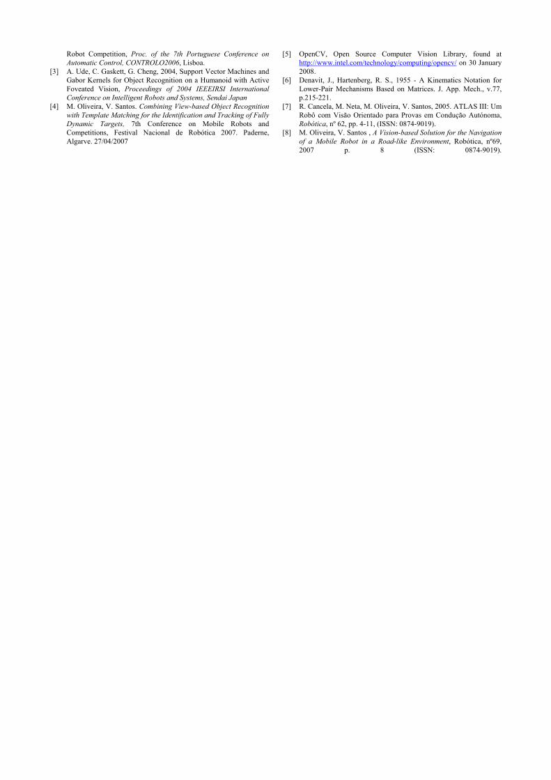
The tracking problem in wide fields is by itself a demanding issue due to the tradeoff between image detail and speed of processing. Current trends [3][4] are converging into foveated vision where attention mechanisms operate on a low resolution wide field image and tele-lenses, or other higher resolution sources, permit target verification or analysis. This multi-camera system requires its own orientation capabilities using pan and/or tilt degrees of freedom, and is mounted in the frontal part of a mobile robot for the Autonomous Driving competition (Figure 2).

Figure 2 – Atlas MV Robot with the multi-camera perception unit

In summary, perception with multi-camera and multi focal length lenses definitely makes the vision process extremely complex due to the innumerous ways in which images are distorted by perspective. Mainly two important reasons exist to undistort image perspective and regain calibrated and Cartesian representation of the environment (at least approximately): to combine or merge images with highly variable points of views, and to perceive a constant geometry of objects and targets during the active perception task.

The remainder of the paper describes the multi-camera perception unit developed, including the camera calibration issues; then a general geometric model for this kind of unit is derived, and finally the text explains the sparse image processing technique that results from image remapping followed by results and future perspectives.

II. MULTI-CAMERA ACTIVE PERCEPTION UNIT The multi-camera perception unit developed includes

I

four cameras and a servo actuated pan and tilt unit, as shown on Figure 3. The pan and tilt is controlled through RS232 serial protocol. It presents a pan range of approximately 270 degrees, and a tilt range of around 90 degrees.

Figure 3 -Multi-camera active perception unit.

Two of the cameras, Cam0 and Cam1, are positioned on the far sides of the unit, and are equipped with 2.1 mm focal length wide angle lenses. They are intended solely for navigation and should therefore provide a complete view of the road’s entire width. For these two cameras, the supporting structure allows to position the following parameters: vergence, torsion about the principal axis and distance to the unit’s centre.

Figure 4 - Positioning of camera at the end of the PTU arm.

Cam2 and Cam3 add up to define a foveated system. Cam2 is also equipped with a wide angle lens. It’s intended to have a wide field of view so that it can effectively search for known objects of interest. It is also called the peripheral camera. Aligned on the same vertical axis is Cam3, whose large focal distance lens allows the extraction of a high detail view of a particular object. This is also called the foveated camera. Figure 5 shows the peripheral/foveated cameras setup in more detail as well as a couple of example images of both the peripheral and the foveated camera.

For the purpose of navigation and more precise geometric evaluation of the environment, each camera undergoes a camera distortion correction namely barrel and similar intrinsic issues. The procedure uses the classic chessboard approach available in several software packages, as in the OpenCV libraries [5] used in this project. For each camera an intrinsic constant matrix K is obtained experimentally to be used further in the perspective projection transform.

Figure 5 - Foveated unit and examples of associated images.

III. THE PTU KINEMATICS MODEL The pan-and-tilt system plus its cameras can be

described as a set of several kinematics open chains and can therefore be modeled using the Denavit-Hartenberg (DH) notation for serial open kinematics chains [6]. For the sake of simplicity and conciseness, only one kinematics chain model is described in detail. The other are easily derived from this one, as mentioned further.

θ1

θ2

θ5

θ6

d4

L1

L5 L6

L2

L3

Figure 6 - Kinematics chain for the “left” part of the PTU

Each “link” in the kinematics chain can be described by 4 parameters where usually only one is variable. Figure 6 illustrates the main kinematics chain where the camera lies at the end of the link with its optical axis aligned with the Z axis of the last coordinate system and its focal plane on the XY plane of this last coordinate frame too; only some more relevant coordinate frames are shown. The angle θ1 is the pan angle, θ2 is the tilt angle, θ5 is the camera vergence (normally fixed in run-time), and θ6 accounts for possible camera roll around its optical axis (normally zero). From the lengths shown (L1, L2, L3, d4, L5, L6), only d4 was made adjustable on the hardware. From Figure 6 the following Denavit-Hartenberg parameters can be obtained:

Link i θi li di αi

1 θ1 0 L1 π/2 2 θ2+ π/2 L2 0 0 3 –π/2 L3 0 π 4 0 0 d4 π/2 5 θ5+ π/2 0 L5 π/2 6 θ6 0 L6 0

Table 1 - D-H parameters for one kinematics chain of the PTU

The geometric transformation from the PTU base

(reference frame - R ) up to the camera focal plane frame (C) is given by the following expression: (1) 0 1 5

1 2R

C = ⋅T A A A6

Q

where is defined by the DH conventions. 1ii

− ATo apply the direct perspective transformation of a

generic point Q into a camera, the point must be in camera coordinates CQ, but once the point is known in the reference frame, RQ, it is easy to relate both coordinate sets by means of the geometric transformation:

(2) ( ) 1C R RCQ T

−= ⋅

RTC, and also its inverse (RTC)–1 is a classical transformation matrix in 3D composed by a rotational (R) and translational (T) parts suited to operate on points expressed in homogeneous coordinates RQ = [X Y Z 1]T. Transformation matrix is then given by:

( )11 12 13 1

1 21 22 23 2

31 32 33 30 0 0 10 0 0 1

RC

r r r tr r r t

T r r r t−

⎡⎢⎡ ⎤ ⎢= =⎢ ⎥ ⎢⎢ ⎥⎣ ⎦ ⎢⎢⎣ ⎦

R T⎤⎥⎥⎥⎥⎥

⎥⎥

⎥⎥

(3)

Admitting especially for this problem that θ6 =0 and L3=0, by expanding equation (1), the following final model for geometric transformation is obtained:

(4) 5 2 1 5 1 5 2 1 5 1 5 2

2 1 2 1 2

5 2 1 5 1 5 2 1 5 1 5 2

S C C C S S C S C C S SS C S S C

C C C S S C C S S C C S

− − − + −⎡ ⎤⎢ ⎥= − −⎢⎢ − +⎣ ⎦

R

(5) 1 5 2 4 5

1 2 2 5

1 5 2 4 5 6

L S S d CL C L L

L C S d S L

−⎡ ⎤⎢= − − −⎢⎢ ⎥− − −⎣ ⎦

T

where the following common convention was used: ( )sini iS θ= and ( )cosi iC θ= .

IV. PERSPECTIVE TRANSFORMATION Once a point is known in the camera coordinate frame,

its coordinates in the image are obtained after the intrinsic matrix of the camera which translates the projection of real word coordinates into pixel coordinates on the image. Due to the nature of the process, coordinates in image pixels are also in the homogeneous format but affected by a scale factor. All this can be translated by the following expression:

(6) ( ) 1Rh CQ

−= K T RQ⋅

]

0

where , and the matrix of camera

intrinsic parameters is

[ ThQ u v w=

0

0

0 000 0 1 0

x

y

xy

αα

⎡ ⎤⎢ ⎥= ⎢ ⎥⎢ ⎥⎣ ⎦

K obtained

experimentally, as mentioned earlier. Naturally, as Qh expresses the image coordinates, then w must be the scale

factor and the following holds: pixuxw

= and pixvyw

= .

Being , it is also immediate to realize the following:

[ 1 TCs s sQ x y z=

0

0

1

x s p

y s s pix

s

u x x xv y y z yw z

αα

+ ix⎡ ⎤ ⎡ ⎤ ⎡ ⎤⎢ ⎥ ⎢ ⎥ ⎢ ⎥= + =⎢ ⎥ ⎢ ⎥ ⎢ ⎥⎢ ⎥ ⎢ ⎥ ⎢ ⎥⎣ ⎦ ⎣ ⎦ ⎣ ⎦

(7)

and also 31 32 33 3sw z Xr Yr Zt t= = + + + (8)

Finally, by multiplying the intrinsic matrix K and the geometric transformation (RTC)–1, the perspective transformation matrix P can be written as:

( )11 12 13 14

1

21 22 23 24

31 32 33 34

RC

p p p pp p p pp p p p

−⎡ ⎤⎢ ⎥⋅ = = ⎢ ⎥⎢ ⎥⎣ ⎦

K T P (9)

It must be reminded that what is sought is the point in the Cartesian space RQ after the known point in the image in pixels: [xpix,ypix]T .

For the current problem (navigation on a flat road) there is an assumption that simplifies the overall problem: all points are expected to be on the same real plane, the ground. This implies that in RQ all points have Z=0. This simplifies the scale factor on Qh yielding now: 31 32 3sw z Xr Yr t= = + + (10)

As matrix P is not invertible and its pseudo inverse is not usable, an analytic solution must be obtained to solve the following: (11) [ ] [ 0 1Tu v w X Y= ⋅P ]T

It is indeed a three equation system in three variables (X,Y,w) whose solution is:

( ) ( )22 34 24 32 14 32 12 34 14 22 12 24pix pixx p p p p y p p p p p p p pX

D− + − − +

= (12)

( ) ( )21 34 24 31 14 31 11 34 11 24 14 21pix pixx p p p p y p p p p p p p pY

D− + − + −

= − (13)

Where ( ) ( )21 32 22 31 31 12 32 11 11 22 12 21pix pixD x p p p p y p p p p p p p p= − + − + − (14)

To conclude the discussion of the model, it is very simple to demonstrate that the right hand of the PTU camera model differs simply in the following: d4 becomes –d4 and θ5 (the vergence) becomes –θ5. Other kinematics chains can be obtained by managing one or more parameters in Table 1.

V. CAMERA REMAPPING Having developed the model of the perception unit, the

transformation of all of the camera’s images is then possible. This transformation is performed for each camera as follows: two auxiliary matrixes called xMap and yMap are created. These matrixes contain the world reference frame x and y coordinates of every image pixel ( ). ,u v

0,..., 1 0,..., 1x

y

Map uP u W v H

Map v⎡ ⎤ ⎡ ⎤

= = − =⎢ ⎥ ⎢ ⎥⎣ ⎦⎣ ⎦

− (15)

In Figure 7, the values of xMap and of yMap are plotted in red.

]

Figure 7 – (X,Y) Mapping values for image pixels (u,v).

However, some pixels of the input image ( ) may not have their source real point on the ground plane. This depends on the camera’s lens vertical opening angle and on the current θ

imgInput

2 value (tilt). When this occurs, the value of xMap returns negative, and the remapping is not possible or not valid. A mask of the remapped pixels, named ( , )Mapped v u , is built for imgInput based on the following condition: (16) ( , ) 0xMap v u ≥

Which is executed for all image pixels and , where W and H correspond to the images

width and height respectively.

0 u W≤ <0 v H≤ <

A. Projection limits definition The projection calculation may lead to the projection of

some pixels to a long distance, i.e., pixels may have high values of xMap or yMap . Figure 7, for example, shows pixels projected up to 1600 mm on the x direction. Because these distances sometimes are not relevant for robot navigation, a clipping operation is applied to avoid unnecessary computation. This operation remaps only the pixels that lie in a predefined rectangle. This rectangle, named projection box ( ) is defined on the ground plane, having in mind how far ( ) and how wide ( ) should the robot require visual information. In addition to the condition stated in (16), two other criteria are imposed whilst building

boxP

maxDist

maxWide

( , )Mapped v u . The first criterion imposes a limit to the value of xMap . max( , )xMap v u Dist≤ (17)

For and . The latest imposes a maximum left and right view distance:

0 u W≤ < 0 v H≤ <

( ) max( , )2y

Wideabs Map v u ≤ (18)

Again, for 0 and u W≤ < 0 v H≤ < . Figure 8 shows an overlaid view of an image and its projection mask.

The dotted arrow indicates the limit mostly defined by the condition of (17) while the full arrow correspondent lines are typically characterized by (18). The simplest approach to build this mask is to cycle through all image pixels, applying equations (12) and (13), evaluating for each the three conditions enumerated in this section.

Figure 8 - Overlay of an input image and its corresponding

( , )Mapped v u mask.

B. Projection Calculation Enhancement The technique is, nonetheless, intended to work in real

time. The time taken during projection calculation is related to the amount of pixels that are projected, i.e., to the imgInput ’s resolution. It is also interesting to note that projection calculation time is not affected by the amount of channels in the image, since the coordinates of a pixel are equal for all of its channels. Only during actual remapping, i.e. the copy operation from coordinates (u, v) to coordinates ( xMap , yMap ), the time increases n times the amount of image’s channels.

Figure 9 – Depth profile for an input image.

Figure 9 illustrates the distance between each pixel (assuming it is projected on the ground plane) and the camera’s plane, as a function of the image pixels coordinates (u, v). The dashed line approximately represents a line obtained by fixing the camera’s principal point column while varying the line coordinate. This observation clearly shows that the distance to the ground plane is a monotonous growing function considering a decreasing line ( ) and a fixed column ( ).

The input is so because the image coordinates are assumed to be top left origin based. Bearing this in mind, and also that pixels that do not intercept the ground plane have values of , a test function can be designed to skip the projection calculation of pixels (with the same ) that have a higher v than the one

whose projection resulted in . On the other hand, if considering a fixed line v

sindecrea gv fixedu

sindecrea gv

( , ) 0xMap v u ≤

fixedu

( , ) 0xMap v u ≤

fixed and a parted center to left decreasing column as well as a center to

right increasing column , sin

center leftdecrea gu →

sincenter rightincrea gu →

( , )gplaneDist u v is also monotonous. Implementing this skip function, however, would require a separate analysis for the left and right

sides of the image, increasing the complexity of both the projection and the skip function. In addition, the amount of pixels that are to be discarded using this calculation enhancement setup is considerably smaller, implying also a smaller time gain. Still, a question may be posed as to why not use both enhancements instead of just one, thus gaining even more time. It is not possible to use both enhancements within the same cycle, since that one must make a decision whether to first scan, i.e., to fix, the line or the column. Thus, only the ; enhancement is applied

fixedu sindecrea gv

C. Projection Scaling Factor The projection of the pixels onto the ground plane

results sometimes in very large images. Let’s assume, for example, a ground projected output image ( ) of

resolution, which corresponds to a 1.6 long per 2.5 meters long . This image is notoriously bigger than the size usually employed for robot navigation. Moreover, the impressive size is not correspondent to the information that lies in the projected image. In fact, disregarding, for now, the multi-camera approach, and considering in the best case scenario that all of Figure 7’s pixels were projected onto the (and that their projections would never be overlapped), this would represent projected pixels. Compared to the ’s total amount of pixels, this number would represent that only 1.9 of the projected image’s pixels were in fact projected. This means that over 98% of the new image’s pixels would have to be synthesized. This number is obviously preposterous, even considering a perfect (all pixels projected and none overlapping) multi-camera approach of half a dozen cameras, there still would be

unmapped pixels in the new image. These calculations reflect the fact that a 1 pixel per millimeter (1 PPM) resolution is not promising with the current perception unit setup, nor was it possible to have a real time system processing such a large image. Hence it became crucial to be able to rescale the output image resolution easily. The easiest approach is to down-sample the 1 PPM image. However, there is a problem in doing this; most down-sampling algorithms are not prepared to operate on sparse images, which is the case after the projection. The alternate approach of first synthesizing a non sparse image from the projected one is even more troubling, not only due to the high unmapped rates described before, but also due to the computational cost of such an operation on a huge image. The solution is to perform on the fly rescaling during the calculation of the projected coordinates. In order to do this, a rescaling factor is defined as a fraction of the default 1 PPM resolution. Rescaling is now just a matter of multiplying

with all of the perception unit kinematics distance related values as well as with the defined limits, and , before doing the

actual projection of the original’s image pixels. With this, the remapping operation automatically outputs a rsf times smaller image than the one defined by . Rescaling causes obviously some pixels’ projections to overlap in the smaller image, but this would also occur if the 1 PPM image would later be down-sampled.

imgOutput1600 2500×

boxP

imgOutput

320 240 76800× =

imgOutput 61600 2500 4 10× = ×

2%

100 (6 1.92) 88%− ×

rsf

rsf

1 2 3 4 5 6, , , , ,L L L d L L

boxP maxDist maxWide

boxP

Al

SeofcoIn

Foww

1. Rescale kinematics distances and ground projection box using rsf

1 2 3 4 5 6, , , , ,L L L d L L

2. Zero both ( , )Mapped v u and masks. ( , )GMapped V U3. Cycle through image pixels:

( )0; ;for u u w u= < + + ) [so that ] fixedu

( )1; 0;for v w v v= − ≥ − − [so that v ] sindecrea g

{ 3.1 Calculate ( , )xMap v u and ( , )yMap v u

3.2 Check P limits and set mapped masks: box

if ( ( , )xMap v u ; ( , )yMap v u is inside ) then boxP{

( , ) 1Mapped v u = ( ( , ), ( , ))y xGMapped Map v u Map v u + +

} 3.3 Check for skip condition and if so skip: if Ma ( , ) 0xp v u ≤ then 1v = − } 4. Remap pixels to : imgOutput

( )0; ;for u u w u= < + +

( )0; ;for v v h v= < − − {

4.1 If remapped, sum pixel to : imgOutput if ( ( , )Mapped v u ) then ( ( , ), ( , )) ( , )img y x imgOutput Map u v Map u v Input v u+ =

} 5. Find remapped pixel value

( )max0; ;for U U Dist U= < + +

( )max0; ;for V V Wide V= < − −

Mapped V U >

{ if G then ( , ) 1

( , )imgOutput V U

( , )

( , )imgOutput V UGMapped V U

=

}

gorithm 1 – Remapping algorithm for single camera projection

D. Projection Remapping ctions V.A, V.B and V.C have described the calculation the remapping matrixes xMap and yMap . In order to mplete a camera projection operation, the pixels of the

imgput must be copied to the : imgOutput

(19) ( , ) ( , )img y x imgOutput Map Map Input v u=

r 0 u W≤ < and 0 v H≤ < . This would be the simplest ay to remap the image. However, some particular cases ere neglected. It is possible that two or more pixels of

the imgInput may overlap, i.e. are projected onto the very

same pixel on the . In this case, the average value of the overlapping pixels should be used. This can be done by using another mask, this time a mask for the

remapped pixels, henceforth named

. It can be defined during the projection calculation simply adding 1 to its value every time a pixel is remapped to that particular position.

imgOutput

imgOutput

( , )GMapped V U

( ( , ), ( , )) _ ( )

( ( ( , ), ( , )) )x y box

y x

f Map v u Map v u is inside P

then GMapped Map v u Map v u + + (20)

For and . After the projection calculation, ’s values will reflect how many pixels have been projected onto each particular position. The can be remapped by summing the contributions of every pixel, dividing in the end by the value of .

0 u W≤ < 0 v H≤ <( , )GMapped V U

imgOutput

( , )GMapped V UThe projection calculation and remapping methodology can thus be described as in Algorithm 1.

VI. MULTI-CAMERA REMAPPING Section V described in detail the remapping algorithm, as well as some techniques that improve its performance. This section intends to approach the usage of multiple cameras for remapping the entire road.

Figure 10 -.Multi camera remapping projected and discarded points.

Due to the dimensions of the car versus the road, as well as the cameras and lens that are employed, it is often not possible to have a complete view of the road using a single camera. Navigation algorithms often rely on road lines contrast with the road to operate. Therefore, the visualization of both road delimiting lines is a key issue in most road navigation trends. For this reason the active perception unit uses two cameras exclusively for navigation purposes. These were previously mentioned as Cam0 and Cam1. Since these are solely dedicated to acquiring visual information of the road, the dual camera system as a whole should capture the entire road. Figure 10 shows the spread of view for both cameras. A rescaling factor was used. A remapping box of 0.1rsf =

[ ]max max4500; 3000Dist Wide= = was defined. This is

reflected by the magenta and blue dots, which are the actually remapped of Cam0 and Cam1 (green and red) respectively.

Multi-camera remapping requires very little adjustments to the technique presented in section V. Kinematics, perspective transformation, projection limits, calculation, rescaling and enhancement must be applied for each camera, but the remapping algorithm handles multiple camera pixel overlapping just the same as single camera pixel overlapping, implying only slight changes in the methodology of Algorithm 1, as shown in Algorithm 2.

0. Cycle N input cameras and repeat Algorithm 1’s first four steps

( )0; ; ( )for i i N increase i= < { Execute Algorithm 1 steps: 1. 2. 3. and 4. { 5. Find remapped pixel values for multi-camera projection

( )max0; ;for U U Dist U= < + +

( )max0; ;for V V Wide V= < + +

Mapped V U >

{ if G then ( , ) 1

( , )

( , )( , )

imgimg

Output V UOu tput V U

GMapped V U=

}

Algorithm 2 – Remapping algorithm for multi camera projection

VII. POST PROJECTION IMAGE PROCESSING Figure 11 shows two input cameras, with a setup similar to the one represented in Figure 10.

Figure 11 - Dual camera input and projected view.

The shown is, as could be anticipated by analyzing the remapping distribution of Figure 10, a sparse image. Furthermore, the information of both cameras is not scattered to in an uniformly distributed manner. This section outlines some image treatment techniques used to extract viable information of the road from the sparse .

imgOutput

imgOutput

imgOutput

Figure 12 – Three examples of the projected bird view using Cam0 and Cam1 as input for several pan/tilt/vergence angles. Final images are also interpolated and smoothed.

A. Sparse image threshold, and morphological closing Immediate threshold of the could have some

advantages. Not synthesizing missing information reduces the risk of creating artifacts on the resulting image. Later, a dilate operation applied to the Boolean, post thresholded image can restore road characteristics. Hopefully, this operation would merge the road features; for average size restoration a subsequent erosion operation should be employed (completing the morphological closure). For this technique to work, one must ensure that the projected information is not scattered beyond a certain limit, otherwise the dilate operation will not merge the road features and the erode operation could erase the information. An example the output of this sequence of operations is shown on Figure 13.

imgOutput

Figure 13 - Sparse after threshold, and morphological closing. imgOutput

B. Sparse Image Linear Interpolation and Smoothing Another possibility is to attempt to synthesize the

missing information based on the one that exists on . A linear interpolation between pixels that hold

information can be implemented. A subsequent smoothing operation can be performed to attempt to soften possible artificial artifacts that maybe created during interpolation. The output of such an operation is shown on Figure 14.

imgOutput

Figure 14 - Sparse interpolated and then smoothed. imgOutput

The advantage of this image in comparison to the one of

Figure 13 is that common image processing techniques do not support sparse image processing. This solution provides a color/grayscale image which in some cases may prove valuable, when compared to a binary image. For example, the area signaled in Figure 14. Because of poor light conditions, a simple threshold operation cannot isolate the signaled region of the line. An adaptive threshold, that makes use of local average pixel’s values to calculate the threshold limit, could extract the line. This operation however, cannot be employed on sparse images since it would consider absent information (black regions of Figure 11) as pixels with zero brightness, ruining the average calculation.

VIII. CONCLUSIONS AND FINAL REMARKS The bird view of the road comprises some very

interesting characteristics, when compared to the input road images. First of all, it’s a single image view of the road, as opposed to the two (or more) input images. This might ease navigation techniques which usually are designed for single image processing. Second, this single image holds information regarding a very wide angle view, capturing both road delimiting lines at all times, hence contributing to the robustness of subsequent navigation algorithms. Third and perhaps most important, the characteristics painted on the road, such as lines, zebra crossings etc., show constant geometric properties such as size and shape. This enables the implementation of much simpler pattern matching algorithms. Previous experience has shown that, before this projection technique was developed, patterns, whose size and shape changed with camera positioning, distance to pattern and others, were very difficult to detect due to the great variability of their properties. It is the authors’ opinion that, in the future, the implementation of previously developed navigation algorithms [7] [8] is expected to be much more straightforward. At the moment, it is possible to remap two input cameras in less than 30 milliseconds using a 1.8GHz Dual Core machine. This performance clearly enables the application of this technique in real time navigation systems.

IX. REFERENCES [1] Almeida, L., Azevedo, J. , Cardeira, C., Costa, P., Fonseca, P. Lima,

P., Ribeiro, F., Santos, V, 2000. Mobile Robot Competitions: Fostering Advances in Research, Development and Education in Robotics. Proc. of the 4th Portuguese Conference on Automatic Control, CONTROLO2000, 4-6 October 2000, Guimarães, Portugal, pp. 592-597

[2] P. Afonso, J. Azevedo, C. Cardeira, B. Cunha, P. Lima, V. Santos, 2006. Challenges and Solutions in an Autonomous Driving Mobile

Robot Competition, Proc. of the 7th Portuguese Conference on Automatic Control, CONTROLO2006, Lisboa.

[3] A. Ude, C. Gaskett, G. Cheng, 2004, Support Vector Machines and Gabor Kernels for Object Recognition on a Humanoid with Active Foveated Vision, Proceedings of 2004 IEEEIRSI International Conference on Intelligent Robots and Systems, Sendai Japan

[4] M. Oliveira, V. Santos. Combining View-based Object Recognition with Template Matching for the Identification and Tracking of Fully Dynamic Targets, 7th Conference on Mobile Robots and Competitions, Festival Nacional de Robótica 2007. Paderne, Algarve. 27/04/2007

[5] OpenCV, Open Source Computer Vision Library, found at http://www.intel.com/technology/computing/opencv/ on 30 January 2008.

[6] Denavit, J., Hartenberg, R. S., 1955 - A Kinematics Notation for Lower-Pair Mechanisms Based on Matrices. J. App. Mech., v.77, p.215-221.

[7] R. Cancela, M. Neta, M. Oliveira, V. Santos, 2005. ATLAS III: Um Robô com Visão Orientado para Provas em Condução Autónoma, Robótica, nº 62, pp. 4-11, (ISSN: 0874-9019).

[8] M. Oliveira, V. Santos , A Vision-based Solution for the Navigation of a Mobile Robot in a Road-like Environment, Robótica, nº69, 2007 p. 8 (ISSN: 0874-9019).