
MSCSE Thesis-Jayed(012162029)23.02.2019 .pdf
56
Machine Learning Based Automatic Pattern Analysis for Banking Data with Improved Feature Selection Md Jayedul Haque Student Id:012162029 A Thesis in The Department of Computer Science and Engineering Presented in Partial Fulfillment of the Requirements For the Degree of Master of Science in Computer Science and Engineering United International University Dhaka, Bangladesh January 2019 © Md Jayedul Haque, 2019
-
Upload
khangminh22 -
Category
Documents
-
view
1 -
download
0
Transcript of MSCSE Thesis-Jayed(012162029)23.02.2019 .pdf

Machine Learning Based Automatic Pattern Analysis for
Banking Data with Improved Feature Selection
Md Jayedul Haque
Student Id:012162029
A Thesis
in
The Department
of
Computer Science and Engineering
Presented in Partial Fulfillment of the Requirements
For the Degree of Master of Science in Computer Science and Engineering
United International University
Dhaka, Bangladesh
January 2019
© Md Jayedul Haque, 2019

i
Approval Certificate
This thesis titled “Machine Learning Based Automatic Pattern Analysis for Banking
Data with Improved Feature Selection” submitted by Md. Jayedul Haque, Student ID:
012162029, has been accepted as Satisfactory in fulfillment of the requirement for the
degree of Master of Science in Computer Science and Engineering on January, 2019.
Board of Examiners
1.
______________________________ Supervisor
Dr. Mohammad Nurul Huda Professor & MSCSE Director
Department of Computer Science & Engineering (CSE)
United International University (UIU)
United City, Madani Avenue, Badda, Dhaka 1212
2.
______________________________ Head Examiner
Dr. Dewan Md. Farid Associate Professor
Department of Computer Science & Engineering (CSE)
United International University (UIU)
United City, Madani Avenue, Badda, Dhaka 1212
3.
______________________________ Examiner-I
Dr. Swakkhar Shatabda Associate Professor and Undergraduate Coordinator
Department of Computer Science & Engineering (CSE)
United International University (UIU)
United City, Madani Avenue, Badda, Dhaka 1212
4.
______________________________ Examiner-II
Suman Ahmmed Asst. Professor & Director - CDIP
Department of Computer Science & Engineering (CSE)
United International University (UIU)
United City, Madani Avenue, Badda, Dhaka 1212
5.
______________________________ Ex-Officio
Dr. Md. Abul Kashem Mia Professor and Dean
School of Science & Engineering
United International University (UIU)
United City, Madani Avenue, Badda, Dhaka 1212

ii
Declaration
This is to certify that the work entitled “Machine Learning Based Automatic Pattern
Analysis for Banking Data with Improved Feature Selection” is the outcome of the
research carried out by me under the supervision of Dr. Mohammad Nurul Huda,
Professor and MSCSE Director, United International University (UIU), Dhaka,
Bangladesh.
________________________________________
Md. Jayedul Haque Department of Computer Science and Engineering
MSCSE Program
Student ID: 012162029
United International University (UIU)
Dhaka, Bangladesh.
In my capacity as supervisor of the candidate’s thesis, I certify that the above statements
are true to the best of my knowledge.
________________________________________
Dr. Mohammad Nurul Huda Professor and MSCSE Director
Department of Computer Science and Engineering
United International University (UIU)
United City, Madani Avenue, Badda, Dhaka 1212.
iii
Abstract
A very famous adage of Adam Smith, “All money is a matter of belief”. It is, of course,
the beginning of the first use of money was observed when the supply of demanded
product was available in the hands of others. It can also be said that the introduction of
money has introduced us to a system called business. Initially, this system gave rise to the
internal economy but later it spread to the whole world. But in the whole world there is a
new system emerged for the flow of economy which is known as bank to everyone. And
through this bank, a country may be importing or exporting every day. Only the economy
of a country is considered good when export is more than import. Due to everyone's
attention of better economy, export can be increased and import can be optimized. So, to
solve this problem statistics can help us greatly. As Statistics, has been using in
determining the existing position of per capita income, unemployment, population growth
rate, housing, schooling medical facilities and so on. In this study not only statistics but
also machine learning tools were used to analyze and forecast the financial banking data
specifically import data. Basically, import data is known to a country as an economic
data. So when we can predict about imports, then deciding how much of the export will
be good for economics can easily be determined. In this study we have worked with
import data of Bangladesh Bank for analysis and forecast the import of Bangladesh,
based on collected data to strengthen the economic condition.

iv
Acknowledgement
I would like to start by expressing my deepest gratitude to the Almighty Allah for giving
me the ability and the strength to finish the task successfully within the scheduled time.
“Machine Learning Based Automatic Pattern Analysis for Banking Data with
Improved Feature Selection” has been prepared to fulfill the requirement of MSCSE
degree. I am very much fortunate that I have received sincere guidance, supervision and
co-operation from various persons.
I would like to express my heartiest gratitude to my supervisor, Dr. Mohammad Nurul
Huda, Professor and MSCSE Director, United International University, for his
continuous guidance, encouragement, and patience, and for giving me the opportunity to
do this work. His valuable suggestions and strict guidance made it possible to
prepare a well-organized thesis report. Besides, I would like to thank Serajam Monira,
Deputy Director of Bangladesh Bank, to help me collecting the import data of
Bangladesh Bank.
Finally, my deepest gratitude and love to my parents for their support, encouragement,
and endless love.
v
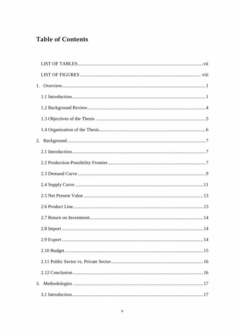
Table of Contents
LIST OF TABLES ......................................................................................................... vii
LIST OF FIGURES ..................................................................................................... viii
1. Overview........................................................................................................................ 1
1.1 Introduction................................................................................................................ 1
1.2 Background Review................................................................................................... 4
1.3 Objectives of the Thesis ............................................................................................ 5
1.4 Organization of the Thesis ......................................................................................... 6
2. Background .................................................................................................................... 7
2.1 Introduction................................................................................................................ 7
2.2 Production-Possibility Frontier .................................................................................. 7
2.3 Demand Curve ........................................................................................................... 9
2.4 Supply Curve ........................................................................................................... 11
2.5 Net Present Value .................................................................................................... 13
2.6 Product Line............................................................................................................. 13
2.7 Return on Investment ............................................................................................... 14
2.8 Import ...................................................................................................................... 14
2.9 Export ...................................................................................................................... 14
2.10 Budget .................................................................................................................... 15
2.11 Public Sector vs. Private Sector ............................................................................. 16
2.12 Conclusion ............................................................................................................. 16
3. Methodologies ............................................................................................................. 17
3.1 Introduction.............................................................................................................. 17
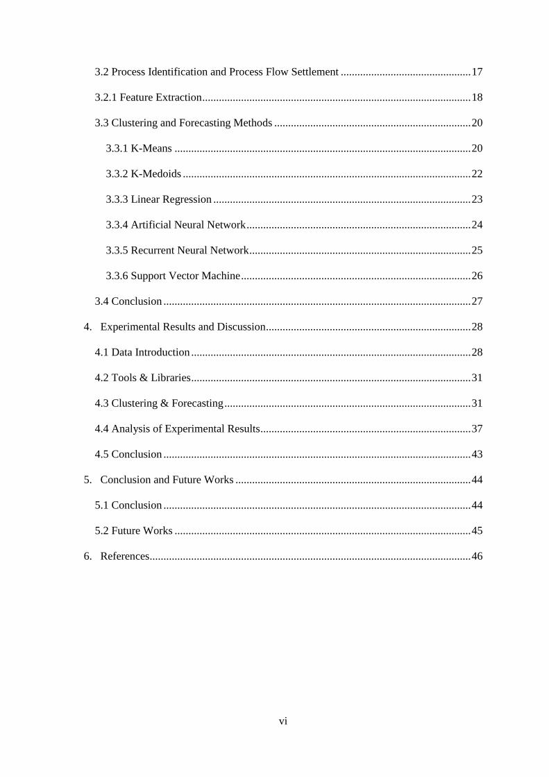
vi
3.2 Process Identification and Process Flow Settlement ............................................... 17
3.2.1 Feature Extraction ................................................................................................. 18
3.3 Clustering and Forecasting Methods ....................................................................... 20
3.3.1 K-Means ........................................................................................................... 20
3.3.2 K-Medoids ........................................................................................................ 22
3.3.3 Linear Regression ............................................................................................. 23
3.3.4 Artificial Neural Network ................................................................................. 24
3.3.5 Recurrent Neural Network ................................................................................ 25
3.3.6 Support Vector Machine ................................................................................... 26
3.4 Conclusion ............................................................................................................... 27
4. Experimental Results and Discussion .......................................................................... 28
4.1 Data Introduction ..................................................................................................... 28
4.2 Tools & Libraries ..................................................................................................... 31
4.3 Clustering & Forecasting ......................................................................................... 31
4.4 Analysis of Experimental Results ............................................................................ 37
4.5 Conclusion ............................................................................................................... 43
5. Conclusion and Future Works ..................................................................................... 44
5.1 Conclusion ............................................................................................................... 44
5.2 Future Works ........................................................................................................... 45
6. References.................................................................................................................... 46
vii
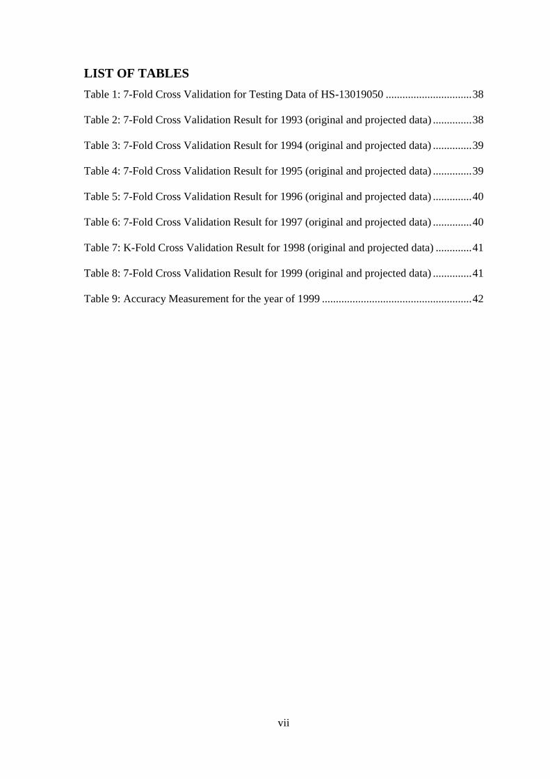
LIST OF TABLES
Table 1: 7-Fold Cross Validation for Testing Data of HS-13019050 ............................... 38
Table 2: 7-Fold Cross Validation Result for 1993 (original and projected data) .............. 38
Table 3: 7-Fold Cross Validation Result for 1994 (original and projected data) .............. 39
Table 4: 7-Fold Cross Validation Result for 1995 (original and projected data) .............. 39
Table 5: 7-Fold Cross Validation Result for 1996 (original and projected data) .............. 40
Table 6: 7-Fold Cross Validation Result for 1997 (original and projected data) .............. 40
Table 7: K-Fold Cross Validation Result for 1998 (original and projected data) ............. 41
Table 8: 7-Fold Cross Validation Result for 1999 (original and projected data) .............. 41
Table 9: Accuracy Measurement for the year of 1999 ...................................................... 42
viii
LIST OF FIGURES
Figure 1: Production Possibility Frontier ............................................................................ 8
Figure 2: Demand Curve ................................................................................................... 10
Figure 3: Supply Curve ...................................................................................................... 12
Figure 4: Pattern Classification process ............................................................................ 18
Figure 5: Scree Plot diagram ............................................................................................. 19
Figure 6: Feature Extraction process ................................................................................. 19
Figure 7: K-Means with 3 Cluster ..................................................................................... 21
Figure 8: K-Means with 5 Cluster ..................................................................................... 21
Figure 9: K-Means with 7 Cluster ..................................................................................... 22
Figure 10: Artificial Neural Network ................................................................................ 25
Figure 11: Recurrent Neural Network ............................................................................... 26
Figure 12: Support Vector Machine .................................................................................. 27
Figure 13: Overview of Data ............................................................................................. 28
Figure 14: Frequency of an individual product in several countries ................................. 29
Figure 15: Frequency of an individual product in different year in Indonesia .................. 30
Figure 16: Amount of an individual product in different year and month in Indonesia .... 31
Figure 17: Number of Cluster ............................................................................................ 32
Figure 18: K-Means Cluster analysis with 7 center according to country ........................ 33
Figure 19: K-Means Cluster analysis with 7 center according to year .............................. 33
Figure 20: K-Medoids with 3 Cluster ................................................................................ 34
Figure 21: K-Medoids with 5 Cluster ................................................................................ 35
Figure 22: K-Medoids with 7 Cluster ................................................................................ 35
Figure 23: Linear Regression Result ................................................................................. 37
Figure 24: Accuracy Measurement Curve ......................................................................... 42
1
Chapter 1
Overview
1.1 Introduction
Since every economy in the world interchange their growth or production along with so
called barter system or financial system. The financial system is a structure based on
legitimate agreements in between institutions to countries, and both the formal and
informal economic partners work together to facilitate or control the international flow of
financial capital for investment and trade finance simultaneously. During the period of
the first modern stimulus of economic globalization, which is widely observed in the late
19th century, the improvement of central bank is noticed after the establishment of
economic revolution. Besides, it is important for Intergovernmental organizations and
multilateral agreements to increase the control, transparency and efficiency of the
international market. The English word ‘Economics’ is derived from the Greek word
called ‘Oikonomia’ which means ‘family management’. Economics was first emerged
during the ancient Greece period of time. Aristotle, who was Greek Philosopher, defined
economics as a 'home management' science. But with the change in civilization and
development, the economic status of individual changes periodically. As a result, in the
definition of Economics is noticed to be changed in an evolutionary manner. By the end
of the 18th century, the name of Adam Smith as the father of the economy defined
economics as 'wealth science'. He says, “Economics is a science that explore into the
environment and reason of the wealth of nations”. In other words, how wealth is
produced and how it is enjoyed, it is the real condition of the economy. After some time,
Alfred Marshall defined Economics by saying, ‘Economics is a study of human life in a
normal way’. In other words, the economy is studying not only resources but also
services. There is a more extensive and feasible definition of economics is noticed in the
current era. In the age of social life, people want unlimited, but limited resources are
available to meet their needs. In the study of economics, limited resources are used to
satisfy the unlimited needs of people. Lionel Robins, the modern economist says,
‘Economics is a science that treats relationships as a lasting and unexpected medium,
which uses alternatives’. So, from the social view economics is a study of how the
2
economy manages economic activities and how they try to meet the unlimited needs by
properly utilizing limited resources. On the other hand, national vision represents the
economic strength of a country from the economy. Economics was not considered as a
separate rule, but part and parcel of philosophy according to the Western world until the
18th–19th century. Industrial revolution and accelerating economic growth of the Great
Depression of the 19th Century made a new view of economics. In the initial stage of the
economy as an intellectual manner or science was dominated by Western thinkers and
their supporters, said by the economists from outside the West. But now one day
economic development brings together the entire world into a platform. The process by
which a nation enhance the economic, social, and political welfare of its people is called
Economic development. This term is often used by economists, politicians and others
between the 20th and the 21st century. But the idea has been used in the West for
centuries. While discussing about economic development people used some more term
like Modernization, Westernization, and especially Industrialization. In the present era,
we can find direct relationships of economic development with environment and
environmental problems. Economic development is like a bridge to interfere in the
public's economic and social welfare. On the other hand, economic growth represents the
productivity of the market and the emergence of GDP. Consequently, as economist
Amartya Sen narrated, “Economic growth is one aspect of the economic development
process ". Since 1945, there have been several periodical changes in the developmental
theory of several major levels. From the 1940s to the 1960s so many modern theory were
introduced to enhance the industrialization. These theories were admired in developing
countries. This period was followed by a short period of time. Those fundamental
development was lightening on human capital development and revival of economic
condition in the 1970s. A new jargon was introduced in the latter 1980s ‘Neoliberalism’
which was emerged to implement the free trade agenda and dismissal of Import
Substitution Industrialization regulatory. In the economy, the study of economic
development that applied to the traditional economy was reached to the national product
thoroughly, or collective results of products and services. Economic development has
taken alarmed with enhancement of the public's entitlement and related nutrition, disease,
education, literacy, power and other socio-economic rehabilitation [1]. Skittering the
backdrop of Keynesian, government revenue policy, and pursuing the neo-economics
economy, emphasizes less intervention with the growth of the countries of higher growth
3
(Singapore, South Korea, Hong Kong) and planned governments (Argentina, Chile,
Sudan, Uganda). Economic development, more generally development economics,
emerged in mid-20th century theoretical paraphrasing of how economies improves [2].
Again, economist Albert O. Hirschman, a familiar person to development economics,
implies that economic development grew to condense on the impoverished places of the
world, to start with in Africa, Asia and Latin America yet on the outpouring of
fundamental thinking and models [3]. As the economy follows banking system, the
history of banking was first identified with the first sample bank where the world's
businessmen, farmers and traders carry goods in distant places. Those banks provided
loans to them. Those banking system were a part of ancient Mesopotamia, about 2000
BCE in Asia and Sumeria. Later, during the Roman Empire in ancient Greece, the
temples were used to provide loans, to accept deposits and to change the money. The
archaeological data of this era shows that ancient China and India were also involved in
money lending and deposition activities. Many historians have said that the primary
historical development of a banking system in medieval and Renaissance Italy and
especially Venice, Florence and Genoa's rich cities. On 14th century, the Bardi and
Peruzzi families studied and dominated banking in Florence and established branches in
other parts of Europe [4]. Founded by Giovanni Medici in 1397, Medici Bank was the
most famous Italian bank [5]. The existence of the oldest bank is still being operated
since 1472 in Italy's Siena headquarters Banca Monte dei Paschi di Siena [6]. The
subsequent development of post-banking, scattered throughout the Holy Roman Empire
from northern Italy, and from northern Europe between the 15th and 16th centuries.
During the Dutch Republic in the 17th century, this was inherited from Amsterdam by
several notable diversities in Amsterdam and 18th century in London. When the
telecommunication and computing improvements took place in the twentieth century, the
operations of banks changed dramatically, and banks moved dramatically in terms of size
and geographical spread. But like the previous banks, now the banks are no longer small.
Now the banks are big because their purpose is very big. Now banks are dealing
internationally so that they need saving of data and information for simplicity and
easiness transaction. Therefore, the data analysis has become essential for the current
banking system. So, in this paper Banking data and several Machine Learning methods
are used to understand the current Banking condition and future steps to enrich the
economy of a country.

4
1.2 Background Review
From the discussion paper of A. Ganesh-Kumar [8], Bangladesh government has no big
stocking policy similar to neighboring India, any gap between domestic supply and
domestic demand is supposed to be met by trade (either imports or exports). Imports a
very basic input of a country to meet the needs of a country. When a govt. set a farsighted
goal it becomes crucial to measure the utility of a nation according to supply. We have
statistical bureau which gives us the forecasted population of the coming age of this
country. So based on this forecasted population govt. should have extrapolation of the
future demand to satisfy their utility. Here is the answer why we need to forecast the data
of import. In this paper we have forecasted the imported amount of an item analyzing the
import data of Bangladesh Bank. There are several attempts in literature to pursue the
needs of food using the Housing and Income Survey (HIES) data for Bangladesh.
Chowdhury (1982) used the Frisch (1959) method for computing its direct and cross-
elasticity demand, based on the small availability of the valuable data, under the terms of
independent freedom, with systemic facilities. On the contrary, a method of demanding
prices, which is called the system of food demand needs. Bouis (1989) thinks that
marginal utility of consumption of any food depends on the level of consumption of all
other foods; he used this method to forecast relating food demand elasticity’s of
Bangladesh using 1973/74 Household Expenditure Survey5 data. Pitt (1983) and Goletti
(1993) used a method called food demand system or Tabit. Pitt (1983) depicted that it is
irrelevant to use Tobit in demand analysis for models that have expenditure or budget
share as dependent variables. On the contrary, Ahmed and Shams (1994) introduced an
ideal model based on primary information (AIDS) from three rounds of household
expenses and nutrition analysis in International Food Policy Research Institute (IFPRI),
from September 1991 to November 1992. The most recent attempt to study demand
elasticity’s for food items in Bangladesh was made by Anwarul Huq and Arshad (2010).
This study focused primarily on price elasticity, cross-price elasticities, and elastic
elaboration of the demands of various food items based on Linear Approximate AIDS
(LAAIDS) model with a correct Stone Price Index. During the years 1983/84, 1988/89,
1991/92, 1995/96, 2000, and 2005/06, it was based on a panel of samples from the
Bangladesh HIES. In 2011 M. Ahsan Akhtar Hasin [9] first analyzed the trend and
seasonality patterns of a nominated item in a retail trade branch in Bangladesh. Then
demand was forecasted having traditional Holt-Winter’s model. Fuzzy uncertainty was
5
done again with the use of Artificial Neural Network (ANN). Eventually, the inaccuracy,
counted in terms of MAPE and were compared for searching the best fitting extrapolating
process. Greece relies almost often with a lower productive economy, less wages and
social transformation with a perfect welfare state. G. Atsalakis [10] introduced a new
strategy for modeling unemployment problem of a country. To create a Neuro-Fuzzy
model, Artificial Neural Networks have been linked to Fuzzy logic which was used in
this study. The input was given as a time series. To assess the performance of the model,
the calculation of classical statistics is calculated. The more results are compared with an
ARMA and an AR model. In some previous studies about demand forecasts, the
traditional statistical method as the moving average, Box-Jenkins were used. Liu et. al.
preferred data mining methodologies for time series and showed enhancement in Box -
Jenkins time series extrapolating outcome [11]. As the statistical model cannot produce
satisfactory outcome, Artificial Intelligence algorithms were tested in many studies with
great success. For example, Neural Network algorithm is generally applied to literature in
several studies [12], [13], [14], [15], [16], and [17]. The given research provides
impressive results with the NN algorithm. Some ANN algorithms jointly applied with
another algorithm intended to provide a more successful method for further study.
Genetic algorithm with RBF neural network algorithm were used in Doganis et. al study
[18]. Autoregressive Integrated Moving Average (ARIMA) model was integrated Neural
Network Algorithm Model which were proposed by Aburto and Weber known as another
hybrid model [19]. In this study, Principal Component Analysis is used for feature
extraction process. On the other hand, K-means and K-medoids are used for clustering
the data. Eventually, we will use Linear Regression, Artificial Neural Network, Support
Vector Machine and Recurrent Neural Network for forecasting and extrapolating based
on import data of Bangladesh Bank. In the experiment and result analysis process K-fold
cross validation is used to train and test the data using Machine Learning tools discussed
above.
1.3 Objectives of the Thesis
We all are familiar with the common jargon which is commonly referred to as
“cookbooks”. Normally, Cookbooks are known as books which is used to teach
the student to decide which buttons to press on a computer without providing an
understanding of what the computer is doing. This study is not repeating the
6
characteristics of cookbook but introduces some tools which is common in
Statistics and Machine Learning for understanding the behavior of the import data
which will help to have a clear view of economic structure of a country.
In addition, Artificial Neural Network, Regression, Support Vector Machine and
Recurrent Neural Network are fairly simple concepts which is used to measure
future indication and behavior. Artificial neural networks, Support Vector
Machine and Recurrent Neural Network are the algorithms that can be applied to
use nonlinear statistical modeling, the most frequent used method for developing
predictive models for different branches like Economics, Medicine science etc..
Eventually, Artificial Neural Networks, Support Vector Machine and Recurrent
Neural Network play a role as a classification method for nonlinear problems.
This study focusses on the analysis of economic data of Bangladesh bank; which
is collected from the server of Bangladesh bank. The first objective is to
understand the data using some statistical tool like frequency distribution and
histogram graph. Then the next counted step is cluster the data to introduce the
ambiguity and identify the anomaly. Then the remaining objective is using
predictive models on the data.
1.4 Organization of the Thesis
Chapter one introduces the emergence of economics with business, area of previous
related studies and states the brief information of economics and finance. A Brief
discussion on the objective of the thesis.
Chapter two introduce the different tools of economics and finance to analyze the result
which will be calculated through the forecasting method.
Chapter three illustrates mainly the basic work flow and methodology of entire study.
Chapter four has been devoted to design the experiments and it also presents results of
experiments, comparisons among different existing methods.
Chapter five concentrates on conclusion of the thesis and recommendation for future
work.
7
Chapter 2
Background
2.1 Introduction
Literally, the meaning of Economics is the branch of study concerned with the
production, consumption, and transfer of wealth. An example of the economics is the
study of the stock market and central banking system. Central Bank provide the
supremacy over domestic production of a country, demand of internal market and export-
import affairs. All these data is known as financial data. The noble objective of this study
is to predict the amount of import commodities which is or will be imported from foreign
country. So, definitely a proper indication or suggestion should be provided after getting
the manipulation of data which is collected from Bangladesh bank. There are so many
tools to analyze the condition and impact of current economic state. Actually these tools
are used to have proper guidance and to take necessary steps. Some tools have been
introduced in this chapter.
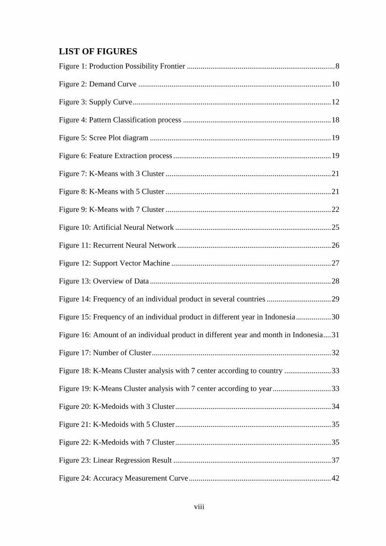
2.2 Production-Possibility Frontier
It is true that the resources of all goods of a country are not endless. So their resources
and technology are limited, which have helped to keep them productive. So using these
limited resources and technology a country have to go for domestic production. These
domestic production may be used to fulfill the internal demand and some to fulfill the
export areas. A production possibility frontier provides the highest possible output
combinations of two goods or services. These goods or services can be gained by an
economy when all available resources are fully and efficiently appointed. As the product
name of collected data set is confidential so a metaphoric example has been used. Let us
give an example by considering an economy which produces only two economic goods,
guns and butter. The gun which represents the military spending and the butter used for
civilian spending. If all the resources and capital is invested to produce the butter then 10
million pounds butter can be produced which is considered as the maximum production
of butter having existing technology and resources. At the other extreme, suppose that all
resources are invested instead of butter to the production of guns. For the sake of limited
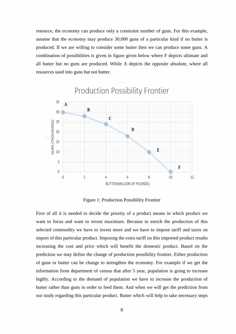
8
resource, the economy can produce only a constraint number of guns. For this example,
assume that the economy may produce 30,000 guns of a particular kind if no butter is
produced. If we are willing to consider some butter then we can produce some guns. A
combination of possibilities is given in figure given below where F depicts ultimate and
all butter but no guns are produced. While A depicts the opposite absolute, where all
resources used into guns but not butter.
Figure 1: Production Possibility Frontier
First of all it is needed to decide the priority of a product means in which product we
want to focus and want to invest maximum. Because to enrich the production of this
selected commodity we have to invest more and we have to impose tariff and taxes on
import of this particular product. Imposing the extra tariff on this imported product results
increasing the cost and price which will benefit the domestic product. Based on the
prediction we may define the change of production possibility frontier. Either production
of guns or butter can be change to strengthen the economy. For example if we get the
information from department of census that after 5 year, population is going to increase
highly. According to the demand of population we have to increase the production of
butter rather than guns in order to feed them. And when we will get the prediction from
our study regarding this particular product. Butter which will help to take necessary steps
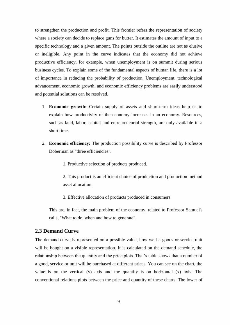
9
to strengthen the production and profit. This frontier refers the representation of society
where a society can decide to replace guns for butter. It estimates the amount of input to a
specific technology and a given amount. The points outside the outline are not as elusive
or ineligible. Any point in the curve indicates that the economy did not achieve
productive efficiency, for example, when unemployment is on summit during serious
business cycles. To explain some of the fundamental aspects of human life, there is a lot
of importance in reducing the probability of production. Unemployment, technological
advancement, economic growth, and economic efficiency problems are easily understood
and potential solutions can be resolved.
1. Economic growth: Certain supply of assets and short-term ideas help us to
explain how productivity of the economy increases in an economy. Resources,
such as land, labor, capital and entrepreneurial strength, are only available in a
short time.
2. Economic efficiency: The production possibility curve is described by Professor
Doberman as "three efficiencies".
1. Productive selection of products produced.
2. This product is an efficient choice of production and production method
asset allocation.
3. Effective allocation of products produced in consumers.
This are, in fact, the main problem of the economy, related to Professor Samuel's
calls, "What to do, when and how to generate".
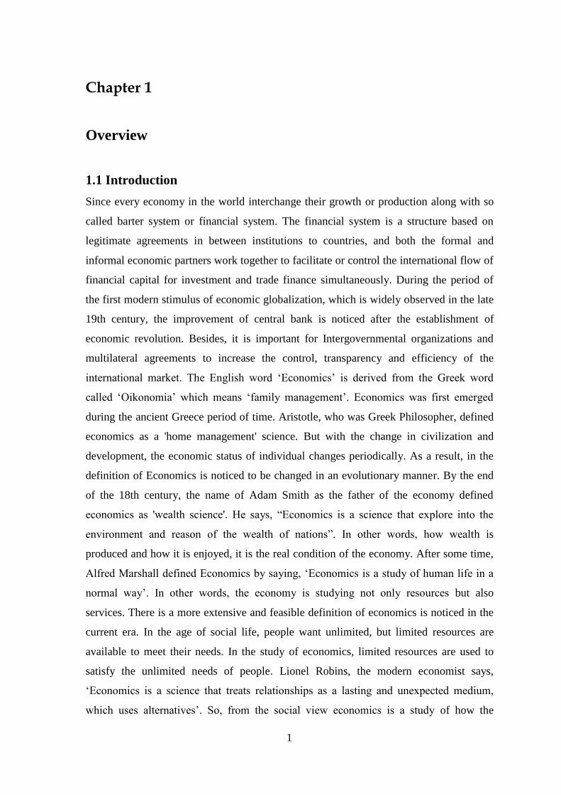
2.3 Demand Curve
The demand curve is represented on a possible value, how well a goods or service unit
will be bought on a visible representation. It is calculated on the demand schedule, the
relationship between the quantity and the price plots. That’s table shows that a number of
a good, service or unit will be purchased at different prices. You can see on the chart, the
value is on the vertical (y) axis and the quantity is on horizontal (x) axis. The
conventional relations plots between the price and quantity of these charts. The lower of
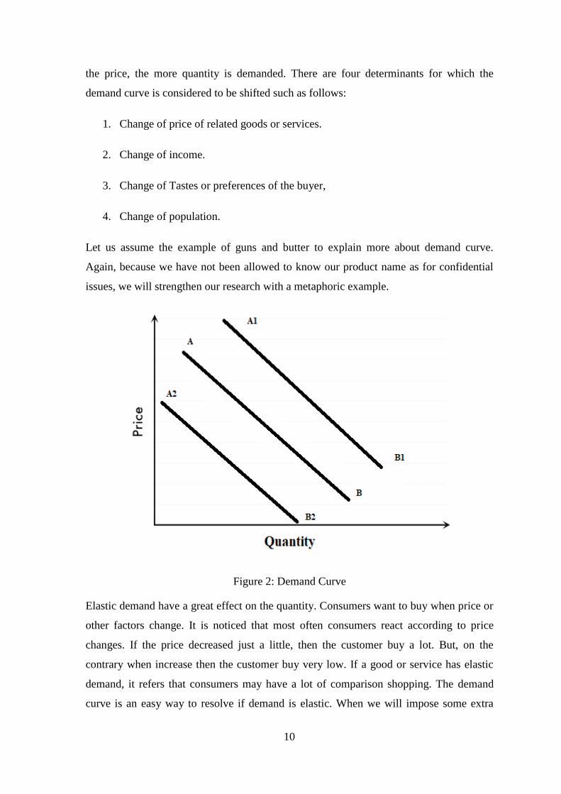
10
the price, the more quantity is demanded. There are four determinants for which the
demand curve is considered to be shifted such as follows:
1. Change of price of related goods or services.
2. Change of income.
3. Change of Tastes or preferences of the buyer,
4. Change of population.
Let us assume the example of guns and butter to explain more about demand curve.
Again, because we have not been allowed to know our product name as for confidential
issues, we will strengthen our research with a metaphoric example.
Figure 2: Demand Curve
Elastic demand have a great effect on the quantity. Consumers want to buy when price or
other factors change. It is noticed that most often consumers react according to price
changes. If the price decreased just a little, then the customer buy a lot. But, on the
contrary when increase then the customer buy very low. If a good or service has elastic
demand, it refers that consumers may have a lot of comparison shopping. The demand
curve is an easy way to resolve if demand is elastic. When we will impose some extra
11
tariff on import of butter and its complementary product then it will shift the demand
curve to the left like A2B2. As a result, the demand of imported product decreases and
domestic product increases. On the other hand, if we facilitate the import of butter and its
complementary product then it will shift the demand curve to the right like A1B1. Which
may make the cause of decimation of domestic production. It is anticipated that this study
will be helpful to the fiscal policy maker to make proper decision. But this study may not
be helpful in case of inelastic product. When the reduction of price do not increase the
quantity of goods or service then it is called inelastic demand. An ideal example of
inelastic demand is drug. No matter how much the cost of drug increased, it does not have
any effect on the demand. For basic need like food, fuel, shoes and prescription drugs
demand considered to be inelastic. Such items are considered as support of life.
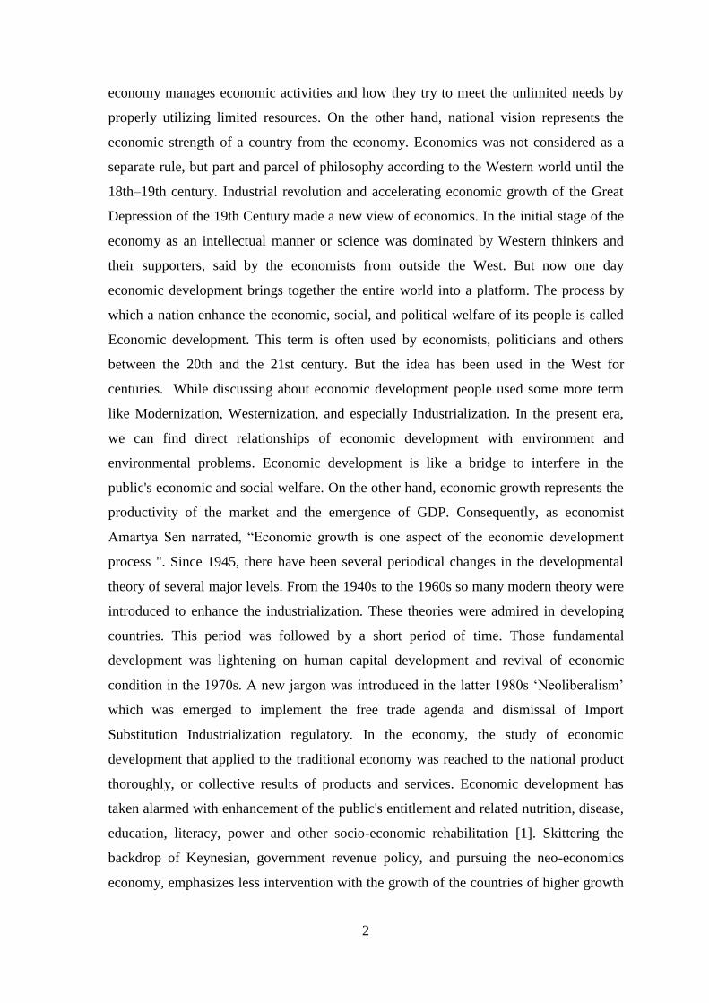
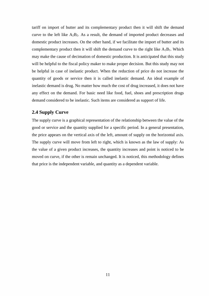
2.4 Supply Curve
The supply curve is a graphical representation of the relationship between the value of the
good or service and the quantity supplied for a specific period. In a general presentation,
the price appears on the vertical axis of the left, amount of supply on the horizontal axis.
The supply curve will move from left to right, which is known as the law of supply: As
the value of a given product increases, the quantity increases and point is noticed to be
moved on curve, if the other is remain unchanged. It is noticed, this methodology defines
that price is the independent variable, and quantity as a dependent variable.
12
Figure 3: Supply Curve
For example, if the price of soybean (HSCODE 12011010) rises, farmers will be
encouraged to cultivate less corn (HSCODE 07104010) and more soybean, and the total
amount of soybean in the market will increase. The term to which increasing price
translates into increasing quantity is called supply elasticity or price elasticity of supply.
If a 50% increase in soybean prices aim the quantity of soybeans made to increase by
50%, the supply elasticity of soybeans is 1. If a 50% increase in soybean prices only
increases the quantity supplied by 10%, the supply elasticity is 0.2. The supply curve is
superficial for goods along with extra elastic supply, and perpendicular for products with
low elastic supply.
If a factor besides price or quantity changes, a new supply curve is noticed along with the
previous curve. Suppose, an amount of new soybean farmers checked into the market,
devastating forests and rising the number of cultivated land tend to soybean cultivation.
In this phenomena, extra soybeans may be made even if the price remains the identical,
refers that the curve itself shifts to the right (S1) in the graph above. In the other words,
supply will wax. Other remaining factors can also alternate the supply curve, like changes
in the production process. If the drought increases the price of water, then the curve will
13
move to the left (S2). From the point of view of the supplier - If the price of a substitute -
such as corn increases, farmers will move towards increasing change and soybean
supplies will decrease (S2). If a new technology, such as a pest-resistant seed, increases
yields, the supply curve will shift right (S1). If the future value of soybean is higher than
the present value, the supply will temporarily shift to the left (S1), as manufacturers have
an encouragement to wait for the sale.
2.5 Net Present Value
The net present value (NPV) method is used to evaluate investments which concatenates
the current amount of all cash inflows and deducts the current amount of all cash
outflows. Challenging factors in determining a product have different ways to measure
the value of future cash flows. A positive net means a good return to the current value,
and a negative net means a bad return than returning from current value. This is one of
the two discount cash flow strategies used to compare investment proposals, where the
revenue duration fluctuates.
2.6 Product Line
Entering the competitors into the market and the products go through the life cycle, the
directors should decide to leave or leave product lines often. A product line is a group of
related products. Home Depot, Inc., There are various product lines such as machinery,
flooring, and paint products. A product line is a group of products related to a brand sold
by the same company. Companies sell multiple product lines under their various brands.
Consumers are more likely to purchase products from brands that they already know
because companies often expand their sources by adding existing product lines.
Companies already produce product lines as marketing strategies to capture the sales of
buyers of the brand. The operating principle is that consumers can respond positively to
their brand and they are willing to buy new products based on their positive experience
with their brand. For example, under a similar brand may be a cosmetic company which
may already launch a product that is selling a high-value product line (makeup, concealer,
powder, blush, eyeliner, eye shadow, mascara and lipstick may also be included) under
one of the well-known brands at the line. But at low price points Product lines can vary
between colors, shapes, quality and prices. The company uses a project line to track
trades, which helps them deciding to select which markets can fulfill their goals.
14
2.7 Return on Investment
Investment Returns (ROI) measures a performance, used an evaluation of an investment
expertise or compared the efficiency of various investment. ROI measures the investment
amount related to investment costs. ROI calculation, investment benefits (or refunds) are
divided by investment costs. The results are expressed as percentages or ratios. The return
on investment formula:
Return on Investment = (profit from Investment - amount of Investment)/amount of
Investment
2.8 Import
If we define in a simple way the term “Imports” refer to the foreign goods and services
which are bought by the government on behalf of the residents of a country. Residents is
a broader concept but in short it includes citizens, businesses, and the institutions. The
primal challenge is not consideration of the way of dealing imports that means how they
are sent. They can be shipped, sent by email, or even hand-carried in personal luggage on
a plane. Only when the imported products will be sold to domestic residents, then they
will be defined as imports. Even tourism products and services are imports. When one
travel outside his country, he is considered that importing any souvenirs he bought on his
trip. When a country imports surpasses its exports value then trade deficit is noticed. If it
imports less than it exports, that creates a trade surplus. Imports make a country
dependent on other countries political and economic power. So, this study can be helpful
to find out the economic condition of our country.
2.9 Export
Exports can be defined in a simple way, interchange of goods and services which is
produced in foreign country purchased by the resident of another country. Good or
service does not matter. It does not matter how it is sent. It can be sent only, or sent by
email, or carrying on a private car in a ship. Any product that is produced locally in the
country and is sold to foreign countries abroad, it is an export. For example, Bangladeshi
shrimp are exported all over the world. As per Export Promotion Bureau data, the export
of shrimps increased by 14 percent year-on-year to $124 million between July and
September of the 2016-17 fiscal year. Here are the major export commodities of
Bangladesh:
15
Garments item
Frozen fish and seafood item
Jute and jute goods
Leather item
According to the Economy Watch the following were Bangladesh’s export partners as of
2008:
U.S: 24.1%
Germany: 15.32%
U.K: 10.05%
France: 7.43%
Netherlands: 5.51%
Italy: 4.50%
Spain: 4.21%
There are so many ways that countries try to increase their exports. First, they will use
trade protectionism to give their industries an advantage. This usually raise the price of
import by imposing tariffs. They also provide subsidies on their own industries to make
their product prices lower. But, once they start doing this, other countries will consider
their tricks with same manner. This will lower trade overall which causes of the Great
Depression.
2.10 Budget
The term budget means extrapolation of revenue and expenses over a particular span of
time; it is examined and re-evaluated on a repeated time. Budgets are used in our daily
life may be in a personal life, a family space, a group of individual, a merchant, a
government, a country, a multinational institution or anything which makes and spends
money. In between companies and organizations, a budget is used as an internal action to
manage and manipulate financial statements to defend from financial loss. Now a days,
budget means a lot for a country as whole income and expenditure is calculated and
provided for this budget.
16
2.11 Public Sector vs. Private Sector
Once upon a time all of the flow of money transacted through the private ventures. But
after the change of economic definition all the transaction became public at all. Now a
days we can see the reform of economic status. At present, many countries have adopted
the policy of Privatization, through which Private Sector is also gaining importance.
Because it makes transparency of action and advances the whole process which is helpful
for any organization and government. For the progress and development of any country,
both the sectors need advancement as only a single sector cannot lead the country in the
way of success. The private sector consist of trade which is owned, managed and
controlled by individual. On the contrary, public sector consist of different trade
enterprises owned, controlled and managed by Government.
2.12 Conclusion
Bangladesh's economy has many problems. Some of them are just basic problems. As
long as these are not resolved, the economic development of the country will not
accelerate. There is considerable difference between economists definition of economic
development. Different people have tried to explain it in the light of their own views. But
in general, economic development refers to the growth of real national income by
fulfilling the basic needs of the people of every country, which constantly contributes to
the enhancement of income and reduction of expenditure. Increasing the employment of
the people at the rate of increasing rates and overall efforts of the people to maintain their
standard of living effects a lot to the economy. According to Williams and Patrick, "The
long-term increase in the per capita outcome and service of the people of any country or
place is defined as economic development". According to Professor Snider, the long-term
or incessant growth process of 'per capita production' is defined as economic
development. According to the renowned economist Yang, "Development is a complex
process of social, economic, political and progress of a person or society."
17
Chapter 3
Methodologies
3.1 Introduction
In the previous chapters, the trend of business and how the economy has emerged in this
series has been observed. Not only this, we also know how the economy has been
introduced money and money introduced banking system. Through this system it has
been collected some data to analyze and make future decision about some transaction. To
do this, it has to use some Machine Learning methods which will be described in detail in
this chapter. In the initial stage, no work is easily seen, but if the working steps can be
divided separately, then the task becomes easier. So the whole task is divided into some
small task to confirm easiness and well understanding.
3.2 Process Identification and Process Flow Settlement
The first challenge of this study was collecting data which became easier when we got
permission to access the import data of Bangladesh Bank. After collecting data
processing become primal as there were so many categorical entry in the numerical field.
So, making numerical data from categorical data was our next task. Some constant
feature were removed to make the computation easier. Then it became easier to apply
methodology of clustering and forecasting. After the using of clustering algorithm we
have to use predictive models to forecast. After getting result we have to take decision
based on the result. But in terms of our study the decision defines that based on previous
data import of particular product is going to increase or decrease.
18
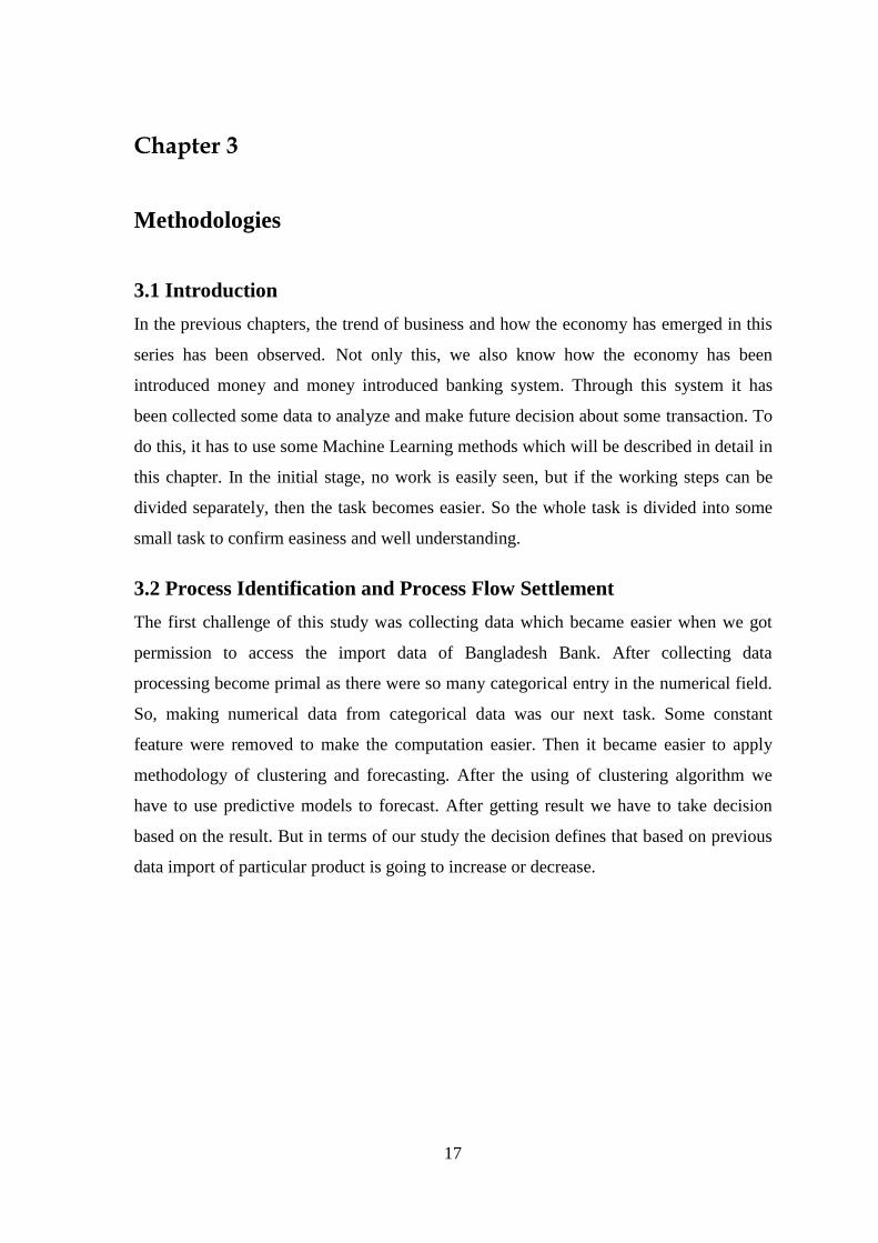
Figure 4: Pattern Classification process
3.2.1 Feature Extraction
In fact, most of the information used is considered very big with redundant element or
stuff. Therefore, no decision should be made on any tuition by this information. It may be
necessary to remove additional information before running the methodology or a tool
should be used that will be able to remove the errors or redundant element from the data.
The basic features are called a subset considering feature attributes. And the expected
features are expected to retain relevant information from input data, so that the expected
action can be done using this less representation instead of the full initial information. A
principal component analysis (or PCA) is a crucial method by which it can simplify a
complex multivariate dataset. It helps to uncover the underlying source of information
variations. A scree plot shows the ratio of the total variation in a dataset, which is
explained by each element in a principal component analysis. This helps to identify how
many components are needed to summarize the data. The result is shown below:
19
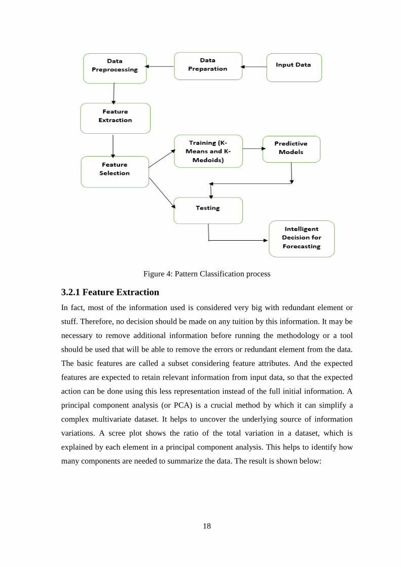
Figure 5: Scree Plot diagram
From the scree plot diagram it can be seen that the amount of variation explained drops
dramatically after the first two component. Which suggests that two component may be
adequate to abbreviate the dataset. Five features have been selected in this study from ten
features.
Figure 6: Feature Extraction process
20
3.3 Clustering and Forecasting Methods
Basically, clustering is used to identify the relationship between the data and
corresponding group. It is available in a particular group that is most relevant to that
group. All the relevant data makes a group of cluster. Then in a nutshell cluster analysis
or clustering is the task of grouping a set of objects in such a way that objects in the same
group (called a cluster) are more similar (in some sense or another) to each other than to
those in other groups (clusters). So we have used clustering so that we can verify whether
there is any similarity-dissimilarity and anarchy between the data. In this study two very
popular clustering tools K-means and K-medoids are used. The methods based on the
data that has been decided on some issues in the future is called forecasting methods.
Linear Regression, Artificial Neural Network, Support Vector Machine and Recurrent
Neural Network all are forecasting tools which are used in this study. Linear Regression
is the method of predicting Real Value with a model like a line. The artificial neural
networking was created from the efforts of the computer program to create the way
people learn and act. Artificial neural network originates by imitating the neural network
of the human nervous system. The neural network helps to make computers more smart,
how the brain works. Besides, Recurrent Neural Network (RNN) is a class of artificial
neural networks that apply to time series data and that use outputs of network units at
time t as the input to other units at time t + 1. On the other hand, Support Vector Machine
(SVM) is a supervised machine learning algorithm that can be used for both classification
and regression premises.
3.3.1 K-Means
K-means (MacQueen, 1967) is one of the simplest unsupervised learning algorithms that
solve the well-known clustering problem. The whole procedure takes data as input and
make output of several group based on input data. In the beginning of this procedure we
define k centroids, one for each cluster. These centroids should be placed in an intelligent
way because different positions cause different results. So, good choices are placed away
from each other as far as possible. The next step is to connect each point to the specified
data set and connect it to the nearest central. When no other point is left, the first step is
considered to be completed and the first cluster is done. Now the cluster needs to count
back to the new centroids to get results from the previous step. After getting these k new
centroids, a new relationship will be created between the same data set points and the
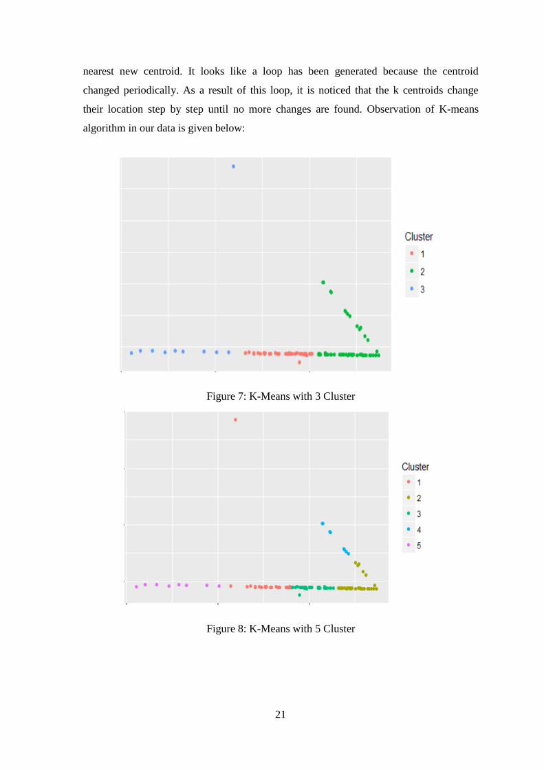
21
nearest new centroid. It looks like a loop has been generated because the centroid
changed periodically. As a result of this loop, it is noticed that the k centroids change
their location step by step until no more changes are found. Observation of K-means
algorithm in our data is given below:
Figure 7: K-Means with 3 Cluster
Figure 8: K-Means with 5 Cluster
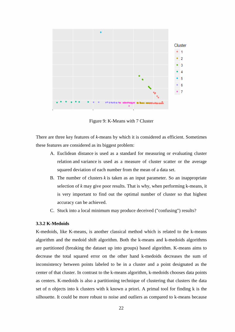
22
Figure 9: K-Means with 7 Cluster
There are three key features of k-means by which it is considered as efficient. Sometimes
these features are considered as its biggest problem:
A. Euclidean distance is used as a standard for measuring or evaluating cluster
relation and variance is used as a measure of cluster scatter or the average
squared deviation of each number from the mean of a data set.
B. The number of clusters k is taken as an input parameter. So an inappropriate
selection of k may give poor results. That is why, when performing k-means, it
is very important to find out the optimal number of cluster so that highest
accuracy can be achieved.
C. Stuck into a local minimum may produce deceived ("confusing") results?
3.3.2 K-Medoids
K-medoids, like K-means, is another classical method which is related to the k-means
algorithm and the medoid shift algorithm. Both the k-means and k-medoids algorithms
are partitioned (breaking the dataset up into groups) based algorithm. K-means aims to
decrease the total squared error on the other hand k-medoids decreases the sum of
inconsistency between points labeled to be in a cluster and a point designated as the
center of that cluster. In contrast to the k-means algorithm, k-medoids chooses data points
as centers. K-medoids is also a partitioning technique of clustering that clusters the data
set of n objects into k clusters with k known a priori. A primal tool for finding k is the
silhouette. It could be more robust to noise and outliers as compared to k-means because
23
it minimizes a sum of general pairwise inconsistencies in the lieu of sum of squared
Euclidean distances. The available choice of the inconsistency function is very rich but in
our method we used the Euclidean distance. A medoid of a finite dataset is a data point
from this set, whose average dissimilarity to all the data points is minimal i.e. it is the
most centrally located point in the set. The most common understanding of k-medoid
clustering is the Partitioning Around Medoids (PAM) algorithm. The algorithm proceeds
in two steps:
1. INITIAL-step: k "centrally located" objects is selected in this step one by one,
which is identified as an initial medoids.
2. SWAP-step: If a selected object with an unselected object is exchanged as a result
the objective function can be decreased, then the exchange is carried out. This is
continued till the objective function can no longer be decreased.
3.3.3 Linear Regression
Linear Regression is a statistical tool which is used to make the relationship between two
variables by modeling a linear equation to observed data. In this context one variable is
considered to be an explanatory variable, and the other is considered to be a dependent
variable. For example, a modeler might want to relate the weights of individuals to their
heights using a linear regression model.
But before trying to build a linear model of observed data, a modeler should first define
whether or not there is any relationship between the variables, in short we can say the co-
relation between two variables. This does not mean that one variable causes the other (for
example, higher income do not cause higher utility), but it can be said that there could be
some significant association between the two variables. A scatterplot is considered a very
powerful tool in determining the strength of the relationship between two variables. If
there appears to be no association between this two variables (i.e., the scatterplot does not
indicate any increasing or decreasing trends), then fitting a linear regression model to the
data probably will not provide a useful model. A valuable numerical measure of
association between two variables is the correlation coefficient r, which is a value
between -1 and 1 indicating the strength of the association of the observed data for the
two variables.
If r = 0 then there is no relationship between the data. Where r = -1 or 1 means strong
relationship between the data. The range of r and it refers
0< r < 0.5 or – 0 <r <-0.5: poorly related
24
0.5 <r < 0.75 or -0.5 <r < -0.75: moderately related
0.75 < r < 1 or -0.75 < r < -1: strongly related
Generally, linear regression refers to a model represents straight line in which the
conditional mean of Y given the value of X.
Y= a + b*X
3.3.4 Artificial Neural Network
An Artificial Neural Network (ANN) is an information processing model that is currently
the most widely used and successful tool in the world, which is analogous to the process
of biological nervous system such as the human brain, process information.
Although Linear Regression has been used, but one thing needs to be made clear that this
problem is not linear. As output amount does not increase accordance with input (year,
month, country). This proves that this relationship is not linear. As a result, hidden layer
and hidden neuron has been used to solve this problem. One hidden layer and four hidden
neuron has been used in Artificial Neural Network. The main purpose of this model is to
imitate the novel structure of information processing methods like human and create
meaningful outputs. Like the linear regression, artificial neural network variables and
predictions are used to create relationships. It works together to solve a special problem
called neurons, which is made up of a large number of highly interconnection processing
materials. Artificial Neural Networks is learnt by itself an example like human brain. An
Artificial Neural Network is used for a specific application, such as speech recognition or
classification, through a learning process. In biological systems we have so many neuron
along with the synaptic connections that is found between the neurons which is used to
propagate information one neuron to next to complete the learning process and making
decision. Similar to biological hierarchy Artificial Neural Network use same connection
between two neurons but virtually not physically.
25
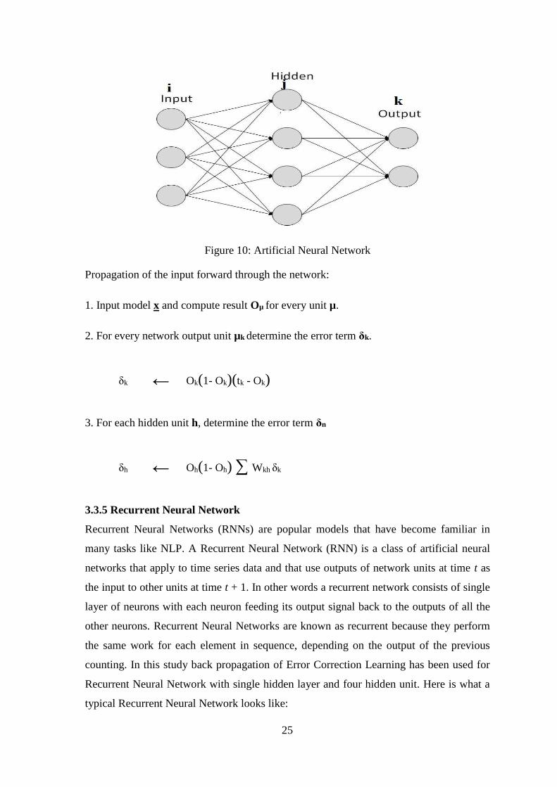
Figure 10: Artificial Neural Network
Propagation of the input forward through the network:
1. Input model x and compute result Oµ for every unit µ.
2. For every network output unit µk determine the error term δk.
δk ← Ok(1- Ok)(tk - Ok)
3. For each hidden unit h, determine the error term δn
δh ← Oh(1- Oh) ∑ Wkh δk
3.3.5 Recurrent Neural Network
Recurrent Neural Networks (RNNs) are popular models that have become familiar in
many tasks like NLP. A Recurrent Neural Network (RNN) is a class of artificial neural
networks that apply to time series data and that use outputs of network units at time t as
the input to other units at time t + 1. In other words a recurrent network consists of single
layer of neurons with each neuron feeding its output signal back to the outputs of all the
other neurons. Recurrent Neural Networks are known as recurrent because they perform
the same work for each element in sequence, depending on the output of the previous
counting. In this study back propagation of Error Correction Learning has been used for
Recurrent Neural Network with single hidden layer and four hidden unit. Here is what a
typical Recurrent Neural Network looks like:
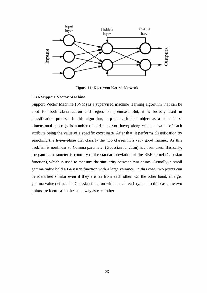
26
Figure 11: Recurrent Neural Network
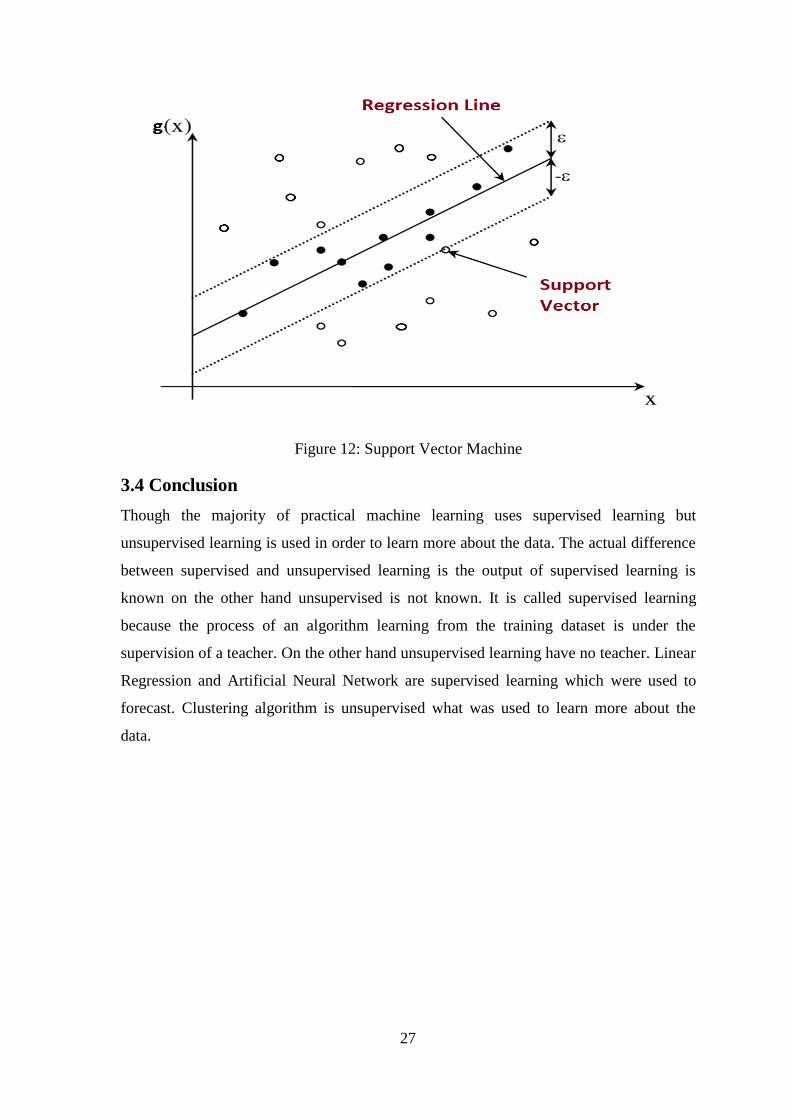
3.3.6 Support Vector Machine
Support Vector Machine (SVM) is a supervised machine learning algorithm that can be
used for both classification and regression premises. But, it is broadly used in
classification process. In this algorithm, it plots each data object as a point in x-
dimensional space (x is number of attributes you have) along with the value of each
attribute being the value of a specific coordinate. After that, it performs classification by
searching the hyper-plane that classify the two classes in a very good manner. As this
problem is nonlinear so Gamma parameter (Gaussian function) has been used. Basically,
the gamma parameter is contrary to the standard deviation of the RBF kernel (Gaussian
function), which is used to measure the similarity between two points. Actually, a small
gamma value hold a Gaussian function with a large variance. In this case, two points can
be identified similar even if they are far from each other. On the other hand, a larger
gamma value defines the Gaussian function with a small variety, and in this case, the two
points are identical in the same way as each other.
27
Figure 12: Support Vector Machine
3.4 Conclusion
Though the majority of practical machine learning uses supervised learning but
unsupervised learning is used in order to learn more about the data. The actual difference
between supervised and unsupervised learning is the output of supervised learning is
known on the other hand unsupervised is not known. It is called supervised learning
because the process of an algorithm learning from the training dataset is under the
supervision of a teacher. On the other hand unsupervised learning have no teacher. Linear
Regression and Artificial Neural Network are supervised learning which were used to
forecast. Clustering algorithm is unsupervised what was used to learn more about the
data.
28
Chapter 4
Experimental Results and Discussion
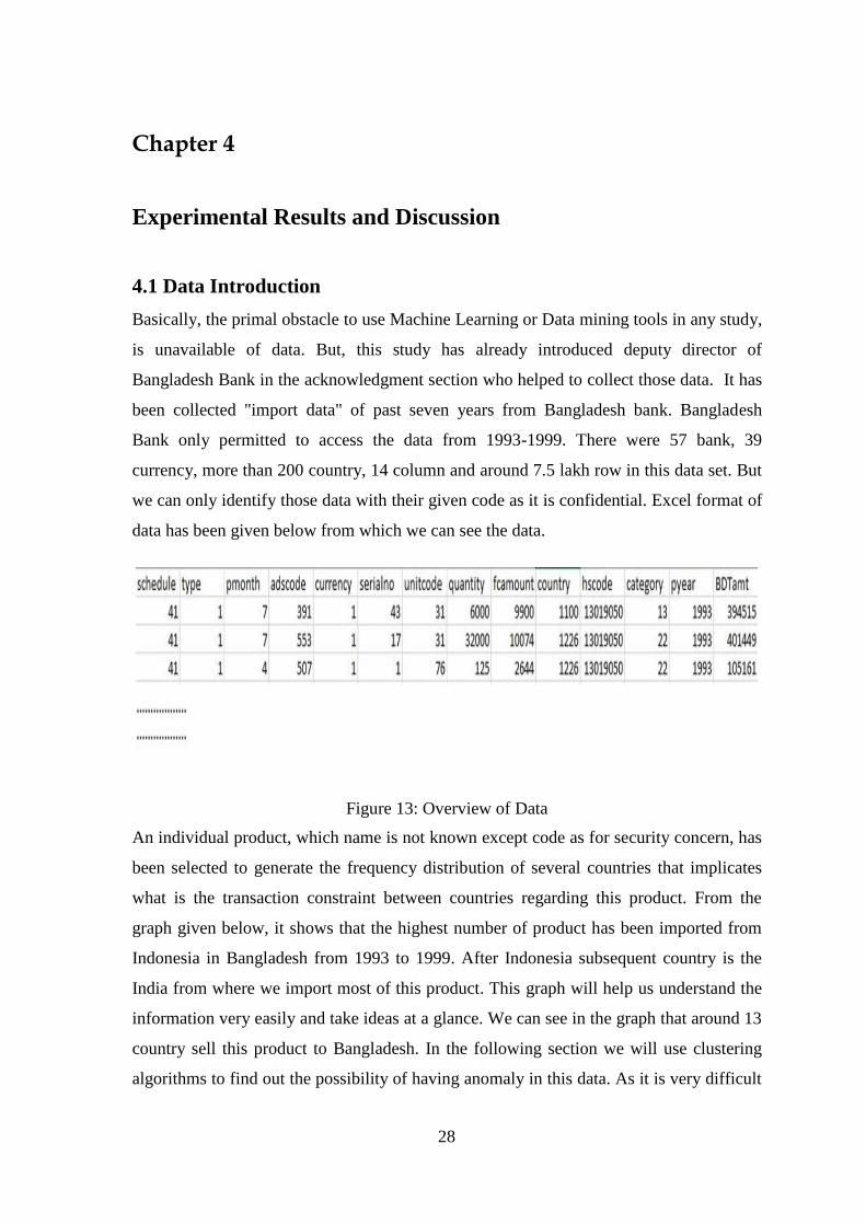
4.1 Data Introduction
Basically, the primal obstacle to use Machine Learning or Data mining tools in any study,
is unavailable of data. But, this study has already introduced deputy director of
Bangladesh Bank in the acknowledgment section who helped to collect those data. It has
been collected "import data" of past seven years from Bangladesh bank. Bangladesh
Bank only permitted to access the data from 1993-1999. There were 57 bank, 39
currency, more than 200 country, 14 column and around 7.5 lakh row in this data set. But
we can only identify those data with their given code as it is confidential. Excel format of
data has been given below from which we can see the data.
Figure 13: Overview of Data
An individual product, which name is not known except code as for security concern, has
been selected to generate the frequency distribution of several countries that implicates
what is the transaction constraint between countries regarding this product. From the
graph given below, it shows that the highest number of product has been imported from
Indonesia in Bangladesh from 1993 to 1999. After Indonesia subsequent country is the
India from where we import most of this product. This graph will help us understand the
information very easily and take ideas at a glance. We can see in the graph that around 13
country sell this product to Bangladesh. In the following section we will use clustering
algorithms to find out the possibility of having anomaly in this data. As it is very difficult
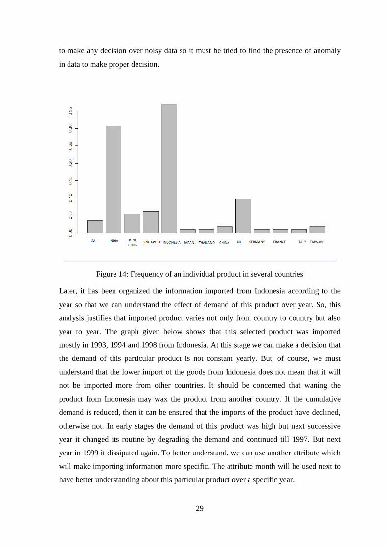
29
to make any decision over noisy data so it must be tried to find the presence of anomaly
in data to make proper decision.
Figure 14: Frequency of an individual product in several countries
Later, it has been organized the information imported from Indonesia according to the
year so that we can understand the effect of demand of this product over year. So, this
analysis justifies that imported product varies not only from country to country but also
year to year. The graph given below shows that this selected product was imported
mostly in 1993, 1994 and 1998 from Indonesia. At this stage we can make a decision that
the demand of this particular product is not constant yearly. But, of course, we must
understand that the lower import of the goods from Indonesia does not mean that it will
not be imported more from other countries. It should be concerned that waning the
product from Indonesia may wax the product from another country. If the cumulative
demand is reduced, then it can be ensured that the imports of the product have declined,
otherwise not. In early stages the demand of this product was high but next successive
year it changed its routine by degrading the demand and continued till 1997. But next
year in 1999 it dissipated again. To better understand, we can use another attribute which
will make importing information more specific. The attribute month will be used next to
have better understanding about this particular product over a specific year.
30
Figure 15: Frequency of an individual product in different year in Indonesia
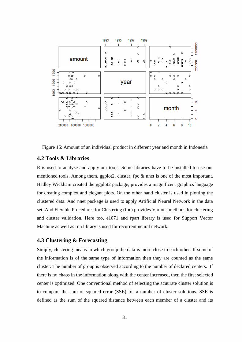
January is represented in the graph given below as 0 and December as 11.
This graph clearly expresses how much the product has been imported in any part of the
year including transacted amount. When we will use predictive models, then this idea will
give us the knowledge to decide whether it is correct or not. It has been plotted a
relationship between three attribute from data set, which depicts that the trading of this
product was high in 1993 but gradually waning as we discussed earlier. Another thing
that is seen here is that the product is imported mostly from July to September. And the
trading amount was between 2 to 6 lakh BDT according to the plotted figure. It is
difficult to analyze each month in 7 consecutive years, but it has to be done together to
understand. Although the information is not obscure, we will continue to do the next
work to find any oddity in this information available every month, which can be
detrimental to our predictive models.
31
Figure 16: Amount of an individual product in different year and month in Indonesia
4.2 Tools & Libraries
R is used to analyze and apply our tools. Some libraries have to be installed to use our
mentioned tools. Among them, ggplot2, cluster, fpc & nnet is one of the most important.
Hadley Wickham created the ggplot2 package, provides a magnificent graphics language
for creating complex and elegant plots. On the other hand cluster is used in plotting the
clustered data. And nnet package is used to apply Artificial Neural Network in the data
set. And Flexible Procedures for Clustering (fpc) provides Various methods for clustering
and cluster validation. Here too, e1071 and rpart library is used for Support Vector
Machine as well as rnn library is used for recurrent neural network.
4.3 Clustering & Forecasting
Simply, clustering means in which group the data is more close to each other. If some of
the information is of the same type of information then they are counted as the same
cluster. The number of group is observed according to the number of declared centers. If
there is no chaos in the information along with the center increased, then the first selected
center is optimized. One conventional method of selecting the acuurate cluster solution is
to compare the sum of squared error (SSE) for a number of cluster solutions. SSE is
defined as the sum of the squared distance between each member of a cluster and its
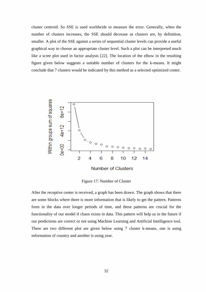
32
cluster centroid. So SSE is used worldwide to measure the error. Generally, when the
number of clusters increases, the SSE should decrease as clusters are, by definition,
smaller. A plot of the SSE against a series of sequential cluster levels can provide a useful
graphical way to choose an appropriate cluster level. Such a plot can be interpreted much
like a scree plot used in factor analysis [22]. The location of the elbow in the resulting
figure given below suggests a suitable number of clusters for the k-means. It might
conclude that 7 clusters would be indicated by this method as a selected optimized center.
Figure 17: Number of Cluster
After the receptive center is received, a graph has been drawn. The graph shows that there
are some blocks where there is more information that is likely to get the pattern. Patterns
form in the data over longer periods of time, and these patterns are crucial for the
functionality of our model if chaos exists in data. This pattern will help us in the future if
our predictions are correct or not using Machine Learning and Artificial Intelligence tool.
There are two different plot are given below using 7 cluster k-means, one is using
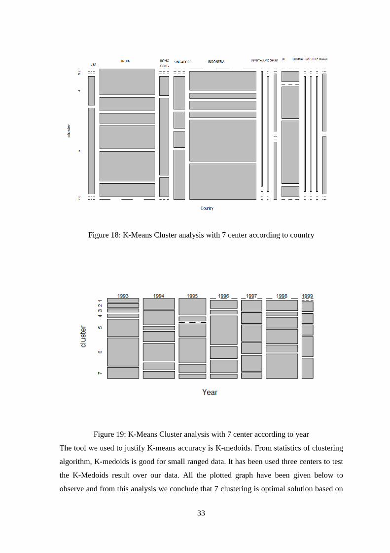
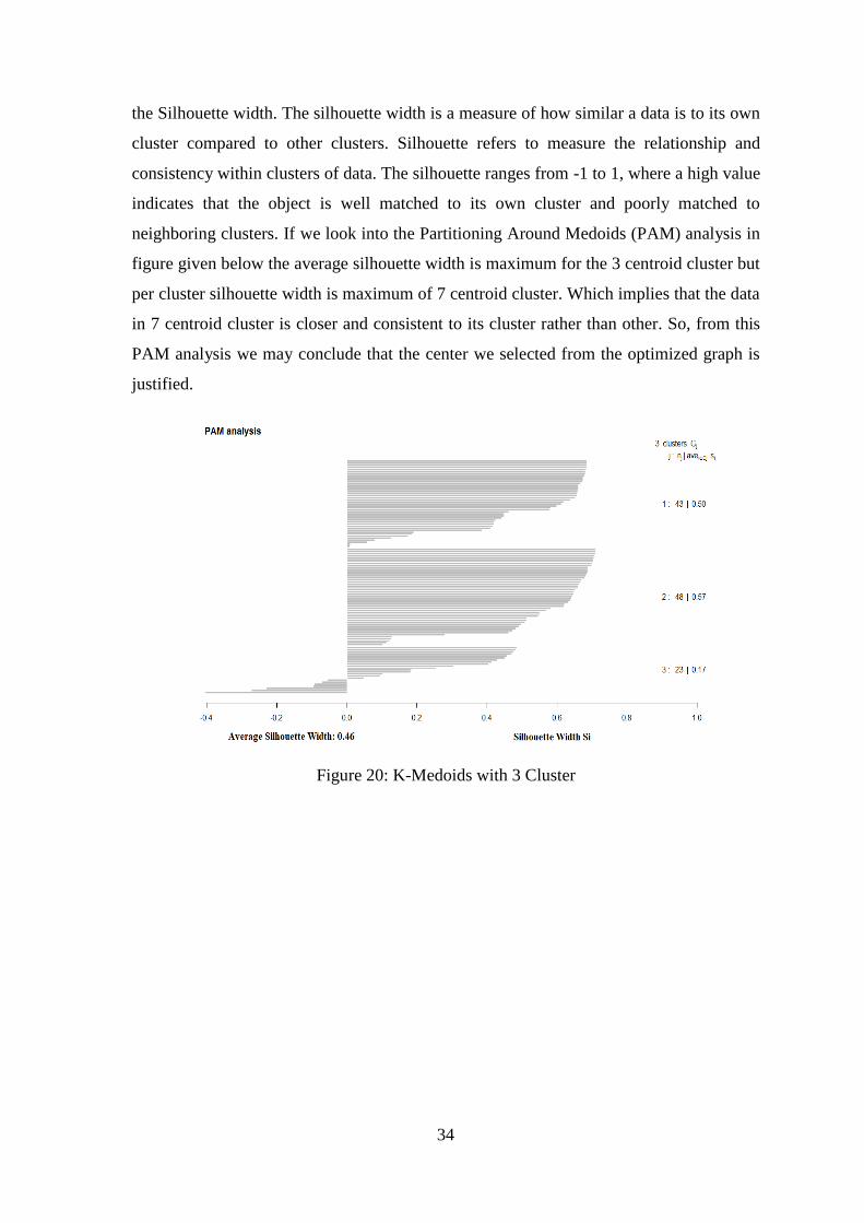
information of country and another is using year.
33
Figure 18: K-Means Cluster analysis with 7 center according to country
Figure 19: K-Means Cluster analysis with 7 center according to year
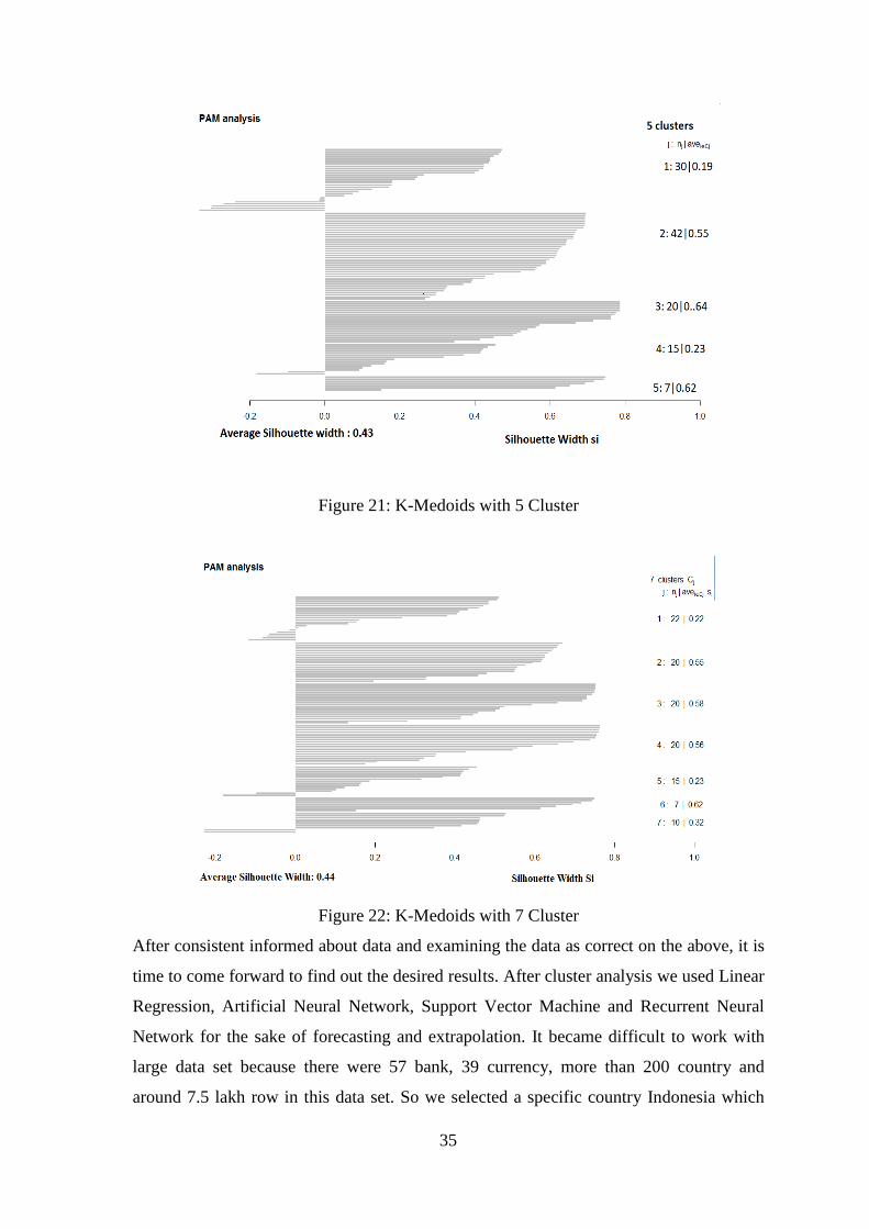
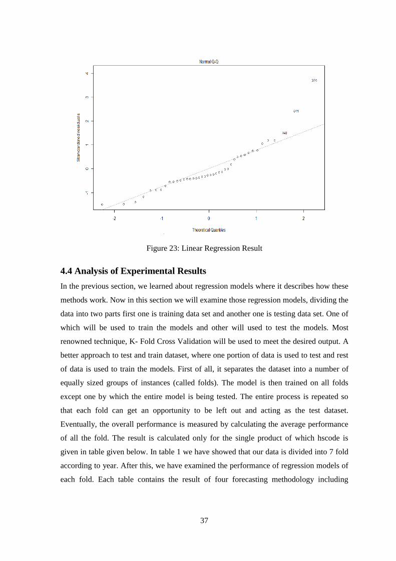
The tool we used to justify K-means accuracy is K-medoids. From statistics of clustering
algorithm, K-medoids is good for small ranged data. It has been used three centers to test
the K-Medoids result over our data. All the plotted graph have been given below to
observe and from this analysis we conclude that 7 clustering is optimal solution based on
34
the Silhouette width. The silhouette width is a measure of how similar a data is to its own
cluster compared to other clusters. Silhouette refers to measure the relationship and
consistency within clusters of data. The silhouette ranges from -1 to 1, where a high value
indicates that the object is well matched to its own cluster and poorly matched to
neighboring clusters. If we look into the Partitioning Around Medoids (PAM) analysis in
figure given below the average silhouette width is maximum for the 3 centroid cluster but
per cluster silhouette width is maximum of 7 centroid cluster. Which implies that the data
in 7 centroid cluster is closer and consistent to its cluster rather than other. So, from this
PAM analysis we may conclude that the center we selected from the optimized graph is
justified.
Figure 20: K-Medoids with 3 Cluster
35
Figure 21: K-Medoids with 5 Cluster
Figure 22: K-Medoids with 7 Cluster
After consistent informed about data and examining the data as correct on the above, it is
time to come forward to find out the desired results. After cluster analysis we used Linear
Regression, Artificial Neural Network, Support Vector Machine and Recurrent Neural
Network for the sake of forecasting and extrapolation. It became difficult to work with
large data set because there were 57 bank, 39 currency, more than 200 country and
around 7.5 lakh row in this data set. So we selected a specific country Indonesia which

36
reduced so many data to compute easily. A common practice is to split the data into a
training and test set. First train the model with separated training set and then test how
well it generalizes to data which has never seen before with the test set. So the model's
performance on given test set will provide insights on how the model is performing. For
the training purpose, the data of 6 year were selected based on fold as we have used k-
fold cross validation. And left one year is used for testing purpose. After training and
preparing Linear Regression, Artificial Neural Network, Support Vector Machine and
Recurrent Neural Network evaluation was necessary to check how accurate the result we
get from the tools. Eventually, three input were taken to compute the BDT amount. For
the neural network, the entire process is completed in two stages: the input values are
linearly united at first stage, after which the result is used as the argument of a nonlinear
activation function. The collector uses the weights wi for each connection and a constant
bias word, with a specific input equal to 1. The activation function must be a non-
decreasing and differentiable function; the most familiar is logistic function. After
applying the Linear Regression on the data set, looking at the trend line, it is understood
how close or far the information is from the trend line. The more close to trend line the
more the data is accurately predicted. Total four predictive method is used for
justification for another because to conclude any decision we must have some
justification with proper authority. In the next section we have discussed briefly about the
result what we have experienced with proper comments. In Statistics, Linear Regression
has been successfully used, but Artificial Intelligence has been very successful in the
Machine Learning, which has also been observed in our study. Recently, Support Vector
Machine and Recurrent Neural Network has become popular and efficient in research
purpose.
37
Figure 23: Linear Regression Result
4.4 Analysis of Experimental Results
In the previous section, we learned about regression models where it describes how these
methods work. Now in this section we will examine those regression models, dividing the
data into two parts first one is training data set and another one is testing data set. One of
which will be used to train the models and other will used to test the models. Most
renowned technique, K- Fold Cross Validation will be used to meet the desired output. A
better approach to test and train dataset, where one portion of data is used to test and rest
of data is used to train the models. First of all, it separates the dataset into a number of
equally sized groups of instances (called folds). The model is then trained on all folds
except one by which the entire model is being tested. The entire process is repeated so
that each fold can get an opportunity to be left out and acting as the test dataset.
Eventually, the overall performance is measured by calculating the average performance
of all the fold. The result is calculated only for the single product of which hscode is
given in table given below. In table 1 we have showed that our data is divided into 7 fold
according to year. After this, we have examined the performance of regression models of
each fold. Each table contains the result of four forecasting methodology including
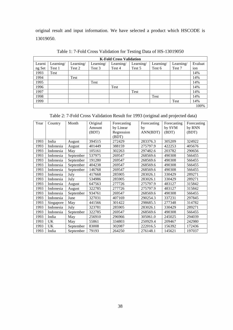
38
original result and input information. We have selected a product which HSCODE is
13019050.
Table 1: 7-Fold Cross Validation for Testing Data of HS-13019050
K-Fold Cross Validation
Learni
ng Set
Learning/
Test 1
Learning/
Test 2
Learning/
Test 3
Learning/
Test 4
Learning/
Test 5
Learning/
Test 6
Learning/
Test 7
Evaluat
ion
1993 Test 14%
1994 Test 14%
1995 Test 14%
1996 Test 14%
1997 Test 14%
1998 Test 14%
1999 Test 14%
100%
Table 2: 7-Fold Cross Validation Result for 1993 (original and projected data)
Year Country Month Original
Amount
(BDT)
Forecasting
by Linear
Regression
(BDT)
Forecasting
by
ANN(BDT)
Forecasting
by SVM
(BDT)
Forecasting
by RNN
(BDT)
1993 India August 394515 272429 283376.3 305209 324922
1993 Indonesia August 401449 388159 275797.9 422253 405676
1993 Indonesia May 105161 302263 297482.6 203782 290656
1993 Indonesia September 537975 269547 268569.6 490308 566455
1993 Indonesia September 191280 269547 268569.6 490308 566455
1993 Indonesia September 404238 269547 268569.6 490308 566455
1993 Indonesia September 146768 269547 268569.6 490308 566455
1993 Indonesia July 417668 285905 283026.1 330429 289271
1993 Indonesia July 534986 285905 283026.1 330429 289271
1993 Indonesia August 647563 277726 275797.9 483127 315842
1993 Indonesia August 322785 277726 275797.9 483127 315842
1993 Indonesia September 934761 269547 268569.6 490308 566455
1993 Indonesia June 327031 407169 290254.3 337231 297845
1993 Singapore May 441566 301422 298685.5 277348 314782
1993 Indonesia July 323781 285905 283026.1 330429 289271
1993 Indonesia September 322785 269547 268569.6 490308 566455
1993 India May 256910 296966 305061.0 245025 294039
1993 UK May 55861 334803 250929.4 209467 242980
1993 UK September 83008 302087 222016.5 156392 172436
1993 India September 79193 264250 276148.1 145621 197037
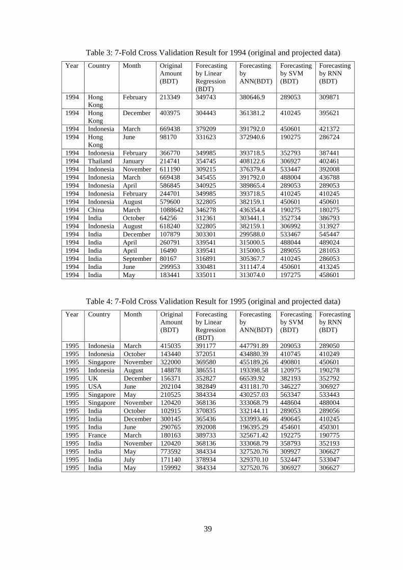
39
Table 3: 7-Fold Cross Validation Result for 1994 (original and projected data)
Year Country Month Original
Amount
(BDT)
Forecasting
by Linear
Regression
(BDT)
Forecasting
by
ANN(BDT)
Forecasting
by SVM
(BDT)
Forecasting
by RNN
(BDT)
1994 Hong
Kong
February 213349 349743 380646.9 289053 309871
1994 Hong
Kong
December 403975 304443 361381.2 410245 395621
1994 Indonesia March 669438 379209 391792.0 450601 421372
1994 Hong
Kong
June 98170 331623 372940.6 190275 286724
1994 Indonesia February 366770 349985 393718.5 352793 387441
1994 Thailand January 214741 354745 408122.6 306927 402461
1994 Indonesia November 611190 309215 376379.4 533447 392008
1994 Indonesia March 669438 345455 391792.0 488004 436788
1994 Indonesia April 586845 340925 389865.4 289053 289053
1994 Indonesia February 244701 349985 393718.5 410245 410245
1994 Indonesia August 579600 322805 382159.1 450601 450601
1994 China March 1088642 346278 436354.4 190275 180275
1994 India October 64256 312361 303441.1 352734 386793
1994 Indonesia August 618240 322805 382159.1 306992 313927
1994 India December 107879 303301 299588.0 533467 545447
1994 India April 260791 339541 315000.5 488044 489024
1994 India April 16490 339541 315000.5 289055 281053
1994 India September 80167 316891 305367.7 410245 286053
1994 India June 299953 330481 311147.4 450601 413245
1994 India May 183441 335011 313074.0 197275 458601
Table 4: 7-Fold Cross Validation Result for 1995 (original and projected data)
Year Country Month Original
Amount
(BDT)
Forecasting
by Linear
Regression
(BDT)
Forecasting
by
ANN(BDT)
Forecasting
by SVM
(BDT)
Forecasting
by RNN
(BDT)
1995 Indonesia March 415035 391177 447791.89 209053 289050
1995 Indonesia October 143440 372051 434880.39 410745 410249
1995 Singapore November 322000 369580 455189.26 490801 450601
1995 Indonesia August 148878 386551 193398.58 120975 190278
1995 UK December 156371 352827 66539.92 382193 352792
1995 USA June 202104 382849 431181.70 346227 306927
1995 Singapore May 210525 384334 430257.03 563347 533443
1995 Singapore November 120420 368136 333068.79 448604 488004
1995 India October 102915 370835 332144.11 289053 289056
1995 India December 300145 365436 333993.46 490645 410245
1995 India June 290765 392008 196395.29 454601 450301
1995 France March 180163 389733 325671.42 192275 190775
1995 India November 120420 368136 333068.79 358793 352193
1995 India May 773592 384334 327520.76 309927 306627
1995 India July 171140 378934 329370.10 532447 533047
1995 India May 159992 384334 327520.76 306927 306627
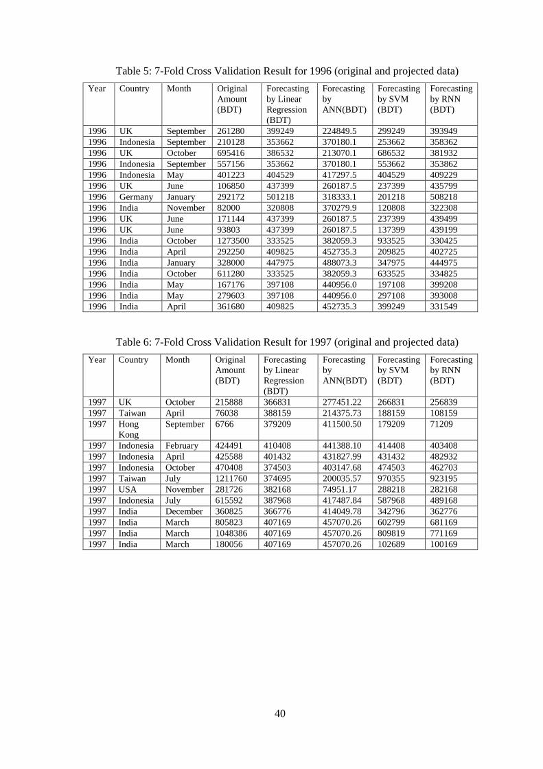
40
Table 5: 7-Fold Cross Validation Result for 1996 (original and projected data)
Year Country Month Original
Amount
(BDT)
Forecasting
by Linear
Regression
(BDT)
Forecasting
by
ANN(BDT)
Forecasting
by SVM
(BDT)
Forecasting
by RNN
(BDT)
1996 UK September 261280 399249 224849.5 299249 393949
1996 Indonesia September 210128 353662 370180.1 253662 358362
1996 UK October 695416 386532 213070.1 686532 381932
1996 Indonesia September 557156 353662 370180.1 553662 353862
1996 Indonesia May 401223 404529 417297.5 404529 409229
1996 UK June 106850 437399 260187.5 237399 435799
1996 Germany January 292172 501218 318333.1 201218 508218
1996 India November 82000 320808 370279.9 120808 322308
1996 UK June 171144 437399 260187.5 237399 439499
1996 UK June 93803 437399 260187.5 137399 439199
1996 India October 1273500 333525 382059.3 933525 330425
1996 India April 292250 409825 452735.3 209825 402725
1996 India January 328000 447975 488073.3 347975 444975
1996 India October 611280 333525 382059.3 633525 334825
1996 India May 167176 397108 440956.0 197108 399208
1996 India May 279603 397108 440956.0 297108 393008
1996 India April 361680 409825 452735.3 399249 331549
Table 6: 7-Fold Cross Validation Result for 1997 (original and projected data)
Year Country Month Original
Amount
(BDT)
Forecasting
by Linear
Regression
(BDT)
Forecasting
by
ANN(BDT)
Forecasting
by SVM
(BDT)
Forecasting
by RNN
(BDT)
1997 UK October 215888 366831 277451.22 266831 256839
1997 Taiwan April 76038 388159 214375.73 188159 108159
1997 Hong
Kong
September 6766 379209 411500.50 179209 71209
1997 Indonesia February 424491 410408 441388.10 414408 403408
1997 Indonesia April 425588 401432 431827.99 431432 482932
1997 Indonesia October 470408 374503 403147.68 474503 462703
1997 Taiwan July 1211760 374695 200035.57 970355 923195
1997 USA November 281726 382168 74951.17 288218 282168
1997 Indonesia July 615592 387968 417487.84 587968 489168
1997 India December 360825 366776 414049.78 342796 362776
1997 India March 805823 407169 457070.26 602799 681169
1997 India March 1048386 407169 457070.26 809819 771169
1997 India March 180056 407169 457070.26 102689 100169
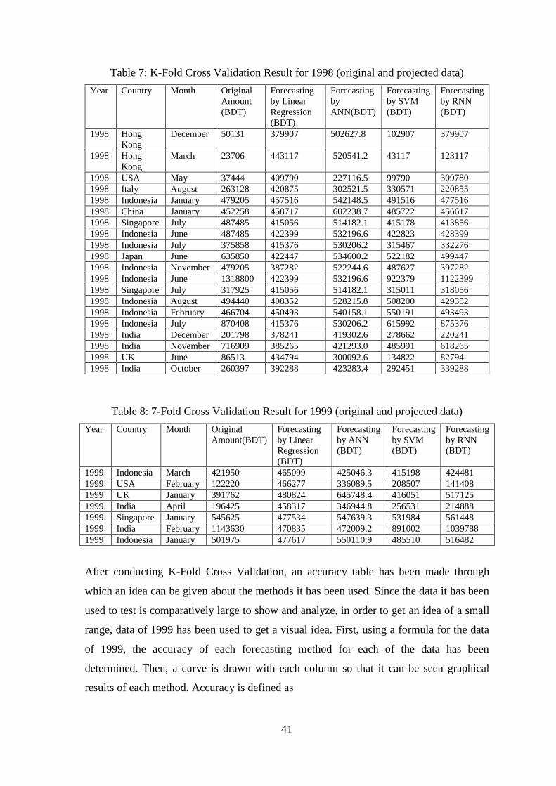
41
Table 7: K-Fold Cross Validation Result for 1998 (original and projected data)
Year Country Month Original
Amount
(BDT)
Forecasting
by Linear
Regression
(BDT)
Forecasting
by
ANN(BDT)
Forecasting
by SVM
(BDT)
Forecasting
by RNN
(BDT)
1998 Hong
Kong
December 50131 379907 502627.8 102907 379907
1998 Hong
Kong
March 23706 443117 520541.2 43117 123117
1998 USA May 37444 409790 227116.5 99790 309780
1998 Italy August 263128 420875 302521.5 330571 220855
1998 Indonesia January 479205 457516 542148.5 491516 477516
1998 China January 452258 458717 602238.7 485722 456617
1998 Singapore July 487485 415056 514182.1 415178 413856
1998 Indonesia June 487485 422399 532196.6 422823 428399
1998 Indonesia July 375858 415376 530206.2 315467 332276
1998 Japan June 635850 422447 534600.2 522182 499447
1998 Indonesia November 479205 387282 522244.6 487627 397282
1998 Indonesia June 1318800 422399 532196.6 922379 1122399
1998 Singapore July 317925 415056 514182.1 315011 318056
1998 Indonesia August 494440 408352 528215.8 508200 429352
1998 Indonesia February 466704 450493 540158.1 550191 493493
1998 Indonesia July 870408 415376 530206.2 615992 875376
1998 India December 201798 378241 419302.6 278662 220241
1998 India November 716909 385265 421293.0 485991 618265
1998 UK June 86513 434794 300092.6 134822 82794
1998 India October 260397 392288 423283.4 292451 339288
Table 8: 7-Fold Cross Validation Result for 1999 (original and projected data)
Year Country Month Original
Amount(BDT)
Forecasting
by Linear
Regression
(BDT)
Forecasting
by ANN
(BDT)
Forecasting
by SVM
(BDT)
Forecasting
by RNN
(BDT)
1999 Indonesia March 421950 465099 425046.3 415198 424481
1999 USA February 122220 466277 336089.5 208507 141408
1999 UK January 391762 480824 645748.4 416051 517125
1999 India April 196425 458317 346944.8 256531 214888
1999 Singapore January 545625 477534 547639.3 531984 561448
1999 India February 1143630 470835 472009.2 891002 1039788
1999 Indonesia January 501975 477617 550110.9 485510 516482
After conducting K-Fold Cross Validation, an accuracy table has been made through
which an idea can be given about the methods it has been used. Since the data it has been
used to test is comparatively large to show and analyze, in order to get an idea of a small
range, data of 1999 has been used to get a visual idea. First, using a formula for the data
of 1999, the accuracy of each forecasting method for each of the data has been
determined. Then, a curve is drawn with each column so that it can be seen graphical
results of each method. Accuracy is defined as
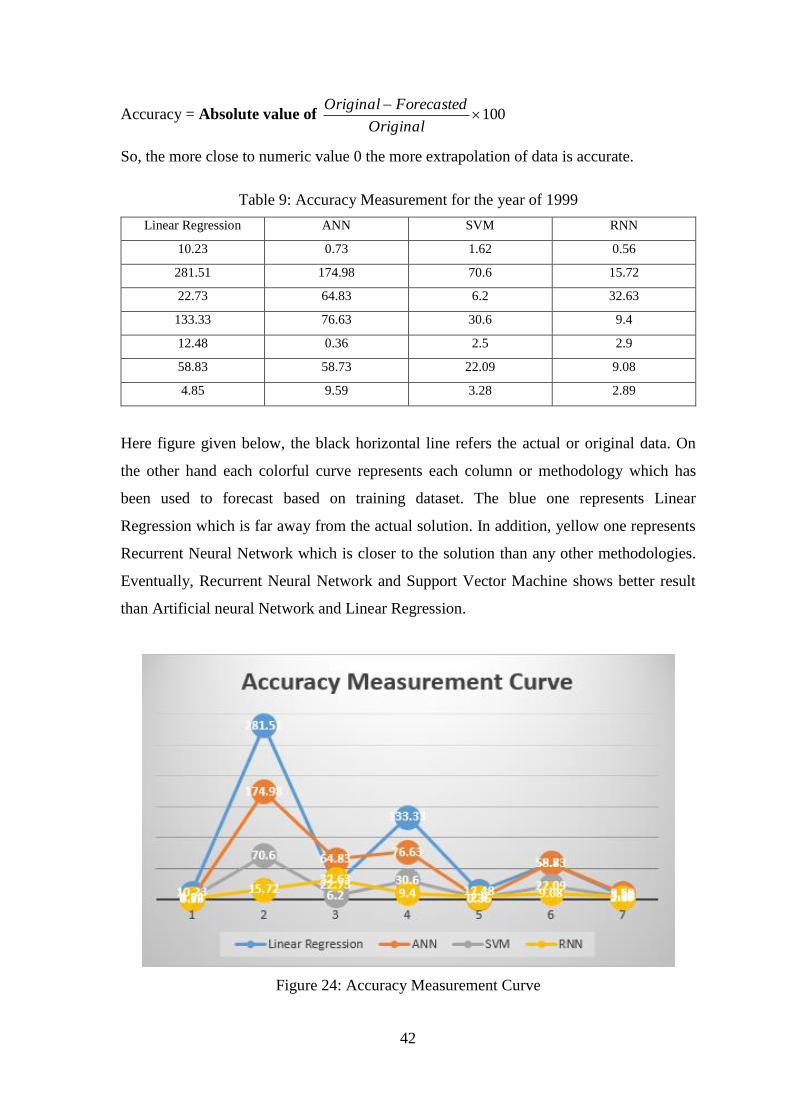
42
Accuracy = Absolute value of 100
Original
ForecastedOriginal
So, the more close to numeric value 0 the more extrapolation of data is accurate.
Table 9: Accuracy Measurement for the year of 1999
Linear Regression ANN SVM RNN
10.23 0.73 1.62 0.56
281.51 174.98 70.6 15.72
22.73 64.83 6.2 32.63
133.33 76.63 30.6 9.4
12.48 0.36 2.5 2.9
58.83 58.73 22.09 9.08
4.85 9.59 3.28 2.89
Here figure given below, the black horizontal line refers the actual or original data. On
the other hand each colorful curve represents each column or methodology which has
been used to forecast based on training dataset. The blue one represents Linear
Regression which is far away from the actual solution. In addition, yellow one represents
Recurrent Neural Network which is closer to the solution than any other methodologies.
Eventually, Recurrent Neural Network and Support Vector Machine shows better result
than Artificial neural Network and Linear Regression.
Figure 24: Accuracy Measurement Curve
43
If it is possible to train all the methods with information from all the past years, then it
can forecast more precisely and accurately how our imported goods may be in the coming
years. Though all the result which is got from this study is hypothetical but it can be a
strategic steps to ensure prosperity and strengthen the economy of a country.
4.5 Conclusion
The most difficult thing to do at the beginning was to collect data that the Bangladesh
Bank has given permission to access. Later it was very important to get ideas about the
information that some formula of statistics have helped us to understand precisely.
Because it is very difficult to know about the work and to know about the next steps if
there is no good sense of data. In spite of many inconveniences we have been able to do it
and we have also fixed some of its authenticity through K-Means clustering
methodologies. One clustering algorithm is actively used for justification for another.
After clustering process prediction process was adopted in this study. Finally, it has
provided methodologies for the prediction for which it has been divided the data into two
sections first on for training and last one for testing purpose. Basically, K-fold cross
validation was used to separate the entire data. And after the test, we got some errors
which can be reduced if we can train our methodologies with more information if
Bangladesh Bank permitted but it should be kept in mind that methods should not be over
fitting. This study can help us to explain more clearly how the imports can be in the next
years.
44
Chapter 5
Conclusion and Future Works
5.1 Conclusion
Product and service forecasting is considered as the value of forecasts to change the
ownership of asset resources and services among others in an economy. Forecasting has
been appreciated in the countries of the economic sector and created in the world
economy, using a combination of model-based analysis and sage judgments. Exponent
increases net trade, import and export and export markets improvement. Net trade is the
amount which is identified by the difference between exports and the imports; imports
and exports are the amount of goods or services imported or exported from different
country or economies; the demand for a country’s exports is measured by the export
market growth which is constructed as a weighted average of import growth in all export
destinations using export shares as weights. This index is measured for the net trade, the
annual growth rate for exports and the importation and the US dollar. So it is very
important to know the upcoming net trade for a developing country which is not possible
without forecasting import commodities and domestic production for export purposes. On
the other hand, there are possibilities of some products which are already imported which
are imported annually. Then government has some policy to make which will be lucrative
for this nation. If this product is imported by government then it should be decreased. On
the other hand if this product is imported by private sector then imposing tax or tariff will
make most benefit for this nation.
If an analysis is done between the domestic and the Indian onions, then it is seen that if
the price of domestic onions is low or equal to Indian onions, then the demand of Indian
onion is shifted to the left which means decreasing the demand of Indian onions. On the
other hand if the price of domestic onions is high than Indian onions then the opposite
happens. To increase the domestic profit Bangladesh should increase the price of
domestic onions which may help government to invest more money in the production of
domestic onions. As a result, this investment will help in increasing the supply of
domestic onions. But as well as imposing taxes on Indian onions, the price of domestic
45
products will be equal to Indian which will keep local market demand better as well as
increasing domestic profits for Bangladesh. But before investing Net Present Value and
Return on Investment should be considered carefully because any unremunerated
decision may cause the economic and political crisis. In the annual budget announcement,
it is verified about these decisions and to take necessary steps. But budgets are not
publicly provided in private sector, like public sector. To talk about private sector they
have product lines so their strategy is different from the public sector. It is hoped that
both sector will be benefited from this study.
5.2 Future Works
After a brief analysis of this study it should be memorized that the only purpose of this
work is to enlighten the critical section of our economy. As a result it will be helpful to
make decision on a particular situation based on analysis. In this study, it remains space
for the future research and development on several fields which can be carried on like
most profitable commodity selection using decision tree, and lucrative budget
combination for import sector using genetic algorithm.
46
References
[1] Michael Todaro and Stephen C. Smith, "Economic Development" (11th ed.). Pearson
Education and Addison-Wesley (2011).
[2] Sen, A (1983). "Development: Which Way Now?". Economic Journal. 93 (372): 745–
62. doi:10.2307/2232744.
[3] Hirschman, A. O. (1981). The Rise and Decline of Development Economics. Essays
in Trespassing: Economics to Politics to Beyond. pp. 1–24.
[4] Hoggson, N. F. (1926) Banking Through the Ages, New York, Dodd, Mead &
Company.
[5] Goldthwaite, R. A. Banks, Places and Entrepreneurs in Renaissance Florence, (1995)
[6] Boland, Vincent (2009-06-12). "Modern dilemma for world's oldest bank". Financial
Times. Retrieved 23 February 2010.
[7] Boone and Kurtz, “Contemporary Business,” 16th edition.
[8] A. Ganesh-Kumar, Sanjay K. Prasad and Hemant Pullabhotla, “Supply and Demand
for Cereals in Bangladesh, 2010–2030,” June 2012.
[9] M.A.A. Hasin, S. Ghosh, M.A. Shareef, “An ANN Approach to Demand Forecasting
in Retail Trade in Bangladesh”, International Journal of Trade, Economics and Finance,
vol. 2, no. 2, April 2011.
[10] G. Atsalakis, C.I. Ucenic, C. H. Skiadas, “Forecasting Unemployment Rate Using a
Neural Network with Fuzzy Inference System,” ICAP, 2007.
[11] L.M. Liu, S. Bhattacharyya, S.L. Sclove, R. Chen, W. J. Lattyak, “Data Mining on
Time Series: An Illustration Using Fast-Food Restaurant Franchise Data”, Computational
Statistics & Data Analysis, vol. 37, pp. 455-476, 2001.
[12] P.C. Chang, Y.W. Wang, C.H. Liu, “The Development of a Weighted Evolving
Fuzzy Neural Network for PCB Sales Forecasting”, Expert Systems with Applications,
vol.32, pp. 86- 96, 2007.
[13] Z.L. Sun, T.M. Choi, K.F. AU, Y. Yu, “Sales Forecasting Using Extreme Learning
Machine With Applications In Fashion Retailing”, Decision Support Systems, vol. 46, pp.
411-419, December 2008.
47
[14] Y. Yu, T. Choi, C. Hui, “An Intelligent Fast Sales Forecasting Model for Fashion
Products”, Expert System with Applications, vol. 38, pp. 7373-7379, 2011.
[15] S.H. Ling, “Genetic Algorithm and Variable Neural Networks: Theory and
Application”, Lambert Academic Publishing, 2010.
[16] K.F. Au, T.M. Choi, Y. Yu, “Fashion Retail Forecasting by Evolutionary Neural
Networks”, International Journal of Production Economics, vol. 114, pp.615-630, 2008.
[17] R.S. Gutierrez, A. Solis, S. Mukhopadhyay, “Lumpy Demand Forecasting Using
Neural Networks”, International Journal of Production Economics, vol. 111, pp. 409-420,
2008.
[18] P. Doganis, A. Alexandridis, P. Patrinos, H. Sarimveis, “Time Series Sales
Forecasting For Short Shelf-Life Food Products Based On Artificial Neural Networks
And Evolutionary Computing”, Journal Of Food Engineering, vol. 75, pp. 196-204, 2006.
[19] L. Aburto, R. Weber, “Improved supply chain management based on hybrid demand
forecasts”, Applied Soft Computing, 2007.
[20] Nahida Sultana Ebney Ayaj Rana, and Rashed Al Mahmud Titumir “Export, Import,
Remittance and FDI: Recent Trends,” Bangladesh Economic Update vol. 5, No. 4, April
2014.
[21] Henrique Steinherz Hippert, Carlos Eduardo Pedreira, and Reinaldo Castro Souza,
Neural Networks for Short-Term Load Forecasting: A Review and Evaluation, IEEE
Transactions on Power Systems, Vol. 16, February 2001.
[22] Peeples, Matthew A. “R Script for K-Means Cluster Analysis”, 2011. Electronic
document, http://www.mattpeeples.net/kmeans.html, [accessed January 27, 2018.]