Motion planning of multi-robot system for airplane stripping
167
HAL Id: tel-02284448 https://tel.archives-ouvertes.fr/tel-02284448 Submitted on 11 Sep 2019 HAL is a multi-disciplinary open access archive for the deposit and dissemination of sci- entific research documents, whether they are pub- lished or not. The documents may come from teaching and research institutions in France or abroad, or from public or private research centers. L’archive ouverte pluridisciplinaire HAL, est destinée au dépôt et à la diffusion de documents scientifiques de niveau recherche, publiés ou non, émanant des établissements d’enseignement et de recherche français ou étrangers, des laboratoires publics ou privés. Motion planning of multi-robot system for airplane stripping Rawan Kalawoun To cite this version: Rawan Kalawoun. Motion planning of multi-robot system for airplane stripping. Robotics [cs.RO]. Université Clermont Auvergne [2017-2020], 2019. English. NNT: 2019CLFAC008. tel-02284448
-
Upload
khangminh22 -
Category
Documents
-
view
0 -
download
0
Transcript of Motion planning of multi-robot system for airplane stripping

HAL Id: tel-02284448https://tel.archives-ouvertes.fr/tel-02284448
Submitted on 11 Sep 2019
HAL is a multi-disciplinary open accessarchive for the deposit and dissemination of sci-entific research documents, whether they are pub-lished or not. The documents may come fromteaching and research institutions in France orabroad, or from public or private research centers.
L’archive ouverte pluridisciplinaire HAL, estdestinée au dépôt et à la diffusion de documentsscientifiques de niveau recherche, publiés ou non,émanant des établissements d’enseignement et derecherche français ou étrangers, des laboratoirespublics ou privés.
Motion planning of multi-robot system for airplanestripping
Rawan Kalawoun
To cite this version:Rawan Kalawoun. Motion planning of multi-robot system for airplane stripping. Robotics [cs.RO].Université Clermont Auvergne [2017-2020], 2019. English. �NNT : 2019CLFAC008�. �tel-02284448�

Ecole doctorale no70: Sciences pour l’ingenieur
THESE
pour obtenir le grade de docteur delivre par l’
Universite Clermont AuvergneSpecialite doctorale “Electronique et Systemes”
presentee et soutenue publiquement par
Rawan KALAWOUN
le 26 Avril 2019
Motion planning of multi-robot system for airplanestripping
JuryNacim Ramdani, Professeur des universites, PRISME (Bourges) RapporteurPhilippe Fraisse, Professeur des universites, LIRMM (Montpellier) RapporteurFabrice Le Bars, Maıtre de conferences, Lab-STICC (Brest) ExaminateurOuiddad Labbani-Igbida, Professeur des universites, XLIM (Limoges) ExaminatriceYoucef Mezouar, Professeur des universites, Institut Pascal (Aubiere) DirecteurSebastien Lengagne, Maıtre de conferences, Institut Pascal (Aubiere) Encadrant
Universite Clermont Auvergne - SIGMA ClermontInstitut Pascal, UMR 6602 CNRS/UCA/SIGMA Clermont, F-63171 Aubiere, France

Abstract
This PHD is a part of a French project named AEROSTRIP, (a partnership between Pascal Institute,
Sigma, SAPPI, and Air-France industries), it is funded by the French Government through the FUI
Program (20th call). The AEROSTRIP project aims at developing the first automated system that
ecologically cleans the airplanes surfaces using a process of soft projection of ecological media on
the surface (corn). My PHD aims at optimizing the trajectory of the whole robotic systems in order
to optimally strip the airplane. Since a large surface can not be totally covered by a single robot base
placement, repositioning of the robots is necessary to ensure a complete stripping of the surface. The
goal in this work is to find the optimal number of robots with their optimal positions required to totally
strip the air-plane. Once found, we search for the trajectories of the robots of the multi-robot system
between those poses. Hence, we define a general framework to solve this problem having four main
steps: the pre-processing step, the optimization algorithm step, the generation of the end-effector
trajectories step and the robot scheduling, assignment and control step.
In my thesis, I present two contributions in two different steps of the general framework: the pre-
processing step, the optimization algorithm step. The computation of the robot workspace is required
in the pre-processing step: we proposed Interval Analysis to find this workspace since it guaran-
tees finding solutions in a reasonable computation time. Though, our first contribution is a new
inclusion function that reduces the pessimism, the overestimation of the solution, which is the main
disadvantage of Interval Analysis. The proposed inclusion function is assessed on some Constraints
Satisfaction Problems and Constraints Optimization problems. Furthermore, we propose an hybrid
optimization algorithm in order to find the optimal number of robots with their optimal poses: it is our
second contribution in the optimization algorithm step. To assess our hybrid optimization algorithm,
we test the algorithm on regular surfaces, such as a cylinder and a hemisphere, and on a complex
surface: a car.
Resume
Cette these est une partie d’un projet francais qui s’appelle AEROSTRIP, un partenariat entre l’Institut
Pascal, Sigma, SAPPI et Air-France industries, il est finance par le gouvernement francais par le pro-
i

gramme FUI (20eme appel). Le projet AEROSTRIP consiste a developper le premier systeme au-
tomatique qui nettoie ecologiquement les surfaces des avions et les pieces de rechange en utilisant un
abrasif ecologique projete a grande vitesse sur la surface des avions (maıs). Ma these consiste a opti-
miser les trajectoires du systeme robotique total de telle facon que le decapage de l’avion soit optimal.
Le deplacement des robots est necessaire pour assurer une couverture totale de la surface a decaper
parce que ces surfaces sont trop grandes et elles ne peuvent pas etre decapees d’une seule position.
Le but de mon travail est de trouver le nombre optimal de robots avec leur positions optimales pour
decaper totalement l’avion. Une fois ce nombre est determine, on cherche les trajectoires des robots
entre ces differentes positions. Alors, pour atteindre ce but, j’ai defini un cadre general composant de
quatre etapes essentiels: l’etape pre-processing, l’etape optimization algorithm, l’etape generation of
the end-effector trajectories et l’etape robot scheduling, assignment and control.
Dans ma these, j’ai deux contributions dans deux differentes etapes du cadre general: l’etape pre-
processing et l’etape optimization algorithm. Le calcul de l’espace de travail du robot est necessaire
dans l’etape pre-processing: on a propose l’Analyse par Intervalles pour trouver cet espace de tra-
vail parce qu’il garantie le fait de trouver des solutions dans un temps de calcul raisonnable. Alors,
ma premiere contribution est une nouvelle fonction d’inclusion qui reduit le pessimisme, la sures-
timation des solutions qui est le principal inconvenient de l’Analyse par Intervalles. La nouvelle
fonction d’inclusion est evaluee sur des problemes de satisfaction de contraintes et des problemes
d’optimisation des contraintes. En plus, on a propose un algorithme d’optimisation hybride pour
trouver le nombre optimal de robots avec leur positions optimales: c’est notre deuxieme contribu-
tion qui est dans l’etape optimization algorithm. Pour evaluer l’algorithme d’optimisation, on a teste
cet algorithme sur des surfaces regulieres, comme un cylindre et un hemisphere, et sur un surface
complexe: une voiture.
ii

Acknowledgements
The presented thesis was developed at Institut Pascal in the Modelling, Autonomy and Control in
Complex system (MACCS) team of ISPR (Images, Perception systems and Robotics) group. I would
like to express my sincere gratitude to this team for giving me the opportunity to participate and
collaborate in meaningful research trends. Without the MACCS team, this thesis would not have
been possible. Undertaking this PhD has been a truly life-changing experience for me and it would
not have been possible to do without the support and guidance that I received from many people.
This work would not have been possible without the financial support of AEROSTRIP project, a
French project funded by the French Government through the FUI Program (20th call). I would like to
express my sincere gratitude to my supervisors Prof. Youcef MEZOUAR and Sebastien LENGAGNE
for the continuous support of my Ph.D study and related research, for their patience, motivation and
immense knowledge. Their guidance helped me in all the time of research and writing of this thesis.
Besides my advisers, I thank my fellow lab-mates, colleagues and professors at the Institut Pascal for
the stimulating discussions, the unconditional support, the invaluable collaboration along the thesis
and the addition of positives experiences in my work and life. I would like to thank all my PhD
colleagues, with whom I have shared moments of deep anxiety but also of big excitement. Their
presence was very important in a process that is often felt as tremendously solitaire.
Some special words of gratitude go to my friends who have always been a major source of support
when things would get a bit discouraging: Dana, Kamal, Hadi, Jessica, Chadi, Rohit, Jose and Mo-
hamed. Thanks guys for always being there for me.
A very special word of thanks goes for my parents, Maamoun and Amina, who have been great over
the years and never raised an eyebrow when I claimed my thesis would be finished “in the next two
weeks” for nearly a year. My hard-working parents have sacrificed their lives for my sisters, my
brother and myself and provided unconditional love and care. I love them so much, and I would not
have made it this far without them. My sisters, Ranime Razan and Ghina, and my brother Mohamad,
have been my best friends all my life and I love them dearly and thank them for all their advice and
support.
iii

iv

Contents
Acknowledgements iii
1 General Introduction 1
1.1 Problematic, Motivation and Objectives . . . . . . . . . . . . . . . . . . . . . . . . 1
1.1.1 Ecological stripping process using corn (AEROSTRIP): . . . . . . . . . . . 4
1.1.2 Project consortiums . . . . . . . . . . . . . . . . . . . . . . . . . . . . . . . 9
1.2 Thesis approach . . . . . . . . . . . . . . . . . . . . . . . . . . . . . . . . . . . . 11
1.2.1 General framework: . . . . . . . . . . . . . . . . . . . . . . . . . . . . . . 11
1.2.2 General problem . . . . . . . . . . . . . . . . . . . . . . . . . . . . . . . . 14
1.3 Manuscript structure . . . . . . . . . . . . . . . . . . . . . . . . . . . . . . . . . . 15
2 State of the art 16
2.1 Robot constraints projections on the surface . . . . . . . . . . . . . . . . . . . . . . 17
2.1.1 Robotic Workspace . . . . . . . . . . . . . . . . . . . . . . . . . . . . . . . 18
2.1.2 Survey on Interval Analysis . . . . . . . . . . . . . . . . . . . . . . . . . . 19
2.2 Optimization of the number of robots . . . . . . . . . . . . . . . . . . . . . . . . . 21
v

vi CONTENTS
2.2.1 Art Gallery History . . . . . . . . . . . . . . . . . . . . . . . . . . . . . . . 21
2.2.2 Camera placement application . . . . . . . . . . . . . . . . . . . . . . . . . 23
2.3 Robot base placement for complete coverage . . . . . . . . . . . . . . . . . . . . . 24
2.4 Path generation of spray painting robots . . . . . . . . . . . . . . . . . . . . . . . . 26
2.4.1 Object model . . . . . . . . . . . . . . . . . . . . . . . . . . . . . . . . . . 28
2.4.2 Mesh segmentation methods . . . . . . . . . . . . . . . . . . . . . . . . . . 30
2.4.3 Path planning algorithms . . . . . . . . . . . . . . . . . . . . . . . . . . . 30
2.4.4 Finalization: Integration techniques . . . . . . . . . . . . . . . . . . . . . . 31
2.4.5 Comparison between different algorithms . . . . . . . . . . . . . . . . . . . 31
2.5 Conclusion . . . . . . . . . . . . . . . . . . . . . . . . . . . . . . . . . . . . . . . 33
3 Interval Analysis Using BSplines and Kronecker product 34
3.1 Problem Statement . . . . . . . . . . . . . . . . . . . . . . . . . . . . . . . . . . . 36
3.2 Interval Analysis . . . . . . . . . . . . . . . . . . . . . . . . . . . . . . . . . . . . 37
3.2.1 Presentation . . . . . . . . . . . . . . . . . . . . . . . . . . . . . . . . . . . 38
3.2.2 Boxes or Interval Vectors . . . . . . . . . . . . . . . . . . . . . . . . . . . . 38
3.2.3 Inclusion function . . . . . . . . . . . . . . . . . . . . . . . . . . . . . . . 39
3.3 Solving CSPs and COPs using IA . . . . . . . . . . . . . . . . . . . . . . . . . . . 46
3.3.1 Bisection . . . . . . . . . . . . . . . . . . . . . . . . . . . . . . . . . . . . 47
3.3.2 Contraction . . . . . . . . . . . . . . . . . . . . . . . . . . . . . . . . . . . 47
3.4 BSplines identification . . . . . . . . . . . . . . . . . . . . . . . . . . . . . . . . . 49
3.4.1 Definition and convex hull property . . . . . . . . . . . . . . . . . . . . . . 50

CONTENTS vii
3.4.2 Multi-dimension BSplines . . . . . . . . . . . . . . . . . . . . . . . . . . . 50
3.4.3 Constraint Evaluation . . . . . . . . . . . . . . . . . . . . . . . . . . . . . . 51
3.4.4 Constraint contraction . . . . . . . . . . . . . . . . . . . . . . . . . . . . . 53
3.5 Implementation . . . . . . . . . . . . . . . . . . . . . . . . . . . . . . . . . . . . . 54
3.5.1 Initial implementation version . . . . . . . . . . . . . . . . . . . . . . . . . 54
3.5.2 Final implementation version . . . . . . . . . . . . . . . . . . . . . . . . . 55
3.6 Tests and results . . . . . . . . . . . . . . . . . . . . . . . . . . . . . . . . . . . . 59
3.6.1 2D Robot feasible space . . . . . . . . . . . . . . . . . . . . . . . . . . . . 59
3.6.2 Planar Robot . . . . . . . . . . . . . . . . . . . . . . . . . . . . . . . . . . 61
3.6.3 3D Robot . . . . . . . . . . . . . . . . . . . . . . . . . . . . . . . . . . . . 65
3.7 Conclusion . . . . . . . . . . . . . . . . . . . . . . . . . . . . . . . . . . . . . . . 71
4 Optimal robot base placements for coverage tasks 72
4.1 Approach to find the optimal number of robots . . . . . . . . . . . . . . . . . . . . 74
4.1.1 Pre-processing step . . . . . . . . . . . . . . . . . . . . . . . . . . . . . . . 75
4.1.2 Discrete optimization problem . . . . . . . . . . . . . . . . . . . . . . . . . 79
4.2 Hybrid optimization algorithm . . . . . . . . . . . . . . . . . . . . . . . . . . . . . 81
4.2.1 Greedy Algorithm . . . . . . . . . . . . . . . . . . . . . . . . . . . . . . . 81
4.2.2 Simulated Annealing . . . . . . . . . . . . . . . . . . . . . . . . . . . . . . 82
4.2.3 Genetic Algorithm . . . . . . . . . . . . . . . . . . . . . . . . . . . . . . . 83
4.2.4 Proposed hybrid algorithm . . . . . . . . . . . . . . . . . . . . . . . . . . . 84
4.3 Improved hybrid optimization algorithm . . . . . . . . . . . . . . . . . . . . . . . . 85
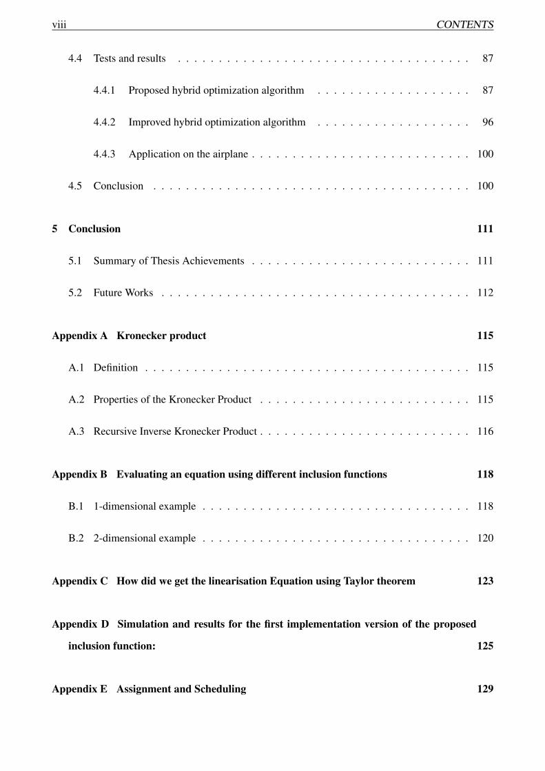
viii CONTENTS
4.4 Tests and results . . . . . . . . . . . . . . . . . . . . . . . . . . . . . . . . . . . . 87
4.4.1 Proposed hybrid optimization algorithm . . . . . . . . . . . . . . . . . . . 87
4.4.2 Improved hybrid optimization algorithm . . . . . . . . . . . . . . . . . . . 96
4.4.3 Application on the airplane . . . . . . . . . . . . . . . . . . . . . . . . . . . 100
4.5 Conclusion . . . . . . . . . . . . . . . . . . . . . . . . . . . . . . . . . . . . . . . 100
5 Conclusion 111
5.1 Summary of Thesis Achievements . . . . . . . . . . . . . . . . . . . . . . . . . . . 111
5.2 Future Works . . . . . . . . . . . . . . . . . . . . . . . . . . . . . . . . . . . . . . 112
Appendix A Kronecker product 115
A.1 Definition . . . . . . . . . . . . . . . . . . . . . . . . . . . . . . . . . . . . . . . . 115
A.2 Properties of the Kronecker Product . . . . . . . . . . . . . . . . . . . . . . . . . . 115
A.3 Recursive Inverse Kronecker Product . . . . . . . . . . . . . . . . . . . . . . . . . . 116
Appendix B Evaluating an equation using different inclusion functions 118
B.1 1-dimensional example . . . . . . . . . . . . . . . . . . . . . . . . . . . . . . . . . 118
B.2 2-dimensional example . . . . . . . . . . . . . . . . . . . . . . . . . . . . . . . . . 120
Appendix C How did we get the linearisation Equation using Taylor theorem 123
Appendix D Simulation and results for the first implementation version of the proposed
inclusion function: 125
Appendix E Assignment and Scheduling 129

Bibliography 130
ix

x
List of Tables
1.1 Dimensions of Airfrance airplanes . . . . . . . . . . . . . . . . . . . . . . . . . . . 9
2.1 comparison table between the three algorithms based on the paint thickness variations
(+: best result, .: acceptable result, -: worst result) . . . . . . . . . . . . . . . . . . . 31
3.1 Computation results of the feasible spaces for the 2-dof planar robot. . . . . . . . . . 60
3.2 Comparison of the evaluation of the end effector {X ,Y,Z} Cartesian position depend-
ing on the diameter of joint position interval for the 4 dof Robot . . . . . . . . . . . 66
3.3 Comparison of the evaluation of the end effector {X ,Y,Z} Cartesian position depend-
ing on the diameter of joint position interval for the 6-dof Robot . . . . . . . . . . . 66
3.4 Comparison of the performances of the three solvers for the posture optimization of
the 4-dof robot. . . . . . . . . . . . . . . . . . . . . . . . . . . . . . . . . . . . . . 69
3.5 Comparison of the performances of the three solver for the posture optimization of
the 6-dof robot. . . . . . . . . . . . . . . . . . . . . . . . . . . . . . . . . . . . . . 69
4.1 The optimal number of robots found using the four optimization algorithms . . . . . 88
4.2 Average of computation time (in seconds) for the four optimization algorithms . . . . 88
4.3 3D discretization: the number of favourite robot poses for a cylinder, a hemisphere
and a car using different types of workspaces . . . . . . . . . . . . . . . . . . . . . 96
xi

4.4 4D discretization: the number of favourite robot poses for a cylinder, a hemisphere
and a car using different types of workspaces . . . . . . . . . . . . . . . . . . . . . 96
4.5 3D discretization: the standard deviation of the computation time (in seconds) of
Hybrid optimization algorithm and Improved Hybrid optimization algorithm applied
on different type of surfaces using different type of workspace . . . . . . . . . . . . 98
4.6 4D discretization: the standard deviation of the results of Hybrid optimization al-
gorithm and Improved Hybrid optimization algorithm applied on different type of
surfaces using different type of workspace . . . . . . . . . . . . . . . . . . . . . . . 99
B.1 Comparing inclusion functions . . . . . . . . . . . . . . . . . . . . . . . . . . . . . 119
D.1 The number of incrementation required to solve Position 1 problem using Solver 1,
Solver 2 and Solver 3/ PRECISION 0.01 . . . . . . . . . . . . . . . . . . . . . . . . 128
D.2 The time (in days / HH:MM:SS) required to solve Position 1 problem using Solver 1,
Solver 2 and Solver 3/ PRECISION 0.01 . . . . . . . . . . . . . . . . . . . . . . . . 128
xii

List of Figures
1.1 Protection for the sanding phase . . . . . . . . . . . . . . . . . . . . . . . . . . . . 2
1.2 Stripping of the bottom part of the airplane manually. . . . . . . . . . . . . . . . . . 4
1.3 Stripping process . . . . . . . . . . . . . . . . . . . . . . . . . . . . . . . . . . . . 5
1.4 Stripping tool model: working principle . . . . . . . . . . . . . . . . . . . . . . . . 6
1.5 Painting layers . . . . . . . . . . . . . . . . . . . . . . . . . . . . . . . . . . . . . 6
1.6 Painted surface (white paint) to be stripped. . . . . . . . . . . . . . . . . . . . . . . 7
1.7 KUKA LightWeight Robot LWR 4+ . . . . . . . . . . . . . . . . . . . . . . . . . . 7
1.8 Crane that will holds the robot and its workspace. . . . . . . . . . . . . . . . . . . . 8
1.9 Graphical representation of the project lots . . . . . . . . . . . . . . . . . . . . . . . 10
1.10 General framework of my PHD . . . . . . . . . . . . . . . . . . . . . . . . . . . . . 12
1.11 The state of the art of our general framework . . . . . . . . . . . . . . . . . . . . . 13
2.1 Orthogonal comb polygon [109] . . . . . . . . . . . . . . . . . . . . . . . . . . . . 22
2.2 Main steps of recent painting path planning techniques. . . . . . . . . . . . . . . . 29
2.3 CAD representations of surfaces [25] . . . . . . . . . . . . . . . . . . . . . . . . . . 29
3.1 A box [a] in R2 . . . . . . . . . . . . . . . . . . . . . . . . . . . . . . . . . . . . . 39
xiii

xiv LIST OF FIGURES
3.2 Image of a box [a] using a function m and its inclusion functions [m] and [m]∗ . . . . 40
3.3 Four different inclusion functions for the same function f . . . . . . . . . . . . . . . 41
3.4 Perception of the centred inclusion function . . . . . . . . . . . . . . . . . . . . . . 42
3.5 2D bisection algorithm on a constraint C . . . . . . . . . . . . . . . . . . . . . . . . 49
3.6 Evaluating intervals using BSplines properties . . . . . . . . . . . . . . . . . . . . . 51
3.7 Presentation of the feasible spaces for the 2-dof robot. (feasible boxes in red, possible
boxes in green, actual feasible space limits in blue.) . . . . . . . . . . . . . . . . . 61
3.8 Comparison of the BSplines Bisection and the Interval Bisection methods to solve CSP. 62
3.9 Comparison of the Interval Contraction and the Interval Bisection methods to solve
CSP. . . . . . . . . . . . . . . . . . . . . . . . . . . . . . . . . . . . . . . . . . . . 63
3.10 Comparison of the BSplines Contraction and the Interval Bisection methods to solve
CSP. . . . . . . . . . . . . . . . . . . . . . . . . . . . . . . . . . . . . . . . . . . . 64
3.11 Comparison of the Bsplines Contraction and the Bsplines Bisection methods to solve
CSP. . . . . . . . . . . . . . . . . . . . . . . . . . . . . . . . . . . . . . . . . . . . 65
3.12 Comparison of the BSplines Bisection and the Interval Bisection methods to solve
optimization problems. . . . . . . . . . . . . . . . . . . . . . . . . . . . . . . . . . 67
3.13 Comparison of the BSplines Contraction and the Interval Bisection methods to solve
CSP. . . . . . . . . . . . . . . . . . . . . . . . . . . . . . . . . . . . . . . . . . . . 68
3.14 Comparison of the BSplines Contraction and the BSplines Bisection methods to solve
optimization problems. . . . . . . . . . . . . . . . . . . . . . . . . . . . . . . . . . 70
3.15 The 6 degrees of freedom robot we use : KUKA LWR . . . . . . . . . . . . . . . . 70
4.1 Car stripping using a KUKA robot . . . . . . . . . . . . . . . . . . . . . . . . . . . 73
4.2 Flowchart used to optimize the number of robots and their poses. . . . . . . . . . . . 74
LIST OF FIGURES xv
4.3 4D discretization for the action car: red circles are the favourite robot poses of F (s =
0.1) . . . . . . . . . . . . . . . . . . . . . . . . . . . . . . . . . . . . . . . . . . . 75
4.4 3D discretization for the action car: red circles are the discretized points of P (s = 0.1) 77
4.5 The set of the initial poses C of the action car (s = 0.1) . . . . . . . . . . . . . . . . 78
4.6 Favorite base placements of the action car for t = 10%. . . . . . . . . . . . . . . . . 78
4.7 Basic terminology if Genetic Algorithm . . . . . . . . . . . . . . . . . . . . . . . . 84
4.8 Basic structure of Genetic Algorithm . . . . . . . . . . . . . . . . . . . . . . . . . . 85
4.9 Discretization of the ground around the action car . . . . . . . . . . . . . . . . . . . 87
4.10 Two dof Robot with a 2D surface that should be totally covered. . . . . . . . . . . . 89
4.11 The number of 2D-robots required to cover the whole 2D-surface using Greedy Algo-
rithm (red: surface, blue: possible robots positions, yellow: favourite robot positions,
small black circle: en-globs the robots position, big black circle: the workspace of the
robot from the given position). . . . . . . . . . . . . . . . . . . . . . . . . . . . . . 90
4.12 The number of 2D-robots required to cover the whole 2D-surface using Simulated
Annealing Greedy Algorithm. . . . . . . . . . . . . . . . . . . . . . . . . . . . . . 90
4.13 The number of 2D-robots required to cover the whole 2D-surface using Greedy Ge-
netic Algorithm. . . . . . . . . . . . . . . . . . . . . . . . . . . . . . . . . . . . . . 91
4.14 The number of 2D-robots required to cover the whole 2D-surface using Hybrid Algo-
rithm. . . . . . . . . . . . . . . . . . . . . . . . . . . . . . . . . . . . . . . . . . . 91
4.15 Surfaces to be covered by robots with the favorite base position (red spheres) . . . . 92
4.16 Optimal base placements of different surfaces (greedy algorithm) . . . . . . . . . . 93
4.17 Optimal base placements of different surfaces (hybrid optimization) . . . . . . . . . 94

xvi LIST OF FIGURES
4.18 The number of robots required to cover the whole cylinder using greedy algorithm
and the proposed hybrid optimization algorithm. . . . . . . . . . . . . . . . . . . . . 95
4.19 The number of robots required to cover the whole sphere using greedy algorithm and
the proposed hybrid optimization algorithm. . . . . . . . . . . . . . . . . . . . . . . 95
4.20 The number of robots required to cover the whole action car using greedy algorithm
and the proposed hybrid optimization algorithm. . . . . . . . . . . . . . . . . . . . . 96
4.21 3D discretization: comparison of the results of Hybrid optimization algorithm and
Improved Hybrid algorithm on a cylinder using the different workspaces . . . . . . . 102
4.22 3D discretization: comparison of the results of the Hybrid optimization algorithm
and Improved Hybrid optimization algorithm on a hemisphere using the different
workspaces . . . . . . . . . . . . . . . . . . . . . . . . . . . . . . . . . . . . . . . 103
4.23 3D discretization: comparison of the results of Hybrid optimization algorithm and
Improved Hybrid optimization algorithm on a car using the different workspaces . . 104
4.24 3D discretization: comparison between the execution time of Hybrid optimization
algorithm and Improved Hybrid optimization algorithm . . . . . . . . . . . . . . . . 105
4.25 4D discretization: comparison of the results of Hybrid optimization algorithm and
Improved Hybrid optimization algorithm on a cylinder using the different workspaces 106
4.26 4D discretization: comparison of the results of Hybrid optimization algorithm and Im-
proved Hybrid optimization algorithm on a hemisphere using the different workspaces 107
4.27 4D discretization: comparison of the results of Hybrid optimization algorithm and
Improved Hybrid optimization algorithm on a car using the different workspaces . . 108
4.28 4D discretization: comparison between the execution time of Hybrid optimization
algorithm and Improved Hybrid optimization algorithm . . . . . . . . . . . . . . . . 109
4.29 The representation of the air-plane with the set of favourite robot base placements
(red circle = favourite robot base placement) . . . . . . . . . . . . . . . . . . . . . . 109
4.30 Optimal base placements to cover airplane using the hybrid optimization algorithm . 110
4.31 The results of the hybrid optimization algorithm on the airplane (the surface should
be at least 80% covered without the wings) . . . . . . . . . . . . . . . . . . . . . . 110
B.1 3D plot of f (q1,q2) = 1−3q1−2q2 +4q1q2 . . . . . . . . . . . . . . . . . . . . . 121
C.1 Taylor Series Expansion of cos(x) . . . . . . . . . . . . . . . . . . . . . . . . . . . 124
D.1 Two dof Robot with a square surface in three different positions and a robot stability
margin . . . . . . . . . . . . . . . . . . . . . . . . . . . . . . . . . . . . . . . . . . 125
D.2 Iteration numbers and computation time of the three different solvers compared to
Solver 1 for a precision of 0.1 . . . . . . . . . . . . . . . . . . . . . . . . . . . . . 127
D.3 Iteration numbers and computation time of the three different solvers compared to
Solver 1 for a precision of 0.01 . . . . . . . . . . . . . . . . . . . . . . . . . . . . . 127
xvii

xviii
Chapter 1
General Introduction
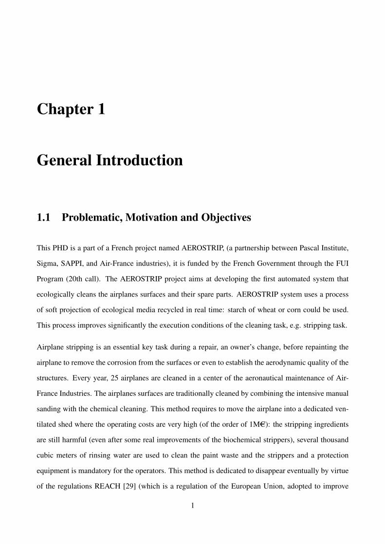
1.1 Problematic, Motivation and Objectives
This PHD is a part of a French project named AEROSTRIP, (a partnership between Pascal Institute,
Sigma, SAPPI, and Air-France industries), it is funded by the French Government through the FUI
Program (20th call). The AEROSTRIP project aims at developing the first automated system that
ecologically cleans the airplanes surfaces and their spare parts. AEROSTRIP system uses a process
of soft projection of ecological media recycled in real time: starch of wheat or corn could be used.
This process improves significantly the execution conditions of the cleaning task, e.g. stripping task.
Airplane stripping is an essential key task during a repair, an owner’s change, before repainting the
airplane to remove the corrosion from the surfaces or even to establish the aerodynamic quality of the
structures. Every year, 25 airplanes are cleaned in a center of the aeronautical maintenance of Air-
France Industries. The airplanes surfaces are traditionally cleaned by combining the intensive manual
sanding with the chemical cleaning. This method requires to move the airplane into a dedicated ven-
tilated shed where the operating costs are very high (of the order of 1MAC): the stripping ingredients
are still harmful (even after some real improvements of the biochemical strippers), several thousand
cubic meters of rinsing water are used to clean the paint waste and the strippers and a protection
equipment is mandatory for the operators. This method is dedicated to disappear eventually by virtue
of the regulations REACH [29] (which is a regulation of the European Union, adopted to improve
1

2 Chapter 1. General Introduction
the protection of human health and the environment from the risks that can be posed by chemicals,
while enhancing the competitiveness of the EU chemicals industry) and the directives of the aircraft
manufacturers. For instance, the AIRBUS A330 official textbook “Structural Repair Manual Airbus
A330” prohibits the use of chemical cleaning products on the composite because they may affect the
resin [110].
Six main types of stripping processes are applied during an aeronautical maintenance as presented
hereafter.
Manual stripping using grinding discs:
This process consists in removing the paint using a grinding tool as it is shown in Figure 1.1. This
method is expensive since it is time consuming, and needs a huge human effort. In addition, it gener-
ates a lot of dusts and it is subjected to severe working conditions. For example, the operator’s hands
are in the air holding a 7 kg sander tool. This frequent holding action causes a health problem: the
risk of Musculoskeletal disorders (MSDs) increases over-time. Usually 30% of the operators suffer
from long-term illnesses. According to Royal Aircraft Services, the manual stripping task requires the
Figure 1.1: Protection for the sanding phase
mobility of at least 4 people working full-time during a week to clean a small airplane. The efficiency
of this work is estimated a few square meters per hour.
Chemical stripping:
This technique has an average efficiency of 40m2
h. It consists in putting chemical products on the
surface and then rinsing it using water. This method is polluting, harmful for the technicians and very
1.1. Problematic, Motivation and Objectives 3
expensive. The chemical stripping is always a risk process to clean any surfaces: even the biochemical
products that replace the chemical products are dangerous. This stripping process generates volumi-
nous waste like rinsing water. In addition, the performance of the biochemical scouring agents, that
are used today, is less effective than the scouring agent that have been forbidden from being exploited.
This chemical cleaning process has additional costs: the immobilization of the airplane during one
week, the cost of the shed ventilation and finally the mandatory investment in forklift trucks and
equipments of complete protection of the operators.
Other methods of abrasives projection (plastic media, water):
Those methods are not intended to be used on composite materials because they are aggressive for
those sensitive materials.
Stripping by Flash lamp or Xenon:
This method uses a technology of pulsed light which entails the technical softening of paints. This
technique is badly adapted to industrial applications because they require high performances in time
and in costs. It is important to use a special head to guide the light for every stripped surface: stripping
huge surfaces become more difficult.
Stripping by laser:
This stripping by laser has the same concept as the lamp Flash, but the stripping process is easier to be
controlled using the laser. This technique is a promising but it is not common in the market because
the airplane could not be exploited before 5 to 9 years after being cleaned. Today, the research labo-
ratory of US Air Forces works on this type of stripping process, and it is applied only on the detached
part of the airplane. The cleaned coating is the only generated waste from the airplane: it is the main
advantage of the stripping by laser. However, this method does not improve the working conditions
of the operators since the manual stripping remains necessary.
Stripping by projection of ecological media:
An ecological stripping process has been recently proposed instead of the intensive manual sanding
stripping process or even the chemical cleaning process. The new stripping technique uses an eco-
logical media to strip airplanes: the starch of wheat or/and corn. Recently, this method appears in
the aeronautical maintenance sectors. This method is promising in terms of optimizing the opera-
tions, reducing the costs and increasing the safety of workers. However, this process is manual, so
4 Chapter 1. General Introduction
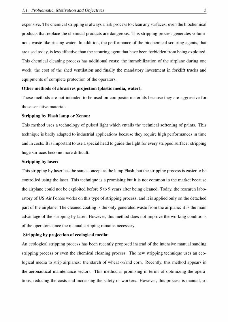
Figure 1.2: Stripping of the bottom part of the airplane manually.
AEROSTRIP project chose to strip airplanes automatically or semi-automatically.
1.1.1 Ecological stripping process using corn (AEROSTRIP):
Description:
The main objectives of AEROSTRIP project is to design and develop the first automated system to
strip airplanes and their spare parts using a closed ecological circuit. AEROSTRIP allies the perfor-
mance, the quality of cleaning, the prevention of the MusculoSkeletal Disorders (MSDs), the opti-
mization of the costs and the execution time. In AEROSTRIP, the objective is to attend less than 30%
of the global costs for the tasks of stripping/cleaning, and the execution time should be half reduced on
a complete airplane. AEROSTRIP project proposed a new stripping process which is semi-automatic,
inexpensive and eco-friendly: the corns are the media used by the stripper. A closed circuit is added
to recycle the corns. The closed circuit avoids dusts and reduces in a significant way the risks of
the MSDs. Moreover, the environmental costs are reduced since the excessive consumption of water
is stopped, the volume of waste is reduced, and the recyclable media are used instead of chemical
products.
AEROSTRIP develops two systems to strip airplanes. The first system is semi-automatic; it is usu-
ally used for the detached parts of the airplanes, e.g. nacelle, motors, etc. This system is considered
semi-automatic since an interaction between a robot and an operator exists: an operator should move

1.1. Problematic, Motivation and Objectives 5
the stripper along the surface. However, the second system is automatic and it is accomplished us-
ing a multi-robot system. In both systems, there are a stripping tool, a robot holding it and a me-
dia projection/recycled system. However, a crane holding the robot is added to the second system.
AEROSTRIP aims to validate its capacity of stripping 85% of the airplane surface automatically, 10%
semi-automatically, and 5% manually.
Figure 1.3: Stripping process
AEROSTRIP proposes a multi-robot system composed of mobile manipulators to strip surfaces. The
stripping tool is mounted on the end-effector of the manipulator. Figure 1.3 shows the stripping pro-
cess of an airplane.
Stripping tool and the media projection/recycled system:
The paint stripping mechanism involves the media bombardment (fine granules of corn) on the painted
surface at high pressure. Three parameters could be adjusted during the stripping process: the pres-
sure, the corn flow and the stripping tool speed. Those parameters must be carefully chosen since the
surface may not be stripped correctly as well as it could be damaged, e.g. a hole could be created on
the surface. The stripping tool is presented in Figure 1.4, it holds a camera that takes pictures of the
surface to be stripped. After bombardment the media is aspirated, it is recycled and it is used again
to strip the surface. The volume of the media is tested each time it is aspirated, if it is larger than a
given threshold it is thrown otherwise it is used to strip again. Five painting layers of different colors

6 Chapter 1. General Introduction
Figure 1.4: Stripping tool model: working principle
compose the aircraft of any AirFrance airplanes: those layers are shown in Figure 1.5. The camera
Figure 1.5: Painting layers
is used to make sure that the surface is stripped. A surface is considered well stripped if the primary
level appears. Several tests have been applied on a sample of an airplane door in order to evaluate the
influence of the pressure, the corn flow, and the stripping tool speed on the stripping quality. It was
proved that the more the corn flow is decreased, the more the cleaning is superficial, and the more the
tool speed is decreased, the more stripping is profound. Figure 1.6 shows the output of the camera
while stripping a sample of an airplane door: three different stripping processes have been shown.
It must be noted that the quality of the paint influences on the choice of the flow, the pressure and
the tool speed of the surface. A sample of the airplane could be used to estimate the previous three
parameters in order to fix them while stripping the whole airplane. However, an accurate fixed ap-
proximation is difficult: the painting layers could be influenced by the sun as well as the rain. Hence,
the painting layers on the top of the airplane are affected by those natural elements which is not the
case of its bottom part. Hence, the corn flow and the tool speed should be adjusted depending on

1.1. Problematic, Motivation and Objectives 7
(a) Bad Stripped surface (b) Mean stripped surface
(c) Well stripped surface
Figure 1.6: Painted surface (white paint) to be stripped.
the part of the airplane. For instance, the corn flow should be increased and the tool speed should be
decreased on the bottom part. However, the opposite case is applied on the top of the airplane.
The robot manipulator holding the stripping tool:
The chosen robot manipulator is the KUKA Light Weight Robot LWR 4+. This manipulator ac-
commodates the motors, gear units, brakes and sensors, as well as the necessary control and power
electronics for 7 axes. This robot can support a payload capacity of 7 kg. This LWR 4+ is 1.1785 m
(a) LWR 4+ (b) Workspace of the robot
Figure 1.7: KUKA LightWeight Robot LWR 4+
of height. The robot is shown in Figure 1.7a and its workspace is presented in Figure 1.7b. The shown
workspace is changeable with the torque limits, the joint positions, the collision and the self-collision

8 Chapter 1. General Introduction
avoidance. Before going further, I would like to add that, during my thesis, I provide a generic code
where the robot could be changed.
The crane holding the robot:
The crane shown in Figure 1.8a will hold the robot. The use of the crane is important when huge
surfaces should be stripped, which is always the case of airplanes. AirFrance has several type of air-
(a) Crane dimensions (A = 11.7m,H =8.9m,C = 2.8m,D = 3.5m,E = 38m)
(b) Workspace of the crane
Figure 1.8: Crane that will holds the robot and its workspace.
planes shown in Table 1.1. As it is clear, the length varies between 22.67 and 72.72 m, the wingspan
between 24.57 and 79.75 m, and the height between 7.59 and 24.09 m. Since the robot can reach 1
m in best cases, a crane is required to cover the whole surface. The crane, shown in Figure 1.8a, is
the mobile platform that will be moved manually between various robot positions, it should hold the
KUKA arm. The crane can reach 30 m of length and 21 m of height. The stripping process is stopped
during the crane’s motion since the movement of the crane introduces some vibrations on the robots
that may affect on the robot behavior so on the stripping quality. Moreover, comparing the workspace
of the robot to the volume of the airplane, the crane should move the KUKA arm lots of times to cover
the whole surface. Though, the optimization of robots base placements and the movement between
them is important in order to decrease the cycle time of the stripping process. During the computing
of the number of robots base placements, the physical limits of the robot such as joint position and
torque limits, collision and self-collision avoidance, and even the stripping tool constraints, should be
taken into account: they influence on the robot workspace, so on the covered surface.

1.1. Problematic, Motivation and Objectives 9
Airplane model Length Wingspan HeightA318(111, 112, 121 et 122) 31,45 34,10 12,79A319(111 a 115, 131 a 133) 33,84 34,10/35,80 11,76
A320(111, 211, 212, 214 a 216, 231 a 233) 37,57 34,10/35,80 11,76A321(111, 112, 131, 211 a 213, 231, 232) 44,51 34,10/35,80 11,76
A330(200, 300, 300, 800, 900) 58,82/63,66 60,30/ 64 16,79/17,39A340(200, 300, 500, 600) 59,39/63,6/67,9/75,3 60,3/63,45 16,7/16,85/17,28
A380-800 72,72 79,75 24,09ATR 42(200, 300, 320, 500, 600) 22,67 24,57 7,59
ATR 72 27,166 27,05 7,72Boeing 777 63,7 a 73,9 60,9 a 64,8 18,5 a 18,6Boeing 787 56,7 60 17
Bombardier CRJ-1000 39,10 26,20 7,50Bombardier CRJ-700 32,41 23,01 7,29
Embraer 170 29,90 26 9,85Embraer 190 36,24 28,72 10,57
Embraer ERJ 145 29,87 20,04 6,75RJ-85 Avroliner (AR8) 28,60 26,33 8,59
Table 1.1: Dimensions of Airfrance airplanes
1.1.2 Project consortiums
Three main entities are responsible of the project: SAPPI of SOFIPLAST, AirFrance industries and
SIGMA. PME SAPPI, R&D subsidiary of the group SOFIPLAST, have developed a solution to strip
airplanes using integrable vegetable media. Hence, they develop the stripping tool that must be used
as an end-effector of the robot during the airplane stripping. In parallel, SIGMA develops a system
controller that controls the movement of the robots between different poses in order to strip the whole
airplane. SIGMA also deals with the operator-machine interaction part since the human operator and
the robot will interact in 10% of the stripping process (semi-automatic part). However, AirFrance
industries supply samples of different airplanes to test the stripping process. In addition, AirFrance
industries test the stripping process on the whole airplane surface. The collaboration between the
three enterprises is shown graphically in Figure 1.9.
Two PHDs, and one post-doc have been funded by AEROSTRIP. The first PHD is tackling the small
system, and the second one is dedicated to the global system. The first PHD will aid in developing
/ implementing the multi-modal control scheme (inputs from multiple sensors) to aid the stripping
tool mounted on the robot to carry out the paint removal process and establish the success criteria.
10 Chapter 1. General Introduction
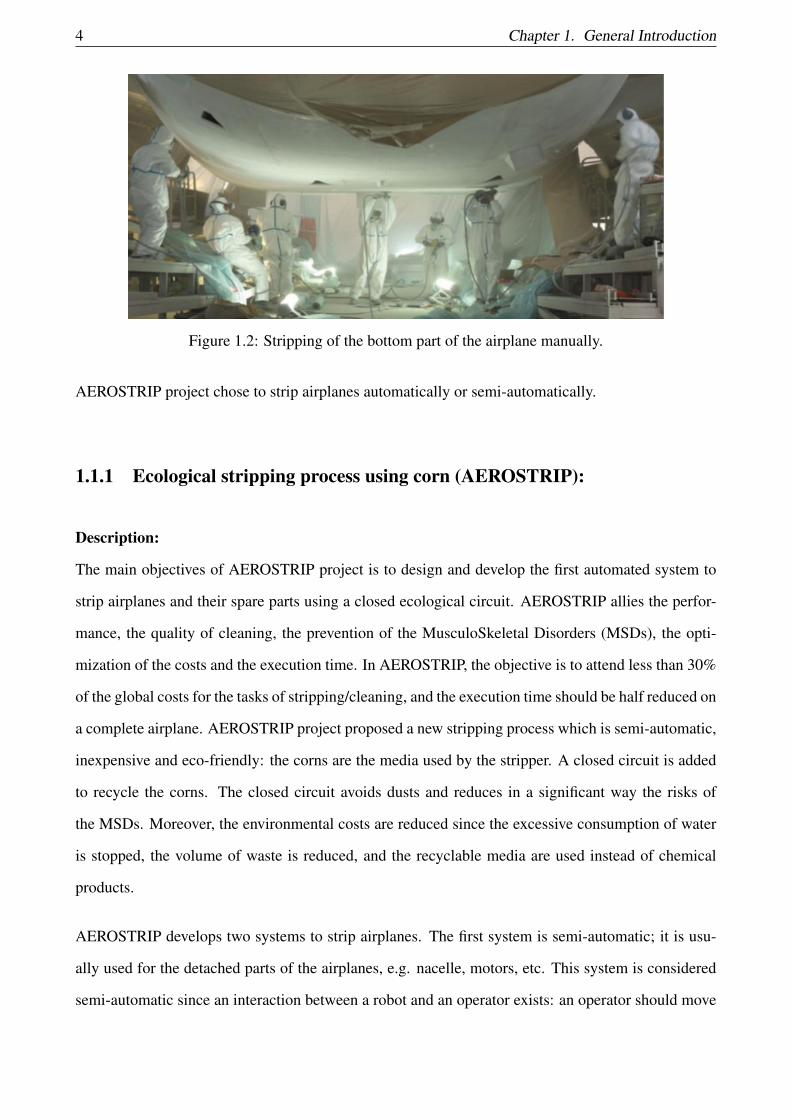
Figure 1.9: Graphical representation of the project lots
The second PHD, which is my PHD, aims at optimizing the trajectory of the whole robotic systems
in order to optimally strip the airplane. Since a large surface can not be totally covered by a single
robot base placement, repositioning of the robots is necessary to ensure a complete stripping of the
surface. However, in the post-doc, the goal is to develop a new image processing strategies to evaluate
automatically and on-line the performance of the airplane stripping. The multi-robot coordination
problems have been also tackled. A new method that allows a team of robots to deploy themselves
around a target object is developed, e.g. an airplane to be stripped.
To attend the optimal trajectories of the mobile platforms, two parameters have important influence:
the surface to be covered (airplanes), and the workspace of the robot. For instance, giving a curved
surface to be stripped, the position of the mobile platform with respect to this surface influences on
the percentage of the stripped surface. Eventually, the relationship between the shape and the robot
position is widely dependent. Due to this dependency, a general framework is proposed in Section 1.2.
1.2. Thesis approach 11
1.2 Thesis approach
Since large surfaces can not be totally covered by a single robot base placement, multi-robot sys-
tem is required. Hence, a repositioning of each robot is necessary to ensure a complete stripping
of the surface. Each robot of this system is hold by a crane which is a mobile platform. The
robots as well as their cranes have some collective behaviours. Multi-robot systems are known by
their benefits in the industrial field. Let enumerate some of their advantages: multi-robot systems
accelerate the task completion [33] (increase the performance), improve the robustness and gave
more accurate solutions [132], they even execute the impossible tasks for single robots [131], etc.
Hence, multi-robot systems were used in many domains such as intelligent security [83], environ-
ment monitoring [38, 117], humanitarian de-mining [71], search and rescue [95], surveillance [87],
health care [116], stripping [57, 69].
To find the optimal trajectories of the mobile platforms, we propose to find the optimal number of
robot base placements required to cover the whole surface. Then, the robots of the multi-robot system
should be distributed between the different optimal robot base placements and the robot trajectories
between those poses should be computed. Those two problems could be solved by following our
approach detailed in Subsection 1.2.1.
1.2.1 General framework:
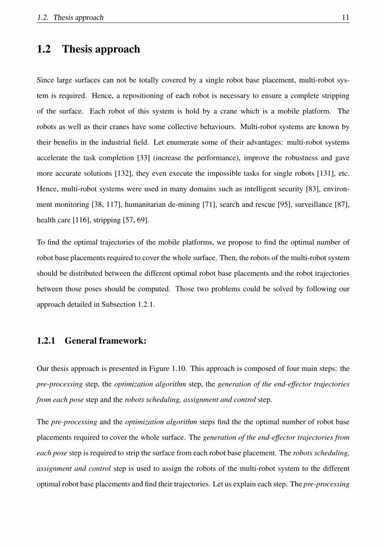
Our thesis approach is presented in Figure 1.10. This approach is composed of four main steps: the
pre-processing step, the optimization algorithm step, the generation of the end-effector trajectories
from each pose step and the robots scheduling, assignment and control step.
The pre-processing and the optimization algorithm steps find the the optimal number of robot base
placements required to cover the whole surface. The generation of the end-effector trajectories from
each pose step is required to strip the surface from each robot base placement. The robots scheduling,
assignment and control step is used to assign the robots of the multi-robot system to the different
optimal robot base placements and find their trajectories. Let us explain each step. The pre-processing

12 Chapter 1. General Introduction
Figure 1.10: General framework of my PHD
step aims at discretizing the volume around the object to be stripped: a set of discretized points is
determined. Hence, the constraints projection on the surface from each discretized point consists in
computing the reachable part of the surface. This computation is accomplished using the constraints
projection function taking into account the different robot constraints: each discretized point will
have a value describing the percentage of the covered surface from this point. A subset of favourite
base placements is selected from the set of discretized points based on the coverage percentage.
This computed set is used in order to find the optimal number of robots with their optimal base
placements required to cover the whole object: it is the optimization algorithm step. Hence, the end-
effector trajectories are generated from each robot base placement (the generation of the end-effector
trajectories from each pose step). Finally, the robots scheduling, assignment and control step of
the general framework solves two different sub-problems, namely an assignment sub-problem and a
control sub-problem. The assignment sub-problem selects which optimal poses should correspond to
each robot in order to generate their trajectories from their initial positions. Once the robot trajectories
have been generated, we apply a controller to make the robots follow them.

1.2. Thesis approach 13
In this thesis, we focus on finding the optimal number of robots with their optimal poses (the op-
timization algorithm step): it is the general problem presented in Section 1.2.2. Then, we present
our contributions that are principally related to this step. However, the trajectories planning of the
end-effector and the robots scheduling, assignment and control steps are quickly tackled in this thesis.
Though, we show the state of the art of the trajectories planning of the end-effector step in Chapter 2
and we develop the formulation of assignment problem in Appendix E.
Figure 1.11: The state of the art of our general framework
The proposed general framework, shown in Figure 1.10, is related to four different state of the art
shown in Figure 1.11. Though, this thesis provides surveys on the robot constraints projection on
the surface, on the optimization of the number of robots, on the robot base placement for a complete
coverage and on the trajectories generation of the end-effector on the surface.
The constraints projection on the surface consists in computing the reachable part of the surface from
a given robot pose: the robot workspace is required. The determination of the robot workspace is
critical, so we present some existing methods used to compute the workspace. In this thesis, Interval
Analysis is used to compute the robot workspace for a reason detailed in chapter 2. However, Interval
Analysis suffers from pessimism which is an overestimation of the solutions. Hence, our first contri-
bution consists in reducing the pessimism of Interval Analysis. Moreover, this new tool was used to
14 Chapter 1. General Introduction
compute the set of joint angles of the robots that respect a set of constraints.
The optimization algorithm step involves two different state of the art: the optimization of the number
of robots and the robot base placement for a complete coverage. This optimization step requires
the workspace to compute the reachable part of the surface. The intersection between the robot
workspace and the surface is used to compute this reachable part of this surface. Since we have the
set of joint angles and not its correspondent workspace, we compute the reachable part of the surface
using different shapes of workspace (spherical, semi-spherical, elliptical). Furthermore, based on this
reachability, we propose an hybrid optimization algorithm to find the optimal number of robots with
their optimal poses to totally cover a surface: the second contribution of our work.
The state of the art related to trajectories generation of the stripping tool on the surface is inspired from
the trajectories generation of the spray painting robot. The same algorithms could be used on both
applications since they are close. We wrote a survey named ”Automated path generation of spray
painting robots: a review” that is submitted to Robotics and Computer-Integrated Manufacturing
journal. A part of this survey is presented in Chapter 2.
1.2.2 General problem
The general problem aims to find the optimal number of robots N and their base placements required
to totally cover the surface. The optimization relies on two parameters: the shape of the surface to be
stripped, and the robot workspace. Defining T as a set of robot poses T = {Ti ∈ SE(3),1 ≤ i ≤ N},
the coverage problem can be formulated as follows:
minN,T
f (N,T,S)
Subject to g(N,T,S) = 0
h(N,T,S)≤ 0
(1.1)
where:
f (N,T,S): is the optimization function,
S: is the surface to be stripped,

1.3. Manuscript structure 15
g(N,T,S) =⋃N
j=1C(S,T j)− λS: is the function to test if the surface is λ% covered (λ% is the
percentage of the covered surface),
h(N,T,S): is the set of additional constraints.
In our problem, we should optimize the number of robots N, so f (N,T,S)= N. It can be noticed that
the task can be achieved using from one robot to N robots. Obviously, when the number of robots
increases the coverage task can be achieved faster. If one robot is only used, it has to be moved N
times while if N robots are used then the task can be achieved at once without moving the robots.
Additional constraints can be taken into account during the optimization using h.
1.3 Manuscript structure
The manuscript is organized in the following way. In Chapter 2, we present the state of the art
related to the robots constraints projection on the surface, the optimization of the number of robots,
the robot base placements for complete coverage and the path generation of spray painting robots.
In Chapter 3, we present the motivation of exploiting Interval Analysis in our context and how it
is used to solve Constraint Satisfaction Problems and Constraint Optimization Problems. A new
method to reduce the pessimism based on the convex hull properties of BSplines and the Kronecker
product is initiated in this chapter. This method is assessed on three different scenarios using three
different robots: a 2D robot, a planar robot and a 3D robot. In Chapter 4, the robot base placement
is deeply studied to reduce the cycle time and increases the coverage task accuracy. We develop an
optimization strategy to find the optimal number of robots with their optimal poses required to cover
the entire surface. The optimization strategy is finalized by an hybrid optimization algorithm that is
assessed on different type of surfaces (a hemisphere, a cylinder and an action car) and using different
workspaces (spherical, semi-spherical and elliptical). Finally, in Chapter 5, we present a summary
about my thesis with some future works.

Chapter 2
State of the art
The general framework, presented in Figure 1.10 in Chapter 1, shows the state of the art related to:
1. The robot constraints projection on the surface (Section 2.1),
2. the optimization of the number of robots (Section 2.2),
3. the robot base placement for a complete coverage (Section 2.3),
4. the trajectories generation of the end-effector on the surface (Section 2.4).
The constraints projection on the surface consists in computing the reachable part of the surface from
a given robot pose: the robot workspace is required. The determination of the robot workspace is
critical, so we present some existed method used to compute the workspace. Then, we present the
state of the art of Interval Analysis which is the mathematical tool that we use to compute the set of
joint angles respecting a set of constraints.
Moreover, the optimization of the number of robot and their poses is inspired from Art Gallery Prob-
lem and camera base placement problems: the state of the art of each problem is presented in this
chapter. Art Gallery Problem consists in computing the minimal number of guards to monitor a
gallery. However, the camera base placement problems distinguish between two sub-problems: how
to place a given number of cameras to optimize the coverage of a surface (FIX problem), or how to
compute the minimal number of cameras required to totally cover a surface (MIN problem). Even-
tually, we are interested in MIN problem. Further, we show the analogy between our problem (the
16

2.1. Robot constraints projections on the surface 17
optimization of the number of robots with their poses to totally cover a surface) and the combination
between Art Gallery problem with camera placement problems.
Besides, the state of the art of a robot base placement for a complete coverage is provided. This
state of the art consists in finding the robot base placement that maximizes the reachability of a given
surface. Several works tackled this problem and a small review is presented in this Chapter.
Finally, the state of the art of path generation of spray painting robots is presented. The painting
process was the first automated process that generates the end-effector trajectories on a surface. We
assumed that path generations in the painting and the stripping processes share the same concepts.
Though, we considered that the same algorithms could be applied for both processes to generate
the end-effector trajectories. The painting process was the source of our inspiration to the proposed
approach developed in Chapter 1.
2.1 Robot constraints projections on the surface
The robot constraints projections on the surface is the determination of the reachable part of the
surface from a given pose. The reachable part is the intersection between the robot workspace and
the surface. During this computation, the different robot constraints should be taken into account:
robot stability, robot dynamic and kinematic constraints, singularity avoidance, etc. Each robot is
characterized by its workspace. In the most of the cases, the workspace of a manipulator is spherical
when none of the constraints is considered. However, this workspace becomes more complex when
the number of constraints increases. In this section, we present the different methods used to compute
the robot workspace and their disadvantages. After that we introduce Interval Analysis: the chosen
mathematical tool used to compute the robot workspace. Some other applications of Interval Analysis
in robotics are also discussed.

18 Chapter 2. State of the art
2.1.1 Robotic Workspace
The workspace of a manipulator robot is the space that can be reached by its end-effector taking into
account a set of constraints. Numerous of analytical and numerical methods have been proposed to
compute a manipulator’s workspace [72, 73, 104, 135]. It is hard to obtain the illustration of the ma-
nipulator workspace when the number of degree of freedom of the robot increases. Several methods
exist in order to estimate the workspace in the Cartesian space.
Analytical methods: The analytical methods provide workspaces that are closed to the real workspaces.
However, the computation becomes complicated when the degree of freedom of the robot increases.
This is due to the non-linear equations and the matrix inversion involved in robot kinematics. More-
over, only certain specific manipulators could be handled by the analytical methods [2]. The analytical
methods are not general and they are not practical. For that, we will not develop those methods in this
thesis: the articles [52, 126, 135] give more details about computing the workspace of revolute joint
manipulators using analytical methods.
Numerical methods: Those methods are general since they can be applied to most of the manipula-
tors robots: they are relatively simple and more flexible. The simplicity and the flexibility come from
the probability methods that don’t involve the inversion of the Jacobian. However, those methods
have an approximation boundary of the workspace. This is insufficient while computing the reach-
able part of the surface since some points may be unreachable and inside the external boundary of the
workspace. For that, we will not develop the numerical methods in our thesis. Nonetheless, for more
information about this method please refer to those articles [72, 77, 104].
Discretization methods: The discretization methods aim at finding the workspace volume. Those
methods consist in discretizing the workspace into nodes using a predefined discretization step [103].
Then, a test is applied on each node to judge if it belongs to the workspace. This test uses the inverse
kinematics and the different robot constraints. This method is suitable for all robots, but its accuracy
depends on the discretization step. Moreover, an accurate workspace needs a small discretization step
and the computation time increases exponentially with the number of the discretized nodes.
Numerical methods based on Interval Analysis: They are an alternative to discretization with the
aim to address the aforementioned drawbacks (the computation time). Interval Analysis provide guar-

2.1. Robot constraints projections on the surface 19
anteed workspace in reasonable computation times [48]. The computation using Interval Analysis is
guaranteed since the rounding errors are taking into account and all the feasibility of all poses inside
the spherical workspace of the robot is explored. In addition, numerical methods based on Interval
Analysis are able to deal with uncertainties.
In the stripping process, huge surfaces with complex shapes are considered: an accurate robot’s
workspace is required in a reasonable computation time. Though, we propose using Interval Analysis
to compute workspace since it deals with uncertainties and it provides guaranteed workspace in a
reasonable computation time. Hence, we will present the state of the art of Interval Analysis in the
section below.
2.1.2 Survey on Interval Analysis
Interval Analysis, abbreviated IA, is a mathematical tool that deals with solving numerical problems
using computers [91]. Interval Analysis will be detailed in Chapter 3. IA allows to find solutions
as finite domains instead of specific values which is a good advantage when the unknown variables
are physical parameters. IA guarantees the solutions since it takes into account numerical round-off
errors. IA is interesting since it deals with uncertainties that are unavoidable due to the manufacturing
tolerance of the robots. The consideration of the uncertainty is essential in many robotic applications:
spatial or medical robotics domain should manage with the uncertainties to ensure the accuracy of
the results. Numerous other issues are addressed using IA such as workspace analysis [17], robots
performance comparison [19], calibration [31] or robust control [34].
IA is used to solve a static vehicle localization problem by considering it as a set-inversion prob-
lem in[81]. In [61], IA is used to estimate the position of a satellite after an assumption that the
positioning problem is a constraint satisfaction problem with continuous variables. This assumption
is added to deal with non-linear state estimation. Jaulin proved that the localization of an underwater
robot can be considered as a continuous constraint satisfaction problem and IA is very efficient to
solve it [62, 65]. He also showed that the efficiency of IA for solving the simultaneous localization
and map building (SLAM) problem: SLAM problem is formulated as a constraint satisfaction prob-
lems [63]. Some experiments have been conducted in the context of to the localization of a submarine
20 Chapter 2. State of the art
robot from the GESMA (Groupe d’Etudes Sous-Marines de l’Atlantique): the Daurade robot is used
for an experiment in the Douarnenez bay, in Brittany (France) [75]. In this approach, the map is rep-
resented by a binary image for a submarine robot localization. The advantage of this new approach is
to represent even unstructured maps: it is efficient in real environment with lots of outliers. A combi-
nation of the best of the probabilistic approach and interval strategies to solve the global localization
problem of underwater robots is proposed in [97]. The proposed method reduces the uncertainty
into a specific limited region. Moreover, separators are used to solve the localization problem of a
robot with sonar measurements in an unstructured environment [32]. The Minkowski sum and the
Minkowski difference concept are used to create the separators and to facilitate the resolution.
Several works chose Interval Analysis to compute the robot workspace. Merlet used Interval Anal-
ysis to compute the workspace of a 6 degree of freedom parallel robot [88] and to compute all the
geometries of a simplified Gough platform [89]. Chablat et al. compute the dexterous workspace and
the largest cube enclosed in this workspace using IA [17]. In parallel, they developed an algorithm to
determine the largest regular dexterous workspace enclosed in the Cartesian workspace [18]. Merlet
solve the forward kinematics of parallel robots taking into account a part of IA advantages: all the
solutions are provided, the computation time is reduced, the different physical constraints of the robot
are added, and the uncertainties in the robot’s model are taken into consideration. All the possible
design of parallel manipulators that satisfy a set of compulsory requirements (taking into account
manufacturing errors) are computed in [53]: this set of solution could not be found using the classical
optimal design methodologies. The wrench-feasible workspace (WFW) of n−parallel robot is com-
puted using an IA approach [47, 48]. IA methodology provides better results since full-dimensional
sets of poses are returned (here boxes). However, the discretization methodology returns a discrete
finite set of individual poses. In addition, the computation time required to test all the poses using the
discretization methodology is higher than the computation time needed using the IA approach.

2.2. Optimization of the number of robots 21
2.2 Optimization of the number of robots
In this section, we present the state of the art of two types of optimization problems for coverage tasks:
searching for the optimal number of cameras required to cover a surface and finding the optimal num-
ber of guards to monitor a gallery. Those two state of the arts are our inspiration in order to optimize
the number of robots and their poses required to cover the whole surface. Moreover, the optimiza-
tion of the number of robots with their poses could be considered as an extension of a combination
between Art Gallery Problem and camera base placements. Over the years, Art Gallery Problem has
been studied in robotics, optimization, vision computational graphics, etc [67]. For instance, it was
used to optimally position TV cameras in a closed room, to distribute the lighting sources in a small
room, or to find the positions of different radar stations in a mountain [99]. It is also used for military
goals especially during infiltrating an area and clearing it of threats. In the opposite side, optimal
cameras and sensors placement have been deeply studied the last decades.
2.2.1 Art Gallery History
Chvatal was the first to tackle this problem in 1973 [28, 39]. His goal was to find the smallest
number of guards needed to cover the whole polygon composed of n-edges. A polygon is generally
composed of n vertices and n edges, where the edge is a line joining two vertices. Chvatal assumed
that n/3 guards are enough to cover a n-edged polygon. Fisk proposed a new algorithm to solve
Art Gallery Problem because the concerned surfaces to monitor became more complex (it is Fisk
assumption) [39]. The proposed technique consisted in dividing the polygon into triangles. Then, all
the vertices were coloured using three different colors: each vertex of a given triangle must have a
different color. Finally, each color had a defined number of vertices. The minimal value of those three
numbers represented the number of guards required to cover this polygon. Kahn et al. were the first
to treat orthogonal art galleries in 1983: they established the lower bound to n/4 and they assumed
that n/4 guards are required to monitor the whole orthogonal surface (see Figure 2.1). They divided
the surface into quadrilateral shapes and used the colors concept to solve the problem. In other
words, they used Fisk assumption. Rectilinear star-shaped polygons were partitioned into convex

22 Chapter 2. State of the art
Figure 2.1: Orthogonal comb polygon [109]
quadrilaterals using a linear algorithm proposed by Sack and Toussaint [107]. This algorithm has
been used by Edelsbrunner et al. to partition the polygon into a subclass of star-shaped polygons and
L-shaped pieces and then one guard is located on each kernel: it is an O(nlogn) algorithm. O’rourke
established a new proof to confirm that n/4 guards should be used to monitor the whole surface [102].
Sack and An proposed an algorithm to judge if a polygon can be covered by one guard on one vertex.
They also developed another O(nlogn) algorithm to decompose any rectilinear polygons into convex
quadrilaterals and locate n/4 guards on the surface. In 1984, Franzblau and Kleitman proved that the
minimum set of guards required to cover a rectilinear monotone polygon could be computed using an
algorithm of O(n2) complexity [40]. Sack and Toussaint published an extensive paper on the guard
placement in rectilinear galleries in 1988 [108]. In 2007, important results were reached by locating
guards on the vertices [30]. A randomized art gallery problem has been appeared over the years.
Gonzalez-Banos were the first to propose the randomized art gallery for determining the set of the
optimal locations that increases the efficiency of the visual sensing [45]. Recently, randomized art
gallery problem is applied on camera placement problems which is developed hereafter.
The camera placement is an extension of Art Gallery problem. We can consider that the optimization
of the number of camera and the optimization of number of robots required to cover the surface are
two similar problems. However, the field of view in the first problem is the camera view, and it is the
reachable part of the surface in the second problem. In the next subsection, we will present a small
survey on the camera placement problem.

2.2. Optimization of the number of robots 23
2.2.2 Camera placement application
In this section, we present the two sub-problems of the camera base placement problems (MIN and
FIX), and we present the standard algorithm used to solve MIN sub-problem. It is important to know
that this paragraph presents the information required to understand our work. To get more informa-
tion about the different algorithms used to solve FIX and MIN sub-problems, for more information
please refer to the survey on the different optimization algorithms used to solve the camera placement
problem [36, 142].
FIX consists in optimizing the placements of a defined number of cameras to maximize the coverage
of a surface. It can be formalized as follows:
maximize f (x1, ...,xNp)
givenNc
∑i=1
bi ≤ m, x j,bi are binary,(2.1)
MIN is the computation of the optimal number of cameras required to totally cover the surface. It can
be formalized as follows:
minimizeNc
∑i=1
bi
given f (x1, ...,xNp)≥ p, x j,bi are binary,
(2.2)
The target space of the camera network can be discretized into a set of possible camera configurations
(yaw and pitch angles, locations). Similarly, the target space of the cameras is discretized into finite
space which can be 2D or 3D, object positions and orientations, or even a combination of all the
above spaces. The discretized camera space is denoted as {ϒi : i = 1, . . . ,Nc} and the target space as
{Λ j : j = 1, . . . ,Np}. {bi : i = 1, · · · ,Nc} and {x j : j = 1, · · · ,Np} are two sets composed of binary
variables. bi = 1 means that a camera is placed or selected at ϒi. x j = 1 indicates that an object at the
position Λ j can be observed by the selected camera.
Greedy algorithm was suggested for solving the MIN problem. Several algorithms have been pre-
sented to solve FIX problem: the greedy heuristics algorithm, the random sampler algorithm based on
24 Chapter 2. State of the art
marginal distribution, the metropolis sampling algorithm, the simulated annealing algorithm. More-
over, any solver of FIX problem (mentioned above) could be applied on a set of values containing
different number of cameras in order to be a MIN solver. After that, the solution is the element of the
set that represents the minimal number of cameras that cover totally the surface. Clearly, it is very
difficult to find the optimal solution using this methodology. In addition, their relevance is limited by
the complexity of the shape to be covered. For all those reasons, we propose an extended optimiza-
tion algorithm to find the optimal number of robots and their base placements. More details about this
strategy could be find in Chapter 4.
2.3 Robot base placement for complete coverage
In this section, we present the algorithm used to optimize one single robot base placement and we
present some recent works that optimize the poses of a set of robots for coverage tasks. The surface
coverage using robots is a common problem divided into two cases according to the robot state during
the task: the robot could be either static or mobile. For the static case, the robot is positioned at a fixed
point to cover a surface, e.g. to achieve painting, stripping, or sand-blasting tasks [9, 105, 125]. In the
mobile robot case, the robot can move to achieve its task like in de-mining, inspection and agricultural
fields coverage. The optimal paths of the mobile robots needed to cover an environment are computed
using some algorithms presented in the works presented in the following papers [1, 11, 37, 101].
Recently, a third type of coverage problem is defined when the surface to cover is larger than the
robot’s workspace. In that case, the surface can not be covered from one given position and the
coverage problem consists in repositioning the robot(s) under the assumption that the coverage task
can not be done continuously and needs to be stopped while repositioning the robot. For instance, the
stripping process is one of the third type of coverage problem. The stripping process may be applied
on large objects with complex geometric shapes. Hence, the stripping task should be applied from
several positions to cover the whole surface: an appropriate set of robot’s base placements of the
multi-robot system should be determined. Searching for the set of robot’s base placements is called
the base placement problem. Moreover, the set of robot’s base placements should be optimized in

2.3. Robot base placement for complete coverage 25
order to increase the robots performance and reduce the cycle time. Some literature are available for
finding an appropriate base placement for one robot in underwater environments [118, 119] and in
manufacturing environments [3, 136].
Generally, the robot workspace is required to find the optimal robot base placement for a given task.
The robot’s capabilities are usually captured using a discrete model of the reachable space. For in-
stance, the reachable space of a humanoid robot is computed using a randomized sampling in [50].
The directional structure of the workspace is introduced based on a workspace discretised into a set
of cubes in [139]. Mitsi et al. considered that the relative position of the robot to the trajectories
of the end-effector influences on the robot performance [92]. They proposed a hybrid optimization
algorithm that combined Genetic Algorithm with quasi-Newton method and Constraints Handlings
methods. The goal of this algorithm was to find the optimal base placement of a single robot allowing
to avoid the singular configuration, and taking into account the discrete end-effector positions. A
spherical sample point is embedded in each cube, and it is marked as reachable if an inverse kinemat-
ics solver finds a solution. The proposed model was used to find positions for mobile manipulators
in [140]. In the latter work, the approach is evaluated on a humanoid robot in door opening and even
grasping tasks. Furthermore, it has been used for stance selection for humanoid grasping tasks [14].
Yang et al. proposed a new method to find the appropriate manipulator base placement [136]. This
strategy avoids the use of the inverse kinematic methodology: the computation of the inverse kine-
matics problems is still a challenge and it limits the flexibility of the method. The proposed strategy
consists in defining a cost function to impel the workspace of a manipulator towards the target points,
considered as critical points. In parallel, the constraints are applied to prove the reachability of the
end-effector to those critical points. Besides, some numerical methods are proposed to compute the
workspace of a manipulator robot. The generated workspace is used for the optimization of the robot
base placements towards a work-cell containing the critical points. Genetic algorithm is used to op-
timize the robot base placement using an objective function taking into account the distance between
the robots and the work-cell [3]. In milling domains, the robot pose maximizing its manipulability
is chosen using genetic algorithm [129]. The best docking position of an Underwater Unmanned
Vehicle is computed using a genetic algorithm after formulating the problem as an optimization prob-
lem [119]. An intersection between a 2D ground plane and the inverse of the predefined reachability
26 Chapter 2. State of the art
representation is used to compute the robot base pose in [128]. The benefit of the direction-selective
performance indexes and the task-dependent during the computation of the optimal base placement
for a robot has been proved in [13]. An orientation-based reachability map has been proposed in [35]
to deal with the robot capability: the robot base placement could be optimally positioned according
to the task’s type.
The above base placement optimization approaches were extended to deal with multiple industrial
robots for the coverage tasks. Hassan et al. proposed a new strategy to distribute the work between
robots for coverage tasks assuming that a reasonable number of robots is intuitively chosen based
on the size of the object [54, 56]. The strategy consists in finding an optimal base placement and
the visiting sequence of the base placements by each robot. A combination between the simulated
annealing and the genetic algorithm has been used to solve this program.
In the next section, we will present the state of the art of path generation of spray painting robots. The
algorithms that are developed in this section could be used to generate the trajectories of the stripping
tool on the surface. Path generation for the stripping robot is not a contribution of this thesis, but
we are presenting some algorithms that could be solutions. Section 2.4 is a part of a survey that we
have recently submitted to “Robotics and Computer-Integrated Manufacturing” journal. This survey
was our inspiration for our approach presented in Chapter 1 since the painting process was applied
on small surfaces and the base placement of the robot was not studied. Our proposed approach is
dedicated for every coverage process, like stripping, painting, etc.
2.4 Path generation of spray painting robots
The first painting robot was developed in 1967 [127]: it painted wheelbarrow boxes passing along a
conveyor. The painting process had two steps: a recording step and a playing step. In the recording
step, also named learning step, a human operator defined the spray gun trajectories, e.g. the end-
effector trajectories, that allow to coat the whole surface to be painted. However, in the playing step,
the robot reproduced the prerequisites trajectories to paint similar surfaces. This painting procedure
is known by different names: the manual tool planning, the manual self-learning programming [42],
2.4. Path generation of spray painting robots 27
the robot teaching procedure [138], or the teaching method [24]. In the latter approach, the painting
quality, the cycle time and, the paint waste strongly rely on the human operator skills. Despite the
employees experience, the satisfactory trajectories are obtained after several attempts in the recording
step. Thus, the cycle time of the recording step increases, and the human operator is more exposed
to the risks of chemical products in the paint substances. Those considerations have led to diverse
alternative approaches for automated path planning of spray painting robots. The automated painting
task is challenging because the generated trajectories:
— rely on the surface shape, on the spray gun model and on the flow paint distribution model;
— may influence on the painting process criteria: the cycle time, the paint waste and/or the paint
uniformity;
— must satisfy several constraints such as the kinematic and dynamic limits of the robots, the gun
orientation's constraints [113], the reachability, the material waste, the surface's temperature
and the type of material deposition pattern (raster or spiral) [70].
In 1991, the first automated algorithm for painting tasks was proposed. Goodman and Hoppensteradt
dealt with the offline programming of painting robots task, and proposed a general framework solving
the latter task on trivial planar surfaces [46]. After that, Suh et al. developed a model representing
the paint flow distribution, and a new path planning algorithm named Automatic Trajectory Planning
System (ATPS) to compute the optimal trajectory of robot end-effector. In the ATPS, the painted
surface was considered as a set of small planes [122]. In 1996, Hertling et al. demonstrated that, for
complex surfaces, the difference between the angle of the spray gun and the normal of the surface is
affecting the painting distribution on the surface. Thus, they introduced a new concept called the zero
paint flow [59]. In 1997, N. Asakawa developed a new path generation algorithm. This algorithm
chooses painting points on the surface and then creates a trajectory by joining those points under the
assumption that the spray gun is always perpendicular to the surface and the distance between the gun
and the surface is always fixed. In 1997, Antonio et al. chose Cauchy curves to model the paint flow
distribution, and developed a framework taking into account the paint uniformity. However, in 2002,
Chen et al. proved that Cauchy curves model is not suitable for free-form surfaces, and they proposed
a new trajectory generation in order to achieve uniform paint thickness [26]. Chen et al. proved that
the gun velocity influences on the paint uniformity [20]. Therefore, they proposed a new trajectory
28 Chapter 2. State of the art
generation algorithm that optimizes all the parameters affecting the paint uniformity: the surface
model, the position the orientation and the velocity of the spray gun, and the paint flow model. Li
et al. proposed a new trajectory optimization algorithm using Genetic Algorithm [82]. However, Lu
generated the gun trajectory for the cylindrical (or almost cylindrical) surfaces, and assumed that
their algorithm could be applied on surfaces with high curvatures [86]. In parallel, Zhou and Ceng
developed path generation algorithms for spherical surfaces [143].
The surfaces to be painted become more complex over time, and as a result the automated painting
process become more difficult. To deal with complex surfaces, Chen et al. proposed a partitioning
of the surface into several simple surfaces, called patches. The path generation algorithm is applied
on each of those patches to define the paint gun trajectories [20, 22]. Some segmentation strategies
dedicated for complex surfaces could be found in [22, 24, 115]. Nowadays, most of painting path
planning techniques are divided into three main steps and may consider several inputs as it is shown
in Figure 2.2.
In this state of the art, we will present the object model, the mesh segmentation algorithms, the path
planning algorithm, the finalization (the integration techniques) and the comparison between different
algorithms.
2.4.1 Object model
The object meshes are modelled using a triangular grid model in common STL (STereo Lithogra-
phy): the Delaunay triangulation. Delaunay triangulation is a type of CAD (Computer-Aided Design)
models. CAD softwares are used by architects, engineers, drafters, artists, and others to create pre-
cision drawings or technical illustrations. CAD softwares can be used to create two-dimensional
(2-D) drawings or three-dimensional (3-D) models. It is usually divided into two main groups: para-
metric surface’s models (see Figure 2.3a) and meshed/tessellated CAD models (see Figure 2.3b).
Several parametric representations exist to represent the covered surface, e.g. Bezier, B-splines,
Nurbs, etc. Those representations are mathematically accurate, but they don’t deal with complex
surfaces [27, 22, 114]. For this reason, the surfaces are usually represented using meshed/Tessellated
CAD model. The triangular grid model in common STL (STereo Lithography) is the most common
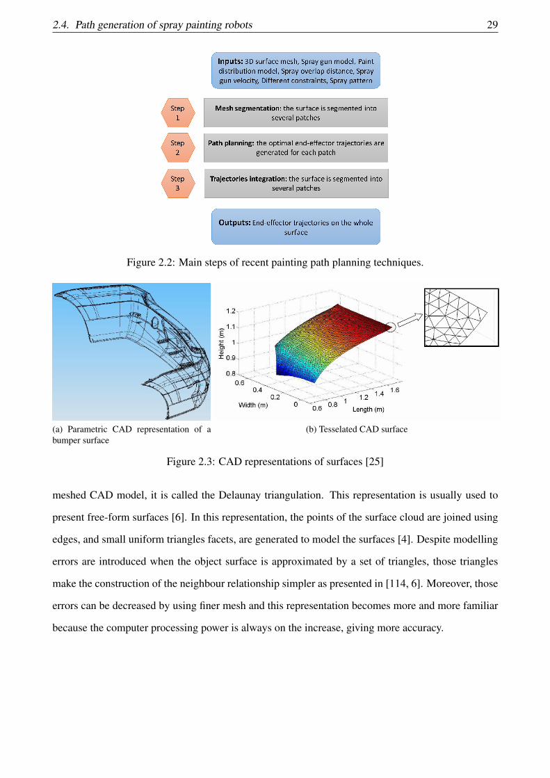
2.4. Path generation of spray painting robots 29
Figure 2.2: Main steps of recent painting path planning techniques.
(a) Parametric CAD representation of abumper surface
(b) Tesselated CAD surface
Figure 2.3: CAD representations of surfaces [25]
meshed CAD model, it is called the Delaunay triangulation. This representation is usually used to
present free-form surfaces [6]. In this representation, the points of the surface cloud are joined using
edges, and small uniform triangles facets, are generated to model the surfaces [4]. Despite modelling
errors are introduced when the object surface is approximated by a set of triangles, those triangles
make the construction of the neighbour relationship simpler as presented in [114, 6]. Moreover, those
errors can be decreased by using finer mesh and this representation becomes more and more familiar
because the computer processing power is always on the increase, giving more accuracy.
30 Chapter 2. State of the art
2.4.2 Mesh segmentation methods
In the automated path generation, the mesh segmentation methods are used to decompose the surfaces
into smaller surfaces (called patches) that have uniform geometrical properties. Hence, each patch can
be painted using the same strategy.
Sheng et al. developed first the combinatorial algorithm to generate different paths on simple sur-
faces [114]. Hence, a surface segmentation step, also named surface partitioning, is added before the
path planning in order to manage with compound surfaces [115]. Sheng et al. segmentation algorithm
deals with complicated multiple patch surfaces. However, the complicated surfaces must have low
curvatures because the segmentation algorithm analyses the surface as a plane. In recent works, Bo
et al. choose to first proceed to normal-based partition and then to topological-based partition [12].
This technique is important since it avoids the different curvatures before the projection of the surface
on a 2D plane.
Xia et al. proposed a new segmentation method [134] to deal with complex surfaces in order to
optimize the paint uniformity, the paint waste and the cycle time: it is the combinatorial algorithm.
Xia et al. added a second step to the combinatorial algorithm: it is called Segmentation Based On
Obstacle Avoidance (SBOOA). SBOOA reduces the cycle time and the painting waste by segmenting
each patch of the surface containing obstacles, e.g. holes. The suitability of SBOOA is evaluated
through the ratio between the percentage of the holes in the surface and the whole surface to be
painted. If this ratio is greater than a given threshold, the paint waste is not acceptable and SBOOA
algorithm is required, otherwise SBOOA segmentation is inessential.
2.4.3 Path planning algorithms
After the mesh segmentation into several sub-surfaces, a path planning algorithm is launched to gener-
ate the spray gun trajectories on each sub-surface. Those trajectories are defined by a set of successive
points. Each point describes the position and the orientation of the spray gun in a Cartesian frame.
Those points are joined to create trajectories in such a way that those trajectories have the less num-

2.4. Path generation of spray painting robots 31
ber of turns: the minimal cycle time is reached [23]. Four main algorithms exist: the combinatorial
algorithm proposed in 2000 by Sheng et al. [114], the offset curve planner proposed in 2008 [8], the
incremental trajectory generation [6] and the trajectory planning [123].
2.4.4 Finalization: Integration techniques
After the surface segmentation and the trajectory generation, a connection between the generated
paths on each patch is required. Hence, an integration between the bordering paths is the solution.
Thus, the generated trajectories on each patch must be stitched taking into account the paint unifor-
mity. Chen et al. were the first one to tackle this problem in [21]. This algorithm is enhanced in [22],
taking into account all the intersection areas, and not only the intersection line. In the same patch,
the overlap distance and the gun velocity values do not change. However, in the intersection area,
those values are changed in order to attend the paint uniformity. Thus, the pattern search method
(optimization algorithm) is used to calculate those values in the integration zone (zone joining two
patches).
Finally, in [20], the same algorithm is used as in [22]. However, Chen chose the steepest-descend
algorithm for the optimization instead of the pattern search method.
2.4.5 Comparison between different algorithms
Surface type Incremental trajectory generation Combinatorial algorithm Offset curve plannerplanar surface . + -curved surface + - .
surface with holes . + -Final result + 2+ 2-
Table 2.1: comparison table between the three algorithms based on the paint thickness variations (+:best result, .: acceptable result, -: worst result)
In this section, we compare the different path generation algorithms, developed by Andulkar and
Chiddarwar [4], Chen and Xi [20], Atkar et al. [9] and Tang and Chen [123], based on our under-
standing as well as on the results of the state-of-the-art. Those algorithms are analysed based on the
paint uniformity which is computed at the end of the painting process. Their behaviour on different
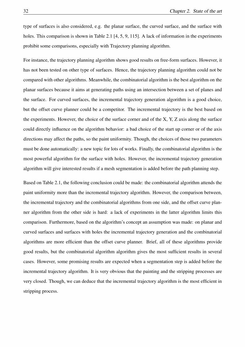
32 Chapter 2. State of the art
type of surfaces is also considered, e.g. the planar surface, the curved surface, and the surface with
holes. This comparison is shown in Table 2.1 [4, 5, 9, 115]. A lack of information in the experiments
prohibit some comparisons, especially with Trajectory planning algorithm.
For instance, the trajectory planning algorithm shows good results on free-form surfaces. However, it
has not been tested on other type of surfaces. Hence, the trajectory planning algorithm could not be
compared with other algorithms. Meanwhile, the combinatorial algorithm is the best algorithm on the
planar surfaces because it aims at generating paths using an intersection between a set of planes and
the surface. For curved surfaces, the incremental trajectory generation algorithm is a good choice,
but the offset curve planner could be a competitor. The incremental trajectory is the best based on
the experiments. However, the choice of the surface corner and of the X, Y, Z axis along the surface
could directly influence on the algorithm behavior: a bad choice of the start up corner or of the axis
directions may affect the paths, so the paint uniformity. Though, the choices of those two parameters
must be done automatically: a new topic for lots of works. Finally, the combinatorial algorithm is the
most powerful algorithm for the surface with holes. However, the incremental trajectory generation
algorithm will give interested results if a mesh segmentation is added before the path planning step.
Based on Table 2.1, the following conclusion could be made: the combinatorial algorithm attends the
paint uniformity more than the incremental trajectory algorithm. However, the comparison between,
the incremental trajectory and the combinatorial algorithms from one side, and the offset curve plan-
ner algorithm from the other side is hard: a lack of experiments in the latter algorithm limits this
comparison. Furthermore, based on the algorithm’s concept an assumption was made: on planar and
curved surfaces and surfaces with holes the incremental trajectory generation and the combinatorial
algorithms are more efficient than the offset curve planner. Brief, all of these algorithms provide
good results, but the combinatorial algorithm algorithm gives the most sufficient results in several
cases. However, some promising results are expected when a segmentation step is added before the
incremental trajectory algorithm. It is very obvious that the painting and the stripping processes are
very closed. Though, we can deduce that the incremental trajectory algorithm is the most efficient in
stripping process.

2.5. Conclusion 33
2.5 Conclusion
In this chapter, we have presented the state of the art related to four fields of research. Each one
is related to one step of the proposed approach. Firstly, we have presented the state of the art of
the robot’s workspace computation. Then, we have presented the mathematical tool that we chose
to compute the workspace in our application: Interval Analysis. A brief survey concerning Interval
Analysis in robotics has been also provided. Interval Analysis is chosen to compute the robot’s
workspace since it provides guaranteed workspace in a reasonable computation time. However, it
suffers from pessimism: a new inclusion function to reduce pessimism will be introduced in Chapter 3.
Two state of the art useful to compute the optimal number of robots with their optimal base placements
has been discussed: the camera placement problem and Art Gallery Problem. We considered that the
problem of optimization of the number of robots is mainly similar to those two problems. The main
difference between those three problems is the field of view. In the camera placement problem, the
optimization is based on the field of view of the camera. Further, the human field view is used to
test the complete coverage in Art Gallery Problem. However, in the robot coverage problem, the
reachable part of the surface is used to check the coverage of a surface. In my thesis, the reachable
part of the surface will be the intersection between the surface and the robot’s workspace already
computed using IA.
The optimization of a single robot base placement for coverage task has been studied. Hence, a com-
bination between the optimization of the number of robots and the robot base placement for complete
coverage is required to solve our general problem (the optimization of the number of robots with their
base placements). This combination leads to a new contribution which is the hybrid optimization
function developed and tested on the coverage problem (striping application). This contribution is
developed in Chapter 4.
Finally, we developed the state of the art related to path generation of spray painting. This state of the
art can be used to generate the trajectories of the stripping tool on the surface. Unfortunately, we did
not have time to implement and to test it.

Chapter 3
Interval Analysis Using BSplines and
Kronecker product
Solving Constraint Satisfaction Problem (CSP) consists in finding the set of variables that respect
a set of constraints. CSP finds all the valid solutions. CSP could be extended to a problem that
should find the set of variables optimizing a criteria function and satisfying a set of constraints namely
Constraint Optimization Problem (COP) [112]. CSPs and COPs are popular in robotics where the
constraints may take several forms: the robot kinematic and dynamic limits, the robot balance or
the different constraints imposed by the desired task. On the one hand, CSP is used in sequential
manipulation planning [85], planning [124], robot control [41]. On the other hand, COPs may be
used for physical parameters identification [66]. The optimization techniques allow robots to perform
motions or to reach a static pose while minimizing criteria like energy consumption or even execution
time [79]. The optimal motion/ pose parameters must also satisfy a set of constraints (such as joint
limits, joints torques, balance, etc) in order to ensure the integrity of the robotic system and the task
completion. Depending on the application, the constraints and the criteria function can vary from
simple (continuous, linear, monotonic, etc) to very complex (discontinuous, non-linear, with local
extremum, etc). In simple cases (quadratic criteria without constraint), the optimal parameters can be
found easily using Lagrange multipliers, active set, etc [100]. For more complex cases, one usually
refer to heuristic algorithms or to some iterative algorithms [74, 130] that produce a solution in a finite
34
35
time. For relatively complex cases (especially with discontinuous or non differentiable functions),
Genetic Algorithms return a solution without any guarantee of the optimality.
Interval Analysis (IA) is a powerful mathematical tool that could be used to solve CSPs as well as
COPs. For instance, optimization techniques based on IA provide actual and optimal results ensuring
the constraints satisfaction and the lack of solutions [51]. In [78], it has been proven that IA is efficient
for finding the feasible space during motion generation: finding a new posture in the feasible space
is faster than generating it explicitly. However in [64], IA is used for parameters estimations since
it deals with uncertainties and ensures the results consistency. Unfortunately, those techniques suffer
from a prohibitive computation time, due to the pessimism induced by the use of Interval Analysis.
The pessimism is an over-estimation of the functions, i.e. the given interval is still conservative (it
contains the actual solution) but it is larger than the actual solution. Pessimism is deeply linked to the
inclusion function (the way to evaluate a function in Interval Analysis). In order to reduce pessimism,
the natural inclusion function can be replaced by the centred, Taylor-centred or Chebyshev inclusion
functions [98]. In this chapter, we propose a new inclusion function for multi-dimensional systems
that decreases the pessimism and the computation time using the convex hull property of BSplines and
Kronecker product. This method was already applied in a one dimensional case to evaluate functions
over time intervals [79]. Our work is an extension to multi-dimensional problems. Our method is
applied on the resolution of CSPs and COPs. We assess the results of our method on robotic systems.
CSPs and COPs are presented in Section 3.1. Section 3.2 introduces IA and explains the IA’s main
drawback, i.e. the pessimism. Besides, Section 3.3 introduces how IA is used to solve CSPs and
COPs. Further, Section 3.4 details the BSplines and the Kronecker properties and how they can
be used to reduce the pessimism. After that, we detail two different implementation versions of
the proposed inclusion function in Section 3.5. The initial implementation version is published as a
conference paper in the “15th International Conference on Intelligent Autonomous Systems” [68] and
is presented in Section 3.5.1. The initial implementation has been improved: the final implementation
version is explained in Section 3.5.2. A paper has been recently submitted in “Reliable Computing
journal” about the final implementation version [80]. Moreover, the simulations and results of the
final implementation version is presented in Section 3.6. The results of the initial implementation
version can be found in Appendix D. Some mathematical tools with some examples can be found in
36 Chapter 3. Interval Analysis Using BSplines and Kronecker product
the following Appendices A, B and C.
3.1 Problem Statement
Constraint Satisfaction Problem is a mathematical problem that consists in finding a set of objects or
states satisfying a set of constraints as defined hereafter:
Find all [q] ∈Q
such as ∀ j ∈ {1, . . . ,m} G j([q]) ∈ [g j,g j](3.1)
Where:
— n is the number of variables composing the set q,
— m is the number of constraints,
— q = {q1, ...,qn} is the set of n variables,
— Q = {[q1 : q1], ..., [qn : qn]} ⊂ Rn is the set of variable domains defined by the minimum and
maximum values of each variable,
— G ([q]) is the set of m constraints. Each constraint of this set G j([q]) must remains within the
interval [g j,g j] with the lower bound g j and the upper bound g j limits.
In robotics, q is composed by a set of variables that could be the joint trajectory parameters [91], the
set of joint angles creating the feasible space with bounding errors [78], etc. Moreover, the constraint
equation G j(q) is usually non-linear and refer to the collision avoidance constraint, the joint position
velocity or torque limits, the manipulability criteria to avoid singularities, the reachability of the end-
effector or the balance constraint etc.
Backtracking, iterative improvement, consistency, and IA [44, 137] are the four major algorithms
usually used to solve CSP. Backtracking algorithms usually use recursive formulations. The problem
is presented as a tree with a constraint on each node: the descent on a given node stops once the
condition is not fulfilled. However, iterative improvement algorithms initialize a random configura-
tion as the initial inputs. After that, the inputs are modified until the solution is reached. Moreover,

3.2. Interval Analysis 37
Consistency algorithms reduce the problem complexity by decreasing its search space. Those algo-
rithms change the problem formulation but the solutions are the same. IA is chosen since it avoids the
lack of the solutions and guarantees them. Several works showed that Interval Analysis is competi-
tive compared to the classic optimization solvers since it provides guaranteed solutions respecting the
constraints.
The mechanical structure of the robot expands uncertainties during solving CSP: IA is the mathemat-
ical tool used to solve CSP to ensure the reliability and to deal with uncertainties [91]. IA can be used
to solve COPs in addition of solving CSPs using Equation 3.1. This transformation can be reached
by adding a criteria function to Equation 3.1. Hence, the resolution of the optimization problem can
be defined as (instead of Equation 3.1):
Find [q]⊂Q⊂ Rn
such as minq
F ([q])
with ∀ j ∈ {1, . . . ,m} G j([q]) ∈ [g j,g j]
(3.2)
Where F ([q]) is the criteria function.
3.2 Interval Analysis
Interval Analysis, also called Interval Arithmetic, is a mathematical tool developed by mathematicians
since the 1950s. Nowadays, Interval Analysis is used in many fields: robotics, global optimization, lo-
calization of robots, parameter estimation, set inversion etc. The results provided by interval methods
are always guaranteed regarding a set of hypotheses [64]. Interval Analysis was initially developed
to take into account the quantification errors introduced by the floating point representation of real
numbers with computers. Nowadays, Interval Analysis is largely used in robotics.

38 Chapter 3. Interval Analysis Using BSplines and Kronecker product
3.2.1 Presentation
Let us define an interval [a] = [a, a] as a connected and closed subset of R, with a = In f ([a]), a =
Sup([a]) and Mid([a]) = a+a2 . The set of all real intervals of R is denoted by IR. Real arithmetic
operations are extended to intervals. Consider an operator ◦ ∈ {+,−,∗,÷} and [a] and [b] two
intervals. Then:
[a]◦ [b] = [in fu∈[a],v∈[b] u◦ v, supu∈[a],v∈[b] u◦ v] (3.3)
This operation can be detailed as follows:
[a]+ [b] = [a+b, a+ b]
[a]− [b] = [a− b, a−b]
[a]∗ [b] = [min{ab,ab, ab, ab},max{ab,ab, ab, ab}]
[a]/[b] = [a]∗ [1/b] i f 0 /∈ [b] else [−∞,∞]
I f f ∈ {cos, sin, sqr, sqrt, log, ...} f ([a]) = [ f (a)|a ∈ [a]]
(3.4)
The propriety of the exponential function, shown in Equation 3.4, is also a property for every mono-
tonic functions.
3.2.2 Boxes or Interval Vectors
An interval real vector [a] is a subset of Rn that can be defined as the Cartesian product of n closed
intervals. [a] is called an interval vector, or also a box and it can be written as:
[a] = [a1]× [a2]×·· ·× [an], with [ai] = [ai, ai] f or i = 1, · · · ,n. (3.5)
where [ai] is the projection of [a] on the ith axis. Similarly to the interval, a box has a lower bound,
an upper bound, a width and a midpoint (also named centre). Let us define a box [a], the lower bound
is lb([a])= [a], (lb([a1]), lb([a2]),· · · ,lb([an]))T = (a1,a2, · · · ,an)T , the upper bound is ub([a])= [a],
(ub([a1]),ub([a2]),· · · ,ub([an]))T = (a1, a2, · · · , an)T . The width of ([a])= ([a1],[a2],· · · ,[an])T is w([a])
, (mid([a1]),· · · ,mid([an]))T . Let [b] be a subset of Rn, the intersection of [a] and [b] is defined as
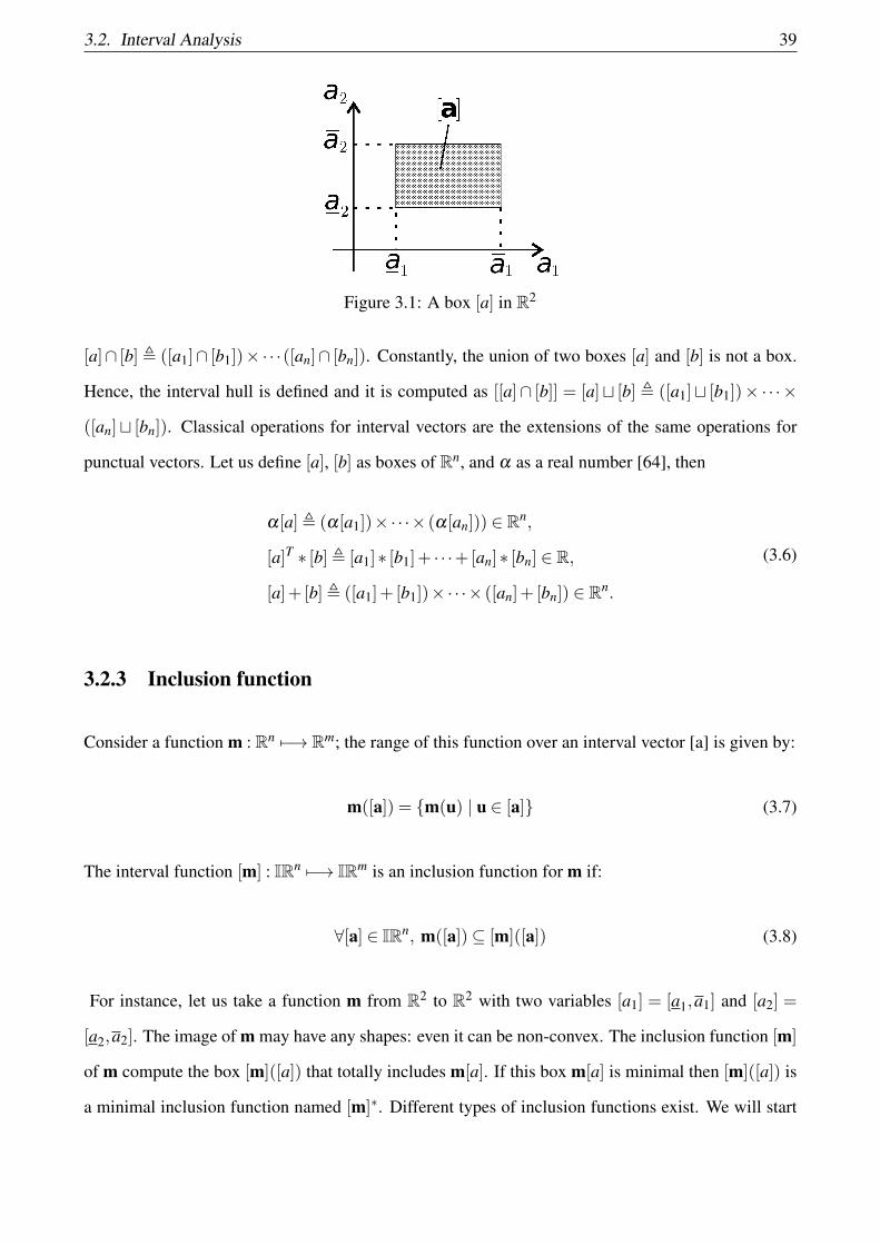
3.2. Interval Analysis 39
Figure 3.1: A box [a] in R2
[a]∩ [b] , ([a1]∩ [b1])×·· ·([an]∩ [bn]). Constantly, the union of two boxes [a] and [b] is not a box.
Hence, the interval hull is defined and it is computed as [[a]∩ [b]] = [a]t [b] , ([a1]t [b1])× ·· ·×
([an]t [bn]). Classical operations for interval vectors are the extensions of the same operations for
punctual vectors. Let us define [a], [b] as boxes of Rn, and α as a real number [64], then
α[a], (α[a1])×·· ·× (α[an])) ∈ Rn,
[a]T ∗ [b], [a1]∗ [b1]+ · · ·+[an]∗ [bn] ∈ R,
[a]+ [b], ([a1]+ [b1])×·· ·× ([an]+ [bn]) ∈ Rn.
(3.6)
3.2.3 Inclusion function
Consider a function m : Rn 7−→ Rm; the range of this function over an interval vector [a] is given by:
m([a]) = {m(u) | u ∈ [a]} (3.7)
The interval function [m] : IRn 7−→ IRm is an inclusion function for m if:
∀[a] ∈ IRn, m([a])⊆ [m]([a]) (3.8)
For instance, let us take a function m from R2 to R2 with two variables [a1] = [a1,a1] and [a2] =
[a2,a2]. The image of m may have any shapes: even it can be non-convex. The inclusion function [m]
of m compute the box [m]([a]) that totally includes m[a]. If this box m[a] is minimal then [m]([a]) is
a minimal inclusion function named [m]∗. Different types of inclusion functions exist. We will start

40 Chapter 3. Interval Analysis Using BSplines and Kronecker product
Figure 3.2: Image of a box [a] using a function m and its inclusion functions [m] and [m]∗
by explaining the trivial inclusion function: the natural inclusion function.
3.2.3.1 Natural inclusion function
The natural inclusion function of m is computed by changing each occurrence of a real variable by its
corresponding interval, so each function by its interval.
Example 3.1. Consider four different expressions of the same function f (a) : R→ R
f1(a) = a(a+1),
f2(a) = a∗a+a,
f3(a) = a2 +a,
f4(a) = (a+12)2− 1
4.
(3.9)
Their different natural inclusion functions for [a] = [−1,1]:
[ f1]([a]) = [a]([a]+1) = [−2,2],
[ f2]([a]) = [a]∗ [a]+ [a] = [−2,2],
[ f3]([a]) = [a]2 +[a] = [−1,2],
[ f4]([a]) = ([a]+12)2− 1
4= [−1
4,2].
(3.10)
Figure 3.3 shows different intervals computed using different inclusion functions. It is clear that
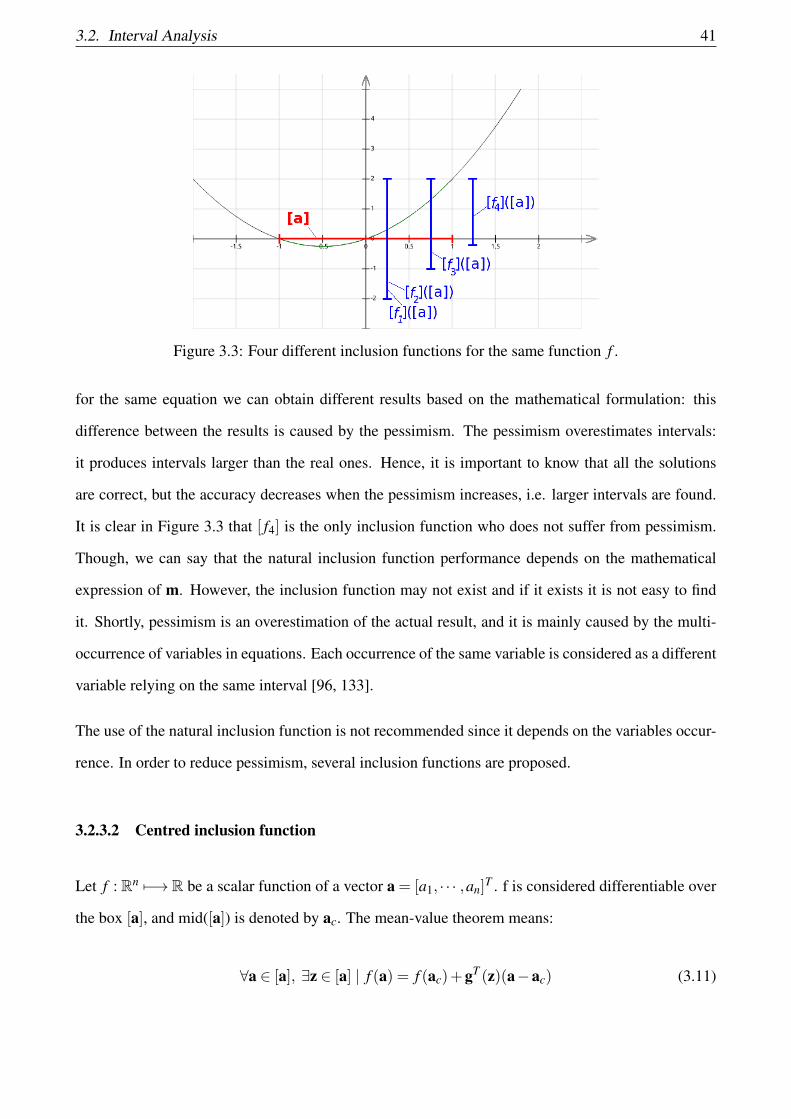
3.2. Interval Analysis 41
Figure 3.3: Four different inclusion functions for the same function f .
for the same equation we can obtain different results based on the mathematical formulation: this
difference between the results is caused by the pessimism. The pessimism overestimates intervals:
it produces intervals larger than the real ones. Hence, it is important to know that all the solutions
are correct, but the accuracy decreases when the pessimism increases, i.e. larger intervals are found.
It is clear in Figure 3.3 that [ f4] is the only inclusion function who does not suffer from pessimism.
Though, we can say that the natural inclusion function performance depends on the mathematical
expression of m. However, the inclusion function may not exist and if it exists it is not easy to find
it. Shortly, pessimism is an overestimation of the actual result, and it is mainly caused by the multi-
occurrence of variables in equations. Each occurrence of the same variable is considered as a different
variable relying on the same interval [96, 133].
The use of the natural inclusion function is not recommended since it depends on the variables occur-
rence. In order to reduce pessimism, several inclusion functions are proposed.
3.2.3.2 Centred inclusion function
Let f : Rn 7−→ R be a scalar function of a vector a = [a1, · · · ,an]T . f is considered differentiable over
the box [a], and mid([a]) is denoted by ac. The mean-value theorem means:
∀a ∈ [a], ∃z ∈ [a] | f (a) = f (ac)+gT (z)(a−ac) (3.11)

42 Chapter 3. Interval Analysis Using BSplines and Kronecker product
where gT is the gradient of f , a column vector with entries gi =∂ f∂ai
, i = 1, · · · ,k. Hence,
∀a ∈ [a], f (a) ∈ f (ac)+ [gT ]([a])([a]−ac) (3.12)
where [gT ] is an inclusion function for gT , so
f (a)⊆ f (ac)+ [gT ]([a])([a]−ac) (3.13)
Thus, the interval function:
[ fc](a), f (ac)+ [gT ]([a])([a]−ac) (3.14)
is the centred inclusion function of f for any given [a]. This function is an affine function having an
uncertain slope [ f ′]([x]). Hence, [ fc](a) can be represented by a cone with a centre (ac, f (ac)). As
it is shown in Figure 3.4, the smaller the width of [a] is, the better the centred inclusion function is.
Hence, we can say that the image illustrates that when w([a])→ 0
w([ fc]([a]))w([ f ]([a]))
→ 1 (3.15)
Figure 3.4: Perception of the centred inclusion function
The centred inclusion function is proposed since the scalar product with [a]−ac reduces the pessimism
when [a] is small. When [a] gets larger, the centred inclusion function efficiency reduces: its effect of
reducing pessimism decreases. The centred inclusion function for a function f from Rn 7−→R can be
noticeably improved by using the mixed centred inclusion function.

3.2. Interval Analysis 43
3.2.3.3 Mixed centred inclusion function
When the centred inclusion function is applied on each variable, the whole function will be the mixed
centred inclusion function. Hence, the expression of the centred inclusion function is generalized for
n variables where a = (a1, · · · ,an)T and m=mid([a]):
f ([a])⊂ f (m)+n
∑i=1
[gi]([a1], · · · , [ai],mi+1, · · · ,mn)∗ ([ai]−mi) (3.16)
The mixed centred inclusion function could get tighter intervals than the centred inclusion function for
multi-dimensional functions. That is because the gradient arguments are mixed in the new inclusion
function: the pessimism is reduced since [ f ](mid([a]), [a])⊂ [ f ]([a]).
3.2.3.4 Taylor inclusion function
Reconsidering the derivation of centred inclusion function, the high-order Taylor series can be used
to approximate the function f : Rn 7−→ R which leads to the Taylor inclusion function. The Taylor
inclusion function can be written as:
[ f ]T ([x]) = f (m)+ f ′(m)([x]−m)+ · · ·+ f n−1(m)([x]−m)(n−1)
(n−1)!+[ f n]([x])
([x]−m)n
n!(3.17)
The evaluation of the Taylor inclusion function requires a computation of the derivatives of f up to nth
order. Hence, this computation may increase the computation time. Taylor inclusion function may be
the best of the previous inclusion functions. But, adding to the computation time, Taylor inclusion
function suffers from large overestimations for non-linear functions. Hence, Chebyshev inclusion
function has been proposed.
3.2.3.5 Chebyshev inclusion function
Chebyshev inclusion function is recommended for non-linear functions [133]. Chebyshev series are
a high accurate approximating series. Hence, Chebyshev inclusion function can control efficiently

44 Chapter 3. Interval Analysis Using BSplines and Kronecker product
the pessimism during interval evaluation, especially for the non-monotonic functions. Chebyshev
inclusion function can be written as
[ fCk ]([x]) =12
f0 +k
∑i=1
fiCi([x]) =12
f0 +k
∑i=1
ficosi[θ ] (3.18)
where x = (x1, · · · ,xn)T . Chebyshev interval method is considered as a kind of non-intrusive ap-
proach: it could be applied on many black box models and on complicated engineering models. It has
been proven that Chebyshev inclusion function controls the pessimism better than Taylor inclusion
function after some numerical tests for solving the mechanical dynamics problems. It is also proven
that Chebyshev inclusion function is easier to implement [133].
3.2.3.6 Bernstein inclusion function
Every multivariate polynomial p : Rm −→R of multi-degree n can be written as a linear combination
of the Bernstein polynomials of order n [43]:
p(x) =n
∑j=0
b(j,n)B(j,n)(x)
.
If p is of the form p(x) = ∑ni=0 aixi then the coefficients of the Bernstein expansion can be computed
with the following formula j-th Bernstein coefficient (of degree n): b(j,n) = ∑ni=0 ai
j! n!i!( j− i)! i!(n− i)!
.
Thus, we can define the Bernstein Form interval extension of order n as follows: B(p)([0,1]m) =
[minj(b(j,n)),maxj(b(j,n))].
The polynomial must first be composed with the appropriate affine translation and scaling that maps
x into [0, 1] to compute the range over an arbitrary interval x, before computing Bernstein expansion.
The main advantage of Bernstein Form interval extension is that it gives the exact range if and only if
min j(b(j,n)) ∈ {b(0,n),b(n,n)} and max j(b(j,n)) ∈ {b(0,n),b(n,n)} [121].

3.2. Interval Analysis 45
3.2.3.7 Horner schemes
Horner schemes consist in manipulating the mathematical form of the equation in order to get a new
form that reduces pessimism. Hence, Horner schemes, also called Horner’s method, transform the
monomial form of a function into an efficient form by factorizing it [96]. Given the polynomial of
one variable x:
p(x) =n
∑i=0
aixi = a0 +a1x+a2x2 + · · ·+anxn (3.19)
where a0, · · · ,an are real numbers. The univariate Horner scheme of Equation 3.19 is
p(x) = a0 + x(a1 + x(a2 + · · ·+ x(an−1 + xan) · · ·)) (3.20)
Univariate Horner schemes consist in transforming the polynomial into another one that contains the
minimal amount of mathematical operations. The multivariate Horner scheme H is defined as follows:
∀a ∈Q : a ∈ H
∀hdep ∈ H : xei .(hdep) ∈ H
∀hdep,hind ∈ H : xei .(hdep)+hind ∈ H
(3.21)
where e ∈ N\0 and the variable xi do not occur in hind .
For instance, let us consider the polynomial form of the function f (x) = 5+ 2x+ 4x2 + 3x3. The
univariate Horner scheme of f is fu(x) = 5+x(2+x(4+x(3))). However, a polynomial of 3 variables
f (x1,x2,x3) = x1x22+x1x3+x1x2
2x3 could have 2 different multivariate Horner schemes. The first mul-
tivariate Horner scheme is f (x1,x2,x3) = x1.(x22.(1+x3)+x3). This form is obtained by extracting x1
then x2. However, f (x1,x2,x3) = x1.(x3.(1+x22)+x2
2) is obtained by extracting x1, then x3. Moreover,
in both cases, the number of occurrence of each variable is reduced, i.e. the pessimism is reduced.
We should know that the different Horner scheme representations may not have the same effect of
reducing pessimism (it depends on the number of occurrence of each variable in the equation).
It has been proved in [96] that transforming a polynomial into a Horner scheme may reduce its over-
approximation, i.e. pessimism, but certainly it does not increase it.
46 Chapter 3. Interval Analysis Using BSplines and Kronecker product
However, Horner schemes need a polynomial form of the function. In robotics, the different con-
straints are trigonometric functions, so it is mandatory to transform the trigonometric constraints into
polynomial forms using Taylor series. Moreover, it is easy to find the Horner schemes manually, but
the complexity increases if a generic program has to find Horner schemes for every proposed function.
Our goal in this PHD is to generalize the constraints when Horner schemes are not useful.
3.2.3.8 Comparison between different inclusion functions:
The natural inclusion function is more efficient than the centred inclusion function for large boxes.
However, the centred inclusion function gives better results once the box get tighter. None of the
existing inclusion function could be judged as the best: a compromise between the complexity and
the efficiency must be done.
In the other hand, Chebyshev inclusion function get tighter interval than Taylor inclusion function.
In addition, Chebyshev inclusion function does not need to calculate the derivatives of the original
function, so it can be used to solve the black box problems. However, Chebyshev inclusion function
is not a rigorous inclusion function because it neglects the numerical and the truncated errors in
integration. Further, Bernstein inclusion function is the best of all the above inclusion functions.
Hence, we got the idea of testing a new inclusion function using the Bernstein concept applied by
another mathematical tool, e.g BSplines concept. In this chapter, we propose a new inclusion function
based on BSplines and Kronecker product properties. This new inclusion function reduces pessimism
and takes into account the numerical and the truncated errors during integration.
3.3 Solving CSPs and COPs using IA
IA is used to solve CSPs (Equation 3.1) and COPs (Equation 3.2). Given input bounds, the algorithm
produces a subset of the input space that satisfies all the constraints (for CSPs) and also minimizes the
criteria function (for COPs). In both problem types, the subset of outputs is a set of small boxes. A
combination between bisection and contraction solves Equations 3.1 and 3.2. Those two operations
are presented hereafter.

3.3. Solving CSPs and COPs using IA 47
3.3.1 Bisection
Bisection is an iterative method that decomposes the set of inputs into smaller sets. The bisection-
based method is generally used to reduce the overestimation since pessimism is linked to the width of
the inputs. Several splitting methods could be used to apply bisection [93].
In COPs, the constraints and the criteria functions are evaluated for a current box. Based on this
evaluation, a decision must be taken: the boxes may be thrown away or may be split into smaller
boxes. A box is thrown away due to a constraint violation or to a large criteria function. The constraint
is considered violated if its interval evaluation has no intersection with the bounds [g j]. The splitting
process is applied to get a tighter evaluation of the constraints and the criteria function, and it ends
when the size of the box is smaller than a given threshold. For sake of simplicity, the box is divided
into two sub-boxes by splitting the largest interval in this box into equal intervals. The above steps are
programmed as it is shown in Algorithm 1. The line 4 could be skipped depending on the application:
some applications do not require a criteria function which is the case of CSPs. At the end of the
bisection algorithm, we get three types of set of boxes: the set of feasible boxes, the set of infeasible
boxes and the set of maybe feasible boxes (properties for CSPs).
In order to make the bisection process more obvious, let us consider two variables [x] = [xa,xb] and
[y] = [ya,yb], find the set of boxes that respects the constraint C having the color green as it is clear
in Figure 3.5. Using the bisection algorithm, we get three types of boxes: the infeasible boxes (in
white), the maybe feasible boxes (in red) and the feasible boxes (in green).
3.3.2 Contraction
Contraction is based on the filtering algorithm concept [60]. The contraction has the same formulation
for CSPs as well as for COPs. It manipulates the equation in order to propagate the constraints in two
ways: from inputs to outputs (Eq.(3.22)) and from outputs to inputs (Eq.(3.23)).
∀ j [g j]← G j([q])∩ [g j] (3.22)
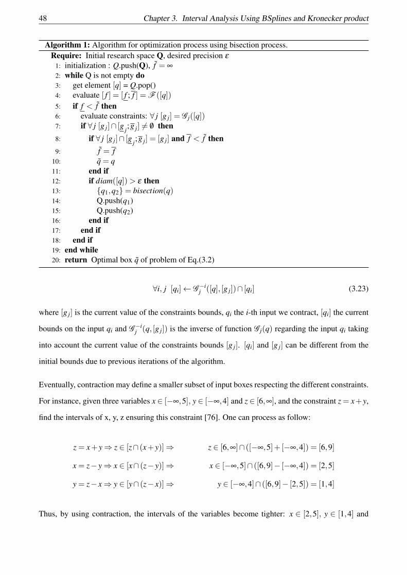
48 Chapter 3. Interval Analysis Using BSplines and Kronecker product
Algorithm 1: Algorithm for optimization process using bisection process.Require: Initial research space Q, desired precision ε
1: initialization : Q.push(Q), f = ∞
2: while Q is not empty do3: get element [q] = Q.pop()4: evaluate [ f ] = [ f ; f ] = F ([q])5: if f < f then6: evaluate constraints: ∀ j [g j] = G j([q])7: if ∀ j [g j]∩ [g j;g j] 6= /0 then8: if ∀ j [g j]∩ [g j;g j] = [g j] and f < f then9: f = f
10: q = q11: end if12: if diam([q])> ε then13: {q1,q2}= bisection(q)14: Q.push(q1)15: Q.push(q2)16: end if17: end if18: end if19: end while20: return Optimal box q of problem of Eq.(3.2)
∀i, j [qi]← G−ij ([q], [g j])∩ [qi] (3.23)
where [g j] is the current value of the constraints bounds, qi the i-th input we contract, [qi] the current
bounds on the input qi and G−ij (q, [g j]) is the inverse of function G j(q) regarding the input qi taking
into account the current value of the constraints bounds [g j]. [qi] and [g j] can be different from the
initial bounds due to previous iterations of the algorithm.
Eventually, contraction may define a smaller subset of input boxes respecting the different constraints.
For instance, given three variables x ∈ [−∞,5], y ∈ [−∞,4] and z ∈ [6,∞], and the constraint z = x+y,
find the intervals of x, y, z ensuring this constraint [76]. One can process as follow:
z = x+ y⇒ z ∈ [z∩ (x+ y)]⇒ z ∈ [6,∞]∩ ([−∞,5]+ [−∞,4]) = [6,9]
x = z− y⇒ x ∈ [x∩ (z− y)]⇒ x ∈ [−∞,5]∩ ([6,9]− [−∞,4]) = [2,5]
y = z− x⇒ y ∈ [y∩ (z− x)]⇒ y ∈ [−∞,4]∩ ([6,9]− [2,5]) = [1,4]
Thus, by using contraction, the intervals of the variables become tighter: x ∈ [2,5], y ∈ [1,4] and

3.4. BSplines identification 49
Figure 3.5: 2D bisection algorithm on a constraint C
z ∈ [6,9].
Generally, a combination between contractions and bisections is used as a solver. Firstly, contraction
reduces the input boxes size: the contraction is applied for each time a function is evaluated (lines 4
and 6 in Algorithm 1). Then, bisection is applied and contraction is called again until the dimension
of the generated boxes is smaller than a threshold. This method is the classic contraction/ bisection.
It uses the inclusion function m during contraction and bisection strategy. Hence, it suffers from
pessimism already explained.
Evaluating a constraint using the proposed inclusion function is detailed in two main sections: the
general principle is developed is Section 3.4 and its implementation is detailed in Section 3.5. Before
going further, I would like to say that we differentiate between two implementation versions: the
first implementation version is developed in Section 3.5.1 and it has been published as an article in
IAS conference [68], and the second implementation version is developed in Section 3.5.2 and it has
submitted to “Reliable computing” journal [80].
3.4 BSplines identification
BSplines properties were already used to tackle pessimism in one dimension: they are tested on
continuous constraints used to optimize robot motion [79]. In this chapter, a generalization of this

50 Chapter 3. Interval Analysis Using BSplines and Kronecker product
concept to multi-dimensional problems is proposed.
3.4.1 Definition and convex hull property
BSplines function is the weighted sum of several basis functions. It is defined by m control points Pi
and basis functions Bi. K is the order of the basis function Bi.
F(q) =m
∑i=1
BKi (q)Pi (3.24)
A BSplines curve is totally inside the convex hull of its control poly-line [79]. This property is
obtained quite easily from the following definition of a basis function:
∀q ∈ [q,q] ∑mi=1 BK
i (q) = 1 (3.25)
This immediately yields:
∀i ∈ [1,m] F ≤ Pi ≤ F ⇒∀q ∈ [q,q] F ≤ F(q)≤ F (3.26)
A conservative estimation of the bounds of F(q) is made based on the minimum and the maximum of
the control points. Thus, a bounding box of the considered function can be computed. However, the
control points of this function must be identified. For instance, let us consider the polynomial function
which is the blue curve in Figure 3.6. Bsplines representation of this curve gave the basis functions
and the control points as it is clear in Figure 3.6a. Hence, using the control points the box that includes
the curve could be deduced, i.e. the interval of the curve is also deduced (see Figure 3.6b).
3.4.2 Multi-dimension BSplines
N-dimensional BSplines are functions defined as:
F(q) =m1
∑i=0
m2
∑j=0
...mn
∑z=0
(Bm1
i (q1)Bm2j (q2)...Bmn
z (qn))×Pi, j,...,z (3.27)

3.4. BSplines identification 51
(a) Bsplines representation of a polynomialfunction
(b) Interval evaluation using control points
Figure 3.6: Evaluating intervals using BSplines properties
Where:
— q = {q1,q2, ...,qn} ∈ [Q]⊂ Rn,
— mi is the degree of the input qi,
— Bmi(qi) is the BSpline Basis function of degree mi relied to input qi,
— Pi, j,...,z are the Control Points grouped into vector P.
As in the one-dimensional case, the BSpline curve is entirely in the convex hull of its control poly-
line:
∀q ∈ [Q] F(q) ∈ [min(P),max(P)] (3.28)
3.4.3 Constraint Evaluation
3.4.3.1 One dimensional case
Considering that all the functions can be described as a polynomial expression of the input as done
in [79], we have:
∀q ∈ [q,q] F(q) ∈n
∑i=0
ai×qi (3.29)
52 Chapter 3. Interval Analysis Using BSplines and Kronecker product
where {a0,a1, . . . ,an} ∈Rn+1 are the coefficients of the polynomial. This equation can be written as:
F(q) = [1,q, . . . ,qn]× [a0,a1, . . . ,an]T (3.30)
and knowing the coefficients ai, the coefficients pi of the equivalent control point are computed, such
as:
F(q) = [1,q, . . . ,qn]×B× [p0, p1, . . . , pn]T (3.31)
where B is a matrix that contains the polynomial parameters of the BSplines basis functions. There-
fore, we can compute the corresponding BSplines parameters as:
[p0, p1, . . . , pn]T = B−1× [a0,a1, . . . ,an]
T (3.32)
Though, we can deduce the bounds of F(q)
∀q ∈ [q,q] F(q) ∈ [min(p0, p1, . . . , pn),max(p0, p1, . . . , pn)] (3.33)
3.4.3.2 N-dimensional case
The same procedure can be applied to the N-dimensional case. Equation 3.45 could be written as:
F(q) = [1,q1,q2,q1q2, . . . ,µi, . . . ]× [a0,a1,a2, . . . ,ai, . . . ]T (3.34)
where µi is the ith monomial. Let us note P the vector of the control points and X the vector of the
polynomial coefficients. P and X are related through the following equation:
P = B−1X (3.35)
Where B can be written as:
B= B1⊗B2⊗ . . .⊗Bi⊗ . . .⊗Bn (3.36)

3.4. BSplines identification 53
Bi are matrices linking the control point to the coefficients of the polynomial expression of the basis
functions of input qi and ⊗ is the Kronecker product as defined hereafter. The Kronecker product
is an operation on two matrices of arbitrary size resulting in a block matrix. Consider two matrices
A and B, where: A =
a1,1 . . . a1,n1
......
...
am1,1 . . . am1,n1
. The kronecker product of A by B can be written as
follows:
A⊗B =
a1,1×B a1,2×B . . . a1,n1×B
a2,1×B a2,2×B . . . a2,n1×B...
......
...
am1,1×B am1,2×B . . . am1,n1×B
More details about Kronecker product can be found in Appendix A. By using the invertible property
of Kronecker product, Equations (3.35) and (3.36) can be turned into:
P =(B−1
1 ⊗B−12 ⊗ . . .⊗B−1
n)
X (3.37)
Equation 3.37 is chosen since it allows a faster computation (more details can be found in Ap-
pendix A).
3.4.4 Constraint contraction
The contraction of a constraint consists in updating the bounds of the constraint function and the
bound of the inputs (see Section 3.3.2). In order to perform the contraction, we consider a new
variable ν j([q], [g j]) such as: for each constraint G j([q]), a new variable ν j([q], [g j]) is defined.
ν j([q], [g j]) = G j([q])− [g j] (3.38)
The control points of this function Pν j can be evaluated through
Pν j = B−1ν j
Xν j (3.39)

54 Chapter 3. Interval Analysis Using BSplines and Kronecker product
where B−1ν j
and Xν j are the matrix and vector representation of the function ν j([q], [g j]). Obviously,
we perform the same decomposition than the one presented in Equation (3.48) to deal with error
component and sparse properties of the computation.
Let us define [µ] the interval value we want to contract that may be the bounds of the constraint [g j]
or the bounds of the input [q]. The contraction process returns to consider
[µ]← [µ]∩(ν j([q], [g j])+ [µ]
)(3.40)
Therefore we can compute the equivalent control point Pµ of ν j([q], [g j])+ [µ] such as:
Pµ = B−1ν j
Xν j +B−1ν j
Xµ = Pν j +B−1ν j
Xµ (3.41)
with Xµ is a zero value vector except for the component corresponding to the monomial µ that is the
opposite of the one of Xν j .
The evaluation of Equation (3.40) is performed as presented in Section 3.5.2.3 taking into account the
error such as in Equation (3.48) and using the sparse properties especially because Xµ contains only
one non-zero value.
3.5 Implementation
3.5.1 Initial implementation version
The initial implementation version can be decomposed into three main steps. Firstly, we have to deal
with non-linear functions. Secondly, we have to contract the monomials composed of one variable.
Thirdly, we should propagate the contraction on monomials composed of several variables.

3.5. Implementation 55
3.5.1.1 How to deal with non-linear functions?
The constraints must be formulated as polynomial equations of the inputs. Nevertheless, robotics
equations are generally non-linear (using sine and cosine). Here we proposed to create intermediate
inputs for cos(qi) and sin(qi). Each time those intermediate inputs are contracted, they propagate the
modification to the input qi that re-propagate on cos(qi) and sin(qi).
3.5.1.2 Monomial contraction:
After the contraction of monomials composed of one variable (q1, q2, etc), others monomials should
be contracted too (composed of more than one variable q1q2, q2q5q7, etc). Consider that the poly-
nomial constraint is a sum of many monomials µi after the linearisation. Considering a monomial
µi = ∏∀k σi,k composed of the multiplication of several input intervals [σi,k], if no input interval con-
tains zero, the input interval can be contracted thanks to:
[σi,k] = [σi,k]∩[In f (ρi);Sup(ρi)]
∏∀k 6=i σi,k(3.42)
The current input set will be considered as infeasible if this intersection returns an empty interval.
Hence, the contraction is propagated to different monomials.
3.5.2 Final implementation version
In the initial implementation step, the vector of the monomial coefficient X is considered constant
and the BSplines matrix Bi is updated regarding the current bounds of [qi]. This technique suffers
from the numerical errors while computing B−1i for narrows intervals on [qi] due to ill-conditioned
matrix. A matrix is considered ill-conditioned if small changes on the inputs may result high changes
on the outputs: in our case we can say that small changes in Bi may introduce huge changes in B−1i ,
though Bi is an ill-conditioned matrix. For instance, consider the linear system AX = Y , where A
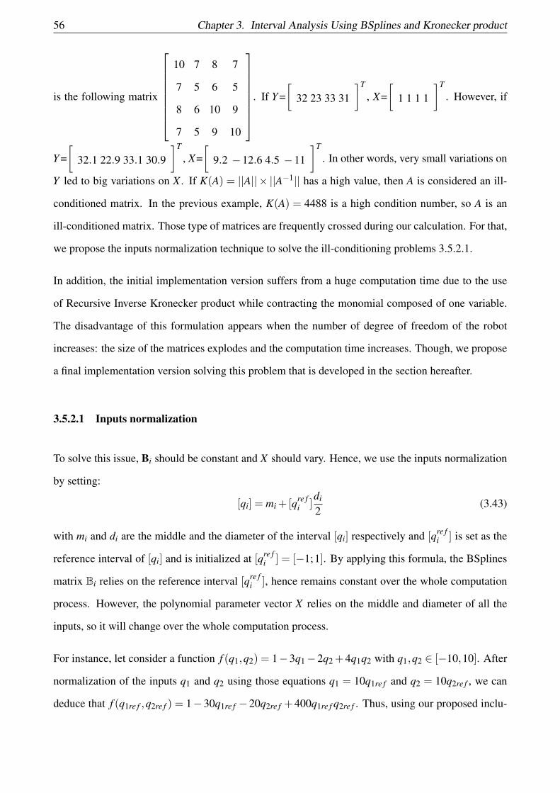
56 Chapter 3. Interval Analysis Using BSplines and Kronecker product
is the following matrix
10 7 8 7
7 5 6 5
8 6 10 9
7 5 9 10
. If Y =
[32 23 33 31
]T
, X=[
1 1 1 1
]T
. However, if
Y =[
32.1 22.9 33.1 30.9
]T
, X=[
9.2 −12.6 4.5 −11
]T
. In other words, very small variations on
Y led to big variations on X . If K(A) = ||A||× ||A−1|| has a high value, then A is considered an ill-
conditioned matrix. In the previous example, K(A) = 4488 is a high condition number, so A is an
ill-conditioned matrix. Those type of matrices are frequently crossed during our calculation. For that,
we propose the inputs normalization technique to solve the ill-conditioning problems 3.5.2.1.
In addition, the initial implementation version suffers from a huge computation time due to the use
of Recursive Inverse Kronecker product while contracting the monomial composed of one variable.
The disadvantage of this formulation appears when the number of degree of freedom of the robot
increases: the size of the matrices explodes and the computation time increases. Though, we propose
a final implementation version solving this problem that is developed in the section hereafter.
3.5.2.1 Inputs normalization
To solve this issue, Bi should be constant and X should vary. Hence, we use the inputs normalization
by setting:
[qi] = mi +[qre fi ]
di
2(3.43)
with mi and di are the middle and the diameter of the interval [qi] respectively and [qre fi ] is set as the
reference interval of [qi] and is initialized at [qre fi ] = [−1;1]. By applying this formula, the BSplines
matrix Bi relies on the reference interval [qre fi ], hence remains constant over the whole computation
process. However, the polynomial parameter vector X relies on the middle and diameter of all the
inputs, so it will change over the whole computation process.
For instance, let consider a function f (q1,q2) = 1−3q1−2q2 +4q1q2 with q1,q2 ∈ [−10,10]. After
normalization of the inputs q1 and q2 using those equations q1 = 10q1re f and q2 = 10q2re f , we can
deduce that f (q1re f ,q2re f ) = 1−30q1re f −20q2re f +400q1re f q2re f . Thus, using our proposed inclu-

3.5. Implementation 57
sion function, we can deduce that f ∈ [−409,451]. More details about this example could be found
in Appendix B.
3.5.2.2 Non linear functions
The final implementation version is also based on a polynomial formulation of the constraint and
criteria functions. However, the problems in robotics are non-linear problems: Taylor approximation
is used to approximate the non-linear functions to polynomial formulations. Consider that s([qi]) ∈
{sin([qi]),cos([qi])}, the linearisation Equation is:
s([qi]) = s(mi)+ds(mi)
dqi
di
2[qre f
i ]+ . . .+[εs(qi)] (3.44)
[εs(qi)] is normalized using [εs,ire f ], ms,i and ds,i as proposed in Equation (3.43). The reference error
interval [εsre fi ] is a new input in Equation (3.36). The interval value [εs(qi)] is updated every change
in the original interval [qi], and so ms,i and ds,i. In parallel, [εs,ire f ] is set to [−1;1]. [εs(qi)] is not
affected by the bisection process. In our work, we consider the first order approximation of non-linear
functions.
Appendix C develops how we obtained Equation 3.44, and how the error [εs(qi)] is computed based
on an example.
3.5.2.3 Constraint Evaluation
The efficient computation of the bounds of a function G j([q]) is developed in this Subsection. In order
to make the computation faster, Equation 3.35 is decomposed as follows:
P = B−1X I +B−1Xε (3.45)
where P ∈Rx is the set of the equivalent control points, X I ∈Rx contains the polynomial coefficients
that refer only to monomials with reference intervals ([qre fi ]) and Xε ∈Rx the polynomial coefficients

58 Chapter 3. Interval Analysis Using BSplines and Kronecker product
that refer to monomials with reference intervals ([qre fi ]) and reference errors [εs,i
re f ]. Obviously X =
X I +Xε .
During the tests, we have noticed that the vectors Xε and X I of Rx includes lots of null values. In
order to speed up the calculation, a sparse representation of the matrices and vectors is proposed:
P = SIX Is +SεXε
s (3.46)
where X Is ∈ Ry is the vector collecting the non-null coefficients of X I and SI ∈ Rx,y is obtained by
removing from B−1 the columns corresponding to the null coefficient of X I , and similarly for Xεs and
Sε .
Since the second term of Equation (3.46) SεXεs relies on non-linear approximation errors, it must
decrease as the width of the input boxes decreases. Hence, the error interval [ε] could be computed
faster using the following equation:
[ε] = Sε .Xεs (3.47)
with ε is the approximation error and Sε is the interval vector where each element is the interval
union of all the values of the corresponding column of Sε . Thus, each equivalent control point given
by SεXεs lies in the interval [ε]. Obviously, [ε] is a pessimistic evaluation of the approximation.
Eventually, the evaluation of G j([q]) is done computing:
P = SI.X Is +[ε] (3.48)
Hence, the function can be evaluated through the minimal and maximal value of P, where each control
point Pk can be computed with:
Pk = SIk.X I
s k +[ε] (3.49)
As presented in Algorithm 1, this evaluation is used in order to assess if the corresponding constraint
remains within a given bounds [g j,g j]. By sequentially computing the control point Pk we can deter-
mine if the corresponding box is overlapping when min∀k
Pk < g j and max∀k
Pk > g j or min∀k
Pk < g j and

3.6. Tests and results 59
max∀k
Pk > g j. As soon as, the overlapping of the constraint is detected, there is no need to compute
the other control points, since the bisection must be performed, hence the evaluation of the process is
stopped.
The polynomial formulation of the constraints and the computation of the sparse matrices and vectors
are done once in a preparation phase, before the beginning of Algorithm 1.
3.6 Tests and results
In this section, we present the results of solving CSPs and COPs using the proposed inclusion function
(final implementation version). The tests and results for the first implementation version are developed
in Appendix D.
The following abbreviations will be used in this section :
— BI: Bisection process using Interval Analysis,
— CI: Contraction and bisection using Interval Analysis,
— BS: Bisection process using the BSplines and Kronecker product properties,
— CS: Contraction and bisection process using the BSplines and Kronecker product properties.
In order to assess our improved inclusion function, we propose 3 different scenarios: one scenario
on a 2D robot (a robot of two degrees of freedom), another on a planar robot (a 2D robot of multiple
degrees of freedom), and the last scenario is on a 3D robot. Those three scenarios are presented in the
sections below.
3.6.1 2D Robot feasible space
In this section, we propose a system of two equations in order to assess our method on Constraint
Satisfaction Problem resolution. The goal is to find the feasible space of a robot, though all the sets
of joint angles that respects Equation 3.50. This problem is defined in Equation 3.1. The system is a

60 Chapter 3. Interval Analysis Using BSplines and Kronecker product
2-dof planar robot q ∈ R2, with joint limits q1,q2 ∈ [−2;2], we set the following constraints :
x = cos(q1)+ cos(q1 +q2) ∈ [1.2;1.8]
y = sin(q1)+ sin(q1 +q2) ∈ [−0.5;0.5](3.50)
The results are presented in Figure 3.7 and in Table 3.1 with a stopping threshold of 0.05. The feasible
boxes are represented in red and the possible boxes are green. For the state-of-the-art methods (BI and
CI), Figures 3.7a and 3.7c show that the pessimism produces possible boxes even if they are totally
inside or outside the feasible space.
One can see that the use of Bsplines properties decreases the pessimism since the number of possible
boxes (green) is reduced and most of them are partially inside and outside the feasible space. CI
method reduces the number of iterations regarding BI method as presented in Table 3.1 even if only a
few possible boxes are removed.
Our new BS method allows the number of iterations to decrease. This method produces fewer but
larger possible boxes as it is shown on Figure 3.7b. Moreover, our new CS method reduces the number
of iterations (nearly half of the BI method) and the number of possible boxes. It also produces a set
of interval with different sizes (due to the non-uniform contraction) as presented on Figure 3.7d.
Regarding the computation time, the BS method has the lowest computation time even if the prepa-
ration phase requires a large computation time (' 250ms). The preparation phase is the phase where
the polynomials, the matrices, the vectors and all the materials required for solving the problem are
computed. However this computation time can be ignored since it is not required to perform it in case
of change of the x or y bound values.
solvernumber ofiterations
computationtime (ms)
(+preparation time)
number offeasible boxes
number ofpossible boxes
BI 1567 24.1 130 716BS 1083 14 (+242) 102 428CI 1431 23.7 130 648CS 743 24 (+262) 136 396
Table 3.1: Computation results of the feasible spaces for the 2-dof planar robot.
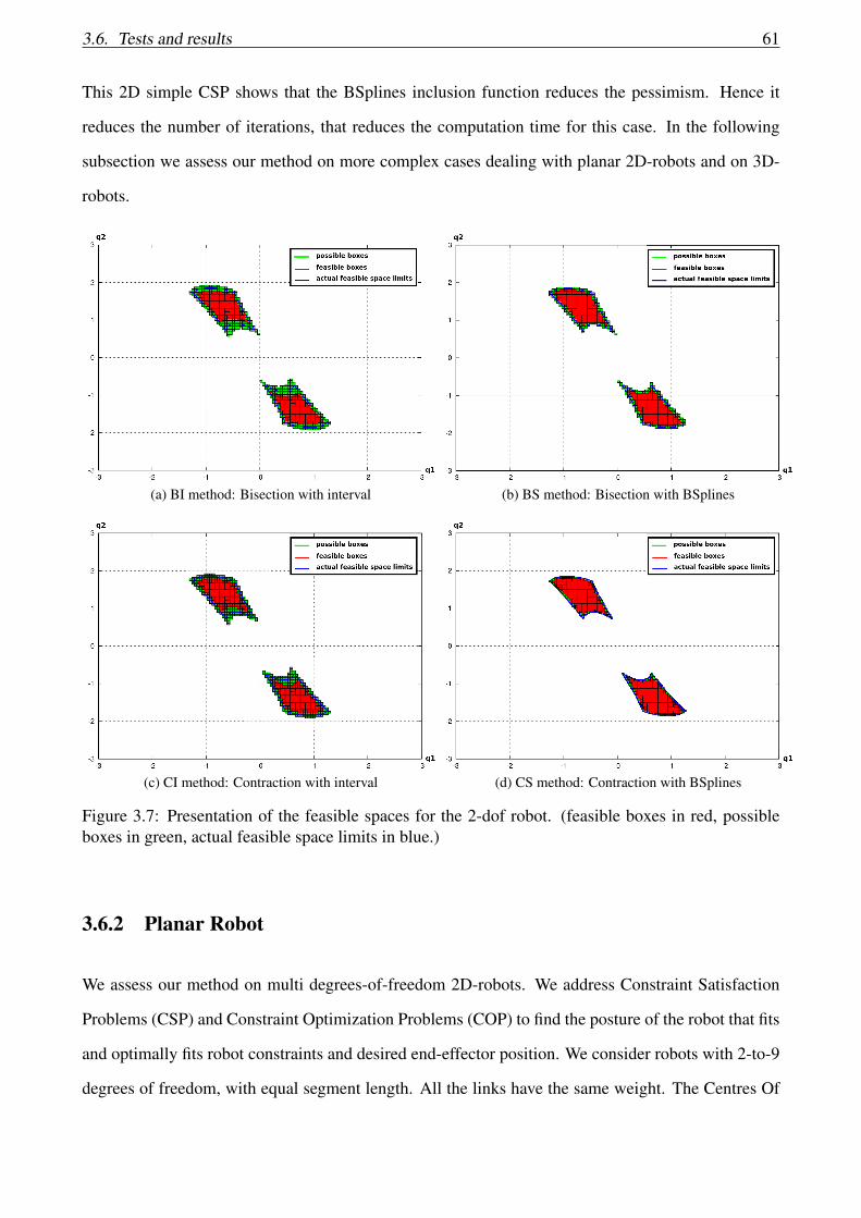
3.6. Tests and results 61
This 2D simple CSP shows that the BSplines inclusion function reduces the pessimism. Hence it
reduces the number of iterations, that reduces the computation time for this case. In the following
subsection we assess our method on more complex cases dealing with planar 2D-robots and on 3D-
robots.
(a) BI method: Bisection with interval (b) BS method: Bisection with BSplines
(c) CI method: Contraction with interval (d) CS method: Contraction with BSplines
Figure 3.7: Presentation of the feasible spaces for the 2-dof robot. (feasible boxes in red, possibleboxes in green, actual feasible space limits in blue.)
3.6.2 Planar Robot
We assess our method on multi degrees-of-freedom 2D-robots. We address Constraint Satisfaction
Problems (CSP) and Constraint Optimization Problems (COP) to find the posture of the robot that fits
and optimally fits robot constraints and desired end-effector position. We consider robots with 2-to-9
degrees of freedom, with equal segment length. All the links have the same weight. The Centres Of
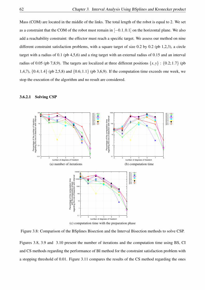
62 Chapter 3. Interval Analysis Using BSplines and Kronecker product
Mass (COM) are located in the middle of the links. The total length of the robot is equal to 2. We set
as a constraint that the COM of the robot must remain in [−0.1,0.1] on the horizontal plane. We also
add a reachability constraint: the effector must reach a specific target. We assess our method on nine
different constraint satisfaction problems, with a square target of size 0.2 by 0.2 (pb 1,2,3), a circle
target with a radius of 0.1 (pb 4,5,6) and a ring target with an external radius of 0.15 and an interval
radius of 0.05 (pb 7,8,9). The targets are localized at three different positions {x,y} : {0.2;1.7} (pb
1,4,7), {0.4;1.4} (pb 2,5,8) and {0.6;1.1} (pb 3,6,9). If the computation time exceeds one week, we
stop the execution of the algorithm and no result are considered.
3.6.2.1 Solving CSP
0.01
0.1
1
10
100
2 3 4 5 6 7 8
Perc
enta
ge o
f th
e n
um
ber
of itera
tion
regard
ing the o
ne o
f bis
ection w
ith inte
rval
number of degrees of freedom
pb 1pb 2pb 3pb 4pb 5pb 6pb 7pb 8pb 9
(a) number of iterations
0.1
1
10
100
1000
2 3 4 5 6 7 8
Perc
enta
ge o
f th
e c
om
puta
tion tim
e
regard
ing the o
ne o
f bis
ection w
ith inte
rval
number of degrees of freedom
pb 1pb 2pb 3pb 4pb 5pb 6pb 7pb 8pb 9
(b) computation time
0.1
1
10
100
1000
10000
100000
2 3 4 5 6 7 8
Perc
enta
ge o
f th
e c
om
puta
tion tim
e
with the p
repara
tion p
hase
regard
ing the o
ne o
f bis
ection w
ith inte
rval
number of degrees of freedom
pb 1pb 2pb 3pb 4pb 5pb 6pb 7pb 8pb 9
(c) computation time with the preparation phase
Figure 3.8: Comparison of the BSplines Bisection and the Interval Bisection methods to solve CSP.
Figures 3.8, 3.9 and 3.10 present the number of iterations and the computation time using BS, CI
and CS methods regarding the performance of BI method for the constraint satisfaction problem with
a stopping threshold of 0.01. Figure 3.11 compares the results of the CS method regarding the ones

3.6. Tests and results 63
10
100
2 3 4 5 6 7
Perc
enta
ge o
f th
e n
um
ber
of itera
tion
regard
ing the o
ne o
f bis
ection w
ith inte
rval
number of degrees of freedom
pb 1pb 2pb 3pb 4pb 5pb 6pb 7pb 8pb 9
(a) number of iterations
100
1000
10000
100000
2 3 4 5 6 7
Perc
enta
ge o
f th
e c
om
puta
tion tim
e
regard
ing the o
ne o
f bis
ection w
ith inte
rval
number of degrees of freedom
pb 1pb 2pb 3pb 4pb 5pb 6pb 7pb 8pb 9
(b) computation time
Figure 3.9: Comparison of the Interval Contraction and the Interval Bisection methods to solve CSP.
of BS method. The resolution of the CSP is done as presented in Algorithm 1. Nevertheless, the
execution of the algorithm is stopped as soon as one solution is found.
Figure 3.8a proves that the number of iteration required to solve the CSP using BS is lower than
the number of iterations using BI. We can deduce that the evaluation of the constraints induces less
pessimism using the Bsplines method. Figure 3.8c shows that the BS method (taking into account the
preparation phase) is faster than the BI method, but only for a large number of degrees of freedom
(n >= 7). We highlight that the BS method produces a result for the problems 1 and 2 with 9 degrees-
of-freedom in nearly 3 hours whereas the BI method cannot find a solution within one week.
Figure 3.9 compares the state-of-the-art CI with BI methods and proves that the number of iterations
is quite reduced, but with a very larger computation time.
Looking at Figure 3.10, it seems that the CS methods have nearly the same performances as the BS
methods. For an easier comparison, we present the results of CS method regarding the ones of the BS
method in Figure 3.11. Despite, we believed that the contraction step reduces the boxes before the
bisection process, hence reduces the number of iterations of the algorithm, it appears that, for some
problems, the number of iterations (and then the computation time) of the CS method is larger than
the number of iterations for the BS method. This phenomena is due to the bisection process. During
the BS method the diameter of the interval is equal to the initial size of the interval divided by 2k, with
k the number of bisection of this interval. The bisection process choose to bisect the input with the
maximal diameter and in case of equality, the first input of the queue is bisected. Since all the inputs

64 Chapter 3. Interval Analysis Using BSplines and Kronecker product
0.01
0.1
1
10
100
2 3 4 5 6 7 8
Perc
enta
ge o
f th
e n
um
ber
of itera
tion
regard
ing the o
ne o
f bis
ection w
ith inte
rval
number of degrees of freedom
pb 1pb 2pb 3pb 4pb 5pb 6pb 7pb 8pb 9
(a) number of iterations
0.1
1
10
100
1000
10000
2 3 4 5 6 7 8
Perc
enta
ge o
f th
e c
om
puta
tion tim
e
regard
ing the o
ne o
f bis
ection w
ith inte
rval
number of degrees of freedom
pb 1pb 2pb 3pb 4pb 5pb 6pb 7pb 8pb 9
(b) computation time
0.1
1
10
100
1000
10000
100000
2 3 4 5 6 7 8
Perc
enta
ge o
f th
e c
om
puta
tion tim
e
with the p
repara
tion p
hase
regard
ing the o
ne o
f bis
ection w
ith inte
rval
number of degrees of freedom
pb 1pb 2pb 3pb 4pb 5pb 6pb 7pb 8pb 9
(c) computation time with the preparation phase
Figure 3.10: Comparison of the BSplines Contraction and the Interval Bisection methods to solveCSP.
have the same initial size, this case of equality appears at each iteration. During the CS method, the
contraction step may reduce one or several input intervals, hence the case of equality may appear at
the beginning of the process and becomes very rare after some iterations. Because of those properties
of the bisection process and of the contraction, the BS method and the CS method do not explore the
search space in the same order, hence a non-intuitive difference on results could be noticed in terms
of computation time and number of iterations.
3.6.2.2 Solving Optimization problem
We also assess our methods on additional optimization problems. We consider the same constraints
than in CSP and consider two different cost functions. The cost function of Problem 1 to 9 is the
sum of the square joint positions ∑ni=1 q2
i . Problem 11 to 19 consider the sum of square joint torques
∑ni=1 Γ2
i as a cost function. As for the CSP, the CI method is not suitable for optimization problem.

3.6. Tests and results 65
10
100
1000
2 3 4 5 6 7 8 9
Perc
enta
ge o
f th
e n
um
ber
of itera
tion
regard
ing the o
ne o
f bis
ection w
ith s
plin
es
number of degrees of freedom
pb 1pb 2pb 3pb 4pb 5pb 6pb 7pb 8pb 9
(a) number of iterations
80
100
200
500
2 3 4 5 6 7 8 9
Perc
enta
ge o
f th
e c
om
puta
tion tim
e
regard
ing the o
ne o
f bis
ection w
ith s
plin
es
number of degrees of freedom
pb 1pb 2pb 3pb 4pb 5pb 6pb 7pb 8pb 9
(b) computation time with the preparation phase
Figure 3.11: Comparison of the Bsplines Contraction and the Bsplines Bisection methods to solveCSP.
Hence, we choose to not present the results of the CI here for the sake of clarity.
Figure 3.12 and Figure 3.13 present the results of the BS method and of the CS method for eighteen
complex optimization process regarding the result of the state-of-the-art BS method. As for solving
a CSP, the two proposed methods produce a fewer number of iterations, but with a comparable com-
putation time. Figure 3.14 compares the results of BS and CS methods. Since there is no contraction
for the evaluation of the cost function, the two methods seem to present nearly the same performance
regarding the number of iterations and the computation time.
3.6.3 3D Robot
To assess the effectiveness of our method on a 3D robot, we consider two different robots (with 4 and
6 degrees of freedom) which derive from the KUKA LWR as presented on Figure 3.15. The 4-dof
robot is obtained by considering constant the joint number 3 and 5.
We consider the constraints about the desired end effector position with a box of 0.02 meter in the
x, y and z directions. We add torque constraint and we consider the cost function as the sum of the
torque square.
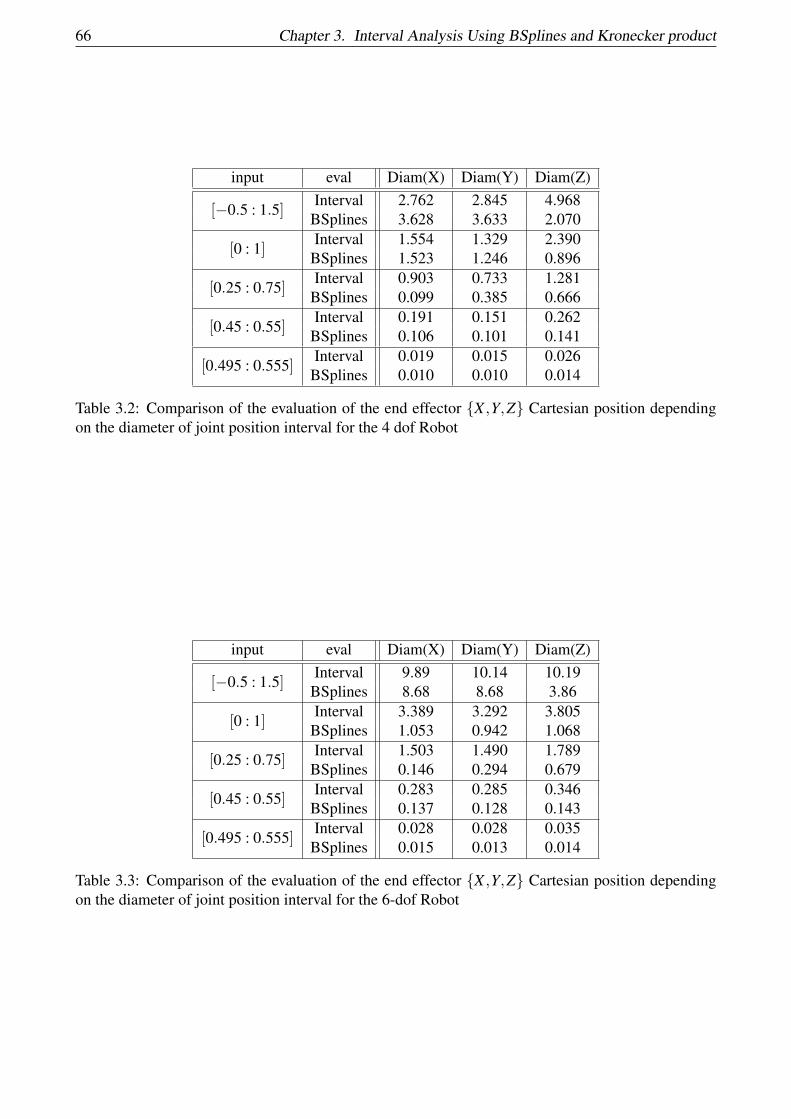
66 Chapter 3. Interval Analysis Using BSplines and Kronecker product
input eval Diam(X) Diam(Y) Diam(Z)
[−0.5 : 1.5]Interval 2.762 2.845 4.968
BSplines 3.628 3.633 2.070
[0 : 1]Interval 1.554 1.329 2.390
BSplines 1.523 1.246 0.896
[0.25 : 0.75]Interval 0.903 0.733 1.281
BSplines 0.099 0.385 0.666
[0.45 : 0.55]Interval 0.191 0.151 0.262
BSplines 0.106 0.101 0.141
[0.495 : 0.555]Interval 0.019 0.015 0.026
BSplines 0.010 0.010 0.014
Table 3.2: Comparison of the evaluation of the end effector {X ,Y,Z} Cartesian position dependingon the diameter of joint position interval for the 4 dof Robot
input eval Diam(X) Diam(Y) Diam(Z)
[−0.5 : 1.5]Interval 9.89 10.14 10.19
BSplines 8.68 8.68 3.86
[0 : 1]Interval 3.389 3.292 3.805
BSplines 1.053 0.942 1.068
[0.25 : 0.75]Interval 1.503 1.490 1.789
BSplines 0.146 0.294 0.679
[0.45 : 0.55]Interval 0.283 0.285 0.346
BSplines 0.137 0.128 0.143
[0.495 : 0.555]Interval 0.028 0.028 0.035
BSplines 0.015 0.013 0.014
Table 3.3: Comparison of the evaluation of the end effector {X ,Y,Z} Cartesian position dependingon the diameter of joint position interval for the 6-dof Robot
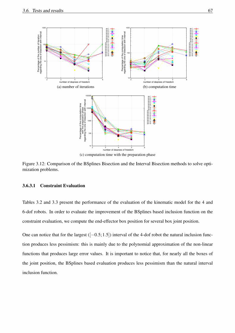
3.6. Tests and results 67
1
10
100
1000
2 3 4 5 6
Perc
enta
ge o
f th
e n
um
ber
of itera
tion
regard
ing the o
ne o
f bis
ection w
ith inte
rval
number of degrees of freedom
pb 1pb 2pb 3pb 4pb 5pb 6pb 7pb 8pb 9
pb 11pb 12pb 13pb 14pb 15pb 16pb 17pb 18pb 19
(a) number of iterations
10
100
1000
2 3 4 5 6
Perc
enta
ge o
f th
e c
om
puta
tion tim
e
regard
ing the o
ne o
f bis
ection w
ith inte
rval
number of degrees of freedom
pb 1pb 2pb 3pb 4pb 5pb 6pb 7pb 8pb 9
pb 11pb 12pb 13pb 14pb 15pb 16pb 17pb 18pb 19
(b) computation time
10
100
1000
10000
100000
2 3 4 5 6
Perc
enta
ge o
f th
e c
om
puta
tion tim
e
with the p
repara
tion p
hase
regard
ing the o
ne o
f bis
ection w
ith inte
rval
number of degrees of freedom
pb 1pb 2pb 3pb 4pb 5pb 6pb 7pb 8pb 9
pb 11pb 12pb 13pb 14pb 15pb 16pb 17pb 18pb 19
(c) computation time with the preparation phase
Figure 3.12: Comparison of the BSplines Bisection and the Interval Bisection methods to solve opti-mization problems.
3.6.3.1 Constraint Evaluation
Tables 3.2 and 3.3 present the performance of the evaluation of the kinematic model for the 4 and
6-dof robots. In order to evaluate the improvement of the BSplines based inclusion function on the
constraint evaluation, we compute the end-effector box position for several box joint position.
One can notice that for the largest ([−0.5;1.5]) interval of the 4-dof robot the natural inclusion func-
tion produces less pessimism: this is mainly due to the polynomial approximation of the non-linear
functions that produces large error values. It is important to notice that, for nearly all the boxes of
the joint position, the BSplines based evaluation produces less pessimism than the natural interval
inclusion function.

68 Chapter 3. Interval Analysis Using BSplines and Kronecker product
1
10
100
1000
2 3 4 5 6
Perc
enta
ge o
f th
e n
um
ber
of itera
tion
regard
ing the o
ne o
f bis
ection w
ith inte
rval
number of degrees of freedom
pb 1pb 2pb 3pb 4pb 5pb 6pb 7pb 8pb 9
pb 11pb 12pb 13pb 14pb 15pb 16pb 17pb 18pb 19
(a) number of iterations
10
100
1000
2 3 4 5 6
Perc
enta
ge o
f th
e c
om
puta
tion tim
e
regard
ing the o
ne o
f bis
ection w
ith inte
rval
number of degrees of freedom
pb 1pb 2pb 3pb 4pb 5pb 6pb 7pb 8pb 9
pb 11pb 12pb 13pb 14pb 15pb 16pb 17pb 18pb 19
(b) computation time
10
100
1000
10000
100000
1e+06
2 3 4 5 6
Perc
enta
ge o
f th
e c
om
puta
tion tim
e
with the p
repara
tion p
hase
regard
ing the o
ne o
f bis
ection w
ith inte
rval
number of degrees of freedom
pb 1pb 2pb 3pb 4pb 5pb 6pb 7pb 8pb 9
pb 11pb 12pb 13pb 14pb 15pb 16pb 17pb 18pb 19
(c) computation time with the preparation phase
Figure 3.13: Comparison of the BSplines Contraction and the Interval Bisection methods to solveCSP.
3.6.3.2 Solving Optimization problem
Since the use of the CI method did not provide good results for solving the CSP of planar robots, we
do not evaluate this method for 3D robots. In this part, we compare the performance of the BI, BS
and CS methods on four different problems for the 4 and 6 dof-robots. The problems 1 and 3 consider
a desired end effector position at {x,y,z} equal to {0.6,0.6,0.6} and {0.4,0.4,0.7} for problems 2
and 4. The problem 1 and 2 consider the nominal maximal torque values and the problem 3 and 4
only 10% of the maximal torque. Consequently, the problem 4 is infeasible, that is used to assess the
performance of our method on infeasible problems.
Table 3.4 and 3.5 emphasize that our methods (BS an CS) solve the optimization problem with less
iterations than the state-of-the-art method (BI). It also emphasizes that the use of the Bsplines prop-
erties reduces the number of iterations, due to a less pessimistic evaluation of the constraints. It is
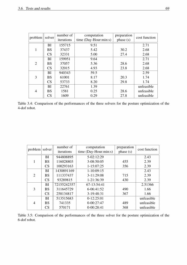
3.6. Tests and results 69
problem solvernumber ofiterations
computationtime (Day-Hour:min:s)
preparationphase (s)
cost function
1BI 155715 9.51 2.71BS 37437 5.42 30.2 2.68CS 32331 5.00 27.4 2.68
2BI 159951 9.64 2.71BS 37057 5.36 28.6 2.68CS 32015 4.93 23.8 2.68
3BI 940343 59.5 2.59BS 61001 8.17 20.3 1.74CS 53733 8.20 29.8 1.74
4BI 22761 1.39 unfeasibleBS 1581 0.25 28.6 unfeasibleCS 1609 0.29 27.8 unfeasible
Table 3.4: Comparison of the performances of the three solvers for the posture optimization of the4-dof robot.
problem solvernumber ofiterations
computationtime (Day-Hour:min:s)
preparationphase (s)
cost function
1BI 944808895 5-02:12:29 2.43BS 116028803 3-08:50:05 455 2.39CS 100293163 1-15:07:25 356 2.39
2BI 1430891169 1-10:09:15 2.43BS 111337437 3-11:29:08 715 2.39CS 93289815 1-21:36:39 430 2.39
3BI 72155242357 67-13:54:41 2.51366BS 311645729 6-06:41:52 490 1.66CS 258134817 3-19:48:31 367 1.66
4BI 513515683 0-12:25:01 unfeasibleBS 741335 0-00:27:47 489 unfeasibleCS 570171 0-00:28:41 368 unfeasible
Table 3.5: Comparison of the performances of the three solver for the posture optimization of the6-dof robot.

70 Chapter 3. Interval Analysis Using BSplines and Kronecker product
90
92
94
96
98
100
102
104
106
108
2 3 4 5 6
Perc
enta
ge o
f th
e n
um
ber
of itera
tion
regard
ing the o
ne o
f bis
ection w
ith inte
rval
number of degrees of freedom
pb 1pb 2pb 3pb 4pb 5pb 6pb 7pb 8pb 9
pb 11pb 12pb 13pb 14pb 15pb 16pb 17pb 18pb 19
(a) number of iterations
90
100
110
120
130
140
150
160
170
180
190
2 3 4 5 6
Perc
enta
ge o
f th
e c
om
puta
tion tim
e
regard
ing the o
ne o
f bis
ection w
ith inte
rval
number of degrees of freedom
pb 1pb 2pb 3pb 4pb 5pb 6pb 7pb 8pb 9
pb 11pb 12pb 13pb 14pb 15pb 16pb 17pb 18pb 19
(b) computation time with the preparation phase
Figure 3.14: Comparison of the BSplines Contraction and the BSplines Bisection methods to solveoptimization problems.
Figure 3.15: The 6 degrees of freedom robot we use : KUKA LWR
also evident that the use of a contraction process (CS) decreases more the number of iterations than
pure bisection processes (BI and BS) since it makes possible to reduce the size of the box during the
bisection process.
Regarding the computation time, it appears that our method is faster than the state-of-the-art BI
method in most of the cases. For the most complex problem (6-dof robot), our method is still the
faster one even when we consider the preparation phase (except for one case). It seems that our
method is more relevant to prove that the problem has no solution (problem 4) since the number of
iterations and the computation time are drastically reduced.

3.7. Conclusion 71
3.7 Conclusion
In robotics, the computation of the feasible space of a robot is a critical research domain and it is
usually solved using Constraint Satisfaction Problem. In this chapter, we have proposed to exploit In-
terval Analysis to solve Constraint Satisfaction Problems and Constraint Optimization Problems. The
solver is based on a combination between bisection and contraction. However, this technique suf-
fers from pessimism. Hence, a novel technique has been proposed to evaluate the inclusion function.
Our method is based on the convex hull properties of BSplines functions and the Kronecker product
properties in order to reduce pessimism. Our algorithm was assessed on different problems using 2D
and 3D robots. We prove that our contribution deals with more complex optimization problems and
decreases the pessimism and the computation time. We should add that finally we did not compute
the feasible workspace in the world coordinate system: the set of joint angles are computed in the
robot coordinate system. This computation is required in order to generate a generic workspace of
a given robot, but we did not solve this problem due to a lack of time. The simplest way to do this
calculation is by using the direct kinematic. The latter generic workspace should be used in order
to find the reachable part of the surface from a given position. Since in this PHD, we did compute
the generic workspace of the robot, we will find the reachable part of the surface by considering a
different kind of workspaces (spherical, semi-spherical, elliptical, etc.)
Chapter 4
Optimal robot base placements for coverage
tasks
Considering the workspace of the robot is known, we can proceed to find the optimal robot base
placements for coverage tasks. The surface coverage using robots is a common problem divided into
two cases according to the robot state during the task: the robot could be either static or mobile.
In static case, the robot should cover a given surface and it should be positioned at a fixed point.
This technique is used in painting, stripping, or sand-blasting tasks [10, 105, 125]. In the latter case,
the surface is supposed totally reachable from the fixed point and the coverage problem returns the
optimal trajectories of the end-effector as solutions. Those end-effector trajectories are required to
sweep the entire surface. In mobile case, robots are moved to achieve their tasks like demining,
inspection and agricultural fields coverage. Several works addressed the generation of optimal paths
of mobile robots required to totally cover an environment [1, 11, 37, 101]. Recently, a third type of
coverage problem appears: the robot is fixed during the coverage task and the surface is larger than
its workspace. Hence, a repositioning of the robot(s) is required to cover the whole surface since
the surface can not be covered from one given position. The repositioning is accomplished under
the assumption that the coverage task can not be done continuously and needs to be stopped during
the robot’s movement. For instance, air-plane stripping and building facades refurbishing are some
coverage tasks that require repositioning the robots to cover the whole object. Another example of
72

73
such tasks is the car stripping using KUKA Light Weight Robots (LWRs) shown in Figure 4.1.
Figure 4.1: Car stripping using a KUKA robot
In this chapter, we provide the third problem and we develop an optimal robot base placements strat-
egy using the repositioning concept. Optimal robot positioning could decrease the task cycle time
and increase its efficiency as well as its accuracy. The proposed strategy requires a combination be-
tween the robot base placements and the coverage problem. The placement of single robot has been
tackled in several domains. Those works were extended to deal with multiple industrial robots for the
coverage tasks. Hassan, Liu et al. proposed a new strategy to distribute the work between robots for
coverage tasks assuming that a reasonable number of robots is intuitively chosen based on the size
of the object [54, 56]. A combination of Simulated Annealing and Genetic algorithm optimization is
used to find the optimal robot base placement in [54]. We have already presented the state of the art
in Chapter 2. Despite the relevance of Hassan et al. strategy, it suffers from several weak points:
1. The number of robots is harder to guess when the surface gets more complex.
2. The end-effector trajectories used as inputs for base placement optimization are not optimal.
They are generated without considering the robot poses.
3. After the base placement optimization, area partitioning and allocation of the surface between
different robot poses is required to improve the end-effector trajectories [55].
4. The total surface coverage is not guaranteed.
To deal with those issues, we propose a new approach for a complete coverage using a multi-robot
system (Section 4.1). An important feature of our approach is that it does not only find the optimal
pose of robots bases but it also provides the optimal number of robots N needed to cover the whole
surface. Contrary to the state of the art, the knowledge of the total number of robots is not required in
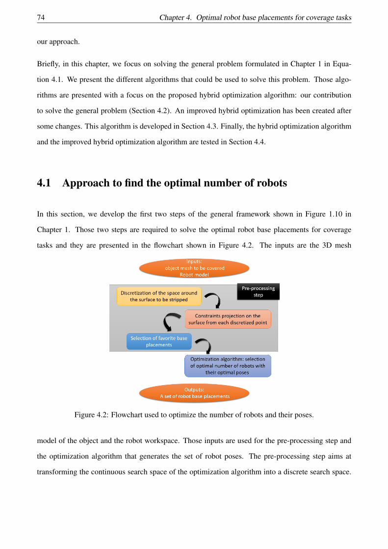
74 Chapter 4. Optimal robot base placements for coverage tasks
our approach.
Briefly, in this chapter, we focus on solving the general problem formulated in Chapter 1 in Equa-
tion 4.1. We present the different algorithms that could be used to solve this problem. Those algo-
rithms are presented with a focus on the proposed hybrid optimization algorithm: our contribution
to solve the general problem (Section 4.2). An improved hybrid optimization has been created after
some changes. This algorithm is developed in Section 4.3. Finally, the hybrid optimization algorithm
and the improved hybrid optimization algorithm are tested in Section 4.4.
4.1 Approach to find the optimal number of robots
In this section, we develop the first two steps of the general framework shown in Figure 1.10 in
Chapter 1. Those two steps are required to solve the optimal robot base placements for coverage
tasks and they are presented in the flowchart shown in Figure 4.2. The inputs are the 3D mesh
Figure 4.2: Flowchart used to optimize the number of robots and their poses.
model of the object and the robot workspace. Those inputs are used for the pre-processing step and
the optimization algorithm that generates the set of robot poses. The pre-processing step aims at
transforming the continuous search space of the optimization algorithm into a discrete search space.

4.1. Approach to find the optimal number of robots 75
The continuous optimization problem is the following:
minN,T
N
Subject to g(N,T,S) = 0
h(N,T,S)≤ 0
(4.1)
After the pre-processing step this continuous optimization problem is transformed into a discrete
optimization problem developed hereafter. Hence, the optimal solution is easier to be reached, and
the execution time decreases.
4.1.1 Pre-processing step
The pre-processing step turns the continuous 4D search space of the robot (x, y, z and θ ) into a finite
set F of favourite robot poses to accelerate solving the optimization problem. To emphasize the pre-
processing step, each sub-step of the pre-processing step will be explained on an action car as an
object to be covered. We chose the action car since it is easy to show the discrete points around it.
For instance, considering a KUKA robot having a spherical workspace, a 4D discretization gives a
finite set F of favourite robot poses illustrated in Figure 4.3. The pre-processing step is composed
of three main steps: the search space discretization, the constraints projection and the favourite base
placement selection.
Figure 4.3: 4D discretization for the action car: red circles are the favourite robot poses of F (s = 0.1)
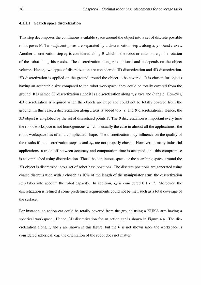
76 Chapter 4. Optimal robot base placements for coverage tasks
4.1.1.1 Search space discretization
This step decomposes the continuous available space around the object into a set of discrete possible
robot poses P. Two adjacent poses are separated by a discretization step s along x, y or/and z axes.
Another discretization step sθ is considered along θ which is the robot orientation, e.g. the rotation
of the robot along his z axis. The discretization along z is optional and it depends on the object
volume. Hence, two types of discretization are considered: 3D discretization and 4D discretization.
3D discretization is applied on the ground around the object to be covered. It is chosen for objects
having an acceptable size compared to the robot workspace: they could be totally covered from the
ground. It is named 3D discretization since it is a discretization along x, y axes and θ angle. However,
4D discretization is required when the objects are huge and could not be totally covered from the
ground. In this case, a discretization along z axis is added to x, y, and θ discretizations. Hence, the
3D object is en-globed by the set of discretized points P. The θ discretization is important every time
the robot workspace is not homogeneous which is usually the case in almost all the applications: the
robot workspace has often a complicated shape. The discretization may influence on the quality of
the results if the discretization steps, s and sθ , are not properly chosen. However, in many industrial
applications, a trade-off between accuracy and computation time is accepted, and this compromise
is accomplished using discretization. Thus, the continuous space, or the searching space, around the
3D object is discretized into a set of robot base positions. The discrete positions are generated using
coarse discretization with s chosen as 10% of the length of the manipulator arm: the discretization
step takes into account the robot capacity. In addition, sθ is considered 0.1 rad. Moreover, the
discretization is refined if some predefined requirements could not be met, such as a total coverage of
the surface.
For instance, an action car could be totally covered from the ground using a KUKA arm having a
spherical workspace. Hence, 3D discretization for an action car is shown in Figure 4.4. The dis-
cretization along x, and y are shown in this figure, but the θ is not shown since the workspace is
considered spherical, e.g. the orientation of the robot does not matter.
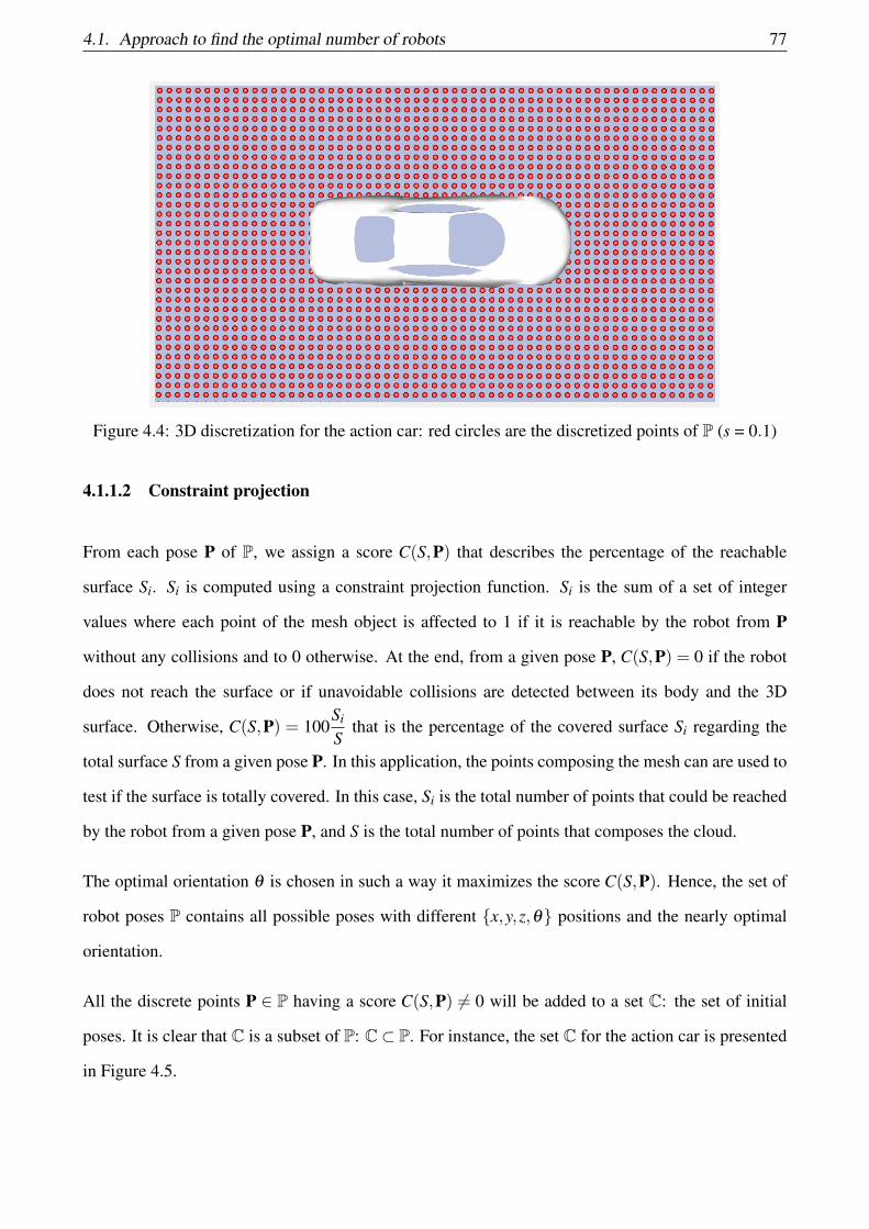
4.1. Approach to find the optimal number of robots 77
Figure 4.4: 3D discretization for the action car: red circles are the discretized points of P (s = 0.1)
4.1.1.2 Constraint projection
From each pose P of P, we assign a score C(S,P) that describes the percentage of the reachable
surface Si. Si is computed using a constraint projection function. Si is the sum of a set of integer
values where each point of the mesh object is affected to 1 if it is reachable by the robot from P
without any collisions and to 0 otherwise. At the end, from a given pose P, C(S,P) = 0 if the robot
does not reach the surface or if unavoidable collisions are detected between its body and the 3D
surface. Otherwise, C(S,P) = 100Si
Sthat is the percentage of the covered surface Si regarding the
total surface S from a given pose P. In this application, the points composing the mesh can are used to
test if the surface is totally covered. In this case, Si is the total number of points that could be reached
by the robot from a given pose P, and S is the total number of points that composes the cloud.
The optimal orientation θ is chosen in such a way it maximizes the score C(S,P). Hence, the set of
robot poses P contains all possible poses with different {x,y,z,θ} positions and the nearly optimal
orientation.
All the discrete points P ∈ P having a score C(S,P) 6= 0 will be added to a set C: the set of initial
poses. It is clear that C is a subset of P: C⊂ P. For instance, the set C for the action car is presented
in Figure 4.5.

78 Chapter 4. Optimal robot base placements for coverage tasks
Figure 4.5: The set of the initial poses C of the action car (s = 0.1)
4.1.1.3 Favourite base placements selection
The favourite selection step is the final sub-step in the pre-processing step. It consists in computing
the set of favourite poses F. The poses in F are all poses of P having a score greater than a given
threshold C(S,P)> t. Every favourite pose F ∈ F is a part of the set of initial poses C as well as the
set of discrete poses P: F⊂ C⊂ P. The set of favourite poses F of a car is shown in Figure 4.6. The
Figure 4.6: Favorite base placements of the action car for t = 10%.
set of favourite poses F will be used during the optimization of the number of robots and their base

4.1. Approach to find the optimal number of robots 79
placements.
4.1.2 Discrete optimization problem
The pre-processing step turns the continuous problem (presented in Equation 4.1) into the discrete
optimization problem given by Equation 4.2. The search space of the optimization problem is reduced
to F. The notations used in this discrete problem are the ones created after the pre-processing step.
Hence, the discrete optimization problem is formulated as follows:
minN,T⊂F
N
Subject to g(N, T, C) = 0
∀l,m ∈ [1, N] hlm(T)≤ 0
(4.2)
With:
— N: the minimal number of robots,
— T: the set of optimal poses of the robots such that T= {Ti ∈ SE(3),1≤ i≤ N},
— C: the set of reachable part of the surface from each pose Ti ∈ T such that C= {Ci,1≤ i≤ N},
— g(N, T, C): function to test if λ% of the surface is covered,
— hlm(T): the set of additional constraints.
Eventually, T ⊂ F ⊂ C ⊂ P. A surface is considered λ% covered if g(N, T, C) =⋃N
l=1 Cl−λS = 0.
One can solve the proposed problem for a total coverage by initializing λ to 1. A collision avoidance
between robots can be considered through the constraint hlm(T) when a multi-robot system is used. In
this case, the distance between any two adjacent robots should be greater than a predefined threshold
δ that is defined with respect to the dimension of the robot workspace, e.g. hlm(T) = ||Tl− Tm||−δ .
This distance is added as a constraint in order to reduce the overlapping of the workspace of two
adjacent robots, and to reduce the collision risk between two adjacent robots.
Since the discretization step may influence on the results, we propose a global optimization algorithm
that solves the flowchart (Figure 4.2) for a given discretization step. Then, if the percentage of the
covered surface is lower than λ , a finer discretization step is considered and the flowchart is solved

80 Chapter 4. Optimal robot base placements for coverage tasks
again based on the finer discretization step. The optimization algorithm (called in line 6) will be one
step of the global algorithm developed in Algorithm 2. This global algorithm is the representation of
the flowchart in the algorithmic language. Thus, the volume around the 3D surface is discretized into
Algorithm 2: Global algorithmInput : Object mesh to be covered, Robot modelOutput: A set of robot base placements
1: Discretization of the volume around the surface: a set of robot base positions P such ask ∈ {1, ...,Ntotal}
2: for k ∈ {1, . . . ,Ntotal} do3: Find Sk such as Sk =C(Pl)4: end for5: Find the favourite robot base positions F6: Optimization algorithm to find N7: if Covered ratio < λ then8: Perform finer discretization9: go to 6
10: end if11: return N and their positions;
a set of robot base poses P (line 1). A constraint projection on the surface is applied for each pose P
in P (line 3). Based on this evaluation, some discretized poses are discarded due to their proximity,
others due to their low coverage: a set of favourite robot base positions is defined F (line 5). After
that, the optimization algorithm is run in order to find the minimal number of robots base positions
based on the favourite base poses F (line 6). We supposed that in this optimization algorithm, we
add a threshold for the number of robots: if the number of robots found during the optimization
algorithm is greater than a given threshold and the percentage of the covered surface is lower than λ ,
the optimization is interrupted. After that, a finer discretization is called (line 8) if the covered ratio
of the total surface is lower than the specified threshold λ . Though, the optimization algorithm will
start again. Otherwise, the algorithm returns the optimal number of robots N with their optimal base
placements.
Finding the optimal number of robot base placements can be solved using a Binary Integer Program-
ming strategy (BIP). However, our problem is a NP-hard problem: an exact solution of the minimum
number of robots is hard to compute using a Binary Integer Programming. Though, we propose a
novel combination between three algorithms: Greedy, Genetic, and Simulated Annealing algorithms
in Section 4.2.

4.2. Hybrid optimization algorithm 81
4.2 Hybrid optimization algorithm
In this Section, we present our hybrid optimization algorithm that merges the advantages of Greedy,
Simulated Annealing and Genetic algorithms. The hybrid optimization algorithm is called in line 6
of the global algorithm. Greedy algorithm is used to find the optimal number of robots. Simulated
Annealing and Genetic algorithms are usually used to optimize the positions of a given number of
robots. Let’s start by briefly presenting those algorithms.
4.2.1 Greedy Algorithm
It is perceptively used to find the optimal number of variables required to respect an optimization
function. It makes a local optimal choice at each iteration, hoping to find a global optimum at the
end of the algorithm. This algorithm reduces complexity during an exhaustive search: it has O(n)
complexity instead of O(nK) where K is the optimal number of robots. Greedy algorithm does not
intend to find the best solution, but it terminates in a reasonable number of steps; finding an optimal
solution to such a complex problem typically requires unreasonably many steps.
Greedy algorithm is developed in Algorithm 3. The algorithm intends to add a robot at each iteration
(line 5), until the percentage of the covered surface is greater than the threshold λ . The coverage test
is included in the constraint g(N, T, C) in line 2. One can initialize λ = 1, if we want a surface totally
covered. The added robot is chosen randomly in such a way that it maximizes the coverage of the
surface, while the previous robot poses are not updated (line 5). This stability of robot poses leads to
local optimal solutions. The coverage of the surface is considered maximized when the added robot
ensures a total coverage greater than the total coverage of the previous iteration. As we will see in the
simulation and results section, Greedy algorithm is not efficient for solving our optimization problem.
Though, we decide that Greedy algorithm will be the fundamental base: instead of adding randomly
a robot at each iteration without changing the positions of the existing robots, a combination between
Simulated Annealing and Genetic algorithm is used to optimize this defined number of robot poses.

82 Chapter 4. Optimal robot base placements for coverage tasks
Algorithm 3: Greedy algorithmInput : The set of favourite robot poses F, the surface to be covered SOutput: Optimal number of robots N and their poses T
1: Set T=∅, N = 0, c =∅2: while g(N, T, C) 6= 0 do3: c= F that maximizes the coverage of the surface S in such a way that c 6∈ T;4: T = T∪{c};5: N = N +1;6: end while7: return N and T;
4.2.2 Simulated Annealing
Simulated Annealing (SA) is a probabilistic technique for approximating the global optimum of a
given function. It is often used when the search space is discrete which is our case [58]. For problems
where finding an approximate global optimum is more important than finding a precise local optimum
in a fixed amount of time, Simulated Annealing may be preferable to alternatives such as gradient
descent. The name and inspiration come from annealing in metallurgy, a technique involving heating
and controlled cooling of a material to increase the size of its crystals and reduce their defects.
Simulated Annealing can be used to generate a solution for combinatorial optimization problems. A
temperature variable is used to simulate the heating process. A high initial value is assigned to the
temperature and then slowly decreases as the algorithm runs. Simulated Annealing avoids the local
optimum by using the temperature procedure [15]: the chance of accepting worse solutions reduces as
long as the temperature decreases. This acceptance decision is made by using an Acceptance function
that depends on the temperature and the percentage of the covered surface using the different robot
poses. The algorithm jumps out of any local optimums by using this Acceptance function, and it
focuses on an area of the search space where an optimal solution could be found.
Simulated Annealing shows robustness and flexibility for global search methods, it can deal with
highly non-linear problems and non-differentiable functions as well as functions with multiple local
optima. SA is suited for stochastic and non-stochastic optimization [49]. SA is also one of the
fastest and universal probabilistic local procedures [16]. Statistically, Simulated Annealing does not
guarantee a global optimal solution, and it gives a good solution. However, it tries to avoid a large

4.2. Hybrid optimization algorithm 83
number of local minima and it often yields a better solution than local optimization [58]. However,
it could not be used alone to find the optimal number of robots: it could optimize the positions of a
given number of robots.
4.2.3 Genetic Algorithm
Genetic Algorithm is a method of search often applied to optimization problems or machine learning.
Genetic Algorithms are part of evolutionary computing, they use an evolutionary analogy, “survival of
the fittest” [120]. Instead of a single point generation at each iteration, Genetic Algorithm generates a
population of points. After that, the best points are chosen as the optimal solution. It is more efficient
than the traditional methods and provides a list of good solutions instead of a single solution. Thus,
Genetic Algorithm increases the likelihood of finding the global optima.
In order to well understand Genetic Algorithm, we must explain some basic terminologies. The pop-
ulation is a subset of all the encoded solutions to the given problem. Each element of this population
is considered as one chromosome. A chromosome is one solution to the given problem and it is
represented by a vector of genes. The gene is one element position of a chromosome. The allele is
the value a gene takes for a particular chromosome. In our application, the chromosome is a vector of
mi elements where each element is an index of one favourite base placement in the vector of favourite
base placements F. The gene is an index of one element in the chromosome. The allele refers to value
inside the gene, so it refers to the index of the robot position in F vector. Figure 4.7 makes clearer
the definition of population, chromosomes, gene and allele. For each iteration in Genetic Algorithm,
we will have a population composed of Npop chromosomes. Each chromosome is composed of mi
elements; where mi is the number of robots in each iteration i.
The basic structure of Genetic Algorithm is presented in Figure 4.8. Genetic Algorithm starts by
a population initialization. After that, for each chromosome in this population, a fitness function
is evaluated. After that, we choose two chromosomes and we generate two children by applying
crossover and mutation (or one of them). Then, the children replace their parents, and the loop is
repeated until the termination criteria is reached: in our case when the percentage of the covered
surface reaches λ%.
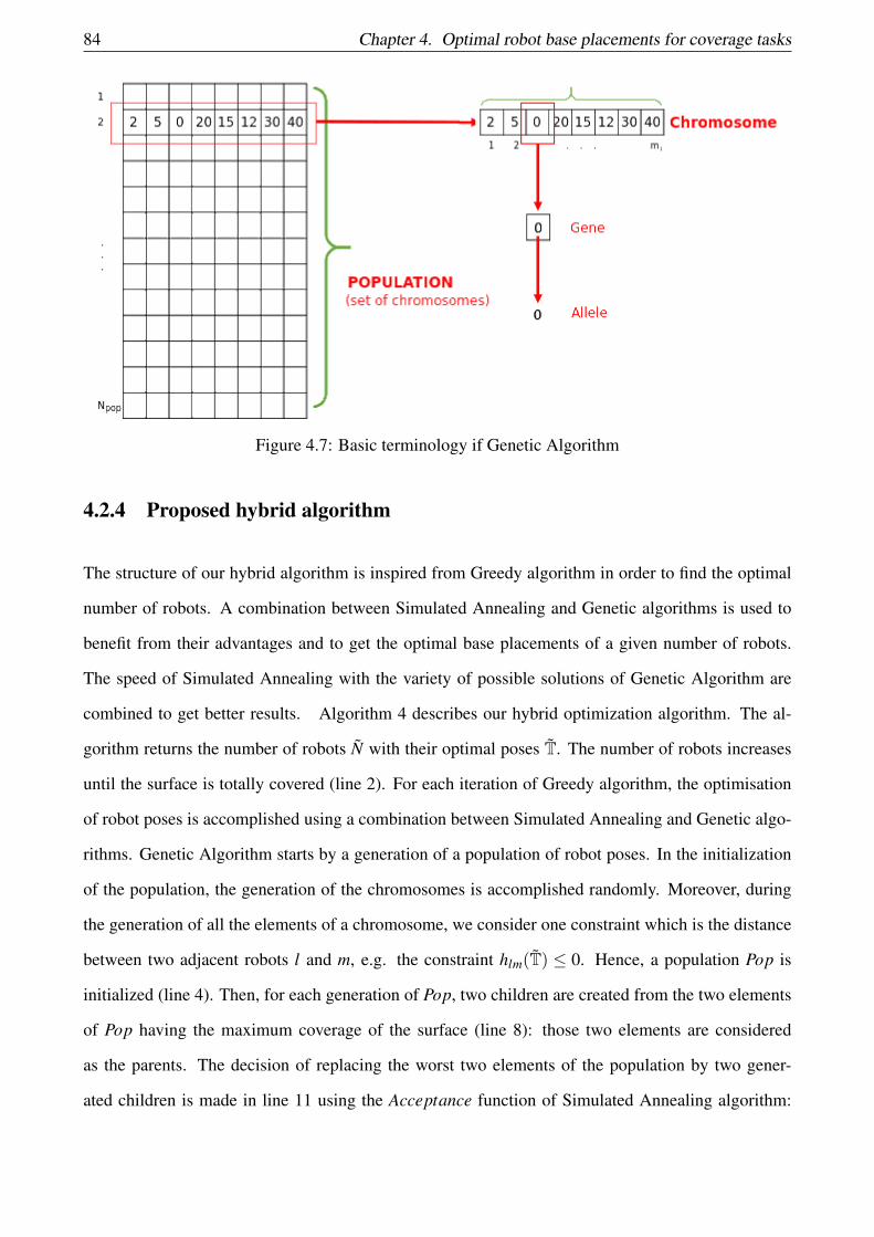
84 Chapter 4. Optimal robot base placements for coverage tasks
Figure 4.7: Basic terminology if Genetic Algorithm
4.2.4 Proposed hybrid algorithm
The structure of our hybrid algorithm is inspired from Greedy algorithm in order to find the optimal
number of robots. A combination between Simulated Annealing and Genetic algorithms is used to
benefit from their advantages and to get the optimal base placements of a given number of robots.
The speed of Simulated Annealing with the variety of possible solutions of Genetic Algorithm are
combined to get better results. Algorithm 4 describes our hybrid optimization algorithm. The al-
gorithm returns the number of robots N with their optimal poses T. The number of robots increases
until the surface is totally covered (line 2). For each iteration of Greedy algorithm, the optimisation
of robot poses is accomplished using a combination between Simulated Annealing and Genetic algo-
rithms. Genetic Algorithm starts by a generation of a population of robot poses. In the initialization
of the population, the generation of the chromosomes is accomplished randomly. Moreover, during
the generation of all the elements of a chromosome, we consider one constraint which is the distance
between two adjacent robots l and m, e.g. the constraint hlm(T) ≤ 0. Hence, a population Pop is
initialized (line 4). Then, for each generation of Pop, two children are created from the two elements
of Pop having the maximum coverage of the surface (line 8): those two elements are considered
as the parents. The decision of replacing the worst two elements of the population by two gener-
ated children is made in line 11 using the Acceptance function of Simulated Annealing algorithm:

4.3. Improved hybrid optimization algorithm 85
Figure 4.8: Basic structure of Genetic Algorithm
exp(( f 1- f 2)/ats)). Those three steps are repeated until the maximum number of generation Ngen is
reached (line 6) or the ending temperature te is attended (line 15). The element of Pop covering the
larger part of the surface is chosen: Rpn (line 19). If all the robots in Rpn covers λ% of the surface,
the loop is broken. Otherwise, the number of robots increases until λ% of the surface is covered.
4.3 Improved hybrid optimization algorithm
In this section, we propose an improvement of the hybrid optimization algorithm. After that, a com-
parison between the hybrid optimization algorithm and the improved hybrid optimization algorithm
is presented. This comparison is based on different types of robot workspaces. The improved hybrid
algorithm consists in dividing the favourite base placements into N zones. Each zone will contain one
robot and the optimization algorithm searches for the best position of each robot in each zone. At
the end, instead of having one huge zone for searching for the optimal positions of N robots, we will
have N different zones. This technique gives solutions closer to the optimal solutions. To attend this
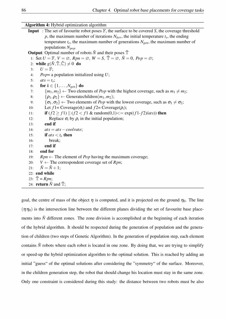
86 Chapter 4. Optimal robot base placements for coverage tasks
Algorithm 4: Hybrid optimization algorithmInput : The set of favourite robot poses F, the surface to be covered S, the coverage threshold
p, the maximum number of iterations Niter, the initial temperature ts, the endingtemperature te, the maximum number of generations Ngen, the maximum number ofpopulations Npop
Output: Optimal number of robots N and their poses T1: Set U = F, V =∅, Rpn =∅, W = S, T=∅, N = 0, Pop =∅;2: while g(N, T, C) 6= 0 do3: U = F;4: Pop= a population initialized using U ;5: ats = ts;6: for k ∈ {1, . . . ,Ngen} do7: {m1,m2}← Two elements of Pop with the highest coverage, such as m1 6= m2;8: {ρ1,ρ2}← Generatechildren(m1,m2);9: {σ1,σ2}← Two elements of Pop with the lowest coverage, such as σ1 6= σ2;
10: Let f 1= Coverage(σi) and f 2= Coverage(ρi);11: if ( f 2≥ f 1) || ( f 2 < f 1 & random(0,1)<= exp(( f 1- f 2)/ats)) then12: Replace σi by ρi in the initial population;13: end if14: ats = ats− coolrate;15: if ats < te then16: break;17: end if18: end for19: Rpn← The element of Pop having the maximum coverage;20: V ← The correspondent coverage set of Rpn;21: N = N +1;22: end while23: T = Rpn;24: return N and T;
goal, the centre of mass of the object η is computed, and it is projected on the ground η0. The line
(ηη0) is the intersection line between the different planes dividing the set of favourite base place-
ments into N different zones. The zone division is accomplished at the beginning of each iteration
of the hybrid algorithm. It should be respected during the generation of population and the genera-
tion of children (two steps of Genetic Algorithm). In the generation of population step, each element
contains N robots where each robot is located in one zone. By doing that, we are trying to simplify
or speed-up the hybrid optimization algorithm to the optimal solution. This is reached by adding an
initial ”guess“ of the optimal solutions after considering the ”symmetry“ of the surface. Moreover,
in the children generation step, the robot that should change his location must stay in the same zone.
Only one constraint is considered during this study: the distance between two robots must be also
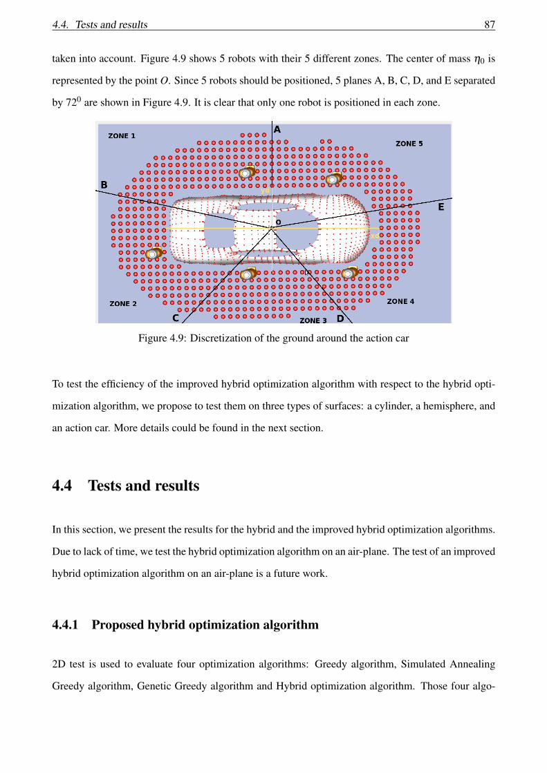
4.4. Tests and results 87
taken into account. Figure 4.9 shows 5 robots with their 5 different zones. The center of mass η0 is
represented by the point O. Since 5 robots should be positioned, 5 planes A, B, C, D, and E separated
by 720 are shown in Figure 4.9. It is clear that only one robot is positioned in each zone.
Figure 4.9: Discretization of the ground around the action car
To test the efficiency of the improved hybrid optimization algorithm with respect to the hybrid opti-
mization algorithm, we propose to test them on three types of surfaces: a cylinder, a hemisphere, and
an action car. More details could be found in the next section.
4.4 Tests and results
In this section, we present the results for the hybrid and the improved hybrid optimization algorithms.
Due to lack of time, we test the hybrid optimization algorithm on an air-plane. The test of an improved
hybrid optimization algorithm on an air-plane is a future work.
4.4.1 Proposed hybrid optimization algorithm
2D test is used to evaluate four optimization algorithms: Greedy algorithm, Simulated Annealing
Greedy algorithm, Genetic Greedy algorithm and Hybrid optimization algorithm. Those four algo-

88 Chapter 4. Optimal robot base placements for coverage tasks
rithms come from some combinations between Greedy algorithm on one side, and Simulated Anneal-
ing and Genetic algorithms on the other side. Hence, those combinations lead to Simulated Annealing
Greedy and Genetic Greedy algorithms. Furthermore, Greedy, Simulated Annealing Greedy, Genetic
Greedy and Hybrid optimization algorithms are compared on a reachability problem using a 2D-robot
as it is explained in Section 4.4.1.1. This 2D test is the initial proof of the efficiency of the hybrid
optimization algorithm. Moreover, Hybrid optimization algorithm is tested on 3D surfaces and the
results are compared to the results given by Greedy algorithm in Section 4.4.1.2.
4.4.1.1 2D test
A test on a 2D-robot with n degrees of freedom and a 2D-surface is applied: the goal is to test the
performance of the four algorithms on simple problems.
Number of robotsAlgorithms Greedy
Simulated Annealing/Greedy
Genetic/Greedy Hybrid
2 19 1 70 813 12 23 30 194 8 51 – –5 10 24 – –6 8 1 – –7 7 – – –8 18 – – –9 11 – – –
10 7 – – –Total 100 100 100 100
Table 4.1: The optimal number of robots found using the four optimization algorithms
Algorithms GreedySimulated Annealing/
GreedyGenetic/Greedy Hybrid
Computation time average/(in s) 0.4172738 0.3998774 1.090686 0.5934172
Table 4.2: Average of computation time (in seconds) for the four optimization algorithms
We consider a 2D robot with 3 degrees of freedom and a 2D polygon in order to evaluate those
algorithms. The task of the robot is to cover the whole perimeter of this polygon considering that

4.4. Tests and results 89
the robot’s workspace is a circle (no need for the discretization along θ ): only the total coverage
of the surface is considered as an optimization criteria (λ = 1). The three links of the robot have
the following lengths: 0.2, 0.3 and 0.15 m (spherical workspace of a radius= 0.65 m), and the 2D
polygon has a perimeter of 10.02 m. The 2D polygon can be englobed by a box of size 4×4.7. The
discretization step along x and y axis is 0.02 m. The object to be covered and the robot are shown in
Figure 4.10. We can see that the dimensions of the object are greater than the dimension of the robot:
the robot should move between different poses to cover the surface. We did the test 100 times for each
algorithm and we did not consider the collision constraints since we want to compare the different
algorithms within the minimal number of constraints. The surface is supposed totally covered if
the red border of the surface is inside the union of the different robot workspaces found during the
optimization algorithm. Table 4.1 presents the results for the four optimization surface on the polygon
surface using the 2D robot. Those tests prove that the hybrid algorithm gives the best results in terms
Figure 4.10: Two dof Robot with a 2D surface that should be totally covered.
of efficiency and robustness. For instance, using the hybrid optimization algorithm, we have two
different values to cover the whole surface: 2 robots (81%), and 3 robots (19%). Moreover, Genetic
Greedy Algorithm gives two possible solutions, but a different distribution of the solutions is noticed:
2 robots (70%), and 3 robots (30%). The results of Simulated Annealing Greedy Algorithm are worse
than the results of the above algorithms, but they are better than the results of Greedy Algorithm. For
instance, Simulated Annealing Greedy Algorithm gives five possibilities of solutions: 2, 3, 4, 5 and
6 robots with 1%, 23%, 51%, 24% and 1% respectively. Greedy Algorithm gives 9 possibilities of
solutions: from 2 to 10 robots with 19%, 12%, 8%, 10%, 8%, 7%, 18%, 11% and 7% respectively.
In parallel, we can conclude using Table 4.2 that Simulated Annealing/ Greedy algorithm is faster

90 Chapter 4. Optimal robot base placements for coverage tasks
than Genetic/ Greedy Algorithm. However, Genetic/ Greedy algorithm gives better results than
(a) (b)
Figure 4.11: The number of 2D-robots required to cover the whole 2D-surface using Greedy Algo-rithm (red: surface, blue: possible robots positions, yellow: favourite robot positions, small blackcircle: en-globs the robots position, big black circle: the workspace of the robot from the givenposition).
(a) (b)
Figure 4.12: The number of 2D-robots required to cover the whole 2D-surface using Simulated An-nealing Greedy Algorithm.
Simulated Annealing/ Greedy algorithm. Moreover, By combining those two algorithms, we get the
best algorithm: Hybrid optimization algorithm. This algorithm has the speed of Simulated Annealing
algorithm and the accuracy of Genetic Algorithm.
Figures 4.11, 4.12, 4.13, and 4.14 show the results of Greedy, Simulated Annealing Greedy, Genetic
Greedy and the hybrid optimization algorithms respectively. So as a conclusion, it is clear that the
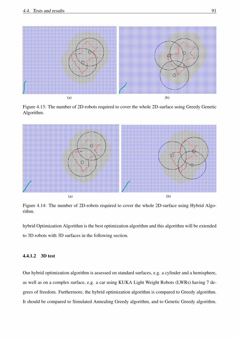
4.4. Tests and results 91
(a) (b)
Figure 4.13: The number of 2D-robots required to cover the whole 2D-surface using Greedy GeneticAlgorithm.
(a) (b)
Figure 4.14: The number of 2D-robots required to cover the whole 2D-surface using Hybrid Algo-rithm.
hybrid Optimization Algorithm is the best optimization algorithm and this algorithm will be extended
to 3D robots with 3D surfaces in the following section.
4.4.1.2 3D test
Our hybrid optimization algorithm is assessed on standard surfaces, e.g. a cylinder and a hemisphere,
as well as on a complex surface, e.g. a car using KUKA Light Weight Robots (LWRs) having 7 de-
grees of freedom. Furthermore, the hybrid optimization algorithm is compared to Greedy algorithm.
It should be compared to Simulated Annealing Greedy algorithm, and to Genetic Greedy algorithm.

92 Chapter 4. Optimal robot base placements for coverage tasks
This comparison is one of our future works. The comparison with Greedy algorithm is considered
since it is the basic algorithm to find the optimal number of robots to cover a whole surface. The in-
puts of both optimization algorithms are the different surface models S and the favourite robot poses
F.
In this application, we consider a spherical workspace with a radius of 1 around the base of the
robot, e.g. the discretization along θ is not necessary. Other types of workspaces will be tested later
on. Hence, the reachable part of the surface from a given position is considered as the intersection
between the spherical workspace and the surface to be covered.
A 3D discretization is considered in this example. The discretization step is set to 0.1 during the
pre-processing step. This step is chosen since it is almost 10% of the highest point in the KUKA
workspace (1.1785m). Each discretized point avoiding collision with the surface and allowing to
reach more than t = 15% of the surface is considered as a favourite robot pose. We found 398
favourite robot poses for the cylinder, 375 for the sphere and 397 for the action car represented as the
red spheres in Figure 4.15. For sake of simplicity, we used the point cloud to compute the percentage
(a) Cylinder (b) Sphere
(c) Action car
Figure 4.15: Surfaces to be covered by robots with the favorite base position (red spheres)
of the covered surface. In global, we consider a convex feasible set, hence if the three points of a
triangle are reachable, this triangle is supposed reachable. Those triangles are inside the reachable set
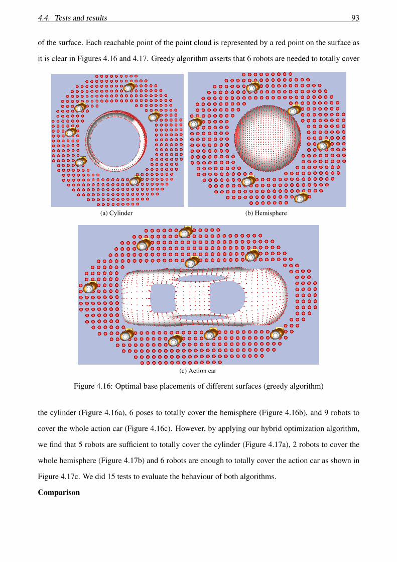
4.4. Tests and results 93
of the surface. Each reachable point of the point cloud is represented by a red point on the surface as
it is clear in Figures 4.16 and 4.17. Greedy algorithm asserts that 6 robots are needed to totally cover
(a) Cylinder (b) Hemisphere
(c) Action car
Figure 4.16: Optimal base placements of different surfaces (greedy algorithm)
the cylinder (Figure 4.16a), 6 poses to totally cover the hemisphere (Figure 4.16b), and 9 robots to
cover the whole action car (Figure 4.16c). However, by applying our hybrid optimization algorithm,
we find that 5 robots are sufficient to totally cover the cylinder (Figure 4.17a), 2 robots to cover the
whole hemisphere (Figure 4.17b) and 6 robots are enough to totally cover the action car as shown in
Figure 4.17c. We did 15 tests to evaluate the behaviour of both algorithms.
Comparison

94 Chapter 4. Optimal robot base placements for coverage tasks
(a) Cylinder (b) Hemisphere
(c) Action car
Figure 4.17: Optimal base placements of different surfaces (hybrid optimization)
As shown in Figures 4.16 and 4.17, the hybrid optimization algorithm gives less number of robots
needed to cover the whole surface. It is clear that the distribution of robot poses around the surface is
more homogeneous when we use our hybrid optimization algorithm. This point could be an advantage
if the number of robots composing the multi-robot system is lower than the optimal number of robots
required to cover the surface. Furthermore, the more the distribution of robot poses is homogeneous
around the surface the more the cycle time is reduced in the most cases, and the less the collision is
between robots. That is because the distance between any two adjacent robot poses is almost equal:
the time required to move the robots of the multi-robot system from one pose to the adjacent pose
is optimized. To assess the behaviour of the proposed algorithm, we ran the code several times for

4.4. Tests and results 95
each surface type. Figures 4.18, 4.19, and 4.20 compare both optimization algorithms by showing
the average of the optimal number of robots (blue columns) and the margin of this number (red
line) required to totally cover the cylinder, the sphere and the action car respectively. We can notice
that for all surface types, the average of the optimal number of robots obtained using the proposed
optimization algorithm is lower than the average of the optimal number of robots found using the
greedy algorithm. Additionally, the margin of the optimal number of robots obtained using the hybrid
optimization algorithm is tighter than the margin computed using the greedy algorithm. Furthermore,
we can deduce that the proposed optimization algorithm is closer to the global optimal solutions for
all surface types.
Figure 4.18: The number of robots required to cover the whole cylinder using greedy algorithm andthe proposed hybrid optimization algorithm.
Figure 4.19: The number of robots required to cover the whole sphere using greedy algorithm and theproposed hybrid optimization algorithm.

96 Chapter 4. Optimal robot base placements for coverage tasks
Figure 4.20: The number of robots required to cover the whole action car using greedy algorithm andthe proposed hybrid optimization algorithm.
4.4.2 Improved hybrid optimization algorithm
SurfaceWorkspace
Spherical Semi-spherical Elliptical
Cylinder 416 416 166Hemisphere 580 580 270
Car 692 692 307
Table 4.3: 3D discretization: the number of favourite robot poses for a cylinder, a hemisphere and acar using different types of workspaces
SurfaceWorkspace
Spherical Semi-spherical Elliptical
Cylinder 3414 3414 1378Hemisphere 2750 2750 785
Car 4906 4906 1960
Table 4.4: 4D discretization: the number of favourite robot poses for a cylinder, a hemisphere and acar using different types of workspaces
In this part, we considered the same surfaces and the same robots already used in Section 4.4.1: a
cylinder, a hemisphere, a car and a KUKA Light Weight Robot (LWRs). However, we used three
different types of robot’s workspace: a spherical, a semi-spherical and an elliptical workspace. In
addition, we test the hybrid optimization algorithm and the improved hybrid optimization algorithm
using 3D and 4D discretizations for each surface type. The discretization step is 0.1 for 3D and 4D
discretizations. The discretization of θ is not considered when the robot’s workspace is a sphere. A
discretized point is considered a favourite robot pose if it avoids collision with the surface and allows

4.4. Tests and results 97
to reach more than t = 15% of the cylinder, t = 9% of the sphere and t = 9% of the car respectively.
The threshold is chosen depending on the mesh refinement: finer is the mesh, smaller is the threshold.
Tables 4.3 and 4.4 show the number of favourite robot poses for a cylinder, a hemisphere and a car
using a spherical, a semi-spherical and an elliptical workspaces for each type of surfaces using 3D
and 4D discretizations respectively. It is clear that the number of favourite poses using a spherical and
a semi-spherical workspace for all the surface types is the same: it is a proof that the θ discretization
works perfectly.
Our algorithms were programmed using the C++ language and executed on the following hardware
and software: CPU Intel(R) Xeon(R) E5-2670, 6.4 GHz, Cache 8 Mo: CentOS Linux release 7.5.1804
(Core) 64 bits. This hardware is a cluster and I would like to thanks Mesocentre Clermont Auvergne,
the owner of this cluster, for their support. Before presenting the results for 3D and 4D discretizations,
we should know that the cluster gives 24 hours to solve an execution code. If the 24 hours finish, the
execution will be interrupted and we will satisfy with the achieved results.
4.4.2.1 3D discretization
We launch 100 times the hybrid and the improved hybrid optimization algorithms on the cylinder,
the hemisphere and the car using three types of workspace for each surface: the elliptical, the semi-
spherical and the spherical workspaces. The goal of both algorithms is to find the minimum number of
robots with their optimal base placements required to cover the whole surface using the correspondent
workspace.
Hence, we present using pie charts the percentage of the minimum number of robots for each case.
Moreover, the results for each surface using the different kind of workspaces and the two versions
of the algorithms are shown in Figure 4.21, 4.22 and 4.23. The pie charts on the left column present
the results for the hybrid optimization algorithm, and the results for the improved hybrid optimization
algorithm are shown in the right column.
After the interpretation of Figure 4.21, 4.22 and 4.23, we can confirm that the improved hybrid op-
timization algorithm gives better results, and even the number of possible solutions is less than the

98 Chapter 4. Optimal robot base placements for coverage tasks
possible solutions given by the hybrid optimization function: the standard deviation of the optimal
number of robots found using the improved hybrid optimization algorithm is less than the standard
deviation of the optimal number of robots found using the hybrid optimization algorithm. One case
is an exceptional case where the standard deviation of the optimal number of robots given by the im-
proved optimization algorithm is greater than the standard deviation of the optimal number of robots
given by the hybrid optimization algorithm: it is the case when the surface is a car and the workspace
is a semi-spherical shape (Figure 4.23b and 4.23c). However, even if the standard deviation is greater,
the minimum number of robots is closer to the optimal solutions: 7, 8 and 9 robots could be found
using the improved hybrid optimization algorithm but 9 and 12 robots are found using the hybrid
optimization algorithm.
Besides, it is clear that the improved hybrid optimization algorithm is slower than the hybrid opti-
mization algorithm in terms of computation times for any surface types and any workspaces as it is
shown in Figure 4.28. However, the standard deviation of the computation time taken by the improved
hybrid optimization algorithm is smaller than the standard deviation of the computation time taken by
the hybrid optimization algorithm (see Table 4.5).
Algorithm SurfaceWorkspace Type
elliptical semi-spherical spherical
Hybridcylinder 2310.326 1373.818 1095.508
hemisphere 903.843 26.401 0.052car 15815.768 6487.729 1554.951
Hybrid Improvedcylinder 56.841 1408.119 527.98
hemisphere 448.421 3.935 0.898car − 2814.569 736.044
Table 4.5: 3D discretization: the standard deviation of the computation time (in seconds) of Hybridoptimization algorithm and Improved Hybrid optimization algorithm applied on different type ofsurfaces using different type of workspace
4.4.2.2 4D discretization
In the 4D discretization, we proceed with same strategy of 3D discretization. However, the number of
possible solutions which are the number of favourite robot poses is higher in this case. In addition, we
test the algorithm using different shapes of workspace: the spherical workspace which covers a huge

4.4. Tests and results 99
part of the surface, the semi-spherical workspace which covers a normal part of the surface and the
elliptical workspace which covers a small part of the surface. Though, we can say that this methodol-
ogy gives better evaluation of the hybrid and the improved hybrid optimization algorithms. We launch
100 times both optimization algorithms on the cylinder, the hemisphere and the car using three types
of workspace for each surface: the elliptical, the semi-spherical and the spherical workspaces.
Moreover, we present using pie charts the percentage of the minimum number of robots for each
simple case. Those results are shown in Figure 4.25, 4.26 and 4.27.
Based on Figure 4.25, 4.26 and 4.27, we can say that in all cases the improved hybrid optimization
algorithm gives results that are more optimal than the results of the hybrid optimization algorithm
with a smaller standard deviation. Concerning the computation time, it is the same situation as we
have in 3D discretization methodology: the improved hybrid optimization algorithm is slower than the
hybrid optimization algorithm (see Figure 4.28). However, the standard deviation of computation time
for the improved hybrid optimization algorithm is smaller than the computation time for the hybrid
optimization algorithm as it is detailed in Table 4.6. Comparing the results of 3D discretization and
4D discretization, we can say that the improved hybrid optimization algorithm is more suitable than
the hybrid optimization algorithm when the number of possible solutions increases. Concerning the
computation time, this calculation should be accomplished off-line, and one calculation is enough for
each surface with a given workspace. Hence, the execution time of the improved hybrid optimization
algorithm can not be considered as a disadvantage in all cases, because the algorithm could find a
solution in a reasonable time.
Algorithm SurfaceWorkspace Type
elliptical semi-spherical spherical
Hybridcylinder 3838.177 328.131 388.146
hemisphere 1060.099 271.394 59.809car 5035.356 2240.024 1078.814
Hybrid Improvedcylinder 1795.463 55.039 177.869
hemisphere 69.915 184.286 11.002car − 576.028 328.026
Table 4.6: 4D discretization: the standard deviation of the results of Hybrid optimization algorithmand Improved Hybrid optimization algorithm applied on different type of surfaces using different typeof workspace
100 Chapter 4. Optimal robot base placements for coverage tasks
4.4.3 Application on the airplane
The hybrid optimization algorithm is tested on an airplane using a KUKA manipulator. This airplane
is shown in Figure 4.29, its length is 14 m, its wingspan is 10 m and its height is 9 m. We chose
a 3D discretization (discretization along x, y and z axes): the discretization is not required in this
application since the workspace is spherical. The discretization step s = 0.4 m along x, y and z axes.
A discretized pose is considered favourite if its coverage score is greater than t = 0.09%. Using
the hybrid optimization algorithm, we find that 9 robots are required to cover 60% of this airplane
as it is clear in Figure 4.30. The computation time is almost 3 days. We can see that there are some
robot positions where the surface is considered reachable but it does not. Those robot positions are
the ones having black circles on the top of the robots. This problem is normal since we are doing
the intersection between the robot workspace and the surface. It will be solved when the constraint
projection on the surface is applied instead of doing the intersection process (the collision constraint
between the robot body and the surface should be considered).
In order to evaluate the algorithm and to reduce the computation time, we test it on an airplane where
the length and the wingspan are 4 m and the height is 4 m. We compute the favourite robot base
placements of this airplane without the wings. In this application, we considered the same values of
parameters as in the previous test (3D discretization where the discretization step s = 0.4 m along x,
y and z axes). Using the hybrid optimization algorithm, we find that 6 robots are required to cover
80.6% of the airplabe as it is clear in Figure 4.31.
4.5 Conclusion
In this chapter, a new approach to distribute tasks between robots of multi-robot systems has been
presented. It aims to find the optimal number of robots and their optimal poses required to cover large
and complex surfaces. An hybrid optimization algorithm is proposed, it combines three optimization
algorithms: greedy, genetic, and simulated annealing. It has been proved that this method returns the
number of robots required to equally cover the surface. After that, we proposed an improved hybrid

4.5. Conclusion 101
optimization algorithm that deals with more complicated problems where the number of possible so-
lutions is very huge. Those algorithms have been assessed on regular surfaces (hemisphere, cylinder)
and on complex surfaces (car, airplane).

102 Chapter 4. Optimal robot base placements for coverage tasks
(a) Results of Hybrid optimization algorithm in orderto cover a cylinder using a robot having an ellipticalworkspace
(b) Results of Improved Hybrid optimization algo-rithm in order to cover a cylinder using a robot hav-ing an elliptical workspace
(c) Results of Hybrid optimization algorithm in orderto cover a cylinder using a robot having a semispher-ical workspace
(d) Results of Improved Hybrid optimization al-gorithm in order to cover a cylinder using a robothaving a semispherical workspace
(e) Results of Hybrid optimization algorithm in orderto cover a cylinder using a robot having a sphericalworkspace
(f) Results of Improved Hybrid optimization algo-rithm in order to cover a cylinder using a robot hav-ing a spherical workspace
Figure 4.21: 3D discretization: comparison of the results of Hybrid optimization algorithm and Im-proved Hybrid algorithm on a cylinder using the different workspaces
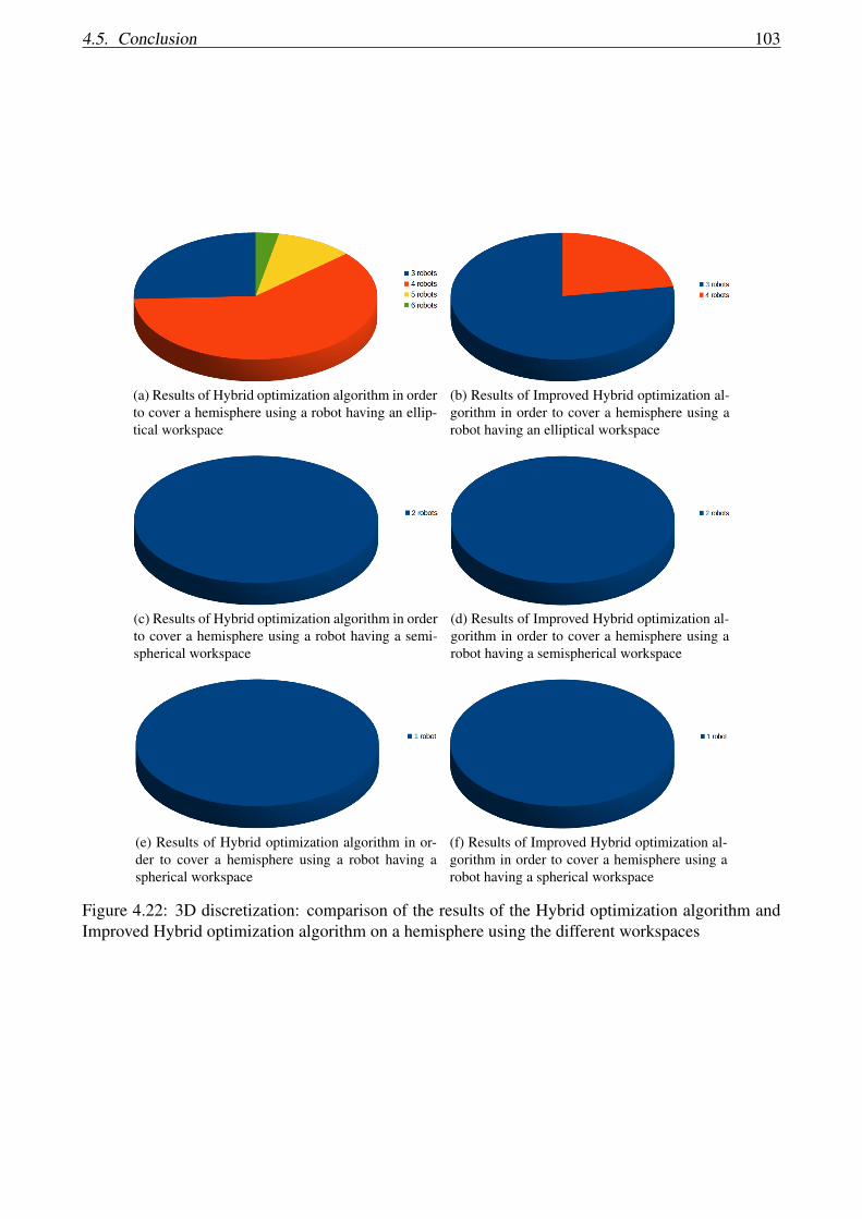
4.5. Conclusion 103
(a) Results of Hybrid optimization algorithm in orderto cover a hemisphere using a robot having an ellip-tical workspace
(b) Results of Improved Hybrid optimization al-gorithm in order to cover a hemisphere using arobot having an elliptical workspace
(c) Results of Hybrid optimization algorithm in orderto cover a hemisphere using a robot having a semi-spherical workspace
(d) Results of Improved Hybrid optimization al-gorithm in order to cover a hemisphere using arobot having a semispherical workspace
(e) Results of Hybrid optimization algorithm in or-der to cover a hemisphere using a robot having aspherical workspace
(f) Results of Improved Hybrid optimization al-gorithm in order to cover a hemisphere using arobot having a spherical workspace
Figure 4.22: 3D discretization: comparison of the results of the Hybrid optimization algorithm andImproved Hybrid optimization algorithm on a hemisphere using the different workspaces
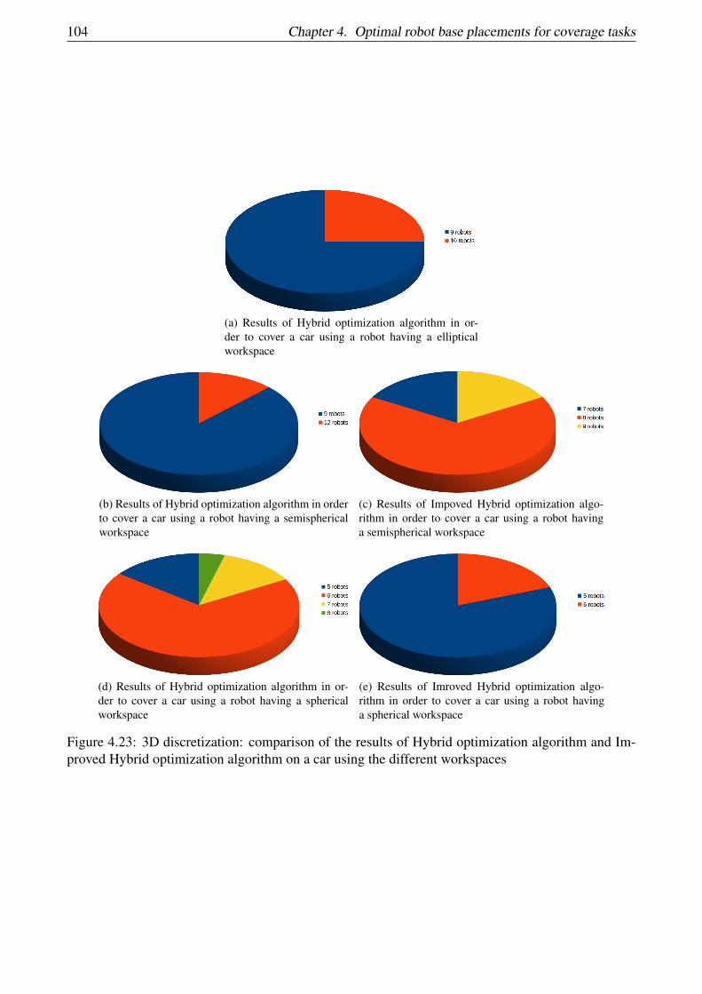
104 Chapter 4. Optimal robot base placements for coverage tasks
(a) Results of Hybrid optimization algorithm in or-der to cover a car using a robot having a ellipticalworkspace
(b) Results of Hybrid optimization algorithm in orderto cover a car using a robot having a semisphericalworkspace
(c) Results of Impoved Hybrid optimization algo-rithm in order to cover a car using a robot havinga semispherical workspace
(d) Results of Hybrid optimization algorithm in or-der to cover a car using a robot having a sphericalworkspace
(e) Results of Imroved Hybrid optimization algo-rithm in order to cover a car using a robot havinga spherical workspace
Figure 4.23: 3D discretization: comparison of the results of Hybrid optimization algorithm and Im-proved Hybrid optimization algorithm on a car using the different workspaces
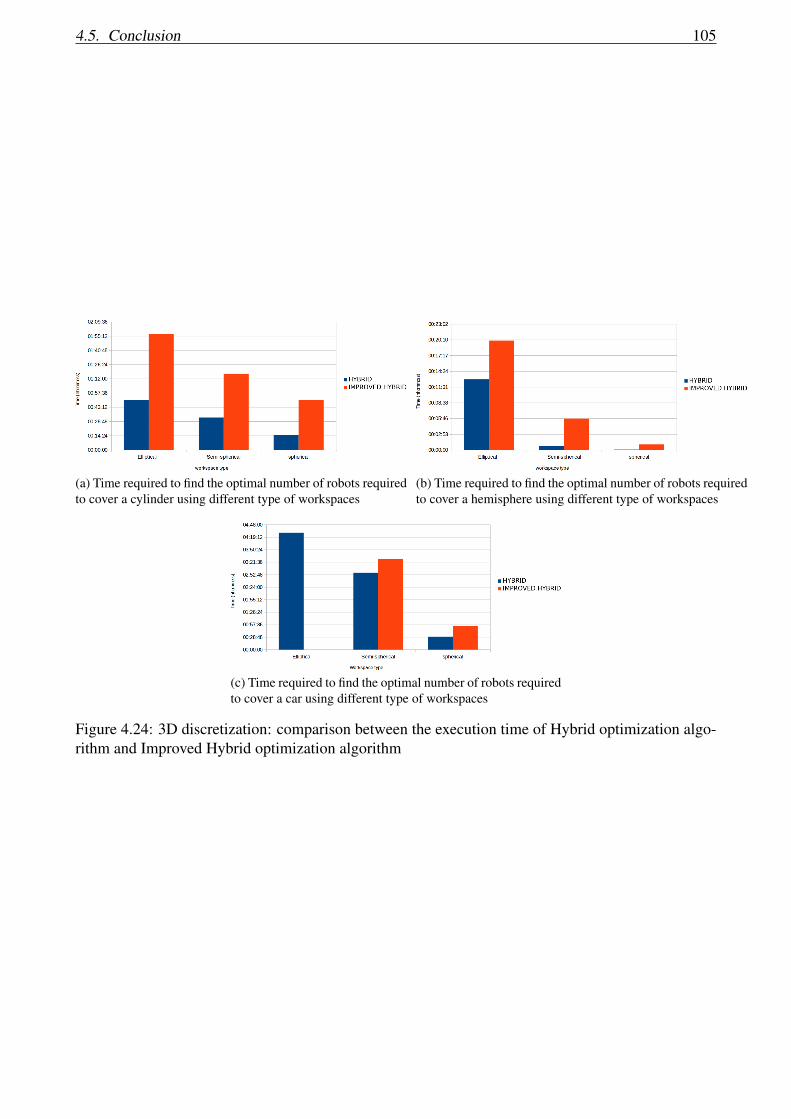
4.5. Conclusion 105
(a) Time required to find the optimal number of robots requiredto cover a cylinder using different type of workspaces
(b) Time required to find the optimal number of robots requiredto cover a hemisphere using different type of workspaces
(c) Time required to find the optimal number of robots requiredto cover a car using different type of workspaces
Figure 4.24: 3D discretization: comparison between the execution time of Hybrid optimization algo-rithm and Improved Hybrid optimization algorithm

106 Chapter 4. Optimal robot base placements for coverage tasks
(a) Results of Hybrid optimization algorihtm in orderto cover a cylinder using a robot having an ellipticalworkspace
(b) Results of Improved Hybrid optimization algo-rihtm in order to cover a cylinder using a robot hav-ing an elliptical workspace
(c) Results of Hybrid optimization algorihtm in orderto cover a cylinder using a robot having a semispher-ical workspace
(d) Results of Improved Hybrid optimization algo-rihtm in order to cover a cylinder using a robot hav-ing a semispherical workspace
(e) Results of Hybrid optimization algorihtm in orderto cover a cylinder using a robot having a sphericalworkspace
(f) Results of Improved Hybrid optimization algo-rihtm in order to cover a cylinder using a robot hav-ing a spherical workspace
Figure 4.25: 4D discretization: comparison of the results of Hybrid optimization algorithm and Im-proved Hybrid optimization algorithm on a cylinder using the different workspaces
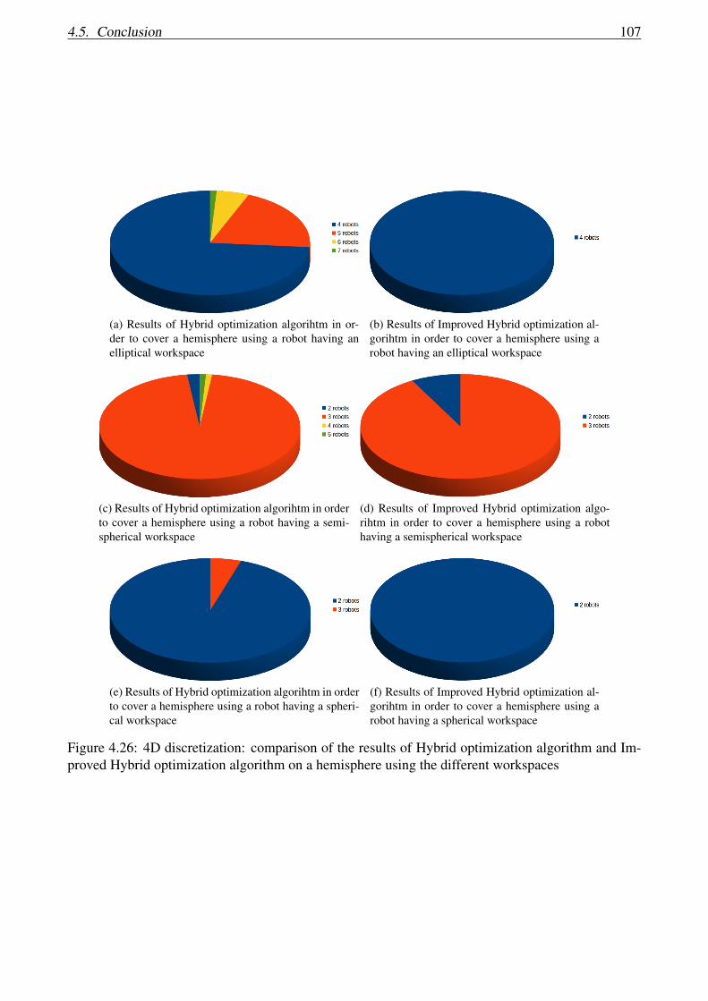
4.5. Conclusion 107
(a) Results of Hybrid optimization algorihtm in or-der to cover a hemisphere using a robot having anelliptical workspace
(b) Results of Improved Hybrid optimization al-gorihtm in order to cover a hemisphere using arobot having an elliptical workspace
(c) Results of Hybrid optimization algorihtm in orderto cover a hemisphere using a robot having a semi-spherical workspace
(d) Results of Improved Hybrid optimization algo-rihtm in order to cover a hemisphere using a robothaving a semispherical workspace
(e) Results of Hybrid optimization algorihtm in orderto cover a hemisphere using a robot having a spheri-cal workspace
(f) Results of Improved Hybrid optimization al-gorihtm in order to cover a hemisphere using arobot having a spherical workspace
Figure 4.26: 4D discretization: comparison of the results of Hybrid optimization algorithm and Im-proved Hybrid optimization algorithm on a hemisphere using the different workspaces

108 Chapter 4. Optimal robot base placements for coverage tasks
(a) Results of Hybrid optimization algorihtm in or-der to cover a car using a robot having an ellipticalworkspace
(b) Results of Hybrid optimization algorihtm in orderto cover a car using a robot having a semisphericalworkspace
(c) Results of Improved Hybrid optimization algori-htm in order to cover a car using a robot having asemispherical workspace
(d) Results of Hybrid optimization algorihtm in or-der to cover a car using a robot having a sphericalworkspace
(e) Results of Improved Hybrid optimization algori-htm in order to cover a car using a robot having aspherical workspace
Figure 4.27: 4D discretization: comparison of the results of Hybrid optimization algorithm and Im-proved Hybrid optimization algorithm on a car using the different workspaces

4.5. Conclusion 109
(a) Time resuired to find the optimal number of robots requiredto cover a cylinder using different type of workspaces
(b) Time resuired to find the optimal number of robots requiredto cover a hemisphere using different type of workspaces
(c) Time resuired to find the optimal number of robots requiredto cover a car using different type of workspaces
Figure 4.28: 4D discretization: comparison between the execution time of Hybrid optimization algo-rithm and Improved Hybrid optimization algorithm
(a) The air-plane model (b) The air-plane model with the set of favourite robot baseplacements
Figure 4.29: The representation of the air-plane with the set of favourite robot base placements (redcircle = favourite robot base placement)

110 Chapter 4. Optimal robot base placements for coverage tasks
Figure 4.30: Optimal base placements to cover airplane using the hybrid optimization algorithm
(a) The optimal robot base placements (b) The covered surface of the airplane (without thewings) from the optimal base placements
Figure 4.31: The results of the hybrid optimization algorithm on the airplane (the surface should beat least 80% covered without the wings)

Chapter 5
Conclusion
5.1 Summary of Thesis Achievements
The automation is now prominent in different fields. In this thesis, we dealt with the automation in
coverage tasks, and more precisely in stripping procedures. The considered application consists in
stripping complex surfaces using a multi-robot system composed of mobile platforms: cranes. The
stripping tool is connected to the crane via an industrial robot manipulator. The mobile platform
is moved manually, and the stripping process is stopped during the robot movement. The goal of
this PhD is to optimize the poses of the whole robotic systems in order to optimally strip the whole
surface. The optimal robot poses must take into account the physical limits of the robotic systems
such as joint position and torque limits, collision and self-collision avoidance.
Our first contribution is the proposition of a general framework to estimate the optimal number of
robots and the related optimal base placement. The general framework has the object mesh to be
covered, and the robot model as inputs and generates the optimal number of robots with their optimal
base placements and the trajectories of each robot of the multi-robot system between those poses as
outputs. The general framework consists in starting by a pre-processing step that provides a set of
discrete favourite base placements. Those base placements are the set of poses that do not collide
with the object mesh, and that cover at least t% of the object. After that, this set of favourite base
placements is used as input of the optimization algorithm in order to find the optimal number of robots
111

112 Chapter 5. Conclusion
N and their optimal base placements T. After that, the trajectories of the end-effector on the object
from each optimal pose are computed. Finally, a distribution of the robots that composes the multiple
robotic system is treated by doing robots scheduling and assignments. Though, the movement of the
robots between their assigned positions is controlled.
The second contribution is related to pessimism in Interval Analysis. We propose to use some proper-
ties of the BSplines and the Kronecker product to reduce the pessimism induced during the evaluation
of mathematical functions in Interval Analysis. We prove that our contribution deals with more com-
plex optimization problems and decreases the computation time. Interval Analysis is used to compute
the set of joint angles that allows a robot to reach a surface from a given position respecting a set of
constraints.
The third contribution is the proposed hybrid optimization algorithm. The main goal of this opti-
mization algorithm is to find the optimal number of robots with their optimal poses required to cover
an entire surface. An hybrid optimization algorithm is proposed, it combines the three optimization
algorithms: greedy, genetic, and simulated annealing. We proved that our hybrid optimization al-
gorithm is more efficient than Greedy optimization algorithm. In addition, we demonstrate that our
hybrid optimization algorithm gives better results in terms of robustness but it requires a little bit more
time. After that, we proposed an improved hybrid optimization function that is more robust when the
problem gets more complicated. However, the improved hybrid optimization function is slower than
the hybrid optimization function.
5.2 Future Works
Despite the huge effort on the thesis, I still have interesting works to accomplish, and other techniques
to test. Though, we count our future works.
— The bisection during solving CSPs or COPs using the proposed inclusion function could be
improved: the control points information could be used in order to guide the bisection process
in an effective way.
5.2. Future Works 113
— The use of multi-threading will also be investigated to decrease the computation time during the
evaluation of the bounds of a given function using the improved proposed inclusion function.
— The proposed inclusion function will be tested on more complex optimization problems such
as robotic motion optimization. It should be also tested on 3D robots taking into account ad-
ditional constraints such as kinematic constraints, collision and self-collision avoidance, singu-
larity avoidance or more dynamic constraints such balance or torque limits.
— The generated workspace using IA method should be used as an input for the hybrid opti-
mization algorithm instead of testing it on regular workspace (spherical, semi-spherical, and
elliptical shapes).
— The system could have different types of robots, so different robot workspace in the same
stripping process: this variety of robots should be considered in the program.
— The improved hybrid optimization algorithm could reach better results by changing the tech-
nique of children generation. The defined angle based on the number of robots should not be
the only criteria to define the border of a zone, but the number of favourite positions in each
zone should be considered during the zone generation.
— A new technique should be tested by considering that we can assign an ”area” on the ground
plane instead of a ”single position” to each mobile manipulator to operate around an object.
Here the analogy is again with human operators, who can move and cover an area (I am thinking
about the example of having several human operators stripping a big air-plane, and how these
human operators would behave to do the task. One could assign an ”area” to each operator).
You can try to optimize this ”area” according to some cost function. Or maybe simply exploit
the fact that the optimization becomes much less expensive computationally (instead of dealing
with many positions of the bases, we would be working only with a few ”areas”). This could
be an interesting fact in itself: it allows to take into account the uncertainty.
— We can also use Interval Analysis in order to take into account the uncertainty of base place-
ment: instead of getting a specific value for a base placement, we will get a box.
— In case the number of robotic systems is limited (the number of optimal robot poses is greater
than the number of robots of the multi-robot system), the robots will be redistributed based
on new optimal path planner that considers the different systems constraints. This step is the

114 Chapter 5. Conclusion
solution of the particular problems presented in Chapter 1. We propose to use the Hungarian
algorithm to solve those assignment problems.
— We can assume the planning of the end effector motion from a given position of the mobile
base can be done with an existing method (CPP, or methods for solving the ”lawn-mower prob-
lem”...) so we can maybe focus on the base placements and not the end effector-trajectory
planning.
— The goal of this thesis was to find the optimal number of robot positions required to cover a
surface. The algorithm used to attend this goal should be adapted to find the optimal positions
of crane around the surface to be covered.
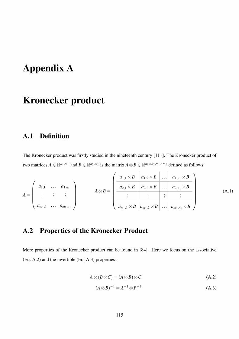
Appendix A
Kronecker product
A.1 Definition
The Kronecker product was firstly studied in the nineteenth century [111]. The Kronecker product of
two matrices A ∈ Rn1,m1 and B ∈ Rn2,m2 is the matrix A⊗B ∈ Rn1×n2,m1×m2 defined as follows:
A=
a1,1 . . . a1,n1
......
...
am1,1 . . . am1,n1
A⊗B =
a1,1×B a1,2×B . . . a1,n1×B
a2,1×B a2,2×B . . . a2,n1×B...
......
...
am1,1×B am1,2×B . . . am1,n1×B
(A.1)
A.2 Properties of the Kronecker Product
More properties of the Kronecker product can be found in [84]. Here we focus on the associative
(Eq. A.2) and the invertible (Eq. A.3) properties :
A⊗ (B⊗C) = (A⊗B)⊗C (A.2)
(A⊗B)−1 = A−1⊗B−1 (A.3)
115

116 Chapter A. Kronecker product
Using Equation (A.3), Equations (3.35) and (3.36) can be turned into :
P =(B−1
1 ⊗B−12 ⊗ . . .⊗B−1
n)
X (A.4)
Assuming B ∈ Rx,x, with x = ∏nk=1 mi , the complexity of the inversion of the matrix B in Equa-
tion (3.35) is O(x3). Using the invertible property, the complexity decreases to O(x∑n m2i ) where
x = ∏n mi, that will allow faster computation. Hence, Equation (A.4) is used to compute control
points.
One can consider the following property relating matrix/vector multiplication and the Kronecker prod-
uct:
A.X = (I⊗A)X (A.5)
Where A is a matrix and X is a vector. Equation (A.5) is used to reduce computation time for the
proposed inclusion function.
A.3 Recursive Inverse Kronecker Product
Using Equation (A.5), Equation (3.37) can be written as following:
P =(B−1
1 ⊗B−12 ⊗ . . .⊗B−1
n)
Xn
=(B−1
1 ⊗ . . .⊗B−1n−1)(
I⊗B−1n)
Xn
=(B−1
1 ⊗ . . .⊗B−1n−1)
Xn−1
With: Xn−1 =(I⊗B−1
n)
Xn
(A.6)
This equation can be used recursively to reduce the computation time. Regarding the low dimension
of the matrix Bi, the inversion is done numerically. However, future works will address this issue
as presented in Section 3.7. As an example, consider two matrices A ∈ R2×2 and B ∈ R2×2, and
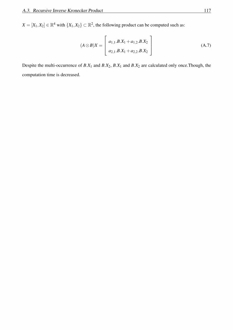
A.3. Recursive Inverse Kronecker Product 117
X = [X1,X2] ∈ R4 with {X1,X2} ⊂ R2, the following product can be computed such as:
(A⊗B)X =
a1,1.B.X1 +a1,2.B.X2
a2,1.B.X1 +a2,2.B.X2
(A.7)
Despite the multi-occurrence of B.X1 and B.X2, B.X1 and B.X2 are calculated only once.Though, the
computation time is decreased.

Appendix B
Evaluating an equation using different
inclusion functions
In this section, we present two examples: one dimensional and two dimensional examples. The
1-dimensional example is used to compare the efficiency of the different inclusion functions. The
2-dimensional example is shown to make clear how we can compute the interval of a function using
BSplines and Kronecker product properties.
B.1 1-dimensional example
For instance, consider the function f defined by f (x) = x2 + sin(x) and the intervals [x1] = [2π
3,4π
3]
and [x2] = [99π
100,101π
100]. We will compare the approximations of f (x1) and f (x2) obtained by using
the natural, the centred, Taylor of order two, Chebyshev of order five, Bernstein inclusion function,
BSplines and minimal inclusion functions, which will be [ f ]n, [ f ]c, [ f ]T 2, [ f ]C5, [ f ]B, [ f ]Bs and [ f ∗]
118
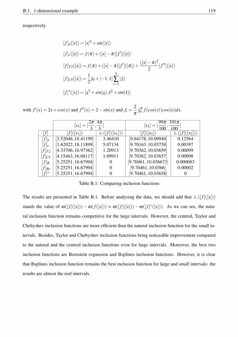
B.1. 1-dimensional example 119
respectively.
[ f ]n([x]) = [x]2 + sin([x])
[ f ]c([x]) = f (π)+([x]−π)[ f ′]([x])
[ f ]T 2([x]) = f (π)+([x]−π)[ f ′]([π])+([x]−π)2
2[ f ′′]([x])
[ f ]C5([x]) =12
f0 +[−1,1]5
∑i=1| fi|
[ f ]∗([x]) = [x2 + sin(x), x2 + sin(x)]
with f ′(x) = 2x+ cos(x) and f ′′(x) = 2− sin(x) and fi =2π
∫π
0 f (cos(x))cos(ix)dx.
[x1] = [2π
3,4π
3] [x2] = [
99π
100,101π
100]
[ f ] [ f ]([x1]) M ([ f ]([x1])) [ f ]([x2]) M ([ f ]([x2]))[ f ]n [3.52046,18.41199] 3.46410 [9.64178,10.09940] 0.12564[ f ]c [1.62022,18.11899] 5.07134 [9.70163,10.03758] 0.00397[ f ]T 2 [4.33706,16.97362] 1.20913 [9.70362,10.03659] 0.00099[ f ]C5 [4.15463,16.68117] 1.09911 [9.70362,10.03657] 0.00098[ f ]B [5.25251,16.67994] 0 [9.70461,10.036673] 0.000083[ f ]Bs [5.25251,16.67994] 0 [9.70461,10.0366] 0.00002[ f ]∗ [5.25251,16.67994] 0 [9.70461,10.03658] 0
Table B.1: Comparing inclusion functions
The results are presented in Table B.1. Before analysing the data, we should add that M ([ f ]([x]))
stands the value of ω([ f ]([x]))−ω( f ([x])) = ω([ f ]([x]))−ω([ f ]∗([x])). As we can see, the natu-
ral inclusion function remains competitive for the large intervals. However, the centred, Taylor and
Chebyshev inclusion functions are more efficient than the natural inclusion function for the small in-
tervals. Besides, Taylor and Chebyshev inclusion functions bring noticeable improvement compared
to the natural and the centred inclusion functions even for large intervals. Moreover, the best two
inclusion functions are Bernstein expansion and Bsplines inclusion functions. However, it is clear
that Bsplines inclusion function remains the best inclusion function for large and small intervals: the
results are almost the real intervals.
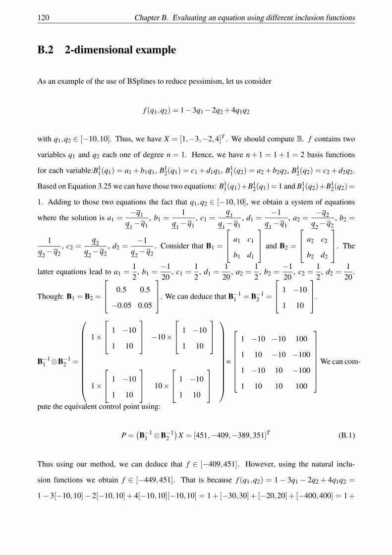
120 Chapter B. Evaluating an equation using different inclusion functions
B.2 2-dimensional example
As an example of the use of BSplines to reduce pessimism, let us consider
f (q1,q2) = 1−3q1−2q2 +4q1q2
with q1,q2 ∈ [−10,10]. Thus, we have X = [1,−3,−2,4]T . We should compute B. f contains two
variables q1 and q2 each one of degree n = 1. Hence, we have n+ 1 = 1+ 1 = 2 basis functions
for each variable:B11(q1) = a1 + b1q1, B1
2(q1) = c1 + d1q1, B11(q2) = a2 + b2q2, B1
2(q2) = c2 + d2q2.
Based on Equation 3.25 we can have those two equations: B11(q1)+B1
2(q1) = 1 and B11(q2)+B1
2(q2) =
1. Adding to those two equations the fact that q1,q2 ∈ [−10,10], we obtain a system of equations
where the solution is a1 =−q1
q1−q1, b1 =
1q1−q1
, c1 =q1
q1−q1, d1 =
−1q1−q1
, a2 =−q2
q2−q2, b2 =
1q2−q2
, c2 =q2
q2−q2, d2 =
−1q2−q2
. Consider that B1 =
a1 c1
b1 d1
and B2 =
a2 c2
b2 d2
. The
latter equations lead to a1 =12
, b1 =−120
, c1 =12
, d1 =1
20, a2 =
12
, b2 =−120
, c2 =12
, d2 =1
20.
Though: B1 = B2 =
0.5 0.5
−0.05 0.05
. We can deduce that B−11 = B−1
2 =
1 −10
1 10
.
B−11 ⊗B−1
2 =
1×
1 −10
1 10
−10×
1 −10
1 10
1×
1 −10
1 10
10×
1 −10
1 10
=
1 −10 −10 100
1 10 −10 −100
1 −10 10 −100
1 10 10 100
We can com-
pute the equivalent control point using:
P =(B−1
1 ⊗B−12)
X = [451,−409,−389,351]T (B.1)
Thus using our method, we can deduce that f ∈ [−409,451]. However, using the natural inclu-
sion functions we obtain f ∈ [−449,451]. That is because f (q1,q2) = 1− 3q1 − 2q2 + 4q1q2 =
1− 3[−10,10]− 2[−10,10] + 4[−10,10][−10,10] = 1+ [−30,30] + [−20,20] + [−400,400] = 1+

B.2. 2-dimensional example 121
[−450,450] = [−449,451]. Using a 3D plot of f , we can deduce that f is limited between −409 and
451 as it is clear in Figure B.1.
Figure B.1: 3D plot of f (q1,q2) = 1−3q1−2q2 +4q1q2
By applying Horner schemes, we got two different expressions of f : f = 1+q1(−3+4q2)−2q2 and
f = 1−3q1−2q2(1−2q1). For those two different expressions we got two intervals [−449,451] and
[−449,451]. Once can deduce that our method reduces pessimism in this example. Horner scheme
works for n = 2 and gives the same results, but his behaviour becomes more critical when n increases.
Hence, the proposed method allows to avoid or at least reduce pessimism for n = 2. Moreover, if the
value of n increases, then the pessimism will be more reduced: the multi-occurrence increases once n
increases.
Let us apply the inputs normalization on this example. After normalization of the inputs q1 and q2 us-
ing those equations q1 = 10q1re f and q2 = 10q2re f , we can deduce that f (q1re f ,q2re f ) = 1−30q1re f −
20q2re f + 400q1re f q2re f . Thus, we have X = [1,−30,−20,400]T and B1 = B2 =
0.5 0.5
−0.5 0.5
.
Hence, B−11 = B−1
2 =
1 −1
1 1
.

122 Chapter B. Evaluating an equation using different inclusion functions
B−11 ⊗B−1
2 =
1×
1 −1
1 1
−1×
1 −1
1 1
1×
1 −1
1 1
−1×
1 −1
1 1
=
1 −1 −1 1
1 1 −1 −1
1 −1 1 −1
1 1 1 1
We can compute
the equivalent control point using:
P =(B−1
1 ⊗B−12)
X = [451,−409,−389,351]T (B.2)
Thus, using our method, we can deduce that f ∈ [−409,451] which is the same interval obtained
without inputs normalization.
Finally, let consider that q1 = q2 ∈ [−1,1] for the same equation
f (q1,q2) = 1−3q1−2q2 +4q1q2
. Thus, we have X = [1,−3,−2,4]T and B1 = B2 =
0.5 0.5
−0.5 0.5
. We can compute the equivalent
control point using:
P =(B−1
1 ⊗B−12)
X = [10,−4,−2,0]T (B.3)
Thus, using our method, we can deduce that f ∈ [−4,10]. However, using the natural inclusion
functions we obtain f ∈ [−8,10]. That is because f (q1,q2) = 1−3q1−2q2+4q1q2 = 1−3[−1,1]−
2[−1,1]+4[−1,1][−1,1] = 1+[−3,3]+[−2,2]+[−4,4] = 1+[−9,9] = [−8,10]. Using a 3D plot of
f , we can deduce that f is limited between −4 and 10. And using the two different Horner schemes
already defined we can deduce that f ∈ [−8,10]. Hence, we can deduce that our method reduces
pessimism for large and tight intervals.

Appendix C
How did we get the linearisation Equation
using Taylor theorem
Taylor’s theorem
Proof. Consider k ≥ 1 an integer and the function f : R→ R which is k times differentiable at the
point a ∈ R. Then, it exists a function hk : R→ R such that
f (x) = f (a)+ f ′(a)(x−a)+f ′′(a)
2!(x−a)2 + · · ·+ f (k)(a)
k!(x−a)k +hk(x)(x−a)k
and limx→a hk(x) = 0. This is called the Peano form of the remainder.
The polynomial appearing in Taylor’s theorem is the k− th order Taylor polynomial of the function f
at the point a:
Pk(x) = f (a)+ f ′(a)(x−a)+f ′′(a)
2!(x−a)2 + · · ·+ f k(a)
k!(x−a)k (C.1)
By applying Equation C.1 on cos(x) ans sin(x), we get the following equations
123

124 Chapter C. How did we get the linearisation Equation using Taylor theorem
cos(x) = cos(a)− sina(x−a)− 12
cosa(x−a)2 +16
sina(x−a)3 + · · ·
sin(x) = sin(a)+ cosa(x−a)− 12
sina(x−a)2− 16
cosa(x−a)3 + · · ·(C.2)
Consider x is qi, let apply the normalization, written in Equation 3.43, on a 2− th order Taylor
polynomial by considering a=mi, we got
cos([qi]) = cos(mi)− sin(mi)di
2[qre f
i ]+ · · ·
sin([qi]) = sin(mi)+ cos(mi)di
2[qre f
i ]+ · · ·(C.3)
Hence, we got Equation 3.44.
For instance, consider the function cos(x) for x = [−4,4]: cos(x), its 3− th and its 5− th order Taylor
polynomials are shown in Figure C.1. Find the error εs for the approximation of cos(x) up to O(x3)
and up to O(x5). Using the below Figure, we can deduce that εs(x3) = [0 ;6.3464 ;6.3464] and
εs(x5) = [0 ;−4.3209 ;−4.3209].
Figure C.1: Taylor Series Expansion of cos(x)
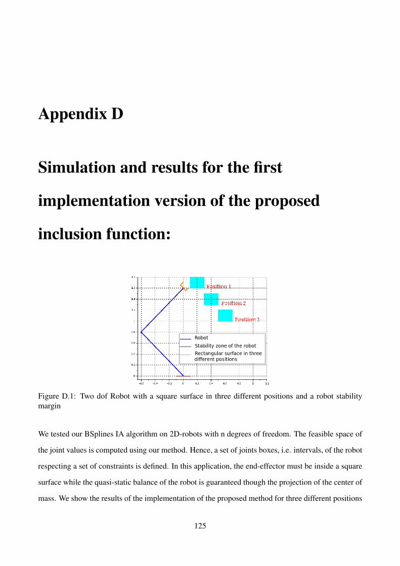
Appendix D
Simulation and results for the first
implementation version of the proposed
inclusion function:
Figure D.1: Two dof Robot with a square surface in three different positions and a robot stabilitymargin
We tested our BSplines IA algorithm on 2D-robots with n degrees of freedom. The feasible space of
the joint values is computed using our method. Hence, a set of joints boxes, i.e. intervals, of the robot
respecting a set of constraints is defined. In this application, the end-effector must be inside a square
surface while the quasi-static balance of the robot is guaranteed though the projection of the center of
mass. We show the results of the implementation of the proposed method for three different positions
125
126Chapter D. Simulation and results for the first implementation version of the proposed inclusion function:
of the square surface as presented in Figure D.1, with a robot of 2, 3, 4 and 5 degrees of freedom
for each position. We consider the 2D robot with a total length of 2, with all the segment of equal
values (2/n) and equal mass, a root position in (0,0) and with all joint limits of [−1.5,1.5]. The size
of the desired square surface is 0.2 with two feasible positions (0.2;1.7), (0.4;1.4) and one infeasible
position (0.6;1.1) (due to balance constraint). The balance of the robot is considered by ensuring that
the projection of its center of mass remains in the interval [−0.1,0.1] (considering that the center of
mass of each segment is at the middle of the segment). The surface reachability decision is based
on the position of the end-effector. This position is computed using a composition of transformation
matrices. The transformation matrix of qi is defined by: Tqi =
cos(qi) −sin(qi) βi
sin(qi) cos(qi) 0
0 0 1
Where
∀i > 1,βi =ln and β0 = 0, since the initial robot position is along y axis. Hence the position of the
end-effector Pf = (Tf (0,2), Tf (1,2)) Where Tf = Tπ/2Tq1...Tqi...Tqn .
We assign 0.01 to the box threshold during the bisection process. We compare three methods: the
classic contraction with the bisection (Solver 1), the BSplines contraction of the monomial that are
composed only of input variables with the bisection (Solver 2), and the BSplines contraction of all
the monomials in the constraints equations with the bisection (Solver 3). The number of iterations
and the computation time required to find the feasible workspace are shown in Figures D.3a and D.3b
respectively, for a threshold of 0.01 and in Figures D.2a and D.2b respectively, for a threshold of 0.1.
The computing time required to find the feasible workspace for a robot of 5 dof using a precision of
0.01 was very huge: more than one week. Hence, we show the results of a robot with 1, 2, 3, and
4 dof for a precision of 0.01. For both thresholds, the number of iterations using the BSplines con-
traction with the bisection (Solver 2, 3) is smaller than the number of iterations in the state-of-the-art
method (Solver 1). Though, BSplines IA uses less number of bisections to find the robot feasible
workspace. Hence, our method decreases pessimism. A comparison between the two solvers using
the BSplines contraction (Solver 2 and 3) shows that (Solver 3) has lower number of iterations than
(Solver 2). Though, the contraction of each monomials of the constraint equation helps to reduce pes-
simism. However, (Solver 3) is slower than (Solver 2), since doing better contractions requires more
computation time (see Figure D.3b, D.2b). It is clear that while increasing the accuracy (decreasing

127
the threshold), our method (Solver 2) becomes faster than the classic method (Solver 1). Hence the
BSplines contraction/ bisection reduces pessimism, and it is faster than the contraction/ bisection for
high accuracy. We proposed two solvers using BSplines contraction: Solver 2 is faster than Solver 3
and 1, but Solver 3 reduces the pessimism more than Solver 2. Tables D.1 and D.2 show the number
of iterations and the computing time required to find the feasible space of our different problems for
a precision of 0.01.
(a) Iteration numbers (b) Computation time
Figure D.2: Iteration numbers and computation time of the three different solvers compared to Solver1 for a precision of 0.1
(a) Iteration numbers (b) Computation time
Figure D.3: Iteration numbers and computation time of the three different solvers compared to Solver1 for a precision of 0.01

128Chapter D. Simulation and results for the first implementation version of the proposed inclusion function:
Position SolverDOF
2 3 4
11 1975 2288339 13567481672 1871 2032347 10866328833 1555 1771783 999374305
21 705 466451 7373519072 681 397469 5365158973 477 326615 488179609
31 21 74895 2312735672 37 63129 1526414193 29 52201 132694819
Table D.1: The number of incrementation required to solve Position 1 problem using Solver 1, Solver2 and Solver 3/ PRECISION 0.01
Position SolverDOF
2 3 4
11 0 / 00 : 00 : 0.05 0 / 00 : 03 : 39 4 / 14 : 39 : 572 0 / 00 : 00 : 0.04 0 / 00 : 01 : 51 2 / 00 : 02 : 093 0 / 00 : 00 : 0.04 0 / 00 : 01 : 58 3 / 01 : 50 : 30
21 0 / 00 : 00 : 0.02 0 / 00 : 00 : 43 2 / 12 : 11 : 182 0 / 00 : 00 : 0.01 0 / 00 : 00 : 21 1 / 00 : 02 : 353 0 / 00 : 00 : 0.01 0 / 00 : 00 : 22 1 / 13 : 14 : 06
31 0 / 00 : 00 : 0.0005 0 / 00 : 00 : 07 0 / 19 : 08 : 452 0 / 00 : 00 : 0.0007 0 / 00 : 00 : 03 0 / 07 : 02 : 043 0 / 00 : 00 : 0.0007 0 / 00 : 00 : 035 0 / 10 : 47 : 06
Table D.2: The time (in days / HH:MM:SS) required to solve Position 1 problem using Solver 1,Solver 2 and Solver 3/ PRECISION 0.01

Appendix E
Assignment and Scheduling
The assignment problem, in the robots scheduling, assignment and control step of the general frame-
work, selects which optimal poses should correspond to each robot in order to generate their trajecto-
ries from their initial positions. This type of problems can be solved using different algorithms such
as The Multiple Traveling Salesman Problem (mTSP), Hungarian algorithm, the primal simplex algo-
rithm and the auction algorithm. We have chosen the Hungarian algorithm since it is fast and simple
and it is suitable for all the problems which can be described as an integer programming [141]. In
this appendix, we present the required formulation for the Hungarian application to our assignment
problem.
The assignment problem can be broken into two sub-problems which can be considered as two suc-
cessive Hungarian problems. The first one assigns Nsys robots to the previously computed N optimal
poses. The second assignment problem computes the necessary trajectories for each robot to reach the
desired poses. Usually Nsys ≤ N, so one robot should visit several poses. During the assignment, sev-
eral goals should be taken into consideration: the robots do not cooperate between them which mean
that each robot must have a separate zone to strip, the cycle time of moving the robots should be min-
imized and the distribution of the robots around the surface should consider the collision avoidance
between them.
Both problems can be formulated using the following formulation: let S= {Si ∈ SE{3},1≤ i≤Nsys}
be the set of initial positions of the robots composing the multi-robot system, T = {T j ∈ SE(3),1 ≤
129

130 Chapter E. Assignment and Scheduling
j ≤ N} be the set of optimal robot poses.
For the first problem, let ci j = distance(SiT j) be the cost of moving a robot from its current position
Si to the j− th optimal pose Tj.
ci j is computed using the weighted cost function C : S×T→ R.
Define the variable xi j =
1 if we assign the element j ∈ T to the element i ∈ S
0 if notThe problem is
Find a bijection f : S→ T
Such that ∑Nsysi=1 ∑
Nj=1 ci jxi j is minimized
Subject to ∑Nj=1 xi j = 1 ∀i = 1, · · · ,Nsys
(E.1)
∑Nj=1 xi j = 1 means that each optimal pose is assigned to one and only one robot.
For the second problem, once the first Hungarian algorithm has solved ST= {S1T1,S1T2, · · · ,SrsT1}=
{ST1,1,ST1,2, · · · ,STrs,1}, which represents the set of assigned optimal poses to the different robots.
For instance, ST1,1 means that the optimal pose T1 is assigned to the robot S1. Let be ui j,kl =
distance(STi j,STkl) the distance between two different robots and their assigned tasks (i 6= k). ui j,kl
is computed using the weighted cost function U : ST×ST→ R.
Define the variable mi j,kl =
1 if we assign the element i j ∈ ST to the element kl ∈ ST
0 if notThe problem is
Find a bijection f : ST→ ST
Such that ∑Nsysi=1 ∑
Nj=1 ∑
Nsysk=1 ∑
Nl=1 ui j,klmi j,kl is maximized such as i 6= k
(E.2)
In this case the cost function has to be maximized to avoid collisions between the robots.

Bibliography
[1] Ercan U Acar, Howie Choset, Yangang Zhang, and Mark Schervish. Path planning for robotic
demining: Robust sensor-based coverage of unstructured environments and probabilistic meth-
ods. The International journal of robotics research, 22(7-8):441–466, 2003.
[2] D Alciatore and C Ng. Determining manipulator workspace boundaries using the monte carlo
method and least squares segmentation. ASME Robotics: Kinematics, Dynamics and Controls,
72:141–146, 1994.
[3] MF Aly, AT Abbas, and Said M Megahed. Robot workspace estimation and base placement
optimisation techniques for the conversion of conventional work cells into autonomous flexible
manufacturing systems. International Journal of Computer Integrated Manufacturing, 23(12):
1133–1148, 2010.
[4] Mayur V. Andulkar and Shital S. Chiddarwar. Incremental approach for trajectory generation
of spray painting robot. Industrial Robot: An International Journal, 42(3):228–241, 2015.
[5] Mayur V Andulkar and Shital S Chiddarwar. Automated CAD Based Trajectory for Spray
Painting Robot: Variable Velocity Approach. In Proceedings of the ASME 2015 International
Design Engineering Technical Conferences {&} Computers and Information in Engineering
Conference, pages 1–10, Boston, Massachusetts, USA, 2015.
[6] Mayur V. Andulkar, Shital S. Chiddarwar, and Akshay S. Marathe. Novel integrated offline
trajectory generation approach for robot assisted spray painting operation. Journal of Manu-
facturing Systems, 37:201–216, 2015.
131

132 BIBLIOGRAPHY
[7] J. K. Antonio, R. Ramabhadran, and T.-L. Ling. A Framework For Optimal Trajectory Planning
For Automated Spray Coating, 1997.
[8] Prasad N Atkar, Howie Choset, and Alfred A Rizzi. Towards Optimal Coverage of 2-
dimensional surfaces embedded in R3 choice of start curve. In Proceedings ofthe 2003 IEEE-
JRSJ Intl Conference on Intelligent Robots and Systems, number October, 2003.
[9] Prasad N Atkar, Aaron Greenfield, David C Conner, Howie Choset, and Alfred A Rizzi. Uni-
form Coverage of Automotive Surface Patches. The International Journal of Robotics Re-
search, 24(11):883–898, 2005.
[10] Prasad N Atkar, Aaron Greenfield, David C Conner, Howie Choset, and Alfred A Rizzi. Uni-
form coverage of automotive surface patches. The International Journal of Robotics Research,
24(11):883–898, 2005.
[11] Andreas Bircher, Kostas Alexis, Michael Burri, Philipp Oettershagen, Sammy Omari, Thomas
Mantel, and Roland Siegwart. Structural inspection path planning via iterative viewpoint re-
sampling with application to aerial robotics. In Robotics and Automation (ICRA), 2015 IEEE
International Conference on, pages 6423–6430. IEEE, 2015.
[12] Zhou Bo, Zhang Xi, Meng Zhengda, and D A I Xianzhong. Off-line Programming System of
Industrial Robot for Spraying Manufacturing Optimization. In Proceedings of the 33rd chinese
control conference, pages 8495–8500, 2014.
[13] G Boschetti, R Rosa, and A Trevisani. Optimal robot positioning using task-dependent and
direction-selective performance indexes: General definitions and application to a parallel robot.
Robotics and Computer-Integrated Manufacturing, 29(2):431–443, 2013.
[14] Felix Burget and Maren Bennewitz. Stance selection for humanoid grasping tasks by inverse
reachability maps. In Robotics and Automation (ICRA), 2015 IEEE International Conference
on, pages 5669–5674. IEEE, 2015.
[15] Franco Busetti. Simulated annealing overview. World Wide Web, 2003.
BIBLIOGRAPHY 133
[16] Burcin Cakir, Fulya Altiparmak, and Berna Dengiz. Multi-objective optimization of a stochas-
tic assembly line balancing: A hybrid simulated annealing algorithm. Computers & Industrial
Engineering, 60(3):376–384, 2011.
[17] Damien Chablat, Ph Wenger, and J Merlet. Workspace analysis of the orthoglide using interval
analysis. In Advances in Robot Kinematics, pages 397–406. Springer, 2002.
[18] Damien Chablat, Ph Wenger, Felix Majou, and J-P Merlet. An interval analysis based study for
the design and the comparison of three-degrees-of-freedom parallel kinematic machines. The
International Journal of Robotics Research, 23(6):615–624, 2004.
[19] Damien Chablat, Philippe Wenger, and Jean-Pierre Merlet. A comparative study between two
three-dof parallel kinematic machines using kinetostatic criteria and interval analysis. arXiv
preprint arXiv:0707.2833, 2007.
[20] Heping Chen and Ning Xi. Automated tool trajectory planning of industrial robots for painting
composite surfaces. International Journal of Advanced Manufacturing Technology, 35(7-8):
680–696, 2006.
[21] Heping Chen, Ning Xi, Zhouhua Wei, Yifan Chen, and J. Dahl. Robot trajectory integration
for painting automotive parts with multiple patches. In 2003 IEEE International Conference
on Robotics and Automation (Cat. No.03CH37422), volume 3, pages 3984–3989 vol.3, Sept
2003.
[22] Heping Chen, Ning Xi, Weihua Sheng, and Yifan Chen. General Framework of Optimal Tool
Trajectory Planning for Free Form Surfaces. Journal of Manufactirung Science and Engineer-
ing, 127(February 2005):49–59, 2005.
[23] Heping Chen, Ning Xi, Weihua Sheng, Jeffrey Dahl, and Zhaojie Li. Optimal tool trajectory
integration in surface manufacturing. IFAC Proceedings Volumes, 38(1):211–216, 2005.
[24] Heping Chen, Fuhlbrigge Thomas, and Li Xiongzi. Automated industrial robot path planning
for spray painting a process: A review. In 4th IEEE Conference on Automation Science and
Engineering, CASE 2008, pages 522–527, 2008.

134 BIBLIOGRAPHY
[25] Heping Chen, Thomas Fuhlbrigge, and Xiongzi Li. A review of CAD-based robot path plan-
ning for spray painting. Industrial Robot: An International Journal, 36(1):45–50, 2009.
[26] Heping Chen Heping Chen, Weihua Sheng Weihua Sheng, Ning Xi Ning Xi, Mumin Song Mu-
min Song, and Yifan Chen Yifan Chen. Automated robot trajectory planning for spray painting
of free form surfaces in automotive manufacturing. In Proceedings 2002 IEEE International
Conference on Robotics and Automation (Cat. No.02CH37292), volume 1, pages 0–5, 2002.
[27] Wei Chen and Dean Zhao. Path planning for spray painting robot of workpiece surfaces.
Mathematical Problems in Engineering, 2013, 2013.
[28] Vasek Chvatal. A combinatorial theorem in plane geometry. Journal of Combinatorial Theory,
Series B, 18(1):39–41, 1975.
[29] European commision site. REACH — Internal Market, Industry, Entrepreneurship and SMEs,
2013. URL https://ec.europa.eu/growth/sectors/chemicals/reach en.
[30] Marcelo C Couto, Cid C De Souza, and Pedro J De Rezende. An exact and efficient algorithm
for the orthogonal art gallery problem. In Computer Graphics and Image Processing, 2007.
SIBGRAPI 2007. XX Brazilian Symposium on, pages 87–94. IEEE, 2007.
[31] David Daney, Nicolas Andreff, Gilles Chabert, and Yves Papegay. Interval method for cali-
bration of parallel robots: Vision-based experiments. Mechanism and Machine Theory, 41(8):
929–944, 2006.
[32] Benoit Desrochers and Luc Jaulin. Minkowski operations of sets with application to robot
localization. arXiv preprint arXiv:1704.03103, 2017.
[33] M Bernardine Dias, Robert Zlot, Nidhi Kalra, and Anthony Stentz. Market-based multirobot
coordination: A survey and analysis. Proceedings of the IEEE, 94(7):1257–1270, 2006.
[34] Olivier Didrit. Analyse par intervalles pour l’automatique; Resolution globale et garantie de
problemes non lineaires en robotique et en commande robuste. PhD thesis, Paris 11, 1997.

BIBLIOGRAPHY 135
[35] Jun Dong and J. C. Trinkle. Orientation-based reachability map for robot base placement.
In 2015 IEEE/RSJ International Conference on Intelligent Robots and Systems (IROS), pages
1488–1493, Sept 2015.
[36] Herbert Edelsbrunner, Joseph O’Rourke, and Emmerich Welzl. Stationing guards in rectilinear
art galleries. Computer vision, graphics, and image processing, 27(2):167–176, 1984.
[37] Brendan Englot and Franz S Hover. Sampling-based coverage path planning for inspection of
complex structures. In Icaps, 2012.
[38] Maria Valera Espina, Raphael Grech, Deon De Jager, Paolo Remagnino, Luca Iocchi, Luca
Marchetti, Daniele Nardi, Dorothy Monekosso, Mircea Nicolescu, and Christopher King.
Multi-robot teams for environmental monitoring. In Innovations in Defence Support Systems–
3, pages 183–209. Springer, 2011.
[39] Steve Fisk. A short proof of chvatal’s watchman theorem. Journal of Combinatorial Theory,
Series B, 24(3):374, 1978.
[40] Deborah S Franzblau and Daniel J Kleitman. An algorithm for covering polygons with rectan-
gles. Information and control, 63(3):164–189, 1984.
[41] Markus PJ Fromherz, Tad Hogg, Yi Shang, and Warren B Jackson. Modular robot control
and continuous constraint satisfaction. In Proc. IJCAI-01 Workshop on Modelling and Solving
Problems with Constraints, pages 47–56, 2001.
[42] A. Gasparetto, R. Vidoni, D. Pillan, and E. Saccavini. Automatic Path and Trajectory Planning
for Robotic Spray Painting. pages 1–6, May 2012.
[43] Marcel Gavriliu. Towards more efficient interval analysis: Corner forms and a remainder
interval Newton method. PhD thesis, California Institute of Technology, 2005.
[44] Esther Gelle and Boi Faltings. Solving mixed and conditional constraint satisfaction problems.
Constraints, 8(2):107–141, 2003.

136 BIBLIOGRAPHY
[45] Hector Gonzalez-Banos. A randomized art-gallery algorithm for sensor placement. In Pro-
ceedings of the seventeenth annual symposium on Computational geometry, pages 232–240.
ACM, 2001.
[46] E. D. Goodman and L. T. W. Hoppensteradt. A method for accurate simulation of robotic spray
application using empirical parameterization. In Robotics and Automation, 1991. Proceedings.,
1991 IEEE International Conference on, pages 1357–1368 vol.2, Apr 1991.
[47] Marc Gouttefarde, Jean-Pierre Merlet, and David Daney. Wrench-feasible workspace of par-
allel cable-driven mechanisms. In Robotics and Automation, 2007 IEEE International Confer-
ence on, pages 1492–1497. IEEE, 2007.
[48] Marc Gouttefarde, David Daney, and Jean-Pierre Merlet. Interval-analysis-based determina-
tion of the wrench-feasible workspace of parallel cable-driven robots. IEEE Transactions on
Robotics, 27(1):1–13, 2011.
[49] Xiaoqing Gracie Gu. The behavior of simulated annealing in stochastic optimization. 2008.
[50] Yisheng Guan and Kazuhito Yokoi. Reachable space generation of a humanoid robot using
the monte carlo method. In Intelligent Robots and Systems, 2006 IEEE/RSJ International
Conference on, pages 1984–1989. IEEE, 2006.
[51] E. Hansen and G.W. Walster. Global optimization using interval analysis. Marcel Dekker, 2nd
edition, 2004.
[52] James A Hansen, KC Gupta, and SMK Kazerounian. Generation and evaluation of the
workspace of a manipulator. The International Journal of Robotics Research, 2(3):22–31,
1983.
[53] F Hao and J-P Merlet. Multi-criteria optimal design of parallel manipulators based on interval
analysis. Mechanism and machine theory, 40(2):157–171, 2005.
[54] M. Hassan, D. Liu, and G. Paul. Modeling and stochastic optimization of complete coverage
under uncertainties in multi-robot base placements. In 2016 IEEE/RSJ International Confer-
ence on Intelligent Robots and Systems (IROS), pages 2978–2984, Oct 2016.
BIBLIOGRAPHY 137
[55] Mahdi Hassan and Dikai Liu. Simultaneous area partitioning and allocation for complete cov-
erage by multiple autonomous industrial robots. Autonomous Robots, 41(8):1609–1628, Dec
2017.
[56] Mahdi Hassan, Dikai Liu, Shoudong Huang, and Gamini Dissanayake. Task oriented area
partitioning and allocation for optimal operation of multiple industrial robots in unstructured
environments. In Control Automation Robotics & Vision (ICARCV), 2014 13th International
Conference on, pages 1184–1189. IEEE, 2014.
[57] Mahdi Hassan, Dikai Liu, Gavin Paul, and Shoudong Huang. An approach to base placement
for effective collaboration of multiple autonomous industrial robots. In Robotics and Automa-
tion (ICRA), 2015 IEEE International Conference on, pages 3286–3291. IEEE, 2015.
[58] Darrall Henderson, Sheldon H Jacobson, and Alan W Johnson. The theory and practice of
simulated annealing. In Handbook of metaheuristics, pages 287–319. Springer, 2003.
[59] P. Hertling, L. Hog, R. Larsen, J. W. Perram, and H. G. Petersen. Task curve planning for
painting robots. i. process modeling and calibration. IEEE Transactions on Robotics and Au-
tomation, 12(2):324–330, Apr 1996.
[60] L. Jaulin, I. Braems, and E. Walter. Interval methods for nonlinear identification and robust
control. In Proceedings of the 41st IEEE Conference on Decision and Control, 2002., volume 4,
pages 4676–4681 vol.4, Dec 2002.
[61] Luc Jaulin. Consistency techniques for the localization of a satellite. In International Workshop
on Global Optimization and Constraint Satisfaction, pages 157–170. Springer, 2002.
[62] Luc Jaulin. Localization of an underwater robot using interval constraint propagation. In
International Conference on Principles and Practice of Constraint Programming, pages 244–
255. Springer, 2006.
[63] Luc Jaulin. A nonlinear set membership approach for the localization and map building of
underwater robots. IEEE Transactions on Robotics, 25(1):88–98, 2009.

138 BIBLIOGRAPHY
[64] Luc Jaulin, Michel Kieffer, Olivier Didrit, and Eric Walter. Applied Interval Analysis with
Examples in Parameter and State Estimation, Robust Control and Robotics. Springer London
Ltd, August 2001.
[65] Luc Jaulin, Frederic Dabe, Alain Bertholom, and Michel Legris. A set approach to the simul-
taneous localization and map building-application to underwater robots. In ICINCO-RA (2),
pages 65–69, 2007.
[66] J. Jovic, A. Escande, K. Ayusawa, E. Yoshida, A. Kheddar, and G. Venture. Humanoid and
human inertia parameter identification using hierarchical optimization. IEEE Transactions on
Robotics, 32(3):726–735, June 2016.
[67] Jeff Kahn, Maria Klawe, and Daniel Kleitman. Traditional galleries require fewer watchmen.
SIAM Journal on Algebraic Discrete Methods, 4(2):194–206, 1983.
[68] Rawan Kalawoun, Sebastien Lengagne, Francois Bouchon, and Youcef Mezouar. Bsplines
properties with interval analysis for constraint satisfaction problem: Application in robotics.
In 15th International Conference on Intelligent Autonomous Systems IAS-15, 2018.
[69] Rawan Kalawoun, Sebastien Lengagne, and Youcef Mezouar. Optimal robot base placements
for coverage tasks. In 14th IEEE International Conference on Automation Science and Engi-
neering (CASE 2018), 2018.
[70] Ju-hsien Kao and Fritz B Prinz. Optimal Motion Planning for Deposition in Layered Manufac-
turing. In 1998 ASME Design Engineering Technical Conferences, page 10, 1998.
[71] Alaa Khamis and Asser ElGindy. Minefield mapping using cooperative multirobot systems.
Journal of Robotics, 2012, 2012.
[72] A Kumar and Mayank S Patel. Mapping the manipulator workspace using interactive computer
graphics. The International journal of robotics research, 5(2):122–130, 1986.
[73] A Kumar and KJ Waldron. The workspaces of a mechanical manipulator. Journal of Mechan-
ical Design, 103(3):665–672, 1981.

BIBLIOGRAPHY 139
[74] Craig Lawrence, Jian L. Zhou, and Andre L. Tits. User’s Guide for CFSQP Version 2.5: A
C Code for Solving (Large Scale) Constrained Nonlinear (Minimax) Optimization Problems,
Generating Iterates Satisfying All Inequality Constraints. Electrical Engineering Department,
Institute for Systems Research University of Maryland, College Park, MD 20742.
[75] Fabrice Le Bars, Alain Bertholom, Jan Sliwka, and Luc Jaulin. Interval slam for underwater
robots; a new experiment. In NOLCOS 2010, page XX, 2010.
[76] Fabrice Le Bars, Alain Bertholom, Jan Sliwka, and Luc Jaulin. Interval SLAM for underwater
robots; a new experiment. In NOLCOS 2010, page XX, France, September 2010.
[77] TW Lee and DCH Yang. On the evaluation of manipulator workspace. Journal of Mechanisms,
Transmissions, and Automation in Design, 105(1):70–77, 1983.
[78] S’ebastien Lengagne, Nacim Ramdani, and Philippe Fraisse. Planning and fast replanning safe
motions for humanoid robots. IEEE Transactions on Robotics, 27(6):1095 –1106, dec. 2011.
[79] S’ebastien Lengagne, Joris Vaillant, Eiichi Yoshida, and Abderrahmane Kheddar. Genera-
tion of Whole-body Optimal Dynamic Multi-Contact Motions. The International Journal of
Robotics Research, page 17, April 2013.
[80] Sebastien Lengagne, Rawan Kalawoun, and Youcef Mezouar. Reducing pessimism in interval
analysis using bsplines properties: Application to robotics. Reliable Computing, submitted.
[81] Olivier Leveque, Luc Jaulin, Dominique Meizel, and Eric Walter. Vehicle localization from
inaccurate telemetric data: a set inversion approach. In 5th IFAC Symposium on Robot Control
SY. RO. CO.’97, volume 1, pages 179–186, 1997.
[82] Fa Zhong Li, De An Zhao, and Gui Hua Xie. Trajectory optimization of spray painting robot
based on adapted genetic algorithm. 2009 International Conference on Measuring Technology
and Mechatronics Automation, ICMTMA 2009, 2:907–910, 2009.
[83] Yi-Lin Liao and Kuo-Lan Su. Multi-robot-based intelligent security system. Artificial Life and
Robotics, 16(2):137, 2011.

140 BIBLIOGRAPHY
[84] Charles F.Van Loan. The ubiquitous kronecker product. Journal of Computational and Applied
Mathematics, 123(1):85 – 100, 2000. Numerical Analysis 2000. Vol. III: Linear Algebra.
[85] T. Lozano-Perez and L. P. Kaelbling. A constraint-based method for solving sequential manip-
ulation planning problems. In 2014 IEEE/RSJ International Conference on Intelligent Robots
and Systems, pages 3684–3691, Sept 2014.
[86] B. Y. Lu. Design and optimization of spray-gun trajectory for spray painting robot. PhD thesis,
Lanzhou University of Technology, 1997.
[87] Alessandro Marino, Lynne E Parker, Gianluca Antonelli, and Fabrizio Caccavale. A decen-
tralized architecture for multi-robot systems based on the null-space-behavioral control with
application to multi-robot border patrolling. Journal of Intelligent & Robotic Systems, 71(3-4):
423–444, 2013.
[88] J-P Merlet. Determination of 6d workspaces of gough-type parallel manipulator and compar-
ison between different geometries. The International Journal of Robotics Research, 18(9):
902–916, 1999.
[89] J-P Merlet. An improved design algorithm based on interval analysis for spatial parallel manip-
ulator with specified workspace. In Robotics and Automation, 2001. Proceedings 2001 ICRA.
IEEE International Conference on, volume 2, pages 1289–1294. IEEE, 2001.
[90] J-P Merlet. Solving the forward kinematics of a gough-type parallel manipulator with interval
analysis. The International Journal of robotics research, 23(3):221–235, 2004.
[91] Jean-Pierre Merlet. Interval analysis and reliability in robotics. International Journal of Reli-
ability and Safety, 3(1-3):104–130, 2009.
[92] S Mitsi, K-D Bouzakis, D Sagris, and G Mansour. Determination of optimum robot base loca-
tion considering discrete end-effector positions by means of hybrid genetic algorithm. Robotics
and Computer-Integrated Manufacturing, 24(1):50–59, 2008.
[93] Ramon E. Moore and Fritz Bierbaum. Methods and Applications of Interval Analysis (SIAM

BIBLIOGRAPHY 141
Studies in Applied and Numerical Mathematics) (Siam Studies in Applied Mathematics, 2.).
Soc for Industrial & Applied Math, 1979.
[94] Y. Takeuchi N. Asakawa. Teachingless spray-painting of sculptured surface by an industrial
robot. In Robotics and Automation, 1997. Proceedings., 1997 IEEE International Conference
on, volume 3, pages 1875–1879 vol.3, Apr 1997.
[95] Keiji Nagatani, Yoshito Okada, Naoki Tokunaga, Seiga Kiribayashi, Kazuya Yoshida,
Kazunori Ohno, Eijiro Takeuchi, Satoshi Tadokoro, Hidehisa Akiyama, Itsuki Noda, et al. Mul-
tirobot exploration for search and rescue missions: A report on map building in robocuprescue
2009. Journal of Field Robotics, 28(3):373–387, 2011.
[96] Lukas Netz. Using horner schemes to improve the efficiency and precision of interval constraint
propagation. 2015.
[97] Renata Neuland, Jeremy Nicola, Renan Maffei, Luc Jaulin, Edson Prestes, and Mariana Kol-
berg. Hybridization of monte carlo and set-membership methods for the global localization of
underwater robots. In Intelligent Robots and Systems (IROS 2014), 2014 IEEE/RSJ Interna-
tional Conference on, pages 199–204. IEEE, 2014.
[98] A. Neumaier. Taylor forms - use and limits. Reliable Computing, 2003.
[99] B Nilsson. Guarding art galleries; methods for mobile guards. Ph. D. thesis, Lund University,
1995.
[100] Jorge Nocedal and Stephen J. Wright. Numerical Optimization. Springer, August 2000.
[101] Timo Oksanen and Arto Visala. Coverage path planning algorithms for agricultural field ma-
chines. Journal of Field Robotics, 26(8):651–668, 2009.
[102] Joseph O’rourke. Art gallery theorems and algorithms, volume 57. Oxford University Press
Oxford, 1987.
[103] Adrian Peidro, Oscar Reinoso, Arturo Gil, Jose Marıa Marın, Luis Paya, and Yerai Berenguer.
Calculation of the boundaries and barriers of the workspace of a redundant serial-parallel robot

142 BIBLIOGRAPHY
using the inverse kinematics. In Proceedings of the 13th International Conference on Infor-
matics in Control, Automation and Robotics, pages 412–420. SCITEPRESS-Science and Tech-
nology Publications, Lda, 2016.
[104] J Rastegar and D Perel. Generation of manipulator workspace boundary geometry using the
monte carlo method and interactive computer graphics. Journal of mechanical design, 112(3):
452–454, 1990.
[105] T. R. Ren, N. M. Kwok, D. K. Liu, and S. D. Huang. Path planning for a robotic arm sand-
blasting system. In 2008 International Conference on Information and Automation, pages
1067–1072, June 2008.
[106] J Sack and O An. Algorithm for decomposing simple rectilinear polygons into convex quadri-
laterals. In Proceedings of the 20th Allerton Conference on Communication, Control, and
Computing, Monticello, pages 64–74, 1982.
[107] J Sack and G Toussaint. A linear-time algorithm for decomposing rectilinear star-shaped poly-
gons into convex quadrilaterals,”. In Proceedings of the 19th Allerton Conference on Commu-
nication, Control, and Computing, Monticello, pages 21–30, 1981.
[108] Jorg-Rudiger Sack and Godfried T Toussaint. Guard placement in rectilinear polygons. In
Machine Intelligence and Pattern Recognition, volume 6, pages 153–175. Elsevier, 1988.
[109] Gorkem Safak. The art-gallery problem: A survey and an extension. Skolan for datavetenskap
och kommunikation, Kungliga Tekniska hogskolan, 2009.
[110] Pascal Institute Clermont Auvregne University SIGMA Clermont University SAPPI groupe
SOFIPLAST, AIR FRANCE INDUSTRIES AIRFRANCE Society. Presentation d’un projet
de R&D du Fonds unique interministreriel. Le projet AEROSTRIP.
[111] Kathrin Schacke. On the kronecker product. 2013.
[112] Peter J Schwartz. Constraint optimization literature review. Technical report, ORSA CORP
ABERDEEN MD, 2015.

BIBLIOGRAPHY 143
[113] Weihua Sheng. A General Framework for Automatic CAD-Guided Tool Planning for Surface
Manufacturing. In Proceedings of the 2003 IEEE International Conference on Robotics {&}
Automation, pages 3504–3509, 2003.
[114] Weihua Sheng, Ning Xi, Mumin Song, Yifan Chen, and Perry Macneille. Automated CAD-
Guided Robot Path Planning for Spray Painting of Compound Surfaces Ford Motor Company.
In Intelligent Robots and Systems, pages 1918–1923, 2000.
[115] Weihua Sheng, Heping Chen, Ning Xi, Yifan Chen, and A Motivation. Tool Path Planning for
Compound Surfaces in Spray Forming Processes. IEEE TRANSACTIONS ON AUTOMATION
SCIENCE AND ENGINEERING, 2(3):240–249, 2005.
[116] Masahiro Shiomi, Koji Kamei, Tadahisa Kondo, Takahiro Miyashita, and Norihiro Hagita.
Robotic service coordination for elderly people and caregivers with ubiquitous network robot
platform. In Advanced Robotics and its Social Impacts (ARSO), 2013 IEEE Workshop on,
pages 57–62. IEEE, 2013.
[117] Florian Shkurti, Anqi Xu, Malika Meghjani, Juan Camilo Gamboa Higuera, Yogesh Girdhar,
Philippe Giguere, Bir Bikram Dey, Jimmy Li, Arnold Kalmbach, Chris Prahacs, et al. Multi-
domain monitoring of marine environments using a heterogeneous robot team. In Intelligent
Robots and Systems (IROS), 2012 IEEE/RSJ International Conference on, pages 1747–1753.
IEEE, 2012.
[118] Panagiotis Sotiropoulos, Nikos Aspragathos, and Fivos Andritsos. Optimum docking of an
unmanned underwater vehicle for high dexterity manipulation. IAENG International Journal
of Computer Science, 38(1):48–56, 2011.
[119] Panagiotis Sotiropoulos, Niccolo Tosi, Fivos Andritsos, and Franck Geffard. Optimal docking
pose and tactile hook-localisation strategy for auv intervention: The difis deployment case.
Ocean Engineering, 46:33–45, 2012.
[120] M. Srinivas and L. M. Patnaik. Genetic algorithms: a survey. Computer, 27(6):17–26, June
1994.

144 BIBLIOGRAPHY
[121] Volker Stahl. Interval methods for bounding the range of polynomials and solving systems of
nonlinear equations. na, 1995.
[122] S. H. Suh, I. K. Woo, and S. K. Noh. Development of an automatic trajectory planning system
(atps) for spray painting robots. pages 1948–1955 vol.3, Apr 1991.
[123] Yang Tang and Wei Chen. Surface modeling of workpiece and tool trajectory planning for
spray painting robot. PLoS ONE, 10(5):1–9, 05 2015.
[124] Noel Nuo Wi Tay, Azhar Aulia Saputra, Janos Botzheim, and Naoyuki Kubota. Service robot
planning via solving constraint satisfaction problem. ROBOMECH Journal, 3(1):17, 2016.
[125] Wing Keung To, Gavin Paul, Ngai Ming Kwok, and Dikai Liu. An efficient trajectory planning
approach for autonomous robots in complex bridge environments. International Journal of
Computer Aided Engineering and Technology, 1(2):185–208, 2009.
[126] YC Tsai and AH Soni. An algorithm for the workspace of a general nr robot. Journal of
Mechanisms, Transmissions, and Automation in Design, 105(1):52–57, 1983.
[127] Nils Underhaug. The world’s first paint robot. Technical report, Power and productivity for a
better world, Barcelona, 2000.
[128] Nikolaus Vahrenkamp, Tamim Asfour, and Rudiger Dillmann. Robot placement based on
reachability inversion. In Robotics and Automation (ICRA), 2013 IEEE International Confer-
ence on, pages 1970–1975. IEEE, 2013.
[129] George-Christopher Vosniakos and Elias Matsas. Improving feasibility of robotic milling
through robot placement optimisation. Robotics and Computer-Integrated Manufacturing, 26
(5):517 – 525, 2010.
[130] Andreas Wachter and Lorenz T. Biegler. On the implementation of a primal-dual interior point
filter line search algorithm for large-scale nonlinear programming. Mathematical Program-
ming, 106:22–57, 2006.

BIBLIOGRAPHY 145
[131] Lujia Wang, Ming Liu, and Max Q-H Meng. Towards cloud robotic system: A case study of
online co-localization for fair resource competence. In Robotics and Biomimetics (ROBIO),
2012 IEEE International Conference on, pages 2132–2137. IEEE, 2012.
[132] Lujia Wang, Ming Liu, Max Q-H Meng, and Roland Siegwart. Towards real-time multi-sensor
information retrieval in cloud robotic system. In Multisensor Fusion and Integration for Intel-
ligent Systems (MFI), 2012 IEEE Conference on, pages 21–26. IEEE, 2012.
[133] Jinglai Wu. Uncertainty analysis and optimization by using the orthogonal polynomials. PhD
thesis, 2015.
[134] Wei Xia, Chunhua Wei, and Xiaoping Liao. Surface segmentation based intelligent trajec-
tory planning and control modeling for spray painting. In 2009 International Conference on
Mechatronics and Automation, pages 4958–4963, Aug 2009.
[135] DCH Yang and TW Lee. On the workspace of mechanical manipulators. Journal of Mecha-
nisms, Transmissions, and Automation in Design, 105(1):62–69, 1983.
[136] Jingzhou James Yang, Wei Yu, Joo Kim, and Karim Abdel-Malek. On the placement of open-
loop robotic manipulators for reachability. Mechanism and Machine Theory, 44(4):671–684,
2009.
[137] Makoto Yokoo and Katsutoshi Hirayama. Algorithms for distributed constraint satisfaction: A
review. Autonomous Agents and Multi-Agent Systems, 3(2):185–207, Jun 2000.
[138] Qiankun Yu, Guolei Wang, and Ken Chen. A Robotic Spraying Path Generation Algorithm for
Free form Surface Based on Constant Coating Overlapping Width. In The 5th Annual IEEE
International Conference on Cyber Technology in Automation, Control and Intelligent Systems,
pages 1045–1049, 2015.
[139] Franziska Zacharias, Christoph Borst, and Gerd Hirzinger. Capturing robot workspace struc-
ture: representing robot capabilities. In Intelligent Robots and Systems, 2007. IROS 2007.
IEEE/RSJ International Conference on, pages 3229–3236. Ieee, 2007.

146 BIBLIOGRAPHY
[140] Franziska Zacharias, Wolfgang Sepp, Christoph Borst, and Gerd Hirzinger. Using a model of
the reachable workspace to position mobile manipulators for 3-d trajectories. In Humanoid
Robots, 2009. Humanoids 2009. 9th IEEE-RAS International Conference on, pages 55–61.
IEEE, 2009.
[141] Yan Zeng, Xuesong Wu, and Jianwen Cao. Research and implementation of hungarian method
based on the structure index reduction for dae systems. Journal of Algorithms & Computational
Technology, 8(2):219–231, 2014.
[142] Jian Zhao, Ruriko Yoshida, Sen ching Samson Cheung, and David Haws. Approximate tech-
niques in solving optimal camera placement problems. International Journal of Distributed
Sensor Networks, 9(11):241913, 2013.
[143] Chun-ye Zhou and Yong Ceng. Meridian trajectory optimization of spray painting robot for
spherical surface. Machinery Design & Manufacture, 11:130–132, 2010.