Monitoring Soil and Ambient Parameters in the IoT Precision ...

sensors

Article

Monitoring Soil and Ambient Parameters in the IoT PrecisionAgriculture Scenario: An Original Modeling ApproachDedicated to Low-Cost Soil Water Content Sensors

Pisana Placidi 1,* , Renato Morbidelli 2 , Diego Fortunati 1, Nicola Papini 1, Francesco Gobbi 1

and Andrea Scorzoni 1

Citation: Placidi, P.; Morbidelli, R.;

Fortunati, D.; Papini, N.; Gobbi, F.;

Scorzoni, A. Monitoring Soil and

Ambient Parameters in the IoT

Precision Agriculture Scenario: An

Original Modeling Approach

Dedicated to Low-Cost Soil Water

Content Sensors. Sensors 2021, 21,

5110. https://doi.org/

10.3390/s21155110

Academic Editors: Zihuai Lin and

Wei Xiang

Received: 12 June 2021

Accepted: 26 July 2021

Published: 28 July 2021

Publisher’s Note: MDPI stays neutral

with regard to jurisdictional claims in

published maps and institutional affil-

iations.

Copyright: © 2021 by the authors.

Licensee MDPI, Basel, Switzerland.

This article is an open access article

distributed under the terms and

conditions of the Creative Commons

Attribution (CC BY) license (https://

creativecommons.org/licenses/by/

4.0/).

1 Dipartimento di Ingegneria, University of Perugia, 06125 Perugia, Italy;[email protected] (D.F.); [email protected] (N.P.);[email protected] (F.G.); [email protected] (A.S.)

2 Dipartimento di Ingegneria Civile e Ambientale, University of Perugia, 06125 Perugia, Italy;[email protected]

* Correspondence: [email protected]

Abstract: A low power wireless sensor network based on LoRaWAN protocol was designed witha focus on the IoT low-cost Precision Agriculture applications, such as greenhouse sensing andactuation. All subsystems used in this research are designed by using commercial components andfree or open-source software libraries. The whole system was implemented to demonstrate thefeasibility of a modular system built with cheap off-the-shelf components, including sensors. Theexperimental outputs were collected and stored in a database managed by a virtual machine runningin a cloud service. The collected data can be visualized in real time by the user with a graphicalinterface. The reliability of the whole system was proven during a continued experiment with twonatural soils, Loamy Sand and Silty Loam. Regarding soil parameters, the system performancehas been compared with that of a reference sensor from Sentek. Measurements highlighted a goodagreement for the temperature within the supposed accuracy of the adopted sensors and a non-constant sensitivity for the low-cost volumetric water contents (VWC) sensor. Finally, for the low-costVWC sensor we implemented a novel procedure to optimize the parameters of the non-linear fittingequation correlating its analog voltage output with the reference VWC.

Keywords: soil water content; sensor networks; distributed sensing; IoT measurements; PrecisionAgriculture; moisture sensor; wireless communication; LoRa; LoRaWAN™

1. Introduction

In recent years, the rapid development and broad application of the IoT (Internet ofThings) concept pushed towards the improvement of best practices in Wireless SensorNetworks (WSNs) [1] in Precision Agriculture (PA) applications, also relevant to Green-houses [2,3]. Smart, cheap, and powerful connected sensor nodes (things) are transformingfrom stand-alone devices to parts of collaborative systems [4,5]. Data are stored, aggregated,and analyzed to improve the precision of temporal-spatial parameters on croplands [6,7].WSN could be made of simple and cheap components: the results provided by complextechnology systems are not necessarily significantly better than the results derived from acombination of descriptive statistics and simple sensors: intrinsic limitations of the sens-ing element could be overcome [8] also providing the measurement readout in a digitalformat [9].

Currently, the sensor networks that characterize the IoT technology have the mainpurpose of collecting data from the surrounding world on intelligent systems for environ-mental applications [10,11]. Additionally, in cloud computing approaches, the collecteddata are analyzed, processed, and used to undertake the correct decisions to optimizenatural resources: it follows that the set of sensors, devices, and storage systems, by

Sensors 2021, 21, 5110. https://doi.org/10.3390/s21155110 https://www.mdpi.com/journal/sensors

https://www.mdpi.com/journal/sensors

https://www.mdpi.com

https://orcid.org/0000-0002-5408-5180

https://orcid.org/0000-0001-8388-2149

https://doi.org/10.3390/s21155110

https://doi.org/10.3390/s21155110

https://creativecommons.org/

https://creativecommons.org/licenses/by/4.0/

https://creativecommons.org/licenses/by/4.0/

https://doi.org/10.3390/s21155110

https://www.mdpi.com/journal/sensors

https://www.mdpi.com/article/10.3390/s21155110?type=check_update&version=1

Sensors 2021, 21, 5110 2 of 28

which the IoT is composed, is very similar to a huge, distributed measurement system, asclearly outlined in [12]. The management of such complex systems is part of the presentBig Data paradigm. Details on sampling techniques, distributed smart monitoring, andmathematical theories of distributed sensor networks can be found in [1,13].

In [14] the authors made a very good literature review on the use of machine learning(ML), a subset of artificial intelligence having a considerable potential to handle numerouschallenges in the establishment of knowledge-based farming systems. In the paper, theauthors considered four main generic categories of applications: crop, water, soil, andlivestock management. In the paper the authors underlined also that (i) the majority ofthe journal papers focused on crop management [15,16]; (ii) several ML algorithms havebeen developed to handle the heterogeneous data coming from agricultural fields [17];(iii) multispectral or RGB images constituted the most common input for ML algorithms,thus justifying the broad usage of Convolutional Neural Networks due to their ability tohandle this type of data more efficiently [18,19]. Moreover, a wide range of parametersregarding the weather as well as the soil, water, and crop quality was used. The mostcommon means of acquiring measurements for ML applications was remote sensing,including imaging from satellites, unmanned vehicles (both ground (UGV) and aerial(UAV)), while in situ and laboratory measurements were also used [20].

Very good reviews of the most common sensors used in agriculture applications arereported in [21,22]. In [23], agricultural sensors have been divided into three main classes:physical property type sensors, biosensors, and micro-electro-mechanical system (MEMS)sensors. Near and remote sensing techniques use IoT sensors for monitoring multipleparameters, such as soil water content, temperature, and pH level, air humidity, temper-ature, light, and pressure [23–26]. The determination of soil water content is a subjectof great value in different scientific fields, such as agronomy, soil physics, geology, soilmechanics, and hydraulics. Physical, mineralogical, chemical, and biological propertiesare also involved. Moreover, soil water content measurements could be affected by soiltemperature [27]. Ambient Relative Humidity (RH) affects leaf growth, photosynthesis,pollination rate, and finally crop yield. A prolonged dry environment or high temperaturecan make the delicate sepals dry quickly and cause the death of flowers before maturity.Hence it is very crucial to control air humidity and temperature. Recent technological ad-vances have enabled real-time sensors to be used directly in the soil, wirelessly transmittingdata without the need for human intervention. It is now possible to set up a large numberof low-cost devices not only capable of transducing a physical quantity of interest butalso of performing some post-processing on raw data to extract useful information, fullycomplying with current regulations [27–29]. Due to the rapid advancement of technologies,the size and the cost of sensors have been reduced, making WSN the foremost driver ofPA [30].

While most previously cited parameters (including soil temperature) can reliably bemonitored through low-cost sensors available in the market, the experimental and accuratedetermination of soil water content with low-cost sensors is still an issue. A summary ofstate of the art on soil water content measurement techniques has been reported in [31].The prices of the most reliable soil water content sensors range between USD 150 and USD5000, thus positioning these sensors far from the IoT world. Instead, the reliability of verylow-cost soil water content sensors easily purchasable in the worldwide internet market isstill a matter of scientific debate [8,32–37] as further highlighted in the next sections.

In this scenario, the objectives of the present work can be summarized as follows:

• Acquisition of basic physical parameters of plants and ambient with low-cost sensors:soil water content and temperature, greenhouse ambient RH, temperature, and light.Even if the present paper will mostly be focused on soil water content and most param-eters will not be discussed, the availability of multiple parameters could be exploitedin the future to build a more intelligent system by using machine learning algorithms.

• Availability of a modular system built with cheap off-the-shelf components alsoproviding capabilities for automation and management of plant irrigation.

Sensors 2021, 21, 5110 3 of 28

• Comparison of the performance of a very low-cost soil moisture sensor with a com-mercially available expensive system using two different types of soil with an originalmodeling approach which helps us to compare measurement results taken at differentsoil depths.

2. IoT Architecture in Precision Agriculture Scenario2.1. Water Waste and Agriculture

The integration of information and control technologies in agriculture processes isknown as Precision Agriculture. To obtain the greatest optimization and profitability PAadapts common farming techniques to the specific conditions of each point of the crop,by applying different technologies: micro-electro-mechanical Systems, Wireless SensorNetworks (WSN), computer systems, and enhanced machinery. PA optimizes productionefficiency, increases quality, minimizes environmental impact, and reduces the use ofresources (energy, water) [38].

The application of IoT allows farmers to boost the production process through planta-tion monitoring, soil and water management, irrigation scheduling, fertilizer optimization,pest control through chemicals as herbicides, delivery tracking. These tasks can be accom-plished by using data from sensors, images, agricultural information management systems,global positioning systems (GPS), and communication networks. This integration resultsin the optimization of scarce resources [39].

Atmospheric changes and, in particular, the sudden rise in temperatures worsen theproblem of searching for fresh water and water storage resources [40]. These problemsare exacerbated in countries characterized by drought and rare rainfall, where the diffi-culty in finding the raw material prevents the development of crops (e.g., the Californiadrought [41]). The scarcity of water in some regions of the world has led farmers to re-evaluate conventional agricultural methods to reduce waste. To this purpose, innovativesystems and methods aimed at PA are needed, where sensor technology, electronic andcommunication engineering, and farming machinery are blended with cloud storage andcomputing. If on one hand, there is a tendency to optimize traditional irrigation systems us-ing intelligent drip systems [42–44], on the other hand, systems and sensors [8] are soughtto measure the soil water content in real-time [45]. In this way, it is possible to know theexact time and the specific position of soil that requires irrigation. However, regardless ofall the advances in the IoT domain, the adoption of PA has been limited to some developedcountries. Because of the lack of resources, remote sensing-based techniques to monitorcrop health are uncommon in developing countries, thus resulting in a loss of yield. [25]

The development of WSN applications in PA makes it possible to increase efficiency,productivity, and profitability in many agricultural production systems while minimizingunintended impacts on wildlife and the environment. The real-time information obtainedfrom the fields can provide a solid base for farmers to adjust strategies at any time. Insteadof making decisions based on some hypothetical average conditions, which may not existanywhere, a precision farming approach recognizes differences and adjusts managementactions accordingly [46].

The combination of WSN, which are cheaper to implement than wired networks [29],with intelligent embedded systems and applying on this combination the technology ofubiquitous systems [40], leads to the development of the design and implementationof low-cost systems for monitoring agricultural environments, suitable for developingcountries and difficult access areas.

2.2. IoT Architectures

Wireless Sensor Networks (WSNs) have extensively been adopted in agriculture [47] aswell as in livestock farming [48] due to installation flexibility especially when wireless trans-mission introduces a significant reduction and simplification in wiring and harness [30,49].In addition, greenhouse technology profits from this technology through automation andinformatization. In [46] an intelligent system, controlling and monitoring greenhouse tem-

Sensors 2021, 21, 5110 4 of 28

perature has been described, aiming at reducing consumed energy while maintaining goodconditions that improve productivity. A review of the common wireless nodes and sensorscapturing environmental parameters related to crops in the agriculture domain is reportedin [29]. Agriculture in the Internet era is quickly becoming a data-intensive industry. Farm-ers need to gather and evaluate a massive amount of information from meteorological andphysical sensors to increase production efficiency [50]. In [51] a description of a modularIoT architecture for several applications including but not limited to healthcare, healthmonitoring, and PA is reported. All the proposed subsystem choices used in that researchare cheap off-the-shelf components with open-source software libraries.

2.3. Radio and Wireless Protocols in PA

The goal of optimizing water use for crops leads also to the development of auto-mated irrigation systems. In [52] wireless sensors are linked by ZigBee radio transceivers,implementing a WSN where soil water content and temperature data are transferred. Thewireless information unit also features a GPRS module that connects to a web server via thepublic mobile network. An online graphical application through Internet access devicesallows operators to remotely monitor the information data. The feasibility of the imple-mented automated irrigation system was demonstrated. However, the total cost was highfor some applications. The cost of each wireless sensor unit was ∼USD 100, whereas thewireless information unit cost was ∼USD 1800.

In addition to ZigBee, the IoT world is pushing new technologies. The Long-Range(LoRa) technology, originally developed for IoT, is investigated in [10] to demonstrate itsuse for implementing Distributed Measurement Systems. The LoRa wireless technologyis designed for sending small packets at a low data rate (0.3–5.5 kbps) at relatively longdistances. The protocol can be used in IoT nodes where energy efficiency is considered themost critical parameter.

The LoRaWAN™ protocol exploits the unlicensed radio spectrum in the Industrial,Scientific, and Medical band. Operating frequencies (433 MHz, 868 MHz, or 915 MHz) de-pend on the particular geographical region. Formally, LoRaWAN™ is a member of the lowpower LPWAN family, i.e., WAN wireless communications that are designed to minimizethe power consumption while covering large areas but offering a relatively small bit rate.The specification defines the device-to-infrastructure of LoRa physical layer parametersand the LoRaWAN™ protocol. The LoRa physical layer or PHY exploits a Chirp SpreadSpectrum (CSS) modulation. Fundamental keywords are low power transmission, lowthroughput, and optimum coverage. The LoRaWAN™ network architecture is deployedin a star-of-stars topology in which gateways relay messages between end-devices and acentral network server. The gateways are connected to the network server via standard IPconnections and act as a transparent bridge, simply converting RF packets to IP packetsand vice versa [53].

LoRa is having success, as confirmed by the high number of papers adopting it(see e.g., [54–58] and references therein). The LoRa alliance sponsors the integration ofLoRaWAN™ into the IoT, and some open implementations of network servers are availablehelping the constant growth of the LoRaWAN™ ecosystem. A fairly complete analysis ofthe scalability of networks based on LoRaWAN™ is reported in [58]. Employing analyticand simulation-based approaches, the authors explore the dimensions of the LoRa networkconfiguration. The chosen spreading factor, a parameter directly related to the bitrate ofthe LoRa message, significantly depends on the number of sensors deployed in the fieldand on the transmission rate, given in packets/day.

3. System Architecture

The modular design of the proposed approach splits the architecture into different lay-ers (Figure 1): (i) wireless nodes (encompassing sensors, actuators, low-power embeddedprocessor, battery), (ii) internet gateway/concentrator, and The Things Network (TTN) [59],a worldwide open-access LoRaWAN™ network, (iii) uplink and downlink connection,

Sensors 2021, 21, 5110 5 of 28

database applications, and user interface placed in a virtual machine in the cloud. Our layerstructure is a simplified version for what is reported in [23] where our layer “i” correspondsto the perception layer, layer “ii” merges the network and the middleware layers, whileour layer “iii” combines the common platform and the application layers. Details on thedifferent blocks of Figure 1 will be given in the following sections.

Sensors 2021, 21, x FOR PEER REVIEW 5 of 29

the bitrate of the LoRa message, significantly depends on the number of sensors deployed in the field and on the transmission rate, given in packets/day.

3. System Architecture The modular design of the proposed approach splits the architecture into different

layers (Figure 1): (i) wireless nodes (encompassing sensors, actuators, low-power embed-ded processor, battery), (ii) internet gateway/concentrator, and The Things Network (TTN) [59], a worldwide open-access LoRaWAN™ network, (iii) uplink and downlink connection, database applications, and user interface placed in a virtual machine in the cloud. Our layer structure is a simplified version for what is reported in [23] where our layer “i” corresponds to the perception layer, layer “ii” merges the network and the mid-dleware layers, while our layer “iii” combines the common platform and the application layers. Details on the different blocks of Figure 1 will be given in the following sections.

Figure 1. System architecture.

3.1. Nodes Two basic wireless nodes have been envisaged, each one equipped with Semtech

SX1272 LoRa Radio: “Greenhouse Node” and “Plant Node”. A single “Greenhouse Node” is needed for a greenhouse. Instead, every plant to be monitored will feature a “Plant Node”.

Both node types share the same structure (Figure 2a), i.e., (1) low power, ARM-based STM32L152RE microcontroller hosted in a NUCLEO_L152RE board, (2) chirp spread spectrum SX1272 LoRa Radio, and (3) sensor shield.

The sensor shield of the Greenhouse Node (Figure 2b) provides the connections to (1) a Si7021, a common and widely used RH and temperature sensor, (2) a Photoresistor for light detection, and (3) a 4.8 V battery.

The Plant Node is dedicated to measuring the fundamental parameters of the soil, i.e., soil water content and soil temperature, and to soil watering. Its dedicated shield

Figure 1. System architecture.

3.1. Nodes

Two basic wireless nodes have been envisaged, each one equipped with SemtechSX1272 LoRa Radio: “Greenhouse Node” and “Plant Node”. A single “GreenhouseNode” is needed for a greenhouse. Instead, every plant to be monitored will featurea “Plant Node”.

Both node types share the same structure (Figure 2a), i.e., (1) low power, ARM-basedSTM32L152RE microcontroller hosted in a NUCLEO_L152RE board, (2) chirp spreadspectrum SX1272 LoRa Radio, and (3) sensor shield.

The sensor shield of the Greenhouse Node (Figure 2b) provides the connections to(1) a Si7021, a common and widely used RH and temperature sensor, (2) a Photoresistor forlight detection, and (3) a 4.8 V battery.

The Plant Node is dedicated to measuring the fundamental parameters of the soil,i.e., soil water content and soil temperature, and to soil watering. Its dedicated shield(Figure 2c) hosts a BD6212HFP H-bridge used for driving a bistable solenoid valve anda power feed interconnection to turn the sensors on and off. Moreover, it is connected to(1) a TMP36 or an LM35 temperature sensor, (2) a “Capacitive Soil Moisture Sensor v1.2”for measuring water content, (3) a bistable solenoid valve, and (4) a 4.8 V battery. Finally, itincludes a 1 MΩ shunt resistor useful to correct a fabrication defect of the batch of sensorwe received.

Sensors 2021, 21, 5110 6 of 28


(Figure 2c) hosts a BD6212HFP H-bridge used for driving a bistable solenoid valve and a power feed interconnection to turn the sensors on and off. Moreover, it is connected to (1) a TMP36 or an LM35 temperature sensor, (2) a “Capacitive Soil Moisture Sensor v1.2” for measuring water content, (3) a bistable solenoid valve, and (4) a 4.8 V battery. Finally, it includes a 1 MΩ shunt resistor useful to correct a fabrication defect of the batch of sensor we received.

(a)

(b) (c)

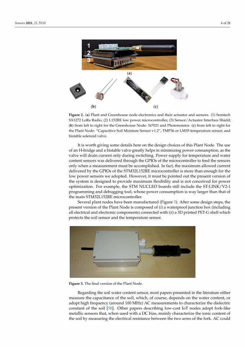
Figure 2. (a) Plant and Greenhouse node electronics and their actuator and sensors. (1) Semtech SX1272 LoRa Radio, (2) L152RE low power microcontroller, (3) Sensor/Actuator Interface Shield; (b) from left to right for the Greenhouse Node: Si7021 and Photoresistor. (c) from left to right for the Plant Node: “Capacitive Soil Moisture Sensor v1.2”, TMP36 or LM35 temperature sensor, and bistable solenoid valve.

It is worth giving some details here on the design choices of this Plant Node. The use of an H-bridge and a bistable valve greatly helps in minimizing power consumption, as the valve will drain current only during switching. Power supply for temperature and water content sensors was delivered through the GPIOs of the microcontroller to feed the sensors only when a measurement must be accomplished. In fact, the maximum allowed current delivered by the GPIOs of the STM32L152RE microcontroller is more than enough for the low power sensors we adopted. However, it must be pointed out the present ver-sion of the system is designed to provide maximum flexibility and is not conceived for power optimization. For example, the STM NUCLEO boards still include the ST-LINK/V2-1 programming and debugging tool, whose power consumption is way larger than that of the main STM32L152RE microcontroller.

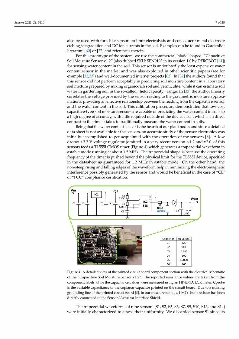
Several plant nodes have been manufactured (Figure 3). After some design steps, the present version of the Plant Node is composed of (i) a waterproof junction box (including all electrical and electronic components) connected with (ii) a 3D printed PET-G shell which protects the soil sensor and the temperature sensor.

Figure 3. The final version of the Plant Node.

Figure 2. (a) Plant and Greenhouse node electronics and their actuator and sensors. (1) SemtechSX1272 LoRa Radio, (2) L152RE low power microcontroller, (3) Sensor/Actuator Interface Shield;(b) from left to right for the Greenhouse Node: Si7021 and Photoresistor. (c) from left to right forthe Plant Node: “Capacitive Soil Moisture Sensor v1.2”, TMP36 or LM35 temperature sensor, andbistable solenoid valve.

It is worth giving some details here on the design choices of this Plant Node. The useof an H-bridge and a bistable valve greatly helps in minimizing power consumption, as thevalve will drain current only during switching. Power supply for temperature and watercontent sensors was delivered through the GPIOs of the microcontroller to feed the sensorsonly when a measurement must be accomplished. In fact, the maximum allowed currentdelivered by the GPIOs of the STM32L152RE microcontroller is more than enough for thelow power sensors we adopted. However, it must be pointed out the present version ofthe system is designed to provide maximum flexibility and is not conceived for poweroptimization. For example, the STM NUCLEO boards still include the ST-LINK/V2-1programming and debugging tool, whose power consumption is way larger than that ofthe main STM32L152RE microcontroller.

Several plant nodes have been manufactured (Figure 3). After some design steps, thepresent version of the Plant Node is composed of (i) a waterproof junction box (includingall electrical and electronic components) connected with (ii) a 3D printed PET-G shell whichprotects the soil sensor and the temperature sensor.


(Figure 2c) hosts a BD6212HFP H-bridge used for driving a bistable solenoid valve and a power feed interconnection to turn the sensors on and off. Moreover, it is connected to (1) a TMP36 or an LM35 temperature sensor, (2) a “Capacitive Soil Moisture Sensor v1.2” for measuring water content, (3) a bistable solenoid valve, and (4) a 4.8 V battery. Finally, it includes a 1 MΩ shunt resistor useful to correct a fabrication defect of the batch of sensor we received.

(a)

(b) (c)

Figure 2. (a) Plant and Greenhouse node electronics and their actuator and sensors. (1) Semtech SX1272 LoRa Radio, (2) L152RE low power microcontroller, (3) Sensor/Actuator Interface Shield; (b) from left to right for the Greenhouse Node: Si7021 and Photoresistor. (c) from left to right for the Plant Node: “Capacitive Soil Moisture Sensor v1.2”, TMP36 or LM35 temperature sensor, and bistable solenoid valve.

It is worth giving some details here on the design choices of this Plant Node. The use of an H-bridge and a bistable valve greatly helps in minimizing power consumption, as the valve will drain current only during switching. Power supply for temperature and water content sensors was delivered through the GPIOs of the microcontroller to feed the sensors only when a measurement must be accomplished. In fact, the maximum allowed current delivered by the GPIOs of the STM32L152RE microcontroller is more than enough for the low power sensors we adopted. However, it must be pointed out the present ver-sion of the system is designed to provide maximum flexibility and is not conceived for power optimization. For example, the STM NUCLEO boards still include the ST-LINK/V2-1 programming and debugging tool, whose power consumption is way larger than that of the main STM32L152RE microcontroller.

Several plant nodes have been manufactured (Figure 3). After some design steps, the present version of the Plant Node is composed of (i) a waterproof junction box (including all electrical and electronic components) connected with (ii) a 3D printed PET-G shell which protects the soil sensor and the temperature sensor.

Figure 3. The final version of the Plant Node. Figure 3. The final version of the Plant Node.

Regarding the soil water content sensor, most papers presented in the literature eithermeasure the capacitance of the soil, which, of course, depends on the water content, oradopt high frequency (around 100 MHz) AC measurements to characterize the dielectricconstant of the soil [58]. Other papers describing low-cost IoT nodes adopt fork-likemetallic sensors that, when used with a DC bias, mainly characterize the ionic content ofthe soil by measuring the electrical resistance between the two arms of the fork. AC could

Sensors 2021, 21, 5110 7 of 28

also be used with fork-like sensors to limit electrolysis and consequent metal electrodeetching/degradation and DC ion currents in the soil. Examples can be found in GardenBotliterature [60] or [27] and references therein.

For this prototype of the system, we use the commercial, blade-shaped, “CapacitiveSoil Moisture Sensor v1.2” (also dubbed SKU: SEN0193 in its version 1.0 by DFROBOT [61])for sensing water content in the soil. This sensor is undoubtedly the least expensive watercontent sensor in the market and was also exploited in other scientific papers (see forexample [32,33]) and well-documented internet projects [62]. In [32] the authors found thatthis sensor did not perform acceptably in predicting soil moisture content in a laboratorysoil mixture prepared by mixing organic-rich soil and vermiculite, while it can estimate soilwater in gardening soil in the so-called “field capacity” range. In [33] the author linearlycorrelates the voltage provided by the sensor reading to the gravimetric moisture approxi-mations, providing an effective relationship between the reading from the capacitive sensorand the water content in the soil. This calibration procedure demonstrated that low-costcapacitive-type soil moisture sensors are capable of predicting the water content in soils toa high degree of accuracy, with little required outside of the device itself, which is in directcontrast to the time it takes to traditionally measure the water content in soils.

Being that the water content sensor is the hearth of our plant nodes and since a detaileddata sheet is not available for the sensors, an accurate study of the sensor electronics wasinitially accomplished to get acquainted with the operation of the sensors [8]. A lowdropout 3.3 V voltage regulator (omitted in a very recent version–v1.2 and v2.0–of thissensor) feeds a TL555I CMOS timer (Figure 4) which generates a trapezoidal waveform inastable mode running at about 1.5 MHz. The trapezoidal shape is because the operatingfrequency of the timer is pushed beyond the physical limit for the TL555I device, specifiedin the datasheet as guaranteed for 1.2 MHz in astable mode. On the other hand, thenon-steep rising and falling edges of the waveform help in minimizing the electromagneticinterference possibly generated by the sensor and would be beneficial in the case of “CE”or “FCC” compliance certification.


After this initial screening of the available samples of Capacitive Soil Moisture Sensor v1.2, we are confident that the measurement results of a single sensor chosen among other homogeneous samples represent the expected behavior of the whole family “S2, S5, S6, S7, S9, S10, S13, and S14”.

The TL555I timer supplies a passive circuit shown in Figure 4, composed of a first stage where the coplanar capacitor of the sensor Cprobe is low-pass connected with a 10 kΩ resistor. Then a peak detector provides the analog output signal that we acquire through the ADC of the microcontroller. Regarding sensor settling time, in [33] it was asserted this sensor should settle in 1-5 min, depending on the saturation level of the soil and how well the wet soil was mixed. We accomplished measurements with the Capaci-tive Soil Moisture Sensor v1.2 immersed in tap water and found that the output voltage could take up to one hour to reach the regime value. This could be due to a non-complete waterproofing of the sensor materials that likely incorporate water molecules. Therefore, the behavior of the Capacitive Soil Moisture Sensor v1.2 after initial watering could not be completely reproducible.

Figure 4. A detailed view of the printed circuit board component section with the electrical sche-matic of the “Capacitive Soil Moisture Sensor v1.2”. The reported resistance values are taken from the component labels while the capacitance values were measured using an HP4275A LCR meter. Cprobe is the variable capacitance of the coplanar capacitor printed on the circuit board. Due to a missing grounding line of the printed circuit board [8], in our measurements, a 1 MΩ shunt resistor has been directly connected to the Sensor/Actuator Interface Shield.

We underline that other more documented and reliable but also more expensive blade-shaped moisture sensors have been commercialized. Examples are the dielectric ca-pacitance sensors ECH2O probe (Decagon Devices, Inc. Pullman, WA USA, now discon-tinued [63,64]) and the PROBE sensor [65], then modified to SMT100 ring-oscillator sensor (Truebner GmbH, Neustadt, Germany [66]) operating at approximately 150 MHz in water and 340 MHz in air.

A worst-case estimation of the overall cost of our plant node is roughly USD 60, where the most impacting figures are the microcontroller board and the LoRa shield.

3.1.1. Soil Volumetric Water Content Fitting Equations Water content measurements were previously accomplished in silica sandy soil with

the Capacitive Soil Moisture Sensor v1.2 in conditions such that the dry unit weight

Figure 4. A detailed view of the printed circuit board component section with the electrical schematicof the “Capacitive Soil Moisture Sensor v1.2”. The reported resistance values are taken from thecomponent labels while the capacitance values were measured using an HP4275A LCR meter. Cprobeis the variable capacitance of the coplanar capacitor printed on the circuit board. Due to a missinggrounding line of the printed circuit board [8], in our measurements, a 1 MΩ shunt resistor has beendirectly connected to the Sensor/Actuator Interface Shield.

The trapezoidal waveforms of nine sensors (S1, S2, S5, S6, S7, S9, S10, S13, and S14)were initially characterized to assess their uniformity. We discarded sensor S1 since its

Sensors 2021, 21, 5110 8 of 28

measured frequency f and duty cycle DC (1.22 MHz and 37.12% respectively) were veryfar from the average operating frequency and duty cycle of the other eight sensors (1.53MHz and 34.48%, with sample standard deviations of 1% and 2.2%, respectively) [8], asreported in Table 1.

Table 1. Selected sensors characteristics.

Sample ID DC/% f /MHz

S1 37.12 1.221S2 35.58 1.533S5 34.36 1.533S6 32.93 1.524S7 34.78 1.552S9 34.36 1.533

S10 35.00 1.510S13 35.12 1.535S14 34.02 1.527

After this initial screening of the available samples of Capacitive Soil Moisture Sensorv1.2, we are confident that the measurement results of a single sensor chosen among otherhomogeneous samples represent the expected behavior of the whole family “S2, S5, S6, S7,S9, S10, S13, and S14”.

The TL555I timer supplies a passive circuit shown in Figure 4, composed of a firststage where the coplanar capacitor of the sensor Cprobe is low-pass connected with a10 kΩ resistor. Then a peak detector provides the analog output signal that we acquirethrough the ADC of the microcontroller. Regarding sensor settling time, in [33] it wasasserted this sensor should settle in 1–5 min, depending on the saturation level of the soiland how well the wet soil was mixed. We accomplished measurements with the CapacitiveSoil Moisture Sensor v1.2 immersed in tap water and found that the output voltage couldtake up to one hour to reach the regime value. This could be due to a non-completewaterproofing of the sensor materials that likely incorporate water molecules. Therefore,the behavior of the Capacitive Soil Moisture Sensor v1.2 after initial watering could not becompletely reproducible.

We underline that other more documented and reliable but also more expensive blade-shaped moisture sensors have been commercialized. Examples are the dielectric capacitancesensors ECH2O probe (Decagon Devices, Inc. Pullman, WA USA, now discontinued [63,64])and the PROBE sensor [65], then modified to SMT100 ring-oscillator sensor (TruebnerGmbH, Neustadt, Germany [66]) operating at approximately 150 MHz in water and 340MHz in air.

A worst-case estimation of the overall cost of our plant node is roughly USD 60, wherethe most impacting figures are the microcontroller board and the LoRa shield.

3.1.1. Soil Volumetric Water Content Fitting Equations

Water content measurements were previously accomplished in silica sandy soil withthe Capacitive Soil Moisture Sensor v1.2 in conditions such that the dry unit weightγdry = Ws/V (Ws = dry soil weight, V = total volume of the soil) could be assumedas a constant [8]. It was demonstrated that this condition guarantees a monotonicallydecreasing Vs output voltage as a function of gravimetric water content (GWC), whichwas approximated using a 2nd order polynomial or an exponential function. In this paper,we will deal with volumetric water content (VWC) instead of GWC. However, the twoparameters are proportional to each other for a given soil where the dry unit weight isconstant. In the remainder of this paper, we will use the following exponential fittingequation between the output voltage Vs of the Capacitive Soil Moisture Sensor v1.2 andthe VWC:

Vs = A exp(−VWC

B

)+ C, (1)

Sensors 2021, 21, 5110 9 of 28

VWC = B ln(

AVs − C

)(2)

being A, B, and C suitable constants. Other fitting equations were also adopted in theliterature for the same sensor. In [32] a 3rd order polynomial function VWC = f (Vs) wasimplemented. In [33] the following equation was used:

VWC =PVs−Q (3)

being P = 2.48 V and Q = 0.72 for a soil composed of dried coconut coir. In the remainderof this paper, we will mainly deal with fitting Equations (2) and (3).

3.1.2. Embedded Software Implementation of Nodes

The C++ code exploits ARM Mbed OS libraries. Mbed OS is an open-source Real-TimeOperating System (RTOS) for the creation and deployment of IoT devices based on ARMprocessors. The code structure is outlined in Figure 5 for the case of the Plant Node.


𝛾 = 𝑊 𝑉⁄ (𝑊 = dry soil weight, V = total volume of the soil) could be assumed as a constant [8]. It was demonstrated that this condition guarantees a monotonically decreas-ing Vs output voltage as a function of gravimetric water content (GWC), which was ap-proximated using a 2nd order polynomial or an exponential function. In this paper, we will deal with volumetric water content (VWC) instead of GWC. However, the two pa-rameters are proportional to each other for a given soil where the dry unit weight is con-stant. In the remainder of this paper, we will use the following exponential fitting equation between the output voltage Vs of the Capacitive Soil Moisture Sensor v1.2 and the VWC: 𝑉 = 𝐴 exp − + 𝐶, (1)

VWC = 𝐵 ln 𝐴𝑉 − 𝐶 (2)

being A, B, and C suitable constants. Other fitting equations were also adopted in the lit-erature for the same sensor. In [32] a 3rd order polynomial function VWC = f(Vs) was im-plemented. In [33] the following equation was used: 𝑉𝑊𝐶 = 𝑃𝑉 − 𝑄 (3)

being P = 2.48 V and Q = 0.72 for a soil composed of dried coconut coir. In the remainder of this paper, we will mainly deal with fitting Equations (2) and (3).

3.1.2. Embedded Software Implementation of Nodes The C++ code exploits ARM Mbed OS libraries. Mbed OS is an open-source Real-

Time Operating System (RTOS) for the creation and deployment of IoT devices based on ARM processors. The code structure is outlined in Figure 5 for the case of the Plant Node.

Figure 5. Embedded software implementation for the Plant Node.

The heart of the firmware is the main.cpp file. The header of main.cpp includes Mbed libraries (e.g., EventQueue.h) and LoRaWAN™ libraries. In particular, LoRaWANInter-face.h encompasses the prototypes of the member functions managing the upper level of the LoRaWAN™ protocol stack, lorawan_data_structures.h includes LoRaWAN param-eters, e.g., network and application key, datarate, duty cycle, antenna gain, buffer size, and SNR while lora_radio_helper.h regards the physical layer and selects the type of shield adopted in our system. The functions of main.cpp dedicated to the Plant Node are listed in the lower part of Figure 5. Among them, we cite the lora_event_handler() which manages the state machine of the LoRa events, the measuring functions for water content (measure_SoilWC()) and temperature (measure_Temp()), and the LoRa send and send_message() and receive_message() functions. The receive function also handles the

Figure 5. Embedded software implementation for the Plant Node.

The heart of the firmware is the main.cpp file. The header of main.cpp includes Mbedlibraries (e.g., EventQueue.h) and LoRaWAN™ libraries. In particular, LoRaWANInter-face.h encompasses the prototypes of the member functions managing the upper levelof the LoRaWAN™ protocol stack, lorawan_data_structures.h includes LoRaWAN pa-rameters, e.g., network and application key, datarate, duty cycle, antenna gain, buffersize, and SNR while lora_radio_helper.h regards the physical layer and selects the typeof shield adopted in our system. The functions of main.cpp dedicated to the Plant Nodeare listed in the lower part of Figure 5. Among them, we cite the lora_event_handler()which manages the state machine of the LoRa events, the measuring functions for watercontent (measure_SoilWC()) and temperature (measure_Temp()), and the LoRa send andsend_message() and receive_message() functions. The receive function also handles thebistable irrigation solenoid valve. In the case of the Greenhouse Node, the actual measuringfunctions regard ambient RH, temperature, and the ambient luminous flux.

Every node transmits a packet conforming to the structure defined in Figure 6. De-pending on the node type (plant or greenhouse node), it will include different values.For example, the Plant Node features node type = 1 and transmits soil water content andtemperature, while the greenhouse node is characterized by node type = 0 and transmitsambient RH, temperature, and light intensity.

Sensors 2021, 21, 5110 10 of 28


bistable irrigation solenoid valve. In the case of the Greenhouse Node, the actual measur-ing functions regard ambient RH, temperature, and the ambient luminous flux.

Every node transmits a packet conforming to the structure defined in Figure 6. De-pending on the node type (plant or greenhouse node), it will include different values. For example, the Plant Node features node type = 1 and transmits soil water content and tem-perature, while the greenhouse node is characterized by node type = 0 and transmits am-bient RH, temperature, and light intensity.

Figure 6. Packet structure.

3.2. The Things Network and Connection to the LoRaWAN™ Gateway Routing and processing procedures of the LoRaWAN™ network are managed by

The Things Network (TTN), acting as an active crossroad between the gateway and the application. For our application, we extensively use the TTN, a network server whose aim is building a global, worldwide open LoRaWAN™ network. They provide a set of open tools and a global, open network to build an IoT application at low cost, featuring maxi-mum security and ready to scale. A secure and collaborative Internet of Things network is built through robust end-to-end encryption, spanning many countries around the globe. A network server does the complicated part in creating a LoRaWAN™ network (handling duplicate packets from multiple gateways, shunting data to servers, handling joins, etc.).

As shown in Figure 1, in the network architecture The Things Network is located between the LoRa concentrator/gateway and the applications. TTN is composed of three main structures: Router, Brokers, and Handler. The Router is in charge of managing the gateway’s status and of planning transmissions. Each Router is associated with one or more Brokers. The assignment of Brokers is to map a device to an application, to forward uplink messages to the proper application, and to forward downlink messages to the cor-rect Router-Gateway path. A Handler is responsible for treating the data of different Ap-plications. To do so, it deals with a Broker where it registers devices and applications. The Handler is also in charge of encrypting and decrypting data.

In our system, the Uplink connection to TTN is carried out by the Radio SW of the gateway (Figure 1) that publishes the node sensor data on a specific uplink topic of the TTN MQTT broker using an internet connection.

Then, through the well-known flow-based programming tool Node-RED [67] run-ning on the Gateway, a specific device is allowed to communicate with the database in-stalled in the virtual machine, as sketched in Figure 1.

The Node-RED flow is composed of two sub-flows, an uplink, and a downlink flow, respectively (Figure 7a).

The uplink sub-flow, after subscribing to the same uplink topic of the TTN broker, is in charge of: • Retrieving through the internet the data received and published by the TTN broker

exploiting the light blue TTN Uplink Node producing an output Node.js buffer; • Converting this Node.js buffer to a string; • Parsing this string by exploiting two function nodes featuring JavaScript codes, dedi-

cated to Water Content and Temperature, respectively, which also compose the query for the database;

• Sending the query to the MySQL database running on the Virtual Machine through a dedicated TCP port (internet connection through MySQL 3306 port) employing the orange node.

Node Type Soil water contentor air RH

Soil/air temperature Light

Figure 6. Packet structure.

3.2. The Things Network and Connection to the LoRaWAN™ Gateway

Routing and processing procedures of the LoRaWAN™ network are managed byThe Things Network (TTN), acting as an active crossroad between the gateway and theapplication. For our application, we extensively use the TTN, a network server whoseaim is building a global, worldwide open LoRaWAN™ network. They provide a set ofopen tools and a global, open network to build an IoT application at low cost, featuringmaximum security and ready to scale. A secure and collaborative Internet of Thingsnetwork is built through robust end-to-end encryption, spanning many countries aroundthe globe. A network server does the complicated part in creating a LoRaWAN™ network(handling duplicate packets from multiple gateways, shunting data to servers, handlingjoins, etc.).

As shown in Figure 1, in the network architecture The Things Network is locatedbetween the LoRa concentrator/gateway and the applications. TTN is composed of threemain structures: Router, Brokers, and Handler. The Router is in charge of managing thegateway’s status and of planning transmissions. Each Router is associated with one ormore Brokers. The assignment of Brokers is to map a device to an application, to forwarduplink messages to the proper application, and to forward downlink messages to thecorrect Router-Gateway path. A Handler is responsible for treating the data of differentApplications. To do so, it deals with a Broker where it registers devices and applications.The Handler is also in charge of encrypting and decrypting data.

In our system, the Uplink connection to TTN is carried out by the Radio SW of thegateway (Figure 1) that publishes the node sensor data on a specific uplink topic of theTTN MQTT broker using an internet connection.

Then, through the well-known flow-based programming tool Node-RED [67] runningon the Gateway, a specific device is allowed to communicate with the database installed inthe virtual machine, as sketched in Figure 1.

The Node-RED flow is composed of two sub-flows, an uplink, and a downlink flow,respectively (Figure 7a).

The uplink sub-flow, after subscribing to the same uplink topic of the TTN broker, isin charge of:

• Retrieving through the internet the data received and published by the TTN brokerexploiting the light blue TTN Uplink Node producing an output Node.js buffer;

• Converting this Node.js buffer to a string;• Parsing this string by exploiting two function nodes featuring JavaScript codes, dedi-

cated to Water Content and Temperature, respectively, which also compose the queryfor the database;

• Sending the query to the MySQL database running on the Virtual Machine through adedicated TCP port (internet connection through MySQL 3306 port) employing theorange node.

Moreover, in the second Node-RED sub-flow the application is allowed to transmitdownlinks to TTN (i.e., to the device) when the bistable solenoid valve must be actuated.This is accomplished by publishing on a specific downlink topic of the TTN broker usingthe internet again. In the NodeRED flow, the first “TCP in” node is ready to receivemessages on a given unassigned TCP port, then a “Reply” JavaScript function returns anobject which contains the ID of the target node and the payload, i.e., the message sent bythe server. The last light blue node is a TTN Downlink Node which publishes these dataon the TTN broker.

Sensors 2021, 21, 5110 11 of 28


Moreover, in the second Node-RED sub-flow the application is allowed to transmit downlinks to TTN (i.e., to the device) when the bistable solenoid valve must be actuated. This is accomplished by publishing on a specific downlink topic of the TTN broker using the internet again. In the NodeRED flow, the first “TCP in” node is ready to receive mes-sages on a given unassigned TCP port, then a “Reply” JavaScript function returns an ob-ject which contains the ID of the target node and the payload, i.e., the message sent by the server. The last light blue node is a TTN Downlink Node which publishes these data on the TTN broker.

Our LoRaWAN™ Gateway is composed of a Raspberry Pi, an iC880a concentrator able to receive packets of different end devices simultaneously sent with different spread-ing factors on up to 8 different channels in parallel, and an interconnecting backplane (Figure 7b). The embedded software of the Gateway is proprietary and supplied by TTN. The gateway receives LoRa packets from nodes and forwards them to The Things Net-work [59] through the MQTT protocol thanks to a wideband network, typically WiFi or Ethernet build. On the other hand, it is well known that for data transmission, MQTT could rely on the TCP protocol but a variant, MQTT-SN, is used over other transports such as UDP (or even Bluetooth). However, TTN does not specify which transport proto-col is exploited in its Raspberry Pi firmware.

(a)

(b)

Figure 7. (a) The Node-RED flow running in the Raspberry of the Gateway. (b) The 8-channel iC880a /Concentrator, with interconnection backplane and Raspberry PI3, is mounted in a plastic box.

3.3. The Virtual Machine in the Cloud, Database Application, and Graphical User Interface At the application level, we installed a Linux virtual machine (Figure 8) that includes: • Web site (HTML, PHP, CSS, and JavaScript) within a web server; • MySQL Database Management System (DBMS) server.

The database is divided into two units: (i) node data section and (ii) web application user data section (e.g., username and password). The node data section is further com-posed of two tables: the first one identifies the node and the second one the sensor with

Figure 7. (a) The Node-RED flow running in the Raspberry of the Gateway. (b) The 8-channel iC880a /Concentrator, withinterconnection backplane and Raspberry PI3, is mounted in a plastic box.

Our LoRaWAN™ Gateway is composed of a Raspberry Pi, an iC880a concentrator ableto receive packets of different end devices simultaneously sent with different spreading fac-tors on up to 8 different channels in parallel, and an interconnecting backplane (Figure 7b).The embedded software of the Gateway is proprietary and supplied by TTN. The gatewayreceives LoRa packets from nodes and forwards them to The Things Network [59] throughthe MQTT protocol thanks to a wideband network, typically WiFi or Ethernet build. Onthe other hand, it is well known that for data transmission, MQTT could rely on the TCPprotocol but a variant, MQTT-SN, is used over other transports such as UDP (or evenBluetooth). However, TTN does not specify which transport protocol is exploited in itsRaspberry Pi firmware.

3.3. The Virtual Machine in the Cloud, Database Application, and Graphical User Interface

At the application level, we installed a Linux virtual machine (Figure 8) that includes:

• Web site (HTML, PHP, CSS, and JavaScript) within a web server;• MySQL Database Management System (DBMS) server.

The database is divided into two units: (i) node data section and (ii) web applicationuser data section (e.g., username and password). The node data section is further composedof two tables: the first one identifies the node and the second one the sensor with itsdata. Finally, the webserver fetches data in the database using PHP and shows themon a web page. CanvasJS is used for the Graphical User Interface (GUI). CanvasJS isdescribed as a JavaScript Charting Library for High Performance and ease of use. It isbuilt using the Canvas element and it can render thousands of data points in a matter ofmilliseconds. CanvasJS is also interactive and can be updated dynamically. Examples of theGUI, operating both from a PC and a smartphone, can be found in the following sections.

Sensors 2021, 21, 5110 12 of 28


its data. Finally, the webserver fetches data in the database using PHP and shows them on a web page. CanvasJS is used for the Graphical User Interface (GUI). CanvasJS is de-scribed as a JavaScript Charting Library for High Performance and ease of use. It is built using the Canvas element and it can render thousands of data points in a matter of milli-seconds. CanvasJS is also interactive and can be updated dynamically. Examples of the GUI, operating both from a PC and a smartphone, can be found in the following sections.

Figure 8. Block diagram of the virtual machine.

The information contained in the database of our virtual machine could represent a starting point for decision-making processes supporting smart monitoring in the frame of PA. A possible implementation could be to develop and enhance the PHP code, used until now to retrieve information from the database, adding a new section where data are ana-lyzed by a dedicated algorithm. The decisions made by the algorithm could be directly sent to the nodes through TTN and the gateways. As an alternative, the watering decision could be directly issued by an application running on the mobile device of the greenhouse manager.

A plant node was placed in a pot hosting a daisy plant, while a greenhouse node was acquiring data in the ambient. Figure 9 includes three plots of our JavaScript GUI showing the soil water content recorded by the Plant Node together with the ambient relative hu-midity and temperature recorded by the greenhouse node in the same room where the plant pot was located.

Figure 8. Block diagram of the virtual machine.

The information contained in the database of our virtual machine could represent astarting point for decision-making processes supporting smart monitoring in the frameof PA. A possible implementation could be to develop and enhance the PHP code, useduntil now to retrieve information from the database, adding a new section where dataare analyzed by a dedicated algorithm. The decisions made by the algorithm could bedirectly sent to the nodes through TTN and the gateways. As an alternative, the wateringdecision could be directly issued by an application running on the mobile device of thegreenhouse manager.

A plant node was placed in a pot hosting a daisy plant, while a greenhouse nodewas acquiring data in the ambient. Figure 9 includes three plots of our JavaScript GUIshowing the soil water content recorded by the Plant Node together with the ambientrelative humidity and temperature recorded by the greenhouse node in the same roomwhere the plant pot was located.


Figure 9. Simultaneous acquisition of ambient temperature and ambient relative humidity (RH) of the greenhouse node and soil water content of a single plant node, shown on the display of a portable device.

4. Materials The functionality and reliability of the whole system were proven during two con-

tinued experiments with two different natural soils, characterized by very different soil hydraulic properties (see Table 2).

Table 2. Main hydraulic properties of study soils. Ks = saturated hydraulic conductivity; θs and θr = saturated and residual water content, respectively; bd = bulk density.

Fine-Textured Soil

(Silty Loam) Coarse-Textured Soil

(Loamy Sand) Ks (mmh−1) 10.0 30.0

θs 0.420 0.295 θr 0.057 0.035

bd (gcm−3) 2.628 2.669

The fine-textured soil (a Silty Loam, according to the United States Department of Agriculture, USDA, classification [68,69]) was composed of 1% gravel, 22% sand, 54% silt, and 23% clay (Figure 10a), while the coarse-textured soil (a Loamy Sand, according to USDA) was composed of 4% gravel, 79% sand, 11% silt, and 6% clay (Figure 10b).

(a) (b)

Figure 10. Grain size distribution of the soils used for the experiments: (a) fine-textured soil (Silty Loam, according to USDA); (b) coarse-textured soil (Loamy Sand, according to USDA).

Figure 9. Simultaneous acquisition of ambient temperature and ambient relative humidity (RH) of the greenhouse nodeand soil water content of a single plant node, shown on the display of a portable device.

Sensors 2021, 21, 5110 13 of 28

4. Materials

The functionality and reliability of the whole system were proven during two con-tinued experiments with two different natural soils, characterized by very different soilhydraulic properties (see Table 2).

Table 2. Main hydraulic properties of study soils. Ks = saturated hydraulic conductivity; θs and θr =saturated and residual water content, respectively; bd = bulk density.

Fine-Textured Soil(Silty Loam)

Coarse-Textured Soil(Loamy Sand)

Ks (mmh−1) 10.0 30.0θs 0.420 0.295θr 0.057 0.035

bd (gcm−3) 2.628 2.669

The fine-textured soil (a Silty Loam, according to the United States Department ofAgriculture, USDA, classification [68,69]) was composed of 1% gravel, 22% sand, 54% silt,and 23% clay (Figure 10a), while the coarse-textured soil (a Loamy Sand, according toUSDA) was composed of 4% gravel, 79% sand, 11% silt, and 6% clay (Figure 10b).


Figure 9. Simultaneous acquisition of ambient temperature and ambient relative humidity (RH) of the greenhouse node and soil water content of a single plant node, shown on the display of a portable device.

4. Materials The functionality and reliability of the whole system were proven during two con-

tinued experiments with two different natural soils, characterized by very different soil hydraulic properties (see Table 2).

Table 2. Main hydraulic properties of study soils. Ks = saturated hydraulic conductivity; θs and θr = saturated and residual water content, respectively; bd = bulk density.

Fine-Textured Soil

(Silty Loam) Coarse-Textured Soil

(Loamy Sand) Ks (mmh−1) 10.0 30.0

θs 0.420 0.295 θr 0.057 0.035

bd (gcm−3) 2.628 2.669

The fine-textured soil (a Silty Loam, according to the United States Department of Agriculture, USDA, classification [68,69]) was composed of 1% gravel, 22% sand, 54% silt, and 23% clay (Figure 10a), while the coarse-textured soil (a Loamy Sand, according to USDA) was composed of 4% gravel, 79% sand, 11% silt, and 6% clay (Figure 10b).

(a) (b)

Figure 10. Grain size distribution of the soils used for the experiments: (a) fine-textured soil (Silty Loam, according to USDA); (b) coarse-textured soil (Loamy Sand, according to USDA). Figure 10. Grain size distribution of the soils used for the experiments: (a) fine-textured soil (Silty Loam, according toUSDA); (b) coarse-textured soil (Loamy Sand, according to USDA).

5. Methods, Tests, and Results

Focusing on the Plant Nodes, the system has been tested during a continued experi-ment where the two different greenhouse soils were watered several times, to verify if thesensor was able to reliably acquire, transmit, and store the ambient temperature and thesoil water content parameters in real time and to show them on the custom GUI.

The measurements were made in a plastic box initially filled with expanded clayaggregate which allowed percolated water to outflow and where a Sentek Drill & DropProbe (hereafter named “reference sensor”) was driven (Figure 11a). Then the remainingtop 30 cm of the box was filled with the chosen soil, either Loamy Sand or Silty Loam.Both soils were packed in 0.05 m lifts and gently tapped into place. This accurate packingmechanism was adopted to achieve homogeneity vertically, to keep perfect contact at theinterface, and to minimize preferential flow along the sides of the box. The reference sensorwas placed at the center of the box. It features an array of water content and temperaturesensors placed at 5 cm, 15 cm, 25 cm, 35 cm, and 45 cm from the top surface.

Sensors 2021, 21, 5110 14 of 28


5. Methods, Tests, and Results Focusing on the Plant Nodes, the system has been tested during a continued experi-

ment where the two different greenhouse soils were watered several times, to verify if the sensor was able to reliably acquire, transmit, and store the ambient temperature and the soil water content parameters in real time and to show them on the custom GUI.

The measurements were made in a plastic box initially filled with expanded clay ag-gregate which allowed percolated water to outflow and where a Sentek Drill & Drop Probe (hereafter named “reference sensor”) was driven (Figure 11a). Then the remaining top 30 cm of the box was filled with the chosen soil, either Loamy Sand or Silty Loam. Both soils were packed in 0.05 m lifts and gently tapped into place. This accurate packing mechanism was adopted to achieve homogeneity vertically, to keep perfect contact at the interface, and to minimize preferential flow along the sides of the box. The reference sen-sor was placed at the center of the box. It features an array of water content and tempera-ture sensors placed at 5 cm, 15 cm, 25 cm, 35 cm, and 45 cm from the top surface.

Then our Plant Node #1 was inserted in the soil at a distance of 10 cm from the Sentek sensor (Figure 11b, where Node #1 is shown without the lid and connected to a 230 ACV-5 DCV adapter during a test measurement). Since the reference sensor and the Plant Node #1 are installed in different positions/depths, this has an impact on the measurements, as explained in the following sections. Data of Plant Node #1 were collected every 5 min for several days while the automatic acquisition system of the reference sensor stored the measurement results every minute. In carrying out the measurements, the soil was wa-tered in consecutive steps.

(a) (b)

Figure 11. The plastic box used for our experiments. (a) Expanded clay aggregate bottom filler, to-gether with a Sentek Drill & Drop Probe. (b) Plant Node #1 and Sentek sensor during acquisition.

Before and after each measurement a calibration was performed on the Capacitive Soil Moisture Sensor v1.2 measuring water content, exposing it for 15 min. to air, then dipping it for 15 min in tap water. The reproducibility of these measurements certifies that the low-cost water content is in working order.

5.1. Measurements in Silty Loam In Figure 12 we compare the water content measured by the reference sensor at a

depth of 5 and 15 cm in Silty Loam. After installing the sensors in a uniformly and slightly moistured Silty Loam (initial volumetric water content of 10%), then four synchronous waterings, clearly visible at a depth of 5 cm, were performed during the last two days of this measurement. The two plots witness the strong dependence of the water content on the soil depth in Silty Loam.

Figure 11. The plastic box used for our experiments. (a) Expanded clay aggregate bottom filler,together with a Sentek Drill & Drop Probe. (b) Plant Node #1 and Sentek sensor during acquisition.

Then our Plant Node #1 was inserted in the soil at a distance of 10 cm from the Senteksensor (Figure 11b, where Node #1 is shown without the lid and connected to a 230 ACV-5DCV adapter during a test measurement). Since the reference sensor and the Plant Node#1 are installed in different positions/depths, this has an impact on the measurements,as explained in the following sections. Data of Plant Node #1 were collected every 5 minfor several days while the automatic acquisition system of the reference sensor stored themeasurement results every minute. In carrying out the measurements, the soil was wateredin consecutive steps.

Before and after each measurement a calibration was performed on the CapacitiveSoil Moisture Sensor v1.2 measuring water content, exposing it for 15 min. to air, thendipping it for 15 min in tap water. The reproducibility of these measurements certifies thatthe low-cost water content is in working order.

5.1. Measurements in Silty Loam

In Figure 12 we compare the water content measured by the reference sensor at adepth of 5 and 15 cm in Silty Loam. After installing the sensors in a uniformly and slightlymoistured Silty Loam (initial volumetric water content of 10%), then four synchronouswaterings, clearly visible at a depth of 5 cm, were performed during the last two days ofthis measurement. The two plots witness the strong dependence of the water content onthe soil depth in Silty Loam.


Figure 12. Water content measured by the reference system at two different depths in Silty Loam: red, 5 cm underground, and green, 15 cm underground.

Figure 13 shows the water content measured by the reference system (5 cm under-ground) and the output voltage of the Capacitive Soil Moisture Sensor v1.2 in Silty Loam (Node #1). The qualitative correlation between the two plots is evident: each watering causes an increase in the measured water content of the reference sensor and a decrease in the output voltage of Node #1. Moreover, the long time elapsed in soil with VWC of about 10% before the first watering guarantees the Capacitive Soil Moisture Sensor v1.2 had plenty of time to reach its settling time. However, we note the lack of linearity of the Capacitive Soil Moisture Sensor v1.2: its sensitivity is too high for small values of water content and it is substantially reduced for volumetric water contents greater than about 15%. The low draining capability of this soil which maintains its water content during the time causes high values of water content and for this reason, the Capacitive Soil Moisture Sensor v1.2 works most of the time almost in saturation. Future improvements for the sensor should be directed towards the linearization of the input/output curve to obtain a constant sensitivity. A detailed discussion of the correlation between the results of the two sensors is reported below.

Figure 13. Water content measured by the reference system (red, 5 cm underground) and the Ca-pacitive Soil Moisture Sensor v1.2 (blue) in Silty Loam. Initial and final peaks of the Node #1 plot represent a calibration of the Capacitive Soil Moisture Sensor v1.2 obtained by placing the sensor for 15 min in the air (maximum peak) and 15 min in tap water (minimum peak).

Figure 12. Water content measured by the reference system at two different depths in Silty Loam:red, 5 cm underground, and green, 15 cm underground.

Sensors 2021, 21, 5110 15 of 28

Figure 13 shows the water content measured by the reference system (5 cm under-ground) and the output voltage of the Capacitive Soil Moisture Sensor v1.2 in Silty Loam(Node #1). The qualitative correlation between the two plots is evident: each wateringcauses an increase in the measured water content of the reference sensor and a decreasein the output voltage of Node #1. Moreover, the long time elapsed in soil with VWC ofabout 10% before the first watering guarantees the Capacitive Soil Moisture Sensor v1.2had plenty of time to reach its settling time. However, we note the lack of linearity of theCapacitive Soil Moisture Sensor v1.2: its sensitivity is too high for small values of watercontent and it is substantially reduced for volumetric water contents greater than about15%. The low draining capability of this soil which maintains its water content during thetime causes high values of water content and for this reason, the Capacitive Soil MoistureSensor v1.2 works most of the time almost in saturation. Future improvements for thesensor should be directed towards the linearization of the input/output curve to obtain aconstant sensitivity. A detailed discussion of the correlation between the results of the twosensors is reported below.


Figure 12. Water content measured by the reference system at two different depths in Silty Loam: red, 5 cm underground, and green, 15 cm underground.

Figure 13 shows the water content measured by the reference system (5 cm under-ground) and the output voltage of the Capacitive Soil Moisture Sensor v1.2 in Silty Loam (Node #1). The qualitative correlation between the two plots is evident: each watering causes an increase in the measured water content of the reference sensor and a decrease in the output voltage of Node #1. Moreover, the long time elapsed in soil with VWC of about 10% before the first watering guarantees the Capacitive Soil Moisture Sensor v1.2 had plenty of time to reach its settling time. However, we note the lack of linearity of the Capacitive Soil Moisture Sensor v1.2: its sensitivity is too high for small values of water content and it is substantially reduced for volumetric water contents greater than about 15%. The low draining capability of this soil which maintains its water content during the time causes high values of water content and for this reason, the Capacitive Soil Moisture Sensor v1.2 works most of the time almost in saturation. Future improvements for the sensor should be directed towards the linearization of the input/output curve to obtain a constant sensitivity. A detailed discussion of the correlation between the results of the two sensors is reported below.

Figure 13. Water content measured by the reference system (red, 5 cm underground) and the Ca-pacitive Soil Moisture Sensor v1.2 (blue) in Silty Loam. Initial and final peaks of the Node #1 plot represent a calibration of the Capacitive Soil Moisture Sensor v1.2 obtained by placing the sensor for 15 min in the air (maximum peak) and 15 min in tap water (minimum peak).

Figure 13. Water content measured by the reference system (red, 5 cm underground) and theCapacitive Soil Moisture Sensor v1.2 (blue) in Silty Loam. Initial and final peaks of the Node #1 plotrepresent a calibration of the Capacitive Soil Moisture Sensor v1.2 obtained by placing the sensor for15 min in the air (maximum peak) and 15 min in tap water (minimum peak).

Figure 14 shows the reference temperature compared to the temperature of Node #1.In addition, in this case a slight difference is detected, most likely due to the distance ofthe two sensors and the intrinsic measurement error. Indeed, the LM35 declares a 0.5 Censured accuracy (at 25 C) while the reference Sentek system has a temperature error of0.1 C.

5.2. Measurements in Loamy Sand

In Figure 15 we compare the water content measured by the reference sensor at adepth of 5 and 15 cm in Loamy Sand. The water content curve at 5 cm clearly shows fiveconsecutive waterings performed during the 2 days of this measurement. On the otherhand, the water content curve at 15 cm shows an increase only after the 3rd watering,clearly witnessing the dependence of water content on the soil depth. Furthermore, dueto the alternation of rainfall and water redistribution periods, the evolution in time of thewetting front is very complex, as [70,71] showed in their schemes with compound profiles.

Figure 16 shows the water content measured by the reference system (5 cm under-ground) and the output voltage of the Capacitive Soil Moisture Sensor v1.2 in Loamy Sand.In addition, for this soil, we obtain a “first sight” reasonable qualitative agreement betweenthe results of the two sensors. Again, we note that the sensitivity of the Capacitive Soil Mois-ture Sensor v1.2 is too high for small values of water content and it is substantially reduced

Sensors 2021, 21, 5110 16 of 28

for volumetric water contents greater than about 10% for this soil material. A detaileddiscussion of the correlation between the results of the two sensors is reported below.


Figure 14 shows the reference temperature compared to the temperature of Node #1. In addition, in this case a slight difference is detected, most likely due to the distance of the two sensors and the intrinsic measurement error. Indeed, the LM35 declares a 0.5 °C ensured accuracy (at 25 °C) while the reference Sentek system has a temperature error of 0.1 °C.

Figure 14. Temperature measured by the reference system (red, 5 cm underground) and the LM35 mounted in Node #1 (blue) in Silty Loam. The rectangular area shows the region where we realized the calibrations of Section 6.2.

5.2. Measurements in Loamy Sand In Figure 15 we compare the water content measured by the reference sensor at a

depth of 5 and 15 cm in Loamy Sand. The water content curve at 5 cm clearly shows five consecutive waterings performed during the 2 days of this measurement. On the other hand, the water content curve at 15 cm shows an increase only after the 3rd watering, clearly witnessing the dependence of water content on the soil depth. Furthermore, due to the alternation of rainfall and water redistribution periods, the evolution in time of the wetting front is very complex, as [70,71] showed in their schemes with compound profiles.

Figure 15. Water content measured by the reference system at two different depths in Loamy Sand: orange, 5 cm underground, and blue, 15 cm underground.

Figure 14. Temperature measured by the reference system (red, 5 cm underground) and the LM35mounted in Node #1 (blue) in Silty Loam. The rectangular area shows the region where we realizedthe calibrations of Section 6.2.


Figure 14 shows the reference temperature compared to the temperature of Node #1. In addition, in this case a slight difference is detected, most likely due to the distance of the two sensors and the intrinsic measurement error. Indeed, the LM35 declares a 0.5 °C ensured accuracy (at 25 °C) while the reference Sentek system has a temperature error of 0.1 °C.

Figure 14. Temperature measured by the reference system (red, 5 cm underground) and the LM35 mounted in Node #1 (blue) in Silty Loam. The rectangular area shows the region where we realized the calibrations of Section 6.2.

5.2. Measurements in Loamy Sand In Figure 15 we compare the water content measured by the reference sensor at a

depth of 5 and 15 cm in Loamy Sand. The water content curve at 5 cm clearly shows five consecutive waterings performed during the 2 days of this measurement. On the other hand, the water content curve at 15 cm shows an increase only after the 3rd watering, clearly witnessing the dependence of water content on the soil depth. Furthermore, due to the alternation of rainfall and water redistribution periods, the evolution in time of the wetting front is very complex, as [70,71] showed in their schemes with compound profiles.

Figure 15. Water content measured by the reference system at two different depths in Loamy Sand: orange, 5 cm underground, and blue, 15 cm underground. Figure 15. Water content measured by the reference system at two different depths in Loamy Sand:orange, 5 cm underground, and blue, 15 cm underground.


Figure 16 shows the water content measured by the reference system (5 cm under-ground) and the output voltage of the Capacitive Soil Moisture Sensor v1.2 in Loamy Sand. In addition, for this soil, we obtain a “first sight” reasonable qualitative agreement between the results of the two sensors. Again, we note that the sensitivity of the Capacitive Soil Moisture Sensor v1.2 is too high for small values of water content and it is substan-tially reduced for volumetric water contents greater than about 10% for this soil material. A detailed discussion of the correlation between the results of the two sensors is reported below.

Figure 16. Water content measured by the reference system (orange, 5 cm underground) and the Capacitive Soil Moisture Sensor v1.2 (blue) in Loamy Sand. Initial and final peaks of the Node #1 plot represent a calibration of the Capacitive Soil Moisture Sensor v1.2 obtained by placing the sen-sor for 15 min in the air (maximum peak) and 15 min in water (minimum peak).

Figure 17 shows the reference temperature compared to the temperature of Node #1. A slight difference is detected, most likely due to the distance of the two sensors and the intrinsic measurement error.

Figure 17. Temperature measured by the reference system (orange, 5 cm underground) and the LM35 mounted in Node #1 (blue) in Loamy Sand.

6. Discussion Measurement outcomes have been discussed in the relevant sections. In this section,

we add some comments and considerations that will help to clarify the experimental ob-servations and will allow us to extract the VWC from the output voltage of the Capacitive Soil Moisture Sensor v1.2.

Figure 16. Water content measured by the reference system (orange, 5 cm underground) and theCapacitive Soil Moisture Sensor v1.2 (blue) in Loamy Sand. Initial and final peaks of the Node #1plot represent a calibration of the Capacitive Soil Moisture Sensor v1.2 obtained by placing the sensorfor 15 min in the air (maximum peak) and 15 min in water (minimum peak).

Sensors 2021, 21, 5110 17 of 28

Figure 17 shows the reference temperature compared to the temperature of Node #1.A slight difference is detected, most likely due to the distance of the two sensors and theintrinsic measurement error.


Figure 16 shows the water content measured by the reference system (5 cm under-ground) and the output voltage of the Capacitive Soil Moisture Sensor v1.2 in Loamy Sand. In addition, for this soil, we obtain a “first sight” reasonable qualitative agreement between the results of the two sensors. Again, we note that the sensitivity of the Capacitive Soil Moisture Sensor v1.2 is too high for small values of water content and it is substan-tially reduced for volumetric water contents greater than about 10% for this soil material. A detailed discussion of the correlation between the results of the two sensors is reported below.

Figure 16. Water content measured by the reference system (orange, 5 cm underground) and the Capacitive Soil Moisture Sensor v1.2 (blue) in Loamy Sand. Initial and final peaks of the Node #1 plot represent a calibration of the Capacitive Soil Moisture Sensor v1.2 obtained by placing the sen-sor for 15 min in the air (maximum peak) and 15 min in water (minimum peak).

Figure 17 shows the reference temperature compared to the temperature of Node #1. A slight difference is detected, most likely due to the distance of the two sensors and the intrinsic measurement error.

Figure 17. Temperature measured by the reference system (orange, 5 cm underground) and the LM35 mounted in Node #1 (blue) in Loamy Sand.

6. Discussion Measurement outcomes have been discussed in the relevant sections. In this section,

we add some comments and considerations that will help to clarify the experimental ob-servations and will allow us to extract the VWC from the output voltage of the Capacitive Soil Moisture Sensor v1.2.

Figure 17. Temperature measured by the reference system (orange, 5 cm underground) and the LM35mounted in Node #1 (blue) in Loamy Sand.

6. Discussion

Measurement outcomes have been discussed in the relevant sections. In this section,we add some comments and considerations that will help to clarify the experimentalobservations and will allow us to extract the VWC from the output voltage of the CapacitiveSoil Moisture Sensor v1.2.

In principle, the results of the reference sensor and the Capacitive Soil Moisture Sensorv1.2 could not exactly be correlated since:

• Node #1 is 10 cm far from the reference sensor and soil compaction and wateringcould not be perfectly uniform in that area;

• Measurement results from Node #1 could be influenced by temperature variations;• The Capacitive Soil Moisture Sensor v1.2 measures an average water content of

approximately the first 5 cm of the soil where it is inserted, while the reference sensoris placed at 5 cm from the soil surface with a wider thickness of influence (spanning adepth between 0 and 10 cm).

Regarding the first observation, sample preparation described in Section 4 includedan accurate packing mechanism to achieve vertical homogeneity. However, this samplepreparation does not guarantee uniform compaction of the soil. In [8] we demonstratedthat compaction has an obvious strong influence on the results of the Capacitive SoilMoisture Sensor v1.2. The 10 cm distance between the reference sensor and the CapacitiveSoil Moisture Sensor v1.2 could affect water content measurement accuracy and causea discrepancy between the reference and the low-cost sensor. Non-uniform watering isa second source of non-uniformity, even if watering was manually performed trying toevenly distribute water. Therefore, non-uniform soil compaction and watering representa random added error to our measurements, which should be kept at a minimum usingexperience and best practices.

Regarding the temperature variations during the measurements, temperature compen-sation of VWC could be feasible. This task has been demonstrated to be necessary in thecase of a temperature spanning about 20 C [27]. In that case, backpropagation neural net-works have been successfully adopted for correcting the soil moisture information from alow-cost sensor using soil temperature data. However, in our experiment, the temperaturevariations are significantly smaller, about 2 C, and a correction was not implemented.

Differently from the previous sources of error, the possible error due to different depthsof the reference and the low-cost sensor could be taken into account by properly modelinginfiltration and redistribution of water during and after rainfall [69–71] as explained in

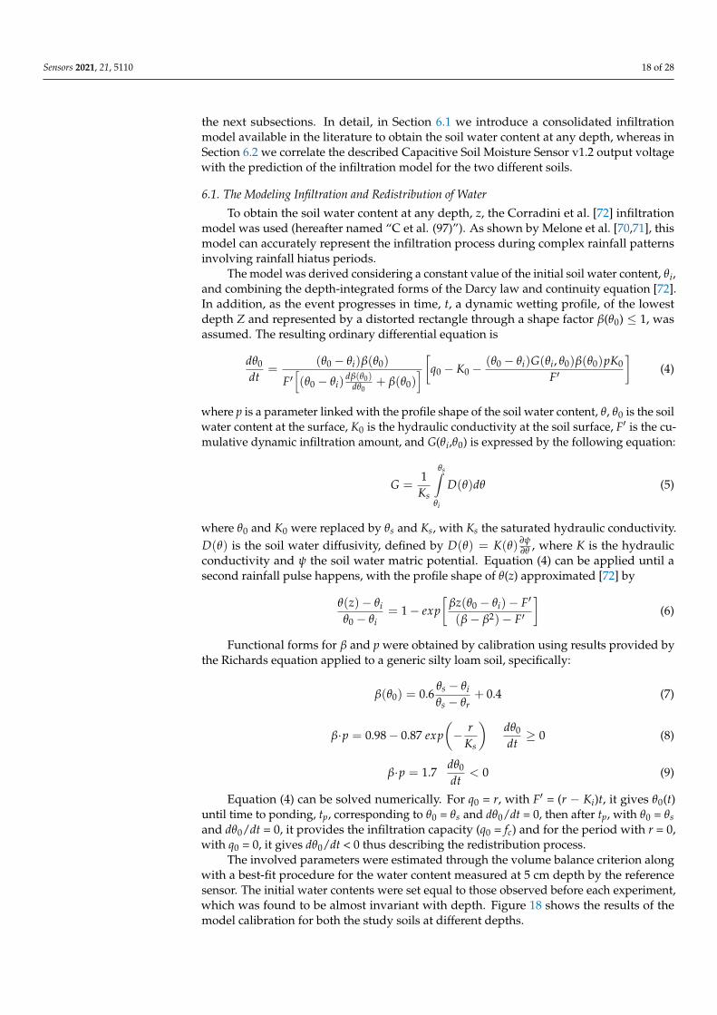
Sensors 2021, 21, 5110 18 of 28

the next subsections. In detail, in Section 6.1 we introduce a consolidated infiltrationmodel available in the literature to obtain the soil water content at any depth, whereas inSection 6.2 we correlate the described Capacitive Soil Moisture Sensor v1.2 output voltagewith the prediction of the infiltration model for the two different soils.

6.1. The Modeling Infiltration and Redistribution of Water

To obtain the soil water content at any depth, z, the Corradini et al. [72] infiltrationmodel was used (hereafter named “C et al. (97)”). As shown by Melone et al. [70,71], thismodel can accurately represent the infiltration process during complex rainfall patternsinvolving rainfall hiatus periods.

The model was derived considering a constant value of the initial soil water content, θi,and combining the depth-integrated forms of the Darcy law and continuity equation [72].In addition, as the event progresses in time, t, a dynamic wetting profile, of the lowestdepth Z and represented by a distorted rectangle through a shape factor β(θ0) ≤ 1, wasassumed. The resulting ordinary differential equation is

dθ0

dt=

(θ0 − θi)β(θ0)

F′[(θ0 − θi)

dβ(θ0)dθ0

+ β(θ0)][q0 − K0 −

(θ0 − θi)G(θi, θ0)β(θ0)pK0

F′

](4)

where p is a parameter linked with the profile shape of the soil water content, θ, θ0 is the soilwater content at the surface, K0 is the hydraulic conductivity at the soil surface, F′ is the cu-mulative dynamic infiltration amount, and G(θi,θ0) is expressed by the following equation:

G =1

Ks

θs∫θi

D(θ)dθ (5)

where θ0 and K0 were replaced by θs and Ks, with Ks the saturated hydraulic conductivity.D(θ) is the soil water diffusivity, defined by D(θ) = K(θ) ∂ψ

∂θ , where K is the hydraulicconductivity and ψ the soil water matric potential. Equation (4) can be applied until asecond rainfall pulse happens, with the profile shape of θ(z) approximated [72] by

θ(z)− θiθ0 − θi

= 1− exp[

βz(θ0 − θi)− F′

(β− β2)− F′

](6)

Functional forms for β and p were obtained by calibration using results provided bythe Richards equation applied to a generic silty loam soil, specifically:

β(θ0) = 0.6θs − θiθs − θr

+ 0.4 (7)

β·p = 0.98− 0.87 exp(− r

Ks

)dθ0

dt≥ 0 (8)

β·p = 1.7dθ0

dt< 0 (9)

Equation (4) can be solved numerically. For q0 = r, with F′ = (r − Ki)t, it gives θ0(t)until time to ponding, tp, corresponding to θ0 = θs and dθ0/dt = 0, then after tp, with θ0 = θsand dθ0/dt = 0, it provides the infiltration capacity (q0 = fc) and for the period with r = 0,with q0 = 0, it gives dθ0/dt < 0 thus describing the redistribution process.

The involved parameters were estimated through the volume balance criterion alongwith a best-fit procedure for the water content measured at 5 cm depth by the referencesensor. The initial water contents were set equal to those observed before each experiment,which was found to be almost invariant with depth. Figure 18 shows the results of themodel calibration for both the study soils at different depths.

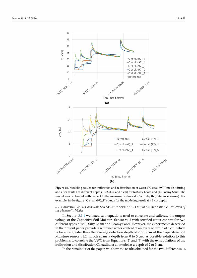
Sensors 2021, 21, 5110 19 of 28


𝐺 = 1𝐾 𝐷 𝜃 𝑑𝜃 (5)

where θ0 and K0 were replaced by θs and Ks, with Ks the saturated hydraulic conductivity. 𝐷 𝜃 is the soil water diffusivity, defined by 𝐷 𝜃 = 𝐾 𝜃 , where K is the hydraulic conductivity and Ψ the soil water matric potential. Equation (4) can be applied until a second rainfall pulse happens, with the profile shape of θ(z) approximated [72] by 𝜃 𝑧 − 𝜃𝜃 − 𝜃 = 1 − 𝑒𝑥𝑝 𝛽𝑧 𝜃 − 𝜃 − 𝐹𝛽 − 𝛽 − 𝐹 (6)

Functional forms for β and p were obtained by calibration using results provided by the Richards equation applied to a generic silty loam soil, specifically: 𝛽 𝜃 = 0.6 𝜃 − 𝜃𝜃 − 𝜃 + 0.4 (7)

𝛽 ∙ 𝑝 = 0.98 − 0.87 𝑒𝑥𝑝 − 0 (8)

𝛽 ∙ 𝑝 = 1.7 0 (9)

Equation (4) can be solved numerically. For q0 = r, with F’ = (r−Ki)t, it gives θ0(t) until time to ponding, tp, corresponding to θ0 = θs and dθ0/dt = 0, then after tp, with θ0 = θs and dθ0/dt = 0, it provides the infiltration capacity (q0 = fc) and for the period with r = 0, with q0 = 0, it gives dθ0/dt < 0 thus describing the redistribution process.

The involved parameters were estimated through the volume balance criterion along with a best-fit procedure for the water content measured at 5 cm depth by the reference sensor. The initial water contents were set equal to those observed before each experiment, which was found to be almost invariant with depth. Figure 18 shows the results of the model calibration for both the study soils at different depths.

(a)


(b)

Figure 18. Modeling results for infiltration and redistribution of water (“C et al. (97)” model) during and after rainfall at different depths (1, 2, 3, 4, and 5 cm) for (a) Silty Loam and (b) Loamy Sand. The model was calibrated with respect to the measured values at a 5 cm depth (Reference sensor). For example, in the figure “C et al. (97)_1” stands for the modeling result at a 1 cm depth.

6.2. Correlation of the Capacitive Soil Moisture Sensor v1.2 Output Voltage with the Prediction of the Hydraulic Model

In Section 3.1.1 we listed two equations used to correlate and calibrate the output voltage of the Capacitive Soil Moisture Sensor v1.2 with certified water content for two different types of soil: Silty Loam and Loamy Sand. However, the experiments described in the present paper provide a reference water content at an average depth of 5 cm, which is for sure greater than the average detection depth of 2 or 3 cm of the Capacitive Soil Moisture sensor v1.2, which spans a depth from 0 to 5 cm. A possible solution to this problem is to correlate the VWC from Equations (2) and (3) with the extrapolations of the infiltration and distribution Corradini et al. model at a depth of 2 or 3 cm.

In the remainder of the paper, we show the results obtained for the two different soils.

6.2.1. Water Content in Silty Loam A three-parameter least-square best fit was calculated between the VWC function

obtained using the Corradini model (hereafter indicated as “C et al. (97)” [72] at different depths of 2 and 3 cm, with Equation (1), obtaining two triplets of A, B, and C values shown in Table 3 where the Placidi model “P et al. (20)”[8] is referred to different depths. Simi-larly, a two-parameter least-square best fit was calculated with the Hrisko model “H (20)” at 2 and 3 cm depths and the model from “C et al. (97)”, obtaining two couples of P and Q values shown in Table 3.

Figure 18. Modeling results for infiltration and redistribution of water (“C et al. (97)” model) duringand after rainfall at different depths (1, 2, 3, 4, and 5 cm) for (a) Silty Loam and (b) Loamy Sand. Themodel was calibrated with respect to the measured values at a 5 cm depth (Reference sensor). Forexample, in the figure “C et al. (97)_1” stands for the modeling result at a 1 cm depth.

6.2. Correlation of the Capacitive Soil Moisture Sensor v1.2 Output Voltage with the Prediction ofthe Hydraulic Model

In Section 3.1.1 we listed two equations used to correlate and calibrate the outputvoltage of the Capacitive Soil Moisture Sensor v1.2 with certified water content for twodifferent types of soil: Silty Loam and Loamy Sand. However, the experiments describedin the present paper provide a reference water content at an average depth of 5 cm, whichis for sure greater than the average detection depth of 2 or 3 cm of the Capacitive SoilMoisture sensor v1.2, which spans a depth from 0 to 5 cm. A possible solution to thisproblem is to correlate the VWC from Equations (2) and (3) with the extrapolations of theinfiltration and distribution Corradini et al. model at a depth of 2 or 3 cm.

In the remainder of the paper, we show the results obtained for the two different soils.

Sensors 2021, 21, 5110 20 of 28

6.2.1. Water Content in Silty Loam

A three-parameter least-square best fit was calculated between the VWC functionobtained using the Corradini model (hereafter indicated as “C et al. (97)” [72] at differentdepths of 2 and 3 cm, with Equation (1), obtaining two triplets of A, B, and C values shownin Table 3 where the Placidi model “P et al. (20)” [8] is referred to different depths. Similarly,a two-parameter least-square best fit was calculated with the Hrisko model “H (20)” at2 and 3 cm depths and the model from “C et al. (97)”, obtaining two couples of P and Qvalues shown in Table 3.

Table 3. Least-square best-fit parameters of Equations (2) and (3) in Silty Loam.

P et al. (20)_3 P et al. (20)_2

A 0.711 0.731B 9.72 10.2C 0.864 0.859

H (20)_3 H (20)_2

P 73.4 75.8Q 55.1 57.2

The plots reporting the water content obtained by using the three models for the twodifferent depths are reported in Figure 19.


Table 3. Least-square best-fit parameters of Equations (2) and (3) in Silty Loam.

P et al. (20)_3 P et al. (20)_2 A 0.711 0.731 B 9.72 10.2 C 0.864 0.859 H (20)_3 H (20)_2

P 73.4 75.8 Q 55.1 57.2

The plots reporting the water content obtained by using the three models for the two different depths are reported in Figure 19.

Figure 19. Comparison among the water infiltration and redistribution “C” model for Silty Loam at a depth of 2 and 3 cm with the VWC obtained from the voltage measured by Node #1 using Equation (2) (“P” curves) and Equation (3) (“H” curves).

In Figure 20 a statistical analysis between all the possible couples of the “C et al. (97)” model and voltage measured by Node #1 using Equation (2) (“P” curves) and Equation (3) (“H” curves) at different depths has been reported. The analysis has been performed by using scattering plots, cross-correlation values, and kernel density estimation accom-plished by using the Seaborn Python3 tool [73]. In the figure, the eight plots in the main diagonal are the calculated histograms of the corresponding eight quantities, together with the estimated Gaussian mixture probability density function. The plots in the lower triangular part represent the scattering plots of each couple of quantities, together with the locally weighted regression curve whereas the values in the upper triangular part, instead, represent the correlation coefficients between each couple of quantities.

Figure 19. Comparison among the water infiltration and redistribution “C” model for Silty Loam ata depth of 2 and 3 cm with the VWC obtained from the voltage measured by Node #1 using Equation(2) (“P” curves) and Equation (3) (“H” curves).

In Figure 20 a statistical analysis between all the possible couples of the “C et al. (97)”model and voltage measured by Node #1 using Equation (2) (“P” curves) and Equation (3)(“H” curves) at different depths has been reported. The analysis has been performed byusing scattering plots, cross-correlation values, and kernel density estimation accomplishedby using the Seaborn Python3 tool [73]. In the figure, the eight plots in the main diagonal arethe calculated histograms of the corresponding eight quantities, together with the estimatedGaussian mixture probability density function. The plots in the lower triangular partrepresent the scattering plots of each couple of quantities, together with the locally weighted

Sensors 2021, 21, 5110 21 of 28

regression curve whereas the values in the upper triangular part, instead, represent thecorrelation coefficients between each couple of quantities.


Figure 20. Statistical analysis with scattering plots, cross-correlation values, and kernel density estimation (KDE) obtained by using the Seaborn Python3 tool [73–75] in Silty Loam.

Looking at homogeneous values (i.e., correlation data obtained at the same depth), The best correlation values we obtained (0.94) are between “C et al. (97)” and “P et al. (20”) at a depth of 3 cm. The 0.94 correlation coefficient is slightly greater than the value of 0.91 obtained between “C et al. (97)” and “P et al. (20)” at a depth of 2 cm. In Figure 21 the comparison among the best results obtained from the correlation are reported for the three models. Even if peaks and valleys of the hydraulic model are not always perfectly repro-duced by the Capacitive Soil Moisture Sensor v1.2 fitting equations, the overall behavior of the “P et al. (20)” model can capture the main features of the VWC at a shallow depth. We note that, due to the peculiarities of experimental systems involving natural soils, it is impossible to obtain results that are completely reproducible from mathematical schemes. For example, inserting different sensors into the soil produces different preferential wa-terways that can turn out in minimally different results, especially when the experimental behavior is compared with mathematical model performances.

Figure 20. Statistical analysis with scattering plots, cross-correlation values, and kernel density estimation (KDE) obtainedby using the Seaborn Python3 tool [73–75] in Silty Loam.

Looking at homogeneous values (i.e., correlation data obtained at the same depth),The best correlation values we obtained (0.94) are between “C et al. (97)” and “P et al. (20”)at a depth of 3 cm. The 0.94 correlation coefficient is slightly greater than the value of0.91 obtained between “C et al. (97)” and “P et al. (20)” at a depth of 2 cm. In Figure 21the comparison among the best results obtained from the correlation are reported for thethree models. Even if peaks and valleys of the hydraulic model are not always perfectlyreproduced by the Capacitive Soil Moisture Sensor v1.2 fitting equations, the overallbehavior of the “P et al. (20)” model can capture the main features of the VWC at ashallow depth. We note that, due to the peculiarities of experimental systems involvingnatural soils, it is impossible to obtain results that are completely reproducible frommathematical schemes. For example, inserting different sensors into the soil producesdifferent preferential waterways that can turn out in minimally different results, especiallywhen the experimental behavior is compared with mathematical model performances.

Sensors 2021, 21, 5110 22 of 28Sensors 2021, 21, x FOR PEER REVIEW 23 of 29

Figure 21. Comparison among the best results obtained from the correlation procedure for the three considered models.

6.2.2. Water Content in Loamy Sand A three-parameter least-square best fit was also calculated in Loamy Sand between

Equation (1) and the VWC function obtained using the “C et al. (97)” model at different depths of 2 and 3 cm. The two triplets of A, B, and C values are reported in Table 4 where the model “P et al. (20)” is referred to different depths. Similarly, a two-parameter least-square best fit was calculated with the Hrisko model “H (20)” at 2 and 3 cm depths and the model from “C et al. (97)”, obtaining two couples of P and Q values shown in Table 4.

Table 4. Least-square best-fit parameters of Equation (2) and Equation (3) in Loamy Sand.

P et al. (20)_3 P et al. (20)_2 A 1.64 1.65 B 8.16 8.41 C 0.85 0.85 H (20)_3 H (20)_2

P 17.44 17.54 Q 2.37 2.1

The plot with the water content for the three models for the two different depths is reported in Figure 22.

Then a statistical analysis with scattering plots, cross-correlation values, and kernel density estimation was accomplished by using the Seaborn Python3 tool (Figure 23) be-tween all the possible couples of models at different depths. Looking at homogeneous values (i.e., correlation data obtained at the same depth), the best correlation values we obtained (0.58) are between “C et al. (97)” and the “Hrisko model”. A much worse corre-lation was obtained for Loamy Sand compared to Silty Loam. However, as highlighted in [54], the behavior of coarse-textured soil (as the Loamy Sand) can be mathematically mod-eled with greater difficulty than that of fine-textured soil (as the Silty Loam).

Figure 21. Comparison among the best results obtained from the correlation procedure for the threeconsidered models.

6.2.2. Water Content in Loamy Sand

A three-parameter least-square best fit was also calculated in Loamy Sand betweenEquation (1) and the VWC function obtained using the “C et al. (97)” model at differentdepths of 2 and 3 cm. The two triplets of A, B, and C values are reported in Table 4where the model “P et al. (20)” is referred to different depths. Similarly, a two-parameterleast-square best fit was calculated with the Hrisko model “H (20)” at 2 and 3 cm depthsand the model from “C et al. (97)”, obtaining two couples of P and Q values shown inTable 4.

Table 4. Least-square best-fit parameters of Equation (2) and Equation (3) in Loamy Sand.

P et al. (20)_3 P et al. (20)_2

A 1.64 1.65B 8.16 8.41C 0.85 0.85

H (20)_3 H (20)_2

P 17.44 17.54Q 2.37 2.1

The plot with the water content for the three models for the two different depths isreported in Figure 22.


Figure 22. Comparison among the water infiltration and redistribution “C” model for Loamy Sand at a depth of 2 and 3 cm with the VWC obtained from the voltage measured by Node #1 using Equation (2) (“P” curves) and Equation (3) (“H” curves).

Figure 23. Statistical analysis with scattering plots, cross-correlation values, and kernel density estimation (KDE) in Loamy Sand.

Figure 24 shows the comparison among the best results obtained from the correlation procedure. Even if a first sight comparison of the three curves shows significant differ-ences, it should be noted that for practical applications of sensors for measuring the soil water content, differences of a few percent are often irrelevant.

Figure 22. Comparison among the water infiltration and redistribution “C” model for Loamy Sand ata depth of 2 and 3 cm with the VWC obtained from the voltage measured by Node #1 using Equation(2) (“P” curves) and Equation (3) (“H” curves).

Sensors 2021, 21, 5110 23 of 28

Then a statistical analysis with scattering plots, cross-correlation values, and kerneldensity estimation was accomplished by using the Seaborn Python3 tool (Figure 23) be-tween all the possible couples of models at different depths. Looking at homogeneousvalues (i.e., correlation data obtained at the same depth), the best correlation values weobtained (0.58) are between “C et al. (97)” and the “Hrisko model”. A much worse corre-lation was obtained for Loamy Sand compared to Silty Loam. However, as highlightedin [54], the behavior of coarse-textured soil (as the Loamy Sand) can be mathematicallymodeled with greater difficulty than that of fine-textured soil (as the Silty Loam).


Figure 22. Comparison among the water infiltration and redistribution “C” model for Loamy Sand at a depth of 2 and 3 cm with the VWC obtained from the voltage measured by Node #1 using Equation (2) (“P” curves) and Equation (3) (“H” curves).

Figure 23. Statistical analysis with scattering plots, cross-correlation values, and kernel density estimation (KDE) in Loamy Sand.

Figure 24 shows the comparison among the best results obtained from the correlation procedure. Even if a first sight comparison of the three curves shows significant differ-ences, it should be noted that for practical applications of sensors for measuring the soil water content, differences of a few percent are often irrelevant.

Figure 23. Statistical analysis with scattering plots, cross-correlation values, and kernel density estimation (KDE) inLoamy Sand.

Figure 24 shows the comparison among the best results obtained from the correlationprocedure. Even if a first sight comparison of the three curves shows significant differences,it should be noted that for practical applications of sensors for measuring the soil watercontent, differences of a few percent are often irrelevant.

Sensors 2021, 21, 5110 24 of 28Sensors 2021, 21, x FOR PEER REVIEW 25 of 29

Figure 24. Comparison among the best results obtained from the correlation procedure for the three considered models.

7. Conclusions A low-power WSN based on LoRaWAN™ was designed with a focus on low-cost

PA applications, such as greenhouse sensing and actuation. Two types of wireless nodes were envisaged, greenhouse node and plant node, and the whole LPWAN was designed and implemented, including an 8-channel gateway/concentrator. The first experimental results were collected and stored in a database managed by a virtual machine running in a cloud service. Since all subsystems adopted in this research are off-the-shelf elements with available open-source software libraries, only a minimal effort is needed when the system is implemented for a different application.

Measurement results were focused on measurements of water content and were col-lected using plant nodes in Loamy Sand and Silty Loam, proving the functionality and reliability of the whole system (sensor nodes, gateway, GUI, Node-RED, and Cloud) and comparing the system behavior with a reference sensor from Sentek. Temperature meas-urements of our plant nodes compare as expected with the reference sensor within the supposed accuracy of the adopted sensors. Regarding water content measurements, a cor-relation was attempted between the results of the cheap Capacitive Soil Moisture Sensor v1.2 and those of the Sentek reference sensor. We realized the low-cost water content sen-sor suffers from a non-constant sensitivity; therefore, non-linear fitting equations are nec-essary for correlating its voltage output with the VWC. We adopted for the Capacitive Soil Moisture Sensor v1.2 two VWC fitting equations taken from the literature. Since the ref-erence sensor and the cheap water content sensor span different soil depths (5 cm and 2-3 cm, respectively), we first modeled the theoretical VWC profiles at different depths us-ing a proven water infiltration and redistribution model, calibrating the model on the ref-erence sensor results at a depth of 5 cm. Then we used the two fitting equations for the Capacitive Soil Moisture Sensor v1.2 and calculated multi-parameter least squares fit to the hydraulic model at 2 and 3 cm depths. A very satisfactory correlation coefficient of 0.94 was obtained for Silty Loam using the exponential/logarithmic “P” model at a depth of 3 cm. Instead, the best correlation value we obtained using the same fitting procedure applied to the results in Loamy Sand was 0.58 at a depth of 2 cm using the hyperbolic “H” model. Despite the low correlation coefficient, the VWC values we obtained with the hy-perbolic “H” model can be considered as representative of the real VWC at a depth of 2 cm, since differences of a few percent are often irrelevant for practical applications of sen-sors for measuring the soil water content.

Figure 24. Comparison among the best results obtained from the correlation procedure for the threeconsidered models.

7. Conclusions

A low-power WSN based on LoRaWAN™ was designed with a focus on low-costPA applications, such as greenhouse sensing and actuation. Two types of wireless nodeswere envisaged, greenhouse node and plant node, and the whole LPWAN was designedand implemented, including an 8-channel gateway/concentrator. The first experimentalresults were collected and stored in a database managed by a virtual machine running in acloud service. Since all subsystems adopted in this research are off-the-shelf elements withavailable open-source software libraries, only a minimal effort is needed when the systemis implemented for a different application.

Measurement results were focused on measurements of water content and werecollected using plant nodes in Loamy Sand and Silty Loam, proving the functionalityand reliability of the whole system (sensor nodes, gateway, GUI, Node-RED, and Cloud)and comparing the system behavior with a reference sensor from Sentek. Temperaturemeasurements of our plant nodes compare as expected with the reference sensor withinthe supposed accuracy of the adopted sensors. Regarding water content measurements,a correlation was attempted between the results of the cheap Capacitive Soil MoistureSensor v1.2 and those of the Sentek reference sensor. We realized the low-cost water contentsensor suffers from a non-constant sensitivity; therefore, non-linear fitting equations arenecessary for correlating its voltage output with the VWC. We adopted for the CapacitiveSoil Moisture Sensor v1.2 two VWC fitting equations taken from the literature. Since thereference sensor and the cheap water content sensor span different soil depths (5 cm and2-3 cm, respectively), we first modeled the theoretical VWC profiles at different depthsusing a proven water infiltration and redistribution model, calibrating the model on thereference sensor results at a depth of 5 cm. Then we used the two fitting equations for theCapacitive Soil Moisture Sensor v1.2 and calculated multi-parameter least squares fit tothe hydraulic model at 2 and 3 cm depths. A very satisfactory correlation coefficient of0.94 was obtained for Silty Loam using the exponential/logarithmic “P” model at a depthof 3 cm. Instead, the best correlation value we obtained using the same fitting procedureapplied to the results in Loamy Sand was 0.58 at a depth of 2 cm using the hyperbolic“H” model. Despite the low correlation coefficient, the VWC values we obtained with thehyperbolic “H” model can be considered as representative of the real VWC at a depth of2 cm, since differences of a few percent are often irrelevant for practical applications ofsensors for measuring the soil water content.

In this work, we demonstrated the lack of linearity of the adopted soil water contentsensor. Notwithstanding this lack of linearity, the introduction of the infiltration model

Sensors 2021, 21, 5110 25 of 28

and of a dedicated statistical analysis allowed us to extract reliable values of the volumet-ric water content for both Silty Loam and Loamy Sand. This procedure represents thenovelty and the potential of the proposed approach. Therefore, future work will addressthe optimization of the sensor performance. To this purpose, it will be useful to betterunderstand the behavior of the sensor from simulations and to optimize the layout ofthe sensor without impacting significantly on the cost, also considering the mechanicalintegration constraints needed for industrialization.

Author Contributions: Conceptualization, P.P., R.M., and A.S.; data curation, P.P., R.M., D.F., N.P.,F.G., and A.S.; formal analysis, P.P., R.M. and A.S.; funding acquisition, P.P.; investigation, R.M., D.F.,N.P. and F.G.; methodology, P.P., and A.S.; Project administration, P.P. and A.S.; Software, D.F., andF.G.; supervision, P.P., R.M., and A.S.; validation, P.P., D.F., N.P. and A.S.; visualization, D.F., and F.G.;writing—original draft, P.P., and A.S.; writing—review and editing, P.P., R.M., and A.S. All authorshave read and agreed to the published version of the manuscript.

Funding: This research was partly funded by the DEPARTMENT OF ENGINEERING OF THEUNIVERSITY OF PERUGIA, Italy, grant “Ricerca di base 2018-RICBA18-PP”, “Ricerca di base 2019-RICBA19-PP”, “Ricerca di base 2020-RICBA20-PP”.

Acknowledgments: Thanks are due to colleagues D. Grohmann, G. Marconi, and M. Cecconi forhelpful discussions and technical support.

Conflicts of Interest: The authors declare no conflict of interest. The funders had no role in the designof the study; in the collection, analyses, or interpretation of data; in the writing of the manuscript, orin the decision to publish the results.

References1. Bandur, Ð.; Jakšic, B.; Bandur, M.; Jovic, S. An analysis of energy efficiency in Wireless Sensor Networks (WSNs) applied in smart

agriculture. Comput. Electron. Agric. 2019, 156, 500–507. [CrossRef]2. Kochhar, A.; Kumar, N. Wireless sensor networks for greenhouses: An end-to-end review. Comput. Electron. Agric. 2019,

163, 104877. [CrossRef]3. Castañeda-Miranda, A.; Castaño, V.M. Internet of things for smart farming and frost intelligent control in greenhouses. Comput.

Electron. Agric. 2020, 176, 105614. [CrossRef]4. Pradeepkumar, D.; Ravi, V. Soft computing hybrids for FOREX rate prediction: A comprehensive review. Comput. Oper. Res. 2018,

99, 262–284. [CrossRef]5. Panigrahi, S.; Behera, H.S. A hybrid ETS–ANN model for time series forecasting. Eng. Appl. Artif. Intell. 2017, 66, 49–59.

[CrossRef]6. Fan, Y.; Zhang, Y.; Chen, Z.; Wang, X.; Huang, B. Comprehensive assessments of soil fertility and environmental quality in plastic

greenhouse production systems. Geoderma 2021, 385, 114899. [CrossRef]7. Guo, Y.; Zhao, H.; Zhang, S.; Wang, Y.; Chow, D. Modeling and optimization of environment in agricultural greenhouses for

improving cleaner and sustainable crop production. J. Clean. Prod. 2021, 285, 124843. [CrossRef]8. Placidi, P.; Gasperini, L.; Grassi, A.; Cecconi, M.; Scorzoni, A. Characterization of Low-Cost Capacitive Soil Moisture Sensors for

IoT Networks. Sensors 2020, 20, 3585. [CrossRef]9. Syafrudin, M.; Alfian, G.; Fitriyani, N.L.; Rhee, J. Performance Analysis of IoT-Based Sensor, Big Data Processing, and Machine

Learning Model for Real-Time Monitoring System in Automotive Manufacturing. Sensors 2018, 18, 2946. [CrossRef] [PubMed]10. Castañeda, A.; Castaño, V.M. Smart frost measurement for anti-disaster intelligent control in greenhouses via embedding IoT and

hybrid AI methods. Measurement 2020, 164, 108043. [CrossRef]11. Rizzi, M.; Ferrari, P.; Flammini, A.; Sisinni, E. Evaluation of the IoT LoRaWAN Solution for Distributed Measurement Applications.

IEEE Trans. Instrum. Meas. 2017, 66, 12. [CrossRef]12. Zamora-Izquierdo, M.A.; Santa, J.; Martínez, J.A.; Martínez, V.; Skarmeta, A.F. Smart farming IoT platform based on edge and

cloud computing. Biosyst. Eng. 2019, 177, 4–17. [CrossRef]13. Iyengar, S.S.; Boroojeni, K.G.; Balakrishnan, N. Mathematical Theories of Distributed Sensor Networks; Springer: Berlin/Heidelberg,

Germany, 2014.14. Benos, L.; Tagarakis, A.; Dolias, G.; Berruto, R.; Kateris, D.; Bochtis, D. Machine Learning in Agriculture: A Comprehensive

Updated Review. Sensors 2021, 21, 3758. [CrossRef]15. Patrício, D.I.; Rieder, R. Computer vision and artificial intelligence in precision agriculture for grain crops: A systematic re-view.

Comput. Electron. Agric. 2018, 153, 69–81. [CrossRef]16. van Klompenburg, T.; Kassahun, A.; Catal, C. Crop yield prediction using machine learning: A systematic literature review.

Comput. Electron. Agric. 2020, 177, 105709. [CrossRef]

http://doi.org/10.1016/j.compag.2018.12.016

http://doi.org/10.1016/j.compag.2019.104877


http://doi.org/10.1016/j.cor.2018.05.020

http://doi.org/10.1016/j.engappai.2017.07.007

http://doi.org/10.1016/j.geoderma.2020.114899

http://doi.org/10.1016/j.jclepro.2020.124843

http://doi.org/10.3390/s20123585

http://doi.org/10.3390/s18092946

http://www.ncbi.nlm.nih.gov/pubmed/30181525

http://doi.org/10.1016/j.measurement.2020.108043

http://doi.org/10.1109/TIM.2017.2746378

http://doi.org/10.1016/j.biosystemseng.2018.10.014

http://doi.org/10.3390/s21113758



Sensors 2021, 21, 5110 26 of 28

17. Liakos, K.G.; Busato, P.; Moshou, D.; Pearson, S.; Bochtis, D. Machine learning in agriculture: A review. Sensors 2018, 18, 2674.[CrossRef] [PubMed]

18. Yuan, Y.; Chen, L.; Wu, H.; Li, L. Advanced agricultural disease image recognition technologies: A review. Inf. Process. Agric.2021, 8, 1–12. [CrossRef]

19. Akbar, A.; Kuanar, A.; Patnaik, J.; Mishra, A.; Nayak, S. Application of Artificial Neural Network modeling for optimization andprediction of essential oil yield in turmeric (Curcuma longa L.). Comput. Electron. Agric. 2018, 148, 160–178. [CrossRef]

20. Vij, A.; Vijendra, S.; Jain, A.; Bajaj, S.; Bassi, A.; Sharma, A. IoT and Machine Learning Approaches for Automation of FarmIrrigation System. Procedia Comput. Sci. 2020, 167, 1250–1257. [CrossRef]

21. Rehman, A.U.; Abbasi, A.Z.; Islam, N.; Shaikh, Z.A. A review of wireless sensors and networks’ applications in agriculture.Comput. Stand. Interfaces 2014, 36, 263–270. [CrossRef]

22. Farooq, M.S.; Riaz, S.; Abid, A.; Umer, T.; Bin Zikria, Y. Role of IoT Technology in Agriculture: A Systematic Literature Review.Electronics 2020, 9, 319. [CrossRef]

23. Shi, X.; An, X.; Zhao, Q.; Liu, H.; Xia, L.; Sun, X.; Guo, Y. State-of-the-Art Internet of Things in Protected Agriculture. Sensors 2019,19, 1833. [CrossRef] [PubMed]

24. Sagheer, A.; Mohammed, M.; Riad, K.; Alhajhoj, M. A Cloud-Based IoT Platform for Precision Control of Soilless GreenhouseCultivation. Sensors 2020, 21, 223. [CrossRef] [PubMed]

25. Shafi, U.; Mumtaz, R.; García-Nieto, J.; Hassan, S.A.; Zaidi, S.A.R.; Iqbal, N. Precision Agriculture Techniques and Practices: FromConsiderations to Applications. Sensors 2019, 19, 3796. [CrossRef]

26. Messina, G.; Modica, G. Applications of UAV Thermal Imagery in Precision Agriculture: State of the Art and Future ResearchOutlook. Remote. Sens. 2020, 12, 1491. [CrossRef]

27. Gnecchi, J.A.G.; Tirado, L.F.; Campos, G.M.C.; Ramirez, R.D.; Gordillo, C.F.E. Design of a Soil Moisture Sensor with TemperatureCompensation Using a Backpropagation Neural Network. In Proceedings of the 2008 Electronics, Robotics and AutomotiveMechanics Conference, Cuernavaca, Mexico, 30 September–3 October 2008; pp. 553–558.

28. Danita, M.; Mathew, B.; Shereen, N.; Sharon, N.; Paul, J.J. IoT Based Automated Greenhouse Monitoring System. In Proceedingsof the 2018 Second International Conference on Intelligent Computing and Control Systems (ICICCS), Madurai, India, 14–15 June2018; pp. 1933–1937.

29. Ruiz-Garcia, L.; Lunadei, L.; Barreiro, P.; Robla, J.I. A Review of Wireless Sensor Technologies and Applications in Agricultureand Food Industry: State of the Art and Current Trends. Sensors 2009, 9, 4728–4750. [CrossRef]

30. BeechamRes. Towards Smart Farming Agriculture Embracing the IoT Vision. Available online: http://www.beechamresearch.com/files/BRL%20Smart%20Farming%20Executive%20Summary.pdf (accessed on 12 May 2020).

31. SU, S.L.; Singh, D.N.; Baghini, M.S. A critical review of soil moisture measurement. Measurement 2014, 54, 92–105. [CrossRef]32. Nagahage, E.A.A.D.; Nagahage, I.S.P.; Fujino, T. Calibration and Validation of a Low-Cost Capacitive Moisture Sensor to Integrate

the Automated Soil Moisture Monitoring System. Agriculture 2019, 9, 141. [CrossRef]33. Hrisko, J. Capacitive Soil Moisture Sensor Theory, Calibration, and Testing. Tech. Rep. 2020, 2, 1–12. [CrossRef]34. Morais, R.; Mendes, J.; Silva, R.; Silva, N.; Sousa, J.; Peres, E. A Versatile, Low-Power and Low-Cost IoT Device for Field Data

Gathering in Precision Agriculture Practices. Agriculture 2021, 11, 619. [CrossRef]35. Figorilli, S.; Pallottino, F.; Colle, G.; Spada, D.; Beni, C.; Tocci, F.; Vasta, S.; Antonucci, F.; Pagano, M.; Fedrizzi, M.; et al. An Open

Source Low-Cost Device Coupled with an Adaptative Time-Lag Time-Series Linear Forecasting Modeling for Apple Trentino(Italy) Precision Irrigation. Sensors 2021, 21, 2656. [CrossRef]

36. Escriba, C.; Bravo, E.G.A.; Roux, J.; Fourniols, J.-Y.; Contardo, M.; Acco, P.; Soto-Romero, G. Toward Smart Soil Sensing in v4.0Agriculture: A New Single-Shape Sensor for Capacitive Moisture and Salinity Measurements. Sensors 2020, 20, 6867. [CrossRef][PubMed]

37. Kojima, Y.; Shigeta, R.; Miyamoto, N.; Shirahama, Y.; Nishioka, K.; Mizoguchi, M.; Kawahara, Y. Low-Cost Soil Moisture ProfileProbe Using Thin-Film Capacitors and a Capacitive Touch Sensor. Sensors 2016, 16, 1292. [CrossRef]

38. Ferrández-Pastor, F.J.; García-Chamizo, J.M.; Nieto-Hidalgo, M.; Pascual, J.M.M.; Mora-Martínez, J. Developing UbiquitousSensor Network Platform Using Internet of Things: Application in Precision Agriculture. Sensors 2016, 16, 1141. [CrossRef]

39. Ferrández-Pastor, F.J.; García-Chamizo, J.M.; Nieto-Hidalgo, M.; Mora-Martínez, J. Precision Agriculture Design Method Using aDistributed Computing Architecture on Internet of Things Context. Sensors 2018, 18, 1731. [CrossRef] [PubMed]

40. Coping with Water Scarcity. UN—Water Thematic Initiatives. A Strategic Issue and Priority for System-Wide Action. 2006.Available online: http://www.unwater.org/publications/coping-water-scarcity/ (accessed on 3 January 2021).

41. Hanak, E.; Mount, J.; Chappelle, C.; Lund, J.; Medellín-Azuara, J.; Moyle, P. Public Policy Institute of California, Water PolicyCenter. What If California’s Drought Continues? 2015. Available online: http://www.ppic.org/publication/what-if-californias-drought-continues/ (accessed on 3 January 2021).

42. Yuanyuan, C.; Zuozhuang, Z. Research and Design of Intelligent Water-saving Irrigation Control System Based on WSN. InProceedings of the 2020 IEEE International Conference on Artificial Intelligence and Computer Applications (ICAICA), Dalian,China, 27–29 June 2020.

43. Mohanraj, I.; Gokul, V.; Ezhilarasie, R.; Umamakeswari, A. Intelligent drip irrigation and fertigation using wireless sensornetworks. In Proceedings of the 2017 IEEE Technological Innovations in ICT for Agriculture and Rural Development (TIAR),Chennai, India, 7–8 April 2017.

http://doi.org/10.3390/s18082674


http://doi.org/10.1016/j.inpa.2021.01.003


http://doi.org/10.1016/j.procs.2020.03.440

http://doi.org/10.1016/j.csi.2011.03.004

http://doi.org/10.3390/electronics9020319

http://doi.org/10.3390/s19081833


http://doi.org/10.3390/s21010223


http://doi.org/10.3390/s19173796

http://doi.org/10.3390/rs12091491

http://doi.org/10.3390/s90604728

http://www.beechamresearch.com/files/BRL%20Smart%20Farming%20Executive%20Summary.pdf

http://www.beechamresearch.com/files/BRL%20Smart%20Farming%20Executive%20Summary.pdf

http://doi.org/10.1016/j.measurement.2014.04.007

http://doi.org/10.3390/agriculture9070141

http://doi.org/10.13140/RG.2.2.36214.83522

http://doi.org/10.3390/agriculture11070619

http://doi.org/10.3390/s21082656

http://doi.org/10.3390/s20236867


http://doi.org/10.3390/s16081292

http://doi.org/10.3390/s16071141

http://doi.org/10.3390/s18061731


http://www.unwater.org/publications/coping-water-scarcity/

http://www.ppic.org/publication/what-if-californias-drought-continues/

http://www.ppic.org/publication/what-if-californias-drought-continues/

Sensors 2021, 21, 5110 27 of 28

44. Walker, J.P.; Willgoose, G.R.; Kalma, J.D. In Situ measurement of soil moisture: A comparison of techniques. J. Hydrol. 2004, 293,85–99. [CrossRef]

45. Tremsin, V.A. Real-Time Three-Dimensional Imaging of Soil Resistivity for Assessment of Moisture Distribution for IntelligentIrrigation. Hydrology 2017, 4, 54. [CrossRef]

46. Subahi, F.; Bouazza, K.E. An Intelligent IoT-Based System Design for Controlling and Monitoring Greenhouse Temperature. IEEEAccess 2020, 8, 125488–125500. [CrossRef]

47. Pawlowski, A.; Guzman, J.L.; Rodríguez, F.; Berenguel, M.; Sánchez, J.; Dormido, S. Simulation of Greenhouse Climate Monitoringand Control with Wireless Sensor Network and Event-Based Control. Sensors 2009, 9, 232–252. [CrossRef]

48. Germani, L.; Mecarelli, V.; Baruffa, G.; Rugini, L.; Frescura, F. An IoT Architecture for Continuous Livestock Monitoring UsingLoRa LPWAN. Electronics 2019, 8, 1435. [CrossRef]

49. Wang, N.; Zhang, N.; Wang, M. Wireless sensors in agriculture and food industry—Recent development and future perspective.Comput. Electron. Agric. 2006, 50, 1–14. [CrossRef]

50. Haseeb, K.; Ud Din, I.; Almogren, A.; Islam, N. An Energy Efficient and Secure IoT-Based WSN Framework: An Application toSmart Agriculture. Sensors 2020, 20, 2081. [CrossRef] [PubMed]

51. Yelamarthi, K.; Aman, M.S.; Abdelgawad, A. An Application-Driven Modular IoT Architecture. Wirel. Commun. Mob. Comput.2017, 2017, 1350929. [CrossRef] [PubMed]

52. Gutiérrez, J.; Villa-Medina, J.F.; Nieto-Garibay, A.; Porta-Gándara, M.Á. Automated Irrigation System Using a Wireless SensorNetwork and GPRS Module. IEEE Trans. Instrum. Meas. 2014, 63, 1. [CrossRef]

53. LoRa Alliance. What is LoRaWAN® Specification. Available online: https://lora-alliance.org/about-lorawan/ (accessed on1 February 2021).

54. Zourmand, A.; Hing, A.L.K.; Hung, C.W.; Abdulrehman, M. Internet of Things (IoT) using LoRa technology. In Proceedings ofthe Conference I2CACIS 2019, Selangor, Malaysia, 29 June 2019.

55. Gu, C.; Tan, R.; Huang, J. SoftLoRa—A LoRa-Based Platform for Accurate and Secure Timing. In Proceedings of the IPSN 19,Montreal, QC, Canada, 16–18 April 2019; pp. 309–310.

56. Van Torre, P.; Ameloot, T.; Rogier, H. Long-range body-to-body LoRa link at 868 MHz. In Proceedings of the 13th EuropeanConference on Antennas and Propagation (EuCAP 2019), Krakow, Polland, 31 March–15 April 2019.

57. Lavric, A.; Popa, V. Internet of Things and LoRa™ Low-Power Wide-Area Networks: A survey. In Proceedings of the InternationalSymposium on Signals, Circuits and Systems (ISSCS), Iasi, Romania, 3–14 July 2017.

58. Mikhaylov, K.; Petaejaejaervi, J.; Haenninen, T. Analysis of capacity and scalability of the LoRa low power wide area networktechnology. In Proceedings of the 22nd European Wireless Conference, Oulu, Finland, 1–6 May 2016.

59. Thethingsnetwork.org. Available online: https://www.thethingsnetwork.org/docs/network/architecture.html (accessed on2 May 2019).

60. FarmBot. Available online: https://farm.bot/ (accessed on 2 May 2019).61. SKU:SEN0193. Available online: https://wiki.dfrobot.com/Capacitive_Soil_Moisture_Sensor_SKU_SEN0193 (accessed on

10 December 2020).62. A WiFi Enabled Soil Moisture Sensor. Available online: https://www.hackster.io/rbaron/a-wifi-enabled-soil-moisture-sensor-

49912b (accessed on 2 May 2021).63. Munyaradzi, M.; Rupere, T.; Nyambo, B.; Mukute, S.; Chinyerutse, M.; Hapanga, T.; Mashonjowa, E. A Low Cost Automatic

Irrigation Controller Driven by Soil Moisture Sensors. Int. J. Agric. Innov. Res. 2013, 2, 1–7.64. Nemali, K.S.; Montesano, F.; Dove, S.K.; van Iersel, M.W. Calibration and performance of moisture sensors in soilless sub-

strates:ECH2O and Theta probes, Scientia. Horticulturae 2007, 112, 227–234. [CrossRef]65. Qu, W.; Bogena, H.R.; Huisman, J.A.; Vereecken, H. Calibration of a Novel Low-Cost Soil Water Content Sensor Based on a Ring

Oscillator. Vadose Zone J. 2013, 12, vzj2012.0139. [CrossRef]66. Bogena, H.R.; Huisman, J.A.; Schilling, B.; Weuthen, A.; Vereecken, H. Effective Calibration of Low-Cost Soil Water Content

Sensors. Sensors 2017, 17, 208. [CrossRef] [PubMed]67. Node-RED. Available online: https://nodered.org/ (accessed on 3 January 2021).68. Linsley, R.K.; Franzini, J.B.; Freyberg, D.L.; Tchobanoglous, G. Water–Resources Engineering; McGraw-Hill Singapore:

Singapore, 1992.69. Morbidelli, R.; Saltalippi, C.; Flammini, A.; Cifrodelli, M.; Picciafuoco, T.; Corradini, C.; Govindaraju, R.S. In-situ measurements

of soil saturated hydraulic conductivity: Assessment of reliability trough rainfall-runoff experiments. Hydrol. Process. 2017, 31,3084–3094. [CrossRef]

70. Melone, F.; Corradini, C.; Morbidelli, R.; Saltalippi, C. Laboratory experimental check of a conceptual model for infiltration undercomplex rainfall patterns. Hydrol. Proc. 2006, 20, 439–452. [CrossRef]

71. Melone, F.; Corradini, C.; Morbidelli, R.; Saltalippi, C.; Flammini, A. Comparison of theoretical and experimental soil moistureprofiles under complex rainfall patterns. J. Hydrol. Eng. 2008, 13, 1170–1176. [CrossRef]

72. Corradini, C.; Melone, F.; Smith, E.R. A unified model for infiltration and redistribution during complex rainfall patterns. J.Hydrol. 1997, 192, 104–124. [CrossRef]

http://doi.org/10.1016/j.jhydrol.2004.01.008

http://doi.org/10.3390/hydrology4040054

http://doi.org/10.1109/ACCESS.2020.3007955

http://doi.org/10.3390/s90100232

http://doi.org/10.3390/electronics8121435


http://doi.org/10.3390/s20072081


http://doi.org/10.1155/2017/1350929


http://doi.org/10.1109/TIM.2013.2276487

https://lora-alliance.org/about-lorawan/

https://www.thethingsnetwork.org/docs/network/architecture.html

https://farm.bot/

https://wiki.dfrobot.com/Capacitive_Soil_Moisture_Sensor_SKU_SEN0193

https://www.hackster.io/rbaron/a-wifi-enabled-soil-moisture-sensor-49912b

https://www.hackster.io/rbaron/a-wifi-enabled-soil-moisture-sensor-49912b

http://doi.org/10.1016/j.scienta.2006.12.013

http://doi.org/10.2136/vzj2012.0139

http://doi.org/10.3390/s17010208


https://nodered.org/

http://doi.org/10.1002/hyp.11247

http://doi.org/10.1002/hyp.5913

http://doi.org/10.1061/(ASCE)1084-0699(2008)13:12(1170)

http://doi.org/10.1016/S0022-1694(96)03110-1

Sensors 2021, 21, 5110 28 of 28

73. Waskom, M.; Botvinnik, O.; O’Kane, D.; Hobson, P.; Ostblom, J.; Lukauskas, S.; Gemperline, D.C.; Augspurger, T.; Halchenko,Y.; Cole, J.B.; et al. mwaskom/seaborn: v0.9.0 (July 2018). Available online: http://seaborn.pydata.org/ (accessed on25 November 2019).

74. Silverman, B.W. Density Estimation for Statistics and Data Analysis; Routledge: New York, NY, USA, 1998.75. Fan, J. Local Polynomial Modelling and Its Applications: Monographs on Statistics and Applied Probability 66; Routledge: New York, NY,

USA, 1996.

http://seaborn.pydata.org/

Monitoring Soil and Ambient Parameters in the IoT Precision ...

Documents

Transcript of Monitoring Soil and Ambient Parameters in the IoT Precision ...