This article was downloaded by: [Asian Institute of Technology], [Rajendra PrasadShrestha]On: 05 October 2011, At: 06:36Publisher: Taylor & FrancisInforma Ltd Registered in England and Wales Registered Number: 1072954 Registeredoffice: Mortimer House, 37-41 Mortimer Street, London W1T 3JH, UK

Journal of Land Use SciencePublication details, including instructions for authors andsubscription information:http://www.tandfonline.com/loi/tlus20

Monitoring farmland loss and projectingthe future land use of an urbanizedwatershed in Yogyakarta, IndonesiaPartoyo a & Rajendra Prasad Shrestha aa Natural Resources Management Field of Study, School ofEnvironment, Resources and Development, Asian Institute ofTechnology, Pathumthani, Thailand

Available online: 05 Oct 2011

To cite this article: Partoyo & Rajendra Prasad Shrestha (2011): Monitoring farmland loss andprojecting the future land use of an urbanized watershed in Yogyakarta, Indonesia, Journal of LandUse Science, DOI:10.1080/1747423X.2011.620993

To link to this article: http://dx.doi.org/10.1080/1747423X.2011.620993

PLEASE SCROLL DOWN FOR ARTICLE

Full terms and conditions of use: http://www.tandfonline.com/page/terms-and-conditions

This article may be used for research, teaching, and private study purposes. Anysubstantial or systematic reproduction, redistribution, reselling, loan, sub-licensing,systematic supply, or distribution in any form to anyone is expressly forbidden.

The publisher does not give any warranty express or implied or make any representationthat the contents will be complete or accurate or up to date. The accuracy of anyinstructions, formulae, and drug doses should be independently verified with primarysources. The publisher shall not be liable for any loss, actions, claims, proceedings,demand, or costs or damages whatsoever or howsoever caused arising directly orindirectly in connection with or arising out of the use of this material.

Journal of Land Use ScienceiFirst, 2011, 1–26

Monitoring farmland loss and projecting the future land use of anurbanized watershed in Yogyakarta, Indonesia

Partoyo and Rajendra Prasad Shrestha*

Natural Resources Management Field of Study, School of Environment, Resources andDevelopment, Asian Institute of Technology, Pathumthani, Thailand

(Received 24 January 2011; final version received 2 September 2011)

This study analyzes land use changes in Yogyakarta, Indonesia, specifically farmlandloss, which has occurred as a result of rapid urbanization by employing remote sens-ing, GIS, and land use modeling techniques. Landsat images from 1992 and 2004 andASTER Terralook images from 2009 were classified using a supervised classificationto generate land use maps. Land use change was detected using a post-classificationmethod. During 1992–2009, high-density built-up areas increased by a factor of 3.7,and 80.47 km2 of farmland was lost due to land conversion to built-up areas duringthe same period. Based on these findings, land uses for the year 2029 were spatiallysimulated using Dyna-CLUE model for three scenarios: business as usual, farmlandprotection, and minimum required farmland. The results reveal that the ongoing trendof land use conversion combined with the lack of implementation of proper spatial poli-cies will lead to a large loss of farmland and that it is desirable to protect prime farmlandfrom urban sprawl.

Keywords: farmland loss; land use simulation; GIS; remote sensing; Dyna-CLUE;Yogyakarta

1. Introduction

Global land use change increased markedly in the twentieth century, although agricul-tural practice shifted away from expansion toward intensification late in the century (FAO2002). Although agricultural intensification can contribute to increased food production,there is widespread concern regarding global food security due to increased scarcity. Thetrend toward scarcity is associated with population growth and is aggravated by farm-land loss (Tan, Li, Xie, and Lu 2005; Mariyono, Harini, and Agustin 2007). Rapid lossof farmland occurs due to the combined effect of rapid economic development, popula-tion growth, urbanization, agricultural restructuring, natural hazards, and land degradation(Heilig 1999; Yang and Li 2000; Seto et al. 2002; Ding 2003; Mariyono et al. 2007).

Farmland preservation is therefore recognized as an important way to address thisissue. In response, a number of measures have been introduced aimed at protecting farm-land, especially farmland with the greatest production potential (Daniels and Nelson 1986;Coughlin 1991; Daniels 1991; Nelson 1992; Alterman 2001; Lichtenberg and Ding 2008).In terms of integrated land use planning, agricultural lands in urban fringe areas are attract-ing increasing concern. Farmland should be protected in such a way that agricultural

*Corresponding author. Email: rajendra@ait.ac.th

ISSN 1747-423X print/ISSN 1747-4248 online© 2011 Taylor & Francishttp://dx.doi.org/10.1080/1747423X.2011.620993http://www.tandfonline.com

Dow

nloa

ded

by [A

sian

Insti

tute

of T

echn

olog

y], [

Raje

ndra

Pra

sad

Shre

stha]

at 0

6:36

05

Oct

ober

201

1

2 Partoyo and R.P. Shrestha

practices and urban environmental functions do not disturb one another (Braimoh andOnishi 2007).

The conversion of agricultural land to urban areas in Indonesia is largely uncontrolled,including the conversion of thousands of hectares of prime irrigated paddy fields to otheruses (Firman 2004). At the national level, agricultural land expansion was 1.78% per yearfrom 1980 to 1989, but it decreased to 0.17% per year from 2000 to 2005. The areaunder irrigated paddy fields increased by 1.6 million hectares from 1981 to 1989 but wasreduced by 0.4 million hectares from 1999 to 2002 (PSE-KP 2007). During that period,the conversion of land use from irrigated paddy fields to non-agricultural purposes reached110,000 hectares per year, particularly in the most populated islands, such as Java andBali. At the national average productivity rate of 4.61 tons of dried unhulled rice (GabahKering Giling (GKG)) per hectare, within a year, the national paddy production decreasedby 507,100 tons of GKG, which is equivalent to 329,615 tons of rice, due to the farm-land conversion (Deptan-RI 2008). If this condition is allowed to continue, it is estimatedthat countrywide rice production will be greatly reduced. Moreover, statistics from theMinistry of Agriculture suggest that the increase of rice productivity has reached the sat-uration point. Additionally, farmland conversion has been considered to have reached analarming state for a decade or so. Therefore, to produce enough rice, it is imperative forIndonesia to prevent farmland conversion (Apriyantono 2007; Deptan-RI 2008).

Indonesia promulgated Law No. 41/2009 regarding sustainable crop land in October2009 (RI 2009). Different from its predecessor, this law is promising in its potential to pre-serve prime farmland, as its new paradigm encourages agricultural policies and approachesto deal with farmland conversion rather than just enact formal legal punishment for default-ers. Article 62 of the law deals with the government protection and empowerment offarmers, farmer groups, farmer cooperatives, and farmer associations to sustain their farm-ing activity. Protection includes the provision of guarantees, such as the price of basic foodcommodities to remain profitable, the acquisition of production facilities and infrastructureagriculture, the marketing of staple food crop production, and the compensation due to cropfailure. Empowerment includes the institutional strengthening of farmers, counseling andtraining to improve the quality of human resources, the provision of facilities for financingsources/capital, and the provision of facilities for accessing knowledge, technology, andinformation (Article 63) (RI 2009).

Farmland preservation is also important from the viewpoint of large investments inirrigation infrastructure, protecting agricultural jobs (Firman 1997) and providing certainpublic goods, such as air cleansing and water filtration (Nelson 1992).

Most of the agricultural land encroached upon by urban growth in Indonesia hasoccurred in Java Island, which is the most populated island, with 58% of the total 237.7 mil-lion population of the country in 2010 (BPS-RI 2010). In Java and Bali together, 1.7 millionhectares have been converted during the last decade, particularly in West, East, and CentralJava, which contain the most fertile land in Java Island. Because Java Island has the mostfertile soil and the highest level of agricultural infrastructure among other islands, theloss of farmland in urban fringe areas may jeopardize the local, regional, or even nationalagricultural base of the economy (Yunus 1990).

Yogyakarta Province is located in the southern part of central Java Island. Land usechange analysis is of high interest in this region due to the high dynamics of the landscape,especially land use change related to rapid urbanization and loss of prime agriculture area.Land use change monitored from 2002 to 2006 by the provincial board of planning anddevelopment of Yogyakarta shows a significant increase in urban area. This urban develop-ment has increasingly encroached upon farmland (BAPPEDA-DIY 2007). Yogyakarta has

Dow

nloa

ded

by [A

sian

Insti

tute

of T

echn

olog

y], [

Raje

ndra

Pra

sad

Shre

stha]

at 0

6:36

05

Oct

ober

201

1

Journal of Land Use Science 3

undergone a transition period toward full implementation of Law No. 41/2009 on farm-land preservation, which requires data inventory and supporting regulation to be preparedduring the transition period. On that premise, this paper aims to do the following: (1) todetect land use changes from 1992 to 2009 and quantify farmland loss during this periodand (2) to assess the impact of the farmland protection policy on future land use.

2. Study area

The study area, the Progo-Opak sub-watershed of Progo-Opak-Oyo watershed, liesbetween the latitudes 07!32" and 08!02" S and stretches between longitudes 110!09" and110!31" E in the Province of the Yogyakarta Special Region (Figure 1). This region con-tains the urban area of Yogyakarta municipality in the center and the Sleman and Bantulregencies in the northern and the southern parts, respectively. The study area covers approx-imately 1502 km2 of land between an altitude of 0 m in the Bantul alluvial plain borderingthe Indian Ocean in the south and 2968 m at the summit of Mount Merapi, an activevolcanic mountain, in the north. Yogyakarta has a tropical monsoon climate with twodistinct seasons. The rainy season spans from October to March, and the dry season isfrom April to September. The average temperature varies between a minimum of 19.0!C

Figure 1. Location of the study area.

Dow

nloa

ded

by [A

sian

Insti

tute

of T

echn

olog

y], [

Raje

ndra

Pra

sad

Shre

stha]

at 0

6:36

05

Oct

ober

201

1

4 Partoyo and R.P. Shrestha

(July) and a maximum of 36.2!C (October), with a relative humidity between a mini-mum of 73.8% (August) and a maximum of 88.7% (January). The average annual rainfallis 1893.6 mm/year, and the monthly average rainfall varies between none in August to709.2 mm in January (BPS-DIY 2008).

This sub-watershed represents the most urbanized region in the southern partof the central Java Island. The population density of Yogyakarta municipality was12,679 people/km2 in 1990, increasing to 12,905 people/km2 by 2005; the surround-ing areas were inhabited by 566 people/km2 and 1104 people/km2 in 1990 and 2005,respectively (BPS-RI 2005).

The Gross Regional Domestic Product (GRDP) of the Province of the YogyakartaSpecial Region during 2003–2009 shows a trend of the largest contribution from sectorssuch as commerce, hotels, and restaurants; however, the contribution from the agriculturesector tends to decrease (BAPPEDA-DIY 2009). This trend indicates that urbanization isincreasingly dominating the area.

The development characteristics in the Yogyakarta Special Region directly affectedthe land use pattern. Land conversion to a built-up environment from 1996 to 2007 wascontinuously increasing. The statistical records show that paddy fields covered 19.86% ofthe total province area in 1996 and reduced to 17.97% in 2007. Meanwhile, residential andindustrial areas increased from 15.74% in 1996 to 16.42% in 2007. The development of res-idential areas was concentrated at the Sleman and Bantul regencies around the Yogyakartamunicipality (BAPPEDA-DIY 2008).

Rice demand has been increasing at a rate of 1.0% per year due to populationgrowth (BPS-RI 2005), and the rate of rice consumption has increased from 69 to87.5 kg/capita/year (Distan-DIY 2009) during the last three decades. Hence, thereis a need to increase rice production and availability. With the current rice yield of6 tons/hectare/season with three crops per season, approximately 400 km2 of wet agri-cultural land for rice area will be needed in the next two decades to meet the demand ofthe inhabitants of Yogyakarta. Although rice import is another source of rice availability inthe area, securing production is a priority policy for maintaining self-sufficiency of rice inIndonesia, especially for rice production regions such as Yogyakarta and its surroundings.

3. Methodology

3.1. Detection of land use/land cover change

This study analyzed land use/land cover changes using Landsat and ASTER Terralooksatellite images acquired for 1992, 2004, and 2009. Change detection was performed byusing post-classification technique.

The Landsat satellite was selected because of its high temporal frequency, thus pro-viding more choices for the most cloud-free images, and there is good familiarity ofthis satellite data by local planning and governing agencies in Indonesia. Moreover,the data are available at no charge from the Global Land Cover Facility (GLCF) atftp://ftp.glcf.umd.edu/glcf/Landsat/. However, the 30 m spatial resolution of Landsat isat the lower end of the suitable range for urban land use/land cover classification (Jensenand Cowen 1999), though it has proved to be appropriate for monitoring land use changeand farmland conversion in urban fringe areas (Li, Zhou, and Chen 2006; Mundia andAniya 2006; Lin 2007). For more recent data and because good quality Landsat data are notavailable due to a slice-off defect, we used ASTER Terralook data with a 15 m spatial res-olution to prepare the land use map of 2009. The ASTER Terralook data were downloadedfrom the USGS Global Visualization site at http://glovis.usgs.gov/.

Dow

nloa

ded

by [A

sian

Insti

tute

of T

echn

olog

y], [

Raje

ndra

Pra

sad

Shre

stha]

at 0

6:36

05

Oct

ober

201

1

Journal of Land Use Science 5

One scene from each of Landsat data was acquired on 16 July 1992 (TM sensor) and7 June 2004 (ETM+) for Path/Row 120/65. Two scenes of ASTER Terralook images wereacquired on 7 July 2009 to cover the study area. All scenes were the most cloud-free andwere acquired in the same season for comparable climatic conditions. The images weregeorectified and georeferenced into the Universal Transverse Mercator (UTM) coordinatesystem. The ASTER Terralook images were resampled into a 30 m grid and registered togeoreferenced Landsat images.

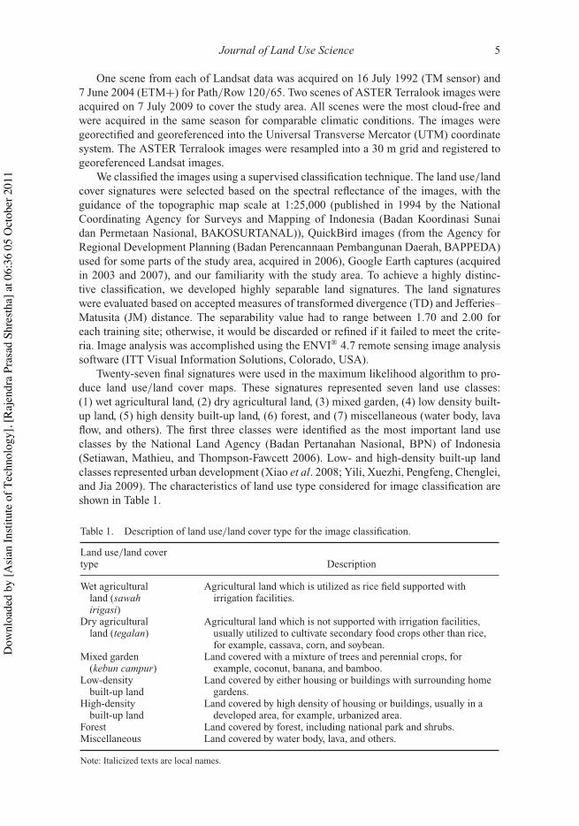
We classified the images using a supervised classification technique. The land use/landcover signatures were selected based on the spectral reflectance of the images, with theguidance of the topographic map scale at 1:25,000 (published in 1994 by the NationalCoordinating Agency for Surveys and Mapping of Indonesia (Badan Koordinasi Sunaidan Permetaan Nasional, BAKOSURTANAL)), QuickBird images (from the Agency forRegional Development Planning (Badan Perencannaan Pembangunan Daerah, BAPPEDA)used for some parts of the study area, acquired in 2006), Google Earth captures (acquiredin 2003 and 2007), and our familiarity with the study area. To achieve a highly distinc-tive classification, we developed highly separable land signatures. The land signatureswere evaluated based on accepted measures of transformed divergence (TD) and Jefferies–Matusita (JM) distance. The separability value had to range between 1.70 and 2.00 foreach training site; otherwise, it would be discarded or refined if it failed to meet the crite-ria. Image analysis was accomplished using the ENVI® 4.7 remote sensing image analysissoftware (ITT Visual Information Solutions, Colorado, USA).

Twenty-seven final signatures were used in the maximum likelihood algorithm to pro-duce land use/land cover maps. These signatures represented seven land use classes:(1) wet agricultural land, (2) dry agricultural land, (3) mixed garden, (4) low density built-up land, (5) high density built-up land, (6) forest, and (7) miscellaneous (water body, lavaflow, and others). The first three classes were identified as the most important land useclasses by the National Land Agency (Badan Pertanahan Nasional, BPN) of Indonesia(Setiawan, Mathieu, and Thompson-Fawcett 2006). Low- and high-density built-up landclasses represented urban development (Xiao et al. 2008; Yili, Xuezhi, Pengfeng, Chenglei,and Jia 2009). The characteristics of land use type considered for image classification areshown in Table 1.

Table 1. Description of land use/land cover type for the image classification.

Land use/land covertype Description

Wet agriculturalland (sawahirigasi)

Agricultural land which is utilized as rice field supported withirrigation facilities.

Dry agriculturalland (tegalan)

Agricultural land which is not supported with irrigation facilities,usually utilized to cultivate secondary food crops other than rice,for example, cassava, corn, and soybean.

Mixed garden(kebun campur)

Land covered with a mixture of trees and perennial crops, forexample, coconut, banana, and bamboo.

Low-densitybuilt-up land

Land covered by either housing or buildings with surrounding homegardens.

High-densitybuilt-up land

Land covered by high density of housing or buildings, usually in adeveloped area, for example, urbanized area.

Forest Land covered by forest, including national park and shrubs.Miscellaneous Land covered by water body, lava, and others.

Note: Italicized texts are local names.

Dow

nloa

ded

by [A

sian

Insti

tute

of T

echn

olog

y], [

Raje

ndra

Pra

sad

Shre

stha]

at 0

6:36

05

Oct

ober

201

1

6 Partoyo and R.P. Shrestha

To validate the image classification result, we conducted field checks during December2009 and April 2010. Due to the time lapse between the satellite images and the fieldsurvey, the field data were mainly collected to provide a secondary source of informationand to resolve any confusion identified during image analysis. A field check is crucial forgenerating data that is retrospective in nature for land use map development in this study.Confirmation from local inhabitants and our familiarity of the study area were the basis ofrefining the preliminary classified land use map.

An accuracy assessment of the classified images was performed by developing a setof sample areas using land use maps produced by the government offices, such as thoseof 1998 and 2002 by BAPPEDA and of 2008 by BPN. Because no ground-truthing waspossible for the abovementioned years, those maps were the best available information.Although assuming that these official maps were true, as they have been widely used byplanners and stakeholders, we performed an additional verification of the selected sampleareas during the second field visit on April 2010. We checked the agreement between theland use of the selected sample areas and the field reality through observations and throughcollecting information from local inhabitants and from the authors’ own familiarity andjudgment as a local inhabitant.

Overall accuracies of 90.49% (kappa coefficient 0.89), 92.29% (kappa coefficient0.91), and 89.51% (kappa coefficient 0.88) were obtained for the 1992, 2004, and2009 images, respectively. All classified images were then used to detect farmland con-version to nonagricultural use. Attention was given to the conversion of wet agriculturalland into built-up areas.

3.2. Evaluation of land potential for rice cultivation

To assess the significance of farmland loss due to the land use change, we evaluated theland potential class of the converted land for rice cultivation. Rice is predominantly plantedin prime farmland, as it is the staple food in the study area. We developed a base map ofland potential for the whole study area and then superimposed the map with a map ofconverted farmland during 1992–2009. It would be a significant loss if the converted landhad a high potential for rice cultivation.

Land potential was evaluated based on the land suitability class for rice cultivation andirrigation support availability. Land suitability is considered an important factor becauseit describes land characteristics that succeed rice cultivation. Higher land suitability andadequate irrigation water availability can be considered as having the higher potential. Twoseparate maps, namely, rice suitability and irrigation support, were prepared to representthese two factors. The land suitability map was developed based on a soil map with a1:50,000 scale and respective soil series data (Puslittanak 1994). We classified the suit-ability of the respected soil series for rice cultivation into ‘suitable (S)’ and ‘not suitable(NS),’ according to the FAO Framework of Land Suitability (FAO 1976) and the crite-ria published by the Ministry of Agriculture of the Republic of Indonesia (AARD 2003).A map of irrigation support availability was developed from the irrigation coverage map of2004 at a scale of 1:50,000 collected from the Agency of Public Works of Province of theYogyakarta Special Region. Irrigation availability was classified into ‘available’ and ‘notavailable’ classes. Both maps were prepared as raster maps with the same extent and gridsize (30 m # 30 m) as the land use map derived from the satellite images.

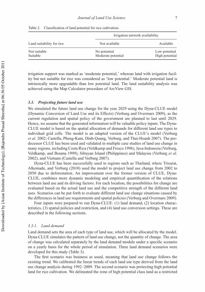
Analysis was performed by cross-tabulation of both criteria, which resulted in fourclasses of land potential for rice cultivation, as shown in Table 2. A nonsuitable landwithout irrigation support was considered as ‘no potential,’ while in contrast any suitableland with irrigation support was classified as ‘high potential.’ Suitable land but without

Dow

nloa

ded

by [A

sian

Insti

tute

of T

echn

olog

y], [

Raje

ndra

Pra

sad

Shre

stha]

at 0

6:36

05

Oct

ober

201

1

Journal of Land Use Science 7

Table 2. Classification of land potential for rice cultivation.

Irrigation network availability

Land suitability for rice Not available Available

Not suitable No potential Low potentialSuitable Moderate potential High potential

irrigation support was marked as ‘moderate potential,’ whereas land with irrigation facil-ity but not suitable for rice was considered as ‘low potential.’ Moderate potential land isintrinsically more upgradable than low potential land. The land suitability analysis wasachieved using the Map Calculator procedure of ArcView GIS.

3.3. Projecting future land use

We simulated the future land use change for the year 2029 using the Dyna-CLUE model(Dynamic Conversion of Land Use and its Effects) (Verburg and Overmars 2009), as thecurrent regulation and spatial policy of the government are planned to last until 2029.Hence, we assume that the generated information will be valuable policy inputs. The Dyna-CLUE model is based on the spatial allocation of demands for different land use types toindividual grid cells. The model is an adapted version of the CLUE’s model (Verburget al. 2002; Castella, Pheng-Kam, Dinh-Quang, Verburg, and Thai-Hoanh 2007). The pre-decessor CLUE has been used and validated in multiple case studies of land use change inmany regions, including Costa Rica (Veldkamp and Fresco 1996), Java-Indonesia (Verburg,Veldkamp, and Bouma 1999), Sibuyan Island (Philippines) and Malaysia (Verburg et al.2002), and Vietnam (Castella and Verburg 2007).

Dyna-CLUE has been successfully used in regions such as Thailand, where Trisurat,Alkemade, and Verburg (2010) used the model to project land use change from 2002 to2050 due to deforestation. An improvement over the former version of CLUE, Dyna-CLUE, combines more dynamic modeling and empirical quantification of the relationsbetween land use and its driving factors. For each location, the possibilities for change areevaluated based on the actual land use and the competitive strength of the different landuses. Scenarios can be put forth to evaluate different land use change situations caused bythe differences in land use requirements and spatial policies (Verburg and Overmars 2009).

Four inputs were prepared to run Dyna-CLUE: (1) land demand, (2) location charac-teristics, (3) spatial policies and restriction, and (4) land use conversion settings. These aredescribed in the following sections.

3.3.1. Land demand

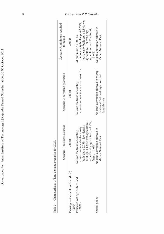
Land demand sets the area of each type of land use, which will be allocated by the model.Dyna-CLUE simulates the pattern of land use change, not the quantity of change. The areaof change was calculated separately by the land demand module under a specific scenarioon a yearly basis for the whole period of simulation. Three land demand scenarios weredeveloped for this study (Table 3).

The first scenario was business as usual, meaning that land use change follows theexisting trend. We calibrated the linear trends of each land use type derived from the landuse change analysis during 1992–2009. The second scenario was protecting high potentialland for rice cultivation. We delineated the zone of high potential class land as a restricted

Dow

nloa

ded

by [A

sian

Insti

tute

of T

echn

olog

y], [

Raje

ndra

Pra

sad

Shre

stha]

at 0

6:36

05

Oct

ober

201

1

8 Partoyo and R.P. Shrestha

Tabl

e3.

Cha

ract

eris

tics

ofla

ndde

man

dsc

enar

ios

for

2029

.

Scen

ario

1:bu

sine

ssas

usua

lSc

enar

io2:

farm

land

prot

ectio

nSc

enar

io3:

min

imum

requ

ired

farm

land

Exi

stin

gw

etag

ricu

lture

land

(km

2)

(200

4)43

8.81

438.

8143

8.81

Proj

ecte

dw

etag

ricu

lture

land

(202

9)Fo

llow

sth

etr

end

ofex

istin

gco

nver

sion

rate

(hig

h-de

nsity

built

-up,

+2.7

5%;l

ow-d

ensi

tybu

ilt-u

p,+1

.8%

;wet

agri

cultu

re,

$0.4

1%;d

ryag

ricu

lture

,$1.

2%;

fore

st,$

1.0%

)

Follo

ws

the

tren

dof

exis

ting

conv

ersi

onra

te(s

ame

assc

enar

io1)

Atm

inim

um40

.000

ha(h

igh-

dens

itybu

ilt-u

p,+2

.63%

;lo

w-d

ensi

tybu

ilt-u

p,+1

.8%

;wet

agri

cultu

re,$

0.39

%;d

ryag

ricu

lture

,$1.

2%;f

ores

t,$1

.0%

)Sp

atia

lpol

icy

No

land

conv

ersi

onal

low

edin

Mer

apiN

atio

nalP

ark

No

land

conv

ersi

onal

low

edin

Mer

api

Nat

iona

lPar

kan

dhi

ghpo

tent

ial

land

for

rice

No

land

conv

ersi

onal

low

edin

Mer

apiN

atio

nalP

ark

Dow

nloa

ded

by [A

sian

Insti

tute

of T

echn

olog

y], [

Raje

ndra

Pra

sad

Shre

stha]

at 0

6:36

05

Oct

ober

201

1

Journal of Land Use Science 9

area for land use other than wet agricultural land. This scenario supports the implementa-tion of agricultural land protection policy, which is currently still in the stage of initiation.The third scenario was setting 400 km2 as a minimum area of wet agricultural land thatshould be available by 2029. This value is based on a prediction by a document from theRegional Long-Term Development Plan (Rencana Pembangunan Jangka Panjang Daerah,RPJPD) year 2009–2029 of Yogyakarta Province (BAPPEDA-DIY 2009).

3.3.2. Location characteristics

The location characteristics included biophysical and socioeconomic factors that affect theland use allocation. These inputs are required to develop the binary logistic regressionmodel, as given in the equation below, which is used by Dyna-CLUE to calculate the prob-abilities of each land use type to be assigned to the preferred pixel. The regression modelsrelate to the occurrence of a land use type and the location characteristics.

Log!

Pi

(1 $ Pi)

"= !0 + !1X1i + !2X2i + · · · + !nXni (1)

where Pi is the probability of a grid cell for the occurrence of the considered land use typeon location i and the X’s are the location factors. The coefficients (!n) are estimated throughthe logistic regression using the land use pattern in 2004 as the dependent variable. We usedthe land use map for 2004 considering the most available ancillary data for location factors.

The regression models were developed for all land use/land cover types except for themiscellaneous type described in Table 1. The literature suggests that a number of factorscan play an important determining role in land use allocation or change, as summarized inTable 4.

We selected 14 factors as determinants of land use allocation or change based on localconditions. These factors were considered as independent variables in this study, includingphysical factors (e.g., elevation, slope, distance to road and capital city, land suitability,and irrigation support availability) and socioeconomic factors (e.g., population density andland ownership). Each factor was prepared as a raster map with a 30 m # 30 m grid size tomatch the resolution of the land use map of 2004.

It is better to use high-resolution data for representing detailed land feature; however,it is not clear whether finer scale information leads to more accurate modeling (Chen andPontius 2011). In our study, we maintained the most possible finest grid size consideringreality of land use/land cover change in the study area, data availability, and software limi-tation for simulation procedure. We developed land use maps from Landsat TM (30 m) andASTER Terralook (15 m) images. The ASTER Terralook images were converted to 30 mas all other images were of 30 m resolution. It would have been better to maintain a 30 mresolution, but the resolution of other coarser GIS data did not allow the 30 m resolution tobe maintained. Although observed conversion of wet agricultural land to nonagriculturalland was at subhectare size, the limitation of Dyna-CLUE in handling the maximum num-ber of grids constrained creating grid size smaller than 60 m # 60 m resolution to cover thestudy area.

To prepare input maps with required resolution to use in Dyna-CLUE, we had to down-scale land suitability map from the scale of 1:50.000 due to unavailability of large scalemap. Considering the area coverage, land use parcel size, and landscape and biophys-ical characteristics of the study area, the used map scale was found to be satisfactory,specifically in the lack of large resolution maps.

Dow

nloa

ded

by [A

sian

Insti

tute

of T

echn

olog

y], [

Raje

ndra

Pra

sad

Shre

stha]

at 0

6:36

05

Oct

ober

201

1

10 Partoyo and R.P. Shrestha

Tabl

e4.

Det

erm

inan

tsof

land

use

chan

ge.

Lan

dus

ech

ange

Maj

orde

term

inan

ts

Con

vers

ion

ofpr

ime

agri

cultu

rall

and

into

resi

dent

ial

and

indu

stri

alar

eain

the

case

ofJa

va(V

erbu

rget

al.

1999

)

Ele

vatio

n,sl

ope,

geol

ogic

alun

it;so

ilfe

rtili

ty,s

oild

rain

age,

soil

perm

eabi

lity,

soil

text

ure;

prec

ipita

tion,

tem

pera

ture

,sun

shin

e,ag

ro-c

limat

iczo

ne,n

umbe

rof

wet

mon

ths;

dist

ance

tone

ares

tcity

,to

near

estr

iver

,and

tone

ares

troa

d;po

pula

tion

dens

ity,f

ract

ion

rura

lpop

ulat

ion,

labo

rfo

rce

dens

ity,f

ract

ion

agri

cultu

rall

abor

forc

e,G

RD

P.U

rban

grow

thby

aca

sest

udy

ofW

uhan

City

inPR

Chi

na(C

heng

and

Mas

ser

2003

)D

ista

nce

toro

ads,

tora

ilway

lines

,to

indu

stri

alce

nter

s,to

city

cent

ers,

and

tori

vers

;de

nsity

ofne

ighb

orin

gw

ater

s,in

dust

rial

area

s,de

velo

pabl

ear

eas,

deve

lope

dar

ea;

popu

latio

nde

nsity

,spa

tialm

aste

rpl

an.

Lan

dus

ech

ange

patte

rns

inth

eN

ethe

rlan

ds(V

erbu

rg,

Rits

ema

van

Eck

,de

Nijs

,Dijs

t,an

dSc

hot,

2004

)E

leva

tion,

grou

ndw

ater

dept

han

dflu

ctua

tion;

soil

orga

nic

mat

ter

cont

ent,

soil

calc

ium

cont

ent,

soil

text

ure,

soil

pH;d

ista

nce

and

trav

eltim

eto

near

estr

ailw

ayst

atio

n,ai

rpor

t,an

dha

rbor

,dis

tanc

ean

dtr

avel

time

tone

ares

tjob

s,di

stan

ceto

near

est

mot

orw

ayin

ters

ectio

n,tr

avel

time

tone

ares

thig

hway

entr

ance

,dis

tanc

ean

dtr

avel

time

tone

ares

ttow

n/ci

ty,t

one

ares

tfor

est/

wat

erar

ea/c

oast

/mai

nri

ver;

nois

ele

vel;

enri

chm

entf

acto

rsfo

rne

ighb

orho

odre

side

ntia

llan

dus

e,in

dust

rial

/com

mer

cial

land

use,

recr

eatio

nall

and

use,

fore

st/n

atur

e;de

sign

ated

mun

icip

aliti

es,d

elin

eatio

nof

cent

ralo

pen

spac

e.R

esid

entia

land

indu

stri

al/c

omm

erci

alla

ndde

velo

pmen

tin

Lag

os,N

iger

ia(B

raim

ohan

dO

nish

i20

07)

Ele

vatio

n,sl

ope;

dist

ance

from

wat

er,d

ista

nce

from

prot

ecte

dfo

rest

,dis

tanc

efr

omw

ater

wor

ks,t

rave

ltim

eto

targ

ets

(maj

orro

ads,

Lag

osIs

land

,the

Cen

tral

Bus

ines

sdi

stri

ct,i

ndus

tria

lcen

ters

,air

port

,and

Har

bor)

;pop

ulat

ion

pote

ntia

l,ne

ighb

orho

odin

dice

s,sp

atia

lpol

icie

s,in

com

epo

tent

ial.

Not

e:G

RD

P,gr

oss

regi

onal

dom

estic

prod

uct.

Dow

nloa

ded

by [A

sian

Insti

tute

of T

echn

olog

y], [

Raje

ndra

Pra

sad

Shre

stha]

at 0

6:36

05

Oct

ober

201

1

Journal of Land Use Science 11

Elevation and slope were derived from the ASTER GDEM provided by METI andNASA at the website: http://www.gdem.aster.ersdac.or.jp/search.jsp. Accessibility was cal-culated as the distance to infrastructure and location centers, such as main road, districtcapital, regency capital, and provincial capital, using the ‘Find Distance’ function ofArcView based on a topographic raster map converted from a vector map of 1:25,000 scalepublished in 1994 by BAKOSURTANAL and an administrative map published in 2009 byBAPPEDA. The population density map was generated from the aggregated data basedon a district (kecamatan) level for 2004 published by BPS (Central Bureau of Statistics-Biro Pusat Statistik). A land ownership map was compiled from land tenure maps of2008 provided by BPN. One of the specific land ownership types in Yogyakarta is SultanGround/Pakualam Ground (SG/PAG), which requires a specific permit from the authorityof the Yogyakarta/Pakualaman kingdom to utilize such land as provisioned by the localculture.

A binary logistic regression analysis was carried out for each land use type, whichresulted in six regression models. To avoid the effect of spatial autocorrelation, the regres-sions were calculated based on selected random samples of grids. For each model, weevaluated the goodness-of-fit using the relative operating characteristics (ROC). The ROCcompares the observed values, that is, the binary data over the whole range of predictedprobabilities. An ROC value of 1.0 indicates a perfectly fit model and a value of 0.5 indi-cates a completely random model (Pontius and Schneider 2001; Braimoh and Onishi2007).

3.3.3. Spatial policies and restrictions

These inputs delineate areas where land use changes are restricted because of policy mea-sures, such as protected areas. We put the existing Merapi Mountain National Park as arestricted area in all scenarios. The park consists of a forest and shrub area surroundingMerapi volcano at the topmost altitude of the study area. In farmland protection scenarios,we put the national park and farmland preserved areas as restricted areas, and hence, nofurther land encroachment was allowed in these areas.

3.3.4. Land use conversion settings

These land use factors directed the dynamics of the simulations by two sets of parameters,namely, conversion elasticity and land use transition settings. The elasticity was estimatedby expert judgment based on capital investment, time, and energy costs needed in convert-ing the land use, ranging from 0 (easy conversion) to 1 (irreversible change), as explainedby Verburg et al. (2002). High values for this parameter were assigned to the built-up areaand forest because these land use types are not likely to be displaced. Medium values weregiven to agricultural land and mixed garden.

The Dyna-CLUE model uses all inputs to calculate the total probability for each gridcell of each land use type based on the local suitability of the location derived from thelogistic regression model, the conversion elasticity, and the competitive strength of the landuse type (Verburg and Overmars 2009). Where no constraints to a specific conversion werespecified, the location was allocated to the land use with the highest total suitability. Usingan iterative process, the competitive strength of the different land use types was adapteduntil the total allocated area of each land use equaled the total land requirements specifiedin the scenario.

Dow

nloa

ded

by [A

sian

Insti

tute

of T

echn

olog

y], [

Raje

ndra

Pra

sad

Shre

stha]

at 0

6:36

05

Oct

ober

201

1

12 Partoyo and R.P. Shrestha

4. Result and discussion

4.1. Land use change

Land use change was detected from land use maps derived from satellite images of theyears 1992, 2004, and 2009. Table 5 summarizes the area coverage of each land use typebased on the satellite image interpretation. In 1992, wet agricultural land was the predom-inant land use type in the study area, covering more than 35% of the area, compared withlow-density built-up land, mixed garden, and dry agricultural land, which covered 19.5%,21.7%, and 16.3%, respectively. These four land use types were also the major land usesin 2004 and 2009. Meanwhile, forest remained constant at approximately 5% of the studyarea during 1992–2009. High-density built-up land, which covered only 1.5% of the studyarea in 1992, significantly expanded to 4.1% and 5.4% in 2004 and 2009, respectively.

Figure 2 shows a clear expansion of built-up land in 1992, 2004, and 2009. The high-density built-up land expanded beyond the municipality boundary toward the northeastand southeast. Comparing the series of land use map, it can be clearly seen that the high-density built-up land has occupied formerly low-density built-up land and wet agriculturalland surrounding the municipality.

In 2009, it was found that some high-density built-up lands developed along the mainroads (Figure 2c). Meanwhile, low-density built-up land has sprawled into the formerlymassive wet agricultural land. This trend has increased land fragmentation, which in turnmay induce greater threats to farmland susceptibility against conversion.

By calculating the area, we found that the major changes in the study area were adecrease in wet and dry agricultural land and an increase in high- and low-density built-up land (Table 5). The prime farmland indicated by wet agricultural land was reduced byalmost 94 km2 in 2004 from 527.39 km2 in 1992, although it slightly increased by 2009.The high-density built-up land was increased by a factor of 2.8 in 2004 from 21.87 km2

in 1992, and it continuously increased until 2009. Meanwhile, low-density built-up landslightly decreased during 2004–2009 after significantly increasing from 293.45 km2 in1992 to more than 355 km2 in 2004.

There are two possible reasons for this development. First, it may be due to the imple-mentation of policies prohibiting land conversion launched by the local governments ofthe Sleman and Bantul regencies. Despite the BPN being in the regency level, the Slemanregency has also established a new institution called the Board of Regional Land Control

Table 5. Coverage area of the land use/land cover categories based on satellite imagesinterpretation.

1992 2004 2009 Change (km2)

LC typeArea(km2) %

Area(km2) %

Area(km2) % 1992–2004 2004–2009

Wet agricultural land 527.39 35.1 433.85 28.9 438.81 29.2 $93.54 4.96Dry agricultural land 244.45 16.3 291.09 19.4 220.78 14.7 46.64 $70.31Mixed garden 325.42 21.7 273.68 18.2 323.02 21.5 $51.74 49.34High-density built-up 21.87 1.5 61.06 4.1 81.32 5.4 39.19 20.26Low-density built-up 293.45 19.5 355.17 23.6 348.02 23.2 61.72 $7.15Forest 75.83 5.0 71.71 4.8 71.48 4.8 $4.12 $0.23Miscellaneous (river,

lava, etc.)13.99 0.9 15.70 1.0 18.83 1.3 1.71 3.13

Total 1502 100 1502 100 1502 100

Dow

nloa

ded

by [A

sian

Insti

tute

of T

echn

olog

y], [

Raje

ndra

Pra

sad

Shre

stha]

at 0

6:36

05

Oct

ober

201

1

Journal of Land Use Science 13

Figure 2. Land use/land cover maps interpreted from satellite images for the years: (a) 1992,(b) 2004, and (c) 2009.

(Badan Pengendalian Pertanahan Daerah, BPPD). Both institutions collaborate in landadministration and land conversion permit issuance. In the Bantul regency, the govern-ment has established tax exemptions for irrigated paddy fields as an incentive for farmersto sustain their farmland. Second, the upgrading of the existing irrigation infrastructurehas extended the coverage of irrigated command areas and prolonged the period of irri-gation water availability, thus making it possible to cultivate three crops of rice per year.We detected a third planting season of paddy fields in the July 2009 ASTER Terralookimage, which was otherwise not found in the image of 2004.

For a detailed understanding of the changes at the spatial level, a pixel-by-pixel landuse/land cover transition analysis was performed by superimposing a pair of digitally clas-sified images and producing a matrix of change. Table 6 shows that during 1992–2004,6.96 km2 and 43.11 km2 of wet agricultural lands in 1992 were converted to high- and low-density built-up areas, respectively, in 2004. Wet agricultural areas were also converted todry land and mixed garden land use, amounting to 77.71 km2 and 78.93 km2, respectively.

Dow

nloa

ded

by [A

sian

Insti

tute

of T

echn

olog

y], [

Raje

ndra

Pra

sad

Shre

stha]

at 0

6:36

05

Oct

ober

201

1

14 Partoyo and R.P. Shrestha

Table 6. Land use/land cover conversion between 1992, 2004, and 2009.

2004 (km2)

WetA DryA MixG HiBu LoBu Forest Misc 1992

1992 (km2) WetA 314.51 77.71 78.93 6.96 43.11 3.15 3.02 527.39DryA 45.98 88.66 51.93 2.33 49.46 5.19 0.9 244.45MixG 66.08 81.16 111.31 2.82 56.56 6.99 0.5 325.42HiBu 1.96 1.02 0.58 15.38 2.44 0.26 0.23 21.87LoBu 1.22 33.51 22.46 33.14 200.36 0.61 2.15 293.45Forest 1.26 7.41 7.86 0.15 2.01 54.57 2.57 75.83Misc 2.84 1.62 0.61 0.28 1.23 0.94 6.07 13.592004 433.85 291.09 273.68 61.06 355.17 71.71 15.44 1502.00

2009 (km2)

2004 (km2) WetA 309.8 40.41 48.73 4.71 25.69 1.5 3.01 433.85DryA 57.95 82.04 75.11 4.01 62.47 7.61 1.9 291.09MixG 51.99 44.25 117.1 2.06 48.81 8.9 0.57 273.68HiBu 6.86 3.3 2.15 44.32 4.22 0.1 0.11 61.06LoBu 6.85 46.1 67.26 26.12 204.6 2.12 2.12 355.17Forest 3.01 3.51 10.97 0 1.13 49.95 3.14 71.71Misc 2.35 1.17 1.70 0.10 1.10 1.30 7.72 15.442009 438.81 220.78 323.02 81.32 348.02 71.48 18.57 1502.00

Note: WetA, wet agricultural land; DryA, dry agricultural land; MixG, mixed garden; HiBu, high-density built-upland; LoBu, low-density built-up land; Misc, miscellaneous.

The latter was caused by either a permanent disruption of the irrigation water facility ortemporary use as dry agricultural land or mixed garden before a formal permit for buildingconstruction was issued by the government authorities.

A similar trend of increasing built-up land at the cost of wet agricultural land wasobserved during 2004–2009. Within a short period of 5 years, 4.71 km2 of wet agriculturalland was converted to high-density built-up land. The wet agricultural land that remainedunchanged from 2004 to 2009 was just 309.8 km2, even less than the area of 314.51 km2

during 1992–2004. Within both periods, high-density built-up areas were predominantlyconverted from low-density built-up areas, which were converted from formerly mixedgarden, dry agricultural land, or wet agricultural land. To a small extent, high density built-up areas were converted directly from wet agricultural land, dry agricultural land, or mixedgarden. The transition of land use change is summarized in Figure 3.

Figure 3 shows the pathways of change observed among the different types of landuse/land cover, particularly the most important change, that is, the conversion to built-up land. We excluded forest and miscellaneous types because both remained relativelyunchanged. The lines indicate pathways, while arrowheads indicate the direction of change.The thickness of the line indicates the intensity of change, while the numbers show thepercent area of change based on the initial land use/land cover. In Figure 3, it is apparentthat the wet agricultural land category appears as source of built-up land, either directly orindirectly.

The built-up land that was formerly wet agricultural land has been converted to meetthe demand of land for housing and industry due to urban development. This conversionhas occurred in various ways. Some rice field plots were directly converted to settlements.Because the conversion occurred either sporadically or massively in a block of plot, itresulted in a low-density and eventually a high-density built-up land. The growth of such

Dow

nloa

ded

by [A

sian

Insti

tute

of T

echn

olog

y], [

Raje

ndra

Pra

sad

Shre

stha]

at 0

6:36

05

Oct

ober

201

1

Journal of Land Use Science 15

High-densitybuilt-up land

1

0.88 0.9

1318

7

1213

Low-densitybuilt-up land

Mixed gardenDry agricultural

land

Wetagricultural

land

Figure 3. Pathways of land use/land cover change in the study area. The numbers show percentarea of change based on original land use/land cover.

new settlements has induced more pressure on the surrounding farmland plots for addi-tional conversion. The construction of the built-up land affected irrigation services due tothe disruption of irrigation facilities and the adverse impacts on irrigation, such as waterpollution. Some plots became less productive because of a lack of irrigation water avail-ability or poor irrigation water quality. In addition, the newly built-up land gradually raisedthe land price of the surrounding area, and this trend of increasing land price was a stimulusfor farmers to sell their plots rather than maintain them for cultivation.

4.2. Land potential for rice cultivation

We assessed the land potential for rice cultivation in the study area. This assessment indi-cated that 34.1% of the study area is suitable for rice cultivation, and 35.2% of the studyarea is supported by irrigation facilities (Table 7). In fact, the irrigation facilities also coverexisting rice fields at some locations of nonsuitable land for rice. The nonsuitable land wasmostly constrained by soil permeability that was too high, caused by coarse soil texture andlow fertility due to low organic matter and clay content (Puslittanak 1994). It is possible

Dow

nloa

ded

by [A

sian

Insti

tute

of T

echn

olog

y], [

Raje

ndra

Pra

sad

Shre

stha]

at 0

6:36

05

Oct

ober

201

1

16 Partoyo and R.P. Shrestha

Table 7. Distribution of land potential in the study area.

Irrigation support availabilityLand suitabilityfor rice Not available Available Total (%)

Not suitable No potential (52.8%) Low potential (13.1%) 65.9Suitable Moderate potential (12.0%) High potential (22.1%) 34.1Total 64.8% 35.2% 100.0

Table 8. Area of existing wet agricultural land according to land potential classification.

Area in 1992 Area in 2009 ChangeLand potentialclass km2 % km2 % km2 km2/year

High potential 189.70 35.97 170.26 38.8 $19.44 1.14Moderate potential 83.33 15.80 65.29 14.88 $18.04 1.06Low potential 84.75 16.07 68.81 15.68 $15.94 0.94No potential 169.61 32.16 134.45 30.64 $35.16 2.07Total 527.39 100 438.81 100 $88.58 5.21

to upgrade the potential of some land for rice cultivation by improving the soil quality.Currently, only 22.1% of the land in the study area has a high potential for rice cultivation.

A cross-tabulation of the maps on land potential and existing farmland in 1992 and2009 indicated an uneven distribution of farmland. Table 8 shows that rice has been culti-vated not only on high potential land but also on areas of low potential. Not more than 39%of wet agricultural land was situated on high potential land during 1992–2009. If we takeinto account the moderate potential land, which is suitable for rice cultivation but currentlywithout irrigation facilities, it accounts to approximately 15% of the total wetland area.The rest of the lands (46%) are of low or nonexistent potential.

Land use change analysis revealed that the wet agricultural land situated on the highpotential land suffered a 1.14 km2 loss per annum (Table 8). This result was confirmed withstatistics released by the Agency of Agriculture and Forestry of the Regency of Sleman andBantul located in the study area. The statistics show that during 2000–2008, the averageprime farmland converted to urban use was 1.09 km2 per annum (Dispertahanan 2009).As prime farmland, the conversion of this high potential land is considered a significantloss. In relation to rice cultivation, this negative trend might threaten rice-harvesting areas,which in turn will reduce rice production.

4.3. Farmland preservation

The Indonesian Law No. 41/2009 requires the government to develop a program offarmland preservation and farmland extension (RI 2009). The main cause of farmlandloss is the encroachment upon prime farmland by urban development. In the study area,high-density built-up land has been multiplied by a factor of 3.7 during 17 years, from21.87 km2 in 1992 to 81.32 km2 in 2009 (Table 9). Low-density built-up land, which con-sists of less dense settlements, also increased though at a lower rate. That both conversionsoccurred in high potential land is a serious concern for sustaining farmland preservation.

Dow

nloa

ded

by [A

sian

Insti

tute

of T

echn

olog

y], [

Raje

ndra

Pra

sad

Shre

stha]

at 0

6:36

05

Oct

ober

201

1

Journal of Land Use Science 17

Table 9. Land potential area coverage according to land use types in 1992 and 2009.

Land useNo

potentialLow

potentialModeratepotential

Highpotential Total

1992 (km2)Wet agricultural

land169.61 84.75 83.33 189.70 527.39

High-densitybuilt-up

17.70 1.39 0.97 1.82 21.87

Low-densitybuilt–up

150.42 49.11 36.26 57.66 293.45

2009 (km2)Wet agricultural

land134.45 68.81 65.29 170.26 438.81

High-densitybuilt-up

60.74 7.49 6.87 6.20 81.32

Low-densitybuilt-up

193.76 58.48 40.73 62.20 355.17

In summary, both high- and low-density built-up lands increasingly occupied high poten-tial land from approximately 59 km2 in 1992 to more than 68 km2 in 2009. This changewas approximately 14% of the total increase of built-up area during the same period.

At an average rice productivity of 6 tons GKG/hectare/season, as reported bythe Agency of Agriculture of Yogyakarta Province (Distan-DIY 2009), approximately1661 tons GKG per season have been lost solely due to the loss of high potential land as aresult of land conversion during the study period. The cumulative effect is enormous and isof serious concern. According to the Board of Food Security and Agricultural Extension ofYogyakarta, at least 400 km2 of paddy field should be preserved to fulfill the rice demand ofthe Yogyakarta population for the next 20 years (2029) (BAPPEDA-DIY 2009). Increasingcropping intensity can be an alternative to increase total rice production, but its contribu-tion will not be comparable to rice yield loss due to farmland conversion. Besides, increasein cropping intensity is not possible everywhere due to biophysical and irrigation limita-tions as high potential area suitable for rice is very limited (Table 7). Indeed, in those highlysuitable areas, growing three crops per year is already in practice.

4.4. Future land use simulation

As discussed earlier, 14 location factors were selected for the land use simulation. Amongthem, seven factors were continuous variables and the rest were binary variables (Table 10).With respect to altitudinal variation in the study area, the southern beach area has the lowestelevation, and the summit of Mount Merapi has the highest. The Bantul alluvial plain isflat, while the hilly area in the western and southeastern parts of the study area has a steepslope (Figure 1).

The binary logistic regression analysis for each land use type, using each type as abinary dependent variable and the 14 location factors as independent variables, resulted inthe regression estimates shown in Table 11. It can be seen from the table that not all of thelocation factors were included in the regression models, and each factor contributed differ-ently depending on the land use type. For high-density built-up land, all factors, except landproperty rights, the land owned by villages, and the lands of SG/PAG, were found to have

Dow

nloa

ded

by [A

sian

Insti

tute

of T

echn

olog

y], [

Raje

ndra

Pra

sad

Shre

stha]

at 0

6:36

05

Oct

ober

201

1

18 Partoyo and R.P. Shrestha

Table 10. Location factors for future land use simulation.

Variable name Variable scale Minimum Maximum

Elevation (m) Continuousvariable

0 2,960

Slope (%) Continuousvariable

0 72

Distance to mainroad (m)

Continuousvariable

0 4,141

Distance to district (m) Continuousvariable

0 5,250

Distance to regency (m) Continuousvariable

0 18,632

Distance to province (m) Continuousvariable

0 34,363

Land suitability for rice Binary variable 0 = not suitable 1 = suitableIrrigation support Binary variable 0 = not available 1 = availablePopulation density

(people/km2)Continuous

variable359 12,085

Land property right Binary variable 0 = nonproperty right 1 = property rightLand utilization right Binary variable 0 = nonutilization

right1 = utilization

rightLand owned by village Binary variable 0 = nonvillage land 1 = village landLand owned by state Binary variable 0 = nonstate land 1 = state landLand of SG/PAG Binary variable 0 = non-SG/PAG 1 = SG/PAG

Note: SG/PAG, Sultan Ground/Pakualam Ground.

significant relations. This result means that the development of high-density built-up landwas not done in consideration of private land tenure, although it was not preferable to buildon the land owned by the state or land with utilization rights. The latter was evidenced by anegative relation between high-density built-up and land utilization rights or land owned bythe state. It should be specifically noted that the land suitable for rice cultivation is highlycorrelated with high-density built-up areas, which implies that high-density built-up landwas developed at locations with a high potential for wet agriculture land. However, dryagricultural land was not a competitor of wet agricultural land because it does not needland suitability for rice and irrigation facilities.

Accessibility-related factors (distance to road, district, and province) showed a negativerelationship with high-density built-up land because of more evidence that this type of landis located close to roads, districts, and provincial capitals. In contrast, a positive relationshipbetween the distance to the regency and high-density built-up land could be due to thistype of land usually being away from the regency. Housing and building developers preferto build in district areas because of cheaper land prices and the greater convenience of thenatural environment. As commonly found, provincial capital was surrounded by a denserbuilt-up area than regency capital. Table 11 shows that low-density built-up land had anegative relationship with distance to regency but a positive relationship with distanceto province, meaning the low-density built-up land was developed close to the regencyand away from the provincial capital. Low-density built-up land was also related to landwith utilization rights, land owned by the state, and the land of the SG/PAG. Currently,low-density built-up land is widespread for these types of land ownership.

The spatial distributions of the seven land use types were explained moderately towell by the selected location factors, as indicated by the ROC values that ranged from

Dow

nloa

ded

by [A

sian

Insti

tute

of T

echn

olog

y], [

Raje

ndra

Pra

sad

Shre

stha]

at 0

6:36

05

Oct

ober

201

1

Journal of Land Use Science 19

Table 11. !-Values of location factors for binary logistic regressions of each land use type.

VariableHigh-densitybuilt-up land

Low-densitybuilt-up land

Wetagricultural

land

Dryagricultural

landMixedgarden Forest

Elevation (m) 0.004 $0.002 $0.003 $0.002 n.s. 0.006Slope (%) $0.13 n.s. $0.04 0.09 0.04 $0.22Distance to

mainroad (m)

$0.0005 n.s. 0.00009 0.0002 0.0001 $0.0003

Distance todistrict (m)

$0.0001 $0.00008 0.0001 0.0001 0.0001 n.s.

Distance toregency (m)

0.0001 $0.00005 $0.00005 $0.00004 $0.00006 n.s.

Distance toprovince (m)

$0.0003 0.0001 0.0001 0.00008 n.s. 0.0002

Landsuitabilityfor rice

0.56 $0.23 $0.93 n.s. n.s. n.s.

Irrigationsupport

$1.10 0.27 1.21 n.s. n.s. $2.49

Populationdensity(people/km2)

0.00001 n.s. n.s. $0.00001 n.s. $0.0001

Land propertyright

n.s. n.s. n.s. n.s. $0.46 n.s.

Landutilizationright

$1.95 2.81 2.73 n.s. n.s. $2.70

Land ownedby village

n.s. n.s. n.s. n.s. n.s. n.s.

Land ownedby state

$1.29 1.45 n.s. 1.05 2.36 n.s.

Land ofSG/PAG

n.s. 1.75 1.44 n.s. $1.11 n.s.

Constant 5.26 $8.36 $6.14 $4.21 $5.08 $0.75ROC 0.94 0.76 0.83 0.81 0.82 0.99

Note: n.s. = not significant at 0.05 level; SG/PAG, Sultan Ground/Pakualam Ground; ROC, relative operatingcharacteristic.

0.76 to 0.99 (Table 11). The lowest ROC of low-density built-up land (0.76) was due to thewidespread location of this land use type in the study area.

Considering the long-term existing trend from 1992 to 2009, the farmland loss isexpected to continue. Based on the logistic regression estimates summarized in Table 11and scenarios described in Table 3, the simulation of land use change from 2004 to2029 using Dyna-CLUE resulted in different patterns of land use (Figure 5).

For validation purposes, we ran Dyna-CLUE to project a land use map from 2004 to2009 under the existing trend scenario. We compared this projected map (Figure 5a) tothe actual land use map of 2009 derived from the satellite image interpretation (Figure 2c).Under visual examination, both maps looked similar. The high-density built-up land clearlyshowed a similar extent and pattern. We can track that some high-density built-up areaswere developed along the main roads. Wet agricultural land, mixed garden, and forestwere also spread out in a similar pattern. This good conformity implies the validity of the

Dow

nloa

ded

by [A

sian

Insti

tute

of T

echn

olog

y], [

Raje

ndra

Pra

sad

Shre

stha]

at 0

6:36

05

Oct

ober

201

1

20 Partoyo and R.P. Shrestha

Dyna-CLUE model for simulating future land use change in the study area. In addition, astatistical approach was performed to validate the model. We calculated the ROC for eachland use type between the projected map and the reference map. The ROC demonstratedhow well the projected map matched the location shown on the reference map (Pontius andSchneider 2001). An ROC of 0.5 indicates a conformity equivalent to random chance whenthe grid cells are difficult to classify. An ROC of 1 indicates perfect conformity (Pontiusand Chen 2006). Table 12 shows that the ROC of each land use type ranged between0.54 and 0.83. The lowest ROC showed slightly better conformity of low-density built-up land with random locations, which means that the location of land use projected bythe model conformed to the reference map. The higher ROC of all other land use typesimplied that, as a whole, the model projected a valid future land use map. Based on theROC value, the prediction was better for the high-density built-up, forest, mixed garden,wet agricultural land, dry agricultural land, and low-density built-up land use types.

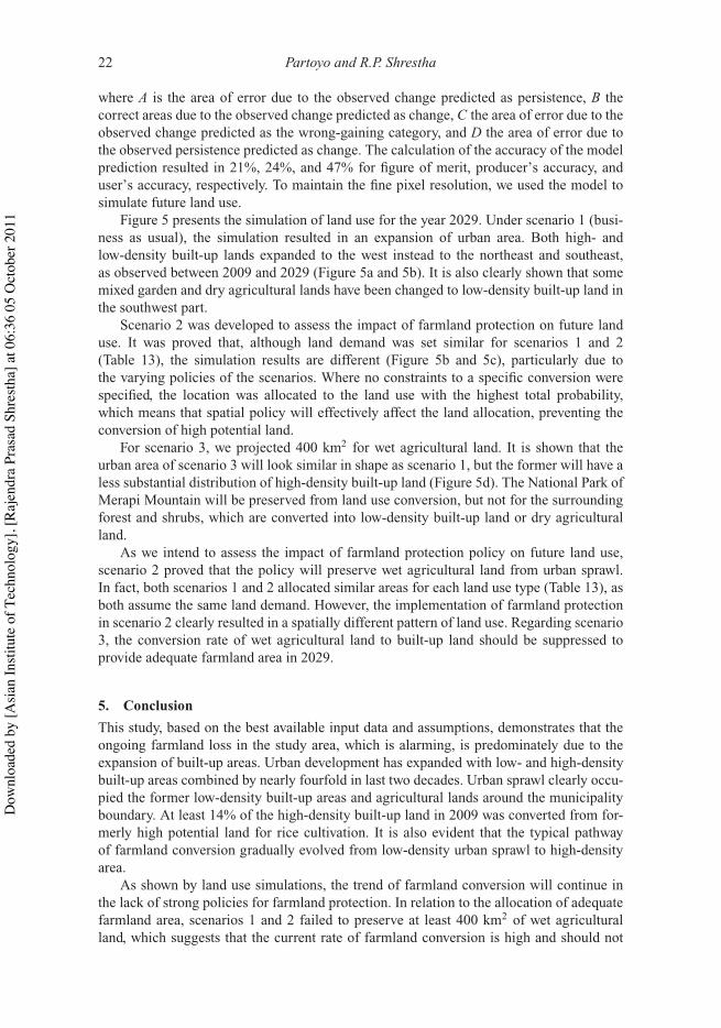
Aside from the above validation for the location of change (i.e., pattern), the model wasalso validated for the quantity of change. By design, Dyna-CLUE simulates the quantityof change with a land demand module using various scenarios. The predictive accuracyof the model for the quantity of change was validated based on a three-map comparisontechnique (Pontius et al. 2008), that is, the reference map of 2004, the reference map of2009, and the predicted map of 2009. Figure 4 presents the results of the overlay of thethree maps.

The black pixels in Figure 4 show where the model predicted change correctly. The darkgray pixels show where the change was observed and the model predicted change; however,the model predicted conversion in the wrong category. The medium gray pixels show theerrors where change was observed at locations where the model predicted persistence. Thelight gray pixels show errors where persistence was observed at locations where the modelpredicts change. The white pixels show locations where the model predicted persistencecorrectly.

Figure 4 allows a visual assessment of the nature of the prediction errors, which arevarious shades of gray. The model is less accurate than its corresponding null model, asthere are more light gray pixels than black pixels, which is common for models using finepixel resolution and for land use change, which includes a large portion of persistenceareas. This result was also indicated by the calculation of the accuracy of the model’sprediction for the quantity of change using values of figures of merit, producer’s accuracy,and user’s accuracy (Pontius et al. 2008) based on the following equations:

Table 12. ROC between projected map and reference map of year2009 for each land use type.

Land use type ROC

High-density built-up 0.83Low-density built-up 0.54Wet agricultural land 0.60Dry agricultural land 0.57Mixed garden 0.62Forest 0.80

Note: ROC, relative operating characteristic.

Dow

nloa

ded

by [A

sian

Insti

tute

of T

echn

olog

y], [

Raje

ndra

Pra

sad

Shre

stha]

at 0

6:36

05

Oct

ober

201

1

Journal of Land Use Science 21

Figure 4. Validation map obtained by overlaying the reference map of year 2004, reference map ofyear 2009, and prediction map for year 2009.

Figure of merit = B(A + B + C + D)

(2)

Producer saccuracy = B(A + B + C)

(3)

User"s accuracy = B(B + C + D)

(4)

Dow

nloa

ded

by [A

sian

Insti

tute

of T

echn

olog

y], [

Raje

ndra

Pra

sad

Shre

stha]

at 0

6:36

05

Oct

ober

201

1

22 Partoyo and R.P. Shrestha

where A is the area of error due to the observed change predicted as persistence, B thecorrect areas due to the observed change predicted as change, C the area of error due to theobserved change predicted as the wrong-gaining category, and D the area of error due tothe observed persistence predicted as change. The calculation of the accuracy of the modelprediction resulted in 21%, 24%, and 47% for figure of merit, producer’s accuracy, anduser’s accuracy, respectively. To maintain the fine pixel resolution, we used the model tosimulate future land use.

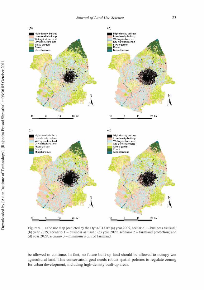
Figure 5 presents the simulation of land use for the year 2029. Under scenario 1 (busi-ness as usual), the simulation resulted in an expansion of urban area. Both high- andlow-density built-up lands expanded to the west instead to the northeast and southeast,as observed between 2009 and 2029 (Figure 5a and 5b). It is also clearly shown that somemixed garden and dry agricultural lands have been changed to low-density built-up land inthe southwest part.

Scenario 2 was developed to assess the impact of farmland protection on future landuse. It was proved that, although land demand was set similar for scenarios 1 and 2(Table 13), the simulation results are different (Figure 5b and 5c), particularly due tothe varying policies of the scenarios. Where no constraints to a specific conversion werespecified, the location was allocated to the land use with the highest total probability,which means that spatial policy will effectively affect the land allocation, preventing theconversion of high potential land.

For scenario 3, we projected 400 km2 for wet agricultural land. It is shown that theurban area of scenario 3 will look similar in shape as scenario 1, but the former will have aless substantial distribution of high-density built-up land (Figure 5d). The National Park ofMerapi Mountain will be preserved from land use conversion, but not for the surroundingforest and shrubs, which are converted into low-density built-up land or dry agriculturalland.

As we intend to assess the impact of farmland protection policy on future land use,scenario 2 proved that the policy will preserve wet agricultural land from urban sprawl.In fact, both scenarios 1 and 2 allocated similar areas for each land use type (Table 13), asboth assume the same land demand. However, the implementation of farmland protectionin scenario 2 clearly resulted in a spatially different pattern of land use. Regarding scenario3, the conversion rate of wet agricultural land to built-up land should be suppressed toprovide adequate farmland area in 2029.

5. Conclusion

This study, based on the best available input data and assumptions, demonstrates that theongoing farmland loss in the study area, which is alarming, is predominately due to theexpansion of built-up areas. Urban development has expanded with low- and high-densitybuilt-up areas combined by nearly fourfold in last two decades. Urban sprawl clearly occu-pied the former low-density built-up areas and agricultural lands around the municipalityboundary. At least 14% of the high-density built-up land in 2009 was converted from for-merly high potential land for rice cultivation. It is also evident that the typical pathwayof farmland conversion gradually evolved from low-density urban sprawl to high-densityarea.

As shown by land use simulations, the trend of farmland conversion will continue inthe lack of strong policies for farmland protection. In relation to the allocation of adequatefarmland area, scenarios 1 and 2 failed to preserve at least 400 km2 of wet agriculturalland, which suggests that the current rate of farmland conversion is high and should not

Dow

nloa

ded

by [A

sian

Insti

tute

of T

echn

olog

y], [

Raje

ndra

Pra

sad

Shre

stha]

at 0

6:36

05

Oct

ober

201

1

Journal of Land Use Science 23

Figure 5. Land use map predicted by the Dyna-CLUE: (a) year 2009, scenario 1 – business as usual;(b) year 2029, scenario 1 – business as usual; (c) year 2029, scenario 2 – farmland protection; and(d) year 2029, scenario 3 – minimum required farmland.

be allowed to continue. In fact, no future built-up land should be allowed to occupy wetagricultural land. This conservation goal needs robust spatial policies to regulate zoningfor urban development, including high-density built-up areas.

Dow

nloa

ded

by [A

sian

Insti

tute

of T

echn

olog

y], [

Raje

ndra

Pra

sad

Shre

stha]

at 0

6:36

05

Oct

ober

201

1

24 Partoyo and R.P. Shrestha

Table 13. Coverage area of each land use type projected by 2029.

Area (km2)Scenario 1:

business as usualScenario 2: farmland

protectionScenario 3: minimum

required farmland

High-densitybuilt-up

105.99 105.99 95.18

Low-densitybuilt-up

526.63 526.63 515.77

Wet agriculturalland

389.19 389.19 400.00

Dry agriculturalland

201.41 201.41 223.04

Mixed garden 206.92 206.92 223.14Forest 58.24 58.24 31.26Miscellaneous 13.62 13.62 13.62

To secure food production, farmland preservation should be given priority againstthe increasing trend of agricultural land conversion to nonagricultural use. Land poten-tial evaluation based on land suitability for rice and the availability of irrigation servicesto delineate the potential areas can be useful in this regard. This should be supported bydesigning and implementing a proper spatial policy for the preservation of such importantland.

AcknowledgmentsThis research was financially supported by the DIKTI Scholarship of the Government of the Republicof Indonesia. The authors gratefully acknowledge Prof. Peter H. Verburg for allowing us to usethe full version of Dyna-CLUE and for the necessary guidance on the software. They also thankProf. Junun Sartohadi and his colleagues for providing digital maps and field assistance. They aregrateful to the anonymous reviewers for their valuable comments and suggestions that enhanced themanuscript. Thanks are also due to GLCF (Global Land Cover Facility), USGS Glovis (United StatesGeological Survey-Global Visualization, METI (the Ministry of Economy, Trade and Industry) ofJapan and US NASA for the free download of remote sensing data.

ReferencesAARD (2003), Technical Guidelines for Land Evaluation for Agricultural Commodities, Bogor:

Agency for Agriculture Research and Development [in Indonesian].Alterman, R. (2001), “Farmland Preservation,” in International Encyclopedia of the Social &

Behavioral Sciences, eds. J.S. Neil and B.B. Paul, Oxford: Pergamon, pp. 5406–5411.Apriyantono, A. (2007), “Preventing food crisis, Indonesia needs 15 million hectares of agriculture

land,” [In Indonesian], http://www.deptan.go.id/news/.BAPPEDA-DIY (2007), Natural Resources Balance of Yogyakarta, Yogyakarta: Board of Planning

and Development of Province of Yogyakarta Special Region [in Indonesian].BAPPEDA-DIY (2008), Regional Medium-Term Development Plan of Province of Yogyakarta

Special Region – Year 2009–2013, Yogyakarta: Board of Planning and Development of Provinceof Yogyakarta Special Region [in Indonesian].

BAPPEDA-DIY (2009), Regional Long-Term Development Plan of Province of Yogyakarta SpecialRegion – Year 2009–2029, Yogyakarta: Board of Planning and Development of Province ofYogyakarta Special Region [in Indonesian].

BPS-DIY (2008), DI Yogyakarta in Figures, Yogyakarta: BPS-Statistics of DI Yogyakarta.BPS-RI (2005), “Population per Province,” [In Indonesian], http://www.datastatistik-indonesia.com/

component/option,com_tabel/kat,1/idtabel,111/Itemid,164/.

Dow

nloa

ded

by [A

sian

Insti

tute

of T

echn

olog

y], [

Raje

ndra

Pra

sad

Shre

stha]

at 0

6:36

05

Oct

ober

201

1

Journal of Land Use Science 25

BPS-RI (2010), Result of Population Census 2010: Agregat Data per Province, Jakarta: Badan PusatStatistik Republik Indonesia [in Indonesian].

Braimoh, A.K., and Onishi, T. (2007), “Spatial Determinants of Urban Land Use Change in Lagos,Nigeria,” Land Use Policy, 24, 502–515.

Castella, J.C., Pheng-Kam, S., Dinh-Quang, D., Verburg, P.H., and Thai-Hoanh, C. (2007),“Combining Top-Down and Bottom-up Modelling Approaches of Land Use/Cover Changeto Support Public Policies: Application to Sustainable Management of Natural Resources inNorthern Vietnam,” Land Use Policy, 24, 531–545.

Castella, J.C., and Verburg, P.H. (2007), “Combination of Process-Oriented and Pattern-OrientedModels of Land-Use Change in a Mountain Area of Vietnam,” Ecological Modelling, 202,410–420.

Chen, H., and Pontius, R.G., Jr. (2011), “Sensitivity of a Land Change Model to Pixel Resolution andPrecision of the Independent Variable,” Environmental Modeling and Assessment, 16, 37–52.

Cheng, J., and Masser, I. (2003), “Urban Growth Pattern Modeling: A Case Study of Wuhan City,PR China,” Landscape and Urban Planning, 62, 199–217.

Coughlin, R.E. (1991), “Formulating and Evaluating Agricultural Zoning Programs,” Journal of theAmerican Planning Association, 57, 183–192.

Daniels, T.L. (1991), “The Purchase of Development Rights: Preserving Agricultural Land and OpenSpace,” Journal of the American Planning Association, 57, 421–431.

Daniels, T.L., and Nelson, A.C. (1986), “Is Oregon’s Farmland Preservation Program Working?,”Journal of the American Planning Association, 52, 22–32.

Deptan-RI (2008), “Reaching 110,000 Hectare per Year, Land Conversion Threatens Food Security,”[In Indonesian], http://222.124.164.132/web/detail.php?sid=185872&actmenu=44.

Ding, C. (2003), “Land Policy Reform in China: Assessment and Prospects,” Land Use Policy, 20,109–120.

Dispertahanan (2009), Statistics of Foodstuff Crop 2009, Sleman: Agency of Agriculture and Forestryof Sleman Regency [in Indonesian].

Distan-DIY (2009), Statistics of Foodstuff Crop 2009, Yogyakarta: Agency of Agriculture of Provinceof Yogyakarta Special Region [in Indonesian].

FAO (1976), A Framework for Land Evaluation, Rome: Food and Agriculture Organization of theUnited Nations.

FAO (2002), World Agriculture: Towards 2015/2030 Summary Report, Rome: Food and AgricultureOrganization of the United Nations.

Firman, T. (1997), “Land Conversion and Urban Development in the Northern Region of West Java,Indonesia,” Urban Studies, 34, 1027–1046.

Firman, T. (2004), “Major Issues in Indonesia’s Urban Land Development,” Land Use Policy, 21,347–355.

Heilig, G.K. (1999), “Can China Feed Itself? – A System for Evaluation of Policy Options,” http://www.iiasa.ac.at/Research/SRD/ChinaFood/index_h.htm.

Jensen, J.R., and Cowen, D.C. (1999), “Remote Sensing of Urban/Suburban Infrastructure andSocio-Economic Attributes,” Photogrammetric Engineering and Remote Sensing, 65, 611–622.

Li, G., Zhou, F., and Chen, J. (2006), “Urban Sprawl and Its Intrinsic Characteristics of CantonalSuzhou From 1984 to 2003,” Chinese Journal of Ecology, 25, 1223–1228.

Lichtenberg, E., and Ding, C. (2008), “Assessing Farmland Protection Policy in China,” Land UsePolicy, 25, 59–68.

Lin, G.C.S. (2007), “Reproducing Spaces of Chinese Urbanisation: New City-Based and Land-Centred Urban Transformation,” Urban Studies, 44, 1827–1855.

Mariyono, J., Harini, R., and Agustin, N.K. (2007), “Impact of Economic Development andPopulation Growth on Agricultural Land Conversion in Jogjakarta: A Dynamic Analysis,”Journal Ekonomi Pembangunan, 8, 50–61.

Mundia, C.N., and Aniya, M. (2006), “Dynamics of Landuse/Cover Changes and Degradation ofNairobi City, Kenya,” Land Degradation and Development, 17, 97–108.

Nelson, A.C. (1992), “Preserving Prime Farmland in the Face of Urbanization: Lessons FromOregon,” Journal of the American Planning Association, 58, 467–488.

Pontius, R.G., Jr, Boersma, W., Castella, J.C., Clarke, K., Nijs, T., Dietzel, C., Duan, Z., Fotsing,E., Goldstein, N., Kok, K., Koomen, E., Lippitt, C.D., McConnell, W., Mohd Sood, A.,Pijanowski, B., Pithadia, S., Sweeney, S., Trung, T.N., Veldkamp, A.T., and Verburg, P.H. (2008),

Dow

nloa

ded

by [A

sian

Insti

tute

of T

echn

olog

y], [

Raje

ndra

Pra

sad

Shre

stha]

at 0

6:36

05

Oct

ober

201

1

26 Partoyo and R.P. Shrestha

“Comparing the Input, Output, and Validation Maps for Several Models of Land Change,”Annals of Regional Science, 42, 11–37.

Pontius, R.G., and Chen, H. (2006), “GEOMOD Modeling: Land-Use & Cover Change Modeling,”http://www.clarku.edu/~rpontius/pontius_chen_2006_idrisi.pdf.

Pontius, R.G., and Schneider, L.C. (2001), “Land Use Change Model Validation by an ROC Methodfor the Ipswich Watershed, Massachusetts, USA,” Agriculture, Ecosystem and Environment, 85,239–248.

PSE-KP (2007), “Policy for Establishing Permanent Food Farming Land,” [In Indonesian], http://pse.litbang.deptan.go.id/ind/index.php?option=com_content&task=view&id=418&Itemid=1.

Puslittanak (1994), Final Report of Survey and Mapping of Land Resources for AgricultureDevelopment, Land Rehabilitation and Soil Conservation, and Watershed Development inYogyakarta Special Province (Scale 1:50,000), Bogor: Centre for Soil and Agroclimate Research,Department of Agriculture Republic of Indonesia [in Indonesian].

RI (2009), “Law No.41/2009 about Sustainable Food Farming Land,” [In Indonesian], http://www.setneg.go.id/index.php?option=com_perundangan&id=2349&task=detail&catid=1&Itemid=42&tahun=2009.

Setiawan, H., Mathieu, R., and Thompson-Fawcett, M. (2006), “Assessing the Applicability of theV-I-S Model to Map Urban Land Use in the Developing World: Case Study of Yogyakarta,Indonesia,” Computers, Environment and Urban Systems, 30, 503–522.

Seto, K.C., Woodcock, C.E., Song, C., Huang, X., Lu, J., and Kaufmann, R.K. (2002), “MonitoringLand-Use Change in the Pearl River Delta Using Landsat TM,” International Journal of RemoteSensing, 23, 1985–2004.

Tan, M., Li, X., Xie, H., and Lu, C. (2005), “Urban Land Expansion and Arable Land Loss in China:A Case Study Of Beijing-Tianjin-Hebei Region,” Land Use Policy, 22, 187–196.

Trisurat, Y., Alkemade, R., and Verburg, P.H. (2010), “Projecting Land-Use Change and ItsConsequences for Biodiversity in Northern Thailand,” Environmental Management, 45,626–639.

Veldkamp, A., and Fresco, L.O. (1996), “CLUE-CR, An Integrated Multi-Scale Model to SimulateLand Use Change Scenarios in Costa Rica,” Ecological Modelling, 91, 231–248.

Verburg, P.H., and Overmars, K.P. (2009), “Combining Top-Down and Bottom-up Dynamics in LandUse Modeling, Exploring the Future of Abandoned Farmlands in Europe With the Dyna-ClueModel,” Landscape Ecology, 24, 1167–1181.

Verburg, P.H., Ritsema van Eck, J.R., de Nijs, T.C.M., Dijst, M.J., and Schot, P. (2004), “Determinantsof Land-Use Change Patterns in the Netherlands,” Environment and Planning B: Planning andDesign, 31, 125–150.

Verburg, P.H., Soepboer, W., Veldkamp, A., Limpiada, R., Espaldon, V., and Mastura, S.S.A. (2002),“Modeling the Spatial Dynamics of Regional Land Use: The CLUE-S Model,” EnvironmentalManagement, 30, 391–405.

Verburg, P.H., Veldkamp, T.A., and Bouma, J. (1999), “Land Use Change under Conditions of HighPopulation Pressure: The Case of Java,” Global Environmental Change, 9, 303–312.

Xiao, R., Weng, Q., Ouyang, Z., Li, W., Schienke, E.W., and Zhang, Z. (2008), “Land SurfaceTemperature Variation and Major Factors in Beijing, China,” Photogrammetric Engineering andRemote Sensing, 74, 451–461.

Yang, H., and Li, X.B. (2000), “Cultivated Land and Food Supply in China,” Land Use Policy, 17,73–88.

Yili, L., Xuezhi, F., Pengfeng, X., Chenglei, S., and Jia, S. (2009), “Urban Heat Island in Summer ofNanjing Based on TM Data,” in Urban Remote Sensing Event, 2009 Joint, pp. 1–5.

Yunus, H.S. (1990), “Searching New Strategies for Managing and Controlling Urban Land Growth:A Preliminary Outlook on Indonesia,” The Indonesian Journal of Geography, 20, 1–10.

Dow

nloa

ded

by [A

sian

Insti

tute

of T

echn

olog

y], [

Raje

ndra

Pra

sad

Shre

stha]

at 0

6:36

05

Oct

ober

201

1