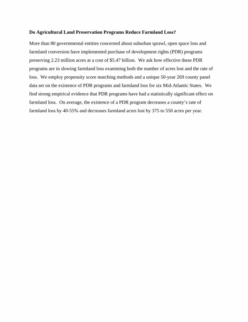
Do Agricultural Land Preservation Programs Reduce Farmland Loss?

Evidence from a Propensity Score Matching Estimator

Xiangping Liu and Lori Lynch

January 2010

Center for Environmental and Resource Economic Policy, Department of Agricultural Economics North Carolina State University Raleigh, NC 27695 919-513-3864 (tel) xiangping_liu@ncsu.edu Department of Agricultural and Resource Economics

2200 Symons Hall University of Maryland College Park, MD 20742 USA 301-405-1264 (tel.) 301-314-9091 (fax) llynch@arec.umd.edu Keywords: Land preservation programs, Purchase of Development Rights (PDR) program, farmland, propensity score, land conversion, urban-rural interface, open-space, resource conservation. Xiangping Liu is a Post-Doctoral Research Associate in the Center for Environmental and Resource Economic Policy, North Carolina State University. Lori Lynch is a Professor in the Department of Agricultural and Resource Economics, University of Maryland. Support for this project was provided by the Harry Hughes Center for Agro-Ecology, Inc. and the Center for Smart Growth Education and Research. We would like to thank Liesl Koch and Janet Carpenter for their research assistance. In addition, the project has benefited from the comments of John List, Jeffrey Smith, Andreas Lange, Erik Lichtenberg, Barrett Kirwan, Laura Taylor, Daniel Phaneuf, and Wally Thurman. As always, any errors remain the full responsibility of the authors.

Do Agricultural Land Preservation Programs Reduce Farmland Loss?

More than 80 governmental entities concerned about suburban sprawl, open space loss and

farmland conversion have implemented purchase of development rights (PDR) programs

preserving 2.23 million acres at a cost of $5.47 billion. We ask how effective these PDR

programs are in slowing farmland loss examining both the number of acres lost and the rate of

loss. We employ propensity score matching methods and a unique 50-year 269 county panel

data set on the existence of PDR programs and farmland loss for six Mid-Atlantic States. We

find strong empirical evidence that PDR programs have had a statistically significant effect on

farmland loss. On average, the existence of a PDR program decreases a county’s rate of

farmland loss by 40-55% and decreases farmland acres lost by 375 to 550 acres per year.

1

Do Agricultural Land Preservation Programs Reduce Farmland Loss?

Introduction

Concerns about suburban sprawl, open space loss and farmland conversion have led

states, counties, municipalities and regional groups to institute programs that arrest or slow land

conversion. Beginning in 1978, Purchase of Development Rights (PDR) programs have been

removing the rights to convert undeveloped lands to promote a continued resource use. These

programs usually attach an easement to a property that restricts the right to convert the land to

residential, commercial and industrial uses in exchange for cash payments and/or tax benefits.

The PDR programs are justified on various grounds including improving efficient development

of urban and rural land, securing local and national food supplies, maintaining the viability of the

local agricultural economy, and protecting rural and environmental amenities (Gardner, 1977;

Hellerstein et al., 2002). While from society’s perspective, the viability of the agricultural

sector, retaining a critical mass of land, and protecting the value of environmental amenities are

all important; they cannot be achieved in the long-run without slowing or arresting farmland loss.

Therefore, we focus on the impact of PDR programs in reducing farmland loss.1

Twenty-three states have state-level PDR programs and 57 local governments operate

PDR programs (American Farmland Trust (AFT), 2009; AFT, 2008) and over 2.23 million acres

are in preserved status as a result. Spending in both state and local programs to purchase these

acres was $5.47 billion (AFT, 2009; AFT, 2008). Citizens continue to pass ballot initiatives to

generate funds to retain open space including farmland: in 2002, $5.7 billion in conservation

funding was authorized; in 2006, $5.73 billion, and in 2008, $8.4 billion (Land Trust Alliance

1 While citizens may support these programs to retain open space rather than farmland or forest per se - they are willing to pay to retain the implicit services provided by these (open space) lands.

2

and Trust for Public Lands, 2008). In 1996, the federal government developed the Farmland

(and Ranchland) Protection Program to provide funding for state and local preservation

programs.

While some evidence exists that PDR programs provide net benefits to society (Feather

and Barnard, 2003; Duke and Ilvento, 2004), little evaluation has been conducted on their

effectiveness in preventing the conversion of farmland. Several studies have evaluated the

impact of (non-permanent) use-value taxation programs that aim to arrest farmland loss (Blewitt

and Lane 1988; Gardner 1994; Lynch and Carpenter 2003; Parks and Quimio 1996). Those

studies found that these programs can impact farmland loss but their impact may be small and

short-term. Few studies examine the impact of the permanent easements conferred by the PDR

programs except for Lynch and Carpenter (2003) and Hailu and Brown (2007). Both studies find

no impact of PDR programs on reducing farmland loss.

We study whether PDR programs reduce farmland loss in the Mid-Atlantic States using a

unique 50-year, 269 county panel dataset on the existence of PDR programs and farmland loss.

We focus on both state and local PDR programs and measure farmland loss as both the rate of

loss and the number of acres lost at the county level. We find strong empirical evidence that PDR

programs have slowed farmland loss.

Assessing the impact of permanent preservation through PDR programs on farmland loss

can be empirically challenging. One cannot construct the proper counterfactual, i.e., one would

like to know what would have happened to the rate and acres of farmland loss in a county with a

PDR program (hereafter a PDR county ) had it not implemented a PDR program. However, a

PDR county cannot be in two states simultaneously, nor can a researcher randomly assign which

3

county has a PDR program and which does not. If PDR programs are established in those

counties with the highest rates of farmland loss and/or the lowest number of farmland acres, the

very existence of the PDR program itself may be predicated on farmland loss. Thus assuming

the programs’ existence was exogenous as was implicitly done by Lynch and Carpenter (2003)

and Hailu and Brown (2007) may be an explanation for the insignificant results.

Nor is simply examining acres preserved sufficient for assessing a program’s impact on

farmland loss. If the PDR programs do not preserve the parcels that would be converted and

instead enrolls those parcels unlikely to be converted, their impact on land conversion may be

insignificant. An example can be seen in Lynch and Liu (2007) who find that a preservation

program increase the number of acres preserved within designated preservation areas but it had

no impact on the rate of land conversion in these areas. In addition, recent evidence suggests

that the positive amenities generated by preservation programs may increase the demand for

housing (and thus land) near the preserved parcels. This demand may create more conversion

pressure and higher housing prices, leading to even further farmland conversion. For example,

Roe, Irwin, and Morrow-Jones (2004) find that preservation efforts themselves could induce

further residential growth. Geoghegan, Lynch and Bucholtz (2003) and Irwin (2002) find that

housing prices adjacent to preserved parcels can increase due to the permanency of adjacent open

space. Towe, Nickerson and Bockstael (2008) find that the percent of preserved land

surrounding a parcel increases its likelihood of conversion in one Maryland county. However,

they do find that the option to preserve one’s land (having a PDR program available) appears to

slow the overall conversion rate.

4

We suggest some of the empirical difficulties related to the incomplete information may

be overcome by using a propensity score matching (PSM) method to estimate the impact of PDR

programs on farmland loss. This method has several benefits – first, the matching protocol

ensures that the PDR counties will be matched to the non-PDR counties that are most similar in

terms of observable characteristics. This provides a more transparent means of decreasing the

influence of outliers and dissimilar counties. Second, because not all counties are equally likely

to have PDR programs, PSM incorporates covariates that may influence the existence of such a

program as well as the farmland loss into the propensity score calculation. It can therefore avoid

the weak instrument issue experienced in an instrumental variable approach. Third, a specific

functional form is not assumed for the outcome equation, the decision process, or the

unobservable terms. Therefore, propensity score matching method requires fewer assumptions

than an instrumental variable approach.

Propensity Score Matching method

Assessing the impact of PDR programs is difficult because of incomplete information.

While one can identify whether a county has a PDR program or not and the level of farmland

loss conditional on the PDR existence, one cannot observe the counterfactual. That is: what

would have happened had the county not had a PDR program. Thus, the fundamental problem in

identifying the impact of PDR programs is constructing the unobservable counterfactuals for the

PDR counties.

We employ the Propensity Score Matching (PSM) method developed by Rosenbaum and

Rubin (1983). PSM methods have been adopted both in studies using micro-level and

aggregated data to evaluate the effect of various policies and social programs. 2 They have been

used to evaluate the land value effects of farmland preservation easement restrictions (Lynch,

Gray and Geoghegan, 2007; Lynch, Gray and Geoghegan, 2009), and the impact of designated

preservation zones on the rate of preservation and conversion (Lynch and Liu, 2007).

Define an indicator variable, D, equal to 1 if a PDR program is in operation in a county

and equal to 0 otherwise. For a specific county, denote as the farmland loss if a PDR program

is in operation ( ) and otherwise (

1Y

1=D 0Y 0=D ). If one could observe the farmland loss for a

county in both states, the effect of having a PDR program would equal ( )01 YY − . Unfortunately,

only or is observed for each county in reality. In a laboratory experimental context,

researchers solve this problem by randomly assigning counties to be PDR or non-PDR counties

then construct an unobserved counterfactual using the randomly assigned non-PDR counties. In

a natural setting however, whether a county is a PDR county or a non-PDR county can depend

on many factors and therefore is not randomly assigned. Matching methods construct a

counterfactual, , for the PDR counties using the non-PDR counties that are similar in their

observed characteristics X which affect the outcome . The average impact of the PDR

programs on the farmland loss in the PDR counties, or the Average Treatment Effect on the

Treated (ATT), is the difference in the means of the farmland loss between the PDR counties and

their constructed counterfactuals.

1Y 0Y

Matching similar counties based on observed characteristics, X, becomes practically

infeasible when the dimension of X is large. The PSM method proposed by Rosenbaum and

5

2The PSM method has been applied to job training programs (Heckman et. al., 1997; Dehejia and Wahba, 2002; Smith and Todd, 2005a), labor market effects of college quality (Black and Smith, 2004), impact of Business Improvement Districts on crime rates (Brooks, 2008), the county-level plant birth effects of environmental regulations (List et. al, 2003), and land market effects of zoning (McMillen and McDonald, 2002).

Rubin (1983) addresses this issue by matching the non-PDR counties with the PDR counties

based on their probability of having a PDR program. The estimated probability of having a PDR

program, , is calculated using the observed characteristics X and serves as a

summary indicator of the conditional variables. The estimated ATT thus is the expected

difference in the mean farmland loss between PDR counties and their corresponding

counterfactuals constructed from the matched non-PDR counties that have the same estimated

propensity scores, :

)1,0()|1( ∈= XDP

|1( XDP = )

{ }1|))|1(,0|())(}1|))|1(,0|({)1|(

)1|()1|(

01

01

01

===−====−==

6

|1(,1| ==

=−==

DXDPDYEXYEEDXDPDYEEDYE

DYEDYEATT

DPD

In the above equation, | 1, is the expected unobserved farmland loss in PDR

counties, and | 0, 1| | 1 is the mean constructed counterfactual using

the matched non-PDR counties with the same estimated propensity scores. The ATT is therefore

the difference in the mean farmland loss between the PDR and non-PDR counties that have the

same estimated propensity scores.

The validity of the matching method is based on the Conditional Independence

Assumption (CIA) which in our context states: whether counties have a PDR program or not is

random after controlling for observed characteristics, X. The CIA requires that we include in X

all factors that affect both whether a county has a PDR program and its farmland loss. Heckman

et al. (1998) relax the strong CIA condition by proposing a Conditional Mean Independence

(CMI) assumption. This assumption implies that the mean farmland loss of the PDR counties

had the PDR programs not existed is the same as that of their matched non-PDR counties given

the set of characteristics, X, or the estimated propensity score, 1| . CMI holds as long

7

as possible unobservable factors had the same impact on the farmland loss in the PDR and non-

PDR counties. This condition is no stricter than the assumption from an OLS regression. It still

requires us to choose a set of conditional variables that affect both farmland loss and whether a

county has a PDR program and not to include any instruments. However, unobservable factors

do not introduce any inconsistency as long as the unobservables affect the farmland loss in PDR

and non-PDR counties the same.

We include in our conditional variable set, X, the factors that affect both the farmland

loss and the probability that the counties have PDR programs, such as agricultural profitability

and viability, demand on land for non-agricultural purposes and open-space, and alternative

employment opportunities for farmers. By matching non-PDR counties to PDR counties with

similar estimated propensity scores, P(D=1|X), we are controlling for the effect of these factors

on farmland loss. After matching, we conduct balancing tests to check if the matched counties

are indeed the same on their observed characteristics. The estimated impacts of PDR programs

are then calculated by taking the difference in the means of farmland loss between the two

matched groups.

We first conduct matching without restriction. Specifically, we match the PDR county

observations with non-PDR ones over the full sample. Using the full sample may provide the

best matches since counties in different geographic locations (states) may reach the same

development stage at the same time while counties within the same state may be at different

development stages at any given time. For example, counties close to metropolitan areas may

have experienced development pressure at an earlier period than more rural counties, all else the

same.

8

Because our panel data involves a long time span, we are concerned that the economic

conditions of a county, such as, housing value, family income, and population density, could be

very different between early and late periods. The large differences in economic conditions

across periods imply that, for example, a county observation in 1973 may not serve as a good

counterfactual for itself in 1992. Hence, we impose restrictions on matching to be within the

same time period to check and minimize the potential bias from unobservable factors related to

time.3 This restriction, however, may result in fewer PDR counties having closely matched

non-PDR counties.

Background and Data

Six Mid-Atlantic States (Delaware, Maryland, New Jersey, New York, Pennsylvania and

Virginia) experienced a 47% decrease in farmland between 1949 and 1997. These states were

also among the first to implement a PDR program at the state or local level. Southampton City

and Suffolk County, New York created the first local PDR programs in the early 1970’s.

Maryland introduced a state-level PDR program in 1977, and by 1997, five of the six states had

state-level PDR programs under which landowners could enroll their land.

PDR programs use easements to remove from farmland the residential, commercial and

industrial uses and typically compensate landowners with monetary payments and/or income and

estate tax benefits. The easements applied are perpetual and restrict all future owners from

converting the parcels. The institutional structures of the PDR programs vary by the minimum

3 We also attempted to match within each state in order to control for heterogeneity across states. Our matching exercise failed to meet balancing tests because PDR counties within states which have state level programs could find few or no similar non-PDR counties. For example, all 3 of the 3 counties in Delaware had farmland preserved by 1997, 20 out of 23 counties in Maryland had farmland preserved by 1987, 15 out of 20 counties in New Jersey had farmland preserved by 1992. The estimated ATTs would be biased when matching within state but are larger than the estimated ATTs when matching without restriction and matching within time period. It is possible after controlling for state and unbalanced covariates, a significant impact of farmland preservation on the rate of farmland loss would be found; we just cannot definitely assign it to the PDR programs using the available data.

9

criteria needed for enrolled farms (soil quality, acreage, proximity to preserved parcels), by

payment mechanisms (auctions, installment payments, points earned based on parcel attributes

(point-systems)), by the source of funding (taxes or bonds), and by geographic specificity of the

programs’ target areas. However, the easement restrictions are similar across the programs.

Easement restrictions to date have been upheld by the courts (Danskin 2000) and thus these

programs prevent conversion of enrolled land to developed use.

We examined both state and local PDR programs and estimate whether these programs

reduce farmland loss. Data on which counties had state or local PDR programs by 1997 was

collected from American Farmland Trust (AFT 2008, AFT 2009). States and counties with PDR

programs were contacted via email, regular mail, and telephone to collect information on how

many acres they had enrolled in 1974, 1978, 1982, 1987, 1992, and 1997. We assign counties as

being treated (a PDR county) in any time period if the county had preserved at least one acre

under a PDR program. In 1974, no county had a PDR program in place and by 1997, 115 out of

the 263 counties had at least one acre enrolled in a PDR program. We measure farmland loss as

the rate of farmland loss and as the total acres lost at the county level. 4 The two variables are

calculated using the number of farmland acres5 collected from the Census of Agriculture for each

county and every agricultural census period6 from 1949 through 1997.7 Specifically, the number

4 The agricultural census does not report to what use farmland has been converted once it leaves agriculture. Some farmland may have reverted to forest, tourism or recreational uses, thus the loss of farmland cannot be automatically attributed to the loss of open space and in some cases this land could be returned to farmland without excessive cost. Therefore, the farmland loss here may be highly correlated with but is not equivalent to farmland conversion. 5 Farmland is defined by the U.S. Agricultural Census to consist of land used for crops, pasture, or grazing. Woodland and wasteland acres are included if they were part of the farm operator’s total operation. Conservation Reserve and Wetlands Reserve Program acreage is also included in this count. 6 The Census of Agricultural was conducted every four years before 1982 and every five years thereafter. For the ease of exposition, we refer to these collectively as “agricultural census period”, recognizing that they represent either four or five years.

of farmland acres lost was calculated as ( )tt LL −+1 , where Lt is the number of acres in initial

period and in the following period. The rate of farmland loss is calculated as 1+tL ⎟⎟⎠

⎞⎜⎜⎝

⎛ −+

t

tt

LLL 1 .

We compiled additional information from the Census of Agriculture on agricultural

activities at the county level. We collected demographic information at the county level for the

years 1950 through 2000 from the Census of Population and Housing (US Department of

Commerce, 1950-1992, 1950-2000). 8 Demographic variables that are calculated as a percentage

change use the initial agricultural census period as the ending period of the percent change

calculation. For example, the percent change in median housing value for time period t was

calculated as ⎟⎟⎠

⎞⎜⎜⎝

⎛ −

−

−

1

1

t

tt

HUHUHU , where HUt is the median housing value at time t. Our analysis

uses data on 263 counties and 10 agricultural census periods, which results in a total of 2,606

observations during the 50-year period.

9

We believe that three primary factors affect both the existence of the PDR programs and

farmland loss at the county level. The first of these factors is the profitability of farming and the

viability of farming sector. To proxy this, we calculate net agricultural returns per acre using the

average sales value minus average expenditures. If agricultural profits are sufficiently large,

landowners will continue to farm rather than converting their land. If agricultural sector is strong

7 We attempted to extend our data to the 2002 Census of Agriculture. However, because the Census is now adjusting the data to deal with non-responses, the data in 2002 were not comparable to those in 1949 through 1997. 8 Because the Census of Population and Housing is conducted every 10 years, we adjusted their data to coincide with the years of the Census of Agriculture, which are collected every four to five years. We assumed that the variables changed at a constant rate between the population and housing census data years. This constant change assumption was used to interpolate the data to the year the agricultural census was collected.

10

9 Counties with fewer than 5 farms in 1949 were excluded from the entire analysis: Bronx, Queens, Richmond, Kings, and New York counties of New York State, and Arlington County of Virginia. Independent cities of Virginia are also included in the analysis. In several cases, due to either aggregation in data or actual boundary changes during the study period, counties and/or independent cities have been combined for this analysis.

11

and viable, farmland owners may think agricultural activities have a future in the county. This

confidence may decrease land conversion and increase enrollment in the PDR programs. In

addition, a strong agricultural presence may result in a higher level of governmental support for

the PDR programs. We use the percentage of labor force in the agricultural sector, the number of

farms, the total acres of farmland in a county, and the percentage of farms operated by someone

who owns all of the farmland he/she farms to proxy the viability of the farming sector.

The second factor is off-farm income. Off-farm income may ensure cash flow and

decrease income fluctuations. The extra security may reduce a farm household’s incentive to

convert their land and increase their incentive to enroll their land in a PDR program. Off-farm

income levels are proxied by the percentage of operators with more than 100 days off-farm work

and the percentage of the population with high school education.

The third factor affecting the existence of a PDR program and farmland loss is the

demand for housing, i.e. land conversion (non-agricultural net return) and the county residents’

willingness to pay for land preservation. We have data on whether a county has been in a

metropolitan area since 1950, the county’s population density, median family income and

median housing value to proxy for this factor. On the one hand, metropolitan counties may face

a higher demand for land conversion and lose farmland due to shorter commuting distance to

employment centers. On the other hand, urban proximity may increase the profitability of

farmland due to both the reduction in transportation costs and reallocation of land to high-valued

crops (Livanis et. al., 2006). Furthermore, farmland may become more valuable to metropolitan

counties as farmland and the related amenities become increasingly scarce. As a result,

metropolitan counties are more likely to establish PDR programs than other counties. Higher

12

median incomes may have two impacts. First, as median family income increases, people

demand larger houses on larger parcels which increases the demand for farmland conversion.

Second, residents with higher incomes may be willing to pay more to preserve the farmland

amenities and support PDR programs. Densely populated counties face a high demand on

housing and thus larger net returns to residential and commercial uses. Higher median housing

value serves as an indicator for land prices and thus returns to farmland conversion.

Tables 1 and 2 provide the names and descriptive statistics for the variables included in

the analysis for the full sample, for the counties with PDR programs and for those without PDR

programs. Table 1 presents the descriptive statistics for the entire time frame of our study (1949-

1997), and Table 2 presents the data for just the period of 1978-1997. The first two columns of

the tables present the descriptive statistics of the two variables that measure farmland loss for all

counties. The average number of acres lost in PDR counties was 4,406 acres per agricultural

census period, smaller than the 10,423 acres in non-PDR counties during 1949-1997. Similarly,

the rate of farmland loss is 4.12% in the PDR counties, which is lower than the 7.51% in the non-

PDR counties. Interestingly, for the 1978-1997 periods, the rate of farmland loss is 4.12% for

the PDR counties but only 3.3% in the non-PDR counties, which implies that counties that have

higher rates of farmland loss are more likely to have PDR programs. The PDR counties have

110,436 acres of farmland, which is fewer than the 144,169 acres in the non-PDR counties

during 1949-1997.

We also created binary variables and include them in our conditional variable set X for

the agricultural census periods: 1978-1982, 1982-1987, and 1987-1992 and 1992-1997. The

13

period 1992-1997 is the excluded category. Because no counties had a PDR program before

1978, we cannot include time variables for the early years.

Empirical estimation

Propensity Score Estimation

As mentioned above, the CIA (or CMI) condition requires that we choose a set of

variables that affects both the existence of PDR programs and farmland loss in the PDR counties

had these programs not exist. No mechanical algorithm exists that can automatically choose a

set of variables that satisfies the identification conditions (Smith and Todd, 2005b). Smith and

Todd (2005b) summarize two types of specification tests motivated by Rosenbaum and Rubin

(1983) that help choose the correct variables to be included in the vector X. The first test

examines whether there are differences in the means of the variables in X between the counties

that have PDR programs (D=1) and ones that do no (D=0) after conditioning on P(D=1|X). The

second test requires dividing the observations into strata based on the estimated propensity score.

These strata are chosen so that there is not a significant difference in the means of estimated

propensity score between PDR counties and non-PDR counties within each stratum (Dehejia and

Wahba, 1999). We estimate our propensity scores using a random effects Logit model

controlling for county effects and using the variables outlined in the previous section. We use

the second specification test as proposed by Dehejia and Wahba (1999, 2002).

Table 3 reports the estimation results for random effects Logit model using the

conditional variables. After controlling for county and time effect, our results show that the

counties with high agricultural profits and more farms are more likely to establish PDR

programs. The opportunities to earn off-farm income seem to positively influence the

14

establishment of a PDR program as well. Counties with higher housing value are also more

likely to establish PDR programs as are metropolitan counties with higher median family

income.

We predict the propensity score for each county observation for each agricultural census

period using the estimated coefficient from the random effects Logit model. Figure 1 depicts the

distributions of the estimated propensity for all 2606 PDR and non-PDR county observations.

The X-axis indicates the estimated propensity score, and the Y-axis indicates the percent of PDR

and non-PDR county observations with the estimated propensity scores falling in each range.

Our predictions reflect reality. The estimated propensity scores for the majority of non-PDR

counties cluster around zero, while they tend to be more evenly distributed but slightly clustered

around 0 and 1 for the PDR counties. Our estimated propensity scores for the PDR and non-

PDR counties, therefore, are not very compatible. They are more evenly distributed for the PDR

counties, but asymmetric for the non-PDR counties. For example, the estimated propensity

scores for more than 60% of the non-PDR county observations fall in the interval between 0 and

0.00002 but none of PDR county observations fall in this range. The common support in which

the estimated propensity score of the two groups overlaps ranges from [0.00002, 0.999].10 Given

the varying distributions of the estimated propensity score for our PDR and non-PDR counties,

we need to select our matching method carefully to improve the efficiency of the estimated

treatment effect.

10 The lower bound for common support is the maximum of the minimum of estimated propensity scores for PDR and non-PDR county observations; the upper bound is the minimum of the maximum of the estimated propensity scores for PDR and non-PDR county observations.

Matching Methods and Bandwidth Selection

Several different matching methods are available. All matching estimators have the

generic form for estimated counterfactuals: | 1 ∑ , | 0,

1| , where j is the index for a non-PDR county that is matched to a PDR county i based on

their estimated propensity scores (j=1,2,…J). The matrix, , contains the weights assigned

to the jth county that is matched to the ith county. Matching estimators construct an estimate of

the expected unobserved counterfactual for each PDR county by taking a weighted average of

the farmland loss for the matched non-PDR counties. What differs among the various matching

estimators is the specific form of the weights. The estimators are asymptotically the same among

all matching methods. However, in a finite sample, different methods can provide different

estimators.

),( jiw

The formula for calculation of average impact of PDR programs on the farmland loss in

the PDR counties, or the ATT, is: ∑ | 1 . In the equation, N is the

number of the PDR county observations, is the farmland loss rate and acres in a PDR county

i, and | 1 is the constructed counterfactuals for county i. The average impact of the

PDR program is therefore the mean difference in the farmland loss between the PDR counties

and counterfactual farmland loss from the matched non-PDR counties.

Nearest-neighbor matching pairs a non-PDR county with a PDR county whose propensity

score are closest in absolute value. We use a non-PDR county repeatedly if it is “observably

identical” to multiple PDR counties given that both Dehejia and Wahba (2002) and Rosenbaum

(2002) found that matching with replacement performs as well as or better than matching without

replacement. Therefore, the non-PDR county observations used to compute the treatment effect 15

are those most similar to the PDR county observations in terms of their observable

characteristics.

Kernel matching and local linear matching techniques match each PDR county with all

non-PDR counties whose estimated propensity scores fall within a specified bandwidth

(Heckman, Ichimura and Todd, 1997). The bandwidth is centered on the estimated propensity

score for the PDR county. The matched non-PDR counties are weighted according to the density

function of the kernel types.11 The closer a non-PDR county’s estimated propensity score is to

the matched PDR county’s propensity score, the more similar the non-PDR county is to the

matched PDR county and therefore it is assigned a larger weight calculated from a kernel

functions defined in each method. More non-PDR counties are utilized under the kernel and local

linear matching as compared to nearest neighbor matching.

Selection of matching methods depends on the distribution of the estimated propensity

scores. Kernel matching operates well with asymmetric distributions because it uses the

additional data where it exists but excludes bad matches. McMillen and McDonald (2002)

suggest that the local linear estimator is less sensitive to boundary effects. For example, when

many observations have near one or zero, it may operate more effectively than other

standard kernel matching. Nearest neighbor matching, however, is more likely to lead to biased

estimation if the distribution of the estimated propensity score between PDR and non-PDR

groups are not very compatible. Given that the estimated propensity scores for the non-PDR

county observation are asymmetrically distributed while for the PDR county observations are

)|1(ˆ XDP =

16

11 A kernel function is a weighting function used in non-parametric estimation techniques. It is usually used to estimate random variables' density functions, or the conditional expectation of a random variable. The following are the five kernel functions that are widely used: epan kernel, normal kernel, biweight kernel, tricube kernel and Gaussian kernel.

17

more evenly distributed for our sample, we expect kernel matching or local linear matching to

perform better than nearest neighbor matching.

Bandwidth and kernel type selection is an important issue in choosing matching method.

Generally speaking, a large bandwidth leads to a larger bias but smaller variance of the estimated

average treatment effect of the PDR programs; a small bandwidth leads to a smaller bias but a

larger variance. The differences among kernel types are embedded in the weights they assign to

non-PDR county observations whose estimated propensity score are farther away from that of

their matched PDR county observations. As the selection of bandwidth and kernel type involves

a trade-off between bias and variance, we use the leave-one-out cross-validation mechanism

proposed by Racine and Li (2004) and utilized by Black and Smith (2004) to determine the best

balance between variance and bias. This method helps choose the “best” matching method (a

combination of matching method, kernel type, and bandwidth) that minimizes Mean Squared

Error (MSE) for the estimators given the distribution of our data taking into account balancing

objectives.

We consider three alternative matching estimators: nearest neighbor estimator, kernel

estimator and local linear estimator. We calculate the Mean Square Errors (MSE) for all the

possible combinations of the three matching methods, five kernel types (epan kernel, biweight

kernel, uniform kernel, tricube kernel, and Gaussian kernel), and six bandwidths (bandwidth =

0.01, 0.02, …, 0.05, 0.1). The leave-one-out cross-validation mechanism suggest that uniform

kernel matching method with bandwidth 0.02 and epan kernel matching method with bandwidth

0.02 are superior choice for constructing counterfactuals when matching without restriction or

within agricultural census period. For a detailed discussion of leave-one-out cross-validation

results, see the Appendix.

Balancing Test

After matching, we check again whether the two matched groups are the same on their

observed characteristics. If unbalanced, the estimated ATT may not be solely the impact of PDR

programs. Instead, it may be a combination of the impacts of PDR programs and the unbalanced

variables. We rely on two of the balancing tests that exist in the empirical literature: the

standardized difference test and a regression-based test.12 The first method is a t-test for the

equality of the means for each covariate in the matched PDR and non-PDR counties. The

regression test estimates coefficients for each covariate on polynomials of the estimated

propensity scores, for l = 1, 2, 3, and the interaction of these polynomials with the

treatment binary variable, . If the estimated coefficients on the interacted terms are

jointly equal to zero according to an F-test, the balancing condition is satisfied.

lXP )](ˆ[

lXPD )](ˆ[*

The two balancing tests give us similar results. The balancing criteria are satisfied for

most of our key covariates for matching without restriction. However, when matches are

restricted to within the same time period, balancing is only achieved when matching within the

common support [0.00002, 0.999]. The only variable that fails the balancing test for the

matching protocol using the full sample is the number of farms. For details of balancing test

results for the period of 1949-1997 and 1978-1997, see Table A1 and A2 in Appendix.

18

12 Another test that has been used in the literature is the Hotelling 2T , which tests the joint null of equal means of all of the variables included in the matching between the PDR counties and the matched non-PDR counties. Smith and Todd (2005b) found that in some cases this test incorrectly treats matched weights as fixed rather than random. Therefore we do not use this balancing test.

19

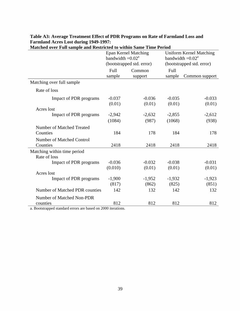
Results

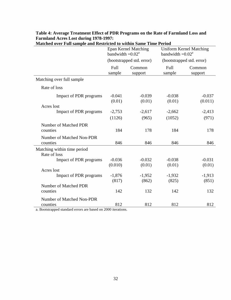
We compute the estimated impacts of PDR programs, the ATTs, for two time periods:

1978-1997 and 1949-1997. Between 1949 and 1978, states began to introduce preferential or

use-value property taxation programs but did so at varying points in time. By 1978, all six states

had some type of preferential taxation programs. The introduction of these preferential taxation

programs could confound the results for the 1949-1978 timeframe. In addition, prior to 1978, no

state had established and enrolled land in a PDR program. Therefore, we believe that a better

ATT estimate that is not confounded by these factors could be derived from the post-1978 time

period and focus on the results from this sub-sample. Our ATT estimates for the rate of farmland

loss and the number of acres lost appear in Table 4 (see Table A4 in Appendix for the results for

1949 - 1997). The bootstrapped standard errors are reported in parentheses under each estimated

treatment effect of the PDR programs in Table 4.13

For the rate of farmland loss under all the matching strategies, the estimated average

impacts of PDR programs range from -0.031 to -0.041. The results suggest that the existence of

a land preservation program in a county reduces the rate of farmland loss by 3 to 4 percentage

points on average. Given that the average rate of farmland loss per time period is 7.35% in the

full sample, this is a 40-55% change in the rate. The change is an even larger percentage for the

sub-sample of 1978-1997 which has an average rate of farmland loss of 3.4%.

For the number of acres lost, the average treatment effects of PDR programs in PDR

counties during 1978-1997 period range from -1,876 to -2,753 acres per agricultural census

13 We use a bootstrapping procedure to construct the standard errors for the average treatment effect. We make 2,000 independent draws from the participating and non-participating observations and form new estimates of the treatment effect for each draw. The bootstrap standard error estimate is the standard deviation of the 2000 new values for the estimated treatment effect of the PDR programs on the PDR counties.

20

period. This suggests that the counties with PDR programs lost fewer acres per year, 375 fewer

acres on the low end and 550 fewer on the high end, than similar non-PDR counties.14 The

effects are equivalent to stopping two or three farms in our study area from being converted

given that the average farm size is around 180 acres in our sample. Compared to the average

acres lost per county per agricultural census period, 10,000 acres, the PDR program reduce the

farmland acres lost by 20-30%.

The average treatment effects of the PDR programs during 1949-1997 are very similar to

those from 1978 through 1997 and are reported in Appendix Table A4. The average reduction in

the rate of farmland loss of each matching protocol from 1949 -1997 are the same as those from

1978-1997. The average reduction in the acres of farmland loss ranged from -2,600 to -2,900 for

matching without restriction. The results for restricting matches within time period for 1949-

1997 are exactly the same as that from 1978-1997, which is not surprising since all the counties

established their PDR programs after 1978. The similarity of the average treatment effect from

1949-1997 and from 1978-1997 suggests that unobserved factors varying across time period

before 1982 did not have a significant impact on farmland loss. Given that no county had a PDR

program with enrolled acreage before 1978, we had some concerns about the potential

unobservable factors related to the early period when computing the propensity scores.

However, beyond the similar estimated propensity scores for the earlier observations, these

earlier observations tended to be assigned small weights in calculating the counterfactuals. 15

14 Recall that these census periods could be four or five years. For the period of 1978-1997, one out of four agricultural census periods was four years (1978-1992) and the remainder was five years each. We thus divide our estimated ATTs by five to compute average annual effects. 15 We also calculate Rosenbaum Bounds which is a sensitive analysis proposed by Rosenbaum (2002) and hidden bias equivalent suggested by Diprete and Gangl (2004) for our matching with no restriction scenario. Our sensitivity analysis suggests that key characteristics that affect farmland loss would have to change from 8-36% to call the results into question. We also calculate an Average Treatment effect or the impact of PDR program on the

21

Conclusions

The two existing studies that look at the effectiveness of PDR program found no impact

of PDR programs on farmland loss. If a high rate of farmland loss is the reason that a county

implements a PDR program, one must take into account the identification problem that this

simultaneity generates. Using the propensity score matching method to compare farmland loss

among counties with and without PDR programs, this analysis finds that PDR programs have

reduced farmland loss.

Our specification includes variables that affect both farmland loss and the existence of a

PDR program. The standardized difference test and balancing in a regression framework suggest

that the average treatment effects are estimated using balanced counties – i.e. the PDR counties

and non-PDR counties that have similar characteristics on variables of interest. Our empirical

results provide strong and robust evidence that PDR programs reduce the rate of farmland loss

by about 3.5-4.5 percentage points (40-55%) for each agricultural census period in the Mid-

Atlantic area. Similarly, between 1,900 and 3,000 farmland acres were retained in farming per

census period, or 375 to 550 acres (two to three farms) a year, in counties with PDR programs.

Our estimate is the average impact on the counties with PDR programs. Given that

counties may have different underlying causes for their farmland loss, our results do not

guarantee that instituting a PDR program will arrest farmland loss in all areas.16 Some farmland

could have converted to forest, tourism or recreational uses rather than residential or commercial

farmland loss for both PDR and non-PDR counties using the approach proposed in Wooldridge (2002). The regression approach returns smaller but similar impacts as our estimated ATTs for the PDR counties. Both analysis therefore suggest that our results are robust and unobserved factors, if there is any, do not have much impact on our estimations (For details of the sensitivity analysis and regression results, see Appendix). 16 For example, some counties in the analysis lost farmland because they lost population rather than because the land was being converted to housing,

22

uses. However, most counties with PDR programs were losing farmland to residential and

commercial uses. Unfortunately, the county-level data precludes us from knowing more about

the spatial distribution or fragmentation of the remaining farmland which may have an impact on

the pattern of suburban development, the open-space amenities, and the long-run viability of the

agricultural sector.

Further research into the impact and the underlying reasons why these programs may

impact farmland loss is important. One future research program would be to study whether the

PDR programs, which focus on preserving farmland, shift developers to convert forest land at an

increased level, and whether PDR programs increase or decrease the net loss of open space.

Second, as we find that PDR programs reduce farmland loss in the counties that have these

programs, it would be interesting to understand through what channel the PDR programs reduce

farmland conversion. Specifically, whether PDR programs impact the density of housing on the

farmland that a county continues to convert and/or induce rejuvenating cities and local towns

and/or stimulate in-fill development. Third, as preserved farmland stays in agriculture forever, it

would be interesting to find out if the preserved land has remained in active farming and thus the

programs have had some impact on agricultural viability.

23

References

American Farmland Trust, 2008, Fact Sheet Status of Local PACE Programs, American Farmland

Trust Farmland Information Center, Northampton, MA.

http://www.farmland.org/news/media/documents/AFT_Pace_Local 7-06.pdf

American Farmland Trust, 2009, Fact Sheet Status of State PACE Programs, American Farmland

Trust Farmland Information Center, Northampton, MA.

http://www.farmlandinfo.org/documents/37757/State_PACE_05-2009_Final.pdf

Black, D., and J. Smith. 2004. “How Robust is the Evidence on the Effects of College Quality?

Evidence from Matching.” Journal of Econometrics, 121(1-2): 99-124.

Blewett, R. A. and J. I. Lane. 1988. “Development Rights and the Differential Assessment of

Agricultural land: Fractional valuation of farmland is ineffective for preserving open space

and subsidizes speculation.” American Journal of Economics and Sociology 47(2): 195-205.

Brooks, L. 2008. “Volunteering to be taxed: Business improvement districts and the extra-

governmental provision of public safety.” Journal of Public Economics 92 (1-2): 388-406.

Danskin, M. 2000. “Conservation Easement Violations: Results from a Study of Land Trusts.” Land

Trust Alliance Exchange 9(1).

Dehejia, R., and S. Wahba. 2002. “Propensity score matching methods for non-experimental causal

studies.” The Review of Economics and Statistics 84: 151-161.

DiPrete, T.A., and M. Gangl. 2004. “Assessing Bias in the Estimation of Causal Effects: Rosenbaum

Bounds on Matching Estimators and Instrumental Variables Estimation with Imperfect

Instruments.” Discussion paper SP I 2004-101. Berlin: WZB.

24

Duke J. M., and T. W. Ilvento. 2004. “A conjoint analysis of public preferences for agricultural land

preservation.” Agricultural and Resource Economics Review 33(2):209-19.

Feather, P., and C. Barnard. 2003. “Retaining Open Space with Purchasable Development Rights

Programs.” Review of Agricultural Economics, 25( 2):369-84.

Gardner, B. D. 1977. “The economics of agricultural land preservation.” American Journal of

Agricultural Economics 59(5.):1027-36.

Gardner, B. L. 1994. “Commercial Agriculture in Metropolitan Areas: Economics and Regulatory

Issues.” Agricultural and Resource Economics Review, 23(1):100-109.

Geoghegan, J., L. Lynch, and S. Bucholtz. 2003. “Capitalization of Open Spaces: Can Agricultural

Easements Pay for Themselves?” Agricultural and Resource Economic Review 32(1):33-45.

Hailu, Y. and C. Brown. 2007. Regional Growth Impacts on Agricultural Land Development: A

Spatial Model for Three States. Agricultural and Resource Economics Review 36(1): 149-

163.

Heckman, J., H. Ichimura, and P. Todd. 1997. “Matching as an econometric evaluation estimator:

evidence from evaluating a job training programme.” Review of Economic Studies 64(4):

605-654.

Heckman, J., H. Ichimura, and P. Todd. 1998. “Matching as an econometric evaluation estimator.”

Review of Economic Studies 65(2): 261-294.

Hellerstein, D., C. Nickerson, J. Cooper, P. Feather, D. Gadsby, D. Mullarkey, A. Tegene, and C.

Barnard. 2002. “Farmland Protection: The Role of Public Preferences for Rural Amenities”,

USDA Economic. Research Service. Agricultural Economic Report AER815.

25

Irwin, E. G. 2002. “The Effects of Open Space on Residential Property Values.” Land Economics

78(4):465-80.

Land Trust Alliance and Trust for Public Lands, 2008. "Voters Approve $8.4 Billion for

Conservation in 2008".

http://www.landtrustalliance.org/policy/conservation-funding/state-funding

List, J., D.L. Millimet and P.G. Fredriksson, W.W. McHone. 2003. “Effects of Environmental

Regulation on Manufacturing Plant births: Evidence from a Propensity Score Matching

Estimator.” The Review of Economics and Statistics 85(4): 944 – 952.

Livanis, G., Moss, C. B., Breneman, V. E. and Nehring, R.F., 2006. “Urban Sprawl and Farmland

Prices.” American Journal of Agricultural Economics, 88( 4): 915-929.

Lynch, L, 2005. “Protecting farmland - Why do we do it? How do we do it? Can we do it better?”

eds. Goetz, S. J., Shortle, J. S., and Bergstrom, J. C., Land use problems and conflicts:

causes, consequences and solutions. Routledge, New York, NY.

Lynch, L. and X. Liu, 2007, “Impact of Designated Preservation Areas on Rate of Preservation and

Rate of Conversion,” American Journal of Agricultural Economics, 89(5):1205-1210.

Lynch, L., and J. E. Carpenter. 2003. “Is There Evidence of a Critical Mass in the Mid-Atlantic

Agricultural Sector between 1949 and 1997?” Agricultural and Resource Economic Review

32(1):116-128.

Lynch, L., W. Gray, and J. Geoghegan, 2007, “Are Farmland Preservation Programs Easement

Restrictions Capitalized into Farmland Prices? What can a Propensity Score Matching

Analysis tell us?” Review of Agricultural Economics, 29(3): 502-509.

26

Lynch, L., W. Gray, and J. Geoghegan, 2010, “An Evaluation of Working Land and Open Space

Preservation Programs in Maryland: Are They Paying Too Much?” Editors: Stephan Goetz

and Floor Brouwer, New Perspectives on Agri-Environmental Policies: A Multidisciplinary

and Transatlantic Approach, Routledge.

McMillen, D. P., and J.F. McDonald. 2002. “Land values in a newly zoned city.” Review of

Economics and Statistics 84(1): 62–72.

Parks, J., and W. Quimio. 1996. “Preserving agricultural land with farmland assessment: New Jersey

as a case study.” Agricultural and Resource Economics Review 25(1):22-27.

Racine, J. S. and Q. Li. 2004. “Nonparametric estimation of regression functions with both

categorical and continuous data.” Journal of Econometrics 119 (1): 99-130.

Roe, H, B., I. G. Elena, and H. A. Morrow-Jones. 2004. “The Effects of Farmland, Farmland

Preservation, and Other Neighborhood Amenities on Housing Values and Residential

Growth.” Land Economics 80(1): 55-75.

Rosenbaum, P. 2002. Observational Studies (2nd edition). New York: Springer Verlag.

Rosenbaum, P., and D. Rubin. 1983. “The Central Role of the Propensity Score in Observational

Studies for Causal Effects.” Biometrika 70:41-55.

Smith, J., and P. Todd. 2005a. “Does Matching Overcome LaLonde’s Critique of Nonexperimental

Estimators?” Journal of Econometrics 125(1-2): 305-53.

Smith, J., and P. Todd. 2005b. “Does Matching Overcome LaLonde’s Critique of Non-experimental

Estimators? Rejoinder.” Journal of Econometrics, 125(1-2): 365-75.

27

Towe, C., C. Nickerson, and N. Bockstael. 2008. “An Empirical Examination of the Timing of Land

Conversions in the Presence of Farmland Preservation Programs.” American Journal of

Agricultural Economics, 90(3): 613-626.

U.S. Department of Agriculture, National Agricultural Statistics Service, (1999), 1997 Census of

Agriculture, 1A, 1B, 1C cd-rom set. National Agricultural Statistics Service, Washington,

DC.

U.S. Department of Agriculture, National Agricultural Statistics Service, 2001, Agricultural

Statistics. National Agricultural Statistics Service, Washington, DC.

U.S. Department of Commerce, Bureau of the Census, Census of Agriculture, 1950 to 1992. Bureau

of the Census, Washington DC.

U.S. Department of Commerce, Bureau of the Census, Census of Population and Housing, 1950 to

2000. Bureau of the Census, Washington DC.

Wooldridge, J. M. 2002. Econometric Analysis of Cross Section and Panel Data, MIT Press, Boston

MA.

0

0.01

0.02

0.03

0.04

0.05

0.06

0.07

0.08

0.05 0.

10.

15 0.2

0.25 0.

30.

35 0.4

0.45 0.

50.

55 0.6

0.65 0.

70.

75 0.8

0.85 0.

90.

95 1

Freq

uenc

y

Estimated Propensity Scores

Figure 1: Distribution for estimated propensity scores for full sample

Counties without PDR programs

Counties wit PDR programs

Note: (1). The diamond and square lines reflect the frequency of county observations whose estimated propensity score fall in each range for PDR and non-PDR county observations. (2). More than 60% of the estimated propensity scores for the non-PDR counties fall in the range of [0-0.05]. In order to improve the visibility of the frequencies in other ranges, the y-axis is limited to 0-0.08.

28

Table 1: Descriptive Statistics by the Full Sample, Counties with and without PDR Programs 1949-1997 for six Mid-Atlantic States

Full Sample (N=2,602)

Counties without PDR programs(N=2,422)

Counties with PDR programs (N=184)

Variable Definition of Variables Mean Std.Dev. Mean Std.Dev. Mean Std.Dev. pcfland Percent change in farmland acres per

agricultural census period 0.0735 0.1179 0.0761 0.1222 0.0412 0.0781 cfland Change in farmland acres per agricultural

census period 10,013 14,520 10,423 14,847 4,406 6,970 Explanatory Variables fland total acres of farmland 142,005 106,974 144,169 108,803 110,436 73,547 medfinc median family income 29,885 11,076 28,683 10,112 46,039 10,847 met =1 if county was a metro area in 1950 0.2206 0.4147 0.2126 0.4093 0.3424 0.4758 nprofper profit per acre (sales minus expenses) 215. 2 461.1 209.7 1181.2 344.7 301.2 numf number of farms in county 981.1 895.1 994.6 906.8 782.4 698 pagffm percent of residents employed in

agriculture, forestry, fisheries and mining 0.0997 0.1061 0.1046 0.1081 0.033 0.0266 medhval median housing value 61,128 33,495 57,249 29,131 113,757 44,033 phighsch percent of adults with a high school

education 0.4774 0.1760 0.4599 0.1690 0.708 0.074 phoffw percent of operators working 100+ days

off the farm 0.4045 0.1041 0.4023 0.1057 0.4313 0.0764 poppera population per acre 0.5514 1.701 0.5599 1.850 0.7319 0.7936 pfulln percent of operators who own all of the

land they farm 0.6725 0.1184 0.6766 0.1203 0.6214 0.0736 presprog = 1, if a county has at least one acre of

farmland enrolled in a PDR program 0.071 0.256 0 0 1 0

Source: U.S. Censuses of Agriculture (1949 to 1997); U.S. Censuses of Population and Housing (1950 to 2000); AFT (2008,2009); primary data collection from state and local PDR programs in the Mid-Atlantic States

29

30

Table 2: Descriptive Statistics by the Full Sample, Counties with and without PDR Programs, 1978-1997 for six Mid-Atlantic States

Full Sample (N=1,291)

Counties without PDR programs (N=1,107)

Counties with PDR programs (N=184)

Variable Definition of Variables Mean Std.Dev. Mean Std.Dev. Mean Std.Dev. pcfland Percent change in farmland acres per

agricultural census period 0.034 0.1024 0.033 0.106 0.0412 0.0781

cfland Change in farmland acres agricultural census period 4,070 8,705 4,014 8,962 4,406 6,970

Explanatory Variables fland total acres of farmland 115,707 84,289 116,583 85,943 110,436 73,547 medfinc median family income 36,928 9,104 35,413 7,817 46,039 10,847 met =1 if county was a metro area in 1950 0.2177 0.4128 0.1969 0.398 0.3424 0.4758 nprofper profit per acre (sales minus expenses) 264 476 250.2 498.3 344.7 301.2 numf number of farms in county 643.7 521 620.6 482.3 782.4 698 pagffm percent of residents employed in

agriculture, forestry, fisheries and mining 0.0546 0.0522 0.0583 0.0545 0.033 0.0266 medhval median housing value 78,825 36,492 73,018 31,554 113,757 44,033 phighsch percent of adults with a high school

education 0.608 0.1235 0.592 0.1222 0.708 0.074 phoffw percent of operators working 100+ days

off the farm 0.4347 0.0897 0.4352 0.092 0.4313 0.0764 poppera population per acre 0.538 1.272 0.5061 1.333 0.7319 0.7936 pfulln percent of operators who own all of the

land they farm 0.627 0.096 0.6283 0.0995 0.6214 0.0736 presprog = 1, if a county has at least one acre of

farmland enrolled in a PDR program 0.1425 0.3497 0 0 1 0 Source: U.S. Censuses of Agriculture (1949 to 1997); U.S. Censuses of Population and Housing (1950 to 2000); AFT (2008,2009); primary data collection from state and local PDR programs in the Mid-Atlantic States

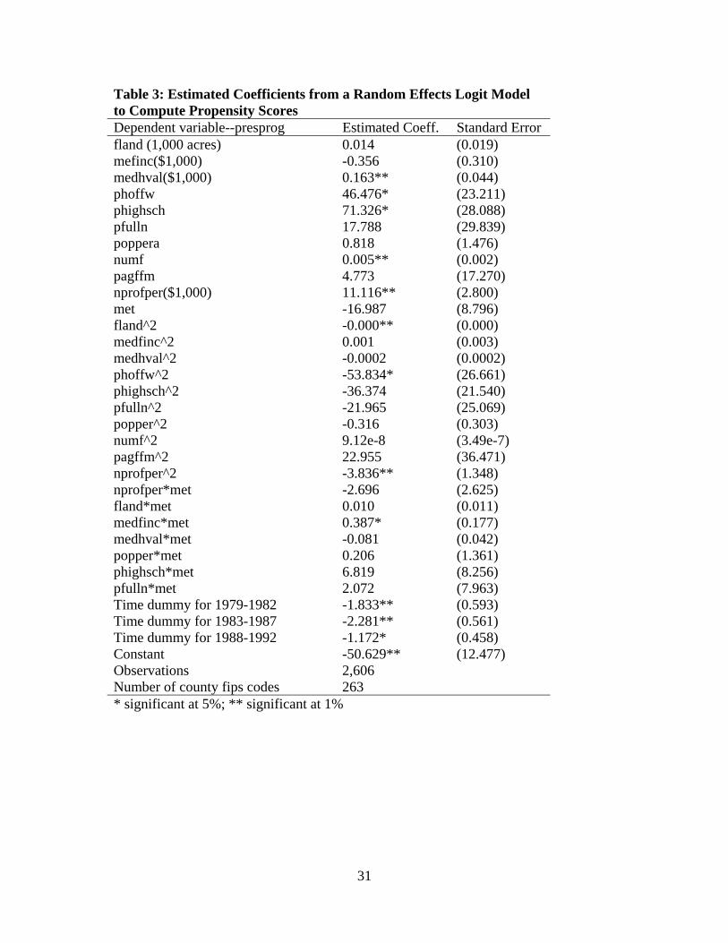
Table 3: Estimated Coefficients from a Random Effects Logit Model to Compute Propensity Scores Dependent variable--presprog Estimated Coeff. Standard Error fland (1,000 acres) 0.014 (0.019) mefinc($1,000) -0.356 (0.310) medhval($1,000) 0.163** (0.044) phoffw 46.476* (23.211) phighsch 71.326* (28.088) pfulln 17.788 (29.839) poppera 0.818 (1.476) numf 0.005** (0.002) pagffm 4.773 (17.270) nprofper($1,000) 11.116** (2.800) met -16.987 (8.796) fland^2 -0.000** (0.000) medfinc^2 0.001 (0.003) medhval^2 -0.0002 (0.0002) phoffw^2 -53.834* (26.661) phighsch^2 -36.374 (21.540) pfulln^2 -21.965 (25.069) popper^2 -0.316 (0.303) numf^2 9.12e-8 (3.49e-7) pagffm^2 22.955 (36.471) nprofper^2 -3.836** (1.348) nprofper*met -2.696 (2.625) fland*met 0.010 (0.011) medfinc*met 0.387* (0.177) medhval*met -0.081 (0.042) popper*met 0.206 (1.361) phighsch*met 6.819 (8.256) pfulln*met 2.072 (7.963) Time dummy for 1979-1982 -1.833** (0.593) Time dummy for 1983-1987 -2.281** (0.561) Time dummy for 1988-1992 -1.172* (0.458) Constant -50.629** (12.477) Observations 2,606 Number of county fips codes 263 * significant at 5%; ** significant at 1%

31

32

Table 4: Average Treatment Effect of PDR Programs on the Rate of Farmland Loss and Farmland Acres Lost during 1978-1997: Matched over Full sample and Restricted to within Same Time Period

Epan Kernel Matching bandwidth =0.02a

Uniform Kernel Matching bandwidth =0.02a

(bootstrapped std. error) (bootstrapped std. error)

Full

sample Common support

Full sample

Common support

Matching over full sample

Rate of loss

Impact of PDR programs -0.041 -0.039 -0.038 -0.037 (0.01) (0.01) (0.01) (0.011) Acres lost Impact of PDR programs -2,753 -2,617 -2,662 -2,413 (1126) (965) (1052) (971)

Number of Matched PDR counties 184 178 184 178

Number of Matched Non-PDR counties 846 846 846 846

Matching within time period Rate of loss Impact of PDR programs -0.036 -0.032 -0.038 -0.031 (0.010) (0.01) (0.01) (0.01) Acres lost Impact of PDR programs -1,876 -1,952 -1,932 -1,913 (817) (862) (825) (851)

Number of Matched PDR counties 142 132 142 132

Number of Matched Non-PDR counties 812 812 812 812

a. Bootstrapped standard errors are based on 2000 iterations.

Appendix

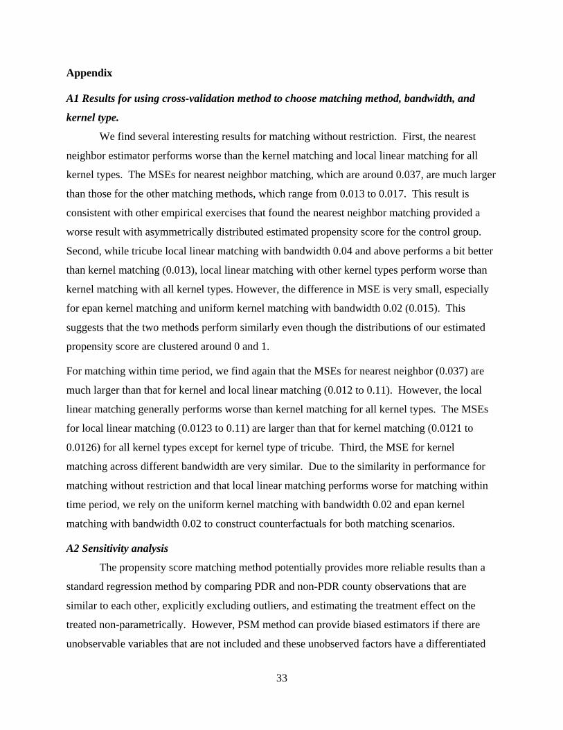
A1 Results for using cross-validation method to choose matching method, bandwidth, and

kernel type.

We find several interesting results for matching without restriction. First, the nearest

neighbor estimator performs worse than the kernel matching and local linear matching for all

kernel types. The MSEs for nearest neighbor matching, which are around 0.037, are much larger

than those for the other matching methods, which range from 0.013 to 0.017. This result is

consistent with other empirical exercises that found the nearest neighbor matching provided a

worse result with asymmetrically distributed estimated propensity score for the control group.

Second, while tricube local linear matching with bandwidth 0.04 and above performs a bit better

than kernel matching (0.013), local linear matching with other kernel types perform worse than

kernel matching with all kernel types. However, the difference in MSE is very small, especially

for epan kernel matching and uniform kernel matching with bandwidth 0.02 (0.015). This

suggests that the two methods perform similarly even though the distributions of our estimated

propensity score are clustered around 0 and 1.

For matching within time period, we find again that the MSEs for nearest neighbor (0.037) are

much larger than that for kernel and local linear matching (0.012 to 0.11). However, the local

linear matching generally performs worse than kernel matching for all kernel types. The MSEs

for local linear matching (0.0123 to 0.11) are larger than that for kernel matching (0.0121 to

0.0126) for all kernel types except for kernel type of tricube. Third, the MSE for kernel

matching across different bandwidth are very similar. Due to the similarity in performance for

matching without restriction and that local linear matching performs worse for matching within

time period, we rely on the uniform kernel matching with bandwidth 0.02 and epan kernel

matching with bandwidth 0.02 to construct counterfactuals for both matching scenarios.

A2 Sensitivity analysis

The propensity score matching method potentially provides more reliable results than a

standard regression method by comparing PDR and non-PDR county observations that are

similar to each other, explicitly excluding outliers, and estimating the treatment effect on the

treated non-parametrically. However, PSM method can provide biased estimators if there are

unobservable variables that are not included and these unobserved factors have a differentiated

33

impact on counties with and without PDR programs. Therefore, we also conduct a sensitivity

analysis by looking at Rosenbaum bounds and hidden bias equivalents (Rosenbaum, 2002;

DiPrete and Gangl, 2004).

17

Rosenbaum bounds is a signed rank test that assesses the potential impact of hidden bias

arising from potentially unobserved variables associated with both having a PDR program and

the rate of farmland loss variables. It assumes that the strength of the impacts from unobservable

factors on having a PDR program and farmland loss is the same. Thus this approach is relatively

conservative and will find bias even if the strength of unobservable factors on the farmland loss

is not as strong as the test assumes.

The estimated propensity score of a PDR county and non-PDR county with identical

characteristics (X) should be equal if all the relevant characteristics that affect both having a PDR

program and farmland loss are included in the propensity score model. The presence of the

unobserved variables leads to differences between the propensity scores of PDR and non-PDR

county observations with identical characteristics. As a result, the odds ratio of a matched pair of

PDR and non-PDR county observations based on these characteristics will no longer be equal to

one. The larger the effect of an unobserved variable on having a PDR program, the larger the

difference between the odds ratio and one will be.

Rosenbaum shows that the odds ratio for matched pairs is bounded by the function of the

strength of the effect. Therefore, a signed rank statistic of each strength level has its upper and

lower bounds and their corresponding p-values. One can determine a critical level of the

strength of effect for a 95% confidence interval. If the unobserved variables affect having a

PDR program and/or farmland loss to a higher degree than the critical effect strength, the

average treatment effects could include zero. (see Rosenbaum (2002) and DiPrete and

Gangl(2004) for more information).

Beyond finding the upper and lower bounds, following DiPrete and Gangl (2004), we

also calculate the hidden bias equivalents on key covariates. Table A4 reports the upper and

lower bounds for Kernel matching with Epan kernel type with bandwidth equal to 0.02 for

17 There are other strategies that assess the impact of hidden bias, the IV approach proposed by DiPrete and Gangl (2004) which is less conservative than Rosenbaum Bounds approach. We use Rosenbaum Bounds as it is the most appropriate for our problem.

34

matching without restriction as well as the hidden bias equivalents’18 The threshold gamma

measures the effect strength of unobservable variables on treatment assignment and equals 1.92

for the rate of farmland loss. Thus the statistical significance of the ATT for the rate of farmland

loss would be called into question if the odds ratio of having a PDR program between the treated

and control groups differs by more than 1.92. However, the ATT can still be significant if the

effect of the unobservable variables on having a PDR program is greater than the effect on

farmland loss.

We calculate the hidden bias equivalents on three key variables: total acres of farmland in

a county, net agricultural profit per acre, and median housing value. At the critical level of

gamma for the rate of farmland loss, any unobserved variable would have to have the same

impact as changing these 3 key variables by 31,000 acres (22%) for total acres of farmland, by

$800 (36%) for net profit per acres, and by $5,810 (10%) for median housing value. For

farmland acres loss, the critical threshold gamma is 1.72. The hidden bias equivalents would be

similar to a change of 24,000 acres (17%) in total acres of farmland, $600 (29%) in net profit per

acre, and $4,710 (8%) in median housing value. These hidden bias equivalents suggest our ATT

results are not very sensitive to changes in key variables or potential unobserved variables.

A3 Regression estimation and average treatment effect

While the ATT effect is significant, it cannot be generalized to the entire population due

to self-selection concerns. An Average Treatment Effect (ATE) is an expected effect of

treatment on a randomly selected county but it requires more restrictive assumptions. To check

how general our estimators are and how well our estimation of ATT addresses the self-selection

issue, we estimate the ATE of PDR programs in a regression framework following Wooldridge

(2002). This model includes the binary variable indicating whether a county has a PDR

program, the estimated propensity scores, and a set of variables that affect outcomes. The

estimated propensity score is expected to control all the information in the variables that is

relevant to estimating the treatment effect.

We specify a random effects model and include time dummies for periods after 1978 to

control for time effects. We estimate the random effects regression for both the full sample and a

18 Given that fact the Rosenbaum bounds approach does not deal with stratified or cluster samples, we are unable to conduct a sensitivity analysis for our matching within time periods.

35

post-1978 sub-sample. We do not remove outliers or those observations that fall out of the range

in which the estimated propensity score for PDR and non-PDR counties overlap in this exercise

(the common support).

For the rate of farmland loss, the estimated coefficient for the PDR program indictor is -

0.024 (standard error is 0.011) for the full sample compared to the ATTs of -0.034 to -0.040

(Table A5). The PDR program coefficient is -0.015 for the post-1978 sub-sample regression

compared to the ATTs of -0.035 to -0.045. The estimated coefficient on the PDR program

indicator in the random effects model for acres of farmland lost is insignificant for the full

sample. For the post-1978 sub-sample, it is statistically significant and equals -1,487 acres

compared to the ATT of -2,013 to -2,284 acres.

On a whole, the results under both approaches are similar with the ATE being slightly

smaller. We therefore conclude that our estimation can be generalized to the whole population

and the self-selection issue is well addressed.

36

Table A1: Balancing Test for the Distribution of the Variables between Matched PDR Counties (X1) and Non-PDR (X0) Counties for Observations 1949-1997: covariates that are not balanced*. Epan Kernel Matching Uniform Kernel Matching (bandwidth =0.02) (bandwidth =0.02) Full sample Common support Full sample Common support Matching over full sample

T-test**

tdummy5 (0:0.03)

tdummy5 (0:0.03)

tdummy5 (0:0.03)

tdummy5 (0:0.03)

tdummy6(0:0.12)

tdummy6(0:0.13)

tdummy6 (0:0.13)

tdummy6(0:0.13)

tdummy10 (0.47:0.25)

tdummy10 (0.47:0.25)

tdummy10 (0.47:0.25)

tdummy10 (0.47:0.25)

Regression Test

phighsch phighsch phighsch phighsch

tdummy1 tdummy1 tdummy1 tdummy1

tdummy3-6 tdummy3-6 tdummy3-6 tdummy3-6

tdummy10 tdummy10 tdummy10 tdummy10

* We present the covariates for which we could reject the H0: no difference in the mean at the 95% confidence level ** the means for the PDR counties and non-PDR counties are in parenthesis tdummy1 to tdummy10 indicates 1949-1954, 1955-1959, 1960-1964, 1965-1969, 1970-1974, 1975-1978, 1979-1982, 1983-1987, 1988-1992, 1993-1997 respectively. Within time period matches are the same as that for sample in the time period 1978-1997: as no county has a PDR program before 1978 (Table A2).

37

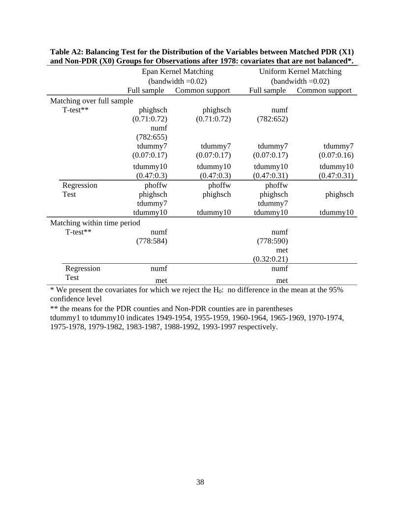
Table A2: Balancing Test for the Distribution of the Variables between Matched PDR (X1) and Non-PDR (X0) Groups for Observations after 1978: covariates that are not balanced*. Epan Kernel Matching Uniform Kernel Matching (bandwidth =0.02) (bandwidth =0.02) Full sample Common support Full sample Common support Matching over full sample

T-test**

phighsch(0.71:0.72)

phighsch(0.71:0.72)

numf (782:652)

numf(782:655) tdummy7 tdummy7 tdummy7

(0.07:0.17) tdummy7

(0.07:0.16)(0.07:0.17) (0.07:0.17)tdummy10 tdummy10

(0.47:0.3)tdummy10 tdummy10

(0.47:0.3) (0.47:0.31) (0.47:0.31)

Regression Test

phoffw phoffw

phoffw phighsch phighsch phighsch phighschtdummy7 tdummy7

tdummy10 tdummy10 tdummy10 tdummy10Matching within time period

T-test**

numf (778:584)

numf (778:590)

met

(0.32:0.21)

Regression Test

numf

numf met met

* We present the covariates for which we reject the H0: no difference in the mean at the 95% confidence level ** the means for the PDR counties and Non-PDR counties are in parentheses tdummy1 to tdummy10 indicates 1949-1954, 1955-1959, 1960-1964, 1965-1969, 1970-1974, 1975-1978, 1979-1982, 1983-1987, 1988-1992, 1993-1997 respectively.

38

39

Table A3: Average Treatment Effect of PDR Programs on Rate of Farmland Loss and Farmland Acres Lost during 1949-1997: Matched over Full sample and Restricted to within Same Time Period

Epan Kernel Matching bandwidth =0.02a (bootstrapped std. error)

Uniform Kernel Matching bandwidth =0.02a (bootstrapped std. error)

Full

sample Common support

Full sample Common support

Matching over full sample

Rate of loss

Impact of PDR programs -0.037 -0.036 -0.035 -0.033 (0.01) (0.01) (0.01) (0.01) Acres lost Impact of PDR programs -2,942 -2,632 -2,855 -2,612 (1084) (987) (1068) (938)

Number of Matched Treated Counties 184 178 184 178

Number of Matched Control Counties 2418 2418 2418 2418

Matching within time period Rate of loss Impact of PDR programs -0.036 -0.032 -0.038 -0.031 (0.010) (0.01) (0.01) (0.01) Acres lost Impact of PDR programs -1,900 -1,952 -1,932 -1,923 (817) (862) (825) (851) Number of Matched PDR counties 142 132 142 132

Number of Matched Non-PDR counties 812 812 812 812

a. Bootstrapped standard errors are based on 2000 iterations.

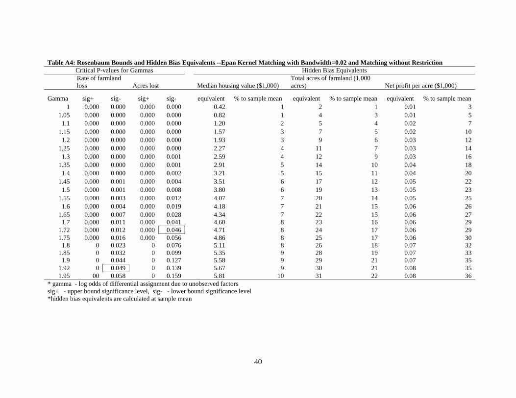
Table A4: Rosenbaum Bounds and Hidden Bias Equivalents --Epan Kernel Matching with Bandwidth=0.02 and Matching without Restriction Critical P-values for Gammas Hidden Bias Equivalents

Rate of farmland loss Acres lost Median housing value ($1,000)

Total acres of farmland (1,000 acres) Net profit per acre ($1,000)

Gamma sig+ sig- sig+ sig- equivalent % to sample mean equivalent % to sample mean equivalent % to sample mean 1 0.000 0.000 0.000 0.000 0.42 1 2 1 0.01 3

1.05 0.000 0.000 0.000 0.000 0.82 1 4 3 0.01 5 1.1 0.000 0.000 0.000 0.000 1.20 2 5 4 0.02 7

1.15 0.000 0.000 0.000 0.000 1.57 3 7 5 0.02 10 1.2 0.000 0.000 0.000 0.000 1.93 3 9 6 0.03 12

1.25 0.000 0.000 0.000 0.000 2.27 4 11 7 0.03 14 1.3 0.000 0.000 0.000 0.001 2.59 4 12 9 0.03 16

1.35 0.000 0.000 0.000 0.001 2.91 5 14 10 0.04 18 1.4 0.000 0.000 0.000 0.002 3.21 5 15 11 0.04 20

1.45 0.000 0.001 0.000 0.004 3.51 6 17 12 0.05 22 1.5 0.000 0.001 0.000 0.008 3.80 6 19 13 0.05 23

1.55 0.000 0.003 0.000 0.012 4.07 7 20 14 0.05 25 1.6 0.000 0.004 0.000 0.019 4.18 7 21 15 0.06 26

1.65 0.000 0.007 0.000 0.028 4.34 7 22 15 0.06 27 1.7 0.000 0.011 0.000 0.041 4.60 8 23 16 0.06 29

1.72 0.000 0.012 0.000 0.046 4.71 8 24 17 0.06 29 1.75 0.000 0.016 0.000 0.056 4.86 8 25 17 0.06 30

1.8 0 0.023 0 0.076 5.11 8 26 18 0.07 32 1.85 0 0.032 0 0.099 5.35 9 28 19 0.07 33

1.9 0 0.044 0 0.127 5.58 9 29 21 0.07 35 1.92 0 0.049 0 0.139 5.67 9 30 21 0.08 35 1.95 00 0.058 0 0.159 5.81 10 31 22 0.08 36

* gamma - log odds of differential assignment due to unobserved factors sig+ - upper bound significance level, sig- - lower bound significance level *hidden bias equivalents are calculated at sample mean

40

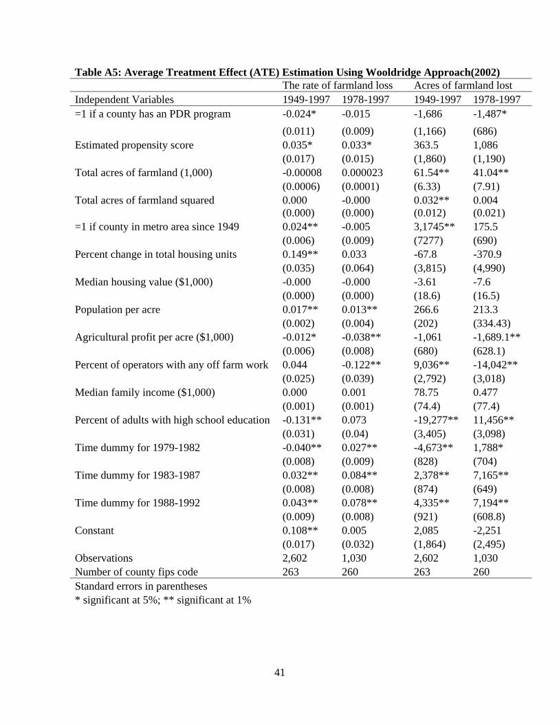
Table A5: Average Treatment Effect (ATE) Estimation Using Wooldridge Approach(2002) The rate of farmland loss Acres of farmland lost

Independent Variables 1949-1997 1978-1997 1949-1997 1978-1997 =1 if a county has an PDR program -0.024* -0.015 -1,686 -1,487*

(0.011) (0.009) (1,166) (686) Estimated propensity score 0.035* 0.033* 363.5 1,086

(0.017) (0.015) (1,860) (1,190) Total acres of farmland (1,000) -0.00008 0.000023 61.54** 41.04**

(0.0006) (0.0001) (6.33) (7.91) Total acres of farmland squared 0.000 -0.000 0.032** 0.004

(0.000) (0.000) (0.012) (0.021) =1 if county in metro area since 1949 0.024** -0.005 3,1745** 175.5

(0.006) (0.009) (7277) (690) Percent change in total housing units 0.149** 0.033 -67.8 -370.9

(0.035) (0.064) (3,815) (4,990) Median housing value ($1,000) -0.000 -0.000 -3.61 -7.6

(0.000) (0.000) (18.6) (16.5) Population per acre 0.017** 0.013** 266.6 213.3

(0.002) (0.004) (202) (334.43) Agricultural profit per acre ($1,000) -0.012* -0.038** -1,061 -1,689.1**

(0.006) (0.008) (680) (628.1) Percent of operators with any off farm work 0.044 -0.122** 9,036** -14,042**

(0.025) (0.039) (2,792) (3,018) Median family income ($1,000) 0.000 0.001 78.75 0.477

(0.001) (0.001) (74.4) (77.4) Percent of adults with high school education -0.131** 0.073 -19,277** 11,456**

(0.031) (0.04) (3,405) (3,098) Time dummy for 1979-1982 -0.040** 0.027** -4,673** 1,788*

(0.008) (0.009) (828) (704) Time dummy for 1983-1987 0.032** 0.084** 2,378** 7,165**

(0.008) (0.008) (874) (649) Time dummy for 1988-1992 0.043** 0.078** 4,335** 7,194**

(0.009) (0.008) (921) (608.8) Constant 0.108** 0.005 2,085 -2,251

(0.017) (0.032) (1,864) (2,495) Observations 2,602 1,030 2,602 1,030 Number of county fips code 263 260 263 260 Standard errors in parentheses * significant at 5%; ** significant at 1%

41