0

Do Agricultural Preservation Programs Affect Farmland Conversion?

Evidence from a Propensity Score Matching Estimator

Xiangping Liu and Lori Lynch Department of Agricultural and Resource Economics

2200 Symons Hall University of Maryland

College Park, MD 20742 USA

301-405-1264 (tel.) llynch@arec.umd.edu

Selected Paper prepared for Presentation at the American Agricultural Economics Association Meeting, Portland, OR, July 29-August 1, 2007

Copyright 2007 by Liu and Lynch. All rights reserved. Readers are asked to contact authors before citing. Keywords: agricultural preservation programs, farmland, propensity score, farmland conversion, urban-rural interface Authors are Graduate Student and Associate Professor in the Department of Agricultural and Resource Economics, University of Maryland. Support for this project was provided by the Maryland Center for Agro-Ecology, Inc. and the Center for Smart Growth Education and Research. We would like to thank Liesl Koch and Janet Carpenter for their research assistance. In addition, the project has benefited from the comments of John List, Jeffrey Smith, and Erik Lichtenberg. As always, any errors remain the full responsibility of the authors.

1

Do Agricultural Preservation Programs Affect Farmland Conversion?

More than 124 governmental entities concerned about suburban sprawl and farmland loss have

implemented farmland preservation programs preserving 1.67 million acres at a cost of $3.723

billion. We ask how effective are these programs in slowing the rate of farmland loss. Using a

unique 50-year 269 county panel data set on preservation programs and farmland loss for six

Mid-Atlantic States, we employ the propensity score matching method to find strong empirical

evidence that these programs have had a statistically significant effect on the rate of farmland

loss. Preservation programs on average decrease the rate of farmland loss by 2.4 percentage

points; a 33% decrease from the average 5-year rate of 7.31%.

Do Agricultural Preservation Programs Affect Farmland Conversion?

Concerns about the loss of farmland and the increase in suburban sprawl led states and

counties to instituted programs to arrest or slow farmland conversion. Beginning in 1978,

farmland preservation programs such as purchase of development rights/purchase of agricultural

conservation easements (PDR/PACE) and transfer of development rights (TDR) have been

established and funded to retain agricultural land. These programs usually attach an easement to

the property that restricts the right to convert the land to residential, commercial and industrial

uses in exchange for a cash payment and/or tax benefit. Farmland preservation programs are

justified on various grounds including efficient development of urban and rural land, local and

national food security, viability of the local agricultural economy, and the protection of rural and

environmental amenities [16, 23].

More than 124 governmental entities1 have implemented farmland preservation programs

[3, 6, 7] and over 1.67 million acres are now in preserved status. Spending in both state and

local programs to purchase these rights was $3.723 billion [6, 7]. Citizens continue to pass ballot

initiatives generating funds for these types of programs: in 2002, $5.7 billion in conservation

funding was authorized; in 2001, $1.7 billion; and in 2000, $7.5 billion, and most recently in

2006, $5.73 billion [25]. And in the last decade, the federal government has provided financial

assistance for state and local purchase of development rights programs to preserve agricultural

land. While some evidence exists that these programs provide net benefits to society [15,14],

little evaluation has been conducted on their effectiveness in retaining farmland. Several studies

have evaluated the impact of (non-permanent) use-value or preferential taxation programs [9, 17,

27, 33, 22] on farmland conversion, yet few have studied the impact of the permanent easements

conferred by the PDR/PACE and TDR programs. Several studies have suggested that the more

2

expensive PDR/PACE programs have preserved too little land and that the TDR programs have

preserved too little or the wrong “type” of farmland [30, 29, 28, 1]. Despite Maryland’s

successful state preservation program which has preserved 198,276 acres, 371,000 acres have

been converted to a residential or commercial use simultaneously [30]. Only half as much

agricultural land was preserved compared to agricultural land converted. Are the programs

preserving land that would not have been converted to date thus having little to no impact on rate

of loss? Therefore, we ask the question: what effect have PDR/PACE and TDR programs had

on the rate of farmland loss?. Using a unique 50-year 269 county panel data set on the existence

of PDR/PACE and TDR programs and farmland loss for six Mid-Atlantic States, we find strong

empirical evidence that these programs have had a statistically significant effect on the rate of

farmland loss.

Assessing the impact of permanent preservation through PDR/PACE and TDR programs

on the rate of farmland loss can be challenging. One cannot construct the proper counterfactual,

i.e. one would like to know what would have happened to the rate of farmland loss in county A if

it had not implemented a program. However, county A can not be in two states simultaneously,

nor can a researcher randomly assign who has a preservation program and who does not. Lynch

and Carpenter [27] found no impact of PDR/PACE and TDR on the farmland loss rate assuming

that the programs’ existence was exogenous. However, farmland preservation programs may be

established in those counties with the highest rates of farmland loss and/or lower levels of

farmland thus the very existence of the program itself may be predicated on the rate of farmland

loss. Acres preserved may not be sufficient to assessing a programs impact on farmland loss.

McConnell, Kopits, and Walls [31] find that preserving a large amount of farmland through a

TDR program does not guarantee a decreased rate of farmland loss if the new housing developed

3

with the TDRs occurs in rural areas on farmland. Similarly, recent evidence suggests that the

positive amenities generated by these preservation programs may increase the demand for

housing near the preserved parcels. This demand then can create more conversion pressure and

higher housing prices. For example, Roe, Irwin, and Morrow-Jones [37] find that preservation

efforts could induce further residential growth in areas with short commutes to employment

centers and small amounts of remaining farmland. Geoghegan, Lynch and Bucholtz [18] and

Irwin [24] found that housing prices adjacent to preserved parcels can increase due to the

permanency of adjacent open space. Furthermore, if the programs are enrolling those parcels

least likely to be converted, their impact on the rate of farmland preservation may be

insignificant.

We suggest we can overcome some of the empirical difficulties by using a propensity

score method to estimate the treatment effect. This method has several benefits – first, the

matching protocol ensures that the counties with farmland preservation programs will be

matched to the counties without programs that are most similar to them in terms of

characteristics. This provides a more transparent mean to decrease the influence of outliers and

dissimilar counties. Second, because not all counties are equally likely to have farmland

preservation programs, this method incorporates pretreatment covariates that may influence the

existence of such a program as well as farmland loss into the propensity score calculation. Third,

a linear functional form is not assumed.

Model

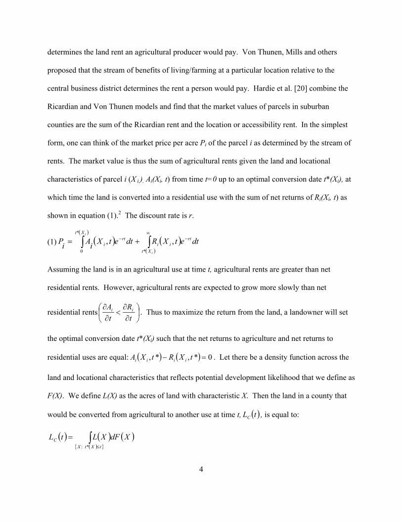
In a competitive land market, risk-neutral landowners seek to maximize the economic

return from their land given the stream of net returns. Ricardian theory states that the

profitability of agricultural land is based on fertility or soil characteristics and this fertility

4

determines the land rent an agricultural producer would pay. Von Thunen, Mills and others

proposed that the stream of benefits of living/farming at a particular location relative to the

central business district determines the rent a person would pay. Hardie et al. [20] combine the

Ricardian and Von Thunen models and find that the market values of parcels in suburban

counties are the sum of the Ricardian rent and the location or accessibility rent. In the simplest

form, one can think of the market price per acre Pi of the parcel i as determined by the stream of

rents. The market value is thus the sum of agricultural rents given the land and locational

characteristics of parcel i (X i,), Ai(Xi, t) from time t=0 up to an optimal conversion date t*(Xi), at

which time the land is converted into a residential use with the sum of net returns of Ri(Xi, t) as

shown in equation (1).2 The discount rate is r.

(1) ( )( )

( )( )∫∫∞

−− +=i

i

Xt

rtii

Xtrt

i dtetXRdtetXiAiP*

*

0

,,

Assuming the land is in an agricultural use at time t, agricultural rents are greater than net

residential rents. However, agricultural rents are expected to grow more slowly than net

residential rents ⎟⎠⎞

⎜⎝⎛

∂∂

<∂∂

tR

tA ii . Thus to maximize the return from the land, a landowner will set

the optimal conversion date t*(Xi) such that the net returns to agriculture and net returns to

residential uses are equal: ( ) ( ) 0*,*, =− tXRtXA iiii . Let there be a density function across the

land and locational characteristics that reflects potential development likelihood that we define as

F(X). We define L(X) as the acres of land with characteristic X. Then the land in a county that

would be converted from agricultural to another use at time t, ( )tLC , is equal to:

( ) ( ) ( )( ){ }∫

≤

=tXtX

C XdFXLtL*:

5

Or all land with characteristics X such that the optimal conversion time t*(Xi) is less than the

current time. Similarly, the land in a county that remain in agricultural production (LA(t)), is

equal to:

( ) ( ) ( )( ){ }∫

>

=tXtX

A XdFXLtL*:

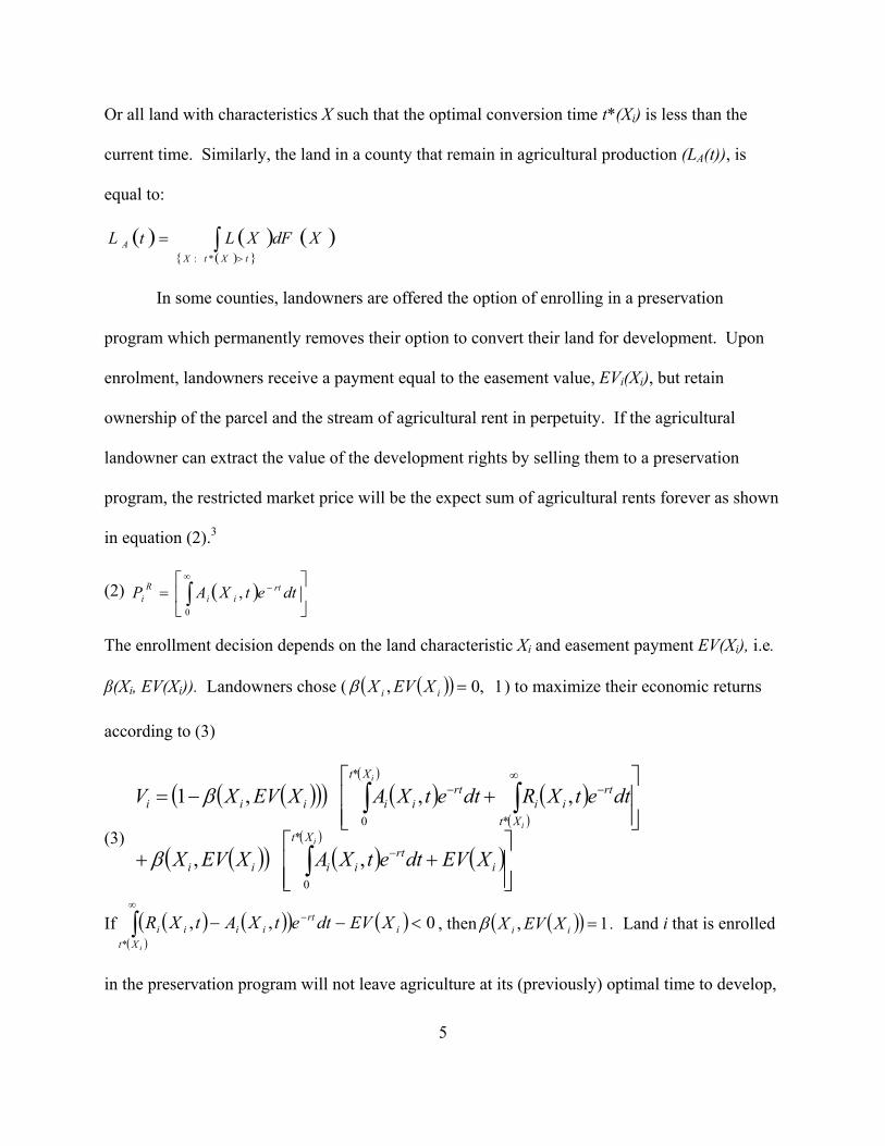
In some counties, landowners are offered the option of enrolling in a preservation

program which permanently removes their option to convert their land for development. Upon

enrolment, landowners receive a payment equal to the easement value, EVi(Xi), but retain

ownership of the parcel and the stream of agricultural rent in perpetuity. If the agricultural

landowner can extract the value of the development rights by selling them to a preservation

program, the restricted market price will be the expect sum of agricultural rents forever as shown

in equation (2).3

(2)

( ) ⎥⎦

⎤⎢⎣

⎡= ∫

∞−

0

, dtetXAP rtii

Ri

The enrollment decision depends on the land characteristic Xi and easement payment EV(Xi), i.e.

β(Xi, EV(Xi)). Landowners chose ( ( )( ) 1,0, =ii XEVXβ ) to maximize their economic returns

according to (3)

(3)

( )( )( ) ( )( )

( )( )

( )( ) ( )( )

( )⎥⎥⎦

⎤

⎢⎢⎣

⎡++

⎥⎥⎦

⎤

⎢⎢⎣

⎡+−=

∫

∫∫−

∞−−

i

Xtrt

iiii

Xt

rtii

Xtrt

iiiii

XEVdtetXAXEVX

dtetXRdtetXAXEVXV

i

i

i

*

0

*

*

0

,,

,,,1

β

β

If ( ) ( )( )( )

( ) 0,,*

<−−∫∞

−i

Xt

rtiiii XEVdtetXAtXR

i

, then ( )( ) 1, =ii XEVXβ . Land i that is enrolled

in the preservation program will not leave agriculture at its (previously) optimal time to develop,

6

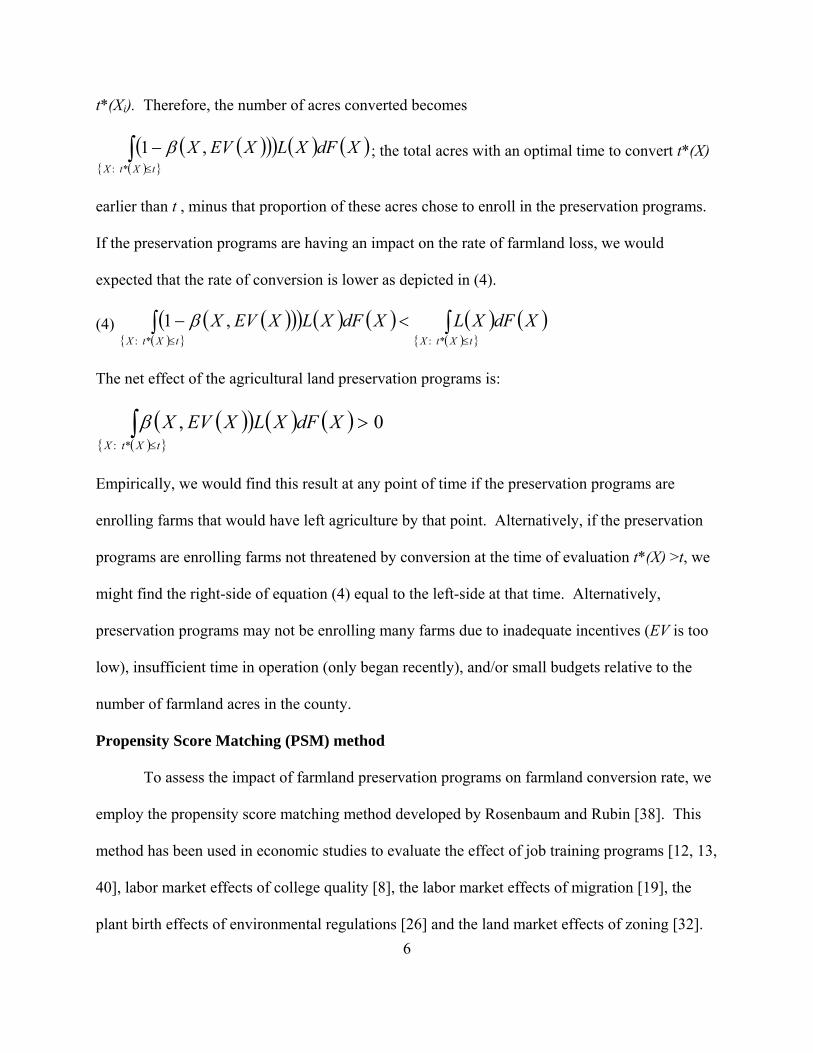
t*(Xi). Therefore, the number of acres converted becomes

( )( )( ) ( ) ( )( ){ }∫

≤

−tXtX

XdFXLXEVX*:

,1 β ; the total acres with an optimal time to convert t*(X)

earlier than t , minus that proportion of these acres chose to enroll in the preservation programs.

If the preservation programs are having an impact on the rate of farmland loss, we would

expected that the rate of conversion is lower as depicted in (4).

(4) ( )( )( ) ( ) ( )( ){ }

( ) ( )( ){ }∫∫

≤≤

<−tXtXtXtX

XdFXLXdFXLXEVX*:*:

,1 β

The net effect of the agricultural land preservation programs is:

( )( ) ( ) ( )( ){ }

0,*:

>∫≤tXtX

XdFXLXEVXβ

Empirically, we would find this result at any point of time if the preservation programs are

enrolling farms that would have left agriculture by that point. Alternatively, if the preservation

programs are enrolling farms not threatened by conversion at the time of evaluation t*(X) >t, we

might find the right-side of equation (4) equal to the left-side at that time. Alternatively,

preservation programs may not be enrolling many farms due to inadequate incentives (EV is too

low), insufficient time in operation (only began recently), and/or small budgets relative to the

number of farmland acres in the county.

Propensity Score Matching (PSM) method

To assess the impact of farmland preservation programs on farmland conversion rate, we

employ the propensity score matching method developed by Rosenbaum and Rubin [38]. This

method has been used in economic studies to evaluate the effect of job training programs [12, 13,

40], labor market effects of college quality [8], the labor market effects of migration [19], the

plant birth effects of environmental regulations [26] and the land market effects of zoning [32].

7

To the best of our knowledge, no one has used this methodology to identifying treatment effects

of farmland preservation programs.

Assessing the impacts of preservation programs is difficult because of incomplete

information. While one can identify whether a county has a preservation program (is treated) or

not (not treated, or in our analysis, a control) and the outcome (rate of farmland loss) conditional

on its treatment, one can not observe the counterfactual, i.e. what would have happened if no

farmland preservation program had been established. Thus, the fundamental problem in

identifying treatment effect is constructing the unobservable counterfactuals for treated

observations.

Let 1Y denote the outcome in the group of observations if treatment has occurred ( 1=D ),

and 0Y denote the outcome for the group of control observations ( 0=D ). If one could observe

the treated and the control states, the average treatment effect, τ, would equal 01 YY − where 1Y

equals the mean outcome of the treatment group and 0Y of the control group. Unfortunately,

only 1Y or 0Y are observed for each observation. In a laboratory experiment, researchers solve

this problem by randomly assigning subjects to be treated or not treated and then construct the

unobserved counterfactual. In a natural setting, however, 01 YY −≠τ because the treatment

condition is not randomly assigned. The propensity score matching (PSM) method proposed by

Rosenbaum and Rubin [38] demonstrates that if data justify matching on some observable vector

of covariates, X, then matching pairs on the estimated probability of selection into treatment or

control groups based on X is also justified. To satisfy the Conditional Independence Assumption

(CIA) and estimate an unbiased treatment effect, one must find a vector of covariates, X, such

that XDY |0 ⊥ ; or )|1(|0 XDPDY =⊥ where )1,0()|1( ∈= XDP is the propensity score that

8

an individual self-selects into treatment groups, and ⊥ denotes independence. If CIA holds, 0Y ,

the outcome for the controls ( 0=D ), can be assigned to the corresponding treated observations

( 1=D ) as their unobserved counterfactuals using certain matching techniques. The CIA

condition is stronger than required therefore we use the Conditional Mean Independence (CMI)

assumption (Heckman, et al.) that ]|[],0|[],1|[ 000 XYEXDYEXDYE ==== ,

)1,0()|1( ∈= XDP to estimate the average treatment effect [21].

The average treatment effect on the treated is thus the expected difference in outcome Y

between the treated observations and their corresponding counterfactuals constructed from the

matched controls: ))(,0|()1|()1|()1|( 0101 XPDYEDYEDYEDYETT =−===−==Δ .

For the weaker condition to hold, the conditioning set of X needs to include all of the

variables that may affect the outcome and the existence of the programs except the treatment

state. In our case, these might include changes in agricultural profitability, demand on land for

non-agricultural purposes, and alternative employment opportunities for farmers. By assuming

the X s are equivalent for the matched treatment and control observations, we are controlling for

the effect which these factors may have on the rate of farmland loss.

We match the treatment and control observations over the full sample (no restriction) and

calculate the overall treatment effect. Using the full sample may provide the best matches since

counties in different geographic states may reach the same development stage at the same time

while counties within the same state may be at very different development stages at any given

time. For example, counties close to metropolitan areas in different states may have experienced

development pressure at an earlier period than counties further away from a city in the same

state, all else the same. Matching over the full sample therefore has the advantage of providing

9

better controls for treated counties than matching within state or within time period. We then ran

balance tests for matches under all three restrictions and calculated the treatment effect over the

matched groups for each of the three protocols.

Background and Data

Six Mid-Atlantic States (Delaware, Maryland, New Jersey, New York, Pennsylvania and

Virginia) experienced a 47% decrease in farmland between 1949 and 1997. The Mid-Atlantic

region was one of the first to implement farmland preservation programs. Southampton City and

Suffolk County, New York created the first local purchase of development rights programs in the

early 1970’s. Maryland and Massachusetts each introduced state-level Purchase of Development

Rights/Purchase of Agricultural Conservation Easement (PDR/PACE) programs in 1977. By

1997, 5 of the 6 states had a state-level agricultural preservation program under which farmland

owners could enroll their land. Calvert County, Maryland was the first to introduce a Transfer of

Development Rights (TDR) program with Montgomery County, Maryland following soon

afterward.

These programs remove the right to convert the property to residential, commercial and

industrial through negative easements in exchange for a monetary payment and/or income and

estate tax benefits. The easements applied are perpetual applying to all future owners of the land

parcels. The institutional structures of the programs vary by minimum criteria for enrolled farms

(soil quality, acreage, proximity to preserved parcels), by payment mechanisms (auctions,

installment, point-system), by the source of funding (taxes, bonds, developers), and by

geographic specificity/designated zones. However, the easement restrictions are similar across

the programs. Easement restrictions to date have been upheld by the courts [11] and thus these

programs can be seen as permanently retaining farmland.

10

Three different types of preservation programs were considered: state PDR/PACE, local

PDR/PACE, and local TDR. Data on which counties had farmland preservation programs was

collected from American Farmland Trust [2, 3, 4, 5]. States and counties with farmland

preservation programs were contacted via email, snail mail and telephone to collect information

on how many acres they had enrolled in 1974, 1979, 1982, 1987, 1992, and 1997. Counties were

credited with having a program if any locality (township) within the county had a program that

had preserved at least 1 acre. In 1974, no county had a preservation program in place. By 1997,

44% of the counties had some preservation activity through a state or local program.

Table 1 presents the date of implementation, the date of first easement purchase, the

number of acres preserved as of January 2002, and the cost of governmentally purchased

easements for the state-level programs. Table 2 presents the date of implementation, the date of

first easement purchase, the number of acres preserved as of January 2002, and the costs of

governmentally purchased easements for the 29 local programs.

Other data were compiled from the Census of Agriculture and the Census of Population

and Housing at the county level for the years 1949 through 2000 [44, 45, 42, 43].4 The analysis

uses data on 263 counties5 and 10 time periods of 4-5 years each6 corresponding to the years the

Census of Agriculture were taken. This resulted in a total of 2609 observations during the 50-

year period.

The data from the Census of Population and Housing, which are collected every 10 years,

was adjusted to coincide with the years of the Census of Agriculture, which are collected every 4

to 5 years. We assumed that the variables changed at a constant rate between the population and

housing census data years. This constant change assumption was used to interpolate the data to

the year the agricultural census was collected. Table 3 provides the names and descriptive

11

statistics for the variables by the full sample, those countries with farmland preservation

programs (“treated’) and those without (“control”) included in the analysis

The outcome variable of interest is the rate of farmland loss for time period t. It is

calculated ast

tt

AAA −+1 , where At is the number of acres in the initial period. The rate of

farmland loss averaged 7.31% for each 4-5 year time period.7 The control counties had an

average rate over the 50-year period of 7.61% while the treated had a rate of 4.23%. Other

differences between the two groups include fewer acre of farmland in the treated counties

(108,734 acres) compared to the control counties (144,199 acres). We also consider the outcome

variable, the change in farmland acres, calculated as tt AA −+1 .

Demographic variables calculated as a percentage change use the initial year of the time

period as the ending year of the percent change calculation. Thus the percent change in housing

median housing value for time period t was calculated as 1

1

−

−−

t

tt

HUHUHU

, where HUt is the

median housing value at time t.

While the census provides the most comprehensive data set over the longest period of

time and largest geographic area, it does not report to what use farmland has been converted

once it leaves agriculture. While we are fairly certain that much of the land was converted to

residential or commercial uses (irreversible conversion for the most part), some farmland may

have reverted to forest, tourism or recreational uses. Thus the loss of farmland cannot be

automatically attributed to the loss of open space and in some cases this land could be returned to

farmland without excessive cost. Given the matching method however, we think we are most

likely matching treatment counties to control counties where the farmland loss is irreversible. In

12

addition, because the unit of observation is a county, one can make no inferences about the

spatial distribution or fragmentation of the remaining farmland which may have an impact on the

long-run viability of the agricultural sector.

Propensity Score Estimation and Common Support

We estimate our propensity scores using a Logit model. CMI condition requires that we

choose a set of variables that affects both the existence of farmland preservation programs and

pretreatment (pre-program) farmland loss. No mechanical algorithm exists that can

automatically choose a set of variables that satisfies the identification conditions [40]. Smith and

Todd [40] summarize two types of specification tests motivated by Rosenbaum and Rubin [38]

that help choose the correct covariates to be included in the vector X. The first test examines

whether there are differences in the means of the covariates in X between the treated (D=1) and

control (D=0) groups after conditioning on P(X). The second test requires dividing the

observations into strata based on the estimated propensity score. These strata are chosen so that

there is not a significant difference in the means between treatment and control groups within

each stratum [12]. We specify the Logit model to include important pre-treatment covariates and

use the second specification test as proposed by Dehejia and Wahba [12, 13].

Farmland loss is impacted by the non-agricultural net return for land,R(Xi,t): variables to

proxy non-agricultural net return include whether a county has been in a metropolitan area since

1950, the population level scaled by the size of the county, median family income, and the

percentage change in median housing value.

Metropolitan counties may have difficulty retaining farmland due to shorter commuting

distance to employment centers. Population increase will increase the net returns to residential

and commercial uses and thus increase the rate of farmland loss. Metropolitan and growing

13

counties may value the farmland as it become increasingly scarce and they see the loss of the

environmental and scenic amenities farmland provided. These counties may be motivated to

establish farmland preservation programs. Higher median incomes may have two impacts. One,

higher median family income may increase the demand for larger houses. Large houses usually

sit on larger parcels. Two, residents with higher income may be willing to pay more to preserve

the farmland amenities. Thus, an increase in the median family income could increase the

demand for farmland accelerating the farmland loss rate and generate higher willingness to pay

for the programs. Percentage change in housing value is also an indicator for land prices and

thus returns to conversion.

Agricultural returns, A(Xi,t),would impact the rate of farmland loss. As net returns

decrease, the relative value of converting becomes higher. In addition, the expectation of the

future may impact a farmland owner’s decision to convert the land. The number of farmland

acres, percentage of labor force in agricultural sectors, and number of farms proxy for the local

importance of agricultural sector. If the agricultural sector is strong, farmland owners may think

they have a future in agricultural activities in the county. This confidence may decrease land

conversion and increase enrollment in the preservation programs. A strong agricultural presence

may also result in a higher level of governmental support for the agricultural land preservation

programs.

The local economy may also impact the rate of farmland loss. Farmers may supplement

their farm income and decrease their risk with off-farm employment allowing them to retain the

farm. Their off-farm income opportunities will be better if they are better educated and the

unemployment rate in a county is low. Off-farm employment benefits are proxied by the percent

of the county level population that has at least a high school education and the unemployment

14

rate. The percentage of operators with more than 100 days off-farm work and the percent of

farms operated by someone who owns some farmland he/she farms are also included as factors

that may impact the rate of farmland loss. These factors can positively or negatively affect the

rate of farmland loss and enrollment in the preservation programs.

Our logit specification passes the specification test. Figure 1 is the distributions of

treated and control groups for all 2609 observations. The X-axis indicates the estimated

propensity score, and the Y-axis indicates the percent of observations in the treated and control

groups that fall in each strata. The estimated propensity scores for the treatment group are quite

evenly distributed, while the distribution of the estimated propensity scores for control group is

asymmetric, with more than 60% of the observations falling in the interval between 0 and

0.0036. There are no treated observations below 0.0036. The common support ranges from

[0.0036, 0.998]. 8 The asymmetric distribution of the estimated propensity score for the control

group requires a careful selection of the matching method to improve the efficiency of the

estimated treatment effect.

Matching Methods and Bandwidth Selection

Several different matching methods are available. All matching estimators have the

generic form for estimated counterfactuals:

{ })0|),(()1|ˆ(

0=== ∑

=∈j

Djjoiio DYjiwDY

j

where j is the index for control observations that are matched to the treated observation i based

on estimated propensity scores (j=1,2,…J). The matrix, ),( jiw , contains the weights assigned to

the jth control observation that is matched to the ith treated observation. Matching estimators

construct an estimate of the expected unobserved counterfactual for each treated observation by

15

taking a weighted average of the outcomes of the control observations. What differs among the

various matching estimators is the specific form of the weights. The estimators are

asymptotically the same among all matching methods. But in a finite sample, different method

can provide quite different estimators.

Nearest-neighbor matching has each observation paired with the control observation

whose propensity score is closest in absolute value [13]. This can be implemented with or

without replacing the control and allowing it to be matched again. Replacement guarantees that

the nearest match is used. Dehejia and Wahba [14] and Rosenbaum [39] both found that

matching with replacement performs as well or better than matching without replacement (in part

because it increases the number of possible matches and avoid the problem that the results are

potentially sensitive to the order in which the treatment observations are matched). If a control is

not the nearest neighbor to any treated observation, then it is not used to compute the average

treatment effect. Therefore, the control observations used to compute the treatment effect are

those most similar to the treated observations in terms of their observable characteristics.

Kernel matching and local linear techniques match each treated county with all control

counties whose estimated propensity scores fall within a specified bandwidth. This bandwidth is

centered on the estimated propensity score for the treated county. The matched controls are

weighted according to the density function of the kernel type. More control counties are utilized

under the kernel and local linear matching as compared to nearest neighbor matching. Uniform

kernel gives equal weight to all of the observations that falls in the chosen bandwidth.

In our case, the estimated propensity scores for the control counties are asymmetrically

distributed while the estimated propensity scores for the treatment counties are more evenly

distributed. Kernel matching operates well with asymmetric distributions because it uses the

16

additional data where it exists but excludes bad matches. McMillen and McDonald [32] suggest

that the local linear estimator is less sensitive to boundary effects. For example, when many

observations have )(ˆ XP near one or zero, it may operate more effectively than other standard

kernel matching techniques.

We consider three alternative matching estimators in our empirical work: nearest

neighbor estimator, kernel estimator and local linear estimator. We calculate the Mean Square

Errors (MSE) for nearest neighbor matching, kernel matching with the five kernel types and

local linear matching with the five kernel types for different bandwidth. We use the minimum

MSE to pick the optimal bandwidth for each kernel type. Secondly, we pick the optimal kernel

type based on the minimum MSE given their optimal bandwidth for each matching method.

Finally, we choose the matching method with the minimum MSE given their optimal kernel type

and bandwidth.

The leave-one-out validation mechanism proposed by Racine and Li [36] and utilized by

Black and Smith [8] is employed to choose among the three matching methods. This mechanism

yields several interesting results. First, the nearest neighbor estimator performs worse than the

kernel matching and local linear matching for all kernel types. The MSEs for nearest neighbor

matching, which are around 0.029, are much larger than those for the other matching methods,

which range from 0.014 to 0.017. This result is consistent with other empirical exercises that

found the nearest neighbor matching provided a worst result with asymmetrically distributed

estimated propensity score for the control group. Second, while tricube local linear matching

with bandwidth 0.1 performs a bit better than kernel matching; the difference is very small,

especially for epan kernel matching and uniform kernel matching with bandwidth 0.01. This

suggests that the two methods perform similarly. Due to the similarity in performance and the

17

relative difficulty in conducting a balancing test for the tricube local linear matching, we rely on

the uniform kernel matching with bandwidth 0.01 and epan kernel matching with bandwidth 0.01

to construct the matching treated and control counties. The formula for calculation of treatment

effect on treated thus is:

{ }∑ ∑∑= =∈=

=−==−=ΔN

ij

Djjoi

N

iiioi

TT DYjiwYN

DYYN

j1 01

11 )]0|),(([1)]1|ˆ([1

Balancing Test

Three types of balancing test methods exist in the empirical literature: standardized

difference test, Hotelling 2T for joint equality test, and a regression-based test. We use the

standardized difference test and the regression-based test.9 The first method is a t-test for

equality of the means for each covariate in the matched treated and control groups. The second

test estimates a regression of each covariate on polynomials of the estimated propensity

scores, lXP )](ˆ[ and the interaction of these polynomials of the estimated propensity score with

the treatment binary variable, lXPD )](ˆ[* ( l, the order of the polynomial, equals 3). If these

estimated coefficients are jointly equal to zero according to an F-test, the balancing condition is

satisfied.

The two balancing tests give us similar results (Table 4).10 The balancing criteria are

satisfied for matching over the full sample using the regression test for both matching methods

(uniform kernel and epan kernel matching). And in the standardized difference test, we accept

the null hypothesis that there is no difference in the means of the covariates.

Results

We compute the estimated impacts of farmland preservation programs for two different

time periods: the first is post-1978 through 1997 and second, the full period from 1949 to 1997.

18

Between 1949 and 1978, states began to introduce preferential or use-value property taxation but

did so at varying points in time which potentially could confound the results and no state had

established a farmland preservation program and enrolled land. Therefore, we hypothesize that a

more pure estimate could be derived from the more limited time period (1978 to 1997). Our

estimates of the impact of existence of an agricultural preservation program on the rate of

farmland loss appear in Table 5 for the 1978 to 1997 time period and Table 6 for the 1949 to

1997 time period. The bootstrap standard errors are reported in the second row of each matching

protocol in Table 5 and Table 6.11 All estimated treatment effects were corrected for bias and

were statistically significant.

The average treatment effects of each matching protocol from 1978-1997 range from

-0.024 to -0.025. We find 162 matches for the 184 treatment observations when matched over

the full sample and 161 matches when matched over the common support. This included 845

control observations. The average treatment effects of each matching protocol from 1949 -1997

are very similar ranging from -0.020 to -0.021. We find 162 matches for the 184 treatment

observations when matched over the full sample and 160 matches when matched over the

common support with 2419 control counties

The average treatment effects of each matching protocol from 1978-1997 range from

number of acres was -2193.2 to -2349. We find 162 matches for the 184 treatment observations

when matched over the full sample and 161 matches when matched over the common support.

This included 845 control observations. The average treatment effects of each matching protocol

from 1949 -1997 are very similar ranging from. We find 162 matches for the 184 treatment

observations when matched over the full sample and 160 matches when matched over the

common support with 2419 control counties. Thus a county with a preservation program loses

19

over 2 thousand fewer farmland acres within the 4-5 year period than a similar county without a

preservation program.

The results suggest that the existence of a farmland preservation program in a county

reduces farmland loss by 0.020 to -0.024 on average (2 percentage points), i.e. we find that

equation (4) is satisfied. Given that the average rate of farmland loss per time period is 7.31% in

the sample, this is an almost 27-33% change in the rate. Looking at the average numbers, a

county with an average of 141,756 acres of farmland had an average loss of 9,922 acres each 4-5

years. Putting the rate into acres terms, we find that for counties with farmland preservation

programs, the farmland conversion decreases to 2,679 acres. This computation is higher than the

actual treatment effect measured for acres but similar enough to add robustness to the result.

Conclusions

Few studies have found that farmland preservation programs are having an impact on the

rate of farmland loss. If a high rate of farmland loss is the reason that a county implements a

program, one must take into account the identification problem that this simultaneity generates.

Using the propensity score matching method to compare farmland loss among counties with and

without farmland preservation programs having similar characteristics, this analysis finds that

farmland preservation programs have reduced the rate of farmland loss.

Our specification includes variables that affect both farmland loss and the existence of

farmland preservation program. The standardized difference test and balancing in a regression

framework suggest that the average treatment effects are estimated using treatment and control

groups that have similar characteristics. The conclusion appears robust that agricultural

preservation programs reduce the rate of farmland loss by about 2 percentage points for each

time period for the Mid-Atlantic area. Matching procedures hinges on the specification of X.

20

We are hopeful that we have accounted for the key variables needed to explain the existence of

farmland preservation programs and farmland loss.

Given that counties may have different underlying causes for their farmland loss, for

example, some counties in the analysis lost farmland because they lost population rather than

because the land was being converted to housing, our results do not suggest that instituting a

farmland preservation program may arrest farmland loss in all areas. Some of the farmland

could have converted to forest, tourism or recreational uses rather than residential or commercial

uses. However, we are fairly certain that most counties with preservation programs were losing

farmland to residential and commercial uses, thus irreversibly. In addition, county-level data

precludes us from knowing more about the spatial distribution or fragmentation of the remaining

farmland which may have an impact on the pattern of suburban development, the open-space

amenities, and the long-run viability of the agricultural sector.

Further research into the impact and the underlying reasons why these programs may

impact farmland loss is important. For example, are farmland preservation programs shifting

developers to convert forest land at an increased level, i.e. is the net loss of open space held

constant, or are they increasing the density of housing on the farmland they continue to convert?

Have the programs had any impact on rejuvenating cities and local towns and/or stimulating in-

fill development? Does this vary by states and could one determine if certain preservation

programs result in different strategies? Similarly, has the preserved land remained in active

farming and have the programs has any impact on agricultural viability?

21

References

[1] A. Adelaja and B. J. Schilling, 1999, Innovative approaches to farmland preservation, in Owen J. Furuseth and Mark B. Lapping, eds., Contested Countryside: The Rural Urban Fringe in North America. Brookfield, Vermont: Ashgate.

[2] American Farmland Trust, 1997, Saving American Farmland: What Works, American Farmland Trust Publications Division: Northampton, MA.

[3] American Farmland Trust, 2001, Fact Sheet: Transfer of Development Rights, American Farmland Trust Technical Assistance Northampton, MA.

[4] American Farmland Trust, 2002a, Fact Sheet: Status of Selected Local Pace Programs, American Farmland Trust Technical Assistance Northampton, MA.

[5] American Farmland Trust, 2002b, Fact Sheet: Status of State PACE Programs, American Farmland Trust Publication Division: Northampton, MA.

[6] American Farmland Trust, 2005, Fact Sheet Status of State PACE Programs, American Farmland Trust Farmland Information Center, Northampton, MA. http://www.farmlandinfo.org/documents/29942/Pace_state_8-05.pdf

[7] American Farmland Trust, 2006, Fact Sheet Status of Local PACE Programs, American Farmland Trust Farmland Information Center, Northampton, MA. http://www.farmland.org/news/media/documents/AFT_Pace_Local__7-06.pdf

[8] D. Black and J. Smith, 2004, How Robust is the Evidence on the Effects of College Quality? Evidence from Matching, Journal of Econometrics, 121(1-2): 99-124.

[9] R. A. Blewett and J. I. Lane, 1988, Development Rights and the Differential Assessment of Agricultural land: Fractional valuation of farmland is ineffective for preserving open space and subsidizes speculation, American Journal of Economics and Sociology 47(2): 195-205.

[10] D. R. Capozza and R. W. Helsley, 1989, The Fundamentals of Land Prices and Urban Growth, Journal of Urban Economics 26 (3): 295-306.

[11] M. Danskin, 2000, Conservation Easement Violations: Results from a Study of Land Trusts, Land Trust Alliance Exchange, winter edition.

[12] R. Dehejia and S. Wahba, 1999, Causal effects in non-experimental studies: Re-evaluating the evaluations of training programs, Journal of the American Statistical Association 94: 1053-1062.

[13] R. Dehejia and S. Wahba, 2002, Propensity score matching methods for non-experimental causal studies, The Review of Economics and Statistics 84: 151-161.

22

[14] J. M. Duke and T. W. Ilvento, 2004, A conjoint analysis of public preferences for agricultural land preservation, Agricultural and Resource Economics Review 33(2):209-19.

[15] P. Feather and C. H. Barnard, 2003, Retaining Open Space with Purchasable Development Rights Programs, Review of Agricultural Economics, 25( 2):369-84

[16] B. D. Gardner, 1977, The economics of agricultural land preservation, American Journal of Agricultural Economics 59(Dec.):1027-36.

[17] B. L. Gardner, 1994, Commercial Agriculture in Metropolitan Areas: Economics and Regulatory Issues, Agricultural and Resource Economics Review, 23(1):100-109.

[18] J. Geoghegan, L. Lynch, and S. Bucholtz, 2003, Capitalization of Open Spaces: Can Agricultural Easements Pay for Themselves? Agricultural and Resource Economic Review 32(1):33-45.

[19] C.J. Ham, X. Li and P.B. Reagan, 2006, Propensity Score Matching, a Distance-Based Measure of Migration, and the Wages of Young Men, working paper (updated).

[20] I. W. Hardie, A. N. Tulika, B. L. Gardner, 2001, The Joint Influence of Agricultural and Nonfarm Factors on Real Estate Values: An Application to the Mid-Atlantic Region, American Journal of Agricultural Economics, 83(1):120-32

[21] J. Heckman, H. Ichimura, and P. Todd, 1998, Matching as an econometric evaluation estimator, Review of Economic Studies 65(2): 261-294.

[22] R. E. Heimlich and W. D. Anderson, 2001, Development at the urban fringe and beyond: Impact on agricultural and rural land. USDA Economic Research Service, AER 803.

[23] D. Hellerstein, C. Nickerson, J. Cooper, P. Feather, D. Gadsby, D. Mullarkey, A. Tegene, and C. Barnard, 2002, Farmland Protection: The Role of Public Preferences for Rural Amenities, USDA Economic Research Service, Agricultural Economic Report no. 815, October.

[24] E. G. Irwin, 2002, The Effects of Open Space on Residential Property Values, Land Economics 78(4):465-80.

[25] Land Trust Alliance and Trust for Public Lands, 2006, Local Conservation measures Get Record Funding. http://www.lta.org/publicpolicy/statelocalnews.htm and http://www.tpl.org/tier3_cd.cfm?content_item_id=20995&folder_id=186

[26] J. List, D.L. Millimet and P.G. Fredriksson, W.W. McHone, 2003, Effects of Environmental Regulation on Manufacturing Plant births: Evidence from a Propensity Score Matching Estimator, The Review of Economics and Statistics 85(4): 944 - 952

23

[27] L. Lynch and J. E. Carpenter, 2003, Is There Evidence of a Critical Mass in the Mid-Atlantic Agricultural Sector between 1949 and 1997? Agricultural and Resource Economic Review 32(1):116-128.

[28] L. Lynch and W. N. Musser, 2001, A Relative Efficiency Analysis of Farmland Preservation Programs, Land Economics 77: 577-94

[29] L. Lynch and S. J. Lovell, 2003, Combining spatial and survey data to explain participation in agricultural land preservation programs, Land Economics 79(2):259-76.

[30] Maryland Agricultural Land Preservation Foundation (MALPF Task Force), 2001, Report of the Maryland Agricultural Land Preservation Task Force. http://www.mdp.state.md.us/planning/MALPP/FINAL2.pdf.

[31] V. McConnell, E. Kopits, and M. Walls, 2005, Farmland Preservation and Residential Density: Can Development Rights Markets Affect Land Use? Agricultural and Resource Economics Review 34(2):131-44.

[32] D. P. McMillen and J.F. McDonald, 2002, Land values in a newly zoned city, Review of Economics and Statistics 84(1): 62–72.

[33] P. J. Parks and W.R.H. Quimio, 1996, Preserving agricultural land with farmland assessment: New Jersey as a case study, Agricultural and Resource Economics Review 25(1):22-27.

[34] A.J. Plantinga, R.N. Lubowski, and R.N. Stavins, 2002, The Effects of Potential Land Development on Agricultural Land Prices, Journal of Urban Economics 52(3):561-81.

[35] A. J. Plantinga and D. J.Miller, 2001, Agricultural Land Values and the Value of Rights to Future Land Development, Land Economics 77( 1): 56-67

[36] J. S. Racine and Q. Li, 2004, Nonparametric estimation of regression functions with both categorical and continuous data, Journal of Econometrics 119 (1): 99-130.

[37] B. Roe, I. G. Elena, and H. A. Morrow-Jones , 2004, The Effects of Farmland, Farmland Preservation, and Other Neighborhood Amenities on Housing Values and Residential Growth, Land Economics 80(1): 55-75.

[38] P. Rosenbaum and D. Rubin, 1983, The Central Role of the Propensity Score in Observational Studies for Causal Effects, Biometrika 70:41-55.

[39] P. Rosenbaum , Observational Studies (New York: Springer Verlag, 1995)

[40] J. Smith and P. Todd, 2005a, Does Matching Overcome LaLonde’s Critique of nonexperimental Estimators? Journal of Econometrics 125(1-2): 305-53.

24

[41] J. Smith and P. Todd, 2005b, Does Matching Overcome LaLonde’s Critique of Nonexperimental Estimators? Rejoinder, Journal of Econometrics, 125(1-2): 365-75.

[42] U.S. Department of Agriculture, National Agricultural Statistics Service, 1999, 1997 Census of Agriculture, 1A, 1B, 1C cd-rom set.

[43] U.S. Department of Agriculture, National Agricultural Statistics Service, 2001, Agricultural Statistics.

[44] U.S. Department of Commerce, Bureau of the Census, Census of Agriculture, 1950 to 1992.

[45] U.S. Department of Commerce, Bureau of the Census, Census of Population and Housing, 1950 to 2000

25

Figure 1:Distribution of Estimated Propensity Scores for Full Sample

0

200

400

600

800

1000

1200

1400

1600

<0.003

628

0.05 0.1 0.2 0.3 0.4 0.5 0.6 0.7 0.8 0.9 1

estimated propensity socre

num

ber

of o

bser

vato

ns

01

26

Table 1. State-level Agricultural Land Preservation Programs by 2002

State Year of inception

Year of first easement purchase

Acres protected (1/2002)

Program funds spent

Funds spent per capita

Delaware 1991 1996 65,117 $ 69,378,401 $87.14 Maryland 1977 1980 198,276 $335,001,530 $48.01 New Jersey 1983 1985 86,986 $375,180,691 $29.34 New York 1996 1998 5,085 $ 10,886,317 $0.57 Pennsylvania 1988 1989 209,338 $560,621,620 $34.12

Virginia No program

Source: American Farmland Trust. 2002.

27

Table 2. Local PDR and TDR Programs begun by 1997 by State and County, 2000 acreage reported

Maryland

Year of inception of first local program

Year of first easement purchase by PDR program

Acres protected (1/2002)

Program funds spent in PDR Programs

Anne Arundel 1991 1992 8,679 $25,200,000 Baltimore 1979 1981 18,537 $51,300,000 Calvert 1978 1992 8,000 Carroll 1979 1980 37,190 $54,210,903 Charles 1992 1,183 Frederick 1991 1993 17,296 Harford 1993 1994 26,800 $48,900,000 Howard 1978 1984 18,176 $187,560,000 Montgomery 1980 1989-pdr 50,931 $28,079,376 Queen Anne's 1987 2,000 Talbot 1989 500 Washington 1991 1992 7,332 New Jersey Morris 1992 1996 3,835 $46,701,384 Burlington 1996 563 New Jersey Pinelands 1981 5,722 New York East Hampton 1982 1982 281 $5,500,000 Eden 1977 31 Perinton 1993 56 Pittsford 1995 1996 962 $8,199,917 Southampton 1980 1980 Southold 1984 1986 1,318 $11,512,250 Suffolk 1974 1976 8,120 $60,142,788 Pennsylvania Bucks 1989 1990 9,550 $50,104,299 Chester* 1989 1990 7,386 $18,500,000 Lancaster 1980 1984 40,190 $80,000,000 York 1990 240 Plumstead Township 1996 1997 1,195 $4,362,949 Solebury Township 1996 1998 1,285 $11,500,000 Virginia Blackburg 1996 23

Source: AFT 2002, 2001

28

Table 3. Descriptive Statistics by the Full Sample, Control Counties, and Treated Counties, 1949-2000 for 6 Mid-Atlantic States Full Sample (N=2609) Control (N=2425) Treated (N=184) Variable Definition of Variables Mean Std.Dev. Mean Std.Dev. Mean Std.Dev. pcfland Percent change in farmland 0.0731 0.1199 0.0761 0.1222 0.0423 0.0781 Explanatory Variables fland total acres of farmland 141,756 106,982 144,199 108,740 1095,640 73,242 medfinc median family income 29,929 11,105 28,705 10,127 46,058 10,842 met =1 if county was a metro area in 1950 0.2227 0.4162 0.2124 0.4091 0.3587 0.4810 nprofper net profit per acre (sales minus expenses) 219. 4 1141.4 209.6 1180.4 348.1 300.5 numf number of farms in county 979.5 894.7 993.9 906.4 789.0 696. 9 pagffm percent of residents employed in

agriculture, forestry, fisheries and mining 0.0994 0.1061 0.1046 0.1081 0.0320 0.0263

pcmhval percent change in median housing value 0.1081 0.0923 0.1105 0.0921 0.0759 0.0891 phighsch percent of adults with a high school

education 0.4778 0.1762 0.4602 0.1691 0.7098 0.0741

phoffw percent of operators working 100+ days off the farm 0.4044 0.1041 0.4023 0.1056 0.4324 0.0760

poppera population per acre 0.5727 1.7958 0.5594 1.8492 0.7488 0.7927 ppartn percent of farms operated by people who

own part of the agricultural land they farm 0.2389 0.0997 0.2367 0.1017 0.2677 0.0620

presprog = 1, if a county has at least one acre of farmland enrolled in farmland preservation programs

0.0851 0.2791 0 0 1 0

punemp percent unemployment 0.0549 0.0219 0.0552 0.0223 0.0518 0.0165 Source: US Census of Agriculture (1949-1997), US Census of Population and Housing (1950-2000), Personal Communication

29

Table 4: Balancing Test for the Distribution of the Variables between Matched Treated (X1) and Control (X0) Groups for Observations after 1978

Epan Kernel

Matching Uniform Kernel

Matching (bandwidth =0.01) (bandwidth =0.01)

Full

sample Common support

Full sample

Common support

Rate of farmland loss Matching over full sample T-test* 0 0 0 0

Regression Test** 0 1 0 1

Acres Lost Matching over full sample T-test* 0 0 0 0

Regression Test** 0 1 0 1

*This is the number of pretreatment covariates where their P-value is below 0.05

**The number of covariates for which the null hypothesis is rejected (p-value <0.05) The variable that is not balanced in matching with common support is the number of farmland acre although the mean for both control and treatment counties is 110,000.

30

Table 5: Comparison of Rate of Farmland Loss for the Matched Treated and Control Counties for Counties during 1978-1997 (N=162 using all observations, N=161 using observations within common support only) Epan Kernel Matching Uniform Kernel Matching (bandwidth =0.01) (bandwidth =0.01)

Full

sample Common support

Full sample

Common support

Rate of farmland loss Matching over full sample ATT* -0.024 -0.024 -0.025 -0.025 Standard error 0.010 0.010 0.009 0.010

Number of Matched Treated Counties 162 161 162 161

Number of Matched Control Counties 845 845 845 845

Acres Lost Matching over full sample ATT* -2349 -2267 -2314 -2193 Standard error 861 873 842 841

Number of matched Treated Counties 162 161 162 161

Number of matched Control Counties 845 845 845 845

Note: *We report the Bias Corrected Average Treatment Effect. For Epan kernel Matching using all observations, the biases for matching over full sample for percentage rate of farmland loss, acres of farmland converted are, Matching within time period and Matching within state are 0, 175, respectively. For uniform kernel matching using all observations, they are 0, 166. For Epan kernel Matching using observations within common support, the biases matching over full sample for matching over full sample for percentage rate of farmland loss, acres of farmland converted are, Matching within time period and Matching within state are 0, 183, respectively. For uniform kernel matching using all observations, they are 0, 161.

31

Table 6: Comparison of Rate of Farmland Loss for the Matched Treated and Control Counties for Counties during 1949-1997 (N= 162 using all observations, N=161 using observations within common support only) Epan Kernel Matching Uniform Kernel Matching (bandwidth =0.01) (bandwidth =0.01)

Full sample Common support Full sample

Common support

Rate of Farmland Loss Matching over full sample ATT* -0.021 -0.020 -0.021 -0.020 Standard error 0.010 0.010 0.022 0.021

Number of Matched Treated Counties 162 161 162 161

Number of Matched Control Counties 2419 2419 2419 2419

Acres Lost Matching over full sample ATT* -1972 -1803 -1989 -1844 Standard error 856 839 857 849

Number of matched Treated Counties 162 161 162 161

Number of matched Control Counties 2419 2419 2419 2419

Note: *We report the Bias Corrected Average Treatment Effect. For Epan kernel Matching using all observations, the biases biases for matching over full sample for percentage rate of farmland loss, acres of farmland converted are, Matching within time period and Matching within state are 0.001, 235, respectively. For uniform kernel matching using all observations, they are 0.001, 240. For Epan kernel Matching using observations within common support, the biases for Matching over full sample, Matching within time period and Matching within state are 0, 158, respectively. For uniform kernel matching using all observations, they are 0.001, 188.

32

Endnotes 1 Although there are 50 TDR programs, only 15 of them have protected farmland. 2 To simplify the model only two land uses are used. However, in some cases the landowner will maximize his or her present value by shifting the land use to commercial, industrial or other alternative land uses. 3 While not explicitly modeled, the landowner could sell the farmland in the future with the easement restrictions attached to the property. However, even with a new owner, no residential, commercial or industrial development would be permitted. 4 We attempted to extend our data to the 2002 Census of Agriculture. However, due to the fact that the Census is now adjusting the data to a deal with non-responses, the data in 2002 were not comparable to those in 1949-50 and beyond. 5 Independent cities of Virginia are also included in the analysis. In several cases, due to either aggregation in data or actual boundary changes during the study period, counties and/or independent cities have been combined for this analysis. 6 Counties with fewer than 5 farms in 1949 were excluded from the entire analysis. Six counties were excluded due to limited agricultural activity in 1949: Bronx, Queens, Richmond, Kings, and New York counties of New York state, and Arlington County of Virginia 7 Farmland is defined by the U.S. Agricultural Census to consist of land used for crops, pasture, or grazing. Woodland and wasteland acres are included if they were part of the farm operator’s total operation. Conservation Reserve and Wetlands Reserve Program acreage is also included in this count. 8 The lower bound for common support is the maximum of the minimum of estimated propensity scores for treated and control; the upper bound is the minimum of the maximum of the estimated propensity scores for treated and control groups. 9 The Hotelling 2T tests the joint null of equal means of all of the variables included in the matching between the treatment group and the matched control group. Smith and Todd [41] found that in some cases this test incorrectly treated matched weights as fixed rather than random. Therefore we rely on the other two balancing test. 10 We report the balancing test for the 1978-1997 period. The balancing tests for 1949-1978 are almost identical. 11 We use a simple bootstrap procedure to construct the standard errors for the average treatment effect. We make 2,000 independent draws from the treatment and control observations and form new estimates of the treatment effect for each draw. The bootstrap standard error estimate is the standard deviation of the 2000 new values for the estimated treatment effect.