Modified log-wake law for turbulent flow in smooth pipes

Journal of Hydraulic Research Vol. 41, No. 5 (2003), pp. 493–501

© 2003 International Association of Hydraulic Engineering and Research

Modified log-wake law for turbulent flow in smooth pipes

Loi log-trainée modifiée pour écoulement turbulent en conduite à paroi lisseJUNKE GUO,Assistant Professor, Department of Civil Engineering, National University of Singapore, 10 Kent Ridge Crescent,Singapore 119260. Email: [email protected]

PIERRE Y. JULIEN,Professor, Engineering Research Center, Department of Civil Engineering, Colorado State University,Fort Collins, CO 80523, USA. Email: [email protected]

ABSTRACTA modified log-wake law for turbulent flow in smooth pipes is developed and tested with laboratory data. The law consists of three terms: a log term,a sine-square term and a cubic term. The log term reflects the restriction of the wall, the sine-square term expresses the contribution of the pressuregradient, and the cubic term makes the standard log-wake law satisfy the axial symmetrical condition. The last two terms define the modified wakelaw. The proposed velocity profile model not only improves the standard log-wake law near the pipe axis but also provides a better eddy viscositymodel for turbulent mixing studies. An explicit friction factor is also presented for practical applications. The velocity profile model and the frictionfactor equation agree very well with Nikuradse’ and other recent data. The eddy viscosity model is consistent with Laufer’s, Nunner’s and Reichardt’sexperimental data. Finally, an equivalent polynomial version of the modified log-wake law is presented.

RÉSUMÉUne loi log-traînée modifiée est développée pour décrire les écoulements turbulents dans les conduites à parois lisses. La loi modifiée consiste en troistermes: un terme logarithmique, un terme de traînée, et un terme cubique de condition limite axiale. Le terme logarithmique représente les conditionsde la paroi, le terme de traînée définit le gradient de pression de l’écoulement, et le dernier terme satisfait la condition limite au centre de la conduite.Le terme de traînée décrit physiquement les conditions de mélange turbulent causées par le gradient de pression. Le coefficient de frottement et lecoefficient de viscosité tourbillonnaire sont décrits de façon analytique. Les équations de profils de vitesse et de coefficient de frottement sont enaccord avec les données expérimentales de Nikuradse et autres données récentes. Le modèle de viscosité tourbillonnaire est consistent avec les donnéesexpérimentales de Laufer, Nunner et Reichardt. Finalement, une version polynomiale de la loi log-traînée modifiée est également présentée.

Keywords: Pipe flow; turbulence; logarithmic matching; log law; log-wake law; velocity profile; velocity distribution; eddy viscosity;friction factor.

1 Introduction

Fully developed turbulent flow in circular pipes has been inves-tigated extensively not only because of its practical importance,but also for the extension of the results to open-channel flows andboundary layer flows. The first systematic study of the velocityprofile in turbulent pipe flows may be credited to Darcy in 1855(Schlichting, 1979, p. 608) who deduced a 3/2-nd-power velocitydefect law from his careful laboratory measurements, i.e.

umax − u

u∗= 5.08

(1 − y

R

)3/2(1)

in which umax = the maximum velocity at the pipe axis,u =the time-averaged velocity at a distancey from the pipe wall,u∗ = the shear velocity, andR = the pipe radius. Equation (1)is seldom used because it is invalid near the pipe wall withξ =y/R < 0.25. Near the wall or in the inner region, Spalding’s law(White, 1991, p. 415) or O’Connor’s law (1995) may be applied.

Revision received February 17, 2003. Open for discussion till February 29, 2004.

493

This study emphasizes the velocity profile away from the pipewall whereyu∗/ν > 30 givenν = fluid kinematic viscosity. Thelaw of the wall or the logarithmic law proposed by von Karmanand Prandtl (Schlichting, 1979, p. 603) is widely used in thisregion. For smooth pipe flow, it is written as

u

u∗= 1

κln

yu∗ν

+ A (2a)

whereν = the von Karman constant. Nikuradse (1932) hasverified (2a) with his classical experiments. When (2a) wasfirst proposed, the value ofκ was suggested to be 0.4. Mostresearchers subsequently preferred the value of 0.41 (Nezu andNakagawa, 1993, p. 51). Recently, Barenblatt (1996, p. 278)showed that for very large Reynolds number, the value of vonKarman constant tends to

κ = 2√3e

≈ 0.42 (2b)

494 Junke Guo and Pierre Y. Julien

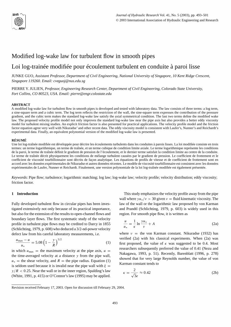
Figure 1 The law of the wall or the logarithmic law.

The value ofA varies in literature; it is about 5.29±0.47 accord-ing to Nezu and Nakagawa (1993, p. 51). Equation (2b) will beexamined later in this paper.

Equation (2a) is applicable away from the wall whereyu∗/ν >

30, as shown in Fig. 1. It is not only valid for steady flow, butis also frequently used as a reference condition in unsteady flowsimulations (Ferziger and Peric, 1997, p. 277). This is becauseeven in unsteady flows, the wall shear stress predominates in thenear-wall flow, and the influence of inertial forces and pressuregradient are vanishingly small.

Laufer (1954) found that the logarithmic law (2a) actuallydeviates from experimental data whenξ = y/R > 0.1 ∼ 0.2.Coles (1956) further confirmed this finding and claimed thatthe deviation has a wake-like shape when viewed from thefreestream. Thus, he called the deviation the law of the wake.Based on Coles’ digital data, Hinze (1975, p. 98) proposed thefollowing expression for the wake function, i.e.

W(ξ) = 2�

κsin2 πξ

2(3)

in which � is Coles wake strength. Finally, one can modify thelogarithmic law by adding the wake function, i.e.

u

u∗=

(1

κln

yu∗ν

+ A

)+ 2�

κsin2 πξ

2(4)

This is called the log-wake law. When applied to pipe flows,the reader can easily show that the log-wake law (4) does notsatisfy the axial symmetrical condition, i.e., the velocity gradientis nonzero at the pipe axis. Besides, the physical interpretationof the wake function is not clear in pipe flows.

Similar to flows in narrow open-channels (Guo and Julien,2001), to correct the velocity gradient at the pipe axis, Guo (1998)proposed the following velocity profile model for pipe flows,

u

u∗= 1

κln

yu∗ν

+ A︸︷︷︸The law of the wall

+ 2�

κsin2 πξ

2− ξ

κ︸︷︷︸Law of the wake

(5a)

orumax − u

u∗= − 1

κ(ln ξ + 1 − ξ) + 2�

κcos2

πξ

2(5b)

in which the Coles wake strength� is due to the pressure-gradient. The log term in (5a) expresses the restriction of thewall, the sine-square term indicates the effect of the pressure-gradient, and the last term reflects the axial boundary correction.According to Coles, the last two terms in (5a), which are the

deviation from the log law, define a law of the wake. It is notedthat although (5a) or (5b) satisfies the axial symmetrical condi-tion, the constant derivative of the linear correction term bringsan additional shear stress in the near wall region, which slightlyperturbs the law of the wall. It is therefore concluded that thelinear function is not the best axial boundary correction.

The purpose of this paper is to develop a physically-basedvelocity profile model for turbulent pipe flows called the modifiedlog-wake law. It is proposed to improve upon Eq. (5b) in the lightof a better physical interpretation of the wake law. The proposedmodified log-wake law is also tested with experimental velocitymeasurements in pipes. Analytical relationships for the turbulenteddy viscosity and for the friction factor are then compared withexperimental data.

2 Development of the modified log-wake law

This section formulates the modified log-wake law in smoothpipes. First a theoretical analysis is considered. Section 2.2proposes the basic structure of the modified log-wake law.Section 2.3 defines the axial boundary correction function. Thefinal formulation of the modified log-wake law is written invelocity-defect form in Section 2.4.

2.1 Theoretical analysis

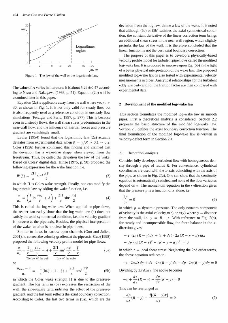
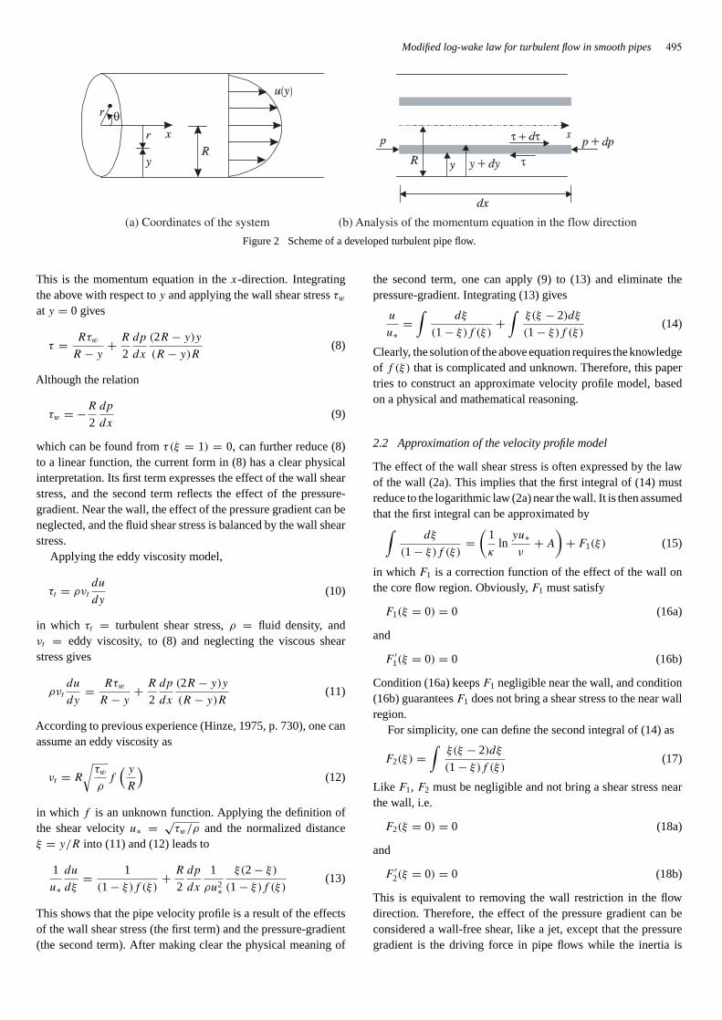
Consider fully developed turbulent flow with homogeneous den-sity through a pipe of radiusR. For convenience, cylindricalcoordinates are used with thex-axis coinciding with the axis ofthe pipe, as shown in Fig. 2(a). One can show that the continuityequation is automatically satisfied and none of the flow variablesdepend onθ . The momentum equation in ther-direction givesthat the pressurep is a function ofx alone, i.e.

∂p

∂r= 0 (6)

in which p = dynamic pressure. The only nonzero componentof velocity is the axial velocityu(r) or u(y) wherey = distancefrom the wall, i.e.y = R − r. With reference to Fig. 2(b),for steady and incompressible flow, the force balance in thex-direction gives

− τ · 2π(R − y)dx + (τ + dτ) · 2π(R − y − dy)dx

− dp · π [(R − y)2 − (R − y − dy)2] = 0

in which τ = local shear stress. Neglecting the 2nd order terms,the above equation reduces to

−τ · 2πdxdy + dτ · 2π(R − y)dx − dp · 2π(R − y)dy = 0

Dividing by 2πdxdy, the above becomes

−τ + dτ

dy(R − y) − dp

dx(R − y) = 0

This can be rearranged as

−dp

dx(R − y) + d[(R − y)τ ]

dy= 0 (7)

Modified log-wake law for turbulent flow in smooth pipes 495

Figure 2 Scheme of a developed turbulent pipe flow.

This is the momentum equation in thex-direction. Integratingthe above with respect toy and applying the wall shear stressτw

aty = 0 gives

τ = Rτw

R − y+ R

2

dp

dx

(2R − y)y

(R − y)R(8)

Although the relation

τw = −R

2

dp

dx(9)

which can be found fromτ(ξ = 1) = 0, can further reduce (8)to a linear function, the current form in (8) has a clear physicalinterpretation. Its first term expresses the effect of the wall shearstress, and the second term reflects the effect of the pressure-gradient. Near the wall, the effect of the pressure gradient can beneglected, and the fluid shear stress is balanced by the wall shearstress.

Applying the eddy viscosity model,

τt = ρνt

du

dy(10)

in which τt = turbulent shear stress,ρ = fluid density, andνt = eddy viscosity, to (8) and neglecting the viscous shearstress gives

ρνt

du

dy= Rτw

R − y+ R

2

dp

dx

(2R − y)y

(R − y)R(11)

According to previous experience (Hinze, 1975, p. 730), one canassume an eddy viscosity as

νt = R

√τw

ρf

( y

R

)(12)

in which f is an unknown function. Applying the definition ofthe shear velocityu∗ = √

τw/ρ and the normalized distanceξ = y/R into (11) and (12) leads to

1

u∗du

dξ= 1

(1 − ξ)f (ξ)+ R

2

dp

dx

1

ρu2∗

ξ(2 − ξ)

(1 − ξ)f (ξ)(13)

This shows that the pipe velocity profile is a result of the effectsof the wall shear stress (the first term) and the pressure-gradient(the second term). After making clear the physical meaning of

the second term, one can apply (9) to (13) and eliminate thepressure-gradient. Integrating (13) gives

u

u∗=

∫dξ

(1 − ξ)f (ξ)+

∫ξ(ξ − 2)dξ

(1 − ξ)f (ξ)(14)

Clearly, the solution of the above equation requires the knowledgeof f (ξ) that is complicated and unknown. Therefore, this papertries to construct an approximate velocity profile model, basedon a physical and mathematical reasoning.

2.2 Approximation of the velocity profile model

The effect of the wall shear stress is often expressed by the lawof the wall (2a). This implies that the first integral of (14) mustreduce to the logarithmic law (2a) near the wall. It is then assumedthat the first integral can be approximated by∫

dξ

(1 − ξ)f (ξ)=

(1

κln

yu∗ν

+ A

)+ F1(ξ) (15)

in which F1 is a correction function of the effect of the wall onthe core flow region. Obviously,F1 must satisfy

F1(ξ = 0) = 0 (16a)

and

F ′1(ξ = 0) = 0 (16b)

Condition (16a) keepsF1 negligible near the wall, and condition(16b) guaranteesF1 does not bring a shear stress to the near wallregion.

For simplicity, one can define the second integral of (14) as

F2(ξ) =∫

ξ(ξ − 2)dξ

(1 − ξ)f (ξ)(17)

Like F1, F2 must be negligible and not bring a shear stress nearthe wall, i.e.

F2(ξ = 0) = 0 (18a)

and

F ′2(ξ = 0) = 0 (18b)

This is equivalent to removing the wall restriction in the flowdirection. Therefore, the effect of the pressure gradient can beconsidered a wall-free shear, like a jet, except that the pressuregradient is the driving force in pipe flows while the inertia is


the driving force in a developed jet. Furthermore, the pipe flowcan be considered a superposition of a wall-bounded shear and awall-free shear. Because of the symmetrical condition,F2 mustreach its maximum value at the pipe axis and satisfy

F ′2(ξ = 1) = 0 (18c)

According to (18b) and (18c), one can approximate the derivativeof F2 as

F ′2(ξ) ∝ sinπξ (19)

The integration of (19) with the boundary condition (18a) gives

F2(ξ) = 2�

κsin2 πξ

2(20a)

or∫ξ(ξ − 2)dξ

(1 − ξ)f (ξ)= 2�

κsin2 πξ

2(20b)

in which the constant 2/π gets buried in� in the integrationand � is introduced as per Coles wake function. Clearly, thesine-square function in pipe flows is due to the effect of pressure-gradient. The value of� might vary with a Reynolds numberslightly, but a universal constant might be good enough for largeReynolds number flows.

Substituting (15) and (20b) into (14) gives

u

u∗=

(1

κln

yu∗ν

+ A

)+ 2�

κsin2 πξ

2+ F1(ξ) (21)

The last two terms disappear near the wall, thus the values ofκ

andA should be the same as those in the law of the wall. It isthen suggestedκ = 2/(

√3e) ≈ 0.42. The value ofA will be

replaced with the maximum velocityumax by using the velocitydefect formulation in Section 2.4. Besides, it is shown later thatthe value of� = κ fits the modified log-wake law well withexperimental data. Therefore, this paper assumes

κ = � = 2√3e

≈ 0.42 (22)

2.3 The axial boundary correction

Because of the axial symmetry, the velocity gradient must be zeroat ξ = 1. From (21), one has

1

u∗du

dξ

∣∣∣∣ξ=1

= 1

κ+ F ′

1(1) = 0

which gives

F ′1(1) = − 1

κ(23)

From (16b) and (23), one can assume

F ′1(ξ) = −ξn−1

κ(24)

in which n > 1. Integrating the above equation and applying(16a) gives

F1(ξ) = − ξn

nκ(25)

Since pipe flows are completely symmetrical about the axis,mathematically, the pipe velocity profile is an even function about

the axisξ = 1. In terms of Taylor series, all odd derivatives atξ = 1 must be zero, i.e.

u = umax + 1

2!d2u

dξ2

∣∣∣∣ξ=1

(1 − ξ)2 + 1

4!d4u

dξ4

∣∣∣∣ξ=1

(1 − ξ)4 + · · ·

To correct the modified log-wake law to the third order term,letting

d3u

dξ3

∣∣∣∣ξ=1

= 0

in (21) where (25) gets applied, one can show that

n = 3 (26)

2.4 The modified log-wake law and its defect form

Combining (21), (22), (25) and (26) leads to the followingmodified log-wake law:

u

u∗=

√3e

2ln

yu∗ν

+ A︸︷︷︸the law of the wall

+ 2 sin2 πξ

2−

√3e

2

ξ3

3︸︷︷︸the modified law of the wake

(27)

Since the last two terms in the above equation express the devia-tion from the law of the wall, following Coles (1956), they definethe law of the wake in this paper, i.e.

W(ξ) = 2 sin2 πξ

2−

√3e

2

ξ3

3(28)

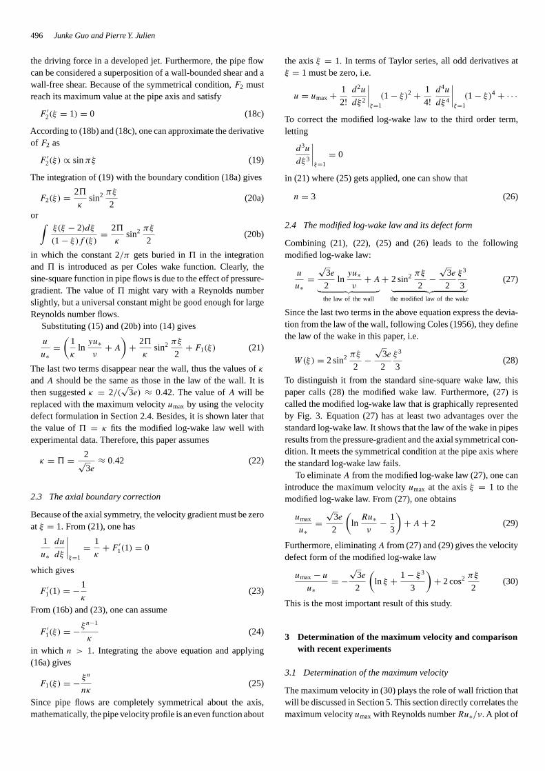
To distinguish it from the standard sine-square wake law, thispaper calls (28) the modified wake law. Furthermore, (27) iscalled the modified log-wake law that is graphically representedby Fig. 3. Equation (27) has at least two advantages over thestandard log-wake law. It shows that the law of the wake in pipesresults from the pressure-gradient and the axial symmetrical con-dition. It meets the symmetrical condition at the pipe axis wherethe standard log-wake law fails.

To eliminateA from the modified log-wake law (27), one canintroduce the maximum velocityumax at the axisξ = 1 to themodified log-wake law. From (27), one obtains

umax

u∗=

√3e

2

(ln

Ru∗ν

− 1

3

)+ A + 2 (29)

Furthermore, eliminatingA from (27) and (29) gives the velocitydefect form of the modified log-wake law

umax − u

u∗= −

√3e

2

(ln ξ + 1 − ξ3

3

)+ 2 cos2

πξ

2(30)

This is the most important result of this study.

3 Determination of the maximum velocity and comparisonwith recent experiments

3.1 Determination of the maximum velocity

The maximum velocity in (30) plays the role of wall friction thatwill be discussed in Section 5. This section directly correlates themaximum velocityumax with Reynolds numberRu∗/ν. A plot of


(a) The effect ofthe wall

Near wall region

Near wall region

Cor

ere

gion

Pipeaxis

(b) The effect of thepressure-gradient

(c) The boundarycorrection

(d) The compositevelocity profile

ξ=1

y

R

Figure 3 Components of the modified log-wake law.

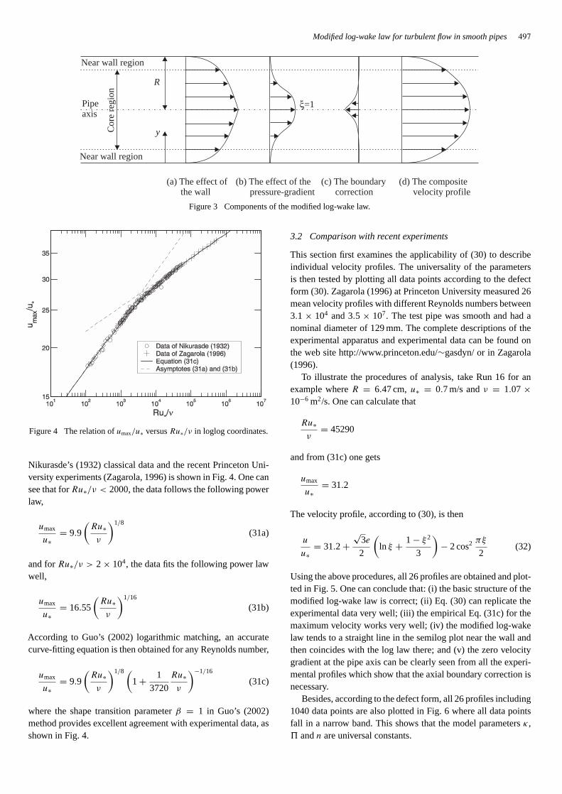
Figure 4 The relation ofumax/u∗ versusRu∗/ν in loglog coordinates.

Nikurasde’s (1932) classical data and the recent Princeton Uni-versity experiments (Zagarola, 1996) is shown in Fig. 4. One cansee that forRu∗/ν < 2000, the data follows the following powerlaw,

umax

u∗= 9.9

(Ru∗ν

)1/8

(31a)

and forRu∗/ν > 2 × 104, the data fits the following power lawwell,

umax

u∗= 16.55

(Ru∗ν

)1/16

(31b)

According to Guo’s (2002) logarithmic matching, an accuratecurve-fitting equation is then obtained for any Reynolds number,

umax

u∗= 9.9

(Ru∗ν

)1/8 (1 + 1

3720

Ru∗ν

)−1/16

(31c)

where the shape transition parameterβ = 1 in Guo’s (2002)method provides excellent agreement with experimental data, asshown in Fig. 4.

3.2 Comparison with recent experiments

This section first examines the applicability of (30) to describeindividual velocity profiles. The universality of the parametersis then tested by plotting all data points according to the defectform (30). Zagarola (1996) at Princeton University measured 26mean velocity profiles with different Reynolds numbers between3.1 × 104 and 3.5 × 107. The test pipe was smooth and had anominal diameter of 129 mm. The complete descriptions of theexperimental apparatus and experimental data can be found onthe web site http://www.princeton.edu/∼gasdyn/ or in Zagarola(1996).

To illustrate the procedures of analysis, take Run 16 for anexample whereR = 6.47 cm, u∗ = 0.7 m/s andν = 1.07 ×10−6 m2/s. One can calculate that

Ru∗ν

= 45290

and from (31c) one gets

umax

u∗= 31.2

The velocity profile, according to (30), is then

u

u∗= 31.2 +

√3e

2

(ln ξ + 1 − ξ2

3

)− 2 cos2

πξ

2(32)

Using the above procedures, all 26 profiles are obtained and plot-ted in Fig. 5. One can conclude that: (i) the basic structure of themodified log-wake law is correct; (ii) Eq. (30) can replicate theexperimental data very well; (iii) the empirical Eq. (31c) for themaximum velocity works very well; (iv) the modified log-wakelaw tends to a straight line in the semilog plot near the wall andthen coincides with the log law there; and (v) the zero velocitygradient at the pipe axis can be clearly seen from all the experi-mental profiles which show that the axial boundary correction isnecessary.

Besides, according to the defect form, all 26 profiles including1040 data points are also plotted in Fig. 6 where all data pointsfall in a narrow band. This shows that the model parametersκ,� andn are universal constants.


100

10–1

10–2

21 4 6553 717

RUN Re

1 3.16×104

2 4.17×104

3 5.67×104

4 7.43×104

5 9.88×104

6 1.46×105

7 1.85×105

17 3.10×106

0 5 10 15 20 25

1 2 3 4 5 17 6 7

u (m/s)

ξ

0 5 10 15 20 25

10 1118 19 8 9

RUN Re

8 2.30×105

9 3.10×105

10 4.09×105

11 5.39×105

18 4.42×106

19 6.07×106

u (m/s)

u (m/s)

0 5 10 15 20 25u (m/s)

8 9 10 1118 19

12 13 14 15 16

RUN Re

12 7.52×105

13 1.02×106

14 1.34×106

15 1.79×106

16 2.35×106

12 13 14 15 16

0 5 10 15 20 25 30 35

20 21 22 23 24 25 26

RUN Re

20 7.71×106

21 1.02×107

22 1.36×107

23 1.82×107

24 2.40×107

25 2.99×107

26 3.53×107

u (m/s)0 5 10 15 20 25 30 35

20 21 22 23 24 25 26

u (m/s)

0 5 10 15 20 25

0

0.2

0.4

0.6

0.8

1

0 5 10 15 20 25u (m/s)

ξ

0

0.2

0.4

0.6

0.8

1

u (m/s)

ξ

0

0.2

0.4

0.6

0.8

1

0 5 10 15 20 25

ξ

0

0.2

0.4

0.6

0.8

1

ξ

100

10–1

10–2

ξ

100

10–1

10–2

ξ

100

10–1

10–2

ξ

Figure 5 Comparison of the modified log-wake law (30) with Zagarola’s (1996) experimental data through individual profiles.

4 Implication for eddy viscosity

Eddy viscosity is important when studying turbulent mixing.With the modified log-wake law, the eddy viscosity can nowbe determined. First, applying (9) to (8) gives the shear stressdistribution:

τ = τw(1 − ξ) (33)

Neglecting the viscous shear stress, from (10) and (33), one canshow that the eddy viscosity can be expressed by

νt

Ru∗= 1 − ξ

(1/u∗)(du/dξ)(34)


103

10–2

10–1

100

0

2

4

6

8

10

12

14(u

max

–u)

/u*

ξ

(a)

Modified log–wake law (30)Data of Zagarola (1996)

0.1 0.2 0.3 0.4 0.5 0.6 0.7 0.8 0.9 10

2

4

6

8

10

12

14(b)

(um

ax–

u)/u

*

ξ

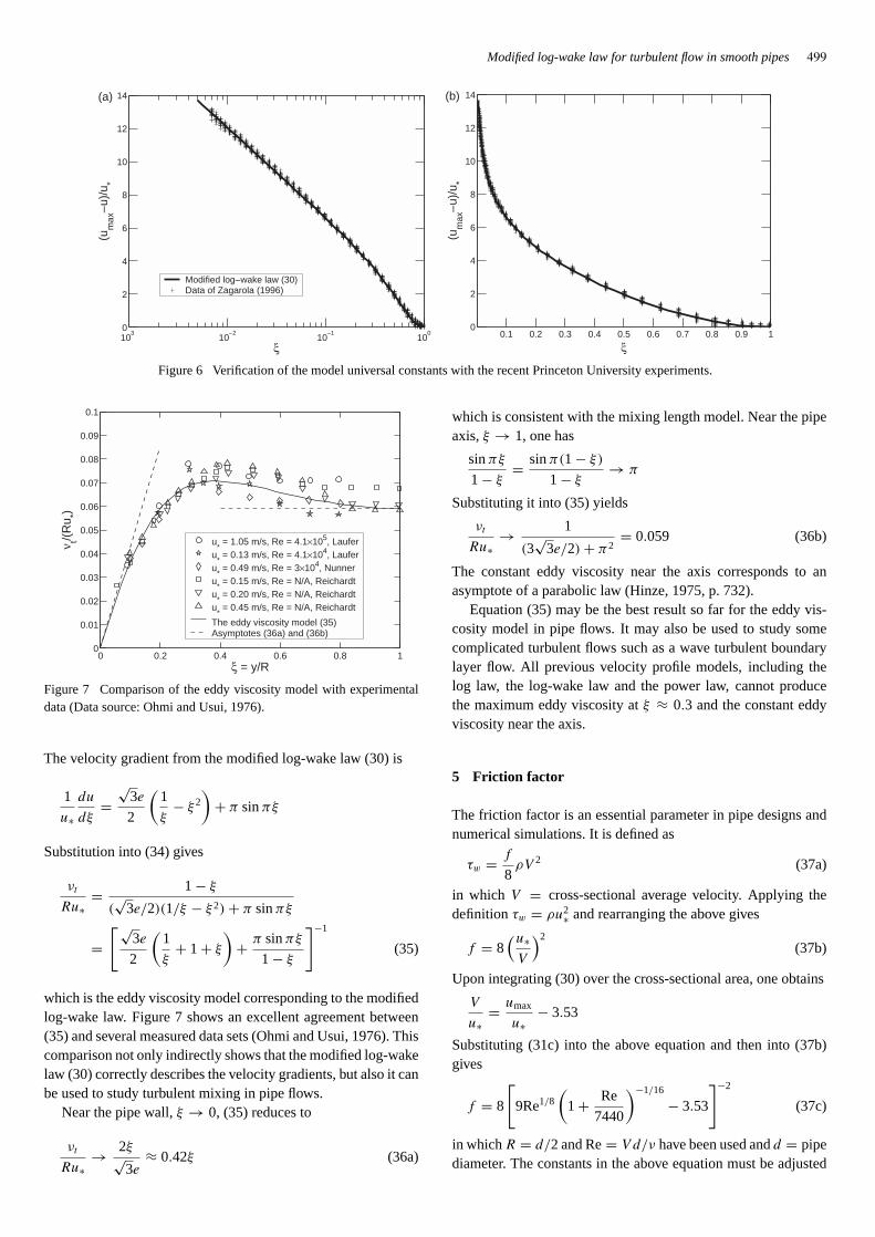
Figure 6 Verification of the model universal constants with the recent Princeton University experiments.

0 0.2 0.4 0.6 0.8 10

0.01

0.02

0.03

0.04

0.05

0.06

0.07

0.08

0.09

0.1

ξ = y/R

ν t/(R

u *)

u* = 1.05 m/s, Re = 4.1×105, Laufer

u* = 0.13 m/s, Re = 4.1×104, Laufer

u* = 0.49 m/s, Re = 3×104, Nunner

u* = 0.15 m/s, Re = N/A, Reichardt



The eddy viscosity model (35)Asymptotes (36a) and (36b)

Figure 7 Comparison of the eddy viscosity model with experimentaldata (Data source: Ohmi and Usui, 1976).

The velocity gradient from the modified log-wake law (30) is

1

u∗du

dξ=

√3e

2

(1

ξ− ξ2

)+ π sinπξ

Substitution into (34) gives

νt

Ru∗= 1 − ξ

(√

3e/2)(1/ξ − ξ2) + π sinπξ

=[√

3e

2

(1

ξ+ 1 + ξ

)+ π sinπξ

1 − ξ

]−1

(35)

which is the eddy viscosity model corresponding to the modifiedlog-wake law. Figure 7 shows an excellent agreement between(35) and several measured data sets (Ohmi and Usui, 1976). Thiscomparison not only indirectly shows that the modified log-wakelaw (30) correctly describes the velocity gradients, but also it canbe used to study turbulent mixing in pipe flows.

Near the pipe wall,ξ → 0, (35) reduces to

νt

Ru∗→ 2ξ√

3e≈ 0.42ξ (36a)

which is consistent with the mixing length model. Near the pipeaxis,ξ → 1, one has

sinπξ

1 − ξ= sinπ(1 − ξ)

1 − ξ→ π

Substituting it into (35) yields

νt

Ru∗→ 1

(3√

3e/2) + π2= 0.059 (36b)

The constant eddy viscosity near the axis corresponds to anasymptote of a parabolic law (Hinze, 1975, p. 732).

Equation (35) may be the best result so far for the eddy vis-cosity model in pipe flows. It may also be used to study somecomplicated turbulent flows such as a wave turbulent boundarylayer flow. All previous velocity profile models, including thelog law, the log-wake law and the power law, cannot producethe maximum eddy viscosity atξ ≈ 0.3 and the constant eddyviscosity near the axis.

5 Friction factor

The friction factor is an essential parameter in pipe designs andnumerical simulations. It is defined as

τw = f

8ρV 2 (37a)

in which V = cross-sectional average velocity. Applying thedefinitionτw = ρu2∗ and rearranging the above gives

f = 8(u∗

V

)2(37b)

Upon integrating (30) over the cross-sectional area, one obtains

V

u∗= umax

u∗− 3.53

Substituting (31c) into the above equation and then into (37b)gives

f = 8

[9Re1/8

(1 + Re

7440

)−1/16

− 3.53

]−2

(37c)

in whichR = d/2 and Re= V d/ν have been used andd = pipediameter. The constants in the above equation must be adjusted


since the viscous sublayer was neglected in the derivation. Forsimplicity, as per (37c), one can assume the friction factor follows

f = a

Re1/4

(1 + Re

b

)1/8

(38a)

For low Reynolds number say Re< 105, the above equationshould reduce to Blasius formula (Schlichting, 1979, p. 597), i.e.

f = 0.3164

Re1/4 (38b)

which gives

a = 0.3164 (38c)

A curve fitting process for high Reynolds number say Re> 2 ×106 gives

b = 4.31× 105 (38d)

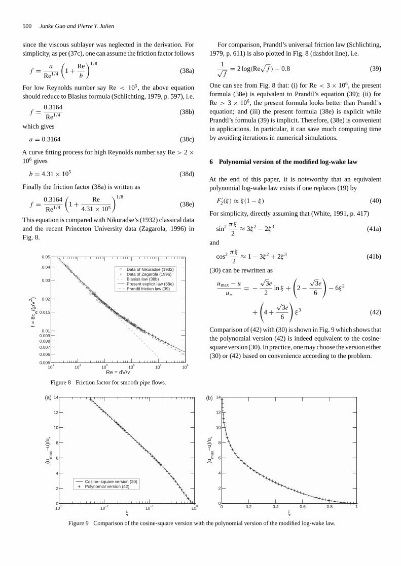
Finally the friction factor (38a) is written as

f = 0.3164

Re1/4

(1 + Re

4.31× 105

)1/8

(38e)

This equation is compared with Nikuradse’s (1932) classical dataand the recent Princeton University data (Zagarola, 1996) inFig. 8.

103

104

105

106

107

108

0.005

0.006

0.007

0.0080.009

0.01

0.015

0.02

0.03

0.04

0.05

Re = dV/ν

f = 8

τ w/(

ρV2 )

Data of Nikuradse (1932)Data of Zagarola (1996)Blasius law (38b)Present explicit law (38e)Prandtl friction law (39)

Figure 8 Friction factor for smooth pipe flows.

103

10–2

10–1

100

0

2

4

6

8

10

12

14

ξ

(um

ax–

u)/u

*

(a)

Cosine–square version (30)Polynomial version (42)

0 0.2 0.4 0.6 0.8 10

2

4

6

8

10

12

14

(um

ax–

u)/u

*

ξ

(b)

Figure 9 Comparison of the cosine-square version with the polynomial version of the modified log-wake law.

For comparison, Prandtl’s universal friction law (Schlichting,1979, p. 611) is also plotted in Fig. 8 (dashdot line), i.e.

1√f

= 2 log(Re√

f ) − 0.8 (39)

One can see from Fig. 8 that: (i) for Re< 3 × 106, the presentformula (38e) is equivalent to Prandtl’s equation (39); (ii) forRe > 3 × 106, the present formula looks better than Prandtl’sequation; and (iii) the present formula (38e) is explicit whilePrandtl’s formula (39) is implicit. Therefore, (38e) is convenientin applications. In particular, it can save much computing timeby avoiding iterations in numerical simulations.

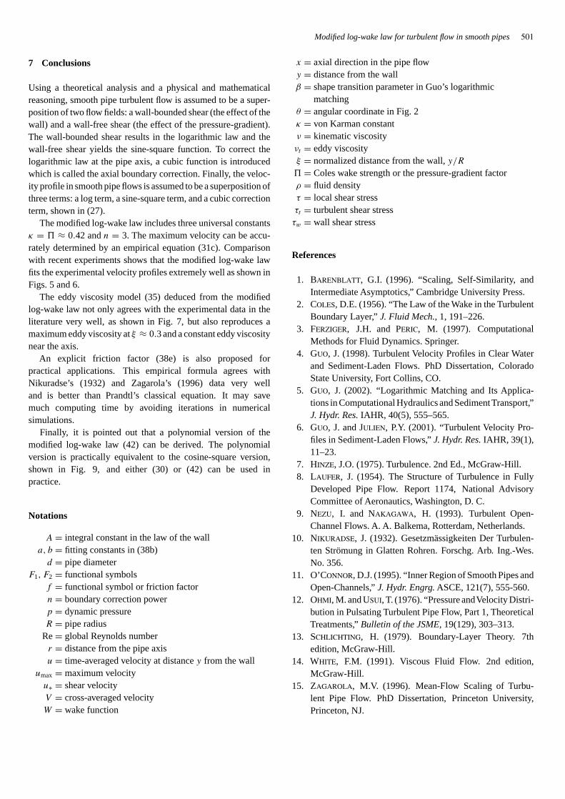
6 Polynomial version of the modified log-wake law

At the end of this paper, it is noteworthy that an equivalentpolynomial log-wake law exists if one replaces (19) by

F ′2(ξ) ∝ ξ(1 − ξ) (40)

For simplicity, directly assuming that (White, 1991, p. 417)

sin2 πξ

2≈ 3ξ2 − 2ξ3 (41a)

and

cos2πξ

2≈ 1 − 3ξ2 + 2ξ3 (41b)

(30) can be rewritten as

umax − u

u∗= −

√3e

2ln ξ +

(2 −

√3e

6

)− 6ξ2

+(

4 +√

3e

6

)ξ3 (42)

Comparison of (42) with (30) is shown in Fig. 9 which shows thatthe polynomial version (42) is indeed equivalent to the cosine-square version (30). In practice, one may choose the version either(30) or (42) based on convenience according to the problem.


7 Conclusions

Using a theoretical analysis and a physical and mathematicalreasoning, smooth pipe turbulent flow is assumed to be a super-position of two flow fields: a wall-bounded shear (the effect of thewall) and a wall-free shear (the effect of the pressure-gradient).The wall-bounded shear results in the logarithmic law and thewall-free shear yields the sine-square function. To correct thelogarithmic law at the pipe axis, a cubic function is introducedwhich is called the axial boundary correction. Finally, the veloc-ity profile in smooth pipe flows is assumed to be a superposition ofthree terms: a log term, a sine-square term, and a cubic correctionterm, shown in (27).

The modified log-wake law includes three universal constantsκ = � ≈ 0.42 andn = 3. The maximum velocity can be accu-rately determined by an empirical equation (31c). Comparisonwith recent experiments shows that the modified log-wake lawfits the experimental velocity profiles extremely well as shown inFigs. 5 and 6.

The eddy viscosity model (35) deduced from the modifiedlog-wake law not only agrees with the experimental data in theliterature very well, as shown in Fig. 7, but also reproduces amaximum eddy viscosity atξ ≈ 0.3 and a constant eddy viscositynear the axis.

An explicit friction factor (38e) is also proposed forpractical applications. This empirical formula agrees withNikuradse’s (1932) and Zagarola’s (1996) data very welland is better than Prandtl’s classical equation. It may savemuch computing time by avoiding iterations in numericalsimulations.

Finally, it is pointed out that a polynomial version of themodified log-wake law (42) can be derived. The polynomialversion is practically equivalent to the cosine-square version,shown in Fig. 9, and either (30) or (42) can be used inpractice.

Notations

A = integral constant in the law of the walla, b = fitting constants in (38b)

d = pipe diameterF1, F2 = functional symbols

f = functional symbol or friction factorn = boundary correction powerp = dynamic pressureR = pipe radius

Re= global Reynolds numberr = distance from the pipe axisu = time-averaged velocity at distancey from the wall

umax = maximum velocityu∗ = shear velocityV = cross-averaged velocityW = wake function

x = axial direction in the pipe flowy = distance from the wallβ = shape transition parameter in Guo’s logarithmic

matchingθ = angular coordinate in Fig. 2κ = von Karman constantν = kinematic viscosityνt = eddy viscosityξ = normalized distance from the wall,y/R

� = Coles wake strength or the pressure-gradient factorρ = fluid densityτ = local shear stressτt = turbulent shear stressτw = wall shear stress

References

1. Barenblatt, G.I. (1996). “Scaling, Self-Similarity, andIntermediate Asymptotics,” Cambridge University Press.

2. Coles, D.E. (1956). “The Law of the Wake in the TurbulentBoundary Layer,”J. Fluid Mech., 1, 191–226.

3. Ferziger, J.H. and Peric, M. (1997). ComputationalMethods for Fluid Dynamics. Springer.

4. Guo, J. (1998). Turbulent Velocity Profiles in Clear Waterand Sediment-Laden Flows. PhD Dissertation, ColoradoState University, Fort Collins, CO.

5. Guo, J. (2002). “Logarithmic Matching and Its Applica-tions in Computational Hydraulics and SedimentTransport,”J. Hydr. Res. IAHR, 40(5), 555–565.

6. Guo, J. and Julien, P.Y. (2001). “Turbulent Velocity Pro-files in Sediment-Laden Flows,”J. Hydr. Res. IAHR, 39(1),11–23.

7. Hinze, J.O. (1975). Turbulence. 2nd Ed., McGraw-Hill.8. Laufer, J. (1954). The Structure of Turbulence in Fully

Developed Pipe Flow. Report 1174, National AdvisoryCommittee of Aeronautics, Washington, D. C.

9. Nezu, I. and Nakagawa, H. (1993). Turbulent Open-Channel Flows. A. A. Balkema, Rotterdam, Netherlands.

10. Nikuradse, J. (1932). Gesetzmässigkeiten Der Turbulen-ten Strömung in Glatten Rohren. Forschg. Arb. Ing.-Wes.No. 356.

11. O’Connor, D.J. (1995). “Inner Region of Smooth Pipes andOpen-Channels,”J. Hydr. Engrg. ASCE, 121(7), 555-560.

12. Ohmi, M. and Usui, T. (1976). “Pressure andVelocity Distri-bution in Pulsating Turbulent Pipe Flow, Part 1, TheoreticalTreatments,”Bulletin of the JSME, 19(129), 303–313.

13. Schlichting, H. (1979). Boundary-Layer Theory. 7thedition, McGraw-Hill.

14. White, F.M. (1991). Viscous Fluid Flow. 2nd edition,McGraw-Hill.

15. Zagarola, M.V. (1996). Mean-Flow Scaling of Turbu-lent Pipe Flow. PhD Dissertation, Princeton University,Princeton, NJ.

Modified log-wake law for turbulent flow in smooth pipes

Documents

Transcript of Modified log-wake law for turbulent flow in smooth pipes