Geoderma 206 (2013) 112–122

Contents lists available at SciVerse ScienceDirect

Geoderma

j ourna l homepage: www.e lsev ie r .com/ locate /geoderma

Modelling trace metal background to evaluate anthropogeniccontamination in arable soils of south-western France

Paul-Olivier Redon a,b, Thomas Bur a,b, Maritxu Guiresse a,b, Jean-Luc Probst a,b, Aurore Toiser a,b,Jean-Claude Revel a,b, Claudy Jolivet c, Anne Probst a,b,⁎a Université de Toulouse; INPT, UPS; EcoLab (Laboratoire Ecologie fonctionnelle et Environnement), ENSAT, Avenue de l'Agrobiopole, 31326 Castanet-Tolosan, Franceb CNRS; EcoLab; ENSAT, 31326 Castanet-Tolosan, Francec INRA, US1106 InfoSol, F-45075 Orléans, France

⁎ Corresponding author at: CNRS, EcoLab, ENSAT, 31Tel.: +33 534323942; fax: +33 534323955.

E-mail address: anne.probst@ensat.fr (A. Probst).

0016-7061/$ – see front matter © 2013 Elsevier B.V. Allhttp://dx.doi.org/10.1016/j.geoderma.2013.04.023

a b s t r a c t

a r t i c l e i n f o

Article history:Received 13 December 2012Received in revised form 7 April 2013Accepted 25 April 2013Available online 25 May 2013

Keywords:Trace metalsAgricultural soilModelStatisticsCalcareousAgricultural land cover

The trace metal (TM) content in arable soils has been monitored across a region of France characterised by alarge proportion of calcareous soils. Within this particular geological context, the objectives were to first de-termine the natural levels of trace metals in the soils and secondly, to assess which sites were significantlycontaminated. Because no universal contamination assessment method is currently available, four differentmethods were applied and compared in order to facilitate the best diagnosis of contamination. First, theTM geochemical background was determined by using basic descriptive statistics and linear regressionmodels calculated with semi-conservative major elements as predictors. The natural concentrations oftrace metals varied greatly due to the high soil heterogeneity encountered on the regional scale and weremore-or-less accurately modelled according to the considered TM. Second, the basic descriptive statisticsand the linear regression methods were then compared with the enrichment factor (EF) method and multi-variate analysis (PCA), in order to evaluate whether the concentrations measured in soils were abnormallyhigh or not. The advantages and disadvantages of each method were discussed and their results used to iden-tify the most probable contamination cases, the influence of the soils characteristics, as well as the agricultur-al land cover. The basic descriptive method was good as a first and easy approach to describe the TM ambientconcentrations, but may misinterpret the natural anomalies as contaminations. Based on geochemical asso-ciations, the linear regression method provided more realistic results even if the relationships betweenmajor and trace metals were not significant for the most mobile TM. The EF method was useful to identifyhigh point source contaminations, but it was not suitable when considering a large dataset of low TM concen-trations. Finally, the PCA method was a good preliminary tool for the description of the global TM concentra-tions in a studied area, but it could only give indication on the highest contaminated points.By comparing the results of the different methods in the studied region, we estimated that 24% of the arablesoils were contaminated by at least one trace metal, mainly Cu in vineyards/orchards and Cd, Pb and/or Zn ingrazing lands. In addition, the calcareous soils exhibited globally higher natural and anthropogenic TM con-centrations than non-calcareous soils, probably because of the lower TM mobility at alkaline pH.

© 2013 Elsevier B.V. All rights reserved.

1. Introduction

Soils constitute a limited andnon-renewable resource that needs to beprotected; however, they are subject to contamination by various tracemetals (TMs). Atmospheric deposits from smelter-related industries orgas combustion, use of chemicals to prevent crop disease, irrigation andapplication of NPK fertilisers, manures and sewage sludge are multiplesources that contribute to the elevation of TM levels in arable soils (Heet al., 2005). Therefore, monitoring the TM concentrations in arable soilsis necessary for the protection of soil quality and food safety. A sustainable

326 Castanet-Tolosan, France.

rights reserved.

management of soils requires the determination of the TM geologicalbackground in order to evaluate the quantities of TMs originating fromanthropogenic and natural sources (Baize and Sterckeman, 2001). Onthe one hand, the anthropogenic fraction is the result of low to moderatediffuse inputs into the soil and of point sources of contamination. On theother hand, the natural background is variable depending on the soil type,because both the parent material and the pedogenesis influence the nat-ural metal concentrations (Bini et al., 2011; Wilson et al., 2008). Conse-quently, the range of local background concentrations must be definedon a regional scale in order to quantify accurately the fraction of exoge-nous metals.

Soil quality guidelines are available in several countries of theworld as indicative levels for the protection of environmental andhuman health. However, European countries are still in discussion to

113P.-O. Redon et al. / Geoderma 206 (2013) 112–122

establish common soil protection policies. Usually, different nationalguidelines are used as limits to define the utilisation potential of arablesoils, but these concentration levels are usually high and do not reflectthe natural local concentrations. Several soil monitoring programmeshave been carried out on a national scale to measure the ranges ofTM concentrations usually encountered in soils. Such concentrationranges might be good indicators of the natural background but theydo not truly evaluate the natural variations on a regional scale.

In the Midi-Pyrénées region of south-western France, a large pro-portion of soils were formed on typical calcareous bedrocks. Moststudies in calcareous soils have shown a high retention of heavy metalson carbonates after application of the contaminants in soil columns(Lafuente et al., 2008; Ouhadi et al., 2010; Plassard et al., 2000) butthe behaviour of natural TMs in these soils remains rarely studiedbecause carbonate rocks are not very common across the globe(Amiotte-Suchet et al., 2003). Within this particular geological context,the TM levels in the soils of theMidi-Pyrénées region needs to be bettercharacterised because this region is also one of the largest agriculturalareas in France.

Several approaches have been documented in the literaturefor determining the background TM levels in soils and sediments(Matschullat et al., 2000; Tobias et al., 1997). As the anthropogenicemissions can be transported over long distances and reach appar-ently undisturbed areas (Hernandez et al., 2003; Steinnes et al.,1997), the background concentrations must be derived from statis-tical analyses applied to a dataset “clean” of outliers. Probabilityplots (Fleischhauer and Korte, 1990; Tobias et al., 1997), basic statis-tics providing ‘baseline values’ (Mrvić et al., 2011; Reimann et al.,2005; Roca et al., 2008), linear relationships between TMs and ele-ments constitutive of the soil (Hamon et al., 2004; Sterckeman etal., 2006b; Zhao et al., 2007) and sediments (N'guessan et al., 2009;Roussiez et al., 2005; Vijver et al., 2008) and geostatistical predic-tions (Saby et al., 2009, 2011) are all various methods for estimatingthe natural levels of TMs in a studied soil dataset.

A second consideration of soil monitoring is the evaluation ofanthropogenic contamination. The observed concentrations in inves-tigated soil samples can be compared with decision limits, such as the‘upper-whisker value’ of a dataset (Micó et al., 2007) or the theoreti-cal background concentration calculated by linear regression or bygeostatistics (Guillén et al., 2011), in order to detect anomalous con-centrations. The enrichment factor (Chester and Stoner, 1973) canalso be used to determine whether the surface layers of soils or sedi-ments are enriched in TMs compared with an uncontaminated refer-ence material (N'guessan et al., 2009; Reimann and de Caritat, 2005).Moreover, multivariate analyses (principal component analysis (PCA)and cluster analysis) are also useful tools for identifying groups ofsamples exhibiting concentrations remarkably different to those ofthe considered soil population (Candeias et al., 2010).

The present study focused on a large collection of arable soilsunder various agricultural practices in the Midi-Pyrénées region (SWFrance) to: (1) define the background levels of TMs in two groups ofagricultural soils (calcareous and non-calcareous); (2) evaluate thesites contaminated by TMs in relation to the agricultural practices.For this purpose, the approach combined in an original way the useof several methods: statistical description, multiple linear regression,enrichment factor and principal component analysis.

2. Materials and methods

2.1. Geological and soil context of the studied area

The studied region (Midi-Pyrénées) is located in south-westernFrance where various geological and pedogenetic processes occurred.The northern part was formed on volcanic and acidic rocks fromthe Massif Central in juxtaposition with calcareous and sedimentaryrocks. In the central part of the basin, the soils were formed on tertiary

molasse and limestone (for details see Perrin et al., 2008). The south ofthe region is characterised by the PyrénéesMountainswith calcareousmassifs, colluviums, glacial drifts and schist in the piedmont and withsedimentary andmetamorphic rocks in the higher mountains. Severalvalleys with alluvial deposits formed by the main rivers (The GaronneRiver and its tributaries) also cross the region.

Consequently, both acidic and alkaline soils are well representedacross the region. Calcareous soils, such as: Calcosols, Calcisols,Colluviosols, Rendosols and Fluviosols (WRB equivalent: Calcaricand Hypereutric Cambisols, Colluvic Regosols, Renzic Leptosols andFluvisols) are developed on the molasse calcareous bedrock or oncolluvium and alluvium. Non-calcareous soils, such as: Brunisols,Luvisols, Rankosols, Fersialsols and Alocrisols (WRB equivalent:Cambisols, Haplic Luvisols, Umbric Leptosols, Haplic and HyperdystricCambisols) originated from acidic bedrocks like gneiss, schist, sand-stone, granite, colluvium or alluvium.

The region is mainly cultivated and the dominant land use con-cerns grasslands, crops, vineyards and orchards. The studied soilshave low organic carbon content because forest soils were not consid-ered in the study.

2.2. Sampling and analyses

Two soil collections from agricultural sites were used in this study.On the one hand, 202 composite samples from 123 sites (one or twodepths per site) and on the other hand, 57 samples from the deeplayer of 57 soil profiles randomly chosen among the 123 sites werecollected and analysed (Figure 1). All these samples were collectedwithin the framework of the French soil quality monitoring network(RMQS). The RMQS network is intended for long-term observationof soil properties and chemical characteristics on a 16-km regulargrid across the 550,000 km2 of French metropolitan territory. The se-lected sites were at the centre of each 16 × 16 km cell. At each site, 25core samples per depth were taken following an unaligned samplingdesign within a 20 × 20 m area and bulked to form one or two com-posite soil samples per site (0–30 cm surface layer and 30–50 cmlayer, if any). For a mechanistic approach, soil profiles were sampledat 57 sites belonging to the 123 sites mentioned above. In each profile,all the soil layers were sampled individually using a core. The numberof samples per site ranged from 2 to 7 layers, depending on the thick-ness of the soil (from 25 to 170 cm deep). The soils were describedand classified according to the French soil classification (Baize andGirard, 2009). The bedrock material was also identified at each site.After field sampling, soil samples were air-dried and sieved to passthrough a 2 mm mesh before analysis.

The samples were analysed after complete dissolution using amixture of HNO3–HF–H2O2 following a procedure described in detailin previous studies (Hernandez et al., 2003; N'guessan et al., 2009).Trace elements (Cd, Co, Cr, Cu, Mo, Ni, Pb, Tl, Zn, Cs, Sc and Sn),major elements (Al, Ca, Fe, K, Mg, Mn and Na), and some soil parame-ters (texture, pH, organic C, and carbonates) weremeasured at the SoilAnalysis Laboratory of INRA at Arras, France (http://www.lille.inra.fr/las). Additional elements (As, Sb, Se and V) were also analysed in theprofile samples. The concentrations were analysed using an ICP-OES(Thermo IRIS INTREPID II XDL) for the major elements and anICP-MS (Perkin-Elmer ELAN 6000) for the trace elements (for analyt-ical details see N'guessan et al., 2009).

2.3. Estimation of natural background concentrations

The dataset was divided into two groups of soils following thecriteria described in Fig. 2. The CaCO3 content, the pH, the bedrockand soil types were used to classify the soils between calcareous andnon-calcareous soils. For each group, the background concentrationsof TMs were estimated by basic statistics and by using multiple linearregressions.

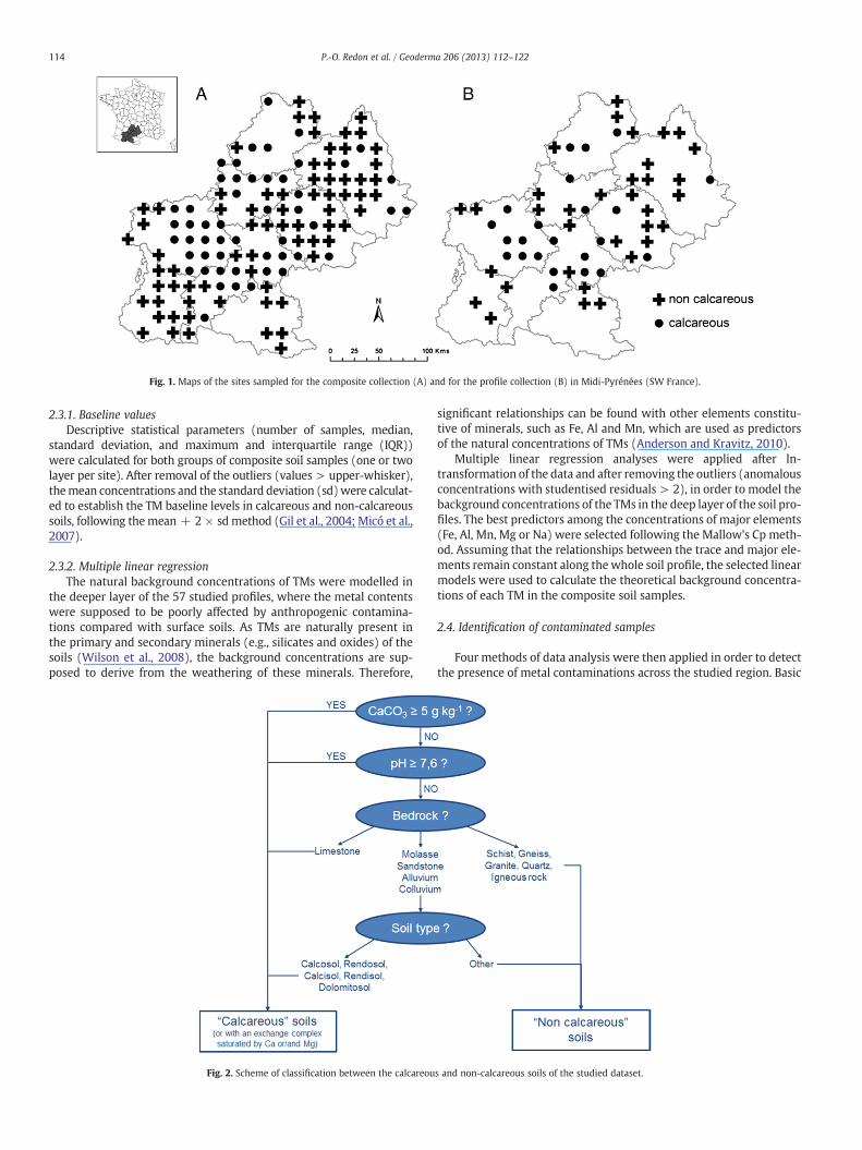
Fig. 1. Maps of the sites sampled for the composite collection (A) and for the profile collection (B) in Midi-Pyrénées (SW France).

114 P.-O. Redon et al. / Geoderma 206 (2013) 112–122

2.3.1. Baseline valuesDescriptive statistical parameters (number of samples, median,

standard deviation, and maximum and interquartile range (IQR))were calculated for both groups of composite soil samples (one or twolayer per site). After removal of the outliers (values > upper-whisker),themean concentrations and the standard deviation (sd)were calculat-ed to establish the TM baseline levels in calcareous and non-calcareoussoils, following themean + 2 × sdmethod (Gil et al., 2004; Micó et al.,2007).

2.3.2. Multiple linear regressionThe natural background concentrations of TMs were modelled in

the deeper layer of the 57 studied profiles, where the metal contentswere supposed to be poorly affected by anthropogenic contamina-tions compared with surface soils. As TMs are naturally present inthe primary and secondary minerals (e.g., silicates and oxides) of thesoils (Wilson et al., 2008), the background concentrations are sup-posed to derive from the weathering of these minerals. Therefore,

Fig. 2. Scheme of classification between the calcareou

significant relationships can be found with other elements constitu-tive of minerals, such as Fe, Al and Mn, which are used as predictorsof the natural concentrations of TMs (Anderson and Kravitz, 2010).

Multiple linear regression analyses were applied after ln-transformation of the data and after removing the outliers (anomalousconcentrations with studentised residuals > 2), in order to model thebackground concentrations of the TMs in the deep layer of the soil pro-files. The best predictors among the concentrations of major elements(Fe, Al, Mn, Mg or Na) were selected following the Mallow's Cp meth-od. Assuming that the relationships between the trace and major ele-ments remain constant along the whole soil profile, the selected linearmodels were used to calculate the theoretical background concentra-tions of each TM in the composite soil samples.

2.4. Identification of contaminated samples

Four methods of data analysis were then applied in order to detectthe presence of metal contaminations across the studied region. Basic

s and non-calcareous soils of the studied dataset.

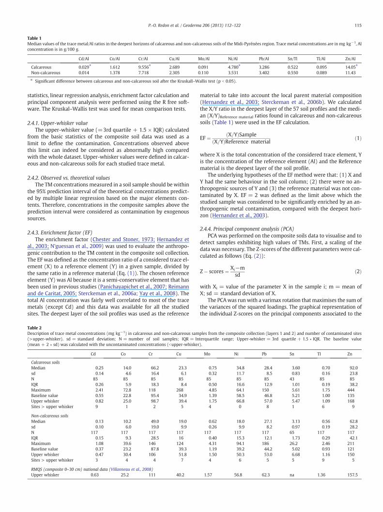
Table 1Median values of the trace metal/Al ratios in the deepest horizons of calcareous and non-calcareous soils of the Midi-Pyrénées region. Trace metal concentrations are in mg kg−1, Alconcentration is in g/100 g.

Cd/Al Co/Al Cr/Al Cu/Al Mo/Al Ni/Al Pb/Al Sn/Tl Tl/Al Zn/Al

Calcareous 0.029⁎ 1.612 9.556⁎ 2.689 0.091 4.780⁎ 3.286 0.522 0.095 14.05⁎

Non-calcareous 0.014 1.378 7.718 2.305 0.110 3.531 3.402 0.550 0.089 11.43

⁎ Significant difference between calcareous and non-calcareous soil after the Kruskall–Wallis test (p b 0.05).

115P.-O. Redon et al. / Geoderma 206 (2013) 112–122

statistics, linear regression analysis, enrichment factor calculation andprincipal component analysis were performed using the R free soft-ware. The Kruskal–Wallis test was used for mean comparison tests.

2.4.1. Upper-whisker valueThe upper-whisker value (=3rd quartile + 1.5 × IQR) calculated

from the basic statistics of the composite soil data was used as alimit to define the contamination. Concentrations observed abovethis limit can indeed be considered as abnormally high comparedwith the whole dataset. Upper-whisker values were defined in calcar-eous and non-calcareous soils for each studied trace metal.

2.4.2. Observed vs. theoretical valuesThe TM concentrations measured in a soil sample should be within

the 95% prediction interval of the theoretical concentrations predict-ed by multiple linear regression based on the major elements con-tents. Therefore, concentrations in the composite samples above theprediction interval were considered as contamination by exogenoussources.

2.4.3. Enrichment factor (EF)The enrichment factor (Chester and Stoner, 1973; Hernandez et

al., 2003; N'guessan et al., 2009) was used to evaluate the anthropo-genic contribution to the TM content in the composite soil collection.The EF was defined as the concentration ratio of a considered trace el-ement (X) to a reference element (Y) in a given sample, divided bythe same ratio in a reference material (Eq. (1)). The chosen referenceelement (Y) was Al because it is a semi-conservative element that hasbeen used in previous studies (Panichayapichet et al., 2007; Reimannand de Caritat, 2005; Sterckeman et al., 2006a; Yay et al., 2008). Thetotal Al concentration was fairly well correlated to most of the tracemetals (except Cd) and this data was available for all the studiedsites. The deepest layer of the soil profiles was used as the reference

Table 2Description of trace metal concentrations (mg kg−1) in calcareous and non-calcareous sam(>upper-whisker). sd = standard deviation; N = number of soil samples; IQR = In(mean + 2 ∗ sd) was calculated with the uncontaminated concentrations (bupper-whisker

Cd Co Cr Cu

Calcareous soilsMedian 0.25 14.0 66.2 23.3sd 0.14 4.6 16.4 6.1N 85 85 85 85IQR 0.26 5.9 18.3 8.4Maximum 2.41 72.8 118 268Baseline value 0.55 22.8 95.4 34.9Upper whisker 0.82 25.0 98.7 39.4Sites > upper whisker 9 1 2 5

Non-calcareous soilsMedian 0.13 10.2 49.0 19.0sd 0.10 6.0 19.0 9.9N 117 117 117 117IQR 0.15 9.3 28.5 16Maximum 1.08 39.6 146 124Baseline value 0.37 23.2 87.8 39.3Upper whisker 0.47 30.4 106 51.8Sites > upper whisker 3 4 4 7

RMQS (composite 0–30 cm) national data (Villanneau et al., 2008)Upper whisker 0.63 25.2 111 40.2

material to take into account the local parent material composition(Hernandez et al., 2003; Sterckeman et al., 2006b). We calculatedthe X/Y ratio in the deepest layer of the 57 soil profiles and the medi-an (X/Y)Reference material ratios found in calcareous and non-calcareoussoils (Table 1) were used in the EF calculation.

EF ¼ X=Yð ÞSampleX=Yð ÞReference material

ð1Þ

where X is the total concentration of the considered trace element, Yis the concentration of the reference element (Al) and the Referencematerial is the deepest layer of the soil profile.

The underlying hypotheses of the EF method were that: (1) X andY had the same behaviour in the soil column; (2) there were no an-thropogenic sources of Y and (3) the reference material was not con-taminated by X. EF = 2 was defined as the limit above which thestudied sample was considered to be significantly enriched by an an-thropogenic metal contamination, compared with the deepest hori-zon (Hernandez et al., 2003).

2.4.4. Principal component analysis (PCA)PCA was performed on the composite soils data to visualise and to

detect samples exhibiting high values of TMs. First, a scaling of thedata was necessary. The Z-scores of the different parameters were cal-culated as follows (Eq. (2)):

Z� scores ¼ Xi−msd

ð2Þ

with Xi = value of the parameter X in the sample i; m = mean ofX; sd = standard deviation of X.

The PCAwas run with a varimax rotation thatmaximises the sum ofthe variances of the squared loadings. The graphical representation ofthe individual Z-scores on the principal components associated to the

ples from the composite collection (layers 1 and 2) and number of contaminated sitesterquartile range; Upper-whisker = 3rd quartile + 1.5 ∗ IQR. The baseline value).

Mo Ni Pb Sn Tl Zn

0.75 34.8 28.4 3.60 0.70 92.00.32 11.7 8.5 0.83 0.16 23.8

85 85 85 43 85 850.50 16.6 12.9 1.01 0.19 38.24.85 64.1 150 5.61 1.75 4441.39 58.5 46.8 5.21 1.00 1351.75 66.8 57.0 5.47 1.09 1684 0 8 1 6 9

0.62 18.0 27.1 3.13 0.56 62.80.26 9.9 8.2 0.97 0.19 28.2

117 117 117 65 117 1170.40 15.3 12.1 1.73 0.29 42.14.31 94.1 186 26.2 2.46 2111.19 39.2 44.2 5.02 0.93 1211.50 50.3 53.0 6.68 1.16 1504 6 5 5 9 5

1.57 56.8 62.3 na 1.36 157.5

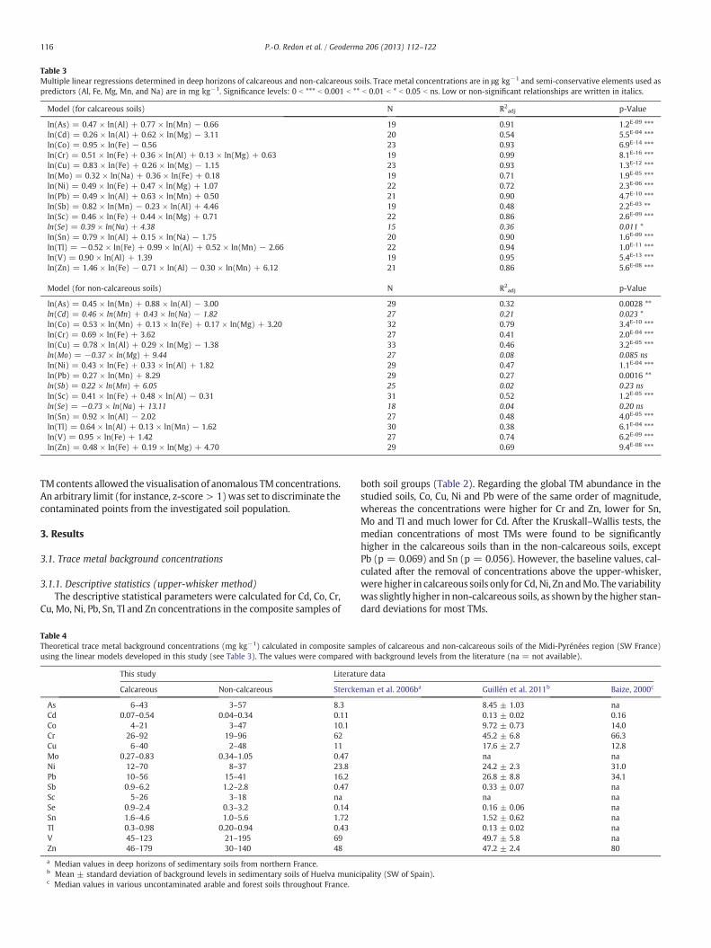
Table 3Multiple linear regressions determined in deep horizons of calcareous and non-calcareous soils. Trace metal concentrations are in μg kg−1 and semi-conservative elements used aspredictors (Al, Fe, Mg, Mn, and Na) are in mg kg−1. Significance levels: 0 b *** b 0.001 b ** b 0.01 b * b 0.05 b ns. Low or non-significant relationships are written in italics.

Model (for calcareous soils) N R2adj p-Value

ln(As) = 0.47 × ln(Al) + 0.77 × ln(Mn) − 0.66 19 0.91 1.2E-09 ***ln(Cd) = 0.26 × ln(Al) + 0.62 × ln(Mg) − 3.11 20 0.54 5.5E-04 ***ln(Co) = 0.95 × ln(Fe) − 0.56 23 0.93 6.9E-14 ***ln(Cr) = 0.51 × ln(Fe) + 0.36 × ln(Al) + 0.13 × ln(Mg) + 0.63 19 0.99 8.1E-16 ***ln(Cu) = 0.83 × ln(Fe) + 0.26 × ln(Mg) − 1.15 23 0.93 1.3E-12 ***ln(Mo) = 0.32 × ln(Na) + 0.36 × ln(Fe) + 0.18 19 0.71 1.9E-05 ***ln(Ni) = 0.49 × ln(Fe) + 0.47 × ln(Mg) + 1.07 22 0.72 2.3E-06 ***ln(Pb) = 0.49 × ln(Al) + 0.63 × ln(Mn) + 0.50 21 0.90 4.7E-10 ***ln(Sb) = 0.82 × ln(Mn) − 0.23 × ln(Al) + 4.46 19 0.48 2.2E-03 **ln(Sc) = 0.46 × ln(Fe) + 0.44 × ln(Mg) + 0.71 22 0.86 2.6E-09 ***ln(Se) = 0.39 × ln(Na) + 4.38 15 0.36 0.011 *ln(Sn) = 0.79 × ln(Al) + 0.15 × ln(Na) − 1.75 20 0.90 1.6E-09 ***ln(Tl) = −0.52 × ln(Fe) + 0.99 × ln(Al) + 0.52 × ln(Mn) − 2.66 22 0.94 1.0E-11 ***ln(V) = 0.90 × ln(Al) + 1.39 19 0.95 5.4E-13 ***ln(Zn) = 1.46 × ln(Fe) − 0.71 × ln(Al) − 0.30 × ln(Mn) + 6.12 21 0.86 5.6E-08 ***

Model (for non-calcareous soils) N R2adj p-Value

ln(As) = 0.45 × ln(Mn) + 0.88 × ln(Al) − 3.00 29 0.32 0.0028 **ln(Cd) = 0.46 × ln(Mn) + 0.43 × ln(Na) − 1.82 27 0.21 0.023 *ln(Co) = 0.53 × ln(Mn) + 0.13 × ln(Fe) + 0.17 × ln(Mg) + 3.20 32 0.79 3.4E-10 ***ln(Cr) = 0.69 × ln(Fe) + 3.62 27 0.41 2.0E-04 ***ln(Cu) = 0.78 × ln(Al) + 0.29 × ln(Mg) − 1.38 33 0.46 3.2E-05 ***ln(Mo) = −0.37 × ln(Mg) + 9.44 27 0.08 0.085 nsln(Ni) = 0.43 × ln(Fe) + 0.33 × ln(Al) + 1.82 29 0.47 1.1E-04 ***ln(Pb) = 0.27 × ln(Mn) + 8.29 29 0.27 0.0016 **ln(Sb) = 0.22 × ln(Mn) + 6.05 25 0.02 0.23 nsln(Sc) = 0.41 × ln(Fe) + 0.48 × ln(Al) − 0.31 31 0.52 1.2E-05 ***ln(Se) = −0.73 × ln(Na) + 13.11 18 0.04 0.20 nsln(Sn) = 0.92 × ln(Al) − 2.02 27 0.48 4.0E-05 ***ln(Tl) = 0.64 × ln(Al) + 0.13 × ln(Mn) − 1.62 30 0.38 6.1E-04 ***ln(V) = 0.95 × ln(Fe) + 1.42 27 0.74 6.2E-09 ***ln(Zn) = 0.48 × ln(Fe) + 0.19 × ln(Mg) + 4.70 29 0.69 9.4E-08 ***

116 P.-O. Redon et al. / Geoderma 206 (2013) 112–122

TMcontents allowed the visualisation of anomalous TMconcentrations.An arbitrary limit (for instance, z-score > 1)was set to discriminate thecontaminated points from the investigated soil population.

3. Results

3.1. Trace metal background concentrations

3.1.1. Descriptive statistics (upper-whisker method)The descriptive statistical parameters were calculated for Cd, Co, Cr,

Cu, Mo, Ni, Pb, Sn, Tl and Zn concentrations in the composite samples of

Table 4Theoretical trace metal background concentrations (mg kg−1) calculated in composite samusing the linear models developed in this study (see Table 3). The values were compared w

This study Literatu

Calcareous Non-calcareous Stercke

As 6–43 3–57 8.3Cd 0.07–0.54 0.04–0.34 0.11Co 4–21 3–47 10.1Cr 26–92 19–96 62Cu 6–40 2–48 11Mo 0.27–0.83 0.34–1.05 0.47Ni 12–70 8–37 23.8Pb 10–56 15–41 16.2Sb 0.9–6.2 1.2–2.8 0.47Sc 5–26 3–18 naSe 0.9–2.4 0.3–3.2 0.14Sn 1.6–4.6 1.0–5.6 1.72Tl 0.3–0.98 0.20–0.94 0.43V 45–123 21–195 69Zn 46–179 30–140 48

a Median values in deep horizons of sedimentary soils from northern France.b Mean ± standard deviation of background levels in sedimentary soils of Huelva municc Median values in various uncontaminated arable and forest soils throughout France.

both soil groups (Table 2). Regarding the global TM abundance in thestudied soils, Co, Cu, Ni and Pb were of the same order of magnitude,whereas the concentrations were higher for Cr and Zn, lower for Sn,Mo and Tl and much lower for Cd. After the Kruskall–Wallis tests, themedian concentrations of most TMs were found to be significantlyhigher in the calcareous soils than in the non-calcareous soils, exceptPb (p = 0.069) and Sn (p = 0.056). However, the baseline values, cal-culated after the removal of concentrations above the upper-whisker,were higher in calcareous soils only for Cd, Ni, Zn andMo. The variabilitywas slightly higher in non-calcareous soils, as shownby the higher stan-dard deviations for most TMs.

ples of calcareous and non-calcareous soils of the Midi-Pyrénées region (SW France)ith background levels from the literature (na = not available).

re data

man et al. 2006ba Guillén et al. 2011b Baize, 2000c

8.45 ± 1.03 na0.13 ± 0.02 0.169.72 ± 0.73 14.045.2 ± 6.8 66.317.6 ± 2.7 12.8na na24.2 ± 2.3 31.026.8 ± 8.8 34.10.33 ± 0.07 nana na0.16 ± 0.06 na1.52 ± 0.62 na0.13 ± 0.02 na49.7 ± 5.8 na47.2 ± 2.4 80

ipality (SW of Spain).

117P.-O. Redon et al. / Geoderma 206 (2013) 112–122

3.1.2. Predicting models of natural concentrations of TMsThe linear models computed in the deep horizon of the calcareous

and non-calcareous soils on the basis of relationships with Al, Fe, Mn,Mg and/or Na are shown in Table 3. The significance of the regres-sions varied according to the soil group and to the considered TM.The models were globally more significant in calcareous, than innon-calcareous soils, because of the better homogeneity of the bed-rock in the former soil group. Among the considered TMs, Co, V andZn were very well predicted by the models in both soil groups. The re-lationships were very significant in calcareous soils but less signifi-cant in non-calcareous soil for As, Cr, Cu, Mo, Ni, Pb, Sn and Tl. Theregression for Mo in non-calcareous soils was not significant. Finally,natural concentrations of Cd, Sb and Se were less well predicted in all

Fig. 3. Observed vs. predicted trace metal concentrations in composite soil samples. Concentrnon-calcareous samples by squares. Black symbols are the observed values above the 95% prfiles collection. Dashed line is the 1:1 line.

soil types. Cd, Sb and Se showed very poor correlations with Fe or Alwhile these two major elements were often the best predictors ofother TM concentrations. Cd and Sb were indeed preferably correlat-ed to Mn. However, at high Fe (>70 g kg−1), Al (>88 g kg−1) andMn (>1.5 g kg−1) concentrations, the relationships were not linearfor several TMs. Thus, the limit of validity for the determination ofthe linear models was set below these concentrations.

Thanks to these linear models established in the deep layers, thetheoretical TM concentrations in the composite samples were cal-culated following the observed concentrations of Fe, Al, Mn, Mg orNa (Table 4). As a result, the ranges of predicted TM concentrationsreflected the variability of the major elements concentrations be-tween sites. However, our results were consistent with previous

ations (μg kg−1) are ln-transformed. Calcareous samples are represented by circles andedicted interval computed from the regression analysis in the deep horizons of the pro-

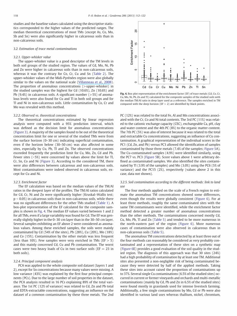
Fig. 4. Box-plot representation of the enrichment factor (EF) of trace metals (Cd, Co, Cr,Cu, Mo, Ni, Pb, Zn and Tl) calculated for the composite samples of the studied soils withthe median TM/Al ratio in deep layer used as a reference. The samples enriched in TMcompared with the deep horizon (EF > 2) are identified by black points.

118 P.-O. Redon et al. / Geoderma 206 (2013) 112–122

studies and the baseline values calculated using the descriptive statis-tics corresponded to the higher values of the predicted ranges. Themedian theoretical concentrations of most TMs (except As, Co, Mo,Sb and Sn) were also significantly higher in calcareous soils than innon-calcareous soils.

3.2. Estimation of trace metal contaminations

3.2.1. Upper-whisker valueThe upper-whisker value is a good descriptor of the TM levels in

both soil groups of the studied region. The values of Cd, Mo, Ni, Pband Zn were higher in calcareous soils than in non-calcareous soils,whereas it was the contrary for Co, Cr, Cu and Sn (Table 2). Theupper-whisker values of the Midi-Pyrénées region were also globallysimilar to the values on the national scale (Villanneau et al., 2008).The proportion of anomalous concentrations (>upper-whisker) inthe studied samples was the highest for Cd (10.6%), Zn (10.6%) andPb (9.4%) in calcareous soils. A significant number (>5%) of anoma-lous levels were also found for Cu and Tl in both soil groups and forTl and Ni in non-calcareous soils. Little contamination by Co, Cr andMo was revealed with this method.

3.2.2. Observed vs. theoretical concentrationsThe theoretical concentrations estimated by linear regression

analysis were computed with a 95% prediction interval, whichwas defined as the decision limit for anomalous concentrations(Figure 3). A majority of the samples found to be out of the theoreticalconcentration limit for one or several of the studied TMs were fromthe surface horizon (0–30 cm) indicating superficial contamination,even if the horizon below (30–50 cm) was also affected in somesites, especially by Cu, Pb, Tl and Zn. The observed concentrationsexceeded frequently the prediction limit for Cu, Mo, Zn, Cd and Pb.Fewer sites (b5%) were concerned by values above the limit for Tl,Cr, Sn, Co and Ni (Figure 3). According to the considered TM, therewere also differences between calcareous and non-calcareous soils.Most contaminations were indeed observed in calcareous soils, ex-cept for Cu and Ni.

3.2.3. Enrichment factorThe EF calculation was based on the median values of the TM/Al

ratios in the deepest layer of the profiles. The TM/Al ratios calculatedfor Cd, Cr, Ni and Zn were significantly higher (Kruskal–Wallis test;p b 0.05) in calcareous soils than in non-calcareous soils, while therewas no significant differences for the other TMs studied (Table 1). Abox-plot representation of the EF calculated for the composite sam-ples is shown in Fig. 4. The median EF values varied between 1 and 2for all TMs, even if a large variabilitywas found for Cd. The EFwas gen-erally slightly higher in the 0–30 cm layer than in the 30–50 cm layer.Several samples exhibiting an EF above 2 were considered as anoma-lous values. Among these enriched samples, the soils were mainlycontaminated by Cd (54% of the sites), Pb (28%), Cu (20%), Mo (18%)and Co (15%). Contamination by the other metals was less frequent(less than 10%). Few samples were very enriched in TMs (EF > 5)and this mainly concerned Cd, Cu and Pb contamination. The worstcases were two heavy loads of Cu in two surface soils (EF = 23 inboth soils).

3.2.4. Principal component analysisPCA was applied to the whole composite soil dataset (layers 1 and

2), except for Sn concentrations because many values were missing. Alow variance (43%) was explained by the first four principal compo-nents (PCs). Due to the large number of soil properties in the dataset,the PCA analysis resulted in 16 PCs explaining 89% of the total vari-ance. The 1st PC (12% of variance) was related to Cd, Zn and Pb totaland EDTA-extractable concentrations, suggesting an influence on thedataset of a common contamination by these three metals. The 2nd

PC (12%) was related to the total Fe, Al and Mn concentrations associ-ated with the Cr, Co and Ni total contents. The 3rd PC (11%) was relat-ed to the cationic exchange capacity (CEC), exchangeable Ca, pH, clayand water content and the 4th PC (8%) to the organic matter content.The 7th PC (5%) was also of interest because it was related to the totaland extractable Cu concentrations, suggesting an influence of Cu con-tamination. A graphical representation of the individual scores in thePC1 (Cd, Zn, and Pb) versus PC3 allowed the identification of samplescontaminated by those three metals (7.4% of the samples; Figure 5A).The Cu-contaminated samples (4.9%) were identified similarly, usingthe PC7 vs. PC3 (Figure 5B). Score values above 1 were arbitrary de-fined as contaminated samples. We also identified the sites contami-nated by Tl (3.9% of the samples) and Mo (3.0%) using the PC6 (5% ofvariance) and the PC15 (2%), respectively (values above 2 in thiscase, data not shown).

3.2.5. Soil contamination according to the different methods: link to landuse

The four methods applied on the scale of a French region to esti-mate the anomalous TM concentrations showed some differences,even though the results were globally consistent (Figure 6). For atleast three methods, roughly the same contaminated sites with thesame TM contaminants were identified, while the enrichment factormethod detected a greater number of anomalous concentrationsthan the other methods. The contaminations concerned mostly Cd,Cu, Mo, Pb, Tl and Zn (Table 5) and tended to be more numerous inthe north-eastern part of the region (Figure 6). More numerouscases of contamination were also observed in calcareous than innon-calcareous soils (Table 5).

The anomalous TM concentrations detected by at least three out ofthe four methods can reasonably be considered as very probably con-taminated and a representation of these sites on a synthetic map(Figure 6E) provides a good evaluation of the soil quality in the stud-ied region. The diagnosis of this approach was that 30 sites (24%)had a high probability of contamination by at least one TM. Additionalsites also presented a non-negligible risk of being contaminated be-cause they were detected by half of the applied methods. Takingthese sites into account raised the proportion of contaminations upto 37%. Several single Cu contaminations (6.5% of the studied sites) oc-curred in current or former vineyards and orchards andmulti-metalliccontaminations (mainly by Cd, Pb and Zn in 6.5% of the studied sites)were found mostly in grasslands used for intense livestock farming.Additionally, a few single contaminations by Mo, Cd or Pb were alsoidentified in various land uses whereas thallium, nickel, chromium,

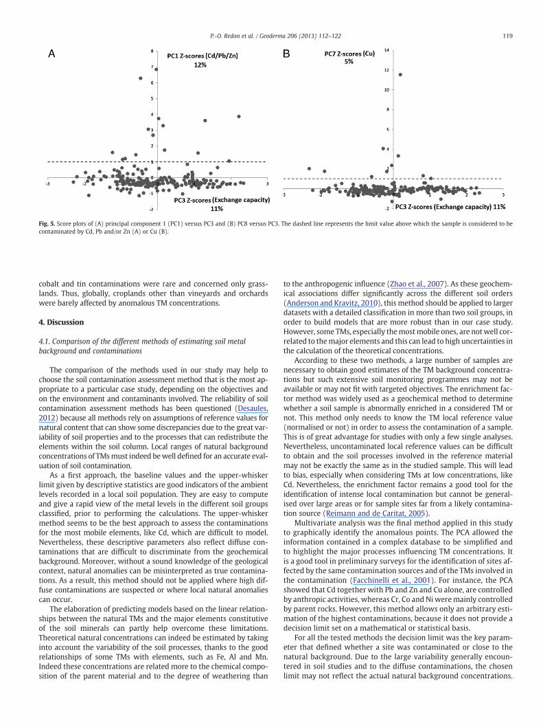
Fig. 5. Score plots of (A) principal component 1 (PC1) versus PC3 and (B) PC8 versus PC3. The dashed line represents the limit value above which the sample is considered to becontaminated by Cd, Pb and/or Zn (A) or Cu (B).

119P.-O. Redon et al. / Geoderma 206 (2013) 112–122

cobalt and tin contaminations were rare and concerned only grass-lands. Thus, globally, croplands other than vineyards and orchardswere barely affected by anomalous TM concentrations.

4. Discussion

4.1. Comparison of the different methods of estimating soil metalbackground and contaminations

The comparison of the methods used in our study may help tochoose the soil contamination assessment method that is the most ap-propriate to a particular case study, depending on the objectives andon the environment and contaminants involved. The reliability of soilcontamination assessment methods has been questioned (Desaules,2012) because all methods rely on assumptions of reference values fornatural content that can show some discrepancies due to the great var-iability of soil properties and to the processes that can redistribute theelements within the soil column. Local ranges of natural backgroundconcentrations of TMsmust indeed bewell defined for an accurate eval-uation of soil contamination.

As a first approach, the baseline values and the upper-whiskerlimit given by descriptive statistics are good indicators of the ambientlevels recorded in a local soil population. They are easy to computeand give a rapid view of the metal levels in the different soil groupsclassified, prior to performing the calculations. The upper-whiskermethod seems to be the best approach to assess the contaminationsfor the most mobile elements, like Cd, which are difficult to model.Nevertheless, these descriptive parameters also reflect diffuse con-taminations that are difficult to discriminate from the geochemicalbackground. Moreover, without a sound knowledge of the geologicalcontext, natural anomalies can be misinterpreted as true contamina-tions. As a result, this method should not be applied where high dif-fuse contaminations are suspected or where local natural anomaliescan occur.

The elaboration of predicting models based on the linear relation-ships between the natural TMs and the major elements constitutiveof the soil minerals can partly help overcome these limitations.Theoretical natural concentrations can indeed be estimated by takinginto account the variability of the soil processes, thanks to the goodrelationships of some TMs with elements, such as Fe, Al and Mn.Indeed these concentrations are related more to the chemical compo-sition of the parent material and to the degree of weathering than

to the anthropogenic influence (Zhao et al., 2007). As these geochem-ical associations differ significantly across the different soil orders(Anderson and Kravitz, 2010), this method should be applied to largerdatasets with a detailed classification in more than two soil groups, inorder to build models that are more robust than in our case study.However, some TMs, especially themostmobile ones, are notwell cor-related to themajor elements and this can lead to high uncertainties inthe calculation of the theoretical concentrations.

According to these two methods, a large number of samples arenecessary to obtain good estimates of the TM background concentra-tions but such extensive soil monitoring programmes may not beavailable or may not fit with targeted objectives. The enrichment fac-tor method was widely used as a geochemical method to determinewhether a soil sample is abnormally enriched in a considered TM ornot. This method only needs to know the TM local reference value(normalised or not) in order to assess the contamination of a sample.This is of great advantage for studies with only a few single analyses.Nevertheless, uncontaminated local reference values can be difficultto obtain and the soil processes involved in the reference materialmay not be exactly the same as in the studied sample. This will leadto bias, especially when considering TMs at low concentrations, likeCd. Nevertheless, the enrichment factor remains a good tool for theidentification of intense local contamination but cannot be general-ised over large areas or for sample sites far from a likely contamina-tion source (Reimann and de Caritat, 2005).

Multivariate analysis was the final method applied in this studyto graphically identify the anomalous points. The PCA allowed theinformation contained in a complex database to be simplified andto highlight the major processes influencing TM concentrations. Itis a good tool in preliminary surveys for the identification of sites af-fected by the same contamination sources and of the TMs involved inthe contamination (Facchinelli et al., 2001). For instance, the PCAshowed that Cd together with Pb and Zn and Cu alone, are controlledby anthropic activities, whereas Cr, Co and Ni weremainly controlledby parent rocks. However, this method allows only an arbitrary esti-mation of the highest contaminations, because it does not provide adecision limit set on a mathematical or statistical basis.

For all the tested methods the decision limit was the key param-eter that defined whether a site was contaminated or close to thenatural background. Due to the large variability generally encoun-tered in soil studies and to the diffuse contaminations, the chosenlimit may not reflect the actual natural background concentrations.

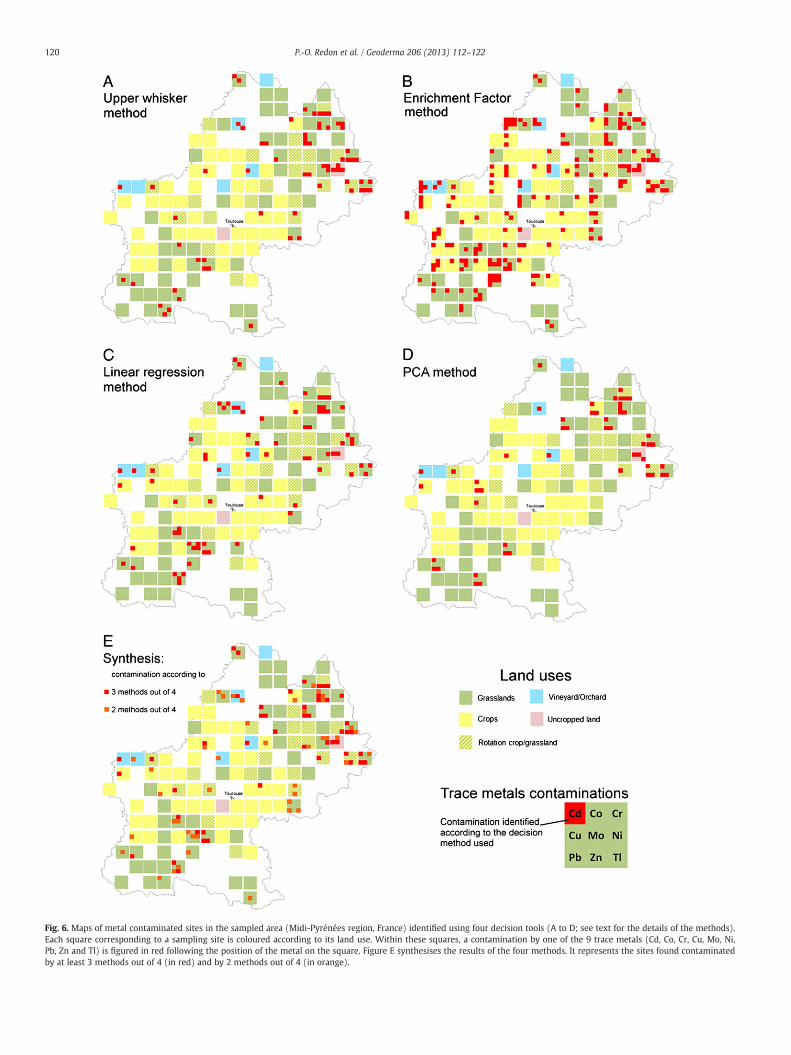
Fig. 6. Maps of metal contaminated sites in the sampled area (Midi-Pyrénées region, France) identified using four decision tools (A to D; see text for the details of the methods).Each square corresponding to a sampling site is coloured according to its land use. Within these squares, a contamination by one of the 9 trace metals (Cd, Co, Cr, Cu, Mo, Ni,Pb, Zn and Tl) is figured in red following the position of the metal on the square. Figure E synthesises the results of the four methods. It represents the sites found contaminatedby at least 3 methods out of 4 (in red) and by 2 methods out of 4 (in orange).

120 P.-O. Redon et al. / Geoderma 206 (2013) 112–122

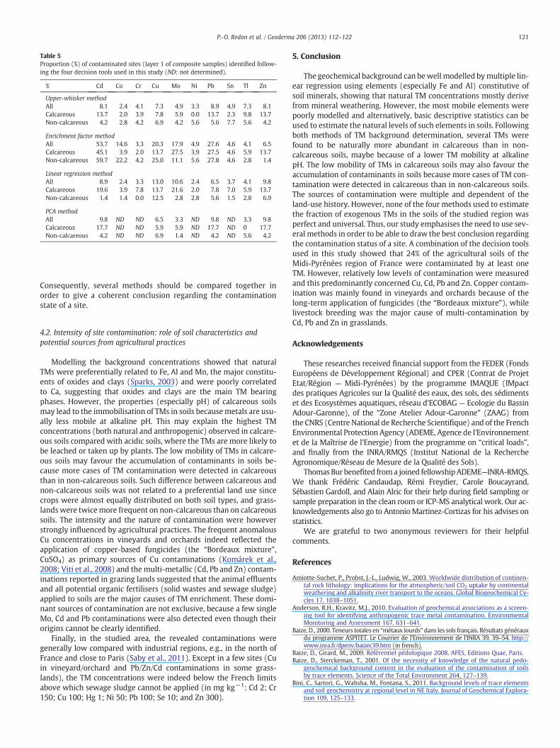
Table 5Proportion (%) of contaminated sites (layer 1 of composite samples) identified follow-ing the four decision tools used in this study (ND: not determined).

% Cd Co Cr Cu Mo Ni Pb Sn Tl Zn

Upper-whisker methodAll 8.1 2.4 4.1 7.3 4.9 3.3 8.9 4.9 7.3 8.1Calcareous 13.7 2.0 3.9 7.8 5.9 0.0 13.7 2.3 9.8 13.7Non-calcareous 4.2 2.8 4.2 6.9 4.2 5.6 5.6 7.7 5.6 4.2

Enrichment factor methodAll 53.7 14.6 3.3 20.3 17.9 4.9 27.6 4.6 4.1 6.5Calcareous 45.1 3.9 2.0 13.7 27.5 3.9 27.5 4.6 5.9 13.7Non-calcareous 59.7 22.2 4.2 25.0 11.1 5.6 27.8 4.6 2.8 1.4

Linear regression methodAll 8.9 2.4 3.3 13.0 10.6 2.4 6.5 3.7 4.1 9.8Calcareous 19.6 3.9 7.8 13.7 21.6 2.0 7.8 7.0 5.9 13.7Non-calcareous 1.4 1.4 0.0 12.5 2.8 2.8 5.6 1.5 2.8 6.9

PCA methodAll 9.8 ND ND 6.5 3.3 ND 9.8 ND 3.3 9.8Calcareous 17.7 ND ND 5.9 5.9 ND 17.7 ND 0 17.7Non-calcareous 4.2 ND ND 6.9 1.4 ND 4.2 ND 5.6 4.2

121P.-O. Redon et al. / Geoderma 206 (2013) 112–122

Consequently, several methods should be compared together inorder to give a coherent conclusion regarding the contaminationstate of a site.

4.2. Intensity of site contamination: role of soil characteristics andpotential sources from agricultural practices

Modelling the background concentrations showed that naturalTMs were preferentially related to Fe, Al and Mn, the major constitu-ents of oxides and clays (Sparks, 2003) and were poorly correlatedto Ca, suggesting that oxides and clays are the main TM bearingphases. However, the properties (especially pH) of calcareous soilsmay lead to the immobilisation of TMs in soils becausemetals are usu-ally less mobile at alkaline pH. This may explain the highest TMconcentrations (both natural and anthropogenic) observed in calcare-ous soils compared with acidic soils, where the TMs are more likely tobe leached or taken up by plants. The low mobility of TMs in calcare-ous soils may favour the accumulation of contaminants in soils be-cause more cases of TM contamination were detected in calcareousthan in non-calcareous soils. Such difference between calcareous andnon-calcareous soils was not related to a preferential land use sincecrops were almost equally distributed on both soil types, and grass-lands were twicemore frequent on non-calcareous than on calcareoussoils. The intensity and the nature of contamination were howeverstrongly influenced by agricultural practices. The frequent anomalousCu concentrations in vineyards and orchards indeed reflected theapplication of copper-based fungicides (the “Bordeaux mixture”,CuSO4) as primary sources of Cu contaminations (Komárek et al.,2008; Viti et al., 2008) and themulti-metallic (Cd, Pb and Zn) contam-inations reported in grazing lands suggested that the animal effluentsand all potential organic fertilisers (solid wastes and sewage sludge)applied to soils are the major causes of TM enrichment. These domi-nant sources of contamination are not exclusive, because a few singleMo, Cd and Pb contaminations were also detected even though theirorigins cannot be clearly identified.

Finally, in the studied area, the revealed contaminations weregenerally low compared with industrial regions, e.g., in the north ofFrance and close to Paris (Saby et al., 2011). Except in a few sites (Cuin vineyard/orchard and Pb/Zn/Cd contaminations in some grass-lands), the TM concentrations were indeed below the French limitsabove which sewage sludge cannot be applied (in mg kg−1: Cd 2; Cr150; Cu 100; Hg 1; Ni 50; Pb 100; Se 10; and Zn 300).

5. Conclusion

The geochemical background can bewell modelled bymultiple lin-ear regression using elements (especially Fe and Al) constitutive ofsoil minerals, showing that natural TM concentrations mostly derivefrom mineral weathering. However, the most mobile elements werepoorly modelled and alternatively, basic descriptive statistics can beused to estimate the natural levels of such elements in soils. Followingboth methods of TM background determination, several TMs werefound to be naturally more abundant in calcareous than in non-calcareous soils, maybe because of a lower TM mobility at alkalinepH. The low mobility of TMs in calcareous soils may also favour theaccumulation of contaminants in soils because more cases of TM con-tamination were detected in calcareous than in non-calcareous soils.The sources of contamination were multiple and dependent of theland-use history. However, none of the four methods used to estimatethe fraction of exogenous TMs in the soils of the studied region wasperfect and universal. Thus, our study emphasises the need to use sev-eral methods in order to be able to draw the best conclusion regardingthe contamination status of a site. A combination of the decision toolsused in this study showed that 24% of the agricultural soils of theMidi-Pyrénées region of France were contaminated by at least oneTM. However, relatively low levels of contamination were measuredand this predominantly concerned Cu, Cd, Pb and Zn. Copper contam-ination was mainly found in vineyards and orchards because of thelong-term application of fungicides (the “Bordeaux mixture”), whilelivestock breeding was the major cause of multi-contamination byCd, Pb and Zn in grasslands.

Acknowledgements

These researches received financial support from the FEDER (FondsEuropéens de Développement Régional) and CPER (Contrat de ProjetEtat/Région — Midi-Pyrénées) by the programme IMAQUE (IMpactdes pratiques Agricoles sur la Qualité des eaux, des sols, des sédimentset des Ecosystèmes aquatiques, réseau d'ECOBAG — Ecologie du BassinAdour-Garonne), of the “Zone Atelier Adour-Garonne” (ZAAG) fromthe CNRS (Centre National de Recherche Scientifique) and of the FrenchEnvironmental Protection Agency (ADEME, Agence de l'Environnementet de la Maîtrise de l'Energie) from the programme on “critical loads”,and finally from the INRA/RMQS (Institut National de la RechercheAgronomique/Réseau de Mesure de la Qualité des Sols).

ThomasBur benefited froma joined fellowshipADEME—INRA-RMQS.We thank Frédéric Candaudap, Rémi Freydier, Carole Boucayrand,Sébastien Gardoll, and Alain Alric for their help during field sampling orsample preparation in the clean room or ICP-MS analytical work. Our ac-knowledgements also go to Antonio Martinez-Cortizas for his advises onstatistics.

We are grateful to two anonymous reviewers for their helpfulcomments.

References

Amiotte-Suchet, P., Probst, J.-L., Ludwig, W., 2003. Worldwide distribution of continen-tal rock lithology: implications for the atmospheric/soil CO2 uptake by continentalweathering and alkalinity river transport to the oceans. Global Biogeochemical Cy-cles 17, 1038–1051.

Anderson, R.H., Kravitz, M.J., 2010. Evaluation of geochemical associations as a screen-ing tool for identifying anthropogenic trace metal contamination. EnvironmentalMonitoring and Assessment 167, 631–641.

Baize, D., 2000. Teneurs totales en “métaux lourds” dans les sols français. Résultats générauxdu programme ASPITET. Le Courrier de l'Environnement de l'INRA 39, 39–54. http://www.inra.fr/dpenv/baizec39.htm (in french).

Baize, D., Girard, M., 2009. Référentiel pédologique 2008. AFES, Editions Quae, Paris.Baize, D., Sterckeman, T., 2001. Of the necessity of knowledge of the natural pedo-

geochemical background content in the evaluation of the contamination of soilsby trace elements. Science of the Total Environment 264, 127–139.

Bini, C., Sartori, G., Wahsha, M., Fontana, S., 2011. Background levels of trace elementsand soil geochemistry at regional level in NE Italy. Journal of Geochemical Explora-tion 109, 125–133.

122 P.-O. Redon et al. / Geoderma 206 (2013) 112–122

Candeias, C., Ferreira da Silva, E., Salgueiro, A.R., Pereira, H.G., Reis, A.P., Patinha, C.,Matos, J.X., Ávila, P.H., 2010. The use of multivariate statistical analysis of geochem-ical data for assessing the spatial distribution of soil contamination by potentiallytoxic elements in the Aljustrel mining area (Iberian Pyrite Belt, Portugal). Environ-mental Earth Sciences 62, 1461–1479.

Chester, R., Stoner, J.H., 1973. Pb in particulates from the lower atmosphere of the easternAtlantic. Nature 245, 27–28.

Desaules, A., 2012. Critical evaluation of soil contamination assessment methods fortrace metals. Science of the Total Environment 426, 120–131.

Facchinelli, A., Sacchi, E., Mallen, L., 2001. Multivariate statistical and GIS-based approachto identify heavy metal sources in soils. Environmental Pollution 114, 313–324.

Fleischhauer, H.L., Korte, N., 1990. Formulation of cleanup standards for trace elementswith probability plots. Environmental Management 14, 95–105.

Gil, C., Boluda, R., Ramos, J., 2004. Determination and evaluation of cadmium, lead andnickel in greenhouse soils of Almería (Spain). Chemosphere 55, 1027–1034.

Guillén, M.T., Delgado, J., Albanese, S., Nieto, J.M., Lima, A., De Vivo, B., 2011. Environ-mental geochemical mapping of Huelva municipality soils (SW Spain) as a toolto determine background and baseline values. Journal of Geochemical Exploration109, 59–69.

Hamon, R.E., McLaughlin, M.J., Gilkes, R.J., Rate, A.W., Zarcinas, B., Robertson, A., Cozens, G.,Radford, N., Bettenay, L., 2004. Geochemical indices allow estimation of heavy metalbackground concentrations in soils. Global Biogeochemical Cycles 18 (Available athttp://www.agu.org/pubs/crossref/2004/2003GB002063.shtml (verified 4May 2012)).

He, Z.L., Yang, X.E., Stoffella, P.J., 2005. Trace elements in agroecosystems and impacts onthe environment. Journal of Trace Elements in Medicine and Biology 19, 125–140.

Hernandez, L., Probst, A., Probst, J.L., Ulrich, E., 2003. Heavy metal distribution in someFrench forest soils: evidence for atmospheric contamination. Science of the TotalEnvironment 312, 195–219.

Komárek, M., Száková, J., Rohošková, M., Javorská, H., Chrastný, V., Balík, J., 2008. Cop-per contamination of vineyard soils from small wine producers: a case study fromthe Czech Republic. Geoderma 147, 16–22.

Lafuente, A.L., González, C., Quintana, J.R., Vázquez, A., Romero, A., 2008. Mobility ofheavy metals in poorly developed carbonate soils in the Mediterranean region.Geoderma 145, 238–244.

Matschullat, J., Ottenstein, R., Reimann, C., 2000. Geochemical background — can wecalculate it? Environmental Geology 39, 990–1000.

Micó, C., Peris, M., Recatalá, L., Sánchez, J., 2007. Baseline values for heavy metals in ag-ricultural soils in an European Mediterranean region. Science of the Total Environ-ment 378, 13–17.

Mrvić, V., Kostić-Kravljanac, L., Čakmak, D., Sikirić, B., Brebanović, B., Perović, V.,Nikoloski, M., 2011. Pedogeochemical mapping and background limit of trace ele-ments in soils of Branicevo Province (Serbia). Journal of Geochemical Exploration109, 18–25.

N'guessan, Y.M., Probst, J.L., Bur, T., Probst, A., 2009. Trace elements in stream bed sed-iments from agricultural catchments (Gascogne region, S-W France): where dothey come from? Science of the Total Environment 407, 2939–2952.

Ouhadi, V.R., Yong, R.N., Shariatmadari, N., Saeidijam, S., Goodarzi, A.R., Safari-Zanjani,M., 2010. Impact of carbonate on the efficiency of heavy metal removal from kao-linite soil by the electrokinetic soil remediation method. Journal of Hazardous Ma-terials 173, 87–94.

Panichayapichet, P., Nitisoravut, S., Simachaya, W., 2007. Spatial distribution and trans-port of heavy metals in soil, ponded-surface water and grass in a Pb-contaminatedwatershed as related to land-use practices. Environmental Monitoring and Assess-ment 135, 181–193.

Perrin, A.-S., Probst, A., Probst, J.-L., 2008. Impact of nitrogenous fertilizers on carbonatedissolution in small agricultural catchments: implications for weathering CO2 uptakeat regional and global scales. Geochimica et Cosmochimica Acta 72, 3105–3123.

Plassard, F., Winiarski, T., Petit-Ramel, M., 2000. Retention and distribution of threeheavy metals in a carbonated soil: comparison between batch and unsaturated col-umn studies. Journal of Contaminant Hydrology 42, 99–111.

Reimann, C., de Caritat, P., 2005. Distinguishing between natural and anthropogenicsources for elements in the environment: regional geochemical surveys versus en-richment factors. Science of the Total Environment 337, 91–107.

Reimann, C., Filzmoser, P., Garrett, R.G., 2005. Background and threshold: critical com-parison of methods of determination. Science of the Total Environment 346, 1–16.

Roca, N., Pazos, M.S., Bech, J., 2008. The relationship between WRB soil units and heavymetals content in soils of Catamarca (Argentina). Journal of Geochemical Explora-tion 96, 77–85.

Roussiez, V., Ludwig, W., Probst, J.-L., Monaco, A., 2005. Background levels of heavymetals in surficial sediments of the Gulf of Lions (NWMediterranean): an approachbased on 133Cs normalization and lead isotope measurements. Environmental Pol-lution 138, 167–177.

Saby, N.P.A., Thioulouse, J., Jolivet, C.C., Ratié, C., Boulonne, L., Bispo, A., Arrouays, D., 2009.Multivariate analysis of the spatial patterns of 8 trace elements using the French soilmonitoring network data. Science of the Total Environment 407, 5644–5652.

Saby, N.P.A., Marchant, B.P., Lark, R.M., Jolivet, C.C., Arrouays, D., 2011. Robustgeostatistical prediction of trace elements across France. Geoderma 162, 303–311.

Sparks, D., 2003. Environmental Soil Chemistry, 2nd ed. Academic Press, London.Steinnes, E., Allen, R.O., Petersen, H.M., Rambæk, J.P., Varskog, P., 1997. Evidence of

large scale heavy-metal contamination of natural surface soils in Norway fromlong-range atmospheric transport. Science of the Total Environment 205, 255–266.

Sterckeman, T., Douay, F., Baize, D., Fourrier, H., Proix, N., Schvartz, C., 2006. Trace ele-ments in soils developed in sedimentary materials from Northern France.Geoderma 136, 912–929.

Sterckeman, T., Douay, F., Baize, D., Fourrier, H., Proix, N., Schvartz, C., Carignan, J., 2006.Trace element distributions in soils developed in loess deposits from northernFrance. European Journal of Soil Science 57, 392–410.

Tobias, F., Bech, J., Algarra, P., 1997. Establishment of the background levels of sometrace elements in soils of NE Spain with probability plots. Science of the Total En-vironment 206, 255–265.

Vijver, M.G., Spijker, J., Vink, J.P.M., Posthuma, L., 2008. Determining metal originsand availability in fluvial deposits by analysis of geochemical baselines andsolid–solution partitioning measurements and modelling. Environmental Pollution156, 832–839.

Villanneau, E., Perry-Giraud, C., Saby, N., Jolivet, C., Marot, F., Maton, D., Floch-Barneaud, A., Antoni, V., Arrouays, D., 2008. Détection de valeurs anomaliquesd'éléments traces métalliques dans les sols à l'aide du Réseau de Mesure de laQualité des Sols. Etude et Gestion des Sols 15, 183–200.

Viti, C., Quaranta, D., Philippis, R., Corti, G., Agnelli, A., Cuniglio, R., Giovannetti, L., 2008.Characterizing cultivable soil microbial communities from copper fungicide-amended olive orchard and vineyard soils. World Journal of Microbiology and Bio-technology 24, 309–318.

Wilson, M.A., Burt, R., Indorante, S.J., Jenkins, A.B., Chiaretti, J.V., Ulmer, M.G., Scheyer,J.M., 2008. Geochemistry in the modern soil survey program. Environmental Mon-itoring and Assessment 139, 151–171.

Yay, O.D., Alagha, O., Tuncel, G., 2008. Multivariate statistics to investigate metal con-tamination in surface soil. Journal of Environmental Management 86, 581–594.

Zhao, F.J., McGrath, S.P., Merrington, G., 2007. Estimates of ambient background con-centrations of trace metals in soils for risk assessment. Environmental Pollution148, 221–229.