a simulation based approach to evaluate the
93
A SIMULATION BASED APPROACH TO EVALUATE THE PERFORMANCE OF FAR, MGC AND SET BACK AS A MEANS OF DENSITY CONTROL IN UNPLANNED RESIDENTIAL AREAS OF DMDP AREA by Anindya Kishore Debnath MASTER OF URBAN AND REGIONAL PLANNING Department of Urban and Regional Planning Bangladesh University of Engineering and Technology Dhaka June 2014
-
Upload
khangminh22 -
Category
Documents
-
view
5 -
download
0
Transcript of a simulation based approach to evaluate the
A SIMULATION BASED APPROACH TO EVALUATE THE
PERFORMANCE OF FAR, MGC AND SET BACK AS A MEANS OF
DENSITY CONTROL IN UNPLANNED RESIDENTIAL AREAS OF
DMDP AREA
by
Anindya Kishore Debnath
MASTER OF URBAN AND REGIONAL PLANNING
Department of Urban and Regional Planning
Bangladesh University of Engineering and Technology
Dhaka
June 2014
CANDIDATE’S DECLARATION
It is hereby declared that this thesis or any part of it has not been submitted elsewhere for
the award of any degree or diploma.
Anindya Kishore Debnath

Dedicated to my beloved parents

The thesis titled “A SIMULATION BASED APPROACH TO EVALUATE THE
PERFORMANCE OF FAR, MGC AND SET BACK AS A MEANS OF DENSITY
CONTROL IN UNPLANNED RESIDENTIAL AREAS OF DMDP AREA”
submitted by Anindya Kishore Debnath, Student No.: 0411152005P, Session: April,
2011, has been accepted as satisfactory in partial fulfillment of the requirement for the
degree MASTER OF URBAN AND REGIONAL PLANNING on June 28, 2014.
BOARD OF EXAMINERS
1. _____________________________________ Dr. Sarwar Jahan Professor Department of Urban and Regional Planning BUET, Dhaka, Bangladesh
Chairman (Supervisor)
2. ______________________________________ Dr. Ishrat Islam Professor Department of Urban and Regional Planning BUET, Dhaka, Bangladesh
Member
3. _______________________________________ Dr. Mohammad Shakil Akther Professor Department of Urban and Regional Planning BUET, Dhaka, Bangladesh
Member (Ex-officio)
4. ________________________________________ Dr. Khurshid Zabin Hossian Taufique Deputy Director, Urban Development Directorate, Ministry of Housing and Public Works, Dhaka.
Member (External)
i
ACKNOWLEDGMENT
This study wouldn’t have been possible without the assistance and support of those
who have been actively involved in the research. First, all praises belong to the
almighty for his grace and mercy throughout this research.
The author would like to express his profound respect and heartfelt gratitude to his
supervisor Dr. Sarwar Jahan, Professor, Department of Urban and Regional Planning,
Bangladesh University of Engineering and Technology (BUET) for his untiring
efforts, valuable guidance, thoughtful suggestions and strong encouragement towards
the successful completion of the study.
The author also expresses his heartiest thanks to Mr. Anindya Das, my childhood
friend and PhD student at Iowa State University, for his support on MATlab without
which the study would become a cucumber job with endless effort.
The author pays deepest homage to his parents whose continuous inspiration,sacrifice,
blessings and moral support encouraged him to complete the study successfully.

ii
ABSTRACT
Furious pace of population growth in Dhaka City is gradually pushing it to a point
where it will be no less than impossible to accommodate its inhabitants with required
amenities and infrastructures. High population density in Dhaka warrants for a
systematic way to be managed and well-served by existing resource and management
capacity of this city. Especially the unplanned residential areas are at a menace. In this
study, attempt has been taken to evaluate the role of FAR, MGC and set back as a
means of density control in unplanned residential areas of DMDP area. To evaluate
and arrive at a recommendable scenario of FAR, MGC and set back various
alternative scenarios have been developed. Four study areas have been selected for
simulating the alternative scenarios using a model developed for determining
desirable density. The model used for the simulation purpose can be seen as an
amalgam of two basic understanding that residential settlement should be developed
providing minimum space for an individual, at the same time, there should be some
space available for providing service facility for the increasing population. Results of
the simulation suggest that if FAR is decreased by 5% and MGC is decreased by 15%
then the unplanned residential areas can still be managed within a reasonable density
limit.

iii
TABLE OF CONTENTS
Page No.
ACKNOWLEDGEMENT i
ABSTRACT ii
TABLE OF CONTENTS iii
LIST OF TABLES V
LIST OF FIGURES V
LIST OF MAPS
V
Chapter 1:INTRODUCTION
1-3
1.1. Background of the Study 1
1.2. Rationale of the Study 2
1.3. Objective of the Study 2
1.4. Scope and Limitations of the Study 3
1.5. Organization of the Report
3
Chapter 2:LITERATURE REVIEW
5-8
Chapter 3:METHODOLGY OF THE STUDY
9-11
3.1 Selection of Study Topic 9
3.2 Literature Review 9
3.3 Formulation of Objectives 10
3.4 Selection of Study Area 10
3.5 Data Collections 10
3.6 Data Processing and Analysis 11
3.7 Development of Alternative Scenarios and Simulation 11
3.8 Findings and Recommendation
11

iv
REFERENCES
Page No.
Chapter 4: STUDY AREA PROFILE
12-20
4.1 DPZ - 2: Old Dhaka East 12
4.2 DPZ - 4: CBD South East 14
4.3 DPZ- 5: Eastern Suburb 16
4.4 DPZ- 10: Western Suburb North
19
Chapter 5: DESCRIPTION OF THE MODEL
21-25
5.1 Establishing Relationship between Floor Area Ratio and
Occupancy Rate
22
5.2 Development of Occupancy Rate Curve (ORC)
23
Chapter 6: SIMULATION OF ALTERNATIVE SCENARIOS
26-38
6.1 Data Processing Using ArcGIS 10 26
6.2 Data Requirement 26
6.3 Developing Alternative Scenarios 28
6.4 Selecting Possible Flat Sizes for a Certain Parcel of Land 29
6.5 Calculating Occupancy Rate 31
6.6 Selection of Community Facility 32
6.7 Construction of Occupancy Rate Curve 33
6.8 Observation of Population from ORC 34
6.9 Discussion on Output of the Simulation 35
6.9.1 Discussion on Output of Level 1 Alternative Scenario 35
6.9.2 Discussion on Output of Level 2 Alternative Scenario 36
6.9.3 Discussion on Output of Level 3 Alternative Scenario
36
Chapter 7: MAJOR FINDINGS AND CONCLUSION
39-41

v
APPENDICES
Page No.
APPENDIX A 42
APPENDIX B 43-46
APPENDIX C 47-79
LIST OF TABLES Page No.
Table 6.1: Distribution of Different Sizes of Plots of the Study Areas with respect to Residential Area and Mixed Land Use area
27
Table 6.2: Description of the Alternative Scenarios 29
Table 6.3: Possible Flats Sizes and no of Flats per Floor for Different Land Sizes
30
Table 6.4: Recommended Planning Standards for Selected Community Facilities
33
Table 6.5: Distribution of Flat sizes of Inhabitants of the Study Areas 34
Table 6.6: Proposed FAR, MGC and Set back for Unplanned Residential Areas
37
LIST OF FIGURES Page No.
Figure 5.1: Simplest Form of Occupancy Rate Curve 23
Figure 5.2: A Typical Occupancy Rate Curve 24
LIST OF MAPS
Page No.
Map 4.1: Existing Landuse of DPZ - 2 13
Map 4.2: Existing Landuse of DPZ - 4 15
Map 4.3: Existing Landuse of DPZ - 5 18
Map 4.3: Existing Landuse of DPZ - 10 20

1
Chapter 1
INTRODUCTION
1.1 Background of the Study
Dhaka, the capital of Bangladesh, with its inception has always been overlooked from
adequate planning studies which have already resulted in innumerous problems in all
respect of urban life. The comparative development concentration over this City has
attracted and still attracting huge influx of people to join in the urban stream. As of
2001, urban population consists of about a quarter of total population (23.39%)
whereas Dhaka alone contributes almost one-third (33.2%) of the total urban
population of Bangladesh (Bhadra and Shammin, 2001). Increasing population
density implies increasing pressure on land, service facilities, housing and overall
urban management system and in a nutshell poses a great threat to the enjoyment of
urban livelihood. Residential density or population density has spatial variation over
any geographic space which should be in conformity with the service facilities or
community facilities that can be provide as per space standard regarding any
particular locality (Debnath, Proma and Nabeela, 2011).
Though Detailed Area Plan (DAP) proposal admits the density variation from area to
area but it could not offer desirable density figure for the Detailed Planning Zones
(DPZs) (RAJUK, 2010). Debnath et.al. (2011) explored that application of the same
rules and regulations in unplanned residential areas of Dhaka City offer a gross
density more than two times higher than the planned residential areas of DMDP area
since land fragmentation of unplanned areas has assumed such a proportion that
unless existing rules and regulations are modified to control the situation of unplanned
residential areas density would continue to be the biggest challenge to handle in the
nearer future. The study intends to evaluate the performance of Floor area ratio
(FAR), Maximum Ground Coverage (MGC) and set back as a means of density
control in unplanned residential areas of Dhaka Metropolitan Development Area
(DMDP).

2
1.2 Rationale of the Study
Dhaka city has already reached the highest densification level compared to its
facilities available in the city. Example: employment opportunity, education and
health facilities, infrastructure and other utility services. This is high time to control
density in the core area of the city (RAJUK, 2010). At the end of plan period (i.e.
2015), about 30% i.e. about 32, 00,000 additional population has to be accommodated
in the fringe area, as well as and in the satellite communities where population density
is very low. In the implementation process DAP needs strict measures for density
control as population densification seems to be the root cause of major problems of
the city. Much of the asking severe problems could have been addressed with more
effective solutions if the trend of increasing density in the unplanned residential areas
could be managed with solutions having backed by rigorous experimental foundation.
Having guided by the existing rules and regulations i.e. FAR, MGC the unplanned
residential areas are already burdened with excessively high population density.
Current prescription of the building construction rules is no longer suitable for the
unplanned residential areas of the DMDP areas since planned and unplanned
residential areas completely different in character. That is why the study would intend
to evaluate the role of FAR, MGC and set back by simulating various alternative
scenarios for the unplanned residential areas and come up with feasible scenario(s)
that is/are more likely to offer a manageable density in the unplanned residential areas
of DMDP as well.
1.3 Objective of the Study
The principal aim of this study is to conduct in-depth analysis on how effective the
Building Construction Rule, 2008 is from the perspective of prevailing density
situation and come up with simulation based modifications in the BCR where
necessary. Following two are the fixed objectives of this study.
a) To simulate alternative density scenarios of unplanned residential areas of
DMDP area through variation of FAR, MGC and set back.
b) To compare the performance of existing and alternative scenarios to arrive at
a desirable density of unplanned residential areas of DMDP area.

3
1.4 Scope and Limitations of the Study
Despite a lot of trials density of Dhaka is still on the increase. Reasons behind the
phenomena offer a multitude of factors which are actually complex in nature when
examined with closer observation. This study would be an endeavour to simulate
present density scenario with the aid of a practical and applicable model developed by
Debnath et.al. (2011) while at the same time prescribe the possible modifications in
the prevailing areas of conflict and contradictions of Building Construction Rule,
2008 which are playing vital role to facilitate the increasing trend of density in
unplanned residential areas of DMDP. To be very explicit, the outcome of the study
would be a prescription of the issues of BCR enabling it to control the population
density while at the same time facilitating the policy makers to take decisions
regarding future residential development of Dhaka.
The study has intended to recommend a modified scenario of FAR, MGC and
minimum set back for unplanned residential area though the sensitivity analysis of the
recommended scenario has not been performed. The implication of the recommended
change would be more visible if such issues could be addressed in this study. But the
present study can work as a backdrop for such kind of research in future.
1.5 Organization of the Report
The report is comprised of seven chapters. The first chapter describes the research
background, objectives, rationale, scopes and limitations.
The second chapter of the report intends to explore the concept of density, factors
influencing density, urban density situation of Dhaka, role of density control
mechanism to guide planned development and dilemmas of density on the quality of
urban life.
The third chapter of the report outlines the methodological framework, the model
used to simulate the alternative scenarios in the study. The fourth chapter provides a

4
brief description of the study areas to make it well connected with the image of an
unplanned residential area.
In the fifth chapter an outline of the brief description of the model and its working
principle to work as a predictor of desirable density is provided. The model used for
the simulation purpose can be seen as an amalgam of two basic understanding that
residential settlement should be developed providing minimum space for an
individual, at the same time, there should be some space available for providing
service facility for the increasing population.
Sixth chapter provides the details of the alternative scenarios, procedure to determine
the desirable density and discussion of the output of the developed alternative
scenarios for all the study areas.
The last chapter of the report presents major findings and intends to draw a conclusive
remark on the results obtained from previous chapters.

5
Chapter 2
LIETRATURE REVIEW
Extreme urban density has become a familiar phenomenon for most of the developing
countries of the world. This chapter intends to explore the concept of density, factors
influencing density, urban density situation, role of density control mechanism to
guide planned development and dilemmas of density on the quality of urban life.
Concept of the urban density is very old; it has been applied ever since the Garden
City movement in England and the early modernists’ movement in Germany
(Churchman, 1999; Pont and Haupt, 2007). The word ‘density’, though familiar at
first glance, is a complex concept upon closer examination. The complexity mainly
stems from the multitude of definitions of the term in different disciplines and under
different contexts. But it is important that the scales of geographic references be
explicitly defined in density calculation; otherwise comparison of density measures
will be difficult (Magri, 1994).
Density is one of the key variables for urban design and planning. Planning policies
based on density initially enable planners to make reliable estimation of the
population capacities of an area chosen as residential zone and vice versa. Different
residential densities generate different urban forms, characteristics, housing types and
ecological footprints (Burton, 2000; Cotton, 2008). There are many factors
influencing density, some of which can be dealt with directly, some indirectly and
others over which there is very little possible action. It is an accepted phenomenon
that a relationship exists between the shape, size, density and uses of a city and its
sustainability (Williams, Burton and Jenks, 2001). It is important to understand the
forces that influence dynamic changes in density.
There are many factors influencing density, some of which can be dealt with directly,
some indirectly and others over which there is very little possible action. But it is at
the same time a very complicated task to incorporate all the factors influencing
density because these factors show a great deal of spatial non- uniformity throughout
the world.

6
The most complicated issue is that there is no benchmark for defining high or low
density above which it can be called high density or below which it can be called low
density. Density is always a subjective issue all over the world. Claudio (2000)
describes that there is no universal recipe for urban densities in terms of an ideal or
most appropriate density particularly for residential development. Whether density is
high or low both of the scenarios generate some positive and negative impacts on the
total environment.
The Town and Country Planning Association (TCPA), UK, policy statement were
made very consciously as higher densities too often have a negative overall effect,
often summed up in the pejorative description “Town cramming”. Higher densities
frequently lead to such undesirable outcomes as the omission or loss of urban space,
localized congestion, excessive noise and a general loss of amenity such as light,
sunshine, and a view of the sky (TCPA, 2003).
For many, though high density has negative connotations both historically and in
contemporary experience, Acioly and Davidson (1996) argue that high density assures
the maximization of public investments including infrastructure, services and
transportation, and allows efficient utilization of land while on the other hand high
density settlement schemes can overload infrastructure and services and put extra
pressure on land and residential spaces, producing crowded and unsuitable
environments for human development.
Most developing countries in the world are undergoing a major demographic
transition with economic, social and technological modernization leading to falling
death rates and rapid population growth (Jones, 2000). Dhaka, the capital of
Bangladesh is now a Mega City. It has expanded considerably from 1947 to 1971. But
its expansion took place to a great extent after independence. Since after liberation till
today, capital city Dhaka accommodates major share of urban population. Present
population of Dhaka City stands more than 1 crore and population density is now
29000 persons/ sq. mile (Islam, 2007).
Countries like Honk Kong, Malaysia, Singapore etc. used to be in poorer and more
unplanned condition than Bangladesh only 20 years back. But, by applying policies

7
with the goal of land use optimization, they have changed portray of their country. For
example, the combination of rapid population growth and limited land resources made
dispersed development unsustainable in Hong Kong. As a response, Hong Kong
switched to high rise and high density development approach. Now, Hong Kong has
the highest urban density in the world. Planners’ work illustrates the forces that
caused Hong Kong to adopt the compact city development model and how policies
are emerging in favour of high rise and high density urban development (Zhang,
2000). The key consideration behind the success of the policies of land optimization is
“Density” (Pont and Haupt, 2007).
Population density does not coincide with required facility, open space, playground,
street width and capacity of natural resource of a specific area, if specific standards
for various service facilities are absent. Service facilities have hierarchy and not all
ranges of facility can go with different population densities. Density standard should
be implied in determining range and class of service facilities (Towers, 2000).
Population density of Dhaka Mega City was found to be 4795 persons/sq. km in 1991
and approximately 8573 persons/sq. km in 2004 (Kamruzzaman and Ogura, 2006).
The gross population density in the Mega City area is 8,573 persons/sq. km, but this
figure hides the reality to a large extent. Less than 40 percent of the mega city area
has been urbanized. By 2015, Dhaka’s projected population of 21.1 million will fill
most of the designated metropolitan area as a result of urban migration, extensions in
the peripheries, and fresh urbanization. DCC comprises only 24 percent of the mega
city, a total of 360 sq. km, but within this small area it has to accommodate a
population of nearly 6 million, plus another million or so daily commuters
(Kamruzzaman and Ogura, 2006).
In the suffocating situation in any unplanned and over populated area, desirable
density calculation is an essential element for a better design of the area and hence
enhancing quality of living. “Well designed developments can enhance the character
and quality of an area; thereby ensuring mixed and balanced communities are created
and enhanced” (Charles, 2007).

8
Density standard should be different for different concentration of residential area.
Transport system should be fully compatible with the density pattern and the standard
should cover this aspect also. For different densities, density standard of various
facilities should be determined such as those are capable to provide for the area as a
whole under its allegiance. The facilities should also be evenly distributed for
providing convenient access to its users (Towers, 2000).
But the thing to note is that there are no grounds for total gloom. With sound plans
and their relentless implementation, Dhaka city with a high density can make a
turnaround as a beautiful and comfortable city in no time. This prospect is really
there.

9
Chapter 3
METHODOLOGY OF THE STUDY
A comprehensive research approach as well as a continuous process has been
undertaken to accomplish the objectives of the study which illustrates the organization
of study. This chapter briefly describes the methodology drew on to carry out the
study.
3.1 Selection of Study Topic
The topic titled ‘A Simulation Based Approach to Evaluate the Performance of Far,
MGC And Set Back as a Means of Density Control in Unplanned Residential Areas of
DMDP Area’ has been initiated as a continuation of the study findings drawn by
Debnath et.al. (2011). They argued that density is hard to be kept within a reasonably
manageable limit in the unplanned residential areas with existing Dhaka Mahanagar
Building Construction Rule (BCR), 2008. That was an attempt to test the implication
of BCR, 2008 and the standards developed for providing community facilities in the
Detailed Area Plan (DAP) prior to the development of a workable and contextual
model of determining desirable residential density. The current study is intended to
evaluate the performance of FAR, MGC and set back as a means of density control by
simulating various alternative scenarios using the model developed by Debnath et.al.
(2011) and thereby drawing a more tuned adjustment in the BCR, 2008 specially for
unplanned residential areas of DMDP so that density in unplanned residential area
remains within a reasonable limit.
3.2 Literature Review
The first step to conduct the study was to study the relevant literature on the study
topic. The direction and concept of the study and formulation of objectives has been
guided by relevant and extensive literature review. Relevant text books, thesis,
published and unpublished journal papers and websites have been studied prior to the
detailed study.
10
3.3 Formulation of Objectives
Formulation of objectives in any research work is the most crucial task because it
guides the subsequent stages of the work. Two specific objectives have been
identified for this study mentioned in chapter one.
3.4 Selection of Study Area
Based on the available GIS database of DMDP only the structures of Group C have
been designated as planned or unplanned residential structures. That is why study
areas have been finalized from the database developed for Group C only. But the
output of the study would be well applicable for entire DMDP area. Four Detailed
Planning Zones (DPZs) of DMDP (DPZ - 2, DPZ - 4, DPZ - 5 and DPZ - 10 of Group
C) have been selected as study areas based on the following two criteria.
i) The simulation has been done only for unplanned residential areas. Therefore, the
study areas should constitute significant percentage of coverage as unplanned
residential area. As a matter of fact, among thirteen DPZs of Group C four DPZs were
identified based on their highest percentage (at least 80%) of area covered with
unplanned residential structures within their respective boundary.
ii) As a land use component, share of residential areas of the study areas have to
constitute the highest percentage of land coverage within their respective study areas
(Table: 1 of appendix A).
3.5 Data collection
Data collection phase involved collection of both primary and secondary data to
achieve the objectives accordingly. Necessary secondary data and maps such as GIS
database, standards for community facilities (secondary school, mosque and open
space etc.) were collected from the RAJUK, Land Development Rule, 2004. Besides
those, secondary data were also collected through internet browsing (such as Dhaka
Mahanagar Building Construction Rule, 2008) and from various government,
planning and development organizations. A random questionnaire survey was
conducted on 200 respondents (50 respondents from each study area) to collect
information on mixed use structures of all the study areas as a part of filling gap in
11
processed information from collected secondary GIS data. The questionnaire is
attached in appendix D.
3.6 Data Processing and Analysis
Secondary maps and data (Group –C, DAP) collected from RAJUK were processed
using ArcGIS 10 to obtain data on residential and mixed land use area for various
sizes of land areas and the processed data were analysed using Microsoft Excel 2007
whereas primary data were processed and analysed using Statistical Package for the
Social Science (SPSS) 12.
3.7 Development of Alternative Scenarios and Simulation
A series of alternative scenarios have been developed to evaluate the role of FAR,
MGC and Set back as a means of density control in unplanned residential areas of
DMDP through simulation. The model used for simulating the alternative scenarios
has been improved from its original stage and translated into MATLab 9a platform.
Details on the alternative scenarios have been listed in chapter six and MATLab
programming algorithm has been provided in appendix A. Briefly, the model to
determinine desirable density has been developed based on literature work, analysis of
past population growth trend, existing land distribution pattern, development rules and
regulations and standards for services and facilities. Here, the concept of desirable
density is based on the fact that the population which an area can accommodate is
dependent on the carrying capacity in terms of the service facility that can be provided
or already exists in the available land of the area. A formula was established to
measure occupancy rate through building a relationship between occupancy rate and
Floor Area Ratio (FAR) based on which Occupancy Rate Curve (ORC) was
constructed incorporating the standards of providing service facilities.
3.8 Findings and Recommendation
Output of the methodology in the form of findings of the study has been summarized
which would help a reader to have an overall idea about the study. Then some
workable and practical recommendations have been proposed based on the analysis
and summary of study findings.

12
Chapter 4
STUDY AREA PROFILE
Four study areas were chosen for the study. These are - DPZ - 2: Old Dhaka East,
DPZ - 4: CBD south east, DPZ - 5: Eastern Suburb and DPZ– 10: Western Suburb
North.
4.1 DPZ - 2: Old Dhaka East
The total area under DPZ-2 is about 1332.85 acres. There are 11 wards in this DPZ.
Entire Sutrapur Thana, parts of Shyampur Thana, ward no. 83 and 90 comprises the
total area of DPZ-2 which is old Dhaka east. The projected population in 2015 will be
6,91,830 and density 519 ppa. On the east of DPZ-2 is the Nawabpur and North
Brook Hall Road running north south. On the south is river Buriganga, starting from
Lalkuthi ghat in the east along the bank of river, it stretches beyond Ujala Match
factory, near Shyampur (RAJUK) residential area. Along this river bank, a large patch
of industrial development has taken place. The old city-east is basically residential
and other mixed landuses. There are several famous residential neighborhoods in this
DPZ-2. The famed Wari, the first planned residential area is situated here. The other
famous localities/ neighborhoods are: Ganderia, Narinda, Swamibagh, Tikatuli,
Lakshmi bazar, Gopibagh, Dayaganj, Kulutola etc. The famous Kaptan bazar, Thatari
Bazar, and Nawabpur markets are the hub of commercial whole-sale functions.
Major Issues and Problem
• Being part of old Dhaka, DPZ-2’s entire area is characterized by long
established posh residential areas of Wari, Ganderia and other famed areas of
Narinda, Tikatuly, Hatkhola, Swamibagh etc. These areas have lost their poshness as
blight sets in the localities and gone for more intensive landuse, like commercial.
• Roads are narrow, traffic conjestion is frequent.
• As blight sets in, non-residential landuse are creeping up without any
development in roads and other urban services.
• The present landuse (residential) is gradually threatened by increasing
advancement of commercial activity including seeping of light industrial uses.

13
Map 4.1: Existing Landuse of DPZ - 2
Source: RAJUK, 2010.
Ü
Ü
Ü
Ü
Ü Ü
ððð ð ð ð ð
Ü
!!
!!!
!!
!!
!
!!
!!
!!
!!
!!
!!
! !! !
! !
! !! !
!!
!!
!!
!!
!
!!
!
!
!
!
!!
!!
!
!!
!!
!!
!!
!!
!!
!!
!!!
!
! !
!!
!!
! ! !!
!!
!!
!!
!!
!!
!!
!!
!!
!!
!!
!!
!!
!
!
!!
!!
!!
!
!
!!!
!!
!!
!!
!!
! !
!!
!!
!!
!!
!!
!!
!!
!!
!!
!!
!!
! !
!!
!!
!!
!!!
!
!!
!!
!!
!
!!
!!
!!
!!
!!
!
!
!!
!!
!!
!!
!!
!
!
!!
!!
!!
!!
!!
!!
!!
!!
!!
!!
!!
!!
!!
!!
!!
!!
! ! !!
! !
!
!!!
!
!
! !
!!
!!
!!
!!
!!!!!!
!
!
!!
!
!!
!!
!
!!
!
!!
!!
!!
!!
!!
!!!!
!!
!!
!!
! ! ! !! !
!!
!!
!!
!!
!!
!!
!!
!
!
!!
!!
!!
!!
! ! ! !
!!
!!
!!
!!
!!
!!!!
!!!
!!!!!
!!
!
!
!!
!!
! !
!!
!!
! ! !
! !
!!
!!
!!
!!
!!!!
!!
!!
!!
!!
! !
!!
! !
! ! ! !
!!
!!
!!
!!
!
!
!!
!!
!!
!!!
!
!!
!!
!
!
!! !
! ! !
! !! !
! !
!!
!!
!!!!!!!!!
!!!
!!
!!
! !
!!
!!
!!
! ! ! !
! ! ! ! ! !
!!
!!
!!
!!
!!
!!
!!
!!
! !
!!!!
!!
!!!!
!!
!!
!!
!!
!
!
!!
!!
! ! ! !
! !! !
! !
!!
!!
!!
!!
!!
!!
!!
!!!
!
!!
!!
!!
!!
! !
!!
! !
!!
!!
!!
!!
! !
!!
!!
!!
! !!
!
!!
!!
!!!!!!!!!
!
!!
!
!
!!
!!
! !
! ! ! !
! !!
!! !
!
!
!!
!!
!!
!!
!!
!!
!!
!!!
!!
!
!
!
! !
!!
!!
!!
!!
!!
!!
!
!!
!!
!!!!!!!!!!
!!
! ! ! !! ! ! !
!!
!
!
!!!!
!!
! !! ! ! !
!!!!!!
!!!
!! !
! !! ! ! !
!!
!!!
!
! !! ! ! !
!!
!!
!!
!!
!
!
!
!
!
!
!!
!!
!!!!
!!
!!
!!
!!
!!
!!
!!
! !! !
! !! ! !
!
!!
! !!
!!
!
!!
!
!!
!!
!!
!!!!!
!!!
!!
!!
!!
!!
!
! !
!
!
!
!
! !
! !!
!
!
!!
!!
! ! !!
!!
!!
!
!
!
!
!!!!
!
!
!!
!!!!
!!
!!
!!
!
!
!!
!!
! ! !!
!
!
! ! ! !! !
!
! !
! !
!
!
! ! ! !
!! ! ! ! !
! !
!
!
!!
!!
!!
!
!!!
!!!!!
!!!
!!
!!
!!!!
!!
!!
!
!
!
!
!!
!!
! ! !!
!
!!
!!
!!
!
!
!!
! !!
!!!
!!!!
!
!!
!!!
!!!!!
!
!
!!
!
!
!
!
!
!
!
! ! ! !
! !
!!
!
!
! ! !!
!!
!!
!!
!
!!!
!!
!
!
! !
!
!!
!
!!
!!
!!
!!
!!
!!
!!!
!
!!!
!!!
!!
!!
!!
!!
! ! ! !
!!
!!
!!
!!
!!
!!
!!
!!
!!
!!!!
!
!!!!
!!
!
!!
!!
!!
!!
! !
! !
!!
! !
! !! !
! !
!!
!!
!!
!!
!!
!!!!
!!
!!
!
!
!
!!
!
!!
!!
!!
!
!
! !
!!
!!
!!
!! ! !
! ! !
!!
!!
!!
!
!
!! !
!!
!!
!!
!!
!
!
!!
!!
!
!
!!
!!
!
!
!!
!!
!!
! !! ! !
!
!
!! !
!!
!!
!!
!!
!!
!!
!!!!!!
!!
!!
!!
!
!
!
!
!!
!
!
!!
!
!
!
! ! !! !
! !! ! !! ! !
!!
!!
!
!
!!
!!
!!
!!
!!
!
!
!!
! ! ! ! ! ! ! !
!!
!!
!!
!!
!!
!!
!
!
!!!!
!!
!
!
!!!!
!!!!
!!
! !
!
!
!
!
!!
!!
! ! !
!
! ! ! !
!
!
!! !!
! !
!!
!!
!!
!!
!!
!!
!!
!
!!
!!!
!!!!!!!!
!!
!!
! !
!!
!!
! !! !
! ! ! !
!
!! ! ! !
! !
!!
!!
!!
!!
!!
!!
!!!
!
!!
!
!!!
!!
!
!
!!!!!
!!
!
! !
!!
!!
!!
! !! ! !
!
! ! !!
! !
!!
!!
!!!
!
!!
!
!!
!
!!
!!
!!
! !
!!
!!
!!
!!
!!
!! ! !
!!
!!
!!
!
!
!
!
! !
!
!
!!
!!
!
!
!!
!
!
!!
!!
!
!
!
!
!!
! !
!
!
!
!
!
!
!
!
!
!
!
! !!
! !
!
!
!
!
!!
!!
! !
!!
!!!!!!!!
!!
! ! ! !! !
!!
!!
!!
!
!! !
!!
!!
!!
!!
!!
!!
!
!
!
! ! ! ! ! ! !
! ! ! !! ! ! ! ! ! !
!!!!!!
!!
!!
!
!!
!!
!!
!!
!!
!!
!!
!!
!
!
!
!!!
!
!
!!
!!
!!
!!
!!
!!
! ! !! !
! ! !! !
! !! !
! !
!
!
!!
!!
!!
!!
!!
!!
!!
!!
!!
!!
!!
!!
!!
!
!!
!
!!
!!
!!
!
!! !
! !! !
! !
!!
!!
!
!
!!
!!
!!!
!!!
!!
!!
!
!!
!!
!!
!!
! ! ! ! ! ! !!
! !! ! !
! !
!!
!!
!
!
!!
!!
!!!
!!!!
!
!!
!!
!!
!!
!
!
!!
! !!
!
!!
!!
!!!!
!!
!!
!!
!!
!!
!
!
!!!!!!
!!
!!
! !
! !
!
!
! !!!
!!
!!
!!
!!
!!!
!
!
!!!
!!
!!
!!
!!
!!
! !! !
! !
!
!
!
!!!
!!
!!
!!
!!
!!
!!
!!!!! !!
!!
!
!
!!
!
!!
!!
!!
! !!!
!!
!!
!!
!!
!
!!!
!!!!!!
!!!!!!
!
!!
!!
!!
!!
!
!!
! !
! !
!! ! !
!!
!! ! !
! !
!!
!!
!!
!!
!!
!!!
!!!!!!!
!!
!!
!!
!!
!!
! !
!
! !
!
!
!
!!
! !
!
!!!
!!!!
!!
!!!!
!!
!!
!!
!!
! !! ! !
! ! !! !
!!!
!!
!
!
!
!!
!!
!!
!!
!!
!!
!!
!
!
!!
!
!!
!
!!!!!!
!
!
!!
!!
!!
!!
!!
!
!
!!!
!
! ! ! !! !
! !! ! !
!
! !
!
!
! ! !
!
! !! !
!!
!!
!
!
!!
!
!
!
!!!
!!
!!!!
!!!!!!
!!
!!
!!
!!
!!
! !!
!
! !! !
!!
! !
!!
!!
!!
!!
!!
!!
!!
!!
!!
!!
! !
!!
!!
!!
!!
!!
!!
!!
!!
!!
!!
!
!!
!!
!!!
!!
!!
!!
!!
!!!
!
!
!
!! !
!
!! ! !
!
! ! !!
!
! !
!!
!!
!
!
!!
!
!
!
!
!!
!!
!
! !
! !!!!!
! !
!!
!!
!!
!!
!!
!
!
!!
!!
!
!
!!
!!
!!
Buriganga River
Dhaka
Motijheel
Wari
Gendaria
Jurain
Demra
Jurain
Wari
Sutrapur
Jurain
Wari
542000.000000
542000.000000
543000.000000
543000.000000
544000.000000
544000.000000
545000.000000
545000.000000
62
00
00
.00
00
00
62
00
00
.00
00
00
62
10
00
.00
00
00
62
10
00
.00
00
00
62
20
00
.00
00
00
62
20
00
.00
00
00
62
30
00
.00
00
00
62
30
00
.00
00
00
Preparation of Detailed Area Plan (DAP) for DMDP Area (Group-C]
!
!
!
!
!!! !!!
!
!!! !!
!!
! !!!
!
!
!
!
!!
! !! !!
! !
!
!! ! !!!
!! !!
!
!
!!
!
!
!
!
!
!
! !!
!
!
!
!
!
!!
!! !
!
!
!
!
! !
!
!
!
!! !
! !
!
!!!!
! !!! !! !
!
! !
!
!!! !!! !
!
! ! !
!
!
!!!
!!
!!
! !
! !
!!
!
! !! !! !!! !! !
!! ! !!!
!
! !
!
! !!!
!!!
!
!!
! !
! !
!!!
! ! !
!! ! !
! !
!! !!
! !
!!
!
!
!
!
!
!
!!!
!
!
! !!
!
!
! !! !
! ! !
!!! ! !
!! !
! !
!! !!
!!! ! !!
!
!
!
!
!! !
!!
!
!
!!!
!
! !
!
!!!!!!
!
!
! !
! !!!
!
!
!
!
! !
!! !
! ! !!!
! ! !
! !
! !! !!!! !
!
! !!! !
! ! !
!!
!
! !!
!!!!
!
!
Group-E(Savar Thana)
Group-A(Tongi/Gajopur Thana)
Group-A(Rupganj Thana)
Purbachal City
Group-B(Narayanganj Thana)
Group-C(DCC Area)
Group-D(Part of Group-C)
Jhilmil
Location-9
DMDP Index Map0 600 1,200 1,800 2,400300
Meters
Legend
!!
! ! ! !
!!
!!!!
Mouza Sheet Boundary
Landuse Categories
Circulation Network
ð ð ðð ð ð
Commercial Activity
Community Service
Education & Research
Governmental Services
Manufacturing and Processing Activity
Mixed Use
Non Governmental Services
Recreational Facilities
Residential
Ü Ü
Ü Ü
Restricted Area
Service Activity
Z Z
Z ZTransport & Communication
Vacant Land
Water Body
Buriganga River
.
Source: Landuse Survey, 2005/2006

14
4.2 DPZ - 4: CBD South East
DPZ-4 consists of Ward No. 32, 33, 36 of Motijheel Thana and 53 and 54 of Ramna
Thana, the areas are Arambagh, Bangabhaban, Fakirapool, Dilkusha C.A., Bank
colony, Motijheel colony, T and T colony, GPO, Chamelibagh, B.B. Avenue, Baitul
Mokarram and Gulistan. The Ward 53 and 54 mahallahs are Baje Kakrail, Bara
Mogbazar, Circuit House, Eskaton, Paschim Malibagh, Ramna (Mintoo road and
Baily road), Siddeswari part-l and part-II. The total area under this DPZ-4 is 1370.73
acres with 3,16,829 in 2010 and as per projection population will be 3,70,090 in 2015.
The dominant landuse are Bangladesh Secretariat, National Mosque, Prime
commercial area Motijheel (CBD) and the stately Bangabhaban. The population and
density of this DPZ shows a continuous upward trend, and the densities of 2010 and
2015 are 231 and 270 persons per acre respectively (RAJUK, 2010).
A review of the existing landuse pattern of this area shows that residential
development is the most dominant landuse (33.06%). Mixed use together with road
network shares 27.14% of the lands. The other types Landuses are insignificant. The
land dedicated for water body is only 3.41% which clearly shows the acute shortage
of open space.
Major Issues and Problems
• Major traffic is generated in this DPZ-4. Motijheel CBD which generates huge
office time traffic from all sides is located here; thereby scene of worst traffic jams
starting right from Baitul Mokarram to end of the Motijheel and Gulistan etc.
• Being a prime mixed use area, this DPZ-4 harbours many different kinds of
activities and uses leading to shopping, gov’t staff quarters, markets, private
residential, recreational’ all these posing as main hub of capital with very difficult
traffic management and scope for further development.
• Water logging, poor drainage system, absent of parking facilities etc. are
common problem in this DPZ.

15
Map 4.2: Existing Landuse of DPZ - 4
Source: RAJUK, 2010.
ðð ðð ð
Ü Ü
Ü Ü Ü Ü Ü Ü Ü
Ü Ü Ü Ü Ü Ü Ü Ü
Ü Ü Ü Ü Ü Ü Ü Ü
Ü Ü Ü Ü Ü Ü Ü Ü
Ü Ü Ü Ü Ü Ü Ü Ü
ð ðð ð ð ð
ðð ð ðð ð ð
ð ðð ð ðð ð
ðð ð
ð ðð ð
ð ð ðð ð ð ð ð
ðð ðð
ðð ðð ð
ðð ð
ðð ððð
ð ðð
ð ðð ð ð
Ü
ððð
ðð
ððð ðð ð ð ð
ðð ðð ð ð
ð
ðð ðð ð
Ü
Ü
ÜÜÜ Ü
Ü
Ü Ü
Ü
Ü Ü
Ü Ü Ü
Ü Ü Ü Ü Ü
Ü Ü Ü Ü Ü Ü Ü
Ü Ü Ü Ü Ü Ü Ü Ü
Ü Ü Ü Ü Ü Ü Ü Ü Ü Ü Ü
Ü Ü Ü Ü Ü Ü Ü Ü
Ü Ü Ü Ü Ü Ü Ü
Ü Ü Ü Ü Ü
Ü
Ü Ü
Ü ÜÜ
Ü
Ü Ü Ü
Ü Ü Ü Ü
Ü Ü Ü Ü Ü
Ü Ü Ü Ü Ü Ü
Ü Ü Ü
Ü
Ü
ð
ð ðð
Ü Ü Ü Ü
Ü Ü Ü Ü
Ü Ü
Ü
Ü Ü Ü Ü
Ü Ü Ü Ü
Ü Ü
Ü
!!
!!
!!
!!
!
!!!
!!!!!
!
! !
!!
!!
!!
!!
!!
!!
!!
!!
!!
!!
!!
!!
!! ! ! ! !
! ! !
!!!!
!!
!!
!!
!!
!!
!!
!!
!!
!!
!
!
!
!
!!!!
!!
!!
!!
!!
!!
!
!!!!
!!
!!
!
!!
!
!
! !
!!
!!
!!
!!
! ! ! !
!!
!!
!
!
!!!!
!!
!!
!
!!
! !!
! !! !
!!
!!
!!
!!
!!
!!
!!
!!
!!
!!
!!
!!
!!
!!
!!
!!
! !
!!
!!
!!
!!
!!
!
!
! !
!
!
!
!
!!
!!
!!
!!
!!
!!!
!
!!
!!
!
!!
!
!
!!
!
!
!
!!
!!
!
!
!
!
!!
!!
!!
!!
!!
!!!!
!!
!!
!!
!!
!!
!!
!!
! !
!!
!!
! !
!!
!!
!!
!!
!
!
!!
!!
!!
!!
!!
!!
!!
!!
!!
!!
!!
!!
! ! !! !!
!
!
! !
!!
!!
!
!
!!
!!
!!!!
!!
!!
!!
! !! !
! !!!
! !
!!
!!
!!
!!
!
!
!!
!!
!!
!!
!!
!!
!!
!
!!
!
!
!!
!
!
! ! ! !!
!!
!!!!
!!!!
!!
!!
! !
!!
!!
!!
!!
!!
!!
!!
!
!!
!
!
!
!!!!!!!!
! !!
!
!!
!
!
!!
!!
!!
!!
!
! !
!
! !
!
!
! !
!!
!
!!
!!
!
!!
!!!!
!!
!!!!
!!
!!
!!
!!
! !! !
!! ! !
!! !
!
!!
!!
!!
!!
!
!
!
!
!!
!!
!
!
!
!
!!
!!
!!
!!
! ! ! ! ! !! ! !
!!
!!
!!
!!!!
!!
!!
!
!!!
!
!
!!
!!
!!
!!
! ! !!
!! ! !
! !
!!
!
!
!!
!!
!!
!!
!!
!!
!
!
!!
!!
! !! !
! ! !!
!!
!!!
!!!
!!
!!
!!
!!
! !
!!
!!
!!
!!
!
!
!!
!!!
!
!
!!!
!!
!!
! !
! !
!!
! !! ! ! !
! !
!!
!!
!!
!!
!!!
!!
!
!!
!
!!
!
! !!
!
!
!
!!
!!
!!
!!
!!!!
!!
!!!
!
!!
!
!
!!
!!
! !
! !
!!
! !
! !!
!
!!
!!
!!
!!
!!
!!
!!
!!!!
!
!
!
!
!!
!
!!
!
!!
!!
! !
!
!
! !
! !
!!
!
!
!!
!!
!!
!!
!!
!!
!!
!!
!!
!! !
!!
!!
!
! !
! !
! !
!!
!!
!!
!!
!!
!!
!!
! !!
!
! !
! !
!!
!!
!!
!!
!
!
!!
!!
!!!!
!
!
!!
!!
!!
!
!
!!
!!
! !
!!
!!
! !
! !
! !
!!
!!
!!
!!
!!
!!!!!
!
!!
!!
!!
!!
!!
!!
!!
!!
! !
!!
! !! !
! !
!
!!
! !
!
!
!!
!
!
!!
!!!
!
!!
!!
!!
!!
!! ! !
!
!
!
!! ! ! !
!!
!!
!!
!!!!!!!
!!
!
!! !
! ! !!
!
!
! !! !
!!
!
!!
!
!!
!
!
! ! !!
!
!
!!
!!
!
!!!!!
!!
!!
!!
!
!
!!
! !
!!
!!
! !
!
!
! !! !
! !
!!
!!
!
!
!!
!!
!!
! !
! !
!!
!!!!
! !! !
!!
!!!!
!!
!!
!!
!!
!!
!!
! !
!!
!!
!!!!
!!
!!
!!
!!
!!
!
!
!!
!!!!
!!
!!
!!
!!
!
! ! !
!!
!!
!!
!!
!!
! ! ! !
!!
!!
!
!!
!!
!
!
!
!!
!!
!!
!
!!!
!!
!
!
!!
!
!!
!!
!!
!!
!!!
!!!
!!!
!!
!!
!
! ! !
! ! ! ! ! !! ! !
!!
!
!
!!
!
!
!!
!!
!!!!
!!!!!!!
!!
!!
!
!!
!!
!!
!! !
!! !
! !
!!
! !
!
!
! !
!!
!!
!!
!!
!!
!!
!!!!
!!
!!
!!
!!!
!!
!!
!
! ! ! ! ! ! ! ! ! !
!
!
!!
!!
!!
!!
! !
!!
!!
!!
!!
!!!!!!!!!
!!
!!
!!!
!
!!
! !
!!
!!
!!
!!
!!
!!
!!
!!!!!!
!!
!!
! !!
!
!!
!
!
!!
!
!
!!
!!
!!
!!
!!
!
!
!!
!!!!
!!!!
!!
!!
!!
!!
!!
! ! ! ! !!
! !
!!
!!
!!
!!
!!!!!!!!!
!!
!
!!
!!
!! !
!
!!
! ! !!
!!
!
!
!!
!!
!!
! ! ! !
!!
!!
!!
!!
!!!
!!!
!!!!
!!
!!
! !!
!
! ! !!
!!
! !
!!
! !
!!!!
!!
!!!!!!
!
!!
!!
!
!
!!
!
!
!!
!!
!!
!
!
!!
!!!!
!!
!!
!!
!!
! ! ! ! !
!
! !
! !
!
!
!!
!
!
! !!
!
!!
!!
!!!!!
!
!!
!!
!! ! !
!
! ! !! !
! !
!!
!!
!!
!! ! !
!!
! !
!
!
!!
!!
!!
!! !
!
!!
!
!
!!
!!
!
!
!
!
!!
!
!
!!
!!
!!
!!
!
!!!
!!
!!
!!
!!!!
!!
!
!
!
!
!
!
!!
!!
!!
!
!
!
!
!!
! ! !
!!
!!
!!
!!
!!!!
!!
!!
!!
!
!!
!
!!
!
!
!!
! !! !
!!
!!
!
!!
!!
!!
!!
!!
!!!!
!!
!!
!
!
! !
! !
!! ! !
!!
!
!
! !
! !
!!
!!
!!
!!
!!
!!
!!
!!
!!
!!
!!
!!
!!
!!
!!
! !! !
!!
!!
!!
!
!!
!!
!
!
!!
!!
!!
!!
!
!
!!
!!
!
!
!!
!!
!!
!
!
!
!
!!
!!
!!
! !
!!
!!
!!
!
!
!!
!!
!
!!
!
!
!
!!
!!
!
!!
!
! !
!!
!!
!
!
!!
!!
!!
!
!
!!
!!
!!
!
!
! !
!!
!!
!!
!
!
!!
!
!
!!
!!
! !
! !
!!
!!
!!
!!
!!
!!
!!
!!
!!
!!
!!
!!
!!
!
!
!!
!!
!!
!!
!!
!!!!
!!
!!
!!
!!
!
!
!!
!!
!!
!
!
! !
!!
!!
!!
!!
!!
!!
!!
!
!
!
!
!!
!!
!
!
!!
!!
!!
!!
!!
!!
!!!
!
!!
!!
!!!
!
!
!!
!!
!!
!!
!!
!!!
!!
!!
!!
!
! !
!
!!
!
! !
!!
!!
!!
!!!
!!
!!
!!
!
!
! !
!
!
!!
!!!
!
!! ! !
!
!
!!
!!
!!
!
!
!!
!!
!!
!!
!!!!!!
!!
!!
!!
!!
!!
!
!
!
!
!!
!!
!!
!!
!!
!
!
!
!
!!
!!!!
!!
!
!
!!
!
!!
!
!!
!!
!!
! !
!!
!!
!!
!!
!!
!!
!!
!!
!!
!!
!!
!!
!!
!!
!!
! !
!!
!!
!!
!!
!!
!!
!!
!!
!!
!!
!!
!!
!!
!!
!!
!!
!!
!
!
!!
!!
!
!
!
!
!!
!!
!!
!!
!!
!! ! !
!
!
!!
!
!
!
!
!!
!!
!!
!!
! !
!!
!!
!!!!
!!
!!!!
!!
!!
!!
!!
! !
!!
!!
!!
! ! ! !
!
!
! !
!!
!!
!!
!!
!
!!
!!!
!
!
! !
! !
!
!
!!
! !! !
!
!!
!!
!!
!!
!
!!
!
!
!!!
!!
!
!
!! !
!! ! !
!!
!!
!!
!!
!!
!!!!!
!
!!!!!
!
!!
!
!
!
!
!!
!!
!!
!!
!
!
!!
!
!
!!
!
!
! !
!
!
!
!
!
!
!!
!!
!!
!
!
!
!
!!
! !
!!
!
!
!
!!
!! !
!
!!!
!
!!
!!
!!!
!
!!
!!
!
!
!
!
!!!!!!
!
!
!!
!!!
!
! !
! !
! ! ! !
!!
! !!
!
!!
!
!
!!
!!
!!
!
!
!!
!!
!!
!!
!!
!!
! ! ! !! ! ! !
!
!
!
!
!!
!!
!!
!
!!!
!!
!!!!
! !
!!
! !
!!
! !
!!!!
!!! !
!!
!!
!!
!!
!!
!!
!!!
!!!!
!!
!
!!
!!
!!
!!
! ! ! ! ! !
!!
!
!
!
!
!!
Banga Bhabon
Banga BandhuNational Stadium
RAJUK Matijheel
hatir
Jhe
el
Shahar Khilgoan
Kakrail
Tejg
oan
I/A
Mahm
udnagar
Wari
Bara Magbazar
Dainikbangla More
Palton
Rajarbagh Police HQ
540000.000000
540000.000000
541000.000000
541000.000000
542000.000000
542000.000000
543000.000000
543000.000000
544000.000000
544000.000000
62
30
00
.0000
00
62
30
00
.0000
00
62
40
00
.0000
00
62
40
00
.0000
00
62
50
00
.0000
00
62
50
00
.0000
00
62
60
00
.000
000
62
60
00
.000
000
62
70
00
.0000
00
62
70
00
.0000
00
Preparation of Detailed Area Plan (DAP) for DMDP Area (Group-C)
!
!
!
!
!!
! !!!
!
!!! !!!!
! !!!
!
!
!
!
!!
! !! !!
! !
! !! ! !
!!
!! !!
!
!
!!
!
!
!
!
!
!
! !
!
!
!
!
!
!
!!
!! !
!
!
!
!
! !
!
!
!
!! !
! !
!
! !!!
! !!!!! !
!
! !
!
!!! !!! !
!
! ! !
!!
!!!
!!
!!
! !
! !
!! !
! !!!! !!! !! !
!! ! !!
!!
! !
!
!
!!!
!!!
!
!!
! !
!
!
!
!!
! ! !
!! !
!
! !! ! !!
! !
!!
!
!! !
!
!
!
!!
!
!
! !!
!
!
!!!
!
! ! !
!!
! ! !
!! !
! ! !! !!
!!! !
!!
!
!
!
! !! !
!!
!
!
!!!
!
! !
!
!!!!
!!
!
!
! !! !!!
!
!
!!
! !
!
! !
! ! !!!! !!
! !! !! !!!! !
!
! !!! ! ! ! !!!
!
! !!
!!!!
!
!
Group-E(Savar Thana)
Group-A(Tongi/Gajopur Thana)
Group-A(Rupganj Thana)
Purbachal City
Group-B(Narayanganj Thana)
Group-C(DCC Area)
Group-D(Part of Group-C)
Jhilmil
Location-9
DMDP Index Map0 700 1,400 2,100 2,800350
Meters
Legend
!!
! ! ! !
!!
!!!! Mouza Sheet Boundary
Circulation Network
ð ðð ð
Commercial Activity
Community Service
Diplomatic
Education & Research
Governmental Services
Historical
Manufacturing and Processing Activity
Mixed Use
Non Governmental Services
Recreational Facilities
Residential
Ü Ü Restricted Area
Service Activity
Z Z
Z ZTransport & Communication
Vacant Land
Water Body
.
Source: Landuse Survey, 2005/2006
16
4.3 DPZ- 5: Eastern Suburb
The total area of DPZ- 5 is 4136 acres. Its population is 12,84,315 and the population
density is 311 persons per acre till 2010. DPZ- 5 extends from Mahanagar Project
near Begunbari Khal on north and running south ward up to Purbo-Jurain near
Shyampur Thana, comprising eighteen wards in total. This is the second largest DPZ
that encompasses unplanned developed areas of Rampura, Hazipara, Banasree
Housing, Khilgaon, Sepaibagh, Taltola, Malibagh, Goran, Basabo, Sabujbagh,
Mugdapara, Kazirbagh, Maniknagar, Shantibagh, Saidabad, Dhalpur, Jatrabari, Mir
Hazaribagh, Muradnagar, Bank colony, Rishi para, WASA Colony etc.
The precariously developed areas in this DPZ have already reached densities similar
to Old Dhaka. The density reportedly will be 311 and 363 persons per acre in 2010
and 2015 respectively. Both the eastern and western parts of the zone have established
urban forms with serious lacking of utility services and road network. Poor living
conditions, concentration of major low income social group and road side dumping
ground with water logging in rainy season are some stereotyped urban scenario of this
zone (RAJUK, 2010).
Major Issues and Problems
Like any other low lying swamps, this DPZ-5 area also requires land filling to be
developed at present state. All the areas of DPZ-5 have been developed quite in an
erratic way barring Khilgaon, Banashree as well as Mahanagar localities. People
living in this area are mostly from middle; lower-middle or even lower class of the
society. Some major problems of this DPZ have pointed below.
Buildings in these areas do not usually reach more than four to six-storey
marks.
Let alone the major geo-physical fault-line that is barring the vertical
expansion of the building blocks, people seem resolute enough to have given
maximum coverage of their precious lands leaving very little or almost no
space for community service.
Shops and bazaars sometimes end up in the important cross-sections of the
area which necessarily does not uphold the impression of a residential area.

17
Internal road infrastructure of the area is truly poor. The linking roads
concerning East and West ends of the area would not meet the challenges of
augmenting population demands.
Having scarcity of acute elementary utility facilities like drainage, sewerage
etc. along with being the dumping zone of DCC turning this area to be
environmentally hazardous as a whole.
The only area where development is getting underway lies in eastern zone.
RAJUK might play a pivotal role to get this area merged with their developing
plan.

18
Map 4.3: Existing Landuse of DPZ - 5
Source: RAJUK, 2010.
ðð
Ü
ÜÜ
ÜÜ
Z Z
Z Z
Z
Z Z
Z Z
Z Z Z
Z Z
Ü
Ü
Ü
Ü
Ü
!
!!
!
!!!!
!!
!
!
!!
! !
!
!
!!
!
!!
!
!!!
!!
!!
! ! ! !
!!
!!
!!
!
! !!
!
!!
!!
!!
!
!!
!!
! !
!!
!!!
!
!!
!!!
!
!
!
!!
!!
!!!
!
! !!
!!
!
!
!
!
!
!! !
!!
!
!!
!!
!!
! !
!
!!
!
!
!
!!!
!!
! !
!!
!!
!!
!!!!
!!
!
!
! !
!!
!!
!!
!!!
!!
!
!!
!!
!
!
!!
! !
!
!
!
!!
!
!!
!!
!
! !!
! !
!
!
!!
!
!
!!
!!
!!
!
!
!!
!!
!!!!
!!
!
!
! !! !
!!
!!
!!
!!
!!
! !
! !
!
!
!!
!!!
!
!!
! ! !!
! !
! !!
!
!
!
!!!
!!
!!
!
!
!
!!
!
!
!!
!!
!
!
!!
!!
!
!
!!
!
!
!!
!
!
!!
!! !
!
!!
!
!
!!!!
!!
!
!
! !
!
!
!!
!!
!!
!
!
!!!!
!!
!! !
!
! !
!!
!!
!!
!
!
!!
!!
!!
! !! !
!!
!!
!!!
!
!
!
!!
! ! !!
!!
!!
!!!
!
!!
!!
! !
!!
!!!
!
!
!
!!
!!
! ! ! !
! !
!!
!!
!
!
!!
!!
!!
! ! ! !
! !
!!
!
!
!
!!
!!
!!
!!
!!
!!
! !
!!!!
!!
! !!
!
!!
!!
!!!!!!!
!
!
!!
!
! !
!
!
!!
!!!!
!!
!!
! ! ! !!!
!!
!!
!
!
!
!!
!
! !! !
!!
!!
!
!
!
!
!
!!
!
!
! !! ! !
! !
!!
!!
! ! !!
!!
!
!
!
!
!!
!!
!
!
! !
!!
!!
!!!
!
!!
!!
! !
!!
!
!
!!
!!
!!
!
!
! !
! ! !
!
!
!!
!
!!! !
! !!
! ! !
!
!
! !
! !
!!
!!!!
!!
!!
!
!!!
!!
!!!!
!!
!!
! ! !
! !
!
!!
!!
!!!
!
!!
!!
!! ! !
!!!!
!!
! ! ! ! !!
!!
!!
!!
!!!!
!!
!!
! !
!
!
!!
!!
!!
!!
!
!
!! !
!!
!
! !
!
!
! !
! ! !!
!!!!
!!!!
!!
!!
! !!! !
!!
!
!!!!
!!
!!
! ! !!
!
!!
!
!
!!
!!
! !
!!
!!
!!
! !
!
!
!!
!!!!
!!
!
!!
! ! !!
!!
!
!
!
!
!!
!!!
!
! ! ! !
! !!
!
!!!!
!!
!
!
!
!
!!
!!
!!
!!
!
!
! ! !!
!!
!
!
!!
!
!
!!
! !
!! !
!
!
!
!!
!!
!!
!!
!!
!!
!!
!!
!
!!
!
!!
!!
!
!
!
!
!!
!!
!!
!!
! !
! !
!!!!!
!
! !
!!
!!
!!
!!!!
!!
!
!
!!
!!!
!
! !!
!
!
!
!
!!
!
! !!
!!
!
!
!
!
!
!!
!!
!!
!
!!
!
!
!!
!!
!
!!
!!
!!
! !
!
! !!
!!
!
!!
!!
!!
!!
!!
!!
! !
!!
! !
!!!!!!
! !
!
!
! ! !!
!
!
!!
!!!!
!!
!
!
! !
!
!!
!!
!!
! !
!!
!
!!
!
!!
!!
!!
!
!
!!
!!
!!
!!!
!!
!!
!
!!
!!
!!
!
!
!!
!
!
!!!
!!!
!!
! ! !
!
!!
!
!!!
!
!
!!
! ! !
!!
!
! !
!
!
!!
!!
!!
!
!
!!
!
! !
! !!
! !!
!
!!!!
!!
!!
!
!! !
! !
!!
!!
!!
!!
!!
!!
!!
!
! ! !
!
!!
!
!!!
!
! !!
!!
!
!
! ! !
!
!!
!!
!!
!
!
!
!
!!
!!
!
!
!
!
!
!
!!
!!
!!
!!
!!
!!
!!
! ! !!
!!
!!
! !!
!
!!
!
!!!
!!
!!
!!
! !
! !!
!
!!!!
!!
!!
! !
! !! !
! !
!
!
!!!!
!!
!
!!
! !! !
!
!
!
!!
!!
!!!!
!!
!! ! !
! !
!!
!!
!!!!
!
!
!
!! !
!!
!!
!!
!!
! !
! !
! !
!! !
!!
!!
!
!!
!!!
!!
! !
!! ! !
!
!!!
!! !
!
!!
!!
!!
!!!!
!
!
! ! ! !
! ! !!
!!
!!!!
!!
!
!
!
!
!!!!
!!
!!
!
!
! !!
!!
!
!!
!!
!!
!!
!!
!!
!!
!
!
!!
!!
!
!
! !
! !
!!
!
!!!
!!!!
!
!!
!
! ! ! !
!
!
!!
!!!!
!!
!!
!
! ! !
!
!
!!
!!
!!
!!
!!
!
!
!!
!
!
!!
!!
!!
! !
!
!!
!
! !!!!!
!
!
!!
! !! ! !
!!
!!!
!!
!!
!!!
!
! !!
! ! !
!
!!
!
!!
!!
!!
!!
! !
! !
!!
!!
!!!!
!!
!!
!!
!!
!!
!!
!!
! !
!!
!
!
!!
!!
!!
!
!
!!
!
! ! !
!!
!!
! !
!
!
!!
!!
!!
! !
!!
!!
!!
!!!!
!!
!
!!
! ! !
! !!
!
!
!
!
!
!!
!!
!!
! !
!!
!!
! !! !
! !
!!
! !
!!!!!!
!
!
!
!
!
!
!
!!
!!
!!!!
!!
!!
! !
!
!!
!!
!!
!!
!
!
! ! ! !
!
!
!!
! !
!!
!
!!
! !
!!!!
!!
!
!
!!
! !
! !
!!
!!
!!!!!!
!
!
! !
! !! ! ! !
! !!
!!
!!!!!
!!
!
!
! !
!
! ! !
!
!
!!
!
!
!
!!!
!!
!!
! ! !
!
!!
!!
!!
!!!!
!
!
!! ! !! !
!!
!
!
!
!
!
!
!!
! ! ! !
! !
!!
!!
!!
!
!
!!
!!
!!
! ! ! !
!
!
!!
!!
!!
!!
!!
!!
!!
! !
!!
!
!!
!
!!
!
!
!
!
!
!
!
!
!!
!!
!
!
!
!
!! !
!
!!
! !! !
!!!!
!!
!!
!!
!!
!
!
!!
!!!
!! ! ! !
!
!
!
!
!
!!
!!!
!
!
!
!
!
!
!
! !!
!!
!!
!!
!!
!!
! !!!
!!
!!
!!
!!
!!
! !
!!
!!
!
!!
!
!
!
!
!
!
!
!
!!
!
!
!
!
!!
!!
!
!
!!
!
!
!!
!!
!!
!!
!!
!!
!!
!
!
!!
!!
!
!
!!
! !
!
!
!!
!!!!
!!
!!
!
!
!
!!!
!
!!!
!!
!
!
!!
!
!!!
!!
!!
!!
!
!
!!
!
! ! !
!
! ! ! !
! !
!
!! !
!
!
!!
!
!!
!! ! !
!!
!!
!
!!!
!!
! !
! ! !
!!
!!
!!
!!
!!
! !! !
!
!
!!
!!
!!
!!
!!
!!
!
!!
!
!
!
!!
!!
!!
! ! !
!
!!!
!
!!!!
!!
!! !
!!
!!!!
!
!! !
!!
!!
!
!
!!
!
!!
! ! !
!
!
!!
! !
!
!!
!!
!
!!
!!
!
!!
!
!
!!
!
!
!
!!
! !
!
!
!
!
!!
!!
!!
!! !
!
!
!
!
!!!
!!!!!
!
!
!!!!
!!!!!!!!
!
!!!
!
!!
!
!
!
!!
!
! !
!!
!
!
! !
!!
! !
!!
!!
! !
!!
!!
!
!
!!
!!
!
!
!
!
!
!!
!!
!!
!
!
!!
!
!
!!
!!!!
!!
Banga Bhabon
Matijheel
hatir
Jhe
el
Shahar Khilgoan
Tejg
oan
I/A
Wari
Bara Magbazar
Rajarbagh Police HQ
Hasanpur
Jurain
Bara Magbazar
Ulun
Shahar Khilgoan
Manda
Meradia
Nondipara
Daskin Goran
Rampura
539000.000000
539000.000000
542000.000000
542000.000000
545000.000000
545000.000000
548000.000000
548000.000000
62
10
00
.00
00
00
62
10
00
.00
00
00
62
40
00
.00
00
00
62
40
00
.00
00
00
62
70
00
.00
00
00
62
70
00
.00
00
00
Preparation of Detailed Area Plan (DAP) for DMDP Area (Group-C)
!
!
!
!
!!! !!!
!
!!! !!
!!
! !!!
!
!
!
!
!!
! !! !!
! !
!
!! ! !
!!
!! !!
!
!
!!
!
!
!
!
!
!
! !!
!
!
!
!
!
!!
!! !
!
!
!
!
! !
!
!
!
!! !
! !
!
! !!!
! !!!!! !
! ! !
!
!!! !!! !
!
! ! !
!
!
!!!
!!
!!
! !
! !
!!
!
! !!!! !!! !! !
!! ! !!!
!
! ! !
! !!!
!!!
!
!!
! !
! !
!!!
! ! !
!! ! !
! !
! ! !!
! !
!!
!
!
!
!
!
!
!!!
!
!
! !!
!
!
!!! !
! ! !
!!! ! !
!! !
! ! !! !!
!!! !
!!
!
!
!
!
!! !
!!
!
!
!!!
!
! !
!
!!!!!!
!
!
! !
! !!
!
!
!
!
!
!!!! !
! ! !!!
! !!
! !
! !! !!!! !
!
! !!! ! !
! !!! !
! !!
!!!!
!
!
Group-E(Savar Thana)
Group-A(Tongi/Gajopur Thana)
Group-A(Rupganj Thana)
Purbachal City
Group-B(Narayanganj Thana)
Group-C(DCC Area)
Group-D(Part of Group-C)
Jhilmil
Location-9
DMDP Index Map0 1,600 3,200 4,800 6,400800
Meters
Legend
!!
! ! ! !
!!
!!!!
Mouza Sheet Boundary
Landuse Categories
Circulation Network
ð ð ðð ð ð
Commercial Activity
Community Service
Education & Research
Governmental Services
Manufacturing and Processing Activity
Mixed Use
Non Governmental Services
Recreational Facilities
Residential
Ü Ü
Ü Ü
Restricted Area
Service Activity
Z Z
Z ZTransport & Communication
Vacant Land
Water Body
.
Source: Landuse Survey, 2005/2006

19
4.4 DPZ- 10: Western Suburb North
The prominent localities of this DPZ are: Agargaon, Shyamolee, Senpara Parbata,
Shewrapara, Bishil, Tolarbagh, Kafrul, Ibrahimpur, Gabtoli, Gaider Tek, Dar-Us-
Salam, Ananda Nagar, Kotbari, Baghbari, Golartek, Diabari, Kallyanpur, Paikpara,
Bangla College, Staff Qurater, Pirer bagh, etc. The far western part of DPZ-10 has
number of water bodies. The DPZ-10 is an unplanned and haphazard built up area
with mostly residential development except Old Airport Area and sub-flood flow zone
near Gabtali along Turag River. The population of this DPZ will be 1049696 with a
density of 263 in 2015 (RAJUK, 2010).
A review of the existing landuse pattern of this area shows that residential
development is the most dominant Landuse (50.05%). Restricted use together with
sub-flood flow zone shares 19.18% of the lands. The other types Landuses are
insignificant. The land dedicated for road network is only 7.48% which clearly shows
the acute shortage of circulation space.
Major Issues and Problems
• This DPZ-10 has no planned residential area. It is entirely developed in a
highly unplanned and haphazard manner.
• There are water logging problem (as the area on the western skirt are very
low-lying) due to land filling activity.
• Private Developer’s activities have already created serious water stagnancy
and also malfunctioning of canals as they fill it up.
• The ongoing housing schemes by private developers on the west of Shyamoli
Ring Road (Adabor) cum embankment road slowly reducing the areas capacity for
capturing flood or rain water.

20
Map 4.4: Existing Landuse of DPZ - 10
Source: RAJUK, 2010.
! !
!!
!!
!
!
!!
!!
!
!
!!
!!
!
!!
!!
!!
!
!
!!
!!
!!
!!
!!
!!
!!
!!
!!
! ! !!
!!
!! ! !
! !
! !
!!
!!
!!
!
!
!!
! !!
!
!!
!!!
!!!!!
!!
!!
!!
!!
!!
!!
!!
!!!
!
! !
!!
!!
!!
!!
!!
!!
!!
!!
!!
!!
!!
!!
!!!!
!!!!
!!
!
!
!!
!
!
! !
!!
!!
! !
!!
!!
! !
!!!
! !!
!!
!!
!!
!!
!!
!!
! !
!!
!!
!!
!
!
!
!
!!!!
!!
!
!
!!
! !
!!
! !! !
!
!
!!
!!
!!
!!
!!
!!
!
!
!! !
!
!!
!!
!!
!!
!!
!!
!!
!
!
!!
!!
!
!
! !
!!
!!
!!
!
!
! ! !
!!
!!
!!
!!
!!
!
!! !
! ! ! !
!!
!
!
!!
!
!
!!
!!
!!
!
!
!
!
!
!!
! !
!
!
!
!
!!
!
!
!!!
!!
!
!
! !
!
!
!
! !
!!
!!
!!
!!
!!
!!
!!
!!
!!!
!
!!
!!
!!
!
!
!
!!
!
!!!
!
!!
!!
!!
!!
!!
!!
!!
!!
!!
!!
!!
!!
!!
!!
!!
! !
! !
!!
!
!
!!
!!
!
!
!!
! !
!! ! ! !
!!
!
!!
!!
!!
!!
!!!
!
!
!
!!
!!
!!!
!
!!
!
!!!
!!
!!
!!
!!
!!
! ! !
!
!!
!
!!
!
! !
!!
!!
!!
!!
!!!
!!!
!!
!!
!!
!!
!!
!!
!!
!
!
! !! !
! !
!
!!
! !
!!
!
!
!!
!!!
!
!!!!
!
!
!!
!!
! !
! !
!
!
!!
!
!
!
!
!
!
!
!!
!!!
! !
! !! !
!
!
!
!!!!!
!
!
!!
!
! !! !
! !
! !
! !!
!
!!
!
!
!!!!
! !
!
!
!
!
! !
!!
!!
!!
!!
!!!
!!!
!!
!!
!!
!!
! !!!
!! !
!!
!
!
!
!
!!
!!
!!
! !
!
!
!
!!
!
!
!!!
!
!
!!
!!
! ! !!
!
!
!
!!!
!!
!!
!!
!!
! ! !!
!
!
!!
!!
!!
! !
! !
!!
!!
!!
!!!!!!
!
!!
!!
!
!!
! ! !!
!!
!!
!!
!!
!!
!!
!!!!!!
!!
!!
!!
!
!
!!
!!
!!
!!
!!
!!
!!
!!!!
!!
!
!
!!
! ! ! ! !
!
! !
!!
!!
!
!
!
!!!
!!
!!
!!!!
!
!
!!!
!
! !
!! ! !
! !
!!
! !
!!
!!
!!
!!
!!
!!
!!
! !! !
!!
! !
!!
!!!!
!!
!!
!!
!
! ! !
!!
! !
!!
! !
! !
!!
!!
!!
! !
!!
!!!!
!!
!!
!!
!!
!!
!!
!!
!!
!!
!!
!!!!!!
!!
! !
!
!
!
!
!
!
!!
!
!
!!
!!
!!
!!!!
!!
!!
!!
!!
!!!
!
!!
!!
!!
!!
!!
!!
!!
!!
!!
!!
! ! !!
! ! ! !! !
!!
!
!! !
!
!
! !! !
! !! !
!
!
!
!
!!
!!
!!
!!!!
!!
!!
!
!! !
!!
!!
! !
!!
!!
! !
!!
!!
!!
!!!
!!
!
!!
!!
!
!!
!
!!
!!
!!
!!
!!
!!
!
!
!!
!
!
!!
!!
!! !
!
!!
! !
!!
!!
!!
! !!
!
! !
!!
!
!
!!
!!!
!
!!!!!
!
!!
!!
!!
!
!
!
!!!!!
!!!
!!!
!!
!!
!!
!!
!!
!!
!!
!!
!!
! !
!
!
! !
!!
!!
! !
! !
!!
!!
! !
!!
!
!
!!
!!
!!
! !
!!
!!
!!
!!
!
!
!!
!
!
!!
!!
! !
! !
!!
!
!
! ! ! !
! !
!
!
!
!!
!
!
!!
!
!!
!
!!
!!
!!
!
!!
!!
!!
!
!
!!
!!
!!
!!
! ! !
! !!
!
!
!!
!!
!!
!!
!!
! ! !!
!!
!!
!!
!!
!!!!
!
!
!!
!!
!!
!
!! !
!!
!!
!!
!!
!!
!!
! !
! !!
!!
!
!!
!!
!!
!!
! !!
!!
!!
!!
!!
!!
!
!! !
!
!!
! !
!!
!!
!!
!!
!!
!!
!!
!! !
!
! !
! ! ! !
!!!
!
!!!!
!!
!!
!!
! !
!
!
!!!!
!
!
!!
!
!
!
!!
!
! !! !
!!
!!
!
! !
!!
!!
!
!!!
!
!
!
!!
!
!
! !! !
!
!
! !
!!!
!!
!!!
!
!
!!
! !
!!
!!
!!
!!
!
!
!
!
!!
!!
!
!
!!
!!
!!
!!!
!
!!
!!
!!
!!!!
!!
!!
!!
!
!
!!
!
!
!!
!!
!!
!! ! !
! !! !
! !! !
!! ! ! !
! ! !
!
!
!
!
!
!
!
!
!!
!!
!!
!!
!
!
!!!!
!
!
!!
!!
!!
!!
!
!
!!
! !
!!
!
!
!!
!
!
!
!!
!!
!!
!
! !
!
!!
!
!!!
!!
!
!
! !
!!
!!
!!
! ! !!
! !
! ! !!
!!
!
!
!!!!
!!
!!
! !
!! !
!!
!!
!!
!!
! !
!!
! !
!!!
!!!
!!
!
! ! !
!!!
!
!
!
!!!!
!!
!!
!!
!!
!!
! !
! !
! !! !
!!
!!
!!!
!
!!
!! !
!!
!!
!!
!!
!!
!!
!
!
!!
!!
!!
!!
!!
!!
!!
!!
!!!!!!
!
!
!!
!
!
!!
!! ! !
!!
!!
!!
!!!
!
!
!!!!!!!
!!
!!!!!
!!!
!!
!!
!!
! !
!
!
!!
! !
!
!!
! !!
! !
! !
!!
! !
! ! !
!
!!
! !
! ! !!
!!
!
!
!!
!!
!!
!!
!!
! !
! !
!!
!!
!!
!!
!!
!!
!!
!!
!!
!
!
!!
!!
!!
!!
!!
!!
!!
!!
!!
!!
!!
!!
!!
!!
!!
!
!
!!
!!
!!
!!!!
!!
!!
!!
!!
!!
! !! !
! ! ! ! ! !
!!
! ! ! ! ! ! !
!
! ! ! !!
!
!!
!
!!
!!
!!
!!
!!!
!
!!
!!
!! ! !
!
!
! !
!
!
!!
!!
!!
!!
!!!
!
!!
!!
!!!!
! !! !
!
!
!
!
! !
!!
!!
!!
!!!!
!
!
! !
!
!
! !
!
!
!!
!
!
!!
!!
!!
!
!
!!
!!
!! ! ! ! !
!
!
!!
!!
!!
!
!
!!
! !
!!
!
!
!!
!!
!!
! !
!!
!!!!!!!!!
!
!!
!!!!!
!!!
!
!!
!!!
!!
!!
!!
!!
!!
!!
!
!
!!
!
!
!!
!!
!!
!!
! !!
!! ! ! !
! !! !
!!
!!
!!
!!
!!
!!
!!
!
!
!!
!
!!
!
!
!
!
!
!!
!!
!!
!!
!!!
!!
!
!!!!
!!
!!
! !
!!
!!
!!
!
!
!!
!
!
!!
!!
!!
!!
!!
!!
!!
!!
!!
!!
!!
!!
!
!
!!
!!
!
!!!
!!
!
!!
!!
!
!!
!
!
!
!
!
!
!!
!!
!!
!!
!!
!!
!!!!!!
!!
!!
!!
!!
!!!!!!
!
!
!
!
!!
!
!
!
!
!
!
!!
!!
!
!
! !
!!
!!
!
!
!!
!!
! !
!
!
! !
!
! ! !
!
!! !
! !
! ! !!
! !
!! !
! ! ! ! !
!!
!!
!
!!!
!!
!!
!!
!!
!!
!!
! !
! !
! !! !
!!
!!
! !
! !
! !!
!
! !
!!
!!
!!
!!
!!
!
!
!!
!!
! !! ! ! !
! ! !!
!!!!!!
!!!!
!!
!!!!! ! ! !
! !
! !
! !
! !
!!
!
!!!
!!
!
!
!!
!!
!!
!!
!
! ! ! !!
!!
!!
Gabtali Bus Terminal
Bisil
Senpara Parbata
Lalsarai
Ibrahimpur
Mohammadpur R/A
Sher-e-Banglanagar
Tejgoan
Old Airport
Tura
g R
ive
r
Basupara
Mirpur-01
Mirpur-10
Ibrahimpur
Boro Shayek
Technical
cha
Paikpara
Jahurabad
Kafrul
535000.000000
535000.000000
536000.000000
536000.000000
537000.000000
537000.000000
538000.000000
538000.000000
539000.000000
539000.000000
540000.000000
540000.000000
62
80
00
.00
00
00
62
80
00
.00
00
00
62
90
00
.00
00
00
62
90
00
.00
00
00
63
00
00
.00
00
00
63
00
00
.00
00
00
63
10
00
.00
00
00
63
10
00
.00
00
00
63
20
00
.00
00
00
63
20
00
.00
00
00
63
30
00
.00
00
00
63
30
00
.00
00
00
Preparation of Detailed Area Plan (DAP) for DMDP Area (Group-C)
!
!
!
!
!!
! !!!
!
!!! !!
!!
! !!!
!
!
!
!
!!
! !! !!
! !
!
!! ! !
!!
!! !!
!
!
!!
!
!
!
!
!
!
! !!
!
!
!
!
!
!!
!! !
!
!
!
!
! !
!
!
!
!! !
! !
!
! !!!
! !!!!! !
!
! !
!
!!! !!! !
!
! ! !
!
!
!!!
!!
!
!
! !
! !
!!
!
! !!!! !!! !! !
!! ! !!!
!
! ! !
! !!!
!!!
!
!!
! !
! !
!!!
! ! !
!
! ! !
! !!! !!
! !
!!
!
!
!
!
!
!
!
!!
!
!
!
!!
!
!
!!! !
! ! !
!!
! ! !
!! !
! ! !! !!
!!! !
!!
!
! !
! !! !
!!
!
!
!!!
!
! !
!
!!!!
!!
!
!
! !! !!!
!
!
!
!
! !
!! !
! ! !!!! !!
! !
! !! !!!! !
!
! !!!
! ! ! !
!!
!
! !!
!!!!
!
!
Group-E(Savar Thana)
Group-A(Tongi/Gajopur Thana)
Group-A(Rupganj Thana)
Purbachal City
Group-B(Narayanganj Thana)
Group-C(DCC Area)
Group-D(Part of Group-C)
Jhilmil
Location-9
DMDP Index Map
0 1,100 2,200 3,300 4,400550Meters
Legend
!!
! ! ! !
!!
!!!! Mouza Sheet Boundary
Landuse Categories
Agriculture
Circulation Network
ð ð
Commercial Activity
Community Service
Education & Research
Governmental Services
Mixed Use
Non Governmental Services
Recreational Facilities
Residential
Ü ÜRestricted Area
Service Activity
Vacant Land
Water Body
.
Source: Landuse Survey, 2005/2006

21
Chapter 5
DESCRIPTION OF THE MODEL
Methodology or model development does not involve any universally prescribed way.
A model or methodology is seen as an alternative option to describe the reality in
terms of empirical data where outcome of any practical experimentation is likely to be
impossible or impracticable to measure. Population density is such a phenomenon that
can be modelled considering various influencing factors affecting it notwithstanding
its modelling is based on the best available data accessibility and the scope of
incorporating all the influencing factors in it. Some attempts have already been made
worldwide to model urban density of which most of them are based on Geographic
Information System (GIS) and in some instances their copyright strategy restricts
others to utilize those for greater human interest or their applicability is restricted due
to their context specific nature and very importantly due to lack of empirical data
availability mostly in developing countries like Bangladesh.
Forecasting the level and nature of future population is a speculative enterprise. At
their simplest, projections can be merely a continuation of the recent past into the
future by extending a straight line graph or adopting a formula which assumes that
current trends will persist unchanged. While developing the model for determining
desirable density for Dhaka City several aspects have been taken into account which
are intended to be incorporated in the methodology so that it can provide a workable
and acceptable density figure and be applied as an effective planning tool. A brief
description of the model is illustrated below.
The model used for the simulation purpose can be seen as an amalgam of two basic
understanding that residential settlement should be developed providing minimum
space for an individual, at the same time, there should be some space available for
providing service facility for the increasing population.
The model developed for determining desirable density for Dhaka City was based on
the understanding that FAR value alone is unable to work as an effective tool for
density control unless and otherwise occupancy rate is considered at the same time

22
because obviously it is the occupancy rate, not the FAR value which ensures
minimum space for an individual in habitable residential area. Again, residential
habitation requires some services without which urban living becomes meaningless.
Therefore provision of service to residential locality requires some space to be
sacrificed against the ever increasing demand of housing in the city.
5.1 Establishing Relationship between Floor Area Ratio and Occupancy Rate
Literal meaning of density simply implies a population figure per amount of space for
which, an inverse calculation namely occupancy rate, is a workable indicator to judge
whether a density figure is low, moderate or high, since occupancy rate offers us to
perceive the amount of space available for an individual. Therefore the concept of
occupancy rate puts an emphasis to think about it before prescribing a density for a
particular area. It is nothing but the occupancy rate to start with while determining
desirable density which can facilitate to maintain a balanced spatial development if it
can be measured in terms of the existing rules and regulations. So, from the very
initial stage of this methodology the intention was to incorporate the existing rules,
regulations and standards as a basis to measure occupancy rate which interns would
provide the desirable density figure.
A relationship can be built between Floor area ratio and occupancy rate from the
fundamental definition of FAR which is the following.
FAR = ���������������������������������
�������������
=
����������������������������
����������������
�������������
����������������
= ���.��������
�������������
����������×
����������
����������������
= ���.��������
�����������������������������

23
Therefore occupancy rate value can be calculated using the following formula.
Occupancy Rate =
The derivation of occupancy rate from the definition of FAR provides an insightful
understanding that the Avg. flat size would be the most decisive factor for
determining desirable density for any locality and obviously the larger the average flat
size the more area for per person would appear. So, a land owner having a larger piece
of land can either construct small number of flats with larger flat size or construct
large number of flats with smaller flat size. Therefore, considering more possible
alternatives of avg. flat size implies computing more occupancy rate values for the
same size of lands which leads to more reliable outputs. But that is also subjected to
an extensive field survey to get an insightful idea about what percentage of people
live in what sizes of flats and identify the factors involved in governing the flat size.
5.2 Development of Occupancy Rate Curve (ORC)
The formula of occupancy rate provides an interesting idea that for a specific flat size
the occupancy rate is a constant value which can be portrayed as a straight line staring
from the origin where developable residential area can be plotted on the horizontal
axis and corresponding population can be plotted on the vertical axis.
Figure 5.1: Simplest Form of Occupancy Rate Curve
The inverse of the slope of the straight line therefore obviously reflects the occupancy
rate value computed for a specific flat size. In addition to that it also reflects the
population growth with respect to the area available for residential development
Avg. Flat size FAR x Avg. Household size
O Developable Area
Pop
ulat
ion
ORC

24
which corresponds to the Dhaka’s population growth scenario with the expansion of
Dhaka City.
But if the supply of community facilities is to follow demand there is an implied
necessity to keep some land undeveloped to accommodate the facilities. Therefore
there emerges the inclusion of area required for providing services in the simplest
form of occupancy curve so as to signify that the area required for providing service
facility (i.e. X1X2) would not be available for residential development and hence
cannot accommodate Y1Y2 population anymore which in some other way ensures a
secured and balanced residential settlement development while at the same time
preserving a specified amount of space for every person.
Figure 5.2: A Typical Occupancy Rate Curve
Though in figure P1 refers to an occupancy rate for the area OX1 and threshold
population OY1, but it requires an area of OX2 to accommodate that threshold
population since it requires an area equivalent to X1X2 for the operation of that service
facility. Therefore it would require an area greater than OX2 for accommodating
population OY2 due to providing space for service facility for the threshold population
OY1. Population OY2 can not be accommodated in the area OX2 because X1X2 is
already preserved for providing service facility.
Now the inclusion of threshold analysis in the updated OCR would provide a more
interesting finding. At point P1 when the service facility is provided for the first time
as it crosses a threshold limit the average cost for providing that service is obviously
P2
O Developable Area
Pop
ulat
ion
ORC
P1
M
X1 X2
Y1
Y2
Y3
X3 X3

25
the highest one but it offers the benefit of the service to be distributed over the
increasing population and as such the average cost declines and becomes minimum
somewhere in between MP2 before another threshold limit encounters at point P2.
Population as much as close to the point P2 means that diseconomies may occur due
to lack of management and limitation of space and require for provision of another
unit of service facility in that particular area until there is enough land available for
such expansion. The conceptual thinking behind the model has been translated into a
programming code in MATLab 9a to conduct the simulation of the alternative
scenarios in a time saving manner. Algorithm of programming code of the model is
attached with the appendix A.
The developed methodology is quite satisfactorily capable of explaining the physical
growth of Dhaka with respect to population size, offering the opportunity to relate
FAR value with occupancy rate and facilitating in determining desirable density for a
locality giving utmost priority to the provision of service facilities over and above
keeping in mind the economies of investment for those facilities.

26
Chapter 6
SIMULATION OF ALTERNATIVE SCENARIOS
The methodology described in the previous chapter offers an insightful understanding
that occupancy rate curve plotted using FAR value and the provision of services
according to the standard can create an idea about what should be the desirable
density for a locality. Simulation of the methodology in case of a built up area
involves a lot of complications that are hardly possible to handle when data
availability greatly constraints all attempts. The outcome of the model for a built up
area like Dhaka City is greatly influenced by the amount of residential land use area,
mixed land use area and the intensity of land fragmentation. The model has been
applied for various alternative scenarios of FAR, MGC and Set back for DPZ-2, DPZ-
4, DPZ-5 and DPZ-10, representative of unplanned residential areas of DMDP.
6.1 Data Processing Using ArcGIS 10
Data used for simulation of the model has been collected in GIS file format from the
RAJUK, custodian of the Detailed Area Plan (DAP). The GIS files were prepared in
2006 based on field survey. But to make the data workable for the model it required a
lot data processing operation. The tasks involved in data processing phases have been
attached with appendix B.
6.2 Data Requirement
Since the model would be used to simulate alternative scenarios for the four
unplanned DPZs (DPZ-2, DPZ-4, DPZ-4 and DPZ 10), it is required detailed
information regarding the amount of residential area, residential structures, mixed
land use area, mixed use structures, distribution of residential areas and mixed land
use areas for different sizes of land parcels. All the required information was extracted
using ArcGIS 10 and the steps followed in the GIS to process all the data are attached
in the appendix B. Following is the summary of the information organized in table
6.1.

27
Table 6.1: Distribution of Different Sizes of Plots of the Study Areas with respect to Residential Area and Mixed Land Use area Land Area (katha)
DPZ 2 DPZ 4 DPZ 5 DPZ 10
Residntial area (acre)
Mixed use (acre)
Residntial area (acre)
Mixed use (acre)
Residntial area (acre)
Mixed use (acre)
Residntial area (acre)
Mixed use (acre)
Less than 2 325.17 221.49 131.71 33.81 1339.06 22.55 903.75 142.82
2-3 80.04 115.61 98.80 34.75 496.95 13.94 475.82 104.03
3-5 52.06 101.66 119.63 37.72 235.08 9.89 419.40 92.25
5-7 13.74 41.93 47.09 23.00 235.08 2.18 94.82 28.51
7-8 3.30 10.99 12.15 9.52 37.79 0.36 23.16 2.78
8-9 2.83 3.23 10.09 7.32 9.24 0.36 20.46 3.22
9-10 1.86 6.00 8.10 3.96 5.77 0.26 14.00 1.15
10-12 2.60 5.60 10.50 8.15 1.65 0.80 17.25 2.71
12-14 0.58 8.19 5.79 11.75 3.14 0.50 7.97 0.00
14-16 1.93 1.80 2.53 1.84 2.20 0.35 7.03 0.00
16-18 0.38 4.35 1.68 4.07 1.27 0.00 2.65 0.00
18-20 0.83 2.34 0.62 1.10 0.84 0.00 0.00 0.00
Above 20 1.18 18.59 4.43 4.69 3.78 0.90 13.54 15.26
Total 486.50 541.80 453.13 181.68 2371.87 52.08 1999.86 392.74
Source: RAJUK, 2010.
In this case the distribution has been made in such a way that land parcel of same FAR value is grouped together to simplify the computation
process. The reason behind considering FAR value for classification of land would be more obvious because calculation of occupancy rate takes

29
28
an account of it. It is quite evident from table 6.1 that most of the land is occupied by
the lower sizes of plots in all the study areas. In case of DPZ-2 about 94% and 81%,
in case of DPZ-4 about 77% and 59%, in case of DPZ-5 87% and 89% and in case of
DPZ-10 90% and 85% area is occupied by plot sizes up to 5 katha for residential and
mixed use area respectively. From the formula of measuring occupancy rate this is
quite easily understandable that the lower the sizes of plots the lower the occupancy
rate for a given household size and FAR value which implies the fact that majority of
the people are living with a very low occupancy rate and hence would contribute to a
very high population density. This is what the current scenario of unplanned
residential area is.
6.3 Developing Alternative Scenarios
Since the focus of this chapter is to simulate various alternative scenarios using the
model developed by Debnath et. al. (2010) an obvious initiation of the task is the
selection of alternative scenarios. The alternative scenarios have been developed at
three levels. At the first level only FAR has been considered as variable keeping the
MGC and minimum set back constant. At the second level only MGC has been
considered as variable keeping the FAR and minimum set back constant and at the
last level FAR and MGC both have been taken as variables keeping only the
minimum set back as constant. It is well understood from the discussion of previous
chapter that an increase in FAR results in the reduction of occupancy rate and thereby
increases population density. Again, though an increase in the MGC increases average
flat size in some instances but it does so at the cost of leaving less set back. That is
why all the alternative scenarios have been developed considering only the decrease
of FAR and MGC. Here, it should be mentioned that set back has been kept intact in
all the alternative scenarios since increasing minimum set back is nothing but
decreasing MGC and vice versa. If set back would have been taken as variable instead
of MGC it would simply add as many as redundant alternative scenarios. The
following table provides the initial descriptive introduction of all the developed
alternatives.

29
Table 6.2: Description of the Alternative Scenarios Alternatives Description of the Alternatives
Zero alternative A scenario that is let go with the current form the rules and regulations
i) Level 1 Only FAR is decreased keeping the MGC and min. set back constant
1A 5% decrease in FAR keeping other things constant
1B 10% decrease in FAR keeping other things constant
1C 15% decrease in FAR keeping other things constant
ii) Level 2 Only MGC is decreased keeping the FAR and min. set back constant
2A 5% decrease in MGC keeping other things constant
2B 10% decrease in MGC keeping other things constant
2C 15% decrease in MGC keeping other things constant
iii) Level 3 FAR and MGC both are decreased keeping the min. set back constant
3A 5% decrease in FAR and 5% decrease in MGC
3B 10% decrease in FAR and 5% decrease in MGC
3C 15% decrease in FAR and 5% decrease in MGC
3D 5% decrease in FAR and 10% decrease in MGC
3E 10% decrease in FAR and 10% decrease in MGC
3F 15% decrease in FAR and 10% decrease in MGC
3G 5% decrease in FAR and 15% decrease in MGC
3H 10% decrease in FAR and 15% decrease in MGC
3I 15% decrease in FAR and 15% decrease in MGC
The datasets to be taken as input for respective alternative scenarios have been
attached with appendix C (table 1 to table 16).
6.4 Selecting Possible Flat Sizes for a Certain Parcel of Land
It is quite evident that the choice made by the land owner greatly varies due to the
land prices, income level of the inhabitants of the respective area. Land owners of
high land price areas are more likely to build larger sizes of flats i.e. less no of flats
per floor rather than smaller sizes of flats in low land price areas. In addition to this,

30
such temptation of the land owners are most likely to occur in planned areas than
unplanned areas and then automatically land price goes higher for that area.
Flat sizes have been decided assuming all the parcel of land as regular rectangle
having a length and width ratio of 3:2. Ground floor area has been measured by
applying set back and cross checking with maximum building coverage according to
the Dhaka Mahanagar Building Construction Act, 2008. Detail discussion on flat size
selection is available in Debnath et.al. (2011). Again, three new modules of flat sizes
have been taken into consideration for alternative scenarios having MGC as variable.
Flat sizes of all modules are listed in the table 6.3.
Table 6.3: Possible Flats Sizes and no of Flats per Floor for Different Land Sizes
Land Area
(katha)
Avg. Flat Size (sft)
With current MGC
Avg. Flat Size (sft)
when MGC is 5% decreased
Avg. Flat Size (sft) when MGC is
10% decreased
Avg. Flat Size (sft) when MGC is
15% decreased
2 455 455 455 455 910 910 910 910
3 700 700 600 600
1400 1400 1200 1200
5 560 560 560 900
1800
1125 1125 1125 2250 2250 2250
7 750 675 675 590
1500 1350 1350 1180 3000 2700 2700 2360
8 860 860 860 720
1720 1720 1720 1440
9 970 970 970 810
1940 1940 1940 1620
10 1035 950 950 850 2070 1900 1900 1700
12 620 620 1075
2150
1075
2150 1240 1240 2480 2480
14 690 690 600 600
1385 1385 1200 1200 2770 2770 2400 2400
16 1008 2015
1008 2015
750 750 1300 1300 2600 2600
18 1130 1525 1525 1420 2260 3050 3050 2835
20 900
1800 900
1800
785 785 1575 1575 3150 3150

31
So, in total sixty three different possible flat sizes have been considered for various
land sizes for which sixty three different occupancy rates have been calculated.
Eventually sixty three occupancy rate curves have been generated. But it does not
necessarily mean that the same task have to perform for every study area. Once this is
done for any study area it is equally applicable for any study area and an Occupancy
Rate Curve (ORC) can even be more informative if it can contain all the information
of all the study areas.
6.5 Calculating Occupancy Rate
Occupancy rate values have been calculated for all the flat sizes decided for various
land sizes following the formula derived in chapter 5. It is quite self-revealing from
the formula that the larger the avg. flat size and the lower the FAR value the higher
the occupancy rate value. For calculating occupancy rate value avg. household size
has been taken as 5 (BBS, 2001) for all flat sizes.
Occupancy Rate for 2 katha Land
From table 6.3 it is shown that two different flats sizes i.e. 455 sft and 910 sft have
been considered for a land having an area of 2 katha. Occupancy rates calculated for
these two flat sizes have been shown below.
Occupancy Rate_455sft =
=
= 29.478 sft/person or 2.7431 m2/ personOr .000677 acre/ person
Occupancy Rate_ 910 sft =
=
= 60.9sft/person or 5.66 m2 / person or 0.001399 acre/person
Avg. Flat size
FAR x Avg. Household size
455 sft
3.15 x 4.9
Avg. Flat size
FAR x Avg. Household size
910 sft
3.15 x 4.9

32
Rest of the occupancy rates can be calculated using the same formula. The calculation
of occupancy rate and generation of occupancy rate curve have been done using
programming code developed in MATLab 9a platform.
6.6 Selection of Community Facility
A very common problem for Dhaka City, like any other cities of developing
countries, is that residential settlement development precedes without prior concern to
the facilities or services that are likely to be provided in a particular area. But the
desirable fact is that some service facilities or utilities (i.e. electricity, gas, drainage
etc.) are needed to be provided ahead of residential settlement development while on
the other hand some facilities specially social infrastructures (i.e. schools, community
centres, cinema halls, shopping centres etc) need a minimum level of population to
ensure the smooth operation of the facilities or services provided or at least to achieve
some sort of cost recovery of economic investment so that a balance can be
established in terms of the carrying capacity of those facilities or services. The
essential difference between these two types of infrastructures is that whereas the
former type of facilities meet generalised impersonal basic needs of a community for
undifferentiated services such as water, sanitation, power and mobility, the latter type
of facility meets the individual and personal needs present in a community. Provision
of social facilities has to follow contemporary demand and standards developed to
keep pace with the changing trend of living style and standard rather than the
anticipation. So planning a community based on desirable density which is modelled
in terms of social infrastructures has some obvious advantages.
It offers an opportunity to the model to be adjusted when the standards for
providing those facilities are modified in future.
It also facilitates to anticipate the gradual demand of physical infrastructure to
a particular area since the gradual expansion of social facilities are likely to
occur when there is at least a minimum level of population for efficient
operation and cost recovery of those social services.
The model for determining for desirable density is based on the concept that the
population which an area can accommodate is dependent on the carrying capacity in
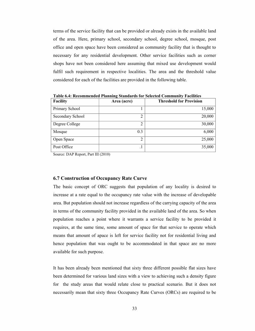
33
terms of the service facility that can be provided or already exists in the available land
of the area. Here, primary school, secondary school, degree school, mosque, post
office and open space have been considered as community facility that is thought to
necessary for any residential development. Other service facilities such as corner
shops have not been considered here assuming that mixed use development would
fulfil such requirement in respective localities. The area and the threshold value
considered for each of the facilities are provided in the following table.
Table 6.4: Recommended Planning Standards for Selected Community Facilities Facility Area (acre) Threshold for Provision
Primary School 1 15,000
Secondary School 2 20,000
Degree College 2 30,000
Mosque 0.3 6,000
Open Space 2 25,000
Post Office .1 35,000
Source: DAP Report, Part III (2010)
6.7 Construction of Occupancy Rate Curve
The basic concept of ORC suggests that population of any locality is desired to
increase at a rate equal to the occupancy rate value with the increase of developable
area. But population should not increase regardless of the carrying capacity of the area
in terms of the community facility provided in the available land of the area. So when
population reaches a point where it warrants a service facility to be provided it
requires, at the same time, some amount of space for that service to operate which
means that amount of apace is left for service facility not for residential living and
hence population that was ought to be accommodated in that space are no more
available for such purpose.
It has been already been mentioned that sixty three different possible flat sizes have
been determined for various land sizes with a view to achieving such a density figure
for the study areas that would relate close to practical scenario. But it does not
necessarily mean that sixty three Occupancy Rate Curves (ORCs) are required to be

34
plotted individually for each study area. Because once an ORC is generated for a
specific flat size it is capable of determining desirable population for any locality
which occupies residential land area for constructing that specific size of flat.
ORCs are constructed keeping the area available for development along the horizontal
axis and the corresponding population on the vertical axis. So the first requirement for
plotting an ORC is to determine the area available for a particular flat size beyond
which extension of the curve would be unnecessary. Area available for particular flat
size has been determined with the aid of table 6.5 and following the procedure
discussed by Debnath et.al (2011). Distribution of residential and mixed use land of
different flat sizes has been provided in table 1 to table 16 of appendix C.
Table 6.5: Distribution of Flat sizes of Inhabitants of the Study Areas
Flat Size (ft) Rampura
(DPZ-4)
Khilgaon
(DPZ-5)
Shaymoli
(DPZ-10)
Wari*
(DPZ-2)
Up to 500 11% 7% 5% 33.3%
501 – 750 43% 58% 54% 33.3%
751 – 1000 31% 25% 21% 20.2%
1001 – 1250 11% 5% 9% 5.9%
1251 – 1500 2% 3% 7% 4.4%
Above 1500 2% 2% 4% 2.7%
Source: Asaduzzaman, 2001and Field Survey, 2014*.
6.8 Observation of Population from ORC
Taking all the previous data as input of the model in MATLab 9a platform desirable
population of all possible flat sizes of all the alternative scenarios has been calculated
(table 17- table 33 of appendix C). Consequently the respective densities have been
calculated for all the alternative scenarios of all the study areas. Summary calculation
of all the scenarios has been attached in table 33 of appendix C.

35
6.9 Discussion on Output of the Simulation
Simulation has been conducted on sixteen different alternative scenarios including the
zero alternative scenario. It has already been mentioned in chapter six that three
different levels of alternative scenarios have been developed to arrive at a conclusive
remarks on the role of FAR, MGC and set back. Output of the first level alternative
scenarios necessitated for the development of the higher level alternative scenarios
which implies decrease only in FAR is of no effective solution to tackle the increasing
density in the unplanned residential areas. Output of the alternative scenarios at
different levels is discussed below.
6.9.1 Discussion on Output of Level 1 Alternative Scenarios
There is no denying the fact that the density at zero alternative scenario is no longer
acceptable for any human settlement. Even if the density standard (350 ppa) stated by
the Private Housing Land Development Act, 2004 is taken as a reference then the
current density is undoubtedly extremely high. That is the sole reason to emphasize on
the modification of existing BCR and development of alternative scenarios to
simulate through an applicable desirable density model. Alternative scenarios of
Level 1 are constituted of the decrease of the FAR only while keeping the other things
constant. Table 33 of appendix C offers that density decreases with the decrease of
FAR value, as discussed in chapter five. In case of alternative scenario 1A, 1B and
1C, density of all study areas except DPZ-2 gets decreased by around 5%, 10% and
15-17% respectively. DPZ-2 exhibits decrease in density by around 15%, 19% and
23% in case of 1A, 1B and 1C alternative scenarios respectively. The reason lies in
the distribution of inhabitants living in different sizes of flats of DPZ-2. Here, it is to
be mentioned that DPZ-2 represents the Old Dhaka. This area is more characterized
with mixed land use rather than as a residential area (RAJUK, 2010). Again, within
residential and mixed land use area almost 67% and 41% area, respectively, is
covered by land sizes of only 2 katha which is likely to result in a greatly small
occupancy rate and thereby great increase in density scenario which is more or less
similar to the situation exists in DPZ-5 (56% residential land and 43% mixed use land
are of less than 2 katha). But still DPZ-2 is more responsive to the decrease in FAR
compared to the DPZ-5 because table 6.5 exhibits that almost 53.5% inhabitants of

36
this study area live in flat sizes less than 500 sft and 750-1000 sft where as in DPZ-5
only 32% inhabitants live in these flat sizes. Again, within these 53.5% inhabitants of
DPZ-2 more than 62% inhabitants live in flat sizes of less than 500 sft only. So, in
case of DPZ-2 a minimum decrease in FAR has resulted in a greater decrease in
density compared to other study areas. But, in summary the extent to which density is
decreased is still not within a reasonable limit of any planned residential areas of
DMDP.
6.9.2 Discussion on Output of Level 2 Alternative Scenario
Alternative scenarios of Level 2 are developed considering decrease of the MGC only
while keeping the other things constant. Decrease in the MGC in different magnitudes
warrants change in the flat sizes of many of the plot sizes which has been listed in
table 6.4. This eventually resulted in the change of land distribution pattern of flat
sizes of all study areas. From table 33 of appendix C, it is observed that density gets
increased in all study areas except in DPZ-10 for alternative scenarios 2B and 2C. The
reason behind such situation lies in the fact that a lower MGC permits lower ground
coverage and thereby allows construction of lower flat sizes which results in lower
occupancy rate and greater density eventually. Decrease of density in DPZ-10 for
alternative scenarios 2B and 2C lies in the fact that these two scenarios have offered
opportunity to construct larger sizes of flats in many instances. Since DPZ-10 is the
only unplanned residential area where more than 20% inhabitants (highest among all
unplanned residential areas) live in flat sizes of 1001 to above 1500 sft this has
resulted in a more favourable land distribution for different land sizes and eventually
offered a decreased density scenario. But considering the output of all the alternative
scenarios of this level for all the study areas it is quite evident to conclude that change
only in the MGC would result in higher density which actually goes against the study
objective. Such experience has led to the development of level 3 alternative scenarios.
6.9.3 Discussion on Output of Level 3 Alternative Scenario
Alternative scenarios of Level 3 are comprised of the decrease of the MGC and FAR
simultaneously while keeping the set back constant. Here nine different alternative
scenarios have been developed and taken as input in the model. Output of this level
offered more interesting findings since only at this level density decreased to a
reasonable limit for some of the study areas. Specially output offered in case of

37
alternative scenario 3G (5% decrease in FAR and 15% decrease in MGC) is quite
acceptable for DPZ-10 and DPZ-4. Density did not decrease in case of DPZ-2 and
DPZ-5 to that extent in comparison to DPZ-10 and DPZ-4 though but it offered
highest percentage of decrease in density for DPZ-5 comparing all the alternative
scenarios of all levels. Still this alternative may prove to be promising for both these
study areas. Because 5% decrease in FAR and 15% decrease in MGC are likely to act
as disincentive for the land owners of small size plots. In response they are more
likely to be guided to follow consolidation strategy. If this scenario is brought into
action by the RAJUK and as a result 50% plots of 3 katha are converted into at least
3-5 katha land then the density of DPZ-2 and DPZ-5 gets decreased to 374 ppa and
362 ppa which is almost 40% decrease of density for both these study areas. Table 6.6
proposes the following modification in the FAR and MGC for different sizes of land.
Table 6.6: Proposed FAR, MGC and Set back for Unplanned Residential Areas
Land Size FAR MGC (%) Minimum Set back (m)
Front Rear Each Side
Below 2 katha 3.00 57.5 1.50 1.00 0.80
2-3 katha 3.15 55.0 1.50 1.00 1.00
3-5 katha 3.35 52.5 1.50 1.50 1.00
5-7 katha 3.55 50.0 1.50 2.00 1.25
7-8 katha 3.80 50.0 1.50 2.00 1.25
8-9 katha 3.80 50.0 1.50 2.00 1.25
9-10 katha 4.00 50.0 1.50 2.00 1.25
10-12 katha) 4.30 50.0 1.50 2.00 1.25
12-14 katha 4.50 47.5 1.50 2.00 1.25
14-16 katha 4.75 45.0 1.50 2.00 1.25
16-18 katha 5.00 45.0 1.50 2.00 1.25
18-20 katha 5.00 42.5 1.50 2.00 1.25
Above 20 katha 5.25 42.5 1.50 2.00 1.50
Based on the discussion above it can be concluded that the alternative scenario 3G i.e.
5% decrease in FAR and 15% decrease in MGC is more likely to offer a density that
is reasonable enough to accept for the unplanned residential areas of DMDP. Again,
this is also true that this uniform change in all unplanned residential areas may not
correspond to a manageable density situation depending on the land distribution

38
pattern and the distribution of inhabitants living in varying flat sizes. Since density is
a spatial phenomena and spatial characteristics vary from space to space that is why
some localities or areas may still require some special form of strategic treatment that
is subject to further research and beyond the scope of this study.

39
Chapter 7
MAJOR FINDINGS AND CONCLUSION
Dhaka City has been experiencing a huge land fragmentation through generations
resulting in additional smaller sizes of plots. Table 6.1 provides an alarming
fragmented land distribution situation allowing a huge population to be
accommodated with too low occupancy rate which may seem to be inhuman from
housing perspective of any developed country. If the situation continues this way,
there will be only huge sum of population but living without the basic service
facilities to lead their lives. A possible way of controlling such scenario can be
achieved through land consolidation, where small land parcels have to be brought
under a scheme to merge and form a larger parcel of land prior to building
construction so that flats of larger sizes can be built and people can live with a higher
occupancy rate. Besides that, larger land areas, still available for development, should
be prevented from constructing smaller sizes of flats in unplanned residential areas so
that less people can be accommodated with higher occupancy rates in those land
areas.
Nowadays smart growth is encouraged throughout the world to achieve a balance
between residential and non-residential uses which further increases access to daily
needs with added advantage of avoiding unnecessary hassle of travelling to avail a
facility. From table 6.1, it is observed that mixed use areas are comparatively lower
than the residential area. Mixed land use should complement with residential uses
therefore restricting the scope of accommodating more people in the unplanned areas.
So, Already built up residential areas should be encouraged to increase mixed use
development as an indirect way of reducing the opportunity for residential habitation
in unplanned residential areas.
FAR value alone is unable to work as an effective tool for density control unless and
otherwise occupancy rate is considered at the same time because obviously it is the
occupancy rate, not the FAR value which ensures minimum space for an individual in
habitable residential area. Again, residential habitation requires some services without
which urban living becomes meaningless. Therefore provision of service to residential

40
locality requires some space to be sacrificed against the ever increasing demand of
housing in the city. This is the basic thinking worked behind the model to determine
desirable density.
The results of the simulation suggest in most the cases that decrease in the FAR
results in the decrease of density in different magnitudes depending on the land
distribution pattern and distribution of people living in different flat sizes. If the FAR
and MGC both are decreased that would act like a disincentive for the land owners of
small plots to greater degree. Eventually this would lean towards a decision of land
consolidation and creating scope for constructing larger sizes flats which will bring
down the density of unplanned residential areas within in a reasonable limit.
CONCLUSION
Dhaka City has already experienced a high population density. Till to date, very little
has been done to control the density of the city. The situation has assumed such a
proportion that unless something is done to stop the ever increasing population within
the city it will loss all its glory in the near future. This study has endeavoured to
evaluate the role of FAR, MGC and set back as a means of density control in
unplanned residential areas of DMDP area. It has taken into account the fact of
controlling density lies in the understanding of the following proposition- residential
settlement should be developed providing minimum space for an individual, at the
same time, there should be some space available for providing service facility for the
increasing population. Considering this understanding a model has been used to
simulate various alternative scenarios to arrive at various density scenarios. The
study concludes with an understanding that decrease in FAR or MGC alone has very
little to do with controlling density in a manageable manner in case of unplanned
residential areas. But when both of these are allowed to decrease by 5% and 15%
respectively density appears to come down to a reasonable limit. Since this change in
the BCR would work as a disincentive for the land owners of the small plots they
would be more willing to construct residential structures following consolidation
strategy. But this is beyond the scope of the study to predict or comment how

41
responsive this scenario would be in the long run or short run. This sensitivity
analysis could have been performed if urban land use transformation, land
development trend, state of capacity of RAJUK to enact and vigilance on abidance of
the prescribed rules and regulations by the citizen of DMDP area.

42
Appendix A
Table 1: Distribution of Residential Areas and Unplanned Residential Areas of the Study Areas.
DPZ No
Total area
(acre)
Share of Residential Area
Share of unplanned residential area within
residential area
2 1314 37% 87%
4 1370.73 33% 83%
5 3174.41 75% 82%
10 3995.35 50% 93%
Algorithm of Programming Code of the Model used for Simulation
Input FAR Input Average Flat
Size Input Average Household
Size
Calculate Occupancy Rate
Generate Occupancy Rate Curve
Input Community Facilities
Determine Desirable Population
Input Land Distribution Pattern

43
Appendix B: Steps of Data Processing
1. Opening a new ArcMap window:
Start menu All Programs ArcGIS ArcMap.
Figure 5.1: Blank Window in ArcMap, ArcGIS Desktop 9.2
2. Extraction of Necessary Shape Files
The necessary information in the form of shape files were extracted from the raw data
collected from the Ganibangla Limited (GBL) following the steps below.
Extraction of Planned and Unplanned Residential Area
Add Data Specify ex_lansuse.shp Select Shape file Add
Figure 5.2: ‘Add Data’ button (left) and Add Data window (right) in ArcMap, ArcGIS
Desktop 9.2
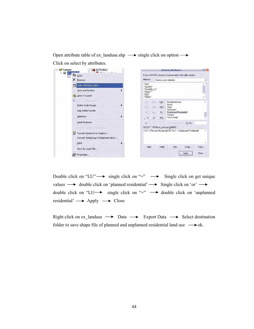
44
Open attribute table of ex_landuse.shp single click on option
Click on select by attributes.
Double click on “LU” single click on “=” Single click on get unique
values double click on ‘planned residential’ Single click on ‘or’
double click on “LU single click on “=” double click on ‘unplanned
residential’ Apply Close
Right click on ex_landuse Data Export Data Select destination
folder to save shape file of planned and unplanned residential land use ok.

45
Using the same process shape files of DPZ 5 boundary, DPZ 9 boundary and DPZ 10
boundary, residential structures, mixed land use area, mixed land use structures were
extracted first and then added in the ArcMap window. Then again various sizes of
land parcels were extracted for DPZ 5, DPZ 9 and DPZ 10 and the amount of
residential and mixed use land were also separated for the above mentioned DPZs
using Arc toolbox. The steps involved to gather this information are shown below
with an example where residential structures of DPZ 5 were separated using Arc
Toolbox.
Separation of Residential Structures of DPZ 5
i. Click on Arc Toolbox button
ii. Double click on ‘analysis tool’

46
iii. Double click on ‘extract’
iv. Double click on ‘clip’ select all residential structure as input feature DPZ_5_boundary as clip feature ok.
Following the same procedure other required shape files such as various sizes of land
parcels later on the following tables have been formed for the three DPZ.

Residen-
tial
Mixed Residen-
tial
Mixed Residen-
tial
Mixed Residen-
tial
Mixed
455 95.17 2.4 202.40 23.56 18.82 4.83 191.29 3.22
910 571.05 14.43 122.77 197.93 112.89 28.98 1147.77 19.33
700 597.4 24.58 63.56 91.81 89.82 31.59 451.78 12.67
1400 59.74 2.46 16.48 23.80 8.98 3.16 45.18 1.27
560 431.9 2.12 31.94 62.39 85.45 26.94 167.92 7.06
1125 103.66 0.51 10.65 20.80 20.51 6.47 40.30 1.70
2250 69.1 0.34 9.46 18.48 13.67 4.31 26.87 1.13
750 244.91 1.12 8.83 26.96 36.22 17.69 180.83 1.68
1500 24.49 0.11 2.29 6.99 3.62 1.77 18.08 0.17
3000 48.98 0.22 2.62 7.99 7.24 3.54 36.17 0.34
860 124.52 1.11 2.39 7.96 10.76 8.43 33.47 0.32
1720 16.07 0.14 0.91 3.03 1.39 1.09 4.32 0.04
970 66.56 0.8 2.05 2.34 8.91 6.46 8.15 0.32
1940 8.88 0.11 0.78 0.89 1.19 0.86 1.09 0.04
1035 23.46 0.49 0.98 3.18 5.94 2.91 4.23 0.19
2070 8.53 0.18 0.87 2.82 2.16 1.06 1.54 0.07
620 43.83 0.33 1.59 3.44 8.08 6.27 1.27 0.62
1240 4.38 0.03 0.53 1.15 0.81 0.63 0.13 0.06
2480 8.77 0.07 0.47 1.02 1.62 1.25 0.25 0.12
690 19.04 0.2 0.37 5.27 4.45 9.04 2.42 0.38
1385 1.9 0.02 0.10 1.37 0.45 0.90 0.24 0.04
2770 3.81 0.04 0.11 1.56 0.89 1.81 0.48 0.08
1008 28.97 1.02 0.95 1.69 1.23 1.47 0.23
2015 14.48 0.91 0.85 0.84 0.61 0.73 0.12
1130 5.71 0.18 2.05 1.12 2.71 0.85 0.00
2260 2.86 0.20 2.30 0.56 1.36 0.42 0.00
900 17.76 0.60 1.70 0.54 0.96 0.74 0.00
1800 2.54 0.23 0.65 0.08 0.14 0.11 0.00
690 28.74 0.72 11.41 3.41 3.61 2.91 0.69
1385 2.87 0.24 3.80 0.34 0.36 0.29 0.07
2770 5.75 0.21 3.38 0.68 0.72 0.58 0.14
3 3.35 0.65
Land Area
(katha)
FAR MGC DPZ 4 DPZ 5
2 3.15 0.675
Avg. Flat
Size (sft)
DPZ 10 DPZ 2
5 3.5 0.625
7 3.75 0.6
8 4 0.6
9 4 0.6
5 0.525
10 4.25 0.575
12 4.5 0.575
47
Appendix C
Above 20 5.5 0.5
Table 1: Land Distribution of Different Flat Sizes in the Study Areas under Zero Alternative Scenario
18 5.25 0.525
20 5.25 0.5
14 4.75 0.55
16

Residen-
tial
Mixed Residen-
tial
Mixed Residen-
tial
Mixed Residen-
tial
Mixed
455 95.17 2.4 202.40 23.56 18.82 4.83 191.29 3.22
910 571.05 14.43 122.77 197.93 112.89 28.98 1147.77 19.33
700 597.4 24.58 63.56 91.81 89.82 31.59 451.78 12.67
1400 59.74 2.46 16.48 23.80 8.98 3.16 45.18 1.27
560 431.9 2.12 31.94 62.39 85.45 26.94 167.92 7.06
1125 103.66 0.51 10.65 20.80 20.51 6.47 40.30 1.70
2250 69.1 0.34 9.46 18.48 13.67 4.31 26.87 1.13
750 244.91 1.12 8.83 26.96 36.22 17.69 180.83 1.68
1500 24.49 0.11 2.29 6.99 3.62 1.77 18.08 0.17
3000 48.98 0.22 2.62 7.99 7.24 3.54 36.17 0.34
860 124.52 1.11 2.39 7.96 10.76 8.43 33.47 0.32
1720 16.07 0.14 0.91 3.03 1.39 1.09 4.32 0.04
970 66.56 0.8 2.05 2.34 8.91 6.46 8.15 0.32
1940 8.88 0.11 0.78 0.89 1.19 0.86 1.09 0.04
1035 23.46 0.49 0.98 3.18 5.94 2.91 4.23 0.19
2070 8.53 0.18 0.87 2.82 2.16 1.06 1.54 0.07
620 43.83 0.33 1.59 3.44 8.08 6.27 1.27 0.62
1240 4.38 0.03 0.53 1.15 0.81 0.63 0.13 0.06
2480 8.77 0.07 0.47 1.02 1.62 1.25 0.25 0.12
690 19.04 0.2 0.37 5.27 4.45 9.04 2.42 0.38
1385 1.9 0.02 0.10 1.37 0.45 0.90 0.24 0.04
2770 3.81 0.04 0.11 1.56 0.89 1.81 0.48 0.08
1008 28.97 1.02 0.95 1.69 1.23 1.47 0.23
2015 14.48 0.91 0.85 0.84 0.61 0.73 0.12
1130 5.71 0.18 2.05 1.12 2.71 0.85 0.00
2260 2.86 0.20 2.30 0.56 1.36 0.42 0.00
900 17.76 0.60 1.70 0.54 0.96 0.74 0.00
1800 2.54 0.23 0.65 0.08 0.14 0.11 0.00
690 28.74 0.72 11.41 3.41 3.61 2.91 0.69
1385 2.87 0.24 3.80 0.34 0.36 0.29 0.07
2770 5.75 0.21 3.38 0.68 0.72 0.58 0.14
3 3.15 0.65
Land
Area
(katha)
FAR MGC DPZ 4 DPZ 5
2 3 0.675
Avg. Flat
Size (sft)
DPZ 10 DPZ 2
5 3.35 0.625
7 3.55 0.6
8 3.8 0.6
9 3.8 0.6
0.525
10 4 0.575
12 4.3 0.575
48
Above
20 5.25 0.5
Table 2: Land Distribution of Different Flat Sizes in the Study Areas under Alternative Scenario 1A
18 5 0.525
20 5 0.5
14 4.5 0.55
16 4.75

Residen-
tial
Mixed Residen-
tial
Mixed Residen-
tial
Mixed Residen-
tial
Mixed
455 95.17 2.4 202.40 23.56 18.82 4.83 191.29 3.22
910 571.05 14.43 122.77 197.93 112.89 28.98 1147.77 19.33
700 597.4 24.58 63.56 91.81 89.82 31.59 451.78 12.67
1400 59.74 2.46 16.48 23.80 8.98 3.16 45.18 1.27
560 431.9 2.12 31.94 62.39 85.45 26.94 167.92 7.06
1125 103.66 0.51 10.65 20.80 20.51 6.47 40.30 1.70
2250 69.1 0.34 9.46 18.48 13.67 4.31 26.87 1.13
750 244.91 1.12 8.83 26.96 36.22 17.69 180.83 1.68
1500 24.49 0.11 2.29 6.99 3.62 1.77 18.08 0.17
3000 48.98 0.22 2.62 7.99 7.24 3.54 36.17 0.34
860 124.52 1.11 2.39 7.96 10.76 8.43 33.47 0.32
1720 16.07 0.14 0.91 3.03 1.39 1.09 4.32 0.04
970 66.56 0.8 2.05 2.34 8.91 6.46 8.15 0.32
1940 8.88 0.11 0.78 0.89 1.19 0.86 1.09 0.04
1035 23.46 0.49 0.98 3.18 5.94 2.91 4.23 0.19
2070 8.53 0.18 0.87 2.82 2.16 1.06 1.54 0.07
620 43.83 0.33 1.59 3.44 8.08 6.27 1.27 0.62
1240 4.38 0.03 0.53 1.15 0.81 0.63 0.13 0.06
2480 8.77 0.07 0.47 1.02 1.62 1.25 0.25 0.12
690 19.04 0.2 0.37 5.27 4.45 9.04 2.42 0.38
1385 1.9 0.02 0.10 1.37 0.45 0.90 0.24 0.04
2770 3.81 0.04 0.11 1.56 0.89 1.81 0.48 0.08
1008 28.97 1.02 0.95 1.69 1.23 1.47 0.23
2015 14.48 0.91 0.85 0.84 0.61 0.73 0.12
1130 5.71 0.18 2.05 1.12 2.71 0.85 0.00
2260 2.86 0.20 2.30 0.56 1.36 0.42 0.00
900 17.76 0.60 1.70 0.54 0.96 0.74 0.00
1800 2.54 0.23 0.65 0.08 0.14 0.11 0.00
690 28.74 0.72 11.41 3.41 3.61 2.91 0.69
1385 2.87 0.24 3.80 0.34 0.36 0.29 0.07
2770 5.75 0.21 3.38 0.68 0.72 0.58 0.14
3 3 0.65
Land
Area
(katha)
FAR MGC DPZ 4 DPZ 5
2 2.85 0.675
Avg. Flat
Size (sft)
DPZ 10 DPZ 2
5 3.15 0.625
7 3.4 0.6
8 3.6 0.6
9 3.6 0.6
0.525
10 3.85 0.575
12 4 0.575
49
Above
20 5 0.5
Table 3: Land Distribution of Different Flat Sizes in the Study Areas under Alternative Scenario 1B
18 4.75 0.525
20 4.75 0.5
14 4.3 0.55
16 4.5

Residen-
tial
Mixed Residen-
tial
Mixed Residen-
tial
Mixed Residen-
tial
Mixed
455 95.17 2.4 202.40 23.56 18.82 4.83 191.29 3.22
910 571.05 14.43 122.77 197.93 112.89 28.98 1147.77 19.33
700 597.4 24.58 63.56 91.81 89.82 31.59 451.78 12.67
1400 59.74 2.46 16.48 23.80 8.98 3.16 45.18 1.27
560 431.9 2.12 31.94 62.39 85.45 26.94 167.92 7.06
1125 103.66 0.51 10.65 20.80 20.51 6.47 40.30 1.70
2250 69.1 0.34 9.46 18.48 13.67 4.31 26.87 1.13
750 244.91 1.12 8.83 26.96 36.22 17.69 180.83 1.68
1500 24.49 0.11 2.29 6.99 3.62 1.77 18.08 0.17
3000 48.98 0.22 2.62 7.99 7.24 3.54 36.17 0.34
860 124.52 1.11 2.39 7.96 10.76 8.43 33.47 0.32
1720 16.07 0.14 0.91 3.03 1.39 1.09 4.32 0.04
970 66.56 0.8 2.05 2.34 8.91 6.46 8.15 0.32
1940 8.88 0.11 0.78 0.89 1.19 0.86 1.09 0.04
1035 23.46 0.49 0.98 3.18 5.94 2.91 4.23 0.19
2070 8.53 0.18 0.87 2.82 2.16 1.06 1.54 0.07
620 43.83 0.33 1.59 3.44 8.08 6.27 1.27 0.62
1240 4.38 0.03 0.53 1.15 0.81 0.63 0.13 0.06
2480 8.77 0.07 0.47 1.02 1.62 1.25 0.25 0.12
690 19.04 0.2 0.37 5.27 4.45 9.04 2.42 0.38
1385 1.9 0.02 0.10 1.37 0.45 0.90 0.24 0.04
2770 3.81 0.04 0.11 1.56 0.89 1.81 0.48 0.08
1008 28.97 1.02 0.95 1.69 1.23 1.47 0.23
2015 14.48 0.91 0.85 0.84 0.61 0.73 0.12
1130 5.71 0.18 2.05 1.12 2.71 0.85 0.00
2260 2.86 0.20 2.30 0.56 1.36 0.42 0.00
900 17.76 0.60 1.70 0.54 0.96 0.74 0.00
1800 2.54 0.23 0.65 0.08 0.14 0.11 0.00
690 28.74 0.72 11.41 3.41 3.61 2.91 0.69
1385 2.87 0.24 3.80 0.34 0.36 0.29 0.07
2770 5.75 0.21 3.38 0.68 0.72 0.58 0.14
3 2.8 0.65
Land
Area
(katha)
FAR MGC DPZ 4 DPZ 5
2 2.7 0.675
Avg. Flat
Size (sft)
DPZ 10 DPZ 2
5 3 0.625
7 3.2 0.6
8 3.4 0.6
9 3.4 0.6
0.525
10 3.6 0.575
12 3.8 0.575
50
Above
20 4.75 0.5
Table 4: Land Distribution of Different Flat Sizes in the Study Areas under Alternative Scenario 1C
18 4.5 0.525
20 4.5 0.5
14 4 0.55
16 4.3

Residen-
tial
Mixed Residen-
tial
Mixed Residen-
tial
Mixed Residen-
tial
Mixed
455 95.17 2.4 202.40 23.56 18.82 4.83 191.29 3.22
910 571.05 14.43 122.77 197.93 112.89 28.98 1147.77 19.33
700 597.4 24.58 63.56 91.81 89.82 31.59 451.78 12.67
1400 59.74 2.46 16.48 23.80 8.98 3.16 45.18 1.27
560 431.9 2.12 31.94 62.39 85.45 26.94 167.92 7.06
1125 103.66 0.51 10.65 20.80 20.51 6.47 40.30 1.70
2250 69.1 0.34 9.46 18.48 13.67 4.31 26.87 1.13
675 82.60 69.10 11.33 34.56 43.08 21.04 216.42 2.01
1350 12.71 103.66 1.50 4.57 2.00 0.98 11.19 0.10
2700 6.35 431.90 0.92 2.80 2.00 0.98 7.46 0.07
860 124.52 1.11 2.39 7.96 10.76 8.43 33.47 0.32
1720 16.07 0.14 0.91 3.03 1.39 1.09 4.32 0.04
970 66.56 0.8 2.05 2.34 8.91 6.46 8.15 0.32
1940 8.88 0.11 0.78 0.89 1.19 0.86 1.09 0.04
950 11.76 0.966 1.64 5.29 7.61 3.72 5.34 0.24
1900 2.24 0.184 0.22 0.71 0.49 0.24 0.43 0.02
620 43.83 0.33 1.59 3.44 8.08 6.27 1.27 0.62
1240 4.38 0.03 0.53 1.15 0.81 0.63 0.13 0.06
2480 8.77 0.07 0.47 1.02 1.62 1.25 0.25 0.12
690 19.04 0.2 0.37 5.27 4.45 9.04 2.42 0.38
1385 1.9 0.02 0.10 1.37 0.45 0.90 0.24 0.04
2770 3.81 0.04 0.11 1.56 0.89 1.81 0.48 0.08
1008 28.97 1.02 0.95 1.69 1.23 1.47 0.23
2015 14.48 0.91 0.85 0.84 0.61 0.73 0.12
1525 1.325 0.19 2.18 0.84 2.03 0.63
3050 1.325 0.19 2.18 0.84 2.03 0.63
900 17.76 0.60 1.70 0.54 0.96 0.74 0.00
1800 2.54 0.23 0.65 0.08 0.14 0.11 0.00
690 28.74 0.72 11.41 3.41 3.61 2.91 0.69
1385 2.87 0.24 3.80 0.34 0.36 0.29 0.07
2770 5.75 0.21 3.38 0.68 0.72 0.58 0.14
4.25 0.55
DPZ 10 DPZ 2 DPZ 4
0.575
4 0.575
4 0.575
0.65
3.35 0.625
3.5 0.6
16
5.5 0.475
4.5 0.55
4.75 0.525
5 0.5
5.25 0.5
5.25 0.475
8
9
10
12
14
51
Table 5: Land Distribution of Different Flat Sizes in the Study Areas under Alternative Scenario 2A
7 3.75
Land
Area
(katha)
FAR
2
3
5
DPZ 5Avg. Flat
Size (sft)
18
20
Above 20
MGC
3.15

Residen-
tial
Mixed Residen-
tial
Mixed Residen-
tial
Mixed Residen-
tial
Mixed
455 95.17 2.4 202.40 23.56 18.82 4.83 191.29 3.22
910 571.05 14.43 122.77 197.93 112.89 28.98 1147.77 19.33
600 407.85 89.17 67.99 98.21 78.67 27.67 457.51 12.83
1200 67.97 14.86 12.05 17.40 20.13 7.08 39.44 1.11
560 431.9 2.12 31.94 62.39 85.45 26.94 167.92 7.06
1125 103.66 0.51 10.65 20.80 20.51 6.47 40.30 1.70
2250 69.1 0.34 9.46 18.48 13.67 4.31 26.87 1.13
675 82.60 69.10 11.33 34.56 43.08 21.04 216.42 2.01
1350 12.71 103.66 1.50 4.57 2.00 0.98 11.19 0.10
2700 6.35 431.90 0.92 2.80 2.00 0.98 7.46 0.07
860 124.52 1.11 2.39 7.96 10.76 8.43 33.47 0.32
1720 16.07 0.14 0.91 3.03 1.39 1.09 4.32 0.04
970 66.56 0.8 2.05 2.34 8.91 6.46 8.15 0.32
1940 8.88 0.11 0.78 0.89 1.19 0.86 1.09 0.04
950 11.76 0.966 1.64 5.29 7.61 3.72 5.34 0.24
1900 2.24 0.184 0.22 0.71 0.49 0.24 0.43 0.02
1075 11.94 1.88 1.78 3.84 8.88 6.90 1.18 0.57
2150 5.31 0.83 0.82 1.76 1.62 1.25 0.47 0.23
600 6.62 0.46 6.51 4.45 9.02 2.80 0.45
1200 1.10 0.08 1.15 1.14 2.31 0.24 0.04
2400 0.25 0.04 0.53 0.21 0.42 0.10 0.02
750 5.84 1.77 1.65 2.09 1.52 2.03 0.32
1300 0.76 0.08 0.08 0.28 0.20 0.10 0.02
2600 0.43 0.08 0.08 0.17 0.12 0.07 0.01
1525 1.325 0.19 2.18 0.84 2.03 0.63
3050 1.325 0.19 2.18 0.84 2.03 0.63
785 0.73 2.06 0.58 1.03 0.78
1575 0.05 0.14 0.02 0.03 0.03
3150 0.05 0.14 0.02 0.03 0.03
690 28.74 0.72 11.41 3.41 3.61 2.91 0.69
1385 2.87 0.24 3.80 0.34 0.36 0.29 0.07
2770 5.75 0.21 3.38 0.68 0.72 0.58 0.14
DPZ 2 DPZ 4 DPZ 5
2 3.15 0.6
Land Area
(katha)
FAR MGC Avg. Flat
Size (sft)
DPZ 10
3 3.35 0.6
5 3.5 0.55
7 3.75 0.55
8 4 0.55
9 4 0.55
10 4.25 0.525
5.25 0.475
12 4.5 0.525
14 4.75 0.5
52
Table 6: Land Distribution of Different Flat Sizes in the Study Areas under Alternative Scenario 2B
20 5.25 0.45
Above 20 5.5 0.45
16 5 0.475
18

Residen-
tial
Mixed Residen-
tial
Mixed Residen-
tial
Mixed Residen-
tial
Mixed
455 95.17 2.4 202.40 23.56 18.82 4.83 191.29 3.22
910 571.05 14.43 122.77 197.93 112.89 28.98 1147.77 19.33
600 407.85 89.17 67.99 98.21 78.67 27.67 457.51 12.83
1200 67.97 14.86 12.05 17.40 20.13 7.08 39.44 1.11
900 352.296 77.49 45.92 89.67 112.38 30.74 217.67 9.16
1800 67.104 14.76 6.14 11.99 7.25 1.98 17.41 0.73
590 76.42 22.98 10.92 33.32 36.16 17.66 209.76 1.95
1180 12.74 3.83 1.93 5.90 9.25 4.52 18.08 0.17
2360 5.66 1.70 0.89 2.70 1.68 0.82 7.23 0.07
720 124.52 1.11 2.39 7.96 10.76 8.43 33.47 0.32
1440 16.07 0.14 0.91 3.03 1.39 1.09 4.32 0.04
810 66.56 0.8 2.05 2.34 8.91 6.46 8.15 0.32
1620 8.88 0.11 0.78 0.89 1.19 0.86 1.09 0.04
850 11.76 0.97 1.64 5.29 7.61 3.72 5.34 0.24
1700 2.24 0.18 0.22 0.71 0.49 0.24 0.43 0.02
1075 11.94 1.88 1.78 3.84 8.88 6.90 1.18 0.57
2150 5.31 0.83 0.82 1.76 1.62 1.25 0.47 0.23
600 6.62 0.46 6.51 4.45 9.02 2.80 0.45
1200 1.10 0.08 1.15 1.14 2.31 0.24 0.04
2400 0.25 0.04 0.53 0.21 0.42 0.10 0.02
750 5.84 1.77 1.65 2.09 1.52 2.03 0.32
1300 0.76 0.08 0.08 0.28 0.20 0.10 0.02
2600 0.43 0.08 0.08 0.17 0.12 0.07 0.01
1420 1.69 0.24 2.70 0.84 2.04 0.76
2835 0.96 0.14 1.65 0.84 2.04 0.51
785 0.73 2.06 0.58 1.03 0.78
1575 0.05 0.14 0.02 0.03 0.03
3150 0.05 0.14 0.02 0.03 0.03
690 28.74 0.72 11.41 3.41 3.61 2.91 0.69
1385 2.87 0.24 3.80 0.34 0.36 0.29 0.07
2770 5.75 0.21 3.38 0.68 0.72 0.58 0.14
DPZ 2 DPZ 4 DPZ 5
2 3.15 0.575
Land
Area
(katha)
FAR MGC Avg. Flat
Size (sft)
DPZ 10
3 3.35 0.55
5 3.5 0.525
7 3.75 0.5
8 4 0.5
0.5
14 4.75 0.475
9 4 0.5
10 4.25 0.5
53
Table 7: Land Distribution of Different Flat Sizes in the Study Areas under Alternative Scenario 2C
20 5.25 0.425
Above
20 5.5 0.425
16 5 0.45
18 5.25 0.45
12 4.5

Residen-
tial
Mixed Residen-
tial
Mixed Residen-
tial
Mixed Residen-
tial
Mixed
455 95.17 2.4 202.40 23.56 18.82 4.83 191.29 3.22
910 571.05 14.43 122.77 197.93 112.89 28.98 1147.77 19.33
700 597.4 24.58 63.56 91.81 89.82 31.59 451.78 12.67
1400 59.74 2.46 16.48 23.80 8.98 3.16 45.18 1.27
560 431.9 2.12 31.94 62.39 85.45 26.94 167.92 7.06
1125 103.66 0.51 10.65 20.80 20.51 6.47 40.30 1.70
2250 69.1 0.34 9.46 18.48 13.67 4.31 26.87 1.13
675 82.60 69.10 11.33 34.56 43.08 21.04 216.42 2.011350 12.71 103.66 1.50 4.57 2.00 0.98 11.19 0.10
2700 6.35 431.90 0.92 2.80 2.00 0.98 7.46 0.07
860 124.52 1.11 2.39 7.96 10.76 8.43 33.47 0.32
1720 16.07 0.14 0.91 3.03 1.39 1.09 4.32 0.04
970 66.56 0.8 2.05 2.34 8.91 6.46 8.15 0.32
1940 8.88 0.11 0.78 0.89 1.19 0.86 1.09 0.04
950 11.76 0.966 1.64 5.29 7.61 3.72 5.34 0.24
1900 2.24 0.184 0.22 0.71 0.49 0.24 0.43 0.02
620 43.83 0.33 1.59 3.44 8.08 6.27 1.27 0.62
1240 4.38 0.03 0.53 1.15 0.81 0.63 0.13 0.06
2480 8.77 0.07 0.47 1.02 1.62 1.25 0.25 0.12
690 19.04 0.2 0.37 5.27 4.45 9.04 2.42 0.38
1385 1.9 0.02 0.10 1.37 0.45 0.90 0.24 0.04
2770 3.81 0.04 0.11 1.56 0.89 1.81 0.48 0.08
1008 28.97 1.02 0.95 1.69 1.23 1.47 0.23
2015 14.48 0.91 0.85 0.84 0.61 0.73 0.12
1525 1.325 0.19 2.18 0.84 2.03 0.63
3050 1.325 0.19 2.18 0.84 2.03 0.63
900 17.76 0.60 1.70 0.54 0.96 0.74 0.00
1800 2.54 0.23 0.65 0.08 0.14 0.11 0.00
690 28.74 0.72 11.41 3.41 3.61 2.91 0.69
1385 2.87 0.24 3.80 0.34 0.36 0.29 0.07
2770 5.75 0.21 3.38 0.68 0.72 0.58 0.14
Above
20 5.25 0.475
18 5 0.5
20 5 0.475
14 4.5 0.525
16 4.75 0.5
10 4 0.55
12 4.3 0.55
8 3.8 0.575
9 3.8 0.575
5 3.35 0.6
7 3.55 0.575
54
Table 8: Land Distribution of Different Flat Sizes in the Study Areas under Alternative Scenario 3A
3 3.15 0.625
Land
Area
(katha)
FAR MGC DPZ 4 DPZ 5
2 3 0.65
Avg. Flat
Size (sft)
DPZ 10 DPZ 2

Residen-
tial
Mixed Residen-
tial
Mixed Residen-
tial
Mixed Residen-
tial
Mixed
455 95.17 2.4 202.40 23.56 18.82 4.83 191.29 3.22
910 571.05 14.43 122.77 197.93 112.89 28.98 1147.77 19.33
700 597.4 24.58 63.56 91.81 89.82 31.59 451.78 12.67
1400 59.74 2.46 16.48 23.80 8.98 3.16 45.18 1.27
560 431.9 2.12 31.94 62.39 85.45 26.94 167.92 7.06
1125 103.66 0.51 10.65 20.80 20.51 6.47 40.30 1.70
2250 69.1 0.34 9.46 18.48 13.67 4.31 26.87 1.13
675 82.60 69.10 11.33 34.56 43.08 21.04 216.42 2.011350 12.71 103.66 1.50 4.57 2.00 0.98 11.19 0.10
2700 6.35 431.90 0.92 2.80 2.00 0.98 7.46 0.07
860 124.52 1.11 2.39 7.96 10.76 8.43 33.47 0.32
1720 16.07 0.14 0.91 3.03 1.39 1.09 4.32 0.04
970 66.56 0.8 2.05 2.34 8.91 6.46 8.15 0.32
1940 8.88 0.11 0.78 0.89 1.19 0.86 1.09 0.04
950 11.76 0.966 1.64 5.29 7.61 3.72 5.34 0.24
1900 2.24 0.184 0.22 0.71 0.49 0.24 0.43 0.02
620 43.83 0.33 1.59 3.44 8.08 6.27 1.27 0.62
1240 4.38 0.03 0.53 1.15 0.81 0.63 0.13 0.06
2480 8.77 0.07 0.47 1.02 1.62 1.25 0.25 0.12
690 19.04 0.2 0.37 5.27 4.45 9.04 2.42 0.38
1385 1.9 0.02 0.10 1.37 0.45 0.90 0.24 0.04
2770 3.81 0.04 0.11 1.56 0.89 1.81 0.48 0.08
1008 28.97 1.02 0.95 1.69 1.23 1.47 0.23
2015 14.48 0.91 0.85 0.84 0.61 0.73 0.12
1525 1.325 0.19 2.18 0.84 2.03 0.63
3050 1.325 0.19 2.18 0.84 2.03 0.63
900 17.76 0.60 1.70 0.54 0.96 0.74 0.00
1800 2.54 0.23 0.65 0.08 0.14 0.11 0.00
690 28.74 0.72 11.41 3.41 3.61 2.91 0.69
1385 2.87 0.24 3.80 0.34 0.36 0.29 0.07
2770 5.75 0.21 3.38 0.68 0.72 0.58 0.14
Above 20 5 0.475
18 4.75 0.5
20 4.75 0.475
14 4.3 0.525
16 4.5 0.5
10 3.85 0.55
12 4 0.55
8 3.6 0.575
9 3.6 0.575
5 3.15 0.6
7 3.4 0.575
55
Table 9: Land Distribution of Different Flat Sizes in the Study Areas under Alternative Scenario 3B
3 3 0.625
Land Area
(katha)
FAR MGC DPZ 4 DPZ 5
2 2.85 0.65
Avg. Flat
Size (sft)
DPZ 10 DPZ 2

Residen-
tial
Mixed Residen-
tial
Mixed Residen-
tial
Mixed Residen-
tial
Mixed
455 95.17 2.4 202.40 23.56 18.82 4.83 191.29 3.22
910 571.05 14.43 122.77 197.93 112.89 28.98 1147.77 19.33
700 597.4 24.58 63.56 91.81 89.82 31.59 451.78 12.67
1400 59.74 2.46 16.48 23.80 8.98 3.16 45.18 1.27
560 431.9 2.12 31.94 62.39 85.45 26.94 167.92 7.06
1125 103.66 0.51 10.65 20.80 20.51 6.47 40.30 1.70
2250 69.1 0.34 9.46 18.48 13.67 4.31 26.87 1.13
675 82.60 69.10 11.33 34.56 43.08 21.04 216.42 2.011350 12.71 103.66 1.50 4.57 2.00 0.98 11.19 0.10
2700 6.35 431.90 0.92 2.80 2.00 0.98 7.46 0.07
860 124.52 1.11 2.39 7.96 10.76 8.43 33.47 0.32
1720 16.07 0.14 0.91 3.03 1.39 1.09 4.32 0.04
970 66.56 0.8 2.05 2.34 8.91 6.46 8.15 0.32
1940 8.88 0.11 0.78 0.89 1.19 0.86 1.09 0.04
950 11.76 0.966 1.64 5.29 7.61 3.72 5.34 0.24
1900 2.24 0.184 0.22 0.71 0.49 0.24 0.43 0.02
620 43.83 0.33 1.59 3.44 8.08 6.27 1.27 0.62
1240 4.38 0.03 0.53 1.15 0.81 0.63 0.13 0.06
2480 8.77 0.07 0.47 1.02 1.62 1.25 0.25 0.12
690 19.04 0.2 0.37 5.27 4.45 9.04 2.42 0.38
1385 1.9 0.02 0.10 1.37 0.45 0.90 0.24 0.04
2770 3.81 0.04 0.11 1.56 0.89 1.81 0.48 0.08
1008 28.97 1.02 0.95 1.69 1.23 1.47 0.23
2015 14.48 0.91 0.85 0.84 0.61 0.73 0.12
1525 1.325 0.19 2.18 0.84 2.03 0.63
3050 1.325 0.19 2.18 0.84 2.03 0.63
900 17.76 0.60 1.70 0.54 0.96 0.74 0.00
1800 2.54 0.23 0.65 0.08 0.14 0.11 0.00
690 28.74 0.72 11.41 3.41 3.61 2.91 0.69
1385 2.87 0.24 3.80 0.34 0.36 0.29 0.07
2770 5.75 0.21 3.38 0.68 0.72 0.58 0.14
Above 20 4.75 0.475
18 4.5 0.5
20 4.5 0.475
14 4 0.525
16 4.3 0.5
10 3.6 0.55
12 3.8 0.55
8 3.4 0.575
9 3.4 0.575
5 3 0.6
7 3.2 0.575
56
Table 10: Land Distribution of Different Flat Sizes in the Study Areas under Alternative Scenario 3C
3 2.8 0.625
Land Area
(katha)
FAR MGC DPZ 4 DPZ 5
2 2.7 0.65
Avg. Flat
Size (sft)
DPZ 10 DPZ 2

Residen-
tial
Mixed Residen-
tial
Mixed Residen-
tial
Mixed Residen-
tial
Mixed
455 95.17 2.4 202.40 23.56 18.82 4.83 191.29 3.22
910 571.05 14.43 122.77 197.93 112.89 28.98 1147.77 19.33
600 407.85 89.17 67.99 98.21 78.67 27.67 457.51 12.83
1200 67.97 14.86 12.05 17.40 20.13 7.08 39.44 1.11
560 431.9 2.12 31.94 62.39 85.45 26.94 167.92 7.06
1125 103.66 0.51 10.65 20.80 20.51 6.47 40.30 1.70
2250 69.1 0.34 9.46 18.48 13.67 4.31 26.87 1.13
675 82.60 69.10 11.33 34.56 43.08 21.04 216.42 2.011350 12.71 103.66 1.50 4.57 2.00 0.98 11.19 0.10
2700 6.35 431.90 0.92 2.80 2.00 0.98 7.46 0.07
860 124.52 1.11 2.39 7.96 10.76 8.43 33.47 0.32
1720 16.07 0.14 0.91 3.03 1.39 1.09 4.32 0.04
970 66.56 0.8 2.05 2.34 8.91 6.46 8.15 0.32
1940 8.88 0.11 0.78 0.89 1.19 0.86 1.09 0.04
950 11.76 0.966 1.64 5.29 7.61 3.72 5.34 0.24
1900 2.24 0.184 0.22 0.71 0.49 0.24 0.43 0.02
1075 11.94 1.88 1.78 3.84 8.88 6.90 1.18 0.57
2150 5.31 0.83 0.82 1.76 1.62 1.25 0.47 0.23
600 6.62 0.46 6.51 4.45 9.02 2.80 0.45
1200 1.10 0.08 1.15 1.14 2.31 0.24 0.04
2400 0.25 0.04 0.53 0.21 0.42 0.10 0.02
750 5.84 1.77 1.65 2.09 1.52 2.03 0.32
1300 0.76 0.08 0.08 0.28 0.20 0.10 0.02
2600 0.43 0.08 0.08 0.17 0.12 0.07 0.01
1525 1.325 0.19 2.18 0.84 2.03 0.63
3050 1.325 0.19 2.18 0.84 2.03 0.63
785 0.73 2.06 0.58 1.03 0.78
1575 0.05 0.14 0.02 0.03 0.03
3150 0.05 0.14 0.02 0.03 0.03
690 28.74 0.72 11.41 3.41 3.61 2.91 0.69
1385 2.87 0.24 3.80 0.34 0.36 0.29 0.07
2770 5.75 0.21 3.38 0.68 0.72 0.58 0.14
Above 20 5.25 0.45
18 5 0.475
20 5 0.45
14 4.5 0.5
16 4.75 0.475
10 4 0.525
12 4.3 0.525
8 3.8 0.55
9 3.8 0.55
5 3.35 0.55
7 3.55 0.55
57
Table 11: Land Distribution of Different Flat Sizes in the Study Areas under Alternative Scenario 3D
3 3.15 0.6
Land Area
(katha)
FAR MGC DPZ 4 DPZ 5
2 3 0.6
Avg. Flat
Size (sft)
DPZ 10 DPZ 2

Residen-
tial
Mixed Residen-
tial
Mixed Residen-
tial
Mixed Residen-
tial
Mixed
455 95.17 2.4 202.40 23.56 18.82 4.83 191.29 3.22
910 571.05 14.43 122.77 197.93 112.89 28.98 1147.77 19.33
600 407.85 89.17 67.99 98.21 78.67 27.67 457.51 12.83
1200 67.97 14.86 12.05 17.40 20.13 7.08 39.44 1.11
560 431.9 2.12 31.94 62.39 85.45 26.94 167.92 7.06
1125 103.66 0.51 10.65 20.80 20.51 6.47 40.30 1.70
2250 69.1 0.34 9.46 18.48 13.67 4.31 26.87 1.13
675 82.60 69.10 11.33 34.56 43.08 21.04 216.42 2.01
1350 12.71 103.66 1.50 4.57 2.00 0.98 11.19 0.10
2700 6.35 431.90 0.92 2.80 2.00 0.98 7.46 0.07
860 124.52 1.11 2.39 7.96 10.76 8.43 33.47 0.32
1720 16.07 0.14 0.91 3.03 1.39 1.09 4.32 0.04
970 66.56 0.8 2.05 2.34 8.91 6.46 8.15 0.32
1940 8.88 0.11 0.78 0.89 1.19 0.86 1.09 0.04
950 11.76 0.966 1.64 5.29 7.61 3.72 5.34 0.24
1900 2.24 0.184 0.22 0.71 0.49 0.24 0.43 0.02
1075 11.94 1.88 1.78 3.84 8.88 6.90 1.18 0.57
2150 5.31 0.83 0.82 1.76 1.62 1.25 0.47 0.23
600 6.62 0.46 6.51 4.45 9.02 2.80 0.45
1200 1.10 0.08 1.15 1.14 2.31 0.24 0.04
2400 0.25 0.04 0.53 0.21 0.42 0.10 0.02
750 5.84 1.77 1.65 2.09 1.52 2.03 0.32
1300 0.76 0.08 0.08 0.28 0.20 0.10 0.02
2600 0.43 0.08 0.08 0.17 0.12 0.07 0.01
1525 1.325 0.19 2.18 0.84 2.03 0.63
3050 1.325 0.19 2.18 0.84 2.03 0.63
785 0.73 2.06 0.58 1.03 0.78
1575 0.05 0.14 0.02 0.03 0.03
3150 0.05 0.14 0.02 0.03 0.03
690 28.74 0.72 11.41 3.41 3.61 2.91 0.69
1385 2.87 0.24 3.80 0.34 0.36 0.29 0.07
2770 5.75 0.21 3.38 0.68 0.72 0.58 0.14
Above 20 5 0.45
18 4.75 0.475
20 4.75 0.45
14 4.3 0.5
16 4.5 0.475
10 3.85 0.525
12 4 0.525
8 3.6 0.55
9 3.6 0.55
5 3.15 0.55
7 3.4 0.55
58
Table 12: Land Distribution of Different Flat Sizes in the Study Areas under Alternative Scenario 3E
3 3 0.6
Land Area
(katha)
FAR MGC DPZ 4 DPZ 5
2 2.85 0.6
Avg. Flat
Size (sft)
DPZ 10 DPZ 2

Residen-
tial
Mixed Residen-
tial
Mixed Residen-
tial
Mixed Residen-
tial
Mixed
455 95.17 2.4 202.40 202.40 18.82 4.83 191.29 3.22
910 571.05 14.43 122.77 122.77 112.89 28.98 1147.77 19.33
600 407.85 89.17 67.99 98.21 78.67 27.67 457.51 12.83
1200 67.97 14.86 12.05 17.40 20.13 7.08 39.44 1.11
560 431.9 2.12 31.94 62.39 85.45 26.94 167.92 7.06
1125 103.66 0.51 10.65 20.80 20.51 6.47 40.30 1.70
2250 69.1 0.34 9.46 18.48 13.67 4.31 26.87 1.13
675 82.60 69.10 11.33 34.56 43.08 21.04 216.42 2.01
1350 12.71 103.66 1.50 4.57 2.00 0.98 11.19 0.10
2700 6.35 431.90 0.92 2.80 2.00 0.98 7.46 0.07
860 124.52 1.11 2.39 7.96 10.76 8.43 33.47 0.32
1720 16.07 0.14 0.91 3.03 1.39 1.09 4.32 0.04
970 66.56 0.8 2.05 2.34 8.91 6.46 8.15 0.32
1940 8.88 0.11 0.78 0.89 1.19 0.86 1.09 0.04
950 11.76 0.966 1.64 5.29 7.61 3.72 5.34 0.24
1900 2.24 0.184 0.22 0.71 0.49 0.24 0.43 0.02
1075 11.94 1.88 1.78 3.84 8.88 6.90 1.18 0.57
2150 5.31 0.83 0.82 1.76 1.62 1.25 0.47 0.23
600 6.62 0.46 6.51 4.45 9.02 2.80 0.45
1200 1.10 0.08 1.15 1.14 2.31 0.24 0.04
2400 0.25 0.04 0.53 0.21 0.42 0.10 0.02
750 5.84 1.77 1.65 2.09 1.52 2.03 0.32
1300 0.76 0.08 0.08 0.28 0.20 0.10 0.02
2600 0.43 0.08 0.08 0.17 0.12 0.07 0.01
1525 1.325 0.19 2.18 0.84 2.03 0.63
3050 1.325 0.19 2.18 0.84 2.03 0.63
785 0.73 2.06 0.58 1.03 0.78
1575 0.05 0.14 0.02 0.03 0.03
3150 0.05 0.14 0.02 0.03 0.03
690 28.74 0.72 11.41 3.41 3.61 2.91 0.69
1385 2.87 0.24 3.80 0.34 0.36 0.29 0.07
2770 5.75 0.21 3.38 0.68 0.72 0.58 0.14
Above 20 4.75 0.45
18 4.5 0.475
20 4.5 0.45
14 4 0.5
16 4.3 0.475
10 3.6 0.525
12 3.8 0.525
8 3.4 0.55
9 3.4 0.55
5 3 0.55
7 3.2 0.55
59
Table 13: Land Distribution of Different Flat Sizes in the Study Areas under Alternative Scenario 3F
3 2.8 0.6
Land Area
(katha)
FAR MGC DPZ 4 DPZ 5
2 2.7 0.6
Avg. Flat
Size (sft)
DPZ 10 DPZ 2

Residen-
tial
Mixed Residen-
tial
Mixed Residen-
tial
Mixed Residen-
tial
Mixed
455 95.17 2.4 202.40 23.56 18.82 4.83 191.29 3.22
910 571.05 14.43 122.77 197.93 112.89 28.98 1147.77 19.33
600 407.85 89.17 67.99 98.21 78.67 27.67 457.51 12.83
1200 67.97 14.86 12.05 17.40 20.13 7.08 39.44 1.11
900 352.296 77.49 45.92 89.67 112.38 30.74 217.67 9.16
1800 67.104 14.76 6.14 11.99 7.25 1.98 17.41 0.73
590 76.42 22.98 10.92 33.32 36.16 17.66 209.76 1.951180 12.74 3.83 1.93 5.90 9.25 4.52 18.08 0.17
2360 5.66 1.70 0.89 2.70 1.68 0.82 7.23 0.07
720 124.52 1.11 2.39 7.96 10.76 8.43 33.47 0.32
1440 16.07 0.14 0.91 3.03 1.39 1.09 4.32 0.04
810 66.56 0.8 2.05 2.34 8.91 6.46 8.15 0.32
1620 8.88 0.11 0.78 0.89 1.19 0.86 1.09 0.04
850 11.76 0.97 1.64 5.29 7.61 3.72 5.34 0.24
1700 2.24 0.18 0.22 0.71 0.49 0.24 0.43 0.02
1075 11.94 1.88 1.78 3.84 8.88 6.90 1.18 0.57
2150 5.31 0.83 0.82 1.76 1.62 1.25 0.47 0.23
600 6.62 0.46 6.51 4.45 9.02 2.80 0.45
1200 1.10 0.08 1.15 1.14 2.31 0.24 0.04
2400 0.25 0.04 0.53 0.21 0.42 0.10 0.02
750 5.84 1.77 1.65 2.09 1.52 2.03 0.32
1300 0.76 0.08 0.08 0.28 0.20 0.10 0.02
2600 0.43 0.08 0.08 0.17 0.12 0.07 0.01
1420 1.69 0.24 2.70 0.84 2.04 0.76
2835 0.96 0.14 1.65 0.84 2.04 0.51
785 0.73 2.06 0.58 1.03 0.78
1575 0.05 0.14 0.02 0.03 0.03
3150 0.05 0.14 0.02 0.03 0.03
690 28.74 0.72 11.41 3.41 3.61 2.91 0.69
1385 2.87 0.24 3.80 0.34 0.36 0.29 0.07
2770 5.75 0.21 3.38 0.68 0.72 0.58 0.14
Above 20 5.25 0.425
18 5 0.45
20 5 0.425
14 4.5 0.475
16 4.75 0.45
10 4 0.5
12 4.3 0.5
8 3.8 0.5
9 3.8 0.5
5 3.35 0.525
7 3.55 0.5
60
Table 14: Land Distribution of Different Flat Sizes in the Study Areas under Alternative Scenario 3G
3 3.15 0.55
Land Area
(katha)
FAR MGC DPZ 4 DPZ 5
2 3 0.575
Avg. Flat
Size (sft)
DPZ 10 DPZ 2

Residen-
tial
Mixed Residen-
tial
Mixed Residen-
tial
Mixed Residen-
tial
Mixed
455 95.17 2.4 202.40 23.56 18.82 4.83 191.29 3.22
910 571.05 14.43 122.77 197.93 112.89 28.98 1147.77 19.33
600 407.85 89.17 67.99 98.21 78.67 27.67 457.51 12.83
1200 67.97 14.86 12.05 17.40 20.13 7.08 39.44 1.11
900 352.296 77.49 45.92 89.67 112.38 30.74 217.67 9.16
1800 67.104 14.76 6.14 11.99 7.25 1.98 17.41 0.73
590 76.42 22.98 10.92 33.32 36.16 17.66 209.76 1.951180 12.74 3.83 1.93 5.90 9.25 4.52 18.08 0.17
2360 5.66 1.70 0.89 2.70 1.68 0.82 7.23 0.07
720 124.52 1.11 2.39 7.96 10.76 8.43 33.47 0.32
1440 16.07 0.14 0.91 3.03 1.39 1.09 4.32 0.04
810 66.56 0.8 2.05 2.34 8.91 6.46 8.15 0.32
1620 8.88 0.11 0.78 0.89 1.19 0.86 1.09 0.04
850 11.76 0.97 1.64 5.29 7.61 3.72 5.34 0.24
1700 2.24 0.18 0.22 0.71 0.49 0.24 0.43 0.02
1075 11.94 1.88 1.78 3.84 8.88 6.90 1.18 0.57
2150 5.31 0.83 0.82 1.76 1.62 1.25 0.47 0.23
600 6.62 0.46 6.51 4.45 9.02 2.80 0.45
1200 1.10 0.08 1.15 1.14 2.31 0.24 0.04
2400 0.25 0.04 0.53 0.21 0.42 0.10 0.02
750 5.84 1.77 1.65 2.09 1.52 2.03 0.32
1300 0.76 0.08 0.08 0.28 0.20 0.10 0.02
2600 0.43 0.08 0.08 0.17 0.12 0.07 0.01
1420 1.69 0.24 2.70 0.84 2.04 0.76
2835 0.96 0.14 1.65 0.84 2.04 0.51
785 0.73 2.06 0.58 1.03 0.78
1575 0.05 0.14 0.02 0.03 0.03
3150 0.05 0.14 0.02 0.03 0.03
690 28.74 0.72 11.41 3.41 3.61 2.91 0.69
1385 2.87 0.24 3.80 0.34 0.36 0.29 0.07
2770 5.75 0.21 3.38 0.68 0.72 0.58 0.14
Above 20 5 0.425
18 4.75 0.45
20 4.75 0.425
14 4.3 0.475
16 4.5 0.45
10 3.85 0.5
12 4 0.5
8 3.6 0.5
9 3.6 0.5
5 3.15 0.525
7 3.4 0.5
61
Table 15: Land Distribution of Different Flat Sizes in the Study Areas under Alternative Scenario 3H
3 3 0.55
Land Area
(katha)
FAR MGC DPZ 4 DPZ 5
2 2.85 0.575
Avg. Flat
Size (sft)
DPZ 10 DPZ 2

Residen-
tial
Mixed Residen-
tial
Mixed Residen-
tial
Mixed Residen-
tial
Mixed
455 95.17 2.4 202.40 23.56 18.82 4.83 191.29 3.22
910 571.05 14.43 122.77 197.93 112.89 28.98 1147.77 19.33
600 407.85 89.17 67.99 98.21 78.67 27.67 457.51 12.83
1200 67.97 14.86 12.05 17.40 20.13 7.08 39.44 1.11
900 352.296 77.49 45.92 89.67 112.38 30.74 217.67 9.16
1800 67.104 14.76 6.14 11.99 7.25 1.98 17.41 0.73
590 76.42 22.98 10.92 33.32 36.16 17.66 209.76 1.951180 12.74 3.83 1.93 5.90 9.25 4.52 18.08 0.17
2360 5.66 1.70 0.89 2.70 1.68 0.82 7.23 0.07
720 124.52 1.11 2.39 7.96 10.76 8.43 33.47 0.32
1440 16.07 0.14 0.91 3.03 1.39 1.09 4.32 0.04
810 66.56 0.8 2.05 2.34 8.91 6.46 8.15 0.32
1620 8.88 0.11 0.78 0.89 1.19 0.86 1.09 0.04
850 11.76 0.97 1.64 5.29 7.61 3.72 5.34 0.24
1700 2.24 0.18 0.22 0.71 0.49 0.24 0.43 0.02
1075 11.94 1.88 1.78 3.84 8.88 6.90 1.18 0.57
2150 5.31 0.83 0.82 1.76 1.62 1.25 0.47 0.23
600 6.62 0.46 6.51 4.45 9.02 2.80 0.45
1200 1.10 0.08 1.15 1.14 2.31 0.24 0.04
2400 0.25 0.04 0.53 0.21 0.42 0.10 0.02
750 5.84 1.77 1.65 2.09 1.52 2.03 0.32
1300 0.76 0.08 0.08 0.28 0.20 0.10 0.02
2600 0.43 0.08 0.08 0.17 0.12 0.07 0.01
1420 1.69 0.24 2.70 0.84 2.04 0.76
2835 0.96 0.14 1.65 0.84 2.04 0.51
785 0.73 2.06 0.58 1.03 0.78
1575 0.05 0.14 0.02 0.03 0.03
3150 0.05 0.14 0.02 0.03 0.03
690 28.74 0.72 11.41 3.41 3.61 2.91 0.69
1385 2.87 0.24 3.80 0.34 0.36 0.29 0.07
2770 5.75 0.21 3.38 0.68 0.72 0.58 0.14
Above 20 4.75 0.425
18 4.5 0.45
20 4.5 0.425
14 4 0.475
16 4.3 0.45
10 3.6 0.5
12 3.8 0.5
8 3.4 0.5
9 3.4 0.5
5 3 0.525
7 3.2 0.5
62
Table 16: Land Distribution of Different Flat Sizes in the Study Areas under Alternative Scenario 3I
3 2.8 0.55
Land Area
(katha)
FAR MGC DPZ 4 DPZ 5
2 2.7 0.575
Avg. Flat
Size (sft)
DPZ 10 DPZ 2

Residen-tial Mixed Residen-
tial
Mixed Residen-
tial
Mixed Residen-tial Mixed
455 87,823 7,090 192,019 27,125 25,080 7,133 237,239 4758
910 263,482 25,904 58,237 122,987 75,222 21,374 711,740 14257
700 381,082 23,919 41,684 77,801 82,744 26,947 387,317 12938
1400 19,054 3,099 5,404 12,144 4,136 1,612 19,367 647
560 359,807 18,650 27,356 62,714 102,805 29,144 188,008 9470
1125 42,987 3,071 4,540 13,772 12,283 4,282 22,460 1123
2250 14,328 1,462 2,017 6,565 4,093 1,531 7,488 401
750 163,222 4,612 6,050 23,219 35,294 18,882 161,973 1790
1500 8,161 598 785 3,727 1,742 944 8,097 89
3000 8,161 341 449 2,130 1,742 944 8,099 89
860 77,198 1,621 1,523 7,900 9,634 8,363 27,888 316
1720 4,981 309 290 1,505 622 540 1,800 20
970 36,278 265 1,158 2,054 7,073 5,674 6,021 280
1940 2,440 42 220 323 472 312 403 15
1035 12,841 194 551 2,779 4,695 2,544 3,112 167
2070 2,334 69 245 988 854 370 566 24
620 42,404 477 1,581 5,313 11,289 9,701 1,651 952
1240 2,119 79 264 886 566 485 85 48
2480 2,121 35 117 394 566 485 81 48
690 17,471 116 34,905 7,725 5,897 13,262 2,984 564
1385 869 11 47 998 297 661 147 28
2770 871 10 26 570 294 661 147 28
1008 19,154 693 1,009 1,614 1,297 1,306 247
2015 4,789 309 449 401 324 324 62
1130 3,536 115 2,028 1,002 2,686 707
2260 886 64 1,141 250 672 175
900 13,809 25 480 2,111 606 1,196 773
1800 1,001 4 92 402 45 85 57
690 29,148 7,034 751 16,734 4,994 5,292 3,966 1016
1385 1,450 1,173 125 2,780 248 264 197 51
2770 1,453 521 55 1,235 248 264 197 51
1,625,260 100,731 382,151 411,505 396,808 167,932 1,804,377 49,478
5.25 0.525
5.25 0.5
5.5 0.5
4.5 0.575
4.75 0.55
5 0.525
0.6
4 0.6
4.25 0.575
0.65
3.5 0.625
3.75 0.6
564,741
Land
Area
(katha)
Avg. Flat
Size (sft)
DPZ 10 DPZ 2
2 0.675
FAR MGC
3
5
7
8
3.15
3.35
4
63
DPZ 4 DPZ 5
9
Table 17: Observation of Population from ORC for Zero Alternative Scenario
1,853,855
10
12
14
16
18
20
Above 20
Total 1,725,991 793,656
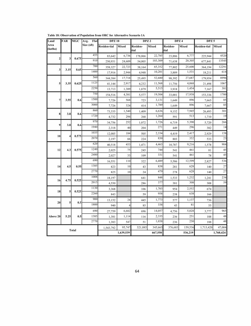
Residen-tial Mixed Residen-
tial
Mixed Residen-
tial
Mixed Residen-tial Mixed
455 83,642 6,736 178,066 22,785 23,886 6,777 225,944 4520
910 250,931 24,609 54,005 103,309 71,638 20,305 677,841 13545
700 358,327 22,723 38,164 65,352 77,802 25,600 364,194 12291
1400 17,916 2,944 4,948 10,201 3,889 1,531 18,211 614
560 344,384 17,718 25,495 52,680 98,392 27,687 179,954 8996
1125 41,144 2,917 4,232 11,568 11,756 4,068 21,498 1067
2250 13,713 1,389 1,879 5,515 3,918 1,454 7,167 381
750 154,516 4,381 5,577 19,504 33,001 17,938 153,336 1700
1500 7,726 568 723 3,131 1,649 896 7,665 85
3000 7,726 324 414 1,789 1,649 896 7,667 85
860 73,335 1,540 1,409 6,636 9,152 7,945 26,493 301
1720 4,732 294 268 1,264 591 513 1,710 19
970 34,756 252 1,072 1,726 6,719 5,390 5,720 266
1940 2,318 40 204 271 449 296 382 14
1035 12,085 184 505 2,334 4,419 2,417 2,929 158
2070 2,197 66 224 830 803 352 533 23
620 40,518 453 1,471 4,463 10,787 9,216 1,578 904
1240 2,025 75 245 744 541 461 81 45
2480 2,027 33 109 331 541 461 78 45
690 16,551 110 322 6,489 5,586 12,599 2,827 536
1385 823 10 43 838 281 628 140 27
2770 825 10 24 479 278 628 140 27
1008 18,197 641 848 1,533 1,232 1,241 234
2015 4,550 286 377 381 308 308 59
1130 3,368 106 1,703 954 2,552 674
2260 843 59 958 238 638 166
900 13,152 24 445 1,773 577 1,137 736
1800 940 4 85 338 43 81 55
690 27,759 6,682 696 14,057 4,756 5,028 3,777 965
1385 1,381 1,114 116 2,335 236 251 188 48
2770 1,383 547 51 1,038 236 250 188 48
1,543,792 95,747 321,885 345,665 376,683 159,536 1,713,420 47,004
5 0.525
5 0.5
5.25 0.5
4.3 0.575
4.5 0.55
4.75 0.525
0.6
3.8 0.6
4 0.575
0.65
3.35 0.625
3.55 0.6
9
Avg. Flat
Size (sft)
DPZ 10 DPZ 2
2
MGC
0.675
3
5
7
8
FAR
3
3.15
3.8
Land
Area
(katha)
64
Table 18: Observation of Population from ORC for Alternative Scenario 1A
1,760,424
10
12
14
16
18
20
Above 20
Total 1,639,539 667,550 536,219
DPZ 4 DPZ 5

Residen-tial Mixed Residen-
tial
Mixed Residen-
tial
Mixed Residen-tial Mixed
455 79,459 6,381 169,052 21,700 22,692 6,420 214,645 4,283
910 238,394 23,314 51,271 98,390 68,057 19,236 643,959 12,832
700 341,276 21,527 36,323 62,240 74,098 24,253 346,859 11,644
1400 17,064 2,789 4,709 9,715 3,704 1,451 17,343 582
560 323,839 16,785 23,957 50,172 92,524 26,230 169,214 8,523
1125 38,689 2,764 3,976 11,017 11,055 3,854 20,214 1,011
2250 1,765 1,316 1,766 5,252 3,684 1,378 6,739 361
750 12,895 4,151 5,338 18,576 31,607 16,994 146,856 1,611
1500 147,992 538 692 2,982 1,579 849 7,342 80
3000 7,399 307 396 1,704 1,579 849 7,344 80
860 7,399 1,459 1,334 6,320 8,670 7,527 25,099 285
1720 69,482 278 254 1,204 560 486 1,620 18
970 4,483 239 1,014 1,643 6,365 5,107 5,419 252
1940 32,928 38 193 258 425 281 362 13
1035 2,197 175 480 2,223 4,198 2,290 2,782 150
2070 11,481 62 213 791 763 333 506 22
620 2,087 429 1,368 4,250 10,035 8,731 1,468 857
1240 37,693 71 228 708 503 437 75 43
2480 1,883 32 101 315 503 437 72 43
690 1,886 104 307 6,180 5,338 11,936 2,702 508
1385 15,816 10 41 798 269 595 133 25
2770 786 9 23 456 266 595 133 25
1008 788 607 807 1,452 1,167 1,176 222
2015 17,239 271 359 361 292 292 56
1130 4,310 101 1,622 906 2,418 640
2260 3,199 56 913 227 604 158
900 801 23 422 1,689 549 1,077 700
1800 12,494 4 81 322 41 77 52
690 893 6,331 661 13,388 4,519 4,763 3,589 914
1385 26,373 1,056 110 2,224 224 237 178 46
2770 1,314 469 - 988 224 237 178 46
1,464,308 90,658 305,346 329,204 356,977 151,139 1,627,849 44,530
4.75 0.525
4.75 0.5
5 0.5
4 0.575
4.3 0.55
4.5 0.525
0.6
3.6 0.6
3.85 0.575
0.65
3.15 0.625
3.4 0.6
9
Avg. Flat
Size (sft)
DPZ 10 DPZ 2
2
MGC
0.675
3
5
7
8
FAR
2.85
3
3.6
Land
Area
(katha)
65
Table 19: Observation of Population from ORC for Alternative Scenario 1B
1,672,380
10
12
14
16
18
20
Above 20
Total 1,554,965 634,550 508,116
DPZ 4 DPZ 5

Residen-tial Mixed Residen-
tial
Mixed Residen-
tial
Mixed Residen-tial Mixed
455 75,277 6,027 160,669 20,615 21,467 6,063 203,351 4,045
910 225,986 22,018 48,728 93,470 51,225 18,168 610,068 12,119
700 318,523 20,331 34,010 59,128 69,059 22,905 323,735 10,997
1400 15,926 2,634 4,409 9,229 3,452 1,370 16,188 550
560 308,412 15,853 22,889 47,663 87,990 24,773 161,152 8,049
1125 36,847 2,610 3,799 10,466 10,513 3,640 19,252 954
2250 12,281 1,243 1,687 4,989 3,503 1,301 6,418 341
750 139,287 3,920 5,040 17,647 29,705 16,050 138,218 1,521
1500 6,964 508 653 2,833 1,484 802 6,910 76
3000 6,964 290 517 1,619 1,484 802 6,912 76
860 65,619 1,378 1,264 6,004 8,177 7,109 23,705 269
1720 4,234 263 241 1,144 528 459 1,530 17
970 31,098 225 961 1,561 6,003 4,823 5,118 238
1940 2,074 36 183 245 401 265 342 13
1035 10,877 165 456 2,112 3,971 2,163 2,636 142
2070 1,977 59 202 751 722 315 480 21
620 35,808 405 1,304 4,038 9,519 8,246 1,394 809
1240 1,789 67 217 673 477 412 71 40
2480 1,791 30 96 299 477 412 69 40
690 14,713 99 287 5,871 4,959 11,273 2,513 480
1385 731 9 39 758 250 562 124 24
2770 733 9 21 433 247 562 124 24
1008 16,473 582 767 1,386 1,102 1,123 210
2015 4,119 260 341 345 276 279 52
1130 3,031 96 1,541 857 2,283 606
2260 759 53 867 214 571 150
900 11,837 21 401 1,604 519 1,017 663
1800 846 3 77 306 38 73 49
690 24,984 5,979 628 12,718 4,275 4,498 3,400 863
1385 1,243 997 104 2,113 212 224 169 43
2770 1,245 443 46 939 212 224 169 43
1,382,451 85,621 289,920 312,744 323,672 142,743 1,536,918 42,057
4.5 0.525
4.5 0.5
4.75 0.5
3.8 0.575
4 0.55
4.3 0.525
0.6
3.4 0.6
3.6 0.575
0.65
3 0.625
3.2 0.6
9
Avg. Flat
Size (sft)
DPZ 10 DPZ 2
2
MGC
0.675
3
5
7
8
FAR
2.7
2.8
3.4
Land
Area
(katha)
66
Table 20: Observation of Population from ORC for Alternative Scenario 1C
1,578,974
10
12
14
16
18
20
Above 20
Total 1,468,073 602,664 466,415
DPZ 4 DPZ 5

Residen-tial Mixed Residen-
tial
Mixed Residen-
tial
Mixed Residen-tial Mixed
455 82,753 3,619 178,823 35,522 24,990 7,282 237,228 4,855
910 248,270 10,878 54,235 149,210 74,950 21,847 711,710 14,572
700 359,080 25,618 38,819 95,688 82,446 32,924 387,300 13,205
1400 17,954 1,282 5,033 12,403 4,121 1,647 19,366 662
560 339,033 2,886 25,476 84,921 102,434 36,669 187,999 9,610
1125 40,505 346 4,228 14,093 12,238 4,384 22,459 1,152
2250 13,500 115 1,878 6,261 4,079 1,460 7,487 383
675 57,635 83,604 8,033 41,814 45,904 25,456 215,382 2,432
1350 4,434 62,709 532 2,765 1,066 593 5,568 60
2700 1,108 130,640 163 847 533 296 1,856 21
860 72,741 1,124 1,419 8,063 9,599 8,539 27,887 324
1720 4,694 71 270 1,535 620 552 1,800 20
970 34,473 718 1,079 2,102 7,047 5,802 6,020 287
1940 2,300 49 205 400 471 386 403 18
950 6,608 941 936 5,154 6,530 3,624 4,279 234
1900 629 90 63 346 210 117 172 10
620 39,955 522 1,473 5,438 11,248 9,911 1,651 980
1240 1,996 24 245 909 564 498 85 47
2480 1,999 28 109 403 564 494 81 47
690 16,462 300 325 7,901 5,876 13,553 2,984 570
1385 818 15 4 1,023 296 672 147 30
2770 821 15 24 583 293 676 147 30
1008 18,672 646 1,026 1,608 1,329 1,306 248
2015 4,513 288 459 400 330 324 65
1525 573 83 1,634 555 1,522 389
3050 286 42 817 277 761 194
900 13,012 447 2,160 604 1,220 773
1800 930 86 413 45 89 57
690 28,773 732 19,807 5,213 6,267 4,155 1,198
1385 1,431 122 3,286 259 311 206 61
2770 1,434 53 1,462 259 311 206 61
1,417,393 325,592 325,871 508,443 405,296 189,521 1,849,625 51,181
4.75 0.525
5.5 0.475
5 0.5
5.25 0.5
5.25 0.475
4 0.575
4.25 0.55
4.5 0.55
3.5 0.6
3.75 0.575
4 0.575
Table 21: Observation of Population from ORC for Alternative Scenario 2A
Total 1,742,985 834,314 594,818 1,900,806
18
20
Above 20
8
9
10
12
14
16
7
67
DPZ 5Avg. Flat
Size (sft)
DPZ 10 DPZ 2 DPZ 4FAR MGCLand
Area
(katha)
2
3
5
3.15 0.65
3.35 0.625

Residen-tial Mixed Residen-
tial
Mixed Residen-
tial
Mixed Residen-tial Mixed
455 79,703 3,619 179,935 35,522 24,988 7,282 237,221 4,855
910 239,121 10,878 54,572 149,210 74,946 21,847 711,688 14,572
600 275,465 108,430 48,747 119,420 84,241 33,645 457,573 15,601
1200 22,954 9,035 4,320 10,579 10,777 4,304 19,722 675
560 326,540 2,886 25,635 84,921 102,428 36,669 187,994 9,610
1125 39,012 346 4,255 14,093 12,237 4,384 22,459 1,152
2250 13,003 115 1,890 6,261 4,078 1,460 7,487 383
675 55,511 83,604 8,083 41,814 45,901 25,456 215,375 2,432
1350 4,271 62,709 535 2,765 1,065 593 5,568 60
2700 1,067 130,640 164 847 533 296 1,856 21
860 70,061 1,124 1,427 8,063 9,598 8,539 27,886 324
1720 4,521 71 272 1,535 620 552 1,800 20
970 33,203 718 1,086 2,102 7,047 5,802 6,020 287
1940 2,215 49 207 400 471 386 403 18
950 6,364 941 942 5,154 6,529 3,624 4,279 234
1900 606 90 63 346 210 117 172 10
1075 6,046 1,714 957 3,501 7,129 6,290 885 520
2150 1,344 378 220 802 650 570 176 105
600 6,340 468 11,224 6,757 15,551 3,971 776
1200 527 41 991 865 1,991 170 34
2400 60 10 228 80 181 35 9
750 4,710 1,515 2,396 2,672 2,207 2,424 465
1300 354 40 67 207 168 69 17
2600 100 20 34 63 50 24 4
1525 552 84 1,634 555 1,522 389
3050 276 42 817 277 761 194
785 627 3,000 744 1,500 934
1575 21 102 13 22 18
3150 11 51 6 11 9
690 27,713 737 19,807 5,213 6,267 4,155 1,198
1385 1,379 122 3,286 259 311 206 61
2770 1,381 54 1,462 259 311 206 61
1,224,399 417,347 337,099 532,432 411,420 192,670 1,921,369 53,502
4.75 0.5
5 0.475
5.25 0.475
4 0.55
4.25 0.525
4.5 0.525
604,090
5.25 0.45
5.5 0.45
Total
20
Above 20
1,641,746 869,530
Table 22: Observation of Population from ORC for Alternative Scenario 2B
3
5
7
8
3.35 0.6
3.5 0.55
3.75 0.55
4 0.55
DPZ 2 DPZ 4 DPZ 5
68
2
Land
Area
(katha)
Avg. Flat
Size (sft)
DPZ 10FAR MGC
3.15 0.6
9
10
12
14
16
18
1,974,870

Residen-
tial
Mixed Residen-
tial
Mixed Residen-
tial
Mixed Residen-
tial
Mixed
455 82,946 3,619 179,357 35,522 24,981 7,282 237,263 4,855
910 248,849 10,878 54,397 149,210 74,925 21,847 711,813 14,572
600 286,672 108,430 48,590 119,420 84,218 33,645 457,653 15,601
1200 23,888 9,035 4,306 10,579 10,774 4,304 19,726 675
900 172,476 65,628 22,858 75,944 83,795 26,035 151,657 7,758
1800 16,426 6,250 1,528 5,077 2,703 838 6,065 309
590 61,147 31,809 8,884 46,122 44,067 24,445 238,859 2,699
1180 5,097 2,651 785 4,083 5,636 3,128 10,294 118
2360 1,132 588 181 934 512 284 2,058 24
720 87,091 1,343 1,700 9,631 11,461 10,199 33,314 387
1440 5,620 85 324 1,833 740 659 2,150 24
810 41,379 860 1,296 2,517 8,436 6,948 7,211 344
1620 2,760 59 247 479 563 462 482 22
850 7,403 1,056 1,050 5,760 7,296 4,051 4,784 261
1700 705 98 70 387 235 131 193 11
1075 6,292 1,714 954 3,501 7,127 6,290 885 520
2150 1,399 378 220 802 650 570 176 105
600 6,598 466 11,224 6,755 15,551 3,971 776
1200 548 41 991 865 1,991 170 34
2400 62 10 228 80 181 35 9
750 4,901 1,510 2,396 2,671 2,207 2,425 465
1300 368 39 67 206 168 69 17
2600 104 20 34 63 50 24 4
1420 787 114 2,174 595 1,643 503
2835 224 33 665 298 823 169
785 625 3,000 744 1,500 935
1575 21 102 13 22 18
3150 11 6 11 9
690 28,840 735 19,807 5,212 6,267 4,156 1,198
1385 1,435 122 3,286 259 311 206 61
2770 1,437 53 1,462 259 311 206 61
1,096,586 244,481 330,545 517,237 386,147 182,155 1,897,478 50,908
5.25 0.425
5.5 0.425
4.75 0.475
5 0.45
5.25 0.45
3.75 0.5
4 0.5
4 0.5
0.575
3.35 0.55
3.5 0.525
3.15
1,948,386
10
12
14
16
18
20
Above 20
Total1,341,067 847,782 568,302
4.25 0.5
4.5 0.5
69
Table 23: Observation of Population from ORC for Alternative Scenario 2C
DPZ 4 DPZ 5
9
Land
Area
(katha)
Avg. Flat
Size (sft)
DPZ 10 DPZ 2
2
3
5
7
8
FAR MGC
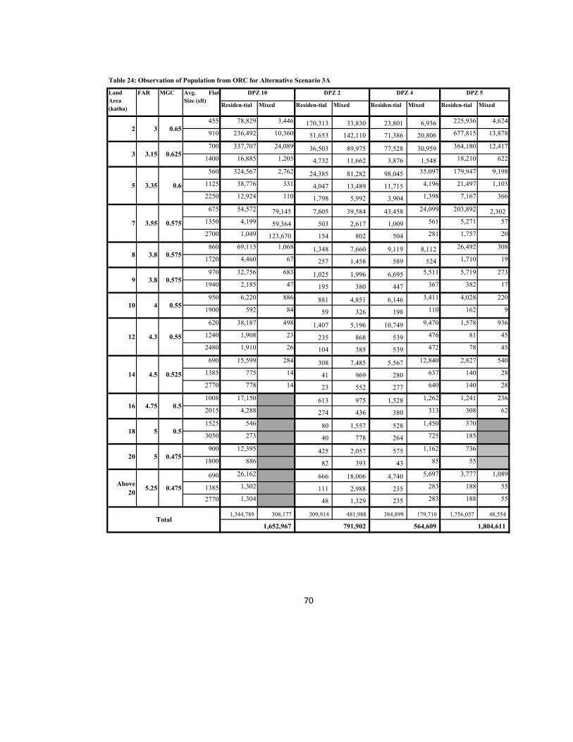
Residen-tial Mixed Residen-tial Mixed Residen-tial Mixed Residen-tial Mixed
455 78,829 3,446 170,313 33,830 23,801 6,936 225,936 4,624
910 236,492 10,360 51,653 142,110 71,386 20,806 677,815 13,878
700 337,707 24,089 36,503 89,975 77,528 30,959 364,180 12,417
1400 16,885 1,205 4,732 11,662 3,876 1,548 18,210 622
560 324,567 2,762 24,385 81,282 98,045 35,097 179,947 9,198
1125 38,776 331 4,047 13,489 11,715 4,196 21,497 1,103
2250 12,924 110 1,798 5,992 3,904 1,398 7,167 366
675 54,572 79,145 7,605 39,584 43,458 24,099 203,892 2,302
1350 4,199 59,364 503 2,617 1,009 561 5,271 57
2700 1,049 123,670 154 802 504 281 1,757 20
860 69,115 1,068 1,348 7,660 9,119 8,112 26,492 308
1720 4,460 67 257 1,458 589 524 1,710 19
970 32,756 683 1,025 1,996 6,695 5,511 5,719 273
1940 2,185 47 195 380 447 367 382 17
950 6,220 886 881 4,851 6,146 3,411 4,028 220
1900 592 84 59 326 198 110 162 9
620 38,187 498 1,407 5,196 10,749 9,470 1,578 936
1240 1,908 23 235 868 539 476 81 45
2480 1,910 26 104 385 539 472 78 45
690 15,599 284 308 7,485 5,567 12,840 2,827 540
1385 775 14 41 969 280 637 140 28
2770 778 14 23 552 277 640 140 28
1008 17,150 613 975 1,528 1,262 1,241 236
2015 4,288 274 436 380 313 308 62
1525 546 80 1,557 528 1,450 370
3050 273 40 778 264 725 185
900 12,395 425 2,057 575 1,162 736
1800 886 82 393 43 85 55
690 26,162 666 18,006 4,740 5,697 3,777 1,089
1385 1,302 111 2,988 235 283 188 55
2770 1,304 48 1,329 235 283 188 55
1,344,789 308,177 309,914 481,988 384,899 179,710 1,756,057 48,554
4.5 0.525
4.75 0.5
5 0.5
1,804,611
2
3
5
7
3.35
3 0.65
3.15 0.625
0.6
3.55 0.575
3.8 0.575
3.8
DPZ 2
Total1,652,967 791,902 564,609
FAR MGC
0.575
4 0.55
4.3 0.55
5 0.475
5.25 0.475
70
Table 24: Observation of Population from ORC for Alternative Scenario 3A
8
Above
20
10
12
14
16
18
20
DPZ 4 DPZ 5
9
Land
Area
(katha)
Avg. Flat
Size (sft)
DPZ 10

Residen-
tial
Mixed Residen-
tial
Mixed Residen-
tial
Mixed Residen-
tial
Mixed
455 74,821 3,274 161,779 32,139 22,611 6,589 214,636 4,393
910 224,480 9,842 49,065 135,000 67,815 19,766 643,932 13,184
700 321,358 22,942 34,761 85,691 73,834 29,484 346,844 11,826
1400 16,068 1,148 4,506 11,107 3,691 1,475 17,343 593
560 304,938 2,597 22,926 76,429 92,195 33,002 169,206 8,649
1125 36,431 311 3,805 12,684 11,015 3,945 20,213 1,037
2250 12,142 104 1,690 5,634 3,671 1,314 6,739 345
675 52,223 75,801 7,283 37,911 41,622 23,080 195,281 2,205
1350 4,018 56,856 482 2,507 966 538 5,048 55
2700 1,004 118,450 148 768 483 269 1,683 19
860 65,427 1,012 1,277 7,257 8,639 7,685 25,098 292
1720 4,222 64 243 1,381 558 497 1,620 18
970 31,006 647 971 1,891 6,343 5,221 5,418 259
1940 2,068 44 185 360 424 348 362 16
950 5,982 853 848 4,669 5,915 3,283 3,877 212
1900 570 81 57 313 190 106 156 9
620 35,493 464 1,309 4,833 9,999 8,810 1,468 871
1240 1,773 21 218 808 501 443 75 42
2480 1,775 25 97 358 501 439 72 42
690 14,893 271 294 7,152 5,319 12,269 2,702 516
1385 740 14 40 926 268 609 133 27
2770 742 14 22 527 265 612 133 27
1008 16,233 581 924 1,447 1,196 1,176 224
2015 4,059 259 413 360 297 292 58
1525 518 76 1,479 502 1,377 352
3050 259 38 739 251 689 176
900 11,765 404 1,954 547 1,103 700
1800 841 77 374 40 80 52
690 24,834 632 17,106 4,503 5,412 3,589 1,035
1385 1,235 105 2,838 224 269 178 52
2770 1,238 46 1,262 224 269 178 52
1,273,158 294,833 294,224 457,436 364,923 170,474 1,668,733 46,056
5 0.475
3 0.625
3.15 0.6
3.4 0.575
3.85 0.55
4 0.55
4.3 0.525
4.75 0.475
4.75 0.5
3.6 0.575
3.6 0.575
2.85 0.65
1,714,788
10
12
14
16
18
20
Above 20
Total1,567,991 751,660 535,396
4.5 0.5
71
Table 25: Observation of Population from ORC for Alternative Scenario 3B
DPZ 4 DPZ 5
9
Land
Area
(katha)
Avg. Flat
Size (sft)
DPZ 10 DPZ 2
2
3
5
7
8
FAR MGC

Residen-
tial
Mixed Residen-
tial
Mixed Residen-
tial
Mixed Residen-
tial
Mixed
455 70,908 3,102 153,213 30,447 21,422 6,242 203,342 4,161
910 212,734 9,324 46,467 127,900 64,249 18,726 610,043 12,490
700 300,033 21,412 32,432 79,978 68,915 27,519 323,722 11,037
1400 15,002 1,072 4,205 10,366 3,445 1,376 16,187 553
560 290,508 2,473 21,827 72,790 87,807 31,431 161,145 8,237
1125 34,708 296 3,623 12,080 10,491 3,758 19,251 987
2250 11,568 99 1,609 5,366 3,496 1,252 6,418 328
675 49,167 71,342 6,852 35,681 39,175 21,723 183,790 2,075
1350 3,783 53,512 454 2,359 909 506 4,751 52
2700 945 111,480 139 723 455 253 1,584 18
860 61,810 956 1,205 6,854 8,160 7,258 23,704 276
1720 3,988 60 229 1,304 527 469 1,530 17
970 29,293 611 917 1,786 5,991 4,931 5,117 244
1940 1,954 42 174 340 400 328 342 15
950 5,595 797 793 4,366 5,532 3,070 3,625 198
1900 533 76 53 293 178 99 146 8
620 33,729 440 1,243 4,592 9,499 8,369 1,394 828
1240 1,685 20 207 768 476 420 71 40
2480 1,687 23 92 340 476 417 69 40
690 13,859 253 274 6,653 4,948 11,413 2,513 480
1385 689 13 37 862 249 566 124 25
2770 691 13 20 491 247 569 124 25
1008 15,517 555 883 1,383 1,143 1,123 214
2015 3,880 248 395 344 283 279 56
1525 491 72 1,401 475 1,305 333
3050 245 36 700 238 652 167
900 11,150 383 1,851 518 1,045 663
1800 797 73 354 38 76 49
690 23,534 599 16,206 4,266 5,127 3,400 980
1385 1,171 99 2,689 212 255 169 50
2770 1,173 44 1,196 212 255 169 50
1,202,826 277,415 278,174 432,012 344,733 160,837 1,575,345 43,483
4.5 0.475
4.75 0.475
4 0.525
4.3 0.5
4.5 0.5
3.2 0.575
3.4 0.575
3.4 0.575
0.65
2.8 0.625
3 0.6
2.7
1,618,829
10
12
14
16
18
20
Above 20
Total1,480,241 710,186 505,571
3.6 0.55
3.8 0.55
72
Table 26: Observation of Population from ORC for Alternative Scenario 3C
DPZ 4 DPZ 5
9
Land
Area
(katha)
Avg. Flat
Size (sft)
DPZ 10 DPZ 2
2
3
5
7
8
FAR MGC

Residen-
tial
Mixed Residen-
tial
Mixed Residen-
tial
Mixed Residen-
tial
Mixed
455 75,713 3,446 171,082 33,830 23,802 6,936 225,946 4,624
910 227,144 10,360 51,887 142,110 71,386 20,806 677,846 13,878
600 258,352 101,950 45,761 112,290 79,222 31,637 430,291 14,669
1200 21,528 8,495 4,055 9,947 10,136 4,048 18,547 635
560 311,737 2,762 24,495 81,282 98,046 35,097 179,956 9,198
1125 37,244 331 4,066 13,489 11,715 4,196 21,498 1,103
2250 12,413 110 1,806 5,992 3,904 1,398 7,167 366
675 59,618 90,023 8,689 45,025 49,433 27,411 231,926 2,619
1350 4,033 59,364 506 2,617 1,009 561 5,271 57
2700 1,007 123,670 155 802 504 281 1,757 20
860 66,383 1,068 1,354 7,660 9,119 8,112 26,494 308
1720 4,284 67 258 1,458 589 524 1,710 19
970 31,461 683 1,030 1,996 6,695 5,511 5,720 273
1940 2,099 47 196 380 447 367 382 17
950 5,975 886 885 4,851 6,146 3,411 4,028 220
1900 569 84 59 326 198 110 162 9
1075 5,762 1,638 913 3,345 6,813 6,011 846 497
2150 1,281 362 210 767 621 544 168 100
600 5,991 442 10,633 6,402 14,733 3,762 735
1200 498 38 939 820 1,887 161 33
2400 57 10 216 76 172 34 8
750 444 144 228 254 210 230 44
1300 335 37 64 196 159 65 16
2600 95 19 32 60 48 23 4
1525 524 80 1,557 528 1,450 370
3050 262 40 778 264 725 185
785 596 2,858 709 1,429 890
1575 20 97 12 21 17
3150 10 48 6 10 9
690 25,128 669 18,006 4,740 5,697 3,778 1,089
1385 1,250 111 2,988 235 283 188 55
2770 1,252 49 1,329 235 283 188 55
1,162,437 405,345 319,671 507,938 394,323 184,065 1,849,614 50,650
5 0.45
5.25 0.45
4.5 0.5
4.75 0.475
5 0.475
3.55 0.55
3.8 0.55
3.8 0.55
0.6
3.15 0.6
3.35 0.55
3
1,900,264
10
12
14
16
18
20
Above 20
Total1,567,783 827,608 578,388
4 0.525
4.3 0.525
73
Table 27: Observation of Population from ORC for Alternative Scenario 3D
DPZ 4 DPZ 5
9
Land
Area
(katha)
Avg. Flat
Size (sft)
DPZ 10 DPZ 2
2
3
5
7
8
FAR MGC

Residen-
tial
Mixed Residen-
tial
Mixed Residen-
tial
Mixed Residen-
tial
Mixed
455 72,072 3,274 162,767 32,139 22,610 6,589 214,629 4,393
910 216,234 9,842 49,365 135,000 67,810 19,766 643,912 13,184
600 246,557 97,098 43,645 106,940 75,442 30,130 409,773 13,971
1200 20,545 8,091 3,868 9,474 9,652 3,855 17,662 604
560 293,736 2,597 23,066 76,429 92,189 33,002 169,201 8,649
1125 35,093 311 3,828 12,684 11,015 3,945 20,213 1,037
2250 11,696 104 1,700 5,634 3,671 1,314 6,739 345
675 50,304 75,801 7,327 37,911 41,619 23,080 195,275 2,205
1350 3,870 56,856 485 2,507 966 538 5,048 55
2700 967 118,450 149 768 483 269 1,683 19
860 63,023 1,012 1,284 7,257 8,639 7,685 25,098 292
1720 4,067 64 245 1,381 558 497 1,620 18
970 29,867 647 977 1,891 6,342 5,221 5,418 259
1940 1,992 44 186 360 424 348 362 16
950 5,762 853 853 4,669 5,915 3,283 3,877 212
1900 549 81 57 313 190 106 156 9
1075 5,372 1,524 850 3,112 6,337 5,591 787 462
2150 1,194 336 196 713 578 506 157 93
600 5,736 423 10,161 6,117 14,078 3,595 702
1200 477 37 897 783 1,803 154 31
2400 54 9 207 72 164 32 8
750 4,237 1,363 2,156 2,405 1,986 2,182 418
1300 318 36 60 186 151 62 15
2600 90 18 30 56 45 22 4
1525 499 76 1,479 502 1,377 352
3050 249 38 739 251 689 176
785 567 2,715 673 1,357 845
1575 19 92 12 20 16
3150 10 46 6 10 8
690 23,921 636 17,106 4,502 5,412 3,588 1,035
1385 1,190 106 2,838 224 269 178 52
2770 1,192 46 1,262 224 269 178 52
1,100,864 376,984 304,234 478,970 370,452 173,354 1,732,997 48,138
4.75 0.45
5 0.45
4.3 0.5
4.5 0.475
4.75 0.475
3.4 0.55
3.6 0.55
3.6 0.55
0.6
3 0.6
3.15 0.55
2.85
1,781,135
10
12
14
16
18
20
Above 20
Total1,477,848 783,204 543,806
3.85 0.525
4 0.525
74
Table 28: Observation of Population from ORC for Alternative Scenario 3E
DPZ 4 DPZ 5
9
Land Area
(katha)
Avg. Flat
Size (sft)
DPZ 10 DPZ 2
2
3
5
7
8
FAR MGC

Residen-
tial
Mixed Residen-
tial
Mixed Residen-
tial
Mixed Residen-
tial
Mixed
455 68,331 3,102 154,141 30,447 21,421 6,242 203,336 4,161
910 205,005 9,324 46,748 127,900 64,245 18,726 610,025 12,490
600 230,290 90,625 40,719 99,812 70,416 28,121 382,449 13,039
1200 19,189 7,551 3,608 8,842 9,009 3,598 16,485 564
560 279,953 2,473 21,959 72,790 87,802 31,431 161,141 8,237
1125 33,447 296 3,645 12,080 10,490 3,758 19,250 987
2250 11,148 99 1,619 5,366 3,496 1,252 6,418 328
675 47,380 71,342 6,894 35,681 39,173 21,723 183,785 2,075
1350 3,645 53,512 456 2,359 909 506 4,751 52
2700 911 111,480 140 723 455 253 1,584 18
860 59,564 956 1,213 6,854 8,159 7,258 23,703 276
1720 3,844 60 231 1,304 527 469 1,530 17
970 28,229 611 922 1,786 5,990 4,931 5,117 244
1940 1,883 42 175 340 400 328 342 15
950 5,392 797 798 4,366 5,531 3,070 3,625 198
1900 514 76 53 293 178 99 146 8
1075 5,107 1,447 808 2,956 6,021 5,312 747 439
2150 1,136 319 186 677 549 481 149 89
600 5,340 394 9,452 5,690 13,096 3,344 653
1200 444 34 835 729 1,677 143 29
2400 50 9 192 67 152 30 7
750 4,051 1,302 2,060 2,298 1,898 2,085 400
1300 304 34 58 178 144 59 14
2600 86 17 29 54 43 21 4
1525 473 72 1,401 475 1,305 333
3050 237 36 700 238 652 167
785 537 2,572 638 1,286 801
1575 18 87 11 19 15
3150 9 44 5 9 8
690 22,679 603 16,206 4,266 5,127 3,400 980
1385 1,128 100 2,689 212 255 169 50
2770 1,130 44 1,196 212 255 169 50
1,040,889 354,113 287,524 452,096 349,845 163,475 1,635,325 45,424
4.5 0.45
4.75 0.45
4 0.5
4.3 0.475
4.5 0.475
3.2 0.55
3.4 0.55
3.4 0.55
0.6
2.8 0.6
3 0.55
2.7
1,680,748
10
12
14
16
18
20
Above 20
Total1,395,002 739,620 513,320
3.6 0.525
3.8 0.525
75
Table 29: Observation of Population from ORC for Alternative Scenario 3F
DPZ 4 DPZ 5
9
Land Area
(katha)
Avg. Flat
Size (sft)
DPZ 10 DPZ 2
2
3
5
7
8
FAR MGC

Residen-
tial
Mixed Residen-
tial
Mixed Residen-
tial
Mixed Residen-
tial
Mixed
455 79,907 3,446 166,567 33,830 23,771 6,936 226,020 4,624
910 239,727 10,360 50,517 142,110 71,294 20,806 678,069 13,878
600 99,542 37,221 16,265 40,994 28,885 11,550 157,139 5,355
1200 22,720 8,495 3,948 9,947 10,123 4,048 18,553 635
900 166,983 62,816 21,334 72,689 80,132 24,919 145,192 7,425
1800 15,903 5,983 1,426 4,860 2,585 803 5,806 296
590 58,553 30,113 8,201 43,662 41,679 23,141 226,176 2,555
1180 4,881 2,509 725 3,866 5,331 2,962 9,747 111
2360 1,084 557 167 885 484 269 1,949 23
720 83,684 1,276 1,574 9,149 10,879 9,690 31,655 368
1440 5,400 80 300 1,741 703 626 2,043 23
810 39,763 817 1,200 2,391 8,007 6,600 6,852 327
1620 2,652 56 228 455 535 439 458 20
850 7,047 994 963 5,422 6,860 3,813 4,503 246
1700 671 92 65 364 221 123 181 10
1075 6,082 1,638 889 3,345 6,804 6,011 846 497
2150 1,352 362 205 767 621 544 168 100
600 6,323 431 10,633 6,393 14,733 3,763 735
1200 525 37 939 819 1,887 161 33
2400 60 9 216 75 172 34 8
750 4,710 1,399 2,276 2,536 2,097 2,304 441
1300 354 36 64 196 159 65 16
2600 100 18 32 59 48 23 4
1420 758 105 2,071 567 1,564 480
2835 216 31 634 284 784 161
785 580 2,858 708 1,429 890
1575 20 97 12 21 17
3150 10 48 6 10 9
690 26,520 651 18,006 4,734 5,697 3,779 1,089
1385 1,319 108 2,988 235 283 188 55
2770 1,322 47 1,329 235 283 188 55
878,158 166,815 278,059 418,664 315,772 152,443 1,527,419 38,930
5 0.425
5.25 0.425
4.5 0.475
4.75 0.45
5 0.45
3.55 0.5
3.8 0.5
3.8 0.5
0.575
3.15 0.55
3.35 0.525
3
1,566,349
10
12
14
16
18
20
Above 20
Total1,044,974 696,723 468,215
4 0.5
4.3 0.5
76
Table 30: Observation of Population from ORC for Alternative Scenario 3G
DPZ 4 DPZ 5
9
Land Area
(katha)
Avg. Flat
Size (sft)
DPZ 10 DPZ 2
2
3
5
7
8
FAR MGC
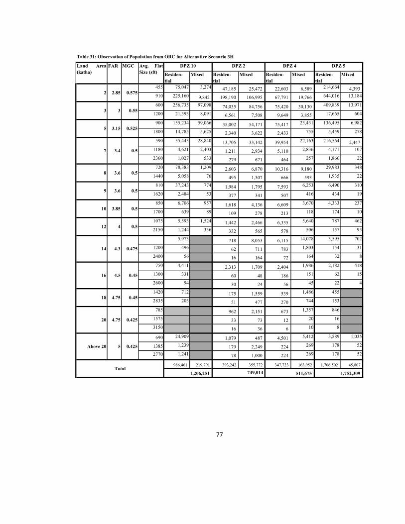
Residen-
tial
Mixed Residen-
tial
Mixed Residen-
tial
Mixed Residen-
tial
Mixed
455 75,047 3,274 47,185 25,472 22,603 6,589 214,664 4,393
910 225,160 9,842 198,190 106,995 67,791 19,766 644,016 13,184
600 256,735 97,098 74,035 84,756 75,420 30,130 409,839 13,971
1200 21,393 8,091 6,561 7,508 9,649 3,855 17,665 604
900 155,234 59,066 35,002 54,171 75,417 23,431 136,495 6,982
1800 14,785 5,625 2,340 3,622 2,433 755 5,459 278
590 55,443 28,840 13,705 33,142 39,954 22,163 216,564 2,447
1180 4,621 2,403 1,211 2,934 5,110 2,836 4,171 107
2360 1,027 533 279 671 464 257 1,866 22
720 78,383 1,209 2,603 6,870 10,316 9,180 29,983 348
1440 5,058 76 495 1,307 666 593 1,935 22
810 37,243 774 1,984 1,795 7,593 6,253 6,490 310
1620 2,484 53 377 341 507 416 434 19
850 6,706 957 1,618 4,136 6,609 3,670 4,333 237
1700 639 89 109 278 213 118 174 10
1075 5,593 1,524 1,442 2,466 6,335 5,640 787 462
2150 1,244 336 332 565 578 506 157 93
5,973 718 8,053 6,115 14,078 3,595 702
1200 496 62 711 783 1,803 154 31
2400 56 16 164 72 164 32 8
750 4,411 2,313 1,709 2,404 1,986 2,182 418
1300 331 60 48 186 151 62 15
2600 94 30 24 56 45 22 4
1420 712 175 1,559 539 1,486 455
2835 203 51 477 270 744 153
785 962 2,151 673 1,357 846
1575 33 73 12 20 16
3150 16 36 6 10 8
690 24,909 1,079 487 4,501 5,412 3,589 1,035
1385 1,239 179 2,249 224 269 178 52
2770 1,241 78 1,000 224 269 178 52
986,461 219,791 393,242 355,772 347,723 163,952 1,706,502 45,807
4.75 0.425
5 0.425
4.3 0.475
4.5 0.45
4.75 0.45
3.4 0.5
3.6 0.5
3.6 0.5
0.575
3 0.55
3.15 0.525
2.85
1,752,309
10
12
14
16
18
20
Above 20
Total1,206,251 749,014 511,675
3.85 0.5
4 0.5
77
Table 31: Observation of Population from ORC for Alternative Scenario 3H
DPZ 4 DPZ 5
9
Land Area
(katha)
Avg. Flat
Size (sft)
DPZ 10 DPZ 2
2
3
5
7
8
FAR MGC

Residen-
tial
Mixed Residen-
tial
Mixed Residen-
tial
Mixed Residen-
tial
Mixed
10 705 3,102 153,618 30,447 21,470 6,242 203,372 4,161
910 211,900 9,324 46,590 127,900 64,393 18,726 610,132 12,490
600 238,035 90,625 40,581 99,812 70,579 28,121 382,516 13,039
1200 19,835 7,551 3,596 8,842 9,030 3,598 16,488 564
900 146,870 56,253 19,577 65,095 72,016 22,315 129,990 6,650
1800 13,988 5,357 1,309 4,352 2,323 719 5,199 265
590 51,837 27,144 7,575 39,357 37,704 20,860 203,833 2,303
1180 4,321 2,262 669 3,485 4,822 2,670 8,784 100
2360 960 502 154 797 438 242 1,756 21
720 73,541 1,142 1,444 8,186 9,769 8,670 28,317 329
1440 4,745 72 275 1,558 631 560 1,827 21
810 34,942 731 1,101 2,139 7,190 5,905 6,129 293
1620 2,331 50 209 407 480 393 410 18
850 6,229 895 888 4,879 6,196 3,431 4,052 221
1700 593 83 60 327 199 111 163 9
1075 5,279 1,447 805 2,956 6,035 5,312 747 439
2150 1,174 319 185 677 550 481 149 89
600 5,520 392 9,452 5,703 3,096 3,344 653
1200 459 34 835 731 1,677 143 29
2400 52 9 192 67 152 30 7
750 4,188 1,298 2,060 2,304 1,898 2,085 400
1300 314 34 58 178 144 59 14
2600 89 17 29 54 43 21 4
1420 670 97 1,863 512 1,408 432
2835 191 28 570 256 705 145
785 535 2,572 639 1,286 801
1575 18 87 11 19 15
3150 9 44 5 9 8
690 23,442 601 16,206 4,275 5,127 3,400 980
1385 1,166 100 2,689 212 255 169 50
2770 1,168 44 1,196 212 255 169 50
854,542 206,860 281,853 439,070 328,986 144,430 1,614,687 43,198
3.8 0.5
4 0.475
4.3 0.45
0.425
0.55
3 0.525
3.2 0.5
3.4 0.5
3.4 0.5
3.6 0.5
4.5 0.45
4.5 0.425
Table 32: Observation of Population from ORC for Alternative Scenario 3I
20
2
3
5
7
8
9
10
12
14
16
18
2.7 0.575
2.8
78
DPZ 5Land
Area
(katha)
Avg. Flat
Size (sft)
DPZ 10 DPZ 2 DPZ 4FAR MGC
Above 20
1,061,402 720,922 473,415 1,657,885 Total
4.75
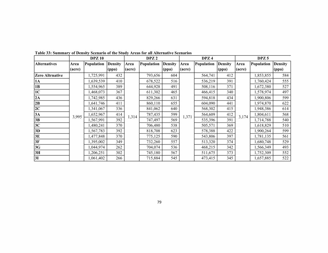
Alternatives Area
(acre)
Population Density
(ppa)
Area
(acre)
Population Density
(ppa)
Area
(acre)
Population Density
(ppa)
Area
(acre)
Population Density
(ppa)
Zero Altrnative 1,725,991 432 793,656 604 564,741 412 1,853,855 584
1A 1,639,539 410 678,522 516 536,219 391 1,760,424 555
1B 1,554,965 389 644,928 491 508,116 371 1,672,380 527
1C 1,468,073 367 611,302 465 466,415 340 1,578,974 497
2A 1,742,985 436 829,266 631 594,818 434 1,900,806 599
2B 1,641,746 411 860,110 655 604,090 441 1,974,870 622
2C 1,341,067 336 841,062 640 568,302 415 1,948,386 614
3A 1,652,967 414 787,435 599 564,609 412 1,804,611 568
3B 1,567,991 392 747,497 569 535,396 391 1,714,788 540
3C 1,480,241 370 706,480 538 505,571 369 1,618,829 510
3D 1,567,783 392 818,708 623 578,388 422 1,900,264 599
3E 1,477,848 370 775,125 590 543,806 397 1,781,135 561
3F 1,395,002 349 732,260 557 513,320 374 1,680,748 529
3G 1,044,974 262 704,074 536 468,215 342 1,566,349 493
3H 1,206,251 302 745,180 567 511,675 373 1,752,309 552
3I 1,061,402 266 715,884 545 473,415 345 1,657,885 522
79
Table 33: Summary of Density Scenario of the Study Areas for all Alternative Scenarios
3,174
DPZ 10 DPZ 2 DPZ 4 DPZ 5
3,995 1,314 1,371
Alternatives Area
(acre)
Population Density
(ppa)
Area
(acre)
Population Density
(ppa)
Area
(acre)
Population Density
(ppa)
Area
(acre)
Population
Zero Altrnative 1,725,991 432 793,656 604 564,741 412 1,853,855
1A 1,639,539 410 678,522 516 536,219 391 1,760,424
1B 1,554,965 389 644,928 491 508,116 371 1,672,380
1C 1,468,073 367 611,302 465 466,415 340 1,578,974
2A 1,742,985 436 829,266 631 594,818 434 1,900,806
2B 1,641,746 411 860,110 655 604,090 441 1,974,870
2C 1,341,067 336 841,062 640 568,302 415 1,948,386
3A 1,652,967 414 787,435 599 564,609 412 1,804,611
3B 1,567,991 392 747,497 569 535,396 391 1,714,788
3C 1,480,241 370 706,480 538 505,571 369 1,618,829
3D 1,567,783 392 818,708 623 578,388 422 1,900,264
3E 1,477,848 370 775,125 590 543,806 397 1,781,135
3F 1,395,002 349 732,260 557 513,320 374 1,680,748
3G 1,044,974 262 704,074 536 468,215 342 1,566,349
3H 1,206,251 302 745,180 567 511,675 373 1,752,309
3I 1,061,402 266 715,884 545 473,415 345 1,657,885
80
Table 33: Summary of Density Scenario of the Study Areas for all Alternative Scenarios
3,174
DPZ 10 DPZ 2 DPZ 4 DPZ 5
3,995 1,314 1,371

Density
(ppa)
584
555
527
497
599
622
614
568
540
510
599
561
529
493
552
522

References
Acioly C. and Davidson F., (1996), “Density in Urban Development”, Building, issues,Vol.8, No.3, Lund Centre for Habitat Studies, Lund University.
Asaduzzaman, (2001), “Spatial Variation of House Rent in Dhaka City” Unpublished graduate Dissertation of Bangladesh University of Engineering and Technology.
Bhadra S. and Shammin S., (2001), Peoples Report on Bangladesh Environment 2002- 2003, MoEF –US. Retrieved on 13 December 2006 at 10am from
http://www.bdix.net/sdnbd_org/world_env_day/2005/data/human_stlmnt/distribution.html
Burton, E., (2000),“The Compact City: Just or Just Compact? A Preliminary Analysis”, Urban Studies, Vol. 37 (11) pp. 1969-2001.
Cotton P., (2008), Your Development: Creating Sustainable Neighbourhoods, http://yourdevelopment.org/factsheet/view/id/58#sec5
Claudio C., (2000), “Can Urban Management Deliver the Sustainable City?,Guided Densification in Brazil vs. Informal Compactness in Egypt”. In Jenks, M. and Burgess, R. 2000.ed. Compact Cities: Sustainable Urban Forms for Developing Countries. Pp:127-140. London: Spon Press.
Debnath, A.K., Proma, N.N, Nabeela, H.Y. (2011) “Towards a Generic Methodology of Determining Desirable Density for Dhaka City: A Case Study on Detailed Planning Zones” Undergraduate Dissertation of Bangladesh University of Engineering and Technology.
Churchman A., (1999), “Disentangling the concept of density”, Journal of Planning Literature, vol 13, no 4, pp389-411.
Islam S., (2007), “Physical Density and Urban Sprawl: A Case of Dhaka City”; Department of Urban Planning and Environment; KungligaTekniskaHögskolan (KTH); p 18 – 19.
Jones, T. L.,(2000),“Compact City Policies for Megacities: Core Areas and Metropolitan Regions”. In Jenks and Burgess, 2000. (ed.) Compact Cities: Sustainable Urban Forms for Developing Countries. Pp: 37-52. London: Spon Press.
Kamruzzaman, M. and N. Ogura (2008).“Housing for the Middle Income Group in Dhaka, Bangladesh” with a focus on Affordability and Option.
Magri S., (1994),“Urban density definitions”, Urban Futures, September.
Pont, M. B. & Haupt, P., (2007),“The relation between urban form and density, Viewpoints”,Vol. 11 (1) pp. 1-3.
RAJUK, (2010), “Detailed Area Plan (DAP) for DMDP Area: Part-III”.
Town and Country Planning Association, (2003),“TCPA Policy Statement”.
Towers G., (2000), “Shelter Is Not Enough – Transforming Multi-Storey Housing”, The Policy Press, Bristol.
Williams, K. Burton, E. Jenks, M. 2001,“Defining Sustainable Urban Form: Introduction” in Williams, K., Burton, E. and Jenks M. (ed.) Achieving Sustainable Urban Form. Pp: 7-8. London :Spon Press.

Zhang, X.Q. (2000), “High-Rise and high Density Compact Urban Form: The Development of Hong Kong”, in Jenks, M. and Burgess, R. (ed.), “Compact Cities: Sustainable Urban Forms for Developing Countries”. Pp: 245-254. London: Spon Pres.