Simulation of variational compliant assemblies with shape errors based on morphing mesh approach

ORIGINAL ARTICLE

Simulation of variational compliant assemblies with shapeerrors based on morphing mesh approach

Pasquale Franciosa & Salvatore Gerbino &

Stanislao Patalano

Received: 22 October 2009 /Accepted: 8 July 2010 /Published online: 23 July 2010# Springer-Verlag London Limited 2010

Abstract Variation analysis of assemblies is a strategic task inmany industrial applications. Parts manufactured throughplastic deformation processes exhibit appreciable shape devia-tions from the nominal geometry due mainly to spring-backphenomena. When these parts are assembled, initial shapedeviations at part level highly influence the final assemblyshape. This work focuses on the modeling and simulation ofshape errors in order to perform variation analysis of compliantassemblies. The aim is to simulate variational shape of partsaccording to a small number of control points chosen on thepart geometry through a morphing mesh procedure. Thesepoints are typically related to measurement or inspection pointsof manufactured parts. From the mesh model of parts, meshnodes are moved by applying the morphing procedure. Inparticular, in order to assure control points belong to the“perturbed” shape, a linear-constrained approach is adopted.The so-morphed parts are used to accomplish the variationalassembly analysis following the classical place, clamp, fasten,and release cycle. In order to achieve statistical results, MonteCarlo simulation is performed: a set of control points drivingthe perturbed parts is generated at each iteration; these parts arethen assembled and results are stored. Numerical results arecompared with ones coming from commercial software thatuses a linear approach based on the sensitivity matrix.

Keywords Monte Carlo FEA .Morphing mesh .

Shape errors . Geometric covariance . Variational assemblies

1 Introduction

Predicting the final assembly shape of compliant non-idealparts is a strategic topic for many industrial applications. Threesources of variation are typically identified in compliantassembly process: part shape variations, fixture variations, andfastening tool variations. Several numerical methods have beendeveloped over the years to simulate and to take into account allthese sources of variation. Most of these methods are based onlinear variational models to provide a fast solution to theproblem [1, 2]. Starting from deviations related to fastening orclamping points, a constant “Sensitivity Matrix,” linkingdeviations at part level to variations at assembly level, isbuilt. Deviations data may be obtained from statistical analysisof the manufactured parts in the assembly line. The SensitivityMatrix may be easily calculated by using any commercialFEA solver, running two consecutive FEA calculations andusing the method of influence coefficients (MIC).

Originally, the Sensitivity Matrix was defined in processinvolving single-station assemblies. Then, in Camelio et al. [3],this concept was extended also to multi-station assemblyprocesses to consider the effects of variation accumulationwhen parts are moved from one station to another. Camelio etal. [4] proposed a more computationally efficient method thanLiu et al. [1], also taking into account geometric covariance bymeans of the statistical principal component analysis method.

However, linear approaches do not provide adequateresults when large deformations occur, or part-to-partcontact conditions have to be taken into account. Liao etal. [5] and Xie et al. [6] showed how contacts among partsbeing assembled highly influence final assembly shape.They proposed to use a non-linear FEA approach to solve

P. Franciosa : S. PatalanoUniversity of Naples Federico II,Naples, Italy

P. Franciosae-mail: [email protected]

S. Patalanoe-mail: [email protected]

S. Gerbino (*)University of Molise, School of Engineering,Termoli (CB), Italye-mail: [email protected]

Int J Adv Manuf Technol (2011) 53:47–61DOI 10.1007/s00170-010-2839-4

the contact problem. Their methods are more accurate thana linear one, but they are very time consuming especially ifcombined with Monte Carlo simulations.

To overcome this lack, an interesting linear contactalgorithm was proposed both in Dalhlström et al. [7] andUngemach et al. [8], by combining a linear contact searchand a contact equilibrium criterion. Their methods may beeasily integrated with the MIC.

In Gerbino et al. [9], a linear methodology, calledstatistical variation analysis and finite element analysis(SVA-FEA), which allows to statistically simulate bothsingle- and multi-station assemblies, starting from theSensitivity Matrix, was proposed. Also, in SVA-FEA, alinear contact algorithm was implemented by using multi-point constraints (MPC) elements of MSC.Nastran®.

In Franciosa et al. [10], a comparison study between SVA-FEA and a commercial CAT software, TAA® (module ofCATIA® CAD system, by Dassault Systèmes), with referenceto a multi-station assembly, was presented. The comparisonshowed high numerical correlation both for mean andstandard deviations.

Many methods and numerical algorithms have beendeveloped over the years, but there are very few works onvalidation of the methods compared with real productioninspection data. Hu et al. [11] presented a simulationmethod, which was verified for one instrument panelconsisting of two parts, assembled with different weldsequences, with part and process variation. A validation of amore complex assembly was presented by Sellem et al.[12]. In Sellem et al. [13], authors concluded also thatmodeling aspects such as type and size of elements,incompatible and compatible meshes, and the use ofcontacts have minor impact on the simulation result.

The present work focuses on the modeling of part shapedeviations and provides a methodology to simulate varia-tional compliant assemblies when these deviations occur.The aim is to generate variational shapes according to asmall set of local deviations defined on nominal parts.Typically, local deviations, assigned at point level, cannotdescribe by itself the whole geometry. In the literature, thisissue is analyzed by introducing the “geometric covariance”concept. The geometric covariance states the geometricalrelation among the neighboring points on the same surface.Obviously, geometric covariance assures surface continuityand smoothness. Merkley [14] proposed to use randomBezier curves. Shape deviations were parameterized byconstraining the displacement of the control points ofBezier curves. This method may be also extended torectangular Bezier patches. However, for complex shapes,the parameterization of the patch becomes not a trivial task,so this method may be inadequate.

Bihlmaier [15] extended Merkley’s work and proposed tomodel the variations of a surface as a finite summation of

sinusoidal waves, each with a different amplitude andwavelength. Then, any surface profile is modeled as asummation of sinusoids, having different wavelengths andamplitudes, represented in the frequency domain using theFourier transform.

A more general method was proposed in Tonks [16]. Totake account of surface variations, a hybrid method was usedto model the surface covariance. Legendre polynomials wereused to model the long wavelengths, and the frequencyspectrum was used to model the shorter wavelengths. Thehybrid method for geometric covariance was validated bymeans of experimental data.

Huang et al. [17] suggested decomposing the shapedeviation by using the direct cosine transform technique.The field of variation was divided into a set of independentdefects. However, this method well works only forrectangular-based surface.

An interesting approach was proposed in Samper et al. [18]by using a modal decomposition analysis. Firstly, the nominalCAD geometry is meshed and the orthogonal modal matrix iscalculated. This matrix is then used to extract the principalmodal shapes. To reach more accuracy, during the modaldecomposition, a large amount of measurement data isneeded. Moreover, a modal solver is required to calculatethe modal matrix. A similar method was proposed also inUngemach et al. [8], where the first eigenvector mode,resulting from a preliminary buckling analysis, was adoptedto generate the initial variational geometry to be used in theassembly process simulation.

Both the modal decomposition and the bucklingeigenvector analyses have no physical significance. However,they give a good approximation of the geometrical covariance.

Starting from modal decomposition, statistically modalanalysis was proposed in Huang et al. [19] to statisticallygenerate geometrical errors. This method decomposes theerror field into few principal modes.

In the present work, a morphing mesh-based approach isused to generate variational shapes, according to deviationsoccurring in a small set of points defined on the nominalgeometry. The proposed method is based on a constraineddeformation approach. Each deviation point (in the follow-ing named control point) determines a local deformation ofthe surface. A weighted function is generated in order totake into account the influence of all control points. Onceparts are “perturbed,” according to the morphing approach,the place, clamp, fasten, and release (PCFR) cycle [20] isaccomplished. This method does not require measurementdata, and it can be adopted in the early steps of the designprocess in “what-if” scenarios. Anyway, measurement datacan be used to validate an existing design.

This paper is arranged as follows: Section 2 summarizes theproposed methodology; the morphing mesh procedure isillustrated in Section 3 and applied to a case study in

48 Int J Adv Manuf Technol (2011) 53:47–61

Section 4; Section 5 shows the proposed methodology tosimulate the PCFR cycle; Section 6 briefly describes thegraphical user interface (GUI) developed to perform thevariation analysis; a complete case study is analyzed inSection 7, in which also a comparison with a commercialsoftware, able to analyze variational assemblies with a linearapproach, is shown; finally, Section 8 draws the conclusions.

2 Methodology overview

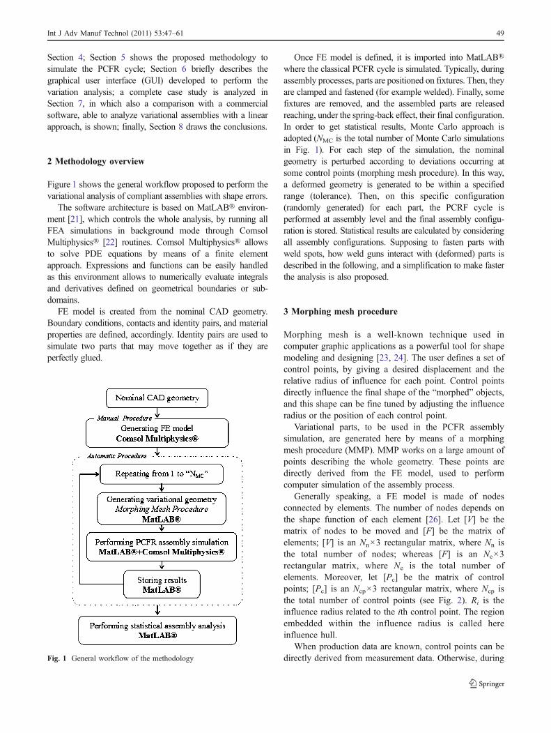
Figure 1 shows the general workflow proposed to perform thevariational analysis of compliant assemblies with shape errors.

The software architecture is based on MatLAB® environ-ment [21], which controls the whole analysis, by running allFEA simulations in background mode through ComsolMultiphysics® [22] routines. Comsol Multiphysics® allowsto solve PDE equations by means of a finite elementapproach. Expressions and functions can be easily handledas this environment allows to numerically evaluate integralsand derivatives defined on geometrical boundaries or sub-domains.

FE model is created from the nominal CAD geometry.Boundary conditions, contacts and identity pairs, and materialproperties are defined, accordingly. Identity pairs are used tosimulate two parts that may move together as if they areperfectly glued.

Once FE model is defined, it is imported into MatLAB®where the classical PCFR cycle is simulated. Typically, duringassembly processes, parts are positioned on fixtures. Then, theyare clamped and fastened (for example welded). Finally, somefixtures are removed, and the assembled parts are releasedreaching, under the spring-back effect, their final configuration.In order to get statistical results, Monte Carlo approach isadopted (NMC is the total number of Monte Carlo simulationsin Fig. 1). For each step of the simulation, the nominalgeometry is perturbed according to deviations occurring atsome control points (morphing mesh procedure). In this way,a deformed geometry is generated to be within a specifiedrange (tolerance). Then, on this specific configuration(randomly generated) for each part, the PCRF cycle isperformed at assembly level and the final assembly configu-ration is stored. Statistical results are calculated by consideringall assembly configurations. Supposing to fasten parts withweld spots, how weld guns interact with (deformed) parts isdescribed in the following, and a simplification to make fasterthe analysis is also proposed.

3 Morphing mesh procedure

Morphing mesh is a well-known technique used incomputer graphic applications as a powerful tool for shapemodeling and designing [23, 24]. The user defines a set ofcontrol points, by giving a desired displacement and therelative radius of influence for each point. Control pointsdirectly influence the final shape of the “morphed” objects,and this shape can be fine tuned by adjusting the influenceradius or the position of each control point.

Variational parts, to be used in the PCFR assemblysimulation, are generated here by means of a morphingmesh procedure (MMP). MMP works on a large amount ofpoints describing the whole geometry. These points aredirectly derived from the FE model, used to performcomputer simulation of the assembly process.

Generally speaking, a FE model is made of nodesconnected by elements. The number of nodes depends onthe shape function of each element [26]. Let [V] be thematrix of nodes to be moved and [F] be the matrix ofelements; [V] is an Nn×3 rectangular matrix, where Nn isthe total number of nodes; whereas [F] is an Ne×3rectangular matrix, where Ne is the total number ofelements. Moreover, let [Pc] be the matrix of controlpoints; [Pc] is an Ncp×3 rectangular matrix, where Ncp isthe total number of control points (see Fig. 2). Ri is theinfluence radius related to the ith control point. The regionembedded within the influence radius is called hereinfluence hull.

When production data are known, control points can bedirectly derived from measurement data. Otherwise, duringFig. 1 General workflow of the methodology

Int J Adv Manuf Technol (2011) 53:47–61 49

the early design stage, control points can be randomlygenerated by using a Monte Carlo simulation.

The displacement, ΔVj, of any mesh node Vj, iscalculated as a weighted mean of all control points [Pc],as stated in Eq. 1.

ΔVj;x ¼XNcp

i¼1Wi Vj

� � �Mi;x

ΔVj;y ¼XNcp

i¼1Wi Vj

� � �Mi;y

ΔVj;z ¼XNcp

i¼1Wi Vj

� � �Mi;z

8>>><>>>:

! ΔVj ¼ W Vj

� �� M½ � ð1Þ

where {W(Vj)} is the weighted (1×Ncp) row vector, and [M]is the morphing matrix (Ncp×3).

The ith weighted element depends on (I) position of thepoint Vj, (II) position of the control point Pci, and (III) itsinfluence radius Ri, as stated in Eq. 2. The influence radiusdefines the 3D region within which any node is influencedby the related control point.

Wi Vj

� � ¼ f Vj;Pci;Ri

� �; 8i ¼ 1; 2; ::;Ncp ð2Þ

f is the basic function and may be assumed as a piecewiseBezier curve or a B-spline-based function as proposed inRaffin et al. [27]. However, in this work, in order to easilyhandle this function, a third degree polynomial function isadopted. Equation 2 can then be re-written as:

Wi Vj

� � ¼ fVj � Pci

�� Ri

� �¼ f ðdÞ ¼ 1� 3 � d2 þ 2 � d3;8i ¼ 1; 2; ::;Ncp

ð3ÞRelation 3 states that function f is equal to 1 when Vj and

Pci are coincident and tends toward zero for points Vj whosedistance from Pci is greater than zero. To assure smoothingshape, function f has zero slopes at the two end points(Fig. 3). In Eq. 3, d is the a-dimensional distance frompoint Vj to control point Pci.

In order to evaluate morphing matrix [M], Eq. 1 isspecified with respect to all control points [Pc]. Then, onecan write:

ΔPc1 ¼ W Pc1ð Þf g � M½ �ΔPc2 ¼ W Pc2ð Þf g � M½ �:::ΔPcNcp ¼ W PcNcp

� �� M½ �

8>>>><>>>>:

! ΔPc½ � ¼ W Pcð Þ½ � � M½ � ð4Þ

where [ΔPc] is the Ncp×3 matrix of displacements relatedto control points, whereas [W(Pc)] is a square matrix of Ncp

order. Then, morphing matrix [M] can be calculated bysolving the following linear system:

M½ � ¼ W Pcð Þ½ ��1 � ΔPc½ � ð5Þ

It should be noted that matrix [W(Pc)] is singular only iftwo control points are coincident. When this happens, thesystem 5 has no unique solution and morphing matrix [M]is un-determined. To solve this issue, the linear system inEq. 5 may be solved with a least-squares approach in whichthe pseudo-inverse of the matrix [W(Pc)] is evaluated [25].Commercial routines are based on the singular valuedecomposition. In this paper, the MatLAB®’s backslash(\) operator is adopted.

Once morphing matrix [M] is known, displacements of anymesh node Vj can be calculated by applying relationship 1.

As it is, MMP allows to move nodes of the mesh takinginto account the displacement of a set of control points.However, no information is available for points belongingto mesh elements. To overcome this limitation, an interpo-lation approach is used. The interpolation function allowsto describe any point of the geometry starting from meshnodes (whose displacements are calculated by applyingEq. 1). The postinterp function, embedded in MatLAB® viaComsol Multiphysics®, is adopted here.

In order to get a more powerful control on thedeformation of the nominal geometry, different influencehulls can be adopted. If the radius of influence is constant,

Fig. 2 Definition of control points and relative influence hulls

Fig. 3 Definition of the basic function, f


the influence hull becomes a sphere. Instead, an ellipsoidcan be derived by defining three principal radii (definedalong the principal directions of the ellipsoid). Moregeneral influence hulls can be defined as proposed inRaffin et al. [27]. However, only spheres and ellipsoids areconsidered here since they offer a more intuitively control.

For a sphere hull, the a-dimensional distance, ds, isdefined as:

ds ¼ffiffiffiffiffiffiffiffiffiffiffiffiffiffiffiffiffiffiffiffiffiffiffiffiffiffiffiffiffiffiffiffiffiffiffiffiffiffiffiffiffiffiffiffiffiffiffiffiffiffiffiffiffiffiffiffiffiffiffiffiffiffiffiffiffiffiffiffiffiffiffiffiffiffiffiffiffiffiffiffiffiffiffiffiffiffiffiffiffiffiffiVj;x � Pci;x

� �2 þ Vj;y � Pci;y

� �2 þ Vj;z � Pci;z

� �2qRs

ð6Þwhereas for an ellipsoid hull, it becomes:

de ¼

ffiffiffiffiffiffiffiffiffiffiffiffiffiffiffiffiffiffiffiffiffiffiffiffiffiffiffiffiffiffiffiffiffiffiffiffiffiffiffiffiffiffiffiffiffiffiffiffiffiffiffiffiffiffiffiffiffiffiffiffiffiffiffiffiffiffiffiffiffiffiffiffiffiffiffiffiffiffiffiffiffiffiffiffiffiffiffiffiffiffiffiffiVj;x � Pci;x

� �2R2e;1

þ Vj;y � Pci;y

� �2R2e;2

þ Vj;z � Pci;z

� �2R2e;3

vuut ð7Þ

where Rs is the radius of the sphere, while Re,1, Re,2, andRe,3 are the principal radii of the ellipsoid.

Having assigned the above parameters, MMP may nowgenerate variational parts. The user has to set the position ofcontrol points, their influence radius and relative displace-ments, and the interpolation function.

ΔP ¼ G P;Pci;Rið Þ !Um ¼ G P;Pci;Rið ÞVm ¼ G P;Pci;Rið ÞWm ¼ G P;Pci;Rið Þ

8><>: ð8Þ

Then, with respect to the global coordinate frame (GCF),directly derived from the CAD model and here called (X0,Y0, Z0), any geometrical point P with (x, y, z) components istransformed by means of the MMP as in Eq. 8. G dependson both the basic and the interpolation function, whereas(Um, Vm, Wm) is the displacement of the point P withrespect to GCF. Below, a case study clarifies how theproposed procedure works.

4 Case study: morphing mesh

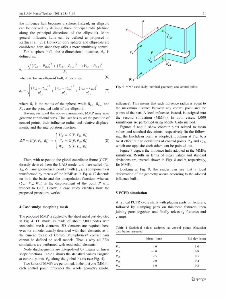
The proposed MMP is applied to the sheet metal part depictedin Fig. 4. FE model is made of about 3,000 nodes withtetrahedral mesh elements. 3D elements are required here,even for a model usually described with shell elements, as inthe current release of Comsol Multiphysics® contact pairscannot be defined on shell models. That is why all FEAsimulations are performed with tetrahedral elements.

Node displacements are interpolated by means of linearshape functions. Table 1 shows the statistical values assignedat control points, Pc, along the global Y axis (see Fig. 4).

Two kinds ofMMPs are performed. In the first one (MMPI),each control point influences the whole geometry (global

influence). This means that each influence radius is equal tothe maximum distance between any control point and thepoints of the part. A local influence, instead, is assigned intothe second simulation (MMPII). In both cases, 1,000simulations are performed using Monte Carlo method.

Figures 5 and 6 show contour plots related to meanvalues and standard deviations, respectively (in the follow-ing, the Euclidean norm is adopted). Looking at Fig. 6, atwist effect due to deviations of control points Pc1 and Pc2,which are opposite each other, can be pointed out.

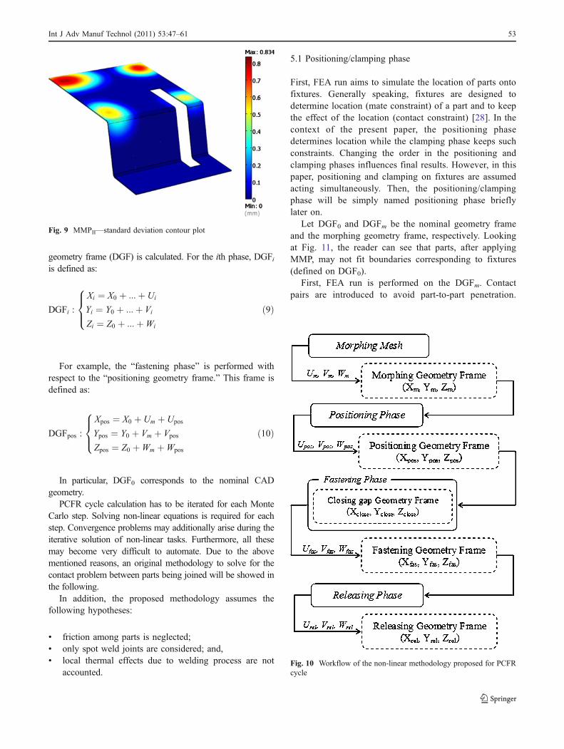
Figure 7 depicts the influence hulls adopted in the MMPIIsimulation. Results in terms of mean values and standarddeviations are, instead, shown in Figs. 8 and 9, respectively,for MMPII.

Looking at Fig. 8, the reader can see that a localdeformation of the geometry occurs according to the adoptedinfluence hulls.

5 PCFR simulation

A typical PCFR cycle starts with placing parts on fixture/s,followed by clamping parts on this/these fixture/s, thenjoining parts together, and finally releasing fixture/s andclamps.

Table 1 Statistical values assigned at control points (Gaussiandistribution assumed)

Mean (mm) Std dev (mm)

Pc1 4.0 1.0

Pc2 −3.0 0.8

Pc3 −2.5 0.5

Pc4 2.0 0.4

Pc5 1.0 0.2

Fig. 4 MMP case study: nominal geometry and control points


A critical aspect is related to the joining and thereleasing phases. In fact, fastening tools force matingsurfaces together at the joining area. Compliant parts tendto deform locally during these operations, and this changescontact conditions: Surfaces initially in contact may moveapart, producing gaps or interferences. Moreover, dependingon the joining method, multi-physics phenomena may occur inthe contact zones, such as material plastic deformation, thermo-structure interaction, thermo-electrical-structure interaction,and friction phenomena.

Over the years, linear approaches, mainly based on theevaluation of the Sensitivity Matrix to do linear PCFRsimulation, have been proposed. However, these methods donot consider the real behavior at the contact interface.

In the present work, a non-linear methodology aiming tonumerically simulate the whole PCFR cycle, taking intoaccount contact area among parts being assembled, isproposed. To do it, a FEM approach is adopted. Figure 10

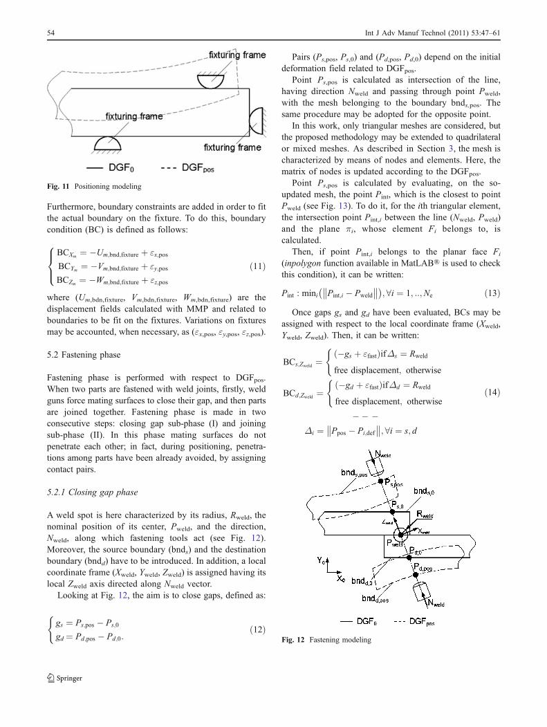
shows the general workflow used to perform the PCFRcycle.

Generally speaking, three consecutive FEA runs arerequired to perform the simulation. The first FEA run is relatedto the positioning and clamping phase (phase I), consideringinitial variational parts, derived from MMP. Fastening phase(phase II) is achieved into the second FEA simulation, takinginto account the deformed geometry derived from the first FEArun. Finally, the releasing phase (phase III) is resolved in thethird FEA run, by applying the residual stresses (initial stresses)calculated during the previous phases.

After the ith phase (i=I, II, III), the geometrical domain isupdated according to the displacement field, (Ui, Vi, Wi). Inthis way, an updated geometry frame, here called deformed

Fig. 8 MMPII—mean contour plot

Fig. 7 MMPII—influence hulls assigned at control points for the localinfluence of the geometry

Fig. 6 MMPI—standard deviation contour plot

Fig. 5 MMPI—mean contour plot


geometry frame (DGF) is calculated. For the ith phase, DGFiis defined as:

DGFi :

Xi ¼ X0 þ :::þ Ui

Yi ¼ Y0 þ :::þ Vi

Zi ¼ Z0 þ :::þWi

8><>: ð9Þ

For example, the “fastening phase” is performed withrespect to the “positioning geometry frame.” This frame isdefined as:

DGFpos :

Xpos ¼ X0 þ Um þ Upos

Ypos ¼ Y0 þ Vm þ Vpos

Zpos ¼ Z0 þWm þWpos

8><>: ð10Þ

In particular, DGF0 corresponds to the nominal CADgeometry.

PCFR cycle calculation has to be iterated for each MonteCarlo step. Solving non-linear equations is required for eachstep. Convergence problems may additionally arise during theiterative solution of non-linear tasks. Furthermore, all thesemay become very difficult to automate. Due to the abovementioned reasons, an original methodology to solve for thecontact problem between parts being joined will be showed inthe following.

In addition, the proposed methodology assumes thefollowing hypotheses:

& friction among parts is neglected;& only spot weld joints are considered; and,& local thermal effects due to welding process are not

accounted.

5.1 Positioning/clamping phase

First, FEA run aims to simulate the location of parts ontofixtures. Generally speaking, fixtures are designed todetermine location (mate constraint) of a part and to keepthe effect of the location (contact constraint) [28]. In thecontext of the present paper, the positioning phasedetermines location while the clamping phase keeps suchconstraints. Changing the order in the positioning andclamping phases influences final results. However, in thispaper, positioning and clamping on fixtures are assumedacting simultaneously. Then, the positioning/clampingphase will be simply named positioning phase brieflylater on.

Let DGF0 and DGFm be the nominal geometry frameand the morphing geometry frame, respectively. Lookingat Fig. 11, the reader can see that parts, after applyingMMP, may not fit boundaries corresponding to fixtures(defined on DGF0).

First, FEA run is performed on the DGFm. Contactpairs are introduced to avoid part-to-part penetration.

Fig. 10 Workflow of the non-linear methodology proposed for PCFRcycle

Fig. 9 MMPII—standard deviation contour plot


Furthermore, boundary constraints are added in order to fitthe actual boundary on the fixture. To do this, boundarycondition (BC) is defined as follows:

BCXm ¼ �Um;bnd;fixture þ "x;pos

BCYm ¼ �Vm;bnd;fixture þ "y;pos

BCZm ¼ �Wm;bnd;fixture þ "z;pos

8><>: ð11Þ

where (Um,bdn,fixture, Vm,bdn,fixture, Wm,bdn,fixture) are thedisplacement fields calculated with MMP and related toboundaries to be fit on the fixtures. Variations on fixturesmay be accounted, when necessary, as (εx,pos, εy,pos, εz,pos).

5.2 Fastening phase

Fastening phase is performed with respect to DGFpos.When two parts are fastened with weld joints, firstly, weldguns force mating surfaces to close their gap, and then partsare joined together. Fastening phase is made in twoconsecutive steps: closing gap sub-phase (I) and joiningsub-phase (II). In this phase mating surfaces do notpenetrate each other; in fact, during positioning, penetra-tions among parts have been already avoided, by assigningcontact pairs.

5.2.1 Closing gap phase

A weld spot is here characterized by its radius, Rweld, thenominal position of its center, Pweld, and the direction,Nweld, along which fastening tools act (see Fig. 12).Moreover, the source boundary (bnds) and the destinationboundary (bndd) have to be introduced. In addition, a localcoordinate frame (Xweld, Yweld, Zweld) is assigned having itslocal Zweld axis directed along Nweld vector.

Looking at Fig. 12, the aim is to close gaps, defined as:

gs ¼ Ps;pos � Ps;0

gd ¼ Pd;pos � Pd;0:

(ð12Þ

Pairs (Ps,pos, Ps,0) and (Pd,pos, Pd,0) depend on the initialdeformation field related to DGFpos.

Point Ps,pos is calculated as intersection of the line,having direction Nweld and passing through point Pweld,with the mesh belonging to the boundary bnds,pos. Thesame procedure may be adopted for the opposite point.

In this work, only triangular meshes are considered, butthe proposed methodology may be extended to quadrilateralor mixed meshes. As described in Section 3, the mesh ischaracterized by means of nodes and elements. Here, thematrix of nodes is updated according to the DGFpos.

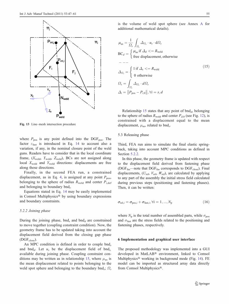
Point Ps,pos is calculated by evaluating, on the so-updated mesh, the point Pint, which is the closest to pointPweld (see Fig. 13). To do it, for the ith triangular element,the intersection point Pint,i between the line (Nweld, Pweld)and the plane πi, whose element Fi belongs to, iscalculated.

Then, if point Pint,i belongs to the planar face Fi

(inpolygon function available in MatLAB® is used to checkthis condition), it can be written:

Pint : mini Pint;i � Pweld

�� ; 8i ¼ 1; ::;Ne ð13Þ

Once gaps gs and gd have been evaluated, BCs may beassigned with respect to the local coordinate frame (Xweld,Yweld, Zweld). Then, it can be written:

BCs;Zweld ¼�gs þ "fastð ÞifΔs ¼ Rweld

free displacement; otherwise

(

BCd;Zweld ¼�gd þ "fastð ÞifΔd ¼ Rweld


(

�� Δi ¼ Ppos � Pi;def

�� ; 8i ¼ s; d

ð14Þ

Fig. 12 Fastening modeling

Fig. 11 Positioning modeling


where Ppos is any point defined into the DGFpos. Thefactor εfast is introduced in Eq. 14 to account also avariation, if any, in the nominal closure point of the weldguns. Readers have to consider that in the local coordinateframe, (Xweld, Yweld, Zweld), BCs are not assigned alonglocal Xweld and Yweld directions: displacements are freealong those directions.

Finally, in the second FEA run, a constraineddisplacement, as in Eq. 4, is assigned at any point Ppos,belonging to the sphere of radius Rweld and center Pi,def

and belonging to boundary bndi.Equations stated in Eq. 14 may be easily implemented

in Comsol Multiphysics® by using boundary expressionsand boundary constraints.

5.2.2 Joining phase

During the joining phase, bnds and bndd are constrainedto move together (coupling constraint condition). Now, thegeometry frame has to be updated taking into account thedisplacement field derived from the closing gap phase(DGFclose).

An MPC condition is defined in order to couple bndsand bndd. Let us be the displacement field of bnds,available during joining phase. Coupling constraint con-ditions may be written as in relationship 15, where μus isthe mean displacement related to points belonging to theweld spot sphere and belonging to the boundary bnds; Ωs

is the volume of weld spot sphere (see Annex A foradditional mathematical details).

mus ¼1

Ωs

ZΩs

ΔΩs � us � dΩs

BCd ¼mus if Δd <¼ Rweld


� ��

ΔΩs ¼1 if Δs <¼ Rweld

0 otherwise

(

Ωs ¼ZΩs

ΔΩs � dΩs

Δi ¼ Ppos � Pi;0

�� ; 8i ¼ s; d

ð15Þ

Relationship 15 states that any point of bndd, belongingto the sphere of radius Rweld and center Pd,0 (see Fig. 12), isconstrained with a displacement equal to the meandisplacement, μus, related to bnds.

5.3 Releasing phase

Third, FEA run aims to simulate the final elastic spring-back, taking into account MPC conditions as defined inSection 5.2.2.

In this phase, the geometry frame is updated with respectto the displacement field derived from fastening phase(DGFfas—note that DGFfas corresponds to DGFclose). Finaldisplacements, (Urel, Vrel, Wrel), are calculated by applyingto any part of the assembly the initial stress field calculatedduring previous steps (positioning and fastening phases).Then, it can be written:

srel;i ¼ spos;i þ sfast;i; 8i ¼ 1; :::;Np ð16Þ

where Np is the total number of assembled parts, while σposand σfast are the stress fields related to the positioning andfastening phases, respectively.

6 Implementation and graphical user interface

The proposed methodology was implemented into a GUIdeveloped in MatLAB® environment, linked to ComsolMultiphysics® working in background mode (Fig. 14). FEmodel can be imported as structured array data directlyfrom Comsol Multiphysics®.

Fig. 13 Line–mesh intersection procedure


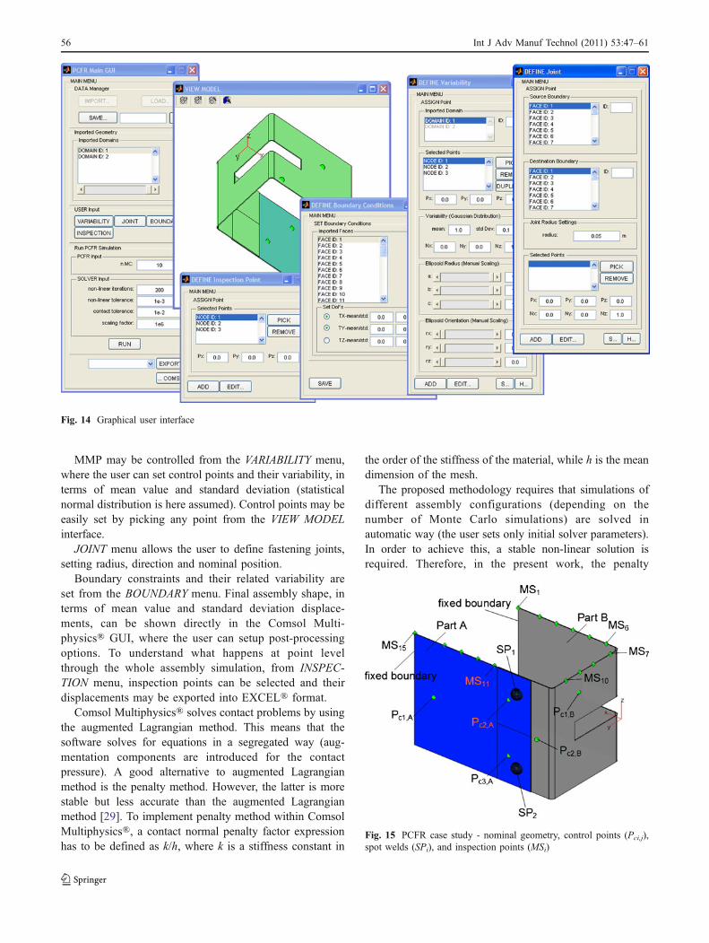
MMP may be controlled from the VARIABILITY menu,where the user can set control points and their variability, interms of mean value and standard deviation (statisticalnormal distribution is here assumed). Control points may beeasily set by picking any point from the VIEW MODELinterface.

JOINT menu allows the user to define fastening joints,setting radius, direction and nominal position.

Boundary constraints and their related variability areset from the BOUNDARY menu. Final assembly shape, interms of mean value and standard deviation displace-ments, can be shown directly in the Comsol Multi-physics® GUI, where the user can setup post-processingoptions. To understand what happens at point levelthrough the whole assembly simulation, from INSPEC-TION menu, inspection points can be selected and theirdisplacements may be exported into EXCEL® format.

Comsol Multiphysics® solves contact problems by usingthe augmented Lagrangian method. This means that thesoftware solves for equations in a segregated way (aug-mentation components are introduced for the contactpressure). A good alternative to augmented Lagrangianmethod is the penalty method. However, the latter is morestable but less accurate than the augmented Lagrangianmethod [29]. To implement penalty method within ComsolMultiphysics®, a contact normal penalty factor expressionhas to be defined as k/h, where k is a stiffness constant in

the order of the stiffness of the material, while h is the meandimension of the mesh.

The proposed methodology requires that simulations ofdifferent assembly configurations (depending on thenumber of Monte Carlo simulations) are solved inautomatic way (the user sets only initial solver parameters).In order to achieve this, a stable non-linear solution isrequired. Therefore, in the present work, the penalty

Fig. 14 Graphical user interface

Fig. 15 PCFR case study - nominal geometry, control points (Pci,j),spot welds (SPi), and inspection points (MSi)


method is adopted, despite that it is generally less accuratethan augmented Lagrangian method.

7 Case study: PCFR cycle

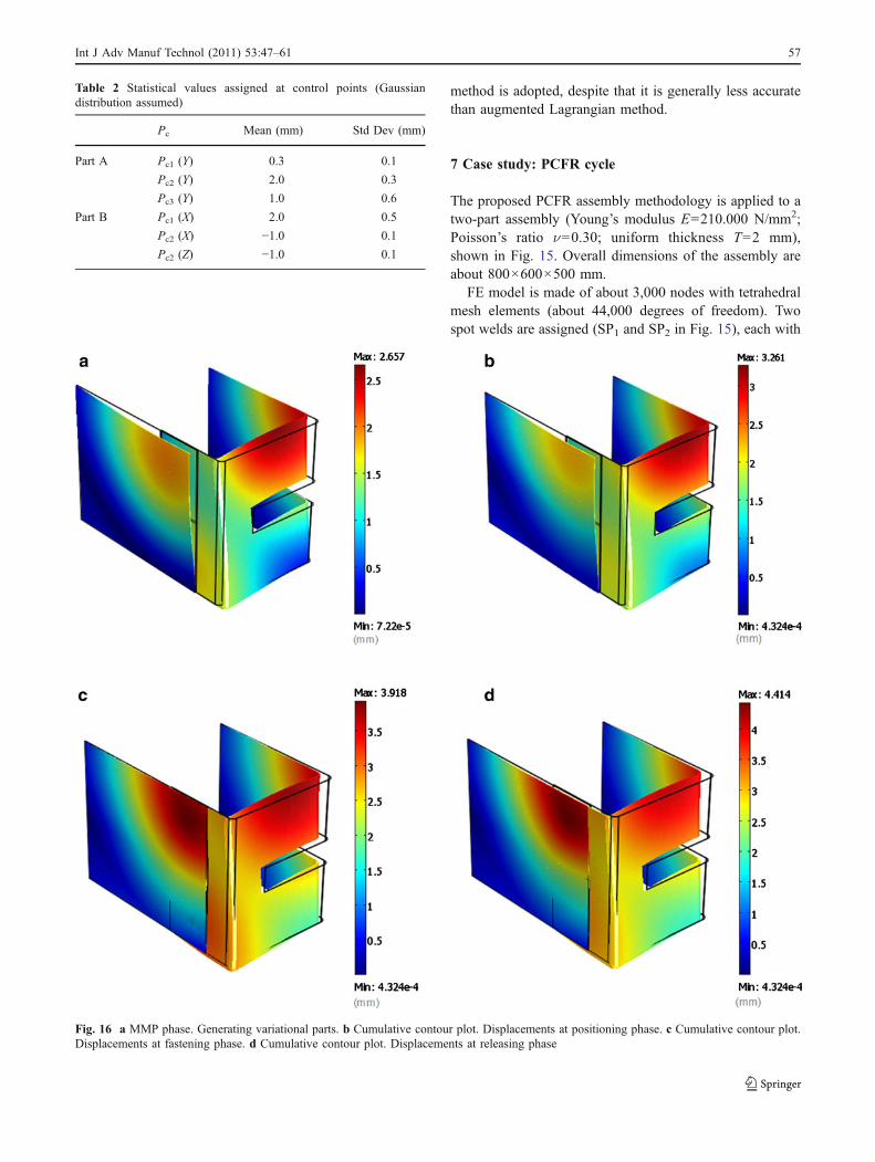
The proposed PCFR assembly methodology is applied to atwo-part assembly (Young’s modulus E=210.000 N/mm2;Poisson’s ratio ν=0.30; uniform thickness T=2 mm),shown in Fig. 15. Overall dimensions of the assembly areabout 800×600×500 mm.

FE model is made of about 3,000 nodes with tetrahedralmesh elements (about 44,000 degrees of freedom). Twospot welds are assigned (SP1 and SP2 in Fig. 15), each with

Table 2 Statistical values assigned at control points (Gaussiandistribution assumed)

Pc Mean (mm) Std Dev (mm)

Part A Pc1 (Y) 0.3 0.1

Pc2 (Y) 2.0 0.3

Pc3 (Y) 1.0 0.6

Part B Pc1 (X) 2.0 0.5

Pc2 (X) −1.0 0.1

Pc2 (Z) −1.0 0.1

Fig. 16 a MMP phase. Generating variational parts. b Cumulative contour plot. Displacements at positioning phase. c Cumulative contour plot.Displacements at fastening phase. d Cumulative contour plot. Displacements at releasing phase


a radius of 20 mm. A fixed fixture is assigned for both parts(“fixed boundary” in Fig. 15). Contact pairs are defined atboundary interface between “part A” and “part B.”Moreover, linear shape functions are adopted to interpolatenode displacements.

Table 2 shows the statistical values assigned at controlpoints. Five hundred Monte Carlo simulations wereperformed in less than 2 h on a notebook with Core Duo1.83 GHz, 2 GB RAM, Win XP 32 bit. Figure 16 depictsmean contour plots for each phase of the PCFR cycle. Theinitial gap existing between part A and part B getsclosed in the fastening phase.

To understand what happens when contact pairs are notassigned, a new simulation is performed (run-time about20 min). Results are shown into Fig. 17a, b with respect toinspection points (MS in Fig. 15), in terms of mean andstandard deviations, respectively.

In order to quantify the difference between the simu-lations with and without contact pairs, root sum square(RSS) index is calculated. Results are shown in Table 3.RSS index is quite low for MMP and positioning phases

(when the number of Monte Carlo simulations increases,RSS index toward zero is expected).

Moreover, RSS index becomes higher for fastening andreleasing phases. This is due to the high influence that contactpairs assume both in the closing gap phase and in the finalreleasing phase.

The above results are related to the non-linear approachdescribed in the present paper. In the following, a comparison ismade with the linear approach behind the commercial TAAmodule integrated into CATIA® CAD system, which imple-ments the model described in Sellem et al. [2], mainly based onthe sensitivity matrix. The case study depicted into Fig. 15 is

Fig. 17 a Mean deviations atinspection points. b Standarddeviations at inspection points

Table 3 Contact pair vs no-contact pair—RSS indices

Phase RSS (mean) RSS (std dev)

MMP 0.1460 0.0619

Positioning 0.1232 0.0819

Fastening 0.2445 0.1091

Releasing 0.2844 0.1132


analyzed in TAA environment, where contact points are alsoactivated. Here, one should note that TAA allows creatingshell mesh elements, whereas the proposed method, asdescribed in Section 4, works only with 3D (tetrahedral)mesh elements for the limitations within Comsol Multiphysicson applying contacts on shell elements.

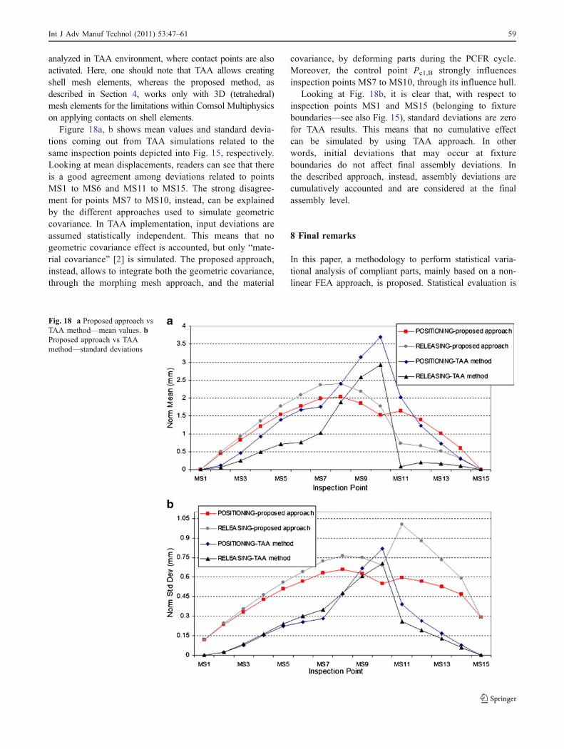
Figure 18a, b shows mean values and standard devia-tions coming out from TAA simulations related to thesame inspection points depicted into Fig. 15, respectively.Looking at mean displacements, readers can see that thereis a good agreement among deviations related to pointsMS1 to MS6 and MS11 to MS15. The strong disagree-ment for points MS7 to MS10, instead, can be explainedby the different approaches used to simulate geometriccovariance. In TAA implementation, input deviations areassumed statistically independent. This means that nogeometric covariance effect is accounted, but only “mate-rial covariance” [2] is simulated. The proposed approach,instead, allows to integrate both the geometric covariance,through the morphing mesh approach, and the material

covariance, by deforming parts during the PCFR cycle.Moreover, the control point Pc1,B strongly influencesinspection points MS7 to MS10, through its influence hull.

Looking at Fig. 18b, it is clear that, with respect toinspection points MS1 and MS15 (belonging to fixtureboundaries—see also Fig. 15), standard deviations are zerofor TAA results. This means that no cumulative effectcan be simulated by using TAA approach. In otherwords, initial deviations that may occur at fixtureboundaries do not affect final assembly deviations. Inthe described approach, instead, assembly deviations arecumulatively accounted and are considered at the finalassembly level.

8 Final remarks

In this paper, a methodology to perform statistical varia-tional analysis of compliant parts, mainly based on a non-linear FEA approach, is proposed. Statistical evaluation is

Fig. 18 a Proposed approach vsTAA method—mean values. bProposed approach vs TAAmethod—standard deviations


performed via Monte Carlo simulations to generate varia-tional parts to be assembled and then released.

The variational shape of parts being assembled isgenerated by using a morphing mesh-based approachborrowed by Computer Graphics. The user can manageand control the input shape by handling a small set ofcontrol points, assigning their position, the influence radius,and the relative displacement. In this way, no measurementdata are directly necessary to perform a preliminaryassembly simulation during the early design stage.

Variational parts are, then, assembled following theclassical PCFR cycle. The geometry domain is updated foreach step of the PCFR cycle. The attention is focused on weldspot joints: how to simulate weld guns clamping parts isdescribed. To improve the solution convergence, an efficientmethod, aiming to simulate fastening and releasing phases, isproposed. To do it, scalar and integral expressions, defined atboundary level, are defined and implemented.

The proposed methodology was implemented into afriendly MatLAB®’s GUI, linked to Comsol Multiphysics®into background mode. The GUI drives user loading theinitial FE model, assigning the input parameters, runningMonte Carlo simulations, and finally, exporting output data.

The proposed morphing mesh-based procedure is applied toa single sheet metal part, highlighting how, by managingcontrol points and their influence hulls, different shape can begenerated.

Finally, a two-part assembly is simulated. Results pointout that contacts may influence final assembly variations.Contacts allow to reach more realistic results but, on theother hand, a very time-consuming simulation is required ina contest of Monte Carlo simulations where hundreds ofFEA calculations are usually run. Selecting the rightbalance between simulation time and goodness of numericalresults is not a trivial task. Solving this issue requires moreinvestigation. Furthermore, a comparative analysis is per-formed with the commercial TAA module, integrated intoCATIA® CAD system, based on a linear approach. Theanalysis points out that TAA does not allow to manage“cumulative” effects when initial deviations are assigned atfixture boundaries, and no geometric covariance can beintroduced. In the present approach, instead, deviations areaccounted during the whole assembly process. Moreover,geometric covariance can be introduced through the morphingmesh-based model. More attention should be addressed also todifferent fastening joints, such as rivets and bolts, and to multi-station assembly processes.

ANNEX A: Integral definition on a boundary

Let Ω be a domain. The aim is to define an integral on asub-domain, Ωs. Supposing Ωs is a spherical sub-domain,

and P a point belonging to Ω, the following condition issatisfied:

ffiffiffiffiffiffiffiffiffiffiffiffiffiffiffiffiffiffiffiffiffiffiffiffiffiffiffiffiffiffiffiffiffiffiffiffiffiffiffiffiffiffiffiffiffiffiffiffiffiffiffiffiffiffiffiffiffiffiffiffiffiffiffix� x0ð Þ2þ y� y0ð Þ2 þ z� z0ð Þ2

q� R ! P � P0k k � R 8P 2 Ω

ð17Þwhere P0 and R are the center and the radius of the sphere,respectively. A step-wise function, ΔΩs , may be defined toaccount all points belonging to domain Ωs. Then, it has:

ΔΩs ¼1 if P � P0k k � R

0 otherwise

(ð18Þ

Now, let l be a physical variable defined into the domainΩ, aiming to be integrated on the sub-domain Ωs, one canwrite:

lint ¼ZΩΔΩs � l � dΩ ð19Þ

Taking in account Eq. 18, lint becomes (where Ωm=Ω−Ωs):

lint ¼ZΩs

ΔΩs � l � dΩs þZΩm

ΔΩs � l � dΩm ¼ZΩs

ΔΩs � l � dΩs ð20Þ

The main value of the physical variable l may beachieved by applying the definition of mean for acontinuous function. Finally, one can write:

lm ¼ 1

Ωs

ZΩs

ΔΩs � l � dΩs ð21Þ

References

1. Liu CS, Hu JS (1997) Variation simulation for deformable sheetmetal assemblies using finite element methods. ASME J ManufSci Eng 119(3):368–374

2. Sellem E, Rivière A (1998) Tolerance Analysis of DeformableAssemblies, Proc. of DETC98, ASME Design EngineeringTechnical Conference, Atlanta, GA. (Paper Number: DETC98-DAC5571)

3. Camelio J, Hu SJ, Ceglarek D (2003) Modeling variationpropagation in multi-station assembly systems with compliantparts. ASME J Mech Des 125(4):673–681

4. Camelio J, Hu SJ, Marin SP (2004) Compliant assembly variationanalysis using component geometric covariance. ASME J ManufSci Eng 126(2):355–360

5. Liao X, Wang GG (2007) Non-linear dimensional variationanalysis for sheet metal assemblies by contact modeling. FiniteElem Anal Des 44:34–44

6. Xie K, Wells L, Camelio JA, Youn BD (2007) Variationpropagation analysis on compliant assemblies considering contactinteraction. ASME J Manuf Sci Eng 129(5):934–942

7. Dahlström S, Lindkvist L (2007) Variation simulation of sheetmetal assemblies using the method of influence coefficients withcontact modelling. ASME J Manuf Sci Eng 129(3):615–622


8. Ungemach G, Mantwill F (2009) Efficient consideration ofcontact in compliant assembly variation analysis. ASME J ManufSci Eng 131(1):1–9

9. Gerbino S, Patalano S, Franciosa P (2008) Statistical variationanalysis of multi-station compliant assemblies based on sensitivitymatrix, J. Comput Appl Technol 33(1):12–23

10. Franciosa P, Gerbino S, Patalano S (2010) Variation analysis ofcompliant assemblies: a comparative study of a multi-stationassembly. Anales de Ingenieria Grafica 21:45–52 (in print)

11. HuM, Lin Z, Lai X, Ni J (2001) Simulation and analysis of assemblyprocesses considering compliant, non-ideal parts and tooling varia-tions. J of Machine Tools and Manufacture 41:2233–2243

12. Sellem E, Riviére A, Hillerin CAD, Clement A (1999) Validationof the Tolerance Analysis of Compliant Assemblies, ASMEDesign Engineering Technical Conference, Las Vegas, Nevada,Sept. 12–15

13. Sellem E, Sellakh R, Riviére A (2001) Testing of ToleranceAnalysis Module for Industrial Interest, 7th CIRP CAT Seminar,ENS de Cachan, France, April 24–25

14. Merkley K (1998) Tolerance analysis of complaint assemblies. Ph.D. Dissertation, Brigham Young University, Utah

15. Bihlmaier BF (1999) Tolerance analysis of flexible assembliesusing finite element and spectral analysis. M.S. Thesis, BrighamYoung University, Utah

16. Tonks M (2002) A robust geometric covariance method forflexible assembly tolerance analysis. M.S. Thesis, Brigham YoungUniversity, Utah

17. Huang W, Ceglarek D (2002) Decomposition mode-based offshare form error by discrete cosine transformation with imple-

mentation to assembly and stamping systems with compliantshares. Annals of CIRP 51:21–26

18. Samper S, Formosa F (2007) Form defect tolerancing by naturalmodes analysis. ASME J Comput Inf Sci Eng 7(4):44–51

19. Huang W, Kong Z (2009) Simulation and integration of geometricand rigid body kinematics errors for assembly variation analysis. Jof Manufacturing Systems 27:36–44

20. Chang M, Gossard DC (1997) Modeling the assembly ofcompliant, non-ideal parts. Comput-Aided Des 29(10):701–708

21. MatLab® (2009) User’s manual. University of Waterloo, Math-works

22. Comsol Multiphysics® (2009) User’s manual. COMSOL AB23. Borrel P, Rappoport A (1994) Simple constrained deformations

for geometric modelling and interactive design. ACM TransGraph 13:137–155

24. Raffin R, Neveu M, Jaar F (2000) Curvilinear displacement offree-form-based deformation. Vis Comput 16:38–46

25. Strang G (2009) An introduction to linear algebra, 4th edn.Wellesley Cambridge Press, Wellesley. ISBN 978-09802327–14

26. Zienkiewicz OC, Taylor RL, Zhu JZ (2005) The finite elementmethod, its basis and fundamentals, 6th edn. Elsevier, Amsterdam

27. Raffin R, Neveu M, Derdouri B (1998) Constrained Deformationfor Geometric Modelling and Object Reconstruction, Proc. WinterSchool Computer Graphics, pp. 299–306

28. Whitney DE (2004) Mechanical assemblies: their design, manu-facture, and role in product develpoment. Oxford UniversityPress, New York

29. Wriggers P (2002) Computational contact mechanics. Wiley, NewYork


Simulation of variational compliant assemblies with shape errors based on morphing mesh approach

Documents

Transcript of Simulation of variational compliant assemblies with shape errors based on morphing mesh approach