Neural Networks to Approach PotentialEnergy Surfaces: Application to aMolecular Dynamics Simulation

DIOGO A. R. S. LATINO,1,2 FILOMENA F. M. FREITAS,1

JOAO AIRES-DE-SOUSA,2 FERNANDO M. S. SILVA FERNANDES1

1Grupo de Simulacao Molecular, CCMM, Departamento de Quımica e Bioquımica, Faculdade deCiencias, Universidade de Lisboa, Campo Grande, 1749–016 Lisboa, Portugal2REQUIMTE, CQFB, Departamento de Quımica, Faculdade de Ciencias e Tecnologia, UniversidadeNova de Lisboa, 2829–516 Caparica, Portugal

Received 16 October 2006; accepted 8 January 2007Published online 7 May 2007 in Wiley InterScience (www.interscience.wiley.com).DOI 10.1002/qua.21398

ABSTRACT: Potential energy surfaces (PES) are crucial to the study of reactive andnonreactive chemical systems by Monte Carlo (MC) or molecular dynamics (MD)simulations. Ideally, PES should have the accuracy provided by ab initio calculationsand be set up as fast as possible. Recently, neural networks (NNs) turned out as asuitable approach for estimating PES from ab initio/DFT energy datasets. However, theaccuracy of the properties determined by MC and MD simulation methods from NNssurfaces has not yet, to our knowledge, been systematically analyzed in terms of theminimum number of energy points required for training and the usage of different NN-types. The goal of this work is to train NNs for reproducing PES represented by well-known analytical potential functions, and then to assess the accuracy of the method bycomparing the simulation results obtained from NNs and analytical PES. Ensembles offeed-forward neural networks (EnsFFNNs) and associative neural networks (ASNNs)are used to estimate the full energy surface. Training sets with different number ofpoints, from 15 differently parameterized Lennard–Jones (LJ) potentials, are used andargon is taken to test the network. MD simulations have been performed using thetabular potential energies, predicted by NNs, for working out thermal, structural, anddynamic properties which are compared with the values obtained from the analyticalfunction.

Correspondence to: F. M. S. S. Fernandes; e-mail: fsilva@fc.ul.ptContract grant sponsor: Fundacao para a Ciencia e Tecnolo,

gia, Portugal.Contract grant number: SFRH/BD/18347.

International Journal of Quantum Chemistry, Vol 107, 2120–2132 (2007)© 2007 Wiley Periodicals, Inc.

Our results show that, at least for LJ-type potentials, NNs can be trained to generateaccurate PES to be used in molecular simulations. © 2007 Wiley Periodicals, Inc. Int JQuantum Chem 107: 2120–2132, 2007

Key words: associative neural networks; ensembles of feed-forward neural networks;potential energy surfaces; molecular dynamics simulations; fitting

Introduction

F itting potential energy surfaces (PES), from abinitio/DFT data, is of high interest in molec-

ular simulations. Monte Carlo (MC) and moleculardynamics (MD) results depend directly on thegiven PES. If on one hand the use of empiricalfunctions to approach PES has theoretical and pro-gramming advantages, on the other hand it has thedisadvantage of being generally less accurate than afull PES obtained by quantum mechanical methods.Ideally, for molecular simulations, a PES shouldhave the accuracy provided by first principles cal-culations and be set up as fast as possible.

One of the approaches to obtain PES for complexsystems is the calculation by ab initio/DFT meth-ods of the potential energies for a set of suitableconfigurations of the system, followed by a fittingto an analytical function. The most common meth-ods use power series in an appropriate coordinatesystem, local functions such as splines and semi-empirical potentials with adjustable parameters toreproduce experimental and theoretical results. TheLondon-Eyring-Polanyi-Sato (LEPS) function to fitab initio data [1, 2] is one example of this strategy.These methodologies, however, have some disad-vantages. They are not able, in general, to repro-duce the most subtle features of PES for complexsystems from a limited number of energy points.

A recent method that does not require the pre-vious knowledge of the analytical form is the cor-rugation reducing procedure [3]. It consists of twoparts: the decomposition of the total molecule sur-face interaction into two contributions (one partstrongly corrugated and the other weakly corru-gated); and the interpolation, separately, of the twocontributions using cubic splines and symmetryadapted functions. This method was used success-fully to study diatomic molecules reacting on metalsurfaces. Despite the good results, it is difficult toextend the method to problems with more than sixdegrees of freedom.

Another method that also does not require theknowledge of a priori analytical forms is the mod-ified Shepard interpolation [4–9]. Basically, it uses

classical trajectory simulations to provide an itera-tive scheme for improving the PES. The surface isthen given by interpolation of local Taylor expan-sions and an iterative procedure places new pointsonly in regions of the configuration space that areimportant for dynamics. This method was used ingas phase reactions [4–6] and a modified one in gassurface reactions [7–9].

A recent strategy to approach PES with similaror better results than the referred methods is theapplication of neural networks (NNs) [10–19].

No et al [10] used a Feed-Forward Neural Net-work (FFNN) to fit a PES for water dimer using astraining points energy values obtained by ab initiomethods. Gassner et al. [11] applied FFNNs to re-produce the three-body interaction energy in thesystem H2OOAl3�OH2O, and compared the radialdistribution function obtained by MC simulationsusing an analytical potential and the PES generatedby FFNNs. The authors showed that an FFNN canbe used to reproduce the dimer energies in thewhole conformational space.

Prudente and Neto [12] also used an FFNN to fitPES and the transition dipole moment of the HCl�

ion using electronic energies calculated by ab initiomethods. The PES obtained by NN was used in thestudy of the photodissociation process. The workshows that for multi-dimensional surfaces the re-sults of FFNNs can be better than those of splines.A similar work was done by Bittencourt et al [13]for the OH� ion also from ab initio data. In this, theproperties evaluated and used to test the accuracyof the NNs fittings were the vibration levels and thetransition probabilities between the A2�� and X2�electronic states.

Cho et al. [14] used an NN to build a polarizableforce field for water. The PES implemented is acombination of an empirical potential (the TIP4Pmodel was used in this part) and a nonempiricalpotential (a FFNN was used to reproduce the manybody interaction energy surface from ab initio cal-culations). The new force field was used in MCsimulations and some structural and thermody-namic properties were compared with experimen-tal data showing that FFNNs could be used in the

NEURAL NETWORKS TO APPROACH POTENTIAL ENERGY SURFACES

VOL. 107, NO. 11 DOI 10.1002/qua INTERNATIONAL JOURNAL OF QUANTUM CHEMISTRY 2121

development of a force field to treat many-bodyinteractions. In the same way, but with differentgoals, Rocha Filho et al. [15] used NNs to fit abinitio data of the H3� to study the ground state PES.

The investigation of reactions in surfaces wasalso performed using NNs. For example, Lorenz etal. [16] applied this method to build continuous PESfor the H2 interacting with the (2 � 2) potassiumcovered Pd (100) surface system and more recently[17] the same authors applied NNs to fit six dimen-sional PES for H2 dissociation on the clean andsulfur covered Pd (100) surfaces. The obtainedmodels were used to describe reaction rates for thedissociative adsorption in those systems and showthat a description of dissociation reactions withNNs are orders of magnitude smaller than those of“on the fly” ab initio dynamics (103–104 against 107

ab initio energy points).Witkoskie and Doren [20] have applied NNs to

represent PES of some prototypical examples ofone, two and three dimensions. The authors try toachieve the optimal number of neurons, the NNconfiguration and the number of data needed to fiteach one of these simple cases.

Toth et al. [21], instead of using energy pointsobtained from ab initio calculations, took diffrac-tion data on liquids to obtain the pair potentials.NNs were then trained with known pair interac-tion-simulated structure factor pairs of one compo-nent systems.

Although NNs are a suitable approach for esti-mating PES from ab initio/DFT energy datasets, theaccuracy of the properties determined by MC andMD simulation methods from NNs generated PEShas not yet, to our knowledge, been systematicallyanalyzed in terms of the minimum number of en-ergy points required for training different NN-types.

The main goal of this work is to train NNs forreproducing PES represented by well-known ana-lytical potential functions, and then to assess theaccuracy of the method by comparing the simula-tion results obtained from NNs and analytical PES.Ensembles of feed-forward neural networks (Ens-FFNNs) [22, 23] and associative neural networks(ASNNs) [24, 25] were the machine learning meth-ods used to estimate the full energy surface. Differ-ently from other authors, we use these methodsinstead of single Feed-Forward Neural Networks(FFNNs). In other problems of modeling and fit-ting, the advantages and greater generalizationability of these two methods over single FFNN havebeen demonstrated. Although the two methods are

supervised learning techniques, the EnsFFNNs is amemory-less method (after the training all informa-tion about the input patterns are stored in the NNweights but there is no explicit storage of the datain the system) while the ASNNs is a combination ofmemory-less and memory-based methods (the dataused to build the models are also stored in a “mem-ory” and the predictions are corrected based onsome local approximations of the stored examples).The advantages of these two methods over the com-mon FFNNs will be demonstrated in this work.

Training sets with different number of points,from 15 differently parameterized Lennard–Jones(LJ) potentials, are used and argon is taken to testthe NNs. MD simulations are performed using thetabular potential energies, predicted by NNs, forworking out thermal, structural and dynamic prop-erties which are then compared with the valuesobtained from the LJ analytical function.

Advantageously, NNs do not require an analyt-ical function on which the model should be built,i.e. neither the functional type (polynomial, expo-nential, logarithmic, etc) nor the number and posi-tion of the parameters in the model function need tobe given.

An important question is whether or not themapping provided by NNs can be more accuratethan other approximation schemes based on inter-polation or spline techniques. That depends, ofcourse, on the complexity of the PES and the num-ber of single energy points obtained for a givensystem. The present article does not address suchquestion, since our calculations are based on a sim-ple analytical potential function from which an ar-bitrary number of energy points can always beworked out. As far as molecular simulations areconcerned when a new method or theory is pro-posed the usual way is to test it with LJ PES, fromwhich a huge amount of physical properties hasbeen calculated along the past years. If the testresults are accurate enough then one can proceedtowards more complex and multi-dimensional PES.This is just the spirit of the present work.

Methodology and ComputationalDetails

The experiments here described involve threemain steps. In the first, six training sets with differ-ent numbers of energy points were generated for 15differently parameterized LJ potentials:

LATINO ET AL.

2122 INTERNATIONAL JOURNAL OF QUANTUM CHEMISTRY DOI 10.1002/qua VOL. 107, NO. 11

u�r� � 4����

r �12

� ��

r �6� (1)

where � is the depth of the potential well, � isapproximately the molecular diameter, and r is thedistance between particles.

For each of these training sets, a test set wasgenerated with the parameters for argon (argonpoints were not used in the training set). The Ens-FFNNs and ASNNs are the machine learning meth-ods used to set up the relation between the input(parameters �, � and the distance between particles,r) and the output (potential energy). In the secondstep, the NN-generated PES of argon, in tabularform, was used in MD simulations. The thermal,structural, and dynamic properties evaluated forthe system were compared with the ones obtainedfrom the analytical PES for argon. To work out thedynamics of the system from the tables predictedby NNs it is necessary to perform interpolations,which introduce some errors. As such, the dynam-ics based on the analytical potential has also beencalculated from tables directly constructed from theanalytical potential for the same number of points.In this way, when the results from the two calcula-tions are compared, the errors due to the interpo-lations are practically eliminated. In the third stepexperiments were performed to assess the ability ofan ASNN trained with a small number of points toimprove the generated PES by using different mem-ories with more points, or by retraining with morepoints. Also, the interpolation ability of the NNwith a different set of descriptors and different setsof curves in the training set was analyzed.

DATASET OF PES GENERATED BY LJPOTENTIAL TO TRAIN AND TEST NN

The two methods used to learn the relationshipbetween the LJ parameters and the potential energyare supervised learning methods. Therefore theyneed a set of pairs to learn: the inputs and thetargets. In our case we have three inputs: the depthof the potential well, �, the distance at which thepotential is equal to 0, �, and the distance betweenparticles, r.

The output is the potential energy, u (r). The LJparameters used for 16 substances [26, 27] are listedin Table I.

Six independent training sets, with differentnumber of energy points, were generated with theanalytical expression for the 15 PES. The PES used

to train and test the models were generated be-tween 0.5 � � and 2.5 � � with different intervalsfor the five training sets and with an interval of�7.246 � 10�4 Å for the test set. These values werechosen because in MD simulations the potentialenergy calculated with distances between particlesshorter than 0.5 � � and larger than 2.5 � � have noinfluence on the simulation results. The number ofobjects in each training set was 1312, 674, 518, 442,390, and 267.

Because of the steep varying nature of the firstpart of the potential, and the requirement that theinput and output of NNs is normalized between 0.1and 0.9, each PES of the training set was divided inone part with r between 0.5 � � and �, and a secondpart with r from � to 2.5 � �. Accordingly, eachdataset was divided into two subsets, and each onewas used to separately train NNs. Each networkmakes predictions for one part of the potential.After this division, the training sets have the fol-lowing number of points (in each part of the curve):1312 (315 � 997), 674 (162 � 512), 518 (162 � 356),442 (162 � 280), 390 (162 � 228), and 267 (96 � 171).

FEED-FORWARD NEURAL NETWORKS

FFNNs [28] were defined with three input neu-rons, one hidden layer of neurons, and one outputneuron. In the input layer and in the hidden layer,an extra neuron (called bias) with the constant

TABLE I ______________________________________Lennard–Jones parameters for the substances usedin the training and test of NNs.

� (K) � (pm)

He 10.22 258.0C2H2 209.11 463.5C2H4 200.78 458.9C2H6 216.12 478.2C6H6 377.46 617.4CCl4 378.86 624.1CO2 201.71 444.4F2 104.29 357.1Kr 154.87 389.5N2 91.85 391.9O2 113.27 365.4Xe 213.96 426.0Ne 35.7 279CH4 137 382Cl2 296.27 448.5Ar 111.84 362.3

NEURAL NETWORKS TO APPROACH POTENTIAL ENERGY SURFACES

VOL. 107, NO. 11 DOI 10.1002/qua INTERNATIONAL JOURNAL OF QUANTUM CHEMISTRY 2123

value of one was also added. A NN converts aseries of input data X, X (x1, x2, . . . , xi, . . . , xm)into one or more output data Y, Y (y1, y2, . . . ,yi , . . . , yn). All the neurons in one layer were con-nected to all the neurons of the next layer. Theseconnections are associated with weights that repre-sent the strength of the connection. All neurons jperform the same basic operations:

1. Obtain input signals from m neurons.2. Convert these signals to a Net input signal

using the expression:

Netj � �i1

m

wijxi (2)

where wji is the strength of the connection betweenneuron i and neuron j, and xi is the input signalfrom neuron i.

3. Transform the Net signal into an output sig-nal:

Outj � f�Netj� �1

1 � exp���Netj � ��. (3)

The function f is called transfer function and in thiscase is a sigmoidal function.

The networks were trained with the ASNN pro-gram from Igor Tetko [24, 25] to predict the poten-tial energy for each pair of particles with a givenseparation, taking as input the distance between theparticles (r) and the LJ parameters (� and �). Cor-rections were performed on the weights during thetraining (learning) using the Levenberg–Marquardtalgorithm [29, 30]. The number of neurons in thehidden layer was optimized for each case, generallyin the range 10–25. Before the training, the wholetraining set is randomly partitioned into a learningset with 50% of the objects and a validation set withthe other 50%. Full cross-validation of the entiretraining set was performed using the leave-one-outmethod (LOO). The activated function used is thelogistic function and each input and output variablewas linearly normalized between 0.1 and 0.9 on thebasis of the training set. The maximum number ofiterations used in the training was set to 5,000 or10,000. The training was stopped when there wasno further improvement in the root mean squarederror for the validation set [31]. After the training,the results were calculated for the learning set, thevalidation set and for the LOO method.

ENSEMBLES OF FEED-FORWARD NEURALNETWORKS

An EnsFFNN is made of several independentlytrained FFNNs that contribute to a single prediction[22, 23]. The final prediction for an object, in ourcase the potential energy, is the average of theoutputs from all FFNNs of the ensemble.

This methodology smoothes random fluctua-tions in the individual predictions of individualFFNNs.

ASSOCIATIVE NEURAL NETWORKS

An Associative Neural Network (ASNN) [24, 25]is a combination of a memory-less (ensemble ofFeed-Forward Neural Networks) and a memory-based method (K-Nearest Neighbor [32] technique).

The EnsFFNNs is combined with a memoryinto a so-called Associative Neural Network(ASNN) [24, 25]. In this work, the memory consistsof a list of potential energy points, represented bytheir three descriptors, and their calculated valueusing the LJ potential. The ASNN scheme is em-ployed for composing a prediction of the potentialenergy from (a) the outputs from the EnsFFNNsand (b) the data in the memory. When a query pointin a PES is submitted to an ASNN, the followingprocedure takes place to obtain a final prediction ofthe potential energy:

1. The descriptors of the energy point are pre-sented to the ensemble, and a number of out-put values are obtained from the differentFFNNs of the ensemble—the output profile ofthe query energy point.

2. The average of the values in the output profileis calculated. This is the uncorrected predic-tion of the potential energy for the querypoint in the PES.

3. Every potential energy point of the memory ispresented to the ensemble to obtain an outputprofile.

4. The memory is searched to find the k-nearest-neighbors of the query energy point. Thesearch is performed in the output space, i.e.the nearest neighbors are the potential energypoints with the most similar output profiles(calculated in Step 3) to the query energypoint (calculated in Step 1). Similarity is heredefined as the Spearman correlation coeffi-cient between output profiles.

LATINO ET AL.

2124 INTERNATIONAL JOURNAL OF QUANTUM CHEMISTRY DOI 10.1002/qua VOL. 107, NO. 11

5. For each of the KNN energy points, an (un-corrected) prediction is also obtained—the av-erage of its output profile.

6. The uncorrected predictions for the KNN en-ergy points (calculated in Step 5) are com-pared with their potential energy values in thememory. The mean error is computed.

7. The mean error computed in Step 6 is addedto the uncorrected prediction of the queryenergy point (computed in Step 2) to yield thecorrected prediction for the query point.

The experiments here described were carried outwith the ASNN program [33].

MOLECULAR DYNAMICS SIMULATIONS

Using the six different training sets (each con-taining a different number of points) six EnsFFNNand six ASNN models were trained and separatelyapplied to generate the PES of argon (external ta-bles with 1,003 points). These 12 external tabularPES were used in MD simulations with cubic peri-odic boundary conditions. The MD program readsand interpolates the potential energy generated byNNs from the external tables. The simulation re-sults were compared with the ones from the LJanalytical function.

The simulations were carried out in the NVTensemble (damped-force method [34]) at differentthermodynamic conditions, with a time step of1.0 � 10�14 s for the numerical integration of New-tons equations of motion (using Verlet’s leap-frog

algorithm [34]) and 50,000 time steps for the equil-ibration and production runs. Different regions ofthe phase diagram of argon were tested.

Results and Discussion

The discussion on training and testing the Ens-FFNNs and ASNNs is followed by the analysis ofthe results from MD simulations using the PESgenerated by the two NN-types and the LJ analyt-ical function. The improvement of the accuracy onthe NN-generated PES using NN retrained, or dif-ferent memories, was investigated, as well as theinterpolation ability of the NN trained with differ-ent set of descriptors and different sets of potentialenergy curves in the training set.

GENERATION OF PES BY ENSFFNNS ANDASNNS (TRAINING AND TESTING)

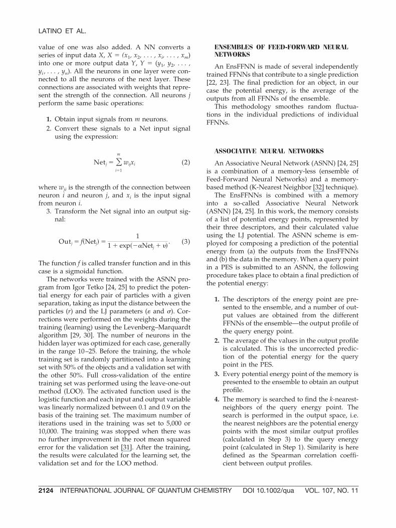
As mentioned earlier, the PES used to train NNswere divided into two parts (0.5 � � � r � �, and� � r � 2.5 � �). For the first part, three trainingsets were used with 315, 162, and 96 energy points.The results of EnsFFNNs and ASNNs for the firstpart of the PES are displayed in the Table II.

For the second part of the curve (r between � and2.5 � �) six different training sets were consideredand the results are displayed in Table III.

NNs with different number of neurons in thehidden layer were used for each training set. Forthe datasets with 997, 512, and 356 energy points a

TABLE II ______________________________________________________________________________________________Mean absolute error (MAE) of training and test sets, using EnsFFNNs and ASNNs, for different training sets inthe first part of PES (0.5 � � < r < �).

NN type Datasets

MAEa/K

315 162 96

EnsFFNNs Learning 231.21 (0.10)b 511.33 (0.19) 2680.79 (1.13)Validation 728.74 (0.67) 2753.77 (1.83) 8928.56 (5.17)LOO 737.15 (0.68) 2772.58 (1.96) 9579.33 (5.77)Test 352.30 (1.05) 649.52 (2.84) 4074.20 (4.90)

ASNNs Learning 790.59 (0.26) 511.33 (0.19) 2219.78 (1.31)Validation 1188.12 (0.76) 2753.77 (1.8) 8567.78 (4.68)LOO 1196.52 (0.77) 2772.58 (1.96) 9288.02 (5.27)Test 812.51 (0.99) 649.52 (2.84) 2008.17 (3.76)

MAE ��ycalc � yexp�/n. ycal, output of the NN; yexp, target.a 315, 162, 96 are the number of energy points used in training.b Values in parentheses indicate the percentages of error.

NEURAL NETWORKS TO APPROACH POTENTIAL ENERGY SURFACES

VOL. 107, NO. 11 DOI 10.1002/qua INTERNATIONAL JOURNAL OF QUANTUM CHEMISTRY 2125

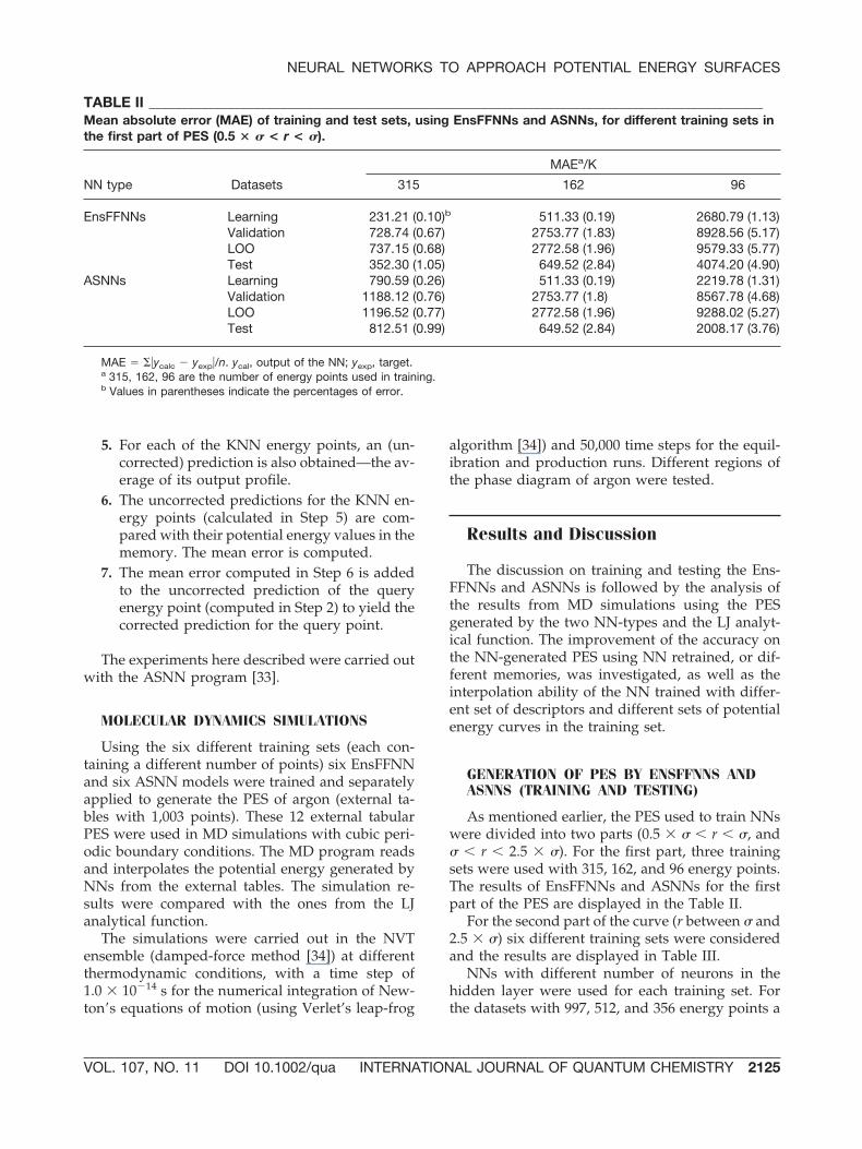
hidden layer with 25 neurons were used, while 15neurons were used for the dataset with 280 energypoints, and 10 hidden neurons for the datasets with228 and 171 energy points. The results with fewerneurons were not much different. In the case of thetraining set with 512 points, a MAE of 0.092 K wasobtained for the test set by an ASNN with 25 hid-den neurons. With 20, 15, 10, and 5 neurons in thehidden layer, MAE of 0.126, 0.167, 0.168, and 0.212K were obtained, respectively.

As expected, higher MAE were observed in thefirst part of the curve, although always lower than5% for the test set. Tables II and III show that theresults using ASNNs are in general better thanthose using only EnsFFNNs, particularly for the testset, and for the NNs trained with fewer points.

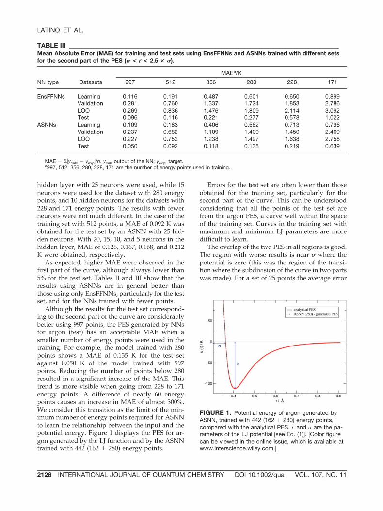
Although the results for the test set correspond-ing to the second part of the curve are considerablybetter using 997 points, the PES generated by NNsfor argon (test) has an acceptable MAE when asmaller number of energy points were used in thetraining. For example, the model trained with 280points shows a MAE of 0.135 K for the test setagainst 0.050 K of the model trained with 997points. Reducing the number of points below 280resulted in a significant increase of the MAE. Thistrend is more visible when going from 228 to 171energy points. A difference of nearly 60 energypoints causes an increase in MAE of almost 300%.We consider this transition as the limit of the min-imum number of energy points required for ASNNto learn the relationship between the input and thepotential energy. Figure 1 displays the PES for ar-gon generated by the LJ function and by the ASNNtrained with 442 (162 � 280) energy points.

Errors for the test set are often lower than thoseobtained for the training set, particularly for thesecond part of the curve. This can be understoodconsidering that all the points of the test set arefrom the argon PES, a curve well within the spaceof the training set. Curves in the training set withmaximum and minimum LJ parameters are moredifficult to learn.

The overlap of the two PES in all regions is good.The region with worse results is near � where thepotential is zero (this was the region of the transi-tion where the subdivision of the curve in two partswas made). For a set of 25 points the average error

TABLE III _____________________________________________________________________________________________Mean Absolute Error (MAE) for training and test sets using EnsFFNNs and ASNNs trained with different setsfor the second part of the PES (� < r < 2.5 � �).

NN type Datasets

MAEa/K

997 512 356 280 228 171

EnsFFNNs Learning 0.116 0.191 0.487 0.601 0.650 0.899Validation 0.281 0.760 1.337 1.724 1.853 2.786LOO 0.269 0.836 1.476 1.809 2.114 3.092Test 0.096 0.116 0.221 0.277 0.578 1.022

ASNNs Learning 0.109 0.183 0.406 0.562 0.713 0.796Validation 0.237 0.682 1.109 1.409 1.450 2.469LOO 0.227 0.752 1.238 1.497 1.638 2.758Test 0.050 0.092 0.118 0.135 0.219 0.639

MAE ��ycalc � yexp�/n. ycal, output of the NN; yexp, target.a997, 512, 356, 280, 228, 171 are the number of energy points used in training.

FIGURE 1. Potential energy of argon generated byASNN, trained with 442 (162 � 280) energy points,compared with the analytical PES. � and � are the pa-rameters of the LJ potential [see Eq. (1)]. [Color figurecan be viewed in the online issue, which is available atwww.interscience.wiley.com.]

LATINO ET AL.

2126 INTERNATIONAL JOURNAL OF QUANTUM CHEMISTRY DOI 10.1002/qua VOL. 107, NO. 11

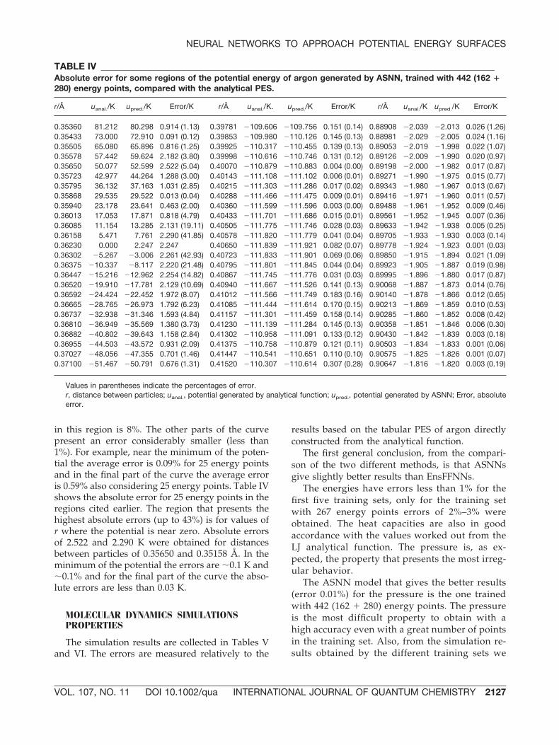
in this region is 8%. The other parts of the curvepresent an error considerably smaller (less than1%). For example, near the minimum of the poten-tial the average error is 0.09% for 25 energy pointsand in the final part of the curve the average erroris 0.59% also considering 25 energy points. Table IVshows the absolute error for 25 energy points in theregions cited earlier. The region that presents thehighest absolute errors (up to 43%) is for values ofr where the potential is near zero. Absolute errorsof 2.522 and 2.290 K were obtained for distancesbetween particles of 0.35650 and 0.35158 Å. In theminimum of the potential the errors are �0.1 K and�0.1% and for the final part of the curve the abso-lute errors are less than 0.03 K.

MOLECULAR DYNAMICS SIMULATIONSPROPERTIES

The simulation results are collected in Tables Vand VI. The errors are measured relatively to the

results based on the tabular PES of argon directlyconstructed from the analytical function.

The first general conclusion, from the compari-son of the two different methods, is that ASNNsgive slightly better results than EnsFFNNs.

The energies have errors less than 1% for thefirst five training sets, only for the training setwith 267 energy points errors of 2%–3% wereobtained. The heat capacities are also in goodaccordance with the values worked out from theLJ analytical function. The pressure is, as ex-pected, the property that presents the most irreg-ular behavior.

The ASNN model that gives the better results(error 0.01%) for the pressure is the one trainedwith 442 (162 � 280) energy points. The pressureis the most difficult property to obtain with ahigh accuracy even with a great number of pointsin the training set. Also, from the simulation re-sults obtained by the different training sets we

TABLE IV _____________________________________________________________________________________________Absolute error for some regions of the potential energy of argon generated by ASNN, trained with 442 (162 �280) energy points, compared with the analytical PES.

r/Å uanal./K upred./K Error/K r/Å uanal./K. upred./K Error/K r/Å uanal./K upred./K Error/K

0.35360 81.212 80.298 0.914 (1.13) 0.39781 �109.606 �109.756 0.151 (0.14) 0.88908 �2.039 �2.013 0.026 (1.26)0.35433 73.000 72.910 0.091 (0.12) 0.39853 �109.980 �110.126 0.145 (0.13) 0.88981 �2.029 �2.005 0.024 (1.16)0.35505 65.080 65.896 0.816 (1.25) 0.39925 �110.317 �110.455 0.139 (0.13) 0.89053 �2.019 �1.998 0.022 (1.07)0.35578 57.442 59.624 2.182 (3.80) 0.39998 �110.616 �110.746 0.131 (0.12) 0.89126 �2.009 �1.990 0.020 (0.97)0.35650 50.077 52.599 2.522 (5.04) 0.40070 �110.879 �110.883 0.004 (0.00) 0.89198 �2.000 �1.982 0.017 (0.87)0.35723 42.977 44.264 1.288 (3.00) 0.40143 �111.108 �111.102 0.006 (0.01) 0.89271 �1.990 �1.975 0.015 (0.77)0.35795 36.132 37.163 1.031 (2.85) 0.40215 �111.303 �111.286 0.017 (0.02) 0.89343 �1.980 �1.967 0.013 (0.67)0.35868 29.535 29.522 0.013 (0.04) 0.40288 �111.466 �111.475 0.009 (0.01) 0.89416 �1.971 �1.960 0.011 (0.57)0.35940 23.178 23.641 0.463 (2.00) 0.40360 �111.599 �111.596 0.003 (0.00) 0.89488 �1.961 �1.952 0.009 (0.46)0.36013 17.053 17.871 0.818 (4.79) 0.40433 �111.701 �111.686 0.015 (0.01) 0.89561 �1.952 �1.945 0.007 (0.36)0.36085 11.154 13.285 2.131 (19.11) 0.40505 �111.775 �111.746 0.028 (0.03) 0.89633 �1.942 �1.938 0.005 (0.25)0.36158 5.471 7.761 2.290 (41.85) 0.40578 �111.820 �111.779 0.041 (0.04) 0.89705 �1.933 �1.930 0.003 (0.14)0.36230 0.000 2.247 2.247 0.40650 �111.839 �111.921 0.082 (0.07) 0.89778 �1.924 �1.923 0.001 (0.03)0.36302 �5.267 �3.006 2.261 (42.93) 0.40723 �111.833 �111.901 0.069 (0.06) 0.89850 �1.915 �1.894 0.021 (1.09)0.36375 �10.337 �8.117 2.220 (21.48) 0.40795 �111.801 �111.845 0.044 (0.04) 0.89923 �1.905 �1.887 0.019 (0.98)0.36447 �15.216 �12.962 2.254 (14.82) 0.40867 �111.745 �111.776 0.031 (0.03) 0.89995 �1.896 �1.880 0.017 (0.87)0.36520 �19.910 �17.781 2.129 (10.69) 0.40940 �111.667 �111.526 0.141 (0.13) 0.90068 �1.887 �1.873 0.014 (0.76)0.36592 �24.424 �22.452 1.972 (8.07) 0.41012 �111.566 �111.749 0.183 (0.16) 0.90140 �1.878 �1.866 0.012 (0.65)0.36665 �28.765 �26.973 1.792 (6.23) 0.41085 �111.444 �111.614 0.170 (0.15) 0.90213 �1.869 �1.859 0.010 (0.53)0.36737 �32.938 �31.346 1.593 (4.84) 0.41157 �111.301 �111.459 0.158 (0.14) 0.90285 �1.860 �1.852 0.008 (0.42)0.36810 �36.949 �35.569 1.380 (3.73) 0.41230 �111.139 �111.284 0.145 (0.13) 0.90358 �1.851 �1.846 0.006 (0.30)0.36882 �40.802 �39.643 1.158 (2.84) 0.41302 �110.958 �111.091 0.133 (0.12) 0.90430 �1.842 �1.839 0.003 (0.18)0.36955 �44.503 �43.572 0.931 (2.09) 0.41375 �110.758 �110.879 0.121 (0.11) 0.90503 �1.834 �1.833 0.001 (0.06)0.37027 �48.056 �47.355 0.701 (1.46) 0.41447 �110.541 �110.651 0.110 (0.10) 0.90575 �1.825 �1.826 0.001 (0.07)0.37100 �51.467 �50.791 0.676 (1.31) 0.41520 �110.307 �110.614 0.307 (0.28) 0.90647 �1.816 �1.820 0.003 (0.19)

Values in parentheses indicate the percentages of error.r, distance between particles; uanal., potential generated by analytical function; upred., potential generated by ASNN; Error, absoluteerror.

NEURAL NETWORKS TO APPROACH POTENTIAL ENERGY SURFACES

VOL. 107, NO. 11 DOI 10.1002/qua INTERNATIONAL JOURNAL OF QUANTUM CHEMISTRY 2127

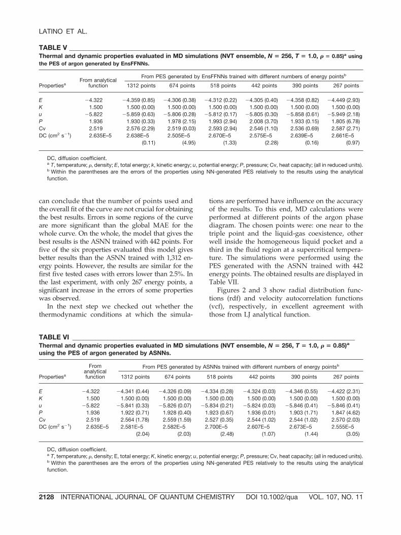
can conclude that the number of points used andthe overall fit of the curve are not crucial for obtainingthe best results. Errors in some regions of the curveare more significant than the global MAE for thewhole curve. On the whole, the model that gives thebest results is the ASNN trained with 442 points. Forfive of the six properties evaluated this model givesbetter results than the ASNN trained with 1,312 en-ergy points. However, the results are similar for thefirst five tested cases with errors lower than 2.5%. Inthe last experiment, with only 267 energy points, asignificant increase in the errors of some propertieswas observed.

In the next step we checked out whether thethermodynamic conditions at which the simula-

tions are performed have influence on the accuracyof the results. To this end, MD calculations wereperformed at different points of the argon phasediagram. The chosen points were: one near to thetriple point and the liquid-gas coexistence, otherwell inside the homogeneous liquid pocket and athird in the fluid region at a supercritical tempera-ture. The simulations were performed using thePES generated with the ASNN trained with 442energy points. The obtained results are displayed inTable VII.

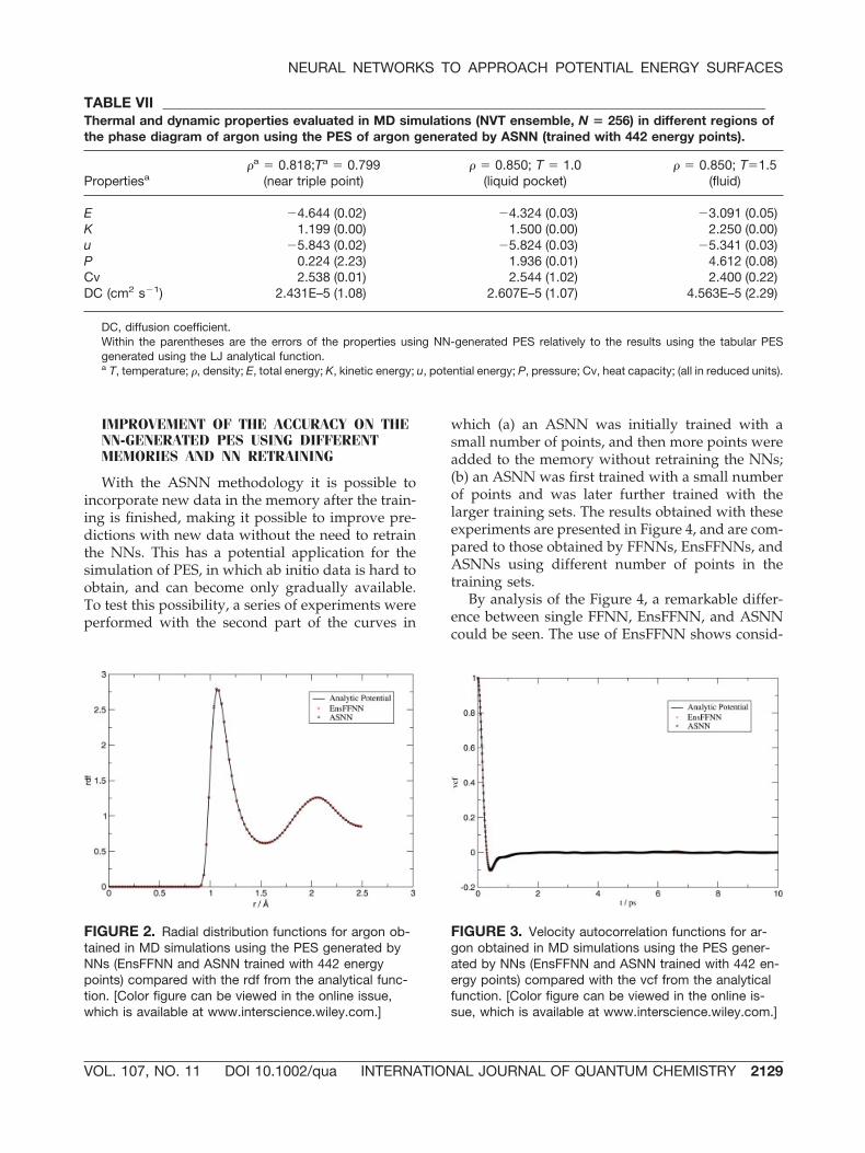
Figures 2 and 3 show radial distribution func-tions (rdf) and velocity autocorrelation functions(vcf), respectively, in excellent agreement withthose from LJ analytical function.

TABLE V ______________________________________________________________________________________________Thermal and dynamic properties evaluated in MD simulations (NVT ensemble, N � 256, T � 1.0, � � 0.85)a usingthe PES of argon generated by EnsFFNNs.

PropertiesaFrom analytical

function

From PES generated by EnsFFNNs trained with different numbers of energy pointsb

1312 points 674 points 518 points 442 points 390 points 267 points

E �4.322 �4.359 (0.85) �4.306 (0.38) �4.312 (0.22) �4.305 (0.40) �4.358 (0.82) �4.449 (2.93)K 1.500 1.500 (0.00) 1.500 (0.00) 1.500 (0.00) 1.500 (0.00) 1.500 (0.00) 1.500 (0.00)u �5.822 �5.859 (0.63) �5.806 (0.28) �5.812 (0.17) �5.805 (0.30) �5.858 (0.61) �5.949 (2.18)P 1.936 1.930 (0.33) 1.978 (2.15) 1.993 (2.94) 2.008 (3.70) 1.933 (0.15) 1.805 (6.78)Cv 2.519 2.576 (2.29) 2.519 (0.03) 2.593 (2.94) 2.546 (1.10) 2.536 (0.69) 2.587 (2.71)DC (cm2 s�1) 2.635E–5 2.638E–5 2.505E–5 2.670E–5 2.575E–5 2.639E–5 2.661E–5

(0.11) (4.95) (1.33) (2.28) (0.16) (0.97)

DC, diffusion coefficient.a T, temperature; �, density; E, total energy; k, kinetic energy; u, potential energy; P, pressure; Cv, heat capacity; (all in reduced units).b Within the parentheses are the errors of the properties using NN-generated PES relatively to the results using the analyticalfunction.

TABLE VI _____________________________________________________________________________________________Thermal and dynamic properties evaluated in MD simulations (NVT ensemble, N � 256, T � 1.0, � � 0.85)a

using the PES of argon generated by ASNNs.

Propertiesa

Fromanalyticalfunction

From PES generated by ASNNs trained with different numbers of energy pointsb

1312 points 674 points 518 points 442 points 390 points 267 points

E �4.322 �4.341 (0.44) �4.326 (0.09) �4.334 (0.28) �4.324 (0.03) �4.346 (0.55) �4.422 (2.31)K 1.500 1.500 (0.00) 1.500 (0.00) 1.500 (0.00) 1.500 (0.00) 1.500 (0.00) 1.500 (0.00)u �5.822 �5.841 (0.33) �5.826 (0.07) �5.834 (0.21) �5.824 (0.03) �5.846 (0.41) �5.846 (0.41)P 1.936 1.922 (0.71) 1.928 (0.40) 1.923 (0.67) 1.936 (0.01) 1.903 (1.71) 1.847 (4.62)Cv 2.519 2.564 (1.78) 2.559 (1.59) 2.527 (0.35) 2.544 (1.02) 2.544 (1.02) 2.570 (2.03)DC (cm2 s�1) 2.635E–5 2.581E–5 2.582E–5 2.700E–5 2.607E–5 2.673E–5 2.555E–5

(2.04) (2.03) (2.48) (1.07) (1.44) (3.05)

DC, diffusion coefficient.a T, temperature; �, density; E, total energy; K, kinetic energy; u, potential energy; P, pressure; Cv, heat capacity; (all in reduced units).b Within the parentheses are the errors of the properties using NN-generated PES relatively to the results using the analyticalfunction.

LATINO ET AL.

2128 INTERNATIONAL JOURNAL OF QUANTUM CHEMISTRY DOI 10.1002/qua VOL. 107, NO. 11

IMPROVEMENT OF THE ACCURACY ON THENN-GENERATED PES USING DIFFERENTMEMORIES AND NN RETRAINING

With the ASNN methodology it is possible toincorporate new data in the memory after the train-ing is finished, making it possible to improve pre-dictions with new data without the need to retrainthe NNs. This has a potential application for thesimulation of PES, in which ab initio data is hard toobtain, and can become only gradually available.To test this possibility, a series of experiments wereperformed with the second part of the curves in

which (a) an ASNN was initially trained with asmall number of points, and then more points wereadded to the memory without retraining the NNs;(b) an ASNN was first trained with a small numberof points and was later further trained with thelarger training sets. The results obtained with theseexperiments are presented in Figure 4, and are com-pared to those obtained by FFNNs, EnsFFNNs, andASNNs using different number of points in thetraining sets.

By analysis of the Figure 4, a remarkable differ-ence between single FFNN, EnsFFNN, and ASNNcould be seen. The use of EnsFFNN shows consid-

TABLE VII ____________________________________________________________________________________________Thermal and dynamic properties evaluated in MD simulations (NVT ensemble, N � 256) in different regions ofthe phase diagram of argon using the PES of argon generated by ASNN (trained with 442 energy points).

Propertiesa�a 0.818;Ta 0.799

(near triple point)� 0.850; T 1.0

(liquid pocket)� 0.850; T1.5

(fluid)

E �4.644 (0.02) �4.324 (0.03) �3.091 (0.05)K 1.199 (0.00) 1.500 (0.00) 2.250 (0.00)u �5.843 (0.02) �5.824 (0.03) �5.341 (0.03)P 0.224 (2.23) 1.936 (0.01) 4.612 (0.08)Cv 2.538 (0.01) 2.544 (1.02) 2.400 (0.22)DC (cm2 s�1) 2.431E–5 (1.08) 2.607E–5 (1.07) 4.563E–5 (2.29)

DC, diffusion coefficient.Within the parentheses are the errors of the properties using NN-generated PES relatively to the results using the tabular PESgenerated using the LJ analytical function.a T, temperature; �, density; E, total energy; K, kinetic energy; u, potential energy; P, pressure; Cv, heat capacity; (all in reduced units).

FIGURE 2. Radial distribution functions for argon ob-tained in MD simulations using the PES generated byNNs (EnsFFNN and ASNN trained with 442 energypoints) compared with the rdf from the analytical func-tion. [Color figure can be viewed in the online issue,which is available at www.interscience.wiley.com.]

FIGURE 3. Velocity autocorrelation functions for ar-gon obtained in MD simulations using the PES gener-ated by NNs (EnsFFNN and ASNN trained with 442 en-ergy points) compared with the vcf from the analyticalfunction. [Color figure can be viewed in the online is-sue, which is available at www.interscience.wiley.com.]

NEURAL NETWORKS TO APPROACH POTENTIAL ENERGY SURFACES

VOL. 107, NO. 11 DOI 10.1002/qua INTERNATIONAL JOURNAL OF QUANTUM CHEMISTRY 2129

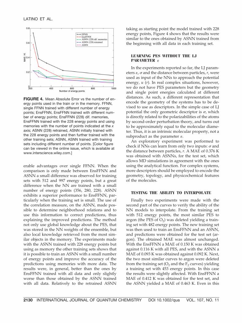
erable advantages over single FFNN. When thecomparison is only made between EnsFFNN andASNN a small difference was observed for trainingsets with 512 and 997 energy points, but a greatdifference when the NN are trained with a smallnumber of energy points (356, 280, 228). ASNNexhibits a superior performance to EnsFFNN, par-ticularly when the training set is small. The use ofthe correlation measure, on the ASNN, made pos-sible to determine neighborhood relations and touse this information to correct predictions, thusexplaining the improved predictions. The methodnot only use global knowledge about the PES, thatwas stored in the NN weights of the ensemble, butalso local knowledge retrieved from the most sim-ilar objects in the memory. The experiments madewith the ASNN trained with 228 energy points butusing as memory the other training sets shows thatit is possible to train an ASNN with a small numberof energy points and improve the accuracy of thepredictions using memories with more data. Theresults were, in general, better than the ones byEnsFFNN trained with all data and only slightlyworse than those obtained by the ASNN trainedwith all data. Relatively to the retrained ASNN

taking as starting point the model trained with 228energy points, Figure 4 shows that the results weresimilar to the ones obtained by ASNN trained fromthe beginning with all data in each training set.

LEARNING PES WITHOUT THE LJPARAMETER �

In the experiments reported so far, the LJ param-eters �, � and the distance between particles, r, wereused as input of the NNs to approach the potentialenergy, u (r). In real complex situations, however,we do not have PES parameters but the geometryand single point energies calculated at differentdistances. As such, a different representation thatencode the geometry of the systems has to be de-vised to use as descriptors. In the simple case of LJpotential the only geometric descriptor is �, whichis directly related to the polarizabilities of the atomsby second-order perturbation theory, and turns outto be approximately equal to the molecular diame-ter. Thus, it is an intrinsic molecular property, not asubproduct as the parameter �.

An exploratory experiment was performed tocheck if NNs can learn from only two inputs: � andthe distance between particles, r. A MAE of 0.376 Kwas obtained with ASNNs, for the test set, whichallows MD simulations in agreement with the onesusing the analytical function. For complex systems,more descriptors should be employed to encode thegeometry, topology, and physicochemical featuresof the molecules.

TESTING THE ABILITY TO INTERPOLATE

Finally two experiments were made with thesecond part of the curves to verify the ability of theNN models to interpolate. From the training setwith 512 energy points, the most similar PES toargon (the PES of O2) was deleted yielding a train-ing set with 482 energy points. The new training setwas then used to train an EnsFFNN and an ASNN,and predictions were obtained for the test set (ar-gon). The obtained MAE was almost unchanged.With the EnsFFNN a MAE of 0.150 K was obtainedagainst 0.116 K with all PES, and with the ASNN aMAE of 0.093 K was obtained against 0.092 K. Next,the two most similar curves to argon were deletedfrom the training set (O2 and the F2 curves) yieldinga training set with 453 energy points. In this casethe results were slightly affected. With EnsFFNN aMAE of 0.412 K was obtained for the test set, andthe ASNN yielded a MAE of 0.463 K. Even in this

FIGURE 4. Mean Absolute Error vs the number of en-ergy points used in the train or in the memory. FFNN,single FFNN trained with different number of energypoints; EnsFFNN, EnsFFNN trained with different num-ber of energy points; EnsFFNN (228) dif. memories,EnsFFNN trained with the 228 energy points and usingmemories with the number of points indicated at the xaxis; ASNN (228) retrained, ASNN initially trained withthe 228 energy points and then further trained with theother training sets; ASNN, ASNN trained with trainingsets including different number of points. [Color figurecan be viewed in the online issue, which is available atwww.interscience.wiley.com.]

LATINO ET AL.

2130 INTERNATIONAL JOURNAL OF QUANTUM CHEMISTRY DOI 10.1002/qua VOL. 107, NO. 11

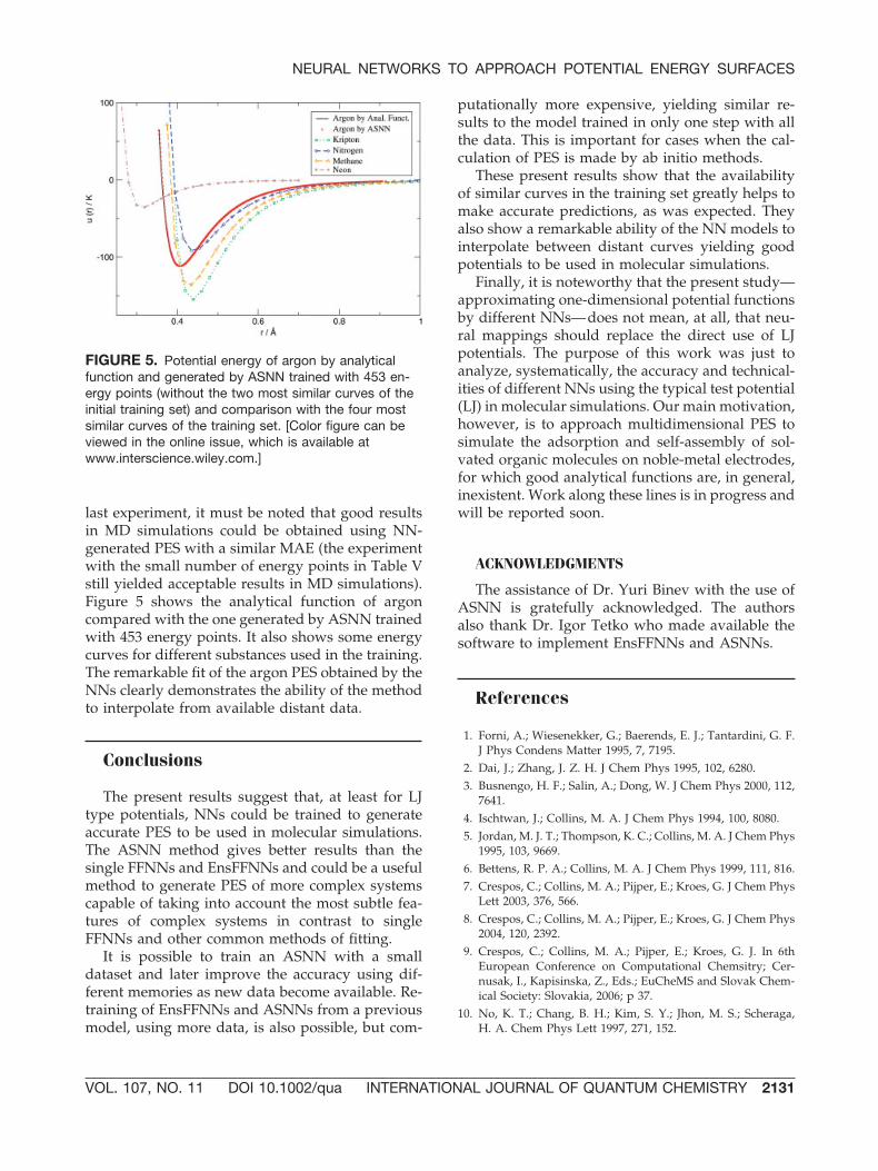
last experiment, it must be noted that good resultsin MD simulations could be obtained using NN-generated PES with a similar MAE (the experimentwith the small number of energy points in Table Vstill yielded acceptable results in MD simulations).Figure 5 shows the analytical function of argoncompared with the one generated by ASNN trainedwith 453 energy points. It also shows some energycurves for different substances used in the training.The remarkable fit of the argon PES obtained by theNNs clearly demonstrates the ability of the methodto interpolate from available distant data.

Conclusions

The present results suggest that, at least for LJtype potentials, NNs could be trained to generateaccurate PES to be used in molecular simulations.The ASNN method gives better results than thesingle FFNNs and EnsFFNNs and could be a usefulmethod to generate PES of more complex systemscapable of taking into account the most subtle fea-tures of complex systems in contrast to singleFFNNs and other common methods of fitting.

It is possible to train an ASNN with a smalldataset and later improve the accuracy using dif-ferent memories as new data become available. Re-training of EnsFFNNs and ASNNs from a previousmodel, using more data, is also possible, but com-

putationally more expensive, yielding similar re-sults to the model trained in only one step with allthe data. This is important for cases when the cal-culation of PES is made by ab initio methods.

These present results show that the availabilityof similar curves in the training set greatly helps tomake accurate predictions, as was expected. Theyalso show a remarkable ability of the NN models tointerpolate between distant curves yielding goodpotentials to be used in molecular simulations.

Finally, it is noteworthy that the present study—approximating one-dimensional potential functionsby different NNs—does not mean, at all, that neu-ral mappings should replace the direct use of LJpotentials. The purpose of this work was just toanalyze, systematically, the accuracy and technical-ities of different NNs using the typical test potential(LJ) in molecular simulations. Our main motivation,however, is to approach multidimensional PES tosimulate the adsorption and self-assembly of sol-vated organic molecules on noble-metal electrodes,for which good analytical functions are, in general,inexistent. Work along these lines is in progress andwill be reported soon.

ACKNOWLEDGMENTS

The assistance of Dr. Yuri Binev with the use ofASNN is gratefully acknowledged. The authorsalso thank Dr. Igor Tetko who made available thesoftware to implement EnsFFNNs and ASNNs.

References

1. Forni, A.; Wiesenekker, G.; Baerends, E. J.; Tantardini, G. F.J Phys Condens Matter 1995, 7, 7195.

2. Dai, J.; Zhang, J. Z. H. J Chem Phys 1995, 102, 6280.3. Busnengo, H. F.; Salin, A.; Dong, W. J Chem Phys 2000, 112,

7641.4. Ischtwan, J.; Collins, M. A. J Chem Phys 1994, 100, 8080.5. Jordan, M. J. T.; Thompson, K. C.; Collins, M. A. J Chem Phys

1995, 103, 9669.6. Bettens, R. P. A.; Collins, M. A. J Chem Phys 1999, 111, 816.7. Crespos, C.; Collins, M. A.; Pijper, E.; Kroes, G. J Chem Phys

Lett 2003, 376, 566.8. Crespos, C.; Collins, M. A.; Pijper, E.; Kroes, G. J Chem Phys

2004, 120, 2392.9. Crespos, C.; Collins, M. A.; Pijper, E.; Kroes, G. J. In 6th

European Conference on Computational Chemsitry; Cer-nusak, I., Kapisinska, Z., Eds.; EuCheMS and Slovak Chem-ical Society: Slovakia, 2006; p 37.

10. No, K. T.; Chang, B. H.; Kim, S. Y.; Jhon, M. S.; Scheraga,H. A. Chem Phys Lett 1997, 271, 152.

FIGURE 5. Potential energy of argon by analyticalfunction and generated by ASNN trained with 453 en-ergy points (without the two most similar curves of theinitial training set) and comparison with the four mostsimilar curves of the training set. [Color figure can beviewed in the online issue, which is available atwww.interscience.wiley.com.]

NEURAL NETWORKS TO APPROACH POTENTIAL ENERGY SURFACES

VOL. 107, NO. 11 DOI 10.1002/qua INTERNATIONAL JOURNAL OF QUANTUM CHEMISTRY 2131

11. Gassner, H.; Probst, M.; Lauenstein, A.; Hermansson, K. JPhys Chem A 1998, 102, 4596.

12. Prudente, F. V.; Neto, J. J. S. Chem Phys Lett 1998, 287, 585.13. Bittencourt, A. C. P.; Prudente, F. V.; Vianna, J. D. M. Chem

Phys 2004, 297, 153.14. Cho, K.-H.; No, K. T.; Scheraga, H. A. J Mol Struct 2002, 641,

77.15. Rocha Filho, T. M.; Oliveira, Z. T.; Malbouisson, L. A. C.;

Gargano, R.; Neto, J. J. S. Int J Quantum Chem 2003, 95, 281.16. Lorenz, S.; Grob, A.; Scheffler, M. Chem Phys Lett 2004, 395,

210.17. Lorenz, S.; Scheffler, M.; Grob, A. Phys Review B 2006, 73,

115431–1-13.18. Raff, L. M.; Malshe, M.; Hagan, M.; Doughan, D. I.; Rockley,

M. G.; Komanduri, R. J Chem Phys 2005, 122, 084104.19. Manzhos, S.; Carrington T., Jr. J Chem Phys 2006, 125,

084109.20. Witkoskie, J. B.; Doren, D. J. J Chem Theory Comput 2005, 1,

14.21. Toth, G.; Kiraly, N.; Vrabecz, A. J Chem Phys 2005, 123,

174109.22. Dietterich, T. G. In The Handbook of Brain Theory and

Neural Networks; Arbib, M. A., Ed.; MIT Press: Cambridge,MA, 2002; pp 405–408.

23. Agrafiotis, D. K.; Cedeno, W.; Lobanov, V. S. J Chem InfComput Sci 2002, 42, 903.

24. Tetko, I. V. Neural Process Lett 2002, 16, 187.

25. Tetko, I. V. J Chem Inf Comput Sci 2002, 42, 717.

26. Cuadros, F.; Cachadina, J.; Ahmuda, W. Mol Eng 1996, 6,319.

27. Hirschfelder, J. O.; Curtiss, C. F.; Bird, R. B. Molecular The-ory of Gases and Liquids; Wiley:New-York, 1954.

28. Zupan, J.; Gasteiger, J. Neural Networks in Chemistry andDrug Design; Wiley-VCH: Weinheim, 1999.

29. Press, W. H.; Teukolsky, S. A.; Vetterlung, W. T.; Flannery,B. P. Numerical Recipes in C, 2nd ed.; Cambridge UniversityPress: New York, 1994; p 998.

30. Shepherd, A. J. Second Order Methods for Neural Networks;Springer-Verlag: London,1997; p 145.

31. Bishop, M. Neural Networks for Pattern Recognition; Ox-ford University Press: Oxford, 1995.

32. Dasarthy, B. Nearest Neighbor (NN) Norms; IEEE ComputerSociety Press: Washington, DC, 1991.

33. VCCLAB, Virtual Computational Chemistry Laboratory.Available at www.vcclab.org. 2005.

34. Allen, M. P.; Tildesley, D. J. Computer Simulation of Liquids;Claredon Press: Oxford, 1987.

LATINO ET AL.

2132 INTERNATIONAL JOURNAL OF QUANTUM CHEMISTRY DOI 10.1002/qua VOL. 107, NO. 11