AC 2007-324: USING NEURAL NETWORKS TO MOTIVATE THE TEACHING OFMATRIX ALGEBRA FOR K-12 AND COLLEGE ENGINEERING STUDENTS

Sharlene Katz, California State University-NorthridgeSharlene Katz is Professor in the Department of Electrical and Computer Engineering atCalifornia State University, Northridge (CSUN) where she has been for over 25 years. Shegraduated from the University of California, Los Angeles with B.S. (1975), M.S. (1976), andPh.D. (1986) degrees in Electrical Engineering. Recently, her areas of research interest have beenin engineering education techniques and neural networks. Dr. Katz is a licensed professionalengineer in the state of California.

Bella Klass-Tsirulnikov, Sami Shamoon College of Engineering (formerly Negev Academic College ofEngineering), Beer Sheva, Israel

Bella Klass-Tsirulnikov is a senior academic lecturer at Sami Shamoon College of Engineering,Beer Sheva, Israel (former Negev Academic College of Engineering). She accomplishedmathematics studies at Lomonosov Moscow State University (1969), received Ph.D. degree inmathematics at Tel Aviv University (1980), and completed PostDoc studies at Technion - IsraelInstitute of Technology (1982). From 1995 she also holds a Professional Teaching Certificate forgrades 7 – 12 of the Israeli Ministry of Education. Dr. Klass-Tsirulnikov participates actively inthe research on functional analysis, specializing in topological vector spaces, as well as in theresearch on mathematics education at different levels.

© American Society for Engineering Education, 2007

Page 12.1557.1

Using Neural Networks to Motivate the Teaching of Matrix

Algebra for K-12 and College Engineering Students

Abstract

Improving the retention of engineering students continues to be a topic of interest to engineering

educators. Reference 1 indicates that seven sessions at the 2006 ASEE Annual Conference were

devoted to this subject. In order to be successful in an engineering program, it is recognized that

students must have a solid background in mathematics. Studies have shown that students will be

more motivated to study and learn mathematics if abstract mathematical concepts are presented

in the context of interesting examples and applications2 – 5

. To become appealing and relevant,

abstract mathematical concepts should be connected to engineering and real life issues, as

suggested by the guidelines of ASEE Engineering K-12 Centre6.

In two previous papers7 - 8

the co-authors have presented methods for improving the teaching of

important mathematical concepts to K-12 and college level engineering students. In reference 7,

the co-authors provided a method of teaching the concept of infinity that combines a rigorous

development of the concept of infinity in freshman level mathematics courses for engineering

students and an intuitive approach to infinity with hands-on exercises for K-12 students. In

reference 8, the co-authors developed materials on topics from number theory, essential to the

field of data security and suitable for K-12 students, as well as for remedial or preparatory

courses for engineering freshmen.

This paper represents the third part in this continuing project of developing methods for

improving the teaching and learning of mathematical concepts for engineering students. It

presents an interesting context in which to teach simple matrix algebra, developing practical

applications that can be used for both K-12 and college level algebra courses. The main

application demonstrated in this paper is the design of a character recognition system, using a

simple neural network. It leads to a series of interesting exercises with practical applications. The

authors contend that these applications will motivate students to practice matrix operations which

otherwise may seem tedious and to further motivate them to focus on their mathematics courses.

I. Introduction

The teaching of matrix algebra takes place in a variety of courses. In K-12, students are typically

introduced to matrix operations in their second year algebra courses and/or pre-calculus. In

college, students come across matrix algebra in pre-calculus, linear algebra, differential

equations and linear systems courses. In lower division college mathematics, the widely used

application of matrix operations is typically the solution of simultaneous equations, based on the

fundamental idea of viewing a system of linear equations as a product of a matrix and a vector

(see for example, section 1.4 of reference 9).

It is not until the upper division engineering courses that students see interesting practical

applications of linear algebra. The standard college textbooks on linear algebra provide

application models of matrix algebra and linear systems used in economics, computer graphics

Page 12.1557.2

and electrical circuit design9-10

. Some of these models are relatively simple, such as the

Cambridge Diet Formula (see Section 1.9 of reference 9). However, the models that are most

important for engineering studies require specific knowledge. The mathematical models in

economics widely use the notions of demand, consumption and equilibrium. The computer

graphics requires understanding of 2D-3D topology. The mathematical model of electrical

networks design is based on Kirchhoff's Laws 9-10

.

Introducing advanced topics of specific disciplines in a basic linear algebra course is a

complicated task. It raises the issues of what are the applications that generate common interest

among freshmen, and how much time-consuming advanced engineering knowledge should be

allowed in a basic mathematical course without hurting freshmen interest. It also brings up the

fundamental question of what is the meaning and essence of teaching mathematics in a way that

is attractive and relevant for engineering students. As teachers, we know that often students are

unable to connect practical matrix applications in upper division engineering courses with the

basics of linear algebra taught during the first year of engineering studies. There is no doubt that

we should think hard about how to teach mathematics to engineering freshmen in the most

appealing and useful way6.

In this paper, we present a design of a simple artificial neural network for character recognition

that exercises basic matrix operations, such as adding and multiplying matrices and finding

determinants. Artificial neural networks are based on the model of biological neural system, and

they can be relatively simply explained to non-professionals. Students will be surprised to learn

that the simple neural network system they designed can correctly recognize a distorted character

not recognizable by their own eyes. The process of designing the network provides useful

exercises for practicing matrix manipulations in an appealing and relevant way.

Section II of this paper briefly presents the topics in matrix algebra that are needed for these

exercises. Since our paper is intended to serve the scientific community of mathematicians,

including K-12 teachers, we feel that some explanation is needed for the terminology and notions

used in the field of artificial neural networks. These explanations are provided in the next two

sections. Section III presents the concept of artificial neural networks, and Section IV overviews

the use of artificial neural networks in designing character recognition systems. Section V

details a method for designing and testing the character recognition system, suitable for both K-

12 students and engineering freshmen. Section VI gives a number of meaningful exercises in

basic matrix algebra that students can perform based on this design method. Section VII

summarizes the paper.

II. Topics in Matrix Algebra

As mentioned earlier, the teaching of matrix algebra takes place in a variety of courses for K-12

students, and entry-level college students. These courses provide ideal opportunities to use the

exercises presented in this paper. Before using these exercises students should be exposed to the

following concepts related to matrix algebra.

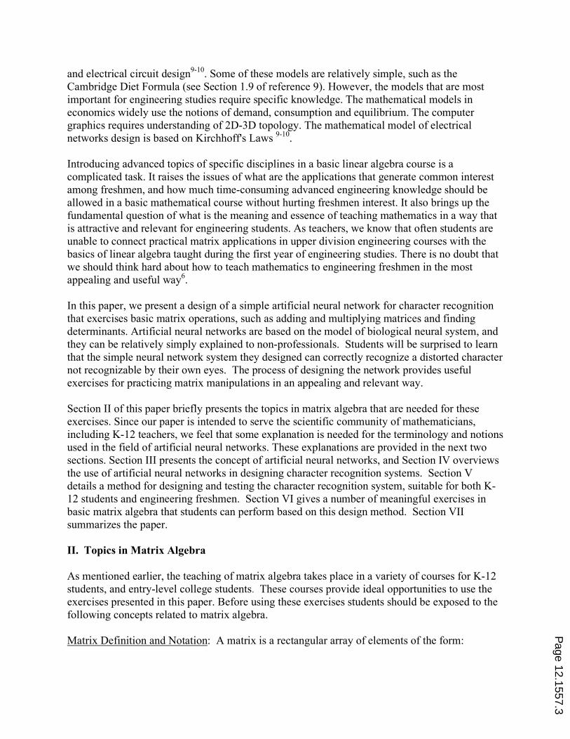
Matrix Definition and Notation: A matrix is a rectangular array of elements of the form:

Page 12.1557.3

A =

a11

a12! a

1n

a21

a22! a

2n

" " "

am1

am2! a

mn

!

"

####

$

%

&&&&

The first subscript of each element denotes the row and second subscript denotes the column.

The matrix that has m rows and n columns is said to be an m x n matrix, or a matrix of size "m by

n".

Matrix Addition and Subtraction: The sum (difference) of two matrices A and B is written A+B

(A-B). Matrices must be the same size to be added or subtracted. The entries in the resulting

sum A+B are aij + bij for i = 1 … m and j = 1 … n. The entries in the difference A-B are aij - bij

for i = 1 … m and j = 1 … n.

Matrix Multiplication: Let A be an m x n matrix and B an r x p matrix. The product of these two

matrices, AB, is only defined if n = r. The resulting product C = AB is an m x p matrix in

which:

cij = aikbkjk=1

n

! ; i=1...m; j=1...p

Transpose of a Matrix: The transpose of an m x n matrix A is an n x m matrix, denoted AT. The

transpose matrix AT has as its rows, the columns of A, or:

A =

a11

a12! a

1n

a21

a22! a

2n

" " "

am1

am2! a

mn

!

"

####

$

%

&&&&

' AT=

a11

a21! a

m1

a12

a22! a

m2

" " "

a1n

a2n! a

mn

!

"

####

$

%

&&&&

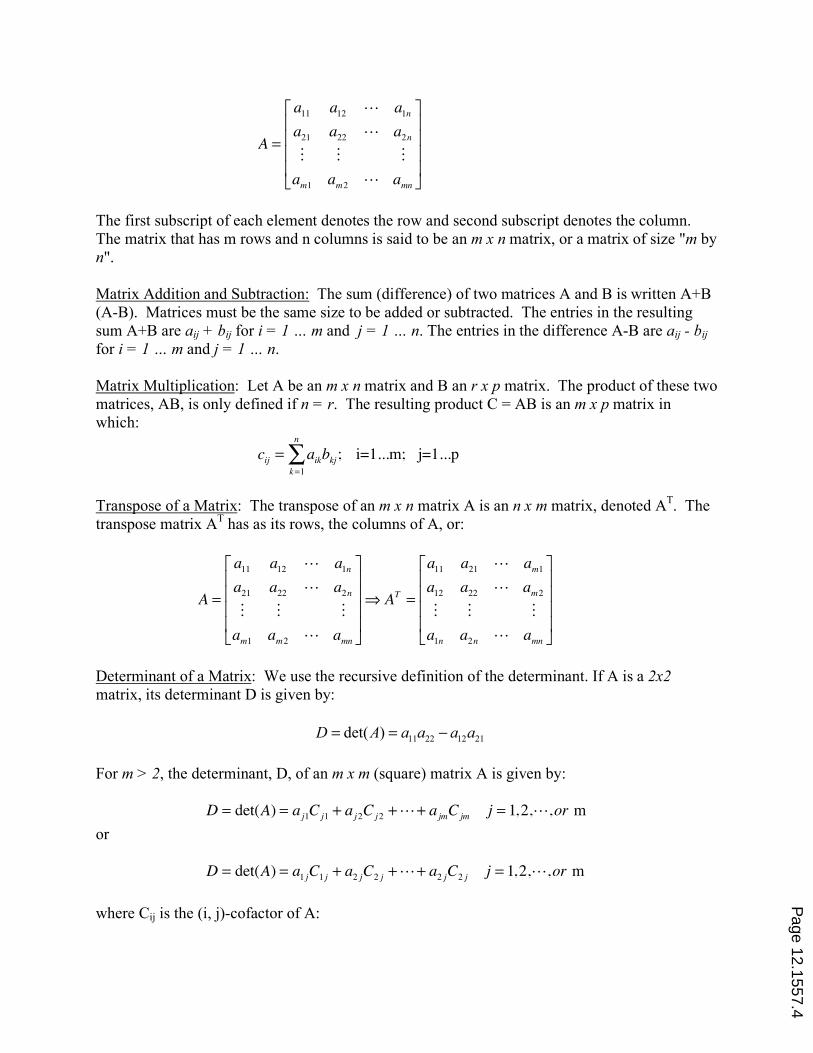
Determinant of a Matrix: We use the recursive definition of the determinant. If A is a 2x2

matrix, its determinant D is given by:

11 22 12 21det( ) D A a a a a= = !

For m > 2, the determinant, D, of an m x m (square) matrix A is given by:

D = det(A) = a j1C j1 + a j2C j2 +!+ a jmC jm j = 1,2,!,or m

or

D = det(A) = a

1 jC1 j + a2 jC2 j +!+ a2 jC2 j j = 1,2,!,or m

where Cij is the (i, j)-cofactor of A:

Page 12.1557.4

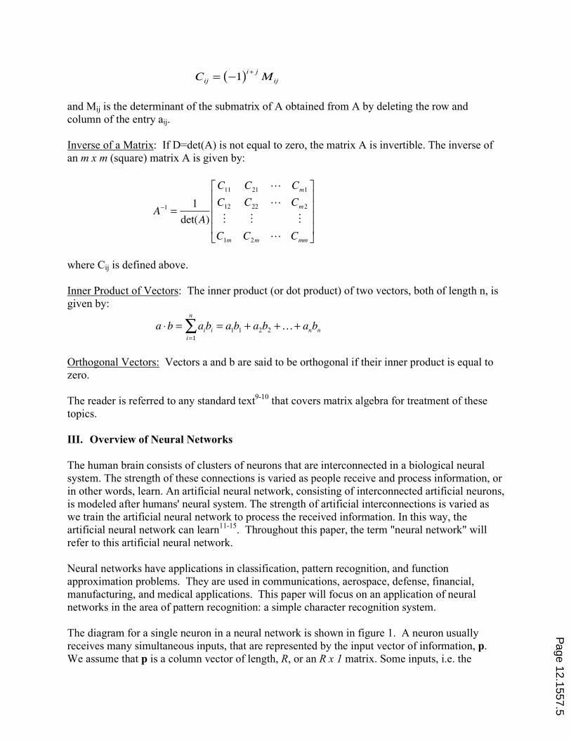
Cij = !1( )i+ jM ij

and Mij is the determinant of the submatrix of A obtained from A by deleting the row and

column of the entry aij.

Inverse of a Matrix: If D=det(A) is not equal to zero, the matrix A is invertible. The inverse of

an m x m (square) matrix A is given by:

A!1=

1

det(A)

C11

C21! C

m1

C12

C22! C

m2

" " "

C1m

C2m! C

mm

"

#

$$$$

%

&

''''

where Cij is defined above.

Inner Product of Vectors: The inner product (or dot product) of two vectors, both of length n, is

given by:

a !b = aibi

i=1

n

" = a1b1+ a

2b2+…+ a

nbn

Orthogonal Vectors: Vectors a and b are said to be orthogonal if their inner product is equal to

zero.

The reader is referred to any standard text9-10

that covers matrix algebra for treatment of these

topics.

III. Overview of Neural Networks

The human brain consists of clusters of neurons that are interconnected in a biological neural

system. The strength of these connections is varied as people receive and process information, or

in other words, learn. An artificial neural network, consisting of interconnected artificial neurons,

is modeled after humans' neural system. The strength of artificial interconnections is varied as

we train the artificial neural network to process the received information. In this way, the

artificial neural network can learn11-15

. Throughout this paper, the term "neural network" will

refer to this artificial neural network.

Neural networks have applications in classification, pattern recognition, and function

approximation problems. They are used in communications, aerospace, defense, financial,

manufacturing, and medical applications. This paper will focus on an application of neural

networks in the area of pattern recognition: a simple character recognition system.

The diagram for a single neuron in a neural network is shown in figure 1. A neuron usually

receives many simultaneous inputs, that are represented by the input vector of information, p.

We assume that p is a column vector of length, R, or an R x 1 matrix. Some inputs, i.e. the

Page 12.1557.5

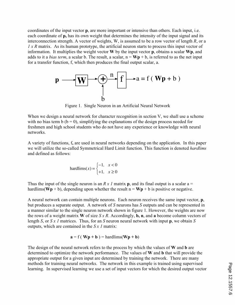
coordinates of the input vector p, are more important or intensive than others. Each input, i.e.

each coordinate of p, has its own weight that determines the intensity of the input signal and its

interconnection strength. A vector of weights, W, is assumed to be a row vector of length R, or a

1 x R matrix. As its human prototype, the artificial neuron starts to process this input vector of

information. It multiplies the weight vector W by the input vector p, obtains a scalar Wp, and

adds to it a bias term, a scalar b. The result, a scalar, n = Wp + b, is referred to as the net input

for a transfer function, f, which then produces the final output scalar, a.

W +

b

pn

a = f ( Wp + b )f

Figure 1. Single Neuron in an Artificial Neural Network

When we design a neural network for character recognition in section V, we shall use a scheme

with no bias term b (b = 0), simplifying the explanations of the design process needed for

freshmen and high school students who do not have any experience or knowledge with neural

networks.

A variety of functions, f, are used in neural networks depending on the application. In this paper

we will utilize the so-called Symmetrical Hard Limit function. This function is denoted hardlims

and defined as follows:

hardlims(x) =!1, x < 0

+1, x " 0

#$%

Thus the input of the single neuron is an R x 1 matrix p, and its final output is a scalar a =

hardlims(Wp + b), depending upon whether the result n = Wp + b is positive or negative.

A neural network can contain multiple neurons. Each neuron receives the same input vector, p,

but produces a separate output. A network of S neurons has S outputs and can be represented in

a manner similar to the single neuron network shown in figure 1. However, the weights are now

the rows of a weight matrix W of size S x R. Accordingly, b, n, and a become column vectors of

length S, or S x 1 matrices. Thus, for an S neuron neural network with input p, we obtain S

outputs, which are contained in the S x 1 matrix:

a = f ( Wp + b ) = hardlims(Wp + b)

The design of the neural network refers to the process by which the values of W and b are

determined to optimize the network performance. The values of W and b that will provide the

appropriate output for a given input are determined by training the network. There are many

methods for training neural networks. The network in this example is trained using supervised

learning. In supervised learning we use a set of input vectors for which the desired output vector

Page 12.1557.6

is known. The desired output for a particular input is referred to as the target output, t. Based on

these given input/output pairs (p, t) we will find W and b.

IV. Character Recognition Systems

A character recognition system takes an input that corresponds to a particular character

(alphabetic, numeric, symbol, etc.). The input characters may be printed or in cursive writing.

For example, optical character recognition systems are able to identify the characters in

handwritten or typed images and are used by post offices to read the zip codes on mail.

Character recognition problems are particularly difficult because of the large number of

variations that can appear on the input for a particular character.

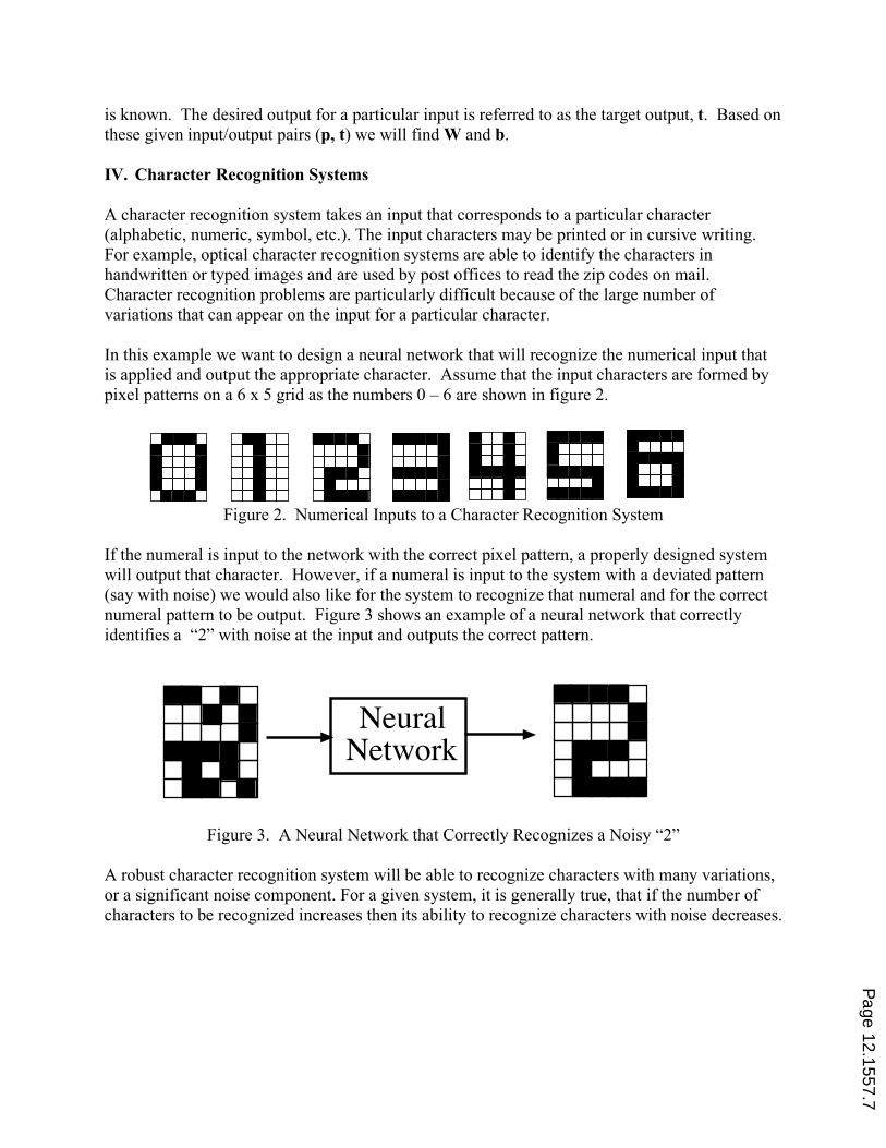
In this example we want to design a neural network that will recognize the numerical input that

is applied and output the appropriate character. Assume that the input characters are formed by

pixel patterns on a 6 x 5 grid as the numbers 0 – 6 are shown in figure 2.

Figure 2. Numerical Inputs to a Character Recognition System

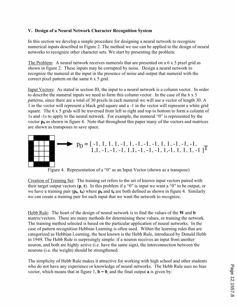
If the numeral is input to the network with the correct pixel pattern, a properly designed system

will output that character. However, if a numeral is input to the system with a deviated pattern

(say with noise) we would also like for the system to recognize that numeral and for the correct

numeral pattern to be output. Figure 3 shows an example of a neural network that correctly

identifies a “2” with noise at the input and outputs the correct pattern.

Figure 3. A Neural Network that Correctly Recognizes a Noisy “2”

A robust character recognition system will be able to recognize characters with many variations,

or a significant noise component. For a given system, it is generally true, that if the number of

characters to be recognized increases then its ability to recognize characters with noise decreases.

Neural

Network

Page 12.1557.7

V. Design of a Neural Network Character Recognition System

In this section we develop a simple procedure for designing a neural network to recognize

numerical inputs described in Figure 2. The method we use can be applied to the design of neural

networks to recognize other character sets. We start by presenting the problem.

The Problem: A neural network receives numerals that are presented on a 6 x 5 pixel grid as

shown in figure 2. These inputs may be corrupted by noise. Design a neural network to

recognize the numeral at the input in the presence of noise and output that numeral with the

correct pixel pattern on the same 6 x 5 grid.

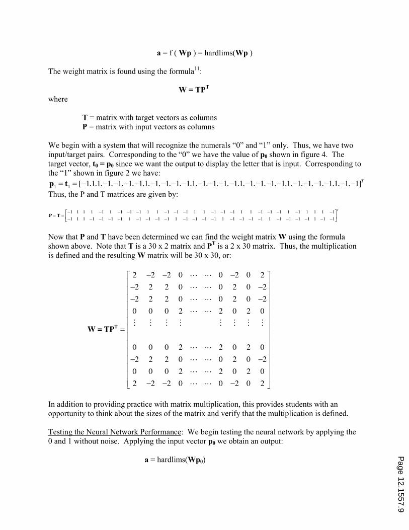
Input Vectors: As stated in section III, the input to a neural network is a column vector. In order

to describe the numeral inputs we need to form this column vector. In the case of the 6 x 5

patterns, since there are a total of 30 pixels in each numeral we will use a vector of length 30. A

1 in the vector will represent a black grid square and a -1 in the vector will represent a white grid

square. The 6 x 5 grids will be traversed from left to right and top to bottom to form a column of

1s and -1s to apply to the neural network. For example, the numeral “0” is represented by the

vector p0 as shown in figure 4. Note that throughout this paper many of the vectors and matrices

are shown as transposes to save space.

p0 = [ -1, 1, 1, 1, -1, 1, -1, -1, -1, 1, 1, -1, -1, -1, 1,1, -1, -1, -1, 1,1, -1, -1, -1, 1,-1, 1, 1, 1, -1 ]T

Figure 4. Representation of a “0” as an Input Vector (shown as a transpose)

Creation of Training Set: The training set refers to the set of known input vectors paired with

their target output vectors (p, t). In this problem if a “0” is input we want a “0” to be output, or

we have a training pair (p0, t0) where p0 and t0 are both defined as shown in figure 4. Similarly

we can create a training pair for each input that we want the network to recognize.

Hebb Rule: The heart of the design of neural network is to find the values of the W and b

matrix/vectors. There are many methods for determining these values, or training the network.

The training method selected is based on the particular application of neural networks. In the

case of pattern recognition Hebbian Learning is often used. Within the learning rules that are

categorized as Hebbian Learning, the best known is the Hebb Rule, introduced by Donald Hebb

in 1949. The Hebb Rule is surprisingly simple: if a neuron receives an input from another

neuron, and both are highly active (i.e. have the same sign), the interconnection between the

neurons (i.e. the weight) should be strengthened.

The simplicity of Hebb Rule makes it attractive for working with high school and other students

who do not have any experience or knowledge of neural networks. The Hebb Rule uses no bias

vector, which means that in figure 1, b = 0, and the final output a is given by:

Page 12.1557.8

a = f ( Wp ) = hardlims(Wp )

The weight matrix is found using the formula11

:

W = TPT

where

T = matrix with target vectors as columns

P = matrix with input vectors as columns

We begin with a system that will recognize the numerals “0” and “1” only. Thus, we have two

input/target pairs. Corresponding to the “0” we have the value of p0 shown in figure 4. The

target vector, t0 = p0 since we want the output to display the letter that is input. Corresponding to

the “1” shown in figure 2 we have:

p1= t

1= [!1,1,1,!1,!1,!1,!1,1,!1,!1,!1,!1,1,!1,!1,!1,!1,1,!1,!1,!1,!1,1,!1,!1,!1,!1,1,!1,!1]

T

Thus, the P and T matrices are given by:

P = T =!1 1 1 1 !1 1 !1 !1 !1 1 1 !1 !1 !1 1 1 !1 !1 !1 1 1 !1 !1 !1 1 !1 1 1 1 !1

!1 1 1 !1 !1 !1 !1 1 !1 !1 !1 !1 1 !1 !1 !1 !1 1 !1 !1 !1 !1 1 !1 !1 !1 !1 1 !1 !1

"

#$

%

&'

T

Now that P and T have been determined we can find the weight matrix W using the formula

shown above. Note that T is a 30 x 2 matrix and PT is a 2 x 30 matrix. Thus, the multiplication

is defined and the resulting W matrix will be 30 x 30, or:

W = TPT=

2 !2 !2 0 ! ! 0 !2 0 2

!2 2 2 0 ! ! 0 2 0 !2

!2 2 2 0 ! ! 0 2 0 !2

0 0 0 2 ! ! 2 0 2 0

" " " " " " " "

0 0 0 2 ! ! 2 0 2 0

!2 2 2 0 ! ! 0 2 0 !2

0 0 0 2 ! ! 2 0 2 0

2 !2 !2 0 ! ! 0 !2 0 2

"

#

$$$$$$$$$$$$$$

%

&

''''''''''''''

In addition to providing practice with matrix multiplication, this provides students with an

opportunity to think about the sizes of the matrix and verify that the multiplication is defined.

Testing the Neural Network Performance: We begin testing the neural network by applying the

0 and 1 without noise. Applying the input vector p0 we obtain an output:

a = hardlims(Wp0)

Page 12.1557.9

which we find to be equal to the target vector t0. Similarly, we find that if we apply the p1

vector, as an input the t1 target vector is output. Again the student will have a chance to practice

matrix multiplication.

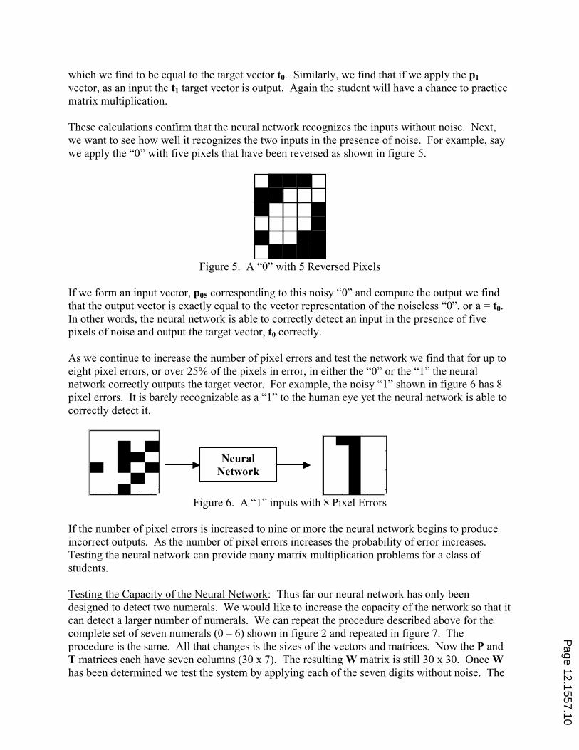
These calculations confirm that the neural network recognizes the inputs without noise. Next,

we want to see how well it recognizes the two inputs in the presence of noise. For example, say

we apply the “0” with five pixels that have been reversed as shown in figure 5.

Figure 5. A “0” with 5 Reversed Pixels

If we form an input vector, p05 corresponding to this noisy “0” and compute the output we find

that the output vector is exactly equal to the vector representation of the noiseless “0”, or a = t0.

In other words, the neural network is able to correctly detect an input in the presence of five

pixels of noise and output the target vector, t0 correctly.

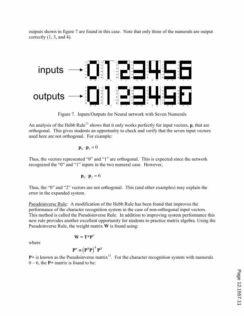
As we continue to increase the number of pixel errors and test the network we find that for up to

eight pixel errors, or over 25% of the pixels in error, in either the “0” or the “1” the neural

network correctly outputs the target vector. For example, the noisy “1” shown in figure 6 has 8

pixel errors. It is barely recognizable as a “1” to the human eye yet the neural network is able to

correctly detect it.

Figure 6. A “1” inputs with 8 Pixel Errors

If the number of pixel errors is increased to nine or more the neural network begins to produce

incorrect outputs. As the number of pixel errors increases the probability of error increases.

Testing the neural network can provide many matrix multiplication problems for a class of

students.

Testing the Capacity of the Neural Network: Thus far our neural network has only been

designed to detect two numerals. We would like to increase the capacity of the network so that it

can detect a larger number of numerals. We can repeat the procedure described above for the

complete set of seven numerals (0 – 6) shown in figure 2 and repeated in figure 7. The

procedure is the same. All that changes is the sizes of the vectors and matrices. Now the P and

T matrices each have seven columns (30 x 7). The resulting W matrix is still 30 x 30. Once W

has been determined we test the system by applying each of the seven digits without noise. The

Neural

Network

Page 12.1557.10

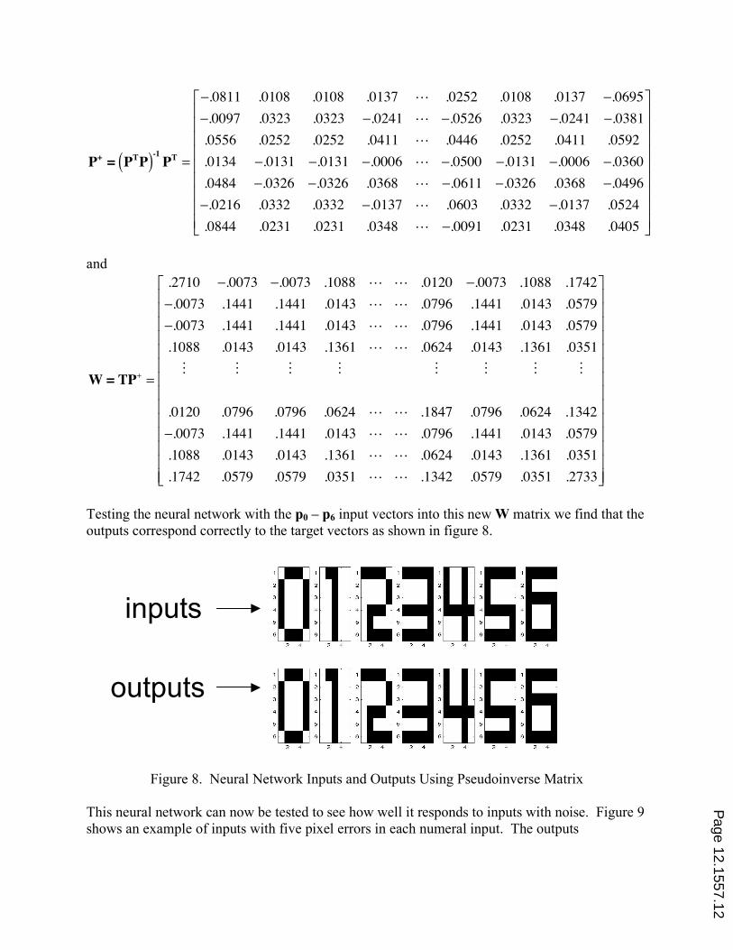
outputs shown in figure 7 are found in this case. Note that only three of the numerals are output

correctly (1, 3, and 4).

Figure 7. Inputs/Outputs for Neural network with Seven Numerals

An analysis of the Hebb Rule11

shows that it only works perfectly for input vectors, p, that are

orthogonal. This gives students an opportunity to check and verify that the seven input vectors

used here are not orthogonal. For example:

p0!p

1= 0

Thus, the vectors represented “0” and “1” are orthogonal. This is expected since the network

recognized the “0” and “1” inputs in the two numeral case. However,

p0!p

2= 6

Thus, the “0” and “2” vectors are not orthogonal. This (and other examples) may explain the

error in the expanded system.

Pseudoinverse Rule: A modification of the Hebb Rule has been found that improves the

performance of the character recognition system in the case of non-orthogonal input vectors.

This method is called the Pseudoinverse Rule. In addition to improving system performance this

new rule provides another excellent opportunity for students to practice matrix algebra. Using the

Pseudoinverse Rule, the weight matrix W is found using:

W = T*P+

where

P+ = PTP( )-1

PT

P+ is known as the Pseudoinverse matrix11

. For the character recognition system with numerals

0 – 6, the P+ matrix is found to be:

inputs

outputs

Page 12.1557.11

P+= P

TP( )

-1

PT=

!.0811 .0108 .0108 .0137 ! .0252 .0108 .0137 !.0695

!.0097 .0323 .0323 !.0241 ! !.0526 .0323 !.0241 !.0381

.0556 .0252 .0252 .0411 ! .0446 .0252 .0411 .0592

.0134 !.0131 !.0131 !.0006 ! !.0500 !.0131 !.0006 !.0360

.0484 !.0326 !.0326 .0368 ! !.0611 !.0326 .0368 !.0496

!.0216 .0332 .0332 !.0137 ! .0603 .0332 !.0137 .0524

.0844 .0231 .0231 .0348 ! !.0091 .0231 .0348 .0405

"

#

$$$$$$$$$

%

&

'''''''''

and

W = TP+=

.2710 !.0073 !.0073 .1088 ! ! .0120 !.0073 .1088 .1742

!.0073 .1441 .1441 .0143 ! ! .0796 .1441 .0143 .0579

!.0073 .1441 .1441 .0143 ! ! .0796 .1441 .0143 .0579

.1088 .0143 .0143 .1361 ! ! .0624 .0143 .1361 .0351

" " " " " " " "

.0120 .0796 .0796 .0624 ! ! .1847 .0796 .0624 .1342

!.0073 .1441 .1441 .0143 ! ! .0796 .1441 .0143 .0579

.1088 .0143 .0143 .1361 ! ! .0624 .0143 .1361 .0351

.1742 .0579 .0579 .0351 ! ! .1342 .0579 .0351 .2733

"

#

$$$$$$$$$$$$$$

%

&

''''''''''''''

Testing the neural network with the p0 – p6 input vectors into this new W matrix we find that the

outputs correspond correctly to the target vectors as shown in figure 8.

Figure 8. Neural Network Inputs and Outputs Using Pseudoinverse Matrix

This neural network can now be tested to see how well it responds to inputs with noise. Figure 9

shows an example of inputs with five pixel errors in each numeral input. The outputs

inputs

outputs

Page 12.1557.12

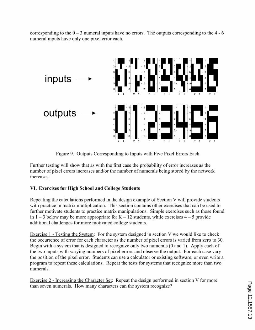
corresponding to the 0 – 3 numeral inputs have no errors. The outputs corresponding to the 4 - 6

numeral inputs have only one pixel error each.

Figure 9. Outputs Corresponding to Inputs with Five Pixel Errors Each

Further testing will show that as with the first case the probability of error increases as the

number of pixel errors increases and/or the number of numerals being stored by the network

increases.

VI. Exercises for High School and College Students

Repeating the calculations performed in the design example of Section V will provide students

with practice in matrix multiplication. This section contains other exercises that can be used to

further motivate students to practice matrix manipulations. Simple exercises such as those found

in 1 – 3 below may be more appropriate for K – 12 students, while exercises 4 – 5 provide

additional challenges for more motivated college students.

Exercise 1 - Testing the System: For the system designed in section V we would like to check

the occurrence of error for each character as the number of pixel errors is varied from zero to 30.

Begin with a system that is designed to recognize only two numerals (0 and 1). Apply each of

the two inputs with varying numbers of pixel errors and observe the output. For each case vary

the position of the pixel error. Students can use a calculator or existing software, or even write a

program to repeat these calculations. Repeat the tests for systems that recognize more than two

numerals.

Exercise 2 - Increasing the Character Set: Repeat the design performed in section V for more

than seven numerals. How many characters can the system recognize?

inputs

outputs

Page 12.1557.13

Exercise 3 - ABC Character Recognition: Design a neural network to recognize the letters A, B,

and C.

Exercise 4 – Alternate Character Sets: Have students create their own character set by writing on

a grid. Design a character recognition system for this new character set.

Exercise 5 - Create an orthogonal character set: Modify the character set in exercise 3 so that the

characters are orthogonal. Compare the performance of this system to the one in exercise 3.

Many similar exercises can be created. Once a student understands the concepts they may invent

their own exercises.

VII. Summary and Conclusions

This paper represents the third part in a continuing project of developing methods for improving

the teaching and learning of mathematical concepts for engineering students. The focus of this

paper is on teaching basic matrix operations and applying them to design a simple neural

network for character recognition. The procedure for carrying out this design is presented, and a

number of exercises that can be performed by college freshmen and advanced K-12 students are

given. The authors contend that these applications will motivate students to practice matrix

operations which otherwise may seem tedious, and to further motivate them to focus on their

mathematics courses. The educational philosophy behind the methods and applications

presented in this paper is based on the "computation-to-abstraction" sequencing of teaching

linear algebra to engineering students, as opposed to the "abstraction-to-computation"

approach16

.

Regarding K-12 students, the authors suggest that a collaborative effort of experienced teachers

in biology, physics and mathematics is required to produce good results and to benefit the

students.

The authors are now testing the practice of teaching the concept of infinity, as described in

reference 7. In the upcoming years, the authors will be testing the ideas of teaching the topics of

number theory, presented in reference 8 and relevant to data security. In the sequel, the authors

will test the methods and exercises described in this paper, to assess their effect on student

learning.

References

1. Proceedings of the 2006 ASEE Annual Conference, Chicago, Illinois, June 2006.

2. van Alphen, Deborah K., and Katz Sharlene, A Study of Predictive Factors for Success in Electrical

Engineering, Proceedings of the 2001 ASEE Annual Conference.

3. Buechler, Dale. "Mathematical Background versus Success in Electrical Engineering," Proceedings of the 2004

ASEE Annual Conference.

Page 12.1557.14

4. Carpenter, Jenna; and Schroeder, Bernd S. W. "Mathematical Support for an Integrated Engineering

Curriculum", Proceedings of the 1999 ASEE Annual Conference.

5. Buechler, Dale, and Papadopoulus, Chris. "Initial Results from a Math Centered Engineering Applications

Course", Proceedings of the 2006 ASEE Annual Conference.

6. Douglas Josh, Iversen Eric, and Kaliyandurg Chitra. "Engineering in the K-12 Classroom: an Analysis of

Current Practices and Guidelines for Future," ASEE Engineering K-12 Centre, November 2004,

http://www.engineeringk12.org/Engineering_in_the_K-12_Classroom.pdf.

7. Klass-Tsirulnikov Bella and Katz Sharlene, "The Concept of Infinity from K-12 to Undergraduate Courses",

Proceedings of the 2006 ASEE Annual Conference, Chicago, Illinois, June 2006.

8. Klass-Tsirulnikov Bella and Katz Sharlene, "Prime Numbers and the Totient Function: the First Step to

Cryptography I the K-12 Classroom," Proceedings of the 5th Annual ASEE Global Colloquium on Engineering

Education, Rio de Janeiro, Brazil, October 2006.

9. Lay, David C., "Linear Algebra and Its Applications," 2nd edition .Addison Wesley, New York,1997.

10. Kolman, B. and D. Hill, "Introductory Linear Algebra with Applications," Prentice-Hall, Englewood Cliffs,

New Jersey, 2001.

11. Hagan, Martin T. , Howard B. Demuth, and Mark Beale, "Neural Network Design," PWS Publishing Company,

Boston, 1996.

12. Picton, Phil, "Neural Networks," 2nd ed., PALGRAVE, New York, 2000.

13. Bishop, Christopher M., "Neural Networks for Pattern Recognition," Oxford University Press, Oxford, 1996.

14. Fausett, Laurene, "Fundamentals of Neural Networks," Prentice Hall, Upper Saddle River, New Jersey, 1994.

15. Haykin, Simon, "Neural Networks," Prentice Hall, Upper Saddle River, New Jersey, 1999.

16. Klapsinou, Alkistis, and Gray, Eddie, "The Intricate Balance between Abstract and Concrete in Linear

Algebra", Proceedings of the 23rd International Conference of the Psychology of Mathematical Education (Ed.

O. Zaslavsky), Vol. 3, pp. 153-160, Haifa, Israel, 1999.

Page 12.1557.15