On fundamental groups related to degeneratable surfaces: conjectures and examples
29
arXiv:1106.5636v1 [math.AG] 28 Jun 2011 ON FUNDAMENTAL GROUPS RELATED TO DEGENERATABLE SURFACES: CONJECTURES AND EXAMPLES MICHAEL FRIEDMAN AND MINA TEICHER 1 Abstract. We argue that for a smooth surface S, considered as a ramified cover over CP 2 , branched over a nodal-cuspidal curve B ⊂ CP 2 , one could use the structure of the fundamental group of the complement of the branch curve π1(CP 2 - B) to understand other properties of the surface and its degeneration and vice-versa. In this paper, we look at embedded-degeneratable surfaces - a class of surfaces admitting a planar degeneration with a few combinatorial conditions imposed on its degeneration. We close a conjecture of Teicher on the virtual solvability of π1(CP 2 - B) for these surfaces and present two new conjectures on the structure of this group, regarding non-embedded- degeneratable surfaces. We prove two theorems supporting our conjectures, and show that for CP 1 × Cg , where Cg is a curve of genus g, π1(CP 2 - B) is a quotient of an Artin group associated to the degeneration. Contents 1. Introduction 1 2. Degenerations and fundamental groups 3 2.1. Notations for planar degeneration 3 2.2. Conditions on the planar degeneration 6 2.3. Necessary condition on π 1 (C 2 − B) 7 2.4. Proof of the main theorem 9 3. Non simply connected scrolls 14 3.1. Background on Braid Monodromy Factorization 15 3.2. The fundamental group related to CP 1 × C 1 18 3.3. The fundamental group related to CP 1 × C g ,g> 1 24 3.4. The fundamental group of the Galois cover of CP 1 × C g 27 References 28 1. Introduction Given a smooth algebraic projective variety X, one of the main techniques used to obtain in- formation on X is to degenerate it to a union of “simpler” varieties. The “simplest” degeneration can be thought as the degeneration of X to a union of dim X–planes, and one would like to use the combinatorial data induced from this arrangement of planes in order to find (or bound) certain invariants of X. When dim X = 1, one would like to degenerate the curve into a line arrangement with only nodes as the singularities. This has been thoroughly investigated. For example, it is known that any smooth plane curve can be degenerated into a union of lines. However, the situation for a curve in CP n ,n> 2 is completely different as there are, for example, smooth curves in CP 3 which cannot be degenerated into a line arrangement with only double points (see [15]). 1 This work is partially supported by the Emmy Noether Research Institute for Mathematics (center of the Minerva Foundation of Germany). 1
Transcript of On fundamental groups related to degeneratable surfaces: conjectures and examples
arX
iv:1
106.
5636
v1 [
mat
h.A
G]
28
Jun
2011
ON FUNDAMENTAL GROUPS RELATED TO DEGENERATABLE SURFACES:
CONJECTURES AND EXAMPLES
MICHAEL FRIEDMAN AND MINA TEICHER1
Abstract. We argue that for a smooth surface S, considered as a ramified cover over CP2, branchedover a nodal-cuspidal curve B ⊂ CP2, one could use the structure of the fundamental group of thecomplement of the branch curve π1(CP2 −B) to understand other properties of the surface and itsdegeneration and vice-versa. In this paper, we look at embedded-degeneratable surfaces - a classof surfaces admitting a planar degeneration with a few combinatorial conditions imposed on itsdegeneration. We close a conjecture of Teicher on the virtual solvability of π1(CP2
− B) for thesesurfaces and present two new conjectures on the structure of this group, regarding non-embedded-degeneratable surfaces. We prove two theorems supporting our conjectures, and show that forCP1
× Cg, where Cg is a curve of genus g, π1(CP2 −B) is a quotient of an Artin group associatedto the degeneration.
Contents
1. Introduction 12. Degenerations and fundamental groups 32.1. Notations for planar degeneration 32.2. Conditions on the planar degeneration 62.3. Necessary condition on π1(C2 −B) 72.4. Proof of the main theorem 93. Non simply connected scrolls 143.1. Background on Braid Monodromy Factorization 153.2. The fundamental group related to CP1 × C1 183.3. The fundamental group related to CP1 × Cg, g > 1 24
3.4. The fundamental group of the Galois cover of CP1 × Cg 27References 28
1. Introduction
Given a smooth algebraic projective variety X, one of the main techniques used to obtain in-formation on X is to degenerate it to a union of “simpler” varieties. The “simplest” degenerationcan be thought as the degeneration of X to a union of dimX–planes, and one would like to usethe combinatorial data induced from this arrangement of planes in order to find (or bound) certaininvariants of X.
When dimX = 1, one would like to degenerate the curve into a line arrangement with onlynodes as the singularities. This has been thoroughly investigated. For example, it is known thatany smooth plane curve can be degenerated into a union of lines. However, the situation for acurve in CPn, n > 2 is completely different as there are, for example, smooth curves in CP3 whichcannot be degenerated into a line arrangement with only double points (see [15]).
1This work is partially supported by the Emmy Noether Research Institute for Mathematics (center of the MinervaFoundation of Germany).
1
2 M. FRIEDMAN, M. TEICHER
When dimX = 2, the problem of investigating projective surfaces in terms of their degenerationto a union of planes has only been investigated partially (see, for example, Zappa’s papers from the1940’s [36] and [11] for a survey on this topic; see also [19] for degeneration of surfaces in CP3). Also,one should allow the existence of more complicated singularities in order to obtain degenerations.But there is another method to extract information on the surface, which is to consider it as abranched cover of the projective plane CP2 with respect to a generic projection. The motivationfor this point of view is Chisini’s conjecture (recently proved by Kulikov [17],[18]): Let B be thebranch curve of generic projection π : S → CP2 of degree at least 5. Then (S, π) is uniquelydetermined by the pair (CP2, B). Moreover, if two surfaces S1 and S2 are deformation equivalent,then their branch curves B1 and B2 are isotopic. Thus, if the fundamental group π1(C2 − B1) isnot isomorphic to π1(C2−B2) then the surfaces are not deformation equivalent. This gives anothermotivation for considering S in terms of its branch curve.
Therefore, it is reasonable to combine the two methods outlined above, i.e., investigating aprojective surface S and its degeneration S0 by looking at their branch curves B and B0. Explic-itly, we want to find the relations between the combinatorics of the planar degeneration and thefundamental group π1(C2 −B).
Several works were done in this direction: for different embeddings of CP1×CP1, for the Veronesesurface Vn ([29], [30] for Vn, n ≥ 3 and [37] for V2), for the Hirzebruch surfaces F1,(a,b) and F2,(2,2)
([14], [6]), for K3 surfaces ([13]), for a few toric surfaces and for CP1 × T (where T is a complextorus. see [7]). For each surface in this list one can associate a graph T to the degenerated surface.In all of the examples mentioned above the fundamental group π1(C2−B) is either a quotient of anassociated Artin group A(T ) (except the Veronese surface V2 ⊂ CP5) or a quotient of a subgroup
of A(T )× A(T ) (where A(T ) is a quotient of A(T ) by a single relation. For example, when T is atree with maximum valence 3, then A(T ) is isomorphic to the braid group Bn, where n = degreeof the surface). In particular, once the embedding of the surface in a projective space is “ampleenough”, the structure of π1(C2 − B) is of the mentioned second type. Thus, a natural questionrises: what are the sufficient conditions on the degeneration such that π1(C2−B) will be isomorphic
to a quotient of a subgroup of A(T )× A(T )? One of the goals of this paper is to give the conditionsunder which the fundamental group has this desired structure. These conditions are in a form ofa local–global condition: if there are enough singular points in the degenerated surface satisfyinga certain local condition, then the fundamental group is isomorphic to the quotient. Under theseconditions, the conjecture posed in [34] regarding the virtual-solvability of the above fundamentalgroup is proven.
Another main result deals with a new set of examples, not satisfying these conditions. Thesurfaces CP1 × Cg, where Cg is a curve of genus g ≥ 1, are studied, and for g ≥ 1 the abovefundamental group is computed. These new examples are essential for the second goal of thispaper: to understand better these groups for non-simply connected surfaces.
The structure of the paper is as follows. Section 2 examines the structure of the fundamentalgroup. Subsections 2.1 and 2.2 introduce the main definitions and restrictions on the degeneration.We then state one of the main theorems in Subsection 2.3: that under a certain condition, there
is an epimorphism from B(2)n to π1(C2 − B). We also present two conjectures on the structure of
π1(C2−B) when the condition does not hold (see Conjectures 2.25 and 2.26). In Subsection 2.4 weprove the main theorem from Subsection 2.3. In Section 3 we prove another main theorem, wherewe compute the group Gg = π1(C2−Bg), where Bg is the branch curve of CP1×Cg. We show that
Gg is (again) a quotient of A(T ), and also compute π1((CP1 ×Cg)Gal) – the fundamental group of
the Galois cover of CP1 × Cg.Acknowledgements: We thank Alberto Calabri and Ciro Ciliberto for refereing the first author
to their paper [9] and for fruitful discussions during the “School (and Workshop) on the Geometryof Special Varieties” which was held at 2007 at the IRST, Fondazione Bruno Kessler in Povo
ON FUNDAMENTAL GROUPS RELATED TO DEGENERATABLE SURFACES 3
(Trento). We also would like to thank Christian Liedtke and Robert Schwartz for stimulating talksand important discussions.
2. Degenerations and fundamental groups
In this section we examine the structure of the fundamental group of the complement of thebranch curve, under some assumptions. Subsection 2.1 introduces the main definitions and nota-tions. We state the main theorem on the structure of the fundamental group of the complement ofthe branch curve in C2, under certain conditions, in Subsection 2.3 and also present two conjectureson the structure of the fundamental group regarding surfaces which do not satisfy the desired con-ditions. The virtual–solvability of this fundamental group is discussed in Subsection 2.3.1, togetherwith the class of surfaces satisfying the desired conditions. In Subsection 2.4 we prove the maintheorem.
2.1. Notations for planar degeneration. We begin with a few definitions.
Definition 2.1. (i) Degeneration: Let ∆ be the complex unit disc. A degeneration of surfaces,parametrized by ∆ is a proper and flat morphism ρ : S → ∆ (where S is a 3–dim variety)such that each fibre St = ρ−1(t), t 6= 0 (where 0 is the closed point of ∆), is a smooth,irreducible, projective surface. The fiber S0 is called the central fiber. A degenerationρ : S → ∆ is said to be embedded in CPr if there is an inclusion i : S → ∆ × CPr and,when denoting the projection p1 : ∆× CPr → ∆, then p1i = ρ.
(ii) Planar degeneration: When the central fiber S0 in the above embedded degeneration is aunion of planes, then we call the degeneration a planar degeneration. A survey on degener-atable surfaces can be found in [11]. Examples of planar degenerations can be found in [9](for scrolls), [23] (for Hirzebruch surfaces), [28] (for veronese surfaces), [21] (for CP1×CP1).
(iii) Regeneration: The regeneration methods are actually, locally, the reverse process of thedegeneration method. In this article it is used as a generic name for finding a degenerationρ : S → ∆ when the central fiber S0 is given. In fact, one can deduce what is the effect ofa regeneration on the corresponding branch curves. The regeneration rules (see Subsection3.1.2) explain the effect of the regeneration on the braid monodromy factorization (seeSubsection 3.1) of the branch curves of the fibers.
(iv) Local fundamental group: Given a planar degeneration ρ : S → ∆, denote by Bt the branchcurve of a generic projection of St to CP
2 (such that the center of projection is the samefor every t). Given a singular point p ∈ B0 choose a small neighborhood U of p suchthat U ∩ Sing(B0) = {p}. Since S0 is a planar degeneration, there are lines ℓi such thatU ∩B0 = ∪(U ∩ ℓi), such that ∩ℓi = {p}. Assume that for the branch curve Bt of generalfiber St,t 6= 0, we have that limt→0(U ∩ Sing(Bt)) = {p}. The local fundamental group of pis defined as π1(U −Bt) and we denote it by Gp.
Let S1 ⊂ CPN be a smooth surface of degree n which admits a planar degeneration ρ : S → ∆,and let f : CPN → CP2 be the generic projection w.r.t. St, for every t. We denote by R theramification curve of S1 and by B ⊂ CP2 its branch curve with respect to a generic projectionπ.= f |S1
: S1 → CP2. Also, let G.= π1(CP
2 −B).We denote by S0 the planar degeneration of S1 (the central fiber of ρ), i.e. S0 is a union of
planes. Let
S0 =n⋃
i=1
Πi
such that each Πi is a plane.
Notation 2.2. n = degS0 = degS1.

4 M. FRIEDMAN, M. TEICHER
Let π0.= f |S0
: S0 → CP2 be the generic projection of S0 to CP2. In this case, the ramificationcurve also degenerates into a union of ℓ lines
R0 =ℓ⋃
i=1
Li,
and thus the degenerated branch curve is of the form
π0(R0) = B0 =
ℓ⋃
i=1
li,
where li = π0(Li).
Notation 2.3. ℓ = degR0 = degB0.
Since R0 is an arrangement of lines in CPN , these lines can intersect each other.
Notation 2.4. m′ = the number of points {Pi}m′
i=1 which lie on more than one line Lj.
For a point x ∈ Li (or x ∈ li) let v(x) be the number of distinct lines in R0 (or B0) on which x
lies. For example, if x ∈ {Pi}m′
i=1, then v(x) > 1.
Notation 2.5. Denote by P = {x ∈ B0 : v(x) > 1}, and let pi = π0(Pi) ∈ B0 (note that
v(pi) = v(Pi)). Denote P ′ .= {pi}m′
i=1.
Remark 2.6. Note also that P ′ = {pi}m′
i=1 P , since there are points (called parasitic intersection
points; see the explanation in Subsection 2.4.1) which are in P but not in {pi}m′
i=1.
Notation 2.7. Recall that R0 = ∪Li. Define the set of lines
M.= {Li ∈ R0 : there is only one point x ∈ Li such that v(x) > 1}.
For each l ∈M , choose a point yl ∈ l s.t. v(yl) = 1. Denote
Y.= {yl}l∈M ;
the set of points is called the set of 2–point.
We recall the definition of Bn, since the local fundamental group of many of the singular pointsof B0 is strongly related to this group.
Definition 2.8. (1) Let X,Y be two half-twists in the braid group Bn = Bn(D,K) (see Subsection3.1 for the notation D,K). We say that X,Y are transversal if they are defined by two simplepaths ξ, η which intersect transversally in one point different from their ends.(2) Let N be the normal subgroup of Bn generated by conjugates of [X,Y ], where X,Y is atransversal pair of half-twists. Define
Bn = Bn/N.
Let x1, ..., xn−1 be the standard generators of Bn. Equivalently, we can define
Bn = Bn/〈〈[x2, x−13 x−1
1 x2x1x3]〉〉
for n > 3. Recall that we can define on Bn two natural homomorphism:(i) deg : Bn → Z s.t. deg(
∏xnii ) =
∑ni.
(ii) σ : Bn → Sn s.t. σ(xi) = (i i+ 1). For properties of Bn see, for example, [22],[31], [35].
(3) The following group plays an important role in finding a presentation of a fundamental groupof the complement of the branch curve. Define, as in [8], the group
B(2)n
.= {(x, y) ∈ Bn × Bn, deg(x) = deg(y), σ(x) = σ(y)}.
ON FUNDAMENTAL GROUPS RELATED TO DEGENERATABLE SURFACES 5
Definition 2.9. Recall that for p ∈ P ′ = {pi}m′
i=1, we denote by Gp the local fundamental group(see Definition 2.1(iv)). Define the following set:
Q.= {p ∈ {pi}
m′
i=1 : there exists an epimorphism of B(2)v(p) ։ Gp, and v(p) > 3}
and denote|Q| = m.
Thus, we have the following relations between the sets of points:
Q.= {xj}
mj=1 ⊂ P ′ .= {pi}
m′
i=1 ⊂ P.
Remark 2.10. The definition of Q is not meaningless: there are singular points p ∈ {pi}m′
i=1,v(p) > 3 which occur during the (described above) degeneration process have an epimorphism
B(2)v(p) ։ Gp, where Gp is the local fundamental group associated to p. For example, let p6 (resp.
p5) a singular point of S0 called a 6−point (resp. 5−point) which is locally an intersection of 6(resp. 5) planes at a point, whose regeneration is described at [22] [23, Definition 4.3.3] (resp. [12]).
Then Gpi is isomorphic to a quotient of B(2)i for i = 6, 5. For the 4−point p4 (s.t. its regeneration
is described at [22], [31]), we get that Gp4 ≃ B4, which is also a quotient of B(2)4 .
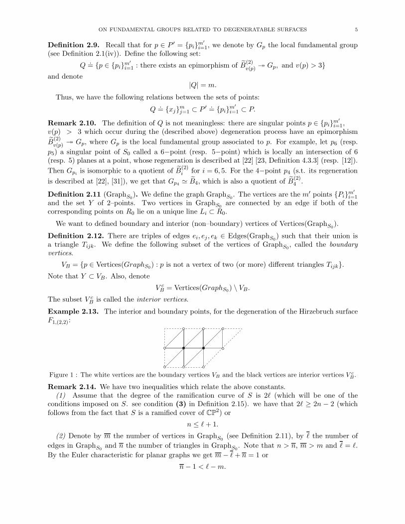
Definition 2.11 (GraphS0). We define the graph GraphS0
. The vertices are the m′ points {Pi}m′
i=1and the set Y of 2–points. Two vertices in GraphS0
are connected by an edge if both of thecorresponding points on R0 lie on a unique line Li ⊂ R0.
We want to defined boundary and interior (non–boundary) vertices of Vertices(GraphS0).
Definition 2.12. There are triples of edges ei, ej , ek ∈ Edges(GraphS0) such that their union is
a triangle Tijk. We define the following subset of the vertices of GraphS0, called the boundary
vertices.
VB = {p ∈ Vertices(GraphS0) : p is not a vertex of two (or more) different triangles Tijk}.
Note that Y ⊂ VB . Also, denote
V cB = Vertices(GraphS0
) \ VB.
The subset V cB is called the interior vertices.
Example 2.13. The interior and boundary points, for the degeneration of the Hirzebruch surfaceF1,(2,2):
Figure 1 : The white vertices are the boundary vertices VB and the black vertices are interior vertices V cB .
Remark 2.14. We have two inequalities which relate the above constants.(1) Assume that the degree of the ramification curve of S is 2ℓ (which will be one of the
conditions imposed on S. see condition (3) in Definition 2.15). we have that 2ℓ ≥ 2n − 2 (whichfollows from the fact that S is a ramified cover of CP2) or
n ≤ ℓ+ 1.
(2) Denote by m the number of vertices in GraphS0(see Definition 2.11), by ℓ the number of
edges in GraphS0and n the number of triangles in GraphS0
. Note that n > n, m > m and ℓ = ℓ.
By the Euler characteristic for planar graphs we get m− ℓ+ n = 1 or
n− 1 < ℓ−m.
6 M. FRIEDMAN, M. TEICHER
2.2. Conditions on the planar degeneration. In this subsection, we introduce the followingconditions that our projective surface S has to satisfy.
Definition 2.15. A surface S = S1 is called simply–degeneratable surface if it satisfies the fol-lowing three conditions:
Condition. (1) S admits a planar degeneration, i.e., ∃ρ : S → ∆ s.t. ρ−1(1) = S1 = S ,ρ−1(0) = S0 and S0 is a union of planes.
Condition. (2) The degeneration of S to S0 induces a degeneration of the branch curve B to B0
that satisfies the following condition: For a plane curve C ⊂ CP2, let Sing(C) be the singularities ofC w.r.t. a fixed generic projection C → CP1. Denote Sing0
.= Sing(B0), Singt = Sing(Bt), t 6= 0.
For each p ∈ Sing0 consider a small enough neighborhood Up of p as in Definition 2.1(iv). Werequire that the set Sing(B) \
⋃p∈Sing0
(Up ∩ Sing(B)) contains only simple branch points.
Condition. (3) The degeneration of the branch curves B → B0 is two-to-one (see [29],[31] forfurther details on two-to-one degenerations of branch curves).
Remark 2.16. We show that the three conditions above are independent. As we are interestedin planar degenerations, we look at the following examples when the degeneration already satisfiesCondition (1).(1) A degeneration of a smooth cubic surface in CP3 (whose branch curve is a sextic with six cusps)into a union of three planes, all of them intersecting in a line, is an example of a surface which doesnot satisfy Conditions (2), (3).(2) A degeneration of a union of three generic hyperplanes in CP3 (whose branch curve is a unionof three lines, intersecting at three different points) into a union of three hyperplanes meeting at asingle point, is an example of a degeneration that satisfies Condition (2) but not (3).(3) A degeneration of a cone over a smooth conic in CP2 into a union of two hyperplanes is anexample of a degeneration that satisfies Condition (3) but not (2).(4) An example of planar degeneration that satisfies Conditions (2), (3) is a degeneration of asmooth quadric in CP3 into a union of two hyperplanes.
We now define a fourth condition imposed on the degeneration: that every boundary vertex hasat least one interior vertex as a “neighbor” (see definition 2.12).
Definition 2.17. A surface S is called embedded–degeneratable surface if it is a simply–degeneratablesurface and it satisfies the following fourth condition:
Condition. (4) We require that for each boundary vertex p ∈ VB there exist an interior vertexpc ∈ V c
B and an edge ep ∈ Edges(GraphS0) s.t. ep connects p and pc.
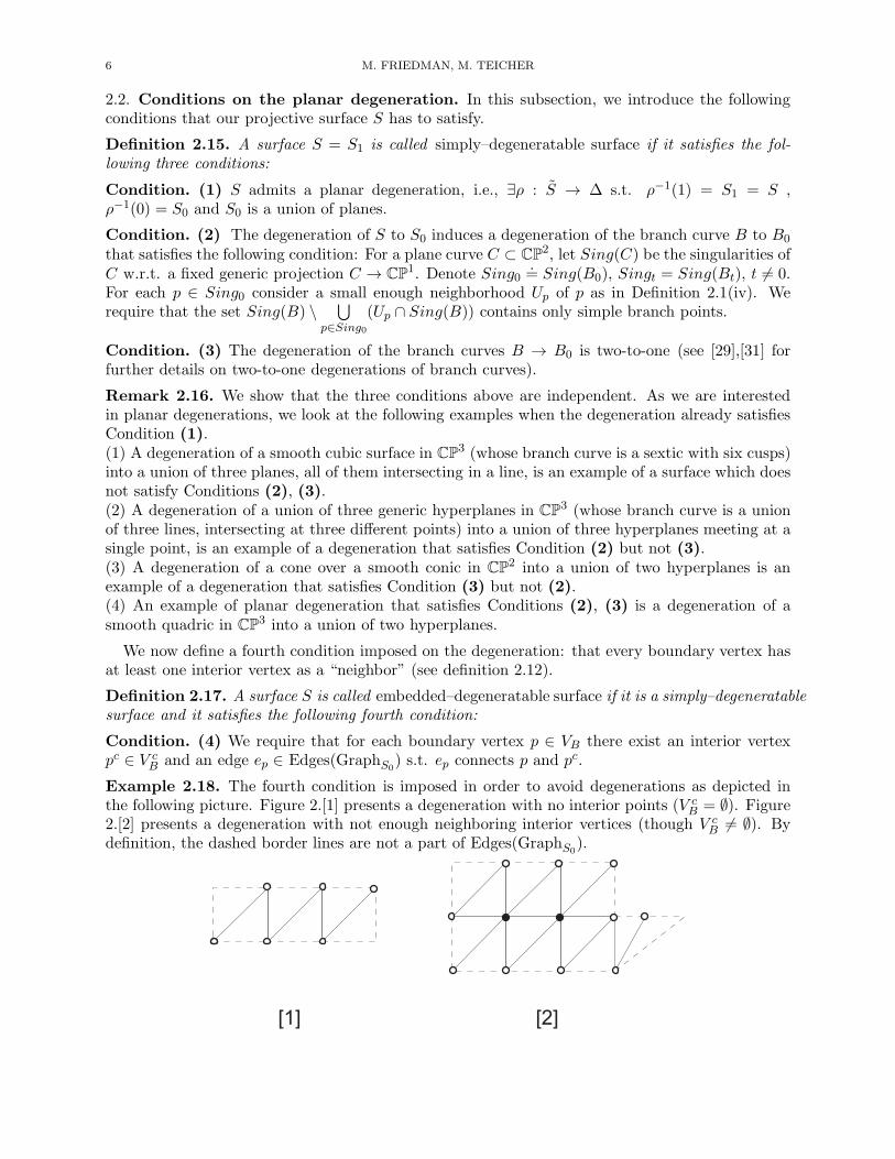
Example 2.18. The fourth condition is imposed in order to avoid degenerations as depicted inthe following picture. Figure 2.[1] presents a degeneration with no interior points (V c
B = ∅). Figure2.[2] presents a degeneration with not enough neighboring interior vertices (though V c
B 6= ∅). Bydefinition, the dashed border lines are not a part of Edges(GraphS0
).
[1] [2]
ON FUNDAMENTAL GROUPS RELATED TO DEGENERATABLE SURFACES 7
Figure 2 : Degenerations which do no satisfy Condition (4).The white vertices are the boundary vertices VB and the black vertices are interior vertices V c
B.
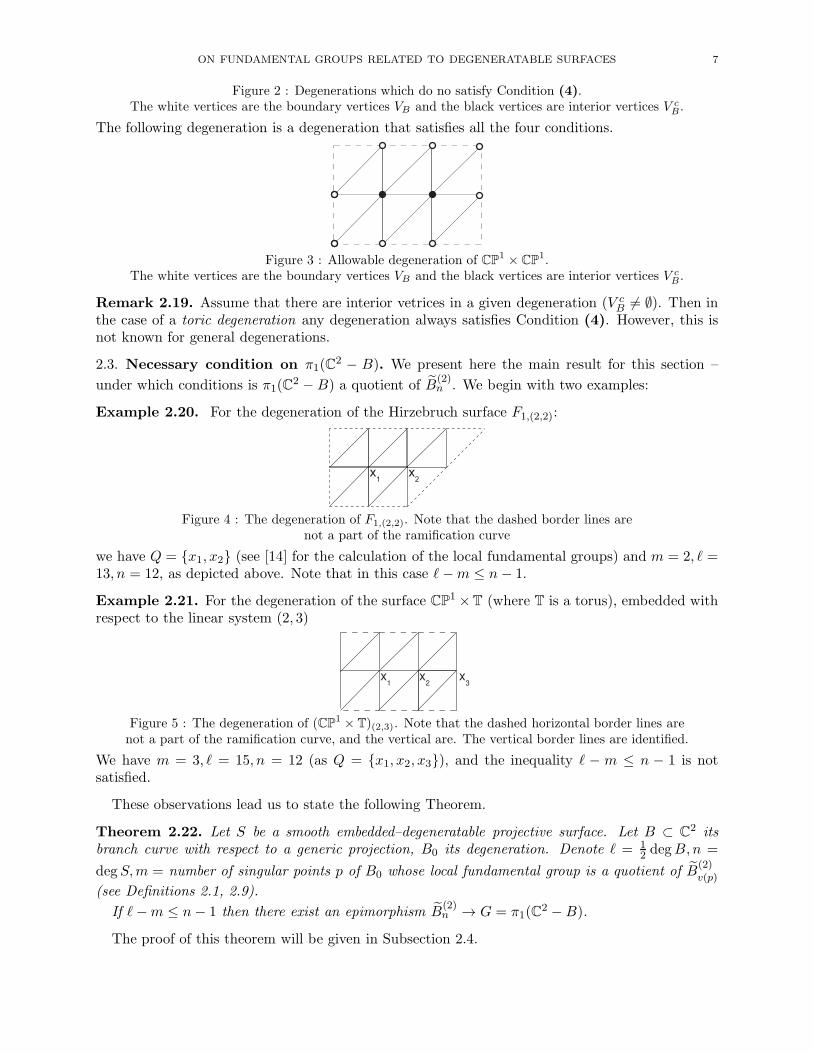
The following degeneration is a degeneration that satisfies all the four conditions.
Figure 3 : Allowable degeneration of CP1 × CP1.The white vertices are the boundary vertices VB and the black vertices are interior vertices V c
B.
Remark 2.19. Assume that there are interior vetrices in a given degeneration (V cB 6= ∅). Then in
the case of a toric degeneration any degeneration always satisfies Condition (4). However, this isnot known for general degenerations.
2.3. Necessary condition on π1(C2 − B). We present here the main result for this section –
under which conditions is π1(C2 −B) a quotient of B(2)n . We begin with two examples:
Example 2.20. For the degeneration of the Hirzebruch surface F1,(2,2):
x1
x2
Figure 4 : The degeneration of F1,(2,2). Note that the dashed border lines arenot a part of the ramification curve
we have Q = {x1, x2} (see [14] for the calculation of the local fundamental groups) and m = 2, ℓ =13, n = 12, as depicted above. Note that in this case ℓ−m ≤ n− 1.
Example 2.21. For the degeneration of the surface CP1 ×T (where T is a torus), embedded withrespect to the linear system (2, 3)
x1
x2
x3
Figure 5 : The degeneration of (CP1 × T)(2,3). Note that the dashed horizontal border lines arenot a part of the ramification curve, and the vertical are. The vertical border lines are identified.
We have m = 3, ℓ = 15, n = 12 (as Q = {x1, x2, x3}), and the inequality ℓ − m ≤ n − 1 is notsatisfied.
These observations lead us to state the following Theorem.
Theorem 2.22. Let S be a smooth embedded–degeneratable projective surface. Let B ⊂ C2 itsbranch curve with respect to a generic projection, B0 its degeneration. Denote ℓ = 1
2 degB,n =
degS,m = number of singular points p of B0 whose local fundamental group is a quotient of B(2)v(p)
(see Definitions 2.1, 2.9).
If ℓ−m ≤ n− 1 then there exist an epimorphism B(2)n → G = π1(C2 −B).
The proof of this theorem will be given in Subsection 2.4.
8 M. FRIEDMAN, M. TEICHER
Example 2.23. We give here a list of known surfaces, satisfying Theorem 2.22: CP1 × CP1 em-bedded with respect to the linear system al1 + bl2, where a, b > 1 (see [22]), the Veronese surfaceVn, n ≥ 3 (see [29], [30]), the Hirzebruch surfaces F1 (embedded with respect to the linear systemaC + bE0, where a, b > 1, C,E0 generate the Picard group of F1, see [14]) and F2 (embedded withrespect to the linear system 2C + 2E0 (see [6]), and a few families of K3 surfaces (see [13]).
Before proving the theorem, we want to review a few surfaces for which the condition in Theorem2.22 does not hold, presenting two conjectures.
For the first conjecture we need the following definition.
Definition 2.24. (1) Given an Artin group A, generated by {xi}ri=1, r > 2, we define the following
quotient:
A = A/〈〈[x2, x−13 x−1
1 x2x1x3]〉〉.
(2) Let deg be the following epimorphism: deg : A → Z s.t. deg(∏xnii ) =
∑ni. Assume there
exists an epimorphism from A to the symmetric group σ : A→ Sn. In this case, define
A(2) .= {(x, y) ∈ A× A,deg(x) = deg(y), σ(x) = σ(y)}.
The first conjecture on the structure of G = π1(C2 −B) is similar to Theorem 2.22, when Q 6= ∅but does not contain enough points.
Conjecture 2.25. For a smooth embedded-degeneratable surface S s.t. |Q| = m ≥ 1 andℓ −m > n − 1 (i.e. does not satisfy the condition in Theorem 2.22) one can associate a graph T
and an Artin group A(T ) such that G is a quotient of A(T )(2)
The condition above means that S has a planar degeneration with 2:1 degeneration of the branchcurve, whose degeneration has singular points in the set Q, but not enough. For example, See [7,Conjecture 3.7] (on the embedding of CP1 × T with respect to the linear system (m,n),m, n > 1)and [3] (for the degeneration of T× T).
We now review a few surfaces for which the set Q is empty.
Conjecture 2.26. For a simply–degeneratable surface S such that the set Q = ∅ (i.e. the degener-ation has only boundary points (see Definition 2.12)) and such that G = π1(C2 −B) has “enough”commutation relations (see Remark 2.27), we conjecture that one can associate a graph T and anArtin group A(T ) such that G is a quotient of A(T ).
Remark 2.27. Recall that G has the natural monodromy epimorphism ϕ : G→ Sn (n = deg(S)),defined by sending each generator to a transposition, describing the sheets which are exchanged.By “enough” commutation relations we mean that for a, b ∈ G such that ϕ(a), ϕ(b) are disjointtranspositions, then a, b commute.
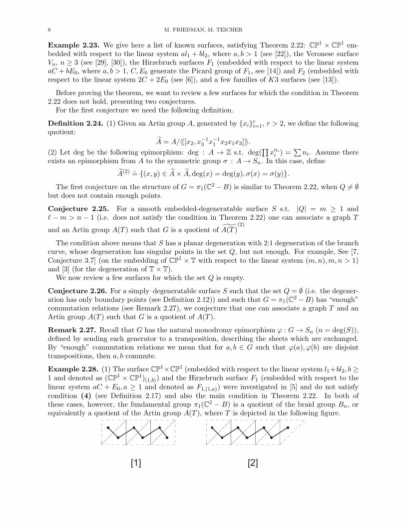
Example 2.28. (1) The surface CP1×CP1 (embedded with respect to the linear system l1+bl2, b ≥1 and denoted as (CP1 × CP1)(1,b)) and the Hirzebruch surface F1 (embedded with respect to thelinear system aC + E0, a ≥ 1 and denoted as F1,(1,a)) were investigated in [5] and do not satisfycondition (4) (see Definition 2.17) and also the main condition in Theorem 2.22. In both ofthese cases, however, the fundamental group π1(C2 − B) is a quotient of the braid group Bn, orequivalently a quotient of the Artin group A(T ), where T is depicted in the following figure.
[1] [2]
ON FUNDAMENTAL GROUPS RELATED TO DEGENERATABLE SURFACES 9
Figure 6 : The degeneration of (CP1 × CP1)(1,3) (figure [1]) and F1,(1,3) (figure [2]) and their associatedgraphs T .
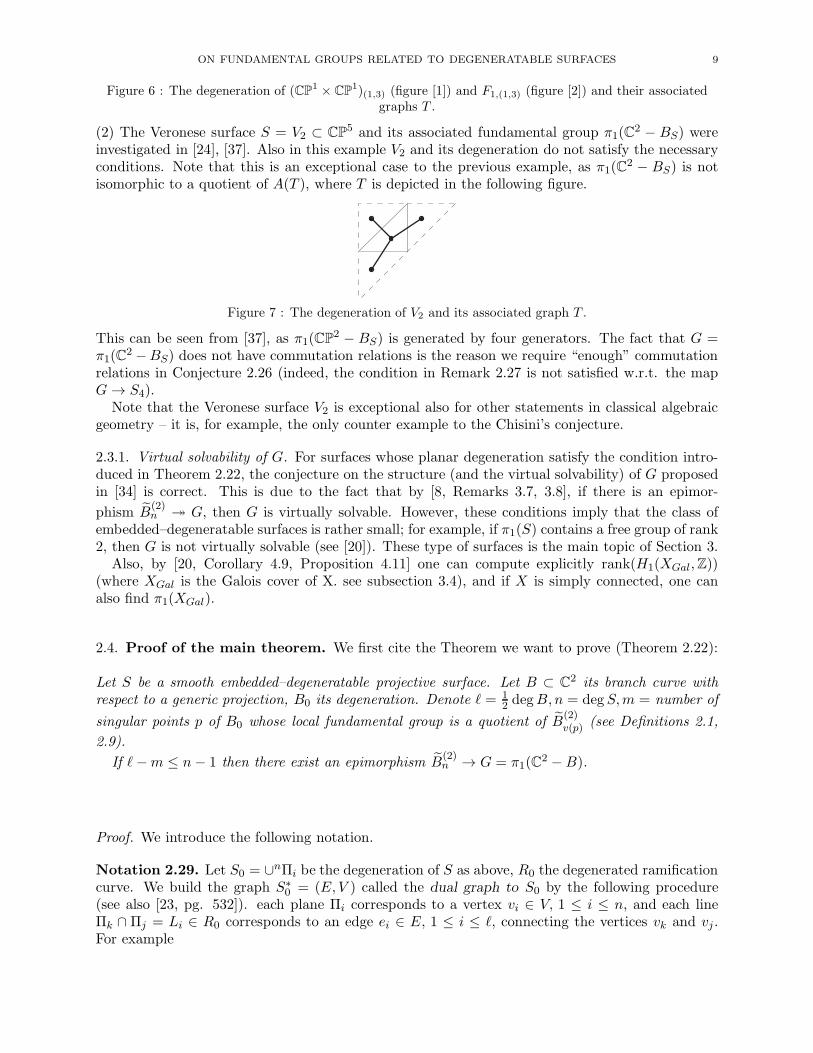
(2) The Veronese surface S = V2 ⊂ CP5 and its associated fundamental group π1(C2 − BS) wereinvestigated in [24], [37]. Also in this example V2 and its degeneration do not satisfy the necessaryconditions. Note that this is an exceptional case to the previous example, as π1(C2 − BS) is notisomorphic to a quotient of A(T ), where T is depicted in the following figure.
Figure 7 : The degeneration of V2 and its associated graph T .
This can be seen from [37], as π1(CP2 − BS) is generated by four generators. The fact that G =
π1(C2 −BS) does not have commutation relations is the reason we require “enough” commutationrelations in Conjecture 2.26 (indeed, the condition in Remark 2.27 is not satisfied w.r.t. the mapG→ S4).
Note that the Veronese surface V2 is exceptional also for other statements in classical algebraicgeometry – it is, for example, the only counter example to the Chisini’s conjecture.
2.3.1. Virtual solvability of G. For surfaces whose planar degeneration satisfy the condition intro-duced in Theorem 2.22, the conjecture on the structure (and the virtual solvability) of G proposedin [34] is correct. This is due to the fact that by [8, Remarks 3.7, 3.8], if there is an epimor-
phism B(2)n ։ G, then G is virtually solvable. However, these conditions imply that the class of
embedded–degeneratable surfaces is rather small; for example, if π1(S) contains a free group of rank2, then G is not virtually solvable (see [20]). These type of surfaces is the main topic of Section 3.
Also, by [20, Corollary 4.9, Proposition 4.11] one can compute explicitly rank(H1(XGal,Z))(where XGal is the Galois cover of X. see subsection 3.4), and if X is simply connected, one canalso find π1(XGal).
2.4. Proof of the main theorem. We first cite the Theorem we want to prove (Theorem 2.22):
Let S be a smooth embedded–degeneratable projective surface. Let B ⊂ C2 its branch curve withrespect to a generic projection, B0 its degeneration. Denote ℓ = 1
2 degB,n = degS,m = number of
singular points p of B0 whose local fundamental group is a quotient of B(2)v(p) (see Definitions 2.1,
2.9).
If ℓ−m ≤ n− 1 then there exist an epimorphism B(2)n → G = π1(C2 −B).
Proof. We introduce the following notation.
Notation 2.29. Let S0 = ∪nΠi be the degeneration of S as above, R0 the degenerated ramificationcurve. We build the graph S∗
0 = (E,V ) called the dual graph to S0 by the following procedure(see also [23, pg. 532]). each plane Πi corresponds to a vertex vi ∈ V, 1 ≤ i ≤ n, and each lineΠk ∩ Πj = Li ∈ R0 corresponds to an edge ei ∈ E, 1 ≤ i ≤ ℓ, connecting the vertices vk and vj .For example
10 M. FRIEDMAN, M. TEICHER
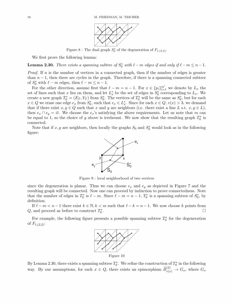
Figure 8 : The dual graph S∗
0 of the degeneration of F1,(2,2).
We first prove the following lemma:
Lemma 2.30. There exists a spanning subtree of S∗0 with ℓ−m edges if and only if ℓ−m ≤ n− 1.
Proof. If n is the number of vertices in a connected graph, then if the number of edges is greaterthan n− 1, then there are cycles in the graph. Therefore, if there is a spanning connected subtreeof S∗
0 with ℓ−m edges, then ℓ−m ≤ n− 1.
For the other direction, assume first that ℓ −m = n − 1. For x ∈ {pi}m′
i=1 we denote by Lx theset of lines such that x lies on them, and let L∗
x be the set of edges in S∗0 corresponding to Lx. We
create a new graph T ∗0 = (ET , VT ) from S∗
0 . The vertices of T∗0 will be the same as S∗
0 , but for eachx ∈ Q we erase one edge ex from S∗
0 , such that ex ∈ L∗x. Since for each x ∈ Q, v(x) > 3, we demand
that if there exist x, y ∈ Q such that x and y are neighbors (i.e. there exist a line L s.t. x, y ∈ L),then ex ∩ ey = ∅. We choose the ex’s satisfying the above requirements. Let us note that m canbe equal to 1, so the choice of y above is irrelavant. We now show that the resulting graph T ∗
0 isconnected.
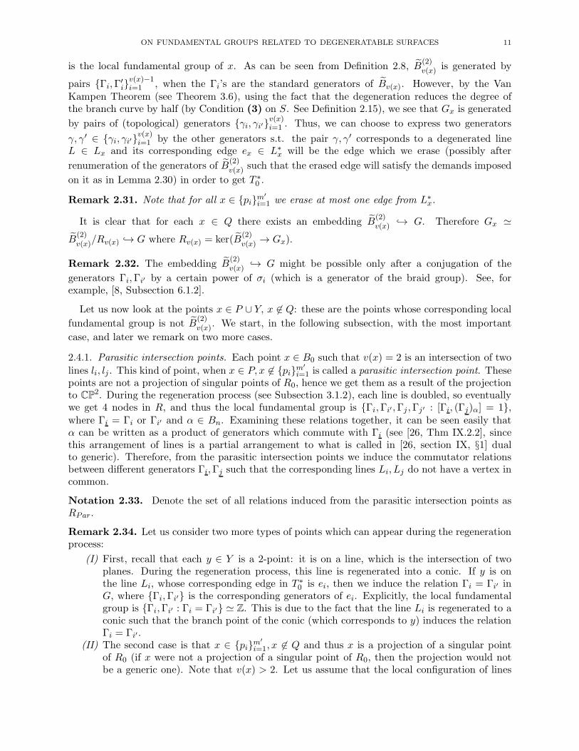
Note that if x, y are neighbors, then locally the graphs S0 and S∗0 would look as in the following
figure:
S0
xy
S0*
ex
ey
Figure 9 : local neighborhood of two vertices
since the degeneration is planar. Thus we can choose ex and ey as depicted in Figure 7 and theresulting graph will be connected. Now one can proceed by induction to prove connectedness. Notethat the number of edges in T ∗
0 is ℓ−m. Since ℓ−m = n − 1, T ∗0 is a spanning subtree of S∗
0 , bydefinition.
If ℓ−m < n− 1 there exist k ∈ N, k < m such that ℓ− k = n− 1. We now choose k points fromQ, and proceed as before to construct T ∗
0 . �
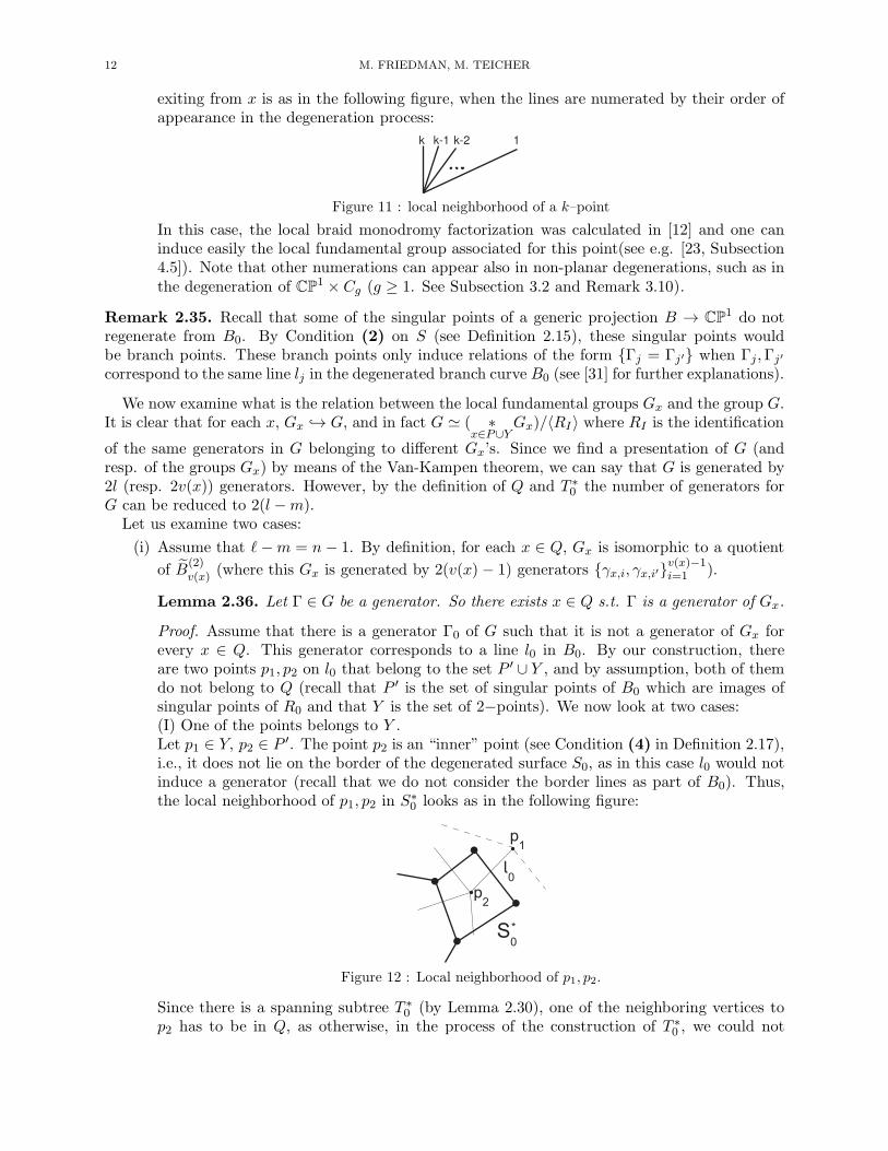
For example, the following figure presents a possible spanning subtree T ∗0 for the degeneration
of F1,(2,2):
Figure 10
By Lemma 2.30, there exists a spanning subtree T ∗0 . We refine the construction of T ∗
0 in the following
way. By our assumptions, for each x ∈ Q, there exists an epimorphism B(2)v(x) → Gx, where Gx
ON FUNDAMENTAL GROUPS RELATED TO DEGENERATABLE SURFACES 11
is the local fundamental group of x. As can be seen from Definition 2.8, B(2)v(x) is generated by
pairs {Γi,Γ′i}
v(x)−1i=1 , when the Γi’s are the standard generators of Bv(x). However, by the Van
Kampen Theorem (see Theorem 3.6), using the fact that the degeneration reduces the degree ofthe branch curve by half (by Condition (3) on S. See Definition 2.15), we see that Gx is generated
by pairs of (topological) generators {γi, γi′}v(x)i=1 . Thus, we can choose to express two generators
γ, γ′ ∈ {γi, γi′}v(x)i=1 by the other generators s.t. the pair γ, γ′ corresponds to a degenerated line
L ∈ Lx and its corresponding edge ex ∈ L∗x will be the edge which we erase (possibly after
renumeration of the generators of B(2)v(x) such that the erased edge will satisfy the demands imposed
on it as in Lemma 2.30) in order to get T ∗0 .
Remark 2.31. Note that for all x ∈ {pi}m′
i=1 we erase at most one edge from L∗x.
It is clear that for each x ∈ Q there exists an embedding B(2)v(x) → G. Therefore Gx ≃
B(2)v(x)/Rv(x) → G where Rv(x) = ker(B
(2)v(x) → Gx).
Remark 2.32. The embedding B(2)v(x) → G might be possible only after a conjugation of the
generators Γi,Γi′ by a certain power of σi (which is a generator of the braid group). See, forexample, [8, Subsection 6.1.2].
Let us now look at the points x ∈ P ∪ Y, x 6∈ Q: these are the points whose corresponding local
fundamental group is not B(2)v(x). We start, in the following subsection, with the most important
case, and later we remark on two more cases.
2.4.1. Parasitic intersection points. Each point x ∈ B0 such that v(x) = 2 is an intersection of two
lines li, lj . This kind of point, when x ∈ P, x 6∈ {pi}m′
i=1 is called a parasitic intersection point. Thesepoints are not a projection of singular points of R0, hence we get them as a result of the projectionto CP2. During the regeneration process (see Subsection 3.1.2), each line is doubled, so eventuallywe get 4 nodes in R, and thus the local fundamental group is {Γi,Γi′ ,Γj ,Γj′ : [Γi, (Γj)α] = 1},where Γi = Γi or Γi′ and α ∈ Bn. Examining these relations together, it can be seen easily thatα can be written as a product of generators which commute with Γi (see [26, Thm IX.2.2], sincethis arrangement of lines is a partial arrangement to what is called in [26, section IX, §1] dualto generic). Therefore, from the parasitic intersection points we induce the commutator relationsbetween different generators Γi,Γj such that the corresponding lines Li, Lj do not have a vertex incommon.
Notation 2.33. Denote the set of all relations induced from the parasitic intersection points asRPar.
Remark 2.34. Let us consider two more types of points which can appear during the regenerationprocess:
(I) First, recall that each y ∈ Y is a 2-point: it is on a line, which is the intersection of twoplanes. During the regeneration process, this line is regenerated into a conic. If y is onthe line Li, whose corresponding edge in T ∗
0 is ei, then we induce the relation Γi = Γi′ inG, where {Γi,Γi′} is the corresponding generators of ei. Explicitly, the local fundamentalgroup is {Γi,Γi′ : Γi = Γi′} ≃ Z. This is due to the fact that the line Li is regenerated to aconic such that the branch point of the conic (which corresponds to y) induces the relationΓi = Γi′ .
(II) The second case is that x ∈ {pi}m′
i=1, x 6∈ Q and thus x is a projection of a singular pointof R0 (if x were not a projection of a singular point of R0, then the projection would notbe a generic one). Note that v(x) > 2. Let us assume that the local configuration of lines
12 M. FRIEDMAN, M. TEICHER
exiting from x is as in the following figure, when the lines are numerated by their order ofappearance in the degeneration process:
1k-2k-1k
Figure 11 : local neighborhood of a k–point
In this case, the local braid monodromy factorization was calculated in [12] and one caninduce easily the local fundamental group associated for this point(see e.g. [23, Subsection4.5]). Note that other numerations can appear also in non-planar degenerations, such as inthe degeneration of CP1 × Cg (g ≥ 1. See Subsection 3.2 and Remark 3.10).
Remark 2.35. Recall that some of the singular points of a generic projection B → CP1 do notregenerate from B0. By Condition (2) on S (see Definition 2.15), these singular points wouldbe branch points. These branch points only induce relations of the form {Γj = Γj′} when Γj,Γj′
correspond to the same line lj in the degenerated branch curve B0 (see [31] for further explanations).
We now examine what is the relation between the local fundamental groups Gx and the group G.It is clear that for each x, Gx → G, and in fact G ≃ ( ∗
x∈P∪YGx)/〈RI〉 where RI is the identification
of the same generators in G belonging to different Gx’s. Since we find a presentation of G (andresp. of the groups Gx) by means of the Van-Kampen theorem, we can say that G is generated by2l (resp. 2v(x)) generators. However, by the definition of Q and T ∗
0 the number of generators forG can be reduced to 2(l −m).
Let us examine two cases:
(i) Assume that ℓ−m = n − 1. By definition, for each x ∈ Q, Gx is isomorphic to a quotient
of B(2)v(x) (where this Gx is generated by 2(v(x) − 1) generators {γx,i, γx,i′}
v(x)−1i=1 ).
Lemma 2.36. Let Γ ∈ G be a generator. So there exists x ∈ Q s.t. Γ is a generator of Gx.
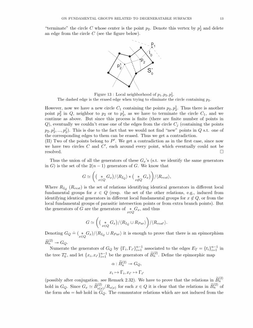
Proof. Assume that there is a generator Γ0 of G such that it is not a generator of Gx forevery x ∈ Q. This generator corresponds to a line l0 in B0. By our construction, thereare two points p1, p2 on l0 that belong to the set P ′ ∪ Y , and by assumption, both of themdo not belong to Q (recall that P ′ is the set of singular points of B0 which are images ofsingular points of R0 and that Y is the set of 2−points). We now look at two cases:(I) One of the points belongs to Y .Let p1 ∈ Y, p2 ∈ P ′. The point p2 is an “inner” point (see Condition (4) in Definition 2.17),i.e., it does not lie on the border of the degenerated surface S0, as in this case l0 would notinduce a generator (recall that we do not consider the border lines as part of B0). Thus,the local neighborhood of p1, p2 in S∗
0 looks as in the following figure:
p1
p2
S0
*
l0
Figure 12 : Local neighborhood of p1, p2.
Since there is a spanning subtree T ∗0 (by Lemma 2.30), one of the neighboring vertices to
p2 has to be in Q, as otherwise, in the process of the construction of T ∗0 , we could not
ON FUNDAMENTAL GROUPS RELATED TO DEGENERATABLE SURFACES 13
“terminate” the circle C whose center is the point p2. Denote this vertex by p12 and deletean edge from the circle C (see the figure below).
p1
p2
S0
*p
21
l0
Figure 13 : Local neighborhood of p1, p2, p12.
The dashed edge is the erased edge when trying to eliminate the circle containing p2.
However, now we have a new circle C1 containing the points p2, p12. Thus there is another
point p22 in Q, neighbor to p2 or to p12, as we have to terminate the circle C1, and wecontinue as above. But since this process is finite (there are finite number of points inQ), eventually we couldn’t erase one of the edges from the circle Cj (containing the points
p2, p12, ..., p
j2). This is due to the fact that we would not find “new” points in Q s.t. one of
the corresponding edges to them can be erased. Thus we get a contradiction.(II) Two of the points belong to P ′. We get a contradiction as in the first case, since nowwe have two circles C and C ′, each around every point, which eventually could not beresolved. �
Thus the union of all the generators of these Gx’s (s.t. we identify the same generatorsin G) is the set of the 2(n − 1) generators of G. We know that
G ≃
((∗
x∈QGx
)/〈RIQ〉 ∗
(∗
x 6∈QGx
))/〈Rrest〉,
Where RIQ (Rrest) is the set of relations identifying identical generators in different localfundamental groups for x ∈ Q (resp. the set of the other relations, e.g., induced fromidentifying identical generators in different local fundamental groups for x 6∈ Q, or from thelocal fundamental groups of parasitic intersection points or from extra branch points). Butthe generators of G are the generators of ∗
x∈QGx, and thus
G ≃
((∗
x∈QGx
)/〈RIQ ∪RPar〉
)/〈Rrest′〉.
Denoting GQ.= ( ∗
x∈QGx)/〈RIQ ∪RPar〉 it is enough to prove that there is an epimorphism
B(2)n ։ GQ.
Numerate the generators of GQ by {Γi,Γi′}n−1i=1 associated to the edges ET = {ti}
n−1i=1 in
the tree T ∗0 , and let {xi, xi′}
n−1i=1 be the generators of B
(2)n . Define the epimorphic map
α : B(2)n ։ GQ,
xi 7→ Γi, xi′ 7→ Γi′
(possibly after conjugation. see Remark 2.32). We have to prove that the relations in B(2)n
hold in GQ. Since Gx ≃ B(2)v(x)/Rv(x) for each x ∈ Q it is clear that the relations in B
(2)n of
the form aba = bab hold in GQ. The commutator relations which are not induced from the
14 M. FRIEDMAN, M. TEICHER
commutator relations in B(2)v(x), x ∈ Q hold in GQ as the set of relations in GQ includes the
set RPar.(ii) Assume that ℓ − m < n − 1. Again, there exist k ∈ N, k < m such that ℓ − k = n − 1.
Previously, in Lemma 2.30, we chose k points from Q to construct T ∗0 . Therefore we can
continue as above. Note that by Remark 2.31, even if the point p2 (in Lemma 2.36) willhave two neighboring vertices ∈ Q, we still could not resolve the circle C.
�
Remark 2.37. Recall that for a degeneratable surface S that satisfies all the conditions, we denotedn = degS, m = number of singular points p of B0 whose local fundamental group is a quotient
of B(2)v(p), and by m the number of vertices in GraphS0
(see Definition 2.11). By the restrictions
imposed by Remark 2.14 and Theorem 2.22, we can bound ℓ = 12degB. Explicitly, for B to be
a branch of curve of degree 2ℓ of a embedded–degeneratable surface s.t. G would be virtuallysolvable, the following inequalities should be satisfied:
(1) max(n,m+ n) < ℓ+ 1 ≤ m+ n.
Remark 2.38. As can be seen from Subsection 2.3.1, Example 2.23 and Remark 2.37, the completeclassification of smooth surfaces whose planar degeneration satisfy the condition introduced inTheorem 2.22 is not yet known, though some new restrictions are now clearer (e.g. inequality (1)).Moreover, [10, Section 8] has found some restrictions on surfaces admitting planar degeneration withsome specific conditions on the singularities of the degenerated surface. These conditions do shedsome light on our class of surfaces. For example, every singular point in the degenerated surface,denoted in [10, Definition 3.5] as Em-point (m > 3), belongs to the set Q (see Definition 2.9).Given a planar degeneration, [10, Theorem 8.4] imposes conditions on the square of the canonicalclass of the surface, when the degenerated surface has some specific singular points. Certainly thistheorem can be generalized to include more cases of singular points in the set Q and to the biggerclasses of embedded–degeneratable surfaces. Moreover, [10, Proposition 8.6] states that for everysurface there might be a birational model of it that is degeneratable into a union of planes withmild singularities pi (s.t. the local fundamental group Gpi is known), though it is not clear whetherif this model is even simply–degeneratable (see Dentition 2.15).
Note also that all the surfaces in Example 2.23 are simply connected, and this raises the conjec-ture that the desired class of surfaces is contained in the class of simply connected surfaces. Indeed,this is supported by that fact that if S is a surface s.t. π1(S) contains a free group of rank 2, thenS does not satisfy the condition in Theorem 2.22 (as G is not virtually solvable). However, this isthe subject of an ongoing research.
3. Non simply connected scrolls
By [20, Proposition 4.13], for a projective complex surface S, if π1(S) is not virtually solvable,then π1(CP
2 − B) is not virtually solvable, where B is the branch curve of S w.r.t. a genericprojection. As Liedtke [20] points out, for S a ruled surface over a curve of genus > 1 , π1(S)contains a free group of rank 2. Therefore, for such an S, there does not exist a planar degenerationwith enough “good” singular points (i.e. points in the set Q. See definition 2.9). However, in thenext section we examine what would be a possible structure for G = π1(C2−B) for such a surface.Specifically, we consider the structure of this group when the set Q is empty.
By Conjecture 2.25, the existence of points in the set Q would imply that G would be a quotient of
A(T )(2), where as in our case (see Thereom 3.35), G is a quotient of A(T ) (where T is an associatedgraph to the degeneration of S), as in Example 2.28(1). This strengthens Conjecture 2.26.
For the convenience of the reader, we begin with recalling the notions of the Braid MonodromyFactorization (BMF) in subsection 3.1. We then investigate the surface CP1 × Cg, where Cg is a
ON FUNDAMENTAL GROUPS RELATED TO DEGENERATABLE SURFACES 15
curve of genus g ≥ 1, and the corresponding fundamental group π1(C2 − Bg), in subsections 3.2and 3.3. Using the results, we compute the fundamental group of the Galois cover of these surfacesin subsection 3.4.
3.1. Background on Braid Monodromy Factorization. Recall that computing the braid mon-odromy is the main tool to compute fundamental groups of complements of curves. The readerwho is familiar with this subject can skip the following definitions to Subsection 3.2. We begin bydefining the braid monodromy associated to a curve.
Let D be a closed disk in R2, K ⊂ Int(D), K finite, n = #K. Recall that the braidgroup Bn(D,K) can be defined as the group of all equivalent diffeomorphisms β of D such thatβ(K) = K , β|∂D = Id |∂D (two diffeomorphisms are equivalent if they induce the same automor-phism on π1(D −K,u)).
Definition 3.1. H(σ) is a half-twist defined by σ.
Let a, b ∈ K, and let σ be a smooth simple path in Int(D) connecting a with b s.t. σ∩K = {a, b}.Choose a small regular neighborhood U of σ contained in Int(D), s.t. U ∩K = {a, b}. Denote byH(σ) the diffeomorphism of D which switches a and b by a counterclockwise 180◦ rotation and isthe identity on D \ U . Thus it defines an element of Bn[D,K], called the half-twist defined by σ .
Denote [A,B] = ABA−1B−1, 〈A,B〉 = ABAB−1A−1B−1. We recall Artin’s presentation of thebraid group:
Theorem 3.2. Bn is generated by the half-twists Hi of a sequence of paths σin−1i=1 (such that σi
connected the ith and the (i+ 1)th points) and all the relations between H1, ...,Hn−1 follow from:
[Hi,Hj] = 1 if |i− j| > 1〈Hi,Hj〉 = 1 if |i− j| = 1.
Assume that all of the points of K are on the X-axis (when considering D in R2). In this situ-ation, if a, b ∈ K, and za,b is a path that connects them, then we denote it by Za,b = H(za,b). Ifza,b is a path that goes below the X-axis, then we denote it by Za,b, or just Za,b. If za,b is a path
that goes above the x-axis, then we denote it by Za,b. We also denote by(c−d)
Za,b ( Za,b(c−d)
) the braid
induced from a path connecting the points a and b below (resp. above) the X-axis, going above(resp. below) it from the point c till point d.
Definition 3.3. The braid monodromy w.r.t. C, π, u Let C be a curve, C ⊆ C2 . Choose O ∈C2, O 6∈ C such that the projection f : C2 → C1 with center O will be generic when restrictingit to C. We denote π = f |C and deg π = deg C by m. Let N = {x ∈ C1
∣∣ #π−1(x) < m}. Takeu /∈ N,and let C1
u = f−1(u). There is a naturally defined homomorphism
π1(C1 −N,u)
ϕ−→ Bm[C1
u,C1u ∩C]
which is called the braid monodromy w.r.t. C, π, u, where Bm is the braid group. We sometimesdenote ϕ by ϕu.
In fact, denoting by E a big disk in C1 s.t. E ⊃ N , we can also take the path in E \N not to bea loop, but just a non-self-intersecting path. This induces a diffeomorphism between the models(D,K) at the two ends of the considered path, where D is a big disk in C1
u, and K = C1u ∩C ⊂ D.
Definition 3.4. ψT the Lefschetz diffeomorphism induced by a path T . Let T be a path in E \Nconnecting x0 with x1, T : [0, 1] → E \ N . There exists a continuous family of diffeomorphisms
16 M. FRIEDMAN, M. TEICHER
ψ(t) : D → D, t ∈ [0, 1], such that ψ(0) = Id, ψ(t)(K(x0)) = K(T (t)) for all t ∈ [0, 1], andψ(t)(y) = y for all y ∈ ∂D. For emphasis we write ψ(t) : (D,K(x0)) → (D,K(T (t)). A Lefschetzdiffeomorphism induced by a path T is the diffeomorphism
ψT = ψ(1) : (D,K(x0)) →∼
(D,K(x1)).
Since ψ(t) (K(x0)) = K(T (t)) for all t ∈ [0, 1], we have a family of canonical isomorphisms
ψν(t) : Bp [D,K(x0)] →
∼Bp [D,K(T (t))] , for all t ∈ [0, 1].
We recall Artin’s theorem on the presentation of the Dehn twist of the braid group as a prod-uct of braid monodromy elements of a geometric-base (a base of π1 = π1(C1 −N,u) with certainproperties; see [26] for definitions).
Theorem 3.5. Let C be a curve transversal to the line in infinity, and ϕ is a braid monodromy ofC,ϕ : π1 → Bm. Let δi be a geometric (free) base (called a g-base) of π1, and ∆2 is the generatorof Center(Bm). Then:
∆2 =∏
ϕ(δi).
This product is also defined as the braid monodromy factorization (BMF) related to a curve C.
Note that if x1, ..., xn−1 are the generators of Bn, then we know that ∆2 = (x1 · . . . · xn−1)n and
thus deg(∆2) = n(n− 1).So in order to find out what is the braid monodromy factorization of ∆2
p, we have to find out whatare ϕ(δi), ∀i. We refer the reader to the definition of a skeleton (see [27]) λxj , xj ∈ N , which is amodel of a set of paths connecting points in the fiber, s.t. all those points coincide when approachingAj =(xj, yj)∈ C, when we approach this point from the right. To describe this situation in greaterdetail, for xj ∈ N , let x′j = xj +α. So the skeleton in xj is defined as a system of paths connecting
the points in K(x′j)∩D(Aj, ε) when 0 < α≪ ε≪ 1, D(Aj , ε) is a disk centered in Aj with radius ε.
For a given skeleton, we denote by ∆〈λxj 〉 the braid by rotates by 180 degrees counterclockwise asmall neighborhood of the given skeleton. Note that if λxj is a single path, then ∆〈λxj〉 = H(λxj).
We also refer the reader to the definition of δx0, for x0 ∈ N (see [27]), which describes the
Lefschetz diffeomorphism induced by a path going below x0, for different types of singular points(tangent, node, branch; for example, when going below a node, a half-twist of the skeleton occursand when going below a tangent point, a full-twist occurs).
We define, for x0 ∈ N , the following number: εx0= 1, 2, 4 when (x0, y0) is a branch / node
/ tangent point (respectively). Explicitly, in local coordinates (x, y) (where (x0, y0) = (0, 0)), abranch is a singular point (w.r.t. the projection) with local equation y2 = x, a node – y2 = x2, anda tangent y(y − x2) = 0. So we have the following statement (see [27, Prop. 1.5]):
Let γj be a path below the real line from xj to u, s.t. ℓ(γj) = δj . So
ϕu(δj) = ϕ(δj) = ∆〈(λxj )
( 1∏
m=j−1
δxm
)〉εxj .
When denoting ξxj = (λxj )
(1∏
m=j−1δxm
)we get
ϕ(δj) = ∆〈(ξxj)〉εxj .
Note that the last formula gives an algorithm to compute the needed factorization. For a detailedexplanation of the braid monodromy, see [26].

ON FUNDAMENTAL GROUPS RELATED TO DEGENERATABLE SURFACES 17
Assume that we have a curve C in CP2 and its BMF. Then we can calculate the groupsπ1(CP
2 − C) and π1(C2 − C) (where C = C ∩ C2). Recall that a g-base is an ordered free baseof π1(D\F, v), where D is a closed disc, F is a finite set in Int(D), v ∈ ∂D which satisfies severalconditions; see [26], [27] for the explicit definition.
Let {Γi} be a g-base of G = π1(Cu−(Cu∩C), u), where Cu = C×u. We cite now the Zariski-VanKampen Theorem (for cuspidal curves) in order to compute the relations between the generatorsin G.
Theorem 3.6. Zariski-Van Kampen (cuspidal curves version) Let C be a cuspidal curve in CP2.
Let C = C2 ∩C. Let ϕ be a braid monodromy factorization w.r.t. C and u. Let ϕ =p∏
j=1V
νjj , where
Vj is a half-twist and νj = 1, 2, 3.For every j = 1 . . . p, let Aj, Bj ∈ π1(Cu−C, u) be such that Aj, Bj can be extended to a g-base of
π1(Cu−C, u) and (Aj)Vj = Bj. Let {Γi} be a g-base of π1(Cu−C, u) corresponding to the {Ai, Bi},where Ai, Bi are expressed in terms of Γi. Then π1(C2 − C, u) is generated by the images of {Γi}in π1(C2 − C, u) and the only relations are those implied from {V
νjj }, as follows:
Aj · B−1j if νj = 1
[Aj, Bj ] = 1 if νj = 2
〈Aj , Bj〉 = 1 if νj = 3.
π1(CP2 − C, ∗) is generated by {Γi} with the above relations and one more relation
∏iΓi = 1.
The following figure illustrates how to find Ai, Bi from the half-twist Vi = H(σ):
σ
u0 u0u0
AVBV
1 2 3 4 5 6
σ
Figure 14
SoAV = Γ−1
4 Γ6Γ4, BV = Γ1.
3.1.1. Example of a BMF. We give here an example of computing a simple Braid MonodromyFactorization, for the following configuration:
1
2
34a
b
b�
c
Figure 15
We will need this factorization in Subsection 3.2, where it will be the factorization of the firstregeneration a certain singular point.
Proposition 3.7. The local braid monodromy factorization of the above configuration is
ϕ = Z4abZ
4b′cZbb′Z
2ac
where the braids Zbb′ , Zac correspond to the following paths:
18 M. FRIEDMAN, M. TEICHER
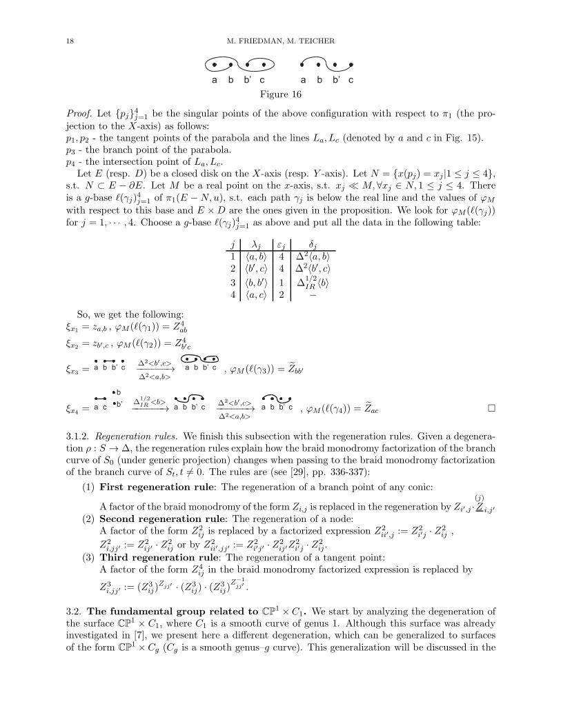
a b b� c a b b� c
Figure 16
Proof. Let {pj}4j=1 be the singular points of the above configuration with respect to π1 (the pro-
jection to the X-axis) as follows:p1, p2 - the tangent points of the parabola and the lines La, Lc (denoted by a and c in Fig. 15).p3 - the branch point of the parabola.p4 - the intersection point of La, Lc.
Let E (resp. D) be a closed disk on the X-axis (resp. Y -axis). Let N = {x(pj) = xj|1 ≤ j ≤ 4},s.t. N ⊂ E − ∂E. Let M be a real point on the x-axis, s.t. xj ≪ M,∀xj ∈ N, 1 ≤ j ≤ 4. Thereis a g-base ℓ(γj)
4j=1 of π1(E −N,u), s.t. each path γj is below the real line and the values of ϕM
with respect to this base and E ×D are the ones given in the proposition. We look for ϕM (ℓ(γj))for j = 1, · · · , 4. Choose a g-base ℓ(γj)
4j=1 as above and put all the data in the following table:
j λj εj δj1 〈a, b〉 4 ∆2〈a, b〉2 〈b′, c〉 4 ∆2〈b′, c〉
3 〈b, b′〉 1 ∆1/2IR 〈b〉
4 〈a, c〉 2 −
So, we get the following:ξx1
= za,b , ϕM (ℓ(γ1)) = Z4ab
ξx2= zb′,c , ϕM (ℓ(γ2)) = Z4
b′c
ξx3= a b b� c
∆2<b′,c>−−−−−−→∆2<a,b>
a b b� c , ϕM (ℓ(γ3)) = Zbb′
ξx4= a c
b
b� ∆1/2IR <b>
−−−−−−→ a b b� c∆2<b′,c>−−−−−−→∆2<a,b>
a b b� c , ϕM (ℓ(γ4)) = Zac �
3.1.2. Regeneration rules. We finish this subsection with the regeneration rules. Given a degenera-tion ρ : S → ∆, the regeneration rules explain how the braid monodromy factorization of the branchcurve of S0 (under generic projection) changes when passing to the braid monodromy factorizationof the branch curve of St, t 6= 0. The rules are (see [29], pp. 336-337):
(1) First regeneration rule: The regeneration of a branch point of any conic:
A factor of the braid monodromy of the form Zi,j is replaced in the regeneration by Zi′,j ·(j)
Z i,j′
(2) Second regeneration rule: The regeneration of a node:A factor of the form Z2
ij is replaced by a factorized expression Z2ii′,j := Z2
i′j · Z2ij ,
Z2i,jj′ := Z2
ij′ · Z2ij or by Z2
ii′,jj′ := Z2i′j′ · Z
2ij′Z
2i′j · Z
2ij.
(3) Third regeneration rule: The regeneration of a tangent point:A factor of the form Z4
ij in the braid monodromy factorized expression is replaced by
Z3i,jj′ := (Z3
ij)Zjj′ · (Z3
ij) · (Z3ij)
Z−1
jj′ .
3.2. The fundamental group related to CP1 ×C1. We start by analyzing the degeneration ofthe surface CP1 × C1, where C1 is a smooth curve of genus 1. Although this surface was alreadyinvestigated in [7], we present here a different degeneration, which can be generalized to surfacesof the form CP1 ×Cg (Cg is a smooth genus–g curve). This generalization will be discussed in the
ON FUNDAMENTAL GROUPS RELATED TO DEGENERATABLE SURFACES 19
next subsection but we give here a rough description of how this degeneration is done. See alsoConstruction 3.27.
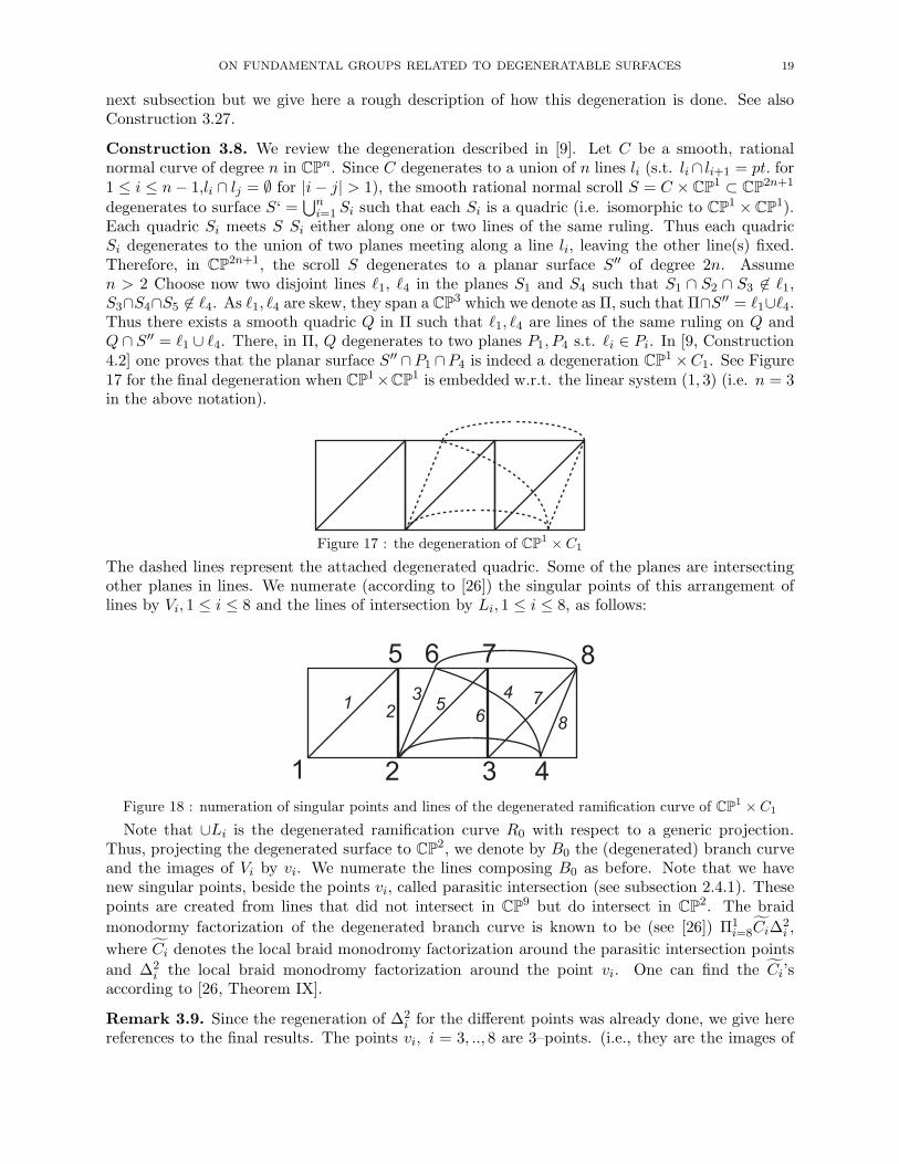
Construction 3.8. We review the degeneration described in [9]. Let C be a smooth, rationalnormal curve of degree n in CPn. Since C degenerates to a union of n lines li (s.t. li∩ li+1 = pt. for1 ≤ i ≤ n− 1,li ∩ lj = ∅ for |i− j| > 1), the smooth rational normal scroll S = C × CP1 ⊂ CP2n+1
degenerates to surface S‘ =⋃n
i=1 Si such that each Si is a quadric (i.e. isomorphic to CP1 ×CP1).Each quadric Si meets S Si either along one or two lines of the same ruling. Thus each quadricSi degenerates to the union of two planes meeting along a line li, leaving the other line(s) fixed.Therefore, in CP2n+1, the scroll S degenerates to a planar surface S′′ of degree 2n. Assumen > 2 Choose now two disjoint lines ℓ1, ℓ4 in the planes S1 and S4 such that S1 ∩ S2 ∩ S3 6∈ ℓ1,S3∩S4∩S5 6∈ ℓ4. As ℓ1, ℓ4 are skew, they span a CP3 which we denote as Π, such that Π∩S′′ = ℓ1∪ℓ4.Thus there exists a smooth quadric Q in Π such that ℓ1, ℓ4 are lines of the same ruling on Q andQ ∩ S′′ = ℓ1 ∪ ℓ4. There, in Π, Q degenerates to two planes P1, P4 s.t. ℓi ∈ Pi. In [9, Construction4.2] one proves that the planar surface S′′ ∩P1 ∩P4 is indeed a degeneration CP1 ×C1. See Figure17 for the final degeneration when CP1×CP1 is embedded w.r.t. the linear system (1, 3) (i.e. n = 3in the above notation).
Figure 17 : the degeneration of CP1 × C1
The dashed lines represent the attached degenerated quadric. Some of the planes are intersectingother planes in lines. We numerate (according to [26]) the singular points of this arrangement oflines by Vi, 1 ≤ i ≤ 8 and the lines of intersection by Li, 1 ≤ i ≤ 8, as follows:
1 2 3 4
5 6 7 8
12
35
6
4 7
8
Figure 18 : numeration of singular points and lines of the degenerated ramification curve of CP1 × C1
Note that ∪Li is the degenerated ramification curve R0 with respect to a generic projection.Thus, projecting the degenerated surface to CP2, we denote by B0 the (degenerated) branch curveand the images of Vi by vi. We numerate the lines composing B0 as before. Note that we havenew singular points, beside the points vi, called parasitic intersection (see subsection 2.4.1). Thesepoints are created from lines that did not intersect in CP9 but do intersect in CP2. The braid
monodormy factorization of the degenerated branch curve is known to be (see [26]) Π1i=8Ci∆
2i ,
where Ci denotes the local braid monodromy factorization around the parasitic intersection points
and ∆2i the local braid monodromy factorization around the point vi. One can find the Ci’s
according to [26, Theorem IX].
Remark 3.9. Since the regeneration of ∆2i for the different points was already done, we give here
references to the final results. The points vi, i = 3, .., 8 are 3–points. (i.e., they are the images of
20 M. FRIEDMAN, M. TEICHER
the points vi which are locally the intersection of three planes. see e.g., [29]) The factors that they
contribute to the factorization (i.e. their local BMFs) are either Z(3)a′,bb′ · Zaa′ or Z
(3)aa′,b · Zbb′ (where
vi = La ∩ Lb). The point v1 is a 2–point and contributes to the factorization the factor Z1,1′ (seeNotation 2.7 and Remark 2.34(I)). For the point v2, see a more explicit explanation in the nextremark.
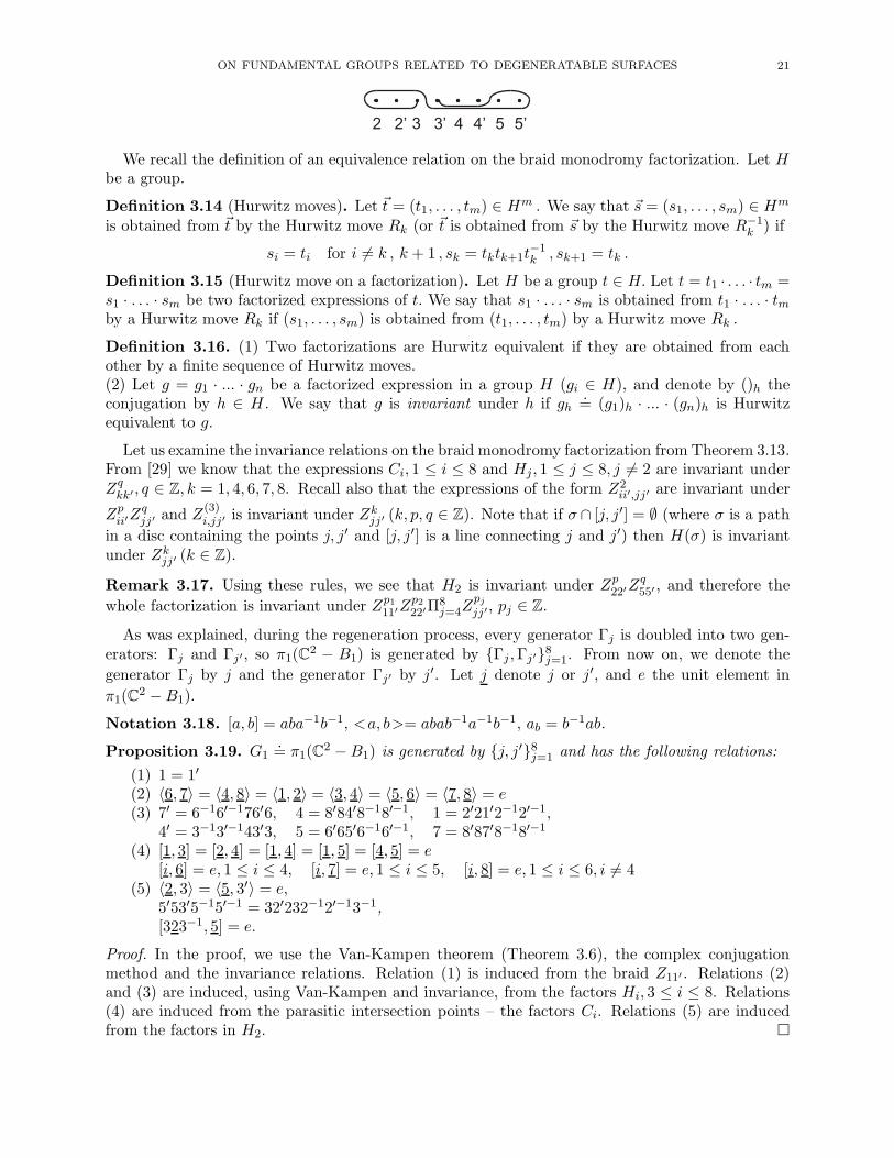
Remark 3.10. In a small neighborhood of v2, the first line that regenerates is L3, which turnsinto a conic (see [29]). The braid monodromy factorization of this first regeneration is presented inProposition 3.7. In the following regenerations we use the regeneration rules (see Subsection 3.1.2):the tangent points (i.e., a braid of the form Z4
...) are regenerated into three cusps (three braids ofthe form Z3
...) and a node (a braid of the form Z2...) into four nodes. Explicitly, the factorization
Z423Z
43′5Z33′Z
225 is replaced by the factorization Z
(3)22′,3Z
(3)3′,55′Z33′
(3)
Z222′,55′ .
Notation 3.11. Denote ϕ(a, b, c) = Z(3)aa′,bZ
(3)b′,cc′Zbb′
(b)
Z2aa′,cc′ where Zbb′ is as Figure 16, when the
points a and c are doubled.
Notation 3.12. B1 = the branch curve of CP1 ×C1 embedded in CP9 w.r.t. a generic projection.
From Remarks 3.10 and 3.9, we can induce the BMF of B1:
Theorem 3.13. The braid monodromy factorization of the branch curve B1 of a generic projectionof CP1 × C1 embedded in CP9 is:
∆2 =1∏
i=8
Ci ·Hi,
where
Ci = id, i = 1, 5, .., 8, C2 = D3 ·D5, C3 = D6 ·D7, C4 = D4 ·D8
where
D3 = Z211′,33′ , D4 = Z2
11′,44′ · Z222′,44′ , D5 = Z
211′,55′ · Z
244′,55′ , D6 = Π4
i=1Z2ii′,66′
(5−5′)
,
D7 = Π5i=1Z
2ii′,77′ , D8 = Πi=1,2,
3,5,6Z
2ii′,88′
and
H1 = Z1,1′ , Hi = Z(3)a′,bb′ · Zaa′ for i = 4, 5, 7, 8, Hi = Z
(3)aa′,b · Zbb′ for i = 3, 6
(when vi = La ∩ Lb, a < b), where Z·, · is the braid induced from the following motion:
Zaa′ :
a a� b b�
Zbb′ :
a a� b b�
Z(3)a′,bb′ =
∏
q=−1,0,1
(Z3a′,b)Zq
b,b′, Z
(3)aa′,b =
∏
q=−1,0,1
(Z3a′,b)Zq
a,a′
and H2 = ϕ(2, 3, 5) where Z33′ (a factor in the factorization H2) is the braid induced from thefollowing motion:
ON FUNDAMENTAL GROUPS RELATED TO DEGENERATABLE SURFACES 21
2 2� 3 3� 4 4� 5 5�
We recall the definition of an equivalence relation on the braid monodromy factorization. Let Hbe a group.
Definition 3.14 (Hurwitz moves). Let ~t = (t1, . . . , tm) ∈ Hm . We say that ~s = (s1, . . . , sm) ∈ Hm
is obtained from ~t by the Hurwitz move Rk (or ~t is obtained from ~s by the Hurwitz move R−1k ) if
si = ti for i 6= k , k + 1 , sk = tktk+1t−1k , sk+1 = tk .
Definition 3.15 (Hurwitz move on a factorization). Let H be a group t ∈ H. Let t = t1 · . . . · tm =s1 · . . . · sm be two factorized expressions of t. We say that s1 · . . . · sm is obtained from t1 · . . . · tmby a Hurwitz move Rk if (s1, . . . , sm) is obtained from (t1, . . . , tm) by a Hurwitz move Rk .
Definition 3.16. (1) Two factorizations are Hurwitz equivalent if they are obtained from eachother by a finite sequence of Hurwitz moves.(2) Let g = g1 · ... · gn be a factorized expression in a group H (gi ∈ H), and denote by ()h theconjugation by h ∈ H. We say that g is invariant under h if gh
.= (g1)h · ... · (gn)h is Hurwitz
equivalent to g.
Let us examine the invariance relations on the braid monodromy factorization from Theorem 3.13.From [29] we know that the expressions Ci, 1 ≤ i ≤ 8 and Hj, 1 ≤ j ≤ 8, j 6= 2 are invariant underZqkk′ , q ∈ Z, k = 1, 4, 6, 7, 8. Recall also that the expressions of the form Z2
ii′,jj′ are invariant under
Zpii′Z
qjj′ and Z
(3)i,jj′ is invariant under Z
kjj′ (k, p, q ∈ Z). Note that if σ ∩ [j, j′] = ∅ (where σ is a path
in a disc containing the points j, j′ and [j, j′] is a line connecting j and j′) then H(σ) is invariantunder Zk
jj′ (k ∈ Z).
Remark 3.17. Using these rules, we see that H2 is invariant under Zp22′Z
q55′ , and therefore the
whole factorization is invariant under Zp111′Z
p222′Π
8j=4Z
pjjj′, pj ∈ Z.
As was explained, during the regeneration process, every generator Γj is doubled into two gen-erators: Γj and Γj′, so π1(C
2 − B1) is generated by {Γj ,Γj′}8j=1. From now on, we denote the
generator Γj by j and the generator Γj′ by j′. Let j denote j or j′, and e the unit element in
π1(C2 −B1).
Notation 3.18. [a, b] = aba−1b−1, <a, b>= abab−1a−1b−1, ab = b−1ab.
Proposition 3.19. G1.= π1(C2 −B1) is generated by {j, j′}8j=1 and has the following relations:
(1) 1 = 1′
(2) 〈6, 7〉 = 〈4, 8〉 = 〈1, 2〉 = 〈3, 4〉 = 〈5, 6〉 = 〈7, 8〉 = e(3) 7′ = 6−16′−176′6, 4 = 8′84′8−18′−1, 1 = 2′21′2−12′−1,
4′ = 3−13′−143′3, 5 = 6′65′6−16′−1, 7 = 8′87′8−18′−1
(4) [1, 3] = [2, 4] = [1, 4] = [1, 5] = [4, 5] = e[i, 6] = e, 1 ≤ i ≤ 4, [i, 7] = e, 1 ≤ i ≤ 5, [i, 8] = e, 1 ≤ i ≤ 6, i 6= 4
(5) 〈2, 3〉 = 〈5, 3′〉 = e,5′53′5−15′−1 = 32′232−12′−13−1,[323−1, 5] = e.
Proof. In the proof, we use the Van-Kampen theorem (Theorem 3.6), the complex conjugationmethod and the invariance relations. Relation (1) is induced from the braid Z11′ . Relations (2)and (3) are induced, using Van-Kampen and invariance, from the factors Hi, 3 ≤ i ≤ 8. Relations(4) are induced from the parasitic intersection points – the factors Ci. Relations (5) are inducedfrom the factors in H2. �
22 M. FRIEDMAN, M. TEICHER
Proposition 3.20. The following relations hold in G1:
(6) 〈2, 3〉 = 〈3, 5〉 = 〈2, 5〉 = e(7) [2−132, 5] = e
Proof. By Proposition 3.19 ((5) and (3)), it is known that
e = 〈3′, 5〉 = 〈4−134′3−14, 5〉 =[4,5]=e
〈34′3−1, 5〉 =〈3,4′〉=e
〈4′−134′, 5〉 =[4′,5]=e
〈3, 5〉.
Thus 〈3, 5〉 = e. Also, we have:
e = 〈2, 3〉 = 〈2, 4′43′4−14′−1〉 =[4,2]=e
〈2, 3′〉 ⇒ 〈2, 3〉 = e.
From relation (5) we get 3′ = 5−15′−132′232−12′−13−15′5 and also
e = 〈3′, 5〉 = 〈5−15′−132′232−12′−13−15′5, 5〉 = 〈32′232−12′−13−1, 5′55′−1〉 =InvarianceZ
55′
〈32′232−12′−13−1, 5′〉 =〈2,3〉=e
〈32′3−1232′−13−1, 5′〉 =[323−1,5′]=e
〈2, 5′〉
and by invariance relations we get 〈2, 5〉 = e. This completes the proof of (6).From (5) we have
e = [323−1, 5] = [2−132, 5] = [2−14′43′4−14′−12, 5] =[4,2]=[4,5]=e
[2−13′2, 5].
Thus [2−132, 5] = e. �
Our next task is to express the generators j′ (j = 1, 2, 3, 5, .., 8) by the generators 1 ≤ j ≤ 8 and4′. This is easy: using (3), we get
(8) 1′ = 1, 2′ = 1−1212−11, 3′ = 4−134′3−14, 8′ = 4−184′8−147′ = 8−18′−178′8, 6′ = 7−167′6−17, 5′ = 6−16′−156′6.
Therefore, the group G is generated by the generators {j}8j=1 ∪ {4′}. We note that all the
commutator and triple relations (i.e., (2), (4), (6), (7)) that involve the generators j′ where j =1, 2, 3, 5, .., 8 can be reduced, since these j′‘s are expressed in terms of the other generators. Ourtask now is to reduce most of the relations coming from the branch points, i.e. (3) and the secondrelation at (5). Notice that all of the relations in (3) are already reduced, as we have used themto define the generators j′ (by (8)). However, one can see that, for example, in the second relationin (5) we can substitute the generators j′ using (8), till we get an expression containing only thegenerators {j}8j=1 ∪ {4′}. Therefore, we get the following relation:
(9) (4′)3−145−16−17−18−14−184′−18−147−16−15−1 = (3)2−11−121−12−113−1 .
Notation 3.21. Denote relation (9) by ρ1.
Note that (9) can be described as a “global” relation, involving almost all the generators of thegroup. We need only to find out what are the “local” relations, involving only the generators 4, 4′, 3and 8.
Proposition 3.22. The following relations hold in G1:
(10) 〈84′8−1, 4〉 = 〈34′3−1, 4〉 = e.(11) [3−143, 84′8−1] = e.
Proof. Knowing that 4′ = 3−13′−143′3 we see that:
〈34′3−1, 4〉 = 〈33−13′−143′33−1, 4〉 = 〈3′, 4〉 =rel.(2)
e.
The same is dome for the second relation, using 4′ = 8−18′−148′8. This proves relation set (10).
ON FUNDAMENTAL GROUPS RELATED TO DEGENERATABLE SURFACES 23
For the relation (11), we use the relation 4 = 8′84′8−18′−1.
[3−143, 84′8−1] = [3−18′84′8−18′−13, 84′8−1] =[3,8]=e
[8′83−14′38−18′−1, 84′8−1] =
[8−18′83−14′38−18′−18, 4′] =Inv. Z
8,8′
[8′3−14′38′−1, 4′] = [3−14′3, 8′−14′8′] =〈3,4〉=〈8′,4〉=e
[4′34′−1, 4′8′4′−1] = [3, 8′] = e.
�
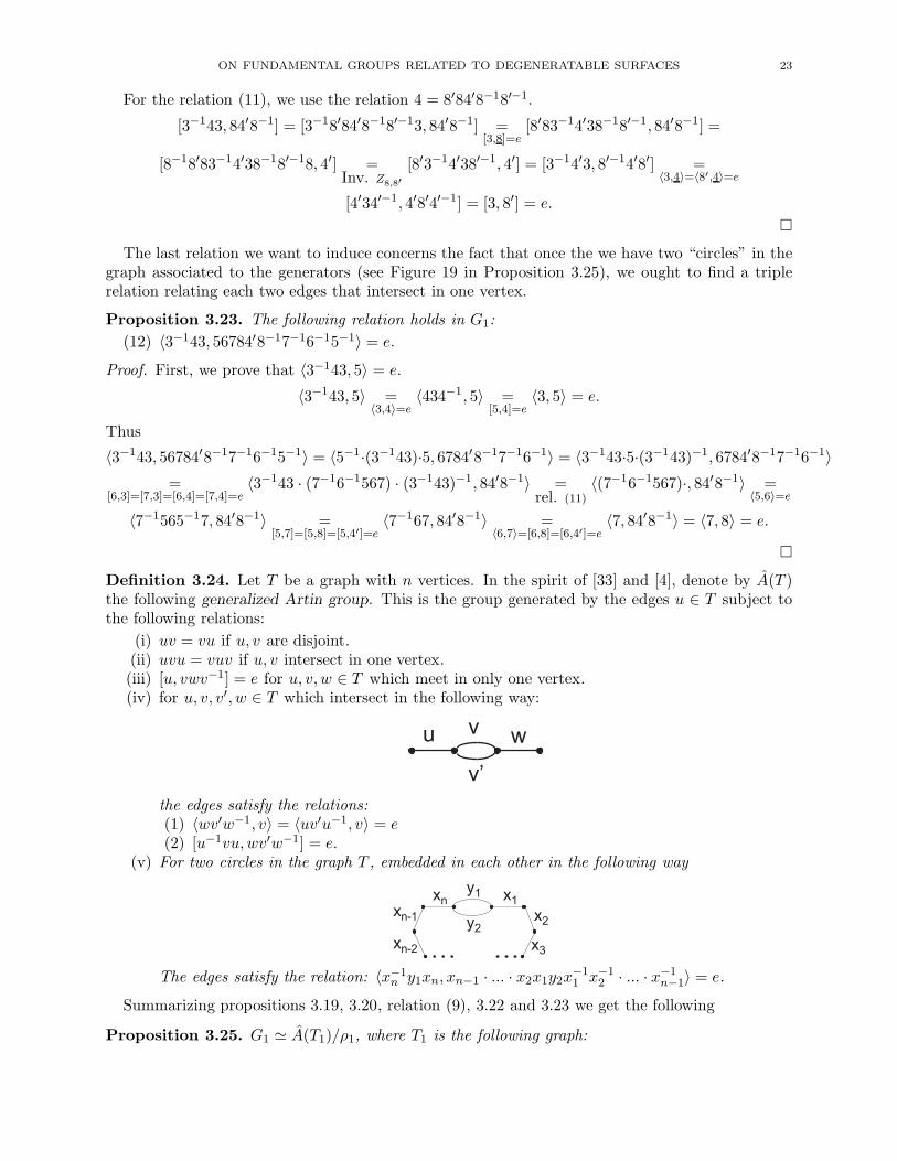
The last relation we want to induce concerns the fact that once the we have two “circles” in thegraph associated to the generators (see Figure 19 in Proposition 3.25), we ought to find a triplerelation relating each two edges that intersect in one vertex.
Proposition 3.23. The following relation holds in G1:
(12) 〈3−143, 56784′8−17−16−15−1〉 = e.
Proof. First, we prove that 〈3−143, 5〉 = e.
〈3−143, 5〉 =〈3,4〉=e
〈434−1, 5〉 =[5,4]=e
〈3, 5〉 = e.
Thus
〈3−143, 56784′8−17−16−15−1〉 = 〈5−1·(3−143)·5, 6784′8−17−16−1〉 = 〈3−143·5·(3−143)−1, 6784′8−17−16−1〉
=[6,3]=[7,3]=[6,4]=[7,4]=e
〈3−143 · (7−16−1567) · (3−143)−1, 84′8−1〉 =rel. (11)
〈(7−16−1567)·, 84′8−1〉 =〈5,6〉=e
〈7−1565−17, 84′8−1〉 =[5,7]=[5,8]=[5,4′]=e
〈7−167, 84′8−1〉 =〈6,7〉=[6,8]=[6,4′]=e
〈7, 84′8−1〉 = 〈7, 8〉 = e.
�
Definition 3.24. Let T be a graph with n vertices. In the spirit of [33] and [4], denote by A(T )the following generalized Artin group. This is the group generated by the edges u ∈ T subject tothe following relations:
(i) uv = vu if u, v are disjoint.(ii) uvu = vuv if u, v intersect in one vertex.(iii) [u, vwv−1] = e for u, v, w ∈ T which meet in only one vertex.(iv) for u, v, v′, w ∈ T which intersect in the following way:
u v
v�
w
the edges satisfy the relations:(1) 〈wv′w−1, v〉 = 〈uv′u−1, v〉 = e(2) [u−1vu,wv′w−1] = e.
(v) For two circles in the graph T , embedded in each other in the following way
y1
y2
x1
x2
x3
xnxn-1
xn-2
The edges satisfy the relation: 〈x−1n y1xn, xn−1 · ... · x2x1y2x
−11 x−1
2 · ... · x−1n−1〉 = e.
Summarizing propositions 3.19, 3.20, relation (9), 3.22 and 3.23 we get the following
Proposition 3.25. G1 ≃ A(T1)/ρ1, where T1 is the following graph:
24 M. FRIEDMAN, M. TEICHER
1 23
4
8
75
4�
6
Figure 19
Remark 3.26. Let T1, T2 be connected disjoint graphs. Then A(T1 ∪ T2) = A(T1)× A(T2).
3.3. The fundamental group related to CP1 × Cg, g > 1. In this subsection, we compute
the BMF of the branch curve Bg of CP1 × Cg, g > 1 and the corresponding fundamental group.We show the connections between these groups and the twisted Artin group defined earlier (seeDefinition 3.24). We begin with the surface CP1 × C2.
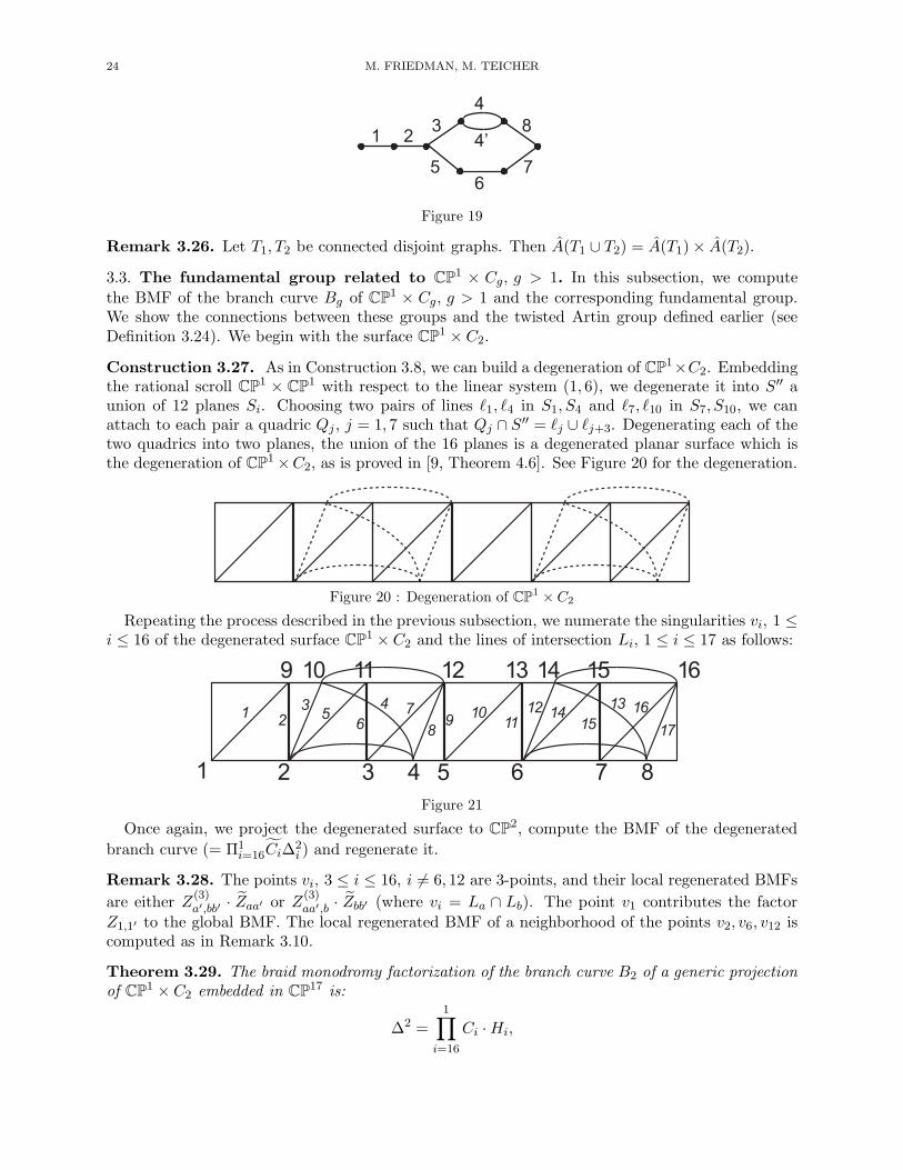
Construction 3.27. As in Construction 3.8, we can build a degeneration of CP1×C2. Embeddingthe rational scroll CP1 × CP1 with respect to the linear system (1, 6), we degenerate it into S′′ aunion of 12 planes Si. Choosing two pairs of lines ℓ1, ℓ4 in S1, S4 and ℓ7, ℓ10 in S7, S10, we canattach to each pair a quadric Qj , j = 1, 7 such that Qj ∩ S
′′ = ℓj ∪ ℓj+3. Degenerating each of thetwo quadrics into two planes, the union of the 16 planes is a degenerated planar surface which isthe degeneration of CP1 ×C2, as is proved in [9, Theorem 4.6]. See Figure 20 for the degeneration.
Figure 20 : Degeneration of CP1 × C2
Repeating the process described in the previous subsection, we numerate the singularities vi, 1 ≤i ≤ 16 of the degenerated surface CP1 × C2 and the lines of intersection Li, 1 ≤ i ≤ 17 as follows:
1 2 3 4
9 10
12
35
6
4 7
8
5 6 7 8
10
11 12 13 14 15 16
9 11
12 1415
13 16
17
Figure 21
Once again, we project the degenerated surface to CP2, compute the BMF of the degenerated
branch curve (= Π1i=16Ci∆
2i ) and regenerate it.
Remark 3.28. The points vi, 3 ≤ i ≤ 16, i 6= 6, 12 are 3-points, and their local regenerated BMFs
are either Z(3)a′,bb′ · Zaa′ or Z
(3)aa′,b · Zbb′ (where vi = La ∩ Lb). The point v1 contributes the factor
Z1,1′ to the global BMF. The local regenerated BMF of a neighborhood of the points v2, v6, v12 iscomputed as in Remark 3.10.
Theorem 3.29. The braid monodromy factorization of the branch curve B2 of a generic projectionof CP1 × C2 embedded in CP17 is:
∆2 =
1∏
i=16
Ci ·Hi,

ON FUNDAMENTAL GROUPS RELATED TO DEGENERATABLE SURFACES 25
where
Ci = id, i = 1, 9, .., 16, C2 = D3 ·D5, C3 = D6 ·D7, C4 = D4 ·D8, C5 = D9 ·D10
C6 = D11 ·D12 ·D14, C7 = D15 ·D16, C8 = D13 ·D17
where
D3 = Z211′,33′ , D4 = Z
211′,44′
(3−3′)
Z222′,44′
(3−3′)
, D5 = Π2i=1Z
2ii′,55′ · Z
244′,55′ , D6 = Π4
i=1Z2ii′,66′
(5−5′)
D7 = Π5i=1Z
2ii′,77′ , D8 = Π3
i=1Z2ii′,88′
(7−7′)
· Z255′,88′
(7−7′)
Z266′,88′ , D9 = Π6
i=1Z2ii′,99′
(7−8′)
D10 = Π8i=1Z
2ii′,10 10′ , D11 = Π9
i=1Z2ii′,11 11′
(10−10′)
, D12 = Π10i=1Z
2ii′,12 12′ , D13 = Π11
i=1Z2ii′,13 13′
(12−12′)
D14 = Π10i=1Z
2ii′,14 14′Z
213 13′,14 14′ , D15 = Π13
i=1Z2ii′,15 15′
(14−14′)
, D16 = Π14i=1Z
2ii′,16 16′
D17 = Π12i=1Z
2ii′,17 17′
(16−16′)
· Z212 12′,17 17′
(16−16′)
Z215 15′,17 17′
and
H1 = Z1,1′ , Hi = Z(3)a′,bb′ · Zaa′ for i = 4, 8, 9, 11, 13, 15, 16, Hi = Z
(3)aa′,b · Zbb′ for i = 3, 5, 7, 10, 14,
Hi = ϕ(a, b, c),where i = 2, 6, 12 and vi is the intersection of the lines of La, Lb, Lc, and Lb isregenerated first.
Let G2.= π1(C2 −B2) be the fundamental group of the complement of the branch curve.
Proposition 3.30. G2 is isomorphic to a quotient of A(T2), where T2 is the following graph:
1 23
4
8
75
4�
6
10 1112
13
16
17
13�
15
9
14
Figure 22
Proof. The existence of the relations (i)-(v) as in Definition 3.24 is induced from the braid mon-odormy factorization of B2, using the Van-Kampen theorem, as in Propositions 3.19, 3.20, 3.22.
�
Notation 3.31. We introduce the following notations:
(i) Let T be a connected planar graph, with no repeated edges, and the valence of each vertexis ≤ 3. We denote these requirements by ⊗.
(ii) For a graph T = (E,V ), v ∈ V , denote by ET,v = Ev the set of all the edges in T one ofwhose ends is v.
(iii) E0v = E \ Ev.
(iv) Let T be a graph satisfying ⊗. Denote by R(Ev) the following expression, induced fromthe edges in Ev:
(A) Ev = {u1, u2}, then R(Ev) = u1u2u1u−12 u−1
1 u−12 , where: v
u1
u2
.

26 M. FRIEDMAN, M. TEICHER
(B) Ev = {u1, u2, u3}, then R(Ev) = u1u2u3u−12 u−1
1 u2u−13 u−1
2 , where:v
u1
u2
u3 .
Definition 3.32. Let T1 = (V1, E1), T2 = (V2, E2) be two graphs satisfying ⊗. Assume there existtwo vertices v1 ∈ V1, v2 ∈ V2 such that the degree d(v1) = i < 3 and d(v2) ≤ 3− i. We create a newgraph T1
⋃v2v1T2 by identifying the vertices v1 and v2. Note that T1
⋃v2v1T2 also satisfies ⊗. Let v
be the identified vertex v1 = v2 in T1⋃v2
v1T2. For example, see the following figure:
v1
T1
v2
T2
T1U T
2
v
v2
v1
Proposition 3.33.
A(T1⋃v2
v1T2) =
{A(T1) ∗ A(T2)
∣∣∣ [u1, u2] = e, u1 ∈ E0v1 , u2 ∈ E2 or u2 ∈ E0
v2 , u1 ∈ E1
R(Ev) = e
}.
Proof. We first note that the degree of v1 is less than 3, so the only possible cases are:
(a) v1
,
v2 (b) v
1
,
v2 (c) v
2
,
v1 .
Cases (b) and (c) are actually the same, so we consider only cases (a) and (b). Since the edgesof T1, T2 are not changed under the identification of v1 and v2, it is obvious that the relationsin A(T1) and A(T2) are satisfied in A(T1
⋃v2v1T2). In addition, for an edge u1 ∈ E1 such that
u1 6∈ Ev1 , u1 is disjoint from any edge u2 ∈ E2. Thus, in A(T1⋃v2
v1T2), the generator corresponding
to u1 commutes with any generator corresponding to u2. The same is true for an edge u2 6∈ Ev2
and edges in E1. We only have to take into account the relation induced from the identificationof v1 and v2. Consider case (a). Ev is a set of two adjacent edges u,w, intersecting at v. So in
A(T1⋃v2
v1T2), by Definition (3.24)(ii), we would have the relation vwv = wvw, or R(Ev) = e. We
follow the same arguments for case (b). �
Notation 3.34. (i) Let T1 = (V1, E1) be the graph in proposition 3.25, T0 = (V0, E0) , andlet δ ∈ V1, α, β ∈ V0 be the following vertices:
δ α β
T1 T0
(ii) For 1 < g, take g−1 copies of T0, and denote by αi, βi, 1 ≤ i ≤ g the corresponding verticesin each T0. Let Tg
.= T1
⋃α1
δ T0⋃α2
β1...⋃αg
βg−1T0.
(iii) We now construct a degenerated model of CP1 × Cg, where Cg is a genus g curve. Embed
CP1 × CP1 by the linear system (1, 3g), degenerate it to a union of 6g planes, attach gquadrics to g pairs of non–intersecting planes and then degenerate the quadrics, as wasdone in Constructions 3.8 and 3.27. The resulting degeneration should be composed fromg “building blocks” as in figure 17. Explicitly
ON FUNDAMENTAL GROUPS RELATED TO DEGENERATABLE SURFACES 27
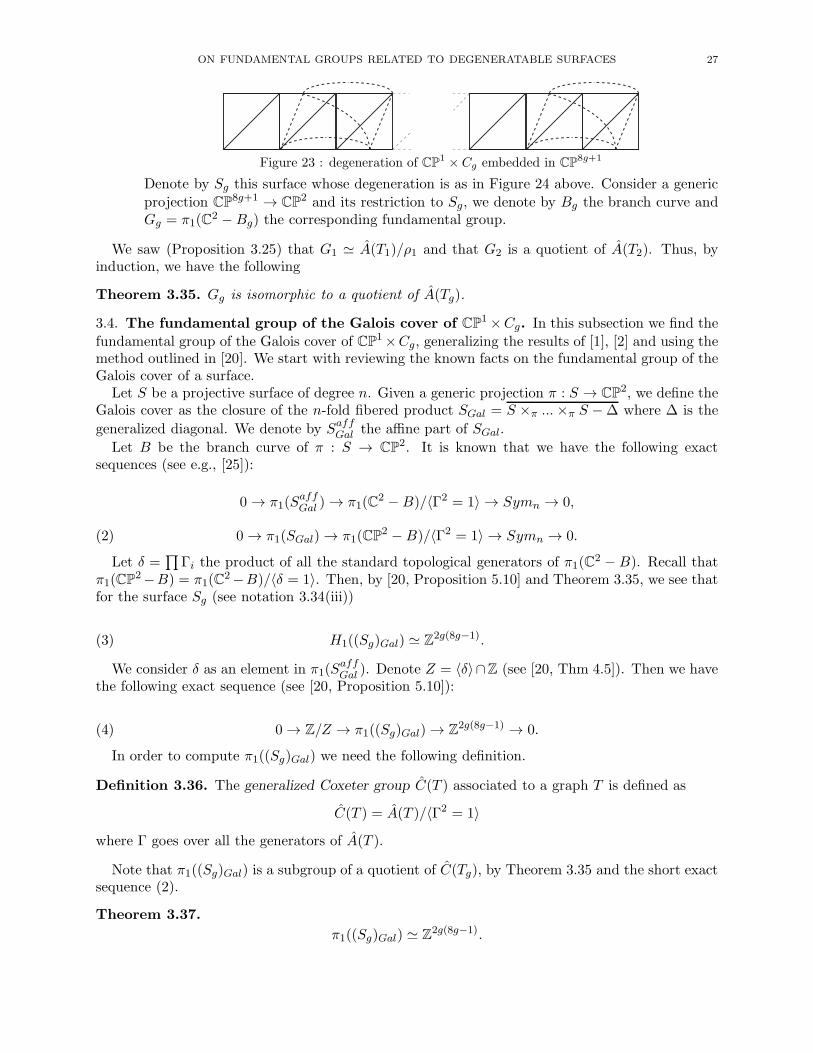
Figure 23 : degeneration of CP1 × Cg embedded in CP8g+1
Denote by Sg this surface whose degeneration is as in Figure 24 above. Consider a generic
projection CP8g+1 → CP2 and its restriction to Sg, we denote by Bg the branch curve andGg = π1(C2 −Bg) the corresponding fundamental group.
We saw (Proposition 3.25) that G1 ≃ A(T1)/ρ1 and that G2 is a quotient of A(T2). Thus, byinduction, we have the following
Theorem 3.35. Gg is isomorphic to a quotient of A(Tg).
3.4. The fundamental group of the Galois cover of CP1 ×Cg. In this subsection we find the
fundamental group of the Galois cover of CP1×Cg, generalizing the results of [1], [2] and using themethod outlined in [20]. We start with reviewing the known facts on the fundamental group of theGalois cover of a surface.
Let S be a projective surface of degree n. Given a generic projection π : S → CP2, we define theGalois cover as the closure of the n-fold fibered product SGal = S ×π ...×π S −∆ where ∆ is the
generalized diagonal. We denote by SaffGal the affine part of SGal.
Let B be the branch curve of π : S → CP2. It is known that we have the following exactsequences (see e.g., [25]):
0 → π1(SaffGal ) → π1(C
2 −B)/〈Γ2 = 1〉 → Symn → 0,
(2) 0 → π1(SGal) → π1(CP2 −B)/〈Γ2 = 1〉 → Symn → 0.
Let δ =∏
Γi the product of all the standard topological generators of π1(C2 − B). Recall thatπ1(CP
2−B) = π1(C2−B)/〈δ = 1〉. Then, by [20, Proposition 5.10] and Theorem 3.35, we see thatfor the surface Sg (see notation 3.34(iii))
(3) H1((Sg)Gal) ≃ Z2g(8g−1).
We consider δ as an element in π1(SaffGal ). Denote Z = 〈δ〉∩Z (see [20, Thm 4.5]). Then we have
the following exact sequence (see [20, Proposition 5.10]):
(4) 0 → Z/Z → π1((Sg)Gal) → Z2g(8g−1) → 0.
In order to compute π1((Sg)Gal) we need the following definition.
Definition 3.36. The generalized Coxeter group C(T ) associated to a graph T is defined as
C(T ) = A(T )/〈Γ2 = 1〉
where Γ goes over all the generators of A(T ).
Note that π1((Sg)Gal) is a subgroup of a quotient of C(Tg), by Theorem 3.35 and the short exactsequence (2).
Theorem 3.37.
π1((Sg)Gal) ≃ Z2g(8g−1).
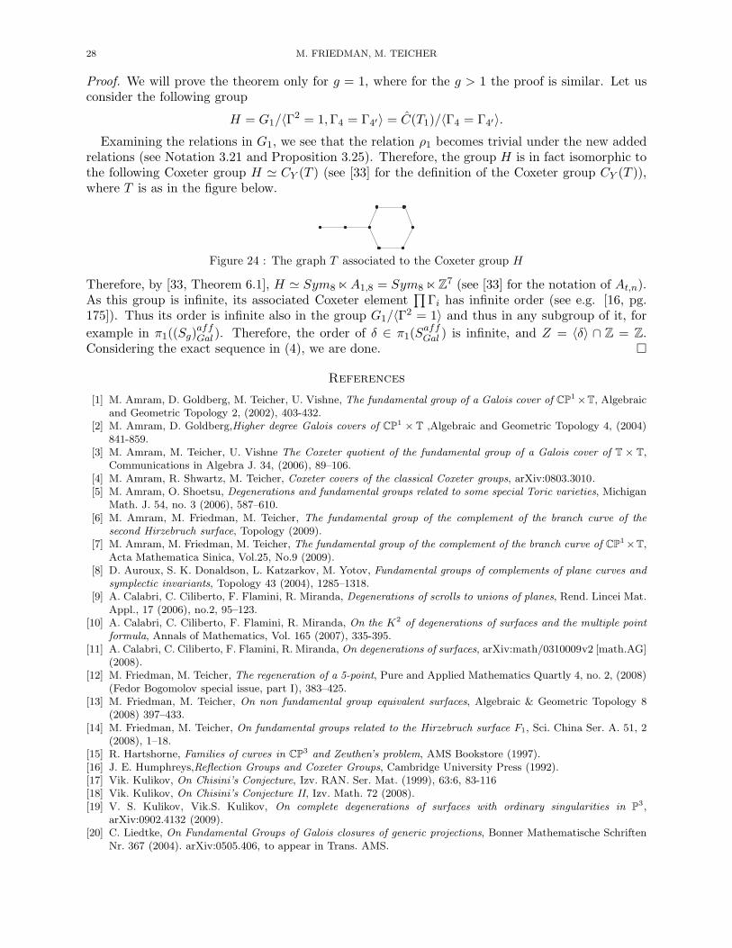
28 M. FRIEDMAN, M. TEICHER
Proof. We will prove the theorem only for g = 1, where for the g > 1 the proof is similar. Let usconsider the following group
H = G1/〈Γ2 = 1,Γ4 = Γ4′〉 = C(T1)/〈Γ4 = Γ4′〉.
Examining the relations in G1, we see that the relation ρ1 becomes trivial under the new addedrelations (see Notation 3.21 and Proposition 3.25). Therefore, the group H is in fact isomorphic tothe following Coxeter group H ≃ CY (T ) (see [33] for the definition of the Coxeter group CY (T )),where T is as in the figure below.
Figure 24 : The graph T associated to the Coxeter group H
Therefore, by [33, Theorem 6.1], H ≃ Sym8⋉A1,8 = Sym8⋉Z7 (see [33] for the notation of At,n).As this group is infinite, its associated Coxeter element
∏Γi has infinite order (see e.g. [16, pg.
175]). Thus its order is infinite also in the group G1/〈Γ2 = 1〉 and thus in any subgroup of it, for
example in π1((Sg)affGal ). Therefore, the order of δ ∈ π1(S
affGal ) is infinite, and Z = 〈δ〉 ∩ Z = Z.
Considering the exact sequence in (4), we are done. �
References
[1] M. Amram, D. Goldberg, M. Teicher, U. Vishne, The fundamental group of a Galois cover of CP1×T, Algebraic
and Geometric Topology 2, (2002), 403-432.[2] M. Amram, D. Goldberg,Higher degree Galois covers of CP1
× T ,Algebraic and Geometric Topology 4, (2004)841-859.
[3] M. Amram, M. Teicher, U. Vishne The Coxeter quotient of the fundamental group of a Galois cover of T × T,Communications in Algebra J. 34, (2006), 89–106.
[4] M. Amram, R. Shwartz, M. Teicher, Coxeter covers of the classical Coxeter groups, arXiv:0803.3010.[5] M. Amram, O. Shoetsu, Degenerations and fundamental groups related to some special Toric varieties, Michigan
Math. J. 54, no. 3 (2006), 587–610.[6] M. Amram, M. Friedman, M. Teicher, The fundamental group of the complement of the branch curve of the
second Hirzebruch surface, Topology (2009).[7] M. Amram, M. Friedman, M. Teicher, The fundamental group of the complement of the branch curve of CP1×T,
Acta Mathematica Sinica, Vol.25, No.9 (2009).[8] D. Auroux, S. K. Donaldson, L. Katzarkov, M. Yotov, Fundamental groups of complements of plane curves and
symplectic invariants, Topology 43 (2004), 1285–1318.[9] A. Calabri, C. Ciliberto, F. Flamini, R. Miranda, Degenerations of scrolls to unions of planes, Rend. Lincei Mat.
Appl., 17 (2006), no.2, 95–123.[10] A. Calabri, C. Ciliberto, F. Flamini, R. Miranda, On the K2 of degenerations of surfaces and the multiple point
formula, Annals of Mathematics, Vol. 165 (2007), 335-395.[11] A. Calabri, C. Ciliberto, F. Flamini, R. Miranda, On degenerations of surfaces, arXiv:math/0310009v2 [math.AG]
(2008).[12] M. Friedman, M. Teicher, The regeneration of a 5-point, Pure and Applied Mathematics Quartly 4, no. 2, (2008)
(Fedor Bogomolov special issue, part I), 383–425.[13] M. Friedman, M. Teicher, On non fundamental group equivalent surfaces, Algebraic & Geometric Topology 8
(2008) 397–433.[14] M. Friedman, M. Teicher, On fundamental groups related to the Hirzebruch surface F1, Sci. China Ser. A. 51, 2
(2008), 1–18.[15] R. Hartshorne, Families of curves in CP3 and Zeuthen’s problem, AMS Bookstore (1997).[16] J. E. Humphreys,Reflection Groups and Coxeter Groups, Cambridge University Press (1992).[17] Vik. Kulikov, On Chisini’s Conjecture, Izv. RAN. Ser. Mat. (1999), 63:6, 83-116[18] Vik. Kulikov, On Chisini’s Conjecture II, Izv. Math. 72 (2008).[19] V. S. Kulikov, Vik.S. Kulikov, On complete degenerations of surfaces with ordinary singularities in P3,
arXiv:0902.4132 (2009).[20] C. Liedtke, On Fundamental Groups of Galois closures of generic projections, Bonner Mathematische Schriften
Nr. 367 (2004). arXiv:0505.406, to appear in Trans. AMS.
ON FUNDAMENTAL GROUPS RELATED TO DEGENERATABLE SURFACES 29
[21] B. Moishezon, Algebraic surfaces and the arithmetic of braids. II, Combinatorial Methods in Topology andAlgebraic Geometry, Rochester, NY, (1982), Contemp. Math., 44, Amer. Math. Soc., Providence, RI, (1985)311-344.
[22] B. Moishezon, On cuspidal branch curves, J. Algebraic Geometry 2 (1993), 309–384.[23] B. Moishezon, A. Robb and M. Teicher, On Galois covers of Hirzebruch surfaces, Math. Ann. 305 (1996),
493–539.[24] B. Moishezon, M. Teicher, Galois covers in theory of algebraic surfaces, Amer. Math. Soc. Pub. PSPM 46 (1987),
47-65.[25] B. Moishezon, M. Teicher, Simply connected algebraic surfaces of positive index, Invent. Math. 89, (1987), 601–
643.[26] B. Moishezon, M. Teicher, Braid group technique in complex geometry, I: Line arrangements in CP2, Contemp.
Math. 78, (1988), 425-555.[27] B. Moishezon, M. Teicher, Braid group technique in complex geometry, II: From arrangements of lines and conics
to cuspidal curves, Algebraic Geometry, Lecture Notes in Math., vol. 1479 (1990), 131-180.[28] B. Moishezon, M. Teicher, Braid group techniques in complex geometry III: Projective degeneration of V3, Con-
temporary Math. 162 (1994), 313-332.[29] B. Moishezon, M. Teicher, Braid group techniques in complex geometry IV: Braid monodromy of the branch curve
S3 of V3 → CP2 and application to π1 : (CP2− S3, ∗), Contemp. Math. 162 (1993), 332-358.
[30] Moishezon, B., Teicher, M., Braid group technique in complex geometry V: The fundamental group of a comple-
ment of a branch curve of a Veronese generic projection, Comm. Anal. Geom. 4 (1) (1996), 1-120.[31] A. Robb, The topology of branch curves of complete intersections, Doctoral Thesis, Columbia University, (1994).[32] A. Robb, On branch curves of Algebraic Surfaces, Stud. Adv. Math. 5, (1997), 193-221.[33] L. Rowen, M. Teicher, U. Vishne, Coxeter covers of the symmetric groups, J. Group Theory 8, (2005), 139-169 .[34] M. Teicher, New Invariants for surfaces, Contemporary Mathematics 231 (1999), 271-281.[35] M. Teicher, On the quotient of the braid group by commutators of transversal half-twists and its group actions,
Topology and its Application 78 (1997), 153-186.[36] G. Zappa, Sulla degenerazione delle superficie algebriche in sistemi di piani distinti, con applicazioni allo studio
delle rigate, Atti R. Accad. d’Italia, Mem. Cl. Sci. FF., MM. e NN., 13 (2) (1943), 989-1021.[37] O. Zariski, On the topological discriminant group of a Riemann surface of genus p, Amer. J. Math., 59, (1937),
335-358.
Michael Friedman, Mina Teicher, Department of Mathematics, Bar-Ilan University, 52900 Ramat
Gan, Israel
E-mail address: [email protected], [email protected]