arX

iv:m

ath/

0301

227v

1 [

mat

h.A

G]

21

Jan

2003

ON THE GEOMETRIC GENUS OF REDUCIBLE SURFACES

AND DEGENERATIONS OF SURFACES TO UNIONS OF PLANES

A. CALABRI, C. CILIBERTO, F. FLAMINI, R. MIRANDA

1. Introduction

In this paper we study some properties of degenerations of surfaces whose general fibre isa smooth projective algebraic surface and whose central fibre is a reduced, connected surfaceX ⊂ Pr, r > 3, which is assumed to be a union of planes. Here we present a first set of resultson the subject; other aspects are still work in progress and will appear later (see [4]).

Our original motivation has been a series of papers by Guido Zappa which appeared inthe 1940–50’s regarding degenerations of scrolls to unions of planes and the computationof bounds for the topological invariants of an arbitrary smooth projective surface which isassumed to degenerate to a union of planes (see [18, 19, 20, 21, 22, 23, 24] and [4]).

Zappa was in turn motivated by earlier papers by Francesco Severi concerning Zeuthen’sproblem, i.e. the existence of degenerations of smooth projective (space) curves to unions oflines with only nodes as singularities (now called stick curves).

Zeuthen’s problem has been studied by several authors, also recently (see e.g. [14]); on thecontrary, unions of planes have been studied only in terms of degenerations of a few types ofsmooth surfaces, e.g. K3 surfaces (see [5, 6, 7, 9]).

In this paper, we first study the geometry and the combinatorics of a union of planes Xconsidered as a reduced, connected surface on its own (cf. §3 and 4); then, we focus on thecase in which X is the central fibre of an embedded degeneration X → ∆, where ∆ is thecomplex unit disk and where X ⊆ ∆ × Pr, r > 3, is a closed subscheme of relative dimensiontwo. In this case, we deduce some properties of the general fibre Xt, t 6= 0, of the degenerationfrom the ones of its central fibre X0 = X (see §5).

It is well-known that, in dimension one, for any integer g > 2 any smooth projective curveof genus g with general moduli and sufficiently general degree can be degenerated to a suitablestick curve (see, e.g. [1] and [17]).

On the contrary, in dimension two, worse singularities than normal crossings are needed inorder to degenerate as many surfaces as possible to unions of planes (cf. [4]).

Here we shall focus on the case of X a union of planes — or more generally a union ofsmooth projective surfaces — whose singularities are:

• in codimension one, double curves which are smooth and irreducible;• multiple points, which are locally analytically isomorphic to the vertex of a cone over

a stick curve with arithmetic genus either zero or one and which is projectively normalin the projective space it spans.

These multiple points will be called Zappatic singularities, whereas a surface like X will becalled a Zappatic surface. If moreover X ⊂ Pr, for some positive r, and if all its irreduciblecomponents are planes, then X is said to be a planar Zappatic surface.

Actually we will concentrate on the so called good Zappatic surfaces, i.e. Zappatic surfaceshaving only Zappatic singularities whose associated stick curve has one of the following dualgraphs (cf. Examples 2.8 and 2.9, Definition 3.6, Figures 2 and 4):

Mathematics Subject Classification (2000): 14J17, 14D06, 14N20; (Secondary) 14B07, 14N10.The first two authors are partially supported by E.C. project EAGER, contract n. HPRN-CT-2000-00099.

1

2 A. CALABRI, C. CILIBERTO, F. FLAMINI, R. MIRANDA

Rn: a chain of length n, with n > 3;Sn: a fork with n− 1 teeth, with n > 4;En: a cycle of order n, with n > 3.

Let us call Rn-, Sn-, En-point the corresponding multiple point of the Zappatic surface X.These singularities play a major role in the whole subject (cf. [4]).

We remark that a Zappatic surface X is locally Gorenstein (i.e. its dualizing sheaf ωX isinvertible) if and only if its Zappatic singularities are only En-points, for any n > 3.

We associate to a good Zappatic surface X a graph GX (see Definition 3.7) which encodesthe configuration of the irreducible components of X as well as its Zappatic singularities.

We shall see (cf. Sections 3 and 4) how to combinatorially compute from the associatedgraph GX some intrinsic and extrinsic invariants of X, e.g. the Euler-Poincare characteristicχ(OX), the geometric genus pg(X) (cf. Remark 3.4), as well as — when X ⊂ P

r, r > 3 —the degree d = deg(X), the sectional genus g, and so on.

When X is further assumed to be the central fibre of a degeneration X → ∆ (resp., of anembedded degeneration X → ∆, where X ⊂ ∆ × Pr, r > 3) we will then compute intrinsic(resp., intrinsic and extrinsic) invariants of the general fibre Xt, for t 6= 0.

We shall see how to directly compute some of the invariants ofX by means of the associatedgraph GX . Determining formulas for a few invariants (e.g. d and g) is quite easy, whereas forother invariants, like χ(OX), it requires some more work.

Actually the computation of the geometric genus is still an open question, in general.Indeed, we first prove the following (cf. Theorem 4.15):

Theorem. Let X =⋃

iXi be a Zappatic surface with global normal crossings, i.e. with onlyE3-points as Zappatic singularities. Denote by ωX the dualizing sheaf of X and by GX theassociated graph of X. Consider the natural map:

Φ :⊕

i

H1(Xi,OXi) →

⊕

i,j

H1(Cij,OCij),

where Cij = Xi ∩Xj (cf. formula (4.8)). Then, the following inequality holds:

(1.1) pg(X) := h0(X,ωX) 6 h2(GX ,C) +

v∑

i=1

pg(Xi) + dim(coker(Φ)).

Furthermore, a sufficient condition for the equality in (1.1) to hold is either that

(i) each irreducible component Xi is a regular surface (i.e. h1(OXi) = 0), or that

(ii) for any irregular component Xj of X, the divisor Cj := Xj ∩ (X \Xj) is ample onXj.

The proof of the above theorem also shows the following:

Corollary. Let X be a planar Zappatic surface with global normal crossings (i.e. only E3-points) and GX be its associated graph. Then, there exists an explicit isomorphism

(1.2) H0(X,ωX) ∼= H2(GX ,C),

where ωX is the dualizing sheaf of X. Therefore

pg(X) := h0(X,ωX) = h2(GX ,C).

From the proof of Theorem 4.15, it will be clear that the isomorphism (1.2) essentiallyfollows from evaluation of residues at the E3-points, with a suitable use of signs.

We show that equality holds in (1.1) when X is smoothable, i.e. when X is the centralfibre of a semistable degeneration X → ∆: this follows by the computation of the geometricgenus pg(Xt) of the general fibre Xt, for t 6= 0, via the Clemens-Schmid exact sequence (cf.Theorem 5.12).

ON THE GEOMETRIC GENUS OF REDUCIBLE SURFACES 3

We remark that our computation of the geometric genus is independent of the fact thatX is the central fibre of a semistable degeneration. We deal with this particular case in §5,where we show that in a semistable degeneration, whose central fibre is a Zappatic surfacewith only E3-points, the geometric genus of the fibres is constant (see Corollary 5.15).

It is still an open problem to find an example for which the strict inequality holds in (1.1).Finally, we will see that the above results can be generalized to a smoothable good Zappatic

surface, i.e. with Rn-, Sn- and En-points, for any n > 3 (see Theorem 5.20).A natural question to ask is which Zappatic singularities are needed in order to degenerate

as many surfaces as possible. Results and some examples contained in [4] suggest that, evenif a given projective surface X needs En-, Rn-, or Sn-points with large n, there might be abirational model of X which needs just R3- and En-points, with n 6 6. For example, in [6]there are interesting examples of K3 surfaces degenerating to a Zappatic surface with at mostR3- and E6-points, called pillow degenerations. However, we do not have enough evidence tostate a reasonable conjecture in this direction.

Acknowledgments. The authors would like to thank Janos Kollar, for some useful discus-sions and references, and the organizers of the Fano Conference, for the very stimulatingatmosphere during the whole week of the meeting.

2. Reducible curves and associated graphs

Let C be a projective curve and let Ci, i = 1, . . . , n, be its irreducible components. We willassume that:

• C is connected and reduced;• C has at most nodes as singularities;• the curves Ci, i = 1, . . . , n, are smooth.

If two components Ci, Cj , i < j, intersect at mij points, we will denote by P hij, h =

1, . . . , mij, the corresponding nodes of C.We can associate to this situation a simple (i.e. with no loops), connected graph GC :

• whose vertices v1, . . . , vn, correspond to the components C1, . . ., Cn;• whose edges ηhij , i < j, h = 1, . . . , mij , joining the vertices vi and vj , correspond to

the nodes P hij of C.

We will assume the graph to be lexicographically oriented, i.e. each edge is assumed to beoriented from the vertex with lower index to the one with higher index.

We will use the following notation:

• v : the number of vertices of GC , i.e. v = n;• e : the number of edges of GC , i.e. the number of nodes of C;• gi : the genus of the curve Ci, which we consider as the weight of the vertex vi;• χ(GC) = v − e is the Euler-Poincare characteristic of GC ;• h1(GC) = 1 − χ(GC) is the first Betti number of GC .

Remark that conversely, given any simple, connected, weighted (oriented) graph G, thereis some curve C such that G = GC .

One has the following basic result:

Theorem 2.1. In the above situation

(2.2) χ(OC) = χ(GC) −v∑

i=1

gi = v − e−v∑

i=1

gi.

4 A. CALABRI, C. CILIBERTO, F. FLAMINI, R. MIRANDA

Proof. Let ν : C → C be the normalization morphism; this defines the exact sequence ofsheaves on C:

(2.3) 0 → OC → ν∗(OC) → τ → 0,

where τ is a sky-scraper sheaf supported at Sing(C). Since the singularities of C are onlynodes, one easily determines H0(C, τ) ∼= Ce. Therefore, by the exact sequence (2.3), one gets

χ(OC) = χ(ν∗(OC)) − e.

By the Leray isomorphism and by the fact that ν is finite, one has χ(ν∗(OC)) = χ(OC). Since

C is a disjoint union of the v = n irreducible components of C, one has χ(OC) = v−∑v

i=1 gi,which proves (2.2). (Cf. also [2] for another proof.)

We remark that formula (2.2) is equivalent to

(2.4) pa(C) = h1(GC) +

v∑

i=1

gi,

(cf. Proposition 3.12).Notice that C is locally Gorenstein, i.e. the dualizing sheaf ωC is invertible. One defines

the geometric genus of C to be

(2.5) pg(C) := h0(C, ωC).

By the Riemann-Roch Theorem, one has

(2.6) pg(C) = pa(C) = h1(GC) +

v∑

i=1

gi = e− v + 1 +

v∑

i=1

gi.

However, one can prove the previous formula combinatorially by showing that there is anatural short exact sequence:

(2.7) 0 →v⊕

i=1

H0(Ci, ωCi) → H0(C, ωC) → H1(GC ,C) → 0

We will not dwell on this now, since we shall show the existence of an analogous sequencein the surface case in §4.

If we have a flat family C → ∆ over a disc ∆ with general fibre Ct a smooth and irreduciblecurve of genus g and special fibre C0 = C, then we can combinatorially compute g via theformula:

g = pa(C) = h1(GC) +

v∑

i=1

gi = e− v + 1 +

v∑

i=1

gi.

Usually we will consider a curve C embedded in a projective space Pr. In this situation

each curve Ci will have a certain degree di, and we will consider the graph GC as doubleweighted, by attaching to each vertex the pair of weights (gi, di). Moreover we will attributeto the graph a further marking number, i.e. the embedding dimension r of C.

The total degree of C is

d =v∑

i=1

di

which is also invariant by flat degeneration.If each curve Ci is a line, the curve C is called a stick curve. In this case the double

weighting is (0, 1) for each vertex, and it will be omitted if no confusion arises.It should be stressed that it is not true that for any simple, connected, double weighted

graph G there is a curve C in a projective space such that GC = G. For example there is nostick curve corresponding to the graph of Figure 1.

ON THE GEOMETRIC GENUS OF REDUCIBLE SURFACES 5

•

• •

•

Figure 1. Dual graph of an “impossible” stick curve.

We now give two examples of stick curves which will be frequently used in this paper.

Example 2.8. Let Tn be any connected tree with n > 3 vertices. This corresponds to anon-degenerate stick curve of degree n in Pn, which we denote by CTn . Indeed one can checkthat, taking a general point pi on each component of CTn , the line bundle OCTn

(p1 + · · ·+ pn)is very ample. Of course CTn has arithmetic genus 0 and is a flat limit of rational normalcurves in Pn.

We will often consider two particular trees Tn: a chain Rn of length n and the fork Sn withn− 1 teeth, i.e. a tree consisting of n− 1 vertices joining a further vertex (see Figures 2.(a)and (b)). The curve CRn is the union of n lines l1, l2, . . . , ln spanning P

n, such that li ∩ lj = ∅if and only if 1 < |i− j|. The curve CSn is the union of n lines l1, l2, . . . , ln spanning Pn, suchthat l1, . . . , ln−1 all intersect ln at distinct points (see Figure 3).

• • • • • • •

•

• • • •••

••

•

•

• •

•

(a) A chain Rn (b) A fork Sn with n− 1 teeth (c) A cycle En

Figure 2. Examples of dual graphs.

Example 2.9. Let Zn be any simple, connected graph with n > 3 vertices and h1(Zn,C) = 1.This corresponds to a projectively normal stick curve of degree n in Pn−1, which we denoteby CZn (as in Example 2.8). The curve CZn has arithmetic genus 1 and it is a flat limit ofelliptic normal curves in P

n−1.We will often consider the particular case of a cycle En of order n (see Figure 2.c). The

curve CEn is the union of n lines l1, l2, . . . , ln spanning Pn−1, such that li ∩ lj = ∅ if and onlyif 1 < |i− j| < n− 1 (see Figure 3).

We remark that CEn is projectively Gorenstein, because ωCEnis trivial, since there is

an everywhere non-zero global section of ωCEn, given by the meromorphic 1-form on each

component with residues 1 and −1 at the nodes (in a suitable order).All the other CZn ’s, instead, are not locally Gorenstein because ωCZn

, although of degreezero, is not trivial. Indeed a graph Zn, different from En, certainly has a vertex with valence1. This corresponds to a line l such that ωCZn

⊗ Ol is not trivial.

3. Zappatic surfaces and associated graphs

First of all, we need to introduce the singularities we will allow.

Definition 3.1 (Zappatic singularity). Let X be a surface and let x ∈ X be a point. Wewill say that x is a Zappatic singularity for X if (X, x) is locally analytically isomorphic toa pair (Y, y) where Y is the cone over either a curve CTn or a curve CZn, n > 3, and y is thevertex of the cone. Accordingly we will say that x is either a Tn- or a Zn-point for X.

Definition 3.2 (Zappatic surface). Let X be a projective surface with its irreducible com-ponents X1, . . . , Xv. We will assume that X has the following properties:

6 A. CALABRI, C. CILIBERTO, F. FLAMINI, R. MIRANDA

•

•

•

•

•

•

• • • • • •

••

•

•

••

•

CRn : a chain of n lines, CSn: a comb with n− 1 teeth, CEn: a cycle of n lines.

Figure 3. Examples of stick curves.

• X is reduced and connected in codimension one;• X1, . . . , Xv are smooth;• the singularities in codimension one of X are at most double curves which are smooth

and irreducible;• the further singularities of X are Zappatic singularities.

A surface like X will be called a Zappatic surface. If moreover X is embedded in a projectivespace Pr and all of its irreducible components are planes, we will say that X is a planarZappatic surface.

Notation 3.3. Let X be a Zappatic surface. Let us denote by:

• Xi : an irreducible component of X, i 6 i 6 v;• Cij := Xi∩Xj , 1 6 i 6= j 6 v, if Xi and Xj meet along a curve, otherwise set Cij = ∅;• gij : the genus of Cij , 1 6 i 6= j 6 v;• C := Sing(X) = ∪i<j Cij, the union of all the double curves of X;• Σijk := Xi ∩Xj ∩Xk, 1 6 i 6= j 6= k 6 v, if Xi ∩Xj ∩Xk 6= ∅, otherwise Σijk = ∅;• mijk : the cardinality of the set Σijk;• P h

ijk : the Zappatic singular point belonging to Σijk, for h = 1, . . . , mijk.

Furthermore, if X ⊂ Pr, for some r, we denote by

• d : the degree of X;• di : the degree of Xi, i 6 i 6 v;• cij : the degree of Cij, 1 6 i 6= j 6 v;• D : a general hyperplane section of X;• g : the arithmetic genus of D;• Di : the (smooth) irreducible component of D lying in Xi, which is a general hyper-

plane section of Xi, 1 6 i 6 v;• gi : the genus of Di, 1 6 i 6 v.

If moreover X is a planar Zappatic surface, then d = v, each non-empty set Σijk is a singletonand mijk = 1, for each i 6= j 6= k.

Remark 3.4. A Zappatic surface X is locally Cohen-Macaulay. Thus the dualizing sheaf ωXis well-defined. If X has only En-points as Zappatic singularities, thenX is locally Gorenstein,hence ωX is an invertible sheaf. If X has global normal crossings, i.e. if X has only E3-pointsas Zappatic singularities, we define the geometric genus of X as:

(3.5) pg(X) := h0(X,ωX).

If X is smoothable, namely if X is the central fibre of a degeneration, we will define itsgeometric genus later in Definition 5.18.

Definition 3.6 (Good Zappatic surface). The good Zappatic singularities are the

• Rn-points, for n > 3,

ON THE GEOMETRIC GENUS OF REDUCIBLE SURFACES 7

• Sn-points, for n > 4,• En-points, for n > 3,

which are the Zappatic singularities whose associated stick curves are respectively CRn , CSn ,CEn (see Examples 2.8 and 2.9, Figures 2, 3 and 4).

A good Zappatic surface is a Zappatic surface with only good Zappatic singularities.

•

D1 D2

D3

X1 X2

X3C13

C12

C23

•

D1

D2

D3

X1

X2

X3

C12 C23

E3-point R3-point

•

D1

D2 D3

D4

X1

X2 X3

X4

C12

C23

C34

•

D1

D2

D3

X1 X2 X3

C12 C23

X4C24

D4

R4-point S4-point

Figure 4. Examples of good Zappatic singularities.

To a good Zappatic surface X we can associate a complex GX , which we briefly call theassociated graph to X.

Definition 3.7 (The associated graph toX). LetX be a good Zappatic surface with Notation3.3. The graph GX associated to X is defined as follows (cf. Figure 5):

• each surface Xi corresponds to a vertex vi;• each double curve Cij correspond to an edge eij joining vi and vj . The edge eij , i < j,

is oriented from the vertex vi to the one vj ;• each En-point P of X is a face of the graph whose n edges correspond to the double

curves concurring at P . This is called a n-face of the graph;• for each Rn-point P , with n > 3, if P ∈ Xi1 ∩ Xi2 ∩ · · · ∩Xin , where Xij meets Xik

along a curve Cij ik only if 1 = |j − k|, we add in the graph a dashed edge joining thevertices corresponding to Xi1 and Xin. The dashed edge ei1,in, together with the othern− 1 edges eij ,ij+1

, j = 1, . . . , n− 1, bound an open n-face of the graph;• for each Sn-point P , with n > 4, if P ∈ Xi1 ∩ Xi2 ∩ · · · ∩ Xin, where Xi1, . . . , Xin−1

all meet Xin along curves Cijin , j = 1, . . . , n − 1, concurring at P , we mark thisin the graph by an a angle spanned by the edges corresponding to the curves Cijin ,j = 1, . . . , n− 1.

8 A. CALABRI, C. CILIBERTO, F. FLAMINI, R. MIRANDA

In the sequel, when we speak of faces of GX we always mean closed faces. Of course eachvertex vi is weighted with the relevant invariants of the corresponding surface Xi. We willusually omit these weights if X is planar, i.e. if all the Xi’s are planes.

Since each Rn-, Sn-, En-point is an element of some set of points Σijk (cf. Notation 3.3),we remark that there can be different faces (as well as open faces and angles) of GX whichare incident on the same set of vertices and edges. However this cannot occur if X is planar.

•

•

•v1

v2

v3•

•

•v1

v2

v3 •

• •

•v1

v3

v4

v2

•

•

••

v1

v2

v4

v3

R3-point E3-point R4-point S4-point

Figure 5. Associated graphs of R3-, E3-, R4- and S4-points (cf. Figure 4).

Notice that angles, open and closed faces of GX have been defined in order to encodethe good Zappatic singularities of X. In other words, the associated graph GX uniquelydetermines the configuration of the good Zappatic singularities of X.

Consider three vertices vi, vj, vk of GX in such a way that vi is joint with vj and vk. Anypoint in Cij∩Cik is either a Rn-, or a Sn-, or an En-point, and the curves Cij and Cik intersecttransversally, by definition of Zappatic singularities. Hence we can compute the intersectionnumber Cij · Cik by adding the number of closed and open faces and of angles involving theedges eij, eik. In particular, if X is planar, for every pair of adjacent edges only one of thefollowing possibilities occur: either they belong to an open face, or to a closed one, or toan angle. Therefore for good, planar Zappatic surfaces we can avoid to mark open 3-faceswithout loosing any information (see Figure 6, cf. Figure 5).

•

•

•v1

v2

v3

Figure 6. Associated graph of a R3-point in a good, planar Zappatic surface.

Remark 3.8. We also notice that, given our choices, if X is good Zappatic and has onlyE3-points, the graph GX comes with a lexicographic orientation of the faces; indeed, letΣijk = Xi∩Xj∩Xk = P 1

ijk, P2ijk, . . . , P

mijk

ijk ; thus, each face of GX corresponds to a sequenceof three vertices i, j, k with i < j < k, together with an integer t such that 1 6 t 6 mijk,hence it will be denoted by f tσ(i),σ(j),σ(k), with σ any permutation of i, j, k, and will be orientedaccording to the orientation of its boundary determined by the sequence of vertices vi, vj, vk.

As for stick curves, if G is a given graph as above, there does not necessarily exist a goodplanar Zappatic surface X such that its associated graph is G = GX .

Example 3.9. Consider the graph G of Figure 7. If G were the associated graph of a goodplanar Zappatic surface X, then X should be a global normal crossing union of 4 planes with5 double lines and two E3 points, P123 and P134, both lying on the double line C13. Sincethe lines C23 and C34 (resp. C14 and C12) both lie on the plane X3 (resp. X1), they shouldintersect. This means that the planes X2, X4 also should intersect along a line, therefore theedge e24 should appear in the graph.

ON THE GEOMETRIC GENUS OF REDUCIBLE SURFACES 9

•

• •

•v1

v3

v4

v2

Figure 7. Graph associated to an impossible planar Zappatic surface.

Before going on, we need some notation.

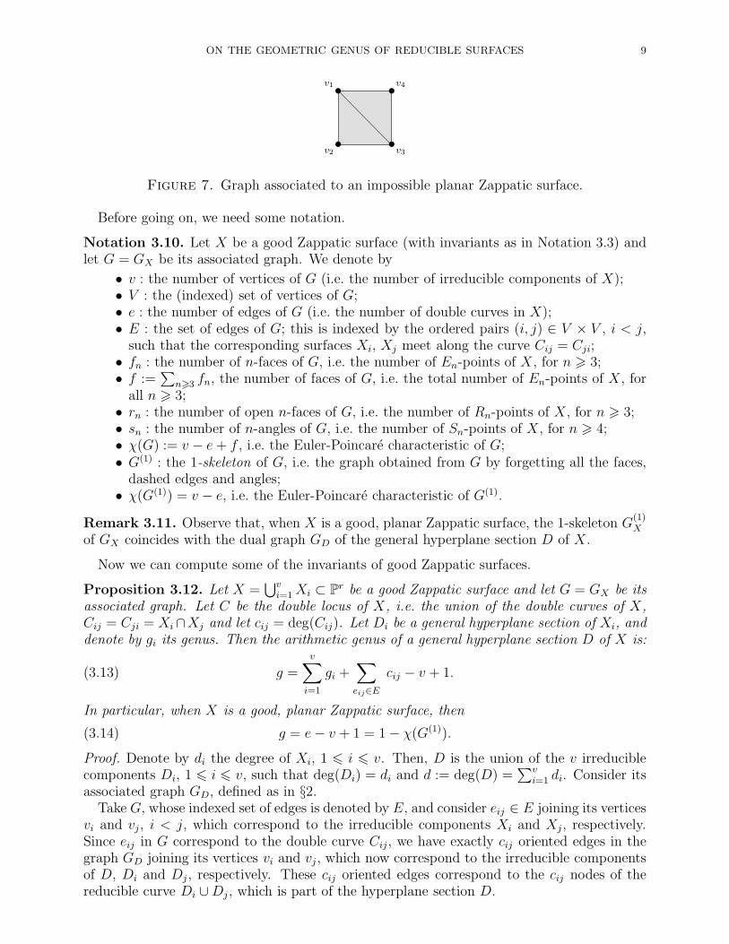
Notation 3.10. Let X be a good Zappatic surface (with invariants as in Notation 3.3) andlet G = GX be its associated graph. We denote by

• v : the number of vertices of G (i.e. the number of irreducible components of X);• V : the (indexed) set of vertices of G;• e : the number of edges of G (i.e. the number of double curves in X);• E : the set of edges of G; this is indexed by the ordered pairs (i, j) ∈ V × V , i < j,

such that the corresponding surfaces Xi, Xj meet along the curve Cij = Cji;• fn : the number of n-faces of G, i.e. the number of En-points of X, for n > 3;• f :=

∑

n>3 fn, the number of faces of G, i.e. the total number of En-points of X, forall n > 3;

• rn : the number of open n-faces of G, i.e. the number of Rn-points of X, for n > 3;• sn : the number of n-angles of G, i.e. the number of Sn-points of X, for n > 4;• χ(G) := v − e+ f , i.e. the Euler-Poincare characteristic of G;• G(1) : the 1-skeleton of G, i.e. the graph obtained from G by forgetting all the faces,

dashed edges and angles;• χ(G(1)) = v − e, i.e. the Euler-Poincare characteristic of G(1).

Remark 3.11. Observe that, when X is a good, planar Zappatic surface, the 1-skeleton G(1)X

of GX coincides with the dual graph GD of the general hyperplane section D of X.

Now we can compute some of the invariants of good Zappatic surfaces.

Proposition 3.12. Let X =⋃vi=1Xi ⊂ Pr be a good Zappatic surface and let G = GX be its

associated graph. Let C be the double locus of X, i.e. the union of the double curves of X,Cij = Cji = Xi∩Xj and let cij = deg(Cij). Let Di be a general hyperplane section of Xi, anddenote by gi its genus. Then the arithmetic genus of a general hyperplane section D of X is:

(3.13) g =v∑

i=1

gi +∑

eij∈E

cij − v + 1.

In particular, when X is a good, planar Zappatic surface, then

(3.14) g = e− v + 1 = 1 − χ(G(1)).

Proof. Denote by di the degree of Xi, 1 6 i 6 v. Then, D is the union of the v irreduciblecomponents Di, 1 6 i 6 v, such that deg(Di) = di and d := deg(D) =

∑vi=1 di. Consider its

associated graph GD, defined as in §2.Take G, whose indexed set of edges is denoted by E, and consider eij ∈ E joining its vertices

vi and vj , i < j, which correspond to the irreducible components Xi and Xj , respectively.Since eij in G correspond to the double curve Cij, we have exactly cij oriented edges in thegraph GD joining its vertices vi and vj , which now correspond to the irreducible componentsof D, Di and Dj , respectively. These cij oriented edges correspond to the cij nodes of thereducible curve Di ∪Dj , which is part of the hyperplane section D.

10 A. CALABRI, C. CILIBERTO, F. FLAMINI, R. MIRANDA

Now, recall that the Hilbert polynomial of D is, with our notation, PD(t) = dt+1− g. Onthe other hand, PD(t) equals the number of independent conditions imposed on hypersurfacesH of degree t≫ 0 to contain D.

From what observed above on GD, it follows that the number of singular points of D is∑

eij∈Ecij . These points impose independent conditions on hypersurfaces H of degree t≫ 0.

Since t≫ 0 by assumption, we get that the map

H0(OPr(t)) → H0(ODi(t))

is surjective and that the line bundle ODi(t) is non-special on Di, for each 1 6 i 6 v. Thus, in

order for H to contain Di we have to impose dit−gi+1−∑

j s.t. eij∈Ecij conditions. Therefore

the total number of conditions for H to contain D is:∑

eij∈E

cij +v∑

i=1

(

dit− gi + 1 −∑

j,eij∈E

cij

)

=∑

eij∈E

cij + dt−v∑

i=1

gi + v −v∑

i=1

∑

j,eij∈E

cij =

= dt+ v −v∑

i=1

gi −∑

eij∈E

cij ,

since∑v

i=1

∑

j,eij∈Ecij = 2

∑

eij∈Ecij. This proves (3.13) (cf. formula (2.4)).

The second part of the statement directly follows from the above computations and fromthe fact that, in the good planar Zappatic case gi = 0 and cij = 1, for each i < j, i.e. GD

coincides with G(1) (cf. Remark 3.11).

By recalling Notation 3.10, one also has:

Proposition 3.15. Let X =⋃vi=1Xi be a good Zappatic surface and GX be its associated

graph. Let C be the double locus of X, which is the union of the curves Cij = Cji = Xi ∩Xj.Then:

(3.16) χ(OX) =v∑

i=1

χ(OXi) −

∑

eij∈E

χ(OCij) + f.

In particular, when X is a good, planar Zappatic surface, then

(3.17) χ(OX) = χ(GX) = v − e+ f.

Proof. We can consider the sheaf morphism:

(3.18)

v⊕

i=1

OXi

λ−→

⊕

16i<j6v

OCij,

defined in the following way: if

πij :⊕

16i<j6v

OCij→ OCij

denotes the projection on the (ij)th-summand, then

(πij λ)(h1, . . . , hv) := hi − hj .

Notice that the definition of λ is consistent with the lexicographic order of the indices andwith the lexicographic orientation of the edges of the graph GX .

Observe that, if X denotes the desingularization of X, then X is isomorphic to the disjointunion of the smooth, irreducible components Xi, 1 6 i 6 v, of X. Therefore, by the verydefinition of OX , we see that

ker(λ) ∼= OX .

ON THE GEOMETRIC GENUS OF REDUCIBLE SURFACES 11

We claim that the morphism λ is not surjective and that its cokernel is a sky-scraper sheafsupported at the En-points of X. To show this, we focus on any irreducible component ofC =

⋃

16i<j6v Cij , the double locus of X.

Fix any index pair (i, j), with i < j, and consider the generator

(3.19) (0, . . . , 0, 1, 0, . . . , 0) ∈⊕

16l<m6v

OClm,

where 1 ∈ OCij, the (ij)th-summand. The obstructions to lift up this element to an element

of⊕

16t6v OXt are given by the presence of good Zappatic singularities of X along Cij .For what concerns the irreducible components of X which are not involved in the intersec-

tion determining a good Zappatic singularity on Cij , the element in (3.19) trivially lifts-upto 0 on each of them. Thus, in the sequel, we shall focus only on the irreducible componentsinvolved in the Zappatic singularity, which will be denoted by Xi, Xj, Xlt , for 1 6 t 6 n−2.

We have to consider different cases, according to the good Zappatic singularity type lyingon the curve Cij = Xi ∩Xj .

• Suppose that Cij passes through a Rn-point P of X, for some n; we have two differentpossibilities. Indeed:(a) let Xi be an “external” surface for P — i.e. Xi corresponds to a vertex of theassociated graph of P which has valence 1. Therefore, we have:

r r r r r· · ·Xi Xj Xl1

Xln−3Xln−2

In this situation, the element in (3.19) lifts up to

(1, 0, . . . , 0) ∈ OXi⊕ OXj

⊕⊕

16t6n−2

OXlt.

(b) let Xi be an “internal” surface for P — i.e. Xi corresponds to a vertex of theassociated graph to P which has valence 2. Thus, we have a picture like:

r r r r r r r· · ·Xl1

Xl2Xl3

Xi Xj Xln−3Xln−2

In this case, the element in (3.19) lifts up to the n-tuple having components:1 ∈ OXi

,0 ∈ OXj

,1 ∈ OXlt

, for those Xlt ’s corresponding to vertices in the graph associated to Pwhich are on the left of Xi and,0 ∈ OXlk

for those Xlk ’s corresponding to vertices in the graph associated to Pwhich are on the right of Xj .

• Suppose that Cij passes through a Sn-point P of X, for any n; as before, we have twodifferent possibilities. Indeed:(a) let Xi corresponds to the vertex of valence n− 1 in the associated graph to P , i.e.

@@

@

HHHHHH

XXXXXXXXXXXX

r

r r r r r r r· · ·· · ·

Xi

Xl1Xl2

XlkXj Xlk+1

Xlk+2Xln−2

In this situation, the element in (3.19) lifts up to the n-tuple having components:1 ∈ OXi

,0 ∈ OXj

,1 ∈ OXlt

, for all 1 6 t 6 n− 2.

12 A. CALABRI, C. CILIBERTO, F. FLAMINI, R. MIRANDA

(b) let Xi corresponds to a vertex of valence 1 in the associated graph to P . SinceCij 6= ∅ by assumption, then Xj has to be the vertex of valence n − 1, i.e. we havethe following picture:

@@

@

HHHHHH

XXXXXXXXXXXX

r

r r r r r r r· · ·· · ·

Xj

Xl1Xl2

XlkXi Xlk+1

Xlk+2Xln−2

Thus, the element in (3.19) lifts up to the n-tuple having components1 ∈ OXi

,0 ∈ OXj

,0 ∈ OXlt

, for all 1 6 t 6 n− 2.• Suppose that Cij passes through an En-point P for X. Then, each vertex of the

associated graph to P has valence 2. Since such a graph is a cycle, it is clear that nolifting of (3.19) can be done.

To sum up, we see that coker(λ) is supported at the En-points of X. Furthermore, if weconsider

⊕

16i<j6v

OCij

evP−−−→ OP = CP , ⊕fij 7→∑

fij(P )

it is clear that, if P is an En-point then

evP

(

⊕

16i<j6v

OCij/ Im(λ)

)

∼= CP .

This means thatcoker(λ) ∼= C

f .

By the exact sequences

0 → OX →⊕

16i6v

OXi→ Im(λ) → 0, 0 → Im(λ) →

⊕

16i<j6v

OCij→ C

f → 0,

we get (3.16).

In the next section we will see how the computation of the geometric genus is much moreinvolved, even in the case of X having only E3-points as Zappatic singularities.

4. The geometric genus of a Zappatic surface with only E3-points

The main purpose of this section is to compute the geometric genus of a projective goodZappatic surface X =

⋃vi=1Xi (cf. Remark 3.4), which is assumed to have only E3-points, i.e.

global normal crossing singularities. In terms of its associated graph, this means that GX isa subgraph of the complete graph on v vertices, which has only 3-faces (i.e. triangles).

We first want to recall some definitions and results, which will be used in the sequel.

Definition 4.1. Let T be a smooth surface and C be a smooth, irreducible curve on T . Letω be a global meromorphic 2-form on T whose polar locus contains C. We may assume thatx, y are local coordinates on T in an analytic neighbourhood of a point of C in such a waythat y = 0 is the local equation defining C. Then, the Poincare residue map (or adjunctionmap)

ωT ⊗ OT (C)RC−−→ ωC

is locally defined by:

ω =f(x, y)

ydx ∧ dy 7→ −f(x, 0) dx

ON THE GEOMETRIC GENUS OF REDUCIBLE SURFACES 13

and −f(x, 0) dx is called the (Poincare) residue of the 2-form ω along C (see [10, p. 147]).If, more generally, C is assumed to be a reduced (possibly reducible) divisor with only

normal crossing singularities, denote by ωC its dualizing sheaf and take local coordinates onT in an analytic neighbourhood of a node of C in such a way that xy = 0 is its local definingequation. If

ω =f(x, y)

xydx ∧ dy,

then one defines the Poincare residue map by considering

(4.2) RC(ω) ∈ H0(C, ωC)

defined as the pair of forms:

(i) ωx = −f(x, 0)

xdx on the branch y = 0,

(ii) ωy =f(0, y)

ydy on the branch x = 0.

Remark 4.3. If R0(ωx) denotes the usual Poincare residue at the point x = 0 of the mero-morphic 1-form ωx on the (smooth) branch y = 0, observe that

(4.4) R0(ωy) = −R0(ωx).

This is consistent with the definition of H0(C, ωC). Indeed, assume that C has only m nodes;then, if ν : C → C is the normalization morphism and if q1, q

′1, q2, q

′2, . . . , qm, q

′m are

the pre-images in C of the m nodes of C, then ωC is the invertible subsheaf

ωC ⊂ ν∗(ωC(

m∑

i=1

(qi + q′i)))

such that a section σ of ν∗(ωC(∑m

i=1(qi + q′i))), viewed as a section of ωC(∑m

i=1(qi + q′i)), is asection of ωC if and only if

Rqi(σ) + Rq′i(σ) = 0, 1 6 i 6 m.

Unless otherwise stated, from now on X =⋃vi=1Xi will denote a projective, Zappatic

surface with E3-points only as Zappatic singularities and we use notation as in Definition 3.2and in Notation 3.10.

It is well known that, for each i:

(4.5) ωXi∼= ωX ⊗ OXi

(−Ci), with Ci := Xi ∩ (X \Xi) =∑

j 6=i

Cij,

where ωXiis the canonical line bundle of Xi, whereas ωX denotes the dualizing sheaf of X.

Note that ωX is an invertible sheaf by the hypotheses on X.As in Remark 3.4, recall that the geometric genus of X is denoted by pg(X) and defined

as pg(X) = h0(X,ωX). In order to compute pg(X), we need some further remarks which willbe fundamental in the sequel.

Remark 4.6. Observe that, if X =⋃vi=1Xi is as above, since the intersection Xi ∩ Xj —

when non-empty — is the double curve Cij = Cji, the index pair (i, j) with i < j uniquelydetermines the double curve Cij . In the same way, when i < j, since the intersection Xi ∩Xj ∩Xk — when non-empty — is the triple point set Σijk = Στ(i)τ(j)τ(k), for k 6= i, j and forany τ ∈ Sym(i, j, k), then the lexicographically ordered index triple uniquely determinesthe triple point set either Σkij, or Σikj , or Σijk, according to the fact that either k < i, ori < k < j, or k > j.

14 A. CALABRI, C. CILIBERTO, F. FLAMINI, R. MIRANDA

Remark 4.7. Since the only Zappatic singularities of X are assumed to be E3-points, thenGX contains neither dashed edges, nor angles, nor open faces, nor n-faces, with n > 4.Furthermore, in such a case the graph GX comes with a lexicographic orientation of the faces(see Remark 3.8). If X is, in particular, planar recall that we have strong constraints on thepossible shape of the graph GX — because of the geometry of planes (cf. Example 3.9)— andeach non-zero mijk equals one.

Observe that by the connectedness hypothesis of X =⋃vi=1Xi, we get that Ci 6= ∅, for

each 1 6 i 6 v. For simplicity of notation, in the sequel we shall always denote by Cij theintersection of Xi and Xj , for any 1 6 i < j 6 v, with the obvious further condition thatCij = Cji = ∅ when the index pair corresponds to two disjoint surfaces in X, i.e. when thereis no edge (vi, vj) in the associated graph GX .

We can define a natural map

(4.8) Φ :v⊕

i=1

H1(Xi,OXi) →

⊕

16i<j6v

H1(Cij ,OCij)

in the following way: if

πij :⊕

16i<j6v

H1(Cij,OCij) → H1(Cij ,OCij

)

denotes the projection on the (ij)th-summand and if r(i)Cij

: H1(Xi,OXi) → H1(Cij ,OCij

)denotes the natural restriction map to Cij as a divisor in Xi, where i < j, then

(4.9) (πij Φ)((a1, . . . , av)) := r(i)Cij

(ai) − r(j)Cij

(aj).

Remark 4.10. Observe that the above definition is consistent with the lexicographic orderof the indices 1 6 i 6 v. In other words, (4.9) means that we consider the curve Cij asa positive curve on the surface Xi and as a negative curve on the surface Xj , when i < j.Furthermore, when the index pair is such that Cij = ∅, we obviously consider H1(Cij ,OCij

)as the zero-vector space and πij Φ as the zero-map.

Take an index pair i < j such that Cij 6= ∅. By the adjunction sequence of Cij on Xi andon Xj, we can consider the two obvious coboundary maps:

(4.11) H1(Xi, ωXi)

H0(Cij, ωCij)

δi

δj

H1(Xj , ωXj).

On the other hand, when the index pair i < j is such that Cij = ∅, then H0(Cij, ωCij) is

considered as the zero-vector space and (4.11) are the zero-maps. Then, we can define themap

(4.12) ∆ :⊕

16i<j6v

H0(Cij, ωCij) →

v⊕

i=1

H1(Xi, ωXi)

in the following way: if

ιij : H0(Cij , ωCij) →

⊕

16i<j6v

H0(Cij , ωCij)

denotes the natural inclusion of the (ij)th-summand and if γij ∈ H0(Cij, ωCij), then

(4.13) (∆ ιij)(γij) := (0, . . . , 0, δi(γij), 0, . . . , 0,−δj(γij), 0, . . . , 0),

ON THE GEOMETRIC GENUS OF REDUCIBLE SURFACES 15

where i < j.Observe that the definition of ∆ is consistent with the lexicographic order of the indices

1 6 i 6 v and with our Remark 4.10.The following preliminary result is an obvious consequence of our definitions.

Proposition 4.14. With notation as above, we have

∆ = Φ∨.

Proof. The proof directly follows from Serre’s duality on each summand and from the factthat the matrix which represents ∆ is the transpose of the one representing Φ.

We are now able to prove the main result of this section.

Theorem 4.15. Let X =⋃vi=1Xi be a projective, good Zappatic surface with only E3-points

as Zappatic singularities. Denote by ωX the dualizing sheaf of X and by GX the associatedgraph of X (see Definition 3.7). Let Φ be the map defined in (4.8) and let pg(X) be thegeometric genus of X as in Remark 3.4. Then the following inequality:

(4.16) pg(X) 6 b2(GX) +

v∑

i=1

pg(Xi) + dim(coker(Φ))

holds, where as costumary b2(GX) is the second Betti number of GX.Furthermore, a sufficient condition for the equality in (4.16) to hold is either that

(i) each irreducible component Xi is a regular surface, for 1 6 i 6 v, or that

(ii) for any irregular component Xj of X, the divisor Cj = Xj ∩ (X \Xj) is ample on Xj.

Proof. To prove the first part of the statement, we construct a homomorphism

(4.17) H0(ωX)f

−→ H2(GX ,C)

and we show that

(4.18) ker(f) ∼=

v⊕

i=1

H0(Xi, ωXi) ⊕ (coker(Φ)).

Then, for what concerns the second part, we prove that either hypothesis (i) or hypothesis(ii) implies the surjectivity of the map (4.17).

Recall that, from our hypotheses it follows that GX is a subgraph of the complete graphon d vertices which contains only 3-faces and that there can be more than one 3-face incidenton the same triple of vertices (equiv. edges). This occurs when (cf. Notation 3.3) mijk > 1,for a given triple vi, vj, vk of vertices of GX . It is obvious that, when Σijk = ∅, then mijk = 0.

To construct f , by (4.5), we consider a global section ω ∈ H0(X,ωX) as a collection

ωi16i6v ∈⊕

16i6v

H0(Xi, ωXi(Ci)),

where each ωi is a global meromorphic 2-form on the corresponding irreducible componentXi having simple polar locus along the (possibly reducible) curve

Ci = Xi ∩ (X \Xi) =∑

j 6=i

Cij,

for each 1 6 i 6 v (recall that Cij = Cji and that Ci 6= ∅ for each 1 6 i 6 v, because of theconnectedness hypothesis of X).

16 A. CALABRI, C. CILIBERTO, F. FLAMINI, R. MIRANDA

Take an index pair i < j such that Cij 6= ∅ and consider Cij , which is both an irreduciblecomponent of Ci and of Cj . As in (4.2), take RCij

(ωi) the Poincare residue of ωi on Cij anddenote it by ωij. Then, we have

(4.19) ωij = −ωji,

for each 1 6 i < j 6 v. In the trivial case Cij = ∅, we have ωij = ωji = 0; so (4.19) holds.Fix an index pair i < j such that Cij 6= ∅. By recalling our Remark 4.6 and by our

hypotheses, when Xi ∩ Xj ∩ Xk 6= ∅ the lexicographically ordered index triple uniquelydetermine the triple point set either Σkij , or Σikj, or Σijk on Cij, according to the case thateither k < i, or i < k < j, or k > j. Now, given i < j as above, we can consider ωijwhich is a meromorphic 1-form on the curve Cij ⊂ Xi having simple poles at the points inΣkij ,Σikj,Σijk ⊂ Cij defined above and determined by those k 6= i, j such that Xi∩Xj∩Xk 6=∅. Otherwise, when k is such that Σijk = ∅, then ωij must be considered as holomorphic atΣijk and its residues at the empty point set are zero; such k’s are determined by those verticesvk in GX which do not form any 3-face with the edge eij = (vi, vj).

On the other hand, if the index pair i < j is such that Cij = ∅, one has that Σkij = Σikj =Σijk = ∅ for each k 6= i, j and that each ωij is zero.

Therefore, for simplicity of notation, for any index pair i < j we write

ωij ∈ H0

(

Cij , ωCij

(

∑

k<i

Σkij +∑

k∈(i,j)

Σikj +∑

k>j

Σijk

))

,

recalling that, if Cij = ∅, the above is the zero-vector space otherwise, if Cij 6= ∅ but sometriple point set is the empty set, its points do not impose any pole to the meromorphic formωij.

In any case, one can compute the Poincare residues at the given points, namely RP rkij

(ωij),

RP sikj

(ωij) and RP tijk

(ωij), for any 1 6 r 6 mkij, 1 6 s 6 mikj and 1 6 t 6 mijk.

To simplify our notation, if e.g. k > j, we write (ωtij)k (or directly ωtijk) to denote the

Poincare residue RP tijk

(ωij) of ωij at the tth point P tijk of the set Σijk, for any 1 6 t 6 mijk.

Similar notation for the other two cases.As observed in Remark 4.6, if we fix i < j < k we focus on the triple point set Σijk of X,

which is given byXi ∩Xj ∩Xk = Cij ∩ Cik ∩ Cjk,

whereCij, Cik ⊂ Xi, Cji = Cij , Cjk ⊂ Xj, Cki = Cik, Ckj = Cjk ⊂ Xk.

Therefore, at any given triple point P tijk, with i < j < k and 1 6 t 6 mijk, one can compute

six different residues. Indeed, once we choose one of the three surfaces as the ambient variety,we have two different possible choices of smooth, irreducible curves (and so of meromorphic1-forms) to use for such a computation. By taking into account (4.19), Remark 4.3 and thelexicographic order of the indices, the residues at P t

ijk satisfy

(4.20) ωtσ(i)σ(j)σ(k) = sgn(σ) ωtijk,

where i < j < k, 1 6 t 6 mijk and where σ ∈ Sym(i, j, k). Therefore, for each sectionω ∈ H0(X,ωX) there is, up to sign, a well determined value associated to each point P t

ijk ∈Σijk. Recall that each such value is zero either if Σijk is the empty point set or if some of thedouble curves is the empty set.

For i < j such that Cij 6= ∅, the subsets of triple points of X lying on the curve Cij areparametrized by those indices k 6= i, j such that the vertex vk of GX forms a number bigger

ON THE GEOMETRIC GENUS OF REDUCIBLE SURFACES 17

than or equal to one of faces with the edge eij = (vi, vj). By the Residue theorem on Cij andby (4.20), we get

(4.21)∑

k 6=i,j

mσk(i)σk(j)σk(k)∑

t=1

sgn(σk) ωtσk(i)σk(j)σk(k) = 0,

where σk ∈ Sym(i, j, k) is the permutation which lexicographically reorders the index triples(i, j, k).

Otherwise, if Cij = ∅, then (4.21) is trivially true, i.e. a sum of zeroes equals zero.Choose, once and for all, the lexicographic orientation on the graph GX . Therefore, if the

edge λij = (vi, vj) belongs to GX , then it is an arrow from vi to vj if and only if i < j. Recallthat a set Σijk, for some i < j < k, corresponds to mijk = |Σijk| faces of GX insisting on thetriple of vertices vi, vj, vk. For any 1 6 t 6 mijk, we associate to the tth-face the residueωtijk computed as above.

From (4.20), (4.21) and from the fact that GX is a 2-dimensional graph, it follows that theabove computations determine a 2-cycle ωtijk of the graph GX .

To sum up, the map f is defined as a composition of maps in the following way:

H0(ωX)i→ ⊕H0(ωXi

(Ci))a

−→ ⊕H0(ωCi)

b−→

b−→ ⊕H0(ωCij

(∑

k,t

P tijk))

c−→ ⊕H0(ωCij

(∑

k,t

P tijk))|P t

ijk) → H2(GX ,C)

where i is the natural inclusion and a, b, c are given by the following exact sequences:

0 → ⊕H0(ωXi) → ⊕H0(ωXi

(Ci))a

−→ ⊕H0(ωCi)

0 → ⊕H0(ωCi(−Cij)) → ⊕H0(ωCi

)b

−→ ⊕H0(ωCi|Cij) ∼= ⊕H0(ωCij

(∑

k,t

P tijk))

0 → ⊕H0(ωCij(∑

l 6=k,r 6=t

P rijl)) → ⊕H0(ωCij

(∑

l,r

P rijl))

c−→ ⊕H0(ωCij

(∑

l,r

P rijl))|P t

ijk)

To compute ker(f), take as above Ci = Xi ∩ (X \Xi) =∑

j 6=iCij , where we recall that

Cij = Cji, for i 6= j, some — but not all — of them possibly empty. As in formulas (4.2) and(4.11), denote by RCi

the Poincare residue map on the reducible, nodal curve Ci ⊂ Xi and byδi the coboundary map on the surface Xi, for 1 6 i 6 v. Thus, the first row of the diagram:

(4.22) 0

v⊕

i=1

H0(ωXi)

ζ

v⊕

i=1

H0(ωXi(Ci))

⊕RCi

v⊕

i=1

H0(ωCi)

⊕δiv⊕

i=1

H1(ωXi)

ker(f)

ι

σ1/2

⊕

i<j

H0(ωCij)

β∆

is naturally defined and exact. Apart from ∆, introduced in (4.12), our aim is to definethe maps ς, ι, σ1/2 and β in such a way that the whole diagram commutes and that thesubsequence determined by the maps ς, σ1/2 and ∆ is exact.

Obviously, ς and ι are natural inclusions by the very definition of H0(X,ωX). For whatconcerns the map β, it suffices to define its image in one direct summand, i.e.

(πh β) :⊕

i<j

H0(ωCij) → H0(ωCh

),

18 A. CALABRI, C. CILIBERTO, F. FLAMINI, R. MIRANDA

where πh is the projection on the hth-summand, for a given h ∈ 1, . . . , v. When h 6= i, j,the image is 0, therefore the relevant summands are the following:

(4.23)

⊕

h<j

H0(ωChj) ⊕

⊕

i<h

H0(ωCih) −→ H0(ωCh

),

(

⊕

h<j

ωhj ,⊕

i<h

ωih

)

7→∑

h<j

ωhj −∑

i<h

ωih,

with the obvious condition that ωlm = 0 when Clm = ∅. First of all observe that β is well-defined by the definition of H0(Ch, ωCh

) (see Remark 4.3); moreover, the coefficients ±1 areuniquely determined by the fact that Ch ⊂ Xh and by Remark 4.10.

To define σ1/2, recall that ker(f) ⊆ H0(X,ωX) ⊂ ⊕vi=1H

0(ωXi(Ci)); thus, an element in

ker(f) is a collection of v meromorphic 2-forms (γ1, . . . , γv) ∈ ⊕vi=1H

0(ωXi(Ci)) such that

γij = −γji, for i < j,

andγtτk(i)τk(j)τk(k) = 0 for each k 6= i, j and for each 1 6 t 6 mτk(i)τk(j)τk(k),

where τk ∈ Sym(i, j, k) is the permutation which lexicographically reorders the index triplei, j, k. As before, we can limit ourselves to define its image on a given direct summand;therefore, if πij is the projection on the (ij)th-summand, with i < j, then we have the followingequivalent expressions

(4.24) (πij σ1/2)(γ1, . . . , γv) =1

2(RCij

(γi) − RCij(γj)) = RCij

(γi) = −RCij(γj).

Observe that σ1/2 is well-defined since the γi’s are in the kernel of f ; furthermore, whenCij = ∅, the image is obviously 0.

By using the definition of ∆ as in (4.13), it is straightforward to check that diagram (4.22)commutes. Furthermore, it is trivial to show that

Im(ς) = ker(σ1/2) and Im(σ1/2) ⊆ ker(∆).

To show the converse, take α ∈ ker(∆), thus (⊕iδi(β(α))) = 0, i.e. β(α) ∈ Im(⊕i(RCi)). This

implies that α ∈ Im(σ1/2).From the fact that the subsequence in (4.22) is exact, it follows that

ker(f) ∼= ker(σ1/2) ⊕ Im(σ1/2) ∼= Im(ς) ⊕ ker(∆) ∼=

d⊕

i=1

H0(ωXi) ⊕ ker(∆).

By Proposition 4.14, it follows that

(4.25) ker(f) ∼=

d⊕

i=1

H0(ωXi) ⊕ coker(Φ).

This proves (4.16).To show that the map f is surjective, we have to reconstruct a global section of ωX once

we have a collection ωtijk ∈ H2(GX ,C).Fix two indices l < m in 1, . . . , d, such that Clm 6= ∅; this means that we consider the

curve Clm as the ambient variety to make our computations. From (4.20), we have threedifferent possibilities:

• if k < l, then RP tklm

(ωlm) = ωtlmk = sgn((k, l,m))ωtklm = ωtklm for any P tklm ∈ Σklm,

where (k, l,m) is a 3-cycle in Sym(k, l,m);• if l < k < m, then RP t

lkm(ωlm) = ωtlmk = sgn((m, k))ωtlkm = −ωtlkm for any P t

lkm ∈ Σlkm,

where (m, k) is a transposition in Sym(l, k,m);

ON THE GEOMETRIC GENUS OF REDUCIBLE SURFACES 19

• if k > m, we directly have RP tklm

(ωlm) = ωtlmk for any P tlmk ∈ Σlmk.

Therefore, by (4.21), on Clm we have:

∑

k<l

mklm∑

t=1

ωtklm −∑

k∈(l,m)∩N

mlkm∑

t=1

ωtlkm +∑

k>m

mlmk∑

t=1

ωtlmk = 0.

This means that the divisor

(4.26) D =∑

k<l

mklm∑

t=1

ωtklmPtklm −

∑

k∈(l,m)∩N

mlkm∑

t=1

ωtlkmPtlkm +

∑

k>m

mlmk∑

t=1

ωtlmkPtlmk ∈ Div(Clm)

is homologous to zero. By the Residue Theorem, (4.26) implies there exists a global mero-morphic 1-form ωlm ∈ H0(Clm, ωClm

(D)) having the given residues at the points in Supp(D),i.e. such that

RP rklm

(ωlm) = ωrklm, RP slkm

(ωlm) = −ωslkm, RP tlmk

(ωlm) = ωtlmk,

where 1 6 r 6 mklm, 1 6 s 6 mlkm and 1 6 t 6 mlmk.The above discussion obviously holds for each choice of index pairs. Fix now an index

1 6 h 6 v and consider on the surface Xh the reducible nodal curve Ch = Xh ∩ (X \Xh);since we are on Xh, by Remark 4.10, we can write

Ch = C+h + C−

h ,

whereC−h =

∑

l<h

Clh, and C+h =

∑

m>h

Chm.

Thus, by the above discussion, on each Clh (resp. Chm) we have a meromorphic 1-form −ωlh(resp. ωhm) inducing the given residues at the given triple points. Fix three indeces i, j, h andconsider the set of triple points given by Xi ∩Xj ∩Xh 6= ∅. Since we are on the surface Xh,such set of points is determined by the intersection of Cih = Chi and Cjh = Chj. We have thefollowing possibilities:

• if i < j < h, the set of triple points is Σijh and on Cih (resp., on Cjh) we have themeromorphic 1-form −ωih (resp., −ωjh); therefore, by (4.20),

RP tijh

(−ωih) + RP tijh

(−ωjh) = ωtijh − ωtijh = 0,

for any 1 6 t 6 mijh;• if h < i < j, the set of triple points is Σhij and on Chi (resp., on Chj) we have the

meromorphic 1-form ωhi (resp., ωhj); as before,

RP thij

(ωhi) + RP thij

(ωhj) = ωthij − ωthij = 0,

for any 1 6 t 6 mhij;• if i < h < j, the set of triple points is Σihj and on Cih (resp., on Chj) we have the

meromorphic 1-form −ωih (resp., ωhj); thus,

RP tihj

(−ωih) + RP tihj

(ωjh) = −ωihj + ωihj = 0,

for any 1 6 t 6 mihj.

In either case, by Remark 4.3, such forms glue together to determine an element inH0(Ch, ωCh

). This can be done for each 1 6 h 6 d, determining a collection ωh ∈⊕v

h=1H0(ωCh

).Assume now to be in the case of hypothesis (i), so each Xh is regular; since h1(Xh, ωXh

) = 0,for each 1 6 h 6 v, by the exact sequences

0 → ωXh→ ωXh

(Ch) → ωCh→ 0, 1 6 h 6 d,

20 A. CALABRI, C. CILIBERTO, F. FLAMINI, R. MIRANDA

the collection of forms ωh lifts up to a collection of forms ωh ∈⊕v

h=1H0(ωXh

(Ch)). Takean index pair with h < k; since Chk is both a component of C+

h on Xh and of C−k on Xk, then

RChk(ωk) = −RChk

(ωh).

This means that the collection ωh is an element of H0(X,ωX), so the map f is surjectiveand formula (4.16) is proved.

Assume now to be in the case of hypothesis (ii); let Xj be an irreducible component of X,which is assumed to be an irregular surface. By Dolbeault cohomology, by the hypothesis onCj and by the Kodaira vanishing theorem, we get the following diagram:

(4.27) H0(ωXj(Cj))

RCjH0(ωCj

)δj

H1(ωXj) 0

H0(Xj ,Ω1Xj

)

trCj

ηj

,

which can be seen to be commutative, where trCjis the trace map of holomorphic 1-forms

on Xj to holomorphic 1-forms on Cj whereas ηj is the map defined by the cup product withthe first Chern class of Cj, ΥCj

∈ H1,1(Xj).From the surjectivity of δj , it follows that

H0(ωCj) ∼= Im(RCj

) ⊕H1(ωXj);

on the other hand, by the Hard Lefschetz theorem, ηj is an isomorphism. Since δj is injectiveon Im(trCj

), then Im(RCj) ∩ Im(trCj

) = 0. On the other hand,

Im(trCj) → H1(ωXj

)

is surjective. Then,H0(ωCj

) ∼= Im(RCj) ⊕ Im(trCj

).

Observe that the elements of Im(trCj) give zero residues at the triple points of X lying on Xj ,

since such elements are restrictions to Cj of global holomorphic 1-forms of Xj. Therefore, theelement ωj ∈ H0(ωCj

) of the collection ωh ∈⊕v

h=1H0(ωCh

), which was constructed fromthe given non-zero collection of residues in H2(GX), is determined via RCj

by an element inH0(ωXj

(Cj)), which is necessarily not zero. Then we can conclude as above, proving also inthis case the surjectivity of f .

In case X is a planar Zappatic surface, Theorem 4.15 implies the following:

Corollary 4.28. Let X =⋃vi=1 Πi be a planar Zappatic surface which has only E3 points as

Zappatic singularities. Then,

pg(X) = b2(GX),(4.29)

q(X) = b1(GX).(4.30)

Proof. Formula (4.29) trivially follows from Theorem 4.15. Notice that, in such a case, theproof of Theorem 3.15 becomes simpler. Indeed, each Σijk (cf. Notation 3.3) is either asingleton or empty, since the double curves are lines (cf. Remark 4.7).

Formula (4.30) follows from (3.17), (4.29) and from the fact that χ(GX) = 1 − b1(GX) +b2(GX).

In §5 we shall extend the above results to a good planar Zappatic surface X, assuming thatX is smoothable, i.e. the central fibre of a degeneration.

ON THE GEOMETRIC GENUS OF REDUCIBLE SURFACES 21

5. Zappatic degenerations

In this section we will focus on degenerations of smooth surfaces to Zappatic ones.

Definition 5.1. Let ∆ be the spectrum of a DVR (equiv. the complex unit disk). Then, adegeneration (of relative dimension n) is a proper and flat algebraic morphism

X

π

∆

such that Xt = π−1(t) is a smooth, irreducible, n-dimensional projective variety, for t 6= 0.If Y is a smooth, projective variety, the degeneration

X

π

⊆ ∆ × Y

∆

is said to be an embedded degeneration in Y of relative dimension n. When it is clear fromthe context, we will omit the term embedded.

A degeneration (equiv. an embedded degeneration) is said to be semistable if the totalspace X is smooth and if the central fibre X0 (where 0 is the closed point of ∆) is a divisor inX with global normal crossings, i.e. X0 =

∑

Vi is a sum of smooth, irreducible componentsVi’s which meet transversally so that locally analitically the morphism π is defined by

(x1, . . . , xn+1)π−→ x1x2 · · ·xk = t ∈ ∆, k 6 n + 1.

Given an arbitrary degeneration π : X → ∆, the well-known Semistable Reduction Theorem(see [11]) states that there exists a base change β : ∆ → ∆ (defined by β(t) = tm, for somem), a semistable degeneration ψ : Z → ∆ and a diagram

Zf

ψ

Xβ X

∆β

∆

such that f is a birational map obtained by blowing-up and blowing-down subvarieties of thecentral fibre. Therefore, statements about degenerations which are invariant under blowing-ups, blowing-downs and base-changes can be proved by directly considering the special caseof semistable degenerations.

From now on, we will be concerned with degenerations of relative dimension two, namelydegenerations of smooth, projective surfaces.

Definition 5.2. Let X → ∆ be a degeneration (equiv. an embedded degeneration) of surfaces.Denote by Xt the general fibre, which is by definition a smooth, irreducible and projectivesurface; let X = X0 denote the central fibre. We will say that the degeneration is Zappatic ifX is a Zappatic surface and X is smooth except for:

• ordinary double points at points of the double locus of X, which are not the Zappaticsingularities of X;

• further singular points at the Zappatic singularities of X of type Tn, for n > 3, andZn, for n > 4.

A Zappatic degeneration will be called good if the central fibre is moreover a good Zappaticsurface. Similarly, an embedded degeneration will be called a planar Zappatic degenerationif its central fibre is a planar Zappatic surface.

Notice that we require the total space X to be smooth at E3-points of X.

22 A. CALABRI, C. CILIBERTO, F. FLAMINI, R. MIRANDA

If X → ∆ is a good Zappatic degeneration, the singularities that X has at the Zappaticsingularities of the central fibre X are explicitly described in [4].

Notation 5.3. Let X → ∆ be a degeneration of surfaces and let Xt be the general fibre,which is by definition a smooth, irreducible and projective surface. Then, we consider someof the intrinsic invariants of Xt:

• χ := χ(OXt);• K2 := K2

Xt;

• pg := pg(Xt);• χtop := χtop(Xt);

If the degeneration is assumed to be embedded in Pr, for some r, then we also have:

• d := deg(Xt);• g := (K +H)H/2 + 1, the sectional genus of Xt.

We will be mainly interested in computing these invariants in terms of the central fibreX. For some of them, this is quite simple. For instance, when X → ∆ is an embeddeddegeneration in Pr, for some r, and if the central fibre X0 = X =

⋃vi=1Xi, where the Xi’s

are smooth, irreducible surfaces of degree di, 1 6 i 6 v, then by the flatness of the family wehave

d =

v∑

i=1

di.

When X → ∆ is a good Zappatic degeneration (in particular a good, planar Zappaticdegeneration), we can easily compute some of the above invariants by using our results of §3.Indeed, by using our Notation 3.10 and Propositions 3.12, 3.15, we get the following results.

Proposition 5.4. Let X → ∆ be a good Zappatic degeneration embedded in Pr. Let X0 =X =

⋃vi=1Xi ⊂ Pr be the central fibre and let G = GX be its associated graph. Let C be

the double locus of X, i.e. the union of the double curves of X, Cij = Cji = Xi ∩ Xj andlet cij = deg(Cij). Let D be a general hyperplane section of X and let Di be the ith smooth,irreducible component of D, which is a general hyperplane section of Xi, and denote by gi itsgenus. Then:

g =

v∑

i=1

gi +∑

eij∈E

cij − v + 1.(5.5)

When X is a good, planar Zappatic surface, if G(1) denotes the 1-skeleton of G, then:

g = 1 − χ(G(1)) = e− v + 1.(5.6)

Proof. It directly follows from our computations in Proposition 3.12 and from the flatness ofthe family of hyperplane sectional curves of the degeneration (cf. formula (2.4)).

Proposition 5.7. Let X → ∆ be a good Zappatic degeneration and let X0 = X =⋃vi=1Xi be

its central fibre. Let G = GX be its associated graph and let E the indexed set of edges of G.Let C be the double locus of X, which is the union of the double curves Cij = Cji = Xi ∩Xj.Denote by gij the genus of the smooth curve Cij. Then

χ =

v∑

i=1

χ(OXi) −

∑

eij∈E

χ(OCij) + f.(5.8)

Moreover, if X → ∆ is a good, planar Zappatic degeneration, then

χ = χ(G) = v − e+ f.(5.9)

ON THE GEOMETRIC GENUS OF REDUCIBLE SURFACES 23

Proof. It follows from Proposition 3.15 and from the invariance of χ under flat degeneration.

In the particular case that X → ∆ is a semistable Zappatic degeneration, i.e. if X hasonly E3-points as Zappatic singularities, then χ can be computed also in a different way bytopological methods (see formula (5.13) in Theorem 5.12).

The above results are indeed more general: X is allowed to have any good Zappatic singu-larity, namely Rn-, Sn- and En-points, for any n > 3, and moreover our computations do notdepend on the fact that X is smoothable, i.e. that X is the central fibre of a degeneration.Notice also that a good Zappatic degeneration is not semistable in general.

For what concerns the geometric genus, assume now — unless otherwise stated — thatthe Zappatic surface X =

⋃vi=1Xi is the central fibre of a semistable Zappatic degeneration

X → ∆, i.e. X is smooth and X has only E3-points as Zappatic singularities. In this case,Theorem 4.15 implies the following:

Proposition 5.10. Let X → ∆ be a semistable Zappatic degeneration and X0 = X =⋃vi=1Xi

be its central fibre. Let GX be the associated graph to X and Φ be the map defined in (4.8).Then, for any t ∈ ∆,

(5.11) pg(Xt) 6 b2(GX) +

v∑

i=1

pg(Xi) + dim(coker(Φ)).

Proof. By semi-continuity, we have pg(Xt) 6 pg(X0) = pg(X). One concludes by using formula(4.16).

On the other hand, pg(Xt) and χ(Xt) can be also computed by topological methods: indeedthe Clemens-Schmid exact sequence relates the mixed Hodge theory of the central fibre Xto that of Xt by means of the monodromy of the total space X (see [15] for definitions andstatements). In our particular situation, the following result holds:

Theorem 5.12 (Clemens-Schmid). Let X → ∆ be a semistable Zappatic degeneration andX0 = X =

⋃vi=1Xi be its central fibre. Let GX be the associated graph to X and Φ be the

map defined in (4.8). Then, for any t 6= 0,

χ(OXt) = χ(GX),(5.13)

pg(Xt) = b2(GX) +

d∑

i=1

pg(Xi) + dim(coker(Φ)).(5.14)

A proof of Theorem 5.12 can be found in [15, “Clemens-Schmid I and II”]. The aboveresult, together with Theorem 4.15, implies the following:

Corollary 5.15. Let X =⋃vi=1Xi be the central fibre of a semistable Zappatic degeneration

X → ∆. Then, for every t ∈ ∆,

(5.16) pg(Xt) = pg(X) = b2(GX) +v∑

i=1

pg(Xi) + dim(coker(Φ)).

In particular, the geometric genus of the fibres of X → ∆ is constant.

Proof. Formula 5.16 trivially follows from (4.16), (5.14) and from semicontinuity.

Recalling the proof of Theorem 4.15, we also have the following:

Corollary 5.17. Let X =⋃

iXi be a Zappatic surface with global normal crossings, i.e. withonly E3-points as Zappatic singularities. Let GX be its associated graph. A necessary conditionfor the smoothability of X is the surjectivity of the homomorphism f : H0(X,ωX) → H2(GX)defined in (4.17).

24 A. CALABRI, C. CILIBERTO, F. FLAMINI, R. MIRANDA

Proof. If X is smoothable, then (5.16) implies that the equality in (4.16) holds. This impliesthat f is surjective by the proof of Theorem 4.15.

The above results naturally suggest the following:

Question. Is the homomorphism f : H0(X,ωX) → H2(GX) in (4.17) always surjective?Equivalently, does the equality in (4.16) always hold?

We believe that the answer to this question should be negative, but we have not been ableto exhibit a counterexample so far.

In case the answer to the above question were negative, it should be interesting to comparethe surjectivity of f with other smoothability conditions, like Friedman’s one in [8].

We now generalize the computations for pg to the case of good Zappatic degenerations, i.e.degenerations where the central fibre X is a union of surfaces having not only E3-points, butalso Rn-, Sn- and En-points for any n > 3.

Definition 5.18. Let X → ∆ be a good Zappatic degeneration and X = X0 be its centralfibre. Consider the semistable reduction X′ → ∆ of X → ∆ together with its central fibreX ′ = X′

0, which is a Zappatic surface with global normal crossings, i.e. with only E3-points.We define the geometric genus as (cf. Remark 3.4):

(5.19) pg(X) := pg(X′) = h0(X ′, ωX′).

As we will see in a moment, the definition is well-posed.

Theorem 5.20. Let X = X0 be a good Zappatic surface which is the central fibre of adegeneration X → ∆ and let GX be its associated graph. Then

(5.21) pg(X) = pg(Xt) = b2(GX) +

v∑

i=1

pg(Xi) + dim(coker(Φ)).

Sketch of the proof. Complete details will appear in [4]. Here we give an outline of the proof.The first step is to understand how to get the semistable reduction locally near Rn-, Sn-

and Em-points, for n > 3 and m > 4.Consider a Rn-point x ∈ X. Then x is an isolated singularity for the total space X and

it is a minimal singularity in the sense of Kollar ([12] and [13]). Let X → X be the blow-upat x. Its exceptional divisor F is a minimal degree surface (of degree n) in Pn+1 = P(TX,x),where TX,x is the tangent space of X at x. Furthermore F is connected in codimension oneand can be explicitly described. In particular one can show that either F is smooth or F hasRm-points, for m 6 n. Some points E4 can appear along the intersection of the exceptionaldivisor with the strict transform of X. In any event, after finitely many blow-ups of thetotal space at points, we resolve the singularities of the total space. It turns out that all thecomponents of the exceptional divisor are rational and all the double curves involved in themare also rational.

The situation is completely similar for Sn-points and En-points, n > 4.Therefore one can get the semistable reduction X′ → ∆ of X → ∆ just by blowing-up X

at points which are good Zappatic singularities of the central fibre. Let σ : X′ → X be thisblow-up and X ′ = X′

0 be the central fibre of X′ → ∆.By (5.19), pg(X) is defined to be pg(X

′); Theorem 4.15 tells how to compute it.Now, our second and last step is to prove that pg(X

′) is given by (5.21) and that pg(X′) =

pg(Xt), for t 6= 0. Since the semistable reduction of X → ∆ involves only the central fibreand since all the exceptional divisors as well as all the curves involved in them are rational,it suffices to prove that b2(GX) = b2(GX′).

Consider an open n-face (resp. a n-angle) Gx of GX , namely Gx is the subgraph withn vertices corresponding to n planes forming a Rn-point (resp. a Sn-point) x. Let G′

x be

ON THE GEOMETRIC GENUS OF REDUCIBLE SURFACES 25

the subgraph of GX′ containing the vertices corresponding to the proper transforms of then planes and the exceptional divisors contained in σ−1(x). The above description of theinfinitesimal neighbourhood of x shows that, as topological spaces, the subgraph Gx is adeformation retract of GX′.

Similarly, if Gx is a closed n-face of GX (i.e. a subgraph with n vertices corresponding ton planes forming an En-point x), then the above description shows that the subgraph G′

x

of GX′ containing the vertices corresponding to the proper transforms of the planes and theexceptional divisors contained in σ−1(x) is a triangulation of Gx.

It follows that the graphs GX and GX′ have the same homological invariants, which is whatwe had to prove.

References

[1] Artin, M., Winters, G., Degenerate fibres and stable reduction of curves, Topology, 10 (1971), 373–383.

[2] Bardelli F., Lectures on stable curves, in Lectures on Riemann surfaces - Proc. on the college onRiemann surfaces, Trieste - 1987, 648–704. Cornalba, Gomez-Mont, Verjovsky, World Scientific,Singapore, 1988.

[3] Barth W., Peters C., and Van de Ven A., Compact Complex Surfaces, Ergebnisse der Mathematik,3. Folge, Band 4, Springer, Berlin, 1984.

[4] Calabri, A., Ciliberto, C., Flamini, F., Miranda, R., On degenerations of projective surfaces to unionsof planes, in progress.

[5] Ciliberto, C., Lopez, A.F., Miranda, R., Projective degenerations of K3 surfaces, Gaussian mapsand Fano threefolds, Invent. Math., 114 (1993), 641–667.

[6] Ciliberto, C., Miranda, R., Teicher, M., Pillow degenerations of K3 surfaces, in Ciliberto et al. (eds.),Application of Algebraic Geometry to Computation, Physics and Coding Theory, Nato Science SeriesII/36, Kluwer Academic Publishers, 2002.

[7] Ciliberto, C., Miranda, R., Teicher, M., Pillow degenerations of K3 surfaces, preprint math.AG, n.020929.

[8] Friedman, R., Global smoothings of varieties with normal crossings, Ann. Math., 118 (1983), 75–114.[9] Friedman, R., Morrison, D.R., (eds.,) The birational geometry of degenerations, Progress in Mathe-

matics 29, Birkhauser, Boston, 1982.[10] Griffiths, P., Harris, J., Principles of Algebraic Geometry, Wiley Classics Library, New York, 1978.[11] Kempf, G., Knudsen, F.F., Mumford, D., and Saint-Donat, B., Toroidal embeddings. I., Lecture

Notes in Mathematics 339, Springer-Verlag, Berlin-New York, 1973.[12] Kollar, J., Toward moduli of singular varieties, Compositio Mathematica, 56 (1985), 369–398.[13] Kollar, J., Shepherd-Barron, N.I., Threefolds and deformations of surface singularities, Invent. math.,

91 (1988), 299–338.[14] Hartshorne, R., Families of curves in P3 and Zeuthen’s problem, Mem. Amer. Math. Soc. 130 (1997),

no. 617.[15] Morrison, D.R., The Clemens-Schmid exact sequence and applications, in Topics in Trascendental

Algebraic Geometry, Ann. of Math. Studies, 106 (1984), 101–119.[16] Persson, U., On degeneration of algebraic surfaces, Memoirs of the American Mathematical Society,

189, AMS, Providence, 1977.[17] Severi, F., Vorlesungen uber algebraische Geometrie, vol. 1, Teubner, Leipzig, 1921.[18] Zappa, G., Caratterizzazione delle curve di diramazione delle rigate e spezzamento di queste in

sistemi di piani, Rend. Sem. Mat. Univ. Padova, 13 (1942), 41–56.[19] Zappa, G., Su alcuni contributi alla conoscenza della struttura topologica delle superficie algebriche,

dati dal metodo dello spezzamento in sistemi di piani, Acta Pont. Accad. Sci., 7 (1943), 4–8.[20] Zappa, G., Applicazione della teoria delle matrici di Veblen e di Poincare allo studio delle superficie

spezzate in sistemi di piani, Acta Pont. Accad. Sci., 7 (1943), 21–25.[21] Zappa, G., Sulla degenerazione delle superficie algebriche in sistemi di piani distinti, con applicazioni

allo studio delle rigate, Atti R. Accad. d’Italia, Mem. Cl. Sci. FF., MM. e NN., 13 (2) (1943),989–1021.

[22] Zappa, G., Invarianti numerici d’una superficie algebrica e deduzione della formula di Picard-Alexander col metodo dello spezzamento in piani, Rend. di Mat. Roma, 5 (5) (1946), 121–130.

26 A. CALABRI, C. CILIBERTO, F. FLAMINI, R. MIRANDA

[23] Zappa, G., Alla ricerca di nuovi significati topologici dei generi geometrico ed aritmetico di unasuperficie algebrica, Ann. Mat. Pura Appl., 30 (4) (1949), 123–146.

[24] Zappa, G., Sopra una probabile disuguaglianza tra i caratteri invariantivi di una superficie algebrica,Rend. Mat. e Appl., 14 (1955), 1–10.

E-mail address : calabri@mat.uniroma2.itCurrent address : Dipartimento di Matematica, Universita degli Studi di Roma “Tor Vergata”, Via della

Ricerca Scientifica, 00133 Roma, ItalyE-mail address : cilibert@mat.uniroma2.itCurrent address : Dipartimento di Matematica, Universita degli Studi di Roma “Tor Vergata”, Via della

Ricerca Scientifica, 00133 Roma, ItalyE-mail address : flamini@mat.uniroma3.itCurrent address : Dipartimento di Matematica Pura ed Applicata, Universita degli Studi di L’Aquila, Via

Vetoio, Loc. Coppito, 67100 L’Aquila, ItalyE-mail address : miranda@math.colostate.eduCurrent address : Department of Mathematics, 101 Weber Building, Colorado State University, Fort Collins,

CO 80523–1874, U.S.A.