1

Electric Potential

Equipotential Surfaces; Potential due to a Point Charge and a Group of Point Charges; Potential

due to an Electric Dipole; Potential due to a Charge Distribution; Relation between Electric Field

and Electric Potential Energy

1. How to find the electric force on a particle 1 of charge q1 when the particle is placed near

a particle 2 of charge q2.

2. A nagging question remains: How does particle 1 “know “of the presence of particle 2?

3. That is, since the particles do not touch, how can particle 2 push on particle 1—how can

there be such an action at a distance?

4. One purpose of physics is to record observations about our world, such as the magnitude

and direction of the push on particle 1. Another purpose is to provide a deeper

explanation of what is recorded.

5. One purpose of this chapter is to provide such a deeper explanation to our nagging

questions about electric force at a distance. We can answer those questions by saying that

particle 2 sets up an electric field in the space surrounding itself. If we place particle 1 at

any given point in that space, the particle “knows” of the presence of particle 2 because it

is affected by the electric field that particle 2 has already set up at that point. Thus,

particle 2 pushes on particle 1 not by touching it but by means of the electric field

produced by particle 2. One purpose of physics is to record observations about our world,

2

Equipotential Surfaces:

Potential energy:

When an electrostatic force acts between two or more charged particles within a system of

particles, we can assign an electric potential energy U to the system.

If the system changes its configuration from an initial state i to a different final state f, the

electrostatic force does work Won the particles. The change ΔU in the potential energy of the

system is

. ΔU = Uf - Ui = -W (1)

The work done by the electrostatic force is path independent. The work W done by the force on

the particle is the same for all paths between points i and f.

Also, we usually set the corresponding reference potential energy to be zero. Suppose that

several charged particles come together from initially infinite separations (state i) to form a

system of neighboring particles (state f ).

Let the initial potential energy Ui be zero, and let Wf represent the work done by the electrostatic

forces between the particles during the move in from infinity. Then, the final potential energy U

of the system is

U = -W∞

Electric Potential:

An electric potential (also called the electric field potential, potential drop or the electrostatic

potential) is the amount of work needed to move a unit of positive charge from a reference point

to a specific point inside the field without producing acceleration.

The electric potential, or voltage, is the difference in potential energy per unit charge between

two locations in an electric field.

Electric potential, the amount of work needed to move a unit charge from a reference point to a

specific point against an electric field. Typically, the reference point is Earth, although any point

beyond the influence of the electric field charge can be used.

The potential energy of a charged particle in an electric field depends on the charge magnitude.

3

For an example, suppose we place a test particle of positive charge 1.60 × 10-19

C at a point in an

electric field where the particle has an electric potential energy of 2.40 × 10-17

J. Then the

potential energy per unit charge is

(2.40 × 10-17

J) / (1.60 × 10-19

C) = 150 J/C

Next, suppose we replace that test particle with one having twice as much positive charge, 3.20 ×

10-19

C. We would find that the second particle has an electric potential energy of 4.80 × 10-17

J,

twice that of the first particle.

However, the potential energy per unit charge would be the same, still 150 J/C.

The potential energy per unit charge at a point in an electric field is called the electric potential V

(or simply the potential) at that point. Thus,

V = U/q (1)

Note that electric potential is a scalar, not a vector.

The electric potential difference ΔV between any two points i and f in an electric field is equal to

the difference in potential energy per unit charge between the two points:

(2)

Put -W for ΔU in above equation

(3)

4

The potential difference between two points is thus the negative of the work done by the

electrostatic force to move a unit charge from one point to the other. A potential difference can

be positive, negative, or zero, depending on the signs and magnitudes of q and W.

If we set Ui = 0 at infinity as our reference potential energy, then by Eq. 1, the electric potential

V must also be zero there. Then from Eq. 3, we can define the electric potential at any point in an

electric field to be

(4)

Work Done by an Applied Force

Suppose we move a particle of charge q from point i to point f in an electric field by applying a

force to it. During the move, our applied force does work Wapp on the charge while the electric

field does work W on it. By the work - kinetic energy theorem, the change ΔK in the kinetic

energy of the particle is

(1)

Now suppose the particle is stationary before and after the move. Then Kf and Ki are both zero,

and Eq. 1 reduces to

Wapp = - W. (2)

The work Wapp done by our applied force during the move is equal to the negative of the work

W done by the electric field - provided there is no change in kinetic energy.

we can relate the work done by our applied force to the change in the potential energy of the

particle during the move.

As we know that ΔU = Uf - Ui = -W, so

ΔU = Uf - Ui = Wapp (3)

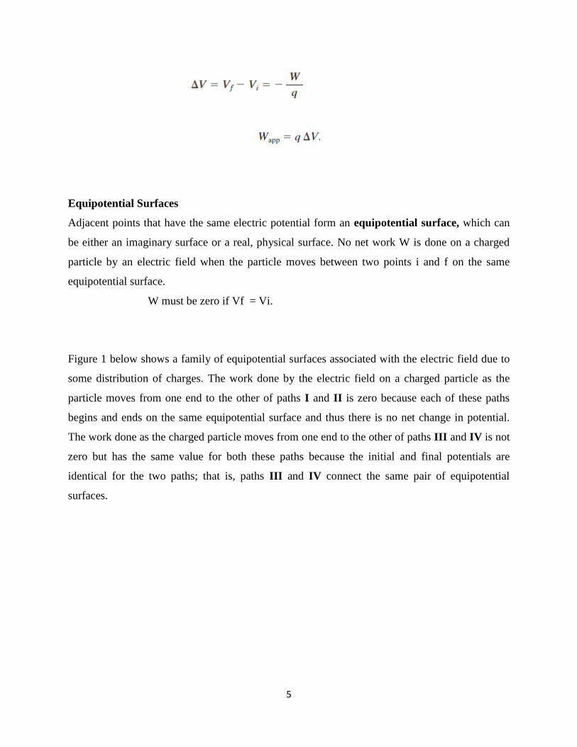
We can relate our work Wapp to the electric potential difference ΔV between the initial and final

locations of the particle.

5

Equipotential Surfaces

Adjacent points that have the same electric potential form an equipotential surface, which can

be either an imaginary surface or a real, physical surface. No net work W is done on a charged

particle by an electric field when the particle moves between two points i and f on the same

equipotential surface.

W must be zero if Vf = Vi.

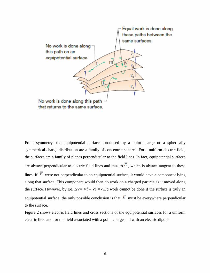
Figure 1 below shows a family of equipotential surfaces associated with the electric field due to

some distribution of charges. The work done by the electric field on a charged particle as the

particle moves from one end to the other of paths I and II is zero because each of these paths

begins and ends on the same equipotential surface and thus there is no net change in potential.

The work done as the charged particle moves from one end to the other of paths III and IV is not

zero but has the same value for both these paths because the initial and final potentials are

identical for the two paths; that is, paths III and IV connect the same pair of equipotential

surfaces.

6

From symmetry, the equipotential surfaces produced by a point charge or a spherically

symmetrical charge distribution are a family of concentric spheres. For a uniform electric field,

the surfaces are a family of planes perpendicular to the field lines. In fact, equipotential surfaces

are always perpendicular to electric field lines and thus to , which is always tangent to these

lines. If were not perpendicular to an equipotential surface, it would have a component lying

along that surface. This component would then do work on a charged particle as it moved along

the surface. However, by Eq. ΔV= Vf – Vi = -w/q work cannot be done if the surface is truly an

equipotential surface; the only possible conclusion is that must be everywhere perpendicular

to the surface.

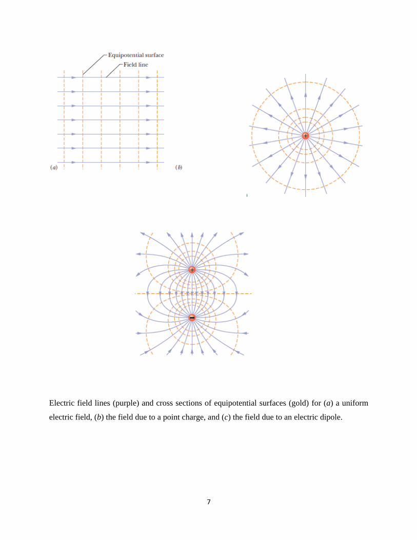
Figure 2 shows electric field lines and cross sections of the equipotential surfaces for a uniform

electric field and for the field associated with a point charge and with an electric dipole.

7

Electric field lines (purple) and cross sections of equipotential surfaces (gold) for (a) a uniform

electric field, (b) the field due to a point charge, and (c) the field due to an electric dipole.

8

Calculating the Potential from the Field

We can calculate the potential difference between any two points i and f in an electric field if we

know the electric field vector E all along any path connecting those points.

To make the calculation, we find the work done on a positive test charge by the field as the

charge moves from i to f.

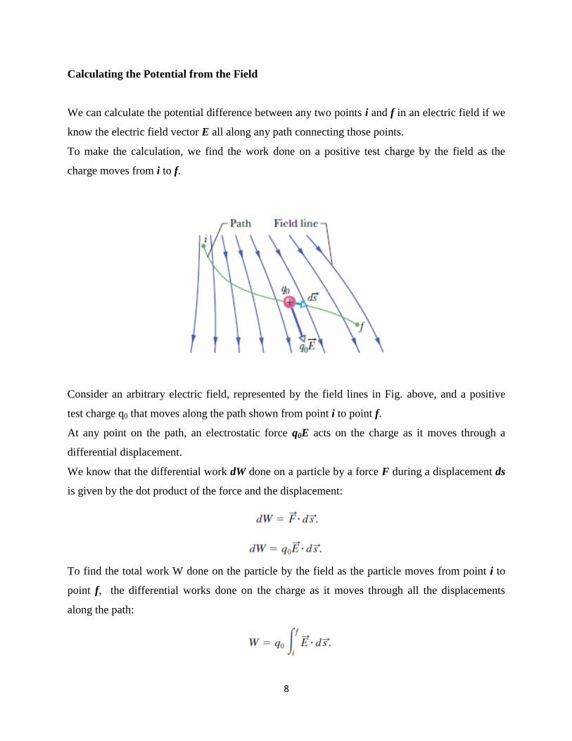
Consider an arbitrary electric field, represented by the field lines in Fig. above, and a positive

test charge q0 that moves along the path shown from point i to point f.

At any point on the path, an electrostatic force q0E acts on the charge as it moves through a

differential displacement.

We know that the differential work dW done on a particle by a force F during a displacement ds

is given by the dot product of the force and the displacement:

To find the total work W done on the particle by the field as the particle moves from point i to

point f, the differential works done on the charge as it moves through all the displacements

along the path:

9

As we know that

So the above equation become

Above equation allows us to calculate the difference in potential between any two points in the

field. If we set potential Vi = 0, then it becomes

Potential Due to a Point Charge

To derive relation ΔV for the space around a charged particle, an expression for the electric

potential V relative to the zero potential at infinity.

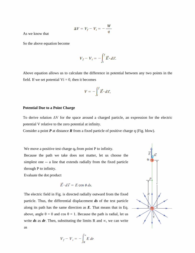
Consider a point P at distance R from a fixed particle of positive charge q (Fig. blow).

We move a positive test charge q0 from point P to infinity.

Because the path we take does not matter, let us choose the

simplest one -- a line that extends radially from the fixed particle

through P to infinity.

Evaluate the dot product

The electric field in Fig. is directed radially outward from the fixed

particle. Thus, the differential displacement ds of the test particle

along its path has the same direction as E. That means that in Eq.

above, angle θ = 0 and cos θ = 1. Because the path is radial, let us

write ds as dr. Then, substituting the limits R and ∞, we can write

as

10

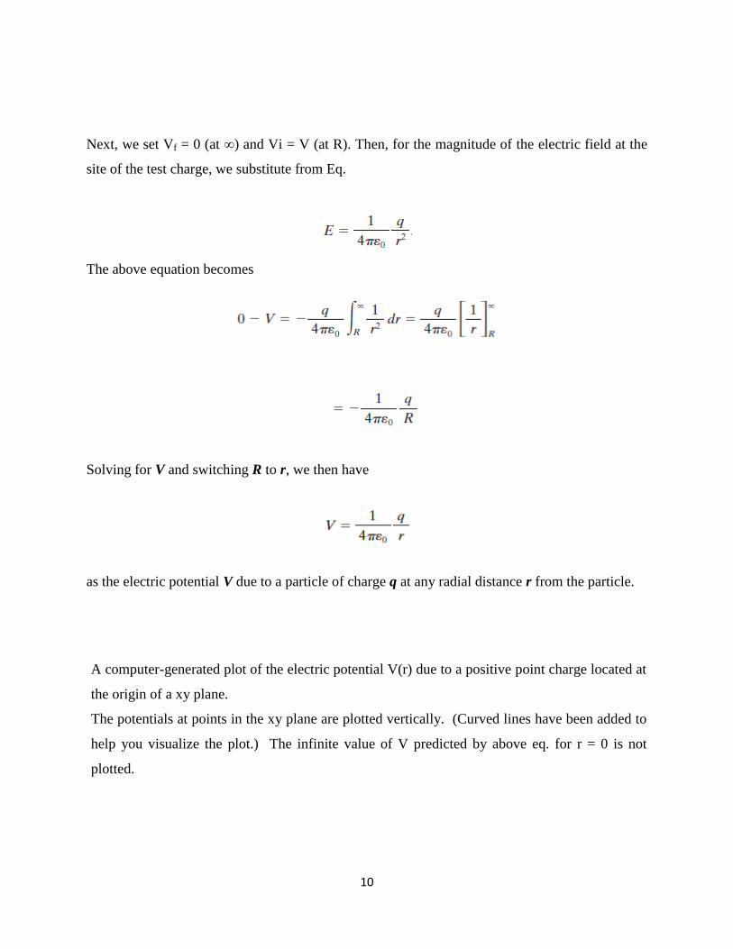
Next, we set Vf = 0 (at ∞) and Vi = V (at R). Then, for the magnitude of the electric field at the

site of the test charge, we substitute from Eq.

The above equation becomes

Solving for V and switching R to r, we then have

as the electric potential V due to a particle of charge q at any radial distance r from the particle.

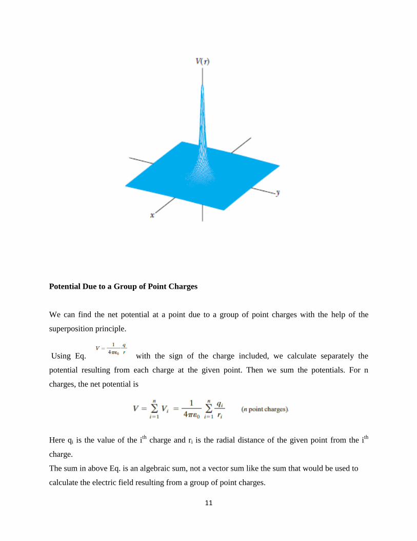
A computer-generated plot of the electric potential V(r) due to a positive point charge located at

the origin of a xy plane.

The potentials at points in the xy plane are plotted vertically. (Curved lines have been added to

help you visualize the plot.) The infinite value of V predicted by above eq. for r = 0 is not

plotted.

11

Potential Due to a Group of Point Charges

We can find the net potential at a point due to a group of point charges with the help of the

superposition principle.

Using Eq. with the sign of the charge included, we calculate separately the

potential resulting from each charge at the given point. Then we sum the potentials. For n

charges, the net potential is

Here qi is the value of the ith

charge and ri is the radial distance of the given point from the ith

charge.

The sum in above Eq. is an algebraic sum, not a vector sum like the sum that would be used to

calculate the electric field resulting from a group of point charges.

12

Here in lies an important computational advantage of potential over electric field: It is a lot easier

to sum several scalar quantities than to sum several vector quantities whose directions and

components must be considered.

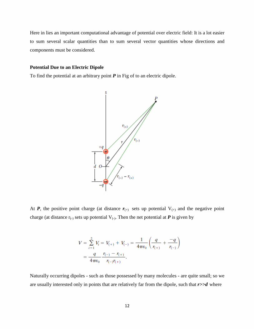
Potential Due to an Electric Dipole

To find the potential at an arbitrary point P in Fig of to an electric dipole.

At P, the positive point charge (at distance r(+) sets up potential V(+) and the negative point

charge (at distance r(-) sets up potential V(-). Then the net potential at P is given by

Naturally occurring dipoles - such as those possessed by many molecules - are quite small; so we

are usually interested only in points that are relatively far from the dipole, such that r>>d where

13

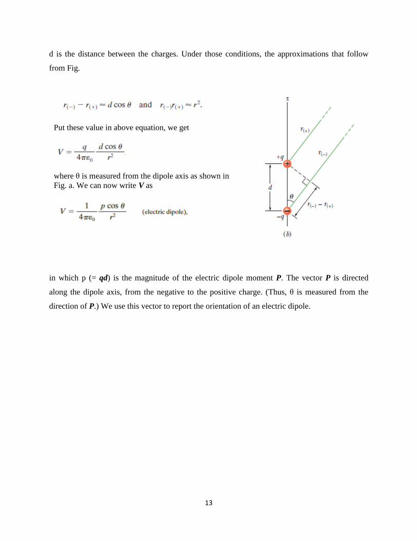
d is the distance between the charges. Under those conditions, the approximations that follow

from Fig.

in which p (= qd) is the magnitude of the electric dipole moment P. The vector P is directed

along the dipole axis, from the negative to the positive charge. (Thus, θ is measured from the

direction of P.) We use this vector to report the orientation of an electric dipole.

Put these value in above equation, we get

where θ is measured from the dipole axis as shown in

Fig. a. We can now write V as

14

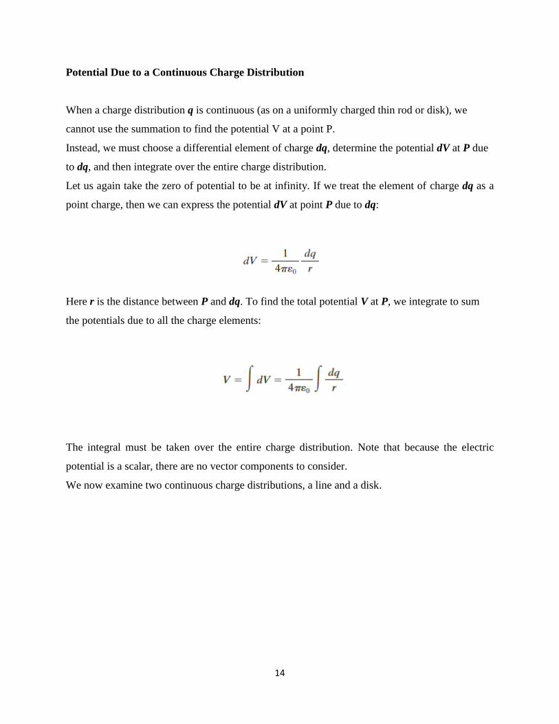
Potential Due to a Continuous Charge Distribution

When a charge distribution q is continuous (as on a uniformly charged thin rod or disk), we

cannot use the summation to find the potential V at a point P.

Instead, we must choose a differential element of charge dq, determine the potential dV at P due

to dq, and then integrate over the entire charge distribution.

Let us again take the zero of potential to be at infinity. If we treat the element of charge dq as a

point charge, then we can express the potential dV at point P due to dq:

Here r is the distance between P and dq. To find the total potential V at P, we integrate to sum

the potentials due to all the charge elements:

The integral must be taken over the entire charge distribution. Note that because the electric

potential is a scalar, there are no vector components to consider.

We now examine two continuous charge distributions, a line and a disk.

15

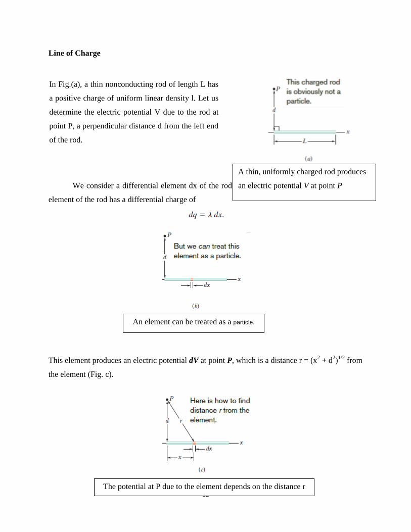
Line of Charge

We consider a differential element dx of the rod as shown in Fig. b. This (or any other)

element of the rod has a differential charge of

This element produces an electric potential dV at point P, which is a distance r = (x2 + d

2)1/2

from

the element (Fig. c).

In Fig.(a), a thin nonconducting rod of length L has

a positive charge of uniform linear density l. Let us

determine the electric potential V due to the rod at

point P, a perpendicular distance d from the left end

of the rod.

A thin, uniformly charged rod produces

an electric potential V at point P

An element can be treated as a particle.

The potential at P due to the element depends on the distance r

16

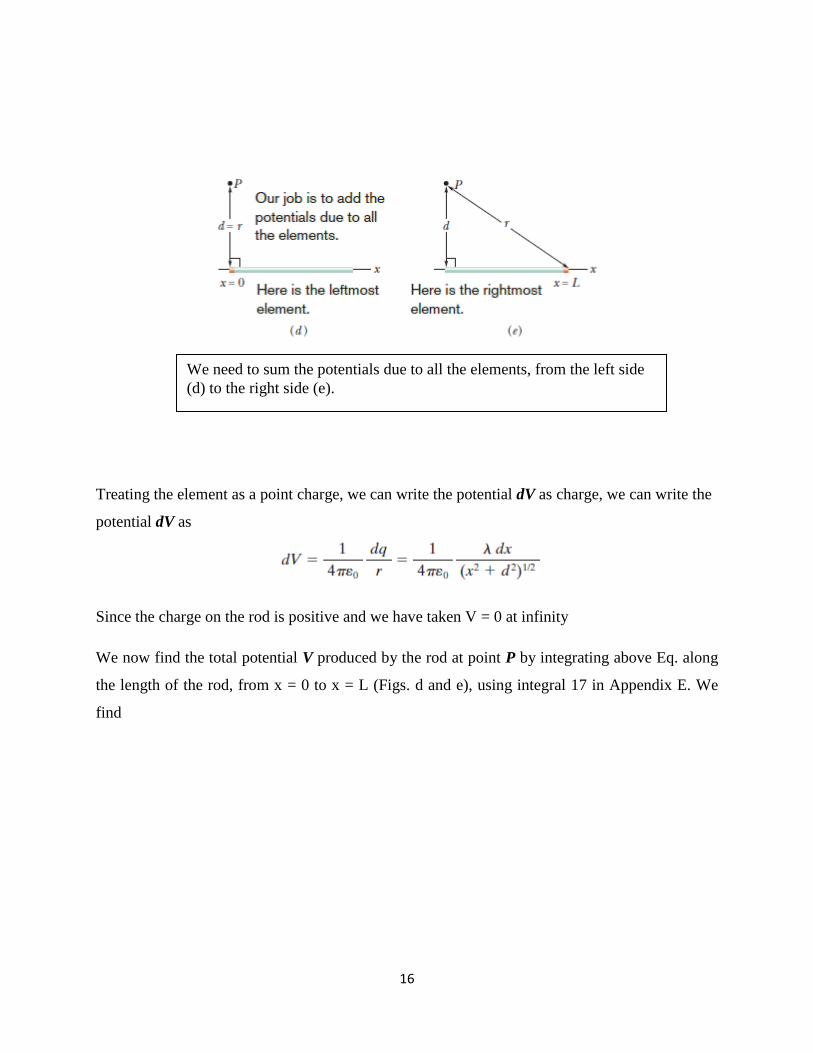
Treating the element as a point charge, we can write the potential dV as charge, we can write the

potential dV as

Since the charge on the rod is positive and we have taken V = 0 at infinity

We now find the total potential V produced by the rod at point P by integrating above Eq. along

the length of the rod, from x = 0 to x = L (Figs. d and e), using integral 17 in Appendix E. We

find

We need to sum the potentials due to all the elements, from the left side

(d) to the right side (e).

17

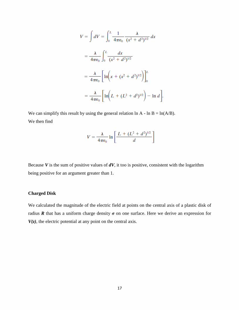
We can simplify this result by using the general relation ln A - ln B = ln(A/B).

We then find

Because V is the sum of positive values of dV, it too is positive, consistent with the logarithm

being positive for an argument greater than 1.

Charged Disk

We calculated the magnitude of the electric field at points on the central axis of a plastic disk of

radius R that has a uniform charge density σ on one surface. Here we derive an expression for

V(z), the electric potential at any point on the central axis.

18

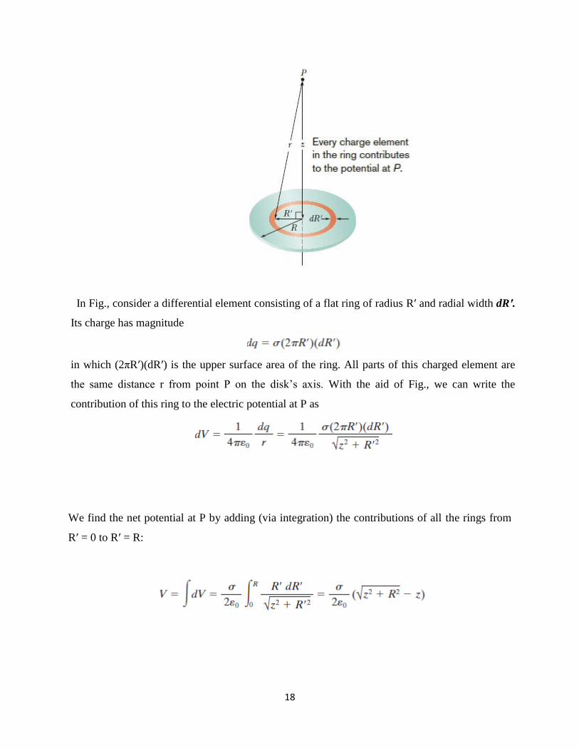
We find the net potential at P by adding (via integration) the contributions of all the rings from

Rʹ = 0 to Rʹ = R:

In Fig., consider a differential element consisting of a flat ring of radius Rʹ and radial width dRʹ.

Its charge has magnitude

in which (2πRʹ)(dRʹ) is the upper surface area of the ring. All parts of this charged element are

the same distance r from point P on the disk’s axis. With the aid of Fig., we can write the

contribution of this ring to the electric potential at P as

19

Note that the variable in the second integral of Eq. is Rʹ and not z, which remains constant while

the integration over the surface of the disk is carried out. (Note also that, in evaluating the

integral, we have assumed that z ≥ 0.)