Data-to-text Generation with Neural Planning
195
Data-to-text Generation with Neural Planning Ratish Surendran Puduppully Doctor of Philosophy Institute for Language, Cognition and Computation School of Informatics University of Edinburgh 2021
-
Upload
khangminh22 -
Category
Documents
-
view
4 -
download
0
Transcript of Data-to-text Generation with Neural Planning

Data-to-text Generation with Neural Planning
Ratish Surendran Puduppully
Doctor of Philosophy
Institute for Language, Cognition and Computation
School of Informatics
University of Edinburgh
2021

AbstractIn this thesis, we consider the task of data-to-text generation, which takes non-linguistic
structures as input and produces textual output. The inputs can take the form of
database tables, spreadsheets, charts, and so on. The main application of data-to-text
generation is to present information in a textual format which makes it accessible to
a layperson who may otherwise find it problematic to understand numerical figures.
The task can also automate routine document generation jobs, thus improving human
efficiency. We focus on generating long-form text, i.e., documents with multiple para-
graphs. Recent approaches to data-to-text generation have adopted the very successful
encoder-decoder architecture or its variants. These models generate fluent (but often
imprecise) text and perform quite poorly at selecting appropriate content and ordering
it coherently. This thesis focuses on overcoming these issues by integrating content
planning with neural models. We hypothesize data-to-text generation will benefit from
explicit planning, which manifests itself in (a) micro planning, (b) latent entity plan-
ning, and (c) macro planning. Throughout this thesis, we assume the input to our
generator are tables (with records) in the sports domain. And the output are summaries
describing what happened in the game (e.g., who won/lost, . . . , scored, etc.).
We first describe our work on integrating fine-grained or micro plans with data-to-
text generation. As part of this, we generate a micro plan highlighting which records
should be mentioned and in which order, and then generate the document while taking
the micro plan into account.
We then show how data-to-text generation can benefit from higher level latent en-
tity planning. Here, we make use of entity-specific representations which are dynam-
ically updated. The text is generated conditioned on entity representations and the
records corresponding to the entities by using hierarchical attention at each time step.
We then combine planning with the high level organization of entities, events, and
their interactions. Such coarse-grained macro plans are learnt from data and given
as input to the generator. Finally, we present work on making macro plans latent
while incrementally generating a document paragraph by paragraph. We infer latent
plans sequentially with a structured variational model while interleaving the steps of
planning and generation. Text is generated by conditioning on previous variational
decisions and previously generated text.
Overall our results show that planning makes data-to-text generation more inter-
pretable, improves the factuality and coherence of the generated documents and re-
duces redundancy in the output document.
iii
Acknowledgements
Foremost I like to thank my advisor Mirella Lapata. A substantial share of my learning
as a PhD student is due to her. I will always appreciate the clarity she had of the big
picture of the thesis. Our weekly research meetings helped me take stock, discuss new
ideas and prioritise my tasks. Her support was even more crucial during the Covid
pandemic. I am thankful for the funding for the months when the thesis took longer
than planned.
I also like to thank Adam Lopez for the helpful discussions and Ivan Titov for
providing constructive feedback during my first-year review. I thank my examiners,
Rico Sennrich and Michael Elhadad, for examining the thesis and viva and providing
constructive feedback.
I like to thank Li Dong, Jonathan Mallinson, Yang Liu, Laura Perez, Yumo Xu,
Rui Cai, Tom Sherborne, Tom Hosking, Parag Jain, Nelly Papalampidi, Hao Zheng,
Reinald Kim Amplayo, and Yao Fu for the many insightful discussions during our
weekly group meetings. I also had a great time collaborating with Li, Jonathan, and
Yao.
I also like to thank Shashi Narayan, Joshua Maynez, and Ryan McDonald at Google
Research London for their wholehearted support during my research internship.
I like to thank my friends who made the PhD journey enjoyable. Spandana, Annie,
and Shashi gave us a warm welcome to Edinburgh. Mihaela and Aurora gave us all
possible help for settling here. Ameya and Vinit were always there when I needed
them. Ruchit made my stay in London memorable. I have enjoyed my conversations
with Anoop and Litton on topics related to research and otherwise. The coffee walks
with Jerin have been a great way to unwind.
I like to thank my family, parents, in-laws, brother, and sister, who have always
wished the best for me. This PhD journey would not have been possible without the
support of Arya, who has stood by me throughout, and our two gems Vedika and
Dhyan, who fill the canvas of life with vivid colors.
iv

Declaration
I declare that this thesis was composed by myself, that the work contained herein is
my own except where explicitly stated otherwise in the text, and that this work has not
been submitted for any other degree or professional qualification except as specified.
(Ratish Surendran Puduppully)
v

Table of Contents
1 Introduction 1
1.1 Motivation . . . . . . . . . . . . . . . . . . . . . . . . . . . . . . . . 1
1.2 Thesis Contributions . . . . . . . . . . . . . . . . . . . . . . . . . . 4
1.3 Thesis Outline . . . . . . . . . . . . . . . . . . . . . . . . . . . . . . 5
2 Background 9
2.1 Fundamentals of Data-to-text Generation . . . . . . . . . . . . . . . 9
2.2 The Architecture of Data-to-text Systems . . . . . . . . . . . . . . . 10
2.3 Datasets . . . . . . . . . . . . . . . . . . . . . . . . . . . . . . . . . 12
2.3.1 ROTOWIRE . . . . . . . . . . . . . . . . . . . . . . . . . . . 15
2.3.2 MLB . . . . . . . . . . . . . . . . . . . . . . . . . . . . . . 16
2.3.3 German ROTOWIRE . . . . . . . . . . . . . . . . . . . . . . 17
2.4 Baseline Encoder-Decoder Models . . . . . . . . . . . . . . . . . . . 19
2.4.1 Record Encoder . . . . . . . . . . . . . . . . . . . . . . . . . 20
2.4.2 Text Generation . . . . . . . . . . . . . . . . . . . . . . . . . 20
2.4.3 Training and Inference . . . . . . . . . . . . . . . . . . . . . 22
2.5 Evaluation . . . . . . . . . . . . . . . . . . . . . . . . . . . . . . . . 22
2.5.1 Automatic Evaluation . . . . . . . . . . . . . . . . . . . . . 22
2.5.2 Human Evaluation . . . . . . . . . . . . . . . . . . . . . . . 25
2.6 Summary . . . . . . . . . . . . . . . . . . . . . . . . . . . . . . . . 26
3 Micro Planning 27
3.1 Problem Formulation . . . . . . . . . . . . . . . . . . . . . . . . . . 28
3.1.1 Record Encoder . . . . . . . . . . . . . . . . . . . . . . . . . 29
3.1.2 Contextualization . . . . . . . . . . . . . . . . . . . . . . . . 30
3.1.3 Micro Planning . . . . . . . . . . . . . . . . . . . . . . . . . 31
3.1.4 Text Generation . . . . . . . . . . . . . . . . . . . . . . . . . 32
vii
3.1.5 Training and Inference . . . . . . . . . . . . . . . . . . . . . 34
3.2 Experimental Setup . . . . . . . . . . . . . . . . . . . . . . . . . . . 34
3.3 Results . . . . . . . . . . . . . . . . . . . . . . . . . . . . . . . . . . 36
3.4 Qualitative Examples . . . . . . . . . . . . . . . . . . . . . . . . . . 43
3.5 Summary . . . . . . . . . . . . . . . . . . . . . . . . . . . . . . . . 43
4 Latent Entity Planning 51
4.1 Motivation . . . . . . . . . . . . . . . . . . . . . . . . . . . . . . . . 51
4.2 Related Work . . . . . . . . . . . . . . . . . . . . . . . . . . . . . . 53
4.3 Encoder-Decoder with Conditional Copy . . . . . . . . . . . . . . . . 56
4.4 Entity Memory and Hierarchical Attention . . . . . . . . . . . . . . . 58
4.4.1 Entity Memory . . . . . . . . . . . . . . . . . . . . . . . . . 58
4.4.2 Hierarchical Attention . . . . . . . . . . . . . . . . . . . . . 59
4.5 Training and Inference . . . . . . . . . . . . . . . . . . . . . . . . . 60
4.6 Experimental Setup . . . . . . . . . . . . . . . . . . . . . . . . . . . 61
4.7 Results . . . . . . . . . . . . . . . . . . . . . . . . . . . . . . . . . . 61
4.8 Qualitative Examples . . . . . . . . . . . . . . . . . . . . . . . . . . 66
4.9 Summary . . . . . . . . . . . . . . . . . . . . . . . . . . . . . . . . 69
5 Macro Planning 71
5.1 Motivation . . . . . . . . . . . . . . . . . . . . . . . . . . . . . . . . 71
5.2 Related Work . . . . . . . . . . . . . . . . . . . . . . . . . . . . . . 74
5.3 Problem Formulation . . . . . . . . . . . . . . . . . . . . . . . . . . 76
5.3.1 Macro Plan Definition . . . . . . . . . . . . . . . . . . . . . 77
5.3.2 Macro Plan Construction . . . . . . . . . . . . . . . . . . . . 79
5.3.3 Paragraph Plan Construction . . . . . . . . . . . . . . . . . . 80
5.4 Model Description . . . . . . . . . . . . . . . . . . . . . . . . . . . 81
5.4.1 Macro Planning . . . . . . . . . . . . . . . . . . . . . . . . . 82
5.4.2 Text Generation . . . . . . . . . . . . . . . . . . . . . . . . . 83
5.4.3 Training and Inference . . . . . . . . . . . . . . . . . . . . . 84
5.5 Experimental Setup . . . . . . . . . . . . . . . . . . . . . . . . . . . 85
5.6 Results . . . . . . . . . . . . . . . . . . . . . . . . . . . . . . . . . . 87
5.7 Discussion . . . . . . . . . . . . . . . . . . . . . . . . . . . . . . . . 94
5.8 Summary . . . . . . . . . . . . . . . . . . . . . . . . . . . . . . . . 99
viii

6 Variational Sequential Planning 1016.1 Introduction . . . . . . . . . . . . . . . . . . . . . . . . . . . . . . . 101
6.2 Related Work . . . . . . . . . . . . . . . . . . . . . . . . . . . . . . 103
6.3 Model . . . . . . . . . . . . . . . . . . . . . . . . . . . . . . . . . . 105
6.4 Experimental Setup . . . . . . . . . . . . . . . . . . . . . . . . . . . 110
6.5 Results . . . . . . . . . . . . . . . . . . . . . . . . . . . . . . . . . . 112
6.5.1 Automatic Evaluation . . . . . . . . . . . . . . . . . . . . . 113
6.5.2 Sample Efficiency . . . . . . . . . . . . . . . . . . . . . . . 118
6.5.3 Evaluation of Paragraph Plan Prediction Accuracy . . . . . . 118
6.5.4 Human Evaluation . . . . . . . . . . . . . . . . . . . . . . . 119
6.6 Discussion . . . . . . . . . . . . . . . . . . . . . . . . . . . . . . . . 121
6.7 Qualitative Examples . . . . . . . . . . . . . . . . . . . . . . . . . . 122
6.8 Conclusion . . . . . . . . . . . . . . . . . . . . . . . . . . . . . . . 124
7 Conclusions 1317.1 Future Work . . . . . . . . . . . . . . . . . . . . . . . . . . . . . . . 134
A Human Evaluation for Fact Verification 137A.1 Fact Verification for ROTOWIRE Instructions . . . . . . . . . . . . . 137
A.2 Fact Verification for MLB Instructions . . . . . . . . . . . . . . . . . 141
B Human Evaluation for Summary Quality 151B.1 Evaluation of Coherence for ROTOWIRE . . . . . . . . . . . . . . . . 151
B.2 Evaluation of Conciseness for ROTOWIRE . . . . . . . . . . . . . . . 153
B.3 Evaluation of Grammaticality for ROTOWIRE . . . . . . . . . . . . . 155
B.4 Evaluation of Coherence for MLB . . . . . . . . . . . . . . . . . . . 159
B.5 Evaluation of Conciseness for MLB . . . . . . . . . . . . . . . . . . 161
B.6 Evaluation of Grammaticality for MLB . . . . . . . . . . . . . . . . 163
Bibliography 167
ix

Chapter 1
Introduction
1.1 Motivation
Data-to-text generation broadly refers to the task of automatically producing textual
output from non-linguistic input (Reiter and Dale, 2000; Gatt and Krahmer, 2018).
The input may be databases of records, spreadsheets, expert system knowledge bases,
simulations of physical systems, etc.
Data-to-text generation has two vital uses: improving access to information and
automating document generation tasks (Reiter and Dale, 2000). The information avail-
able in spreadsheets and database tables may vary in format, size, granularity, etc. This
disparity can restrict access to such data to trained experts. Expressing such informa-
tion in textual form can make it accessible to laypersons too. In the second scenario,
document generation often needs to be performed by people whose main job is un-
related. For example, doctors need to create notes of patient details, their symptoms,
diagnosis, and prescriptions. Software developers spend a considerable amount of their
time writing comments and documentation of their code. Data-to-text generation can
automate part of this document generation task and improve the efficiency of their job.
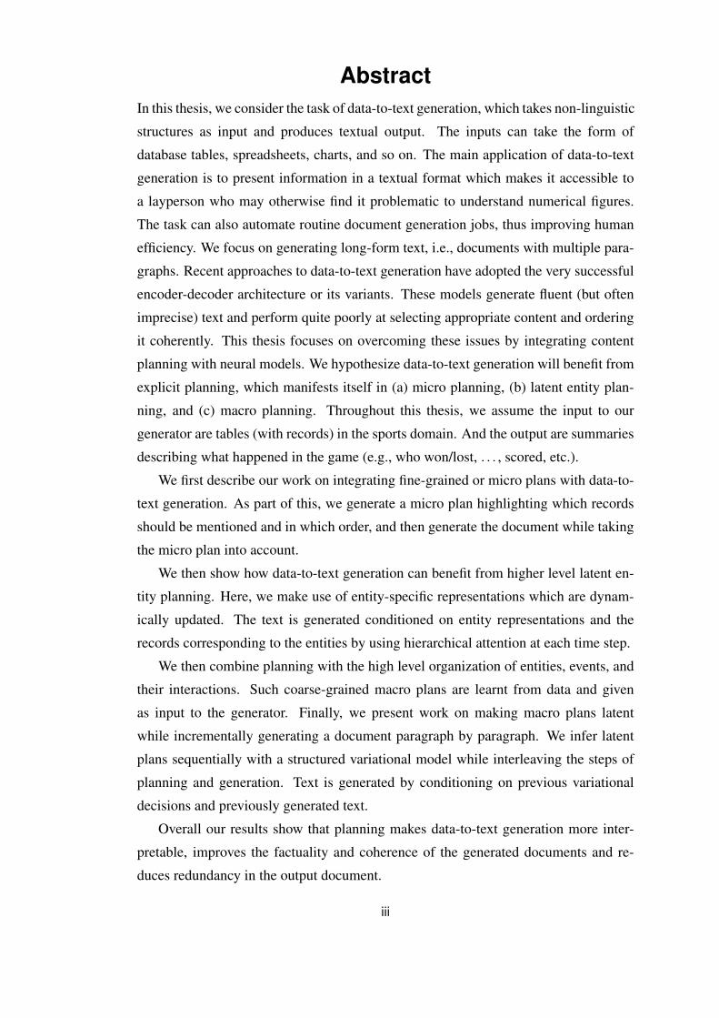
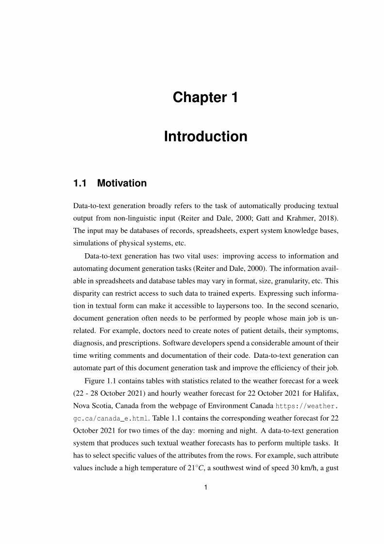
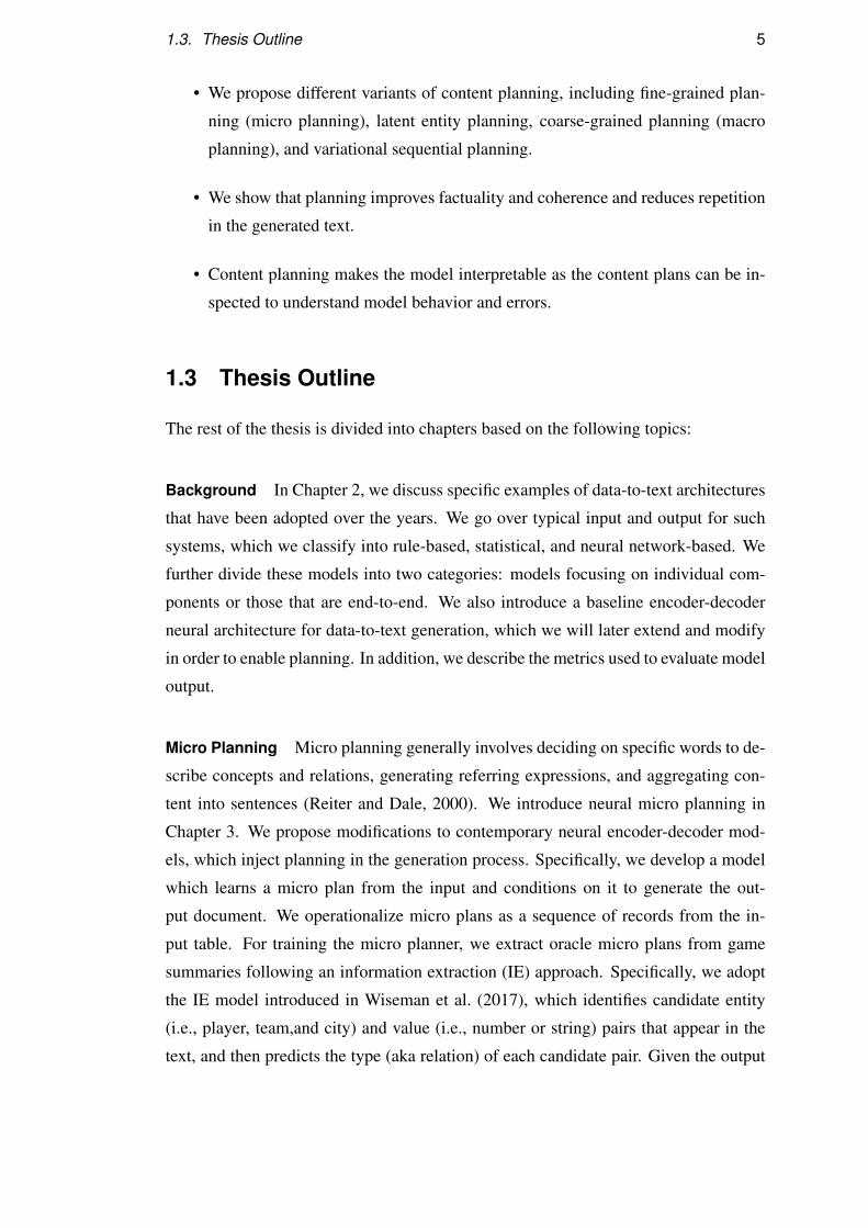
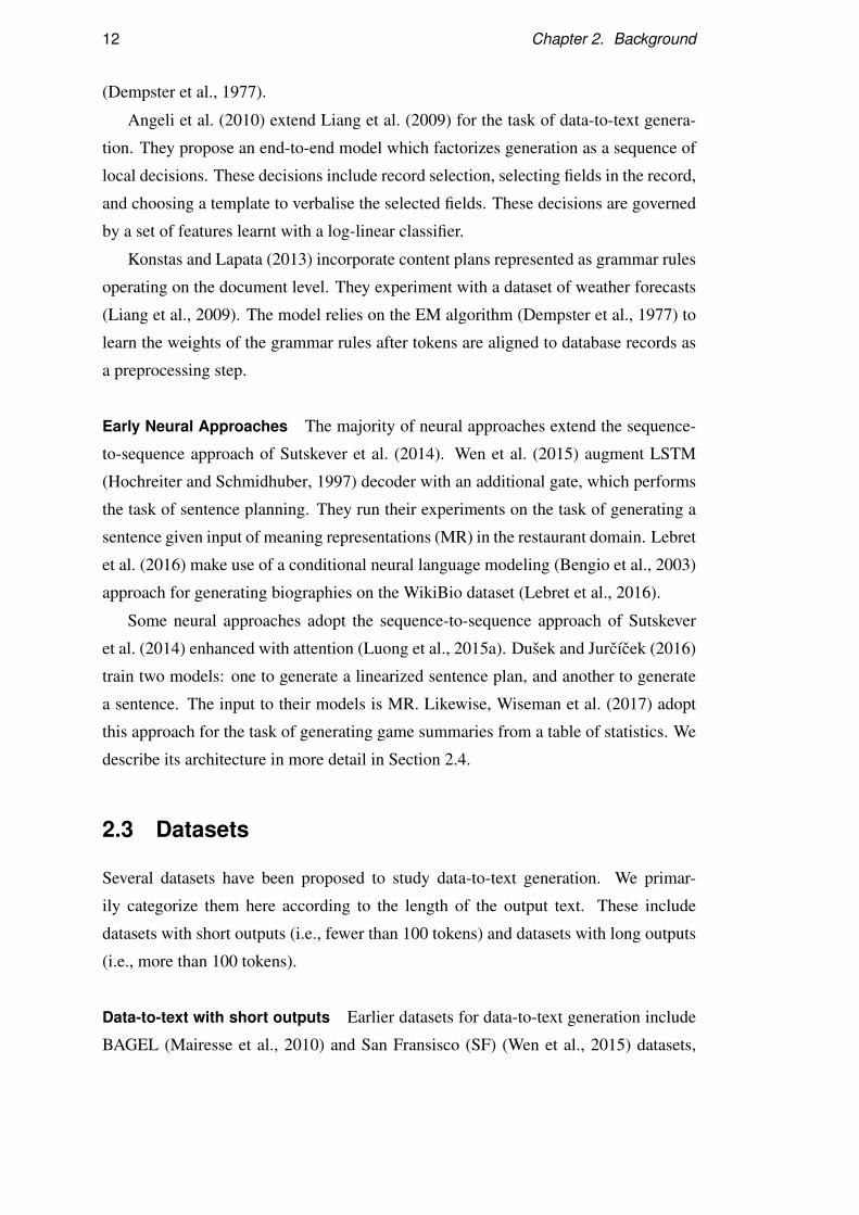
Figure 1.1 contains tables with statistics related to the weather forecast for a week
(22 - 28 October 2021) and hourly weather forecast for 22 October 2021 for Halifax,
Nova Scotia, Canada from the webpage of Environment Canada https://weather.
gc.ca/canada_e.html. Table 1.1 contains the corresponding weather forecast for 22
October 2021 for two times of the day: morning and night. A data-to-text generation
system that produces such textual weather forecasts has to perform multiple tasks. It
has to select specific values of the attributes from the rows. For example, such attribute
values include a high temperature of 21◦C, a southwest wind of speed 30 km/h, a gust
1
2 Chapter 1. Introduction
Figure 1.1: The tables show the weather forecast for seven days between 22 - 28
October 2021 (top) and the hourly forecast for 22 October 2021 (bottom) for Halifax,
Nova Scotia, Canada. The information is accessed from the webpage of Environment
Canada.
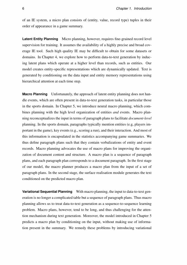
1.1. Motivation 3
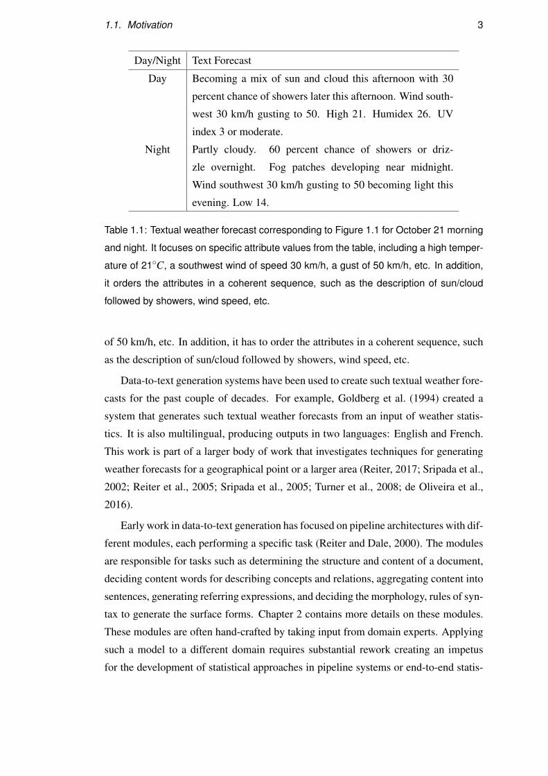
Day/Night Text Forecast
Day Becoming a mix of sun and cloud this afternoon with 30
percent chance of showers later this afternoon. Wind south-
west 30 km/h gusting to 50. High 21. Humidex 26. UV
index 3 or moderate.
Night Partly cloudy. 60 percent chance of showers or driz-
zle overnight. Fog patches developing near midnight.
Wind southwest 30 km/h gusting to 50 becoming light this
evening. Low 14.
Table 1.1: Textual weather forecast corresponding to Figure 1.1 for October 21 morning
and night. It focuses on specific attribute values from the table, including a high temper-
ature of 21◦C, a southwest wind of speed 30 km/h, a gust of 50 km/h, etc. In addition,
it orders the attributes in a coherent sequence, such as the description of sun/cloud
followed by showers, wind speed, etc.
of 50 km/h, etc. In addition, it has to order the attributes in a coherent sequence, such
as the description of sun/cloud followed by showers, wind speed, etc.
Data-to-text generation systems have been used to create such textual weather fore-
casts for the past couple of decades. For example, Goldberg et al. (1994) created a
system that generates such textual weather forecasts from an input of weather statis-
tics. It is also multilingual, producing outputs in two languages: English and French.
This work is part of a larger body of work that investigates techniques for generating
weather forecasts for a geographical point or a larger area (Reiter, 2017; Sripada et al.,
2002; Reiter et al., 2005; Sripada et al., 2005; Turner et al., 2008; de Oliveira et al.,
2016).
Early work in data-to-text generation has focused on pipeline architectures with dif-
ferent modules, each performing a specific task (Reiter and Dale, 2000). The modules
are responsible for tasks such as determining the structure and content of a document,
deciding content words for describing concepts and relations, aggregating content into
sentences, generating referring expressions, and deciding the morphology, rules of syn-
tax to generate the surface forms. Chapter 2 contains more details on these modules.
These modules are often hand-crafted by taking input from domain experts. Applying
such a model to a different domain requires substantial rework creating an impetus
for the development of statistical approaches in pipeline systems or end-to-end statis-
4 Chapter 1. Introduction
tical models to overcome this challenge (Liang et al. 2009; Angeli et al. 2010; Konstas
and Lapata 2013, inter alia). As statistical models learn the weights of features from
data, they can be more easily adapted to different domains, however, the features need
to be manually defined. In recent times, the application of neural networks for data-
to-text generation has become popular (Wiseman et al. 2017; Lebret et al. 2016; Mei
et al. 2016, inter alia). Neural approaches do away with feature engineering and are
often learnt end-to-end from the examples containing instances of input paired with
output text. The success of neural networks has also been due to advances in com-
puting power, including advancements in graphical processing units (GPU), which are
highly optimised for parallel operations on matrices in neural networks. Concurrently,
large-scale datasets have been developed, which has made it feasible for the automatic
extraction of features from the data.
1.2 Thesis Contributions
Despite producing overall fluent text, neural systems have difficulty capturing long-
term structure and generating documents more than a few sentences long. Wiseman
et al. (2017) show that neural text generation techniques perform poorly at content
selection, they struggle to maintain inter-sentential coherence, and more generally a
reasonable ordering of the selected facts in the output text. Additional challenges in-
clude avoiding redundancy and being faithful to the input. Interestingly, comparisons
with rule-based methods show that neural techniques do not fare well on metrics of
content selection recall and factual output generation (i.e., they often hallucinate state-
ments which are not supported by the facts in the database).
A content plan provides information about the content and structure of the output
document. We hypothesize that explicitly modeling content planning should help in
alleviating some of the issues with the neural models. The reasons for our hypothesis
include the prevalence of planning components in pre-neural pipeline architectures.
Expecting the neural decoder to perform content selection, generate fluent text, main-
tain inter-sentential coherence in the document, and stay faithful to the input table, all
at the same time, is too much of an ask. We believe that content planning can serve as
an intermediate stage between the input and output. Content plans should enable the
decoder to focus on the less challenging tasks of predicting tokens conformant to the
plan.
The contributions of the thesis include:
1.3. Thesis Outline 5
• We propose different variants of content planning, including fine-grained plan-
ning (micro planning), latent entity planning, coarse-grained planning (macro
planning), and variational sequential planning.
• We show that planning improves factuality and coherence and reduces repetition
in the generated text.
• Content planning makes the model interpretable as the content plans can be in-
spected to understand model behavior and errors.
1.3 Thesis Outline
The rest of the thesis is divided into chapters based on the following topics:
Background In Chapter 2, we discuss specific examples of data-to-text architectures
that have been adopted over the years. We go over typical input and output for such
systems, which we classify into rule-based, statistical, and neural network-based. We
further divide these models into two categories: models focusing on individual com-
ponents or those that are end-to-end. We also introduce a baseline encoder-decoder
neural architecture for data-to-text generation, which we will later extend and modify
in order to enable planning. In addition, we describe the metrics used to evaluate model
output.
Micro Planning Micro planning generally involves deciding on specific words to de-
scribe concepts and relations, generating referring expressions, and aggregating con-
tent into sentences (Reiter and Dale, 2000). We introduce neural micro planning in
Chapter 3. We propose modifications to contemporary neural encoder-decoder mod-
els, which inject planning in the generation process. Specifically, we develop a model
which learns a micro plan from the input and conditions on it to generate the out-
put document. We operationalize micro plans as a sequence of records from the in-
put table. For training the micro planner, we extract oracle micro plans from game
summaries following an information extraction (IE) approach. Specifically, we adopt
the IE model introduced in Wiseman et al. (2017), which identifies candidate entity
(i.e., player, team,and city) and value (i.e., number or string) pairs that appear in the
text, and then predicts the type (aka relation) of each candidate pair. Given the output
6 Chapter 1. Introduction
of an IE system, a micro plan consists of (entity, value, record type) tuples in their
order of appearance in a game summary.
Latent Entity Planning Micro planning, however, requires fine-grained record level
supervision for training. It assumes the availability of a highly precise and broad cov-
erage IE tool. Such high quality IE may be difficult to obtain for some datasets or
domains. In Chapter 4, we explore how to perform data-to-text generation by induc-
ing latent plans which operate at a higher level than records, such as entities. Our
model creates entity-specific representations which are dynamically updated. Text is
generated by conditioning on the data input and entity memory representations using
hierarchical attention at each time step.
Macro Planning Unfortunately, the approach of latent entity planning does not han-
dle events, which are often present in data-to-text generation tasks, in particular those
in the sports domain. In Chapter 5, we introduce neural macro planning, which com-
bines planning with the high level organization of entities and events. Macro plan-
ning reconceptualizes the input in terms of paragraph plans to facilitate document-level
planning. In the sports domain, paragraphs typically mention entities (e.g, players im-
portant in the game), key events (e.g., scoring a run), and their interaction. And most of
this information is encapsulated in the statistics accompanying game summaries. We
thus define paragraph plans such that they contain verbalizations of entity and event
records. Macro planning advocates the use of macro plans for improving the organi-
zation of document content and structure. A macro plan is a sequence of paragraph
plans, and each paragraph plan corresponds to a document paragraph. In the first stage
of our model, the macro planner produces a macro plan from the input of a set of
paragraph plans. In the second stage, the surface realisation module generates the text
conditioned on the predicted macro plan.
Variational Sequential Planning With macro planning, the input to data-to-text gen-
eration is no longer a complicated table but a sequence of paragraph plans. Thus macro
planning allows us to treat data-to-text generation as a sequence-to-sequence learning
problem. Macro plans, however, tend to be long, and thus challenging for the atten-
tion mechanism during text generation. Moreover, the model introduced in Chapter 5
predicts a macro plan by conditioning on the input, without making use of informa-
tion present in the summary. We remedy these problems by introducing variational

1.3. Thesis Outline 7
sequential planning in Chapter 6. We infer latent plans sequentially with a structured
variational model while interleaving the steps of planning and generation. Text is gen-
erated by conditioning on previous variational decisions and previously generated text.
Part of the content covered in the thesis have been earlier presented in Puduppully et al.
(2019a) (Chapter 3), Puduppully et al. (2019b) (Chapter 4), Puduppully and Lapata
(2021) (Chapter 5), Puduppully et al. (2022) (Chapter 6).

Chapter 2
Background
In this chapter, we will look first into earlier work in data-to-text generation, and dis-
cuss the characteristics of datasets used in this field. We will then study a baseline
neural encoder-decoder model for data-to-text generation, which will form the foun-
dation of our own work. We will finally review the metrics which we use to evaluate
the model output.
2.1 Fundamentals of Data-to-text Generation
Reiter and Dale (2000) define the input to a data-to-text generation system as a 4-tuple
〈 k, c, u, d 〉, where, k is knowledge source, c is the communicative goal, u is the user
model, and d is the discourse history1.
The knowledge source represents the information available to the data-to-text sys-
tem and can be a database, table, knowledge base, etc. Information in the knowledge
source can be in turn numeric or textual. The communicative goal indicates the goal
to be achieved by the output of an invocation of the data-to-text system. An example
of a communicative goal could be to generate a weather forecast for a given day or a
month. The user model indicates the specification of the intended audience of the data-
to-text system. For example, the data-to-text system of Portet et al. (2009) produces
summaries of neonatal intensive care unit data tailored in terms of the vocabulary and
the requisite amount of detail for disparate classes of users, including nurses, junior
doctors, and parents. The discourse history stores previous interactions of the user
1Reiter and Dale (2000) and other earlier work use the term Natural Language Generation (NLG)to mean data-to-text generation. However, in recent times NLG has come to encompass text-to-textgeneration tasks too. These include text summarization, sentence simplification, paraphrasing, etc. So,we use the term data-to-text generation to mean that the input is non-linguistic data.
9
10 Chapter 2. Background
with the data-to-text system. In the context of a dialog system, it is also similar to di-
alog history. The discourse history starts empty and will accumulate over interactions
with the system. It stores entity mentions and can help generate pronouns and referring
expressions.
The output of a data-to-text system is text. The text can be in English or other
languages too. For example, FOG (Goldberg et al., 1994) produces weather forecasts
in two languages: English and French. The output may also contain information to
help render the text onto a device, such as HTML markup for rendering webpages. It
can also include discourse information such as the division of the text into paragraphs,
sections, and so on.
2.2 The Architecture of Data-to-text Systems
Reiter and Dale (2000) propose a pipeline architecture for data-to-text generation. It
adopts separate stages for document planning, micro planning, and linguistic realisa-
tion. Document planning determines the document’s content and structure organizing
it into discourse. Micro planning involves aggregating content into sentences, deciding
specific words to describe concepts and relations, and generating referring expressions.
Linguistic realisation applies the rules of syntax, morphology, and orthographic pro-
cessing to generate surface forms.
In this section, we extend from Konstas (2014) and classify earlier architectures
into three types of systems: rule-based ones, those making use of statistical models,
and those based on neural models.
Rule-based individual components Early work in data-to-text generation made use
of hand-built content selection components (Kukich, 1983; McKeown, 1992; Reiter
and Dale, 1997). Many early content planners have been based on theories of dis-
course coherence (Hovy, 1993; Scott and de Souza, 1990a). Other work has relied on
generic planners (Dale, 1988) or schemas (Duboue and McKeown, 2002). In all cases,
content plans are created manually, sometimes through corpus analysis (Duboue and
McKeown, 2001). A few researchers (Mellish et al., 1998; Karamanis, 2004) adopt a
generate-and-rank architecture where a large set of candidate plans is produced and the
best one is selected according to a ranking function. There have been multiple systems
developed for surface realisation (Elhadad and Robin, 1996; Bateman, 1997; Lavoie
and Rainbow, 1997). Among these, Elhadad and Robin (1996) propose a grammar

2.2. The Architecture of Data-to-text Systems 11
known as SURGE (Systemic Unification Realization Grammar of English) based on
the Functional Unification Formalism (FUF) (Elhadad, 1989). The SURGE grammar
processes the output of the micro planner to generate text in the English language.
Rule-based end-to-end Goldberg et al. (1994) create one of the first end-to-end sys-
tems for data-to-text generation. Their system called FOG generates weather forecasts
in two languages (English and French) based on weather statistics.
Statistical individual components There have also been instances of content selec-
tion components learnt from data (Barzilay and Lapata, 2005; Duboue and McKeown,
2001, 2003; Kim and Mooney, 2010). For example, Barzilay and Lapata (2005) pro-
pose an approach that learns to perform content selection by considering all the entities
together in a table and not in isolation from each other. They show that such collective
content selection captures the contextual relationships between the entities, thus im-
proving the accuracy of content selection. In addition, statistical approaches have been
applied to sentence planning (Stent et al., 2004; Walker et al., 2001, 2002). Specifi-
cally, Stent et al. (2004) learn a ranker for sentence plans from training data of sentence
plans paired with the human ratings of their corresponding sentences generated using
RealPro (Lavoie and Rainbow, 1997).
Statistical end-to-end Langkilde and Knight (1998) propose a model for generat-
ing sentences from meaning representations called abstract meaning representations
(AMR). The AMR structure is first converted to word lattices. Following this, a corpus-
based statistical model with word bigram information is used for the linguistic deci-
sions to transform the word lattices to sentences.
Belz (2008) proposes a model which comprises two stages. The first stage is a
base generator containing rules for the specific domain and task. The second stage is
responsible for choosing between the rules based on probabilities learnt from the train-
ing dataset. They evaluate on the SUMTIME-METEO corpus (Sripada et al., 2002),
which pairs numerical marine weather forecast data with human written weather fore-
casts.
Liang et al. (2009) model text generation as a hierarchical process of selection
of records, fields in records, and words to describe the fields. Their system learns
the alignment of records (and their fields) with segments of output text. They train
the model following the unsupervised approach of Expectation Maximization (EM)
12 Chapter 2. Background
(Dempster et al., 1977).
Angeli et al. (2010) extend Liang et al. (2009) for the task of data-to-text genera-
tion. They propose an end-to-end model which factorizes generation as a sequence of
local decisions. These decisions include record selection, selecting fields in the record,
and choosing a template to verbalise the selected fields. These decisions are governed
by a set of features learnt with a log-linear classifier.
Konstas and Lapata (2013) incorporate content plans represented as grammar rules
operating on the document level. They experiment with a dataset of weather forecasts
(Liang et al., 2009). The model relies on the EM algorithm (Dempster et al., 1977) to
learn the weights of the grammar rules after tokens are aligned to database records as
a preprocessing step.
Early Neural Approaches The majority of neural approaches extend the sequence-
to-sequence approach of Sutskever et al. (2014). Wen et al. (2015) augment LSTM
(Hochreiter and Schmidhuber, 1997) decoder with an additional gate, which performs
the task of sentence planning. They run their experiments on the task of generating a
sentence given input of meaning representations (MR) in the restaurant domain. Lebret
et al. (2016) make use of a conditional neural language modeling (Bengio et al., 2003)
approach for generating biographies on the WikiBio dataset (Lebret et al., 2016).
Some neural approaches adopt the sequence-to-sequence approach of Sutskever
et al. (2014) enhanced with attention (Luong et al., 2015a). Dušek and Jurcícek (2016)
train two models: one to generate a linearized sentence plan, and another to generate
a sentence. The input to their models is MR. Likewise, Wiseman et al. (2017) adopt
this approach for the task of generating game summaries from a table of statistics. We
describe its architecture in more detail in Section 2.4.
2.3 Datasets
Several datasets have been proposed to study data-to-text generation. We primar-
ily categorize them here according to the length of the output text. These include
datasets with short outputs (i.e., fewer than 100 tokens) and datasets with long outputs
(i.e., more than 100 tokens).
Data-to-text with short outputs Earlier datasets for data-to-text generation include
BAGEL (Mairesse et al., 2010) and San Fransisco (SF) (Wen et al., 2015) datasets,
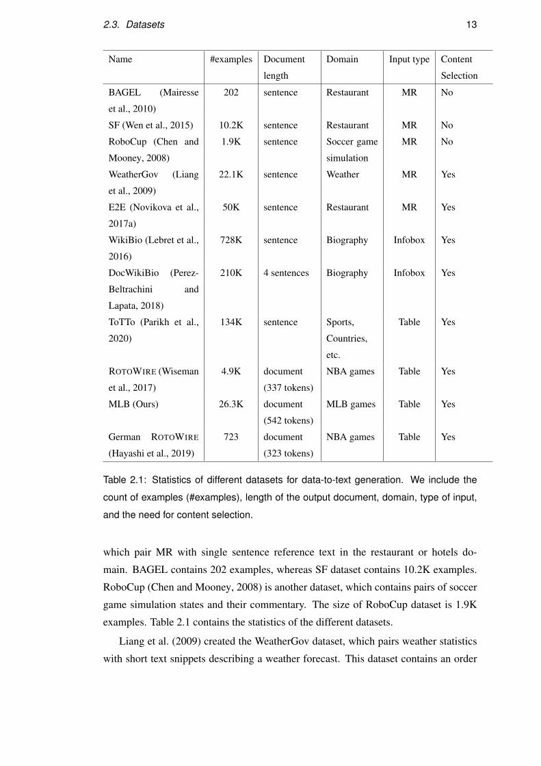
2.3. Datasets 13
Name #examples Document
length
Domain Input type Content
Selection
BAGEL (Mairesse
et al., 2010)
202 sentence Restaurant MR No
SF (Wen et al., 2015) 10.2K sentence Restaurant MR No
RoboCup (Chen and
Mooney, 2008)
1.9K sentence Soccer game
simulation
MR No
WeatherGov (Liang
et al., 2009)
22.1K sentence Weather MR Yes
E2E (Novikova et al.,
2017a)
50K sentence Restaurant MR Yes
WikiBio (Lebret et al.,
2016)
728K sentence Biography Infobox Yes
DocWikiBio (Perez-
Beltrachini and
Lapata, 2018)
210K 4 sentences Biography Infobox Yes
ToTTo (Parikh et al.,
2020)
134K sentence Sports,
Countries,
etc.
Table Yes
ROTOWIRE (Wiseman
et al., 2017)
4.9K document
(337 tokens)
NBA games Table Yes
MLB (Ours) 26.3K document
(542 tokens)
MLB games Table Yes
German ROTOWIRE
(Hayashi et al., 2019)
723 document
(323 tokens)
NBA games Table Yes
Table 2.1: Statistics of different datasets for data-to-text generation. We include the
count of examples (#examples), length of the output document, domain, type of input,
and the need for content selection.
which pair MR with single sentence reference text in the restaurant or hotels do-
main. BAGEL contains 202 examples, whereas SF dataset contains 10.2K examples.
RoboCup (Chen and Mooney, 2008) is another dataset, which contains pairs of soccer
game simulation states and their commentary. The size of RoboCup dataset is 1.9K
examples. Table 2.1 contains the statistics of the different datasets.
Liang et al. (2009) created the WeatherGov dataset, which pairs weather statistics
with short text snippets describing a weather forecast. This dataset contains an order

14 Chapter 2. Background
Flat MR Natural Language Reference
name[Loch Fyne],
eatType[restaurant], food[French],
priceRange[less than £20],
familyFriendly[yes]
Loch Fyne is a family-friendly restau-
rant providing wine and cheese at a low
cost
Loch Fyne is a French family friendly
restaurant catering to a budget of below
£20.
Loch Fyne is a French restaurant with a
family setting and perfect on the wallet.
Table 2.2: Example from the E2E dataset (Novikova et al., 2017a) showing a flattened
meaning representation (MR) and three natural language references. The references
differ in the content selection of the attributes.
of magnitude larger number of examples (22.1K). However, it is now known that the
weather forecasts were not produced by a human annotator but by a template system
followed by post-editing (Reiter, 2017).
Novikova et al. (2017a) created the E2E dataset where the input is a MR in the
restaurant/hotel domain, and the reference text describes the MR. An example from
this dataset is shown in Table 2.2. Highlights of this dataset, compared to the earlier
datasets, include the need for content selection among the attributes in the MR and
diverse vocabulary in the reference text. The size of E2E dataset is 50K examples.
Lebret et al. (2016) introduced the WikiBio dataset, which contains Wikipedia in-
foboxes paired with a single-sentence biography from its corresponding Wikipedia ar-
ticle. An infobox is a table of attributes and their values. Table 2.3 shows an example
from the dataset. The dataset contains 728K samples. Perez-Beltrachini and Lapata
(2018) proposed an extension to the WikiBio dataset where the output biography can
be multi-sentence text (an average of 4 sentences and 100 tokens). This dataset size is
210K.
Parikh et al. (2020) created a dataset for the controlled generation of text. The input
is a table from Wikipedia in which some of the cells are highlighted. The task is to
describe the highlighted cells in the context of the table. Table 2.4 contains an example
from the dataset. The size of the dataset is 134K.

2.3. Datasets 15
Table Summary
Frederick Parker-Rhodes
Born 21 November 1914 Newington,
Yorkshire
Arthur Frederick Parker-Rhodes
(21 November 1914 – 2 March
1987) was an English linguist,
plant pathologist, computer
scientist, mathematician,
mystic, and mycologist, who
also introduced original theories
in physics.
Died 2 March 1987 (aged 72)
Nationality British
Known for Contributions to computa-
tional linguistics, combinatorial
physics, bit-string physics, plant
pathology, and mycology
Scientific career
Fields Mycology, Plant Pathology,
Mathematics, Linguistics,
Computer Science
Author abbrev. (botany) Park.-Rhodes
Table 2.3: An example from the WikiBio dataset (Lebret et al., 2016) with Wikipedia
infobox and its corresponding single-sentence biography
Data-to-text with longer outputs Creating summaries of sports games has been
a topic of interest since the early beginnings of generation systems (Robin, 1994;
Tanaka-Ishii et al., 1998). A few recent datasets focus on long document generation
in the sports domain, and typically consist of pairs of game statistics and their corre-
sponding game summaries. We describe these datasets in more detail in the following
sections since they form the basis of all the experiments reported in this thesis.
2.3.1 ROTOWIRE
ROTOWIRE (Wiseman et al., 2017) is a dataset of NBA basketball game summaries,
paired with corresponding box-score tables. The statistics of the dataset are shown in
Table 2.8. The summaries are professionally written, relatively well structured, and
long (337 words on average). The summaries are targeted towards fantasy basketball
fans. The number of record types is 39, the average number of records is 628, the
vocabulary size is 11.3K words, and the token count is 1.6M. The dataset is ideally
suited for document-scale generation. Table 2.5 contains an example of ROTOWIRE
dataset.
16 Chapter 2. Background
Table Title Roger Craig (American Football)
Section Title National Football League Statistics
Rushing Receiving
Year Team Att Yds Avg TD Rec Yds Avg TD Reference text
1983 SF 176 725 4.1 8 48 427 8.9 4
Craig finished
his eleven NFL
seasons with
8,189 rushing
yards, 566
receptions for
4,911 receiving
yards
1984 SF 155 649 4.2 7 71 675 9.5 3
1985 SF 214 1,050 4.9 9 92 1,016 11.0 6
1986 SF 204 830 4.1 7 81 624 7.7 0
1987 SF 215 815 3.8 3 66 492 7.5 1
1988 SF 310 1,502 4.8 9 76 534 7.0 1
1989 SF 271 1,054 3.9 6 49 473 9.7 1
1990 SF 141 439 3.1 1 25 201 8.0 0
1991 LA 162 590 3.6 1 17 136 8.0 0
1992 MIN 105 416 4.0 4 22 164 7.5 0
1993 MIN 38 119 3.1 1 19 169 8.9 1
Career 1,991 8,189 4.1 56 566 4,911 8.7 17
Table 2.4: An example from the ToTTo dataset (Parikh et al., 2020). It shows a table
from Wikipedia with a few cells highlighted in yellow. The task is to generate a one-
sentence description of the highlighted cells in context of the table.
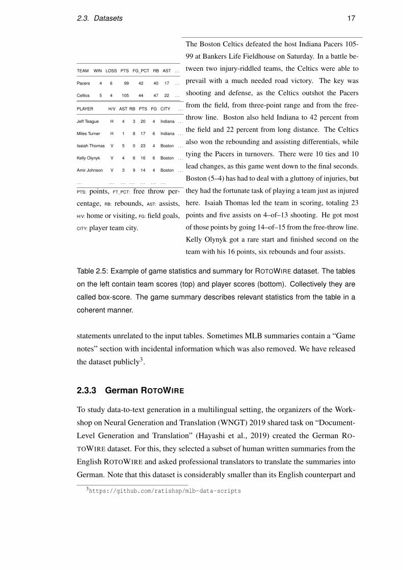
2.3.2 MLB
In this thesis we also created a new dataset for major league baseball (MLB) (see ex-
ample in Table 2.6 and statistics of the dataset in Table 2.8). The MLB dataset contains
pairs of MLB game statistics and their human written summaries. The summaries are
obtained from the ESPN website2. Compared to ROTOWIRE, MLB summaries are
longer (approximately by 50%) and the input records are richer and more structured
(with the addition of play-by-play). Moreover, the MLB dataset is five times larger in
terms of data size (i.e., pairs of tables and game summaries). Table 2.6 shows (in a
table format) the scoring summary of a MLB game, a play-by-play summary with de-
tails of the most important events in the game recorded chronologically (i.e., in which
play), and a human-written summary.
For MLB we created a split of 22,821/1,739/1,744 instances. Game summaries
were tokenized using NLTK (Bird et al., 2009) and hyphenated words were separated.
Sentences containing quotes were removed as they included opinions and non-factual
2http://www.espn.com/mlb/recap?gameId={gameid}
2.3. Datasets 17
TEAM WIN LOSS PTS FG_PCT RB AST . . .
Pacers 4 6 99 42 40 17 . . .
Celtics 5 4 105 44 47 22 . . .
PLAYER H/V AST RB PTS FG CITY . . .
Jeff Teague H 4 3 20 4 Indiana . . .
Miles Turner H 1 8 17 6 Indiana . . .
Isaiah Thomas V 5 0 23 4 Boston . . .
Kelly Olynyk V 4 6 16 6 Boston . . .
Amir Johnson V 3 9 14 4 Boston . . .
. . . . . . . . . . . . . . . . . . . . .
PTS: points, FT_PCT: free throw per-
centage, RB: rebounds, AST: assists,
H/V: home or visiting, FG: field goals,
CITY: player team city.
The Boston Celtics defeated the host Indiana Pacers 105-
99 at Bankers Life Fieldhouse on Saturday. In a battle be-
tween two injury-riddled teams, the Celtics were able to
prevail with a much needed road victory. The key was
shooting and defense, as the Celtics outshot the Pacers
from the field, from three-point range and from the free-
throw line. Boston also held Indiana to 42 percent from
the field and 22 percent from long distance. The Celtics
also won the rebounding and assisting differentials, while
tying the Pacers in turnovers. There were 10 ties and 10
lead changes, as this game went down to the final seconds.
Boston (5–4) has had to deal with a gluttony of injuries, but
they had the fortunate task of playing a team just as injured
here. Isaiah Thomas led the team in scoring, totaling 23
points and five assists on 4–of–13 shooting. He got most
of those points by going 14–of–15 from the free-throw line.
Kelly Olynyk got a rare start and finished second on the
team with his 16 points, six rebounds and four assists.
Table 2.5: Example of game statistics and summary for ROTOWIRE dataset. The tables
on the left contain team scores (top) and player scores (bottom). Collectively they are
called box-score. The game summary describes relevant statistics from the table in a
coherent manner.
statements unrelated to the input tables. Sometimes MLB summaries contain a “Game
notes” section with incidental information which was also removed. We have released
the dataset publicly3.
2.3.3 German ROTOWIRE
To study data-to-text generation in a multilingual setting, the organizers of the Work-
shop on Neural Generation and Translation (WNGT) 2019 shared task on “Document-
Level Generation and Translation” (Hayashi et al., 2019) created the German RO-
TOWIRE dataset. For this, they selected a subset of human written summaries from the
English ROTOWIRE and asked professional translators to translate the summaries into
German. Note that this dataset is considerably smaller than its English counterpart and
3https://github.com/ratishsp/mlb-data-scripts
18 Chapter 2. Background
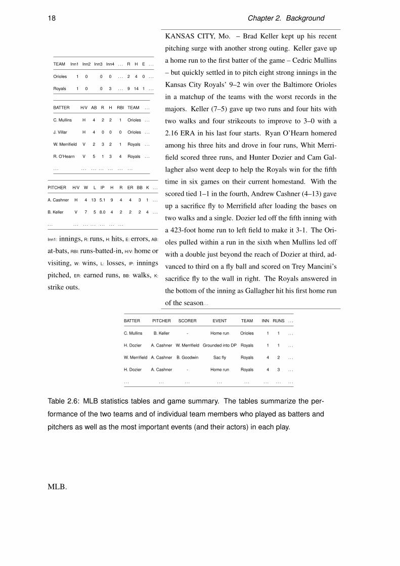
TEAM Inn1 Inn2 Inn3 Inn4 . . . R H E . . .
Orioles 1 0 0 0 . . . 2 4 0 . . .
Royals 1 0 0 3 . . . 9 14 1 . . .
BATTER H/V AB R H RBI TEAM . . .
C. Mullins H 4 2 2 1 Orioles . . .
J. Villar H 4 0 0 0 Orioles . . .
W. Merrifield V 2 3 2 1 Royals . . .
R. O’Hearn V 5 1 3 4 Royals . . .
. . . . . . . . . . . . . . . . . . . . .
PITCHER H/V W L IP H R ER BB K . . .
A. Cashner H 4 13 5.1 9 4 4 3 1 . . .
B. Keller V 7 5 8.0 4 2 2 2 4 . . .
. . . . . . . . . . . . . . . . . . . . .
Inn1: innings, R: runs, H: hits, E: errors, AB:
at-bats, RBI: runs-batted-in, H/V: home or
visiting, W: wins, L: losses, IP: innings
pitched, ER: earned runs, BB: walks, K:
strike outs.
KANSAS CITY, Mo. – Brad Keller kept up his recent
pitching surge with another strong outing. Keller gave up
a home run to the first batter of the game – Cedric Mullins
– but quickly settled in to pitch eight strong innings in the
Kansas City Royals’ 9–2 win over the Baltimore Orioles
in a matchup of the teams with the worst records in the
majors. Keller (7–5) gave up two runs and four hits with
two walks and four strikeouts to improve to 3–0 with a
2.16 ERA in his last four starts. Ryan O’Hearn homered
among his three hits and drove in four runs, Whit Merri-
field scored three runs, and Hunter Dozier and Cam Gal-
lagher also went deep to help the Royals win for the fifth
time in six games on their current homestand. With the
scored tied 1–1 in the fourth, Andrew Cashner (4–13) gave
up a sacrifice fly to Merrifield after loading the bases on
two walks and a single. Dozier led off the fifth inning with
a 423-foot home run to left field to make it 3-1. The Ori-
oles pulled within a run in the sixth when Mullins led off
with a double just beyond the reach of Dozier at third, ad-
vanced to third on a fly ball and scored on Trey Mancini’s
sacrifice fly to the wall in right. The Royals answered in
the bottom of the inning as Gallagher hit his first home run
of the season. . .
BATTER PITCHER SCORER EVENT TEAM INN RUNS . . .
C. Mullins B. Keller - Home run Orioles 1 1 . . .
H. Dozier A. Cashner W. Merrifield Grounded into DP Royals 1 1 . . .
W. Merrifield A. Cashner B. Goodwin Sac fly Royals 4 2 . . .
H. Dozier A. Cashner - Home run Royals 4 3 . . .
. . . . . . . . . . . . . . . . . . . . . . . .
Table 2.6: MLB statistics tables and game summary. The tables summarize the per-
formance of the two teams and of individual team members who played as batters and
pitchers as well as the most important events (and their actors) in each play.
MLB.
2.4. Baseline Encoder-Decoder Models 19
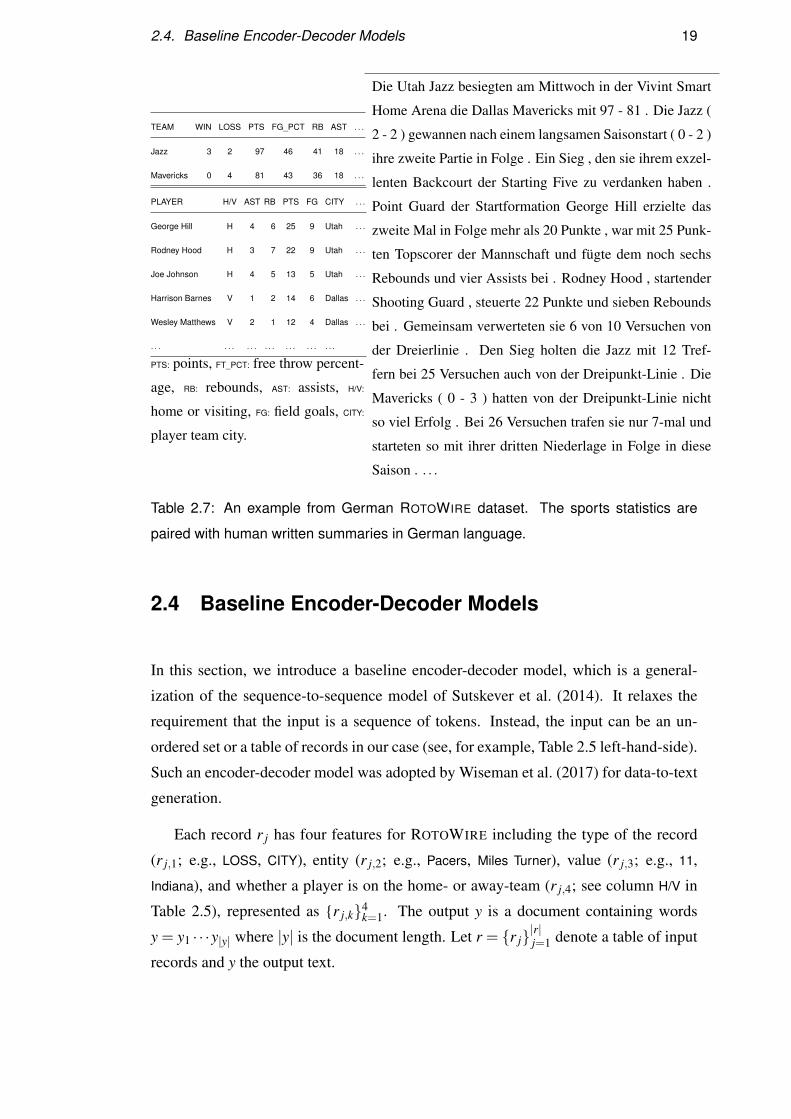
TEAM WIN LOSS PTS FG_PCT RB AST . . .
Jazz 3 2 97 46 41 18 . . .
Mavericks 0 4 81 43 36 18 . . .
PLAYER H/V AST RB PTS FG CITY . . .
George Hill H 4 6 25 9 Utah . . .
Rodney Hood H 3 7 22 9 Utah . . .
Joe Johnson H 4 5 13 5 Utah . . .
Harrison Barnes V 1 2 14 6 Dallas . . .
Wesley Matthews V 2 1 12 4 Dallas . . .
. . . . . . . . . . . . . . . . . . . . .
PTS: points, FT_PCT: free throw percent-
age, RB: rebounds, AST: assists, H/V:
home or visiting, FG: field goals, CITY:
player team city.
Die Utah Jazz besiegten am Mittwoch in der Vivint Smart
Home Arena die Dallas Mavericks mit 97 - 81 . Die Jazz (
2 - 2 ) gewannen nach einem langsamen Saisonstart ( 0 - 2 )
ihre zweite Partie in Folge . Ein Sieg , den sie ihrem exzel-
lenten Backcourt der Starting Five zu verdanken haben .
Point Guard der Startformation George Hill erzielte das
zweite Mal in Folge mehr als 20 Punkte , war mit 25 Punk-
ten Topscorer der Mannschaft und fügte dem noch sechs
Rebounds und vier Assists bei . Rodney Hood , startender
Shooting Guard , steuerte 22 Punkte und sieben Rebounds
bei . Gemeinsam verwerteten sie 6 von 10 Versuchen von
der Dreierlinie . Den Sieg holten die Jazz mit 12 Tref-
fern bei 25 Versuchen auch von der Dreipunkt-Linie . Die
Mavericks ( 0 - 3 ) hatten von der Dreipunkt-Linie nicht
so viel Erfolg . Bei 26 Versuchen trafen sie nur 7-mal und
starteten so mit ihrer dritten Niederlage in Folge in diese
Saison . . . .
Table 2.7: An example from German ROTOWIRE dataset. The sports statistics are
paired with human written summaries in German language.
2.4 Baseline Encoder-Decoder Models
In this section, we introduce a baseline encoder-decoder model, which is a general-
ization of the sequence-to-sequence model of Sutskever et al. (2014). It relaxes the
requirement that the input is a sequence of tokens. Instead, the input can be an un-
ordered set or a table of records in our case (see, for example, Table 2.5 left-hand-side).
Such an encoder-decoder model was adopted by Wiseman et al. (2017) for data-to-text
generation.
Each record r j has four features for ROTOWIRE including the type of the record
(r j,1; e.g., LOSS, CITY), entity (r j,2; e.g., Pacers, Miles Turner), value (r j,3; e.g., 11,
Indiana), and whether a player is on the home- or away-team (r j,4; see column H/V in
Table 2.5), represented as {r j,k}4k=1. The output y is a document containing words
y = y1 · · ·y|y| where |y| is the document length. Let r = {r j}|r|j=1 denote a table of input
records and y the output text.

20 Chapter 2. Background
RW MLB DE-RW
Vocab Size 11.3K 38.9K 9.5K
# Tokens 1.5M 14.3M 234K
# Instances 4.9K 26.3K 723
# Record Types 39 53 39
Avg Records 628 565 628
Avg Length (tokens) 337.1 542.1 323.6
Table 2.8: Dataset statistics for ROTOWIRE (RW), MLB and German ROTOWIRE (DE-
RW) including vocabulary size, number of tokens, number of instances (i.e., table-
summary pairs), number of record types, average number of records and average sum-
mary length.
2.4.1 Record Encoder
The input to this model is a table of unordered records, each represented as fea-
tures {r j,k}4k=1. Following previous work (Yang et al., 2017; Wiseman et al., 2017),
we embed features into vectors, and then use a multilayer perceptron to obtain a vector
representation r j for each record:
r j = ReLU(Wr[r j,1;r j,2;r j,3;r j,4]+br)
where [; ] indicates vector concatenation, Wr ∈ Rn×4n,br ∈ Rn are parameters, and
ReLU is the rectifier activation function.
2.4.2 Text Generation
The probability of output text y conditioned on input table r is modeled as:
p(y|r) =|y|
∏t=1
p(yt |y<t ,r)
where y<t = y1 . . .yt−1. We use the encoder-decoder architecture with an attention
mechanism (Bahdanau et al., 2015; Luong et al., 2015a) to compute p(y|r).The text decoder is based on a recurrent neural network with LSTM (Hochreiter
and Schmidhuber, 1997) units. The decoder is initialized to the average of the record
vectors, avg({r j}|r|j=1). At decoding step t, the input of the LSTM unit is the embedding
of the previously predicted word yt−1. Let dt be the hidden state of the t-th LSTM unit.
2.4. Baseline Encoder-Decoder Models 21
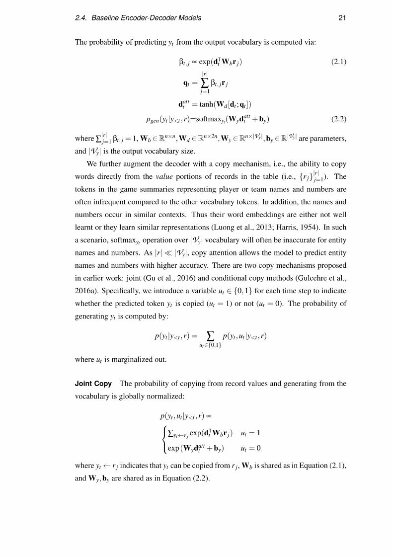
The probability of predicting yt from the output vocabulary is computed via:
βt, j ∝ exp(dᵀt Wbr j) (2.1)
qt =|r|
∑j=1
βt, jr j
dattt = tanh(Wd[dt ;qt ])
pgen(yt |y<t ,r)=softmaxyt(Wydattt +by) (2.2)
where ∑|r|j=1 βt, j = 1, Wb ∈Rn×n,Wd ∈Rn×2n,Wy ∈Rn×|Vy|,by ∈R|Vy| are parameters,
and |Vy| is the output vocabulary size.
We further augment the decoder with a copy mechanism, i.e., the ability to copy
words directly from the value portions of records in the table (i.e., {r j}|r|j=1). The
tokens in the game summaries representing player or team names and numbers are
often infrequent compared to the other vocabulary tokens. In addition, the names and
numbers occur in similar contexts. Thus their word embeddings are either not well
learnt or they learn similar representations (Luong et al., 2013; Harris, 1954). In such
a scenario, softmaxyt operation over |Vy| vocabulary will often be inaccurate for entity
names and numbers. As |r| � |Vy|, copy attention allows the model to predict entity
names and numbers with higher accuracy. There are two copy mechanisms proposed
in earlier work: joint (Gu et al., 2016) and conditional copy methods (Gulcehre et al.,
2016a). Specifically, we introduce a variable ut ∈ {0,1} for each time step to indicate
whether the predicted token yt is copied (ut = 1) or not (ut = 0). The probability of
generating yt is computed by:
p(yt |y<t ,r) = ∑ut∈{0,1}
p(yt ,ut |y<t ,r)
where ut is marginalized out.
Joint Copy The probability of copying from record values and generating from the
vocabulary is globally normalized:
p(yt ,ut |y<t ,r) ∝∑yt←r j exp(dᵀt Wbr j) ut = 1
exp(Wydattt +by) ut = 0
where yt← r j indicates that yt can be copied from r j, Wb is shared as in Equation (2.1),
and Wy,by are shared as in Equation (2.2).

22 Chapter 2. Background
Conditional Copy The variable ut is first computed as a switch gate, and then is used
to obtain the output probability:
p(ut = 1|y<t ,r) = sigmoid(wu ·dt +bu)
p(yt ,ut |y<t ,r) =p(ut |y<t ,r)∑yt←r j βt, j ut = 1
p(ut |y<t ,r)pgen(yt |y<t ,r) ut = 0
where βt, j and pgen(yt |y<t ,r) are computed as in Equations (2.1) to (2.2), and wu ∈Rn,bu ∈ R are parameters.
2.4.3 Training and Inference
The model is trained to maximize the log-likelihood of the gold output text given the
table records:
max ∑(r,y)∈D
log p(y|r)
where D represents training examples (input records and game summaries). During
inference, the output for input r is predicted by:
y = argmaxy′
p(y′|r)
where y′ represents output text candidates. We utilize beam search to approximately
obtain the best results.
2.5 Evaluation
2.5.1 Automatic Evaluation
BLEU For automatic evaluation, we make use of BLEU (Papineni et al., 2002). It
compares candidate output with reference summary and produces a score between 1
and 100. It matches n-grams between the two texts, considering matches from uni-
gram till 4-grams. These matching n-grams are used to compute a weighted average of
modified n-gram precision. Furthermore, BLEU has a recall based component called
brevity penalty (BP), which penalises outputs shorter than the reference length. BP
operates at the corpus statistic level and is computed using decayed exponential com-
parison of the candidate summary length and the reference summary length. More
2.5. Evaluation 23
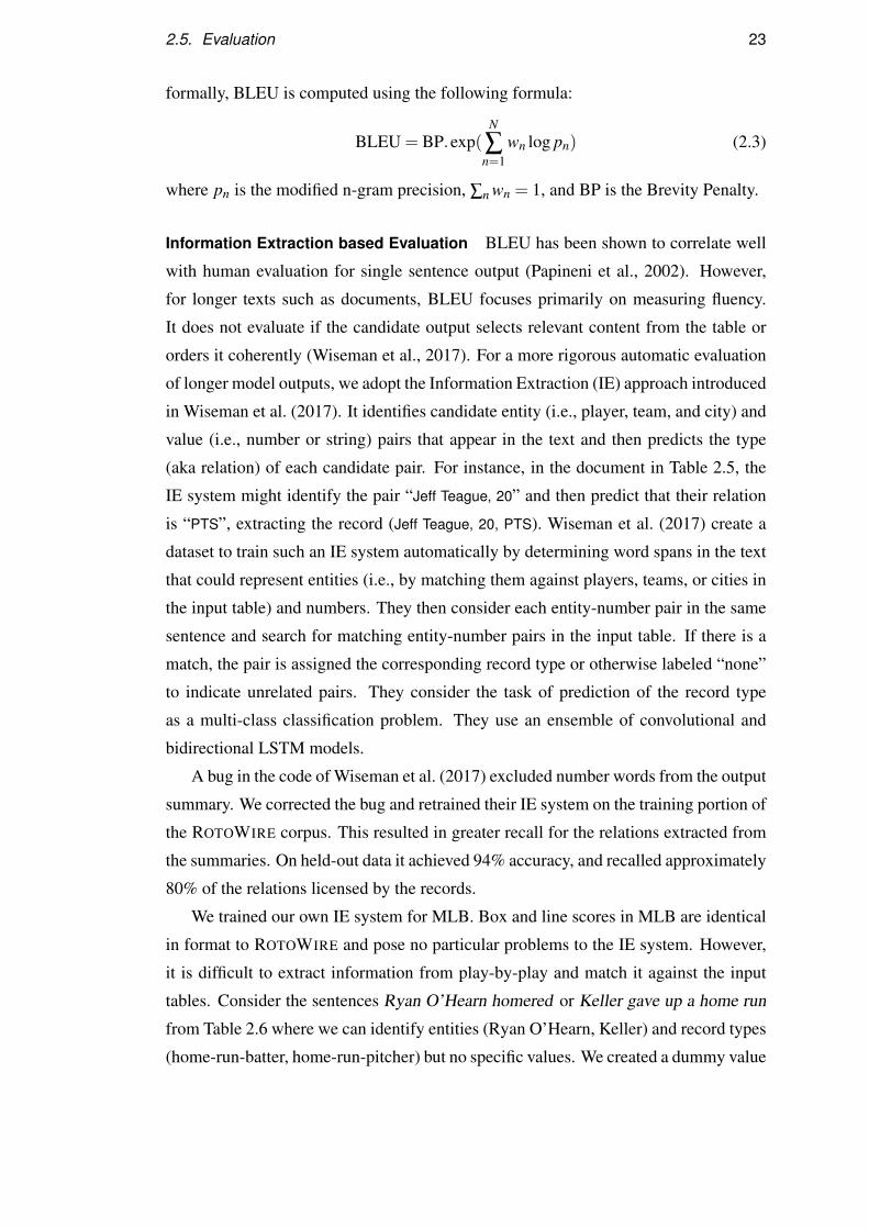
formally, BLEU is computed using the following formula:
BLEU = BP.exp(N
∑n=1
wn log pn) (2.3)
where pn is the modified n-gram precision, ∑n wn = 1, and BP is the Brevity Penalty.
Information Extraction based Evaluation BLEU has been shown to correlate well
with human evaluation for single sentence output (Papineni et al., 2002). However,
for longer texts such as documents, BLEU focuses primarily on measuring fluency.
It does not evaluate if the candidate output selects relevant content from the table or
orders it coherently (Wiseman et al., 2017). For a more rigorous automatic evaluation
of longer model outputs, we adopt the Information Extraction (IE) approach introduced
in Wiseman et al. (2017). It identifies candidate entity (i.e., player, team, and city) and
value (i.e., number or string) pairs that appear in the text and then predicts the type
(aka relation) of each candidate pair. For instance, in the document in Table 2.5, the
IE system might identify the pair “Jeff Teague, 20” and then predict that their relation
is “PTS”, extracting the record (Jeff Teague, 20, PTS). Wiseman et al. (2017) create a
dataset to train such an IE system automatically by determining word spans in the text
that could represent entities (i.e., by matching them against players, teams, or cities in
the input table) and numbers. They then consider each entity-number pair in the same
sentence and search for matching entity-number pairs in the input table. If there is a
match, the pair is assigned the corresponding record type or otherwise labeled “none”
to indicate unrelated pairs. They consider the task of prediction of the record type
as a multi-class classification problem. They use an ensemble of convolutional and
bidirectional LSTM models.
A bug in the code of Wiseman et al. (2017) excluded number words from the output
summary. We corrected the bug and retrained their IE system on the training portion of
the ROTOWIRE corpus. This resulted in greater recall for the relations extracted from
the summaries. On held-out data it achieved 94% accuracy, and recalled approximately
80% of the relations licensed by the records.
We trained our own IE system for MLB. Box and line scores in MLB are identical
in format to ROTOWIRE and pose no particular problems to the IE system. However,
it is difficult to extract information from play-by-play and match it against the input
tables. Consider the sentences Ryan O’Hearn homered or Keller gave up a home run
from Table 2.6 where we can identify entities (Ryan O’Hearn, Keller) and record types
(home-run-batter, home-run-pitcher) but no specific values. We created a dummy value
24 Chapter 2. Background
of -1 for such cases and the IE system was trained to predict the record type of entity
value pairs such as (Ryan O’Hearn, -1) or (Keller, -1).
Wiseman et al. (2017) define three metrics based on the output of the IE system
described above. Let y be the gold summary and y the model output.
• Relation Generation (RG) measures the precision and count of relations ex-
tracted from y that also appear in records r.
• Content Selection (CS) measures the precision and recall of relations extracted
from y that are also extracted from y.
• Content Ordering (CO) measures the complement of the normalized Damerau-
Levenshtein (DL) distance (Brill and Moore, 2000) between the sequences of
relations extracted from y and y.
The DL distance for two strings p and s with lengths i and j respectively is
computed recursively as follows (Boytsov, 2011):
Ci, j =
min
0 i = j = 0
Ci−1, j +1 i > 0
Ci, j−1 +1 j > 0
Ci−1, j−1 +1[p[i] 6= s[ j]] i, j > 0
Ci−2, j−2 +1 p[i] = s[ j−1], p[i−1] = s[ j] and i, j > 1
where 1[x] = 1 if x is true, and 0 otherwise.
Each recursive call corresponds to one of the following cases:
– Ci−1, j +1 corresponds to deletion of p[i]
– Ci, j−1 +1 corresponds to deletion of s[ j]
– Ci−1, j−1+1[p[i] 6= s[ j]] checks for match between the characters p[i] and s[ j]
– Ci−2, j−2 + 1 corresponds to transposition of characters p[i], p[i−1] with s[ j]and s[ j−1]
2.5. Evaluation 25
2.5.2 Human Evaluation
We also asked participants to assess model output in terms of relation generation,
grammaticality, coherence, and conciseness. We conducted our study on the Amazon
Mechanical Turk (AMT) crowdsourcing platform, following best practices for human
evaluation in NLG (van der Lee et al., 2019). Specifically, to ensure consistent ratings,
we required crowdworkers to have an approval rating greater than 98% and a mini-
mum of 1,000 previously completed tasks. Raters were restricted to English speaking
countries (i.e., US, UK, Canada, Ireland, Australia, or NZ). Participants were allowed
to provide feedback on the task or field questions (our interface accepts free text).
We performed two types of studies aiming to assess a) whether the generated text
is faithful to the input table and b) whether it is well-written. In our first study, we
presented crowdworkers with sentences randomly selected from summaries along with
their corresponding box score (and play-by-play in case of MLB) and asked them
to count supported and contradicting facts (ignoring hallucinations, i.e., unsupported
facts). We did not require crowdworkers to be familiar with NBA or MLB. Instead,
we provided a cheat sheet explaining the semantics of box score tables. In addition,
we provided examples of sentences with supported/contradicting facts. Appendix A
contains additional details of the experimental setup for human evaluation for factuality
estimation.
Our second study evaluated the quality of the generated summaries. We presented
crowdworkers with a pair of summaries and asked them to choose the better one in
terms of the three metrics:
• Grammaticality (is the summary written in well-formed English?),
• Coherence (is the summary well structured and well organized and does it have
a natural ordering of the facts?) and
• Conciseness (does the summary avoid unnecessary repetition including whole
sentences, facts or phrases?).
We provided example summaries showcasing good and bad output. For this task, we
required that the crowdworkers be able to comfortably comprehend NBA/MLB game
summaries. We elicited preferences with Best-Worst Scaling (Louviere and Wood-
worth, 1991; Louviere et al., 2015), a method shown to be more reliable than rating
scales. The score of a system is computed as the number of times it is rated best mi-
nus the number of times it is rated worst (Orme, 2009). The scores range from −100
26 Chapter 2. Background
(absolutely worst) to +100 (absolutely best). Appendix B contains additional details
of the experimental setup for human evaluation for quality estimation.
2.6 Summary
In this chapter, we discussed what makes a data-to-text system in terms of input, output
and model architecture. We reviewed architectures adopted by earlier systems focusing
on rule-based approaches, statistical models and neural networks. We also presented
a baseline encoder-decoder neural architecture for data-to-text generation. In addi-
tion, we described datasets often used for the development of data-to-text generation
systems and introduced the metrics used to evaluate model output.
In the next chapter, we show how to inject micro planning in the neural model
introduced in Section 2.4. Specifically, we learn a micro plan from the input and
condition on it to generate the output document. We operationalize micro plans as a
sequence of records from the input table.
Chapter 3
Micro Planning
In the previous chapter, we looked into the earlier work in data-to-text generation,
discussed the datasets we plan to use in our experiments, and automatic metrics for
the evaluation of model output. We have also seen examples of earlier architectures
for data-to-text generation, which adopt a pipeline approach with separate stages for
document planning, micro planning, and surface realisation. The neural approaches
do away with individual modules, instead they train a model to perform data-to-text
generation in an end-to-end manner.
Micro planning involves deciding specific words to describe concepts and rela-
tions, generating referring expressions, and aggregating content into sentences (Reiter
and Dale, 2000). In this chapter, we show how to inject micro planning in contempo-
rary neural models. Our model learns a micro plan from the input and conditions on the
micro plan in order to generate the output document. We operationalize micro plan as
a sequence of records from the input table. An explicit micro planning mechanism has
at least three advantages for multi-sentence document generation: it is a fine-grained
representation of the document, thereby enabling the decoder to concentrate on the
less challenging task of surface realization; it makes the process of data-to-text gen-
eration more interpretable by generating an intermediate representation; and reduces
redundancy in the output, since it is less likely for the micro plan to contain the same
information in multiple places.
We train our micro planning and surface realisation modules jointly using neural
networks and evaluate model performance on the ROTOWIRE (Wiseman et al., 2017)
and MLB datasets. Automatic and human evaluation show that micro planning im-
proves generation considerably over competitive baselines.
27

28 Chapter 3. Micro Planning
TEAM WIN LOSS PTS FG_PCT RB AST . . .
Pacers 4 6 99 42 40 17 . . .
Celtics 5 4 105 44 47 22 . . .
PLAYER H/V AST RB PTS FG CITY . . .
Jeff Teague H 4 3 20 4 Indiana . . .
Miles Turner H 1 8 17 6 Indiana . . .
Isaiah Thomas V 5 0 23 4 Boston . . .
Kelly Olynyk V 4 6 16 6 Boston . . .
Amir Johnson V 3 9 14 4 Boston . . .
. . . . . . . . . . . . . . . . . . . . .
PTS: points, FT_PCT: free throw per-
centage, RB: rebounds, AST: assists,
H/V: home or visiting, FG: field goals,
CITY: player team city.
The Boston Celtics defeated the host Indiana Pacers 105-99 at Bankers
Life Fieldhouse on Saturday. In a battle between two injury-riddled
teams, the Celtics were able to prevail with a much needed road vic-
tory. The key was shooting and defense, as the Celtics outshot the
Pacers from the field, from three-point range and from the free-throw
line. Boston also held Indiana to 42 percent from the field and 22
percent from long distance. The Celtics also won the rebounding and
assisting differentials, while tying the Pacers in turnovers. There were
10 ties and 10 lead changes, as this game went down to the final sec-
onds. Boston (5–4) has had to deal with a gluttony of injuries, but
they had the fortunate task of playing a team just as injured here. Isa-
iah Thomas led the team in scoring, totaling 23 points and five assists
on 4–of–13 shooting. He got most of those points by going 14–of–15
from the free-throw line. Kelly Olynyk got a rare start and finished
second on the team with his 16 points, six rebounds and four assists.
Table 3.1: Example of data-records and document summary for ROTOWIRE dataset
3.1 Problem Formulation
The input to our model is a table of records (see Table 3.1 left hand-side). Let M be
the number of features in each record. For example, in ROTOWIRE, each record r j
has four features including its type (r j,1; e.g., LOSS, CITY), entity (r j,2; e.g., Pacers,
Miles Turner), value (r j,3; e.g., 11, Indiana), and whether a player is on the home- or
away-team (r j,4; see column H/V in Table 3.1), represented as {r j,k}Mk=1. The output y
is a document containing tokens y = y1 · · ·y|y| where |y| is the document length. The
overall architecture of our model consists of two stages: (a) micro planning operates
on the input records of a database and produces a micro plan specifying which records
are to be verbalized in the document and in which order (see Table 3.2) and (b) text
generation produces the output text given the micro plan as input; at each decoding
step, the generation model attends over vector representations of the records in the
micro plan.
Let r = {r j}Lj=1 denote a table of input records where L = |r|, and y the output text.
We model p(y|r) as the joint probability of text y and micro plan z, given input r. We
further decompose p(y,z|r) into p(z|r), a micro planning phase, and p(y|r,z), a text
3.1. Problem Formulation 29
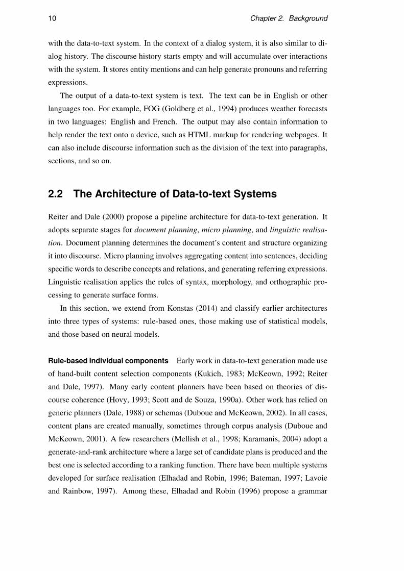
r1 r2 r3 r4 . . . rL EOM
· · · · ·
rc1 rc2 rc3 rc4 rcL re. . . h1 h2 h3 h4
rs rc3 rcL rc1
rc3 rcL rc1
Vector Encoder Decoder · Contextualization
e1 e2 e3
y2 y1 BOSy3
d3 d2 d1d4
y1y2y3y4
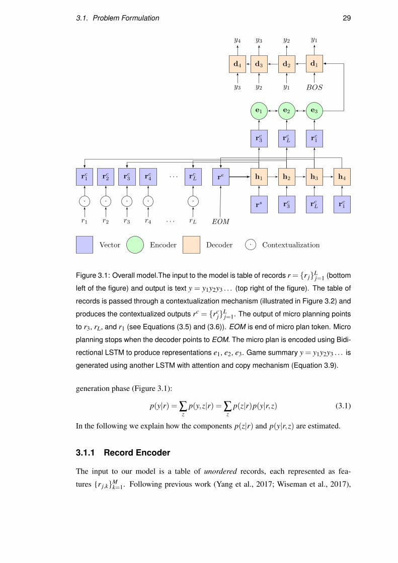
Figure 3.1: Overall model.The input to the model is table of records r = {r j}Lj=1 (bottom
left of the figure) and output is text y = y1y2y3 . . . (top right of the figure). The table of
records is passed through a contextualization mechanism (illustrated in Figure 3.2) and
produces the contextualized outputs rc = {rcj}L
j=1. The output of micro planning points
to r3, rL, and r1 (see Equations (3.5) and (3.6)). EOM is end of micro plan token. Micro
planning stops when the decoder points to EOM. The micro plan is encoded using Bidi-
rectional LSTM to produce representations e1, e2, e3. Game summary y = y1y2y3 . . . is
generated using another LSTM with attention and copy mechanism (Equation 3.9).
generation phase (Figure 3.1):
p(y|r) = ∑z
p(y,z|r) = ∑z
p(z|r)p(y|r,z) (3.1)
In the following we explain how the components p(z|r) and p(y|r,z) are estimated.
3.1.1 Record Encoder
The input to our model is a table of unordered records, each represented as fea-
tures {r j,k}Mk=1. Following previous work (Yang et al., 2017; Wiseman et al., 2017),
30 Chapter 3. Micro Planning
r3,1 r3,2 r3,3 r3,4
r3,1 r3,2 r3,3 r3,4
r3
·Sigmoid
ratt3
inter-attention
r3,4r3,3r3,2r3,1
r2,1 r2,2 r2,3 r2,4
. . . . . . . . . . . .
Name Type ValueHome/Away
. . . . . . . . . . . .
rc3
Vector · Element-wise multiplication
Figure 3.2: Contextualization for micro planning. r3,1, r3,2, r3,3 and r3,4 are the four
features of the record r3 in ROTOWIRE. Computation of r3 is detailed in Equation (3.2),
ratt3 in Equation (3.3), and rc
3 in Equation (3.4). rc3 represents the contextualized repre-
sentation of r3.
we embed features into vectors by making use of word embeddings, and then use a
multilayer perceptron to obtain a vector representation r j for each record:
r j = ReLU(Wr[r j,1;r j,2;r j,3; . . . ;r j,M]+br) (3.2)
where [; ] indicates vector concatenation, Wr ∈ Rn×Mn,br ∈ Rn are parameters, and
ReLU is the rectifier activation function.
3.1.2 Contextualization
The context of a record can be useful in determining its importance vis-a-vis other
records in the table. For example, in ROTOWIRE if a player scores many points, it
is likely that other meaningfully related records such as field goals, three-pointers, or
rebounds will be mentioned in the output summary. To better capture such depen-
dencies among records, we make use of the contextualization mechanism as shown in
Figure 3.2.
We first compute the attention scores α j,k over the input table and use them to
3.1. Problem Formulation 31
obtain an attentional vector rattj for each record r j:
α j,k ∝ exp(rᵀj Wark)
c j = ∑k 6= j
α j,krk
rattj = Wg[r j;c j] (3.3)
where Wa ∈ Rn×n,Wg ∈ Rn×2n are parameter matrices, and ∑k 6= j α j,k = 1.
We next apply the contextualization gating mechanism to r j, and obtain the new
record representation rcj via:
g j = sigmoid(ratt
j)
rcj = g j� r j (3.4)
where� denotes element-wise multiplication, and gate g j ∈ [0,1]n controls the amount
of information flowing from r j. In other words, each element in rj is weighed by the
corresponding element of the contextualization gate g j.
3.1.3 Micro Planning
In our generation task, the output text is long but follows a canonical structure. In
ROTOWIRE, for example, game summaries typically begin by discussing which team
won/lost, following with various statistics involving individual players and their teams
(e.g., who performed exceptionally well or under-performed), and finishing with any
upcoming games. We hypothesize that generation would benefit from an explicit plan
specifying both what to say and in which order. Our model learns such micro plans
from training data. However, notice that ROTOWIRE (see Table 3.1) and most similar
data-to-text datasets do not naturally contain micro plans. Fortunately, we can obtain
these relatively straightforwardly following an information extraction approach (which
we explain in Section 3.2).
Suffice it to say that plans are extracted by mapping the text in the summaries onto
entities in the input table, their values, and types (i.e., relations). A plan is a sequence
of pointers with each entry pointing to an input record {r j}Lj=1. An excerpt of a plan is
shown in Table 3.2. The order in the plan corresponds to the sequence in which entities
appear in the game summary. Let z = z1 . . .z|z| denote the micro planning sequence.
Each zk points to an input record, i.e., zk ∈ {r j}Lj=1. Given the input records, the

32 Chapter 3. Micro Planning
probability p(z|r) is decomposed as:
p(z|r) =|z|
∏k=1
p(zk|z<k,r) (3.5)
where z<k = z1 . . .zk−1.
Since the output tokens of the micro planning stage correspond to positions in the
input sequence, we make use of Pointer Networks (Vinyals et al., 2015). The latter use
attention to point to the tokens of the input sequence rather than creating a weighted
representation of source encodings. As shown in Figure 3.1, given {r j}Lj=1, we use
an LSTM decoder to generate tokens corresponding to positions in the input. The
first hidden state of the decoder is initialized by avg({rcj}L
j=1), i.e., the average of
record vectors. At decoding step k, let hk be the hidden state of the LSTM. We model
p(zk = r j|z<k,r) as the attention over input records:
p(zk = r j|z<k,r) ∝ exp(hᵀk Wcrc
j) (3.6)
where the probability is normalized to 1, and Wc are parameters. Once zk points to
record r j, we use the corresponding vector rcj as the input of the next LSTM unit in the
decoder.
3.1.4 Text Generation
The probability of output text y conditioned on micro plan z and input table r is mod-
eled as:
p(y|r,z) =|y|
∏t=1
p(yt |y<t ,z,r) (3.7)
where y<t = y1 . . .yt−1. We use the encoder-decoder architecture with an attention
mechanism to compute p(y|r,z).We first encode the micro plan z into {ek}
|z|k=1 using a bidirectional LSTM. Because
the micro plan is a sequence of input records, we directly feed the corresponding record
vectors {rcj}L
j=1 as input to the LSTM units, which share the record encoder with the
first stage.
The text decoder is also based on a recurrent neural network with LSTM units.
The decoder is initialized with the hidden states of the final step in the encoder. At
decoding step t, the input of the LSTM unit is the embedding of the previously pre-
dicted word yt−1. Let dt be the hidden state of the t-th LSTM unit. The probability of
predicting yt from the output vocabulary is computed via:
βt,k ∝ exp(dᵀt Wbek) (3.8)

3.1. Problem Formulation 33
Value Entity Type H/V
Boston Celtics TEAM-CITY V
Celtics Celtics TEAM-NAME V
105 Celtics TEAM-PTS V
Indiana Pacers TEAM-CITY H
Pacers Pacers TEAM-NAME H
99 Pacers TEAM-PTS H
42 Pacers TEAM-FG_PCT H
22 Pacers TEAM-FG3_PCT H
5 Celtics TEAM-WIN V
4 Celtics TEAM-LOSS V
Isaiah Isaiah_Thomas FIRST_NAME V
Thomas Isaiah_Thomas SECOND_NAME V
23 Isaiah_Thomas PTS V
5 Isaiah_Thomas AST V
4 Isaiah_Thomas FGM V
13 Isaiah_Thomas FGA V
Kelly Kelly_Olynyk FIRST_NAME V
Olynyk Kelly_Olynyk SECOND_NAME V
16 Kelly_Olynyk PTS V
6 Kelly_Olynyk REB V
4 Kelly_Olynyk AST V
. . . . . . . . . . . .
Table 3.2: Micro plan for the game summary in Table 3.1. It contains a se-
quence of records, with each record containing four features: Value, Entity, Type and
Home(H)/Visiting(V) side. The sequence of records in micro plan aligns with the their
description in the game summary.
qt = ∑k
βt,kek
dattt = tanh(Wd[dt ;qt ])
pgen(yt |y<t ,z,r)=softmaxyt(Wydattt +by) (3.9)
where ∑k βt,k = 1, Wb ∈ Rn×n,Wd ∈ Rn×2n,Wy ∈ Rn×|Vy|,by ∈ R|Vy| are parameters,
34 Chapter 3. Micro Planning
and |Vy| is the output vocabulary size.
We further augment the decoder with a copy mechanism, i.e., the ability to copy
words directly from the value portions of records in the micro plan (i.e., {zk}|z|k=1).
We experimented with joint (Gu et al., 2016) and conditional copy methods (Gulcehre
et al., 2016a). See Section 2.4.2 in Chapter 2 for details on the differences between the
two mechanisms.
Following Gulcehre et al. (2016a) and Wiseman et al. (2017), if yt appears in the
micro plan during training, we assume that yt is copied (i.e., ut = 1).1
3.1.5 Training and Inference
Our model is trained to maximize the log-likelihood of the gold2 micro plan given table
records r and the gold output text given the micro plan and table records:
max ∑(r,z,y)∈D
log p(z|r)+ log p(y|r,z)
where D represents training examples (input records, plans, and game summaries).
During inference, the output for input r is predicted by:
z = argmaxz′
p(z′|r)
y = argmaxy′
p(y′|r, z)
where z′ and y′ represent micro plan and output text candidates, respectively. For each
stage, we utilize beam search to approximately obtain the best results.
3.2 Experimental Setup
Data We performed experiments on two datasets. The first one is ROTOWIRE (Wise-
man et al., 2017) which contains NBA basketball game statistics matched with human-
written summaries. In addition, we experiment with MLB dataset which contains base-
ball statistics and corresponding human-authored summaries obtained from the ESPN
website.1Following previous work (Gulcehre et al., 2016a; Wiseman et al., 2017) we learn whether yt can be
copied from candidate zk by applying supervision during training. Specifically, we retain zk when therecord entity and its value occur in same sentence in y.
2Strictly speaking, the micro plan is silver standard since it was not created by an expert but is theoutput of a fairly accurate IE system.
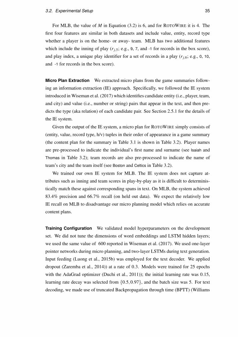
3.2. Experimental Setup 35
For MLB, the value of M in Equation (3.2) is 6, and for ROTOWIRE it is 4. The
first four features are similar in both datasets and include value, entity, record type
whether a player is on the home- or away- team. MLB has two additional features
which include the inning of play (r j,5; e.g., 9, 7, and -1 for records in the box score),
and play index, a unique play identifier for a set of records in a play (r j,6; e.g., 0, 10,
and -1 for records in the box score).
Micro Plan Extraction We extracted micro plans from the game summaries follow-
ing an information extraction (IE) approach. Specifically, we followed the IE system
introduced in Wiseman et al. (2017) which identifies candidate entity (i.e., player, team,
and city) and value (i.e., number or string) pairs that appear in the text, and then pre-
dicts the type (aka relation) of each candidate pair. See Section 2.5.1 for the details of
the IE system.
Given the output of the IE system, a micro plan for ROTOWIRE simply consists of
(entity, value, record type, h/v) tuples in their order of appearance in a game summary
(the content plan for the summary in Table 3.1 is shown in Table 3.2). Player names
are pre-processed to indicate the individual’s first name and surname (see Isaiah and
Thomas in Table 3.2); team records are also pre-processed to indicate the name of
team’s city and the team itself (see Boston and Celtics in Table 3.2).
We trained our own IE system for MLB. The IE system does not capture at-
tributes such as inning and team scores in play-by-play as it is difficult to determinis-
tically match these against corresponding spans in text. On MLB, the system achieved
83.4% precision and 66.7% recall (on held out data). We expect the relatively low
IE recall on MLB to disadvantage our micro planning model which relies on accurate
content plans.
Training Configuration We validated model hyperparameters on the development
set. We did not tune the dimensions of word embeddings and LSTM hidden layers;
we used the same value of 600 reported in Wiseman et al. (2017). We used one-layer
pointer networks during micro planning, and two-layer LSTMs during text generation.
Input feeding (Luong et al., 2015b) was employed for the text decoder. We applied
dropout (Zaremba et al., 2014)) at a rate of 0.3. Models were trained for 25 epochs
with the AdaGrad optimizer (Duchi et al., 2011)); the initial learning rate was 0.15,
learning rate decay was selected from {0.5,0.97}, and the batch size was 5. For text
decoding, we made use of truncated Backpropagation through time (BPTT) (Williams
36 Chapter 3. Micro Planning
and Peng, 1990) and set the truncation size to 100, i.e. we divide the the summary
into blocks of size equal to the truncation size, and backpropagate the gradients to the
encoder parameters and to the start of the current block. We set the beam size to 5
during inference. All models are implemented in OpenNMT-py (Klein et al., 2017a).
3.3 Results
Automatic Evaluation We evaluated model output using the metrics defined in Wise-
man et al. (2017) and introduced in Chapter 2. The idea is to employ a fairly accurate
IE system on the gold and automatic summaries and compare whether the identified
relations align or diverge.
Automatic Evaluation for ROTOWIRE Our results on the ROTOWIRE development
set are summarized in Table 3.3. We compare our Neural Content Planning model
(NCP for short) against the two encoder-decoder (ED) models presented in Wiseman
et al. (2017) with joint copy (JC) and conditional copy (CC), respectively. In addition
to our own re-implementation of these models, we include the best scores reported in
Wiseman et al. (2017) which were obtained with an encoder-decoder model enhanced
with conditional copy. Table 3.3 also shows results when NCP uses oracle micro plans
(OR) as input. In this case, we use the micro plans extracted using the IE approach
in Section 3.2 as z in Equation 3.7 instead of the predicted micro plan. In addition,
we report the performance of a template-based generator (Wiseman et al., 2017) which
creates a document consisting of eight template sentences: an introductory sentence
(who won/lost), six player-specific sentences (based on the six highest-scoring players
in the game), and a conclusion sentence. See Table 3.11 for an example.
As can be seen, NCP improves upon vanilla encoder-decoder models (ED+JC,
ED+CC), irrespective of the copy mechanism being employed. In fact, NCP achieves
comparable scores with either joint or conditional copy mechanism which indicates
that it is the micro planner which brings performance improvements. Overall, NCP+CC
achieves best content selection and content ordering scores in terms of BLEU. Com-
pared to the best reported system in Wiseman et al. (2017), we achieve an absolute
improvement of approximately 12% in terms of relation generation; content selection
precision also improves by 5% and recall by 15%, content ordering increases by 3%,
and BLEU by 1.5 points. The results of the oracle system (NCP+OR) show that con-
tent selection and ordering do indeed correlate with the quality of the micro plan and

3.3. Results 37
ModelRG CS CO
BLEU# P% P% R% DLD%
TEMPL 54.29 99.92 26.61 59.16 14.42 8.51
WS-2017 23.95 75.10 28.11 35.86 15.33 14.57
ED+JC 22.98 76.07 27.70 33.29 14.36 13.22
ED+CC 21.94 75.08 27.96 32.71 15.03 13.31
NCP+JC 33.37 87.40 32.20 48.56 17.98 14.92
NCP+CC 33.88 87.51 33.52 51.21 18.57 16.19
NCP+OR 21.59 89.21 88.52 85.84 78.51 24.11
Table 3.3: Automatic evaluation on ROTOWIRE development set using relation gener-
ation (RG) count (#) and precision (P%), content selection (CS) precision (P%) and re-
call (R%), content ordering (CO) in normalized Damerau-Levenshtein distance (DLD%),
and BLEU.
that any improvements in our planning component would result in better output. As far
as the template-based system is concerned, we observe that it obtains low BLEU and
CS precision but scores high on CS recall and RG metrics. This is not surprising as the
template system is provided with domain knowledge which our model does not have,
and thus represents an upper-bound on content selection and relation generation. We
also measured the degree to which the game summaries generated by our model con-
tain redundant information as the proportion of non-duplicate records extracted from
the summary by the IE system. 84.5% of the records in NCP+CC are non-duplicates
compared to Wiseman et al. (2017) who obtain 72.9% showing that our model is less
repetitive.
We further conducted an ablation study with the conditional copy variant of our
model (NCP+CC) to establish whether improvements are due to better contextualiza-
tion (CX) and/or micro planning (CP). We see in Table 3.4 that contextualization and
micro planning individually contribute to performance improvements over the base-
line (ED+CC), and accuracy further increases when both components are taken into
account. In addition we evaluated these components on their own (independently of
text generation) by comparing the output of the planner (see p(z|r) in Equation 3.5)
against micro plans obtained using the IE system (see row NCP in Table 3.4). Com-
pared to the full system (NCP+CC), content selection precision and recall are higher
(by 4.5% and 2%, respectively) as well as content ordering (by 1.8%). In another
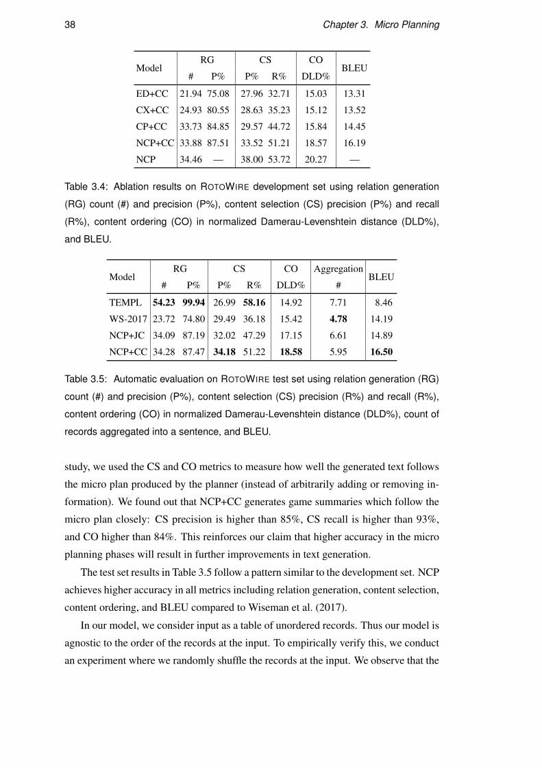
38 Chapter 3. Micro Planning
ModelRG CS CO
BLEU# P% P% R% DLD%
ED+CC 21.94 75.08 27.96 32.71 15.03 13.31
CX+CC 24.93 80.55 28.63 35.23 15.12 13.52
CP+CC 33.73 84.85 29.57 44.72 15.84 14.45
NCP+CC 33.88 87.51 33.52 51.21 18.57 16.19
NCP 34.46 — 38.00 53.72 20.27 —
Table 3.4: Ablation results on ROTOWIRE development set using relation generation
(RG) count (#) and precision (P%), content selection (CS) precision (P%) and recall
(R%), content ordering (CO) in normalized Damerau-Levenshtein distance (DLD%),
and BLEU.
ModelRG CS CO Aggregation
BLEU# P% P% R% DLD% #
TEMPL 54.23 99.94 26.99 58.16 14.92 7.71 8.46
WS-2017 23.72 74.80 29.49 36.18 15.42 4.78 14.19
NCP+JC 34.09 87.19 32.02 47.29 17.15 6.61 14.89
NCP+CC 34.28 87.47 34.18 51.22 18.58 5.95 16.50
Table 3.5: Automatic evaluation on ROTOWIRE test set using relation generation (RG)
count (#) and precision (P%), content selection (CS) precision (R%) and recall (R%),
content ordering (CO) in normalized Damerau-Levenshtein distance (DLD%), count of
records aggregated into a sentence, and BLEU.
study, we used the CS and CO metrics to measure how well the generated text follows
the micro plan produced by the planner (instead of arbitrarily adding or removing in-
formation). We found out that NCP+CC generates game summaries which follow the
micro plan closely: CS precision is higher than 85%, CS recall is higher than 93%,
and CO higher than 84%. This reinforces our claim that higher accuracy in the micro
planning phases will result in further improvements in text generation.
The test set results in Table 3.5 follow a pattern similar to the development set. NCP
achieves higher accuracy in all metrics including relation generation, content selection,
content ordering, and BLEU compared to Wiseman et al. (2017).
In our model, we consider input as a table of unordered records. Thus our model is
agnostic to the order of the records at the input. To empirically verify this, we conduct
an experiment where we randomly shuffle the records at the input. We observe that the
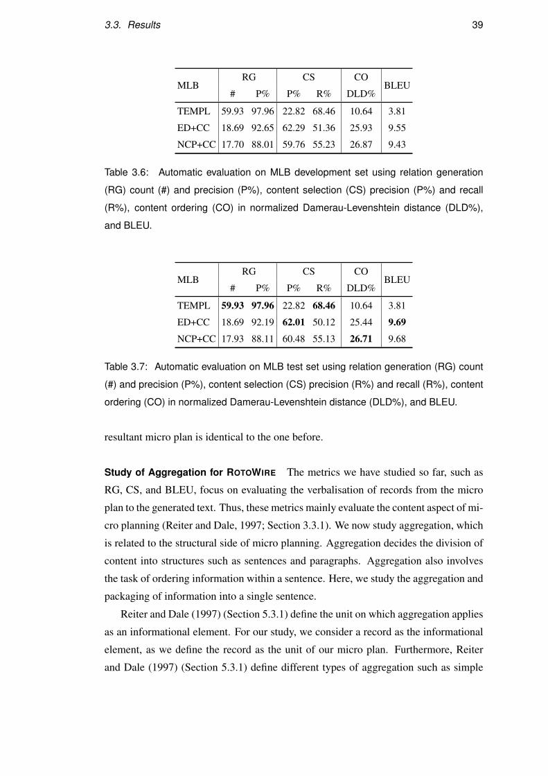
3.3. Results 39
MLBRG CS CO
BLEU# P% P% R% DLD%
TEMPL 59.93 97.96 22.82 68.46 10.64 3.81
ED+CC 18.69 92.65 62.29 51.36 25.93 9.55
NCP+CC 17.70 88.01 59.76 55.23 26.87 9.43
Table 3.6: Automatic evaluation on MLB development set using relation generation
(RG) count (#) and precision (P%), content selection (CS) precision (P%) and recall
(R%), content ordering (CO) in normalized Damerau-Levenshtein distance (DLD%),
and BLEU.
MLBRG CS CO
BLEU# P% P% R% DLD%
TEMPL 59.93 97.96 22.82 68.46 10.64 3.81
ED+CC 18.69 92.19 62.01 50.12 25.44 9.69
NCP+CC 17.93 88.11 60.48 55.13 26.71 9.68
Table 3.7: Automatic evaluation on MLB test set using relation generation (RG) count
(#) and precision (P%), content selection (CS) precision (R%) and recall (R%), content
ordering (CO) in normalized Damerau-Levenshtein distance (DLD%), and BLEU.
resultant micro plan is identical to the one before.
Study of Aggregation for ROTOWIRE The metrics we have studied so far, such as
RG, CS, and BLEU, focus on evaluating the verbalisation of records from the micro
plan to the generated text. Thus, these metrics mainly evaluate the content aspect of mi-
cro planning (Reiter and Dale, 1997; Section 3.3.1). We now study aggregation, which
is related to the structural side of micro planning. Aggregation decides the division of
content into structures such as sentences and paragraphs. Aggregation also involves
the task of ordering information within a sentence. Here, we study the aggregation and
packaging of information into a single sentence.
Reiter and Dale (1997) (Section 5.3.1) define the unit on which aggregation applies
as an informational element. For our study, we consider a record as the informational
element, as we define the record as the unit of our micro plan. Furthermore, Reiter
and Dale (1997) (Section 5.3.1) define different types of aggregation such as simple
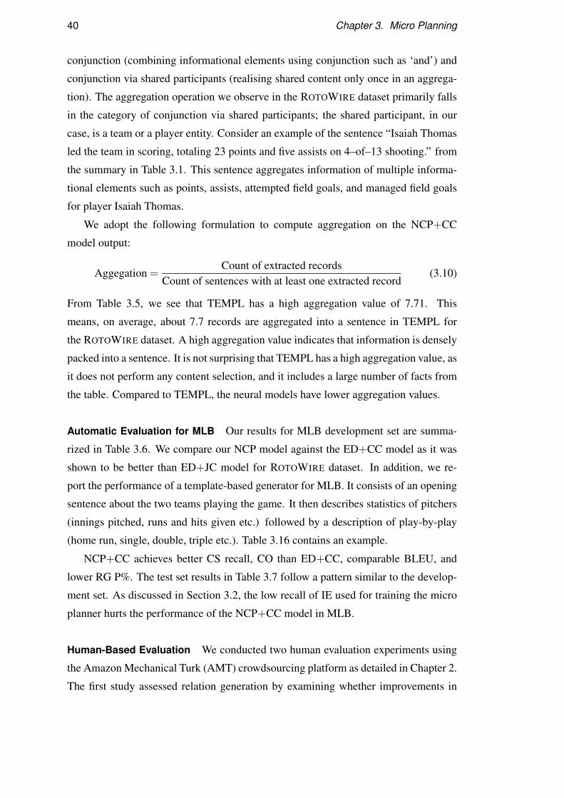
40 Chapter 3. Micro Planning
conjunction (combining informational elements using conjunction such as ‘and’) and
conjunction via shared participants (realising shared content only once in an aggrega-
tion). The aggregation operation we observe in the ROTOWIRE dataset primarily falls
in the category of conjunction via shared participants; the shared participant, in our
case, is a team or a player entity. Consider an example of the sentence “Isaiah Thomas
led the team in scoring, totaling 23 points and five assists on 4–of–13 shooting.” from
the summary in Table 3.1. This sentence aggregates information of multiple informa-
tional elements such as points, assists, attempted field goals, and managed field goals
for player Isaiah Thomas.
We adopt the following formulation to compute aggregation on the NCP+CC
model output:
Aggegation =Count of extracted records
Count of sentences with at least one extracted record(3.10)
From Table 3.5, we see that TEMPL has a high aggregation value of 7.71. This
means, on average, about 7.7 records are aggregated into a sentence in TEMPL for
the ROTOWIRE dataset. A high aggregation value indicates that information is densely
packed into a sentence. It is not surprising that TEMPL has a high aggregation value, as
it does not perform any content selection, and it includes a large number of facts from
the table. Compared to TEMPL, the neural models have lower aggregation values.
Automatic Evaluation for MLB Our results for MLB development set are summa-
rized in Table 3.6. We compare our NCP model against the ED+CC model as it was
shown to be better than ED+JC model for ROTOWIRE dataset. In addition, we re-
port the performance of a template-based generator for MLB. It consists of an opening
sentence about the two teams playing the game. It then describes statistics of pitchers
(innings pitched, runs and hits given etc.) followed by a description of play-by-play
(home run, single, double, triple etc.). Table 3.16 contains an example.
NCP+CC achieves better CS recall, CO than ED+CC, comparable BLEU, and
lower RG P%. The test set results in Table 3.7 follow a pattern similar to the develop-
ment set. As discussed in Section 3.2, the low recall of IE used for training the micro
planner hurts the performance of the NCP+CC model in MLB.
Human-Based Evaluation We conducted two human evaluation experiments using
the Amazon Mechanical Turk (AMT) crowdsourcing platform as detailed in Chapter 2.
The first study assessed relation generation by examining whether improvements in
3.3. Results 41
relation generation attested by automatic evaluation metrics are indeed corroborated
by human judgments. We did not require crowdworkers to be familiar with NBA
or MLB. Instead, we provided a cheat sheet explaining the semantics of box score
tables. In addition, we provided examples of sentences with supported/ contradicting
facts. For ROTOWIRE, we compared our best performing model (NCP+CC), with
gold reference summaries (Gold), a template system (TEMPL) and the best model of
Wiseman et al. (2017) (WS-2017). For MLB, we compared NCP+CC with ED+CC,
Gold, and TEMPL. AMT workers were asked to identify supporting and contradicting
facts mentioned in each sentence. We randomly selected 30 games from the test set.
Each sentence was rated by three workers. Altogether 49 crowdworkers participated
in this study.
The left two columns in Table 3.8 contain the average number of supporting and
contradicting facts per sentence as determined by the crowdworkers, for each model.
The template-based system has the highest number of supporting facts, even com-
pared to the human gold standard. TEMPL does not perform any content selection,
it includes a large number of facts from the database and since it does not perform
any generation either, it exhibits a few contradictions. On ROTOWIRE, compared to
WS-2017 and the Gold summaries, NCP+CC displays a larger number of supporting
facts. All models are significantly3 different in the number of supporting facts (#Supp)
from TEMPL (using a one-way ANOVA with post-hoc Tukey HSD tests). NCP+CC
is significantly different from WS-2017 and Gold. With respect to contradicting facts
(#Cont), Gold and TEMPL are not significantly different from each other but are sig-
nificantly different from the neural systems (WS-2017, NCP+CC). On MLB, NCP+CC
yields a number of supporting facts comparable to Gold, but significantly lower than
ED+CC and TEMPL. Contradicting facts are significantly higher for NCP+CC com-
pared to ED+CC, TEMPL and Gold.
In the second experiment, we assessed the generation quality of our model. For
this task, we required that the crowdworkers be able to comfortably comprehend NBA/
MLB game summaries. We elicited judgments for the same 30 games used in the first
study. For each game, participants were asked to compare summaries from the candi-
date systems. We arranged every 4-tuple of competing summaries into 6 pairs. Every
pair was shown to three crowdworkers, who were asked to decide which summary
was best and which one was worst according to three three criteria: Grammaticality,
Coherence, and Conciseness. Altogether 46 crowdworkers participated in this study.
3Using a one-way ANOVA with post-hoc Tukey HSD; p≤ 0.05.
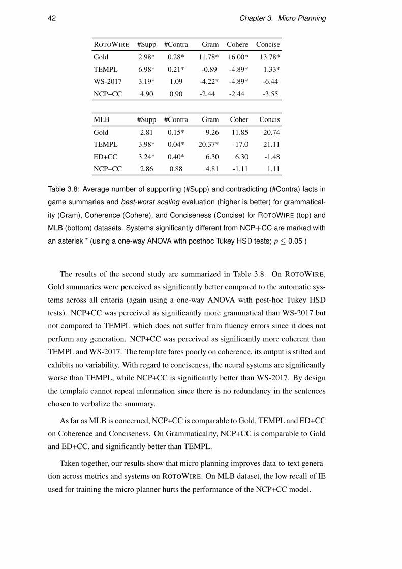
42 Chapter 3. Micro Planning
ROTOWIRE #Supp #Contra Gram Cohere Concise
Gold 2.98* 0.28* 11.78* 16.00* 13.78*
TEMPL 6.98* 0.21* -0.89 -4.89* 1.33*
WS-2017 3.19* 1.09 -4.22* -4.89* -6.44
NCP+CC 4.90 0.90 -2.44 -2.44 -3.55
MLB #Supp #Contra Gram Coher Concis
Gold 2.81 0.15* 9.26 11.85 -20.74
TEMPL 3.98* 0.04* -20.37* -17.0 21.11
ED+CC 3.24* 0.40* 6.30 6.30 -1.48
NCP+CC 2.86 0.88 4.81 -1.11 1.11
Table 3.8: Average number of supporting (#Supp) and contradicting (#Contra) facts in
game summaries and best-worst scaling evaluation (higher is better) for grammatical-
ity (Gram), Coherence (Cohere), and Conciseness (Concise) for ROTOWIRE (top) and
MLB (bottom) datasets. Systems significantly different from NCP+CC are marked with
an asterisk * (using a one-way ANOVA with posthoc Tukey HSD tests; p≤ 0.05 )
The results of the second study are summarized in Table 3.8. On ROTOWIRE,
Gold summaries were perceived as significantly better compared to the automatic sys-
tems across all criteria (again using a one-way ANOVA with post-hoc Tukey HSD
tests). NCP+CC was perceived as significantly more grammatical than WS-2017 but
not compared to TEMPL which does not suffer from fluency errors since it does not
perform any generation. NCP+CC was perceived as significantly more coherent than
TEMPL and WS-2017. The template fares poorly on coherence, its output is stilted and
exhibits no variability. With regard to conciseness, the neural systems are significantly
worse than TEMPL, while NCP+CC is significantly better than WS-2017. By design
the template cannot repeat information since there is no redundancy in the sentences
chosen to verbalize the summary.
As far as MLB is concerned, NCP+CC is comparable to Gold, TEMPL and ED+CC
on Coherence and Conciseness. On Grammaticality, NCP+CC is comparable to Gold
and ED+CC, and significantly better than TEMPL.
Taken together, our results show that micro planning improves data-to-text genera-
tion across metrics and systems on ROTOWIRE. On MLB dataset, the low recall of IE
used for training the micro planner hurts the performance of the NCP+CC model.
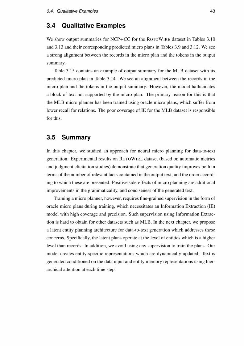
3.4. Qualitative Examples 43
3.4 Qualitative Examples
We show output summaries for NCP+CC for the ROTOWIRE dataset in Tables 3.10
and 3.13 and their corresponding predicted micro plans in Tables 3.9 and 3.12. We see
a strong alignment between the records in the micro plan and the tokens in the output
summary.
Table 3.15 contains an example of output summary for the MLB dataset with its
predicted micro plan in Table 3.14. We see an alignment between the records in the
micro plan and the tokens in the output summary. However, the model hallucinates
a block of text not supported by the micro plan. The primary reason for this is that
the MLB micro planner has been trained using oracle micro plans, which suffer from
lower recall for relations. The poor coverage of IE for the MLB dataset is responsible
for this.
3.5 Summary
In this chapter, we studied an approach for neural micro planning for data-to-text
generation. Experimental results on ROTOWIRE dataset (based on automatic metrics
and judgment elicitation studies) demonstrate that generation quality improves both in
terms of the number of relevant facts contained in the output text, and the order accord-
ing to which these are presented. Positive side-effects of micro planning are additional
improvements in the grammaticality, and conciseness of the generated text.
Training a micro planner, however, requires fine-grained supervision in the form of
oracle micro plans during training, which necessitates an Information Extraction (IE)
model with high coverage and precision. Such supervision using Information Extrac-
tion is hard to obtain for other datasets such as MLB. In the next chapter, we propose
a latent entity planning architecture for data-to-text generation which addresses these
concerns. Specifically, the latent plans operate at the level of entities which is a higher
level than records. In addition, we avoid using any supervision to train the plans. Our
model creates entity-specific representations which are dynamically updated. Text is
generated conditioned on the data input and entity memory representations using hier-
archical attention at each time step.
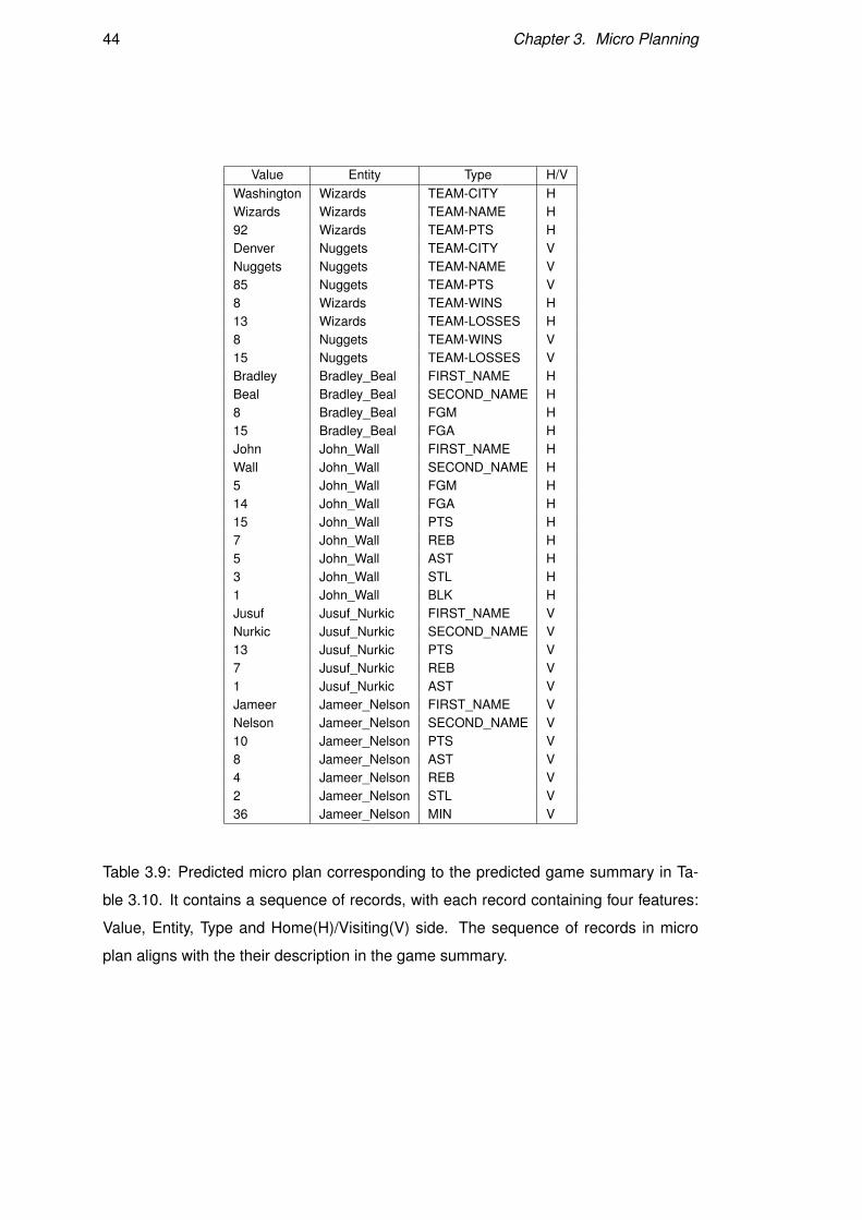
44 Chapter 3. Micro Planning
Value Entity Type H/VWashington Wizards TEAM-CITY HWizards Wizards TEAM-NAME H92 Wizards TEAM-PTS HDenver Nuggets TEAM-CITY VNuggets Nuggets TEAM-NAME V85 Nuggets TEAM-PTS V8 Wizards TEAM-WINS H13 Wizards TEAM-LOSSES H8 Nuggets TEAM-WINS V15 Nuggets TEAM-LOSSES VBradley Bradley_Beal FIRST_NAME HBeal Bradley_Beal SECOND_NAME H8 Bradley_Beal FGM H15 Bradley_Beal FGA HJohn John_Wall FIRST_NAME HWall John_Wall SECOND_NAME H5 John_Wall FGM H14 John_Wall FGA H15 John_Wall PTS H7 John_Wall REB H5 John_Wall AST H3 John_Wall STL H1 John_Wall BLK HJusuf Jusuf_Nurkic FIRST_NAME VNurkic Jusuf_Nurkic SECOND_NAME V13 Jusuf_Nurkic PTS V7 Jusuf_Nurkic REB V1 Jusuf_Nurkic AST VJameer Jameer_Nelson FIRST_NAME VNelson Jameer_Nelson SECOND_NAME V10 Jameer_Nelson PTS V8 Jameer_Nelson AST V4 Jameer_Nelson REB V2 Jameer_Nelson STL V36 Jameer_Nelson MIN V
Table 3.9: Predicted micro plan corresponding to the predicted game summary in Ta-
ble 3.10. It contains a sequence of records, with each record containing four features:
Value, Entity, Type and Home(H)/Visiting(V) side. The sequence of records in micro
plan aligns with the their description in the game summary.

3.5. Summary 45
The Washington Wizards defeated the visiting Denver Nuggets 92-85 at Verizon Center on Monday.
The Wizards (8-13) came into this game winners of five of their last eight games, but the Wizards (8-15)
jumped out to a 10-point lead at the end of the first quarter. Bradley Beal led the way for the Wizards
with a game-high 26 points on 8-of-15 shooting from the field. John Wall shot 5-of-14 from the field
on his way to 15 points, to go along with seven rebounds, five assists, three steals and one block. JusufNurkic chipped in 13 points, seven rebounds and one assist. Jameer Nelson filled out the stat sheet
with 10 points, eight assists, four rebounds and two steals in 36 minutes. As a team, it was a forgettable
shooting night for the Nuggets, as the team shot just 46 percent from the field. Next up, the Nuggets
play the second game of a back-to-back when they host the Denver Nuggets on Wednesday, while the
Wizards host the Portland Trail Blazers on Friday.
Table 3.10: NCP+CC model output for ROTOWIRE corresponding to the micro plan in
Table 3.9. The tokens in summary corresponding to the records in the micro plan are
bold faced. We see a strong alignment between the records in micro plan and the game
summary in the model output. In addition, the model output exhibits coherent ordering
of facts.
The Washington Wizards (8-13) defeated the Denver Nuggets (8-15) 92-85. Bradley Beal scored 26
points (8-15 FG, 4-7 3PT, 6-6 FT) to go with 3 rebounds. Nikola Jokic scored 17 points (6-10 FG, 0-0
3PT, 5-7 FT) to go with 11 rebounds. Markieff Morris scored 15 points (5-12 FG, 0-0 3PT, 5-5 FT) to go
with 3 rebounds. John Wall scored 15 points (5-14 FG, 0-4 3PT, 5-6 FT) to go with 7 rebounds. Danilo
Gallinari scored 14 points (3-11 FG, 1-8 3PT, 7-9 FT) to go with 4 rebounds. Jusuf Nurkic scored 13
points (6-6 FG, 0-0 3PT, 1-2 FT) to go with 7 rebounds. The Washington Wizards’ next game will be at
home against the Dallas Mavericks, while the Denver Nuggets will travel to play the Bulls.
Table 3.11: Example of template model output corresponding to the example in Table
3.10. We see that the template output is stilted and exhibits no variability.
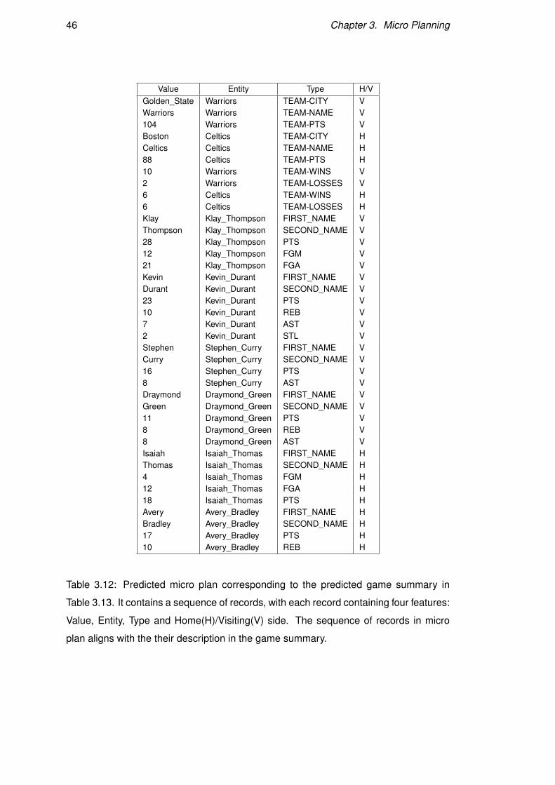
46 Chapter 3. Micro Planning
Value Entity Type H/VGolden_State Warriors TEAM-CITY VWarriors Warriors TEAM-NAME V104 Warriors TEAM-PTS VBoston Celtics TEAM-CITY HCeltics Celtics TEAM-NAME H88 Celtics TEAM-PTS H10 Warriors TEAM-WINS V2 Warriors TEAM-LOSSES V6 Celtics TEAM-WINS H6 Celtics TEAM-LOSSES HKlay Klay_Thompson FIRST_NAME VThompson Klay_Thompson SECOND_NAME V28 Klay_Thompson PTS V12 Klay_Thompson FGM V21 Klay_Thompson FGA VKevin Kevin_Durant FIRST_NAME VDurant Kevin_Durant SECOND_NAME V23 Kevin_Durant PTS V10 Kevin_Durant REB V7 Kevin_Durant AST V2 Kevin_Durant STL VStephen Stephen_Curry FIRST_NAME VCurry Stephen_Curry SECOND_NAME V16 Stephen_Curry PTS V8 Stephen_Curry AST VDraymond Draymond_Green FIRST_NAME VGreen Draymond_Green SECOND_NAME V11 Draymond_Green PTS V8 Draymond_Green REB V8 Draymond_Green AST VIsaiah Isaiah_Thomas FIRST_NAME HThomas Isaiah_Thomas SECOND_NAME H4 Isaiah_Thomas FGM H12 Isaiah_Thomas FGA H18 Isaiah_Thomas PTS HAvery Avery_Bradley FIRST_NAME HBradley Avery_Bradley SECOND_NAME H17 Avery_Bradley PTS H10 Avery_Bradley REB H
Table 3.12: Predicted micro plan corresponding to the predicted game summary in
Table 3.13. It contains a sequence of records, with each record containing four features:
Value, Entity, Type and Home(H)/Visiting(V) side. The sequence of records in micro
plan aligns with the their description in the game summary.
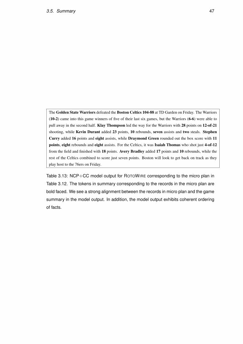
3.5. Summary 47
The Golden State Warriors defeated the Boston Celtics 104-88 at TD Garden on Friday. The Warriors
(10-2) came into this game winners of five of their last six games, but the Warriors (6-6) were able to
pull away in the second half. Klay Thompson led the way for the Warriors with 28 points on 12-of-21shooting, while Kevin Durant added 23 points, 10 rebounds, seven assists and two steals. StephenCurry added 16 points and eight assists, while Draymond Green rounded out the box score with 11points, eight rebounds and eight assists. For the Celtics, it was Isaiah Thomas who shot just 4-of-12from the field and finished with 18 points. Avery Bradley added 17 points and 10 rebounds, while the
rest of the Celtics combined to score just seven points. Boston will look to get back on track as they
play host to the 76ers on Friday.
Table 3.13: NCP+CC model output for ROTOWIRE corresponding to the micro plan in
Table 3.12. The tokens in summary corresponding to the records in the micro plan are
bold faced. We see a strong alignment between the records in micro plan and the game
summary in the model output. In addition, the model output exhibits coherent ordering
of facts.
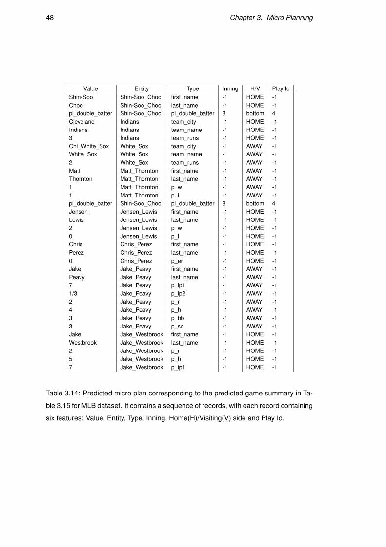
48 Chapter 3. Micro Planning
Value Entity Type Inning H/V Play IdShin-Soo Shin-Soo_Choo first_name -1 HOME -1Choo Shin-Soo_Choo last_name -1 HOME -1pl_double_batter Shin-Soo_Choo pl_double_batter 8 bottom 4Cleveland Indians team_city -1 HOME -1Indians Indians team_name -1 HOME -13 Indians team_runs -1 HOME -1Chi_White_Sox White_Sox team_city -1 AWAY -1White_Sox White_Sox team_name -1 AWAY -12 White_Sox team_runs -1 AWAY -1Matt Matt_Thornton first_name -1 AWAY -1Thornton Matt_Thornton last_name -1 AWAY -11 Matt_Thornton p_w -1 AWAY -11 Matt_Thornton p_l -1 AWAY -1pl_double_batter Shin-Soo_Choo pl_double_batter 8 bottom 4Jensen Jensen_Lewis first_name -1 HOME -1Lewis Jensen_Lewis last_name -1 HOME -12 Jensen_Lewis p_w -1 HOME -10 Jensen_Lewis p_l -1 HOME -1Chris Chris_Perez first_name -1 HOME -1Perez Chris_Perez last_name -1 HOME -10 Chris_Perez p_er -1 HOME -1Jake Jake_Peavy first_name -1 AWAY -1Peavy Jake_Peavy last_name -1 AWAY -17 Jake_Peavy p_ip1 -1 AWAY -11/3 Jake_Peavy p_ip2 -1 AWAY -12 Jake_Peavy p_r -1 AWAY -14 Jake_Peavy p_h -1 AWAY -13 Jake_Peavy p_bb -1 AWAY -13 Jake_Peavy p_so -1 AWAY -1Jake Jake_Westbrook first_name -1 HOME -1Westbrook Jake_Westbrook last_name -1 HOME -12 Jake_Westbrook p_r -1 HOME -15 Jake_Westbrook p_h -1 HOME -17 Jake_Westbrook p_ip1 -1 HOME -1
Table 3.14: Predicted micro plan corresponding to the predicted game summary in Ta-
ble 3.15 for MLB dataset. It contains a sequence of records, with each record containing
six features: Value, Entity, Type, Inning, Home(H)/Visiting(V) side and Play Id.
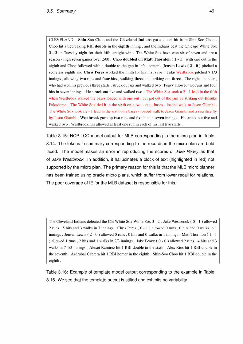
3.5. Summary 49
CLEVELAND – Shin-Soo Choo and the Cleveland Indians got a clutch hit from Shin-Soo Choo .
Choo hit a tiebreaking RBI double in the eighth inning , and the Indians beat the Chicago White Sox
3 - 2 on Tuesday night for their fifth straight win . The White Sox have won six of seven and are a
season - high seven games over .500 . Choo doubled off Matt Thornton ( 1 - 1 ) with one out in the
eighth and Choo followed with a double to the gap in left - center . Jensen Lewis ( 2 - 0 ) pitched a
scoreless eighth and Chris Perez worked the ninth for his first save . Jake Westbrook pitched 7 1/3innings , allowing two runs and four hits , walking three and striking out three . The right - hander ,
who had won his previous three starts , struck out six and walked two . Peavy allowed two runs and four
hits in seven innings . He struck out five and walked two . The White Sox took a 2 - 1 lead in the fifth
when Westbrook walked the bases loaded with one out , but got out of the jam by striking out Kosuke
Fukudome . The White Sox tied it in the sixth on a two - out , bases - loaded walk to Jason Giambi .
The White Sox took a 2 - 1 lead in the sixth on a bases - loaded walk to Jason Giambi and a sacrifice fly
by Jason Giambi . Westbrook gave up two runs and five hits in seven innings . He struck out five and
walked two . Westbrook has allowed at least one run in each of his last five starts .
Table 3.15: NCP+CC model output for MLB corresponding to the micro plan in Table
3.14. The tokens in summary corresponding to the records in the micro plan are bold
faced. The model makes an error in reproducing the scores of Jake Peavy as that
of Jake Westbrook. In addition, it hallucinates a block of text (highlighted in red) not
supported by the micro plan. The primary reason for this is that the MLB micro planner
has been trained using oracle micro plans, which suffer from lower recall for relations.
The poor coverage of IE for the MLB dataset is responsible for this.
The Cleveland Indians defeated the Chi White Sox White Sox 3 - 2 . Jake Westbrook ( 0 - 1 ) allowed
2 runs , 5 hits and 3 walks in 7 innings . Chris Perez ( 0 - 1 ) allowed 0 runs , 0 hits and 0 walks in 1
innings . Jensen Lewis ( 2 - 0 ) allowed 0 runs , 0 hits and 0 walks in 1 innings . Matt Thornton ( 1 - 1
) allowed 1 runs , 2 hits and 1 walks in 2/3 innings . Jake Peavy ( 0 - 0 ) allowed 2 runs , 4 hits and 3
walks in 7 1/3 innings . Alexei Ramirez hit 1 RBI double in the sixth . Alex Rios hit 1 RBI double in
the seventh . Asdrubal Cabrera hit 1 RBI homer in the eighth . Shin-Soo Choo hit 1 RBI double in the
eighth .
Table 3.16: Example of template model output corresponding to the example in Table
3.15. We see that the template output is stilted and exhibits no variability.

Chapter 4
Latent Entity Planning
In the previous chapter, we looked into how micro planning can be applied for data-to-
text generation. Given a table as input, micro planning predicts a sequence of records
which is utilised by the text generation module to create the game summary. Micro
planning, however, requires fine-grained record level supervision for training. It as-
sumes or requires the availability of a highly precise and broad coverage Information
Extraction tool. Such supervision may be difficult to obtain for some datasets or do-
mains. In this chapter, we explore how we can perform data-to-text generation by
inducing latent plans which operate at a higher level than records, such as entities.
4.1 Motivation
Figure 4.1 is an example from the MLB dataset containing statistics related to the game
and its summary. We are interested in the generation of descriptive texts such as the
game summary. Descriptive texts are often characterized as “entity coherent” which
means that their coherence is based on the way entities (also known as domain objects
or concepts) are introduced and discussed in the discourse (Karamanis et al., 2004).
Without knowing anything about baseball or how game summaries are typically writ-
ten, a glance at the text in Figure 4.1 reveals that it is about a few entities, namely
players who had an important part in the game (e.g., Brad Keller, Hunter Dozier) and
their respective teams (e.g., Orioles, Royals). The prominent role of entities in achiev-
ing discourse coherence has been long recognized within the linguistic and cognitive
science literature (Kuno, 1972; Chafe, 1976; Halliday and Hasan, 1976; Karttunen,
1976; Clark and Haviland, 1977; Prince, 1981), with Centering Theory (Grosz et al.,
1995) being most prominent at formalizing how entities are linguistically realized and
51
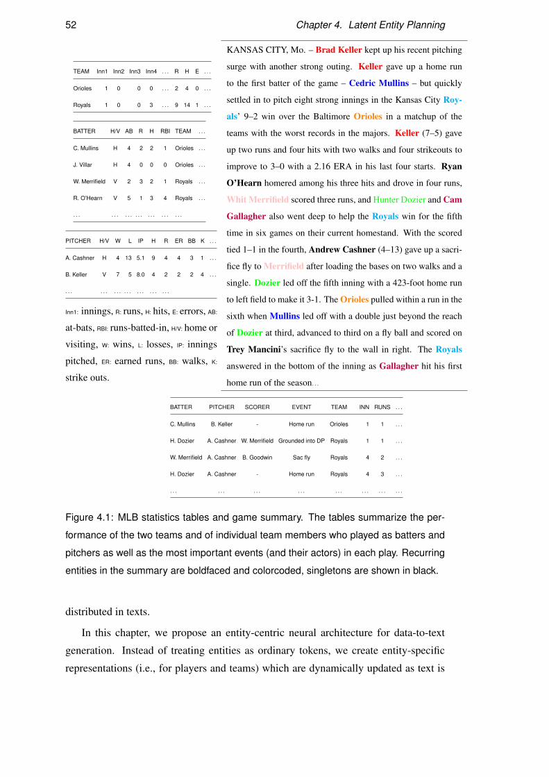
52 Chapter 4. Latent Entity Planning
TEAM Inn1 Inn2 Inn3 Inn4 . . . R H E . . .
Orioles 1 0 0 0 . . . 2 4 0 . . .
Royals 1 0 0 3 . . . 9 14 1 . . .
BATTER H/V AB R H RBI TEAM . . .
C. Mullins H 4 2 2 1 Orioles . . .
J. Villar H 4 0 0 0 Orioles . . .
W. Merrifield V 2 3 2 1 Royals . . .
R. O’Hearn V 5 1 3 4 Royals . . .
. . . . . . . . . . . . . . . . . . . . .
PITCHER H/V W L IP H R ER BB K . . .
A. Cashner H 4 13 5.1 9 4 4 3 1 . . .
B. Keller V 7 5 8.0 4 2 2 2 4 . . .
. . . . . . . . . . . . . . . . . . . . .
Inn1: innings, R: runs, H: hits, E: errors, AB:
at-bats, RBI: runs-batted-in, H/V: home or
visiting, W: wins, L: losses, IP: innings
pitched, ER: earned runs, BB: walks, K:
strike outs.
KANSAS CITY, Mo. – Brad Keller kept up his recent pitching
surge with another strong outing. Keller gave up a home run
to the first batter of the game – Cedric Mullins – but quickly
settled in to pitch eight strong innings in the Kansas City Roy-
als’ 9–2 win over the Baltimore Orioles in a matchup of the
teams with the worst records in the majors. Keller (7–5) gave
up two runs and four hits with two walks and four strikeouts to
improve to 3–0 with a 2.16 ERA in his last four starts. Ryan
O’Hearn homered among his three hits and drove in four runs,
Whit Merrifield scored three runs, and Hunter Dozier and Cam
Gallagher also went deep to help the Royals win for the fifth
time in six games on their current homestand. With the scored
tied 1–1 in the fourth, Andrew Cashner (4–13) gave up a sacri-
fice fly to Merrifield after loading the bases on two walks and a
single. Dozier led off the fifth inning with a 423-foot home run
to left field to make it 3-1. The Orioles pulled within a run in the
sixth when Mullins led off with a double just beyond the reach
of Dozier at third, advanced to third on a fly ball and scored on
Trey Mancini’s sacrifice fly to the wall in right. The Royals
answered in the bottom of the inning as Gallagher hit his first
home run of the season. . .
BATTER PITCHER SCORER EVENT TEAM INN RUNS . . .
C. Mullins B. Keller - Home run Orioles 1 1 . . .
H. Dozier A. Cashner W. Merrifield Grounded into DP Royals 1 1 . . .
W. Merrifield A. Cashner B. Goodwin Sac fly Royals 4 2 . . .
H. Dozier A. Cashner - Home run Royals 4 3 . . .
. . . . . . . . . . . . . . . . . . . . . . . .
Figure 4.1: MLB statistics tables and game summary. The tables summarize the per-
formance of the two teams and of individual team members who played as batters and
pitchers as well as the most important events (and their actors) in each play. Recurring
entities in the summary are boldfaced and colorcoded, singletons are shown in black.
distributed in texts.
In this chapter, we propose an entity-centric neural architecture for data-to-text
generation. Instead of treating entities as ordinary tokens, we create entity-specific
representations (i.e., for players and teams) which are dynamically updated as text is
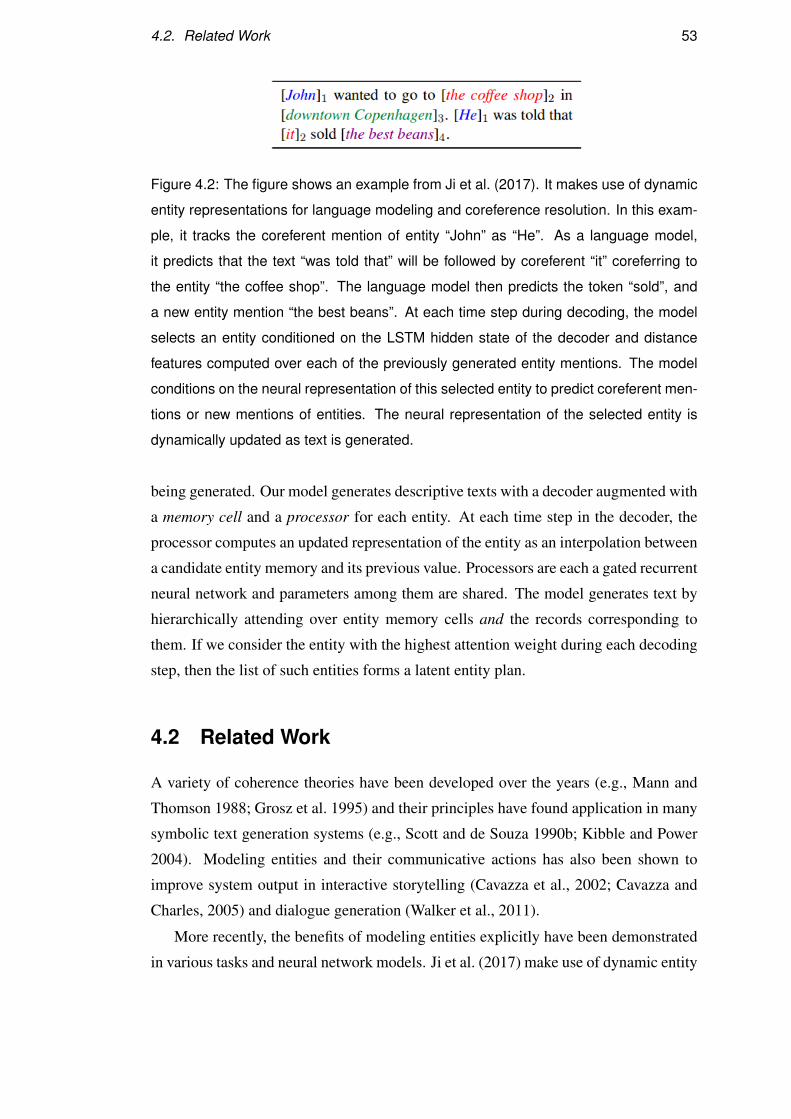
4.2. Related Work 53
Figure 4.2: The figure shows an example from Ji et al. (2017). It makes use of dynamic
entity representations for language modeling and coreference resolution. In this exam-
ple, it tracks the coreferent mention of entity “John” as “He”. As a language model,
it predicts that the text “was told that” will be followed by coreferent “it” coreferring to
the entity “the coffee shop”. The language model then predicts the token “sold”, and
a new entity mention “the best beans”. At each time step during decoding, the model
selects an entity conditioned on the LSTM hidden state of the decoder and distance
features computed over each of the previously generated entity mentions. The model
conditions on the neural representation of this selected entity to predict coreferent men-
tions or new mentions of entities. The neural representation of the selected entity is
dynamically updated as text is generated.
being generated. Our model generates descriptive texts with a decoder augmented with
a memory cell and a processor for each entity. At each time step in the decoder, the
processor computes an updated representation of the entity as an interpolation between
a candidate entity memory and its previous value. Processors are each a gated recurrent
neural network and parameters among them are shared. The model generates text by
hierarchically attending over entity memory cells and the records corresponding to
them. If we consider the entity with the highest attention weight during each decoding
step, then the list of such entities forms a latent entity plan.
4.2 Related Work
A variety of coherence theories have been developed over the years (e.g., Mann and
Thomson 1988; Grosz et al. 1995) and their principles have found application in many
symbolic text generation systems (e.g., Scott and de Souza 1990b; Kibble and Power
2004). Modeling entities and their communicative actions has also been shown to
improve system output in interactive storytelling (Cavazza et al., 2002; Cavazza and
Charles, 2005) and dialogue generation (Walker et al., 2011).
More recently, the benefits of modeling entities explicitly have been demonstrated
in various tasks and neural network models. Ji et al. (2017) make use of dynamic entity
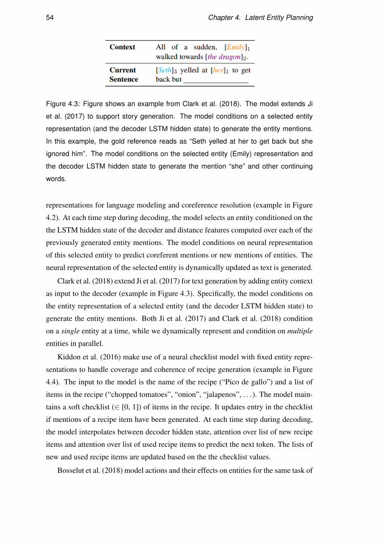
54 Chapter 4. Latent Entity Planning
Figure 4.3: Figure shows an example from Clark et al. (2018). The model extends Ji
et al. (2017) to support story generation. The model conditions on a selected entity
representation (and the decoder LSTM hidden state) to generate the entity mentions.
In this example, the gold reference reads as “Seth yelled at her to get back but she
ignored him”. The model conditions on the selected entity (Emily) representation and
the decoder LSTM hidden state to generate the mention “she” and other continuing
words.
representations for language modeling and coreference resolution (example in Figure
4.2). At each time step during decoding, the model selects an entity conditioned on the
the LSTM hidden state of the decoder and distance features computed over each of the
previously generated entity mentions. The model conditions on neural representation
of this selected entity to predict coreferent mentions or new mentions of entities. The
neural representation of the selected entity is dynamically updated as text is generated.
Clark et al. (2018) extend Ji et al. (2017) for text generation by adding entity context
as input to the decoder (example in Figure 4.3). Specifically, the model conditions on
the entity representation of a selected entity (and the decoder LSTM hidden state) to
generate the entity mentions. Both Ji et al. (2017) and Clark et al. (2018) condition
on a single entity at a time, while we dynamically represent and condition on multiple
entities in parallel.
Kiddon et al. (2016) make use of a neural checklist model with fixed entity repre-
sentations to handle coverage and coherence of recipe generation (example in Figure
4.4). The input to the model is the name of the recipe (“Pico de gallo”) and a list of
items in the recipe (“chopped tomatoes”, “onion”, “jalapenos”, . . . ). The model main-
tains a soft checklist (∈ [0, 1]) of items in the recipe. It updates entry in the checklist
if mentions of a recipe item have been generated. At each time step during decoding,
the model interpolates between decoder hidden state, attention over list of new recipe
items and attention over list of used recipe items to predict the next token. The lists of
new and used recipe items are updated based on the the checklist values.
Bosselut et al. (2018) model actions and their effects on entities for the same task of
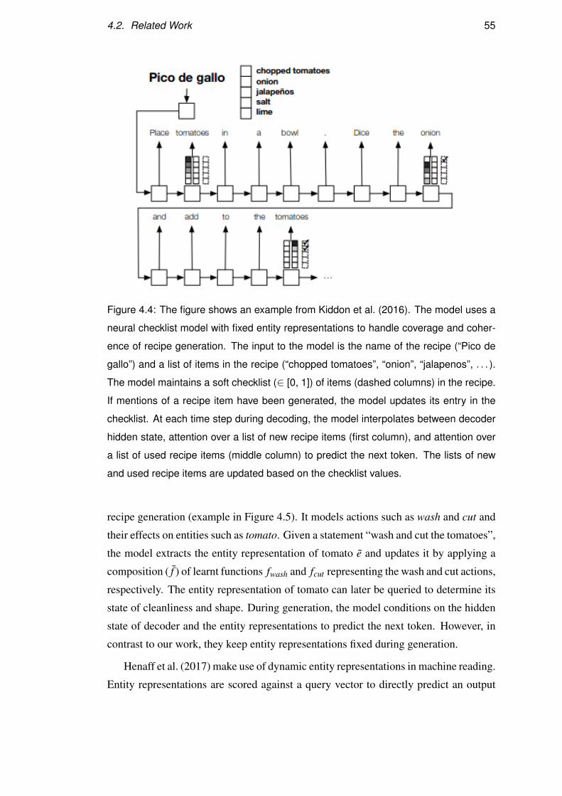
4.2. Related Work 55
Figure 4.4: The figure shows an example from Kiddon et al. (2016). The model uses a
neural checklist model with fixed entity representations to handle coverage and coher-
ence of recipe generation. The input to the model is the name of the recipe (“Pico de
gallo”) and a list of items in the recipe (“chopped tomatoes”, “onion”, “jalapenos”, . . . ).
The model maintains a soft checklist (∈ [0, 1]) of items (dashed columns) in the recipe.
If mentions of a recipe item have been generated, the model updates its entry in the
checklist. At each time step during decoding, the model interpolates between decoder
hidden state, attention over a list of new recipe items (first column), and attention over
a list of used recipe items (middle column) to predict the next token. The lists of new
and used recipe items are updated based on the checklist values.
recipe generation (example in Figure 4.5). It models actions such as wash and cut and
their effects on entities such as tomato. Given a statement “wash and cut the tomatoes”,
the model extracts the entity representation of tomato e and updates it by applying a
composition ( f ) of learnt functions fwash and fcut representing the wash and cut actions,
respectively. The entity representation of tomato can later be queried to determine its
state of cleanliness and shape. During generation, the model conditions on the hidden
state of decoder and the entity representations to predict the next token. However, in
contrast to our work, they keep entity representations fixed during generation.
Henaff et al. (2017) make use of dynamic entity representations in machine reading.
Entity representations are scored against a query vector to directly predict an output
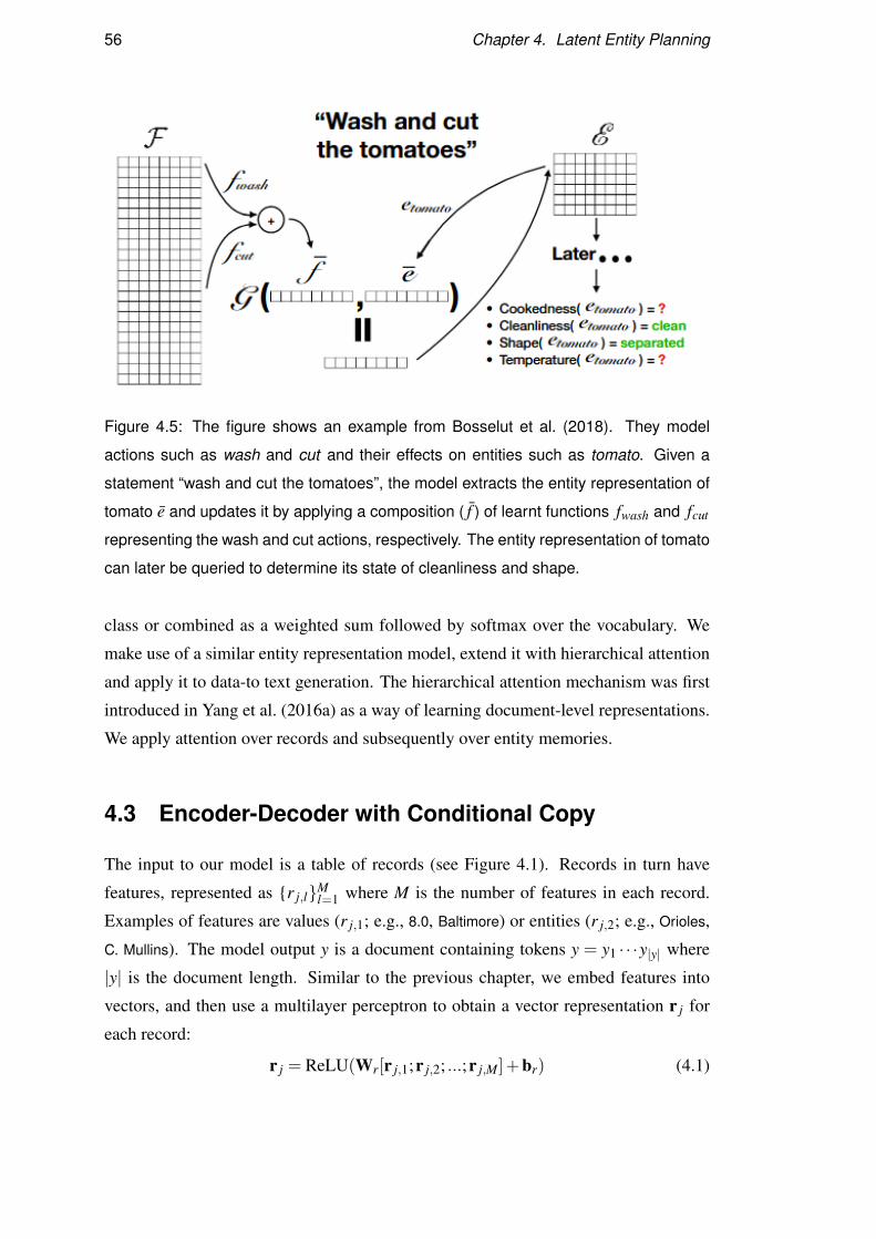
56 Chapter 4. Latent Entity Planning
Figure 4.5: The figure shows an example from Bosselut et al. (2018). They model
actions such as wash and cut and their effects on entities such as tomato. Given a
statement “wash and cut the tomatoes”, the model extracts the entity representation of
tomato e and updates it by applying a composition ( f ) of learnt functions fwash and fcut
representing the wash and cut actions, respectively. The entity representation of tomato
can later be queried to determine its state of cleanliness and shape.
class or combined as a weighted sum followed by softmax over the vocabulary. We
make use of a similar entity representation model, extend it with hierarchical attention
and apply it to data-to text generation. The hierarchical attention mechanism was first
introduced in Yang et al. (2016a) as a way of learning document-level representations.
We apply attention over records and subsequently over entity memories.
4.3 Encoder-Decoder with Conditional Copy
The input to our model is a table of records (see Figure 4.1). Records in turn have
features, represented as {r j,l}Ml=1 where M is the number of features in each record.
Examples of features are values (r j,1; e.g., 8.0, Baltimore) or entities (r j,2; e.g., Orioles,
C. Mullins). The model output y is a document containing tokens y = y1 · · ·y|y| where
|y| is the document length. Similar to the previous chapter, we embed features into
vectors, and then use a multilayer perceptron to obtain a vector representation r j for
each record:
r j = ReLU(Wr[r j,1;r j,2; ...;r j,M]+br) (4.1)
4.3. Encoder-Decoder with Conditional Copy 57
where [; ] indicates vector concatenation, Wr ∈ Rn×nM,br ∈ Rn are parameters, and
ReLU is the rectifier activation function.
Let {e j}|r|j=1 denote the output of the encoder. We use an LSTM decoder to compute
the probability of each target word, conditioned on previously generated words, and
on e j. In the case of ROTOWIRE, we follow previous work (Wiseman et al., 2017 and
Chapter 3) and consider e j = r j. The first hidden state of the decoder is initialized by
the average of the record vectors, avg({e j}|r|j=1).
In the case of MLB, information encoded in play-by-play is sequential. Recall,
that it documents the most important events in a game in chronological order. To
account for this, we encode MLB records into {e j}|r|j=1 with a Bidirectional LSTM. We
impose an ordering on records in the box score i.e., home team followed by away team,
followed by home team players and away team players, which is in turn followed by
play-by-play where records are naturally ordered by time. The decoder is initialized
with the concatenation of the hidden states of the final step of the encoder.
At time step t, the input to the decoder LSTM is the embedding of the previously
predicted word yt−1. Let dt denote the hidden state of the t-th LSTM unit. We compute
attention scores αt, j over the encoder output e j and obtain dynamic context vector qt
as the weighted sum of the hidden states of the input:
αt, j ∝ exp(dᵀt Wae j)
qt = ∑j
αt, je j
dattt = tanh(Wc[dt ;qt ]) (4.2)
where Wa ∈ Rn×n,∑ j αt, j = 1, Wc ∈ Rn×2n, and dattt is the attention vector.
The probability of output text y conditioned on the input table r is modeled as:
pgen(yt |y<t ,r)=softmaxyt(Wydattt +by) (4.3)
where Wy ∈ R|Vy|×n, by ∈ R|Vy| are parameters and |Vy| is the output vocabulary size.
As in Chapter 3, we further augment the decoder with a copy mechanism i.e., the
ability to copy values from the input; copy implies yt = r j,1 for some t and j (e.g.,
Royals, Orioles, 9, 2 in the summary in Figure 4.1 are copied from r). We use the
conditional copy method proposed in Gulcehre et al. (2016a) where a binary variable
is introduced as a switch gate to indicate whether yt is copied or not (Section 2.4.2 in
Chapter 2).
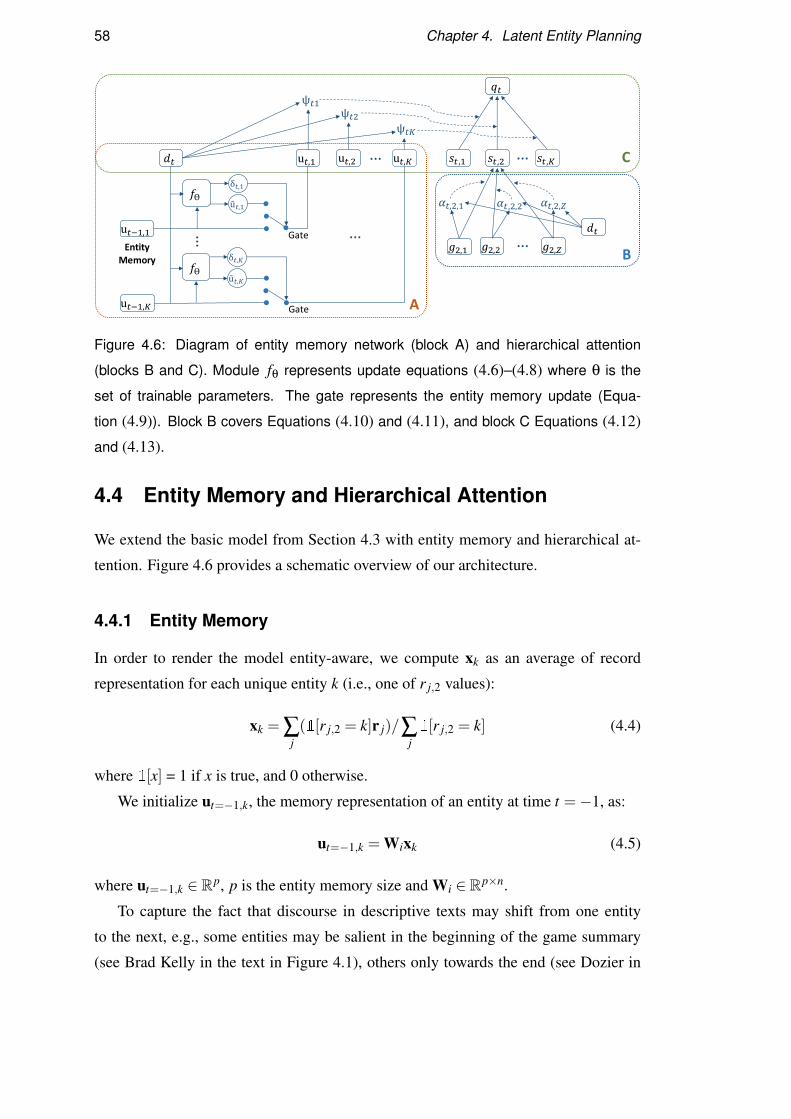
58 Chapter 4. Latent Entity Planning
Gate𝑔2,1 𝑔2,2 𝑔2,𝑍
𝑠𝑡,2
𝑑𝑡
𝛼𝑡,2,1 𝛼𝑡,2,2 𝛼𝑡,2,𝑍
𝑠𝑡,1 𝑠𝑡,𝐾
𝑞𝑡
u𝑡,1 u𝑡,2 u𝑡,𝐾𝑑𝑡
ψ𝑡1ψ𝑡2
ψ𝑡𝐾
𝑓ϴδ𝑡,1
ũ𝑡,1
Entity Memory
u𝑡−1,1
𝑓ϴδ𝑡,𝐾
ũ𝑡,𝐾
Gateu𝑡−1,𝐾 A
B
C…
…
…
…
…
Figure 4.6: Diagram of entity memory network (block A) and hierarchical attention
(blocks B and C). Module fθ represents update equations (4.6)–(4.8) where θ is the
set of trainable parameters. The gate represents the entity memory update (Equa-
tion (4.9)). Block B covers Equations (4.10) and (4.11), and block C Equations (4.12)
and (4.13).
4.4 Entity Memory and Hierarchical Attention
We extend the basic model from Section 4.3 with entity memory and hierarchical at-
tention. Figure 4.6 provides a schematic overview of our architecture.
4.4.1 Entity Memory
In order to render the model entity-aware, we compute xk as an average of record
representation for each unique entity k (i.e., one of r j,2 values):
xk = ∑j(1[r j,2 = k]r j)/∑
j1[r j,2 = k] (4.4)
where 1[x] = 1 if x is true, and 0 otherwise.
We initialize ut=−1,k, the memory representation of an entity at time t =−1, as:
ut=−1,k = Wixk (4.5)
where ut=−1,k ∈ Rp, p is the entity memory size and Wi ∈ Rp×n.
To capture the fact that discourse in descriptive texts may shift from one entity
to the next, e.g., some entities may be salient in the beginning of the game summary
(see Brad Kelly in the text in Figure 4.1), others only towards the end (see Dozier in
4.4. Entity Memory and Hierarchical Attention 59
Figure 4.1), and a few throughout (e.g., references to teams), we update entity repre-
sentations at each time step during decoding. We use gate γt to indicate whether there
should be an update in the entity representation:
γt = σ(Wddt +bd) (4.6)
where t >= 0, σ is the sigmoid function, Wd ∈ Rp×p, and bd ∈ Rp.
We also compute δt,k, the extent to which the entity representation should change,
and ut,k , the memory of the candidate entity:
δt,k =γt�σ(Wedt+be+W f ut−1,k+b f ) (4.7)
ut,k =Wgdt (4.8)
where � denotes element-wise multiplication, We,∈ Rp×n, W f ∈ Rp×p, be,b f ∈ Rp,
and γt ,δt,k ∈ [0,1]p (see block A in Figure 4.6).
An element in gate γt will have value approaching 1 if an update in any ut−1,k is
required. The value of an element in gate δt,k will approach 1 if the corresponding
value of the element in ut−1,k changes. Equation (4.9) computes the update in entity
memory as an interpolation over the gated representation of the previous value of the
entity memory and the candidate entity memory:
ut,k = (1−δt,k)�ut−1,k +δt,k� ut,k (4.9)
where ut,k represents entity k at time t.
Previous work (Henaff et al., 2017; Ji et al., 2017; Clark et al., 2018) employs a nor-
malization term over ut,k. We empirically found that normalization hurts performance
and hence did not include it in our model.
4.4.2 Hierarchical Attention
We hypothesize that our generator should first focus on entities (e.g., the main players
and their teams) and then on the records corresponding to theses entities (e.g, player
performance in the game). Our model implements this view of text generation via a
hierarchical attention mechanism which we explain below. We also expect that focus-
ing on entities first should improve the precision of the texts we generate as the entity
distribution will constrain the probability distribution of records corresponding to each
entity.
To better understand the hierarchical attention mechanism, we can view the encoder
output e j as a 2-dimensional array gk,z where k ∈ [1,K] represents entities and z ∈

60 Chapter 4. Latent Entity Planning
[1,Z] represents records of entities and there is a one-to-one correspondence between
positions j and k,z. We compute attention over gk,z, the encoder output, as:
αt,k,z ∝ exp(dᵀt Wagk,z) (4.10)
where Wa ∈ Rn×n, ∑z αt,k,z = 1 (see block B in Figure 4.6). We compute the entity
context as:
st,k = ∑z
αt,k,zgk,z (4.11)
while attention over entity vectors ut,k is:
Ψt,k ∝ exp(dᵀt Whut,k) (4.12)
with Wh ∈ Rn×p, ∑k Ψt,k = 1. And the encoder context qt (see block C in Figure 4.6)
is computed as follows:
qt = ∑k
Ψt,kst,k (4.13)
We feed qt into Equation (4.2) and compute pgen(yt |y<t ,r), the probability of generat-
ing output text y conditioned on records r, as shown in Equation (4.3).
We experimented with feeding ∑k Ψt,kut,k as input context along the lines of Clark
et al. (2018); however, results on the development dataset degraded performance, and
we did not pursue this approach further.
We note that in our decoder, we have a hierarchical attention over entity represen-
tations and the records corresponding to the entities. This attention over entity rep-
resentations constitutes a (latent) entity plan if we consider the mode of the attention
distributions.
4.5 Training and Inference
Our training objective maximizes the log likelihood of output text given an input table
of records:
max ∑(r,y)∈D
log p(y|r)
where D is the training set consisting of pairs of record tables and output game sum-
maries. During inference, we make use of beam search to approximately obtain the
best output y among candidate outputs y′:
y = argmaxy′
p(y′|r)
4.6. Experimental Setup 61
4.6 Experimental Setup
Data We performed experiments on two datasets. The first one is ROTOWIRE (Wise-
man et al., 2017) which contains NBA basketball game statistics matched with human-
written summaries. In addition, we experiment with MLB dataset which contains base-
ball statistics and corresponding human-authored summaries obtained from the ESPN
website.
Information Extraction For automatic evaluation, we make use of the Information
Extraction (IE) approach proposed in Wiseman et al. (2017) and introduced in Chapter
2.
Training Configuration Model hyperparameters were tuned on the development set.
We used the AdaGrad optimizer (Duchi et al., 2011) with an initial learning rate
of 0.15, decayed by 0.97 for every epoch after the 4th epoch. We used truncated
BPTT (Williams and Peng, 1990) of length 100 and made use of input feeding (Luong
et al., 2015b). All models were implemented on a fork of OpenNMT-py (Klein et al.,
2017a).
System Comparisons We compared our model with: (1) TEMPL is a template-
based generator; we reused TEMPL from Wiseman et al. (2017) for ROTOWIRE and
Chapter 3 for MLB. (2) ED+CC is the encoder-decoder model with conditional copy
from Section 4.3 and the best performing system in Wiseman et al. (2017); (3) NCP+CCis the best performing system using micro planning; it generates content plans by mak-
ing use of Pointer Networks (Vinyals et al., 2015) to point to the input e j; the resultant
content plans are then encoded using a BiLSTM followed by an LSTM decoder with
an attention and copy mechanism.
4.7 Results
Automatic Evaluation We first discuss the results of automatic evaluation using the
IE metrics defined in Wiseman et al. (2017) and introduced in Chapter 2. In addition,
we also report BLEU (Papineni et al., 2002) with the gold summaries as reference.
Table 4.1 (top) summarizes our results on the ROTOWIRE test set. We report results
for our latent entity planning model (ENT), the best system of Wiseman et al. (2017)
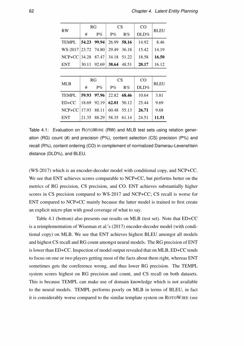
62 Chapter 4. Latent Entity Planning
RWRG CS CO
BLEU# P% P% R% DLD%
TEMPL 54.23 99.94 26.99 58.16 14.92 8.46
WS-2017 23.72 74.80 29.49 36.18 15.42 14.19
NCP+CC 34.28 87.47 34.18 51.22 18.58 16.50
ENT 30.11 92.69 38.64 48.51 20.17 16.12
MLBRG CS CO
BLEU# P% P% R% DLD%
TEMPL 59.93 97.96 22.82 68.46 10.64 3.81
ED+CC 18.69 92.19 62.01 50.12 25.44 9.69
NCP+CC 17.93 88.11 60.48 55.13 26.71 9.68
ENT 21.35 88.29 58.35 61.14 24.51 11.51
Table 4.1: Evaluation on ROTOWIRE (RW) and MLB test sets using relation gener-
ation (RG) count (#) and precision (P%), content selection (CS) precision (P%) and
recall (R%), content ordering (CO) in complement of normalized Damerau-Levenshtein
distance (DLD%), and BLEU.
(WS-2017) which is an encoder-decoder model with conditional copy, and NCP+CC.
We see that ENT achieves scores comparable to NCP+CC, but performs better on the
metrics of RG precision, CS precision, and CO. ENT achieves substantially higher
scores in CS precision compared to WS-2017 and NCP+CC; CS recall is worse for
ENT compared to NCP+CC mainly because the latter model is trained to first create
an explicit micro plan with good coverage of what to say.
Table 4.1 (bottom) also presents our results on MLB (test set). Note that ED+CC
is a reimplementation of Wiseman et al.’s (2017) encoder-decoder model (with condi-
tional copy) on MLB. We see that ENT achieves highest BLEU amongst all models
and highest CS recall and RG count amongst neural models. The RG precision of ENT
is lower than ED+CC. Inspection of model output revealed that on MLB, ED+CC tends
to focus on one or two players getting most of the facts about them right, whereas ENT
sometimes gets the coreference wrong, and thus lower RG precision. The TEMPL
system scores highest on RG precision and count, and CS recall on both datasets.
This is because TEMPL can make use of domain knowledge which is not available
to the neural models. TEMPL performs poorly on MLB in terms of BLEU, in fact
it is considerably worse compared to the similar template system on ROTOWIRE (see
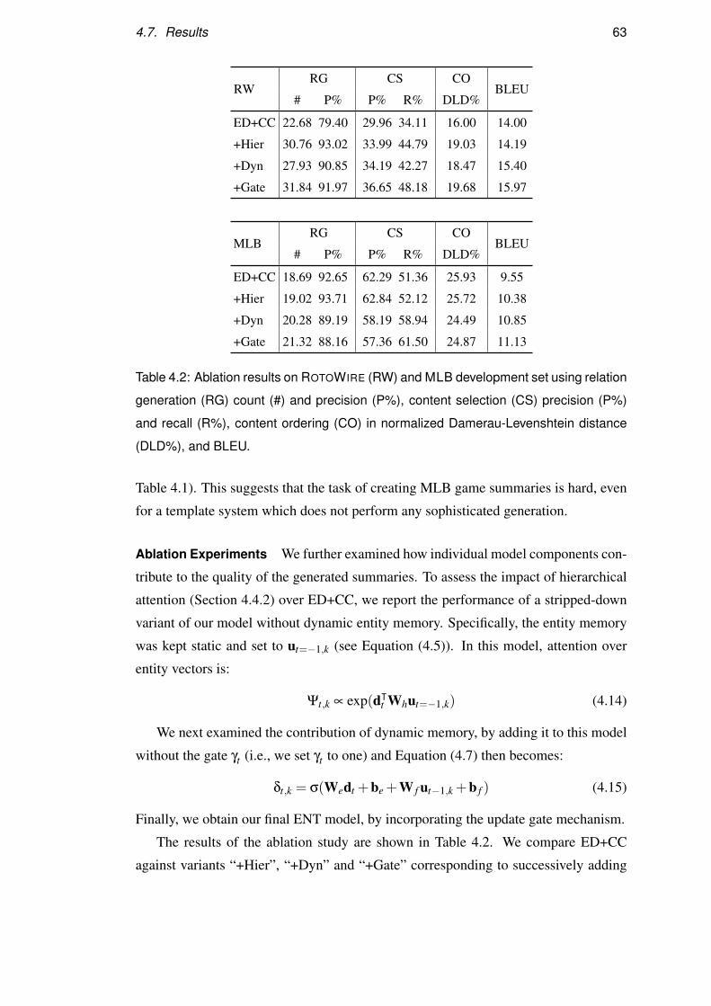
4.7. Results 63
RWRG CS CO
BLEU# P% P% R% DLD%
ED+CC 22.68 79.40 29.96 34.11 16.00 14.00
+Hier 30.76 93.02 33.99 44.79 19.03 14.19
+Dyn 27.93 90.85 34.19 42.27 18.47 15.40
+Gate 31.84 91.97 36.65 48.18 19.68 15.97
MLBRG CS CO
BLEU# P% P% R% DLD%
ED+CC 18.69 92.65 62.29 51.36 25.93 9.55
+Hier 19.02 93.71 62.84 52.12 25.72 10.38
+Dyn 20.28 89.19 58.19 58.94 24.49 10.85
+Gate 21.32 88.16 57.36 61.50 24.87 11.13
Table 4.2: Ablation results on ROTOWIRE (RW) and MLB development set using relation
generation (RG) count (#) and precision (P%), content selection (CS) precision (P%)
and recall (R%), content ordering (CO) in normalized Damerau-Levenshtein distance
(DLD%), and BLEU.
Table 4.1). This suggests that the task of creating MLB game summaries is hard, even
for a template system which does not perform any sophisticated generation.
Ablation Experiments We further examined how individual model components con-
tribute to the quality of the generated summaries. To assess the impact of hierarchical
attention (Section 4.4.2) over ED+CC, we report the performance of a stripped-down
variant of our model without dynamic entity memory. Specifically, the entity memory
was kept static and set to ut=−1,k (see Equation (4.5)). In this model, attention over
entity vectors is:
Ψt,k ∝ exp(dᵀt Whut=−1,k) (4.14)
We next examined the contribution of dynamic memory, by adding it to this model
without the gate γt (i.e., we set γt to one) and Equation (4.7) then becomes:
δt,k = σ(Wedt +be +W f ut−1,k +b f ) (4.15)
Finally, we obtain our final ENT model, by incorporating the update gate mechanism.
The results of the ablation study are shown in Table 4.2. We compare ED+CC
against variants “+Hier”, “+Dyn” and “+Gate” corresponding to successively adding
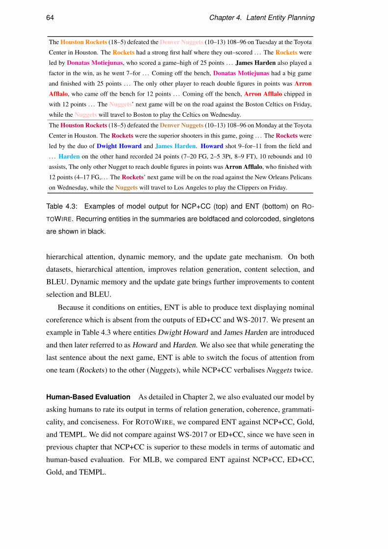
64 Chapter 4. Latent Entity Planning
The Houston Rockets (18–5) defeated the Denver Nuggets (10–13) 108–96 on Tuesday at the Toyota
Center in Houston. The Rockets had a strong first half where they out–scored . . . The Rockets were
led by Donatas Motiejunas, who scored a game–high of 25 points . . . James Harden also played a
factor in the win, as he went 7–for . . . Coming off the bench, Donatas Motiejunas had a big game
and finished with 25 points . . . The only other player to reach double figures in points was ArronAfflalo, who came off the bench for 12 points . . . Coming off the bench, Arron Afflalo chipped in
with 12 points . . . The Nuggets’ next game will be on the road against the Boston Celtics on Friday,
while the Nuggets will travel to Boston to play the Celtics on Wednesday.
The Houston Rockets (18–5) defeated the Denver Nuggets (10–13) 108–96 on Monday at the Toyota
Center in Houston. The Rockets were the superior shooters in this game, going . . . The Rockets were
led by the duo of Dwight Howard and James Harden. Howard shot 9–for–11 from the field and
. . . Harden on the other hand recorded 24 points (7–20 FG, 2–5 3Pt, 8–9 FT), 10 rebounds and 10
assists, The only other Nugget to reach double figures in points was Arron Afflalo, who finished with
12 points (4–17 FG,. . . The Rockets’ next game will be on the road against the New Orleans Pelicans
on Wednesday, while the Nuggets will travel to Los Angeles to play the Clippers on Friday.
Table 4.3: Examples of model output for NCP+CC (top) and ENT (bottom) on RO-
TOWIRE. Recurring entities in the summaries are boldfaced and colorcoded, singletons
are shown in black.
hierarchical attention, dynamic memory, and the update gate mechanism. On both
datasets, hierarchical attention, improves relation generation, content selection, and
BLEU. Dynamic memory and the update gate brings further improvements to content
selection and BLEU.
Because it conditions on entities, ENT is able to produce text displaying nominal
coreference which is absent from the outputs of ED+CC and WS-2017. We present an
example in Table 4.3 where entities Dwight Howard and James Harden are introduced
and then later referred to as Howard and Harden. We also see that while generating the
last sentence about the next game, ENT is able to switch the focus of attention from
one team (Rockets) to the other (Nuggets), while NCP+CC verbalises Nuggets twice.
Human-Based Evaluation As detailed in Chapter 2, we also evaluated our model by
asking humans to rate its output in terms of relation generation, coherence, grammati-
cality, and conciseness. For ROTOWIRE, we compared ENT against NCP+CC, Gold,
and TEMPL. We did not compare against WS-2017 or ED+CC, since we have seen in
previous chapter that NCP+CC is superior to these models in terms of automatic and
human-based evaluation. For MLB, we compared ENT against NCP+CC, ED+CC,
Gold, and TEMPL.
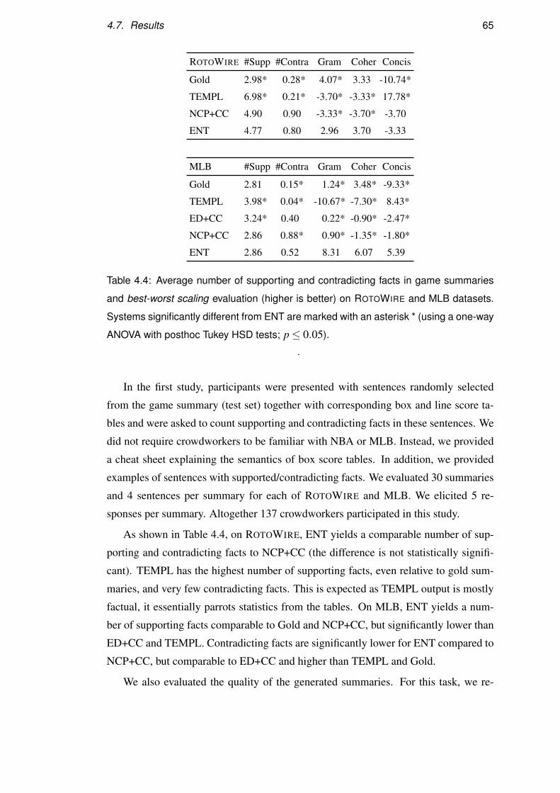
4.7. Results 65
ROTOWIRE #Supp #Contra Gram Coher Concis
Gold 2.98* 0.28* 4.07* 3.33 -10.74*
TEMPL 6.98* 0.21* -3.70* -3.33* 17.78*
NCP+CC 4.90 0.90 -3.33* -3.70* -3.70
ENT 4.77 0.80 2.96 3.70 -3.33
MLB #Supp #Contra Gram Coher Concis
Gold 2.81 0.15* 1.24* 3.48* -9.33*
TEMPL 3.98* 0.04* -10.67* -7.30* 8.43*
ED+CC 3.24* 0.40 0.22* -0.90* -2.47*
NCP+CC 2.86 0.88* 0.90* -1.35* -1.80*
ENT 2.86 0.52 8.31 6.07 5.39
Table 4.4: Average number of supporting and contradicting facts in game summaries
and best-worst scaling evaluation (higher is better) on ROTOWIRE and MLB datasets.
Systems significantly different from ENT are marked with an asterisk * (using a one-way
ANOVA with posthoc Tukey HSD tests; p≤ 0.05).
.
In the first study, participants were presented with sentences randomly selected
from the game summary (test set) together with corresponding box and line score ta-
bles and were asked to count supporting and contradicting facts in these sentences. We
did not require crowdworkers to be familiar with NBA or MLB. Instead, we provided
a cheat sheet explaining the semantics of box score tables. In addition, we provided
examples of sentences with supported/contradicting facts. We evaluated 30 summaries
and 4 sentences per summary for each of ROTOWIRE and MLB. We elicited 5 re-
sponses per summary. Altogether 137 crowdworkers participated in this study.
As shown in Table 4.4, on ROTOWIRE, ENT yields a comparable number of sup-
porting and contradicting facts to NCP+CC (the difference is not statistically signifi-
cant). TEMPL has the highest number of supporting facts, even relative to gold sum-
maries, and very few contradicting facts. This is expected as TEMPL output is mostly
factual, it essentially parrots statistics from the tables. On MLB, ENT yields a num-
ber of supporting facts comparable to Gold and NCP+CC, but significantly lower than
ED+CC and TEMPL. Contradicting facts are significantly lower for ENT compared to
NCP+CC, but comparable to ED+CC and higher than TEMPL and Gold.
We also evaluated the quality of the generated summaries. For this task, we re-
66 Chapter 4. Latent Entity Planning
quired that the crowdworkers be able to comfortably comprehend NBA/ MLB game
summaries. We presented participants with two summaries at a time and asked them
to choose which one is better in terms of Grammaticality, Coherence, and Concise-
ness. We divided the four competing systems (Gold, TEMPL, NCP+CC, and ENT)
into six pairs of summaries for ROTOWIRE and the five competing systems (Gold,
TEMPL, ED+CC, NCP+CC, and ENT) into ten pairs for MLB. We elicited judgments
for 30 test summaries for ROTOWIRE and MLB; each summary was rated by 3 partic-
ipants. Altogether 145 crowdworkers participated in this study.
As shown in Table 4.4, on ROTOWIRE Gold receives highest scores in terms of
Grammaticality, which is not unexpected. ENT comes close, achieving better scores
than NCP+CC and TEMPL, even though our model only enhances the coherence of
the output. Participants find ENT on par with Gold on Coherence and better than
NCP+CC and TEMPL whose output is stilted and exhibits no variability. In terms
of Conciseness, TEMPL is rated best, which is expected since it does not contain
any duplication, the presented facts are mutually exclusive; ENT is comparable to
NCP+CC and better than Gold.
As far as MLB is concerned, ENT achieves highest scores on Grammaticality and
Coherence. It is rated high on Conciseness also, second only to TEMPL whose scores
are lowest on Grammaticality and Coherence. Perhaps surprisingly, Gold is rated lower
than ENT on all three metrics; we hypothesize that participants find Gold’s output too
verbose compared to the other systems. Recall that MLB gold summaries are relatively
long, the average length is 542 tokens compared to ROTOWIRE whose summaries are
almost half as long (see Table 2.8). The average length of output summaries for ENT
is 327 tokens.
Taken together, our results show that ENT performs better than comparison sys-
tems on both ROTOWIRE and MLB.
4.8 Qualitative Examples
Table 4.5 contain examples of model outputs for ROTOWIRE, and Table 4.6 contains
model outputs for MLB. Because it conditions on entities, ENT is able to produce text
displaying nominal coreference compared to other models.

4.8. Qualitative Examples 67
Template
The Atlanta Hawks ( 44 - 30 ) defeated the Detroit Pistons ( 39 - 35 ) 112 - 95 . Paul Millsap scored
23 points ( 8 - 13 FG , 3 - 4 3PT , 4 - 5 FT ) to go with 9 rebounds . Tobias Harris scored 21 points (
10 - 20 FG , 1 - 3 3PT , 0 - 0 FT ) to go with 10 rebounds . Andre Drummond scored 19 points ( 7 -
11 FG , 0 - 0 3PT , 5 - 9 FT ) to go with 17 rebounds . Kent Bazemore scored 17 points ( 7 - 9 FG , 3
- 5 3PT , 0 - 0 FT ) to go with 4 rebounds . Aron Baynes scored 15 points ( 5 - 6 FG , 0 - 0 3PT , 5 - 6
FT ) to go with 7 rebounds . Al Horford scored 13 points ( 6 - 15 FG , 1 - 5 3PT , 0 - 0 FT ) to go with
5 rebounds . The Atlanta Hawks ’ next game will be at home against the Dallas Mavericks, while the
Detroit Pistons will travel to play the Bulls .
ENT
The Atlanta Hawks ( 44 - 30 ) defeated the Detroit Pistons ( 39 - 35 ) 112 - 95 on Monday at the Palace
of Auburn Hills . The Hawks got off to a quick start in this one , out - scoring the Pistons 27 - 15 in the
first quarter alone . The Hawks were the superior shooters in this game , going 45 percent from the field
and 38 percent from the three - point line , while the Pistons went 39 percent from the floor and just 24
percent from beyond the arc . The Hawks were led by the duo of Paul Millsap and Andre Drummond. Millsap finished with 23 points ( 8 - 13 FG , 3 - 4 3Pt , 4 - 5 FT ) , nine rebounds and four blocked
shots , while Drummond had 19 points ( 7 - 11 FG , 5 - 9 FT ) , 17 rebounds and two blocked shots . It
was his second double - double in a row , as he ’s combined for 45 points and 19 rebounds over his last
two games . He ’s now averaging 15 points and 7 rebounds on the season . Jeff Teague was the other
starter to reach double figures in points , as he finished with 12 points ( 3 - 13 FG , 2 - 3 3Pt , 4 - 4 FT
) and 12 assists . The Hawks ’ next game will be at home against the Cleveland Cavaliers on Friday ,
while the Pistons will travel to Los Angeles to play the Clippers on Friday .
Table 4.5: Example game summaries from the template-based system and our ENT
model for ROTOWIRE. Recurring entities in the summaries are boldfaced and color-
coded, singletons are shown in black.
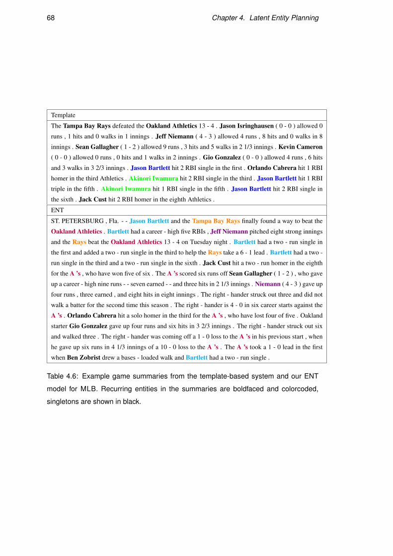
68 Chapter 4. Latent Entity Planning
Template
The Tampa Bay Rays defeated the Oakland Athletics 13 - 4 . Jason Isringhausen ( 0 - 0 ) allowed 0
runs , 1 hits and 0 walks in 1 innings . Jeff Niemann ( 4 - 3 ) allowed 4 runs , 8 hits and 0 walks in 8
innings . Sean Gallagher ( 1 - 2 ) allowed 9 runs , 3 hits and 5 walks in 2 1/3 innings . Kevin Cameron( 0 - 0 ) allowed 0 runs , 0 hits and 1 walks in 2 innings . Gio Gonzalez ( 0 - 0 ) allowed 4 runs , 6 hits
and 3 walks in 3 2/3 innings . Jason Bartlett hit 2 RBI single in the first . Orlando Cabrera hit 1 RBI
homer in the third Athletics . Akinori Iwamura hit 2 RBI single in the third . Jason Bartlett hit 1 RBI
triple in the fifth . Akinori Iwamura hit 1 RBI single in the fifth . Jason Bartlett hit 2 RBI single in
the sixth . Jack Cust hit 2 RBI homer in the eighth Athletics .
ENT
ST. PETERSBURG , Fla. - - Jason Bartlett and the Tampa Bay Rays finally found a way to beat the
Oakland Athletics . Bartlett had a career - high five RBIs , Jeff Niemann pitched eight strong innings
and the Rays beat the Oakland Athletics 13 - 4 on Tuesday night . Bartlett had a two - run single in
the first and added a two - run single in the third to help the Rays take a 6 - 1 lead . Bartlett had a two -
run single in the third and a two - run single in the sixth . Jack Cust hit a two - run homer in the eighth
for the A ’s , who have won five of six . The A ’s scored six runs off Sean Gallagher ( 1 - 2 ) , who gave
up a career - high nine runs - - seven earned - - and three hits in 2 1/3 innings . Niemann ( 4 - 3 ) gave up
four runs , three earned , and eight hits in eight innings . The right - hander struck out three and did not
walk a batter for the second time this season . The right - hander is 4 - 0 in six career starts against the
A ’s . Orlando Cabrera hit a solo homer in the third for the A ’s , who have lost four of five . Oakland
starter Gio Gonzalez gave up four runs and six hits in 3 2/3 innings . The right - hander struck out six
and walked three . The right - hander was coming off a 1 - 0 loss to the A ’s in his previous start , when
he gave up six runs in 4 1/3 innings of a 10 - 0 loss to the A ’s . The A ’s took a 1 - 0 lead in the first
when Ben Zobrist drew a bases - loaded walk and Bartlett had a two - run single .
Table 4.6: Example game summaries from the template-based system and our ENT
model for MLB. Recurring entities in the summaries are boldfaced and colorcoded,
singletons are shown in black.
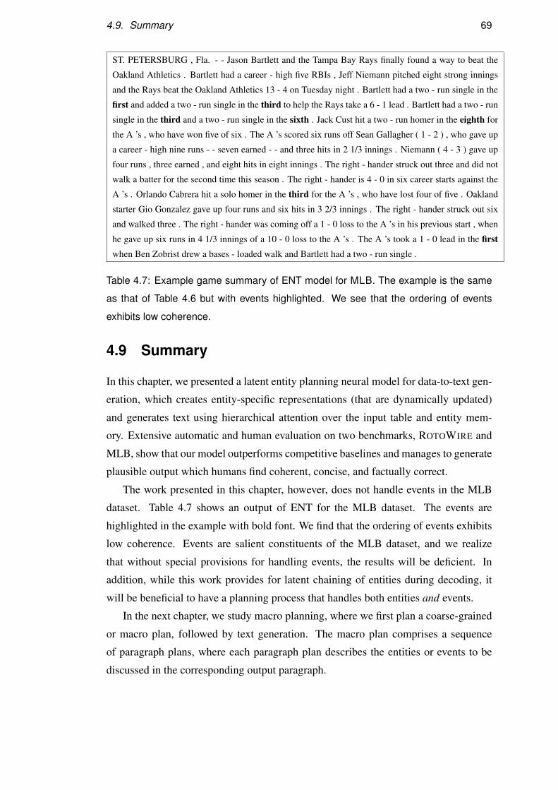
4.9. Summary 69
ST. PETERSBURG , Fla. - - Jason Bartlett and the Tampa Bay Rays finally found a way to beat the
Oakland Athletics . Bartlett had a career - high five RBIs , Jeff Niemann pitched eight strong innings
and the Rays beat the Oakland Athletics 13 - 4 on Tuesday night . Bartlett had a two - run single in the
first and added a two - run single in the third to help the Rays take a 6 - 1 lead . Bartlett had a two - run
single in the third and a two - run single in the sixth . Jack Cust hit a two - run homer in the eighth for
the A ’s , who have won five of six . The A ’s scored six runs off Sean Gallagher ( 1 - 2 ) , who gave up
a career - high nine runs - - seven earned - - and three hits in 2 1/3 innings . Niemann ( 4 - 3 ) gave up
four runs , three earned , and eight hits in eight innings . The right - hander struck out three and did not
walk a batter for the second time this season . The right - hander is 4 - 0 in six career starts against the
A ’s . Orlando Cabrera hit a solo homer in the third for the A ’s , who have lost four of five . Oakland
starter Gio Gonzalez gave up four runs and six hits in 3 2/3 innings . The right - hander struck out six
and walked three . The right - hander was coming off a 1 - 0 loss to the A ’s in his previous start , when
he gave up six runs in 4 1/3 innings of a 10 - 0 loss to the A ’s . The A ’s took a 1 - 0 lead in the firstwhen Ben Zobrist drew a bases - loaded walk and Bartlett had a two - run single .
Table 4.7: Example game summary of ENT model for MLB. The example is the same
as that of Table 4.6 but with events highlighted. We see that the ordering of events
exhibits low coherence.
4.9 Summary
In this chapter, we presented a latent entity planning neural model for data-to-text gen-
eration, which creates entity-specific representations (that are dynamically updated)
and generates text using hierarchical attention over the input table and entity mem-
ory. Extensive automatic and human evaluation on two benchmarks, ROTOWIRE and
MLB, show that our model outperforms competitive baselines and manages to generate
plausible output which humans find coherent, concise, and factually correct.
The work presented in this chapter, however, does not handle events in the MLB
dataset. Table 4.7 shows an output of ENT for the MLB dataset. The events are
highlighted in the example with bold font. We find that the ordering of events exhibits
low coherence. Events are salient constituents of the MLB dataset, and we realize
that without special provisions for handling events, the results will be deficient. In
addition, while this work provides for latent chaining of entities during decoding, it
will be beneficial to have a planning process that handles both entities and events.
In the next chapter, we study macro planning, where we first plan a coarse-grained
or macro plan, followed by text generation. The macro plan comprises a sequence
of paragraph plans, where each paragraph plan describes the entities or events to be
discussed in the corresponding output paragraph.

Chapter 5
Macro Planning
In Chapter 3, we have seen how micro planning can benefit text generation. Micro
planning involves a two stage approach of first predicting a fine-grained content plan,
followed by text generation. We have seen that micro planning works well for the
ROTOWIRE dataset but not for the MLB dataset. The primary reason for this is micro
planning requires oracle micro plans during training, which necessitates an Information
Extraction (IE) model with high coverage and precision. Such Information Extraction
is easier to run on datasets such as ROTOWIRE, as the entities along with the values can
be detected with simple pattern matching. In the case of MLB, as discussed in Chapter
4, the IE has lower precision and coverage, as the entity and value pairs cannot be easily
detected with simple pattern matching. Consequently, supervision for oracle micro
plans is difficult to obtain for MLB. One approach might be to forego IE altogether
following the latent entity planning approach proposed in Chapter 4 which focuses
on entities and how they are organized throughout the document, and achieves better
results than micro planning. Unfortunately, it does not handle events in the MLB
dataset.
In this chapter, we propose macro planning, which combines planning with the
high level organization of entities and events.
5.1 Motivation
We focus on macro planning, the high-level organization of information and how it
should be presented which we argue is important for the generation of long, multi-
paragraph documents (see text (C) in Figure 5.1 which is an example from MLB
dataset).
71
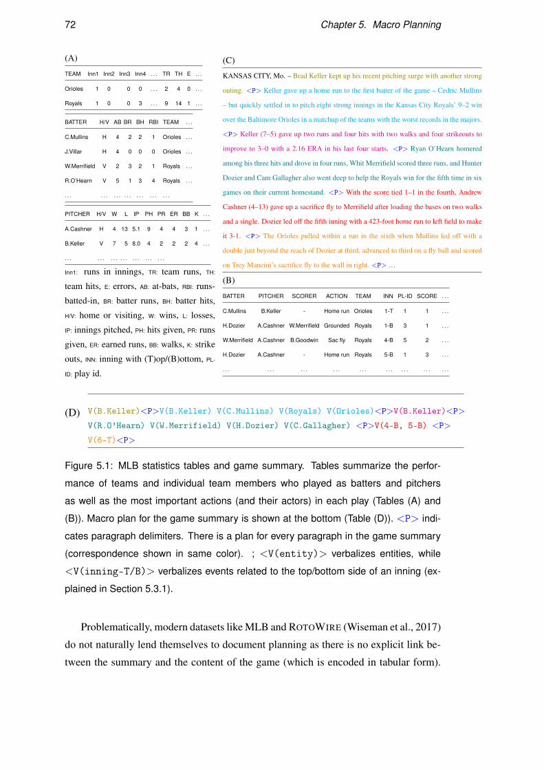
72 Chapter 5. Macro Planning
(A)
TEAM Inn1 Inn2 Inn3 Inn4 . . . TR TH E . . .
Orioles 1 0 0 0 . . . 2 4 0 . . .
Royals 1 0 0 3 . . . 9 14 1 . . .
BATTER H/V AB BR BH RBI TEAM . . .
C.Mullins H 4 2 2 1 Orioles . . .
J.Villar H 4 0 0 0 Orioles . . .
W.Merrifield V 2 3 2 1 Royals . . .
R.O’Hearn V 5 1 3 4 Royals . . .
. . . . . . . . . . . . . . . . . . . . .
PITCHER H/V W L IP PH PR ER BB K . . .
A.Cashner H 4 13 5.1 9 4 4 3 1 . . .
B.Keller V 7 5 8.0 4 2 2 2 4 . . .
. . . . . . . . . . . . . . . . . . . . .
Inn1: runs in innings, TR: team runs, TH:
team hits, E: errors, AB: at-bats, RBI: runs-
batted-in, BR: batter runs, BH: batter hits,
H/V: home or visiting, W: wins, L: losses,
IP: innings pitched, PH: hits given, PR: runs
given, ER: earned runs, BB: walks, K: strike
outs, INN: inning with (T)op/(B)ottom, PL-
ID: play id.
(C)
KANSAS CITY, Mo. – Brad Keller kept up his recent pitching surge with another strong
outing. <P> Keller gave up a home run to the first batter of the game – Cedric Mullins
– but quickly settled in to pitch eight strong innings in the Kansas City Royals’ 9–2 win
over the Baltimore Orioles in a matchup of the teams with the worst records in the majors.
<P> Keller (7–5) gave up two runs and four hits with two walks and four strikeouts to
improve to 3–0 with a 2.16 ERA in his last four starts. <P> Ryan O’Hearn homered
among his three hits and drove in four runs, Whit Merrifield scored three runs, and Hunter
Dozier and Cam Gallagher also went deep to help the Royals win for the fifth time in six
games on their current homestand. <P> With the score tied 1–1 in the fourth, Andrew
Cashner (4–13) gave up a sacrifice fly to Merrifield after loading the bases on two walks
and a single. Dozier led off the fifth inning with a 423-foot home run to left field to make
it 3-1. <P> The Orioles pulled within a run in the sixth when Mullins led off with a
double just beyond the reach of Dozier at third, advanced to third on a fly ball and scored
on Trey Mancini’s sacrifice fly to the wall in right. <P> . . .
(B)
BATTER PITCHER SCORER ACTION TEAM INN PL-ID SCORE . . .
C.Mullins B.Keller - Home run Orioles 1-T 1 1 . . .
H.Dozier A.Cashner W.Merrifield Grounded Royals 1-B 3 1 . . .
W.Merrifield A.Cashner B.Goodwin Sac fly Royals 4-B 5 2 . . .
H.Dozier A.Cashner - Home run Royals 5-B 1 3 . . .
. . . . . . . . . . . . . . . . . . . . . . . . . . .
(D) V(B.Keller)<P>V(B.Keller) V(C.Mullins) V(Royals) V(Orioles)<P>V(B.Keller)<P>
V(R.O’Hearn) V(W.Merrifield) V(H.Dozier) V(C.Gallagher) <P>V(4-B, 5-B) <P>
V(6-T)<P>
Figure 5.1: MLB statistics tables and game summary. Tables summarize the perfor-
mance of teams and individual team members who played as batters and pitchers
as well as the most important actions (and their actors) in each play (Tables (A) and
(B)). Macro plan for the game summary is shown at the bottom (Table (D)). <P> indi-
cates paragraph delimiters. There is a plan for every paragraph in the game summary
(correspondence shown in same color). ; <V(entity)> verbalizes entities, while
<V(inning-T/B)> verbalizes events related to the top/bottom side of an inning (ex-
plained in Section 5.3.1).
Problematically, modern datasets like MLB and ROTOWIRE (Wiseman et al., 2017)
do not naturally lend themselves to document planning as there is no explicit link be-
tween the summary and the content of the game (which is encoded in tabular form).
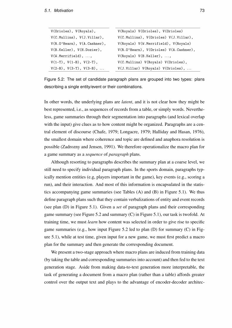
5.1. Motivation 73
V(Orioles), V(Royals),
V(C.Mullins), V(J.Villar),
V(R.O’Hearn), V(A.Cashner),
V(B.Keller), V(H.Dozier),
V(W.Merrifield), . . .,
V(1-T), V(1-B), V(2-T),
V(2-B), V(3-T), V(3-B), . . .
V(Royals) V(Orioles), V(Orioles)
V(C.Mullins), V(Orioles) V(J.Villar),
V(Royals) V(W.Merrifield), V(Royals)
V(R.O’Hearn), V(Orioles) V(A.Cashner),
V(Royals) V(B.Keller), . . .,
V(C.Mullins) V(Royals) V(Orioles),
V(J.Villar) V(Royals) V(Orioles), . . .
Figure 5.2: The set of candidate paragraph plans are grouped into two types: plans
describing a single entity/event or their combinations.
In other words, the underlying plans are latent, and it is not clear how they might be
best represented, i.e., as sequences of records from a table, or simply words. Neverthe-
less, game summaries through their segmentation into paragraphs (and lexical overlap
with the input) give clues as to how content might be organized. Paragraphs are a cen-
tral element of discourse (Chafe, 1979; Longacre, 1979; Halliday and Hasan, 1976),
the smallest domain where coherence and topic are defined and anaphora resolution is
possible (Zadrozny and Jensen, 1991). We therefore operationalize the macro plan for
a game summary as a sequence of paragraph plans.
Although resorting to paragraphs describes the summary plan at a coarse level, we
still need to specify individual paragraph plans. In the sports domain, paragraphs typ-
ically mention entities (e.g, players important in the game), key events (e.g., scoring a
run), and their interaction. And most of this information is encapsulated in the statis-
tics accompanying game summaries (see Tables (A) and (B) in Figure 5.1). We thus
define paragraph plans such that they contain verbalizations of entity and event records
(see plan (D) in Figure 5.1). Given a set of paragraph plans and their corresponding
game summary (see Figure 5.2 and summary (C) in Figure 5.1), our task is twofold. At
training time, we must learn how content was selected in order to give rise to specific
game summaries (e.g., how input Figure 5.2 led to plan (D) for summary (C) in Fig-
ure 5.1), while at test time, given input for a new game, we must first predict a macro
plan for the summary and then generate the corresponding document.
We present a two-stage approach where macro plans are induced from training data
(by taking the table and corresponding summaries into account) and then fed to the text
generation stage. Aside from making data-to-text generation more interpretable, the
task of generating a document from a macro plan (rather than a table) affords greater
control over the output text and plays to the advantage of encoder-decoder architec-
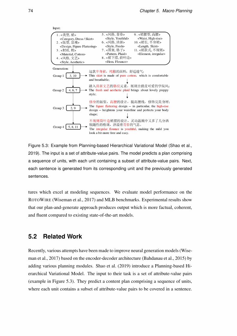
74 Chapter 5. Macro Planning
Figure 5.3: Example from Planning-based Hierarchical Variational Model (Shao et al.,
2019). The input is a set of attribute-value pairs. The model predicts a plan comprising
a sequence of units, with each unit containing a subset of attribute-value pairs. Next,
each sentence is generated from its corresponding unit and the previously generated
sentences.
tures which excel at modeling sequences. We evaluate model performance on the
ROTOWIRE (Wiseman et al., 2017) and MLB benchmarks. Experimental results show
that our plan-and-generate approach produces output which is more factual, coherent,
and fluent compared to existing state-of-the-art models.
5.2 Related Work
Recently, various attempts have been made to improve neural generation models (Wise-
man et al., 2017) based on the encoder-decoder architecture (Bahdanau et al., 2015) by
adding various planning modules. Shao et al. (2019) introduce a Planning-based Hi-
erarchical Variational Model. The input to their task is a set of attribute-value pairs
(example in Figure 5.3). They predict a content plan comprising a sequence of units,
where each unit contains a subset of attribute-value pairs to be covered in a sentence.
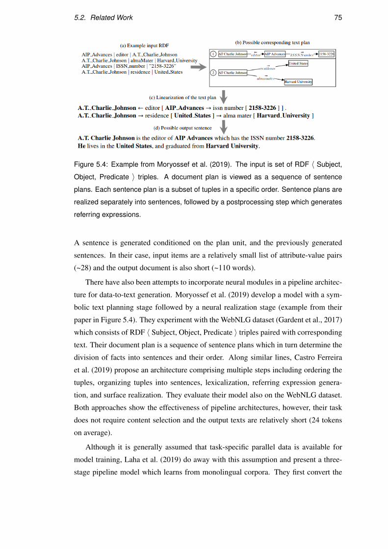
5.2. Related Work 75
Figure 5.4: Example from Moryossef et al. (2019). The input is set of RDF 〈 Subject,
Object, Predicate 〉 triples. A document plan is viewed as a sequence of sentence
plans. Each sentence plan is a subset of tuples in a specific order. Sentence plans are
realized separately into sentences, followed by a postprocessing step which generates
referring expressions.
A sentence is generated conditioned on the plan unit, and the previously generated
sentences. In their case, input items are a relatively small list of attribute-value pairs
(~28) and the output document is also short (~110 words).
There have also been attempts to incorporate neural modules in a pipeline architec-
ture for data-to-text generation. Moryossef et al. (2019) develop a model with a sym-
bolic text planning stage followed by a neural realization stage (example from their
paper in Figure 5.4). They experiment with the WebNLG dataset (Gardent et al., 2017)
which consists of RDF 〈 Subject, Object, Predicate 〉 triples paired with corresponding
text. Their document plan is a sequence of sentence plans which in turn determine the
division of facts into sentences and their order. Along similar lines, Castro Ferreira
et al. (2019) propose an architecture comprising multiple steps including ordering the
tuples, organizing tuples into sentences, lexicalization, referring expression genera-
tion, and surface realization. They evaluate their model also on the WebNLG dataset.
Both approaches show the effectiveness of pipeline architectures, however, their task
does not require content selection and the output texts are relatively short (24 tokens
on average).
Although it is generally assumed that task-specific parallel data is available for
model training, Laha et al. (2019) do away with this assumption and present a three-
stage pipeline model which learns from monolingual corpora. They first convert the
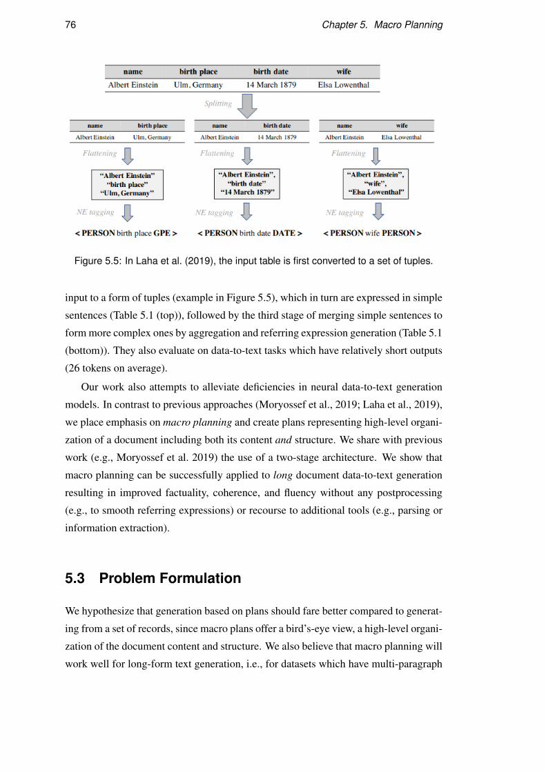
76 Chapter 5. Macro Planning
Figure 5.5: In Laha et al. (2019), the input table is first converted to a set of tuples.
input to a form of tuples (example in Figure 5.5), which in turn are expressed in simple
sentences (Table 5.1 (top)), followed by the third stage of merging simple sentences to
form more complex ones by aggregation and referring expression generation (Table 5.1
(bottom)). They also evaluate on data-to-text tasks which have relatively short outputs
(26 tokens on average).
Our work also attempts to alleviate deficiencies in neural data-to-text generation
models. In contrast to previous approaches (Moryossef et al., 2019; Laha et al., 2019),
we place emphasis on macro planning and create plans representing high-level organi-
zation of a document including both its content and structure. We share with previous
work (e.g., Moryossef et al. 2019) the use of a two-stage architecture. We show that
macro planning can be successfully applied to long document data-to-text generation
resulting in improved factuality, coherence, and fluency without any postprocessing
(e.g., to smooth referring expressions) or recourse to additional tools (e.g., parsing or
information extraction).
5.3 Problem Formulation
We hypothesize that generation based on plans should fare better compared to generat-
ing from a set of records, since macro plans offer a bird’s-eye view, a high-level organi-
zation of the document content and structure. We also believe that macro planning will
work well for long-form text generation, i.e., for datasets which have multi-paragraph

5.3. Problem Formulation 77
Input Output
〈 PERSON birth place GPE 〉 〈 PERSON was born in GPE 〉〈 PERSON birth date DATE 〉 〈 PERSON has birthday on DATE 〉〈 PERSON wife PERSON 〉 〈 PERSON is the wife of PERSON 〉
Operation Input Output
Aggregation Albert Einstein was born in Ulm,
GermanyAlbert. Einstein has
birthday on 14 March 1879.
Albert Einstein was born in Ulm,
Germany and has birthday on 14
March 1879.
Referring ex-
pression genera-
tion
Albert Einstein was born in Ulm,
Germany and has birthday on 14
March 1879. Elsa Lowenthal is
the wife of Albert Einstein.
Albert Einstein was born in Ulm,
Germany and has birthday on 14
March 1879. Elsa Lowenthal is
the wife of him.
Table 5.1: In the second stage in Laha et al. (2019) (top table), the tuples are converted
to simple sentences. In the third stage (below table), individual sentences are converted
to more complex ones by aggregation (first row) and referring expression generation
(second row).
target texts, a large vocabulary space, and require content selection.
We assume the input to our model is a set of paragraph plans E = {ei}|E |i=1 where
ei is a paragraph plan. We model the process of generating output summary y given Eas a two step process, namely the construction of a macro plan x based on the set of
paragraph plans, followed by the generation of a summary given a macro plan as input.
We now explain how the set E is obtained and each step is realized. We discuss our
model considering mainly an example from the MLB dataset but also touch on how
the approach can be straightforwardly adapted to ROTOWIRE (Wiseman et al., 2017).
5.3.1 Macro Plan Definition
A macro plan consists of a sequence of paragraph plans separated by a paragraph dis-
course marker <P>, i.e., x = e1 <P> e2 . . .<P> ek where e1,e2,ek ∈ E . A paragraph
plan ei in turn is a sequence of entities and events describing the game. By entities we
mean individual players or teams and the information provided about them in box score
statistics (see rows and column headings in Figure 5.1 Table (A)), while events refer to
information described in play-by-play (see Table (B)). In baseball, plays are grouped
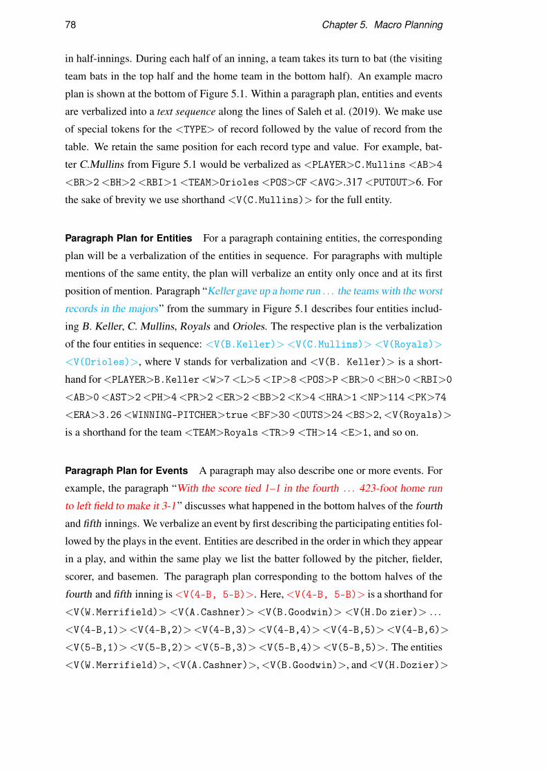
78 Chapter 5. Macro Planning
in half-innings. During each half of an inning, a team takes its turn to bat (the visiting
team bats in the top half and the home team in the bottom half). An example macro
plan is shown at the bottom of Figure 5.1. Within a paragraph plan, entities and events
are verbalized into a text sequence along the lines of Saleh et al. (2019). We make use
of special tokens for the <TYPE> of record followed by the value of record from the
table. We retain the same position for each record type and value. For example, bat-
ter C.Mullins from Figure 5.1 would be verbalized as <PLAYER>C.Mullins <AB>4
<BR>2<BH>2<RBI>1<TEAM>Orioles<POS>CF<AVG>.317 <PUTOUT>6. For
the sake of brevity we use shorthand <V(C.Mullins)> for the full entity.
Paragraph Plan for Entities For a paragraph containing entities, the corresponding
plan will be a verbalization of the entities in sequence. For paragraphs with multiple
mentions of the same entity, the plan will verbalize an entity only once and at its first
position of mention. Paragraph “Keller gave up a home run . . . the teams with the worst
records in the majors” from the summary in Figure 5.1 describes four entities includ-
ing B. Keller, C. Mullins, Royals and Orioles. The respective plan is the verbalization
of the four entities in sequence: <V(B.Keller)><V(C.Mullins)><V(Royals)>
<V(Orioles)>, where V stands for verbalization and <V(B. Keller)> is a short-
hand for <PLAYER>B.Keller<W>7<L>5<IP>8<POS>P<BR>0<BH>0<RBI>0
<AB>0<AST>2<PH>4<PR>2<ER>2<BB>2<K>4<HRA>1<NP>114<PK>74
<ERA>3.26<WINNING-PITCHER>true<BF>30<OUTS>24<BS>2, <V(Royals)>
is a shorthand for the team <TEAM>Royals <TR>9 <TH>14 <E>1, and so on.
Paragraph Plan for Events A paragraph may also describe one or more events. For
example, the paragraph “With the score tied 1–1 in the fourth . . . 423-foot home run
to left field to make it 3-1” discusses what happened in the bottom halves of the fourth
and fifth innings. We verbalize an event by first describing the participating entities fol-
lowed by the plays in the event. Entities are described in the order in which they appear
in a play, and within the same play we list the batter followed by the pitcher, fielder,
scorer, and basemen. The paragraph plan corresponding to the bottom halves of the
fourth and fifth inning is <V(4-B, 5-B)>. Here, <V(4-B, 5-B)> is a shorthand for
<V(W.Merrifield)> <V(A.Cashner)> <V(B.Goodwin)> <V(H.Do zier)> .. .
<V(4-B,1)><V(4-B,2)><V(4-B,3)><V(4-B,4)><V(4-B,5)><V(4-B,6)>
<V(5-B,1)><V(5-B,2)><V(5-B,3)><V(5-B,4)><V(5-B,5)>. The entities
<V(W.Merrifield)>, <V(A.Cashner)>, <V(B.Goodwin)>, and <V(H.Dozier)>
5.3. Problem Formulation 79
correspond in turn to W. Merrifield, A. Cashner, B. Goodwin, and H. Dozier while
<V(5-B,1)> refers to the first play in the bottom half of the fifth inning (see the
play-by-play table in Figure 5.1) and abbreviates the following detailed plan: <INN>5
<HALF>B <BATTING>Royals <PITCHING>Orioles <PL-ID>1 <PBYP-RUNS> 1
<PBYP-RBI> 1 <PBYP-OUTS> 0 <PBYP-BALLS> 0 <PBYP-STRIKES> 0 <BATTER>H.Dozier
<PITCHER>A. Cashner <ACTION>Home-run <SCORES> Royals-3-Orioles-1,
etc.
The procedure described above is not specific to MLB and can be ported to other
datasets with similar characteristics such as ROTOWIRE. However, ROTOWIRE does
not provide play-by-play information, and as a result there is no event verbalization for
this dataset.
5.3.2 Macro Plan Construction
We provided our definition for macro plans in the previous sections, however, it is
important to note that such macro plans are not readily available in data-to-text bench-
marks like MLB and ROTOWIRE (Wiseman et al., 2017) which consist of tables of
records r paired with a gold summary y (see Tables (A)–(C) in Figure 5.1). We now
describe our method for obtaining macro plans x from r and y.
Similar to Moryossef et al. (2019), we define macro plans to be conformant with
gold summaries such that (1) they have the same splits into paragraphs — entities and
events within a paragraph in y are grouped into a paragraph plan in x; and (2) the
order of events and entities in a paragraph and its corresponding plan are identical. We
construct macro plans by matching entities and events in the summary to records in the
tables. Furthermore, paragraph delimiters within summaries form natural units which
taken together give rise to a high-level document plan.
We match entities in summaries with entities in tables using exact string match,
allowing for some degree of variation in the expression of team names (e.g., A’s for
Athletics and D-backs for Diamondbacks). Information pertaining to innings appears
in the summaries in the form of ordinal numbers (e.g., first, ninth ) modifying the noun
inning and can be relatively easily identified via pattern matching (e.g., in sentences
like “Dozier led off the fifth inning”). However, there are instances where the men-
tion of innings is more ambiguous (e.g., “With the scored tied 1–1 in the fourth, An-
drew Cashner (4-13) gave up a sacrifice fly”). Here the mention of fourth refers to
the fourth inning. However, the text doesn’t mention explicitly that it is an inning.
80 Chapter 5. Macro Planning
We could disambiguate such mentions manually and then train a classifier to learn
to predict whether an inning is mentioned. Instead, we explore a novel annotation-
free method which makes use of the pretrained language model GPT2 (Radford et al.,
2019). Specifically, we feed the context preceding the ordinal number to GPT2 (i.e.,
the current paragraph up to the ordinal number and the paragraph preceding it) and if
inning appears in the top 10 next word predictions, we consider it a positive match. On
a held out dataset, this method achieves 98% precision and 98% recall at disambiguat-
ing inning mentions.
To resolve whether the summary discusses the top or bottom side of an inning, we
compare the entities in the paragraph with the entities in each half-inning (play-by-play
Table (B) in Figure 5.1) and choose the side with the greater number of entity matches.
For instance, Andrew Cashner, Merrifield and fourth inning uniquely resolves to the
bottom half of the fourth inning.
5.3.3 Paragraph Plan Construction
Figure 5.1 shows the macro plan we obtain for game summary (C). Importantly, macro
plan (D) is the outcome of a content selection process after considering several candi-
date paragraph plans as input. So, what are the candidate paragraph plans which give
rise to macro plan (D)? To answer this question, we examined the empirical distribu-
tion of paragraph plans in MLB and ROTOWIRE (training portion). Interestingly, we
found that ~79% of the paragraph plans in MLB refer to a single event or a single
player (and team(s)). In ROTOWIRE, ~92% of paragraphs are about a single team or a
single player (and team(s)) or a pair of players.
Based on this analysis, we assume that paragraph plans can be either one (verbal-
ized) entity/event or a combination of at most two. Under this assumption, we explic-
itly enumerate the set of candidate paragraph plans in a game. For the game in Fig-
ure 5.1, candidate paragraph plans are shown in Figure 5.2. The first table groups plans
based on individual verbalizations describing the team(s), players, and events taking
place in specific innings. The second table groups pairwise combinations thereof. In
MLB, such combinations are between team(s) and players. In ROTOWIRE, we also
create combinations between players. Such paragraph plans form set E based on which
macro plan x is constructed to give rise to game summary y.
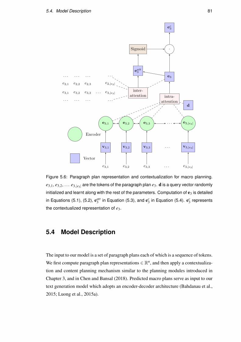
5.4. Model Description 81
e3,1 e3,2 e3,3 . . . e3,|e3|
v3,1 v3,2 v3,3 . . . v3,|e3|
e3,1 e3,2 e3,3 . . . e3,|e3|
intra-attention
d
e3
·Sigmoid
eatt3
inter-attention
e3,|e3|. . .e3,3e3,2e3,1
e2,1 e2,2 e2,3 e2,|e2|
. . . . . . . . . . . .
. . . . . . . . . . . .
ec3
Vector
Encoder
Figure 5.6: Paragraph plan representation and contextualization for macro planning.
e3,1, e3,2, . . . e3,|e3| are the tokens of the paragraph plan e3. d is a query vector randomly
initialized and learnt along with the rest of the parameters. Computation of e3 is detailed
in Equations (5.1), (5.2), eatt3 in Equation (5.3), and ec
3 in Equation (5.4). ec3 represents
the contextualized representation of e3.
5.4 Model Description
The input to our model is a set of paragraph plans each of which is a sequence of tokens.
We first compute paragraph plan representations ∈Rn, and then apply a contextualiza-
tion and content planning mechanism similar to the planning modules introduced in
Chapter 3, and in Chen and Bansal (2018). Predicted macro plans serve as input to our
text generation model which adopts an encoder-decoder architecture (Bahdanau et al.,
2015; Luong et al., 2015a).
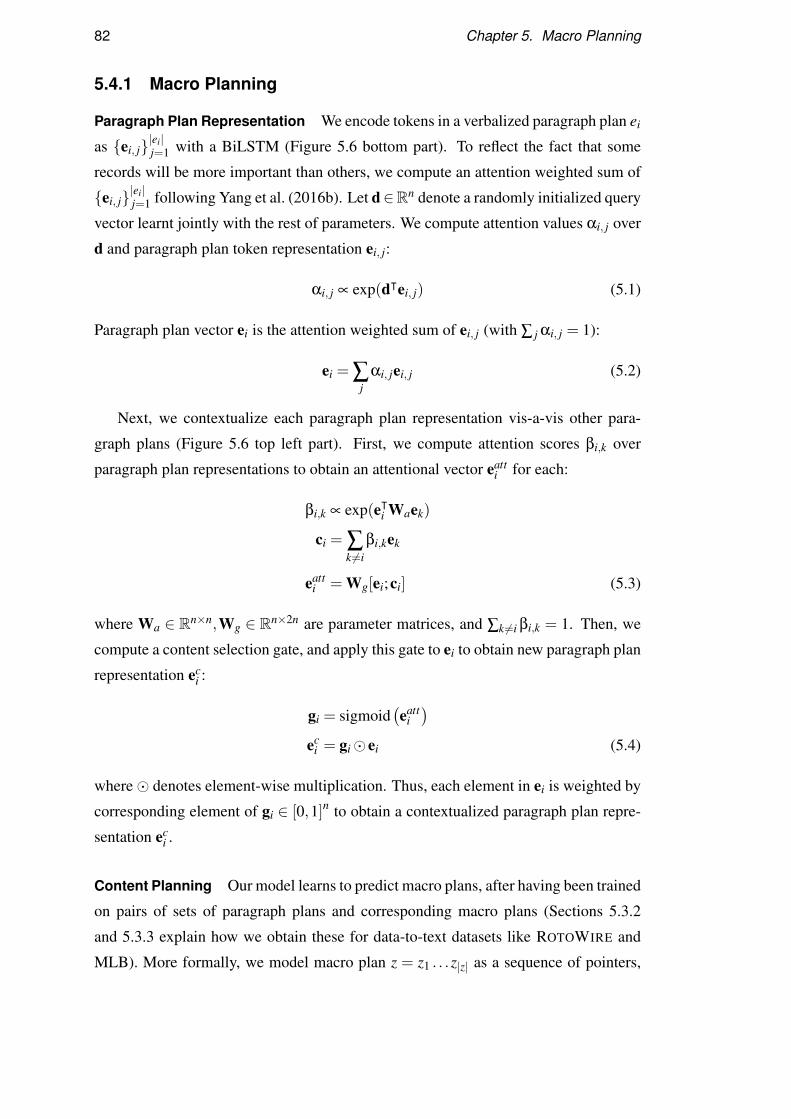
82 Chapter 5. Macro Planning
5.4.1 Macro Planning
Paragraph Plan Representation We encode tokens in a verbalized paragraph plan ei
as {ei, j}|ei|j=1 with a BiLSTM (Figure 5.6 bottom part). To reflect the fact that some
records will be more important than others, we compute an attention weighted sum of
{ei, j}|ei|j=1 following Yang et al. (2016b). Let d∈Rn denote a randomly initialized query
vector learnt jointly with the rest of parameters. We compute attention values αi, j over
d and paragraph plan token representation ei, j:
αi, j ∝ exp(dᵀei, j) (5.1)
Paragraph plan vector ei is the attention weighted sum of ei, j (with ∑ j αi, j = 1):
ei = ∑j
αi, jei, j (5.2)
Next, we contextualize each paragraph plan representation vis-a-vis other para-
graph plans (Figure 5.6 top left part). First, we compute attention scores βi,k over
paragraph plan representations to obtain an attentional vector eatti for each:
βi,k ∝ exp(eᵀi Waek)
ci = ∑k 6=i
βi,kek
eatti = Wg[ei;ci] (5.3)
where Wa ∈ Rn×n,Wg ∈ Rn×2n are parameter matrices, and ∑k 6=i βi,k = 1. Then, we
compute a content selection gate, and apply this gate to ei to obtain new paragraph plan
representation eci :
gi = sigmoid(eatt
i)
eci = gi� ei (5.4)
where� denotes element-wise multiplication. Thus, each element in ei is weighted by
corresponding element of gi ∈ [0,1]n to obtain a contextualized paragraph plan repre-
sentation eci .
Content Planning Our model learns to predict macro plans, after having been trained
on pairs of sets of paragraph plans and corresponding macro plans (Sections 5.3.2
and 5.3.3 explain how we obtain these for data-to-text datasets like ROTOWIRE and
MLB). More formally, we model macro plan z = z1 . . .z|z| as a sequence of pointers,
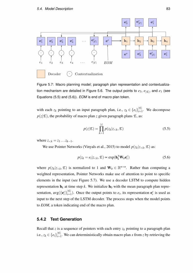
5.4. Model Description 83
e1 e2 e3 e4 . . . e|E| EOM
· · · · ·
ec1 ec2 ec3 ec4 ec|E| ee. . . h1 h2 h3 h4
es ec3 ec|E| ec1
ec3 ec|E| ec1
Decoder · Contextualization
Figure 5.7: Macro planning model; paragraph plan representation and contextualiza-
tion mechanism are detailed in Figure 5.6. The output points to e3, e|E |, and e1 (see
Equations (5.5) and (5.6)). EOM is end of macro plan token.
with each zk pointing to an input paragraph plan, i.e., zk ∈ {ei}|E |i=1. We decompose
p(z|E), the probability of macro plan z given paragraph plans E , as:
p(z|E) =|z|
∏k=1
p(zk|z<k,E) (5.5)
where z<k = z1 . . .zk−1.
We use Pointer Networks (Vinyals et al., 2015) to model p(zk|z<k,E) as:
p(zk = ei|z<k,E) ∝ exp(hᵀk Wbec
i ) (5.6)
where p(zk|z<k,E) is normalized to 1 and Wb ∈ Rn×n. Rather than computing a
weighted representation, Pointer Networks make use of attention to point to specific
elements in the input (see Figure 5.7). We use a decoder LSTM to compute hidden
representation hk at time step k. We initialize h0 with the mean paragraph plan repre-
sentation, avg({eci }|E |i=1). Once the output points to ei, its representation ec
i is used as
input to the next step of the LSTM decoder. The process stops when the model points
to EOM, a token indicating end of the macro plan.
5.4.2 Text Generation
Recall that z is a sequence of pointers with each entry zk pointing to a paragraph plan
i.e., zk ∈ {ei}|E |i=1. We can deterministically obtain macro plan x from z by retrieving the
84 Chapter 5. Macro Planning
paragraph plans being pointed to, adding <P> separators in between. The conditional
output probability p(y|x) is modeled as:
p(y|x) =|y|
∏t=1
p(yt |y<t ,x)
where y<t = y1 . . .yt−1.
To compute p(y|x), we use an encoder-decoder architecture enhanced with an at-
tention mechanism (Bahdanau et al., 2015; Luong et al., 2015a). We encode macro
plan x with a bidirectional LSTM (Hochreiter and Schmidhuber, 1997). At time step t,
we lookup the embedding of the previously predicted word yt−1 and feed it as input
to the decoder which is another LSTM unit. The decoder attends over hidden states
of the macro plan to predict yt . We further incorporate a copy mechanism (Gulcehre
et al., 2016b) in the decoder to enable copying values directly from the macro plan.
We expect the text generation model to learn to generate summary tokens while fo-
cusing on the corresponding macro plan and that the output summary will indeed fol-
low the plan in terms of the entities and events being described and their order. At the
same time, we believe that text generation is relatively easier as the encoder-decoder
model is relieved from the tasks of document structuring and information selection.
5.4.3 Training and Inference
We train two independent models for macro planning and text generation. Our training
objective for macro planning aims to maximize the log likelihood of the macro plan
given the paragraph plans:
maxθ
∑(E ,z)∈D
log p(z|E ;θ)
where D is the training set consisting of pairs of (sets of) paragraph plans and macro
plans, and θ are model parameters.
Our training objective for text generation aims to maximize the log likelihood of
the output text given the macro plan:
maxφ
∑(x,y)∈F
log p(y|x;φ)
where F is the training set consisting of pairs of macro plans and game summaries,
and φ are model parameters.
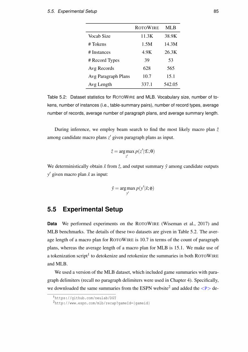
5.5. Experimental Setup 85
ROTOWIRE MLB
Vocab Size 11.3K 38.9K
# Tokens 1.5M 14.3M
# Instances 4.9K 26.3K
# Record Types 39 53
Avg Records 628 565
Avg Paragraph Plans 10.7 15.1
Avg Length 337.1 542.05
Table 5.2: Dataset statistics for ROTOWIRE and MLB. Vocabulary size, number of to-
kens, number of instances (i.e., table-summary pairs), number of record types, average
number of records, average number of paragraph plans, and average summary length.
During inference, we employ beam search to find the most likely macro plan z
among candidate macro plans z′ given paragraph plans as input.
z = argmaxz′
p(z′|E ;θ)
We deterministically obtain x from z, and output summary y among candidate outputs
y′ given macro plan x as input:
y = argmaxy′
p(y′|x;φ)
5.5 Experimental Setup
Data We performed experiments on the ROTOWIRE (Wiseman et al., 2017) and
MLB benchmarks. The details of these two datasets are given in Table 5.2. The aver-
age length of a macro plan for ROTOWIRE is 10.7 in terms of the count of paragraph
plans, whereas the average length of a macro plan for MLB is 15.1. We make use of
a tokenization script1 to detokenize and retokenize the summaries in both ROTOWIRE
and MLB.
We used a version of the MLB dataset, which included game summaries with para-
graph delimiters (recall no paragraph delimiters were used in Chapter 4). Specifically,
we downloaded the same summaries from the ESPN website2 and added the <P> de-
1https://github.com/neulab/DGT2http://www.espn.com/mlb/recap?gameId={gameid}
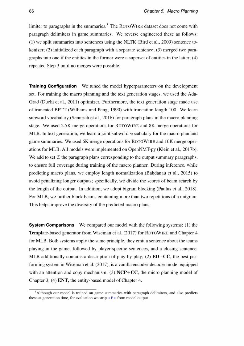
86 Chapter 5. Macro Planning
limiter to paragraphs in the summaries.3 The ROTOWIRE dataset does not come with
paragraph delimiters in game summaries. We reverse engineered these as follows:
(1) we split summaries into sentences using the NLTK (Bird et al., 2009) sentence to-
kenizer; (2) initialized each paragraph with a separate sentence; (3) merged two para-
graphs into one if the entities in the former were a superset of entities in the latter; (4)
repeated Step 3 until no merges were possible.
Training Configuration We tuned the model hyperparameters on the development
set. For training the macro planning and the text generation stages, we used the Ada-
Grad (Duchi et al., 2011) optimizer. Furthermore, the text generation stage made use
of truncated BPTT (Williams and Peng, 1990) with truncation length 100. We learn
subword vocabulary (Sennrich et al., 2016) for paragraph plans in the macro planning
stage. We used 2.5K merge operations for ROTOWIRE and 8K merge operations for
MLB. In text generation, we learn a joint subword vocabulary for the macro plan and
game summaries. We used 6K merge operations for ROTOWIRE and 16K merge oper-
ations for MLB. All models were implemented on OpenNMT-py (Klein et al., 2017b).
We add to set E the paragraph plans corresponding to the output summary paragraphs,
to ensure full coverage during training of the macro planner. During inference, while
predicting macro plans, we employ length normalization (Bahdanau et al., 2015) to
avoid penalizing longer outputs; specifically, we divide the scores of beam search by
the length of the output. In addition, we adopt bigram blocking (Paulus et al., 2018).
For MLB, we further block beams containing more than two repetitions of a unigram.
This helps improve the diversity of the predicted macro plans.
System Comparisons We compared our model with the following systems: (1) the
Template-based generator from Wiseman et al. (2017) for ROTOWIRE and Chapter 4
for MLB. Both systems apply the same principle, they emit a sentence about the teams
playing in the game, followed by player-specific sentences, and a closing sentence.
MLB additionally contains a description of play-by-play; (2) ED+CC, the best per-
forming system in Wiseman et al. (2017), is a vanilla encoder-decoder model equipped
with an attention and copy mechanism; (3) NCP+CC, the micro planning model of
Chapter 3; (4) ENT, the entity-based model of Chapter 4.
3Although our model is trained on game summaries with paragraph delimiters, and also predictsthese at generation time, for evaluation we strip <P> from model output.
5.6. Results 87
5.6 Results
Automatic Evaluation For automatic evaluation, following earlier work (Wiseman
et al. 2017 and Chapters 3 and 4, inter alia) we report BLEU (Papineni et al., 2002)
with the gold summary as reference but also make use of the Information Extraction
(IE) metrics from Wiseman et al. (2017) which are defined over the output of an IE
system.We reused the IE model from Chapter 3 for ROTOWIRE but retrained it for
MLB to improve its precision and recall.
Specifically, we improved the precision of the IE system for MLB by making use
of event detection. The earlier system matches entities (e.g., Mullins from Figure 5.1)
to record types (e.g., double batter) no matter which play they occur in, thus resulting
in too many false positives. Instead, we extract inning information from model output
summaries following the steps in Section 5.3.2, and narrow down the valid candidates
for record types to those present in the plays of a specific inning. For example, we
verify if double by Mullins indeed occurred in the sixth inning. We thus increase
the recall of play-by-play by including more record types such as ground out, triple,
sacrifice fly, etc.
Furthermore, the implementation of Wiseman et al. (2017) computes RG, CS, and
CO excluding duplicate relations. This artificially inflates the performance of models
whose outputs contain repetition. We include duplicates in the computation of the IE
metrics (and recreate them for all comparison systems).
Table 5.3 (top) presents our results on the ROTOWIRE test set. In addition to
Templ, NCP+CC, ENT, and ED+CC we include the best performing model of Wise-
man et al. (2017) (WS-2017; note that ED+CC is an improved re-implementation of
their model), and the model of Rebuffel et al. (2020) (RBF-2020) which represents the
state of the art on ROTOWIRE. This model has a Transformer encoder (Vaswani et al.,
2017) with a hierarchical attention mechanism over entities and records within entities.
The models of Saleh et al. (2019), Iso et al. (2019), and Gong et al. (2019) make use
of additional information not present in the input (e.g., previous/next games, summary
writer) and are not directly comparable to the systems in Table 5.3. Results for the
MLB test set are in the bottom portion of Table 5.3.
Templ has the highest RG precision and count on both datasets. This is not surpris-
ing, by design Templ is always faithful to the input. However, notice that it achieves
the lowest BLEU amongst comparison systems indicating that it mostly regurgitates
facts with low fluency. Macro achieves the highest RG precision amongst all neural
88 Chapter 5. Macro Planning
ROTOWIRERG CS CO
BLEU# P% P% R% F% DLD%
Templ 54.3 99.9 27.1 57.7 36.9 13.1 8.46
WS-2017 34.1 75.1 20.3 36.3 26.1 12.4 14.19
ED+CC 35.9 82.6 19.8 33.8 24.9 12.0 14.99
NCP+CC 40.8 87.6 28.0 51.1 36.2 15.8 16.50
ENT 32.7 91.7 34.7 48.5 40.5 16.6 16.12
RBF-2020 44.9 89.5 23.9 47.0 31.7 14.3 17.16
Macro 42.1 97.6 34.1 57.8 42.9 17.7 15.46
−Plan(4) 36.2 81.3 22.1 38.6 28.1 12.1 14.00
MLBRG CS CO
BLEU# P% P% R% F% DLD%
Templ 62.3 99.9 21.6 55.2 31.0 11.0 4.12
ED+CC 32.5 91.3 27.8 40.6 33.0 17.1 9.68
NCP+CC 19.6 81.3 44.5 44.1 44.3 21.9 9.68
ENT 23.8 81.1 40.9 49.5 44.8 20.7 11.50
Macro 30.8 94.4 40.8 54.9 46.8 21.8 12.62−Plan(SP,4) 25.1 92.7 40.0 44.6 42.2 21.9 11.09
Table 5.3: Evaluation on ROTOWIRE and MLB test sets; relation generation (RG)
count (#) and precision (P%), content selection (CS) precision (P%), recall (R%)
and F-measure (F%), content ordering (CO) in complement of normalized Damerau-
Levenshtein distance (DLD%), and BLEU.
models for ROTOWIRE and MLB. We obtain an absolute improvement of 5.9% over
ENT for ROTOWIRE and 13.3% for MLB. In addition, Macro achieves the highest CS
F-measure for both datasets. On ROTOWIRE, Macro achieves the highest CO score,
and the highest BLEU on MLB. On ROTOWIRE, in terms of BLEU, Macro is worse
than comparison models (e.g., NCP+CC or ENT). Inspection of the output showed that
the opening paragraph, which mostly describes how the two teams fared, is generally
shorter in Macro, leading to shorter summaries and thus lower BLEU. There is high
variance in the length of the opening paragraph in the training data4 and Macro ver-
balizes the corresponding plan conservatively. Ideas such as length normalisation (Wu
4The length of the opening paragraph ranges from 6 tokens to 258 tokens in ROTOWIRE.
5.6. Results 89
Macro CS-P CS-R CS-F CO
ROTOWIRE 81.3 73.2 77.0 45.8
MLB 80.6 63.3 70.9 31.4
Table 5.4: Evaluation of macro planning stage; content selection precision (CS-P), recall
(CS-R), F-measure (CS-F) and content ordering (CO) between the inferred plans and
gold plans in terms of entities and events for ROTOWIRE (RW) and MLB test sets.
et al., 2016) or length control (Kikuchi et al., 2016; Takeno et al., 2017; Fan et al.,
2018) could help alleviate this; however, we do not pursue them further for fair com-
parison with the other models.
The Contribution of Macro Planning To study the effect of macro planning in more
detail, we further compared Macro against text generation models (see Section 5.4.2)
which are trained on verbalizations of the tabular data (and gold summaries) but do
not make use of document plans or a document planning mechanism. On ROTOWIRE,
the model was trained on verbalizations of players and teams, with the input arranged
such that the verbalization of the home team was followed by the visiting team, the
home team players and the visiting team players. Mention of players was limited to
the four best ones, following Saleh et al. (2019) (see−Plan(4) in Table 5.3). For MLB,
we additionally include verbalizations of innings focusing on scoring plays which are
likely to be discussed in game summaries (see −Plan(SP,4) in Table 5.3). Note that
by preprocessing the input in such a way some simple form of content selection takes
place simply by removing extraneous information which the model does not need to
consider.
Across both datasets,−Plan variants appear competitive. On ROTOWIRE−Plan(4)
is better than ED+CC in terms of content selection but worse compared to ENT. On
MLB, −Plan(SP,4) is again superior to ED+CC in terms of content selection but not
ENT whose performance lags behind when considering RG precision. Taken together,
these results confirm that verbalizing entities and events into a text sequence is effec-
tive. At the same time, we see that −Plan variants are worse than Macro across most
metrics which underlines the importance of an explicit planning component.
Table 5.4 presents intrinsic evaluation of the macro planning stage. Here, we com-
pare the inferred macro plan with the gold macro plans. We use the CS and CO metrics
but compute them over entities and events instead of relations. We see that our macro
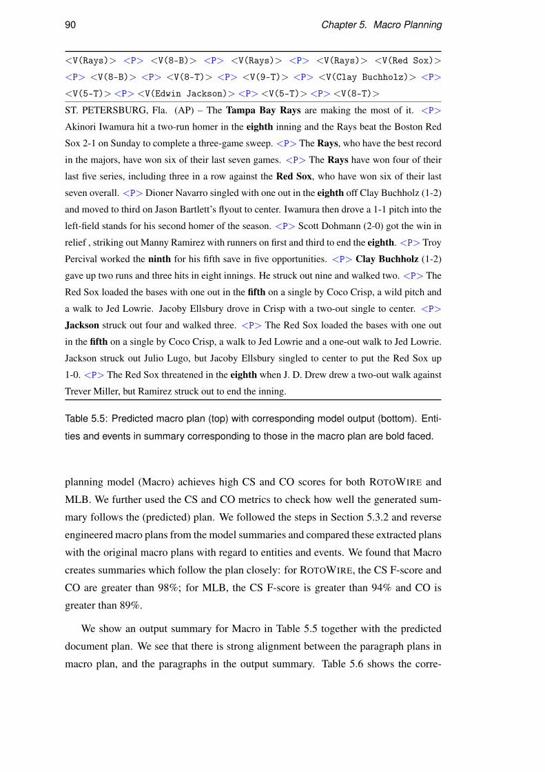
90 Chapter 5. Macro Planning
<V(Rays)> <P> <V(8-B)> <P> <V(Rays)> <P> <V(Rays)> <V(Red Sox)>
<P> <V(8-B)> <P> <V(8-T)> <P> <V(9-T)> <P> <V(Clay Buchholz)> <P>
<V(5-T)> <P> <V(Edwin Jackson)> <P> <V(5-T)> <P> <V(8-T)>
ST. PETERSBURG, Fla. (AP) – The Tampa Bay Rays are making the most of it. <P>
Akinori Iwamura hit a two-run homer in the eighth inning and the Rays beat the Boston Red
Sox 2-1 on Sunday to complete a three-game sweep. <P> The Rays, who have the best record
in the majors, have won six of their last seven games. <P> The Rays have won four of their
last five series, including three in a row against the Red Sox, who have won six of their last
seven overall. <P> Dioner Navarro singled with one out in the eighth off Clay Buchholz (1-2)
and moved to third on Jason Bartlett’s flyout to center. Iwamura then drove a 1-1 pitch into the
left-field stands for his second homer of the season. <P> Scott Dohmann (2-0) got the win in
relief , striking out Manny Ramirez with runners on first and third to end the eighth. <P> Troy
Percival worked the ninth for his fifth save in five opportunities. <P> Clay Buchholz (1-2)
gave up two runs and three hits in eight innings. He struck out nine and walked two. <P> The
Red Sox loaded the bases with one out in the fifth on a single by Coco Crisp, a wild pitch and
a walk to Jed Lowrie. Jacoby Ellsbury drove in Crisp with a two-out single to center. <P>
Jackson struck out four and walked three. <P> The Red Sox loaded the bases with one out
in the fifth on a single by Coco Crisp, a walk to Jed Lowrie and a one-out walk to Jed Lowrie.
Jackson struck out Julio Lugo, but Jacoby Ellsbury singled to center to put the Red Sox up
1-0. <P> The Red Sox threatened in the eighth when J. D. Drew drew a two-out walk against
Trever Miller, but Ramirez struck out to end the inning.
Table 5.5: Predicted macro plan (top) with corresponding model output (bottom). Enti-
ties and events in summary corresponding to those in the macro plan are bold faced.
planning model (Macro) achieves high CS and CO scores for both ROTOWIRE and
MLB. We further used the CS and CO metrics to check how well the generated sum-
mary follows the (predicted) plan. We followed the steps in Section 5.3.2 and reverse
engineered macro plans from the model summaries and compared these extracted plans
with the original macro plans with regard to entities and events. We found that Macro
creates summaries which follow the plan closely: for ROTOWIRE, the CS F-score and
CO are greater than 98%; for MLB, the CS F-score is greater than 94% and CO is
greater than 89%.
We show an output summary for Macro in Table 5.5 together with the predicted
document plan. We see that there is strong alignment between the paragraph plans in
macro plan, and the paragraphs in the output summary. Table 5.6 shows the corre-
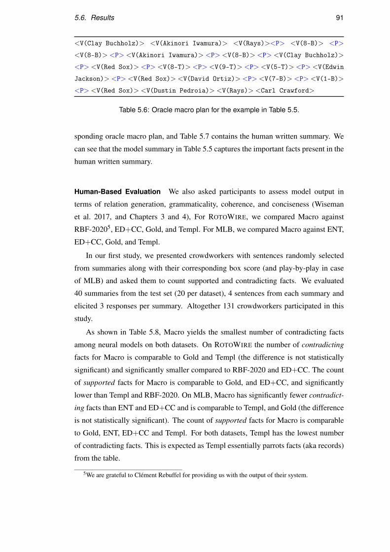
5.6. Results 91
<V(Clay Buchholz)> <V(Akinori Iwamura)> <V(Rays)><P> <V(8-B)> <P>
<V(8-B)> <P> <V(Akinori Iwamura)> <P> <V(8-B)> <P> <V(Clay Buchholz)>
<P> <V(Red Sox)> <P> <V(8-T)> <P> <V(9-T)> <P> <V(5-T)> <P> <V(Edwin
Jackson)> <P> <V(Red Sox)> <V(David Ortiz)> <P> <V(7-B)> <P> <V(1-B)>
<P> <V(Red Sox)> <V(Dustin Pedroia)> <V(Rays)> <Carl Crawford>
Table 5.6: Oracle macro plan for the example in Table 5.5.
sponding oracle macro plan, and Table 5.7 contains the human written summary. We
can see that the model summary in Table 5.5 captures the important facts present in the
human written summary.
Human-Based Evaluation We also asked participants to assess model output in
terms of relation generation, grammaticality, coherence, and conciseness (Wiseman
et al. 2017, and Chapters 3 and 4), For ROTOWIRE, we compared Macro against
RBF-20205, ED+CC, Gold, and Templ. For MLB, we compared Macro against ENT,
ED+CC, Gold, and Templ.
In our first study, we presented crowdworkers with sentences randomly selected
from summaries along with their corresponding box score (and play-by-play in case
of MLB) and asked them to count supported and contradicting facts. We evaluated
40 summaries from the test set (20 per dataset), 4 sentences from each summary and
elicited 3 responses per summary. Altogether 131 crowdworkers participated in this
study.
As shown in Table 5.8, Macro yields the smallest number of contradicting facts
among neural models on both datasets. On ROTOWIRE the number of contradicting
facts for Macro is comparable to Gold and Templ (the difference is not statistically
significant) and significantly smaller compared to RBF-2020 and ED+CC. The count
of supported facts for Macro is comparable to Gold, and ED+CC, and significantly
lower than Templ and RBF-2020. On MLB, Macro has significantly fewer contradict-
ing facts than ENT and ED+CC and is comparable to Templ, and Gold (the difference
is not statistically significant). The count of supported facts for Macro is comparable
to Gold, ENT, ED+CC and Templ. For both datasets, Templ has the lowest number
of contradicting facts. This is expected as Templ essentially parrots facts (aka records)
from the table.
5We are grateful to Clément Rebuffel for providing us with the output of their system.
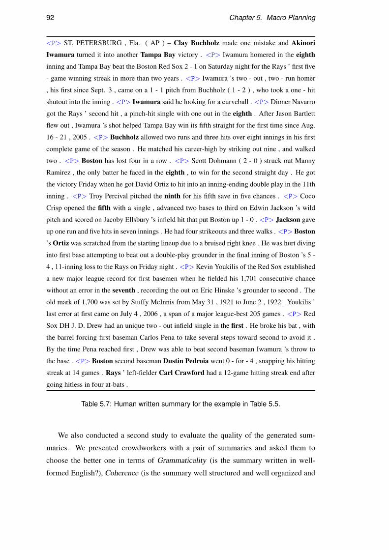
92 Chapter 5. Macro Planning
<P> ST. PETERSBURG , Fla. ( AP ) – Clay Buchholz made one mistake and Akinori
Iwamura turned it into another Tampa Bay victory . <P> Iwamura homered in the eighth
inning and Tampa Bay beat the Boston Red Sox 2 - 1 on Saturday night for the Rays ’ first five
- game winning streak in more than two years . <P> Iwamura ’s two - out , two - run homer
, his first since Sept. 3 , came on a 1 - 1 pitch from Buchholz ( 1 - 2 ) , who took a one - hit
shutout into the inning . <P> Iwamura said he looking for a curveball . <P> Dioner Navarro
got the Rays ’ second hit , a pinch-hit single with one out in the eighth . After Jason Bartlett
flew out , Iwamura ’s shot helped Tampa Bay win its fifth straight for the first time since Aug.
16 - 21 , 2005 . <P> Buchholz allowed two runs and three hits over eight innings in his first
complete game of the season . He matched his career-high by striking out nine , and walked
two . <P> Boston has lost four in a row . <P> Scott Dohmann ( 2 - 0 ) struck out Manny
Ramirez , the only batter he faced in the eighth , to win for the second straight day . He got
the victory Friday when he got David Ortiz to hit into an inning-ending double play in the 11th
inning . <P> Troy Percival pitched the ninth for his fifth save in five chances . <P> Coco
Crisp opened the fifth with a single , advanced two bases to third on Edwin Jackson ’s wild
pitch and scored on Jacoby Ellsbury ’s infield hit that put Boston up 1 - 0 . <P> Jackson gave
up one run and five hits in seven innings . He had four strikeouts and three walks . <P> Boston
’s Ortiz was scratched from the starting lineup due to a bruised right knee . He was hurt diving
into first base attempting to beat out a double-play grounder in the final inning of Boston ’s 5 -
4 , 11-inning loss to the Rays on Friday night . <P> Kevin Youkilis of the Red Sox established
a new major league record for first basemen when he fielded his 1,701 consecutive chance
without an error in the seventh , recording the out on Eric Hinske ’s grounder to second . The
old mark of 1,700 was set by Stuffy McInnis from May 31 , 1921 to June 2 , 1922 . Youkilis ’
last error at first came on July 4 , 2006 , a span of a major league-best 205 games . <P> Red
Sox DH J. D. Drew had an unique two - out infield single in the first . He broke his bat , with
the barrel forcing first baseman Carlos Pena to take several steps toward second to avoid it .
By the time Pena reached first , Drew was able to beat second baseman Iwamura ’s throw to
the base . <P> Boston second baseman Dustin Pedroia went 0 - for - 4 , snapping his hitting
streak at 14 games . Rays ’ left-fielder Carl Crawford had a 12-game hitting streak end after
going hitless in four at-bats .
Table 5.7: Human written summary for the example in Table 5.5.
We also conducted a second study to evaluate the quality of the generated sum-
maries. We presented crowdworkers with a pair of summaries and asked them to
choose the better one in terms of Grammaticality (is the summary written in well-
formed English?), Coherence (is the summary well structured and well organized and
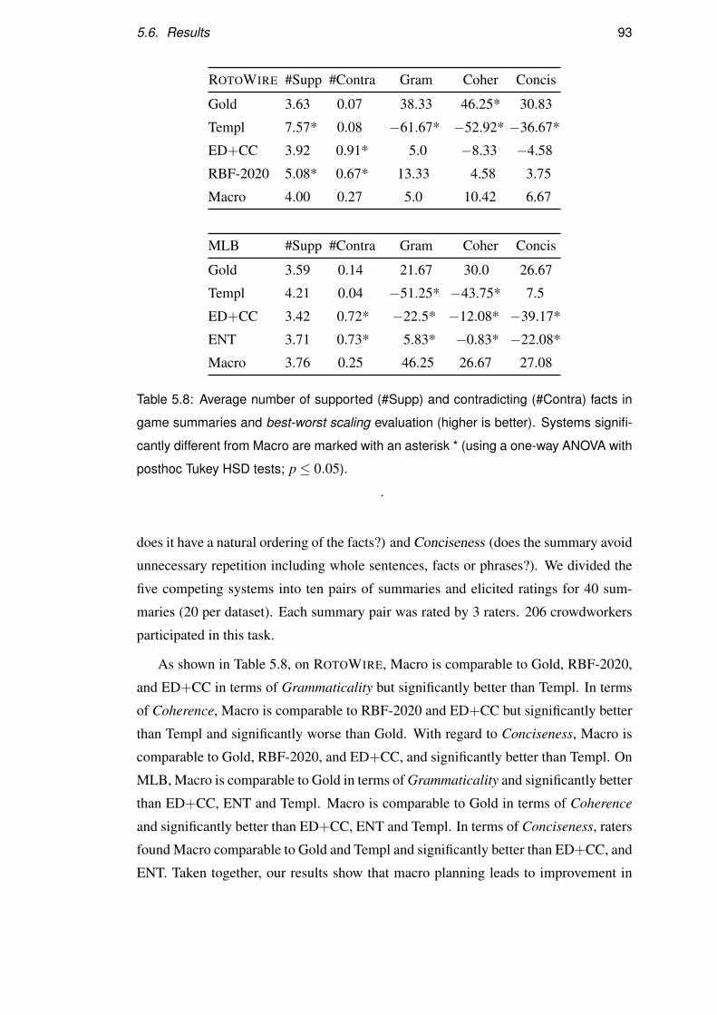
5.6. Results 93
ROTOWIRE #Supp #Contra Gram Coher Concis
Gold 3.63 0.07 38.33 46.25* 30.83
Templ 7.57* 0.08 −61.67* −52.92* −36.67*
ED+CC 3.92 0.91* 5.0 −8.33 −4.58
RBF-2020 5.08* 0.67* 13.33 4.58 3.75
Macro 4.00 0.27 5.0 10.42 6.67
MLB #Supp #Contra Gram Coher Concis
Gold 3.59 0.14 21.67 30.0 26.67
Templ 4.21 0.04 −51.25* −43.75* 7.5
ED+CC 3.42 0.72* −22.5* −12.08* −39.17*
ENT 3.71 0.73* 5.83* −0.83* −22.08*
Macro 3.76 0.25 46.25 26.67 27.08
Table 5.8: Average number of supported (#Supp) and contradicting (#Contra) facts in
game summaries and best-worst scaling evaluation (higher is better). Systems signifi-
cantly different from Macro are marked with an asterisk * (using a one-way ANOVA with
posthoc Tukey HSD tests; p≤ 0.05).
.
does it have a natural ordering of the facts?) and Conciseness (does the summary avoid
unnecessary repetition including whole sentences, facts or phrases?). We divided the
five competing systems into ten pairs of summaries and elicited ratings for 40 sum-
maries (20 per dataset). Each summary pair was rated by 3 raters. 206 crowdworkers
participated in this task.
As shown in Table 5.8, on ROTOWIRE, Macro is comparable to Gold, RBF-2020,
and ED+CC in terms of Grammaticality but significantly better than Templ. In terms
of Coherence, Macro is comparable to RBF-2020 and ED+CC but significantly better
than Templ and significantly worse than Gold. With regard to Conciseness, Macro is
comparable to Gold, RBF-2020, and ED+CC, and significantly better than Templ. On
MLB, Macro is comparable to Gold in terms of Grammaticality and significantly better
than ED+CC, ENT and Templ. Macro is comparable to Gold in terms of Coherence
and significantly better than ED+CC, ENT and Templ. In terms of Conciseness, raters
found Macro comparable to Gold and Templ and significantly better than ED+CC, and
ENT. Taken together, our results show that macro planning leads to improvement in
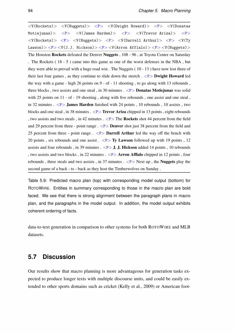
94 Chapter 5. Macro Planning
<V(Rockets)> <V(Nuggets)> <P> <V(Dwight Howard)> <P> <V(Donatas
Motiejunas)> <P> <V(James Harden)> <P> <V(Trevor Ariza)> <P>
<V(Rockets)> <P> <V(Nuggets)> <P> <V(Darrell Arthur)> <P> <V(Ty
Lawson)><P><V(J.J. Hickson)><P><V(Arron Afflalo)><P><V(Nuggets)>
The Houston Rockets defeated the Denver Nuggets , 108 - 96 , at Toyota Center on Saturday
. The Rockets ( 18 - 5 ) came into this game as one of the worst defenses in the NBA , but
they were able to prevail with a huge road win . The Nuggets ( 10 - 13 ) have now lost three of
their last four games , as they continue to slide down the stretch . <P> Dwight Howard led
the way with a game - high 26 points on 9 - of - 11 shooting , to go along with 13 rebounds ,
three blocks , two assists and one steal , in 30 minutes . <P> Donatas Motiejunas was solid
with 25 points on 11 - of - 19 shooting , along with five rebounds , one assist and one steal ,
in 32 minutes . <P> James Harden finished with 24 points , 10 rebounds , 10 assists , two
blocks and one steal , in 38 minutes . <P> Trevor Ariza chipped in 13 points , eight rebounds
, two assists and two steals , in 42 minutes . <P> The Rockets shot 44 percent from the field
and 29 percent from three - point range . <P> Denver shot just 38 percent from the field and
25 percent from three - point range . <P> Darrell Arthur led the way off the bench with
20 points , six rebounds and one assist . <P> Ty Lawson followed up with 19 points , 12
assists and four rebounds , in 39 minutes . <P> J. J. Hickson added 14 points , 10 rebounds
, two assists and two blocks , in 22 minutes . <P> Arron Afflalo chipped in 12 points , four
rebounds , three steals and two assists , in 37 minutes . <P> Next up , the Nuggets play the
second game of a back - to - back as they host the Timberwolves on Sunday .
Table 5.9: Predicted macro plan (top) with corresponding model output (bottom) for
ROTOWIRE. Entities in summary corresponding to those in the macro plan are bold
faced. We see that there is strong alignment between the paragraph plans in macro
plan, and the paragraphs in the model output. In addition, the model output exhibits
coherent ordering of facts.
data-to-text generation in comparison to other systems for both ROTOWIRE and MLB
datasets.
5.7 Discussion
Our results show that macro planning is more advantageous for generation tasks ex-
pected to produce longer texts with multiple discourse units, and could be easily ex-
tended to other sports domains such as cricket (Kelly et al., 2009) or American foot-
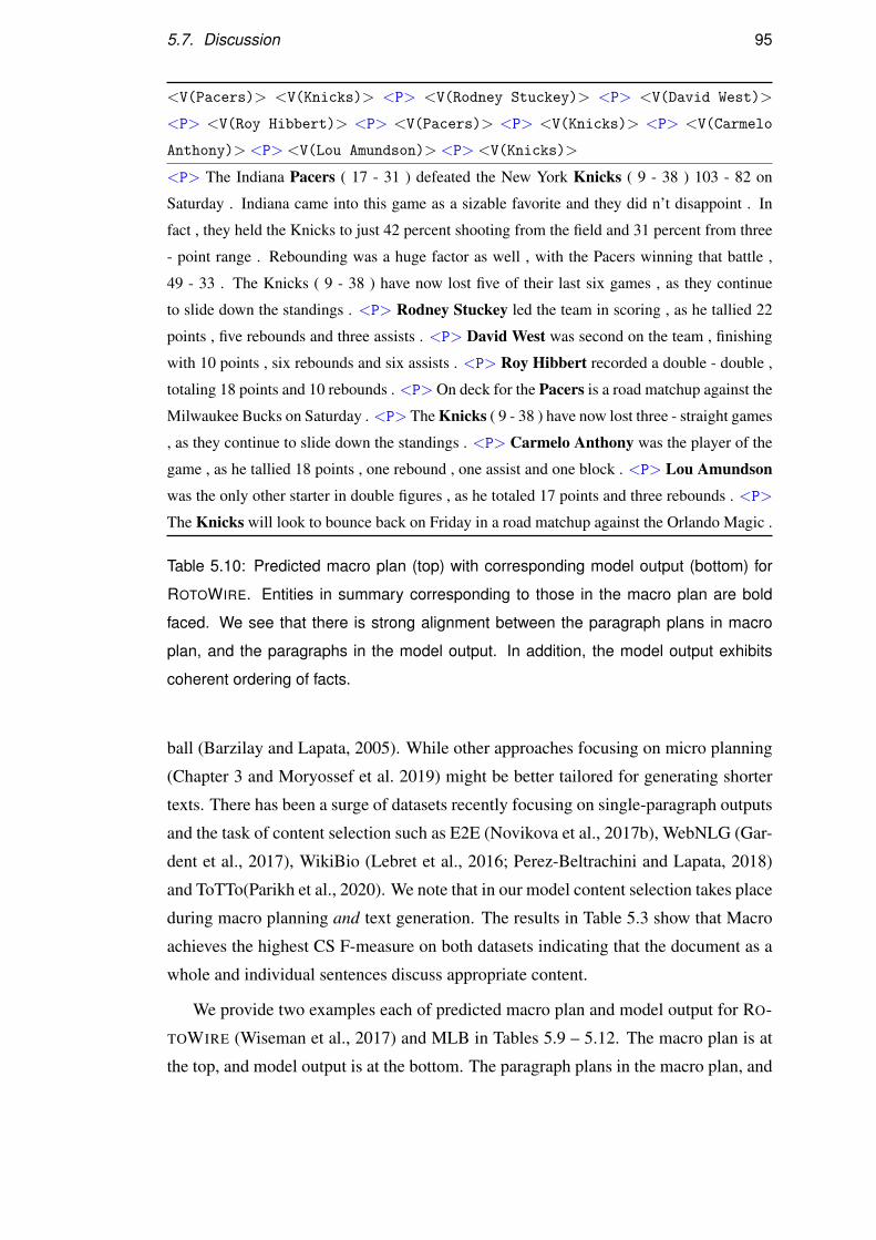
5.7. Discussion 95
<V(Pacers)> <V(Knicks)> <P> <V(Rodney Stuckey)> <P> <V(David West)>
<P> <V(Roy Hibbert)> <P> <V(Pacers)> <P> <V(Knicks)> <P> <V(Carmelo
Anthony)> <P> <V(Lou Amundson)> <P> <V(Knicks)>
<P> The Indiana Pacers ( 17 - 31 ) defeated the New York Knicks ( 9 - 38 ) 103 - 82 on
Saturday . Indiana came into this game as a sizable favorite and they did n’t disappoint . In
fact , they held the Knicks to just 42 percent shooting from the field and 31 percent from three
- point range . Rebounding was a huge factor as well , with the Pacers winning that battle ,
49 - 33 . The Knicks ( 9 - 38 ) have now lost five of their last six games , as they continue
to slide down the standings . <P> Rodney Stuckey led the team in scoring , as he tallied 22
points , five rebounds and three assists . <P> David West was second on the team , finishing
with 10 points , six rebounds and six assists . <P> Roy Hibbert recorded a double - double ,
totaling 18 points and 10 rebounds . <P> On deck for the Pacers is a road matchup against the
Milwaukee Bucks on Saturday . <P> The Knicks ( 9 - 38 ) have now lost three - straight games
, as they continue to slide down the standings . <P> Carmelo Anthony was the player of the
game , as he tallied 18 points , one rebound , one assist and one block . <P> Lou Amundson
was the only other starter in double figures , as he totaled 17 points and three rebounds . <P>
The Knicks will look to bounce back on Friday in a road matchup against the Orlando Magic .
Table 5.10: Predicted macro plan (top) with corresponding model output (bottom) for
ROTOWIRE. Entities in summary corresponding to those in the macro plan are bold
faced. We see that there is strong alignment between the paragraph plans in macro
plan, and the paragraphs in the model output. In addition, the model output exhibits
coherent ordering of facts.
ball (Barzilay and Lapata, 2005). While other approaches focusing on micro planning
(Chapter 3 and Moryossef et al. 2019) might be better tailored for generating shorter
texts. There has been a surge of datasets recently focusing on single-paragraph outputs
and the task of content selection such as E2E (Novikova et al., 2017b), WebNLG (Gar-
dent et al., 2017), WikiBio (Lebret et al., 2016; Perez-Beltrachini and Lapata, 2018)
and ToTTo(Parikh et al., 2020). We note that in our model content selection takes place
during macro planning and text generation. The results in Table 5.3 show that Macro
achieves the highest CS F-measure on both datasets indicating that the document as a
whole and individual sentences discuss appropriate content.
We provide two examples each of predicted macro plan and model output for RO-
TOWIRE (Wiseman et al., 2017) and MLB in Tables 5.9 – 5.12. The macro plan is at
the top, and model output is at the bottom. The paragraph plans in the macro plan, and
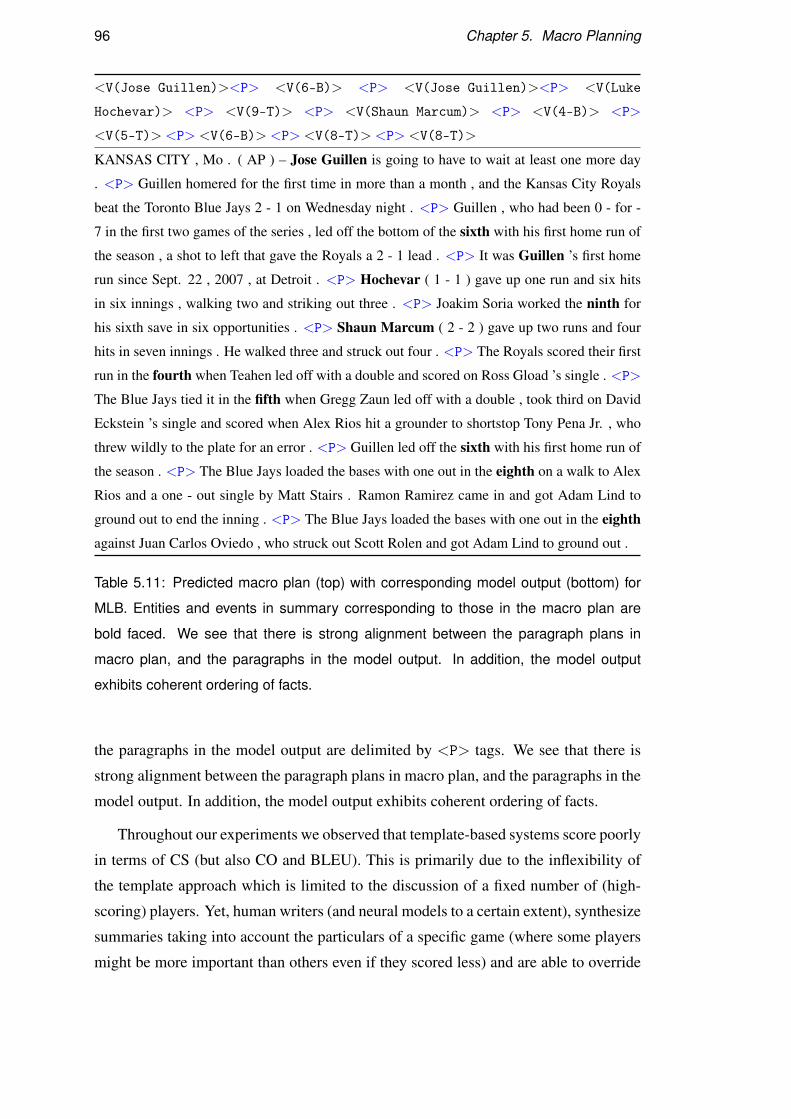
96 Chapter 5. Macro Planning
<V(Jose Guillen)><P> <V(6-B)> <P> <V(Jose Guillen)><P> <V(Luke
Hochevar)> <P> <V(9-T)> <P> <V(Shaun Marcum)> <P> <V(4-B)> <P>
<V(5-T)> <P> <V(6-B)> <P> <V(8-T)> <P> <V(8-T)>
KANSAS CITY , Mo . ( AP ) – Jose Guillen is going to have to wait at least one more day
. <P> Guillen homered for the first time in more than a month , and the Kansas City Royals
beat the Toronto Blue Jays 2 - 1 on Wednesday night . <P> Guillen , who had been 0 - for -
7 in the first two games of the series , led off the bottom of the sixth with his first home run of
the season , a shot to left that gave the Royals a 2 - 1 lead . <P> It was Guillen ’s first home
run since Sept. 22 , 2007 , at Detroit . <P> Hochevar ( 1 - 1 ) gave up one run and six hits
in six innings , walking two and striking out three . <P> Joakim Soria worked the ninth for
his sixth save in six opportunities . <P> Shaun Marcum ( 2 - 2 ) gave up two runs and four
hits in seven innings . He walked three and struck out four . <P> The Royals scored their first
run in the fourth when Teahen led off with a double and scored on Ross Gload ’s single . <P>
The Blue Jays tied it in the fifth when Gregg Zaun led off with a double , took third on David
Eckstein ’s single and scored when Alex Rios hit a grounder to shortstop Tony Pena Jr. , who
threw wildly to the plate for an error . <P> Guillen led off the sixth with his first home run of
the season . <P> The Blue Jays loaded the bases with one out in the eighth on a walk to Alex
Rios and a one - out single by Matt Stairs . Ramon Ramirez came in and got Adam Lind to
ground out to end the inning . <P> The Blue Jays loaded the bases with one out in the eighth
against Juan Carlos Oviedo , who struck out Scott Rolen and got Adam Lind to ground out .
Table 5.11: Predicted macro plan (top) with corresponding model output (bottom) for
MLB. Entities and events in summary corresponding to those in the macro plan are
bold faced. We see that there is strong alignment between the paragraph plans in
macro plan, and the paragraphs in the model output. In addition, the model output
exhibits coherent ordering of facts.
the paragraphs in the model output are delimited by <P> tags. We see that there is
strong alignment between the paragraph plans in macro plan, and the paragraphs in the
model output. In addition, the model output exhibits coherent ordering of facts.
Throughout our experiments we observed that template-based systems score poorly
in terms of CS (but also CO and BLEU). This is primarily due to the inflexibility of
the template approach which is limited to the discussion of a fixed number of (high-
scoring) players. Yet, human writers (and neural models to a certain extent), synthesize
summaries taking into account the particulars of a specific game (where some players
might be more important than others even if they scored less) and are able to override
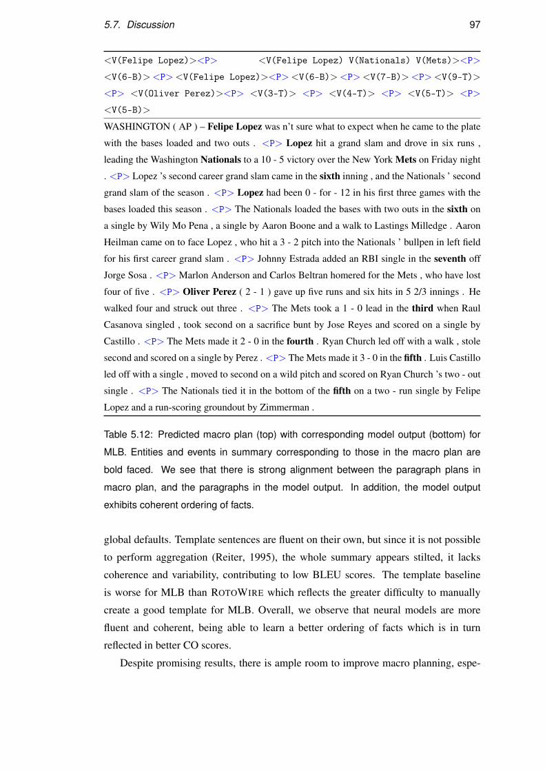
5.7. Discussion 97
<V(Felipe Lopez)><P> <V(Felipe Lopez) V(Nationals) V(Mets)><P>
<V(6-B)><P><V(Felipe Lopez)><P><V(6-B)><P><V(7-B)><P><V(9-T)>
<P> <V(Oliver Perez)><P> <V(3-T)> <P> <V(4-T)> <P> <V(5-T)> <P>
<V(5-B)>
WASHINGTON ( AP ) – Felipe Lopez was n’t sure what to expect when he came to the plate
with the bases loaded and two outs . <P> Lopez hit a grand slam and drove in six runs ,
leading the Washington Nationals to a 10 - 5 victory over the New York Mets on Friday night
. <P> Lopez ’s second career grand slam came in the sixth inning , and the Nationals ’ second
grand slam of the season . <P> Lopez had been 0 - for - 12 in his first three games with the
bases loaded this season . <P> The Nationals loaded the bases with two outs in the sixth on
a single by Wily Mo Pena , a single by Aaron Boone and a walk to Lastings Milledge . Aaron
Heilman came on to face Lopez , who hit a 3 - 2 pitch into the Nationals ’ bullpen in left field
for his first career grand slam . <P> Johnny Estrada added an RBI single in the seventh off
Jorge Sosa . <P> Marlon Anderson and Carlos Beltran homered for the Mets , who have lost
four of five . <P> Oliver Perez ( 2 - 1 ) gave up five runs and six hits in 5 2/3 innings . He
walked four and struck out three . <P> The Mets took a 1 - 0 lead in the third when Raul
Casanova singled , took second on a sacrifice bunt by Jose Reyes and scored on a single by
Castillo . <P> The Mets made it 2 - 0 in the fourth . Ryan Church led off with a walk , stole
second and scored on a single by Perez . <P> The Mets made it 3 - 0 in the fifth . Luis Castillo
led off with a single , moved to second on a wild pitch and scored on Ryan Church ’s two - out
single . <P> The Nationals tied it in the bottom of the fifth on a two - run single by Felipe
Lopez and a run-scoring groundout by Zimmerman .
Table 5.12: Predicted macro plan (top) with corresponding model output (bottom) for
MLB. Entities and events in summary corresponding to those in the macro plan are
bold faced. We see that there is strong alignment between the paragraph plans in
macro plan, and the paragraphs in the model output. In addition, the model output
exhibits coherent ordering of facts.
global defaults. Template sentences are fluent on their own, but since it is not possible
to perform aggregation (Reiter, 1995), the whole summary appears stilted, it lacks
coherence and variability, contributing to low BLEU scores. The template baseline
is worse for MLB than ROTOWIRE which reflects the greater difficulty to manually
create a good template for MLB. Overall, we observe that neural models are more
fluent and coherent, being able to learn a better ordering of facts which is in turn
reflected in better CO scores.
Despite promising results, there is ample room to improve macro planning, espe-
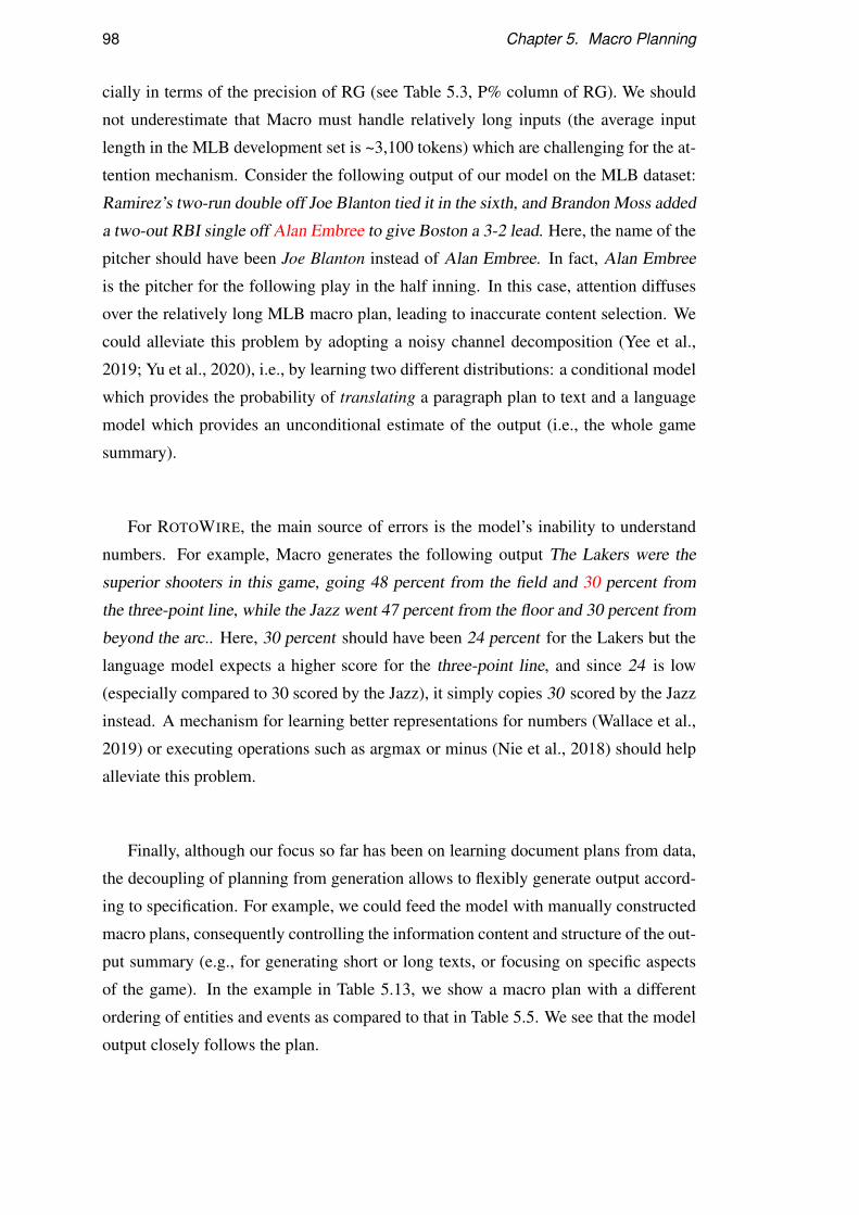
98 Chapter 5. Macro Planning
cially in terms of the precision of RG (see Table 5.3, P% column of RG). We should
not underestimate that Macro must handle relatively long inputs (the average input
length in the MLB development set is ~3,100 tokens) which are challenging for the at-
tention mechanism. Consider the following output of our model on the MLB dataset:
Ramirez’s two-run double off Joe Blanton tied it in the sixth, and Brandon Moss added
a two-out RBI single off Alan Embree to give Boston a 3-2 lead. Here, the name of the
pitcher should have been Joe Blanton instead of Alan Embree. In fact, Alan Embree
is the pitcher for the following play in the half inning. In this case, attention diffuses
over the relatively long MLB macro plan, leading to inaccurate content selection. We
could alleviate this problem by adopting a noisy channel decomposition (Yee et al.,
2019; Yu et al., 2020), i.e., by learning two different distributions: a conditional model
which provides the probability of translating a paragraph plan to text and a language
model which provides an unconditional estimate of the output (i.e., the whole game
summary).
For ROTOWIRE, the main source of errors is the model’s inability to understand
numbers. For example, Macro generates the following output The Lakers were the
superior shooters in this game, going 48 percent from the field and 30 percent from
the three-point line, while the Jazz went 47 percent from the floor and 30 percent from
beyond the arc.. Here, 30 percent should have been 24 percent for the Lakers but the
language model expects a higher score for the three-point line, and since 24 is low
(especially compared to 30 scored by the Jazz), it simply copies 30 scored by the Jazz
instead. A mechanism for learning better representations for numbers (Wallace et al.,
2019) or executing operations such as argmax or minus (Nie et al., 2018) should help
alleviate this problem.
Finally, although our focus so far has been on learning document plans from data,
the decoupling of planning from generation allows to flexibly generate output accord-
ing to specification. For example, we could feed the model with manually constructed
macro plans, consequently controlling the information content and structure of the out-
put summary (e.g., for generating short or long texts, or focusing on specific aspects
of the game). In the example in Table 5.13, we show a macro plan with a different
ordering of entities and events as compared to that in Table 5.5. We see that the model
output closely follows the plan.
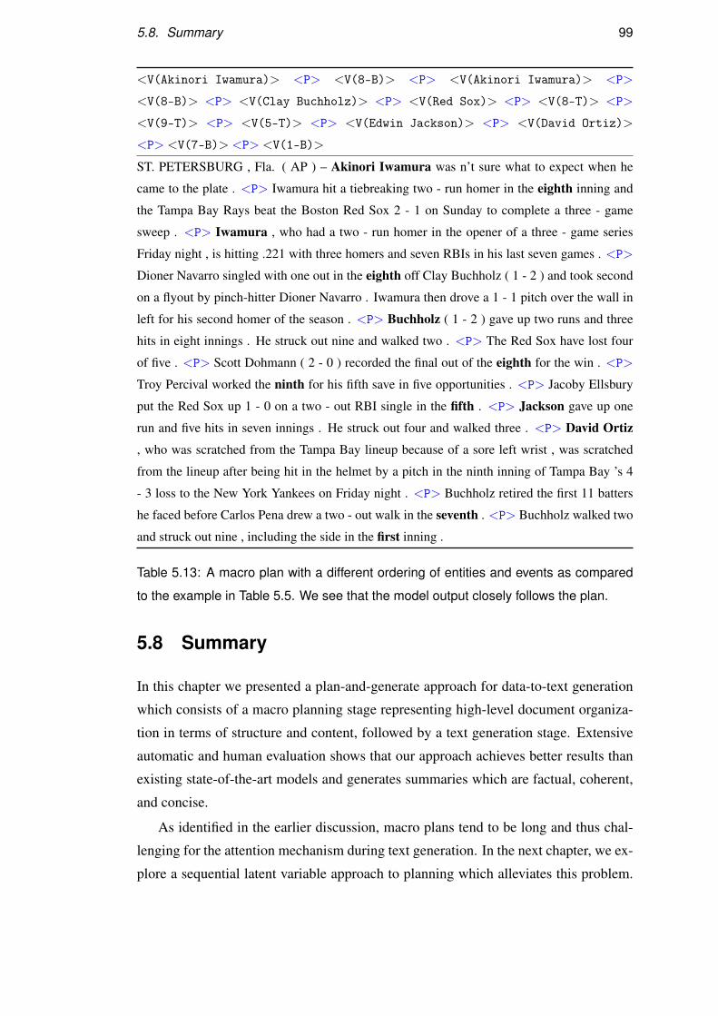
5.8. Summary 99
<V(Akinori Iwamura)> <P> <V(8-B)> <P> <V(Akinori Iwamura)> <P>
<V(8-B)> <P> <V(Clay Buchholz)> <P> <V(Red Sox)> <P> <V(8-T)> <P>
<V(9-T)> <P> <V(5-T)> <P> <V(Edwin Jackson)> <P> <V(David Ortiz)>
<P> <V(7-B)> <P> <V(1-B)>
ST. PETERSBURG , Fla. ( AP ) – Akinori Iwamura was n’t sure what to expect when he
came to the plate . <P> Iwamura hit a tiebreaking two - run homer in the eighth inning and
the Tampa Bay Rays beat the Boston Red Sox 2 - 1 on Sunday to complete a three - game
sweep . <P> Iwamura , who had a two - run homer in the opener of a three - game series
Friday night , is hitting .221 with three homers and seven RBIs in his last seven games . <P>
Dioner Navarro singled with one out in the eighth off Clay Buchholz ( 1 - 2 ) and took second
on a flyout by pinch-hitter Dioner Navarro . Iwamura then drove a 1 - 1 pitch over the wall in
left for his second homer of the season . <P> Buchholz ( 1 - 2 ) gave up two runs and three
hits in eight innings . He struck out nine and walked two . <P> The Red Sox have lost four
of five . <P> Scott Dohmann ( 2 - 0 ) recorded the final out of the eighth for the win . <P>
Troy Percival worked the ninth for his fifth save in five opportunities . <P> Jacoby Ellsbury
put the Red Sox up 1 - 0 on a two - out RBI single in the fifth . <P> Jackson gave up one
run and five hits in seven innings . He struck out four and walked three . <P> David Ortiz
, who was scratched from the Tampa Bay lineup because of a sore left wrist , was scratched
from the lineup after being hit in the helmet by a pitch in the ninth inning of Tampa Bay ’s 4
- 3 loss to the New York Yankees on Friday night . <P> Buchholz retired the first 11 batters
he faced before Carlos Pena drew a two - out walk in the seventh . <P> Buchholz walked two
and struck out nine , including the side in the first inning .
Table 5.13: A macro plan with a different ordering of entities and events as compared
to the example in Table 5.5. We see that the model output closely follows the plan.
5.8 Summary
In this chapter we presented a plan-and-generate approach for data-to-text generation
which consists of a macro planning stage representing high-level document organiza-
tion in terms of structure and content, followed by a text generation stage. Extensive
automatic and human evaluation shows that our approach achieves better results than
existing state-of-the-art models and generates summaries which are factual, coherent,
and concise.
As identified in the earlier discussion, macro plans tend to be long and thus chal-
lenging for the attention mechanism during text generation. In the next chapter, we ex-
plore a sequential latent variable approach to planning which alleviates this problem.

100 Chapter 5. Macro Planning
We generate game summaries using a sequence of interleaved planning and genera-
tion steps. At each step, we select a paragraph plan from the set of paragraph plans,
conditioned on the previously selected paragraph plans and previously generated para-
graphs. We then generate the corresponding output paragraph conditioned primarily
on the current paragraph plan, previous paragraph plans, and previously generated
paragraphs.
Chapter 6
Variational Sequential Planning
In the previous chapter, we introduced macro planning in neural generation. We recon-
ceptualized the input in terms of paragraph plans arguing that generation from this in-
put rather than tabular data facilitates document-level planning. We advocated the use
of macro plans for improving the organization of document content and structure. A
macro plan is a sequence of paragraph plans, and each paragraph plan corresponds to
a document paragraph. The intermediate macro plan renders generation more inter-
pretable (differences in the output can be explained by differences in macro planning).
It also makes modeling easier, the input is no longer a complicated table but a se-
quence of paragraph plans which in turn allows us to treat data-to-text generation as
a sequence-to-sequence learning problem. Nevertheless, decoding to a long document
remains challenging for at least two reasons. Firstly, the macro plan may be encoded
as a sequence but a very long one (more than 3,000 tokens) which the decoder has to
attend to at each time step in order to generate a summary token-by-token. Secondly,
the prediction of the macro plan is conditioned solely on the input and does not make
use of information present in the summary.
In this chapter, we address these shortcomings by introducing variational sequential
planning. We infer latent (document) plans sequentially with a structured variational
model, while interleaving the steps of planning and generation. Text is now generated
by conditioning on previous variational decisions and previously generated text.
6.1 Introduction
In Figure 5.1, we saw a example from the MLB dataset which pairs human written
summaries (Table C) with major league baseball game statistics. Game summaries
101
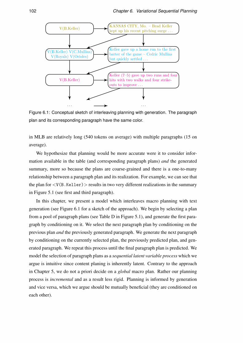
102 Chapter 6. Variational Sequential Planning
V(B.Keller)KANSAS CITY, Mo. – Brad Kellerkept up his recent pitching surge . . .
V(B.Keller) V(C.Mullins)V(Royals) V(Orioles)
Keller gave up a home run to the firstbatter of the game – Cedric Mullinsbut quickly settled . . .
V(B.Keller)Keller (7–5) gave up two runs and fourhits with two walks and four strike-outs to improve . . .
. . . . . .
Figure 6.1: Conceptual sketch of interleaving planning with generation. The paragraph
plan and its corresponding paragraph have the same color.
in MLB are relatively long (540 tokens on average) with multiple paragraphs (15 on
average).
We hypothesize that planning would be more accurate were it to consider infor-
mation available in the table (and corresponding paragraph plans) and the generated
summary, more so because the plans are coarse-grained and there is a one-to-many
relationship between a paragraph plan and its realization. For example, we can see that
the plan for <V(B.Keller)> results in two very different realizations in the summary
in Figure 5.1 (see first and third paragraph).
In this chapter, we present a model which interleaves macro planning with text
generation (see Figure 6.1 for a sketch of the approach). We begin by selecting a plan
from a pool of paragraph plans (see Table D in Figure 5.1), and generate the first para-
graph by conditioning on it. We select the next paragraph plan by conditioning on the
previous plan and the previously generated paragraph. We generate the next paragraph
by conditioning on the currently selected plan, the previously predicted plan, and gen-
erated paragraph. We repeat this process until the final paragraph plan is predicted. We
model the selection of paragraph plans as a sequential latent variable process which we
argue is intuitive since content planing is inherently latent. Contrary to the approach
in Chapter 5, we do not a priori decide on a global macro plan. Rather our planning
process is incremental and as a result less rigid. Planning is informed by generation
and vice versa, which we argue should be mutually beneficial (they are conditioned on
each other).
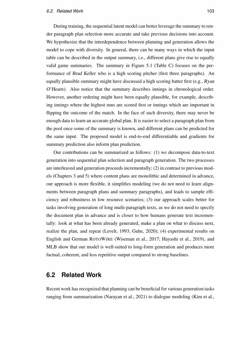
6.2. Related Work 103
During training, the sequential latent model can better leverage the summary to ren-
der paragraph plan selection more accurate and take previous decisions into account.
We hypothesize that the interdependence between planning and generation allows the
model to cope with diversity. In general, there can be many ways in which the input
table can be described in the output summary, i.e., different plans give rise to equally
valid game summaries. The summary in Figure 5.1 (Table C) focuses on the per-
formance of Brad Keller who is a high scoring pitcher (first three paragraphs). An
equally plausible summary might have discussed a high scoring batter first (e.g., Ryan
O’Hearn). Also notice that the summary describes innings in chronological order.
However, another ordering might have been equally plausible, for example, describ-
ing innings where the highest runs are scored first or innings which are important in
flipping the outcome of the match. In the face of such diversity, there may never be
enough data to learn an accurate global plan. It is easier to select a paragraph plan from
the pool once some of the summary is known, and different plans can be predicted for
the same input. The proposed model is end-to-end differentiable and gradients for
summary prediction also inform plan prediction.
Our contributions can be summarized as follows: (1) we decompose data-to-text
generation into sequential plan selection and paragraph generation. The two processes
are interleaved and generation proceeds incrementally; (2) in contrast to previous mod-
els (Chapters 3 and 5) where content plans are monolithic and determined in advance,
our approach is more flexible, it simplifies modeling (we do not need to learn align-
ments between paragraph plans and summary paragraphs), and leads to sample effi-
ciency and robustness in low resource scenarios; (3) our approach scales better for
tasks involving generation of long multi-paragraph texts, as we do not need to specify
the document plan in advance and is closer to how humans generate text incremen-
tally: look at what has been already generated, make a plan on what to discuss next,
realize the plan, and repeat (Levelt, 1993; Guhe, 2020); (4) experimental results on
English and German ROTOWIRE (Wiseman et al., 2017; Hayashi et al., 2019), and
MLB show that our model is well-suited to long-form generation and produces more
factual, coherent, and less repetitive output compared to strong baselines.
6.2 Related Work
Recent work has recognized that planning can be beneficial for various generation tasks
ranging from summarization (Narayan et al., 2021) to dialogue modeling (Kim et al.,

104 Chapter 6. Variational Sequential Planning
Input Table: Match date: Saturday, 22nd October 2018
Team Name City At Home? W L Pts Reb
Chicago Bulls Bulls Chicago Home 3 1 100 21
LA Lakers Lakers Los Angeles Away 2 5 80 25
Player Name Surname Team Pts Reb Ast . . .
Michael Jordan Michael Jordan Chicago Bulls 25 10 10 . . .
Shaquille O’ Neal Shaquille O’ Neal LA Lakers 30 15 11 . . .
. . . . . . . . . . . . . . . . . . . . . . . .
Content Plan
S1: Chicago_Bulls city, Chicago_Bulls name, LA_Lakers city, LA_Lakers name,
Chicago_Bulls points, LA_Lakers points, Match date, EOS.
S2: LA_Lakers name, LA_Lakers wins, LA_Lakers losses, Shaquille_ONeal surname,
Shaquille_ONeal points, EOS.
S3: Chicago_Bulls city, Chicago_Bulls name, Chicago_Bulls wins, Chicago_Bulls
losses, Michael_Jordan name, Michael_Jordan surname, Michael_Jordan points,
Michael_Jordan rebounds, EOS.
Realization
S1: The Chicago Bulls won against the Los Angeles Lakers 100 - 80 on Saturday.
S2: It was a poor showing for the Lakers (2 - 5) in spite of O’Neal’s 30 point contribu-
tion.
S3: The Chicago Bulls’ (3 - 1) best player was, predictably, Michael Jordan with 25
points and 10 rebounds.
Table 6.1: Example from Narayan et al. (2020). They predict each record of the micro
plan conditioned on the table and previously predicted records. They add a special
token identifying the end of sentence plan. This model first extracts sentence plans and
then verbalizes them one-by-one by conditioning on previously generated sentences.
2020). Narayan et al. (2020) treat content selection as task similar to extractive sum-
marization (example in Table 6.1). Specifically, they post-process micro plans from
Chapter 3 with special tokens identifying the end of a sentence. They predict each
record of the micro plan conditioned on the table and previously predicted records.
Their model first extracts sentence plans and then verbalizes them one-by-one by con-
ditioning on previously generated sentences.
Our approach builds on Chapter 5 where macro planning is proposed as a way of
6.3. Model 105
organizing high-level document content. We follow the same formulation of content
planning as paragraph plan prediction. Our model thus operates over larger content
units compared to related work (Chapter 3 and Narayan et al., 2020) and performs the
tasks of micro- and macro-planning in one go. In contrast to Chapter 5, we predict
paragraph plans and their corresponding paragraphs jointly in an incremental fashion.
Our approach is reminiscent of psycholinguistic models of speech production (Levelt,
1993; Taylor and Taylor, 1990; Guhe, 2020) which postulate that different levels of
processing (or modules) are responsible for language generation; these modules work
in an incremental fashion, each producing output as soon as the information it needs is
available and the output is processed immediately by the next module.
We assume plans form a sequence of paragraphs which we treat as a latent vari-
able and learn with a structured variational model. Sequential latent variables (Chung
et al., 2015; Fraccaro et al., 2016; Goyal et al., 2017) have previously found applica-
tion in modeling attention in sequence-to-sequence networks (Shankar and Sarawagi,
2019), document summarization (Li et al., 2017), controllable generation (Li and Rush,
2020; Fu et al., 2020), and knowledge-grounded dialogue (Kim et al., 2020). Ye et al.
(2020) use latent variables to disentangle the content from the structure (operational-
ized as templates) of the output text. Their approach generates diverse output output by
sampling from the template-specific sample space. They apply their model to single-
sentence generation tasks (Lebret et al., 2016; Reed et al., 2018) (example in Table
6.2).
6.3 Model
Following Chapter 5, we assume that at training time our model has access to a pool of
paragraph plans E (see Table D in Figure 5.1) which represent a clustering of records.
Given E , we aim to generate a sequence of paragraphs y = [y1, ...,yT ] that describe the
data following a sequence of chosen plans z = [z1, ...,zT ]. Let yt denote a paragraph,
which can consist of multiple sentences, and T the count of paragraphs in a summary.
With a slight abuse of notation, superscripts denote indices rather than exponentiation.
So, yti refers to the i-th word in the t-th paragraph. A plan z = [z1, ...,zT ] is a list of
discrete variables where zt = j means that we choose the j-th item from pool E of
candidate plans to guide the generation of paragraph yt .
106 Chapter 6. Variational Sequential Planning
Table name[nameVariable], eatType[pub], food[Japanese],
priceRange[average], customerRating[low], area[riverside]
Template1 [name] is a [food] restaurant, it is a [eatType] and it has an [priceRange]
cost and [customerRating] rating. it is in [area].
Sentence1 nameVariable is a Japanese restaurant, it is a pub and it has an average
cost and low rating. it is in riverside.
Template2 [name] has an [priceRange] price range with a [customerRating] rating,
and [name] is an [food] [eatType] in [area].
Sentence2 nameVariable has an average price range with a low rating, and
nameVariable is an Japanese pub in riverside.
Template3 [name] is a [eatType] with a [customerRating] rating and [priceRange]
cost, it is a [food] restaurant and[name] is in [area].
Sentence3 nameVariable is a pub with a low rating and average cost, it is a Japanese
restaurant and nameVariable is in riverside.
Table 6.2: Example from Ye et al. (2020). They propose an approach to disentangle
content from the structure (which they operationalize as templates) of text. They cre-
ate a dataset of pairs of table and corresponding sentence and replace all sentence
tokens which match with the record values in the table with a keyword indicating the
record type. With this, they aim to remove content information from the sentence and
only retain the structure information. The processed sentences resemble Template1,
Template2, and Template3 in the example above. They learn a model to produce tem-
plates by training on this dataset. During inference, they can generate diverse output
by sampling from different templates.
Generation with Latent Plans The core technique of our model is learning the se-
quence of latent plans that guides long document generation. We consider a condi-
tional generation setting where the input E is a set of paragraph plans and the output
y1:T are textual paragraphs following selected sequence z = z1:T . Our goal is to induce
variables z that indicate which paragraphs are being talked about and in which order.
Similar to previous work (Li and Rush, 2020; Fu et al., 2020), we model this process
as a conditional generative model that produces both y and z and factorizes as:
pθ(y,z|E) =∏t
pθ(zt |y<t ,z<t ,E)pθ(yt |y<t ,z1:t ,E) (6.1)
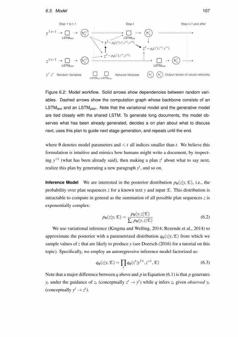
6.3. Model 107
y1:t−1
z1:t−1
LSTMtext
LSTMplan
h yt-1 h y
t
hzthz
t-1
LSTMplan
LSTMtext
Step 1 to t-1 Step t Step t+1 and after
zt ∼ pθ(zt |z<t, y<t)
yt∼ pθ(yt |zt, z<t, y<t)zt ∼ qϕ(zt |z<t, y1:t)
yt zt Random VariablesLSTMplan
Network Modules hzt Output tensor of neural networkshy
t
LSTMtext
Figure 6.2: Model workflow. Solid arrows show dependencies between random vari-
ables. Dashed arrows show the computation graph whose backbone consists of an
LSTMtext and an LSTMplan. Note that the variational model and the generative model
are tied closely with the shared LSTM. To generate long documents, the model ob-
serves what has been already generated, decides a on plan about what to discuss
next, uses this plan to guide next stage generation, and repeats until the end.
where θ denotes model parameters and < t all indices smaller than t. We believe this
formulation is intuitive and mimics how humans might write a document, by inspect-
ing y<t (what has been already said), then making a plan zt about what to say next,
realize this plan by generating a new paragraph yt , and so on.
Inference Model We are interested in the posterior distribution pθ(z|y,E), i.e., the
probability over plan sequences z for a known text y and input E . This distribution is
intractable to compute in general as the summation of all possible plan sequences z is
exponentially complex:
pθ(z|y,E) =pθ(y,z|E)
∑z pθ(y,z|E)(6.2)
We use variational inference (Kingma and Welling, 2014; Rezende et al., 2014) to
approximate the posterior with a parametrized distribution qφ(z|y,E) from which we
sample values of z that are likely to produce y (see Doersch (2016) for a tutorial on this
topic). Specifically, we employ an autoregressive inference model factorized as:
qφ(z|y,E) = ∏t
qφ(zt |y1:t ,z<t ,E) (6.3)
Note that a major difference between q above and p in Equation (6.1) is that p generates
yt under the guidance of zt (conceptually zt → yt) while q infers zt given observed yt
(conceptually yt → zt).
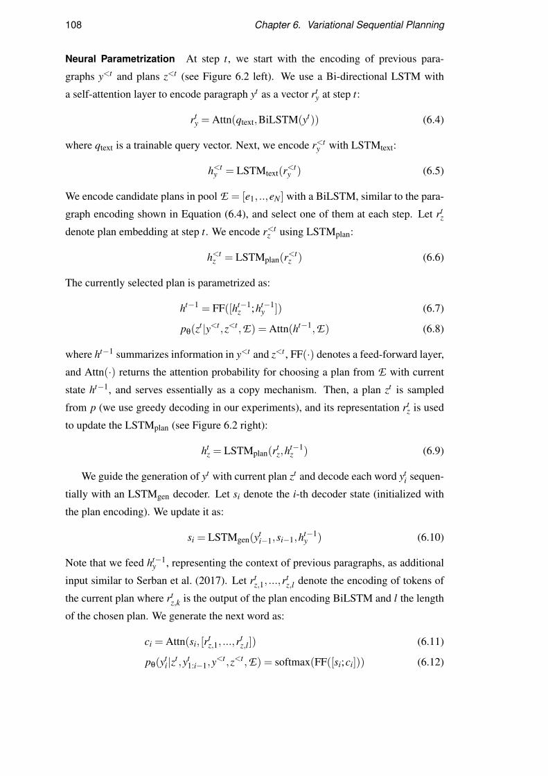
108 Chapter 6. Variational Sequential Planning
Neural Parametrization At step t, we start with the encoding of previous para-
graphs y<t and plans z<t (see Figure 6.2 left). We use a Bi-directional LSTM with
a self-attention layer to encode paragraph yt as a vector rty at step t:
rty = Attn(qtext,BiLSTM(yt)) (6.4)
where qtext is a trainable query vector. Next, we encode r<ty with LSTMtext:
h<ty = LSTMtext(r<t
y ) (6.5)
We encode candidate plans in pool E = [e1, ..,eN ] with a BiLSTM, similar to the para-
graph encoding shown in Equation (6.4), and select one of them at each step. Let rtz
denote plan embedding at step t. We encode r<tz using LSTMplan:
h<tz = LSTMplan(r<t
z ) (6.6)
The currently selected plan is parametrized as:
ht−1 = FF([ht−1z ;ht−1
y ]) (6.7)
pθ(zt |y<t ,z<t ,E) = Attn(ht−1,E) (6.8)
where ht−1 summarizes information in y<t and z<t , FF(·) denotes a feed-forward layer,
and Attn(·) returns the attention probability for choosing a plan from E with current
state ht−1, and serves essentially as a copy mechanism. Then, a plan zt is sampled
from p (we use greedy decoding in our experiments), and its representation rtz is used
to update the LSTMplan (see Figure 6.2 right):
htz = LSTMplan(rt
z,ht−1z ) (6.9)
We guide the generation of yt with current plan zt and decode each word yti sequen-
tially with an LSTMgen decoder. Let si denote the i-th decoder state (initialized with
the plan encoding). We update it as:
si = LSTMgen(yti−1,si−1,ht−1
y ) (6.10)
Note that we feed ht−1y , representing the context of previous paragraphs, as additional
input similar to Serban et al. (2017). Let rtz,1, ...,r
tz,l denote the encoding of tokens of
the current plan where rtz,k is the output of the plan encoding BiLSTM and l the length
of the chosen plan. We generate the next word as:
ci = Attn(si, [rtz,1, ...,r
tz,l]) (6.11)
pθ(yti|zt ,yt
1:i−1,y<t ,z<t ,E) = softmax(FF([si;ci])) (6.12)
6.3. Model 109
where c denotes the context vector. In addition, we equip the decoder with copy atten-
tion (Gulcehre et al., 2016b) to enable copying tokens from zt . Once paragraph yt has
been generated, we obtain its encoding rty with Equation (6.4), and update LSTMtext
(see Figure 6.2 middle):
hty = LSTMtext(rt
y,ht−1y ) (6.13)
We parametrize the variational model so that it shares the LSTMs for encoding y
and E with the generative model:
ht = FF([ht−1z ;ht
y]) (6.14)
qφ(zt |y1:t ,z<t ,E) = Attn(ht ,E) (6.15)
Note that Equation (6.14) differs from Equation (6.7) in that it uses the updated hty
instead of the previous ht−1y because now yt is observed. The variational distribution is
again parametrized by the attention probability. Essentially, p and q are strongly tied
to each other with the shared LSTM encoders.
Although we primarily focus on the inference, and how the latent plan can improve
the generation of long documents, we note that the model sketched above could be
parametrized differently, e.g., by replacing the encoder and decoder with pretrained
language models like BART (Lewis et al., 2020). However, we leave this to future
work.
Training We optimize the standard evidence lower bound (ELBO) loss:
L0 = log pθ(y|E)−D(qφ(z|y,E) ‖ pθ(z|y,E))
= Eqφ(z|y,E)[log pθ(y,z|E)− logqφ(z|y,E)]
where log pθ(y|E) is the log-evidence from the data, and D(qφ(z|y,E) ‖ pθ(z|y,E)) the
Kullback-Leibler divergence between qφ and the true posterior.
Advantageously, we can exploit oracle plans (see Table E in Figure 5.1 and the
description in Section 6.4 for how these were created) to obtain weak labels z∗ which
we use as distant supervision to the inference model:
L1 = Ez∗[logqφ(z∗|y,E)] (6.16)
L = L0 +λL1 (6.17)
Such distant supervision is essential for stabilizing training (it would be extremely
challenging to optimize the model in a fully unsupervised way) and for mitigating
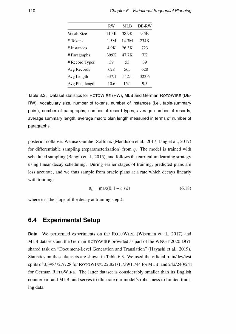
110 Chapter 6. Variational Sequential Planning
RW MLB DE-RW
Vocab Size 11.3K 38.9K 9.5K
# Tokens 1.5M 14.3M 234K
# Instances 4.9K 26.3K 723
# Paragraphs 399K 47.7K 7K
# Record Types 39 53 39
Avg Records 628 565 628
Avg Length 337.1 542.1 323.6
Avg Plan length 10.6 15.1 9.5
Table 6.3: Dataset statistics for ROTOWIRE (RW), MLB and German ROTOWIRE (DE-
RW). Vocabulary size, number of tokens, number of instances (i.e., table-summary
pairs), number of paragraphs, number of record types, average number of records,
average summary length, average macro plan length measured in terms of number of
paragraphs.
posterior collapse. We use Gumbel-Softmax (Maddison et al., 2017; Jang et al., 2017)
for differentiable sampling (reparameterization) from q. The model is trained with
scheduled sampling (Bengio et al., 2015), and follows the curriculum learning strategy
using linear decay scheduling. During earlier stages of training, predicted plans are
less accurate, and we thus sample from oracle plans at a rate which decays linearly
with training:
εk = max(0,1− c∗ k) (6.18)
where c is the slope of the decay at training step k.
6.4 Experimental Setup
Data We performed experiments on the ROTOWIRE (Wiseman et al., 2017) and
MLB datasets and the German ROTOWIRE provided as part of the WNGT 2020 DGT
shared task on “Document-Level Generation and Translation” (Hayashi et al., 2019).
Statistics on these datasets are shown in Table 6.3. We used the official train/dev/test
splits of 3,398/727/728 for ROTOWIRE, 22,821/1,739/1,744 for MLB, and 242/240/241
for German ROTOWIRE. The latter dataset is considerably smaller than its English
counterpart and MLB, and serves to illustrate our model’s robustness to limited train-
ing data.

6.4. Experimental Setup 111
All three datasets were preprocessed following the method of Chapter 5. A para-
graph plan for an entity was constructed by verbalizing its records in a fixed sequence
of record type followed by its value. For example, pitcher B.Keller from Figure 5.1
would be verbalized as <PLAYER>B.Keller <H/V>V <W>7 <L>5 <IP>8 <PH>4
. . . . We denote this using the shorthand <V(B.Keller)>. The paragraph plan for
an event is the verbalization of the players in the event followed by the verbalization
of play-by-plays. Candidate paragraph plans E are obtained by enumerating entities
and events and their combinations (see Table D in Figure 5.1). Oracle macro plans are
obtained by matching the mentions of entities and events in the gold summary with the
input table. We make use of these oracle macro plans during training. The versions
of MLB and ROTOWIRE created in Chapter 5 contain paragraph delimiters for gold
summaries; we preprocessed the German ROTOWIRE in a similar fashion.
Table 6.3 also shows the average length of the macro plan in terms of the number
of paragraph plans it contains. This is 10.6 for ROTOWIRE, 15.1 for MLB, and 9.5 for
German RotoWire.
Training Configuration We train our model with the AdaGrad optimizer (Duchi
et al., 2011) and tune parameters on the development set. We learn a joint subword
vocabulary (Sennrich et al., 2016) for paragraph plans and summaries with 6K merge
operations for ROTOWIRE, 16K merge operations for MLB, and 2K merge operations
for German ROTOWIRE. The model is implemented on a fork of OpenNMT-py (Klein
et al., 2017b). For efficiency, we batch using summaries instead of individual para-
graphs. Batch sizes for MLB, ROTOWIRE, and German-ROTOWIRE are 8, 5, and 1
respectively. We set λ to 2 in Equation (6.17). In Equation (6.18), c is 1/100,000 for
MLB, 1/50,000 for ROTOWIRE, and 1/30,000 for German-ROTOWIRE.
During inference in MLB, similar to Chapter 5, we block the repetition of para-
graph plan bigrams (i.e., we disallow the repetition of (zt ,zt+1)) and select the para-
graph plan with the next higher probability in Equation (6.8). In addition, we block
consecutive repetitions, and more than two repetitions of a unigram. During training
we observed high variance in the length of paragraphs yt since the same plan can result
in a shorter or longer paragraph. For example, <V(B.Keller)> corresponds to two
paragraphs (first and third paragraph) with different lengths in Figure 5.1. We found
that this encourages the model to be conservative and generate relatively short output.
We control the paragraph length (Fan et al., 2018) by creating discrete bins, each con-
taining approximately an equal number of paragraphs. During training, we prepend
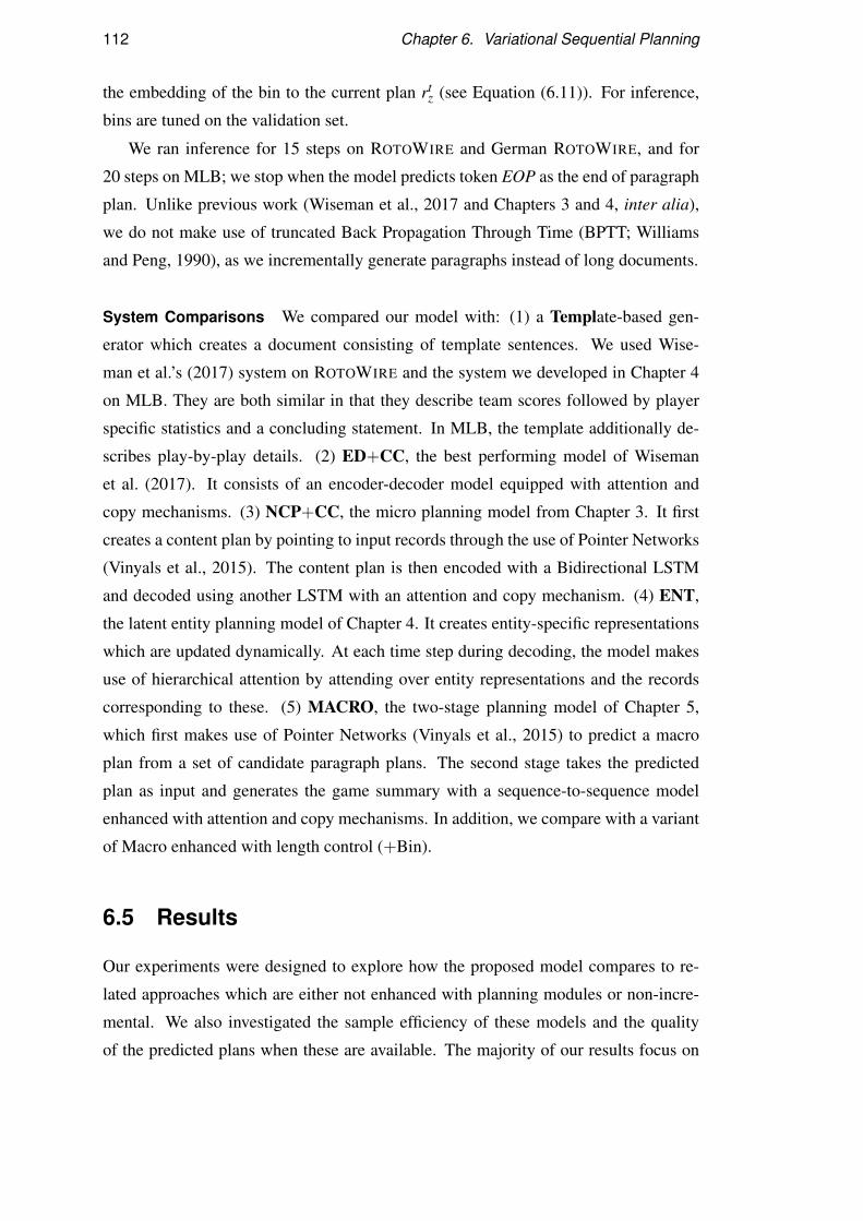
112 Chapter 6. Variational Sequential Planning
the embedding of the bin to the current plan rtz (see Equation (6.11)). For inference,
bins are tuned on the validation set.
We ran inference for 15 steps on ROTOWIRE and German ROTOWIRE, and for
20 steps on MLB; we stop when the model predicts token EOP as the end of paragraph
plan. Unlike previous work (Wiseman et al., 2017 and Chapters 3 and 4, inter alia),
we do not make use of truncated Back Propagation Through Time (BPTT; Williams
and Peng, 1990), as we incrementally generate paragraphs instead of long documents.
System Comparisons We compared our model with: (1) a Template-based gen-
erator which creates a document consisting of template sentences. We used Wise-
man et al.’s (2017) system on ROTOWIRE and the system we developed in Chapter 4
on MLB. They are both similar in that they describe team scores followed by player
specific statistics and a concluding statement. In MLB, the template additionally de-
scribes play-by-play details. (2) ED+CC, the best performing model of Wiseman
et al. (2017). It consists of an encoder-decoder model equipped with attention and
copy mechanisms. (3) NCP+CC, the micro planning model from Chapter 3. It first
creates a content plan by pointing to input records through the use of Pointer Networks
(Vinyals et al., 2015). The content plan is then encoded with a Bidirectional LSTM
and decoded using another LSTM with an attention and copy mechanism. (4) ENT,
the latent entity planning model of Chapter 4. It creates entity-specific representations
which are updated dynamically. At each time step during decoding, the model makes
use of hierarchical attention by attending over entity representations and the records
corresponding to these. (5) MACRO, the two-stage planning model of Chapter 5,
which first makes use of Pointer Networks (Vinyals et al., 2015) to predict a macro
plan from a set of candidate paragraph plans. The second stage takes the predicted
plan as input and generates the game summary with a sequence-to-sequence model
enhanced with attention and copy mechanisms. In addition, we compare with a variant
of Macro enhanced with length control (+Bin).
6.5 Results
Our experiments were designed to explore how the proposed model compares to re-
lated approaches which are either not enhanced with planning modules or non-incre-
mental. We also investigated the sample efficiency of these models and the quality
of the predicted plans when these are available. The majority of our results focus on
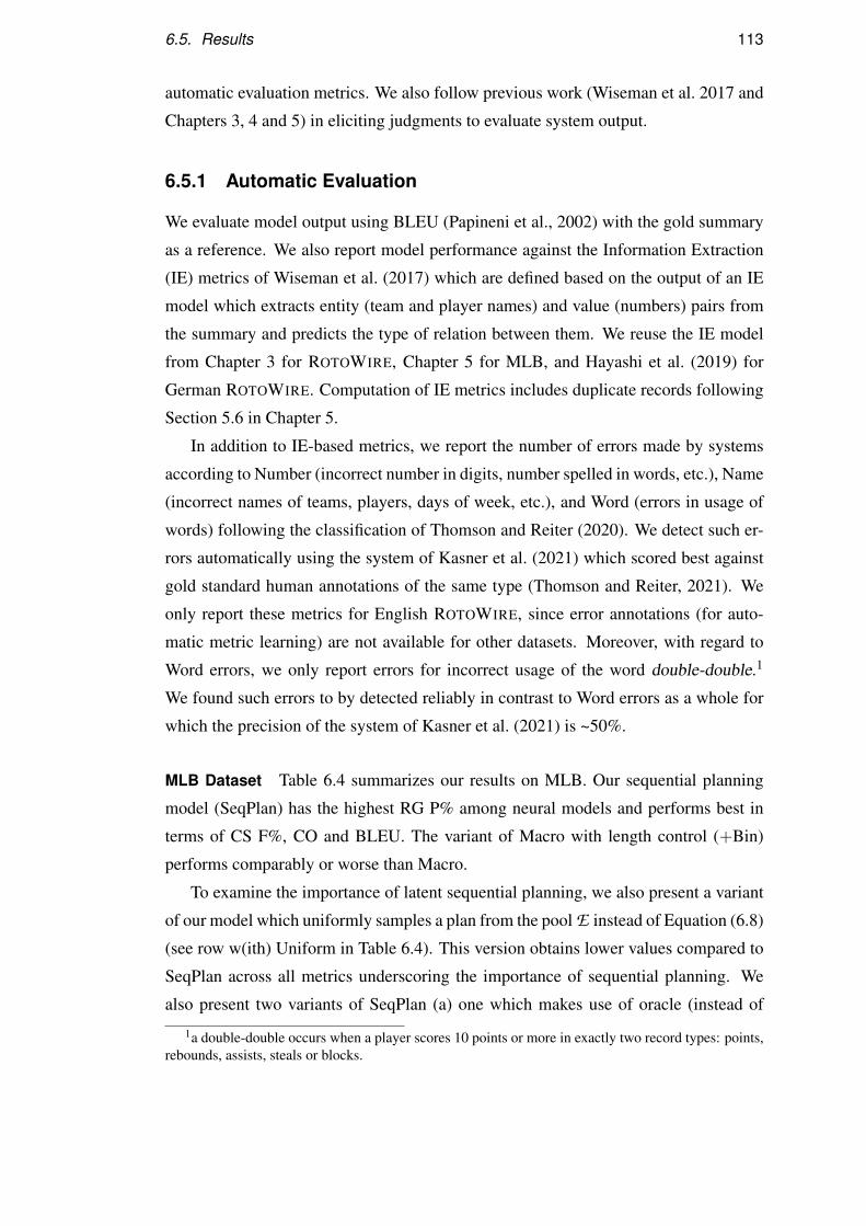
6.5. Results 113
automatic evaluation metrics. We also follow previous work (Wiseman et al. 2017 and
Chapters 3, 4 and 5) in eliciting judgments to evaluate system output.
6.5.1 Automatic Evaluation
We evaluate model output using BLEU (Papineni et al., 2002) with the gold summary
as a reference. We also report model performance against the Information Extraction
(IE) metrics of Wiseman et al. (2017) which are defined based on the output of an IE
model which extracts entity (team and player names) and value (numbers) pairs from
the summary and predicts the type of relation between them. We reuse the IE model
from Chapter 3 for ROTOWIRE, Chapter 5 for MLB, and Hayashi et al. (2019) for
German ROTOWIRE. Computation of IE metrics includes duplicate records following
Section 5.6 in Chapter 5.
In addition to IE-based metrics, we report the number of errors made by systems
according to Number (incorrect number in digits, number spelled in words, etc.), Name
(incorrect names of teams, players, days of week, etc.), and Word (errors in usage of
words) following the classification of Thomson and Reiter (2020). We detect such er-
rors automatically using the system of Kasner et al. (2021) which scored best against
gold standard human annotations of the same type (Thomson and Reiter, 2021). We
only report these metrics for English ROTOWIRE, since error annotations (for auto-
matic metric learning) are not available for other datasets. Moreover, with regard to
Word errors, we only report errors for incorrect usage of the word double-double.1
We found such errors to by detected reliably in contrast to Word errors as a whole for
which the precision of the system of Kasner et al. (2021) is ~50%.
MLB Dataset Table 6.4 summarizes our results on MLB. Our sequential planning
model (SeqPlan) has the highest RG P% among neural models and performs best in
terms of CS F%, CO and BLEU. The variant of Macro with length control (+Bin)
performs comparably or worse than Macro.
To examine the importance of latent sequential planning, we also present a variant
of our model which uniformly samples a plan from the pool E instead of Equation (6.8)
(see row w(ith) Uniform in Table 6.4). This version obtains lower values compared to
SeqPlan across all metrics underscoring the importance of sequential planning. We
also present two variants of SeqPlan (a) one which makes use of oracle (instead of
1a double-double occurs when a player scores 10 points or more in exactly two record types: points,rebounds, assists, steals or blocks.
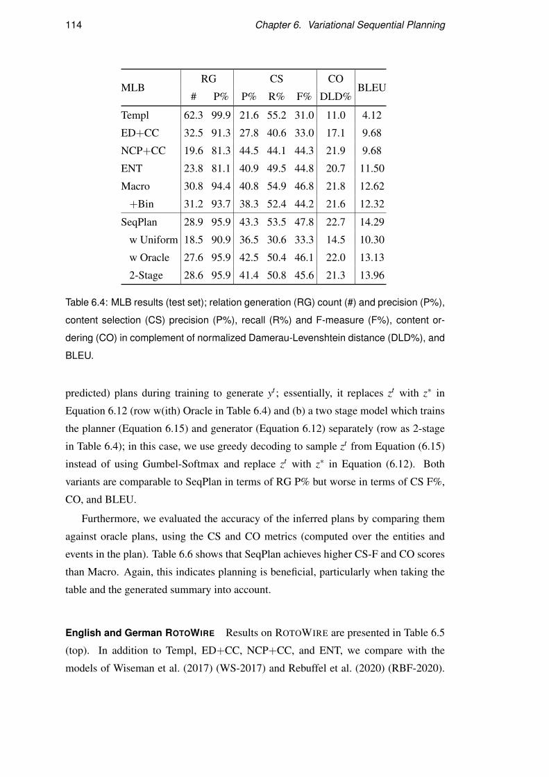
114 Chapter 6. Variational Sequential Planning
MLBRG CS CO
BLEU# P% P% R% F% DLD%
Templ 62.3 99.9 21.6 55.2 31.0 11.0 4.12
ED+CC 32.5 91.3 27.8 40.6 33.0 17.1 9.68
NCP+CC 19.6 81.3 44.5 44.1 44.3 21.9 9.68
ENT 23.8 81.1 40.9 49.5 44.8 20.7 11.50
Macro 30.8 94.4 40.8 54.9 46.8 21.8 12.62
+Bin 31.2 93.7 38.3 52.4 44.2 21.6 12.32
SeqPlan 28.9 95.9 43.3 53.5 47.8 22.7 14.29
w Uniform 18.5 90.9 36.5 30.6 33.3 14.5 10.30
w Oracle 27.6 95.9 42.5 50.4 46.1 22.0 13.13
2-Stage 28.6 95.9 41.4 50.8 45.6 21.3 13.96
Table 6.4: MLB results (test set); relation generation (RG) count (#) and precision (P%),
content selection (CS) precision (P%), recall (R%) and F-measure (F%), content or-
dering (CO) in complement of normalized Damerau-Levenshtein distance (DLD%), and
BLEU.
predicted) plans during training to generate yt ; essentially, it replaces zt with z∗ in
Equation 6.12 (row w(ith) Oracle in Table 6.4) and (b) a two stage model which trains
the planner (Equation 6.15) and generator (Equation 6.12) separately (row as 2-stage
in Table 6.4); in this case, we use greedy decoding to sample zt from Equation (6.15)
instead of using Gumbel-Softmax and replace zt with z∗ in Equation (6.12). Both
variants are comparable to SeqPlan in terms of RG P% but worse in terms of CS F%,
CO, and BLEU.
Furthermore, we evaluated the accuracy of the inferred plans by comparing them
against oracle plans, using the CS and CO metrics (computed over the entities and
events in the plan). Table 6.6 shows that SeqPlan achieves higher CS-F and CO scores
than Macro. Again, this indicates planning is beneficial, particularly when taking the
table and the generated summary into account.
English and German ROTOWIRE Results on ROTOWIRE are presented in Table 6.5
(top). In addition to Templ, ED+CC, NCP+CC, and ENT, we compare with the
models of Wiseman et al. (2017) (WS-2017) and Rebuffel et al. (2020) (RBF-2020).
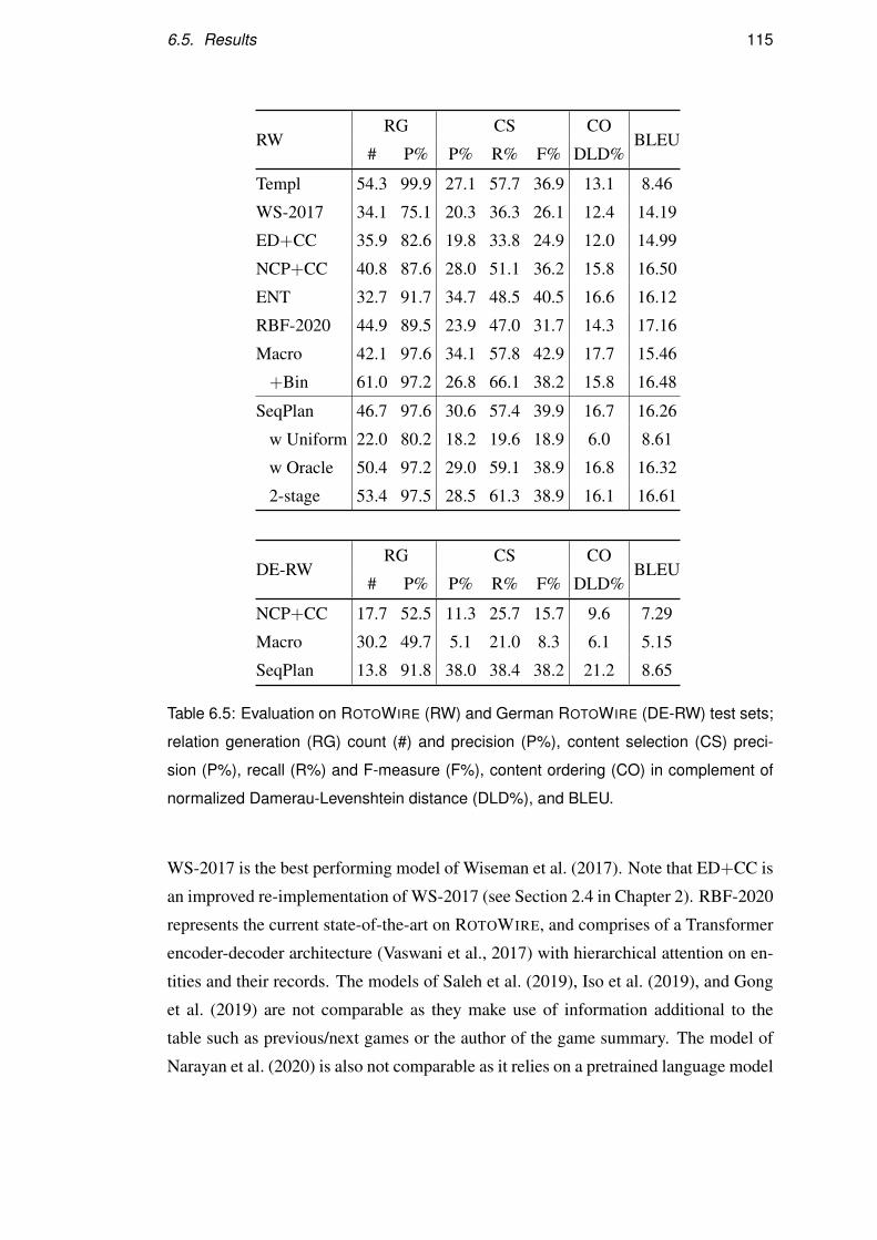
6.5. Results 115
RWRG CS CO
BLEU# P% P% R% F% DLD%
Templ 54.3 99.9 27.1 57.7 36.9 13.1 8.46
WS-2017 34.1 75.1 20.3 36.3 26.1 12.4 14.19
ED+CC 35.9 82.6 19.8 33.8 24.9 12.0 14.99
NCP+CC 40.8 87.6 28.0 51.1 36.2 15.8 16.50
ENT 32.7 91.7 34.7 48.5 40.5 16.6 16.12
RBF-2020 44.9 89.5 23.9 47.0 31.7 14.3 17.16
Macro 42.1 97.6 34.1 57.8 42.9 17.7 15.46
+Bin 61.0 97.2 26.8 66.1 38.2 15.8 16.48
SeqPlan 46.7 97.6 30.6 57.4 39.9 16.7 16.26
w Uniform 22.0 80.2 18.2 19.6 18.9 6.0 8.61
w Oracle 50.4 97.2 29.0 59.1 38.9 16.8 16.32
2-stage 53.4 97.5 28.5 61.3 38.9 16.1 16.61
DE-RWRG CS CO
BLEU# P% P% R% F% DLD%
NCP+CC 17.7 52.5 11.3 25.7 15.7 9.6 7.29
Macro 30.2 49.7 5.1 21.0 8.3 6.1 5.15
SeqPlan 13.8 91.8 38.0 38.4 38.2 21.2 8.65
Table 6.5: Evaluation on ROTOWIRE (RW) and German ROTOWIRE (DE-RW) test sets;
relation generation (RG) count (#) and precision (P%), content selection (CS) preci-
sion (P%), recall (R%) and F-measure (F%), content ordering (CO) in complement of
normalized Damerau-Levenshtein distance (DLD%), and BLEU.
WS-2017 is the best performing model of Wiseman et al. (2017). Note that ED+CC is
an improved re-implementation of WS-2017 (see Section 2.4 in Chapter 2). RBF-2020
represents the current state-of-the-art on ROTOWIRE, and comprises of a Transformer
encoder-decoder architecture (Vaswani et al., 2017) with hierarchical attention on en-
tities and their records. The models of Saleh et al. (2019), Iso et al. (2019), and Gong
et al. (2019) are not comparable as they make use of information additional to the
table such as previous/next games or the author of the game summary. The model of
Narayan et al. (2020) is also not comparable as it relies on a pretrained language model
116 Chapter 6. Variational Sequential Planning
CS CODatasets P% R% F% DLD%
Macro 73.6 45.9 56.5 27.0
ML
B
SeqPlan 74.4 51.1 60.6 27.1
Macro 81.5 62.7 70.9 36.3R
WSeqPlan 79.1 61.6 69.3 35.5
Macro 86.8 34.2 49.0 30.1
DE
-RW
SeqPlan 73.1 60.8 66.4 31.0
Table 6.6: Evaluation of macro planning stage (test set); content selection (CS) preci-
sion (P%), recall (R%) and F-measure (F%), content ordering (CO) in complement of
normalized Damerau-Levenshtein distance (DLD%).
(Rothe et al., 2020) to generate the summary sentences. Table 6.5 (bottom) shows our
results on German ROTOWIRE. We compare against NCP+CC’s entry in the WNGT
2019 shared task (Hayashi et al., 2019), and our implementation of Macro. Saleh et al.
(2019) are not comparable as they pretrain on 32M parallel English-German, 420M
English and 534M German monolingual data.
On ROTOWIRE, we find that SeqPlan achieves highest RG P% amongst neural
models, and performs on par with Macro (it obtains higher BLEU but lower CS F%
and CO scores). The +Bin variant of Macro performs better on BLEU but worse on
other metrics. As in Table 6.4, w Uniform struggles across metrics corroborating our
hypothesis that latent sequential planning improves generation performance. The other
two variants (w Oracle and 2-Stage) are worse than SeqPlan in RG P% and CS F%,
comparable in CO, and slightly higher in terms of BLEU.
On German, our model is best across metrics achieving an RG P% of 91.8% which
is higher by 42% (absolute) compared to of Macro. In fact, the RG P% of SeqPlan is
superior to Saleh et al. (2019) whose model is pretrained with additional data and is
considered state of the art (Hayashi et al., 2019). RG# is lower mainly because of a
bug in the German IE which excludes number records. RG# for NCP+CC and Macro
is too high because the summaries contain a lot of repetition. The same record will
repeat at least once with NCP+CC and three times with Macro, whereas only 7% of
the records are repeated with SeqPlan.
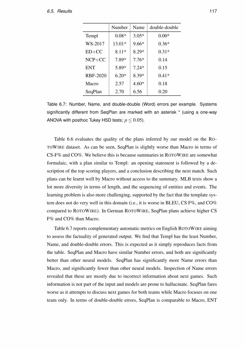
6.5. Results 117
Number Name double-double
Templ 0.08* 3.05* 0.00*
WS-2017 13.01* 9.66* 0.36*
ED+CC 8.11* 8.29* 0.31*
NCP+CC 7.89* 7.76* 0.14
ENT 5.89* 7.24* 0.15
RBF-2020 6.20* 8.39* 0.41*
Macro 2.57 4.60* 0.18
SeqPlan 2.70 6.56 0.20
Table 6.7: Number, Name, and double-double (Word) errors per example. Systems
significantly different from SeqPlan are marked with an asterisk * (using a one-way
ANOVA with posthoc Tukey HSD tests; p≤ 0.05).
Table 6.6 evaluates the quality of the plans inferred by our model on the RO-
TOWIRE dataset. As can be seen, SeqPlan is slightly worse than Macro in terms of
CS-F% and CO%. We believe this is because summaries in ROTOWIRE are somewhat
formulaic, with a plan similar to Templ: an opening statement is followed by a de-
scription of the top scoring players, and a conclusion describing the next match. Such
plans can be learnt well by Macro without access to the summary. MLB texts show a
lot more diversity in terms of length, and the sequencing of entities and events. The
learning problem is also more challenging, supported by the fact that the template sys-
tem does not do very well in this domain (i.e., it is worse in BLEU, CS F%, and CO%
compared to ROTOWIRE). In German ROTOWIRE, SeqPlan plans achieve higher CS
F% and CO% than Macro.
Table 6.7 reports complementary automatic metrics on English ROTOWIRE aiming
to assess the factuality of generated output. We find that Templ has the least Number,
Name, and double-double errors. This is expected as it simply reproduces facts from
the table. SeqPlan and Macro have similar Number errors, and both are significantly
better than other neural models. SeqPlan has significantly more Name errors than
Macro, and significantly fewer than other neural models. Inspection of Name errors
revealed that these are mostly due to incorrect information about next games. Such
information is not part of the input and models are prone to hallucinate. SeqPlan fares
worse as it attempts to discuss next games for both teams while Macro focuses on one
team only. In terms of double-double errors, SeqPlan is comparable to Macro, ENT
118 Chapter 6. Variational Sequential Planning
(a) (b)
Figure 6.3: Sample efficiency for (a) MLB and (b) ROTOWIRE datasets. SeqPlan and
Macro are trained on different portions (%) of the training dataset and performance is
measured with RG P%.
and NCP+CC, and significantly better than WS-2017, ED+CC, and RBF-2020.
6.5.2 Sample Efficiency
We also evaluated whether SeqPlan is more sample efficient in comparison to Macro,
by examining how RG P% varies with (training) data size. As shown in Figure 6.3,
the difference between SeqPlan and Macro is more pronounced when relatively little
data is available. For example, with 10% of training data, RG P% for SeqPlan on MLB
is 85.7% and 92.1% on ROTOWIRE. In contrast, Macro obtains 63.3% on MLB and
47.1% on ROTOWIRE. As more training data becomes available, the difference in RG
P% decreases. The slope of increase in RG P% for Macro is higher for ROTOWIRE
than MLB. We hypothesize this is because MLB has longer summaries with more
paragraphs, and is thus more difficult for Macro to learn alignments between paragraph
plans and text paragraphs in the game summary.
6.5.3 Evaluation of Paragraph Plan Prediction Accuracy
We evaluated the accuracy of the predicted paragraph plan depending on whether the
paragraph is observed or not. Essentially we compared the accuracy of qφ in Equation
(15) and pθ in Equation (8), respectively. Table 6.8 presents the results. We see that
plan prediction accuracy is higher when the paragraph is observed. This validates our
modeling decision of making use of qφ to predict the paragraph plan during training.
6.5. Results 119
Dataset Model yt is observed yt is not observed
MLB SeqPlan 80.3 24.9
Random 1.3 1.3
ROTOWIRE SeqPlan 81.8 48.8
Random 1.8 1.8
Table 6.8: Accuracy of paragraph plan prediction for SeqPlan and Random with ob-
served paragraph yt and without.
6.5.4 Human Evaluation
We used the Amazon Mechanical Turk (AMT) crowdsourcing platform for our judg-
ment elicitation study as detailed in Chapter 2. We compared SeqPlan with Gold,
Templ, ED+CC, and Macro; we did not compare against ENT as Chapter 5 has shown
that it performs poorly against Macro. For ROTOWIRE, we additionally compared
against RBF-2020.
We conducted two elicitation studies. The first one provided raters with boxscores
(and play-by-plays in the case of MLB), along with sentences randomly extracted from
game summaries. We asked them to count supported and contradicting facts (ignoring
hallucinations). This evaluation was conducted on 40 summaries (20 for each dataset),
with four sentences per summary, each rated by three participants. Altogether, we had
177 participants.
Table 6.9 (columns #Supp and #Contra) presents our results. On MLB, all sys-
tems display a comparable count of supported facts (differences are not statistically
significant), with the exception of Templ which contains significantly more. In terms
of contradicting facts, SeqPlan performs on par with Macro, Gold and Templ, and is
significantly better than ED+CC. On ROTOWIRE, in terms of supported facts, Seq-
Plan performs on par with the other neural models, is significantly higher than Gold,
and significantly lower than Templ. In terms of contradicting facts, SeqPlan performs
on par with Macro, Gold and Templ, and significantly better than ED+CC and RBF-
2020. Templ achieves the lowest count of contradicting facts and the highest count of
supported facts for both the datasets. This is no surprise as it essentially regurgitates
facts (i.e., records) from the table.
In our second study, raters were asked to choose the better summary from a pair
of summaries based on Coherence, Conciseness, and Grammaticality. We assessed 40
summaries from the test set (20 for each dataset). Each summary pair was rated by

120 Chapter 6. Variational Sequential Planning
MLB #Supp #Contra Gram Coher Concis
Gold 3.59 0.14 21.67 29.17 14.17
Templ 4.21* 0.04 −58.33* −48.33* 9.17
ED+CC 3.42 0.72* −32.50* −18.33* −48.33*
Macro 3.76 0.25 37.50 15.00 22.50
SeqPlan 3.68 0.19 31.67 22.50 2.50
ROTOWIRE #Supp #Contra Gram Coher Concis
Gold 3.63* 0.07 42.67* 40.67 28.00
Templ 7.57* 0.08 −57.33* −55.33* −34.67*
ED+CC 3.92 0.91* 4.00 −14.67* −13.33
RBF-2020 5.08 0.67* 6.00 1.33 −0.67
Macro 4.00 0.27 0.67 7.33 10.00
SeqPlan 4.84 0.17 4.00 20.67 10.67
Table 6.9: Average number of supported (#Supp) and contradicting (#Contra) facts in
game summaries and best-worst scaling evaluation for Coherence (Coher), Concise-
ness (Concis), and Grammaticality (Gram); higher is better. Systems significantly differ-
ent from SeqPlan are marked with an asterisk * (using a one-way ANOVA with posthoc
Tukey HSD tests; p≤ 0.05).
.
three participants. Altogether, 377 raters participated in this task.
On MLB, SeqPlan is significantly more coherent than ED+CC and Templ, and is
comparable with Gold and Macro. A similar picture emerges with grammaticality. Se-
qPlan is as concise as Gold, Macro and Templ, and significantly better than ED+CC.
On ROTOWIRE, SeqPlan is significantly more coherent than Templ and ED+CC, but
on par with Macro, RBF-2020 and Gold. In terms of conciseness, SeqPlan is compara-
ble with Gold, Macro, RBF-2020, and ED+CC, and significantly better than Templ. In
terms of grammaticality, SeqPlan is comparable with Macro, RBF-2020, and ED+CC,
significantly better than Templ, and significantly worse than Gold.
6.6. Discussion 121
<V(Cardinals)> → <V(9-T)> → <V(Cardinals)> → <V(Cardinals)>
<V(Brewers)>→ <V(9-T)>→ <V(8-B)>→ <V(8-T)>→ <V(8-B)>→ <V(9-B)>→<V(Brewers)>→ <V(Adam Wainwright)>→ <V(Brewers)>→ <V(3-T)>→ <V(3-B)>
→ <V(Carlos Villanueva)>
ST. LOUIS – The St. Louis Cardinals have been waiting for their starting rotation. <P> Skip
Schumaker drove in the go-ahead run with a double in the ninth inning, and the Cardinals beat the
Milwaukee Brewers 4-3 on Wednesday night to avoid a three-game sweep. <P> The Cardinals
have won four of five, and have won four in a row. <P> The Cardinals have won four of five, in-
cluding a three-game sweep by the Brewers. <P> Brian Barton led off the ninth with a pinch-hit
double off Derrick Turnbow (0-1) and moved to third on Cesar Izturis’ sacrifice bunt. Schumaker
drove in Barton with a double down the left-field line. <P> Ryan Braun, who had two hits, led off
the eighth with a double off Ryan Franklin (1-1). Braun went to third on a wild pitch and scored
on Corey Hart’s triple into the right-field corner. <P> Albert Pujols was intentionally walked to
load the bases with one out in the eighth, and Guillermo Ankiel flied out. Troy Glaus walked to
load the bases for Kennedy, who hit a sacrifice fly off Guillermo Mota. <P> Ryan Franklin (1-1)
got the win despite giving up a run in the eighth. Ryan Braun led off with a double and scored
on Corey Hart’s one-out triple. <P> Jason Isringhausen pitched a perfect ninth for his seventh
save in nine chances. He has converted his last six save opportunities and has n’t allowed a run
in his last three appearances. <P> The Brewers lost for the seventh time in eight games. <P>
Wainwright allowed two runs and four hits in seven innings. He walked four and struck out six.
<P> Brewers manager Ron Roenicke was ejected by home plate umpire Bill Miller for arguing a
called third strike. <P> The Cardinals took a 2-0 lead in the third. Albert Pujols walked with two
outs and Rick Ankiel walked. Glaus then lined a two-run double into the left-field corner. <P>
The Brewers tied it in the third. Jason Kendall led off with a double and scored on Rickie Weeks’
double. Ryan Braun’s RBI single tied it at 2. <P> Villanueva allowed two runs and three hits in
seven innings. He walked four and struck out one.
Table 6.10: Predicted macro plan (top) and generated output from our model. Tran-
sitions between paragraph plans are shown using→. Paragraphs are separated with
<P> delimiters. Entities and events in the summary corresponding to the macro plan
are boldfaced.
6.6 Discussion
Table 6.10 gives an example of SeqPlan output. We see that the game summary follows
the macro plan closely. In addition, the paragraph plans and the paragraphs exhibit co-
herent ordering. Table 6.11 shows the oracle macro plan for the example in Table 6.10,
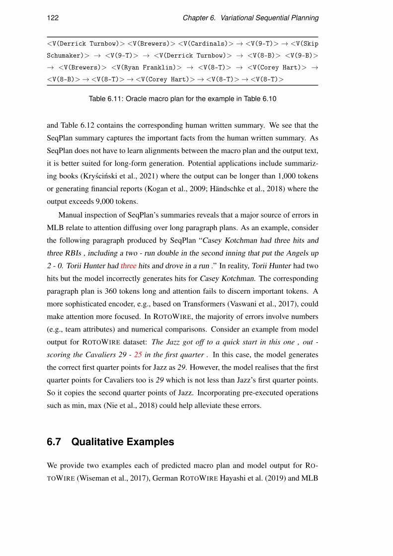
122 Chapter 6. Variational Sequential Planning
<V(Derrick Turnbow)> <V(Brewers)> <V(Cardinals)> → <V(9-T)> → <V(Skip
Schumaker)> → <V(9-T)> → <V(Derrick Turnbow)> → <V(8-B)> <V(9-B)>
→ <V(Brewers)> <V(Ryan Franklin)> → <V(8-T)> → <V(Corey Hart)> →<V(8-B)>→ <V(8-T)>→ <V(Corey Hart)>→ <V(8-T)>→ <V(8-T)>
Table 6.11: Oracle macro plan for the example in Table 6.10
and Table 6.12 contains the corresponding human written summary. We see that the
SeqPlan summary captures the important facts from the human written summary. As
SeqPlan does not have to learn alignments between the macro plan and the output text,
it is better suited for long-form generation. Potential applications include summariz-
ing books (Kryscinski et al., 2021) where the output can be longer than 1,000 tokens
or generating financial reports (Kogan et al., 2009; Händschke et al., 2018) where the
output exceeds 9,000 tokens.
Manual inspection of SeqPlan’s summaries reveals that a major source of errors in
MLB relate to attention diffusing over long paragraph plans. As an example, consider
the following paragraph produced by SeqPlan “Casey Kotchman had three hits and
three RBIs , including a two - run double in the second inning that put the Angels up
2 - 0. Torii Hunter had three hits and drove in a run .” In reality, Torii Hunter had two
hits but the model incorrectly generates hits for Casey Kotchman. The corresponding
paragraph plan is 360 tokens long and attention fails to discern important tokens. A
more sophisticated encoder, e.g., based on Transformers (Vaswani et al., 2017), could
make attention more focused. In ROTOWIRE, the majority of errors involve numbers
(e.g., team attributes) and numerical comparisons. Consider an example from model
output for ROTOWIRE dataset: The Jazz got off to a quick start in this one , out -
scoring the Cavaliers 29 - 25 in the first quarter . In this case, the model generates
the correct first quarter points for Jazz as 29. However, the model realises that the first
quarter points for Cavaliers too is 29 which is not less than Jazz’s first quarter points.
So it copies the second quarter points of Jazz. Incorporating pre-executed operations
such as min, max (Nie et al., 2018) could help alleviate these errors.
6.7 Qualitative Examples
We provide two examples each of predicted macro plan and model output for RO-
TOWIRE (Wiseman et al., 2017), German ROTOWIRE Hayashi et al. (2019) and MLB

6.7. Qualitative Examples 123
MILWAUKEE (AP) – Derrick Turnbow is finally throwing strikes now. Unfortunately for
the Brewers, the Cardinals are well aware of that. <P> Skip Schumaker doubled in the go-
ahead run in the ninth and St. Louis put Turnbow ’s first three pitches in play to overcome a
fielding blunder in the eighth in a 4-3 win over Milwaukee on Monday night. <P> Schumaker
had been 0-for-4 before his hit. <P> Brian Barton, who pinch hit for reliever Ryan Franklin,
doubled off a 95 mph fastball from Turnbow (0-1) to start the inning. After Cesar Izturis
sacrificed Barton to second by bunting a 96 mph fastball, Schumaker came up and took another
95 mph fastball to the wall for an RBI double. <P> Turnbow, who has been frustrated since
he ’s no longer the primary set-up man, has failed to inspire any confidence for the Brewers
since his precipitous decline starting July 2006. After converting 62 of his first 70 save chances
with a 2.60 ERA, he ’s only converted two of nine with a 6.75 ERA in his last 109 games. <P>
After seven strong innings from Cardinals starter Adam Wainwright, Franklin (1-1) got the win
despite giving up an unearned run by limiting the damage in the eighth, and Jason Isringhausen
earned his seventh save in eight chances with a perfect ninth on six pitches. <P> It appeared
the Brewers had all the momentum before Franklin stopped them cold. <P> With St. Louis
leading 3-2, Ryan Braun doubled to start the eighth inning and right fielder Ryan Ludwick
charged hard on a fly ball from Corey Hart, but slipped and lost the ball in the lights. <P> It
nearly hit him in the head, but instead bounced harmlessly behind him for a triple that left Hart
shaking his head in disbelief at his RBI that tied it at 3 after he made an errant play himself in
the top half of the inning. <P> But Franklin didn’t allow Milwaukee to take the lead as Hart
was caught in a rundown when he tried to score on contact off a chopper by Bill Hall and J.J.
Hardy grounded out to end the inning. <P> In the top half of the eighth, St. Louis went ahead
3-2 as a result of Hart’s gaffe in right field on Ludwick’s fly ball that hit the webbing of Hart’s
glove to put Ludwick on third with no outs. <P> Hart said he lost the ball in the lights, too.
<P> Reliever Brian Shouse, who came in to start the eighth after Carlos Villanueva retired 13
of his last 14 batters, walked Albert Pujols – he had three of St. Louis’ seven in the game and
has reached base safely every game this season – and got Rick Ankiel to pop out. <P> But
reliever Guillermo Mota could n’t keep the Cardinals off the board after walking Troy Glaus
despite having him down 0-2. With the bases loaded, Adam Kennedy ’s sacrifice fly gave St.
Louis a 3-2 lead.
Table 6.12: Human written summary for the example in Table 6.10
in Tables 6.13 – 6.18. The macro plan is at the top and the game summary is below.
We see that there is strong alignment between the macro plan and the game summary.
In addition, the game summary exhibits coherent ordering of facts.
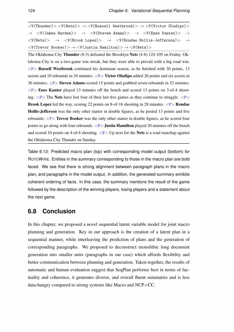
124 Chapter 6. Variational Sequential Planning
<V(Thunder)> <V(Nets)> → <V(Russell Westbrook)> → <V(Victor Oladipo)>
→ <V(James Harden)> → <V(Steven Adams)> → <V(Enes Kanter)> →<V(Nets)> → <V(Brook Lopez)> → <V(Rondae Hollis-Jefferson)> →<V(Trevor Booker)>→ <V(Justin Hamilton)>→ <V(Nets)>
The Oklahoma City Thunder (8-5) defeated the Brooklyn Nets (4-8) 124-105 on Friday. Ok-
lahoma City is on a two-game win streak, but they were able to prevail with a big road win.
<P> Russell Westbrook continued his dominant season, as he finished with 30 points, 13
assists and 10 rebounds in 34 minutes. <P> Victor Oladipo added 26 points and six assists in
36 minutes. <P> Steven Adams scored 15 points and grabbed seven rebounds in 32 minutes.
<P> Enes Kanter played 13 minutes off the bench and scored 13 points on 3-of-4 shoot-
ing. <P> The Nets have lost four of their last five games as they continue to struggle. <P>
Brook Lopez led the way, scoring 22 points on 8-of-16 shooting in 28 minutes. <P> Rondae
Hollis-Jefferson was the only other starter in double figures, as he posted 13 points and five
rebounds. <P> Trevor Booker was the only other starter in double figures, as he scored four
points to go along with four rebounds. <P> Justin Hamilton played 20 minutes off the bench
and scored 10 points on 4-of-6 shooting. <P> Up next for the Nets is a road matchup against
the Oklahoma City Thunder on Sunday.
Table 6.13: Predicted macro plan (top) with corresponding model output (bottom) for
ROTOWIRE. Entities in the summary corresponding to those in the macro plan are bold
faced. We see that there is strong alignment between paragraph plans in the macro
plan, and paragraphs in the model output. In addition, the generated summary exhibits
coherent ordering of facts. In this case, the summary mentions the result of the game
followed by the description of the winning players, losing players and a statement about
the next game.
6.8 Conclusion
In this chapter, we proposed a novel sequential latent variable model for joint macro
planning and generation. Key in our approach is the creation of a latent plan in a
sequential manner, while interleaving the prediction of plans and the generation of
corresponding paragraphs. We proposed to deconstruct monolithic long document
generation into smaller units (paragraphs in our case) which affords flexibility and
better communication between planning and generation. Taken together, the results of
automatic and human evaluation suggest that SeqPlan performs best in terms of fac-
tuality and coherence, it generates diverse, and overall fluent summaries and is less
data-hungry compared to strong systems like Macro and NCP+CC.
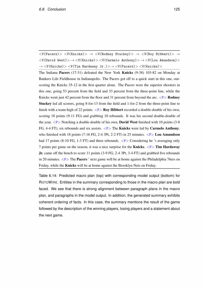
6.8. Conclusion 125
<V(Pacers)> <V(Knicks)> → <V(Rodney Stuckey)> → <V(Roy Hibbert)> →<V(David West)>→<V(Knicks)><V(Carmelo Anthony)>→<V(Lou Amundson)>
→ <V(Knicks)> <V(Tim Hardaway Jr.)>→ <V(Pacers)> <V(Knicks)>
The Indiana Pacers (17-31) defeated the New York Knicks (9-38) 103-82 on Monday at
Bankers Life Fieldhouse in Indianapolis. The Pacers got off to a quick start in this one, out-
scoring the Knicks 35-12 in the first quarter alone. The Pacers were the superior shooters in
this one, going 53 percent from the field and 33 percent from the three-point line, while the
Knicks went just 42 percent from the floor and 31 percent from beyond the arc. <P> Rodney
Stuckey led all scorers, going 8-for-13 from the field and 1-for-2 from the three-point line to
finish with a team-high of 22 points. <P> Roy Hibbert recorded a double-double of his own,
scoring 18 points (9-11 FG) and grabbing 10 rebounds. It was his second double-double of
the year. <P> Notching a double-double of his own, David West finished with 10 points (3-8
FG, 4-4 FT), six rebounds and six assists. <P> The Knicks were led by Carmelo Anthony,
who finished with 18 points (7-16 FG, 2-4 3Pt, 2-2 FT) in 25 minutes. <P> Lou Amundson
had 17 points (8-10 FG, 1-3 FT) and three rebounds. <P> Considering he ’s averaging only
7 points per game on the season, it was a nice surprise for the Knicks. <P> Tim Hardaway
Jr. came off the bench to score 11 points (3-9 FG, 2-4 3Pt, 3-4 FT) and grabbed five rebounds
in 20 minutes. <P> The Pacers ’ next game will be at home against the Philadelphia 76ers on
Friday, while the Knicks will be at home against the Brooklyn Nets on Friday.
Table 6.14: Predicted macro plan (top) with corresponding model output (bottom) for
ROTOWIRE. Entities in the summary corresponding to those in the macro plan are bold
faced. We see that there is strong alignment between paragraph plans in the macro
plan, and paragraphs in the model output. In addition, the generated summary exhibits
coherent ordering of facts. In this case, the summary mentions the result of the game
followed by the description of the winning players, losing players and a statement about
the next game.
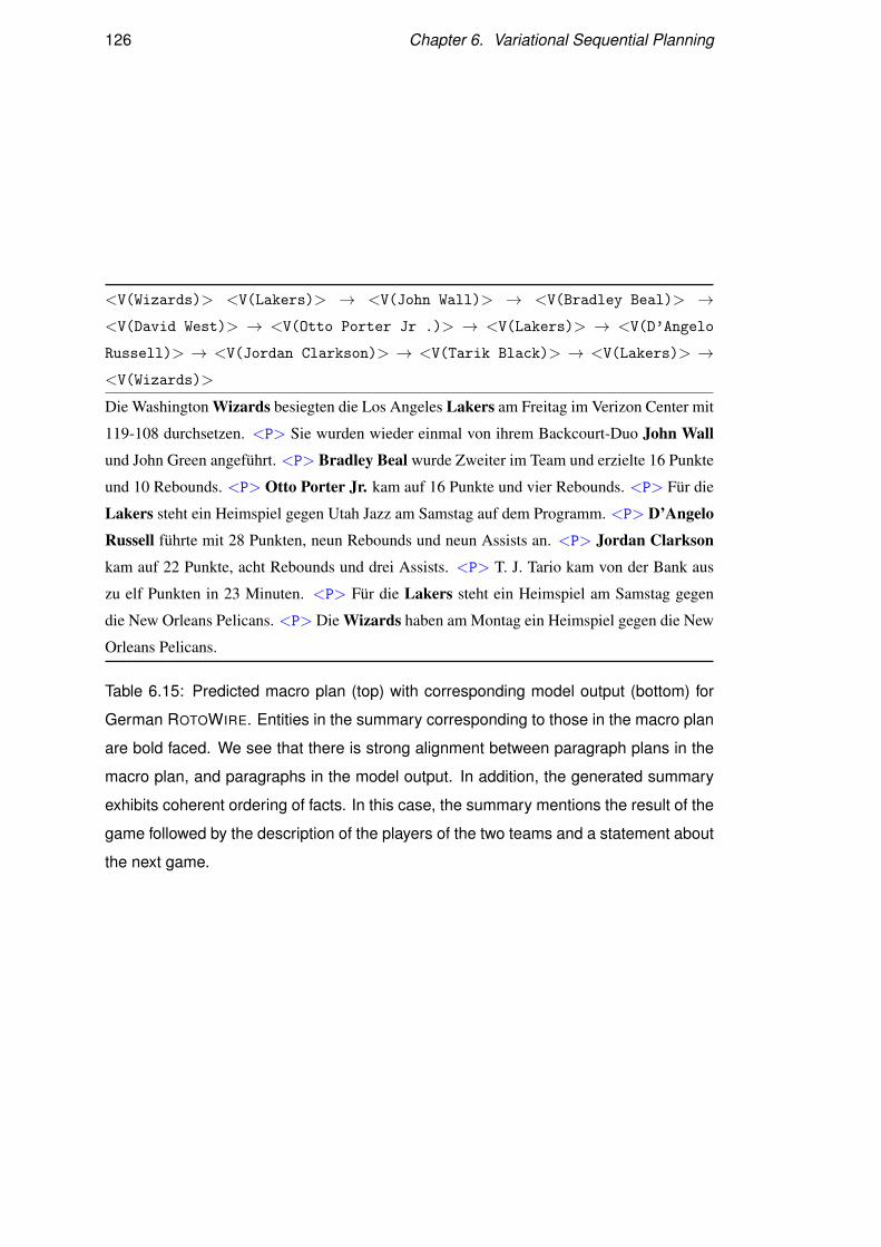
126 Chapter 6. Variational Sequential Planning
<V(Wizards)> <V(Lakers)> → <V(John Wall)> → <V(Bradley Beal)> →<V(David West)> → <V(Otto Porter Jr .)> → <V(Lakers)> → <V(D’Angelo
Russell)> → <V(Jordan Clarkson)> → <V(Tarik Black)> → <V(Lakers)> →<V(Wizards)>
Die Washington Wizards besiegten die Los Angeles Lakers am Freitag im Verizon Center mit
119-108 durchsetzen. <P> Sie wurden wieder einmal von ihrem Backcourt-Duo John Wall
und John Green angeführt. <P> Bradley Beal wurde Zweiter im Team und erzielte 16 Punkte
und 10 Rebounds. <P> Otto Porter Jr. kam auf 16 Punkte und vier Rebounds. <P> Für die
Lakers steht ein Heimspiel gegen Utah Jazz am Samstag auf dem Programm. <P> D’Angelo
Russell führte mit 28 Punkten, neun Rebounds und neun Assists an. <P> Jordan Clarkson
kam auf 22 Punkte, acht Rebounds und drei Assists. <P> T. J. Tario kam von der Bank aus
zu elf Punkten in 23 Minuten. <P> Für die Lakers steht ein Heimspiel am Samstag gegen
die New Orleans Pelicans. <P> Die Wizards haben am Montag ein Heimspiel gegen die New
Orleans Pelicans.
Table 6.15: Predicted macro plan (top) with corresponding model output (bottom) for
German ROTOWIRE. Entities in the summary corresponding to those in the macro plan
are bold faced. We see that there is strong alignment between paragraph plans in the
macro plan, and paragraphs in the model output. In addition, the generated summary
exhibits coherent ordering of facts. In this case, the summary mentions the result of the
game followed by the description of the players of the two teams and a statement about
the next game.

6.8. Conclusion 127
<V(Celtics)> <V(Pacers)> → <V(Isaiah Thomas)> → <V(Myles Turner)>
→ <V(Amir Johnson)> → <V(Monta Ellis)> → <V(Thaddeus Young)> →<V(Pacers)>→ <V(Jeff Teague)>→ <V(Al Jefferson)>→ <V(Pacers)>
Die Boston Celtics (5-4) besiegten die Indiana Pacers (4-6) am Mittwoch mit 112:99 in der
Verlängerung im Staples Center. Die Celtics (5-4) befinden sich weiter auf ihrem unglaublichen
Pfad der Durchschnittlichkeit und haben in ihren letzten 15 Spielen abwechselnd gewonnen.
<P> Isaiah Thomas tat sein Bestes, um mit 23 Punkten, elf Rebounds und fünf Assists fort-
setzte. <P> Myles Turner erreichte ein Double-Double mit 17 Punkten und acht Rebounds.
<P> Amir Johnson war der einzige andere Starter mit zweistelliger Punkteanzahl und kam
auf 14 Punkte, neun Rebounds, drei Assists und einen Steal. <P> Monta Ellis steuerte 15
Punkte, vier Rebounds und vier Assists. <P> Thaddeus Young führte mit 10 Punkten die
Bank an. <P> Für die Pacers folgt am Freitag ein weiteres Heimspiel gegen die Denver
Nuggets. <P> Jeff Teague kam auf 20 Punkte und vier Assists. <P> Al Jefferson war in 17
Minuten von der Bank sehr gut, mit 10 Punkten, drei Rebounds und zwei Assists. <P> Für
die Pacers steht ein Heimspiel am Samstag gegen die New Orleans Pelicans.
Table 6.16: Predicted macro plan (top) with corresponding model output (bottom) for
German ROTOWIRE. Entities in the summary corresponding to those in the macro plan
are bold faced. We see that there is strong alignment between paragraph plans in the
macro plan, and paragraphs in the model output. In addition, the generated summary
exhibits coherent ordering of facts. In this case, the summary mentions the result of the
game followed by the description of the players of the two teams and a statement about
the next game.
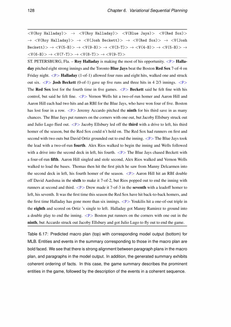
128 Chapter 6. Variational Sequential Planning
<V(Roy Halladay)> → <V(Roy Halladay)> <V(Blue Jays)> <V(Red Sox)>
→ <V(Roy Halladay)> → <V(Josh Beckett)> → <V(Red Sox)> → <V(Josh
Beckett)> → <V(5-B)> → <V(9-B)> → <V(3-T)> → <V(4-B)> → <V(5-B)> →<V(6-B)>→ <V(7-T)>→ <V(8-T)>→ <V(9-T)>
ST. PETERSBURG, Fla. – Roy Halladay is making the most of his opportunity. <P> Halla-
day pitched eight strong innings and the Toronto Blue Jays beat the Boston Red Sox 7-of-4 on
Friday night. <P> Halladay (1-of-1) allowed four runs and eight hits, walked one and struck
out six. <P> Josh Beckett (0-of-1) gave up five runs and three hits in 4 2/3 innings. <P>
The Red Sox lost for the fourth time in five games. <P> Beckett said he felt fine with his
control, but said he felt fine. <P> Vernon Wells hit a two-of-run homer and Aaron Hill and
Aaron Hill each had two hits and an RBI for the Blue Jays, who have won four of five. Boston
has lost four in a row. <P> Jeremy Accardo pitched the ninth for his third save in as many
chances. The Blue Jays put runners on the corners with one out, but Jacoby Ellsbury struck out
and Julio Lugo flied out. <P> Jacoby Ellsbury led off the third with a drive to left, his third
homer of the season, but the Red Sox could n’t hold on. The Red Sox had runners on first and
second with two outs but David Ortiz grounded out to end the inning. <P> The Blue Jays took
the lead with a two-of-run fourth. Alex Rios walked to begin the inning and Wells followed
with a drive into the second deck in left, his fourth. <P> The Blue Jays chased Beckett with
a four-of-run fifth. Aaron Hill singled and stole second, Alex Rios walked and Vernon Wells
walked to load the bases. Thomas then hit the first pitch he saw from Manny Delcarmen into
the second deck in left, his fourth homer of the season. <P> Aaron Hill hit an RBI double
off David Aardsma in the sixth to make it 7-of-2, but Rios popped out to end the inning with
runners at second and third. <P> Drew made it 7-of-3 in the seventh with a leadoff homer to
left, his seventh. It was the first time this season the Red Sox have hit back-to-back homers, and
the first time Halladay has gone more than six innings. <P> Youkilis hit a one-of-out triple in
the eighth and scored on Ortiz ’s single to left. Halladay got Manny Ramirez to ground into
a double play to end the inning. <P> Boston put runners on the corners with one out in the
ninth, but Accardo struck out Jacoby Ellsbury and got Julio Lugo to fly out to end the game.
Table 6.17: Predicted macro plan (top) with corresponding model output (bottom) for
MLB. Entities and events in the summary corresponding to those in the macro plan are
bold faced. We see that there is strong alignment between paragraph plans in the macro
plan, and paragraphs in the model output. In addition, the generated summary exhibits
coherent ordering of facts. In this case, the game summary describes the prominent
entities in the game, followed by the description of the events in a coherent sequence.
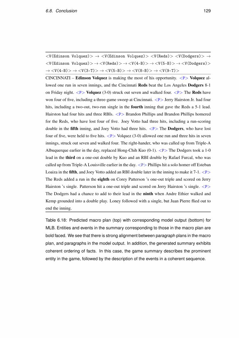
6.8. Conclusion 129
<V(Edinson Volquez)> → <V(Edinson Volquez)> <V(Reds)> <V(Dodgers)> →<V(Edinson Volquez)>→<V(Reds)>→<V(4-B)>→<V(5-B)>→<V(Dodgers)>
→ <V(4-B)>→ <V(3-T)>→ <V(5-B)>→ <V(8-B)>→ <V(9-T)>
CINCINNATI – Edinson Volquez is making the most of his opportunity. <P> Volquez al-
lowed one run in seven innings, and the Cincinnati Reds beat the Los Angeles Dodgers 8-1
on Friday night. <P> Volquez (3-0) struck out seven and walked four. <P> The Reds have
won four of five, including a three-game sweep at Cincinnati. <P> Jerry Hairston Jr. had four
hits, including a two-out, two-run single in the fourth inning that gave the Reds a 5-1 lead.
Hairston had four hits and three RBIs. <P> Brandon Phillips and Brandon Phillips homered
for the Reds, who have lost four of five. Joey Votto had three hits, including a run-scoring
double in the fifth inning, and Joey Votto had three hits. <P> The Dodgers, who have lost
four of five, were held to five hits. <P> Volquez (3-0) allowed one run and three hits in seven
innings, struck out seven and walked four. The right-hander, who was called up from Triple-A
Albuquerque earlier in the day, replaced Hong-Chih Kuo (0-1). <P> The Dodgers took a 1-0
lead in the third on a one-out double by Kuo and an RBI double by Rafael Furcal, who was
called up from Triple-A Louisville earlier in the day. <P> Phillips hit a solo homer off Esteban
Loaiza in the fifth, and Joey Votto added an RBI double later in the inning to make it 7-1. <P>
The Reds added a run in the eighth on Corey Patterson ’s one-out triple and scored on Jerry
Hairston ’s single. Patterson hit a one-out triple and scored on Jerry Hairston ’s single. <P>
The Dodgers had a chance to add to their lead in the ninth when Andre Ethier walked and
Kemp grounded into a double play. Loney followed with a single, but Juan Pierre flied out to
end the inning.
Table 6.18: Predicted macro plan (top) with corresponding model output (bottom) for
MLB. Entities and events in the summary corresponding to those in the macro plan are
bold faced. We see that there is strong alignment between paragraph plans in the macro
plan, and paragraphs in the model output. In addition, the generated summary exhibits
coherent ordering of facts. In this case, the game summary describes the prominent
entity in the game, followed by the description of the events in a coherent sequence.

Chapter 7
Conclusions
In this thesis, we have focused on data-to-text generation, which aims to produce tex-
tual output from non-linguistic input. Most recent work on data-to-text generation
makes use of neural networks to address this task focusing almost exclusively on the
encoder-decoder architecture. Such models are often trained in an end-to-end manner
without specific modules for document or micro planning. The expectation is that these
models will learn to perform planning on their own without the addition of any special-
purpose mechanisms or changes to the encoder-decoder architecture. Despite produc-
ing overall fluent text, neural systems have difficulty capturing long-term structure and
generating documents more than a few sentences long. Wiseman et al. (2017) showed
that neural text generation techniques perform poorly at content selection, struggle to
maintain inter-sentential coherence, and more generally a reasonable ordering of the
selected facts in the output text. Additional challenges include avoiding redundancy
and being faithful to the input. More recently, Maynez et al. (2020) conducted a large-
scale human evaluation exercise to study the faithfulness of model output for the task
of abstractive summarization. In this study, they asked human raters to annotate spans
in summaries that are not faithful to the input document. They compared different vari-
ants of neural models, including pretrained models and found that the latter are faithful
only 26.9% of the time to the input document.
In this thesis, we have argued that the introduction of planning can address some of
these challenges in neural data-to-text generation. We have hypothesized that content
planning can serve as an intermediate stage between the (data) input and (textual) out-
put. The content plan provides information about what should be communicated and
in what structure in the output document, which in turn enables the decoder to focus
on the less challenging task of predicting tokens conformant to the plan.
131
132 Chapter 7. Conclusions
Micro planning generally involves deciding on specific words to describe concepts
and relations, generating referring expressions, and aggregating content into sentences
(Reiter and Dale, 2000). We introduced neural micro planning in Chapter 3. We
proposed modifications to contemporary neural encoder-decoder models, which inject
planning in the generation process. Specifically, we developed a model which learns
a micro plan from the input and conditions on it to generate the output document. We
operationalized micro plans as a sequence of records from the input table. For training
the micro planner, we extracted oracle micro plans from game summaries following
an information extraction (IE) approach. Specifically, we adopted the IE model intro-
duced in Wiseman et al. (2017), which identifies candidate entity (i.e., player, team,and
city) and value (i.e., number or string) pairs that appear in the text, and then predicts
the type (aka relation) of each candidate pair. Given the output of an IE system, a
micro plan consists of (entity, value, record type) tuples in their order of appearance in
a game summary.
Micro planning, however, requires fine-grained record level supervision for train-
ing. It assumes the availability of a highly precise and broad coverage IE tool. For
MLB, the IE has lower precision and coverage, as it is difficult to detect entity-value
pairs with simple pattern matching. Consequently, supervision for oracle micro plans
is not easy to obtain and the reliance on IE as a preprocessing step makes the approach
domain dependent and less scalable. In Chapter 4, we explored how to perform data-
to-text generation by inducing latent plans which operate at a higher level than records,
such as entities. Our model creates entity-specific representations which are dynami-
cally updated. Text is generated by conditioning on the data input and entity memory
representations using hierarchical attention at each time step.
Unfortunately, the approach of latent entity planning does not handle events, which
are often present in data-to-text generation tasks, in particular those in the sports do-
main. For example, in the MLB dataset the play-by-play table documents the most
important events in a game in chronological order. In Chapter 5, we introduced neural
macro planning, which combines planning with the high level organization of entities
and events. Macro planning reconceptualizes the input in terms of paragraph plans to
facilitate document-level planning. In the sports domain, paragraphs typically men-
tion entities (e.g, players important in the game), key events (e.g., scoring a run), and
their interaction. And most of this information is encapsulated in the statistics ac-
companying game summaries. We thus define paragraph plans such that they contain
verbalizations of entity and event records. Macro planning advocates the use of macro
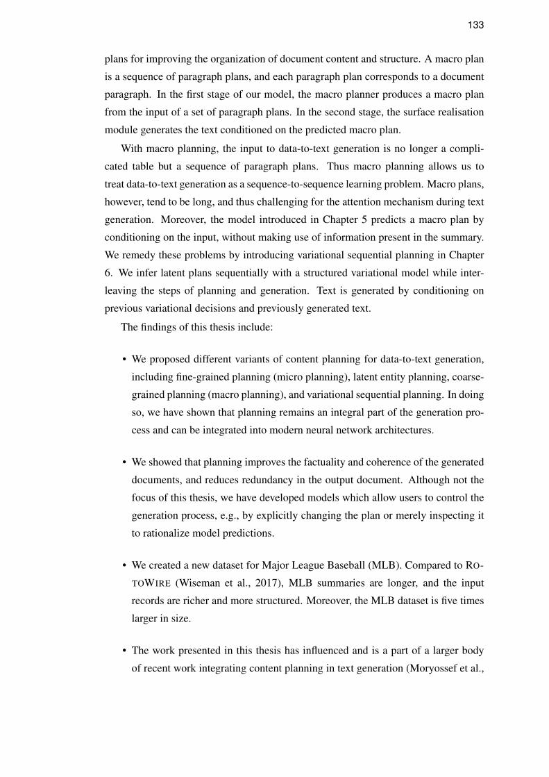
133
plans for improving the organization of document content and structure. A macro plan
is a sequence of paragraph plans, and each paragraph plan corresponds to a document
paragraph. In the first stage of our model, the macro planner produces a macro plan
from the input of a set of paragraph plans. In the second stage, the surface realisation
module generates the text conditioned on the predicted macro plan.
With macro planning, the input to data-to-text generation is no longer a compli-
cated table but a sequence of paragraph plans. Thus macro planning allows us to
treat data-to-text generation as a sequence-to-sequence learning problem. Macro plans,
however, tend to be long, and thus challenging for the attention mechanism during text
generation. Moreover, the model introduced in Chapter 5 predicts a macro plan by
conditioning on the input, without making use of information present in the summary.
We remedy these problems by introducing variational sequential planning in Chapter
6. We infer latent plans sequentially with a structured variational model while inter-
leaving the steps of planning and generation. Text is generated by conditioning on
previous variational decisions and previously generated text.
The findings of this thesis include:
• We proposed different variants of content planning for data-to-text generation,
including fine-grained planning (micro planning), latent entity planning, coarse-
grained planning (macro planning), and variational sequential planning. In doing
so, we have shown that planning remains an integral part of the generation pro-
cess and can be integrated into modern neural network architectures.
• We showed that planning improves the factuality and coherence of the generated
documents, and reduces redundancy in the output document. Although not the
focus of this thesis, we have developed models which allow users to control the
generation process, e.g., by explicitly changing the plan or merely inspecting it
to rationalize model predictions.
• We created a new dataset for Major League Baseball (MLB). Compared to RO-
TOWIRE (Wiseman et al., 2017), MLB summaries are longer, and the input
records are richer and more structured. Moreover, the MLB dataset is five times
larger in size.
• The work presented in this thesis has influenced and is a part of a larger body
of recent work integrating content planning in text generation (Moryossef et al.,
134 Chapter 7. Conclusions
2019; Fu et al., 2019; Shao et al., 2019; Zhao et al., 2020; Shen et al., 2020;
Narayan et al., 2020, 2021, inter alia).
7.1 Future Work
In this section we look into possible avenues for future work, and discuss extensions
to the models presented in this thesis.
Combining Micro and Macro Planning In the future, we envisage creating a model
which combines the merits of micro and macro planning. In this model, macro plan-
ning will be responsible for overall document coherence and selection of paragraph
plans, while micro planning will assume the responsibility of generating an accu-
rate, succinct, and fluent paragraph. Training a micro planner, however, requires fine-
grained supervision. Such supervision in the form of relations extracted using IE suf-
fers from low coverage and precision for some datasets such as MLB. We will need to
investigate techniques to train micro planners using partial supervision. For example,
we could use IE to extract relations that are high precision but possibly low recall. Un-
like the approach in Chapter 3, where the micro plan contains all the relations in the
game summary, the micro plan will now include a subset of high precision relations.
The surface realiser will then describe these relations from the micro plan and may
also describe other relations directly from the macro plan.
Discrete Reasoning In this thesis we have worked with two sports datasets, namely
MLB and ROTOWIRE, both of which require discrete reasoning. Consider a sentence
from a ROTOWIRE game summary “The host Toronto Raptors defeated the Philadel-
phia 76ers, 122 - 95, at Air Canada Center on Monday.”. Generating such a sentence
requires the model to know which team scored higher. For the statement “Sergio Ro-
driguez, Ersan Ilyasova, Nik Stauskas and Richaun Holmes all finished with 11 points
apiece.”, the model needs to compare scores of multiple players, reason that they are
equal, and then generate the statement. Currently, the models presented in this thesis
have a basic understanding of numbers acquired through word embeddings. It will be
interesting to explore better numerical reasoning in the context of generation. Incorpo-
rating ideas from models used for QA datasets such as DROP (Dua et al., 2019)1 requir-
ing discrete reasoning seems a promising research direction. Recent work in data-to-
1DROP stands for Discrete Reasoning Over Paragraphs
7.1. Future Work 135
text generation has incorporated pre-executed operations such as min, max (Nie et al.,
2018). Wallace et al. (2019) show that character-level embeddings are better than word
embeddings for encoding numbers when evaluated on DROP (Dua et al., 2019). Com-
bining character embeddings with pre-executed operations (Nie et al., 2018) would be
an interesting research direction to explore.
Pretrained Language Models Pretrained language models such as BART (Lewis
et al., 2020) or T5 (Raffel et al., 2020) have recently found many applications in Natural
Language Generation, including summarization (Rothe et al., 2021) and data-to-text
generation of small outputs (Kale and Rastogi, 2020). These pretrained models can
handle a maximum length of 512 tokens for the input and output, a restriction imposed
by the Transformer (Vaswani et al., 2017) architecture. In Chapter 5, the input to
text generation stage is a lengthy macro plan, and the output is the whole document.
Longer inputs and outputs preclude the usage of pretrained language models. With the
approach of variational sequential planning in Chapter 6, the input to text generation
stage is a single paragraph plan, and the output is a paragraph of text. Thus, it is
now feasible to initialize our variational sequential model with pretrained models and
finetune on the RotoWire/MLB dataset. As pretrained models have been trained on
large amounts of text, they will help improve the fluency of generated summaries.
Other Generation Tasks Finally, we hypothesize that micro and macro planning will
be applicable to other generation tasks like summarization. Recent work by Narayan
et al. (2021) produces content plans containing a list of entities while generating sum-
maries. Their summaries are around four sentences long. Future work can involve
enriching their micro plans with relations between entities. Such relations can be ob-
tained using an Information Extraction approach (Angeli et al., 2015). Likewise, macro
planning and variational sequential planning can be applicable to long-form summa-
rization tasks such as summarizing books (Kryscinski et al., 2021), where the output
can be longer than 1,000 tokens.

Appendix A
Human Evaluation for Fact Verification
In this chapter and the next, we will go through the instructions provided to raters
who conducted the human evaluation studies. We asked participants to assess model
output in terms of relation generation, grammaticality, coherence, and conciseness for
the two datasets: ROTOWIRE and MLB. We conducted our study on the Amazon
Mechanical Turk (AMT) crowdsourcing platform. In this chapter, we will describe
the instructions provided to the raters for the task of fact verification of model outputs
for ROTOWIRE and MLB. In the next chapter, we will describe the instructions for
evaluating the quality of model outputs in terms of grammaticality, coherence, and
conciseness. Section A.1 describes the instructions to raters for fact verification of
ROTOWIRE and Section A.2 describes the instructions to raters for fact verification of
MLB. The annotation scripts for fact verification have been adapted from the scripts
produced by Wiseman et al. (2017).
A.1 Fact Verification for ROTOWIRE Instructions
Table A.1 describes the title and description of the task, along with the qualifications
required by the raters. The title and description is presented to the raters whereas the
qualifications are used to automatically filter raters in the platform.
Instructions This questionnaire will ask you to determine whether an English sen-
tence correctly reports the facts in an NBA basketball game’s box- and line-score ta-
bles. You do not need to be familiar with basketball to answer these questions; we
explain how to read the tables below!
This task contains validation instances (for which answers are known) that will be used
137
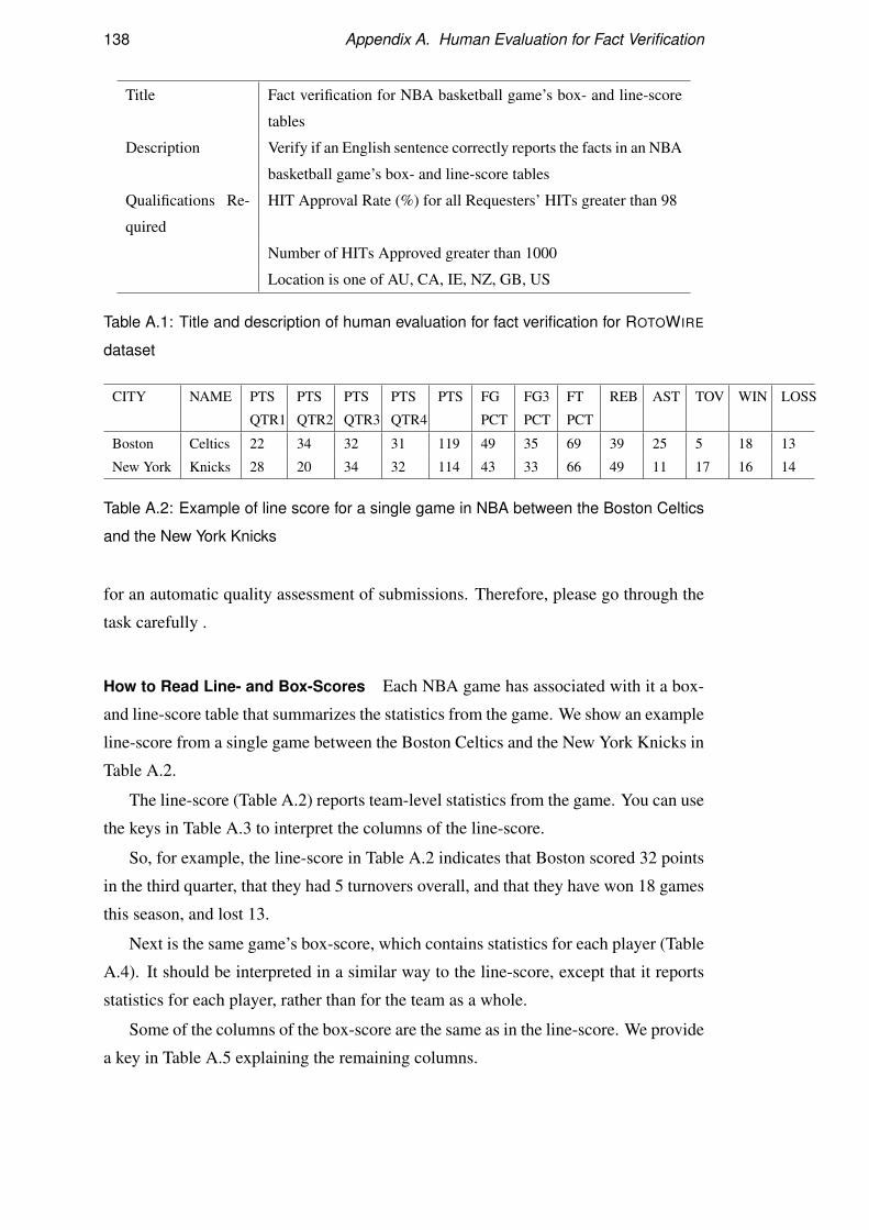
138 Appendix A. Human Evaluation for Fact Verification
Title Fact verification for NBA basketball game’s box- and line-score
tables
Description Verify if an English sentence correctly reports the facts in an NBA
basketball game’s box- and line-score tables
Qualifications Re-
quired
HIT Approval Rate (%) for all Requesters’ HITs greater than 98
Number of HITs Approved greater than 1000
Location is one of AU, CA, IE, NZ, GB, US
Table A.1: Title and description of human evaluation for fact verification for ROTOWIRE
dataset
CITY NAME PTS
QTR1
PTS
QTR2
PTS
QTR3
PTS
QTR4
PTS FG
PCT
FG3
PCT
FT
PCT
REB AST TOV WIN LOSS
Boston Celtics 22 34 32 31 119 49 35 69 39 25 5 18 13
New York Knicks 28 20 34 32 114 43 33 66 49 11 17 16 14
Table A.2: Example of line score for a single game in NBA between the Boston Celtics
and the New York Knicks
for an automatic quality assessment of submissions. Therefore, please go through the
task carefully .
How to Read Line- and Box-Scores Each NBA game has associated with it a box-
and line-score table that summarizes the statistics from the game. We show an example
line-score from a single game between the Boston Celtics and the New York Knicks in
Table A.2.
The line-score (Table A.2) reports team-level statistics from the game. You can use
the keys in Table A.3 to interpret the columns of the line-score.
So, for example, the line-score in Table A.2 indicates that Boston scored 32 points
in the third quarter, that they had 5 turnovers overall, and that they have won 18 games
this season, and lost 13.
Next is the same game’s box-score, which contains statistics for each player (Table
A.4). It should be interpreted in a similar way to the line-score, except that it reports
statistics for each player, rather than for the team as a whole.
Some of the columns of the box-score are the same as in the line-score. We provide
a key in Table A.5 explaining the remaining columns.
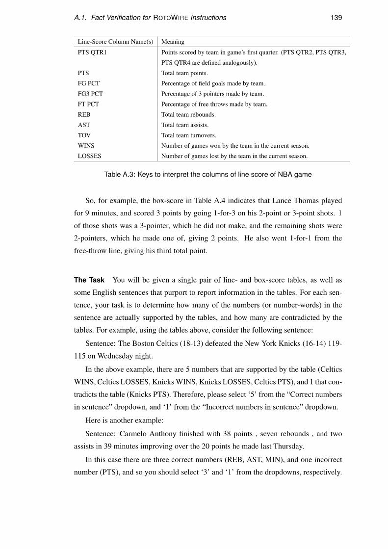
A.1. Fact Verification for ROTOWIRE Instructions 139
Line-Score Column Name(s) Meaning
PTS QTR1 Points scored by team in game’s first quarter. (PTS QTR2, PTS QTR3,
PTS QTR4 are defined analogously).
PTS Total team points.
FG PCT Percentage of field goals made by team.
FG3 PCT Percentage of 3 pointers made by team.
FT PCT Percentage of free throws made by team.
REB Total team rebounds.
AST Total team assists.
TOV Total team turnovers.
WINS Number of games won by the team in the current season.
LOSSES Number of games lost by the team in the current season.
Table A.3: Keys to interpret the columns of line score of NBA game
So, for example, the box-score in Table A.4 indicates that Lance Thomas played
for 9 minutes, and scored 3 points by going 1-for-3 on his 2-point or 3-point shots. 1
of those shots was a 3-pointer, which he did not make, and the remaining shots were
2-pointers, which he made one of, giving 2 points. He also went 1-for-1 from the
free-throw line, giving his third total point.
The Task You will be given a single pair of line- and box-score tables, as well as
some English sentences that purport to report information in the tables. For each sen-
tence, your task is to determine how many of the numbers (or number-words) in the
sentence are actually supported by the tables, and how many are contradicted by the
tables. For example, using the tables above, consider the following sentence:
Sentence: The Boston Celtics (18-13) defeated the New York Knicks (16-14) 119-
115 on Wednesday night.
In the above example, there are 5 numbers that are supported by the table (Celtics
WINS, Celtics LOSSES, Knicks WINS, Knicks LOSSES, Celtics PTS), and 1 that con-
tradicts the table (Knicks PTS). Therefore, please select ‘5’ from the “Correct numbers
in sentence” dropdown, and ‘1’ from the “Incorrect numbers in sentence” dropdown.
Here is another example:
Sentence: Carmelo Anthony finished with 38 points , seven rebounds , and two
assists in 39 minutes improving over the 20 points he made last Thursday.
In this case there are three correct numbers (REB, AST, MIN), and one incorrect
number (PTS), and so you should select ‘3’ and ‘1’ from the dropdowns, respectively.
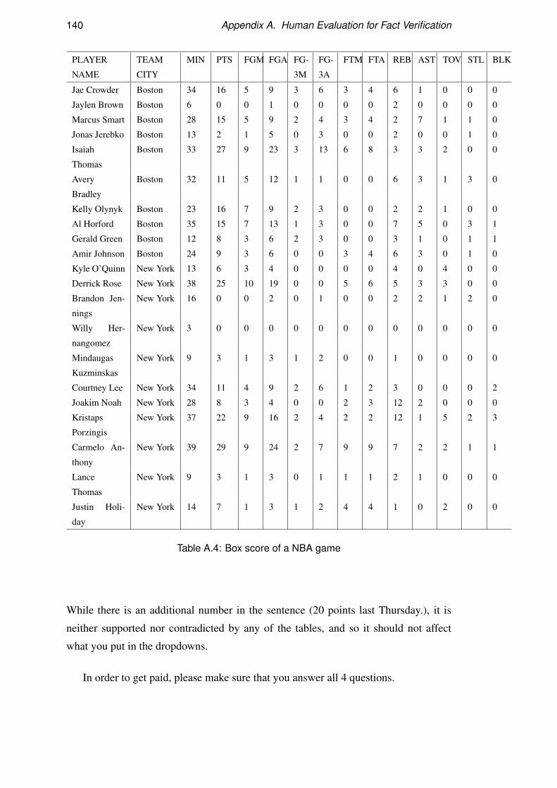
140 Appendix A. Human Evaluation for Fact Verification
PLAYER
NAME
TEAM
CITY
MIN PTS FGM FGA FG-
3M
FG-
3A
FTM FTA REB AST TOV STL BLK
Jae Crowder Boston 34 16 5 9 3 6 3 4 6 1 0 0 0
Jaylen Brown Boston 6 0 0 1 0 0 0 0 2 0 0 0 0
Marcus Smart Boston 28 15 5 9 2 4 3 4 2 7 1 1 0
Jonas Jerebko Boston 13 2 1 5 0 3 0 0 2 0 0 1 0
Isaiah
Thomas
Boston 33 27 9 23 3 13 6 8 3 3 2 0 0
Avery
Bradley
Boston 32 11 5 12 1 1 0 0 6 3 1 3 0
Kelly Olynyk Boston 23 16 7 9 2 3 0 0 2 2 1 0 0
Al Horford Boston 35 15 7 13 1 3 0 0 7 5 0 3 1
Gerald Green Boston 12 8 3 6 2 3 0 0 3 1 0 1 1
Amir Johnson Boston 24 9 3 6 0 0 3 4 6 3 0 1 0
Kyle O’Quinn New York 13 6 3 4 0 0 0 0 4 0 4 0 0
Derrick Rose New York 38 25 10 19 0 0 5 6 5 3 3 0 0
Brandon Jen-
nings
New York 16 0 0 2 0 1 0 0 2 2 1 2 0
Willy Her-
nangomez
New York 3 0 0 0 0 0 0 0 0 0 0 0 0
Mindaugas
Kuzminskas
New York 9 3 1 3 1 2 0 0 1 0 0 0 0
Courtney Lee New York 34 11 4 9 2 6 1 2 3 0 0 0 2
Joakim Noah New York 28 8 3 4 0 0 2 3 12 2 0 0 0
Kristaps
Porzingis
New York 37 22 9 16 2 4 2 2 12 1 5 2 3
Carmelo An-
thony
New York 39 29 9 24 2 7 9 9 7 2 2 1 1
Lance
Thomas
New York 9 3 1 3 0 1 1 1 2 1 0 0 0
Justin Holi-
day
New York 14 7 1 3 1 2 4 4 1 0 2 0 0
Table A.4: Box score of a NBA game
While there is an additional number in the sentence (20 points last Thursday.), it is
neither supported nor contradicted by any of the tables, and so it should not affect
what you put in the dropdowns.
In order to get paid, please make sure that you answer all 4 questions.

A.2. Fact Verification for MLB Instructions 141
Box-Score Column Name Meaning
MIN Minutes a player was in the game.
FGM How many field-goals (2-point or 3-point shots) a player made.
FGA How many field-goals (2-point or 3-point shots) a player attempted.
FG3M How many 3-point shots a player made.
FG3A How many 3-point shots a player attempted.
FTM How many free-throws a player made.
FTA How many free-throws a player attempted.
STL Number of steals made by a player.
BLK Number of blocks made by a player.
Table A.5: Keys to interpret the box score of NBA game
Consent Statement We invite you to participate in a research study related to the
production of informative text. There are no risks or benefits associated with partici-
pating in this study, but you will be paid for your participation as indicated in the HIT.
Your participation is of course voluntary, and you may withdraw at any time. If you
have any questions, concerns, or complaints, please email r.puduppully [at] sms [dot]
ed [dot] ac [dot] uk.
If your browser has JavaScript turned on, a counter will be displayed at the bottom
of the page indicating how many questions have been answered. It is highly recom-
mended that you turn on JavaScript and use this tool before submitting to ensure that
all questions have been answered and you can receive payment.
Are you a native speaker of English? Yes/No (Your answer to this question does
not affect the payment.)
Optional: Please use this space to provide feedback on the task or ask any ques-
tions. This will not affect acceptance of the HIT or your payment.
A.2 Fact Verification for MLB Instructions
Table A.6 describes the title and description of the task, along with the qualifications
required by the raters. The title and description is presented to the raters whereas the
qualifications are used to automatically filter raters in the platform.
Instructions This questionnaire will ask you to determine whether an English sen-
tence correctly reports the facts in an MLB baseball game’s box, line-score and play-
by-play tables. You do not need to be familiar with baseball to answer these questions;
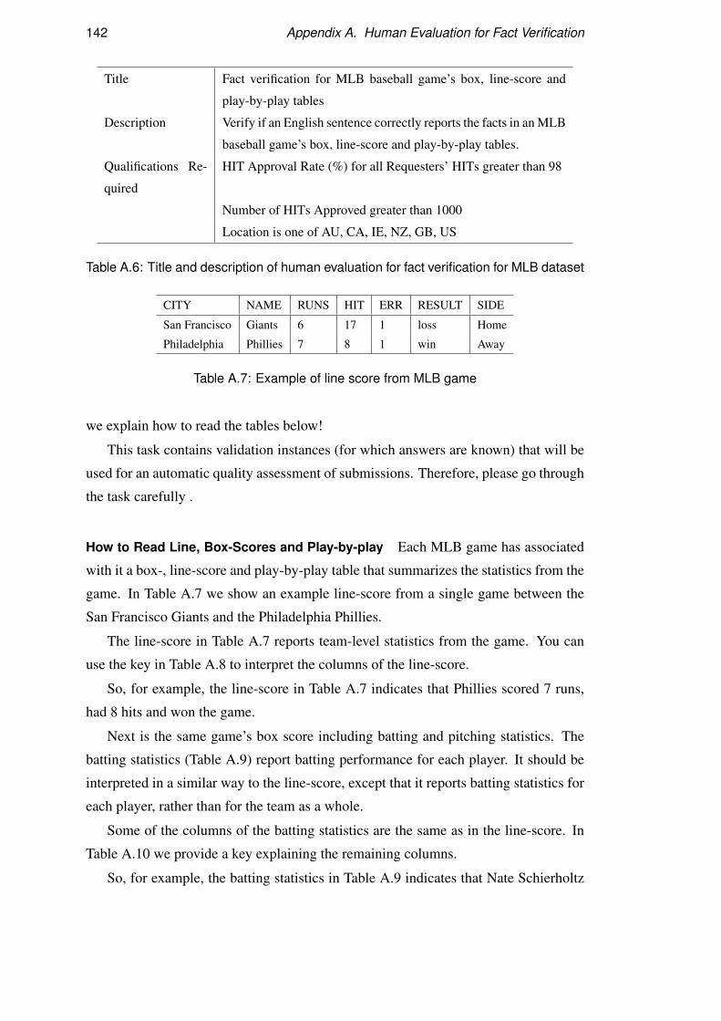
142 Appendix A. Human Evaluation for Fact Verification
Title Fact verification for MLB baseball game’s box, line-score and
play-by-play tables
Description Verify if an English sentence correctly reports the facts in an MLB
baseball game’s box, line-score and play-by-play tables.
Qualifications Re-
quired
HIT Approval Rate (%) for all Requesters’ HITs greater than 98
Number of HITs Approved greater than 1000
Location is one of AU, CA, IE, NZ, GB, US
Table A.6: Title and description of human evaluation for fact verification for MLB dataset
CITY NAME RUNS HIT ERR RESULT SIDE
San Francisco Giants 6 17 1 loss Home
Philadelphia Phillies 7 8 1 win Away
Table A.7: Example of line score from MLB game
we explain how to read the tables below!
This task contains validation instances (for which answers are known) that will be
used for an automatic quality assessment of submissions. Therefore, please go through
the task carefully .
How to Read Line, Box-Scores and Play-by-play Each MLB game has associated
with it a box-, line-score and play-by-play table that summarizes the statistics from the
game. In Table A.7 we show an example line-score from a single game between the
San Francisco Giants and the Philadelphia Phillies.
The line-score in Table A.7 reports team-level statistics from the game. You can
use the key in Table A.8 to interpret the columns of the line-score.
So, for example, the line-score in Table A.7 indicates that Phillies scored 7 runs,
had 8 hits and won the game.
Next is the same game’s box score including batting and pitching statistics. The
batting statistics (Table A.9) report batting performance for each player. It should be
interpreted in a similar way to the line-score, except that it reports batting statistics for
each player, rather than for the team as a whole.
Some of the columns of the batting statistics are the same as in the line-score. In
Table A.10 we provide a key explaining the remaining columns.
So, for example, the batting statistics in Table A.9 indicates that Nate Schierholtz
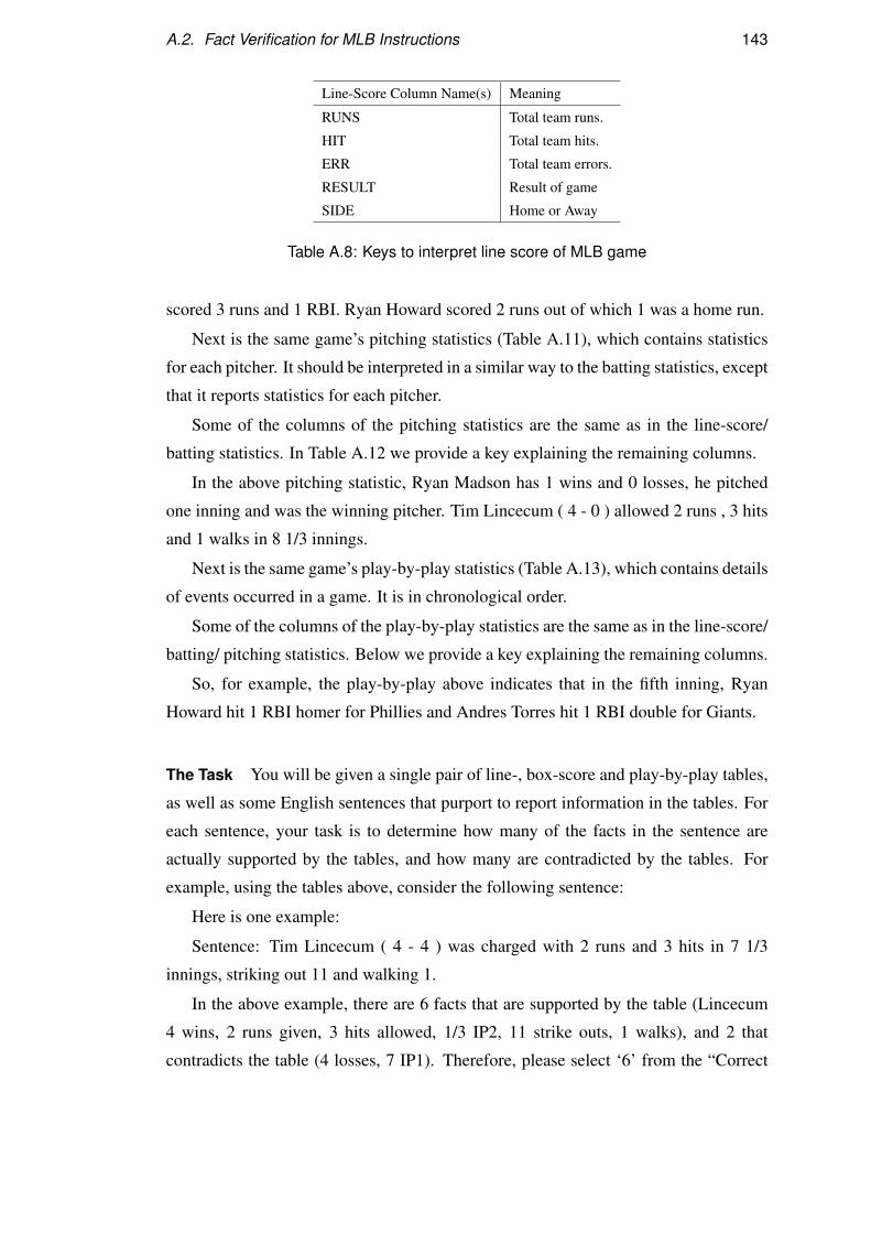
A.2. Fact Verification for MLB Instructions 143
Line-Score Column Name(s) Meaning
RUNS Total team runs.
HIT Total team hits.
ERR Total team errors.
RESULT Result of game
SIDE Home or Away
Table A.8: Keys to interpret line score of MLB game
scored 3 runs and 1 RBI. Ryan Howard scored 2 runs out of which 1 was a home run.
Next is the same game’s pitching statistics (Table A.11), which contains statistics
for each pitcher. It should be interpreted in a similar way to the batting statistics, except
that it reports statistics for each pitcher.
Some of the columns of the pitching statistics are the same as in the line-score/
batting statistics. In Table A.12 we provide a key explaining the remaining columns.
In the above pitching statistic, Ryan Madson has 1 wins and 0 losses, he pitched
one inning and was the winning pitcher. Tim Lincecum ( 4 - 0 ) allowed 2 runs , 3 hits
and 1 walks in 8 1/3 innings.
Next is the same game’s play-by-play statistics (Table A.13), which contains details
of events occurred in a game. It is in chronological order.
Some of the columns of the play-by-play statistics are the same as in the line-score/
batting/ pitching statistics. Below we provide a key explaining the remaining columns.
So, for example, the play-by-play above indicates that in the fifth inning, Ryan
Howard hit 1 RBI homer for Phillies and Andres Torres hit 1 RBI double for Giants.
The Task You will be given a single pair of line-, box-score and play-by-play tables,
as well as some English sentences that purport to report information in the tables. For
each sentence, your task is to determine how many of the facts in the sentence are
actually supported by the tables, and how many are contradicted by the tables. For
example, using the tables above, consider the following sentence:
Here is one example:
Sentence: Tim Lincecum ( 4 - 4 ) was charged with 2 runs and 3 hits in 7 1/3
innings, striking out 11 and walking 1.
In the above example, there are 6 facts that are supported by the table (Lincecum
4 wins, 2 runs given, 3 hits allowed, 1/3 IP2, 11 strike outs, 1 walks), and 2 that
contradicts the table (4 losses, 7 IP1). Therefore, please select ‘6’ from the “Correct
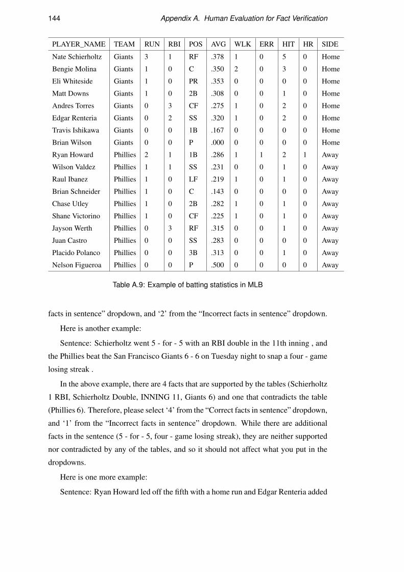
144 Appendix A. Human Evaluation for Fact Verification
PLAYER_NAME TEAM RUN RBI POS AVG WLK ERR HIT HR SIDE
Nate Schierholtz Giants 3 1 RF .378 1 0 5 0 Home
Bengie Molina Giants 1 0 C .350 2 0 3 0 Home
Eli Whiteside Giants 1 0 PR .353 0 0 0 0 Home
Matt Downs Giants 1 0 2B .308 0 0 1 0 Home
Andres Torres Giants 0 3 CF .275 1 0 2 0 Home
Edgar Renteria Giants 0 2 SS .320 1 0 2 0 Home
Travis Ishikawa Giants 0 0 1B .167 0 0 0 0 Home
Brian Wilson Giants 0 0 P .000 0 0 0 0 Home
Ryan Howard Phillies 2 1 1B .286 1 1 2 1 Away
Wilson Valdez Phillies 1 1 SS .231 0 0 1 0 Away
Raul Ibanez Phillies 1 0 LF .219 1 0 1 0 Away
Brian Schneider Phillies 1 0 C .143 0 0 0 0 Away
Chase Utley Phillies 1 0 2B .282 1 0 1 0 Away
Shane Victorino Phillies 1 0 CF .225 1 0 1 0 Away
Jayson Werth Phillies 0 3 RF .315 0 0 1 0 Away
Juan Castro Phillies 0 0 SS .283 0 0 0 0 Away
Placido Polanco Phillies 0 0 3B .313 0 0 1 0 Away
Nelson Figueroa Phillies 0 0 P .500 0 0 0 0 Away
Table A.9: Example of batting statistics in MLB
facts in sentence” dropdown, and ‘2’ from the “Incorrect facts in sentence” dropdown.
Here is another example:
Sentence: Schierholtz went 5 - for - 5 with an RBI double in the 11th inning , and
the Phillies beat the San Francisco Giants 6 - 6 on Tuesday night to snap a four - game
losing streak .
In the above example, there are 4 facts that are supported by the tables (Schierholtz
1 RBI, Schierholtz Double, INNING 11, Giants 6) and one that contradicts the table
(Phillies 6). Therefore, please select ‘4’ from the “Correct facts in sentence” dropdown,
and ‘1’ from the “Incorrect facts in sentence” dropdown. While there are additional
facts in the sentence (5 - for - 5, four - game losing streak), they are neither supported
nor contradicted by any of the tables, and so it should not affect what you put in the
dropdowns.
Here is one more example:
Sentence: Ryan Howard led off the fifth with a home run and Edgar Renteria added
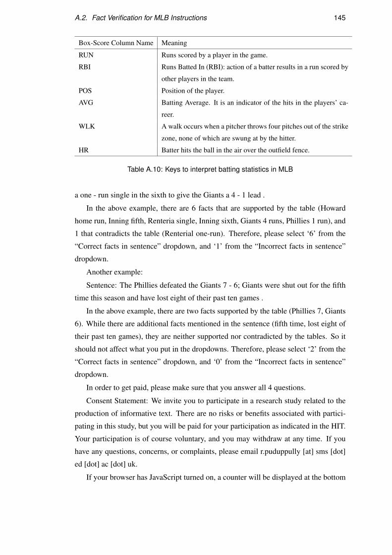
A.2. Fact Verification for MLB Instructions 145
Box-Score Column Name Meaning
RUN Runs scored by a player in the game.
RBI Runs Batted In (RBI): action of a batter results in a run scored by
other players in the team.
POS Position of the player.
AVG Batting Average. It is an indicator of the hits in the players’ ca-
reer.
WLK A walk occurs when a pitcher throws four pitches out of the strike
zone, none of which are swung at by the hitter.
HR Batter hits the ball in the air over the outfield fence.
Table A.10: Keys to interpret batting statistics in MLB
a one - run single in the sixth to give the Giants a 4 - 1 lead .
In the above example, there are 6 facts that are supported by the table (Howard
home run, Inning fifth, Renteria single, Inning sixth, Giants 4 runs, Phillies 1 run), and
1 that contradicts the table (Renterial one-run). Therefore, please select ‘6’ from the
“Correct facts in sentence” dropdown, and ‘1’ from the “Incorrect facts in sentence”
dropdown.
Another example:
Sentence: The Phillies defeated the Giants 7 - 6; Giants were shut out for the fifth
time this season and have lost eight of their past ten games .
In the above example, there are two facts supported by the table (Phillies 7, Giants
6). While there are additional facts mentioned in the sentence (fifth time, lost eight of
their past ten games), they are neither supported nor contradicted by the tables. So it
should not affect what you put in the dropdowns. Therefore, please select ‘2’ from the
“Correct facts in sentence” dropdown, and ‘0’ from the “Incorrect facts in sentence”
dropdown.
In order to get paid, please make sure that you answer all 4 questions.
Consent Statement: We invite you to participate in a research study related to the
production of informative text. There are no risks or benefits associated with partici-
pating in this study, but you will be paid for your participation as indicated in the HIT.
Your participation is of course voluntary, and you may withdraw at any time. If you
have any questions, concerns, or complaints, please email r.puduppully [at] sms [dot]
ed [dot] ac [dot] uk.
If your browser has JavaScript turned on, a counter will be displayed at the bottom
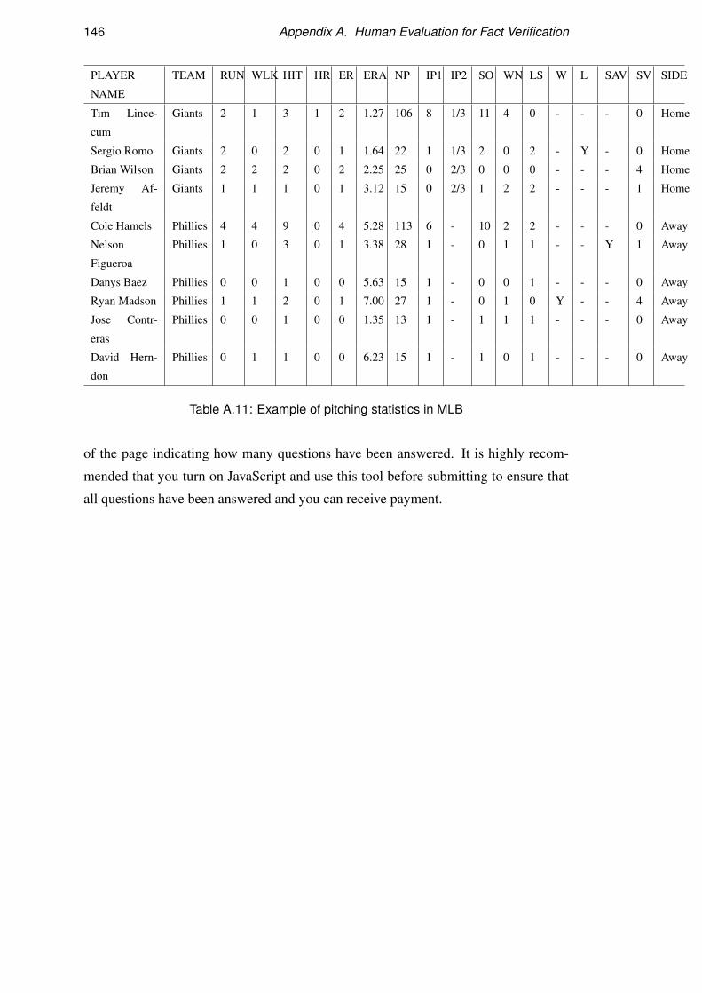
146 Appendix A. Human Evaluation for Fact Verification
PLAYER
NAME
TEAM RUN WLK HIT HR ER ERA NP IP1 IP2 SO WN LS W L SAV SV SIDE
Tim Lince-
cum
Giants 2 1 3 1 2 1.27 106 8 1/3 11 4 0 - - - 0 Home
Sergio Romo Giants 2 0 2 0 1 1.64 22 1 1/3 2 0 2 - Y - 0 Home
Brian Wilson Giants 2 2 2 0 2 2.25 25 0 2/3 0 0 0 - - - 4 Home
Jeremy Af-
feldt
Giants 1 1 1 0 1 3.12 15 0 2/3 1 2 2 - - - 1 Home
Cole Hamels Phillies 4 4 9 0 4 5.28 113 6 - 10 2 2 - - - 0 Away
Nelson
Figueroa
Phillies 1 0 3 0 1 3.38 28 1 - 0 1 1 - - Y 1 Away
Danys Baez Phillies 0 0 1 0 0 5.63 15 1 - 0 0 1 - - - 0 Away
Ryan Madson Phillies 1 1 2 0 1 7.00 27 1 - 0 1 0 Y - - 4 Away
Jose Contr-
eras
Phillies 0 0 1 0 0 1.35 13 1 - 1 1 1 - - - 0 Away
David Hern-
don
Phillies 0 1 1 0 0 6.23 15 1 - 1 0 1 - - - 0 Away
Table A.11: Example of pitching statistics in MLB
of the page indicating how many questions have been answered. It is highly recom-
mended that you turn on JavaScript and use this tool before submitting to ensure that
all questions have been answered and you can receive payment.
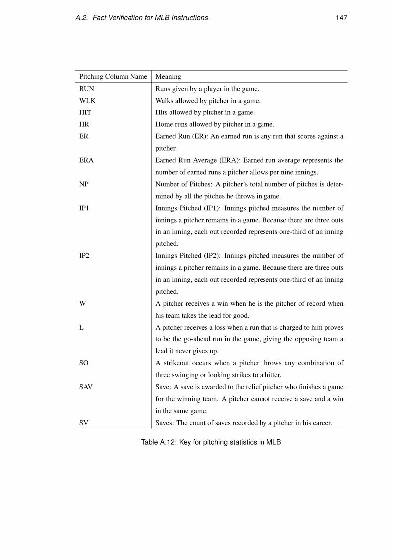
A.2. Fact Verification for MLB Instructions 147
Pitching Column Name Meaning
RUN Runs given by a player in the game.
WLK Walks allowed by pitcher in a game.
HIT Hits allowed by pitcher in a game.
HR Home runs allowed by pitcher in a game.
ER Earned Run (ER): An earned run is any run that scores against a
pitcher.
ERA Earned Run Average (ERA): Earned run average represents the
number of earned runs a pitcher allows per nine innings.
NP Number of Pitches: A pitcher’s total number of pitches is deter-
mined by all the pitches he throws in game.
IP1 Innings Pitched (IP1): Innings pitched measures the number of
innings a pitcher remains in a game. Because there are three outs
in an inning, each out recorded represents one-third of an inning
pitched.
IP2 Innings Pitched (IP2): Innings pitched measures the number of
innings a pitcher remains in a game. Because there are three outs
in an inning, each out recorded represents one-third of an inning
pitched.
W A pitcher receives a win when he is the pitcher of record when
his team takes the lead for good.
L A pitcher receives a loss when a run that is charged to him proves
to be the go-ahead run in the game, giving the opposing team a
lead it never gives up.
SO A strikeout occurs when a pitcher throws any combination of
three swinging or looking strikes to a hitter.
SAV Save: A save is awarded to the relief pitcher who finishes a game
for the winning team. A pitcher cannot receive a save and a win
in the same game.
SV Saves: The count of saves recorded by a pitcher in his career.
Table A.12: Key for pitching statistics in MLB

148 Appendix A. Human Evaluation for Fact Verification
BATTER PITCHER BASE1 BASE2 BASE3 SCORER/S EVENT RUN RBI Runs
(H)
Runs
(A)
INN SIDE
Ryan
Howard
Tim
Lince-
cum
- - - - Home
Run
1 1 0 1 5 top
Andres
Torres
Cole
Hamels
- Andres
Torres
- Nate
Schier-
holtz
Double 1 1 1 1 5 bottom
Andres
Torres
Cole
Hamels
Andres
Torres
Nate
Schier-
holtz
Matt
Downs
Bengie
Molina
Walk 1 1 2 1 6 bottom
Edgar
Renteria
Cole
Hamels
Edgar
Renteria
Nate
Schier-
holtz
Andres
Torres
Matt
Downs,
Nate
Schier-
holtz
Single 2 2 4 1 6 bottom
Jayson
Werth
Brian
Wilson
- Jayson
Werth
- Shane
Victorino,
Chase Ut-
ley, Ryan
Howard
Double 3 3 4 4 9 top
Placido
Polanco
Jeremy
Affeldt
- Shane
Vic-
torino
- Brian
Schneider
Wild
Pitch
1 - 4 5 10 top
Andres
Torres
Ryan
Madson
Andres
Torres
- - Nate
Schier-
holtz
Single 1 1 5 5 10 bottom
Wilson
Valdez
Sergio
Romo
- Wilson
Valdez
- Raul
Ibanez
Double 1 1 5 6 11 top
Shane
Victorino
Sergio
Romo
- Shane
Vic-
torino
- Wilson
Valdez
Field
Error
1 - 5 7 11 top
Nate
Schier-
holtz
Nelson
Figueroa
- Nate
Schier-
holtz
Juan
Uribe
Eli White-
side
Double 1 1 6 7 11 bottom
Table A.13: Example of play-by-play statistics in MLB
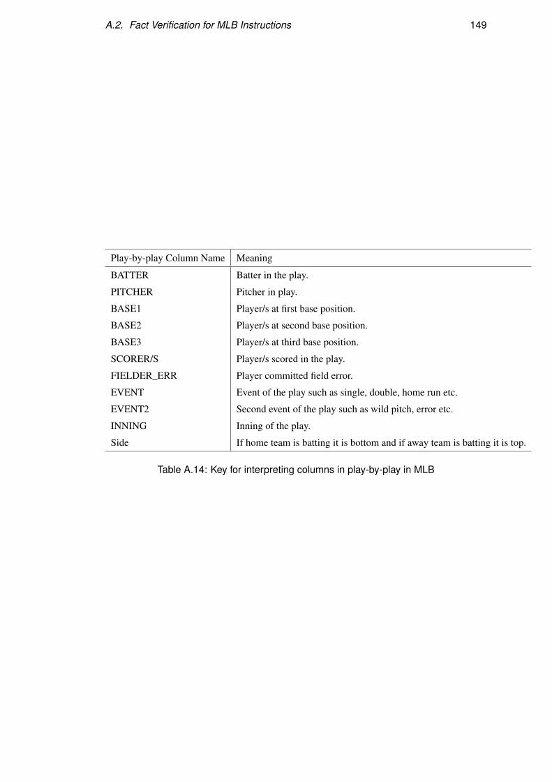
A.2. Fact Verification for MLB Instructions 149
Play-by-play Column Name Meaning
BATTER Batter in the play.
PITCHER Pitcher in play.
BASE1 Player/s at first base position.
BASE2 Player/s at second base position.
BASE3 Player/s at third base position.
SCORER/S Player/s scored in the play.
FIELDER_ERR Player committed field error.
EVENT Event of the play such as single, double, home run etc.
EVENT2 Second event of the play such as wild pitch, error etc.
INNING Inning of the play.
Side If home team is batting it is bottom and if away team is batting it is top.
Table A.14: Key for interpreting columns in play-by-play in MLB

Appendix B
Human Evaluation for Summary
Quality
In the previous chapter, we went through the instructions provided to raters for the
human evaluation study for fact verification. In this chapter, we go through the in-
structions provided to raters for the human evaluation study related to the quality of
the summary including coherence, conciseness and grammaticality. Sections B.1- B.3
describe the instructions for the tasks for evaluation of coherence, conciseness and
grammaticality respectively for ROTOWIRE dataset. Sections B.4- B.6 describe the
instructions for evaluation of coherence, conciseness and grammaticality respectively
for MLB dataset.
B.1 Evaluation of Coherence for ROTOWIRE
General Instructions Attempt HITs if you are a native speaker of English or a near-
native speaker who can comfortably comprehend summary of NBA basketball games
written in English. We are happy to receive feedback and improve this job accordingly.
Feel free to send your comments to: r.puduppully [at] sms [dot] ed [dot] ac [dot] uk.
Your responses are confidential. Any publications based on these will not include your
specific responses, but rather aggregate information from many individuals. We will
not ask any information that can be used to identify who you are.
Evaluate Sports Summaries of (NBA) basketball games Your task it to read two
short texts which have been produced by different automatic systems. These systems
typically take a large table as input which contains statistics of a basketball game and
151
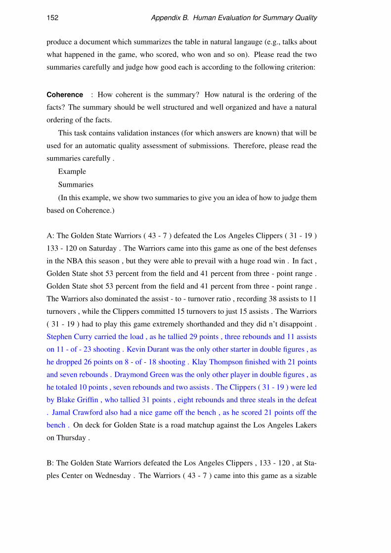
152 Appendix B. Human Evaluation for Summary Quality
produce a document which summarizes the table in natural langauge (e.g., talks about
what happened in the game, who scored, who won and so on). Please read the two
summaries carefully and judge how good each is according to the following criterion:
Coherence : How coherent is the summary? How natural is the ordering of the
facts? The summary should be well structured and well organized and have a natural
ordering of the facts.
This task contains validation instances (for which answers are known) that will be
used for an automatic quality assessment of submissions. Therefore, please read the
summaries carefully .
Example
Summaries
(In this example, we show two summaries to give you an idea of how to judge them
based on Coherence.)
A: The Golden State Warriors ( 43 - 7 ) defeated the Los Angeles Clippers ( 31 - 19 )
133 - 120 on Saturday . The Warriors came into this game as one of the best defenses
in the NBA this season , but they were able to prevail with a huge road win . In fact ,
Golden State shot 53 percent from the field and 41 percent from three - point range .
Golden State shot 53 percent from the field and 41 percent from three - point range .
The Warriors also dominated the assist - to - turnover ratio , recording 38 assists to 11
turnovers , while the Clippers committed 15 turnovers to just 15 assists . The Warriors
( 31 - 19 ) had to play this game extremely shorthanded and they did n’t disappoint .
Stephen Curry carried the load , as he tallied 29 points , three rebounds and 11 assists
on 11 - of - 23 shooting . Kevin Durant was the only other starter in double figures , as
he dropped 26 points on 8 - of - 18 shooting . Klay Thompson finished with 21 points
and seven rebounds . Draymond Green was the only other player in double figures , as
he totaled 10 points , seven rebounds and two assists . The Clippers ( 31 - 19 ) were led
by Blake Griffin , who tallied 31 points , eight rebounds and three steals in the defeat
. Jamal Crawford also had a nice game off the bench , as he scored 21 points off the
bench . On deck for Golden State is a road matchup against the Los Angeles Lakers
on Thursday .
B: The Golden State Warriors defeated the Los Angeles Clippers , 133 - 120 , at Sta-
ples Center on Wednesday . The Warriors ( 43 - 7 ) came into this game as a sizable
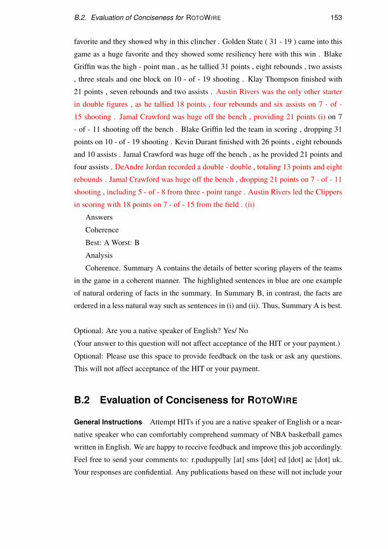
B.2. Evaluation of Conciseness for ROTOWIRE 153
favorite and they showed why in this clincher . Golden State ( 31 - 19 ) came into this
game as a huge favorite and they showed some resiliency here with this win . Blake
Griffin was the high - point man , as he tallied 31 points , eight rebounds , two assists
, three steals and one block on 10 - of - 19 shooting . Klay Thompson finished with
21 points , seven rebounds and two assists . Austin Rivers was the only other starter
in double figures , as he tallied 18 points , four rebounds and six assists on 7 - of -
15 shooting . Jamal Crawford was huge off the bench , providing 21 points (i) on 7
- of - 11 shooting off the bench . Blake Griffin led the team in scoring , dropping 31
points on 10 - of - 19 shooting . Kevin Durant finished with 26 points , eight rebounds
and 10 assists . Jamal Crawford was huge off the bench , as he provided 21 points and
four assists . DeAndre Jordan recorded a double - double , totaling 13 points and eight
rebounds . Jamal Crawford was huge off the bench , dropping 21 points on 7 - of - 11
shooting , including 5 - of - 8 from three - point range . Austin Rivers led the Clippers
in scoring with 18 points on 7 - of - 15 from the field . (ii)
Answers
Coherence
Best: A Worst: B
Analysis
Coherence. Summary A contains the details of better scoring players of the teams
in the game in a coherent manner. The highlighted sentences in blue are one example
of natural ordering of facts in the summary. In Summary B, in contrast, the facts are
ordered in a less natural way such as sentences in (i) and (ii). Thus, Summary A is best.
Optional: Are you a native speaker of English? Yes/ No
(Your answer to this question will not affect acceptance of the HIT or your payment.)
Optional: Please use this space to provide feedback on the task or ask any questions.
This will not affect acceptance of the HIT or your payment.
B.2 Evaluation of Conciseness for ROTOWIRE
General Instructions Attempt HITs if you are a native speaker of English or a near-
native speaker who can comfortably comprehend summary of NBA basketball games
written in English. We are happy to receive feedback and improve this job accordingly.
Feel free to send your comments to: r.puduppully [at] sms [dot] ed [dot] ac [dot] uk.
Your responses are confidential. Any publications based on these will not include your
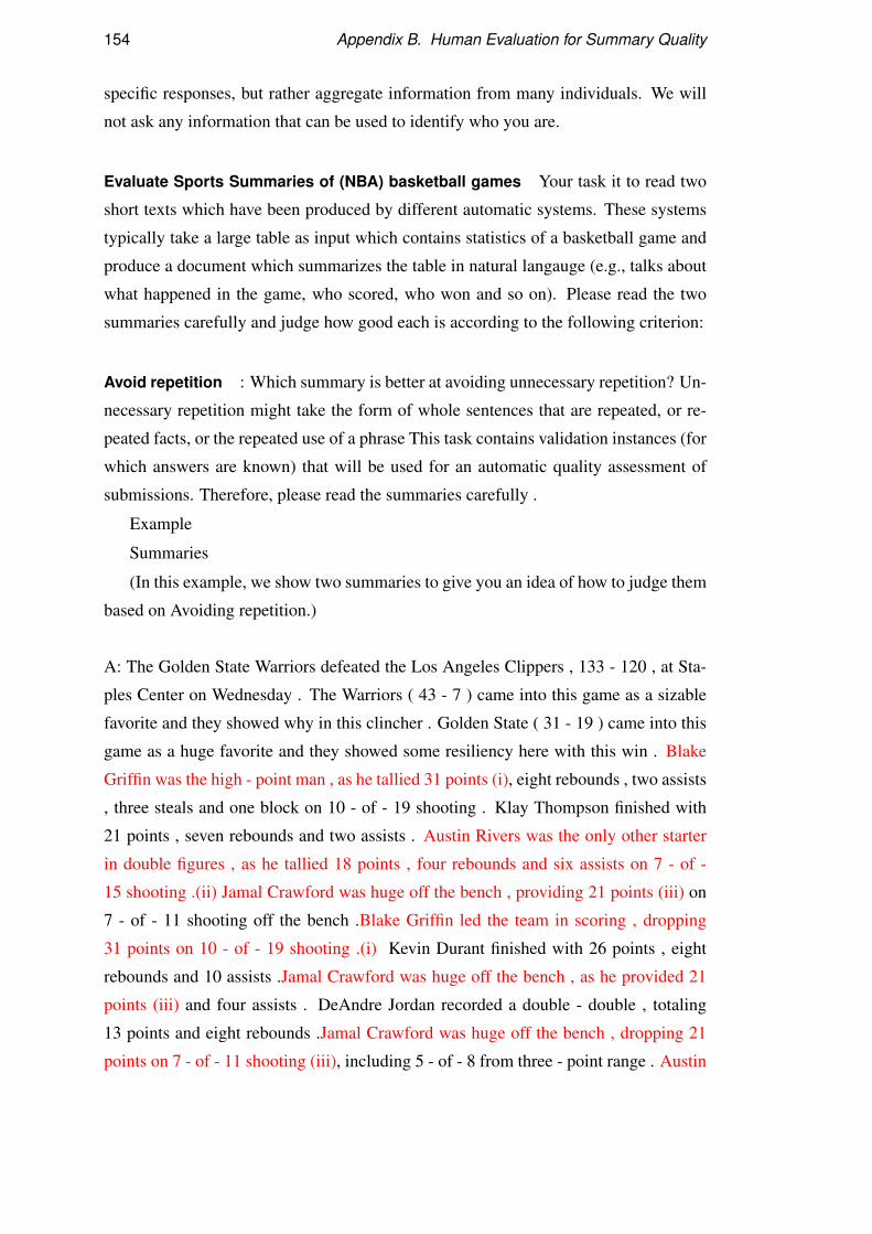
154 Appendix B. Human Evaluation for Summary Quality
specific responses, but rather aggregate information from many individuals. We will
not ask any information that can be used to identify who you are.
Evaluate Sports Summaries of (NBA) basketball games Your task it to read two
short texts which have been produced by different automatic systems. These systems
typically take a large table as input which contains statistics of a basketball game and
produce a document which summarizes the table in natural langauge (e.g., talks about
what happened in the game, who scored, who won and so on). Please read the two
summaries carefully and judge how good each is according to the following criterion:
Avoid repetition : Which summary is better at avoiding unnecessary repetition? Un-
necessary repetition might take the form of whole sentences that are repeated, or re-
peated facts, or the repeated use of a phrase This task contains validation instances (for
which answers are known) that will be used for an automatic quality assessment of
submissions. Therefore, please read the summaries carefully .
Example
Summaries
(In this example, we show two summaries to give you an idea of how to judge them
based on Avoiding repetition.)
A: The Golden State Warriors defeated the Los Angeles Clippers , 133 - 120 , at Sta-
ples Center on Wednesday . The Warriors ( 43 - 7 ) came into this game as a sizable
favorite and they showed why in this clincher . Golden State ( 31 - 19 ) came into this
game as a huge favorite and they showed some resiliency here with this win . Blake
Griffin was the high - point man , as he tallied 31 points (i), eight rebounds , two assists
, three steals and one block on 10 - of - 19 shooting . Klay Thompson finished with
21 points , seven rebounds and two assists . Austin Rivers was the only other starter
in double figures , as he tallied 18 points , four rebounds and six assists on 7 - of -
15 shooting .(ii) Jamal Crawford was huge off the bench , providing 21 points (iii) on
7 - of - 11 shooting off the bench .Blake Griffin led the team in scoring , dropping
31 points on 10 - of - 19 shooting .(i) Kevin Durant finished with 26 points , eight
rebounds and 10 assists .Jamal Crawford was huge off the bench , as he provided 21
points (iii) and four assists . DeAndre Jordan recorded a double - double , totaling
13 points and eight rebounds .Jamal Crawford was huge off the bench , dropping 21
points on 7 - of - 11 shooting (iii), including 5 - of - 8 from three - point range . Austin
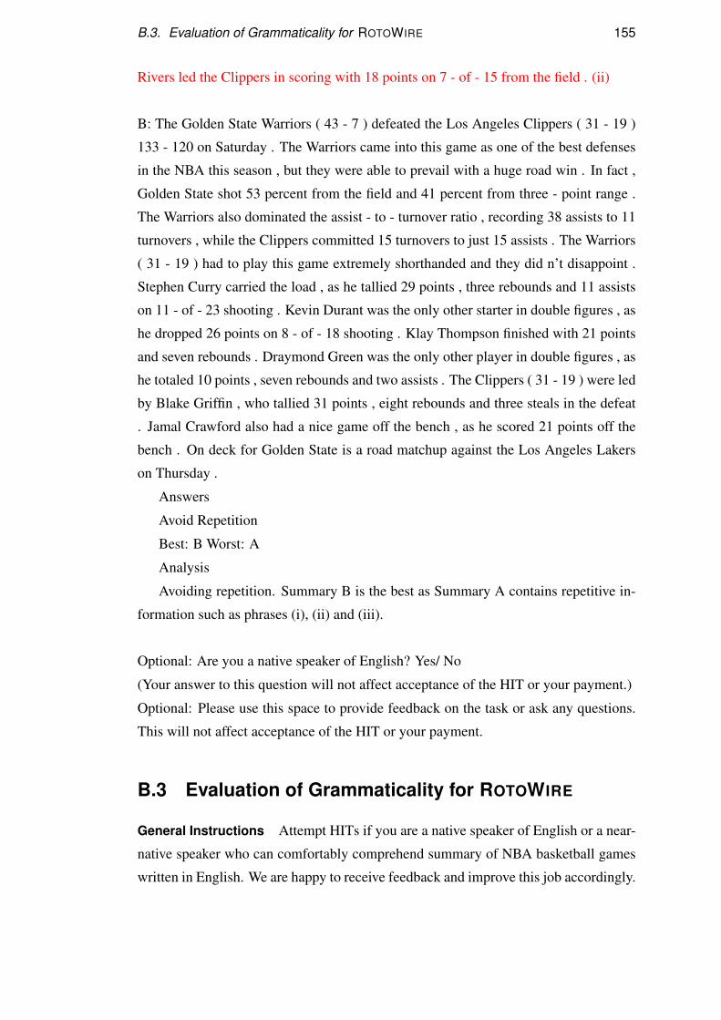
B.3. Evaluation of Grammaticality for ROTOWIRE 155
Rivers led the Clippers in scoring with 18 points on 7 - of - 15 from the field . (ii)
B: The Golden State Warriors ( 43 - 7 ) defeated the Los Angeles Clippers ( 31 - 19 )
133 - 120 on Saturday . The Warriors came into this game as one of the best defenses
in the NBA this season , but they were able to prevail with a huge road win . In fact ,
Golden State shot 53 percent from the field and 41 percent from three - point range .
The Warriors also dominated the assist - to - turnover ratio , recording 38 assists to 11
turnovers , while the Clippers committed 15 turnovers to just 15 assists . The Warriors
( 31 - 19 ) had to play this game extremely shorthanded and they did n’t disappoint .
Stephen Curry carried the load , as he tallied 29 points , three rebounds and 11 assists
on 11 - of - 23 shooting . Kevin Durant was the only other starter in double figures , as
he dropped 26 points on 8 - of - 18 shooting . Klay Thompson finished with 21 points
and seven rebounds . Draymond Green was the only other player in double figures , as
he totaled 10 points , seven rebounds and two assists . The Clippers ( 31 - 19 ) were led
by Blake Griffin , who tallied 31 points , eight rebounds and three steals in the defeat
. Jamal Crawford also had a nice game off the bench , as he scored 21 points off the
bench . On deck for Golden State is a road matchup against the Los Angeles Lakers
on Thursday .
Answers
Avoid Repetition
Best: B Worst: A
Analysis
Avoiding repetition. Summary B is the best as Summary A contains repetitive in-
formation such as phrases (i), (ii) and (iii).
Optional: Are you a native speaker of English? Yes/ No
(Your answer to this question will not affect acceptance of the HIT or your payment.)
Optional: Please use this space to provide feedback on the task or ask any questions.
This will not affect acceptance of the HIT or your payment.
B.3 Evaluation of Grammaticality for ROTOWIRE
General Instructions Attempt HITs if you are a native speaker of English or a near-
native speaker who can comfortably comprehend summary of NBA basketball games
written in English. We are happy to receive feedback and improve this job accordingly.
156 Appendix B. Human Evaluation for Summary Quality
Feel free to send your comments to: r.puduppully [at] sms [dot] ed [dot] ac [dot] uk.
Your responses are confidential. Any publications based on these will not include your
specific responses, but rather aggregate information from many individuals. We will
not ask any information that can be used to identify who you are.
Evaluate Sports Summaries of (NBA) basketball games Your task it to read two
short texts which have been produced by different automatic systems. These systems
typically take a large table as input which contains statistics of a basketball game and
produce a document which summarizes the table in natural langauge (e.g., talks about
what happened in the game, who scored, who won and so on). Please read the two
summaries carefully and judge how good each is according to the following criterion:
Grammaticality : Are the sentences grammatical and well-formed? The summary
sentences should be grammatically correct. You should not rate the document as whole
but rather whether the sentences could be written by a native speaker or by someone
who is a learner and makes mistakes. Choose the more grammatical summary.
This task contains validation instances (for which answers are known) that will be
used for an automatic quality assessment of submissions. Therefore, please read the
summaries carefully .
Example
Summaries
(In this example, we show two summaries to give you an idea of how to judge them
based on Grammaticality.)
A: The Milwaukee Bucks ( 18 - 17 ) defeated the New York Knicks ( 5 - 31 ) 95 -
82 on Sunday at Madison Square Garden in New York . The Bucks were able to have
a great night defensively , giving themselves the scoring advantage in all four quar-
ters . The Bucks showed superior shooting , going 46 percent from the field , while
the Knicks went only 41 percent from the floor . The Bucks also out - rebounded the
Knicks 48 - 36 , giving them in an even further advantage which helped them secure
the 13 - point victory on the road . Brandon Knight led the Bucks again in this one
. He went 6 - for - 14 from the field and 1 - for - 3 from beyond the arc to score 17
points , while also handing out five assists . He ’s now averaging 21 points per game
over his last three games , as he ’s consistently been the offensive leader for this team
. Zaza Pachulia also had a strong showing , finishing with 16 points ( 6 - 12 FG , 4 - 4

B.3. Evaluation of Grammaticality for ROTOWIRE 157
FT ) and a team - high of 14 rebounds . It marked his second double - double in a row
and fourth on the season , as the inexperienced centers on the Knicks ’ roster were n’t
able to limit him . Notching a double - double of his own , Giannis Antetokounmpo
recorded 16 points ( 6 - 9 FG , 1 - 1 3Pt , 3 - 6 FT ) and 12 rebounds . The 12 rebounds
matched a season - high , while it was his second double - double of the season . Com-
ing off the bench for a big night was Kendall Marshall . He went 6 - for - 8 from the
field and 3 - for - 3 from the free throw line to score 15 points in 20 minutes . The
Knicks really struggled to score without Carmelo Anthony and Amare Stoudemire .
Tim Hardaway Jr led the team as the starting shooting guard , going 6 - for - 13 from
the field and 3 - for - 5 from the three - point line to score 17 points , while also adding
four assists . He ’s now scored 17 or more points in three out of his last four games
, as he has put it on himself to pick up the slack with other key players sitting out .
J. R. Smith also put together a solid outing as a starter . He finished with 15 points
and seven rebounds in 37 minutes . Like Haradaway Jr , he ’s also benefitted from
other guys sitting out , and has now combined for 37 points over his last two games .
While he did n’t have his best night defensively , Cole Aldrich scored 12 points ( 6 -
10 FG ) and grabbed seven rebounds in 19 minutes . The only other Knick to reach
double figures in points was Jason Smith , who came off the bench for 10 points ( 3 -
11 FG , 4 - 4 FT ) . The Bucks ’ next game will be at home against the Phoenix Suns
on Tuesday , while the Knicks will travel to Memphis to play the Grizzlies on Monday .
B: The Milwaukee Bucks (18-17) defeated the New York Knicks (5-31) 95-82 on Sun-
day at Madison Square Garden in New York. Giving himself the benefit of scoring
in all four quarters, the Bucks got a good night for defensive defense. The Bucks
went 46 percent off the field, while the Knicks went only 41 percent off the floor. The
Bucks also knocked out - the Knicks rebuilt 48 - 36, giving them another advantage
that helped them to a 13-point victory on the road. In it, Brandon Knight re-led the
Bucks. He scored 17 - 6 - 14 - off the field and 1 - for - 3 off the arc, while also aid-
ing five. He is now averaging 21 points per game in the last three games, as he is the
team’s consistently offensive leader. Zaza Pachulia also excelled with a high perfor-
mance with 16 points (6 - 12 FG, 4 - 4 FT) and one team - 14 rebounds. This marked
the second consecutive double and fourth double of the season because the inexperi-
enced centers on the Knicks ’roster couldn’t limit him. Giannis Antetokounmpo, in
his own double-double position, reported 16 points (6 - 9 FG, 1 - 1 3 PT, 3 - 6 FT)
and 12 rebounds. 12 rebounds matched the season - high, it was his second double of
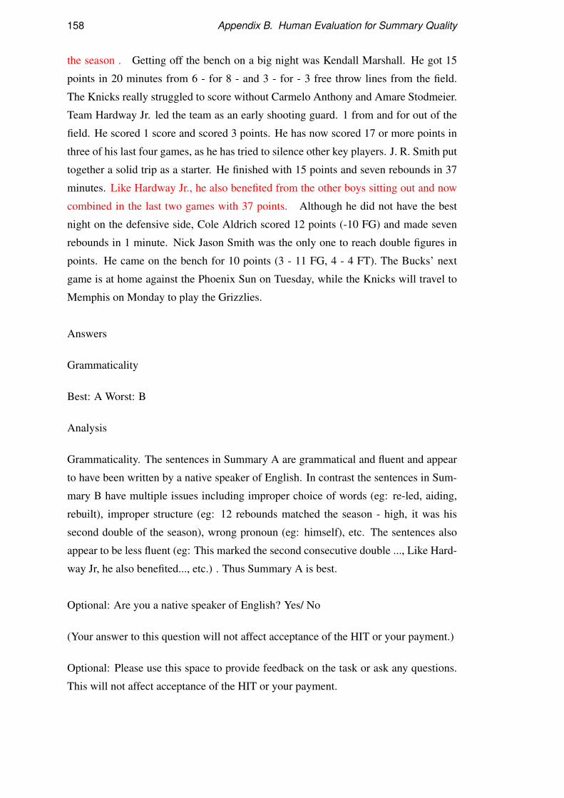
158 Appendix B. Human Evaluation for Summary Quality
the season . Getting off the bench on a big night was Kendall Marshall. He got 15
points in 20 minutes from 6 - for 8 - and 3 - for - 3 free throw lines from the field.
The Knicks really struggled to score without Carmelo Anthony and Amare Stodmeier.
Team Hardway Jr. led the team as an early shooting guard. 1 from and for out of the
field. He scored 1 score and scored 3 points. He has now scored 17 or more points in
three of his last four games, as he has tried to silence other key players. J. R. Smith put
together a solid trip as a starter. He finished with 15 points and seven rebounds in 37
minutes. Like Hardway Jr., he also benefited from the other boys sitting out and now
combined in the last two games with 37 points. Although he did not have the best
night on the defensive side, Cole Aldrich scored 12 points (-10 FG) and made seven
rebounds in 1 minute. Nick Jason Smith was the only one to reach double figures in
points. He came on the bench for 10 points (3 - 11 FG, 4 - 4 FT). The Bucks’ next
game is at home against the Phoenix Sun on Tuesday, while the Knicks will travel to
Memphis on Monday to play the Grizzlies.
Answers
Grammaticality
Best: A Worst: B
Analysis
Grammaticality. The sentences in Summary A are grammatical and fluent and appear
to have been written by a native speaker of English. In contrast the sentences in Sum-
mary B have multiple issues including improper choice of words (eg: re-led, aiding,
rebuilt), improper structure (eg: 12 rebounds matched the season - high, it was his
second double of the season), wrong pronoun (eg: himself), etc. The sentences also
appear to be less fluent (eg: This marked the second consecutive double ..., Like Hard-
way Jr, he also benefited..., etc.) . Thus Summary A is best.
Optional: Are you a native speaker of English? Yes/ No
(Your answer to this question will not affect acceptance of the HIT or your payment.)
Optional: Please use this space to provide feedback on the task or ask any questions.
This will not affect acceptance of the HIT or your payment.

B.4. Evaluation of Coherence for MLB 159
B.4 Evaluation of Coherence for MLB
General Instructions Attempt HITs if you are a native speaker of English or a near-
native speaker who can comfortably comprehend summary of MLB baseball games
written in English. We are happy to receive feedback and improve this job accordingly.
Feel free to send your comments to: r.puduppully [at] sms [dot] ed [dot] ac [dot] uk.
Your responses are confidential. Any publications based on these will not include your
specific responses, but rather aggregate information from many individuals. We will
not ask any information that can be used to identify who you are.
Evaluate Sports Summaries of (MLB) baseball games Your task it to read two
short texts which have been produced by different automatic systems. These systems
typically take a large table as input which contains statistics of a baseball game and
produce a document which summarizes the table in natural langauge (e.g., talks about
what happened in the game, who scored, who won and so on). Please read the two
summaries and judge how good each is according to the following criterion:
Coherence : How coherent is the summary? How natural is the ordering of the facts?
The summary should be well structured and well organized and have a natural ordering
of the facts. This task contains validation instances (for which answers are known) that
will be used for an automatic quality assessment of submissions. Therefore, please
read the summaries carefully.
Example
Summaries
(In this example, we show two summaries to give you an idea of how to judge them
based on Coherence.)
A: HOUSTON – Alex Bregman hit a two - run homer , and Dallas Keuchel won for the
first time in more than a month . Bregman homered and drove in three runs , Keuchel
pitched seven strong innings and the Houston Astros beat the Tampa Bay Rays 6 - 2
on Tuesday night . The Astros won for the fifth time in six games and moved within a
half-game of the first-place Los Angeles Angels in the AL West . Tampa Bay lost for
the fifth time in six games . The Rays have lost four straight and eight of 10 . Bregman
’s homer was his second in as many games . Keuchel ( 9 - 12 ) allowed nine hits and
two runs with four strikeouts in seven innings . Blake Snell ( 4 - 7 ) allowed nine hits
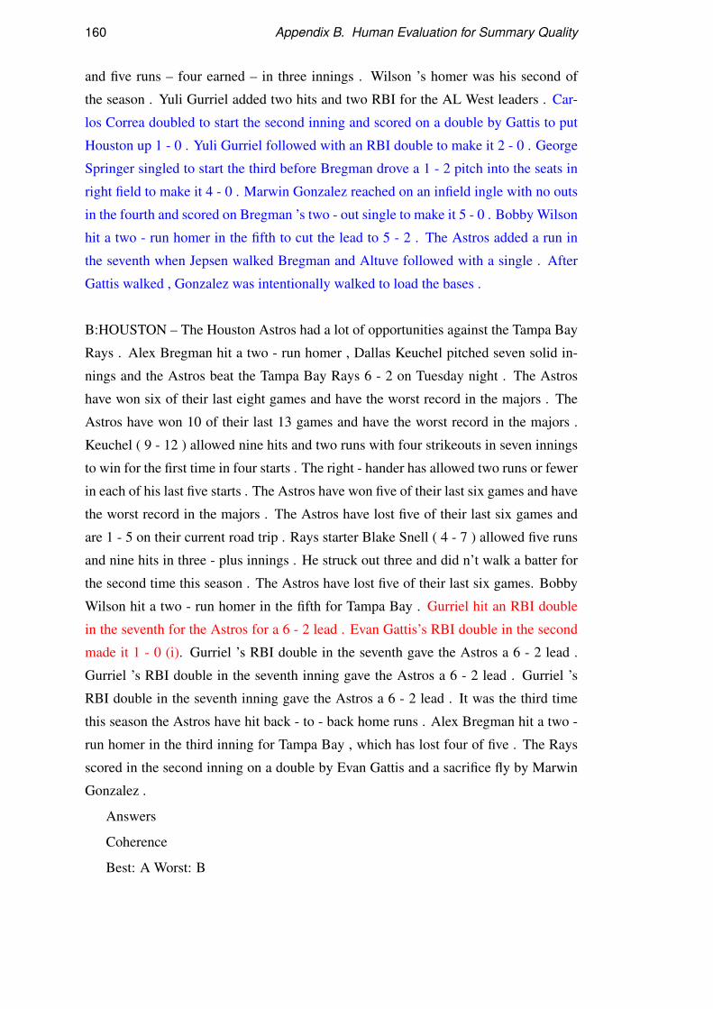
160 Appendix B. Human Evaluation for Summary Quality
and five runs – four earned – in three innings . Wilson ’s homer was his second of
the season . Yuli Gurriel added two hits and two RBI for the AL West leaders . Car-
los Correa doubled to start the second inning and scored on a double by Gattis to put
Houston up 1 - 0 . Yuli Gurriel followed with an RBI double to make it 2 - 0 . George
Springer singled to start the third before Bregman drove a 1 - 2 pitch into the seats in
right field to make it 4 - 0 . Marwin Gonzalez reached on an infield ingle with no outs
in the fourth and scored on Bregman ’s two - out single to make it 5 - 0 . Bobby Wilson
hit a two - run homer in the fifth to cut the lead to 5 - 2 . The Astros added a run in
the seventh when Jepsen walked Bregman and Altuve followed with a single . After
Gattis walked , Gonzalez was intentionally walked to load the bases .
B:HOUSTON – The Houston Astros had a lot of opportunities against the Tampa Bay
Rays . Alex Bregman hit a two - run homer , Dallas Keuchel pitched seven solid in-
nings and the Astros beat the Tampa Bay Rays 6 - 2 on Tuesday night . The Astros
have won six of their last eight games and have the worst record in the majors . The
Astros have won 10 of their last 13 games and have the worst record in the majors .
Keuchel ( 9 - 12 ) allowed nine hits and two runs with four strikeouts in seven innings
to win for the first time in four starts . The right - hander has allowed two runs or fewer
in each of his last five starts . The Astros have won five of their last six games and have
the worst record in the majors . The Astros have lost five of their last six games and
are 1 - 5 on their current road trip . Rays starter Blake Snell ( 4 - 7 ) allowed five runs
and nine hits in three - plus innings . He struck out three and did n’t walk a batter for
the second time this season . The Astros have lost five of their last six games. Bobby
Wilson hit a two - run homer in the fifth for Tampa Bay . Gurriel hit an RBI double
in the seventh for the Astros for a 6 - 2 lead . Evan Gattis’s RBI double in the second
made it 1 - 0 (i). Gurriel ’s RBI double in the seventh gave the Astros a 6 - 2 lead .
Gurriel ’s RBI double in the seventh inning gave the Astros a 6 - 2 lead . Gurriel ’s
RBI double in the seventh inning gave the Astros a 6 - 2 lead . It was the third time
this season the Astros have hit back - to - back home runs . Alex Bregman hit a two -
run homer in the third inning for Tampa Bay , which has lost four of five . The Rays
scored in the second inning on a double by Evan Gattis and a sacrifice fly by Marwin
Gonzalez .
Answers
Coherence
Best: A Worst: B
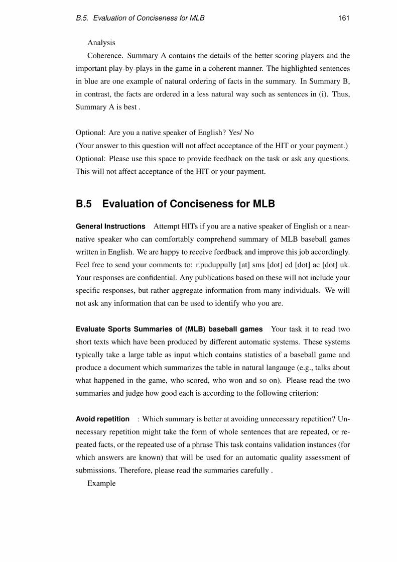
B.5. Evaluation of Conciseness for MLB 161
Analysis
Coherence. Summary A contains the details of the better scoring players and the
important play-by-plays in the game in a coherent manner. The highlighted sentences
in blue are one example of natural ordering of facts in the summary. In Summary B,
in contrast, the facts are ordered in a less natural way such as sentences in (i). Thus,
Summary A is best .
Optional: Are you a native speaker of English? Yes/ No
(Your answer to this question will not affect acceptance of the HIT or your payment.)
Optional: Please use this space to provide feedback on the task or ask any questions.
This will not affect acceptance of the HIT or your payment.
B.5 Evaluation of Conciseness for MLB
General Instructions Attempt HITs if you are a native speaker of English or a near-
native speaker who can comfortably comprehend summary of MLB baseball games
written in English. We are happy to receive feedback and improve this job accordingly.
Feel free to send your comments to: r.puduppully [at] sms [dot] ed [dot] ac [dot] uk.
Your responses are confidential. Any publications based on these will not include your
specific responses, but rather aggregate information from many individuals. We will
not ask any information that can be used to identify who you are.
Evaluate Sports Summaries of (MLB) baseball games Your task it to read two
short texts which have been produced by different automatic systems. These systems
typically take a large table as input which contains statistics of a baseball game and
produce a document which summarizes the table in natural langauge (e.g., talks about
what happened in the game, who scored, who won and so on). Please read the two
summaries and judge how good each is according to the following criterion:
Avoid repetition : Which summary is better at avoiding unnecessary repetition? Un-
necessary repetition might take the form of whole sentences that are repeated, or re-
peated facts, or the repeated use of a phrase This task contains validation instances (for
which answers are known) that will be used for an automatic quality assessment of
submissions. Therefore, please read the summaries carefully .
Example
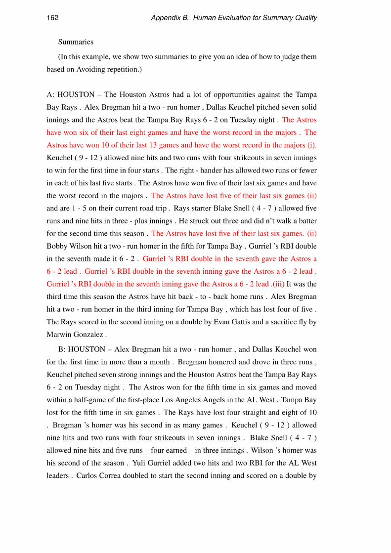
162 Appendix B. Human Evaluation for Summary Quality
Summaries
(In this example, we show two summaries to give you an idea of how to judge them
based on Avoiding repetition.)
A: HOUSTON – The Houston Astros had a lot of opportunities against the Tampa
Bay Rays . Alex Bregman hit a two - run homer , Dallas Keuchel pitched seven solid
innings and the Astros beat the Tampa Bay Rays 6 - 2 on Tuesday night . The Astros
have won six of their last eight games and have the worst record in the majors . The
Astros have won 10 of their last 13 games and have the worst record in the majors (i).
Keuchel ( 9 - 12 ) allowed nine hits and two runs with four strikeouts in seven innings
to win for the first time in four starts . The right - hander has allowed two runs or fewer
in each of his last five starts . The Astros have won five of their last six games and have
the worst record in the majors . The Astros have lost five of their last six games (ii)
and are 1 - 5 on their current road trip . Rays starter Blake Snell ( 4 - 7 ) allowed five
runs and nine hits in three - plus innings . He struck out three and did n’t walk a batter
for the second time this season . The Astros have lost five of their last six games. (ii)
Bobby Wilson hit a two - run homer in the fifth for Tampa Bay . Gurriel ’s RBI double
in the seventh made it 6 - 2 . Gurriel ’s RBI double in the seventh gave the Astros a
6 - 2 lead . Gurriel ’s RBI double in the seventh inning gave the Astros a 6 - 2 lead .
Gurriel ’s RBI double in the seventh inning gave the Astros a 6 - 2 lead .(iii) It was the
third time this season the Astros have hit back - to - back home runs . Alex Bregman
hit a two - run homer in the third inning for Tampa Bay , which has lost four of five .
The Rays scored in the second inning on a double by Evan Gattis and a sacrifice fly by
Marwin Gonzalez .
B: HOUSTON – Alex Bregman hit a two - run homer , and Dallas Keuchel won
for the first time in more than a month . Bregman homered and drove in three runs ,
Keuchel pitched seven strong innings and the Houston Astros beat the Tampa Bay Rays
6 - 2 on Tuesday night . The Astros won for the fifth time in six games and moved
within a half-game of the first-place Los Angeles Angels in the AL West . Tampa Bay
lost for the fifth time in six games . The Rays have lost four straight and eight of 10
. Bregman ’s homer was his second in as many games . Keuchel ( 9 - 12 ) allowed
nine hits and two runs with four strikeouts in seven innings . Blake Snell ( 4 - 7 )
allowed nine hits and five runs – four earned – in three innings . Wilson ’s homer was
his second of the season . Yuli Gurriel added two hits and two RBI for the AL West
leaders . Carlos Correa doubled to start the second inning and scored on a double by
B.6. Evaluation of Grammaticality for MLB 163
Gattis to put Houston up 1 - 0 . Yuli Gurriel followed with an RBI double to make it 2
- 0 . George Springer singled to start the third before Bregman drove a 1 - 2 pitch into
the seats in right field to make it 4 - 0 . Marwin Gonzalez reached on an infield ingle
with no outs in the fourth and scored on Bregman ’s two - out single to make it 5 - 0
. Bobby Wilson hit a two - run homer in the fifth to cut the lead to 5 - 2 . The Astros
added a run in the seventh when Jepsen walked Bregman and Altuve followed with a
single . After Gattis walked , Gonzalez was intentionally walked to load the bases .
Answers
Avoid Repetition
Best: B Worst: A
Analysis
Avoiding repetition. Summary B is the best as Summary A contains repetitive in-
formation such as phrases (i), (ii) and (iii).
Optional: Are you a native speaker of English? Yes/ No
(Your answer to this question will not affect acceptance of the HIT or your payment.)
Optional: Please use this space to provide feedback on the task or ask any questions.
This will not affect acceptance of the HIT or your payment.
B.6 Evaluation of Grammaticality for MLB
General Instructions Attempt HITs if you are a native speaker of English or a near-
native speaker who can comfortably comprehend summary of MLB baseball games
written in English. We are happy to receive feedback and improve this job accordingly.
Feel free to send your comments to: r.puduppully [at] sms [dot] ed [dot] ac [dot] uk.
Your responses are confidential. Any publications based on these will not include your
specific responses, but rather aggregate information from many individuals. We will
not ask any information that can be used to identify who you are.
Evaluate Sports Summaries of (MLB) baseball games Your task it to read two
short texts which have been produced by different automatic systems. These systems
typically take a large table as input which contains statistics of a baseball game and
produce a document which summarizes the table in natural langauge (e.g., talks about
what happened in the game, who scored, who won and so on).
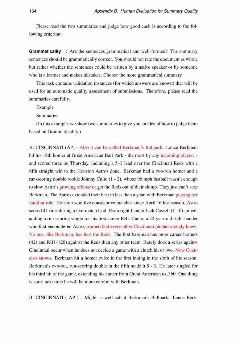
164 Appendix B. Human Evaluation for Summary Quality
Please read the two summaries and judge how good each is according to the fol-
lowing criterion:
Grammaticality : Are the sentences grammatical and well-formed? The summary
sentences should be grammatically correct. You should not rate the document as whole
but rather whether the sentences could be written by a native speaker or by someone
who is a learner and makes mistakes. Choose the more grammatical summary.
This task contains validation instances (for which answers are known) that will be
used for an automatic quality assessment of submissions. Therefore, please read the
summaries carefully.
Example
Summaries
(In this example, we show two summaries to give you an idea of how to judge them
based on Grammaticality.)
A: CINCINNATI (AP) - Also it can be called Berkman’s Ballpark. Lance Berkman
hit his 18th homer at Great American Ball Park - the most by any incoming player. -
and scored three on Thursday, including a 5–3 lead over the Cincinnati Reds with a
fifth straight win to the Houston Astros done. Berkman had a two-run homer and a
run-scoring double rookie Johnny Cuito (1 - 2), whose 96 mph fastball wasn’t enough
to slow Astro’s growing offense or get the Reds out of their slump. They just can’t stop
Berkman. The Astros extended their best in less than a year, with Berkman playing her
familiar role. Houston won five consecutive matches since April 16 last season. Astro
scored 41 runs during a five-match lead. Even right-hander Jack Cassell (1 - 0) joined,
adding a run-scoring single for his first career RBI. Cueto, a 22-year-old right-hander
who first encountered Astro, learned that every other Cincinnati pitcher already knew:
No one, like Berkman, has hurt the Reds. The first baseman has more career homers
(42) and RBI (120) against the Reds than any other team. Rarely does a series against
Cincinnati occur when he does not decide a game with a clutch hit or two. Now Cueto
also knows. Berkman hit a homer twice in the first inning in the sixth of his season.
Berkman’s two-out, run-scoring double in the fifth made it 5 - 3. He later singled for
his third hit of the game, extending his career from Great American to .360. One thing
is sure: next time he will be more careful with Berkman.
B: CINCINNATI ( AP ) – Might as well call it Berkman’s Ballpark. Lance Berk-
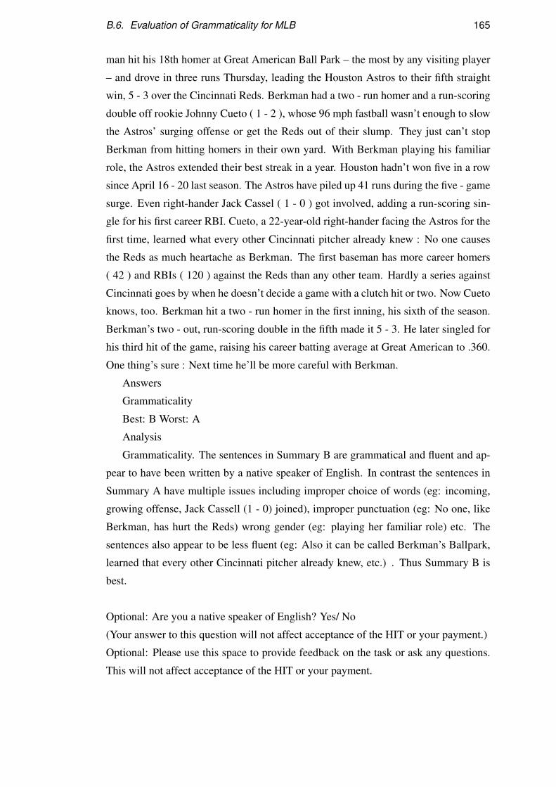
B.6. Evaluation of Grammaticality for MLB 165
man hit his 18th homer at Great American Ball Park – the most by any visiting player
– and drove in three runs Thursday, leading the Houston Astros to their fifth straight
win, 5 - 3 over the Cincinnati Reds. Berkman had a two - run homer and a run-scoring
double off rookie Johnny Cueto ( 1 - 2 ), whose 96 mph fastball wasn’t enough to slow
the Astros’ surging offense or get the Reds out of their slump. They just can’t stop
Berkman from hitting homers in their own yard. With Berkman playing his familiar
role, the Astros extended their best streak in a year. Houston hadn’t won five in a row
since April 16 - 20 last season. The Astros have piled up 41 runs during the five - game
surge. Even right-hander Jack Cassel ( 1 - 0 ) got involved, adding a run-scoring sin-
gle for his first career RBI. Cueto, a 22-year-old right-hander facing the Astros for the
first time, learned what every other Cincinnati pitcher already knew : No one causes
the Reds as much heartache as Berkman. The first baseman has more career homers
( 42 ) and RBIs ( 120 ) against the Reds than any other team. Hardly a series against
Cincinnati goes by when he doesn’t decide a game with a clutch hit or two. Now Cueto
knows, too. Berkman hit a two - run homer in the first inning, his sixth of the season.
Berkman’s two - out, run-scoring double in the fifth made it 5 - 3. He later singled for
his third hit of the game, raising his career batting average at Great American to .360.
One thing’s sure : Next time he’ll be more careful with Berkman.
Answers
Grammaticality
Best: B Worst: A
Analysis
Grammaticality. The sentences in Summary B are grammatical and fluent and ap-
pear to have been written by a native speaker of English. In contrast the sentences in
Summary A have multiple issues including improper choice of words (eg: incoming,
growing offense, Jack Cassell (1 - 0) joined), improper punctuation (eg: No one, like
Berkman, has hurt the Reds) wrong gender (eg: playing her familiar role) etc. The
sentences also appear to be less fluent (eg: Also it can be called Berkman’s Ballpark,
learned that every other Cincinnati pitcher already knew, etc.) . Thus Summary B is
best.
Optional: Are you a native speaker of English? Yes/ No
(Your answer to this question will not affect acceptance of the HIT or your payment.)
Optional: Please use this space to provide feedback on the task or ask any questions.
This will not affect acceptance of the HIT or your payment.


Bibliography
Angeli, G., Johnson Premkumar, M. J., and Manning, C. D. (2015). Leveraging lin-
guistic structure for open domain information extraction. In Proceedings of the
53rd Annual Meeting of the Association for Computational Linguistics and the 7th
International Joint Conference on Natural Language Processing (Volume 1: Long
Papers), pages 344–354, Beijing, China. Association for Computational Linguistics.
Angeli, G., Liang, P., and Klein, D. (2010). A simple domain-independent probabilistic
approach to generation. In Proceedings of the 2010 Conference on Empirical Meth-
ods in Natural Language Processing, pages 502–512, Cambridge, MA. Association
for Computational Linguistics.
Bahdanau, D., Cho, K., and Bengio, Y. (2015). Neural machine translation by jointly
learning to align and translate. In Bengio, Y. and LeCun, Y., editors, 3rd Interna-
tional Conference on Learning Representations, ICLR 2015, San Diego, CA, USA,
May 7-9, 2015, Conference Track Proceedings.
Barzilay, R. and Lapata, M. (2005). Collective content selection for concept-to-text
generation. In Proceedings of Human Language Technology Conference and Con-
ference on Empirical Methods in Natural Language Processing, pages 331–338,
Vancouver, British Columbia, Canada. Association for Computational Linguistics.
Bateman, J. A. (1997). Enabling technology for multilingual natural language genera-
tion: The kpml development environment. Nat. Lang. Eng., 3(1):15–55.
Belz, A. (2008). Automatic generation of weather forecast texts using compre-
hensive probabilistic generation-space models. Natural Language Engineering,
14(4):431–455.
Bengio, S., Vinyals, O., Jaitly, N., and Shazeer, N. (2015). Scheduled sampling for
sequence prediction with recurrent neural networks. In Proceedings of the 28th
167
168 Bibliography
International Conference on Neural Information Processing Systems - Volume 1,
NIPS’15, pages 1171–1179, Cambridge, MA, USA. MIT Press.
Bengio, Y., Ducharme, R., Vincent, P., and Janvin, C. (2003). A neural probabilistic
language model. J. Mach. Learn. Res., 3(null):1137–1155.
Bird, S., Klein, E., and Loper, E. (2009). Natural Language Processing with Python.
O’Reilly Media.
Bosselut, A., Levy, O., Holtzman, A., Ennis, C., Fox, D., and Choi, Y. (2018). Simulat-
ing action dynamics with neural process networks. In 6th International Conference
on Learning Representations, ICLR 2018, Vancouver, BC, Canada, April 30 - May
3, 2018, Conference Track Proceedings. OpenReview.net.
Boytsov, L. (2011). Indexing methods for approximate dictionary searching: Compar-
ative analysis. ACM J. Exp. Algorithmics, 16.
Brill, E. and Moore, R. C. (2000). An improved error model for noisy channel spelling
correction. In Proceedings of the 38th Annual Meeting of the Association for Com-
putational Linguistics, pages 286–293, Hong Kong. Association for Computational
Linguistics.
Castro Ferreira, T., van der Lee, C., van Miltenburg, E., and Krahmer, E. (2019). Neu-
ral data-to-text generation: A comparison between pipeline and end-to-end architec-
tures. In Proceedings of the 2019 Conference on Empirical Methods in Natural Lan-
guage Processing and the 9th International Joint Conference on Natural Language
Processing (EMNLP-IJCNLP), pages 552–562, Hong Kong, China. Association for
Computational Linguistics.
Cavazza, M. and Charles, F. (2005). Dialogue generation in character-based interactive
storytelling. In AIIDE, pages 21–26.
Cavazza, M., Charles, F., and Mead, S. J. (2002). Character-based interactive story-
telling. IEEE Intelligent systems, 17(4):17–24.
Chafe, W. L. (1976). Givenness, contrastiveness, definiteness, subjects, topics, a nd
point of view. In Li, C. N., editor, Subject and topic, pages 25–55. Academic Press,
New York.
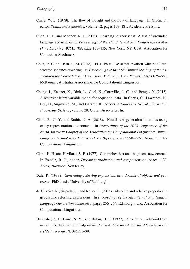
Bibliography 169
Chafe, W. L. (1979). The flow of thought and the flow of language. In Givón, T.,
editor, Syntax and Semantics, volume 12, pages 159–181. Academic Press Inc.
Chen, D. L. and Mooney, R. J. (2008). Learning to sportscast: A test of grounded
language acquisition. In Proceedings of the 25th International Conference on Ma-
chine Learning, ICML ’08, page 128–135, New York, NY, USA. Association for
Computing Machinery.
Chen, Y.-C. and Bansal, M. (2018). Fast abstractive summarization with reinforce-
selected sentence rewriting. In Proceedings of the 56th Annual Meeting of the As-
sociation for Computational Linguistics (Volume 1: Long Papers), pages 675–686,
Melbourne, Australia. Association for Computational Linguistics.
Chung, J., Kastner, K., Dinh, L., Goel, K., Courville, A. C., and Bengio, Y. (2015).
A recurrent latent variable model for sequential data. In Cortes, C., Lawrence, N.,
Lee, D., Sugiyama, M., and Garnett, R., editors, Advances in Neural Information
Processing Systems, volume 28. Curran Associates, Inc.
Clark, E., Ji, Y., and Smith, N. A. (2018). Neural text generation in stories using
entity representations as context. In Proceedings of the 2018 Conference of the
North American Chapter of the Association for Computational Linguistics: Human
Language Technologies, Volume 1 (Long Papers), pages 2250–2260. Association for
Computational Linguistics.
Clark, H. H. and Haviland, S. E. (1977). Comprehension and the given- new conract.
In Freedle, R. O., editor, Discourse production and comprehension, pages 1–39.
Ablex, Norwood, NewJersey.
Dale, R. (1988). Generating referring expressions in a domain of objects and pro-
cesses. PhD thesis, University of Edinburgh.
de Oliveira, R., Sripada, S., and Reiter, E. (2016). Absolute and relative properties in
geographic referring expressions. In Proceedings of the 9th International Natural
Language Generation conference, pages 256–264, Edinburgh, UK. Association for
Computational Linguistics.
Dempster, A. P., Laird, N. M., and Rubin, D. B. (1977). Maximum likelihood from
incomplete data via the em algorithm. Journal of the Royal Statistical Society. Series
B (Methodological), 39(1):1–38.
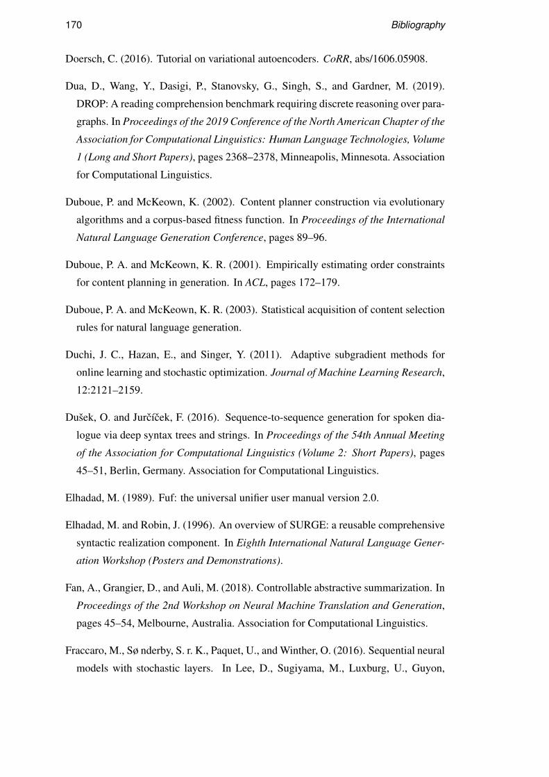
170 Bibliography
Doersch, C. (2016). Tutorial on variational autoencoders. CoRR, abs/1606.05908.
Dua, D., Wang, Y., Dasigi, P., Stanovsky, G., Singh, S., and Gardner, M. (2019).
DROP: A reading comprehension benchmark requiring discrete reasoning over para-
graphs. In Proceedings of the 2019 Conference of the North American Chapter of the
Association for Computational Linguistics: Human Language Technologies, Volume
1 (Long and Short Papers), pages 2368–2378, Minneapolis, Minnesota. Association
for Computational Linguistics.
Duboue, P. and McKeown, K. (2002). Content planner construction via evolutionary
algorithms and a corpus-based fitness function. In Proceedings of the International
Natural Language Generation Conference, pages 89–96.
Duboue, P. A. and McKeown, K. R. (2001). Empirically estimating order constraints
for content planning in generation. In ACL, pages 172–179.
Duboue, P. A. and McKeown, K. R. (2003). Statistical acquisition of content selection
rules for natural language generation.
Duchi, J. C., Hazan, E., and Singer, Y. (2011). Adaptive subgradient methods for
online learning and stochastic optimization. Journal of Machine Learning Research,
12:2121–2159.
Dušek, O. and Jurcícek, F. (2016). Sequence-to-sequence generation for spoken dia-
logue via deep syntax trees and strings. In Proceedings of the 54th Annual Meeting
of the Association for Computational Linguistics (Volume 2: Short Papers), pages
45–51, Berlin, Germany. Association for Computational Linguistics.
Elhadad, M. (1989). Fuf: the universal unifier user manual version 2.0.
Elhadad, M. and Robin, J. (1996). An overview of SURGE: a reusable comprehensive
syntactic realization component. In Eighth International Natural Language Gener-
ation Workshop (Posters and Demonstrations).
Fan, A., Grangier, D., and Auli, M. (2018). Controllable abstractive summarization. In
Proceedings of the 2nd Workshop on Neural Machine Translation and Generation,
pages 45–54, Melbourne, Australia. Association for Computational Linguistics.
Fraccaro, M., Sø nderby, S. r. K., Paquet, U., and Winther, O. (2016). Sequential neural
models with stochastic layers. In Lee, D., Sugiyama, M., Luxburg, U., Guyon,
Bibliography 171
I., and Garnett, R., editors, Advances in Neural Information Processing Systems,
volume 29. Curran Associates, Inc.
Fu, Y., Feng, Y., and Cunningham, J. P. (2019). Paraphrase generation with latent bag
of words. In Wallach, H. M., Larochelle, H., Beygelzimer, A., d’Alché-Buc, F., Fox,
E. B., and Garnett, R., editors, Advances in Neural Information Processing Systems
32: Annual Conference on Neural Information Processing Systems 2019, NeurIPS
2019, December 8-14, 2019, Vancouver, BC, Canada, pages 13623–13634.
Fu, Y., Tan, C., Bi, B., Chen, M., Feng, Y., and Rush, A. (2020). Latent template
induction with gumbel-crfs. In Larochelle, H., Ranzato, M., Hadsell, R., Balcan,
M. F., and Lin, H., editors, Advances in Neural Information Processing Systems,
volume 33, pages 20259–20271. Curran Associates, Inc.
Gardent, C., Shimorina, A., Narayan, S., and Perez-Beltrachini, L. (2017). Creat-
ing training corpora for NLG micro-planners. In Proceedings of the 55th Annual
Meeting of the Association for Computational Linguistics (Volume 1: Long Papers),
pages 179–188, Vancouver, Canada. Association for Computational Linguistics.
Gatt, A. and Krahmer, E. (2018). Survey of the state of the art in natural language
generation: Core tasks, applications and evaluation. J. Artif. Intell. Res., 61:65–170.
Goldberg, E., Driedger, N., and Kittredge, R. I. (1994). Using natural-language pro-
cessing to produce weather forecasts. IEEE Expert: Intelligent Systems and Their
Applications, 9(2):45–53.
Gong, H., Feng, X., Qin, B., and Liu, T. (2019). Table-to-text generation with ef-
fective hierarchical encoder on three dimensions (row, column and time). In Pro-
ceedings of the 2019 Conference on Empirical Methods in Natural Language Pro-
cessing and the 9th International Joint Conference on Natural Language Processing
(EMNLP-IJCNLP), pages 3143–3152, Hong Kong, China. Association for Compu-
tational Linguistics.
Goyal, A., Sordoni, A., Côté, M.-A., Ke, N. R., and Bengio, Y. (2017). Z-forcing:
Training stochastic recurrent networks. In Guyon, I., Luxburg, U. V., Bengio, S.,
Wallach, H., Fergus, R., Vishwanathan, S., and Garnett, R., editors, Advances in
Neural Information Processing Systems, volume 30. Curran Associates, Inc.
172 Bibliography
Grosz, B. J., Joshi, A. K., and Weinstein, S. (1995). Centering: A framework for
modeling the local coherence of discourse. Computational Linguistics, 21(2):203–
225.
Gu, J., Lu, Z., Li, H., and Li, V. O. (2016). Incorporating copying mechanism in
sequence-to-sequence learning. In Proceedings of the 54th Annual Meeting of the
Association for Computational Linguistics (Volume 1: Long Papers), pages 1631–
1640.
Guhe, M. (2020). Incremental conceptualization for language production. Psychology
Press.
Gulcehre, C., Ahn, S., Nallapati, R., Zhou, B., and Bengio, Y. (2016a). Pointing the
unknown words. In Proceedings of the 54th Annual Meeting of the Association for
Computational Linguistics (Volume 1: Long Papers), pages 140–149.
Gulcehre, C., Ahn, S., Nallapati, R., Zhou, B., and Bengio, Y. (2016b). Pointing the
unknown words. In Proceedings of the 54th Annual Meeting of the Association
for Computational Linguistics (Volume 1: Long Papers), pages 140–149, Berlin,
Germany. Association for Computational Linguistics.
Halliday, M. A. K. and Hasan, R. (1976). Cohesion in English. Longman, London.
Händschke, S. G., Buechel, S., Goldenstein, J., Poschmann, P., Duan, T., Walgenbach,
P., and Hahn, U. (2018). A corpus of corporate annual and social responsibility
reports: 280 million tokens of balanced organizational writing. In Proceedings of
the First Workshop on Economics and Natural Language Processing, pages 20–31,
Melbourne, Australia. Association for Computational Linguistics.
Harris, Z. S. (1954). Distributional structure. <i>WORD</i>, 10(2-3):146–162.
Hayashi, H., Oda, Y., Birch, A., Konstas, I., Finch, A., Luong, M.-T., Neubig, G., and
Sudoh, K. (2019). Findings of the third workshop on neural generation and trans-
lation. In Proceedings of the 3rd Workshop on Neural Generation and Translation,
pages 1–14, Hong Kong. Association for Computational Linguistics.
Henaff, M., Weston, J., Szlam, A., Bordes, A., and LeCun, Y. (2017). Tracking
the world state with recurrent entity networks. In 5th International Conference on
Learning Representations, ICLR 2017, Toulon, France, April 24-26, 2017, Confer-
ence Track Proceedings. OpenReview.net.

Bibliography 173
Hochreiter, S. and Schmidhuber, J. (1997). Long short-term memory. Neural Compu-
tation, 9:1735–1780.
Hovy, E. H. (1993). Automated discourse generation using discourse structure rela-
tions. Artificial intelligence, 63(1-2):341–385.
Iso, H., Uehara, Y., Ishigaki, T., Noji, H., Aramaki, E., Kobayashi, I., Miyao, Y.,
Okazaki, N., and Takamura, H. (2019). Learning to select, track, and generate
for data-to-text. In Proceedings of the 57th Annual Meeting of the Association for
Computational Linguistics, pages 2102–2113, Florence, Italy. Association for Com-
putational Linguistics.
Jang, E., Gu, S., and Poole, B. (2017). Categorical reparametrization with gumble-
softmax. In International Conference on Learning Representations (ICLR 2017).
OpenReview.net.
Ji, Y., Tan, C., Martschat, S., Choi, Y., and Smith, N. A. (2017). Dynamic entity rep-
resentations in neural language models. In Proceedings of the 2017 Conference on
Empirical Methods in Natural Language Processing, pages 1831–1840. Association
for Computational Linguistics.
Kale, M. and Rastogi, A. (2020). Text-to-text pre-training for data-to-text tasks. In
Proceedings of the 13th International Conference on Natural Language Generation,
pages 97–102, Dublin, Ireland. Association for Computational Linguistics.
Karamanis, N. (2004). Entity coherence for descriptive text structuring. PhD thesis,
School of Informatics, University of Edinburgh.
Karamanis, N., Poesio, M., Mellish, C., and Oberlander, J. (2004). Evaluating
centering-based metrics of coherence. In Proceedings of the 42nd Annual Meet-
ing of the Association for Computational Linguistics (ACL-04).
Karttunen, L. (1976). Discourse referents. In McCawley, J. D., editor, Syntax and
Semantics: Notes from the Linguistic Underground, volume 7, pages 363–86. Aca-
demic Press, New York.
Kasner, Z., Mille, S., and Dušek, O. (2021). Text-in-context: Token-level error detec-
tion for table-to-text generation. In Proceedings of the 14th International Confer-
ence on Natural Language Generation, pages 259–265, Aberdeen, Scotland, UK.
Association for Computational Linguistics.
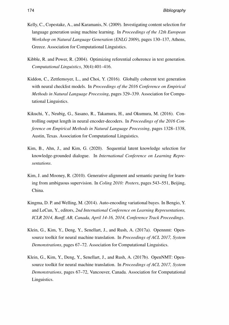
174 Bibliography
Kelly, C., Copestake, A., and Karamanis, N. (2009). Investigating content selection for
language generation using machine learning. In Proceedings of the 12th European
Workshop on Natural Language Generation (ENLG 2009), pages 130–137, Athens,
Greece. Association for Computational Linguistics.
Kibble, R. and Power, R. (2004). Optimizing referential coherence in text generation.
Computational Linguistics, 30(4):401–416.
Kiddon, C., Zettlemoyer, L., and Choi, Y. (2016). Globally coherent text generation
with neural checklist models. In Proceedings of the 2016 Conference on Empirical
Methods in Natural Language Processing, pages 329–339. Association for Compu-
tational Linguistics.
Kikuchi, Y., Neubig, G., Sasano, R., Takamura, H., and Okumura, M. (2016). Con-
trolling output length in neural encoder-decoders. In Proceedings of the 2016 Con-
ference on Empirical Methods in Natural Language Processing, pages 1328–1338,
Austin, Texas. Association for Computational Linguistics.
Kim, B., Ahn, J., and Kim, G. (2020). Sequential latent knowledge selection for
knowledge-grounded dialogue. In International Conference on Learning Repre-
sentations.
Kim, J. and Mooney, R. (2010). Generative alignment and semantic parsing for learn-
ing from ambiguous supervision. In Coling 2010: Posters, pages 543–551, Beijing,
China.
Kingma, D. P. and Welling, M. (2014). Auto-encoding variational bayes. In Bengio, Y.
and LeCun, Y., editors, 2nd International Conference on Learning Representations,
ICLR 2014, Banff, AB, Canada, April 14-16, 2014, Conference Track Proceedings.
Klein, G., Kim, Y., Deng, Y., Senellart, J., and Rush, A. (2017a). Opennmt: Open-
source toolkit for neural machine translation. In Proceedings of ACL 2017, System
Demonstrations, pages 67–72. Association for Computational Linguistics.
Klein, G., Kim, Y., Deng, Y., Senellart, J., and Rush, A. (2017b). OpenNMT: Open-
source toolkit for neural machine translation. In Proceedings of ACL 2017, System
Demonstrations, pages 67–72, Vancouver, Canada. Association for Computational
Linguistics.
Bibliography 175
Kogan, S., Levin, D., Routledge, B. R., Sagi, J. S., and Smith, N. A. (2009). Predict-
ing risk from financial reports with regression. In Proceedings of Human Language
Technologies: The 2009 Annual Conference of the North American Chapter of the
Association for Computational Linguistics, pages 272–280, Boulder, Colorado. As-
sociation for Computational Linguistics.
Konstas, I. (2014). Joint models for concept-to-text generation.
Konstas, I. and Lapata, M. (2013). A global model for concept-to-text generation. J.
Artif. Int. Res., 48(1):305–346.
Kryscinski, W., Rajani, N., Agarwal, D., Xiong, C., and Radev, D. (2021). Booksum:
A collection of datasets for long-form narrative summarization.
Kukich, K. (1983). Design of a knowledge-based report generator. In 21st Annual
Meeting of the Association for Computational Linguistics.
Kuno, S. (1972). Functional sentence perspective. Linguistic Inquiry, 3:269–320.
Laha, A., Jain, P., Mishra, A., and Sankaranarayanan, K. (2019). Scalable micro-
planned generation of discourse from structured data. Computational Linguistics,
45(4):737–763.
Langkilde, I. and Knight, K. (1998). Generation that exploits corpus-based statisti-
cal knowledge. In 36th Annual Meeting of the Association for Computational Lin-
guistics and 17th International Conference on Computational Linguistics, Volume
1, pages 704–710, Montreal, Quebec, Canada. Association for Computational Lin-
guistics.
Lavoie, B. and Rainbow, O. (1997). A fast and portable realizer for text generation
systems. In Fifth Conference on Applied Natural Language Processing, pages 265–
268, Washington, DC, USA. Association for Computational Linguistics.
Lebret, R., Grangier, D., and Auli, M. (2016). Neural text generation from structured
data with application to the biography domain. In Proceedings of the 2016 Con-
ference on Empirical Methods in Natural Language Processing, pages 1203–1213,
Austin, Texas. Association for Computational Linguistics.
Levelt, W. J. (1993). Speaking: From intention to articulation, volume 1. MIT press.
176 Bibliography
Lewis, M., Liu, Y., Goyal, N., Ghazvininejad, M., Mohamed, A., Levy, O., Stoy-
anov, V., and Zettlemoyer, L. (2020). BART: Denoising sequence-to-sequence pre-
training for natural language generation, translation, and comprehension. In Pro-
ceedings of the 58th Annual Meeting of the Association for Computational Linguis-
tics, pages 7871–7880, Online. Association for Computational Linguistics.
Li, P., Lam, W., Bing, L., and Wang, Z. (2017). Deep recurrent generative decoder
for abstractive text summarization. In Proceedings of the 2017 Conference on Em-
pirical Methods in Natural Language Processing, pages 2091–2100, Copenhagen,
Denmark. Association for Computational Linguistics.
Li, X. L. and Rush, A. (2020). Posterior control of blackbox generation. In Proceed-
ings of the 58th Annual Meeting of the Association for Computational Linguistics,
pages 2731–2743, Online. Association for Computational Linguistics.
Liang, P., Jordan, M., and Klein, D. (2009). Learning semantic correspondences with
less supervision. In Proceedings of the Joint Conference of the 47th Annual Meet-
ing of the ACL and the 4th International Joint Conference on Natural Language
Processing of the AFNLP, pages 91–99, Suntec, Singapore. Association for Com-
putational Linguistics.
Longacre, R. E. (1979). The paragraph as a grammatical unit. In Givón, T., editor,
Syntax and Semantics, volume 12, pages 115–133. Academic Press Inc.
Louviere, J. J., Flynn, T. N., and Marley, A. A. J. (2015). Best-worst scaling: Theory,
methods and applications. Cambridge University Press.
Louviere, J. J. and Woodworth, G. G. (1991). Best-worst scaling: A model for the
largest difference judgments. University of Alberta: Working Paper.
Luong, T., Pham, H., and Manning, C. D. (2015a). Effective approaches to attention-
based neural machine translation. In Proceedings of the 2015 Conference on Empir-
ical Methods in Natural Language Processing, pages 1412–1421, Lisbon, Portugal.
Association for Computational Linguistics.
Luong, T., Pham, H., and Manning, C. D. (2015b). Effective approaches to attention-
based neural machine translation. In Proceedings of the 2015 Conference on Empir-
ical Methods in Natural Language Processing, pages 1412–1421.
Bibliography 177
Luong, T., Socher, R., and Manning, C. (2013). Better word representations with recur-
sive neural networks for morphology. In Proceedings of the Seventeenth Conference
on Computational Natural Language Learning, pages 104–113, Sofia, Bulgaria. As-
sociation for Computational Linguistics.
Maddison, C. J., Mnih, A., and Teh, Y. W. (2017). The concrete distribution: A con-
tinuous relaxation of discrete random variables. In International Conference on
Learning Representations (ICLR 2017). OpenReview.net.
Mairesse, F., Gašic, M., Jurcícek, F., Keizer, S., Thomson, B., Yu, K., and Young,
S. (2010). Phrase-based statistical language generation using graphical models and
active learning. In Proceedings of the 48th Annual Meeting of the Association for
Computational Linguistics, pages 1552–1561, Uppsala, Sweden. Association for
Computational Linguistics.
Mann, W. C. and Thomson, S. A. (1988). Rhetorical structure theory. Text, 8(3):243–
281.
Maynez, J., Narayan, S., Bohnet, B., and McDonald, R. (2020). On faithfulness and
factuality in abstractive summarization. In Proceedings of the 58th Annual Meeting
of the Association for Computational Linguistics, pages 1906–1919, Online. Asso-
ciation for Computational Linguistics.
McKeown, K. (1992). Text generation. Cambridge University Press.
Mei, H., Bansal, M., and Walter, M. R. (2016). What to talk about and how? selective
generation using LSTMs with coarse-to-fine alignment. In Proceedings of the 2016
Conference of the North American Chapter of the Association for Computational
Linguistics: Human Language Technologies, pages 720–730, San Diego, California.
Association for Computational Linguistics.
Mellish, C., Knott, A., Oberlander, J., and O’Donnell, M. (1998). Experiments using
stochastic search for text planning. Natural Language Generation.
Moryossef, A., Goldberg, Y., and Dagan, I. (2019). Step-by-step: Separating planning
from realization in neural data-to-text generation. In Proceedings of the 2019 Con-
ference of the North American Chapter of the Association for Computational Lin-
guistics: Human Language Technologies, Volume 1 (Long and Short Papers), pages
2267–2277, Minneapolis, Minnesota. Association for Computational Linguistics.
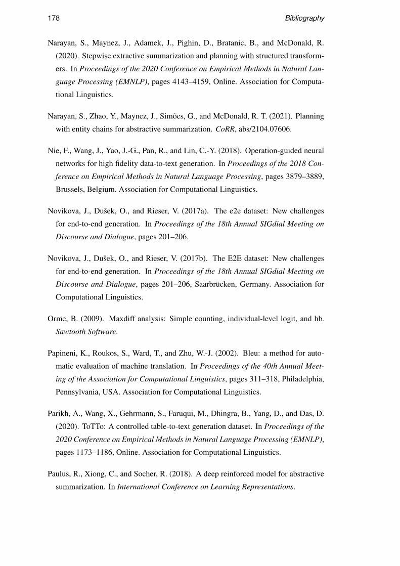
178 Bibliography
Narayan, S., Maynez, J., Adamek, J., Pighin, D., Bratanic, B., and McDonald, R.
(2020). Stepwise extractive summarization and planning with structured transform-
ers. In Proceedings of the 2020 Conference on Empirical Methods in Natural Lan-
guage Processing (EMNLP), pages 4143–4159, Online. Association for Computa-
tional Linguistics.
Narayan, S., Zhao, Y., Maynez, J., Simões, G., and McDonald, R. T. (2021). Planning
with entity chains for abstractive summarization. CoRR, abs/2104.07606.
Nie, F., Wang, J., Yao, J.-G., Pan, R., and Lin, C.-Y. (2018). Operation-guided neural
networks for high fidelity data-to-text generation. In Proceedings of the 2018 Con-
ference on Empirical Methods in Natural Language Processing, pages 3879–3889,
Brussels, Belgium. Association for Computational Linguistics.
Novikova, J., Dušek, O., and Rieser, V. (2017a). The e2e dataset: New challenges
for end-to-end generation. In Proceedings of the 18th Annual SIGdial Meeting on
Discourse and Dialogue, pages 201–206.
Novikova, J., Dušek, O., and Rieser, V. (2017b). The E2E dataset: New challenges
for end-to-end generation. In Proceedings of the 18th Annual SIGdial Meeting on
Discourse and Dialogue, pages 201–206, Saarbrücken, Germany. Association for
Computational Linguistics.
Orme, B. (2009). Maxdiff analysis: Simple counting, individual-level logit, and hb.
Sawtooth Software.
Papineni, K., Roukos, S., Ward, T., and Zhu, W.-J. (2002). Bleu: a method for auto-
matic evaluation of machine translation. In Proceedings of the 40th Annual Meet-
ing of the Association for Computational Linguistics, pages 311–318, Philadelphia,
Pennsylvania, USA. Association for Computational Linguistics.
Parikh, A., Wang, X., Gehrmann, S., Faruqui, M., Dhingra, B., Yang, D., and Das, D.
(2020). ToTTo: A controlled table-to-text generation dataset. In Proceedings of the
2020 Conference on Empirical Methods in Natural Language Processing (EMNLP),
pages 1173–1186, Online. Association for Computational Linguistics.
Paulus, R., Xiong, C., and Socher, R. (2018). A deep reinforced model for abstractive
summarization. In International Conference on Learning Representations.
Bibliography 179
Perez-Beltrachini, L. and Lapata, M. (2018). Bootstrapping generators from noisy
data. In Proceedings of the 2018 Conference of the North American Chapter of the
Association for Computational Linguistics: Human Language Technologies, Vol-
ume 1 (Long Papers), pages 1516–1527, New Orleans, Louisiana. Association for
Computational Linguistics.
Portet, F., Reiter, E., Gatt, A., Hunter, J., Sripada, S., Freer, Y., and Sykes, C. (2009).
Automatic generation of textual summaries from neonatal intensive care data. Arti-
ficial Intelligence, 173(7):789–816.
Prince, E. (1981). Toward a taxonomy of given- new information. In Cole, P., editor,
Radical pragmatics, pages 223 – 255. Academic Press, New York/London.
Puduppully, R., Dong, L., and Lapata, M. (2019a). Data-to-text generation with con-
tent selection and planning. In Proceedings of the 33rd AAAI Conference on Artifi-
cial Intelligence, Honolulu, Hawaii.
Puduppully, R., Dong, L., and Lapata, M. (2019b). Data-to-text generation with en-
tity modeling. In Proceedings of the 57th Annual Meeting of the Association for
Computational Linguistics, pages 2023–2035, Florence, Italy. Association for Com-
putational Linguistics.
Puduppully, R., Fu, Y., and Lapata, M. (2022). Data-to-text generation with variational
sequential planning. Transactions of the Association for Computational Linguistics
(to appear), abs/2202.13756.
Puduppully, R. and Lapata, M. (2021). Data-to-text generation with macro planning.
Transactions of the Association for Computational Linguistics, abs/2102.02723.
Radford, A., Wu, J., Child, R., Luan, D., Amodei, D., and Sutskever, I. (2019). Lan-
guage models are unsupervised multitask learners.
Raffel, C., Shazeer, N., Roberts, A., Lee, K., Narang, S., Matena, M., Zhou, Y., Li,
W., and Liu, P. J. (2020). Exploring the limits of transfer learning with a unified
text-to-text transformer. Journal of Machine Learning Research, 21(140):1–67.
Rebuffel, C., Soulier, L., Scoutheeten, G., and Gallinari, P. (2020). A hierarchical
model for data-to-text generation. In European Conference on Information Re-
trieval, pages 65–80. Springer.
180 Bibliography
Reed, L., Oraby, S., and Walker, M. (2018). Can neural generators for dialogue learn
sentence planning and discourse structuring? In Proceedings of the 11th Interna-
tional Conference on Natural Language Generation, pages 284–295, Tilburg Uni-
versity, The Netherlands. Association for Computational Linguistics.
Reiter, E. (1995). NLG vs. templates. CoRR, cmp-lg/9504013v1.
Reiter, E. (2017). You need to understand your corpora! the weathergov example.
Reiter, E. and Dale, R. (1997). Building applied natural language generation systems.
Nat. Lang. Eng., 3(1):57–87.
Reiter, E. and Dale, R. (2000). Building natural language generation systems. Cam-
bridge University Press, New York, NY.
Reiter, E., Sripada, S., Hunter, J., Yu, J., and Davy, I. (2005). Choosing words in
computer-generated weather forecasts. Artif. Intell., 167(1-2):137–169.
Rezende, D. J., Mohamed, S., and Wierstra, D. (2014). Stochastic backpropagation
and approximate inference in deep generative models. In Proceedings of the 31th
International Conference on Machine Learning, ICML 2014, Beijing, China, 21-
26 June 2014, volume 32 of JMLR Workshop and Conference Proceedings, pages
1278–1286. JMLR.org.
Robin, J. (1994). Revision-based generation of Natural Language Summaries provid-
ing historical Background. PhD thesis, Ph. D. thesis, Columbia University.
Rothe, S., Maynez, J., and Narayan, S. (2021). A thorough evaluation of task-specific
pretraining for summarization. In Proceedings of the 2021 Conference on Empirical
Methods in Natural Language Processing, pages 140–145, Online and Punta Cana,
Dominican Republic. Association for Computational Linguistics.
Rothe, S., Narayan, S., and Severyn, A. (2020). Leveraging pre-trained checkpoints
for sequence generation tasks. Transactions of the Association for Computational
Linguistics, 8:264–280.
Saleh, F., Berard, A., Calapodescu, I., and Besacier, L. (2019). Naver labs Europe’s
systems for the document-level generation and translation task at WNGT 2019. In
Proceedings of the 3rd Workshop on Neural Generation and Translation, pages 273–
279, Hong Kong. Association for Computational Linguistics.
Bibliography 181
Scott, D. and de Souza, C. S. (1990a). Getting the message across in rst-based text
generation. Current research in natural language generation, 4:47–73.
Scott, D. and de Souza, C. S. (1990b). Getting the message across in RST-based text
generation. In Dale, R., Mellish, C., and Zock, M., editors, Current Research in
Natural Language Generation, pages 47–73. Academic Press, New York.
Sennrich, R., Haddow, B., and Birch, A. (2016). Neural machine translation of rare
words with subword units. In Proceedings of the 54th Annual Meeting of the Asso-
ciation for Computational Linguistics (Volume 1: Long Papers), pages 1715–1725,
Berlin, Germany. Association for Computational Linguistics.
Serban, I. V., Sordoni, A., Lowe, R., Charlin, L., Pineau, J., Courville, A. C., and
Bengio, Y. (2017). A hierarchical latent variable encoder-decoder model for gen-
erating dialogues. In Singh, S. P. and Markovitch, S., editors, Proceedings of the
Thirty-First AAAI Conference on Artificial Intelligence, February 4-9, 2017, San
Francisco, California, USA, pages 3295–3301. AAAI Press.
Shankar, S. and Sarawagi, S. (2019). Posterior attention models for sequence to se-
quence learning. In International Conference on Learning Representations.
Shao, Z., Huang, M., Wen, J., Xu, W., and Zhu, X. (2019). Long and diverse text gener-
ation with planning-based hierarchical variational model. In Proceedings of the 2019
Conference on Empirical Methods in Natural Language Processing and the 9th In-
ternational Joint Conference on Natural Language Processing (EMNLP-IJCNLP),
pages 3257–3268, Hong Kong, China. Association for Computational Linguistics.
Shen, X., Chang, E., Su, H., Niu, C., and Klakow, D. (2020). Neural data-to-text
generation via jointly learning the segmentation and correspondence. In Proceedings
of the 58th Annual Meeting of the Association for Computational Linguistics, pages
7155–7165, Online. Association for Computational Linguistics.
Sripada, S., Reiter, E., and Hawizy, L. (2005). Evaluation of an NLG system using
post-edit data: Lessons learnt. In Proceedings of the Tenth European Workshop on
Natural Language Generation (ENLG-05).
Sripada, S., Reiter, E., Hunter, J., and Yu, J. (2002). Sumtime-meteo: Parallel corpus
of naturally occurring forecast texts and weather data.
182 Bibliography
Stent, A., Prasad, R., and Walker, M. (2004). Trainable sentence planning for complex
information presentations in spoken dialog systems. In Proceedings of the 42nd
Annual Meeting of the Association for Computational Linguistics (ACL-04), pages
79–86, Barcelona, Spain.
Sutskever, I., Vinyals, O., and Le, Q. V. (2014). Sequence to sequence learning with
neural networks. In Advances in Neural Information Processing Systems 27, pages
3104–3112. Curran Associates, Inc.
Takeno, S., Nagata, M., and Yamamoto, K. (2017). Controlling target features in neural
machine translation via prefix constraints. In Proceedings of the 4th Workshop on
Asian Translation (WAT2017), pages 55–63, Taipei, Taiwan. Asian Federation of
Natural Language Processing.
Tanaka-Ishii, K., Hasida, K., and Noda, I. (1998). Reactive content selection in the gen-
eration of real-time soccer commentary. In 36th Annual Meeting of the Association
for Computational Linguistics and 17th International Conference on Computational
Linguistics, Volume 2, pages 1282–1288, Montreal, Quebec, Canada. Association
for Computational Linguistics.
Taylor, M. M. and Taylor, I. (1990). Book reviews: Speaking: From intention to
articulation. Computational Linguistics, 16(1).
Thomson, C. and Reiter, E. (2020). A gold standard methodology for evaluating ac-
curacy in data-to-text systems. In Proceedings of the 13th International Conference
on Natural Language Generation, pages 158–168, Dublin, Ireland. Association for
Computational Linguistics.
Thomson, C. and Reiter, E. (2021). Generation challenges: Results of the accuracy
evaluation shared task. In Proceedings of the 14th International Conference on Nat-
ural Language Generation, pages 240–248, Aberdeen, Scotland, UK. Association
for Computational Linguistics.
Turner, R., Sripada, S., Reiter, E., and Davy, I. (2008). Using spatial reference frames
to generate grounded textual summaries of georeferenced data. In Proceedings of
the Fifth International Natural Language Generation Conference, pages 16–24, Salt
Fork, Ohio, USA. Association for Computational Linguistics.
Bibliography 183
van der Lee, C., Gatt, A., van Miltenburg, E., Wubben, S., and Krahmer, E. (2019).
Best practices for the human evaluation of automatically generated text. In Proceed-
ings of the 12th International Conference on Natural Language Generation, pages
355–368, Tokyo, Japan. Association for Computational Linguistics.
Vaswani, A., Shazeer, N., Parmar, N., Uszkoreit, J., Jones, L., Gomez, A. N., Kaiser,
L. u., and Polosukhin, I. (2017). Attention is all you need. In Guyon, I., Luxburg,
U. V., Bengio, S., Wallach, H., Fergus, R., Vishwanathan, S., and Garnett, R., ed-
itors, Advances in Neural Information Processing Systems 30, pages 5998–6008.
Curran Associates, Inc.
Vinyals, O., Fortunato, M., and Jaitly, N. (2015). Pointer networks. In Cortes, C.,
Lawrence, N. D., Lee, D. D., Sugiyama, M., and Garnett, R., editors, Advances in
Neural Information Processing Systems 28, pages 2692–2700. Curran Associates,
Inc.
Walker, M. A., Grant, R., Sawyer, J., Lin, G. I., Wardrip-Fruin, N., and Buell, M.
(2011). Perceived or not perceived: Film character models for expressive nlg. In In-
ternational Conference on Interactive Digital Storytelling, pages 109–121. Springer.
Walker, M. A., Rambow, O., and Rogati, M. (2001). SPoT: A trainable sentence
planner. In Second Meeting of the North American Chapter of the Association for
Computational Linguistics.
Walker, M. A., Rambow, O. C., and Rogati, M. (2002). Training a sentence planner
for spoken dialogue using boosting. Computer Speech & Language, 16(3):409–433.
Spoken Language Generation.
Wallace, E., Wang, Y., Li, S., Singh, S., and Gardner, M. (2019). Do NLP models know
numbers? probing numeracy in embeddings. In Proceedings of the 2019 Conference
on Empirical Methods in Natural Language Processing and the 9th International
Joint Conference on Natural Language Processing (EMNLP-IJCNLP), pages 5307–
5315, Hong Kong, China. Association for Computational Linguistics.
Wen, T.-H., Gašic, M., Mrkšic, N., Su, P.-H., Vandyke, D., and Young, S. (2015).
Semantically conditioned LSTM-based natural language generation for spoken di-
alogue systems. In Proceedings of the 2015 Conference on Empirical Methods in
Natural Language Processing, pages 1711–1721, Lisbon, Portugal. Association for
Computational Linguistics.

184 Bibliography
Williams, R. J. and Peng, J. (1990). An efficient gradient-based algorithm for on-line
training of recurrent network trajectories. Neural Computation, 2(4):490–501.
Wiseman, S., Shieber, S., and Rush, A. (2017). Challenges in data-to-document gen-
eration. In Proceedings of the 2017 Conference on Empirical Methods in Natural
Language Processing, pages 2253–2263, Copenhagen, Denmark. Association for
Computational Linguistics.
Wu, Y., Schuster, M., Chen, Z., Le, Q. V., Norouzi, M., Macherey, W., Krikun, M.,
Cao, Y., Gao, Q., Macherey, K., Klingner, J., Shah, A., Johnson, M., Liu, X.,
Kaiser, L., Gouws, S., Kato, Y., Kudo, T., Kazawa, H., Stevens, K., Kurian, G.,
Patil, N., Wang, W., Young, C., Smith, J., Riesa, J., Rudnick, A., Vinyals, O.,
Corrado, G., Hughes, M., and Dean, J. (2016). Google’s neural machine trans-
lation system: Bridging the gap between human and machine translation. CoRR,
abs/1609.08144v2.
Yang, Z., Blunsom, P., Dyer, C., and Ling, W. (2017). Reference-aware language
models. In Proceedings of the 2017 Conference on Empirical Methods in Natural
Language Processing, pages 1851–1860, Copenhagen, Denmark.
Yang, Z., Yang, D., Dyer, C., He, X., Smola, A., and Hovy, E. (2016a). Hierarchical at-
tention networks for document classification. In Proceedings of the 2016 Conference
of the North American Chapter of the Association for Computational Linguistics:
Human Language Technologies, pages 1480–1489. Association for Computational
Linguistics.
Yang, Z., Yang, D., Dyer, C., He, X., Smola, A., and Hovy, E. (2016b). Hierarchical
attention networks for document classification. In Proceedings of the 2016 Con-
ference of the North American Chapter of the Association for Computational Lin-
guistics: Human Language Technologies, pages 1480–1489, San Diego, California.
Association for Computational Linguistics.
Ye, R., Shi, W., Zhou, H., Wei, Z., and Li, L. (2020). Variational template machine for
data-to-text generation. In International Conference on Learning Representations.
Yee, K., Dauphin, Y., and Auli, M. (2019). Simple and effective noisy channel mod-
eling for neural machine translation. In Proceedings of the 2019 Conference on
Empirical Methods in Natural Language Processing and the 9th International Joint
Bibliography 185
Conference on Natural Language Processing (EMNLP-IJCNLP), pages 5696–5701,
Hong Kong, China. Association for Computational Linguistics.
Yu, L., Sartran, L., Stokowiec, W., Ling, W., Kong, L., Blunsom, P., and Dyer, C.
(2020). Better document-level machine translation with bayes’ rule. Transactions
of the Association for Computational Linguistics, 8:346–360.
Zadrozny, W. and Jensen, K. (1991). Semantics of paragraphs. Computational Lin-
guistics, 17(2):171–210.
Zaremba, W., Sutskever, I., and Vinyals, O. (2014). Recurrent neural network regular-
ization. arXiv preprint arXiv:1409.2329.
Zhao, C., Walker, M., and Chaturvedi, S. (2020). Bridging the structural gap between
encoding and decoding for data-to-text generation. In Proceedings of the 58th An-
nual Meeting of the Association for Computational Linguistics, pages 2481–2491,
Online. Association for Computational Linguistics.