A Simulation-Based Approach to Decision Making with Partial Information

Decision AnalysisVol. 9, No. 4, December 2012, pp. 329–347ISSN 1545-8490 (print) ISSN 1545-8504 (online) http://dx.doi.org/10.1287/deca.1120.0252

© 2012 INFORMS

A Simulation-Based Approach toDecision Making with Partial Information

Luis V. Montiel, J. Eric BickelGraduate Program in Operations Research and Industrial Engineering, University of Texas at Austin,

Austin, Texas 78712 [email protected], [email protected]

The construction of a probabilistic model is a key step in most decision and risk analyses. Typically this isdone by defining a single joint distribution in terms of marginal and conditional distributions. The difficulty

of this approach is that often the joint distribution is underspecified. For example, we may lack knowledgeof the marginal distributions or the underlying dependence structure. In this paper, we suggest an approachto analyzing decisions with partial information. Specifically, we propose a simulation procedure to create acollection of joint distributions that match the known information. This collection of distributions can then beused to analyze the decision problem. We demonstrate our method by applying it to the Eagle Airlines casestudy used in previous studies.

Key words : decision analysis; dependence; simulation; sensitivity to dependence; copulas; Eagle AirlinesHistory : Received on April 5, 2012. Accepted on August 28, 2012, after 2 revisions. Published online in Articles

in Advance October 26, 2012.

1. IntroductionIn many decision problems, we lack complete infor-mation regarding the underlying joint probability dis-tribution. For example, marginal distributions and/orprobabilistic dependencies may not be completelyspecified. Differing methodological areas within themanagement sciences view this lack of specificityin differing ways. To some, the lack of informationstems from a belief that the underlying probabilitydistribution is “unknown.” Others regard the incom-plete information as simply an acknowledgment thatit has yet to be assessed. We do not distinguishbetween these perspectives in this paper. Instead, wepresent a methodology that is useful in either case.For those that believe the underlying distributions areunknown, our procedure will allow them to modelthis uncertainty explicitly. For those that see this asan issue of assessment, the methods discussed hereinwill help to ensure that the assessed distributions areconsistent with the available information and quan-tify the benefit of further elicitations.

Although the lack of information could stem froman under specification of marginal distributions, weare primarily motivated by underspecification ofthe probabilistic dependence structure. Probabilistic

dependencies are inherent to many decision envi-ronments, including medicine (Chessa et al. 1999),nuclear power (Cooke and Waij 1986), and oilexploration (Bickel and Smith 2006, Bickel et al. 2008).Failure to capture these relationships can have impor-tant and sometimes tragic consequences (Apostolakisand Kaplan 1981, Smith et al. 1992). For example,the Space Shuttle Challenger accident was appar-ently caused, in part, by engineers’ failure to under-stand the dependency between ambient temperatureand o-ring resiliency (Presidential Commission on theSpace Shuttle Challenger Accident 1986).

Probabilistic dependence is often ignored becauseit complicates probability assessments (Lowell 1994,Korsan 1990). Winkler (1982) identified the assess-ment and modeling of probabilistic dependence asone of the most important research topics facing deci-sion analysts. He suggested the development of sensi-tivity analyses that would identify key dependenciesand decision-making methods that use less thanfull probabilistic information. Miller (1990, p. 443)argued, “We need a way to assess and process depen-dent probabilities efficiently. If we can find generallyapplicable methods for doing so, we could make sig-nificant advances in our ability to analyze and model

329

Montiel and Bickel: Decision Making with Partial Information330 Decision Analysis 9(4), pp. 329–347, © 2012 INFORMS

complex decision problems.” These critical challengeshave gone largely unanswered.

In this paper, we present a new methodology formodeling decisions given partial probabilistic infor-mation. In particular, we create the set of all possi-ble discrete distributions that are consistent with theinformation that we do have. We then (uniformly)sample from this set using the joint distribution simu-lation (JDSIM) procedure (Montiel 2012, Montiel andBickel 2012), which is based on the hit-and-run sam-pler (Smith 1984). Our procedure is perhaps bestthought of as a sensitivity analysis, because we donot claim that all distributions in our set are equallylikely. Indeed, specifying the probability distributionover the set of all probability distributions presents itsown difficulties.

Other approaches to the problem discussed here fallinto three primary categories: (i) approximation meth-ods that specify a single joint probability distributiongiven partial information, (ii) sensitivity analysis pro-cedures that partially explore the space of feasiblejoint distributions, and (iii) “robust” decision-makingmethods that attempt to ensure some minimum levelof performance.

The most prominent example in the first categoryis the maximum entropy method (maxent) pioneeredby Jaynes (1957, 1968), in which a single distribution(the one that is most uncertain, or has the highestentropy) is selected from the set of all possible dis-tributions that are consistent with the given informa-tion. This approach was further developed by Irelandand Kullback (1968), who were the first to approx-imate a discrete joint distribution given informationon the lower-order component distributions. Lowell(1994) also used maxent to specify a joint distributiongiven lower-order assessments (e.g., pairwise condi-tional assessments). More recently, Abbas (2006) andBickel and Smith (2006) explored the use of maxentto facilitate the modeling of dependence.

A closely related approach is the specification of acopula (Sklar 1959), which encodes the dependencebetween marginal distributions. For example, Jouiniand Clemen (1996), Frees et al. (1996), and Clemenand Reilly (1999) all used copulas to construct jointdistributions based on lower-order assessments. Inthe copula-based approach, the continuous joint dis-tribution is often discretized to facilitate modeling

within a discrete decision-tree framework. In thispaper, we compare our proposed methodology to thenormal-copula (NC) approach, illustrated by Clemenand Reilly (1999) (hereafter, CR).

In the second category, sensitivity procedures havebeen developed to explore portions of the set of pos-sible joint distributions. For example, Lowell (1994)developed a sensitivity analysis procedure to iden-tify important pairwise conditional probability assess-ments. As discussed above, CR proposed the use ofa normal copula, characterized by pairwise correla-tion coefficients. They then perturbed the correlationmatrix to explore a set of possible joint distribu-tions. This set is restricted to joint distributions thatcan be modeled with a normal copula. Reilly (2000)developed a sensitivity approach that uses syntheticvariables based on a pairwise correlation coefficientmatrix.

Finally, in the third category, robust proceduressuch as maximin or robust optimization (Ben-Tal et al.2009) evaluate decisions based on their worst possibleoutcomes. We do not directly address these methods.We note, however, that identifying the worst pos-sible joint distribution is often difficult. Our proce-dure could be used in a robust setting to “stress test”decisions.

This paper is organized as follows. Section 2 des-cribes a new procedure to generate joint probabil-ity distributions when only partial information isavailable. Section 3 introduces an illustrative exam-ple that we use to demonstrate our approach.Section 4 applies our new procedure to this exam-ple. Section 5 concludes and discusses future researchdirections.

2. Proposed ApproachMontiel (2012) developed the JDSIM procedure, andMontiel and Bickel (2012) showed how JDSIM can beused to generate random collections of joint distri-butions. In this paper, we demonstrate how to useJDSIM to model decision problems with incompleteinformation and compare our procedure to the useof copulas. In this section, we summarize JDSIM andrefer the interested reader to Montiel and Bickel (2012)for additional details.

JDSIM samples from the set of all possible discretejoint distributions that are consistent with the given

Montiel and Bickel: Decision Making with Partial InformationDecision Analysis 9(4), pp. 329–347, © 2012 INFORMS 331

information, provided that this information can bedescribed by a set of linear constraints. In this way,JDSIM provides not one, but a collection of discretejoint distributions under which the decision can beevaluated. The procedure begins with the specifica-tion of linear constraints on the joint distribution (e.g.,specification of marginal probabilities or pairwise cor-relations) and the creation of a convex polytope ,the “truth set,” that matches the given information.By “truth” we mean that any distribution within thisset is consistent with the assessments and thereforecould be the “true” joint distribution.

We illustrate the characterization of using asimple example with two binary random variables,V1 and V2. This distribution has four joint events(Figure 1(a)), whose probabilities must be positiveand sum to one (Figure 1(b)). The truth set can beexpressed as a hyperplane in four dimensions oras a full-dimensional polytope in three dimensions(Figure 1(c)). We can constrain to match marginalassessments such as P4V2 = Up5 = P1 + P3 = 006, asshown in Figure 1(d). When constraints are consistent,nonredundant, and nondegenerate, each constraintreduces the dimension of by one. Then, adding asecond marginal constraint will reduce to a one-dimensional line, and adding a correlation constraintwill reduce to a single point. Note that the additionof inconsistent constraints (assessments) produces aninfeasible set. Hence, for the remainder of this paper,we assume that all assessed information is consistentsuch that is not empty.

Formally, we can define the truth set as =

8p Ap = b1p ≥ 09, where A ∈ m1n is a matrix of mrows and n columns, b ∈ m is a column vector ofassessed information, and p ≥ 0 is a vector that repre-sents the joint probability distribution. The linear sys-tem, Ap = b, defining the truth set from Figure 1 is

[

1 1 1 1

1 0 1 0

]

P1

P2

P3

P4

=

[

1

006

]

0 (1)

2.1. Truth Set DefinitionWe now introduce the notation that we use todefine . We organize this notation into three groups:indices and sets, data, and explored variables. Indices and

sets describe the notation used to create the struc-tural constraints. Data represents the input informa-tion. Explored variables are the probabilities of the jointevents that define the discrete joint distributions.

2.1.1. Notation.Indices and Sets:

: Ordered set of random variables indexedby i = 11 0 0 0 1 v.

Ɔi: Ordered set of possible outcomes forrandom variable i indexed by ri =

1121 0 0 0 1 Ɔi.i

ri∈Ɔi: Realization for random variable i having

outcome ri.: Ordered set of all joint outcomes, =Ɔ1 ×

Ɔ2 × · · · ×Ɔv.k ∈: Joint realization k = 41

r112

r21 0 0 0 1v

rv5

indexed by k = 1121 0 0 0 1∏v

i=1 Ɔi.i

ri⊂: Proper subset i

ri= 4k k ∈1i

ri∈k).

Data:

qiri

: Probability that random variable i obtains thevalue i

ri.

i1 j : Rank correlation between random variables i

and j .

Explored Variables:

p: Vector of joint probabilities to be explored.pk

∈ p: Probability of the discrete joint outcome k.

2.1.2. Illustration of the Notation. To illustratethe notation, we use the example in Figure 1.1 The setof random variables = 4V11V25 is indexed as i = 112.The set of possible outcomes (i.e., branches on thedecision tree) for V1 and V2 are Ɔ1 = 4High, Low) andƆ2 = 4Up, Down), respectively. These sets are indexedas r1 = 112 for High or Low and r2 = 112 for Upor Down, respectively. The notation i

rirefers to par-

ticular realizations (i.e., to particular branches). Forexample, 1

r1= High, 1

r2= Low, 2

r1= Up, and 2

r2=

Down. In this example, the set of all joint outcomes isdefined as = 411213145, where 1 = 41

r112

r15,

2 = 41r112

r25, 3 = 41

r212

r15, and 4 = 41

r212

r25. The

proper subset 2r1

= 41135 includes the elements of

1 See the online supplement for a spreadsheet illustrating ournotation and constraints, available at http://dx.doi.org/10.1287/deca.1120.0252.


Figure 1 Example Characterization of the Truth Set

(a) Probability tree; four joint events (b) Probabilities sum to one; P1 + P2 + P3 + P4 = 1

(c) Projection to 3D; P1 + P2 + P3 ≤ 1 (d) Add marginal information; P1 + P3 = 0.6

Up

Up

Down

Down

High

V1

P1

P1

P2

P2

P3

P3P4

P2 P2

P1

P3

P1

P3

P4

V2 | V1

Low

(0, 0, 1, 0)

(0, 0, 0, 1)

(0, 1, 0, 0)

(1, 0, 0, 0)

(0, 0, 1)(0, 0, 0)

(1, 0, 0)

(0, 1, 0)

(0, 0, 4, 0.6)

(0.6, 0, 4, 0)

(0.6, 0, 0)

(0, 0, 0.6)

for which realization 2r1

has obtained (i.e., the firstand third branches in Figure 1).

We require the joint probabilities to sum to one,which implies that p1

+ p2+ p3

+ p4= 1. Like-

wise, the assessed probability q2r1

≡ P4V2 = Up5 =

P4V1 = High, V2 = Up5+P4V1 = Low, V2 = Up5= p1+

p3= 006. The rank correlation 112 between V1 and

V2 was not used in Figure 1. Finally, the vector p =

4p11 p2

1 p31 p4

5≡ 4P11P21P31P45 represents a feasiblediscrete joint probability distribution, which we willexplore with our simulation procedure.

We now describe general forms of linear constraintsthat we consider in this paper.

2.1.3. Constraints for Necessary and SufficientConditions. First, we require p = 4p1

1 p21 0 0 0 1 p

5

to be a probability mass function (pmf). Equations(2a) and (2b) accomplish this by requiring the ele-ments of p to sum to one and be nonnegative,

respectively. In our matrix notation, the first row ofA is a vector of ones, and the first element of b is aone, as in Equation (1). If no additional constraints areincluded, then is the unit simplex, which is compactand convex. Therefore, the addition of other linearconstraints will maintain the convexity of :

∑

k∈

pk= 11 (2a)

pk≥ 01 ∀k ∈0 (2b)

2.1.4. Constraints for Marginal Distributions.Equation (3) constrains to match the marginalassessments 4qi

ri5. This equation can be extended to

cover pairwise, three-way, or higher-order joint prob-ability information as long as the assessed beliefs areconsistent. In this case, A includes a row of zeroesand ones, the arrangement of which depends upon


the random variable in question (see Equation (1)),and b adds one parameter qi

rifor each constraint:

∑

k∈iri

pk= qi

ri∀ i ∈1 i

ri∈Ɔi0 (3)

2.1.5. Constraints for Rank Correlations. Equa-tion (4a) matches any rank correlation information(see Appendix A) that we might have, where wehave used the definition of rank correlation providedby Nelsen (1991) and MacKenzie (1994). The

4i1 j5k

are coefficients calculated using Equations (4b), (4c),and (4d). Thus, Equation (4a) is linear in the jointprobabilities. We now briefly discuss the other com-ponents of Equation (4a). Below, we show how to useEquation (4a) within the context of our example.

Equation (4c) corresponds to the H -volume definedby Nelsen (2005), and Bk

= 6Ik4Vi5 × Ik

4Vj57 is therectangular area defined by interval (4d).

∑

k∈

4i1 j5k

pk=

i1 j + 3

3∀ i1 j ∈1 (4a)

4i1 j5k

=V4xy52 6Bk

7

q+

k 4Vi5· q+

k 4Vj 5

∀k ∈ and i1 j ∈1 (4b)

V4xy52 6Bk7= 4pi+k · p

j+

k 52− 4pi+k · p

j−

k 52

− 4pi−k · pj+

k 52+ 4pi−k · p

j−

k 521 (4c)

Ik4Vi5≡ 6pi+k 1 pi−k 7 and Ik

4Vj5≡ 6pj+

k 1 pj−

k 70 (4d)

The cumulative probabilities pi+k = P4Vi ≤ +

k 4Vi55and pi−k = P4Vi ≤−

k 4Vi55 are defined such that +

k 4Vi5is the marginal outcome i

riof random variable i at

the joint realization k, and −

k 4Vi5 is the marginaloutcome i

ri−1 of the random variable i given thejoint realization k. Hence, i

ri−1 is the marginal out-come immediately smaller than i

riin the marginal

distribution of the random variable i. Finally, q+

k 4Vi5=

P4Vi = +

k 4Vi55 is the marginal probability of vari-able Vi, having the outcome i

riat the joint

realization k.Equation (4a) requires that the marginal probabili-

ties of Vi and Vj are known. Returning to our previousexample in Figure 1, if we assume q1

r1= 007 and q2

r1=

006, then the truth set is reduced to a line with end-points 400310041003105 and 400610011010035. The coef-ficients in Equation (4a) are

411251

=41·152 −41·00452 −4003·152 +4003·00452

007 ·006=10821

411252

=41·00452 −41·052 −4003·00452 +4003·052

007 ·004=00521

411253

=4003·152 −4003·00452 −40·152 +40·00452

003·006=00421

411254

=4003·00452 −4003·052 −40·00452 +40·052

003·004=00120

Hence, the rank correlation constraint is given by

1082·p1+0052·p2

+0042·p3+0012·p4

=i1 j +3

30 (5)

Within the truth set, feasible rank correlationsrange from 0.54 at 400610011010035 to −0036 at400310041003105. Specifying a particular correlationwithin this range would reduce the truth set to a sin-gle point, uniquely specifying a joint distribution p.

2.2. Sampling After characterizing , we uniformly sample p fromthe truth set using JDSIM. Our algorithm adapts thehit-and-run sampler (Smith 1984), which is the fastestknown algorithm to uniformly sample the interior ofan arbitrary polytope. The goal of this procedure is tocreate a discrete representation of that replicates thedispersion of the distributions within the set. Figure 2provides a graphical representation of the algorithmin two dimensions. Our procedure was explained indetail in Montiel and Bickel (2012), but we briefly sum-marize it here for convenience. The interested readershould see Montiel and Bickel (2012) for technicaldetails, including convergence properties and guid-ance regarding the required number of samples.

The sampler is initialized (Step 1) by generating anarbitrary point xi ∈ and setting the counter i = 0.Step 2 generates a set of directions D ⊆ n using anuncorrelated multivariate standard-normal distribu-tion and standardizing the directions. Step 3 selectsa uniformly distributed direction di ∈ D. Step 4 findsthe line L=∩ 8x x = xi +di1 a real scalar gener-ated by extending the direction di in both directionsuntil the boundary of is reached. Step 5 selects arandom point xi+1 ∈ L uniformly distributed over theline. Finally, Step 6 evaluates the counter and stopsif i =N (where N is the desired number of samples);otherwise the counter is incremented by one and thesampler returns to Step 2.

It is important to bear in mind that each sam-pled point is a complete joint pmf. We calculate the


Figure 2 Illustration of the Hit-and-Run Sampler in Two Dimensions

element-wise average of all sampled joint distribu-tions and refer to this as the average of sampledobservations (ASO). Because the ASO is a convexcombination of points in , and is convex, the ASOis a feasible joint distribution in .

3. Illustrative ExampleWe now describe the illustrative example that weuse to demonstrate our procedure. The Eagle Air-lines example was introduced by Clemen (1996) andlater extended by Clemen and Reilly (1999) and Reilly(2000). See Figure 3. We describe the example with anexcerpt from Reilly (2000, p. 559):

Dick Carothers, the owner of Eagle Airlines, is decid-ing whether to invest 0 0 0$521500 in a money market orto expand his fleet with the purchase of [an airplane;we will refer to this as the “Expand” alternative]. Hisdecision criterion is whether the new plane will gener-ate more profit than a money market alternative. Theinfluence diagram in [Figure 3] illustrates the relevantvariables. 0 0 0

The profit function is given by: Profit =

Total Revenue − Total Cost1 where

Total Revenue

= Charter Ratio ∗ Hours Flown ∗ Charter Price

+ 41 − Charter Ratio5 ∗ Hours Flown ∗ Capacity

∗ Number of Seats ∗ Price Level1

Total Cost

= Hours Flown ∗ Operating Cost + Insurance

+Purchase Price∗Percentage Financed∗Interest Rate1

where Charter Price is 3025 ∗ Price Level and theNumber of Seats is five. Computing the profit usingthe base values [described below], Carothers’s annualprofit is $9,975, which is $5,775 more than the mini-mum of $4,200 (based on the opportunity cost of cap-ital). The deterministic model indicates that Carothersshould expand his fleet now. Some of the inputs, how-ever, are highly variable, and these could possiblylower the profit below the $4,200 benchmark.

Based on sensitivity analysis, Reilly (2000)showed that four variables most affect the decision:Price Level (PL), Hours Flown (H ), Capacity (C), andOperating Cost per Hour (O). CR provided the 0.10(Low), 0.50 (Base), and 0.90 (High) fractiles for eachuncertainty and the Spearman rank correlationsbetween each pair of uncertainties, which we repeatin Table 1.

The noncritical uncertainties are fixed at theirbase values, which are Charter Ratio = 50%, PercentageFinanced = 40%, Interest Rate = 1105%, Insurance =

$201000, Purchase Price = $871500, Number of Seats = 5,and Charter Price = 3025 ∗ Price Level.

To apply their NC procedure, CR assumed thatthe marginal distributions shown in Table 1 are fromknown families. In particular, they assumed that PLand H are scaled-beta distributions, C is beta, and Ois normally distributed. CR’s parameter assumptionsfor each uncertainty are presented in Table 2.

With this information, CR proposed a single contin-uous joint probability density function (pdf), based onan NC, and discretized it using the Extended Pearson–Tukey (EPT) technique (Keefer and Bodily 1983,


Figure 3 Influence Diagram for Eagle Airline’s Decision

Percentagefinanced

Interestrate

Purchaseprice

Operatingcost

Insurance

Fixedcost

Totalcost

Variablecost

Hourflown

Capacity

Flightrevenue

Totalrevenue

Charterrevenue

Charterratio

Pricelevel

Profit

Pearson and Tukey 1965). The EPT technique weightsthe 0.05, 0.50, and 0.95 fractiles with probabilitiesof 0.185, 0.630, and 0.185, respectively. CR’s discretecumulative distribution function (cdf) for the Expandalternative is shown in Figure 4 as a solid black line.This figure should be compared to CR’s “discreteapproximation” in their Figure 5.

Because CR used the EPT technique, they fixed theprobabilities for marginal and conditional distribu-tions, as described above, and solved for the 0.05,0.50, and 0.95 fractiles. In our simulation procedure,we fix the values and solve for the probabilities. Thisapproach is helpful for comparing our procedure toan approximation such as maxent, which is not a

Table 1 Ranges and Spearman Correlations for Critical InputVariables

Fractile

Low Base High Spearman correlations

Uncertainty 0.10 0.50 0.90 PL H C O

PL $95 $100 $108 1H 500 800 1,000 −0050 1C 40% 50% 60% −0025 0050 1O $230 $245 $260 0 0 0025 1

Table 2 Marginal Distributions for Eagle Airlines

Uncertainty Distribution Parameters Range

PL Scaled beta = 91 = 15 6$810941$1330967H Scaled beta = 41 = 2 66609111,1350267C Beta = 201 = 20 60117O Normal = 2451 = 11072 4−1+5

function of values and instead solves for probabilities.Therefore, to better compare our procedure to thatof CR, we have discretized their joint pdf by fixingthe marginal values at the 0.05, 0.50, and 0.95 frac-tiles (using their pdf assumptions in Table 2) and thensolving for probabilities using moment matching (seeAppendix B). This discrete cdf is shown in Figure 4as the solid gray line. Although the two approachesare not identical, the discretizations are very close. Weuse the moment matching cdf in the remainder of thispaper.

One potential difficulty with CR’s procedure, orthat of Wang and Dyer (2012), is that it does notpreserve the original pairwise correlation assess-ments. This occurs because the discretization withthree points reduces the possible correlation range,producing a new correlation matrix bounded by6−0074100747. Our approach, in contrast, preserves theassessed correlations. Of course, the expert wouldneed to understand that the correlation range is not6−1117 when they were assessing the rank correlationbetween discrete random variables with only threepossible outcomes. Table 3 presents the rank correla-tion matrix implied by CR’s discrete cdf (the gray linein Figure 4). See Appendix C for more detail.

Table 3 NC Implied Spearman Correlation Matrix

PL H C O

PL 0074H −0038 0074C −0019 0038 0074O 0 0 0019 0074


Figure 4 Eagle Airlines cdf, Under Original Discretization (Black) and New Discretization (Gray)

Profit Orig. NC

Mean

Std. dev.

Inv. risk

$12,642

$20,275

35.74%

–40 –20 4.2 20 40 60 80 1000

10

20

30

40

50

60

70

80

90

100C

umul

ativ

e pr

obab

ility

(%

)

Moment matching NC cdf

Original CR’s NC cdf

Profit (thousands of $)

M.M. NC

$12,678

$20,265

36.91%

4. Application to EagleAirlines Decision

In this section, we apply our JDSIM procedure tothe Eagle Airlines case. We consider three informa-tion cases. The first case assumes we have informationregarding only the marginal probabilities. The sec-ond case includes the previous marginal probabilitiesand adds information regarding the rank correlationbetween PL and H . The final case is equivalent to theoriginal problem as presented by CR, and includes allthe marginal assessments and pairwise correlations.To facilitate comparison of our results to those of CR,our JDSIM procedure uses the correlations presentedin Table 3.

We begin by assuming that we have informationregarding only the marginal assessments. To compareour procedure to that of CR, we also use the EPT tech-nique. In addition to the 0.50 fractile, the EPT tech-nique requires the 0.05 and 0.95 fractiles, which werenot provided by CR. We estimate these fractiles usingCR’s distributional assumptions in Tables 1 and 2 andpresent the results in Table 4. We now assume thatboth the NC and JDSIM methods begin with Table 4.It is important to understand that this “preprocess-ing” is only done so that we can compare our proce-dure with CR. In practice, one would simply need toassess the information provided in Table 4.

Table 4 Fractiles Used in Eagle Airlines Example

Fractile

Low 4l5 Base 4b5 High 4h5

Uncertainty 0.05 0.5 0.95

PL ($) 93047 100 110005H (hours) 432092 800 11053060C (%) 37014 50 62086O ($) 225072 245 264028

4.1. Case 1: Given Information RegardingMarginals Alone

Under the NC procedure, we would use the marginalassessments provided in Table 4. We would next needto assume the marginal distributions belonged to aparticular continuous family. This was done by CRyielding their assumptions in Table 2. Because we areassuming that dependence information is unavailable,it is unclear how to specify the correlation matrix. Forthe benefit of the comparison, and following commonpractice, we assume that all correlations are zero.

The JDSIM method, in contrast, does not requirethe specification of marginal pdf families or a correla-tion matrix. Rather, we form a polytope that containsall possible joint distributions matching the marginalassessments given in Table 4. The polytope describ-ing these marginal assessments has 72 dimensions,


Figure 5 Risk Profile Range Given Only Marginal Information, Minimum and Maximum Probability Bounds (Dashed), Theoretical Bounds (Solid),ASO (Black), and NC (Gray)

Profit NC

Mean

Std. dev.

Inv. risk

$12,326

$23,605

38.05%

–40 –20 4.2 20 40 60 80 100


0

10

20

30

40

50

60

70

80

90

100C

umul

ativ

e pr

obab

ility

(%

)

Theoretical LB

Probability LB

NC cdf

ASO cdf

Probability UB

Theoretical UB

29.42%

$12,303

$23,641

ASO

resulting from 81 joint probabilities (four randomvariables with three outcomes each), one constraintthat requires the probabilities to sum to one, and eightconstraints to match the marginal assessments 481 −

1 − 8 = 725.The polytope is defined using Equations (2a),

(2b), and (3). Equations (2a) and (2b) constrain thejoint probabilities pk

∈ p to sum to one and to benonnegative. Equation (3) selects subsets of the jointprobabilities and constrains their sum to be equal tothe marginal assessments. For example, if we orderthe random variables as 4PL1H1C1O5, each havingvalues 4l1 b1h5, there are 81 joint events. Using dotnotation, 4h1 ·1 ·1 ·5 refers to the 27 joint events withPL equal to 110.05 (the 95th percentile). From themarginal assessments, we know that ph1 ·1 ·1 · = 00185,which defines Equation (6). Similar equations can bedefined for the remaining 11 marginal assessments(12 in total). However, four of these constraints areredundant given Equation (2a), reducing the totalnumber of linear constraints to nine.

ph1 ·1 ·1 · =∑

i∈F

∑

j∈F

∑

k∈F

ph1 i1 j1 k = 001851 ∀ F ≡ 8l1 b1h90 (6)

We apply the JDSIM procedure to the polytopeto create a discrete representation of by sampling10 million discrete joint distributions (run time of

five hours using Mathematica 8 on an Intel centralprocessing unit Q6700 at 2.67 GHz with 8 GB of ran-dom access memory), all of which are consistent withthe information provided by CR. This sample size ismore than sufficient to ensure uniform coverage of .For a full analysis of JDSIM’s required sample size,we refer the reader to Montiel and Bickel (2012) andMontiel (2012).

We calculate the mean and standard deviationof profit for each sampled joint distribution. Addi-tionally, we calculate the frequency with which theExpand alternative yields less than the Money Market(MM) threshold of $4,200. We refer to this frequencyas the “investment risk.” Based on our 10 million dis-tributions, we calculate frequency distributions for themean profit, the standard deviation of profit, and theinvestment risk. Table 5 shows these percentiles alongwith their theoretical lower bound (LB) and upperbound (UB), which we describe shortly. This tableshould be compared to CR’s Table 5.

The observed mean profit ranges from $10,160 to$14,340, with an average () and standard deviation ()of $12,303 and $496, respectively. The expected profitunder the NC is $12,326. Our observed profit rangeand the percentiles closely match the results of CR’ssensitivity results (see their Table 5).


Table 5 Percentiles for Mean Profit, Standard Deviation of Profit, and Investment Risks for JDSIM Joint Distributions Given Only MarginalInformation

Percentiles Statistics

LB 0% 10% 25% 50% 75% 90% 100% UB

Mean ($) 4,332 10,160 11,667 11,968 12,304 12,637 12,940 14,340 21,750 12,303 496Std. dev. ($) NA 17,300 21,750 22,613 23,576 24,552 25,456 29,580 NA 23,591 1,444Inv. risk (%) 0.00 19.50 26.25 27.65 29.30 31.12 32.79 40.95 74.00 29.42 2.54

We refer to the 0th and 100th percentiles as “proba-bility bounds” because there could exist cdfs in thatresult in profits outside of this range. However, wedid not observe them in 10 million samples. Becausethe minimum expected profit that we sampled was$10,160, every simulated joint distribution had a meanprofit greater than the value of the MM alternative.Thus, in this case, the assessment of probabilisticdependence or differing marginal distributions, whichstill match the assessments in Table 4, is very unlikelyto change the recommendation that Eagle Airlinesshould expand (assuming they are risk neutral).

The standard deviations of our sampled cdfsranged from $17,300 to $29,580, with an averageof $23,641. The standard deviation of profit underthe NC is $23,605. On the high end, our resultsclosely match those of CR. However, the smalleststandard deviations in our sample were larger thanCR’s. We conjecture that this result is related to dif-ferences in our discretization procedure and CR’smarginal/copula assumptions. Referring back to Fig-ure 4, we see that our discretization procedure (fixedvalues) results in a slightly wider cdf (longer tails)than CR’s approach (fixed probabilities). Furthermore,their marginal distributions (see Table 2) are eithernormal or close to normal, implying that they havevery thin tails. Likewise, CR modeled dependencewith a normal copula, which also enforces thinnertails. JDSIM is not constrained by these assumptionsand is therefore sampling from distributions that aremost likely more spread and contain nonzero highermoments (e.g., skewness and kurtosis).

Table 5 indicates that investment risk, whichaveraged 29.42%, ranges from 19.50% to 40.95%.Although the Expand alternative’s expected profitalways exceeds the MM, there may be a large prob-ability of underperforming this benchmark. This sur-prisingly large range is driven by the underlying

dependence structure, which highlights the impor-tance of modeling and assessing dependence. The NCinvestment risk is 38.05%. The most significant differ-ence between the ASO and NC cdfs is at the level ofindividual fractiles—their first two moments are rela-tively close.

The LB and UB in Table 5 were derived from alinear program (LP) described in Appendix D. Weprovide these hard bounds for the mean profit andinvestment risk only. Determining the minimum andmaximum possible standard deviation requires solv-ing an NP-hard problem, and this was not attempted.The expected-profit LB is $4,332, which is greater thanthe MM. Thus, it is impossible to generate a jointdistribution matching the assessments in Table 4 thatwould underperform the MM investment.

The LB and UB are quite distant from the minimum($10,160) and maximum ($14,340) expected profits.The joint distributions associated with these hardbounds contain many events with zero probability.For example, the joint distributions for the expectedprofit LB and UP are, respectively,

8pl1 h1 l1h = 001851 pb1 b1 b1 b = 00631 ph1 l1h1 l = 001851

0 otherwise9 and

8pl1 l1 l1h = 001851 pb1 b1 b1 b = 00631 ph1h1h1 l = 001851

0 otherwise90

These distributions, consisting mostly of zeros, arelocated at the vertices of the polytope. As such, theyare geometrically extreme and unlikely to be sampled.They are also extreme from a dependence perspective,because they assume perfect dependence between therandom variables. For example, under the minimumexpected profit distribution, if PL is at its base value,then H , C, and O are certain to be at their base valuesas well.


This difference between the minimum and maxi-mum sampled values (i.e., the probability bounds)and the theoretical bounds is explained by what wecall the “sea urchin” effect (Appendix E). In high-dimension polytopes, the vertices become “thin” andcomprise a very small portion of the total volume.Hence, JDSIM is unlikely to sample them. We do notbelieve this is a limitation of the sampling method.To the contrary, these distributions are extreme. If theunderlying dependence was as strong as the distri-butions above require (e.g., perfect), we believe theexpert would know this and could therefore expressit as a constraint. Under these conditions, the JDSIMmethodology would only sample distributions thatincluded the expressed level of dependence.

The cdfs for this case are presented in Figure 5. TheASO cdf is the solid black line, and the independencecdf (based on an NC) is the solid gray line. The dot-ted lines are the minimum and maximum probabilitybounds that were sampled during our 10 million tri-als. These bounds are not individual cdfs, but repre-sent the minimum (lower line) and maximum (upperline) cumulative probabilities that were sampled ateach profit level. Likewise, the thin solid lines repre-sent the theoretical minimum and maximum. Thesebounds were calculated using the LP described inAppendix D. All cdfs must fall within these latterbounds. The vertical dashed line denotes the MMvalue, and a vertical solid line denotes zero profit. Thechance of underperforming MM matches the invest-ment risk in Table 5.

We pause here to emphasize the scope and impor-tance of our results. We have sampled 10 million jointdistributions from the set of all discrete joint distri-butions matching the marginal constraints (Table 4).In other words, we have sampled from the set ofall possible marginal distributions and dependencestructures, rather than a set limited to marginals fromparticular families (e.g., beta) and whose dependencestructure can be defined with a particular copula(e.g., normal). These 10 million joint distributionsfall within the bounds denoted by the dotted lines.The (NC-based) independence cdf falls within thesebounds, but is rather extreme (relative to the probabil-ity bounds) for profits between −$31000 and $25,000.The ASO cdf might be thought of as being more rep-resentative of the set of possible joint distributions

than the independence cdf. The ASO and the indepen-dence cdfs differ rather dramatically at a profit levelof $4,200, which is the MM benchmark.

4.2. Case 2: Given Information RegardingMarginals and One Pairwise Correlation

This section analyzes the case where the dependencestructure is constrained by a single pairwise correla-tion. Specifically, we consider CR’s implied correla-tion between PL and H , which is equal to −0038 (seeTable 3). We make no assumptions regarding the otherfive pairwise correlations. The truth set is generatedusing Equations (2a), (2b), (3), and (4a). As mentionedin §4.1, Equations (2a), (2b), and (3) ensure the sam-pled points are pmfs that match the marginal assess-ments. We add one more constraint (Equation (4a)) tofix the rank correlation between PL and H .

To illustrate Equation (4a), we describe the con-struction of one of the 81 coefficients for the jointevents. Using the notation from §2.1, the 50th jointevent corresponds to (b1h1 b1 b) and is described as50 = 4PL = $1001H = 11053061C = 50%1O = $2455.Equations (4a)–(4d) then yield

B50= 6I50

4PL5× I504H57= 6pPL+

50 1 pPL−

50 7× 6pH+

50 1 pH−

50 7

= 6008151001857× 610010081571

V4xy52 6B507

q+

504PL5q+

504H5

=4pPL+

50 pH+

50 52 −4pPL+

50 pH−50 52 −4pPL−

50 pH+

50 52 +4pPL−50 pH−

50 52

P4PL=1005P4H =11053065

= 4400815 · 10052− 400815 · 0081552

− 400185 · 10052

+ 400185 · 00815525 · 40063 · 001855−1

= 108150

Calculating similar coefficients for all 81 joint eventsdefines Equation (4a) and yields

000342pl1 l1 ·1 · + 00185pl1 b1 ·1 · + 003358pl1 h1 ·1 · + 00185pb1 l1 ·1 ·

+ pb1 b1 ·1 · + 10815pb1h1 ·1 · + 003358ph1 l1 ·1 · + 10815ph1b1 ·1 ·

+ 302942ph1h1 ·1 · =PL1H + 3

30

The maximum correlation occurs at pl1 b1 ·1 · = pl1 h1 ·1 · =

pb1 l1 ·1 · = pb1h1 ·1 · = ph1 l1 ·1 · = ph1b1 ·1 · = 0, pl1 l1 ·1 · = 001851pb1 b1 ·1 · = 00631 ph1h1 ·1 · = 00185 and has a value of 0.74,as shown in Table 3.


Table 6 Percentiles for Mean Profit, Standard Deviation of Profit, and Investment Risks for JDSIM Joint Distributions Given Marginal Informationand One Pairwise Correlation Coefficient


LB 0% 10% 25% 50% 75% 90% 100% UB

Mean ($) 4,877 9,215 10,376 10,641 10,919 11,198 11,441 12,570 16,691 10,916 414Std. dev. ($) NA 16,500 19,820 20,499 21,269 22,062 22,833 26,180 NA 21,296 1,174Inv. risk (%) 0.57 20.50 25.87 27.40 29.25 31.17 32.99 42.20 73.43 29.36 2.78

We apply the JDSIM procedure to the new poly-tope and create a discrete representation of the newtruth set by sampling 10 million possible joint dis-tributions. Each sampled distribution has marginalsequal to 0.185, 0.63, and 0.185 of 4l1 b1h5, respectively,and rank correlation PL1H = −0038. Table 6 summa-rizes our results.

The sampled mean profit ranges from $9,215 to$12,570, with an average value of $10,916 and astandard deviation of $414. The NC expected profitis also $10,916. The distribution of the mean profitshows that under the new information, the Expandalternative is less attractive than before. This occursbecause the correlation between PL and H is nega-tive; higher prices result in fewer hours being flown.However, purchasing the plane is still more attrac-tive than investing in the money market, even at thetheoretical bounds (LB and UB). The standard devi-ations are slightly lower than in Case 1 because we

Figure 6 Risk Profile Range Given Marginal Information and One Pairwise Correlation Coefficient, Minimum and Maximum Probability Bounds(Dashed), Theoretical Bounds (Solid), ASO (Black), and NC (Gray)

Profit NC

Mean

Std. dev.

Inv. risk

$10,916

$21,274

37.90% 29.36%

–40 –20 4.2 20 40 60 80 100


0

10

20

30

40

50

60

70

80

90

100

Cum

ulat

ive

prob

abili

ty (

%)

Theoretical LB

Probability LB

NC cdf

ASO cdf

Probability UB

Theoretical UB

$10,916

$21,332

ASO

have introduced negative dependence between PL

and H . The investment risk now ranges from 20.50%to 42.20%, with an average of 29.36%.

The cdfs for this case are presented in Figure 6. TheASO cdf assumes that PL1H = −0038 and all other cor-relations are unspecified. The NC cdf assumes thatPL1H = −0038 and all other correlations are zero. As inCase 1, the NC cdf is near the probability bounds forprofits of −$31000 to $25,000. Again, the ASO seemsto be more representative than the NC of the set ofpossible distributions.

4.3. Case 3: Given Information RegardingMarginals and All Pairwise Correlations

In this section, we adopt all of the informationprovided by CR and used in their NC approach.Specifically, we use the marginal assessments fromthe EPT discretization, given in Table 4, and theimplied correlations from Table 3. The implied


Table 7 Percentiles for Mean Profit, Standard Deviation of Profit, and Investment Risks for JDSIM Joint Distributions Given Marginal Informationand all Pairwise Correlation Coefficients


LB 0% 10% 25% 50% 75% 90% 100% UB

Mean ($) 12,049 12,448 12,583 12,620 12,662 12,704 12,741 12,910 13,271 12,662 62Std. dev. ($) NA 18,530 19,767 20,063 20,400 20,750 21,051 22,280 NA 20,404 499Inv. risk (%) 9.55 18.45 24.63 25.98 27.54 29.18 30.76 36.50 63.72 27.64 2.36

correlations are used to make the comparison to CRas fair as possible. The new polytope is defined usingEquations (2a), (2b), (3), and (4a), as illustrated in§§4.1 and 4.2. To the previous 10 constraints (andthe nonnegativity constraints), we add five new con-straints to fix the values of all the pairwise correla-tions, defining a 66-dimensional polytope.

Table 7 displays a summary of our 10 million sam-ples of the new polytope using JDSIM. The additionalconstraints have significantly affected the mean profitdistribution. The minimum and maximum sampledmean profits are now $12,448 and $12,910, respec-tively, with an average of $12,662 and a standard devi-ation of $62. The NC expected profit is $12,678, whichmatches the value given in Figure 4. Additionally,the difference between the theoretical mean profit UBand LB is only $1,222, which is considerably less thanin our previous cases. What little difference there is

Figure 7 Risk Profile Range Given Marginal Information and All Pairwise Correlation Coefficients, Minimum and Maximum Probability Bounds(Dashed), Theoretical Bounds (Solid), ASO (Black), and NC (Gray)

Profit NC

Mean

Std. dev.

Inv. risk

$12,678

$20,265

36.91%

–40 –20 4.2 20 40 60 80 100


0

10

20

30

40

50

60

70

80

90

100

Cum

ulat

ive

prob

abili

ty (

%)

Theoretical LB

Probability LB

NC cdf

ASO cdf

Probability UB

Theoretical UB

$12,662

$20,410

ASO

27.64%

between mean profits is due to dependence in thejoint distribution that cannot be described by pairwisecorrelations.

The new distribution of the standard deviation ofprofit ranges from $18,530 to $22,280, with an aver-age $20,404. The distribution of the investment riskhas been shifted toward lower values (although theLB has increased), with a new range from 18.45% to36.50%. The average investment risk is now 27.64%.

The bounds for the cdfs when all pairwise correla-tions are known are shown in Figure 7. Both the prob-ability and the absolute boundaries are narrower thanbefore. CR’s NC cdf falls slightly outside of the prob-ability bounds for profit values of −$21000 to $25,000.This suggests that the NC approach, which specifies asingle joint distribution, may not generate an approx-imation that is representative of the set of all distri-butions matching the assessed information.


We conjecture that the extreme behavior of the NCwith respect to the probability bounds is related tothe structure provided by the normal copula. The nor-mal pdf has maximum entropy for a given mean andstandard deviation. We suspect that joint distributionsformed with a normal copula are also high in entropy.Indeed, in our case, CR’s NC cdf and the (not shown)maximum-entropy cdf (given marginal and all pair-wise correlations) are very close to each other, with amaximum absolute difference among the probabilitiesof the joint events of 0.0037, whereas the correspond-ing difference between NC and ASO is 0.1992. A max-ent joint distribution based on marginals and pairwisecorrelations will enforce higher-order dependenciesthat are as close to independence as possible. This cdfwill then tend to be an extreme point within our truthset. As a simple illustration, assume two identicalbinary random variables with marginals of 800910019and unknown correlation. With this information, allthe possible distributions are a convex combinationof 8009101010019 and 800810011001109. Hence, formsa line section with center at 800851000510005100059,whereas maxent is located at 800811000910009100019,close to the second extreme point.

4.4. Comparing the Three Information CasesFigure 8, (a)–(c), compares the pdfs (frequencies) ofour sampled expected profits, standard deviations,and investment risk, respectively. The distributionfor Case 1, using only marginal information, is pre-sented as the dotted line filled in white. Case 2, usingmarginal information and one pairwise correlationcoefficient, is presented as the dashed line filled ingray. Finally, Case 3, with all marginal informationand pairwise correlation assessments, is presented ina solid line filled in black. The vertical lines corre-spond to the probability bounds for each case markin dotted (Case 1), dashed (Case 2), and solid lines(Case 3).

The range of outcomes for Case 1 (only marginals)stems from our having not constrained marginal fam-ilies or the dependence structure. The addition of anegative correlation between PL and H , in Case 2,shifted the set of possible profits to the left andnarrowed it somewhat. The specification of all pair-wise correlations, in Case 3, constrained the set

Figure 8 Sampled Distributions for Mean Profit, Standard Deviationof Profit, and Investment Risk Given Marginals Only(White), Marginals and One Pairwise Correlation (Gray),and Marginals and All Pairwise Correlations (Black)

10,000 11,000 12,000 13,000 14,000

Mean profit

0.001

0.002

0.003

0.004

0.005

0.006

Freq

uenc

y

(a) Mean profit

18,000 20,000 22,000 24,000 26,000 28,000 30,000

Std. dev. profit

0.0002

0.0004

0.0006

0.0008

Freq

uenc

y(b) Standard deviation

0.20 0.25 0.30 0.35 0.40

Investment risk

5

10

15

Freq

uenc

y

(c) Investment risk

Case 3Case 1 Case 2

considerably. The variability that does exist is relatedto our marginals’ not having been based on knownfamilies and that higher-order dependencies (beyondpairwise) were not fixed. This indicates that assessing


these higher-order distributions (e.g., all three-wayassessments) will not improve the decision.

The investment-risk distributions show less sensi-tivity to the dependence structure. Although addi-tional constraints had a significant impact on thedistribution of expected profit and the standard devi-ation of profit, the probability of it being less than$4,200 has not changed significantly.

5. ConclusionsBoth the JDSIM and the NC approaches providemethods to model probabilities and decisions whenonly partial probabilistic information is available. TheNC approach requires (1) the assumption of marginaldistributions (e.g., Table 2) that fit the providedassessments (e.g., Table 4) and (2) a copula to spec-ify a single joint probability distribution. These twoassumptions specify a single joint distribution. JDSIM,in contrast, explores the set of all joint distributionsthat match the available information.

JDSIM provides a flexible and powerful tool toanalyze stochastic decision models when the jointdistribution is incompletely specified. The method-ology is easy to implement, develops a collectionof joint distributions, and represents a significantextension to previous approximation models suchas the copula-based approach illustrated by CR. Wedemonstrated the JDSIM procedure with a canonicalexample based on marginal and pairwise rank corre-lation coefficients. The methodology can be extendedto more than four random variables, to randomvariables with more than three possible outcomes,and to higher-order conditioning such as three-wayassessments.

On average, the profit joint distributions producedby JDSIM resulted in expected values and stan-dard deviations similar to those of NC. The primarydifference, in the case examined here, seems to be dif-fering estimates for particular cumulative probabili-ties. For example, the NC cdf produced cumulativeprobabilities for midrange profits that were extremerelative to our sample. This is potentially importantin the Eagle Airlines case because this profit rangeincluded the value of the competing alternative. Thus,the two methods might produce very different esti-mates of investment risk (the probability of under per-forming the competing alternative). This being said,

more research needs to be done to better understandif it is possible to faithfully represent the JDSIM sam-ple with a single joint distribution across a range ofapplications.

JDSIM’s strength is also a potential weakness,because the decision is not valued or made under asingle distribution, but rather under thousands (pos-sibly millions) of feasible distributions. NC providesa single, approximate distribution, but, as discussedabove, our results suggest that this approximationmay not be representative of the set of possiblejoint distributions. The accuracy of the normal copulaapproach is an open question, but one that could beaddressed by comparing it to the JDSIM results.

The information provided by this new simulationprocedure provides insight regarding the shape of thetruth set. At this point, we do not claim to knowthe likelihood of the distributions in the sampled col-lection. However, we can clearly state that assum-ing independence in scenarios with incomplete orunknown information provides approximations thatare extreme relative to the other distributions in thetruth set. This provides yet another example of theimportance of not ignoring dependence.

Future research will use JDSIM to quantify theaccuracy of common approximation methods such asmaxent. Although maxent is commonly used, its accu-racy has not been studied carefully. The results pre-sented in this paper suggest that maxent is a ratherextreme assumption. For example, if a correlation isnot specified, maxent assumes it is zero. In this sense,maxent may not be representative of the set of all dis-tributions matching a given set of constraints on theunderlying distributions.

Electronic CompanionAn electronic companion to this paper is available aspart of the online version at http://dx.doi.org/10.1287/deca.1120.0252.

AcknowledgmentsThe authors thank Tianyang Wang, the associate editor,and two anonymous referees for their helpful commentsand suggestions on a draft of this paper. This work wassupported by the National Science Foundation under J. E.Bickel’s CAREER grant [Grant SES-0954371].


Appendix A. Spearman’s Correlation DerivationIn this addendum, we derive the Spearman’s correlation(Equation (4a)) from basic principles. Following Nelsen(1991, p. 55; 2005, p. 170) we define Spearman’s rank corre-lation for 4Vi1Vj5 to be the Pearson’s product moment cor-relation for 4U1V 5= 4F 4Vi51 F 4Vj55. Thus,

rVi1Vj

=Cov4U1V 5

√

Var4U5 · Var4V 50 (A1)

Because U and V are uniform with mean 1/2 and variance1/12, we have

rVi1Vj

=E4UV 5−E4U5E4V 5√

Var4U5 · Var4V 5=

E4UV 5− 1/41/12

= 12 ·E4UV 5− 30 (A2)

Nelsen (1991, p. 55) evaluates E4UV 5 using a copula, wheredC4u1v5= u · v · c4u1v5:

rVi1Vj

= 12∫ 1

0

∫ 1

0u · v · dC4u1v5− 3

= 12∫ 1

0

∫ 1

0u · v · c4u1v5dudv− 30 (A3)

Equation (A3) is also given by MacKenzie (1994, p. 14).The following step uses the fact that

∫ 10 x dx =

∫

0 x dx +∫ 1 x dx1 ∀ ∈ 60117, where the functions p−

k 4Vi5 and p+

k 4Vi5generate a partition of the range of F 4Vi5 over the 60117interval. The total number of elements in the sum is equalto the cardinality of and is indexed by k:

rVi1Vj

= 12∫ 1

0

∫ 1

0u · v · c4u1v5dudv− 3

= 12∑

k∈

∫ p+

k 4Vi5

p−k 4Vi5

∫ p+

k 4Vj 5

p−k 4Vj 5

u · v · c4u1v5dudv− 30 (A4)

Equation (A4) appears in MacKenzie (1994, p. 14), but underthe restriction that the 60117 interval is divided into equalsegments. Here, we allow for unequal segments to accountfor nonuniform marginals.

Recall that p+

k 4Vi5 and p−k 4Vi5 are constructed with the

marginal information, which we assume has been pro-vided, and represents points in the cumulative marginaldistribution F 4Vi5. These functions define the intervalsIk

4Vi5 and Ik4Vj5 for every k defining a grid (possibly

uneven). We illustrate the partition with an example pro-vided in Figure A.1, where the section I6

4Vi5 × I64Vj5 =

6p+

6 4V151 p−6 4V157 × 6p+

6 4V251 p−6 4V257 is shaded, assuming the

marginal distributions of Vi and Vj are P4V1 = 05 = 002,P4V1 = 15 = 004, P4V1 = 25 = 004, and P4V2 = 05 = 003,P4V2 = 15= 003, P4V2 = 25= 002, P4V2 = 35= 002. The sectionis 64002 + 004510027× 64003 + 003510037.

Once the partition is created, we define c4u1v5 to beuniform inside each partition. Thus, by choosing c4u1v5 =

c4k4Vi51k4Vj55 constant for each section on the grid,

Figure A.1 Grid Generated by the Interval Ik 4Vi 5

(1, 1)P6

+(V1) = 0.6

(0, 1)(0, 0.6)(0, 0.2)

Section for k = 6

(0, 0)

(0.3, 0)

(0.6, 0)

(0.8, 0)

(1, 0)

P6+(V2) = 0.6

P6–(V2) = 0.3

P6– (V1) = 0.2

V2

V1

where k4Vi5 is the marginal realization of Vi in the jointrealization k, we can take it out of the integral, whichyields

rVi1Vj

= 12∑

k∈

∫ p+

k 4Vi5

p−k 4Vi5

∫ p+

k 4Vj 5

p−k 4Vj 5

u · v · c4u1v5dudv− 3 (A5a)

= 12∑

k∈

c4k4Vi51k4Vj55

·

∫ p+

k 4Vi5

p−k 4Vi5

∫ p+

k 4Vj 5

p−k 4Vj 5

u · vdudv− 30 (A5b)

Equations (A5a) and (A5b) are a generalization of Equa-tion (3.9) of MacKenzie (1994, p. 14), which was derivedunder the restriction that the 60117 interval is divided intoequal segments. We now evaluate the integrals and rear-range terms to make the equation more compact:

rVi1Vj

=124

∑

k∈

c4k4Vi51k4Vj5566p+

k 4Vi5p+

k 4Vj572

− 6p+

k 4Vi5p−

k 4Vj572− 6p−

k 4Vi5p+

k 4Vj572

+ 6p−

k 4Vi5p−

k 4Vj5727− 30 (A6)

Nelsen (2005, p. 8) defines the H -volume as

Vx2∗y2 6Ik4Vi5× Ik

4Vj57

= 6p+

k 4Vi5p+

k 4Vj572− 6p+

k 4Vi5p−

k 4Vj572

− 6p−

k 4Vi5p+

k 4Vj572+ 6p−

k 4Vi5p−

k 4Vj5720 (A7)

Substituting Equation (A7) into Equation (A6), we getEquation (A8):

rVi1Vj

= 3∑

k∈

c4k4Vi51k4Vj55Vx2∗y2 6Ik4Vi5× Ik

4Vj57− 30

(A8)We can interpret the probability of each part of the grid as

the volume assigned, where q+

k 4Vi5and q+

k 4Vj 5are the length

and width (given by the marginals of Vi and Vj ), respec-tively, and c4k4Vi51k4Vj55 is the height of each subsection,as shown in Figure A.2:

c4k4Vi51k4Vj55=pk

q+

k 4Vi5· q+

k 4Vj 5

0 (A9)


Figure A.2 c4k 4Vi 51 k 4Vj 55 Describes the Height of the Section k

(1, 0)

(0.8, 0)

(0.6, 0)

(0.3, 0)

(0, 0)

k = 6

(0, 0.2)

q + 6(v2)

(0, 0.6)(0, 1)

(1, 1)P6

+(V1)

P6+(V2)

P6–(V1)

P6–(V2)

V2

V1

c (6(v1), 6(v2))

Substituting Equation (A9) into Equation (A8), we obtainEquation (A10):

rVi1Vj

= 3∑

k∈

pk

Vx2∗y2 6Ik4Vi5× Ik

4Vj57

q+

k 4Vi5· q+

k 4Vj 5

− 30 (A10)

We define the parameter 4i1 j5k as

4i1 j5k

=V4xy52 6Ik

4Vi5×Ik4Vj57

q+

k 4Vi5·q+

k 4Vj 5

∀k ∈ and i1 j ∈0 (A11)

Given the marginals of Vi and Vj , the parameter 4i1 j5k is

a known constant for every subindex k, where q+

k 4Vi5=

p+

k 4Vi5− p−k 4Vi50 Finally, substituting Equation (A11) into

Equation (A10), we get Equation (A12):

∑

k∈

4i1 j5k

pk=

i1 j + 3

3∀ i1 j ∈0 (A12)

Spearman’s rank correlation is then the weighed sum ofthe probabilities, where the weights are constants definedby the marginal probabilities of Vi and Vj . Therefore, theSpearman’s rank correlation (Equation (A12)) is linear in theprobabilities and can be expressed as linear equalities.

Appendix B. Moment MatchingDiscretization ProcedureCR’s procedure uses the EPT technique to discretize theircontinuous joint distribution. Specifically, CR fixed prob-abilities and then solved for conditional fractiles. Thisapproach is difficult to compare to the JDSIM procedure,which fixes values and solves for probabilities. To facili-tate comparison, we use a different discretization based onmoment matching. We start by discretizing the marginaldistributions using the EPT technique and fix the values ofthe 0.05, 0.50, and 0.95 fractiles for all uncertainties. Afterdiscretizing the marginals, we proceed to discretize the con-ditional distributions using moment matching to find therespective probabilities (Smith 1993, Bickel et al. 2011).

The joint probability distribution can be decomposedusing Equation (B1):

P4PL1H1C1O5 = P4PL5 · P4H PL5 · P4C PL1H5

· P4O PL1H1C50 (B1)

We start by discretizing P4PL5 using EPT and the valuesof the 0.05, 0.50, and 0.95 fractiles with outcomes $93.47,$100.00, and $110.05, respectively. For these values, wedefine the probabilities pPLl 1 pPLb , and pPLh as 0.185, 0.63, and0.185, respectively. Next, we discretize P4H PL = $1000005using the fixed values 843209218001110530609 for H and usemoment matching to find the correct probabilities pHlb , p

Hbb ,

and pHhb . To completely discretize H PL, we solve Equa-tions (B2a), (B2b), and (B2c) for the three possible discreteoutcomes of PL:

pHlb + pHbb + pHhb = 11 (B2a)

432092 · pHlb + 800000 · pHbb + 11053060 · pHhb = E6H PL71 (B2b)

443209252· pHlb + 480000052

· pHbb + 41105306052· pHhb = E6H2

PL70

(B2c)

We discretize P4C PL1H5 using equivalent equationsmatching E6C PL1H7 and E6C2 PL1H7 and equivalentcoefficients based on the fixed values for C to definepCl 0001 p

Cb 000, and pCh 000. The complete discretization of P4C

PL1H5 requires solving a total of nine moment matchingproblems, one for each joint outcome of 8PL1H9. Finally, asimilar procedure is applied to P4O PL1H1C5, solving atotal of 27 moment matching problems. After discretizingall 39 conditional distributions, we apply Equation (B3) asfollows:

P4PL= l1H =b1C=h1O=b5=pPLl ·pHb l ·pChl1b ·p

Ob l1b1h0 (B3)

This alternative discretization fixes the values of the vari-ables and models the probabilistic dependence using theprobabilities of the joint events, which enables comparisonour approach with CR. As shown in Figure 4, the two dis-cretizations are very close.

Appendix C. Rank Correlation Range inDiscrete DistributionsTypically, the rank correlation X1Y between two randomvariables X1Y is perceived to be −1 ≤ X1Y ≤ 1, where thecorrelation between a variable and itself is defined withthe maximum degree of association X1X = 1. However, thesame concept only applies to discrete distributions whenthe number of discrete points tends to infinity. For most dis-crete distributions, X1Y is bounded by a scalar am< 1. Forexample, when X and Y have each m equally likely realiza-tions, MacKenzie (1994) proved that am = 1−1/m2. Then, therank correlation is bounded by −1+1/m2 ≤ X1Y ≤ 1−1/m2,and as the number of realizations increases, limm→ am = 1.Nešlehová (2007) also found similar behavior for more gen-eral bounds where X and Y have arbitrary marginals.

As an illustration of this fact, recall that the maximumassociation dictates that P4Y = yi X = xi5 = 1 for every i.For example, in §4.2 we calculate the maximum PL1H byassigning joint probabilities such that P4PL = l H = l5 =

P4PL = b H = b5 = P4PL = h H = h5 = 1, which results in


pl1 l1 ·1 · = 00185, pb1 b1 ·1 · = 0063, ph1h1 ·1 · = 00185, with all otherprobabilities equal to zero. Then, using Equation (4a) andas shown in §4.2, we can calculate that the maximum cor-relation possible is supPL1H = 0074. Given that the rankcorrelation uses P4X5 instead of X, and that P4PL5 = P4H5in distribution, we have that PL1PL = supPL1H = 0074, asshown in Table 3.

Appendix D. Absolute Bounds for Risk ProfilesGiven the system of linear equations Ap = b1 ∀p ≥ 0, whereA is the matrix of coefficients of Equations (2a), (2b), (3), and(4a), and b represents the expert assessments, the decisionvariable p has 81 elements, one for each joint outcome ofthe cdf, and each joint outcome has a corresponding profitv = 4v11v21 0 0 0 1 v815. Then, for an arbitrary profit u, the LBand UB of the cdf at u are calculated using the indicatorfunction 1≤u4vi5= 1 if vi ≤ u and 0 otherwise.

The objective function cup, where cu = 41≤u4v1511≤u4v251 0 0 0 11≤u4v8155 is used to find the cdf with themin 4max5 cumulative probability of the random profitX been less than a value u, in other words, min 4max5P4X ≤ u5. Then, for any u, the lower (upper) bound can becalculated with Equation (D1):

min 4max5 cup

s.t. Ap = b ∀p ≥ 00 (D1)

To produce a complete risk profile LB (UB), we need tosolve Equation (D1) for u = v1 to u = v81. The value of theobjective function for each of the 81 LPs produces the min(max) absolute bound. By selecting cu = v, the same LPprovide the theoretical lower (upper) bounds for the meanprofits.

Appendix E. The Sea Urchin Effect:Volume in High-Dimension PolytopesThe description of the n-content (the volume in n dimen-sions) of a body in high dimensions is often unintuitive.

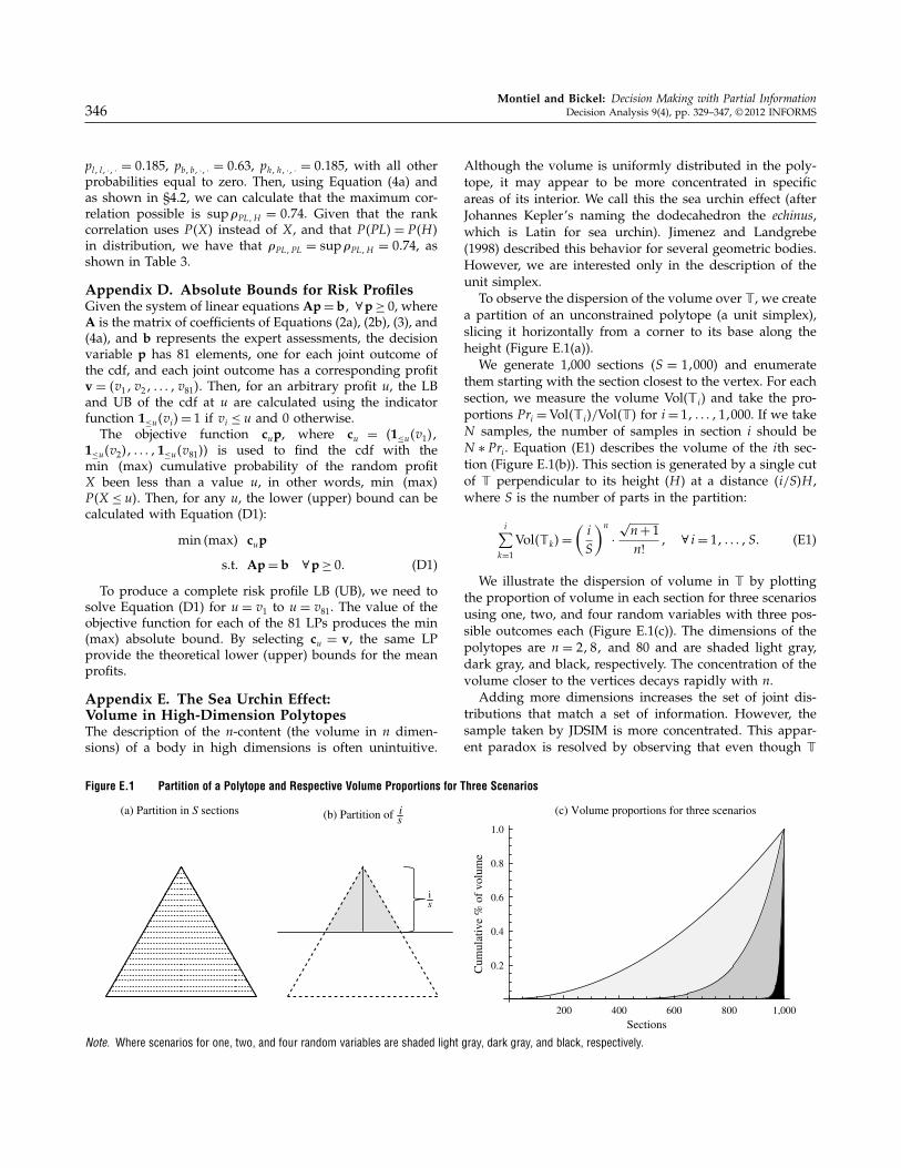
Figure E.1 Partition of a Polytope and Respective Volume Proportions for Three Scenarios

200 400 600 800 1,000

Sections

0.2

0.4

0.6

0.8

is

1.0

Cum

ulat

ive

% o

f vo

lum

e

(a) Partition in S sections (c) Volume proportions for three scenariosis(b) Partition of

Note. Where scenarios for one, two, and four random variables are shaded light gray, dark gray, and black, respectively.

Although the volume is uniformly distributed in the poly-tope, it may appear to be more concentrated in specificareas of its interior. We call this the sea urchin effect (afterJohannes Kepler’s naming the dodecahedron the echinus,which is Latin for sea urchin). Jimenez and Landgrebe(1998) described this behavior for several geometric bodies.However, we are interested only in the description of theunit simplex.

To observe the dispersion of the volume over , we createa partition of an unconstrained polytope (a unit simplex),slicing it horizontally from a corner to its base along theheight (Figure E.1(a)).

We generate 1,000 sections 4S = 110005 and enumeratethem starting with the section closest to the vertex. For eachsection, we measure the volume Vol(i) and take the pro-portions Pri = Vol4i5/Vol45 for i = 11 0 0 0 111000. If we takeN samples, the number of samples in section i should beN ∗ Pri. Equation (E1) describes the volume of the ith sec-tion (Figure E.1(b)). This section is generated by a single cutof perpendicular to its height (H ) at a distance 4i/S5H ,where S is the number of parts in the partition:

i∑

k=1

Vol4k5=

(

i

S

)n

·

√n+ 1n!

1 ∀ i = 11 0 0 0 1 S0 (E1)

We illustrate the dispersion of volume in by plottingthe proportion of volume in each section for three scenariosusing one, two, and four random variables with three pos-sible outcomes each (Figure E.1(c)). The dimensions of thepolytopes are n = 2181 and 80 and are shaded light gray,dark gray, and black, respectively. The concentration of thevolume closer to the vertices decays rapidly with n.

Adding more dimensions increases the set of joint dis-tributions that match a set of information. However, thesample taken by JDSIM is more concentrated. This appar-ent paradox is resolved by observing that even though


is larger, the total n-content√n+ 1/n! decreases to zero as

n goes to infinity. This decay occurs more quickly in thecorners of the polytope.

ReferencesAbbas AE (2006) Entropy methods for joint distributions in decision

analysis. IEEE Trans. Engrg. Management 53(1):146–159.Apostolakis G, Kaplan S (1981) Pitfalls in risk calculations. Reliabil-

ity Engrg. 2(2):135–145.Ben-Tal A, Ghaoui LE, Nemirovski A (2009) Robust Optimization

(Princeton University Press, Princeton, NJ).Bickel JE, Smith JE (2006) Optimal sequential exploration: A binary

learning model. Decision Anal. 3(1):16–32.Bickel JE, Lake LW, Lehman J (2011) Discretization, simulation,

and Swanson’s (inaccurate) mean. SPE Econom. Management3(3):128–140.

Bickel JE, Smith JE, Meyer JL (2008) Modeling dependence amonggeologic risks in sequential exploration decisions. ReservoirEval. Engrg. 3(4):233–251.

Chessa AG, Dekker R, Van Vliet B, Steyerberg EW, Habbema JDF(1999) Correlations in uncertainty analysis for medical deci-sion making: An application to heart-valve replacement. Med-ical Decision Making 19(3):276–286.

Clemen RT (1996) Making Hard Decisions. An Introduction to DecisionAnalysis, 2nd ed. (Duxbury Press, Belmont, CA).

Clemen RT, Reilly T (1999) Correlations and copulas for decisionand risk analysis. Management Sci. 45(2):208–224.

Cooke RM, Waij R (1986) Monte Carlo sampling for generalizedknowledge dependence with application to human reliability.Risk Anal. 6(3):335–343.

Frees EW, Carriere J, Valdez EA (1996) Annuity valuation withdependent mortality. J. Risk Insurance 63(2):229–261.

Ireland CT, Kullback S (1968) Contingency tables with givenmarginals. Biometrika 55(1):179–188.

Jaynes ET (1957) Information theory and statistical mechanics. Phys-ical Rev. 106(4):620–630.

Jaynes ET (1968) Prior probabilities. IEEE Trans. Systems Sci. Cyber-netics 4(3):227–241.

Jimenez L, Landgrebe D (1998) Supervised classification in highdimensional space: Geometrical, statistical and asymptoticalproperties of multivariate data. IEEE Trans. Systems, Man,Cybernetics 28(1):39–54.

Jouini MN, Clemen RT (1996) Copula models for aggregatingexpert opinions. Oper. Res. 44(3):444–457.

Keefer DL, Bodily SE (1983) Three-point approximations for con-tinuous random variables. Management Sci. 29(5):595–609.

Korsan RJ (1990) Towards better assessment and sensitivity pro-cedures. Oliver RM, Smith JQ, eds. Influence Diagrams, Belief

Nets and Decision Analysis (John Wiley & Sons, New York),427–454.

Lowell DG (1994) Sensitivity to relevance in decision analysis.Ph.D. thesis, Engineering and Economic Systems, StanfordUniversity, Stanford, CA.

MacKenzie GR (1994) Approximately maximum entropy multi-variate distributions with specified marginals and pairwisecorrelations. Ph.D. thesis, Department of Decision Sciences,University of Oregon, Eugene.

Miller AC (1990) Towards better assessment and sensitivity proce-dures by R. J. Korsan: Discussion by Allen C. Miller. OliverRM, Smith JQ, eds. Influence Diagrams, Belief Nets and DecisionAnalysis (John Wiley & Sons, New York), 442–443.

Montiel LV (2012) Approximations, simulation, and accuracy ofmultivariate discrete probability distributions in decision anal-ysis. Ph.D. thesis, University of Texas at Austin, Austin.

Montiel LV, Bickel JE (2012) Generating a random collectionof discrete joint probability distributions subject to partialinformation. Methodology Comput. Appl. Probab., ePub aheadof print May 22, http://www.springerlink.com/content/263823150021hl36/.

Nelsen RB (1991) Copulas and association. Dall’Aglio G, Kotz S,Salinetti G, eds. Advances in Probability Distributions with GivenMarginals (Kluwer Academic, Dordrecht, The Netherlands),51–74.

Nelsen RB (2005) An Introduction to Copulas, 2nd ed. (Springer,Portland, OR).

Nešlehová J (2007) On rank correlation measures for non-continuousrandom variables. J. Multivariate Anal. 98(3):544–567.

Pearson ES, Tukey JW (1965) Approximate means and standarddeviations based on distances between percentage points offrequency curves. Biometrika 52(3/4):553–546.

Presidential Commission on the Space Shuttle Challenger Accident(1986) Report of the Presidential Commission on the SpaceShuttle Challenger Accident. Presidential Commission on theSpace Shuttle Challenger Accident, Washington, DC.

Reilly T (2000) Sensitivity analysis for dependent variables. DecisionSci. 31(3):551–572.

Sklar A (1959) Fonctions de répartition à n dimensions et leursmarges. Publ. Inst. Statist. Univ. Paris 8:229–231.

Smith JE (1993) Moment methods for decision analysis. ManagementSci. 39(3):340–358.

Smith RL (1984) Efficient Monte Carlo procedures for generatingpoints uniformly distributed over bounded regions. Oper. Res.32(6):1296–1308.

Smith RL, Ryan PB, Evans JS (1992) The effect of neglecting corre-lations when propagating uncertainty and estimating the pop-ulation distribution of risk. Risk Anal. 12(4):467–474.

Wang T, Dyer JS (2012) A copulas-based approach to modelingdependence in decision trees. Oper. Res. 60(1):225–242.

Winkler RL (1982) Research directions in decision making underuncertainty. Decision Sci. 13(4):517–533.

A Simulation-Based Approach to Decision Making with Partial Information

Documents

Transcript of A Simulation-Based Approach to Decision Making with Partial Information