Chair of Drilling and Completion Engineering

Master's Thesis

Integrated Approach to Evaluate the

Drilling Solutions for Downhole Drilling

Problems

Martin Štulec

March 2020

i

Martin Štulec m01435778

Master Thesis 2020 supervised by

Univ.-Prof. Dipl.-Ing. Dr.mont. Gerhard Thonhauser

Dipl.-Ing. Asad Elmgerbi

Integrated Approach to Evaluate the Drilling Solutions for Downhole Drilling Problems

This is to my family and friends who have been

my biggest support during these years.

iii

Abstract The role of oil and gas in the modern world is still very important. As the crude oil price is at low level, there is a constant need to improve drilling efficiency and to reduce drilling costs to the minimum. In order to do so, drilling efficiency needs to be improved. The best way to improve drilling efficiency is to evaluate different drilling methods.

The main objective of this thesis is to develop the evaluation decision-making process in evaluating preventive barriers for the downhole drilling problems. There are various solutions available at the market. One of the evaluation tools used for deciding which method would be the most cost efficient is weighted matrix method. However, this method has some limitations, as there are a lot of assumptions and uncertainties associated with the input parameters. Therefore, in order to enhance the evaluation of the decision- making process, another evaluation tool was presented. That is the probability of success method. Afterwards, these two tools were combined into an integrated approach. This was done in order to evaluate the preventive barriers for downhole drilling problems in the best possible way.

To test these developed methods in a real situation, a case study was performed to validate the approach. The main objective of a case study was an investigation of drilling operations in re-entry drilling for W-1 JR well on F-1 field. Based on drilling reports NPT (Non-Productive Time) was extracted and root causes were established. After calculating the NPT, three main problems surfaced: bit balling, high torque and drag and stuck pipe. For dealing with these problems, different methods are proposed to reduce or to mitigate encountered drilling problems in following re-entry campaign in that field area. To evaluate proposed drilling methods, an integrated approach was used, which determined that the best solution for bit balling is to change drilling hydraulics. On the other hand, the best solution for the high torque and drag and stuck pipe would be rotary steerable system.

Zusammenfassung Die Rolle von Öl und Gas in der modernen Welt ist nach wie vor sehr wichtig. Da der Rohölpreis auf einem niedrigen Niveau liegt, besteht ein ständiger Bedarf die Bohrleistung zu verbessern und die Bohrkosten auf ein Minimum zu reduzieren. Dazu muss die Bohrleistung effizienter gemacht werden. Der beste Weg dies zu verwirklichen, ist die Bewertung verschiedener Bohrmethoden.

Das Hauptziel dieser Arbeit war die Entwicklung eines Entscheidungsprozesses zur Bewertung und der Vorbeugung von Bohrproblemen im Bohrloch. Am Markt stehen verschiedene Lösungen zur Verfügung. Eines der Werkzeuge, die im Kampf gegen dieses Problem eingesetzt werden können, ist die Methode der gewichteten Matrix. Diese Methode weist jedoch Einschränkungen auf.

Daher wurde ein weiteres Bewertungsinstrument vorgestellt, um den Bewertungsentscheidungsprozess zu verbessern. Es ist die Erfolgswahrscheinlichkeitsmethode. Anschließend wurden diese beiden Tools zu einem integrierten Ansatz kombiniert. Dies wurde durchgeführt, um die vorbeugenden Barrieren für Bohrlochprobleme bestmöglich zu bewerten.

Um die entwickelten Methoden in einer reellen Situation zu testen, wurde eine Fallstudie durchgeführt, um den Ansatz zu validieren. Das Hauptziel der Fallstudie war eine Untersuchung der Bohrvorgänge beim Wiedereintrittsbohren für das Bohrloch W-1 JR auf dem Feld F-1. Basierend auf Bohrberichten wurde die NPT (Non-Productive Time) extrahiert und die Ursachen ermittelt. Aufgrund der Hauptursache für die NPT werden verschiedene Methoden vorgeschlagen, um die aufgetretenen Bohrprobleme in der folgenden Wiedereintrittskampagne in diesem Feldbereich zu verringern. Zur Bewertung der vorgeschlagenen Bohrmethoden wurde ein integrierter Ansatz verwendet.

Acknowledgements Primary, I would like to thank all the professors from Montanuniversität Leoben, from whome I have learned a lot during my study.

This work would not have been possible without the support of Mr. Čubrić, the head of drilling and completion at INA, and the whole INA company for supporting me and providing me with the necessary data.

The greatest thanks go to my family for providing me with unfailing support and continuous encouragement throughout my years of study and through the process of writing this thesis. Without them and their support all this would not be possible. Thank you very much for everything.

And finally, one big thanks to my girlfriend Ana for being my biggest support, especially in the toughest times of my studies, when everything seemed meaningless.

5.5.2 High Torque & Drag ...............................................................................................70 5.5.3 Stuck pipe .................................................................................................................72

5.6 Integrated Approach ......................................................................................................73 5.6.1 Bit Balling .................................................................................................................73 5.6.2 High Torque and Drag............................................................................................74 5.6.3 Stuck Pipe .................................................................................................................75

5.7 Case Study Conclusion ..................................................................................................76

Chapter 6 Conclusion ...............................................................................................................77

1

Chapter 1 Introduction

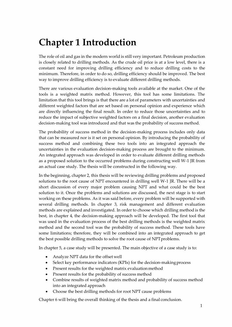
The role of oil and gas in the modern world is still very important. Petroleum production is closely related to drilling methods. As the crude oil price is at a low level, there is a constant need for improving drilling efficiency and to reduce drilling costs to the minimum. Therefore, in order to do so, drilling efficiency should be improved. The best way to improve drilling efficiency is to evaluate different drilling methods.

There are various evaluation decision-making tools available at the market. One of the tools is a weighted matrix method. However, this tool has some limitations. The limitation that this tool brings is that there are a lot of parameters with uncertainties and different weighted factors that are set based on personal opinion and experience which are directly influencing the final result. In order to reduce those uncertainties and to reduce the impact of subjective weighted factors on a final decision, another evaluation decision-making tool was introduced and that was the probability of success method.

The probability of success method in the decision-making process includes only data that can be measured nor is it set on personal opinion. By introducing the probability of success method and combining these two tools into an integrated approach the uncertainties in the evaluation decision-making process are brought to the minimum. An integrated approach was developed in order to evaluate different drilling methods as a proposed solution to the occurred problems during constructing well W-1 JR from an actual case study. The thesis will be constructed in the following way.

In the beginning, chapter 2, this thesis will be reviewing drilling problems and proposed solutions to the root cause of NPT encountered in drilling well W-1 JR. There will be a short discussion of every major problem causing NPT and what could be the best solution to it. Once the problems and solutions are discussed, the next stage is to start working on these problems. As it was said before, every problem will be supported with several drilling methods. In chapter 3, risk management and different evaluation methods are explained and investigated. In order to choose which drilling method is the best, in chapter 4, the decision-making approach will be developed. The first tool that was used in the evaluation process of the best drilling methods is the weighted matrix method and the second tool was the probability of success method. These tools have some limitations; therefore, they will be combined into an integrated approach to get the best possible drilling methods to solve the root cause of NPT problems.

In chapter 5, a case study will be presented. The main objective of a case study is to:

Analyze NPT data for the offset well Select key performance indicators (KPIs) for the decision-making process Present results for the weighted matrix evaluation method Present results for the probability of success method Combine results of weighted matrix method and probability of success method

into an integrated approach Choose the best drilling methods for root NPT cause problems

Chapter 6 will bring the overall thinking of the thesis and a final conclusion.

2

Chapter 2 Drilling Problems, Causes,

and Solutions

Extracting hydrocarbon from an underground reservoir is tightly connected to a lot of uncertainties. However, the key to achieving the drilling objectives is to design drilling methods based on anticipated drilling problems. The best-case scenario in drilling is to avoid situations where drilling problems arise. Some of the drilling problems are compromised with drill string failures, wellbore instability, well path control, kicks, stuck pipe, hole deviation, bit balling, well path control, lost circulation, formation damage, high torque & drag, etc.

This chapter will keep the main focus only on three of these problems: bit balling, high torque & drag and stuck pipe. The main reason for that stands behind the fact that those are the three main reasons for NPT during constructing wellbore W-1 JR. This chapter will bring detailed explanations of the problems closer to the reader by explaining the problem and its cause with proposed solutions to the problems.

Proposed solutions can be the proactive type and mitigation type. Proactive type of solutions involves preventive maintenance, which itself requires a clear understanding of the operating conditions. Mitigation type of solutions involves solutions that could only reduce the risk of loss from an undesirable event, or in this case, NPT. The main characteristic of a proactive type of solution is preplanning, while a mitigation type of solution is characterized by finding a solution while performing drilling operations.

2.1 Bit Balling

2.1.1 Introduction Bit balling is one of the drilling operational issues that can happen anytime when drilling. Bit balling is a condition in which rock cuttings stick to the bit while drilling through Gumbo clay (i.e., Sticky clay), water-reactive clay, and shale formations [3]. This could lead to several problems such as a reduction in the rate of penetration (ROP), an increase in torque, an increase in standpipe pressure (SSP) if the nozzles are stuck as well. Bit performance in shale has been recognized as very important and studied for over 50 years. There are numerous amounts of literature on factors that affect bit performance in shale. The published research goes from understanding and characterization of the behavior of shales. In the 1960s and 1970s, research mostly kept their primary focus on bit tooth indentation and on the rock itself. With the arrival of PDC bits in the late 1970s, recent work has focused more on bit design and PDC cutter, interactions between shale and drilling fluids while trying to understand the failure behavior of shale. The most common problem associated with drilling through shale is bit balling. This problem is mostly described on the U.S. gulf coast and in a different place as the “plastic shale problem” [4].

After the rock is drilled and the cuttings are freed from the rock’s surface, the radial effective stress acting on the cuttings is given by the following formula [1]:

3

𝜎 𝑒𝑓𝑓 𝑟 = 𝑃𝑚𝑢𝑑 − 𝑃𝑝𝑜𝑟𝑒 − 𝑃𝑠𝑤𝑒𝑙𝑙𝑖𝑛𝑔

where, 𝑃𝑚𝑢𝑑 = Uniform mud pressure, which replaces the in-situ stress as the cutting is released 𝑃𝑝𝑜𝑟𝑒 = Pore pressure 𝑃𝑠𝑤𝑒𝑙𝑙𝑖𝑛𝑔 = Swelling pressure, which acts as a tensile force on clay platelets

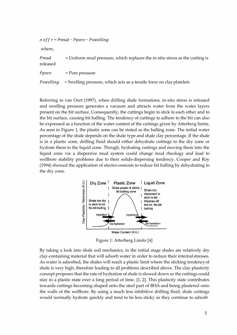
Referring to van Oort (1997), when drilling shale formations, in-situ stress is released and swelling pressure generates a vacuum and attracts water from the water layers present on the bit surface. Consequently, the cuttings begin to stick to each other and to the bit surface, causing bit balling. The tendency of cuttings to adhere to the bit can also be expressed as a function of the water content of the cuttings given by Atterberg limits. As seen in Figure 1, the plastic zone can be stated as the balling zone. The initial water percentage of the shale depends on the shale type and shale clay percentage. If the shale is in a plastic zone, drilling fluid should either dehydrate cuttings to the dry zone or hydrate them to the liquid zone. Though, hydrating cuttings and moving them into the liquid zone via a dispersive mud system could change mud rheology and lead to wellbore stability problems due to their solids-dispersing tendency. Cooper and Roy (1994) showed the application of electro-osmosis to reduce bit balling by dehydrating to the dry zone.

Figure 1: Atterberg Limits [4]

By taking a look into shale soil mechanics, in the initial stage shales are relatively dry clay-containing material that will adsorb water in order to reduce their internal stresses. As water is adsorbed, the shales will reach a plastic limit where the sticking tendency of shale is very high, therefore leading to all problems described above. The clay plasticity concept proposes that the rate of hydration of shale is slowed down so the cuttings could stay in a plastic state over a long period of time. [1, 2]. This plasticity state contributes towards cuttings becoming shaped onto the steel part of BHA and being plastered onto the walls of the wellbore. By using a much less inhibitive drilling fluid, shale cuttings would normally hydrate quickly and tend to be less sticky as they continue to adsorb

4

water thus quickly passing through the plastic stage and into a liquid stage where the shale has little cohesive strength and readily disperses.

Talking about clay properties, actually, Atterberg limits are being discussed, Figure 1. Atterberg limits are defined as the liquid limit, plastic limit, and plastic index. The liquid limit (LL) is the moisture content, expressed as a percentage by the weight of the oven- dry clay. The plastic limit (PL) is the lowest moisture content, expressed as a percentage by weight of the oven-dry clay. The plastic index (PI) is the difference between the liquid limit and the plastic limit. It gives the moisture content range through which soil is considered to be plastic. Different studies show that clay and shale behavior can be summarized by stating that the liquid limit and plastic limit of shale are primarily a function of the percent clay fraction. The ratio of PL/LL was seen to increase according to clay type: (Na-montmorillonite < Illite < Kaolinite), and to the valency and hydrated ionic radius of the associated cation.

(Na+ < K+ <Ca2+ <Mg2+ <Fe3+ <Al3+).

The presence of non-clay minerals in shale will reduce the magnitude of the PL and LL, but the ratio will remain the same. In order for cuttings accretion to occur, the following three criteria must be met [4]:

1. The shale must have sufficient moisture to be in a plastic state when getting in contact with the drilling fluid. A deformation of the shale structure can readily occur when the plastic state is achieved.

2. The surface of the shale cutting must be sticky enough to form a bond with other surfaces that it makes contact with. The “stickiness” of the shale surface can be enhanced by rapid surface water absorption from the drilling fluid, as well with some drilling fluid polymeric additives.

3. The surfaces of the cuttings must be pushed together with sufficient force to deform the clays and create a bond. This force can be both mechanically and hydraulically generated.

There are numerous different factors impacting accretion such as [5]:

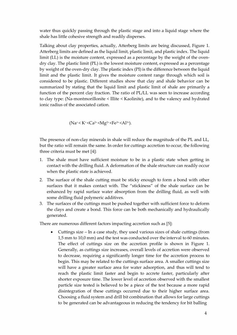
Cuttings size – In a case study, they used various sizes of shale cuttings (from 1,5 mm to 10,0 mm) and the test was conducted over the interval to 60 minutes. The effect of cuttings size on the accretion profile is shown in Figure 1. Generally, as cuttings size increases, overall levels of accretion were observed to decrease, requiring a significantly longer time for the accretion process to begin. This may be related to the cuttings surface area. A smaller cuttings size will have a greater surface area for water adsorption, and thus will tend to reach the plastic limit faster and begin to accrete faster, particularly after shorter exposure time. The lower level of accretion observed with the smallest particle size tested is believed to be a piece of the test because a more rapid disintegration of these cuttings occurred due to their higher surface area. Choosing a fluid system and drill bit combination that allows for large cuttings to be generated can be advantageous in reducing the tendency for bit balling

5

and accretion. This requires, however, that hydraulics be optimized for removal of the cuttings from around the BHA and for hole cleaning with these larger cuttings. Poor hydraulic hole cleaning will lead to both mechanical deterioration of cuttings over time, and a longer exposure of cuttings to the drilling fluid. Both of these scenarios will contribute to an increased tendency for accretion.

Figure 2: Effect of Cuttings Size on Accretion [5]

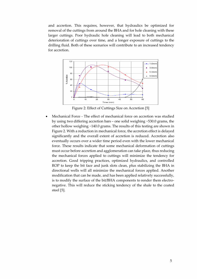
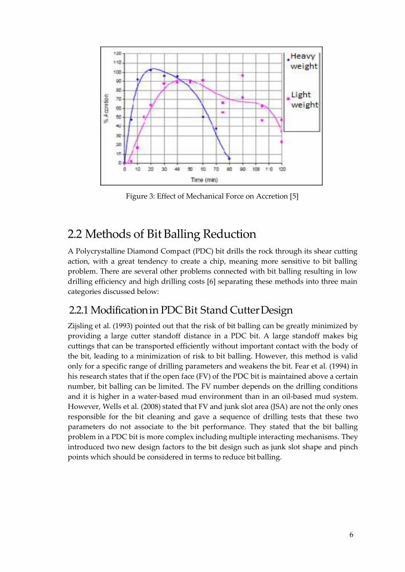
Mechanical Force - The effect of mechanical force on accretion was studied by using two differing accretion bars – one solid weighing ~530.0 grams, the other hollow weighing ~140.0 grams. The results of this testing are shown in Figure 2. With a reduction in mechanical force, the accretion effect is delayed significantly and the overall extent of accretion is reduced. Accretion also eventually occurs over a wider time period even with the lower mechanical force. These results indicate that some mechanical deformation of cuttings must occur before accretion and agglomeration can take place, thus reducing the mechanical forces applied to cuttings will minimize the tendency for accretion. Good tripping practices, optimized hydraulics, and controlled ROP to keep the bit face and junk slots clean, plus stabilizing the BHA in directional wells will all minimize the mechanical forces applied. Another modification that can be made, and has been applied relatively successfully, is to modify the surface of the bit/BHA components to render them electro- negative. This will reduce the sticking tendency of the shale to the coated steel [5].

6

Figure 3: Effect of Mechanical Force on Accretion [5]

2.2 Methods of Bit Balling Reduction A Polycrystalline Diamond Compact (PDC) bit drills the rock through its shear cutting action, with a great tendency to create a chip, meaning more sensitive to bit balling problem. There are several other problems connected with bit balling resulting in low drilling efficiency and high drilling costs [6] separating these methods into three main categories discussed below:

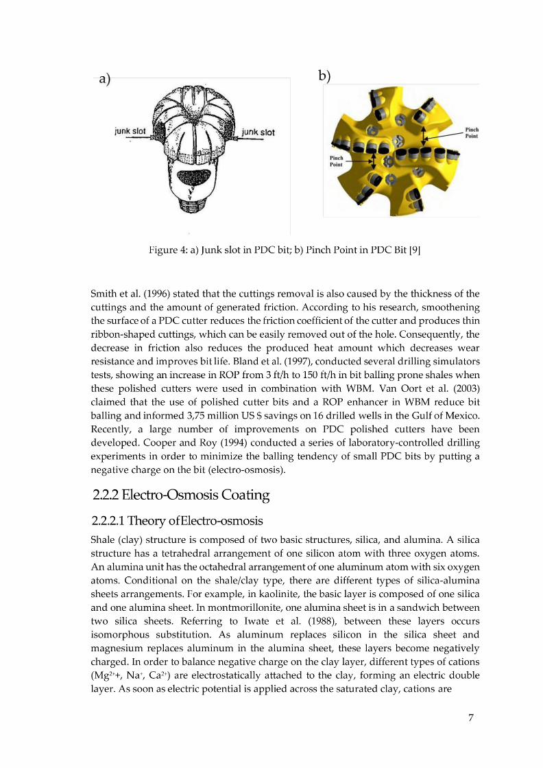
2.2.1 Modification in PDC Bit Stand Cutter Design Zijsling et al. (1993) pointed out that the risk of bit balling can be greatly minimized by providing a large cutter standoff distance in a PDC bit. A large standoff makes big cuttings that can be transported efficiently without important contact with the body of the bit, leading to a minimization of risk to bit balling. However, this method is valid only for a specific range of drilling parameters and weakens the bit. Fear et al. (1994) in his research states that if the open face (FV) of the PDC bit is maintained above a certain number, bit balling can be limited. The FV number depends on the drilling conditions and it is higher in a water-based mud environment than in an oil-based mud system. However, Wells et al. (2008) stated that FV and junk slot area (JSA) are not the only ones responsible for the bit cleaning and gave a sequence of drilling tests that these two parameters do not associate to the bit performance. They stated that the bit balling problem in a PDC bit is more complex including multiple interacting mechanisms. They introduced two new design factors to the bit design such as junk slot shape and pinch points which should be considered in terms to reduce bit balling.

8

attracted to the cathode, at the same time anions move forward to the anode. With the ion’s movement, hydration shells are carried with them. Since the cations are more mobile than anions in a clay-rich shale, there is as well a net water flow towards the cathode. This flow is called electro-osmosis and its magnitude depends on the coefficient of electro-osmosis hydraulic conductivity and on the electric potential gradient

2.2.2.2 Bit Balling Reduction through Electro-Osmosis The electro-osmosis process has been used for waste site remediation, reduction of friction, soil stabilization, shallow borehole stabilization, and petroleum production. Cooper and Roy (1991-1994) were the first to present this mechanism to reduce bit balling. They conducted a series of drilling experiments and concluded that if a drill bit is negative charged (cathode), then there is an osmotic flow of water out of shale towards the bit. This water produces a thin lubricating layer on the bit surface and this way reduces the sticking tendency of the clay. Cooper and Roy’s work includes drilling parameters, testing setup and fluids specifications. Significant results from their work are:

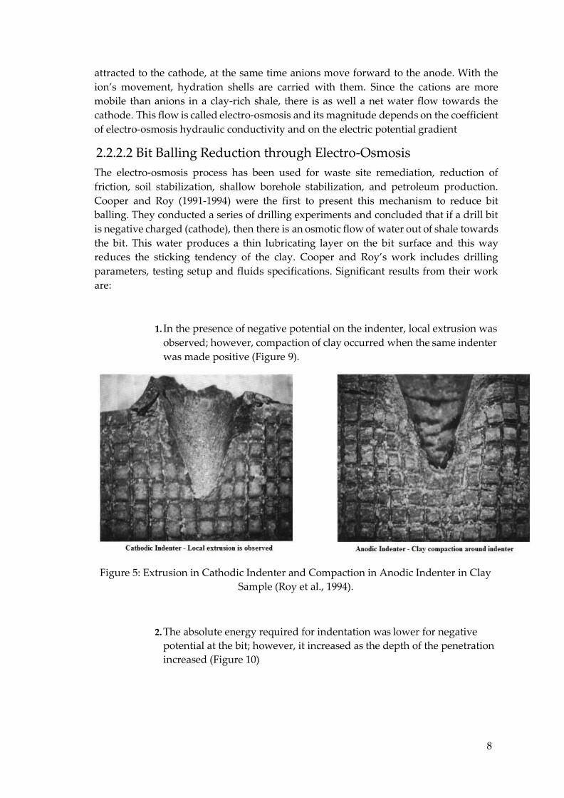
1. In the presence of negative potential on the indenter, local extrusion was observed; however, compaction of clay occurred when the same indenter was made positive (Figure 9).

Figure 5: Extrusion in Cathodic Indenter and Compaction in Anodic Indenter in Clay Sample (Roy et al., 1994).

2. The absolute energy required for indentation was lower for negative

potential at the bit; however, it increased as the depth of the penetration increased (Figure 10)

9

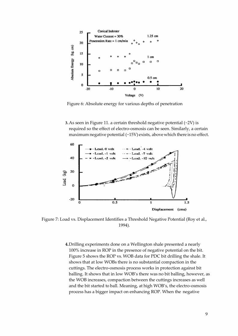
Figure 6: Absolute energy for various depths of penetration

3. As seen in Figure 11. a certain threshold negative potential (~2V) is

required so the effect of electro-osmosis can be seen. Similarly, a certain maximum negative potential (~15V) exists, above which there is no effect.

Figure 7: Load vs. Displacement Identifies a Threshold Negative Potential (Roy et al., 1994).

4. Drilling experiments done on a Wellington shale presented a nearly

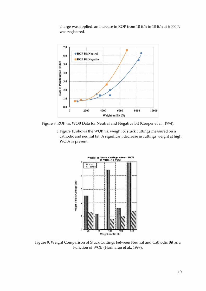
100% increase in ROP in the presence of negative potential on the bit. Figure 5 shows the ROP vs. WOB data for PDC bit drilling the shale. It shows that at low WOBs there is no substantial compaction in the cuttings. The electro-osmosis process works in protection against bit balling. It shows that in low WOB’s there was no bit balling, however, as the WOB increases, compaction between the cuttings increases as well and the bit started to ball. Meaning, at high WOB’s, the electro-osmosis process has a bigger impact on enhancing ROP. When the negative

10

charge was applied, an increase in ROP from 10 ft/h to 18 ft/h at 6 000 N was registered.

Figure 8: ROP vs. WOB Data for Neutral and Negative Bit (Cooper et al., 1994).

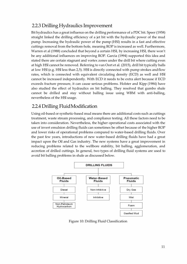
5. Figure 10 shows the WOB vs. weight of stuck cuttings measured on a cathodic and neutral bit. A significant decrease in cuttings weight at high WOBs is present.

Figure 9: Weight Comparison of Stuck Cuttings between Neutral and Cathodic Bit as a Function of WOB (Hariharan et al., 1998).

11

2.2.3 Drilling Hydraulics Improvement Bit hydraulics has a great influence on the drilling performance of a PDC bit. Speer (1958) straight linked the drilling efficiency of a jet bit with the hydraulic power of the mud pump. Increasing the hydraulic power of the pump (HSI) results in a fast and effective cuttings removal from the bottom-hole, meaning ROP is increased as well. Furthermore, Warren et al (1988) concluded that beyond a certain HSI, by increasing HSI, there won’t be any additional influences on improving ROP. Garcia (1994) supported this idea and stated there are certain stagnant and vortex zones under the drill bit where cutting even at high HSI cannot be removed. Referring to van Oort et al. (2015), drill bit typically balls at low HSI (e.g. HSI less than 2,5). HSI is directly connected with pump strokes and flow rates, which is connected with equivalent circulating density (ECD) as well and HSI cannot be increased independently. With ECD it needs to be extra alert because if ECD exceeds fracture pressure, it can cause serious problems. Holster and Kipp (1984) have also studied the effect of hydraulics on bit balling. They resolved that gumbo shale cannot be drilled and stay without balling issue using WBM with anti-balling, nevertheless of the HSI usage.

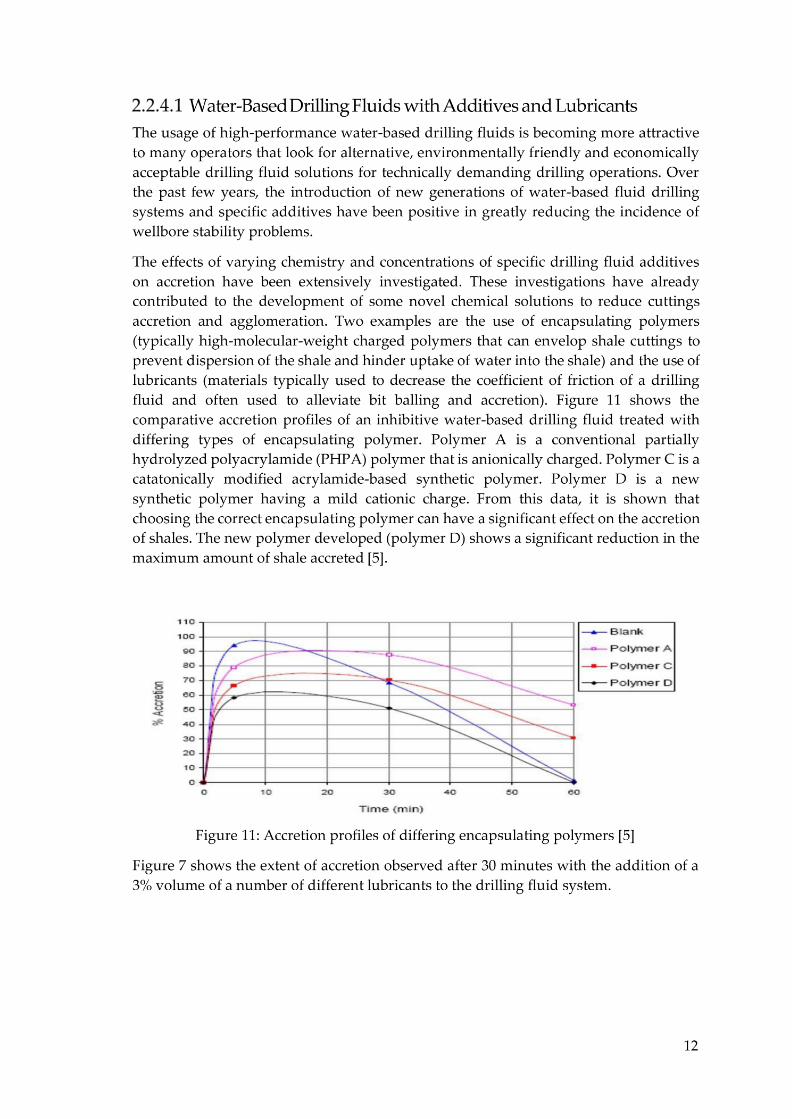
2.2.4 Drilling Fluid Modification Using oil-based or synthetic-based mud means there are additional costs such as cuttings treatment, waste stream processing, and compliance testing. All these factors need to be taken into consideration. Nevertheless, the higher operational costs associated with the use of invert emulsion drilling fluids can sometimes be offset because of the higher ROP and lower risks of operational problems compared to water-based drilling fluids. Over the past few years, introductions of new water-based drilling fluids have had a great impact upon the Oil and Gas industry. The new systems have a great improvement in reducing problems related to the wellbore stability, bit balling, agglomeration, and accretion of drilled cuttings. In general, two types of drilling fluid systems are used to avoid bit balling problems in shale as discussed below.

Figure 10: Drilling Fluid Classification

14

Strict environmental regulations Higher per barrel costs Difficulties in obtaining high-quality resistivity logs Oil emulsion blocks in tight gas sands Sensitivity to severe lost circulation Incompatibility with cement, resulting in cement problems High waste-disposal costs

2.3 High Torque and Drag

2.3.1 Overview With the global trend moving toward ultra-extended reach wells and complex geometry wells, we can no more ignore the drilling limitations caused by high torque and drag forces. Extreme torque and drag values, especially unplanned, can be damaging to the drilling operations. Over the years, engineers have developed several ways to challenge the drilling limitations caused by high torque and drag value in order to drill further and deeper. In this chapter, a discussion about torque and drag together with methods on how to reduce them will be guided.

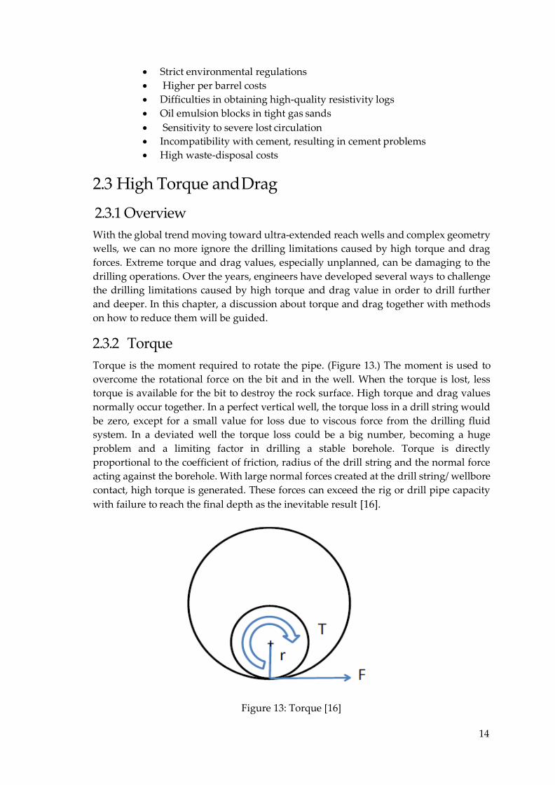
2.3.2 Torque Torque is the moment required to rotate the pipe. (Figure 13.) The moment is used to overcome the rotational force on the bit and in the well. When the torque is lost, less torque is available for the bit to destroy the rock surface. High torque and drag values normally occur together. In a perfect vertical well, the torque loss in a drill string would be zero, except for a small value for loss due to viscous force from the drilling fluid system. In a deviated well the torque loss could be a big number, becoming a huge problem and a limiting factor in drilling a stable borehole. Torque is directly proportional to the coefficient of friction, radius of the drill string and the normal force acting against the borehole. With large normal forces created at the drill string/ wellbore contact, high torque is generated. These forces can exceed the rig or drill pipe capacity with failure to reach the final depth as the inevitable result [16].

Figure 13: Torque [16]

16

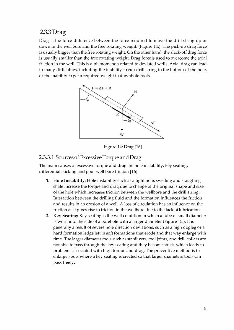
Figure 15: Key Seating [25]

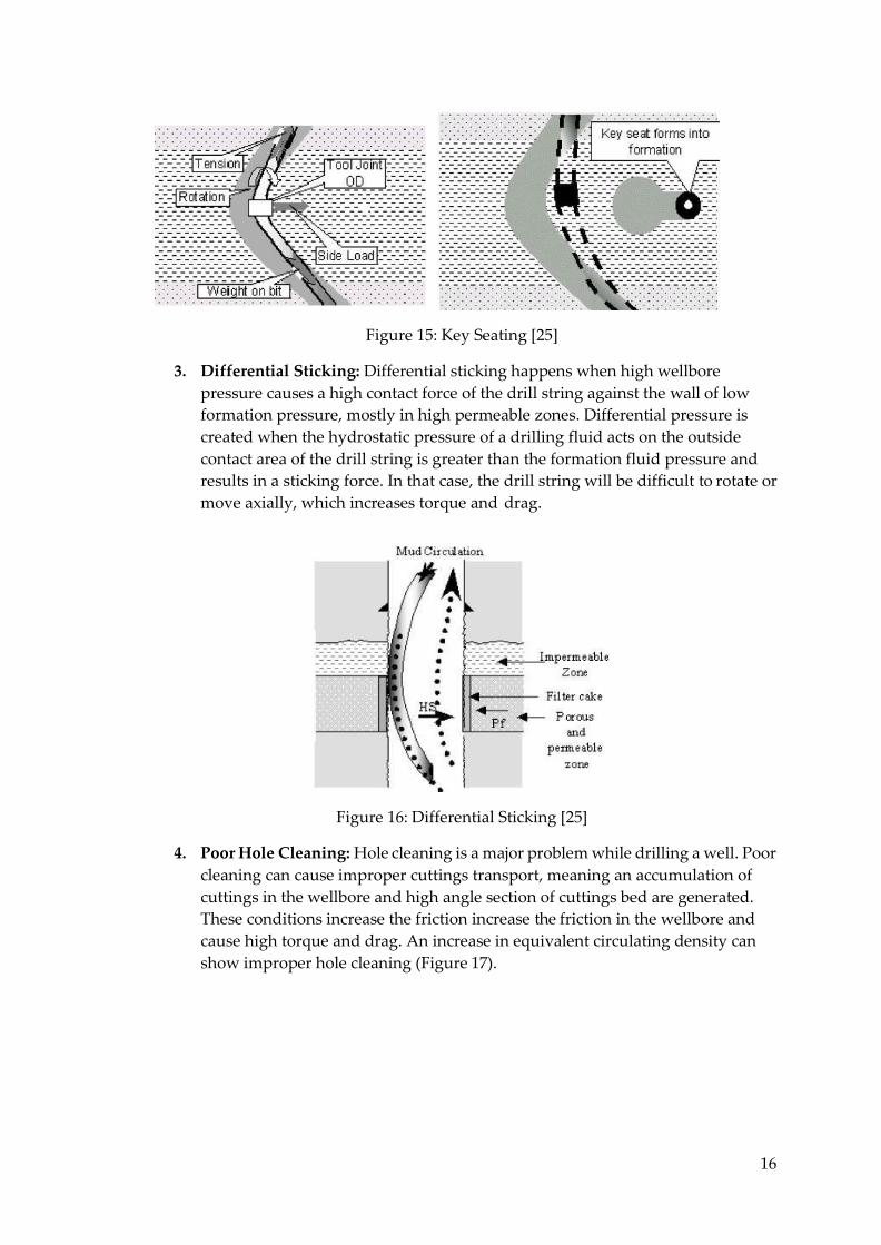
3. Differential Sticking: Differential sticking happens when high wellbore pressure causes a high contact force of the drill string against the wall of low formation pressure, mostly in high permeable zones. Differential pressure is created when the hydrostatic pressure of a drilling fluid acts on the outside contact area of the drill string is greater than the formation fluid pressure and results in a sticking force. In that case, the drill string will be difficult to rotate or move axially, which increases torque and drag.

Figure 16: Differential Sticking [25]

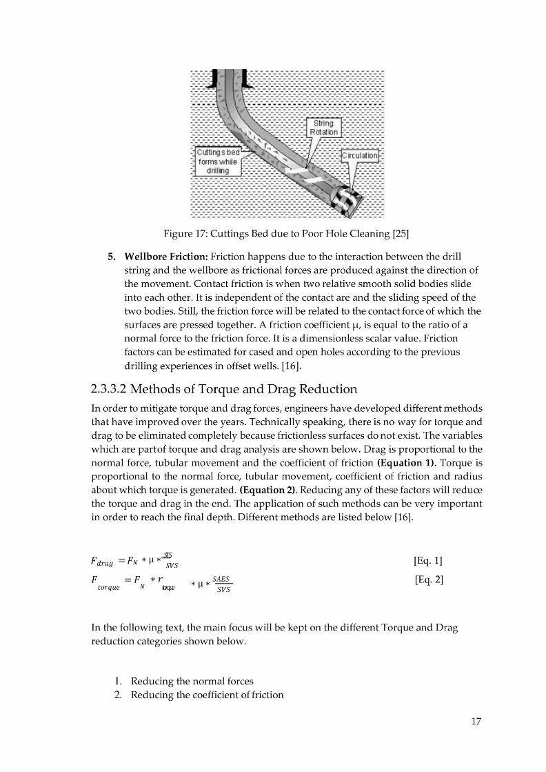
4. Poor Hole Cleaning: Hole cleaning is a major problem while drilling a well. Poor cleaning can cause improper cuttings transport, meaning an accumulation of cuttings in the wellbore and high angle section of cuttings bed are generated. These conditions increase the friction increase the friction in the wellbore and cause high torque and drag. An increase in equivalent circulating density can show improper hole cleaning (Figure 17).

18

3. Increasing dynamic vs. static conditions 4. Increasing system capabilities

The lead paragraphs in each section explain the different classes of torque and drag reduction and the methods that fall in each class.

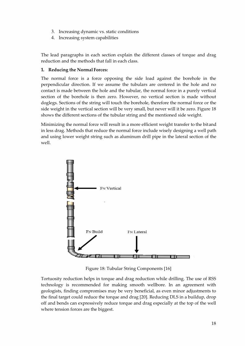
1. Reducing the Normal Forces:

The normal force is a force opposing the side load against the borehole in the perpendicular direction. If we assume the tubulars are centered in the hole and no contact is made between the hole and the tubular, the normal force in a purely vertical section of the borehole is then zero. However, no vertical section is made without doglegs. Sections of the string will touch the borehole, therefore the normal force or the side weight in the vertical section will be very small, but never will it be zero. Figure 18 shows the different sections of the tubular string and the mentioned side weight.

Minimizing the normal force will result in a more efficient weight transfer to the bit and in less drag. Methods that reduce the normal force include wisely designing a well path and using lower weight string such as aluminum drill pipe in the lateral section of the well.

Figure 18: Tubular String Components [16]

Tortuosity reduction helps in torque and drag reduction while drilling. The use of RSS technology is recommended for making smooth wellbore. In an agreement with geologists, finding compromises may be very beneficial, as even minor adjustments to the final target could reduce the torque and drag [20]. Reducing DLS in a buildup, drop off and bends can expressively reduce torque and drag especially at the top of the well where tension forces are the biggest.

19

2. Reducing the Coefficient of Friction

In the oil & gas industry, many attempts have been made to reduce the coefficient of friction in order to reduce torque and drag. The coefficient of friction is a measure of the degree of resistance of the two elements sliding against each other. In a downhole operation, the coefficient of friction refers to the metal to the metal contact or metal to the formation contact between the drill string and the casing or the open hole. In a normal condition, the modeled cased hole coefficient of friction in a water-based mud will be 0.25, while the coefficient of friction in an open hole will be 0.35. Depending on the well conditions, the rate of penetration, the formation, and the mud system selection, the friction factor can be changed at the discrepancy of the user. Even a 10.00% reduction in the coefficient of friction will significantly increase the chance to reach the final depth. Some of the ways the oil industry has lowered the coefficient of friction are listed below.

Lubricants

Lubricants are additives to the drilling fluid system that have been used to reduce torque and drag forces. In the oil & gas industry, lubricants are mostly used in combination with drilling mud that cools the bit and lubricates the string. Over the years, various different additives have been tested to optimize the lubrication by maximizing the reduction of the coefficient of friction. Lubricants can reduce the coefficient of friction up to 40.00%. Nevertheless, it is very important to fully understand that tests that show an 80.00% reduction in the coefficient of friction often result in a 5.00 – 15.00% reduction of torque and drag in field conditions.

Field experiences are different, from successes to failures. In the Gulf of Mexico, a drilling company had high torque that threatened to exceed the makeup torque of their drill pipes in 2008. They switched the complete drilling fluid system in order to lower the surface torque 5.00 – 15.00% but have ended in torque increase by 7.00%.

A drilling company from Russia found out that a lubricant with a 90.00% reduction in the coefficient of friction in lab conditions will reduce torque by an average of 10.00% in a field condition [16].

Hole Cleaning

In wells where hole cleaning is inappropriate, unwanted cuttings in the hole decrease the potential for a drill string to move and rotate. It can increase the rate of wear of downhole tools as well. Cuttings are most probable to accumulate up in the high build section. This makes the removal of the cuttings from the hole awfully difficult. Thus, pipe rotation is actually a very important parameter to consider in order to ensure good hole cleaning. Increasing the RPM of the drill string will result in better cutting transportation out of the hole. Increasing the mud flow lets the cuttings to be suspended and carried up to the surface. High viscosity pills, also known as sweeps are used to reduce cuttings beds.

The oil & gas industry has industrialized mechanical tools that can maximize hole cleaning in the deviated section of the well while drilling by taking cuttings up into the high flow are of highly deviated wellbore sections. Proper hole cleaning can eliminate problems with cutting build in a wellbore and excessive torque and drag. The prime profits of the mechanical hole cleaning tools are the increase in cleaning efficiency,

20

operational safety, time-saving and the increase in wellbore stability and quality. The tools have specially designed grooves in the tubular that heave the cuttings upward when rotating the drill string. The grooved upset shovel the cuttings and heaves them upward. It rises the recirculation of cuttings, resulting in more effective cuttings removal. The tools can improve hole cleaning efficiency up to 60.00% and torque and drag reduction up to 30.00% [16].

Co-Polymer Beads

This is a mechanical way to reduce the coefficient of friction. Co-polymer beads are implanted between the drill string and bore hole to reduce the coefficient of friction. It does not distress the chemical characteristics of a drilling fluid system. The size of these beds ranges from fine grade to coarse grade classes. As a replacement for having metal to metal contact during the drilling, the drill string slides down the well bore, rolling on the beds.

The biggest problem using beads is the major solid build up if the beds are not properly removed. Therefore, beds must be recovered and recycled. This can be accomplished by circulating drilling mud to the surface [16].

Mechanical Friction Reduction Subs

Mechanical friction reduction subs have been tested and proven in a fight against friction reduction. Practices of mechanical reduction tools have shown to be very effective in several wells in the Gulf of Mexico [20]. Different types of mechanical reduction tools exist in the industry. Some of them consist of mechanical rollers or a sleeve on bearings, which then becomes the effective contact surface. The low friction in a smooth bearing relative to rough steel against the rough steel decreases the torque and drag meaningfully. The mechanical reduction friction subs are normally placed one pre in the sections of the well that feels the highest side force. In the wells where torque and drag become higher, mechanical reduction subs have been deployed as a contingency and halted drilling before reaching final depth. The use of these mechanical friction reduction subs has reduced torque and drag in the way to continue drilling (Long et al. 2009). Although these mechanical friction reduction tools have larger OD and they are heavier than drill pipe, which would in normal conditions give higher torque and drag, the final effect is compensated by the reduction of friction that these tools deliver. Another advantage is that casing wear is reduced by the use of these tools.

3. Increasing Dynamic vs. Static Friction Conditions

Dynamic friction is lower than static friction. Different various methods are used in order to increase dynamic friction condition vs static friction, rotating pipe while tripping in as well.

Pressure Pulse Friction Reducing Tool (PPFRT)

A PPFRT is a type of mechanical friction reduction tool that sends a vibration into the string to break static friction. It oscillates in a string and makes axial movement in it. A PPFRT can meaningfully improve weight transfer to the bit and reduce the friction during drilling. This way rate of penetration is improved and anti-stalling for rotary steerable systems as well. A PPDRTs are particularly helpful in non-rotating scenarios,

21

such as slide drilling. A PPFRTs vibrate and excite the drill string to decrease friction. Thus, in return improves the ROP by more efficient power transfer to the bit.

A PPFRTs use one of the earliest torque and drag reduction methods. There are three main components that structure a PPFRT: the power section, the bearing system, and the pulsing system. When fluid is pumped into the drill string through the power section, the rotor is making rotation in the stator and makes a flow path that lets the pulsing valve assembly to produce a series of fast pressure pulse oscillations that result in axial movement in the string. A PPFRT also induces a series of vibrations in the axial direction, together serves as a means to break the static friction produced by contact between the formation and the drill string.

4. Increasing System Capabilities

Another big impact on the extension of drilling deeper holes has been an increase in the size of drilling rigs and the strength of string components. Instead of trying to reduce the friction factor, drilling rigs and string components have increased in strength and size to withstand more demanding conditions. With more challenging wells, increased drag and torque forces have often been met by increasing the whole system capabilities rather than trying to reduce the friction during the drilling operations

Tubular Grade

S-135 strength grade pipe has been standardized in the oil and gas drilling operations for many years. Recent innovations include the development of 150.00 kpsi and higher strength of drill pipes. E, G and X drilling pipes with 75.00 to 105.00 kpsi yields have been used for sour service operations, but numerous will be soon replaced with sour service drill pipe that has a minimum yield strength of 120.00 kpsi.

Rotary Shoulder Connections

Different advancements have been made in rotary shoulder connections in order to ensure that the tubular connections can withstand high torque and drag scenarios. As more high torque and drag complicated wells have been drilled, it has become essential to improve upon the conventional connections that API verified in the 1960s. The biggest innovation was the development of double-shouldered connections, which have allowed drill strings to grip much larger amounts of torque. More than a few generations of double shouldered connections have been developed in the past few years, with the most recent using a double start threat to increase torque capacity and reduce makeup time during long tripping operations.

Rig Capabilities

Bigger, more powerful drilling rigs are becoming more common in the oil and gas industry. Top drives have moved in various areas from strict offshore rigs to include land rigs. The most challenging wells in today’s oil and gas industry use the biggest, most powerful rigs in existence, with hookload and torque capabilities that exceed those of ten years earlier by far.

Rotary Steerable Systems

22

A wellbore drilled with a mud motor with a bent sub in practice has greater tortuosity than with an RSS technology. This is due to the steering principles of such tools. Directional drillers are getting the desired DLS by switching from rotary drilling to sliding drilling as needed. Rotary drilling mode creates smaller holes than a sliding mode. Drilling with a mud motor will create bigger holes than drilling with an RSS technology. In sliding mode, a high DLS is accomplished to correct for the direction achieved by rotary drilling, this is because of a combination of gravity and centralizer placement. The reason why mud motors create much more tortuosity than an RSS stands behind this continued alteration. Adding a mud motor to the RSS will increase the rate of penetration, while RPM at the surface will be reduced to the minimum values and in this way will reduce the torque. Using RSS technology in combination with integrated mud motor will reduce surface torque as compared to a conventional RSS [19, 20].

2.4 Stuck Pipe

2.4.1 Introduction Stuck pipe is one of the most common problems met in drilling. This chapter will briefly explain the different mechanisms and how to prevent stuck-pipe. When the pipe is stuck, means that the drill string cannot be moved and pulled out of the hole without damaging the pipe or exceeding the maximum hook load of the rig. It results in NPT due to the requirement to free the drill string. If the attempts to free the drill string are unsuccessful, then fishing operations are required which also could in the end also result negative. The drill pipe gets stuck due to different situations. From the industry experience the most frequent are:

Differential sticking Formation-related sticking Mechanical sticking

In the following text stuck pipe mechanisms will be explained more into details.

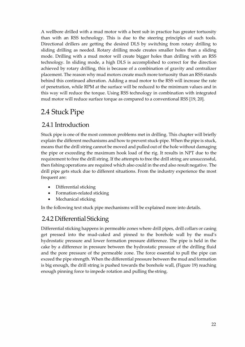
2.4.2 Differential Sticking Differential sticking happens in permeable zones where drill pipes, drill collars or casing get pressed into the mud-caked and pinned to the borehole wall by the mud’s hydrostatic pressure and lower formation pressure difference. The pipe is held in the cake by a difference in pressure between the hydrostatic pressure of the drilling fluid and the pore pressure of the permeable zone. The force essential to pull the pipe can exceed the pipe strength. When the differential pressure between the mud and formation is big enough, the drill string is pushed towards the borehole wall, (Figure 19) reaching enough pinning force to impede rotation and pulling the string.

23

Figure 19: Differential Pressure Stuck Pipe [25]

This state occurs when the pipe is not rotating. The dimension of the pining force is related to differential pressure, formation permeability, zone thickness, thickness and slickness of filter cake, hole and pipe size and time length the drill string remains stuck against the formation. As it can be concluded, the scale of the issue can be variable. [23]

ΔF= (Hs – pf) +*A * f

Where:

ΔF – pining force

Hs – hydrostatic pressure of mud

Pf – formation pressure

f- friction factor, allows for variation in the magnitude of contact between steel and filter cakes of different composition

A – contact area

A= h * t

Where:

h- thickness of permeable zone

t- thickness of filter cake

What can be seen from the formulas is that the magnitude of the differential force is very sensitive to changes in the values of friction factor and the contact area between the drill string and the borehole, because of the fact both are time-dependent. [24] In other words, when the pipe stays stationary in the well, the filter cake is becoming thicker. Furthermore, during a time, the friction factor increases with a consequence of more water being filtered out of the filter cake. Additionally, the differential force is dependent on differential pressure. Some indicators of differential sticking stuck pipe while drilling permeable zones are:

o Increase in torque and drag o Drilling fluid circulation is not interrupted

25

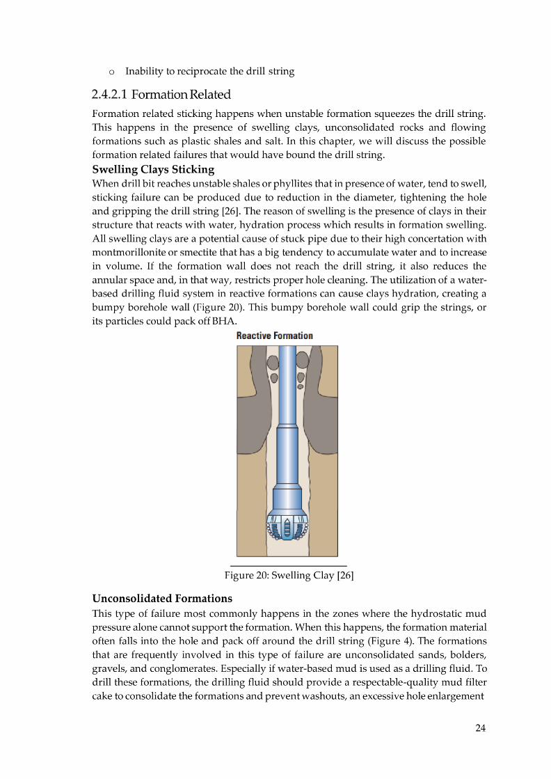
caused by erosion due to the low cohesion of the drilled material or by the high mudflow intensity near the drill bit. This problem is closely connected with the mud saturation. Problems will also appear if insufficient filter cake is deposited on loose, unconsolidated sand.

Figure 21: Pack off caused by unconsolidated formations [25]

Unstable Formations

Before the formation is drilled, the rock strength is in equilibrium with the in-situ rock stress. While the borehole is being drilled, the balance between the rock strength and in- situ stress starts to being distressed. This perturbation and the additional action of the mud can donate to the out of order of equilibrium. These factors can donate to potentially cause an instability problem in the walls of the borehole. The hole collapse in mechanical failures is mostly connected with an increment of the borehole diameter of the hole because of brittle failure and caving of the wellbore wall. If the cuttings are not transported, it is a potential source of stuck pipe (Figure 21). This generally occurs in brittle rocks, but it also can happen in weak rock. In general, brittle formations are responsible for this type of failure. These types of formations cause brittle shear failure producing cavings. The shape of produced cavings will strongly depend on the failure mode that is acting. It can be shear or radial tensile failure mode. Shear failure might occur when the shear stress is maximum at the borehole wall and the failure will be started when it is maximized. Such situations can be found when pressure increases and effective stress suddenly decreases near the wellbore wall. In contrast, tensile failure happens when the tangential stress is equal to the tensile strength of the rock, which happens more often in sedimentary and unconsolidated rock.

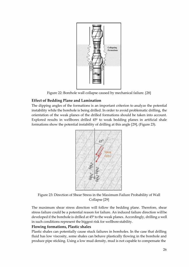
26

Figure 22: Borehole wall collapse caused by mechanical failure. [28]

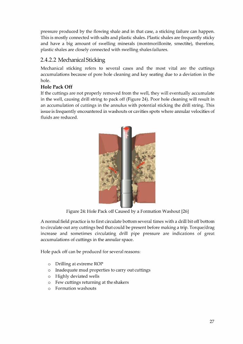
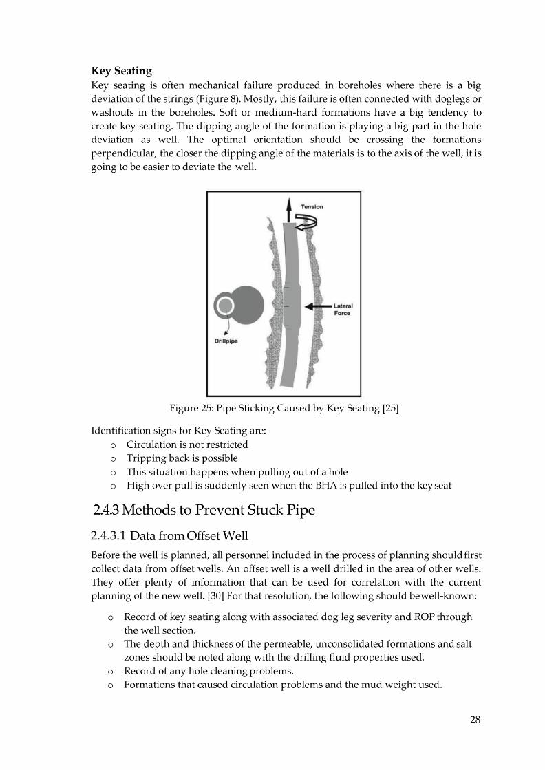
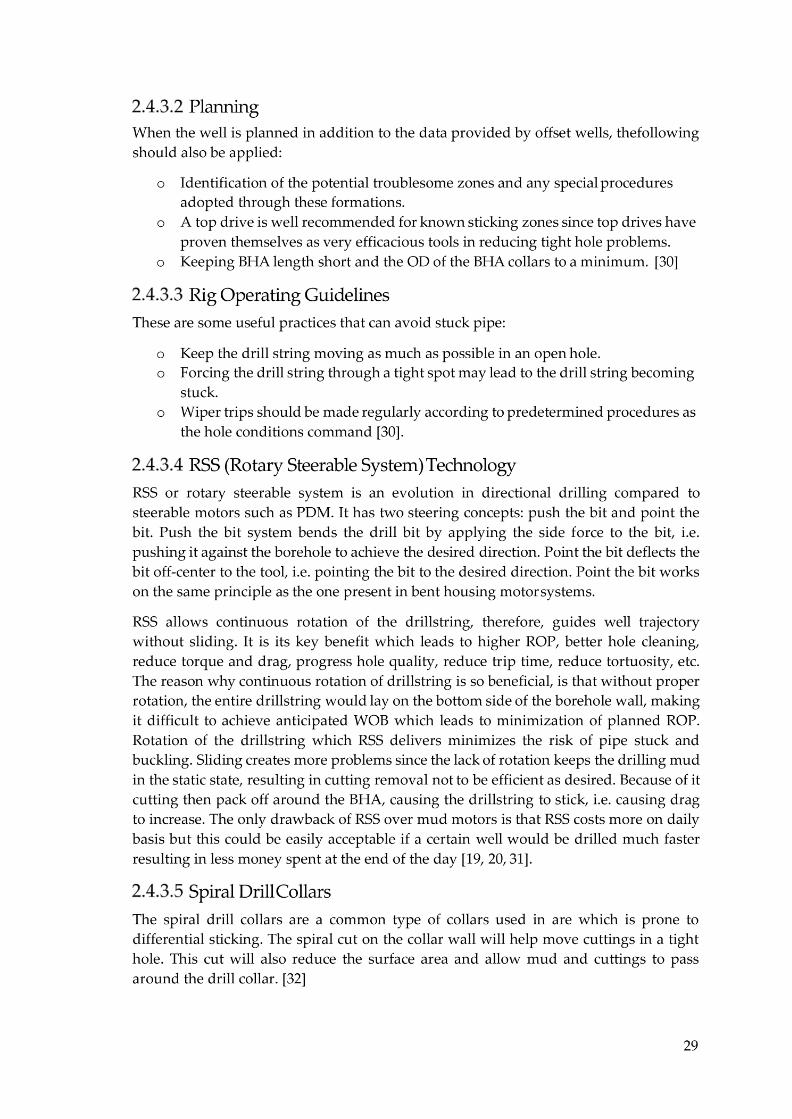
Effect of Bedding Plane and Lamination

The dipping angles of the formations is an important criterion to analyze the potential instability while the borehole is being drilled. In order to avoid problematic drilling, the orientation of the weak planes of the drilled formations should be taken into account. Explored results in wellbores drilled 45º to weak bedding planes in artificial shale formations show the potential instability of drilling at this angle [29], (Figure 23).

Figure 23: Direction of Shear Stress in the Maximum Failure Probability of Wall Collapse [29]

The maximum shear stress direction will follow the bedding plane. Therefore, shear stress failure could be a potential reason for failure. An induced failure direction will be developed if the borehole is drilled at 45º to the weak planes. Accordingly, drilling a well in such conditions represent the biggest risk for wellbore stability.

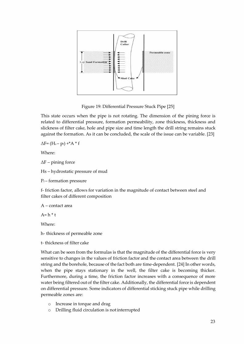
Flowing formations, Plastic shales Plastic shales can potentially cause stuck failures in boreholes. In the case that drilling fluid has low viscosity, some shales can behave plastically flowing in the borehole and produce pipe sticking. Using a low mud density, mud is not capable to compensate the

30

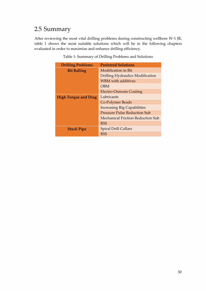
2.5 Summary After reviewing the most vital drilling problems during constructing wellbore W-1 JR, table 1 shows the most suitable solutions which will be in the following chapters evaluated in order to maximize and enhance drilling efficiency.

Table 1: Summary of Drilling Problems and Solutions

Drilling Problems Preferred Solutions

Bit Balling Modification in Bit Drilling Hydraulics Modification WBM with additives OBM Electro-Osmosis Coating

High Torque and Drag Lubricants Co-Polymer Beads Increasing Rig Capabilities Pressure Pulse Reduction Sub Mechanical Friction Reduction Sub RSS

Stuck Pipe Spiral Drill Collars RSS

31

Chapter 3 Risk Management and

Evaluation Methods

3.1 Risk Estimation Risk is an indispensable part of every organization, whether an institution, an enterprise, a unit or an enterprise, faces risk. Most organizations consider the risk a negative phenomenon, so they view it as an expected loss resulting from the likelihood of a loss occurring and the value of the loss. The problem with this definition is that risk is viewed as something negative, or as a potential loss. However, management is increasingly seeking to monitor risk through:

Range that covers risks and chances, Gains and losses that include both positive and negative results, Probability of occurrence and consequence [49].

Risk represents uncertainty about the outcome of expected events in the future, that is, a situation where we are not sure what will happen and reflects the likelihood of possible outcomes around some expected value. In doing so, the expected value is the average result of repeated contingencies [50].

The results of the manager's assessment depend on whether the assessment is made in safe conditions or when there is risk or uncertainty. Related factors that make the decision-making framework are the type of problem, decision making, and the solution to the problem. Confidence in the correctness of the decision is very high when made in security conditions, lower in risk circumstances and lowest in uncertainty. The goal is to make the best alternative decision, whose choice is a complex problem and depends on:

possible alternatives, consequences, values, facts taken into account in the case making a decision, used methods [51].

When it comes to risks, businesses have three options. They can try to reduce them by changing their business or performing some specific activities to improve control and flexibility. In addition to reducing the risk, companies may either choose to retain the risks as they are, or at least part of the risk may try to transfer to someone else, for example by purchasing insurance contracts or other financial instruments [52].

Risks are an everyday issue of strategic management, development, study and organizational theories. Risk represents a unit of uncertainty, and given its measurability, risk can also be managed.

Risk management is the process of measuring, assessing and developing strategies to control it. Enterprise risk management refers to events and circumstances that may

32

adversely affect the enterprise (affecting the very survival of the enterprise, human and capital resources, products, and services, consumers, as well as external influences on society, the market and the environment).

Risk management is done in several different ways, such as reducing, avoiding, associating, taking over and moving risk. Participants in the risk management process are the project director, head of the risk department, potential risk bearer and activity bearer. Based on research and study of the state of the enterprise, risk managers make suggestions for eliminating risk factors in order to reduce risk and uncertainty and allow normal conditions for the quality work of the company. A well-organized risk management process must carefully and expertly identify and analyze risk.

Risk management is not about avoiding risk, it is about making decisions that risk is taking, and is an added value to the organization and its participants. Risk management makes several points in its implementation process:

creates a framework for future activity (consistency and control), Improves decision making (planning, prioritization through a

comprehensive and structured understanding of business activities, volatility and project opportunities/ threats),

contributes to a more efficient use/ allocation of resources, reduces the volatility of less important business areas, preserves and strengthens the assets and image of the organization, optimizes implementation activity [53].

Risk management should develop the process by which the enterprise strategy and its implementation are implemented. The risk management process begins with the strategic goals of the organization, continues with risk assessment, risk reporting, decision making about residual risk, and ends with oversight.

Methods and procedures used for risk analysis and assessment are specifically defined in relation to each type of risk. Risk analysis and assessment can be carried out on the basis of qualitative and quantitative methods such as questionnaires, stress tests, and scenario analyses.

In the assessment, it is also necessary to distinguish between gross and net risk assessment. Gross risk assessment refers to the assessment of the situation prior to the application of risk management measures and the net risk assessment takes into account existing risk management measures.

In the first step, the risk assessment must always be qualitative. A quantitative assessment is conducted after some risk has been defined as significant. Qualitative assessment is only used if a quantitative assessment is impossible or economically unreasonable for some types of risk. In that case, the qualitative assessment shall be explained in detail.

The result of risk analysis and assessment are all risks in the company that has been taken into account within the available risk-bearing capacity of the company. The result of analysis and assessment are risky (net) positions that are actively influenced by risk management measures, with the aim of reducing the likelihood of occurrence (e.g. by

33

establishing controls and limiting the amount of damage) or limiting the amount of loss (e.g. risk transfer).

It is necessary to ensure that the management of the company is informed about the current risk profile, or about possible losses from individual risks so that the management of the company can adequately respond by taking management measures and changes [54].

Risk measurement. Successful risk management requires accurate and rapid measurement of risk exposure.

There are several methods of measuring risk, but they all have the same objective, which is to estimate the variation of a measuring magnitude, such as profit and market value of instruments, with the influence of input parameters such as interest rate, exchange rate or other parameters. Some methods, or specific quantitative risk indicators, can most often be grouped into three types:

Sensitivity - shows changes in the measurement magnitude caused by a unit change in one of the input parameters (e.g. a change in the value of bonds caused by a 1% change in the interest rate)

Variability - shows the variations around the mean of one of the input parameters or measurement size

Risk projection - shows the magnitudes with the worst-case scenario for the event occurrence set point.

Different types of risk indicators create a complete picture of the effects of risk because they cover its different dimensions. Risk projections are the most comprehensive risk measurement methods because they integrate sensitivity and variability with the effect of uncertainty.

The VaR method (Value at risk) is a third group of measurement methods and is one of the most commonly used methods. A standard for measuring and controlling market risk, called VARs, is generally defined as the maximum expected loss of a particular financial position or portfolio with a fixed time horizon under normal market circumstances and with a predetermined confidence level.

Risk insurance. Managing transferable business risks means, to the extent possible, to ensure business risks and thus counteract the negative effects, i.e. reduce them to a tolerable minimum. Risk management can be defined as taking actions designed to minimize the negative impact that risk may have on an entity's expected cash flows, that is, deciding what risks an entity should be exposed to, and to what extent, and what risks an entity will provide and by external or internal methods, and applying payment security instruments [55].

Risk control. The risk management system contributes to sustainable success, enabling continuous business success based on the principles of quality and control, sustainable development, social responsibility, and business ethics. The viability and success of the business enable systematic risk management based on standardized and controlled processes. After identifying, analyzing and assessing risks, an important step in

34

considering the transgressions in risk management control and standardization is the choice of techniques to use for each. Risk management has two basic approaches: physical control methods and financial control methods.

Once the defined and selected risk control actions become a part of the risk management process. The actual implementation of actions in the process is a particular issue for organizational management, and the methods alone do not provide detailed support for the way in which this is performed.

In order to standardize approaches to the construction of risk management systems and risk management processes, international standards have been developed. Norms or standards have been adopted in all industries, so there are ISO standards characteristic primarily in the trade of goods and services, the Basel standard in banking and the Solvency standard in the insurance industry [55].

The risk management system protects the company and all its partners and associates by adding value to them by creating a backbone that enables them to carry out activities consistently and in a controlled manner. In addition to improving the decision-making process, it enhances business transparency and planning and prioritization through a comprehensive and structured understanding of the volatility of business activities.

3.2 Evaluation Decision Methods Decision making is an important factor in every business, that is, it is crucial because it affects the success of the business. Therefore, the company is expected to make reasonable and constructive decisions. Often, different criteria should be taken into account when making decisions. For this reason, tools are used prior to decision making to identify more clearly the key factors that drive the best decision. For the evaluation decision-making process, two methods will be used. Those are the weighted decision matrix method and the probability of success method.

3.2.1 Weighted Matrix Method Weighted Matrix (WM) is a simple method that can be extremely useful when complex decisions need to be made. This is especially true of situations where there are numerous alternatives and criteria that are of varying importance and all of the above should be analyzed or taken into account.

WM is often used in design as a quantitative method for evaluating alternatives. It is a tool that compares alternatives based on multiple criteria at different levels of importance. It can be used to rank all alternatives with respect to the main reference and thus obtain the order of alternatives in order of importance [56].

35

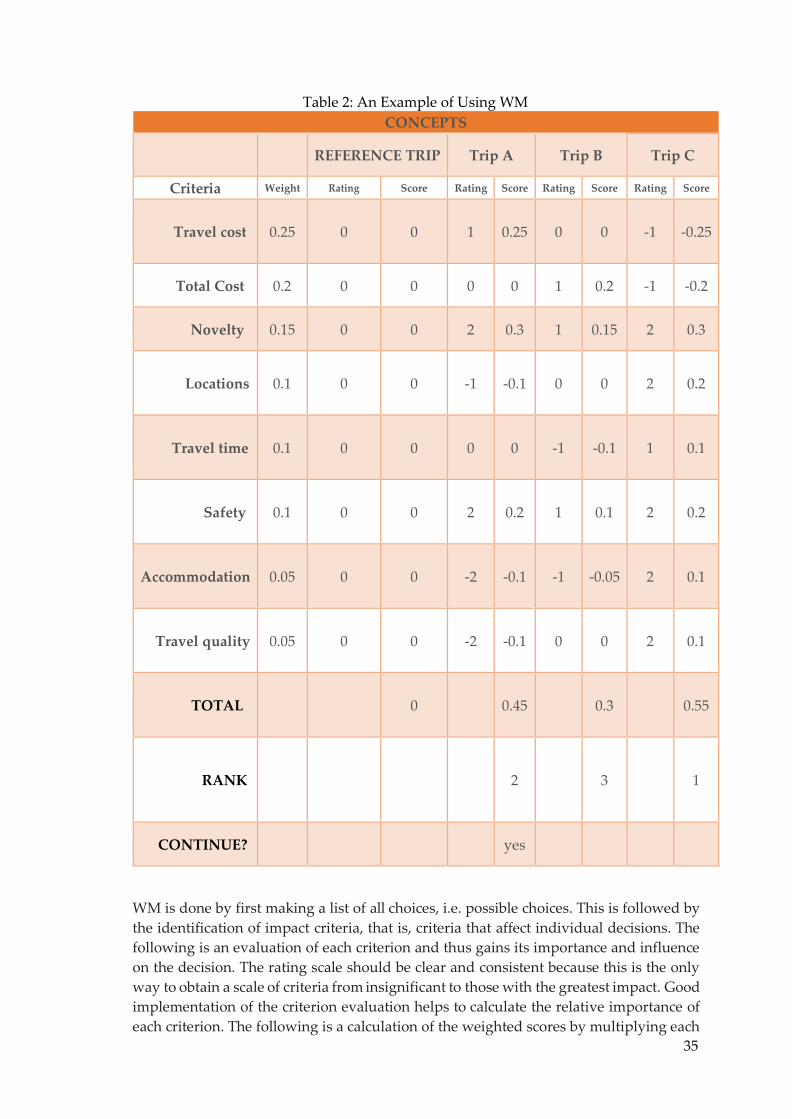
Table 2: An Example of Using WM CONCEPTS

REFERENCE TRIP Trip A Trip B Trip C

Criteria Weight Rating Score Rating Score Rating Score Rating Score

Travel cost 0.25 0 0 1 0.25 0 0 -1 -0.25

Total Cost 0.2 0 0 0 0 1 0.2 -1 -0.2

Novelty 0.15 0 0 2 0.3 1 0.15 2 0.3

Locations 0.1 0 0 -1 -0.1 0 0 2 0.2

Travel time 0.1 0 0 0 0 -1 -0.1 1 0.1

Safety 0.1 0 0 2 0.2 1 0.1 2 0.2

Accommodation 0.05 0 0 -2 -0.1 -1 -0.05 2 0.1

Travel quality 0.05 0 0 -2 -0.1 0 0 2 0.1

TOTAL

0

0.45

0.3

0.55

RANK

2

3

1

CONTINUE?

yes

WM is done by first making a list of all choices, i.e. possible choices. This is followed by the identification of impact criteria, that is, criteria that affect individual decisions. The following is an evaluation of each criterion and thus gains its importance and influence on the decision. The rating scale should be clear and consistent because this is the only way to obtain a scale of criteria from insignificant to those with the greatest impact. Good implementation of the criterion evaluation helps to calculate the relative importance of each criterion. The following is a calculation of the weighted scores by multiplying each

36

choice score by their importance. The results obtained for each alternative are added together to arrive at a final result for each alternative. The end results are then compared with one another [57].

3.2.2 Probability of Success Method Probability theory is a mathematical discipline that deals with the study of random phenomena, that is, empirical events whose outcomes are not always strictly defined. One of the basic tools in probability theory is an experiment that examines the link between cause and effect. The outcome of an experiment is often influenced by multiple conditions and if the experiment is repeated several times under the same conditions, some regularity occurs within the set of outcomes. Probability theory deals with such regularities by introducing a quantitative measure in the form of a real positive number, that is, probability. Probability estimates the possibility, that is, the inability to achieve the outcome.

The basic concepts of probability may differ depending on the point of view, and the results and interpretations of the results may differ. The laws of probability are not always simple and easy to understand. Everyday experience and logic used in life are

39

weighted matrix method and the probability of success method, is a consequence of the specificity of the risk assessment and their impact on the decisions or changes. These methods provide a good insight into the direction of decision-making, i.e. how future activities should be conducted. For this reason, it was decided to use the methods mentioned above.

When it comes to methods for comparing risk assessment, a matrix of predefined values can be extracted. This method of risk assessment uses three parameters: resource value, threats, and vulnerabilities. Each of these parameters is scrutinized for possible consequences, while threats are considered for the respective vulnerabilities. Also, the method is the ranking of threats by risk assessment. This method of risk assessment formally uses only two parameters: the impact on the resource (resource value) and the likelihood of a threat. It is implicitly understood that the impact on the resource is equivalent to the value of the resource, while threats are viewed against the corresponding vulnerabilities. In this way, the estimated risk becomes a function of several parameters.

The assessment of the value of the realization and the possible consequences is also used for comparative risk assessment. The risk assessment process in this method is somewhat more complex than in the previous two and is carried out in two steps. The first is to define the value of a resource based on the potential consequences of a threat. Then, based on vulnerabilities and threats, the probability of realization is determined [63].

3.3 Monte Carlo Simulation Monte-Carlo methods are stochastic (deterministic) simulation methods, algorithms that predict the behavior of complex mathematical systems using random or quasi-random numbers and large numbers of calculations and repetitions. Monte Carlo simulation is synonymous with simulations that solve probabilistic problems. The values of the random variable for which the simulation is performed are selected from the probability distribution function corresponding to the actual occurrence of the default and are entered into a computer program.

All values of the dependent variable have the same probability resulting from the selected distribution function. Namely, any way to solve a problem that relies on generating a large number of random numbers and observing the proportion of those numbers that exhibit the desired properties is called the Monte Carlo method. The Monte Carlo Method was designed by Stanislaw Ulam in 1946 while working on the development of nuclear weapons at the Los Alamos National Laboratory and was named after the Monte Carlo casinos where Uncle S. Ulama often gambled. The value of the method was soon recognized by John von Neumann, who wrote the program for the first electronic computer, ENIAC, which solved the problems of neutron diffusion in fissile materials by the Monte Carlo method.

The value of the Monte Carlo algorithm lies in the fact that it gives all possible outcomes as a result, but also the probability of occurrence of each of these outcomes. Furthermore, it is possible to perform sensitivity analysis over Monte Carlo simulation results in order to identify the factors that most influence the outcome of the process in order to limitor

40

emphasize their influence, depending on their nature. The algorithm can be explained as follows [64]:

1. Mathematically model the business process. 2. Find variables whose values are not completely certain. 3. Determine density functions that well describe the frequencies at which random

variables take their values. 4. If there are correlations among the variables, make a correlation matrix. 5. In each iteration assign a random value to each variable derived from the density

function taking into account the correlation matrix. 6. Calculate the output values and save the results. 7. Repeat steps 5 and 6 n times. 8. Analyze the simulation results statistically.

The Monte Carlo method is similar to what-if analysis except that what-if does not take into account the likelihood of an event, while the Monte Carlo method also takes probabilistic into account, making it a more appropriate tool for decision-making under risk conditions.

The Monte Carlo simulation is the most accurate maximum loss estimation method, also known as a statistical simulation method, where statistical simulation is defined as any method that uses sequences of random numbers to perform a simulation.

The Monte Carlo simulation is very similar to the historical method in that the assumptions about future risk based on historical data are used in the calculations. The difference is that hypothetical changes in market factors are not created on the basis of past observed changes, but rather through statistical simulation adequately generating returns similar to those of the past.

Also, after the simulation obtained, the risk value is determined with a certain level of probability as in the historical method. The method allows the use of estimation parameters of theoretical distributions based on historical data, taking into account market expectations, which can become more demanding and precise as needed [65]

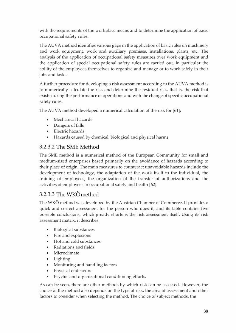
3.3.1 Probability Distribution Probability distributions have been designed to fit special purposes. The probability distribution can be discrete or continuous depending on the nature of the variable. Binormal, Poisson and Multinomial are called discrete distributions while normal, lognormal and triangular are continuous distribution examples.

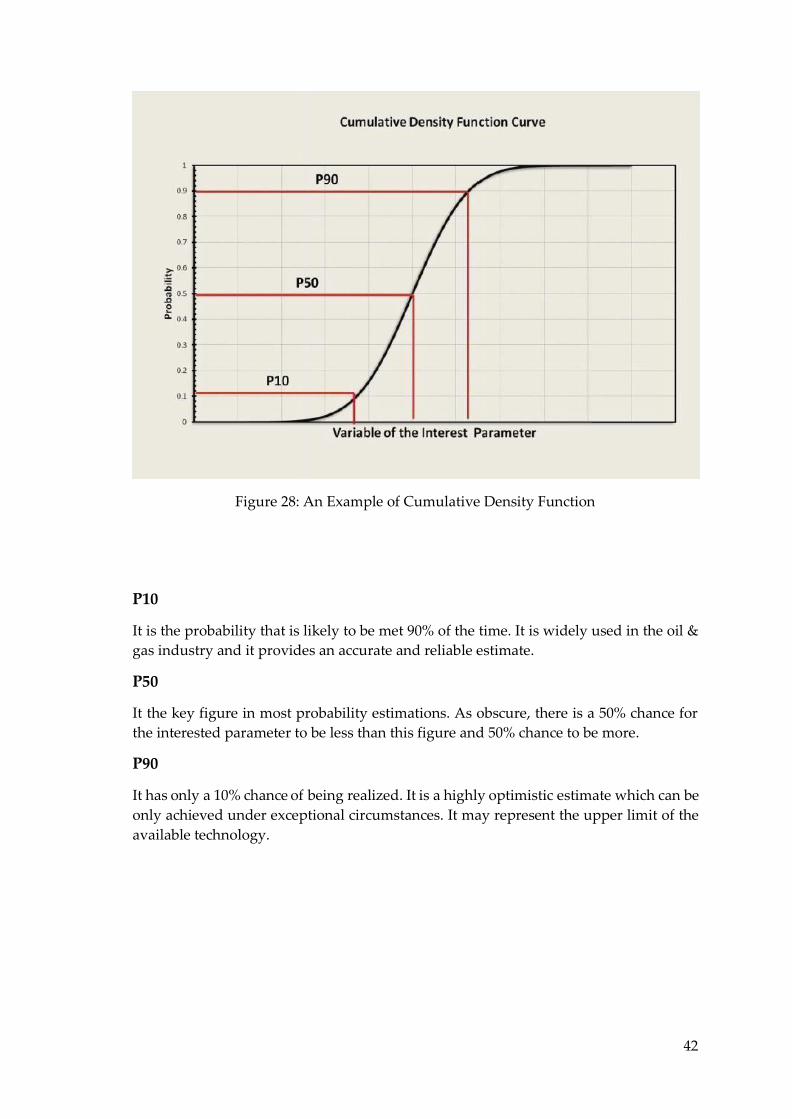
There are two ways to illustrate the continuous probability distributions. The first one is the probability density function that shows variables of the interested parameter with their frequencies. The second one is cumulative density function and it shows variables of the interested parameter with their probabilities.

The probability of any variable that is presented in the cumulative density function graphic is determined by calculating the area on the left side of the interested variable under the curve in the probability density function graphic.

42

Figure 28: An Example of Cumulative Density Function

P10

It is the probability that is likely to be met 90% of the time. It is widely used in the oil & gas industry and it provides an accurate and reliable estimate.

P50

It the key figure in most probability estimations. As obscure, there is a 50% chance for the interested parameter to be less than this figure and 50% chance to be more.

P90

It has only a 10% chance of being realized. It is a highly optimistic estimate which can be only achieved under exceptional circumstances. It may represent the upper limit of the available technology.

44

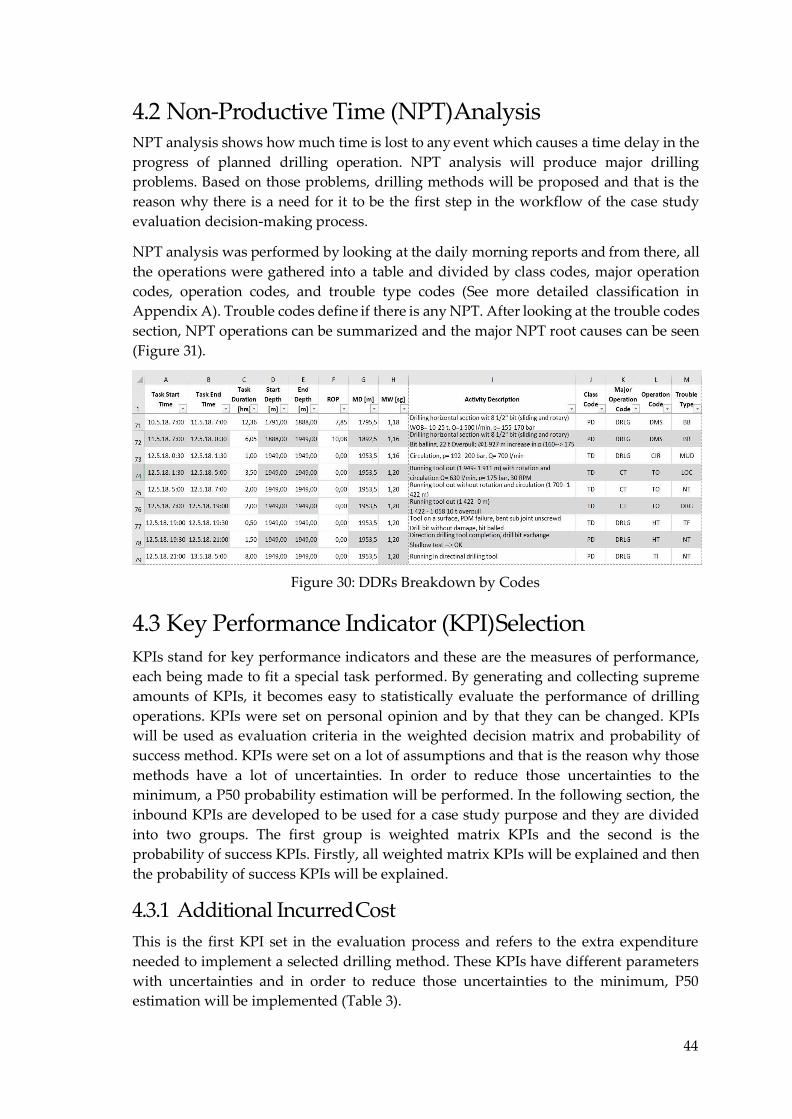
4.2 Non-Productive Time (NPT) Analysis NPT analysis shows how much time is lost to any event which causes a time delay in the progress of planned drilling operation. NPT analysis will produce major drilling problems. Based on those problems, drilling methods will be proposed and that is the reason why there is a need for it to be the first step in the workflow of the case study evaluation decision-making process.

NPT analysis was performed by looking at the daily morning reports and from there, all the operations were gathered into a table and divided by class codes, major operation codes, operation codes, and trouble type codes (See more detailed classification in Appendix A). Trouble codes define if there is any NPT. After looking at the trouble codes section, NPT operations can be summarized and the major NPT root causes can be seen (Figure 31).

Figure 30: DDRs Breakdown by Codes

4.3 Key Performance Indicator (KPI) Selection KPIs stand for key performance indicators and these are the measures of performance, each being made to fit a special task performed. By generating and collecting supreme amounts of KPIs, it becomes easy to statistically evaluate the performance of drilling operations. KPIs were set on personal opinion and by that they can be changed. KPIs will be used as evaluation criteria in the weighted decision matrix and probability of success method. KPIs were set on a lot of assumptions and that is the reason why those methods have a lot of uncertainties. In order to reduce those uncertainties to the minimum, a P50 probability estimation will be performed. In the following section, the inbound KPIs are developed to be used for a case study purpose and they are divided into two groups. The first group is weighted matrix KPIs and the second is the probability of success KPIs. Firstly, all weighted matrix KPIs will be explained and then the probability of success KPIs will be explained.

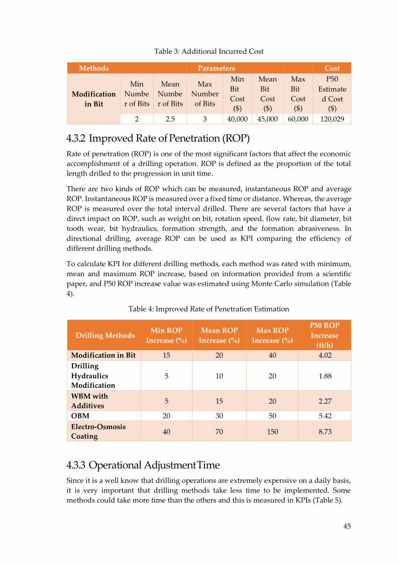
4.3.1 Additional Incurred Cost This is the first KPI set in the evaluation process and refers to the extra expenditure needed to implement a selected drilling method. These KPIs have different parameters with uncertainties and in order to reduce those uncertainties to the minimum, P50 estimation will be implemented (Table 3).

45

Table 3: Additional Incurred Cost

Methods Parameters Cost

Modification

in Bit

Min Number of Bits

Mean Number of Bits

Max Number of Bits

Min Bit Cost ($)

Mean Bit Cost ($)

Max Bit Cost ($)

P50 Estimate d Cost

($) 2 2.5 3 40,000 45,000 60,000 120,029

4.3.2 Improved Rate of Penetration (ROP) Rate of penetration (ROP) is one of the most significant factors that affect the economic accomplishment of a drilling operation. ROP is defined as the proportion of the total length drilled to the progression in unit time.

There are two kinds of ROP which can be measured, instantaneous ROP and average ROP. Instantaneous ROP is measured over a fixed time or distance. Whereas, the average ROP is measured over the total interval drilled. There are several factors that have a direct impact on ROP, such as weight on bit, rotation speed, flow rate, bit diameter, bit tooth wear, bit hydraulics, formation strength, and the formation abrasiveness. In directional drilling, average ROP can be used as KPI comparing the efficiency of different drilling methods.

To calculate KPI for different drilling methods, each method was rated with minimum, mean and maximum ROP increase, based on information provided from a scientific paper, and P50 ROP increase value was estimated using Monte Carlo simulation (Table 4).

Table 4: Improved Rate of Penetration Estimation

Drilling Methods

Min ROP

Increase (%)

Mean ROP

Increase (%)

Max ROP

Increase (%)

P50 ROP

Increase

(ft/h)

Modification in Bit 15 20 40 4.02 Drilling

Hydraulics

Modification

5

10

20

1.88

WBM with

Additives 5 15 20 2.27

OBM 20 30 50 5.42 Electro-Osmosis

Coating 40 70 150 8.73

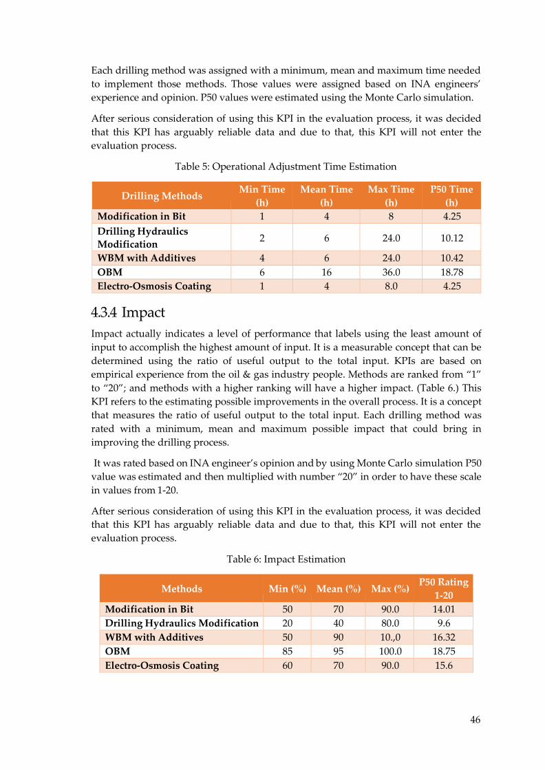
4.3.3 Operational Adjustment Time Since it is a well know that drilling operations are extremely expensive on a daily basis, it is very important that drilling methods take less time to be implemented. Some methods could take more time than the others and this is measured in KPIs (Table 5).

46

Each drilling method was assigned with a minimum, mean and maximum time needed to implement those methods. Those values were assigned based on INA engineers’ experience and opinion. P50 values were estimated using the Monte Carlo simulation.

After serious consideration of using this KPI in the evaluation process, it was decided that this KPI has arguably reliable data and due to that, this KPI will not enter the evaluation process.

Table 5: Operational Adjustment Time Estimation

Drilling Methods Min Time

(h)

Mean Time

(h)

Max Time

(h)

P50 Time

(h)

Modification in Bit 1 4 8 4.25

Drilling Hydraulics

Modification 2 6 24.0 10.12

WBM with Additives 4 6 24.0 10.42 OBM 6 16 36.0 18.78 Electro-Osmosis Coating 1 4 8.0 4.25

4.3.4 Impact Impact actually indicates a level of performance that labels using the least amount of input to accomplish the highest amount of input. It is a measurable concept that can be determined using the ratio of useful output to the total input. KPIs are based on empirical experience from the oil & gas industry people. Methods are ranked from “1” to “20”; and methods with a higher ranking will have a higher impact. (Table 6.) This KPI refers to the estimating possible improvements in the overall process. It is a concept that measures the ratio of useful output to the total input. Each drilling method was rated with a minimum, mean and maximum possible impact that could bring in improving the drilling process.

It was rated based on INA engineer’s opinion and by using Monte Carlo simulation P50 value was estimated and then multiplied with number “20” in order to have these scale in values from 1-20.

After serious consideration of using this KPI in the evaluation process, it was decided that this KPI has arguably reliable data and due to that, this KPI will not enter the evaluation process.

Table 6: Impact Estimation

Methods Min (%) Mean (%) Max (%) P50 Rating

1-20

Modification in Bit 50 70 90.0 14.01 Drilling Hydraulics Modification 20 40 80.0 9.6 WBM with Additives 50 90 10.,0 16.32 OBM 85 95 100.0 18.75 Electro-Osmosis Coating 60 70 90.0 15.6

47

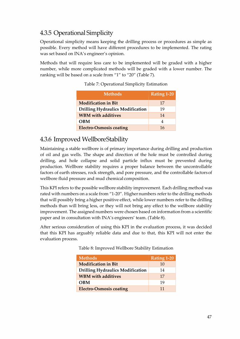
4.3.5 Operational Simplicity Operational simplicity means keeping the drilling process or procedures as simple as possible. Every method will have different procedures to be implemented. The rating was set based on INA’s engineer’s opinion.

Methods that will require less care to be implemented will be graded with a higher number, while more complicated methods will be graded with a lower number. The ranking will be based on a scale from “1” to “20” (Table 7).

Table 7: Operational Simplicity Estimation

Methods Rating 1-20

Modification in Bit 17 Drilling Hydraulics Modification 19 WBM with additives 14 OBM 4 Electro-Osmosis coating 16

4.3.6 Improved Wellbore Stability Maintaining a stable wellbore is of primary importance during drilling and production of oil and gas wells. The shape and direction of the hole must be controlled during drilling, and hole collapse and solid particle influx must be prevented during production. Wellbore stability requires a proper balance between the uncontrollable factors of earth stresses, rock strength, and pore pressure, and the controllable factors of wellbore fluid pressure and mud chemical composition.

This KPI refers to the possible wellbore stability improvement. Each drilling method was rated with numbers on a scale from “1-20”. Higher numbers refer to the drilling methods that will possibly bring a higher positive effect, while lower numbers refer to the drilling methods than will bring less, or they will not bring any effect to the wellbore stability improvement. The assigned numbers were chosen based on information from a scientific paper and in consultation with INA’s engineers’ team. (Table 8).

After serious consideration of using this KPI in the evaluation process, it was decided that this KPI has arguably reliable data and due to that, this KPI will not enter the evaluation process.

Table 8: Improved Wellbore Stability Estimation

Methods Rating 1-20

Modification in Bit 10 Drilling Hydraulics Modification 14 WBM with additives 17 OBM 19 Electro-Osmosis coating 11

48

In the following lines all KPIs related to the probability of success method will be explained.

4.3.7 Additional Incurred Cost These KPIs are the same for the weighted matrix method and for the probability of success method.

4.3.8 NPT Reduction Savings This KPI refers to the possible NPT reduction. There are three main drilling problems and each problem has its own NPT. When NPT is related to the drilling methods, the next step is to multiply the number of hours of NPT with the hourly rig rate in order to have this KPI as a cost unit.

4.3.9 Improved Rate of Penetration Savings This KPI is related to the ROP enhancement. If the average ROP is going to be increased, the total drilling distance will be drilled in a short period of time. This KPI calculates the saved time in a case if the distance will be drilled faster, and then that saved time is multiplied with the hourly rig rate to get this KPI as a cost unit.

4.4 Weighted Matrix Method

4.4.1 Matrix Creation In this part, different KPIs are established and the corresponding scales are considered for the selection of the optimum drilling methods. KPI is defined as one of the parameters considered in the evaluation of the methods. Each KPI has an attribute scale used to score methods on how well it meets the objective for this attribute. In order to evaluate available methods against each KPI, KPI scales that explicitly reflect the impact on the system selection process are needed. The KPI used in matrix weighted method are listed below:

1. Additional Incurred Cost 2. Improved Rate of Penetration 3. Operational Simplicity 4. Improved Wellbore Stability

4.4.2 Assign Scores to the Methods Using the KPI Scales For the extra cost and time consuming to implement KPIs, minimum values are defined and for the rest of the KPIs, the maximum values are defined.

4.4.3 Assign Weighted Factor to the Criteria The final result is moving forward, but still, some work needs to be done. At this point, all criteria are equally important. If the number one thing which needs to be considered as cost due to budgetary decision, then the scores in that column deserve more weight than the others. That means it is time to give weights to all criteria to get a handle on

49

which method scores best in the factors that matter the most to the final decision. In general, weight factors are selected from a decision-maker. For this case study, the base- case weight factors were assigned by the author’s personal opinion and by that it can be changed.

A scoring system is going to be used here, using a number from “1” to “5”. Ranking a factor as a “1” means it’s pretty unimportant in regards to the final decision, while a “5” means it’s highly important. By the way, it’s effortlessly fine to have two pieces of criteria with the same score (Figure 30).

4.4.4 Weighted Score Calculation This part involves simple math’s operation. For the extra cost and time consuming to implement KPIs, which are defined as a minimum value, the calculation is performed as it follows: 𝑀𝑖𝑛𝑖𝑚𝑢𝑚 𝐾𝑃𝐼 𝑉𝑎𝑙𝑢𝑒

( 𝐾𝑃𝐼

) ∗ 𝐾𝑃𝐼 𝑤𝑒𝑖𝑔ℎ𝑡𝑖𝑛𝑖𝑛𝑔 𝑓𝑎𝑐𝑡𝑜𝑟

For the rest of the KPIs calculation is performed as it follows: 𝐾𝑃𝐼 ( ) ∗ 𝐾𝑃𝐼 𝑤𝑒𝑖𝑔ℎ𝑡𝑖𝑛𝑖𝑛𝑔 𝑓𝑎𝑐𝑡𝑜𝑟 𝑀𝑎𝑥𝑖𝑚𝑢𝑚 𝐾𝑃𝐼 𝑉𝑎𝑙𝑢𝑒

4.4.5 Add the Weighted Scores The complete search optimization model for the system selection problem with four KPIs and the weighted factors are used to find the best-case drilling technology for the re-entry campaign. It is noted that KPIs scores are not evaluated for the empty cells because those KPIs scores are not relevant to the particular subgroups, or because these are already included in technologies within other subjects.

After the optimization system has given the best method, another decision method should be involved in the overall decision-making process.

4.5 Probability of Success Method The probability of success method is an evaluation tool based on the probabilistic model, assessing the conditional relationship between two target groups. Each target group is defined with several KPIs and each also has its own probability. Cumulative density is a simple multiplication of selected group probability values, defined as discrete values in range 0-1. Reverse density, as its name says, is a multiplication of selected group probability values, defined as values in range 1-0. In the final step, reverse density and cumulative density are being plotted into one graph. The intersection point of the two densities implies the possible savings cost.

4.5.1 Input Data In this part, different KPIs are established and divided into two groups. The first group consists of negative indicators (NKPI) which include:

1. Additional Incurred Cost

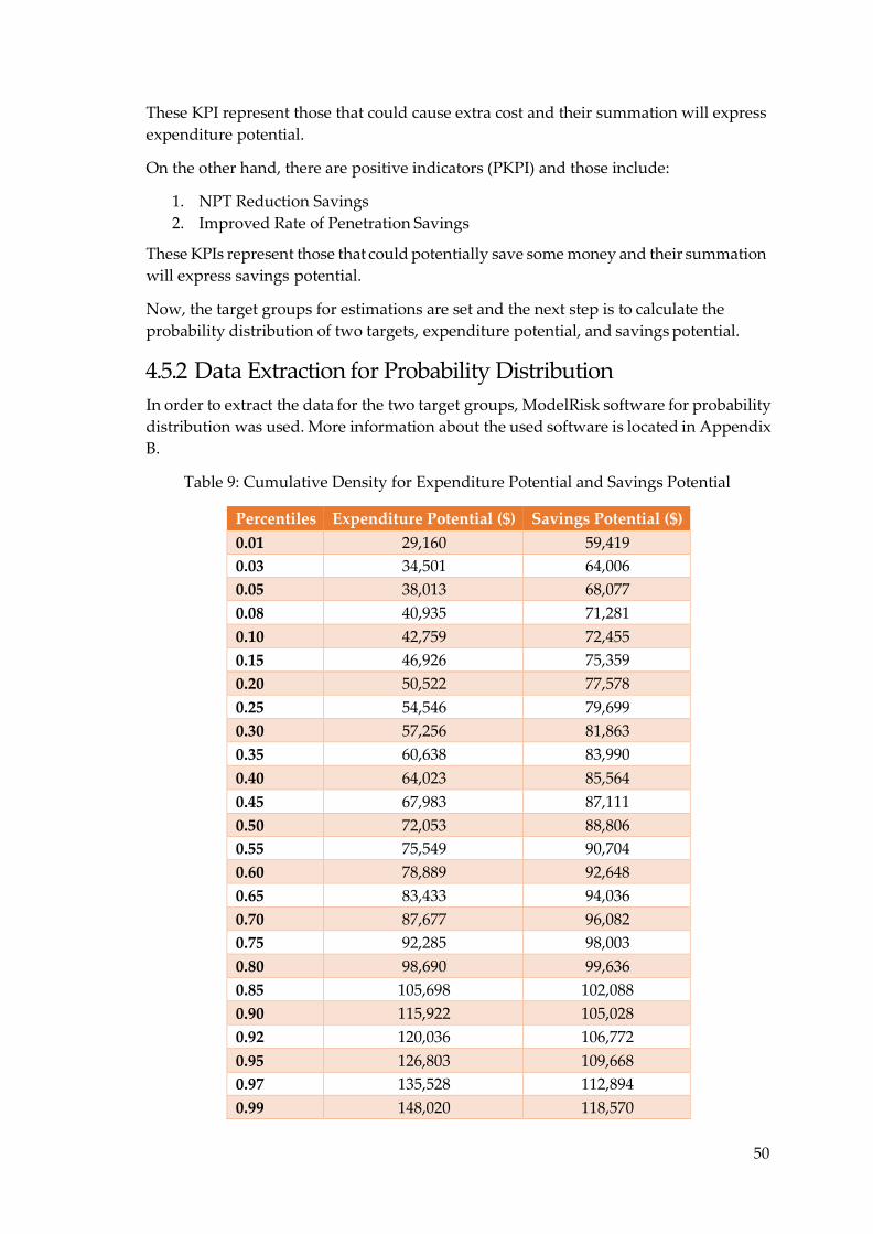
50

These KPI represent those that could cause extra cost and their summation will express expenditure potential.

On the other hand, there are positive indicators (PKPI) and those include:

1. NPT Reduction Savings 2. Improved Rate of Penetration Savings

These KPIs represent those that could potentially save some money and their summation will express savings potential.

Now, the target groups for estimations are set and the next step is to calculate the probability distribution of two targets, expenditure potential, and savings potential.

4.5.2 Data Extraction for Probability Distribution In order to extract the data for the two target groups, ModelRisk software for probability distribution was used. More information about the used software is located in Appendix B.

Table 9: Cumulative Density for Expenditure Potential and Savings Potential

Percentiles Expenditure Potential ($) Savings Potential ($)

0.01 29,160 59,419 0.03 34,501 64,006 0.05 38,013 68,077 0.08 40,935 71,281 0.10 42,759 72,455 0.15 46,926 75,359 0.20 50,522 77,578 0.25 54,546 79,699 0.30 57,256 81,863 0.35 60,638 83,990 0.40 64,023 85,564 0.45 67,983 87,111 0.50 72,053 88,806 0.55 75,549 90,704 0.60 78,889 92,648 0.65 83,433 94,036 0.70 87,677 96,082 0.75 92,285 98,003 0.80 98,690 99,636 0.85 105,698 102,088 0.90 115,922 105,028 0.92 120,036 106,772

0.95 126,803 109,668 0.97 135,528 112,894 0.99 148,020 118,570

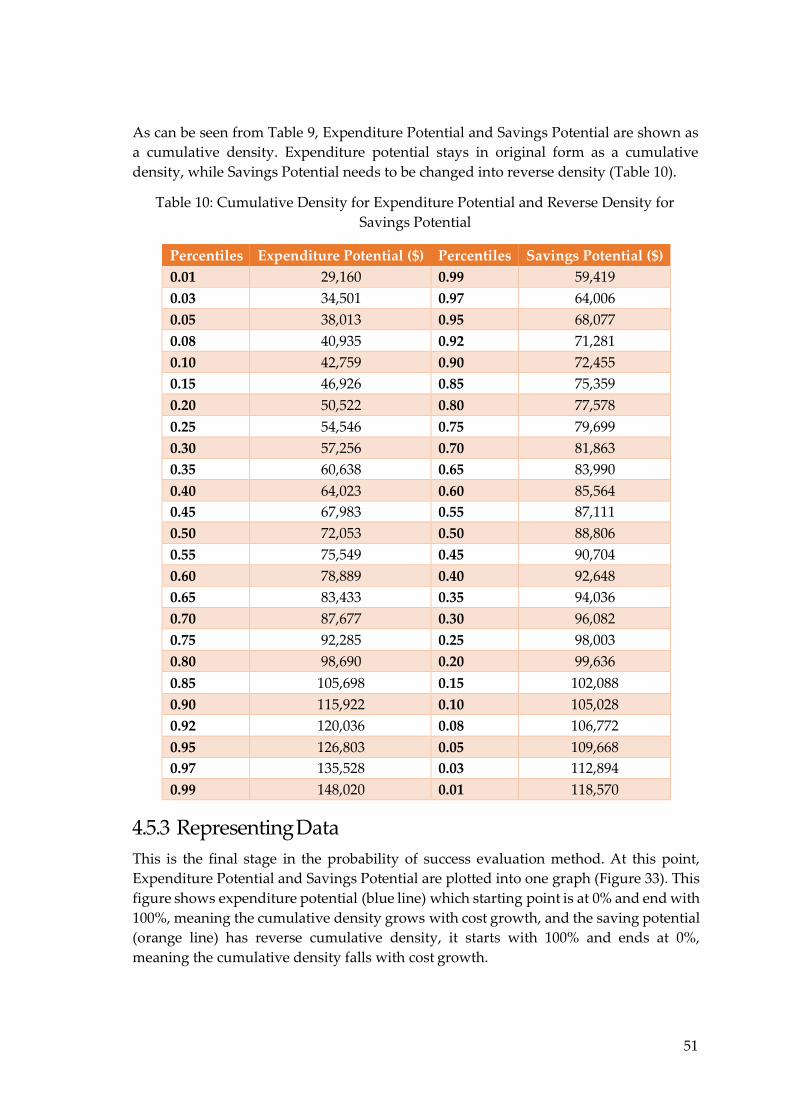
51

As can be seen from Table 9, Expenditure Potential and Savings Potential are shown as a cumulative density. Expenditure potential stays in original form as a cumulative density, while Savings Potential needs to be changed into reverse density (Table 10).

Table 10: Cumulative Density for Expenditure Potential and Reverse Density for Savings Potential

Percentiles Expenditure Potential ($) Percentiles Savings Potential ($)

0.01 29,160 0.99 59,419 0.03 34,501 0.97 64,006 0.05 38,013 0.95 68,077 0.08 40,935 0.92 71,281 0.10 42,759 0.90 72,455 0.15 46,926 0.85 75,359 0.20 50,522 0.80 77,578 0.25 54,546 0.75 79,699 0.30 57,256 0.70 81,863 0.35 60,638 0.65 83,990 0.40 64,023 0.60 85,564 0.45 67,983 0.55 87,111 0.50 72,053 0.50 88,806 0.55 75,549 0.45 90,704 0.60 78,889 0.40 92,648 0.65 83,433 0.35 94,036 0.70 87,677 0.30 96,082 0.75 92,285 0.25 98,003 0.80 98,690 0.20 99,636

0.85 105,698 0.15 102,088 0.90 115,922 0.10 105,028 0.92 120,036 0.08 106,772 0.95 126,803 0.05 109,668 0.97 135,528 0.03 112,894 0.99 148,020 0.01 118,570

4.5.3 Representing Data This is the final stage in the probability of success evaluation method. At this point, Expenditure Potential and Savings Potential are plotted into one graph (Figure 33). This figure shows expenditure potential (blue line) which starting point is at 0% and end with 100%, meaning the cumulative density grows with cost growth, and the saving potential (orange line) has reverse cumulative density, it starts with 100% and ends at 0%, meaning the cumulative density falls with cost growth.

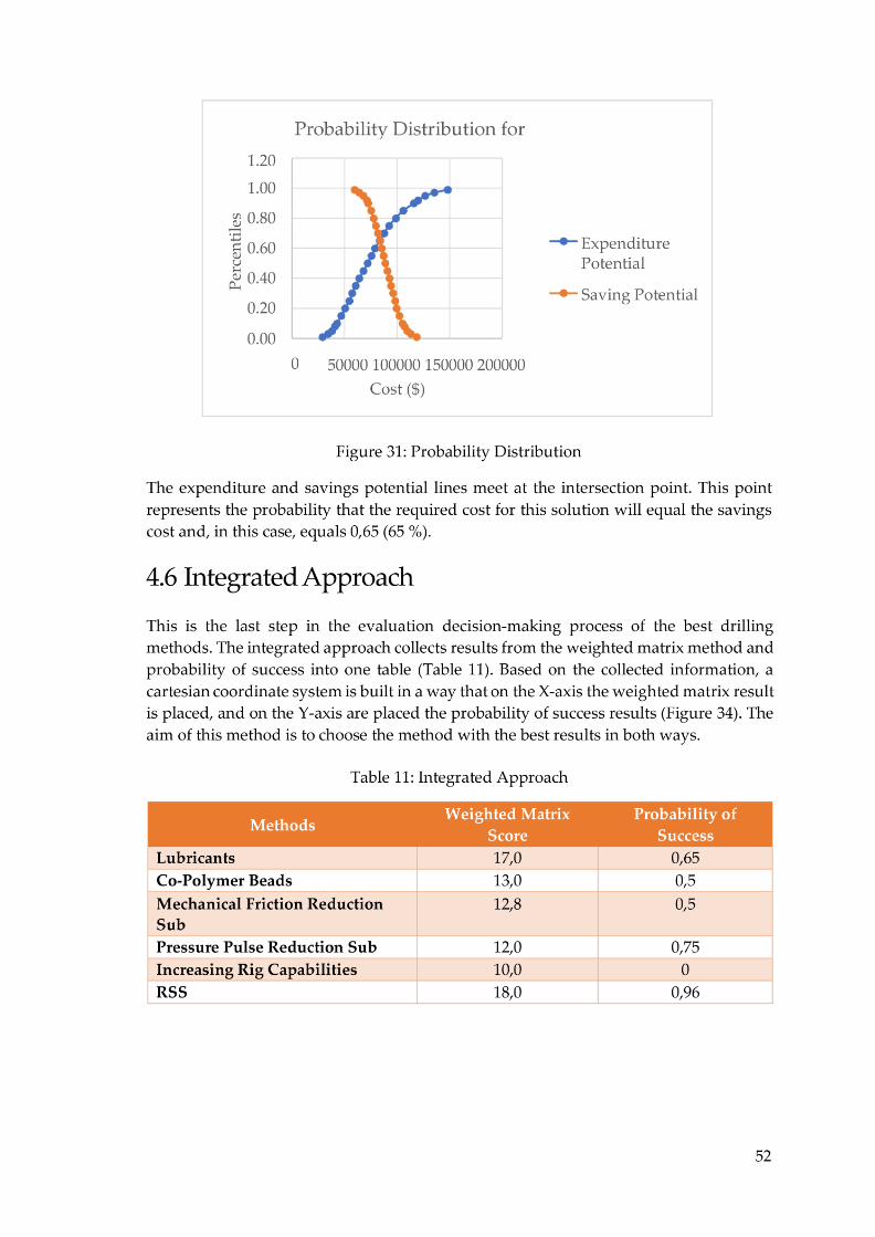
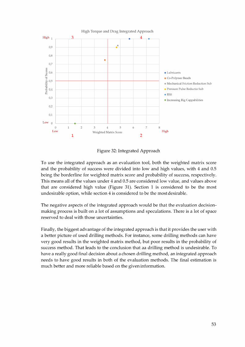
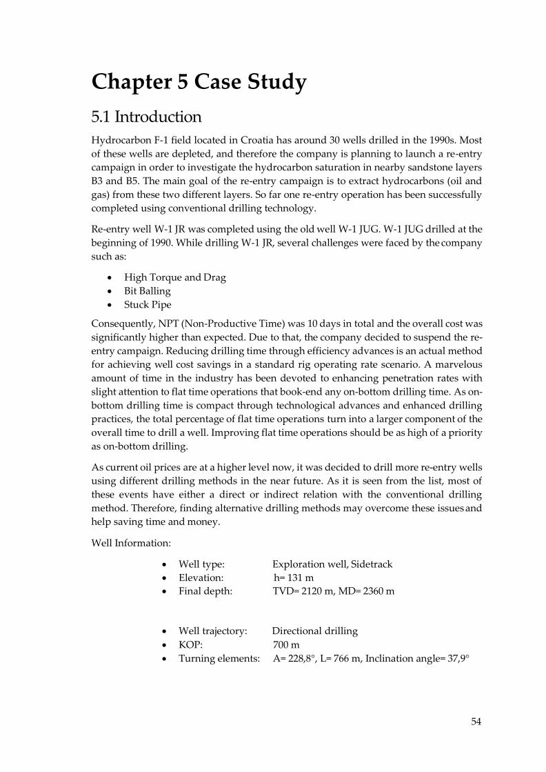
54

Chapter 5 Case Study

5.1 Introduction Hydrocarbon F-1 field located in Croatia has around 30 wells drilled in the 1990s. Most of these wells are depleted, and therefore the company is planning to launch a re-entry campaign in order to investigate the hydrocarbon saturation in nearby sandstone layers B3 and B5. The main goal of the re-entry campaign is to extract hydrocarbons (oil and gas) from these two different layers. So far one re-entry operation has been successfully completed using conventional drilling technology.

Re-entry well W-1 JR was completed using the old well W-1 JUG. W-1 JUG drilled at the beginning of 1990. While drilling W-1 JR, several challenges were faced by the company such as:

High Torque and Drag Bit Balling Stuck Pipe

Consequently, NPT (Non-Productive Time) was 10 days in total and the overall cost was significantly higher than expected. Due to that, the company decided to suspend the re- entry campaign. Reducing drilling time through efficiency advances is an actual method for achieving well cost savings in a standard rig operating rate scenario. A marvelous amount of time in the industry has been devoted to enhancing penetration rates with slight attention to flat time operations that book-end any on-bottom drilling time. As on- bottom drilling time is compact through technological advances and enhanced drilling practices, the total percentage of flat time operations turn into a larger component of the overall time to drill a well. Improving flat time operations should be as high of a priority as on-bottom drilling.

As current oil prices are at a higher level now, it was decided to drill more re-entry wells using different drilling methods in the near future. As it is seen from the list, most of these events have either a direct or indirect relation with the conventional drilling method. Therefore, finding alternative drilling methods may overcome these issues and help saving time and money.

Well Information:

Well type: Exploration well, Sidetrack Elevation: h= 131 m Final depth: TVD= 2120 m, MD= 2360 m

Well trajectory: Directional drilling KOP: 700 m Turning elements: A= 228,8°, L= 766 m, Inclination angle= 37,9°

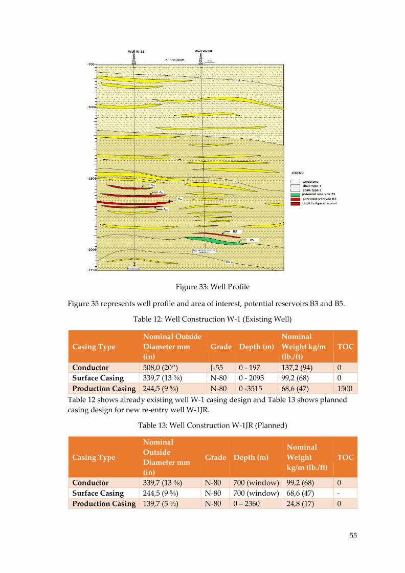
55

Figure 33: Well Profile

Figure 35 represents well profile and area of interest, potential reservoirs B3 and B5.

Table 12: Well Construction W-1 (Existing Well)

Casing Type

Nominal Outside

Diameter mm

(in)

Grade

Depth (m)

Nominal

Weight kg/m

(lb./ft)

TOC

Conductor 508,0 (20“) J-55 0 - 197 137,2 (94) 0 Surface Casing 339,7 (13 ⅜) N-80 0 - 2093 99,2 (68) 0 Production Casing 244,5 (9 ⅝) N-80 0 -3515 68,6 (47) 1500

Table 12 shows already existing well W-1 casing design and Table 13 shows planned casing design for new re-entry well W-1JR.

Table 13: Well Construction W-1JR (Planned)

Casing Type

Nominal

Outside

Diameter mm

(in)

Grade

Depth (m)

Nominal

Weight

kg/m (lb./ft)

TOC

Conductor 339,7 (13 ⅜) N-80 700 (window) 99,2 (68) 0 Surface Casing 244,5 (9 ⅝) N-80 700 (window) 68,6 (47) - Production Casing 139,7 (5 ½) N-80 0 – 2360 24,8 (17) 0

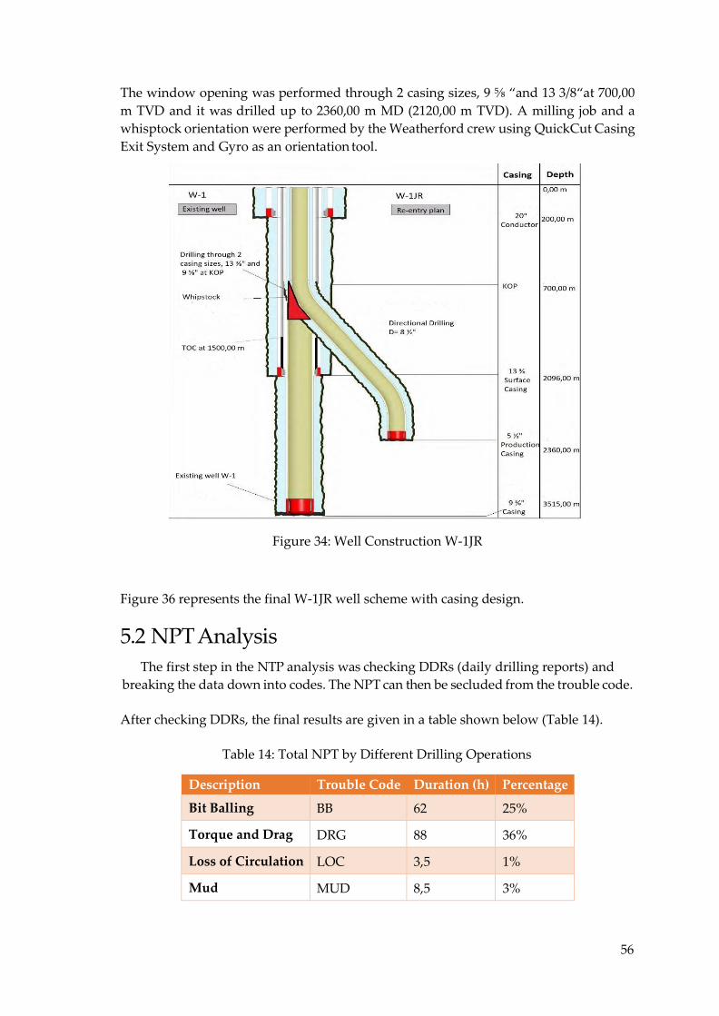
56

The window opening was performed through 2 casing sizes, 9 ⅝ “and 13 3/8“at 700,00 m TVD and it was drilled up to 2360,00 m MD (2120,00 m TVD). A milling job and a whisptock orientation were performed by the Weatherford crew using QuickCut Casing Exit System and Gyro as an orientation tool.

Figure 34: Well Construction W-1JR

Figure 36 represents the final W-1JR well scheme with casing design.

5.2 NPT Analysis The first step in the NTP analysis was checking DDRs (daily drilling reports) and

breaking the data down into codes. The NPT can then be secluded from the trouble code.

After checking DDRs, the final results are given in a table shown below (Table 14).

Table 14: Total NPT by Different Drilling Operations

Description Trouble Code Duration (h) Percentage

Bit Balling BB 62 25%

Torque and Drag DRG 88 36%

Loss of Circulation LOC 3,5 1%

Mud MUD 8,5 3%

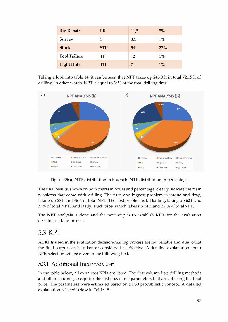
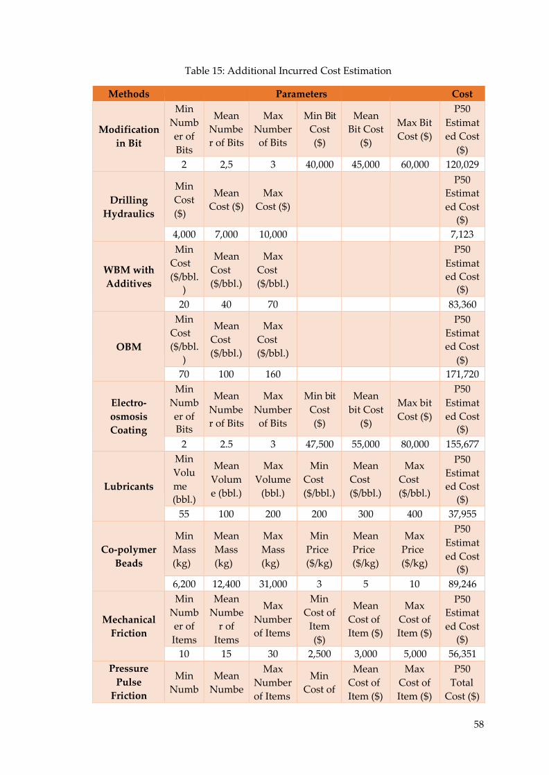
58

Table 15: Additional Incurred Cost Estimation

Methods Parameters Cost

Modification

in Bit

Min Number of Bits

Mean Number of Bits

Max Number of Bits

Min Bit Cost ($)

Mean Bit Cost

($)

Max Bit Cost ($)

P50 Estimated Cost

($) 2 2,5 3 40,000 45,000 60,000 120,029

Drilling

Hydraulics

Min Cost ($)

Mean

Cost ($)

Max

Cost ($)

P50 Estimat ed Cost

($) 4,000 7,000 10,000 7,123

WBM with

Additives

Min Cost ($/bbl.

)

Mean Cost ($/bbl.)

Max Cost ($/bbl.)

P50 Estimat ed Cost

($)

20 40 70 83,360

OBM

Min Cost ($/bbl.

)

Mean Cost ($/bbl.)

Max Cost ($/bbl.)

P50 Estimat ed Cost

($) 70 100 160 171,720

Electro-

osmosis

Coating

Min Numb er of Bits

Mean Numbe r of Bits

Max Number of Bits

Min bit Cost ($)

Mean bit Cost

($)

Max bit Cost ($)

P50 Estimat ed Cost

($) 2 2.5 3 47,500 55,000 80,000 155,677

Lubricants

Min Volu me (bbl.)

Mean Volum e (bbl.)

Max Volume

(bbl.)

Min Cost ($/bbl.)

Mean Cost ($/bbl.)

Max Cost ($/bbl.)

P50 Estimat ed Cost

($) 55 100 200 200 300 400 37,955

Co-polymer

Beads

Min Mass (kg)

Mean Mass (kg)

Max Mass (kg)

Min Price ($/kg)

Mean Price ($/kg)

Max Price ($/kg)

P50 Estimat ed Cost

($) 6,200 12,400 31,000 3 5 10 89,246

Mechanical

Friction

Min Numb er of Items

Mean Numbe

r of Items

Max Number of Items

Min Cost of

Item ($)

Mean Cost of Item ($)

Max Cost of Item ($)

P50 Estimat ed Cost

($) 10 15 30 2,500 3,000 5,000 56,351

Pressure

Pulse

Friction

Min Numb

Mean Numbe

Max Number of Items

Min Cost of

Mean Cost of Item ($)

Max Cost of Item ($)

P50 Total

Cost ($)

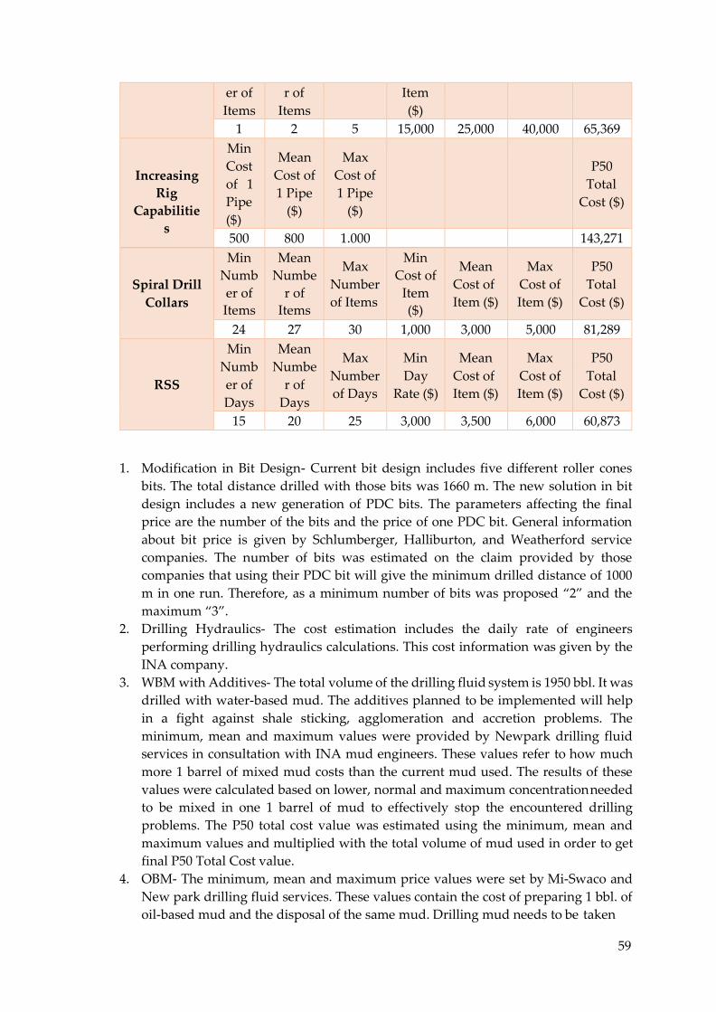
59

er of Items

r of Items

Item ($)

1 2 5 15,000 25,000 40,000 65,369

Increasing

Rig

Capabilitie

s

Min Cost of 1 Pipe ($)

Mean Cost of 1 Pipe

($)

Max Cost of 1 Pipe

($)

P50

Total Cost ($)

500 800 1.000 143,271

Spiral Drill

Collars

Min Numb er of Items

Mean Numbe

r of Items

Max Number of Items

Min Cost of

Item ($)

Mean Cost of Item ($)

Max Cost of Item ($)

P50 Total

Cost ($)

24 27 30 1,000 3,000 5,000 81,289

RSS

Min Numb er of Days

Mean Numbe

r of Days

Max Number of Days

Min Day

Rate ($)

Mean Cost of Item ($)

Max Cost of Item ($)

P50 Total

Cost ($)

15 20 25 3,000 3,500 6,000 60,873

1. Modification in Bit Design- Current bit design includes five different roller cones bits. The total distance drilled with those bits was 1660 m. The new solution in bit design includes a new generation of PDC bits. The parameters affecting the final price are the number of the bits and the price of one PDC bit. General information about bit price is given by Schlumberger, Halliburton, and Weatherford service companies. The number of bits was estimated on the claim provided by those companies that using their PDC bit will give the minimum drilled distance of 1000 m in one run. Therefore, as a minimum number of bits was proposed “2” and the maximum “3”.

2. Drilling Hydraulics- The cost estimation includes the daily rate of engineers performing drilling hydraulics calculations. This cost information was given by the INA company.

3. WBM with Additives- The total volume of the drilling fluid system is 1950 bbl. It was drilled with water-based mud. The additives planned to be implemented will help in a fight against shale sticking, agglomeration and accretion problems. The minimum, mean and maximum values were provided by Newpark drilling fluid services in consultation with INA mud engineers. These values refer to how much more 1 barrel of mixed mud costs than the current mud used. The results of these values were calculated based on lower, normal and maximum concentration needed to be mixed in one 1 barrel of mud to effectively stop the encountered drilling problems. The P50 total cost value was estimated using the minimum, mean and maximum values and multiplied with the total volume of mud used in order to get final P50 Total Cost value.

4. OBM- The minimum, mean and maximum price values were set by Mi-Swaco and New park drilling fluid services. These values contain the cost of preparing 1 bbl. of oil-based mud and the disposal of the same mud. Drilling mud needs to be taken

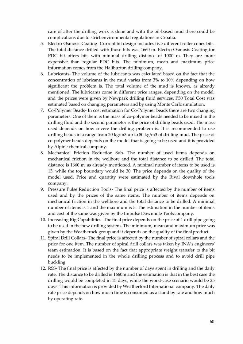
60

care of after the drilling work is done and with the oil-based mud there could be complications due to strict environmental regulations in Croatia.

5. Electro-Osmosis Coating- Current bit design includes five different roller cones bits. The total distance drilled with those bits was 1660 m. Electro-Osmosis Coating for PDC bit offers bits with minimal drilling distance of 1000 m. They are more expensive than regular PDC bits. The minimum, mean and maximum price information comes from the Haliburton drilling company.

6. Lubricants- The volume of the lubricants was calculated based on the fact that the concentration of lubricants in the mud varies from 3% to 10% depending on how significant the problem is. The total volume of the mud is known, as already mentioned. The lubricants come in different price ranges, depending on the model, and the prices were given by Newpark drilling fluid services. P50 Total Cost was estimated based on changing parameters and by using Monte Carlo simulation.

7. Co-Polymer Beads- In cost estimation for Co-Polymer beads there are two changing parameters. One of them is the mass of co-polymer beads needed to be mixed in the drilling fluid and the second parameter is the price of drilling beads used. The mass used depends on how severe the drilling problem is. It is recommended to use drilling beads in a range from 20 kg/m3 up to 80 kg/m3 of drilling mud. The price of co-polymer beads depends on the model that is going to be used and it is provided by Alpine chemical company.

8. Mechanical Friction Reduction Sub- The number of used items depends on mechanical friction in the wellbore and the total distance to be drilled. The total distance is 1660 m, as already mentioned. A minimal number of items to be used is 15, while the top boundary would be 30. The price depends on the quality of the model used. Price and quantity were estimated by the Rival downhole tools company.

9. Pressure Pulse Reduction Tools- The final price is affected by the number of items used and by the prices of the same items. The number of items depends on mechanical friction in the wellbore and the total distance to be drilled. A minimal number of items is 1 and the maximum is 5. The estimation in the number of items and cost of the same was given by the Impulse Downhole Tools company.

10. Increasing Rig Capabilities- The final price depends on the price of 1 drill pipe going to be used in the new drilling system. The minimum, mean and maximum price was given by the Weatherock group and it depends on the quality of the final product.

11. Spiral Drill Collars- The final price is affected by the number of spiral collars and the price for one item. The number of spiral drill collars was taken by INA’s engineers' team estimation. It is based on the fact that appropriate weight transfer to the bit needs to be implemented in the whole drilling process and to avoid drill pipe buckling.

12. RSS- The final price is affected by the number of days spent in drilling and the daily rate. The distance to be drilled is 1660m and the estimation is that in the best case the drilling would be completed in 15 days, while the worst-case scenario would be 25 days. This information is provided by Weatherford International company. The daily rate price depends on how much time is consumed as a stand by rate and how much by operating rate.

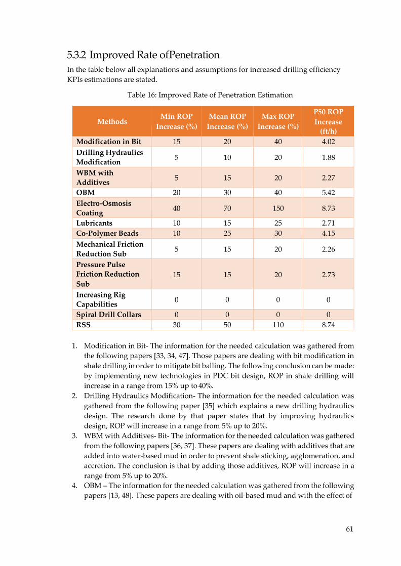
61

5.3.2 Improved Rate of Penetration In the table below all explanations and assumptions for increased drilling efficiency KPIs estimations are stated.

Table 16: Improved Rate of Penetration Estimation

Methods

Min ROP

Increase (%)

Mean ROP

Increase (%)

Max ROP

Increase (%)

P50 ROP

Increase

(ft/h)

Modification in Bit 15 20 40 4.02 Drilling Hydraulics

Modification 5 10 20 1.88

WBM with

Additives 5 15 20 2.27

OBM 20 30 40 5.42 Electro-Osmosis

Coating 40 70 150 8.73

Lubricants 10 15 25 2.71 Co-Polymer Beads 10 25 30 4.15

Mechanical Friction

Reduction Sub 5 15 20 2.26

Pressure Pulse

Friction Reduction

Sub

15

15

20

2.73

Increasing Rig

Capabilities 0 0 0 0

Spiral Drill Collars 0 0 0 0 RSS 30 50 110 8.74

1. Modification in Bit- The information for the needed calculation was gathered from

the following papers [33, 34, 47]. Those papers are dealing with bit modification in shale drilling in order to mitigate bit balling. The following conclusion can be made: by implementing new technologies in PDC bit design, ROP in shale drilling will increase in a range from 15% up to 40%.

2. Drilling Hydraulics Modification- The information for the needed calculation was gathered from the following paper [35] which explains a new drilling hydraulics design. The research done by that paper states that by improving hydraulics design, ROP will increase in a range from 5% up to 20%.

3. WBM with Additives- Bit- The information for the needed calculation was gathered from the following papers [36, 37]. These papers are dealing with additives that are added into water-based mud in order to prevent shale sticking, agglomeration, and accretion. The conclusion is that by adding those additives, ROP will increase in a range from 5% up to 20%.

4. OBM – The information for the needed calculation was gathered from the following papers [13, 48]. These papers are dealing with oil-based mud and with the effect of

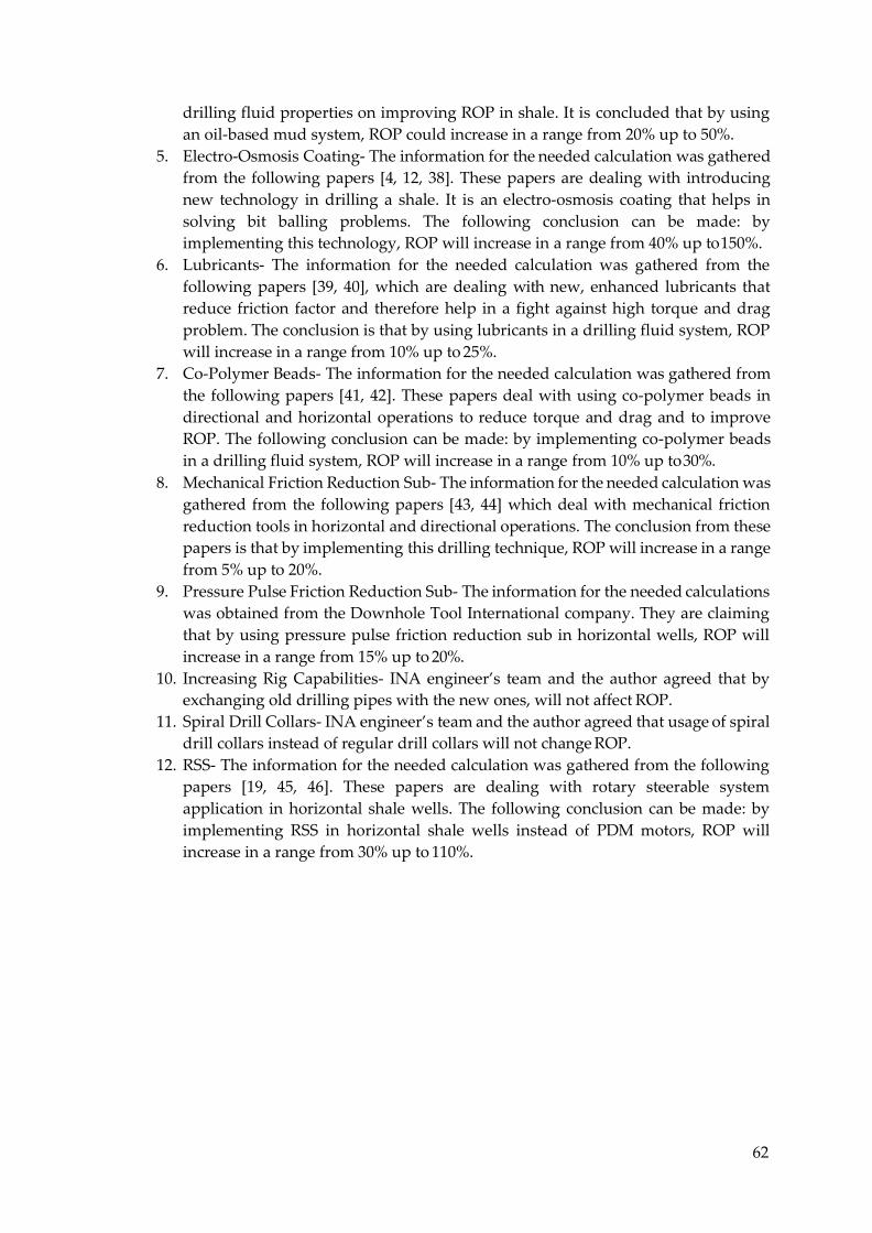
62

drilling fluid properties on improving ROP in shale. It is concluded that by using an oil-based mud system, ROP could increase in a range from 20% up to 50%.

5. Electro-Osmosis Coating- The information for the needed calculation was gathered from the following papers [4, 12, 38]. These papers are dealing with introducing new technology in drilling a shale. It is an electro-osmosis coating that helps in solving bit balling problems. The following conclusion can be made: by implementing this technology, ROP will increase in a range from 40% up to 150%.

6. Lubricants- The information for the needed calculation was gathered from the following papers [39, 40], which are dealing with new, enhanced lubricants that reduce friction factor and therefore help in a fight against high torque and drag problem. The conclusion is that by using lubricants in a drilling fluid system, ROP will increase in a range from 10% up to 25%.

7. Co-Polymer Beads- The information for the needed calculation was gathered from the following papers [41, 42]. These papers deal with using co-polymer beads in directional and horizontal operations to reduce torque and drag and to improve ROP. The following conclusion can be made: by implementing co-polymer beads in a drilling fluid system, ROP will increase in a range from 10% up to 30%.

8. Mechanical Friction Reduction Sub- The information for the needed calculation was gathered from the following papers [43, 44] which deal with mechanical friction reduction tools in horizontal and directional operations. The conclusion from these papers is that by implementing this drilling technique, ROP will increase in a range from 5% up to 20%.

9. Pressure Pulse Friction Reduction Sub- The information for the needed calculations was obtained from the Downhole Tool International company. They are claiming that by using pressure pulse friction reduction sub in horizontal wells, ROP will increase in a range from 15% up to 20%.

10. Increasing Rig Capabilities- INA engineer’s team and the author agreed that by exchanging old drilling pipes with the new ones, will not affect ROP.

11. Spiral Drill Collars- INA engineer’s team and the author agreed that usage of spiral drill collars instead of regular drill collars will not change ROP.

12. RSS- The information for the needed calculation was gathered from the following papers [19, 45, 46]. These papers are dealing with rotary steerable system application in horizontal shale wells. The following conclusion can be made: by implementing RSS in horizontal shale wells instead of PDM motors, ROP will increase in a range from 30% up to 110%.

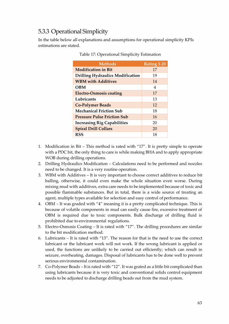
63

5.3.3 Operational Simplicity In the table below all explanations and assumptions for operational simplicity KPIs estimations are stated.

Table 17: Operational Simplicity Estimation

Methods Rating 1-20

Modification in Bit 17 Drilling Hydraulics Modification 19 WBM with Additives 14 OBM 4 Electro-Osmosis coating 17 Lubricants 13 Co-Polymer Beads 12 Mechanical Friction Sub 18 Pressure Pulse Friction Sub 16 Increasing Rig Capabilities 20 Spiral Drill Collars 20 RSS 18

1. Modification in Bit – This method is rated with “17”. It is pretty simple to operate

with a PDC bit, the only thing to care is while making BHA and to apply appropriate WOB during drilling operations.

2. Drilling Hydraulics Modification – Calculations need to be performed and nozzles need to be changed. It is a very routine operation.

3. WBM with Additives – It is very important to choose correct additives to reduce bit balling, otherwise, it could even make the whole situation even worse. During mixing mud with additives, extra care needs to be implemented because of toxic and possible flammable substances. But in total, there is a wide source of treating an agent, multiple types available for selection and easy control of performance.

4. OBM – It was graded with “4” meaning it is a pretty complicated technique. This is because of volatile components in mud can easily cause fire, excessive treatment of OBM is required due to toxic components. Bulk discharge of drilling fluid is prohibited due to environmental regulations.

5. Electro-Osmosis Coating – It is rated with “17”. The drilling procedures are similar to the bit modification method.

6. Lubricants – It is rated with “13”. The reason for that is the need to use the correct lubricant or the lubricant work will not work. If the wrong lubricant is applied or used, the functions are unlikely to be carried out efficiently; which can result in seizure, overheating, damages. Disposal of lubricants has to be done well to prevent serious environmental contamination.

7. Co-Polymer Beads – It is rated with “12”. It was grated as a little bit complicated than using lubricants because it is very toxic and conventional solids control equipment needs to be adjusted to discharge drilling beads out from the mud system.

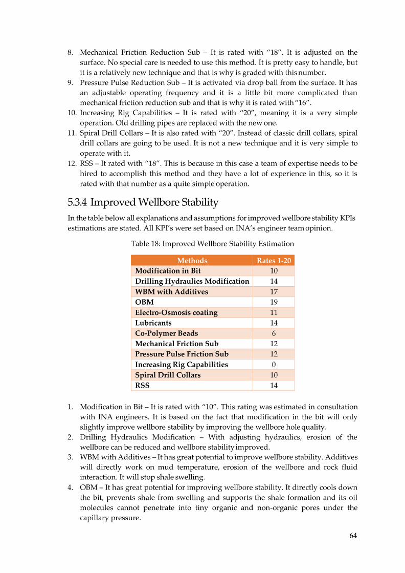
64

8. Mechanical Friction Reduction Sub – It is rated with “18”. It is adjusted on the surface. No special care is needed to use this method. It is pretty easy to handle, but it is a relatively new technique and that is why is graded with this number.

9. Pressure Pulse Reduction Sub – It is activated via drop ball from the surface. It has an adjustable operating frequency and it is a little bit more complicated than mechanical friction reduction sub and that is why it is rated with “16”.

10. Increasing Rig Capabilities – It is rated with “20”, meaning it is a very simple operation. Old drilling pipes are replaced with the new one.

11. Spiral Drill Collars – It is also rated with “20”. Instead of classic drill collars, spiral drill collars are going to be used. It is not a new technique and it is very simple to operate with it.

12. RSS – It rated with “18”. This is because in this case a team of expertise needs to be hired to accomplish this method and they have a lot of experience in this, so it is rated with that number as a quite simple operation.

5.3.4 Improved Wellbore Stability In the table below all explanations and assumptions for improved wellbore stability KPIs estimations are stated. All KPI’s were set based on INA’s engineer team opinion.

Table 18: Improved Wellbore Stability Estimation

Methods Rates 1-20

Modification in Bit 10 Drilling Hydraulics Modification 14 WBM with Additives 17 OBM 19 Electro-Osmosis coating 11 Lubricants 14 Co-Polymer Beads 6 Mechanical Friction Sub 12 Pressure Pulse Friction Sub 12 Increasing Rig Capabilities 0 Spiral Drill Collars 10 RSS 14

1. Modification in Bit – It is rated with “10”. This rating was estimated in consultation

with INA engineers. It is based on the fact that modification in the bit will only slightly improve wellbore stability by improving the wellbore hole quality.

2. Drilling Hydraulics Modification – With adjusting hydraulics, erosion of the wellbore can be reduced and wellbore stability improved.

3. WBM with Additives – It has great potential to improve wellbore stability. Additives will directly work on mud temperature, erosion of the wellbore and rock fluid interaction. It will stop shale swelling.

4. OBM – It has great potential for improving wellbore stability. It directly cools down the bit, prevents shale from swelling and supports the shale formation and its oil molecules cannot penetrate into tiny organic and non-organic pores under the capillary pressure.

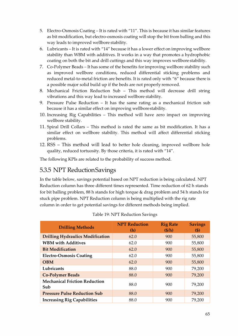
65

5. Electro-Osmosis Coating – It is rated with “11”. This is because it has similar features as bit modification, but electro-osmosis coating will stop the bit from balling and this way leads to improved wellbore stability.

6. Lubricants – It is rated with “14” because it has a lower effect on improving wellbore stability than WBM with additives. It works in a way that promotes a hydrophobic coating on both the bit and drill cuttings and this way improves wellbore stability.

7. Co-Polymer Beads – It has some of the benefits for improving wellbore stability such as improved wellbore conditions, reduced differential sticking problems and reduced metal-to-metal friction are benefits. It is rated only with “6” because there is a possible major solid build up if the beds are not properly removed.

8. Mechanical Friction Reduction Sub – This method will decrease drill string vibrations and this way lead to increased wellbore stability.

9. Pressure Pulse Reduction – It has the same rating as a mechanical friction sub because it has a similar effect on improving wellbore stability.

10. Increasing Rig Capabilities – This method will have zero impact on improving wellbore stability.

11. Spiral Drill Collars – This method is rated the same as bit modification. It has a similar effect on wellbore stability. This method will affect differential sticking problems.

12. RSS – This method will lead to better hole cleaning, improved wellbore hole quality, reduced tortuosity. By those criteria, it is rated with “14”.

The following KPIs are related to the probability of success method.

5.3.5 NPT Reduction Savings In the table below, savings potential based on NPT reduction is being calculated. NPT Reduction column has three different times represented. Time reduction of 62 h stands for bit balling problem, 88 h stands for high torque & drag problem and 54 h stands for stuck pipe problem. NPT Reduction column is being multiplied with the rig rate column in order to get potential savings for different methods being implied.

Table 19: NPT Reduction Savings

Drilling Methods NPT Reduction

(h)

Rig Rate

($/h)

Savings

($)

Drilling Hydraulics Modification 62.0 900 55,800 WBM with Additives 62.0 900 55,800 Bit Modification 62.0 900 55,800 Electro-Osmosis Coating 62.0 900 55,800 OBM 62.0 900 55,800 Lubricants 88.0 900 79,200 Co-Polymer Beads 88.0 900 79,200 Mechanical Friction Reduction

Sub 88.0 900 79,200

Pressure Pulse Reduction Sub 88.0 900 79,200 Increasing Rig Capabilities 88.0 900 79,200

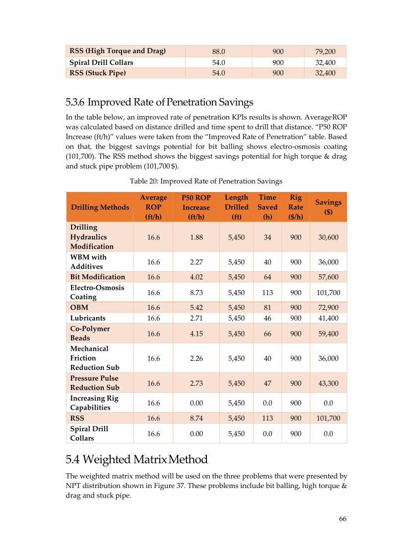
66

RSS (High Torque and Drag) 88.0 900 79,200

Spiral Drill Collars 54.0 900 32,400 RSS (Stuck Pipe) 54.0 900 32,400

5.3.6 Improved Rate of Penetration Savings In the table below, an improved rate of penetration KPIs results is shown. Average ROP was calculated based on distance drilled and time spent to drill that distance. “P50 ROP Increase (ft/h)” values were taken from the “Improved Rate of Penetration” table. Based on that, the biggest savings potential for bit balling shows electro-osmosis coating (101,700). The RSS method shows the biggest savings potential for high torque & drag and stuck pipe problem (101,700 $).

Table 20: Improved Rate of Penetration Savings

Drilling Methods

Average

ROP

(ft/h)

P50 ROP

Increase

(ft/h)

Length

Drilled

(ft)

Time

Saved

(h)

Rig

Rate

($/h)

Savings

($)

Drilling

Hydraulics

Modification

16.6

1.88

5,450

34

900

30,600

WBM with

Additives 16.6 2.27 5,450 40 900 36,000

Bit Modification 16.6 4.02 5,450 64 900 57,600 Electro-Osmosis

Coating 16.6 8.73 5,450 113 900 101,700

OBM 16.6 5.42 5,450 81 900 72,900 Lubricants 16.6 2.71 5,450 46 900 41,400 Co-Polymer

Beads 16.6 4.15 5,450 66 900 59,400

Mechanical

Friction

Reduction Sub

16.6

2.26

5,450

40

900

36,000

Pressure Pulse

Reduction Sub 16.6 2.73 5,450 47 900 43,300

Increasing Rig

Capabilities 16.6 0.00 5,450 0.0 900 0.0

RSS 16.6 8.74 5,450 113 900 101,700 Spiral Drill

Collars 16.6 0.00 5,450 0.0 900 0.0

5.4 Weighted Matrix Method The weighted matrix method will be used on the three problems that were presented by NPT distribution shown in Figure 37. These problems include bit balling, high torque & drag and stuck pipe.

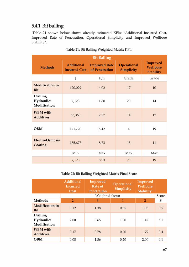
67

5.4.1 Bit balling Table 21 shown below shows already estimated KPIs: “Additional Incurred Cost,

Improved Rate of Penetration, Operational Simplicity and Improved Wellbore Stability”.

Table 21: Bit Balling Weighted Matrix KPIs

Bit Balling

Methods

Additional

Incurred Cost

Improved Rate

of Penetration

Operational

Simplicity

Improved

Wellbore

Stability

$ ft/h Grade Grade

Modification in

Bit

120,029

4.02

17

10

Drilling

Hydraulics

Modification

7,123

1.88

20

14

WBM with

Additives

83,360

2.27

14

17

OBM

171,720

5.42

4

19

Electro-Osmosis

Coating

155,677

8.73

15

11

Min Max Max Max

7,123 8.73 20 19

Table 22: Bit Balling Weighted Matrix Final Score

Additional

Incurred

Cost

Improved

Rate of

Penetration

Operational

Simplicity

Improved

Wellbore

Stability

Weighted factor Score Methods 2 3 1 2 8 Modification in

Bit 0.12 1.38 0.85 1.05 3.5

Drilling

Hydraulics

Modification

2.00

0.65

1.00

1.47

5.1

WBM with

Additives 0.17 0.78 0.70 1.79 3.4

OBM 0.08 1.86 0.20 2.00 4.1

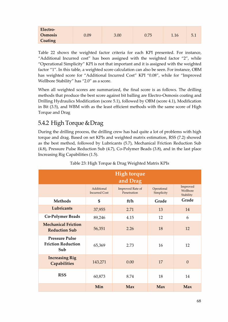
68

Electro-

Osmosis

Coating

0.09

3.00

0.75

1.16

5.1

Table 22 shows the weighted factor criteria for each KPI presented. For instance, “Additional Incurred cost” has been assigned with the weighted factor “2”, while “Operational Simplicity” KPI is not that important and it is assigned with the weighted factor “1”. In this table, a weighted score calculation can also be seen. For instance, OBM has weighted score for “Additional Incurred Cost” KPI “0.08”, while for “Improved Wellbore Stability” has “2.0” as a score.

When all weighted scores are summarized, the final score is as follows. The drilling methods that produce the best score against bit balling are Electro-Osmosis coating and Drilling Hydraulics Modification (score 5.1), followed by OBM (score 4.1), Modification in Bit (3.5), and WBM with as the least efficient methods with the same score of High Torque and Drag

5.4.2 High Torque & Drag During the drilling process, the drilling crew has had quite a lot of problems with high torque and drag. Based on set KPIs and weighted matrix estimation, RSS (7.2) showed as the best method, followed by Lubricants (5.7), Mechanical Friction Reduction Sub (4.8), Pressure Pulse Reduction Sub (4.7), Co-Polymer Beads (3.8), and in the last place Increasing Rig Capabilities (1.5).

Table 23: High Torque & Drag Weighted Matrix KPIs

High torque

and Drag Additional

Incurred Cost Improved Rate of

Penetration Operational Simplicity

Improved Wellbore Stability

Methods $ ft/h Grade Grade

Lubricants 37,955 2.71 13 14

Co-Polymer Beads 89,246 4.15 12 6

Mechanical Friction

Reduction Sub

56,351

2.26

18

12

Pressure Pulse

Friction Reduction

Sub

65,369

2.73

16

12

Increasing Rig

Capabilities

143,271

0.00

17

0

RSS

60,873

8.74

18

14

Min Max Max Max

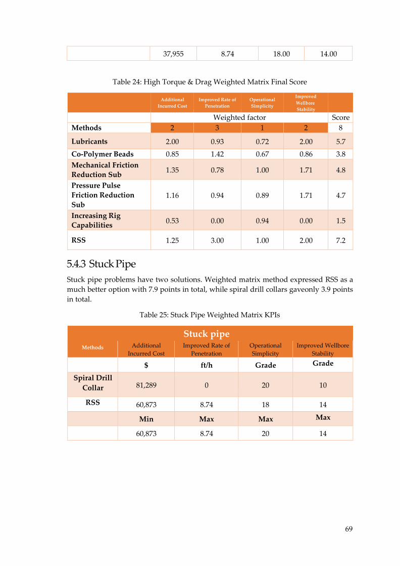
69

37,955 8.74 18.00 14.00

Table 24: High Torque & Drag Weighted Matrix Final Score

Additional

Incurred Cost

Improved Rate of

Penetration

Operational

Simplicity

Improved

Wellbore

Stability

Weighted factor Score Methods 2 3 1 2 8

Lubricants 2.00 0.93 0.72 2.00 5.7

Co-Polymer Beads 0.85 1.42 0.67 0.86 3.8

Mechanical Friction

Reduction Sub 1.35 0.78 1.00 1.71 4.8

Pressure Pulse

Friction Reduction

Sub

1.16

0.94

0.89

1.71

4.7

Increasing Rig

Capabilities 0.53 0.00 0.94 0.00 1.5

RSS 1.25 3.00 1.00 2.00 7.2

5.4.3 Stuck Pipe Stuck pipe problems have two solutions. Weighted matrix method expressed RSS as a much better option with 7.9 points in total, while spiral drill collars gaveonly 3.9 points in total.

Table 25: Stuck Pipe Weighted Matrix KPIs

Stuck pipe

Methods Additional Incurred Cost

Improved Rate of Penetration

Operational Simplicity

Improved Wellbore Stability

$ ft/h Grade Grade

Spiral Drill

Collar

81,289

0

20

10

RSS 60,873 8.74 18 14 Min Max Max Max

60,873 8.74 20 14

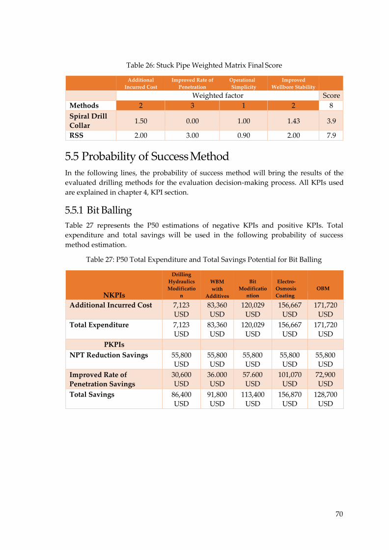
70

Table 26: Stuck Pipe Weighted Matrix Final Score

Additional

Incurred Cost

Improved Rate of

Penetration

Operational

Simplicity

Improved

Wellbore Stability

Weighted factor Score Methods 2 3 1 2 8

Spiral Drill

Collar 1.50 0.00 1.00 1.43 3.9

RSS 2.00 3.00 0.90 2.00 7.9

5.5 Probability of Success Method In the following lines, the probability of success method will bring the results of the evaluated drilling methods for the evaluation decision-making process. All KPIs used are explained in chapter 4, KPI section.

5.5.1 Bit Balling Table 27 represents the P50 estimations of negative KPIs and positive KPIs. Total expenditure and total savings will be used in the following probability of success method estimation.

Table 27: P50 Total Expenditure and Total Savings Potential for Bit Balling

NKPIs

Drilling

Hydraulics

Modificatio

n

WBM

with

Additives

Bit

Modificatio

ntion

Electro-

Osmosis

Coating

OBM

Additional Incurred Cost 7,123 USD

83,360 USD

120,029 USD

156,667 USD

171,720 USD

Total Expenditure 7,123 USD

83,360 USD

120,029 USD

156,667 USD

171,720 USD

PKPIs

NPT Reduction Savings 55,800 USD

55,800 USD

55,800 USD

55,800 USD

55,800 USD

Improved Rate of

Penetration Savings

30,600 USD

36.000 USD

57.600 USD

101,070 USD

72,900 USD

Total Savings 86,400 USD

91,800 USD

113,400 USD

156,870 USD

128,700 USD

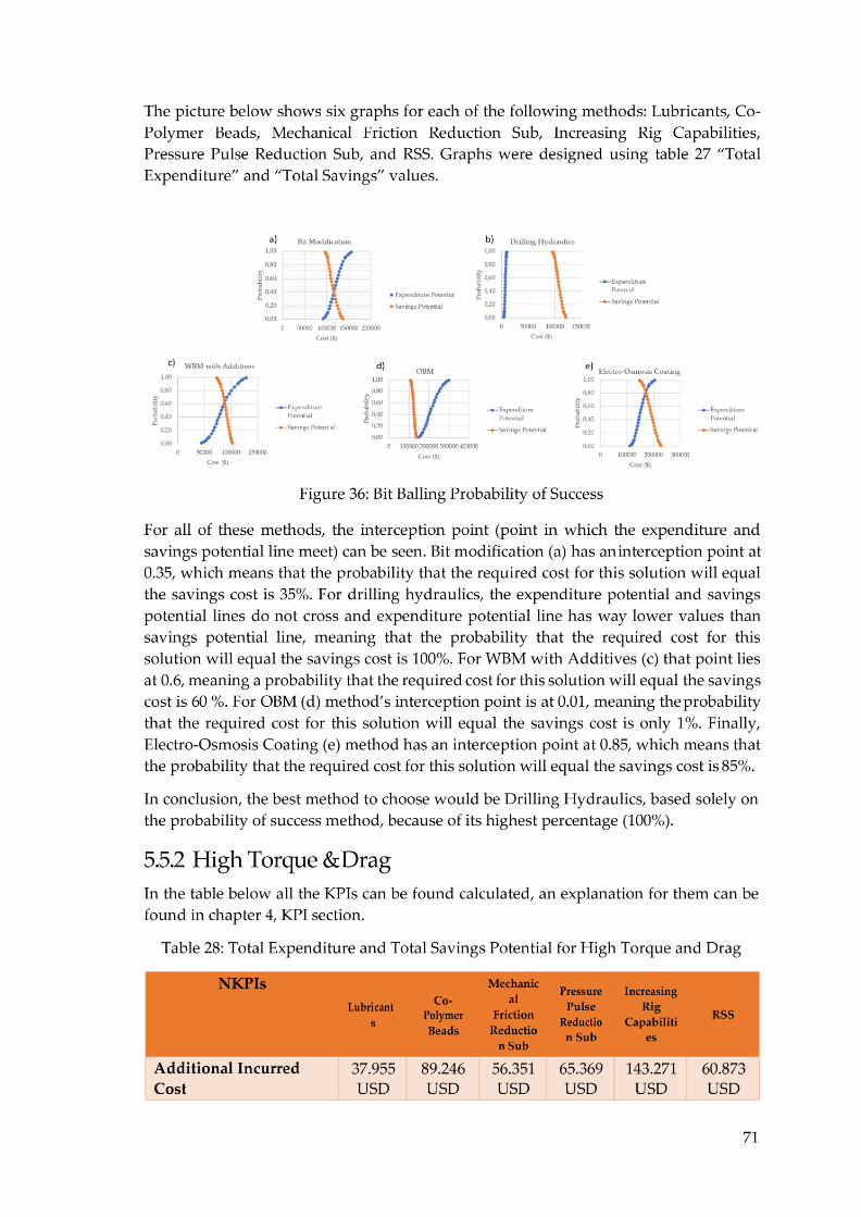
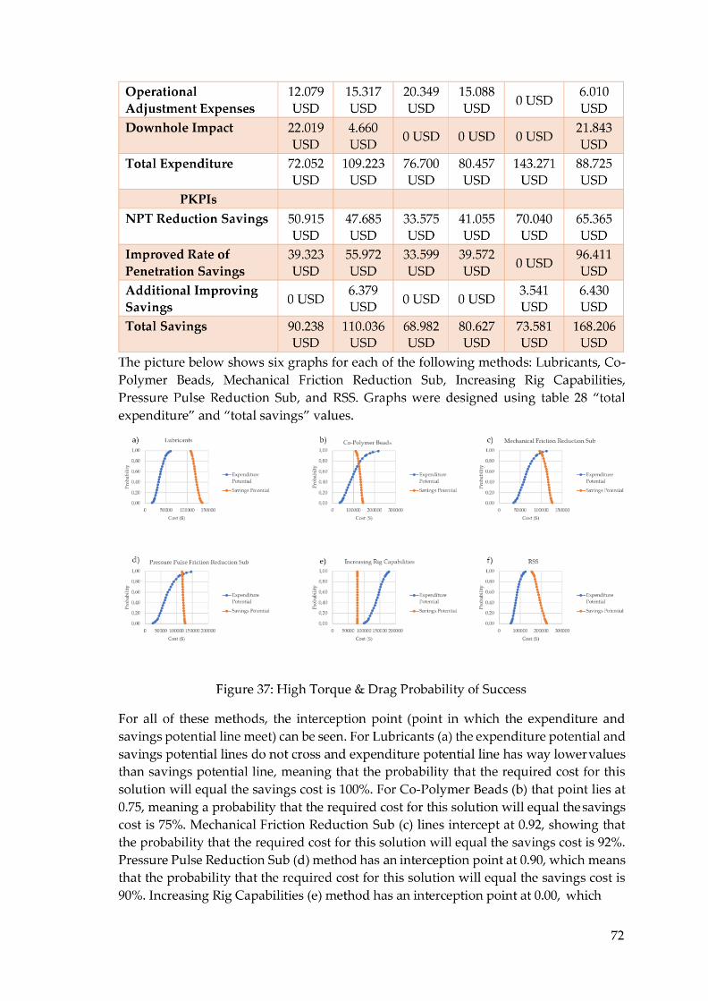
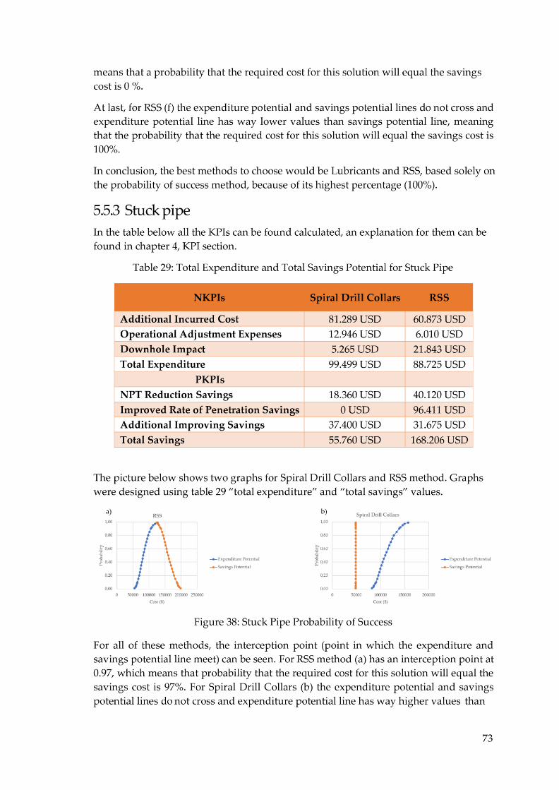
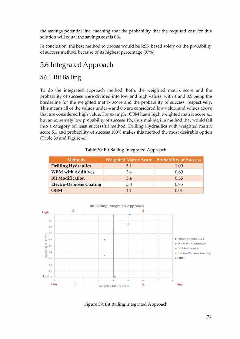
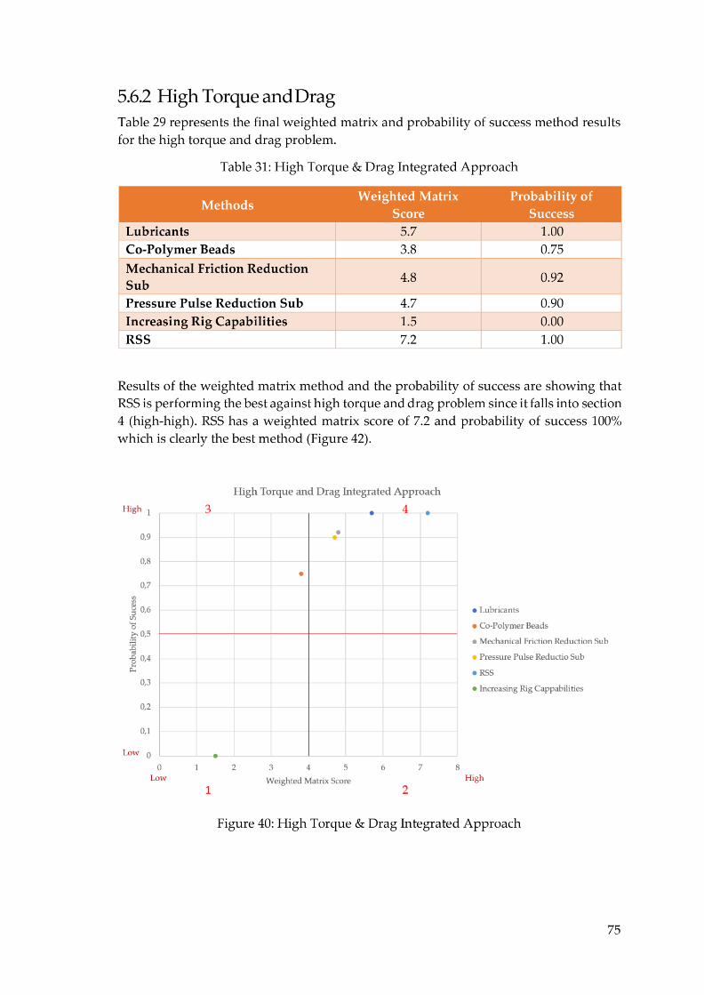
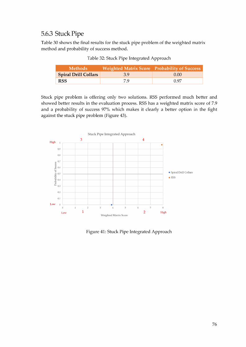
77

5.7 Case Study Conclusion In order to evaluate the drilling performance and to choose the best methods for re-entry drilling, it is very important to collect all data available, produced during the drilling process, regardless of whether they are meta or sensor data. Collected data will reduce the rate of uncertainty in the final assessment.

Additionally, collected data were analyzed for the purpose of getting non-productive time, setting the basis for further work on the case study. Non-productive time analysis produces three main root causes. Those are bit balling, high torque & drag, and stuck pipe. Given results were fundamental to propose the best methods for each main of the NPT root cause problems. Assumed solutions were evaluated based on two different tools. The first estimation tool was the weighted matrix method. The limitation of this tool lies in the fact that the final solution is tightly connected with the uncertainty in different parameters and weighted factors that are set based on the INA engineer’s experience. This means that the final weighted matrix method solution is mostly based on personal opinion and quite subjective.

To enhance the decision-making process different decision tool was presented, the probability of success method. This tool brings the final decision based on two sets of KPI’s. Those are positive and negative KPI’s expressed as a cost unit and based on them the final decision is being brought.

When these two tools were combined together, they produced an integrated approach solution for each root problem cause of NPT. Based on the given results, the best method for bit balling is drilling hydraulics; high torque & drag and stuck pipe share the same solution and that solution is the rotary steerable system. Most of the calculations and assumed parameters for decision-making tools have been done with the cooperation of INA’s engineers.

78

Chapter 6 Conclusion

The objectives of the thesis were to:

Familiarize the reader with the drilling problems that occurred during re-entry drilling

Analyze the well in terms of NPT, identify major NPT events and their root causes and quantify the amount of NPT

Propose a different solution to the occurring problems Come up with a decision-making process to decide the best method for each

problem Currently used drilling methods come with a lot of problems that cause money loss. That’s why it’s important to do preplanning and use concepts that can estimate which method would be the most efficient. In most preplanning scenarios, the weighted matrix method is used. This method assigns scores to drilling methods based on different parameters involved in the decision-making process. The challenge with this method is that the parameters come with uncertainty, since they are estimated by humans and the final score is based on their personal opinion, therefore they can vary depending on the company giving the data and the analyst. To make the estimation stronger, drilling methods alternatives were also evaluated by the probability of success method. With this method, calculations were made as a percentage of chance that some method will be successful. This percentage comes as a result of data extracted from other similar scientific articles, meaning it is based on previous experience established in the oil and gas business.

The case study, presented in this thesis, deals with these two methods, and in the end combines them in an integrated approach, which points out to the most efficient method based on a score given by WM and probability given by POS. The integrated approach was tested for a real case scenario to evaluate different proposed drilling methods considering the root cause of NPT, during constructing the sidetrack well W1-JR.

The integrated approach has shown as a good alternative to used methods in an evaluation process. Although it is not the most reliable approach, it is certainly better to use two different evaluating methods integrated into one approach, instead of just using one, since the unreliability of parameters is reduced. There is still some room left for improvement. To get a more trustworthy output, input data should be more precise. In a case study, there were a lot of uncertainties and a lot of estimations. To ensure good results of an integrated approach more detailed information from other offset wells should be available. The multidisciplinary approach and teamwork of geophysics, geologist, reservoir, production and drilling engineers is a necessary precondition for maximum trustworthy results.

79

References 1. Eric van Oort, SPE, Shell E&P Technology. “Physico-Chemical Stabilization of

Shales”, SPE 37263, 1997. 2. Van Oort, E. “On the Physical and Chemical Stability of Shales.” Journal of Petroleum

Science and Engineering, v38, (2003) 213-235. 3. Sideney J. Green, Arnis Judzis, David Curry, “Single Cutter Testing Improves

Undertanding of Deepwater Hammer Drilling Performance”, SPE 97173-MS, 2005

4. G.A. Cooper’, Sanjit Roy, “Prevention of Bit Balling by Electro-Osmosis”, SPE 27882, 1994

5. G. De Stefano, Shrieve Chemicals, S. Young, M-I Swaco, “The Prevention and Cure of Bit Balling in Water Based Drilling Fluids”, OMC, 2009

6. P.R. Hariharan and G.A. Cooper, U. of California, and A.H. Hale, * Shell E&P Technology Co. *IADC Mem, “Bit Balling Reduction by Electro-Osmosis While Drilling Shale Using a Model BHA (Bottom Hole Assembly)”, SPE 39311, 1998

7. D.H. Zijsling, Eggbeater PDC Drillbit Design Eliminates Balling in Water Based Drilling Fluids”, SPE, 1993

8. M.J. Fear, “An Expert System for Drill Bit Selection”, SPE 27470, 1994

9. M. Wells, T. Marvel, C. Buershauesn, H, Christensen, a Baker Hughes company, “Bit Balling Mittigation in PDC Bit Design”, SPE 114673, 2008

10. Smith, L., Mody, F.K., Hale, A., and Romslo, N. “Successful Field Application of an Electro-Negative Coating to Reduce Bit Balling Tendencies in Water Based Mud.” SPE 35110, SPE/IADC Drilling Conference, New Orleans, March 12-15, 1996.

11. R. Bland, T. Jones, “Reducing Drilling Cost by Drilling Faster”, SPE 38616, 1997

12. P.R. Hariharan and G.A. Cooper, U. of California, and A.H. Hale,* Shell E&P Technology Co. *IADC Mem, “Bit Balling Reduction by Electro-Osmosis While Drilling Shale Using a Model BHA (Bottom Hole Assembly)”, SPE 39311, 1998

13. Eric van Ooort, M. Ahmad, The University of Texas at Austin;R. Spencer, Baker Hughes, “ROP Enhancement in Shales through Osmotic Processes”, 2015

14. Young, S. et al. “Organo-Amine Chemistry – An Innovative Key to Achieving Invert Emulsion Performance with Water- Based Drilling Fluids.” SPE 80275, SPE Oilfield Chemistry Symposium, Houston, February 5-8, 2003.

15. Warren, T. M. and Armagost, "Laboratory Drilling Performance of PDC Bits,” SPE Drillin g Engineering. June 1988

16. McCormick J.E., Evans C.D., Le J., Chiu T., "The Practice and Evolution of Torque and Drag Reduction: Theory and Field Results," 2012 International Petroleum Technology Conference held in Bangkok, Thailand, 7-9 February 2012, IPTC 14863.

17. Johancsik, C.A., Friesch, D.B., and Dawson, R. “Torque and Drag in Directional Wells- Prediction and Measurement”. Journal of Petroleum Technology 36: 987-992., 1984

80

18. WiperTrip Drilling and Well Engineering Resources, www.wipertrip.com/stuck- pipe/causes/363-mechanical-sticking-cause-of-stuck-pipe.html, last visited on October 2018

19. J. Sugiura, S. Jones, PathFinder Energy Services, “Rotary Steerable System Enhances Drilling Performance on Horizontal Shale Wells”, SPE 131357, 2010

20. J. Maehs, S. Renne, B. Logan, Appache Corporation, Baker Hughes, “Proven Methods and Techniques to Reduce Torque and Drag in the Pre-Planning and Drilling Execution of Oil and Gas Wells”, SPE 128329, 2011

21. Agbaji, Armstrong L. et al.: “Optimizing the Planning, Design and Drilling of Extended Reach and Complex Wells” paper SPE 136901 presented at the Abu Dhabi International Petroleum Conference, Abu Dhabi, UAE., 1-4 November 2010.

22. Bone, Glenn. et al.: “Mature Field Benefits from Application of High-End Technology” paper SPE 92624 presented at the SPE/IADC Drilling Conference, Amsterdam, The Netherlands., 23-25 February 2005.

23. Chilingarian G.V., Vorabutr P. Drilling and drilling fluids

24. M.S. Farahat Drilling problems; 1992

25. Azar J.J and Samuel, 2007, Drilling Engineering

26. Lake, Larry W. 2005. Petroleum Engineering Handbook

27. Bailey etal. 1991, Problems and solutions. 28. Qadir Tunio etal, 2011 Is It Possible to Ignore Problems Rising During Vertical

Drilling? A Review

29. Islam A. 2009, Underbalanced Drilling in Shale (UDB) - Perspective of Factors Influences Mechanical Borehole Instability

30. Anadrill Schlumberger 1997, Stuck Pipe Self Learning Course

31. International Journal for Research in Applied Science & Engineering Technology (IJRASET) ISSN: 2321-9653; IC Value: 45.98; SJ Impact Factor:6.887 Volume 5 Issue VIII, August 2017- Available at www.ijraset.com ©IJRASET (UGC Approved Journal): All Rights are Reserved 64 Powered Rotary Steerable System Technology B.Antony Fayaz1 ,Govindan.S2 1,2 Department of Petroleum Engineering, AMET University, Chennai -603112

32. DRILL COLLAR STRING DESIGN AND ITS EFFECT ON DRILLING M.E.R. By Fred

K. Fox, Member ATh1E, and Nadim Nasir, Engineering Enterprises, Inc., Houston, Texas

33. Dr. Michael Wells, PLUERE, Inc:Tim Marvel, Chad Beuershausen, and Baker Hughes company, “Bit Balling Mitigation in PDC Bit Design”, SPE 114673, 2008

34. A. Phillips, D. Gavia, A. Noel, M. Savage, “Adaptive PDC Drill Bit Reduces Stick-Slip and Improves ROP in Midland Basin”, SPE 189706-MS, 2018

35. J.E. Akin, N.R. Dove, S.K. Smith, V.P. Perrin, Chevron “New Nozzle Hydraulics Increase ROP for PDC and Rock Bits”, SPE 37578-MS, 1997

36. F.J. Schluh, A. Coragliotti,C.D. DiCicco, R.A. Nagatani, A. Rea, “Characterization of Encapsulated Oil as an Additive to Water-Based Drilling Fluids: Operational Improvements in Lubricity, Drag and ROP”, SPE 169547-MS, 2014

37. F.B. Growcock, L.A. Sinor, A.R. Reece, J.R. Powers, “Innovative Additives Can Increase the Drilling Rates of Water-Based Muds”, SPE 28708-MS, 1994

38. . Rujhan Mat and Mohd Zulkifi Bin Zakaria, Petronas Carigali, Steve Radford and Darren Eckstrom, Hughes Christensen/Baker Hughes “Innovative Low-Friction

81

Coating Reduces PDC Balling and Doubles ROP Drilling Shales with WBM” SPE 74514, 2002

39. .https://www.halliburton.com/content/dam/ps/public/bar/contents/Case_Histories/ web/DRIL-N-SLIDE-KurdistanIraq.pdf

40. https://www.newpark.com/evolube-g/ 41. http://www.alpinemud.com/services_products/alpine_drill_beads.aspx

42. Mojtaba Kalihor Mohammadi and Korush Tamasabi Nowtarki, Pars Drilling Fluids Co.,” A Case Study on the Successful Application of Solids Lubricants in Directional and Horizontal Operations to Reduce Torque and Drag and Improve ROP”, SPE- 176473-MS, 2015

43. Paradigm Runner™ Subs Reduce Torque and Improve ROP, delivering Outstanding Drilling Performance.

44. John E. McCormick, SPE and German Osorio, Weatherford International Ltd, “Adjustable Gauge Stabilizer and Torque and Drag Reduction Tools Reduce Overall Drilling Times ba at Least 20%; A Case study”, SPE 141673, 2011

45. Thaiprasert, N., Pensook, T., Tangcharoen, N. and Pattanapong, K, PTTEP. „Drilling Performance Improvement with Rotary Steerable System RSS for Shallow Soft Formation in the Gulf of Thailand “, International Petroleum Technology Conference, 2016

46. Moody, M. and Boonen, P. „Borehole Quality Analysis Comparing Rotary Steerable Tools to Conventional Directional Drilling Assemblies “, PathFinder Energy Services, 2005

47. D. Crane, Y. Zhang, G. Skoff, „Inovative PDC Cutter with Elongated Ridge Combines Shear and Crush Action to Improve PDC Bit Performance”, SPE 183984- MS, 2017

48. A.M. Paiaman, M. K. Ghassem, B. Salamani, “Effect of Drilling Fluid Properties on Rate of Penetration” Original Scientific Paper, 2009

49. Bulat. T.: Poslovni rizik i povezanost s revizijom, RRIF, br.1/2007, Zagreb (2007)

50. Srića V.: Menadžment rizika, Veleučilište u Šibeniku, Šibenik (2011)

51. http://www.ef.uns.ac.rs/Download/menadzment_rizikom_master/2009-11- 05_teorija_rizika.pdf

52. Narayanan M. P., Nanda V. K., „Financije za strateško odlučivanje“, Mate d.o.o., Zagreb (2004)

53. http://www.ztel.fer.unizg.hr/_download/repository/UR11_Tjedan_03_(procjene_rizi ka,_tehnike).pdf

54. „Smjernice za identificiranje, mjerenje i praćenje rizika kojima je u svojem poslovanju izloženo društvo za osiguranje odnosno društvo za reosiguranje“ http://narodne- novine.nn.hr/clanci/sluzbeni/2009_12_155_3859.html

55. Andrijanić I, Gregurek M, Merkaš Z., „Upravljanje poslovnim rizicima“, Libertas, Plejada, 2016.

56. https://deseng.ryerson.ca/dokuwiki/design:weighted_decision_matrix

57. https://airfocus.io/blog/weighted-decision-matrix-prioritization/

82

58. Očevčić, H., „Model procjene vjerojatnosti neželjenih događaja u informacijskom sustavu upotrebom Gayesovog teorema“, Osijek: Sveučilište u Osijeku, 2015

59. https://www.mhnederlof.nl/pos.html

60. https://cran.r-project.org/web/packages/RBesT/vignettes/PoS_codata.html 61. Fabijanić K., Kacian N., Štefan V., „Priručnik stručnjaka za zaštitu na radu I.dio“,

IPROZ, Zagreb, 2009

62. Telebec K., Šegović M., Stary D. „Priručnik za izradu procjene opasnosti u malim i srednjim poduzećima prema prilagođenoj SME metodi“, ZIRS, Zagreb, 1997

63. Šegudović, H. „Prednosti i nedostaci metoda za kvalitativnu analizu rizika“, Zagreb: Infigo d.o.o., 2006

64. Crnjac Milić, D., „Mogunost primjene Monte Carlo metode na primjeru agronomskog problema prilikom donošenja odluka u uvjetima rizika“, Ekonomski vjesnik, 2012

65. https://bib.irb.hr/datoteka/859678.Mundjar_Zemljak_-_Value-at-Risk_-_Poucak_-

_2016-04.pdf

83

Nomenclature BHA Bottom Hole Assembly

HT Handling Tools

KOP Kick off Point

KPI Key Performance Indicator

LOG Logging

LWD Logging While Drilling

NPT Non-Productive Time

MWD Measuring While Drilling

OBM Oil Based Mud

WBM Water Based Mud

PDM Positive Displacement Motor

RPM Revolutions per Minute

RSS Rotary Steerable System

TDS Top Drive System

WBM Water Based Mud

WOB Weight on Bit

WOC Wait of Cement

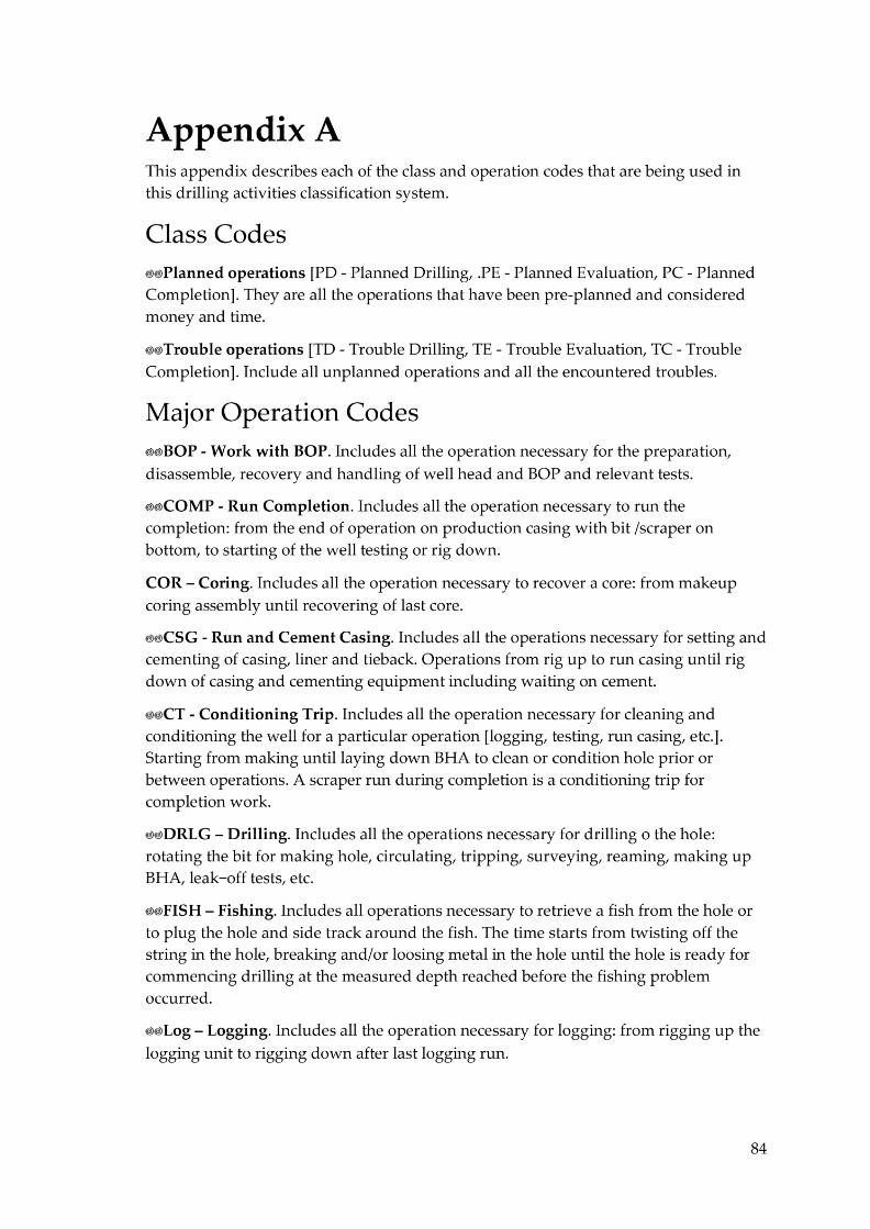
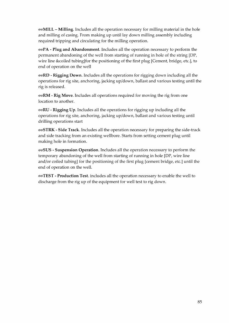
90

Appendix B Software Available in the Market

While using probabilistic estimation and/or Monte Carlo simulation, a number of software can be used as a tool. Software selection differs with users and organizations. Some companies have established their own software or spreadsheet for drilling cost estimating purpose. Some organizations operate available commercial software for their forecast. Frequently, the commercial software used in cost valuation activity is a spreadsheet-based application which allows users to perform Monte Carlo simulation from their present spreadsheet software. Major oil field service companies also offer well cost valuation and risk analysis software as one of their services. In this case, the software providers generally propose other services and/or software which have the potential to enhance the competence of cost estimation.

Model Risk Software

Model Risk is a spreadsheet-based application which is right for prognostic modelling, forecasting, simulation and optimization. It uses Monte Carlo simulation to estimate and record the results of thousands of diverse scenarios. Analysis of these cases exposes the range of possible outcome, their likelihood to occur, the input that most impact the model and the key point that should be focused on.

RiskAnalysis with Model Risk

You can complete a risk analysis in some ways, but one method includes building a spreadsheet model. A good spreadsheet model can be actual helpful in identifying where your risk might be, since cells with formulas and cell references classify causal relationships among variables. One of the disadvantages of conventional spreadsheet models, however, is that you can only enter one value in a cell at a time. A spreadsheet will not let you to enter a range or multiple values for a cell, only one value at a time. So, calculating the range needs you to replace the uncertain value several times to see what effect the minimum, most likely, and maximum values have. Calculating more realistic "what-if" scenarios is the same, except it requires you to transform your spreadsheet even more.

Model Risk helps you outline those uncertain variables in a whole new way: by defining the cell with a range or a set of values. So, you can define your price range let say for an example between 3000$ and 5000$, instead of a using single point estimate of 3200$. This principle can be used for any time we have some uncertainty in our forecast. It then uses the clear range in a simulation. In addition, Model Risk preserves track of the results of each scenario for you.

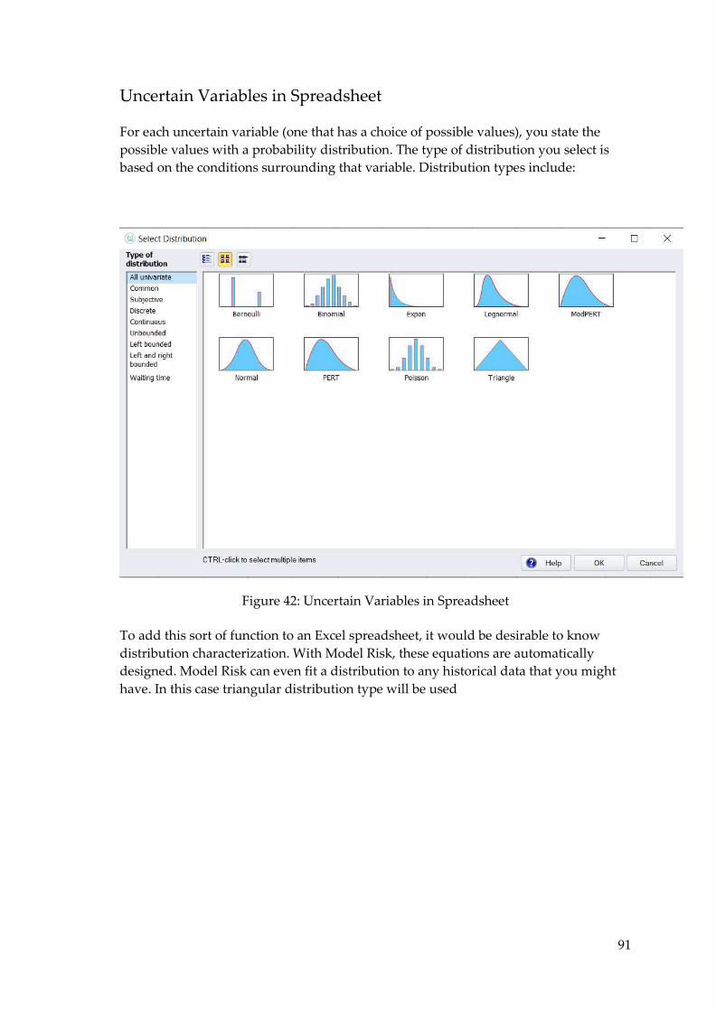
91

Uncertain Variables in Spreadsheet

For each uncertain variable (one that has a choice of possible values), you state the possible values with a probability distribution. The type of distribution you select is based on the conditions surrounding that variable. Distribution types include:

Figure 42: Uncertain Variables in Spreadsheet

To add this sort of function to an Excel spreadsheet, it would be desirable to know distribution characterization. With Model Risk, these equations are automatically designed. Model Risk can even fit a distribution to any historical data that you might have. In this case triangular distribution type will be used

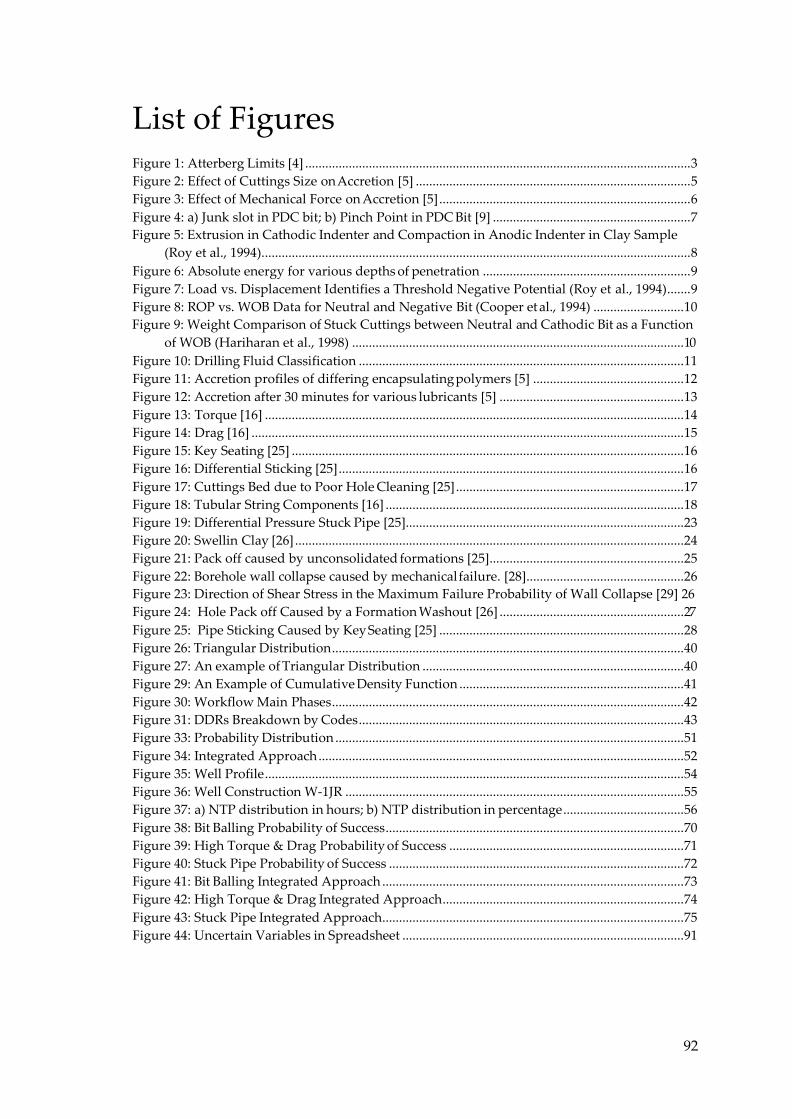
92

List of Figures Figure 1: Atterberg Limits [4] ................................................................................................................... 3 Figure 2: Effect of Cuttings Size on Accretion [5] .................................................................................. 5 Figure 3: Effect of Mechanical Force on Accretion [5] ........................................................................... 6 Figure 4: a) Junk slot in PDC bit; b) Pinch Point in PDC Bit [9] ........................................................... 7 Figure 5: Extrusion in Cathodic Indenter and Compaction in Anodic Indenter in Clay Sample

(Roy et al., 1994). ............................................................................................................................... 8 Figure 6: Absolute energy for various depths of penetration .............................................................. 9 Figure 7: Load vs. Displacement Identifies a Threshold Negative Potential (Roy et al., 1994) ....... 9 Figure 8: ROP vs. WOB Data for Neutral and Negative Bit (Cooper et al., 1994) ........................... 10 Figure 9: Weight Comparison of Stuck Cuttings between Neutral and Cathodic Bit as a Function

of WOB (Hariharan et al., 1998) ................................................................................................... 10 Figure 10: Drilling Fluid Classification ................................................................................................. 11 Figure 11: Accretion profiles of differing encapsulating polymers [5] ............................................. 12 Figure 12: Accretion after 30 minutes for various lubricants [5] ....................................................... 13 Figure 13: Torque [16] ............................................................................................................................. 14 Figure 14: Drag [16] ................................................................................................................................. 15 Figure 15: Key Seating [25] ..................................................................................................................... 16 Figure 16: Differential Sticking [25] ....................................................................................................... 16 Figure 17: Cuttings Bed due to Poor Hole Cleaning [25] .................................................................... 17 Figure 18: Tubular String Components [16] ......................................................................................... 18 Figure 19: Differential Pressure Stuck Pipe [25]................................................................................... 23 Figure 20: Swellin Clay [26] .................................................................................................................... 24 Figure 21: Pack off caused by unconsolidated formations [25] .......................................................... 25 Figure 22: Borehole wall collapse caused by mechanical failure. [28] ............................................... 26 Figure 23: Direction of Shear Stress in the Maximum Failure Probability of Wall Collapse [29] 26 Figure 24: Hole Pack off Caused by a Formation Washout [26] ....................................................... 27 Figure 25: Pipe Sticking Caused by Key Seating [25] ......................................................................... 28 Figure 26: Triangular Distribution ......................................................................................................... 40 Figure 27: An example of Triangular Distribution .............................................................................. 40 Figure 29: An Example of Cumulative Density Function ................................................................... 41 Figure 30: Workflow Main Phases ......................................................................................................... 42 Figure 31: DDRs Breakdown by Codes ................................................................................................. 43 Figure 33: Probability Distribution ........................................................................................................ 51 Figure 34: Integrated Approach ............................................................................................................. 52 Figure 35: Well Profile ............................................................................................................................. 54 Figure 36: Well Construction W-1JR ..................................................................................................... 55 Figure 37: a) NTP distribution in hours; b) NTP distribution in percentage .................................... 56 Figure 38: Bit Balling Probability of Success ......................................................................................... 70 Figure 39: High Torque & Drag Probability of Success ...................................................................... 71 Figure 40: Stuck Pipe Probability of Success ........................................................................................ 72 Figure 41: Bit Balling Integrated Approach .......................................................................................... 73 Figure 42: High Torque & Drag Integrated Approach ........................................................................ 74 Figure 43: Stuck Pipe Integrated Approach.......................................................................................... 75 Figure 44: Uncertain Variables in Spreadsheet .................................................................................... 91

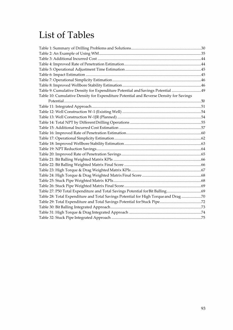
93

List of Tables Table 1: Summary of Drilling Problems and Solutions ....................................................................... 30 Table 2: An Example of Using WM .................................................................................................................. 35 Table 3: Additional Incurred Cost ......................................................................................................... 44 Table 4: Improved Rate of Penetration Estimation .............................................................................. 44 Table 5: Operational Adjustment Time Estimation ............................................................................. 45 Table 6: Impact Estimation ..................................................................................................................... 45 Table 7: Operational Simplicity Estimation .......................................................................................... 46 Table 8: Improved Wellbore Stability Estimation ................................................................................ 46 Table 9: Cumulative Density for Expenditure Potential and Savings Potential .............................. 49 Table 10: Cumulative Density for Expenditure Potential and Reverse Density for Savings

Potential ........................................................................................................................................... 50 Table 11: Integrated Approach ............................................................................................................... 51 Table 12: Well Construction W-1 (Existing Well) ................................................................................ 54 Table 13: Well Construction W-1JR (Planned) ..................................................................................... 54 Table 14: Total NPT by Different Drilling Operations ........................................................................ 55 Table 15: Additional Incurred Cost Estimation ................................................................................... 57 Table 16: Improved Rate of Penetration Estimation ............................................................................ 60 Table 17: Operational Simplicity Estimation ........................................................................................ 62 Table 18: Improved Wellbore Stability Estimation .............................................................................. 63 Table 19: NPT Reduction Savings .......................................................................................................... 64 Table 20: Improved Rate of Penetration Savings ................................................................................. 65 Table 21: Bit Balling Weighted Matrix KPIs ......................................................................................... 66 Table 22: Bit Balling Weighted Matrix Final Score .............................................................................. 66 Table 23: High Torque & Drag Weighted Matrix KPIs ....................................................................... 67 Table 24: High Torque & Drag Weighted Matrix Final Score ............................................................ 68 Table 25: Stuck Pipe Weighted Matrix KPIs ......................................................................................... 68 Table 26: Stuck Pipe Weighted Matrix Final Score .............................................................................. 69 Table 27: P50 Total Expenditure and Total Savings Potential for Bit Balling ................................... 69 Table 28: Total Expenditure and Total Savings Potential for High Torque and Drag .................... 70 Table 29: Total Expenditure and Total Savings Potential for Stuck Pipe .......................................... 72 Table 30: Bit Balling Integrated Approach ............................................................................................ 73 Table 31: High Torque & Drag Integrated Approach ......................................................................... 74 Table 32: Stuck Pipe Integrated Approach ........................................................................................... 75