Research papers

Modelling the inherent optical properties and estimating theconstituents' concentrations in turbid and eutrophic waters

Elamurugu Alias Gokul a, Palanisamy Shanmugam a,n, Balasubramanian Sundarabalan a,Arvind Sahay b, Prakash Chauhan b

a Ocean Optics and Imaging Laboratory, Department of Ocean Engineering, Indian Institute of Technology Madras, Chennai 600036, Indiab Space Applications Centre, Ahmedabad 380015, India

a r t i c l e i n f o

Article history:Received 23 January 2014Received in revised form21 May 2014Accepted 23 May 2014Available online 4 June 2014

Keywords:Remote sensingModellingOptical propertiesChlorophyllTurbidityCoastal waters

a b s t r a c t

Retrieval of the inherent optical properties and estimation of the constituents' concentrations fromsatellite ocean colour data in turbid and eutrophic waters are important as these products provideinnovative opportunities for the study of biological and biogeochemical properties in such opticallycomplex waters. This paper intends to develop models to retrieve absorption coefficients of phyto-plankton, suspended sediments and coloured dissolved organic matter and describe vertical profiles ofchlorophyll and suspended sediments from satellite ocean colour data. These models make use of therelationships between remote sensing reflectance ratios Rrs (555)/Rrs (443) and Rrs (620)/Rrs (490) versus aph(443) and aph (555), and acdom (443), and ad (443) to derive the model parameters. Validation with the in-situdata obtained from coastal waters around India and other regional waters (e.g., NASA bio-Optical MarineAlgorithm Data-Set, NOMAD) shows that the new models are more accurate in terms of producing thespectral absorption coefficients (aph, ad, acdom across the entire visible wavelengths 400–700 nm) in a widevariety of waters. Further comparison with existing models shows advantage of the new models that haveimportant implications for remote sensing of turbid coastal and eutrophic waters. The retrieved absorptioncoefficients of phytoplankton and suspended sediments (non-algal matter) are also found to relate better tochlorophyll and total suspended sediments. Taking advantages of this, we derive models to determine anddescribe the vertical profiles of chlorophyll and suspended sediment concentrations along the depth.The model parameters are derived empirically. These new parameterizations show potential in estimatingthe vertical profiles of chlorophyll and suspended sediments with good accuracy. These results suggestrobustness and suitability of the new models for studying the ecologically important components of opticallycomplex turbid and eutrophic waters using remote sensing data.

& 2014 Elsevier Ltd. All rights reserved.

1. Introduction

Understanding the dynamic processes of turbid and eutrophicwaters is extremely important in ecological and remote sensingstudies as their constituents such as phytoplankton, suspendedsediments and coloured dissolved organic matter fluctuate largelyover a short period of time due to the various physical, chemical,biological and geological processes (Edwards et al., 2004;Urtizberea et al., 2013; Greenwood and Craig, 2014). These threesubstances are generally considered to be responsible for varia-tions in the absorption coefficients phytoplankton, non-algal

particles (decomposed phytoplankton and suspended sediments)and coloured dissolved organic matter (also known as yellowsubstances). For the past decades, considerable progress has beenmade to understand the relationships between absorption coeffi-cients and chlorophyll and suspended sediment concentrations(Bricaud et al., 1995, 1998; Garver et al., 1994; Reynolds et al.,2001), because these properties modulate the underwater lightfields having impact on aquatic life and transport and transforma-tion processes from local, regional to global scales (Shanmugam,2011a).

Though shipboard measurements of such properties are gen-erally accurate and useful, their coverage and sampling are limitedin both space and time leading to potentially biased results. In therecent decades, satellite remote sensing has been identified as aneffective tool to provide a synoptic description of the various

Contents lists available at ScienceDirect

journal homepage: www.elsevier.com/locate/csr

Continental Shelf Research

http://dx.doi.org/10.1016/j.csr.2014.05.0130278-4343/& 2014 Elsevier Ltd. All rights reserved.

n Corresponding author.E-mail address: pshanmugam@iitm.ac.in (P. Shanmugam).

Continental Shelf Research 84 (2014) 120–138

optical and biological properties of marine waters, to addressmarine environmental issues, and to investigate a variety of topicsincluding marine primary productivity, ecosystem dynamics, sedi-mentation and pollution (Steidinger and Haddad, 1981; Campbelland Esaias, 1983; Carder and Steward, 1985; Harding et al., 1992;Behrenfeld and Falkowski, 1997; Andrew Bailey and Werdell,2006; Marrari et al., 2006; Volpe et al., 2007; Platt et al., 2009;Brewin et al., 2010). Though some success has been achieved inthe above studies, the retrieval of optical properties and constitu-ents' concentrations of coastal oceanic waters from satellite oceancolour data remains a severe problem due to uncertainties in thealgorithm design and uncertainties in the satellite-derived reflec-tance products.

Oceanic colour remote sensing is a very difficult inversionproblem in which conceptual and practical limits are oftenencountered. This means that retrieving as much information aspossible about the water body is to be solely from water-leavingradiances or remote sensing reflectances. These measurementsmay contain substantial errors due to poor atmospheric correctionor inaccurate radiometric calibration (Le and Hu, 2013; RakeshKumar and Shanmugam, 2014). More recent studies (Shanmugamet al., 2010; Surya Prakash and Shanmugam, 2013) have addressedsome of the key issues and inherent difficulties of inverting remotesensing reflectance measurements to obtain the inherent opticalproperties (IOPs) and constituents' concentrations of coastal ocea-nic waters (see Shanmugam et al., 2010 and references therein).

10°30’0’’N

10°0’0’’N

9°30’0’’N

79°0’0’’E 79°30’0’’E 80°0’0’’E 80°30’0’’E 81°0’0’’E

79°0’0’’E 79°30’0’’E 80°0’0’’E 80°30’0’’E 81°0’0’’E

10°30’0’’N

10°0’0’’N

9°30’0’’N

90°0’0’’W 85°0’0’’W 80°0’0’’W 75°0’0’’W

40°0’0’’N

35°0’0’’N

30°0’0’’N

25°0’0’’N

90°0’0’’W 85°0’0’’W 80°0’0’’W 75°0’0’’W

40°0’0’’N

35°0’0’’N

30°0’0’’N

25°0’0’’N

Fig. 1. (a) Location map with station points in highly turbid waters off Point Calimere on the southeast coast of India. Note that this region is always dominated by a highlevel of turbidity due to the prevailing oceanographic conditions. (b) Location map with sampling points for the NOMAD data (west coast of Florida and Chesapeake bay)used in this study.

E.A. Gokul et al. / Continental Shelf Research 84 (2014) 120–138 121

Inversions are often effected based on an assumed model thatrelates the known quantities (as inputs) and the desired quantities(as outputs). The model may be simple if historical data relatingcertain IOPs or water constituents' concentrations to the ratio ofremote sensing reflectance at two or more wavelengths are usedto find a best-fit function with some empirically derived coeffi-cients (Shanmugam, 2011a, 2011b and references therein). Theaccuracy of the estimated property by that model will depend onthe scatter in the original data, and on whether the water bodybeing studied is similar to the one used to determine the function.Other methods are also used to invert remote sensing reflectanceto derive the IOPs and water constituents' concentrations, forinstance, a neural network method in which it is often not obvioushow a particular input is related to a particular output. Thus, theaccuracy of a neural network inversion depends on how wellthe neural network represents nature and on the data used to trainthe network algorithm. Solving direct problems through radiativetransfer models to predict the reflectance for each of many differentsets of IOPs is another way by which the IOPs associated with thepredicted reflectances that mostly match the measured reflectancesare taken to be the solution of the inversion problem (Sundarabalanet al., 2013 and references therein). Unfortunately, in such directproblems a small error (say 5%) in the IOPs or boundary conditionsleads to a correspondingly small error in the computed radiance (andthus reflectance). With inversion problems such small errors in thecomputed radiometric quantities could lead to large errors, or evenunphysical results in the retrieved IOPs (see the results in SuryaPrakash and Shanmugam (2013)). Analytical and some semi-analytical models are examples though they appear in principle tobe quite complex and satisfactory.

Direct inversion of ocean colour is generally composed of twosteps: deriving inherent optical properties (IOPs) from apparentoptical properties (AOPs) and then retrieving water constituents'concentrations such as chlorophyll-a (Chl-a), coloured dissolvedorganic matter (CDOM), and total suspended sediments (TSS) fromthe derived IOPs.

The first part of the paper outlines the empirical relationshipsbetween AOPs (e.g., Remote sensing reflectance) and IOPs (absorptioncoefficients of phytoplankton pigments, suspended sediments andcoloured dissolved organic matter). These algorithms use the blue–green reflectance ratios to derive the respective absorption coefficientsby means of polynomial and exponential functions. The majority ofthe band ratio algorithms use the ratios of Rrs (443)/Rrs (555), Rrs (490)/Rrs (555) and Rrs (620)/Rrs (490) (Gross et al., 2000; Shanmugam, 2011a,2011b; Surya Prakash and Shanmugam, 2012). These algorithms arewidely used because of the ease of computation, which allows fastprocessing of the remotely sensed data. The purpose of retrieving IOPs

and constituents' concentrations of the water column from remotesensing data is to enable studies for monitoring ecologically importantcomponents, biological and biochemical properties of turbid andeutrophic waters at a high temporal scale.

This paper also compares the results of new models withthose of the existing techniques (such as the constrained LinearMatrix (LM) model by Boss and Roesler (2006); multiband quasi-analytical model (QAA) by Lee et al. (1996), GSM semi-analyticalmodel (GSM) by Maritorena et al. (2002) (IOCCG Report Number5 at http://www.ioccg.org/reports_ioccg.html), Tiwari–Shanmu-gam model (TS) by Surya Prakash and Shanmugam (2013), CDOMmodel by Shanmugam (2011), and ag model by Lee et al. (2002))using a large number of in-situ data from coastal waters aroundsouthern India and other regional waters (NOMAD data). The IOPsare calculated at specific bands in the visible domain (i.e., 412, 443,490, 510, 555 and 670 nm) since the absorption coefficients of IOPsare better pronounced (high) in these bands. The IOPs retrievedand used for this comparison include the absorption coefficients ofphytoplankton aph(λ), coloured dissolved organic matter acdom(λ)and detrital particles ad(λ). The mean relative error (MRE), rootmeans square error (RMSE) and regression coefficients are com-puted and used to quantify uncertainties of the derived IOPs.

The second part of the paper aims to estimate the verticalprofiles of chlorophyll and total suspended sediment concentra-tions. The Chl-a vertical profile is often used in analytical andempirical models to estimate total biomass and primary produc-tion from satellite ocean colour data (Sathyendranath and Platt,1993). Previously, efforts have been made to determine Chl-avertical profiles based on a Gaussian distribution model. Moreland Berthon (1989) observed some systematic trends in Chl-aprofile shapes which were related to nine tropic categories anddeveloped a global algorithm for estimating the profile para-meters, which define the whole Chl-a profile regardless of theregion and season. Platt et al. (1988) and Lewis et al. (1983)proposed a more general Gaussian distribution superimposed on aconstant background to describe Chl-a profiles that may beobserved in coastal, upwelling, open oceans and Arctic waters(Siswanto et al., 2005; Kameda and Matsumura, 1998). However,when the global algorithms are applied to a regional scale thealgorithm performance is often reduced (Wozniak et al., 2000;Siegel et al., 2001). Therefore, tuning the model parameterizationfor a specific region seems to be a reasonable option if one is toestimate the Chl-a vertical profile. The present study also aimsto determine the spatial and temporal variability of chlorophyll, todetermine the association among four parameters which controlthe vertical distribution of chlorophyll pigment, and to establishan empirical relationship between those parameters (in surfacelayers) so that satellite data can be used to determine the verticalprofiles of chlorophyll in turbid coastal and eutrophic waters.Turbidity is widely used as a surrogate for TSS, since it is easilymonitored and recorded by turbidity probes that can be readilydeployed in-situ (Glysson and Gray, 2002; Lewis, 2002;Schoellhamer, 2002; Old et al., 2003). In this case, turbidity canbe continuously recorded and converted to a record of TSS usingan empirically derived calibration relationship relating TSS toturbidity (Jean et al., 2008). This study presents a model toestimate TSS profiles and compare these profiles with the observedprofiles in turbid coastal waters.

2. Data and methods

2.1. In-situ data

In-situ bio-optical data were collected from around 75 stationsin coastal waters off Point Calimere on the southeast part of India.

Phytoplankton absorption coefficient aph (λ) Detritus absorption coefficient ad (λ)

CDOM absorption coefficient acdom (λ)

Chlorophyll Chl-a and Total suspended sediment concentrations at the surface level

Estimation of Chl-a and TSS vertical profiles along the depth

Remote sensing reflectance (Rrs)

Fig. 2. Summary of the steps involved in the development and application of ourmodels.

E.A. Gokul et al. / Continental Shelf Research 84 (2014) 120–138122

Fig. 1a shows the location map with sampling stations from wherethese in-situ data were collected on different cruises during 12–20August 2012, 03–11 July 2013 and 24–31 August 2013. To makethe model suitable for highly eutrophic waters, in-situ datawere also obtained in bloom-dominated lagoon waters aroundChennai (map not shown for brevity). Thus, our in-situ data are

representative of a wide range of optical conditions encounteredin moderately clear, turbid and eutrophic waters. Besides, anupdated NASA bio-Optical Marine Algorithm Data Set (hereafterreferred to as “NOMAD”) (Werdell and Bailey, 2005) was obtainedfrom the NASA Ocean Biology Processing Group and used to assessthe performance of the models. Though the NOMAD dataset is a

0.001

0.01

0.1

1

0.01 0.1 1 10Rrs(555/443)

a ph(

443)

(m-1

)

NOMADIndian

0.0001

0.001

0.01

0.1

1

10

0.1 1 10Rrs(555/443)

a ph(6

70)m

-1)

0.0001

0.001

0.01

0.1

1

0.01 0.1 1 10Rrs(620/490)

a d(4

43)(

m-1

)

0.001

0.01

0.1

1

10

100

0.0001 0.01 1 100aph(443)(m-1)

Chl

(mg

m-3

)

1

10

100

1000

ad(443)(m-1)

TSS

(g m

-3)

1

10

100

1000

0.01 0.1 1 10 100Turbidity

TSS

(g m

-3)

0.001

0.01

0.1

1

1010

0.01 0.1 1 10

0.1 1 10Rrs(555/443)

a cdo

m(4

43)(m

-1)

Fig. 3. (a and b) Relationships between aph(443), aph(670) and Rrs(555)/Rrs(443) from the in-situ data (N¼180), (c and d) relationships between ad(443), acdom(443) andRrs(620/490), Rrs(555/443), respectively, from the in-situ data (N¼180), (e and f) relationships between Chl, TSS and aph(443) and ad(443), respectively, from thein-situ data, and (g) relationship between turbidity and TSS from the Indian in-situ data.

E.A. Gokul et al. / Continental Shelf Research 84 (2014) 120–138 123

global, high quality in-situ bio-optical data set collected over awide range of optical properties, tropic status, and geographicallocations in open ocean waters, estuaries, and coastal waters(NE4459), a careful examination of these data pertaining to ourstudy in turbid coastal waters resulted in 246 data that contain theabsorption coefficients of phytoplankton (aph), detrital particles(ad), and coloured dissolved organic matter (acdom) and remotesensing reflectance (Rrs) data essentially from similar waters onthe west coast of Florida, Tamba Bay and Chesapeake Bay (Chenet al., 2010; Cannizzaro et al., 2013; Le and Hu, 2013). This datasetis conveniently split into two parts – NOMAD-1 (N¼120) forderiving model parameters and coefficients and NOMAD-2(N¼126) for validating the model results. Similarly, the in-situdata collected from relatively clear, turbid and eutrophic waters onthe southeast coast of India consist of aph, ad, and acdom and Rrsdata; some of which are used for the model parameterizations (soas to represent a wide variety of waters including eutrophicwaters) and the remaining data are reserved for validating themodel results. The NOMAD in-situ data have the following pairs ofdata with significant variability – aph (443) 0.0086 to 0.68 and Rrs(443) 0.0005 to 0.0084; ag (443) 0.0066 to 0.70065 and Rrs (443)0.0007 to 0.0217; ad (443) 0.00076 to 0.23256 and Rrs (443) 0.0008to 0.0144). The Indian in-situ data contain aph (443) 0.034 to 0.49and Rrs (443) 0.00049–0.04173; ag (443) 0.072 to 0.25 and Rrs (443)0.001676–0.019203; ad (443) 0.008995 to 1.156759 and Rrs (443)0.00049–0.04173. Many of these data include coastal stationsthat are affected by constituents other than phytoplankton suchas coloured matter and suspended sediments from land-run off.Because of the insufficient in-situ measurements it is difficult tosubdivide these data and regions in an objective way.

2.2. In-situ IOP measurements data

The in-situ profiles of the inherent optical properties, fluores-cence chlorophyll, turbidity, and physical oceanographic data(salinity, temperature and depth) were obtained by several sensorsnamely AC-S, BB9 and FLNTU (WETLAB Inc.) and CTD (Seabird)sensors. These sensors mounted on an underwater frame werelowered into the water column using a winch system on the shipand a single cable was used to transmit power to the instrumentsand data to a rugged laptop computer on the deck. The AC-Sinstrument was used to measure the absorption coefficient (a) andbeam attenuation coefficient (c) in the visible wavelengths (350–750 nm) as a function of depth. Temperature and salinity correc-tions were applied to the measured absorption and attenuationcoefficients (Pegau et al., 1997; Sundarabalan et al., 2013). The BB9sensor was used to measure the backscattering coefficients “bb” atnine wavelengths 412, 440, 488, 510, 532, 595, 650, 676 and 715.The FLNTU sensors were used to measure chlorophyll and turbid-ity and the SeaBird CTD sensor to measure the conductivity–temperature–depth profile data.

2.2.1. In-situ phytoplankton and detrital (non-algal) particleabsorption data

Water samples for the determination of optical properties ofphytoplankton and detrital particles were collected from eachstation using Niskin bottles (and pre-rinsed bucket for surfacewaters) and filtered through 25 mm glass fibre filters (WhatmanGF/F) under low vacuum pressure. Optical densities of totalparticulate matter (ODtot(λ)) retained on the filter were measuredusing the glass-fibre filter technique and the absorption coeffi-cients of total particles were computed. The absorption coeffi-cients of non-algal particles were determined by a methanolextraction technique and were subtracted with total absorptioncoefficients to obtain the absorption coefficients of phytoplankton.Detailed procedures of determining these absorption coefficientscan be found in Ahn and Shanmugam (2007). For each station,absorption coefficients of total particles, non-algal particles andphytoplankton were calculated as follows (Mitchell et al., 2002):

atotðλÞ ¼2:3Af

βVf½½ODfpðλÞ�ODbf ðλÞ��ODnull� ð1Þ

adðλÞ ¼2:3Af

βVf½½ODf ssðλÞ�ODbf ðλÞ��ODnull� ð2Þ

aphðλÞ ¼ atotðλÞ�adðλÞ ð3Þ

where Vf is the volume of water filtered, Af the filter paperclearance area, ODfp the optical density of particulate filter, ODfss

the optical density of suspended sediments filter (particulate filterafter methanol extraction), ODbf the optical density of blank filter,ODnull the optical density at the near infrared wavelength. Nullwavelength residual correction with the near infrared wavelengthwhere particle absorption is minimal was performed. β the pathlength amplification correction factor which is given below

β¼ C0þC1½ODfpðλÞ�ODnullðλÞ�C2 ð4Þ

where C0¼0.0, C1¼1.220 and C2¼�0.254 are the coefficients ofleast squares regression fits of the measured data (Mitchell,1990).

2.2.2. In-situ CDOM absorption dataGenerally, CDOM absorption coefficients were obtained

by spectrophotometric measurements after filtration of watersamples through 0.45 μm membrane syringe filters (25 mm)previously rinsed with ultra pure Milli-Q water. During eachsampling, 50 ml of filtered samples were collected and stored inglass flasks in the dark at 4 1C for analysis in laboratory. Afterreturning to the laboratory, samples for spectrophotometric ana-lyses were allowed to warm to room temperature and absorbancescans from 350 to 900 nm (at 1 nm sample intervals) wereconducted using a Shimadzu UV–Visible Spectrophotometer(UV-2600) and Perkin-Elmer Lambda-35 Spectrophotometer. Theabsorbance measurements were performed by placing a 10 cmquartz cuvette containing Milli-Q water in the optical path of thereference beam, and a 10 cm quartz cuvette containing the filteredseawater sample in the optical path of the sample beam. Thespectral absorption coefficients of CDOM were then computedfrom the measured absorbance (Shanmugam, 2011a; Mitchell etal., 2002). For each station, CDOM absorption coefficients weredetermined as follows:

agðλÞ ¼2:303

l½½ODsðλÞ�ODbsðλÞ��ODnull� ð5Þ

where ODs,bs,null is the optical density of filtrate water, purifiedwater (FSW), at null absorption wavelength, optical path length:l¼0.1 m¼10 cm and ag referred in unit as m�1.

Table 1Spectral constant values obtained from the relationships of phytoplankton aph(λ)versus the remote sensing reflectance ratio [Rrs (555)/Rrs (443)] fitted to cubicpolynomial function with R2 0.90-0.91.

λ (nm) a0 a1 a2 a3

412 0.0008 0.0304 0.0376 �0.0048443 0.088 0.0047 0.0547 �0.0067489 0.0102 � 0.0145 0.0464 �0.0059510 0.0058 0.0125 0.0356 �0.0045555 �0.0008 0.0029 0.0131 �0.0019670 0.0043 � 0.0214 0.0448 �0.0063683 0.0058 � 0.0281 0.0424 �0.0059

E.A. Gokul et al. / Continental Shelf Research 84 (2014) 120–138124

2.2.3. In-situ total suspended sediments concentrationThe surface water samples were collected from each station

using Niskin bottles (pre-rinsed bucket for surface waters) forthe determination of suspended sediment concentration. Thesesamples were then filtered through 25 mm glass fibre filters(Whatman GF/F) under low vacuum pressure (approximately120 mmHg) and subsequently weighed (w1). After filtration, thefilter papers were dried at 60 1C for 4 h and weighed (w2) (at roomtemperature). For each station, total suspended sediment concen-tration was determined as follows:

TSS¼ ðw2�w1Þ=ðV � 0:001Þ ð6Þwhere V is the volume of water filtered and TSS is the totalsuspended sediments (in units of g m�3).

2.3. In-situ AOP measurements data

The remote sensing reflectance is a measure of radianceresulting from the photons that emerge the ocean surface indirection (θ,ϕ) (often called water-leaving radiance Lw (W m�2

nm�1 sr�1)) to the sunlight incident at the surface (often calledsurface irradiance) Es (W m�2 nm�1), so that it can be detected bypassive remote sensors (radiometer) pointed in the oppositedirection. Reflected light in the visible domain (400–700 nm) isparticularly useful in the study of upper ocean processes as manyimportant biogeochemical components of the seawater absorb and

scatter light effectively in this spectral range. For each station, in-situ radiometric measurements (above the seawater) were carriedout using RAMSES (Trios) hyperspectral radiometers. The totalradiance (Lt), sky radiance (Lsky) and downwelling irradiance (Edþ)were measured by RAMSES ARC and ACC sensors. The MSDA_XEsoftware was used to record the radiance and irradiance data andexport them from the database to a PC on the deck for furtherprocessing. The measured total radiance data were subsequentlycorrected for the contribution of skylight reflection Lsky and Fresnelreflectance (ρ) of air–sea interface using Lw ¼ Lt�ρLsky (ρ¼0.028)in order to determine the desired water-leaving radiance (Lw)which is the key quantity that carries enormous information aboutthe optical properties of the ocean (Shanmugam, 2011a, 2011b).For each station, remote sensing reflectance was calculated asfollows:

Rrsð0þ λÞ ¼ LwðλÞ=Edð0þλÞ ð7ÞThe Rrs(λ), referred in units of sr�1, is an apparent optical property

(AOP) that contains the information on the water constituents.

3. Model description

Establishing the relationships between remote sensing reflec-tance and respective absorption coefficients have allowed us toderive empirical equations to estimate the absorption coefficients

0

5

10

15

20

Chlsurface

Chl

max

0

2

4

6

8

10

12

Chlsurface

Zmax

0

1

2

3

4

5

Chlsurface

sigm

a

0

1

2

3

4

5

6

7

8

Chlsurface

Chl

max

02468

10121416

Chlsurface

Zmax

0

1

2

3

4

5

0 2 4 6 8 10 0 2 4 6 8 10 02 4 6 8 10

0 0.2 0.4 0.6 0.8 1 0 0.2 0.4 0.6 0.8 1 0 0.2 0.4 0.6 0.8 1

Chlsurface

sigm

a

Fig. 4. (a–c) Regression lines for the Gaussian parameters for chlorophyll in high concentration category. (d–f) Regression lines for the Gaussian parameters for chlorophyll inLow concentration category.

Table 2Empirical formula to estimate the Gaussian parameters as a function of the surface Chlorophyll concentration for two scenarios.

Gaussian parameters High concentration (1.0 mg m�3rChlsurface) R2 Gaussian parameters Low concentration(Chlsurfaceo1.0 mg m�3) R2

Chlmax 2.5455� (Chlsurface)�1.5661 0.9 Chlmax �8.2880� (Chlsurface)þ3.662 0.8ZM 0.7614� (Chlsurface)þ3.9007 0.87 ZM �12.247� (Chlsurface)þ35.479 0.8Sigma �0.402� (Chlsurface)þ4.395 0.92 Sigma 3.1606� (Chlsurface)þ11.199 0.8

E.A. Gokul et al. / Continental Shelf Research 84 (2014) 120–138 125

of phytoplankton, detrital matter and coloured dissolved sub-stances in clear, turbid and eutrophic waters. Fig. 2 schematicallyshows the major steps involved in the development and applica-tion of such models, which are described in detail in what follows.

3.1. Absorption coefficient

The total absorption coefficients can be partitioned into indi-vidual contributions of the optically active constituents of

seawater such as water molecules aw, phytoplankton aph, coloureddissolved organic matter acdom and detrital particles ad.

aðλÞ ¼ awðλÞþaphðλÞþacdomðλÞþadðλÞ ð8ÞThe aw(λ) values are constants taken from Pope and Fry (1997).

All other absorption coefficients of the seawater constituents aretreated as variables and parameterized as a function of the remotesensing reflectance ratios (Rrs (555)/Rrs (443) and Rrs (620)/Rrs(490)).

10-4

10-2

100

102

Insitu - aph(443)[m-1]

Mod

el -

a ph(4

43)[m

-1]

10-4

10-2

100

102

Insitu - aph(490)[m-1]

Mod

el -

a ph(4

90)[m

-1]

10-4 10-2 100 102 10-6 10-4 10-2 100 10210-6

10-4

10-2

100

102

Insitu - aph(510)[m-1]

Mod

el -

a ph(5

10)[m

-1]

10-6

10-4

10-2

100

102

Insitu - aph(555)[m-1]

Mod

el -

a ph(5

55)[m

-1]

10-6 10-4 10-2 100 102 10-6 10-4 10-2 100 10210-6

10-4

10-2

100

102

Insitu - aph(670)[m-1]

Mod

el -

a ph(6

70)[m

-1]

10-6 10-4 10-2 100 10210-6

10-4

10-2

100

102

Insitu - aph(683)[m-1]

Mod

el -

a ph(6

83)[m

-1]

10-4 10-2 100 10210-4 10-2 100 102

10-4

10-2

100

102

Insitu - aph(412)[m-1]

Mod

el -

a ph(4

12)[m

-1] GS

QAALMTSNM

Fig. 5. Comparison of the modelled aph(λ) with in-situ aph(λ) data from other regional waters (NOMAD). Note that the Rrs (683) values were not available for the QAA toproduce aph (683).

E.A. Gokul et al. / Continental Shelf Research 84 (2014) 120–138126

3.1.1. Absorption by phytoplanktonA new empirical algorithm for estimating aph(λ) has been

developed based on the remote sensing reflectance ratio (Rrs(555)/Rrs (443)) and aph(λ) values in the specified visible wave-lengths (412, 443, 490, 531, 555, 670 and 683 nm) (Surya Prakashand Shanmugam, 2012). This model gives estimates of aph withspecified Rrs(λ) values, like the chlorophyll (Chl) parameterization.Similar parameterizations for determining the shapes of aph(λ) forall visible wavelengths (400–700 nm) are derived using theNOMAD-1 in-situ data and India in-situ data (Fig. 3a and b andTable 1). The relationships between the spectral absorption

coefficients of phytoplankton at 443–683 nm versus the remotesensing reflectance ratio Rrs (555)/Rrs (443) provide the best-fitrelationships with notably high correlation coefficients for thesewavelengths. The model constants obtained from these relation-ships represent a third order polynomial equation which isexpressed as

aph ¼ a0ðλÞþa1ðλÞ �Rrsð555ÞRrsð443Þ

� �þa2ðλÞ �

Rrsð555ÞRrsð443Þ

� �2

þa3ðλÞ �Rrsð555ÞRrsð443Þ

� �3

ð9Þ

10-4

10-2

100

102

Insitu - aph(443)[m-1]

Mod

el -

a ph(4

43)[m

-1]

10-4

10-2

100

102

Insitu - aph(490)[m-1]

Mod

el -

a ph(4

90)[m

-1]

10-4 10-2 100 102 10-4 10-2 100 10210-4

10-2

100

102

Insitu - aph(510)[m-1]M

odel

- a ph

(510

)[m-1

]

10-4

10-2

100

102

Insitu - aph(670)[m-1]

Mod

el -

a ph(6

70)[m

-1]

10-4 10-2 100 10210-4

10-2

100

102

Insitu - aph(683)[m-1]

Mod

el -

a ph(6

83)[m

-1]

10-4 10-2 100 10210-4 10-2 100 10210-4

10-2

100

102

Insitu - aph(555)[m-1]

Mod

el -

a ph(5

55)[m

-1]

10-4 10-2 100 10210-4 10-2 100 10210-4

10-2

100

102

Insitu - aph(412)[m-1]

Mod

el -

a ph(4

12)[m

-1] GSM

QAALMTSNM

Fig. 6. Comparison of the modelled aph(λ) with in-situ aph(λ) data from Indian waters. Note that the Rrs(683) values were not used (for brevity) for the QAA to produce aph(683).

E.A. Gokul et al. / Continental Shelf Research 84 (2014) 120–138 127

In the above equation, λ is the wavelength and a0, a1, a2, and a3are the constants. The spectral values of the coefficients a0, a1, a2,and a3 of the cubic polynomial equation represent the variation ofaph(λ) as a function of the remote sensing reflectance ratio at 555and 443 nm.

3.1.2. Absorption by coloured dissolved organic matter and detritalparticles

The coloured dissolved organic matter and detrital particleshave similar absorption spectral shapes (both vary exponentiallywith wavelength), thus they are modelled by an exponentialrelation (Shanmugam, 2011a).

acdom=d ¼ acdom=dðλrÞ � e�Sðλ�λr Þ ð10Þ

where λr is the reference wavelength at 443 nm. S is the spectralslope coefficient (nm�1) of exponential that determines theshape of the absorption curve acdom/d. The value of spectral slopeparameter (Sd/cdom) was derived for the wavelengths 400–700 nmaccording to Surya Prakash and Shanmugam (2013).

Sd=cdom ¼ 1443�412

� �� log 10

ad=cdomð412Þad=cdomð443Þ

!ð11Þ

The empirical relationships between ad (443), acdom (443)and Rrs (620)/Rrs (490) and Rrs (555)/Rrs (443) respectively wereestablished using the NOMAD-1 in-situ data and Indian in-situdata (Fig. 3c and d). A goodness of fit was found between ad (443),acdom (443) and Rrs (620)/Rrs (490) and Rrs (555)/Rrs (443) withcorrelation coefficient (R2)40.9. Statistical regression analysesdemonstrated the best-fit power functions as described below:

adð443Þ ¼ 0:3314� Rrsð620ÞRrsð490Þ

� �1:516

R2 ¼ 0:93 ð12Þ

acdomð443Þ ¼ 0:1005� Rrsð555ÞRrsð443Þ

� �1:4499

R2 ¼ 0:92 ð13Þ

3.2. Estimating chlorophyll and total suspended sediments at seasurface level from IOPs

Satellite retrieval of chlorophyll-a concentration in oceanicwaters is considerably more complex than the laboratory filterpad absorption measurements of aph and the correspondingchlorophyll extraction. However, it can be shown that Chl-a isdirectly proportional to the phytoplankton absorption coefficientsand this forms the basis for the retrieval algorithm developed inthis study. Fig. 3e and f shows that the phytoplankton andsuspended sediment (detrital) absorption coefficients at 443 nmare found to relate to the measured Chl-a concentration (mg m�3)and total suspended sediments (TSS) concentration (g m�3) by thepower law relations

Chl¼ AðaphÞB ð14Þ

TSS¼ AðadÞB ð15Þ

Chl¼ 29:127� ðaphð443ÞÞ1:3184 ð16Þ

TSS¼ 55:823� ðadð443ÞÞ0:5269 with R2 ¼ 0:9 ð17ÞHolliday et al. (2003) derived an empirical relationship bet-

ween turbidity (NTU) and the total suspended sediment concen-tration (TSS, g m�3), as shown in Fig. 3g. A goodness of fit wasfound between TSS and NTU, with correlation coefficient (R2) 0.9.

TSS¼ 19:52� ðNTUÞ0:4414 ð18Þ

where A and B are the empirical coefficients. These power functionequations are found adequate to describe the constituents' con-centrations in turbid and eutrophic waters of the study area.

3.3. Estimating chlorophyll and total suspended sediments verticalprofiles

The vertical profiles of chlorophyll-a was fitted to the followingequation (Lewis et al., 1983):

ChlðzÞ ¼ Chlsurf aceþChlmax � eð� ðZ�ZM Þ=2s2Þ ð19ÞThe Gaussian curve is determined by four parameters, Chlsurface

is chlorophyll-a (mg m�3) at surface level, Chlmax the maximumchlorophyll concentration, ZM the depth of subsurface chlorophyllmaximum (in metres), and (s) the standard deviation (in metres).All four parameters derived from the fitting procedure werecalculated using our in-situ data. Fig. 4 shows that linear regres-sion models of the Chlmax, ZM, and Sigma (s) as a function ofsurface chlorophyll have good agreement to built the Gaussiancurve. Table 2 is the list of linear regression equations to estimatethe three Gaussian parameters (Chlmax, ZM and Sigma) as a functionof surface chlorophyll concentrations. All regression models haveR2 greater than 0.8. Chlorophyll concentrations at the sea surface(Chlsurface) were grouped into the two categories of high concen-tration (1.0 mg m�3rChlsurface) and low concentration (Chlsurfaceo1.0 mg m�3). The criterion for defining these two categories wasthat Chlmax and ZM have to be statistically different in eachcategory at the 100% confidence level. These categories coincideclosely with the trophic categories defined by Morel and Berthon(1989) for the world oceans, and they represent waters rangingfrom very oligotrophic (with integrated chlorophyll less than10 mg m�2) to very eutrophic (integrated chlorophyll more than100 g m�2) situations. Finally, the capability of these models inestimating the vertical distribution was tested using the in-situdata from several cruises in relatively clear and turbid coastalwaters of southern India (off Point Calimere) during August 2012to November 2013. The vertical profiles of the suspended sedimentconcentration were fitted to the following equation:

TSSðZÞ ¼ TSSSurf ace � ððZ�1Þ0:0383Þ ð20Þwhere TSSSurface is the concentration of total suspended sedimentsat surface level (g m�3) and Z is the depth (in metres). If one canmeasure TSS at the surface level by the absorption coefficients ofdetrital particles, then the depth profiles of the TSS can beestimated accurately by considering the surface TSS as a referencedepth and the mean slope can be calculated from in-situ data(Ritchie et al., 1978).

4. Results

4.1. Absorption coefficient of phytoplankton

The new model and existing inversion models were applied totwo independent in-situ data sets (NOMAD-2 in-situ data and ourin-situ data) and the results were examined carefully to assesstheir validity and associated issues. Comparison of these modelresults with in-situ data shows that the results of the new modelshave good agreement with the in-situ aph data for the selectedseven wavelengths (412, 443, 490, 530, 555, 670 and 683 nm)(Figs. 5 and 6). Other models tend to either overestimate orunderestimate the aph values at different wavelengths. Whenapplied to the NOMAD-2 in-situ data, it is evident that the LMmodel produced abnormally/erroneously high values (i.e., 10 m�1

at 412–555 nm) – i.e., N¼10 out of N¼126 valid data (for NOMADdata) and N¼5 out of 60 valid data (for Indian in-situ data). On the

E.A. Gokul et al. / Continental Shelf Research 84 (2014) 120–138128

other hand, the QAA model produced negative aph(λ) values andthe number of negative values varied among the key wavelengths:for example 3 negative values at 490 nm and 13 negative values at510 nm and 683 nm for the NOMAD data. The GSM model alsoproduced some negative values for the NOMAD and Indian data,but its number of negative aph(λ) values was minimal compared tothat of the QAA model (note that these negative values are notshown in the log–log scatter plots). Though the TS model showsgood agreement with in-situ data when compared to the LM, QAA

and GSMmodels, its RMSE andMRE values (see Fig. 11) are noticeablyhigher than those of the new model. As a result, the new modelretrieved more accurate aph values at all the key wavelengths (withno abnormal and negative values). The abnormal and negative valuesproduced by the LM and QAA models could be related to theirimproper parameterizations, eventually limiting the use of oceancolour data to derive the phytoplankton absorption coefficients inturbid coastal waters and other regional waters (Shanmugam et al.,2010; Surya Prakash and Shanmugam, 2013).

10-4

10-2

100

102

Insitu - ad(412)[m-1]

Mod

el -

a d(412

)[m-1

]

10-4 10-2 100 102 10-6 10-4 10-2 100 10210-6

10-4

10-2

100

102

Insitu - ad(443)[m-1]

Mod

el -

a d(443

)[m-1

]

10-6

10-4

10-2

100

102

Insitu - ad(490)[m-1]

Mod

el -

a d(490

)[m-1

]

10-6 10-4 10-2 100 102 10-6 10-4 10-2 100 10210-6

10-4

10-2

100

102

Insitu - ad(510)[m-1]M

odel

- a d(5

10)[m

-1]

10-6

10-4

10-2

100

102

Insitu - ad(555)[m-1]

Mod

el -

a d(555

)[m-1

]

10-6 10-4 10-2 10010-6

10-4

10-2

100

Insitu - ad(683)[m-1]

Mod

el -

a d(683

)[m-1

]

10-6 10-4 10-2 100 10210

-610

-410

-210

010-6

10-4

10-2

100

Insitu - a d(670)[m-1]

Mod

el -

ad

(670

)[m-1

]

Fig. 7. Comparison of the modelled ad(λ) with in-situ ad(λ) data from other regional waters (NOMAD).

E.A. Gokul et al. / Continental Shelf Research 84 (2014) 120–138 129

4.2. Absorption coefficient of detrital particles

The simple empirical relationship between the reflectance ratio(Rrs (620)/Rrs (490)) and absorption coefficients of detrital particlesat a reference wavelength 443 nm presented in this study is anattempt to derive ad(λ) products, since most of the previousmodels have been developed to retrieve the combined products

of dissolved organic matter and detrital particles. Here twoindependent in-situ data sets (NOMAD-2 in-situ data and Indianin-situ data) were used to assess the performance of the newmodel. Figs. 7 and 8 compare the model estimates of ad(λ) within-situ ad(λ) data from the above in-situ data sets. The new modelresults appear to be in good agreement with in-situ ad(λ) data forthe selected seven wavelengths (412, 443, 490, 530, 555, 670 and

10-4 10-2 100 10210-4

10-2

100

102

Insitu - ad(443)[m-1]

Mod

el -

a d(443

)[m-1

]10-4

10-2

100

102

Insitu - ad(490)[m-1]

Mod

el -

a d(490

)[m-1

]

10-4 10-2 100 102 10-4 10-2 100 10210-4

10-2

100

102

Insitu - ad(510)[m-1]

Mod

el -

a d(510

)[m-1

]

10-4

10-2

100

102

Insitu - ad(555)[m-1]

Mod

el -

a d(555

)[m-1

]

10-6 10-4 10-2 100 10210-6

10-4

10-2

100

102

Insitu - ad(683)[m-1]

Mod

el -

a d(683

)[m-1

]

10-4 10-2 100 102 10-6 10-4 10-2 100 10210-6

10-4

10-2

100

102

Insitu - ad(670)[m-1]

Mod

el -

a d(6

70)[m

-1 ]

10-4 10-2 100 10210-4

10-2

100

102

Insitu - ad(412)[m-1]

Mod

el -

a d(412

)[m-1

]

Fig. 8. Comparison of the modelled ad(λ) with in-situ ad(λ) data from Indian waters.

E.A. Gokul et al. / Continental Shelf Research 84 (2014) 120–138130

683 nm). Note that the results of the new model for high ad values(samples collected in eutrophic waters with high levels of detritalparticles) are closely consistent with in-situ ad(λ) and generallyfollow the 1:1 line (Fig. 8). The statistical results are summarizedin Table 3 for all the selected wavelengths from 412 to 683 nm. It isevident that the new model ad(λ) values show very good agree-ment with in-situ aph(λ) at 412, 443, 490, 555, 670 and 683 nm,with low statistical errors (RMSE – 0.30–0.38 with an average of0.30, MRE – 0.08–0.05 with an average of �0.009, slope – 0.86–0.83, R2 – 0.78–0.86, intercept values – 0.38–0.49 for NOMAD data;RMSE – 0.29–0.32 with an average of 0.25, MRE – 0.30–0.017 withan average of �0.08, slope – 0.94–1.2, R2 – 0.80–0.91, interceptvalues – 0.16–0.42 for Indian data). The above results are encoura-ging because the ad, as an important biogeochemical property, isnearly empirically derived from the ocean colour measurements.This approach is highly applicable to both highly turbid andeutrophic waters.

4.3. Absorption coefficient of coloured dissolved organic matter

Application of the three inversion models (including newmodel-NM) applied to two independent data sets shows that thenew model performed better than other two models (Shanmugam(2011) CDOM model and Lee ag model) in terms of producingaccurate acdom(λ) values for the selected seven wavelengths (412,443, 490, 530, 555, 670 and 683 nm). Figs. 9 and 10 show thescatter plots of the model acdom versus in-situ acdom at thesewavelengths. The acdom(λ) derived from the Shanmugam (2011)CDOM model show good agreement with the NOMAD in-situ data,although deviating (underestimation) with Indian in-situ dataespecially at longer wavelengths (and toward higher acdom values).The Lee model highly underestimates acdom(λ) values at all thewavelengths (most data points below the 1:1 line) for both theNOMAD and Indian in-situ data. Statistical error analyses per-formed on these two data sets (Fig. 12) indicate significantly lowerrors for the new model than for the other two models (acrossthe entire visible wavelengths). These results clearly demonstratethat the new model definitely improved the accuracy of acdom(λ)retrievals when compared to the existing models in turbid andeutrophic waters.

4.4. Validation of the modelled chlorophyllwith in-situ data

On the basis of the inversion model, a new absorption-basedchlorophyll algorithm has been derived. Fig. 13 shows that theabsorption IOP-based retrievals of chlorophyll are better compar-able with 60 in-situ chlorophyll surface data collected from coastalwaters around southern India. Unlike the reflectance ratio algo-rithms, the new IOP-based algorithm allows studies of chlorophyllvariability as a function of phytoplankton and CDOM absorption.The new model that is based on the linear relationship to estimatethree Gaussian parameters (Chlmax, ZM, and Sigma) as a function ofthe surface chlorophyll predicts chlorophyll vertical profiles withgood accuracy. Once the vertical distribution of chlorophyllis determined, these three parameters can be obtained morereliably. To test our algorithm predicting the Gaussian parameterswith chlorophyll data, the in-situ data collected from turbid andeutrophic waters around southern India were used. Fig. 14 showsthe comparison between the modelled chlorophyll vertical profilesand in-situ chlorophyll vertical profiles. It becomes obvious thatthe depth profiles of chlorophyll predicted by the new model arein good agreement with those of the in-situ data, therebyconfirming the validity of the present model.

4.5. Validation of the modelled total suspended sediments datawith in-situ data

The substantial agreement of the IOP-based retrievals of TSSand in-situ TSS from coastal waters around southern India isshown in Fig. 15. The scatter plot depicts good agreement betweenthe modelled TSS and in-situ TSSwith the correlation coefficient R2

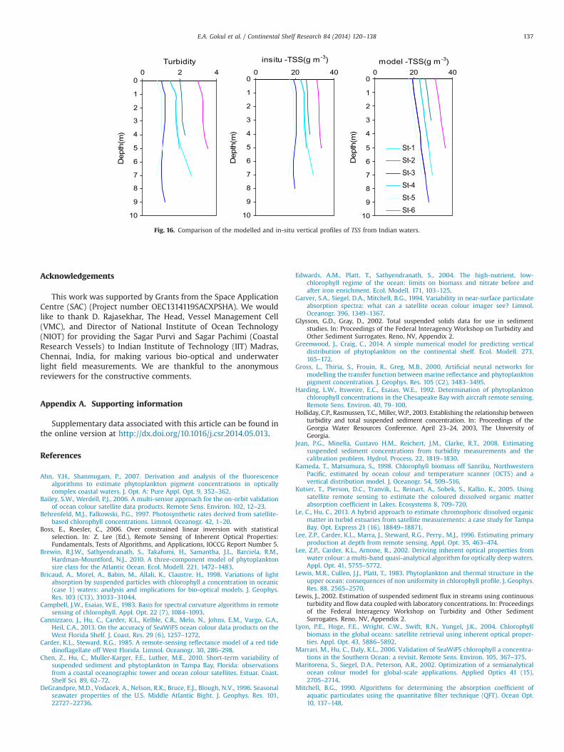
– 0.8. Fig. 16 shows that the vertical profiles of TSS predicted by thenew model are better comparable with the in-situ profiles of TSSfor different scenarios.

5. Discussion

Assessment of the biogeochemical variables especially in turbidand eutrophic waters is extremely important for ecological andenvironmental studies. To date, there are only a few studies on theIOP modelling and retrieval of water constituents in these waters.To overcome the limitations of the previous models, new modelshave been developed in this study to produce accurate absorptioncoefficient products and water constituents' concentrations inhighly turbid and eutrophic waters. The results of the existinginversion models when applied to two different independent datasets (NOMAD-2 in-situ data and our in-situ data) showed anapparent deviation with the measured absorption coefficients inhighly turbid waters. By contrast, results of the newmodel showedgood agreement with the in-situ absorption coefficients (aph, adand acdom). Several empirical and semi-analytical models exist toderive aph (λ) products from satellite ocean colour data. However,most of these models are generally applicable to open oceanwaters. The new model is more suitable for retrieving phytoplank-ton absorption coefficients from satellite ocean colour data inhighly turbid and eutrophic waters. The performance of this modelwas assessed using two independent data sets and its results werecompared with those of the existing inversion models (e.g., LM,GSM, QAA and TS). These inversion models showed large discre-pancies between their modelled values and in-situ data in highlyturbid and eutrophic waters. In particular, GSM predicted aphvalues at 412 nm highly deviating from the in-situ data. On theother hand, the QAA modelled aph values at 670 nm showed pooragreement with in-situ data. Compared to the QAA and GSM, theLM predicted aph values had good agreement with in-situ data at

Table 3Statistical comparisons between the modelled and in-situ data (NOMAD and Indianin-situ data).

MRE Bias RMSE R2 Slope Intercept

NOMAD-2 in-situ dataad (412) �0.082 �0.159 0.304 0.866 0.869 �0.389ad (443) �0.059 �0.124 0.287 0.868 0.856 �0.405ad (490) �0.025 �0.058 0.270 0.865 0.838 �0.419ad (510) �0.015 �0.037 0.270 0.862 0.832 �0.434ad (555) 0.008 0.021 0.280 0.850 0.818 �0.457ad (670) 0.053 0.169 0.367 0.791 0.800 �0.495ad (683) 0.057 0.185 0.381 0.780 0.801 �0.492Average �0.082 �0.159 0.304 0.866 0.869 �0.389

Indian in-situ dataad (412) 0.302 0.217 0.297 0.910 0.946 0.167ad (443) 0.178 0.161 0.251 0.915 0.963 0.122ad (490) 0.101 0.114 0.224 0.913 1.002 0.117ad (510) 0.054 0.068 0.221 0.902 1.050 0.134ad (555) 0.003 0.004 0.185 0.922 1.060 0.095ad (670) �0.006 �0.011 0.308 0.829 1.219 0.422ad (683) �0.017 �0.036 0.329 0.806 1.227 0.425Average 0.302 0.217 0.297 0.910 0.946 0.167

E.A. Gokul et al. / Continental Shelf Research 84 (2014) 120–138 131

blue green wavelengths. The failure and instability of theseinversion models in turbid coastal waters are already discussedin Shanmugam et al. (2010) and Surya Prakash and Shanmugam(2013). Though the aph values predicted by the TS model closelymatched with the NOMAD in-situ data across the entire visiblewavelength region, it still yielded errors when applied to theIndian in-situ data. However, the new model seemed to be stableacross the entire visible wavelength region (with low errors) whenapplied to both the Indian in-situ data and NOMAD in-situ data.Thus, one can expect more accurate aph products from this newmodel using satellite data.

The dynamic variation of the absorption coefficients of detritalparticles (suspended sediments and non-algal matter) is usuallyhigh in turbid coastal and eutrophic waters. Our model resultssuggest that the reflectance ratio (Rrs(620)/Rrs(490)) is best suited inretrieving more accurate ad(λ) values in these waters. On the otherhand, satellite remote sensing has the potential to monitor CDOMdistributions in the global ocean at high spatial and temporal scales,enabling to scale up to the level of large ecosystems and biomes(Kutser et al., 2005; Zhao et al., 2009). Currently, a few Inversionmodels (including the Shanmugam (2011) model and Lee ag model)are used to derive the absorption coefficients of coloured dissolved

10-4 10-2 100 10210-4

10-2

100

102

Insitu - acdom

(443)[m-1]

Mod

el -

acd

om(4

43)[m

-1]

10-6 10-4 10-2 100 10210-6

10-4

10-2

100

102

Insitu - acdom

(490)[m-1]

Mod

el -

a cdom

(490

)[m-1

]

10-6 10-4 10-2 100 10210-6

10-4

10-2

100

102

Insitu - acdom(510)[m-1]M

odel

- a cd

om(5

10)[m

-1]

10-6 10-4 10-2 100 10210-6

10-4

10-2

100

102

Insitu - acdom(555)[m-1]

Mod

el -

a cdom

(555

)[m-1

]

10-6

10-4

10-2

100

10-6

10-4

10-2

100

Insitu - acdom

(683)[m-1]

Mod

el -

a cdom

(683

)[m-1

]

10-4 10-2 100 10210-4

10-2

100

102

Insitu - acdom(412)[m-1]

Mod

el -

a cdom

(412

)[m-1

] Shanmugam2011 modelLee modelNM

10-8 10-6 10-4 10-2 100 10210-8

10-6

10-4

10-2

100

102

Insitu - acdom(670)[m-1]

Mod

el -

a cdom

(670

)[m-1

]

Fig. 9. Comparison of the modelled acdom(λ) with in-situ acdom(λ) data from other regional waters (NOMAD).

E.A. Gokul et al. / Continental Shelf Research 84 (2014) 120–138132

organic matter in coastal and open ocean waters. When applied tothe independent in-situ data sets, these models produced acdom (λ)values with relatively large errors in highly turbid and eutrophicwaters. By contrast, acdom(λ) estimates of the new model wereconsistent with in-situ acdom(λ) data when compared to those of theother two models applied to the same in-situ data sets. As a result,the MRE values, slopes, intercepts and R2 values were found quitestable across the entire visible wavelengths, and were considerablylower than those of the other two models which signify that betterestimates occur in waters with rich acdom content.

On the basis of the historical reflectance ratios, ship-bornemeasurement findings (DeGrandpre et al., 1996) and radiativetransfer theory, a new absorption-based chlorophyll algorithm has

been derived. For chlorophyll variability, the exact role of CDOMabsorption is not yet understood but it is hypothesized here to berelated to phytoplankton photoacclimation, i.e., the increasedabsorption of CDOM leads to decreased light availability (Lyonet al., 2004; Shanmugam, 2011a). In this study, we have describedempirical models for inferring the vertical structure of Chl-awithin the water column by estimating the three profile para-meters (Chlmax, ZM, and Sigma) that determine the Chl-a profileshape. These parameters have been derived from Chlsurface regard-less of the season and water mass features. ZM is the parameterthat demonstrates a clear, gradual deepening from the clear waterto turbid water region. Such a across-shelf successive change in ZMoccurs concurrently with decreasing Chlsurface, enabling ZM to be

10-4 10-2 100 10210-4

10-2

100

102

Insitu - acdom(443)[m-1]

Mod

el -

a cdom

(443

)[m-1

]

10-4 10-2 100 10210-4

10-2

100

102

Insitu - acdom(490)[m-1]

Mod

el -

a cdom

(490

)[m-1

]

10-4 10-2 100 10210-4

10-2

100

102

Insitu - acdom(510)[m-1]M

odel

- a cd

om(5

10)[m

-1]

10-4 10-2 100 10210-4

10-2

100

102

Insitu - acdom(555)[m-1] Insitu - acdom(670)[m-1]

Mod

el -

a cdom

(555

)[m-1

]

10-6 10-4 10-2 100 10210-6

10-4

10-2

100

102M

odel

- a cd

om(6

70)[m

-1]

10-4 10-2 100 10210-4

10-2

100

102

Insitu - acdom(683)[m-1]

Mod

el -

a cdom

(683

)[m-1

]

10-4 10-2 100 102 10410-4

10-2

100

102

104

Insitu - acdom(412)[m-1]

Mod

el -

a cdom

(412

)[m-1

]

Shanmugam2011 modelLee modelNM

Fig. 10. Comparison of the modelled acdom(λ) with in-situ acdom(λ) data from Indian waters.

E.A. Gokul et al. / Continental Shelf Research 84 (2014) 120–138 133

0

0.5

1

1.5

2

2.5

3

Wavelemgth (nm)

RM

SE

-0.6

-0.4

-0.2

0

0.2

0.4

0.6

Wavelemgth (nm)

MR

E

-0.4

-0.2

0

0.2

0.4

0.6

0.8

Wavelemgth (nm)

BIA

S

-2.5-2

-1.5-1

-0.50

0.51

1.52

Wavelemgth (nm)

INTE

RC

EP T

00.20.40.60.8

11.21.41.61.8

2

Wavelemgth (nm)

SLO

PE

00.10.20.30.40.50.60.70.80.9

1

Wavelemgth (nm)

R2

-2

-1.5

-1

-0.5

0

0.5

1

1.5

2

Wavelemgth (nm)

-1-0.8-0.6-0.4-0.2

00.20.40.60.8

1

Wavelemgth (nm)

-1.5

-1

-0.5

0

0.5

1

1.5

Wavelemgth (nm)

00.20.40.60.8

11.21.41.61.8

2

Wavelemgth (nm)

00.10.20.30.40.50.60.70.80.9

1

Wavelemgth (nm)

0

0.5

1

1.5

2

2.5

3

3.5

4

412 443 490 510 555 670 683

412 443 490 510 555 670 683

412 443 490 510 555 670 683

412 443 490 510 555 670 683

412 443 490 510 555 670 683

412 443 490 510 555 670 683

412 443 490 510 555 670 683

412 443 490 510 555 670 683

412 443 490 510 555 670 683

412 443 490 510 555 670 683

412 443 490 510 555 670 683

412 443 490 510 555 670 683

Wavelemgth (nm)

R2

INTE

RC

EPT

MR

EB

IAS

SLO

PE

RM

SE

NM TS

QAA GSM

LM

Fig. 11. Results of the statistical analyses (RMSE, MRE, Bias, intercept, slope and R2 from top to bottom) performed on the (a) NOMAD-2 in-situ aph(λ) data (N¼120) and(b) Indian in-situ aph(λ) data (N¼60).

E.A. Gokul et al. / Continental Shelf Research 84 (2014) 120–138134

00.20.40.60.8

11.21.41.6

412 443 490 510 555 670

Wavelength (nm)R

MS

E

NMShanmugam(2011)modelLee model

-0.1

0.1

0.3

0.5

412 443 490 510 555 670

Wavelength (nm)

MR

E

-0.4

-0.2

0

0.2

0.4

0.6

0.8

1

1.2

412 443 490 510 555 670

Wavelength (nm)

BIA

S

-0.8

0

0.8

1.6

2.4

412 443 490 510 555 670

Wavelength (nm)

INTE

RC

EP

T

0

0.8

1.6

2.4

412 443 490 510 555 670

Wavelength (nm)

SLO

PE

0

0.2

0.4

0.6

0.8

1

412 443 490 510 555 670

Wavelength (nm)

R

0

0.4

0.8

1.2

1.6

2

2.4

412 443 490 510 555 670

Wavelength (nm)

RM

SE

-0.40

0.40.81.21.6

22.42.83.23.6

4

412 443 490 510 555 670

Wavelength (nm)

MR

E

-0.4

0

0.4

0.8

1.2

1.6

2

2.4

412 443 490 510 555 670

Wavelength (nm)

BIA

S

-1

0

1

2

3

4

5

412 443 490 510 555 670

Wavelength (nm)

INTE

RC

EP

T

0

1

2

3

4

412 443 490 510 555 670

Wavelength (nm)

SLO

PE

0

0.2

0.4

0.6

0.8

1

412 443 490 510 555 670

Wavelength (nm)

R

Fig. 12. Results of the statistical analyses (RMSE, MRE, Bias, intercept, slope and R2 from top to bottom) performed on the (a) NOMAD-2 in-situ acdom(λ) data (N¼90) and(b) Indian in-situ acdom(λ) data (N¼45).

E.A. Gokul et al. / Continental Shelf Research 84 (2014) 120–138 135

well predicted from Chlsurface and accounted for 470% of thevariation in measured ZM. In most studies on the prediction ofChl-profiles parameters, ZM seemed to be the most predic-table parameter, because of its gradual variability along thelatitudinal, across-shelf and from the coast to offshore directions(Sathyendranath et al., 1995; Watt et al., 1999; Richardson et al.,2003).

6. Conclusion

In the present study, new empirical methods have beendeveloped to estimate the absorption coefficients of phytoplank-ton, detrital particles and coloured dissolved organic matter atcertain key wavelengths (412, 443, 490, 510, 555, 670 and683 nm). These absorption coefficients were used to determinethe concentration of chlorophyll and total suspended sediments atjust below the water surface from which the extended verticalprofiles of Chl and TSS were estimated at each station. The modelsuse the remote sensing reflectance (Rrs) as an input to estimate therequired IOPs (aph, ad and acdom) and subsequently predict Chl andTSS concentrations at surface and bottom layers of the watercolumn. The absorption coefficients derived by the present modelswere not only validated with in-situ data but also compared with

the existing inversion techniques (such as GSM, QAA, LM, TSmodel, Shanmugam (2011) CDOM model, and Lee ag model). Thecomparison of the new model results with two independent in-situ data sets (NOMAD and Indian data) showed good agreementbetween the predicted and observed values of the absorptioncoefficients and water constituents' concentrations. The newmodels produce excellent absorption spectral curves in the entirevisible wavelength region. The newmodels overcome many issues,reduce uncertainty in the retrieved absorption products andprovide greater stability (with low errors) across the entire visiblewavelengths. Vertical distributions of the chlorophyll in coastalwaters around southern India can be estimated from chlorophyllat the surface, which makes it possible to calculate three para-meters (Chlmax, ZM, and Sigma) of the Gaussian curve. Based on thetotal suspended sediment concentration estimated at the surfacelevel, the vertical profiles of TSS can be estimated. The resultsobtained from this study clearly demonstrate that the new modelscan be used to produce accurate IOP (absorption) products, waterconstituents' concentrations (Chl-a and TSS concentration) andtheir vertical profiles in turbid coastal waters. The present modelswould be helpful to extend the radiative transfer models to give usthe ability to predict the underwater light field distributions forprimary production calculation and various ecological studies incoastal waters around southern India.

0.01

0.1

1

10

100

0.01 0.1 1 10 100In situ - Chl (mg m-3)

Mod

el -

Chl

(mg

m-3)

Fig. 13. Comparison of the modelled Chl concentration with in-situ Chl concentra-tion from Indian waters.

0

2

4

6

8

10

12

14

16

18

20

Dep

th (m

)

0

2

4

6

8

10

12

14

16

18

20

0 10 20 30 0 10 20 30In-situ Chl (mg m-3) model-Chl (mg m-3)

Dep

th (m

)

St-1

St-2

St-3

St-4

St-5

Fig. 14. Comparison of the modelled chlorophyll vertical profile data with in-situ chlorophyll vertical profile data from Indian waters.

1

10

100

1000

1 10 100 1000

In situ-TSS(g m-3)

mod

el -T

SS

(g m

-3)

Fig. 15. Comparison of the modelled TSS concentration with in-situ TSS concentra-tion data from Indian waters.

E.A. Gokul et al. / Continental Shelf Research 84 (2014) 120–138136

Acknowledgements

This work was supported by Grants from the Space ApplicationCentre (SAC) (Project number OEC1314119SACXPSHA). We wouldlike to thank D. Rajasekhar, The Head, Vessel Management Cell(VMC), and Director of National Institute of Ocean Technology(NIOT) for providing the Sagar Purvi and Sagar Pachimi (CoastalResearch Vessels) to Indian Institute of Technology (IIT) Madras,Chennai, India, for making various bio-optical and underwaterlight field measurements. We are thankful to the anonymousreviewers for the constructive comments.

Appendix A. Supporting information

Supplementary data associated with this article can be found inthe online version at http://dx.doi.org/10.1016/j.csr.2014.05.013.

References

Ahn, Y.H., Shanmugam, P., 2007. Derivation and analysis of the fluorescencealgorithms to estimate phytoplankton pigment concentrations in opticallycomplex coastal waters. J. Opt. A: Pure Appl. Opt. 9, 352–362.

Bailey, S.W., Werdell, P.J., 2006. A multi-sensor approach for the on-orbit validationof ocean colour satellite data products. Remote Sens. Environ. 102, 12–23.

Behrenfeld, M.J., Falkowski, P.G., 1997. Photosynthetic rates derived from satellite-based chlorophyll concentrations. Limnol. Oceanogr. 42, 1–20.

Boss, E., Roesler, C., 2006. Over constrained linear inversion with statisticalselection. In: Z. Lee (Ed.), Remote Sensing of Inherent Optical Properties:Fundamentals, Tests of Algorithms, and Applications, IOCCG Report Number 5.

Brewin, R.J.W., Sathyendranath, S., Takafumi, H., Samantha, J.L., Barciela, R.M.,Hardman-Mountford, N.J., 2010. A three-component model of phytoplanktonsize class for the Atlantic Ocean. Ecol. Modell. 221, 1472–1483.

Bricaud, A., Morel, A., Babin, M., Allali, K., Claustre, H., 1998. Variations of lightabsorption by suspended particles with chlorophyll a concentration in oceanic(case 1) waters: analysis and implications for bio-optical models. J. Geophys.Res. 103 (C13), 31033–31044.

Campbell, J.W., Esaias, W.E., 1983. Basis for spectral curvature algorithms in remotesensing of chlorophyll. Appl. Opt. 22 (7), 1084–1093.

Cannizzaro, J., Hu, C., Carder, K.L., Kelble, C.R., Melo, N., Johns, E.M., Vargo, G.A.,Heil, C.A., 2013. On the accuracy of SeaWiFS ocean colour data products on theWest Florida Shelf. J. Coast. Res. 29 (6), 1257–1272.

Carder, K.L., Steward, R.G., 1985. A remote-sensing reflectance model of a red tidedinoflagellate off West Florida. Limnol. Oceanogr. 30, 286–298.

Chen, Z., Hu, C., Muller-Karger, F.E., Luther, M.E., 2010. Short-term variability ofsuspended sediment and phytoplankton in Tampa Bay, Florida: observationsfrom a coastal oceanographic tower and ocean colour satellites. Estuar. Coast.Shelf Sci. 89, 62–72.

DeGrandpre, M.D., Vodacek, A., Nelson, R.K., Bruce, E.J., Blough, N.V., 1996. Seasonalseawater properties of the U.S. Middle Atlantic Bight. J. Geophys. Res. 101,22727–22736.

Edwards, A.M., Platt, T., Sathyendranath, S., 2004. The high-nutrient, low-chlorophyll regime of the ocean: limits on biomass and nitrate before andafter iron enrichment. Ecol. Modell. 171, 103–125.

Garver, S.A., Siegel, D.A., Mitchell, B.G., 1994. Variability in near-surface particulateabsorption spectra: what can a satellite ocean colour imager see? Limnol.Oceanogr. 396, 1349–1367.

Glysson, G.D., Gray, D., 2002. Total suspended solids data for use in sedimentstudies. In: Proceedings of the Federal Interagency Workshop on Turbidity andOther Sediment Surrogates. Reno, NV, Appendix 2.

Greenwood, J., Craig, C., 2014. A simple numerical model for predicting verticaldistribution of phytoplankton on the continental shelf. Ecol. Modell. 273,165–172.

Gross, L., Thiria, S., Frouin, R., Greg, M.B., 2000. Artificial neural networks formodelling the transfer function between marine reflectance and phytoplanktonpigment concentration. J. Geophys. Res. 105 (C2), 3483–3495.

Harding, L.W., Itsweire, E.C., Esaias, W.E., 1992. Determination of phytoplanktonchlorophyll concentrations in the Chesapeake Bay with aircraft remote sensing.Remote Sens. Environ. 40, 79–100.

Holliday, C.P., Rasmussen, T.C., Miller, W.P., 2003. Establishing the relationship betweenturbidity and total suspended sediment concentration. In: Proceedings of theGeorgia Water Resources Conference. April 23–24, 2003, The University ofGeorgia.

Jean, P.G., Minella, Gustavo H.M., Reichert, J.M., Clarke, R.T., 2008. Estimatingsuspended sediment concentrations from turbidity measurements and thecalibration problem. Hydrol. Process. 22, 1819–1830.

Kameda, T., Matsumura, S., 1998. Chlorophyll biomass off Sanriku, NorthwesternPacific, estimated by ocean colour and temperature scanner (OCTS) and avertical distribution model. J. Oceanogr. 54, 509–516.

Kutser, T., Pierson, D.C., Tranvik, L., Reinart, A., Sobek, S., Kallio, K., 2005. Usingsatellite remote sensing to estimate the coloured dissolved organic matterabsorption coefficient in Lakes. Ecosystems 8, 709–720.

Le, C., Hu, C., 2013. A hybrid approach to estimate chromophoric dissolved organicmatter in turbid estuaries from satellite measurements: a case study for TampaBay. Opt. Express 21 (16), 18849–18871.

Lee, Z.P., Carder, K.L., Marra, J., Steward, R.G., Perry., M.J., 1996. Estimating primaryproduction at depth from remote sensing. Appl. Opt. 35, 463–474.

Lee, Z.P., Carder, K.L., Arnone, R., 2002. Deriving inherent optical properties fromwater colour: a multi-band quasi-analytical algorithm for optically deep waters.Appl. Opt. 41, 5755–5772.

Lewis, M.R., Cullen, J.J., Platt, T., 1983. Phytoplankton and thermal structure in theupper ocean: consequences of non uniformity in chlorophyll profile. J. Geophys.Res. 88, 2565–2570.

Lewis, J., 2002. Estimation of suspended sediment flux in streams using continuousturbidity and flow data coupled with laboratory concentrations. In: Proceedingsof the Federal Interagency Workshop on Turbidity and Other SedimentSurrogates. Reno, NV, Appendix 2.

Lyon, P.E., Hoge, F.E., Wright, C.W., Swift, R.N., Yungel, J.K., 2004. Chlorophyllbiomass in the global oceans: satellite retrieval using inherent optical proper-ties. Appl. Opt. 43, 5886–5892.

Marrari, M., Hu, C., Daly, K.L., 2006. Validation of SeaWiFS chlorophyll a concentra-tions in the Southern Ocean: a revisit. Remote Sens. Environ. 105, 367–375.

Maritorena, S., Siegel, D.A., Peterson, A.R., 2002. Optimization of a semianalyticalocean colour model for global-scale applications. Applied Optics 41 (15),2705–2714.

Mitchell, B.G., 1990. Algorithms for determining the absorption coefficient ofaquatic particulates using the quantitative filter technique (QFT). Ocean Opt.10, 137–148.

0

1

2

3

4

5

6

7

8

9

10

insitu -TSS(g m-3)

Dep

th(m

)

0

1

2

3

4

5

6

7

8

9

10

Turbidity

Dep

th(m

)

0

1

2

3

4

5

6

7

8

9

10

0 20 400 2 4 0 20 40model -TSS(g m-3)

Dep

th(m

)

St-1

St-2

St-3

St-4

St-5

St-6

Fig. 16. Comparison of the modelled and in-situ vertical profiles of TSS from Indian waters.

E.A. Gokul et al. / Continental Shelf Research 84 (2014) 120–138 137

Mitchell, B.G., Kahru, M., Wieland, J., Stramska, M., 2002. Determination of spectralabsorption coefficients of particles, dissolved material and phytoplankton fordiscrete water samples. Ocean Optics Protocols for Satellite Ocean ColourSensor Validation, Revision, 3, pp. 231–257.

Morel, A., Berthon, J.F., 1989. Surface pigments, algal biomass profiles and potentialproduction of the euphotic layer: relationships reinvestigated in view ofremote-sensing applications. Limnol. Oceanogr. 34, 1545–1562.

Old, G.H., Leeks, G.J.L., Packman, J.C., Smith, B.P.G., Lewis, S., Hewitt, E.J., Holmes, M.,Young, A., 2003. The impact of a convectional summer rainfall event on riverflow and fine sediment transport in a highly urbanised catchment Bradford,West Yorkshire. Sci. Total Environ. 314, 495–512.

Pegau, W.S., Gray., D., Zaneveld., J.R.V., 1997. Absorption and attenuation of visibleand near-infrared light in water: dependence on temperature and salinity.Appl. Opt. 36 (24), 6035–6046.

Platt, T., Sathyendranath, S., Caverhill, C.M., Lewis, M.R., 1988. Ocean primaryproduction and available light: further algorithms for remote sensing. Deep-SeaRes. (A) 35, 855–879.

Platt, T., White III, G.N., Zhai, L., Sathyendranath, S., Roy, S., 2009. The phenology ofphytoplankton blooms: ecosystem indicators from remote sensing. Ecol.Modell. 220 (21), 3057–3069.

Pope, R.M., Fry, E.S., 1997. Absorption spectrum (380–700 nm) of pure water. II.Integrating cavity measurements. Appl. Opt. 36, 8710–8723.

Rakesh Kumar, S., Shanmugam, P., 2014. A novel method for estimation of aerosolradiance and its extrapolation in the atmospheric correction of satellite dataover optically complex oceanic waters. Remote Sensing of Environment 142,188–206.

Reynolds, R.A., Stramski, D., Mitchell, B.G., 2001. A chlorophyll-dependent Semi-analytical model derived from field measurements of absorption and back-scattering coefficients within the Southern Ocean. J. Geophys. Res. 106,7125–7138.

Richardson, A.J., Silulwane, N.F., Mitchell-Innes, B.A., Shillington, F.A., 2003.A dynamic quantitative approach for predicting the shape of phytoplanktonprofiles in the ocean. Prog. Oceanogr. 59 (2–3), 301–319.

Ritchie, J.C., McHenry, J.R., Schiebe, F.R., 1978. The vertical distribution of suspendedsediments in reservoirs. J. Water Pollut. Control Fed. 50 (4), 734–738.

Sathyendranath, S., Platt, T., 1993. Estimators of primary production for interpreta-tion of remotely sensed data on ocean colour. J. Geophys. Res. 98, 14561–14576.

Sathyendranath, S., Longhurst, A., Caverhill, C.M., Platt, T., 1995. Regionally andseasonally differentiated primary production in the North Atlantic. Deep-SeaRes. (I) 42, 1773–1802.

Schoellhamer, D.H., 2002. Use of optical properties to monitor turbidity andsuspended-sediment concentration. In: Proceedings of the Federal InteragencyWorkshop on Turbidity and Other Sediment Surrogates. Reno, NV, pp. 15–16.

Siegel, D.A., Westberry, T.K., O'Brien, M.C., Nelson, N.B., Michaels, A.F., Morrison, J.R.,Scott, A., Caporelli, E.A., Sorensen, J.C., Maritorena, S., Garver, S.A., Brody, E.A.,

Ubante, M.A., Hammer, M.A., 2001. Bio-optical modelling of primary produc-tion on regional scales: the Bermuda Bio Optics project. Deep-Sea Res. 48 (II),1865–1896.

Siswanto, E., Ishizaka, J., Yokouchi, K., 2005. Estimating chlorophyll-a verticalprofiles from satellite data and the implication for primary production in theKuroshio Front of the East China Sea. J. Oceanogr. 61, 575–589.

Shanmugam, P., Ahn, Y.H., Ryu, J.H., Sundarabalan, V.B., 2010. An evaluation ofinversion models for retrieval of inherent optical properties from ocean colourin coastal and open sea waters around Korea. J. Oceanogr. 66 (6), 815–830.

Shanmugam, P., 2011a. New models for retrieving and partitioning the coloureddissolved organic matter in the global ocean: implications for remote sensing.Remote Sens. Environ. 115, 1501–1521.

Shanmugam, P., 2011b. A new bio-optical algorithm for the remote sensing of algalblooms in complex ocean waters”. J. Geophys. Res. 116, 1–12.

Sundarabalan, V.B., Shanmugam, P., Manjusha, S.S., 2013. Radiative transfer model-ling of upwelling light field in coastal waters. J. Quant. Spectrosc. Radiat. Transf.121, 30–44.

Steidinger, K.A., Haddad, K.D., 1981. Biologic and hydrographic aspects of red tides.Bioscience 31 (11), 814–819.

Surya Prakash, T., Shanmugam, P., 2013. An evaluation of models for the satellite-estimation of phytoplankton absorption coefficients in coastal/oceanic waters.IEEE J. Sel. Top. Appl. Earth Obs. Remote Sens. 7, 364–371.

Surya Prakash, T., Shanmugam, P., 2012. An optical model for the remote sensing ofabsorption coefficients of phytoplankton in oceanic/coastal waters. Adv.Remote Sens. 1 (2), 19–34.

Urtizberea, A., Dupont, N., Rosland, R., Aksnes, D.L., 2013. Sensitivity of euphoticzone properties to CDOM variations in marine ecosystem models. Ecol. Modell.256, 16–22.

Volpe, G., Santoleri, R., Vellucci, V., Ribera d'Alcala, M., Marullo, S., D'Ortenzio, F.,2007. The colour of the Mediterranean Sea: global versus regional bio-opticalalgorithms evaluation and implication for satellite chlorophyll estimates.Remote Sens. Environ. 107, 625–638.

Watt, L., Sathyendranath., S., Caverhill, C.M., Maass, H., Platt, T., Owen, N.J.P., 1999.Modelling new production in the northwest Indian Ocean region. Mar. Ecol.Prog. Ser. 183, 1–12.

Werdell, P.J., Bailey, S.W., 2005. An improved in-situ bio-optical data set for oceancolour algorithm development and satellite data product validation. RemoteSens. Environ. 98 (1), 122–140.

Wozniak, B., Dera, J., Ficek, D., Majchrowski, R., Kaczmarek, S., Ostrowska, M.,Koblentz-Mishke, O.I., 2000. Model of the in vivo spectral absorption of algalpigments. Oceanologia 42 (1), 177–190.

Zhao, J., Cao, W., Wang, G., Yang, D., Yang, Y., Sun, Z., Zhou, W., Liang, S., 2009. Thevariations in optical properties of CDOM throughout an algal bloom event.Estuar. Coast. Shelf Sci. 82, 225–232.

E.A. Gokul et al. / Continental Shelf Research 84 (2014) 120–138138