Fast semianalytical Monte Carlo simulation for time-resolved light propagation in turbid media

Tinet et al. Vol. 13, No. 9 /September 1996 /J. Opt. Soc. Am. A 1903

Fast semianalytical Monte Carlo simulationfor time-resolved light

propagation in turbid media

Eric Tinet, Sigrid Avrillier, and Jean Michel Tualle

Laboratoire de Physique des Lasers, Universite Paris XIII, 93430 Villetaneuse, France

Received July 26, 1995; accepted February 28, 1996; revised manuscript received April 1, 1996

The statistical estimator concept, created in the nuclear engineering field, has been adapted to the elaborationof a new and fast semianalytical Monte Carlo numerical simulation for time-resolved light-scattering prob-lems. This concept has also been generalized to the case of unmatched boundaries. The model, discussed indetail in this paper, contains two stages. The first stage is the information generator in which, for each scat-tering event, the contribution to the total reflectance and transmittance is evaluated and subtracted from thephoton current energy. This procedure reduces the number of photons required to produce a given accuracy,which makes it possible to store all event positions and energies. In the second stage, called the informationprocessor, the results of the first stage are used to calculate analytically any desired result. Examples aregiven for scattering slabs of isotropic or anisotropic scatterers when collimated-beam incidence is used.Reflections at the boundaries are taken into account. The results obtained either with this new method orwith classical Monte Carlo methods are very similar. However, the convergence of our new model is muchbetter and, because of the separation into two stages, any quantity related to the problem can be easily calcu-lated afterward without recomputing the simulation. © 1996 Optical Society of America.

Key words: radiative transfer, Monte Carlo simulation, time resolved, space resolved.

1. INTRODUCTION

Optical propagation through turbid media is of great in-terest in many fields such as atmospheric and ocean op-tics, telecommunications, photobiology, and photomedi-cine. The optical properties of the medium related tolight propagation are the absorption and scattering coef-ficients per unit length, ma and ms , the index of refraction,and the single-scattering phase function. These opticalproperties can be efficiently derived from total reflectionand total transmission measurements1 or from the studyof the temporal spreading of an ultrashort light pulse as itpropagates through the scattering medium.2–5

An important and challenging problem that can also besolved by time-resolved measurements is the optical im-age formation through such turbid media. Recently,various time-gating techniques have been introduced6,7 intransillumination imaging to select the early portion ofthe transmitted diffuse pulse, which carries the least dis-torted information about the objects embedded inside themedium. The main problem is that the number of earlyreceived photons strongly decreases as the optical thick-ness of the medium increases and as the gating time de-creases. For a given thickness the image resolution isthen directly related to the minimum detectable energylevel. To investigate the feasibility of such experiments,one can use measured optical coefficients to treat the for-ward problem, that is, to evaluate the number of receivedphotons as a function of the medium thickness and of thegating time.8,9 Propagation of light in homogeneous scat-tering media can be mathematically described by the ra-diative transfer equation. However, no general analyti-cal solution of this equation has ever been found.

0740-3232/96/0901903-13$10.00

Accurate analytical solutions using approximate methodssuch as diffusion approximation10,11 are limited to simpleparticular cases for which photons undergo a large num-ber of scattering events. For more realistic situationssuch analytical treatments are usually inapplicable. Inparticular, the diffusion approximation is inaccurate nearthe source, where measurements are often performed,and is not suitable in time-resolved problems, even farfrom the source, to evaluate the number of early photonswhich undergo a very small number of scattering events.For more realistic investigations classical Monte Carlo

(CMC) simulations based on the stochastic nature of lightpropagation in the medium can be used. In these simu-lations the photons are generated at the surface of themedium, and the ray is traced through the volume.10,12–17

The random path length between two successive scatter-ing events is calculated, taking into account absorptionand scattering probabilities. At an interaction point thephoton is assumed to deposit a portion ma/(ma 1 ms) of itscurrent weight and to emerge from this point in anotherdirection with a portion ms/(ma 1 ms) of its currentweight. This new direction is selected from a randomdistribution based on the phase function p(cos u), where uis the scattering angle. Reflections at the boundaries arecomputed by using Fresnel’s equations. The MonteCarlo methods do not require extra simplifying assump-tions compared with the transport equation, and the pre-cision of the results depends only on the number of pho-tons used in the simulation.The main advantage of this method is its ability to deal

with any situation regarding the emission–reception ge-ometry, the medium boundaries, and the scattering char-acteristics of the medium. Any quantities, such as spa-

© 1996 Optical Society of America

1904 J. Opt. Soc. Am. A/Vol. 13, No. 9 /September 1996 Tinet et al.

tial and angular energy distributions and energy flowthrough a given surface, can be calculated.However, owing to their random nature, CMC simula-

tions suffer from the fact that the calculation time may beprohibitively long if the photons of interest represent avery small portion of the incident light. This disadvan-tage is particularly encountered in the simulation of time-resolved light-scattering measurements when the me-dium thickness is increased or when the gating time isvery short. The probability that a photon trajectory in-tersects the receiver at a given time is then so small thata very large number of trajectories is necessary to pro-duce reliable statistical results.A part of this problem can be solved by a procedure18

that analytically evaluates during the simulation the por-tion of the scattered light that goes directly from each in-teraction point to the receiver. Much fewer photons arethen required to yield a given accuracy of the final result,but the calculation time is still very long for large opticalthicknesses.19

In order to overcome these difficulties, we adapted thestatistical estimator concept used in the nuclear engineer-ing field20,21 to the design of a new three-dimensionalsemianalytical Monte Carlo simulation (MC3) that usestwo processes. The first process is a fast informationgenerator (the simulation itself), which creates and storesall the information. In this process the direct contribu-tion of each interaction point to the total reflectance andtransmittance, that is, the part of the scattered light thatescapes the medium with no additional scattering events,is evaluated and subtracted from the photon weight. Inthis way only the photon energy that is confined to themedium continues to be taken into account, and the pho-ton energy is then closer to the statistical average value.Thus fewer photons are required to produce a given accu-racy in the evaluation of the volume energy distributionaverage value. The reduced number of necessary pho-tons makes it possible now to store all events and to pre-serve all the information generated during the simula-tion.The second process is the information processor, which

analytically evaluates the part of the signal that is due toeach event stored during the first process. Because ofthe separation of the two processes, any quantity relatedto the radiative transfer in the studied medium can beeasily evaluated afterward without recomputing thesimulation. The design of this simulation is discussed indetail in this paper for the simple geometry of a homoge-neous isotropic or anisotropic scattering medium slab ofinfinite lateral extension, with or without reflectingboundaries, when collimated-beam incidence is used.

2. METHODA. Information GeneratorWe will see in Subsection 2.B, concerning the informationprocessor, that the energy received at a given pointM canbe analytically evaluated by the summation of the contri-butions of all the scattering points stored in the informa-tion processor. For this evaluation it is necessary toknow the photon energies and directions at the storedpoints. This knowledge can be obtained from the mini-

mal storage of the successive scattering positions of thephotons. However, it is more efficient to store also thephoton energies, which reduces the amount of computa-tion in the information processor. The aim of the infor-mation generator is therefore to calculate and to store thephoton energies and positions at the successive scatteringevents.The medium is assumed to be a homogeneous slab

(thickness d) of scattering material with known opticalproperties. The direction of the incident light is normalto the upper surface and defined by the unit vector i of thez axis.

1. Escape FunctionLet a photon arrive at a scattering point P(x, y, z) with adirection defined by the unit vector s (see Fig. 1), and letEs be the energy scattered in all directions s8 from thisscattering point.In the case of index matching, the direct contribution of

this scattered light to the total reflectance R, with no ad-ditional scattering events between the scattering pointand the upper surface of the medium, can be expressed by

dR 5 EsE0

2p

dwE0

1

p~s8 • s!exp~2m tz/w8!dw8

5 Es Esc~w, m tz !, (1)

where m t 5 ma 1 ms is the extinction coefficient, w is theazimuthal angle (indicated in Fig. 1), s8• s is the cosine ofthe scattering angle u, p(s8• s) is the phase function,w 5 s • i, and w8 5 2 s8• i.In the case of isotropic scattering p(s8 • s) 5 1/4p, and

the escape function Esc(w, m tz) is independent of the ini-tial direction of the photon. The integration over w8 isthen easy to calculate, and we obtain

Esc~w, m tz ! 5 Esc~m tz !

5 @exp~2m tz ! 2 m tzE1~m tz !#/2, (2)

where E1 is the exponential integral function.22

When there is no index matching, one must take intoaccount the infinite number of multiple reflections at the

Fig. 1. Definition of the quantities used in the calculation of theescape function. d is the thickness of the medium, s is the pho-ton’s incidence direction at the interaction point P, s8 is the di-rection scanned by the double integration necessary to evaluatethe escape function, w is the azimuthal angle, and u is the scat-tering angle. The shape and the orientation of the phase func-tion p(s • s8) are indicated on this figure around P.


medium boundaries. For the general case of anisotropicscattering we obtain after summation the following es-cape function (Fig. 2):

Fig. 2. Definition of the quantities used in the calculation of theescape function when there is no index matching. d, s, s8, w,and u have the same meanings as in Fig. 1. The escape functiontakes into account the infinite number of multiple reflections atthe medium boundaries. The first three reflections for a given uare indicated.

Ea

b

p~j!dj 5 1. (5)

A random value jrand of j is given by

rand 5 Ea

jrandp~j!dj, (6)

where 0 < rand < 1 is a uniformly distributed pseudo-random number.As a consequence, jrand 5 F(rand), where the expres-

sion for F depends on the probability-density functionp(j). The photon’s new direction, sj11, is determined by aprocedure discussed later.Propagation. In CMC simulations the probability-

density function for the path length between two interac-tion points is p(L) 5 m t exp(2m tL); therefore Lrand5 2ln(1 2 rand)/m t .In our model this probability-density function cannot

be used, since the direct contributions to the total reflec-tance and transmittance have already been taken into ac-count, which implies that the next interaction point has tobe located inside the medium. The choice of the randomlength Lrand between two interaction points must then be

Esc~w, n, m tz !

5 E0

2p

dwE0

1

dw8@1 2 r~n, w8!#$p~s8 • s!exp~2m tz/w8! 1 r~n, w8!p~2s8 • s!exp@2m t~2d 2 z !/w8#%

1 2 @r~n,w8!exp~2m td/w8!#2, (3)

where n 5 ni/ne is the ratio of the internal (ni) and theexternal (ne) refractive indexes and r(n, w8) is theFresnel’s expression for unpolarized-light specular reflec-tion.Similarly, the direct contribution to the total transmit-

tance, that is, with no additional scattering events, can beexpressed by dT 5 Es Esc[2w, n, m t(d 2 z)]. The restof the scattered energy (Es 2 dR 2 dT) is either ab-sorbed or scattered inside the volume.The total absorbed energy throughout the volume dur-

ing the direct escapes from the medium by the upper andlower boundaries can be simply calculated to give

dA 5 Es~ma /m t!$1 2 Esc~w, n, m tz !

2 Esc@2w, n, m t~d 2 z !#%. (4)

This result obviously corresponds to (ma/m t)3 (Es 2 dR 2 dT).The complementary energy (ms/m t)(Es 2 dR 2 dT)

will undergo the next scattering event.

2. Determination of a New Scattering PointAt the scattering event number j a new direction and anew path length are calculated to find the position of thenext ( j 1 1) scattering event by using the principle ofrandom sampling of a known parameter from its probabil-ity distribution. Let j be a parameter needed in a MonteCarlo simulation, defined over the interval [a, b], whoseprobability-density function p(j) is normalized as

modified.In the case of index matching, the probability p(L) is

p~L ! 5 @m t exp~2m tL !#/C1 , (7)

where C1 is a normalization constant given by

C1 5 E0

Z/m

dl m t exp~2m tl ! 5 1 2 exp~2m tZ/m!, (8)

where m 5 usj11 • iu. Z 5 z if sj11 aims upward, andZ 5 d 2 z if sj11 aims downward. We thus have

Lrand 5 2ln~1 2 C1 rand!/m t . (9)

When there is no index matching, contrary to classicalsimulations, the probability p(L) is discontinuous and de-creases as the number of reflections increases (see Fig. 3).At the reflection point number i the path length is givenby Li 5 [Z 1 (i 2 1)d]/m. If Li < L , Li 1 1 (L0 5 0),the probability p(L) is

pi~L ! 5 @ri~n, m!m t exp~2m tL !#/C. (10)

The normalization constant C is now given by

C 5 E0

Z/m

dl m t exp~2m tl !

1 (i 5 1

`

ri~n, m!ELi

Li11

dl m t exp~2m tl !. (11)

The integration of this expression gives C 5 C1 1 C2 ,


with C2 5 (12 C1)[r(n, m)2 r]/(12 r), where r(n, m, d)5 r(n, m)exp( 2 mtd/m) is the attenuation after one re-flection and one pass across the medium.To calculate the random length Lrand as a function of

rand, it is necessary to know the number of reflections ibetween the original point and the new scattering point.The values ai of the random variable rand correspondingto the Li , that is, to the discontinuities of p(L) that aredue to the reflections, can be easily determined: Forrand 5 a0 5 0, Lrand 5 0, the first reflection occurs forrand 5 a1 , with

a1 5 E0

L1dl p0~l !, (12)

and the reflection i occurs for rand 5 ai , with

ai 5 ai 2 1 1 ELi21

Lidl pi 2 1~l !. (13)

The calculation gives ai 5 1 2 (C2/C)ri21 or, inversely,

i 5 1 1 ln[(1 2 ai)C/C2]/ln r.For a given value of the pseudorandom number rand, i

is determined by the relation ai , rand , ai11, that is,by

i 5 int$1 1 ln@~1 2 rand!C/C2#/ln r%. (14)

If i 5 0,

Lrand 5 2ln$1 2 C rand%/m t . (15)

If i > 1,

Fig. 3. (a) Probability-density function for the path length be-tween two interaction points when there is no index matching,(b) corresponding trajectory of the photon. Since the direct con-tributions to the total reflectance and transmittance have al-ready been taken into account by means of the escape function,the photon must be confined in the medium. As a consequence,the probability-density function for the photon’s propagationlength is discontinuous and decreases on account of Beer’s lawand the reflections at the medium surfaces. Reflection i occursat the path length Li , which corresponds to a value ai in the ran-dom generator space. At each reflection the probability p(L) ismultiplied by r(n, m), where m is the cosine of the angle betweenthe photon’s direction after the interaction point Pj and thez-axis unit vector i.

rand 5 ai 1 ELi

Lranddl pi~l !,

Lrand 5 Li 21m t

lnF1 2C2

r~n, m!~1 2 C1! S rand 2 ai1 2 ai

D G .(16)

That is [see Fig. 3(b)],

Lrand 5 Li 1 Lrandom . (17)

Since the photon leaves the scattering point Pj defined by(x, y, z) j , with a new direction sj11 defined by(u, v, w) j11, the next position is given by

xj11 5 xj 1 uj11Lrand ,

yj11 5 yj 1 vj11Lrand ,

zj11 5 6 wj11Lrandom or zj11 5 d 6 wj11Lrandom ,(18)

depending on the sign of wj11 and the parity of the num-ber i of reflections.Scattering. In this paper we use the Henyey–

Greenstein phase function23 for the random determina-tion of a new direction sj11. In the coordinate system de-fined by the photon’s direction of motion the generationlaw for the scattering angle u is

cos u 5 $1 1 g2 2 @~1 2 g2!/~1 2 g 1 2g rand!#2%/2g

(19)for anisotropic scattering and cos u 5 1 2 2 rand wheng 5 0. The rotation angle w is uniformly distributed be-tween 0 and 2p, since the scattering particles are ran-domly oriented. The photon’s new direction with respectto the original coordinates is obtained by coordinatetransformation. However, the direct contributions to thetotal reflectance and transmittance have already beentaken into account. The probability for a photon, scat-tered in the selected direction, to stay in the medium isthen given by the normalization constant C used for thepropagation (C1 in the case of index matching). The re-jection method is well suited to take this probability intoaccount. A new random number rand is sampled; ifrand , C, this direction is accepted; otherwise, anotherpair of (u, w) values is tried.One can notice that the choice of the Henyey–

Greenstein phase function is not compulsory, since MonteCarlo simulations can deal with any phase function, evenwith an experimentally measured phase function.

3. Structure of the Three-Dimensional Monte CarloSimulation Information Generator AlgorithmIf Es; j is the energy scattered at the interaction pointnumber j, the energy Es; j11 that will be scattered by thenext scattering point is analytically evaluated from Es; jas

Es; j11 5 Es; j~ms /m t!$1 2 Esc~wj , n, m t zj!

2 Esc@wj , n, m t~d 2 zj!#%. (20)

Of course, the two double integrations necessary to evalu-ate the Escape function are not performed for each scat-tering point: Before the Monte Carlo simulation isstarted, the values of the Escape function, which depend


for a given medium on the scattering point optical depthand on the cosine of the angle between the photon’s inci-dent direction and the z axis, are first calculated by a pre-processing program and tabulated as a two-dimensionalarray. The size of this table is determined by the desiredaccuracy and by the phase function anisotropy.A new direction sj11 is selected from the w and u ran-

dom generation, and a new path length Lrand is calcu-lated, as described above, from a random number randuniformly distributed between 0 and 1. The position ofthe j 1 1 interaction point is calculated and stored. Thissequence is repeated as long as Es; j is greater than acritical weight determined by the desired accuracy.Besides the fact that the photon weight rapidly de-

creases, one of the advantages of this simulation, com-pared with CMC simulations, is that no additional testsare required concerning the ray–boundary intersections,since the photon has to stay inside the medium.Let tj be the elapsed time between the photon input at

the upper surface and the interaction point number j.The energies Es; j and the times tj can be either stored orlater calculated from the stored positions of the scatteringpoints. These successive positions are thus the absoluteminimum information needed for a complete resolution ofthe problem.

B. Information ProcessorThe information processor uses the information createdand stored by the information generator to compute anyquantity of interest. This calculation is completely ana-lytical. The idea is to evaluate and accumulate the con-tributions of all the stored scattering events to the quan-tity (see Fig. 4).We give here the evaluation of the time-resolved inten-

sity flowing through a small surface at a given point Minside the medium.In the case of index matching the total energy (time in-

tegrated) received by a small element of area DS, at pointM in the medium volume, is the sum of the contributionsof all the stored scattering points Pj :

E 5 (j51

J

Ej . (21)

The energy Ej , received with no additional scatteringevent from the scattering point number j, is

Ej 5 Es; j p~sj • mj,0!exp~2m tdj,0!DS cos~n, mj,0!/dj,02,

(22)

where Es; j is the total energy radiated by Pj , n is a unitvector normal to the surface DS, dj,0 is the distance fromthe scattering point Pj to the observation point M, andp(sj • mj,0) is the phase function for the angle betweenthe observation directionmj,0 5 PjM/dj,0 and the incidentphoton propagation direction sj 5 Pj21Pj/iPj21Pji atpoint Pj .When there is no index matching, each stored scatter-

ing point Pj(xj , yj , zj), with an incident photon directionsj(xj , yj , zj), has multiple images Pj,i

up and Pj,idown that are

due to multiple reflections on the surfaces (see Fig. 5)

with corresponding apparent incident directions sj,iup and

sj,idown (up indicates the reflectance surface, and down indi-cate the transmittance surface):

sj,iup 5 sj,i

down 5 sj,i 5 S 11

~21 !iD sj . (23)

sj,iup and sj,i

down are given either by sj or by its image in theup or down boundary plane, depending on the number ofreflections undergone by the photon (see Fig. 5).The image positions are given by the following recur-

sive formulas:

H zj,i11down 5 2d 2 zj,i

up ,zj,i11up 5 2zj,i

down , (24)

with zj,0up 5 zj,0

down 5 zj (xj,i and yj,i are always equal to xjand yj).

Fig. 4. Schematic diagram of the analytical evaluation of theenergy received at the observation point M in the informationprocessor stage. This energy is obtained by summation of thecontributions of all the stored scattering points Pj . sj is the di-rection of the photon when it reaches Pj , and mj,0 is the obser-vation direction.

Fig. 5. Multiple images Pj,iX of a scattering point Pj that are due

to multiple reflections at the medium boundaries. For example,Pj,3up is the third reflected image point seen through the upper sur-

face. Its distance to M is dj,3up , which unit vector is mj,3

up . Theapparent incidence photon direction at Pj,3

up is sj,3up . As a conse-

quence, the amplitude of the phase function for this point isp(sj,3

up• mj,3

up). The apparent positions of the images, seen fromthe observation point M, are computed recursively, and their con-tributions to the desired quantity are taken into account, just asfor regular scattering points.


As in the case of index matching, the total time-integrated energy received at the element of area DS, atpoint M(xm , ym , zm) on the surface, is

E 5 (j51

J

Ej . (25)

But now the energy Ej , received from Pj , is due to the di-rect line-of-sight propagation from Pj to M and to thepropagation from the multiple images of Pj to M:

Ej 5 Es; j p~sj • mj,0!exp~2m tdj,0!DS cos~n, mj,0!/dj,02

1 (i51

Iup

Es; j,iup 1 (

i51

Idown

Es; j,idown , (26)

where

Es; j,iX 5 Es; j r

i~n,m j,iX !p~sj,i • mj,i

X !

3 exp~2m tdj,iX !DS cos~n,mj,i

X !/~dj,iX !2

is the contribution of the ith reflection seen through thesurface X (up or down).dj,iX is the distance between M and the ith image Pj,i

X ofPj seen through the surface X:

dj,iX 5 @~xm 2 xj!

2 1 ~ym 2 yj!2 1 ~zm 2 zj,i

X !2#1/2.(27)

mj,iX is the unit vector defining the direction from the ith

image to the observation point M:

mj,iX 5

1

dj,iX S xm 2 xj

ym 2 yjzm 2 zj,i

XD . (28)

r(n, m j,iX ) is the Fresnel expression for specular reflection

for the angle U defined by m j,iX 5 cos (U), with m j,i

X

5 mj,iX• i.

The summation is stopped when the collected energyEs; j,iX becomes lower than a given value e related to the

desired accuracy in the determination of E.A few scattering points very near the detector can con-

tribute a disproportionate score, which would reduce theconvergence efficiency of this next-event estimator. Inthat case the variations of the phase function on the de-tector surface may also not be negligible. For the few in-volved events a numerical integration is performed. Thisintegration is similar to the calculation of the Escapefunction but is limited to the detector surface.If the observation point M is located out of the medium,

each stored scattering point Pj(xj , yj , zj) has only mul-tiple images through the most distant surface of the me-dium. For example, if M is on the transmittance side ofthe slab, only the Pj,i

up image points contribute to the sig-nal.For time-resolved measurements the distances be-

tween the successive scattering events and between animage and the observation point (dj,i

X ) are known. Thusthe time coordinate for each component of the sum is de-termined. The different contributions are added in thecorresponding time intervals.In the case of nonindex matching, the expressions ob-

tained above may seem complicated, but in fact they arevery fast to calculate because they are completely analyti-cal and their terms are simple functions. If the mediumis optically thick, there are many scattering points j butfew surface reflections i. On the other hand, if the me-dium is thin, there are few interaction points j becausemost of the light is transmitted, but each point j gives alot of multiple reflections i. In both cases the doublesummation on j and i is limited to a reasonable number ofterms.One can use the information processor to compute any

quantity of interest as long as it concerns the same me-dium and the same source geometry. No additionalMonte Carlo simulations are then required. This is aconsiderable advantage compared with the requirementsof CMC methods. Let us imagine, for example, an ex-periment that needs detection optimization. Differentdetector sizes can be used as well as different focusing op-tics positions or characteristics. Each detection configu-ration collects different photons. It is possible to simu-late all the possibilities with a classical simulator, butthis would be time consuming and would require a hugestorage capacity. With our model this type of detectionoptimization is straightforward.Bruscaglioni and Zaccanti18 use a similar information

processor after a CMC evaluation of the photon positions.Their Monte Carlo simulator is simpler than ours, be-cause most of the complexity of MC3 is due to trajectorycomputations. It also requires less memory than MC3,since it does not need the Escape function table. How-ever, MC3 is faster because it uses fewer photons: EachMC3 photon position corresponds more closely to the av-erage distribution of energy in the scattering medium vol-ume.

3. SOME EXAMPLES OF THREE-DIMENSIONAL MONTE CARLOSIMULATION RESULTSWe have systematically compared the results provided byMC3 with many calculated results available in the litera-ture or computed in our laboratory with classical simula-tors. These comparisons were made for a wide range ofoptical coefficients: ma/ms ranging from 103 to 1023, op-tical thicknesses (ma 1 ms)d from 1021 to `, mean cosineof the scattering angle g from 0 to 0.99, and refractive in-dex mismatch (n int/next) from 0.5 to 2. The evaluatedquantities were either total time- and space-integrated,space-resolved or time-resolved, or both time- and space-resolved reflectances or transmittances. The results pro-vided by MC3 were always very similar to the results pro-vided by the classical simulators. However, MC3converges faster than the CMC models for the most com-plex situations. As an illustration, we present some ofthese comparisons.For these comparisons both CMC and MC3 simulations

were performed on the same computer (a 90-MHz Pen-tium PC) and used the same compiler (Watcom 32-bitC/C11 version 10.0a) with the manufacturer’s recom-mended compiler options for generating the fastest 32-bitcode for Pentium processors. For a fair comparison thesame level of programming optimization was used. Infact, most of the code was identical for the two simulators.


They used the same input–output functions, the samerepresentation of data, and the same internal functions(random number generator, Henyey–Greenstein-basedscattering function, and calculation of Fresnel specularreflections). Of course, only the simulation kernels weredifferent.

A. Examples That Can Easily Be Computed byClassical Monte Carlo SimulatorsTotal time- and space-integrated reflectances and trans-mittances are easy to evaluate with any Monte Carlosimulator, and many data are available in the literature.In Tables 1–3 we present a comparison between datafrom van de Hulst24 and results obtained either with a(CMC) or with our MC3 simulator. Total reflectancesand transmittances are given as functions of the albedo,of the anisotropy factor g, and of the optical thickness.In the case of index matching 106 photons were used inthe Monte Carlo simulators to produce an accuracy betterthan 1023.In Tables 4–6 we compare the results given by a CMC

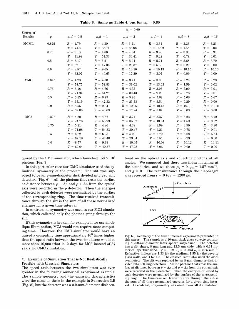
simulator (MCML), created by Wang and Jacques,25 andour CMC and MC3 simulators. The parameters are thesame as those in Tables 1–3, but there is no index match-ing. Again, 106 photons are used, and the accuracy isnow approximately 1023.In both cases MC3 provides results in very good agree-

ment with the other methods. It is, however, not advan-

tageous to use the MC3 simulator for such problems be-cause it runs two to five times slower than classicalsimulators for a comparable accuracy. This is due to thefact that total reflectances or transmittances represent animportant part of the injected energy, and the increase ofinformation provided by MC3 photons does not compen-sate for the added computing complexity.

B. More Difficult ExampleWe present here the results obtained for time-resolvedtransmittance through a 10-mm-thick glass cuvette con-taining a suspension of 200-nm-diameter latex spheres ( g5 0.19, ma 5 0, and ms 5 2.85 mm21). The cuvette is il-luminated at t 5 0 by a normally incident pencil colli-mated beam of infinitesimal duration. The detection ge-ometry corresponds to an 8-mm-long and 12.5-mm-wideslit with a 0.31 numerical aperture. There is no indexmatching, and the refractive indexes are 1.33 for the me-dium, 1.55 for the cuvette glass walls, and 1 for air. Themultiple reflections in the glass walls are taken into ac-count, but the wall thickness is supposed to be smallenough that the photons are not laterally displaced in theglass. The transmittance collected through the slit wasrecorded on a 1000-ps time range, starting from the firstpossible hit on the slit (44 ps) (see Fig. 6).For approximately the same level of noise MC3 used

5 3 106 photons and consumed only 1/16 of the time re-

Table 1. Total Time- and Space-Integrated Reflectance (R) and Transmittance (T) of a Slab (in Percent)a

Source ofResults

v0 5 0.99

g m td 5 0.5 m td 5 1 m td 5 2 m td 5 4 m td 5 8 m td 5 16

VdH 0.875 R 5 1.57 R 5 3.27 R 5 6.91 R 5 14.17 R 5 25.84 R 5 37.53T 5 97.89 T 5 95.58 T 5 90.56 T 5 80.01 T 5 60.81 T 5 35.21

0.75 R 5 3.65 R 5 7.60 R 5 15.44 R 5 28.43 R 5 43.30 R 5 53.00T 5 95.78 T 5 91.12 T 5 81.60 T 5 64.65 T 5 41.63 T 5 19.30

0.5 R 5 8.79 R 5 17.07 R 5 30.53 R 5 46.98 R 5 60.01 R 5 65.61T 5 90.57 T 5 81.45 T 5 66.03 T 5 45.27 T 5 24.38 T 5 8.60

0.0 R 5 19.89 R 5 33.29 R 5 49.75 R 5 64.50 R 5 72.88 R 5 75.13T 5 79.40 T 5 65.10 T 5 46.57 T 5 27.55 T 5 12.21 T 5 2.96

CMC 0.875 R 5 1.57 R 5 3.27 R 5 6.90 R 5 14.15 R 5 25.88 R 5 37.46T 5 97.89 T 5 95.58 T 5 90.57 T 5 80.03 T 5 60.77 T 5 35.32

0.75 R 5 3.65 R 5 7.60 R 5 15.44 R 5 28.43 R 5 43.31 R 5 52.98T 5 95.77 T 5 91.12 T 5 81.60 T 5 64.65 T 5 41.64 T 5 19.37

0.5 R 5 8.79 R 5 17.08 R 5 30.53 R 5 47.03 R 5 60.00 R 5 65.54T 5 90.56 T 5 81.45 T 5 66.03 T 5 45.21 T 5 24.42 T 5 8.68

0.0 R 5 19.88 R 5 33.22 R 5 49.70 R 5 64.47 R 5 72.91 R 5 75.11T 5 79.42 T 5 65.17 T 5 46.63 T 5 27.59 T 5 12.18 T 5 2.96

MC3 0.875 R 5 1.57 R 5 3.26 R 5 6.92 R 5 14.17 R 5 25.83 R 5 37.54T 5 97.89 T 5 95.59 T 5 90.55 T 5 80.02 T 5 60.81 T 5 35.17

0.75 R 5 3.64 R 5 7.60 R 5 15.44 R 5 28.44 R 5 43.29 R 5 52.98T 5 95.78 T 5 91.12 T 5 81.59 T 5 64.64 T 5 41.65 T 5 19.36

0.5 R 5 8.79 R 5 17.08 R 5 30.53 R 5 46.99 R 5 59.99 R 5 65.56T 5 90.57 T 5 81.44 T 5 66.02 T 5 45.26 T 5 24.40 T 5 8.66

0.0 R 5 19.89 R 5 33.29 R 5 49.77 R 5 64.48 R 5 72.87 R 5 75.11T 5 79.41 T 5 65.10 T 5 46.55 T 5 27.57 T 5 12.20 T 5 2.96

aComparison of numerical data from van de Hulst24 (VdH) and the results obtained with a classical Monte Carlo (CMC) simulator and our MC3 simu-lator. The parameters are the albedo v0 5 0.99, the anisotropy factor g, and the optical thickness m td. There is index matching. 106 photons are usedin the Monte Carlo simulators to produce an accuracy better than 1023.


Table 2. Same as Table 1, but for v0 5 0.80

Source ofResults

v0 5 0.80



0.75 R 5 2.31 R 5 4.03 R 5 6.18 R 5 7.74 R 5 8.13 R 5 8.15T 5 87.16 T 5 74.83 T 5 53.49 T 5 25.36 T 5 5.00 T 5 0.17

0.5 R 5 5.74 R 5 9.64 R 5 13.72 R 5 15.85 R 5 16.15 R 5 16.15T 5 82.83 T 5 67.00 T 5 42.15 T 5 15.39 T 5 1.84 T 5 0.02

0.0 R 5 14.01 R 5 21.08 R 5 26.59 R 5 28.40 R 5 28.53 R 5 28.53T 5 73.78 T 5 54.14 T 5 28.59 T 5 7.51 T 5 0.46 T 5 0.00


0.75 R 5 2.30 R 5 4.01 R 5 6.17 R 5 7.74 R 5 8.12 R 5 8.14T 5 87.16 T 5 74.87 T 5 53.52 T 5 25.38 T 5 4.99 T 5 0.17

0.5 R 5 5.73 R 5 9.63 R 5 13.70 R 5 15.82 R 5 16.13 R 5 16.11T 5 82.87 T 5 67.01 T 5 42.18 T 5 15.39 T 5 1.85 T 5 0.03

0.0 R 5 14.04 R 5 21.09 R 5 26.63 R 5 28.44 R 5 28.58 R 5 28.56T 5 73.74 T 5 54.16 T 5 28.60 T 5 7.51 T 5 0.46 T 5 0.00

MC3 0.875 R 5 0.98 R 5 1.70 R 5 2.64 R 5 3.44 R 5 3.74 R 5 3.74T 5 88.99 T 5 78.62 T 5 60.35 T 5 33.92 T 5 9.59 T 5 0.65

0.75 R 5 2.31 R 5 4.04 R 5 6.17 R 5 7.75 R 5 8.14 R 5 8.16T 5 87.16 T 5 74.83 T 5 53.49 T 5 25.34 T 5 5.00 T 5 0.17

0.5 R 5 5.74 R 5 9.63 R 5 13.72 R 5 15.85 R 5 16.15 R 5 16.17T 5 82.83 T 5 67.01 T 5 42.15 T 5 15.39 T 5 1.83 T 5 0.02

0.0 R 5 14.02 R 5 21.09 R 5 26.62 R 5 28.39 R 5 28.55 R 5 28.52T 5 73.78 T 5 54.14 T 5 28.58 T 5 7.51 T 5 0.46 T 5 0.00


Source ofResults

v0 5 0.60



0.75 R 5 1.39 R 5 2.12 R 5 2.73 R 5 2.98 R 5 3.00 R 5 3.00T 5 79.28 T 5 61.85 T 5 36.49 T 5 11.77 T 5 1.06 T 5 0.01

0.5 R 5 3.52 R 5 5.28 R 5 6.58 R 5 6.98 R 5 7.00 R 5 7.00T 5 76.02 T 5 56.29 T 5 29.55 T 5 7.44 T 5 0.41 T 5 0.00

0.0 R 5 9.27 R 5 12.95 R 5 15.10 R 5 15.53 R 5 15.54 R 5 15.54T 5 69.28 T 5 47.14 T 5 21.11 T 5 3.94 T 5 0.12 T 5 0.00


0.75 R 5 1.38 R 5 2.12 R 5 2.75 R 5 2.98 R 5 2.99 R 5 2.99T 5 79.32 T 5 61.86 T 5 36.55 T 5 11.81 T 5 1.06 T 5 0.01

0.5 R 5 3.52 R 5 5.26 R 5 6.60 R 5 6.99 R 5 7.01 R 5 7.00T 5 76.12 T 5 56.34 T 5 29.58 T 5 7.43 T 5 0.41 T 5 0.01

0.0 R 5 9.24 R 5 12.96 R 5 15.09 R 5 15.52 R 5 15.54 R 5 15.54T 5 69.32 T 5 47.16 T 5 31.08 T 5 3.94 T 5 0.13 T 5 0.00

MC3 0.875 R 5 0.59 R 5 0.89 R 5 1.16 R 5 1.28 R 5 1.29 R 5 1.29T 5 80.68 T 5 64.58 T 5 40.67 T 5 15.38 T 5 1.97 T 5 0.03

0.75 R 5 1.39 R 5 2.12 R 5 2.73 R 5 2.98 R 5 3.00 R 5 3.00T 5 79.28 T 5 61.83 T 5 36.49 T 5 11.76 T 5 1.06 T 5 0.01

0.5 R 5 3.53 R 5 5.28 R 5 6.58 R 5 6.98 R 5 7.01 R 5 7.00T 5 76.02 T 5 56.29 T 5 29.56 T 5 7.44 T 5 0.41 T 5 0.01

0.0 R 5 9.27 R 5 12.95 R 5 15.07 R 5 15.52 R 5 15.54 R 5 15.53T 5 69.28 T 5 47.13 T 5 21.13 T 5 3.94 T 5 0.12 T 5 0.00


Table 4. Total Time- and Space-Integrated Reflectance (R) and Transmittance (T) of a Slab (in percent)a

Source ofResults

v0 5 0.99


MCML 0.875 R 5 7.92 R 5 10.47 R 5 15.05 R 5 21.79 R 5 27.69 R 5 30.16T 5 90.99 T 5 87.20 T 5 79.79 T 5 66.78 T 5 48.87 T 5 28.99

0.75 R 5 10.86 R 5 15.81 R 5 23.53 R 5 31.88 R 5 37.71 R 5 40.97T 5 87.83 T 5 81.35 T 5 70.25 T 5 54.93 T 5 37.25 T 5 18.50

0.5 R 5 16.03 R 5 23.86 R 5 33.69 R 5 42.70 R 5 49.36 R 5 52.51T 5 82.40 T 5 72.80 T 5 59.31 T 5 43.28 T 5 25.51 T 5 9.47

0.0 R 5 22.42 R 5 33.11 R 5 45.07 R 5 55.13 R 5 61.16 R 5 62.93T 5 75.85 T 5 63.30 T 5 47.63 T 5 30.76 T 5 14.70 T 5 3.67


0.75 R 5 10.94 R 5 15.83 R 5 23.50 R 5 31.79 R 5 37.71 R 5 41.06T 5 87.75 T 5 81.34 T 5 70.27 T 5 55.01 T 5 37.23 T 5 18.30

0.5 R 5 16.09 R 5 23.95 R 5 33.75 R 5 42.73 R 5 49.37 R 5 52.55T 5 82.32 T 5 72.71 T 5 59.24 T 5 43.23 T 5 25.46 T 5 9.39

0.0 R 5 22.47 R 5 33.11 R 5 45.00 R 5 55.09 R 5 61.28 R 5 63.02T 5 75.79 T 5 63.32 T 5 47.69 T 5 30.77 T 5 14.59 T 5 3.61

MC3 0.875 R 5 7.94 R 5 10.47 R 5 15.10 R 5 21.82 R 5 27.80 R 5 30.23T 5 90.97 T 5 87.25 T 5 79.80 T 5 66.78 T 5 48.91 T 5 28.91

0.75 R 5 10.93 R 5 15.90 R 5 23.57 R 5 31.90 R 5 37.69 R 5 40.83T 5 87.79 T 5 81.36 T 5 70.30 T 5 55.00 T 5 37.26 T 5 18.44

0.5 R 5 16.08 R 5 24.01 R 5 33.83 R 5 42.69 R 5 49.38 R 5 52.49T 5 82.37 T 5 72.75 T 5 59.20 T 5 43.31 T 5 25.50 T 5 9.51

0.0 R 5 22.45 R 5 33.11 R 5 44.88 R 5 54.63 R 5 61.12 R 5 63.00T 5 75.81 T 5 63.30 T 5 47.66 T 5 30.81 T 5 15.07 T 5 3.69

aComparison of the results obtained with a classical Monte Carlo (MCML) simulator25 and with our CMC and MC3 simulators. The parameters are thealbedo v0 5 0.99, the anisotropy factor g, and the optical thickness m td. There is no index matching (n int 5 1.4, next 5 1). 106 photons are used, and theaccuracy is approximately 1023.


Source ofResults

v0 5 0.80



0.75 R 5 6.59 R 5 7.16 R 5 7.26 R 5 6.66 R 5 6.32 R 5 6.31T 5 78.38 T 5 64.34 T 5 42.65 T 5 18.37 T 5 3.35 R 5 0.12

0.5 R 5 8.90 R 5 10.35 R 5 10.98 R 5 10.66 R 5 10.55 R 5 10.55T 5 72.52 T 5 55.38 T 5 32.08 T 5 10.85 T 5 1.24 T 5 0.02

0.0 R 5 12.86 R 5 15.99 R 5 17.76 R 5 18.08 R 5 18.11 R 5 18.02T 5 66.30 T 5 46.59 T 5 23.20 T 5 5.74 T 5 0.35 T 5 0.00


0.75 R 5 6.60 R 5 7.16 R 5 7.27 R 5 6.68 R 5 6.32 R 5 6.30T 5 78.39 T 5 64.36 T 5 42.68 T 5 18.35 T 5 3.37 T 5 0.11

0.5 R 5 8.88 R 5 10.44 R 5 10.99 R 5 10.65 R 5 10.53 R 5 10.53T 5 72.59 T 5 55.21 T 5 32.06 T 5 10.88 T 5 1.25 T 5 0.02

0.0 R 5 12.86 R 5 16.01 R 5 17.79 R 5 18.08 R 5 18.06 R 5 18.08T 5 66.26 T 5 46.58 T 5 23.14 T 5 5.74 R 5 0.34 T 5 0.00

MC3 0.875 R 5 5.59 R 5 5.66 R 5 5.45 R 5 4.81 R 5 4.32 R 5 4.25T 5 81.98 T 5 70.54 T 5 51.81 T 5 26.99 T 5 6.95 T 5 0.45

0.75 R 5 6.66 R 5 7.22 R 5 7.29 R 5 6.74 R 5 6.31 R 5 6.29T 5 78.40 T 5 64.36 T 5 42.71 T 5 18.41 T 5 3.36 T 5 0.11

0.5 R 5 8.96 R 5 10.52 R 5 11.03 R 5 10.66 R 5 10.48 R 5 10.57T 5 72.60 T 5 55.43 T 5 32.20 T 5 10.86 T 5 1.25 T 5 0.02

0.0 R 5 12.86 R 5 15.98 R 5 17.64 R 5 17.97 R 5 18.07 R 5 17.99T 5 66.27 T 5 46.56 T 5 23.12 T 5 5.70 T 5 0.34 T 5 0.00



Source ofResults

v0 5 0.60



0.75 R 5 5.18 R 5 4.86 R 5 4.34 R 5 3.96 R 5 3.90 R 5 3.91T 5 71.99 T 5 54.33 T 5 30.41 T 5 9.22 T 5 0.79 T 5 0.01

0.5 R 5 6.17 R 5 6.21 R 5 5.94 R 5 5.71 R 5 5.68 R 5 5.70T 5 67.15 T 5 47.34 T 5 23.37 T 5 5.50 T 5 0.29 T 5 0.00

0.0 R 5 8.57 R 5 9.65 R 5 10.10 R 5 10.13 R 5 10.15 R 5 10.16T 5 62.07 T 5 40.65 T 5 17.29 T 5 3.07 T 5 0.09 T 5 0.00


0.75 R 5 5.18 R 5 4.86 R 5 4.33 R 5 3.96 R 5 3.90 R 5 3.91T 5 71.94 T 5 54.27 T 5 30.43 T 5 9.20 T 5 0.78 T 5 0.01

0.5 R 5 6.15 R 5 6.25 R 5 5.93 R 5 5.69 R 5 5.68 R 5 5.67T 5 67.19 T 5 47.32 T 5 23.33 T 5 5.54 T 5 0.29 R 5 0.00

0.0 R 5 8.55 R 5 9.64 R 5 10.06 R 5 10.13 R 5 10.13 R 5 10.12T 5 62.06 T 5 40.63 T 5 17.24 T 5 3.07 T 5 0.09 T 5 0.00

MC3 0.875 R 5 4.80 R 5 4.37 R 5 3.74 R 5 3.37 R 5 3.23 R 5 3.22T 5 74.76 T 5 58.79 T 5 35.87 T 5 13.04 T 5 1.59 T 5 0.02

0.75 R 5 5.21 R 5 4.86 R 5 4.39 R 5 3.99 R 5 3.90 R 5 3.90T 5 71.98 T 5 54.33 T 5 30.47 T 5 9.21 T 5 0.78 T 5 0.01

0.5 R 5 6.22 R 5 6.25 R 5 5.99 R 5 5.70 R 5 5.68 T 5 5.64T 5 67.19 T 5 47.40 T 5 23.34 T 5 5.51 T 5 0.29 T 5 0.00

0.0 R 5 8.57 R 5 9.64 R 5 10.05 R 5 10.03 R 5 10.12 R 5 10.11T 5 62.04 T 5 40.57 T 5 17.25 T 5 3.06 T 5 0.09 T 5 0.00

quired by the CMC simulator, which launched 150 3 106

photons (Fig. 7).In this particular case our CMC simulator used the cy-

lindrical symmetry of the problem: The slit was sup-posed to be an 8-mm-diameter disk divided into 320 ringdetectors (Fig. 6). All the photons that cross the surfaceat distance between r 2 Dr and r 1 Dr from the opticalaxis were recorded in the r detector. Then the energiescollected by each detector were normalized by the surfaceof the corresponding ring. The time-resolved transmit-tance through the slit is the sum of all these normalizedenergies for a given time interval.In contrast, no symmetry was used in our MC3 simula-

tion, which collected only the photons going through theslit.If this symmetry is broken, for example if we use an ob-

lique illumination, MC3 would not require more comput-ing time. However, the CMC simulator would have re-quired a computing time approximately 103 times higher;thus the speed ratio between the two simulators would bemore than 16,000 (that is, 2 days for MC3 instead of 87years for CMC simulation).

C. Example of Simulation That is Not RealisticallyFeasible with Classical SimulatorsThe speed ratio between the two simulators was evengreater in the following numerical experiment example.The sample geometry and the emission characteristicswere the same as those in the example in Subsection 3.B(Fig. 8), but the detector was a 0.2-mm-diameter disk cen-

tered on the optical axis and collecting photons at allangles. We supposed that there was index matching atthe boundaries, and we chose ma 5 0, ms 5 1.57 mm21,and g 5 0. The transmittance through the diaphragmwas recorded from t 5 0 to t 5 1200 ps.

Fig. 6. Geometry of the first numerical experiment presented inthis paper: The sample is a 10-mm-thick glass cuvette contain-ing a 200-nm-diameter latex sphere suspension. The detectorhas a slit shape, 8 mm long and 12.5 mm wide, with a 0.31 nu-merical aperture (NA). g 5 0.19, ma 5 0, and ms 5 2.85 mm21.Refractive indices are 1.33 for the medium, 1.55 for the cuvetteglass walls, and 1 for air. The classical simulator used the axialsymmetry: The slit was replaced by an 8-mm-diameter disk di-vided into 320 ring detectors. All the photons that cross the sur-face at distance between r 2 Dr and r 1 Dr from the optical axiswere recorded in the r detector. Then the energies collected byeach detector were normalized by the surface of the correspond-ing ring. The time-resolved transmittance through the slit isthe sum of all these normalized energies for a given time inter-val. In contrast, no symmetry was used in our MC3 simulation.


The treatment of this example was more difficult be-cause the diaphragm surface was one third of the previ-ous slit surface, and there was no possibility of increasingthe collecting surface by the use of symmetry. Moreover,

Fig. 7. (a) Results obtained with a CMC simulator for the caseillustrated in Fig. 6 (150 3 106 photons), (b) results obtainedwith the MC3 simulator for the case illustrated in Fig. 6 (5 3 106

photons), (c) results from (a) and (b) plotted together. The re-sults obtained by each of the two simulators are the same, butMC3 required only 1/16 of the computation time used by theCMC simulator. Dotted curve, CMC simulator; solid curve,MC3 simulator.

Fig. 8. The second numerical experiment used a 10-mm-thickindex-matched sample. The detector is a 0.2-mm-diameter diskcentered on the optical axis and collecting photons at all angles.The chosen optical coefficients are ma 5 0, ms 5 1.57 mm21, andg 5 0.

Fig. 9. Result provided by the CMC simulation for the case il-lustrated in Fig. 8. With 109 photons it is not possible to discernthe shape of the transmitted pulse.

Fig. 10. Result provided by the MC3 simulator for the case il-lustrated in Fig. 8. 106 photons are sufficient to produce a goodevaluation of this curve. In this case a MC3 photon required ap-proximately only twice the average time needed by a classicalsimulator photon.


when there is no index matching, any photon goingthrough one surface completely escapes from the medium.The number of collected events for a given number ofsimulated photons was therefore much lower than in thefirst example.These drastic collecting conditions are not unrealistic.

On the contrary, they give signals of the same order ofmagnitude as the typical signals expected for imagingthrough biological tissues.With use of 109 photons the classical simulator did not

allow us to discern the shape of the transmitted pulse(Fig. 9). Only a few photons were collected. On theother hand, MC3 provided a good evaluation of the pulsewith only 106 photons (Fig. 10), and a MC3 photon re-quired approximately only twice the average time neededby a CMC simulator photon.A general rule may be that the weaker is the desired

signal, the greater is the speed ratio between MC3 andCMC simulation.All the curves presented here have been directly ob-

tained from the simulators. In order to produce a bettersignal-to-noise ratio, no numerical filters are used. Onecan notice that the noise structure of the MC3 simulatoris different from the noise structure of CMC simulators.In MC3 a single scattering point may contribute to manyspace- and time-adjacent data. In CMC simulation aphoton gives randomly dispersed space and time data.As a consequence, the noise structure of MC3 is less ran-dom or at least is more suitable for the design of an ap-propriate filter.

4. CONCLUSIONThe three-dimensional semianalytical Monte Carlo simu-lation (MC3) presented in this paper is somewhat moresophisticated than classical Monte Carlo (CMC) simula-tions and may require a large amount of memory. How-ever, this simulation is currently used in our laboratoryfor a wide range of applications, and it has proven to bestable and reliable.Its efficiency, measured for example by the signal-to-

noise ratio corresponding to a given computing time, is fargreater than that with CMC simulators when the evalu-ated signal is weak; and the weaker is this signal, thegreater is this difference. This means that the computa-tion time required by MC3 does not increase as fast as itdoes in CMC simulation. This characteristic is interest-ing, since the major drawback of Monte Carlo methods isthe fast increase of the required computing time as thenumber of photons contributing to the desired quantitybecomes smaller.Another point is that, by using this simulator, it is pos-

sible to store all the scattering events within a reasonablestorage capacity and later to evaluate analytically any de-sired quantity from the stored points. As a consequence,a single simulation can provide rapidly any number of re-sults as long as the illumination source and the scatteringmedium are not modified. There is no need to store vol-ume energy distribution in a spatial or temporal grid,which can be problematic for classical simulationschemes.26

When the MC3 simulator is used to calculate only one

result, that is, when the information stored during thesimulation is not supposed to be used for the calculationof other quantities, it is more convenient to merge the in-formation generator and the information processor. Thestorage of all the scattering points can then be avoided,and the simulator is faster and needs less memory.The efficiency of Monte Carlo simulators is related to

the quantity of information obtained for a given amountof computation. Two approaches are then possible: Theclassical simulator algorithm uses a large number of pho-tons but minimizes the amount of calculations per pho-ton; MC3 uses fewer photons with more complex calcula-tions. This last type of approach is interesting as long asthe collected information increases faster than theamount of computation. As a consequence, CMC simula-tion and MC3 are complementary techniques: When thedesired signal is high, for example, with total reflectanceor transmittance, classical simulation is more efficientthan MC3, but as soon as the detection probability ofCMC photons becomes too low for practical use, MC3 out-paces classical simulation.More investigation is required to design Monte Carlo

simulators that could give accurate results in a few min-utes on standard PC computers, but the MC3 simulator,or any Monte Carlo simulator based on equivalent prin-ciples, is a positive step for fast and accurate investiga-tions in the field of photon transport in scattering media.

REFERENCES1. R. Graaf, M. H. Koelink, F. F. M. de Mul, W. G. Zijlstra, A.

C. M. Dassel, and J. G. Aarnoudse, ‘‘Condensed MonteCarlo simulations for the description of light transport,’’Appl. Opt. 32, 426–434 (1993).

2. S. L. Jacques, ‘‘Time-resolved reflectance spectroscopy inturbid tissues,’’ IEEE Trans. Biomed. Eng. 36, 1155–1161(1989).

3. M. S. Patterson, J. D. Moulton, B. C. Wilson, and B.Chance, ‘‘Applications of time-resolved light scatteringmeasurements to photodynamic therapy dosimetry,’’ inPhotodynamic Therapy: Mechanisms II, T. J. Dougherty,ed., Proc. SPIE 1203, 62–75 (1990).

4. G. Zaccanti, P. Bruscaglioni, A. Ismaelli, L. Carraresi, M.Gurioli, and Q. Wei, ‘‘Transmission of a pulsed thin lightbeam through thick turbid media: experimental results,’’Appl. Opt. 31, 2141–2147 (1992).

5. K. Suzuki, Y. Yamashita, K. Ohta, and B. Chance, ‘‘Quan-titative measurement of optical parameters in the breastusing time-resolved spectroscopy: phantom and prelimi-nary in vivo results,’’ Invest. Radiol. 29, 410–414 (1994).

6. M. D. Duncan, R. Mahon, L. L. Tankersley, and J. Reintjes,‘‘Time-gated imaging through scattering media usingstimulated Raman amplification,’’ Opt. Lett. 16, 1868–1870(1991).

7. M. R. Hee, J. A. Izatt, J. M. Jacobson, and G. Fujimoto,‘‘Femtosecond transillumination optical coherence tomogra-phy,’’ Opt. Lett. 18, 950–952 (1993).

8. J. C. Hebden, ‘‘Evaluating the spatial resolution perfor-mance of a time-resolved optical imaging system,’’ Med.Phys. 19, 1081–1087 (1992).

9. A. H. Gandjbakhche, R. Nossal, and R. F. Bonner, ‘‘Resolu-tion limits for optical transillumination of abnormalitiesdeeply embedded in tissues,’’ Med. Phys. 21, 185–191(1994).

10. R. A. J. Groenhuis, H. A. Ferwerda, and J. J. Ten Bosh,‘‘Scattering and absorption of turbid materials determinedfrom reflection measurements. 1. Theory,’’ Appl. Opt.22, 2456–2461 (1983).

11. S. T. Flock, M. S. Patterson, B. C. Wilson, and D. R. Wy-


man, ‘‘Monte Carlo modelling of light propagation in highlyscattering tissues: model predictions and comparison withdiffusion theory,’’ IEEE Trans. Biomed. Eng. 36, 1162–1167(1989).

12. E. A. Bucher, ‘‘Computer simulation of light pulse propaga-tion for communication through thick clouds,’’ Appl. Opt.12, 2391–2400 (1973).

13. R. R. Meier, J. S. Lee, and D. E. Anderson, ‘‘Atmosphericscattering of middle uv radiation from an internal source,’’Appl. Opt. 17, 3216–3225 (1978).

14. B. C. Wilson and G. Adam, ‘‘A Monte Carlo model for theabsorption and flux distributions of light in tissue,’’ Med.Phys. 10, 824–830 (1983).

15. S. L. Jacques, ‘‘Time-resolved propagation of ultrashort la-ser pulses within turbid tissues,’’ Appl. Opt. 28, 2223–2229(1989).

16. S. Avrillier, E. Tinet, and E. Delettre, ‘‘Monte Carlo simu-lation of collimated beam transmission through turbid me-dia,’’ J. Phys. (Paris) 51, 2521–2542 (1990).

17. G. Zaccanti, ‘‘Monte Carlo study of light propagation in op-tically thick media: point source case,’’ Appl. Opt. 30,2031–2041 (1991).

18. P. Bruscaglioni and G. Zaccanti, ‘‘Multiple scattering indense media,’’ in Scattering in Volumes and Surfaces, M.Nietol Vesperinas and J. Dainty, eds. (Elsevier, New York,1990), pp. 53–71.

19. G. Zaccanti, University of Florence, Physics Department, 3Via S. Marta, 50139 Firenze, Italy (personal communica-tion, 1994).

20. G. Goertzel and M. H. Kalos, ‘‘Monte Carlo methods intransport problems,’’ in Series I of Progress in Nuclear En-ergy (Pergamon, New York, 1958), Vol. 2, pp. 315–369.

21. M. H. Kalos and P. Whitlock, ‘‘Random walks and integralequations,’’ in Monte Carlo Methods (Wiley, New York,1986), Vol. I, Chap. 7, pp. 145–156.

22. M. Abramowitz and I. A. Stegun, Handbook of Mathemati-cal Functions with Formulas, Graphs and MathematicalTables (Dover, New York, 1970).

23. L. Henyey and J. Greenstein, ‘‘Diffuse radiation in the Gal-axy,’’ Astrophys. J. 93, 70–83 (1941).

24. H. C. van de Hulst, Multiple Light Scattering, Tables, For-mulas and Applications (Academic, New York, 1980).

25. L. Wang and S. L. Jacques, ‘‘Monte Carlo simulation of pho-ton distribution in multi-layered turbid media in ANSIstandard C,’’ (Copyright University of Texas, M.D. Ander-son Cancer Center, 1515 Holcombe Boulevard, Houston,Texas 77030, 1992).

26. C. M. Gardner and A. J. Welch, ‘‘Improvements in the ac-curacy and statistical variance of the Monte Carlo simula-tion of light distribution in tissue,’’ in Laser–Tissue Inter-action III, S. L. Jacques, ed., Proc. SPIE 1646, 400–409(1992).

Fast semianalytical Monte Carlo simulation for time-resolved light propagation in turbid media

Documents

Transcript of Fast semianalytical Monte Carlo simulation for time-resolved light propagation in turbid media