Modelling Issues in the Seismic Analysis of Concrete Gravity Dams

DAM ENGINEERING Vol XXIV Issue 2 1

Modelling Issues in the Seismic Analysis ofConcrete Gravity Dams

Arnab Banerjee(1), D K Paul(1) & R N Dubey(1)

ABSTRACT

Modelling issues in the seismic analysis of dams are challenging. This paper addresses the

various modelling issues of a concrete gravity dam, with the help of various field problems.

The issues regarding the modelling of these types of dams, e.g. infinite reservoir with truncated

boundaries, and semi-infinite soil medium with finite domain, are discussed. The issues

related to the input motion of earthquake excitation are also considered, a comparative

study of different modelling issues has been made, and the appropriate modelling of a

dam-reservoir-foundation system, along with suitable simulation of seismic input, has

been suggested for the evaluation of a dam’s response.

Keywords: Dam-foundation-reservoir interaction; concrete gravity dams; compressible fluid

element; incompressible fluid; absorbing boundary; seismic analysis.

1. INTRODUCTION

Concrete gravity dams are considered to be one of the most important civil engineering

structures in the world. A gravity dam stores a large amount of water in its reservoir,

the pressure of which is resisted by the dam. Earthquakes, however, can cause catastrophic

failure of these dams and, hence, safety analysis is of utmost importance. Many

researchers have investigated the dynamic behaviour of gravity dams using different

modelling techniques.

Modelling of a dam-reservoir-foundation system has the following major issues: depending

upon the accuracy of results, modelling of the concrete gravity dam is chosen. The dam can

either be analyzed by assuming the dam is fixed at the base[19], or by considering its foundation

flexibility[9]. Simplified analysis procedures for the earthquake-resistant design of concrete

gravity dams is also used to estimate the stability of the dam section[7,8]. CADAM software

can effectively be used to measure a dam’s response, and its stability against sliding and

overturning[14]. Use of the finite element method is another effective way to analyze the

dam-foundation-reservoir water system together.

(1)Department of Earthquake Engineering, Indian Institute of Technology Roorkee, Roorkee, India.

Banerjee paper publish:. 6/3/14 18:38

DAM ENGINEERING Vol XXIV Issue 22

Reservoirs have considerable effect on the earthquake response of a gravity dam. There

are three ways to consider reservoir effect in the seismic response analysis of the dam system,

i.e. Westergaard, Lagrangian and Eularian approaches.

The Westergaard approach considers a virtual lumped mass on the wet surface, which

simulates the hydrodynamic effect on the upstream face of the dam[22,25,1]. In the Eulerian

approach[3,6,16,26,4,18,2,12] the degree-of-freedom in structure and fluid are displacement and

pressure, respectively, and a special compatibility equation is required to establish the

compatibility between reservoir water and the dam-foundation system. In the Lagrangian

approach displacement is the variable for both the impounded reservoir water and the dam-

foundation system, and no compatibility equation is required[23,10].

The generation of an infinite medium is a big modelling issue in any finite element analysis.

To solve a field problem a finite boundary is required to be specified. Generally, the boundary

of an infinite field can be formulated using four approaches, i.e. the elementary boundary,

the local boundary, the consistent boundary, and the infinite element approach[24,27,20,21].

Rollers assigned at the truncated edge of the soil or rock are known as an elementary

boundary. In a local boundary viscous dampers are used at the truncated face of the soil

layer. The foundation system is represented as Kelvin elements in a consistent boundary.

Infinite element has both near- and far-field nodes. Far-field nodes map the infinite extent

of soil. The interpolation function of this element is different compared to the continuum

plane strain or plane stress elements[5].

The application of earthquake input motions has great importance in seismic analysis.

Issues such as rock outcrop motion, free field motion, base motion at foundation level, and

motion at the soil boundaries, need to be understood and implemented correctly. The free

field earthquake motion is generally specified at the rock outcrop and, as a rule, a site-specific

response spectrum is also given for rock outcrop. Deconvolution is performed by calculating

the complex impedance of the rock for a particular depth[13].

In this paper the comparison of responses between Westergaard’s approach and the

acoustic element approach are presented. The scope of this paper is extended to allow

comparison of the seismic responses for elementary and local boundaries assigned at the

truncated edge of the semi-infinite soil. The site-specific response spectra, and corresponding

accelerogram, is given at the rock outcrop. The outcrop accelerogram is deconvoluted at the

base of the soil boundary, and this deconvoluted input motion is applied at the base of the

considered soil profile for analysis.

2. DAM DATA

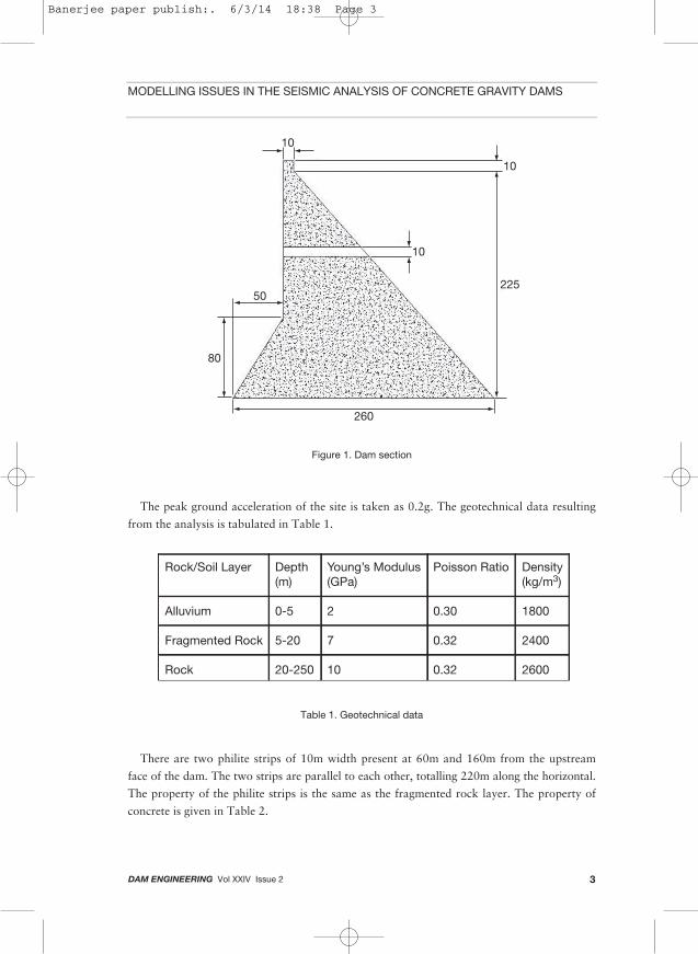
A concrete gravity dam with a height of 235m, a base width of 260m, a downstream slope

of 1:0.9, and an upstream slope of 1:0.625, is chosen as a numerical example. The thickness

of every monolith is 15m, and each one is separated by a construction joint. The dam section

is shown in Figure 1.

ARNAB BANERJEE, D K PAUL & R N DUBEY



The peak ground acceleration of the site is taken as 0.2g. The geotechnical data resulting

from the analysis is tabulated in Table 1.

There are two philite strips of 10m width present at 60m and 160m from the upstream

face of the dam. The two strips are parallel to each other, totalling 220m along the horizontal.

The property of the philite strips is the same as the fragmented rock layer. The property of

concrete is given in Table 2.

MODELLING ISSUES IN THE SEISMIC ANALYSIS OF CONCRETE GRAVITY DAMS

10

10

10

225

260

50

80

Figure 1. Dam section

Table 1. Geotechnical data



Bulk modulus and density of water are taken as 2.07GPa and 1000kg/m3, respectively.

The damping values of each material is tabulated in Table 3.

3. FINITE ELEMENT ANALYSIS OF THEDAM-RESERVOIR-FOUNDATION SYSTEM

The dam’s body and foundation are modelled using the Lagrangian approach. Two-dimensional

plane stress elements are used to model the dam’s monoliths.

The foundation soil is infinitely extended for both in-plane and out-of-plane directions.

Two-dimensional plane strain elements are suitable to model the foundation soil or rock.

The appropriate near-field portion of soil/rock is considered for modelling the foundation.

The waves reflected back from the truncated boundary. To generate the non-reflecting

boundary, P-wave and S-wave dampers are used at the nodes of the boundary. The

transmissibility coefficient (TC) and reflection coefficient (RC) for a wave falling at the

interface of the two mediums is calculated by:

(1)

(2)

To ensure the radiating boundary condition, TC = 1 and RC = 0 should be satisfied. The

coefficient of these dampers are such that impedance (Z) given by dampers should be equal


Table 2. Property of concrete

Table 3. Damping value



to the impedance of the foundation soil/rock. Impedance of a material is the product of

density (ρ) and shear wave velocity (Vs).

(3)

The coefficient of P-wave dampers (Cp) and S-wave dampers (Cs) are calculated as:

(4)

(5)

The impounded reservoir effect can be modelled taking water as:

1. Incompressible

In the case of incompressible water the effect of the reservoir is considered as Westergaard’s

added mass on the upstream face of the dam. The virtual masses of water are tied or lumped

at the nodes of the upstream wet face of the dam according to IS:1893-1984. Using pressure

distribution at the upstream face, according to Equations 6 and 7, virtual masses are calculated

due to hydrodynamic effect:

(6)

(7)

2. Compressible

If the impounded reservoir water is considered compressible then the reservoir can be modelled

as acoustic fluid elements. In an acoustic fluid or Eularian system the fluid field is of constant

volume. The acoustic element has a degree-of-freedom in terms of pressure at the nodes of the

element. When fluid is flowing through a constant volume field then pressure is induced at the

inner boundary of the field. For example, pressure is induced at the inner surface of a pipe

(which is constant in volume) when water flows through it. In acoustic analysis the mesh

remains stationary (Eularian), but the acoustic media is assumed to flow through the mesh.

The acoustic element needs the bulk modulus and density of fluid for analysis.

The equilibrium equation for the acoustic medium is given by:

(8)

(9)




where p is the dynamic pressure, x is the spatial position of the fluid particle, uf and uf are

the velocity and acceleration of the fluid particle, ρf is the density of fluid, γ is the volumetric

drag coefficient, and Kf is the bulk modulus of the fluid.

Element type AC2D8, an 8-node quadratic 2D acoustic quadrilateral, is used to model the

impounded reservoir water.

The link element is used to model the fluid-structure interface, which can convert pressure

into displacement. The conceptual representation of the link element is shown in Figure 2,

and the connecting matrix is given in Equation 10.

(10)

A free surface is assigned at the top surface of the impounded reservoir water, where

pressure is zero.

The non-reflecting (absorbing) boundary is generated at the truncated edge of the infinite

reservoir. The equation of the absorbing boundary is as follows:

(11)

Assigning impedance to the truncated boundary infinite domain is generated in the

case of the acoustic medium. Using Equation 12, a non-reflecting boundary is created in

ABAQUS:


v v

v

vu

u

u

u

uuuv v

7

6 65 5p

p p

p p p

p p

8 8v4 4

1 2 3 1 2

7

3

Lagrangesolid

element

Acousticßuid

element

Link element

Figure 2. Fluid link element

. ..



(12)

where is the wave number, ρ is the complex density, f is the geometric factor for

the curvilinear coordinate system used at the boundary, and β is the spreading loss.

Combining Equation 8 with Equation 12, the non-reflecting boundary condition is generated

in terms of impedance:

(13)

by Fourier inversion:

(14)

For γ = 0, Equation 14 converts to:

(15)

Comparing Equation 11 with Equation 15 it can be concluded that for a non-reflecting

boundary the geometric factor for the curvilinear coordinate (f) = 1 and, correspondingly,

the spreading loss (β) = 0.

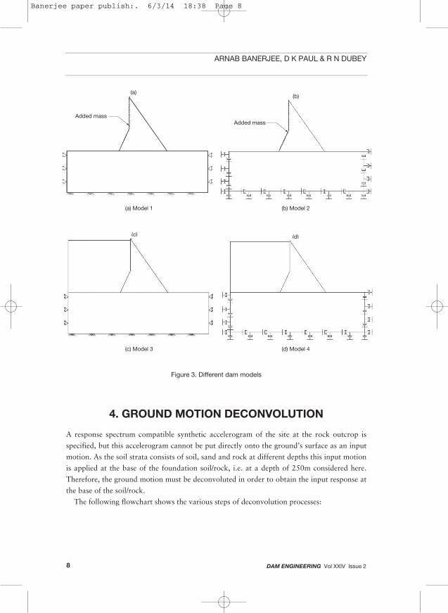
The four different types of dam models, having different modelling aspects, are

shown in Figure 3. For Model 1 the reservoir water is considered incompressible and

the elementary boundary assigned at the truncated soil boundary. In Model 2 the reservoir

water is considered incompressible and the viscous boundary assigned at the truncated

soil boundary. For Model 3 the reservoir water is considered compressible and the elementary

boundary assigned at the truncated soil boundary, and in Model 4 the reservoir water

is considered compressible and the viscous boundary assigned at the truncated soil

boundary.


~



4. GROUND MOTION DECONVOLUTION

A response spectrum compatible synthetic accelerogram of the site at the rock outcrop is

specified, but this accelerogram cannot be put directly onto the ground’s surface as an input

motion. As the soil strata consists of soil, sand and rock at different depths this input motion

is applied at the base of the foundation soil/rock, i.e. at a depth of 250m considered here.

Therefore, the ground motion must be deconvoluted in order to obtain the input response at

the base of the soil/rock.

The following flowchart shows the various steps of deconvolution processes:


Added mass

(a)

Added mass

(b)

(c) (d)

(a) Model 1 (b) Model 2

(c) Model 3 (d) Model 4

Figure 3. Different dam models



The transfer function depends on the complex impedance ratio, depth, shear wave velocity,

and damping of the soil.

To consider the soil-structure interaction it is convenient to apply the motion at the base

of the foundation soil. The necessity of the deconvolution is explained in Figure 4. In this

process the input motion at the base of the foundation soil/rock is determined based on the

specified rock outcrop motion. This generally gives a motion having less peak amplitude.

This input motion is applied at the base of the dam-foundation-reservoir system to obtain

the dam response.

The accelerogram at the rock outcrop is given in Figure 5, having a PGA of 0.2g. The

deconvoluted time history at the base of the foundation soil/rock at the depth of 250m is

given in Figure 6. The peak value of the motion is reduced to 0.12g.


Surface

Base Deconvolution

Rockoutcrop

Figure 4. Deconvolution of motion



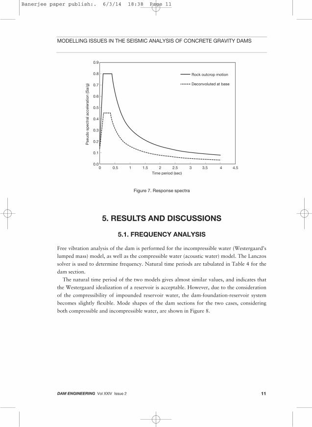
After deconvolution the corresponding new response spectrum at the base of the soil

foundation is shown, along with the response spectra at rock outcrop (see Figure 7).

These same input motion/response spectra at the base of the soil foundation are taken as

the input to the dam-foundation-reservoir system.


0.2

0.1

0

-0.1

-0.2

5 10 15 20 25 30 35Time (sec)

Accelerogram at 250m depth

Acc

eler

atio

n(g

)

Figure 6. Motion at 250m depth

0.2

0.1

0

-0.1

-0.2

5 10 15 20 25 30 35Time (sec)

Accelerogram at Rock outcrop

Acc

eler

atio

n(g

)

Figure 5. Motion at rock outcrop



5. RESULTS AND DISCUSSIONS

5.1. FREQUENCY ANALYSIS

Free vibration analysis of the dam is performed for the incompressible water (Westergaard’s

lumped mass) model, as well as the compressible water (acoustic water) model. The Lanczos

solver is used to determine frequency. Natural time periods are tabulated in Table 4 for the

dam section.

The natural time period of the two models gives almost similar values, and indicates that

the Westergaard idealization of a reservoir is acceptable. However, due to the consideration

of the compressibility of impounded reservoir water, the dam-foundation-reservoir system

becomes slightly flexible. Mode shapes of the dam sections for the two cases, considering

both compressible and incompressible water, are shown in Figure 8.


0.9

0.8

0.7

0.6

0.5

0.4

0.3

0.2

0.1

0.0

Pse

udo

spec

tral

acce

lera

tion

(Sa/

g)

0 0.5 1 1.5 2 2.5 3 3.5 4 4.5Time period (sec)

Rock outcrop motion

Deconvoluted at base

Figure 7. Response spectra




Table 4. Natural time period of dam section

+3.273e-07+3.000e-07+2.727e-07+2.455e-07+2.182e-07+1.909e-07+1.636e-07+1.364e-07+1.091e-07+8.182e-08+5.455e-08+2.727e-08+0.000e+00

U, magnitude (a)

+1.039e+00+9.525e-01+8.659e-01+7.793e-01+6.927e-01+6.062e-01+5.196e-01+4.330e-01+3.464e-01+2.598e-01+1.732e-01+8.659e-02+0.000e+00

U, magnitude (b)

First mode shape in dam (T = 1.06sec) - water compressible

First mode shape in dam (T = 1.03sec) - water incompressible



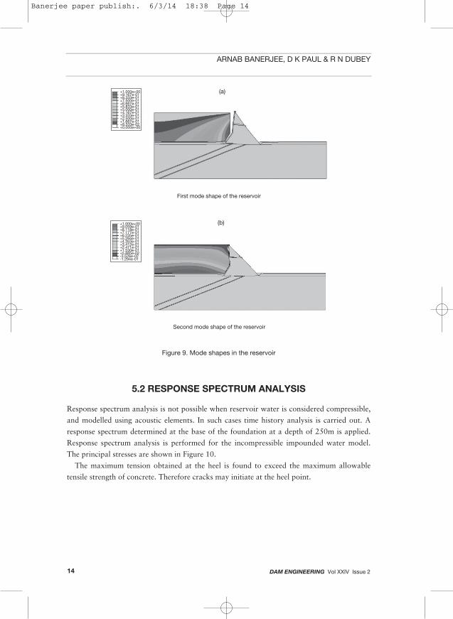
The pressure variations of the impounded water in the reservoir in different modes are

shown in Figure 9.

The first mode shape shows the parabolic distribution of pressure, which matches the

parabolic pressure distribution as reported in previous literature.


+1.440e-07+1.320e-07+1.200e-07+1.080e-07+9.601e-08+8.401e-08+7.201e-08+6.000e-08+4.800e-08+3.600e-08+2.400e-08+1.200e-08+0.000e+00

U, magnitude (c)

+1.206e+00+1.106e+00+1.005e+01+9.047e-01+8.042e-01+7.037e-01+6.031e-01+5.026e-01+4.021e-01+3.016e-01+2.010e-01+1.005e-01+0.000e+00

U, magnitude (d)

Figure 8. Mode shapes in dam body

Second mode ahape in dam (T = 0.75 sec) - water compressible

Second mode shape in dam (T = 0.76sec) - water incompressible



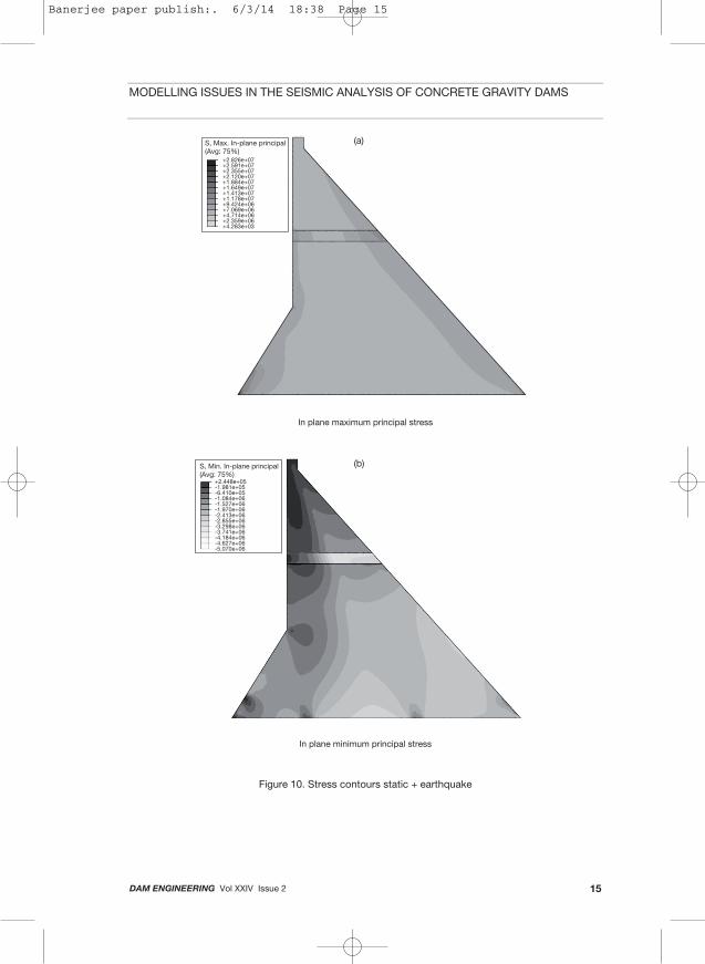
5.2 RESPONSE SPECTRUM ANALYSIS

Response spectrum analysis is not possible when reservoir water is considered compressible,

and modelled using acoustic elements. In such cases time history analysis is carried out. A

response spectrum determined at the base of the foundation at a depth of 250m is applied.

Response spectrum analysis is performed for the incompressible impounded water model.

The principal stresses are shown in Figure 10.

The maximum tension obtained at the heel is found to exceed the maximum allowable

tensile strength of concrete. Therefore cracks may initiate at the heel point.


+1.000e+00+9.167e-01+8.333e-01+7.500e-01+6.667e-01+5.833e-01+5.000e-01+4.167e-01+3.333e-01+2.500e-01+1.667e-01+8.333e-02+0.000e+00

(a)

+1.000e+00+9.059e-01+8.118e-01+7.177e-01+6.235e-01+5.294e-01+4.353e-01+3.412e-01+2.471e-01+1.530e-01+5.885e-02-3.526e-02-1.294e-01

(b)

First mode shape of the reservoir

Second mode shape of the reservoir

Figure 9. Mode shapes in the reservoir




+2.826e+07+2.591e+07+2.355e+07+2.120e+07+1.884e+07+1.649e+07+1.413e+07+1.178e+07+9.424e+06+7.069e+06+4.714e+06+2.359e+06+4.283e+03

S, Max. In-plane principal(Avg: 75%)

(a)

+2.448e+05-1.981e+05-6.410e+05-1.084e+06-1.527e+06-1.970e+06-2.413e+06-2.855e+06-3.298e+06-3.741e+06-4.184e+06-4.627e+06-5.070e+06

S, Min. In-plane principal(Avg: 75%)

(b)

In plane maximum principal stress

In plane minimum principal stress

Figure 10. Stress contours static + earthquake



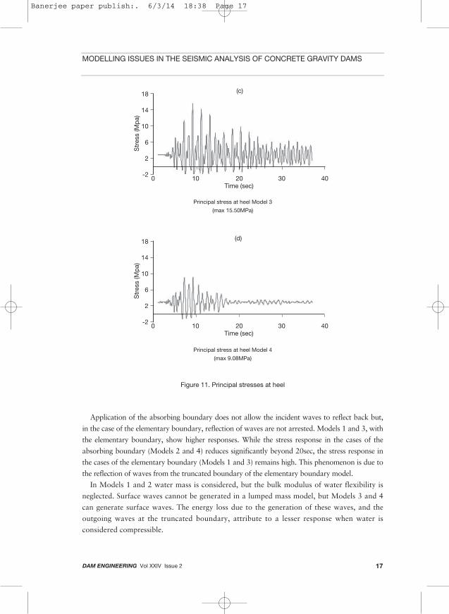
5.3 TIME HISTORY ANALYSIS

Prior to application of the acceleration shown in Figure 6, baseline correction is applied

to the acceleration time history. The accelerogram is applied at the bottom of the rock

foundation. The free surface of the impounded reservoir water is modelled by assigning

p = 0 at the top surface. Non-reflecting boundary is assigned at the truncated edge of

the reservoir. The principal stresses at the heel for the different models are plotted in

Figure 11.


18

14

10

6

2

-20 10

Time (sec)3020 40

Str

ess

(Mp

a)

(a)

0 10Time (sec)

3020 40

Str

ess

(Mp

a)

18

14

10

6

2

-2

(b)

Principal stress at heel Model 1

(max 12.90MPa)


(max 10.10MPa)



Application of the absorbing boundary does not allow the incident waves to reflect back but,

in the case of the elementary boundary, reflection of waves are not arrested. Models 1 and 3, with

the elementary boundary, show higher responses. While the stress response in the cases of the

absorbing boundary (Models 2 and 4) reduces significantly beyond 20sec, the stress response in

the cases of the elementary boundary (Models 1 and 3) remains high. This phenomenon is due to

the reflection of waves from the truncated boundary of the elementary boundary model.

In Models 1 and 2 water mass is considered, but the bulk modulus of water flexibility is

neglected. Surface waves cannot be generated in a lumped mass model, but Models 3 and 4

can generate surface waves. The energy loss due to the generation of these waves, and the

outgoing waves at the truncated boundary, attribute to a lesser response when water is

considered compressible.


0 10Time (sec)

3020 40

Str

ess

(Mp

a)

18

14

10

6

2

-2

(c)

0 10Time (sec)

3020 40

Str

ess

(Mp

a)

18

14

10

6

2

-2

(d)


(max 15.50MPa)

Figure 11. Principal stresses at heel


(max 9.08MPa)



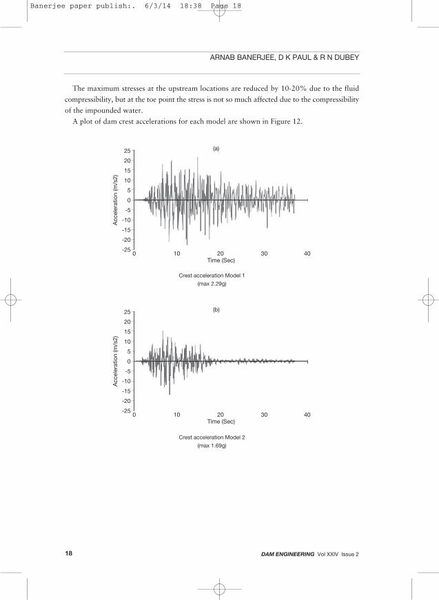
The maximum stresses at the upstream locations are reduced by 10-20% due to the fluid

compressibility, but at the toe point the stress is not so much affected due to the compressibility

of the impounded water.

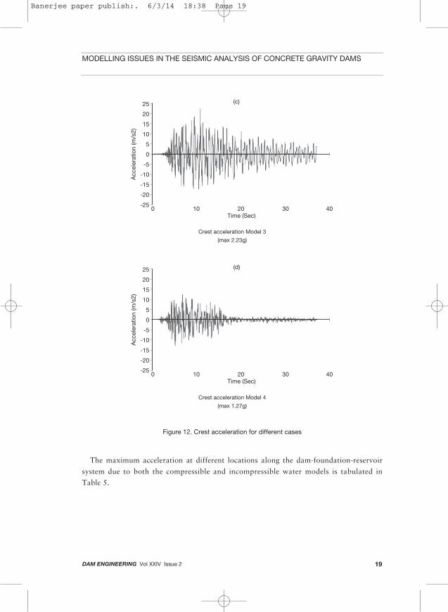
A plot of dam crest accelerations for each model are shown in Figure 12.


25

20

15

10

5

0

-5

-10

-15

-20

-25

Acc

eler

atio

n(m

/s2)

Time (Sec)0 10 20 30 40

(a)

25

20

15

10

5

0

-5

-10

-15

-20

-25

Acc

eler

atio

n(m

/s2)

Time (Sec)0 10 20 30 40

(b)

Crest acceleration Model 1

(max 2.29g)


(max 1.69g)



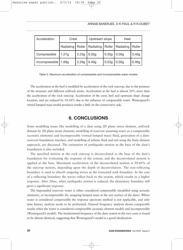
The maximum acceleration at different locations along the dam-foundation-reservoir

system due to both the compressible and incompressible water models is tabulated in

Table 5.


25

20

15

10

5

0

-5

-10

-15

-20

-25

Acc

eler

atio

n(m

/s2)

Time (Sec)0 10 20 30 40

(c)

25

20

15

10

5

0

-5

-10

-15

-20

-25

Acc

eler

atio

n(m

/s2)

Time (Sec)0 10 20 30 40

(d)


(max 2.23g)


(max 1.27g)

Figure 12. Crest acceleration for different cases




The acceleration at the heel is modified by acceleration of the rock outcrop, due to the presence

of the structure and different soil/rock strata. Acceleration at the heel is almost 30% more than

the acceleration of the rock outcrop. Acceleration of the crest, heel and upstream slope change

location, and are reduced by 18-24% due to the influence of compressible water. Westergaard’s

virtual lumped mass model produces results a little on the conservative side.

6. CONCLUSIONS

Some modelling issues like modelling of a dam using 2D plane stress element, soil/rock

domain by 2D plane strain elements, modelling of reservoir assuming water as a compressible

(acoustic elements) and incompressible (virtual lumped mass) fluid, generation of a dam-

reservoir-foundation interface, and modelling of infinite fluid and soil using the finite element

approach, are discussed. The estimation of earthquake motion at the base of the dam’s

foundation is also included.

The specified motion at the rock outcrop is deconvoluted at the base of the dam’s

foundation for evaluating the response of the system, and the deconvoluted motion is

applied at the base. Maximum acceleration of the deconvoluted motion is 50-60% of

the outcrop motion, depending upon the depth of deconvolution. The non-reflecting

boundary is used to absorb outgoing waves at the truncated rock boundary. In the case

of a reflecting boundary the waves reflect back to the system, which results in a higher

response. After 20sec, when earthquake motion is reduced, the elementary boundary still

gives a significant response.

The impounded reservoir water is either considered compressible (modelled using acoustic

elements), or incompressible (by assigning lumped mass at the wet surface of the dam). Where

water is considered compressible the response spectrum method is not applicable, and only

time history analysis needs to be performed. Natural frequency analysis shows comparable

results when the water is considered compressible (acoustic element model) and incompressible

(Westergaard’s model). The fundamental frequency of the dam system in the two cases is found

to be almost identical, suggesting that Westergaard’s model is a good idealization.

Table 5. Maximum acceleration of compressible and incompressible water models



The distribution of pressure in water shows an almost parabolic variation in the first

mode of the reservoir, in the case of a changing upstream slope. Due to the interaction

with fluid, the acceleration and stresses at the upstream face of the dam are found to be

18-24%, and 10-15% less than the lumped mass approach, respectively, as wave propagation

is not considered in the incompressible water model, whereas in the acoustic water model

surface waves are generated and not reflected back from the boundary. The energy loss

can be considered in terms of damping at the upstream face. The assignment of a higher

damping value (7% instead of 5%) for the full dam section in the case of an incompressible

model gives a comparable response to the compressible water model.

The most suitable model of a dam-foundation-reservoir system is obtained when acoustic

elements are used for the impounded water. Truncated reservoir and soil boundaries are

replaced with absorbing boundaries, and appropriate input motion is considered at the base

of the foundation rock.

REFERENCES

Journals

[1] Bayraktar, A, Sevim, B, Altunisk, A C, ‘Finite Element Model Updating Effects on

Nonlinear Seismic Response of Arch Dam-reservoir-foundation Systems’, Finite Element in

Analysis & Design, Vol 47, Issue 2, pp85-97 (2011).

[2] Bleich, H H, Sandler, I S, ‘Interaction Between Structures and Bilinear Fluids’,

International Journal of Solids & Structures, Vol 6, Issue 5, pp617-639 (1970).

[3] Calayir, Y, Dumanoglu, A A & Bayraktar, A, ‘Earthquake Analysis of Gravity Dam-

reservoir Systems Using the Eulerian and Lagrangian Approach’, Computers & Structures,

Vol 59, Issue 5, pp877-890 (1996).

[4] Dungar, R, ‘An Efficient Method of Fluid-structure Coupling in the Dynamic Analysis of

Structures’, International Journal for Numerical Methods in Engineering, Vol 13, Issue 1,

pp93-107 (1978).

[5] Fenves, G & Chopra, A K, ‘Simplified Earthquake Analysis of Concrete Gravity Dams’,

Journal of Structural Engineering, ASCE, Vol 113, Issue 8, pp1688-1708 (1987).

[6] Fok, K L & Chopra, A K, ‘Hydrodynamic and Foundation Flexibility Effects in the

Earthquake Response of Arch Dam’, Journal of Structural Engineering, ASCE, Vol 112,

Issue 8, pp1810-1828 (1986).




[7] Hamdan, F H, ‘Near-field Fluid-structure Interaction Using Lagrangian Fluid Finite

Element’, Computers & Structures, Vol 71, Issue 2, pp123-141 (1999).

[8] Kalateh, F & Attarnejad, R, ‘Finite Element Simulation of Acoustic Cavitation in the

Reservoir and Effects on Dynamic Response of Concrete Dams’, Finite Element in Analysis

& Design, Vol 47, Issue 5, pp543-558 (2011).

[9] Leclerc, M, Leger, P & Tinawi, R, ‘Computer Aided Stability Analysis of Gravity Dams-

CADAM’, Advances in Engineering Software, Vol 34, Issue 7, pp403-420 (2003).

[10] Maity, D & Bhattacheryya, S K, ‘Time Domain Analysis of Infinite Reservoir by Finite

Element Method Using a Novel Far Boundary Condition’, Finite Element in Analysis &

Design, Vol 32, Issue 2, pp85-96 (1999).

[11] Ross, M R, Sprague, M A, Felippa, C A & Par, K C, ‘Treatment of Acoustic Fluid-

structure Interaction by Localized Lagrange Multipliers and Comparison to Alternative

Interface-coupling Methods’, Computer Methods in Applied Mechanics & Engineering, Vol

198, Issues 9-12, pp986-1005 (2009).

[12] Saini S S & Vishwanath, M K, [1977], ‘Simplified Procedure for the Aseismic Design of

Concrete Gravity Dams’, Bulletin ISET, Vol 14, pp1-16 (1977).

[13] Westergaard, H M, ‘Water Pressures on Dams During Earthquakes’, Transactions,

ASCE, Vol 98, No. 2, pp418-433 (1933).

[14] Wilson, E L & Khalvati, M, ‘Finite Elements for the Dynamic Analysis of Fluid-solid

Systems’, International Journal for Numerical Methods in Engineering, Vol 19, Issue 11,

pp1657-1668 (1983).

[15] Zanger, C N, ‘Hydrodynamic Pressure on Dam Due to Horizontal Earthquake’, Proc.

Soc. Exp. Stress Anal., Vol 10, pp93-102 (1953).

[16] Zienkiewicz, O C, Paul, D K & Hinton, E, ‘Cavitations in Fluid Structure Response

(with particular reference to dam on earthquake loading)’, Earthquake Engineering &

Structural Dynamics, Vol 11, Issue 4, pp463-481 (1983).

Books

[1] Bathe, K J, ‘Finite Element Procedures’, PHI Learning Pvt., Eastern Economy Edition

(2010).




[2] Cook, R D, Malkus, D S, Plesha, M E & Witt, R J, ‘Concepts and Applications of Finite

Element Analysis’, 4th Edition, Wiley India Edition (2005).

[3] Indian Standard 1893-1984: ‘Criteria for Earthquake Resistant Design of Structures’,

Indian Standards Institution, New Delhi , India (1984).

[4] Kramer, S L, ‘Geotechnical Earthquake Engineering’, Prentice Hall, Upper Saddle River,

NJ, US (1996).

[5] ‘ProShake User’s Manual’, Version1.1, EduPro Civil System, Redmond, WA, US.

[6] Simulia, ‘Abaqus Analysis Manual’ (2011).

[7] Simulia, ‘Abaqus Users’ Manual’ (2011).

[8] Wolf, J P, ‘Dynamic Soil-structure Interaction’, Prentice Hall, Englewood Cliffs, NJ, US

(1985).

[9] Zienkiewicz, O C & Taylor, R L, ‘The Finite Element Method for Solid and Structural

Mechanics’, Elsevier (2005).

Thesis

[1] Fenves, G & Chopra, A K, ‘Simplified Analysis of Earthquake Resistance Design of

Concrete Gravity Dams’, Report No. UCB/EERC-85/10, Earthquake Engineering Research

Center, University of California, Berkeley, CA, US (1986).

[2] Paul, D K, ‘Efficient Dynamic Solution for Single and Coupled Multiple Field Problems’,

Ph.D. Thesis, University College of Swansea, UK (1982).



Modelling Issues in the Seismic Analysis of Concrete Gravity Dams

Documents

Transcript of Modelling Issues in the Seismic Analysis of Concrete Gravity Dams