Modelling DNA Hairpins
74
DNA and ssDNA Experimental results Lattice model PBD-Polymer model Conclusion Modelling DNA Hairpins Jalal Errami 1 Supervisors: M. Peyrard 1 N. Theodorakopoulos 2 1 Laboratoire de Physique Ecole Normale Supérieure de Lyon 2 TPCI/NHRF, Athens Fachbereich Physik Universität Konstanz May 11, 2007/ Lyon
-
Upload
khangminh22 -
Category
Documents
-
view
1 -
download
0
Transcript of Modelling DNA Hairpins

DNA and ssDNA Experimental results Lattice model PBD-Polymer model Conclusion
Modelling DNA Hairpins
Jalal Errami1
Supervisors: M. Peyrard1 N. Theodorakopoulos2
1Laboratoire de PhysiqueEcole Normale Supérieure de Lyon
2TPCI/NHRF, AthensFachbereich PhysikUniversität Konstanz
May 11, 2007/ Lyon

DNA and ssDNA Experimental results Lattice model PBD-Polymer model Conclusion
Outline
1 DNA molecule and Single-Stranded DNA
2 Experimental properties of DNA Hairpins
3 A two dimensional lattice model
4 PBD-Polymer model for DNA Hairpins

DNA and ssDNA Experimental results Lattice model PBD-Polymer model Conclusion
Outline
1 DNA molecule and Single-Stranded DNA
2 Experimental properties of DNA Hairpins
3 A two dimensional lattice model
4 PBD-Polymer model for DNA Hairpins

DNA and ssDNA Experimental results Lattice model PBD-Polymer model Conclusion
The DNA molecule
Structure and conformation
DNA is a very long helicoidal molecule composed of twochains of desoxyribonucleotides:
(W. Saenger, Principles of Nucleic Acid Structure,Springer-Verlag)
A nucleotide is composed of three molecular parts

DNA and ssDNA Experimental results Lattice model PBD-Polymer model Conclusion
The DNA molecule
Structure and conformation
A nucleotide is composed of three molecular partsA cyclic sugar (desoxyribose)A purine or a pyrimidine base:Adenine-Guanine-Cytosine-ThymineA phosphate linked to the sugar
(W. Saenger, Principles of Nucleic Acid Structure, Springer-Verlag)

DNA and ssDNA Experimental results Lattice model PBD-Polymer model Conclusion
The DNA molecule
Properties
The stability of DNA results from various interactionsHydrogen bonding between complementary basesStacking interaction between base-pairs
Melting of DNA→ The two strands of the DNA can be dissociated by heat→ The melting can be followed by the UV absorbancemeasurement

DNA and ssDNA Experimental results Lattice model PBD-Polymer model Conclusion
Single-Stranded DNA
DNA Hairpins
Single Strands of DNA with complementary bases at itstwo ends→ 5’-CCCAA-(N)n-TTGGG-3’Schematic secondary structure
(S. Cuesta-López et al, Eur. Phys. J. E 16, 235-246)

DNA and ssDNA Experimental results Lattice model PBD-Polymer model Conclusion
Single-Stranded DNA
Interest
Biological interestLoop formation is a first step in the folding of the RNA
DNA hairpins provide very sensitive probes for short DNAsequences

DNA and ssDNA Experimental results Lattice model PBD-Polymer model Conclusion
Single-Stranded DNA
Interest
Physical interestDNA hairpins are simple systems for the understanding ofthe self-assembly of DNA
Modelling the fluctuations of hairpins is more challengingthan the thermal denaturation of DNA→ it is not simply the reverse process of its opening

DNA and ssDNA Experimental results Lattice model PBD-Polymer model Conclusion
Outline
1 DNA molecule and Single-Stranded DNA
2 Experimental properties of DNA Hairpins
3 A two dimensional lattice model
4 PBD-Polymer model for DNA Hairpins

DNA and ssDNA Experimental results Lattice model PBD-Polymer model Conclusion
Thermodynamic properties
Measurement Principle
Molecular Beacons (G. Bonnet et al, Proc. Natl. Acad. Sci. USA 95, 8602-8606)
→ Oligonucleotides with a fluorophore and a quencher attachedat its two ends: 5’-CCCAA-(N)n-TTGGG-3’
Fluorescence Resonance Energy TransferThe conformational state is directly reported by thefluorescenceThe fraction of open beacons can be measured
f (T ) =I(T ) − Ic
I0 − Ic

DNA and ssDNA Experimental results Lattice model PBD-Polymer model Conclusion
Thermodynamic properties
Results
Melting curves for different loop sequences
The melting temperature Tm decreaseswith the loop length
The decay is most important for poly(A)
Tm is higher for a poly(T) than apoly(A)-loop

DNA and ssDNA Experimental results Lattice model PBD-Polymer model Conclusion
Kinetic properties
Measurement principle
Fluorescence Correlation Spectroscopy→ Measurement of the autocorrelation function that gives thesum of the kinetic rates k− and k+
The equilibrium constant gives the ratio of the kinetic rates
K (T ) =f (T )
1 − f (T )
K (T ) =k−(T )
k+(T )

DNA and ssDNA Experimental results Lattice model PBD-Polymer model Conclusion
Kinetic properties
Results
Rates of opening and closing in Arrhenius plot
Kinetics of opening do not depend onthe loop sequence
The rate of closing decreases with theloop length
The activation energy is only affected bythe nature of the loop

DNA and ssDNA Experimental results Lattice model PBD-Polymer model Conclusion
Outline
1 DNA molecule and Single-Stranded DNA
2 Experimental properties of DNA Hairpins
3 A two dimensional lattice model
4 PBD-Polymer model for DNA Hairpins

DNA and ssDNA Experimental results Lattice model PBD-Polymer model Conclusion
Presentation of the model
Description of the model
(S. Cuesta-López, J. Errami, F. Falo,and M. Peyrard, J. Biol. Phys. 31,273-301)
Total energy of the chain
E = nAEA +12
ns∑
j=1
ns∑
j′=1
e(j, j ′)
e(j, j ′) = δ(tj − tj′)δ(djj′ − 1)a(j)a(j ′)EHB(tj )
Hydrogen bonds betweencomplementary bases
EHB < 0
Flexibility of the chain and stackinginteraction
EA > 0

DNA and ssDNA Experimental results Lattice model PBD-Polymer model Conclusion
Equilibrium properties
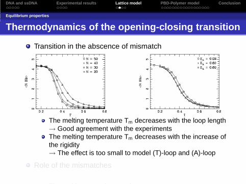
Thermodynamics of the opening-closing transition
Transition in the abscence of mismatch
The melting temperature Tm decreases with the loop length→ Good agreement with the experimentsThe melting temperature Tm decreases with the increase ofthe rigidity→ The effect is too small to model (T)-loop and (A)-loop
Role of the mismatches
The melting curve is smoother
DNA and ssDNA Experimental results Lattice model PBD-Polymer model Conclusion
Equilibrium properties
Thermodynamics of the opening-closing transition
Transition in the abscence of mismatch
The melting temperature Tm decreases with the loop length→ Good agreement with the experimentsThe melting temperature Tm decreases with the increase ofthe rigidity→ The effect is too small to model (T)-loop and (A)-loop
Role of the mismatches
The melting curve is smoother

DNA and ssDNA Experimental results Lattice model PBD-Polymer model Conclusion
Equilibrium properties
Thermodynamics of the opening-closing transition
Role of the mismatches
The melting curve is smootherThe melting curve shows an aditional fairly sharp kink→ The mismatched closings are metastable states

DNA and ssDNA Experimental results Lattice model PBD-Polymer model Conclusion
Monte Carlo Kinetics
Kinetics of opening and closing
Chemical equilibriumbetween closed and openstates
d [C]
dt= −ko[C] + kcl [O]
d [O]
dt= +ko[C] − kcl [O]
ko =1τ
11 + Ke
kcl =1τ
Ke
1 + Ke
→ Studying the opening ofthe hairpins we can also getthe kinetics of closing

DNA and ssDNA Experimental results Lattice model PBD-Polymer model Conclusion
Discussion
Thermodynamic and kinetic results are in qualitativeagreement with respect to the experiments
No quantitative comparisons are possibleThere is not enough degrees of freedom in the model
The difference between poly(T) and poly(A) is not welldescribed
To get good statisitcs the calculation could become verylong

DNA and ssDNA Experimental results Lattice model PBD-Polymer model Conclusion
Outline
1 DNA molecule and Single-Stranded DNA
2 Experimental properties of DNA Hairpins
3 A two dimensional lattice model
4 PBD-Polymer model for DNA Hairpins

DNA and ssDNA Experimental results Lattice model PBD-Polymer model Conclusion
The model
Presentation of the model
The model of the hairpin contains two partsThe loop which is treated as a polymer in three dimensionsThe stem which is an extension of the ends of the loop withadditional interactions: PBD-model
(J. Errami, N. Theodorakopoulos and M. Peyrard, Modelling DNA beacons at the mesoscopic scale,submitted to European Physical Journal E)
R=y+d
M=5
m=1 2 3 4 5
n=1
n=2
n=5
n=4
n=3
n=6
n=7
n=8n=9
n=10
N=10
r=y1+d

DNA and ssDNA Experimental results Lattice model PBD-Polymer model Conclusion
The model
PBD-Model for melting
PBD modeln n+1n-1
V(y )n W(y , y )
n n-1
y
Modelling the interactions at the scale of the baseHydrogen bonding between complementary bases
V (yn) = D`
e−ayn − 1´2
Coupling between consecutive base-pairs
W (yn, yn−1) =K2
h
1 + ρe−α(yn+yn−1)i
(yn − yn−1)2

DNA and ssDNA Experimental results Lattice model PBD-Polymer model Conclusion
Polymer models
Freely Rotating Chain
The root mean square distance scales as√
N for largeN
⟨
R2⟩
= Nl21 + cos θ
1 − cos θ
The chain has a “stiffness”
limN→∞
〈R · u0〉 ≡ lp =l
1 − cos θ
→ It also corresponds to the correlation length in thecontinuum limit approximation
End-to-end distance probability distributionR scales as
√N for large N
→ The probability distribution is Gaussian for large N

DNA and ssDNA Experimental results Lattice model PBD-Polymer model Conclusion
Polymer models
Kratky-Porod Chain (KP)
rj
R
Hamiltonian of the chain
H = −ǫ
N−1∑
j=1
(
rj · rj+1 − l2)
The persistence length depends on the temperature
lp = − l
ln[
coth b − 1b
] ≈ lb = l × ǫl2
kBT
No analytical expression for the end-to-end probabilitydistribution→ Powerful numerical calculation in terms of a finitesum of Bessel functions

DNA and ssDNA Experimental results Lattice model PBD-Polymer model Conclusion
Polymer models
Growth of a polymer chain S(r |R)
r R
Probability of the growth chain PN+2(r)→ derived from PN(R)
∫
∞
0dRPN(R)S(r |R) = PN+2(r) ∀r , N
The conditional probability distribution S(r |R)
∫
∞
0drS(r |R) = 1 ∀R
Distribution of the added bond vectors assumed to be Gaussian

DNA and ssDNA Experimental results Lattice model PBD-Polymer model Conclusion
Polymer models
Conditional probability distribution S(r |R)
Effective Gaussian approach→ Approximate PN(R) by a Gaussian chain that gives the correctpersistence lengthThe Gaussian approximation can be rough for small N but quite goodfor the extention of the chain
0 20 40 60 80r
0
0,05
0,1
0,15
0,2
Pro
babi
lity
dist
ribu
tion
, N=1
2
50 100 150 200r
0
0,02
0,04
0,06
0,08
0,1
Pro
babi
lity
dist
ribu
tion
, N=3
0

DNA and ssDNA Experimental results Lattice model PBD-Polymer model Conclusion
Thermodynamics
Partition function
Construction of the reduced partition function of the hairpin
Partition function of a chain for a given end-to-end distanceR
ZN(R) = Z totN PN(R)
Suppose that we add one bond at each end
ZN+2(rM−1) = PN+2(rM−1)Z totN+2
Introducing the S function
ZN+2(rM−1) = Z totN+2
∫
drMS(rM−1|rM)PN(rM)

DNA and ssDNA Experimental results Lattice model PBD-Polymer model Conclusion
Thermodynamics
Partition function
Construction of the reduced partition function of the hairpin
Then we put the additional interactions according to thePBD model
ZN+2(rM−1) = Z totN+2
e−βV (rM−1)
∫
drM e−β(W (rM−1,rM )+V (rM ))S(rM−1|rM)PN (rM)
Finally we extend the process to the hairpin
Z (r) =Zloop(N+2(M−1))e−βV (r)×
∫ +∞
0
M∏
i=2
dri
M∏
i=2
S(ri−1|ri)e−β[V (ri )+W (ri−1,ri )]PN(rM)

DNA and ssDNA Experimental results Lattice model PBD-Polymer model Conclusion
Thermodynamics
Melting curves
Free energy landscape
F (r) = −kbT ln Z (r)
10 100r
-1,5
-1,4
-1,3
-1,2
-1,1
F(r
)
→ The shape of F (r) justifies the image of the two-state systemMelting curves
f =Keq
1 + Keq=
POPC
1 + POPC
= PO =
∫ +∞
rcdrZ (r)
∫ +∞
0 drZ (r)

DNA and ssDNA Experimental results Lattice model PBD-Polymer model Conclusion
Thermodynamics
FRC Model
Melting curves equivalent to poly(T)k=0.025 eV.Å−2, α=6.9 Å−1,δ = 0.35, ρ = 5. D=0.112 eV,θ = 50◦,◦: N=12: �: N=16;⋄: N=21; △: N=30
260 280 300 320 340 360 380 400 420 440Temperature
0
0,2
0,4
0,6
0,8
1
P O
�: D=0.112 eV, θ = 50◦;⋄: D=0.119 eV, θ = 45◦;△: D=0.100 eV, θ = 64◦
10 15 20 25 30N
290
300
310
320
330
340
T m

DNA and ssDNA Experimental results Lattice model PBD-Polymer model Conclusion
Thermodynamics
FRC model
Melting curves equivalent to poly(A)D=0.112 eV, k=0.025 eV.Å−2, α=6.9 Å−1, δ = 0.35, ρ = 5,θ = 48◦, ◦: N=12; �: N=16; ⋄: N=21; △: N=30
260 280 300 320 340 360 380 400 420 440Temperature
0
0,2
0,4
0,6
0,8
1
P O
10 15 20 25 30 35 40N
300
305
310
315
320
325
330
T m
N θ = 50◦, ∆P∆T Tm θ = 48◦, ∆P
∆T Tm Poly(T) (Exp) Poly(A) (Exp)12 3.6 3.7 11 916 3.7 3.8 11 8.521 3.7 3.8 11 8.530 3.9 4.0 11 7.5

DNA and ssDNA Experimental results Lattice model PBD-Polymer model Conclusion
Thermodynamics
KP model
Melting curves equivalent to poly(T)D=0.107 eV, k=0.025 eV.Å−2, α=6.9 Å−1, δ = 0.35, ρ = 5,ǫ = 0.0018 eV .Å−2. •: N=12; �: N=16; ⋄: N=21; △: N=30
260 280 300 320 340 360 380 400 420 440Temperature
0
0,2
0,4
0,6
0,8
1
P O
10 15 20 25 30N
300
310
320
330
340
T m
N ǫ=0.0018 eV.Å−2, ∆P∆T Tm Poly(T) (Exp), ∆P
∆T Tm
12 3.2 1116 3.4 1121 3.45 1130 3.8 11
DNA and ssDNA Experimental results Lattice model PBD-Polymer model Conclusion
Thermodynamics
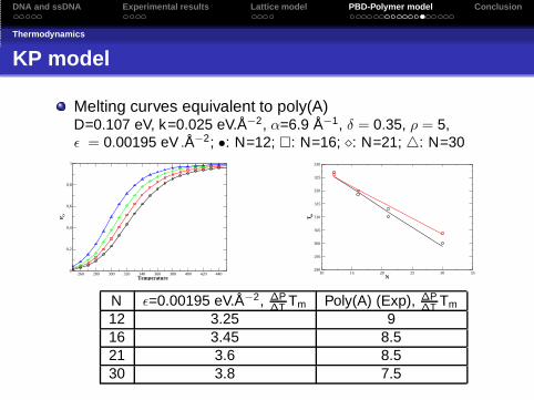
KP model
Melting curves equivalent to poly(A)D=0.107 eV, k=0.025 eV.Å−2, α=6.9 Å−1, δ = 0.35, ρ = 5,ǫ = 0.00195 eV .Å−2; •: N=12; �: N=16; ⋄: N=21; △: N=30
260 280 300 320 340 360 380 400 420 440Temperature
0
0,2
0,4
0,6
0,8
1
P O
10 15 20 25 30 35N
290
295
300
305
310
315
320
325
330
T m
N ǫ=0.00195 eV.Å−2, ∆P∆T Tm Poly(A) (Exp), ∆P
∆T Tm
12 3.25 916 3.45 8.521 3.6 8.530 3.8 7.5

DNA and ssDNA Experimental results Lattice model PBD-Polymer model Conclusion
Kinetics
Theoretical predictions
Transition state theory
k1
k−1
k2
k−2
C T O
k−1op = k−1
1 +C̄C
C̄Ok−1−2
k−1cl = k−1
−2 +C̄O
C̄Fk−1
1
The system is evolving on a one-dimensional free energysurface
k−1op = ZC
∫ +∞
−∞
dre−βF (r)J2(r)
D(r)=
ZC
ZOk−1
cl
J(r) =
∫ r−∞
dx e−β(F(x)−F(r ))
ZC∀ r < rT
∫ +∞
r dx e−β(F(x)−F(r ))
ZO∀ r > rT

DNA and ssDNA Experimental results Lattice model PBD-Polymer model Conclusion
Kinetics
FRC model
Rates of opening and closingD=0.112 eV, k=0.025 eV.Å−2, α=6.9 Å−1, δ = 0.35, ρ = 5.Left: θ = 50◦; •: N=12; �: N=16; ⋄: N=21; △: N=30.Right: N=21, black: θ = 50◦, red:θ = 48◦
3 3,2 3,4 3,6 3,8 41000/T
1e-06
1e-05
0,0001
k op, k
cl
2,5 3 3,5 41000/T
1e-06
1e-05
0,0001
0,001
0,01
k op, k
cl
Eop, model Ecl , model Eop, exp Ecl , expPoly(T) 11.5 -0.33 32 3.4Poly(A) 11.5 -0.33 32 17.4

DNA and ssDNA Experimental results Lattice model PBD-Polymer model Conclusion
Kinetics
KP model
Rates of opening and closingD=0.107 eV, k=0.025 eV.Å−2, α=6.9 Å−1, δ = 0.35, ρ = 5.Left: ǫ=0.0018 eV.Å−2; ◦: N=12; �: N=16; ⋄: N=21; △: N=30.Right: N=21, black: ǫ=0.0018 eV.Å−2, red: ǫ=0.00195 eV.Å−2
3 3,1 3,2 3,3 3,4 3,5 3,6 3,7 3,8 3,9 41000/T
1e-06
1e-05
0,0001
0,001
k op, k
cl
2,6 2,8 3 3,2 3,4 3,6 3,8 41000/T
1e-06
1e-05
0,0001
0,001
0,01
k op, k
cl
Eop, model Ecl , model Eop, exp Ecl , expPoly(T) 10 +1 32 3.4Poly(A) 10 +1 32 17.4

DNA and ssDNA Experimental results Lattice model PBD-Polymer model Conclusion
Kinetics
Effect of D and ǫ on the kinetics
3 3,5 4 4,5 51000/T
1e-10
1e-08
1e-06
0,0001
0,01
k op, k
cl
◦: D=0.08 eV; �: D=0.09 eV;⋄: D=0.10 eV; △: D=0.11 eV,×: D=0.12 eV
3 3,2 3,4 3,6 3,8 41000/T
1e-06
1e-05
0,0001
k cl
◦: ǫ=0.0040 eV.Å−2,�: ǫ=0.0010 eV.Å−2

DNA and ssDNA Experimental results Lattice model PBD-Polymer model Conclusion
Discussion
ThermodynamicsWe are able to describe the dependance of Tm with theloop length for poly(T) and poly(A)We get too large transition widths
KineticsOur results are in qualitative agreements with theexperimentsWe can describe the kinetics of poly(T)We are missing something to deal with the problem ofpoly(A)

DNA and ssDNA Experimental results Lattice model PBD-Polymer model Conclusion
We have studied the self assembly of DNA Hairpins withtwo modelsLattice model
The results are qualitatively goodIt helps us in the understanding of the physics of the system
PBD-Polymer modelThe results are in semi-quantitative agreement with theexperimentsIt shows some limitations→ The behavior of a single strand of DNA depends on itssequence
Poly(T) can be viewed as a polymerPoly(A)?

DNA and ssDNA Experimental results Lattice model PBD-Polymer model Conclusion

DNA and ssDNA Experimental results Lattice model PBD-Polymer model Conclusion
Microscopic model→Modelling of all the interactions between the atoms
Potential describing the stretching of covalent bonds
kbond (r − r0)2
Potential of angular rigidity
kf (θ − θ0)2
Potential of torsion
kg(1 + cos φ)
Lennard-Jones potential for non-bonding interactions
4ǫ
[
(σ
r
)12−
(σ
r
)6]

DNA and ssDNA Experimental results Lattice model PBD-Polymer model Conclusion
Poland-Scheraga model
Model consists on an alternating sequence of ordered andunordered states
The ordered state is energetically favoured over anunordered state
→ w = exp“
−E
kbT
”
The entropy of the unbound state depends solely on itslength
→ S ∝ sl
lc
The phase transition is governed by the value of c
c ≤ 1 no phase transition1 < c ≤ 2 continuous phase transitionc ≥ 2 first order phase transition

DNA and ssDNA Experimental results Lattice model PBD-Polymer model Conclusion
Monte Carlo simulation in the canonical ensemble
Minimization of the Free Energy→ Find the Thermodynamic properties of the systemTry to deduce the Kinetics using MC-step→ Selection of local motions of the chain
(a) (b) (c)

DNA and ssDNA Experimental results Lattice model PBD-Polymer model Conclusion
Effect of the width of the Morse potentialD=0.112 eV, k=0.025 eV.Å−2, δ = 0.35, ρ = 5, θ = 50◦ andN=21. •: α=4.0 Å−1; �: α=5.0 Å−1; ⋄: α=6.0 Å−1; △: α=7.5 Å−1
200 250 300 350 400 450 500Temperature
0
0,2
0,4
0,6
0,8
1
PO
4 5 6 7 8 α
310
320
330
340
350
360
370
Tm
a (Å−1) S 6= 1, ∆P∆T Tm
4 3.45 3.56 3.8
7.5 4.1

DNA and ssDNA Experimental results Lattice model PBD-Polymer model Conclusion
Effect of the rigidity of the stemD=0.112 eV, α=6.9 Å−1, δ = 0.35, ρ = 5, θ = 50◦ and N=21. •:k=0.010 eV.Å−2; �: k=0.020 eV.Å−2; ⋄: k=0.040 eV.Å−2; △:k=0.060 eV.Å−2
200 250 300 350 400 450 500Temperature
0
0,2
0,4
0,6
0,8
1
PO
0 0,01 0,02 0,03 0,04 0,05 0,06 0,07k
290
300
310
320
330
340
350
Tm
k(eV.Å−2) S 6= 1, ∆P∆T Tm
0.01 4.10.020 40.040 3.80.06 3.7